Global existence of quasilinear, nonrelativistic wave equations satisfying the null condition
65
arXiv:math/0409363v1 [math.AP] 20 Sep 2004 GLOBAL EXISTENCE OF QUASILINEAR, NONRELATIVISTIC WAVE EQUATIONS SATISFYING THE NULL CONDITION JASON METCALFE, MAKOTO NAKAMURA, AND CHRISTOPHER D. SOGGE 1. Introduction The purpose of this paper is to provide a proof of global existence of solutions to gen- eral quasilinear, multiple speed systems of wave equations satisfying the null condition. The techniques presented are sufficient to handle both Minkowski wave equations and Dirichlet-wave equations in the exterior of certain compact obstacles. For the latter case, fix a smooth, compact obstacle K⊂ R 3 . We, then, wish to examine the quasilinear system (1.1) ✷u = F (u,du,d 2 u), (t,x) ∈ R + × R 3 \K u(t, · )| ∂K =0 u(0, · )= f, ∂ t u(0, · )= g. Here (1.2) ✷ =(✷ c1 , ✷ c2 ,..., ✷ cD ) denotes a vector-valued multiple speed d’Alembertian where ✷ cI = ∂ 2 t − c 2 I Δ and Δ = ∂ 2 1 + ∂ 2 2 + ∂ 2 3 is the standard Laplacian. For clarity, we will assume that we are in the nonrelativistic case. That is, we assume that the wave speeds c I are positive and distinct. Straightforward modifications can be made to allow various components to have the same speed. For convenience, we will take c 0 = 0 and (1.3) 0= c 0 <c 1 <c 2 < ··· <c D throughout. We now describe our conditions on the nonlinearity F . First of all, F is assumed to be linear in d 2 u. F is also required to vanish to second order. That is, ∂ α F (0, 0, 0) = 0, |α|≤ 1. Additionally, we assume ∂ 2 u F (0, 0, 0) = 0. Thus, F may be decomposed as F (u,du,d 2 u)= B(du)+ Q(du,d 2 u)+ R(u,du,d 2 u)+ P (u,du) The first and third authors were supported in part by the NSF. 1
-
Upload
johnshopkins -
Category
Documents
-
view
0 -
download
0
Transcript of Global existence of quasilinear, nonrelativistic wave equations satisfying the null condition

arX
iv:m
ath/
0409
363v
1 [
mat
h.A
P] 2
0 Se
p 20
04
GLOBAL EXISTENCE OF QUASILINEAR, NONRELATIVISTIC
WAVE EQUATIONS SATISFYING THE NULL CONDITION
JASON METCALFE, MAKOTO NAKAMURA, AND CHRISTOPHER D. SOGGE
1. Introduction
The purpose of this paper is to provide a proof of global existence of solutions to gen-eral quasilinear, multiple speed systems of wave equations satisfying the null condition.The techniques presented are sufficient to handle both Minkowski wave equations andDirichlet-wave equations in the exterior of certain compact obstacles.
For the latter case, fix a smooth, compact obstacle K ⊂ R3. We, then, wish to examine
the quasilinear system
(1.1)
2u = F (u, du, d2u), (t, x) ∈ R+ × R3\K
u(t, · )|∂K = 0
u(0, · ) = f, ∂tu(0, · ) = g.
Here
(1.2) 2 = (2c1,2c2
, . . . ,2cD)
denotes a vector-valued multiple speed d’Alembertian where
2cI= ∂2
t − c2I∆
and ∆ = ∂21 + ∂2
2 + ∂23 is the standard Laplacian. For clarity, we will assume that we
are in the nonrelativistic case. That is, we assume that the wave speeds cI are positiveand distinct. Straightforward modifications can be made to allow various components tohave the same speed. For convenience, we will take c0 = 0 and
(1.3) 0 = c0 < c1 < c2 < · · · < cD
throughout.
We now describe our conditions on the nonlinearity F . First of all, F is assumed tobe linear in d2u. F is also required to vanish to second order. That is,
∂αF (0, 0, 0) = 0, |α| ≤ 1.
Additionally, we assume
∂2uF (0, 0, 0) = 0.
Thus, F may be decomposed as
F (u, du, d2u) = B(du) +Q(du, d2u) +R(u, du, d2u) + P (u, du)
The first and third authors were supported in part by the NSF.
1

2 JASON METCALFE, MAKOTO NAKAMURA, AND CHRISTOPHER D. SOGGE
where, for 1 ≤ I ≤ D,
(1.4) BI(du) =∑
1≤J,K≤D0≤j,k≤3
AI,jkJK ∂ju
J∂kuK ,
(1.5) QI(du, d2u) =∑
1≤J,K≤D0≤j,k,l≤3
BIJ,jkK,l ∂lu
K∂j∂kuJ ,
(1.6) RI(u, du, d2u) =∑
1≤J≤D0≤j,k≤3
CIJ,jk(u, du)∂j∂kuJ
with CIJ,jk(u, du) = O(|u|2+|du|2), and P (u, du) = O(|u|3+|du|3) near (u, du) = 0. Hereand throughout, we use the notation x0 = t and ∂0 = ∂t when convenient. Additionally,
du = u′ = ∇t,xu denotes the space-time gradient. The constants BIJ,jkK,l are real, as
are the CIJ,jk(u, du) terms. Moreover, the quasilinear terms are assumed to satisfy thesymmetry conditions
(1.7) BIJ,jkK,l = BJI,jk
K,l = BIJ,kjK,l ,
(1.8) CIJ,jk(u, du) = CIJ,kj(u, du) = CJI,jk(u, du).
In order to establish global existence, we require that the quadratic terms satisfy thefollowing null condition:
(1.9)∑
0≤j,k≤3
AJ,jkJJ ξjξk = 0, whenever
ξ20c2J
− ξ21 − ξ22 − ξ23 = 0, J = 1, 2, . . . , D,
(1.10)∑
0≤j,k,l≤3
BJJ,jkJ,l ξjξkξl = 0, whenever
ξ20c2J
− ξ21 − ξ22 − ξ23 = 0, J = 1, 2, . . . , D.
This null condition guarantees that the self-interaction of each wave family is nonres-onant and is the natural one for systems of quasilinear wave equations with multiplespeeds. It is equivalent to the requirement that no plane wave solution of the system isgenuinely nonlinear. This follows from an observation of John and Shatah, and we referthe reader to John [11] (p. 23) and Agemi-Yokoyama [1]. Additionally, in the setting ofelasticity, Tahvilday-Zadeh [39] (see also Sideris [33]) observed that (1.9), (1.10) removedthe physically unrealistic restrictions on the growth of the stored energy imposed by thenull conditions used, for example, in [28], [34], and [38]. While general global existenceof solutions to (1.1) is only known (even in the Minkowski setting) under the assumptionof (1.9), (1.10), recent works of Lindblad-Rodnianski [24, 25] suggest that a weak formof the null condition may be sufficient.
We now wish to describe our assumptions on the obstacle K ⊂ R3. As mentioned
above, we assume that K is smooth and compact, but not necessarily connected. Byshifting and scaling, we may take
0 ∈ K ⊂ |x| < 1

QUASILINEAR WAVE EQUATIONS SATISFYING THE NULL CONDITION 3
with no loss of generality. The only additional assumption is that there is exponentialdecay of local energy. Specifically, if u is a solution to the homogeneous wave equation
2u = 0
u(t, · )|∂K = 0
and the Cauchy data u(0, · ), ∂tu(0, · ) are supported in |x| < 4, then we assume thatthere are constants c, C > 0 so that
(1.11)(
∫
x∈R3\K : |x|<4|u′(t, x)|2 dx
)1/2
≤ Ce−ct∑
|α|≤1
‖∂αx u
′(0, · )‖2.
If the obstacle is nontrapping, a stronger version of (1.11) holds with |α| = 0 (no lossof derivative). See, e.g., Morawetz-Ralston-Strauss [30]. In the presence of trapped rays,Ralston [31] observed that this stronger version could not hold, and Ikawa [9, 10] showedthat (1.11) holds for certain finite unions of convex obstacles.
In order to solve (1.1), we must also require that the data satisfies certain compatibilityconditions. Briefly, if we let Jku = ∂αu : 0 ≤ |α| ≤ k and fix m, we can write∂k
t u(0, · ) = ψk(Jkf, Jk−1g), 0 ≤ k ≤ m for any formal Hm solution of (1.1). Here, ψk
is called a compatibility function and depends on F , Jkf , and Jk−1g. The compatibilitycondition for (1.1) with (f, g) ∈ Hm × Hm−1 states that the ψk vanish on ∂K when0 ≤ k ≤ m− 1. Additionally, we say that (f, g) ∈ C∞ satisfy the compatibility conditionto infinite order if this holds for all m. See, e.g., [15] for a more detailed description ofthe compatibility conditions.
We can now state our main result.
Theorem 1.1. Let K be a fixed compact obstacle with smooth boundary satisfying (1.11).Assume that F (u, du, d2u) and 2 are as above and that (f, g) ∈ C∞(R3\K) satisfy the
compatibility conditions to infinite order. Then, there is an ε0 > 0 and an integer N > 0so that for all ε < ε0, if
(1.12)∑
|α|≤N
‖〈x〉|α|∂αx f‖2 +
∑
|α|≤N−1
‖〈x〉1+|α|∂αx g‖2 ≤ ε,
then (1.1) has a unique global solution u ∈ C∞([0,∞) × R3\K).
As mentioned above, we will also handle the Minkowski case. Assuming that F and2 are as above, we show that solutions of
(1.13)
2u = F (u, du, d2u), (t, x) ∈ R+ × R3
u(0, · ) = f, ∂tu(0, · ) = g
exist globally for small data. Specifically, we will prove
Theorem 1.2. Assume that F and 2 are as above. Then, there are constants ε0, N > 0so if f, g are smooth functions satisfying
(1.14)∑
|α|≤N
‖〈x〉|α|∂αx f‖2 +
∑
|α|≤N−1
‖〈x〉1+|α|∂αx g‖2 ≤ ε,
for all ε < ε0, then the system (1.13) has a unique global solution u ∈ C∞([0,∞) × R3).

4 JASON METCALFE, MAKOTO NAKAMURA, AND CHRISTOPHER D. SOGGE
We note that during preparation of this paper it was discovered that Theorem 1.2was proven independently by Katayama [12] using different techniques. Additionally, in[13], Katayama explored the possibility of allowing F to contain certain terms of theform uJ∂uK if you assume the null condition of [34], [38] rather than (1.9), (1.10). Theobstacle result, Theorem 1.1, is new.
By allowing general higher order terms, Theorem 1.2 extends the previously knownresults on multiple speed wave equations due to Sideris-Tu [35], Agemi-Yokoyama [1],Kubota-Yokoyama [21], and Katayama [14]. In a similar way, Theorem 1.1 extends theprevious result of the authors [27].
In studying both the Minkowski setting and the exterior domain, we will be usingmodifications of the method of commuting vector fields due to Klainerman [19]. We willrestrict to the class of vector fields Γ = Z,L that seem “admissible” for boundary valueproblems and studies of multiple speed wave equations. Here, Z denotes the generatorsof space-time translations and spatial rotations
(1.15) Z = ∂i, xj∂k − xk∂j , 0 ≤ i ≤ 3, 1 ≤ j < k ≤ 3and L is the scaling vector field
(1.16) L = t∂t + r∂r .
Additionally, we will write r = |x| and
(1.17) Ωjk = xj∂k − xk∂j
for the generators of spatial rotations. The generators of the Lorentz rotations, xi∂t + t∂i
when cI = 1, have an associated speed and have unbounded normal components on theboundary of our compact obstacle, and thus seem ill-suited to the problems in question.Katayama [12, 13] has shown that these hyperbolic rotations can be used in a limitedfashion in the study of multiple speed wave equations, but we do not require thosetechniques here.
The most significant new difficulty in this case versus the one considered in [27] isthe cubic terms not involving derivatives. Those involving derivatives can generally behandled using energy methods. In the approaches of Christodoulou [3] and Klainerman[19], such terms not involving derivatives were handled with a certain adapted energyinequality that resembles, e.g., the work of Morawetz [29]. This method relies on the useof the Lorentz rotations, and it is not clear how to adapt it to the current setting.
The new argument that we utilize uses an analog of a pointwise estimate that wasestablished by Kubota-Yokoyama [21]. When combined with the pointwise estimatesof Keel-Smith-Sogge [17] and sharp Huygens’ principle, we are able to establish lowregularity decay of our solution u. These improved estimates allow us to handle thecubic terms without derivatives discussed in the previous paragraph. In [27], using onlythe estimates of [17], the authors were only able to get such decay for the gradient of thesolution u′.
As in Keel-Smith-Sogge [16, 17], we will utilize a class of weighted L2tL
2x-estimates
where the weight is a negative power of 〈x〉 = 〈r〉 =√
1 + r2. Such estimates permitus to use the O(〈x〉−1) decay that is obtained from Sobolev inequalities rather than themore standard O(t−1) decay which is difficult to prove without the use of the Lorentzrotations. Additionally, such estimates allow us to handle the boundary terms that arise
QUASILINEAR WAVE EQUATIONS SATISFYING THE NULL CONDITION 5
in the energy estimates of nonlinear wave equations if we no longer have the convenientassumption of star-shapedness on the obstacle. This was one of the main innovations ofMetcalfe-Sogge [28].
As in our previous work [27], we will require a class of weighted Sobolev estimates.The weights involve powers of r and 〈t − r〉. In the Minkowski setting, these estimatesare originally due to Klainerman-Sideris [20] and Hidano-Yokoyama [6].
This paper is organized as follows. In the next section, we gather our preliminaryestimates that will be needed to show global existence in Minkowski space. In particular,we collect the pointwise estimates of Keel-Smith-Sogge [17] and Kubota-Yokoyama [21].In Section 3, we prove Theorem 1.2. In Section 4, we gather the estimates that wewill require to prove Theorem 1.1. Finally, in Sections 5-7, we prove our main theorem,Theorem 1.1.
2. Preliminary estimates in Minkowski space
In this section we gather the estimates for the free wave equation that we will require inorder to prove global existence.
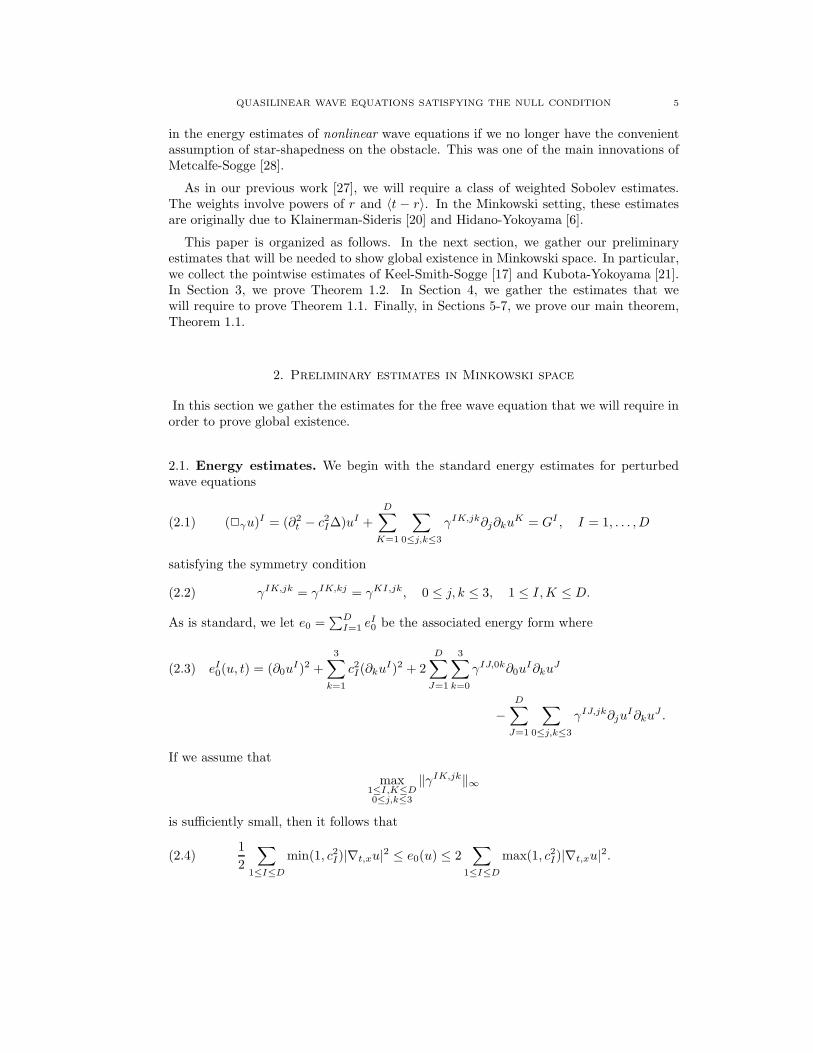
2.1. Energy estimates. We begin with the standard energy estimates for perturbedwave equations
(2.1) (2γu)I = (∂2
t − c2I∆)uI +
D∑
K=1
∑
0≤j,k≤3
γIK,jk∂j∂kuK = GI , I = 1, . . . , D
satisfying the symmetry condition
(2.2) γIK,jk = γIK,kj = γKI,jk, 0 ≤ j, k ≤ 3, 1 ≤ I,K ≤ D.
As is standard, we let e0 =∑D
I=1 eI0 be the associated energy form where
(2.3) eI0(u, t) = (∂0u
I)2 +
3∑
k=1
c2I(∂kuI)2 + 2
D∑
J=1
3∑
k=0
γIJ,0k∂0uI∂ku
J
−D
∑
J=1
∑
0≤j,k≤3
γIJ,jk∂juI∂ku
J .
If we assume that
max1≤I,K≤D0≤j,k≤3
‖γIK,jk‖∞
is sufficiently small, then it follows that
(2.4)1
2
∑
1≤I≤D
min(1, c2I)|∇t,xu|2 ≤ e0(u) ≤ 2∑
1≤I≤D
max(1, c2I)|∇t,xu|2.

6 JASON METCALFE, MAKOTO NAKAMURA, AND CHRISTOPHER D. SOGGE
If we set E(u, t)2 =∫
R3 e0(u, t) dx to be the associated energy, then we have the energyinequality
(2.5)∑
|α|≤M
∂tE(Γαu, t) ≤ C∑
|α|≤M
‖ΓαG(t, · )‖2 +∑
|α|≤M
‖[2γ ,Γα]u(t, · )‖2
+ C∑
|α|≤M
E(Γαu, t)∑
0≤j,k,l≤31≤I,K≤D
‖∂lγIK,jk(t, · )‖∞.
In addition to the energy estimate (2.5), we will need the following L2tL
2x estimate of
Keel-Smith-Sogge [16] (Proposition 2.1).
Lemma 2.1. Suppose that u ∈ C∞(R×R3) vanishes for large x for every t. Then, there
is a uniform constant C so that
(2.6) (log(2 + t))−1/2‖〈x〉−1/2u′‖L2([0,t]×R3) ≤ C‖u′(0, · )‖2 + C
∫ t
0
‖2u(s, · )‖2 ds.
2.2. Pointwise estimates. In this section, we will gather the pointwise estimates thatwill be needed in the sequel. The estimates that are presented are variants of those inKeel-Smith-Sogge [17], Sogge [38], and Kubota-Yokoyama [21]. The key innovation inour approach to Theorem 1.2 is the use of both of these pointwise estimates and sharpHuygens’ principle to allow us to get good pointwise bounds for u (not just u′ as in[27]). This pointwise bound allows us to handle the higher order terms without havingto strengthen the null condition (as in [21]).
In our first estimate, we will concentrate on the scalar wave equation 2 = (∂2t − ∆).
The transition to vector valued, multiple speed wave equations is straightforward.
Lemma 2.2. Let u be the solution of 2u(t, x) = F (t, x) with initial data u(0, · ) = f ,∂tu(0, · ) = g for (t, x) ∈ R+ × R
3. Then,
(2.7) (1 + t+ |x|)|u(t, x)| ≤ C∑
|α|≤4
‖〈x〉|α|∂αf‖2 + C∑
|α|≤3
‖〈x〉1+|α|∂αg‖2
+ C∑
µ+|α|≤3µ≤1
∫ t
0
∫
R3
|LµZαF (s, y)| dy ds〈y〉 .
Proof of Lemma 2.2: For vanishing Cauchy data, (2.7) can be found in Keel-Smith-Sogge [17] and Sogge [38]. Thus, it will suffice to show the estimate for cos(t
√−∆)f and
(sin(t√−∆)/
√−∆)g. The proof is similar to that in [17] for the inhomogeneous case. If
we assume that F = 0 above, we will show
(2.8) (1 + t+ |x|)|u(t, x)| ≤ C∑
|α|+µ≤3µ≤1
∫
R3
(
|(r∂r)µZα∇f | dy〈y〉 +
∫
R3
|(r∂r)µZαf | dy
〈y〉2
+
∫
R3
|(r∂r)µZαg| dy〈y〉
)
Our desired estimate (2.7) follows, then, via the Schwarz inequality.

QUASILINEAR WAVE EQUATIONS SATISFYING THE NULL CONDITION 7
Let us first consider (sin(t√−∆)/
√−∆)g. Using the positivity of the fundamental
solution for the wave equation, we have
|x|∣
∣
∣
sin(t√−∆)√
−∆g∣
∣
∣=t |x|4π
∣
∣
∣
∫
|θ|=1
g(x− tθ) dσ(θ)∣
∣
∣
≤ 1
2
∫ t+|x|
|t−|x||‖sg(s · )‖L∞
θ(S2) ds.
(2.9)
By the embedding H2,1θ → L∞
θ it follows that
(2.10) |x|∣
∣
∣
sin(t√−∆)√
−∆g∣
∣
∣≤ C
∑
|α|≤2
∫
|t−|x||≤|y|≤t+|x||Ωαg(y)| dy|y| .
For t ≥ 10|x|, apply the relation sg(sθ) = −∫ ∞
s ∂τ (τg(τθ)) dτ to (2.9) to see that
t∣
∣
∣
sin(t√−∆)√
−∆g∣
∣
∣≤ C
t
|x|
∫ t+|x|
|t−|x||
∫ ∞
s
1
τ‖τ∂τ (τg(τθ))‖L∞
θ(S2) dτ ds
≤ C
∫ ∞
|t−|x||‖τg(τ · )‖L∞
θ(S2) + ‖τ(τ∂τ )g(τ · )‖L∞
θ(S2) dτ
≤ C∑
µ≤1,|α|≤2
∫
|t−|x||≤|y||(|y|∂|y|)µΩαg(y)| dy|y| .
(2.11)
By (2.10) and (2.11), we obtain
(2.12) (t+ |x|)∣
∣
∣
sin(t√−∆)√
−∆g∣
∣
∣≤ C
∑
µ≤1,|α|≤2
∫
|t−|x||≤|y||(|y|∂|y|)µΩαg(y)| dy|y| .
We now wish to show that
(2.13) (1 + t+ |x|)∣
∣
∣
sin(t√−∆)√
−∆g∣
∣
∣≤ C
∑
|α|+µ≤3µ≤1
∫
R3
|(|y|∂|y|)µZαg(y)| dy|y| .
For t+ |x| ≥ 1, (2.13) clearly follows from (2.12). For t+ |x| ≤ 1, let χ denote a smoothfunction with χ(x) ≡ 1 for |x| ≤ 1 and χ(x) ≡ 0 for |x| > 2, and let v be the solution tothe shifted wave equation
(2.14) 2v(t, x) = 0, v(0, · ) = 0, ∂tv(0, x) = (χg)(x1 − 10, x2, x3).
By finite propagation, we have that sin t√−∆√
−∆g = v(t, x1 + 10, x2, x3) for t+ |x| ≤ 1, and
(2.13) follows by applying (2.12) to v.
Finally, we turn to the task of showing that our desired result
(2.15) (1 + t+ |x|)∣
∣
∣
sin(t√−∆)√
−∆g∣
∣
∣≤ C
∑
|α|+µ≤3µ≤1
∫
R3
|(|y|∂|y|)µZαg(y)| dy〈y〉
follows from (2.13). For χ as above, write g = χg + (1 − χ)g. When g is replaced by(1−χ)g, (2.15) follows directly from (2.13). When g is replaced by χg, we instead apply

8 JASON METCALFE, MAKOTO NAKAMURA, AND CHRISTOPHER D. SOGGE
(2.13) to the shifted function v. It is this use of the shifted function that introduces thetranslations on the right sides of (2.13) and (2.15).
Next, we consider cos(t√−∆)f . We have
∣
∣
∣cos(t
√−∆)f
∣
∣
∣=
∣
∣
∣∂t
( t
4π
∫
|θ|=1
f(x− tθ) dσ(θ))∣
∣
∣
≤∣
∣
∣
sin t√−∆
t√−∆
f∣
∣
∣+
∣
∣
∣
sin t√−∆√
−∆|∇f |
∣
∣
∣.
(2.16)
By (2.15), the |∇f | part is bounded by the right side of (2.8). For the first part, repeatingthe arguments of (2.9) and (2.11), we have
(t+ |x|)∣
∣
∣
sin(t√−∆)
t√−∆
f∣
∣
∣≤ t+ |x|
2t|x|
∫ t+|x|
|t−|x||‖sf(s · )‖L∞
θ(S2) ds
≤ t+ |x|2t|x| (t+ |x| − |t− |x||)
∫ ∞
|t−|x||‖∂τ (τf(τ · ))‖L∞
θ(S2) dτ
≤ C∑
µ≤1,|α|≤2
∫
|y|≥|t−|x|||(|y|∂|y|)µΩαf(y)| dy|y|2 .
(2.17)
Using the shifted function as in (2.13) and (2.15), it follows that
(2.18) (1 + t+ |x|)∣
∣
∣
sin(t√−∆)
t√−∆
f∣
∣
∣≤ C
∑
|α|+µ≤3µ≤1
∫
|(|y|∂|y|)µZαf(y)| dy
〈y〉2
as desired.
We now wish to explore the version of the pointwise estimate of Kubota-Yokoyama [21]that we will use. We define the “neighborhoods” of the characteristic cones r = |x| = cItfor 2cI
. That is, with the cI as in (1.3), set
(2.19) ΛI = (t, |x|) ∈ [1,∞) × [1,∞) : |r − cIt| ≤ δtwhere δ = 1
3 min1≤I≤D(cI − cI−1) and I = 1, 2, . . . , D. Note that for (t, x) 6∈ ΛI , |cI t−|x|| ≈ t+ |x|. Additionally, define
(2.20) z(s, λ) =
(1 + |λ− cJs|), for (s, λ) ∈ ΛJ , J = 1, 2, . . . , D
(1 + λ), otherwise.
With this notation, we then have
Lemma 2.3. Let I = 1, 2, . . . , D, and assume that GI(t, x) is a continuous function of
(t, x) ∈ R+ × R3. Let wI be the solution of (∂2
t − c2I∆)wI = GI with vanishing Cauchy
data at time t = 0. Then,
(2.21) (1 + r + t)(
1 + log1 + r + cIt
1 + |r − cIt|)−1
|wI(t, x)|
≤ C sup(s,y)∈DI(t,r)
|y|(1 + s+ |y|)1+µz1−µ(s, |y|)|GI(s, y)|
QUASILINEAR WAVE EQUATIONS SATISFYING THE NULL CONDITION 9
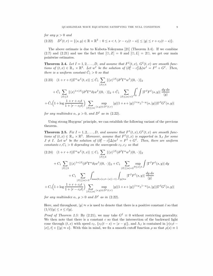
for any µ > 0 and
(2.22) DI(t, r) = (s, y) ∈ R × R3 : 0 ≤ s < t, |r − cI(t− s)| ≤ |y| ≤ r + cI(t− s).
The above estimate is due to Kubota-Yokoyama [21] (Theorem 3.4). If we combine(2.7) and (2.21) and use the fact that [2, Z] = 0 and [2, L] = 22, we get our mainpointwise estimates.
Theorem 2.4. Let I = 1, 2, . . . , D, and assume that F I(t, x), GI(t, x) are smooth func-
tions of (t, x) ∈ R+ × R3. Let wI be the solution of (∂2
t − c2I∆)wI = F I + GI . Then,
there is a uniform constant C1 > 0 so that
(2.23) (1 + r + t)|ΓαwI(t, x)| ≤ C1
∑
|β|≤4
‖〈x〉|β|(∂βΓαwI)(0, · )‖2
+ C1
∑
|β|≤3
‖〈x〉1+|β|(∂βΓα∂twI)(0, · )‖2 + C1
∑
|β|≤|α|+3
∫ t
0
∫
|ΓβF I(s, y)| dy ds〈y〉
+ C1
(
1+ log1 + r + cIt
1 + |r − cIt|)
∑
|β|≤|α|sup
(s,y)∈DI(t,r)
|y|(1+ s+ |y|)1+µz1−µ(s, |y|)|ΓβGI(s, y)|
for any multiindex α, µ > 0, and DI as in (2.22).
Using strong Huygens’ principle, we can establish the following variant of the previoustheorem.
Theorem 2.5. Fix I = 1, 2, . . . , D, and assume that F I(t, x), GI(t, x) are smooth func-
tions of (t, x) ∈ R+ × R3. Moreover, assume that F I(t, x) is supported in ΛJ for some
J 6= I. Let wI be the solution of (∂2t − c2I∆)wI = F I + GI . Then, there are uniform
constants c, C1 > 0 depending on the wavespeeds cI , cJ so that
(2.24) (1 + r + t)|ΓαwI(t, x)| ≤ C1
∑
|β|≤4
‖〈x〉|β|(∂βΓαwI)(0, · )‖2
+ C1
∑
|β|≤3
‖〈x〉1+|β|(∂βΓα∂twI)(0, · )‖2 + C1
∑
|β|≤|α|+2
sup0≤s≤t
∫
|ΓβF I(s, y)| dy
+ C1
∑
|β|≤|α|+3
∫ t
max(0,c|cIt−|x||−1)
∫
|y|≈s
|ΓβF I(s, y)| dy ds〈y〉
+C1
(
1+ log1 + r + cIt
1 + |r − cIt|)
∑
|β|≤|α|sup
(s,y)∈DI(t,r)
|y|(1+ s+ |y|)1+µz1−µ(s, |y|)|ΓβGI(s, y)|
for any multiindex α, µ > 0 and DI as in (2.22).
Here, and throughout, |y| ≈ s is used to denote that there is a positive constant c so that(1/c)|y| ≤ s ≤ c|y|.Proof of Theorem 2.5: By (2.21), we may take GI ≡ 0 without restricting generality.We then note that there is a constant c so that the intersection of the backward lightcone through (t, x) with speed cI , cI(t − s) = |x − y|, and ΛJ is contained in [c|cIt −|x||, t]× |y| ≈ s. With this in mind, we fix a smooth cutoff function ρ so that ρ(s) ≡ 1

10 JASON METCALFE, MAKOTO NAKAMURA, AND CHRISTOPHER D. SOGGE
for s ≥ c|cIt− |x|| and ρ(s) ≡ 0 for s ≤ c|cIt− |x|| − 1. Notice that by strong Huygens’principle, we have ΓαwI(t, x) = Γαw where w is the solution to
2cIΓαw(s, y) = ρ(s)ΓαF I(s, y) + ρ(s)[2cI
,Γα]F I(s, y)
and Γαw has the same Cauchy data as Γαw.
The result now follows from an application of (2.7) to Γαw. So long as the scalingvector field L in the third term on the right of (2.7) does not hit ρ, the bound (2.24)follows and the third term on the right is unnecessary. If the L in (2.7) is applied to ρ,we get an additional term which is bounded by
C∑
|β|≤|α|+2
∫ c|cIt−|x||
max(0,c|cIt−|x||−1)
∫
|y|≈s
s|ρ′(s)||ΓβF (s, y)| dy ds〈y〉 .
Since |y| ≈ s and the time integral is taken over an interval of length at most one, thisterm is easily seen to be dominated by the third term in (2.24) which completes theproof.
2.3. Null form estimates and Sobolev-type estimates. In this section, we gatherour bounds on the null forms and some weighted Sobolev-type estimates. The first ofthese is the null form estimate. See, e.g., [35], [38].
Lemma 2.6. Suppose that the quadratic parts of the nonlinearity Q(du, d2u), B(du)satisfy the null conditions (1.9) and (1.10). Then,
(2.25)∣
∣
∣
∑
0≤j,k,l≤3
BKK,jkK,l ∂lu∂j∂kv
∣
∣
∣≤ C〈r〉−1(|Γu||∂2v| + |∂u||∂Γv|) + C
〈cKt− r〉〈t+ r〉 |∂u||∂2v|,
and
(2.26)∣
∣
∣
∑
0≤j,k≤3
AK,jkKK ∂ju∂kv
∣
∣
∣≤ C〈r〉−1(|Γu||∂v| + |∂u||Γv|) + C
〈cKt− r〉〈t+ r〉 |∂u||∂v|.
For the Sobolev-type results, we begin with
Lemma 2.7. Suppose that h ∈ C∞(R3). Then, for R > 1,
(2.27) ‖h‖L∞(R/2<|x|<R) ≤ CR−1∑
|α|+|β|≤2
‖Ωα∂βxh‖L2(R/4<|x|<2R).
This has become a rather standard result. See Klainerman [18]. A proof can also befound, e.g., in [16].
Additionally, we have the following space-time weighted Sobolev results.
Lemma 2.8. Let u ∈ C∞0 (R+ × R
3). Then,
(2.28) 〈r〉1/2|u(t, x)| ≤ C∑
|α|≤1
‖Zαu′(t, · )‖2,
(2.29) ‖〈cIt− r〉∂2u(t, · )‖2 ≤ C∑
|β|≤1
‖Γβu′(t, · )‖2 + C‖〈t+ r〉2cIu(t, · )‖2,

QUASILINEAR WAVE EQUATIONS SATISFYING THE NULL CONDITION 11
(2.30) 〈r〉1/2〈cIt− r〉|u′(t, x)| ≤ C∑
|β|≤1
‖Zβu′(t, · )‖2 + C∑
|β|≤1
‖〈cIt− r〉Zβ∂2u(t, · )‖2,
(2.31) 〈r〉〈cI t− r〉1/2|u′(t, x)| ≤ C∑
|β|≤2
‖Zβu′(t, · )‖2 + C∑
|β|≤1
‖〈cIt− r〉Zβ∂2u(t, · )‖2.
The estimates (2.28) and (2.31) are shown in Sideris [33] (Proposition 3.3). (2.29)is due to Klainerman-Sideris [20] (Lemma 2.3 and Lemma 3.1). (2.30) is from Hidano-Yokoyama [6] (Lemma 4.1) and follows from (2.28).
Lastly, by interpolating between (2.30) and (2.31), it is easy to see that
(2.32) 〈r〉1/2+µ〈cIt− r〉1−µ|Γαu′(t, x)| ≤ C∑
|β|≤|α|+2
‖Γβu′(t, · )‖2
+ C∑
|β|≤|α|+1
‖〈cIt− r〉Γβ∂2u(t, · )‖2
for any 0 ≤ µ ≤ 1/2.
3. Global existence in Minkowski space
Here we prove Theorem 1.2. We will take N = 71 in (1.14). This, however, is notoptimal.
To proceed, we shall require a standard local existence theorem.
Theorem 3.1. Let f ∈ H71(R3) and g ∈ H70(R3). Then, there is a T > 0 dependent on
the norm of the data so that the initial value problem (1.13) has a C2 solution satisfying
(3.1) u ∈ L∞([0, T ];H71(R3)) ∩C0,1([0, T ];H70(R3)).
The supremum of all such T is equal to the supremum of all T such that the initial value
problem has a C2 solution with ∂αu bounded for all |α| ≤ 2.
This result is a multi-speed analog of Theorem 6.4.11 in [7] (which is stated only forscalar wave equations). Since the proof is based only on energy inequalities, the sameargument yields Theorem 3.1 provided we assume the symmetry conditions (1.7) and(1.8).

12 JASON METCALFE, MAKOTO NAKAMURA, AND CHRISTOPHER D. SOGGE
We are now ready to set up our continuity argument. If ε is as above, we will assumethat we have a solution of our equation (1.13) for 0 ≤ t ≤ T satisfying the following:
∑
|α|≤50
‖Γαu′(t, · )‖2 ≤ A0ε(3.2)
(1 + t+ |x|)∑
|α|≤40
|ΓαuI(t, x)| ≤ A1ε(
1 + log1 + t+ |x|
1 + |cIt− |x||)
(3.3)
(1 + t+ |x|)∑
|α|≤60
|ΓαuI(t, x)| ≤ A2ε(1 + t)1/10 log(2 + t)(
1 + log1 + t+ |x|
1 + |cIt− |x||)
(3.4)
(1 + t+ |x|)∑
|α|≤39
|Γαu′(t, x)| ≤ B1ε(3.5)
∑
|α|≤70
‖Γαu′(t, · )‖2 ≤ B2ε(1 + t)1/40(3.6)
∑
|α|≤65
‖〈x〉−1/2Γαu′‖L2(St) ≤ B3ε(1 + t)1/20(log(2 + t))1/2.(3.7)
Here St denotes the time strip [0, t] × R3.
By (1.14), we have the estimate
D∑
I=1
∑
|α|≤67
(1 + C1 + C1)∑
|β|≤4
‖〈x〉|β|(∂βΓαuI)(0, x)‖2
+∑
|β|≤3
‖〈x〉1+|β|(∂βΓα∂tuI)(0, x)‖2 ≤ C2ε
for some constant C2 > 0. Here C1 and C1 are the constants occurring in (2.23) and (2.24)respectively. In our estimates above, we choose A0 = A1 = A2 = A ≥ 10 max(1, C2).
We shall then prove that for ε sufficiently small,
i.) (3.2) holds with A0 replaced by A0/2.ii.) (3.3), (3.4) hold with A1, A2 replaced by A1/2, A2/2 respectively.iii.) (3.2)-(3.4) imply (3.5)-(3.7) for a suitable choice of constants B1, B2, B3.
We will prove items (i.)-(iii.) in the next three subsections respectively.
Before we begin with the proof of (i.), we will set up some preliminary results underthe assumption of (3.2)-(3.7). Let us first prove
(3.8)∑
|α|≤58
〈r〉1/2+µ〈cIt− r〉1−µ|Γα∂uI(t, x)| ≤ Cε(1 + t)1/40, 0 ≤ µ ≤ 1/2.
Indeed, by (2.32) and (2.29), we have that the left side of (3.8) is controlled by
C∑
|α|≤60
‖Γαu′(t, · )‖2 + C∑
|α|≤59
‖〈t+ r〉Γα2cI
uI(t, · )‖2.

QUASILINEAR WAVE EQUATIONS SATISFYING THE NULL CONDITION 13
By (3.6), the first term is controlled by the right side of (3.8). Thus, it remains to show
(3.9)∑
|α|≤59
‖〈t+ r〉Γα2cI
uI(t, · )‖2 ≤ Cε(1 + t)1/40.
By our definition of 2u, we have that the left side of (3.9) is bounded by
C∑
|α|≤30
‖〈t+ r〉Γαu′(t, · )‖∞∑
|α|≤60
‖Γαu′(t, · )‖2
+ C∑
1≤J,K≤D
∥
∥
∥〈t+ r〉
∑
|α|≤31
|ΓαuJ |∑
|α|≤31
|ΓαuK |∑
|α|≤59
|Γαu|∥
∥
∥
2
+ C∑
1≤J,K≤D
∥
∥
∥〈t+ r〉
∑
|α|≤31
|ΓαuJ |∑
|α|≤31
|ΓαuK |∑
|α|≤60
|Γα∂u|∥
∥
∥
2.
By (3.5) and (3.6), we see that the first term is controlled by Cε2(1 + t)1/40 as desired.For the second term, we apply (3.3) to see that we have the bound
Cε2∥
∥
∥
(
1 + log1 + t+ |x|
1 + |cJ t− |x||)(
1 + log1 + t+ |x|
1 + |cKt− |x||)
(1 + t+ |x|)−1∑
|α|≤59
|Γαu(t, · )|∥
∥
∥
2.
We, then, see that this is O(ε3) using (3.4). The bound for the third term follows similarlyfrom applications of (3.3) and (3.6).
If we argued similarly, using (3.2) instead of (3.6), it follows that
(3.10)∑
|α|≤48
〈r〉1/2+µ〈cI t− r〉1−µ|Γα∂uI(t, x)| ≤ Cε, 0 ≤ µ ≤ 1/2,
and
(3.11)∑
|α|≤49
‖〈cIt− r〉Γα∂2uI(t, · )‖2 ≤ Cε.
Indeed, the latter follows from (2.29) and the proof of (3.9) where, as mentioned above,we use the lossless estimate (3.2) rather than (3.6).
3.1. Proof of (i.): In this section, we will show that (3.2)-(3.7) allow you to prove (3.2)with A0 replaced by A0/2. By the standard energy inequality (see, e.g., [37]), the squareof the left side of (3.2) is controlled by
(3.12)∑
|α|≤50
‖Γαu′(0, · )‖22 +
∑
|α|≤50
∫ t
0
∫
∣
∣
∣〈∂0Γ
αu,2Γαu〉∣
∣
∣dy ds.
It follows from (1.14) and our choice of A0 that the first term is controlled by (A0/10)2ε2.Thus, it will suffice to show that
(3.13)∑
|α|≤50
∫ t
0
∫
∣
∣
∣〈∂0Γ
αu,2Γαu〉∣
∣
∣dy ds ≤ Cε3.

14 JASON METCALFE, MAKOTO NAKAMURA, AND CHRISTOPHER D. SOGGE
The left side of (3.13) is dominated by
(3.14) C
∫ t
0
∫
R3
D∑
K=1
∑
|α|≤50
|∂0ΓαuK |
∑
|α|+|β|≤50
∣
∣
∣
∑
0≤j,k,l≤3
BKK,jkK,l ∂lΓ
αuK∂j∂kΓβuK∣
∣
∣dy ds
+ C
∫ t
0
∫
R3
D∑
K=1
∑
|α|≤50
|∂0ΓαuK |
∑
|α|+|β|≤50
∣
∣
∣
∑
0≤j,k,l≤3
AK,jkKK ∂jΓ
αuK∂kΓβuK∣
∣
∣dy ds
+ C
∫ t
0
∫
R3
∑
1≤I,J,K≤D(I,K) 6=(K,J)
∑
|α|≤50
|∂ΓαuK |∑
|α|≤50
|∂ΓαuI |∑
|α|≤51
|∂ΓαuJ | dy ds
+ C
∫ t
0
∫
R3
∑
|α|≤50
|∂0Γαu|
(
∑
|α|≤31
|Γαu|)2 ∑
|α|≤52
|Γαu| dy ds.
Due to constants that are introduced when LνZα commutes with ∂j,k,l, the coefficients
AK,jkKK , BKK,jk
K,l become new constants AK,jkKK , BKK,jk
K,l . It is known, however, that Γ
preserves the null forms. That is, since the original constants satisfy (1.9) and (1.10), so
do the new ones AK,jkKK and BKK,jk
K,l . See, e.g., Sideris-Tu [35] (Lemma 4.1).
The first three terms are handled as in [27]. Let us begin with the null terms (i.e., thefirst two terms in (3.14)). By (2.25) and (2.26), these terms are dominated by
(3.15) C
∫ t
0
∫
R3
∑
|α|≤50
|Γαu′|∑
|α|≤51
|Γαu|∑
|α|≤51
|Γαu′| dy ds〈y〉
+ C
∫ t
0
∫
R3
D∑
K=1
〈cKs− r〉〈s+ r〉
(
∑
|α|≤51
|Γα∂uK |)3
dy ds
In order to handle the contribution by the first term of (3.15), notice that by (3.4)∑
|α|≤51
|Γαu(s, y)| ≤ Cε〈s+ |y|〉−9/10+.
Thus, the first term in (3.15) has a contribution to (3.14) which is dominated by
(3.16) Cε
∫ t
0
〈s〉−9/10+∑
|α|≤51
‖〈y〉−1/2Γαu′(s, · )‖22 ds
by the Schwarz inequality. By (3.7), it follows that this contribution is O(ε3).
In order to show that the second term in (3.15) satisfies a similar bound, we apply(3.8) with µ = 0 and the Schwarz inequality to see that it is controlled by
(3.17) Cε
∫ t
0
(1 + s)1/40
∫
R3
1
〈r〉1/2〈s+ r〉∑
|α|≤51
|Γα∂u|2 dy ds
≤ C
∫ t
0
〈s〉−19/40∑
|α|≤51
‖〈y〉−1/2 Γαu′(s, · )‖22 ds.
It then follows from (3.7) that this term also has an O(ε3) contribution to (3.14).

QUASILINEAR WAVE EQUATIONS SATISFYING THE NULL CONDITION 15
We now wish to show that the multi-speed terms
(3.18)
∫ t
0
∫
R3
∑
|α|≤50
|∂ΓαuK |∑
|α|≤50
|∂ΓαuI |∑
|α|≤51
|∂ΓαuJ | dy ds
with (I,K) 6= (K, J) have an O(ε3) contribution to (3.14). For simplicity, let us assumethat I 6= K, I = J . A symmetric argument will yield the same bound for the remainingcases. If we set δ < |cI − cK |/3, it follows that |y| ∈ [(cI − δ)s, (cI + δ)s] ∩ |y| ∈[(cK − δ)s, (cK + δ)s] = ∅. Thus, it will suffice to show the bound when the spatialintegral is taken over the complements of each of these sets separately. We will show thebound over |y| 6∈ [(cK − δ)s, (cK + δ)s]. The same argument will symmetrically yieldthe bound over the other set.
If we apply (3.8) with µ = 0, we see that over the indicated set, (3.18) is bounded by
(3.19) Cε
∫ t
0
∫
|y|6∈[(cK−δ)s,(cK+δ)s]〈s+ r〉−39/40〈r〉−1/2
∑
|α|≤51
|∂ΓαuI |2 dy ds
≤ Cε
∫ t
0
〈s〉−19/40∑
|α|≤51
‖〈y〉−1/2Γαu′(s, · )‖22 ds.
Thus, it again follows from (3.7) that this term is O(ε3).
Finally, it remains to bound the contribution to (3.14) by the cubic terms (the fourthterm in (3.14)). If we apply (3.3) and (3.4), it is clear that this term is dominated by
Cε3∫ t
0
∫
(log(1 + s+ |y|))4(1 + s+ |y|)29/10
∑
|α|≤50
|∂0Γαu| dy ds.
By Schwarz inequality and (3.6), we see that this term is O(ε4) which completes the proofof (3.13).
3.2. Proof of (ii.): In this section, we wish to show that our pointwise estimates (3.3)and (3.4) hold with A1, A2 replaced by A1/2, A2/2 respectively. Let us begin with (3.3).
Fix a smooth cutoff function ηJ satisfying ηJ (s) ≡ 1, s ∈ [(cJ +(δ/2))−1, (cJ−(δ/2))−1]where, as in (2.19), δ = (1/3)minI(cI − cI−1), and ηJ (s) ≡ 0, s 6∈ [(cJ + δ)−1, (cJ − δ)−1].We also set β to be a smooth function satisfying β(x) ≡ 1, |x| < 1 and β(x) ≡ 0, |x| ≥ 2.Then, let ρJ(x, t) = (1−β)(x)ηJ (|x|−1t). By construction when |x| ≥ 2, ρJ is identically1 in a conic neighborhood of cJ t = |x| and is supported on ΛJ .
We then set
(3.20) F I =∑
1≤J≤DJ 6=I
∑
0≤j,k,l≤3
BIJ,jkJ,l ρJ∂lu
J∂j∂kuJ +
∑
1≤J≤DJ 6=I
∑
0≤j,k≤3
AI,jkJJ ρJ∂ju
J∂kuJ

16 JASON METCALFE, MAKOTO NAKAMURA, AND CHRISTOPHER D. SOGGE
and GI = F I − F I . By (2.24) and our choice of C2, we have that the left side of (3.3) isdominated by
(3.21)
C2ε+C(
1+log1 + r + cIt
1 + |r − cIt|)
∑
|β|≤40
sup(s,y)∈DI(t,r)
|y|(1+s+|y|)1+µz1−µ(s, |y|)|ΓβGI(s, y)|
+C∑
|β|≤43
∫ t
max(0,c|cIt−|x||−1)
∫
|y|≈s
|ΓβF I(s, y)| dy ds〈y〉 +C∑
|β|≤42
sup0≤s≤t
∫
|ΓβF I(s, y)|dy.
By construction, we have C2ε ≤ (A1/10)ε.
We now turn to the second to last term in (3.21). Since |y| ≈ s on the support of ρJ ,it follows that this term is controlled by
C∑
1≤J≤DJ 6=I
∫ t
max(0,c|cIt−|x||−1)
1
1 + s
∫
|y|≈s
∑
|β|≤44
|Γβ∂uJ |2 dy ds
≤ C(
1 + log1 + t
1 + |cIt− |x||)
sup0≤s≤t
∑
|β|≤44
‖Γβu′(s, · )‖22.
The correct bound for the right side then follows from (3.2). If we apply the Schwarzinequality, it follows that the last term in (3.21) is dominated by
C∑
|β|≤43
sup0≤s≤t
‖Γβu′(s, · )‖22.
Thus, by (3.2), we get the desired bound for the F I terms in (3.21).
It remains to examine the GI term in (3.21). The proof of (3.3) will be complete if wecan show that
(3.22)∑
|β|≤40
sup(s,y)∈DI(t,r)
|y|(1 + s+ |y|)1+µz1−µ(s, |y|)|ΓβGI(s, y)| ≤ Cε2.
When GI is replaced by the null forms∑
0≤j,k≤3
AI,jkII ∂ju
I∂kuI +
∑
0≤j,k,l≤3
BII,jkI,l ∂lu
I∂j∂kuI ,
we apply (2.25) and (2.26) to bound this term by
(3.23) C sup(s,y)∈DI(t,r)
(1 + s+ |y|)1+µz1−µ(s, |y|)∑
|β|≤41
|ΓβuI |∑
|β|≤41
|Γβ∂uI |
+ C sup(s,y)∈DI(t,r)
|y|(1 + s+ |y|)µz1−µ(s, |y|)〈cIs− |y|〉∑
|β|≤21
|Γβ∂uI |∑
|β|≤41
|Γβ∂uI |.
For the first term in (3.23), if we apply (3.4), we see that it is controlled by
Cε sup(s,y)∈DI(t,r)
(1 + s+ |y|)1/10+µ+z1−µ(s, |y|)∑
|β|≤41
|Γβ∂uI |.
It follows, then, that this is O(ε2) by (3.10). Indeed, if (s, |y|) ∈ ΛI , then s ≈ |y|and z(s, |y|) = 〈cIs − |y|〉. For (s, |y|) 6∈ ΛI , it follows that s + |y| ≈ |cIs − |y|| and
QUASILINEAR WAVE EQUATIONS SATISFYING THE NULL CONDITION 17
z1−µ(s, |y|) ≤ 〈y〉1−µ. Similarly, by (3.10), it follows that the second term in (3.23) isbounded by
Cε sup(s,y)∈DI(t,r)
|y|1/2(1 + s+ |y|)µz1−µ(s, |y|)∑
|β|≤41
|Γβ∂uI |.
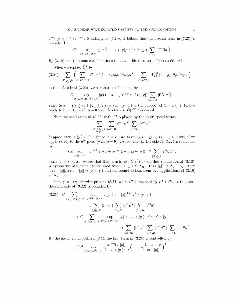
By (3.10) and the same considerations as above, this is in turn O(ε2) as desired.
When we replace GI by
(3.24)∑
1≤J≤DJ 6=I
(
∑
0≤j,k,l≤3
BIJ,jkJ,l (1 − ρJ)∂lu
J∂j∂kuJ +
∑
0≤j,k≤3
AI,jkJJ (1 − ρJ)∂ju
J∂kuJ)
in the left side of (3.22), we see that it is bounded by
C sup(s,y)∈supp(1−ρJ )
|y|(1 + s+ |y|)1+µz1−µ(s, |y|)∑
|β|≤41
|Γβ∂uJ |2.
Since 〈cJs − |y|〉 & 〈s + |y|〉 & z(s, |y|) for (s, |y|) in the support of (1 − ρJ), it followseasily from (3.10) with µ = 0 that this term is O(ε2) as desired.
Next, we shall examine (3.22) with GI replaced by the multi-speed terms∑
1≤J,K≤DK 6=J
∑
|α|≤41
∂ΓαuK∑
|α|≤41
∂ΓαuJ .
Suppose that (s, |y|) ∈ ΛJ . Since J 6= K, we have |cKs − |y|| & (s + |y|). Thus, if weapply (3.10) to the uK piece (with µ = 0), we see that the left side of (3.22) is controlledby
Cε sup(s,|y|)∈ΛJ
|y|1/2(1 + s+ |y|)µ(1 + |cJs− |y||)1−µ∑
|β|≤41
|Γβ∂uJ |.
Since |y| ≈ s on ΛJ , we see that this term is also O(ε2) by another application of (3.10).A symmetric argument can be used when (s, |y|) ∈ ΛK . If (s, |y|) 6∈ ΛJ ∪ ΛK , then|cJs − |y||, |cKs− |y|| ≈ (s + |y|) and the bound follows from two applications of (3.10)with µ = 0.
Finally, we are left with proving (3.22) when GI is replaced by RI + P I . In this case,the right side of (3.22) is bounded by
(3.25) C∑
1≤J,K,L≤D
sup(s,y)∈DI(t,r)
|y|(1 + s+ |y|)1+µz1−µ(s, |y|)
×∑
|β|≤22
|ΓβuJ |∑
|β|≤22
|ΓβuK |∑
|β|≤40
|ΓβuL|
+ C∑
1≤J,K,L≤D
sup(s,y)∈DI(t,r)
|y|(1 + s+ |y|)1+µz1−µ(s, |y|)
×∑
|β|≤22
|ΓβuJ |∑
|β|≤22
|ΓβuK |∑
|β|≤41
|Γβ∂uL|.
By the inductive hypothesis (3.3), the first term in (3.25) is controlled by
Cε3 sup(s,y)∈DI(t,r)
z1−µ(s, |y|)(1 + s+ |y|)1−µ
(
1 + log1 + s+ |y|z(s, |y|)
)3
.
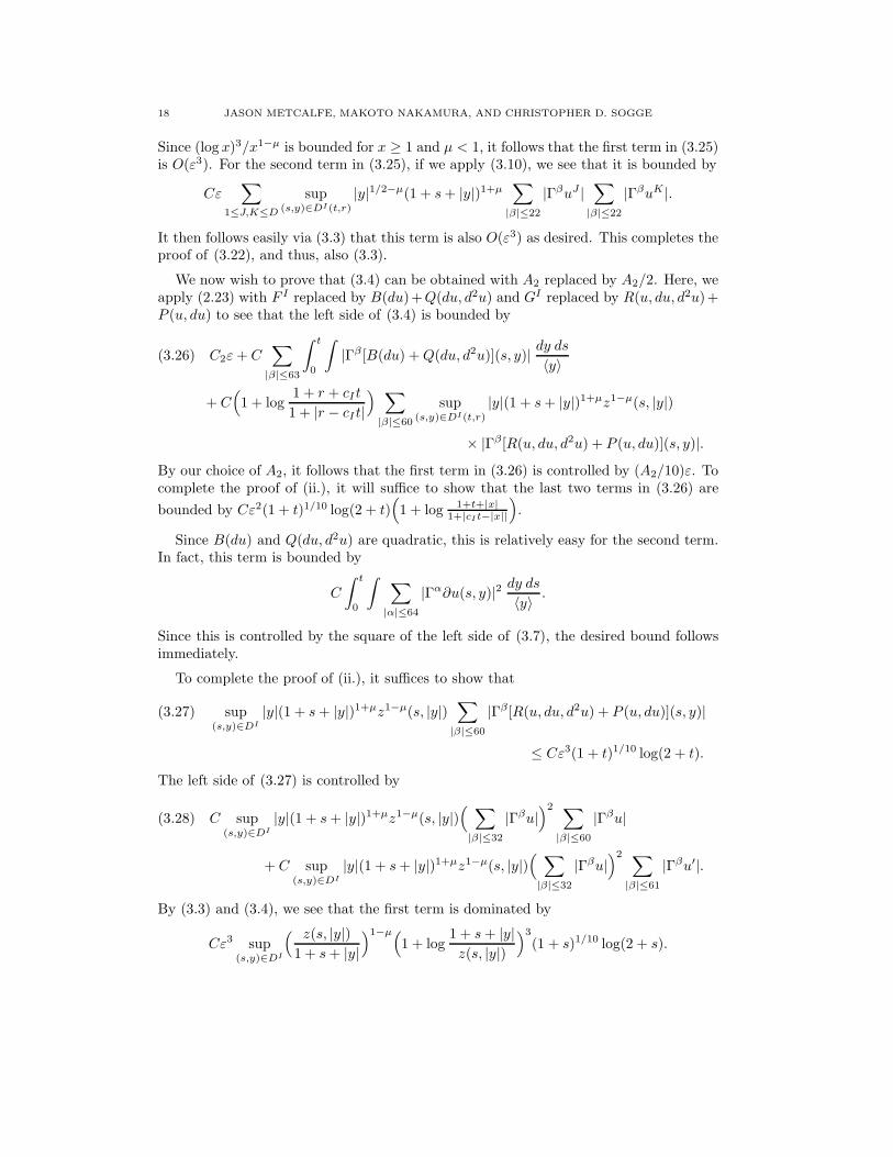
18 JASON METCALFE, MAKOTO NAKAMURA, AND CHRISTOPHER D. SOGGE
Since (log x)3/x1−µ is bounded for x ≥ 1 and µ < 1, it follows that the first term in (3.25)is O(ε3). For the second term in (3.25), if we apply (3.10), we see that it is bounded by
Cε∑
1≤J,K≤D
sup(s,y)∈DI(t,r)
|y|1/2−µ(1 + s+ |y|)1+µ∑
|β|≤22
|ΓβuJ |∑
|β|≤22
|ΓβuK |.
It then follows easily via (3.3) that this term is also O(ε3) as desired. This completes theproof of (3.22), and thus, also (3.3).
We now wish to prove that (3.4) can be obtained with A2 replaced by A2/2. Here, weapply (2.23) with F I replaced by B(du)+Q(du, d2u) and GI replaced by R(u, du, d2u)+P (u, du) to see that the left side of (3.4) is bounded by
(3.26) C2ε+ C∑
|β|≤63
∫ t
0
∫
|Γβ [B(du) +Q(du, d2u)](s, y)| dy ds〈y〉
+ C(
1 + log1 + r + cIt
1 + |r − cIt|)
∑
|β|≤60
sup(s,y)∈DI(t,r)
|y|(1 + s+ |y|)1+µz1−µ(s, |y|)
× |Γβ[R(u, du, d2u) + P (u, du)](s, y)|.By our choice of A2, it follows that the first term in (3.26) is controlled by (A2/10)ε. Tocomplete the proof of (ii.), it will suffice to show that the last two terms in (3.26) are
bounded by Cε2(1 + t)1/10 log(2 + t)(
1 + log 1+t+|x|1+|cIt−|x||
)
.
Since B(du) and Q(du, d2u) are quadratic, this is relatively easy for the second term.In fact, this term is bounded by
C
∫ t
0
∫
∑
|α|≤64
|Γα∂u(s, y)|2 dy ds〈y〉 .
Since this is controlled by the square of the left side of (3.7), the desired bound followsimmediately.
To complete the proof of (ii.), it suffices to show that
(3.27) sup(s,y)∈DI
|y|(1 + s+ |y|)1+µz1−µ(s, |y|)∑
|β|≤60
|Γβ[R(u, du, d2u) + P (u, du)](s, y)|
≤ Cε3(1 + t)1/10 log(2 + t).
The left side of (3.27) is controlled by
(3.28) C sup(s,y)∈DI
|y|(1 + s+ |y|)1+µz1−µ(s, |y|)(
∑
|β|≤32
|Γβu|)2 ∑
|β|≤60
|Γβu|
+ C sup(s,y)∈DI
|y|(1 + s+ |y|)1+µz1−µ(s, |y|)(
∑
|β|≤32
|Γβu|)2 ∑
|β|≤61
|Γβu′|.
By (3.3) and (3.4), we see that the first term is dominated by
Cε3 sup(s,y)∈DI
( z(s, |y|)1 + s+ |y|
)1−µ(
1 + log1 + s+ |y|z(s, |y|)
)3
(1 + s)1/10 log(2 + s).

QUASILINEAR WAVE EQUATIONS SATISFYING THE NULL CONDITION 19
As above, since (log x)3/x1−µ is bounded for x > 1 and µ small, we easily obtain thedesired bound. For the second term in (3.28), applying (2.27) and (3.6) we see that it isdominated by
Cε(1 + t)1/40 sup(s,y)
(1 + s+ |y|)1+µz1−µ(s, |y|)(
∑
|β|≤32
|Γβu|)2
.
Applying (3.3) yields the desired bound (3.27) and finishes the proof of (ii.).
3.3. Proof of (iii.): In this section, we finish the continuity argument, and thus theproof of Theorem 1.2, by showing that (3.5)-(3.7) follow from (3.2)-(3.4).
We begin with (3.5). Outside of ΛI , log 1+t+|x|1+|cIt−|x|| is O(1), and (3.5) follows directly
from (3.3). Within ΛI , we have t ≈ |x|, and (3.5) follows from (2.27) and (3.2).
Next, we want to show that the higher order energy bound (3.6) holds. We will apply(2.5) with
(3.29) γIJ,jk = −∑
1≤K≤D0≤l≤3
BIJ,jkK,l ∂lu
K − CIJ,jk(u, u′)
and
(3.30) GI = BI(du) + P I(u, du).
In order to prove (3.6), by (2.4), (3.2), and an induction argument, it will suffice to provethe following.
Lemma 3.2. Assume that (3.2)-(3.5) hold and M ≤ 70. Additionally, suppose that
(3.31)∑
|α|≤M−1
E(Γαu, t) ≤ Cε(1 + t)Cε+σ
with σ > 0. Then, there is a constant C′ so that
(3.32)∑
|α|≤M
E(Γαu, t) ≤ C′ε(1 + t)C′ε+C′σ.
Proof of Lemma 3.2: Since
(3.33)∑
|α|≤M
|[2γ ,Γα]u| ≤ C
∑
|α|≤M−1
|Γα2u| + C
∑
|α|+|β|≤M|β|≤M−1
|ΓαγΓβ∂2u|
and since (3.3) and (3.5) imply that
(3.34)∑
|α|≤N
|Γαγ| ≤ Cε
1 + t

20 JASON METCALFE, MAKOTO NAKAMURA, AND CHRISTOPHER D. SOGGE
for N ≤ 39, it follows from (2.5) that
(3.35)∑
|α|≤M
∂tE(Γαu, t) ≤ C∑
|α|≤M
‖ΓαB(du)(t, · )‖2 + C∑
|α|≤M
‖ΓαP (u, du)(t, · )‖2
+ C∑
|α|≤M−1
‖ΓαQ(du, d2u)(t, · )‖2 + C∑
|α|≤M−1
‖ΓαR(u, du, d2u)(t, · )‖2
+ C∑
|α|+|β|≤M|β|≤M−1
‖ΓαγΓβ∂2u‖2 +Cε
1 + t
∑
|α|≤M
E(Γαu, t).
Note that it follows from (3.5) that
(3.36)∑
|α|≤M
‖ΓαBI(du)(t, · )‖2 +∑
|α|≤M−1
‖ΓαQI(du, d2u)(t, · )‖2
≤ Cε
1 + t
∑
|α|≤M
E(Γαu, t).
Additionally, by (3.3), we have
∑
|α|≤M
‖ΓαP I(u, du)(t, · )‖2 +∑
|α|≤M−1
‖ΓαRI(u, du, d2u)(t, · )‖2
≤ Cε2∑
|α|≤M,|β|≤1
∥
∥
∥
(1 + log(1 + t)
1 + t+ |x|)2
Γα∂βu(t, · )∥
∥
∥
2.
Since the coefficients of Γ are O(1 + t+ |x|), it follows from (3.3) that this is
(3.37) ≤ Cε3(1 + t)−3/2+ + Cε2(1 + log(1 + t))2
1 + t
∑
|α|≤M−1
E(Γαu, t)
+Cε2(1 + log(1 + t))2
(1 + t)2
∑
|α|≤M
E(Γαu, t).
The first term on the right side corresponds to the case |α| = |β| = 0 on the right sideof the previous equation. Similarly, the second term is for the case |β| = 0, and the lastterm bounds the case |α|, |β| 6= 0. By a similar argument, the fifth term on the right of(3.35) is also controlled by the right sides of (3.36) and (3.37). Thus, we see that
(3.38)∑
|α|≤M
∂tE(Γαu, t) ≤ Cε
1 + t
∑
|α|≤M
E(Γαu, t)
+ Cε3(1 + t)−3/2+δ +Cε2(1 + log(1 + t))2
1 + t
∑
|α|≤M−1
E(Γαu, t).
Integrating both sides in t, applying the smallness assumption on the data (1.14)and the inductive hypothesis (3.31), and using Gronwall’s inequality yields (3.32) asdesired.
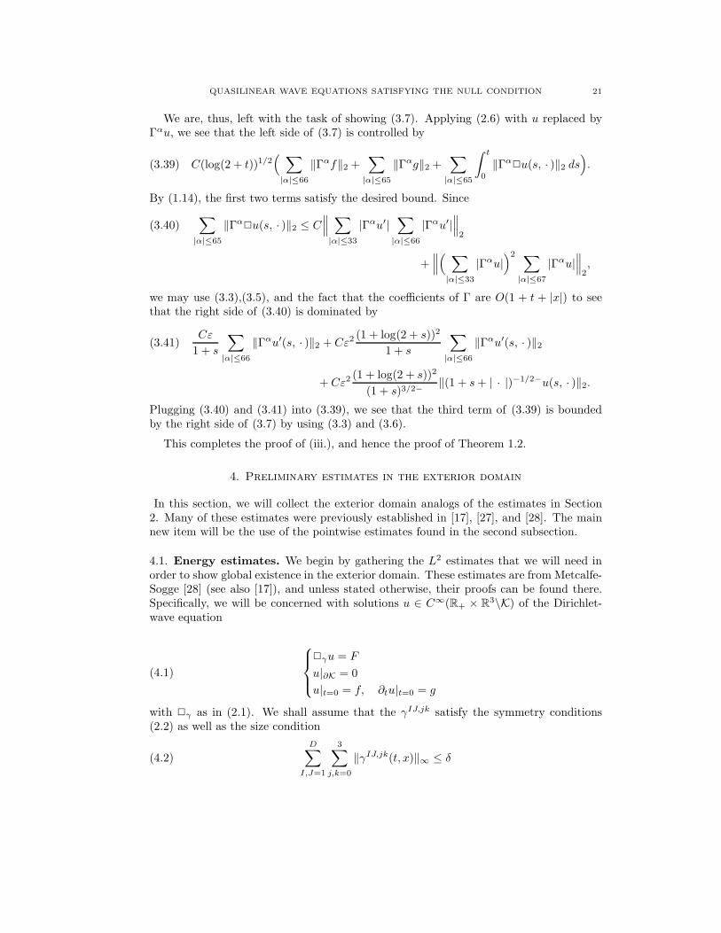
QUASILINEAR WAVE EQUATIONS SATISFYING THE NULL CONDITION 21
We are, thus, left with the task of showing (3.7). Applying (2.6) with u replaced byΓαu, we see that the left side of (3.7) is controlled by
(3.39) C(log(2 + t))1/2(
∑
|α|≤66
‖Γαf‖2 +∑
|α|≤65
‖Γαg‖2 +∑
|α|≤65
∫ t
0
‖Γα2u(s, · )‖2 ds
)
.
By (1.14), the first two terms satisfy the desired bound. Since
(3.40)∑
|α|≤65
‖Γα2u(s, · )‖2 ≤ C
∥
∥
∥
∑
|α|≤33
|Γαu′|∑
|α|≤66
|Γαu′|∥
∥
∥
2
+∥
∥
∥
(
∑
|α|≤33
|Γαu|)2 ∑
|α|≤67
|Γαu|∥
∥
∥
2,
we may use (3.3),(3.5), and the fact that the coefficients of Γ are O(1 + t + |x|) to seethat the right side of (3.40) is dominated by
(3.41)Cε
1 + s
∑
|α|≤66
‖Γαu′(s, · )‖2 + Cε2(1 + log(2 + s))2
1 + s
∑
|α|≤66
‖Γαu′(s, · )‖2
+ Cε2(1 + log(2 + s))2
(1 + s)3/2− ‖(1 + s+ | · |)−1/2−u(s, · )‖2.
Plugging (3.40) and (3.41) into (3.39), we see that the third term of (3.39) is boundedby the right side of (3.7) by using (3.3) and (3.6).
This completes the proof of (iii.), and hence the proof of Theorem 1.2.
4. Preliminary estimates in the exterior domain
In this section, we will collect the exterior domain analogs of the estimates in Section2. Many of these estimates were previously established in [17], [27], and [28]. The mainnew item will be the use of the pointwise estimates found in the second subsection.
4.1. Energy estimates. We begin by gathering the L2 estimates that we will need inorder to show global existence in the exterior domain. These estimates are from Metcalfe-Sogge [28] (see also [17]), and unless stated otherwise, their proofs can be found there.Specifically, we will be concerned with solutions u ∈ C∞(R+ × R
3\K) of the Dirichlet-wave equation
(4.1)
2γu = F
u|∂K = 0
u|t=0 = f, ∂tu|t=0 = g
with 2γ as in (2.1). We shall assume that the γIJ,jk satisfy the symmetry conditions(2.2) as well as the size condition
(4.2)
D∑
I,J=1
3∑
j,k=0
‖γIJ,jk(t, x)‖∞ ≤ δ

22 JASON METCALFE, MAKOTO NAKAMURA, AND CHRISTOPHER D. SOGGE
for δ sufficiently small (depending on the wave speeds). The energy estimate will involvebounds for the gradient of the perturbation terms
‖γ′(t, · )‖∞ =
D∑
I,J=1
3∑
j,k,l=0
‖∂lγIJ,jk(t, · )‖∞,
and the energy form associated with 2γ , e0(u) =∑D
I=1 eI0(u), where eI
0(u) is given by(2.3).
The most basic estimate will lead to a bound for
EM (t) = EM (u)(t) =
∫ M∑
j=0
e0(∂jt u)(t, x) dx.
Lemma 4.1. Fix M = 0, 1, 2, . . . , and assume that the perturbation terms γIJ,jk satisfy
(2.2) and (4.2). Suppose also that u ∈ C∞ solves (4.1) and for every t, u(t, x) = 0 for
large x. Then there is an absolute constant C so that
(4.3) ∂tE1/2M (t) ≤ C
M∑
j=0
‖2γ∂jt u(t, · )‖2 + C‖γ′(t, · )‖∞E1/2
M (t).
Before stating the next result, let us introduce some notation. If P = P (t, x,Dt, Dx)is a differential operator, we shall let
[P, γkl∂k∂l]u =∑
1≤I,J≤D
∑
0≤k,l≤3
|[P, γIJ,kl∂k∂l]uJ |.
In order to generalize the above energy estimate to include the more general vectorfields L,Z, we will need to use a variant of the scaling vector field L. We fix a bumpfunction η ∈ C∞(R3) with η(x) = 0 for x ∈ K and η(x) = 1 for |x| > 1. Then, set
L = η(x)r∂r + t∂t. Using this variant of the scaling vector field and an elliptic regularityargument, one can establish
Proposition 4.2. Suppose that the constant in (4.2) is small. Suppose further that
(4.4) ‖γ′(t, · )‖∞ ≤ δ/(1 + t),
and
(4.5)∑
j+µ≤N0+ν0
µ≤ν0
(
‖Lµ∂jt 2γu(t, · )‖2 + ‖[Lµ∂j
t , γkl∂k∂l]u(t, · )‖2
)
≤ δ
1 + t
∑
j+µ≤N0+ν0
µ≤ν0
‖Lµ∂jt u
′(t, · )‖2 +Hν0,N0(t),

QUASILINEAR WAVE EQUATIONS SATISFYING THE NULL CONDITION 23
where N0 and ν0 are fixed. Then
(4.6)∑
|α|+µ≤N0+ν0
µ≤ν0
‖Lµ∂αu′(t, · )‖2
≤ C∑
|α|+µ≤N0+ν0−1µ≤ν0
‖Lµ∂α2u(t, · )‖2 +C(1 + t)Aδ
∑
µ+j≤N0+ν0
µ≤ν0
(∫
e0(Lµ∂j
t u)(0, x) dx
)1/2
+ C(1 + t)Aδ(
∫ t
0
∑
|α|+µ≤N0+ν0−1µ≤ν0−1
‖Lµ∂α2u(s, · )‖2 ds+
∫ t
0
Hν0,N0(s) ds
)
+ C(1 + t)Aδ
∫ t
0
∑
|α|+µ≤N0+ν0
µ≤ν0−1
‖Lµ∂αu′(s, · )‖L2(|x|<1) ds,
where the constants C and A are absolute constants.
In practice Hν0,N0(t) will involve L2
x norms of |Lµ∂αu′|2 with µ + |α| much smallerthan N0 + ν0, and so the integral involving Hν0,N0
can be dealt with using an inductiveargument and the weighted L2
tL2x estimates that will be presented at the end of this
subsection.
In proving our existence results for (1.1), the key step will be to obtain a priori L2-estimates involving LµZαu′. Begin by setting
(4.7) YN0,ν0(t) =
∫
∑
|α|+µ≤N0+ν0
µ≤ν0
e0(LµZαu)(t, x) dx.
We, then, have the following proposition which shows how the LµZαu′ estimates can beobtained from the ones involving Lµ∂αu′.
Proposition 4.3. Suppose that the constant δ in (4.2) is small and that (4.4) holds.
Then,
(4.8) ∂tYN0,ν0≤ CY
1/2N0,ν0
∑
|α|+µ≤N0+ν0
µ≤ν0
‖2γLµZαu(t, · )‖2 + C‖γ′(t, · )‖∞YN0,ν0
+ C∑
|α|+µ≤N0+ν0+1µ≤ν0
‖Lµ∂αu′(t, · )‖2L2(|x|<1).
As in [16] and [17] we shall also require some weighted L2tL
2x estimates. They will
be used, for example, to control the local L2 norms such as the last term in (4.8). Forconvenience, for the remainder of this subsection, allow 2 = ∂2
t − ∆ to denote theunit speed, scalar d’Alembertian. The transition from the following estimates to thoseinvolving (1.2) is straightforward. Also, allow
ST = [0, T ]× R3\K
to denote the time strip of height T in R+ × R3\K.
24 JASON METCALFE, MAKOTO NAKAMURA, AND CHRISTOPHER D. SOGGE
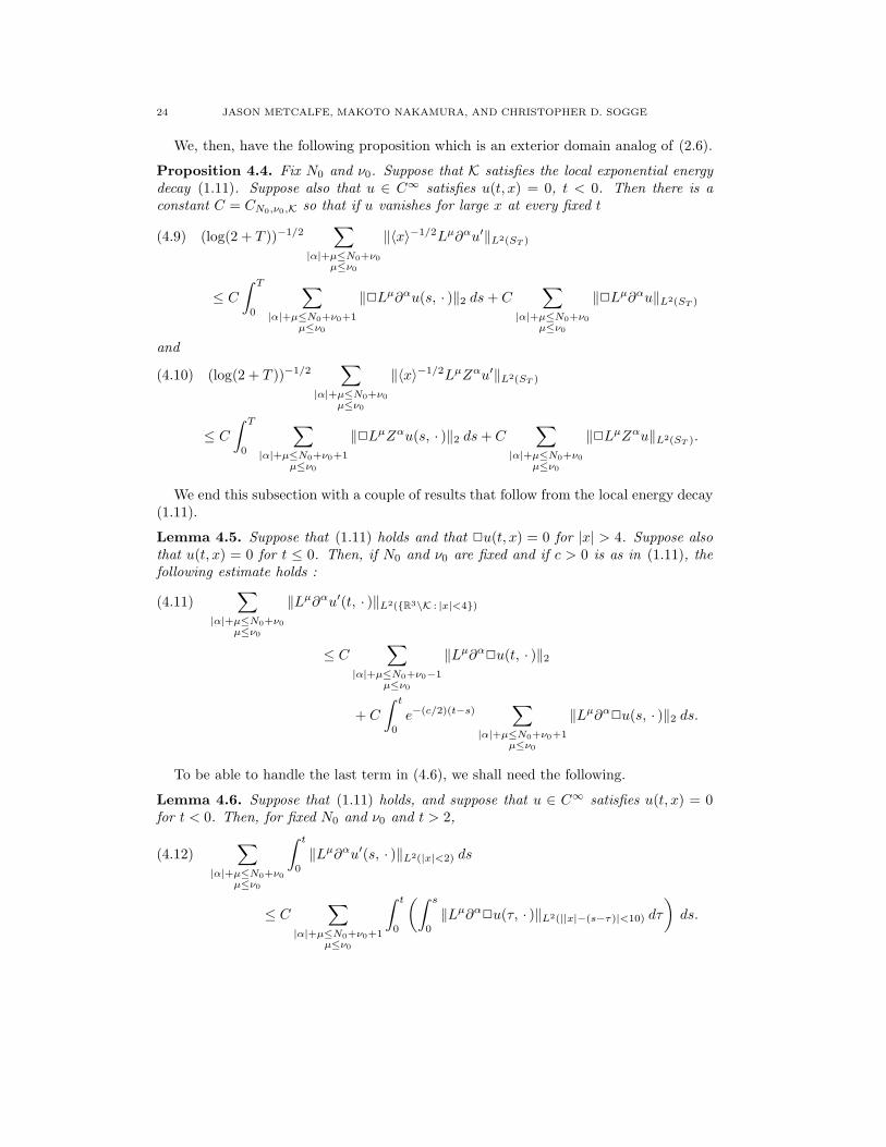
We, then, have the following proposition which is an exterior domain analog of (2.6).
Proposition 4.4. Fix N0 and ν0. Suppose that K satisfies the local exponential energy
decay (1.11). Suppose also that u ∈ C∞ satisfies u(t, x) = 0, t < 0. Then there is a
constant C = CN0,ν0,K so that if u vanishes for large x at every fixed t
(4.9) (log(2 + T ))−1/2∑
|α|+µ≤N0+ν0
µ≤ν0
‖〈x〉−1/2Lµ∂αu′‖L2(ST )
≤ C
∫ T
0
∑
|α|+µ≤N0+ν0+1µ≤ν0
‖2Lµ∂αu(s, · )‖2 ds+ C∑
|α|+µ≤N0+ν0
µ≤ν0
‖2Lµ∂αu‖L2(ST )
and
(4.10) (log(2 + T ))−1/2∑
|α|+µ≤N0+ν0
µ≤ν0
‖〈x〉−1/2LµZαu′‖L2(ST )
≤ C
∫ T
0
∑
|α|+µ≤N0+ν0+1µ≤ν0
‖2LµZαu(s, · )‖2 ds+ C∑
|α|+µ≤N0+ν0
µ≤ν0
‖2LµZαu‖L2(ST ).
We end this subsection with a couple of results that follow from the local energy decay(1.11).
Lemma 4.5. Suppose that (1.11) holds and that 2u(t, x) = 0 for |x| > 4. Suppose also
that u(t, x) = 0 for t ≤ 0. Then, if N0 and ν0 are fixed and if c > 0 is as in (1.11), the
following estimate holds :
(4.11)∑
|α|+µ≤N0+ν0
µ≤ν0
‖Lµ∂αu′(t, · )‖L2(R3\K : |x|<4)
≤ C∑
|α|+µ≤N0+ν0−1µ≤ν0
‖Lµ∂α2u(t, · )‖2
+ C
∫ t
0
e−(c/2)(t−s)∑
|α|+µ≤N0+ν0+1µ≤ν0
‖Lµ∂α2u(s, · )‖2 ds.
To be able to handle the last term in (4.6), we shall need the following.
Lemma 4.6. Suppose that (1.11) holds, and suppose that u ∈ C∞ satisfies u(t, x) = 0for t < 0. Then, for fixed N0 and ν0 and t > 2,
(4.12)∑
|α|+µ≤N0+ν0
µ≤ν0
∫ t
0
‖Lµ∂αu′(s, · )‖L2(|x|<2) ds
≤ C∑
|α|+µ≤N0+ν0+1µ≤ν0
∫ t
0
(∫ s
0
‖Lµ∂α2u(τ, · )‖L2(||x|−(s−τ)|<10) dτ
)
ds.

QUASILINEAR WAVE EQUATIONS SATISFYING THE NULL CONDITION 25
4.2. Pointwise estimates. Here, we will describe the various pointwise estimates thatwe shall require. These include variants of those of Keel-Smith-Sogge [17] and Metcalfe-Sogge [28] and exterior domain analogs of the estimates of Kubota-Yokoyama [21].
Let us begin with the former. We will need analogs of the pointwise estimates of [17]and [28] that allow Cauchy data that vanishes in a neighborhood of the obstacle. That is,we will estimate solutions of the scalar wave equation with boundary (∂2
t − ∆)w(t, x) =F (t, x). Additionally, we will require that w(0, x) = ∂tw(0, x) = 0 if |x| ≤ 6, andF (t, x) = 0 if |x| ≤ 6 and 0 ≤ t ≤ 1. With these assumptions, we can greatly reduce thetechnical details involving the compatibility conditions. In the sequel, we will reduce ourstudy to this case. Assuming, as we do throughout, that K ⊂ x ∈ R
3 : |x| < 1, wehave
Theorem 4.7. Suppose that the local energy decay bounds (1.11) hold for K. Addition-
ally, assume that w(t, x) = 0 for x ∈ ∂K, w(0, x) = ∂tw(0, x) = 0 for |x| ≤ 6, and
F (t, x) = 0 if 0 ≤ t ≤ 1 and |x| ≤ 6. Then, if |α| = M ,
(4.13) (1 + t+ |x|)|LνZαw(t, x)| ≤ C∑
j+|β|+k≤ν+M+8j≤1
‖〈x〉j+|β|∂βx∂
k+jt w(0, x)‖2
+ C
∫ t
0
∫
R3\K
∑
|β|+µ≤M+ν+7µ≤ν+1
|LµZβF (s, y)| dy ds|y|
+ C
∫ t
0
∑
|β|+µ≤M+ν+4µ≤ν+1
‖Lµ∂βF (s, · )‖L2(x∈R3\K : |x|<2) ds.
Proof of Theorem 4.7: If w has vanishing Cauchy data with F (t, x) = 0 for 0 ≤ t ≤ 1 andx ∈ R
3\K, (4.13) follows from Theorem 3.1 in [28]. We, thus, may assume F (t, x) = 0 for0 ≤ t < ∞ and |x| ≤ 6 and that the Cauchy data is as stated above. The proof followsfrom the arguments of [28] for the inhomogeneous case very closely. We include a sketchof the proof for completeness.
We first note that if we argue as in [17] (Lemma 4.2) we have
(4.14) (1 + t+ |x|)|LνZαw(t, x)| ≤ C∑
j+|β|+k≤M+ν+4j≤1
‖〈x〉j+|β|∂βx∂
k+jt w(0, x)‖2
+ C∑
|β|+µ≤M+ν+3µ≤ν+1
∫ t
0
∫
R3\K|LµZβF (s, y)| dy ds|y|
+ C∑
|β|+µ≤M+ν+1µ≤ν
sup0≤s≤t|y|≤2
(1 + s)|Lµ∂βw(s, y)|.
While the arguments in [17] are given for vanishing Cauchy data, straightforward modi-fications allow the current setting.

26 JASON METCALFE, MAKOTO NAKAMURA, AND CHRISTOPHER D. SOGGE
It remains to prove bound in the region |x| < 2. We show
(4.15)∑
|β|+µ≤M+ν+1µ≤ν
sup0≤s≤t|y|≤2
(1 + s)|Lµ∂βw(s, y)| ≤ C∑
j+|α|+k≤M+ν+8j≤1
‖〈x〉j+|α|∂αx ∂
j+kt w(0, x)‖2
+ C∑
|β|+µ≤M+ν+7µ≤ν+1
∫ t
0
∫
R3\K|LµZβF (s, y)| dy ds|y| .
To see this, write w = w0 + wr where w0 solves the boundaryless wave equation (∂2t −
∆)w0 = F with initial data w0(0, · ) = w(0, · ) and ∂tw0(0, · ) = ∂tw(0, · ). If we fixη ∈ C∞
0 (R3) with η(x) ≡ 1 for |x| < 2 and η(x) ≡ 0 for |x| ≥ 3 and set w = ηw0 +wr, itfollows that w = w for |x| < 2. Thus, it will suffice to show (4.15) with w replaced by w.Notice that w solves the Dirichlet-wave equation
(∂2t − ∆)w = −2∇η · ∇xw0 − (∆η)w0
with vanishing initial data since the support of η does not intersect the supports of F ,w(0, · ) and ∂tw(0, · ) and that this forcing term vanishes unless 2 ≤ |x| ≤ 3.
In order to complete the proof, we begin by noting the following consequence of theFundamental Theorem of Calculus:
sup|y|≤2
|(1 + s)Lµ∂βw(s, y)| ≤ C∑
j=0,1
sup|y|≤2
∫ s
0
|(τ∂τ )jLµ∂βw(τ, y)| dτ.
Using Sobolev’s lemma and the fact that the Dirichlet condition allows us to control wlocally by w′, we see that the left hand side of (4.15) is bounded by
C∑
|β|+µ≤M+ν+3µ≤ν
∑
j=0,1
∫ t
0
‖(τdτ)jLµ∂βw(τ, y)‖L2(R3\K,|x|≤4)dτ
≤ C∑
|β|+µ≤M+ν+3µ≤ν+1
∫ t
0
‖Lµ∂βw′(τ, y)‖L2(R3\K,|x|≤4)dτ
By (4.11), it follows that the right side of the above estimate is controlled by
C
∫ t
0
∑
|β|+µ≤M+ν+5µ≤ν+1
‖Lµ∂βw0(s, · )‖L∞(2≤|x|≤3) ds.

QUASILINEAR WAVE EQUATIONS SATISFYING THE NULL CONDITION 27
From (2.10), (2.16), and the fact that 1/t ≤ 1/|y| on the domain of integration in(2.10), we have
(4.16) ‖Lµ∂βw0(s, · )‖L∞(2≤|x|≤3) ≤ C∑
|α|≤2
∫
|s−|y||≤4
|(Ωα∇Lµ∂βw0)(0, y)|dy
|y|
+ C∑
|α|≤2
∫
|s−|y||≤4
|(ΩαLµ∂βw0)(0, y)|dy
|y|2
+ C∑
|α|≤2
∫
|s−|y||≤4
|(Ωα∂tLµ∂βw0)(0, y)|
dy
|y|
+ C∑
|α|≤2
∫ s
0
∫
|s−τ−|y||≤4
|Ωα(∂2t − ∆)Lµ∂βw0(τ, y)|
dy dτ
|y| .
Since the sets Λs = y : |s− |y|| ≤ 4 satisfy Λs ∩Λ′s = ∅ if |s− s′| ≥ 10, if we sum over
|β| + µ ≤ M + ν + 5, µ ≤ ν + 1, and integrate over s ∈ [0, t], we conclude that the leftside of (4.15) is controlled by
C∑
k+|β|≤M+ν+7
∫
〈x〉|β||(∂β∂kt ∇w)(0, y)| dy|y|
+ C∑
k+|β|≤M+ν+7
∫
〈x〉|β||(∂β∂kt w)(0, y)| dy|y|2
+ C∑
k+|β|≤M+ν+7
∫
〈x〉|β||(∂β∂kt ∂tw)(0, y)| dy|y|
+ C∑
|β|+µ≤M+ν+7µ≤ν+1
∫ t
0
∫
R3\K|LµZβF (s, y)| dy ds|y| .
Using the Schwarz inequality, (4.15), and thus (4.13), follows.
For the remainder of the estimates in this section, it will suffice to take w to be asolution to the following Dirichlet-wave equation with vanishing initial data.
(4.17)
(∂2t − c2I∆)w(t, x) = F (t, x), (t, x) ∈ R+ × R
3\Kw(t, x) = 0, x ∈ ∂Kw(t, x) = 0, t ≤ 0.
In the sequel, we will reduce showing that (1.1) has a global solution to showing that anequivalent system of nonlinear wave equations with vanishing data has a global solution.Since the previous theorem will suffice to make this reduction, it is unnecessary to considernonvanishing Cauchy data in the subsequent estimates.
We will need the following version of (4.13) that does not require a loss of a scalingvector field on the right.
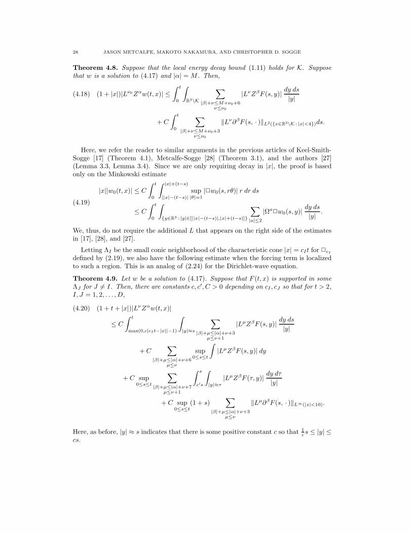
28 JASON METCALFE, MAKOTO NAKAMURA, AND CHRISTOPHER D. SOGGE
Theorem 4.8. Suppose that the local energy decay bound (1.11) holds for K. Suppose
that w is a solution to (4.17) and |α| = M . Then,
(4.18) (1 + |x|)|Lν0Zαw(t, x)| ≤∫ t
0
∫
R3\K
∑
|β|+ν≤M+ν0+6ν≤ν0
|LνZβF (s, y)| dy ds|y|
+ C
∫ t
0
∑
|β|+ν≤M+ν0+3ν≤ν0
‖Lν∂βF (s, · )‖L2(x∈R3\K : |x|<4)ds.
Here, we refer the reader to similar arguments in the previous articles of Keel-Smith-Sogge [17] (Theorem 4.1), Metcalfe-Sogge [28] (Theorem 3.1), and the authors [27](Lemma 3.3, Lemma 3.4). Since we are only requiring decay in |x|, the proof is basedonly on the Minkowski estimate
|x||w0(t, x)| ≤ C
∫ t
0
∫ |x|+(t−s)
||x|−(t−s)|sup|θ|=1
|2w0(s, rθ)| r dr ds
≤ C
∫ t
0
∫
y∈R3 : |y|∈[||x|−(t−s)|,|x|+(t−s)]
∑
|a|≤2
|Ωa2w0(s, y)|
dy ds
|y| .
(4.19)
We, thus, do not require the additional L that appears on the right side of the estimatesin [17], [28], and [27].
Letting ΛI be the small conic neighborhood of the characteristic cone |x| = cIt for 2cI
defined by (2.19), we also have the following estimate when the forcing term is localizedto such a region. This is an analog of (2.24) for the Dirichlet-wave equation.
Theorem 4.9. Let w be a solution to (4.17). Suppose that F (t, x) is supported in some
ΛJ for J 6= I. Then, there are constants c, c′, C > 0 depending on cI , cJ so that for t > 2,I, J = 1, 2, . . . , D,
(4.20) (1 + t+ |x|)|LνZαw(t, x)|
≤ C
∫ t
max(0,c|cIt−|x||−1)
∫
|y|≈s
∑
|β|+µ≤|α|+ν+3µ≤ν+1
|LµZβF (s, y)| dy ds|y|
+ C∑
|β|+µ≤|α|+ν+6µ≤ν
sup0≤s≤t
∫
|LµZβF (s, y)| dy
+ C sup0≤s≤t
∑
|β|+µ≤|α|+ν+7µ≤ν+1
∫ s
c′s
∫
|y|≈τ
|LµZβF (τ, y)| dy dτ|y|
+ C sup0≤s≤t
(1 + s)∑
|β|+µ≤|α|+ν+3µ≤ν
‖Lµ∂βF (s, · )‖L∞(|x|<10).
Here, as before, |y| ≈ s indicates that there is some positive constant c so that 1cs ≤ |y| ≤
cs.

QUASILINEAR WAVE EQUATIONS SATISFYING THE NULL CONDITION 29
We shall need an analog of Lemma 2.3, the result of Kubota-Yokoyama [21], forDirichlet-wave equations. With z as in (2.20), we have
Theorem 4.10. Let I = 1, 2, . . .D, and let w be a solution to (4.17). Then, for any
µ > 0,
(4.21) (1 + t+ r)(
1 + log1 + t+ r
1 + |cIt− r|)−1
|Lν0Zαw(t, x)|
≤ C sup(s,y)
|y|(1 + s+ |y|)1+µz1−µ(s, |y|)∑
|β|+ν≤|α|+ν0
ν≤ν0
|LνZβF (s, y)|
+ C sup(s,y)
|y|(1 + s+ |y|)1+µz1−µ(s, |y|)∑
|β|+ν≤|α|+ν0+3ν≤ν0
|Lν∂β∂F (s, y)|.
The proofs of Theorem 4.9 and Theorem 4.10 are quite similar, and we will onlyprovide the proof of the latter. In order to prove Theorem 4.9, we need only replace theapplications of (2.21) by (2.24) which is the appropriate free space analog of (4.20).
Proof of Theorem 4.10: We begin by claiming that
(4.22) (1 + t+ r)(
1 + log1 + t+ r
1 + |cIt− r|)−1
|Lν0Z
αw(t, x)|
≤ C sup(s,y)
|y|(1 + s+ |y|)1+µz1−µ(s, |y|)∑
|β|+ν≤|α|+ν0
ν≤ν0
|LνZβF (s, y)|
+ C sup(s,y),|y|<2
(1 + s)∑
|β|+ν≤|α|+ν0+1ν≤ν0
|Lν∂βw(s, y)|.
Indeed, over |x| < 2, the left side is clearly bounded by the second term on the rightside since the coefficients of Z are O(1) on this set. To see the estimate on |x| ≥ 2, wefix a cutoff function ρ ∈ C∞ where ρ(x) ≡ 0 for |x| < 3/2 and ρ(x) ≡ 1 for |x| > 2. Ifwe let wj denote the solutions to the boundaryless wave equations (∂2
t − c2I∆)wj = Gj ,j = 1, 2 where G1 = ρ(∂2
t − c2I∆)w and G2 = −2c2I∇ρ · ∇xw − c2I(∆ρ)w, we see thatw = w1 + w2. Since [2, Z] = 0 and [2, L] = 22, we can establish the bound for the w1
piece by applying (2.21). Arguing as in Lemma 4.2 of Keel-Smith-Sogge [17], we see thatthe w2 term is bounded by the second term on the right side of (4.22).
To finish the proof, it thus suffices to show
(4.23) sup0≤s≤t
(1 + s)∑
|β|+ν≤|α|+ν0+1ν≤ν0
‖Lν∂βw(s, · )‖L∞(|x|<2)
≤ C sup(s,y)
|y|(1 + s+ |y|)1+µz1−µ(s, |y|)∑
ν≤ν0
|LνF (s, y)|
+ C sup(s,y)
|y|(1 + s+ |y|)1+µz1−µ(s, |y|)∑
|β|+ν≤|α|+ν0+3ν≤ν0
|Lν∂β∂F (s, y)|.

30 JASON METCALFE, MAKOTO NAKAMURA, AND CHRISTOPHER D. SOGGE
When F (s, y) = 0 for |y| > 10, we can apply the following lemma, which is essentiallyLemma 3.3 from [27].
Lemma 4.11. Suppose that w is as above. Suppose further that (∂2t − c2I∆)w(s, y) =
F (s, y) = 0 if |y| > 10. Then,
(4.24) (1 + t) sup|x|<2
|Lν∂αw(t, x)| ≤ C sup0≤s≤t
∑
|β|+µ≤|α|+ν+2µ≤ν
(1 + s)‖Lµ∂βF (s, · )‖2.
Since F is supported on |y| < 10 and since |y| is bounded below on the complementof K, it follows that this term is controlled by the right side of (4.23).
We also need an estimate for solutions whose forcing terms vanish near the obstacle.Assume now that F (s, y) = 0 for |y| < 5 and write w = w0 + wr where w0 solvesthe boundaryless wave equation (∂2
t − c2I∆)w0 = F with vanishing initial data. Fixingη ∈ C∞
0 (R3) satisfying η(x) ≡ 1 for |x| < 2 and η(x) ≡ 0 for |x| ≥ 3 and settingw = ηw0 +wr, we see that w = w on |x| < 2. Since w solves the Dirichlet-wave equation
(∂2t − c2I∆)w = −2cI∇η · ∇xw0 − c2I(∆η)w0 = G
and G vanishes unless 2 ≤ |x| ≤ 3, we may apply Lemma 4.11 to see
(1 + t) sup|x|<2
∑
|β|+ν≤|α|+ν0+1ν≤ν0
|Lν∂βw(t, x)| ≤ (1 + t) sup|x|<2
∑
|β|+ν≤|α|+ν0+1ν≤ν0
|Lν∂βw(t, x)|
≤ C sup0≤s≤t
∑
|β|+ν≤|α|+ν0+3ν≤ν0
(1 + s)|Lν∂βw′0(s, · )‖L∞(|x|<3)
+ C sup0≤s≤t
(1 + s)∑
ν≤ν0
‖Lνw0(s, · )‖L∞(|x|<3).
We thus see that (4.23) follows from an application of (2.21).
4.3. Sobolev-type estimates. In this subsection, we state the exterior domain analogsof Lemma 2.8 that we will require. The proofs of the relevant extensions to the exteriordomain can be found in [27] (Lemma 4.2 and Lemma 4.3).
Lemma 4.12. Suppose that u(t, x) ∈ C∞0 (R × R
3\K) vanishes for x ∈ ∂K. Then, if
|α| = M and ν are fixed
(4.25) ‖〈cIt− r〉LνZα∂2u(t, · )‖2 ≤ C∑
|β|+µ≤M+ν+1µ≤ν+1
‖LµZβu′(t, · )‖2
+ C∑
|β|+µ≤M+νµ≤ν
‖〈t+ r〉LµZβ(∂2t − c2I∆)u(t, · )‖2 + C(1 + t)
∑
µ≤ν
‖Lµu′(t, · )‖L2(|x|<2).

QUASILINEAR WAVE EQUATIONS SATISFYING THE NULL CONDITION 31
and
(4.26) r1/2+θ〈cI t− r〉1−θ |∂LνZαu(t, x)| ≤ C∑
|β|+µ≤M+ν+2µ≤ν+1
‖LµZβu′(t, · )‖2
+C∑
|β|+µ≤M+ν+1µ≤ν
‖〈t+ r〉LµZβ(∂2t − c2I∆)u(t, · )‖2 +C(1+ t)
∑
µ≤ν
‖Lµu′(t, · )‖L∞(|x|<2)
for any 0 ≤ θ ≤ 1/2.
5. The continuity argument in the exterior domain
In this section, we will prove the main result, Theorem 1.1. We shall take N = 322in the smallness hypothesis (1.12). This can be improved considerably, but here we willtake such a liberty in order to avoid unnecessary technicalities.
Our global existence theorem will be based on the following local existence result.
Theorem 5.1. Suppose that f and g are as in Theorem 1.1 with N ≥ 7 in (1.12). Then,
there is a T > 0 so that the initial value problem (1.1) with this initial data has a C2
solution satisfying
u ∈ L∞([0, T ];HN(R3\K)) ∩ C0,1([0, T ];HN−1(R3\K)).
The supremum of such T is equal to the supremum of all T where the initial value problem
has a C2 solution with ∂αu bounded for all |α| ≤ 2. Also, one can take T ≥ 2 if
‖f‖HN + ‖g‖HN−1 is small enough.
This is essentially from Keel-Smith-Sogge [15] (Theorem 9.4 and Lemma 9.6). Thesewere only stated for diagonal single-speed systems. Since the proofs relied only on energyestimates, the results extend to the current setting provided (1.7) and (1.8) hold.
Prior to setting up the continuity argument, it is convenient to reduce to an equivalentsystem of nonlinear equations with vanishing Cauchy data. By doing so, we will avoidcomplications related to the compatibility conditions. We first reduce to an equivalentsystem of nonlinear equations whose data vanish in a neighborhood of the obstacle.Initially, we note that if ε in (1.12) is sufficiently small, then there is a constant C so that
(5.1) sup0≤t≤2
∑
|α|≤322
‖∂αu(t, · )‖L2(|x|≤10) ≤ Cε.
This, again, follows from the local existence theory (see, e.g., [15]). On the other hand,over t ∈ [0, 2] × |x| ≥ 6, by finite propagation speed, u corresponds to a solution ofthe boundaryless wave equation 2u = F (u, du, d2u). If we take N = 322 in (1.14), it isclear that the analogs of (3.4) and (3.6) yield(5.2)
sup0≤t≤2
∑
|α|+µ≤321
‖LµZαu′(t, · )‖L2(|x|≥6) + sup0≤t≤2|x|≥6
(1 + t+ |x|)∑
|α|+µ≤311
|LµZαu(t, x)| ≤ Cε.
Here we have used our assumption that K ⊂ |x| < 1.
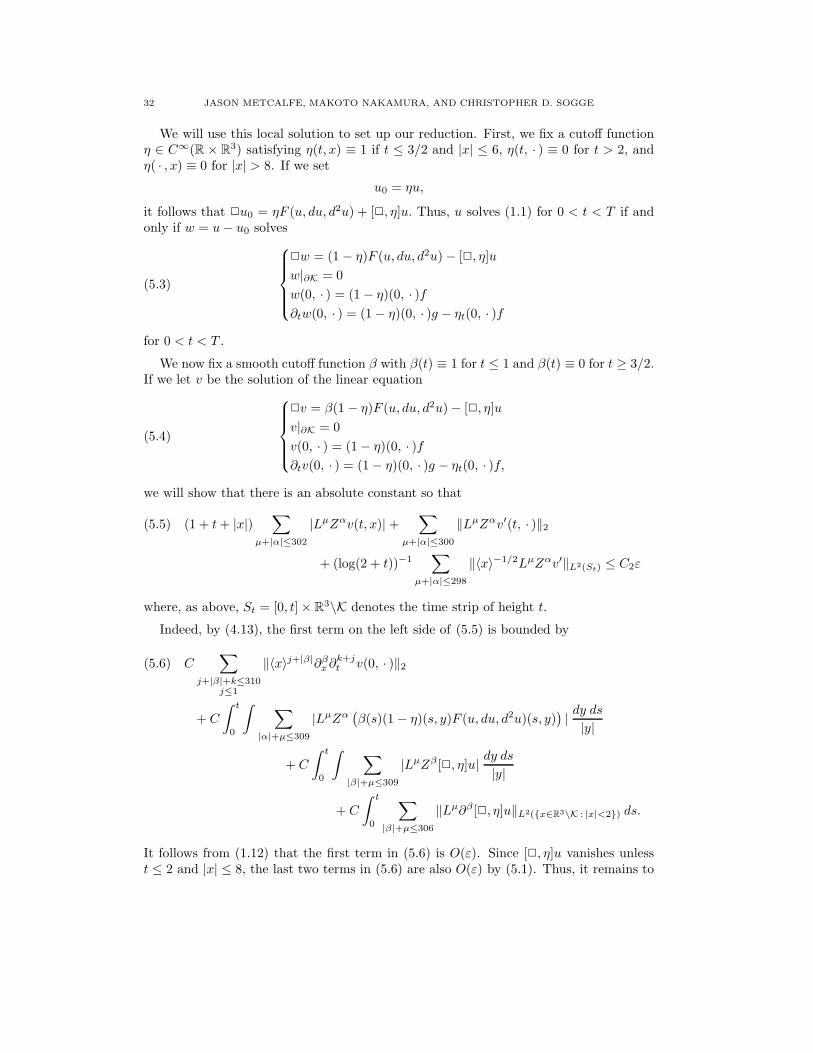
32 JASON METCALFE, MAKOTO NAKAMURA, AND CHRISTOPHER D. SOGGE
We will use this local solution to set up our reduction. First, we fix a cutoff functionη ∈ C∞(R × R
3) satisfying η(t, x) ≡ 1 if t ≤ 3/2 and |x| ≤ 6, η(t, · ) ≡ 0 for t > 2, andη( · , x) ≡ 0 for |x| > 8. If we set
u0 = ηu,
it follows that 2u0 = ηF (u, du, d2u) + [2, η]u. Thus, u solves (1.1) for 0 < t < T if andonly if w = u− u0 solves
(5.3)
2w = (1 − η)F (u, du, d2u) − [2, η]u
w|∂K = 0
w(0, · ) = (1 − η)(0, · )f∂tw(0, · ) = (1 − η)(0, · )g − ηt(0, · )f
for 0 < t < T .
We now fix a smooth cutoff function β with β(t) ≡ 1 for t ≤ 1 and β(t) ≡ 0 for t ≥ 3/2.If we let v be the solution of the linear equation
(5.4)
2v = β(1 − η)F (u, du, d2u) − [2, η]u
v|∂K = 0
v(0, · ) = (1 − η)(0, · )f∂tv(0, · ) = (1 − η)(0, · )g − ηt(0, · )f,
we will show that there is an absolute constant so that
(5.5) (1 + t+ |x|)∑
µ+|α|≤302
|LµZαv(t, x)| +∑
µ+|α|≤300
‖LµZαv′(t, · )‖2
+ (log(2 + t))−1∑
µ+|α|≤298
‖〈x〉−1/2LµZαv′‖L2(St) ≤ C2ε
where, as above, St = [0, t] × R3\K denotes the time strip of height t.
Indeed, by (4.13), the first term on the left side of (5.5) is bounded by
(5.6) C∑
j+|β|+k≤310j≤1
‖〈x〉j+|β|∂βx∂
k+jt v(0, · )‖2
+ C
∫ t
0
∫
∑
|α|+µ≤309
|LµZα(
β(s)(1 − η)(s, y)F (u, du, d2u)(s, y))
| dy ds|y|
+ C
∫ t
0
∫
∑
|β|+µ≤309
|LµZβ [2, η]u| dy ds|y|
+ C
∫ t
0
∑
|β|+µ≤306
‖Lµ∂β[2, η]u‖L2(x∈R3\K : |x|<2) ds.
It follows from (1.12) that the first term in (5.6) is O(ε). Since [2, η]u vanishes unlesst ≤ 2 and |x| ≤ 8, the last two terms in (5.6) are also O(ε) by (5.1). Thus, it remains to

QUASILINEAR WAVE EQUATIONS SATISFYING THE NULL CONDITION 33
study the second term in (5.6). This term is bounded by
C
∫ 3/2
0
∫
|y|≥6
∑
|α|+µ≤310
|LµZαu′(s, y)|2 dy ds|y|
+ C
∫ 3/2
0
∫
|y|≥6
∑
|α|+µ≤311
|LµZαu(s, y)|3 dy ds|y| .
This is also clearly O(ε) by (5.2).
For the second term on the left of (5.5), we use the standard energy integral method(see, e.g., Sogge [37], p.12) to see that
∂t
∑
|α|+µ≤300
‖LµZαv′(t, · )‖22
≤ C(
∑
|α|+µ≤300
‖LµZαv′(t, · )‖2
)(
∑
|α|+µ≤300
‖LµZα2v(t, · )‖2
)
+ C∑
|α|+µ≤300
∣
∣
∣
∫
∂K∂0L
µZαv(t, · )∇LµZαv(t, · ) · n dσ∣
∣
∣,
where n is the outward normal at a given point on ∂K. Since K ⊂ |x| < 1 and since2v = β(t)(1 − η)2u− [2, η]u, it follows that
(5.7)∑
µ+|α|≤300
‖LµZαv′(t, · )‖22 ≤ C
∑
|α|+µ≤300
‖LµZαv′(0, · )‖22
+ C(
∫ t
0
∑
|α|+µ≤300
‖LµZαβ(s)(1 − η)(s, · )F (u, du, d2u)(s, · )‖2 ds)2
+ C(
∫ t
0
∑
|α|+µ≤300
‖LµZα(−[2, η]u)(s, y)‖2 ds)2
+ C
∫ t
0
∑
|α|+µ≤301
‖Lµ∂αv′(s, · )‖2L2(|x|<1) ds.
The first term is O(ε) by (1.12). Since [2, η]u is compactly supported in both t and x,the third term in the right of (5.7) is also O(ε) by (5.1). Using the bound that we justobtained for the first term in the left of (5.5), it follows that the last term in (5.7) alsosatisfies the desired bound. We are left with studying the second term in (5.7). This isclearly controlled by
C(
∫ 3/2
0
∑
|α|+µ≤301
‖|LµZαu′(s, · )|2‖L2(|x|>6) ds)2
+ C(
∫ 3/2
0
∑
|α|+µ≤302
‖|LµZαu(s, · )|3‖L2(|x|>6) ds)2
.
These terms are also easily seen to be O(ε) by (5.2), which establishes the estimate forthe second term in (5.5).

34 JASON METCALFE, MAKOTO NAKAMURA, AND CHRISTOPHER D. SOGGE
Finally, it remains to show that the third term on the left side of (5.5) is O(ε). To doso, we first notice that by (4.26) we have
(5.8) r〈cI t− r〉1/2|∂LµZαvI(t, x)| ≤ C∑
|β|+ν≤300
‖LνZβv′(t, · )‖2
+C∑
|β|+ν≤299
‖〈t+ r〉LνZβ(∂2t − c2I∆)vI(t, · )‖2 +C(1 + t)
∑
ν≤298
‖Lνv′(t, · )‖L∞(|x|<2).
for µ+ |α| ≤ 298. The first and last term on the right side of (5.8) are clearly O(ε) by thebounds for the first two terms in the left side of (5.5). Since 2v = β(1 − η)2u− [2, η]u,the second term on the right of (5.8) is controlled by
C∑
|β|+ν≤300
sup0≤t≤3/2
‖〈r〉|LνZβu′(t, · )|2‖L2(|x|>6)
+ C∑
|β|+ν≤301
sup0≤t≤3/2
‖〈r〉|LνZβu(t, · )|3‖L2(|x|>6) + C∑
|α|≤300
sup0≤t≤2
‖∂αt,xu‖L2(|x|≤8).
This is also O(ε) by (5.1) and (5.2). Thus, we have
(5.9)∑
µ+|α|≤298
r〈cI t− r〉1/2|∂LµZαvI(t, x)| ≤ Cε.
In order to use this to bound the last term on the left of (5.5), notice that we canwrite
(5.10)∑
µ+|α|≤298
‖〈x〉−1/2LµZαv′‖2L2(St)
≤ C∑
µ+|α|≤298
∫ t
0
1
1 + s‖LµZαv′(s, · )‖2
L2(|x|≥c1s/2) ds
+ C∑
µ+|α|≤298
∫ t
0
‖〈x〉−1/2LµZαv′(s, · )‖2L2(|x|≤c1s/2) ds.
By the bound for the second term on the left side of (5.5), the first term in (5.10) is clearlycontrolled by Cε2 log(2 + t). If we apply (5.9) to the second term in (5.10), assuming asin §4 that the wavespeeds satisfy 0 < c1 < c2 < · · · < cD, we see that it is controlled by
Cε2∫ t
0
1
1 + s‖〈x〉−3/2‖2
L2(|x|≤c1s/2) ds.
This is easily seen to be bounded by Cε2(log(2+ t))2, which completes the proof of (5.5).
The bounds (5.5) will allow us in many instances to restrict our study to w− v whichis the solution of
(5.11)
2(w − v) = (1 − β)(1 − η)F (u, du, d2u), (t, x) ∈ R+ × R3\K
(w − v)(t, x) = 0, x ∈ ∂K(w − v)(t, x) = 0, t ≤ 0.
Here, as mentioned earlier, we have vanishing Cauchy data, which allows us to avoidtechnical details involving the compatibility conditions.
Depending on the linear estimates we employ, at times we shall use certain L2 and L∞
bounds for u while at other times we shall use them for w−v or w. Since u = (w−v)+v+u0
QUASILINEAR WAVE EQUATIONS SATISFYING THE NULL CONDITION 35
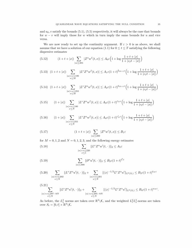
and u0, v satisfy the bounds (5.1), (5.5) respectively, it will always be the case that boundsfor w − v will imply those for w which in turn imply the same bounds for u and viceversa.
We are now ready to set up the continuity argument. If ε > 0 is as above, we shallassume that we have a solution of our equation (1.1) for 0 ≤ t ≤ T satisfying the followingdispersive estimates
(5.12) (1 + t+ |x|)∑
|α|≤201
|ZαwI(t, x)| ≤ A0ε(
1 + log1 + t+ |x|
1 + |cIt− |x||)
(5.13) (1 + t+ |x|)∑
|α|+ν≤190ν≤M
|LνZαwI(t, x)| ≤ A1ε(1 + t)bM+1ε(
1 + log1 + t+ |x|
1 + |cIt− |x||)
(5.14) (1 + t+ |x|)∑
|α|+ν≤255ν≤M
|LνZαwI(t, x)| ≤ A2ε(1 + t)bM+1ε(
1 + log1 + t+ |x|
1 + |cIt− |x||)
(5.15) (1 + |x|)∑
|α|+ν≤180ν≤N
|LνZαwI(t, x)| ≤ A3ε(1 + t)cN ε(
1 + log1 + t+ |x|
1 + |cIt− |x||)
(5.16) (1 + |x|)∑
|α|+ν≤255ν≤N
|LνZαwI(t, x)| ≤ A4ε(1 + t)c′N ε(
1 + log1 + t+ |x|
1 + |cIt− |x||)
(5.17) (1 + t+ |x|)∑
|α|≤200
|Zαw′(t, x)| ≤ B1ε
for M = 0, 1, 2 and N = 0, 1, 2, 3, and the following energy estimates
(5.18)∑
|α|+ν≤220ν≤1
‖LνZαw′(t, · )‖2 ≤ A5ε
(5.19)∑
|α|≤300
‖∂αu′(t, · )‖2 ≤ B2ε(1 + t)Cε
(5.20)∑
|α|+ν≤202ν≤N
‖LνZαu′(t, · )‖2 +∑
|α|+ν≤201ν≤N
‖〈x〉−1/2LνZαu′‖L2(St) ≤ B3ε(1 + t)aN ε
(5.21)∑
|α|+ν≤297−8Nν≤N
‖LνZαu′(t, · )‖2 +∑
|α|+ν≤295−8Nν≤N
‖〈x〉−1/2LνZαu′‖L2(St) ≤ B4ε(1 + t)aN ε.
As before, the L2x norms are taken over R
3\K, and the weighted L2tL
2x-norms are taken
over St = [0, t] × R3\K.
36 JASON METCALFE, MAKOTO NAKAMURA, AND CHRISTOPHER D. SOGGE
In (5.19), C is independent of the losses aM , bM , cM , aM , bM , and c′M . The otherassociated losses satisfy
(5.22) aM ≪ bM ≪ cM ≪ aM ≪ bM ≪ c′M ≪ aM+1
for M = 1, 2, 3, and
C ≪ a0 = c0 = a0 ≪ c′0 ≪ a1.
It is worth noting that (5.14), (5.17), (5.18), (5.19), and (5.21) are the estimatesthat made up the simpler argument in the preceding paper [27]. (5.12) is the main newestimate required in order to handle the higher order terms that do not involve derivatives.The remaining estimates are technical pieces that are needed (or convenient) to make theargument work.
In the estimates (5.12)-(5.16) and (5.18), we take Aj = 4C2 where j = 0, 1, . . . , 5 andC2 is the uniform constant appearing in the bounds (5.5) for v. If ε is small, all of theseestimates are valid for T = 2 by Theorem 5.1. With this in mind, we shall prove that forε > 0 sufficiently small depending on B1, . . . , B4
(i.) (5.12)-(5.16) and (5.18) are valid with Aj replaced by Aj/2;(ii.) (5.17) and (5.19)-(5.21) are a consequence of (5.12)-(5.16) and (5.18) for suitable
constants Bj .
By the local existence theorem, it will follow that a solution exists for all t > 0 if ε > 0is sufficiently small. We now explore (i.) and (ii.) in the next two sections respectively.
6. Proof of (i.)
In this section, we will show step (i.) of the proof of Theorem 1.1. Specifically, we mustshow that (5.12)-(5.16) and (5.18) hold with Aj replaced by Aj/2 under the assumptionof (5.12)-(5.21).
6.1. Preliminaries: We begin with some preliminary estimates that follow from (5.12)-(5.21).
First, we shall prove that if |α| + ν ≤ 270, ν ≤ 2, then there is a constant b so that
(6.1) 〈r〉1/2+θ〈cIt− r〉1−θ|LνZα∂uI(t, x)| ≤ Cε(1 + t)bε, 0 ≤ θ ≤ 1/2
for any 0 ≤ θ ≤ 1/2. Additionally,
(6.2) ‖〈t+ r〉LνZα2u(t, · )‖2 ≤ Cε(1 + t)bε.
for |α| + ν ≤ 271 and ν ≤ 2.

QUASILINEAR WAVE EQUATIONS SATISFYING THE NULL CONDITION 37
By (4.26), (6.1) follows from (5.13), (5.21), and (6.2). It, thus, suffices to show (6.2).To do so, notice that the left side can be controlled by
(6.3) C∥
∥
∥
(
〈t+ r〉∑
|α|+ν≤190ν≤2
|LνZαu′(t, · )|)
∑
|α|+ν≤272ν≤2
|LνZαu′(t, · )|∥
∥
∥
2
+ C∥
∥
∥〈t+ r〉
(
∑
|α|+ν≤190ν≤2
|LνZαu(t, · )|)2 ∑
|α|+ν≤273ν≤2
|LνZαu(t, · )|∥
∥
∥
2.
For the first term, if we apply (5.13), we establish the bound
Cε(1 + t)b3ε(1 + log(1 + t))∑
|α|+ν≤272ν≤2
‖LνZαu′(t, · )‖2.
The desired estimate for the first term, thus, follows from (5.21).
For the second term in (6.3), we will again apply (5.13). Since the coefficients ofΓ = L,Z are O(t + r), it follows that this term is controlled by
Cε2(log(2 + t))2(1 + t)2b3ε[
∑
|α|+ν≤272ν≤2
‖LνZαu′(t, · )‖2 + ‖〈t+ r〉−1u(t, · )‖2
]
.
The desired bound then follows from (5.12) and (5.21), thus completing the proof of(6.2).
We will argue similarly to show a lossless version of (6.1) and (6.2) that does notinvolve the scaling vector field L. In particular, we shall prove, for |α| ≤ 218 and any0 ≤ θ ≤ 1/2,
(6.4) r(1/2)+θ〈cI t− r〉1−θ |Zα∂uI(t, · )| ≤ Cε,
and for |α| ≤ 219,
(6.5) ‖〈t+ r〉Zα2u(t, · )‖2 ≤ Cε.
As before, (6.4) follows from (6.5) by (4.26), (5.17), and (5.18).
In order to show (6.5), we again expand the left side to get the bound
(6.6) C∥
∥
∥〈t+ r〉
∑
|α|≤190
|Zαu′(t, · )|∑
|α|≤220
|Zαu′(t, · )|∥
∥
∥
2
+ C∥
∥
∥〈t+ r〉
(
∑
|α|≤190
|Zαu(t, · )|)2 ∑
|α|≤221
|Zαu(t, · )|∥
∥
∥
2.
By (5.1), (5.17) and (5.18), the first term is O(ε) as desired. Applying (5.1) and (5.12)to the second term in (6.6), we see that it is dominated by
Cε2(1 + log(1 + t))2∑
|α|≤221
‖〈t+ |x|〉−1|Zαu(t, · )|‖2.
By (5.1) and (5.14), it follows that this term is O(ε) if ε > 0 is sufficiently small. Thiscompletes the proof of (6.5).

38 JASON METCALFE, MAKOTO NAKAMURA, AND CHRISTOPHER D. SOGGE
Notice that (6.1) and (6.4) hold when u is replaced by w−v. Indeed, since |LµZα2(w−
v)| .∑
|β|+ν≤|α|+µν≤µ
|LνZβ2u|, (6.2) and (6.5) hold with w − v substituted for u. Thus,
the appropriate versions of (6.1) and (6.4) are consequences of (4.26), (5.1), (5.5), (5.13),(5.17), (5.18) and (5.21).
6.2. Proof of (5.12): Assuming (5.12)-(5.21), we must show that (5.12) holds with A0
replaced by A0/2. Since the better bounds (5.5) hold for v, it will suffice to show
(6.7) (1 + t+ |x|)∑
|α|≤201
|Zα(w − v)I(t, x)| ≤ Cε2(
1 + log1 + t+ |x|
1 + |cIt− |x||)
.
Fix a smooth cutoff function ηJ satisfying ηJ(s) ≡ 1 for s ∈ [(cJ + (δ/2))−1, (cJ −(δ/2))−1] with δ = (1/3)min(cI − cI−1), and ηJ(s) ≡ 0 for s 6∈ [(cJ + δ)−1, (cJ − δ)−1].Then, set ρJ(t, x) = ηJ (|x|−1t). Since we may assume that 0 ∈ K, we have that |x| isbounded below on the complement of K, and the function ρJ is smooth and homogeneousof degree 0 in (t, x). Clearly, ρJ is identically one on a conic neighborhood of |x| = cJ t,and its support does not intersect any |x| = cIt for I 6= J . Let
(6.8) F I =∑
1≤J≤DJ 6=I
ρJ
∑
0≤j,k,l≤3
BIJ,jkJ,l ∂lu
J∂j∂kuJ +
∑
1≤J≤DJ 6=I
ρJ
∑
0≤j,k≤3
AI,jkJJ ∂ju
J∂kuJ ,
and set GI = F I − F I .
By (4.20) and (4.21), we have that the left side of (6.7) is bounded by
(6.9) C
∫ t
max(0,c|cIt−|x||−1)
∫
|y|≈s
∑
|α|+ν≤204ν≤1
|LνZαF I(s, y)| dy ds|y|
+ C∑
|α|≤207
sup0≤s≤t
∫
|ZαF I(s, y)| dy
+ C sup0≤s≤t
∫ s
c′s
∫
|y|≈τ
∑
|α|+ν≤208ν≤1
|LνZαF I(τ, y)| dy dτ|y|
+ C sup0≤s≤t
(1 + s)∑
|α|≤204
‖∂αF I(s, · )‖L∞(|x|<10)
+ C(
1 + log1 + t+ |x|
1 + |cIt− |x||)
sup(s,y)
|y|(1 + s+ |y|)1+µz1−µ(s, |y|)∑
|α|≤201
|ZαGI(s, y)|
+ C(
1 + log1 + t+ |x|
1 + |cIt− |x||)
sup(s,y)
|y|(1 + s+ |y|)1+µz1−µ(s, |y|)∑
|α|≤204
|∂α∂GI(s, y)|.
We need to show that each of these terms is bounded by Cε2(
1 + log 1+t+|x|1+|cIt−|x||
)
.
QUASILINEAR WAVE EQUATIONS SATISFYING THE NULL CONDITION 39
For the first term in (6.9), it follows immediately that we have the bound
C
∫ t
max(0,c|cIt−|x||−1)
1
1 + s
∫
|y|≈s
∑
|α|+ν≤205ν≤1
|LνZα∂uJ |2 dy ds
≤ C(
1 + log1 + t
1 + |cIt− |x||)
sup0≤s≤t
∑
|α|+ν≤205ν≤1
‖LνZαu′(s, · )‖22.
The desired bound follows from (5.1) and (5.18). The third term in (6.9) can be han-dled quite similarly. The second term above is easily seen to be O(ε2) by the Schwarzinequality, (5.1), and (5.18). The fourth term above is bounded by
sup0≤s≤t
(1 + t)∥
∥
∥
∑
|α|≤103
|∂α∂uJ |∑
|α|≤205
|∂α∂uJ |∥
∥
∥
∞.
If we apply (5.1) and (5.17), this is controlled by
Cε sup0≤s≤t
∑
|α|≤205
‖∂αu′‖∞.
Thus, by Sobolev’s lemma, (5.1), and (5.18), we see that this term is also O(ε2).
It remains to show that
(6.10) sup(s,y)
|y|(1 + s+ |y|)1+µz1−µ(s, |y|)∑
|α|≤201
|ZαGI(s, y)|
+ sup(s,y)
|y|(1 + s+ |y|)1+µz1−µ(s, |y|)∑
|α|≤204
|∂α∂GI(s, y)|
is O(ε2).
When GI is replaced by the null forms∑
0≤j,k≤3
AI,jkII ∂ju
I∂kuI +
∑
0≤j,k,l≤3
BII,jkI,l ∂lu
I∂j∂kuI ,
we can apply (2.25) and (2.26) to see that (6.10) is controlled by
(6.11) C sup(s,y)
(1 + s+ |y|)1+µz1−µ(s, |y|)∑
|α|+ν≤207ν≤1
|LνZαuI(s, y)|∑
|α|≤206
|Zα∂uI(s, y)|
+C sup(s,y)
|y|(1+s+ |y|)µz1−µ(s, |y|)〈cIs−|y|〉∑
|α|≤103
|Zα∂uI(s, y)|∑
|α|≤206
|Zα∂uI(s, y)|.
For the first term, if we apply (5.1) and (5.14), we get the bound
Cε sup(s,y)
(1 + s+ |y|)µ+b2ε+z1−µ(s, |y|)∑
|α|≤206
|Zα∂uI |.
If µ and ε are sufficiently small, the desired O(ε2) bound follows from (6.1). Indeed, if(s, |y|) ∈ ΛI , then z(s, |y|) = 〈cIs − |y|〉 and |y| & (1 + s + |y|). On the other hand, if(s, |y|) 6∈ ΛI , then 〈cIs− |y|〉 & 〈s+ |y|〉 and 〈y〉1−µ & z1−µ(s, |y|).

40 JASON METCALFE, MAKOTO NAKAMURA, AND CHRISTOPHER D. SOGGE
For the second term in (6.11), we apply (6.4) to obtain the bound
Cε sup(s,y)
|y|1/2(1 + s+ |y|)µz1−µ(s, |y|)∑
|α|≤206
|Zα∂uI |.
Using considerations as above, this is O(ε2) by a subsequent application of (6.4).
When GI is replaced by∑
1≤J≤DJ 6=I
∑
0≤j,k,l≤3
(1 − ρJ)BIJ,jkJ,l ∂lu
J∂j∂kuJ +
∑
1≤J≤DJ 6=I
∑
0≤j,k≤3
(1 − ρJ )AI,jkJJ ∂ju
J∂kuJ ,
(6.10) is dominated by
C∑
1≤J≤DJ 6=I
sup(s,y) 6∈ΛJ
|y|(1 + s+ |y|)1+µz1−µ(s, |y|)(
∑
|α|≤206
|Zα∂uJ |)2
.
Since 〈cJs− |y|〉1−µ & 〈s+ |y|〉1−µ & z1−µ(s, |y|) on the support of (1− ρJ), these termsare O(ε2) by two applications of (6.4) with θ = 0.
If GI in (6.10) is replaced by the remaining quadratic terms∑
1≤J,K≤DJ 6=K
∑
0≤j,k,l≤3
BIJ,jkK,l ∂lu
K∂j∂kuJ +
∑
1≤J,K≤DJ 6=K
∑
0≤j,k≤3
AI,jkJK ∂ju
J∂kuK ,
we see that it is bounded by
(6.12) C∑
1≤J,K≤DJ 6=K
sup(s,y)
|y|(1 + s+ |y|)1+µz1−µ(s, |y|)∑
|α|≤206
|Zα∂uJ |∑
|α|≤206
|Zα∂uK |.
If (s, y) 6∈ ΛJ ∪ ΛK , then we can argue as in the previous case to see that this is O(ε2).Thus, let us assume that (s, y) ∈ ΛJ , and hence (s, y) 6∈ ΛK . The reverse case will followsymmetrically. For such (s, y), we have z1−µ(s, |y|) = 〈cJs− |y|〉1−µ. Thus, by (6.4), wesee that in this case (6.12) is controlled by
Cε∑
1≤K≤DK 6=J
sup(s,y)∈ΛJ
|y|1/2−µ(1 + s+ |y|)1+µ∑
|α|≤206
|Zα∂uK |.
Since 〈cKs − |y|〉 & 〈s + |y|〉 and |y| ≈ s on ΛJ , the desired O(ε2) bound follows from(6.4).
Finally, when GI is replaced by the cubic terms RI + P I , (6.10) is dominated by
(6.13) C sup(s,y)
|y|(1 + s+ |y|)1+µz1−µ(s, |y|)(
∑
|α|≤201
|Zαu(s, y)|)3
+ C sup(s,y)
|y|(1 + s+ |y|)1+µz1−µ(s, |y|)(
∑
|α|≤104
|Zαu(s, y)|)2 ∑
|α|≤206
|Zα∂u(s, y)|.
By the inductive hypothesis (5.12), the first term in (6.13) is controlled by
Cε3 sup(s,y)
z1−µ(s, |y|)(1 + s+ |y|)1−µ
(
1 + log1 + s+ |y|z(s, |y|)
)3
.

QUASILINEAR WAVE EQUATIONS SATISFYING THE NULL CONDITION 41
Since (log x)3/x1−µ is bounded for x ≥ 1 and µ < 1, it follows that this term is O(ε3).For the second term in(6.13), by (6.4), we have the bound
Cε sup(s,y)
|y|1/2−µ(1 + s+ |y|)1+µ(
∑
|α|≤104
|Zαu(s, y)|)2
.
This term is then easily seen to be O(ε3) by (5.1) and (5.12) which completes the proof.
6.3. Proof of (5.13): In this section, we show that if you assume (5.12)-(5.21), then youcan prove (5.13) with A1 replaced by A1/2. By the arguments in the previous section,this clearly holds when M = 0. As before, by (5.5), it suffices to show
(6.14)(
1 + log1 + t+ |x|
1 + |cIt− |x||)−1
(1 + t+ |x|)∑
|α|+ν≤190ν≤M
|LνZα(w − v)I(t, x)|
≤ Cε2(1 + t)bM+1ε.
Since 2(w − v) = (1 − β)(1 − η)2u = (1 − β)(1 − η)(B +Q+ R + P ), by (4.13) and(4.21), we see that the left side of (6.14) is dominated by
(6.15) C
∫ t
0
∫
∑
|α|+ν≤197ν≤M+1
|LνZα(BI +QI)(s, y)| dy ds|y|
+ C sup(s,y)
|y|(1 + s+ |y|)1+µz1−µ(s, |y|)∑
|α|+ν≤190ν≤M
|LνZα(RI + P I)(s, y)|
+ C sup(s,y)
|y|(1 + s+ |y|)1+µz1−µ(s, |y|)∑
|α|+ν≤193ν≤M
|Lν∂α∂(RI + P I)(s, y)|.
Here we have used the fact that the last term in (4.13) is controlled by the second termin the right of (4.13) using Sobolev estimates and the fact that we may assume 0 ∈ Kwithout loss of generality.
By (1.4) and (1.5), we have that the first term in (6.15) is dominated by
C∑
|α|+ν≤198ν≤M+1
‖〈x〉−1/2LνZαu′‖2L2(St)
.
It, thus, follows from (5.20) that these terms are bounded by Cε2(1+ t)2aM+1ε as desired.

42 JASON METCALFE, MAKOTO NAKAMURA, AND CHRISTOPHER D. SOGGE
The last two terms of (6.15) are controlled by a constant times
(6.16) sup(s,y)
|y|(1 + s+ |y|)1+µz1−µ(s, |y|)(
∑
|α|≤190
|Zαu(s, y)|)2 ∑
|α|+ν≤190ν≤M
|LνZαu(s, y)|
+ sup(s,y)
|y|(1 + s+ |y|)1+µz1−µ(s, |y|)(
∑
|α|+ν≤190ν≤M−1
|LνZαu(s, y)|)3
+ sup(s,y)
|y|(1+s+ |y|)1+µz1−µ(s, |y|)(
∑
|α|+ν≤190ν≤M
|LνZαu(s, y)|)2 ∑
|α|+ν≤195ν≤M
|LνZα∂u(s, y)|.
For the first term in (6.16), we apply (5.1), (5.12), and (5.13) to obtain the bound
Cε3(1 + t)bM+1ε sup(s,y)
z1−µ(s, |y|)(1 + s+ |y|)1−µ
(
1 + log1 + s+ |y|z(s, |y|)
)3
≤ Cε3(1 + t)bM+1ε.
If we apply (5.13) and argue similarly, it follows that the second term is controlled by
Cε3(1 + t)3bM ε. Finally, for the third term in (6.16), we first apply (6.1) to see that it iscontrolled by
Cε sup(s,|y|)
|y|1/2−µ(1 + s+ |y|)1+µ(1 + s)bε(
∑
|α|+ν≤190ν≤M
|LνZαu(s, y)|)2
.
It, thus, follows from the inductive hypothesis (5.13) that this term is O(ε3) if ε > 0 issufficiently small, which completes the proof of (5.13).
6.4. Proof of (5.14): In this section, by proving(6.17)(
1 + log1 + t+ |x|
1 + |cIt− |x||)−1
(1 + t+ |x|)∑
|α|+ν≤255ν≤M
|LνZα(w − v)I(t, x)| ≤ Cε2(1 + t)bM+1ε,
we show that (5.14) holds with A2 replaced by A2/2 for M = 0, 1, 2.
Here, again, we apply (4.13) and (4.21) to see that the left side of (6.17) is controlledby
(6.18) C∑
|α|+ν≤262ν≤M+1
∫ t
0
∫
|LνZα(QI +BI)(s, y)| dy ds|y|
+ C sup(s,y)
|y|(1 + s+ |y|)1+µz1−µ(s, |y|)∑
|α|+ν≤255ν≤M
|LνZα(RI + P I)(s, y)|
+ C sup(s,y)
|y|(1 + s+ |y|)1+µz1−µ(s, |y|)∑
|α|+ν≤258ν≤M
|Lν∂α∂(RI + P I)(s, y)|.

QUASILINEAR WAVE EQUATIONS SATISFYING THE NULL CONDITION 43
The first term is controlled by
C∑
|α|+ν≤263ν≤M+1
‖〈x〉−1/2LνZαu′‖2L2(St)
≤ Cε2(1 + t)2aM+1ε
by (5.21). For the last two terms in (6.18), which involve the cubic nonlinearities, wehave the bound
(6.19) C sup(s,y)
|y|(1 + s+ |y|)1+µz1−µ(s, |y|)(
∑
|α|≤131
|Zαu(s, y)|)2 ∑
|α|+ν≤255ν≤M
|LνZαu(s, y)|
+ C sup(s,y)
|y|(1 + s+ |y|)1+µz1−µ(s, |y|)(
∑
|α|+ν≤131ν≤M
|LνZαu(s, y)|)2 ∑
|α|+ν≤255ν≤M−1
|LνZαu(s, y)|
+C sup(s,y)
|y|(1+s+|y|)1+µz1−µ(s, |y|)(
∑
|α|+ν≤131ν≤M
|LνZαu(s, y)|)2 ∑
|α|+ν≤260ν≤M
|LνZαu′(s, y)|.
Using the fact that (log x)3/x1−µ is bounded for x ≥ 1 and µ < 1, the first term isdominated by Cε3(1 + t)bM+1ε by (5.12) and (5.14). Similarly, using (5.13) and (5.14),
the second term is controlled by Cε3(1 + t)2bM+1ε+bM ε. Again arguing as in the proofof (5.13), the final term in (6.19) is easily seen to be O(ε3) if ε > 0 is sufficiently smallusing (6.1) and (5.13). This completes the proof of (6.17), and hence, that of (5.14).
6.5. Proof of (5.15): In the proof of part (ii.), we will require pointwise estimates thatallow up to three occurences of the scaling vector field L. This is not the case for theprevious estimates due to the loss of an L associated to (4.13). Here, we may argue asin the proofs of the previous esimates (in particular, that of (5.13)) replacing (4.13) by(4.18).
Clearly (5.15) holds when N = 0 by (5.12). Thus, by (5.5), in order to show that(5.15) holds with A3 replaced by A3/2, it suffices to show
(6.20)(
1+ log1 + t+ |x|
1 + |cIt− |x||)−1
(1+ |x|)∑
|α|+ν≤180ν≤N
|LνZα(w−v)I (t, x)| ≤ Cε2(1+ t)cN ε
for N = 1, 2, 3.

44 JASON METCALFE, MAKOTO NAKAMURA, AND CHRISTOPHER D. SOGGE
Since 2(w − v) = (1 − β)(1 − η)2u = (1 − β)(1 − η)(B +Q+ R+ P ), by (4.18) and(4.21), we see that the left side of (6.20) is controlled by
(6.21) C
∫ t
0
∫
∑
|α|+ν≤186ν≤N
|LνZα(BI +QI)(s, y)| dy ds|y|
+ C sup(s,y)
|y|(1 + s+ |y|)1+µz1−µ(s, |y|)∑
|α|+ν≤180ν≤N
|LνZα(RI + P I)(s, y)|
+ C sup(s,y)
|y|(1 + s+ |y|)1+µz1−µ(s, |y|)∑
|α|+ν≤183ν≤N
|Lν∂α∂(RI + P I)(s, y)|.
As above, using (5.20), the first term is bounded by
C∑
|α|+ν≤187ν≤N
‖〈x〉−1/2LνZαu′‖2L2(St)
≤ Cε2(1 + t)2aN ε.
The cubic terms require a little additional care. To begin, we have that the last twoterms of (6.21) are controlled by
(6.22) C sup(s,y)
|y|(1 + s+ |y|)1+µz1−µ(s, |y|)(
∑
|α|≤186
|Zαu(s, y)|)2 ∑
|α|+ν≤180ν≤N
|LνZαu(s, y)|
+ C sup(s,y)
|y|(1 + s+ |y|)1+µz1−µ(s, |y|)(
∑
|α|≤186
|Zαu(s, y)|)2 ∑
|α|+ν≤188ν≤N
|LνZαu′(s, y)|
+ C sup(s,y)
|y|(1 + s+ |y|)1+µz1−µ(s, |y|)(
∑
|α|+ν≤189ν≤N−1
|LνZαu(s, y)|)3
.
Applying (5.1) and (5.15) to the first term and using (2.27) and (5.20) in the second,we see that the first two terms of (6.22) are controlled by
Cε(1 + t)cN ε sup(s,y)
(1 + s+ |y|)1+µz1−µ(s, |y|)(
1 + log1 + s+ |y|z(s, |y|)
)(
∑
|α|≤186
|Zαu(s, y)|)2
Here, we have used that (5.22) gives aN ≤ cN . If we in turn apply (5.12), we see thatthis is bounded by the right side of (6.20) as desired. When N = 1, this is sufficient tocomplete the proof. When N = 2, 3, we must also consider the last term in (6.22). Thebound here, however, follows quite simply from three applications of (5.13) (and (5.1)).
Doing so, we see that this last term is controlled by Cε3(1+ t)3bN ε. Since we may choose
cN > 3bN (see (5.22)), this is sufficient to complete the proof of (6.20).
6.6. Proof of (5.16): In this section, we will argue much as in the previous section toestablish the higher order pointwise estimate that permits three occurences of L. Here,

QUASILINEAR WAVE EQUATIONS SATISFYING THE NULL CONDITION 45
we must establish (5.16) with A4 replaced by A4/2. This is accomplished by showing
(6.23)(
1+ log1 + t+ |x|
1 + |cIt− |x||)−1
(1+ |x|)∑
|α|+ν≤255ν≤N
|LνZα(w−v)I (t, x)| ≤ Cε2(1+ t)c′N ε
for N = 0, 1, . . . , 4 and using (5.5).
Applying (4.18) and (4.21) and arguing as in the proof of (5.15), we see that the leftside of (6.23) is dominated by
(6.24) C∑
|α|+ν≤262ν≤N
‖〈x〉−1/2LνZαu′‖2L2(St)
+ C sup(s,y)
|y|(1 + s+ |y|)1+µz1−µ(s, |y|)(
∑
|α|≤132
|Zαu(s, y)|)2 ∑
|α|+ν≤255ν≤N
|LνZαu(s, y)|
+ C sup(s,y)
|y|(1 + s+ |y|)1+µz1−µ(s, |y|)(
∑
|α|≤132
|Zαu(s, y)|)2 ∑
|α|+ν≤260ν≤N
|LνZαu′(s, y)|
+ C sup(s,y)
|y|(1 + s+ |y|)1+µz1−µ(s, |y|)∑
|α|+ν≤132ν≤N
|LνZαu(s, y)|(
∑
|α|+ν≤255ν≤N−1
|LνZαu(s, y)|)2
+ C sup(s,y)
|y|(1 + s+ |y|)1+µz1−µ(s, |y|)∑
|α|+ν≤132ν≤N
|LνZαu(s, y)|
×∑
|α|+ν≤132ν≤N−1
|LνZαu(s, y)|∑
|α|+ν≤260ν≤N−1
|LνZαu′(s, y)|.
Choosing c′N > max(2aN , 2bN + cN) as we may, we see that this is bounded by theright side of (6.23). Indeed, the bound for the first term in (6.24) follows directly from(5.21). For the second term, we apply (5.1), (5.12), and (5.16) as before. This suffices tohandle the N = 0 case. In order to complete the proof for N = 1, 2, 3, we similarly, boundthe third term using applications of (2.27), (5.1), (5.12), and (5.21). To get control overthe fourth term, we apply (5.1), (5.14), and (5.15). Using (5.1), (5.13), (5.15), and (6.1),one can see that the last term is O(ε3) for small ε which completes the proof of (6.23).
6.7. Proof of (5.18): In order to complete the proof of part (i.), it remains to show thatthe low order, lossless energy inequality (5.18) with A5 replaced by A5/2 follows from(5.12)-(5.21). Since v satisfies the better bound (5.5), it suffices to establish
(6.25)∑
|α|+ν≤220ν≤1
‖LνZα(w − v)′(t, · )‖22 ≤ Cε3.

46 JASON METCALFE, MAKOTO NAKAMURA, AND CHRISTOPHER D. SOGGE
By the standard energy integral method, we have that the left side of (6.25) is boundedby
C∑
|α|+ν≤220ν≤1
∫ t
0
∫
R3\K|〈∂0L
νZα(w − v),2LνZα(w − v)〉| dy ds
+ C∑
|α|+ν≤220ν≤1
∣
∣
∣
∫ t
0
∫
∂K∂0L
νZα(w − v)∇xLνZα(w − v) · n dσ ds
∣
∣
∣
where n is the outward normal at a given point on K and 〈 · , · 〉 is the standard Euclideaninner product on R
D. Since K ⊂ |x| < 1 and since the coefficients of Z are O(1) on∂K, it follows that the last term in controlled by
C
∫ t
0
∫
x∈R3\K : |x|<1
∑
|α|+ν≤221ν≤1
|Lν∂α(w − v)′(s, y)|2 dy ds.
Additionally, by the commutation properties of Γ with 2 and the fact that 2(w − v) =(1 − β)(1 − η)2u, we see that the left side of (6.25) is dominated by
C
∫ t
0
∫
R3\K
∑
|αj |+νj≤220νj≤1;j=1,2
∣
∣
∣〈∂0L
ν1Zα1(w − v), Lν2Zα2F (u, du, d2u)〉∣
∣
∣dy ds
+ C
∫ t
0
∫
x∈R3\K : |x|<1
∑
|α|+ν≤221ν≤1
|Lν∂α(w − v)′(s, y)|2 dy ds.

QUASILINEAR WAVE EQUATIONS SATISFYING THE NULL CONDITION 47
If we expand using the definition of F (u, du, d2u), the preceding equation is controlledby
(6.26) C
∫ t
0
∫
R3\K
D∑
K=1
∑
|α|+ν≤220ν≤1
∣
∣
∣∂0L
νZα(w − v)K∣
∣
∣
×∑
|α|+ν≤220ν≤1
∑
|β|+µ≤220µ≤1
∣
∣
∣
∑
0≤j,k,l≤3
BKK,jkK,l ∂lL
νZαuK∂j∂kLµZβuK
∣
∣
∣dy ds
+C
∫ t
0
∫
R3\K
D∑
K=1
∑
|α|+ν≤220ν≤1
∣
∣
∣∂0L
νZα(w−v)K∣
∣
∣
∑
|α|+ν≤220ν≤1
∑
|β|+µ≤220µ≤1
∣
∣
∣
∑
0≤j,k≤3
AK,jkKK ∂jL
νZαuK
× ∂kLµZβuK
∣
∣
∣dy ds
+ C
∫ t
0
∫
R3\K
∑
1≤I,J,K≤D(I,K) 6=(K,J)
∑
|α|+ν≤220ν≤1
|LνZα∂(w − v)K |∑
|α|+ν≤220ν≤1
|LνZα∂uI |
×∑
|α|+ν≤221ν≤1
|LνZα∂uJ | dy ds
+ C
∫ t
0
∫
R3\K
∑
|α|+ν≤220ν≤1
|LνZα∂(w − v)|(
∑
|α|+ν≤222ν≤1
|LνZαu|)3
dy ds
+ C
∫ t
0
∫
x∈R3\K : |x|<1
∑
|α|+ν≤221ν≤1
|Lν∂α(w − v)′(s, y)|2 dy ds.
By Lemma 4.1 of Sideris-Tu [35], the constants AK,jkKK and BKK,jk
K,l satisfy (1.9) and (1.10).
The first two terms in (6.26) satisfy the bounds of Lemma 2.6. The third term involvesquadratic interactions between waves of different speeds, and the fourth term is thecumulative effect of the nonlinearities of higher order. The arguments to bound the firstthree terms and the final term follow from those in [27]. For completeness, we sketch theargument.
Let us first handle the null terms. By (2.25) and (2.26), the first two terms in (6.26)are controlled by
(6.27) C
∫ t
0
∫
R3\K
∑
|α|+ν≤221ν≤2
|LνZαu|∑
|α|+ν≤221ν≤2
|LνZαu′|∑
|α|+ν≤220ν≤1
|LνZα(w − v)′| dy ds|y|
+ C
∫ t
0
∫
R3\K
D∑
K=1
〈cKs− r〉〈s+ r〉
∑
|α|+ν≤220ν≤1
|LνZα∂(w − v)K |(
∑
|α|+ν≤221ν≤1
|LνZαu′|)2
dy ds.

48 JASON METCALFE, MAKOTO NAKAMURA, AND CHRISTOPHER D. SOGGE
To handle the first term of (6.27), notice that by (5.1), (5.5), and (5.14), we have∑
|α|+ν≤221ν≤2
|LνZαu(s, y)| ≤ Cε〈s+ |y|〉−1+b3ε log(2 + s),
which means that the first term of (6.27) has a contribution to (6.26) which is dominatedby
Cε
∫ t
0
log(2 + s)
〈s〉1−b3ε
∑
|α|+ν≤221ν≤2
‖〈y〉−1/2LνZαu′(s, · )‖2
×∑
|α|+ν≤220ν≤1
‖〈y〉−1/2LνZα(w − v)′(s, · )‖2 ds
by the Schwarz inequality. Thus, if we subsequently apply the Schwarz inequality, (5.1),(5.5), and (5.21), we see that this contribution is O(ε3) for ε > 0 small.
We now want to show that the second term of (6.27) satisfies a similar bound. If weapply (6.1), we see that the second term of (6.27) is controlled by
Cε
∫ t
0
(1 + s)−(1/2)+bε
∫
R3\K
1
r1/2〈s+ r〉1/2
∑
|α|+ν≤221ν≤1
|LνZαu′|2 dy ds.
For ε sufficiently small, it follows similarly that this term is O(ε3) by the L2tL
2x estimates
of (5.21).
For the multi-speed terms (i.e. the third term in (6.26)), let us for simplicity assumethat I 6= K, I = J . A symmetric argument will yield the same bound for the remainingcases. If we set δ < |cI − cK |/3+, it follows that |y| ∈ [(cI − δ)s, (cI + δ)s] ∩ [(cK −δ)s, (cK + δ)s] = ∅. Thus, it will suffice to show the bound when the spatial integralis taken over the complements of each of these sets separately. We will show the boundover |y| 6∈ [(cK − δ)s, (cK + δ)s]. A symmetric argument will yield the bound over theother set.
If we apply (6.1), we see that over |y| 6∈ [(cK − δ)s, (cK + δ)s] the third term in(6.26) is bounded by
Cε
∫ t
0
1
〈s〉(1/2)−bε
∫
|y|6∈[(cK−δ)s,(cK+δ)s]
1
r
∑
|α|+ν≤221ν≤1
|LνZα∂uI |2 dy ds.
Arguing as above, it is easy to see that these multiple speed quadratic terms are alsoO(ε3) by (5.21).
Next, we need to show that the last term in (6.26) enjoys an O(ε4) contribution. Thisis clear, however, since this term is bounded by
∫ t
0
∑
|α|+ν≤221ν≤1
‖Lν∂α(w − v)′(s, · )‖2∞ ds,
and an application of (6.17) yields the desired bound.

QUASILINEAR WAVE EQUATIONS SATISFYING THE NULL CONDITION 49
In order to finish the proof of (6.25), and hence that of part (i.), it remains to boundthe cubic terms in (6.26). By (5.1) and (5.14), it follows that this fourth term of (6.26)is controlled by
Cε3∫ t
0
∫
R3\K
(log(2 + s))3(1 + s)3b2ε
(1 + s+ |y|)3∑
|α|+ν≤220ν≤1
|LνZα∂(w − v)| dy ds.
By the Schwarz inequality, (5.5), and (5.18), this last term is also O(ε4) if ε is sufficientlysmall. Thus, we have shown (6.25) and have finished the proof of (i.).
7. Proof of (ii.)
We now begin part (ii.) of the continuity argument. In particular, we need to show that(5.17), (5.19), (5.20), and (5.21) follow from (5.12)-(5.16) and (5.18). This will completethe proof of Theorem 1.1.
7.1. Proof of (5.17): In this subsection, we briefly prove that (5.17) holds. Indeed, if(t, x) 6∈ ΛI , it follows that 〈cIt − |x|〉 & 〈t + |x|〉. Thus, away from the associated light
cone, we have that 1 + log 1+t+|x|1+|cIt−|x| is O(1). Hence, by (5.12), we have
(1 + t+ |x|)∑
|α|≤200
|Zα∂wI(t, x)| ≤ Cε
when (t, x) 6∈ ΛI . For (t, |x|) ∈ ΛI , it follows that |x| ≈ t. Thus, by (2.27), we have
(1 + t+ |x|)∑
|α|≤200
|Zα∂wI(t, x)| ≤ C∑
|α|≤202
‖Zαw′(t, · )‖2
provided (t, x) ∈ ΛI . Since the right side of this equation is O(ε) by (5.18), we haveestablished (5.17) as desired.
7.2. Proof of (5.19): The next step is to show that we have the higher order, lossyenergy estimates and mixed norm estimates when the scaling vector field does not occur.Here, we modify the arguments of [28] to allow the general higher order terms in thenonlinearity.
In the notation of §2, we have 2γu = B(du) +P (u, du) where B(du) +P (u, du) is thesemilinear part of the nonlinearity and
γIJ,jk = γIJ,jk(u, du) = −∑
1≤K≤D0≤l≤3
BIJ,jkK,l ∂lu
K − CIJ,jk(u, du).
Also, note that by (5.12) and (5.17)
(7.1)∑
|α|≤1
‖∂αγ(s, · )‖∞ ≤ Cε
1 + s.

50 JASON METCALFE, MAKOTO NAKAMURA, AND CHRISTOPHER D. SOGGE
We begin by proving (5.19). To do so, we first estimate the energy of ∂jt u for j ≤M ≤
300. Notice that by (4.3) and (7.1), we have
(7.2) ∂tE1/2M (u)(t) ≤ C
∑
j≤M
‖2γ∂jt u(t, · )‖2 +
Cε
1 + tE
1/2M (u)(t).
Note also that for M = 1, 2, . . .
∑
j≤M
|2γ∂jtu| ≤ C
(
∑
j≤M
|∂jtu
′| +∑
j≤M−1
|∂jt ∂
2u|)
∑
|α|≤200
|∂αu′|
+ C(
|u| +∑
j≤M
|∂jt u
′| +∑
j≤M−1
|∂jt ∂
2u|)(
∑
|α|≤200
|∂αu|)2
.
Using (5.1), (5.12), and (5.17), it follows that this is bounded by
Cε
1 + t
(
∑
j≤M
|∂jt u
′| +∑
j≤M−1
|∂jt ∂
2u|)
+Cε
(1 + t+ |x|)3− .
If we use elliptic regularity and repeat this argument, we get∑
j≤M−1
‖∂jt ∂
2u(t, · )‖2 ≤ C∑
j≤M
‖∂jtu
′(t, · )‖2 + C∑
j≤M−1
‖∂jt 2u(t, · )‖2
≤ C∑
j≤M
‖∂jtu
′(t, · )‖2 +Cε
1 + t
∑
j≤M−1
‖∂jt ∂
2u(t, · )‖2 +Cε3
(1 + t)3/2− .
If ε is small, we can absorb the second term into the left side of the preceding inequality.Therefore, if we combine the last two estimates, we conclude that
∑
j≤M
‖2γ∂jtu(t, · )‖2 ≤ Cε
1 + t
∑
j≤M
‖∂jt u
′(t, · )‖2 +Cε3
(1 + t)3/2− .
If we use this in (7.2), we get that for small ε > 0
∂tE1/2M (u)(t) ≤ Cε
1 + tE
1/2M (u)(t) +
Cε3
(1 + t)3/2−
since 12E
1/2M (u)(t) ≤ ∑
j≤M ‖∂jtu
′(t, · )‖2 ≤ 2E1/2M (u)(t) when ε is small. Since (1.12)
implies that E1/2300 (u)(0) ≤ Cε, Gronwall’s inequality yields
(7.3)∑
j≤300
‖∂jtu
′(t, · )‖2 ≤ 2E1/2300 (u)(t) ≤ Cε(1 + t)Cε
for some constant C > 0. By elliptic regularity, this leads to the bound (5.19) if ε > 0 issufficiently small.
7.3. Proof of the base case, N = 0, of (5.20) and (5.21): We begin by showing
(7.4) (log(2 + t))−1/2∑
|α|≤298
‖〈x〉−1/2∂αu′‖L2(St) ≤ C(1 + t)Cε
QUASILINEAR WAVE EQUATIONS SATISFYING THE NULL CONDITION 51
where C is the constant appearing in (5.19). By (4.9), (5.1), and (5.5), we have
(log(2 + t))−1/2∑
|α|≤298
‖〈x〉−1/2∂αu′‖L2(St)
≤ Cε(log(2 + t))1/2 + (log(2 + t))−1/2∑
|α|≤298
‖〈x〉−1/2∂α(w − v)′‖L2(St)
≤ Cε(log(2 + t))1/2 + C∑
|α|≤299
∫ t
0
‖∂α2(w − v)(s, · )‖2 ds
+ C∑
|α|≤298
‖∂α2(w − v)‖L2(St).
(7.5)
Since ∂α2(w − v) = ∂α(1 − β)(1 − η)2u, the right side is
≤ Cε(log(2 + t))1/2 + C∑
|α|≤299
∫ t
0
‖∂α2u(s, · )‖2 ds+ C
∑
|α|≤298
‖∂α2u‖L2(St).
If we apply (5.1), (5.12), and (5.17) as in the proof of (5.19), it is easy to see that
∑
|α|≤299
‖∂α2u(s, · )‖2 ≤ Cε
1 + s
∑
|α|≤300
‖∂αu′(s, · )‖2 +Cε3
(1 + s)3/2− .
If we plug this into the previous equation and apply (5.19), (7.4) follows immediately.
We next wish to show
(7.6)∑
|α|≤297
‖Zαu′(t, · )‖2 ≤ Cε(1 + t)a0ε
for some a0 ≥ C. In order to show this, we will argue inductively. That is, for M ≤ 297,we will assume that
(7.7)∑
|α|≤M−1
‖Zαu′(t, · )‖2 ≤ Cε(1 + t)Cε,
and we will use this to show
(7.8)∑
|α|≤M
‖Zαu′(t, · )‖2 ≤ Cε(1 + t)C′ε+σ
where σ > 0 can be chosen arbitrarily small. Notice that the base case follows triviallyfrom (5.18).
In order to control the left side of (7.8), we use (4.8). To do so, we must estimate thefirst term in its right side. We have
(7.9)∑
|α|≤M
‖2γZαu(t, · )‖2 ≤ C
∑
|γ|≤200
‖Zγu′(t, · )‖∞∑
|α|≤M
‖Zαu′(t, · )‖2
+ C∑
|β|,|γ|≤200,|α|≤M
‖Zβu(t, · )Zγu(t, · )Zαu′(t, · )‖2
+ C∑
|β|,|γ|≤200,|α|≤M
‖Zβu(t, · )Zγu(t, · )Zαu(t, · )‖2

52 JASON METCALFE, MAKOTO NAKAMURA, AND CHRISTOPHER D. SOGGE
By (5.1), (5.12), and (5.17), the first two terms are controlled by
Cε
1 + t
∑
|α|≤M
‖Zαu′(t, · )‖2 ≤ Cε
1 + tY
1/2M,0(t)
where YM,0(t) is as in (4.7). Since the coefficients of Z are O(|x|), we can apply (5.1)and (5.12) to see that the last term in (7.9) is dominated by
Cε3
(1 + t)3/2− +Cε2(1 + log(1 + t))2
1 + t
∑
|α|≤M−1
‖Zαu′(t, · )‖2.
The first term here corresponds to the case |α| = |β| = |γ| = 0 in the last term of (7.9).
Plugging these bounds for (7.9) into (4.8) and applying (7.1) yields
(7.10) ∂tYM,0(t) ≤Cε
1 + tYM,0(t)
+ Y1/2M,0(t)
( Cε3
(1 + t)3/2− +Cε2(1 + log(1 + t))2
1 + t
∑
|α|≤M−1
‖Zαu′(t, · )‖2
)
+ C∑
|α|≤M+1
‖∂αu′(t, · )‖2L2(|x|<1)
if ε is sufficiently small. Therefore, by Gronwall’s inequality, (1.12), and the inductivehypothesis (7.7), we have
YM,0(t) ≤ C(1 + t)Cε[
ε2 +(
sup0≤s≤t
Y1/2M,0(s)
)
ε2(1 + t)Cε+σ
+∑
|α|≤M+1
‖〈x〉−1/2∂αu′‖2L2(St)
]
.
If we apply (7.4) to the last term, we see that (7.8) follows. By induction, this yields(7.6).
Using (4.10), this in turn implies
(7.11) (log(2 + t))−1/2∑
|α|≤295
‖〈x〉−1/2Zαu′‖L2(St) ≤ Cε(1 + t)a0ε
which completes the proof of N = 0 cases of (5.20) and (5.21).
7.4. Proof of (5.20) and (5.21) for N > 0: In order to complete the proof of Theorem1.1, we must show that (5.20) and (5.21) hold for N = 1, 2, 3. To do so, we argueinductively in N . We fix an N and assume that (5.21) holds with N replaced by N − 1.It then remains to show (5.20) and (5.21) for that N .
We begin with the task of showing (5.20). The first step will be to show that
(7.12)∑
|α|+µ≤205µ≤N
‖Lµ∂αu′(t, · )‖2 ≤ Cε(1 + t)Aε+σ .

QUASILINEAR WAVE EQUATIONS SATISFYING THE NULL CONDITION 53
For this, we shall want to use (4.6). We must first establish an appropriate version of(4.5) for N0 + ν0 ≤ 205, ν0 ≤ N . For this, we note that for M ≤ 205,
∑
j+µ≤Mµ≤N
(
|Lµ∂jt 2γu| + |[Lµ∂j
t ,2 − 2γ ]u|)
≤ C(
∑
j≤M−N
|LN∂jt ∂u| +
∑
j≤M−N−1
|LN∂jt ∂
2u|)(
∑
|α|≤200
|∂αu′| +(
∑
|α|≤200
|∂αu|)2)
+ C∑
|α|+µ≤M−200µ≤N
|Lµ∂αu′|∑
|α|+µ≤Mµ≤N−1
|Lµ∂αu′|
+ C∑
|α|+µ≤Mµ≤N−1
|Lµ∂αu′|∑
|α|+µ≤max(M/2,M−200)µ≤N−1
|Lµ∂αu′|
+ C(
∑
|α|+µ≤M+1µ≤N−1
|Lµ∂αu|)2 ∑
|α|+µ≤180µ≤N
|Lµ∂αu|.
Using elliptic regularity, (2.27), (5.1), (5.12), and (5.18), we conclude that
∑
j+µ≤Mµ≤N
(
‖Lµ∂jt 2γu(t, · )‖2 + ‖[Lµ∂j
t ,2 − 2γ ]u(t, · )‖2
)
≤ Cε
1 + t
∑
j+µ≤Mµ≤N
‖Lµ∂jt u
′(t, · )‖2
+ C∑
|α|+µ≤M−200µ≤N
‖〈x〉−1/2Lµ∂αu′(t, · )‖2
∑
|α|+µ≤207µ≤N−1
‖〈x〉−1/2LµZαu′(t, · )‖2
+ C∑
|α|+µ≤max(M,2+M/2)µ≤N−1
‖〈x〉−1/2LµZαu′(t, · )‖22
+ C∥
∥
∥
(
∑
|α|+µ≤M+1µ≤N−1
|Lµ∂αu(t, · )|)2 ∑
|α|+µ≤180µ≤N
|Lµ∂αu(t, · )|∥
∥
∥
2.
Based on this, (4.5) holds with δ = Cε and
HN,M−N(t) = C∑
|α|+µ≤M−200µ≤N
‖〈x〉−1/2Lµ∂αu′(t, · )‖22
+ C∑
|α|+µ≤207µ≤N−1
‖〈x〉−1/2LµZαu′(t, · )‖22
+ C∥
∥
∥
(
∑
|α|+µ≤M+1µ≤N−1
|Lµ∂αu(t, · )|)2 ∑
|α|+µ≤180µ≤N
|Lµ∂αu(t, · )|∥
∥
∥
2
Since M + 1 ≤ 206, (5.1), (5.14), and (5.15) imply that this last term is controlled by
Cε3(1 + log(1 + t))3(1 + t)2bN +cN
∥
∥
∥
1
(1 + t+ |x|)21
|x|∥
∥
∥
2≤ Cε3
(1 + t)1+

54 JASON METCALFE, MAKOTO NAKAMURA, AND CHRISTOPHER D. SOGGE
if ε is sufficiently small.
Since the conditions on the data give∫
e0(Lν∂j
t u)(0, x) dx ≤ Cε2 if j + ν ≤ 300, itfollows from (4.6) and the inductive hypothesis ((5.21) with N replaced by N − 1) thatfor M ≤ 205
(7.13)∑
|α|+µ≤Mµ≤N
‖Lµ∂αu′(t, · )‖2 ≤ Cε(1 + t)Cε+σ
+ C(1 + t)Cε∑
|α|+µ≤M−200µ≤N
‖〈x〉−1/2Lµ∂αu′‖2L2(St)
+ C(1 + t)Cε
∫ t
0
∑
|α|+µ≤Mµ≤N−1
‖Lµ∂αu′(s, · )‖L2(|x|<1) ds
for some constant σ > 2aN−1ε.
If we apply (4.12), (5.1), and (5.5), we get that the last integral is dominated byCε log(2 + t) plus
∫ t
0
∑
|α|+µ≤Mµ≤N−1
‖Lµ∂α(w − v)′(s, · )‖L2(|x|<1) ds
≤ C∑
|α|+µ≤M+1µ≤N−1
∫ t
0
(
∫ s
0
‖Lµ∂α2(w − v)(τ, · )‖L2(||x|−(s−τ)|<10) dτ
)
ds.
Since 2(w − v) = (1 − β)(1 − η)2u, we conclude that this last term is bounded by
(7.14)∑
|α|+µ≤M+1µ≤N−1
∫ t
0
(
∫ s
0
‖Lµ∂α2u(τ, · )‖L2(||x|−(s−τ)|<10) dτ
)
ds.
As in [28], when 2u is replaced by the quadratic terms B(du) +Q(du, d2u) in (7.14),we see from an application of (2.27) that the integrand is bounded by
∑
|α|+µ≤209µ≤N−1
‖〈x〉−1/2LµZαu′(τ, · )‖2L2(||x|−(s−τ)|<20).
Since the sets (τ, x) : ||x|−(j−τ)| < 20, j = 0, 1, 2, . . . have finite overlap, we concludethat, in this case, the last integral in (7.13) is bounded by
Cε log(2 + t) + C∑
|α|+µ≤209µ≤N−1
‖〈x〉−1/2LµZαu′‖2L2(St)
≤ Cε(1 + t)2aN−1ε.
The last inequality follows from the inductive hypothesis.

QUASILINEAR WAVE EQUATIONS SATISFYING THE NULL CONDITION 55
When 2u is replaced by the higher order terms P (u, du) + R(u, du, d2u), we see that(7.14) is bounded by(7.15)
C
∫ t
0
(
∫ s
0
∥
∥
∥
(
∑
|α|+µ≤208µ≤N−2
|Lµ∂αu(τ, · )|)2 ∑
|α|+µ≤208µ≤N−1
|Lµ∂αu(τ, · )|∥
∥
∥
L2(||x|−(s−τ)|<10)dτ
)
ds
By (5.1), (5.14), and (5.16), we have that
(
∑
|α|+µ≤208µ≤N−2
|Lµ∂αu(τ, · )|)2 ∑
|α|+µ≤208µ≤N−1
|Lµ∂αu(τ, · )|
≤ Cε3(1 + t)2bN−1ε+c′N−1ε+(1 + t)−1(1 + |x|)−2.
Since the norm is taken over |x| ≈ (t− s), it follows that (7.15) is bounded by Cε3(1 +
t)2bN−1ε+c′N−1ε+. Since we may take aN > 2bN−1 + c′N−1, this will be sufficient forN ≥ 2. When N = 1, there are no occurences of L in (7.15), and appropriate boundsfollow simply from (5.1), (5.12), and (5.16).
Plugging this into (7.13), we see that
(7.16)∑
|α|+µ≤Mµ≤N
‖Lµ∂αu′(t, · )‖2 ≤ Cε(1 + t)Cε+σ
+ C(1 + t)Cε∑
|α|+µ≤M−200µ≤N
‖〈x〉−1/2Lµ∂αu′‖2L2(St)
which yields (7.12) for M ≤ 200.
For M > 200, (7.12) will follow from a simple induction argument using the followinglemma.
Lemma 7.1. Under the above assumptions, if M ≤ 205, 1 ≤ N ≤ 4, and
(7.17)∑
|α|+ν≤Mν≤N
‖Lν∂αu′(t, · )‖2 +∑
|α|+ν≤M−3ν≤N
‖〈x〉−1/2Lν∂αu′‖L2(St)
+∑
|α|+ν≤M−4ν≤N
‖LνZαu′(t, · )‖2 +∑
|α|+ν≤M−6ν≤N
‖〈x〉−1/2LνZαu′‖L2(St) ≤ Cε(1 + t)Cε+σ
with σ > 0, then there is a constant C′ so that
(7.18)∑
|α|+ν≤M−2ν≤N
‖〈x〉−1/2Lν∂αu′‖L2(St) +∑
|α|+ν≤M−3ν≤N
‖LνZαu′(t, · )‖2
+∑
|α|+ν≤M−5ν≤N
‖〈x〉−1/2LνZαu′‖L2(St) ≤ C′ε(1 + t)C′ε+C′σ.
56 JASON METCALFE, MAKOTO NAKAMURA, AND CHRISTOPHER D. SOGGE
Proof of Lemma 7.1: Let us start with the first term on the left side of (7.18). Using(4.9), (5.1), and (5.5) as in (7.5), we see that
(log(2 + t))−1/2∑
|α|+ν≤M−2ν≤N
‖〈x〉−1/2Lν∂αu′‖L2(St)
is controlled by Cε(log(2 + t))1/2 plus
(7.19) C∑
|α|+ν≤M−1ν≤N
∫ t
0
‖Lν∂α2u(s, · )‖2 ds+ C
∑
|α|+ν≤M−2ν≤N
‖Lν∂α2u‖L2(St).
When 2u is replaced by the quadratic terms B(du) + Q(du, d2u), the first term in(7.19) is controlled by
C
∫ t
0
∥
∥
∥
∑
|α|≤200
|∂αu′(s, · )|∑
|α|+ν≤Mν≤N
|Lν∂αu′(s, · )|∥
∥
∥
2ds
+ C
∫ t
0
∥
∥
∥
∑
|α|≤M
|∂αu′(s, · )|∑
|α|+ν≤M−200ν≤N
|Lν∂αu′(s, · )|∥
∥
∥
2ds
+ C
∫ t
0
∥
∥
∥
(
∑
|α|+ν≤Mν≤N−1
|Lν∂αu′(s, · )|)2∥
∥
∥
2ds.
Notice that by (5.17) and (7.17), the desired bound holds for the first term. By (2.27),the last term is bounded by
C∑
|α|+ν≤M+2ν≤N−1
‖〈x〉−1/2LνZαu′‖2L2(St)
,
and the appropriate bound follows from the (5.21) with N replaced by N − 1. This issufficient to show that the result holds for this case when M ≤ 200. When M ≥ 201, wemust also handle the second term above. By (2.27), this is controlled by
C∑
|α|≤M
‖〈x〉−1/2∂αu′‖2L2(St)
+ C∑
|α|+ν≤M−198ν≤N
‖〈x〉−1/2LνZαu′‖2L2(St)
,
and the bounds follow from (7.4) and (7.17). When 2u is quadratic, the desired estimatesfor the last term in (7.19) follow from very similar arguments.
It remains to bound (7.19) when 2u is replaced by the higher order terms P (u, du) +R(u, du, d2u). Since M + 1 ≤ 206, by (5.1), (5.14) and (5.16), we have
∥
∥
∥
(
∑
|α|+ν≤M+1ν≤N−1
|Lν∂αu(s, · )|)2 ∑
|α|+ν≤M+1ν≤N
|Lν∂αu(s, · )|∥
∥
∥
2≤ Cε2(1 + t)−1−
for ε > 0 sufficiently small. Upon integration, it is easy to see that these terms satisfy thedesired bounds, and this finishes the proof that the first term on the left side of (7.18) isdominated by its right side.

QUASILINEAR WAVE EQUATIONS SATISFYING THE NULL CONDITION 57
To control the second term in (7.18), we will use (4.8). This means that we mustestimate the first term in its right side, which satisfies
∑
|α|+ν≤M−3ν≤N
‖2γLνZαu(s, · )‖2 ≤ C
∥
∥
∥
∑
|α|≤200
|Zαu′(s, · )|∑
|α|+ν≤M−3ν≤N
|LνZαu′(s, · )|∥
∥
∥
2
+ C∥
∥
∥
∑
|α|≤M−3
|Zαu′(s, · )|∑
|α|+ν≤M−203ν≤N
|LνZαu′(s, · )|∥
∥
∥
2
+ C∥
∥
∥
(
∑
|α|+ν≤M−3ν≤N−1
|LνZαu′(s, · )|)2∥
∥
∥
2
+ C∥
∥
∥
(
∑
|α|+ν≤M−2ν≤N−1
|LνZαu(s, · )|)2 ∑
|α|+ν≤M−2ν≤N
|LνZαu(s, · )|∥
∥
∥
2.
Applying (5.1) and (5.17) to the first term, (2.27) to the second and third terms, and(5.1), (5.14), and (5.16) to the cubic term, we have that this is dominated by
(7.20)Cε
1 + sY
1/2M−3−N,N(s) + C
∑
|α|+ν≤M−1ν≤N−1
‖〈x〉−1/2LνZαu′(s, · )‖22
+ C∑
|α|+ν≤M−203ν≤N
‖〈x〉−1/2LνZαu′(s, · )‖22 + Cε3(1 + s)−1−
with YM−3−N,N(t) as in (4.7).
Plugging this into (4.8), applying the inductive hypothesis ((5.21) with N replaced byN − 1), using Gronwall’s inequality, and arguing as in the proof of (7.6), we see that thebound for the second term in (7.18) follows for M ≤ 203. When M ≥ 203, we must alsodeal with the third term in (7.20), but this is done trivially by applying (7.17).
Using (4.10) and the arguments that procede, this in turn implies that the third termin (7.18) is bounded by the right side, which completes the proof.
From (7.16) and the lemma, one gets (7.12) and (5.20).
In order to complete the proof of Theorem 1.1, one must show that (5.21) follows from(5.12)-(5.20) and (5.21) with N replaced by N − 1. The first step is to show that
(7.21)∑
|α|+ν≤Mν≤N
‖Lν∂αu′(t, · )‖2 ≤ Cε(1 + t)AN ε
for some AN . For this, as in the proof of (7.12), we will use (4.6) once we are able toestablish an appropriate version of (4.5) for N0 + ν0 ≤ 300 − 8N , ν0 ≤ N . Notice that
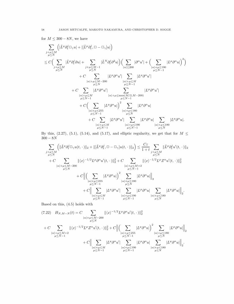
58 JASON METCALFE, MAKOTO NAKAMURA, AND CHRISTOPHER D. SOGGE
for M ≤ 300 − 8N , we have
∑
j+µ≤Mµ≤N
(
|Lµ∂jt 2γu| + |[Lµ∂j
t ,2 − 2γ ]u|)
≤ C(
∑
j+µ≤Mµ≤N
|Lµ∂jt ∂u| +
∑
j+µ≤M−1µ≤N
|LN∂jt ∂
2u|)(
∑
|α|≤200
|∂αu′| +(
∑
|α|+µ≤190µ≤N−1
|Lµ∂αu|)2)
+ C∑
|α|+µ≤M−200µ≤N
|Lµ∂αu′|∑
|α|+µ≤Mµ≤N−1
|Lµ∂αu′|
+ C∑
|α|+µ≤Mµ≤N−1
|Lµ∂αu′|∑
|α|+µ≤max(M/2,M−200)µ≤N−1
|Lµ∂αu′|
+ C(
∑
|α|+µ≤255µ≤N−1
|Lµ∂αu|)2 ∑
|α|+µ≤180µ≤N
|Lµ∂αu|
+ C∑
|α|+µ≤Mµ≤N−1
|Lµ∂αu′|∑
|α|+µ≤190µ≤N−1
|Lµ∂αu|∑
|α|+µ≤180µ≤N
|Lµ∂αu|.
By this, (2.27), (5.1), (5.14), and (5.17), and elliptic regularity, we get that for M ≤300 − 8N
∑
j+µ≤Mµ≤N
(
‖Lµ∂jt 2γu(t, · )‖2 + ‖[Lµ∂j
t ,2 − 2γ ]u(t, · )‖2
)
≤ Cε
1 + t
∑
j+µ≤Mµ≤N
‖Lµ∂jtu
′(t, · )‖2
+ C∑
|α|+µ≤M−200µ≤N
‖〈x〉−1/2Lµ∂αu′(t, · )‖22 + C
∑
|α|+µ≤M+2µ≤N−1
‖〈x〉−1/2LµZαu′(t, · )‖22
+ C∥
∥
∥
(
∑
|α|+µ≤255µ≤N−1
|Lµ∂αu|)2 ∑
|α|+µ≤180µ≤N
|Lµ∂αu|∥
∥
∥
2
+ C∥
∥
∥
∑
|α|+µ≤Mµ≤N−1
|Lµ∂αu′|∑
|α|+µ≤190µ≤N−1
|Lµ∂αu|∑
|α|+µ≤180µ≤N
|Lµ∂αu|∥
∥
∥
2.
Based on this, (4.5) holds with
(7.22) HN,M−N (t) = C∑
|α|+µ≤M−200µ≤N
‖〈x〉−1/2Lµ∂αu′(t, · )‖22
+ C∑
|α|+µ≤M+2µ≤N−1
‖〈x〉−1/2LµZαu′(t, · )‖22 + C
∥
∥
∥
(
∑
|α|+µ≤255µ≤N−1
|Lµ∂αu|)2 ∑
|α|+µ≤180µ≤N
|Lµ∂αu|∥
∥
∥
2
+ C∥
∥
∥
∑
|α|+µ≤Mµ≤N−1
|Lµ∂αu′|∑
|α|+µ≤190µ≤N−1
|Lµ∂αu|∑
|α|+µ≤180µ≤N
|Lµ∂αu|∥
∥
∥
2.

QUASILINEAR WAVE EQUATIONS SATISFYING THE NULL CONDITION 59
Notice that by (5.1), (5.14), and (5.15), the third term on the right of (7.22) is con-trolled by Cε3(1 + t)−1−. Also notice that by (5.1), (5.13), and (5.15), the last term in(7.22) is dominated by
Cε2(1 + t)bN ε+cN ε+
1 + t
∑
|α|+µ≤Mµ≤N−1
‖〈x〉−1Lµ∂αu′(t, · )‖2.
From this, we see that
(7.23)
∫ t
0
HN,M−N(s) ds ≤ Cε3 + C∑
|α|+µ≤M−200µ≤N
‖〈x〉−1/2Lµ∂αu′‖2L2(St)
+ C∑
|α|+µ≤M+2µ≤N−1
‖〈x〉−1/2LµZαu′‖2L2(St)
+ Cε2∫ t
0
(1 + s)−1+bN ε+cN ε+∑
|α|+µ≤Mµ≤N−1
‖〈x〉−1Lµ∂αu′(s, · )‖2 ds.
If one applies the Schwarz inequality and uses (5.21) (with N replaced by N − 1), thelast term above is O(ε3) for sufficiently small ε.
If we use this in (4.6) and apply the inductive hypothesis to handle terms that involveN − 1 or fewer occurences of L, we see that
(7.24)∑
|α|+µ≤Mµ≤N
‖Lµ∂αu′(t, · )‖2 ≤ Cε(1 + t)Cε+σ
+ C(1 + t)Cε∑
|α|+µ≤M−200µ≤N
‖〈x〉−1/2Lµ∂αu′‖2L2(St)
+ C(1 + t)Cε
∫ t
0
∑
|α|+µ≤Mµ≤N−1
‖Lµ∂αu′(s, · )‖L2(|x|<1) ds
since the conditions on the data give∫
e0(Lv∂j
t u)(0, x) ds ≤ Cε2 if ν + j ≤ 300.
As before, if we apply (4.12), (5.1), and (5.5), the last integral is dominated byCε log(2 + t) plus
(7.25)∑
|α|+µ≤M+1µ≤N−1
∫ t
0
(
∫ s
0
‖Lµ∂α2u(τ, · )‖L2(||x|−(s−τ)|<10) dτ
)
ds.
When 2u is replaced by B(du) + Q(du, d2u), as in the proof of (7.12), we can apply(2.27) and finite overlap of the sets (τ, x) : ||x| − (j − τ)| < 20, j = 0, 1, 2, . . . to seethat this is bounded by
C∑
|α|+µ≤M+3µ≤N−1
‖〈x〉−1/2LµZαu′‖2L2(St)
≤ Cε2(1 + t)2aN−1ε.
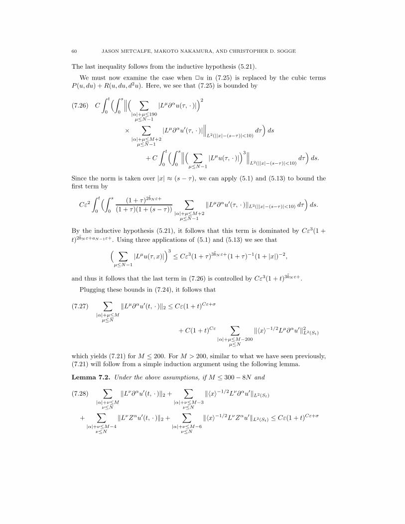
60 JASON METCALFE, MAKOTO NAKAMURA, AND CHRISTOPHER D. SOGGE
The last inequality follows from the inductive hypothesis (5.21).
We must now examine the case when 2u in (7.25) is replaced by the cubic termsP (u, du) +R(u, du, d2u). Here, we see that (7.25) is bounded by
(7.26) C
∫ t
0
(
∫ s
0
∥
∥
∥
(
∑
|α|+µ≤190µ≤N−1
|Lµ∂αu(τ, · )|)2
×∑
|α|+µ≤M+2µ≤N−1
|Lµ∂αu′(τ, · )|∥
∥
∥
L2(||x|−(s−τ)|<10)dτ
)
ds
+ C
∫ t
0
(
∫ s
0
∥
∥
∥
(
∑
µ≤N−1
|Lµu(τ, · )|)3∥
∥
∥
L2(||x|−(s−τ)|<10)dτ
)
ds.
Since the norm is taken over |x| ≈ (s − τ), we can apply (5.1) and (5.13) to bound thefirst term by
Cε2∫ t
0
(
∫ s
0
(1 + τ)2bN ε+
(1 + τ)(1 + (s− τ))
∑
|α|+µ≤M+2µ≤N−1
‖Lµ∂αu′(τ, · )‖L2(||x|−(s−τ)|<10) dτ)
ds.
By the inductive hypothesis (5.21), it follows that this term is dominated by Cε3(1 +
t)2bN ε+aN−1ε+. Using three applications of (5.1) and (5.13) we see that
(
∑
µ≤N−1
|Lµu(τ, x)|)3
≤ Cε3(1 + τ)3bN ε+(1 + τ)−1(1 + |x|)−2,
and thus it follows that the last term in (7.26) is controlled by Cε3(1 + t)3bN ε+.
Plugging these bounds in (7.24), it follows that
(7.27)∑
|α|+µ≤Mµ≤N
‖Lµ∂αu′(t, · )‖2 ≤ Cε(1 + t)Cε+σ
+ C(1 + t)Cε∑
|α|+µ≤M−200µ≤N
‖〈x〉−1/2Lµ∂αu′‖2L2(St)
which yields (7.21) for M ≤ 200. For M > 200, similar to what we have seen previously,(7.21) will follow from a simple induction argument using the following lemma.
Lemma 7.2. Under the above assumptions, if M ≤ 300 − 8N and
(7.28)∑
|α|+ν≤Mν≤N
‖Lν∂αu′(t, · )‖2 +∑
|α|+ν≤M−3ν≤N
‖〈x〉−1/2Lν∂αu′‖L2(St)
+∑
|α|+ν≤M−4ν≤N
‖LνZαu′(t, · )‖2 +∑
|α|+ν≤M−6ν≤N
‖〈x〉−1/2LνZαu′‖L2(St) ≤ Cε(1 + t)Cε+σ

QUASILINEAR WAVE EQUATIONS SATISFYING THE NULL CONDITION 61
with σ > 0, then there is a constant C′ so that
(7.29)∑
|α|+ν≤M−2ν≤N
‖〈x〉−1/2Lν∂αu′‖L2(St) +∑
|α|+ν≤M−3ν≤N
‖LνZαu′(t, · )‖2
+∑
|α|+ν≤M−5ν≤N
‖〈x〉−1/2LνZαu′‖L2(St) ≤ C′ε(1 + t)C′ε+C′σ.
Proof of Lemma 7.2: Here we use arguments similar to those applied to prove Lemma7.1. We begin by showing that the first term on the left side of (7.29) satisfies the bound.Using (4.9), (5.1), and (5.5) as in (7.5), we see that
(7.30) (log(2 + t))−1/2∑
|α|+ν≤M−2ν≤N
‖〈x〉−1/2Lν∂αu′‖L2(St) ≤ Cε(log(2 + t))1/2
+ C∑
|α|+ν≤M−1ν≤N
∫ t
0
‖Lν∂α2u(s, · )‖2 ds+ C
∑
|α|+ν≤M−2ν≤N
‖Lν∂α2u‖L2(St).
Notice that the second term in the right side of (7.30) is
(7.31) ≤ C
∫ t
0
∥
∥
∥
∑
|α|+ν≤190ν≤N−1
|Lν∂αu′(s, · )|∑
|α|+ν≤Mν≤N
|Lν∂αu′(s, · )|∥
∥
∥
2ds
+ C
∫ t
0
∥
∥
∥
∑
|α|+ν≤Mν≤N−1
|Lν∂αu′(s, · )|∑
|α|+ν≤M−190ν≤N
|Lν∂αu′(s, · )|∥
∥
∥
2ds
+ C
∫ t
0
∥
∥
∥
∑
|α|+ν≤190ν≤N−1
|Lν∂αu(s, · )|∑
|α|+ν≤180ν≤N
|Lν∂αu(s, · )|∑
|α|+ν≤Mν≤N
|Lν∂αu′(s, · )|∥
∥
∥
2ds
+ C
∫ t
0
∥
∥
∥
(
∑
ν≤N−1
|Lνu(s, · )|)2 ∑
ν≤N
|Lνu(s, · )|∥
∥
∥
2ds.
By (5.1), (5.13), and (5.15), it follows that the last term is O(ε3). Applying (5.1), (5.13),and (5.15) to the first and third terms and using (2.27) and the Schwarz inequality onthe second, we see that (7.31) is
≤ Cε3 + Cε
∫ t
0
(1 + s)−1+bN ε+cN ε+∑
|α|+ν≤Mν≤N
‖Lν∂αu′‖2 ds
+ C∑
|α|+ν≤M+2ν≤N−1
‖〈x〉−1/2LνZαu′(s, · )‖L2(St)
∑
|α|+ν≤M−190ν≤N
‖〈x〉−1/2Lν∂αu′‖L2(St).
When N ≤ 190, the last term above is unnecessary, and the bound follows from (7.28).For N > 190, one uses (7.28) and the inductive hypothesis (5.21) to bound the additional

62 JASON METCALFE, MAKOTO NAKAMURA, AND CHRISTOPHER D. SOGGE
term. Since the same arguments can be employed to bound the last term in (7.30), thisfinishes the proof of the bound for the first term in the left side of (7.29).
To control the second term on the left side of (7.29), we will use (4.8). The main stepis to estimate the first term on its right. Here, we have
(7.32)∑
|α|+ν≤M−3ν≤N
‖2γLνZαu(t, · )‖2 ≤ C
∥
∥
∥
∑
|α|≤200
|Zαu′(t, · )|∑
|α|+ν≤M−3ν≤N
|LνZαu′(t, · )|∥
∥
∥
2
+ C∥
∥
∥
∑
|α|≤M−3
|Zαu′(t, · )|∑
|α|+ν≤M−203ν≤N
|LνZαu′(t, · )|∥
∥
∥
2
+ C∥
∥
∥
(
∑
|α|+ν≤M−3ν≤N−1
|LνZαu′(t, · )|)2∥
∥
∥
2
+ C∥
∥
∥
(
∑
|α|+ν≤190ν≤N−1
|LνZαu(t, · )|)2 ∑
|α|+ν≤M−3ν≤N
|LνZαu′(t, · )|∥
∥
∥
2
+ C∥
∥
∥
∑
|α|+ν≤190ν≤N−1
|LνZαu(t, · )|∑
|α|+ν≤180ν≤N
|LνZαu(t, · )|∑
|α|+ν≤M−3|α|≥1,ν≤N
|LνZαu(t, · )|∥
∥
∥
2
+ C∥
∥
∥
∑
|α|+ν≤190ν≤N−1
|LνZαu(t, · )|∑
|α|+ν≤180ν≤N
|LνZαu(t, · )|∑
|α|+ν≤M−3ν≤N−1
|LνZαu′(t, · )|∥
∥
∥
2
+ C∥
∥
∥
(
∑
µ≤N−1
|Lµu(t, · )|)2 ∑
µ≤N
|Lµu(t, · )|∥
∥
∥
2.
With YM−N−3,N (t) as in (4.7), we can apply (5.1) and (5.17) to bound the first term inthe right by
Cε
1 + tY
1/2M−N−3,N (t).
By applying (5.1) and (5.13), the same bound holds for the fourth term in the right sideof (7.32). Using (2.27), the second and third terms in the right of (7.32) are controlledby
C∑
|α|+ν≤M−1ν≤N−1
‖〈x〉−1/2LνZαu′(t, · )‖22 + C
∑
|α|+ν≤M−203ν≤N
‖〈x〉−1/2LνZαu′(t, · )‖22.
Since the coefficients of Z are O(|x|), one may use (5.1), (5.13) and (5.15) to bound thefifth and sixth terms in the right side of (7.32) by
Cε2(1 + t)−1+bN ε+cN ε+(
∑
|α|+ν≤M−4ν≤N
‖LνZαu′(t, · )‖2 +∑
|α|+ν≤M−3ν≤N−1
‖LνZαu′(t, · )‖2
)
Finally, the last term in (7.32) is easily seen to be ≤ Cε3(1 + t)−1− by (5.1), (5.13), and(5.15).

QUASILINEAR WAVE EQUATIONS SATISFYING THE NULL CONDITION 63
If we use these bounds for (7.32) in (4.8), we see that
(7.33) ∂tYM−N−3,N (t) ≤ Cε
1 + tYM−N−3,N (t)
+ CY1/2M−N−3,N (t)
[
∑
|α|+ν≤M−1ν≤N−1
‖〈x〉−1/2LνZαu′(t, · )‖22
+∑
|α|+ν≤M−203ν≤N
‖〈x〉−1/2LνZαu′(t, · )‖22
+ ε2(1 + t)−1+bN ε+cN ε+(
∑
|α|+ν≤M−4ν≤N
‖LνZαu′(t, · )‖2 +∑
|α|+ν≤M−3ν≤N−1
‖LνZαu′(t, · )‖2
)
+ ε3(1 + t)−1−]
+ C∑
|α|+ν≤M−2ν≤N
‖Lν∂αu′(t, · )‖2L2(|x|<1).
Thus, by Gronwall’s inequality, we have
(7.34) YM−N−3,N (t) ≤ C(1 + t)2Cε[
ε+∑
|α|+ν≤M−1ν≤N−1
‖〈x〉−1/2LνZαu′‖2L2(St)
+∑
|α|+ν≤M−203ν≤N
‖〈x〉−1/2LνZαu′‖2L2(St)
+ ε2∫ t
0
(1 + s)−1+bN ε+cN ε+∑
|α|+ν≤M−4ν≤N
‖LνZαu′(s, · )‖2 ds
+ ε2∫ t
0
(1 + s)−1+bN ε+cN ε+∑
|α|+ν≤M−3ν≤N−1
‖LνZαu′(s, · )‖2 ds]2
+ C(1 + t)Cε∑
|α|+ν≤M−2ν≤N
‖〈x〉−1/2Lν∂αu′‖2L2(St)
since YM−N−3,N (0) ≤ Cε2 by (1.12).
For M ≤ 203, the third term on the right does not appear, and the proof of the bound
∑
|α|+ν≤M−3ν≤N
‖LνZαu′(t, · )‖22 ≤ CYM−N−3,N (t) ≤ Cε2(1 + t)C′ε+C′σ
is completed by applying the inductive hypothesis (5.21) (with N replaced by N − 1)to the second and fifth terms on the right, applying (7.28) to the fourth term on theright, and using the bound for the first term on the left of (7.29) to control the last termin (7.34). For M > 203, a subsequent application of (7.28) to the third term in (7.34)completes the proof of the bound for the second term in the left of (7.29).

64 JASON METCALFE, MAKOTO NAKAMURA, AND CHRISTOPHER D. SOGGE
Using (4.10) and the arguments above, this in turn implies that the third term in(7.29) is controlled by its right side, which completes the proof of the lemma.
By (7.27) and the lemma, we get (7.21). The inductive argument using the lemmaalso yields (5.21) which completes the proof of Theorem 1.1.
References
[1] R. Agemi and K. Yokoyama: The null condition and global existence of solutions to systems of
wave equations with different speeds, Advances in Nonlinear Partial Differential Equations andStochastics, (1998), 43–86.
[2] N. Burq: Decroissance de lenergie locale de l’equation des ondes pour le problme exterieur et
absence de rsonance au voisinage du reel, Acta Math. 180 (1998), 1–29.[3] D. Christodoulou: Global solutions of nonlinear hyperbolic equations for small initial data, Comm.
Pure Appl. Math. 39 (1986), 267-282.[4] D. Gilbarg and N. Trudinger: Elliptic partial differential equations of second order, Springer,
Second Ed., Third Printing, 1998.[5] K. Hidano: An elementary proof of global or almost global existence for quasi-linear wave equa-
tions, Tohoku Math. J., 56 (2004), 271–287.[6] K. Hidano and K. Yokoyama: A remark on the almost global existence theorems of Keel, Smith,
and Sogge, preprint.[7] L. Hormander: Lectures on nonlinear hyperbolic equations, Springer-Verlag, Berlin, 1997.[8] L. Hormander: L1, L∞ estimates for the wave operator, Analyse Mathematique et Applications,
Gauthier-Villars, Paris, 1988, pp. 211-234.[9] M. Ikawa: Decay of solutions of the wave equation in the exterior of two convex bodies, Osaka J.
Math. 19 (1982), 459–509.[10] M. Ikawa: Decay of solutions of the wave equation in the exterior of several convex bodies, Ann.
Inst. Fourier (Grenoble), 38 (1988), 113–146.
[11] F. John, Nonlinear wave equations, formation of singularities, Amer. Math. Soc., 1990.[12] S. Katayama, Global existence for a class of systems of nonlinear wave equations in three space
dimensions, preprint.[13] S. Katayama, Global existence for systems of wave equations with nonresonant nonlinearities and
null forms, preprint.[14] S. Katayama, A remark on systems of nonlinear wave equations with different propagation speeds,
preprint.[15] M. Keel, H. Smith, and C. D. Sogge: Global existence for a quasilinear wave equation outside of
star-shaped domains, J. Funct. Anal. 189 (2002), 155–226.[16] M. Keel, H. Smith, and C. D. Sogge: Almost global existence for some semilinear wave equations,
J. D’Analyse, 87 (2002), 265–279.[17] M. Keel, H. Smith, and C. D. Sogge: Almost global existence for quasilinear wave equations in
three space dimensions, J. Amer. Math. Soc. 17 (2004), 109–153.[18] S. Klainerman: Uniform decay estimates and the Lorentz invariance of the classical wave equation,
Comm. Pure Appl. Math. 38 (1985), 321–332.[19] S. Klainerman: The null condition and global existence to nonlinear wave equations, Lectures in
Applied Math. 23 (1986), 293–326.[20] S. Klainerman and T. Sideris: On almost global existence for nonrelativistic wave equations in 3d,
Comm. Pure Appl. Math. 49 (1996), 307–321.[21] K. Kubota and K. Yokoyama: Global existence of classical solutions to systems of nonlinear wave
equations with different speeds of propagation, Japan. J. Math. 27 (2001), 113–202.[22] P. D. Lax, C. S. Morawetz, and R. S. Phillips: Exponential decay of solutions of the wave equation
in the exterior of a star-shaped obstacle, Comm. Pure Appl. Math. 16 (1963), 477–486.[23] P. D. Lax and R. S. Phillips: Scattering theory, revised edition, Academic Press, San Diego, 1989.[24] H. Lindblad and I. Rodnianski, The weak null condition for Einstein’s equations, C. R. Math.
Acad. Sci. Paris 336 (2003), 901–906.[25] H. Lindblad and I. Rodnianski, Global existence for the Einstein vacuum equations in wave coor-
dinates, preprint.
QUASILINEAR WAVE EQUATIONS SATISFYING THE NULL CONDITION 65
[26] R. B. Melrose: Singularities and energy decay of acoustical scattering, Duke Math. J. 46 (1979),43–59.
[27] J. Metcalfe, M. Nakamura, and C. D. Sogge: Global existence of solutions to multiple speed systems
of quasilinear wave equations in exterior domains, to appear in Forum Math.[28] J. Metcalfe and C. D. Sogge: Hyperbolic trapped rays and global existence of quasilinear wave
equations, to appear in Invent. Math.[29] C. S. Morawetz: The decay of solutions of the exterior initial-boundary problem for the wave
equation, Comm. Pure Appl. Math. 14 (1961), 561–568.[30] C. S. Morawetz, J. Ralston, and W. Strauss: Decay of solutions of the wave equation outside
nontrapping obstacles, Comm. Pure Appl. Math. 30 (1977), 447–508.[31] J. V. Ralston: Solutions of the wave equation with localized energy, Comm. Pure Appl. Math. 22
(1969), 807–923.[32] Y. Shibata and Y. Tsutsumi: On a global existence theorem of small amplitude solutions for
nonlinear wave equations in an exterior domain, Math. Z. 191 (1986), 165-199.[33] T. Sideris: Nonresonance and global existence of prestressed nonlinear elastic waves, Ann. of Math.
151 (2000), 849–874.[34] T. Sideris: The null condition and global existence of nonlinear elastic waves, Inven. Math. 123
(1996), 323–342.[35] T. Sideris and S.Y. Tu: Global existence for systems of nonlinear wave equations in 3D with
multiple speeds, SIAM J. Math. Anal. 33 (2001), 477–488.[36] H. Smith and C. D. Sogge: Global Strichartz estimates for nontrapping perturbations of the Lapla-
cian, Comm. Partial Differential Equations 25 (2000), 2171–2183.[37] C. D. Sogge: Lectures on nonlinear wave equations, International Press, Cambridge, MA, 1995.[38] C. D. Sogge: Global existence for nonlinear wave equations with multiple speeds, Harmonic analysis
at Mount Holyoke (South Hadley, MA, 2001), 353–366, Contemp. Math., 320, Amer. Math. Soc.,Providence, RI, 2003.
[39] A. S. Tahvildar-Zadeh, Relativistic and nonrelativistic elastodynamics with small shear strains,Ann. Inst. H. Poincare-Phys. Theor. 69 (1998), 275–307.
[40] K. Yokoyama: Global existence of classical solutions to systems of wave equations with critical
nonlinearity in three space dimensions J. Math. Soc. Japan 52 (2000), 609–632.
School of Mathematics, Georgia Institute of Technology, Atlanta, GA 30332-0160
Graduate School of Information Sciences, Tohoku University, Sendai 980-8579, Japan
Department of Mathematics, Johns Hopkins University, Baltimore, MD 21218