The obstacle problem for quasilinear stochastic PDE's
37
The Annals of Probability 2010, Vol. 38, No. 3, 1143–1179 DOI: 10.1214/09-AOP507 © Institute of Mathematical Statistics, 2010 THE OBSTACLE PROBLEM FOR QUASILINEAR STOCHASTIC PDE’S 1 BY ANIS MATOUSSI 2 AND LUCRETIU STOICA 3 University of Le Mans and University of Bucharest We prove an existence and uniqueness result for the obstacle problem of quasilinear parabolic stochastic PDEs. The method is based on the proba- bilistic interpretation of the solution by using the backward doubly stochastic differential equation. 1. Introduction. We consider the following stochastic PDE, in R d , du t (x) + 1 2 u t (x) + f t (x,u t (x), ∇ u t (x)) + div g t (x,u t (x), ∇ u t (x)) dt (1) + h t (x,u t (x), ∇ u t (x)) · ←− dB t = 0, over the time interval [0,T ], with a given final condition u T = and f,g = (g 1 ,...,g d ), h = (h 1 ,...,h d 1 ) nonlinear random functions. The differential term with ←− dB t refers to the backward stochastic integral with respect to a d 1 - dimensional Brownian motion on (, F , P, (B t ) t ≥0 ). We use the backward nota- tion because in the proof we will employ the doubly stochastic framework intro- duced by Pardoux and Peng [16] (see also Bally and Matoussi [2] and Matoussi and Xu [13]). In the case where f and g do not depend of u and ∇ u, and if h is identically null, the equation (1) becomes a linear parabolic equation, ∂ t u(t,x) + 1 2 u(t,x) + f(t,x) + div g(t,x) = 0. (2) If v : [0,T ]× R d → R is a given function such that v(T,x) ≤ (x), we may roughly say that the solution of the obstacle problem for (2) is a function u ∈ Received May 2009; revised September 2009. 1 Supported in part by the research project MATPYL of the Fédération de Mathématiques des Pays de la Loire. 2 Supported in part by chaire Risques Financiers de la fondation du risque, CMAP-École Polytech- niques, Palaiseau-France. 3 Supported in part by the Contract CEx06-11-18. AMS 2000 subject classifications. Primary 60H15, 60G46; secondary 35H60. Key words and phrases. Stochastic partial differential equation, obstacle problem, backward dou- bly stochastic differential equation, regular potential, regular measure. 1143
-
Upload
khangminh22 -
Category
Documents
-
view
0 -
download
0
Transcript of The obstacle problem for quasilinear stochastic PDE's

The Annals of Probability2010, Vol. 38, No. 3, 1143–1179DOI: 10.1214/09-AOP507© Institute of Mathematical Statistics, 2010
THE OBSTACLE PROBLEM FOR QUASILINEARSTOCHASTIC PDE’S1
BY ANIS MATOUSSI2 AND LUCRETIU STOICA3
University of Le Mans and University of Bucharest
We prove an existence and uniqueness result for the obstacle problemof quasilinear parabolic stochastic PDEs. The method is based on the proba-bilistic interpretation of the solution by using the backward doubly stochasticdifferential equation.
1. Introduction. We consider the following stochastic PDE, in Rd ,
dut (x) + [12�ut(x) + ft (x, ut (x),∇ut(x))
+ divgt (x, ut (x),∇ut(x))]dt(1)
+ ht (x, ut (x),∇ut(x)) · ←−dBt = 0,
over the time interval [0, T ], with a given final condition uT = � and f,g =(g1, . . . , gd), h = (h1, . . . , hd1) nonlinear random functions. The differentialterm with
←−dBt refers to the backward stochastic integral with respect to a d1-
dimensional Brownian motion on (�, F ,P, (Bt)t≥0). We use the backward nota-tion because in the proof we will employ the doubly stochastic framework intro-duced by Pardoux and Peng [16] (see also Bally and Matoussi [2] and Matoussiand Xu [13]).
In the case where f and g do not depend of u and ∇u, and if h is identicallynull, the equation (1) becomes a linear parabolic equation,
∂tu(t, x) + 12�u(t, x) + f (t, x) + divg(t, x) = 0.(2)
If v : [0, T ] × Rd → R is a given function such that v(T , x) ≤ �(x), we may
roughly say that the solution of the obstacle problem for (2) is a function u ∈
Received May 2009; revised September 2009.1Supported in part by the research project MATPYL of the Fédération de Mathématiques des Pays
de la Loire.2Supported in part by chaire Risques Financiers de la fondation du risque, CMAP-École Polytech-
niques, Palaiseau-France.3Supported in part by the Contract CEx06-11-18.AMS 2000 subject classifications. Primary 60H15, 60G46; secondary 35H60.Key words and phrases. Stochastic partial differential equation, obstacle problem, backward dou-
bly stochastic differential equation, regular potential, regular measure.
1143

1144 A. MATOUSSI AND L. STOICA
L2([0, T ];H 1(Rd)) such that the following conditions are satisfied in (0, T )×Rd :
(i) u ≥ v, dt ⊗ dx-a.e.,
(ii) ∂tu + 12�u + f + divg ≤ 0,
(3)(iii) (u − v)
(∂tu + 1
2�u + f + divg) = 0,
(iv) uT = �, dx-a.e.
The relation (ii) means that the distribution appearing in the LHS of the inequal-ity is a nonpositive measure. The relation (iii) is not rigourously stated. We mayroughly say that one has ∂tu + 1
2�u + f + divg = 0 on the set {u > v}.If one expresses the obstacle problem for (2) in terms of variational inequalities
one should also ask that the solution has a minimality property (see Bensoussan–Lions [3], page 250, or Mignot–Puel [14]).
The work of El Karoui et al. [9] treats the obstacle problem for (2) within theframework of backward stochastic differential equations (BSDE in short). Namely,the equation (2) is considered with f depending of u and ∇u, while the functiong is null (as well h) and the obstacle v is continuous. The solution is representedstochastically as a process and the main new object of this BSDE framework is acontinuous increasing process that controls the set {u = v}. This increasing processdetermines in fact the measure from the relation (ii). Bally et al. [1] point out thatthe continuity of this process allows one to extend the classical notion of strongvariational solution (see Theorem 2.2 of [3], page 238) and express the solutionto the obstacle as a pair (u, ν) where ν equals the LHS of (ii) and is supported bythe set {u = v}. Moreover, based on this observation Matoussi and Xu [12] gen-eralized the work under monotonicity and general growth conditions. They havealso used the penalization method and stochastic flow technics (see [2] and [11]for more details on this method). In the present paper, we similarly consider thesolution as a pair (u, ν), point of view which has the advantage of expressing thenotion of solution independently of the double stochastic framework and withoutthe minimality property of Mignot–Puel [14], which would be very difficult tomanipulate in the case of the stochastic PDE. In Section 2.2, we are going to ex-amine the potential and the measure associated to a continuous increasing process.We call such potentials and measures, regular potentials, respectively regular mea-sures.
Now let us consider the final condition to be a fixed function � ∈ L2(Rd) andthe obstacle v be a random continuous function, v :� × [0, T ] × R
d → R. Thenthe obstacle problem for the equation (1) is defined as a pair (u, ν), where ν is arandom regular measure and u ∈ L2(� × [0, T ];H 1(Rd)) satisfies the following

OBSTACLE PROBLEM FOR STOCHASTIC PDE’S 1145
relations:
(i′) u ≥ v, dP ⊗ dt ⊗ dx-a.e.,
(ii′) dut (x) + [12�ut(x) + ft (x, ut (x),∇ut(x))
+ divgt (x, ut (x),∇ut(x))]dt
(4)+ ht (x, ut (x),∇ut(x)) · ←−
dBt = −ν(dt, dx) a.s.,
(iii′) ν(u > v) = 0 a.s.,
(iv′) uT = �, dP ⊗ dx-a.e.
In Section 2.4, we explain the rigorous sense of the relation (iii′) which is basedon the quasi-continuity of u. The main result of our paper is Theorem 4 whichensures the existence and uniqueness of the solution of the obstacle problem for(1). The method of proof is based on the penalization procedure and the doublystochastic calculus which is essential, although the definition of the solution andthe statement of the result avoids the doubly stochastic framework.
Similarly to the case treated in El Karoui et al. [9], the most difficult point isto show that the approximating sequence converges uniformly on the trajectoriesover the coincidence set {u = v}. This is proven in Lemma 7. The existence anduniqueness of the solution for equation (1) (without obstacle) has already beenproven in [7]. An essential ingredient in the treatment of the quasilinear part isthe probabilistic representation of the divergence term obtained in [17] as well asthe doubly stochastic representation corresponding to the divergence term of thestochastic PDE in [7]. We must mention the work of Nualard and Pardoux [15] andDonati-Martin and Pardoux [8] who studied a particular class of obstacle problemfor stochastic PDE driven by some space–time white noise by using a differenttechniques.
Finally, we would like to thank our friend Vlad Bally for a stimulating discus-sion on the obstacle problem we had “la Gare de Montparnasse” and the refereefor helping us to improve the presentation.
2. Preliminaries. The basic Hilbert space of our framework is L2(Rd), andwe employ the usual notation for its scalar product and its norm,
(u, v) =∫
Rdu(x)v(x) dx, ‖u‖2 =
(∫Rd
u2(x) dx
)1/2
.
In general, we shall use the notation
(u, v) =∫
Rdu(x)v(x) dx,
where u, v are measurable functions defined in Rd and uv ∈ L1(Rd).

1146 A. MATOUSSI AND L. STOICA
Our evolution problem will be considered over a fixed time interval [0, T ] andthe norm for a function L2([0, T ] × R
d) will be denoted by
‖u‖2,2 =(∫ T
0
∫Rd
|u(t, x)|2 dx dt
)1/2
.
Another Hilbert space that we use is the first order Sobolev space H 1(Rd) =H 1
0 (Rd). Its natural scalar product and norm are
(u, v)H 1(Rd ) = (u, v) + (∇u,∇v), ‖u‖H 1(Rd ) = (‖u‖22 + ‖∇u‖2
2)1/2,
where we denote the gradient by ∇u(t, x) = (∂1u(t, x), . . . , ∂du(t, x)).Of special interest is the subspace F ⊂ L2([0, T ];H 1(Rd)) consisting of all
functions u(t, x) such that t �→ ut = u(t, ·) is continuous in L2(Rd). The naturalnorm on F is
‖u‖T = sup0≤t≤T
‖ut‖2 +(∫ T
0‖∇ut‖2 dt
)1/2
.
The Lebesgue measure in Rd will be sometimes denoted by m. The space of
test functions which we employ in the definition of weak solutions of the evolutionequations (1) or (2) is DT = C∞([0, T ])⊗ C∞
c (Rd), where C∞([0, T ]) denotes thespace of real functions which can be extended as infinite differentiable functionsin the neighborhood of [0, T ] and C∞
c (Rd) is the space of infinite differentiablefunctions with compact support in R
d .
2.1. The probabilistic interpretation of the divergence term. The operator ∂t +12�, which represents the main linear part in the equation (1), is probabilisticallyinterpreted by the Brownian motion in R
d . We shall view the Brownian motion asa Markov process, and therefore we next introduce some detailed notation for it.The sample space is �′ = C([0,∞);R
d), the canonical process (Wt)t≥0 is definedby Wt(ω) = ω(t), for any ω ∈ �′, t ≥ 0 and the shift operator, θt :�′ → �′, isdefined by θt (ω)(s) = ω(t + s), for any s ≥ 0 and t ≥ 0. The canonical filtrationF 0
t = σ(Ws; s ≤ t) is completed by the standard procedure with respect to theprobability measures produced by the transition function
Pt(x, dy) = qt (x − y)dy, t > 0, x ∈ Rd,
where qt (x) = (2πt)−d/2 exp(−|x|2/2t) is the Gaussian density. Thus, we geta continuous Hunt process (�′,Wt , θt , F , Ft ,P
x). We shall also use the back-ward filtration of the future events F ′
t = σ(Ws; s ≥ t) for t ≥ 0. P0 is the Wiener
measure, which is supported by the set �′0 = {ω ∈ �′,w(0) = 0}. We also set
�0(ω)(t) = ω(t) − ω(0), t ≥ 0, which defines a map �0 :�′ → �′0. Then � =
(W0,�0) :�′ → Rd × �′
0 is a bijection. For each probability measure on Rd , the

OBSTACLE PROBLEM FOR STOCHASTIC PDE’S 1147
probability Pμ of the Brownian motion started with the initial distribution μ is
given by
Pμ = �−1(μ ⊗ P
0).
In particular, for the Lebesgue measure in Rd , which we denote by m = dx, we
have
Pm = �−1(dx ⊗ P
0).
These relations are saying that W0 is independent of �0. It is known that eachcomponent (Wi
t )t≥0 of the Brownian motion, i = 1, . . . , d , is a martingale underany of the measures P
μ. The next lemma shows that (Wit−r , F ′
t−r ), r ∈ (0, t], is abackward local martingale under P
m.
LEMMA 1. Let 0 < s < t . If A ∈ σ(Wt) is such that Em[|Wt |;A] < ∞, then
one has Em[|Ws |;A] < ∞. Moreover, for each B ∈ F ′
t , and i = 1, . . . , d , one has
Em[Wi
s ;A ∩ B] = Em[Wi
t ;A ∩ B].PROOF. We note that Wt is uniformly distributed, and consequently for each
c > 0, the set Ac = {|Wt | ≤ c} satisfies
Em[|Wt |;Ac] < ∞.
This shows that the class of the sets to which applies the statement is rather large.The vector (W0,Ws −W0,Wt −Ws) has the distribution m⊗ N (0, s)⊗ N (0, t −
s), under the measure Pm. Then one deduce that (Ws,Wt −Ws) has the distribution
m ⊗ N (0, t − s) and we may write, for ϕ1, ϕ2 ∈ Cc(Rd),
Em[ϕ1(Wt − Ws)ϕ2(Wt)] =
∫Rd
∫Rd
ϕ1(y)ϕ2(x + y)qt−s(y) dy dx
=(∫
Rdϕ2(x) dx
)(∫Rd
ϕ1(y)qt−s(y) dy
).
This relation shows that the vector (Wt − Ws,Wt) has the distribution N (0, t −s)⊗m, under P
m.Then the obvious inequality |Ws | ≤ |Wt |+|Wt −Ws |(1{|Wt |≤1} +|Wt |) allows one to deduce the first assertion of the lemma.
In order to check the second assertion of the lemma, we write
Em[Wi
s ;A ∩ B] = Em[Wi
t ;A ∩ B] − Em[Wi
t − Wis ;A ∩ B]
and all that it remains to check is that the last term is null. In order to show this,one first observes that the distribution of the vector (Wt −Ws,Wt,Wt1 −Wt,Wt2 −Wt1, . . . ,Wtn −Wtn−1) is N (0, t − s)⊗m⊗ N (0, t1 − t)⊗· · ·⊗ N (0, tn − tn−1),for each system s < t < t1 < · · · < tn. Then one has, for each B ∈ σ(Wt1 −Wt, . . . ,Wtn − Wtn−1),
Em[Wi
t − Wis ;A ∩ B] = E
0[Wit − Wi
s ]m(A)P0(B) = 0,

1148 A. MATOUSSI AND L. STOICA
which implies the assertion of the lemma. �
Now let us assume that f and |g| belong to L2([0, T ] × Rd) and u ∈ F is a
solution of the deterministic equation (2). Let us denote by∫ t
sgr ∗ dWr =
d∑i=1
(∫ t
sgi(r,Wr) dWi
r +∫ t
sgi(r,Wr)
←−dWi
r
).(5)
Then one has the following representation (Theorem 3.2 in [17]).
THEOREM 1. The following relation holds Pm-a.s. for each 0 ≤ s ≤ t ≤ T :
ut(Wt) − us(Ws) =d∑
i=1
∫ t
s∂iur(Wr) dWi
r −∫ t
sfr(Wr) dr − 1
2
∫ t
sgr ∗ dWr.(6)
In [17], one uses the backward martingale←−Mμ,i defined under an arbitrary P
μ,with μ a probability measure in R
d , in order to express the integral∫ ts gr ∗ dWr .
Though formally the definition looks different, one easily sees that it is the sameobject.
2.2. Regular measures. In this section, we shall be concerned with some factsrelated to the time–space Brownian motion, with the state space [0, T [×R
d, cor-responding to the generator ∂t + 1
2�. Its associated semigroup will be denotedby (Pt )t>0. We may express it in terms of the Gaussian density of the semigroup(Pt )t>0 in the following way:
Ptψ(s, x) =⎧⎨⎩
∫Rd
qt (x, y)ψ(s + t, y) dy, if s + t < T ,
0, otherwise,
where ψ : [0, T [×Rd → R is a bounded Borel measurable function, s ∈ [0, T [, x ∈
Rd and t > 0. So we may also write (Ptψ)s = Ptψt+s if s + t < T . The cor-
responding resolvent has a density expressed in terms of the density qt too, asfollows:
Uαψ(t, x) =∫ T
t
∫Rd
e−α(s−t)qs−t (x − y)ψ(s, y) dy ds
or
(Uαψ)t =∫ T
te−α(s−t)Ps−tψs ds.
In particular, this ensures that the excessive functions with respect to the time–space Brownian motion are lower semicontinuous. In fact, we will not use directlythe time space process, but only its semigroup and resolvent. For related factsconcerning excessive functions, the reader is referred to [4] or [6]. Some furtherproperties of this semigroup are presented in the next lemma.

OBSTACLE PROBLEM FOR STOCHASTIC PDE’S 1149
LEMMA 2. The semigroup (Pt )t>0 acts as a strongly continuous semi-group of contractions on the spaces L2([0, T [×R
d) = L2([0, T [;L2(Rd)) andL2([0, T [;H 1(Rd)).
PROOF. Obviously, it is enough to check the following relations:
limr→0
(∫ T −r
0‖Prut+r − ut‖2
2 dt +∫ T
T −r‖ut‖2
2 dt
)= 0,
limr→0
(∫ T −r
0‖∇(Prut+r − ut )‖2
2 dt +∫ T
T −r‖∇ut‖2
2 dt
)= 0.
First, we note that for each function u ∈ L2([0, T [×Rd) and r > 0, one has
limr→0
∫ T −r
0‖ut+r − ut‖2
2 dt = 0.
This property is obvious for a function u ∈ Cc([0, T [×Rd) and then it is obtained
by approximation for any function in L2([0, T [×Rd). Then the relation
limr→0
∫ T −r
0‖Prut+r − ut‖2
2 dt = 0,
easily follows. From it, one deduces the strong continuity of (Pt )t>0 on L2([0, T [×R
d).
In order to prove the same property in the space L2([0, T [;H 1(Rd)), one shouldstart with the relation
limr→0
∫ T −r
0‖∇(ut+r − ut)‖2
2 dt = 0,
which holds for each u ∈ C∞c ([0, T [×R
d) and then repeat, with obvious modifica-tions, the previous reasoning. �
The next definition restricts our attention to potentials belonging to F , which isthe class of potentials appearing in our parabolic case of the obstacle problem.
DEFINITION 1. (i) A function ψ : [0, T ] × Rd → R is called quasicontinuous
provided that for each ε > 0, there exists an open set, Dε ⊂ [0, T ] × Rd, such that
ψ is finite and continuous on Dcε and
Pm({ω ∈ �′|∃t ∈ [0, T ] s.t. (t,Wt(ω)) ∈ Dε}) < ε.
(ii) A function u : [0, T ] × Rd → [0,∞] is called a regular potential, provided
that its restriction to [0, T [×Rd is excessive with respect to the time–space semi-
group, it is quasicontinuous, u ∈ F and limt→T ut = 0 in L2(Rd).

1150 A. MATOUSSI AND L. STOICA
Observe that if a function ψ is quasicontinuous, then the process (ψt (Wt))t∈[0,T ]is continuous. Next, we will present the basic properties of the regular potentials.Do to the expression of the semigroup (Pt )t>0 in terms of the density, it followsthat two excessive functions which represent the same element in F should coin-cide.
THEOREM 2. Let u ∈ F . Then u has a version which is a regular potential ifand only if there exists a continuous increasing process A = (At )t∈[0,T ] which is(Ft )t∈[0,T ]-adapted and such that A0 = 0, E
m[A2T ] < ∞ and
(i) ut (Wt) = E[AT |Ft ] − At Pm-a.s.
for each t ∈ [0, T ]. The process A is uniquely determined by these properties.Moreover, the following relations hold:
(ii) ut (Wt) = AT − At −d∑
i=1
∫ T
t∂ius(Ws) dWi
s Pm-a.s.,
(iii) ‖ut‖22 +
∫ T
t‖∇us‖2
2 ds = Em(AT − At)
2,
(iv) (u0, ϕ0) +∫ T
0
(1
2(∇us,∇ϕs) + (us, ∂sϕs)
)ds
=∫ T
0
∫Rd
ϕ(s, x)ν(ds dx)
for each test function ϕ ∈ DT , where ν is the measure defined by
(v) ν(ϕ) = Em
∫ T
0ϕ(t,Wt) dAt , ϕ ∈ Cc([0, T ] × R
d).
PROOF. We first remark that the uniqueness of the increasing process in therepresentation (i) follows from the uniqueness in the Doob–Meyer decomposition.
Let us now assume that u is a regular potential which is a version of u. Wewill use an approximation of u constructed with the resolvent. By the resolventequation, one has
αUαu = αU0(u − αUαu).
Let us set f n = n(u − nUnu) and un = nUnu = U0fn. Since u is excessive, one
has f n ≥ 0 and un,n ∈ N∗, is an increasing sequence of excessive functions with
limit u. In fact un,n ∈ N∗, are potentials and their trajectories are continuous.
On the other hand, the trajectories t → ut (Wt) are continuous on [0, T [ by thequasi-continuity of u. The process (ut (Wt))t∈[0,T [ is a super-martingale, and be-cause limt→T ut = 0 in L2, it is a potential and the trajectories have null limits

OBSTACLE PROBLEM FOR STOCHASTIC PDE’S 1151
at T . Therefore, this approximation also holds uniformly on the trajectories, onthe closed interval [0, T ],
limn→∞ sup
0≤t≤T
|unt (Wt) − ut (W)| = 0 P
m-a.s.
The function un solves the equation (∂t +L)un+f n = 0 with the condition unT = 0
and its backward representation is
unt (Wt) =
∫ T
tf n
s (Ws) ds −d∑
i=1
∫ T
t∂iu
ns (Ws) dWi
s .
If we set Ant = ∫ t
0 f ns (Ws) ds, after conditioning, this representation gives
unt (Wt) = An
T − Ant −
d∑i=1
∫ T
t∂iu
ns (Ws) dWi
s = Em[An
T /Ft ] − Ant .(∗)
In particular, one deduces
un0(W0) = E
m[AnT /F0] = An
T −d∑
i=1
∫ T
0∂iu
ns (Xs) dWi
s .
Also from the relation (∗), it follows that
Em(An
T − Ant )
2 = Em
(un
t (Wt) +d∑
i=1
∫ T
t∂iu
ns (Ws) dWi
s
)2
(∗∗)
= ‖unt ‖2
2 +∫ T
t‖∇un
s ‖22 ds.
A similar relation holds for differences, in particular one has
Em(An
T − AkT )2 = ‖un
0 − uk0‖2 + 2
∫ T
0‖∇(un
s − uks )‖2
2 ds.
On the other hand, the preceding lemma ensures that limα→∞ αUα = I, in thespace L2([0, T [;H 1(Rd)), which implies
limn→0
∫ T
0‖∇(un
t − ut )‖22 dt = 0.
These last relations imply that there exists a limit limn AnT =: AT in the sense of
L2(Pm).
Let us denote by Mn = (Mnt )t∈[0,T ],M = (Mt)t∈[0,T ] the martingales given by
the conditional expectations Mnt = E
m[AnT /Ft ],Mt = E
m[AT /Ft ]. Then one haslimn→∞ Mn = M, in L2(Pm), and hence
limn→∞ E
m sup0≤t≤T
|Mnt − Mt |2 = 0.

1152 A. MATOUSSI AND L. STOICA
Then the relation unt (Wt) = Mn
t − Ant shows that the processes An,n ∈ N
∗, alsoconverge uniformly on the trajectories to a continuous process A = (At )t∈[0,T ].The inequality
sup0≤t≤T
|Ant − At | ≤ AT + |An
T − AT |
ensures the conditions to pass to the limit and get
limn→∞ E
m sup0≤t≤T
|Ant − At |2 = 0.
Passing to the limit in the relations (∗) and (∗∗) one deduces the relations (i), (ii)and (iii).
In order to check the relation (iv) from the statement, we observe that the rela-tion is fulfilled by the functions un,
(un0, ϕ0) +
∫ T
0
(1
2(∇un
s ,∇ϕs) + (uns , ϕs)
)ds =
∫ T
0
∫Rd
ϕ(s, x)f n(s, x) ds dx
= Em
∫ T
0ϕ(s,Ws) dAn
s ,
where ϕ is arbitrary in DT . In order to get the relation (iv), it would suffice to passto the limit with n → ∞ in this relation. The only term which poses problems isthe last one. The uniform convergence on the trajectories implies that, P
m-a.s., themeasures dAn
t weakly converge to dAt . Therefore, one has
limn→∞
∫ T
0ϕt(Wt) dAn
t =∫ T
0ϕt(Wt) dAt P
m-a.s.
On the other hand, one has∣∣∣∣∫ T
0ϕt(Wt) dAn
t
∣∣∣∣ ≤ sup0≤t≤T
ϕ2t (Wt ) + A2
T + |AnT − AT |2.
By Itô’s formula and Doob’s inequality, one has
Em
(sup
0≤t≤T
ϕ2(t,Wt))
≤ 4‖ϕ0‖2 + 4Em
(∫ T
0|∂tϕ(t,Wt)|dt
)2
+ 16Em
∫ T
0|∇ϕ|2(t,Wt) dt
+ 2Em
(∫ T
0|�ϕ|(t,Wt) dt
)2
≤ 4‖ϕ0‖2 + 4T
∫ T
0‖∂tϕt‖2
2 dt + 16∫ T
0‖∇ϕt‖2
2 dt
+ 2T
∫ T
0‖�ϕt‖2
2 dt < ∞.

OBSTACLE PROBLEM FOR STOCHASTIC PDE’S 1153
The preceding estimate ensures the possibility of passing to the limit and deducingthat
limn
Em
∫ T
0ϕ(s,Ws) dAn
s = Em
∫ T
0ϕ(s,Ws) dAs,
and thus we obtain the relation (iv).Let us now consider the converse. Assume that u ∈ F and A is a continuous
increasing process adapted to (Ft )t∈[0,T ] and satisfying the relation (i). In order tosimplify the subsequent notation, it is convenient to extend our given function byputting ut = 0 for t > T . Now, we shall show that
Pr(ut+r ) ≤ ut , t ∈ [0, T ], r > 0.(7)
By the Markov property, one gets
Prut+r (Wt) = EWt [ut+r (Wr)] = E
m[ut+r (Wr+t )|Ft ]= E
m[E
m[AT |Ft+r ] − At+r |Ft
] = Em[AT |Ft ] − At+r ,
where the last line comes from the relation (i). This shows that
Prut+r (Wt) ≤ ut(Wt) Pm-a.s.
and as the distribution of Wt under Pm is m, we deduce the inequality (7). More-
over, this inequality shows by iteration that if r ≤ r ′, then
Pr ′ut+r ′ ≤ Prut+r .(8)
By the properties of the semigroup density and since t → ut is continuous withvalues in L2, it follows that, for each r > 0, Prut+r , t ∈ [0, T ], has a continuousversion in [0, T ] × R
d defined by
ur(t, x) =∫
Rdqr(x, y)ut+r (y) dy.
The inequality (8) shows in fact that ur is supermedian with respect to (Pt )t>0 and,because of continuity, in fact it is excessive. Then u = limr→0 ur is also excessiveand since limr→0 Prut+r = ut , in L2, clearly u is a version of u. The process(ut (Wt))t∈[0,T ] is a cdlg supermartingale, and more precisely a potential. By therelation (i), this process admits a continuous version. It follows that itself is con-tinuous and, as a consequence, one has the following convergence, uniformly onthe trajectories:
limr→0
sup0≤t≤T
|urt (Wt) − ut (Wt)| = 0 P
m-a.s.
On the other hand, by the representation (i) one has
Em sup
0≤t≤T
|ut (Wt)|2 < ∞,

1154 A. MATOUSSI AND L. STOICA
which leads to
limr→0
Em sup
0≤t≤T
|urt (Wt) − ut (W)|2 = 0.
This relation implies that u is quasicontinuous, and hence it is a regular potential,completing the proof. �
It is known in the probabilistic potential theory that the regular potentials areassociated to continous additive functionals (see [4], Section IV.3 or [10], The-orem 5.4.2). In the above theorem, the additive aspect is not evident. In fact, itis hidden in the relation (i) of Theorem 2. This relation implies that, for t ≤ s,
As − At is measurable with respect to the completion of σ(Wr/r ∈ [t, s]). Thiscan directly be proven but it also follows from the approximation of A by An. Forthe processes An,n ∈ N, this measurability property obviously holds. And thismeasurability ensures the fact that A corresponds to an additive functional for thetime–space process, which we are not explicitly using.
The measure ν from the theorem, expressed in the relation (v), is also com-pletely determined by the relation (iv), because the test functions are dense inCc([0, T ] × R
d). A natural question now is whether one Radon measure on[0, T ]× R
d can be associated via the relation (iv) from the theorem to two distinctpotentials. The answer is that there is only one such potential and more preciselyit can be directly expressed with the density qt (x, y) in terms of the measure, asone can see from the next lemma.
LEMMA 3. Let u be a regular potential and ν a Radon measure on [0, T ]×Rd
such that relation (iv) holds. Then one has
(φ,ut ) =∫ T
t
∫Rd
(∫Rd
φ(x)qs−t (x − y)dx
)ν(ds dy)
for each φ ∈ L2(Rd) and t ∈ [0, T ].
PROOF. We first remark that the relation (iv) is in fact equivalent to the fol-lowing more explicit one
(ut , ϕt ) +∫ T
t
(1
2(∇us,∇ϕs) + (us, ∂sϕs)
)ds =
∫ T
t
∫Rd
ϕ(s, x)ν(ds dx),
with any ϕ ∈ DT and t ∈ [0, T ].Clearly, it is sufficient to prove the lemma for φ ∈ Cc(R
d) such that φ ≥ 0.
Then we set ψ(s, y) = ∫Rd φ(x)qs−t (x − y)dx, for s ∈ [t, T ] and y ∈ R
d . Thenψs = Ps−tφ and the map s → ψs is in C 1(]t, T ];L2(Rd)) and ∂sψ = 1
2�ψs. Letη ∈ Cc(R+) be a decreasing function such that η = 1 on the interval [0,1] andη = 0 for x ≥ 2. Set ηn(x) = η(
|x|n
), so that (ηn)n∈N is an increasing sequence inCc(R
d) with limit 1Rd . For each fixed n, the function ηnψ can be approximated

OBSTACLE PROBLEM FOR STOCHASTIC PDE’S 1155
by convolution with smooth functions and then by test functions from DT , andconsequently we may write the relation (iv) in the form
(ut , ηnψt) +∫ T
t
(1
2(∇us,∇(ηnψs)) + (us, ηn ∂sψs)
)ds
=∫ T
t
∫Rd
ηn(x)ψ(s, x)ν(ds dx).
Then it is easy to see that we may pass to the limit with n → ∞, in this relationtoo. Then we get
(ut ,ψt ) +∫ T
t
(1
2(∇us,∇ψs) + (us, ∂sψs)
)ds =
∫ T
t
∫Rd
ψ(s, x)ν(ds dx),
which becomes the relation asserted by the lemma, on account of the relation∂sψ = 1
2�ψs. �
We now introduce the class of measures which intervene in the notion of solu-tion to the obstacle problem.
DEFINITION 2. A nonnegative Radon measure ν defined in [0, T ] × Rd is
called regular provided that there exists a regular potential u such that the relation(iv) from the above theorem is satisfied.
As a consequence of the preceding lemma, we see that the regular measures arealways represented as in the relation (v) of the theorem, with a certain increas-ing process. We also note the following properties of a regular measure, with thenotation from the theorem.
1. A set B ∈ B([0, T ] × Rd) satisfies the relation ν(B) = 0 if and only if∫ T
0 1B(t,Wt) dAt = 0 Pm-a.s.
2. If a set B ∈ B(]0, T [×Rd) is polar, in the sense that
Pm({ω ∈ �′|∃t ∈ [0, T ], (t,Wt(ω)) ∈ B}) = 0,
then ν(B) = 0.
3. If ψ1,ψ2 : [0, T ] × Rd → R are Borel measurable and such that ψ1(t, x) ≥
ψ2(t, x), dt ⊗ dx-a.e., and the processes (ψit (Wt))t∈[0,T ], i = 1,2, are a.s. con-
tinuous, then one has ν(ψ1 < ψ2) = 0.
2.3. Hypotheses. Let B = (Bt )t≥0 be a standard d1-dimensional Brownianmotion on a probability space (�, F B,P). So Bt = (B1
t , . . . ,Bd1
t ) takes values in
Rd1
. Over the time interval [0, T ] we define the backward filtration (F Bs,T )s∈[0,T ]
where F Bs,T is the completion in F B of σ(Br − Bs; s ≤ r ≤ T ).

1156 A. MATOUSSI AND L. STOICA
We denote by HT the space of H 1(Rd)-valued predictable and F Bt,T -adapted
processes (ut )0≤t≤T such that the trajectories t → ut are in F a.s. and
‖u‖2T < ∞.
In the remainder of this paper, we assume that the final condition � is a givenfunction in L2(Rd) and the functions appearing in equation (1),
f : [0, T ] × � × Rd × R × R
d → R,
g = (g1, . . . , gd) : [0, T ] × � × Rd × R × R
d → Rd,
h = (h1, . . . , hd1) : [0, T ] × � × Rd × R × R
d → Rd1
,
are random functions predictable with respect to the backward filtration(F B
t,T )t∈[0,T ]. We set
f (·, ·, ·,0,0) := f 0, g(·, ·, ·,0,0) := g0 = (g01, . . . , g0
d)
and
h(·, ·, ·,0,0) := h0 = (h01, . . . , h
0d1)
and assume the following hypotheses.
ASSUMPTION (H). There exist nonnegative constants C,α,β such that
(i) |f (t,ω, x, y, z) − f (t,ω, x, y′, z′)| ≤ C(|y − y′| + |z − z′|).(ii) (
∑d1
j=1 |hj (t,ω, x, y, z) − hj (t,ω, x, y′, z′)|2)1/2 ≤ C|y − y′| + β|z − z′|.(iii) (
∑di=1 |gi(t, x, y, z) − gi(t,ω, x, y′, z′)|2)1/2 ≤ C|y − y′| + α|z − z′|.
(iv) The contraction property (as in [7]): α + β2
2 < 12 .
ASSUMPTION (HD2).
E(‖f 0‖22,2 + ‖g0‖2
2,2 + ‖h0‖22,2) < ∞.
ASSUMPTION (HO). The obstacle v(t,ω, x) is a predictable random functionwith respect to the backward filtration (F B
t,T ). We also assume that t �→ v(t,ω,Wt)
is P ⊗ Pm-a.s. continuous on [0, T ] and satisfies
v(T , ·) ≤ �(·).We recall that a usual solution (nonreflected one) of the equation (1) with final
condition uT = �, is a processus u ∈ HT such that for each test function ϕ ∈ DT
and any ∀t ∈ [0, T ], we have a.s.∫ T
t
[(us, ∂sϕs) + 1
2(∇us,∇ϕs) + (gs,∇ϕs)
]ds − (�,ϕT ) + (ut , ϕt )
(9)
=∫ T
t(fs, ϕs) ds +
∫ T
t(hs, ϕs) · ←−
dBs.
OBSTACLE PROBLEM FOR STOCHASTIC PDE’S 1157
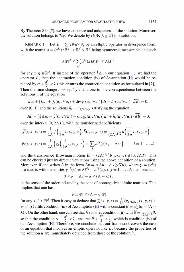
By Theorem 8 in [7], we have existence and uniqueness of the solution. Moreover,the solution belongs to HT . We denote by U (�,f, g,h) this solution.
REMARK 1. Let L = ∑ij ∂ia
ij ∂j be an elliptic operator in divergence form,with the matrix a = (aij ) : Rd → R
d × Rd being symmetric, measurable and such
that
λ|ξ |2 ≤ ∑ij
aij (x)ξ iξ j ≤ �|ξ |2
for any x, ξ ∈ Rd . If instead of the operator 1
2� in our equation (1), we had theoperator L, then the contraction condition (iv) of Assumption (H) would be re-
placed by α + β2
2 < λ (this ensures the contraction condition as formulated in [7]).Then the time change t → 1
2�t ′ yields a one to one correspondence between the
solutions u of the equation
dut + [Lut + ft (ut ,∇ut) + divgt (ut ,∇ut)]dt + ht (ut ,∇ut) · ←−dBt = 0,
over [0, T ] and the solutions ut = u1/(2�)t satisfying the equation
dut + [12�ut + ft (ut ,∇ut ) + div gt (ut ,∇ut )
]dt + ht (ut ,∇ut ) · ←−
dBt = 0,
over the interval [0,2�T ], with the transformed coefficients
f (t, x, y, z) = 1
2�f
(1
2�t,x, y, z
), h(t, x, y, z) = 1
(2�)1/2 h
(1
2�t,x, y, z
),
gi(t, x, y, z) = 1
2�
(gi
(1
2�t,x, y, z
)+ ∑
j
aij (x)zj − �zi
), i = 1, . . . , d,
and the transformed Brownian motion Bt = (2�)1/2B1/(2�)t , t ∈ [0,2�T ]. Thiscan be checked just by direct calculations using the above definition of a solution.Moreover, if one writes L in the form Lu = ��u − div(γ∇u), where γ = (γ ij )
is a matrix with the entries γ ij (x) = �δij − aij (x), i, j = 1, . . . , d, then one has
0 ≤ γ = �I − a ≤ (� − λ)I,
in the sense of the order induced by the cone of nonnegative definite matrices. Thisimplies that one has
|γ (x)ξ | ≤ (� − λ)|ξ |for any x, ξ ∈ R
d . Then it easy to deduce that gt (x, y, z) = 12�
(g1/(2�)t (x, y, z) +γ (x)z) fulfils condition (iii) of Assumption (H) with a constant α = 1
2�(α + (� −
λ)). On the other hand, one can see that h satisfies condition (ii) with β = 1(2�)1/2 β,
so that the condition α + β2
2 < λ, ensures α + β2
2 < 12 , which is condition (iv) of
our Assumption (H). Therefore, we conclude that our framework covers the caseof an equation that involves an elliptic operator like L, because the properties ofthe solution u are immediately obtained from those of the solution u.

1158 A. MATOUSSI AND L. STOICA
2.4. Quasi-continuity properties. In this section, we are going to prove thequasi-continuity of the solution of the linear equation, that is, when f,g,h do notdepend of u and ∇u. To this end, we first extend the double stochastic Itô’s formulato our framework. We start by recalling the following result from [7] (stated forlinear SPDE).
THEOREM 3. Let u ∈ HT be a solution of the equation
dut + 12�ut dt + (ft + divgt ) dt + ht
←−dBt = 0,
where f,g,h are predictable processes such that
E
∫ T
0[‖ft‖2
2 + ‖gt‖22 + ‖ht‖2
2]dt < ∞ and ‖�‖22 < ∞.
Then, for any 0 ≤ s ≤ t ≤ T , one has the following stochastic representation, P ⊗P
m-a.s.,
u(t,Wt) − u(s,Ws) = ∑i
∫ t
s∂iu(r,Wr) dWi
r −∫ t
sfr(Wr) dr
(10)
− 1
2
∫ t
sg ∗ dW −
∫ t
shr(Wr) · ←−
dBr.
We remark that FT and F B0,T are independent under P⊗P
m and therefore in the
above formula the stochastic integrals with respect to dWt and←−dWt act indepen-
dently of F B0,T and similarly the integral with respect to
←−dBt acts independently of
FT .In particular, the process (ut (Wt))t∈[0,T ] admits a continuous version which we
usually denote by Y = (Yt )t∈[0,T ] and we introduce the notation Zt = ∇ut(Wt).As a consequence of this theorem, we have the following result.
COROLLARY 1. Under the hypothesis of the preceding theorem, one has thefollowing stochastic representation for u2, P ⊗ P
m-a.e., for any 0 ≤ t ≤ T ,
u2t (Wt) − �2(WT ) = 2
∫ T
t
[usfs(Ws) − 1
2|∇us |2(Ws)
− 〈∇us, gs〉(Ws) + 1
2|hs |2(Ws)
]ds
(11)
+∫ T
t(urgr)(Wr) ∗ dWr − 2
∑i
∫ T
t(ur∂iur)(Wr) dWi
r
+ 2∫ T
t(urhr)(Wr) · ←−
dBr.

OBSTACLE PROBLEM FOR STOCHASTIC PDE’S 1159
Moreover, one has the estimate
EEm
(sup
t≤s≤T
|Ys |2)
+ E
[∫ T
t‖∇us‖2
2 ds
](12)
≤ c
[‖φ‖2
2 + E
∫ T
t[‖fs‖2
2 + ‖gs‖22 + ‖hs‖2
2]ds
]for each t ∈ [0, T ].
REMARK 2. With the notation introduced above, one can write the relation(11) as
|Yt |2 +∫ T
t|Zr |2 dr = |YT |2 + 2
∫ T
tYrfr(Wr) dr − 2
∫ T
t〈Zr, gr(Wr)〉dr
+∫ T
tYrgr(Wr) ∗ dWr − 2
∑i
∫ T
tYrZi,r dWi
r(13)
+ 2∫ T
tYrhr(Wr) · ←−
dBr +∫ T
t|hr |2(Wr) dr.
PROOF OF COROLLARY 1. Assume first that g is uniformly bounded and be-longs to (HT )d , so that E
∫ T0 ‖divgt‖2
2 dt < ∞. Then we may represent the solu-tion in the form
ut (Wt) − us(Ws) = ∑i
∫ t
s∂iur(Wr) dWi
r −∫ t
s[fr(Wr) + divgr(Wr)]dr
−∫ t
shr(Wr) · ←−
dBr.
By Lemma 1.3 of [16], we may write
u2t (Wt ) − u2
s (Ws) = −2∫ t
s[ur(fr + divgr)(Wr) − |∇ur |2(Wr) − |hr |2(Wr)]dr
+ 2∑i
∫ t
s(ur ∂iur)(Wr) dWi
r − 2∫ t
s(urhr)(Wr) · ←−
dBr.
On the other hand, by Lemma 3.1 of [17], one has
−2∫ t
sdiv(urgr)(Wr) dr =
∫ t
surgr(Wr) ∗ dWr,
so that the preceding relation immediately leads to the relation (11). Then the stan-dard calculations of BDSDE involving Young’s inequality, BDG inequality andGronwall’s lemma give the estimate (12).
Finally, to obtain the result with general g one proceeds by approximation. �

1160 A. MATOUSSI AND L. STOICA
In the deterministic case, it was proven in [17] that the solution of a quasilinearequation has a quasicontinuous version. Here, we shall prove the same propertyfor the solution of an SPDE as is stated in the next proposition.
PROPOSITION 1. Under the hypothesis of Theorem 3, there exists a function�u : [0, T ]×�×R
d → R which is a quasicontinuous version of u, in the sense thatfor each ε > 0, there exits a predictable random set Dε ⊂ [0, T ] × � × R
d suchthat P-a.s. the section Dε
ω is open and �u(·,ω, ·) is continuous on its complement(Dε
ω)c and
P ⊗ Pm(
(ω,ω′)|∃t ∈ [0, T ] s.t. (t,ω,Wt(ω′)) ∈ Dε) ≤ ε.
In particular, the process (ut (Wt))t∈[0,T ] has continuous trajectories, P ⊗ Pm-a.s.
PROOF. Let us choose k ∈ N with k > d2 , so that the Sobolev space Hk(Rd) is
continuously imbedded in the space of Hölder continuous functions Cγ (Rd), withγ = 1 + [d
2 ] − d2 . We first assume that φ ∈ Hk(Rd) and f , g1, . . . , gd , h1, . . . , hd1
belong to L2([0, T ] × �;Hk(Rd)). By Theorem 8 in [7], applied with respect tothe Hilbert space Hk(Rd), one deduces that the solution u = U (�,f, g,h) hasthe trajectories t → ut(ω, ·) continuous in Hk(Rd) which implies that they arein C[[0, T ] × R
d). On the other hand, we have from (12) the following generalestimate
EEm
(sup
0≤t≤T
u(t,Wt)2)
≤ cE
[‖�‖2
2 +∫ T
0(‖ft‖2
2 + ‖gt‖22 + ‖ht‖2
2) dt
].
Now, for general (�,f, g,h), one chooses an approximating sequence of data(�n,f n, gn,hn) which are Hk(Rd)-valued and such that
E
(‖�n − �n+1‖2 +
∫ T
0[‖f n
t − f n+1t ‖2
2 + ‖gnt − gn+1
t ‖22 + ‖hn
t − hn+1t ‖2
2]dt
)≤ 1
2n.
Let un be the sequence of P-a.s. continuous solutions of the equation associated to(�n,f n, gn,hn). Then set Eε
n = {|un − un+1| > ε} and Dεk = ⋃
n≥k Eεn. Then we
have
ε2P ⊗ P
m((ω,ω′)|∃t ∈ [0, T ] s.t. (t,ω,Wt(ω
′)) ∈ Eεn
)≤ EE
m[
sup0≤t≤T
(un
t (Wt) − un+1t (Wt)
)2]≤ c
2n.
Further, one takes ε = 1n2 to get
P ⊗ Pm(
(ω,ω′)|∃t ∈ [0, T ] s.t. (t,ω,Wt(ω′)) ∈ Dε
k
) ≤∞∑
n=k
cn4
2n.

OBSTACLE PROBLEM FOR STOCHASTIC PDE’S 1161
This shows the statement. �
We also need the quasicontinuity of the solution associated to a random regularmeasure, as stated in the next proposition. We first give the formal definition ofthis object.
DEFINITION 3. We say that u ∈ HT is a random regular potential providedthat u(·,ω, ·) has a version which is a regular potential, P(dω)-a.s. The randomvariable ν :� → M([0, T ] × R
d) with values in the set of regular measures on[0, T ]×R
d is called a regular random measure, provided that there exits a randomregular potential u such that the measure ν(ω)(dt dx) is associated to the regularpotential u(·,ω, ·), P(dω)-a.s.
The relation between a random measure and its associated random regular po-tential is described by the following proposition.
PROPOSITION 2. Let u be a random regular potential and ν be the associatedrandom regular measure. Let u be the excessive version of u, that is, u(·,ω, ·) isa.s. an (Pt )t>0-excessive function which coincides with u(·,ω, ·), dt dx-a.e. Thenwe have the following properties:
(i) For each ε > 0, there exists a (F Bt,T )t∈[0,T ]-predictable random set Dε ⊂
[0, T ]×�×Rd such that P -a.s. the section Dε
ω is open and u(·,ω, ·) is continuouson its complement (Dε
ω)c and
P ⊗ Pm(
(ω,ω′)|∃t ∈ [0, T ] s.t. (t,ω,Wt(ω)) ∈ Dεω
) ≤ ε.
In particular, the process (ut (Wt))t∈[0,T ] has continuous trajectories, P ⊗ Pm-a.s.
(ii) There exists a continuous increasing process A = (At )t∈[0,T ] defined on� × �′ such that As − At is measurable with respect to the P ⊗ P
m-completionof F B
t,T ∨ σ(Wr/r ∈ [t, s]), for any 0 ≤ s ≤ t ≤ T , and such that the followingrelations are fulfilled a.s., with any ϕ ∈ D and t ∈ [0, T ]:
(a) (ut , ϕt ) + ∫ Tt (1
2(∇us,∇ϕs) + (us, ∂sϕs)) ds = ∫ Tt
∫Rd ϕ(s, x)ν(ds dx),
(b) ut (Wt) = E[AT |Ft ∨ F Bt,T ] − At ,
(c) ut (Wt) = AT − At − ∑di=1
∫ Tt ∂ius(Ws) dWi
s ,(d) ‖ut‖2
2 + ∫ Tt ‖∇us‖2
2 ds = Em(AT − At)
2,(e) ν(ϕ) = E
m∫ T
0 ϕ(t,Wt) dAt .
PROOF. The proof of this proposition results from the approximation proce-dure used in the proof of Theorem 2.
(i) Let r > 0. The process �ur = (�urt )t∈[0,T ], defined by �ur
t = Prut+r , has theproperty that (t, x) →�ur
t is jointly continuous P-a.s. We also have
limr→0
EEm sup
0≤t≤T
|�urt (Wt) −�ut (Wt)|2 = 0,

1162 A. MATOUSSI AND L. STOICA
by the arguments used at the end of the proof of Theorem 2. This one concludes asin the proof of the preceding proposition.
(ii) The construction of the increasing process described in Theorem 2 holdsglobally for a random regular potential producing on a.e. trajectory ω ∈ �, theincreasing process corresponding to u(·,ω, ·). �
We remark that, taking the expectation of the relation (i.i.d.) of this propositionone gets
EEm(A2
T ) = E
(‖u0‖2
2 +∫ T
0‖∇ut‖2
2 dt
).
3. Existence and uniqueness of the solution of the obstacle problem.
3.1. The weak solution. We now precise the definition of the solution of ourobstacle problem. We recall that the data satisfy the hypotheses of Section 2.3.
DEFINITION 4. We say that a pair (u, ν) is a weak solution of the obstacleproblem for the SPDE (1) associated to (�,f, g,h, v), if:
(i) u ∈ HT and u(t, x) ≥ v(t, x), dP⊗dt ⊗dx a.e. and u(T , x) = �(x), dP⊗dx a.e.,
(ii) ν is a random regular measure on (0, T ) × Rd ,
(iii) for each ϕ ∈ DT , and t ∈ [0, T ],∫ T
t
[(us, ∂sϕs) + 1
2(∇us,∇ϕs)
]ds − (�,ϕT ) + (ut , ϕt )
=∫ T
t[(fs(us,∇us), ϕs) − (gs(us,∇us),∇ϕs)]ds(14)
+∫ T
t(hs(us,∇us), ϕs) · ←−
dBs +∫ T
t
∫Rd
ϕs(x)ν(ds, dx),
(iv) if u is a quasicontinuous version of u, then one has∫ T
0
∫Rd
(us(x) − vs(x)
)ν(ds dx) = 0 a.s.
We note that a given solution u can be written as a sum u = u1 + u2, where u1satisfies a linear equation u1 = U (�,f (u,∇u), g(u,∇u),h(u,∇u)) with f,g,h
determined by u, while u2 is the random regular potential corresponding to themeasure ν. By Propositions 1 and 2, the conditions (ii) and (iii) imply that theprocess u always admits a quasicontinuous version, so that the condition (iv)makes sense. We also note that if u is a quasicontinuous version of u, then thetrajectories of W do not visit the set {u < v}, P ⊗ P
m-a.s.Here is the main result of our paper.

OBSTACLE PROBLEM FOR STOCHASTIC PDE’S 1163
THEOREM 4. Assume that the Assumptions (H), (HD2) and (HO) hold. Thenthere exists a unique weak solution of the obstacle problem for the SPDE (1) asso-ciated to (�,f, g,h, v).
In order to solve the problem, we will use the backward stochastic differentialequation technics. In fact, we shall follow the main steps of the second proof in[9], based on the penalization procedure.
The uniqueness assertion of Theorem 4 results from the following comparisonresult.
THEOREM 5. Let �′, f ′, v′ be similar to �,f, v and let (u, ν) be the solutionof the obstacle problem corresponding to (�,f, g,h, v) and (u′, ν′) the solutioncorresponding to (�′, f ′, g, h, v′). Assume that the following conditions hold:
(i) � ≤ �′, dx ⊗ dP-a.e.(ii) f (u,∇u) ≤ f ′(u,∇u), dt dx ⊗ P-a.e.
(iii) v ≤ v′, dt dx ⊗ P-a.e.
Then one has u ≤ u′, dt dx ⊗ P-a.e.
PROOF. The proof is identical to that of the similar result of El Karoui et al.([9], Theorem 4.1).
One starts with the following version of Itô’s formula, written with some qua-sicontinuous versions u,u′ of the solutions u,u′ in the term involving the regularmeasures ν, ν′,
E‖(ut − u′t )
+‖22 + E
∫ T
t‖∇(us − u′
s)+‖2
2 ds
= E‖(� − �′)+‖22 + 2E
∫ T
t
((us − u′
s)+, fs(us,∇us) − f ′
s (u′s,∇u′
s))ds
+ 2E
∫ T
t
∫Rd
(us − u′s)
+(x)(ν − ν′)(ds dx)
+ 2E
∫ T
t
(∇(us − u′s)
+, gs(us,∇us) − gs(u′s,∇u′
s))ds
+ E
∫ T
t‖hs(us,∇us) − hs(u
′s,∇u′
s)‖22 ds.
We remark that the inclusion {u > u′} ⊂ {u > v}∪ {v > v′} ∪ {v′ > u′} and the factthat the set {v > v′} ∪ {v′ > u′} is not visited by W , imply that ν(u > u′) = 0, a.s.Therefore, ∫ T
t
∫Rd
(us − u′s)
+(x)(ν − ν′)(ds dx) ≤ 0 a.s.
and then one concludes the proof by Gronwall’s lemma. �

1164 A. MATOUSSI AND L. STOICA
3.2. Approximation by the penalization method. For n ∈ N, let un be a solu-tion of the following SPDE
dunt (x) + 1
2�unt (x) dt + f (t, x, un
t (x),∇unt (x)) dt
+ n(un
t (x) − vt (x))−
dt + div(g(t, x, unt (x),∇un
t (x))) dt(15)
+ h(t, x, unt (x),∇un
t (x)) · ←−dBt = 0
with final condition unT = �.
Now set fn(t, x, y, z) = f (t, x, y, z) + n(y − vt (x))− and νn(dt, dx) :=n(un
t (x) − vt (x))− dt dx. Clearly for each n ∈ N, fn is Lipschitz continuousin (y, z) uniformly in (t, x) with Lipschitz coefficient C + n. For each n ∈ N,Theorem 8 in [7] ensures the existence and uniqueness of a weak solutionun ∈ HT of the SPDE (15) associated with the data (�,fn, g,h). We denote byYn
t = un(t,Wt), Zn = ∇un(t,Wt) and St = v(t,Wt). We shall also assume that un
is quasi-continuous, so that Yn is P ⊗ Pm-a.e. continuous. Then (Y n,Zn) solves
the BSDE associated to the data (�,fn, g,h)
Y nt = �(WT ) +
∫ T
tfr(Wr,Y
nr ,Zn
r ) dr + n
∫ T
t(Y n
r − Snr )− dr
+ 1
2
∫ T
tgr(Wr,Y
nr ,Zn
r ) ∗ dW
(16)
+∫ T
thr(Wr,Y
nr ,Zn
r ) · ←−dBr
− ∑i
∫ T
tZn
i,r dWir .
We define Knt = n
∫ t0 (Y n
s − Ss)− ds and establish the following lemmas.
LEMMA 4. The triple (Y n,Zn,Kn) satisfies the following estimates
EEm|Yn
t |2 + λεEEm
∫ T
t|Zn
r |2 dr
≤ cEEm
[|�(WT )|2 +
∫ T
t
(|f 0s (Ws)|2 + |g0
s (Ws)|2 + |h0s (Ws)|2)
ds
](17)
+ cεEEm
∫ T
t|Yn
r |2 dr + cδEEm
(sup
t≤r≤T
|Sr |2)
+ δEEm(Kn
T − Knt )2,
where λε = 1 − 2α − β2 − ε, cε, cδ are a positive constants and ε > 0, δ > 0 canbe chosen small enough such that λε > 0.

OBSTACLE PROBLEM FOR STOCHASTIC PDE’S 1165
PROOF. By using Itô’s formula (13) for (Y n,Zn), we get
|Ynt |2 +
∫ T
t|Zn
r |2 dr = |�(WT )|2 + 2∫ T
tY n
s fs(Ws,Yns ,Zn
s ) ds
+ 2∫ T
tY n
s dKns − 2
∫ T
t〈Zn
s , gs(Ws,Yns ,Zn
s )〉ds
+∫ T
tY n
s gs(Ws,Yns ,Zn
s ) ∗ dW − 2∑i
∫ T
tY n
s Zni,s dWi
s(18)
+ 2∫ T
tY n
s hs(Ws,Yns ,Zn
s ) · ←−dBs
+∫ T
t|hs(Ws,Y
ns ,Zn
s |2 ds.
Using Assumption (H) and taking the expectation in the above equation underP ⊗ P
m, we get
EEm|Yn
t |2 + EEm
∫ T
t|Zn
s |2 ds
≤ E|�(WT )|2 + cεEEm
∫ T
t[|f 0
s (Ws)|2 + |g0s (Ws)|2 + |h0
s (Ws)|2]ds
+ cεEEm
∫ T
t|Yn
s |2 ds + (2α + β2 + ε)EEm
∫ T
t|Zn
s |2 ds
+ 1
γEE
m[
supt≤s≤T
|Ss |2]+ γ EE
m[(KnT − Kn
t )2],
where ε > 0, γ > 0 are a arbitrary constants and cε is a constant which can bedifferent from line to line. We have used the inequality
∫ Tt Y n
s dKns ≥ ∫ T
t Sns dKn
s
and then we have applied Schwartz’s inequality. We also have used the fact thatunder the measure P
m the forward–backward integral∫
Ynr g(r,Wr,Y
nr ,Zn
r ) ∗ dW
as well the other stochastic integrals with respect to the brownian terms have nullexpectation under P⊗P
m. Finally, Gronwall’s lemma leads to the desired inequali-ty. �
LEMMA 5.
EEm[(Kn
T − Knt )2] ≤ c′[EE
m|Ynt |2 + ‖�‖2
2]
+ cε
[EE
m∫ T
t[|Yn
s |2 + |Zns |2]ds(19)
+ E
∫ T
t[‖f 0
s ‖22 + ‖g0
s ‖22 + ‖h0
s‖22]ds
].

1166 A. MATOUSSI AND L. STOICA
PROOF. Let now (un)n∈N be the weak solutions of the following linear typeequations
dunt + 1
2�unt + divgt (u
nt ,∇un
t ) dt + ht (unt ,∇un
t ) · ←−dBt = 0,
with final condition unT = 0. Set Y n
t = un(t,Wt) and Zn = ∇un(t,Wt). Then bythe estimate (12), one has
EEm
[|Y n
t |2 +∫ T
0|Zn
s |ds
]≤ c�,(20)
where � = EEm
∫ T0 [|gs(Ws,Y
ns ,Zn
s )|2 + |hs(Ws,Yns ,Zn
s )|2]ds. Since un − un
verifies the equation
∂t (unt − un
t ) + 12�(un − un
t ) + ft (unt ,∇un
t ) + n(unt − vt )
− dt = 0,
we have the stochastic representation
Ynt − Y n
t = �(WT ) +∫ T
tfr(Wr,Y
nr ,Zn
r ) dr + KnT − Kn
t
− ∑i
∫ T
t(Zn
i,r − Zni,r ) dWi
r
from which one easily obtains the estimate
EEm[(Kn
T − Knt )2]
≤ cEEm
[|Yn
t |2 + |Y nt |2 + |�(WT )|2
+∫ T
t(|f 0
s (Ws)|2 + |Yns |2 + |Zn
s |2) ds +∫ T
t|Zn
s |2 ds
].
Hence, using (20), we get
EEm[(Kn
T − Knt )2]
≤ c′EE
m[|Ynt |2 + |�(WT )|2]
+ c′εEE
m
[∫ T
t(|Yn
s |2 + |Zns |2) ds
+∫ T
t[|f 0
s (Ws)|2 + |g0s (Ws)|2 + |h0
s (Ws)|2]ds
],
which gives our assertion. �
LEMMA 6. The triple (Y n,Zn,Kn) satisfies the following estimate
EEm
(sup
0≤s≤T
|Yns |2
)+ EE
m∫ T
0|Zn
s |2 ds + EEm(Kn
T )2
≤ c
[‖�‖2
2 + EEm
(sup
0≤s≤T
|Ss |2)
+ E
∫ T
0[‖f 0
s ‖22 + ‖g0
s ‖22 + ‖h0
s‖22]ds
],

OBSTACLE PROBLEM FOR STOCHASTIC PDE’S 1167
where c > 0 is a constant.
PROOF. From (17) and (19), we get
(1 − δc′)EEm|Yn
s |2 + (1 − 2α − β2 − ε − δc′ε)EE
m∫ T
s|Zn
r |2 dr
≤ (1 + c′δ)‖�‖22 + (cε + δc′
ε)� + (cε + δc′ε)EE
m∫ T
s|Yn
r |2 ds
+ cδEEm
(sup
t≤r≤T
|Sr |2),
where � = EEm
∫ Tt [|f 0
s (Ws)|2 + |g0s (Ws)|2 + |h0
s (Ws)|2]ds. It then follows fromGronwall’s lemma that
sup0≤s≤T
EEm(|Yn
s |2) + EEm
∫ T
s|Zn
r |2 dr + EEm(Kn
T )2
≤ c1
[‖�‖2
2 + EEm
(sup
0≤r≤T
|Sr |2)
+ E
∫ T
s[‖f 0
r ‖22 + ‖g0
r ‖22 + ‖h0
r‖22]dr
].
Coming back to the equation (16) and using Bukholder–Davis–Gundy inequalityand the last estimates, we get our statement. �
In order to prove the strong convergence of the sequence (Y n,Zn,Kn), we shallneed the following result.
LEMMA 7 (The essential step).
limn→∞ EE
m[
sup0≤t≤T
((Y n
t − St )−)2
]= 0.(21)
PROOF. Let (un)n∈N be the sequence of solutions of the penalized SPDE de-fined in (15). From Lemma 6, it follows that the sequence (f (un,∇un), g(un,
∇un), h(un,∇un))n∈N is bounded in L2([0, T ] × � × Rd;R
1+d+d1). We may
choose then a subsequence which is weakly convergent to a system of predictableprocesses (f , g, h) and, on account of the Lemma 13 in the Appendix, we obtaina sequence of families of coefficients of convex combinations, (ak)k∈N, such thatthe sequences
f k = ∑i∈Ik
αki f (ui,∇ui), gk = ∑
i∈Ik
αki g(ui,∇ui)
and
hk = ∑i∈Ik
αki h(ui,∇ui)

1168 A. MATOUSSI AND L. STOICA
converge strongly, that is,
limk→∞E
∫ T
0‖f k
t − ft‖22 dt = 0
and similarly for gk , g and hk , h.Now for i ≥ n, we denote by ui,n the solution of the equation
dui,nt + [1
2�ui,nt − nu
i,nt + nvt + ft (u
i,∇ui) + divgt (ui,∇ui)
]dt
(22)+ ht (u
i,∇ui) · ←−dBt = 0
with final condition ui,nT = vT . By comparison (Theorem 5), we have that ui,n ≤ ui .
Further, we set uk = ∑i∈Ik
αki u
i,nk , where nk = inf Ik and we deduce that
uk ≤ ∑i∈Ik
αki u
i ≤ limn→∞un,(23)
where the last inequality comes from the monotonicity of the sequence un. More-over, we observe that uk is a solution of the equation
dukt + [1
2�ukt − nku
kt + nkvt + f k
t + div gkt
]dt + hk
t · ←−dBt = 0(24)
with final condition ukT = vT .
Now we are going to take the advantage of the fact that the equations satisfied bythe sequence of solutions uk have strongly convergent coefficients. Let us denoteby Y k the continuous version on [0, T ] of the process (uk(Wt))t∈[0,T ], for anyk ∈ N. We will prove now that there exists a subsequence such that
limk→∞ sup
0≤t≤T
|Y kt − St | = 0 P ⊗ P
m-a.s.(25)
Since the equation (24) is linear, the solution decomposes as a sum of four termseach corresponding to one of the coefficients f k, gk, hk, v. So it is enough to treatseparately each term.
(a) In the case where f ≡ 0, g ≡ 0, h ≡ 0 one obtains the term correspondingto v. Then the relation (25) is a direct consequence of the Lemma 11.
(b) In the case where v ≡ 0, g ≡ 0, h ≡ 0, the representation of Y k is given by
Y kt =
∫ T
te−nk(s−t)f k
s (Ws) ds −d∑
i=1
∫ T
te−nk(s−t) ∂i u
kr (Ws) dWi
s .
Thus, we have∣∣∣∣∫ T
te−nk(s−t)f k
s (Ws) ds
∣∣∣∣ ≤ 1√2nk
(∫ T
t(f k
s (Ws))2 ds
)1/2
.

OBSTACLE PROBLEM FOR STOCHASTIC PDE’S 1169
This shows that limk→∞ sup0≤t≤T | ∫ Tt e−nk(s−t)f k
s (Ws) ds| = 0,P ⊗ Pm-a.s., on
some subsequence. For the second term in the expression of Y k , we make an inte-gration by parts formula to get∫ T
te−nk(s−t) ∂i u
ks (Ws) dWi
s = e−nk(T −t)Ui,kT − U
i,kt + nk
∫ T
tUi,k
s e−nk(s−t) ds,
where Ui,ks = ∫ s
0 ∂iukr (Wr) dWi
r . By the Corollary 3 of Section 4, we know that themartingales Ui,k, k ∈ N, converges to zero in L2, and hence on a subsequence wehave limk→∞ sup0≤t≤T |Ui,k
t | = 0,P ⊗ Pm-a.s. Then by Lemma 12, we see that
for that subsequence
limk→∞ sup
0≤t≤T
∣∣∣∣∫ T
te−nk(s−t) ∂i u
ks (Ws) dWi
s
∣∣∣∣ = 0 P ⊗ Pm-a.s.
Therefore, the desired result (25) holds also in this case. This time we getlimk→∞ sup0≤t≤T |Y k
t | = 0,P ⊗ Pm-a.s.
(c) In the case where f ≡ 0, h ≡ 0, v ≡ 0, the representation of Y k is given by
Y kt =
∫ T
te−nk(s−t)gk
s ∗ dW −d∑
i=1
∫ T
te−nk(s−t) ∂i u
kr (Ws) dWi
s
= ∑i
∫ T
te−nk(s−t)gk
s (Ws) dWis + ∑
i
∫ T
te−nk(s−t)gk
s (Ws)←−dWi
s
−d∑
i=1
∫ T
te−nk(s−t) ∂i u
kr (Ws) dWi
s .
Now the proof is similar to that of the preceding case. We treat only the secondterm in the last expression. We set
←−U i,k
s = ∫ Ts gk
r (Wr)←−dWm,i
r . Integration by partsformula gives∫ T
te−nk(s−t) d
←−U i,k
s = ←−U
i,kt − e−nk(T −t)←−U i,k
T − nk
∫ T
t
←−U i,k
s e−nk(s−t) ds.
On the other hand, the convergence gk → g implies that the backward martingale(←−U
i,kt )t∈[0,T ] converges to (
∫ Tt gi,r (Wr)
←−dWm,i
r )t∈[0,T ] in L2(P ⊗ Pm). The other
terms in the above expression of Y k may be handled similarly by integration byparts and taking into account Corollary 4. Using again Lemma 12, as in the preced-ing case, we get the relation (25) in the form limk→∞ sup0≤t≤T |Y k
t | = 0,P ⊗ Pm-
a.s.(d) In the case where f ≡ 0, g ≡ 0, v ≡ 0, the representation of Y k is given by
Y kt = −
d∑i=1
∫ T
te−nk(s−t) ∂i u
kr (Ws) dWi
s +∫ T
te−nk(s−t)hk
s · ←−dBs.
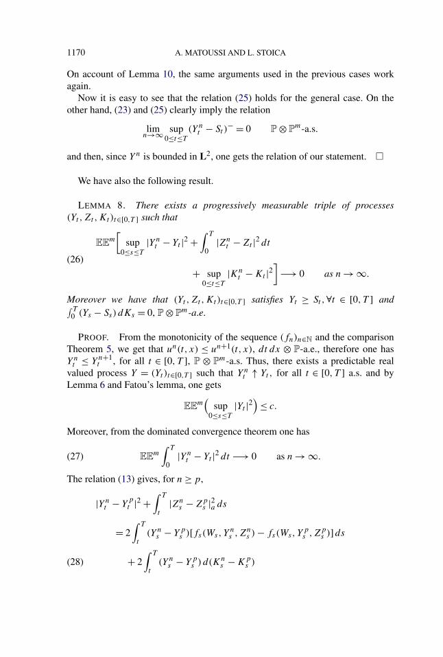
1170 A. MATOUSSI AND L. STOICA
On account of Lemma 10, the same arguments used in the previous cases workagain.
Now it is easy to see that the relation (25) holds for the general case. On theother hand, (23) and (25) clearly imply the relation
limn→∞ sup
0≤t≤T
(Y nt − St )
− = 0 P ⊗ Pm-a.s.
and then, since Yn is bounded in L2, one gets the relation of our statement. �
We have also the following result.
LEMMA 8. There exists a progressively measurable triple of processes(Yt ,Zt ,Kt)t∈[0,T ] such that
EEm
[sup
0≤s≤T
|Ynt − Yt |2 +
∫ T
0|Zn
t − Zt |2 dt
(26)
+ sup0≤t≤T
|Knt − Kt |2
]−→ 0 as n → ∞.
Moreover we have that (Yt ,Zt ,Kt)t∈[0,T ] satisfies Yt ≥ St ,∀t ∈ [0, T ] and∫ T0 (Ys − Ss) dKs = 0, P ⊗ P
m-a.e.
PROOF. From the monotonicity of the sequence (fn)n∈N and the comparisonTheorem 5, we get that un(t, x) ≤ un+1(t, x), dt dx ⊗ P-a.e., therefore one hasYn
t ≤ Yn+1t , for all t ∈ [0, T ], P ⊗ P
m-a.s. Thus, there exists a predictable realvalued process Y = (Yt )t∈[0,T ] such that Yn
t ↑ Yt , for all t ∈ [0, T ] a.s. and byLemma 6 and Fatou’s lemma, one gets
EEm
(sup
0≤s≤T
|Yt |2)
≤ c.
Moreover, from the dominated convergence theorem one has
EEm
∫ T
0|Yn
t − Yt |2 dt −→ 0 as n → ∞.(27)
The relation (13) gives, for n ≥ p,
|Ynt − Y
pt |2 +
∫ T
t|Zn
s − Zps |2a ds
= 2∫ T
t(Y n
s − Yps )[fs(Ws,Y
ns ,Zn
s ) − fs(Ws,Yps ,Zp
s )]ds
+ 2∫ T
t(Y n
s − Yps ) d(Kn
s − Kps )(28)

OBSTACLE PROBLEM FOR STOCHASTIC PDE’S 1171
− 2∫ T
t〈Zn
s − Zps , gs(Ws,Y
ns ,Zn
s ) − gs(Ws,Yps ,Zp
s )〉ds
+∫ T
t(Y n
s − Yps )[gs(Xs,Y
ns ,Zn
s ) − gs(Ws,Yps ,Zp
s )] ∗ dW
− 2∑i
∫ T
t(Y n
s − Yps )(Zn
i,s − Zpi,s) dWi
s
+ 2∫ T
t(Y n
s − Yps )[hs(Ws,Y
ns ,Zn
s ) − hs(Ws,Yps ,Zp
s )] · ←−dBs
+∫ T
t|hs(Ws,Y
ns ,Zn
s ) − hs(Ws,Yps ,Zp
s )|2 ds.
By standard calculation, one deduces that
EEm
∫ T
t|Zn
s − Zps |2 ds ≤ cEE
m∫ T
t|Yn
s − Yps |2
+ 4EEm
∫ T
t(Y n
s − Ss)− dKp
s(29)
+ 4EEm
∫ T
t(Y p
s − Ss)− dKn
s .
Therefore from Lemma 7, (27) and (29) one gets
EEm
∫ T
0|Yn
t − Ypt |2 dt
(30)
+ EEm
∫ T
0|Zn
t − Zpt |2 dt −→ 0 as n,p → ∞.
The rest of the proof is the same as in El Karoui et al. ([9], pages 721–722), in par-ticular we get that there exists a pair (Z,K) of progressively measurable processeswith values in R
d × R such that
EEm
[sup
0≤s≤T
|Ynt − Yt |2 +
∫ T
0|Zn
t − Zt |2 dt
+ sup0≤t≤T
|Knt − Kt |2
]−→ 0 as n → ∞.
It is obvious that (Kt)t∈[0,T ] is an increasing continuous process. On the otherhand, since from Lemma 7 we have limn→∞ EE
m[sup0≤t≤T ((Y nt − St )
−)2] = 0,then, P ⊗ P
m-a.s.,
Yt ≥ St ∀t ∈ [0, T ],(31)

1172 A. MATOUSSI AND L. STOICA
which yields that∫ T
0 (Ys −Ss) dKs ≥ 0. Finally, we also have∫ T
0 (Ys −Ss) dKs = 0since on the other hand the sequences (Y n)n≥0 and (Kn)n≥0 converge uniformly(at least for a subsequence), respectively, to Y and K and∫ T
0(Y n
s − Ss) dKns = −n
∫ T
0
((Y n
s − Ss)−)2
ds ≤ 0. �
As a consequence of the last proof, we obtain the following generalization ofthe RBSDE introduced in [9].
COROLLARY 2. The limiting triple of processes (Yt ,Zt ,Kt)t∈[0,T ] is a solu-tion of the following reflected backward doubly stochastic differential equation (inshort RBDSDE):
Yt = �(WT ) +∫ T
tfr(Wr,Yr,Zr) dr + KT − Kt
+ 1
2
∫ T
tgr(Wr,Yr,Zr) ∗ dW(32)
+∫ T
thr(Wr,Yr,Z
nr ) · ←−
dBr − ∑i
∫ T
tZi,r dWi
r
with Yt ≥ St ,∀t ∈ [0, T ], (Kt)t∈[0,T ] is an increasing continuous process, K0 = 0and ∫ T
0(Ys − Ss) dKs = 0.(33)
PROOF OF THEOREM 4. Since∫ T
0(‖un
t − upt ‖2
2 + ‖∇unt − ∇u
pt ‖2
2) dt = Em
∫ T
0(|Yn
t − Ypt |2 + |Zn
t − Zpt |2) dt,
by the preceding lemma one deduces that the sequence (un)n∈N is a Cauchy se-quence in L2(�×[0, T ];H 1(Rd)) and hence has a limit u in this space. Also fromthe preceding lemma, it follows that dKn
t weakly converges to dKt , P ⊗ Pm-a.e.
This implies that
limn
∫ T
0
∫Rd
n(un − v)−ϕ(t, x) dt dx = limn
Em
∫ T
0ϕt(Wt) dKn
t
=∫ T
0
∫Rd
ϕ(t, x)ν(dt dx),
where ν is the regular measure defined by∫ T
0
∫Rd
ϕ(t, x)ν(dt dx) = Em∫ T
0ϕt (Wt) dKt .

OBSTACLE PROBLEM FOR STOCHASTIC PDE’S 1173
Writing the equation (15) in the weak form and passing to the limit one ob-tains the equation (14) with u and this ν. The arguments we have explained af-ter Definition 4 ensure that u admits a quasicontinuous version �u. Then one de-duces that (�ut (Wt))t∈[0,T ] should coincide with (Yt )t∈[0,T ], P ⊗ P
m-a.e. There-fore, the inequality Yt ≥ St implies u ≥ v, dt ⊗ P ⊗ dx-a.e. and the relation∫ T
0 (Yt − St ) dKt = 0 implies the relation (iv) of Definition 4. �
4. Some technical lemmas.
LEMMA 9. Let f ∈ L2([0, T ] × Rd;R) and denote by (un)n∈N the sequence
of solutions of the equations(∂t + 1
2�)un − nun + f = 0 ∀n ∈ N,
with final condition unT = 0. Then we have∫ T
0‖∇un
t ‖22 dt ≤ c
[1
n
∫ T
0‖ft‖2
2 dt +∫ T
0e−2n(T −t)‖ft‖2
2 dt
].(34)
PROOF. It is well known that the solution (un)n∈N is expressed in terms of thesemigroup Pt by
unt =
∫ T
te−n(s−t)Ps−t fs ds.
A direct calculation shows that one has
n
∫ T
te−n(s−t)Ps−tu
0s ds = u0
t − unt ,
which leads to
unt = e−n(T −t)u0
t + n
∫ T
te−n(s−t)(u0
t − Ps−tu0s ) ds.(35)
The function �unt = e−n(T −t)u0
t is a solution of the equation (∂t + 12�)�un − n�un +
f = 0 where ft = e(T −t)ft . Therefore, one has the following estimate for the gra-dient of the first term in the expression of un∫ T
0e−n(T −t)‖∇u0
t ‖22 dt ≤ c
∫ T
0e−2n(T −t)‖ft‖2
2 dt(36)
(see Lemma 5 of [7] for details). In order to estimate the gradient of the secondterm of the expression of un, we first remark that
u0t − Ps−tu
0s =
∫ s
tPr−t fr dr,

1174 A. MATOUSSI AND L. STOICA
so that one has∥∥∥∥n∇∫ T
te−n(s−t)(u0
t − Ps−tu0s ) ds
∥∥∥∥2≤ n
∫ T −t
0e−ns
∫ s
0‖∇Prft+r‖2 dr ds
≤ nc
∫ T −t
0e−ns
∫ s
0
1√r‖ft+r‖2 dr ds,
where we have used the well-known inequality
‖∇Prϕ‖2 ≤ c√r‖ϕ‖2 for ϕ ∈ L2.
Then we estimate the time integral of the norm of the gradient, which is the ex-pression we are interested in,∫ T
0
∥∥∥∥n∇∫ T
te−n(s−t)(u0
t − Ps−tu0s ) ds
∥∥∥∥2
2dt
≤ c2∫ T
0
[∫ T −t
0ne−ns
∫ s
0
1√r‖ft+r‖2 dr ds
]2
dt
= c2∫ T
0
∫ s
0
∫ T
0
∫ s′
0
∫ T −s∨s′
0ne−nsne−ns′ 1√
r‖ft+r‖2
× 1√r ′ ‖ft+r ′‖2 dt dr ′ ds′ dr ds
≤∫ T
0‖ft‖2
2 dt
(∫ T
0
1
2
√sne−ns ds
)2
≤ c
n
∫ T
0‖ft‖2
2 dt.
This estimate together with (36) imply the statement (34). �
Obviously, the lemma implies that limn→∞∫ T
0 ‖∇unt ‖2
2 dt = 0. We need astrengthened version of this relation, which is presented in the next corollary whoseproof is easy, so you omit it.
COROLLARY 3. Let f,f n ∈ L2([0, T ] × Rd;R), n ∈ N, be such that
limn→∞∫ T
0 ‖f nt − ft‖2
2 dt = 0. Then the solutions (un)n∈N of the equations(∂t + 1
2�)un − nun + f n = 0,
with final condition unT = 0, satisfy the relation limn→∞
∫ T0 ‖∇un
t ‖22 dt = 0.
COROLLARY 4. Let gn, g ∈ L2([0, T ] × Rd;R
d) be such thatlimn→∞
∫ T0 ‖gn
t − gt‖22 dt = 0. Then the solutions (un)n∈N of the equations(
∂t + 12�
)un − nun + divgn = 0,
with final condition unT = 0, satisfy the relation limn→∞
∫ T0 ‖∇un
t ‖22 dt = 0.

OBSTACLE PROBLEM FOR STOCHASTIC PDE’S 1175
PROOF. We regularize g by setting gεi,t = Pεgi,t for i = 1, . . . , d, ε > 0, t ∈
[0, T ]. Then gεi ∈ H 1
0 (Rd) and f ε = divgε is in L2([0, T ] × Rd;R). Moreover,
we have limε→0∫ T
0 ‖gεt − gt‖2
2 dt = 0. Let uε,n be the solution of the equation(∂t + 1
2�)uε,n − nuε,n + f ε = 0,
with final condition uε,nT = 0. By Lemma 5 of [7], one has∫ T
0‖∇un
t − ∇uε,nt ‖2
2 dt ≤ c
∫ T
0‖gn
t − gεt ‖2
2 dt
≤ c
∫ T
0(‖gn
t − gt‖22 + ‖gε
t − gt‖22) dt.
On the other hand, Lemma 9 implies, for ε fixed, limn→∞∫ T
0 ‖∇uε,nt ‖2
2 dt = 0.From these facts, one easily concludes the proof. �
LEMMA 10. Let h,hn,n ∈ N, be L2(Rd;Rd1
)-valued predictable processeson [0, T ] with respect to (F B
t,T )t≥0 and such that
E
∫ T
0‖ht‖2
2 dt < ∞, E
∫ T
0‖hn
t ‖22 dt < ∞
and
limn→∞ E
∫ T
0‖hn
t − ht‖22 dt = 0.
Let (un)n∈N be the solutions of the equations
dunt + [1
2�unt − nun
t
]dt + hn
t · ←−dBt = 0,
with final condition unT = 0, for each n ∈ N. Then one has
limn→∞
∫ T
0‖∇un
t ‖22 dt = 0.
PROOF. We regularize the process h by setting hεi,t = Pεhi,t for i = 1, . . . ,
d1, ε > 0, t ∈ [0, T ]. Then hεi,t ∈ H 1
0 (Rd) and E∫ T
0 ‖∇hεt ‖2
2 dt < ∞ and
limε→0 E∫ T
0 ‖hεt − ht‖2
2 dt = 0. Let uε,n be the solution of the equation
duε,nt + 1
2�uε,nt − nu
ε,nt + hε
t · ←−dBt = 0
with final condition uε,nT = 0, for each n ∈ N. The relation (iii) of Proposition 6 in
[7] written with respect to the Hilbert space H = H 10 (Rd) takes the form
E
[‖∇u
ε,nt ‖2
2 +∫ T
t
∥∥∥∥1
2�uε,n
s
∥∥∥∥2
ds + n
∫ T
t‖∇uε,n
s ‖22 ds
]= E
∫ T
t‖∇hε
s‖22 ds.

1176 A. MATOUSSI AND L. STOICA
In particular, one has ∫ T
t‖∇uε,n
s ‖2 ds ≤ 1
n
∫ T
t‖∇hε
s‖22 ds.
Now we write the relation (iii) of Proposition 6 in [7] for the solution un − uε,n
with respect to the Hilbert space H = L2(Rd),
E
[‖un
0 − uε,n0 ‖2 +
∫ T
0‖∇un
s − ∇uε,ns ‖2
2 ds + n
∫ T
0‖un
s − uε,ns ‖2
2 ds
]
= E
∫ T
0‖hn
s − hεs‖2
2 ds.
In particular, one obtains
E
∫ T
0‖∇un
s − ∇uε,ns ‖2
2 ds ≤ E
∫ T
0‖hn
s − hεs‖2
2 ds.
From this and the preceding inequality, one deduces
lim supn→∞
E
∫ T
0‖∇un
s ‖22 ds ≤ E
∫ T
0‖hs − hε
s‖22 ds.
Letting ε → 0, one deduces the relation from the statement. �
LEMMA 11. Let v : [0, T ] × Rd → R be a function such that the process
(vt (Wt))t∈[0,T ] admits a version S = (St )t∈[0,T ] with continuous trajectories on[0, T ] and such that the random variable S∗ = sup0≤t≤T St satisfies the conditionE
m[S∗]2 < ∞. Let un be the solution of the equation(∂t + 1
2�)un − nun + nv = 0,
with the terminal condition unT = vT . Let Yn = (Y n
t )t∈[0,T ] be a continuous versionof the process (un
t (Wt))t∈[0,T ], for each n ∈ N. Then the following holds:
limn→∞ E
m[
sup0≤t≤T
|Ynt − St |2
]= 0.
PROOF. Let us set �unt = e−ntun
t and observe that this function is a solution ofthe equation (
∂t + 12�
)�un +�v = 0,
with �vt = e−ntvt and terminal condition �unT = �vT . Writing the representation of
Theorem 3 with g = h = 0 for �un(Wt), one obtains
�unt (t,Wt) = e−nT vT −
d∑i=1
∫ T
t∂i�un
r (Wr) dWir + n
∫ T
te−nrvr(Wr) dr,

OBSTACLE PROBLEM FOR STOCHASTIC PDE’S 1177
and this leads to the representation of our process Yn, given by
Ynt = E
m
[e−n(T −t)ST + n
∫ T
te−n(r−t)Sr dr
∣∣∣Ft
].
Then one has
|St − Yt | ≤ Em
[∣∣∣∣St − e−n(T −t)ST − n
∫ T
te−n(r−t)Sr dr
∣∣∣∣∣∣∣Ft
].
Let us denote by
V n = sup0≤t≤T
∣∣∣∣St − e−n(T −t)ST − n
∫ T
te−n(r−t)Sr dr
∣∣∣∣.Obviously, one has V n ≤ 2S∗. On the other hand, one has for any fixed δ > 0,
V n ≤ sup|t−s|≤δ
|St − Ss | + 2e−nδS∗.(37)
This follows from Lemma 12. From the inequality (37), one deduces thatlimn→∞ V n = 0,P
m-a.s., and hence from the dominated convergence theorem,one gets limn→∞ E
m[V n]2 = 0. Since
|St − Ynt | ≤ E
m[V n|Ft ],Doob’s theorem implies the assertion of the lemma. �
Finally, we mention the following calculus lemma.
LEMMA 12. Let ϕ ∈ C([0,1];R) and δ ∈ (0, T ), λ > 0. Then one has∣∣∣∣λ∫ δ
0e−λtϕ(t) dt + e−λδϕ(δ) − ϕ(0)
∣∣∣∣ ≤ sup0≤t≤δ
|ϕ(t) − ϕ(0)|
and ∣∣∣∣λ∫ T
te−λ(s−t)ϕ(s) ds + e−λ(T −t)ϕ(T ) − ϕ(t)
∣∣∣∣≤ sup
|s−r|≤δ,s≥0|ϕ(s) − ϕ(r)| + 2e−λδ‖ϕ‖∞.
PROOF. The first inequality follows from the relation λ∫ δ
0 e−λt dt + e−λδ = 1.In order to check the second relation, one dominates the expression of the left-handside by∣∣∣∣λ∫ t+δ
te−λ(s−t)ϕ(s) ds + e−λδϕ(t + δ) − ϕ(t)
∣∣∣∣+ e−λδ
∣∣∣∣λ∫ T
t+δe−λ(s−(t+δ))ϕ(s) ds + e−λ(T −(t+δ))ϕ(T ) − ϕ(t + δ)
∣∣∣∣and then apply the first relation to dominate the first term. �

1178 A. MATOUSSI AND L. STOICA
APPENDIX
The next lemma is a classical result in convex analysis, known as Mazur’s the-orem (see [5], Remark 5, page 38). We state here the result with some notationthat is useful for our proof. Let X be a Banach space and (xn)n∈N a sequenceof elements in X. We call finite family of coefficients of a convex combination afamily a = {αi |i ∈ I } where I is a finite subset of N, αi > 0 for each i ∈ I and∑
i∈I αi = 1. The convex combination that corresponds to such a family of coeffi-cients is the point expressed in terms of our sequence by
∑i∈I αixi .
LEMMA 13. Let (xn)n∈N be a weakly convergent sequence of elements in X
with limit x. Then there exits a sequence (ak)k∈N of families of coefficients ofconvex combinations, ak = {αk
i |i ∈ Ik}, such that the corresponding convex com-binations xk = ∑
i∈Ikαk
i xi , k ∈ N, converge strongly to x: limk→∞ ‖xk − x‖ = 0.
REFERENCES
[1] BALLY, V., CABALLERO, E., EL KAROUI, N. and FERNANDEZ, B. (2004). Reflected BSDE’sPDE’s and variational inequalities. Report, INRIA.
[2] BALLY, V. and MATOUSSI, A. (2001). Weak solutions for SPDEs and backward doubly sto-chastic differential equations. J. Theoret. Probab. 14 125–164. MR1822898
[3] BENSOUSSAN, A. and LIONS, J.-L. (1978). Applications des Inéquations Variationnellesen Contrôle Stochastique. Méthodes Mathématiques de l’Informatique 6. Dunod, Paris.MR0513618
[4] BLUMENTHAL, R. M. and GETOOR, R. K. (1968). Markov Processes and Potential Theory.Pure and Applied Mathematics 29. Academic Press, New York. MR0264757
[5] BRÉZIS, H. (2005). Analyse Fonctionnelle—Theorie et Application. Dunod, Paris.[6] DELLACHERIE, C. and MEYER, P.-A. (1975). Probabilités et Potentiel. Chapitres XII à XVI.
Actualités Scientifiques et Industrielles 1372. Hermann, Paris. MR898005[7] DENIS, L. and STOICA, L. (2004). A general analytical result for non-linear SPDE’s and ap-
plications. Electron. J. Probab. 9 674–709 (electronic). MR2110016[8] DONATI-MARTIN, C. and PARDOUX, É. (1993). White noise driven SPDEs with reflection.
Probab. Theory Related Fields 95 1–24. MR1207304[9] EL KAROUI, N., KAPOUDJIAN, C., PARDOUX, E., PENG, S. and QUENEZ, M. C. (1997).
Reflected solutions of backward SDE’s, and related obstacle problems for PDE’s. Ann.Probab. 25 702–737. MR1434123
[10] FUKUSHIMA, M., OSHIMA, Y. and TAKEDA, M. (1994). Dirichlet Forms and Symmet-ric Markov Processes. de Gruyter Studies in Mathematics 19. de Gruyter, Berlin.MR1303354
[11] MATOUSSI, A. and SCHEUTZOW, M. (2002). Stochastic PDEs driven by nonlinear noise andbackward doubly SDEs. J. Theoret. Probab. 15 1–39. MR1883201
[12] MATOUSSI, A. and XU, M. (2008). Sobolev solution for semilinear PDE with obstacle undermonotonicity condition. Electron. J. Probab. 13 1035–1067. MR2424986
[13] MATOUSSI, A. and XU, M. (2010). Reflected backward doubly SDE and obstacle problem forsemilinear stochastic PDE’s. Preprint, Univ. Maine.
[14] MIGNOT, F. and PUEL, J.-P. (1975). Solution maximum de certaines inéquations d’évolutionparaboliques, et inéquations quasi variationnelles paraboliques. C. R. Acad. Sci. ParisSér. A–B 280 A259–A262. MR0390866
OBSTACLE PROBLEM FOR STOCHASTIC PDE’S 1179
[15] NUALART, D. and PARDOUX, É. (1992). White noise driven quasilinear SPDEs with reflection.Probab. Theory Related Fields 93 77–89. MR1172940
[16] PARDOUX, É. and PENG, S. G. (1994). Backward doubly stochastic differential equations andsystems of quasilinear SPDEs. Probab. Theory Related Fields 98 209–227. MR1258986
[17] STOICA, I. L. (2003). A probabilistic interpretation of the divergence and BSDE’s. StochasticProcess. Appl. 103 31–55. MR1947959
LABORATOIRE MANCEAU DE MATHÉMATIQUES
UNIVERSITÉ DU MAINE
AVENUE OLIVIER MESSIAEN
72085 LE MANS CEDEX 9FRANCE
E-MAIL: [email protected]
INSTITUTE OF MATHEMATICS “SIMION STOILOW”OF THE ROMANIAN ACADEMY
AND
FACULTY OF MATHEMATICS
UNIVERSITY OF BUCHAREST
STR. ACADEMIEI 14BUCHAREST RO-70109ROMANIA
E-MAIL: [email protected]