A flocking and obstacle avoidance algorithm for mobile robots.

FOI-R--1383--SEOctober 2004

1650-1942

Scientific report

Magnus Lindhé

A flocking and obstacle avoidancealgorithm for mobile robots

System Technology DivisionSE-172 90 STOCKHOLM

Sweden

Swedish Defence Research AgencySystem Technology DivisionSE-172 90 STOCKHOLMSweden

FOI-R--1383--SEOctober 2004

1650-1942

Scientific report

Magnus Lindhé

A flocking and obstacle avoidance algorithm formobile robots

Issuing organization

Swedish Defence Research AgencySystem Technology DivisionSE-172 90 STOCKHOLMSweden

Author/s (editor/s)

Magnus Lindhé

Report title

A flocking and obstacle avoidance algorithm for mobile robots

Abstract

Mobile robots cooperating in groups offer several advantages such as redundancy and flexibility andcan sometimes perform tasks that would be impossible for one single robot. We have developed a newalgorithm for navigating a group of robots to a predefined target while avoiding obstacles and stayingtogether in a formation. The algorithm merges a potential-based method that provides the shortestunobstructed path to the goal with an approach from coverage control, where the centroids of Voronoipartitions are used to optimize the placement of sensors in a scalar field.

Our algorithm guarantees safety: there will be no collisions between robots or with obstacles of arbitrary shape. It has shown reliable goal convergence in simulations, and the robots form a hexagonallattice when moving in open fields. Further, the algorithm is completely decentralized and the processing load for each robot is virtually unaffected by adding more group members.

This report provides a description of the algorithm and its properties, as well as results from simulationsin both Matlab and Fenix, a graphical simulation environment developed at FOI, where the robots aremodeled as the US Army HMMWV all-terrain vehicle.

Keywords

Flocking, Obstacle Avoidance, Car-like robots, Cooperative control

Further bibliographic information

ISSN

1650-1942Distribution

By sendlist

Report number, ISRN

FOI-R--1383--SE

Report type

Scientific reportResearch area code

CombatMonth year

October 2004

Project no.

E6003Customers code

Commissioned ResearchSub area code

Weapons and ProtectionProject manager

Peter AlvåApproved by

Monica DahlénSponsoring agency

Swedish Armed ForcesScientifically and technically responsible

Karl Henrik Johansson

Language

English

Pages

52

Price Acc. to pricelist

Security classification Unclassified

ii

Utgivare

Totalförsvarets forskningsinstitutAvdelningen för SystemteknikSE-172 90 STOCKHOLMSweden

Författare/redaktör

Magnus Lindhé

Rapportens titel

En navigationsalgoritm för flockar av autonoma mobila robotar

Sammanfattning

Mobila robotar som samarbetar i grupp ger flera fördelar, t.ex. redundans och flexibilitet. Dessutomger det möjlighet att lösa vissa uppgifter som vore omöjliga för en ensam robot. Vi har utvecklat enny algoritm för att förflytta grupper av robotar till ett förutbestämt mål, utan att de kolliderar medvarandra eller med hinder. På vägen håller de ihop i en formation. Vi har kombinerat en potentialbaserad metod, som används för att hitta kortaste vägen till målet, och en yttäckningsmetod som utnyttjartyngdpunkterna för Voronoi-regioner för att optimera placeringen av sensorer i ett skalärt fält.

Vår algoritm är bevisat säker mot kollisioner, oavsett form på hindren. Den har visat sig ge pålitligkonvergens till målet i simuleringar och robotarna bildar hexagonala gitterformationer när de rör sigpå öppna ytor. Algoritmen är dessutom helt decentraliserad och mängden beräkningar som varje robotbehöver göra ökar försumbart när fler gruppmedlemmar tillkommer.

Den här rapporten beskriver algoritmen och dess egenskaper och redovisar resultat från simuleringari två olika miljöer. Dels har vi simulerat i Matlab och dels i Fenix, en grafisk datormiljö utvecklad avFOI, där robotarna har modellerats efter amerikanska arméns terrängfordon HMMWV.

Nyckelord

Formationer, hinderundvikande, robotbilar, samverkande robotar

Övriga bibliografiska uppgifter

ISSN

1650-1942Distribution

Enligt missiv

Rapportnummer, ISRN

FOI-R--1383--SE

Klassificering

Vetenskaplig rapportForskningsområde

BekämpningMånad, år

Oktober 2004

Projektnummer

E6003Verksamhetsgren

Uppdragsfinansierad verksamhetDelområde

VVS med styrda vapenProjektledare

Peter AlvåGodkänd av

Monica DahlénUppdragsgivare/kundbeteckning

FörsvarsmaktenTekniskt och/eller vetenskapligt ansvarig

Karl Henrik Johansson

Språk

Engelska

Antal sidor

52

Pris Enligt prislista

Sekretess Öppen

iii

Contents

1 Introduction 11.1 Problem definition . . . . . . . . . . . . . . . . . . . . . . . . . . . . . 11.2 Report outline . . . . . . . . . . . . . . . . . . . . . . . . . . . . . . . 21.3 Reader’s guide . . . . . . . . . . . . . . . . . . . . . . . . . . . . . . . 3

2 Background 52.1 Motivation for robotics . . . . . . . . . . . . . . . . . . . . . . . . . . . 52.2 Challenges in mobile robotics . . . . . . . . . . . . . . . . . . . . . . . 6

2.2.1 Actuators . . . . . . . . . . . . . . . . . . . . . . . . . . . . . . 62.2.2 Positioning . . . . . . . . . . . . . . . . . . . . . . . . . . . . . 72.2.3 Control and processing . . . . . . . . . . . . . . . . . . . . . . 82.2.4 Communication . . . . . . . . . . . . . . . . . . . . . . . . . . . 9

2.3 Autonomous navigation . . . . . . . . . . . . . . . . . . . . . . . . . . 92.4 Multi-robot cooperation and formations . . . . . . . . . . . . . . . . . 9

3 Flocking with obstacle avoidance 113.1 Earlier approaches . . . . . . . . . . . . . . . . . . . . . . . . . . . . . 113.2 Combining coverage control and navigation functions . . . . . . . . . . 113.3 Coverage control . . . . . . . . . . . . . . . . . . . . . . . . . . . . . . 123.4 Navigation functions . . . . . . . . . . . . . . . . . . . . . . . . . . . . 123.5 Proposed algorithm . . . . . . . . . . . . . . . . . . . . . . . . . . . . 133.6 Properties of the algorithm . . . . . . . . . . . . . . . . . . . . . . . . 14

3.6.1 Dead-locks . . . . . . . . . . . . . . . . . . . . . . . . . . . . . 19

4 Simulation in Matlab 234.1 Results . . . . . . . . . . . . . . . . . . . . . . . . . . . . . . . . . . . 234.2 Implementational aspects . . . . . . . . . . . . . . . . . . . . . . . . . 23

4.2.1 Numerical integration . . . . . . . . . . . . . . . . . . . . . . . 234.2.2 Line of sight . . . . . . . . . . . . . . . . . . . . . . . . . . . . 264.2.3 Finding the optimal step . . . . . . . . . . . . . . . . . . . . . . 27

4.3 Practical experiences . . . . . . . . . . . . . . . . . . . . . . . . . . . . 294.3.1 Trimming the integration regions to a convex shape . . . . . . 294.3.2 Voronoi regions in vertex form . . . . . . . . . . . . . . . . . . 30

5 Implementation in Fenix 315.1 System overview . . . . . . . . . . . . . . . . . . . . . . . . . . . . . . 315.2 Implementational issues . . . . . . . . . . . . . . . . . . . . . . . . . . 325.3 Software structure . . . . . . . . . . . . . . . . . . . . . . . . . . . . . 325.4 Robot dynamics and controller . . . . . . . . . . . . . . . . . . . . . . 345.5 Values used for the simulations . . . . . . . . . . . . . . . . . . . . . . 385.6 Results . . . . . . . . . . . . . . . . . . . . . . . . . . . . . . . . . . . 40

6 Sensor deployment 436.1 Sensor types . . . . . . . . . . . . . . . . . . . . . . . . . . . . . . . . . 436.2 Switching from navigation to sensing . . . . . . . . . . . . . . . . . . . 44

v

FOI-R--1383--SE vi

7 Conclusions 477.1 Suggestions for future work . . . . . . . . . . . . . . . . . . . . . . . . 47

Bibliography 48

Preface

This report, written at the Department of Autonomous Systems at the Swedish Defence Research Agency (FOI), constitutes my master’s thesis. It is the final elementof my Master of Science in Electrical Engineering at the Royal Institute of Technology(KTH).

The last years of my studies have been funded by the Armed Forces Engineer Programme, aiming at providing the Swedish Armed Forces with specialized officers whohave both a military background as well as a Master of Science. As FOI representsthe highest level of military research and development in Sweden, it was a naturalchoice to apply for a master’s thesis project here.

The work has been supervised by Petter Ögren at the Department of AutonomousSystems and by Karl-Henrik Johansson at the Department of Sensors, Signals andSystems at KTH. Karl-Henrik Johansson has also acted as examiner.

A shorter version of this report was presented by the author at the Reglermöte2004, at Chalmers University of Technology in Gothenburg, [1].

Work planning and experiences

This project got off to a flying start in the beginning of February, when Petter presented his idea of combining coverage control with obstacle avoidance. We decided totry to produce the outline of a paper by the beginning of March, so I had to quicklytake in the papers on coverage control before starting on the Matlab code for thesimulations. During the next four weeks I simulated the algorithm and came up withproblems that Petter and I had to solve. After the basic framework was designed andtested, I spent some time documenting the first phase of the project and studying howthe algorithm could be extended to sensor positioning in the target area.

The second phase was to implement it in Fenix, which made me have to brushup on my C++ skills before understanding the structure of the software. The actualprogramming took five weeks and then I spent two weeks documenting and makingscreenshots and films for the presentations. The final phase of the work has been topresent it at the Reglermöte and work on the properties of formation stability andgoal convergence.

During the work I have learned a lot about robotics in general and computationalgeometry and path planning in particular. It also gave me a better understandingof research methodology, which is not taught much in other undergraduate courses.Attending the Reglermöte was very rewarding, both professionally and personally, asI got some insight into current issues in the control community as well as inspirationfor possible future postgraduate studies.

Acknowledgements

The first mentioning of course goes to my supervisor Petter, as thanks for all hisscientific as well as moral support. He has always been available to help wheneverinnocent, albeit virtual, robots have lost their lives due to my mistakes or flaws inthe algorithm. Most of the ideas contained in this report originate from him.

I also owe thanks to Emil Salling at FOI, who has spent many hours customizingFenix for my application and editing the screenshot films that I showed at the Reg

vii

FOI-R--1383--SE viii

lermöte. One day I will summon the courage to ask my future boss for a flatscreenlike Emil’s...

Had it not been for Karl-Henrik Johansson at S3, I would probably not havefound this master’s thesis project and he has been a valuable sounding board for thedevelopment of the algorithm as well as the presentation of it.

Finally I would like to thank all those who have made my time at FOI pleasant,be it as room-mates, Fenix technicians, spontaneous coffee-room lecturers, rewardinglunch company or otherwise. I hope to see you again in my future career!

Stockholm, 11th of June 2004

Magnus Lindhé

1. Introduction

1.1 Problem definition

The object of this project has been to develop and study a new algorithm for movinga group of robots from one place to another, without colliding with each other or anyobstacles. While doing so the group should stay together, preferably in a geometricallydefined formation. The algorithm was then to be tested in a realistic setting. FOIhas a testbed for robotics applications, consisting of rebuilt radio-controlled carsand Fenix, a graphical computer simulation environment. The interface between thesystem and the controller is the same in both environments, so the same controlprogram can be run both in the cars and in the computer. Since there are currentlyonly two robots available in hardware, a decision was made to implement the systemin Fenix. The developed algorithm is a combination of two recently presented researchpapers, on navigation functions, [2] , and coverage control, [3]. The idea was to extendthem to get the desired formation properties and eventually study the issues of safety,goal convergence and under what conditions formations were formed.

The main difficulty when trying to achieve goal convergence, flocking and collisionavoidance is that of prioritizing the sometimes contradictory requirements. Figure1.1 illustrates the chosen order of priorities:

1. The highest priority is given to safety , i.e. collision avoidance.

2. The second priority is goal convergence. For collision safety the robots shouldof course not all reach the exact goal coordinates, but rather a set of equilibriumpositions, tightly arranged around it.

3. Finally the robots should stay together in a flock while moving. We call thisflock cohesion.

We consider a group of kinematic robots pi that have the following dynamics:

pi(k + 1) = pi(k) + ui(k)||ui|| ≤ umax

Each robot is equipped with a sensor that can detect neighboring agents within theradius Rmax. Equivalently, it can have some means of communication, used to inquireabout the position of other robots within Rmax. We believe this to be a more realisticassumption than the one made in [3] , where the sensors are assumed to have infiniterange. It is also assumed that the positioning problem (described in the backgroundsection) has been solved, so that we have access to an accurate position estimate.All robots have processing capabilities that allow them to locally run the algorithmthat will be presented. Finally they have knowledge of the location of all obstacles.This is not always true in real-world implementations, but then the robots can beequipped with a sensor for obstacles and the navigation function can be calculatedwith respect to all obstacles in view from the robot. All other areas are assumed tobe free space. If the robot later discovers more obstacles, they can be added to themap and the navigation function is recalculated. This can lead to the robot going

1

FOI-R--1383--SE 2

Figure 1.1: A group of robots moving around some obstacles before stopping aroundthe goal, marked by an X. This illustrates the chosen order of priorities for thealgorithm. Safety is given the highest priority, then comes goal convergence andfinally flock cohesion.

into dead ends, but as soon as it discovers this the map will be redrawn and it willtry another, presumably better, path.

Robots with more realistic dynamics, such as car-like vehicles, can also be controlled with the proposed algorithm. As an example of this, we use the followingmodel in Fenix (deduced in section 5.4):

x = v cos θ

y = v sin θ,

θ =v

Ltan δ

v = u

This requires a hierarchical controller structure, as depicted in Figure 1.2. Thehigh-level algorithm uses the position of the vehicle and that of the neighbors tocalculate the next waypoint as well as a region where the vehicle controller is free tomanoeuvre. This ensures collision-safety even in the case of non-holonomic dynamics,when the vehicle may need to make parallel parking movements to reach its waypoint.

1.2 Report outline

The report starts with an introduction to robotics, in section 2. It motivates theuse of robots in general and groups of robots moving in formations in particular. Italso contains a presentation of some of the most important hardware building blocksused in robotics, to give an understanding of some considerations that have governedthe development of the algorithm. The theoretical core of the report is contained insection 3. It briefly accounts for the concepts of navigation functions and coveragecontrol before presenting our new algorithm. It ends with a section on proven ortheoretically predicted properties of the algorithm.

Then two sections follow, describing the simulations first in Matlab and then inFenix. They both present the results of the simulations and some problems that havebeen encountered when implementing the algorithm on that specific platform. Thesection on Fenix also contains some information on the structure of the software andan account of how a controller was developed to drive the car between waypointsdesignated by the higher-level algorithm.

Thus far the report considers the problem of only navigating the robots. In section6 the problem is extended to also consider different sensing tasks in an area surround

3 FOI-R--1383--SE

Position

Calculates waypoints onthe way to the globalgoal.

Sensors

between waypoints.

Drives the vehicle

Vehicle controller

SteeringThrustBrakes on/off

PositionVelocity

Flocking and obstacleavoidance algorithm

WaypointSafe region

PositionVelocity

NeighborsObstacles

Figure 1.2: The hierarchical controller structure used to control vehicles with morerealistic dynamics.

ing the designated goal. Some sensor types that could be of interest in a militarycontext are presented, as well as a simple way of switching between navigation andsensing within the framework of the algorithm. Finally there are some conclusions onthe algorithm as a whole and an account of some issues that are still open to research.

1.3 Reader’s guide

The background section is intended for readers who are new to the field of robotics.Those who want a motivation for formation movement and groups of robots can godirectly to section 2.4. All readers should read section 3 , as it contains the necessarytheory to understand the algorithm, possibly with the exception of section 3.6.

Sections 4 (Simulations in Matlab) and 5 (Simulations in Fenix) are independentand can be read in arbitrary order. Subsection 5.3 is mainly intended for those whowant to understand the software and/or develop it further.

Section 6 , on deployment in the target area, can be understood separately exceptfor the extension of the navigation algorithm, which requires that one has understoodthe theory in section 3.

2. Background

This section will provide some background information on robotics in general andmobile robots in particular for readers who are unfamiliar with the field. We give somemotivations for the use of robots and then present the underlying technical challengeswhen designing a mobile robotic system. This will serve to explain the governinglimitations when we focus on high-level autonomous navigation and formation keepingin the rest of the report.

Since this work has been carried out at the Swedish Defence Research Agencythe main focus is on military applications and we have chosen to limit the scopeto ground vehicles. The limitation lies not so much in the general theory as in theassumption on vehicle dynamics in the problem definition and the choice of interestingsensor types in section 6. As an example, an unmanned aerial vehicle (UAV) withaircraft-like design cannot stop and turn on the spot, and in underwater applicationsradio direction finding or computer vision are not as feasible and interesting as thestandard method of acoustic detection and ranging.

2.1 Motivation for robotics

Robots should be used to relieve humans of tasks that fall under the four D:s ofrobotics: dirty, dull, dangerous or difficult [4]. Much like man has always developedtechnology to free time for other more challenging tasks, now the time has come forrobots. Stationary industrial robots have become standard and many of the keytechnologies for mobile robots, such as power-efficient yet fast processors, sensorsand communication circuits are getting cheaper and smaller by the day. This isdriven by their use in consumer products, but as a side effect it makes robotics moreeconomically attractive.

Industrial robots can carry out tasks where humans are exposed to high noiselevels, uncomfortable working positions or unhealthy environments such as solvents,spray paint or radioactivity. They also make new products and methods of manufacturing available by giving unprecedented precision to welding and cutting operations.In military applications, mobile robots can do dangerous disposal of explosive ordnance, exposed reconnaissance missions or long-distance transportation. The USDefence Advanced Research Project Agency (DARPA) has shown great interest inthe field, issuing the DARPA Grand Challenge, a desert race between Los Angelesand Las Vegas for autonomously navigating offroad cars [5]. The best car managed todrive 11 kilometres before getting off course, which serves to underline the difficultiesinvolved in autonomous navigation.

A more peaceful use for robots will be to aid in caring for the numerous after-wargeneration of Swedes that will soon be retired and can be expected to need morehealth care. Simple or unergonomic tasks may be performed by robots to give medicalpersonnel more quality time with the patients. In space, robots have landed onMars before the technology allows humans to safely travel there. Because of thelong distances the robots cannot be remotely operated from Earth, but instead gethigh-level commands such as waypoints or predefined experiments to perform. Resultsare then transmitted back to scientists on Earth [6].

5

FOI-R--1383--SE 6

2.2 Challenges in mobile robotics

By mobile robot we mean a robot that is not attached, mechanically or electrically,to anything and that is completely self-contained. Such a robot needs to be able todisplace itself, find its position, detect obstacles or other objects, communicate with asupervisor and/or other robots and finally process all the data into sensible outputs.All of these requirements present challenges that are subject of inter-disciplinaryresearch.

Figure 2.1: Examples of mobile research robots. Left: The Pioneer 2 from ActiveMedia. The “coffee-brewer” is a laser scanner, above which a camera is mounted.Middle: The BrainStem Bug from Acroname, Inc., a six-legged walking robot withultra-sound sonars for obstacle detection. Right: The Lynxmotion 4WD2 all-terrainchassis with L5 Arm, from Lynxmotion.

2.2.1 Actuators All components that are used to mechanically execute the outputs of the control system are called actuators. In the case of robotics they can bewheels, tracks or legs for moving, manipulator arms for handling objects, motorsturning a camera head and so on. For the purpose of this overview we will restrictthe presentation to popular systems for propulsion of mobile robots.

The three most common methods of traction for mobile robots are wheels, tracksand legs. Wheels have the advantage of being reliable, simple and allowing highspeeds. Tracks work better in uneven or soft terrain but are less suited for deadreckoning as they tend to slip, especially when turning. They also use more energyand require more maintenance than wheels. Legged robots are still in the researchphase and require much more power and sophisticated control. The advantages arethat they allow the robot to access very difficult terrain, a key feature in futureapplications such as nuclear power plant maintenance and earthquake victim searchand rescue. A legged robot would be able to go wherever a human could.

A system on wheels can have some different configurations, representing tradeoffsbetween ease of control and other desirable properties such as speed, cheap actuatorsand agility. Figure 2.2 depicts three popular configurations. Model A has all wheelsturnable and powered, which gives very good maneuverability at the expense of amore difficult mechanical design. B is called a “unicycle” and is very popular forsimple experiment robots since it contains very little mechanics. Note that the twopowered wheels are individually actuated, enabling the robot to turn on the spot.Drawbacks are that it cannot move sideways without turning first, and the passivecastor wheels make it unsuited for rough terrain. Finally C has “car-like dynamics”,with powered back wheels and steerable front wheels. It can go fast and there areready-made platforms ranging from cheap radio controlled cars to full-size trucks,but controlling it is more difficult. Moving sideways requires a whole sequence ofback-and-forth manoeuvres, as in parallel parking.

7 FOI-R--1383--SE

Turnable and powered

Turnable, not powered Fix and powered

CBA

��

��

��

��

��

��

��

��

��

Figure 2.2: Three common wheel configurations for mobile robots.

2.2.2 Positioning In order to be useful and to find its goal, a robot must knowits position. This can be in the sense of the robot knowing its coordinates, be itglobal coordinates or relative to e.g. a room, or in a topological sense, e.g. knowingthat it is “in the corridor between the kitchen and the library”. Tomatis et al., [7] ,have mixed the two methods in a robot that navigates to the correct room in an officebuilding by first using a topological approach and then orients itself inside the roomusing local coordinates. They remark that this is very similar to the way a humanwould do it: when going to a room he orients himself coarsely by counting passeddoors or corridors, while inside he switches to exact positioning to place the coffeemug in the coffee machine.

The basic method for positioning is usually dead reckoning, by simply countingthe number of revolutions of the wheels or tracks, or in case of legs, by countingsteps and using more complex geometry. It has the advantage of being simple, butsince it involves integration it inevitably suffers from accumulating errors. Slippage,uneven surfaces and sensor errors will eventually make the dead reckoning positionestimate drift away from the true position. The same is true for more advancedinertial navigation systems containing gyros, accelerometers and/or magnetic fluxmeters used as compasses. They can be more or less accurate but always have somefinite drift, giving rise to a growing error.

To correct the dead reckoning one needs to use a parallel system where the erroris bounded, see below. The standard approach is then to fuse the data from bothsystems by using a Kalman filter, [8]. This can give a better position estimate andalso an estimate of the drift that is used to improve the performance of the inertialnavigation system.

One such system that can be used in parallel is satellite navigation, most popularlyGPS. It works only in outdoor applications where there is a free line of sight to a largeportion of the sky, thus there are problems in dense cities and no reliable estimate atall indoors. As an example of what accuracies can be obtained we take the LassenLP GPS receiver from Trimble, a small low-power GPS receiver suited for roboticsapplications. It has a stated horizontal uncertainty of less than six metres for 50% ofits measurements and less than nine metres for 90% of the measurements, [9]. Thereare several more advanced approaches, such as receiving both carrier frequencies ofthe GPS system and use the extra information to correct for atmospheric effects ortracking the phase of the signal, which can give accuracies in the order of centimetres,[10]. Another commonly used technique is differential GPS (DGPS) with a stationaryreceiver at a surveyed position, producing corrections that can be used in real-time

FOI-R--1383--SE 8

or for post-processing to significantly improve the accuracy of other receivers in theproximity (tens of kilometres from the stationary receiver).

In a military context the GPS system has some important weaknesses. First ofall it is controlled by the United States, which makes it possible for the US militaryto degrade the accuracy of the signal (as was done with the publicly available signaluntil 2000). If civilian GPS receivers are used against US troops in a conflict, theycould decide to degrade the signal again or even make it unavailable, which wouldhave an impact also on countries that do not participate in the conflict. Secondly,the signal is very weak once it reaches Earth, so even very small jammers could havea substantial impact on the performance of GPS receivers in a large area. Theseproblems make it necessary not to depend entirely on GPS for critical positioning ofmilitary systems.

A consequence of the design of the GPS system is that a receiver that has localizeditself also has access to a very accurate time estimate. In the Lassen LP the errors arein the order of less than a microsecond [9]. If one has the possibility to use specificallyplaced beacons or other transmitters with known locations, they can be used in muchthe same way as the satellites of the GPS system. The beacons can transmit light,sound or radio waves and the method typically requires some signal processing tofilter out echoes and surrounding noise before calculating a position estimate.

Many research robots also have sonar-type sensors, emitting a signal and thenlistening for echoes that indicate objects. They can be fairly unsophisticated ultrasound sonars that have the advantage of also providing good warning for collisions,or more advanced laser scanners that can produce a high-resolution 3D image of theimmediate surroundings. A normal radar would fit into this category too, but its bulkiness and coarser resolution make it more interesting in the case of UAVs. By lookingfor characteristic landmarks such as walls, corners or trees a sonar-type sensor cancontribute to the positioning. A problem with ultrasonic sonars is that very smoothsurfaces tend to deflect the waves much like a mirror deflects light, without giving thediffuse echo that can be detected by the sonar.

In recent years there has been rapid development in the field of computer vision,strongly affected by the abundance of cheap digital cameras and computing power.Fitting a robot with a camera can aid the positioning, although even the most sophisticated systems today depend on highly controlled environments such as clear roadsidemarkings and colour-coded objects or using the image to avoid movement or clearlydistinguishable obstacles only. Human image recognition contains several layers ofsophisticated image processing, intuition and experience that are far from what canbe artificially achieved today.

A related research area is that of simultaneous localization and mapping, SLAM.Here the robot has no a priori knowledge of the environment, but is given the task ofbuilding its own map and positioning itself in it as it goes along.

2.2.3 Control and processing The robot needs a “brain”, making sense of allthe sensor data, applying a control algorithm to it and finally producing output tothe actuators. The rapid development in computer technology has made it possible tofit even small robots with considerable processing capacity, without using too muchof the precious electric power. The programs running in a robot are often dividedhierarchically, where the lowest level consists of driving the actuators and filteringsensor data. Higher-level programs make strategical decisions on paths, goals andpriorities. An important issue when designing software for robots is that of safety.There must be low-level safety routines that can quickly detect potentially dangerousconditions without the need for extensive calculations. Furthermore the system needsto be stable to avoid the risk of hang-ups that could disable the safety routines.

9 FOI-R--1383--SE

2.2.4 Communication Adding a means of communication to a robot can enhance its performance considerably. It can relay sensor data to an operator, reducethe need for on-board computation by communicating with a central controller and coordinate actions within a group. As with processing, technology makes rapid progressgiving cheaper, smaller and less energy consuming circuits. Communication is mostcommonly done through radio links, that can range from transponders or Bluetoothcircuits with ranges of a few metres to the directional antennas and high-power transceivers used to communicate with robots in space. Networks can have a fix configuration or be ad hoc, where the topology is dynamic. Depending on what nodes are withinrange at a given moment, messages can then be relayed different paths to increasethe overall range of the system, at the expense of more demanding network protocols.In a military context, the problem of jamming requires that the system does not failwithout communications or has countermeasures, for example directional antennasor frequency-hopping radios. An enemy can also be expected to use deception, i.e.sending false messages, and to use triangulation to localize the transmitter.

2.3 Autonomous navigation

The objective of autonomous navigation is to be able to tell a robot where to go, butlet it figure out on its own how to get there. There are two dominating approachesto the subject; planning and reaction. Planning depends heavily on modeling theworld and, in a classical control or optimization manner, finding the best solution byapplying mathematical methods to the model. The resulting output is then used inthe real world and the difference between the predicted and actual outcome is fed backinto the algorithm to correct the world estimate. There exist many proven methodsfor analyzing planning algorithms, but the drawbacks are the high computationaldemands as the world model gets more complicated.

The other approach is based on reacting directly to sensor input from the surrounding world. It borders on the domains of artificial intelligence, AI, and is motivatedby the study of animal and human behaviour. Arkin, [11] , uses the terms attention,behaviours and intentions. Attention controls the sensors so that they focus on whatis important at the moment. This can for example mean a camera focusing on a suspected obstacle or microphones tuning to the sound of walking feet when the robotexpects to meet someone. The point of focusing attention is to reduce the amount ofsensor data that has to be processed. Then the robot has a whole set of behaviours,such as avoiding obstacles, going towards the goal, slowing down in crowds and so on.The behaviours are fed by all relevant sensors and output a recommended actuatorresponse. Finally the intentions of the robot has to accumulate all the recommendations into one action. If the intention is to reach the goal at any cost, the robot willlisten to the “towards the goal” behaviour unless maybe the “obstacle avoidance”gives a very strong impulse to stop, because of a massive brick wall ahead. On theother hand a robot with the intention of guiding visitors through a museum shouldgive more weight to the “slow down in crowds” behaviour than arriving at the goal.

Figure 2.3 schematically depicts these building blocks of a reactive control system. The advocates of reactive control underline that “the world itself is the bestmodel” and must be superior to theoretical approximations, plus the lesser need forcomputation that gives cheaper hardware and faster reactions. Drawbacks are thatthe methods of reactive control are difficult to analyze and this gives problems inguaranteeing properties of the algorithms and makes tuning a trial-and-error process.

2.4 Multi-robot cooperation and formations

Using several robots that cooperate in a group has several advantages over solvingthe same task with one single robot, [12]:

FOI-R--1383--SE 10

obstacles

in crowds

Go togoal

Avoid

Inte

ntio

ns

Behaviours

...

Attention

Slow down

Camera

Sonar

ActionMicrophone

Figure 2.3: The structure of a reactive control system, with sensors governed byattention, different behaviours that recommend actions and finally the intentions thatdecide what recommendation(s) to follow.

1. Redundancy: If one robot is destroyed or gets stuck, the group as a whole canstill function, albeit with reduced performance.

2. Simplicity: Instead of making one robot loaded with advanced sensors, sometasks can be performed by several simpler robots. They can be serially manufactured to lower the overall cost.

3. Flexibility: Groups of simple robots can easily be rearranged or partitioned insubgroups to adapt to new environments or functions.

4. Distributed sensing: Some tasks such as area surveillance or sweeping are bettersolved by groups of sensors than a single one. Robots in prescribed formationscan also do triangulation and satellites can do so called deep space interferometry, which requires sensor spacings far wider than what can be achieved ona single satellite.

When using groups of robots, it is often beneficial to encode some form of groupcohesion in their navigation algorithms. The groups are then typically categorized asflocks or formations. In a flock, the members stay together but can have arbitrarypositions inside the group. This is opposed to the term formation, which is used todescribe a rigid configuration of the participating robots. There are some reasons whymoving in flocks or formations can be of interest. First, it facilitates communicationwithin the group and second, it makes it easier to supervise for an operator, muchlike a kindergarten teacher tries to keep the children together during an excursion.Second, if the group has a sensing task, it may require that they move in a prescribedformation to coordinate their sensors and get full coverage. Finally, if somethinghappens to one of the robots, it will be easier to help it if the others are nearby.Of course there are also situations in a military context when it can be dangerousto move in flocks, since it may increase the risk of detection. And perhaps the beststrategy for crossing a minefield is not to move in a flock but on a line, following thepath of the first robot.

3. Flocking with obstacle avoidance

In this section we describe the developed algorithm for moving a group of agents toa target area while maintaining group cohesion and not colliding with obstacles orother agents. The words robot and agent will be used interchangeably in the followingtext. We will also use the term formation in a looser sense than described above, todescribe a group where the robots have assumed a prescribed configuration, but arefree to break it if needed to ensure goal convergence.

3.1 Earlier approaches

There are several approaches to moving in formations and avoiding obstacles described in the literature, while the combination of the two is less studied. Manyexisting schemes use potential-based methods. In these, every neighbor is assigneda potential with a minimum at the desired inter-agent distance and the agent is controlled according to the negative gradient of the sum of all potentials. It strives tomove to a position where the potential has a minimum. Obstacles are given potentialstoo, that are added to the sum. This approach can lead to an agent being pushedinto an obstacle by a group of neighbors, whose common influence may overcomethe repulsion from the obstacle. A way to overcome this is by giving the obstacle arepulsive influence that approaches infinity as the distance to it goes to zero. On theother hand, this risks producing the effect of an agent being pushed into a neighbordue to the much stronger influence from an obstacle.

Many of the schemes described above also have the disadvantage of representingobstacles as single points. This works well for circular obstacles, but in case of moregeneral shapes the approach is less successful. The obstacle can then be representedby a virtual neighbor placed at the point on the obstacle boundary closest to theagent. Non convex boundaries can give abrupt changes of the position of the virtualneighbor, making the agent trajectory irregular and inefficient.

3.2 Combining coverage control and navigation functions

The idea of our algorithm is based on a proposition by Cortes et al., [3] , combinedwith the concept of navigation functions, [2]. We divide an area Q ⊆ R2 into socalled Voronoi regions around every agent. The Voronoi regions are then intersectedwith the obstacle-free space before the centre of mass is calculated for every region,weighted with the navigation function. The navigation function is a scalar functionthat roughly maps every free point in Q to the length of the shortest obstacle-freepath to the goal. Finally the agents move to the respective centres of mass of eachVoronoi region before the procedure is repeated. If a Voronoi region is unboundedin any direction, we add virtual mirror neighbors, whose positions are those of allneighbors, but mirrored in the position of the agent and at a fixed distance.

The new algorithm has several advantages over existing schemes. First it guarantees collision avoidance, both with other agents and obstacles. Second, it often givesgoal convergence in the sense that all agents will be gathered around the goal aftera finite time. Finally, simulation results as well as theoretical analyses of simplified

11

FOI-R--1383--SE 12

settings indicate that a flock of agents moving in an open field will exhibit groupcohesion in terms of forming a hexagonal lattice formation.

In the next sections we describe the coverage control algorithm and navigationfunctions in more detail.

3.3 Coverage control

Cortes et al., [3] , study the problem of positioning a number of sensors

P = {p1, p2 . . . pN}, pi ∈ Q,

in order to observe an area, Q , which is assumed to be a convex subset of R2. Let theprobability density for a detectable event be φ(q) and the performance of the sensorsdecrease with the distance from the sensor to the event. A cost function can then beformulated as

HV (P ) =∫

Q

mini

||q − pi||2 dφ(q).

This can be interpreted as the expected squared distance from an event to the closestsensor, i.e. E(mini ||q − pi||2).

It turns out that the gradient of this function with respect to the sensor positionspi is

∂HV (P )∂pi

= 2MVi(pi − CVi

),

where

MV =∫

V

φ(q) dq,

CV =1

MV

∫V

qφ(q) dq. (3.1)

The quantities MV and CV are the generalized mass and centre of mass (centroid),respectively, and Vi , i = 1, . . . , N , are the Voronoi regions associated with P , asdefined next.

Definition 3.3.1 (Voronoi partitions) The collection V (P ) = {V1, V2, . . . , VN} isa Voronoi partition corresponding to the points P = {p1, p2, . . . , pN} if

Vi = {q : ||q − pi|| ≤ ||q − pj ||, ∀j 6= i},

where ||.|| denotes the Euclidean norm. The sets Vi are denoted Voronoi regions.

Cortes et al. propose a solution to the coverage control problem on feedback formusing a gradient descent control law:

pi = −kprop(pi − CVi).

Via a LaSalle argument it is then shown, among other things, that pi convergesasymptotically to the set of critical points of HV , i.e. points where ∂HV (P )

∂pi= 0.

3.4 Navigation functions

The concept of navigation functions was introduced by Rimon and Koditschek, [13].The navigation function, NF : Q ⊆ R2 → R , is an artificial potential that maps allobstacle-free points in Q to a scalar value. It has only one minimum, local as well asglobal, located at the goal.

The original navigation function is, however, not very well suited for computation.Ögren et al., [2] , have suggested a modified version that is piecewise differentiableand has local maxima of measure zero. It is constructed as follows:

13 FOI-R--1383--SE

5 5 6 7

8 9

8

5

6

7

8

9

12 2 3

4

0 11

1

2

2 2

3 4

3

323

434

4 5 6

Figure 3.1: An example of a navigation function in a subset of Q. The grid spacingis assumed to be 1 and the goal point by definition has the value 0. Note how thetwo points of value 9 form a ridge of measure zero.

1. Make a grid covering Q and remove all vertexes and edges that are on the insideof obstacles.

2. Designate one of the vertexes as the goal.

3. For each remaining vertex, calculate the shortest distance to the goal.

4. For points inside grids, NF is obtained by linear interpolation of the values atthe three adjacent vertices. The grid is divided along a diagonal, chosen so thatthe resulting two triangles have the same slope or meet in a maximum, not aminimum. Finally the value is obtained by interpolation on the vertices of thetriangle that covers the point.

Figure 3.1 shows an example of navigation function values in a subset of Q aroundthe goal.

3.5 Proposed algorithm

As mentioned in the problem formulation, we consider a group of kinematic robots pi

that have the following dynamics:

pi(k + 1) = pi(k) + ui(k)||ui|| ≤ umax

To calculate the control of vehicle j ∈ {1 . . . N} we let

Pj = {pi : ||pi − pj || ≤ Rmax, i 6= j}

define the set of neighbors within sensing radius. We also define Sj as the sensorcoverage area of agent j , i.e Sj = {q : ||q − pj || ≤ Rmax} , and we let Lj be all partsof Q that are within the line of sight from agent j. The following algorithm is carriedout by vehicle j at each iteration:

FOI-R--1383--SE 14

0. Initialization: Set d to the desired inter-vehicle distance. The design parameter kφ is discussed below, but can normally be set to kφ = 1. Finally choosea small scalar ε > 0 , which will be the minimum step length.

1. Mirror neighbors: If pj is not inside the convex hull of its sensed neighbors,Pj , i.e. the Voronoi region is unbounded in some direction, then for each pi ∈ Pj

create a new momentary mirror neighbor pi as

pi = pj − dpi − pj

||pi − pj ||.

Let Pj = Pj ∪ {pi}.

2. Voronoi region: Calculate Vj from the position of the neighboring vehiclesand mirror neighbors, Pj .

3. Centroid: Calculate CV according to (3.1), with φ(q) = e−kφ·NF (q) and V =Vj ∩ Lj ∩ Sj .

4. Choice of target: Calculate pj′ from the following optimization problem:

minpj

′||pj

′ − CV ||2, (3.2)

s.t. NF (pj′) < NF (pj) − ε, (3.3)

pj′ ∈ Vj , (3.4)

pj′ ∈ Lj , (3.5)

||pj′ − pj || ≤ Rmax/2. (3.6)

If there is no feasible solution, set pj′ = pj .

5. Execution: Apply the control uj = pj′ − pj and repeat from step 1.

One could make a few remarks on the algorithm:

Remark 3.5.1 (Mirror neighbors) The purpose of the mirror neighbors is to achieveflocking in open areas. Without them the vehicles at the boundary of a flock will tendto “float away”. This effect is reversed by introducing the mirror neighbors.

Remark 3.5.2 (Decentralization) The algorithm is completely decentralized as itonly requires that the robot has knowledge about its surroundings, up to the sensorradius. There are two alternative ways for the robots to know the positions of theirneighbors: Either they have a means of communicating their position to all neighbors,or every robot is equipped with a sensor that can measure the positions of all nearbyrobots. Avoiding ambiguities in the Voronoi partitioning requires that all robots makethe partitioning at the same time instances (which can be solved by accurate on-boardclocks or centralized time-keeping as in the GPS system) or that the update intervalis sufficiently short in relation to the speed of the robots.

3.6 Properties of the algorithm

In this section we give some theoretical results on the properties of the proposedalgorithm. We consider the issues of safety, goal convergence and formation stability. We also suggest some modifications that have not yet been integrated into thealgorithm. As stated above, the highest priority has been given to safety so thatneither the robots nor stationary objects in the surroundings will be damaged. Thisis guaranteed by the following proposition.

Proposition 3.6.1 (Safety) There will be no collisions with obstacles or other vehicles.

15 FOI-R--1383--SE

Proof. The Voronoi regions will be correct at least to the radius of Rmax/2 , sincethe sensor can see to the radius of Rmax. Thus the inner part of the Voronoi region,to which the step is restricted by (3.4) and (3.6), will never be entered by anotheragent. The step will furthermore never collide with an obstacle due to (3.5). 2

This result can also be expanded to a robot with non-zero dimensions. Theobstacles then need to be grown by one robot radius and all Voronoi region boundaries have to be moved inwards by the same distance. Even if two robots step to thevery boundaries of their Voronoi regions, there will still be a margin that prevents acollision.

Under very special circumstances, described in section 3.6.1 , the robots can findthemselves in situations where they have not reached the goal but still cannot findfeasible points to go to. This seems to lead to a stable, but not asymptotically stable,dead-lock that stops some robots from reaching the goal. Such a complete lockinghas never occurred in simulations, instead the algorithm has produced reliable goalconvergence in all tested environments. The following result describes this:

Proposition 3.6.2 (Goal convergence) The agents will move towards the goal until they reach a configuration such that the optimization problem (3.2)–(3.6) has nofeasible solution for any agent.

Proof. This follows from condition (3.3) and the fact that NF (x) ≥ 0 , withequality only at the goal. 2

We would ideally want to prove that the robots will stay together in a collectedformation when moving in open fields, where NF has a constant gradient. Simulationshave showed that the robots tend to form a hexagonal lattice, which seems logical asit provides a configuration where all inter-robot distances are d , as encoded in themirror neighbor mechanism. In the following analysis, when referring to the hexagonallattice formation we shall mean the formation depicted in Figure 3.2. There are stillsome open research problems, but judging from the special cases where we have beenable to prove formation stability and the appealing behaviour in the simulations, wehave confidence in the mechanism of mirror neighbors.

−2.5 −2 −1.5 −1 −0.5 0 0.5 1 1.5 2 2.5−2

−1.5

−1

−0.5

0

0.5

1

1.5

2

6

4

3

Figure 3.2: We denote the above formation the hexagonal lattice formation. In thefigure, some agents are numbered according to how many neighbors they have atdistance d.

The following lemma shows that the hexagonal lattice formation is a stationaryconfiguration, but does not guarantee stability.

Lemma 3.6.3 (Hexagonal Lattice) Assume constraint (3.3) is not active. If thevehicles are in a open area with constant NF gradient, then the hexagonal latticeformation with inter vehicle distances d is a stationary configuration for all vehicles.

FOI-R--1383--SE 16

Proof. If all the vehicles are positioned in the hexagonal lattice formation, thenso will all the mirror neighbors. Thus all vehicles will have identical perfect hexagonsfor Voronoi regions. The fact that the gradient of NF is constant in the region makesthe NF values of two different hexagonal regions differ by a constant term only,NF (q1) = NF (q2)+M , where q1 and q2 are the same positions in different hexagons.This makes φ(NF (q1)) = φ(NF (q2)+M) = e−kφ(NF (q2)+M) = φ(NF (q1))e−kφM , i.e.φ differs by a constant factor. Finally, since a constant factor does not influence CV

the motion of all vehicles will be identical and the configuration is stationary. 2

In one dimension it can be proved that two robots will converge to the inter-vehicledistance d:

Lemma 3.6.4 (One-dimensional two vehicle stability) Let two vehicles movein one dimensional space towards the goal. If they are within sensing range of eachother, all other vehicles or obstacles are beyond the distance Rmax and constraint (3.3)is inactive, then the two vehicles will converge exponentially to the preferred distanced.

Proof. In one dimension for x ≤ 0 we get NF = −x and thus φ(x) = ekφx.For symmetry reasons, both Voronoi regions will have width c. A region having itsleftmost boundary at x = b has the following mass and centroid:

MV =∫ b+c

b

ekφx dx =ekφb

kφ(ekφc − 1)

CVx=

1MV

∫ b+c

b

x ekφx dx

= b +1

kφ (ekφc − 1)[ekφc(kφc − 1) + 1]

Apparently the relative position of the centroid in the Voronoi region does notdepend on b. We are thus free to place the origin of our new coordinate systeminbetween the two vehicles and let the equal distance to each of them be a/2. Afterone iteration the new inter-agent distance anew becomes

anew = CV2x − CV1x = 0 − (−d + a

2) =

d + a

2.

Assuming that a = d + δ we see that

anew =d + a

2=

d + d + δ

2= d +

δ

2.

Thus the deviation from the preferred distance is halved at every iteration stepand the convergence is exponential. 2

The fact that the two lemmas above show results that are independent of kφ

indicates that we can get clues to the general behaviour of the formation by using thesimplification kφ = 0.

Lemma 3.6.5 (Three-vehicle flocking) Assume there are three vehicles within sensing range of each other and all other vehicles and obstacles are beyond the distanceRmax. If these three vehicles are controlled according to (3.2) with kφ = 0 , assuming the constraint (3.3) is inactive, then the vehicles will converge to an equilateraltriangular formation with the side d.

Proof. Consider vehicle p , and note that its Voronoi region will be a parallelogram due to the placement of the mirror neighbors. This set will furthermore satisfy

17 FOI-R--1383--SE

p2

p2

▲

▲

x

a

dp

p1

p1

CV

Figure 3.3: The setting for Lemma 3.6.5. The solid lines denote the Voronoi region.Using kφ = 0, CV is at the geometric centre of the parallelogram.

constraint (3.5) and assume initially that it also satisfies constraint (3.6). In a parallelogram, the centroid is at equal distances from any pair of two opposite edges.Without loss of generality we consider one vehicle with distance x to one of its twoneighbors and a being the separation of the two sides, as depicted in Figure 3.3.

A motion from pj to the centroid CV now yields the following change in the xdirection.

Ñx =a

2− x

2,

=12(d

2+

x

2− x),

=14(d − x).

We see that x → d and thus all three sides of the triangle tend towards length d. Thisqualitative behavior can also be seen to hold in cases where constraint (3.6) is active.This is due to the fact that the circle is centered at pj . 2

In a more general setting, with an arbitrary number of robots, we can show thata robot far away from the formation will move towards it:

Lemma 3.6.6 (General flock cohesion) If the vehicles are controlled only according to (3.2), with kφ = 0 and disregarding (3.3) and (3.6), then a vehicle not containedin the convex hull of its neighbors, Pj , will move such that at least one neighbor willbe closer than, or at a distance d , and at least one will be at d or farther away.

Proof. Let the position of a vehicle, not contained in the convex hull of its neighbors, be pj and the positions of all its neighbors, Pj , be pi. Assume ||pj − pi|| > d ,for all i. Since pj is not in the interior of the convex hull of its neighbors, we candraw a line through pj , separating the neighbors from their mirror images. Let L bethe one such line that maximizes the distance to the closest mirror neighbor. We willnow argue that CV is on the side of L containing the real neighbors.

If the neighbors were at a distance d from pj , then L would split Vj into twoparts differing only by a 180-degree rotation, having CV somewhere on the line L.Furthermore, Vj would have two corners where L intersects its boundary.

Moving the neighbors back to their true positions will therefore only grow the partof Vj on the neighbors’ side, thus moving CV towards this side as well.

FOI-R--1383--SE 18

Therefore, pj will move towards the neighbors, until the assumption ||pj −pi|| > dno longer holds. The opposite argument, with ||pj − pi|| < d , is completely analogous. 2

The main difficulty when analyzing the algorithm is that it is nonlinear and theinfluence of one neighbor generally depends on the positions of other neighbors aswell. While being difficult to analyze, it is well suited for computer simulations, sowe have simulated a setting with a group of robots in a hexagonal lattice formation.We then perturbed the position of one robot at a time, while keeping all others fix.The original configuration is illustrated in Figure 3.2.

Three different positions in the formation are indicated in Figure 3.2 , numberedaccording to how many close neighbors they have. We have analyzed every suchposition in the lattice numerically by perturbing the agent while fixing all neighbors.The mirror neighbors are of course not fix, since their positions depend on the positionof the agent being tested. For every relative perturbation Ñpj from the originalposition pj we plotted the ratio

U =||CV j − pj ||

||Ñpj ||≥ 0.

This gave a scalar field U : R2 → R. If, for small perturbations Ñpj , the scalarfield is less than one, this means that the centroid will always be closer to the originalposition than the perturbed position. As the agent will go to its centroid, this meansthat it will eventually return to its original position after a perturbation. This doesnot constitute a formal proof, since we have only perturbed one agent and stabilityrequires that all agents can be perturbed simultaneously and since we have onlysampled U at a finite number of points. However, as we will see below this methodhas produced some interesting results.

It was found that with the current strategy for mirror neighbors, position 4 inthe lattice is not asymptotically stable. When the agent is perturbed so that it isjust inside the convex hull of its neighbors, it has no mirror neighbors. This meansthat its Voronoi region will extend far outside the formation, until it is truncated atRmax. This is illustrated in Figure 3.4 , where the truncation at Rmax is not takeninto account. The agent will break away from the formation when it moves towardsthe distant centroid. In the next iteration it will find itself outside the convex hull ofits neighbors, create mirror neighbors and move towards the formation again. Despitethis effect, in Figure 4.3 a group moving over an open field displays an almost perfectformation. We think that this could be because the sensor radius Rmax = 3 is sosmall in comparison to the preferred distance d = 2 that the protruding Voronoiregion does not extend very far. The effect is more evident in Fenix, where the sensorradius has been chosen to twice the preferred inter-robot distance. On open fields,vehicles at the edge of the formation exhibit a zig-zagging motion that may be stablein a limit cycle sense, but not asymptotically stable.

We decided to test a modified strategy for the mirror neighbors: An agent alwaysmirrors all neighbors within the distance 1.5 d. If it is still not inside the convex hullof its neighbors and the mirror neighbors, it mirrors all other neighbors within thesensing radius. Using this strategy, we tested all positions in the lattice, with promising results. We got U < 1 for all displacements ||Ñpj || < 0.25 d , which indicatesthat all positions are asymptotically stable. We also found that

||Ñpj || → 0 ⇒ U → 0.75.

It seems intuitive that U should approach the same value for all positions, sincefor very small displacements all agents experience similar surroundings of six symmetrically distributed neighbors and mirror neighbors. This modified mirror neighborstrategy has not yet been integrated into the algorithm and tested in simulations ofa complete moving group.

19 FOI-R--1383--SE

1 2 3 4 5 6

−4.5

−4

−3.5

−3

−2.5

−2

−1.5

−1

−0.5

0

0.5

4

Figure 3.4: When the agent at position 4 is perturbed inwards, it has no mirrorneighbors. Its Voronoi region then extends too far and its centroid is at a largedistance from the formation. This makes the agent leave the formation.

The above lemmas and simulations lead us to believe that, when using the modifiedstrategy for mirror neighbors, the robots will gather to form a formation when movingover an open field where the gradient of NF is constant. This is also indicated bythe simulations described in the following sections.

3.6.1 Dead-locks Under very special conditions one or more robots can findthemselves in situations where they have not reached the goal but still cannot findfeasible points to go to. We will first study how this can happen to one single robot.

A single robot that gets very close to a corner before turning it, can find thatthere is no point within its line of sight that satisfies the condition that the navigationfunction has to decrease by at least ε in every step, (3.3). The situation is describedfurther in Section (4.2.3) below. There are feasible points where NF decreases, butnot by as much as prescribed by condition (3.3). The condition was originally includedto guarantee an upper bound on the goal convergence time, but as this has provedinsufficient the obvious suggestion would be to remove it. We have not fully analyzedthis yet, but as described in section 4.2.3 , we have already included a mechanismin the simulations that has the same effect. Another reason for requiring that thenavigation function decreases monotonically is to get more appealing trajectories,where the robots never step backwards, and this is of course sacrificed if (3.3) isremoved.

There have also been situations where several robots have blocked each otherwhen rounding corners or entering passages. Two examples of such situations aredepicted in Figure 3.5. This has never led to a permanent blocking in the simulations,as round-off errors and other numerical effects have eventually moved the agentsenough to resolve the blocking. This indicates that the blockings are at least notasymptotically stable, as is confirmed for case A by the following analysis.

Example 3.6.7 (Dead-lock stability) A blocking situation as depicted in Figure3.5 A, where the Voronoi boundary L has a −45◦ slope and NF (p1) = NF (p2) <NF (qc) + ε − δ , where δ is a small arbitrary scalar, is not asymptotically stable.

Proof. Note that all points satisfying (3.3) are to the right of the obstacle butbelow L , so they belong to the Voronoi region of agent p2 but is out of its line ofsight. As the level curves of NF all have ±45◦ slope, there is no point within the lineof sight from p2 that satisfies condition (3.3) unless the agent moves above the lineL. So for small movements of any of the agents, agent p2 will remain stationary.

FOI-R--1383--SE 20

L

A

��

��

cq2

p

1p

B

��

��

��

��

Figure 3.5: Two examples of situations when several robots are blocking each other.The dashed lines depict the boundaries of their Voronoi regions and the goal is locatedin the downwards direction.

To study how agent p1 is affected by small movements of both agents, we willwithout loss of generality study small movements of L. It can be translated (as inFigure 3.6 A) or rotated (Figure 3.6 B), or a combination thereof. Assume that V1 isthe Voronoi region of agent p1 and that p? is the point in V1 such that

NF (p?) ≤ NF (q) ∀ q ∈ V1,

i.e. the best position in V1.In Figure 3.6 A we see that a small translation α < δ of L , corresponding to a

small movement of both agents, will lead to a decrease α of NF (p?) , which is notenough to fulfill constraint (3.3).

A

maxR

L’

L

B

��

��

α

L’L

��

��

Figure 3.6: The two possible types of movements for the separator line L betweentwo agents; translation (A) and rotation (B).

Even for very small clockwise rotations of L , as depicted in Figure 3.6 B, NF (p?)will decrease with a large value. But for p? to be a feasible point, it has to fulfillconstraint (3.6), i.e. be within the distance Rmax/2 from the agent. So for smalldisplacements of the agents, L will not rotate enough to reveal points that simultaneously satisfy constraints (3.3) and (3.6). Consequently, even a combination of asufficiently small rotation and a translation will not lead to agent p1 finding a feasibletarget point, so agent p1 will also remain stationary for small movements of any ofthe agents. Thus, for a sufficiently small displacement, none of the agents will move.That means that the equilibrium is stable but not asymptotically stable. 2

Even though the blockings do not seem to be asymptotically stable, they still delaythe goal convergence considerably. This is most clearly seen in Fenix where manyrobots are to pass a narrow bridge, as described in section 5.6. We have therefore

21 FOI-R--1383--SE

devised a modification of the algorithm that will allow robots to detect a blocking andgive way to others. The symmetry can easily be broken using individual ID numbers,assigned to every robot.

The suggested modification can be described as:

• Remove constraint (3.3).

• If a robot takes a step in a direction where NF increases and there is at leastone neighbor within its sensing radius that has a lower ID, it signals that it willstand still during a predefined period of time (typically one iteration).

• During this time, all surrounding robots can intrude on its space by calculating asymmetric Voronoi regions. Instead of making boundary lines half-waybetween the two robots, they can for example use 95% of the distance and leave5% to the robot giving way.

The reason to take a step away from the goal is typically that there is a congestionahead, so the above criteria should be able to detect that. Simulations have showedpromising results, where a group of robots typically approach a narrow passage, takeone step back and then stand still with the exception of the one with the lowest ID.Then all others start moving again, back away and stand still to let the robot withthe next lowest ID through, and so on. We have made preliminary simulations of thisalgorithm under the same conditions as described in Figure 4.1 and it decreased thenumber of iterations required for goal convergence approximately from 500 to 200.Testing this more thoroughly and analyzing it in theory is an interesting direction offuture work.

4. Simulation in Matlab

In this chapter we present some results from computer simulations, performed inMatlab. A group of 20 robots is simulated in two different settings. First we studyan environment with irregular and non convex obstacles to underline the advantageof not having to make geometric assumptions about obstacle shape. We then test thesame group in an open field to explore the formation properties.

4.1 Results

Figure 4.1 shows four snapshots of a group of 20 robots, moving from the startingpoint in the lower right corner of the area to the goal in the upper right part, markedby an x. The vehicle positions are depicted by stars for the first and third snapshotand by dots for the second and fourth snapshot. The robots first perform a split/rejoinmanoeuvre, then squeeze the formation when passing the corridor and finally gatheraround the goal. Due to the constraint NF (k + 1) < NF (k) − ε , the agents aredistributed only in the third quadrant around the goal. In Figure 4.1 the preferredinter-agent distance is d = 1 and the maximum sensing radius is Rmax = 3. Theparameter kφ is chosen to 1.

Figure 4.2 shows the same setting, but with kφ = 0. This removes the influence ofthe NF on CV and the only thing driving the vehicles towards the goal is constraint(3.3). This causes the vehicles to move much slower, but as can be seen in the figure,the spacing during the corridor traversal is somewhat wider. The snapshots are nottaken at the same time instances in the different Matlab plots.

To explore the flocking behavior in detail two simulations are run in an open areawith no obstacles. Figure 4.3 shows an almost perfect hexagonal lattice resulting fromthe settings kφ = 1, d = 2 and Rmax = 3. This was indicated, but not guaranteed,by the preliminary results in the theoretical analysis. The distance between agentsagrees well with the preferred distance used.

Surprisingly enough, setting kφ = 0 gives less group cohesion, as seen in Figure4.4. The transversal inter-agent distances are fairly correct, but the flock seems tohave drifted apart in the direction of motion. The explanation is to be found inconstraint (3.3). If kφ is high enough, (3.3) will be satisfied by CV itself, and theresulting behavior will be as if the constraint were not there. If, however kφ is lowenough, as in the kφ = 0 case, the vehicles would stand still in perfect formation if itwere not for constraint (3.3). The constraint forces the vehicle to move in a directionother than CV , thus obstructing the formation maintenance.

4.2 Implementational aspects

This sections describes some issues that we faced when implementing the algorithm.

4.2.1 Numerical integration The formula for the centroid (3.1) requires calculating a surface integral over the intersected Voronoi region V = Vj ∩ Lj ∩ Sj . To dothis we made a grid

G = {q : q = pj + 0.25 (n ex + m ey), n,m ∈ Z} (4.1)

23

FOI-R--1383--SE 24

0 5 10 15 200

5

10

15

20

25

30

Figure 4.1: A group of 20 agents moving around irregular obstacles. The agentsare depicted by stars for the first and third snapshot and dots for the second andfourth. The parameters are Rmax = 3, d = 1 and kφ = 1. This gave the fastest goalconvergence, at the expense of flock spacing in the corridor between the obstacles.

25 FOI-R--1383--SE

0 5 10 15 200

5

10

15

20

25

30

Figure 4.2: A group of 20 agents moving around irregular obstacles. The agents aredepicted by stars for the first and third snapshot and dots for the second and fourth.The parameters are Rmax = 3, d = 1 and kφ = 0. The group takes longer to reachthe goal, but the inter-agent spacing is more appealing.

FOI-R--1383--SE 26

0 2 4 6 8 10 12 14 16 18 200

2

4

6

8

10

12

14

16

18

20

Figure 4.3: A group of 20 agents moving in a free field. The agents are depicted bydots for the first and third snapshots, and by stars for the second. The parametersare Rmax = 3, d = 2 and kφ = 1. The group assumes an almost perfect hexagonallattice formation.

i.e. a grid with spacing 0.25 that contains pj . The motivation for choosing gridspacing 0.25 was that is also the spacing of the grid used for calculating the navigationfunction. All points in the grid were then tested against conditions (3.4)–(3.6) andthe mass and centroid were calculated as

MV =∑

q∈V ∩G

φ(q) (4.2)

CV x =1

MV

∑q∈V ∩G

xqφ(q) (4.3)

CV y =1

MV

∑q∈V ∩G

yqφ(q). (4.4)

4.2.2 Line of sight Condition (3.5) as well as finding the intersected Voronoiregion for integration as described above require a method to determine if a givenpoint is within line of sight from the agent. Since the obstacles are given on bitmapform there is no vector representation of their boundaries, so the only informationthat can be extracted from the map is whether a specified point is occupied by anobstacle or not. The method also has to be reasonably fast, as the test is to beperformed on all points included in the integration.

To satisfy these requirements we chose to use an approach from computer graphics,[14]. The idea is to study only the first octant, i.e. all points in the angle interval0–45◦ from the agent. For every point we make a binary matrix of which otherpoints are obscured if the generator point is occupied by an obstacle. The matrixcorresponding to the generator point (1, 0.75) is illustrated in Figure 4.5. Points thatcorrespond to a one in the matrix are plotted, those that correspond to a zero are

27 FOI-R--1383--SE

0 2 4 6 8 10 12 14 16 18 200

2

4

6

8

10

12

14

16

18

20

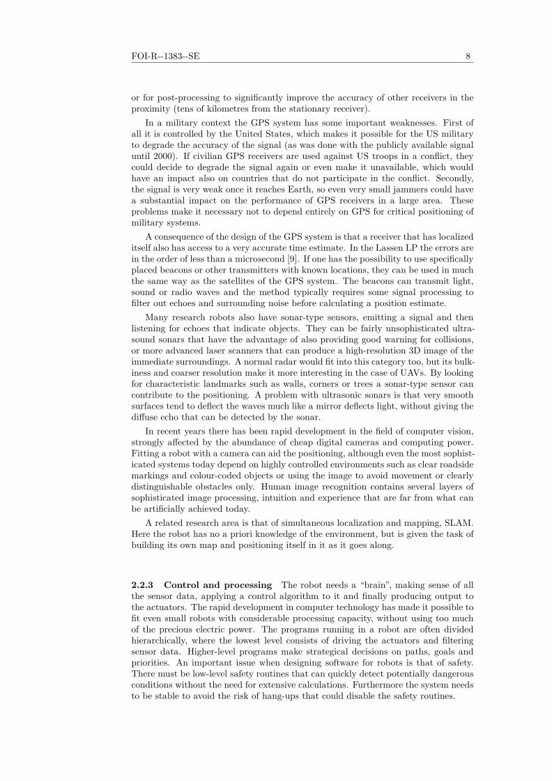
Figure 4.4: A group of 20 agents moving in a free field. The agents are depicted bydots for the first and third snapshots, and by stars for the second. The parametersare Rmax = 3, d = 2 and kφ = 0. Due to the requirement that NF has to decreasemonotonically, the formation keeping is disturbed.

not. The generator point is marked by a star (but is set to zero in the matrix). Sincewe have information on the obstacles only in the grid points, the calculation is veryconservative, assuming that the obstacle occupies one grid length above and belowthe generator point. The analysis is performed only for generator points in the firstoctant (including the 45◦ diagonal), but points outside this sector may be marked asobscured.

By transposing the matrices, flipping them up–down and left–right we can use thesame set for analyzing occupied points in any octant, thereby reducing the amountof memory required for the precalculated data. Finally all matrices corresponding tooccupied points are superimposed on the grid, using an AND operation, leaving onlythe points that are not obscured by any obstacle.

4.2.3 Finding the optimal step Step five in the algorithm is formulated asan optimization over all points that fill the conditions (3.3)–(3.6), but in the actualimplementation we have to make a finite list of candidate points. We use three typesof candidate points, described below in order of priority.

As the first candidate we use the centroid itself, since it is obviously the choiceminimizing ||pd − CV ||2. The only difficulty is testing condition (3.5), i.e. that thereis free sight from the agent to the centroid. We have chosen a safe approach, testingthe four points in G (4.1) that surround the centroid. If they are all within line ofsight, the centroid is considered to be feasible too and the agent steps directly there.

If that is not the case we test which of the feasible points in G have a lowernavigation function value than the present position, and give each of them a scalarvalue ||pd − CV ||2. Among all remaining candidates, we step to the one with thelowest value.

When trying this approach we discovered that agents sometimes got stuck when

FOI-R--1383--SE 28

0 0.5 1 1.5 2 2.5 3

0

0.5

1

1.5

2

2.5

3

Figure 4.5: An illustration of the table showing what points are obscured, viewedfrom the origin, if the point with coordinates (1, 0.75), marked by a star, is occupied.The double arrow indicates the assumed obstacle shape, one grid length above andbelow the generator point.

turning sharp corners. The situation is depicted in Figure 4.6 where the goal issituated far up left, outside the figure. The agent is denoted by a diamond shapedsymbol, standing in the grid square just below the corner. The thin lines are levelcurves of NF (q) and the dots are the points in G. Due to a “ridge” in the navigationfunction, no point belonging to G has a lower navigation function value than thepresent position, so the agent would stand still. In situations like this we introducefour special candidate points

(x, y)right = (x+ + 0.9 · (x+ − x), y),(x, y)up = (x, y+ + 0.9 · (y+ − y)),

(x, y)left = (x− + 0.9 · (x− − x), y),(x, y)down = (x, y− + 0.9 · (y− − y)),

where (x, y) are the coordinates of the agent and x+ is the x-coordinate of the vertexin the obstacle grid closest to the right of the agent. The other coordinates x− , y+

and y− are defined analogously.

The special candidate points are thus mirror images of the agent, mirrored in thefour sides of the obstacle grid square that the agent stands in. But because of the0.9 factor the mirror images are closer to the sides than the agent, so one of themalways has a navigation function value that is a little lower than that of the presentposition. This candidate point is then chosen, although the decrease of the navigationfunction might not be as large as prescribed by (3.4). It is important to note that thecreation of the special candidate points does not violate the presented algorithm, butis a consequence of the discretization needed for computer implementation. Equations(3.2)–(3.6) are formulated as an optimization over a continuous set, so we are freeto test any candidates in the set. The violation instead lies in the special candidatepoint not fulfilling equation (3.4), which also represents a form of discretization. Asuggestion on how to overcome this in future versions was given in section 3.6.

29 FOI-R--1383--SE

5.4 5.6 5.8 6 6.2 6.4

3.4

3.6

3.8

4

4.2

4.4

Figure 4.6: An agent about to turn a corner, making use of one of the four specialcandidate points denoted by stars. The agent is denoted as a diamond shape, thedots are points q ∈ G and the lines are level curves of the navigation function NF (q).The goal is far up left, outside of the figure.

4.3 Practical experiences

The aim of this section is to briefly account for some issues that we have encounteredduring the development of the algorithm. Hopefully it could be useful for someonetrying to implement the algorithm or develop it further.

4.3.1 Trimming the integration regions to a convex shape The first andgreatest problem has been that of rounding sharp corners. Our initial thought wasthat just intersecting the Voronoi regions with the obstacle-free space and then integrate over this area, V , to find CV might move the centroid away from the cornerenough for the robot not to collide with it. So in this early version, the robot alwaysstepped directly to the centroid, without checking if it was safe. This did not alwayswork, instead the robots in some situations tended to cut the corners as depicted inFigure 4.7.

We quickly concluded that one way to ensure an obstacle-free step to the centroidwould be to make sure that the integration region was always convex. So we workedfor a while on strategies for trimming the region into always being convex while stillpreserving enough of its original shape to get forward motion at all times. It proveddifficult, so eventually we instead reformulated the problem into an optimizationframework (3.2)–(3.6). This gave the possibility to explicitly require that the pathchosen be within line of sight, thereby guaranteeing us against obstacle collisions.

Another problem with the first approach was that agents could “see through” thinwalls, including points that were within Rmax but on the other side of obstacles inthe integration. This could lead to an agent stepping right into or through a wall,but was solved when we required that all points in the integration region had to bewithin line of sight.

FOI-R--1383--SE 30

2 3 4 5 6 7 8 90

1

2

3

4

5

6

7

Figure 4.7: An agent cutting a corner because there is no constraint that the targetpoint of a step has to be in line of sight from the agent. The agent is depicted as adiamond shape, the dots are points that belong to the integration region V and theline shows the calculated step. The goal is outside the figure, far up left.

4.3.2 Voronoi regions in vertex form When calculating the Voronoi regionswe first used an elaborate scheme for finding the vertexes of the region. This includedalso finding “virtual” vertexes, where an unbounded region was truncated at thedistance Rmax from the agent. It was based on the idea of first finding the separatorlines half way between the agent and every neighbor, and then walking along theinnermost polygon formed by the lines (or by arcs centered at the agent and withradius Rmax). This lead to long calculations and numerical problems when severallines crossed very close. So we eventually settled for another representation of theVoronoi region; that of normal vectors of the separator lines. Every neighbor pi toagent pj generates a separator line with normal vector

ei =pj − pi

||pj − pi||,

and a scalar

bi = [pi +12(pj − pi)] · ei.

Any point q then belongs to the Voronoi region if and only if q ·ei ≥ b for all neighborsi. The condition can be formulated as a matrix multiplication to test for all separatorlines at the same time, so it executes very efficiently in Matlab.

5. Implementation in Fenix

As a complement to testing our algorithm in Matlab, we wanted a more realisticenvironment. FOI has developed a system consisting of physical robots and a graphical computer simulator, sharing a common controller interface. So an applicationprogrammer can make a program for the computer environment and then reuse thesame code in the physical robots. The simulator software is called Fenix, and thischapter describes the system and our implementation.

5.1 System overview

Figure 5.1: One of the radio-controlled cars at FOI.

The physical robots in the FOI testbed for robot controllers are redesigned radio-controlled cars (Figure 5.1). Every car is equipped with a card-PC, actuatorsfor thrust (and thus braking) and steering, a WLAN transceiver for short-range communication and a GPS receiver for navigation. The platform is rugged enough foroutdoor terrain use, although the surface needs to be reasonably smooth because ofthe diameter of the wheels. At the moment only two cars are operational, so to betterdemonstrate the flocking properties of our algorithm we decided to implement it inFenix. It has a ready-made car model whose actuators have the same interface asthe actuators of the physical car. The information available to the controller is also

31

FOI-R--1383--SE 32

the same as in reality. The controller can extract the position of the car (althoughthere is no error as in a GPS measurement) and, as will be explained in subsection5.3 , inter-agent communication is simulated by using a global list of positions whereevery single agent can only get a list of its neighbors within a specified radius. Asdescribed in the background section, a side-effect of having a GPS receiver on the caris that it has access to a very accurate time estimate. This is used to synchronizeall cars and make them plan their next step at the same time. This is crucial foravoiding ambiguities in the Voronoi partitioning of the available space.

In this section the terms target and goal will be used for two different things. Thegoal is the global goal determined before executing the program and it is the samefor all robots. The term target refers to the individual target that is assigned toeach individual robot by its flocking algorithm, and it is updated at every replanninginterval.

5.2 Implementational issues

This section describes some problems that arose when implementing the algorithm ina more realistic environment, and the solutions to them.

In Section 3.5 is described how we find the centroid of every Voronoi region byintegration:

CV =1

MV

∫V

qφ(q) dq

withφ(q) = e−kφ·NF (q).

This worked well in Matlab, where the world had the dimensions 10 × 10 units.The highest NF value was around 30, so (given that kφ = 1) φ ∈ (9 · 10−14, 1) , whichlies well within the range of the floating-point type of Matlab. But when we enlargedthe world by almost a factor 1000, this was no longer true. The C++ variable typesand mathematical functions could not handle numbers that small. Just changingkφ , i.e. scaling the navigation function, did not work either, as it gave centroidsthat almost coincided with the geometric centroids. The solution was normalize thenavigation function in the region around the agent and use

φ(q) = e−kφ·(NF (q)−NF (pj)),

where pj is the position of the agent. This way we both reduced the deviation from1 and distributed the NF values more evenly around 1 to make better use of the fullrange of the floating-point types.

We have also expanded all obstacles by 4 m to compensate for the width andlength of the robots. Our algorithm ensures that the centre of the robot does notcollide with anything, but this sometimes lead to the robot going too close to theedge of an obstacle.

5.3 Software structure

The application programmer makes a C++ class that implements a controller forthe car and is called at every update interval by the simulation engine. In principlethe same code could then be transferred to the card-PC of the physical cars andused there as well. The structure of this software is described in this section, whichis mainly intended for someone who wants to reuse the existing code or get hintsfor a similar programming task. It assumes that the reader has basic knowledgeof C++ and object-oriented programming and it does not add significantly to theunderstanding of the more abstract overall algorithm.

All objects in the simulated world are created by an object factory, i.e. an underlying program that takes input from a script file and then creates as many instances

33 FOI-R--1383--SE

ID, position, neighbors

ObscuringMask

remove(x,y)

NavigationFunction

VehicleSteeringControllerMagnus

FlockingAlgorithm

SheepDogs

Voronoi

VehicleContainer

VoronoiRegion

CurrentMask

(x,y) occupied or not

(x,y)

NF(x,y)

ID, position, neighbors

CurrentTarget,VoronoiRegion

(height < k => obstacle)

(x,y)

in worst case, stand stillpossible to the centroid or,

Calculate mirror

regionCalculate Voronoi

neighbor positions

Maintain a map ofthe integration region

Keep record of whichpoints are occupied byobstacles

when the program startsCalculate NF(x,y) once

(Class or function names are given in boldface.)

choose a point as close as

which points obscure which

Heightmap file

Precalculated table of

Neighbors => mirror neighbors MirrorNeighbors

=> Voronoi region

Voronoi region - occupied

not in line of sight) => => integration region

points - obscured points (i.e.

Neighbors + mirror n. =>

=> centroidIntegration using NF =>

Check that the centroid is afeasible target, otherwise

IDpos

IDpos

IDpos

IDpos

IDpospos

ID, SensorRadiusPreferredDistance

SteeringThrustBrakes on/off

PositionVelocity

IDposition

position of [ID]neighbors of [ID]

ID

synchronized intervalsFlockingAlgorithm) at

IDpos

IDpos

IDpos

Drive the car straight towardsthe current target, withoutleaving the current Voronoiregion

Report ID and position to theglobal list and replan (with

Figure 5.2: Software structure of the car controller

of different objects as the file specifies. It also connects the objects to each otherand initializes them as described in the script. An example of this is that the caris described as a chassis, connected by springs to four wheels. Then actuators areinitialized and connected to the wheels and finally an instance of the VehicleSteeringControllerMagnus class is created and given handles to the actuators. Whenthe script file specifies that 20 cars should be created, 20 similar instances are set upand connected, with one VehicleSteeringControllerMagnus object each. A managerclass places the cars at different positions so that they will not collide from the start.

The basis of the car controller is the VehicleSteeringControllerMagnus class, thatissues the actual actuator commands. They are of three types; first the steeringcommand that has to be in the interval (−1, 1) , with -1 meaning full steering to theleft. Then there is the thrust command that is also in the interval (−1, 1) , with 1meaning full forward thrust and -1 full reverse thrust. Finally there is a separatebraking command that overrides the thrust command. It has only two states: on oroff, and when the brakes are on the thrust does not matter, the wheels are brakinghard. The VehicleSteeringControllerMagnus class contains a few important variables:

• mIDNumber: The global ID of the car that is controlled by this instance. It isissued by the VehicleContainer class as described below.

• drivingMode: The state of the controller state machine, described in subsection5.4.

• planningMode: The state of the replanning state machine, responsible for recalculating the current target and Voronoi region at synchronized intervals. Italso reports the position of the car to the global list (VehicleContainer) beforereplanning, so that all positions in the list are updated.

• currentTarget: The coordinates of the current target that the controller shoulddrive to.

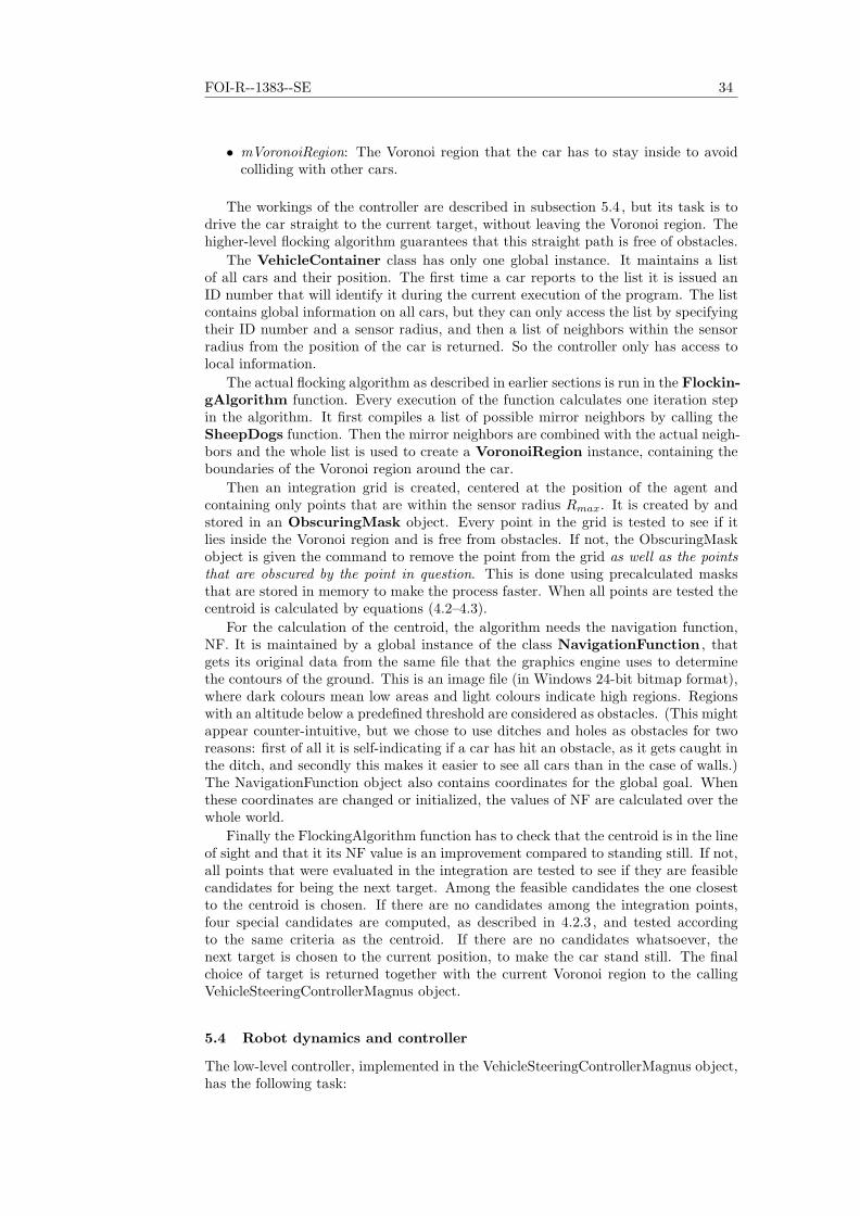
FOI-R--1383--SE 34

• mVoronoiRegion: The Voronoi region that the car has to stay inside to avoidcolliding with other cars.

The workings of the controller are described in subsection 5.4 , but its task is todrive the car straight to the current target, without leaving the Voronoi region. Thehigher-level flocking algorithm guarantees that this straight path is free of obstacles.

The VehicleContainer class has only one global instance. It maintains a listof all cars and their position. The first time a car reports to the list it is issued anID number that will identify it during the current execution of the program. The listcontains global information on all cars, but they can only access the list by specifyingtheir ID number and a sensor radius, and then a list of neighbors within the sensorradius from the position of the car is returned. So the controller only has access tolocal information.

The actual flocking algorithm as described in earlier sections is run in the FlockingAlgorithm function. Every execution of the function calculates one iteration stepin the algorithm. It first compiles a list of possible mirror neighbors by calling theSheepDogs function. Then the mirror neighbors are combined with the actual neighbors and the whole list is used to create a VoronoiRegion instance, containing theboundaries of the Voronoi region around the car.

Then an integration grid is created, centered at the position of the agent andcontaining only points that are within the sensor radius Rmax. It is created by andstored in an ObscuringMask object. Every point in the grid is tested to see if itlies inside the Voronoi region and is free from obstacles. If not, the ObscuringMaskobject is given the command to remove the point from the grid as well as the pointsthat are obscured by the point in question. This is done using precalculated masksthat are stored in memory to make the process faster. When all points are tested thecentroid is calculated by equations (4.2–4.3).

For the calculation of the centroid, the algorithm needs the navigation function,NF. It is maintained by a global instance of the class NavigationFunction , thatgets its original data from the same file that the graphics engine uses to determinethe contours of the ground. This is an image file (in Windows 24-bit bitmap format),where dark colours mean low areas and light colours indicate high regions. Regionswith an altitude below a predefined threshold are considered as obstacles. (This mightappear counter-intuitive, but we chose to use ditches and holes as obstacles for tworeasons: first of all it is self-indicating if a car has hit an obstacle, as it gets caught inthe ditch, and secondly this makes it easier to see all cars than in the case of walls.)The NavigationFunction object also contains coordinates for the global goal. Whenthese coordinates are changed or initialized, the values of NF are calculated over thewhole world.

Finally the FlockingAlgorithm function has to check that the centroid is in the lineof sight and that it its NF value is an improvement compared to standing still. If not,all points that were evaluated in the integration are tested to see if they are feasiblecandidates for being the next target. Among the feasible candidates the one closestto the centroid is chosen. If there are no candidates among the integration points,four special candidates are computed, as described in 4.2.3 , and tested accordingto the same criteria as the centroid. If there are no candidates whatsoever, thenext target is chosen to the current position, to make the car stand still. The finalchoice of target is returned together with the current Voronoi region to the callingVehicleSteeringControllerMagnus object.

5.4 Robot dynamics and controller

The low-level controller, implemented in the VehicleSteeringControllerMagnus object,has the following task:

35 FOI-R--1383--SE

• Drive the car from an arbitrary position and orientation to the target specifiedby higher level algorithms.

• The orientation of the car at the target is not important.

• There is line of sight from the start position to the target, but if the car has tomanoeuvre it must not leave its Voronoi region.

Since the controller does not know in what direction the car will have to go in thenext iteration, we decided not to put any constraints on the final orientation of thecar. Instead we prioritized to quickly reach the target.

The car model in the simulation environment is modeled after the US Army HMMWV all-terrain vehicle that is four-wheel driven, weighs 2.3 tons and measuresabout 5 by 2 metres. Since its physical dimensions are so much larger than those ofthe radio-controlled cars the simulated world has been enlarged to a width of severalkilometres. To make this section more general we have avoided specifying numericalvalues, but the values used for our simulations are listed in section 5.5.

v

r

δ

δ

L

(x,y)

θ

Figure 5.3: A model for the car.

Our car model is depicted in Figure 5.3. When steering, the wheels actually turneach around their own vertical axis and not around a common axis as in the model,but the effect is the same. How does the heading θ change over time? Let us assumethat the car moves with a constant steering angle δ. It will then follow a circle withradius r , and basic trigonometry tells us that

L

r= tan δ. (5.1)

During the time dt the car will travel the distance v dt along the circle. The headingthen changes as

v dt = r dθ ⇒ dθ

dt=

v

r=

v

Ltan δ.

The coordinates of the rear of the car evolve depending on θ and v and to accountfor the inertia of the car we added an integrator to the speed dynamics. The whole

FOI-R--1383--SE 36

model becomes, [15]:

x = v cos θ

y = v sin θ,

θ =v

Ltan δ

v = u

In [15] it is shown that the time-optimal path for such a vehicle consists of a numberof circular arcs of minimum turning radius, combined with straight line segments.Both the position and orientation of the car at the start and end points can bespecified, but as stated above, we decided to relax this by just specifying the finalposition. Using these results, we decided on a simple and robust controller that startsby turning towards the target with a minimum turning radius and a constant speed,chosen not to give slipping, and then to drive straight ahead at a higher speed untilit reaches the target. The speed is maintained by a simple P-controller:

u = kv (vdesired − v).

The surface of the simulated environment is rather slippery, so if the car uses toomuch thrust there is a risk of slipping. We therefore chose kv = 0.5 , which empiricallyproved a good compromise between fast acceleration and avoiding slipping even whenthe reference signal, vdesired , changed fast. After a few accidents when the aboveP-controller tried to slow down by reversing the thrust and thereby lost the grip, weadded a simple rule that if the speed is more than 2 m/s above the desired (whenthe P-controller saturates), we use the brakes to slow down instead, as this gives amuch better grip. When turning, the steering angle δ is given its maximal or minimalvalue, depending on direction, and the speed is adapted to avoid slipping while stillefficiently performing the manoeuvre. When the car is turned towards the goal itswitches to driving straight ahead with a higher speed and a P-controller that directsthe car towards the target:

δ =β

δmax(5.2)

where β is the angle between the velocity vector and the relative vector from the carto the target, chosen to be positive when the target is to the right of the car.

0 50 100 1500

10

20

30

40

50

60

70

80

90

100

Initial speed (km/h)

Bra

king

dis

tanc

e (m

)

Figure 5.4: The braking distance, s m, as a function of speed, v m/s. The starsdenote measured values and the line is the interpolating curve s = 0.033v + 0.048v2.

37 FOI-R--1383--SE

Finally the car needs to be stopped at the target and this is done by “bang-bangcontrol”. We constantly predict the braking distance as a function of the current speedand hit the brakes when that distance plus five metres (a safety margin) remains to thetarget. When testing the brakes at different speeds we obtained the data in Figure 5.4.We made a least-square fit with a second-degree polynomial, as the braking distanceis usually a function of the kinetic energy, which in turn is proportional to the squareof the speed. It showed that the constant term was in the order of a few centimeters,so we neglected it and made a new least-square fit to a simpler polynomial of the type

s = a v + b v2,

where we got the values a=0.033 s and b=0.048 s2/m. The applicability of thisapproach is confirmed by the excellent fit of the curve, depicted in Figure 5.4.

The controller above worked well, except for so called small-scale controllabilityproblems, i.e. when the target was very close to the original position of the car.Everyone who has driven a car knows that it is easier to drive it to a point fiftymetres away than a point just one metre to the side. The problem of small-scalecontrollability concerns areas that cannot be reached by the above scheme of a forwardturn and driving straight. Figure 5.5 depicts the different zones around the car,particularly the near zones NL and NR where this occurs. The radius R is theturning radius of the car and was determined by testing on flat ground. All othertarget locations could be reached by the controller. So we added two backing stateswhen the car drives backwards in a circle of minimum radius until it points in thedirection of the target. To reach targets in NL , the car reverses with full right steeringalong the boundary of NR , which makes its forward direction sweep over the wholeof NL. The opposite works for targets in NR. The car then drives straight ahead tothe target as described above.

RF

LNRN

LF

R R

Figure 5.5: The different target zones for the car controller. NL 6∈ FL and NR 6∈ FR.R is the turning radius of the car. A target right behind the car can be considered tobelong to any of the zones FR or FL.

Then the problem of not leaving the Voronoi region remains. As the higher-levelalgorithm guarantees that the target will be inside the convex Voronoi region, thiswill only be an issue if the car has to turn before driving straight ahead. When doingthis it constantly predicts its position two time steps ahead and checks that it will beinside the Voronoi region and not occupied by an obstacle. If the predicted positionis not feasible, the car reverses both its forward velocity and steering, so a rightforward turn becomes a left backwards turn and vice versa. This is what a human

FOI-R--1383--SE 38

driver does when parallel parking. If the car risks leaving the Voronoi region whenreversing to reach a target in a near zone, it drives straight ahead for 10 m (or untilit reaches another Voronoi boundary) and then replans the whole manoeuvre. This isnot necessarily optimal, but it was an easy way to find a strategy that works even inthis very odd case. Figure 5.6 illustrates three possible trajectories of the controller.

a b c

X

XX

Figure 5.6: Three trajectories produced by the car controller. The triangle shows theinitial position and orientation of the car, and the x is the target location. In a) thecar has sufficient space to turn, while in b) the dashed line shows the boundaries ofthe Voronoi region that must not be passed. In c) the target is in the near left zone,so the car reverses before driving straight ahead.

We implemented this as a state machine, as described in Figure 5.7. To preventunnecessary manoeuvering when the car was very close to the target we chose a distance D , inside which the car is considered “close enough” so it stands still. Afterevery replanning, i.e. a new calculation of target and Voronoi region, the state machine is reset to the START state. If only one or very few cars are used, the targets aresometimes placed so far ahead that the cars have not reached the targets, and thushave high speeds, when replanning. When this happens we decided to skip the lowspeed turning phase and make the course corrections at high speed instead to makethe motion smoother. To avoid skidding off the desired path because of too steepturns, this is only allowed if the new target is within an angle α from the forwarddirection.

5.5 Values used for the simulations

We have deliberately avoided specifying values of many constants mentioned in theabove text, so as to make it more general and applicable to any size and type ofcar-like robot. In this section we specify the values for the simulations that will bediscussed in the next section.

Figure 5.8 shows a map of the simulated world, where the black areas are obstacles.We chose to use ditches, about 15 m deep, as obstacles instead of walls or hills for tworeasons. Firstly it enables us to overlook the whole course and see all cars at once.Secondly, if a car hits a wall it might bounce off the obstacle without the observernoticing it, while if it falls into a ditch it stays there.

39 FOI-R--1383--SE

Table 5.1: Values used for the simulations in section 5.6.Quantity Variable

nameValue Remark

Grid spacing for integrationand NF

10 m

Width and length of theworld

2048 m

Maximum height of the world 20 mIntegration factor kφ 0.05 Defined in Section 3.5.Replanning interval tr 1 s A short interval gives smooth

motion, but longer intervals improve formation stability.

Sensor radius Rmax 200 mPreferred distance d 100 m This is adapted to the granular

ity of the integration grid.Car controller update interval tc 50 ms This was set by the simulation

engine.Near-target distance D 10 m This is how close to the target

the car controller is “satisfied”and stops.

Straight ahead angle 10◦ Within this angle from the forward direction the controller considers the target to be straightahead, and uses the control law(5.2).

High-speed turn angle α 30◦ See the controller state diagram(Figure 5.7).

Maximum speed 110 km/h The desired speed when drivingstraight ahead towards the target.

Curve speed vc 20 km/h The desired speed when makingminimum-radius turns.

Prediction horizon 1.5 s When making turns, the controller predicts the position of thecar this far ahead in time, tocheck that the position is safe.It is chosen to be the approximate braking time when travelingat curve speed.

Turning radius R 10 m See Figure 5.5. The actual radius was measured to 8 m, so thisincludes a margin.

Maximum turning angle δmax 30◦ Estimated value, but agrees wellwith (5.1).

FOI-R--1383--SE 40

target straight

ANALOGOUSLY

ANALOGOUSLY

ahead

>D AND NOT "HighSpeed"

<D OR

<D

<D

>D AND

<D

OR doneoutside

"HighSpeed"

Target in FL Target in FR

START

STAND STILLSTART

in NRTarget

sideout-

aheadtarget straight

aheadtarget straight

in NLTarget

STAND STILL

towards targetStraight ahead

10 mStraight ahead

turnForward right

turnReverse left

turnReverse left

outside

outside

Td

Td

Td

TdTd

Td

αc"HighSpeed" means that v>v AND the target is

located within an angle from the forward direction.

towards targetStraight ahead

STAND STILL

Figure 5.7: State diagram for the car controller, where the left part is omitted as it isanalogous to the right side. The zones are named according to Figure 5.5 , dT is thedistance to the target and D is the distance “close enough” to the goal. Dashed boxesare references to another state, repeated for clarity. The speed vc refers to the speedused for minimum-radius turns. The condition “outside” means that the predictedposition of the car is outside the Voronoi region.

5.6 Results

We have simulated three scenarios in the world described in Section 5.5: First wetried letting one single car start at position A and drive to the goal, then we started agroup of ten cars at A to see how they coped with the obstacles and finally we starteda group of 20 cars at B to study formation stability.

The single car reached the goal in 1 min 13 s. When turning the corners of theobstacles it slowed down to the curve speed vc , which delayed the driving considerablybut increased safety. It hit the target head on, without any need to make additionalcorrections before coming to a complete stop.

The group of ten cars also arrived safely at the goal, and reached the configurationdepicted in Figure 5.9 after 2 min 45 s. There was a tendency of the cars blockingeach other when driving onto the narrow bridge at C, but it never led to a lockingsituation with all cars standing still. There were no collisions even at the start, whenthe cars were lined up only ten metres from each other. The small-scale behaviourof the controller worked well, carefully backing or turning away from the others. Wetried starting the group from different positions around the world and the obstacleavoidance worked well, except for some rare cases when the cars stood still for a longtime waiting for their “turn” to pass a narrow bridge. When standing still the carsslide slowly to the side due to imperfections in the simulation engine, and this couldlead to tipping over the edge into a ditch. This sliding mechanism has, on the otherhand, also resolved some locking situations when several cars have blocked each otherat narrow entrances.

When simulating the group of 20 cars, the computer could not run the simulation

41 FOI-R--1383--SE

Figure 5.8: A map of the simulated world that measures 2× 2 km2 . The black areasare obstacles in the shape of ditches. The goal is indicated, as well as starting pointsA and B and the entrance of a narrow passage at C.

in real time due to the increased processing load. In a physical, truly distributedimplementation this would not be a problem, as the only added complexity for theindividual agent is that of computing more boundaries for the Voronoi region. It wasdiscovered that the stability of the formations depended on the replanning interval tr

of the algorithm. Long intervals gave the cars time to reach their targets between everyiteration, so the algorithm worked much like in the simplified Matlab environment.As can be seen in Figure 5.10 , the cars do not form a truly hexagonal lattice butstay well collected. The reasons that they do not form a lattice are probably thatthe surface is uneven, which acts as a disturbance, and that robots on the side of theformation tend to zig-zag ahead as described in section 3.6. When the replanninginterval was shortened the cars rarely made it to their targets. This smoothed themotion since they did not stop, but it disturbed the formations much like the casedescribed in section 4.1 , as the cars did not really go to the centroids of their Voronoiregions.

Figure 5.9: A screenshot from the simulation program showing ten cars at the goal,marked by a tree.

Figure 5.10: A screenshot from the simulation program, showing twenty cars movingin a loose formation. The goal is located outside the picture, far up to the left.

6. Sensor deployment

The preceding sections have described an algorithm for moving a flock of robots fromarbitrary starting points to a goal, using sensors mainly as a means of detectingobstacles or other robots. We now study how to use the sensors to detect an externalevent, once the group has reached the goal area. A simple way of switching fromnavigation to a sensor-coverage strategy is presented and this can be done in thesame algorithm framework as described above.

This is a useful approach for military applications, where the most popular usefor mobile robots so far is as sensor platforms. Robots can be sent into dangerousareas, they can stay inactive and wait for very long periods of time without anyneed for supplies and UAVs can be made much smaller and thus stealthier thanmanned aircraft containing support systems for the pilot. As the costs for the neededhardware decrease even further, small robots can be used in masses for missions thatwere earlier too unimportant or unqualified for military personnel. An example ofthis is given by Rybski et al., [16] , who describe a system of rovers. They are largerrobots that carry small scouts that can be launched in areas of interest. The scoutscan roll or jump with limited control and are equipped with sensors and radio linksto relay sensor data to the rover.

6.1 Sensor types

There are many sensor types that can be of interest in military applications, such as:

• Cameras, working in the infrared or visible spectrum. The images can be fullyor partially processed by the robot or simply fed to an operator that does theinterpretation. An example of partial processing can be detecting motion ortank-like objects in the image and then alerting an operator, which reduces theworkload of the operator in case of a large amount of sensors.

• Artificial noses sniffing for explosives, even those who are contained in underground mines. [17]

• Down-looking radar, used for minesweeping.

• Microphones, listening for the sound of artillery firing. The location of the firingunit can then be determined by solving for the time of arrival of the sound waveto different robots.

• Antennas, used both to detect and possibly record enemy radio traffic and alsofor locating the transmitter.

• The robot itself can be used as a “sensor” for brute minesweeping. The operatorsimply drives along a desired path to see if the robot triggers a mine.

The behaviour of the individual robot as well as the flock has to be adaptedto the type of sensor used. Artificial noses and down-looking radar have a limitedfootprint, so the robots need to sweep the area of interest. Others are non-isotropic,such as cameras or directional microphones, and thus require that the direction of

43

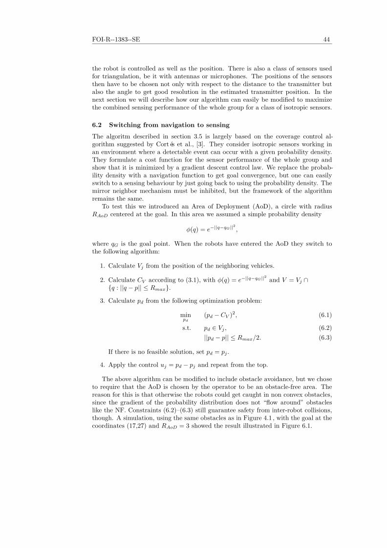
FOI-R--1383--SE 44

the robot is controlled as well as the position. There is also a class of sensors usedfor triangulation, be it with antennas or microphones. The positions of the sensorsthen have to be chosen not only with respect to the distance to the transmitter butalso the angle to get good resolution in the estimated transmitter position. In thenext section we will describe how our algorithm can easily be modified to maximizethe combined sensing performance of the whole group for a class of isotropic sensors.

6.2 Switching from navigation to sensing

The algoritm described in section 3.5 is largely based on the coverage control algorithm suggested by Cortés et al., [3]. They consider isotropic sensors working inan environment where a detectable event can occur with a given probability density.They formulate a cost function for the sensor performance of the whole group andshow that it is minimized by a gradient descent control law. We replace the probability density with a navigation function to get goal convergence, but one can easilyswitch to a sensing behaviour by just going back to using the probability density. Themirror neighbor mechanism must be inhibited, but the framework of the algorithmremains the same.

To test this we introduced an Area of Deployment (AoD), a circle with radiusRAoD centered at the goal. In this area we assumed a simple probability density

φ(q) = e−||q−qG||2 ,

where qG is the goal point. When the robots have entered the AoD they switch tothe following algorithm:

1. Calculate Vj from the position of the neighboring vehicles.

2. Calculate CV according to (3.1), with φ(q) = e−||q−qG||2 and V = Vj ∩{q : ||q − p|| ≤ Rmax}.

3. Calculate pd from the following optimization problem:

minpd

(pd − CV )2, (6.1)

s.t. pd ∈ Vj , (6.2)||pd − p|| ≤ Rmax/2. (6.3)

If there is no feasible solution, set pd = pj .

4. Apply the control uj = pd − pj and repeat from the top.

The above algorithm can be modified to include obstacle avoidance, but we choseto require that the AoD is chosen by the operator to be an obstacle-free area. Thereason for this is that otherwise the robots could get caught in non convex obstacles,since the gradient of the probability distribution does not “flow around” obstacleslike the NF. Constraints (6.2)–(6.3) still guarantee safety from inter-robot collisions,though. A simulation, using the same obstacles as in Figure 4.1 , with the goal at thecoordinates (17,27) and RAoD = 3 showed the result illustrated in Figure 6.1.

0 5 10 15 200

5

10

15

20

25

30

Figure 6.1: A group of 20 agents moving around irregular obstacles and then switchingto a sensing behaviour in the Area of Deployment around the goal, marked by an x.The agents are depicted by dots for the first and third snapshot and stars for thesecond. The parameters are Rmax = 3, d = 1, kφ = 1 and RAoD = 3.

7. Conclusions

This report presents a new algorithm for navigating groups of robots from one placeto another without colliding with each other or obstacles, regardless of their shape.When the robots are moving in open fields they stay together in a formation thatfacilitates inter-robot communication and provides good overview for an operator.We use navigation functions to find the shortest unobstructed path to the goal andthe centroids of Voronoi regions to avoid collisions while still inducing motion towardsthe goal. Finally we have added the concept of mirror neighbors, which keeps theflock together and produces formations in open fields. Simulations have shown thatthe algorithm performs well and we have been able to prove that there will be nocollisions. It provides a clear order of priority between the different requirements,where safety has precedence over goal convergence, which in turn is more importantthan formation keeping.

The algorithm has the advantage of being decentralized, meaning that every robotneeds only information about its closest surroundings and there is no central coordinator. The computational demands are almost unaffected by the number of participating robots, which makes the algorithm suitable for scaling to large groups. Finallyone can easily switch from navigation to sensing behaviour within the framework ofthe algorithm by just replacing the navigation function by a probability distributionof the event that is to be detected.

If the algorithm is to be used for controlling underwater vehicles or other kinds ofrobots that can move in three dimensions, it can be extended to allow for that. Allcomponents, such as the navigation function, Voronoi regions, centroids and mirrorneighbors can be generalized to higher dimensions in a straightforward manner. Asthe algorithm is designed for a kinematic robot model (that can assume any velocitywithout limitations in acceleration), it is not suited for controlling vehicles such asUAVs. As was the case for the cars in Fenix, this requires a lower-level controller thatsteers the robots between the waypoints generated by our algorithm. This lower-levelcontroller also has to handle situations when the waypoint is not moving, which couldprove difficult in the case of an aircraft.

7.1 Suggestions for future work

Ideas for future work can roughly be divided into two categories: studying and improving the navigation algorithm and adding more behaviours when the group switchesto sensing in the target area.

Concerning the navigation algorithm, we still have no complete proofs of formationstability. Formally, the question could be stated as: Under what conditions will aflock of robots following the proposed algorithm form a hexagonal lattice formationwhen moving over an open field where the navigation function forms a plane? Andwill that formation be stable? To avoid dead-locks, it would also be of interest tomodify the algorithm to allow the robots to give way based on some criterion. Thiscould simply be the ID of each robot, as explained in Section 3.6.1 , who has thelowest NF value or maybe a reaction-diffusion system as described in [18]. To furtherreduce the problem of crowding around bottlenecks, the preferred distance d could beadapted according to the speed of the robot or the whole group. When going fast,

47

FOI-R--1383--SE 48

they could maintain large distances, while in narrow spaces it would be acceptableto go closer. The distance d could also be controlled by an operator, who switchesthe value depending on the terrain and threat level. While navigating, there couldalso be “fuzzy” obstacles, such as enemy sites or other places associated with a cost,rather than physical obstacles. Maybe one can add some scalar penalty function tothe NF before calculating the centroids, so as to make the robots reluctant to goclose to that point.

When the robots reach the goal area and switch to a sensing behaviour, it would beof interest to expand the proposed sensor-placement strategy to allow for non-isotropicsensors or triangulation tasks. The robots could form a giant antenna array, eitherfor localizing a jammer or avoid it or for transmitting home despite heavy jamming.Maybe an antenna array can be formed iteratively by the robots moving around whiletransmitting, until the resulting radiation pattern has the desired form?

Finally one could imagine that the probability density function (PDF) mentionedin section 6 is dynamically updated according to sensor data. A discovered event(e.g. an enemy vehicle) can generate a narrow peak in the PDF, which will attractthe robot whose Voronoi region it belongs to. No other robots will be affected byit. If the single pursuing robot loses contact with the event, its position is predicted,with an added uncertainty. In lack of new sensor readings the peak in the PDF isgradually smoothed and when the pursuer cannot cover all of it due to the limitedsensor radius, more robots will be attracted and will help in reaquiring the event.If the event is discovered again, the peak is narrowed again and the closest robottakes over the pursuit. Such a sequence of detection, prediction and reaquisition isillustrated in Figure 7.1.

0 500 10000

1

2

3

4

5A

[m]

PD

F

0 500 10000

1

2

3

4

5B

[m]

PD

F

0 500 10000

1

2

3

4

5C

[m]

PD

F

0 500 10000

1

2

3

4

5D

[m]

PD

F

0 500 10000

1

2

3

4

5E

[m]

PD

F

0 500 10000

1

2

3

4

5F

[m]

PD

F

Figure 7.1: A sequence showing in one dimension how the PDF is dynamically updated to reflect the sensor data. Figure A shows the PDF before the robots havedetected anything. They will distribute evenly around the peak at x = 700m. In B,a robot has detected a target, which generates a peak in the PDF. If there are nomore indications, the peak is moved according to the estimated velocity of the targetand widened to represent the increasing uncertainty of its position. This is depictedin Figures C-E. Finally, a robot detects the target again in Figure F, which leads toa new peak in the PDF.

Bibliography

[1] M. Lindhé, P. Ögren and K-H. Johansson. Flocking with obstacle avoidance usingmethods from coverage control. Presented at the Reglermöte 2004 at ChalmersUniversity of Technology, Sweden, May 26-27, 2004.

[2] P. Ögren and N. E. Leonard. A Convergent Dynamic Window Approach toObstacle Avoidance. To appear in IEEE Transactions on Robotics and Automation.

[3] J. Cortés, S. Martinez, T. Karatas, F. Bullo. Coverage Control for Mobile SensingNetworks. Accepted for publication in IEEE Trans. on Robotics and Automation.

[4] J. L. Fuller. Robotics: Introduction, Programming, and Projects. Prentice Hall,1999.

[5] Ny Teknik. “Arméns nya robotbil kör ökenrally”.http://www.nyteknik.se/art/27529 , last visited on 2004-03-15.

[6] C. R. Weisbin, J. Blitch, D. Lavery, E. Krotkov, C. Shoemaker, L. Matthies andG. Rodriguez. Miniature Robots for Space and Military Missions. IEEE Robotics& Automation Magazine , vol. 6, no. 3, pp. 9-18, 1999.

[7] N. Tomatis, I. Nourbakhsh, K. Arras, R. Siegwart. A Hybrid Approach for Robust and Precise Mobile Robot Navigation with Compact Environment Modeling.Proceedings of the 2001 IEEE International Conference on Robotics & Automation, Seoul, Korea, May 21-26, 2001.

[8] R. G. Brown and P. Y. C. Hwang. Introduction to random signals and appliedKalman filtering. John Wiley & Sons, 1992.

[9] Datasheet for the Lassen LP GPS receiver module, from Trimble NavigationLimited. http://www.trimble.com/lassenlp.html , last visited on 2004-05-24.

[10] Datasheet for the Trimble 5800 RTK GPS surveying system, from Trimble Navigation Limited. http://www.trimble.com/5800.html , last visited on 2004-05-24.

[11] R. C. Arkin. Behavior-Based Robotics. Massachusetts Institute of Technology,1998.

[12] Y. Uny Cao, A. S. Fukunaga and A. B. Kahng. Cooperative Mobile Robotics:Antecedents and Directions. Published in Autonomous Robots , volume 4, issue1, 1997.

[13] E. Rimon and D. Koditschek. Exact Robot Navigation Using Artificial PotentialFunctions. IEEE Transactions on Robotics and Automation. pp. 501-518, Vol. 8,No. 5, October 1992.

[14] J. Hall. A Fast Algorithm for Calculating Shading and Visibility in aTwo-Dimensional Field. http://www.cs.pdx.edu/ idr/graphics/los.html , last visited on 2004-03-11.

51

FOI-R--1383--SE 52

[15] D. Anisi Optimal Motion Control of a Ground Vehicle. Master Thesis Report at the Swedish Defence Research Agency, July 2003. (Report numberFOI-R–0961–SE)

[16] P. E. Rybski, N. P. Papanikolopoulos, S. A. Stoeter, D. G. Krantz, K. B. Yesin,M. Gini, R. Voyles, D. F. Hougen, B. Nelson and M. D. Erickson. Enlistingrangers and scouts for reconnaissance and surveillance. IEEE Robotics & Automation Magazine , vol. 7, no. 4, pp. 14-24, 2000.

[17] Information on the research on artificial nosesby the Walt Group at Tufts University, MA.http://ase.tufts.edu/chemistry/walt/research/projects/ExplosivesDetectionPage.htm ,last visited on 2004-05-28.

[18] Y. Ikemoto, Y. Hasegawa, T. Fukuda and K. Matsuda. Zipping, Weaving : Control of Vehicle Group Behavior in Non-signalized Intersection. Proceedings of the2004 IEEE International Conference on Robotics & Automation, New Orleans,LA, April 2004,

A flocking and obstacle avoidance algorithm for mobile robots.

Documents

Transcript of A flocking and obstacle avoidance algorithm for mobile robots.