Evolving flocking in embodied agents based on local andglobal application of Reynolds’ rules

Rita Moreira Parada Ramos

Thesis to obtain the Master of Science Degree in

Information Systems and Computer Engineering

Supervisors: Prof. Susana Margarida da Silva VieiraProf. Sancho Moura Oliveira

Examination Committee

Chairperson: Prof. Francisco Joao Duarte Cordeiro Correia dos SantosSupervisor: Prof. Susana Margarida da Silva Vieira

Member of the Committee: Prof. Alexandra Bento Moutinho

June 2019

Acknowledgments

I would like to thank my advisers, Professor Susana Vieira and Professor Sancho Oliveira, for all the

guidance and supervision given. A special thanks to Professor Anders Christensen that also advise and

ensure the quality of this dissertation, being always available and with willingness to help. I am very

grateful to all for providing me such great learning experience.

I also would like to acknowledge IT- Instituto de Telecomunicacoes and FCT – Foundation of Science

and Technology, which partly supported this study.

To my family, in particular, my mother and father, for all the love and support, and for how much

they care about my education. To my grand-mother, which taught me the value of hard work (”when

something has to be done, it deserves to be well done”). To my friends, for their encouragement and

understanding the various skipped night-outs. And to my love, Cesar Costa. There are no words to

thank him enough, for how much he helped during the process, for enduring with me so many weekends

at home, for being always there when needed.

Abstract

In large scale systems of embodied agents, such as robot swarms, the ability to flock is essential in many

task. However, the conditions necessary to evolve self-organised flocking behaviours remain unknown.

In this dissertation, we study and demonstrate how evolutionary techniques can be used to syn-

thesise flocking behaviours, in particular, how fitness functions should be designed to evolve high-

performing controllers. In our study, we consider Reynolds’ seminal work on flocking, the boids model.

We identify two approaches that can be used to automatically synthesise robot controllers for flocking

behaviour, both using a simple, explicit fitness function inspired by Reynolds’ flocking rules.

In the first approach, the components of the fitness function are directly based on Reynolds’ three

local rules that enforce respectively separation, cohesion and alignment between neighbouring robots.

We found that embedding Reynolds’ rules in the fitness function can lead to the successful evolution of

flocking behaviours, but with the condition that the fitness scores the three components in respect to the

whole swarm, rather than only considering local interactions. In the second approach, we show that not

all Reynolds’ principles are needed to evolve flocking. In particular, the alignment need not be explicitly

rewarded to successfully evolve flocking.

Our study thus represents a significant step towards the use of evolutionary techniques to synthesise

collective behaviours for tasks in which embodied agents need to move as a single, cohesive group.

Keywords

Flocking, Evolutionary Robotics, Genetic Algorithms, Neural Networks, Robotic Controllers.

iii

Resumo

Em sistemas de grande escala de agentes, tais como grupos de robos autonomos, a capacidade de

flocking e essencial em diversas tarefas. No entanto, continua por explorar as condicoes necessarias

para evoluir o comportamento de flocking.

Nesta dissertacao, estudamos e demonstramos como as tecnicas de computacao evolucionarias

podem ser usadas para desenvolver comportamentos de flocking, em particular, como as funcoes de

avaliacao devem ser desenhadas para desenvolver controladores de elevado desempenho. Neste es-

tudo, usamos como base o trabalho de Reynolds sobre flocking. Implementamos duas abordagens que

permitem sintetizar automaticamente controladores para robos desempenharem comportamentos de

flocking, ambas usando uma funcao de avaliacao simples e explicita, inspirada nas regras de Reynolds.

Na primeira abordagem, os componentes da funcao de avaliacao baseiam-se directamente nas

tres regras locais de Reynolds que promovem separacao, coesao e alinhamento entre robos vizinhos.

Descobrimos que incorporar as regras de Reynolds na funcao de avaliacao pode levar a evolucao de

comportamentos de flocking, mas apenas quando a sua aplicacao e global, abrangendo todo o grupo,

em vez de se considerar apenas interacoes locais. Na segunda abordagem, mostramos que nem todos

os princıpios de Reynolds sao necessarios para evoluir flocking. Em particular, o alinhamento nao

precisa de ser explicitamente recompensado para evoluir com sucesso flocking.

Este estudo representa, assim, um passo significativo em direccao ao uso de tecnicas evolucionarias

na sintetizacao de comportamentos colectivos para tarefas nas quais sistemas de multi-agentes pre-

cisam de se mover como um todo.

Palavras Chave

Flocking, Robotica Evolucionaria, Algoritmos Geneticos, Redes Neuronais, Controladores Roboticos.

v

Contents

1 Introduction 1

1.1 Research Questions . . . . . . . . . . . . . . . . . . . . . . . . . . . . . . . . . . . . . . . 3

1.2 Objectives . . . . . . . . . . . . . . . . . . . . . . . . . . . . . . . . . . . . . . . . . . . . . 3

1.3 Scientific Contribution . . . . . . . . . . . . . . . . . . . . . . . . . . . . . . . . . . . . . . 3

1.4 Dissertation outline . . . . . . . . . . . . . . . . . . . . . . . . . . . . . . . . . . . . . . . . 4

2 State of the Art 5

2.1 Evolutionary Robotics . . . . . . . . . . . . . . . . . . . . . . . . . . . . . . . . . . . . . . 8

2.2 Flocking in Robotics . . . . . . . . . . . . . . . . . . . . . . . . . . . . . . . . . . . . . . . 10

2.2.1 Hand-coded design . . . . . . . . . . . . . . . . . . . . . . . . . . . . . . . . . . . 10

2.2.2 Evolutionary Robotics . . . . . . . . . . . . . . . . . . . . . . . . . . . . . . . . . . 11

3 Adapting Reynolds’ flocking model with evolutionary techniques 15

3.1 Robot Model . . . . . . . . . . . . . . . . . . . . . . . . . . . . . . . . . . . . . . . . . . . 16

3.2 Simulator . . . . . . . . . . . . . . . . . . . . . . . . . . . . . . . . . . . . . . . . . . . . . 18

3.3 Controller Architecture and Evolutionary Algorithm . . . . . . . . . . . . . . . . . . . . . . 19

3.4 Metrics . . . . . . . . . . . . . . . . . . . . . . . . . . . . . . . . . . . . . . . . . . . . . . 21

3.5 Results and Discussion . . . . . . . . . . . . . . . . . . . . . . . . . . . . . . . . . . . . . 22

3.5.1 Experimental setup inspired by Reynolds’ local rules - Local setup . . . . . . . . . 22

3.5.2 Experimental setup scoring global behaviour - Global setup . . . . . . . . . . . . . 23

4 From Reynolds’ principles to the evolution of flocking in agents 27

4.1 Experimental setup without the Cohesion component - No Cohesion setup . . . . . . . . 28

4.2 Experimental setup without the Alignment component - No Alignment setup . . . . . . . . 31

5 Generalisation 35

5.1 Swarm size (N) . . . . . . . . . . . . . . . . . . . . . . . . . . . . . . . . . . . . . . . . . . 36

5.1.1 Swarm size - 5, 8, 11, 16 robots . . . . . . . . . . . . . . . . . . . . . . . . . . . . 36

5.1.2 Swarm size - 20, 30, 50, 100 robots . . . . . . . . . . . . . . . . . . . . . . . . . . 38

5.2 Time-steps (T) . . . . . . . . . . . . . . . . . . . . . . . . . . . . . . . . . . . . . . . . . . 41

vii

6 Conclusion 43

6.1 Conclusions . . . . . . . . . . . . . . . . . . . . . . . . . . . . . . . . . . . . . . . . . . . . 44

viii

List of Figures

2.1 Examples of flocking behaviour in nature. Left: European starlings (Sturnus vulgaris); Top

right: Minnows (Phoxinus phoxinus); Bottom right: Desert locusts (Schistocerca gregaria).

Respective sources: http://www.lovethesepics.com/wp-content/uploads/2012/11/

Flock-of-Starlings.jpg; [1]; https://www.preventionweb.net/news/view/48722 . . 6

2.2 The three simple rules of Reynolds’ boids model. This image was adapted from Reynolds

work [2]. . . . . . . . . . . . . . . . . . . . . . . . . . . . . . . . . . . . . . . . . . . . . . . 7

3.1 Sensors used by each robot. Up: Illustration of a case in which the Alignment sensor

would receive maximum value, 0.5, since all robots within the sensor range have the

same orientation. Bottom: The four robot sensors with the respective readings. Note

that, although in sensor 2 and sensor 4 more than one robot is within the range, only the

closest robot contributes to the reading of the sensor. . . . . . . . . . . . . . . . . . . . . 17

3.2 Example of possible configurations in the interface of JBotEvolver. . . . . . . . . . . . . . 18

3.3 Representation of the robot controller architecture: a Continuous Time Recurrent Neural

Network (CTRNN) with the corresponding input neurons, hidden layer and output neurons. 19

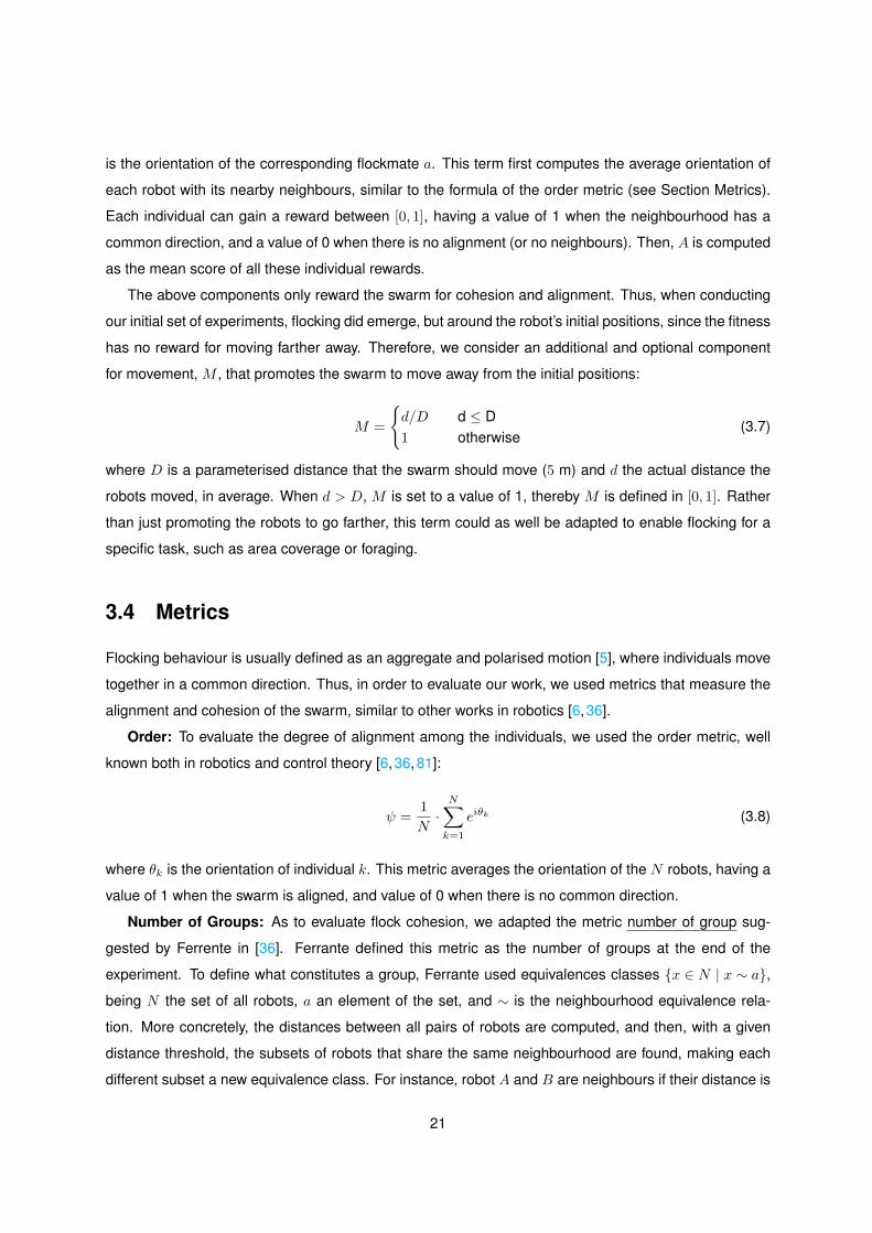
3.4 Left: Fitness trajectories of the highest-scoring controllers evolved in each evolutionary

run. Right: Distribution of the post-evaluation fitness scores achieved by the highest-

scoring controller of the 30 evolutionary runs conducted. The box-plot summarises results

from 400 post-evaluation samples. . . . . . . . . . . . . . . . . . . . . . . . . . . . . . . . 23

3.5 The figure summarises results of the average from the 400 post-evaluation samples of

the highest-scoring controller in terms of the metrics presented in Section Metrics. Left:

The order metric trajectory across the 3000 simulation steps. Centre: box-plot of the

distribution of the number of groups metric. Right: The swarm cohesion trajectory across

the 3000 simulation steps. . . . . . . . . . . . . . . . . . . . . . . . . . . . . . . . . . . . . 24

3.6 Example of the behaviour displayed by the highest-performing controller, with 5, 8, 11 and

16 robots, from left to right. The lines represent the trajectory of the robots. . . . . . . . . 24

ix

3.7 Left: Fitness trajectories of the controllers in each of the 6000 generations. Right: Distri-

bution of the post-evaluation fitness scores achieved by the highest-scoring controller. . . 25

3.8 The metrics scores achieved by the highest-scoring controllers of Global setup and the

Local setup. Left: the order metric. Centre: the number of groups metric. Right: the

swarm cohesion metric. . . . . . . . . . . . . . . . . . . . . . . . . . . . . . . . . . . . . . 26

3.9 Example of the behaviour displayed by the highest-performing controller evolved in the

Global setup, with 5, 8, 11 and 16 robots, from left to right. Observing the beginning of

trajectory, we can see the robots evolved the strategy of moving closely around their initial

positions, in order to first form an aligned group before moving away. . . . . . . . . . . . . 26

4.1 Left: Fitness trajectories of the 30 controllers within 6000 generations. Right: The box-plot

summarises results from 400 post-evaluation samples achieved by the highest-scoring

controller of the No Cohesion setup . . . . . . . . . . . . . . . . . . . . . . . . . . . . . . 29

4.2 The metrics scores achieved by the highest-score controller of the No Cohesion setup

and the Global setup. Left: The order metric. Centre: the number of groups metric. Right:

the swarm cohesion metric. . . . . . . . . . . . . . . . . . . . . . . . . . . . . . . . . . . . 29

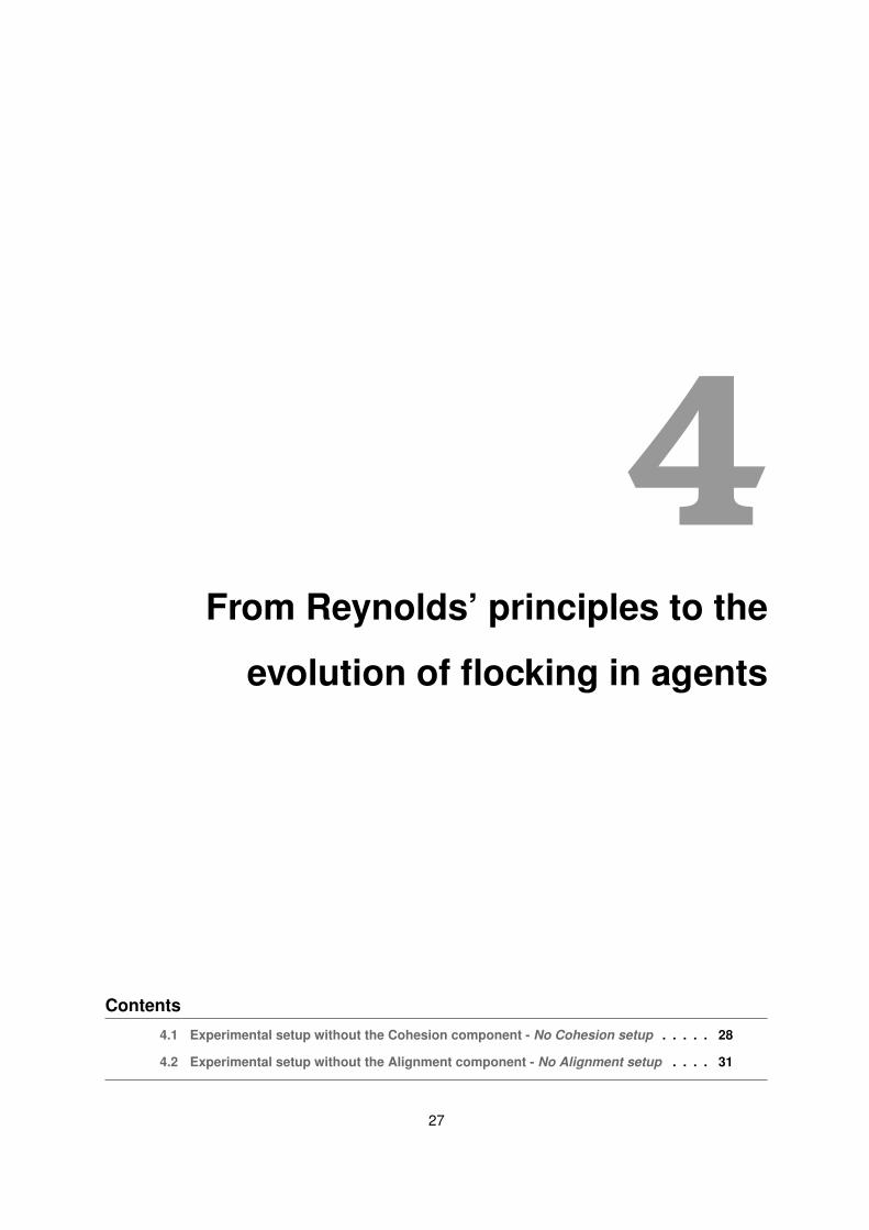
4.3 Example of the behaviour displayed by the highest-performing controller evolved in the No

Cohesion setup, with 5, 8, 11 and 16 robots, from left to right. Different colours represent

different groups, being the black colour used to represent the main group, i.e, the group

with high number of robots. . . . . . . . . . . . . . . . . . . . . . . . . . . . . . . . . . . . 30

4.4 The figure shows order metric of the post-evaluation samples with an extended number

of time-steps, 6000 time-steps. . . . . . . . . . . . . . . . . . . . . . . . . . . . . . . . . . 31

4.5 Left: Fitness trajectories of the 30 controllers within 6000 generations. Right: Box-plot of

the results of the 400 post-evaluation samples achieved by the highest-scoring controller

of the No Alignment setup. . . . . . . . . . . . . . . . . . . . . . . . . . . . . . . . . . . . 32

4.6 The metrics scores achieved by the highest-score controller of the No Alignment setup

and the Global setup. Left: The order metric. Centre: the number of groups metric. Right:

the swarm cohesion metric. . . . . . . . . . . . . . . . . . . . . . . . . . . . . . . . . . . . 33

4.7 Example of the behaviour displayed by the highest-performing controller of the No Align-

ment setup, with 5, 8, 11 and 16 robots, from left to right. The behaviour displayed is

similar to one in Fig 3.9. . . . . . . . . . . . . . . . . . . . . . . . . . . . . . . . . . . . . . 33

5.1 The order metric by the highest-score controller of the Global setup (left) and No Align-

ment setup (right), with 5, 8, 11 and 16 robots. . . . . . . . . . . . . . . . . . . . . . . . . 36

5.2 The number of group metric achieved by the highest-score controller of the Global setup

(left) and No Alignment setup (right), with 5, 8, 11 and 16 robots. . . . . . . . . . . . . . . 37

x

5.3 The swarm cohesion metric achieved by the highest-score controller of the Global setup

(left) and No Alignment setup (right), with 5, 8, 11 and 16 robots. . . . . . . . . . . . . . . 37

5.4 The order metric achieved by the highest-score controller of the Global setup (left) and

No Alignment setup (right), with 20, 30, 50 and 100 robots. . . . . . . . . . . . . . . . . . 39

5.5 The number of groups metric achieved by the highest-score controller of the Global setup

(left) and No Alignment setup (right), with 20, 30, 50 and 100 robots. . . . . . . . . . . . . 40

5.6 The swarm cohesion metric achieved by the highest-score controller of the Global setup

(left) and No Alignment setup (right), with 20, 30, 50 and 100 robots. . . . . . . . . . . . . 40

5.7 The metrics scores achieved by the highest-scoring controllers of Global setup and the

No Alignment setup with 9000 time-steps. Left: the order metric. Centre: the number of

groups metric. Right: the swarm cohesion metric. . . . . . . . . . . . . . . . . . . . . . . . 42

xi

xii

Acronyms

ER Evolutionary Robotics

ANNs Artificial Neural Networks

EA Evolutionary algorithms

RL Reinforcement Learning

CTRNN Continuous Time Recurrent Neural Network

xiii

xiv

1Introduction

Contents

1.1 Research Questions . . . . . . . . . . . . . . . . . . . . . . . . . . . . . . . . . . . . . . 3

1.2 Objectives . . . . . . . . . . . . . . . . . . . . . . . . . . . . . . . . . . . . . . . . . . . 3

1.3 Scientific Contribution . . . . . . . . . . . . . . . . . . . . . . . . . . . . . . . . . . . . 3

1.4 Dissertation outline . . . . . . . . . . . . . . . . . . . . . . . . . . . . . . . . . . . . . . 4

1

There has been a growing interest in using robots in tasks, such as navigation, search and rescue,

and environmental monitoring that require high degrees of autonomy, mobility, flexibility and robust-

ness [3]. Such tasks can be addressed by the promising approach of swarm robotics [4], that aims

to produce robust, scalable and flexible systems that exhibit self-organised collective behaviour. The

general idea in swarm robotics is to use large groups of autonomous collaborating robots with relatively

simple hardware and decentralised control, rather than a single or a few complex robots.

Flocking is one of the collective behaviours that are exhibited in nature. Flocking became widely

studied after the seminal work of Reynolds [5], in which he defined three simple, behavioural rules

(cohesion, separation and alignment) that were able to generate realistic flocking behaviour in computer

animation. Flocking has since become an area of study in several fields beyond biology and computer

animation, such as robotics, statistical physics, and control theory [6–9].

In swarm robotics, collective behaviours such as flocking can be achieved with automatic design

methods. Evolutionary Robotics (ER) is the field that aims to synthesise controllers for autonomous

robots, in which the evaluation and optimisation of controllers are holistic in a self-organisation pro-

cess [10], therefore, not requiring manual and detailed specifications of the desired behaviour by the

experimenter [11]. The underlying idea is inspired in Darwin’s theory of evolution, which through an ar-

tificial selection process, the fittest individuals are the ones chosen to populate the next generation [12].

Throughout ER research, numerous behaviours have successfully been evolved, such as aggre-

gation, dispersion, foraging, and so forth [13–17]. However, it is still unclear how high-performance

flocking behaviours can be automatically synthesised by means of artificial evolution. To date, flock-

ing has primarily be achieved with hand-programmed control [6, 18, 19]. However, manual specification

of the behaviours can prevent non-obvious solutions from being discovered [10]. In addition, such an

approach is often limited when it comes to tasks and environments that are not entirely characterised

prior to robots’ deployment. It might not be easy for the designer to find the individual behaviours and

the necessary interactions that lead to flocking in an unspecified environment or situation, which can

help to explain why flocking studies have been mostly conducted in simulation or in controlled labo-

ratory conditions. Automatic design methods are an alternative approach to design agents through a

self-organised process without the need to specify or understand all the necessary interactions among

the robots and the environment. Thus, an automatic design method, such as ER, has the potential to

synthesise flocking behaviours for different environments and task scenarios.

In this thesis, we study how to automatically synthesise robot controllers for self-organised flocking

behaviour based on artificial evolution. In particular, we consider Reynolds’ seminal work on flocking,

adapting Reynolds’ flocking model with evolutionary techniques.

2

1.1 Research Questions

The questions that we aim to answer in the end of this thesis are the following:

• Which fitness functions and experimental setups are necessary for the successful evolutionary

design of flocking behaviour?

• Can flocking behaviour emerge by adapting Reynolds’ flocking model with evolutionary tech-

niques? If so, are all Reynolds’ principles necessary to evolve flocking?

1.2 Objectives

The goal of this thesis is to find which fitness function components and elements of experimental setups

are necessary to evolve flocking, in order to enable the synthesis of robot controllers to carrying out

tasks that require flocking. We aim to formulate fitness functions that explicitly and effectively reward

flocking behaviours, namely by adapting Reynolds’ manually specified rules (separation, cohesion and

alignment) as components in the evaluation function.

Flocking has the potential to be integrated in the evolution of other collective behaviours that benefit

from the same principles of flocking, indeed, aggregation and coordinated motion can play an important

role in patrolling tasks, environment monitoring, foraging and similar real-world tasks that can be under-

taken by swarms of autonomous robots. Thus, the study of synthesise flocking behaviours can be of

help to synthesise other collective behaviours for tasks in which embodied agents need to move as a

single, cohesive group.

In summary, the objectives are:

• to study how fitness functions and experimental setups should be design to evolve high-performing

controllers.

• compare the evolved behaviours with Reynolds’ preprogrammed behaviours, such as studying if

the evolved solution requires all Reynolds’ principles to emerge flocking.

• contribute to the use of evolutionary techniques to synthesise collective behaviours for tasks in

which embodied agents need to move as a single, cohesive group.

1.3 Scientific Contribution

The work conducted in this dissertation has resulted in one journal submission to PlosOne:

• R. P. Ramos, S. Oliveira, S. Vieira, A. L. Christensen, ”Evolving flocking in embodied agents based

on local and global application of Reynolds’ rules”, under review.

3

1.4 Dissertation outline

This dissertation is organised into 5 chapters. We started by giving a brief introduction and description

of our study in Chapter 1, and go on to present the related work in Chapter 2. We provide an overview

of flocking behaviour, followed by the field of evolutionary robotics, and, finally, we discuss work related

to flocking in robotics, particularly focusing on the ER field. Then, in Chapter 3, we demonstrate our ap-

proach to automatically synthesise robot controllers for flocking behaviour by adapting Reynolds’ flocking

rules. We present the methods and materials used and discuss the experimental results. In the follow-

ing chapter, Chapter 4, we compare the evolved behaviours with Reynolds’ preprogramed behaviours,

providing a description of the conducted experiments and analysing the obtained results. Chapter 6

summarises our dissertation, along with future directions in which our work can be further studied.

4

2State of the Art

Contents

2.1 Evolutionary Robotics . . . . . . . . . . . . . . . . . . . . . . . . . . . . . . . . . . . . 8

2.2 Flocking in Robotics . . . . . . . . . . . . . . . . . . . . . . . . . . . . . . . . . . . . . 10

5

Flocking is a collective behaviour of coordination motion that can be observed in numerous species,

such as birds, fishes and locusts. For example, European starlings (Sturnus vulgaris) are one of the

most popular bird species known to exhibition highly synchronised and coherent flocks [20,21]. Minnows

(Phoxinus phoxinus) are known to form polarised swimming groups with variant shapes, being commonly

used in studies of schooling [1]. Other example is the Desert Locusts (Schistocerca gregaria) that

exhibits flocking when above a given density: as the number of locust increase, a disordered movement

of individuals changes to a cohesive movement from dense clusters [22,23] (see Figure 2.1).

Figure 2.1: Examples of flocking behaviour in nature. Left: European starlings (Sturnus vulgaris);Top right: Minnows (Phoxinus phoxinus); Bottom right: Desert locusts (Schistocerca gre-garia). Respective sources: http://www.lovethesepics.com/wp-content/uploads/2012/11/

Flock-of-Starlings.jpg; [1]; https://www.preventionweb.net/news/view/48722

In biology, there are several evolutionary hypotheses that explain the emergence of flocking be-

haviour in nature. This include safety from predators, which itself can be attributed to different rea-

sons [24]: flocking can confuse predators accuracy of vision [25]; provide increased vigilance [26, 27];

decrease the individual chance of being caught (it is mostly the ones at the periphery that are at risk) [28],

and so on. Another advantage of flocking is foraging efficiency: many studies have shown that individ-

uals find food faster in a foraging group than on its own [24, 29–31]. Other hypotheses for flocking

behaviour in animals include mating success [32,33] and energy efficiency [34,35].

Apart from biology, flocking was not a subject of particular interest for most fields. Flocking became

a more popular field of study after Reynolds proposed the first computational model of flocking, the

boids model [5]. In his work, Reynolds formally defined flocking behaviour as “polarised, non-colliding,

aggregate motion”, and showed that only three simple rules are necessary to obtain flocking: (i) flock

centering, (ii) collision avoidance, (iii) velocity matching (see Figure 2.2. With these rules, each individual

should attempt to be at close distance from each other (i), without colliding with one another (ii), while

trying to match its velocity with their neighbours (iii). Although for Reynolds, both the speed and the

orientation are taken into account in the velocity rule, several studies only consider relevant the orienta-

6

tion to obtain flocking [6,36], including Reynolds himself that later on described the third rules as ”steer

towards the average heading of local flockmates” [2]. Therefore, the third rule can also be described

simply as each individual trying to align with the average orientation of its neighbours. In literature,

these rules are also respectively known as cohesion, separation and alignment.

Figure 2.2: The three simple rules of Reynolds’ boids model. This image was adapted from Reynolds work [2].

Although Reynolds was particular interested in generating a realistic behaviour of flocking in com-

puter animation, ever since flocking has been a subject of interest in several fields apart from biology, and

computer animation, including robotics. In robotics, studying flocking or any other collective behaviour

is usually tackled in Swarm Robotics [37–39]. This new approach makes use of large groups of sim-

ple autonomous robots that are capable of performing local communications, as opposed to centralised

control. Inspired in social insects, the main properties of swarm robotics systems are the following [37]:

• Robustness: the swarm continues to operate properly in the event of faults, even if some robots

stop working.

• Flexibility : the robots are capable to adapt to different tasks, environments, and unforeseen situa-

tions.

• Scalability : the swarm is capable of operating independent of the group size, with either few or

thousand individuals.

Swarm Robotics System can either be achieved by hand-coded design methods or via automatic

design methods. The most common method is the first one, consisting in manually programming the

robot controllers [38]. In a trial and error process, the experimenter designs by hand the individual

behaviours of the each robot in order to achieve the desired collective behaviour. Hand-coded design

methods can be further divided into two main categories [36, 38]: (i) the finite state machine design,

usually with state transitions governed by probabilities, similar to some behaviour models of social in-

sects [40]; (ii) the virtual physics-based design, a method inspired by physics, where every single robot

is considered as a virtual particle conditioned to the virtual forces exerted by the other individuals and/or

by the environment.

7

Attempting to achieve the collective behaviour by manually programming the individual behaviours

might be too complex and challenging for the designer, since it is not easy to foreseen all the behaviour

rules of the individual robots and the interactions (among them and the environment) that are necessary

to emerge the global behaviour [10, 41]. Even if the collective behaviour can be designed by hand-

coded methods, the solutions are limited to the designer’s knowledge, preventing non-obvious and more

efficient solutions to be find. Also, being a trial and error process, hand-coded design methods have a

bottleneck in terms of development time and effort needed [42]. In addition, this approach is often limited

when it comes to unforeseen situations, namely when tasks or terrains are not entirely characterised

prior to robots’ deployment.

To overcome some of the limitations inherent to hand-coded design methods, swarm robotics sys-

tems might be alternatively design via automatic means. In swarm robots, two main paradigms of

automatic designed methods are used [36, 38]: (i) Reinforcement Learning (RL) [43]; (ii) Evolutionary

Robotics (ER) [10]. In Reinforcement Learning, an agent receives feedback from its actions, allow-

ing them to learn by a trial-and-error process. Although RL has been successfully applied to single

robots [44–46], this approach is not much suitable to swarm robotics, because it proves difficult to de-

compose the global reward into individual rewards [38]. Thus, only few works about swarm robotics

have used RL [47, 48]. A more promising automatic method is Evolutionary Robotics (see the following

subsection).

In the remaining of this section, we introduce evolutionary robotics, the design method that we use

in this research to the synthesis of swarm robotic controllers. Afterwards, we review literature in the field

of robotics related with flocking. We present some of the seminal works that used hand-coded design

and then give a more detailed description of the works in ER.

2.1 Evolutionary Robotics

Evolutionary robotics is the field of research that applies evolutionary computation techniques to syn-

thesise controllers for autonomous robots [49]. Through a process analogous to natural evolution, an

evolutionary algorithm evaluates and optimises the robots controllers in a holistic manner [50]. The un-

derlying idea is inspired in Darwin’s theory of evolution, it consists of optimising a population of genomes

in genotype space with blind variations and survival of the fittest, as embodied in the neo-Darwinian syn-

thesis [12].

In ER, Artificial Neural Networks (ANNs) are typically used as robotic controllers [41], processing the

values of the robot sensors and outputting the corresponding actuators values. An ANN is computational

model based on the neural structure of the human brain [51]. A neural network is composed by an input

and output layer of neurons, and can also have one or more hidden layers in order to cope with problems

8

that are not linearly separable [52]. When using ANNs as robot controllers, the neurons in the input layer

correspond to the robot’s sensors and the neurons in the output layer correspond to the robot’s actuators.

To evolve the controllers, the parameters of the neural networks (such as the the connection weights)

are then optimised by an evolutionary algorithm.

Evolutionary algorithms (EA), such as genetic algorithms, are optimisation methods that attempt

to find solutions for a given problem inspired by Darwinian evolution [53]. The evolutionary process

starts with an initial population of candidate solutions, usually generated randomly. In each iteration,

the performance of each candidate solution is evaluated according to a fitness function provided by the

experimenter [41]. The candidates with highest fitness score are then selected to become part of next

iteration and to populate it (by means of mutation and/or crossover). This process continues iteratively

until a given stopping criteria, such as a fixed number of iterations. It should be highlighted the important

role of the fitness function in the evolutionary process, since achieving the desired solution is intimately

dependent on the formulation of a suitable fitness function. A reviewed of fitness functions used in the

field of evolutionary robotics can be found in [41].

Using EA as a means to optimise the parameters of ANNs allows for the self-organisation of the

controller, eliminating the need for manual and detailed specification of the of behaviour. In ER, ANNs

are well-suited and commonly used to control autonomous robots for a number of reasons, including [54]:

• The straightforward mapping between sensors and actuators

• Robustness to noise

• Capability to approximate any continuous function arbitrarily well (having the right network archi-

tecture)

• Small changes in weights typically correspond to small changes in behaviour, thereby creating a

Smooth fitness landscape

The potential of ER to automate the design of behavioral control was defend by several researchers

over inefficient preprogrammed approaches [49, 55–57], and throughout approximately two decades of

ER research, numerous robots controllers have been successfully evolved [58–60]. Furthermore, ER

can be a valuable approach for designing controllers for swarm robotics systems, given that it elimi-

nates the difficult manual task of finding the individual behaviours and the interactions that lead to the

emergence of the desired collective behaviour. Examples of studies that have demonstrated evolved

controllers for swarm robotics tasks can be found in [13–17], where numerous collective behaviours

were successfully evolved, such as aggregation, chain formation, coordinated motion. Besides engi-

neering purposes, ER has also the advantage of answering more biology questions, since the evolved

solutions can provide insight about natural selection pressures [50].

9

Despite the numerous advantages of ER, there are several issues that prevent it from being a widely

adopted design method for behavioral control [61]. One of those issues is the Reality gap [62], the

non-trival problem of how to successfully transfer the control evolved in simulation to real robotic hard-

ware. However, the potential to evolve robotic controllers, beyond simulation and controlled laboratory

conditions, has already been demonstrated in realist environments [15]. Another issue is the difficulty to

evolve suitable controllers for complex tasks, in which the evolution soonly becomes trapped in a local

minimum (known as the bootstrapping problem [41]. In fact, it can be claimed that so far most of the

behaviours evolved have relative low complexity and may actually be achieved with hand-coded design

methods [11, 38]. Also, there are not still standard practices in the field [11], which makes it hard to

compare studies, as well as, it does not facilitate the studies to be replicated and extended by other

researchers. Another problem of ER, considered by some researchers [36, 38], is the widespread use

of neural networks as controllers, given the fact that ANNs are black-boxes and, therefore, difficult to

reverse engineer. Further details on the state of the art in evolutionary robotics see [50].

2.2 Flocking in Robotics

2.2.1 Hand-coded design

In robotics, most studies use control rules, similar to the ones used in Reynolds’ study. In general, the

cohesion and separation rules (proximal control) are used, but only some works include the alignment

rule (alignment control), as described by Ferrante in his doctoral thesis [36].

Giving examples of works that use alignment control, Turgut et al. [6] were the first to achieve flocking

without relying on external computation or communication devices. The authors presented a flocking

behaviuor, using proximal control and alignment, that can lead a swarm to move coherent in a random

direction while avoiding obstacles. Celikkanat and Sahin, [63] extended this behaviour, enabling the

swarm to flock toward a desired direction, by externally guiding just some members. Pessoa el al. [64]

presented outdoor flocking with aerial robots, relying on local interactions. The decentralised control

algorithm was similar to Reynolds’ model: for cohesion, a position constraint was used; to avoid collisions

a short-range repulsion was needed; and a velocity alignment term was used.

When alignment control is not used, and instead alignment is achieved implicitly, the orientation of

the swarm is usually induced by having multiple informed robots knowing about a goal direction [36].

Using local communication, Nembrini [65] presented a minimalist method for flocking, showing a swarm

capable of maintaining cohesive and avoiding obstacles while moving toward a light beacon, that was

just perceived by a minority of the robots. Spears [66] achieved flocking by developing a framework

of artificial physics based on attraction/repulsion forces. The robots were able to form a regular lattice

structure and keeping its formation while moving to a light-source known by most of the robots. Recently,

10

Toshiyuki et al. [67] proposed a flocking model that uses stochastic learning automaton where each robot

can be dynamically selected to be a follower or move as a leader to the known target direction. More

examples of works with or without alignment control can be found in Ferrante et al.’s study [18], where

the authors successfully achieved flocking without alignment control and neither with goal direction.

Despite the interesting work done so far, in most of these works, the robots have a initially knowl-

edge about the goal direction, but in real-word tasks, such as search and rescue, usually there is no

information about the location of the particular goal. Also, if most members are informed about the goal

direction, this may result in flocking to the goal just because of this global information, and not because

of being a self-organising process, as it often is in nature.

2.2.2 Evolutionary Robotics

In ER, Zaera et al. [68] were among the first to report on attempts to evolve controllers that could

exhibit behaviours similar to flocking, schooling or herding, but without success. Zaera et al. intended

to develop neural network-based sensorimotor controllers for schooling behaviour in three dimensions,

using realistic Newtonian kinematics, such as inertia and drag. The authors tried to evolve behaviour

based on the definitions of flocking suggested in the literature (such as Reynolds’ rules [5]), namely

by rewarding individuals for moving at the same speed or for maintaining a certain distance to their

neighbours, but they only succeeded in evolving simple group behaviours: aggregation and dispersion.

The authors expressed the difficulty in formulating an explicit fitness function that is able to measure

the degree of schooling exhibited by a group of agents, claiming that schooling behaviours arises from

complex interactions of a number of factors, which are hard to capture in a simple fitness function. The

authors furthermore claimed that it can be more difficult to evolve schooling than using manual design

methods. It should be noted, however, that Zaera et al. neither specified the fitness functions that were

tried, nor did they provide a detailed and quantitative analysis of the obtained behaviours. In addition,

some assumptions that were taken could explain the lack of success, as referred in [69] subsequent

work. First,the neural networks were limited to only 5 hidden nodes. Secondly, the inputs of the neural

network were based on 3d simulated vision, and, consequently, the number of input nodes were much

higher than the hidden nodes. Also, the experiments had a small number of generations, only 100, which

may not be sufficient to evolve a complex behaviour like flocking. Finally, the lack of success might also

be a consequence of the amount of complexity involved in simulating in 3d and using realistic Newtonian

kinematics.

In a subsequent attempt to evolve flocking behaviour, Felt and Koonce [69] modeled their approach

closely to Zaera et al.’s work, but with a number of significant differences that made them believe they

would have more success. First, their work was not subject to realistic laws of physics and agents moved

in two dimensions rather than three. In addition, the agents were provided with complete information

11

about their closest neighbours, instead of simulating vision. Another difference between the two papers

is that a greater amount of generations were run, 1000 generations rather than 100, since the authors

implemented a parallelised framework instead of using a sequential one. Finally, the authors claimed

they had a more flexible neural network, provided by unbounded weights, more hidden nodes and with

different mutation method. Despite these differences, the authors were also unable to evolve controllers

that could exhibit flocking behaviour, even with several attempts of different fitness function and training

scenarios. They started by giving the individuals a positive score for being at a given distance from their

neighbours, and receiving zero fitness if getting to close. This fitness function led to the fragmentation of

multiple groups, so the authors them tried to penalise the individuals that got too close to one another.

In the beginning, the authors obtained a similar behaviour to flocking, since agents formed a cohesive

group that move coherent in a random direction, but after some time, the individuals move farther apart

from one another, remaining alone in longer simulations. Other variants of fitness functions were tried,

namely giving rewards to alignment, to reach a food patch, and so on, but again without much success.

Similar to Zaera et al.’s findings [68], Felt and Koonce [69] concluded that ”finding a good fitness function

for the genetic algorithm is equally difficult, if not more difficult, than the task of hand–coding a controller

that imitates flocking (...)”.

Instead of trying to explicitly encode flocking in the fitness function, Ward et al. [70] had more success

than Zaera et al. [68], claiming that the obtained results ”would have been difficult, if possible at all, to

foresee or even implement” with manual design methods. The authors evolved controllers for flocking (or

schooling) behaviour, designated as E-BOIDS (evolved boids), as recognition to Reynolds’ boids model.

In their work, predators and prey coevolve to produce the desired behaviour, inspired by biological

hypothesis that flocking emerges in the presence of predators. These artificial agents are placed in a

two-dimensional environment with food sources randomly spreaded. Both these agents are composed

by a simple feed-forward, fully connected network. The input layer attempts to have realistic fish sensors,

consisting of a set of two different types of sensory modalities: vision input nodes for the distance and

direction of the closest preys, predators and food sources; and lateral line nodes for detecting local

changes in water pressure. And the output layer has two nodes for controlling the motion, to turn

left or right, respectively. As to the fitness function, it is based on the energy values of each agent.

Each individual starts with a certain amount of energy to spent in a given behaviour, such as moving,

eating, and mating; that can either consume or increase the energy of the individual (ex: Eating Food

corresponds to +20 or +25, if the individual is a prey or a predator, respectively). Then, at the end of the

generation, the selected individuals are the ones that have higher energy values. This simple and implicit

fitness function led to some interesting results, where preys learned to get close to one another, as well

to the food, and predators learned to pursue preys. The authors conducted more experiments with and

without predators, showing that predators helps to promote preys to flock (but without a significant effect).

12

Despite the interesting results, one might question if flocking really occurs, since there were not metrics

to measure the cohesion and alignment among the preys. The authors tried to provide a detailed and

quantitative analysis about their work, but they only used the Euclidean distance to measure the distance

between the agents and the food, which gives little information about the degree of cohesion and none

about alignment. In fact, the images in the paper show multiple fragmenting groups of preys, instead of

a single cohesive flock moving in a common direction.

Baldassarre et al. [16] evolved behavioural control that enabled a swarm of four simulated Khepera

robots to aggregate and move as a group toward a light source. Although the study is not strictly focused

on flocking, it is actually one of the the most frequently cited papers in ER about flocking behaviour, since

flocking emerged in one of the experiments. In their work, the robots were placed in a bounded and

rectangle-shaped environment, containing two target lights at opposite extremes, one at the west wall

and the other at east wall. Only one light at a time is turned on, switching when the swarm gets close to

the light that is turned on. To control the robots, the authors evolved neural networks with only two layers:

an input layer with 17 input nodes, 16 for each input sensor (infrared, light and sound sensors) and 1 bias

node; and an output layer with two output nodes to control the left and right wheels. To force the swarm

to pursue the light as a compact group, the authors formulated the fitness function with two components,

a compactness component and a speed component. The compactness component leads the robots

to form and remain a single cohesive group, and the speed component promotes movement in the

direction of the light target. From a set of 10 evolutionary runs, a variety of strategies emerged, including

flocking in one out of the 10 runs. The swarm was able to form a cohesive group and move efficiently

to the light. Indeed, flocking strategy significantly outperforms the others in respect to reaching faster

the target light. By further analysing the flocking strategy, the authors observed that evolved individuals

had different behavioural roles, such as leader and followers. The authors concluded by highlighting the

potential of artificial evolution for automating the design of the desired behaviours which contradict the

findings of Zaera et al. [68].

In a more recent contribution, Witkowski and Ikegami [71] evolved neural networks able to display

flocking behaviour in a foraging task via signalling. In this work, simulated agents are place in a three-

dimensional environment containing a randomly distributed food patch. The agents behaviour is deter-

mined by a fully connected three-layer neural network. The input layer has six input nodes corresponding

to signaling sensors so that the agent can detect signals emitted by its neighbours, and the output layer

has three output nodes to control the agent’s motion and signaling. As in [70], the authors used an

implicit fitness function that is based on the virtual energy level of each agent. The agents spent energy

when moving or emitting signals, and gained energy when eating. The individuals with highest energy

values are then the ones selected. Results obtained show the agents organising into a cluster and pro-

gressively moving toward the food source, resembling flocking behaviour. The communication between

13

agents via signalling promoted the flocking behaviour and helped establish temporary leaders-followers

relations.

Similar works can be found in [72–75], in which flocking was not encoding explicit in the fitness

function, but rather evolved in the presence of biological hypothesis, mostly scenarios involving prey-

predators. Another flocking work, which does not belong to ER but should be refered, is [76], since it

one of the most successful works to achieve flocking with automatic design methods, in particular, rein-

forcement learning. Mataric [76] developed a flocking behaviour based on safe-wandering, aggregation,

dispersion, and homing behaviours, in which robots are able to move cohesively toward a goal direction

known by them all.

Overall, there are only few studies that report on attempts at evolving flocking behaviour in evolu-

tionary robotics, and the conditions necessary to evolve flocking behaviour for a swarm of autonomous

robots are still unclear. In particular, it remains unexplored how to design fitness functions to explicitly

and effectively reward flocking behaviours. In this dissertation, we show evolutionary techniques can be

used to automatically synthesise robot controllers for flocking behaviour, using a simple, explicit fitness

function inspired by Reynolds’ flocking rules.

14

3Adapting Reynolds’ flocking model

with evolutionary techniques

Contents

3.1 Robot Model . . . . . . . . . . . . . . . . . . . . . . . . . . . . . . . . . . . . . . . . . . 16

3.2 Simulator . . . . . . . . . . . . . . . . . . . . . . . . . . . . . . . . . . . . . . . . . . . . 18

3.3 Controller Architecture and Evolutionary Algorithm . . . . . . . . . . . . . . . . . . . 19

3.4 Metrics . . . . . . . . . . . . . . . . . . . . . . . . . . . . . . . . . . . . . . . . . . . . . 21

3.5 Results and Discussion . . . . . . . . . . . . . . . . . . . . . . . . . . . . . . . . . . . 22

15

Several studies have already reported successful in achieving flocking behaviour with hand-programmed

control [6, 18, 19]. The work of Reynolds shows that only three simple rules are sufficient to emerge

flocking. Having simple preprogrammed rules to design flocking, one might wonder why is relevant, be-

yond interest, to synthesise such behaviour with artificial intelligence. There are many real-word tasks,

such as patrolling, map, foraging, where group of autonomous robots are required to exhibited a specif

behaviour while at the same time have the need to flock. Indeed, flocking has great potential in ex-

ploratory tasks, since a group of robots moving together provides increasing sensing capabilities. In

such scenarios, it might not be trivial to manually program a robot model that can integrate flocking rules

with the corresponding behaviour required for the task, and that also takes into account all the possible

interactions with the environment. In addition, design method are specially limited when it comes to

situations or environments that are not entirely characterised prior to robots’ deployment. Such helps to

explain that flocking studies mostly conducted in controlled laboratory conditions, and not generalised yet

to real world scenarios. On the other hand, automatic design methods rely on a self-organised process

without the need to specify or understand all the necessary interactions, thereby having the potential to

synthesise flocking behaviours for different environments and task scenarios. Motivated by this, in this

chapter we study how to automatically synthesise robot controllers for self-organised flocking behaviour

based on artificial evolution. In our approach, we started by considered the seminal work of Reynolds

on flocking, the boids model, by adapting its manually specified rules with evolutionary techniques.

This chapter is organised as follows. We start by presenting the materials and methods: Section

3.1 introduces the robot model and Section 3.2 presents the simulator, we then describe the controller

architecture and evolutionary algorithm in Section 3.3, and defined the metrics in Section 3.4. After the

methodology, we present experimental results and discussion in Section 3.5.

3.1 Robot Model

In this study, we use a circular differential drive robot model with a diameter of 10 cm. The two wheels

enable the robots to move at speeds up to 10 cm/s. Each robot is further equipped with limited onboard

sensors: one alignment sensor to perceive the neighbours’ average orientations, and four robot sensors

to detect the neighbours’ distance, both with a range of 25 cm. It should be noted that both the robot

model and the sensors were defined for the purpose of simulation, which could be adapted for a specif

real-world task. In real-world scenarios, the alignment sensor could be replaced by a compass sensor,

and the robot sensors could be replaced by ultrasonic sensors.

The alignment sensor computes the average relative orientation of the robot to its neighbours within

the range of the sensor, shown in Figure 3.1(up). The sensor’s value is [0, 1]. If the robot has the same

orientation as its neighbours, the reading sensor has a value of 0.5. Otherwise, if the average orientation

16

is in ]0, π] or in ]− π, 0[, the reading sensor is between [0, 0.5[ and ]0.5, 1], respectively.

Figure 3.1: Sensors used by each robot. Up: Illustration of a case in which the Alignment sensor would receivemaximum value, 0.5, since all robots within the sensor range have the same orientation. Bottom: Thefour robot sensors with the respective readings. Note that, although in sensor 2 and sensor 4 more thanone robot is within the range, only the closest robot contributes to the reading of the sensor.

The four robot sensors provide information about the distance to the closest neighbour in four sec-

17

tions around the robot, shown in Figure 3.1(bottom). Each sensor has an opening angle of 90◦ and a

range of 25 cm. The reading of a sensor depends linearly on the distance of the closest robot within the

sensor’s field of view, according to the following equation:

R = 1− dnrange

(3.1)

where dn is the distance to the closest neighbour.

We use an unbounded environment. The robots are initially placed at random initial positions and

with random orientations within a square. The side length of the square depends on the number of

robots according to the following formula: 15

√#robots

5 , which means that the robots start relatively close

to one another. In our experiments, we used different configurations of swarm sizes, namely 5, 8, 11

and 16 robots, to promote the evolution of general and scalable behaviours.

3.2 Simulator

The experiments were conducted in simulation by using JBotEvolver, a Java-based open-source, mul-

tirobot simulation platform and neuroevolution framework [77]. JbotEvolver allows the experimenter to

choose or define the robot model, the corresponding sensors and actuators, the environment, the con-

troller architecture and evolutionary algorithm (see Fig 3.2). In JbotEvolver, the experiments can be

executed sequentially, in parallel or with distributed computing. To speed-up the experiments, we opt to

use Conillon [78], a platform that is connected to JBotEvolver that allows for distributed computing.

Figure 3.2: Example of possible configurations in the interface of JBotEvolver.

The use of open-source software allows the experiments in this paper to be replicated and extended

18

by other researchers. The code, the configuration files, and the results can be found at [79].

3.3 Controller Architecture and Evolutionary Algorithm

In evolutionary robotics, artificial neural networks (ANNs) are often used as robotic controllers [41].

As input, the ANN takes normalised readings from the robot’s sensors and the ANN’s output control the

robot’s actuators. We use a Continuous Time Recurrent Neural Network (CTRNN) [80], with three layers

of neurons: a reactive input layer fully connected to a hidden layer, which, in turn, is fully connected to an

output layer. The input layer has one neuron for each input sensor and the output layer has one neuron

per actuator. Thus, our CTRNN has a total of five input neurons (four robot sensors and one alignment

sensor), two output neurons (one for each of the two wheel actuators), and a hidden layer of 10 neurons

(see Fig 3.3).

Figure 3.3: Representation of the robot controller architecture: a CTRNN with the corresponding input neurons,hidden layer and output neurons.

The parameters of the neural network, such as the connection weights, are then optimised by an

evolutionary algorithm, to synthesise controllers. We use a simple generational evolutionary algorithm

with a population size of 100 genomes. Each genome was evaluated over 24 samples: six samples for

19

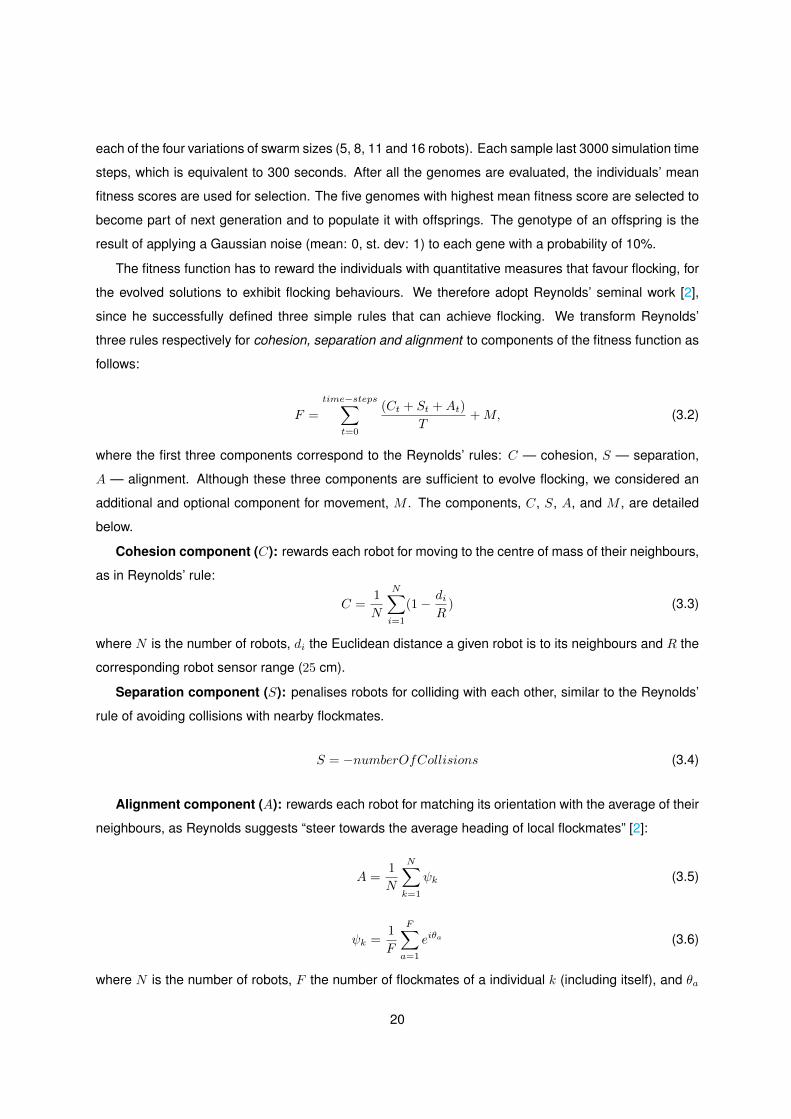
each of the four variations of swarm sizes (5, 8, 11 and 16 robots). Each sample last 3000 simulation time

steps, which is equivalent to 300 seconds. After all the genomes are evaluated, the individuals’ mean

fitness scores are used for selection. The five genomes with highest mean fitness score are selected to

become part of next generation and to populate it with offsprings. The genotype of an offspring is the

result of applying a Gaussian noise (mean: 0, st. dev: 1) to each gene with a probability of 10%.

The fitness function has to reward the individuals with quantitative measures that favour flocking, for

the evolved solutions to exhibit flocking behaviours. We therefore adopt Reynolds’ seminal work [2],

since he successfully defined three simple rules that can achieve flocking. We transform Reynolds’

three rules respectively for cohesion, separation and alignment to components of the fitness function as

follows:

F =

time−steps∑t=0

(Ct + St +At)

T+M, (3.2)

where the first three components correspond to the Reynolds’ rules: C — cohesion, S — separation,

A — alignment. Although these three components are sufficient to evolve flocking, we considered an

additional and optional component for movement, M . The components, C, S, A, and M , are detailed

below.

Cohesion component (C): rewards each robot for moving to the centre of mass of their neighbours,

as in Reynolds’ rule:

C =1

N

N∑i=1

(1− diR) (3.3)

where N is the number of robots, di the Euclidean distance a given robot is to its neighbours and R the

corresponding robot sensor range (25 cm).

Separation component (S): penalises robots for colliding with each other, similar to the Reynolds’

rule of avoiding collisions with nearby flockmates.

S = −numberOfCollisions (3.4)

Alignment component (A): rewards each robot for matching its orientation with the average of their

neighbours, as Reynolds suggests “steer towards the average heading of local flockmates” [2]:

A =1

N

N∑k=1

ψk (3.5)

ψk =1

F

F∑a=1

eiθa (3.6)

where N is the number of robots, F the number of flockmates of a individual k (including itself), and θa

20

is the orientation of the corresponding flockmate a. This term first computes the average orientation of

each robot with its nearby neighbours, similar to the formula of the order metric (see Section Metrics).

Each individual can gain a reward between [0, 1], having a value of 1 when the neighbourhood has a

common direction, and a value of 0 when there is no alignment (or no neighbours). Then, A is computed

as the mean score of all these individual rewards.

The above components only reward the swarm for cohesion and alignment. Thus, when conducting

our initial set of experiments, flocking did emerge, but around the robot’s initial positions, since the fitness

has no reward for moving farther away. Therefore, we consider an additional and optional component

for movement, M , that promotes the swarm to move away from the initial positions:

M =

{d/D d ≤ D1 otherwise

(3.7)

where D is a parameterised distance that the swarm should move (5 m) and d the actual distance the

robots moved, in average. When d > D, M is set to a value of 1, thereby M is defined in [0, 1]. Rather

than just promoting the robots to go farther, this term could as well be adapted to enable flocking for a

specific task, such as area coverage or foraging.

3.4 Metrics

Flocking behaviour is usually defined as an aggregate and polarised motion [5], where individuals move

together in a common direction. Thus, in order to evaluate our work, we used metrics that measure the

alignment and cohesion of the swarm, similar to other works in robotics [6,36].

Order: To evaluate the degree of alignment among the individuals, we used the order metric, well

known both in robotics and control theory [6,36,81]:

ψ =1

N·N∑k=1

eiθk (3.8)

where θk is the orientation of individual k. This metric averages the orientation of the N robots, having a

value of 1 when the swarm is aligned, and value of 0 when there is no common direction.

Number of Groups: As to evaluate flock cohesion, we adapted the metric number of group sug-

gested by Ferrente in [36]. Ferrante defined this metric as the number of groups at the end of the

experiment. To define what constitutes a group, Ferrante used equivalences classes {x ∈ N | x ∼ a},

being N the set of all robots, a an element of the set, and ∼ is the neighbourhood equivalence rela-

tion. More concretely, the distances between all pairs of robots are computed, and then, with a given

distance threshold, the subsets of robots that share the same neighbourhood are found, making each

different subset a new equivalence class. For instance, robot A and B are neighbours if their distance is

21

smaller than the defined threshold, and if B is also neighbour of C, this results in an equivalence class

constituted by robots A, B and C. In the end, the total number of of groups is equal to the number of

equivalence classes.

Swarm Cohesion: Evaluating flock cohesion just in terms of group splits can be limiting, given that

it is also important to consider the number of robots in each subgroup. When the swarm splits, it is

preferable that only a few robots leave the main group, than the main group splits into two or more large

subgroups. Considering this, we used an additional metric that computes the proportion of robots that

remain in the main group:

1− NrlN

(3.9)

whereNrl is the number of robots that leave the main group, i.e. the group with the majority of the robots.

3.5 Results and Discussion

A total of 30 evolutionary runs were conducted, each lasting 6000 generations. For the highest-scoring

controller evolved in each run, we conducted a post-evaluation with 400 samples, 100 for each of the

four combinations of number of robots (5, 8, 11 and 16 robots). In this section, we present the results

obtained, and we analyse the performance and behaviours of the evolved solutions according to the

metrics presented in Section Metrics.

3.5.1 Experimental setup inspired by Reynolds’ local rules - Local setup

Figure 3.4(left) shows the fitness trajectories of the 30 evolutionary runs. The highest-scoring con-

troller obtained an average fitness of 2.63 ± 0.11 during post evaluation, as shown by the box-plot in

Fig 3.4(right).

We scored the evolved behaviours according to the metrics presented in Section Metrics to evaluate

the flocking performance, see Fig 3.5. Figure 3.5(left) summarises the performance of the highest-

scoring controller in terms of alignment (the order metric). The results show that the evolved solution

scored a mean value of 0.82± 0.06 during the experiment.

Figure 3.5(centre) shows the performance of the highest-scoring controller in respect to the number

of groups metric. The evolved solution had a mean number of groups of 1.92 ± 0.38 at the end of the

experiment. Thus, the swarm tends to fragment into two or three groups.

We then evaluated the proportion of robots that tend to leave the swarm with the swarm cohesion

metric, shown in Fig3.5(right). The highest-scoring controller achieved a mean value of 0.80 ± 0.05.

Inspecting the results, we observe that, as the evolution progresses, an increasing number of robots

tend to leave the group, leading to a swarm cohesion of 0.75 ± 0.23 in the end of the experiment. This

22

Figure 3.4: Left: Fitness trajectories of the highest-scoring controllers evolved in each evolutionary run. Right:Distribution of the post-evaluation fitness scores achieved by the highest-scoring controller of the 30evolutionary runs conducted. The box-plot summarises results from 400 post-evaluation samples.

means that, when the swarm fragmented, by the end of the experiment, around 25% of the robots have

left the swarm.

Examples of evolved behaviours for the four different configurations of number of robots (5, 8, 11 and

16) can be seen in Fig 3.6. Similar to the quantitative results, we can observe that overall the swarm

is able to align and remain cohesive, but it tends to fragment into local groups. These results can be

explained by the fitness function itself promoting only local cohesion and local alignment, since it was

adapted from the local rules of Reynolds: robots learn to flock, but only with their immediate neighbours.

Since the fitness function inspired by Reynolds’ rules is based on what each individual can perceive

thus emphasises local quantities, we decided to conduct an additional set of experiments in which the

fitness function takes into account the global behaviour rather than only local interactions.

3.5.2 Experimental setup scoring global behaviour - Global setup

In the previous experiment, we observed that scoring local behaviour resulted in local flocks rather than

global coordinated motion. In this section, we reformulate the fitness function so that it is based on

global alignment and global cohesion, changing the alignment and cohesion components as follows:

F g =

time−steps∑t=0

(Cgt + St +Agt )

T+M, (3.10)

23

Figure 3.5: The figure summarises results of the average from the 400 post-evaluation samples of the highest-scoring controller in terms of the metrics presented in Section Metrics. Left: The order metric trajectoryacross the 3000 simulation steps. Centre: box-plot of the distribution of the number of groups metric.Right: The swarm cohesion trajectory across the 3000 simulation steps.

Figure 3.6: Example of the behaviour displayed by the highest-performing controller, with 5, 8, 11 and 16 robots,from left to right. The lines represent the trajectory of the robots.

Alignment component (Ag): scores the orientation of the swarm, promoting a common direction

between all individuals. This term is computed using the same formula of the order metric:

Ag =1

N·N∑k=1

eiθk (3.11)

Cohesion component (Cg): rewards the swarm for keeping together as a group by using the for-

mula:

Cg =1

NumberofGroups(3.12)

where the term NumberofGroups is the same as in Section Metrics. As before, the cohesion component

is defined in [0, 1].

For this new experimental setup, we used the same configuration of runs, generations and post-

evaluation as in the previous setup. When referring to the two setups, they will hereinafter be referred as

24

Local setup: the setup in which the fitness function, F , is based on local application of Reynolds’ rules

(the previous section); and Global setup: the setup in which the fitness function, F g is based on global

application of Reynolds’ rules (this section).

The 30 fitness trajectories of the controllers within the 6000 generation can be seen in Fig 3.7(left).

The highest scoring controller achieved an average fitness of 2.83 ± 0.21 in post-evaluation, as shown

by the box-plot in Fig 3.7(right).

Figure 3.7: Left: Fitness trajectories of the controllers in each of the 6000 generations. Right: Distribution of thepost-evaluation fitness scores achieved by the highest-scoring controller.

Evaluating the performance of the evolved solution, we can observe that the highest-scoring con-

troller outperformed the best one evolved in the Local setup, in respect to all metrics, see Fig 3.8. Re-

garding alignment, the results show that the evolved solution achieved aligned motion, scoring a mean

value of 0.96± 0.08, outperforming the 0.82± 0.06 of the Local setup.

In terms of group splitting, the swarm remains cohesive during the experiments, obtaining a mean

score of 1.19 ± 0.16 number of groups. In the Local setup, the swarm tends to split into two or three

groups, whereas in the Global setup, by scoring global cohesion, the swarm is generally able to remain

a single cohesive group.

As for the swarm cohesion metric, the highest-scoring controller achieved a mean value of 0.96±0.03

during the experiment, and scoring a mean value of 0.89±0.17 in the end of the experiment. Thus, when

the swarm splits, only a small proportion of the robots tends to leave the main group, with only 11% of the

robots leaving the group in the end of the experiment (opposed to the 25% fragmentation displayed by

the highest-scoring controller evolved in the Local setup). Given that our experiments were configured

25

to use 5, 8, 11 and 16 robots, this translates into an average of just 1 to 2 robots leaving the group.

Observing the plot in Fig 3.8(right) with respect to the Global setup, we can also see an interesting

steep increase in the first 500 steps (50 seconds), suggesting that the swarm size somehow increased.

This can be explained by the fact that, in the beginning of the experiment, robots are placed close to each

other, but at random positions, which does not ensure that every robot is seen by its nearest neighbours.

To cope with this, the robots evolved the strategy of moving closely around their initial positions as to find

their neighbours, and only then moving farther away as a single flock (observe Fig 3.9). This can also be

seen in the plot of the order metric, for which the swarm also takes 500 steps to achieve alignment, the

time needed to ensure the group is formed by every robot and that they are all aligned before moving

away from their initial positions.

Figure 3.8: The metrics scores achieved by the highest-scoring controllers of Global setup and the Local setup.Left: the order metric. Centre: the number of groups metric. Right: the swarm cohesion metric.

The results show that the evolved solutions successfully achieved flocking. By adapting the rules of

Reynolds from local interactions to be global behaviour, robots no longer aligned and move according to

their local neighbours, but instead to the all swarm, leading to a synchronised coordinated motion.

Figure 3.9: Example of the behaviour displayed by the highest-performing controller evolved in the Global setup,with 5, 8, 11 and 16 robots, from left to right. Observing the beginning of trajectory, we can see therobots evolved the strategy of moving closely around their initial positions, in order to first form analigned group before moving away.

26

4From Reynolds’ principles to the

evolution of flocking in agents

Contents

4.1 Experimental setup without the Cohesion component - No Cohesion setup . . . . . 28

4.2 Experimental setup without the Alignment component - No Alignment setup . . . . 31

27

After finding that adapting the local rules of Reynolds as global components of a fitness function can

successfully lead to flocking, we then studied if all Reynolds’ principles are necessary to embed in the

fitness function to evolve flocking. We start by formulating the fitness function to no longer contain the

Cohesion component. Then, we conduct experiments without the Alignment component. It should be

noted that the third component, Separation, was not removed from the fitness function unlike the others,

since a penalty for collision is generally required in a fitness function of swarm scenarios. Without a

penalty that promotes obstacle avoidance, when transferring from simulation to real robotic hardware,

robots will collide with each other, damaging their hardware and becoming inoperable in real world tasks.

The sections in this chapter are the following: Section 4.1 reports the experimental setup and results

without the cohesion component; and Section 4.2 without the alignment component.

4.1 Experimental setup without the Cohesion component - No Co-

hesion setup

To study if the global versions of all of Reynolds’ principles are required to emerge flocking, we formu-

lated the fitness function of the Global setup (F g) by starting to remove the cohesion component.

Fnc =

time−steps∑t=0

(Agt + St)

T+M, (4.1)

In this experimental setup, No Cohesion setup, we will conduct the experiments in the same condi-

tions of the Global setup, i.e. the same configuration of runs, generations and post-evaluation.

Figure 4.1(left) shows the fitness trajectories of the 30 controllers within the 6000 generations. And

the distribution of the post-evaluation fitness scores achieved by the highest-scoring controller can be

seen in Fig 4.1(right), showing an average fitness of 1.95± 0.08. Note that the fitness no longer rewards

cohesion, and therefore has a theoretical maximum value of 2 instead of 3 as in the previous setups.

We then evaluated the performance of the highest-score controller and compared with the best one

of the Global setup, as shown in Fig 4.2. Fig 4.2(left) shows that the evolved solution successfully

achieved aligned motion with a mean value of 0.97±0.07, achieving in the Global setup a relatively lower

score of 0.96± 0.08.

Although the solution had a high performance in respect to alignment, it failed to achieve cohesion,

as shown by the remain metrics. Regarding the metric Number of Groups, we see in Fig 4.2(centre) that

the swarm tends to fragment into two and three groups. The highest-scoring controller scored a mean

number of groups of 2.03± 0.34 at the end of the experiment, hence not being able to remain cohesive,

unlike the best one of the Global setup that achieved a mean value of 1.19± 0.16.

As for the swarm cohesion metric, results show that a high number of robots tend to leave the

28

Figure 4.1: Left: Fitness trajectories of the 30 controllers within 6000 generations. Right: The box-plot summarisesresults from 400 post-evaluation samples achieved by the highest-scoring controller of the No Cohesionsetup

swarm, as seen in Fig 4.2(right). During the experiment, the evolve solution only achieved a mean value

of 0.77± 0.12, and scoring a mean value of 0.60± 0.23 in the end of the experiment. Thereby, the swarm

displays 40% fragmentation by the end of the experiment, whereas, in the Global setup, only a small

proportion of 11% robots tended to leave the swarm.

Figure 4.2: The metrics scores achieved by the highest-score controller of the No Cohesion setup and the Globalsetup. Left: The order metric. Centre: the number of groups metric. Right: the swarm cohesion metric.

In the No Cohesion setup, the results show that flocking did not emerge, with the evolved solution

only achieving alignment. Given that the fitness function does not reward cohesion but alignment, it

was expected aligned motion. However, it was not expected to achieve such high degree of alignment

29

(0.97 ± 0.07 order) with groups splits of two to three groups. How can the robots keep moving aligned

if they are not in the same group? Observing the Fig 4.3, we can see the robots moving in the same

direction, but with distinct groups being next/in front to one another, without seeing each other, but still

moving in the same trajectory. Thus, even thought most robots do not see each other, they still achieve

high degree of alignment since they are all moving in the same way: following a curvilinear trajectory.

Having all robots following a curvilinear trajectory makes it easier for a unseen robot to reunite with

the swarm, whereas with a linear trajectory, a slightly change on the wheels of the unseen robot would

make the robot disperse more and more over time. Observing for instance the figure in the scenario

of 11 robots, we see robots that were separate that afterwards become neighbours again only due to

following the same trajectory: in the last time-steps the robots belonging to the green group join the

swarm again.

Figure 4.3: Example of the behaviour displayed by the highest-performing controller evolved in the No Cohesionsetup, with 5, 8, 11 and 16 robots, from left to right. Different colours represent different groups, beingthe black colour used to represent the main group, i.e, the group with high number of robots.

Naturally, extending the experiment to more time-steps, the solution will eventually have a decrease

degree of alignment, but actually this strategy to move in curvilinear way as shown to be robust to more

time steps, as show in Figure 4.4. The solution remains aligned after twice the 3000 time-steps used

in training, obtaining a mean value of 0.97 ± 0.07 at 6000 time-steps, only becoming in a disorder state

around the 10000 time-steps.

30

Figure 4.4: The figure shows order metric of the post-evaluation samples with an extended number of time-steps,6000 time-steps.

4.2 Experimental setup without the Alignment component - No

Alignment setup

In this setup, No Alignment setup, the fitness function was formulated to no longer contain the Alignment

component, hence the fitness function only rewards the robots for moving as a cohesive group.

Fna =

time−steps∑t=0

(Cgt + St)

T+M, (4.2)

The fitness trajectories of the No Alignment setup can be seen in Fig 4.5(left), with the same number

of runs and generations as used in the previous setups. Figure 4.5(right) summarises the post-evaluation

fitness scores of the highest-scoring controller, achieving a mean fitness of 1.87± 0.15 (note that the fit-

ness no longer rewards alignment, and therefore has a theoretical maximum value of 2 instead of 3).

31

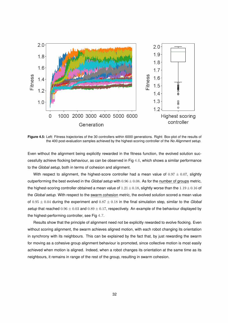
Figure 4.5: Left: Fitness trajectories of the 30 controllers within 6000 generations. Right: Box-plot of the results ofthe 400 post-evaluation samples achieved by the highest-scoring controller of the No Alignment setup.

Even without the alignment being explicitly rewarded in the fitness function, the evolved solution suc-

cessfully achieve flocking behaviour, as can be observed in Fig 4.6, which shows a similar performance

to the Global setup, both in terms of cohesion and alignment.

With respect to alignment, the highest-score controller had a mean value of 0.97 ± 0.07, slightly

outperforming the best evolved in the Global setup with 0.96± 0.08. As for the number of groups metric,

the highest-scoring controller obtained a mean value of 1.21± 0.18, slightly worse than the 1.19± 0.16 of

the Global setup. With respect to the swarm cohesion metric, the evolved solution scored a mean value

of 0.95 ± 0.04 during the experiment and 0.87 ± 0.18 in the final simulation step, similar to the Global

setup that reached 0.96 ± 0.03 and 0.89 ± 0.17, respectively. An example of the behaviour displayed by

the highest-performing controller, see Fig 4.7.

Results show that the principle of alignment need not be explicitly rewarded to evolve flocking. Even

without scoring alignment, the swarm achieves aligned motion, with each robot changing its orientation

in synchrony with its neighbours. This can be explained by the fact that, by just rewarding the swarm

for moving as a cohesive group alignment behaviour is promoted, since collective motion is most easily

achieved when motion is aligned. Indeed, when a robot changes its orientation at the same time as its

neighbours, it remains in range of the rest of the group, resulting in swarm cohesion.

32

Figure 4.6: The metrics scores achieved by the highest-score controller of the No Alignment setup and the Globalsetup. Left: The order metric. Centre: the number of groups metric. Right: the swarm cohesion metric.

Figure 4.7: Example of the behaviour displayed by the highest-performing controller of the No Alignment setup,with 5, 8, 11 and 16 robots, from left to right. The behaviour displayed is similar to one in Fig 3.9.

33

34

5Generalisation

Contents

5.1 Swarm size (N) . . . . . . . . . . . . . . . . . . . . . . . . . . . . . . . . . . . . . . . . . 36

5.2 Time-steps (T) . . . . . . . . . . . . . . . . . . . . . . . . . . . . . . . . . . . . . . . . . 41

35

In previous chapters, we evolved controllers that effectively demonstrate flocking behaviour. In our

experimental setups, we showed that both in Global setup and No Alignment setup the evolved solutions

successfully displayed self-organised flocking. In this section, we assess how general the evolved solu-

tions are. To this end, we conduct additional set of post-evaluation experiments using the highest-scoring

controller of the Global setup and No Alignment setup.

This chapter is divided into 2 sections. In Section 5.1, we study generalisation with respect to swarm

size, and, in section 5.2, regarding the duration of the experiment.

5.1 Swarm size (N)

5.1.1 Swarm size - 5, 8, 11, 16 robots

To study how general the behaviours are in respect to swarm size, we start by evaluating the evolved

behaviours with the four variations of swarm sizes used in the experiments: 5, 8, 11 and 16 robots.

In Figs 5.1, 5.2, 5.3, we present the performance of highest-scoring controller of the Global setup

on the left and the highest-scoring controller of the No Alignment setup on the right, with respect to

the order metric, number of groups and swarm cohesion, respectively. Observing the figures, in both

solutions we see a decrease of flocking performance in all metrics as the number of robots increase.

Figure 5.1: The order metric by the highest-score controller of the Global setup (left) and No Alignment setup(right), with 5, 8, 11 and 16 robots.

36

Figure 5.2: The number of group metric achieved by the highest-score controller of the Global setup (left) and NoAlignment setup (right), with 5, 8, 11 and 16 robots.

Figure 5.3: The swarm cohesion metric achieved by the highest-score controller of the Global setup (left) and NoAlignment setup (right), with 5, 8, 11 and 16 robots.

37

Analysing the performance of the Global setup regarding alignment, Fig 5.1, the highest-scoring

controller scored a mean value of 0.98 ± 0.05, 0.96 ± 0.09, 0.96 ± 0.06 and 0.95 ± 0.09 with 5, 8, 11 and

16 robots, respectively. Results show that the evolved solution obtains similar values for the different

variations of swarm sizes, achieving aligned motion in all. As for the metric number of groups, the

highest-scoring controller obtained 1.08± 1.08, 1.17± 0.38, 1.22± 0.43, 1.29± 0.51 with 5, 8, 11 and 16

robots, respectively. Therefore, for the four different configuration of swarm sizes, the evolved solution

was able to remain in one single cohesive group. Regarding swarm cohesion, during the experiment,

the highest-scoring controller obtained a mean value of 0.98±0.08, 0.95±0.11, 0.95±0.10 and 0.94±0.11

for each of the four swarm size variations mentioned above. As the evolution progresses, more robots

tend to leave the group, leading in the last time-step to a swarm cohesion of 0.91 ± 0.16 with 5 robots

(i.e 9% fragmentation: ≈ 0 robots ), 0.91± 0.16 with 8 robots (9% fragmentation: ≈ 1 robot ), 0.88± 0.16

with 11 robots(12% fragmentation: ≈ 1 robot ), and 0.85 ± 0.18 with 16 robots (15% fragmentation: ≈ 2

robots ). Therefore, just 0 to 2 robots tend to leave the group.

As for the No Alignment setup the highest-scoring controller also achieve alignment motion in the

four variations of swarm size, scoring 0.98 ± 0.07, 0.97 ± 0.06, 0.97 ± 0.08 and 0.96 ± 0.05, respectively.

Regarding the number of groups metric, the highest-scoring controller achieved 1.11± 0.30, 1.18± 0.39,

1.23± 0.52 and 1.32± 0.52 with 5, 8, 11 and 16 robots, respectively. On average, the evolved behaviours

are able to remain as a single group, but note that, comparing with the Global setup, the scores have

more variance. With respect to the proportion of robots that tend to leave the swarm, the swarm cohesion

metric, the solution achieved a mean value of 0.97± 0.09, 0.96± 0.10, 0.95± 0.12 and 0.95± 0.10 during

the experiment for each of the different swarm size configurations. In the end of the experiment, the

highest-scoring controller scored 0.91 ± 0.15 with 5 robots (9% fragmentation: ≈ 0 robots), 0.86 ± 0.20

with 8 robots (14% fragmentation: ≈ 1 robots), 0.89±0.16 with 11 robots (11% fragmentation: ≈ 1 robots),

and 0.81±0.19 with 16 robots (19% fragmentation: ≈ 3 robots). The solution had a lower performance of

swarm cohesion compared with the best one of the Global setup (particularly for the case of 16 robots),

but still only a small percentage of robots tend to leave the group: 0 to 3 robots.

Overall, results show that, even though the performance decreased as the swarm size increased,

both the evolved solutions successfully displayed flocking behaviour in any of the four swarm size varia-

tions.

5.1.2 Swarm size - 20, 30, 50, 100 robots

In the previous section, we assessed the performance of the evolved behaviours in respect to the four

swarm size variations used in the experiments (5, 8, 11 and 16 robots). In this section, we study if

the evolved behaviours are able to scale to a higher number of robots. To this end, we conduct post-

evaluation experiments in which we test with different configurations of swarm sizes than those used

38

in the evolutionary process. Having used in our experiments 5, 8, 11 and 16 robots, which translate

to an average of 10 robots, we decide to test with twice and tree times as many, 20 and 30 robots.

Furthermore, to assess if the evolved behaviours could handle extremely large numbers of robots, we

also test with 50 and 100 robots. So, the highest-scoring controller of the Global setup and No Alignment

setup were tested with 20, 30, 50 and 100, each with 100 post-evaluation samples.

As in the previous section, the figures on this section, Figs 5.4, 5.5, 5.6 , show the performance

of highest-scoring controller of the Global setup on the left and the highest-scoring controller of the

No Alignment setup on the right regarding the order metric, number of groups and swarm cohesion,

respectively. Inspecting all figures, we observe that both solutions did not scale to higher number of

robots, particularly the highest-scoring controller of the No Alignment setup.

Figure 5.4: The order metric achieved by the highest-score controller of the Global setup (left) and No Alignmentsetup (right), with 20, 30, 50 and 100 robots.

Evaluating the flocking performance with respect to the order metric, the solutions only achieved

aligned motion with 20 robots, scoring the highest-scoring controller of the Global setup a mean value

of 0.95 ± 0.06 and the best one of No Alignment setup a mean value of 0.96 ± 0.05. When the number

of robots is increased to 30, 50 and 100 robots, the solutions have difficulty in reaching aligned motion,

as well as on keeping aligned. As seen in Fig 5.4, as the number of robots increase, it takes more time

for the order trajectory to increase, and as the time progresses, the order trajectory starts to decrease.

The highest-scoring controller of the Global setup scored 0.91 ± 0.12 with 30 robots, 0.87 ± 0.13 with

39

Figure 5.5: The number of groups metric achieved by the highest-score controller of the Global setup (left) and NoAlignment setup (right), with 20, 30, 50 and 100 robots.

Figure 5.6: The swarm cohesion metric achieved by the highest-score controller of the Global setup (left) and NoAlignment setup (right), with 20, 30, 50 and 100 robots.

40

50 robots, and 0.79± 0.17 with 100 robots and the highest-scoring controller of the No Alignment setup

scored a mean value of 0.94± 0.08, 0.84± 0.15, 0.68± 0.18, respectively.

As for the number of groups metric, for each test of 20, 30, 50, 100 robots, the highest-score controller

of the Global setup achieved 1.42± 0.61, 1.74± 0.89, 2.08± 1.02, 3.48± 1.73, and the best controller of

the No Alignment setup scored 1.38± 0.63, 1.71± 0.88, 2.91± 1.50, 4.16± 1.82, respectively. As before,

the evolved solutions were only able to scale up to 20 robots.

Finally, regarding the swarm cohesion metric, the highest-scoring controller of the Global scored a

mean value of 0.93±0.11, 0.90±0.13, 0.87±0.13, 0.81±0.14, and the best one of the No Alignment setup

scored 0.94 ± 0.11, 0.91 ± 0.12, 0.82 ± 0.13, 0.83 ± 0.12 with 20, 30, 50 and 100 robots, respectively. In

the end of the experiment, both highest-scoring controllers, the Global and No Alignment setup scored

each: 0.80 ± 0.18 vs. 0.76 ± 0.24 with 20 robots (20% vs. 24% fragmentation: ≈ 4 robots vs. 5 robots),

0.74 ± 0.18 vs. 0.67 ± 0.22 with 30 robots (26% vs. 33% fragmentation: ≈ 8 robots vs. 10 robots),

0.67 ± 0.19 vs. 0.45 ± 0.18 with 50 robots (33% vs. 55% fragmentation: ≈ 17 robots vs. 28 robots), and

0.57± 0.19 vs. 0.51± 0.21 with 100 robots (43% vs. 49% fragmentation: ≈ 43 robots vs. 49 robots). With

the exception of 20 robots, a high proportion of robots tend to leave the group in both solutions.

Results show that the higher the number of robots, the harder is for the evolved solutions to move

as a single, cohesive flock. The solutions were only able to scale to 20 robots, failing to scale to higher

numbers of robots. As future work, we will attempt to promote general and scalable behaviours. For

instance, by conducting experiments that use a (i) higher variability of swam sizes and (ii) higher numbers

of robots. At the time, when designing our experiments, we thought we were promoting general and

scalable behaviours by using 5, 8, 11 and 16 swarm size variations, instead of just using one fix number

of robots. But, on the retrospective, our four variations have small differences of 3 to 5 robots between

each, and we used small swarm sizes. This explains why it was harder for evolved solutions to display

the same behaviour for a bigger numbers of robots.

5.2 Time-steps (T)

In this section, we study if the evolved behaviours can generalise to experiments of longer duration by

conducting post-evaluation experiments with higher number of time-steps. We test the highest-scoring

controller of the Global setup and the highest-scoring controller of the No Alignment setup with 9000

time-steps, which is three times more than the time-steps used in the experiments (3000 time-steps).

Figure 5.7 shows the performance of the evolved solutions in respect to all metrics. Inspecting the

results, we observe that both solutions failed to generalise to higher number of time-steps, having the

highest-scoring controller of the Global setup more difficulty in adapting to more time-steps.

Regarding the order metric, the highest-scoring controller of the Global setup scored 0.90 ± 0.09,

41

Figure 5.7: The metrics scores achieved by the highest-scoring controllers of Global setup and the No Alignmentsetup with 9000 time-steps. Left: the order metric. Centre: the number of groups metric. Right: theswarm cohesion metric.

and the best one of the No Alignment setup achieved 0.93 ± 0.06. Observing Fig 5.7(left), the evolved

behaviours start to misalign after the 3000 time-steps, scoring the highest-scoring controller of the Global

setup and No Alignment setup a mean value of 0.72± 0.23 and 0.85± 0.18, respectively, in the last time-

step. As for the number of groups metric, Fig 5.7(centre), the evolved solution of the Global setup

obtained a mean value of 2.13 ± 0.94 and the best one evolved in the No Alignment setup scored

2.11 ± 0.76. Thus, both solutions failed to remain as one single flock, instead splitting into two to four

groups. Regarding swarm cohesion, the evolved solution of the Global setup achieved a mean value of

0.79 ± 0.15, and the highest-scoring controller of the No Alignment scored 0.80 ± 0.12. As seen in Fig

5.7(right), as the time increases the evolved solutions tend to fragment more and more: the best solution

of Global setup scored, in the end of the experiment, a mean value of 0.53 ± 0.20 (47% fragmentation),

and the best solution of the No Alignment setup scored a mean value of 0.63±0.23 (37% fragmentation).

We conclude that the evolved behaviours were not able to adapt to longer experiments duration.

After the 3000 time-steps, the performance of evolved behaviours start to decrease and continue to

decrease as the time increases. This shows that both solution specialised to the 3000 time-steps of the

evolutionary process. As future work, it would be important to run the experiments with more time-steps

for them to become more robust and general to different duration experiments.

42

6Conclusion

Contents

6.1 Conclusions . . . . . . . . . . . . . . . . . . . . . . . . . . . . . . . . . . . . . . . . . . 44

43

In this chapter, we summarise and discuss the main contributions of our study. Also, we highlight

future work that can follow the study of this dissertation.

6.1 Conclusions

In this dissertation, we demonstrated how controllers can be synthesise to allow for the evolution of

flocking behaviour. Inspired by Reynolds’ flocking rules, we explored simple, explicit fitness functions to

evolve controllers that effectively demonstrate self-organised flocking. We started by adapting Reynolds’

three local behavioural rules to components of the fitness function, which scored separation, cohesion

and alignment in respect to robots’ neighbours. Having the fitness scores based on the individuals’ con-

formity to Reynolds’ rules only resulted in local, fragmented flocking behaviours. We therefore modify

the components of the fitness function so that they consider the entire group of agents simultaneously,

and find that scoring global behaviour lead to global coordinated motion: the evolved solutions success-

fully displayed self-organised flocking. Our results showed that flocking can be evolved by embedding

the rules of Reynolds in a fitness function, with the condition that Reynolds’ local rules become global

instead.

We then conducted additional experiments (i) without scoring cohesion in the fitness function, fol-

lowed by (ii) no longer scoring alignment. The purpose of these experiments was to study if all of

Reynolds’ rules are necessary to evolve flocking. We found that flocking can be achieved without explic-

itly rewarding alignment. Without scoring alignment, the swarm still achieves aligned motion with each

robot moving in synchrony with its neighbours. Although the fitness function only rewards the robots for

moving as a cohesive group, the fitness is itself inherently promoting alignment behaviour, since cohe-

sive motion can be easily achieved when motion is aligned. A robot has less chances to lose sight of

the group if it changes the orientation at the time time as their neighbours.

Furthermore, we assess how general the evolved behaviours were in terms of swarm size and the

duration of the experiment. Results show that the evolved solutions specialised to the time-steps and

swarm sizes used in the evolutionary process. Thus, future work includes designing and configuring

experiments as to consider sufficient number of time-steps, as well as, a higher variability of swam sizes

and higher numbers of robots.

In this dissertation, we have shown that controllers can be evolved to display flocking, a complex

behaviour, with a simple explicit fitness function, contrary to what was claimed in previous work [68].

Our study represented a significant step toward the use of evolutionary techniques to self-organised

flocking. We further believe that represents a step in the evolution of other collective behaviours that

benefit from the same principles of flocking. In our ongoing work, we are studying how to integrate

flocking in the evolution of such behaviours. Having a large number of autonomous robots that can

44

cooperate to move as a single, cohesive group provides great sensing capabilities, which is beneficial for

several real-world-tasks, specially exploratory tasks, such as search and rescue, foraging, patrolling and

environment monitoring. A possible experiment here would involve a scenario of cooperation between

a preprogrammed robot and evolved robots in a navigation task, with the goal of all robots having to go

to a target location. The preprogrammed robot would have the capacity to travel to a specify endpoint,

and the remain robots would need to follow the preprogrammed robot. We could evolve such controllers

by simply using the flocking fitness function presented in this dissertation. Since the fitness rewards

moving as a single cohesive flock, the solutions that do not follow the preprogrammed robot will be

penalised, and, hence, surviving the ones that follow the preprogrammed robot to the target location.

With this, it would not be need to conceive a fitness function that explicitly score the robots to follow the

preprogrammed robots, neither to evolve behaviour that attempts to find the target location.

Another direction that can be taken is the study of evolving flocking for robots with disruptive motion,

such as the jumping locomotion. When the robot motion is disruptive, it is harder to obtain flocking,

since individuals are no longer able to continuously perceive the orientation of their neighbours. Usually,

such challenges are not taking into account in the literature, because it is assumed that robots are

equipped with holonomic motion and large sensor ranges [82]. Using a discrete motion can also be of

increasing complexity in the Evolutionary Robotics field, since discrete actions can make the evolutionary

process harder. Indeed, continuous parameters are usually prefered to discrete ones, due to the fact

that smooth parameters of sensors and actuators tend to lead to small changes in behaviour, thereby

creating a smooth fitness landscape [54, 83, 84]. To the date, and to the best of our knowledge, we

have been the only authors that successfully demonstrated how controllers can be evolved for a robot

capable of jumping [59]. In that study, we only conduct simulation-based experiments using only one

robot capable of jumping, without actually studying large-scale systems of autonomous jumping robots.

Thus, the study of evolving flocking behaviour for robots with jumping locomotion could not only present

novel contributions in the evolution of flocking behaviour, but also could further contribute to the study of

evolving controllers that can take advantage of jumping locomotion.

45

46

Bibliography

[1] B. Partridge, “The effect of school size on the structure and dynamics of minnow schools,” Animal

Behaviour, vol. 28, no. 1, pp. 68–IN3, 1980.

[2] C. Reynolds, “Webpage of craig reynolds. boids: Background and update,” http://www.red3d.com/

cwr/boids/, visited 2019-03-13, 2001.

[3] S. M. Thayer, M. B. Dias, B. Nabbe, B. L. Digney, M. Hebert, and A. Stentz, “Distributed robotic

mapping of extreme environments,” in Mobile Robots XV and Telemanipulator and Telepresence

Technologies VII, vol. 4195. International Society for Optics and Photonics, 2001, pp. 84–96.

[4] M. Dorigo, M. Birattari, and M. Brambilla, “Swarm robotics,” Scholarpedia, vol. 9, no. 1, p. 1463,

2014, revision #138643.

[5] C. W. Reynolds, “Flocks, herds and schools: A distributed behavioral model,” ACM SIGGRAPH

Computer Graphics, vol. 21, no. 4, pp. 25–34, 1987.

[6] A. E. Turgut, H. Celikkanat, F. Gokce, and E. Sahin, “Self-organized flocking in mobile robot

swarms,” Swarm Intelligence, vol. 2, no. 2-4, pp. 97–120, 2008.

[7] T. Vicsek and A. Zafeiris, “Collective motion,” Physics Reports, vol. 517, no. 3, pp. 71–140, 2012.

[8] J. Toner and Y. Tu, “Flocks, herds, and schools: A quantitative theory of flocking,” Physical review

E, vol. 58, no. 4, p. 4828, 1998.

[9] R. Olfati-Saber, “Flocking for multi-agent dynamic systems: Algorithms and theory,” IEEE Transac-

tions on automatic control, vol. 51, no. 3, pp. 401–420, 2006.

[10] S. Nolfi, “Evolutionary robotics: Exploiting the full power of self-organization,” Connection Science,

vol. 10, pp. 167—-184, 1998.

[11] S. Doncieux, J.-B. Mouret, N. Bredeche, and V. Padois, “Evolutionary robotics: Exploring new

horizons,” New horizons in evolutionary robotics, pp. 3–25, 2011.

47

[12] S. J. Gould, The structure of evolutionary theory. Harvard University Press, 2002.

[13] V. Trianni, R. Groß, T. H. Labella, E. Sahin, and M. Dorigo, “Evolving aggregation behaviors in a

swarm of robots,” in European Conference on Artificial Life. Springer, 2003, pp. 865–874.

[14] V. Sperati, V. Trianni, and S. Nolfi, “Evolving coordinated group behaviours through maximisation of

mean mutual information,” Swarm Intelligence, vol. 2, no. 2, pp. 73–95, 2008.

[15] M. Duarte, V. Costa, J. Gomes, T. Rodrigues, F. Silva, S. M. Oliveira, and A. L. Christensen, “Evo-

lution of collective behaviors for a real swarm of aquatic surface robots,” PLoS ONE, vol. 11, no. 3,

p. e0151834, 2016.

[16] G. Baldassarre, S. Nolfi, and D. Parisi, “Evolving mobile robots able to display collective behaviors,”

Artificial Life, vol. 9, no. 3, pp. 255–267, 2003.

[17] R. Groß and M. Dorigo, “Evolution of solitary and group transport behaviors for autonomous robots

capable of self-assembling,” Adaptive Behavior, vol. 16, no. 5, pp. 285–305, 2008.

[18] E. Ferrante, A. E. Turgut, C. Huepe, A. Stranieri, C. Pinciroli, and M. Dorigo, “Self-organized flocking

with a mobile robot swarm: a novel motion control method,” Adaptive Behavior, vol. 20, no. 6, pp.

460–477, 2012.

[19] J. Nembrini, “Minimalist coherent swarming of wireless networked autonomous mobile robots,” Uni-

versity of the West of England, Tech. Rep., 2005.

[20] C. Feare, The starling. Oxford University Press, 1984.

[21] M. Ballerini, N. Cabibbo, R. Candelier, A. Cavagna, E. Cisbani, I. Giardina, A. Orlandi, G. Parisi,

A. Procaccini, M. Viale et al., “Empirical investigation of starling flocks: a benchmark study in

collective animal behaviour,” Animal behaviour, vol. 76, no. 1, pp. 201–215, 2008.

[22] J. Buhl, D. J. Sumpter, I. D. Couzin, J. J. Hale, E. Despland, E. R. Miller, and S. J. Simpson, “From

disorder to order in marching locusts,” Science, vol. 312, no. 5778, pp. 1402–1406, 2006.

[23] P. Symmons and K. Cressman, “Desert locust guidelines: biology and behaviour,” FAO, Rome,

2001.

[24] T. J. Pitcher, “Functions of shoaling behaviour in teleosts,” in The behaviour of teleost fishes.

Springer, 1986, pp. 294–337.

[25] L. Landeau and J. Terborgh, “Oddity and the ‘confusion effect’in predation,” Animal Behaviour,

vol. 34, no. 5, pp. 1372–1380, 1986.

48

[26] H. R. Pulliam, “On the advantages of flocking,” Journal of theoretical Biology, vol. 38, no. 2, pp.

419–422, 1973.

[27] M. A. Elgar, “Predator vigilance and group size in mammals and birds: a critical review of the

empirical evidence,” Biological Reviews, vol. 64, no. 1, pp. 13–33, 1989.

[28] B. L. Partridge, “The structure and function of fish schools,” Scientific american, vol. 246, no. 6, pp.

114–123, 1982.

[29] J. R. Krebs, M. H. MacRoberts, and J. Cullen, “Flocking and feeding in the great tit parus major–an

experimental study,” Ibis, vol. 114, no. 4, pp. 507–530, 1972.

[30] T. Pitcher, A. Magurran, and I. Winfield, “Fish in larger shoals find food faster,” Behavioral Ecology

and Sociobiology, vol. 10, no. 2, pp. 149–151, 1982.

[31] C. H. Ryer and B. L. Olla, “Social mechanisms facilitating exploitation of spatially variable ephemeral

food patches in a pelagic marine fish,” Animal Behaviour, vol. 44, no. 1, pp. 69–74, 1992.

[32] C. Brown and K. N. Laland, “Social learning in fishes: a review,” Fish and fisheries, vol. 4, no. 3, pp.

280–288, 2003.

[33] G. M. Werner and M. G. Dyer, “Evolution of herding behavior in artificial animals,” in From Ani-

mals to Animats 2: Proceedings of the Second International Conference on Simulation of Adaptive

Behavior, vol. 2. MIT Press, 1993, p. 393.

[34] T. Pitcher and B. Partridge, “Fish school density and volume,” Marine Biology, vol. 54, no. 4, pp.

383–394, 1979.

[35] M. Ballerini, N. Cabibbo, R. Candelier, A. Cavagna, E. Cisbani, I. Giardina, V. Lecomte, A. Orlandi,

G. Parisi, A. Procaccini et al., “Interaction ruling animal collective behavior depends on topological

rather than metric distance: Evidence from a field study,” Proceedings of the national academy of

sciences, vol. 105, no. 4, pp. 1232–1237, 2008.

[36] E. Ferrante, “Information transfer in a flocking robot swarm,” Ph.D. dissertation, Ph. D. thesis, Uni-

versite libre de Bruxelles, Brussels, BE, 2013.

[37] E. Sahin, “Swarm robotics: From sources of inspiration to domains of application,” in International

workshop on swarm robotics. Springer, 2004, pp. 10–20.

[38] M. Brambilla, E. Ferrante, M. Birattari, and M. Dorigo, “Swarm robotics: a review from the swarm

engineering perspective,” Swarm Intelligence, vol. 7, no. 1, pp. 1–41, 2013.

49

[39] Y. Mohan and S. Ponnambalam, “An extensive review of research in swarm robotics,” in Nature &

Biologically Inspired Computing, 2009. NaBIC 2009. World Congress on. IEEE, 2009, pp. 140–

145.

[40] E. Bonabeau, A. Sobkowski, G. Theraulaz, J.-L. Deneubourg et al., “Adaptive task allocation in-

spired by a model of division of labor in social insects.” in BCEC, 1997, pp. 36–45.

[41] A. L. Nelson, G. J. Barlow, and L. Doitsidis, “Fitness functions in evolutionary robotics: A survey

and analysis,” Robotics and Autonomous Systems, vol. 57, no. 4, pp. 345–370, 2009.

[42] M. Duarte, S. Oliveira, and A. L. Christensen, “Hierarchical evolution of robotic controllers for com-

plex tasks,” in Development and Learning and Epigenetic Robotics (ICDL), 2012 IEEE International

Conference on. IEEE, 2012, pp. 1–6.

[43] L. P. Kaelbling, M. L. Littman, and A. W. Moore, “Reinforcement learning: A survey,” Journal of

artificial intelligence research, vol. 4, pp. 237–285, 1996.

[44] S. Mahadevan and J. Connell, “Automatic programming of behavior-based robots using reinforce-

ment learning,” Artificial intelligence, vol. 55, no. 2-3, pp. 311–365, 1992.

[45] S. Schaal and C. G. Atkeson, “Robot juggling: implementation of memory-based learning,” IEEE

Control Systems, vol. 14, no. 1, pp. 57–71, 1994.

[46] J. Kober, J. A. Bagnell, and J. Peters, “Reinforcement learning in robotics: A survey,” The Interna-

tional Journal of Robotics Research, vol. 32, no. 11, pp. 1238–1274, 2013.

[47] M. J. Mataric, “Reinforcement learning in the multi-robot domain,” Autonomous Robots, vol. 4, no. 1,

pp. 73–83, 1997.

[48] L. Panait and S. Luke, “Cooperative multi-agent learning: The state of the art,” Autonomous agents

and multi-agent systems, vol. 11, no. 3, pp. 387–434, 2005.

[49] S. Nolfi and D. Floreano, Evolutionary robotics: The biology, intelligence, and technology of self-

organizing machines. MIT press, 2000.

[50] F. Silva, L. Correia, and A. L. Christensen, “Evolutionary Robotics,” Scholarpedia, vol. 11, no. 7, p.

33333, 2016, revision #168217.

[51] R. J. Schalkoff, Artificial neural networks. McGraw-Hill New York, 1997, vol. 1.

[52] I. Basheer and M. Hajmeer, “Artificial neural networks: fundamentals, computing, design, and ap-

plication,” Journal of microbiological methods, vol. 43, no. 1, pp. 3–31, 2000.

[53] C. Darwin et al., “On the origin of species,” 1859.

50

[54] D. Floreano and F. Mondada, “Automatic creation of an autonomous agent: Genetic evolution of a

neural network driven robot,” in Proceedings of the third international conference on Simulation of

adaptive behavior: From Animals to Animats 3, no. LIS-CONF-1994-003. MIT Press, 1994, pp.

421–430.

[55] I. Harvey, P. Husbands, D. Cliff, A. Thompson, and N. Jakobi, “Evolutionary robotics: the sussex

approach,” Robotics and autonomous systems, vol. 20, no. 2-4, pp. 205–224, 1997.

[56] C. Leger, Darwin2K: An evolutionary approach to automated design for robotics. Springer Science

& Business Media, 2012, vol. 574.

[57] H. Lipson and J. B. Pollack, “Automatic design and manufacture of robotic lifeforms,” Nature, vol.

406, no. 6799, pp. 974–978, 2000.

[58] D. Floreano, J.-C. Zufferey, and J.-D. Nicoud, “From wheels to wings with evolutionary spiking cir-

cuits,” Artificial Life, vol. 11, no. 1-2, pp. 121–138, 2005.

[59] R. Ramos, M. Duarte, S. M. Oliveira, and A. L. Christensen, “Evolving controllers for robots with

multimodal locomotion,” in International Conference on Simulation of Adaptive Behavior. Springer,

2016, pp. 340–351.

[60] D. Floreano and F. Mondada, “Evolution of homing navigation in a real mobile robot,” IEEE Transac-

tions on Systems, Man, and Cybernetics, Part B (Cybernetics), vol. 26, no. 3, pp. 396–407, 1996.

[61] F. Silva, M. Duarte, L. Correia, S. M. Oliveira, and A. L. Christensen, “Open issues in evolutionary

robotics,” Evolutionary computation, vol. 24, no. 2, pp. 205–236, 2016.

[62] N. Jakobi, “Evolutionary robotics and the radical envelope-of-noise hypothesis,” Adaptive behavior,

vol. 6, no. 2, pp. 325–368, 1997.

[63] H. Celikkanat and E. Sahin, “Steering self-organized robot flocks through externally guided individ-

uals,” Neural Computing and Applications, vol. 19, no. 6, pp. 849–865, 2010.

[64] G. Vasarhelyi, C. Viragh, G. Somorjai, N. Tarcai, T. Szorenyi, T. Nepusz, and T. Vicsek, “Outdoor

flocking and formation flight with autonomous aerial robots,” in Intelligent Robots and Systems

(IROS 2014), 2014 IEEE/RSJ International Conference on. IEEE, 2014, pp. 3866–3873.

[65] J. Melhuish, “Minimalist coherent swarming of wireless networked autonomous mobile robots,” in

From Animals to Animats: Proceedings of the Seventh International Conference on Simulation of

Adaptive Behavior, vol. 7, 2002, p. 373.

[66] W. M. Spears, D. F. Spears, J. C. Hamann, and R. Heil, “Distributed, physics-based control of

swarms of vehicles,” Autonomous Robots, vol. 17, no. 2, pp. 137–162, 2004.

51

[67] Y. Toshiyuki, S. Nakatani, A. Adachi, M. Kadota, and K. Ohkura, “Adaptive role assignment for self-

organized flocking of a real robotic swarm,” Artificial Life and Robotics, vol. 21, no. 4, pp. 405–410,

2016.

[68] N. Zaera, D. Cliff, and J. Bruten, “(not) evolving collective behaviours in synthetic fish,” in In Proceed-

ings of International Conference on the Simulation of Adaptive Behavior. MIT Press, Cambridge,

MA, 1996, pp. 635–642.

[69] N. Felt and P. Koonce, “Evolving flocking navigation controllers for adaptive swarms,” 2012.

[70] C. R. Ward, F. Gobet, and G. Kendall, “Evolving collective behavior in an artificial ecology,” Artificial

Life, vol. 7, no. 2, pp. 191–209, 2001.

[71] O. Witkowski and T. Ikegami, “Emergence of swarming behavior: foraging agents evolve collective

motion based on signaling,” PLoS ONE, vol. 11, no. 4, p. e0152756, 2016.

[72] H. Kwasnicka, U. Markowska-Kaczmar, and M. Mikosik, “Flocking behaviour in simple ecosystems

as a result of artificial evolution,” Applied Soft Computing, vol. 11, no. 1, pp. 982–990, 2011.

[73] R. S. Olson, A. Hintze, F. C. Dyer, D. B. Knoester, and C. Adami, “Predator confusion is sufficient to

evolve swarming behaviour,” Journal of The Royal Society Interface, vol. 10, no. 85, p. 20130305,

2013.

[74] R. S. Olson, D. B. Knoester, and C. Adami, “Evolution of swarming behavior is shaped by how

predators attack,” Artificial Life, vol. 22, no. 3, pp. 299–318, 2016.

[75] J. Demsar and I. L. Bajec, “Evolution of collective behaviour in an artificial world using linguistic

fuzzy rule-based systems,” PLoS ONE, vol. 12, no. 1, pp. 1–20, 2017.

[76] M. J. Mataric, “Interaction and intelligent behavior.” MASSACHUSETTS INST OF TECH CAM-

BRIDGE ARTIFICIAL INTELLIGENCE LAB, Tech. Rep., 1994.

[77] M. Duarte, F. Silva, T. Rodrigues, S. M. Oliveira, and A. L. Christensen, “Jbotevolver: A versatile

simulation platform for evolutionary robotics,” in Proceedings of the 14th International Conference

on the Synthesis & Simulation of Living Systems. MIT Press, Cambridge, MA, 2014, pp. 210–211.

[78] H. Silva, S. M. Oliveira, and A. L. Christensen, “Conillon: A lightweight distributed computing plat-

form for desktop grids,” in 6th Iberian Conference on Information Systems and Technologies (CISTI

2011). IEEE, 2011, pp. 1–6.

[79] R. P. Ramos, S. Oliveira, and A. L. Christensen, “Code, configuration files and results,” 2019,

accessed: 2019-03-13. [Online]. Available: https://github.com/RitaRamo/flocking-evolver/tree/rita/

JBotRita/experiments

52

[80] R. D. Beer and J. C. Gallagher, “Evolving dynamical neural networks for adaptive behavior,” Adap-

tive behavior, vol. 1, no. 1, pp. 91–122, 1992.

[81] T. Vicsek, A. Czirok, E. Ben-Jacob, I. Cohen, and O. Shochet, “Novel type of phase transition in a

system of self-driven particles,” Physical review letters, vol. 75, no. 6, p. 1226–1229, 1995.

[82] S. Hauert, S. Leven, M. Varga, F. Ruini, A. Cangelosi, J.-C. Zufferey, and D. Floreano, “Reynolds

flocking in reality with fixed-wing robots: communication range vs. maximum turning rate,” in Intelli-

gent Robots and Systems (IROS), 2011 IEEE/RSJ International Conference on. IEEE, 2011, pp.

5015–5020.

[83] J. M. C. Gomes, “Evolution of self-organising behaviours with novelty search,” Ph.D. dissertation,

Faculdade de Ciencias da Universidade de Lisboa, 2012.

[84] M. A. F. Duarte et al., “Engineering evolutionary control for real-world robotic systems,” Ph.D. dis-

sertation, University Institute of Lisbon (ISCTE-IUL), 2016.

53

54