Development of an Obstacle Detection and Avoidance System ...

Development of an Obstacle Detectionand Avoidance System for ROV

Ørjan Grefstad

Marine Technology

Supervisor: Ingrid Schjølberg, IMTCo-supervisor: Ole Alexander Eidsvik, IMT

Vegard Wie Henriksen, IKM Technology

Department of Marine Technology

Submission date: June 2018

Norwegian University of Science and Technology

Project DescriptionSubsea inspection, maintanance and repair (IMR) missions require remotely operated ve-hicles (ROVs). These tasks are traditionally performed manually, but is well suited for au-tomation. The vehicles considered in this project are therefore fully actuated ROVs and/orAUVs. Survey AUVs with torpedo shape and no sway actuation are thus not considered.

This project is part of addressing the main challenge of increasing the level of au-tonomy and robustness for automatic mapping, monitoring and intervention, high-levelplanning/re-planning and reconfiguration of single and multiple vehicles subject to theparticular mission, environmental condition, available energy, communication constraints,and any failure conditions.

This project will consider a Merlin class ROVs, which is a Class 3 work class-ROVwith fully electric propulsion. The vehicle is equipped with a front-facing, single beamsonar that should be used to implement an obstacle detection and avoidance system. Thedeveloped system should be able to give commands to the vehicles autopilot system andprovide a level of safety during automatic operations. IKM Technology facilitates a high-fidelity simulator to aid the development and verification of the proposed motion planningalgorithms prior to full-scale tests.

ScopeThe following subtasks should be addressed:

1. Develop an algorithm for obstacle detection using measurements from a sonar andavailable maps. The sonar is single beam, front facing with 180 degrees viewingangle. Secondary input is two-dimensional map data.

2. Develop a motion-planning algorithm for obstacle avoidance using the developedobstacle detection algorithm.

3. Use the algorithms and design a guidance system that can give commands to anautopilot system. Assume the autopilot is capable of dynamic positioning and pathfollowing of curved paths by providing it waypoints.

4. Implement and verify the guidance system in Matlab/Python.

5. Verify the developed system using the high-fidelity Merlin simulator at Bryne.

6. Verify the developed system in full-scale experiments by implementing the solutioninto the existing guidance and control system.

7. Conclude your results.

Supervisor: Professor Ingrid SchjølbergCo-supervisor: Vegard Wie Henriksen, IKM Technology AS

Abstract

Unmanned underwater vehicles, such as remotely operated vehicles (ROVs) and autonomousunderwater vehicles (AUVs) are commonly used for inspection, maintenance and repair(IMR) missions in the oil and gas industry. This is a cost-driven industry and advances inautonomy is a key factor to reduce the mission expenses.

Collision avoidance is one of the main challenges in the field of AUVs. In this thesis asystem for detecting obstacles and planning a new path around the obstacles is proposed.The system is divided into three modules: an object detection module, a collision avoid-ance module and a guidance module.

The object detection module uses a single-beam mechanically scanning sonar to pop-ulate a probabilistic occupancy grid. The sonar data is related to the probability of occu-pancy through a dynamic inverse-sonar model. The occupancy grid is vehicle-fixed andthus position or velocity data is needed for translating and turning the grid. The translationand rotation is archived using an image processing technique known as affine transforma-tion.

A global occupancy grid has to account for the growth of the positional uncertainty,and thus the accuracy of the map will fall over time. With a local map the obstacles will becorrectly located with respect to the vehicle, which is sufficient for the purpose of collisionavoidance. The obstacles are detected through a contour detection algorithm. The detectedcontours are then expanded to make a safety margin around the obstacles.

The collision avoidance module compares the current path with the detected obstaclesand initiates a path recalculation if they coincide. The path recalculation is done witha combination of Voronoi diagrams and a modified version of Dijkstra’s shortest pathalgorithm. Once a new path is calculated, it is smoothed using Fermat’s spiral and sent tothe guidance system.

The guidance system is a classic line of sight guidance scheme, with a velocity de-pendent lookahead distance. The velocity guidance uses the path curvature as an inputparameter. This enables the guidance system to reduce the commanded velocity whensharp turns are detected.

Several simulations were performed and the complete system was tested on a ROVstationed on the Snorre B oil field. During the field experiments, it was confirmed thata mechanically scanning single-beam sonar is sufficient as the only sensor for detectingand avoiding obstacles in an underwater environment. The technology is also applicableto AUVs as the calculated paths have a continuous curvature.

Regarding further developments of this system, it is suggested to look into other guid-ance schemes, such as trajectory tracking. The object detection system would benefit fromintroducing additional sensors, such as cameras for detection of close obstacles.

i

Sammendrag

Ubemannede undervannsfarkoster, som fjernstyrte kjøretøyer (ROVer) og autonome un-dervannsfarkoster (AUV), brukes ofte til inspeksjon, vedlikehold og reparasjon (IMR) op-erasjoner i oljesektoren. Dette er en kostnadsdrevet industri, og fremskritt i autonomi eren sentral faktor for a redusere kostander forbundet med IMR operasjoner.

Kollisjonsunngaelse er en av hovedutfordringene innen AUV-feltet. I denne oppgavener det foreslatt et system for a oppdage hindringer og planlegge en ny bane rundt hindrin-gene. Systemet er delt inn i tre moduler: en modul for a oppdage objekter, en for a oppdagekollisjoner og planlegge en ny bane og en navigasjonsmodul.

Modulen for objektoppdagelse bruker en sonar med en mekanisk roterende strale.Disse dataene blir sa brukt for a beregene sannsynligheten for at celler i et rutenett haren hindring i seg. Sonardataene er relatert til sannsynligheten i rutenettet gjennom en dy-namisk omvendt sonarmodell. Rutenettet er festet til kjøretøyet, og dermed er det behovfor posisjon- eller hastighetsdata for a flytte og rotere rutenettet. Dette gjøres ved hjelp aven bildebehandlingsteknikk kalt affin transformasjon.

Et globalt rutenett er nødt til a ta hensyn til posisjonsusikkerheten, og dermed vilnøyaktigheten falle over tid. Med et lokalt rutenett er hindringene være riktig plasserti forhold til kjøretøyet, noe som er tilstrekkelig for a en unnga en kollisjon. Objekteneoppdages gjennom en konturdeteksjonsalgoritme. Konturene blir deretter ekspandert fora lage en sikkerhetsmargin rundt dem.

Modulen for kollisjonsunngaelse sammenligner den naværende banen med de kjentehindringene og setter i gang beregningen av en ny bane, hvis det er fare for kollision.Denne beregningen er gjennomført med en kombinasjon av Voronoi-diagrammer og enmodifisert versjon av Dijkstras algoritme for a finne korteste rute. Nar en ny bane erberegnet, blir den glattet med Fermats spiral og sendt til navigasjonssystemet.

Navigasjonssystemet er et klassisk siktelinjesystem (LOS) med en hastighetsavhengigsynsavstand. Hastighetsveiledningen bruker banekurvaturen som en inngangsparameter.Dette gjør det mulig for Navigasjonssystemet a redusere hastigheten nar skarpe svingeroppdages.

Flere simuleringer ble kjørt og hele systemet ble testet pa en ROV stasjonert pa SnorreB platformen. Ved hjelp av disse testene ble det bekreftet at en sonar med en mekaniskroterende strale er tilstrekkelig som den eneste sensoren for a oppdage og unnga hindringeri et undervannsomrade. Teknologien virker ogsa for AUVer fordi de beregnede banene haren kontinuerlig krumning.

For videre forskning og utvikling av dette systemet anbefales det a undersøke andrenavigasjonssystemer, slik som banesporing. Det vil være hensiktsmessig a inkludere fleresensorer i modulen for objektdeteksjon, for eksempel et kamera slik at det blir letterea oppdage hindringer pa nært hold.

iii

Preface

This thesis is the product of my work during the spring semester of 2018 at the Departmentof Marine Technology, Norwegian University of Science and Technology (NTNU). Thework is based on the results of the project thesis from the fall semester of 2017. The workhas been carried out under the supervision and guidance of Professor Ingrid Schjølbergand in cooperation with IKM Technology.

I would like to thank Professor Ingrid Schjølberg for interesting discussions and valuablehelp on the thesis. I would also like to express gratitude to Vegard Wie Henriksen, ØyvindLøberg Aakre and Vidar Eriksen at IKM Technology for input and help during the fieldexperiment and implementation of the system. In addition, I would like to thank IKMSubsea for the ability to perform field experiments and their ROV pilots for their help inflying the ROV and interpreting sonar images.

Ørjan GrefstadTrondheim, June 25, 2018

v

Table of Contents

Abstract i

Sammendrag iii

Preface v

Table of Contents x

List of Tables xi

List of Figures xiv

Abbreviations xv

1 Introduction 11.1 Background and Motivation . . . . . . . . . . . . . . . . . . . . . . . . 11.2 Scope . . . . . . . . . . . . . . . . . . . . . . . . . . . . . . . . . . . . 21.3 Contributions and Thesis Outline . . . . . . . . . . . . . . . . . . . . . . 2

2 Background 52.1 Spatial Mapping Using Occupancy grids . . . . . . . . . . . . . . . . . . 5

2.1.1 Occupancy Grids . . . . . . . . . . . . . . . . . . . . . . . . . . 52.1.2 Inverse sensor model . . . . . . . . . . . . . . . . . . . . . . . . 62.1.3 Forward sensor model . . . . . . . . . . . . . . . . . . . . . . . 6

2.2 Image Processing . . . . . . . . . . . . . . . . . . . . . . . . . . . . . . 72.2.1 Image representation . . . . . . . . . . . . . . . . . . . . . . . . 72.2.2 Histogram . . . . . . . . . . . . . . . . . . . . . . . . . . . . . . 72.2.3 Thresholding . . . . . . . . . . . . . . . . . . . . . . . . . . . . 82.2.4 Dilation . . . . . . . . . . . . . . . . . . . . . . . . . . . . . . . 82.2.5 Contour detection . . . . . . . . . . . . . . . . . . . . . . . . . . 92.2.6 Affine Transformation . . . . . . . . . . . . . . . . . . . . . . . 10

2.3 Voronoi Diagrams . . . . . . . . . . . . . . . . . . . . . . . . . . . . . . 11

vii

2.4 Dijkstra’s Algorithm . . . . . . . . . . . . . . . . . . . . . . . . . . . . 122.5 Fermat’s Spiral . . . . . . . . . . . . . . . . . . . . . . . . . . . . . . . 122.6 Coordinate Systems . . . . . . . . . . . . . . . . . . . . . . . . . . . . . 12

2.6.1 World Geodetic System - 1984 . . . . . . . . . . . . . . . . . . . 122.6.2 Universal Transverse Mercator . . . . . . . . . . . . . . . . . . . 132.6.3 Body-fixed reference frame . . . . . . . . . . . . . . . . . . . . 13

2.7 Translation between reference frames . . . . . . . . . . . . . . . . . . . 132.8 Guidance and Control . . . . . . . . . . . . . . . . . . . . . . . . . . . . 14

2.8.1 Line-Of-Sight Guidance . . . . . . . . . . . . . . . . . . . . . . 142.8.2 PID-controller . . . . . . . . . . . . . . . . . . . . . . . . . . . 152.8.3 Reference Models . . . . . . . . . . . . . . . . . . . . . . . . . 15

2.9 Software frameworks . . . . . . . . . . . . . . . . . . . . . . . . . . . . 152.9.1 Python . . . . . . . . . . . . . . . . . . . . . . . . . . . . . . . 152.9.2 OpenCV . . . . . . . . . . . . . . . . . . . . . . . . . . . . . . 162.9.3 Software for field test . . . . . . . . . . . . . . . . . . . . . . . . 162.9.4 Software for Simulation . . . . . . . . . . . . . . . . . . . . . . 17

3 Underwater Acoustics 193.1 Acoustics . . . . . . . . . . . . . . . . . . . . . . . . . . . . . . . . . . 19

3.1.1 Sound attenuation . . . . . . . . . . . . . . . . . . . . . . . . . 203.1.2 Sea surface and seafloor interaction losses . . . . . . . . . . . . . 203.1.3 Ambient Noise . . . . . . . . . . . . . . . . . . . . . . . . . . . 203.1.4 Reverberation . . . . . . . . . . . . . . . . . . . . . . . . . . . . 203.1.5 Target strengths . . . . . . . . . . . . . . . . . . . . . . . . . . . 213.1.6 Doppler Effect . . . . . . . . . . . . . . . . . . . . . . . . . . . 21

3.2 Sonar equation . . . . . . . . . . . . . . . . . . . . . . . . . . . . . . . 223.3 Measurement and discretization . . . . . . . . . . . . . . . . . . . . . . 22

3.3.1 Statistical Detection Theory . . . . . . . . . . . . . . . . . . . . 233.4 Types of Sonar . . . . . . . . . . . . . . . . . . . . . . . . . . . . . . . 23

3.4.1 Single Beam Sonars . . . . . . . . . . . . . . . . . . . . . . . . 243.4.2 Multibeam Sonars . . . . . . . . . . . . . . . . . . . . . . . . . 243.4.3 Compressed High-Intensity Radar Pulse . . . . . . . . . . . . . . 24

3.5 Other Applications for Underwater Acoustics . . . . . . . . . . . . . . . 243.5.1 Communication . . . . . . . . . . . . . . . . . . . . . . . . . . . 243.5.2 Localization . . . . . . . . . . . . . . . . . . . . . . . . . . . . . 25

4 Collision Avoidance 274.1 Object detection . . . . . . . . . . . . . . . . . . . . . . . . . . . . . . . 29

4.1.1 Occupancy Grid . . . . . . . . . . . . . . . . . . . . . . . . . . 294.1.2 Measurement model . . . . . . . . . . . . . . . . . . . . . . . . 294.1.3 Motion . . . . . . . . . . . . . . . . . . . . . . . . . . . . . . . 324.1.4 From occupancy grid to obstacles . . . . . . . . . . . . . . . . . 33

4.2 Collision Detection . . . . . . . . . . . . . . . . . . . . . . . . . . . . . 364.3 Path planning . . . . . . . . . . . . . . . . . . . . . . . . . . . . . . . . 36

4.3.1 Voronoi Diagrams . . . . . . . . . . . . . . . . . . . . . . . . . 374.3.2 Dijkstra’s algorithm . . . . . . . . . . . . . . . . . . . . . . . . 38

viii

4.3.3 Removal of unnecessary waypoints . . . . . . . . . . . . . . . . 384.3.4 Fermat Spirals . . . . . . . . . . . . . . . . . . . . . . . . . . . 394.3.5 Conversion between coordinate systems . . . . . . . . . . . . . . 39

4.4 Guidance and Control . . . . . . . . . . . . . . . . . . . . . . . . . . . . 41

5 Experimental setup 435.1 Simulation with MORSE . . . . . . . . . . . . . . . . . . . . . . . . . . 435.2 Simulation with Merlin Simulator . . . . . . . . . . . . . . . . . . . . . 445.3 Field Experiments . . . . . . . . . . . . . . . . . . . . . . . . . . . . . . 44

5.3.1 Equipment . . . . . . . . . . . . . . . . . . . . . . . . . . . . . 455.4 Computer . . . . . . . . . . . . . . . . . . . . . . . . . . . . . . . . . . 47

6 Simulation Results 496.1 Object Detection . . . . . . . . . . . . . . . . . . . . . . . . . . . . . . 516.2 Guidance System . . . . . . . . . . . . . . . . . . . . . . . . . . . . . . 516.3 Collision Avoidance . . . . . . . . . . . . . . . . . . . . . . . . . . . . . 556.4 Merlin Simulation . . . . . . . . . . . . . . . . . . . . . . . . . . . . . . 57

7 Full-Scale Experiments 597.1 Object detection . . . . . . . . . . . . . . . . . . . . . . . . . . . . . . . 617.2 Guidance System . . . . . . . . . . . . . . . . . . . . . . . . . . . . . . 637.3 Collision Avoidance . . . . . . . . . . . . . . . . . . . . . . . . . . . . . 67

8 Discussion 738.1 Object Detection . . . . . . . . . . . . . . . . . . . . . . . . . . . . . . 738.2 Guidance System . . . . . . . . . . . . . . . . . . . . . . . . . . . . . . 758.3 Collision Avoidance . . . . . . . . . . . . . . . . . . . . . . . . . . . . . 768.4 Performance . . . . . . . . . . . . . . . . . . . . . . . . . . . . . . . . . 77

9 Conclusions and Further Work 799.1 Conclusion . . . . . . . . . . . . . . . . . . . . . . . . . . . . . . . . . 799.2 Further Work . . . . . . . . . . . . . . . . . . . . . . . . . . . . . . . . 80

9.2.1 Object Detection . . . . . . . . . . . . . . . . . . . . . . . . . . 809.2.2 Guidance System . . . . . . . . . . . . . . . . . . . . . . . . . . 809.2.3 Collision Avoidance . . . . . . . . . . . . . . . . . . . . . . . . 809.2.4 Simulations . . . . . . . . . . . . . . . . . . . . . . . . . . . . . 81

Bibliography 83

Appendix 87

A Abstract for Paper Contribution to 2018 IEEE OES Autonomous UnderwaterVehicle Symposium 89

B Complete results for a selection of field trials 93B.1 Complete results for collision avoidance test at May 15th, 15:39 . . . . . 93B.2 Revised results for collision avoidance test at May 15th, 15:39 . . . . . . 101

ix

C List of Electronic Attachments 109C.1 Attachments delivered in DAIM . . . . . . . . . . . . . . . . . . . . . . 109C.2 Source code . . . . . . . . . . . . . . . . . . . . . . . . . . . . . . . . . 109

x

List of Tables

2.1 Comparison between different contour approximations. . . . . . . . . . . 9

4.1 Possible collision avoidance statuses, and their corresponding response inthe guidance system . . . . . . . . . . . . . . . . . . . . . . . . . . . . . 42

5.1 Key properties of Tritech SuperSeaking DST Sonar[38] . . . . . . . . . . 46

7.1 Key parameters for all field-tests. . . . . . . . . . . . . . . . . . . . . . . 61

8.1 Mean runtime for collision avoidance algorithm, with different contourapproximations. . . . . . . . . . . . . . . . . . . . . . . . . . . . . . . . 77

xi

List of Figures

2.1 Example of the histogram from raw data plot. . . . . . . . . . . . . . . . 82.2 Example of image dilation. . . . . . . . . . . . . . . . . . . . . . . . . . 92.3 Example of different contour approximations. . . . . . . . . . . . . . . . 102.4 Example of Voronoi diagram . . . . . . . . . . . . . . . . . . . . . . . . 112.5 A screen-shot of the IKM Autopilot Server. . . . . . . . . . . . . . . . . 17

4.1 Flowchart of the object detection and collision avoidance process. . . . . 284.2 Three different methods for finding the return echoes over a certain threshold. 304.2 Three different methods for finding the return echoes over a certain thresh-

old (cont.). . . . . . . . . . . . . . . . . . . . . . . . . . . . . . . . . . . 314.3 Overlap between grid cells and sonar-cone and angles used in the genera-

tion of lookup-tables. . . . . . . . . . . . . . . . . . . . . . . . . . . . . 324.4 Object detection procedure. . . . . . . . . . . . . . . . . . . . . . . . . . 344.4 Object detection procedure (cont.). . . . . . . . . . . . . . . . . . . . . . 354.5 Voronoi diagram and path calculation. . . . . . . . . . . . . . . . . . . . 374.6 Relationship between the n-, veh- and g-reference-frames. . . . . . . . . 414.7 A smooth path and the original waypoints are to the right. The velocity

profile and curvature of the path is to the left. . . . . . . . . . . . . . . . 42

5.1 Close up screenshot of the ROV used in the MORSE simulations. . . . . 435.2 Screenshot from the simulated environment in IKM’s simulator. . . . . . 445.3 Location of the Snorre field[33]. . . . . . . . . . . . . . . . . . . . . . . 445.4 3D model of Merlin UCV, with the location of the sonar highlighted. Cour-

tesy of IKM Technology. . . . . . . . . . . . . . . . . . . . . . . . . . . 455.5 Picture from the control-room at IKM Subsea’s headquarters at Bryne.

Courtesy of IKM Subsea. . . . . . . . . . . . . . . . . . . . . . . . . . . 465.6 Communication with ROV. . . . . . . . . . . . . . . . . . . . . . . . . . 47

6.1 Map of the simulated environment used during the MORSE-simulations.The objects are numbered. . . . . . . . . . . . . . . . . . . . . . . . . . 50

6.2 Screenshot from the simulated environment used during the MORSE-simulations. 50

xiii

6.3 Results from simulated object detection trial. The detected obstacles arelogged every 10 seconds and plotted as transparent polygons. . . . . . . . 51

6.4 North-east plot of the path of the ROV during simulated guidance systemtrial. The ROAs are plotted at each waypoint. . . . . . . . . . . . . . . . 52

6.5 Plot of the heading, the reference signal and setpoint of the heading, duringsimulated trial of the guidance system. . . . . . . . . . . . . . . . . . . . 53

6.6 Plot of the difference between the heading and the reference signal of theheading, during simulated trial of the guidance system. . . . . . . . . . . 53

6.7 Plot of the cross-track error during simulated trial of the guidance system. 546.8 Plot of the surge velocity of the ROV during simulated trial of the guidance

system. The plot also shows the reference signal and the setpoint. . . . . . 546.9 First path re-calculation during simulated trial of the complete collision

avoidance system. . . . . . . . . . . . . . . . . . . . . . . . . . . . . . . 556.10 Second path re-calculation during simulated trial of the complete collision

avoidance system. . . . . . . . . . . . . . . . . . . . . . . . . . . . . . . 566.11 Last path re-calculation during simulated trial of the complete collision

avoidance system. . . . . . . . . . . . . . . . . . . . . . . . . . . . . . . 57

7.1 Map of the subsea area of the Snorre B field. . . . . . . . . . . . . . . . . 607.2 Detected objects and position of the ROV on a round-trip from the garage

around module C and D. . . . . . . . . . . . . . . . . . . . . . . . . . . 627.3 Closer look at the view in Fig. 7.2. . . . . . . . . . . . . . . . . . . . . . 637.4 North-East plot of flight-path. The numbers indicate when a new waypoint

is selected. . . . . . . . . . . . . . . . . . . . . . . . . . . . . . . . . . . 647.5 Close-up look at the first part of the path in Fig. 7.4. . . . . . . . . . . . . 647.6 Plot of heading, heading reference and desired heading for the flight-path

from Fig. 7.4. The numbers indicate when a new waypoint is selected. . . 657.7 Plot of surge velocity, surge velocity reference and desired surge veloc-

ity for the flight-path from Fig. 7.4. The numbers indicate when a newwaypoint is selected. . . . . . . . . . . . . . . . . . . . . . . . . . . . . 66

7.8 Plot of cross-track error for the flight-path from Fig. 7.4. The numbersindicate when a new waypoint is selected. . . . . . . . . . . . . . . . . . 67

7.9 Excerpt from test of the collision avoidance system. . . . . . . . . . . . . 687.10 Excerpt from test of the collision avoidance system. . . . . . . . . . . . . 697.11 Excerpt from test of the collision avoidance system. . . . . . . . . . . . . 707.12 Excerpt from test of the collision avoidance system. . . . . . . . . . . . . 71

8.1 ROV with sonar cone and blind-spot at an altitude of two meters. . . . . . 748.2 Example of a path following a concave structure, with a convex contour

approximation and the Teh-Chin contour approximation. . . . . . . . . . 78

xiv

Abbreviations

UCV = Ultra Compact VehicleROV = Remotely Operated VehicleAUV = Autonomous Underwater VehicleUID = Underwater Intervention DroneDOF = Degree of FreedomIMU = Inertial Measurement UnitDST = Digital Sonar TechnologyUDP = User Datagram ProtocolIP = Internet ProtocolRGB = Red-Green-BlueMORSE = Modular Open Robots Simulation EngineMOOS = Mission Oriented Operating SuiteGUI = Graphical User InterfaceGPU = Graphical Processing UnitIMR = Inspection, Maintenance and RepairSNR = Signal to Noise RatioCHIRP = Compressed High Intensity Radar PulseEM = ElectromagneticLBL = Long Base LineSBL = Short Base LineUSBL = Ultra Short Base LineLOS = Line-of-sightINS = Inertial Navigation SystemWGS84 = World Geodetic System - 1984WP = WaypointVD = Voronoi DiagramROA = Region of Acceptance

xv

Chapter 1Introduction

1.1 Background and MotivationUnmanned underwater vehicles, such as remotely operated vehicles (ROVs) and autonomousunderwater vehicles (AUVs) are commonly used for inspection, maintenance and repair(IMR) missions in the oil and gas industry. This is a cost-driven industry and advances inautomation is a key factor to reduce the mission expenses.

ROVs are underwater robots connected to the surface or an underwater hub throughan umbilical transferring power and information. Due to the supply of power from thesurface, ROVs can normally carry large payloads and tools, such as robotic arms, multiplecameras and powerful lights. ROVs are normally fully actuated, meaning that it can becontrolled in all degrees of freedom (DOFs).

AUVs are not directly connected to the surface, and thus the power supply is limited.Communication with the surface is possible through acoustic transmissions, but the datarate is limited. In contrast to ROVs, AUVs are normally underactuated, which limits thehover capabilities.

The industry-driven innovation is currently moving towards resident underwater inter-vention drones (UIDs) [16], where the goal is to have vehicles with the intervention po-tential of an ROV with the freedom of an UAV. This is a way of greatly reducing costs, asthe need for costly surface intervention vessels is removed. A resident and tetherless UIDcan also service several subsea production areas as it can move freely between dockingstations. The need for such innovation is expressed in Equinor’s (former Statoil) devel-opment schedule for the next 4-7 year period [16], where they plan to install a pilot forautonomous UIDs that can fly between docking stations. This goal introduces the need forinnovation in several areas such as power, communication and autonomy systems.

The National Research Council [6] defines an autonomous vehicle as an ”unmannedvehicle with some level of autonomy built in”, which includes vehicles such as UAVs andUIDs, but also less autonomous vehicles such as ROVs. The National Research Council[6] also defines four levels of autonomy, where the highest level of autonomy describesa system where all mission-related functions are executed automatically. Several other

1

Chapter 1. Introduction

descriptions of an autonomous system exist in the literature, but the main point is that thesystem should be able to sense, plan and act on its own. The ability to sense, plan and actintroduces the possibility of performing complex tasks without human intervention.

Collision avoidance is one of the main challenges in the field of autonomous underwa-ter operations. This challenge is often solved using multibeam sonars, in a simultaneouslocalization and mapping (SLAM) approach as done by Palomer et al. [30] or with imagerecognition based techniques such as the method proposed by Braginsky and Guterman[2]. To accommodate these methods a multibeam sonar is needed. Multibeam sonars havesuperior performance for obstacle detection as they scan a large sector in one scan. Thesuperior performance does however come at a price, the cost is significantly higher, thephysical size is larger and the power consumption is higher. These factors is a concernwhen UIDs are shifted towards battery power, which requires smaller vehicles to reducepower usage. However; a single beam sonar does not scan the entire sector in front of thevehicle at once, which complicates the object detection process. This has been done withoccupancy grids by authors such as Ganesan et al. [13] and with a potential field methodby authors such as Solari et al. [32].

1.2 ScopeThe objective of this thesis can be formulated on the basis of the challenges presented inthe previous section. In order to perform safe autonomous ROV operations, the followingtasks should be performed.

1. Perform a literature study on underwater object detection, sonar theory and collisionavoidance.

2. Propose and develop a set of algorithms to perform collision detection and avoid-ance.

3. Verify the developed system in simulations using the MORSE simulator.

4. Implement and verify a guidance system, using the high-fidelity Merlin simulator atIKM’s headquarters at Bryne.

5. Perform preliminary field tests of the collision avoidance system using the residentMerlin UCV at the Snorre B oil field.

1.3 Contributions and Thesis OutlineThe contribution of the thesis is a collision avoidance system combining the theory of oc-cupancy grids for single-beam sonar object detection and Voronoi diagrams for the plan-ning of a new path. The work in this thesis resulted in a contribution to 2018 IEEE OESAutonomous Underwater Vehicle Symposium, and the preliminary abstract is presented inthe appendix. The outline of the thesis is as follows:

2

1.3 Contributions and Thesis Outline

In Chapter 2 the background theory necessary for the developed algorithms are presentedtogether with a short literature study regarding occupancy grids, Voronoi Diagrams andFermat’s spiral is presented. The chapter also includes a presentation of the softwareframeworks used in the thesis.

In Chapter 3 a study of underwater acoustics, with a special focus on relevant theory forsingle-beam sonars are presented.

In Chapter 4 the developed system is presented. The chapter describes the object detectionmodule, the collision avoidance module and the guidance module. The main contributionsof the thesis are presented in this chapter.

In Chapter 5 the experimental setup for the MORSE simulations, the Merlin simulatorsimulations and the field trials are presented.

In Chapter 6 the results from the simulations are presented.

In Chapter 7 the results from the field trials at the Snorre B oil field are presented.

In Chapter 8 the results from Ch. 7 and Ch. 8 are discussed.

In Chapter 9 a conclusion is formulated and suggestions for further work in the subjectare presented.

In Appendix A the preliminary abstract of a contribution to the 2018 IEEE OES Au-tonomous Underwater Vehicle Symposium is presented.

In Appendix B additional results from the field trials are presented.

Appendix C lists the electronic attachments delivered in DAIM.

3

Chapter 1. Introduction

4

Chapter 2Background

In this chapter previous work in the field of underwater collision avoidance will be pre-sented. Then the necessary background theory for the developed collision avoidance sys-tem will be presented. The last section is a short introduction of the software used inthe thesis. In this chapter previous work in the field of underwater collision avoidanceand the necessary background theory for the developed collision avoidance system willbe presented. Finally, section 2.9 presents a short introduction of the software used in thethesis.

2.1 Spatial Mapping Using Occupancy grids

An occupancy grid is a powerful tool for a robot moving in an unknown environment. Itcan be used as a basis for obstacle detection, collision avoidance and simultaneous local-ization and mapping(SLAM). The first occupancy grids were developed in the early 90’sby Elfes [8]. Since then it has become the dominant solution for environment modeling formobile robots. An occupancy grid is a spatial representation of the robot’s surroundings.It is most common to divide the grid into a set of equally spaced quadratic cells, but it isalso possible to use a polar occupancy grid. The occupancy grid map can be given eitheras a set of probabilities of occupancy or as a binary set of occupied or empty cells.

2.1.1 Occupancy Grids

In this section, the mathematics behind the occupancy grid is described. Most of theinformation in this section is based on Elfes [8] and Thrun [37].

An occupancy grid is a mapping of the environment into grid cells. Each grid cellcontains an estimate of the probability of occupancy. In addition, each grid cell can alsocontain a binary occupied or not occupied value. To make the estimation problem lesscomplex the high-dimensional problem is decomposed into a set of binary problems, onefor each cell.

5

Chapter 2. Background

The state of one cell with index (x, y) can either be occupied, mx,y or not occupied,mx,y . The occupancy grid mapping problem can then be formulated as the probability ofeach cell being occupied given the measurements, as stated in Eq. (2.1) [37].

p(m|Zt) = p(m|zt, zt−1, . . . , z0) (2.1)

where zt is the range measurement at time instant t, and Zt is all the range measurementsup to time t. These measurements also might include the pose of the vehicle as well asthe sonar heading, beam-width and other relevant parameters. These measurements haveinformation about all the grid cells overlapping the sonar beam up to the measurementdistance. The formulation in Eq. (2.1) is hard to compute, due to the interdependence ofthe cells and can be simplified by making two basic assumptions [37]:

• Static world assumption: The past sensor readings are conditionally independent,given knowledge of the map.

• Cell independence assumption: Different grid cells are conditionally independent,given knowledge of the individual cell.

Using these assumptions together with Bayes’ theorem the recursive equation for updatinggrid cells can be written on a log-odds form [37]

ltx,y = logp(mx,y|zt)

1− p(mx,y|zt)+ log

p(mx,y)

1− p(mx,y)+ lt−1x,y (2.2)

where ltx,y is the log-odds of a grid cell at time t. This equation consists of two parts,the prior p(mx,y) which depends on the expected obstacle density in the environmentand p(mx,y|zt) which is the probability that there is an obstacle given the current sensormeasurement. This probability is called the inverse sensor model.

2.1.2 Inverse sensor modelThe probability p(mx,y|zt) is the probability of the grid cell being occupied given thesensor measurement zt. In other words, this is a mapping from the measurement to thecause. Elfes [8] used a probability density function depending on the range and angle,where both parameters were modeled as Gaussian uncertainties. This model was laterextended by Konolige [21] to include multiple targets and specular reflections.

The inverse sensor model was extended by Zhou et al. [44], which uses a dynamicinverse-sensor model based on the sonar equation where the probabilities are adjusted forthe incident angle. The incident angle is calculated by using linear regression on all cellsabove a certain threshold to find the face of the obstacle, and subsequently computing theangle between the sonar beam and the face of the obstacle.

2.1.3 Forward sensor modelThe mapping from measurement to cause in the inverse sensor model is the opposite ofhow the measurement process is done. Thrun [37] introduced a method for Occupancy grid

6

2.2 Image Processing

mapping with a forward sensor model. The forward sensor model computes the probabilityof getting the measurement given the obstacle, p(Zt|m).

This method creates more accurate maps, but due to computationally expensive op-timization algorithms, the method is not capable of running in real time. The greatestdifference between the forward and inverse sensor model is that the forward model doesnot have to assume independence of cells.

Shvets et al. [31] extended the method by using a gradient descent optimization method,and claim that it is capable of running in real time, but no such experiments have yet beencarried out.


Several different image processing techniques were used throughout the thesis. This sec-tion describes these techniques and how a digital image is represented.

2.2.1 Image representation

In a computer, an image is represented as a series of bytes. Some common image repre-sentations are:

• Grey-scale image where each pixel is represented by an unsigned byte, with aninteger value between 0 and 255.

• Red-green-blue (RGB) image where each pixel are represented by 3 bytes, one foreach color. This is the most common for color-images.

• Blue-green-red (BGR) image. This uses the same structure as RGB images, but withthe colors switched. This is the format used by OpenCV.

With a higher level interface, such as in Python, the images are represented as a matrixMh×w×c, where h is the height of the image, w is the width of the image and c is thenumber of colors. With this matrix structure, the coordinate system of an image has they-axis flipped as opposed to the normal Cartesian coordinate system.

2.2.2 Histogram

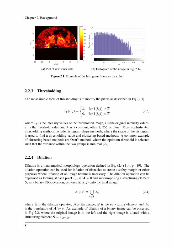
Histograms are used for images as a way for quantifying the distribution of pixel intensi-ties. An example of a gray-scale histogram for a plot of raw sonar data can be observed inFig. 2.1b. Histograms can be used for applications such as identifying the correct thresh-old value. In this thesis, histograms were used to identify a good threshold value for thesonar signals.

7


-30 -20 -10 0 10 20 30

x [m]

20

10

0

-10

y [m

]

0

20

40

60

80

100

120

140

160

180

(a) Plot of raw sonar data.

100

101

102

103

104

105

Nu

mb

er

of

pix

els

0 50 100 150 200 250

Bin

(b) Histogram of the image in Fig. 2.1a.

Figure 2.1: Example of the histogram from raw data plot.

2.2.3 Thresholding

The most simple form of thresholding is to modify the pixels as described in Eq. (2.3).

IT (i, j) =

k, for I(i, j) ≥ T0, for I(i, j) < T

(2.3)

where IT is the intensity values of the thresholded image, I is the original intensity values,T is the threshold value and k is a constant, often 1, 255 or True. More sophisticatedthresholding methods include histogram-shape methods, where the shape of the histogramis used to find a thresholding value and clustering-based methods. A common exampleof clustering based methods are Otsu’s method, where the optimum threshold is selectedsuch that the variance within the two groups is minimal [29].

2.2.4 Dilation

Dilation is a mathematical morphology operation defined in Eq. (2.4) [14, p. 19]. Thedilation operation can be used for inflation of obstacles to create a safety margin or otherpurposes where inflation of an image feature is necessary. The dilation operation can beexplained as looking at each pixel ai,j ∈ A 6= 0 and superimposing a structuring elementS, as a binary OR-operation, centered at (i, j) onto the final image.

A⊕ S ≡⋃s∈S

As (2.4)

where ⊕ is the dilation operator, A is the image, S is the structuring element and As

is the translation of A by s. An example of dilation of a binary image can be observedin Fig 2.2, where the original image is to the left and the right image is dilated with astructuring element S = 120×20.

8


(a) Original image. 200×200pixels

(b) Dilated image. S =120×20

Figure 2.2: Example of image dilation.

2.2.5 Contour detection

A contour is a continuous curve around the boundary of an object, where the object is nor-mally defined by the image intensity. A contour detection algorithm can efficiently trans-form the pixel information to geometrical shapes, which are useful for a collision avoid-ance algorithm. Computer vision tools, such as OpenCV usually use a border following-algorithm developed by Suzuki and Be [34] to detect the contours. This algorithm worksbest on binary images, and thus thresholding has to be performed first. The result of run-ning the algorithm on an image will be the set of every border point of each contour. Thiscan consume a lot of memory and thus it is common to approximate the contours withfewer points. A simple way to do this is to remove all points on a straight line, except theendpoints. A more accurate representation can be archived by using Teh and Chin [35]’salgorithm for detecting dominant points on a closed curve. To further reduce the numberof points the contours can be approximated as different shapes, such as rectangles, ellipsesor a convex shape. In Fig. 2.3 an example of the different contour approximation methodscan be observed, and in Tab. 2.1 an overview of the number of points is shown.

Approximation method Number of points

No approximation 1203Simple approximation 156Teh-Chin approximation 82Convex approximation 14

Table 2.1: Number of approximation points for different contour approximations for the shapeshown in Fig. 2.3.

9


Figure 2.3: Example of different contour approximations.

2.2.6 Affine Transformation

An affine transformation is a map between two affine spaces, where collinearities are pre-served [40]. Affine transformations are commonly used for many different purposes inimage manipulation. Some examples are scaling, reflection, rotation and translation ofimages. The transformation is done by multiplying the transformation matrix, M with theposition of each pixel in the image, to get a new position as shown in Eq. (2.5) [40]. Whenevery pixel has a new position, an interpolation algorithm has to be applied as the newpositions are not necessarily in a position that fit the integer requirements of an image.A common interpolation method for images is a bicubic interpolation, but other methods,such as a nearest-neighbour interpolation or a linear interpolation can also be used.

T = MP = M[x, y, 1

]T(2.5)

10

2.3 Voronoi Diagrams

where T =[x′, y′

]Tis the vector of transformed xy-coordinates. Some common trans-

formation matrices are shown in Eq. (2.6).

M rotation =

[cos θ sin θ 0− sin θ cos θ 0

], P =

[x− x0, y − y0, 1

](2.6)

M translation =

[1 0 ∆x0 1 ∆y

](2.7)

M translation =

[s 0 00 s 0

](2.8)

where (x0, y0) is the point to rotate around, (∆x,∆y) is the translation and s is a scalefactor.

2.3 Voronoi DiagramsA Voronoi diagram is a method of dividing a plane, X into regions based on the distanceto a set of finite points. These points are called generator points, P = p1, ..., p2. Ametric function d(x, pi) associates each point x ∈ X into a region, Ri such that themetric function for all points in the region is less than or equal to the metric function forall other regions. This can be expressed mathematically as in Eq. (2.9) [23].

Ri = x ∈X|d(x, pi) ≤ d(x, pj) ∀i 6= j (2.9)

A common candidate for the metric function is the Euclidean distance, as expressed inEq. (2.10).

d(x, pi) = |x− pi| =√

(xx − pix)2

+(xy − piy

)2(2.10)

From this, a set of lines, vi ∈ V can be chosen as the the borders of the regions Ri. UsingEq. (2.10) as the metric function will result in the set V being connected by a set E ofstraight edges.

0 20 40 60 80 100 120 140 160 180 2000

20

40

60

80

100

120

140

160

180

200

Voronoi edges

Voronoi vertices

Generator points

Figure 2.4: Example of Voronoi diagram, showing the generator points, the vertices and the edges.

11


2.4 Dijkstra’s AlgorithmDijkstra’s algorithm is an algorithm used for finding the shortest path between nodes ina graph. It was first developed by Dijkstra [7], but further developments made by Fred-man and Tarjan [12] drastically reduced the runtime of the algorithm from O(|V |2) toO(|E| + |V | log |V |), where V is the number of nodes and E is the number of edges.The algorithm visits all nodes in the graph uniformly and finds the shortest paths betweenthem. A more common variation of the algorithm finds the shortest path between a sourceand sink node.

Yen [43] made a variation of the algorithm that can be used to find the k-shortest path,meaning the second shortest path, the third shortest path and the k-shortest path. Thisalgorithm is the basis for a modification made by Lekkas [23]. This algorithm uses theoptimal path from the previous run, but once a node is invalid due to clearance constraintsall connections to this node are removed. A new path is then constructed from the previousnode to the goal node. The final path will then be constructed of the initial path up to, butnot containing the invalid node and the new path to the goal node.

2.5 Fermat’s SpiralA path consisting of straight line segments is possible to follow with a fully actuated ROV,but due to the curvature discontinuous nature of such a curve, a full stop would be requiredat each waypoint. A better solution would be to modify the path such that the curvatureis continuous and as small as possible. A solution to this is presented by Lekkas [23],where Fermat’s spiral is used to make a continuous curvature path. Fermat’s spiral is ageometrical curve which can be described in Cartesian coordinates as done by Lekkas[23]: [

xy

]=

[x0 + a

√θ cos (ρθ + χ0)

y0 + a√θ sin (ρθ + χ0)

](2.11)

where a is a scaling factor, ρ = 1,−1 is the turning direction and χ0 is the initial tan-gent angle. The formulation of Fermat’s spiral in Eq. (2.11) can then be used to jointwo straight line path segments in a continuous curvature path consisting of two mirroredcurves [23]. A continuous path is not suitable for a waypoint based guidance system, andthus a discretization should be performed.

2.6 Coordinate SystemsIn this thesis, several different reference frames and coordinate systems are in use. Adescription of these reference frames is presented in this section.

2.6.1 World Geodetic System - 1984The World Geodetic System (WGS84) is a geodetic reference system centered at theEarth’s center of mass [27]. This is the reference system used by Global Positioning

12

2.7 Translation between reference frames

System (GPS), and the position is provided as a latitude and longitude.

2.6.2 Universal Transverse MercatorThe Universal Transverse Mercator (UTM) projection is a 2-dimensional coordinate sys-tem. The projection is divided into 60 different zones [20]. A position consists of nor-thing, easting and a grid zone. It is also possible to specify a vertical position. In thisthesis all coordinates given in UTM-coordinates are in zone 32 North, which covers mostof the southern part of Norway, and the offshore-areas. The UTM system can be used as aNorth-East-Down (NED) coordinate system, denoted n.

2.6.3 Body-fixed reference frameA body-fixed reference frame is a moving coordinate frame that is fixed to the body. Inthis thesis two different body-fixed reference frames are used. The vehicle reference frameis denoted with veh subscript and has units meters. The axis are defined, by Fossen [9] as:

• xveh - Longitudinal axis, from aft to fore

• yveh - Transverse axis from port to starboard

• zveh - Normal axis from top to bottom

The grid reference frame is a two-dimensional body-fixed reference frame used for the oc-cupancy grid and is denoted with a g subscript. This reference frame has no units. The ori-gin of g is located at the upper left corner of the grid, which has a position (xveh, yveh) =(rscale,−rscale) with rscale being the sonar range. The horizontal x-axis is from left toright and the vertical y-axis is from top to bottom. An example of this coordinate systemcan be seen in Fig. 4.6.

2.7 Translation between reference framesThe transformation of velocities between the vehicle-fixed reference frame and the NED-frame is done by using the rotation matrix Rn

veh(Θnb), as described by Fossen [9, p. 22].Assuming stability and small angles in pitch and roll, the rotation matrix can be reducedto Rn

veh(ψ), which is shown in Eq. (2.12).

Rnveh(ψ) =

cos(ψ) − sin(ψ) 0sin(ψ) cos(ψ) 0

0 0 1

(2.12)

The transformations between veh and n, and back are then

vveh = Rnveh(ψ)vn (2.13)

vn = (Rnveh(ψ))

Tvveh (2.14)

The conversion between the latitude and longitude in the WGS84 reference frame to NEDin UTM coordinates can be done by tools such as the Helmert 7 point transformation,described in [27]. The transformation uses a set of 7 parameters to do the transformation.

13


2.8 Guidance and Control

The guidance system of a vehicle is a system that translates high-level objectives to set-points for the control system. A typical guidance system will decide the heading neededto get the vehicle to converge on a path, or keep the vehicle in a stable position.

2.8.1 Line-Of-Sight Guidance

Line-of-Sight (LOS) guidance is a 3-point guidance scheme, which is commonly used forpath following of straight-line paths. The idea behind this guidance scheme is to force thevehicle to track the path. This is done by constructing a vector from the vehicle, to eitherthe next waypoint on the path or to a point on the line between two waypoints. The desiredheading angle can then be calculated from the LOS-vector. The following definitions arebased on Fossen [9, Ch. 10.3].

The first step is to calculate the cross-track error, e(t) and the along-track distance,s(t) as shown in Eq. (2.15).

ε(t) =[s(t), e(t)

]T= Rp(αk)T (pn(t)− pn

k ) (2.15)

where Rp is the rotation matrix, defined in Eq. (2.16) from the path-frame to the NED-frame of reference, αk is the angle between the line segment and the north-axis, defined inEq. (2.17), pn(t) is the vehicle position and pn

k is the LOS-point.

Rp(αk) ≡[cos(αk) − sin(αk)sin(αk) cos(αk)

](2.16)

αk = arctan

(yk+1 − ykxk+1 − xk

)(2.17)

where the waypoints are defined as WPk = (Nk, Ek) = (xk, yk). The desired course-angle can then be calculated as

χd(e) = χp + χr(e) = αk + arctan

(−e(t)∆(t)

)(2.18)

where ∆(t) is a look-ahead-distance which could be fixed or time-varying. A switchingmechanism is needed, such that a new waypoint can be selected once the vehicle is closeenough. This is normally done by the use of a region-of-acceptance (ROA). The ROA canbe understood as a circle enclosing the waypoint, and the switch to the next waypoint willhappen when the vehicle enters this circle. The ROA is defined in Eq. (2.19).

|pn(t)− pnk | = |ε(t)| ≤ ROAk (2.19)

To achieve the motion control objective a velocity-guidance law is needed as well. Thislaw can be fixed velocity or it can be a time-varying velocity depending on for examplethe curvature.

14

2.9 Software frameworks

2.8.2 PID-controllerA PID-controller is a commonly used control-loop consisting of the different terms: pro-portional (P), integral (I) and derivative (D). These three terms is efficient and easy wayof controlling a dynamic system. The P-term handles the error, the I-term takes careof steady-state offset and the D-term prevents rapid change. Mathematically the PID-controller can be formulated as in Eq. (2.20). The error is defined as x(t) = x(t)− xd(t),where x is the state to be controlled and xd(t) is the desired state. The control objective isthen to force x(t) to zero.

τ = Kpx+Kddx

dt+

∫ t

0

xdt (2.20)

where τ is the control-action and Kp,Kd,Ki are tunable gains. All the terms are notnecessary for every application. For a heading controller, it is normally sufficient witha PD-controller and the surge-velocity can normally be handled with PI-controller. Acontroller does not normally handle big steps in the desired state well, and thus a smoothreference signal is often needed.

2.8.3 Reference ModelsA reference model is a method for creating a smooth trajectory for the controller. Thisis helpful for avoiding steps, which in the worst case can make a controller unstable. Acommon way of designing a reference model is a low-pass filter. Another solution is touse a mass-damper-spring system, which is convenient for marine vehicles, according toFossen [9]. The transfer-function for such a system is given as

h(s) =ω2n

s2 + 2ζωns+ ω2n

(2.21)

where ωn is the natural frequency and ζ is the relative damping ratio. ωn and ζ are tunablevariables, which should be as close as possible to the real signal.

2.9 Software frameworksIn this section, a brief overview of the different software frameworks used in this projectis presented. All of the software mentioned in this section is open-source if not statedotherwise.

2.9.1 PythonPython is a high-level programming language, well suited for rapid prototyping. It has anextensive standard library, which makes code development effective.

The NumPy library is an open-source library for mathematics. It has good support formatrices and vectors. One of the main advantages of NumPy is that the core functions ofthe library are written as compiled C/C++ code, which makes it computationally effective.

15


The SciPy library is an extensive library for mathematics and scientific programming.It has support for making Voronoi diagrams, using Dijkstra’s algorithm and a variety ofinterpolation algorithms.

The pyProj wrapper for PROJ.4 is a library for performing cartographic transforma-tions and geodetic computations [41]. This is a useful library for transforming betweenlatitude and longitude in the WGS84 system to UTM-coordinates.

PyQt is a Python interface to the Qt framework for Graphical User Interface(GUI)programming. This is a useful and powerful tool to easily make a cross-platform GUI forPython code.

PyQtGraph is an extension to PyQt which makes plotting and displaying/images easierand faster.

2.9.2 OpenCV

The OpenCv library is a software library for computer vision and machine learning. Thelibrary is written in C++, but has interfaces for multiple languages across several platforms[28]. In this thesis the main use is for it’s contour and drawing features

2.9.3 Software for field test

IKM Autopilot Server

The IKM Autopilot Server(APS) software is a proprietary guidance and control softwarefor IKM’s ROVs. The software runs on the onshore control rack, and communicates withthe ROV over a network connection. The APS can operate in five different modes, whichare listed below[1]:

• Dynamic Positioning

• Semi Automatic Mode

• Circular Inspection Mode

• Path following of predefined paths

• Cruise mode for external path following algorithms

In this thesis Dynamic Positioning and Cruise Mode(CM) are the only modes necessary.The CM accepts desired trajectories in surge, sway, heave and yaw, which is then filteredthrough a reference model. The APS reads position data from an INS onboard the ROV,and uses this data to calculate the control action. The communication interface to theAPS is a binary data protocol, which uses UDP-messages as means of transportation. Ascreen-shot of the APS is shown in Fig. 2.5

16

2.9 Software frameworks

Figure 2.5: A screen-shot of the IKM Autopilot Server.

2.9.4 Software for Simulation

Modular Open Robots Simulation Engine

MORSE (Modular Open Robots Simulation Engine) is an open source python based robotsimulator [22]. The simulator integrates Blender game engine for 3D rendering and editingand the Bullet Physics Library for rigid-body physics simulations. MORSE is written inpython which makes it easy to modify and extend the simulator. MORSE also integratesseveral middle-wares, such as MOOS and ROS. Through these middle-wares, MORSE canboth send and receive messages in an easy manner.

Blender

Blender is an open source software suite for 3D modelling and rendering. In MORSE, theBlender game engine is used to render the environment and robots, as well as providinginput to several sensors, such as the sonar.

Bullet Physics Library

Bullet Physics Library is physics engine used by blender for simulation rigid-body dynam-ics and collisions.

17


Mission Oriented Operating Suite

MOOS (Mission Oriented Operating Suite) is an open source software package, whosemain goal is to provide infrastructure for autonomous marine vehicles. In this sectionMOOSDB and pyMOOS will be the main focus, as these are the only parts of the MOOSpackage used in this thesis. The MOOS communication network’s core is the MOOSDBapplication [26]. This is a server application that handles all the MOOS messages in thenetwork. In this communications network, all applications can send and receive messagesto and from the server, but not to each other. The messages have to follow a strict format,which is handled by the python interface to MOOS, pyMOOS. pyMOOS is capable ofsending and receiving messages as well as handling message queues and executing call-back functions when a message is received.

18

Chapter 3Underwater Acoustics

This section presents a description of sonar theory. A short section is also dedicated toother uses of underwater acoustics. Most of this information is based on Hodges [17].

Sonars can be divided into two main groups, namely active and passive sonars. In thissection, only active sonars will be discussed, as passive sonars do not have much of anapplication for collision avoidance. In an active sonar system sound waves are emittedfrom a transmitter/projector. These sound waves propagate through the medium and arereflected by a target. The reflected sound waves will then propagate back to a hydrophone,which is the receiver. A common name to use for transmitters and hydrophones is a trans-ducer, and in most systems, they are the same unit. In the following text, transducer willbe used when they are the same unit, and hydrophone/transmitter will be used when theyare separate.

3.1 Acoustics

Acoustic waves can move through a medium as longitudinal and transverse waves. Dueto the lack of shear strength in water, only transverse waves are possible. The relationshipbetween the velocity and frequency is given in Eq. (3.1).

c = λf (3.1)

where λ is the wavelength, f is the frequency and c is the speed of sound through water.The speed of sound through water depends on several different parameters, where the mostimportant are temperature, salinity and depth.

During the signal’s travel from the transducer to the target, and back it is distorted andweakened by different factors, such as sound attenuation, ambient noise, reverberation,which will be discussed below.

19

Chapter 3. Underwater Acoustics

3.1.1 Sound attenuationThe term sound attenuation includes losses caused by surfaces absorbing sound and trans-forming it into heat energy, as well as well as losses caused by the interaction with thesurface and seafloor. The sound that is absorbed by the ocean itself is mainly caused bytwo factors: the excitation of ions from magnesium sulfate, boric acid and carbonate andthe viscosity of the water [17, p. 92-92]. The most common equation for calculating thesound attenuation is given by Thorp [36] as

α = 1.09

(0.1

f2

1 + f2+ 40

f2

4100 + f2

)(3.2)

where α is the intensity absorption coefficient given in dB/km and the frequency is givenin kHz. A more thorough calculation, that also includes temperature, salinity, viscosity,depth, pH, and pressure is given by Francois and Garrison [10, 11].

3.1.2 Sea surface and seafloor interaction lossesThe interaction with the sea surface causes losses that are heavily dependent on the seastate and are deemed outside the scope of the thesis as ROVs on IMR missions mostlyoperate well below the wave interaction depth.

The sound also interacts with the seafloor, which is typically not a solid object, andthus absorbs much energy. The energy absorption is heavily dependent on the type of thesea floor.

3.1.3 Ambient NoiseThe dominant source of ambient noise is from thrusters and engines [4, p. 380-381], bothfrom close and far-away surface vessel. According to Christ and Wernli Sr. [4] the ambientnoise from surface vessels is approximately 40 dB stronger than other sources. Some othersources are listed below.

• Seismic background noise

• Turbulent pressure fluctuations

• Surface waves

• Second order pressure effects

• Marine life

3.1.4 ReverberationThe transmitted sound can return from several different sources than the target. Thesereturning sound waves are called reverberation and can originate from inhomogeneities inthe water, air bubbles, marine life, seafloor and sea surface. Reverberation is often the

20

3.1 Acoustics

dominant source of noise for high-frequency sonars [17, p. 143]. The level of reverbera-tion, Rl can according to Hodges [17, p. 153-154] be calculated as

Rl = 10 log

(I0r4Ss

∫Bt (θ, φ)Br (θ, φ) dA

)(3.3)

Where Bt and Br are the beam patterns of the transmitter and receiver, depending onthe horizontal angle, θ and the vertical angle φ. The range of the sonar is r, and thetransmission power is I0. Ss is the backscattering strength, which is determined by thesurface type and incident angle. This strength can vary from −45dB for soft ground to−25dB for solid ground. The strength will also increase with the frequency for smoothsurfaces.

3.1.5 Target strengths

The target strength refers to the targets ability to return an echo. According to [17, p. 167]the target strength is defined as

Nts = 10 log

(IrIi

)(3.4)

where Ir is the reflected sound intensity at a 1 meter distance and Ii is the incident acousticintensity. The target strength is heavily dependent on the geometry and reflective proper-ties of the target.

3.1.6 Doppler Effect

The Doppler effect is the change in frequency when there is a relative velocity betweenthe observer and the source[17, p. 9-10]. If the source and observer are moving away fromeach other the frequency will be reduced, and if they are moving towards each other thefrequency will increase. This relationship is given by Hodges [17, p. 9] as

fr = fsc− vrc− vs

(3.5)

where fr is the observed frequency, fs is the source frequency, c is the sound velocity andvr and vs is the velocity of the observer and source. In the ocean, this can be approximatedby

∆f ≈ 3.5 ∗ 10−4fs∆v (3.6)

where ∆f is the change in frequency and ∆v is the relative velocity in knots.For a ROV with a typical operational velocity of 1.5 knots and a sonar frequency of

625 kHz the resulting frequency shift is 0.35 kHz, which is negligible. For an AUV with anoperational velocity of 5 knots and a sonar frequency of 625 kHz the resulting frequencyshift will be over 1 kHz, which should be considered by a digital sonar system.

21


3.2 Sonar equation

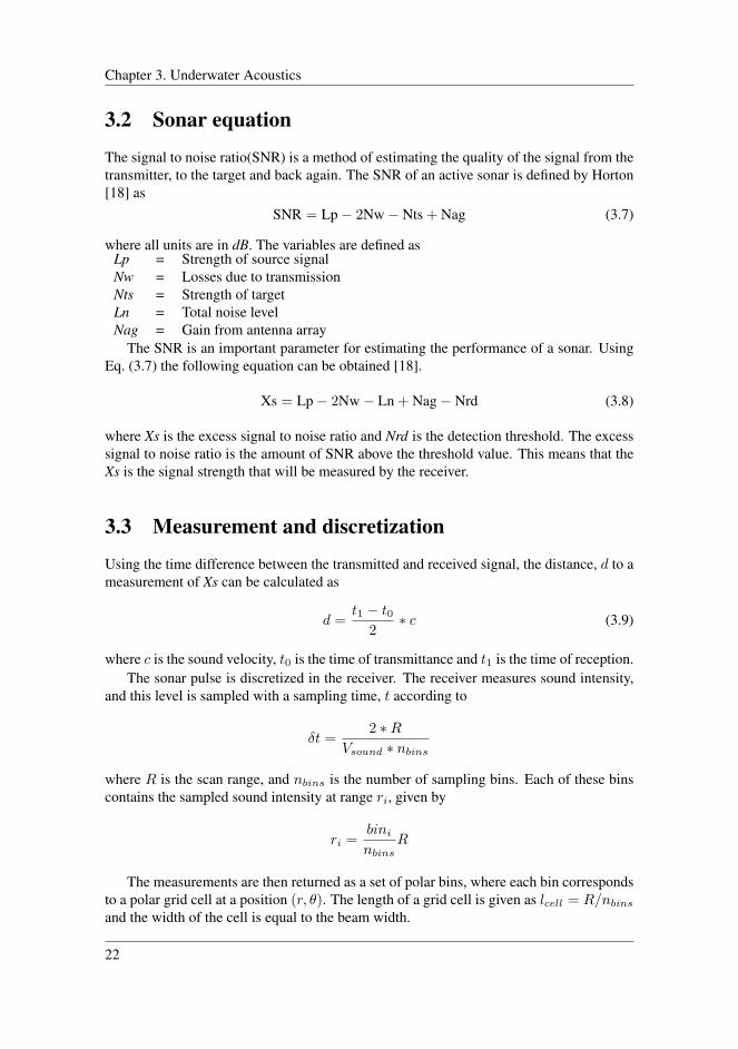
The signal to noise ratio(SNR) is a method of estimating the quality of the signal from thetransmitter, to the target and back again. The SNR of an active sonar is defined by Horton[18] as

SNR = Lp− 2Nw− Nts + Nag (3.7)

where all units are in dB. The variables are defined asLp = Strength of source signalNw = Losses due to transmissionNts = Strength of targetLn = Total noise levelNag = Gain from antenna array

The SNR is an important parameter for estimating the performance of a sonar. UsingEq. (3.7) the following equation can be obtained [18].

Xs = Lp− 2Nw− Ln + Nag− Nrd (3.8)

where Xs is the excess signal to noise ratio and Nrd is the detection threshold. The excesssignal to noise ratio is the amount of SNR above the threshold value. This means that theXs is the signal strength that will be measured by the receiver.

3.3 Measurement and discretization

Using the time difference between the transmitted and received signal, the distance, d to ameasurement of Xs can be calculated as

d =t1 − t0

2∗ c (3.9)

where c is the sound velocity, t0 is the time of transmittance and t1 is the time of reception.The sonar pulse is discretized in the receiver. The receiver measures sound intensity,

and this level is sampled with a sampling time, t according to

δt =2 ∗R

Vsound ∗ nbins

where R is the scan range, and nbins is the number of sampling bins. Each of these binscontains the sampled sound intensity at range ri, given by

ri =bininbins

R

The measurements are then returned as a set of polar bins, where each bin correspondsto a polar grid cell at a position (r, θ). The length of a grid cell is given as lcell = R/nbinsand the width of the cell is equal to the beam width.

22

3.4 Types of Sonar

3.3.1 Statistical Detection Theory

In this section, the classic approach to statistical detection theory will be presented. Thereceived signals can be divided into two categories[17, Ch. 12]:

• H0 : Null hypothesis, no target present

• H1 : Alternative hypothesis, target present

These two hypotheses can either be true or false, which makes two different types of errorspossible, namely false alarms when the null hypothesis is true, but is falsely rejected andfalse rests when the alternative hypothesis is true, but the null hypothesis is selected. Theprobability of H0 and H1 can according to [17, p. 202] be calculated by Baye’s theoremas

P (H0|yt)) =p0 (yt)P (H0)

p(yt)(3.10)

P (H1|yt)) =p1 (1− P (H0))

p(yt)(3.11)

where P (Hi|yt) is the probability of Hi being true, and pi(y) is the probability densityfunction for the measurement. This can also be rewritten as the likelihood ratio

λ =p1(yt)

p0(yt)(3.12)

p1 can be modelled as a white noise signal with a Gaussian probability distribution. Theprobability of detection versus the probability of false alarm can be modelled as a ROC(Receiveroperating characteristics) curve where the probabilities are parameterized by a detectionthreshold[17, p. 205]. This curve will depend on the SNR and other environmental char-acteristics and is a useful tool for choosing the correct parameters in a model.

3.4 Types of Sonar

This section presents a brief overview of different sonar configurations. The two maintypes of sonars are passive and active. Passive sonars only listen for sound waves andactive sonars transmit the sound waves as well. Most sonars use directional transducers,and they can be further divided by the use of a single transducer(single beam) or an ar-ray of transducers(multibeam) [5, p. 401-416]. Single and multibeam sonars are furtherdescribed below.

Another categorization is imaging and profiling sonars. Profiling sonars only returnthe strongest echoes, which corresponds to the cross-section of the scanned object, whileimaging sonars return all the echoes along the sonar beam. Profiling sonars are mostlyused for depth profiles and bottom characterization, while imaging sonars are very usefulfor object detection and collision avoidance.

23


3.4.1 Single Beam SonarsSingle beam sonars have three possible configurations: Fixed, mechanically rotating andmechanically translating. Fixed sonars are not useful for object detection.

Mechanically rotating sonars use a stepper motor to rotate the sonar head a small stepbetween each subsequent scan. At each step, the transducer sends out a highly directionalpulse of acoustic energy. The transducer listens for a predefined time interval correspond-ing to the time the signal uses to travel to the set range and back again. When the listeningperiod is done the stepper motor rotates one step and repeats the process. The frame rate islimited by the travel time for the sound, as well as the time it takes to rotate the transducer.For a 50 m range and a 180 field of view, with steps of 3, assuming a sound velocity of1500 m/s the complete field of view is updated in approximately 4 seconds.

A side-scan sonar uses the same technology, but the difference is in the locomotion ofthe sonar head. The side-scan sonar is linearly translated, either by the movement of anAUV, a tow fish, etc. or by a motor.

3.4.2 Multibeam SonarsA multibeam sonar system transmits one wide pulse of acoustic energy and the backscat-ter is received by an array of highly directional receivers. The time delay between thedifferent receivers enable the sonar to distinguish the direction of the signal. Multibeamsonars requires much computing power and more complex electronics than single beamsonars, and this drives the price up. Due to the complex calculations, the frame rate incommercially available multibeam sonars is limited to around 10 frames per second at ashort range [5, p. 403]. To allow the distinction of different echoes a technique calledCHIRP is used.

3.4.3 Compressed High-Intensity Radar PulseCompressed High-Intensity Radar Pulse (CHIRP) is a great tool to increase the resolutionfrom both single- and multibeam sonars. CHIRP sends out a signal consisting of a widerange of frequencies[5, p. 410-413]. This signal burst functions as a ’signature’ and usingsignal processing techniques more of the noise can be filtered out and targets closer to-gether can be distinguished. With a bandwidth of 100 kHz the resolution can be improvedby a factor of 5. Another advantage over single or dual frequency sonar is the reducedpower consumption from the high-speed digital circuitry.

3.5 Other Applications for Underwater AcousticsIn addition to sonars, underwater acoustics is also useful for communication and localiza-tion. These applications are briefly discussed below.

3.5.1 CommunicationSound waves transmitted from a hydrophone can be used to send information over greaterdistances than the electromagnetic(EM)-waves commonly used above the sea surface[45,

24

3.5 Other Applications for Underwater Acoustics

p. 3-4]. The main advantage over the EM-spectrum is small power loss as the waves prop-agate through water. The main disadvantage is the low propagation speed and bandwidth.The information is transmitted through phase- and frequency modulation.

3.5.2 LocalizationAcoustic positioning is based on triangulation between transducers [25] and can be usedwith transducers mounted either on the seafloor, or on a support vessel. The time differencebetween the departure and arrival of the signals is used to calculate the position relative toeach other. The positioning systems can be divided into three different classes, dependenton the distance between the transducers(baseline).

Ultra Short Base Line

Ultra-Short-Base-Line(USBL)/Super-Short-Base-Line(SSBL) systems normally mount onesingle unit, containing an array of three or four transducers, on a surface vessel [24, p. 29].The baseline is normally less than 10 cm. The underwater vehicle has a transponder thatsends out an acoustic pulse. The position is calculated by the time of flight and the bearingis calculated by using the phase difference between the transponders. The global positioncan then be calculated by using the navigation system of the surface vessel. USBL sys-tems loose accuracy with depth, as the angular distance between the transducers, becomesmaller.

Short Base Line

Short-Base-Line(SBL) has a baseline from 5m to 20 m. Normally three to four hy-drophones are placed on the surface vessel’s hull[25]. The bearing and position is cal-culated in the same manner as for USBL. SBL systems are more expensive to install andrequires more calibration than USBL systems, but they are more accurate.

Long Base Line

In Long-Base-Line(LBL) positioning the pulse transmitted from the vehicle transducer ismeasured by hydrophones fixed to the sea floor. The position and orientation are thencalculated by triangulation. LBL systems are more accurate than SBL and USBL systems,but the disadvantage is that the hydrophones must be mounted on the sea floor and thencalibrated.

25


26

Chapter 4

Collision Avoidance

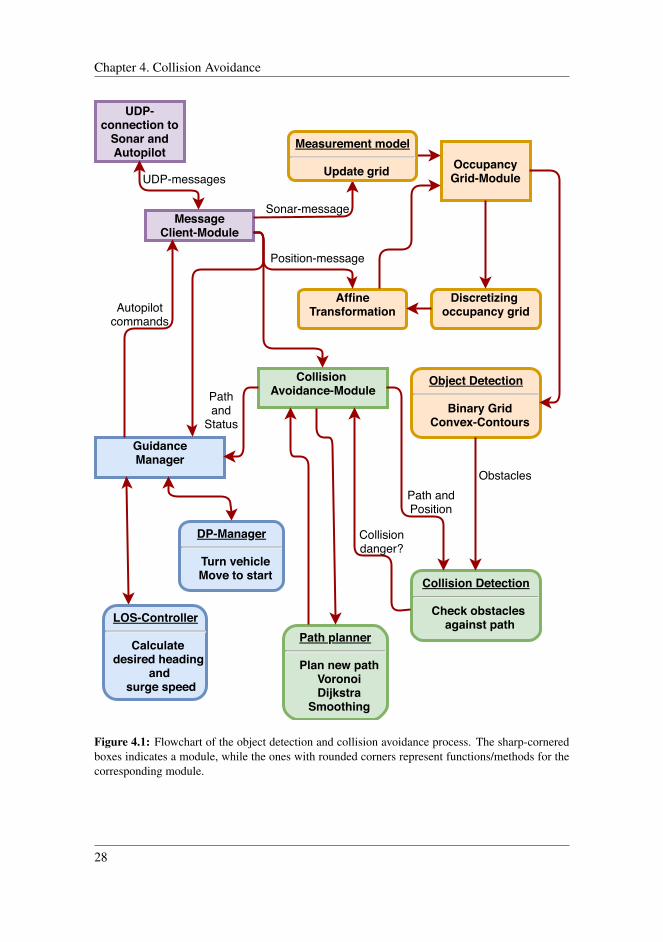
The task of avoiding collisions can be divided into three different parts: object detection,path planning and path execution. This chapter describes this process in depth, whilepresenting the developed algorithms. An overview of the different modules composing thecomplete system can be seen in the flowchart in Fig. 4.1.

27

Chapter 4. Collision Avoidance

OccupancyGrid-ModuleUDP-messages

UDP-connection to

Sonar andAutopilot

Message Client-Module

Discretizing occupancy grid

Sonar-message

Affine Transformation

Position-message

Measurement model

Update grid

Collision Avoidance-Module

Object Detection

Binary Grid Convex-Contours

Collision Detection

Check obstacles against path

Path andPosition

Obstacles

Collisiondanger?

Path planner

Plan new pathVoronoiDijkstra

Smoothing

Guidance Manager

Pathand

Status

Autopilotcommands

LOS-Controller

Calculate desired heading

and surge speed

DP-Manager

Turn vehicleMove to start

Figure 4.1: Flowchart of the object detection and collision avoidance process. The sharp-corneredboxes indicates a module, while the ones with rounded corners represent functions/methods for thecorresponding module.

28

4.1 Object detection

4.1 Object detectionThe purpose of the object detection module is to use the available sensor data to generatea object map, that is as accurate as possible.

4.1.1 Occupancy GridA local occupancy grid is constructed as a an m×m matrix of real numbers. The positionof the sonar is placed at (c, c) with c = m−1

2 and the size of each cell is given as l × l,where l = rscale

c . The cell size is dependent on the current range of the sonar. Each cellcontains the log-odds representation of the probability of occupation PO(i, j) of that cell.

4.1.2 Measurement modelWhen a new measurement is obtained, the occupancy grid has to be updated. The firststep here is to determine if any of the return echoes could belong to an obstacle. Threedifferent methods was used. The first method use a threshold value which is a functionof the operators sonar settings. This method has the benefit of being easy to tune usingthe IKM sonar software to adjust the settings for base and span. The threshold value istransformed according to Eq. (4.1).

Tf =T × span

255+ base (4.1)

where Tf is the final threshold and T is the selected threshold value. The data above Tf isthen selected as hits. This method can be observed in Fig. 4.2a.

The second method analyses the shape of the signal. The method is described in Alg. 1,and an example can be observed in Fig. 4.2b.

Algorithm 1: Pseudo-code for threshold method 2.Data: signal, threshold TOutput: prets = Convolution of signal and In×1p = All peaks in s, where a peak is a point with lower values on both sidesv = All valleys in s, where a valley is a point with higher values on both sidesRemove consecutive peaks in p, such that only the tallest remainsRemove consecutive valleys in v, such that only the lowest remainsRemove insignificant peaks in pRemove insignificant valleys in vpret = peaks in p where p− v > T

The last method selects a threshold based on the value in the sample after the samplehaving the greatest gradient. The gradient has to be above a threshold Tg to be considereda hit, otherwise the threshold will be selected as 255. An example of this method is shownin Fig. 4.2c.

29


0 100 200 300 400 500 600 700 800

Bin

0

20

40

60

80

100

120

140

160

180

Valu

eData

Data over threshold

Threshold

(a) Threshold Method 1.

0 100 200 300 400 500 600 700 800 900

Bin

0

20

40

60

80

100

120

Valu

e

Smooth signal

Peaks

Valleys

Selected Peaks

(b) Threshold Method 2.

Figure 4.2: Three different methods for finding the return echoes over a certain threshold.

30


0 100 200 300 400 500 600 700 800

Bin

0

20

40

60

80

100

120

140

160

180V

alu

e

Data

Data over threshold

Threshold

Max gradient

(c) Threshold Method 3.

Figure 4.2: Three different methods for finding the return echoes over a certain threshold (cont.).

The grid can now be updated in two different ways depending on the already detectedobstacles. If the scan-line intersects an obstacle the Zhou-method[44] is used, otherwisethe Thrun-method[37] is used. Both methods are described in Ch. 2.1.2. The intersectioncheck is done by a binary-AND-check, where the matrix has the convex-obstacle-contoursand the second matrix contains a straight line from the sonar position to the end of the grid,in the same direction as the scan-line. If the scan-line and a contour intersects, the anglebetween them is calculated as the angle between the scan-line and the first intersectingline-segment of the contour.

Both the Thrun-method and the Zhou-method requires the cells which overlaps thesonar-cone. An example of the overlap between the sonar-cone and the grid cells is shownin Fig. 4.3. This is done by a range-scale independent lookup table. The table is structuredas two arrays of lists, one for each beam-width, where each row in the array corresponds toa sonar-cone angle discretized in steps of 1

16gradian. This results in 6400 rows. Each rowcontains a sorted list of the indices of the cells in the corresponding sonar-cone. A cell isoverlapping the sonar-cone if at least one of the angles are between the limits of the sonar-cone. The indices are sorted by the distance from the center. The indices corresponds to aflat indexing-scheme, where each row of the matrix is placed into a single row. This formof indexing speeds up the process.

31


0 1 2 3 4 5 6 7

Cell column

4

3

2

1

0

Cell

row

Small Angle

Large Angle

Angle

Sonar Cone

Grid cell

Cell center

Overlapping cells

Figure 4.3: Overlap between grid cells and sonar-cone and angles used in the generation of lookup-tables.

4.1.3 Motion

The occupancy grid is vehicle fixed, and thus any motion of the vehicle needs to be takeninto account. The motion can be modeled as probabilistic or deterministic, but due to thehigh accuracy of relative motion it is reasonable to model the motion as deterministic.Using the approach given by Ganesan et al. [13] the probabilities of occupation proved todiminish quickly, and thus a new approach is described here. Each cell in the occupancygrid,G can be discretized as n×n smaller cells, such that the discretized grid,Gd becomesmn ×mn cells. The discretized grid is centered at (cd, cd) with cd = m∗n

2 and the sizeof each cell is given as lc × ld, where ld = rscale

cd. The relation between the two grids are

then given by Eq. (4.2), where ⊗ is the Kronecker product.

Gd = G⊗ In×n (4.2)

The rotation and translation of the grid is archived through an affine-transformation, asdescribed in Ch. 2.2.6 with a transformation-matrix, T as described in Eq. (4.3) and linearinterpolation over the transformation. The border points are chosen as pinitial.

T =

[α β (1− α) cd − βcd −∆xg−β α βcd + (1− α) cd + ∆yg

](4.3)

32


, where the variables are defined in Eq. 4.4.

α = cos ∆ψ

β = sin ∆ψ

∆xg = ∆yvehcd

rscale

∆yg = ∆xvehcd

rscale(4.4)

, where g denotes the grid reference frame and veh denotes the vehicle reference frame.

4.1.4 From occupancy grid to obstacles

Going from the probabilistic occupancy grid representation to an obstacle representationsuited for the path planning algorithm involves several steps. These are listed below.

• Binary thresholding

• Contour detection

• Filtering out small contours

• Dilation to include safety margins

• Finding contours of dilated map

• Approximating contours as convex hulls

The the thresholding process is shown in Eq. (4.5).

Bd (i, j) =

1 if Pd (i, j) ≥ Pth

0 if Pd (i, j) < Pth

(4.5)

where Bd is the discretized binary grid and Pth is the thresholding value. To save compu-tation time, Pth can be log-odds representation of the probability. The contours are thenextracted as described in Ch. 2.2.5 and the areas of each contour is calculated. All con-tours with an area smaller than a certain threshold is filtered out, as these are likely due tonoise or obstacles such as fish.The grid is then dilated, as described in Ch. 2.2.4, with astructuring element, E given in Eq. (4.6)

E = 1n×n ,where n =Dcdrscale

(4.6)

where D is the safety margin. The contours of the dilated image is then extracted as aconvex hull. The complete process can be observed in Fig. 4.4. After the objects aredetected the next step is to check if there is a collision danger.

33


-30 -20 -10 0 10 20 30

0

5

10

15

20

25

30

-10

-8

-6

-4

-2

0

2

4

6

8

10

(a) Original occupancy grid. The plot is in the log-odds scale.

-30 -20 -10 0 10 20 30

0

5

10

15

20

25

30

0

1

(b) Binary grid.

-30 -20 -10 0 10 20 30

0

5

10

15

20

25

30

0

1

Detected Obstacles

(c) First contour detection

Figure 4.4: Object detection procedure.

34


-30 -20 -10 0 10 20 30

0

5

10

15

20

25

30

0

1

Filtered Obstacles

(d) Small contours filtered away.

-30 -20 -10 0 10 20 30

0

5

10

15

20

25

30

0

1

Dilated Contours

(e) Dilated contours.

-30 -20 -10 0 10 20 30

0

5

10

15

20

25

30

-10

-5

0

5

10

Convex contours

(f) Convex contours on top of original occupancy grid. The plot is in the log-odds scale.

Figure 4.4: Object detection procedure (cont.).

35


4.2 Collision Detection

Collision detection is an important part of the system. A simple way of doing this is todraw the path and the obstacles on two different binary images and do a logical AND-check. This procedure is illustrated in algorithm 2. The path is drawn as a line, witha thickness corresponding to the width of the vehicle. The collision margin around theobstacles are already implemented during the the object-detection part.

Algorithm 2: Pseudo-code for collision checkData: waypointList, obstacleContours, rangeScale, gridSize,

vehicleMarginOutput: collisionIndex, -1 if no collision

obstacleGrid = binary drawing of all obstacleContourspathWidth = vehicleMargin× gridSize/(2× rangeScale)pathSegments = segments between a waypoint and the nextcollisionIndex = −1for segment s of pathSegments do

pathGrid = binary drawing of segment with pathWidthif any item in (pathGrid&&obstacleGrid) = True then

collisionIndex = ibreak

4.3 Path planning

The purpose of the path planning module is to calculate a new and effective path once acollision has been detected. An example of the path planning process could be seen inFig. 4.5. The process is described below.

36

4.3 Path planning

-30 -20 -10 0 10 20 30

East [m]

0

10

20

30

40

50

60

No

rth

[m

]Obstacles

VD ridges

Start WP

End WP

(a) Voronoi diagram.

-30 -20 -10 0 10 20 30

East [m]

0

10

20

30

40

50

60

No

rth

[m

]

Obstacles

Valid VD

ridges

Invalid VD

ridges

Start WP

End WP

(b) Voronoi diagram with invalid vertices andridges removed. Connections between thefirst and final waypoints and the vertices oftheir respective region are added.

-30 -20 -10 0 10 20 30

East [m]

0

10

20

30

40

50

60

No

rth

[m

]

Obstacles

Valid VD

ridges

Old path

Djikstra path

Start WP

End WP

(c) Voronoi diagram with only valid paths.The old path is shown together with the firststep of calculating the new path.

-30 -20 -10 0 10 20 30

East [m]

0

10

20

30

40

50

60

No

rth

[m

]

Obstacles

Djikstra path

Smoothed with

Fermat's spiral

Obsolete WPs

removed

Start WP

End WP

(d) The path from Fig. 4.5b with obso-lete waypoints removed and the smooth finalpath.

Figure 4.5: Voronoi diagram and path calculation.

4.3.1 Voronoi Diagrams

The Voronoi diagrams (VD) described in section 2.3 can be implemented into a path plan-ning algorithm. The generator points can be chosen as the vertices of of the contour pointsfrom the object detection algorithm, and thus the set V will consist of the points fur-thest away from each obstacle. This can be observed in Fig. 4.5a, where the green circles

37


indicate a vertex of V and the green lines is the set V itself. In addition to this fourcorner-points are added. The positions of these corner-points are chosen as the outermostpoints of the occupancy grid corners and the last waypoint included in the optimizationprocess. It is also possible to add the center-points between the corner-points to get ad-ditional possible paths. To get a set of safe piece-wise linear paths, all paths intersectingwith an obstacle has to be removed. This can be observed in Fig. 4.5b, where the invalidpaths and vertices is purple.

The start and end positions also has to be included to get a complete path. Thesepositions are included as a vertex, which are connected to all other vertices surroundingthe corresponding region. In addition to these two points, another fixed point is insertedstraight ahead of the vehicle to account for the run-time of the algorithm. The position ofthis point is a tuneable parameter, that should be tuned according to the cruising velocityof the vehicle.

The next step is to find the shortest valid path, and here Dijkstra’s algorithm is a goodcandidate.

4.3.2 Dijkstra’s algorithm

The first step in Dijkstra’s algorithm is to populate the distance matrix D with the distancesof each valid path in the Voronoi diagram. D(i, j) = D(j, i) is the distance between nodei and j. A distance of zero indicates that there is no connection. Running Dijkstra’s algo-rithm, as described in section 2.4 will return the shortest path between the two waypoints.

4.3.3 Removal of unnecessary waypoints

The path found by Dijkstra’s algorithm is the optimal solution to the shortest path alongthe edges of the VD, but this is not the overall optimal solution. The VD generates edgesthat are as far away as possible from the obstacles, which results in a path that has a greaterclearance-margin than necessary, as well as containing too many waypoints. An algorithminspired by [23] is developed to remove the unnecessary waypoints. First, almost co-linear waypoints are removed based on path-segment heading threshold. The next step isto remove waypoints that has a greater clearance-margin than necessary, which is done bychecking if a waypoint can be removed, without violating the clearance constraints. If awaypoint can be removed, a check is performed to see if removing the next waypoint ismore beneficial. This process is outlined in Alg. 3.

38

4.3 Path planning

Algorithm 3: Algorithm for removal of unnecessary nodes. The Pa→b→c notationis the path segment from node na trough node nb to node nc, and |P | is the lengthof path segment P . collisionDanger() is function checking whether a path-segmentis violating clearance constraints.

Data: List of points in optimal path, PL

Output: PL with unnecessary waypoints removed

for nodes ni in PL doP0→2 = ni → ni+2

if collisionDanger(P0→2) thenP1→3 = ni+1 → ni+3

if collisionDanger(P1→3) thenif |P0→2→3| > |P0→1→3| then

Remove ni+2

elseRemove ni+1

elseRemove ni+1

The resulting path consists of linear path-segments, which gives a non-continuous cur-vature. Flying this path with a fully-actuated vehicle will cause the vehicle to slow downto a full stop between each path-segment, which is ineffective. The path is unfeasible fora under-actuated vehicle. To solve this problem, the path has to be smoothed to ensure acontinuous curvature.

4.3.4 Fermat Spirals

The smoothing of the calculated path is done as described in Ch. 2.5. Once a feasible andsmooth path is generated it is translated to the NED-frame as described in Ch. 4.3.5 andsent to the guidance system along with a status update from the algorithm. The possiblestatuses and their corresponding responses are described in Tab. 4.1. An example of thesmoothed path can be seen in Fig. 4.7b.

The resulting smooth path might violate the clearance constraints. In this case, Di-jkstra’s algorithm has to be run again, but with a modification suggested by [23]. Thismodification erases the connection to the first node resulting in a constraint violation andcalculates a new path from there. The algorithm can be run multiple times to generate afeasible path. If the algorithm can not find a feasible and smooth path, the guidance systemreceives the non-smoothed path.

4.3.5 Conversion between coordinate systems

Conversion between the different reference frames and coordinate systems are frequent.In addition to the transformations presented in Ch. 2.7 it is also necessary to transform

39


waypoints from g to veh, which is shown in Eq. (4.7). The conversion back is presentedin Eq. (4.8)

xveh = (cy − yg)rscalecy

yveh = (xg − cx)rscalecx

(4.7)

where c is half the number of cells in the associated direction.

xg = round(cx

(yvehrscale

+ 1

))yg = round

(cy

(1− xveh

rscale

)) (4.8)

where round is the rounding and conversion to an integer. This is necessary as the gridreference-frame consists of a finite number of cells, rather than a position.

The transformation of a position from the vehicle frame of reference to the NED-frameis shown in Eq. (4.9) and back again in Eq. (4.10)

r =√x2veh + y2veh

α = arctan

(yvehxveh

)N = pN + r cos (α+ ψ)

E = pE + r sin (α+ ψ)

(4.9)

r =√

(N − pN )2 + (E − pE)2

β = arctan

(E − pEN − pN

)− ψ

xveh = r cos(β)

yveh = r sin(β)

(4.10)

The relations between the coordinate systems are shown in Fig. 4.6.

40


-20 -10 0 10 20 30

East

-10

-5

0

5

10

15

20

25

30

No

rth

Vehicle

Grid lines

XVEH

YVEH

Xg

Yg

XNED

YNED

Figure 4.6: Relationship between the n-, veh- and g-reference-frames.


The guidance-system is responsible for providing input to the vehicles control system. ALOS-guidance system with surge-velocity control is implemented as described in Ch. 2.8,with a few modifications.

The lookahead-distance is implemented as a lookahead-time, such that lookahead-distance is a time-varying parameter dependent on the vehicle velocity. The region ofacceptance is reduced if the curvature is large, resulting in close waypoints.

The setpoint for the surge-controller is also time-varying. When a new path is calcu-lated, the guidance-system will calculate the curvature for each path-segment-corner andsubsequently choose the correct velocity for the turn. The turn velocity is implementedas a constant multiplied by the curvature between the path-segments. An example of thevelocity along the path in Fig. 4.7b is shown in Fig. 4.7a.

As the vehicle will need some time to reduce the velocity to the turn-velocity a break-distance is implemented in the same manner as the region of acceptance.

The guidance system tries to make the transition between paths as smooth as possible,which means that as long as the vehicle is on the new path, or sufficiently close to it, thenew path is started immediately. If these conditions are not satisfied, the vehicle will stopand enter DP-mode to reach the start of the new path.

The guidance system receives status updates from the collision avoidance algorithm.The different statuses and their corresponding responses are listed in Tab. 4.1. The Nofeasible path status triggers the guidance system to a full stop. The mean values of thestarboard and port sides of the occupancy grid is then calculated, such that the vehicle canstart to turn towards the side with the smallest obstacle density.

41


0 2 4 6 8 10 12 14 16

Distance [m]

0

0.05

0.1

0.15

0.2

0.25

0.3

0.35

0.4

[m/s

]

0

0.1

0.2

0.3

0.4

0.5

0.6

0.7

0.8

0.9

[rad/m

]

Velocity

Curvature

(a) Curvature and velocity profile along thepath.

0 1 2 3 4 5 6 7 8

East [m]

0

1

2

3

4

5

6

No

rth

[m

]

Smooth path

Waypoints

(b) Smooth path and original waypoints.

Figure 4.7: A smooth path and the original waypoints are to the right. The velocity profile andcurvature of the path is to the left.

Status Response

No danger Continue current pathNo feasible path Stop and turnSmooth path violates collision margin Execute non-smooth path, with stops between WPsNew route OK Execute new path

Table 4.1: Possible collision avoidance statuses, and their corresponding response in the guidancesystem

In addition to the LOS-guidance system, a control system was also needed for thesimulations. It was decided that a simple PID-controller was sufficient for controllingaltitude, heading and surge-velocity. The tuning was straightforward due to the noise-freesignals.

42

Chapter 5Experimental setup

In this chapter, the experimental setup during the simulations and field experiments aredescribed. The chapter is divided into one section for each of the simulators and onesection for the field experiments. The computer used for the MORSE simulations and thecollision avoidance system is described in Ch. 5.4.

5.1 Simulation with MORSE

The initial simulations were done with the modified version of the MORSE simulator de-veloped by Henriksen et al. [15]. The communication was done trough MOOSDB, whichprovided an easy communication interface. A description of the simulated environmentand the ROV is provided in Ch. 6. A screenshot of the ROV can be seen in Fig. 5.1.

Figure 5.1: Close up screenshot of the ROV used in the MORSE simulations.

43

Chapter 5. Experimental setup

5.2 Simulation with Merlin Simulator

The Merlin Simulator is a high-fidelity ROV simulator, complete with a normal controlsystem. This is a useful simulator for testing the communication with the IKM Autopilotserver and getting some initial tuning values for the field experiments. The simulator lacksthe possibility of extracting sonar data, and thus no object detection or collision avoidancetests could be carried out. An example of a simulated environment in the simulator isshown in Fig. 5.2.

Figure 5.2: Screenshot from the simulated environment in IKM’s simulator.

5.3 Field Experiments

All field experiments are performed at Equinor’s Snorre B field. The field is located in the34/4 block. The approximate position of the semi-submersible drilling rig can be observedin Fig. 5.3.

Figure 5.3: Location of the Snorre field[33].

44

5.3 Field Experiments

5.3.1 Equipment

The equipment used in the field experiments include the ROV, the sonar and the positioningsystem. This equipment is described below.

Merlin UCV

The drilling rig has a resident ROV, which means that it is permanently stationed subsea.A 3D-model of the ROV is shown in Fig. 5.4. The ROV is called Merlin UCV and is awork-class ROV, with electric propulsion. The dimension of the ROV 2.5m×1.5m×1.5m.

Figure 5.4: 3D model of Merlin UCV, with the location of the sonar highlighted. Courtesy of IKMTechnology.

Onshore Control Room

The ROV can be controlled from an onshore control room at IKM’s headquarters at Bryne.A picture from the control room can be seen in Fig. 5.5.

45


Figure 5.5: Picture from the control-room at IKM Subsea’s headquarters at Bryne. Courtesy ofIKM Subsea.

Tritech SuperSeaking Mechanically Scanning Sonar

The Merlin UCV is equipped with a mechanically scanning sonar called SuperSeakingDST. This sonar is manufactured by Tritech. The SuperSeaking sonar is utilizing DigitalSonar Technology(DST) as well as Compressed High-Intensity Radar Pulse(CHIRP). Thesonar has two separate transducers with frequencies centered around 650 kHz and 325 kHzto accommodate high resolutions and long ranges.

The SuperSeaking sonar has an RS-232 interface for serial communication. The serialdata is then sent over Ethernet as UDP-packages. The communication protocol is definedin [39]

Some key properties of the SuperSeaking sonar are listed in tab 5.1.

Specifications High-Frequency Low-Frequency

Frequency center 650 kHz 325 kHzHorizontal beam width 1.5 3.0

Vertical beam width 40.0 20.0

Maximum range 100 m 300 mMinimum range 40 cmMaximum range resolution 15 mmMechanical resolution 0.45, 0.9, 1.8 and 3.6

Source level 210 dB re 1 µm

Table 5.1: Key properties of Tritech SuperSeaking DST Sonar[38]

Inertial Navigation System

The Merlin ROVs are equipped with an INS called Sprint 500, which uses a combinationof accelerometers, gyroscopes, Doppler velocity log (DVL), depth sensors and positionmeasurements from transponders to estimate the ROV’s position.

46

5.4 Computer

Acoustic Positioning System

The rig at Snorre B is equipped with a super-short-base-line acoustic positioning system,see section 3.5.2, from Kongsberg called HPR-400. According to [1] the accuracy isapproximately 6 meters.

Communication

The test computer was connected to the wired network in the control room and messageswere sent over UDP to the IKM Autopilot Server (APserver). The APserver communicateswith the with the control room, which forwards the commands offshore. This process isoutlined in Fig. 5.6.

ROV Offshore Control Room

Onshore Control Room

Collision Avoidance

System

Offshore Onshore

UDPSerialTCP/IP

Figure 5.6: Communication with ROV.

5.4 ComputerThe collision avoidance system was run on an Acer Aspire Nitro VN7-791G with a 4-coreIntel Core i7-4720HQ processor with a clock frequency of 2.6GHz [19]. The laptop has8 GB of DDR3L SDRAM, with a clock frequency of 1600 MHz and a NVIDIA GeForceGTX 860M - 2 GB GDDR5 SDRAM graphics processor. The graphics processor was notused for the collision avoidance algorithm, but is necessary for the running the simulationsthrough MORSE/Blender.

47


48

Chapter 6

Simulation Results

In this chapter the results from several simulations are presented. The first three sectionscontains different simulations, using MORSE to test the guidance system, the object de-tection system and the complete collision avoidance system. The last section is a test ofthe guidance system, and the communication with the IKM’s Autopilot program, usingtheir simulator.

The simulated environment used in the MORSE simulations contains several simpleobstacles, such as ellipsoidal and rectangular pillars, as well as a more complex obstacleconsisting of three small cylinders and a wall on one side. A map of this environment isshown in Fig. 6.1 and a picture of the environment is shown in Fig. 6.2. In all the experi-ments the sonar was running with an update frequency of 16 Hz, which is approximatelyequal to the update frequency of the sonar used in the field trials. The range of the sonarwas 30 m and the beam width and height was equal to those of the SuperSeaKing sonar.The shorter range is due to the available ROV model being smaller than the Merlin UCV.A Gaussian distributed noise, with a mean of 10 and standard deviation of 2.9 was addedto the sonar-signal. The cruising velocity was set to 0.4m/s ≈ 0.8knots. The ROV is quitedifferent from the one used in the field-trial, but the result are still useful.

49

Chapter 6. Simulation Results

-30 -20 -10 0 10 20 30 40

East [m]

-40

-30

-20

-10

0

10

20

Nort

h [m

]

1

2

3

45

67

8

Figure 6.1: Map of the simulated environment used during the MORSE-simulations. The objectsare numbered.

Figure 6.2: Screenshot from the simulated environment used during the MORSE-simulations.

The simulations carried out in IKM’s simulator was for testing the communication withthe autopilot server. The simulator has high fidelity dynamics, but there is no possibilityof outputting sonar-data for usage in the system, and thus no test were carried out on theobject detection part. The test where run without a tether, as no automatic tether system isimplemented.

50

6.1 Object Detection

6.1 Object DetectionThe object detection system was tested in several different trials on the simulated environ-ment described above. The vehicle was flying pre-planned paths or controlled manually.The results from one of these experiments is shown in Fig. 6.3, where the vehicle is fly-ing a pre-planned path. The detected obstacles are logged every 10 seconds, and plottedas transparent shapes, such that obstacles that are detected on multiple occasions are lesstransparent. It can be observed that all the objects are clearly detected. There are alsoobjects detected at (N,E) ≈ (−5,−45), (40,−20) and (10,−40), which are caused bysteep terrain elevations at these positions, which can be observed in the background inFig. 6.2. There is also an object at (N,E) ≈ (3,−15), which is due to cluttered noise.As can be observed from the opacity of the object, it was only detected for a short while,and as soon as the ROV moved, the probability was below the threshold again. It shouldbe noted that all the objects appear larger than they are, which is due to the applied safety-margin of two meters.

Figure 6.3: Results from simulated object detection trial. The detected obstacles are logged every10 seconds and plotted as transparent polygons.

6.2 Guidance SystemIn this section a trial of the guidance system is presented. The ROV is flown trough a pathin the simulated environment. A plot of the path is shown in Fig. 6.4. The figure showsboth the planned path and the flown path, as well as the ROAs for each waypoint (WP).It should be noted that there is a deviation from the path after WP9, as the ROV does notmanage to slow down sufficiently. This deviation can also be seen in Fig. 6.7, where the

51


cross-track error is shown. The reason for this is a too high velocity, which can be observedin Fig. 6.8, where an excerpt from the velocity profile is shown. The guidance system triesto reduce the velocity before WP9, but the distance available for the velocity reduction isnot sufficient, and thus the velocity trough the turn is too large. There is a large deviationat WP4 as well, but this is mainly due to the large angle between the path-segments andthe size of the region of acceptance (ROA). As the ROV reach the ROA of WP4, the pathsegment between WP4 and WP5 is selected, but the ROV is still not on the path. It shouldbe noted the ROV reduces the cross-track error fast, as it converges towards the new pathsegment.

In Fig. 6.5 a plot of the heading throughout the path is displayed. It should be notedthat the setpoint is too fast for the ROV, but the reference signal smooths out the steps inthe setpoint. The difference between the heading angle and the reference signal can beseen in Fig. 6.6. This error is sufficiently small, except right after the change to WP4. Thissuggests that the acceleration of the reference signal should have been smaller.

The overall performance of the guidance system is sufficient, but the large cross-trackerror after WP9, might be a problem when a path is close to an obstacle.

-25 -20 -15 -10 -5 0 5 10 15 20 25

East [m]

-15

-10

-5

0

5

10

15

20

25

Nort

h [m

]

1

23

4

5

67

89

10

1112

13

14

15 Installation Line

Position

Path

ROA

Figure 6.4: North-east plot of the path of the ROV during simulated guidance system trial. TheROAs are plotted at each waypoint.

52

6.2 Guidance System

12:49:30 12:50:00 12:50:30 12:51:00 12:51:30

Time

-90

-80

-70

-60

-50

-40

-30

-20

-10

0

Yaw

- [D

eg]

12

3

4

5

6

7

8

9

10

11

12

13

14

15

Real

Setpoint

Reference

Figure 6.5: Plot of the heading, the reference signal and setpoint of the heading, during simulatedtrial of the guidance system.

12:49:30 12:50:00 12:50:30 12:51:00 12:51:30

Time

-4

-3

-2

-1

0

1

2

3

Headin

g E

rror

- [D

eg]

1

2

34

5

67

8

9

10

11

12

13 14 15

Figure 6.6: Plot of the difference between the heading and the reference signal of the heading,during simulated trial of the guidance system.

53


12:49:30 12:50:00 12:50:30 12:51:00 12:51:30

Time

-0.8

-0.6

-0.4

-0.2

0

0.2

0.4

0.6

0.8

1

1.2

Cro

ss tra

ck e

rror

- [m

]

1

23

4

5

6

7

8 9

10

11

12

13

14

15

Figure 6.7: Plot of the cross-track error during simulated trial of the guidance system.

12:50:30 12:50:40 12:50:50 12:51:00 12:51:10

Time

0.1

0.15

0.2

0.25

0.3

0.35

0.4

0.45

Surg

e v

elo

city -

[m

/s]

6

7

8

9

10

11

12

Velocity

Setpoint

Reference

Figure 6.8: Plot of the surge velocity of the ROV during simulated trial of the guidance system. Theplot also shows the reference signal and the setpoint.

54

6.3 Collision Avoidance


In this section a collision avoidance test is performed in the simulated environment. Anexcerpt from the results is provided in Fig. 6.9-6.11. In Fig. 6.9 the first re-planning ofthe path is presented. It should be noted that only object 7 is detected as this point, eventhough both object 5 and 6 is within the sonar field of view. The reasons for this is that thesonar beam started from the left, and has not yet reached these objects. The new path isplanned in a wide curve around the detected obstacle, which is due to the nature of VDs.The VD finds the lines which are as far apart from the generator points as possible, andsince only one obstacle is present the only present generator points are the edges of thegrid and the obstacle.

-40

-30

-20

-10 0 1

0 2

0 3

0 4

0

East [m]

-30

-20

-10

0

10

20

30

Nort

h [m

]

Installation Line

Obstacles

Sonar Field of View

ROV

Old Path

New Path

End of optimization

Actual Path

Figure 6.9: First path re-calculation during simulated trial of the complete collision avoidance sys-tem.

In Fig. 6.10 another path recalculation is shown. It should be noted that all the obstaclesthat has been inside the sonar field of view is now detected. The steep terrain at the edge ofthe map is also detected as an obstacle in (N,E) ≈ (5,−45). It should be noted that theold path is not passing trough obstacle 1, but rather the width of the vehicle, and thus thepath is overlapping the detected obstacle. A new path is calculated around the obstacles.

55


-40

-30

-20

-10 0 1

0 2

0 3

0 4

0

East [m]

-30

-20

-10

0

10

20

30

Nort

h [m

]

Installation Line

Obstacles

Sonar Field of View

ROV

Old Path

New Path

End of optimization

Actual Path

Figure 6.10: Second path re-calculation during simulated trial of the complete collision avoidancesystem.

In Fig. 6.11 the old path is to close to obstacle 1, as the detected part of the obstaclehas grown when the ROV moved closer. The path is thus adjusted to get a better clear-ance. It should be noted that obstacle 5-7 has disappeared as they are no longer inside theoccupancy grid.

56

6.4 Merlin Simulation

-40

-30

-20

-10 0 1

0 2

0 3

0 4

0

East [m]

-30

-20

-10

0

10

20

30

Nort

h [m

]

Installation Line

Obstacles

Sonar Field of View

ROV

Old Path

New Path

End of optimization

Actual Path

Figure 6.11: Last path re-calculation during simulated trial of the complete collision avoidancesystem.

6.4 Merlin SimulationSeveral simulations were done in the Merlin Simulator, but no results are presented asthe simulations were done to fix the communication with the IKM Autopilot Server. TheROV model in the simulator is not the same as the one used in the field experiments, butthe tuning provided good initital tuning values.

57


58

Chapter 7

Full-Scale Experiments

The complete system consisting of the object detection module, the path planning moduleand the guidance system was tested through real-time experiments at the Snorre B field.The raw network traffic was logged, but most of the data presented here is the result oflog-files generated by the developed system. A map of the area can be seen in Fig. 7.1.Most of the experiments starts from the garage, as this is where the ROV is tethered to.The chapter is divided into three different sections, where the object detection module istested first, then the guidance-system. The last section is a test of the complete system.Some key parameters that are equal in all of the experiments are given in Tab. 7.1.

59

Chapter 7. Full-Scale Experiments

457900 457950 458000 458050

East [m]

6821460

6821510

6821560

No

rth

[m

]

Garage and

spool

Toolstand Module A

Module B

Scrap

metalModule C Module D

Module E

Module F

Module G

Installation Line

Installation Point

Figure 7.1: Map of the subsea area of the Snorre B field.

60


Parameter Value

Sonar range 50 mSonar frequency 650 kHz

Obstacle safety-margin 2 mVehicle safety-margin Equal to vehicle beamDistance for second waypoint 4 mCo-linear threshold for removal of waypoints 2 deg

Cruising velocity 0.5m/s ≈ 1knotLOS look-ahead time 20 sHeading update limit 0.5 degTurn-velocity factor 1

32

Initial probability 0.5Binary probability threshold 0.6Free probability 0.3Occupied probability 0.7Discrete grid size 1601× 1601Occupancy grid size 100× 100Minimum rotation of grid 0.5 degMinimum translation of grid 1 discrete grid cell

Table 7.1: Key parameters for all field-tests.


The purpose of this trial was to test the object detection capabilities of the system. TheROV was flown by a pilot from the garage, around a subsea-module and back again. Theresults from this flight is presented in Fig. 7.2. The detection data is logged once every 10seconds and plotted over the map of the area. The detected obstacles are marked with redtransparent, filled polygons. This results in object being detected on multiple occasionsbeing a darker shade of red. It should be noted that the ROV sometimes appear to be flyingstraight through the detected obstacles. This is foremost due to the safety margin of of twometers included in the object detection procedure, as mentioned in Ch. 4.1.4, but also dueto the ROV was flying above them. The ROV is flying at a mean altitude of approximately2 meters until it reaches module C, then the mean altitude is increased to 3.5 meters forthe remainder of the flight. It can be observed that all obstacles are clearly detected. Itshould be noted that there is some drift in the position, which can be observed by lookingat the tool stand in Fig. 7.3, which has changed location between the beginning and theend. The detected obstacles appear larger than the obstacles on the map, and this is due to asafety-margin of two meters. It should also be noted that the algorithm has some problemsaccurately detecting the south-side of module D. This is likely due to the high altitude andproximity to the module, which causes the sonar to miss it completely.

61


Figure 7.2: Detected objects and position of the ROV on a round-trip from the garage around moduleC and D.

62

7.2 Guidance System

Figure 7.3: Closer look at the view in Fig. 7.2.

7.2 Guidance System

In this trial the purpose was to test the developed guidance system. The trial started be-tween module A and B and was terminated when sufficient data was gathered, near moduleD. A North-east plot over the map is shown in Fig. 7.4. The result from this trial can be ob-served in Fig. 7.4-7.8. The numbers indicate when a new waypoint was selected. This shifthappen when the ROA, indicated in orange in Fig. 7.4 is reached. In Fig. 7.5 a close-upof Fig. 7.4 can be observed. It is apparent that there are some deviations in the beginning,which can also be observed in the plot of the cross-track error in Fig. 7.8. This is due toaggressive tuning and the fact that the ROV did not start from a steady state.

63


4579

70

4579

80

4579

90

4580

00

4580

10

4580

20

4580

30

East [m]

6821

530

6821

540

6821

550

6821

560

6821

570

6821

580

No

rth

[m

]

12

34

5

6

7

Installation Line

Installation Point

Position

Path

ROA

Figure 7.4: North-East plot of flight-path. The numbers indicate when a new waypoint is selected.

4579

63

4579

65

4579

67

4579

69

4579

71

4579

73

East [m]

6821

559

6821

561

6821

563

6821

565

6821

567

No

rth

[m

]

1

2

3

4

Installation Line

Installation Point

Position

Path

ROA

Figure 7.5: Close-up look at the first part of the path in Fig. 7.4.

64

7.2 Guidance System

In Fig. 7.6 a plot of the commanded heading from the LOS-controller together withthe reference-signal and the estimated heading is shown. It should be noted that there issome deviations in the beginning, but as soon as the heading has had time to stabilize, theROV is able to follow the commanded heading sufficiently good. When a new waypoint isselected there is a step in the LOS-output, but this is handled well by the reference signal.

15:15:00 15:15:30 15:16:00 15:16:30 15:17:00 15:17:30 15:18:00

Time May 15, 2018

100

110

120

130

140

150

160

Ya

w -

[D

eg

]

2

3

4

5

6

7

Los output

Real

Reference signal

Figure 7.6: Plot of heading, heading reference and desired heading for the flight-path from Fig. 7.4.The numbers indicate when a new waypoint is selected.

In Fig. 7.7 the surge velocity of the ROV is shown. The last two minutes are omitted, tomake the first part more visible. During the last two minutes, the velocity profile appearssimilar as from 15:16:30 to 15:18:00. I can be seen that between the second and thirdwaypoint, the setpoint for the velocity is reduced to accommodate the sharper turn radius.Notice that the ROV is not able to follow the reduction in velocity, as the waypoints areto close together. After the the third waypoint, there are no more sharp turns, and thus thevelocity-setpoint is adjusted back to the normal velocity again. It should be noticed thatthe ROV is never able to reach the commanded velocity, which is due to improper tuningof the surge-controller.

65


15:15:00 15:15:30 15:16:00 15:16:30 15:17:00 15:17:30 15:18:00

Time May 15, 2018

0.05

0.1

0.15

0.2

0.25

0.3

0.35

0.4

0.45

0.5

0.55

Su

rge

ve

locity -

[m

/s]

2

3

45 6 7

Los output

Real

Reference signal

Figure 7.7: Plot of surge velocity, surge velocity reference and desired surge velocity for the flight-path from Fig. 7.4. The numbers indicate when a new waypoint is selected.

In Fig. 7.8 a plot of the cross-track error can be observed. The cross-track error islarge in the beginning, which is due to the same reasons mentioned above. it should benoticed that for the last waypoints, there is a sudden spike in the cross-track error. This isdue to ROA = 2m, which in causes the cross-track error to be evaluated against the nextpath-segment.

66


15:15:00 15:15:30 15:16:00 15:16:30 15:17:00 15:17:30 15:18:00

Time May 15, 2018

-1

-0.5

0

0.5

1

1.5

Cro

ss-t

rack e

rro

r -

[m]

2

3

4

5 6 7

Figure 7.8: Plot of cross-track error for the flight-path from Fig. 7.4. The numbers indicate when anew waypoint is selected.

The results presented in this section indicate that the tuning of the controllers are notperfect, but due to the limited time available for testing the tuning was considered satis-factory.


In this experiment the goal was to test the complete system. A path from the garage, goingtrough several obstacles towards module G was planned. As the vehicle progresses alongthe path, and discovers new obstacles, new paths are calculated and executed. During theexperiment the obstacles and occupancy grid is logged every 10 seconds, and the detectedobstacles are logged along with the path recalculation data every time a new path is cal-culated. An excerpt results can be observed in Fig. 7.9-7.10. All the plots of new pathsin this experiment can be found in Appendix B.1 and a movie with the all the logged datacan be found in Appendix B.1.

In Fig. 7.9 it can be observed that the old path is passing through one of the detectedobstacles. The system then calculates a new path around the obstacle. The sharp turnbetween module C and D is due to an earlier recalculation of the path. It should be notedthat the toolstand and module A is not detected as obstacles. Due to the altitude andclose proximity several subsequent scans has showed a clear path, and thus reduced theprobability below the detection threshold. These issues are further discussed in the nextchapter.

67


457940 457960 457980 458000 458020 458040

East [m]

6821

500

6821

520

6821

540

6821

560

6821

580

6821

600

No

rth

[m

]

Installation Line

Installation Point

Obstacles

Sonar Field of View

ROV

Old Path

New Path

End of optimization

Figure 7.9: Excerpt from test of the collision avoidance system.

In Fig. 7.10 module C has barely come into the sonar field-of-view and the old path isonce again passing straight trough the detected obstacles. The calculated path is the bestpossibility given the known information, but as can be seen from the map, it is passingstraight through module C. The scrap-metal is not yet visible due to the current orientationof the sonar-head.

68


457940 457960 457980 458000 458020 458040

East [m]

6821

500

6821

520

6821

540

6821

560

6821

580

6821

600

No

rth

[m

]

Installation Line

Installation Point

Obstacles

Sonar Field of View

ROV

Old Path

New Path

End of optimization


In Fig. 7.11 and 7.12 the same input data is used. Fig. 7.11 is the real-time recalculationof the path, and Fig. 7.12 is post-processing with a revised algorithm. As can be seen inFig. 7.11 the new path takes an unnecessary long detour around module D. This is due tothe nature of VD’s, where the edges are as far away from each generator point as possible.In Fig. 7.12 a revised algorithm, where the midpoints between the corner points are addedas generator and the revised removal of unnecessary waypoints described in Ch. 4.3.3.This algorithm has proved to calculate similar path-lengths in most cases, but significantlyshorter in cases similar to this one. The new path includes a u-turn, but the path-length isshorter. Looking at the past recalculations in Appendix B.1 and the new calculations inAppendix B.2 with the revised method, it can be observed that the path on the west-sideof module C would have been selected earlier, and thus removed the need for a u-turn.

69


457940 457960 457980 458000 458020 458040

East [m]

6821

500

6821

520

6821

540

6821

560

6821

580

6821

600

No

rth

[m

]

Installation Line

Installation Point

Obstacles

Sonar Field of View

ROV

Old Path

New Path

End of optimization


70


457940 457960 457980 458000 458020 458040

East [m]

6821

500

6821

520

6821

540

6821

560

6821

580

6821

600

No

rth

[m

]

Installation Line

Installation Point

Obstacles

Sonar Field of View

ROV

Old Path

New Path

End of optimization

Alt: 1.7 m

Figure 7.12: Excerpt from test of the collision avoidance system. This recalculation is done afterthe experiment, using a revised version of the recalculation method. The input data is the same as inFig. 7.11.

71


72

Chapter 8Discussion

In this chapter the results presented in Ch. 6 and Ch. 7 will be discussed and compared.The chapter is divided into the same sections as the result chapters. In addition, Ch. 8.4evaluates the runtime efficiency of the developed algorithms.

8.1 Object DetectionThe results show that the object detection module is capable of efficiently and reliablydetecting obstacles with some exceptions.

During the initial simulations, the three different methods described in Ch. 4.1.2 foridentifying a hit from the sonar signal was tested. All three methods gave satisfactoryresults, with method two giving the most accurate results. During the first field trial, it wasdiscovered that method 2 and 3 gave too many false positives. Method 1 requires moretuning than the other two, but due to the coupling with the sonar settings, it is easy to tunefor a skilled ROV pilot.

Occupancy grids rely heavily on two assumptions, the static world assumption (SWA)and the cell independence assumption (CIA). These two assumptions are imperfect, whichmight cause some problems. The SWA assumes a static world, which is mostly true for asubsea production environment, but for other environments, there might be other movingand unknown objects, which violates the assumption. The CIA is violated due to the factthat each measurement gives information about a set of grid cells, not a single cell. Thereliance on CIA is somewhat reduced as the dynamic inverse-sonar model is introduced asthe probability of occupancy is in fact connected to the neighbouring cells. The SWA isnot considered a problem in this thesis as fish and other small moving obstacles are filteredout, and larger moving obstacles normally have a known position.

A local occupancy grid has several benefits compared to global occupancy grid. Aglobal occupancy grid has to account for the growth of the positional uncertainty, andthus the accuracy of the map will fall over time. With a local map, the obstacles will becorrectly located with respect to the vehicle, which is sufficient for the purpose of collisionavoidance. A global map will also require a lot of memory to retain all the information. As

73

Chapter 8. Discussion

an example: The discretized local grid has a resolution of 256 cellsm2 when a sonar range of

50 is used, with double precision floating point which amounts to a storage space of 20.48MB. Using the same parameters for the main subsea-area of the Snorre B field, whichoccupies approximately 20000m2. This amounts to 44 MB, while an area of 1km2 wouldtake up 2 GB of memory.

On of the main problems with underwater-SLAM is the need for reliable features to useas landmarks. Reliable features can be easy to find in man-made environments, such as thesubsea-production area considered in this thesis, but for other scenarios it can be difficult.One example of such a scenario is a vehicle moving between two sub-sea production areas,where unknown obstacles might recede.

During the field trials, it was discovered that the location of the sonar is of great im-portance. As the sonar is mounted more than a meter from the bottom of the ROV and thevertical beam-width is 40 when the sonar is at the high frequency, there will be a consid-erable blind-spot close to the ROV. This can be observed in Fig.8.1. This blind-spot causesthe scans to have no echo of objects close to ROV, which in turn reduces the probability ofoccupation. Due to time constraints on the field trials, this problem was not addressed andfurther investigation is needed.

Figure 8.1: ROV with sonar cone and blind-spot at an altitude of two meters.

A major difference between the simulations and the field trials is the accuracy of theposition and velocity measurements. During the simulations the correct position and ve-locity measurements where available noise free. During the field trials the position andvelocity data were estimated by an INS system. This system experience drift over timeand a steady-state error of approximately 90 meters was discovered. To account for thiserror an offset was added. To acquire this offset value, the ROV was flown to a fixedlocation and the difference in estimated position was compared to the position from the

74

8.2 Guidance System

map. There was also some drift during the trials, as noted in the object detection trial inCh. 7.1. Even though this drift can be a problem for accurate localization of the ROVand subsequently the validation of the results, it is not a problem for the collision avoid-ance system. The ROV has an accurate compass and the velocity measurements from theDVL is accurate, which results in the change in translation and rotation of the grid beingaccurate.

The occupancy grid has some tunable parameters. The size of the discrete grid waschosen on the basis the of maximal number of bins generated by the sonar. During theearlier versions of the object detection module, the raw data had to be interpolated to fitthe grid cells, and thus the same number of cells as bins was needed. The occupancy gridsize was reduced from this, such that multiple hits has the possibility of affecting the samecell. With a smaller cell size, a single-grid cell would only be updated once during a 180

scan, and no detection of obstacle would occur. Another important parameter is the initial,free and occupied probabilities. The initial probability was set to pinit = 0.5, since it isunknown.

The simulations were run with different values for free and occupied probabilities. Itwas found that pfree = 0.7 and poccupied = 0.3 gave the best detection to false positiveratio. The threshold value used for the object detection was found to be effective at 0.6.During the initial field experiments the hit threshold, T = 170 was found to bee accurate,in collaboration with the pilots.

8.2 Guidance SystemThe results in Ch. 6.2 and Ch. 7.2 indicates that the guidance system is performing suf-ficiently with respect to cross-track errors. The line-of-sight (LOS) guidance, with thevariable lookahead distance is providing the control system with a desired heading, whichmakes the ROV converge to the chosen path. The cross-track errors are small during theexecution of the paths, but there are some errors when a new path is started and the vehicleis not aligned with the path. The velocity dependent lookahead distance then makes theLOS-guidance to aggressive, which causes the convergence to the path to be more timeconsuming than necessary.

The region of acceptance (ROA) was implemented as a variable region, dependent onthe proximity of the waypoints (WPs). This did not cause any problems when the ROAbecame small, but it should be considered for further work. A better solution would be toimplement the WP-switching with respect to the along-track distance instead of a ROA, assuggested by [9, p. 265].

The surge-velocity guidance did not work as well as expected. The time allocatedto reducing the velocity was not enough, and more time should have been spent on thetuning. Another problem with this algorithm was that the smoothing was done in the pathplanning and the velocity guidance was working against each other. The velocity guidanceconsiders only the angle between two path-segments, which is small due to the smoothing.A possible solution to this problem is discussed in Ch. 9.2.2. It was discovered that thepath following algorithms implemented on the Merlin UCV was not capable of the fastWP-switching needed by the collision avoidance system. To fix this problem the surge-velocity guidance algorithms were developed.

75


During the field experiments it was discovered that reference signal for both the surge-velocity and the heading was faster than the dynamics of the system. This caused someunnecessary oscillations, but due to time constraints during these experiments no addi-tional tuning was performed.

8.3 Collision AvoidanceThe complete collision avoidance system was tested both in simulations and in the fieldtests. In this section, the results from both of these trials will be discussed.

Both the simulations and the field tests showed similar results. The obstacles weredetected in a timely manner and a new path was calculated.

The Voronoi diagram (VD) is an effective method for finding a set of feasible paths.From this set of feasible paths, the shortest one is found through the use of Dijkstra’salgorithm. Dijkstra’s algorithm provides the optimal solution from the feasible set, but notthe overall optimal path. The algorithm handles multiple obstacles very well, and is ableto calculate a good path through them.

The VD has several possible configurations of the generator points as discussed inCh. 4.3.1. The runtime difference for these configurations are presented in Tab. 8.1. On thebasis of this comparison the convex-contour method was chosen, even though the accuracyof the obstacle representation is lower. Due to the real time requirements of the system, along runtime can cause problems. As stated in Ch. 8.1 the runtime comparison was doneon a sample grid, but more complex grids can significantly increase the runtime. Duringthe field trials the algorithm sometimes ran for up to 2 seconds, which with a normal AUVvelocity of 4 knots would give a travel distance of approximately 4 m. To account for this awaypoint was inserted straight ahead of the vehicle as discussed in Ch. 4.5a. The insertionof this point also turned out to make it easier for the guidance system to transition betweenpaths, as the first piece of the new path had the same orientation as the current piece of theold path. The other possibility of changing the generator points, is to use the mid-pointsbetween the corner-points, as described in Ch. 4.5a. During the trials, both possibilitieswere tested, and using the mid-points turned out to select negligible longer paths in mostcases. In cases where the only path is around an obstacle at the outer corner of the grid,the mid-point method selected significantly shorter paths and was thus chosen as the finalmethod.

The location of the destination point inserted into the VD has a large impact on howthe final path will look. The initial algorithm used the first WP outside the occupancy gridas the destination point. This worked well in most cases. However; when the old pathreentered the grid, the new path ended up in a loop. To solve this problem, a check to findthe first WP after the last time the path exits the grid was implemented.

The path smoothing with the use of Fermat’s spiral worked well, and a minimal curva-ture path was generated and subsequently discretized into the necessary number of way-points.

A problem with the developed collision avoidance system is that a new path is onlygenerated once the current path intersects a detected obstacle. This occasionally causedthe vehicle to fly a longer path than necessary, as new information about the obstacles weregathered. A system where the path was recalculated more often was developed to solve

76

8.4 Performance

this problem, but the path was then changed more often than the guidance system couldhandle.

8.4 Performance

During the development of the algorithm several options for the contour approximationsdescribed in Ch. 2.2.5 were evaluated with regards to performance. A test script wasconstructed, where the input was an image of dilated contours. The test script then detectedthe contours, using the appropriate approximation. The collision avoidance algorithm wasthen run, until a new path was calculated. This script was run 10 times for each contourapproximation. A runtime comparison for the data set used in Ch. 4.3 in can be seen inTab. 8.1.

Approximation Mean time

No approximation more than 6000 msSimple 4344 msTeh-Chin 2893 msConvex 662 ms

Table 8.1: Mean runtime for collision avoidance algorithm, with different contour approximationsfrom dilated contours to a finished path. Each method was run 10 times, and a mean value was cal-culated. The simulation was stopped after one minute runtime. The dilated contours were generatedfrom the same data as in Ch. 4.3.

The results indicate that the convex contour approximation is about four times as fastas the Teh-Chin approximation and 6.5 times as fast as the simple approximation. TheTeh-Chin approximation has the benefit of accurately displaying convexity-defects, whichcould be helpful for large concave structures, such as the example shown in Fig. 8.2. A fastalgorithm does, however, have more benefits than such special cases, and thus the convexcontour approximations was selected for the algorithm.

77


-20 0 20 40 60 80 100

East

-10

0

10

20

30

40

50

60

70N

ort

h

Concave approximation

Path around concave

approximation

Teh-Chin approximation

Path around Teh-Chin

approximation

Figure 8.2: Example of a path following a concave structure, with a convex contour approximationand the Teh-Chin contour approximation.

When running the complete collision avoidance algorithm the CPU-utilization wasbelow 30 %. Most of this CPU-usage is due to the graphic display of the program, whichis only needed for the convenience of the user. This suggests that the algorithm is capableof running on on-board hardware on other underwater-vehicles such as AUVs.

78

Chapter 9Conclusions and Further Work

In this chapter a conclusion will be formulated based on the results in Ch. 6 and Ch. 7, andthe discussion in Ch. 8. In the end recommendations for further work will be presented.

9.1 Conclusion

In this thesis, the problem of avoiding obstacles when following a pre-defined path wasinvestigated. An effective approach using a single-beam sonar to populate a probabilisticvehicle-fixed occupancy grid, and subsequently detect obstacles was found. The detectedobstacles were used to calculate a new collision free and smooth path adhering to the vehi-cles constraints. The complete collision avoidance system was simulated using a simulatorcalled MORSE and implemented on IKM Subsea’s Merlin UCV. Both the simulations andthe field trials showed promising results, where the system was capable of efficiently de-tecting and avoiding obstacles.

The presented approach has several advantages over other methods such as SLAM-based methods. Using a vehicle-fixed grid greatly reduces the computational complexityas well as removing the reliance on landmarks, which can be hard to detect in a noisy envi-ronment. The vehicle-fixed grid also has the advantage of being independent of positionalerror-growth.

It was shown that a mechanically scanning single-beam sonar is sufficient as the onlysensor for detecting obstacles in the vehicles planned path. The presented object detectionprocedure has some weaknesses, which were discussed.

The developed system for calculation of new paths is efficient, but the results are notalways optimal. The usage of Voronoi diagrams and Dijkstra’s algorithm always gives acollision-free path, but it might be longer than necessary. These aspects were thoroughlydiscussed, and suggestions for improvements will be presented in the next section.

79

Chapter 9. Conclusions and Further Work

9.2 Further WorkThis section will present a proposal for further work, with aspects of the thesis that needsimprovement and exploration.

9.2.1 Object Detection

With respect to the object detection system, several challenges have emerged during thework that should be addressed. The tuning of the sonar is a process that is easy for askilled ROV pilot, but this takes a lot of practice, and thus further research should be doneto develop either an algorithm that is independent of the sonar tuning, or tunes the sonarautomatically. The current system uses operator controlled range and step settings, but theaccuracy of the system could be increased by applying bat-inspired techniques for aimingand adjusting the sonar beam as described by Yamada et al. [42]. The main problem intesting such a system is that the ROV pilots rely heavily on the sonar for navigation, and arethus reluctant to release control over it. This could also be combined with a dynamicallysized occupancy grid to fit the obstacle density.

The rotation and translation of the grid follow a deterministic manner, but the positionand orientation are seldom perfectly known, and a probabilistic implementation of therotation and translation, as done by Ganesan et al. [13] should be considered. The currenttranslation of the grid relies on position updates, but to make the system more independentof inaccurate and unknown variables, this should be changed to use velocity measurementsinstead.

9.2.2 Guidance System

As described in Ch. 8.2, the velocity was occasionally too high trough sharp turns. Apossible solution to this problem is to consider the curvature trough several waypoints, notjust the first. It is also recommended to look into other guidance options, such as trajectorytracking.

9.2.3 Collision Avoidance

The collision avoidance system has some drawbacks that should be addressed. Whenan obstacle in the current path is detected it would be preferable if the guidance systemis notified immediately, such that no collisions can happen during the time it takes tocalculate a new path. Another drawback is that a path recalculation is only triggered byan obstacle on the current path. This can cause the vehicle to fly sub-optimal paths as newinformation is discovered. To solve this problem it is possible to try to recalculate the routemore often, and change the route if the new route is better.

This system only considers paths in the two-dimensional space, but Voronoi diagramscan easily be extended to work in a 3D-space, but this will most likely not be possiblewithout the use of extra sensors, such as a camera, an extra sonar or a 3D-sonar to extractinformation about the height of obstacles. Adding data from a camera will also improvethe detection capabilities at a close range.

80

9.2 Further Work

9.2.4 SimulationsThe sonar model in MORSE has a few drawbacks as mentioned earlier. The simulatorcould be drastically improved by implementing a more realistic sonar model. To do thismore research on underwater acoustics and comparison with real sonar data would beneeded. The work done on accurate sonar simulators on GPUs done by Cerqueira et al.[3] is a good place to start.

81

Chapter 9. Conclusions and Further Work

82

Bibliography

[1] Aakre, Ø. L., 2017. IKM Technology Autopilot Server User Manual. Tech. rep., IKMTechnology.

[2] Braginsky, B., Guterman, H., 2016. Obstacle Avoidance Approaches for Au-tonomous Underwater Vehicle: Simulation and Experimental Results. IEEE Journalof Oceanic Engineering 41 (4), 882–892.

[3] Cerqueira, R., Trocoli, T., Neves, G., Joyeux, S., Albiez, J., Oliveira, L., 2017. Anovel GPU-based sonar simulator for real-time applications. Computers and Graph-ics (Pergamon) 68, 66–76.

[4] Christ, R. D., Wernli Sr., R. L., 2014. Chapter 14 - Underwater Acoustics BT - TheROV Manual (Second Edition). In: The ROV Manual (Second Edition). Butterworth-Heinemann, Oxford, pp. 369–385.

[5] Christ, R. D., Wernli Sr., R. L., 2014. Chapter 15 - Sonar BT - The ROV Manual(Second Edition). In: The ROV Manual (Second Edition). Butterworth-Heinemann,Oxford, pp. 387–424.

[6] Council, N. R., 2005. Autonomous Vehicles in Support of Naval Operations. TheNational Academies Press, Washington, DC.

[7] Dijkstra, E., 1959. A note on two problems in connexion with graphs. NumerischeMathematik 1 (1), 269–271.

[8] Elfes, A., 1989. Using occupancy grids for mobile robot perception and navigation.Computer 22 (6), 46–57.

[9] Fossen, T. I., 2011. Handbook of Marine Craft Hydrodynamics and Motion Control.Wiley.

[10] Francois, R. E., Garrison, G. R., 1982. Sound absorption based on ocean measure-ments: Part I: Pure water and magnesium sulfate contributions. Journal of the Acous-tical Society of America 72 (3), 896–907.

83

[11] Francois, R. E., Garrison, G. R., 1982. Sound absorption based on ocean measure-ments. Part II: Boric acid contribution and equation for total absorption. Journal ofthe Acoustical Society of America 72 (6), 1879–1890.

[12] Fredman, M., Tarjan, R., 1987. Fibonacci heaps and their uses in improved networkoptimization algorithms. Journal of the ACM (JACM) 34 (3), 596–615.

[13] Ganesan, V., Chitre, M., Brekke, E., 2016. Robust underwater obstacle detection andcollision avoidance. Autonomous Robots 40 (7), 1165–1185.

[14] Goutsias, J., 2000. Mathematical Morphology and its Applications to Image andSignal Processing.

[15] Henriksen, E. H., Schjølberg, I., Gjersvik, T. B., 2016. UW MORSE: The under-water Modular Open Robot Simulation Engine. In: 2016 IEEE/OES AutonomousUnderwater Vehicles (AUV). pp. 261–267.

[16] Hermansen, A., 2017. How we think UIDs will be used by Statoil in the future.Accessed 2018-06-25.URL https://32zn56499nov99m251h4e9t8-wpengine.netdna-ssl.com/wp-content/uploads/2017/07/ID2017_Att09_Statoil_TomGlancy.pdf

[17] Hodges, R. P., 2010. Underwater Acoustics: Analysis, Design and Performance ofSonar. John Wiley and Sons, Ltd.

[18] Horton, J. W., 1959. Fundamentals of sonar. United States Naval Institute, Annapolis.

[19] Intel Corporation, 2018. Intel R© Core i7-4720HQ Processor Specifications. Accessed2018-06-23.URL https://ark.intel.com/products/78934/Intel-Core-i7-4720HQ-Processor-6M-Cache-up-to-3_60-GHz

[20] Kartverk, S., 2017. Jordas rutenett. Accessed 2018-06-24.URL https://www.kartverket.no/Kunnskap/Kart-og-kartlegging/Jordas-rutenett/

[21] Konolige, K., 1997. Improved Occupancy Grids for Map Building. AutonomousRobots 4 (4), 351–367.

[22] LAAS-CNRS, ISAE-SUPAERO, MORSE, 2016. What is MORSE? The MORSESimulator Documentation. Accessed 2017-11-16.URL https://www.openrobots.org/morse/doc/latest/what_is_morse.html

[23] Lekkas, A. M., 2014. Guidance and path-planning systems for autonomous vehicles.Ph.D. thesis, Trondheim.

[24] Ludvigsen, M., 2010. An ROV toolbox for optical and acoustical seabed investiga-tions. Ph.D. thesis, Norges teknisk-naturvitenskapelige universitet, Fakultet for in-geniørvitenskap og teknologi, Institutt for marin teknikk.

84

https://32zn56499nov99m251h4e9t8-wpengine.netdna-ssl.com/wp-content/uploads/2017/07/ID2017_Att09_Statoil_TomGlancy.pdf



https://ark.intel.com/products/78934/Intel-Core-i7-4720HQ-Processor-6M-Cache-up-to-3_60-GHz

https://ark.intel.com/products/78934/Intel-Core-i7-4720HQ-Processor-6M-Cache-up-to-3_60-GHz

https://www.kartverket.no/Kunnskap/Kart-og-kartlegging/Jordas-rutenett/

https://www.kartverket.no/Kunnskap/Kart-og-kartlegging/Jordas-rutenett/

https://www.openrobots.org/morse/doc/latest/what_is_morse.html

https://www.openrobots.org/morse/doc/latest/what_is_morse.html

[25] Milne, P. H., 1983. Underwater acoustic positioning systems. Spon, London.

[26] Newman, P., 2009. Under the Hood of the MOOS Communications API. Accessed2017-11-17.URL http://www.robots.ox.ac.uk/˜pnewman/MOOSDocumentation/CommsArchitecture/latex/CommsArchitecture.pdfhttps://oceanai.mit.edu/svn/moos-ivp-aro/releases/moos-ivp-4.2.2/MOOS/Docs/CommsArchitecture/latex/CommsArchitecture.pdf

[27] NIMA, 2000. Department of Defense World Geodetic System 1984. Technical Re-port 8350.2, Third Edition, 175.

[28] OpenCV Development Team, 2018. The OpenCV Library. Accessed 2018-05-03.URL https://opencv.org/about.html

[29] Otsu, N., 1979. A Threshold Selection Method from Gray-Level Histograms. Sys-tems, Man and Cybernetics, IEEE Transactions on 9 (1), 62–66.

[30] Palomer, A., Ridao, P., Ribas, D., 2016. Multibeam 3D underwater SLAM with prob-abilistic registration. Sensors (Switzerland) 16 (4).

[31] Shvets, E. A., Shepelev, D. A., Nikolaev, D. P., 2016. Occupancy grid mapping withthe use of a forward sonar model by gradient descent. Journal of CommunicationsTechnology and Electronics 61 (12), 1474–1480.

[32] Solari, F. J., Rozenfeld, A. F., Sebastian, V. A., Acosta, G. G., 2017. Artificial po-tential fields for the obstacles avoidance system of an AUV using a mechanical scan-ning sonar. In: 2016 3rd IEEE/OES South American International Symposium onOceanic Engineering, SAISOE 2016. Institute of Electrical and Electronics Engi-neers Inc., Grupo INTELYMEC, Centro de Investigaciones en Fısica e IngenierıaDel Centro (CIFICEN), Consejo Nacional de Investigaciones Cientıficas y Tecnicas(CONICET), Facultad de Ingenierıa, Universidad Nacional Del Centro de la Provin-cia de Buenos Aires (UNCPBA),.

[33] Statoil, 2018. Snorre. Accessed 2018-06-08.URL https://www.equinor.com/no/hva-vi-gjoer/norwegian-continental-shelf-platforms/snorre.html

[34] Suzuki, S., Be, K., 1985. Topological structural analysis of digitized binary imagesby border following. Computer Vision, Graphics, and Image Processing 30 (1), 32–46.

[35] Teh, C. H., Chin, R. T., 1989. On the detection of dominant points on digital curves.IEEE Transactions on Pattern Analysis and Machine Intelligence 11 (8), 859–872.

[36] Thorp, W. H., 1967. Analytic Description of the Lowa Frequency Attenuation Coef-ficient. Journal of the Acoustical Society of America 42 (1), 270.

85

http://www.robots.ox.ac.uk/~pnewman/MOOSDocumentation/CommsArchitecture/latex/CommsArchitecture.pdf https://oceanai.mit.edu/svn/moos-ivp-aro/releases/moos-ivp-4.2.2/MOOS/Docs/CommsArchitecture/latex/CommsArchitecture.pdf





https://opencv.org/about.html

https://www.equinor.com/no/hva-vi-gjoer/norwegian-continental-shelf-platforms/snorre.html

https://www.equinor.com/no/hva-vi-gjoer/norwegian-continental-shelf-platforms/snorre.html

[37] Thrun, S., 2003. Learning Occupancy Grid Maps with Forward Sensor Models. Au-tonomous Robots 15 (2), 111–127.

[38] Tritech, 2017. Tritech Knowledge Base. Accessed 2017-11-20.URL http://www.tritech.co.uk/uploaded_files/WhatareCHIRPSonars.pdf

[39] Tritech International Limited, 2009. Software Notes for controlling and operatingSeaKing / SeaPrince RS-232 Profiler Heads ( or Sonar Heads in Profiling Mode ).Tech. Rep. May 2005.

[40] Weisstein, E. W., n.d. Affine Transformation. Accessed 2018-06-23.URL http://mathworld.wolfram.com/AffineTransformation.html

[41] Whitaker, J., 2018. Package pyproj. Accessed 2018-06-22.URL http://jswhit.github.io/pyproj/

[42] Yamada, Y., Ito, K., Oka, A., Tateiwa, S., Ohta, T., Kobayashi, R., Hiryu, S., Watan-abe, Y., 2015. Obstacle-avoidance navigation by an autonomous vehicle inspired bya bat biosonar strategy.

[43] Yen, J., 1972. Finding the lengths of all shortest paths in n-node nonnegative-distancecomplete networks using 1 2 n 3 additions and n 3 comparisons. Journal of the ACM(JACM) 19 (3), 423–424.

[44] Zhou, M., Bachmayer, R., Deyoung, B., 2016. Mapping for control in an underwaterenvironment using a dynamic inverse-sonar model. In: 2016 OCEANS MTS/IEEEMonterey, OCE 2016. Institute of Electrical and Electronics Engineers Inc., Fac-ulty of Engineering and Applied Science, Memorial University of Newfoundland,St. John’s, NL, Canada, pp. 1–8.

[45] Zhou, S., 2014. OFDM for underwater acoustic communications. Wiley.

86

http://www.tritech.co.uk/uploaded_files/What are CHIRP Sonars.pdf

http://www.tritech.co.uk/uploaded_files/What are CHIRP Sonars.pdf

http://mathworld.wolfram.com/AffineTransformation.html

http://mathworld.wolfram.com/AffineTransformation.html

http://jswhit.github.io/pyproj/

Appendix AAbstract for Paper Contribution to2018 IEEE OES AutonomousUnderwater Vehicle Symposium

89

XXX-X-XXXX-XXXX-X/XX/$XX.00 ©20XX IEEE

Navigation and collision avoidance of underwater vehicles using sonar data

Ørjan Grefstad Dept of Marine Technology

NTNU Trondheim, Norway

[email protected]

Ingrid Schjølberg Dept of Marine Technology

NTNU Trondheim, Norway

[email protected]

Abstract— Collision avoidance is one of the main challenges in the field of autonomous underwater vehicles (AUV). In this paper a method for detecting obstacles, using a single-beam mechanically scanning sonar, including planning of an optimal path around the obstacles is proposed. The obstacle detection is archived with an inverse-sonar model updating a vehicle-fixed occupancy grid. A new and obstacle-free path is planned using Voronoi diagrams and Dijkstra’s algorithm. The path is smoothed using Fermat’s spiral and a LOS-guidance system with a time-varying lookahead-distance as guidance. The method is implemented and a full-scale test is performed from IKM’s onshore control room on a remotely operated vehicle (ROV) operating at Statoil’s Snorre B oil field. The technology is applicable to ROVs and AUVs in underwater operations.

Keywords—obstacle detection, collision avoidance, path planning, single-beam sonar

I. INTRODUCTION

Underwater vehicles and specifically remotely operated vehicles (ROVs) are commonly used for Inspection, Maintenance and Repair (IMR) missions in the oil and gas industry. This is a cost-driven industry and advances in automation is key-factor to reduce the mission expenses. One of the main difficulties during automated missions is the risk of collision. The collision avoidance challenge is often solved using multi-beam sonars, in a Simultaneous Localization And Mapping approach [1] or with the image recognition based techniques [2]. By using a single-beam sonar the costs can be significantly reduced. The object detection challenge is thougher with single-beam sonars , but can be solved with occupancy grids [3] or with a potential field method [4].

In this paper, occupancy grids are populated using the dynamic inverse-sonar model developed in [5]. The detected obstacles are then used as input to an online re-planning algorithm. This algorithm is motived by the work presented in [6]

II. SYSTEM DESCRIPTION

The system developed in this paper is tested on IKM’s Merlin UCV, which is a work-class ROV permanently situated at Statoil’s Snorre B oil field. The ROV is shown in Fig. 1. However, the method is applicable also to autonomous underwater vehicles (AUVs). The ROV has a Doppler-velocity log aided INS system, which together with a hydro-acoustic positioning system, situated at the rig provides accurate attitude and position information. This is a useful tool in the verification of the developed system.

The ROV is equipped with a Tritech Super SeaKing sonar. The mounting position of the sonar is highlighted in Fig. 1Feil! Fant ikke referansekilden.. The sonar is a single

beam, mechanically scanning sonar, which utilizes CHIRP technology with frequencies centred at either 325 kHz or 675 kHz.

The ROV is operated from IKM’s onshore control-room at Bryne, Norway, which makes it accessible for testing of new algorithms. The communication with the ROV’s control system and the sonar is performed with UDP-messages following a binary protocol. The position updates are received as NMEA-messages.

METHODS AND IMPLEMENTATION

The collision avoidance system is divided into three modules. First, the obstacles are detected in the object detection module. The detected obstacles are then passed on to the path planning module, which checks for potential collision threats, and calculates a new path if needed. The last module is the guidance system.

III. RESULTS

The system is first tested for object detection capabilities, then the complete system is tested with pre-planned paths, going straight through obstacles.

Fig. 1: The Merlin UCV. The sonar position is highlighted in blue.

Fig. 2: Recalculation of the path during collision

A. Obstacle detection

In the first test the ROV was flown by a pilot, from the garage, around a subsea-module and back again. The results from this test can be observed in Fig. 3. A snapshot of the detected obstacles is taken every 10 seconds and then plotted in the same figure. The altitude of the ROV is controlled by the pilot and thus it appears to be flying straight through some obstacles, such as the toolstand and Module 4. In these cases, the ROV was flying above them. The ROV is flying at a mean altitude of approximately 2 meters until it reaches Module 2, then the mean altitude is increased to 3.5 meters for the remainder of the flight. It can be observed that all obstacles are clearly detected. It should be noted that there is some drift in the position, which can be observed by looking at the tool stand, which has changed location between the beginning and the end. The detected obstacles appear larger than the obstacles on the map, and this is due to a safety-margin of two meters. It should also be noted that the algorithm has some problems accurately detecting the south-side of Module 3. This is likely due to the high altitude and proximity to the module, which causes the sonar to miss it completely.

B. Collision Avoidance

Several tests on collision avoidance are performed. All of the tests start close to the garage, with a preplanned path. The ROV was never able to reach the destination point due to constraints with the tether and ongoing operations.

Results from the first collision avoidance test can be observed in Fig. 2. It should be noted that most of the obstacles in the sonar’s field of view are detected. The only undetected obstacle is Module 4 (see Fig. 3), which is due to proximity and altitude. The system is calculating a short deviation from the planned route, and is able to avoid the obstacle before the new path rejoins the old one. Right after the point where the optimization stops, between Module 2 and 3, there is a sharp bend in the path. This is the result of an earlier path recalculation. Since it is outside the optimized region, it is not smoothed away before it is closer to the optimized region. Fig. 5 shows a later time in the same test. The planned path on the east-side of Module 2 and 3 is longer than the one on the west-side, and thus the shorter one is selected. There is also an opening between Module 2 and 3, but due to the width of the ROV, this path is not feasible. It

should be noted that the small obstacle south-east of Module 4 has disappeared from the grid, as the ROV flew at a high altitude close to it, and therefore several scans showed no obstacles.

The second test is made a few days later, with a different configuration of the sonar. The sonar configuration is decided by the pilot, and has implications for the effectiveness of the algorithm. When looking at Feil! Fant ikke referansekilden.Fig. 6 and Fig. 4 it can be observed that the obstacles appear smaller. This is due to the change in the sonar configuration causing less distinguishable return echoes. The system still manages to calculate a route around the obstacles.

IV. DISCUSSION AND CONCLUSIONS

This paper has presented an effective method for detecting obstacles using a single-beam sonar, as well as an effective way of calculating a new obstacle-free path. A vehicle-fixed local occupancy grid has several advantages over a global


avoidance test 1.


avoidance test 2

Fig. 3: Obstacle detection test. Some obstacles on the map are labeled

map. The complexity is reduced, and thus calculation time is significantly less. The major advantage is that the grid can be completely decoupled from global positions. The changes in position can then come from only a doppler-velocity log and a compass.

The full-scale test showed that the system is capable of detecting the obstacles in its path in an effective manner. A new and obstacle-free path is calculated and executed. The full-scale test showed that a mechanically-scanning single-beam sonar is adequate for detecting and avoiding obstacles.

The dependence on the sonar configuration is a problem that should be addressed, either through making the detection algorithm independent of the sonar configuration, or by making an algorithm that can automatically tune the sonar.

This system only considers paths in the two-dimensional space, but Voronoi diagrams can easily be extended to work in a 3D-space, but this will most likely not be possible without the use of extra sensors, such as a camera, an extra sonar or a 3D-sonar to extract information about the height of obstacles.

Adding data from a camera will also improve the detection capabilities at a close range. The methods are applicable to any underwater vehicle equipped with a single beam sonar.

REFERENCES

[1] A. Palomer, P. Ridao, and D. Ribas, “Multibeam 3D underwater SLAM with probabilistic registration,”

Sensors (Switzerland), vol. 16, no. 4, 2016. [2] B. Braginsky and H. Guterman, “Obstacle

Avoidance Approaches for Autonomous Underwater Vehicle: Simulation and Experimental Results,” IEEE J. Ocean. Eng., vol. 41, no. 4, pp.

882–892, 2016. [3] V. Ganesan, M. Chitre, and E. Brekke, “Robust

underwater obstacle detection and collision avoidance,” Auton. Robots, vol. 40, no. 7, pp. 1165–

1185, 2016. [4] F. J. Solari, A. F. Rozenfeld, V. A. Sebastian, and

G. G. Acosta, “Artificial potential fields for the obstacles avoidance system of an AUV using a mechanical scanning sonar,” in 3rd IEEE/OES South American International Symposium on Oceanic Engineering, SAISOE 2016, 2017.

[5] M. Zhou, R. Bachmayer, and B. Deyoung, “Mapping for control in an underwater environment

using a dynamic inverse-sonar model,” in 2016 OCEANS MTS/IEEE Monterey, OCE 2016, 2016,

pp. 1–8. [6] A. M. Lekkas, Guidance and Path-Planning

Systems for Autonomous Vehicles, no. April. 2014. [7] S. Thrun, “Learning Occupancy Grid Maps with

Forward Sensor Models,” Auton. Robots, vol. 15, no. 2, pp. 111–127, 2003.

[8] M. Candeloro, A. M. Lekkas, A. J. Sørensen, and T. I. Fossen, “Continuous Curvature Path Planning using Voronoi diagrams and Fermat’s spirals,”

IFAC Proc. Vol., vol. 46, no. 33, pp. 132–137, 2013. [9] T. I. Fossen, Handbook of Marine Craft

Hydrodynamics and Motion Control. 2011.

Fig. 6: Recalculation of the path during collision avoidance test 2

Appendix BComplete results for a selection offield trials

B.1 Complete results for collision avoidance test at May15th, 15:39

The collision avoidance results in this section are presented in chronological order.

457940 457960 457980 458000 458020 458040

East [m]

6821

500

6821

520

6821

540

6821

560

6821

580

6821

600

No

rth

[m

]

Installation Line

Installation Point

Obstacles

Sonar Field of View

ROV

Old Path

New Path

End of optimization

93

457940 457960 457980 458000 458020 458040

East [m]

6821

500

6821

520

6821

540

6821

560

6821

580

6821

600

No

rth

[m

]Installation Line

Installation Point

Obstacles

Sonar Field of View

ROV

Old Path

New Path

End of optimization

457940 457960 457980 458000 458020 458040

East [m]

6821

500

6821

520

6821

540

6821

560

6821

580

6821

600

No

rth

[m

]

Installation Line

Installation Point

Obstacles

Sonar Field of View

ROV

Old Path

New Path

End of optimization

94

457940 457960 457980 458000 458020 458040

East [m]

6821

500

6821

520

6821

540

6821

560

6821

580

6821

600

No

rth

[m

]Installation Line

Installation Point

Obstacles

Sonar Field of View

ROV

Old Path

New Path

End of optimization

457940 457960 457980 458000 458020 458040

East [m]

6821

500

6821

520

6821

540

6821

560

6821

580

6821

600

No

rth

[m

]

Installation Line

Installation Point

Obstacles

Sonar Field of View

ROV

Old Path

New Path

End of optimization

95

457940 457960 457980 458000 458020 458040

East [m]

6821

500

6821

520

6821

540

6821

560

6821

580

6821

600

No

rth

[m

]Installation Line

Installation Point

Obstacles

Sonar Field of View

ROV

Old Path

New Path

End of optimization

457940 457960 457980 458000 458020 458040

East [m]

6821

500

6821

520

6821

540

6821

560

6821

580

6821

600

No

rth

[m

]

Installation Line

Installation Point

Obstacles

Sonar Field of View

ROV

Old Path

New Path

End of optimization

96

457940 457960 457980 458000 458020 458040

East [m]

6821

500

6821

520

6821

540

6821

560

6821

580

6821

600

No

rth

[m

]Installation Line

Installation Point

Obstacles

Sonar Field of View

ROV

Old Path

New Path

End of optimization

457940 457960 457980 458000 458020 458040

East [m]

6821

500

6821

520

6821

540

6821

560

6821

580

6821

600

No

rth

[m

]

Installation Line

Installation Point

Obstacles

Sonar Field of View

ROV

Old Path

New Path

End of optimization

97

457940 457960 457980 458000 458020 458040

East [m]

6821

500

6821

520

6821

540

6821

560

6821

580

6821

600

No

rth

[m

]Installation Line

Installation Point

Obstacles

Sonar Field of View

ROV

Old Path

New Path

End of optimization

457940 457960 457980 458000 458020 458040

East [m]

6821

500

6821

520

6821

540

6821

560

6821

580

6821

600

No

rth

[m

]

Installation Line

Installation Point

Obstacles

Sonar Field of View

ROV

Old Path

New Path

End of optimization

98

457940 457960 457980 458000 458020 458040

East [m]

6821

500

6821

520

6821

540

6821

560

6821

580

6821

600

No

rth

[m

]Installation Line

Installation Point

Obstacles

Sonar Field of View

ROV

Old Path

New Path

End of optimization

457940 457960 457980 458000 458020 458040

East [m]

6821

500

6821

520

6821

540

6821

560

6821

580

6821

600

No

rth

[m

]

Installation Line

Installation Point

Obstacles

Sonar Field of View

ROV

Old Path

New Path

End of optimization

99

457940 457960 457980 458000 458020 458040

East [m]

6821

500

6821

520

6821

540

6821

560

6821

580

6821

600

No

rth

[m

]Installation Line

Installation Point

Obstacles

Sonar Field of View

ROV

Old Path

New Path

End of optimization

100

B.2 Revised results for collision avoidance test at May15th, 15:39

The revised collision avoidance results in this section are presented in chronological order.

457940 457960 457980 458000 458020 458040

East [m]

6821

500

6821

520

6821

540

6821

560

6821

580

6821

600

No

rth

[m

]

Installation Line

Installation Point

Obstacles

Sonar Field of View

ROV

Old Path

New Path

End of optimization

Alt: 4.9 m

101

457940 457960 457980 458000 458020 458040

East [m]

6821

500

6821

520

6821

540

6821

560

6821

580

6821

600

No

rth

[m

]Installation Line

Installation Point

Obstacles

Sonar Field of View

ROV

Old Path

New Path

End of optimization

Alt: 2.8 m

457940 457960 457980 458000 458020 458040

East [m]

6821

500

6821

520

6821

540

6821

560

6821

580

6821

600

No

rth

[m

]

Installation Line

Installation Point

Obstacles

Sonar Field of View

ROV

Old Path

New Path

End of optimization

Alt: 3.3 m

102

457940 457960 457980 458000 458020 458040

East [m]

6821

500

6821

520

6821

540

6821

560

6821

580

6821

600

No

rth

[m

]Installation Line

Installation Point

Obstacles

Sonar Field of View

ROV

Old Path

New Path

End of optimization

Alt: 3.2 m

457940 457960 457980 458000 458020 458040

East [m]

6821

500

6821

520

6821

540

6821

560

6821

580

6821

600

No

rth

[m

]

Installation Line

Installation Point

Obstacles

Sonar Field of View

ROV

Old Path

New Path

End of optimization

Alt: 3.2 m

103

457940 457960 457980 458000 458020 458040

East [m]

6821

500

6821

520

6821

540

6821

560

6821

580

6821

600

No

rth

[m

]Installation Line

Installation Point

Obstacles

Sonar Field of View

ROV

Old Path

New Path

End of optimization

Alt: 3.0 m

457940 457960 457980 458000 458020 458040

East [m]

6821

500

6821

520

6821

540

6821

560

6821

580

6821

600

No

rth

[m

]

Installation Line

Installation Point

Obstacles

Sonar Field of View

ROV

Old Path

New Path

End of optimization

Alt: 2.9 m

104

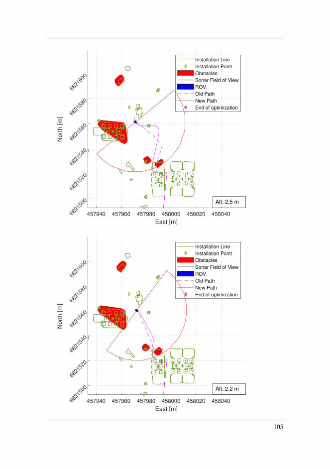
457940 457960 457980 458000 458020 458040

East [m]

6821

500

6821

520

6821

540

6821

560

6821

580

6821

600

No

rth

[m

]Installation Line

Installation Point

Obstacles

Sonar Field of View

ROV

Old Path

New Path

End of optimization

Alt: 2.5 m

457940 457960 457980 458000 458020 458040

East [m]

6821

500

6821

520

6821

540

6821

560

6821

580

6821

600

No

rth

[m

]

Installation Line

Installation Point

Obstacles

Sonar Field of View

ROV

Old Path

New Path

End of optimization

Alt: 2.2 m

105

457940 457960 457980 458000 458020 458040

East [m]

6821

500

6821

520

6821

540

6821

560

6821

580

6821

600

No

rth

[m

]Installation Line

Installation Point

Obstacles

Sonar Field of View

ROV

Old Path

New Path

End of optimization

Alt: 2.6 m

457940 457960 457980 458000 458020 458040

East [m]

6821

500

6821

520

6821

540

6821

560

6821

580

6821

600

No

rth

[m

]

Installation Line

Installation Point

Obstacles

Sonar Field of View

ROV

Old Path

New Path

End of optimization

Alt: 2.5 m

106

457940 457960 457980 458000 458020 458040

East [m]

6821

500

6821

520

6821

540

6821

560

6821

580

6821

600

No

rth

[m

]Installation Line

Installation Point

Obstacles

Sonar Field of View

ROV

Old Path

New Path

End of optimization

Alt: 2.2 m

457940 457960 457980 458000 458020 458040

East [m]

6821

500

6821

520

6821

540

6821

560

6821

580

6821

600

No

rth

[m

]

Installation Line

Installation Point

Obstacles

Sonar Field of View

ROV

Old Path

New Path

End of optimization

Alt: 2.2 m

107

457940 457960 457980 458000 458020 458040

East [m]

6821

500

6821

520

6821

540

6821

560

6821

580

6821

600

No

rth

[m

]Installation Line

Installation Point

Obstacles

Sonar Field of View

ROV

Old Path

New Path

End of optimization

Alt: 1.7 m

108

Appendix CList of Electronic Attachments

C.1 Attachments delivered in DAIMThe attached files delivered electronically in DAIM is listed here.

• A video describing the work done in the thesis was made as a mandatory assignment.

• PDF-version of abstract for paper contribution to 2018 IEEE OES Autonomous Un-derwater Vehicle Symposium. The abstract is an A4-document, which means that itcan be difficult to read in the B5-format.

C.2 Source codeThe source code developed in the project is available at https://github.com/orjan1992/pySonar.

109

https://github.com/orjan1992/pySonar

https://github.com/orjan1992/pySonar

Development of an Obstacle Detection and Avoidance System ...

Documents

Transcript of Development of an Obstacle Detection and Avoidance System ...