The Organized Melee: Emergence of Collective Behavior inConcentrated Suspensions of Swimming Bacteria and

Associated Phenomena

Item type text; Electronic Dissertation

Authors Cisneros, Luis

Publisher The University of Arizona.

Rights Copyright © is held by the author. Digital access to thismaterial is made possible by the University Libraries,University of Arizona. Further transmission, reproductionor presentation (such as public display or performance) ofprotected items is prohibited except with permission of theauthor.

Downloaded 14-Mar-2016 13:19:48

Link to item http://hdl.handle.net/10150/195513

THE ORGANIZED MELEE

EMERGENCE OF COLLECTIVE BEHAVIOR IN CONCENTRATEDSUSPENSIONS OF SWIMMING BACTERIA AND ASSOCIATED

PHENOMENA

by

Luis Cisneros Salerno

A Dissertation Submitted to the Faculty of the

DEPARTMENT OF PHYSICS

In Partial Fulfillment of the RequirementsFor the Degree of

DOCTOR OF PHILOSOPHY

In the Graduate College

THE UNIVERSITY OF ARIZONA

2008

2

THE UNIVERSITY OF ARIZONA

GRADUATE COLLEGE

As members of the Dissertation Committee, we certify that we have read the disserta-

tion prepared by Luis Cisneros Salerno entitled The Organized Melee, Emergence of

Collective Behavior in Concentrated Suspensions of Swimming Bacteria and Associated

Phenomena and recommend that it be accepted as fulfilling the dissertation requirement

for the Degree of Doctor of Philosophy

Raymond Goldstein Date: 12/04/2008

John Kessler Date: 12/04/2008

Dimitrios Psaltis Date: 12/04/2008

Koen Visscher Date: 12/04/2008

Alex Cronin Date: 12/04/2008

Final approval and acceptance of this dissertation is contingent upon the candidate’s

submission of the final copies of the dissertation to the Graduate College.

I hereby certify that I have read this dissertation prepared under my direction and

recommend that it be accepted as fulfilling the dissertation requirement.

Dissertation Director : Raymond Goldstein Date: 12/04/2008

Dissertation Director : John Kessler Date: 12/04/2008

3

STATEMENT BY AUTHOR

This dissertation has been submitted in partial fulfillment of requirements for an advanceddegree at The University of Arizona and is deposited in the University Library to be madeavailable to borrowers under rules of the Library.

Brief quotations from this dissertation are allowable without special permission, providedthat accurate acknowledgment of source is made. Requests for permission for extendedquotation from or reproduction of this manuscript in whole or in part may be granted bythe head of the major department or the Dean of the Graduate College when in his or herjudgment the proposed use of the material is in the interests of scholarship. In all otherinstances, however, permission must be obtained from the author.

SIGNED: Luis Cisneros Salerno

4

ACKNOWLEDGEMENTS

I am grateful to many ones.

First, to my family in Venezuela. I will never have enough words to express it.

To Krisna Ruette, for her presence and company during much of this journey, for

being the reason of so many good things in my life.

To my good friends and fellow researchers Chris Dombrowski, Sujoy Ganguly, Idan

Tuval and Martin A. Bees. They were all constant sources of support in many different

fronts, from the hard work in the lab to the happy hours and the laughter. Many thanks.

I’m also grateful to my adviser Raymond Goldstein for his tutoring. His vision and

commitment to science are certainly an inspiration to me. To John Kessler for being a

mentor in so many ways. With his caring guidance he truly showed me the way. I am

honored that I had the opportunity to learn so much from him.

To my dear friends, very specially Justine Pechuzal for giving me solace during really

hard times. To Maite Guardiola, for being there always. To Herman Uys, Pascal Herzer,

Aleix Serrat and Nick Erhardt, my brothers and buddies in all circumstances. And to all

those many more that comprise my climbing family in Tucson. Thanks for sharing with

me the passion for the outdoors. Thanks for being part of it.

Finally, in the words of Julieta Parra:

“Gracias a la vida que me ha dado tanto”

5

... to Josechu .

6

TABLE OF CONTENTS

LIST OF FIGURES . . . . . . . . . . . . . . . . . . . . . . . . . . . . . . . . . 8

ABSTRACT . . . . . . . . . . . . . . . . . . . . . . . . . . . . . . . . . . . . . 15

CHAPTER 1 INTRODUCTION . . . . . . . . . . . . . . . . . . . . . . . . . 161.1 The Subject of Study: Bacillus subtilis . . . . . . . . . . . . . . . . . . 161.2 Hydrodynamics of Self Propelled Particles . . . . . . . . . . . . . . . . . 22

1.2.1 The Stokes Flow . . . . . . . . . . . . . . . . . . . . . . . . . . 221.2.2 Self Propulsion . . . . . . . . . . . . . . . . . . . . . . . . . . . 26

1.3 Bioconvection . . . . . . . . . . . . . . . . . . . . . . . . . . . . . . . . 301.4 Flocking Phenomena . . . . . . . . . . . . . . . . . . . . . . . . . . . . 311.5 Biofilms . . . . . . . . . . . . . . . . . . . . . . . . . . . . . . . . . . . 331.6 Dissertation Format . . . . . . . . . . . . . . . . . . . . . . . . . . . . . 34

CHAPTER 2 PRESENT STUDY . . . . . . . . . . . . . . . . . . . . . . . . . 362.1 Growing and imaging Bacillus subtilis . . . . . . . . . . . . . . . . . . . 362.2 Particle Imaging Velocimetry (PIV) . . . . . . . . . . . . . . . . . . . . 372.3 The Chemotactic Boycott Effect: gravity mediated collective behavior . . 392.4 Collective Behavior (independent of gravity) . . . . . . . . . . . . . . . . 46

2.4.1 The Zooming BioNematic (ZBN) phase . . . . . . . . . . . . . . 462.4.2 Reversal of Bacterial Locomotion . . . . . . . . . . . . . . . . . 502.4.3 Up swimming . . . . . . . . . . . . . . . . . . . . . . . . . . . . 522.4.4 Coherence Order Parameter as a measure of ZBN . . . . . . . . . 522.4.5 Modeling ZBN . . . . . . . . . . . . . . . . . . . . . . . . . . . 54

2.5 Discussion on Group Hydrodynamics . . . . . . . . . . . . . . . . . . . 562.6 Bipolar arrangements of flagella in cells near solid boundaries . . . . . . 58

REFERENCES . . . . . . . . . . . . . . . . . . . . . . . . . . . . . . . . . . . . 61

APPENDIX A SELF-CONCENTRATION AND LARGE-SCALE COHER-ENCE IN BACTERIAL DYNAMICS . . . . . . . . . . . . . . . . . . . . . 69References . . . . . . . . . . . . . . . . . . . . . . . . . . . . . . . . . . . . . 80

APPENDIX B BACTERIAL SWIMMING AND OXYGEN TRANSPORTNEAR CONTACT LINES . . . . . . . . . . . . . . . . . . . . . . . . . . . . 82B.1 Introduction . . . . . . . . . . . . . . . . . . . . . . . . . . . . . . . . . 84

TABLE OF CONTENTS – Continued

7

B.2 Materials and Methods . . . . . . . . . . . . . . . . . . . . . . . . . . . 85B.3 Results . . . . . . . . . . . . . . . . . . . . . . . . . . . . . . . . . . . . 87B.4 Mathematical Model . . . . . . . . . . . . . . . . . . . . . . . . . . . . 88B.5 Comparison With Experiment . . . . . . . . . . . . . . . . . . . . . . . 90B.6 Chemotactic Singularity . . . . . . . . . . . . . . . . . . . . . . . . . . 93B.7 Conclusions . . . . . . . . . . . . . . . . . . . . . . . . . . . . . . . . . 96B.8 Appendix . . . . . . . . . . . . . . . . . . . . . . . . . . . . . . . . . . 97B.9 References . . . . . . . . . . . . . . . . . . . . . . . . . . . . . . . . . . 98

APPENDIX C REVERSAL OF BACTERIAL LOCOMOTION AT AN OB-STACLE . . . . . . . . . . . . . . . . . . . . . . . . . . . . . . . . . . . . . 100References . . . . . . . . . . . . . . . . . . . . . . . . . . . . . . . . . . . . . 110

APPENDIX D FLUID DYNAMICS OF SELF-PROPELLED MICRO-ORGANISMS, FROM INDIVIDUAL TO CONCENTRATED POPULA-TIONS . . . . . . . . . . . . . . . . . . . . . . . . . . . . . . . . . . . . . . 112D.1 Introduction . . . . . . . . . . . . . . . . . . . . . . . . . . . . . . . . . 114D.2 Collective Phenomena: The Zooming BioNematic (ZBN) . . . . . . . . . 119D.3 Coherence of polar and angular order: a novel use of PIV . . . . . . . . . 121D.4 Recruiting into ZBN domains . . . . . . . . . . . . . . . . . . . . . . . . 130D.5 Modeling self-propelled microorganisms . . . . . . . . . . . . . . . . . . 132D.6 Flows and Forces . . . . . . . . . . . . . . . . . . . . . . . . . . . . . . 134D.7 Turbulence at Re 1? . . . . . . . . . . . . . . . . . . . . . . . . . . . 142D.8 Discussion . . . . . . . . . . . . . . . . . . . . . . . . . . . . . . . . . . 146D.9 Acknowledgements . . . . . . . . . . . . . . . . . . . . . . . . . . . . . 148D.10 References . . . . . . . . . . . . . . . . . . . . . . . . . . . . . . . . . . 148

APPENDIX E UNEXPECTED BIPOLAR FLAGELLAR ARRANGEMENTSAND LONG-RANGE FLOWS DRIVEN BY BACTERIA NEAR SOLIDBOUNDARIES . . . . . . . . . . . . . . . . . . . . . . . . . . . . . . . . . . 154E.1 Introduction . . . . . . . . . . . . . . . . . . . . . . . . . . . . . . . . . 156E.2 Materials and Methods . . . . . . . . . . . . . . . . . . . . . . . . . . . 156E.3 Experimental Results . . . . . . . . . . . . . . . . . . . . . . . . . . . . 157E.4 Numerical Simulations . . . . . . . . . . . . . . . . . . . . . . . . . . . 162E.5 Summary and Significance . . . . . . . . . . . . . . . . . . . . . . . . . 163E.6 Acknowledgments . . . . . . . . . . . . . . . . . . . . . . . . . . . . . 164E.7 References . . . . . . . . . . . . . . . . . . . . . . . . . . . . . . . . . . 164

8

LIST OF FIGURES

1.1 Typical flagellar configuration on a B. subtilis directed motion (“run”mode). The bundle in the back propels the cell in the direction depictedby the arrow. . . . . . . . . . . . . . . . . . . . . . . . . . . . . . . . . 18

1.2 Incoherent flagellar deployment, induced by reverse rotation of one orseveral motors, in a peritrichous bacterium (“tumble” mode). Each flag-ella exerts push forces as depicted. The effect on the cell is random reori-entation. . . . . . . . . . . . . . . . . . . . . . . . . . . . . . . . . . . 19

1.3 Flow around a “dumbbell” swimmer, modeled as a dipole force on thefluid. . . . . . . . . . . . . . . . . . . . . . . . . . . . . . . . . . . . . 28

2.1 Boycott effect of Precipitation: normal vs tilted conditions. In the firstcase precipitates move down (blue arrow) pulled by gravity and the fluidmust go through, encountering large resistance (red arrows). In the tiltedcase, the region under the left wall is depleted and the fluid can quicklyflow in it (large red arrow), forcing precipitates to move to the right anddown as indicated by blue arrows. This configuration offers less resis-tance to the motion of the fluid, inducing faster and more efficient precip-itation. . . . . . . . . . . . . . . . . . . . . . . . . . . . . . . . . . . . 40

2.2 Chemotactic Boycott effect: bioconvection on a flat Vs a slanted menis-cus. In the first case, a typical convection plume is depicted. Cells “pre-cipitate” in it and then swim up on the sides. In the second case, cellson the top (concentrated) layer are gravitationally pulled down to the left.Depletion zones are formed in the right hand side of convection plumes,creating regions of reduced resistance to the up-moving fluid. Meanwhilein the left hand side, up-going cells run into down-going cells. , but sincethe plume is much more concentrated, up-going cells are forced to moveto the left in average,. These conditions produce an overall turn-over ofthe system, or a net motion of cells down to the left. . . . . . . . . . . . 41

2.3 Self Concentration Mechanism for a sessile drop (a) and a hanging drop(b): (i) chemotaxis toward the surface (ii) formation of depletion zones(iii) gravitational effects concentrate cells on the edge for (a) and the but-ton for (b). . . . . . . . . . . . . . . . . . . . . . . . . . . . . . . . . . 42

LIST OF FIGURES – Continued

9

A.1 Bioconvection in a sessile drop of diameter 1 cm. Top: images 5 min-utes apart show the traveling-wave bio-Boycott convection that appearsfirst. Bottom: images 2 minutes apart show self-concentration seen fromabove, beginning as vertical plumes which migrate outward. . . . . . . . 72

A.2 Dark-field side views of self-concentrative flows between two coverslipsspaced 1 mm apart. (a) uniform initial concentration, (b) & (c) develop-ment of depletion layer as cells swim upward, (d)-(f) plumes carried tonose of drop, dragged by surface layer. Depletion and accumulation layerthicknesses l and d are shown. Scale bar is 1 mm. . . . . . . . . . . . . . 73

A.3 Bacterial “turbulence” in a sessile drop, viewed from below through thebottom of a petri dish. Gravity is perpendicular to the plane of the pic-ture, and the horizontal white line near top is the air-water-plastic contactline.The central fuzziness is due to collective motion, not quite capturedat the frame rate of 1/30 s. Scale bar is 35 µm. . . . . . . . . . . . . . . 75

A.4 Flows at the bottom of a pendant drop. Instantaneous bacterial swimmingvector field. Arrow at right denotes a speed of 35µm/s. . . . . . . . . . . 76

A.5 Correlation functions in a pendant drop. (a) Average spatial correlationI(r) (solid) along with several traces at particular times; (b) Average tem-poral correlation J(t) (solid) with two particular traces. . . . . . . . . . 79

B.1 (A) Apparatus for simultaneous darkfield and fluorescence imaging offluid drops. Laser (L), shutter (S), beam expander lenses (L1 & L2),dichroic beamsplitter (D), long-pass filter (LPF), fiber-optic ring light(RL), digital camera (C). Chamber has anti-reflection areas (AR) to re-duce glare and hydrophobic areas (H) to pin the drop. (B) Boundaryconditions and coordinates in the wedge, described in text. . . . . . . . . 86

B.2 Stages leading to self-concentration in a sessile drop, observed experi-mentally (left) and by numerical computations with the model describedin text (right). (A,A’) drop momentarily after placement in chamber.(B,B’) formation of depletion zone after 150 s, prior to appreciable fluidmotion, (C,C’) lateral migration of accumulation layer toward drop edgesand creation of vortex (shown in Fig. B.3), after 600 s. Color schemedescribes the rescaled bacteria concentration ρ. Scale bar is 0.5 mm. . . . 88

LIST OF FIGURES – Continued

10

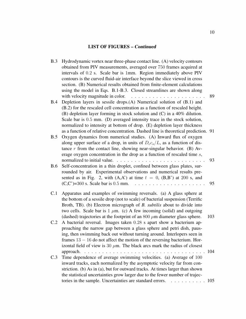
B.3 Hydrodynamic vortex near three-phase contact line. (A) velocity contoursobtained from PIV measurements, averaged over 750 frames acquired atintervals of 0.2 s. Scale bar is 1mm. Region immediately above PIVcontours is the curved fluid-air interface beyond the slice viewed in crosssection. (B) Numerical results obtained from finite-element calculationsusing the model in Eqs. B.1-B.3. Closed streamlines are shown alongwith velocity magnitude in color. . . . . . . . . . . . . . . . . . . . . . 89

B.4 Depletion layers in sessile drops.(A) Numerical solution of (B.1) and(B.2) for the rescaled cell concentration as a function of rescaled height.(B) depletion layer forming in stock solution and (C) in a 40% dilution.Scale bar is 0.5 mm. (D) averaged intensity trace in the stock solution,normalized to intensity at bottom of drop. (E) depletion layer thicknessas a function of relative concentration. Dashed line is theoretical prediction. 91

B.5 Oxygen dynamics from numerical studies. (A) Inward flux of oxygenalong upper surface of a drop, in units of Dccs/L, as a function of dis-tance r from the contact line, showing near-singular behavior. (B) Av-erage oxygen concentration in the drop as a function of rescaled time s,normalized to initial value. . . . . . . . . . . . . . . . . . . . . . . . . . 93

B.6 Self-concentration in a thin droplet, confined between glass plates, sur-rounded by air. Experimental observations and numerical results pre-sented as in Fig. 2, with (A,A’) at time t = 0, (B,B’) at 200 s, and(C,C’)=360 s. Scale bar is 0.5 mm. . . . . . . . . . . . . . . . . . . . . 95

C.1 Apparatus and examples of swimming reversals. (a) A glass sphere atthe bottom of a sessile drop (not to scale) of bacterial suspension (TerrificBroth, TB). (b) Electron micrograph of B. subtilis about to divide intotwo cells. Scale bar is 1 µm. (c) A few incoming (solid) and outgoing(dashed) trajectories at the footprint of an 800 µm diameter glass sphere. 103

C.2 A bacterial reversal. Images taken 0.28 s apart show a bacterium ap-proaching the narrow gap between a glass sphere and petri dish, paus-ing, then swimming back out without turning around. Interlopers seen inframes 13− 16 do not affect the motion of the reversing bacterium. Hor-izontal field of view is 30 µm. The black arcs mark the radius of closestapproach. . . . . . . . . . . . . . . . . . . . . . . . . . . . . . . . . . . 104

C.3 Time dependence of average swimming velocities. (a) Average of 100inward tracks, each normalized by the asymptotic velocity far from con-striction. (b) As in (a), but for outward tracks. At times larger than shownthe statistical uncertainties grow larger due to the fewer number of trajec-tories in the sample. Uncertainties are standard errors. . . . . . . . . . . 105

LIST OF FIGURES – Continued

11

C.4 Statistical results for 100 reversals. (a) Asymptotic outward vs. inwardvelocities, showing tight clustering around line of equalities (dashed).Uncertainties are standard errors. (b) Histogram of asymptotic velocityratio, with Gaussian fit. . . . . . . . . . . . . . . . . . . . . . . . . . . . 107

C.5 Statistical analysis of accelerations and decelerations during rever-sals.Histograms are for the time to decelerate to rest from a steady ve-locity far away from the wedge on an incoming trajectory, and the timeto accelerate from rest to the asymptotic velocity. The average decelera-tions/accelerations deduced from those times and velocities are shown. . 108

C.6 Statistical analysis of docking. Main figure shows histogram of dock-ing times with two binning choices. Insets show histograms of the angle∆θ between in and out trajectories, and a correlation plot between thoseangles and the docking times. Grey bars indicate maxima and minimaobserved within each bin, not statistical uncertainties. . . . . . . . . . . 109

D.1 Two Bacillus subtilis cells about to separate after cell division. Flagellacan be seen emerging from the body. Many of them have been broken dur-ing sample preparation for this transmission electron micrograph. Scalebar is 1 µm. . . . . . . . . . . . . . . . . . . . . . . . . . . . . . . . . . 115

D.2 B. subtilis cells concentrated at a sloping water/air interface. This menis-cus is produced by an air bubble in contact with the glass bottom of abacterial culture 3 mm deep. Near the top of the image bacteria have accu-mulated, forming a monolayer of cells perpendicular to the air/water/glasscontact line. Their lateral proximity and the adjacent surfaces immobilizethem. Toward the bottom of the image the fluid becomes progressivelydeeper; the swimming cells exhibit collective dynamics. The accumula-tion occurs because bacteria swim up the gradient of oxygen produced bytheir consumption and by diffusion from the air bubble. The black specsare spherical latex particles 2 µm in diameter. . . . . . . . . . . . . . . . 117

D.3 One randomly chosen instant of the bacterial swimming vector field esti-mated by PIV analysis. The arrow in the extreme lower left corner repre-sents a magnitude of 50 µm/sec. The turbulent appearance of the flow isevident here. . . . . . . . . . . . . . . . . . . . . . . . . . . . . . . . . . 118

D.4 Vorticity of the swimming velocity vector field shown in Fig. D.3. Colorbar indicates vorticity in sec−1. The graphing method discretizes vorticitylevels. . . . . . . . . . . . . . . . . . . . . . . . . . . . . . . . . . . . . 123

LIST OF FIGURES – Continued

12

D.5 Correlation functions from PIV analysis. (a) Spatial correlation functionof velocity Iv(r). Four examples, corresponding to four different times,are shown in colors; the black trace is the average over 1000 time realiza-tions. (b) Temporal correlation function of velocity Jv(t). Four examplescorresponding to four particular locations in the field of view are shownin colors. Black is the average over space. Plots of the vorticity spa-tial correlation IΩ(r) (c) and temporal correlation JΩ(t) (d) are shown forfour examples and, again in black, for the average. The oscillations in (c)correspond to alternation in the handedness of vorticity, as shown in Fig.D.4. Error bars in (a) and (b) indicate typical statistical uncertainties. . . . 124

D.6 Instantaneous coherence measure ΦR (Eq. D.5) for R = 1 (a), R = 2(b), R = 3 (c) and R = 4 (d). Axes and R are in PIV grid units (' 2µm each). Gray boxes in the lower left corner indicate, in each case, thesize and shape of the local averaging region used to estimate the measure.The color bar on the right indicates scale levels for values of ΦR. Theplotting method discretizes the countour levels. Note the near absence ofdark blue regions, which would indicate counterstreaming. . . . . . . . . 126

D.7 Histograms of the order parameter PR(t) for different values of R, theradius of the sampling area. Each one is generated with 1000 time steps.The skewing of the distributions becoming two-peaked at low R (highresolution) may indicate bimodality in the coherent phase, or an approxi-mately aligned transient phase. . . . . . . . . . . . . . . . . . . . . . . . 128

D.8 Area fraction of coherent regions distributed over the whole range of ΦR,averaged over 1000 time frames. Error bars indicate standard deviation ineach case. . . . . . . . . . . . . . . . . . . . . . . . . . . . . . . . . . . 129

D.9 Upswimming of bacteria in a shear flow. (a) Trajectory and orientationof a particular bacterial cell swimming in a flow, with velocity in the+y direction, and shear dVy/dz ∼ 1.0 sec−1. The small arrows showthe apparent swimming direction and the projection of the body size onthe plane of observation. (b) Trajectory of the velocity vectors in thelaboratory reference frame. Vector on right indicates fluid flow direction.The velocity of the bacterium can be transverse to its orientation. . . . . . 131

D.10 Diagram of a model swimmer and velocities VB and VT induced on thefluid, and the velocity vr of backward thrust of T out of B. . . . . . . . . 133

D.11 Perspective view of the sphere-stick model and the wall. . . . . . . . . . 135D.12 Plan and side views of velocity field around one organism near a wall.

The numbers indicate contours where the fluid speed is 5%, 10%, 25%,50%, 75% and 90% of the maximum speed. The infinite plane wall islocated at x = 0. . . . . . . . . . . . . . . . . . . . . . . . . . . . . . . 138

LIST OF FIGURES – Continued

13

D.13 Streamlines of the velocity field around one organism near a wall. Planand side views. . . . . . . . . . . . . . . . . . . . . . . . . . . . . . . . 138

D.14 Velocity field around two organisms near a wall and resultant forces ex-erted by each organism on the fluid in order to move parallel to the walland to each other. The forces are (2.72,−1.71,−0.22)|FB| (left organ-ism) and (2.72, 1.71,−0.22)|FB| (right organism), where FB is the dragon the sphere given by Eq. D.8. . . . . . . . . . . . . . . . . . . . . . . . 139

D.15 Velocity field around several organisms above a wall (top) and a closerview of the velocity between them (bottom). . . . . . . . . . . . . . . . . 140

D.16 Streamlines of the velocity field around several organisms near and abovea wall. The flow is the same as that in Fig. D.15. . . . . . . . . . . . . . . 141

D.17 Experimentally observed distribution of velocities as a function of theirangular spread. Within localities where angular spread is defined by Φ(Eq. D.5) with R = 2, velocity distributions are plotted as histograms forΦ2 > −1.0:black, Φ2 > 0.8:blue, Φ2 > 0.9:red and Φ2 > 0.95:green.These plots imply that improved collective co-directionality correlatewith higher mean speeds and displacement of lower thresholds of prob-ability to higher speeds. The black histogram includes measurements ofthe magnitudes of all velocities, codirectional or not; it is approximatelyMaxwellian. Its lower mean than the colored curves indicates that thecollective codirectional locomotion of cells is associated with speeds thatare on average higher than those for uncorrelated ones. . . . . . . . . . . 143

D.18 Schematic diagram of a phalanx, a coherent domain of cells swimming tothe left with collective velocity U. Arrows indicate direction of transversefluid flow as in Figs. D.15 and D.16 due to the collective motion insidethe domain. . . . . . . . . . . . . . . . . . . . . . . . . . . . . . . . . . 146

E.1 Stationary flow field (mean over 20 sec) surrounding a stuck cell and cor-responding streamlines computed from a regular grid of initial points.The arrow in the lower right corner represents 10 µm s−1. . . . . . . . . . 158

E.2 (a) perpendicular U⊥ and parallel U‖ components of velocity U as a func-tion of the distance along the cell axis for a stuck cell (black & blue,respectively) and for a free swimming cell (red & green). (b) as for a)except that data is for V and distance is transverse to the cell axis. (c)velocity components . . . . . . . . . . . . . . . . . . . . . . . . . . . . 159

LIST OF FIGURES – Continued

14

E.3 Simulation streamlines in a plane (neglecting flows into the page) abovean organism with two flagella close to an infinite wall. Inset: depictionof reduced model. Flagella are swept clockwise due to the asymmetry ofthe lower no-slip and upper (nominally) stress-free boundaries, and theresulting traction afforded the lower half of each flagellum. . . . . . . . . 160

E.4 Dynamic flowfield due to several stuck bacteria (both long and short) in athin layer of fluid. . . . . . . . . . . . . . . . . . . . . . . . . . . . . . . 162

15

ABSTRACT

Suspensions of the aerobic bacteria Bacilus subtilis develop patterns and flows from the

interplay of motility, chemotaxis and buoyancy. In sessile drops, such bioconvectively

driven flows carry plumes down the slanted meniscus and concentrate cells at the drop

edge, while in pendant drops such self-concentration occurs at the bottom. These dynam-

ics are explained quantitatively by a mathematical model consisting of oxygen diffusion

and consumption, chemotaxis, and viscous fluid dynamics. Concentrated regions in both

geometries comprise nearly close-packed populations, forming the collective “Zooming

BioNematic” (ZBN) phase. This state exhibits large-scale orientational coherence, anal-

ogous to the molecular alignment of nematic liquid crystals, coupled with remarkable

spatial and temporal correlations of velocity and vorticity, as measured by both novel

and standard applications of particle imaging velocimetry. To probe mechanisms lead-

ing to this phase, response of individual cells to steric stress was explored, finding that

they can reverse swimming direction at spatial constrictions without turning the cell body.

The consequences of this propensity to flip the flagella are quantified, showing that ”for-

wards” and ”backwards” motion are dynamically and morphologically indistinguishable.

Finally, experiments and mathematical modeling show that complex flows driven by pre-

viously unknown bipolar flagellar arrangements are induced when B. subtilis are confined

in a thin layer of fluid, between asymmetric boundaries. The resulting driven flow cir-

culates around the cell body ranging over several cell diameters, in contrast to the more

localized flows surrounding free swimmers. This discovery extends our knowledge of

the dynamic geometry of bacteria and their flagella, and reveals new mechanisms for

motility-associated molecular transport and intercellular communication.

16

CHAPTER 1

INTRODUCTION

The transport and dynamical properties of systems of interacting self-propelled particles

have generated much attention as a new direction of modern Statistical Mechanics. These

systems are evidently far from equilibrium and may exhibit phase transitions, cooperative

behavior and self organization [1, 2, 3].

Naturally, reaching out to biological problems is one of the main motivations for en-

gaging in this kind of research. Many similar processes comprise this category: flocking

of birds and fish, correlated motion of insects, ocean krill or pedestrians, traffic systems,

to name some. Furthermore, beautiful and striking examples are found in the realm of mi-

croscopic organisms. Bacteria, uni and multi cellular algae, spermatozoa and protists are

able to propel themselves in aqueous media. They exhibit diverse swimming strategies

and interactions with each other and their surrounding environment, generating a wide

spectrum of complex phenomena. These are not only interesting dynamical systems, they

are also of capital relevance to modern-day biological sciences and nanotechnology as

well as biomedical and industrial applications. Moreover, the fact that microorganisms

are simple life forms, experimentally easy to manage, make them perfect protagonists of

this story.

1.1 The Subject of Study: Bacillus subtilis

All the experimental research presented in this dissertation was conducted on Bacillus

subtilis, a species of aerobic non-pathogenic soil bacteria. They are rod shaped, with typ-

ical dimensions of about 4µm long and slightly less than 1µm diameter. A large portion

of the bio-hydrodynamical research found in the literature has also focused on other kinds

17

of morphologically similar bacteria, principally Escherichia coli [4] and Salmonella ty-

phymurium [5], but most aspects of the physics involved in all those are approximately

equivalent and fit for comparison [6, 7, 8].

In water, their standard habitat, these bacteria move by the use of their helical flagella,

stiff complex polymeric structures about 15µm long, 20nm in diameter and 4µm pitch

attached by flexible joints to motors embedded within the cell membrane. In the bacteria

mentioned here, flagella typically rotate at approximately 100 Hz, exerting drag forces on

the viscous fluid and producing propulsion [6, 9].

Now, the dynamics of an incompressible fluid of uniform density ρ is described by the

Navier-Stokes equation and the continuity equation:

ρ

(∂u

∂t+ u ·∇u

)= −∇p+ µ∇2u + f (1.1)

∇ · u = 0 (1.2)

where u is the fluid velocity, p is the pressure, f is the external force density field and µ

the viscosity of the fluid. This equation can be nondimensionalized by implementing:

u→ u

Vt→ t

(V

L

)x→ x

L

where V and L are the characteristic speed and length scales of the system. Introducing

here the Reynolds number, Re, as the ratio of kinetic energy density (or dynamic pressure)

ρV 2 and shear viscous stress µV/L [10],

Re =(ρV )

(µV/L)=ρV L

µ

we obtain eq. (1.1) in dimensionless form:

Re(∂u

∂t+ u ·∇u

)= −∇p′ + ∇2u + f ′ (1.3)

where p′ = p(L/µV ) and f ′ = f(ρL2/µV ).

An important aspect of the physics of the world where swimming microorganisms live

is that the associated Reynolds number is very small [11, 9]. A typical bacterium swims at

18

Figure 1.1: Typical flagellar configuration on a B. subtilis directed motion (“run” mode).The bundle in the back propels the cell in the direction depicted by the arrow.

a speed of∼ 20−40µm/s [12, 13]. For liquid water ρ = 1g/cm3 and µ = 10−2g/(cm ·s).

Therefore Re ∼ 10−4 − 10−5, which means that the system is dominated by viscosity: in

order to move an object at constant speed one must exert on it a constant force while all

the kinetic energy is readily dissipated by friction. Furthermore, in Re 1 regimes the

terminal velocity is reached in a very short time compared to other typical time scales.

This means that moving objects are steadily force-free: viscous drag forces balance any

other force on that may produce motion, like gravity for example. In this regime, the

inertial terms on the left hand side of equations (1.3) and (1.1) can be neglected, reducing

the equations of motion to the much simpler Stokes form [14, 15, 16]: ∇p = µ∇2u + f

∇ · u = 0(1.4)

For instance, an analogy for the propelling mechanism of flagellated bacteria is the

action of a corkscrew going through a solid volume; cells pretty much screw their flagella

into the viscous fluid to push or pull themselves against it1.

B. subtillis are peritrichously flagellated bacteria, i.e. flagella are randomly distributed

over the cell body. Hydrodynamic attraction between them cause the formation of a

propulsive bundle within which they co-rotate and produce directed cell motion [6, 7,

9, 5, 17, 18, 19]. This motion is generally along the direction of the cell body’s main axis,

such that the viscous drag is minimal. In this case the bundle is located on the back of the1This is really just a approximate analogy. Re is small but not zero, therefore the fluid is not really a

“solid” volume and is deformed under the action of the flagella. In this sense, there is a degree of “slipping”

on the action of the helical flagella rotation with respect to the advance of the cell. The swimming speed of

an individual is approximately 11% of the helix wave speed [8, 5]

19

Figure 1.2: Incoherent flagellar deployment, induced by reverse rotation of one or severalmotors, in a peritrichous bacterium (“tumble” mode). Each flagella exerts push forces asdepicted. The effect on the cell is random reorientation.

cell, opposite to the direction of motion [9] (see fig. 1.1)

Spontaneous reversal of rotation on one or several motors may occur as a function of

the surrounding concentration of chemicals. When this takes place the bundle itself could

come apart producing the cell to immediately stop and randomly reorient (see fig. 1.2).

For suspensions of the bacteria Escherichia coli it is commonly accepted that the com-

bination of these two modes of behavior, “run” and “tumble”, leads to a biased random

walk that permits cells to respond to chemical stimuli and have preferred motion along

chemical gradients. Such faculty of organism to react and move according to chemical

stimuli is termed Chemotaxis [20, 9, 4]. In this context, bacterial response to chemical

gradients consists of a simple sampling process. Certain chemical sensors in the mem-

brane can measure the amount of a relevant molecule at the cell’s location. Then, by

comparing samples at different times when the cell moves, the gradient of the concentra-

tion of such chemical in the direction of the motion can be estimated . If the direction of

motion is “not favorable”, the probability of tumbling events is increased, making the cell

likely to “choose” a different direction in a short time. On the other hand, the tumbling

probability is reduced under favorable conditions, producing longer straight motion in the

direction of the gradient. This simple set of rules can produce an average migration of

cells to places where the system comprises either higher or lower chemical concentra-

20

tions according to the case (i.e “positive” and “negative” chemotaxis) [9]. Observations

by J.O. Kessler et al [21] strongly suggest that this is not necessarily the only possible

model of chemotaxis. In particular, long cells of the bacteria B. subtilis, the ones studied

in this dissertation, don’t seem to have these two distinct modes of operation, but a rather

smooth reorientation mechanism, leading to curved continuous trajectories. This process

is probably associated with a larger rotational drag and/or a different scheme of flagellar

bundling-debuldling mechanics. These kind of details of bacterial dynamics require more

research and are not covered in this work.

Another important aspect that should be considered for the characterization of these

systems has to do with its transport properties. The idea can be readily introduced by

looking at the mass transport (advection-diffusion) equation for a chemical concentration

field c with uniform advection v

∂c

∂t= −∇ · J = −∇ · [−D∇c+ uc] (1.5)

which can be written in dimensionless form using: x→ x/L, t→ t(V/L) and u→ u/V

∂c

∂t=

1

Pe∇2c− u ·∇c (1.6)

where Pe is the Peclet number, a dimensionless quantity defined as Pe = TD/Tv. In

this relation Tv ∼ L/V is the advection time, associated with a characteristic length L

and speed V , and TD ∼ L2/D is the diffusion time, or the time taken by particles with

diffusively D to diffuse a distance L. Then

Pe =V L

D

gives the ratio of transport by Brownian motion versus transport by advection in the sys-

tem. The number Pe is generally defined for a particular type of particle diluted in the

fluid. A value Pe> 1 means that particles are moved mostly by the process characterized

by V (i.e. fluid flow or swimming) while Pe< 1 indicates that particles are transported

mostly by diffusion.

21

Since the typical velocities in a low Re system are small, diffusion could easily over-

come advection. Assuming that the local fluid speeds are directly related to the cell mo-

tion, it can be said that V ∼ 20µm/s. But fluid flows induced by objects moving at low

Re decay very fast with the distance; in the case of moving cells this scale is in the order

of only a few micrometers [22, 14, 23]. Now, given that D ∼ 3 × 10−5cm2/s for small

molecules like O22, then Pe∼ 10−2, showing that, in principle, advection is irrelevant

when compared to diffusion at this level3.

Because of the rapid spatial decay of the flow around cells, in a sufficiently diluted

bacterial suspensions the intercellular space has virtually no fluid flow induced by them,

and hence there is no possible large scale advective transport due only to bacterial swim-

ming. Yet at small scales, i.e. in the neighborhood of an individual, the very flagella which

propel the cell inevitably stir up the fluid by means of their high-speed rotation and the

bundling/unbundling process inducing mixing and modifying the local chemical gradient

[24, 25]. In this case, different natural speed could be more relevant than the swimming

speed, and conditions may turn out to be advective4. This fact has proven to be true for the

microscopic algae Volvox, where local fluid stirring allows the transport of nutrients into

large colonies of cells where diffusion is no longer a feasible delivery system [26, 27, 28].

By this virtue, if many cells are close to each other, and their behavior is coordinated in

the appropriate way, the collective hydrodynamics of the assembly could be cooperative

2The diffusivity of particles in a viscous fluid is given by the well known StokesEinstein Relation for a

sphere [10]:

D =kBT

6πµr(1.7)

where kB is the Boltzmann’s constant, T the temperature and r the size of the particle. Therefore, all other

things fixed, the Peclet number depends directly on the size of the particle.3For large molecules, like polysaccharides exuded by cells, D 10−5 and its Pe can easily be large.4In this case, if Pe > 1 then V L > D ∼ 10−5, this means that the corresponding Reynolds number

for such small scale flow will be Re = ρV L/µ > 10−1. So for some regime the Pe can be larger than

unity while Re is still smaller than one, but the assumption of very small Re will not necessarily be true

anymore. Then inertial effects, or at least the Ossen’s approximation, may have to be taken into account in

a hydrodynamical model of small scale mixing.

22

and greatly enhance mass transport at the level of the whole system. This could be cap-

tured in the dimensional analysis by the emergence of larger length scales (cell cluster

size for instance) while keeping “fast” speed scales associated with local mixing.

Fast enough delivery of chemicals, like nutrients, in a crowded populations of organ-

isms is clearly an important biological problem that could induce the kind of adaptations

yielding such coordinated behavior.

1.2 Hydrodynamics of Self Propelled Particles

1.2.1 The Stokes Flow

It was already stated that for Re 1 the dynamics of an incompressible fluid of uniform

density ρ is described by the Stokes equations (1.4).

In particular, the flow u induced by a solid sphere of radius a moving at velocity v in

a viscous fluid which is asymptotically at rest (i.e. u|r→∞ = 0), with no external forces

applied, is given by the well known Stokes creeping flow solution5. In polar coordinates:ur = v cos θ

(3a2r− a3

2r3

)uθ = v sin θ

(−3a

4r− a3

4r3

)p− po = −3

2µvar2

cos θ,

(1.8)

where θ is the axial angle with respect to v and po is the ambient pressure.

The viscous drag force exerted by the sphere to the fluid, necessary to generate such

a flow, can be calculated by evaluating the stress tensor σij = 2µEij at r = a, where

Eij =1

2

(∂ui∂xj

+∂uj∂xi

)5Oseen introduced a correction to these solutions by considering nonlinear convective terms of the form

(u·∇)u, which are related to accelerations due to spatial changes in the flow. These effects can be neglected

for very low Re [10]

23

is the strain-rate tensor. In particular, the ith component of the drag force per unit area is

given by

(fD)i = nj −pδij + σijr=a = −poni −3µvi2a

(1.9)

with n a unit vector along v. Then the total drag force can be integrated over the sphere’s

surface to give the well known Stokes Law

FD = −∮

fDdA = µ(6πa)v (1.10)

In more general terms, as a good approximation, the Stokes law gives the relation

between the speed and the drag force on an object moving in a very viscous medium:

FD = µCv (1.11)

where C is a tensor that depends on the geometry of the object. For example, the Slender-

Body Theory method [14, 22, 23] gives that for a long rigid ellipsoid, the drag coefficients

parallel and normal to the axis are:

C‖ ∼4πl

log(2l/a)− 1/2(1.12)

C⊥ ∼8πl

log(2l/a) + 1/2(1.13)

where l and a are the two semi-diameters of the ellipsoid, with a l.

Now, solutions to (1.4) corresponding to certain singular forms of f in an unbounded

flow are called fundamental solutions. Such forces are termed fundamental singularities

[29, 30] and correspond to Green’s functions of the linear differential equation (1.4). In

particular, a singular point force located in r0

f(r) = µ(8πα)δ(r− r0) (1.14)

characterized by a “strength vector” α is called a Stokeslet [29]; the corresponding solu-

tion to (1.4) is given by

u(r, r0) =α

r′+

(α · r′)r′

r′3(1.15)

24

where r′ = r− r0.

The long range fundamental flow field decays as r−1. Also, the general solution to the

inhomogeneous Stokes equation with arbitrary force density f(r) can be written as

u(r) =1

µ(8πα)

∫f(r′) · u(r− r′)dr′. (1.16)

And the total force exerted by a stokeslet on a given volume of fluid is determined by

FV =

∫V

fdV = µ(8πα) (1.17)

which can be compared with the Stokes’ law (1.10) by taking

α =3

4av (1.18)

Simple substitution of this term in (1.15) gives exactly the leading terms (O(r−1)) in (1.9),

indicating that in the far field, a sphere can be approximated by a stokeslet.

The linearity of the Stokes equations implies that the superposition of solutions is also

a solution. In particular, a linear superposition of stokeslets centered on a set of points

rifS = µ(8π)

∑αiδ(r− ri) (1.19)

can be used to enforce non-slip boundary conditions in those points. In other words,

to prescribe flow velocities vi in the set of points ri, relation (1.18) can be used to

determine the force strength of stokeslets centered in each of them, and the flow anywhere

else is given by:

u(r) =∑

u(r− ri) (1.20)

This is called the Singularities Method. In this way, fundamental forces can be used in

a similar way as point charges in electrostatics. The drag and field due to any object mov-

ing with respect to the fluid can be estimated by integrating contributions of point forces

along its surface (and not its volume!). The Slender-Body Theory method, mentioned

above, is an elegant application of this method.

25

On the other hand, when all the details of the particular geometry of an object, ex-

cept its size, are lost in the far field, a stokeslet can be used as a singular approximation

to the drag force. But derivatives of any order of the field (1.15) are also solutions to

(1.4). Therefore more details can be introduced by the use of higher order singularities

which correspond to higher order terms in the formal multipole expansion of the arbitrary

solution.

Particles immersed in a fluid are able to excite long-range flows as they move, but

reciprocally, because they are suspended in the fluid, they will also move in response to

the flow induced by other particles. By generating and reacting to the fluid’s local veloc-

ity, particles experience hydrodynamical interactions with each other. Such interactions

introduce non linear terms and time dependency in the Stoke’s equations of the n-body

system yielding complex rheological behavior.

The first law of Faxen [15] provides a simple framework to relate an small particle’s

velocity wi to the forces and flows that it experiences6:

wi = u(ri) + vi = u(ri) +1

µC−1(F)i (1.21)

where u(ri) is the net fluid flow at the particle’s location ri. This term is given by a

relation of the form (1.20), which is a linear superposition of the flows induced by every

particle in the system. The term vi is the “relative velocity” of the particle with respect

to the net flow, and is determined by the force on the particle and the drag coefficients

according to (1.11). Analytical or numerical solutions for this n-body problem are only

known for very restricted cases in the context of Sedimentation Theory, where Fi =

mg, and its complexity increases very quickly with n; for example, for arbitrary initial

conditions, three particles are enough to produce chaotic dynamics [31, 32, 33].

Considering the case of self-propelled particles, the forces Fi are now drag terms as-

sociated to cell alignment and the propulsion mechanism. Thus, these forces have orienta-6There is a possible third term proportional to the size of the particle and to∇2u(r) which accounts for

a gradient of the pressure over the size of the particle which can produce a “lift” force. This term can be

ignored for objects that are sufficiently small with respect to the length scales of the flow L ≈ µ/(V ρ).

26

tions given by the swimming speed of the cells, that not only point in arbitrary directions

to but have a dynamical behavior in itself. Reorientation dynamics is determined by the

balance of viscous and external torques on the cell body [34, 35]. Therefore, in the same

way as the flow advects the cells suspended in the fluid, as prescribed by (1.21), other

topological effects, like the vorticity ω and the strain-rate E, rotate and reorient them.

These hydrodynamical effects are particularly important for elongated organisms, like

bacteria, and the complexities of the hydrodynamical interaction picture given by them

are quite evident.

On the other hand, more details about the physics of self propulsion must be observed.

1.2.2 Self Propulsion

The distinctive aspect of a self propelled object is that is able to transform internal energy

into motion. This is usually done by means of some traction appendage, like legs, fins,

cilia or flagella, or by means of some other form of shape shifting mechanism, like a

full body deformation. In the case of swimming microorganisms, they exert local forces

over the surrounding viscous fluid in order to push (or pull) themselves through. Now,

given that the Stokes equations are linear and time reversible, an average displacement

of the cell can only be achieved if the propelling mechanism is nonreciprocal, breaking

the time reversal symmetry. This principle is formulated as The Scallop Theorem [11].

This theorem shows, as a prototypical example, that even though a reciprocal opening

and closing of the shell of a scallop produce the corresponding back and forth motions

with respect to the fluid, it does not produce net propulsion after each cycle is completed

because such translations are complementary when Re 1. A rotating flagella is a good

example of a simple biological solution to this problem, since the rotation of a structure

with a given “handness” (like helix chirality) is nonreciprocal.

Ignoring the details of how the forces are actually exerted on the fluid, a stokeslet can

be considered as a natural first order description of the fluid flow produced by a small self

propelled particle, as is generally done in sedimentation problems. But some care have to

27

be taken to simultaneously include the local force due to the propeller and the force due

to viscous drag. In the realm of motion governed by the Stokes equation, the viscous drag

always oppose the motion, and therefore, any moving object is indeed force-free at all

times. Trying to describe a swimmer by a point force very soon leads an inconsistency. A

sedimenting particle is in equilibrium because the external force (i.e. gravity) is canceled

by the the opposing drag. But this external force acts only on the particle and not on the

fluid7. Then, the only force on the fluid is given by FD(r), which is the reaction force to

the drag on the particle. In the case of a self propelled particle, the “push” exerted by the

propeller on the fluid is a local force Fm(r). Also, if motion is produced, there is drag

opposing it. Then the force balance on the fluid gives

FD(r) + Fm(r) = 0

since these are the same forces on the cell body, which is force-free. Therefore there is no

net force over the fluid. This is a static situation that can not produce any motion, yielding

a contradiction.

If the particle is moving, it must produce a flow field and some force has to be locally

exerted over the fluid. But there are no more forces in the system, and if they do not

cancel each other, the particle would not be in equilibrium, breaking the rules of Stokes

motion. Then, how can a particle self-propel in a very viscous fluid?

The simplest model to accommodate the induction of a fluid flow with force-free

structures is the use of a dipole force [36, 37, 38]. Consider the swimmer to be a thin rod

of length L with opposite point forces of equal magnitude f on its ends. The back force

pushes fluid backward, by means of the propeller, and the front force pushes fluid forward

due to viscous drag.

This model is equivalent to a dumbbell-shaped swimmer, i.e. two identical spheres at

a constant distance. This is the simplest model that captures the leading order far-field

effects of the hydrodynamics of low Re swimmers without specifying details about their

7Assuming of course that the fluid is asymptotically steady.

28

Figure 1.3: Flow around a “dumbbell” swimmer, modeled as a dipole force on the fluid.

shape or its mechanism of propulsion [37] (see figure 1.3).

If all the drag on the swimmer is concentrated on the two spheres and the propulsion

is given by a force Fm exerted by a “phantom” flagellum over the tail in the direction of

the axis n. The force balance on the cell body giveFm − Fc − FD = 0

Fc − FD = 0

(1.22)

where the first equation is for the tail and the second one is for head.

The force Fc is an internal constraint that keeps together structure of the cell. The

drag force is FD = µCv (C = 6πa for spheres) and opposes the motion. Solving this

simple relations yields Fc = FD and Fm = 2FD. As expected, the propeller must exerts

a force that is equal and opposite to the total drag over the cell. On the other hand, the

force balance over the fluid is represented on each sphere as Fh and Ft. For the head we

have a strength given by the drag in the usual manner

Fh = FD = µCv

29

and for the tail we have a superposition of drag and push

Ft = FD − Fm = −µCv

Therefore, the forces on the fluid are given by a dipole force, also termed “stresslet”.

An stresslet is a second order fundamental solution to the Stokes’ equation (1.4), it in-

duces a local flow field in the fluid and is force-free. Now, the introduction of a phantom

flagella simplifies matters, encapsulating the mechanism of propulsion of the swimmer in

some kind of mysterious external-local force that pushes the swimmer. By this mean, the

direction of motion, for distance, is assumed ad hoc.

A more realistic model was proposed originally by John Kessler [21]. Consider two

bodies of different size that move with respect to each other. The idea of two opposing

local forces is conserved, but now they represent motions for two parts of the cell. The

head stands for the actual body of a microorganism and the tail depicts the hydrodynam-

ical effect of flagellum. In reality, the continuous rotation of a helical flagella produces

motion by drag [6, 24, 9]. But this process could be pictured as a big sphere (body) push-

ing against a small sphere (flagella) in order to produce that drag and move in the opposite

direction. Since rotation is a continuous process, this is a virtual motion representing the

instantaneous effect of the flagellar push. Since the virtual push is always in the same

direction (no retraction is considered), this process breaks the time inversion symmetry of

the Stokes equations.

Let vb and vf respectively be the speeds of the body and the flagella with respect to the

fluid pointing in opposite directions. And let Cb and Cf be given by their corresponding

sizes. The balance of forces over the fluid Fb = Ff gives

Cbvb = Cfvf (1.23)

since the only forces are the ones given by Stokes drag on each sphere. On the other hand,

if w is the “relative instantaneous speed” between body and flagella

vf = w − vb (1.24)

30

Putting (1.23) and (1.24) together, we obtain thatvb =

Cf

Cf +Cbw

vf = Cb

Cf +Cbw

(1.25)

where all the terms in the right hand side are parameters of the model.

This scheme is more illustrative about the details of the swimming mechanism. Partic-

ularly, the asymmetry on the flow field introduced by the explicit difference in velocities

of body and flagella will determine the direction of motion in spite of the force balance.

But since the stokeslets involved are still equal in strength, the long-range effects are topo-

logically identical to the field produced by a dumbbell model. More elaborated models

for self propelled motion can be develop based on these basic principles [39? , 40, 41]

1.3 Bioconvection

In a given bacterial suspension, the combination of chemotaxis, consumption of oxygen

by cells and its replenishment from the fluid-air interface can create striking hydrody-

namic flows.

For instance, in a shallow concentrated suspension of initially uniformly distributed

cells, the organisms quickly consume the dissolved oxygen, swim up the developing in-

ward gradient of diffusing oxygen and accumulate under the air interface forming a dense

layer. But bacteria are approximately 10% denser than water, therefore this stratification

is buoyantly unstable and evolve in the manner of a Rayleigh-Taylor instability. This

phenomenon is called “Bioconvection”. It manifests in the form of spacial-temporal vari-

ations of the concentration of organisms, coupled with convection of the fluid where they

live. With a horizontal meniscus, plumes, rolls, and other complex patterns take on a

variety of forms much richer than in the familiar thermal convection [35, 42, 12]. Such

convective dynamics can also occur with swimming cells of algae induced by swimming

toward the light or against gravity.

31

A continuum model for bioconvection requires a set of coupled differential equations

including the Navier-Stokes equation and continuity equation for the fluid, a reaction-

difussion equation for the concentration of oxygen (which includes a consumption term)

and an equation for the conservation of cells, including a model for chemotaxis [35, 42,

12, 13]. A more detailed explanation of such a model will be given in the next chapter.

On a sessile drop geometry, the meniscus curves down to the liquid-solid-air interface.

In this case the heavy accumulation layer in the top is pulled by gravity and “slides” along

the slopping meniscus towards the contact line simultaneously breaking up into plumes

that fall into the drop. This process produce a high concentration of cells near the edge

of the drop giving the conditions that support the collective dynamics which is the main

subject of this dissertation.

1.4 Flocking Phenomena

Many organisms in nature are able to move coherently in large groups. Such organized

behavior is observed in flocks of birds and schools of fish, for example. But despite the

widespread nature of this phenomenon, is only recently that many of its characterizing

features have been identified.

Vicsek [1] first recognized that systems of self propelled objects can be categorized

as non equilibrium dynamical systems, with many degrees of freedom, capable to have

phase transitions into self organized behavior. This work presents a discrete model with

simple step rules, where each particle determines the new direction of motion on each

time step by averaging the directions of its neighbors. A level of noise is additionally

introduced in order to account for randomization processes. This simple model proved to

be enough to exhibit transition to an ordered phase. Later Tuner and Tu [2] pointed out

that this is equivalent to a XY Heisenberg ferromagnetic model, and proceeded to propose

a continuous version of the model. In both cases, the organized behavior is defined as a

global “polarization”, meaning that, in average, all organisms move approximately in the

same direction.

32

There has been much interest in this topic ever since, and many different variations

had been suggested [43, 44, 45, 46, 47, 48, 49, 37, 3, 50, 51, 52, 53, 39, 54, 40, 55, 56].

Most notable are works by Ramaswamy’s group [57, 58, 59, 36], who first associated

this problem with certain aspects from Nematic Liquid Crystals phenomenology and in-

troduced a model containing hydrodynamic equations. This approach is more adequate

for describing organisms suspended in a fluid medium. Linearization of these equations

proved that purely nematic (polarized) order in a suspension of self-propelled particles is

always destabilized at small wave numbers as a consequence of the interplay of hydrody-

namic flow with fluctuations in the ordering direction and cell concentration. Then much

care must be taken in order to claim the existence of a stable, totally coherent, motion

phase for these systems.

In spite of the great amount of work that has been published addressing these issues,

there is still a surprising lack of experimental data. In this dissertation I will present

mostly experimental results and my working progress directed on the characterization and

understanding the nature of this phenomenon for the particular case of microorganisms.

While is obvious that a similarity group comprising all flocking phenomena exist, there

are also very important differences between particular cases. Specifically, low Re systems

rely heavily on Stokes’ hydrodynamics, while flocks of birds, fish or cars are ruled by

completely different physical interactions.

Concentrated suspensions of bacteria produce a striking non trivial collective dynam-

ics that consists of the partition of the system into organized regions, within which the

cells move coherently [60, 61]. These domains manifest in the form of eddies, or vor-

texes, that seem to have characteristic size scale and life time after which they disperse

or fold over into the rest of the system. Vortices are formed and destroyed everywhere

continually in an apparent spacial-temporal chaos similar to a turbulent behavior, quite

surprising for a system with very low Reynolds number8.

8Many body interactions and moving boundary conditions can introduce nonlinearities and time depen-

dency in the Stokes system leading to chaotic dynamics.

33

Any sensible theory that explains bacterial self organization must include some com-

bination of steric repulsion and close-field hydrodynamic interactions because the spacing

conditions in this regime are close-packed. But since all the simplifications that are usu-

ally taken in hydrodynamical interaction models are far-field approximations, this task is

still an open problem in many ways.

Also, as suggested before, flows generated cooperatively by flagella of individual or-

ganisms can drive significant advective transport of molecular solutes associated with

life-processes [26, 27, 28]. Without any doubt, the transport properties of a system of

cells engaged on a collective behavior affects their own conditions of living. Studies on

this subject have obvious implications on unveiling fundamental biology questions, like

the emergence of multicellular life and the origins of cellular differentiation, which are a

highly organized collective behaviors in themselves. Also the enhancement of transport of

solutes by a self-organized dynamics will certainly influence cell to cell communication

necessary for such processes as quorum sensing and subsequent biofilm formation.

1.5 Biofilms

Individual nomadic bacteria that encounter a surface under favorable conditions for

growth almost invariably undergo a lifestyle change, giving up their ability to swim and

settling down to establish a sedentary community [62, 63]. It is now commonly recog-

nized that the large majority of bacterial biomass in nature is found forming these kinds

of communities attached to surfaces, called biofilms, rather than dispersed and free swim-

ming in liquid media. Teeth plaque, the slippery coating on river stones and infected

wounds are examples of such ubiquitous communities. They are densely packed systems

where cells share secreted molecules, like enzymes and extracellular polymers. Such

polymers form an structural matrix where the cells are embedded providing rigidity and

physical robustness to the biofilm and protecting it from aggressive external agents, such

as dehydration, UV radiation, antibiotics, and predator grazing. At the same time, these

structures provide a substrate that facilitate cooperative enzymatic activity and cell-cell

34

signaling (quorum sensing) [62]. These systems may exhibit complex organization, where

different tasks are divided among the cells on sophisticated cooperative architectures, akin

to simple multicellular life forms.

Most microbial species can form biofilms, and there is growing evidence that there

are important physiological differences between free individuals and communal ones.

Expression of such differences is controlled by regulatory mechanisms that underlie the

switch between the two lifestyles.

Biofilms have a role in infectious diseases, antibiotic resistance and biofouling, among

many other things. It is also a collective phenomenon and its connection to other bio-fluid

dynamic processes discussed in this work have to be eventually addressed. In the context

of the present work, when a surface is close to a concentrated suspension of swimming

cells, collective phenomena can set the initial conditions on the formation of a bacterial

biofilm.

1.6 Dissertation Format

I have presented the relevant aspects on the physics of swimming bacteria and introduced

the collective behavior that they may exhibit when the cell number concentration is near

to close packed conditions. It seems natural to think that concentration is a “thermo-

dynamical variable” controlling this phase transition9. When cells are more and more

concentrated the average distance between them is smaller. At some critical distance they

start interacting appreciably with each other, either hydrodynamically or sterically, ex-

citing collective modes of organization that may to propagate, or scale, throughout the

system.

In what follows, experimental results are presented, along with some theoretical and

numerical analysis to support some conclusions. The main body of this thesis consist

of five appendices featuring my published work in this subject. All this research was

9The average bacterial swimming speed could probably be framed as a thermodynamical variable as

well.

35

carried out while working in Dr. Goldstein’s lab as part of my doctoral program under his

tutelage. It all involved wide-ranging cooperation, not only between different researchers

in this lab, but also from several other institutions.

The first , second and fourth appendices are articles focussed on large scale bacte-

rial dynamics, like chemotaxis and collective behavior. The other two present single cell

motility phenomena relevant to cell interactions with each other and the surrounding en-

vironment, which contribute to the understanding of the self organization process at the

cell level.

In the second chapter I summarize the most important results comprising these five

articles.

36

CHAPTER 2

PRESENT STUDY

The experimental and theoretical approach, results and conclusions of my research studies

are presented in detail in the papers appended at the end of this dissertation. This chapter

is a summary of the most important findings on those papers and, as such, it should be

read in conjunction with them.

The content of this chapter does not necessarily focus on each of those articles in-

dependently, but instead, follows a logical structure based on sub-subjects. In this way,

each section summarizes the finding on a different aspect of the collective dynamics of

bacteria, which may be covered in more than one paper. Each article will be appropriately

cited according to the context.

2.1 Growing and imaging Bacillus subtilis

Samples of B. subtilis (strain 1085B) are prepared by adding 1 ml of −20C stock1 to

50 ml of terrific broth (TB) (Ezmix Terrific Broth, Sigma; 47.6 g of broth mix and 8 ml

of glycerin in 1 liter of distilled water) and incubated for 18 hours in a shaker bath at

37C and 100 rpm. Then 1ml of bacteria suspension is mixed with 50ml of fresh TB and

incubated for another 5 hours. This preparation produce long (∼ 4 − 5µm) and motile

cells appropriate for experiments. The samples are then set in whatever particular geom-

etry is desired and observed under a microscope or any other optical setup for imaging.

Movies of the dynamics of the cells are taken with a digital camera and processed with a

commercial Particle-Imaging-Velocimetry (PIV) system.

1Stocks are prepared from spores inoculated on a 50-50 mix of TB medium and glycerin and then frozen.

37

2.2 Particle Imaging Velocimetry (PIV)

In order to generate experimental data from our experiments, is desirable to quantify the

motion of bacteria, or its surrounding fluid, based on recorded movies of the evolving

system. The digital Particle Imaging Velocimetry (PIV) method was employed to do this.

PIV is a measurement technique for obtaining instantaneous velocity fields from a

sequence of images of a fluid system [64, 65, 66]. The method consist of implementing

a pattern matching algorithm to measure the most probable displacement of small rectan-

gular regions from one frame to the next in the sequence. The algorithm does not require

the tracking of individual particles, but enough features are necessary in order to properly

carry out the image matching operation.

If the first sample region (i.e pixel gray scale values) at time step t is f(m,n) and the

second, at time step (t+ 1), is g(m,n) then

g(m,n) = [f(m,n)⊗ d(m,n)] + ξ(m,n)

=

[L∑k=1

L∑l=1

d(k −m, l − n)f(k, l)

]+ ξ(m,n) (2.1)

where d(m,n) is a spatial displacement function and the operation ⊗ denotes the spatial

convolution. Indices denote pixels and L is the pixel size of the field of view. The term

ξ(m,n) is an additive noise process accounting for “lost” particles (i.e. particles moving

out of the sampling region or out of the plane), non-uniformity of the flow inside the

sampling region or other sampling error effects.

Under ideal conditions, the displacement function is indeed the Dirac delta function

centered in (i, j),

d(m,n) ∼ δ(m− i, n− j)

which corresponds directly to an average displacement of the particles in the sampled

region. The points (m,n) and (i, j) are obviously the “initial” and “final” positions asso-

ciated to such a displacement.

38

The method of choice in finding the displacement function d(m,n) is the use of spatial

cross correlation function between regions f(m,n) and g(m,n)

φfg(m,n) =1

N

L∑k=1

L∑l=1

f(k, l)g(k +m, l + n) (2.2)

where the normalization constant is

N =L∑k=1

L∑l=1

f(k, l)L∑

m=1

L∑n=1

g(m,n)

A high cross correlation value is observed when images match with their correspond-

ing spatially shifted partners. Small correlation peaks may be observed when images of

different particles coincidentally match at different frames. The former is known as true

correlations while the latter is called random correlation. The highest peak in the correla-

tion landscape generated by (2.2) represents the best match between the functions f(m,n)

and g(m,n), and its location (i, j) corresponds to the location of the displacement delta

function δ(m− i, n− j).

In practice, Fast Fourier Transforms are generally used to calculate cross correlation

in an efficient way: rather than performing a sum over all elements of the sampled region,

the operation can be reduced to a complex conjugate multiplication of each corresponding

pair of Fourier coefficients.

The resulting set of coefficients are then inversely transformed to obtain the cross

correlation function φfg.

Once the highest peak in the two dimensional discrete landscape of correlation values

is found, a parabolic or exponential (Gaussian) curve fit gives its location with sub-pixel

accuracy.

Summarizing, digital image pairs are recorded at a fixed frame rate (∆t)−1 and opti-

mal displacements ∆r(i, j) of small regions are directly estimated to sub-pixel accuracy

by using the approximation d(i, j) ≈ δ(i− p, j − q), which gives

∆rx(i, j) = i− p (2.3)

∆ry(i, j) = j − q (2.4)

39

where p and q have real (subpixel) values. Then the corresponding local instantaneous

velocity value is obtained by

ut(i, j) =∆r(i, j)

∆t(2.5)

In this fashion, a two dimensional vector field is estimated from each pair of images.

A sequence of such fields gives a full discrete sample of the observed velocity field.

2.3 The Chemotactic Boycott Effect: gravity mediated collective behavior

As it was mentioned in the introduction, when the bioconvection process occurs on a

sessile drop, cells migrate upward forming an accumulation layer that slides down along

the sloping meniscus into the contact line, producing a high concentration of cells in that

region. Appendices A and B respectively present experimental and theoretical results on

this process. In what follows, I proceed to explain the experimental observations and the

most important aspects of the model.

Bacteria consume κo ∼ 106 oxygen molecules per second per cell [9]. The typ-

ical cell concentration in an incubated suspension (after five hours in shaker-bath) is

n ∼ 109 cells/cm3 and the saturation oxygen concentration is cs ∼ 1017molecules/cm3.

Under these circumstances, the oxygen is consumed in TC = cs/(κon) ∼ 100 seconds.

On the other hand, in a drop about h ∼ 10−1cm deep, oxygen repletion by diffusion from

the air/fluid boundary, with a diffusion constantDo ∼ 10−5cm2/s, happens in a time scale

of TD = h2/Do ∼ 103 seconds, which is 10 times slower. This gives a good sense of how

quickly consumption can generate a gradient of oxygen concentration in the system.

At the same time, chemotactic behavior make cells react to this gradient, producing

a flux towards the surface where more oxygen is diffusing into the system. In this initial

process, a sharply bounded depletion region is observed (see figure A.2), indicating that

for concentrations of oxygen under a certain critical value the cells considerably lose

motility and are no longer able to chemotax [12].

The cells that reach the slanted surface form an thick accumulation layer that is grav-

40

Figure 2.1: Boycott effect of Precipitation: normal vs tilted conditions. In the first caseprecipitates move down (blue arrow) pulled by gravity and the fluid must go through,encountering large resistance (red arrows). In the tilted case, the region under the leftwall is depleted and the fluid can quickly flow in it (large red arrow), forcing precipitatesto move to the right and down as indicated by blue arrows. This configuration offers lessresistance to the motion of the fluid, inducing faster and more efficient precipitation.

itationally pulled down the slopping meniscus. Because bacteria are denser than water,

this layer is also buoyantly unstable in the more horizontal part of the slope, forming

convection plumes that penetrate into the drop. The physics involved in the layer down-

sliding is similar to the Boycott effect [67, 68], which occurs when a container with fluid

and sedimenting particles is tilted from vertical. Settling depletes the fluid right under

the upper wall of the container, making it buoyant relative to nearby non-yet-depleted

fluid. The induced relative buoyancy creates a boundary flow that stirs the entire medium

accelerating the settling process (see figure 2.1).

In the chemotactic version, a sedimenting depletion region is formed next to precip-

itating convection plumes, forcing suspended cells to move towards to contact line. See

more details on figure 2.2.

These flows bring large number of cells to the contact line region, where a stable

vortex, axis parallel to the contact line, is formed by the combination of incompressibil-

41

Figure 2.2: Chemotactic Boycott effect: bioconvection on a flat Vs a slanted meniscus.In the first case, a typical convection plume is depicted. Cells “precipitate” in it andthen swim up on the sides. In the second case, cells on the top (concentrated) layer aregravitationally pulled down to the left. Depletion zones are formed in the right handside of convection plumes, creating regions of reduced resistance to the up-moving fluid.Meanwhile in the left hand side, up-going cells run into down-going cells. , but sincethe plume is much more concentrated, up-going cells are forced to move to the left inaverage,. These conditions produce an overall turn-over of the system, or a net motion ofcells down to the left.

42

Figure 2.3: Self Concentration Mechanism for a sessile drop (a) and a hanging drop(b): (i) chemotaxis toward the surface (ii) formation of depletion zones (iii) gravitationaleffects concentrate cells on the edge for (a) and the button for (b).

ity conditions and gravitational forcing. This vortex is similar to a convection roll and

entrains cells in the neighborhood.

If a pendant drop geometry is chosen instead, cells, still moving up the oxygen gradi-

ent, swimming to the air/fluid interface located under the drop, concentrate on it and slide

down to the bottom, where a large accumulation layer is formed but no recirculation is

observed (see figure 2.3).

Due to the absence of a contact line boundary, the self-concentration mechanism in

this geometry induces an accumulation region with a more isotropic dynamics than in the

sessile drop.

The self-concentration mechanism, the bioconvection process and chemotactic Boy-

cott effect can be described by a set of coupled partial differential equations for oxygen

concentration c, cell concentration n and fluid velocity u respectively (see Appendix B)

43

The flux of oxygen concentration c was already introduced in (1.5):

Jc = −Dc∇c+ uc (2.6)

where the first term is the transport by diffusion (Dc ∼ 10−5cm2/s), and the second

term is the transport given by fluid advection. The equation for c is a reaction-difussion

equation of the form:∂c

∂t= −∇ · Jc − nκcΘ(c− c∗) (2.7)

The last term is the consumption term: κ ∼ 106 molecules/s is the rate of consumption of

oxygen per cell and Θ(c − c∗) is the step function, which “turns off” the consumption if

c < c∗, the critical value of c bellow which cells stop functioning.

On the other hand, the flux of cells can be written as

Jn = −Dn∇n+ un+ [γΘ(c− c∗)∇c]n (2.8)

where n is the local concentration of cells. The factor Dn is the effective bacterial diffu-

sion, due to random motion, related to the typical cell swimming speed V ∼ 20−30µm/s

and the mean free time (time at which cells change direction) τ ∼ 1s by Dn ≈ V 2τ/3

[9], which gives

Dn ∼ 10−5 − 10−6cm2/s.

For this problem, this term is assumed to be uniform, so that ∇Dn = 0. This can be

expected to be true for diluted systems where cell interactions are not important. But for

concentrated systems this is not valid. In such a case the random motion, and hence the

cell diffusion, is strongly affected by the local concentration n and the fluid u induced by

the the cells.

The second term in (2.8) is the advection of cells by the fluid flow. The third term

is a model of chemotaxis. The part enclosed in brackets is a drift velocity, proportional

to ∇c, that induces migration of cells in the direction of the gradient. The constant

γ = Tn/cs = lvc/cs is a scaling factor, with cs ∼ 1017cm−3 the saturation concentration,

l the distance from the surface of the drop to the edge of the depletion zone, and vc the

44

chemotactic speed corresponding to Tn = 100 seconds, which is the time taken for cells

to climb the gradient and form the depletion zone2. The step function is introduced to

account for the effect of the motility cut-off in c < c∗. The dynamics of n is given by

∂n

∂t= −∇ · Jn (2.9)

Since the division time of bacteria is long (∼ 100 minutes), no cell multiplication is

considered in this model, and the total number os cells is conserved. Finally, the dynamics

of the fluid is described by the Navier-Stokes equation and the incompressibility condition

ρ

(∂u

∂t+ u ·∇u

)= −∇p+ µ∇2u−∆ρgz + ∇ ·Σ (2.10)

∇ · u ≈ 0 (2.11)

where

∆ρ = nVb(ρb − ρ) (2.12)

with ρb and Vb the density and volume of a single cell and gz the acceleration of gravity.

The term Σ is the bulk deviatoric stress tensor, which accounts for the effect that the cells

may have on the bulk fluid motion [34]. For a dilute system, the Boussinesq approxima-

tion can be adopted: the presence of cells in only accounted in the form of a negative

buoyant force [12, 13],

Equation (2.11) is only approximate because the system cells/fluid is really a two

phase system, where incompressibility is satisfied for the combination and not necessarily

for the velocity fields of each phase independently. In other words, because of the relative

motion between cells and fluid, volume is not precisely conserved in the usual manner.

But for small concentrations of microorganisms the relation (2.11) can be safely assumed.

2The notation in these estimations was changed with respect to the original article in Appendix B to

simplify the discussion. A more general definition for γ was used there, but ultimately estimated in an

equivalent form.

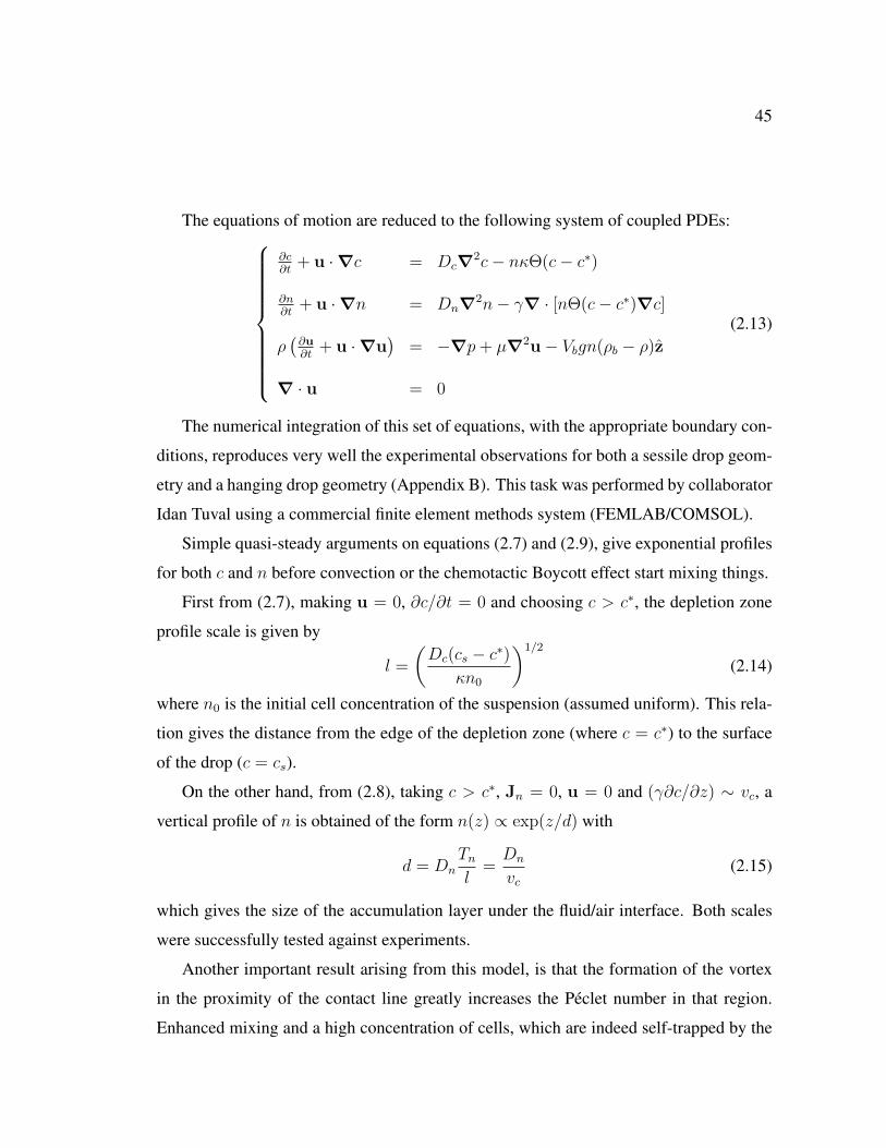
45

The equations of motion are reduced to the following system of coupled PDEs:

∂c∂t

+ u ·∇c = Dc∇2c− nκΘ(c− c∗)

∂n∂t

+ u ·∇n = Dn∇2n− γ∇ · [nΘ(c− c∗)∇c]

ρ(∂u∂t

+ u ·∇u)

= −∇p+ µ∇2u− Vbgn(ρb − ρ)z

∇ · u = 0

(2.13)

The numerical integration of this set of equations, with the appropriate boundary con-

ditions, reproduces very well the experimental observations for both a sessile drop geom-

etry and a hanging drop geometry (Appendix B). This task was performed by collaborator

Idan Tuval using a commercial finite element methods system (FEMLAB/COMSOL).

Simple quasi-steady arguments on equations (2.7) and (2.9), give exponential profiles

for both c and n before convection or the chemotactic Boycott effect start mixing things.

First from (2.7), making u = 0, ∂c/∂t = 0 and choosing c > c∗, the depletion zone

profile scale is given by

l =

(Dc(cs − c∗)

κn0

)1/2

(2.14)

where n0 is the initial cell concentration of the suspension (assumed uniform). This rela-

tion gives the distance from the edge of the depletion zone (where c = c∗) to the surface

of the drop (c = cs).

On the other hand, from (2.8), taking c > c∗, Jn = 0, u = 0 and (γ∂c/∂z) ∼ vc, a

vertical profile of n is obtained of the form n(z) ∝ exp(z/d) with

d = DnTnl

=Dn

vc(2.15)

which gives the size of the accumulation layer under the fluid/air interface. Both scales

were successfully tested against experiments.

Another important result arising from this model, is that the formation of the vortex

in the proximity of the contact line greatly increases the Peclet number in that region.

Enhanced mixing and a high concentration of cells, which are indeed self-trapped by the

46

vortex, produce an almost singular variation of the oxygen flux on the edge of the drop

and increase the overall oxygen uptake. In other words, chemotaxis, bioconvection, hy-

drodynamics and the particular boundary conditions at the edge of the drop work together

to “pump” oxygen into the system.

The self-concentration mechanism is a hydrodynamical phenomenon, and no cell-cell

signaling is needed. But the consequent enhanced mixing obviously affects the eventual

cell-cell communications, as well as the transport of nutrients or other chemicals across

the system, and may have an influence on other biological processes like quorum sensing

and biofilm formation. Meanwhile, it can lead to approximately closed-packed bacterial

concentrations, setting the conditions for the emergence of a chaotic collective dynamics,

as is reported in Appendix A

2.4 Collective Behavior (independent of gravity)

Nearly close-packed populations of Bacillus subtilis form a collective phase with large-

scale orientational coherence, instantaneously analogous to the molecular alignment of

nematic liquid crystals, and with the dynamical appearance of turbulence. A theory for

these observations was first conjectured in the article in Appendix A and developed further

on Appendix D. The phenomenon was first reported by Kessler et al [12, 69].

2.4.1 The Zooming BioNematic (ZBN) phase

Bacterial suspension samples are allowed to self-concentrate in either a sessile drop or a

hanging drop geometry. A microscope is used to perform magnified imaging (20x - 40x)

of the highly concentrated region. Under this setup, individual cells can be observed, but

the field of view is still 20 to 50 times larger that a single organism, enough to capture

large scale behavior in the system.

Movies are recorded using a digital video camera, PIV analysis is performed to esti-

47

mate the corresponding velocity fields and then statistically analyzed3. PIV measurements

are projections of the three-dimensional flow on the observation plane, but experimental

conditions in all the cases are restricted to thin layers. Under this circumstances, off the

plane motion along the perpendicular 3rd dimension should not play a big role in the

dynamics.

As it has been mentioned (§1.4), a dynamically coherent collective cell locomotion

develops on these samples. Correlated domains manifest as jets and surges, straddled

by vortices, that move around, fold over and are continuously created and destroyed in a

highly chaotic way. Remarkable spatial and temporal correlations of velocity and vorticity

are observed, indicating that the various swirls, vortices and jets have natural length and

time scales . To address these, time and space correlations were explicitly calculated for

the velocity field v(r, t) given by PIV:

Jv(x, t) =〈v(x, s+ t) · v(x, s)〉s − 〈v(x, s)〉2s

〈v2(x, s)〉s − 〈v(x, s)〉2s(2.16)

Iv(r, t) =〈v(x + r, t) · v(x, t)〉x,θ − 〈v(x, t)〉2x

〈v2(x, t)〉x − 〈v(x, t)〉2x(2.17)

These statistical measures are presented in figure A.5 and show that a typical scale of

a vortex is∼ 100 µm and typically exist for a second or two. The space correlation curves

display pronounced oscillation for particular time steps, reflecting the relative distance of

vortices at any given time. Meanwhile, the time correlations for particular spacial loca-

tions also have oscillations, demonstrating that a directional surge is followed by a return

flow. Such surges, and their shear field, organize eddies in a vortex street fashion. This

process can recruit local organisms into the rotating internally driven domains. The ob-

served transient large scale vortices and surges offers a good route to enhanced diffusion

since efficient transport can be established with the combination of circulation in vorti-

cal regions and ballistic motion in the surges. Similar results are presented in Appendix

D, but it is argued that, even though these curves predict characteristic lengths, they do

3The PIV analysis is done on the motion of cells and not on the fluid that surrounds them.

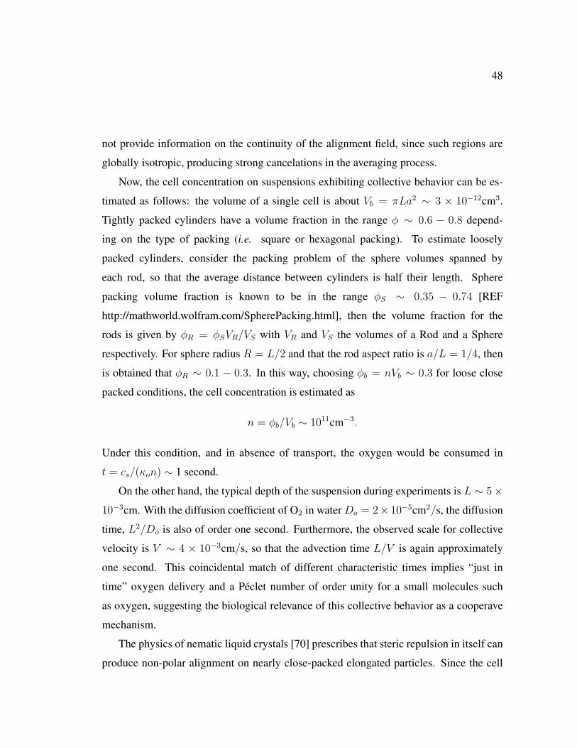
48

not provide information on the continuity of the alignment field, since such regions are

globally isotropic, producing strong cancelations in the averaging process.

Now, the cell concentration on suspensions exhibiting collective behavior can be es-

timated as follows: the volume of a single cell is about Vb = πLa2 ∼ 3 × 10−12cm3.

Tightly packed cylinders have a volume fraction in the range φ ∼ 0.6 − 0.8 depend-

ing on the type of packing (i.e. square or hexagonal packing). To estimate loosely

packed cylinders, consider the packing problem of the sphere volumes spanned by

each rod, so that the average distance between cylinders is half their length. Sphere

packing volume fraction is known to be in the range φS ∼ 0.35 − 0.74 [REF

http://mathworld.wolfram.com/SpherePacking.html], then the volume fraction for the

rods is given by φR = φSVR/VS with VR and VS the volumes of a Rod and a Sphere

respectively. For sphere radius R = L/2 and that the rod aspect ratio is a/L = 1/4, then

is obtained that φR ∼ 0.1 − 0.3. In this way, choosing φb = nVb ∼ 0.3 for loose close

packed conditions, the cell concentration is estimated as

n = φb/Vb ∼ 1011cm−3.

Under this condition, and in absence of transport, the oxygen would be consumed in

t = cs/(κon) ∼ 1 second.

On the other hand, the typical depth of the suspension during experiments is L ∼ 5×10−3cm. With the diffusion coefficient of O2 in water Do = 2× 10−5cm2/s, the diffusion

time, L2/Do is also of order one second. Furthermore, the observed scale for collective

velocity is V ∼ 4 × 10−3cm/s, so that the advection time L/V is again approximately

one second. This coincidental match of different characteristic times implies “just in

time” oxygen delivery and a Peclet number of order unity for a small molecules such

as oxygen, suggesting the biological relevance of this collective behavior as a cooperave

mechanism.

The physics of nematic liquid crystals [70] prescribes that steric repulsion in itself can

produce non-polar alignment on nearly close-packed elongated particles. Since the cell

49

bodies are rod-shaped, concentrated populations tend to form domains within which the

self-stacked cell bodies are approximately parallel to each other, separated by regions of

disalignment. This is true for an instantaneous state of the system in any given time, as

can be observed on a figure (D.1). But conditions here are dynamic, cells are constantly

moving relative to the fluid and to each other.

In the context on liquid crystals, thermal equilibrium set a framework where is possi-

ble to formulate a free energy associated to elastic properties, like splay, twist and bend,

which can not be trivially introduced in this case. It is observed that cells in an align-

ment domain also move in the same direction. Therefore, unlike liquid crystals, such

domains are motile, dynamically polar and are characterized by coherence of both align-

ments and polarity, exhibiting fast and uniform collective velocities. The term “Zooming

BioNematic” (ZBN) was introduced to name this phase.

The simplest existing models that address the collective phenomena include ad hoc

terms in the equations of motion to capture the tendency towards parallel motion, simi-

larly to XY spin models and widely used to describe flocking phenomena [1, 2, 46, 3].

These models exclude hydrodynamic effects. Given their construction, these models pre-

dict the existence of true long-range swimming order, with parallelism extending across

the whole system, and not quite what is been observed experimentally for this particular

system. The mechanism for the disruption of this long-range order is suggested from

sedimentation phenomena, where intermittent large-scale coherent regions are also ob-

served. In that case, the origin of order is nonlocal hydrodynamic interactions, which

make nearby particles settle faster than those in isolation. A localized high concentration

of sediments develops a jet descending faster than its surroundings and entraining nearby

fluid to produce paired, oppositely signed vortices. In the same way, suspensions of self

propelled microorganisms nearby parallel cells may swim faster than those misaligned or

in isolation since they are advected by each others flow fields. Regions of aligned cellular

motion can then induce large scale structures, like vortices, that disrupt any global order

in the system. The intermittent character of the dynamics is probably also related to a

50

hydrodynamical instability of ordered suspensions proposed in Simha et al [57].

Now, what are the ingredients necessary on a formal quantitative theory for this phe-

nomenon?

While the essential features of the swimming of individual organisms are known

[71, 72, 9], the details about how the flows associated with locomotion couple many

such swimmers to each other and to nearby surfaces are just starting to be explored. Un-

derstanding the manners in which a moving “phalanx” can recruit more cells into it is an

important ingredient of model for the emergence of the collective phase. Two of such

mechanisms will be discussed below.

2.4.2 Reversal of Bacterial Locomotion

What happens when the locomotion of a single cell is impeded by an obstacle like a wall,

another cell or a group of cells?

The article Cisneros et al ’06, Appendix C, shows that single bacteria can reverse their

swimming direction at an obstacle. It is also discussed that reversal of motion is relevant

in the context of the collective motion (ZBN) as a mechanism for “wrong way” oriented

individuals to join the majority behavior; in oder words, a way to “recruit” cells into ZBN

coherent polar domains.

Large glass spheres (ø∼ 800µm) were placed a diluted suspension of B. subtilis in on

a petri dish. Cells swim along the bottom of the dish and into the gap around the sphere’s

contact point. If the angle between the swimming trajectory and the normal to the sphere

is not large, cells can reverse their motion when they hit the point where the gap’s height

is about 1.1 µm, just about the cell’s width. Cells do not turn around to do this, instead,

the former front end turns into the new back end and vise-versa. In order to do this the

cell must flip the flagellar bundle from one end to the other or break it apart to somehow

reconstitute it again in the other side.

Analysis of 100 trajectories prove that B. subtilis move at a constant speed when away

from the gap (as is expected). Interestingly, for each individual the swimming speed is

51

independent of the polar orientation of motion (see Appendix C), i.e. “forward” and

“backward” swimming speeds are identical.

An instructive asymmetry is observed in the acceleration before and after the reversal.

Cells come to rest in about 2 seconds while, after initiating the reversed motion are back

at the terminal speed in only 1 second. It was interpreted that this is a consequence of the

two different geometrical conditions where the flagella bundle is in each case. When the

cell is moving into the gap, the bundle is pointing out into the wide part of it, while when

is moving out of the gap, is pointing into the narrow part. Interactions with the walls

are different in both cases, giving different conditions of viscous drag and propulsive

efficiency.

Another important conclusion is that reversals can occur very fast, indeed under the

time resolution of the experimental data4. Given the wide range of values observed for the

difference in angle between incoming and outgoing trajectories ∆θ, and its independence

from the time taken to reverse (“docking” time) td, it is inferred that is the details of

the debundling-rebundling process what determines the angle, and not angular brownian

motion of the docked pivoting cell, in which case ∆θ ∝√td would be satisfied.

On close-packed conditions, the capacity of cells to have equivalent motion in ei-

ther direction, and to quickly reverse from one to the other, can lead to easier dynamical

organization and recruitment into coherent phalanxes. On a concentrated region, steric

repulsion excites quorum polarity and the hydrodynamics induce the full ZBN coherence.

Once the cells are restricted to move in nematic conditions, inversion of motion can con-

tribute to the dynamical coherence by allowing individuals to join the swimming direction

of the majority.

4Video tracking of cells was performed by subsampling 1 in 5 frames on regular video RS-170 format

(30 fps), then the data has a time resolution of 1/6 s

52

2.4.3 Up swimming

The swimming trajectories of living organisms can be modified by local shear and vor-

ticity. In the article by Cisneros et al ’07 (Appendix D) it was shown that individual

B. subtilis cells tend to swim upstream in a shear flow near a surface. The question of

whether this happens due to hydrodynamical reorientation while swimming or a behav-

ioral response is not clear yet. It is suggested that this phenomenon could be important

as another mechanism for recruiting individuals into groups of co-directionally swim-

ming cells. Due to superposition and incompressibility, such groups of coherent swim-

mers could displace considerable amounts of fluid, generating shear flows in the regions

surrounding them. Particularly, outgoing shear flows can be produced behind the mov-

ing phalanx that could induce reorientation and up-swimming of wondering cells in the

vicinity, providing a mechanism to recruit them into the phalanx.

This fact was tested experimentally by recording trajectories of cells in a controlled

shear flow (see Appendix D). Sixty five cases of cells reorienting in the flow and going up-

stream were observed, proving that is a possible behavior of cells5. It must be pointed out

that in this experimental setup, up-swimming did not seem stable, as cells may turn and

let themselves be advected downstream between upstream segments. How that process

depends on the intensity of the flow, or the shear, or the happening of tumbling events,

is not clear. A more sophisticated experiment with precise control on the shear flow is

required to elucidate and quantify more features.

2.4.4 Coherence Order Parameter as a measure of ZBN

As it was mentioned before, the analysis of correlation functions for the velocity field, as

defined in (2.16) and (2.17), or the corresponding ones for the vorticity field (see (D.3)

and (D.4)), reveal that the ZBN system has characteristic length and time scales. But

this analysis does not provide information on the continuity of the large scale coherence

5The probability of up-swimming events is not known at this point.

53

because the orientation field is not uniform. Coherent regions fold and split smoothly in

time and space, and therefore these types of “rigid” measures, based on direct averaging

statistics, observe lots of cancelations from opposing velocities that may indeed belong

to the same region. A higher order analysis is then necessary to capture the continuous

character of the organized alignment and motion

A novel method of analysis of the velocity field was introduced in Cisneros et al ’07

(Appendix D) to provide that insight.

Locally averaged streamlines of velocity provide a local director vector similar to the

one used to characterize liquid crystalline phases. A fundamental difference is that the

swimming co-direction defines a polar coherent behavior, breaking the polar symmetry of

standard nematic liquid crystalline order. Spatial deviations of streamline directions from

the local average provide a quantitative measure of the coherence in such a neighborhood.

Large deviations indicate orientational singularities, such as motion into the orthogonal,

unobservable, 3rd dimension or the presence of a boundary between unrelated regions.

Small deviations provide information about the degree of splay and bend as in the analysis

of the free energy of liquid crystals.

The natural choice for a measure of local coherence is the local average ΦR = 〈cos θ〉Rof the cosine of the angle between adjacent unit vectors of velocity, averaged over a small

region defined byR. This can be written in terms of the discrete velocity field vij(t) given

by PIV:

ΦR(i, j, t) =1

NR

∑(l,m)∈BR(i,j)

vij(t) · vlm(t)

|vij(t)||vlm(t)|, (2.18)

where BR(i, j) is a quasi-circular region of radius R, centered at (i, j) which determines

the resolution of coarse graining6 When ΦR ∼ 1 the vectors inside the region BR are

nearly parallel. Values close to zero indicate strong misalignment and negative values

imply locally opposing streamlines.

The global continuity of angular and polar correlations is well captured by this6Large values of R produce strong local smoothing, hiding details of the chaotic nature of flow. Too

small values of R produce results more sensitive to noise and the specific shape of the averaging region.

54

method. Figure D.6 shows the extent of continuous domains, derived from one data

set, using different values of R. Red-colored regions correspond to high coherence:

0.8 < ΦR < 1. Inside these domains all velocities are parallel within an angle slightly

lower than 37 degrees.

As a next step, an order parameter can be defined as

PR(t) = 〈ΦR(t)〉 , (2.19)

where the average extends over the entire area for each time step. This quantity gives the

total average level of organization in the system under observation.

Some more analysis, see Appendix D, show that these measures of the system are

robust. Particularly, the fraction of the system on a particular coherence level Φ and the

values of PR are more or less stationary in time. Then this methodology could be a good

candidate for a way to measure and characterize the collective phase. For instance, it

could potentially be used to determine the transition to the ZBN phase as a function of

cell concentration n.

2.4.5 Modeling ZBN

The dynamical system of cells and water is driven by rotation of the helical flagella that

emerge from the bodies of the bacteria. The flagella push the fluid backward in order to

produce propulsion. Under concentrated conditions, since the flagella are typically three

times longer than the cell bodies, the flow generated by them exerts a backward drag on

others cells located behind that particular one. Since these other cells also push the fluid

forward, flows in the interior of domains are rather small, and propulsion arises mostly at

the periphery of the concentrated region.

In order to examine the nature of such flows in concentrated populations, a simple

mathematical model was numerically implemented by collaborator R. Cortez in the article

Cisneros et al ’07 (Appendix D).

The model is very similar to the ones described in the Introduction (§1.2.2). A self

55

propelled micro-organism is portrayed as an asymmetric dumb-bell swimmer: a large

spherical body attached to a thin cylinder, which corresponds to a thruster. The two

parts move with respect to each other to produce motion; the thruster is an instantaneous

representation of the effect of drag due to a rotating bundle.

In order to have more details on the topology of the fields, boundary conditions on the

artificial cell were imposed, instead of using a dipole force reduction. Numerically this is

done by discretizing the surface of the moving objects, spheres and cylinders, which move

at prescribed velocities. The method of Regularized Stokeslets [73] was used by Cortez to

calculate the corresponding induced flow. This method consists in placing a regularized

singular solutions (i.e. a numerical non-singular approximation to a stokeslet obtained by

assuming a smooth and narrow function for the force density, instead of a delta function)

on all points of the discretized surfaces and superimposing their contributions on each

place in space. Imposing non-slip boundary conditions on a nearby boundary can also be

considered by the use of the method of images .

By this mean, it was possible to obtain some insight into the details of flows and

forces in the neighborhood of surfaces and between nearby groups of cells. For example

an evident attractive force is measured between side to side swimmers and between cells

and walls. Cells push fluid backward and forward along their axis, leaving the central

region in an inflow due to lowered pressure and fluid incompressibility (see figure D.12).

When two cells are close, or a cell is close to a wall, such inflows will produce an at-

tractive hydrodynamical interaction. By the same token, on a concentrated group of cells,

there is little front-back penetration of fluid, due to internal cancelations, and much of

the fluid exchange is lateral. The forward/backward flow of leading heads/end tails in the

group generate the collective forward propulsion but is only important in the periphery. A

great reduction of the flow between closely-spaced organisms is indeed found in simula-

tions, implying compensation of forces and small inter-cell advection. The fluid between

swimmers in a coherently moving and tidy group is carried around with the cells.

These principles form the basis for a heuristic model for the locomotion of coherent

56

groups of swimming cells. and argued to play an important role in the observed dynamics

of the collective state.

2.5 Discussion on Group Hydrodynamics

The distribution of speeds of uncorrelated cells, in a dilute suspension, has been shown to

be approximately Maxwellian [REF Kessler and Hill]. In particular, individual swimming

velocities can vary a lot over a single second of observation time. But when these cells

form phalanxes on a ZBN phase, they all have approximately the same velocity. This is

a remarkable change in the statistics of the dynamics. In Cisneros et al ’07 (Appendix

D) is shown that regions of high coherence have larger typical speeds. This result can be

associated to hydrodynamical interactions: packs of coherent cells are able to move faster

than individual cells due to drag reduction and mutual advection.

Now, high coherence is very unstable: the ZBN phase has a strong turbulent charac-

ter. To address the fundamental question of how this highly nonlinear dynamics can be

sustained on a highly dissipative system the key is to focus on its non-equilibrium nature.

Energy is being injected locally at all times by swimmers, and somehow cascades down

in the frequency space, exciting larger scale dynamical modes. For understanding how

this happens, group hydrodynamics must be taken into account.

Considering the force or power densities produced by the self propelled microorgan-

isms, a dimensionless ratio can be constructed from the Stokes force density exerted on

the fluid:

Fn = cnµav (2.20)

where a is a characteristic length scale for a cell, c is a Stokes geometrical factor (c = 6π

for a sphere), n is the concentration of cells and v the typical swimming speed. As

observed from simulations (Appendix D), there is not much fluid flow between cells that

are close to each other. Then the viscous dissipation can be estimated on the scale of

57

coherent structures instead of individual organisms

Fµ =µU/L

L=µU

L2(2.21)

where U and L are respectively the collective speed and length scale, and µU/L is the

collective shear stress. Then, based on these arguments, a dimensionless number, called

Bacterial Swimming Number Bs is defined

Bs =FnFµ

= cna3

(L

a

)2 ( vU

)(2.22)

For nearly packed cells n ∼ 1011cm3, with a = 10−4cm, L ∼ 10−2 (from correlations

length), and v/U ∼ 1 then

Bs ∼ 104.

This “alternative Re number” for an active energy-source fluid explains the possibility of

turbulent-appearing dynamics for this system.

To estimate the collective velocity U of a phalanx, consider a cylinder of aligned co-

directionally swimming bacteria. The propulsion of the cylindrical domain is due to the

forces exerted on the fluid by the flagella of a few layers of cells at the rear of the cylinder.

Equivalently, the cells at the front push fluid forward. Transverse flows enter and leave

the side of the cylinder to conserve fluid volume, but do not produce any net propulsion

(see fig. D.15). Then force balance on the fluid gives:

FC = CµLU = FS (2.23)

where FC is the drag of a rigid cylinder moving with speed U and FS is the push net

propelling force of S layers of cells in the back. If the concentration of bacteria on the

surface of the cylinder is n2/3 and the cross area is πR2 then FS = S(πR2)(acµn2/3v)

and the collective speed is given by:

U =c

C

(SπR2an2/3

L

)v (2.24)

58

This dimensional analysis gives a relation for the collective speed in terms of geometrical

factors, which will be determined by the way cells pack together, and the shape of the

phalanx. The important aspect of this relation is the fact that U and v are not necessary

equal, in particular, is interesting that for certain geometrical combination the collective

speed could be larger than v. This is a common result in precipitation theory: given

by the fact that the drag force scales with the size of the object (R) while the external

force (weight) scales with its volume (R3), producing the terminal velocity to scale as

R2. Hence, at low Re when mass density is conserved, larger objects fall faster. But in

the case of ZBN collective motion, the analogy is not direct, as the propelling force does

not scale with the volume of the region but the cross section surface. If we consider a

blob shaped region, instead of a cylinder, an identical analysis, substituting L with R, and

making C ∼ 6π give the simpler relationship:

U ∼(Scπ

C

)Ran2/3v (2.25)

which shows that the collective velocity can scale with the size of the phalanx.

Domains have typical size of R ∼ 10−2 cm, a ∼ 10−6 cm and n2/3 ∼ 2 × 107cm−2

for close packed cells, and Scπ/C ∼ 10, therefore U ∼ v

2.6 Bipolar arrangements of flagella in cells near solid boundaries

Is already been suggested that the geometry and dynamics of the fluid flow around active

bacteria affects both cell-cell hydrodynamical interactions and chemical communication.

When cells are adjacent to surfaces these flows are especially significant for the distri-

bution of exuded polymers involved in the synthesis of biofilms. It is conventionally

accepted [9] that flagella on motile bacteria have one of two configurations: a single polar

co-rotating bundle posterior to a running cell, and a random incoherent distribution if it

tumbles. In the article included in Appendix E details about flagellar arrangement in cells

confined in a thin layer of fluid next to a solid boundary were studied.

59

The experiment consisted on placing a drop of a diluted bacterial suspension, with

small tracer spheres (Ø= 0.2µm) in it, on a glass coverslip. The drop is let to wet the

surface and then part of the fluid is removed with a pipette yielding a very thin layer of

fluid. Under this conditions the cells are trapped between the glass and the meniscus at

depths of about 1 µm on the edge of the drop. Observations were made in that region

using a microscope. By recording digital images of the motion of the beads around the

cells, the flow driven by flagella can be estimated using a PIV system.

Some cells get trapped in the shallow fluid between the upper free fluid surface and

the bottom solid boundary. This is probably due to a wedging effect, but the particular

forces that anchor the cell can be either interfacial or electrostatic. In this conditions,

a stuck cell produces a startling flow around itself featuring a completely unexpected

geometry in terms of the paradigmatic flagellar arrangements described previously. Such

a flow circulates in the clockwise direction around the cell for all the cases observed. Only

active cells that get stuck produce a flow of this nature.

The flow generated by free swimming cells was also measured. In this case, the field

intensity was hardly above the noise level and not much can be said beyond that. The flow

due to a swimming cell is about an order of magnitude smaller than the one produced by

a stuck cell.

By sampling the flow in the two principal axis of a cell the rates of decay were es-

timated to be exponential for the close field. Far field is expected to decay as a power

law, but is experientially occluded, or masked, by the noise level. The close field on the

other hand is roughly exponential due to a superposition of singular solutions of different

orders. Also, beyond the obvious rotation there is a flow outward along the parallel axis

and inward along the perpendicular axis (see figure E.2), suggesting stresslet-like flow

added to the circulation. This result implies the presence of forces due to flagella bundles,

pushing the fluid away in a direction approximately along to the cell body. Assuming that

the number of flagella is directly linked to the local strength of the flow, the particular ge-

ometry that this presents evoke a flagellar arrangement consisting on two opposite polar

60

bundles slightly skewed from the symmetry axis. The reason for this geometry is that flag-

ella, being so close to the solid boundary, interact strongly with it. This interaction leads

to rolling traction, but the cell is anchored, and therefore the flagella pivot with respect to

it, until arrested by the body. The process produce aggregation and hence bundling in it

two preferred oblique directions with respect to the bacterial body (see inset on fig. E.3).

When helical flagellar bundles are skewed and pointing in opposite directions the induced

fluid flow will have a transverse component yielding a circulating character rather than

just a push on the parallel direction.

A simplified computational model was constructed to test this hypothesis. The de-

scribed geometry was prescribed and the flow was calculated by collaborators Ricardo

Ortiz and Ricardo Cortex using the method of regularized Stokeslets (see Appendix E)

and a remarkable match with experimental observation was accomplished.

These results prove that interactions with nearby boundaries may induce complicated

dynamics on multi-flagellated microorganisms, giving clear evidence that we can not al-

ways assume simple geometries to model their behavior, as customary. In this particular

context, when several cells are close to each other, the superposition of their respective

induced flows are complex and highly mixing as is shown experimentally in Appendix

E. These effects are relevant for quorum sensing, the formation of biofilms and transport

properties of concentrated populations of bacteria close to a boundary.

61

REFERENCES

[1] T. Vicsek, A. Czirok, E. Ben-Jacob, I. Cohen, and O. Shochet, Novel type of phase

transition in a system of self-driven particles, Physical Review Letters 75, 1226

(1995).

[2] J. Toner and Y. Tu, Long-range order in a two-dimensional dynamical xy model:

How birds fly together, Physical Review Letters 75, 4326 (1995).

[3] J. Toner, Y. Tu, and S. Ramaswamy, Hydrodynamics and phases of flocks, Annals of

Physics 318, 170 (2005).

[4] H. C. Berg, E. coli in Motion, The Biological and Medical Physics/Biomedical En-

gineering Series (Springer, New York, 2004).

[5] Y. Magariyama, S. Sugiyama, and S. Kudo, Bacterial swimming and rotation rate

of bunbled flagella, FEMS Microbiology Letters 199, 125 (2001).

[6] C. Brennen and H. Winet, Fluid mechanics of propulsion by cilia and flagella, An-

nual Reviews Fluid Mechanics 9, 339 (1977).

[7] R. M. Macnab, Bacterial flagella rotating in bundles: A study in helical geometry,

Proceedings of the National Academy of Sciences 74, 221 (1977).

[8] Y. Magariyama, S. Sugiyama, K. Muramoto, I. Kawagishi, Y. Imae, and S. Kudo,

Simultaneous measurement of bacterial flagellar rotation rate and swimming speed,

Biophysical Journal 69, 2154 (1995).

[9] H. C. Berg, Random Walks in Biology, Princeton Paperbacks (Princeton University

Press, Princeton, New Jersey, 1993), rev. ed. ed.

62

[10] G. Batchelor, An Introduction to Fluid Dynamics (Cambridge University Press,

1997).

[11] E. Purcell, Life at low reynolds number, American Journal of Physics 45, 3 (1977).

[12] J. O. Kessler and N. Hill, in Physics of Biological Systems: From Molecules to

Species, edited by H. Flyvbjerg, J. Hertz, M. H. Jensen, O. G. Mouritsen, and

K. Snepen (Springer, Berlin, 1997), vol. 480 of Springer Lecture Notes in Physics,

pp. 325–340.

[13] J. O. Kessler, G. D. Burnett, and K. E. Remik, in Nonlinear science at the dawn

of the 21st century, edited by P. Christiansen, M. Sørensen, and A. Scott (Springer,

Berlin, 2000), vol. 542 of Springer Lecture Notes in Physics, chap. 21, pp. 409–426.

[14] G. Batchelor, Slender-body theory for particles of arbitrary cross-section in stokes

flow, Journal of Fluid Mechanics 44, 419 (1970).

[15] G. Batchelor, Sedimentation in a dilute dispersion of spheres, Journal of Fluid Me-

chanics 52, 245 (1972).

[16] J. Happel and H. Brenner, Low Reynolds Number Hydrodynamics (Springer, 1973).

[17] M. Kim and T. R. Powers, Hydrodynamic interactions between rotating helices,

Physical Review E 69, 061910 (2004).

[18] H. Flores, E. Lobaton, S. Mendez-Diez, S. Tlupova, and R. Cortez, A study of bac-

terial flagellar bundling, Bulletin of Mathematical Biology 67, 137 (2005).

[19] R. Cortez, L. Fauci, and A. Medovikov, The method of regularized stokeslets in three

dimensions: Analysis validation, and application to helical swimming, Physics of

Fluids 17, 031504 (2005).

[20] E. F. Keller and L. A. Segel, Model for chemotaxis, Journal of Theoretical Biology

30, 225 (1971).

63

[21] J. O. Kessler, personal Communication.

[22] R. Cox, The motion of long slender bodies in a viscous fluid. part 1. general theory,

Journal of Fluid Mechanics 44, 791 (1970).

[23] A. T. Chwang and T. Y.-T. Wu, Hydromechanics of low-reynolds-number flow. part

4. translation of spheroids, Journal of Fluid Mechanics 75, 677 (1976).

[24] J. Blake and S. Otto, Ciliary propulsion, chaotic filtration and a ’blinking’ stokeslet,

Journal of Engineering Mathematics 30, 151 (1996).

[25] S. Otto, A. Annacopoulos, and J. Blake, Transport and mixing in stokes flow: the

effect of chaotic dynamics on the blinking stokeslet, Journal of Fluid Mechanics 430,

1 (2001).

[26] C. Solari, S. Ganguly, J. O. Kessler, R. E. Michod, and R. E. Goldstein, Multi-

cellularity and the functional interdependence of motility and molecular transport,

Proceedings of the National Academy of Sciences 103, 1353 (2006).

[27] M. B. Short, C. Solari, S. Ganguly, T. R. Powers, J. O. Kessler, and R. E. Goldstein,

Flows driven by flagella of multicellular organisms enhance long-range molecular

transport, Proceedings of the National Academy of Sciences 103, 8315 (2006).

[28] C. Solari, J. O. Kessler, and R. E. Goldstein, Motility, mixing and multicellularity,

Genetic Programming and Evolvable Machines 8, 115 (2007).

[29] A. T. Chwang and T. Y.-T. Wu, Hydromechanics of low-reynolds-number flow. part

2. singularity method for stokes flows, Journal of Fluid Mechanics 67, 787 (1975).

[30] T. Dabros, A singularity method for calculating hydrodynamics forces and particle

velocities in low-reynolds-number flows, Journal of Fluid Mechanics 156, 1 (1985).

[31] L. Hocking, The behaviour of clusters of spheres falling in a viscous fluid. part 2.

slow motion theory, Journal of Fluid Mechanics 20, 129 (1964).

64

[32] R. E. Caflisch, C. Lim, J. H. Luke, and A. S. Sangani, Periodic solutions for three

sedimenting spheres, Physics of Fluids 31, 3175 (1988).

[33] I. M. Janosi, T. Tel, D. E. Wolf, and A. Gallas, Chaotic particle dynamics in viscous

flows: The three-particle stokeslet problem, Physical Review E 56, 2858 (1997).

[34] T. Pedley and J. O. Kessler, A new continuum model for suspensions of gyrotactic

micro-organisms, Journal of Fluid Mechanics 212, 155 (1990).

[35] T. Pedley and J. O. Kessler, Hydrodynamic phenomena in suspensions of swimming

microorganisms, Annual Reviews Fluid Mechanics 24, 313 (1999).

[36] Y. Hatwalne, S. Ramaswamy, M. Rao, and R. A. Simha, Rheology of active-particle

suspensions, Physical Review Letters 92, 118101 (2004).

[37] J. P. Hernandez-Ortiz, C. G. Stoltz, and M. D. Graham, Transport and collective

dynamics in suspensions of confined swimming particles, Physical Review Letters

95, 204501 (2005).

[38] L. H. Cisneros, R. Cortez, C. Dombrowski, and R. E. Goldstein, Fluid dynamics of

self-propelled microorganisms, from individuals to concentrated populations, Ex-

periments in Fluids 43, 737 (2007).

[39] D. Saintillan and M. J. Shelley, Orientational order and instabilities in suspensions

of self-locomoting rods, Physical Review Letters 99, 058101 (2007).

[40] D. Saintillan and M. J. Shelley, Instabilities and pattern formation in active particle

suspensions: Kinetic theory and continuum simulations. [my paper] david saintil-

lan, michael shelley, Physical Review Letters 100, 178103 (2008).

[41] L. H. Cisneros, J. O. Kessler, R. Ortiz, R. Cortez, and M. A. Bees, Unexpected

bipolar flagellar arrangements and long-range flows driven by bacteria near solid

boundaries, Physical Review Letters 101, 168102 (2008).

65

[42] A. Hillesdon, T. Pedley, and J. O. Kessler, The development of concentration gradi-

ents in a suspension of chemotactic bacteria, Bulletin of Mathematical Biology 57,

299 (1995).

[43] E. V. Albano, Self-organized collective displacement of self-driven individuals,

Physical Review Letters 77, 2129 (1996).

[44] N. Shimoyama, K. Sugawara, T. Mizuguchi, Y. Hayakawa, and M. Sano, Collective

motion in a system of motile elements, Physical Review Letters 76, 3870 (1996).

[45] A. Czirok, H. E. Stanley, and T. Vicsek, Spontaneously ordered motion of self-

propelled particles, J. Phys. A: Math. Gen. 30, 1375 (1997).

[46] A. Czirok, A.-L. Barabasi, and T. Vicsek, Collective motion of self-propelled par-

ticles: Kinetic phase transition in one dimension, Physical Review Letters 82, 209

(1999).

[47] R. Kemkemer, V. Teichgraber, S. Schrank-Kaufmann, D. Kaufmann, and H. Gruler,

Nematic order-disorder state transition in a liquid crystal analogue formed by

oriented and migrating amoeboid cells, The European Physical Journal E 3, 101

(2000).

[48] H. Levine and W.-J. Rappel, Self-organization in systems of self-propelled particles,

Physical Review E 63, 017101 (2000).

[49] T. Newman and R. Grima, Many-body theory of chemotactic cell-cell interactions,

Physical Review E 70, 051916 (2004).

[50] I. H. Riedel, K. Kruse, and J. Howard, A self-organized vortex array of hydrody-

namically entrained sperm cells, Science 309, 300 (2005).

[51] M. Nagy, I. Daruka, and T. Vicsek, New aspects of the continous phase transition in

the scalar noise model (snm) of collective motion, Physica A 373, 445 (2006).

66

[52] F. Peruani, A. Deutsch, and M. Bar, Nonequilibrium clustering of self-propelled

rods, Physical Review E 74, 030904(R) (2006).

[53] B. Szabo, J. Szollosi, Z. Juranyi, D. Selmeczi, and T. Vicsek, Phase transition in the

collective migration of tissue cells: Experimental and model, Physical Review E 74,

061908 (2006).

[54] N. Sambelasvili, A. Lau, and D. Cai, Dynamics of bacterial flows: Emergence of

spatiotemporal coherent structures, Physics Letters A 360, 507 (2007).

[55] V. Mehandia and P. R. Nutt, The collective dynamics of self-propelled particles,

Journal of Fluid Mechanics 595, 239 (2008).

[56] C. W. Wolgemuth, Collective swimming and the dynamics of bacterial turbulence,

Biophysical Journal 95, 1564 (2008).

[57] R. A. Simha and S. Ramaswamy, Hydrodynamic fluctuations and instabilities in

ordered suspensions of self-propelled particles, Physical Review Letters 89, 058101

(2002).

[58] R. A. Simha and S. Ramaswamy, Statistical hydrodynamics of ordered suspensions

of self-propelled particles: waves, giant number fluctuations and instabilities, Phys-

ica A 306, 262 (2002).

[59] S. Ramaswamy, R. A. Simha, and J. Toner, Active nematics on a substrate: Giant

number fluctuations and long-time tails, Europhysics Letters 62, 196 (2003).

[60] N. H. Mendelson, A. Bourque, K. Wilkening, K. R. Anderson, and J. C. Watkins,

Organized cell swimming motions in bacillus subtilis colonies: Pattern of short-lived

whirls and jets, Journal of Bacteriology 181, 600 (1999).

67

[61] C. Dombrowski, L. Cisneros, S. Chatkaew, R. E. Goldstein, and J. O. Kessler, Self-

concentration and large-scale coherence in bacterial dynamics, Physical Review

Letters 93, 098103 (2004).

[62] M. R. Parsek and E. Greenberg, Sociomicrobiology: the connections between quo-

rum sensing and biofilms, TRENDS in Microbiology 13, 27 (2005).

[63] R. Kolter and E. Greenberg, The superficial life of microbes, Nature 441, 300 (2006).

[64] C. Willert and M. Gharib, Digital particle image velocimetry, Experiments in Fluids

10, 181 (1991).

[65] R. Keane and R. Adrian, Theory of cross-correlation analysis of piv images, Applied

Scientific Research 49, 191 (1992).

[66] D. sofware User’s Manual, FlowManager software and Introduction to PIV Instru-

mentation, Dantec Dynamics A/S, Skovlunde Denmark (2002).

[67] A. Acrivos and E. Herbolzheimer, Enhanced sedimentation in settling tanks with

inclined walls, Journal of Fluid Mechanics 92, 435 (1979).

[68] J. Duran and T. Mazozi, Granular boycott effect: How to mix granulates, Physical

Review E 60, 6199 (1999).

[69] J. O. Kessler and M. Wojciechowski, in Bacteria as Multiellular Organisms, edited

by J. A. Shapiro and M. Dworkin (Oxford Univerity Press, New York, 1997),

chap. 15, pp. 417–450.

[70] P. deGennes and J. Prost, The physics of liquid crystals (Oxford Univerity Press,

Oxford, 1993).

[71] S. Childress, Mechanics of swimming and flying, Cambridge Studies in Mathemati-

cal Biology (Cambridge University Press, Cambridge, 1981).

68

[72] S. J. Lighthill, Mathematical Biofluiddinamics, no. 17 in Regional Conference

Series in Applied Mathematics (Society for Industrial and Applied Mathematics,

Philadelphia, 1975).

[73] R. Cortez, The method of regularized stokeslets, SIAM J. Sci. Comput. 23, 1204

(2001).

69

APPENDIX A

SELF-CONCENTRATION AND LARGE-SCALE COHERENCE IN

BACTERIAL DYNAMICS

Christopher C. Dombrowski1, Luis H. Cisneros1, Sunita Chatkaew1, Raymond E.

Goldstein1,2 and John O. Kessler1

1 Department of Physics, University of Arizona. 2 Program of Applied Mathematics, University

of Arizona.

Published in Physical Review Letters, Vol. 93, 098103 (2004).

DOI: 10.1103/PhysRevLett.93.098103

c©2004 The American Physical Society

ABSTRACT

Suspensions of aerobic bacteria often develop flows from the interplay of chemotaxis and

buoyancy. We find in sessile drops that flows related to those in the Boycott effect of sed-

imentation carry bioconvective plumes down the slanted meniscus and concentrate cells

at the drop edge, while in pendant drops such self-concentration occurs at the bottom. On

scales much larger than a cell, concentrated regions in both geometries exhibit transient,

reconstituting, high-speed jets straddled by vortex streets. A mechanism for large-scale

coherence is proposed based on hydrodynamic interactions between swimming cells.

70

Self-Concentration and Large-Scale Coherence in Bacterial Dynamics

Christopher Dombrowski,1 Luis Cisneros,1 Sunita Chatkaew,1 Raymond E. Goldstein,1,2 and John O. Kessler1

1Department of Physics, University of Arizona, Tucson, Arizona 85721, USA2Program in Applied Mathematics, University of Arizona, Tucson, Arizona 85721, USA

(Received 23 December 2003; published 24 August 2004)

Suspensions of aerobic bacteria often develop flows from the interplay of chemotaxis and buoyancy.We find in sessile drops that flows related to those in the Boycott effect of sedimentation carrybioconvective plumes down the slanted meniscus and concentrate cells at the drop edge, while inpendant drops such self-concentration occurs at the bottom. On scales much larger than a cell,concentrated regions in both geometries exhibit transient, reconstituting, high-speed jets straddledby vortex streets. A mechanism for large-scale coherence is proposed based on hydrodynamicinteractions between swimming cells.

DOI: 10.1103/PhysRevLett.93.098103 PACS numbers: 87.18.Ed, 05.65.+b, 47.20.–k, 47.54.+r

Bacterial chemotaxis, oriented swimming alongchemical gradients, is generally viewed as locomotionin an otherwise quiescent fluid [1]. Yet, the very flagellawhich propel the cell inevitably stir up the fluid throughtheir high-speed rotation, bundling, and unbundling.Conventional arguments [2] showing the irrelevance ofadvection compared to diffusion are based on the small-ness of the Peclet number Pe ! UL=D. For a swimmer ofmicron scale L, moving at a speed U of several bodylengths per second, and D" 10#5 cm2 s#1 a solute dif-fusion constant, we have Pe" 10#2, confirming this foran isolated swimmer. Yet, the collective hydrodynamicsof concentrated assemblies of cells greatly changes thissituation, yielding Pe> 1. Such assemblies can arise dueto the joint action of chemotaxis, a symmetry breakingsource of metabolite(s), and gravity. Once concentrated,the collectively driven hydrodynamics globally outcom-petes diffusion.

Here we report striking collective effects in bacterialsuspensions in which strong microscale mixing arisesfrom two related aspects of cellular swimming in fluiddrops: self-concentration and large-scale dynamic coher-ence. The first arises from chemotactically generatedaccumulations of cells that encounter, then slide down aslanted meniscus, resulting in even higher concentrations(Figs. 1 and 2). Dynamic coherence develops withinthat nearly close packed population. It appears as jetsand surges, straddled by vortices, often moving>100 !m=s, over scales >100 !m, yielding Pe * 1.These speeds and lengths exceed greatly the swimmingspeeds and size of the organisms. Ours are perhaps thefirst flow visualizations to provide information on themanner by which swimming bacteria may order.Although these patterns are different from ordering sug-gested by early theories [3–5] proposed to describe‘‘flocking,’’ they may provide evidence of an instabilityrecently proposed [6,7]. Finally, we suggest links to quo-rum sensing [8] and biofilm formation [9].

Experiments were conducted on suspensions of strains1085 and YB886 of Bacillus subtilis, a peritrichouslyflagellated rod-shaped bacterium 4$ 0:7 !m. Sporesstored on agar or sand were used to inoculate nutrientmedium [10]. Drops of suspension were studied on plasticor glass-bottomed petri dishes. To minimize evaporativeflows that can advect suspended particles to the drop edge[11], high humidity in the closed chamber was main-tained by additional fluid reservoirs. Control experimentswith microspheres showed no evidence of such flows.Dark-field videos of macroscopic patterns were obtainedwith a digital camera (Hamamatsu C-7300) viewing lightscattered by the sample. Bright-field objectives on in-verted microscopes were used for higher magnifications.Particle tracking studies with commercial software(Motion Analysis Corp.) were also performed.

The consumption of dissolved oxygen by cells and itsreplenishment from the fluid-air interface sets the stage

FIG. 1. Bioconvection in a sessile drop of diameter 1 cm.Top: images 5 min apart show the traveling-wave bio-Boycottconvection that appears first at the drop edge. Bottom: images2 min apart show self-concentration seen from above, begin-ning as vertical plumes which migrate outward.

VOLUME 93, NUMBER 9 P H Y S I C A L R E V I E W L E T T E R S week ending27 AUGUST 2004

098103-1 0031-9007=04=93(9)=098103(4)$22.50 ! 2004 The American Physical Society 098103-1

71

Bacterial chemotaxis, oriented swimming along chemical gradients, is generally

viewed as locomotion in an otherwise quiescent fluid [1]. Yet, the very flagella which

propel the cell inevitably stir up the fluid through their high-speed rotation, bundling, and

unbundling. Conventional arguments [2] showing the irrelevance of advection compared

to diffusion are based on the smallness of the Peclet number Pe = UL/D. For a swim-

mer of micron scale L, moving at a speed U of several body-lengths per second, and

D ∼ 10−5 cm2s−1 a solute diffusion constant, we have

Pe ∼ 10−2,

confirming this for an isolated swimmer. Yet, the collective hydrodynamics of concen-

trated assemblies of cells greatly changes this situation, yielding Pe > 1. Such assemblies

can arise due to the joint action of chemotaxis, a symmetry breaking source of metabo-

lite(s),and gravity. Once concentrated, the collectively driven hydrodynamics globally

outcompetes diffusion.

Here we report striking collective effects in bacterial suspensions in which strong

microscale mixing arises from two related aspects of cellular swimming in fluid drops:

self-concentration and large-scale dynamic coherence. The first arises from chemotacti-

cally generated accumulations of cells that encounter, then slide down a slanted meniscus,

resulting in even higher concentrations (Figs. A.1 & A.2). Dynamic coherence develops

within that nearly close packed population. It appears as jets and surges, straddled by

vortices, often moving > 100µm/s, over scales > 100µm, yielding Pe & 1. These speeds

and lengths exceed greatly the swimming speeds and size of the organisms. Ours are per-

haps the first flow visualizations to provide information on the manner by which swim-

ming bacteria may order. Although these patterns are different from ordering suggested

by early theories [3, 4, 5] proposed to describe “flocking,” they may provide evidence of

an instability recently proposed [6, 7]. Finally, we suggest links to quorum sensing [8]

and biofilm formation [9].

Experiments were conducted on suspensions of strains 1085 and YB886 of Bacillus

subtilis, a peritrichously flagellated rod-shaped bacterium 4 × 0.7 µm. Spores stored on

72

Figure A.1: Bioconvection in a sessile drop of diameter 1 cm. Top: images 5 minutesapart show the traveling-wave bio-Boycott convection that appears first. Bottom: images2 minutes apart show self-concentration seen from above, beginning as vertical plumeswhich migrate outward.

agar or sand were used to innoculate nutrient medium [10]. Drops of suspension were

studied on plastic or glass-bottomed petri dishes. To minimize evaporative flows that can

advect suspended particles to the drop edge [11], high humidity in the closed chamber was

maintained by additional fluid reservoirs. Control experiments with microspheres showed

no evidence of such flows. Dark-field videos of macroscopic patterns were obtained with

a digital camera (Hamamatsu C-7300) viewing light scattered by the sample. Bright-field

objectives on inverted microscopes were used for higher magnifications. Particle tracking

studies with commercial software (Motion Analysis Corp.) were also performed.

The consumption of dissolved oxygen by cells and its replenishment from the fluid-air

interface sets the stage for bioconvection. Bacteria consume∼ 106 oxygen molecules/sec

[1]. At a typical cell concentration n ∼ 109 cm−3 [12], the saturation oxygen concen-

tration cs ∼ 1.5 × 1017 cm−3 is consumed within minutes [10], and the bacteria swim

toward the surface, up the developing inward gradient of diffusing oxygen. A bacterium

is about 10 percent denser than the fluid, so the buoyantly unstable surface accumulation

73

Figure A.2: Dark-field side views of self-concentrative flows between two coverslipsspaced 1 mm apart. (a) uniform initial concentration, (b) & (c) development of depletionlayer as cells swim upward, (d)-(f) plumes carried to nose of drop, dragged by surfacelayer. Depletion and accumulation layer thicknesses l and d are shown. Scale bar is 1mm.

74

of cells produces heavy, bacteria-rich plumes. With a horizontal meniscus, the plumes,

rolls and other complex bioconvection patterns take on a variety of forms much richer

[10] than in the familiar thermal convection [13]. Figure A.1(top) shows that in a sessile

drop with slanting interface of center thickness h ∼ 2 mm on glass, the first “plumes”

are stripes perpendicular to the contact line [14]. They may travel along it, particularly if

the meniscus curvature varies. As the cell density increases over time plumes of diameter

∼ 1 mm migrate outward at a velocity ∼ 0.01 cm/s, depending on the slant angle [Fig.

A.1(bottom)]. They coexist with meniscus stripes for several hours then die down.

Viewing self-concentration from the side in Hele-Shaw geometry clarifies this pro-

cess. Early in bioconvection, cells move toward the surface from a depletion region of

thickness l [10, 15] (Figs. A.2 (a)-(c)). The bottom of the deplation zone is marked by a

very sharp boundary with the high cell concentration below. The cells remain in the latter

region because the oxygen concentration is so low that their motility is greatly reduced

(at least until large-scale mixing re-introduces oxygen). In our experiments, chemotactic

migration of cells out of the depletion zone takes ∼ 100 s, consistent with traversal of

a 0.1 cm layer with a typical chemotactic velocity vc ∼ 10−3 cm/s. The thickness d of

the ultimate layer of high concentration (Fig. A.2 (e)), can be estimated in a model of

chemotaxis with nt = −∇ · j, where the flux

j = −Dn∇n+ nvc,

and Dn ∼ 10−5 cm2/s is the bacterial diffusion coefficient. In a quasi-steady state there

is an exponential profile on a scale d ∼ Dn/vc ∼ 0.01 cm, small compared both to the

plume width and depth of the drop, as in our observations. Figures A.2 (e) and (f) show

that the surface layer breaks up into plumes that are pulled down the meniscus under

gravity rather than penetrate fully through the bulk fluid.

Though more complex, this dynamic is akin to the Boycott effect in sedimentation

[16], in which tilting a chamber produces along the upper slanted wall a depletion of

particles and an upward current that entrains bulk fluid. Here, the sliding velocity of the

75

Figure A.3: Bacterial “turbulence” in a sessile drop, viewed from below through the bot-tom of a petri dish. Gravity is perpendicular to the plane of the picture, and the horizontalwhite line near top is the air-water-plastic contact line.The central fuzziness is due tocollective motion, not quite captured at the frame rate of 1/30 s. Scale bar is 35 µm.

layer arises from a balance between the gravitational force and drag from the subphase

[17]; one finds

u ∼ hd∆ρg sin(θ)/η

with θ the interfacial tangent angle. With h ∼ 0.2 cm, d ∼ 0.01 cm, ∆ρ ∼ 0.10φ ∼ 0.001

g/cm3, η = 0.01P , and θ ' 0.1, we find u ∼ 0.01 cm/s, consistent with the observed

velocity [18]. Flow along the slanting meniscus brings cells to the contact line and fluid

recirculates toward the drop center, stirring up the region below the original depletion

zone, but, most cells remain trapped in the meniscus region. Flow visualization indicates

a vortex in the “nose” region [19], and it appears that entrainment in that flow augmented

by high oxygen concentration near the meniscus trumps return advection as a transport

mechanism.

76

0 50 100 150 200 2500

50

100

150

200

X (µm)

Y (

µm)

Figure A.4: Flows at the bottom of a pendant drop. Instantaneous bacterial swimmingvector field. Arrow at right denotes a speed of 35µm/s.

In drops pendant from the ceiling of a closed chamber, oxygentaxis and sliding co-

operate to bring cells to the lowest part, where they accumulate to high concentration

in minutes, far faster than possible by gravitational sedimentation at the Stokes settling

speed ∼ 0.2 µm/s. In self-concentrated regions of sessile and also pendant geometries,

we find transient, reconstituting, coherent structures [10]. Figure A.3 shows the turbu-

lent appearance of the swimming near the contact line [20], where the volume fraction

is & 0.1. Lacking symmetry-breaking by the contact line, patterns in pendant drops

are more isotropic. These flows were analyzed with particle-imaging-velocimetry (PIV,

Dantec), the bacteria acting both as flow generators and markers – the cinemagraphic

mode. Such measurements are projections into the in-plane dimensions x‖ = (x, y) of

three-dimensional patterns, albeit confined to thin layers. Figure A.4 shows a typical ve-

locity field v(x‖), with a meandering jet of high collective velocities (∼ 50 µm/s) and

surrounding vortices. The vortices nearest the leftward-directed jet flow clockwise above

and counterclockwise below, as in a Kelvin-Helmholtz instability, or, anomalously at such

low Reynolds numbers, a von Karman vortex street.

77

We have computed the velocity correlation

I(r‖) = (〈v(x‖ + r‖, t) · v(x‖, t)〉x − 〈v〉2x)/(〈v2〉x − 〈v〉2x)

as a function of in-plane distance, and averaged over orientations of r‖ to find I(r‖) as a

function of the magnitude r‖, and the temporal correlation

J(t) = (〈v(x‖, s+ t) · v(x‖, s)〉s − 〈v〉2s)/(〈v2〉s − 〈v〉2s).

Figure A.5a shows the first for a pendant drop, averaged over 500 images (16.7 s), along

with several of the correlations from pairs of frames. The latter display quite pronounced

oscillations reflecting the particular positions of the vortices. The average is of course

much smoother but clearly shows anticorrelation extending out to ∼ 100 µm, thus defin-

ing the typical scale of a vortex. The associated decay of the temporal correlation in

Fig. A.5b shows that the vortical regions maintain coherence only for a few seconds,

the “natural” time scale τ = 〈domain size〉/〈domain speed〉. This scale may reflect the

“run-and-tumble” behavior sometimes prevelant in nutrient-depleted suspensions [1]. The

average correlation in Fig. A.5b implies that a collectively generated directional surge is

followed by a return flow, and the two particular cases demonstrate vortex street genera-

tion. Clearly, these oscillations of the fluid are not inertial, but driven and maintained by

its inhabitants. The surge and associated shear organizes the gyres, and their shear field in

turn recruits the local organisms into rotating, internally driven transient domains. While

our focus here is on visualization of bacterial swimming patterns, we have also found that

micron-size tracers display greatly enhanced diffusion and even superdiffusive behavior

over a range of time scales [21], as seen also in bacteria confined to a soap film [22].

Our demonstration of transient, large-scale vortices offers a likely origin for enhanced

diffusion: lengthy circulation in the vortical regions followed by “ballistic” motion be-

tween them, as seen in rotating fluid layers with persistent vortices [23]. We find that the

effective passive tracer (microsphere) diffusion constant can be as large as 10−5 − 10−4

cm2/s, which can be understood from the processes of trapping and release from these

large vortices, since Deff ∼ 〈domain size〉2/〈lifetime〉 ∼ 10−4 cm2/s.

78

A quantitative theory of the large-scale coherence, intermittency, and high collective

velocities requires a novel theoretical synthesis; here we conjecture some key ingredients.

The large regions of parallel swimming are indeed reminiscent of flocking, some contin-

uum models of which [3, 4, 5] include local nonlinearities in a Navier-Stokes dynamics

for the swimming velocity to capture the tendency toward parallel motion. These predict

the existence of true long-range swimming order, with parallelism extending to infinity.

While we see coherent structures on large scales, they have a finite size and limited tempo-

ral duration. One mechanism for the disruption of long-range order is suggested from sed-

imentation, where intermittent, large-scale coherent regions are well-known [24]. Their

origin is nonlocal hydrodynamic interactions which make nearby spheres settle faster

than those in isolation. Thus, a fluctuation increasing the local concentration leads to a

jet descending faster than its surroundings, which entrains nearby fluid to produce paired,

oppositely-signed vortices. An analogous effect should occur in swimming suspensions

because nearby parallel cells swim faster than those misaligned or in isolation since they

are advected by each others’ flow fields as their motors output constant power. In more

dilute suspensions we observe numerous examples of nearby pairs of cells swimming

markedly faster than an individual [25]. This is perhaps not unrelated to the recent pro-

posal for an intrinsic instability of ordered suspensions [7]. It is also possible that the

finite depth of the accumulation layer may also play a role in determining the vortical

domain size.

There are also implications for the dynamics of intercellular signaling and quorum

sensing [8], by which bacteria sense their collective concentration by secreted and de-

tected chemicals. Typical models of chemotactic pattern formation rely on the Keller-

Segel model [26], in which diffusion, consumption, and chemotaxis compete, but fluid

flow is ignored. Our results show that in the concentrated regime the temporal evolution

must include an advective component, the fluid velocity determined self-consistently with

the density. Finally, we also find that bacteria become lodged in the narrow wedge-shaped

region at the edge of the water, air, solid contact. Initial accumulations of few cells often

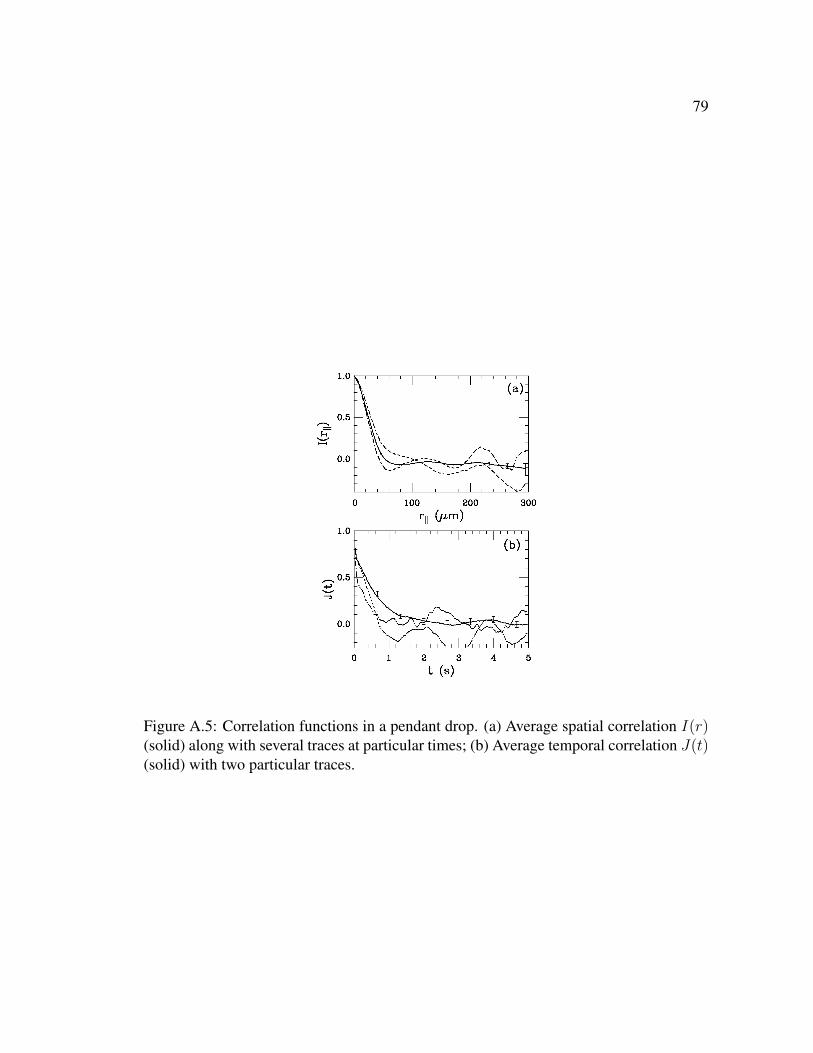
79

Figure A.5: Correlation functions in a pendant drop. (a) Average spatial correlation I(r)(solid) along with several traces at particular times; (b) Average temporal correlation J(t)(solid) with two particular traces.

80

act to trap many more, suggesting the nucleation of a biofilm, a dense multicellular struc-

ture of bacteria and secreted polymers [9]. This experimental setup may provide a useful

setting to study in detail the triggering and growth of such films.

We are grateful to D. Coombs, K. Glassner, J. Lega, A.I. Pesci, T. Squires, and

K. Visscher for helpful discussions. This work was supported in part by NSF Grant

MCB0210854.

References

[1] H. C. Berg, Random Walks in Biology (Princeton University Press, Princeton, N.J.,

1983).

[2] H. C. Berg and E. M. Purcell, Biophys. J. 20, 193 (1977).

[3] J. Toner and Y. Tu, Phys. Rev. Lett. 75, 4326 (1995).

[4] T. Vicsek et al., Phys. Rev. Lett. 75, 1226 (1995).

[5] A. Czirok, A.-L. Barabasi, and T. Vicsek, Phys. Rev. Lett. 82, 209 (1999).

[6] R. A. Simha and S. Ramaswamy, Phys. Rev. Lett. 89, 058101 (2002).

[7] Y. Hatwalne, S. Ramaswamy, M. Rao, and R. A. Simha, Phys. Rev. Lett. 92, 118101

(2004).

[8] B. L. Bassler, Cell 109, 421 (2002).

[9] G. O’Toole, H. B. Kaplan, and R. Kolter, Annu. Rev. Microbiol. 54, 49 (2000).

[10] J. O. Kessler and M. F. Wojciechowski, in Bacteria as Multicellular Organisms,

edited by J. A. Shapiro and M. Dworkin (Oxford University Press., New York,

1997), p. 417.

[11] R. D. Deegan et al., Nature 389, 827 (1997).

81

[12] A B. subtilis cell occupies approximately 1 µm3, so a volume fraction φ of 1%

corresponds to n ∼ 1010 cm−3.

[13] M. C. Cross and P. C. Hohenberg, Rev. Mod. Phys. 65, 851 (1993).

[14] N. H. Mendelson and J. Lega, J. Bacteriol. 180, 3285 (1998).

[15] A. J. Hillesdon, T. J. Pedley, and J. O. Kessler, B. Math. Biol. 57, 299 (1995).

[16] M. Ungarish, Hydrodynamics of Suspensions (Springer-Verlag, Berlin, 1993).

[17] D. K. Lubensky and R. E. Goldstein, Phys. Fluids 8, 843 (1996).

[18] K. Glasner, et al. (to be published).

[19] C. Dombrowski, et al., (to be published).

[20] Somewhat similar patterns appear on agar substrates; N.H. Mendelson, et al, J. Bac-

teriol. 181, 600 (1999).

[21] J. O. Kessler, in Proceedings of the International Conference on Differential Equa-

tions, vol. 2, edited by B. Fiedler, K. Groger, and J. Sprekels (World Scientific,

Singapore, 2000), p. 1284.

[22] X.-L. Wu and A. Libchaber, Phys. Rev. Lett. 84, 3017 (2000).

[23] T. H. Solomon, E. R. Weeks, and H. L. Swinney, Phys. Rev. Lett. 71, 3975 (1993).

[24] P. N. Segre, E. Herbolzheimer, and P. M. Chaikin, Phys. Rev. Lett. 79, 2574 (1997).

[25] J. O. Kessler et al., in Proceedings of the Workshop on Traffic and Granular Flow

’97, edited by M. Schreckenberg and D. E. Wolf (Springer-Verlag, Singapore, 1998),

p. 37.

[26] E. F. Keller and L. A. Segel, J. Theor. Biol. 30, 225 (1971).

82

APPENDIX B

BACTERIAL SWIMMING AND OXYGEN TRANSPORT NEAR CONTACT

LINES

Idan Tuval1, Luis H. Cisneros2, Christopher C. Dombrowski2, Charles W. Wolgemuth3,

John O. Kessler2 and Raymond E. Goldstein1,4

1 Institut Mediterrani d’Estudis Avanats, Palma de Mallorca, Spain. 2 Department of Physics,

University of Arizona. 3 Department of Cell Biology, University of Connecticut Health Center.4 Program of Applied Mathematics, University of Arizona.

Published in Proceedings of the National Academy of Sciences, Vol. 102, 2277 (2005).

DOI: 10.1073/pnas.0406724102

c©2005 The National Academy of Sciences

ABSTRACT

Aerobic bacteria often live in thin fluid layers near solidairwater contact lines, in which

the biology of chemotaxis, metabolism, and cellcell signaling is intimately connected to

the physics of buoyancy, diffusion, and mixing. Using the geometry of a sessile drop,

we demonstrate in suspensions of Bacillus subtilis the self-organized generation of a per-

sistent hydrodynamic vortex that traps cells near the contact line. Arising from upward

oxygentaxis and downward gravitational forcing, these dynamics are related to the Boy-

cott effect in sedimentation and are explained quantitatively by a mathematical model

consisting of oxygen diffusion and consumption, chemotaxis, and viscous fluid dynam-

ics. The vortex is shown to advectively enhance uptake of oxygen into the suspension, and

the wedge geometry leads to a singularity in the chemotactic dynamics near the contact

line.

83

Bacterial swimming and oxygen transport nearcontact linesIdan Tuval†, Luis Cisneros‡, Christopher Dombrowski‡, Charles W. Wolgemuth§, John O. Kessler‡,and Raymond E. Goldstein‡¶!

†Institut Mediterrani d’Estudis Avançats, Consejo Superior de Investigaciones Cientificas, Universitat de les Illes Balears, E-07071 Palma de Mallorca,Spain; ‡Department of Physics, University of Arizona, Tucson, AZ 85721; §Department of Cell Biology, University of Connecticut Health Center,Farmington, CT 06030; and ¶Program in Applied Mathematics, University of Arizona, Tucson, AZ 85721

Edited by Harry L. Swinney, University of Texas, Austin, TX, and approved January 4, 2005 (received for review September 10, 2004)

Aerobic bacteria often live in thin fluid layers near solid–air–watercontact lines, in which the biology of chemotaxis, metabolism, andcell–cell signaling is intimately connected to the physics of buoy-ancy, diffusion, and mixing. Using the geometry of a sessile drop,we demonstrate in suspensions of Bacillus subtilis the self-orga-nized generation of a persistent hydrodynamic vortex that trapscells near the contact line. Arising from upward oxygentaxis anddownward gravitational forcing, these dynamics are related to theBoycott effect in sedimentation and are explained quantitativelyby a mathematical model consisting of oxygen diffusion andconsumption, chemotaxis, and viscous fluid dynamics. The vortexis shown to advectively enhance uptake of oxygen into thesuspension, and the wedge geometry leads to a singularity in thechemotactic dynamics near the contact line.

bioconvection " chemotaxis " singularity " Bacillus subtilis

The interplay of chemotaxis and diffusion of nutrients orsignaling chemicals in bacterial suspensions can produce a

variety of structures with locally high concentrations of cells,including phyllotactic patterns (1), filaments (2), and concen-trations in fabricated microstructures (3). Less well exploredare situations in which concentrating hydrodynamic f lowsactually arise from these ingredients. Here we report a detailedexperimental and theoretical study of an intriguing mechanismtermed the ‘‘chemotactic Boycott effect.’’ Described brief lybefore (4), it is intimately associated with buoyancy-drivenf lows, metabolite diffusion, and slanted air–water menisci.The ubiquity of contact lines and their transport singularities(5) suggest importance of these observations in biofilm for-mation (6). The large-scale stirring created by these f lowsillustrate important advective contributions to intercellularsignaling, as in quorum sensing (7).

The chemotactic Boycott effect takes its name from a phe-nomenon in sedimentation (8) that occurs when the chambercontaining a fluid with settling particles is tilted from vertical.Settling depletes the fluid near the upper wall, making it buoyantrelative to nearby fluid, whereupon it rises. This boundary flowstirs up the entire medium, greatly accelerating the settlingprocess. In the chemotactic version, negatively buoyant aerobicbacteria swim up to the free surface of a sessile drop and slidedown the slanted meniscus, producing high concentrations ofcells near the three-phase contact line. In earlier work where thiswas observed (4), the detailed nature of hydrodynamic flowsnear the contact line was unclear. Here, by direct visualizationand particle-imaging velocimetry (PIV), we show that the slidingsurface layer drives a circulating hydrodynamic vortex in themeniscus region that is central to the microecology. Althoughcounterintuitive in viscous flows, persistent circulation driven byforcing at the free surface is consistent with the classic analysisfor vortex generation in wedge geometry (9).

The initial discussion of the chemotactic Boycott effect lackeda quantitative explanation in terms of the coupled dynamics ofoxygen transport and consumption, chemotaxis, and viscous

fluid dynamics. Here we present numerical and analytical resultson one such model and show that they provide a good accountingof the major experimental observations. The characteristic f luidvelocity U and length scale L associated with the vortex are bothsignificantly larger than those of a single bacterium. In compar-ing the relative importance of advective to diffusive transport ofa solute, it is natural to incorporate U, L, and the diffusionconstant D into the dimensionless Peclet number Pe ! UL#D,with Pe "" 1 indicating that diffusion is the dominant transportmechanism and Pe ## 1 is the advection-dominated regime. Wefind that the Boycott-like flows lead to Pe ## 1, just the oppositeof the situation at the scale of a single bacterium. In addition, byanalogy with evaporative singularities in sessile drops (5, 10), wefind a singularity in the oxygen-uptake rate at the contact line.Along with the large-scale stirring of fluid in the drop, this f lowsignificantly enhances the overall oxygen concentration in themedium, showing that collective effects can improve the viabilityof the population, as demonstrated by remarkable collectiveactivity (4) of the extremely concentrated organisms near thedrop edge.

Materials and MethodsExperiments were conducted with Bacillus subtilis strain 1085B.Samples were prepared by adding 1 ml of $20°C stock to 50 ml ofterrific broth (TB) (Ezmix Terrific Broth, Sigma; 47.6 g of broth mixand 8 ml of glycerin in 1 liter of distilled water) and incubating for18 h (VWR model 1217 shaker bath; 37°C, 100 rpm), after which1 ml of the bacterial suspension was added to 50 ml of TB andincubated for 5 h. The 5-h culture was then slowly added to thechamber with a syringe (21-gauge needle). The $20° stock wasprepared by adding spores on sand to 10 ml of TB at roomtemperature in a Petri dish and allowing for %24 h of growth. Onemilliliter of 24-h stock was added to 50 ml of TB and incubated for18 h. One milliliter of the 18-h culture was added to 50 ml of TBand incubated for 5 h. Aliquots composed of 0.75 ml of 5-h culturemixed gently with 0.25 ml of glycerin were placed in cold storage.The chambers (Fig. 1A) were constructed from microscope slidescemented together with UV curing adhesive (Norland, Cranbury,NJ); care was taken to remove excess adhesive to avoid interferencewith visualizations near the contact line and to seal the chamberadequately to avoid evaporation and associated flows. The spacebetween the vertical slides that form the front and back of thechamber was typically 1 mm. Imaging was achieved with a digitalcharge-coupled device camera [Hamamatsu (Ichinocho, Japan)C7300; 1,024 & 1,024 pixels; 12 bit] under computer control(National Instruments, Austin, TX) attached to a macrophotogra-phy bellows (PB-6, Nikon) with a 105-mm f#2.8 lens. Dark-fieldillumination was a 4-cm-diameter fiber-optic ring light (Navitar,

This paper was submitted directly (Track II) to the PNAS office.

Abbreviation: PIV, particle-imaging velocimetry.!To whom correspondence should be addressed at: Department of Physics, University ofArizona, 1118 East 4th Street, Tucson, AZ 85721. E-mail: gold@physics.arizona.edu.

© 2005 by The National Academy of Sciences of the USA

www.pnas.org#cgi#doi#10.1073#pnas.0406724102 PNAS " February 15, 2005 " vol. 102 " no. 7 " 2277–2282

APP

LIED

PHYS

ICA

LSC

IEN

CES

84

B.1 Introduction

The interplay of chemotaxis and diffusion of nutrients or signaling chemicals in bacte-

rial suspensions can produce a variety of structures with locally high concentrations of

cells, including phyllotactic patterns [1], filaments [2], and concentrations in fabricated

microstructures [3]. Less well explored are situations in which concentrating hydrody-

namic flows actually arise from these ingredients. Here we report a detailed experimen-

tal and theoretical study of an intriguing mechanism termed the chemotactic Boycott ef-

fect. Briefly described earlier [4], it is intimately associated with buoyancy-driven flows,

metabolite diffusion, and slanted air-water meniscii. The ubiquity of contact lines and

their transport singularities [5] suggest importance of these observations in biofilm for-

mation [6]. The large-scale stirring created by these flows illustrate important advective

contributions to intercellular signaling, as in quorum sensing [7].

The chemotactic Boycott effect takes its name from a phenomenon in sedimentation

[8] that occurs when the chamber containing a fluid with settling particles is tilted from

vertical. Settling depletes the fluid near the upper wall, making it buoyant relative to

nearby fluid, whereupon it rises. This boundary flow stirs up the entire medium, greatly

accelerating the settling process. In the chemotactic version, negatively-buoyant aerobic

bacteria swim up to the free surface of a sessile drop, and slide down the slanted meniscus,

producing high concentrations of cells near the three-phase contact line. In earlier work

where this was observed [4], the detailed nature of hydrodynamic flows near the contact

line was unclear. Here, by direct visualization and particle-imaging velocimetry (PIV)

we show that the sliding surface layer drives a circulating hydrodynamic vortex in the

meniscus region that is central to the microecology. While counterintuitive in viscous

flows, persistent circulation driven by forcing at the free surface is consistent with the

classic analysis for vortex generation in wedge geometry [9].

The initial discussion of the chemotactic Boycott effect lacked a quantitative explana-

tion in terms of the coupled dynamics of oxygen transport and consumption, chemotaxis,

85

and viscous fluid dynamics. Here we present numerical and analytical results on one such

model, and show they provide a good accounting of the major experimental observations.

The characteristic fluid velocity U and length scale L associated with the vortex are both

significantly larger than those of a single bacterium. In comparing the relative importance

of advective to diffusive transport of a solute, it is natural to incorporate U , L, and the

diffusion constant D into the dimensionless Peclet number Pe = UL/D, with Pe 1

indicating that diffusion is the dominant transport mechanism and Pe 1 the advection-

dominated regime. We find the Boycott-like flows lead to Pe 1, just the opposite of

the situation at the scale of a single bacterium. In addition, by analogy with evaporative

singularities in sessile drops [5, 10], we find a singularity in the oxygen uptake rate at

the contact line. Along with the large-scale stirring of fluid in the drop, this significantly

enhances the overall oxygen concentration in the medium, showing that collective effects

can improve the viability of the population, as demonstrated by remarkable collective

activity [4] of the extremely concentrated organisms near the drop edge.

B.2 Materials and Methods

Experiments were conducted with B. subtilis strain 1085B. Samples were prepared by

adding 1 ml of−20 C stock to 50 ml of Terrific Broth (TB; Ezmix Terrific Broth, Sigma:

47.6g broth mix and 8 ml glycerin in 1 l dH2O) and incubating for 18 h (shaker bath; 37

C, 100 rpm), after which 1 ml was added to 50 ml of TB and incubated for 5 h. The 5

h culture was then slowly added to the chamber with a syringe (21G needle). The −20

stock was prepared by adding spores on sand to 10 ml. Terrific Broth at room temperature

in a petri dish and allowing for ∼ 24 h of growth. One ml of 24 h stock was added to 50

ml TB and incubated for 18 h. One ml of the 18 h culture was added to 50 ml of TB and

incubated 5 h. Aliquots composed of 0.75 ml of 5 h culture mixed gently with 0.25 ml

glycerin were placed in cold storage. The chambers (Figure B.1A) were constructed from

microscope slides cemented together with UV-curing adhesive (Norland); care was taken

to remove excess adhesive to avoid interference with visualizations near the contact line,

86

Figure B.1: (A) Apparatus for simultaneous darkfield and fluorescence imaging of fluiddrops. Laser (L), shutter (S), beam expander lenses (L1 & L2), dichroic beamsplitter(D), long-pass filter (LPF), fiber-optic ring light (RL), digital camera (C). Chamber hasanti-reflection areas (AR) to reduce glare and hydrophobic areas (H) to pin the drop. (B)Boundary conditions and coordinates in the wedge, described in text.

and to seal the chamber adequately to avoid evaporation and associated flows. The space

between the vertical slides which form the front and back of the chamber was typically 1

mm. Imaging was achieved with a digital ccd camera (Hamamatsu C7300, 1024×1024

pixels, 12 bit) under computer control (National Instruments), attached to a macropho-

tography bellows (PB-6, Nikon) with a 105 mm f/2.8 lens. Dark field illumination was a

4 cm diameter fiber optic ring light (Navitar) behind the sample chamber. PIV measure-

ments were conducted by adding 5 µl of fluorescent microspheres (Molecular Probes,

F8825 Carboxylate-modified, 1.0 µm, Nile red) to 1 ml of suspension, illuminating with

a DPSS laser (100 mW, 532 nm) reflected from a dichroic mirror (Z542RDC, Chroma

Technology), and visualizing through a longpass filter (HQ542LP, Chroma). Analysis

was performed with PIV software (Dantec Dynamics).

87

B.3 Results

Figures B.2A-C show images of the main stages of the chemotactic Boycott effect. After

a drop of well-mixed suspension is placed in the chamber, the first spatial structure that

forms is a “depletion layer” of thickness ` ∼ 1 mm below the fluid-air interface, which

appears dark in our imaging method because of the absence of cells. This region arises

from the consumption of dissolved oxygen by the uniformly dispersed cells, followed by

their chemotactic migration up the oxygen gradient to the source of oxygen - the free

surface. No cellular motion is seen below the depletion layer, suggesting that the oxy-

gen concentration there has fallen to the critical value, denoted c∗, below which motility

vanishes. In a flattened sessile drop the bottom of the depletion layer follows the shape

of the air-water meniscus, displaced downward by the layer thickness. This layer forms

within 100 s, consistent with consumption of the saturation dissolved oxygen concentra-

tion cs ∼ 1017 cm−3 by cells at concentration n0 ∼ 109 cm−3, with a consumption rate

κ ∼ 106 oxygen molecules per second. This is also consistent with the time t` = `/vc

for a cell with a typical chemotactic velocity vc ∼ 10µm/s to traverse the thickness `. Ul-

timately, the cells congregate in a narrow surface “accumulation layer” whose thickness

d ∼ 100µm.

While the accumulation layer slides along the meniscus to the contact line it is un-

stable to plume formation on a length scale comparable to the layer thickness, consistent

with the fundamental instability of bioconvection in fluids with a horizontal meniscus

[11]. The Boycott effect occurs at the slant region; the resultant surface and return flows

distort the plumes that would otherwise fall straight down. This surface flow is opposite

to that of the conventional Boycott effect, whereas the depletion layer here is buoyantly

forced in the usual direction, creating a unique shear double layer. Typical fluid velocities

at the free surface are in the range 20 − 200 µm/s, accelerating as the meniscus slope

increases near the contact line. Finally, due to incompressibility requirements, a well-

developed vortex appears near each of the contact lines and shows persistence over many

88

Figure B.2: Stages leading to self-concentration in a sessile drop, observed experimen-tally (left) and by numerical computations with the model described in text (right). (A,A’)drop momentarily after placement in chamber. (B,B’) formation of depletion zone after150 s, prior to appreciable fluid motion, (C,C’) lateral migration of accumulation layertoward drop edges and creation of vortex (shown in Fig. B.3), after 600 s. Color schemedescribes the rescaled bacteria concentration ρ. Scale bar is 0.5 mm.

tens of minutes. The closed streamlines (Fig. B.3A) show the sense of circulation created

by the downward gravitational forcing on the accumulation layer and the recirculation

into the bulk required by fluid incompressibility. Despite the outward flow at the bottom

of the vortex, the optical density indicates that cells are trapped near the contact line.

B.4 Mathematical Model

The dynamics of the oxygen concentration c, cell concentration n, and fluid velocity u,

are described by coupled PDEs [12],

ct + u ·∇c = Dc∇2c− nκf(c) (B.1)

nt + u ·∇n = Dn∇2n−∇ · [µr (c)n∇c] (B.2)

ρ (ut + u ·∇u) = −∇p+ η∇2u− Vbgn∆ρz . (B.3)

In (B.1) the oxygen diffusion constant is Dc ∼ 2 × 10−5 cm2/s, and the dimensionless

function f(c) modulates the oxygen consumption rate κ, asymptoting to unity at large

c, but vanishing as c → 0. As the experimental timescales are minutes and the cell

89

Figure B.3: Hydrodynamic vortex near three-phase contact line. (A) velocity contoursobtained from PIV measurements, averaged over 750 frames acquired at intervals of 0.2s. Scale bar is 1mm. Region immediately above PIV contours is the curved fluid-air inter-face beyond the slice viewed in cross section. (B) Numerical results obtained from finite-element calculations using the model in Eqs. B.1-B.3. Closed streamlines are shownalong with velocity magnitude in color.

division time is∼ 100 minutes, the dynamics (B.2) of n conserve the total number of cells.

The bacterial diffusion constant Dn arises as a consequence of the random swimming

trajectories and is estimated to be Dn ∼ 10−6 − 10−5 cm2/s. Chemotaxis is described

by the second term on the r.h.s. of (B.2), with a velocity proportional to the oxygen

gradient [13]; the coefficient µ may be interpreted as µ = av0/cs, so that the chemotactic

velocity is v0 when the gradient is cs/a, where a is a characteristic length. Like the

function f(c), the motility function r(c) is unity at large c and vanishes rapidly for c

below the motility cutoff c∗; we approximate it and f(c) by the step function Θ(c − c∗).

Subject to incompressibility, ∇ · u = 0, the fluid equations (B.3) utilize the Boussinesq

approximation in which the density variations due to bacteria appear only in the buoyant

forcing, with ∆ρ = ρb − ρ, where Vb and ρb are the bacterial volume and density and ρ

is the pure fluid density. In the Appendix we provide a non-dimensionalization of these

equations convenient for numerical studies.

90

The boundary conditions on c, n, and u are central to the global flows and possible

singularities. As shown in Fig. B.1B, there is no flux (of cells or of oxygen) through the

substrate, under the drop and to its side, and no cell flux through the fluid-air interface.

That interface is stress-free, while the fluid-glass boundary has no slip. Since the oxygen

diffusion coefficient in the air is three orders of magnitude larger than that in the fluid,

the oxygen concentration outside the drop can be assumed equal to its saturation value cs

inside the fluid and on the free surface. Oxygen diffusion in the drop is equivalent to that

in the enlarged space whose bottom is the reflection of the meniscus across the fluid-glass

interface. This lens-shaped region has a sharp point which is the source of a chemotactic

singularity in the same way that a pointed electrical conductor produces a singular electric

field.

B.5 Comparison With Experiment

The phenomena shown in Figs. B.2 and B.3 can now be explained, beginning with for-

mation of the depletion and accumulation layers. Forming first in the absence of fluid

flow, we need only consider Eqs. B.1 and B.2 with u = 0,and even more simply in a

one-dimensional vertical cut through the drop. Quasi-steady-state profiles of c and n are

found in which c varies exponentially down from the free surface until it intercepts c∗.

From this one deduces

` =

(Dc (cs − c∗)

κn0

)1/2

, d =Dn

vc. (B.4)

The result ` ∼ n−1/20 can be verified by a dilution experiment. Figs. B.4 B & C show

two drops, the first from the standard bacterial suspension with cell concentration n0, the

second a dilution to 0.4n0. The increase in ` is apparent. Vertical traces of the optical

intensity through the height of the drop, averaged over 40 s, yield profiles like that shown

in Fig. B.4D, from which ` is determined. We see good agreement with the numerical

results in Fig. B.4A although at the very high cell concentrations in the accumulation

layer the optical intensity saturates, the likely explanation for the relatively small intensity

91

Figure B.4: Depletion layers in sessile drops.(A) Numerical solution of (B.1) and (B.2)for the rescaled cell concentration as a function of rescaled height. (B) depletion layerforming in stock solution and (C) in a 40% dilution. Scale bar is 0.5 mm. (D) averagedintensity trace in the stock solution, normalized to intensity at bottom of drop. (E) de-pletion layer thickness as a function of relative concentration. Dashed line is theoreticalprediction.

there. With parameters discussed above, we fit ` for the undiluted solution with c∗ =

0.3cs, and then ` of the diluted solution lies accurately on the prediction (Fig. B.4E).

Numerical studies of the PDEs with a curved fluid-air interface are readily accom-

plished with finite-element methods. Calculations were done with Femlab (Comsol,Inc.).

The coupled PDEs for handled using the “general” form, with high order Lagrange el-

ements (quintic for Eqs. B.1 & B.2 and quartic-quadratic for Eq. B.3), on a triangular

mesh consisting of ∼ 1000 nodes, and a fifth-order time integration scheme in the non-

linear time-dependent solver. We focus here on two-dimensional dynamics, equivalent

to the assumption of translational invariance with respect to the direction along the con-

tact line. The essential features of the flow are found as well in numerical studies using

Darcy’s law for flow between the vertical plates of the experimental chamber. Overhead

92

views of sessile drops reveal that in the third dimension the vortex breaks up into a ra-

dial form of bioconvective plumes [4]. Elsewhere we discuss these in more detail. Our

two-dimensional computations, shown in Figs. B.2 A’-C’, reproduce the observations;

the depletion layer tracing the shape of the meniscus, the variations in thickness of the

accumulation layer over the boundary of the drop, and the plume instability. Figure B.3B

shows that the vortex is also captured accurately.

Except close to the contact line, the accumulation layer is very thin compared to the

depth of the drop, so the gravitational forcing that acts on it is essentially concentrated

at the surface. When combined with the no-slip boundary condition at the bottom of the

drop, this defines one of the scenarios in Moffatt’s analysis of viscous eddies in sharp

corners [9]. Theory predicts a set of progressively smaller vortices adjacent to the main

vortex. We have not seen evidence of these, either in experiment or simulations, but

they are expected to be extremely weak and are likely outside the resolution of both

approaches. Theory also suggests that the conditions under which vortices develop can

depend sensitively on the far-field conditions and the wedge angle. Our numerical results

indicate the existence of a vortex at least over a range of angles from π/4 to π/2.

The velocities U in the vortex can reach 0.01 cm/s, with a size of 0.1 cm, so the

Peclet number can approach ∼ 102. Numerical studies show that the combination of

accumulated bacteria and greatly-enhanced stirring in the wedge lead to (i) a near-singular

variation in oxygen flux near the contact line (Fig. B.5A), and (ii) an increase in oxygen

uptake into the drop. Figure B.5B shows that the average oxygen concentration initially

drops precipitously as consumption dominates, but it slowly returns to a high value as

stirring enhances the uptake from the air above. Without the hydrodynamic coupling

between cell concentration and buoyancy, the oxygen concentration remains low after the

initial consumptive drop. Not only oxygen, but also nutrients will be ferried to the contact

line region from areas in the bulk of the drop.

93

Figure B.5: Oxygen dynamics from numerical studies. (A) Inward flux of oxygen alongupper surface of a drop, in units of Dccs/L, as a function of distance r from the contactline, showing near-singular behavior. (B) Average oxygen concentration in the drop as afunction of rescaled time s, normalized to initial value.

B.6 Chemotactic Singularity

Some insight into the oxygen flux near the contact line is obtained by making use of the

electrostatic analogy mentioned above. Close enough to the contact line the numerics

indicate that the velocity along the upper free surface tends to zero, so advective contri-

butions vanish asymptotically there. The simplest steady-state oxygen diffusion problem,

for which ∇2c = 0 inside the drop and c = cs on the free surface, is mathematically

equivalent to the equation defining the electrostatic potential in that same region, the ex-

terior of the drop being a conductor [5]. This mapping reveals [14] that a singularity arises

from a solution of the form

c(r, φ) ∼ cs +∞∑m=1

amrmπ/2θ cos(mπφ/2θ) , (B.5)

with polar coordinates (r, φ) as in Fig. B.1B. This form enforces the condition c = cs on

the drop surface (φ = θ) and the no-flux condition on the glass substrate (φ = 0). Upon

successive differentiation, the potentially most singular term is m = 1, and we expect

a1 < 0 since c ≤ cs in the drop interior. Noting that |∇c| ∼ rπ/2θ−1 and ∇2c ∼ rπ/2θ−2,

singularities appear in two cases:

94

1. θ > π/2, an overhanging meniscus. This case is like the familiar “lightning rod”

effect. Both the Fick’s law oxygen flux,−Dc∇c, and the chemotactic flux, µrn∇c,

diverge as r → 0, leading to a singular accumulation at the contact line.

2. π/4 < θ < π/2, as in Figs. B.2 - B.4: Here, |∇c| is finite as r → 0, but has

a diverging slope. Expanding the chemotaxis term in the dynamics (B.3), we see

terms of the form µr[∇n ·∇c + n∇2c], the former implying a potential cusp in

the cell concentration n. Although weaker than case 1, there still is a singular

accumulation driven by the diffusional singularity of oxygen.

Let us consider in more detail the typical case θ < π/2. There is a positive, bidirectional

feedback loop involving the chemotactic response to the oxygen singularity. The singu-

larity is reinforced by the accumulation of bacteria which consume the oxygen. A rough

idea of this can be gleaned by examining a steady state balance between the dominant

terms in the chemotaxis equation (B.2), setting D∇2n ∼ µrn∇2c to find a distribution

n ∼ exp(−Γrπ/2θ), with Γ > 0, that decays away from the contact line very sharply.

Since the local oxygen consumption rate is proportional to n, the inward flux of oxygen

mirrors the bacterial concentration distribution, as in Fig. B.5B. While a more precise

treatment requires a fully self-consistent calculation of the coupled oxygen and bacterial

concentrations, this result illustrates the dramatic accumulation of bacteria in the contact

region.

The development of the self-trapping vortex and the associated high concentration

of bacteria near the contact line depend crucially on the no-flux boundary conditions at

the substrate. A dramatic demonstration of this is seen in the flows in a “supported”

drop. This geometry was achieved by turning over the experimental chamber, allowing

a previously sessile drop to slide down from the chamber base toward the opening at the

opposite end. Surface tension supports the drop, with free uptake of oxygen around the

whole meniscus. As shown in Fig. B.6, the bottom interface is very flat, giving an effec-

tive contact angle exceeding π/2, but with no substrate the dynamics are nonsingular. We

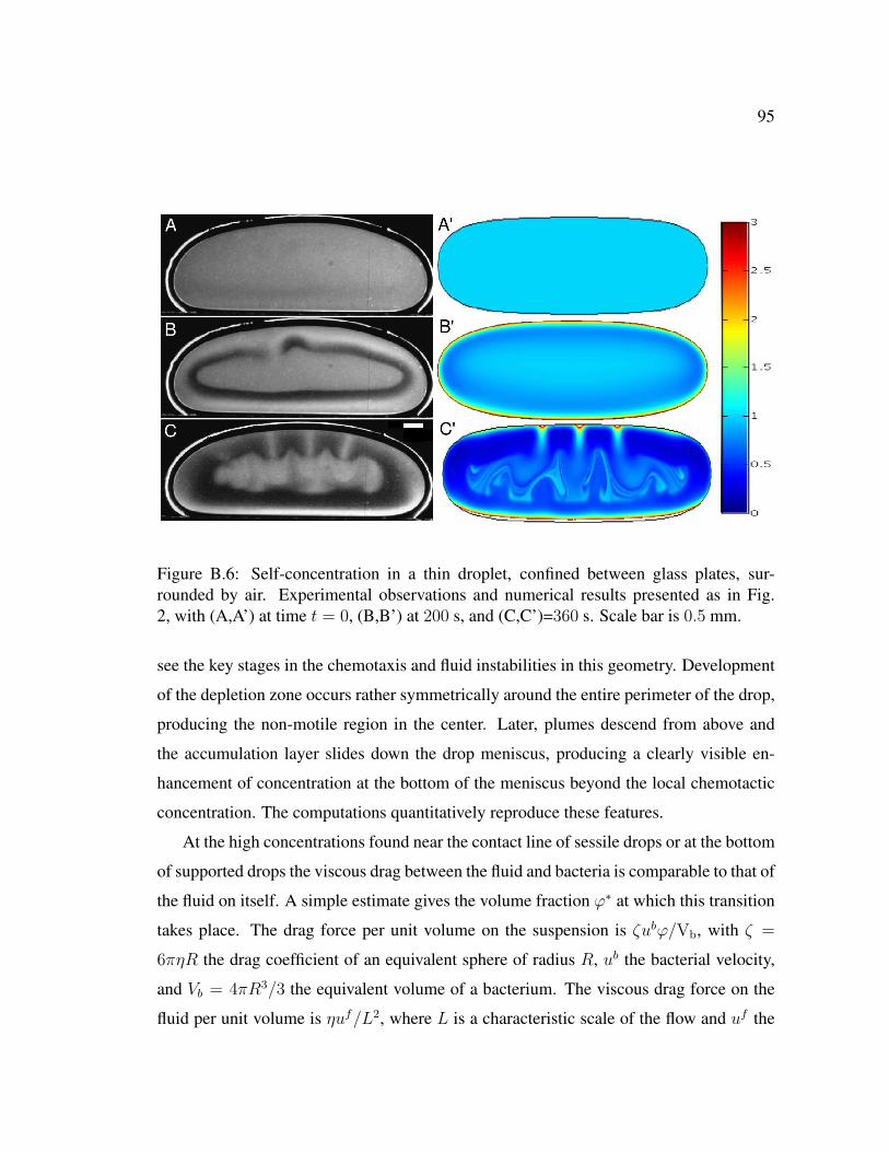
95

Figure B.6: Self-concentration in a thin droplet, confined between glass plates, sur-rounded by air. Experimental observations and numerical results presented as in Fig.2, with (A,A’) at time t = 0, (B,B’) at 200 s, and (C,C’)=360 s. Scale bar is 0.5 mm.

see the key stages in the chemotaxis and fluid instabilities in this geometry. Development

of the depletion zone occurs rather symmetrically around the entire perimeter of the drop,

producing the non-motile region in the center. Later, plumes descend from above and

the accumulation layer slides down the drop meniscus, producing a clearly visible en-

hancement of concentration at the bottom of the meniscus beyond the local chemotactic

concentration. The computations quantitatively reproduce these features.

At the high concentrations found near the contact line of sessile drops or at the bottom

of supported drops the viscous drag between the fluid and bacteria is comparable to that of

the fluid on itself. A simple estimate gives the volume fraction ϕ∗ at which this transition

takes place. The drag force per unit volume on the suspension is ζubϕ/Vb, with ζ =

6πηR the drag coefficient of an equivalent sphere of radius R, ub the bacterial velocity,

and Vb = 4πR3/3 the equivalent volume of a bacterium. The viscous drag force on the

fluid per unit volume is ηuf/L2, where L is a characteristic scale of the flow and uf the

96

fluid velocity. Equating these two gives

ϕ∗ =2

9

(R

L

)2uf

ub, (B.6)

independent of viscosity. Taking R ∼ 2 µm as a representative bacterium radius and

L ∼ 100 µm, the thickness of the accumulation layer, and uf/ub ∼ 5 [4], then ϕ∗ ∼5 × 10−4, corresponding to a concentration n ∼ 5 × 108 cm−3, comparable to a typical

initial homogeneous concentration in the drop. For volume fractions in excess of ϕ∗, the

fluid and bacterial velocities should be treated equally; one method to accomplish this

uses two-phase fluid flow [15]. With the low Reynolds numbers of the typical flows, the

coupled dynamics of the bacterial and fluid velocities ub and uf are

ζ(uf − ub

)= −(1− ϕ)∇p+ ηf∇2uf (B.7)

ζ(ub − uf

)= − ϕ∇p− Db

ϕ∇ϕ−∆ρgz + µr∇c (B.8)

with the continuity condition, ∇ ·(ϕub + (1− ϕ)uf

)= 0. Numerical investigations of

(B.7) and (B.8) coupled to the oxygen dynamics (B.1) show qualitatively similar results

for the overall bioconvective flows to those obtained with the Navier-Stokes equations

(B.3), but as well provide a more quantitatively correct description of the dense regime.

B.7 Conclusions

We have shown that the interplay of chemotaxis, buoyancy, and meniscus geometry is

responsible for persistent fluid circulation and high cell densities in the neighborhood

of contact lines. This circulation is strong enough to render advection dominant over

diffusion and enhance the overall oxygen uptake into the medium. Driven entirely by

chemotaxis and metabolism of individual cells, no explicit cell-cell communication is

necessary for these phenomena to occur. Nevertheless, the creation of a micro-ecological

structure by a self-organized dynamic will likely influence concurrent cell-cell communi-

cation which is necessary for such processes as quorum sensing and subsequent biofilm

97

formation [16], with its well-known complex transition from planktonic to sessile cells

[17]. The geometrically-mediated concentrative mechanism described here results in ap-

proximately close-packed bacteria exhibiting rapid coherent chaotic dynamics, including

collectively-driven flow of fluid through the array [4]. Our experiments have shown (un-

published) that the shallow fluid/air/substrate contact is a geometric constraint immobiliz-

ing bacteria. Initial cells nucleate a growing immobile assembly. The chaos of swimming

concentrated planktonic cells undoubtedly transports molecular nutrients and facilitiates

quorum signaling adjacent to sessile individuals, supplies recruits to the sessile popula-

tion, and transports tumbling, eventually settling chunks of biofilm generated elsewhere.

This scenario is a setting for biofilm progression, inward from the wetting region. It is

of special interest that the flow of fluid adjacent to the initially adherent cells is driven

only by the dynamics of the huge number of adjacent bacteria dispersing molecular infor-

mation, unlike the situation presented by Egland et al. [18] where communication in an

imposed flow depends on immediate adjacency. The possibility [19] that anoxia can be

a negative signal for surface adhesion in E. coli provides further evidence that advective

contributions from large-scale flows might play a role in the formation of biofilms.

We are grateful to K. Glasner for important discussions. This work was sup-

ported in part by NSF MCB0210854 (LC,CD,JOK,REG), NSF MCB 0327716 and NIH

R01 GM072004 (CW), and the Spanish Ministerio de Ciencia y Tecnologia, contract

BFM2000-1108 (CONOCE) (IT).

B.8 Appendix

Here we discuss some mathematical details involving the non-dimensionalization of the

governing equations. We rescale (B.1)-(B.3) to identify the dimensionless control pa-

rameters. If L ∼ 0.1 cm is the depth of the drop, we define the rescaled variables

x = r/L, s = Dnt/L2, χ = c/cs, ρ = n/n0, π = L2p/ηDn, v = Lu/Dn. Defin-

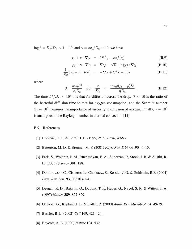
98

ing δ = Dc/Dn ∼ 1− 10, and α = av0/Dn ∼ 10, we have

χs + v ·∇χ = δ∇2χ− ρβf(χ) (B.9)

ρs + v ·∇ρ = ∇2ρ− α∇ · [r (χ) ρ∇χ] (B.10)1

Sc(vs + v ·∇v) = −∇π +∇2v − γρz (B.11)

where

β =κn0L

2

csDn

Sc =ν

Dc

γ =vn0g(ρb − ρ)L3

ηDn

. (B.12)

The time L2/Dn ∼ 103 s is that for diffusion across the drop, β ∼ 10 is the ratio of

the bacterial diffusion time to that for oxygen consumption, and the Schmidt number

Sc ∼ 103 measures the importance of viscosity to diffusion of oxygen. Finally, γ ∼ 103

is analogous to the Rayleigh number in thermal convection [11].

B.9 References

[1] Budrene, E. O. & Berg, H. C. (1995) Nature 376, 49-53.

[2] Betterton, M. D. & Brenner, M. P. (2001) Phys. Rev. E 64,061904-1-15.

[3] Park, S., Wolanin, P. M., Yuzbashyan, E. A., Silberzan, P., Stock, J. B. & Austin, R.

H. (2003) Science 301, 188.

[4] Dombrowski, C., Cisneros, L., Chatkaew, S., Kessler, J. O. & Goldstein, R.E. (2004)

Phys. Rev. Lett. 93, 098103-1-4.

[5] Deegan, R. D., Bakajin, O., Dupont, T. F., Huber, G., Nagel, S. R. & Witten, T. A.

(1997) Nature 389, 827-829.

[6] O’Toole, G., Kaplan, H. B. & Kolter, R. (2000) Annu. Rev. Microbiol. 54, 49-79.

[7] Bassler, B. L. (2002) Cell 109, 421-424.

[8] Boycott, A. E. (1920) Nature 104, 532.

99

[9] Moffatt, H. K. (1964) J. Fluid Mech. 18, 1-18.

[10] Deegan, R. D., Bakajin, O., Dupont, T. F., Huber, G., Nagel, S. R. & Witten, T. A.

(2000) Phys. Rev. E 62, 756-765.

[11] Pedley, T. J. & Kessler, J. O. (1992) Annu. Rev. Fluid Mech. 24, 313-358.

[12] Hillesdon, A. J., Pedley, T. J. & Kessler, J. O. (1995) B. Math. Biol. 57, 299-344.

[13] Keller, E. F. & Segel, L. A. (1971) J. Theor. Biol. 30, 225-234.

[14] Jackson, J. D. (1962) Classical Electrodynamics (Wiley, New York).

[15] Drew, D. A. & Segel, L. A. (1971) Stud. Appl. Math. 50, 205-231.

[16] Davies, D. G., Parsek, M. R., Pearson, J. P., Iglewski, B. H., Costerton, J. W. &

Greenberg, E. P. (1998) Science 280, 295-298.

[17] Costerton, B (2004) Proc. Natl. Acad. Sci. 101, 16983-16984.

[18] Egland, P. G., Palmer, R. J., Jr. & Kolenbrander, P. E. (2004) Proc. Natl. Acad. Sci.

101, 16917-16922.

[19] Landini, P. & Zehnder, A. J. B. (2002) J. Bacteriol. 184, 1522-1529.

100

APPENDIX C

REVERSAL OF BACTERIAL LOCOMOTION AT AN OBSTACLE

Luis H. Cisneros1, Christopher C. Dombrowski1, Raymond E. Goldstein1,2,3 and John O.

Kessler1

1 Department of Physics, University of Arizona. 2 Program of Applied Mathematics, University

of Arizona. 3 BIO5 Institute, University of Arizona.

Published in Physical Review E, Vol. 73, 030901(R) (2006).

DOI: 10.1103/PhysRevE.73.030901

c©2006 The American Physical Society

ABSTRACT

Recent experiments have shown large-scale dynamic coherence in suspensions of the bac-

terium B. subtilis, characterized by quorum polarity, collective parallel swimming of cells.

To probe mechanisms leading to this, we study the response of individual cells to steric

stress, and find that they can reverse swimming direction at spatial constrictions without

turning the cell body. The consequences of this propensity to flip the flagella are quanti-

fied by measurements of the inward and outward swimming velocities, whose asymptotic

values far from the constriction show near perfect symmetry, implying that ”forwards”

and ”backwards” are dynamically indistinguishable, as with E. coli.

101

Reversal of bacterial locomotion at an obstacle

Luis Cisneros,1 Christopher Dombrowski,1 Raymond E. Goldstein,1,2,3 and John O. Kessler1

1Department of Physics, University of Arizona, Tucson, Arizona 85721, USA2Program in Applied Mathematics, University of Arizona, Tucson, Arizona 85721, USA

3BIO5 Institute, University of Arizona, Tucson, Arizona 85721, USA!Received 14 January 2006; published 14 March 2006"

Recent experiments have shown large-scale dynamic coherence in suspensions of the bacterium B. subtilis,characterized by quorum polarity, collective parallel swimming of cells. To probe mechanisms leading to this,we study the response of individual cells to steric stress, and find that they can reverse swimming direction atspatial constrictions without turning the cell body. The consequences of this propensity to flip the flagella arequantified by measurements of the inward and outward swimming velocities, whose asymptotic values far fromthe constriction show near perfect symmetry, implying that “forwards” and “backwards” are dynamicallyindistinguishable, as with E. coli.

DOI: 10.1103/PhysRevE.73.030901 PACS number!s": 87.17.Jj, 87.18.Hf, 47.63.Gd

A growing body of work has addressed the spontaneousdevelopment of collective patterns by self-propelled organ-isms #1$. Based on analogies with phase transitions of liquidcrystalline and spin systems, phenomenological models#2–4$ suggested there could be a transition to a state withlong-range order of swimming orientation. Instead, experi-ments on E. coli in suspended soap films #5$ and B. subtilisin fluid drops #6–8$ have shown transient, recurring jets andvortices which disrupt that putative long-range order. Exten-sions of those models to include hydrodynamic interactionsbetween swimming cells #9,10$ and recent numerical studiesof large numbers of hydrodynamically interacting force di-poles #11$ strongly support the conjecture #7$ that such inter-actions are responsible for these coherent structures.

By itself, steric repulsion of nearly close-packed rodlikecells can produce nonpolar populations: cell bodies alignedas in a nematic liquid crystal. Unidirectional collectiveswimming requires polar alignment, which we term “quo-rum polarity”; all cells locomoting in the same direction.Because of the rapid, uniform collective velocity of thesealigned domains, we call this the “Zooming BioNematic”!ZBN". The search for mechanisms generating quorum po-larity served as motivation for the present work. We ask:What happens when the locomotion of a bacterium is im-peded by an obstacle? The obstacle might be a wall, anothercell or group of cells, perhaps swimming oppositely along acollision trajectory.

Quantitative visualization of the behavior of individualcells is not yet possible in the setting of collective dynamics.Accordingly, we constructed a model experiment to investi-gate the possibility that hydrodynamic or mechanical stresscan cause spontaneous reversal of swimming direction, amechanism for “wrong way” oriented individuals, hemmedin by neighbors, to join the majority of oppositely directedswimmers, without having to change orientation of the cellbody. A reversal entails flipping the bundle of propelling fla-gella from the original “rear” of the cell to reconstitute at theformer “front” end, which becomes the new “rear.” Such aprocess can provide quorum polarity and can recruit newmembers to the transient, recurring phalanxes of swimmingcells in the ZBN. Such reversals are most properly associated

with peritrichously flagellated cells !those covered with nu-merous flagella". This paper is devoted to B. subtilis; ourpreliminary studies show that E. coli also reverses at ob-stacles, but less frequently.

Figure 1!a" depicts the experiment, in which macroscopicglass spheres !Sigma-Aldrich, G1152; %800 !m" lie at thebottom of a 1-ml drop of bacterial suspension, 2 cm in di-ameter, placed on the upper surface of a polystyrene Petridish. Experiments were conducted on B. subtilis strain

FIG. 1. Apparatus and examples of swimming reversals. !a" Aglass sphere at the bottom of a sessile drop !not to scale" of bacte-rial suspension !Terrific Broth, TB". !b" Electron micrograph of B.subtilis about to divide into two cells. The scale bar is 1 !m. !c" Afew incoming !solid" and outgoing !dashed" trajectories at the foot-print of an 800-!m-diam glass sphere.

PHYSICAL REVIEW E 73, 030901!R" !2006"

RAPID COMMUNICATIONS

1539-3755/2006/73!3"/030901!4"/$23.00 ©2006 The American Physical Society030901-1

102

A growing body of work has addressed the spontaneous development of collective

patterns by self-propelled organisms [1]. Based on analogies with phase transitions of

liquid crystalline and spin systems, phenomenological models [2, 3, 4] suggested there

could be a transition to a state with long-range order of swimming orientation. Instead,

experiments on E. coli in suspended soap films [5] and B. subtilis in fluid drops [6, 7, 8]

have shown transient, recurring jets and vortices which disrupt that putative long-range

order. Extensions of those models to include hydrodynamic interactions between swim-

ming cells [9, 10] and recent numerical studies of large numbers of hydrodynamically-

interacting force dipoles [11] strongly support the conjecture [7] that such interactions are

responsible for these coherent structures.

By itself, steric repulsion of nearly close-packed rod-like cells can produce non-polar

populations: cell bodies aligned as in a nematic liquid crystal. Unidirectional collective

swimming requires polar alignment, which we term “quorum polarity”: all cells loco-

moting in the same direction. Because of the rapid, uniform collective velocity of these

aligned domains, we call this the “Zooming BioNematic” (ZBN). The search for mech-

anisms generating quorum polarity served as motivation for the present work. We ask:

What happens when the locomotion of a bacterium is impeded by an obstacle? The ob-

stacle might be a wall, another cell or group of cells, perhaps swimming oppositely along

a collision trajectory.

Quantitative visualization of the behavior of individual cells is not yet possible in the

setting of collective dynamics. Accordingly, we constructed a model experiment to inves-

tigate the possibility that hydrodynamic or mechanical stress can cause spontaneous rever-

sal of swimming direction, a mechanism for “wrong way” oriented individuals, hemmed

in by neighbors, to join the majority of oppositely-directed swimmers, without having to

change orientation of the cell body. A reversal entails flipping the bundle of propelling

flagella from the original “rear” of the cell to reconstitute at the former “front” end, which

becomes the new “rear.” Such a process can provide quorum polarity and can recruit new

members to the transient, recurring phalanxes of swimming cells in the ZBN. Such rever-

103

Figure C.1: Apparatus and examples of swimming reversals. (a) A glass sphere at thebottom of a sessile drop (not to scale) of bacterial suspension (Terrific Broth, TB). (b)Electron micrograph of B. subtilis about to divide into two cells. Scale bar is 1 µm. (c)A few incoming (solid) and outgoing (dashed) trajectories at the footprint of an 800 µmdiameter glass sphere.

sals are most properly associated with peritrichously flagellated cells (those covered with

numerous flagella). This paper is devoted to B. subtilis; our preliminary studies show that

E. coli also reverses obstacles, but less frequently.

Figure C.1a depicts the experiment, in which macroscopic glass spheres (Sigma-

Aldrich, G1152; ∼ 800 µm) lie at the bottom of a 1 ml drop of bacterial suspension,

2 cm in diameter, placed on the upper surface of a polystyrene Petri dish. Experiments

were conducted on B. subtilis strain 1085B, prepared from stock [8]. An electron mi-

crograph (Fig. C.1b) shows that these cells are ∼ 4 microns long (considerably longer

than E. coli) with a very large number of flagella whose length is typically 5 − 10 µm.

The sessile drop was obtained from a Terrific Broth (TB, Sigma, T9179) suspension in-

104

Figure C.2: A bacterial reversal. Images taken 0.28 s apart show a bacterium approachingthe narrow gap between a glass sphere and petri dish, pausing, then swimming back outwithout turning around. Interlopers seen in frames 13−16 do not affect the motion of thereversing bacterium. Horizontal field of view is 30 µm. The black arcs mark the radius ofclosest approach.

cubated 3.5 h in a shaker bath, checked for motility, and then diluted 1000-fold with TB.

Swimming (Fig. C.2) was imaged at 20× magnification on a Nikon TE2000U inverted

microscope with an analog ccd camera (Sony XC-ST50, 30 fps), written to videotape and

digitized for tracking by Metamorph (Universal Imaging Corp.). Additional studies used

a high-speed camera (Kodak ES310T, 125 fps).

As the plastic petri dish is permeable to oxygen, bacteria routinely swim along the

bottom of the drop, next to the surface of the dish. B. subtilis grown under the conditions

described above do not display the classic “run-and-tumble” behavior so well-known in

E. coli [12]. Rather, and especially near a surface, they tend to execute long, perhaps

slightly curved swimming trajectories [13, 14] with few apparent tumbles. Without direct

visualization of flagella, we can not rule out tumbles with very small angular changes;

our observations show that spontaneous tumbles with large angular changes in swimming

direction are almost entirely absent. Those cells swimming near the bottom occasionally

approach the narrow, convex-wedge-shaped gap near the sphere’s contact point, as shown

in Fig. C.2. Generally, if the angle between their swimming trajectory and the normal

to the sphere is large, they simply turn away from the narrowest regions and continue

swimming. Relatively straight-on collisions generally produce reversals. An incoming

track and its reversed successor is a “V”-shaped pair (Fig. C.1b). The video sequences

105

Figure C.3: Time dependence of average swimming velocities. (a) Average of 100 inwardtracks, each normalized by the asymptotic velocity far from constriction. (b) As in (a),but for outward tracks. At times larger than shown the statistical uncertainties grow largerdue to the fewer number of trajectories in the sample. Uncertainties are standard errors.

show, without question, that the cell body does not turn around while docked; the forward

end of the cell coming into the gap becomes the backward end afterwards; the flagellar

bundle flipps from one end of the cell to the other. Our findings extend those of Turner and

Berg [15], that E. coli swims with either end forward. They did not investigate reversal

dynamics at obstacles or swimming speed symmetries.

We collected 100 reversal trajectories, five of which are shown in Fig. C.1b. Many

display curvature, likely from interaction of the chiral flagellar bundle with the surface,

as seen with E. coli [13, 14]. Using the∼ 30 µm radius circle around the sphere’s surface

contact point from which bacteria are excluded (Fig. C.1c), we estimate reversals occur

at gap heights of ∼ 1.1 µm, slightly larger than the nominal cell diameter of 0.7 µm.

These cells are covered with flagella and pilli (Fig. C.1), so it is plausible that a 1 µm

constriction would stop their motion.

106

From the full spatial trajectories, we obtained the inward and outward velocities as

a function of time relative to the stopping time tstop of the inward motion, and the time

trestart when outward motion begins again. Normalizing the velocities of inward and

outward trajectories by each track’s asymptotic value, v∞in and v∞out, and then averaging

all 100 such runs, we obtain the average rescaled inward and outward velocities shown in

Figs. C.3a and C.3b. It is evident that earlier than several seconds before stopping and

later than a few seconds after resuming swimming, the velocities are nearly independent

of time (and hence of position). The distances associated with these transition times are

approximately 10− 20 µm.

Figure C.4a shows the asymptotic outward and inward velocities. Over a range from

∼ 10 − 30 µm/s the data cluster near the line of equality. A least squares fit forced

through the origin yields a slope of 1.01±0.01, showing statistical symmetry. A histogram

(Fig. C.4b) of the ratio v∞out/v∞in shows a Gaussian distribution with mean of 1.05 and a

width of 0.11, again indicating near statistical equality. We infer that swimming ability is

independent of the polar location of the flagellar bundle.

As bacteria swim into the gap they experience ever-increasing viscous drag [16] due to

the looming proximity of the surface of the sphere. They decelerate to rest on a timescale

of ∼ 2 s. Following a reversal, the acceleration timescale is more rapid, about 1 s. This

asymmetry is easily seen in the temporal traces in Fig. C.3 and is further quantified in Fig.

C.5 as histograms of stopping and starting intervals τstop and τstart and the accelerations

deduced from them as ai = v∞in /τstop and ao = v∞out/τstart. The stopping intervals have

a greater mean value than the starting intervals, and the accelerations are also larger than

the decelerations.

We interpret these results as a consequence of the different position of the flagellar

bundle in the two cases. During inward trajectories, the bundle behind the cell points

out into the wider region of the wedge, while during an outward trajectory that bundle,

again behind the cell, points into the narrowest regions of the wedge close to the point of

contact of the sphere with the substrate. These two orientations differ in viscous drag and

107

Figure C.4: Statistical results for 100 reversals. (a) Asymptotic outward vs. inwardvelocities, showing tight clustering around line of equalities (dashed). Uncertainties arestandard errors. (b) Histogram of asymptotic velocity ratio, with Gaussian fit.

108

Figure C.5: Statistical analysis of accelerations and decelerations during rever-sals.Histograms are for the time to decelerate to rest from a steady velocity far awayfrom the wedge on an incoming trajectory, and the time to accelerate from rest to theasymptotic velocity. The average decelerations/accelerations deduced from those timesand velocities are shown.

propulsive efficiency. Just the opposite asymmetry is observed during tumbles in free-

swimming E. coli [12]: abrupt deceleration followed by more gradual acceleration as the

bundle reforms. Monotrichously flagellated organisms (with a single flagellum) such as

Vibrio alginolyticus, display similar behavior to that found here: reversals of trajectories

without cell reversal, asymptotic equality of speeds far from an obstacle, and asymmetry

close in [17].

The time spent “docked” may vary from a few milliseconds to a few seconds, as sum-

marized in the histogram of Figure C.6, from which we deduce that the mean time parked

in the wedge is ∼ 1s. Is also evident that reversals occur very quickly, indicating that

typical rebundling time of flagella may be shorter than the time resolution of our process.

The incoming and outgoing trajectories define an angle ∆θ, the distribution of which is

shown in the top inset of Fig. C.6. The angle is broadly distributed and shows no par-

ticular correlation with the docking interval itself, indicating that the observed ”pivoting”

of the docked cell is random. It is important to note that this is true even for very fast

109

Figure C.6: Statistical analysis of docking. Main figure shows histogram of dockingtimes with two binning choices. Insets show histograms of the angle ∆θ between in andout trajectories, and a correlation plot between those angles and the docking times. Greybars indicate maxima and minima observed within each bin, not statistical uncertainties.

reversals, where the range of ∆θ is surprisingly large and there is very little time to pivot.

This may prove that the randomness observed does not necessarily come only from some

kind of “angular wandering” of the docked cell, but also from details on the unbundling-

rebundling process. Dynamical minutiae of reversals will be different in each case, lead-

ing to a wide distribution of final orientations of the cell. Without direct visualization of

flagella [18], we do not know when rebundling completes during a reversal.

It is remarkable that such a major morphological transition as flipping the flagellar

bundle appears not to entail consequences beyond swimming at normal speed in the op-

posite direction. There is a further reversal of symmetry. During smooth forward loco-

motion, all the flagella rotate clockwise at typically 100 turns/s, seen from the cell body.

The cell body rotates appropriately to balance torques. When a swimming cell reverses

direction by flipping its flagella, the rotation of its flagella and body reverse relative to

an observer in the laboratory. When the reversing cell interacts with a domain of the

ZBN, the lab frame is defined by the director axis, which points along the collectively

110

determined velocity, and by the collectively driven rotation of the fluid. Consider a con-

centrated population of cells swimming in a particular direction, as in the ZBN. When a

“wrong way” swimmer reverses within a phalanx, it changes from contra- to co-rotation

relative to its surround. The relative rotation of neighboring cells produces flows orthogo-

nal to the main direction of collective locomotion. In the gap between them, contrarotating

neighbors generate microflows of order 100 µm/s. Corotating neighbors produce strong

shear rates of order 100 s−1, estimated by considering flagellar bundles of diameter ∼ 1

µm, rotating at rates of ∼ 100 rps, separated by ∼ 1 µm. Shears of this magnitude in

the noisy dynamics of the ZBN are ideal generators of flows which enhance mixing, as in

the dynamics of blinking stokeslets [19]. Especially significant is improved intercellular

signalling, as required for quorum sensing.

We thank Koen Visscher for discussions and D. Bentley for assistance with the micro-

graph in Fig. C.1. This work was supported in part by NSF Grants MCB-0210854 and

PHY0551742, and NIH Grant R01 GM72004-01.

References

[1] J. Toner, Y. H. Tu, and S. Ramaswamy, Ann. Phys. 318, 170 (2005).

[2] J. Toner and Y. Tu, Phys. Rev. Lett. 75, 4326 (1995).

[3] T. Vicsek, A. Czirok, C. Ben-Jacob, I. Cohen, and O. Shochet, Phys. Rev. Lett. 75,

1226 (1995).

[4] A. Czirok, A.-L. Barabasi, and T. Vicsek, Phys. Rev. Lett. 82, 209 (1999).

[5] X.-L. Wu and A. Libchaber, Phys. Rev. Lett. 84, 3017 (2000).

[6] N. H. Mendelson and J. Lega, J. Bacteriol. 181, 600 (1999).

[7] C. Dombrowski, L. Cisneros, S. Chatkaew, R. E. Goldstein, and J. O. Kessler, Phys.

Rev. Lett. 93, 098103 (2004).

111

[8] I. Tuval, L. Cisneros, C. Dombrowski, C. W. Wolgemuth, J. O. Kessler, and R. E.

Goldstein, Proc. Natl. Acad. Sci. (USA) 102, 2277 (2005).

[9] R. A. Simha and S. Ramaswamy, Phys. Rev. Lett. 89, 058101 (2002).

[10] Y. Hatwalne, S. Ramaswamy, M. Rao, and R. A. Simha, Phys. Rev. Lett. 92, 118101

(2004).

[11] J. P. Hernandez-Ortiz, C. G. Stoltz, and M. D. Graham, Phys. Rev. Lett. 95, 204501

(2005).

[12] H. C. Berg and D. A. Brown, Nature 239, 500 (1972).

[13] W. R. DiLuzio, L. Turner, M. Mayer, P. Garstecki, D. B. Weibel, H. C. Berg, and

G. M. Whitesides, Nature 435, 1271 (2005).

[14] E. Lauga, W. R. DiLuzio, G. M. Whitesides, and H. A. Stone, Biophys. J. 90, 400

(2006).

[15] L. Turner and H. C. Berg, Proc. Natl. Acad. Sci. (USA) 92, 477 (1995).

[16] H. Brenner, Chem. Eng. Sci. 16, 242 (1961).

[17] Y. Magariyama et al., Biophys. J. 88, 3648 (2005).

[18] L. Turner, W. S. Ryu, and H. C. Berg, J. Bacteriol. 182, 2793 (2000).

[19] H. Aref, J. Fluid Mech. 143, 1 (1984).

112

APPENDIX D

FLUID DYNAMICS OF SELF-PROPELLED MICRO-ORGANISMS, FROM

INDIVIDUAL TO CONCENTRATED POPULATIONS

Luis H. Cisneros1, Ricardo Cortez2, Christopher Dombrowski1,

Raymond E. Goldstein1,3 and John O. Kessler1

1Department of Physics, University of Arizona. 2Department of Mathematics, Tulane University.3D.A.M.T.P., University of Cambridge, UK.

Published in Experiments in Fluids, Vol. 43, 737 (2008).

DOI 10.1007/s00348-007-0387-y

c©2007 Springer-Verlag

ABSTRACT

Nearly close-packed populations of the swimming bacterium Bacillus subtilis form a

collective phase, the “Zooming BioNematic” (ZBN). This state exhibits large-scale ori-

entational coherence, analogous to the molecular alignment of nematic liquid crystals,

coupled with remarkable spatial and temporal correlations of velocity and vorticity, as

measured by both novel and standard applications of particle imaging velocimetry. The

appearance of turbulent dynamics in a system which is nominally in the regime of Stokes

flow can be understood by accounting for the local energy input by the swimmers, with a

new dimensionless ratio analogous to the Reynolds number. The interaction between or-

ganisms and boundaries, and with one another, is modeled by application of the methods

of regularized Stokeslets.

113

RESEARCH ARTICLE

Fluid dynamics of self-propelled microorganisms,from individuals to concentrated populations

Luis H. Cisneros Æ Ricardo Cortez ÆChristopher Dombrowski Æ Raymond E. Goldstein ÆJohn O. Kessler

Received: 13 February 2007 / Revised: 16 July 2007 / Accepted: 21 August 2007! Springer-Verlag 2007

Abstract Nearly close-packed populations of the swim-ming bacterium Bacillus subtilis form a collective phase, the

‘‘Zooming BioNematic’’ (ZBN). This state exhibits large-

scale orientational coherence, analogous to the molecularalignment of nematic liquid crystals, coupled with remark-

able spatial and temporal correlations of velocity and

vorticity, as measured by both novel and standard applica-tions of particle imaging velocimetry. The appearance of

turbulent dynamics in a system which is nominally in the

regime of Stokes flow can be understood by accounting forthe local energy input by the swimmers, with a new

dimensionless ratio analogous to the Reynolds number. The

interaction between organisms and boundaries, and with one

another, is modeled by application of the methods of regu-larized Stokeslets.

1 Introduction

The fluid dynamics of fast, large self-propelled objects,

ranging from krill to whales, mosquitoes to eagles, is

extensively studied and intuitively understood (Childress1981). In these cases the Reynolds number Re ranges fromsomewhat[1 to enormous. At the other end of the spec-

trum are microscopic swimmers: bacteria, uni- and multi-cellular algae, and protists: which, although capable of

swimming many body lengths per second, live in the

regime Re ! 1. While the essential features of the swim-ming of individual organisms of this type are known

(Lighthill 1975; Berg 2003), the manner in which the flows

associated with locomotion couple many such swimmers toeach other and to nearby surfaces are only now being fully

explored. Flows generated cooperatively by flagella ofunicellular organisms and by those of multicellular

organisms can also drive significant advective transport of

molecular solutes associated with life-processes (Solariet al. 2006, 2007; Short et al. 2006).

In this paper we provide experimental and theoretical

insights into the remarkable collective dynamics of a par-ticular bacterial system, expanding on our original reports

(Dombrowski et al. 2004; Tuval et al. 2005). Much micro-

bio-hydrodynamical research has focused on the morpho-logically similar swimming bacteria Escherichia coli,Salmonella typhymurium and Bacillus subtilis. The chief

results described in this paper are derived from ourinvestigations of fluid dynamical phenomena driven by

individual and collective swimming of B. subtilis.

L. H. Cisneros " C. Dombrowski " R. E. Goldstein "J. O. Kessler (&)Department of Physics, University of Arizona,1118 E. 4th St., Tucson, AZ 85721, USAe-mail: kessler@physics.arizona.edu

L. H. Cisnerose-mail: cisneros@physics.arizona.edu

C. Dombrowskie-mail: dombrows@gmail.com

R. CortezDepartment of Mathematics, Tulane University,6823 St. Charles Ave., New Orleans, LA 70118, USAe-mail: rcortez@tulane.edu

R. E. GoldsteinDepartment of Applied Mathematics and Theoretical Physics,Centre for Mathematical Sciences, University of Cambridge,Wilberforce Road, Cambridge CB3 0WA, UKe-mail: R.E.Goldstein@damtp.cam.ac.uk

123

Exp Fluids

DOI 10.1007/s00348-007-0387-y

114

D.1 Introduction

The fluid dynamics of fast, large self-propelled objects, ranging from krill to whales,

mosquitoes to eagles, is extensively studied and intuitively understood [1]. In these cases

the Reynolds number Re ranges from somewhat >1 to enormous. At the other end of the

spectrum are microscopic swimmers - bacteria, uni- and multicellular algae, and protists

- which, although capable of swimming many body lengths per second, live in the regime

Re 1. While the essential features of the swimming of individual organisms of this

type are known [2, 3], the manner in which the flows associated with locomotion couple

many such swimmers to each other and to nearby surfaces are only now being fully ex-

plored. Flows generated cooperatively by flagella of unicellular organisms and by those of

multicellular organisms can also drive significant advective transport of molecular solutes

associated with life-processes [4, 6, 5].

In this paper we provide experimental and theoretical insights into the remarkable

collective dynamics of a particular bacterial system, expanding on our original reports [7,

8]. Much micro-bio-hydrodynamical research has focused on the morphologically similar

swimming bacteria Escherichia coli, Salmonella typhymurium and Bacillus subtilis. The

chief results described in this paper are derived from our investigations of fluid dynamical

phenomena driven by individual and collective swimming of B. subtilis.

Individual cells of these generally non-pathogenic soil bacteria are rod-shaped (Fig.

D.1). Their length ranges from two to eight micrometers, depending on nutrition and

growth stage. In typical experiments they are approximately 4 µm long and somewhat

less than 1 µm in diameter. They are peritrichously flagellated: the helical flagella, their

means of propulsion, are distributed randomly over the cell body, emerging from motors

that are fixed within the cell membrane. The shafts are able to rotate at various rates, typ-

ically on the order of 100 Hz. The flagella themselves are complex polymeric structures

approximately 20 nm in diameter, with a length of 10-15 µm, considerably greater than

a cell’s body, and a helical pitch of ∼ 2 − 4 µm. They are attached to the motors by a

115

Figure D.1: Two Bacillus subtilis cells about to separate after cell division. Flagellacan be seen emerging from the body. Many of them have been broken during samplepreparation for this transmission electron micrograph. Scale bar is 1 µm.

flexible hook which acts as a universal joint. When a bacterial cell swims smoothly for-

ward, hydrodynamic interactions between the many helical flagella cause the formation

of a propulsive bundle within which they co-rotate. The swimming speed of an individual

is approximately 11% of the helix wave speed [9, 10]. The motors are fueled by proton

gradients; their direction of rotation is reversible. Spontaneous reversals may occur as a

function of the surrounding concentration of chemicals and of other factors and can play

a major role in chemotaxis [11, 3]. The cell bodies are not polar. The flagellar bundle can

form at either end of a cell, whether E. coli [12] or B. subtilis [13], an important aspect of

group locomotion discussed later.

A single swimming bacterium has associated with it an extensive flow field which

is produced entirely by drag forces on the fluid, exerted forward by the cell body and

backward by the flagella. No wake remains behind moving cells or cell groups. When a

cell stops rotating its flagella, all motion of the fluid and of the cell ceases. Motor boats

are not analogs. The viscous forces are described by Slender Body Theory and extensions

of Faxen’s and Stokes’ laws [14]. A key feature of these dynamics is that for an isolated

swimmer the net propulsive force of the flagella must equal the opposing drag force of

the body connected to the flagella, taking into account the effect of nearby surfaces or

other organisms. While the creeping flow equations are linear and time reversible, in

116

real world situations these features are only approximate or worse. Deviations from the

ideal occur when flows affect boundary conditions such as location and orientation of

nearby cells, the speed and directionality of flagella beating and the deformation of nearby

interfaces. Some of these situations apply to the phenomena discussed in this paper,

e.g. the effect of flows generated by the bacteria on their own spatial distribution and

motional dynamics, which then modify the flows. A full accounting for these effects is

necessary for a complete theory of the collective dynamics, but this is not yet at hand.

The basic phenomenology of this collective behavior and its quantification by particle

imaging velocimetry (PIV) are described in Secs. D.2 and D.3.

The swimming trajectories of living organisms can be modified by local shear and

vorticity. For example, we describe in Section D.4, that B. subtilis tend to swim upstream

in a shear flow. Should we ascribe this to hydrodynamic interactions that passively orient

cells which simply continue to rotate their flagella? Or perhaps might we infer that,

when bacteria experience shear stress, they “want” to swim upstream? In section D.4

we show one example of this phenomenon, adequate for the purpose of demonstrating

its importance for recruiting individuals into groups of co-directionally swimming cells.

However, the specific recorded trajectories of more than sixty cells show wide variations

in in detail. There may be many microscopic origins for the recruitment of cells into

correlated groups leading eventually to the collective behavior, but inferences concerning

fundamentals of micro-bio-hydrodynamics require experiments designed to disentangle

the physics from the biology.

Micro-organisms use, exude, and respond to the presence of biologically significant

molecules. Chemical interactions provide an avenue for change of the collective dynamic.

Emission of molecules involved in signalling, and exudates of biopolymers that may rad-

ically change the viscosity of the embedding fluid, are both involved in quorum sensing

[15] and the formation of biofilms [16]. Before occurrence of these radical events, sub-

tle chemical interactions can influence the biology and modify the behavior of individual

cells. Even at low concentrations, polymer exudates modify the properties of the sus-

117

Figure D.2: B. subtilis cells concentrated at a sloping water/air interface. This meniscusis produced by an air bubble in contact with the glass bottom of a bacterial culture 3mm deep. Near the top of the image bacteria have accumulated, forming a monolayerof cells perpendicular to the air/water/glass contact line. Their lateral proximity and theadjacent surfaces immobilize them. Toward the bottom of the image the fluid becomesprogressively deeper; the swimming cells exhibit collective dynamics. The accumulationoccurs because bacteria swim up the gradient of oxygen produced by their consumptionand by diffusion from the air bubble. The black specs are spherical latex particles 2 µmin diameter.

pension. For instance, we observe that in slightly aged cultures of still normally motile

bacteria, passive marker particles, as well as the bacteria themselves, can be coupled by

polymer strands of cellular origin. We have observed [17] that the water/air interface can

accumulate bacterially-synthesized polymer surfactants that trap and immobilize bacteria

arriving there. A nominally free surface becomes a stiff, no-slip boundary. We infer that

the bacteria are immobilized because the flagellar motors are too weak to overcome the

implied yield stress. Vigorously shaking a culture bounded by such an interface frees the

bacteria. After shaking stops, the newly unoccupied surface soon becomes again popu-

lated by bacteria stuck in the inferred interfacial layer of polymer, while in the bulk fluid

many cells swim normally, some attached to each other by polymers, forming immobile

multicellular clumps. In biofluid mechanics, before reaching definitive conclusions about

mechanisms involving free surfaces: caveat emptor.

On a larger scale, response to chemical gradients can initiate behavior that creates

118

Figure D.3: One randomly chosen instant of the bacterial swimming vector field estimatedby PIV analysis. The arrow in the extreme lower left corner represents a magnitude of 50µm/sec. The turbulent appearance of the flow is evident here.

striking hydrodynamic flows (Figs. D.2 and D.3). For instance, respiration of B. subtilis

depletes dissolved oxygen in the fluid medium. Transport from an interface between the

aqueous suspension of these cells and the surrounding air replenishes it. Bacteria swim

up the resultant gradient of oxygen concentration. In a shallow suspension the cells swim

upward, toward the air. Accumulation at the interface results in an unstable gradient of

mean fluid density, since the bacteria are approximately 10% denser than water. Such

convective dynamics also occur with swimming cells of algae [18, 19], plants that swim

upward, toward light, and/or because of orientation of the cells in the earth’s gravitational

field. The initial volume fraction is typically fairly low in these situations, ≈ 10−3 or

less. Theoretical approaches can therefore use Navier-Stokes equations that include a

smoothed gravitational body force proportional to the local concentration of organisms

and their mass density. An additional equation models transport of organisms due to

swimming and advection by the flow [20, 21, 8].

These unstable stratifications evolve in the usual manner by a Rayleigh-Taylor in-

stability which, in turn, can lead to highly concentrated populations [7, 8] (Fig. D.2).

These concentrated accumulations of cells support the collective dynamics discussed

119

here, which were first reported in a more qualitative manner some time ago [22, 49].

Closely related phenomena, jets and whirls, that occur near the edges of bacterial cul-

tures that grow and expand on wet agar surfaces have been reported [23]. Likewise, such

phenomena can be seen in concentrated bacterial populations trapped in suspended thin

aqueous films [24, 25]. Models of various types have been proposed to address these

phenomena, from very simple discrete-particle dynamics not involving hydrodynamics

[26] to continuum models based on ideas from liquid crystal physics [27, 51], two-fluid

models [29, 30], numerical studies of idealized swimmers [31] and hydrodynamic mod-

els [32]. The emerging consensus is that hydrodynamic interactions between the bacteria

are sufficient to account for the observed collective behavior, although some models sug-

gest that steric interactions alone in a collection of self-propelled objects will produce the

collective dynamics [33].

In Sections D.5 and D.6 we describe some further mathematical aspects of model-

ing individual swimming dynamics and collective motions in bacterial systems. These

results give insight into the details of flows and forces in the neighborhood of surfaces,

and between nearby groups of cells. In particular, the great reduction in flow between

closely-spaces organisms is argued to play an important role in the observed dynamics of

the collective state, and forms the basis for a heuristic model for the locomotion of coher-

ent groups of swimming cells. Section D.7 outlines scaling arguments for turbulent-like

behavior at low Re through the introduction of a new dimensionless quantity reflecting

the power input from swimming organisms. The discussion in Sec. D.8 highlights a

number of important open questions for future work.

D.2 Collective Phenomena: The Zooming BioNematic (ZBN)

The Zooming BioNematic collective phase, occurs when the bacterial cells are very con-

centrated, i.e. nearly close-packed. They form codirectionally swimming domains that

move chaotically, giving the appearance of turbulence. As is shown in Section D.7, these

regions may move at speeds larger than the average speed of single organisms. Mainte-

120

nance of a sustaining environment is required when working with suspensions of living

organisms. B. subtilis require oxygen for swimming. The dynamics of the ZBN phase,

driven by swimming, continue unabated for hours, suggesting that an adequate supply of

oxygen and nutrients is available to the bacteria. Molecular transport into the bacterial

suspension from the adjacent air involves molecular diffusion and also advection by col-

lectively generated streaming. Bacteria consume ∼ 106 molecules of O2 per second per

cell. As the solubility of oxygen is ∼ 1017 molecules/cm3, and the concentration of cells

is ∼ 1011cm−3, in absence of transport into the suspension the oxygen would be gone in

about one second. During experiments on the ZBN, the typical depth of the suspension is

L ∼ 5 × 10−3cm. With the diffusion coefficient of O2 in water D = 2 × 10−5cm2/sec,

the diffusion time, L2/D is also of order one second. A scale for collective velocity is

V ∼ 4 × 10−3cm/sec (Fig. D.17 below), so that the advection time is again approxi-

mately one second. This fortuitous combination of characteristic times implies “just in

time” oxygen delivery. The Peclet number, Pe = V L/D, which measures the relative

importance of advection and diffusion, is therefore of order unity for a small molecule

such as oxygen; it can be considerably greater for larger molecules. The complex and

quite fascinating details of the transport processes of food, waste products, and of molec-

ular signals need extensive investigation, another example of the convolution of biology

and fluid dynamics. The biochemistry of metabolism and sensory processes also plays a

major role. Recent work [4, 6] describe investigations on diffusive transport necessarily

augmented by advection due to the motion of flagella. There, the context is an aspect of

the origin of multicellularity in a family of algae. In a sense, the collective behavior of a

bacterial population converts it too into a type of multicellular “individual” [34].

The volume of a single B. subtilis is ∼ 1.5 × 10−12 cm3. Since the bodies are rod-

shaped, concentrated populations, e.g. n ∼ 1011 cm−3, tend to form domains within

which the self-stacked cell bodies are approximately parallel. The entire high concen-

tration region consists of such domains separated by regions of disalignment (Fig. D.2,

D.3). All the cells in one domain swim in the same direction, so that, unlike the analo-

121

gous liquid crystals, the domains move and are dynamically polar. The cell bodies have

no intrinsic polarity; on any one cell, the propelling flagella can flip to either end of the

rod-shaped body. This appears to be one mechanism for quorum polarity: individual or-

ganisms joining the swimming direction of the majority. A domain is thus characterized

by coherence of body alignment and polarity, hence coherence of swimming direction.

The domains zoom about; they spontaneously form and disintegrate, giving the appear-

ance of internally maintained turbulence. The next section describes PIV measurements

of spatial and temporal correlations of velocity, vorticity and polar alignment.

The dynamical system of cells and water is driven by rotation of the helical flagella

that emerge from the bodies of the bacteria. The flagella propel (force) the fluid phase

backward; they exert an equal and opposite force on the bodies from which they emerge.

Since the flagella are typically three times longer than the cell bodies, the flow gener-

ated by the flagella of a particular cell exerts a backward drag on the bodies of several

cells located behind that particular one. Flows in the interior of domains are therefore

rather small; propulsion arises mostly at the periphery. Further discussion and relevant

calculations follow in Sections D.5 and D.6, which also present results on cohesive hy-

drodynamic interactions.

D.3 Coherence of polar and angular order: a novel use of PIV

Our experiments were conducted with B. subtilis strain 1085B suspended in terrific broth

(TB) (Ezmix Terrific Broth, Sigma; 47.6 g of broth mix and 8 ml of glycerin in 1 liter of

distilled water). Samples were prepared by adding 1 ml of −20C stock to 50 ml of TB

and incubating for 18 hours in a shaker bath at 37C and 100 rpm. Then, 1 ml of bacteria

suspension (concentration of around 109cells/cm3) was mixed with 50 ml of fresh TB and

incubated for another 5 hours.

A single drop of suspension was placed on a glass-bottomed petri dish to be observed

with an inverted microscope using a 20x bright field objective. This magnification is suffi-

cient to observe individual cells and produce a reasonably wide field of view. Additional

122

water reservoirs were placed in the closed chamber to induce high humidity and avoid

evaporative flows at the edge of the drop. The sessile drop is imaged from below through

the bottom of the petri dish and near the contact line, where dimensions of the medium

are close to a thin layer and self-concentration mechanisms provide very high accumu-

lations of cells [7]. Videos where obtained using a high-speed digital camera (Phantom

V5) at a rate of 100 frames per second and with a resolution of 512× 512 pixels. Sets of

1000 frames were subsequently obtained from each of those videos and processed with a

commercial particle-imaging-velocimetry system (DANTEC Flow Manager) in the cin-

emagraphic mode. The PIV system can estimate the most probable displacement of small

rectangular regions in the image by implementing a simple pattern matching algorithm

between two consecutive images [35, 36]. A sampling grid of 42× 42 windows, each 16

pixels wide with 25% overlap, was chosen. Each window represents 2.7 µm. Given the

displacement of these small evaluation regions at a given frame rate, a discrete velocity

field is returned for each time step. The observed system is a layer with a sloping upper

surface, varying in thickness from “zero” to ∼ 200 µm. These measurements are projec-

tions of a three-dimensional field into the plane defined by the area of view and the optical

depth of field.

Measurement of the coherence lengths and times that characterize the dynamics of the

ZBN can be done by the implementation of a PIV analysis either on the recorded motion

of passive tracer particles or on the suspended bacteria themselves. The data presented

here uses the latter technique. Passive tracer data is too sparse when the concentration of

tracer particles is sufficiently low so as not to affect the basic phenomena. On the other

hand, optical problems arise in the highly concentrated ZBN phase. The close-packed

cells scatter light, producing distortion and diffraction effects that reduce the quality of

the image. Individual cells are difficult to resolve in this setup. Though more work is

needed to increase precision of velocity measures, analysing these diffuse images with

PIV captures well the overall dynamics of the system in a quantitative way. A snapshot

of the velocity field is shown in Fig. D.3; the corresponding vorticity is in Fig. D.4.

123

Figure D.4: Vorticity of the swimming velocity vector field shown in Fig. D.3. Color barindicates vorticity in sec−1. The graphing method discretizes vorticity levels.

The motion of the suspension appears turbulent. Coherent regions, surges, plumes and

jets occur intermittently. These domains of aligned motility are many hundreds of times

larger than bacterial dimensions, remaining coherent for a second or longer. Observed

cinemagraphically, the leading segments of such plumes often roll up into spirals, then

disperse, either spontaneously or due to interactions with neighboring coherent regions.

These observations relate to the trajectories, the paths of groups consisting of hundreds or

thousands of bacteria. PIV provides only a quasi-instantaneous snapshot of streamlines

associated with a derived velocity field.

Correlation functions were estimated from the quantitative data. The temporal corre-

lation function of velocity is defined as the following statistic over the vector field v(x, t):

Jv(x, t) =〈v(x, s+ t) · v(x, s)〉s − 〈v(x, s)〉2s

〈v2(x, s)〉s − 〈v(x, s)〉2s. (D.1)

The space correlation function is defined as

Iv(r, t) =〈v(x + r, t) · v(x, t)〉x,θ − 〈v(x, t)〉2x

〈v2(x, t)〉x − 〈v(x, t)〉2x, (D.2)

124

Figure D.5: Correlation functions from PIV analysis. (a) Spatial correlation functionof velocity Iv(r). Four examples, corresponding to four different times, are shown incolors; the black trace is the average over 1000 time realizations. (b) Temporal correlationfunction of velocity Jv(t). Four examples corresponding to four particular locations inthe field of view are shown in colors. Black is the average over space. Plots of thevorticity spatial correlation IΩ(r) (c) and temporal correlation JΩ(t) (d) are shown forfour examples and, again in black, for the average. The oscillations in (c) correspond toalternation in the handedness of vorticity, as shown in Fig. D.4. Error bars in (a) and (b)indicate typical statistical uncertainties.

125

where 〈·〉s is the average over time frames and 〈·〉x indicates the average over space co-

ordinates x = (x, y). The first term in (D.2) is also averaged over all angles θ of r. Then

Iv(r) depends only on the magnitude r ≡ |r|.Similar definitions are used for the correlation of the vorticity scalar field Ω(x, t),

JΩ(x, t) =〈Ω(x, s+ t)Ω(x, s)〉s − 〈Ω(x, s)〉2s

〈Ω2(x, s)〉s − 〈Ω(x, s)〉2s(D.3)

and

IΩ(r, t) =〈Ω(x + r, t)Ω(x, t)〉x,θ − 〈Ω(x, t)〉2x

〈Ω2(x, t)〉x − 〈Ω(x, t)〉2x. (D.4)

Using these measures on the PIV data, we obtain 1000 different curves for Iv and IΩ,

one for each time realization, and 42 × 42 = 1764 curves for Jv and JΩ, one for each

possible discrete coordinate in the PIV sampling grid. We further calculate averages of

these sets to show the overall mean behavior of the correlation functions. Graphs are

shown in Fig. D.5. Comparison of the average plots with plots of individual cases show

that, in light of the prevalence of positive and negative correlations, averaging does not

provide good insights into dynamic events. The oscillations of correlation are somewhat

reminiscent of vortex streets at high Re.

These analyses reveal correlation lengths of velocity on the order of 10 µm, which is

about a typical vortex radius in Fig. D.4. We also observe anticorrelation extending for

more than 70 µm and coherence in time that persists for at least a second, suggestively

close to the advection time mentioned at the end of section D.1. While these measures

define some characteristic length and time scales of the system, these curves do not pro-

vide information on the continuity and dominance of extensive coherence of alignment

and collective polar motion. A novel method of analysis of the velocity field, using the

streamlines derived from PIV [7] was employed to provide that insight.

The local velocity of domains of concentrated bacteria correlates with the direction

of the axis of the cell bodies. In this way, the direction of the associated streamlines

averaged over suitably chosen areas can provide a measure of the orientation of a local

director vector, traditionally used to characterize liquid crystalline phases. In this context,

126

Figure D.6: Instantaneous coherence measure ΦR (Eq. D.5) for R = 1 (a), R = 2 (b),R = 3 (c) and R = 4 (d). Axes and R are in PIV grid units (' 2 µm each). Gray boxesin the lower left corner indicate, in each case, the size and shape of the local averagingregion used to estimate the measure. The color bar on the right indicates scale levels forvalues of ΦR. The plotting method discretizes the countour levels. Note the near absenceof dark blue regions, which would indicate counterstreaming.

127

the swimming co-direction defines the polarity of coherent behavior absent from standard

liquid crystalline order [37]. Spatially rapid deviations of streamline directions from the

local average provide a quantitative measure of the end of coherence within the projected

plane. They may signal the occurrence of orientational singularities, such as excursions

into the orthogonal dimension or the presence of boundaries that define unrelated regions

of coherence that collide or fold into each other. Relatively low angle deviations of the

director provide data on the splay and bend parameters that occur in the analysis of the

liquid crystal energy.

We now introduce a new method of analysis which consists of defining a scalar field to

measure the level of coherent directional motion in the velocity field. The obvious choice

is a local average ΦR = 〈cos θ〉R of the cosine of the angle between adjacent unit vectors

of velocity, averaged over a small region defined by R. This average over the measured

velocity field vij(t) is

ΦR(i, j, t) =1

NR

∑(l,m)∈BR(i,j)

vij(t) · vlm(t)

|vij(t)||vlm(t)|, (D.5)

where BR(i, j) is a quasi-circular region of radius R, centered at (i, j), containing NR

elements. When ΦR ∼ 1 the vectors inside the regionBR are nearly parallel. Values close

to zero indicate strong misalignment. Negative values imply locally opposing streamlines.

Resolution and noise level are determined by the choice of R.

Standard correlation functions based on the velocity field, as in Fig. D.5, hide in-

formation on the contiguousness of correlations. Analyzing the streamline field in this

novel way exhibits the global continuity of angular and polar correlations. The extent of

the resultant sinuous domains depends on the choice of the averaging area ∼ R2. Large

values of R produce a strong smoothing of the local data, which may hide the details of

the chaotic nature of flow by means of statistical cancellations. Hence, small values of

R should be preferred. But on the other hand, too small values of R produce results that

are more sensitive to noise in the raw data or that are biased by the specific shape of the

averaging region, connected to the fact that the grid chosen for the PIV is square. Figure

128

0.2 0.3 0.4 0.5 0.6 0.7 0.8 0.9 10

0.02

0.04

0.06

0.08

0.1

0.12

0.14

0.16

0.18

0.2

<PR

>

Fre

quen

cy

R=1

R=2

R=3

R=4

Figure D.7: Histograms of the order parameter PR(t) for different values of R, the radiusof the sampling area. Each one is generated with 1000 time steps. The skewing of thedistributions becoming two-peaked at low R (high resolution) may indicate bimodality inthe coherent phase, or an approximately aligned transient phase.

D.6 shows the extent of continuous domains, derived from one data set, using different

values of R. The regions colored dark red corresponds to 0.8 < ΦR < 1, which selects

regions of high coherence. Inside these domains all velocities are parallel within an angle

slightly lower than 37 degrees.

For liquid crystals, the conventional order parameter involves 〈cos2 θ〉, thereby avoid-

ing polarity. For the domains of coherent directional motion considered here, we can

define an order parameter as

PR(t) = 〈ΦR(t)〉 , (D.6)

where this average extends over the entire area, i.e. all elements of the PIV image at time

t. This quantity can be treated as a time series. We find that PR(t) displays a stationary

value with random fluctuations. Figure D.7 shows histograms of these order parameters.

This method of analysis will be used to determine the onset of the ZBN phase as a function

of cell concentration n.

What is the distribution of values of ΦR in the whole field of view for each time

step? What fraction of the total area in the level map of ΦR do they span? This approach

asks for the probability of finding any given level of coherence in the flow, or the por-

129

−.95 −.75 −.55 −.35 −.15 0 .15 .35 .55 .75 .950

0.1

0.2

0.3

0.4

0.5

0.6

ΦR

Are

a F

ract

ion

R=1

R=2

R=3

R=4

Figure D.8: Area fraction of coherent regions distributed over the whole range of ΦR,averaged over 1000 time frames. Error bars indicate standard deviation in each case.

tion of the total that is spanned by each contour level in Fig. D.6. These area fraction

distributions are shown in Fig. D.7 for four values of R. The data set in [−1, 1] is parti-

tioned in bins of size 0.2. We see an obvious shift of the center of the distribution when

R is changed. It is interesting that each distribution is basically constant, concluded by

seeing that fluctuations (error bars) are typically small, meaning that the fraction of the

system with a particular coherence level stays more or less the same over time. Given

the three-dimensional volume-filling nature of the bacterial population, this average tem-

poral stability of projected coherent area implies zero net divergence of swimmers. The

up/down rate of departure is matched by incomers.

Another possibility is that the whole dynamics is limited to a very narrow layer and

is therefore quasi-two dimensional. But this is not the case, for we have observed that

cells and clumps of cells or passive tracers tumble and move in and out of the focal

plane, clearly proving that the dynamics is three-dimensional. Dynamics of recruiting

and dropping of individuals into and out of phalanxes could be related to the topological

details, with clear implications for mixing and transport phenomena. We expect that this

observation will eventually provide a significant link to a more complete analysis.

130

D.4 Recruiting into ZBN domains

The recruiting of swimmers into a co-directionally swimming domain of cells, a phalanx,

depends on several mechanisms. We have discovered, as discussed below, that individual

cells of B. subtilis have a strong tendency to swim upstream in a shear flow. Similar obser-

vations have been made recently [38], in which upstream swimming of E. coli was found

immediately adjacent to a surface. In contrast, our finding is not restricted to motion on

the surface bounding a fluid, but simply in close enough proximity to be in a region of

shear. In the context of the ZBN, shear flows can emerge from groups of co-directionally

swimming cells, for a tightly knit group of propagating cells generates a backwash flow

field, a lateral influx, and a flow forward, in the swimming direction. These flows, which

are due to incompressibility, are shown in Section D.5 (Figs. D.12 and D.13 below).

They provide a mechanism for recruiting more individuals into a phalanx. Another orga-

nizing/recruiting mechanism occurs when one of these bacteria encounters an obstacle. It

can flip the propelling flagella from “back” to “front,” resulting in reversal of locomotion,

without turning the bacterial cell body [13]. This action may be a behavioral manifes-

tation of flagellar dynamics and orientational instability. Paradoxically, it can aid polar

alignment in groups, just because the individual cells are not themselves polar. Individual

mis-oriented cells can react by joining a colliding “obstacle”, a moving phalanx of others.

Swimming bacteria were suspended in Poiseuille flows within flat microslides (Vitro-

dynamics) with a 0.1 mm lumen. A fine motion linear actuator (Newport 850G) was used

to depress a non-sticking syringe (Hamilton Gastight #1702) to produce a continuous

and smooth fluid flow. This flow was coupled through a micropipette (∼ 50 µm) which

is inserted into one side of the flat microslide. The velocity profile was determined by

tracking 2 µm fluorescent particles (Bangs Labs) near the focal plane. By comparing the

out-of-focus beads with their images at known distances from the focal plane, the depth

and velocity of the tracer particles can be used to determine the 3D velocity field and the

shear. Cell trajectories in these experiments were visualized by tracking the position of

131

Figure D.9: Upswimming of bacteria in a shear flow. (a) Trajectory and orientation of aparticular bacterial cell swimming in a flow, with velocity in the +y direction, and sheardVy/dz ∼ 1.0 sec−1. The small arrows show the apparent swimming direction and theprojection of the body size on the plane of observation. (b) Trajectory of the velocityvectors in the laboratory reference frame. Vector on right indicates fluid flow direction.The velocity of the bacterium can be transverse to its orientation.

132

both ends of cells through a sequence of images in the plane of focus. The vector orienta-

tion of a cell was determined from the distance between the ends of the cell and the angle

of the connecting line segment. The angle and length give the projection of the cell body

in the plane of focus. Velocity of the cells is calculated from the change in position of the

cell from one frame to the next. This velocity represents the speed and direction that the

cell is moving in the lab reference frame. Due to the external shear stress experienced by

the cell the velocity vector does not necessarily point in the same direction as its orien-

tation. Data were obtained on 65 individual tracks that exhibit these characteristics, each

modified by idiosyncratic details.

Figure D.9 shows one representative trajectory. Reading from right to left, the trajec-

tory consists of a downstream segment with the cell oriented across the flow, an upstream

segment, and then again downstream. This behavior may be entirely hydrodynamic or it

may be a behavioral response to differential shear stress. Orientation of the cell transverse

to the swimming direction occurs in many cases, but not all. When it does, it implies the

dissolution of the flagellar bundle, with individual flagella emerging approximately per-

pendicular to the body axis, as if driven by the fluid “wind” in which they operate. Our

optical resolution is insufficient to ascertain whether the cell bodies and flagella are at

different levels in the shear field, a possible explanation of the phenomenon. The inter-

actions of cells with shear, the deconvolution of cell path lines and fluid stream lines and

analysis of cell body orientation in relation to swimming direction are current endeavors

covering many such observations.

D.5 Modeling self-propelled microorganisms

There is a long history of models for the swimming of individual microorganisms, dating

back to classical works on flagellated eukaryotes [39], ciliates [40, 46], and bacteria [41].

Very recent work has addressed the complex circular swimming of individual E. coli near

surfaces [42], where the specific interactions between helical flagella and a boundary

are crucial. In this section we wish to return to the very simplest of models to exam-

133

Figure D.10: Diagram of a model swimmer and velocities VB and VT induced on the fluid,and the velocity vr of backward thrust of T out of B.

ine the nature of flows in concentrated populations. In the creeping flow regime where

Re 1, featuring linearity, superposition and time independence, a simple model of

a self-propelled organism consists of two parts, a “body” B and an attached extendable

“thruster” T that emerges from B. When forces within B provide an incremental back-

ward push to T, the resulting increment of motion generates a surrounding field of fluid

velocity. The motion of B is “forward” with velocity VB relative to the surrounding sta-

tionary fluid; the motion of T is backward with velocity VT . The velocity with which T

emerges from B is vr. Hence, since T is attached to B,

VT = vr −VB.

When the respective drag coefficients are RB and RT , force balance is achieved when

FB = RB|VB| = RT |vr −VB| = RT |VT | = FT , (D.7)

where FB and FT are the forward and backward force magnitudes on the fluid. A

schematic diagram of swimmers and velocities is shown in Fig. D.10, where the sphere

and the ellipsoid indicate respectively B and T, which move with a relative velocity vr.

The rotation rate of the flagella helix, times the helix pitch, times an efficiency factor, is

represented by vr.

For bacteria, T represents the rotating bundle of helical flagella. An increment of mo-

tion consists of a slight turn of the bundle during an increment of time. For the simplified

case presented here, we ignore rotation. This model generates the salient features of the

fluid flow field that surrounds a self-propelled organism or, by superposition, a group of

134

organisms. This model does not intend to elucidate the development over time of the lo-

comotion of one or more swimmers, as in the models of Hernandez-Ortiz [31], Saintillan

and Shelley [43], and the asymmetric stresslet of model of Cortez et al. [44]. Rather, it

produces an instantaneous field of flow over the entire available space, as required by the

time independence of Stokes flow. We re-emphasize that since the increment of linear

displacement between B and T models an incremental turn of the propelling bundle of

flagellar helices, it is inappropriate to consider an actual finite elongation of of the organ-

ism followed by retraction of T to its original position. Calculation of the flow field of

one or more organisms requires enforcement of no-slip conditions at bounding surfaces

and at surfaces of the organisms. The computational model presented below considers B

a sphere and T a rod of finite diameter. Forward and backward velocities, calculated by

force balance, are used to specify VB and VT .

D.6 Flows and Forces

Each organism consists of one sphere (body B) of radius aB and a cylinder (flagellum

bundle T) of length `, radius aT along the z-axis, as depicted in Figure D.11. The figure

also shows an infinite plane wall which will be included in some of our computations.

When the wall is present, it is located at xw = 0. The head has velocity (0, 0, VB) and the

tail has velocity (0, 0, VT ). The approximate balance of forces is achieved as follows.

The drag force on an isolated sphere moving at velocity (0, 0, VB) is

FB = RBVB = 6πµaBVB(0, 0, 1), (D.8)

where µ is the fluid viscosity and RB represents the drag coefficient for the sphere. The

force required to move a cylinder of length ` and radius aT along its axis with velocity

(0, 0, VT ) is

FT = RTVT =4πµ`

ln(`2/a2T )− 1

VT (0, 0, 1), (D.9)

135

Figure D.11: Perspective view of the sphere-stick model and the wall.

where RT is the drag coefficient of the cylinder. Force balance requires FB + FT = 0

which yields

VT = −3

2

aB`

[ln(`2/a2

T )− 1]VB. (D.10)

Given the instantaneous velocities of the head and tail of the organism, our goal is to

compute the surface forces that produce these velocities at all the surface points. For this

we use the method of Regularized Stokeslets [45, 44]. Briefly, the method assumes that

each force is exerted not exclusively at a single point, but rather in a small sphere centered

at a point xk. The force distribution is given by

F(x) = Fk φ(x− xk), (D.11)

where φ is a smooth narrow function (like a Gaussian) with total integral equal to 1.

The limit of φ(x) as the width (given by a parameter ε) approaches zero is a Dirac delta

δ(x). The role of the function φ is to de-singularize the velocity field that results from the

application of a single force. For example, given a force Fkφ(x) centered at xk and using

the regularizing function

φ(x) =15ε4

8π(|x|2 + ε2)7/2, (D.12)

the resulting velocity is

u(x) =

(1

8πµ

)gk

(|x− xk|2 + ε2)3/2, (D.13)

136

where

gk = [|x− xk|2 + 2ε2]Fk + [Fk · (x− xk)](x− xk) . (D.14)

This is called a Regularized Stokeslet [45, 44]. For a collection ofN forces distributed

on a discrete set of points covering the surfaces of the sphere and cylinder, the resulting

velocity obtained by superposition is

u(x) =

(1

8πµ

) N∑k=1

gk(|x− xk|2 + ε2)3/2

. (D.15)

Eq. D.15 is the relationship between the forces exerted by the organisms on the fluid

and the fluid velocity when there are no walls bounding the flow. This formula is used

as follows: the surfaces (sphere and cylinder) of all organisms are discretized and an un-

known force is placed at each point of the discretization. We assume that the velocities

of all spheres and all cylinders are known to be VB and VT (they can be different for dif-

ferent organisms). Then Eq. D.15 is used to set up and solve a linear system of equations

for the surface forces of all organisms simultaneously. For N surface points per organism

and M organisms, the size of the linear system is 3NM × 3NM . This ensures that the

velocity on any one organism that results from the superposition of the Stokeslets on all

organisms exactly equals the given boundary condition.

For the computations with flow near an infinite plane wall, the boundary conditions

of zero flow at the wall are enforced using the method of images. The image system

required to exactly cancel the flow due to a singular Stokeslet was developed by Blake

[40]. It requires the use of a Stokeslet, a dipole and a doublet outside the fluid domain,

below the wall. This image system does not enforce zero flow at the wall when using

the regularized Stokeslets in Eq. D.15. However, the image system can be extended to

the case of the regularized Stokeslet through the use of regularized dipoles and doublets.

The details, discussed in [47], show that for any value of ε > 0, the system of images for

the regularized Stokeslet exactly cancels the flow at the wall and reduces to the original

system derived by Blake as ε→ 0. The result of the images is a variation of Eq. D.15 but

the procedure to determine the forces is as before.

137

We consider first a single organism moving parallel to an infinite plane wall. The

table below shows the dimensionless parameters used. Since the cylinder is simply a way

of representing the effect of the flagellum bundle and the sphere is a simplification of

the cell body, the specific dimensions of these elements do not exactly correspond to the

organism. However, for a model motor rotating at 75 Hz and a helical flagellum with

pitch 3 µm, the wave speed is 225 µm/sec. The observed swimming speed of an organism

is about 11% of the wave speed, or about 25 µm/sec. Thus, the length scale used for the

dimensionless parameters was L = 25µm so that the dimensionless sphere speed is 1. A

cell body of radius 2.5µm has dimensionless radius 0.1, and so on. All parameters except

for VT were chosen as dimensionless values representative of the problem. The cylinder

velocity VT was computed using Eq. D.10.

parameter description

aB = 0.1 radius of the sphere

aT = 0.02 radius of the cylinder

` = 0.4 length of the cylinder

VB = −1.0 velocity of the sphere

VT = 1.8718 velocity of the cylinder

In all simulations presented here, the discretizations resulted in 86 points per sphere

and 88 points per cylinder. This give a maximum discretization size (longitudinal or

latitudinal distance between neighboring particles) of h = 0.0524. The regularization

parameter was set to ε = 0.0571 which is slightly larger than the discretization size. This

is a typical choice based on accuracy considerations [44].

Figure D.12 shows the fluid velocity in a plane parallel to the wall and through the

organism, and the flow in a plane through the organism and perpendicular to the wall. The

contour lines are at 5%, 10%, 25%, 50%, 75% and 90% of the maximum speed. Those

contours reveal the extent of the fluid disturbance created by an organism. Figure D.13

shows the streamlines of the instantaneous velocity field, revealing circulation patterns.

Consider now two organisms next to each other prescribed to move parallel to an

138

−0.6 −0.4 −0.2 0 0.2 0.4 0.6

−1

−0.8

−0.6

−0.4

−0.2

0

0.2

0.4

0.6

0.8

y

z

5%

10%

25%

75%

0.1

0.2

0.3

0.4

0.5

0.6

0.7

0.8

0.9

1

1.1

−1 −0.8 −0.6 −0.4 −0.2 0 0.2 0.4 0.6z

plane y = 0

x

5% 10%

25%

75%

Figure D.12: Plan and side views of velocity field around one organism near a wall. Thenumbers indicate contours where the fluid speed is 5%, 10%, 25%, 50%, 75% and 90%of the maximum speed. The infinite plane wall is located at x = 0.

−1 −0.8 −0.6 −0.4 −0.2 0 0.2 0.4 0.6 0.8 1−1

−0.8

−0.6

−0.4

−0.2

0

0.2

0.4

0.6

0.8

y

z

0

0.2

0.4

0.6

0.8

1

1.2

−1 −0.8 −0.6 −0.4 −0.2 0 0.2 0.4 0.6 0.8z

plane y = 0

x

Figure D.13: Streamlines of the velocity field around one organism near a wall. Plan andside views.

139

−0.5 0 0.5 1−1.5

−1

−0.5

0

0.5

1

y

z

−0.5

0

0.5

1

−1

−0.5

0

0.50

0.1

0.2

0.3

0.4

0.5

yzx

Figure D.14: Velocity field around two organisms near a wall and resultant forces exertedby each organism on the fluid in order to move parallel to the wall and to each other. Theforces are (2.72,−1.71,−0.22)|FB| (left organism) and (2.72, 1.71,−0.22)|FB| (rightorganism), where FB is the drag on the sphere given by Eq. D.8.

infinite plane wall and to each other. The parameters are the same as those used in the

previous example. Just as in the case of a single organism, the flow pattern suggests that

the flow tends to “push” the organisms toward the wall and toward each other. This can

be quantified by computing the total forces exerted by the organisms on the fluid in order

to move parallel to the wall and to each other. Figure D.14 shows the velocity field and

the resulting forces exerted on the fluid by each of the two organisms. It is apparent

that there is a component of the force pointing away from the wall, indicating that this

component is needed to counteract the attraction effect of the wall in order to keep the

organisms moving parallel to it. Similarly, the component of the force pointing away from

the neighboring organism is required to counteract the attraction induced by the flow field,

as noted in earlier work [48]. These results agree with experiments [25] showing that two

bacteria swimming near each other, co-directionally, continue for long distances in these

parallel paths.

We next compute the flow around several organisms placed in a common plane above

140

−0.5 0 0.5 1−1

−0.5

0

0.5

1

1.5

y

z

0 0.2 0.4 0.6−0.5

0

0.5

1

y

z

Figure D.15: Velocity field around several organisms above a wall (top) and a closer viewof the velocity between them (bottom).

the wall. The velocity is determined in that plane in order to visualize the effect of the

prescribed motion of the group. Figure D.15 shows the velocity around the organisms

and a close-up view of the flow between some of them, while Fig. D.16) shows the

streamlines for the same configuration. The computed geometries and magnitudes of the

flows generated by the locomotion provide some understanding of the forces between

swimming organisms and between organisms and adjacent no-slip surfaces. The forces

on each swimmer (Fig. D.14) show the attraction of the cells to each other and to the

nearby plane.

Additional computations show that in the absence of the plane, the vertical compo-

nents vanish (by symmetry), and the horizontal attractive components diminish. The at-

tractive force is due to transverse flow toward the organism axis (Fig. D.12), required by

conservation of volume: the body propels water forward, the tail pushes water backward,

leaving a central region of inflow due to lowered pressure. In the absence of the nearby

141

−0.5 0 0.5 1−1

−0.5

0

0.5

1

1.5

y

z

Figure D.16: Streamlines of the velocity field around several organisms near and above awall. The flow is the same as that in Fig. D.15.

plane, the influx is weaker because of cylindrical symmetry. The same influx can be seen

toward the centers (between body and tail) of organisms which are members of a multi-

organism phalanx (Fig. D.15). Transverse flows between the body of a follower and the

tail of a preceder are also seen in the upper image of Fig. D.15. Whether a sum over

transverse flows in a 3D domain consisting of many close-packed organisms provides net

radial cohesion remains to be seen.

Figs D.15 and D.16 also show the flows that penetrate or surround a group. It is ev-

ident that there is very little front-to-back penetration of fluid. The exchange is mostly

lateral. The leading heads push water forward, the tail-end cells push water backward,

generating much of the collective forward propulsion. The low velocities of flow in the

interior (lower panels of Fig. D.15 and Fig. D.16) imply compensating forces and rel-

atively little advective communication between cells, as discussed in the introduction.

Similar calculations performed on groups of ten cells, and on staggered pairs show that

the associated interior flows are weak, but vortical regions, as in Fig D.16, or even more

spectacular, can significantly enhance transport of suspended particles or molecules.

142

D.7 Turbulence at Re 1?

To the casual observer, the ZBN phase of a concentrated suspension of swimming B.

subtilis appears turbulent. More quantitatively, the analysis of the collective dynamics,

using PIV based on the motion of the bacteria can reveal not only the correlation functions

discussed earlier, but the entire distribution of velocities. Such statistical information can

form the basis of analysis of the energy flows in these systems, from the “injection” scale

of individual bacteria up to the system size. In this section we briefly discuss that velocity

distribution and offer some dimensional analysis regarding an effective Reynolds number

for these flows.

One important feature of the ZBN is that the collective speeds of coherent subpop-

ulations of bacteria can be greater than the swimming speeds of individual cells. The

distribution of speeds of uncorrelated cells of B. subtilis was shown to be approximately

Maxwellian over an entire population [49]. The swimming speed of individual cells can

vary greatly even over observation times as short as one second [50]. When these lo-

comoting cells form a phalanx, they all have approximately the same velocity. The his-

togram of speeds from our PIV studies, over the entire data set, regardless of angles be-

tween streamlines, is again approximately Maxwellian (Fig. D.17, black curve). Can the

analysis be improved by selecting data over only those regions where the angles between

streamlines are smaller than some specified value, i.e for regions of directional coherence?

Does greater co-directionality correlate with a lesser variation in speeds within a domain?

Using three thresholds of Φ, 0.8, 0.9 and 0.95, we obtain histograms of the speeds found

in progressively more co-linear regions (Fig. D.17, red, blue, green curves). These distri-

butions are not Maxwellian; there is a finite lower threshold. This threshold measures the

minimum speed required for coherence, for the swimming organisms to form a phalanx.

The tail of the distributions at maximum velocity does not change appreciably for differ-

ent values of Φ, indicating an upper limit of speed for these particular bacteria, a limit

likely associated with physical constraints on the mechanism of propulsion. It is signif-

143

0 10 20 30 40 50 60 70 80 90 1000

0.005

0.01

0.015

0.02

0.025

0.03

V [µm/sec]

P(V

)

Figure D.17: Experimentally observed distribution of velocities as a function of theirangular spread. Within localities where angular spread is defined by Φ (Eq. D.5)with R = 2, velocity distributions are plotted as histograms for Φ2 > −1.0:black,Φ2 > 0.8:blue, Φ2 > 0.9:red and Φ2 > 0.95:green. These plots imply that improvedcollective co-directionality correlate with higher mean speeds and displacement of lowerthresholds of probability to higher speeds. The black histogram includes measurements ofthe magnitudes of all velocities, codirectional or not; it is approximately Maxwellian. Itslower mean than the colored curves indicates that the collective codirectional locomotionof cells is associated with speeds that are on average higher than those for uncorrelatedones.

icant that the most probable value of the speed, the peak of the distribution, increases

with higher values of Φ, and that the width of the distributions does not decrease. Speeds

are greater in regions of greater coherence. The spread of velocities occurs because the

histograms include data for many coherent domains.

Let us turn now to the question of how to understand the existence of a turbulent

dynamic at a formally low Re. Considering the suspension as a simple fluid, the conven-

tional Reynolds number, the ratio of inertial and viscous forces, is

Re =UL

ν,

where ν is the kinematic viscosity, the mean collective velocity U ∼ 5 × 10−3 cm/sec,

L ∼ 10−2 cm is a typical correlation length (Fig D.5). Thus, Re 1 for the typical value

ν ∼ 10−2 cm2/sec. An increase of ν due to suspension effects further decreases Re. How

144

can the quasi-turbulence be sustained?

One can analyze the observed dynamics by considering the force or power densities

produced by the swimming organisms. A suitable dimensionless ratio can be constructed

from the Stokes force that a single bacterial cell must exert to move itself at velocity v,

f = cµav, (D.16)

where a is a characteristic length scale for the cell, µ is the viscosity of the medium and c

is a geometrical factor of order 101 (for a sphere in an infinite medium c = 6π). If there

is a concentration of n cells per unit volume the force density is

Fn = cnµav . (D.17)

On the scale of the coherent structures, the viscous dissipation force density in the collec-

tive phase is estimated as

Fµ =µU

L2, (D.18)

where µU/L is the collective shear stress. Then, based on these arguments, we define the

dimensionless “Bacterial swimming number” Bs ,

Bs =FnFµ

= cna3

(L

a

)2 ( vU

). (D.19)

For the nearly close-packed ZBN phase, n ∼ 1011cm−3. Taking the velocity ratio

of order unity, a of order 10−4 cm, and L ≈ 10−2 cm, the observed correlation length,

Bs ∼ 104. This “alternative Reynolds number” explains the possibility of a turbulent

dynamics when Re 1. The large magnitude of Bs sweeps away details on the assump-

tions of parameters values. Note that even though the fluid dynamics is produced by the

motion of flagella, so energy is injected locally into the system, the perceived turbulence

is associated with large scales when compared with the cell-flagella complex.

This result can also be obtained via the standard non-dimensionalization of the Navier-

Stokes equation with an included force/volume exerted by the swimming organisms. This

appears as the divergence of the deviatoric stress tensor Σ, where a typical form of stress

145

tensor would be Σ ∼ cnµa2vσ, where again a is a characteristic size of the swimmer,

and where the dimensionless tensor σ encodes the internal orientations of the swimmers.

Hence, the fluid flow u is described by

ρDu

Dt= −∇p+ µ∇2u + cnµaγv , (D.20)

where ρ is the mean density of the suspension, we have introduced the local velocity v,

and γ is a function that models the propulsive force of one organism. γ accounts for

the fact that a single organism exerts on the fluid equal and opposite forces, displaced

by approximately one organism length. Eq. D.20 applies only to the case of rather low

concentrations of bacteria. Dividing this equation by the term µU/L2 delivers a new

dimensionless number Bs′, based on stresses, as the magnitude of the forcing term:

Bs′ = cnµaγ|v|

µU/L2γ = cnL2aγ

( vU

). (D.21)

This dimensionless ratio is similar in spirit to Bs, except that now U and L ought to

arise out of (D.20) as parameters that give a particular scale to the system. Note that

both Bs and Bs′ are essentially geometric factors, the viscosity having cancelled [8].

Avoiding vectorial aspects of these arguments, a power-based ratio Bsp can be defined as

Fnv/FµU , yielding

Bsp = cna3

(L

a

)2 ( vU

)2

. (D.22)

Observing that v/U ∼ 1, we note that Bs ' Bsp.

We now sketch the outline of a model that uses the results of experiments together

with an extrapolation of the calculation results in the previous section, e.g. Figs. D.15

and D.16. To estimate the collective velocity U of a phalanx, we consider a cylinder

of aligned co-directionally swimming bacteria each swimming with the mean velocity v

(Fig. D.18). The propulsion of the cylindrical domain is due to the forces exerted on the

fluid by the flagella emerging from one or more layers of cells at the rear of the cylinder.

The bodies of cells at the front push fluid forward. Transverse flows enter and leave the

side of the cylinder, with presumably a net volume conserving, and perhaps temporarily

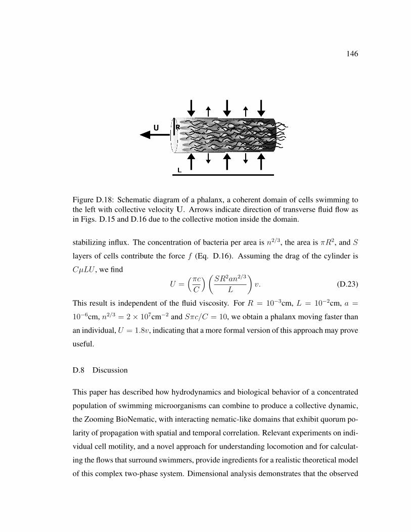
146

Figure D.18: Schematic diagram of a phalanx, a coherent domain of cells swimming tothe left with collective velocity U. Arrows indicate direction of transverse fluid flow asin Figs. D.15 and D.16 due to the collective motion inside the domain.

stabilizing influx. The concentration of bacteria per area is n2/3, the area is πR2, and S

layers of cells contribute the force f (Eq. D.16). Assuming the drag of the cylinder is

CµLU , we find

U =(πcC

)(SR2an2/3

L

)v. (D.23)

This result is independent of the fluid viscosity. For R = 10−3cm, L = 10−2cm, a =

10−6cm, n2/3 = 2× 107cm−2 and Sπc/C = 10, we obtain a phalanx moving faster than

an individual, U = 1.8v, indicating that a more formal version of this approach may prove

useful.

D.8 Discussion

This paper has described how hydrodynamics and biological behavior of a concentrated

population of swimming microorganisms can combine to produce a collective dynamic,

the Zooming BioNematic, with interacting nematic-like domains that exhibit quorum po-

larity of propagation with spatial and temporal correlation. Relevant experiments on indi-

vidual cell motility, and a novel approach for understanding locomotion and for calculat-

ing the flows that surround swimmers, provide ingredients for a realistic theoretical model

of this complex two-phase system. Dimensional analysis demonstrates that the observed

147

speeds of the collective domains are plausible, and that the occurrence of “turbulent” dy-

namics at Re 1 can be understood by considering the input of (swimming) energy

from the occupants of the fluid.

We demonstrate that the results of PIV, obtained from high frame rate video mi-

croscopy images of the swimming cells, i.e. under difficult circumstances, can provide

useful data on velocity and vorticity distributions, the latter exhibiting a rather satisfying

alternation of signs, somewhat like vortex streets. It should be remembered that the PIV

data were obtained from the bacteria, the motile suspended phase, not from added tracers

in the water. Moreover, we have developed a novel measure of angular alignment (and

deviation), based on the velocity vector field. That analysis shows the remarkable spatial

extent of continuous alignment, as well as singular regions of defects. Whereas averages

over many quasi-instantaneous correlations of vorticity and velocity show decays of order

one second, the alignment data exhibits remarkable stability.

Transport of biologically significant molecules, for cell-cell communication, supply

of nutrients and elimination of wastes, and for respiration can be greatly enhanced by the

chaotic advection that accompanies the intermittent collisions, reconstitution and decay

of the zooming domains. We have proposed a heuristic model of the formation of prop-

agating coherent regions whose ingredients are the transverse flows and inward forces

that accompany swimming (Fig. D.14), up-flow swimming in shear flows (Sec. D.4),

flipping of flagella at obstacles [13], and, of course, geometrically determined stacking

(steric repulsion).

What determines the breakup of domains? Extrapolating from Fig. D.15 and calcula-

tions, not shown here, for phalanxes comprising more swimmers, the flow inside a domain

is quite weak. The supply of oxygen to the interior cells (note Fig. D.16) would be insuf-

ficient to maintain average levels of concentration. The interior cells will therefore swim

transversely, up the gradient of oxygen concentration, or swim ever more slowly; both

scenarios imply breakup. The swimming velocity distribution of individual cells is ap-

proximately Maxwellian, and very oxygen dependent [22]. The uniform speed of cells in

148

phalanxes is therefore quite remarkable. The decay time of averaged correlations is about

one second (Fig. D.5) and oxygen supply times (Sec. D.1) are about the same. This would

seem to be more than a coincidence. There are other possible contributors to the decay of

coherence. Interior cells may begin tumbling in search of a more favorable chemical en-

vironment; phalanxes that collide break up; the head end of elongated domains, as in Fig.

D.18, may buckle (we occasionally observe very explicit cases of roll-up); instability of

nematics [28, 51] may also be a factor. The problem of understanding this intermittency

clearly demands further work.

D.9 Acknowledgements

This research has been supported by DOE W31-109-ENG38 and NSF PHY 0551742

at the University of Arizona, NSF DMS 0094179 at Tulane, and the Schlumberger Chair

Fund in Cambridge. We should like especially to thank Matti M. Laetsch for her contribu-

tions to Section D.4, David Bentley for help with Fig. D.1, and T.J. Pedley for discussions

and comments on the manuscript.

D.10 References

[1] Childress S (1981) Mechanics of swimming and flying. Cambridge University Press,

Cambridge

[2] Lighthill MJ (1975) Mathematical biofluiddynamics. SIAM, Philadelphia

[3] Berg HC (2003) E. coli in motion. Springer, New York

[4] Solari CA, Ganguly S, Kessler JO, Michod RE, Goldstein RE (2006) Multicellu-

larity and the functional interdependence of motility and molecular transport. Proc

Natl Acad Sci (USA) 103:1353–1358

149

[5] Solari CA, Kessler JO, Goldstein RE (2007) Motility, mixing, and multicellularity.

Gen Prog Evolv Mach 8:115–129

[6] Short MB, Solari CA, Ganguly S, Powers TR, Kessler JO, Goldstein RE (2006)

Flows driven by flagella of multicellular organisms enhance long-range molecular

transport. Proc Natl Acad Sci (USA) 103:8315–8319

[7] Dombrowski C, Cisneros L, Chatkaew S, Goldstein RE, Kessler JO (2004) Self-

concentration and large-scale coherence in bacterial dynamics. Phys Rev Lett

93:098103

[8] Tuval I, Cisneros L, Dombrowski C, Wolgemuth CW, Kessler JO, Goldstein RE

(2005) Bacterial swimming and oxygen transport near contact lines. Proc Natl Acad

Sci (USA) 102:2277–2282

[9] Magariyama Y, Sugiyama S, Muramoto K, Kawagishi I, Imae Y, Kudo S (1995)

Simultaneous measurement of bacterial flagellar rotation rate and swimming speed.

Biophys J 69:2154–2162

[10] Magariyama Y, Sugiyama S, Kudo S (2001) Bacterial swimming speed and rotation

rate of bundled flagella. FEMS Microbiol Lett 199:125–129

[11] Berg HC (1993) Random walks in biology. Princeton University Press, Princeton

[12] Turner, L, Berg, HC (1995) Cells of Escherichia coli swim either end forward. Proc

Natl Acad Sci (USA) 92:477–479

[13] Cisneros L, Dombrowski C, Goldstein RE, Kessler JO (2006) Reversal of bacterial

locomotion at an obstacle. Phys Rev E 73:030901

[14] Pozrikidis C (1997) Introduction to theoretical and computational fluid dynamics.

Oxford University Press, New York

150

[15] Miller MB, Bassler BL (2001) Quorum sensing in bacteria. Ann Rev Microbiol

55:165–199

[16] Kolter R, Greenberg EP (2006) Microbial sciences. the superficial life of microbes.

Nature 441:300–302

[17] Cisneros et al, unpublished

[18] Pedley TJ, Kessler JO (1992) Hydrodynamic phenomena in suspensions of swim-

ming microorganisms. Ann Rev Fluid Mech 24:313–358

[19] Hill NA, Pedley TJ (2005) Bioconvection. Fluid Dyn Res 37:1–20

[20] Hillesdon AJ, Pedley TJ, Kessler JO (1995) The development of concentration gra-

dients in a suspension of chemotactic bacteria. Bull Math Biol 57:299–344

[21] Hillesdon AJ, Pedley TJ (1996) Bioconvection in suspensions of oxytactic bacteria:

linear theory. J Fluid Mech 324:223–259.

[22] Kessler JO, Wojciechowski MF (1997) Collective behavior and dynamics of swim-

ming bacteria. in Bacteria as multicellular organisms. pp 417–450 (ed Shapiro JA,

Dworkin M). Oxford University Press, New York

[23] Mendelson NH, Bourque A, Wilkening K, Anderson KR, Watkins JC (1999) Orga-

nized cell swimming motions in Bacillus subtilis colonies: patterns of short-lived

whirls and jets. J Bact 181:600–609

[24] Wu XL, Libchaber A (2000) Particle diffusion in a quasi-two-dimensional bacterial

bath. Phys Rev Lett 84:3017–3020

[25] Sokolov A, Aranson IS, Kessler JO, Goldstein RE (2007) Concentration dependence

of the collective dynamics of swimming bacteria. Phys Rev Lett 98:158102

151

[26] Vicsek T, Czirok A, Ben-Jacob E, Cohen I, Shochet O (1995) Novel type of phase

transition in a system of self-driven particles. Phys Rev Lett 75: 1226-1229

[27] Toner J, Tu Y (1995) Long-range order in a two-dimensional dynamical XY model:

how birds fly together. Phys Rev Lett 75: 4326-4329

[28] Simha RA, Ramaswamy S (2002) Hydrodynamic fluctuations and instabilities in

ordered suspensions of self-propelled particles. Phys Rev Lett 89:058101

[29] Lega J, Mendelson NH (1999) Control-parameter-dependent Swift-Hohenberg

equation as a model for bioconvection patterns. Phys Rev E 59:6267–6274

[30] Lega J, Passot T (2003) Hydrodynamics of bacterial colonies: a model. Phys Rev E

67:031906

[31] Hernandez-Ortiz JP, Stoltz CG, Graham, MD (2005) Transport and collective dy-

namics in suspensions of confined swimming particles. Phys Rev Lett 95:204501

[32] Aranson IS, Sokolov A, Kessler JO, Goldstein RE (2007) Model for dynamical co-

herence in thin films of self-propelled microorganisms. Phys Rev E 75:040901

[33] Sambelashvili N, Lau AWC, Cai D (2007) Dynamics of bacterial flow: emergence

of spatiotemporal coherent structures. Phys Lett A 360: 507-511

[34] Shapiro JA, Dworkin M (1997) Bacteria as multicellular organisms. Oxford Univer-

sity Press, New York

[35] Willert CE, Gharib M (1991) Digital particle image velocimetry. Exp Fluids 10:181–

193

[36] Keane RD, Adrian R (1992) Theory of cross-correlation analysis of PIV images.

Appl Sci Res 49:191–215

152

[37] de Gennes PG, Prost J (1993) The physics of liquid crystals. Oxford University

Press, Oxford

[38] Hill J, Kalkanci O, McMurry JL, Koser H (2007) Hydrodynamic surface interactions

enable Escherichia coli to seek efficient routes to swim upstream. Phys Rev Lett

98:068101

[39] Taylor, GI (1952) The action of waving cylindrical tails in propelling microscopic

organisms. Proc R Soc London A 211:225–239

[40] Blake JR (1971) A note on the the image system for a stokeslet in a no-slip boundary.

Proc Camb Phil Soc 70:303-310

[41] Ramia M, Tullock DL, Phan-Thien N (1993) The role of hydrodynamic interaction

in the locomotion of microorganisms. Biophys J 65:755–778

[42] Lauga E, DiLuzio WR, Whitesides GM, Stone HA (2006) Swimming in circles:

motion of bacteria near solid boundaries. Biophys J 90:400-412

[43] Saintillan D, Shelley MJ (2007) Orientational order and instabilities in suspensions

of swimming micro-organisms. Phys Rev Lett 99:058102

[44] Cortez R, Fauci L, Medovikov A (2005) The method of regularized Stokeslets in

three dimensions: analysis, validation and application to helical swimming. Phys

Fluids 17:1–14

[45] Cortez R (2001) The method of regularized Sokeslets. SIAM J Sci Comput 23:1204–

1225

[46] Blake JR (1971) A spherical envelope approach to ciliary propulsion. J Fluid Mech

46:199-208

[47] Ainley J, Durkin S, Embid R, Boindala P, Cortez R (2007) The method of images

for regularized stokeslets. submitted.

153

[48] Nasseri S, Phan–Thien N (1997) Hydrodynamic interaction between two nearby

swimming micromachines. Comput Mech 20:551–559

[49] Kessler JO, Hill NA (1997) Complementarity of physics, biology and geometry

in the dynamics of swimming micro-organisms. in Physics of biological systems.

Springer Lecture Notes in Physics 480:325–340 (ed H. Flyvbjerg, et al). Springer

Verlag, Berlin

[50] Kessler JO, Burnett GD, Remick KE (2000) Mutual dynamics of swimming mi-

croorganisms and their fluid habitat. in Nonlinear science at the dawn of the 21st

century. Springer Lecture Notes in Physics 542:409–426. (ed P.L. Christiansen, M.P.

Srensen and A.C. Scott). Springer-Verlag, Berlin

[51] Simha RA, Ramaswamy S (2002) Statistical hydrodynamics of ordered suspensions

of self-propelled particles: waves, giant number fluctuations and instabilities. Phys-

ica A 306:262–269

154

APPENDIX E

UNEXPECTED BIPOLAR FLAGELLAR ARRANGEMENTS AND

LONG-RANGE FLOWS DRIVEN BY BACTERIA NEAR SOLID BOUNDARIES

Luis H. Cisneros1, Ricardo Ortiz2, Ricardo Cortez2, John O. Kessler1, Martin A. Bees3

1 Department of Physics, University of Arizona. 2 Department of Mathematics, Tulane

University. 3 Department of Mathematics, University of Glasgow, UK.

Published in Physical Review Letters, Vol. 101, 168102 (2008).

DOI 10.1103/PhysRevLett.101.168102

c©2008 The American Physical Society

ABSTRACT

Experiments and mathematical modeling show that complex flows driven by unexpected

flagellar arrangements are induced when peritrichously flagellated bacteria are confined

in a thin layer of fluid, between asymmetric boundaries. The flagella apparently form a

dynamic bipolar assembly rather than the single bundle characteristic of free swimming

bacteria, and the resulting flow is observed to circulate around the cell body. It ranges

over several cell diameters, in contrast to the small extent of the flows surrounding free

swimmers. Results also suggest that flagellar bundles on bacteria that lie flat on a solid

substrate, have an effective rotation rate slower than “free” flagella. This discovery ex-

tends our knowledge of the dynamic geometry of bacteria and their flagella, and reveals

new mechanisms for motility-associated molecular transport and intercellular communi-

cation.

155

Unexpected Bipolar Flagellar Arrangements and Long-Range Flows Drivenby Bacteria near Solid Boundaries

Luis H. Cisneros and John O. KesslerDepartment of Physics, University of Arizona, 1118 E 4th St, Tucson, Arizona 85721, USA*

Ricardo Ortiz and Ricardo CortezDepartment of Mathematics, Tulane University, 6823 St. Charles Avenue, New Orleans, Louisiana 70118, USA+

Martin A. BeesDepartment of Mathematics, University of Glasgow, Glasgow, G12 8QW, United Kingdom‡

(Received 16 May 2008; published 16 October 2008)

Experiments and mathematical modeling show that complex flows driven by unexpected flagellar

arrangements are induced when peritrichously flagellated bacteria are confined in a thin layer of fluid,

between asymmetric boundaries. The flagella apparently form a dynamic bipolar assembly rather than the

single bundle characteristic of free swimming bacteria, and the resulting flow is observed to circulate

around the cell body. It ranges over several cell diameters, in contrast to the small extent of the flows

surrounding free swimmers. Results also suggest that flagellar bundles on bacteria that lie flat on a solid

substrate have an effective rotation rate slower than ‘‘free’’ flagella. This discovery extends our knowledge

of the dynamic geometry of bacteria and their flagella, and reveals new mechanisms for motility-

associated molecular transport and intercellular communication.

DOI: 10.1103/PhysRevLett.101.168102 PACS numbers: 47.63.Gd, 47.63.mf, 87.18.Fx, 87.18.Gh

Introduction.—The geometry and dynamics of flowaround active bacteria [1] determine cell-cell interactions,chemical communication, and transport. When cells areadjacent to surfaces, these flows are especially significantfor the distribution of exuded polymers involved in thesynthesis of biofilms [2]. Bacillus subtilis are rod-shapedbacteria, typically 4 !m long with a diameter of 1 !m,propelled by 6 or more helical flagella [3] randomly (i.e.,peritrichously) distributed about cell body. The flagella arestiff helical polymeric structures (6–20 !m long; 20 nmdiameter; 3 !m pitch; rotating at !100Hz) attached byflexible joints to motors embedded in the cell wall [1,4].Flagella on swimming bacteria conventionally are thoughtto adopt one of two arrangements. Mutual hydrodynamicattraction between flagella produces a single, polar, andcorotating bundle posterior to a (requisitely) swimmingcell. Reverse rotation of one or more motors producesunbundling, yielding incoherent flagellar deployment andcell tumbling (random reorientation) [4–7].

We report novel flagella-driven flows that circulateabout cells of B. subtilis immobilized at a solid surface.These flows imply that the surface induces an unexpectedgeometry: a bipolar arrangement of flagellar bundles. Theflows, the associated spatial arrangement of flagella, andsupporting evidence from a mathematical model constitutea sea change in the understanding of the physics of fluidmotion due to bacteria in the vicinity of solid boundaries.When several bacteria are arranged in close proximity, asin natural situations, we find that they drive cell-scaleunsteady circulation that facilitates long-range transportand mixing [8–10]. Recent and consistent results [10]

describe mixing close to a boundary enhanced by theattachment of a dense carpet of bacteria (flow due toindividuals, however, was not reported).Materials and methods.—B. subtilis 1085B was cultured

in Ezmix Terrific Broth (TB; Sigma: 47.6 g broth mix and8 mL glycerin /L distilled water). Samples were preparedby adding 1 mL stock ("20 #C) to 50 mLTB (18 h shaker-bath incubation; 37 #C; 100 rpm). Plates of 50 mL of TBwere inoculated with 1 mL of suspension, and 5 h incuba-tion obtains long, motile cells. Then, 1:100 dilutions wereprepared with fresh TB and carboxylate-modified micro-spheres (Molec. Probes: F8809 - FluoSpheres 0:21 !m), aspassive tracers.A drop of this bacteria-bead suspension was placed on a

glass coverslip, then partially removed with a pipette,yielding a thin layer of fluid. Cells were trapped betweenglass and meniscus at depths of $1 !m at the drop edge.Imaging used an inverted microscope (Nikon Diaphot

300; 100x objective) with a high-speed camera (PhantomV5; 100 Hz at 256% 256 pixel resolution). Samples wereenclosed within a chamber containing water reservoirs tocontrol humidity and avoid evaporative flows. Particle-image-velocimetry software (Dantec) was used to estimatevelocity fields from image sequences.Experimental results.—By observing the motion of pas-

sive tracers, we can estimate the flagella-driven flow. Weanalyze two cases: when cells are stuck between the upper‘‘free’’ and lower ‘‘no-slip’’ boundaries, and when they area body length from the boundaries and so free to swim withstandard kinetics, but are still confined to the shallow fluidlayer.

PRL 101, 168102 (2008) P HY S I CA L R EV I EW LE T T E R Sweek ending

17 OCTOBER 2008

0031-9007=08=101(16)=168102(4) 168102-1 ! 2008 The American Physical Society

156

E.1 Introduction

The geometry and dynamics of flow around active bacteria [1] determines cell-cell inter-

actions, and chemical communication and transport. When cells are adjacent to surfaces

these flows are especially significant for the distribution of exuded polymers involved in

the synthesis of biofilms [2]. Bacillus subtilis are rod-shaped bacteria, typically 4 µm long

with a diameter of 1 µm, propelled by 6 or more helical flagella [3] randomly (i.e. per-

itrichously) distributed about cell body. The flagella are stiff helical polymeric structures

(6-20 µm long; 20 nm diameter; 3 µm pitch; rotating at 100 Hz) attached by flexible

joints to motors embedded in the cell wall [1, 4]. Flagella on swimming bacteria conven-

tionally are thought to adopt one of two arrangements. Mutual hydrodynamic attraction

between flagella produces a single, polar and co-rotating bundle posterior to a (requisitely)

swimming cell. Reverse rotation of one or more motors produces unbundling, yielding

incoherent flagellar deployment and cell tumbling (random re-orientation) [5, 6, 7, 4].

We report novel flagella-driven flows that circulate about cells of B. subtilis immo-

bilized at a solid surface. These flows imply that the surface induces an unexpected ge-

ometry: a bipolar arrangement of flagellar bundles. The flows, the associated spatial

arrangement of flagella, and supporting evidence from a mathematical model, constitute

a sea change in the understanding of the physics of fluid motion due to bacteria in the

vicinity of solid boundaries. When several bacteria are arranged in close proximity, as

in natural situations, we find that they drive cell-scale unsteady circulation that facilitates

long-range transport and mixing [8, 9, 10]. Recent and consistent results [10] describe

mixing close to a boundary enhanced by the attachment of a dense carpet of bacteria (flow

due to individuals, however, was not reported).

E.2 Materials and Methods

B. subtilis 1085B was cultured in Ezmix Terrific Broth (TB; Sigma: 47.6 g broth mix

and 8 mL glycerin / L distilled water). Samples were prepared by adding 1 mL stock

157

(−20C) to 50 mL TB (18 h shaker-bath incubation; 37C; 100 rpm). 50 mL of TB was

inoculated with 1 mL of suspension, and 5 h incubation obtains long, motile cells. 1:100

dilutions were prepared with fresh TB with 1 part carboxylate-modified microspheres

(Molec. Probes: F8809 - FluoSpheres 0.21 µm), as passive tracers.

A drop of this bacteria-bead suspension was placed on a glass coverslip, then partially

removed with a pipette, yielding a thin layer of fluid. Cells were trapped between glass

and meniscus at depths of ≈ 1 µm at the drop edge.

Imaging used an inverted microscope (Nikon Diaphot 300; 100x objective) with a

high-speed camera (Phantom V5; 100Hz at 256x256 pixel resolution). Samples were

enclosed within a chamber containing water reservoirs to control humidity and avoid

evaporative flows. Particle-image-velocimetry software (Dantec) was used to estimate

velocity fields from image sequences.

E.3 Experimental Results

By observing the motion of passive tracers, we can estimate the flagella-driven flow. We

analyze two cases: when cells are stuck between the upper “free” and lower “no-slip”

boundaries, and when they are a body length from the boundaries and so free to swim

with standard kinetics, but are still confined to the shallow fluid layer.

i) Stuck cells: Swimming bacteria may become trapped near the edge of the drop

where the fluid is shallow. This is most likely due to wedging of the cell between solid

and free surfaces (interfacial forces) or electrostatic attraction. In Fig E.1 we present the

flow field around one such immobile bacterium. Although this organism appears ready to

divide, the result is typical of stuck cells.

Fig E.1 shows two-dimensional streamlines (lines such that dx/ux = dy/uy, where

ux and uy are flow velocity components). The lengths of the arrows indicate that the flow

decays rapidly with distance from the cell body.

The most startling geometric feature of the flow is its circulation. The geometry of

this flow is unexpected, and it does not fit the standard models of bacteria as bodies with

158

Figure E.1: Stationary flow field (mean over 20 sec) surrounding a stuck cell and cor-responding streamlines computed from a regular grid of initial points. The arrow in thelower right corner represents 10 µm s−1.

single polar flagellar bundles [5, 6, 7]. (Inactive cells, either dead or deflagellated, do

not generate flow.) We explore this observation by sampling the velocity field along the

principal axes: set U and V equal to the velocity measured along and perpendicular to the

cell axis, respectively. The magnitudes of these quantities provide a measure of how the

flow decays with distance (Fig E.2). Furthermore, it is clear that the flow rotates around

the cell body, but also that there is flow “outwards” along the parallel axis and “inwards”

along the perpendicular axis, suggesting stresslet-like flow added to the circulation and

hinting at the presence of flagellar bundles with similar orientation to the cell body. Equiv-

alent results were obtained for other stuck bacteria (we observed 25 such flows out of 27

observations of stuck cells of various lengths, i.e. in various stages of growth). The mag-

nitude of the flow is best fitted by an exponential in the region close to the cell (within

2 bodylengths), before velocities become commensurate with noise. As a function of D,

distance from the centre of the cell, V ∝ e−kD where k ≈ 14µm−1 (when average behav-

ior along all directions is measured, k = (0.26± 0.033) µm−1). Any far field polynomial

dependence is experimentally occluded by noise, but the exponential near field behaviour

159

Figure E.2: (a) perpendicular U⊥ and parallel U‖ components of velocity U as a functionof the distance along the cell axis for a stuck cell (black & blue, respectively) and for afree swimming cell (red & green). (b) as for a) except that data is for V and distance istransverse to the cell axis. (c) velocity components

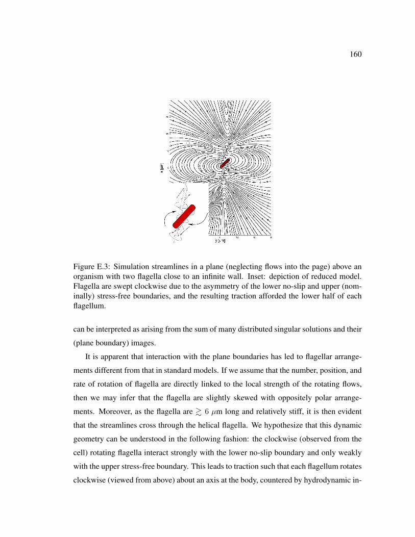
160

Figure E.3: Simulation streamlines in a plane (neglecting flows into the page) above anorganism with two flagella close to an infinite wall. Inset: depiction of reduced model.Flagella are swept clockwise due to the asymmetry of the lower no-slip and upper (nom-inally) stress-free boundaries, and the resulting traction afforded the lower half of eachflagellum.

can be interpreted as arising from the sum of many distributed singular solutions and their

(plane boundary) images.

It is apparent that interaction with the plane boundaries has led to flagellar arrange-

ments different from that in standard models. If we assume that the number, position, and

rate of rotation of flagella are directly linked to the local strength of the rotating flows,

then we may infer that the flagella are slightly skewed with oppositely polar arrange-

ments. Moreover, as the flagella are & 6 µm long and relatively stiff, it is then evident

that the streamlines cross through the helical flagella. We hypothesize that this dynamic

geometry can be understood in the following fashion: the clockwise (observed from the

cell) rotating flagella interact strongly with the lower no-slip boundary and only weakly

with the upper stress-free boundary. This leads to traction such that each flagellum rotates

clockwise (viewed from above) about an axis at the body, countered by hydrodynamic in-

161

teractions and mechanical properties of the flagella [11, 12]. Such rotation, arrested by

the body, can produce aggregation,or bundling, of flagella in two preferred oblique direc-

tions with respect to the bacterial body, as depicted in Fig E.3 (inset; simply illustrated

by two flagella). We emphasise again that this geometry is quite different from the gener-

ally assumed backwardly-oriented, propulsive arrangement of flagella. Here, there is no

“backward”, since the cell is immobile. When flagella in these skewed, oppositely polar

arrangements rotate about their axes, their helical shape ought to drive circulating flow

of some form; rather than just propelling fluid parallel to the direction of each helical

axis, the flow has a transverse component. To better understand this inference, in Sec-

tion E.4 we investigate a computational model constructed according to the hypothesised

geometry depicted in Fig E.3.

ii) Free swimming cells: The magnitude of the flow generated by free swimming bac-

teria is much smaller and decays faster spatially than the flow due to stuck cells. Fig E.2

shows the components of U and V for a cell swimming right to left, as a function of

the distance from the cell. The flow speeds along the cell axis are an order of magnitude

smaller than for a stuck bacterium. The error bars, due to Brownian motion of the marker

beads, almost hide the flow (positive at the rear of the cell, negative at the front). The

lateral flow V⊥ is a little larger and negative everywhere due to the transverse thrust of the

cell’s curved trajectory.

iii) Multi-cell PIV: Fig E.4 presents the flow field around several stuck cells in a

thin layer of fluid. As well as the usual rotating flows about individuals, more compli-

cated flows arise due to interactions between cells, and their flagella. This leads to large

scale rotating flows between cells and around the multi-cell complex, with immediate

implications for biofilms. These flows are time dependent, presumably due in part to in-

termittencies in the rotation of the many flagella involved in generating the flow. Such

flows aid the transport of molecules for metabolism and inter-organism communication,

as well as exuded polymers for the synthesis of biofilms [10].

162

Figure E.4: Dynamic flowfield due to several stuck bacteria (both long and short) in a thinlayer of fluid.

E.4 Numerical Simulations

We shall show that asymmetric boundaries drive rotating flow, but one boundary is suffi-

cient to reveal qualitative features, and is computationally less involved than two. Flow

simulations were performed using the method of regularized Stokeslets [13, 14, 15],

which provides expressions to compute fluid motion generated by forces that arise on

the surface of a moving organism [14]. The velocity field due to the application of N

surface forces is

u(x) =

(1

8πµ

) N∑k=1

(|x|2 + 2ε2) fk + [fk · x]x

(|x|2 + ε2)3/2,

where x is the vector from the force location xk to the evaluation point x. For a flow

bounded by an infinite plane wall, the method is augmented with a system of images to

automatically satisfy a no-slip condition [16].

Fig. E.3 shows the arrangement of the flagella and the streamlines of the computed

163

flow. Despite the simplified model, there is a remarkable match with experimentally

observed (Fig E.1) topologies of the fluid velocity, including the two off-axis eddies,

supporting the hypothesized arrangement of flagella as inferred from experiments. The

qualitative features of the Stokes flow solutions are independent of the flagellar angular

velocity, ω2: to agree with experiments we find ω2 = 7 Hz. This rate of rotation of the

flagella inferred from the computation together with the observed velocity of the marker

beads strongly suggests that the rotation of lateral flagella bundles on stuck cells is hin-

dered (effective rate ca. 10 times less than the “standard” 100 Hz). This result applies

equally to [10], where similar bead velocities were found. The infinite plane wall is lo-

cated at z = 0 µm with streamlines computed on z = 2 µm. The cell body is placed

0.022 µm from the wall, and has radius and length Rb = 0.84 µm and Lb = 8 µm, respec-

tively. The fluid velocity is set to zero on the body surface. Both flagella have identical

dimensions with length Lh = 15.57 µm, radius Rh = 0.05 µm, and pitch P = 2.4 µm.

The angles between the flagella axes and the cell body axis are π/8, and both are left

handed and rotate clockwise. Setting the flagella bundles to rotate with different rates

induces a peanut shaped flow even more similar to Fig E.1. It is remarkable that the ex-

ponent of the decay with distance from the cell body on the numerical field is well fitted

k ∼ 0.18− 0.25 µm−1, in reasonable agreement with the experiments.

E.5 Summary and Significance

Interactions between bacteria and plane boundaries are complex: flagella do not align and

bundle “behind” the cell body. Instead, they form a distributed envelope that drives a

flow circulating around the body. That flow extends over dimensions greater than the cell

body’s; it decays exponentially in the near-field with exponent approximately equal to 14

µm−1. This result contrasts starkly with the more localized flow in the vicinity of a trans-

lating bacterium. It is quite remarkable that these experimental results are well matched

by computational modeling using the method of regularised Stokeslets, based on a simple,

logically constructed geometric arrangement of the flagella. The consonance of experi-

164

ment and computation yields substantial cross-validation. We believe that it is possible

to use our modeling technique to predict the geometry of flows surrounding groups of

constrained cells (Fig E.4). Designing substrates that elicit appropriate arrangements of

cell groups could lead to controllable, locally driven complex micro-flows.

What is the broader significance, for quorum sensing (i.e. cell-cell communication)

and the development of biofilms? If cells signal each other, as in the quorum sensing step

of biofilm initiation [17], they will do it while constrained, rather than freely swimming.

Furthermore, “real life” situations of significance involve many interacting bacteria. Our

observations, and those on glued cells [10], confirm that stuck bacterial groups with active

flagella drive intermittent, complex and far-ranging flows that appear to mix and provide

advective transport.

The hydrodynamic interaction of micro-organisms with each other and with surfaces

is crucial in understanding the initiation of biofilms and the development of their polymer-

mediated stability [2, 18]. The present results, on extensive flows driven by immobile cells

near a wall, are a crucial step in reaching that understanding.

E.6 Acknowledgments

Support: DOE W31-10t-ENG38 (LHC & JOK); NSF DMS 0612625 (RO & RC); EP-

SRC EP/D073308/1 (MAB). We thank R.E. Goldstein, S. Ganguly and, especially, C.

Dombrowski for useful comments.

E.7 References

[1] L. Cisneros, R. Cortez, C. Dombrowski, R. Goldstein, & J. Kessler. Exp. Fluids,

43:737–753, 2007.

[2] R. Kolter & E.P. Greenberg, Nature 441, 300 (2006)

[3] M. Ito, N. Terahara, S. Fujinami & T.A. Krulwich. J. Mol. Biol. 352:396-408 (2005).

165

[4] L. Turner, W.S. Ryu & H.C. Berg. J. Bacteriol., 182:2793-2801, 2000.

[5] R.M. Macnab. Proc. Nat. Acad. Sci., 74:221–25, 1977.

[6] C. Brennen & H. Winet Ann. Rev. Fluid Mech., 9:339–98, 1977.

[7] H.C. Berg, Random walks in Biology. Princeton University Press, Priceton (1993)

[8] H. Aref. Stirring by chaotic advection. J. Fluid Mech., 143: 1-21, 1984.

[9] S.R. Otto, A.N. Yannacopoulos, & J.R. Blake. J. Fluid Mech., 430: 1-26, 2001.

[10] N. Darnton, L. Turner, K. Breuer & H.C. Berg. Biophys. J., 86:1863-70, 2004.

[11] T. Goto, K. Nakata, K. Baba, M. Nishimura & Y. Magariyama. Biophys. J., 89:3771-

79, 2005.

[12] E. Lauga, W.R. Diluzio, G.M. Whitesides & H.A. Stone Biophys. J., 90:400–12,

2006.

[13] R. Cortez. SIAM J. Sci. Comput., 23(4):1204–1225 (electronic), 2001.

[14] R. Cortez, L. Fauci, & A. Medovikov. Phys. Fluids, 17:1–14, 2005.

[15] H. Flores, E. Lobaton, S. Mendez-Diez, S. Tlupova, R. Cortez. Bull. Math. Biol.,

67:137–68, 2005.

[16] J. Ainley, S. Durkin, R. Embid, P. Boindala,& R. Cortez. J. Comput. Phys.,

227:4600–4616, 2008.

[17] M.R. Parsek & E.P. Greenberg, Trends Microbiol., 13, 27(2005)

[18] S.A. West, S.P. Diggle, A. Buckling, A. Gardner, & A.S. Griffin, Annu. Rev. Ecol.

Evol. Syst., 38, 53 (2007)