BIPED LOCOMOTION: STABILITY ANALYSIS, GAIT ... - CORE

BIPED LOCOMOTION: STABILITY ANALYSIS, GAIT

GENERATION AND CONTROL

By

Dip Goswami

SUBMITTED IN PARTIAL FULFILLMENT OF THE

REQUIREMENTS FOR THE DEGREE OF

DOCTOR OF PHILOSOPHY

AT

DEPARTMENT OF ELECTRICAL AND COMPUTER ENGINEERING,

NATIONAL UNIVERSITY OF SINGAPORE

4 ENGINEERING DRIVE 3, SINGAPORE 117576

AUGUST 2009

Table of Contents

Table of Contents ii

List of Tables vi

List of Figures vii

Acknowledgements xii

Abstract xiii

1 Introduction 1

1.1 The Biped Locomotion . . . . . . . . . . . . . . . . . . . . . . . . . . 2

1.2 Postural Stability . . . . . . . . . . . . . . . . . . . . . . . . . . . . . 8

1.2.1 Zero-Moment-Point . . . . . . . . . . . . . . . . . . . . . . . . 9

1.2.2 Foot-Rotation-Indicator Point . . . . . . . . . . . . . . . . . . 13

1.2.3 Biped Model With Point-Foot . . . . . . . . . . . . . . . . . . 15

1.3 Actuator-level Control . . . . . . . . . . . . . . . . . . . . . . . . . . 16

1.3.1 Internal dynamics and Zero-dynamics . . . . . . . . . . . . . . 20

1.4 Gait Generation . . . . . . . . . . . . . . . . . . . . . . . . . . . . . . 21

1.5 Dissertation Outline . . . . . . . . . . . . . . . . . . . . . . . . . . . 23

2 Biped Walking Gait Optimization considering Tradeoff between Sta-

bility Margin and Speed 26

2.1 Biped Model, Actuators and Mechanical Design . . . . . . . . . . . . 28

2.2 Biped Inverse Kinematics . . . . . . . . . . . . . . . . . . . . . . . . 30

2.2.1 Generalized Coordinates . . . . . . . . . . . . . . . . . . . . . 30

2.2.2 Inverse Kinematics . . . . . . . . . . . . . . . . . . . . . . . . 31

2.3 Biped Walking Gait . . . . . . . . . . . . . . . . . . . . . . . . . . . . 35

2.3.1 Choice of Walking Parameters . . . . . . . . . . . . . . . . . . 38

ii

2.4 Genetic Algorithm . . . . . . . . . . . . . . . . . . . . . . . . . . . . 39

2.5 GA Based Parameter Optimization . . . . . . . . . . . . . . . . . . . 40

2.5.1 Constrains on Walking Parameters . . . . . . . . . . . . . . . 40

2.5.2 Postural Stability Considering ZMP . . . . . . . . . . . . . . . 40

2.5.3 Cost Function . . . . . . . . . . . . . . . . . . . . . . . . . . . 42

2.6 Computation of ZMP . . . . . . . . . . . . . . . . . . . . . . . . . . . 44

2.6.1 ZMP Expression . . . . . . . . . . . . . . . . . . . . . . . . . 46

2.7 Simulations and Experiments . . . . . . . . . . . . . . . . . . . . . . 48

2.7.1 Effect of λ on walking performance . . . . . . . . . . . . . . . 51

2.7.2 Effect of step-time (T ) on walking performance . . . . . . . . 58

2.8 Conclusions . . . . . . . . . . . . . . . . . . . . . . . . . . . . . . . . 59

3 Disturbance Rejection by Online ZMP Compensation 60

3.1 ZMP Measurement . . . . . . . . . . . . . . . . . . . . . . . . . . . . 62

3.1.1 Biped Model . . . . . . . . . . . . . . . . . . . . . . . . . . . 62

3.1.2 Force Sensors . . . . . . . . . . . . . . . . . . . . . . . . . . . 63

3.1.3 Measurement of ZMP . . . . . . . . . . . . . . . . . . . . . . . 64

3.2 Online ZMP Compensation . . . . . . . . . . . . . . . . . . . . . . . 69

3.3 Applications, Experiments and Results . . . . . . . . . . . . . . . . . 74

3.3.1 Improvement of Walking on Flat Surface . . . . . . . . . . . . 75

3.3.2 Rejecting Disturbance due to Sudden Push . . . . . . . . . . . 75

3.3.3 Walking Up and Down a Slope . . . . . . . . . . . . . . . . . 77

3.3.4 Carrying Weight during Walking . . . . . . . . . . . . . . . . 78

3.4 Conclusions . . . . . . . . . . . . . . . . . . . . . . . . . . . . . . . . 80

4 Jumping Gaits of Planar Bipedal Robot with Stable Landing 85

4.1 The Biped Jumper . . . . . . . . . . . . . . . . . . . . . . . . . . . . 88

4.1.1 Biped Jumper: BRAIL 2.0 . . . . . . . . . . . . . . . . . . . . 88

4.1.2 Foot Compliance Model and Foot Design . . . . . . . . . . . . 92

4.1.3 Jumping Sequences . . . . . . . . . . . . . . . . . . . . . . . . 93

4.1.4 The Lagrangian Dynamics of the Biped in Take-off and Touch-

down Phases . . . . . . . . . . . . . . . . . . . . . . . . . . . . 96

4.1.5 Lagrangian Dynamics Computation of the at the Take-off and

Touch-down phases . . . . . . . . . . . . . . . . . . . . . . . . 98

4.1.6 The Lagrangian Dynamics of the Biped in Flight Phase . . . . 101

4.1.7 Impact Model and Angular Momentums . . . . . . . . . . . . 103

4.1.8 Jumping Motion and Angular Momentum relations . . . . . . 104

4.2 Control Law Development . . . . . . . . . . . . . . . . . . . . . . . . 106

4.3 Selection of Desired Gait . . . . . . . . . . . . . . . . . . . . . . . . . 106

iii

4.3.1 Take-off phase Gait . . . . . . . . . . . . . . . . . . . . . . . . 109

4.3.2 Flight phase Gait . . . . . . . . . . . . . . . . . . . . . . . . . 109

4.3.3 Touch-down phase Gait . . . . . . . . . . . . . . . . . . . . . 111

4.4 Landing Stability Analysis . . . . . . . . . . . . . . . . . . . . . . . . 111

4.4.1 Switched Zero-Dynamics (SZD): Touch-down phase . . . . . . 112

4.4.2 Stability of SZD . . . . . . . . . . . . . . . . . . . . . . . . . . 115

4.4.3 Closed-loop Dynamics: Touch-down phase . . . . . . . . . . . 121


4.5.1 Jumping Gait Simulations . . . . . . . . . . . . . . . . . . . . 129

4.5.2 Jumping Experiment on BRAIL 2.0 . . . . . . . . . . . . . . . 134

4.5.3 Comments on Simulations and Experimental Results . . . . . 141

4.6 Conclusions . . . . . . . . . . . . . . . . . . . . . . . . . . . . . . . . 142

4.6.1 Future Directions . . . . . . . . . . . . . . . . . . . . . . . . . 143

5 Rotational Stability Index (RSI) Point: Postural Stability in Bipeds144

5.1 Planar Biped: Two-link model . . . . . . . . . . . . . . . . . . . . . . 147

5.1.1 Dynamics . . . . . . . . . . . . . . . . . . . . . . . . . . . . . 149

5.1.2 Internal Dynamics . . . . . . . . . . . . . . . . . . . . . . . . 150

5.1.3 Postural Stability . . . . . . . . . . . . . . . . . . . . . . . . . 150

5.2 Rotational Stability and Rotational Stability Index (RSI) Point . . . 154

5.2.1 Planar Bipeds and Rotational Stability . . . . . . . . . . . . . 155

5.2.2 CM criteria for Rotational Stability . . . . . . . . . . . . . . . 159

5.2.3 Discussions on the RSI Point . . . . . . . . . . . . . . . . . . 161

5.3 RSI Point Based Stability Criteria . . . . . . . . . . . . . . . . . . . . 163

5.3.1 Gaits with θ2 6= 0 . . . . . . . . . . . . . . . . . . . . . . . . 164

5.3.2 Backward foot-rotation . . . . . . . . . . . . . . . . . . . . . . 164

5.3.3 Stability Criterion . . . . . . . . . . . . . . . . . . . . . . . . 166

5.3.4 Comparison with other Ground Reference Points . . . . . . . 166


5.4.1 Simulations . . . . . . . . . . . . . . . . . . . . . . . . . . . . 170

5.4.2 Experiments . . . . . . . . . . . . . . . . . . . . . . . . . . . . 177

5.5 Conclusions . . . . . . . . . . . . . . . . . . . . . . . . . . . . . . . . 179

6 Conclusions and Future Directions 180

6.1 Conclusions . . . . . . . . . . . . . . . . . . . . . . . . . . . . . . . . 180

6.2 Future Directions . . . . . . . . . . . . . . . . . . . . . . . . . . . . . 182

iv

7 Author’s Publications 184

7.1 International Journal . . . . . . . . . . . . . . . . . . . . . . . . . . . 184

7.2 International Conference . . . . . . . . . . . . . . . . . . . . . . . . . 185

Bibliography 186

v

List of Tables

2.1 Parameters of the BRAIL 1.0. . . . . . . . . . . . . . . . . . . . . . . 29

2.2 Parameters of GA. . . . . . . . . . . . . . . . . . . . . . . . . . . . . 39

2.3 Optimum Walking Parameters obtained through GA optimization. . . 49

2.4 Walking Parameters for different step-time (T) with λ = 0.1. . . . . . 59

2.5 Walking Parameters for different step-time (T) with λ = 0.15. . . . . 59

3.1 Parameters of the Biped-Model (MaNUS-I) . . . . . . . . . . . . . . . 64

4.1 Parameters of the BRAIL 2.0 biped . . . . . . . . . . . . . . . . . . . 90

4.2 DH Parameters of the Robot . . . . . . . . . . . . . . . . . . . . . . . 99

4.3 Robot’s Jumping Gait . . . . . . . . . . . . . . . . . . . . . . . . . . 130

4.4 Different Parameters Values at Jumping Phases. . . . . . . . . . . . . 131

4.5 V maxxcm and V max

ID . . . . . . . . . . . . . . . . . . . . . . . . . . . . . . . 133

vi

List of Figures

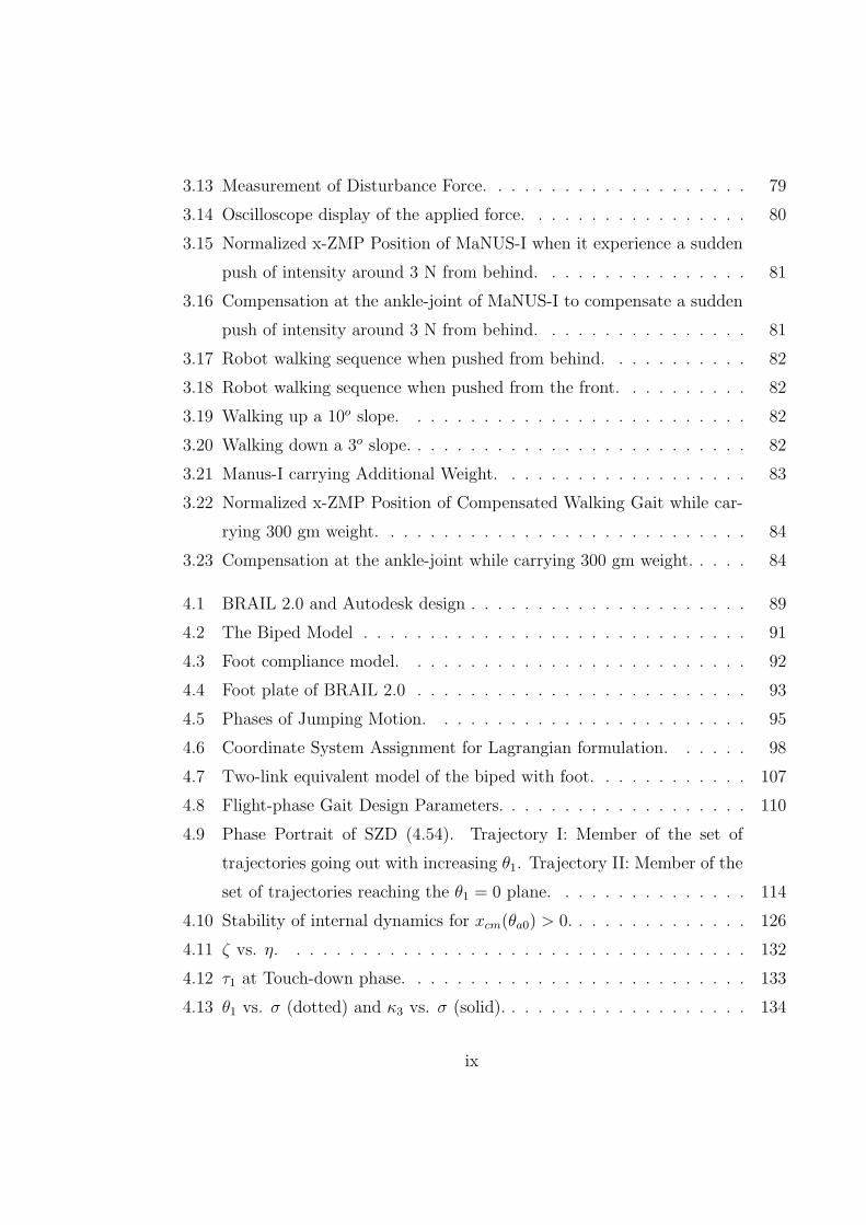
1.1 Sagittal, Frontal and Transverse planes. . . . . . . . . . . . . . . . . . 3

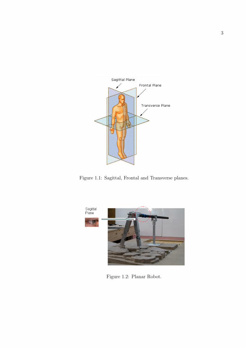
1.2 Planar Robot. . . . . . . . . . . . . . . . . . . . . . . . . . . . . . . . 3

1.3 Single-support and double-support phases. . . . . . . . . . . . . . . . 4

1.4 Biped Locomotion. . . . . . . . . . . . . . . . . . . . . . . . . . . . . 4

1.5 Support Polygon. . . . . . . . . . . . . . . . . . . . . . . . . . . . . . 8

1.6 Zero-Moment-Point. M: Total Mass of the system, ~a is the linear accel-

eration, ~FGRF is the ground-reaction force, ZMP (xzmp, yzmp) is where

~FGRF acts. . . . . . . . . . . . . . . . . . . . . . . . . . . . . . . . . 10

1.7 Inverted Pendulum Model. . . . . . . . . . . . . . . . . . . . . . . . . 12

1.8 FRI Point. M: Total mass, Mfoot: Foot mass, afoot: Foot acceleration,

τankle: Torque input at the ankle joint, CMfoot : CM of the foot. . . . 14

1.9 Periodic Motion. . . . . . . . . . . . . . . . . . . . . . . . . . . . . . 16

2.1 Generalized Coordinates. . . . . . . . . . . . . . . . . . . . . . . . . . 30

2.2 Biped model: Mass Distribution. . . . . . . . . . . . . . . . . . . . . 31

2.3 The Biped. . . . . . . . . . . . . . . . . . . . . . . . . . . . . . . . . 32

2.4 Biped Reference Points for Inverse Kinematics. . . . . . . . . . . . . . 33

2.5 Biped: Inverse Kinematic Parameters. . . . . . . . . . . . . . . . . . 33

2.6 Gait Generation Parameters. . . . . . . . . . . . . . . . . . . . . . . . 36

2.7 The GA algorithm for obtaining optimal walking parameters for a spe-

cific value of λ. . . . . . . . . . . . . . . . . . . . . . . . . . . . . . . 41

2.8 Fitness trend with λ = 0.15. . . . . . . . . . . . . . . . . . . . . . . . 50

vii

2.9 The walking gait with λ = 0.15 : θ1, θ12, θ2, θ11, θ3, θ10 (time in Second

vs. angle in degree). . . . . . . . . . . . . . . . . . . . . . . . . . . . 52

2.10 The walking gait with λ = 0.15 : θ4, θ9, θ5, θ8, θ6, θ7 (time in Second

vs. angle in degree). . . . . . . . . . . . . . . . . . . . . . . . . . . . 53

2.11 Biped walking for one step-time with λ = 0.15. . . . . . . . . . . . . . 54

2.12 yzmp vs. xzmp for one step-time with λ = 0.15, s = 0.13, n = 0.109, H =

0.014, h = 0.020. . . . . . . . . . . . . . . . . . . . . . . . . . . . . . . 55

2.13 yzmp and xzmp vs. time for one step-time with λ = 0.15, s = 0.13, n =

0.109, H = 0.014, h = 0.020 (dotted line is xzmp and solid line is yzmp). 55


0.026, h = 0.010. . . . . . . . . . . . . . . . . . . . . . . . . . . . . . . 56




0.01, h = 0.022. . . . . . . . . . . . . . . . . . . . . . . . . . . . . . . 57



3.1 Biped Model in the frontal and sagittal plane. . . . . . . . . . . . . . 63

3.2 Biped Model of MaNUS-I in visualNastran 4D environment. . . . . . 65

3.3 MaNUS-I. . . . . . . . . . . . . . . . . . . . . . . . . . . . . . . . . . 66

3.4 Mechanical Installation of Force Sensors. . . . . . . . . . . . . . . . . 67

3.5 Force-to-Voltage Converter Circuit. . . . . . . . . . . . . . . . . . . . 67

3.6 Positions of the foot sensors at the bottom of the feet. . . . . . . . . . 67

3.7 Reading of the Force Sensors. . . . . . . . . . . . . . . . . . . . . . . 67

3.8 Simplified model of the Biped in Sagittal and Frontal Planes. . . . . . 68

3.9 The block diagram for online ZMP compensation. . . . . . . . . . . . 74

3.10 Normalized x-ZMP Position of Uncompensated Walking Gait. . . . . 76

3.11 Normalized x-ZMP Position of Compensated Walking Gait. . . . . . . 77

3.12 Compensation at the ankle-joint during walking on a flat surface. . . 78

viii

3.13 Measurement of Disturbance Force. . . . . . . . . . . . . . . . . . . . 79

3.14 Oscilloscope display of the applied force. . . . . . . . . . . . . . . . . 80

3.15 Normalized x-ZMP Position of MaNUS-I when it experience a sudden

push of intensity around 3 N from behind. . . . . . . . . . . . . . . . 81

3.16 Compensation at the ankle-joint of MaNUS-I to compensate a sudden

push of intensity around 3 N from behind. . . . . . . . . . . . . . . . 81

3.17 Robot walking sequence when pushed from behind. . . . . . . . . . . 82

3.18 Robot walking sequence when pushed from the front. . . . . . . . . . 82

3.19 Walking up a 10o slope. . . . . . . . . . . . . . . . . . . . . . . . . . 82

3.20 Walking down a 3o slope. . . . . . . . . . . . . . . . . . . . . . . . . . 82

3.21 Manus-I carrying Additional Weight. . . . . . . . . . . . . . . . . . . 83

3.22 Normalized x-ZMP Position of Compensated Walking Gait while car-

rying 300 gm weight. . . . . . . . . . . . . . . . . . . . . . . . . . . . 84

3.23 Compensation at the ankle-joint while carrying 300 gm weight. . . . . 84

4.1 BRAIL 2.0 and Autodesk design . . . . . . . . . . . . . . . . . . . . . 89

4.2 The Biped Model . . . . . . . . . . . . . . . . . . . . . . . . . . . . . 91

4.3 Foot compliance model. . . . . . . . . . . . . . . . . . . . . . . . . . 92

4.4 Foot plate of BRAIL 2.0 . . . . . . . . . . . . . . . . . . . . . . . . . 93

4.5 Phases of Jumping Motion. . . . . . . . . . . . . . . . . . . . . . . . 95

4.6 Coordinate System Assignment for Lagrangian formulation. . . . . . 98

4.7 Two-link equivalent model of the biped with foot. . . . . . . . . . . . 107

4.8 Flight-phase Gait Design Parameters. . . . . . . . . . . . . . . . . . . 110

4.9 Phase Portrait of SZD (4.54). Trajectory I: Member of the set of

trajectories going out with increasing θ1. Trajectory II: Member of the

set of trajectories reaching the θ1 = 0 plane. . . . . . . . . . . . . . . 114

4.10 Stability of internal dynamics for xcm(θa0) > 0. . . . . . . . . . . . . . 126

4.11 ζ vs. η. . . . . . . . . . . . . . . . . . . . . . . . . . . . . . . . . . . 132

4.12 τ1 at Touch-down phase. . . . . . . . . . . . . . . . . . . . . . . . . . 133

4.13 θ1 vs. σ (dotted) and κ3 vs. σ (solid). . . . . . . . . . . . . . . . . . . 134

ix

4.14 Variations of the joint torques in experimental and simulation studies:

(a) τ2, (b) τ3 and (c) τ4. . . . . . . . . . . . . . . . . . . . . . . . . . 137

4.15 Variations of the joint angular positions in experimental and simulation

studies: (a) θ2, (b) θ3 and (c) θ4. . . . . . . . . . . . . . . . . . . . . 138

4.16 Variations of the joint angular velocities in experimental and simulation

studies: (a) θ2, (b) θ3 and (c) θ4. . . . . . . . . . . . . . . . . . . . . 139

4.17 Jump Sequence with control input (4.43) and desired gait as per Table

4.5.1. . . . . . . . . . . . . . . . . . . . . . . . . . . . . . . . . . . . . 140

5.1 (a) Foot-Rotation in frontal plane (b) Foot-rotation in double-support

phase (sagittal plane) (c) Foot-rotation in single-support phase (sagit-

tal plane) (d) Foot-rotation in swinging leg (sagittal plane). . . . . . 145

5.2 Tiptoe Model. . . . . . . . . . . . . . . . . . . . . . . . . . . . . . . . 147

5.3 Tiptoe Configuration: Two-link model. . . . . . . . . . . . . . . . . . 148

5.4 Phase Portrait of (5.10). Trajectory I: Member of the set of trajectories

going out with increasing θ1. Trajectory II: Member of the set of

trajectories reaching the θ1 = 0 plane. . . . . . . . . . . . . . . . . . . 153

5.5 Rotational Stability. . . . . . . . . . . . . . . . . . . . . . . . . . . . . 155

5.6 RSI point and Phase Portrait. . . . . . . . . . . . . . . . . . . . . . . 161

5.7 Rotational Stability for stationary biped. . . . . . . . . . . . . . . . . 162

5.8 RSI point xRSI > 0. Biped is rotational stable even if xcm(θ) < 0. . . 162

5.9 Forward and backward foot-rotation. . . . . . . . . . . . . . . . . . . 165

5.10 ZMP/FRI/CP/FZMP and RSI: (a) Foot is not going to rotate. (b)

Foot is about to rotate. (c) Foot is rotated, and bipedal posture is

rotational stable. . . . . . . . . . . . . . . . . . . . . . . . . . . . . . 167

5.11 ZMP/FRI/CP and RSI: ZMP/CP/FRI indicate whether the foot is

about to rotate or not, RSI point indicates whether the bipedal posture

will lead to a flat-foot posture or not. . . . . . . . . . . . . . . . . . . 167

5.12 Parameters of BRAIL 2.0 . . . . . . . . . . . . . . . . . . . . . . . . 169

5.13 θ1 Vs. xRSI θ1 Vs. xcm and : θ10 = 0.6 rad and σ0 = −0.0289 kgm2s−1. 171

x

5.14 θ1 Vs. σ: θ10 = 0.6 rad and σ0 = −0.0289 kgm2s−1. . . . . . . . . . . 172

5.15 θ1 Vs. xRSI and θ1 Vs. xcm: θ10 = 0.3 rad and σ0 = 0.0542 kgm2s−1. 173

5.16 θ1 Vs. σ: θ10 = 0.3 rad and σ0 = 0.0542 kgm2s−1. . . . . . . . . . . . 173

5.17 θ1 Vs. xRSI and θ1 Vs. xcm: Pushed from the backside and rotational

stable. . . . . . . . . . . . . . . . . . . . . . . . . . . . . . . . . . . . 174

5.18 θ1 Vs. σ: Pushed from the backside and rotational stable. . . . . . . . 175

5.19 θ1 Vs. σ: Pushed from the backside and ‘rotational unstable’. . . . . 176

5.20 θ1 Vs. σ: Pushed from the backside and ‘rotational unstable’. . . . . 176

5.21 BRAIL 2.0: Push from back. . . . . . . . . . . . . . . . . . . . . . . . 178

xi

Acknowledgements

With immense pleasure I express my sincere gratitude, regards and thanks to my

supervisors A/Prof. Prahlad Vadakkepat for his excellent guidance, invaluable sug-

gestions and continuous encouragement at all the stages of my research work. His

interest and confidence in me was the reason for all the success I have made. I have

been fortunate to have him as my advisor as he has been a great influence on me,

both as a person and as a professional.

Many thanks goes to Prof. QG Wong, Prof. Tong Heng Lee, A/Prof. Loh Ai

Poh and Dr. Tang for their kind help and suggestions. I would like to express my

appreciation to Mr. Burra Pavan Kumar, Mr. Jin Yongying and Mr. Phoon Duc

Kien for their support. Moreover, I would like to thank my colleagues Mr. Jim Tan,

Mr. Daniel Hong, Mr. Ng Buck Sin and Mr. Pramod Kumar for various constructive

discussions and suggestions. Finally, I show my appreciation to the lab officer Mr.

Tan Chee Siong for his support and friendly behavior.

I acknowledge the chance provided to me to pursuit doctoral study in National

University of Singapore. I express my deepest appreciation to all the member of

Electrical And Computer Engineering for the wonderful research environment and

immense support. I do love to remember the time I spend with them.

I am deeply indebted to my beloved wife for her support, understanding and

encouragement in every aspects of life. Without her, I would not possibly have

achieved whatever I have. Finally, I am grateful to my parents for their support.

xii

Abstract

Locomotion is an important domain of research in Bipedal Robots. Dynamics of

the foot-link plays a key role in the stability of biped locomotion. Biped locomotion

can be either with flat-foot (foot-link does not loose contact with ground surface) or

with foot-rotation (foot-link rotates about toe). The initial part of this dissertation

presents a flat-foot optimal walking gait generation method. The optimality in gait

is achieved by utilizing Genetic Algorithm considering a tradeoff between walking

speed and stability. The optimal flat-foot walking gaits are implemented on a biped

robot - BRAIL 1.0. The robustness of such gaits in presence of disturbances is

enhanced by applying zero-moment-point (ZMP) compensation into the robot’s ankle-

joint. Effectiveness of the ZMP compensation technique is validated by utilizing

the technique to maintain postural stability when a humanoid robot, MaNUS-I, is

subjected to disturbances (in the form of push from front or back, carrying weight

in the back and climbing up/down slopes). Such flat-foot gaits are suitable when

the biped is moving slowly. However, the foot-link can rotate during relatively faster

bipedal activities.

The bipeds, with foot-rotation, have an additional passive degree-of-freedom at the

joint between toe and ground. Such bipeds are underactuated as they have one degree-

of-freedom greater than the number of available actuators during the single-support

phase. Underactuated biped dynamics (with foot-rotation) has two-dimensional zero-

dynamics submanifold of the full-order bipedal model. Stability of the associated

zero-dynamics is essential for the stability of the biped locomotion with foot-rotation.

The nature of zero-dynamics is governed by the structure of the biped, foot/ground

xiii

xiv

contact surface and certain control parameters.

Landing stability of bipedal jumping gaits is studied considering the stability

of the associated zero-dynamics. In the landing phase of jumping gaits, switching

occurs between configurations with flat-foot and with foot-rotation. The associated

bipedal zero-dynamics in jumping gait is modeled as a switching system. Stability of

the switching zero-dynamics is investigated by two novel concepts - critical potential

index and critical kinetic index. Utilizing the stability concepts, stable landing is

achieved while implementing the jumping gait on a biped robot - BRAIL 2.0.

A novel concept of rotational stability is introduced for the stability analysis of

biped locomotion with foot-rotation. The rotational stability of underactuated biped

is measured by introducing a ground-reference-point Rotational Stability Index (RSI)

point. The concepts of rotational stability and Rotational Stability Index point in-

vestigates the stability of associated zero-dynamics. A stability criterion, based on

Rotational Stability Index point, is established for the stability in biped locomotion

with foot-rotation.

Chapter 1

Introduction

Locomotion is the ability of animal life to move from one place to another. The

diversity of animal locomotion is astounding and surprisingly complex. The means

of biological locomotion depends on the morphology, scale, and environment of the

organism. Similar argument is applicable for the man-made machines. Airplanes use

wings, army tanks use tracks for traversing uneven terrain and automobiles use wheels.

In case of environments with discontinuous ground support such as rocky slope or

stairs, it is arguable that the most appropriate and versatile means of locomotion

is legs. Legs enable the avoidance of support discontinuities in the environment

by stepping over them. Moreover, legs are the obvious choice for locomotion in

environments designed for humans.

Robots are machines which perform complicated often repetitive tasks autonomously.

Depending on the application, there are various types of robots such as industrial

robots, domestic robots or hobbyist’s robots. The robots which look like human be-

ing are generally referred as humanoid robots. There are several humanoid robots

reported in the literature. Waseda University is a leading research group in humanoid

1

2

robot since they started the WABOT project in 1970. They have developed a vari-

ety of humanoid robots including WABOT-1 (1973), the musician robot WABOT-2

(1984), and a walking biped robot WABIAN (WAseda BIpedal humANoid) (1997) [1].

The biped robot model called HOAP [2] is commercially marketed by Fujitsu. In

2000, Honda released a humanoid robot- ASIMO which has twelve degree-of-freedom

(DOF) in two legs and fourteen DOF in each arm.

Humanoid robots use two legs for accomplishing locomotion which is called biped

locomotion. The motivation for the research on bipedal locomotion is its much-needed

mobility required for maneuvering in environments meant for humans. Wheeled ve-

hicles can only move efficiently on relatively flat terrains whereas a legged robot can

make use of suitable footholds to traverse in rugged terrains. Bipedal locomotion is

a lesser stable activity than say four-legged locomotion, as multi-legged robots have

more footholds for support. Bipedal locomotion allows, instead, greater maneuver-

ability especially in constraint spaces.

1.1 The Biped Locomotion

Robots with two legs are biped robots or bipeds. Bipeds accomplish locomotion by

specific motion in various planes: sagittal, frontal and transverse planes (Fig. 1.1).

The sagittal plane is the longitudinal plane that divides the body into right and

left sections. The frontal plane is the plane parallel to the long axis of the body

and perpendicular to the sagittal plane that separates the body into front and back

portions. A transverse plane is a plane perpendicular to sagittal and frontal planes

which divides the body into top and bottom portions.

Sometimes, the motion is restricted to one plane and such robots are planar robots.

3

Figure 1.1: Sagittal, Frontal and Transverse planes.

Figure 1.2: Planar Robot.

4

Figure 1.3: Single-support and double-support phases.

Figure 1.4: Biped Locomotion.

5

An examples of planar robot is RABBIT (Fig. 1.2) [3]. Typically, motion in a

particular plane is realized by a combination of DOFs in that plane. An actuator

or a servo motor is used to implement one DOF. Actuators are placed at the joints.

During biped locomotion either single or double feet are in contact with the ground.

Biped Locomotion with single foot-ground contact is single-support phase while that

with double foot-ground contact is double-support phase (Fig. 1.3). When only one

leg is in contact with the ground, the contacting leg is the stance leg and the other is

the swing leg.

Research on biped locomotion can be classified into three major directions: pos-

tural stability analysis, control and gait generation (Fig. 1.4). Biped is posturally

stable if it is able to keep itself upright and maintain the posture. Stability of a

bipedal activity such as walking, hopping and jumping is analyzed by looking into its

postural stability while performing those activities. Several techniques are reported

for postural stability analysis which is discussed subsequently in this dissertation.

Biped locomotion is realized by combination of time-functions of angular positions

and velocities of its joint actuators. Such time-functions are called trajectories. The

combination of joint trajectories is known as gait. Computing gaits for ceratin activity

is known as gait generation. Gait generation essentially brings in issues associated

with biped’s postural stability. Gaits are modified based on the postural stability of

the biped (Fig. 1.4). Reported gait generation techniques are discussed in section

1.4. Gaits are implemented into the biped’s joint actuators by providing appropriate

control inputs. Proper choice of control inputs at the actuators achieve specific joint

positions and velocity profiles. Actuator-level control design is a key aspect to look

into because of its importance in proper realization of gaits. Relevant literature on

6

control system design is explored in section 1.3.

In this dissertation, various aspects of postural stability analysis, gait generation

and control design are looked into for biped locomotion. Bipedal robots are modeled

by a set of higher-order nonlinear differential equations. Such equations are known as

biped dynamics. Knowledge of biped dynamics depends on the knowledge of certain

mechanical parameters of the biped.

Biped robots are often considered as open kinematic chain during single-support

phase. The dynamical equations of such open kinematic chains are as per (1.1).

M(θ)θ + V (θ, θ) +G(θ) = τ, (1.1)

where M is the n×n inertial matrix about toe (of the supporting leg) with n being the

number of DOF of the biped, V is n× 1 vector containing Coriolis, centrifugal terms,

and G is the n × 1 gravity vector, τ is the external force/torque vector and θ is the

joint angular position vector. The computations ofM , V and G are usually performed

using Newton-Euler dynamics formulation or Lagrangian dynamics formulation [4,5].

With biped being modeled as Lagrangian dynamics (1.1), an appropriate control

design computes the external input τ to realize “stable” biped gaits. The word -

“stability” - can be defined and analyzed in various perspectives. In biped locomotion,

“stability” can be in two perspectives. The first notion is of “stability” in bipedal

gaits - normally referring to the postural stability of the biped while executing the

gaits. Postural stability can be either static stability, dynamic stability [6] or orbital

stability/periodicity [7]. A statically stable gait is one where the bipeds Center of

Mass (CM) does not leave the support polygon1. The “statically stable” biped gaits

are posturally stable in every posture associated with the gait. Biped is able to

1The convex hull of the foot-support area is the support polygon (Fig. 1.5).

7

keep itself upright during the entire statically stable gait. In statically stable gaits,

the biped is posturally stable even if it become stationary. On the other hand, in

“dynamically stable” gait the biped is able to keep itself upright even if the gaits have

certain posturally unstable phases. Loosely, a dynamically stable gait is a periodic

gait where the bipeds center of pressure (CP) leaves the support polygon and yet the

biped does not overturn. The “orbital stability” is a special case of dynamic stability.

In orbital stability, ceratin postures are attained periodically. Such postures might

be posturally unstable i.e., the biped is upright but would not be able to maintain

the posture for long time.

The second notion is of “stability” in biped dynamics - normally refers to the

stability issues associated with the biped dynamics. Such notion of stability is used

in actuator-level control design. Stability of biped dynamics can be either in the

sense of Lyapunov or Bounded Input Bounded Output (BIBO). “Stability in the

sense of Lyapunov” is based on the Lyapunov’s work, The General Problem of Mo-

tion Stability, which was publishes in 1892. Lypunov’s work includes two methods -

so-called linearization method and direct method. The linearization method draws

conclusions about the nonlinear system’s local stability around an equilibrium point

from the stability properties of its linear approximation [8]. The direct method is

not restricted to local motion, and determines the stability properties of a nonlinear

system by constructing a scalar “energy-like” function for the system and examining

the function’s variations [8]. On the other hand, BIBO stability mainly addresses

boundedness properties of the system input, output and intermediate states.

8

Figure 1.5: Support Polygon.

1.2 Postural Stability

The postural stability of bipedal systems depends on the presence, shape and size of

the feet. The convex hull of the foot-support area is the support polygon (Fig. 1.5).

Postural stability of bipeds is often analyzed by the locations of the certain reference

points on the surface on which the biped is located. Such ground reference points

depend on various dynamical parameters and mechanical structure of the biped. A

number of ground reference points are reported in the literature to investigate the

postural stability of the biped locomotion. Zero-Moment-Point (ZMP) [9] and Foot-

Rotation-Indicator (FRI) Point [10] are the most useful ground reference points for

bipedal postural stability analysis. While utilizing such concepts, the possibility of

support foot rotation is often considered as lose of postural balance. Stability con-

cepts like ZMP or FRI point investigate the possibility of such foot-rotation during

locomotion. Such rotational stabilities of the foot link is termed as “rotational equi-

librium”2 of the foot. In some of the reported research, point-foot bipeds are used for

anthropomorphic gait analysis [7,11,12]. The motivation of such biped models comes

from the fact that an anthropomorphic walking gait should have a fully actuated

phase where the stance foot is flat on the ground, followed by an underactuated phase

2The term “rotational equilibrium” is used in [10] to refer to the rotational properties of the foot.

9

where the stance foot heel lifts from the ground and the stance foot rotates about

toe. The point-foot biped model is simpler than a more complete anthropomorphic

gait model.

1.2.1 Zero-Moment-Point

Postural stability of legged systems is analyzed by the concept of ZMP introduced by

Vukobratovie in early nineties [6]. For systems with non-trivial support polygon area,

the postural stability is commonly analyzed by Zero-Moment-Point (ZMP). ZMP is

defined as the point on the ground where the net moment of the inertial forces and

the gravity forces has no component along the horizontal axes. For stable (static)

locomotion, the necessary and sufficient condition is to have the ZMP within the

support polygon at all stages of the locomotion gait [6]. In Fig 1.6, (xzmp, yzmp) is

the location of ZMP.

~τzmp = (~rcm − ~rzmp) × (M~g +M~a) = 0,

xzmp = xcm − axaz + g

Zcm − τy~rcmMaz +Mg

,

yzmp = ycm − ayaz + g

Zcm +τx~rcm

Maz +Mg,

(1.2)

where ~rcm and ~rzmp are the Cartesian position vectors of the CM and ZMP respec-

tively, ~τzmp is the moment at the ZMP.

Another well-known concept for analyzing postural stability of biped systems with

non-trivial support polygon area is the center-of-pressure (CP). CP is defined as the

point on the ground where the resultant of the ground-reaction-force acts. When ZMP

10

Figure 1.6: Zero-Moment-Point. M: Total Mass of the system, ~a is the linear accel-eration, ~FGRF is the ground-reaction force, ZMP (xzmp, yzmp) is where ~FGRF acts.

11

is within the support polygon created by the robot feet, CP coincides with ZMP [10].

CP is not defined outside the foot support polygon. Therefore, if ZMP falls outside

the foot support polygon, that point is termed as Fictitious ZMP (FZMP) [9] or

Foot-Rotation-Indicator (FRI) Point [10]. If ZMP falls outside the support polygon,

the biped becomes unstable. The degree of instability is indicated by its distance

from the foot boundary. The stability concepts such as FZMP or FRI is addressed

in detail in the subsequent chapters of the dissertation.

While using the concept of ZMP for postural stability analysis, the biped dynamics

is very often replaced by a simplified model which approximately reflects the dynamic

behavior of the original system to minimize the difficulty in computing and analyzing

full system dynamics. The idea of replacing the whole biped with a concentrated mass

at the CM, is widely used for the simplification of ZMP-based stability analysis. Such

simplified models are commonly referred as inverted pendulum models (IPM) [13,14].

In Fig. 1.7, the entire biped model is replaced by one mass placed at the location

of the CM (xcm, ycm, h). If the vertical height of the CM is kept constant during

locomotion, the dynamic behavior of the system is expressed by (1.3).

xcm =g

hxcm +

1

mhτy,

ycm =g

hycm − 1

mhτx, (1.3)

where g is the gravitational acceleration, (τx, τy) are the torques applied about the x

and y-axes respectively. Let (xzmp, yzmp) be the position of the ZMP.

12

Figure 1.7: Inverted Pendulum Model.

xzmp = − τymg

,

yzmp =τxmg

. (1.4)

Using (1.4) in (1.3) the ZMP expressions become,

xzmp = xcm − h

gy,

yzmp = ycm − h

gx. (1.5)

(1.3), (1.4) and (1.5) provide a linear model to manipulate the position of the CM.

Such a linear model is well-known as the Linear Inverted Pendulum Model (LIPM) for

its linearity [13,14]. In [13,14], the LIPM is used for checking and maintaining ZMP

criterion in real-time. The CM is manipulated according to the reference ZMP. In [14],

13

the ZMP tracking problem is formulated as a servo problem. The ZMP reference is

tracked using LIMP by a method called preview control which uses future inputs to

compute the present output. In [16], two-mass inverted pendulum model is used for

designing linear optimal control, which uses ZMP as a feedback, to track the ZMP

trajectory.

Another approach for simplifying biped dynamics is to identify the loosely coupled

components and decouple the original dynamics into a number of linear and lesser

complex dynamics. In [17], the reference ZMP positions are tracked by a decoupled

and linearized version of the complete biped dynamics.

1.2.2 Foot-Rotation-Indicator Point

During biped locomotion, “rotational equilibrium” of the foot is an important crite-

rion for the evaluation and control of bipedal gaits. FRI is defined as the point on

the foot-ground contact surface, within or outside the support polygon, at which the

resultant moment of the force/torque impressed on the foot is normal to the surface.

Alternatively, FRI point is the point on the foot-ground contact surface where the net

ground-reaction-force would have to act to prevent foot-rotation. The location of the

FRI point indicates the existence of unbalanced torque on the foot i.e., possibility of

foot-rotation. The further away the FRI point from the support polygon boundary

is, the more the possibility of foot-rotation and greater the instability. In Fig 1.8,

XFRI is the location of the FRI point. The expression of the FRI point is given by,

XFRI = XAnkle +−MZAnkleXCM +Mfootg(CM

xfoot −XAnkle) + τAnkle

Mg +MZCM. (1.6)

14

Figure 1.8: FRI Point. M: Total mass, Mfoot: Foot mass, afoot: Foot acceleration,τankle: Torque input at the ankle joint, CMfoot : CM of the foot.

For a stationary robot, the rotational equilibrium of the feet is determined by the

location of the ground projection of the center-of-mass (GCM). However, when the

robot is in motion, the rotational properties of the foot are decided by the position

of the Foot-Rotation-Indicator (FRI) point [10]. FRI point coincides with ZMP/CP

when it is located within the support polygon. If it falls outside the support poly-

gon, that indicates postural instability. The FRI point explains similar scenarios as

FZMP3.

The FRI point is utilized by a number of researchers for analyzing stability in

biped locomotion [3,18,19]. In [3,18], the FRI concept is used for generating periodic

anthropomorphic biped locomotion. The walking process is divided into two phases:

fully-actuated phase during flat-foot stance phase and underactuated phase while the

3 [9] describes FRI point to be same as FZMP or ZMP when located outside the support polygon.

15

heel lifts off the walking surface. Conditions are established using FRI to ensure

periodic occurrence of the two phases. In [3], a method is described for directly

controlling the position of the FRI point using ankle torque.

1.2.3 Biped Model With Point-Foot

From recent literature [7,11,12] it is noticed that several researchers are investigating

the stability of biped systems with point foot i.e., biped without foot-link. Due to the

absence of foot-link (and support polygon), stability concepts such as ZMP and FRI

are not applicable to such systems. The concepts like orbital stability and periodicity

are useful for analyzing the stability of such bipedal systems.

The success of Raibert’s control law for a one-legged hopper [11] motivated others

to analytically characterize the stability of the point-foot biped systems. Due to the

absence of statically stable posture in single-support phase (except when CM coincides

with the point-foot), the locomotion studies of point-foot biped systems are mainly

performed for periodic activities such as walking, running, hopping or jogging (not

standing or jumping) (Fig. 1.9). Absence of active actuation at the joint between

point-foot and the ground makes these systems underactuated. The stability of the

underactuated systems is essentially governed by its non-trivial zero-dynamic4 [77].

The zero-dynamics of such bipeds does not have any stable equilibrium or posturally

stable posture [7]. However, the zero-dynamics can move from one bounded unstable

solution to another periodically, leading to bounded zero-dynamics. The concepts

of orbital stability and periodicity are applied to establish the periodicity of zero-

dynamics by Raibert [11] and Koditchek [12]. In [12], Poincare return map is used

4The concepts of zero-dynamics is discussed in detail in section 1.3.

16

Figure 1.9: Periodic Motion.

to show periodicity of motion of a simplified spring-damped hopping robot. Similar

concept is used by Grizzle et al. [7] to establish the conditions of periodicity for stable

walking/running of a planar point-foot biped.

1.3 Actuator-level Control

Bipedal gaits are implemented by designing appropriate control inputs for the actu-

ators. Several control approaches for gait generation are reported in the literature.

The traditional control approach [20–22, 59] is to generate the gaits by means of

generating joint-trajectories and controlling each joint for trajectory-tracking so as

to mimic the human locomotion. The trajectory-based control is either performed

by decoupled control-techniques or simplification of robot dynamics. While using

decoupled control-techniques to each joint actuators, the effects of the other dynam-

ical components are treated as disturbances [16, 24]. The complexity of the robot

dynamics necessitate significant simplification of the dynamic equations to generate

the actuator-level control input and the control is designed based on the simplified

dynamical equations [13, 14, 53]. The trajectory-based control is inefficient in energy

usage [25, 26]. The joints are encumbered by motors and high-reduction gearing,

making joint movements inefficient when the actuators are switched on to control.

17

Nevertheless, trajectory-based control techniques are still versatile and successful in

biped locomotion.

In direct contrast to trajectory-based control, passive dynamic walking pioneered

by Ted McGeer [44, 82] is another approach towards bipedal walking. Passive dy-

namic walkers make use of inherent dynamics of the mechanism to generate stable

periodic walking motions [25, 61]. Collins [83] successfully built the world’s first 3D

passive-dynamic walker that can walk down a 3o slope without any actuation. Sub-

sequently, the group developed a minimally powered version of the passive-dynamic

walker (Cornell biped) [26].

Biologically-inspired bipedal locomotion control is yet another popular area cur-

rently under research. There exist intra-spinal neural circuits capable of producing

syncopated oscillatory outputs controlling the walking pattern in vertebrates [85].

These neural circuits are often termed neural oscillators or Central Pattern Generator

(CPG). Complete quadrupedal stepping [64], for example, in a cat can be generated

on a flat, horizontal surface, when a section of its midbrain is electrically stimulated.

Nakanishi [65] used learning for bipedal locomotion. Morimoto [66] used reinforce-

ment learning adaptation for walking down the slope which was implemented on a

5-link biped model. In some reported works, the dynamical effects of robotic systems

are taken care of by learning techniques such as neural network or cerebellar-model

articulation computer (CMAC) . In [54–56], the neural network is used to predict the

dynamical effect of the robot to design actuator-level control inputs.

Non-linear control-techniques are often used to achieve accurate lower level control

goal in robotic applications [4, 50, 52]. Such techniques are especially utilized when

the biped dynamics is known with sufficient accuracy. In this dissertation, mainly

18

non-linear control techniques are used for actuator-level control. Most commonly

used control techniques are input-output linearization [8] and output-zeroing [77]. In

the following discussions various non-linear control techniques and terminologies are

explained. Consider the non-linear system and output function as (1.7).

x = f(x) + g(x)u,

y = h(x). (1.7)

where x is the state vector, u is the input vector and f(.), h(.), g(.) are vectors of

non-linear functions. A specific example of (1.7) system is given by (1.8).

The input-output linearization [8] and output-zeroing are explained based on the

example equations given in (1.8).

x1 = sin(x1) + x2,

x2 = x22 + u,

y = x1. (1.8)

The objective is to design the input u such that the state x1 tracks a desired

trajectory xd1(t). The desired xd1(t) is such that its time derivatives, up to a sufficiently

high order, are assumed to be known and bounded.

Input-output linearization 5 The key aspect of the method is to find a direct

relation between the system output y(t) and input u(t). Consider (1.8) for

example,

5Refer to Chapter 6 in [8] for more details.

19

y = x1 = sin(x1) + x2,

y = cos(x1)(sin(x1) + x2) + x22 + u = N(x) + u. (1.9)

Choice of input u = −N(x) + v results in a simple linear double-integrator

relationship (1.10) between the output y and the new input v.

y = v. (1.10)

With v being as per (1.11), the closed-loop dynamics becomes e+k2e+k1e = 0.

v = xd1(t) − k1e− k2e,

e = x1(t) − xd1(t). (1.11)

The output function y is differentiated once or more to get an explicit relation-

ship between output and input. If the output function is differentiated r times

to generate as explicit relationship between the output (y) and input (u) func-

tions, then the relative degree of the system is r. In this example, the relative

degree of the system is two. For all controllable systems, r ≤ n.

Output-zeroing 6 This method is similar to the input-output linearization method

except that the output functions are chosen such that the system objectives are

achieved when the output is zero. Hence, the objective reduces to achieving

a zero output. Consider (1.8) as example. To convert the problem into the

output-zeroing form, the output function can be chosen as y(t) = x1(t)− xd1(t).

When y(t) = 0, x1(t) = xd1(t).

6Refer to Chapter 8 in [77] for more details.

20

1.3.1 Internal dynamics and Zero-dynamics

Input-output linearization and output-zeroing techniques are motivated in the context

of output tracking. The output function can be one state or a combination of various

states. However, such techniques do not essentially guarantee that all the system

states are stable even in the sense of BIBO. For example, if x2 → ∞ in the example

(1.8) with u = −N(x)+v, the input function also becomes unbounded i.e., u→ −∞.

Hence, even if the output y is tracked, the system is not BIBO stable. Such stability

issues brings in the concepts such as internal dynamics and zero-dynamics [8,77,98].

In the system given by (1.8) with u = −N(x) + v, a part of the dynamics (1.10)

has been rendered “unobservable”7 in the input-output linearization/ output-zeroing

techniques. This part of the dynamics is called internal dynamics, because it can

not be seen from the external input-output relationship. In the example, the internal

dynamics is represented by the equation,

x2 = x22 −N(x) + v. (1.12)

For stable tracking control design, the internal dynamics should be BIBO stable.

Therefore, the effectiveness of the control techniques depends on the stability of the

internal dynamics.

The zero-dynamics (ZD) is defined as the internal dynamics of the system when

the system output is kept at zero by the input [8, 77]. ZD for the example (1.8) is

given by (1.13).

x2 = x22 −N(x) + v|x1=xd

1

. (1.13)

7Although observability is not defined for nonlinear systems, the word -“unobservable”- is usedfor better understanding as per [8].

21

If xd1 = 0, (1.13) leads to x2 = −x2. For the linear systems stability of internal or

zero dynamics is determined by the locations of the system zeros and the stability of

ZD implies global stability of the internal dynamics. The study of ZD is a simpler way

of determining the stability of the internal dynamics. The local asymptotic stability

of ZD guarantees the local stability of the internal dynamics.

In nonlinear systems only local stability is guaranteed for the internal dynamics

even if the zero-dynamics is globally stable. For non-linear systems, further stability

analysis is required to ensure stability of the associated internal dynamics.

In the presence of foot-rotation, the biped dynamics have an additional passive

degree-of-freedom due to the joint between toe and ground. Such biped dynamics

has nonlinear two-dimensional zero-dynamics, stability of which is essential for the

stability of the biped locomotion with foot-rotation.

1.4 Gait Generation

The most strait-forward approach to generate the biped joint trajectories is by solving

inverse kinematics [50]. With the increase in DOF of the robot, it becomes compu-

tationally impractical to compute inverse kinematics. However, such an approach

is suitable for off-line generation of the joint trajectories. Gait generation further

involves major research directions such as actuator-level trajectory generation using

simplified bipedal models [15, 27–29], joint trajectory generation based on postural

stability analysis [13,14,17,50], biologically inspired approaches to generate gaits and,

learning and optimization of bipedal gaits [45–48].

Dynamics of biped systems is non-linear and difficult to analyze [6]. In certain

studies simplified biped models are utilized. The most popular and widely used model

22

is the Inverted Pendulum Model [15,27–29]. In this model the whole body is replaced

with a concentrated mass located at the center-of-mass (CM). Bio-mechanical con-

cepts and inverted pendulum models are often utilized to generate walking gaits for

simplified two-legged mechanisms [26,44]. Inverted pendulum model is useful for sta-

bility analysis of bipeds by computing the ZMP which is the point on the ground

where the resultant of every moment is zero [29]. Combining one DOF inverted

pendulum model for the stance leg and two DOF inverted pendulum model for the

swing leg simplifies the walking gait generation [27]. Self-excitation control of inverted

pendulum model leads to passive dynamic walking [28]. A running-cart-table model

simplifies the estimation of variation in ZMP during bipedal activities [14]. Energy

optimal gait is achieved in [51].

The postural stability of legged systems is ensured by keeping the ZMP within

the area covered by foot, i.e. the support polygon. The most common approach for

gait generation is to compute joint trajectories maintaining postural stability using

system dynamics [13, 14, 17]. Decoupling the subsystems reduces the complexity in

bipedal gait generation [30]. Decoupled and linearized dynamic equations simplify

ZMP computation [17]. Injection of torque at the ankle provides ZMP compensation

to maintain postural stability during various bipedal activities [99]. By maintaining

the CM at a specific height, the linear inverted pendulum model generates stable

walking gait [13]. ZMP based gait generation is utilized by the ASIMO humanoid [39].

Biologically inspired approaches generate natural walking gaits [45–48] for biped

locomotion [31, 32, 40, 41]. Neural oscillators are suitable for learning stable walking

patterns on unknown surface conditions [31]. Genetic Algorithm (GA) is an effective

23

tool to optimize neural oscillators generating natural walking patterns [32]. In bio-

logical systems, Central Pattern Generators (CPG) produce the basic rhythmic leg

movements as well as leg coordination [42, 43]. Biological locomotion mostly relies

on CPG and sensory feedback (reflexive mechanism) [42, 43]. The concept of CPG

is realized using adaptive neural oscillators in [40]. Human-like reflexive-mechanisms

are often used for learning walking gaits [41].

1.5 Dissertation Outline

The inverse kinematics of a twelve DOF biped robot is formulated in terms of cer-

tain parameters. The biped walking gaits are developed using the parameters. The

walking gaits are optimized using Genetic Algorithm. The optimization is carried out

considering relative importance of stability margin and walking speed. The stability

margin depends on the position of Zero-Moment-Point (ZMP) while walking speed

varies with step-size. ZMP is computed by an approximation-based method which

does not require system dynamics. The optimal walking gaits are experimentally

realized on a biped robot. The research on walking gait optimization is discussed in

Chapter 2.

A novel method of ZMP compensation is proposed to improve the stability of

locomotion of a biped which is subjected to disturbances. A compensating torque is

injected into the ankle-joint of the foot of the robot to improve stability. The value of

the compensating torque is computed from the reading of the force sensors located at

the four corners of each foot. The effectiveness of the method is verified on a humanoid

robot, MANUS-I. With the compensation technique, the robot successfully rejected

disturbances in different forms. It carried an additional weight of 390 gm (17% of

24

body weight) while walking. Also, it walked up a 10o slope and walked down a 3o

slope. Chapter 3 discusses the ZMP compensation method and various applications.

Landing stability of jumping gaits for a four-link planar two-legged robot is stud-

ied. Rotation of the foot during jumping leads to underactuation due to the passive

degree-of-freedom at toe resulting in non-trivial zero-dynamics. Compliance between

the foot and ground is modeled as a spring-damper system. Foot rotation along

with compliance model introduce switching in the zero-dynamics. The stability con-

ditions for the “switching zero-dynamics” and closed-loop dynamics are established.

The stability of the switching zero-dynamics is investigated using Multiple Lyapunov

Function [93] approach. “Critical potential index” and “critical kinetic index” are

introduced as measures of the stability of the closed-loop dynamics of the biped dur-

ing landing. Landing stability is achieved utilizing the stability conditions. Stable

jumping motion is experimentally realized on a biped robot. The research on jumping

gait and landing stability analysis are discussed in Chapter 4.

The stability of a planar biped robot is investigated in perspective of foot rotation

during locomotion. With foot already rotated, the biped leads to tip-toe configuration

which is modeled as an underactuated planar two-link kinematics. The stability of the

tip-toed biped robots is analyzed by introducing the concept of “rotational stability”.

The rotational stability investigates if the biped would lead to a flat-foot posture or

topple forward from the particular tip-toe configuration. The rotational stability is

quantified by the location of a ground reference point named as “rotational stability

index (RSI)” point. The conditions are established to achieve rotational stability of

a planar tip-toed biped using the concept of RSI point. The studies are validated in

simulations and are experimented in a biped robot. The traditional stability criteria

25

such as ZMP [9] and FRI [10] are not applicable to analyze biped stability when foot

is already rotated. The RSI point is established as a stability criteria for bipedal

stability even in the presence of foot rotation. Chapter 5 discusses the RSI point and

its applications.

Conclusions are drawn and future research scopes are discussed in section 6.

Chapter 2

Biped Walking Gait Optimizationconsidering Tradeoff betweenStability Margin and Speed

Several techniques exist to learn and optimize bipedal gaits based on objectives such

as minimizing energy consumption, maximizing stability margin, speed and learning

rate. Neural Network (NN) [15, 31, 32, 41, 42], reinforcement learning (RL, Geng)

[31], imitation-based approaches [33] and GA [32, 38] are tools used for learning and

optimization of bipedal gaits.

Neural Network (NN) is a tool for functional approximation. NN is a widely

used technique for gait generation. Unsupervised and supervised learning methods

are adopted in training NN. Reinforcement learning [32] (unsupervised) [31, 49] and,

human motion capture data (supervised) are useful training tools for NN. Human

motion capture data and GA are utilized to train NN for bipedal gait generation [33].

In the unsupervised approach, the learning process is dependent on the feedbacks

from the training environment [41]. Supervised training of NN requires large number

of training data for generalization.

Reinforcement Learning (RL) is yet another adaptive learning tool. RL relies

26

27

on sensory feedback from the environment [31, 49]. The associated learning process

should utilize enough training data to enhance the generalization capabilities of the

learned gaits, which is a tedious task. It is desirable to utilize the kinematic and

dynamic models for faster dynamic walking.

Visual information of human locomotion or motion capture data are often used in

biped locomotion to imitate human walking gait [33]. Performance of the imitation-

based approaches depends on the vision systems used for capturing motion data.

They are difficult to experimentally realize due to lack of dynamical analysis and

hardware restrictions.

A genetic algorithm (GA) is a search technique used in computing to find exact

or approximate solutions to optimization and search problems. GA is a powerful tool

to resolve the issues related to the optimality of biped gaits [32,38]. GA is utilized for

bipedal gait generation by minimizing a weighted cost function of the input energy

and ZMP error, generating training data set for a three layer NN [38]. However, the

effects of hardware and mechanical constraints are not clearly brought out due to

lack of experimental validation. The impact of variations in parameters and walking

speed on dynamic stability is also not addressed.

Apart from the optimal training of NN, GA is useful for other purposes in bipedal

locomotion. Some researchers [34, 36] used GA to smoothen the path followed by a

biped robot avoiding obstacles. GA optimized computed-torque control architecture

improves actuator-level control [35]. GA optimized spline trajectories result in bipedal

gaits with minimal energy consumption [37].

In this research1, GA is utilized to optimize the gait parameters in solving the

1The work is published and details of the publication are “Goswami Dip, Vadakkepat Prahladand Phung Duc Kien, Genetic algorithm-based optimal bipedal walking gait synthesis considering

28

inverse kinematics model. The walking gaits are generated based on the optimal

walking parameters. The description of the biped, actuators and the mechanical

design are provided in Section 2.1. Inverse Kinematics is formulated for a twelve

DOF biped robot in terms of certain gait parameters. Inverse kinematic model and

walking gait generation are described respectively in Sections 2.2 and 2.3. The walking

gaits are optimized using GA considering the relative importance between stability

margin and speed of walking. Section 2.5 discusses the GA based gait optimization.

The ZMP computation method for gait optimization is outlined in Section 2.6. The

optimized walking gait is experimentally realized on a biped robot. The tradeoff

between walking speed and stability margin are brought out. With increase in speed,

walking becomes dynamic (less stable) and vice versa. The experimental results are

discussed in Section 2.7, while the chapter is concluded in Section 2.8.

2.1 Biped Model, Actuators and Mechanical De-

sign

The biped robot, Bio Robotics Application in Locomotion (BRAIL 1.0), considered

consists of two legs (Fig. 2.3). The waist-link connects the two legs. Each leg has

three links: foot-link, shank-link and thigh-link. The joint between the foot-link and

shank-link is the ankle, the joint between shank-link and thigh-link is the knee while

the one between thigh-link and waist-link is the hip. The biped has twelve DOF.

Two DOF at ankle, one DOF at knee and three DOF at hip, i.e., six DOF in each

leg (Fig. 2.1). Each DOF corresponds to an independent actuator.

tradeoff between stability margin and speed, Robotica (2008).”

29

Table 2.1: Parameters of the BRAIL 1.0.

Parameters Valuesm1 0.07 Kgm2 0.02 Kgm3 0.14 Kgm4 0.21 Kgd1 0.19 Meterd2 0.15 Meterw 0.12 MeterL 0.02 MeterBx 0.1 MeterBy 0.14 MeterFx1 0.03 MeterFx2 0.07 MeterFy 0.055 Meter

The links are made of light-weight aluminium which leads to their little contribu-

tion to the overall mass or inertia of the link. The overall mass or inertia of the links

are computed based on the positions and weights of the actuators which are located

at the joints between two links. The link masses are assumed concentrated at the

joints located at the distal ends. The mass distribution of the biped is shown in Fig.

2.2. ’d1’ indicates the thigh-link length and ’d2’ the shank-link length. ’Fy’ and ’Fx’

are the foot width and length. ’Fx1’ and ’Fx2’ are the distances from the ankle to the

rear and front edges of the foot. ’By’ and ’Bx’ are the hip-link width and length. The

distance between two hip-joints is ’w’ and the distance between the ankle-joint and

CM of the foot is ’L’. Table 2.1 provides the biped parameter values.

Dynamixel motors (DX − 113) from Robotis Inc. (www.tribotix.com) are used

as actuators. The motors are compact and light-weight (58 grams) providing high-

torque (a maximum holding torque of 1.02 Nm). The motors have a control-network

30

Figure 2.1: Generalized Coordinates.

with position and velocity feedbacks. Each motor along with associated mechanical

components weighs around 70 grams which is reflected in Table 2.1. The control

instructions are sent to the motors from MATLAB environment by RS-485 serial

communication. The mechanical structure of the biped is shown in Fig. 2.3.

2.2 Biped Inverse Kinematics

2.2.1 Generalized Coordinates

The biped has twelve DOFs realized by twelve actuators placed at the joints. Any

specific configuration of the biped is expressed by a 12 × 1 vector of generalized

coordinates, [θ1, θ2 · · · θ12]T as shown in Fig. 2.1.

31

Figure 2.2: Biped model: Mass Distribution.

2.2.2 Inverse Kinematics

The Cartesian coordinates of the reference points Pi(Pix, Piy, Piz) are shown in Fig.

2.4. P0,12 are the ankle joints, P3,10 are the knee joints, and P6 is the hip joint. P0,3,6

are joints of the stance leg and P10,12 are the joints of the swing leg. Positions of the

motors are such that the CM of the foot-links do not coincide with the ankle-joints.

The point P0m is the Cartesian coordinate of the CM of the stance leg foot-link while

P12m is that of the swing leg foot-link.

The inverse kinematic parameters are defined as (Fig. 2.5):

xl = P0x − P6x, yl = −P6y, zl = P0z − P6z,

xr = P12x − P6x, yr = −P6y, zr = P12z − P6z. (2.1)

32

Figure 2.3: The Biped.

33

Figure 2.4: Biped Reference Points for Inverse Kinematics.

Figure 2.5: Biped: Inverse Kinematic Parameters.

34

xl and xr are the displacements of the hip along sagittal plane with respect to the

corresponding ankle. yl and yr are the displacements of the hip along frontal plane

with respect to the corresponding ankle. zl and zr are the heights of the hip from the

ankle. Four angular quantities (Fig. 2.5) are defined as per (2.2).

θA = cos−1[d2

1 + d22 − x2

l − y2l − z2

l

2d1d2

]

θB = cos−1[d1sin(θA)√x2l + y2

l + z2l

]

θC = cos−1[d2

1 + d22 − x2

r − y2r − z2

r

2d1d2

]

θD = cos−1[d1sin(θC)√x2r + y2

r + z2r

] (2.2)

The expressions for the generalized coordinates in terms of the inverse kinematic

parameters are provided in (2.3). For straight walking, yl = yr and θ4 = θ9 = 0.

35

θ1 = tan−1(ylzl

),

θ12 = tan−1(yrzr

),

θ6 = −θ1,

θ7 = −θ12,

θ3 = π − θA,

θ10 = π − θC ,

θ5 =π

2− θA + θB + sin−1(

xl√x2l + y2

l + z2l

),

θ8 =π

2− θC + θD + sin−1(

xr√x2r + y2

r + z2r

),

θ4 = 0,

θ9 = 0,

θ2 = θ3 − θ5,

θ11 = θ10 − θ8.

(2.3)

2.3 Biped Walking Gait

Walking gait is often defined as alternating phases of single and double support. The

walking gait is expressed in terms of the following parameters (Fig. 2.6): step-length

s, bending-height h, maximum lifting-height H, maximum frontal-shift n and step-

time T . During walking, the height of the waist-link is kept constant.

The biped walking motion is generated by choosing an appropriate time function

for the three reference points: the stance leg ankle-joint coordinate P0(P0x, P0y, P0z),

36

Figure 2.6: Gait Generation Parameters.

the stance leg hip-joint coordinate P6(P6x, P6y, P6z) and the swing leg ankle-joint

coordinate P12(P12x, P12y, P12z). P0 is stationary for 0 ≤ t ≤ T and acts as a reference

for P6 and P12. For T < t ≤ 2T , the positions of P0 and P12 are interchanged. P0,

P6 and P12 are chosen intuitively. P0 and P12 are selected according to the desired

leg movement for a specific activity. The choice of P6 depends on the mechanical

structure of the biped as it involves shifting of the ZMP from one foot to another.

In a walking cycle, 0 ≤ t ≤ 2T , P0 and P12 for straight walking are provided by

(2.4).

37

P0x(t) = (s

2)sin(

π

T(t − T

2))(u(t − 2T ) − u(t − T )),

P0y(t) = −w(u(t − 2T ) − u(t − T )),

P0z(t) = Hsin(π(P0x(t)

s+ 0.5))(u(t − 2T ) − u(t − T )),

P12x(t) = (s

2)sin(

π

T(t − T

2))(u(t) − u(t − T )),

P12y(t) = −w(u(t) − u(t − T )),

P12z(t) = Hsin(π(P12x(t)

s+ 0.5))(u(t) − u(t − T )), (2.4)

where H, w, s, n are as shown in Fig. 2.6 and u(.) is a unit step function given by

(2.5).

u(t) =

1 if t ≥ 0,

0 otherwise.(2.5)

P6 for straight walking is given by (2.6).

P6x(t) = (s

4)sin(

π

T(τ − T

2)),

P6y(t) = nsin(π

2(sin(

τπ

2T) + 1))sin(π

t

T),

P6z(t) = (d1 + d2 − h), (2.6)

where for 0 ≤ t ≤ T , τ = t and for T ≤ t ≤ 2T , τ = t − T . When P0, P6

and P12 are as per (2.4) and (2.6), the biped robot walks straight. The walking gait

is generated by sampling the functions (2.4) and (2.6) at certain intervals. In (2.4)

and (2.6), t and T govern the sampling process which decides the walking speed

and the smoothness of the walking gaits. With ∆t as the sampling interval, ( T∆t

)

indicates the number of samples in T seconds or sampling frequency. A low sampling

38

rate ( T∆t

) results in mechanical vibration during walking which can lead to erratic

movement and instability. A high sampling rate ( T∆t

) causes computational burden

on the hardware making the walking process very slow. For a given system, the

values of T and ∆t should be chosen accordingly. There can be various combinations

of walking parameters i.e. s, h, H and n that generate straight walking gaits. The

details of the GA is discussed in Section 2.4 and the cost function to compute optimal

walking parameters is illustrated in Section 2.5.

2.3.1 Choice of Walking Parameters

In single-support phase (of walking gaits), maximum frontal-shift n involves shifting

of ZMP from one foot to another. For lower value of n, the biped might not be

able to lift the foot from the ground. Therefore, the maximum frontal-shift n is an

important parameter to choose walking gait. The bending-height h decides the height

of the biped’s CM. With higher CM, the stability margin during walking decreases.

Moreover, torque/power requirement at ankle joint increase when CM is higher. It is

desirable to keep the biped’s CM at lower height to make it more stable. This leads

to choice of the bending-height h as one of the walking parameters. The step-length

s and maximum lifting-height H are different for various desired gaits. For example,

H has to be at least higher than the height of the stair to climb the stair and step-

length s will be half compared to s for the strait walking on flat surface. Therefore,

the step-length s and the maximum lifting-height H are obvious choice for walking

parameters.

The torque or power requirement at the biped’s joints can be found out by comput-

ing exact biped dynamics. The computation of dynamics for twelve DOF structure

39

Table 2.2: Parameters of GA.

Parameters ValuesChromosome Size 4Population Size 30No of Epoch 30Mutation Rate 0.1Crossover Rate 0.8

is both computationally expensive and impractical. In this research, we have not

computed biped dynamics. However, it is possible to intuitively comment on the

relations between torque/power requirements and the walking parameters. If we keep

the step-length s and maximum lifting-height H low, the power consumption will

lesser but speed of walking is dependent on s. Therefore, we need certain tradeoff

between power requirement/speed. The more the value off the bending-height h, the

more the torque/power requirement.

2.4 Genetic Algorithm

Genetic Algorithm (GA), with parameters in Table 2.4, is utilized to optimize the

walking parameters by maximizing the cost function (2.11). The details of the cost

function is discussed in section 2.5. The block diagram of the GA algorithm is shown

in the Fig. 2.7. Floating point strings are used and the initial population is chosen

randomly satisfying the constrains in (2.7). Single-point crossover is performed by

swapping the values of two chromosomes after tournament selection. Mutation is

carried out by flipping the values of alleles. For example,

40

Before Mutation: 0.05 ≤ s = 0.07 ≤ 0.13

After Mutation: s = (0.05 + 0.13) − 0.07.

2.5 GA Based Parameter Optimization

This section discusses the selection of the parameters s, h, H and n for straight

walking, considering the step-time T as unity. The values of the parameters are

computed considering a tradeoff between stability and speed of walking.

2.5.1 Constrains on Walking Parameters

Mechanical design of the biped robot brings constrains on the maximum and minimum

ranges of feasible values of the walking parameters. Following are the constrains on

the walking parameters which are arrived at experimentally with biped BRAIL 1.0

(Fig. 2.3).

0.05 ≤ s ≤ 0.13,

0.001 ≤ n ≤ 0.13,

0.001 ≤ H ≤ 0.13,

0.001 ≤ h ≤ 0.13. (2.7)

2.5.2 Postural Stability Considering ZMP

For legged systems with foot, the ZMP should fall inside the support polygon (Fig.

1.5) for postural stability. In double-support walking phase the both feet are in

41

Figure 2.7: The GA algorithm for obtaining optimal walking parameters for a specificvalue of λ.

42

contact with the ground, while only the stance leg is in contact with the ground in

single-support phase. During single-support phase, the area of the support polygon

is same as the area covered by the stance leg foot. For postural stability in single-

support phase, the ZMP must be located with the area covered by the foot.

For the biped model considered, let the Cartesian coordinate of the ZMP be

(xzmp, yzmp, 0). In single-support phase, the ZMP must be located in the area covered

by the stance foot i.e., Fx×Fy (Fig. 2.2). According to the coordinate convention in

the Fig. 2.2, foot link is located from −Fx1 to Fx2 in sagittal plane and −Fy

2to Fy

2in

frontal plane. The conditions for postural stability of the biped are (in single-support

phase),

−Fx1 ≤ xzmp ≤ Fx2,

−Fy2

≤ yzmp ≤Fy2. (2.8)

Walking is static if the conditions in (2.8) are satisfied during the entire walking

cycle. In dynamic walking, the conditions are not met for the entire walking cycle.

In this work, the condition (2.8) is utilized to decide on the type of walking (static

or dynamic) corresponding to a particular combination of walking parameters.

2.5.3 Cost Function

Stability of biped systems is quantified by the distance of its ZMP from the stance

foot ankle-joint during single-support phase. Closer the ZMP (xzmp, yzmp, 0) to the

ankle-joint, greater the stability margin. Hence, the walking gait with maximum

stability margin is obtained by minimizing (2.9).

43

Q =

∫ T

0

(x2zmp + y2

zmp)dt. (2.9)

The walking parameters corresponding to the minimum value of Q generates gaits

with maximum stability margin. When walking speed is factored in the optimization

process, the step-length (’s’ ) appears in the cost function. Let us define functions,

f1 =1

Q,

f2 = s. (2.10)

Let the maximum numerical values of f1 and f2 are fmax1 and fmax2 respectively.

The expression for the normalized cost function is given in (2.11).

f =λf1

fmax1

+(1 − λ)f2

fmax2

, (2.11)

where 0 ≤ λ ≤ 1. The cost function (2.11) has maximum value with either λ = 1.0 or

λ = 0. λ is not used as a parameter in the GA-based optimization2, rather it is left

unchanged during the optimization process. The optimal walking gait parameters are

obtained maximizing the cost function (2.11) for a specific value of λ. The walking

parameters corresponding to λ = 1 generate the most stable gait3. Speed of walking

is maximum when λ = 0. Intuitively, when the step-length ’s’ is smaller, stability

margin is higher. Small step-length ’s’ produces slow walking. GA is utilized to

obtain the optimal walking parameters by maximizing the cost function (2.11) after

2λ is kept constant during the optimization process. The effect of λ on walking performance isdiscussed in section 2.7.1.

3With the walking parameters corresponding to the maximum value of f1.

44

selecting λ as a tradeoff between the walking speed and stability margin. Using GA,

the optimal walking parameters are obtained for different λ values.

In the GA-based gait generation approach, the following points are noticeable:

• Bipedal gaits to follow curvilinear paths are generated by choosing appropriate

expressions for the hip yaw angles θ4 and θ9 in (2.3). For example, θ9 = K, a

positive constant for 0 ≤ t ≤ T and θ4 = K for T < t ≤ 2T makes the robot

move in a circular path. Due to mechanical constraints and walking stability,

K ≤ 80 and λ ≥ 0.7 are maintained.

• Various kinds of bipedal locomotion (for example stair climbing, obstacle avoid-

ing) can be generated using the inverse kinematics (2.3). However, the expres-

sions for P0, P6 and P12 in (2.4) and (2.6) will change for different activities.

Depending on the size (height) of the obstacle (stair), the optimal values of

parameters s, h, H and n be different.

2.6 Computation of ZMP

To compute the cost function (2.11), the ZMP positions are required at every in-

tegration step. Conventional methods [6] of computing ZMP involve computation

of system dynamics which is tedious and requires high computational effort. An

approximation-based approach of ZMP computation is used in this work which does

not require system dynamics.

45

CM, (xcm, ycm, zcm), of the biped robot is given by,

xcm =

∑imiPix∑imi

,

ycm =

∑imiPiy∑imi

,

zcm =

∑imiPiz∑imi

. (2.12)

The ZMP, (xzmp, yzmp, 0), is related to CM by [10],

xzmp = xcm +

∑i miPixPiz −

∑i miPizPix

g∑

i mi+

∑i Miy

g∑

i mi,

yzmp = ycm +

∑i miPiyPiz −

∑i miPizPiy

g∑

i mi−

∑i Mix

g∑

i mi, (2.13)

where Mix and Miy are the moments of the links due to rotation about x and y axes

respectively. The moments can be computed from the system dynamic equations

using Newton-Euler dynamic formulation [4]. In the biped model described in Section

2.1, the masses are concentrated at the link ends making the inertia tensor of the links

zero. Due to zero inertia tensor, the moments, Mix and Miy, are zero [4]. ZMP is

computed by,

xzmp = xcm +

∑i miPixPiz −

∑i miPizPix

g∑

i mi,

yzmp = ycm +

∑i miPiyPiz −

∑i miPizPiy

g∑

i mi. (2.14)

Using (2.4), (2.6) and (2.14), it is possible to determine the closed-form expressions

of ZMP which is provided in Section 2.6.1. Link masses are approximately 5% to 10%

of the actuator masses. Height of hip-link being kept unchanged during walking, the

robot has nominal rotational movements. Even when the links have distributed mass

(which is not the case in this biped model), numerical values of Mix and Miy are

46

negligible. However, the third terms in (2.13) are not negligible for fast bipedal

activities like running and jumping, or when the link masses and dimensions are

comparable to those of the actuators leading to the necessity to compute system

dynamics.

2.6.1 ZMP Expression

The following expressions are used in the computation of the biped CM (2.12) [99,101].

Considering the biped’ mass distribution (Fig. 2.2) and the reference points (Fig. 2.4),

the following expressions are derived.

∑i miPix = −(m2 + 2m4)xl + m1d2cos(θ1)cos(θB)

+ m3Lcos(θ1)cos(θB) + m1(xr + d2cos(θ1)cos(θB))

+ m3(xr + Lcos(θ1)cos(θB)),

∑i miPiy = −m4yl − m2(

w

2+ yl) − m4(w + yl)

+ m1d2sin(θ1)sin(θB) + m3Lsin(θ1)sin(θB)

− m1(d2sin(θ1)sin(θB) + w)

− m3(Lsin(θ1)sin(θB) + w),

∑i miPiz = m3Lcos(θ1)cos(θB) + m1d2cos(θ1)cos(θB)

+ (m2 + 2m4)P6z + m1(zr − zl + d2cos(θ1)cos(θB))

+ m3(zr − zl + Lcos(θ1)cos(θB)),

∑i mi = 2(m1 + m3 + m4) + m2.

(2.15)

47

For the computation of the biped’s ZMP expression (2.14), the following expres-

sions are used [101],

∑i miPixPiz = m1P3xP3z + (m2 + 2m4)P6xP6z

+ m1P10xP10z + m3Pm12xPm12z + m3Pm0xPm0z,

∑i miPizPix = m1P3zP3x + (m2 + 2m4)P6zP6x

+ m1P10zP10x + m3Pm12zPm12x + m3Pm0zPm0x,

∑i miPiyPiz = m1P3yP3z + m4P6yP6z

+ m2(P6y −w

2)P6z + m4(P6y − w)P6z

+ m1P10yP10z + m3Pm12yPm12z + m3Pm0yPm0z,

∑i miPizPiy = m1P3zP3y + (m2 + 2m4)P6zP6y

+ m1P10zP10y + m3Pm12zPm12y + m3Pm0zPm0y.

(2.16)

In (2.16), the expressions of P6(P6x, P6y, P6z) are given by (2.6). The expressions of

P3(P3x, P3y, P3z), P10(P10x, P10y, P10z), P0m(P0mx, P0my, P0mz) and P12m(P12mx, P12my, P12mz)

are computed using (2.4) and (2.6). The expressions of the above reference points are

given by (Fig. 2.4),

P3x = d2cos(θB)cos(θ1),

P3y = d2sin(θB)sin(θ1),

P3z = d2cos(θ1)cos(θ2),

P3 = [P3x, P3y, P3z]T . (2.17)

48

P10x = xr − xl + d2cos(θD)cos(θ12),

P10y = d2sin(θD)sin(θ12) − w,

P10z = zr − zl + d2cos(θ11)cos(θ12),

P10 = [P10x, P10y, P10z]T . (2.18)

P0mx = Lcos(θB)cos(θ1),

P0my = Lsin(θB)sin(θ1),

P0mz = Lcos(θ1)cos(θ2),

P0m = [P0mx, P0my, P0mz]T . (2.19)

P12mx = xr − xl + Lcos(θD)cos(θ12),

P12my = Lsin(θD)sin(θ12) − w,

P12mz = zr − zl + Lcos(θ11)cos(θ12),

P12m = [P12mx, P12my, P12mz]T . (2.20)

Using (2.15) to (2.20), the closed-form expressions of ZMP are computed with

sufficient accuracy without computing system dynamics.

2.7 Simulations and Experiments

The ZMP expressions (2.14) are computed in MATLAB/Simulink environment. These

expressions are converted into C language code by using ‘ccode’4 command for faster

computation and simulation. Fourth order Runge-Kutta method of numerical inte-

gration, with fixed time step of 0.0001 second, is used for GA based optimization. The

4‘ccode’ command converts a MATLAB expression into C language expression.

49

Table 2.3: Optimum Walking Parameters obtained through GA optimization.

maximum maximumstep-length frontal-shift lifting-height bending-height

λ s n H h f0.10 0.125 0.128 0.010 0.022 0.9440.15 0.130 0.109 0.014 0.020 0.9650.20 0.124 0.130 0.006 0.017 0.9260.40 0.119 0.108 0.018 0.016 0.9030.60 0.104 0.112 0.013 0.016 0.8570.90 0.057 0.127 0.017 0.018 0.9391.0 0.055 0.120 0.026 0.010 1.000

optimal walking parameters are computed in Microsoft VC++ environment using the

C code generated.

The optimal walking parameters are used in MATLAB environment to compute

the inverse kinematic solutions for the biped to walk straight and to generate the

control instructions for the motors. These instructions are sent to the motors using

RS-485 serial communication protocol making the biped walk straight. As the DX-

113 motors are capable of communicating with MATLAB, inverse kinematic is solved

online and the instructions are sent to the motors.

For computing the cost function f in (2.11), fmax1 and fmax2 are required. fmax1 is

found out using GA (discussed in section 2.4) with cost function f1. fmax1 is 442.522

corresponding to the maximum value of cost function f1. fmax2 is obtained biped’s

mechanical constraints (2.7) and is equal to 0.13.

Several simulations were run to compute the optimal walking parameters for dif-

ferent values of λ (Table 2.7). When the stability margin is less, the nature of walking

is more static. Static gaits are slower compared to dynamics gaits. Hence, walking

50

Figure 2.8: Fitness trend with λ = 0.15.

becomes slower with higher stability margin. Parameters corresponding to λ = 1

produce gaits with highest stability margin. Experimentally, it is seen that the biped

falls down while trying to walk with parameters for λ < 0.1. Table 2.7 shows the op-

timum walking parameters for different λ varying from 0.1 to 1.0. Dynamics walking

is observed for λ < 0.2. Walking gaits are realized for λ evenly varying from 0.1 to

0.2. λ = 0.15 provides satisfactory walking performance on tiled surface. Fig. 2.8

shows the fitness trend in GA based optimization which converges within 15 epoches.

Integration time step for evaluating the cost function f in the optimization process is

0.0001 seconds and a single generation corresponds to 300000 time steps. Step-time

T is 1 seconds and ∆t is 0.1 seconds. In an Intel Pentium IV processor, the overall

optimization process takes approximately 10 minutes.

51

As the inverse kinematic is solved at every sampling instant and the communica-

tion between MATLAB and the motors has some time delay, the time for one step of

walking (∼ 1.2seconds) is more than the step-time T . The biped’s walking gait with

λ = 0.15 is shown in Figs. 2.9 and 2.10 for 10 step-times. The screenshot of the biped

walking experiment is shown in Fig 2.11. The walking speed is about 0.125 m/s.

The variation of ZMP for single step-time of walking cycle with λ = 0.15 is

shown in Figs. 2.12 and 2.13. The shaded portions in the figures indicate the single-

support phase. The single-support phase is sensed by the current-intake-feedback

from the motors. For postural stability of the biped in single-support phase, the

ZMP should be within the following ranges (from (2.8)): −0.03 ≤ xzmp ≤ 0.07 and,

−0.0275 ≤ yzmp ≤ 0.0275. In Figs. 2.12 and 2.13, it is seen that the above conditions

are not satisfied in certain phases of walking cycle. Therefore, the dynamic walking

is generated with λ = 0.15.

2.7.1 Effect of λ on walking performance

During biped walking (static or dynamic) the duration when the biped is not statically

stable decides the stability margin. Stability margin varies with λ. With increase in

λ the stability margin increases and vice-versa5. Stable walking on different surface

conditions requires different stability margins. For example, while walking on tiled

surface λ = 0.15 provides satisfactory walking performance. λ = 0.2 is required for

satisfactory walking performance on plywood surface. λ = 0.9 provides stable walking

parameters when wires of thickness 3 millimeters are placed on the walking surface.

The value of λ can be adjusted for stable walking depending on the surface condition

5With increase in λ in (2.11), more weight is given on stability than speed.

52

Figure 2.9: The walking gait with λ = 0.15 : θ1, θ12, θ2, θ11, θ3, θ10 (time in Secondvs. angle in degree).

53

Figure 2.10: The walking gait with λ = 0.15 : θ4, θ9, θ5, θ8, θ6, θ7 (time in Secondvs. angle in degree).

54

Figure 2.11: Biped walking for one step-time with λ = 0.15.

55

−0.07 −0.06 −0.05 −0.04 −0.03 −0.02 −0.01 0 0.01−0.03

−0.02

−0.01

0

0.01

0.02

0.03

0.04

0.05

Yzmp (Meter)

Xzm

p (M

eter

)

Figure 2.12: yzmp vs. xzmp for one step-time with λ = 0.15, s = 0.13, n = 0.109, H =0.014, h = 0.020.

0 0.2 0.4 0.6 0.8 1−0.08

−0.06

−0.04

−0.02

0

0.02

0.04

0.06

Seconds

Met

er

Figure 2.13: yzmp and xzmp vs. time for one step-time with λ = 0.15, s = 0.13, n =0.109, H = 0.014, h = 0.020 (dotted line is xzmp and solid line is yzmp).

56

−0.07 −0.06 −0.05 −0.04 −0.03 −0.02 −0.01 0 0.01−0.01

−0.005

0

0.005

0.01

0.015

0.02

0.025

Yzmp (Meter)

Xzm

p (M

eter

)


0 0.2 0.4 0.6 0.8 1−0.07

−0.06

−0.05

−0.04

−0.03

−0.02

−0.01

0

0.01

0.02

0.03

Seconds

Met

er


57

−0.07 −0.06 −0.05 −0.04 −0.03 −0.02 −0.01 0−0.03

−0.02

−0.01

0

0.01

0.02

0.03

0.04

0.05

Yzmp (Meter)

Xzm

p (M

eter

)


0 0.2 0.4 0.6 0.8 1−0.08

−0.06

−0.04

−0.02

0

0.02

0.04

0.06

Seconds

Met

er


58

or disturbances.

The stability margin is maximum with parameters for λ = 1.0. Figs. 2.14 and

2.15 show the variation of ZMP for one step-time when walking on tiled surface. The

ZMP positions meet the conditions for static stability (2.8) for the entire walking

cycle. Parameters corresponding to λ = 1 produce static walking. The static walking

speed is ∼ 0.05 m/s.

Figs. 2.16 and 2.17 show the variation of ZMP for one step-time when walking

on tiled surface with λ = 0.1. In certain phases of the walking gait, the conditions in

(2.8) are not satisfied leading to dynamic walking. With λ = 0.1, the stability margin

is lesser and the walking speed is higher (∼ 0.128 m/s) than those with λ = 0.15.

2.7.2 Effect of step-time (T ) on walking performance

With increasing step-time T, the walking process slows down increasing the stability

margin and, both f1 and fmax1 increase. However, f1fmax1

does not change, keeping

the value of f almost unchanged. Table 2.7.2 and 2.7.2 show the optimal walking

parameters for λ = 0.1 and λ = 0.15 respectively with different values of T. The

parameters does not vary much with T . With increase in T and constant ∆t, the

sampling frequency ( T∆t

) increases. Sampling frequency decreases when T decreases

with constant ∆t. If ( T∆t

) is constant, the value of T does not have any effect on

walking performance. Although, ( T∆t

) can be changed to adjust the walking speed, it

is recommended to vary λ or step-length ’s’ adjusted the walking speed.

59

Table 2.4: Walking Parameters for different step-time (T) with λ = 0.1.

T s n H h fmax1 f2.0 0.119 0.12 0.01 0.0215 1258.90 0.93961.5 0.12 0.125 0.01 0.02120 979.51 0.94120.8 0.125 0.119 0.01 0.0210 382.66 0.94850.5 0.121 0.128 0.01 0.0220 202.87 0.9445

Table 2.5: Walking Parameters for different step-time (T) with λ = 0.15.

T s n H h fmax1 f2.0 0.126 0.12 0.014 0.0215 1258.90 0.95961.5 0.130 0.11 0.014 0.0220 979.51 0.96120.8 0.130 0.12 0.014 0.0200 382.66 0.95850.5 0.129 0.11 0.014 0.0210 202.87 0.9645

2.8 Conclusions

In this work, the walking gait generation of a twelve DOF biped robot is considered.

Closed-form solution of the inverse kinematics of the biped is computed. The in-

verse kinematics is expressed in terms of certain gait parameters. The walking gait

is generated based on the parameters. The walking gait is parameterized in terms

of four factors i.e. Step length, Bending-height, Maximum Lifting-height and Maxi-

mum Frontal-shifting. These walking parameters are then optimized using GA. The

optimization is performed as a tradeoff between postural stability and walking speed.

The optimal gaits are experimentally realized on a biped robot.

Chapter 3

Disturbance Rejection by OnlineZMP Compensation

Humans have always been fascinated by humanoid robots - robots that look and

function like humans. A particular area of research interest currently being pursued

actively in humanoid robotics is the control of biped locomotion.

Based on the ZMP criterion, various algorithms of trajectory planning have been

suggested. Most of these algorithms involve the calculation of the desired joint tra-

jectories via inverse kinematics to satisfy the ZMP criterion and the calculation of

various joint torques needed. One such approach is to specify a desired hip trajectory

while satisfying the ZMP criterion [21, 67]. Successful examples of such techniques

include Manus-I [68] and the Honda Asimo Robot [22].

ZMP compensation is an approach to alter joint trajectories or joint torques to

enable the robot to react to the disturbances from the environment by keeping the

ZMP within the support polygon. In Kim’s [67] work, a constant compensation pro-

cedure is discussed. The reference angles to the ankle roll and pitch joints are changed

by a constant amount when the ZMP moves out of an area in the support polygon.

In Honda Robot [22], ZMP compensation is done by revising the prescribed ZMP

60

61

during walking when there is deviation from the desired ZMP. The problem of walk-

ing on uneven terrain is addressed in this work. In [59], a stable walking pattern

generation problem is addressed by ZMP compensation. The ZMP compensation is

done by the trunk motion while walking on a flat surface. In [20], ZMP compen-

sation is done by whole-body-motion control for stable walking pattern generation.

In Mitobe’s [69] work, the ground reaction forces and cartesian coordinates of the

robot is measured and fed back to control the position of the robot by manipulat-

ing the position of the ZMP. The control mechanism involves very precise control

of the joint-angular position of the robot which needs high-gain-feedback. In this

work, mainly the smoothness of the walking gait of the robot is considered. Kajita el

al. [14] introduced preview control where ZMP compensation problem is addressed as

a servo problem. The effectiveness of the method is verified in simulation while the

robot is walking on a spiral path. In [70] simulation study of ZMP compensation by

modifying the trajectories of the different joints is done for walking on a flat surface.

The physical implementation of a trajectory-based compensation technique is ex-

amined on Manus-I [68] in this work1. Manus-I has 12 degrees of freedom in the

lower body and each joint is driven by an Radio-Controlled servo motor [74]. A Dig-

ital Signal Processor (DSP) (Motorola 56F807) controls walking motion of the robot

by sending the desired joint trajectory signals to various leg joint motors. The ZMP

at each instant is measured using force sensors located at the corners of each foot

bottom. The DSP controller receives and processes the data from the force sensors.

Compensation for the ankle reference angles is calculated according to the deviation

1The work is published and details of the publication are “Prahlad Vadakkepat, Dip Goswamiand Chia Meng Hwee, Disturbance Rejection by Online ZMP Compensation, Robotica, vol. 26, pp.9-17, 2007.”

62

of the ZMP.

The biped model, the force sensors and the method to measure ZMP are discussed

in section 3.1. The online ZMP compensation technique for disturbance rejection is

discussed in section 3.2. The compensation technique is used for the stabilization

of the biped locomotion while walking on a flat terrain, walking up/down the slope,

carrying weight and experiencing sudden push from front or back. Section 3.3 dis-

cusses about the four different applications of the compensation method in biped

locomotion. The chapter is concluded in section 3.4.

3.1 ZMP Measurement

3.1.1 Biped Model

The biped model, considered in this work, has six DOF in each leg: two DOF at the

ankle, one at the knee and three at the hip. The biped model has the mass distribution

as shown in Fig. 3.1. The masses of the links are considered as point-mass because the

links are made of very light-weight material with motor-weight being the dominant

part. The mass of the upper body is also considered as point-mass and taken into

account by the mass m2. The values of the parameters of the robot-model (Fig. 3.1)

are shown in Table 3.1.1. The model of the bipedal lower part of the Humanoid

MaNUS-I is developed in visualNastran 4D simulation environment (Fig. 3.2). The

real robot is shown in Fig. 3.3.

63

Figure 3.1: Biped Model in the frontal and sagittal plane.

3.1.2 Force Sensors

Tekscan FlexiForce force sensors are used to measure the forces acting on the feet

of the robot. An illustration of the mechanical installation of the force sensors is

provided in Fig. 3.4.

The electrical resistance of the force sensors (RF ) are inversely proportional to the

magnitude of the normal force acting on the force sensors. A simple electrical circuit

(Fig. 3.5) converts the force measured into voltage by (3.1) [73],

RF =ϑ

Force,

Vadc = (390KΩ

RF + 390KΩ) × Vref , (3.1)

64

Table 3.1: Parameters of the Biped-Model (MaNUS-I)

Parameters Valuesm1 0.07 Kgm2 1.52 Kgm3 0.14 Kgm4 0.21 Kgd1 0.15 meterd2 0.12 meterw 0.06 meterA 0.002 meterBx 0.1 meterBy 0.14 meterFx1 0.045 meterFx2 0.08 meterFy 0.055 meter

where ϑ is the calibration constant, Vref = 5 V and Vadc is the voltage measured by

the analog-to-digital converter of the DSP.

The positions of the force sensors at the bottom of the feet of the robot, are

illustrated in Figs. 3.6 and 3.7. fi’s and Pi’s represent respectively the readings and

positions of the eight force sensors.

3.1.3 Measurement of ZMP

The center-of-pressure (CP) is defined as the point on the ground where the resultant

of the ground-reaction force acts. When the ZMP is within the support polygon, the

CP coincides with ZMP [6]. Therefore, the measurement of ZMP is dependent on

how the foot contact points are modelled. The pressure, sensed by the ZMP sensor,

is distributed over the contact points. In [71], a ZMP sensor is devised which models

the contact between the biped’s feet and the ground as a collection of infinite points.

65

Figure 3.2: Biped Model of MaNUS-I in visualNastran 4D environment.

The force, sensed at each contact point, is measured by a voltage generated by an

equivalent electrical circuit.

In our work, the contact points are four force sensors are placed at the four cor-

ner of the foot (Fig. 3.6). The principle of ZMP computation utilizes the method

described in [71]. This makes the computational and implementation effort consid-

erably less without compromising much in accuracy.

During walking, when one leg is swinging, the mass of the whole body can be

replaced by the total mass of the robot located at the center of mass (CM) of the

robot as point-mass and is connected to the stance foot like an inverted pendulum.

66

Figure 3.3: MaNUS-I.

The simplified model shown in Fig. 3.8 is used to approximate the biped model in

the rest of the chapter. In Fig. 3.8, ’c’ is the CM of the robot with one leg swinging

and ’a’ is the ankle-joint of the other leg which is on the ground. xi and yi (i = 1, 2)

are the positions of the force sensors in x and y directions, in sagittal and frontal

plane respectively. ’l ’ is the distance of the CM from ankle-joint in sagittal plane.

L is the distance of ZMP from the ankle joint. ’l ’ can be considered as a link with

concentrated point-mass at the end. φ is the angle between the link and the z-axis. α

is the angle between L and the z-axis. τ is the torque at the ankle-joint about y-axis.

67

Figure 3.4: Mechanical Installation ofForce Sensors.

Figure 3.5: Force-to-Voltage ConverterCircuit.

Figure 3.6: Positions of the foot sensorsat the bottom of the feet.

Figure 3.7: Reading of the Force Sensors.

68

Figure 3.8: Simplified model of the Biped in Sagittal and Frontal Planes.

Fext is the disturbance force applied to the robot as disturbance. ’m’ is the total mass

of the robot and ’g’ is the gravitational acceleration.

The motions in the sagittal and frontal planes are considered separately because

the motions in these two planes are weakly coupled [72]. The ZMP in x-direction is

calculated from the motion in sagittal plane by (3.2),

F1(x1 − xzmp) − F2(x2 + xzmp) = 0

=⇒ xzmp =F1x1 − F2x2

F1 + F2

,

(3.2)

where F1 = f2 + f3 or F1 = f6 + f7 and F2 = f1 + f4 or F2 = f5 + f8, when the right

69

leg or the left leg is on the ground. x1 = 4 cm, x2 = 1.5 cm (Figs. 3.6 and 3.7). The

ZMP in y-direction is calculated from the motion in frontal plane by (3.3),

F3(y1 − yzmp) − F4(y2 + yzmp) = 0

=⇒ yzmp =F3y1 − F4y2

F3 + F4

,

(3.3)

where F3 = f1 + f2 or F3 = f5 + f6 and F4 = f3 + f4 or F4 = f7 + f8, when the right

leg or the left leg is on the ground. y1 = y2 = 2.75 cm (Figs. 3.6 and 3.7).

3.2 Online ZMP Compensation

The compensation technique proposed in this work mainly focuses on the sagittal

plane motion. The method can also be extended for the frontal plane motion. Without

loss of generality, the compensation is done based on the following assumptions:

A1 The motion of the biped is confined to the sagittal plane.

A2 It is assumed that the compensation torque ∆τ causes change in acceleration

of the compensating link, ∆φ, while link-velocities do not change due to the

action of ∆τ , ∆φ ≈ 0. The physical significance of this assumption is that

biped’s movements are slow enough to neglect effects of the coriolis (φ∆φ) and

the centrifugal ((∆φ)2) forces.

A3 It is assumed that when the biped is on the move, the ZMP is always within

the support polygon. This assumption ensures that during walking, when one

leg is swinging, the other foot is in contact with the ground without any foot

70

rotation2.

A4 It is assumed that the value of ’l ’ is constant and almost equal to the height of the

CM during walking, as x and y components of the CM are much less compared

to the z-component of the CM which comes to l ≈ 0.1 m for MaNUS-I.

A5 | Llcos(φ+α) | 1 in (3.10). As the height of the ankle-joint is smaller compared

to the height of CM, 0 < Ll< 1 and | cos(φ + α) |< 1. When 0 < L

l 1,

i.e. xzmp is close to the ankle-joint, | Llcos(φ + α) | 1. When the value of L

l

is relatively high i.e. xzmp is far from the ankle-joint, α is larger which means

cos(φ+ α) is small leading to | Llcos(φ+ α) | 1.

A6 The amount of disturbance, which is rejected, is restricted by the torque rating

of the motor. It is assumed that the disturbances vary gradually and that the

torque requirement at the ankle actuator does not exceed the torque-rating of

the ankle actuators.

A7 A ‘safety zone’, closer to the ankle-joint, is defined in a range of 0.25 to 0.5 of the

normalized foot-length. If the x-ZMP is within the ‘safety zone’, it is assumed

that no disturbance is acting on the robot.

A8 When the x-ZMP value is beyond the ‘safety zone’, it is assumed that disturbance

is acting on the robot. The disturbance can be both due to the external forces

and due to the shifting of robot’s weight during walking.

When the x-ZMP is located within the ‘safety zone’, no compensation is provided.

When the x-ZMP falls (due to external disturbance or robot’s weight shifting) beyond

2The concepts such as ZMP and FRI are not applicable if the foot is rotated. Bipedal stabilitywith foot rotation is discussed in chapter 5.

71

the ‘safety zone’ compensation is activated. Let, at the (k−1)th sampling interval, the

x-ZMP position is xzmp. The moment about xzmp during (k − 1)th sampling interval

is given by,

Mk−1zmp = F1(x1 − xzmp) − F2(x2 + xzmp) = 0.

(3.4)

When a disturbance force (Fext) is acting on the robot in x-direction, at kth sampling

interval the moment about xzmp is computed using (3.2) and (3.4)3,

Mk

zmp = (F1 + ∆F1)(x1 − xzmp) − (F2 + ∆F2)(x2 + xzmp)

= ∆F1(x1 − xzmp) − ∆F2(x2 + xzmp)

= ∆F1x1 − ∆F2x2 − (∆F1 + ∆F2)xzmp

= ∆F1x1 − ∆F2x2 −(∆F1 + ∆F2)

F1 + F2

(F1x1 − F2x2). (3.5)

The values of ∆F1 and ∆F2 are measured from the changes in the force sensor reading

between successive sampling intervals. Therefore, Mk

zmp is measurable. The system

is equivalent to a two-link planner manipulator with joints located at xzmp and the

ankle-joint ’a’. The length of the two links are ’L’ and ’l’. The torques τ and Mkzmp

are acting at the two joints which are located at xzmp and ’a’ respectively (Fig. 3.8).

Dynamics of the above two-link robotic system is computed by the Lagrangian

formulation [6]. Without compensation, the ankle-joint torques τ and Mkzmp are given

by4,

τ = Jφ+mlgsin(φ) + Fextlcos(φ),

Mkzmp = (J +mlLcos(φ+ α))φ+mlgcos(φ) +mLgsin(α), (3.6)

3Without compensation.4Derivation is available in Chapter 3 in [6].

72

where ’J’ is the moment of inertia of the robot about y-axis of the ankle-joint i.e.

J = ml2. If there is no compensation provided, the ZMP will shift. The shift in ZMP

value can be calculated from the force sensor readings as discussed in Section 3.1.3.

Without compensation, the x-ZMP value shifts by an amount,

∆xzmp =Mk

zmp

F1 + F2 + ∆F1 + ∆F2

. (3.7)

The compensation acts only if (xzmp + ∆xzmp) goes beyond the designated ‘safety

zone’. Let, ∆τ is the compensation torque applied at the ankle-joint during kth

sampling interval which makes the moment about xzmp zero. The system is equivalent

to a two-link planner manipulator with a zero torque at xzmp and (τ + ∆τ) acting at

ankle-joint ’a’. With the assumption A2, the system dynamics is given by,

τ + ∆τ = J(φ+ ∆φ) +mlgsin(φ) + Fextlcos(φ),

0 = (J +mlLcos(φ+ α))(φ+ ∆φ) +mlgcos(φ) +mLgsin(α). (3.8)

Therefore, the compensation torque ∆τ is computed from (3.6) and (3.8),

∆τ

M k

zmp

= − J

J +m · l · Lcos(φ+ α)

=⇒ ∆τ = −M

k

zmp

1 + m·l·Lcos(φ+α)J

.

(3.9)

Considering the assumption A5, it is claimed that,

∆τ = −M

k

zmp

1 + m·l·Lcos(φ+α)ml2

= −M

k

zmp

1 + Llcos(φ+ α)

=⇒ ∆τ ≈ −M k

zmp. (3.10)

73

Thus, the compensation torque ∆τ , which is required at the ankle-pitch joint, is

computed from the force sensor readings. The required torque is provided by the

proper adjustment of φ by changing the ankle-pitch-joint angular position, using

(3.6) and (3.8).

∆τ = −Mkzmp = J∆φ = J

∆φ

(∆t)2= η∆φ,

∆φ =−Mk

zmp

η, (3.11)

where ∆t is the sampling interval of the DSP controller and η = J(∆t)2

is a constant.

∆t = 12.5 ms for the DSP controller used in this work. The total mass of the whole

robot is m = 2(m3 + m1 + m4) + m2 = 2.36 kg. The numerical values of ’J’ and η,

for MaNUS-I, are given by5,

J = ml2 = 0.0236 kg-m2,

η =J

(∆t)2= 151.04. (3.12)

The compensation at the ankle-joint’s reference angle for disturbance rejection is com-

puted by (3.11) and (3.12). Similarly, compensation is possible for the disturbances

in other forms or directions.

The disturbances are compensated by changing the reference angle of the ankle-

pitch-joint. The overall block diagram of the ZMP compensation technique is shown

in Fig. 3.9. In Fig. 3.9, φ is the reference position of the ankle-pitch-joint without

compensation. The reference value of the ankle-pitch-joint servo controller is changed

by ∆φ amount for disturbance rejection. From the above analysis, it is seen that,

• The proposed ZMP compensation technique is applicable to any bipedal system

as long as the system closely follows the assumptions A1-A8.

5m=2.36 kg and l=0.1 m.

74

• The proposed ZMP compensation technique does not require exact disturbance

modeling.

• The torque-rating of the ankle-joint motors decides the maximum amount of

disturbance that can be compensated by the above technique. The higher the

ankle-joint motor torque-rating is, higher the ability to reject disturbances.

In order to evaluate the effectiveness of the compensation technique, it is applied to

MaNUS-I for disturbance compensation in different applications.

Figure 3.9: The block diagram for online ZMP compensation.

3.3 Applications, Experiments and Results

Experimentations were performed on the robot - MaNUS-I. The robot was developed

in Mechatronics and Automation Laboratory, Electrical and Computer Engg dept,

75

National University of Singapore in 2001. MaNUS-I is the overall humanoid champion

at FIRA Roboworld Cup (www.fira.net) competition in the years 2003, 2005 and 2006.

It has won first runner up in FIRA Roboworld Cup competition 2004.

3.3.1 Improvement of Walking on Flat Surface

The x-ZMP positions of the MaNUS-I robot are computed from the force measure-

ments while walking on a flat surface using (3.2). The x-ZMP value is normalized

to the length between the front and back force sensors. The compensation technique

comes into play whenever the x-ZMP position goes beyond the ‘safety zone’. The

compensation angle at the ankle-joint is calculated using (3.5), (3.11) and (3.12).

The robot is made to walk on a flat surface without compensation and with compen-

sation over a period of 20 seconds. Figs. 3.10 and 3.11 show the recorded x-ZMP

positions once the walking gait is stabilized starting from a standing position. Fig.

3.12 shows the amount of compensation required at the ankle-pitch-joint to keep the

x-ZMP position within the ‘safety zone’. It is clear from the results that the com-

pensator is able to reduce the magnitude of fluctuation of the ZMP keeping its value

within the ‘safety zone’.

3.3.2 Rejecting Disturbance due to Sudden Push

With the compensation at place, the robot’s walking gait is robust to sudden dis-

turbances such as a slight push from behind or from the front. When the robot

experiences a push, the ZMP shifts momentarily out of the expected position and

goes beyond the ‘safety zone’. By ankle-joint-compensation the robot is able to re-

vert back the x-ZMP position within the ‘safety zone’ after certain walking cycles

76

Figure 3.10: Normalized x-ZMP Position of Uncompensated Walking Gait.

depending on the amount of the disturbance.

The robot MaNUS-I was kept in standing posture and it is pushed from backside

or front side. In order to provide a measure of the horizontal disturbance force that

the robot can reject, force sensors are attached at the front and back of the robot

body, 40 cm from the ground (Fig. 3.13) while the total height of the robot is 50

cm. The force, which is applied to the robot, is measured using an oscilloscope

by recording the Vadc of the Force-to-Voltage converter circuit (Fig. 3.5). A short

impulse of force is applied to the force sensor over a time period of about 0.5 seconds

in order to measure the maximum force that the robot is able to withstand without

falling down. A typical oscilloscope display of the force is shown in Fig. 3.14. Fig.

3.15 shows the normalized x-ZMP position of the robot when it experiences a sudden

77

Figure 3.11: Normalized x-ZMP Position of Compensated Walking Gait.

push of intensity around 3 N from behind. The compensation required at the ankle-

pitch-joint for rejecting the above disturbance is shown in Fig. 3.16.

The amount of maximum disturbance which can be rejected is dependent on the

torque-rating of the ankle-pitch-joint actuator. MaNUS-I uses radio-controlled servo

motor with a torque rating 0.13 Nm at the ankle-joints. The maximum forward force

(from behind) that the robot can reject is around 3 Newton while it is able to reject

a maximum backward force of about 1.2 N. The walking sequences of the robot with

backward and forward disturbances are shown in Figs. 3.17 and 3.18 respectively.

3.3.3 Walking Up and Down a Slope

While the robot walks down/up the slope, the biped’s x-ZMP moves out of the ‘safety

zone’. In order to bring back back the x-ZMP within the ‘safety zone’, compensation

78

Figure 3.12: Compensation at the ankle-joint during walking on a flat surface.

is provided at the ankle-joint.

While walking up/down the slope, the compensation angle varies with inclination

of the slope. As the compensation angle is changing slowly, the robot adapts to a

change in inclination successfully only after about 1 to 2 seconds depending on the

angle of inclination. Due to limitation in ankle-pitch-joint actuator torque-rating,

robot is able to walk up a maximum slope of 10o and walk down a maximum slope

of 3o on a wooden plank. Figs. 3.19 and 3.20 show the humanoid, MaNUS-I, walking

up and down the slope.

3.3.4 Carrying Weight during Walking

For walking with additional weight, a basket is attached on the back of Manus-I

(Fig. 3.21). Due to additional weight at the back, biped’s x-ZMP moves beyond

79

Figure 3.13: Measurement of Disturbance Force.

‘safety zone’. After the compensation technique is applied, the x-ZMP moves into

the ‘safety zone’ and the robot is able to carry a maximum of 26 batteries including

a metal basket with a total weight of 390 gm and continue walking on a flat surface.

The mass of the robot being 2.36 kg, the additional weight is approximately 17% of

the robot’s weight.

Fig. 3.22 shows the normalized x-ZMP position of the robot while carrying an

additional weight of 300 gm at the back for 20 seconds. The compensation required

at the ankle-pitch-joint during this period is shown in Fig. 3.23. As the constant

additional weight causes the ZMP to shift, the compensation method adjusts the

ankle-pitch-angle gradually until the ZMP moves within the ‘safety Zone’.

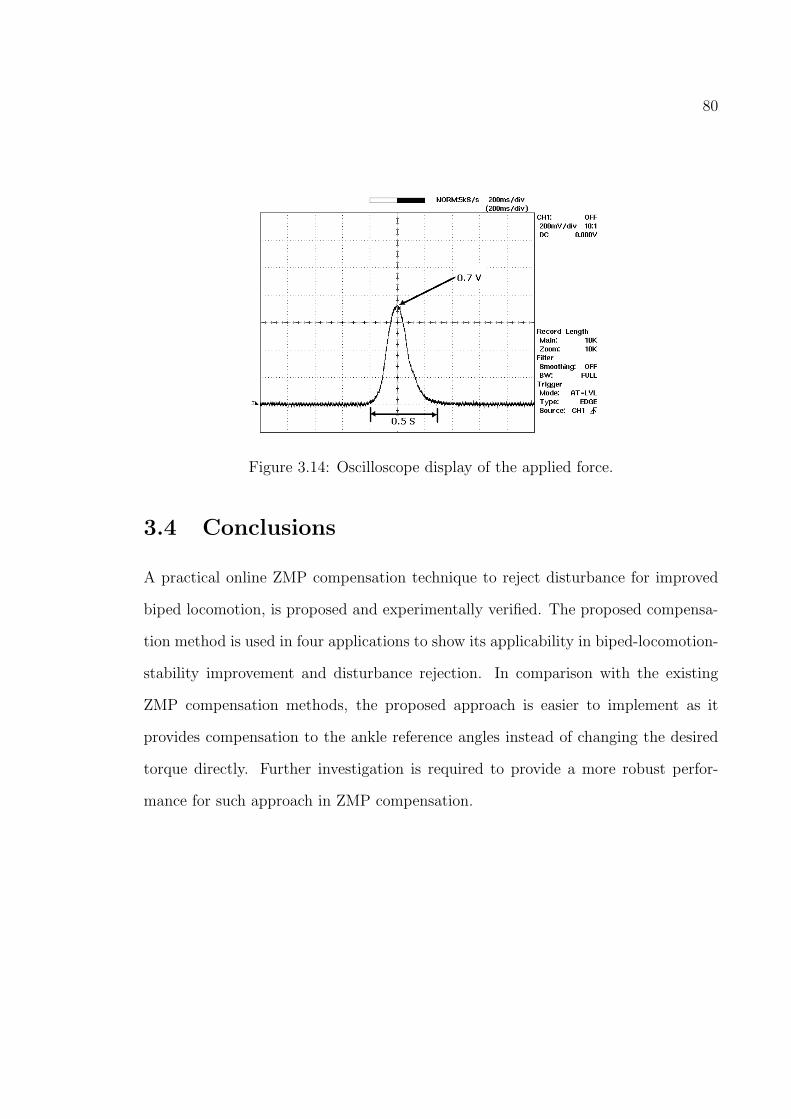
80

Figure 3.14: Oscilloscope display of the applied force.

3.4 Conclusions

A practical online ZMP compensation technique to reject disturbance for improved

biped locomotion, is proposed and experimentally verified. The proposed compensa-

tion method is used in four applications to show its applicability in biped-locomotion-

stability improvement and disturbance rejection. In comparison with the existing

ZMP compensation methods, the proposed approach is easier to implement as it

provides compensation to the ankle reference angles instead of changing the desired

torque directly. Further investigation is required to provide a more robust perfor-

mance for such approach in ZMP compensation.

81

Figure 3.15: Normalized x-ZMP Position of MaNUS-I when it experience a suddenpush of intensity around 3 N from behind.

Figure 3.16: Compensation at the ankle-joint of MaNUS-I to compensate a suddenpush of intensity around 3 N from behind.

82

Figure 3.17: Robot walking sequence when pushed from behind.

Figure 3.18: Robot walking sequence when pushed from the front.

Figure 3.19: Walking up a 10o slope. Figure 3.20: Walking down a 3o slope.

83

Figure 3.21: Manus-I carrying Additional Weight.

84

Figure 3.22: Normalized x-ZMP Position of Compensated Walking Gait while carry-ing 300 gm weight.

Figure 3.23: Compensation at the ankle-joint while carrying 300 gm weight.

Chapter 4

Jumping Gaits of Planar BipedalRobot with Stable Landing

Flat-foot biped locomotion is considered while utilizing the ZMP-based stability crite-

rion [16,99]. Unbalanced moments at the foot leads to foot-rotation about a point on

the foot boundary. The occurrence of foot-rotation changes the absolute orientation of

the biped which brings in a passive DOF making the bipedal systems underactuated.

The absolute orientation of the biped is considered as an additional passive DOF

in certain biped models [7, 76, 87, 100]. Such biped models are underactuated in

nature resulting in nontrivial zero-dynamics [77]. It is essential to investigate the

stability of the associated zero-dynamics (ZD) while dealing with underactuated sys-

tems. Periodic trajectories with the specific properties result in stable zero-dynamics

of a two-link acrobot [100]. The periodic nature of the locomotion/gait is utilized to

stabilize the ZD [7, 11, 12, 76]. Poincare return map is an effective tool to validate

periodicity and orbital stability [7,76]. Simplified biped models such as spring-damper

systems are helpful in establishing periodicity in locomotion [12].

The concept of orbital stability is useful while dealing with the associated stability

issues in point-foot bipeds [7,11,76]. By periodically attaining certain postures, even

85

86

though statically unstable, the orbital stability is achieved. Similar concepts are

useful in analyzing stability of periodic activities such as running and hopping.

Fast dynamical activities like running, jumping or hopping are reported [11, 12,

78, 79] and experimentally realized [80], [81]. The Flight phase is common in these

activities when the physical system looses contact with the ground. In the Flight

phase it is noticeable that ground-reaction-force (GRF) becomes zero and angular

momentum is conserved.

GRF is often used as a feedback to control the jumping motion [59,82–84]. GRF

data obtained from human jumping phases is utilized to compute the biped jumping

gaits by optimizing the inertial forces [82]. Simplification of bipedal dynamics, for

example inverted pendulum model, is helpful in developing force control strategies

for jumping gait generation [83, 84]. Time of application of the control-scheme is

important in designing the effective force-control strategies for vertical jumping [59].

In a number of studies, angular momentum is used for jumping motion control

[58,85,86]. Mita et el. utilize an angular momentum conservation principle to develop

an optimal control strategy to produce jumping motion [85]. The fight phase is

initiated by non-zero angular momentum of a two-link planar robot in [85]. The

motion of a four-link gymnastic robot is controlled using feedback linearizarion by

Buss et al. [86]. Non-holonomic motion planning needs identification of few discrete

states duringFlight phase [86]. Hyon et al. [58] report back-handspring experiment

by controlling the angular momentum about center-of-mass (CM).

Unlike running and hopping, jumping is aperiodic. Hence, the concepts of peri-

odicity and orbital stability are not applicable to resolve the stability issues involved

in jumping. Although, static stability is possible in point-foot bipeds, presence of

87

foot essentially provides greater stability margin. Foot compliance model is required

to obtain statically stable equilibrium for biped with foot. The traditional stability

concepts such as ZMP and FRI are not suitable to address the situation when foot

compliance model along with foot-rotation is considered. Flat-foot biped locomotion,

which is not always the case with the foot compliance model, is normally assumed

for ZMP-based stability analysis. The location of FRI point indicates whether the

foot is about to rotate or not. The FRI point is not relevant once the foot rotates.

Stability considerations for the activities like back-handspring, handstand, somersault

are reported in [57, 58] which are confined to gait generation and control strategies.

The stability issues involved with foot compliance and foot-rotation are not explicitly

resolved.

Stability analysis associated with foot compliance model and foot-rotation during

landing is the major motivation of the current work. Stability issues involved with

landing in jumping motion of a biped structure are investigated in the work. The

jumping gait is generated for a biped robot taking foot-rotation into consideration.

The biped model becomes underactuated due to the presence of passive DOF at the

contact between the toe and the ground. Foot compliance with ground is modeled

as a spring-damper system [92]. The control problem for an underactuated model

along with the foot compliance is formulated as output zeroing problem [77] where

the output functions are constructed according to the desired jumping performance.

The underactuated model with foot compliance results in a switching system with

“switching zero-dynamics.” The conditions for landing stability are derived to stabilize

the switching system. The stability of the switching system depends on the two

quantities which are named as “critical potential index” and “critical kinetic index”.

88

The jumping motion is experimentally realized and stability conditions are validated.

Section 4.1 describes the biped jumping robot and the computation of the asso-

ciated dynamics. The control strategy is discussed in Section 4.2 while a selection

procedure of desired gaits for the output functions is discussed in Section 4.3. The

landing stability analysis is provided in Section 4.4. The simulations and experimen-

tations of the jumping gait are described in Section 4.5 and conclusions are drawn in

Section 4.6.

4.1 The Biped Jumper

4.1.1 Biped Jumper: BRAIL 2.0

BRAIL 2.0 (Bio-Robotics Activities in Locomotion 2.0) is a six degree-of-freedom

(DOF) two legged robot. Each leg has three links: Foot, Shank and Thigh. The free

end of the Foot link is the toe. The joint between the Foot link and the Shank link

is the ankle. The joint between the Shank link and the Thigh link is the knee while

that between the two Thigh links of the legs is the hip. Each leg has three joints and

each joint has one actuator. The link attached at the hip is the Torso link. A weight

is attached at the distal end of the Torso link. The amount and location of the weight

on the Torso link are adjustable. The biped has a total of seven links. BRAIL 2.0

can not bend in frontal plane as it does not have any ‘roll’ DOF in its legs. BRAIL’s

motion is restricted to sagittal plane making it a planar robot.

The mechanical design is done in Autodesk Inventor (usa.autodesk.com). The

Autodesk design and the robot BRAIL 2.0 are shown in Fig. 4.1. The robot weighs

1.37 kg and is 0.451 m high. The biped model, developed in Autodesk Inventor, is

89

Figure 4.1: BRAIL 2.0 and Autodesk design

90

Table 4.1: Parameters of the BRAIL 2.0 biped

Link Length Mass CM Inertia about CM(m) (kg) (m) (kgm2)

1 d1=0.12 m1 = 0.32a 0.085 4.56 × 10−5

2 d2=0.1 m2 = 0.13a 0.05 4.6 × 10−5

3 d3=0.107 m3 = 0.61a 0.0535 3.65 × 10−4

4 d4=0.19 m4=0.31 0.17 2.88 × 10−4

am1/m2/m3: Sum of the Foot/Shank/Thigh masses in the two legs.

imported to Msc. Visualnastran (www.mscsoftware.com) simulation environment.

The biped parameters in Table 4.1 are collected from Msc. Visualnastran simulation

environment and are used in the computation of the biped dynamics.

The biped jumping motion is studied with respect to the ground or any other

flat surface in the sagittal plane (Fig. 4.2). The lengths and masses of the Foot,

Shank, Thigh and Torso links are di and mi (with i = 1, 2, 3, 4) respectively. The

world coordinate system (X-Y ) is fixed and absolute. The initial position of the toe

is indicated by (x0, y0). The two legs are aligned to have identical pose in sagittal

plane so as to act as a single leg. In sagittal plane the biped has four links and

three joints (i.e. active DOFs). The Cartesian coordinates of the ankle, knee and

hip joints are (x1, y1), (x2, y2) and (x3, y3) with respect to X-Y. The body angular

coordinate vector θb = (θ2, θ3, θ4)T describes the shape of the biped. The relative

angles (θ2, θ3, θ4) are known as shape variables and are realized by an actuator each

in the legs. In consequence, each DOF consists of two actuators placed at the same

location of the two legs in sagittal plane. θ1 is the absolute angle between the foot and

the ground. The vector of generalized coordinates θa := (θ1, θTb )T indicates absolute

posture of the biped. Angles are positive in the counter-clockwise direction.

91

Figure 4.2: The Biped Model

Actuators

The RX-64 motors from Robotis Inc (www.robotis.com) are used as actuators. The

motors weigh 116 g and provide a maximum torque of 6.4 Nm. With two actuators

at each joints in sagittal plane, the maximum torque available at any joint is 12.8

Nm. These actuators are run in ‘endless turn’/torque control mode. While controlling

torque, the torque input to the motor can be adjusted at a resolution of about 0.1% of

the maximum available torque at the current supply voltage. The actuators provide

angular positions, velocities and joint torque as feedback.

92

Figure 4.3: Foot compliance model.

Controller

The motors are controlled using a CM2 controller board (www.robotis.com). The

CM2 board uses an ATmega128 16 MHz processor. The controller can be connected to

the PC using a RS232 port through which HEX code, generated from C programmes,

are downloaded. A unique ID is set for each actuator for the controller to communicate

with them. The motors utilize RS-485 communication protocol to use the daisy chain

technology. The controller can read the joint angular positions, velocities and torques

of the each actuator connected in the daisy chain.

4.1.2 Foot Compliance Model and Foot Design

The foot-ground compliance model is shown in Fig. 4.3 by replacing the Foot link

with a human foot. The entire contact-surface between the foot and the ground is

represented by a pivot and a spring-damper system located at the toe and the ankle

respectively.

The assumptions on the foot compliance model are:

93

Figure 4.4: Foot plate of BRAIL 2.0

C1 When the foot is flat, the entire foot-ground contact surface is represented by

the contacts at the toe and ankle.

C2 The toe-ground contact acts as a rigid pivot and the biped does not slip, rebound

or penetrate at this point, that is, the vertical component of the ground reac-

tion force is positive and the ratio of the horizontal component to the vertical

component does not exceed the coefficient of static friction [7, 76].

C3 The ankle-ground contact acts as a spring-damper system where the biped can

rebound or penetrate.

The Foot link of BRAIL 2.0 is shown in Fig. 4.4. Foot bottoms are cushioned by

rubber sheets. The rubber cushioning helps to avoid slipping and provides damping

to help shock absorption during jumping. The Foot link has two plates connected

together at ankle while the toe part has only one plate. This makes the ankle-ground

joint better damped and stronger to absorb impacts during landing.

4.1.3 Jumping Sequences

The jumping process is divided into three phases: Take-off phase, Flight phase, and

Touch-down phase (Fig. 4.5). The biped’s absolute position is specified by the

Cartesian Coordinates of CM (xcm, ycm) with respect to the world coordinate frame

94

X-Y. In the Take-off phase the Foot link is in contact with the ground and ycm > 0.

The biped is said to be in Touch-down phase when the Foot link is in contact with

the ground and ycm < 0. There is no contact with the ground in Flight phase.

At the time of initiation of the Flight phase y0 > 0. In Flight phase the biped’s

CM evolves according to Newton’s second law,

xcm = 0,

ycm = −g.

(4.1)

In the Take-off and Touch-down phases, the CM (xcm(θa), ycm(θa)) of the biped

can be computed with respect to the toe position:

xcm(θa) =

∑4i=1mixcmi∑4i=1mi

,

ycm(θa) =

∑4i=1miycmi∑4i=1mi

,

fcm(θa) =

xcm(θa)

ycm(θa)

, (4.2)

where mi and (xcmi, ycmi) indicate the mass and position of the CM of the ith link

respectively. Therefore, the linear velocity of the biped’s CM (with respect to the

toe) is given by:xcm(θa)

ycm(θa)

=

∂fcm(θa)

∂θaθa. (4.3)

While standing statically on flat-foot in sagittal plane, the biped is statically stable

if condition (4.4) is satisfied [6].

0 ≤ xcm(θa) ≤ footlength = d1. (4.4)

95

Figure 4.5: Phases of Jumping Motion.

Without loss of generality, it is assumed that the jumping motion starts from a

statically stable posture with the origin of the world coordinate system coinciding

with the position of the toe. The toe is in contact with the ground in both Take-off

and Touch-down phases and, the toe-ground contact acts as a rigid pivot during these

phases. Impact occurs when the toe touches the ground soon after the Flight phase

or just before the Touch-down phase. Due to the impact, the joint angular velocities

change instantaneously while the joint angular positions remain unchanged. The

desired gaits in three jumping phases are computed off-line ensuring landing stability.

Stability of the jumping gaits depends on the biped dynamics and control strategies.

The control strategies ensure asymptotic convergence to a statically stable posture at

the end of the Touch-down phase.

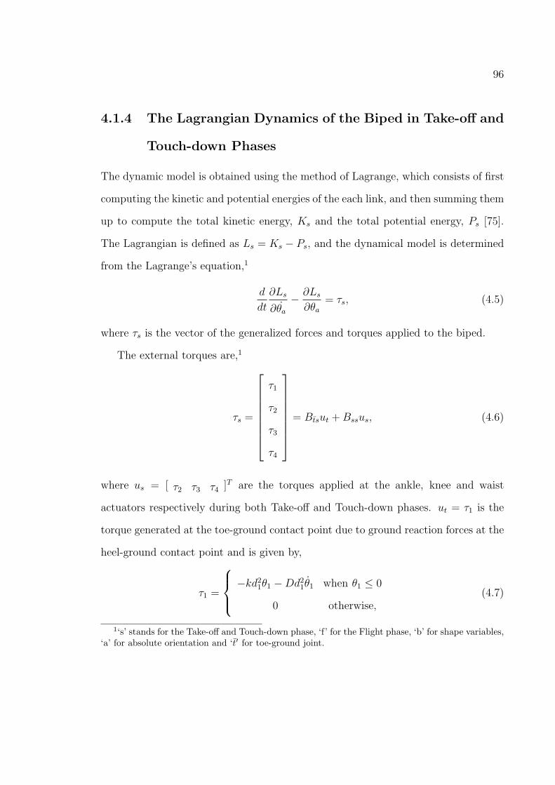
96

4.1.4 The Lagrangian Dynamics of the Biped in Take-off and

Touch-down Phases

The dynamic model is obtained using the method of Lagrange, which consists of first

computing the kinetic and potential energies of the each link, and then summing them

up to compute the total kinetic energy, Ks and the total potential energy, Ps [75].

The Lagrangian is defined as Ls = Ks − Ps, and the dynamical model is determined

from the Lagrange’s equation,1

d

dt

∂Ls

∂θa− ∂Ls∂θa

= τs, (4.5)

where τs is the vector of the generalized forces and torques applied to the biped.

The external torques are,1

τs =

τ1

τ2

τ3

τ4

= Btsut +Bssus, (4.6)

where us = [ τ2 τ3 τ4 ]T are the torques applied at the ankle, knee and waist

actuators respectively during both Take-off and Touch-down phases. ut = τ1 is the

torque generated at the toe-ground contact point due to ground reaction forces at the

heel-ground contact point and is given by,

τ1 =

−kd21θ1 −Dd2

1θ1 when θ1 ≤ 0

0 otherwise,(4.7)

1‘s’ stands for the Take-off and Touch-down phase, ‘f’ for the Flight phase, ‘b’ for shape variables,‘a’ for absolute orientation and ‘t′ for toe-ground joint.

97

where k and D are the spring constant and damping of the ankle-ground contact and,

Bts =

1

0

0

0

, Bss =

0 0 0

1 0 0

0 1 0

0 0 1

. (4.8)

The dynamic model during take-off and touch-down phases can therefore be written

as,1

Ms(θb)θa + Vs(θb, θa) +Gs(θa) = τs, (4.9)

where Ms is the 4 × 4 inertial matrix about toe, Vs is 4 × 1 vector containing the

Coriolis and centrifugal terms, and Gs is the 4× 1 gravity vector. The computations

of Ms, Vs and Gs are provided in Section 4.1.5.

As the inertial matrix only depends on the shape variables, the Ms(θb) is inde-

pendent of θ1 [76]. The kinetic and potential energies of the robot in the take-off and

touch-down phases are given by,

Ks =1

2θaTMs(θb)θa, (4.10)

Ps = mgycm(θa),

where m is the total mass of the robot.

Introducing the state vector xs := (θTa , θTa )T , the Lagrangian model (4.9) is ex-

pressed as

xs =

θa

M−1s (−Vs −Gs +Btsut)

+

0

M−1s Bssus

= fs(xs) + gs(xs)us, (4.11)

where xsε∆s, ∆s := xs = (θTa , θTa )T | y0 = 0, y1 ≥ 0, y2 > 0, y3 > 0, y4 > 0, θaε<4.

98

Figure 4.6: Coordinate System Assignment for Lagrangian formulation.

4.1.5 Lagrangian Dynamics Computation of the at the Take-

off and Touch-down phases

For Lagrangian formulation of the biped, coordinate system assignment is shown in

Fig. 4.6. The Denavit-Hartenberg (DH) [5] parameters are defined by,

Ai : The distance from Zi to Zi+1 measured along Xi.

Hi : The distance from Xi−1 to Xi measured along Zi

φi : The angle between Xi−1 to Xi measured about Zi.

αi : The angle between Zi to Zi+1 measured about Xi.

99

Table 4.2: DH Parameters of the Robot

i αi−1 Ai−1 Hi φi1 0 0 0 θ1

2 0 d1 0 θ2

3 0 d2 0 θ3

4 0 d3 0 θ4

Table 4.1.5 gives the values of DH parameters of the biped kinematic model in

Fig. 4.6.

The general form of the homogeneous transformation matrix between (i−1)th and

ith link is given by [5],

T i−1i =

cφi −sφi 0 Ai−1

sφicαi−1 cφicαi−1 −sαi−1 −sαi−1Hi

sφisαi−1 cφisαi−1 cαi−1 cαi−1Hi

0 0 0 1

,

where s(.) indicates sin(.) and c(.) indicates cos(.). The partial derivative of T i−1i

with respect to φi is given by,

∂T i−1

i

∂φi= T i−1

i Q,

T 0i = T 0

1 · T 12 · T 2

3 · · · T i−1i , (4.12)

where Q is given by,

Q =

0 −1 0 0

1 0 0 0

0 0 0 0

0 0 0 0

.

100

Let us define,

Uij =∂T 0

i

∂θj(4.13)

=

T 0j QT

ji j ≤ i

0 j > i

and,

Uijk =∂Uij∂θk

(4.14)

=

T 0kQT

kj QT

ji i ≥ j ≥ k

T 0j QT

jkQT

ki i ≥ k ≥ j

0 i < j or i > k

The elements of the inertial matrix Ms is given by,

Ms,i,k =4∑

j=max(i,k)

Trace(UjkJjUTji). (4.15)

The elements of Vs and Gs matrices are given by,

Vs,i =4∑

k=1

4∑

m=1

hikmθkθm,

Gs,i =4∑

j=i

(−mjgUjirjj),

i = 1, 2, 3, 4, (4.16)

where hikm, g and Jj are given by,

vikm =4∑

j=max(i,k,m)

Trace(UjkmJjUTji),

g = [0 − 9.81 0 0]T m/s2,

Ji = rirTi mi, (4.17)

where ri is the center of mass of the ith link with respect to ith coordinate system.

101

4.1.6 The Lagrangian Dynamics of the Biped in Flight Phase

In the Flight phase, the generalized vector coordinates are θf := (θ1, θbT , xcm, ycm)T .

In terms of the generalized coordinates of the robot, θf , the total kinetic and potential

energies in the Flight phase become,1

Kf =1

2θfTDf (θb)θf , (4.18)

Pf = mgycm,

where Df is as per (4.19).

Df =

Mf (θb) 04×2

02×4 mI2×2

. (4.19)

I2×2 is 2× 2 unity matrix and Mf (θb) is the inertial matrix of the robot about the

center of mass [7] which is given by,

Mf (θb) = Ms(θb) −m∂fcm(θa)

∂θa

T ∂fcm(θa)

∂θa. (4.20)

Defining Lagrangian Lf = Kf − Pf , the Lagrangian equation becomes,

d

dt

∂Lf

∂θf− ∂Lf∂θf

= τf , (4.21)

which leads to a model of the form,

Df (θb)θf + Vf (θf , θf ) +Gf (θf ) = τf . (4.22)

The elements of the 6 × 1 vectors Vf and Gf are computed by [75],

Vf,k =6∑

i,j

vijkθiθj,

Gf,k =∂Pf∂θk

, (4.23)

102

where

vijk =1

2[∂Df,k,j

∂θi+∂Df,k,i

∂θj− ∂Df,i,j

∂θk]. (4.24)

The external torques are

τf =

0

τ2

τ3

τ4

0

0

= Bsfuf , (4.25)

where uf = [ τ2 τ3 τ4 ]T are the torques applied at the ankle, knee and waist

actuators respectively during the Flight phase. And,

Bsf =

0 0 0

1 0 0

0 1 0

0 0 1

0 0 0

0 0 0

. (4.26)

Introducing state vector xf := (θTf , θTf )T , the model (4.22) becomes

xf =

θf

D−1f (−Vf −Gf )

+

0

D−1f Bsfuf

= ff (xf ) + gf (xf )uf , (4.27)

where xfε∆f , ∆f := xf = (θTf , θTf )T | y0 > 0, y1 > 0, y2 > 0, y3 > 0, y4 > 0, θfε<6.

103

4.1.7 Impact Model and Angular Momentums

The impact takes place when the toe touches the ground at the end of the Flight phase.

The impact model is assumed non-elastic with the velocity of the toe becoming zero

instantaneously leading to discontinuity in joint velocities [91]. The position vector

(θa) does not change due to impact. The toe-ground contact acts as an ideal pivot

after the impact. The positions and velocities just before and after the impact are

denoted by ‘−′ and ‘+′ respectively. Using the model in [91], the joint velocities just

after impact are obtained.

The Cartesian position of the toe is expressed in terms of the robot’s CM as per

(4.28).

x0

y0

=

xcm

ycm

− fcm(θa). (4.28)

The impact model in [91] models the ground reaction force at impact as impulse

with intensity IG. The impact is assumed non-elastic with the velocity of the toe

becoming zero instantaneously while the position vector does not change. The toe-

ground contact acts as an ideal pivot after the impact. As the velocity of the toe

becomes zero after the impact,

0

0

=

x+cm

y+cm

− ∂fcm(θa)

∂θaθ+a . (4.29)

The impact model is expressed as [91],

Mf (θb) 0

0 mI2

(

θ+a

x+cm

y+cm

− θ−f ) =

∂fTcm(θa)∂θa

I2

IG. (4.30)

104

The IG is expressed from (4.29) and (4.30),

IG = m(∂fcm(θa)

∂θaθ+a −

x−cm

y−cm

). (4.31)

Using (4.31) in (4.30),

Mf (θb)(θ+a − θ−a ) =

∂fcm(θa)

∂θa

T

IG = m∂fcm(θa)

∂θa

T

(∂fcm(θa)

∂θaθ+a −

x−cm

y−cm

). (4.32)

This further leads to,

(Mf (θb) − m∂fcm(θa)

∂θa

T ∂fcm(θa)

∂θa)θ+a = Mf (θb)θ

−

a −m∂fcm(θa)

∂θa

T

x−cm

y−cm

,

=⇒Ms(θb)θ+a = [Mf (θb);m

∂fcm(θa)

∂θa

T

]θf−

,

=⇒ θ+a = Ms(θb)

−1[Mf (θb);m∂fcm(θa)

∂θa

T

]θf−

. (4.33)

4.1.8 Jumping Motion and Angular Momentum relations

The jumping motion is divided into three successive phases: Take-off phase, Flight

phase and Touch-down phase. At the beginning of the Take-off phase the robot is

in statically stable posture. In Take-off phase ycm > 0. The transition from the

Take-off phase to the Flight phase is initiated by causing the velocity of the toe to

become positive i.e. y0 > 0. The control law in Flight phase decides the time of

transition from the Take-off phase to the Flight phase. In Take-off phase, the angular

momentum of the biped about the toe is given by [7],

σ =∂Ks

∂θ1

= Ms,1θa. (4.34)

105

The first row of (4.9) yields,

σ = −Gs,1 + τ1 = −mgxcm(θa) + τ1. (4.35)

To achieve continuity in position and velocity variables, the initial values of the states,

xf , in the Flight phase are taken as the values at the end of the Take-off phase. Let

σcm denote the angular momentum of the biped about its center of mass. In the

Flight phase, σcm is computed by [7],

σcm =∂Kf

∂θ1

= Mf,1θa, (4.36)

The first row of (4.22) yields,

σcm = 0, (4.37)

where the initial value of σcm, at the beginning of the Flight phase, is computed from

the final values of the Take-off phase [7],

σcm = σ −m(xcmycm − ycmxcm). (4.38)

In addition, last two rows of (4.22) are,

xcm = 0,

ycm = −g. (4.39)

Impact takes place at the end of the Flight phase when the toe touches the ground.

Due to the effect of impact the velocities change instantaneously while the position

does not. The angular momentum after the impact is computed from (4.40).

σ+ = Ms,1(θ+a )θ+

a . (4.40)

106

4.2 Control Law Development

The control law for all phases is formulated as an output zeroing problem resulting

in nontrivial zero dynamics [77]. The output functions for all the three phases are

defined as,

h(θb, t) = θb − θdb (t), (4.41)

where θdb (t) is the vector of three desired shape variable trajectories. The desired

trajectories in Take-off, Flight and Touch-down phases are referred as θdbs(t), θdbf (t)

and θdbl(t) respectively.

From (4.41), the following equations can be derived2,

h(θb, t) =∂h

∂xx− θdb (t) = LFh− θdb (t),

h(θb, t) = (LGLFh)u+ L2Fh− θdb (t). (4.42)

F, G and x come from the system equations (4.11) and (4.27). They are fs, gs and

xs for Take-off and Touch-down phases and ff , gf and xf for the Flight phase. The

feedback controller is defined as,

u(x) = [LGLFh]−1[v(h, LFh) − L2

Fh+ θdb (t)],

v(h, LFh) = −Kd(θb − θdb (t)) −Kp(θb − θdb (t)), (4.43)

where Kd and Kp are constants such that h+Kdh+Kph = 0 is stable.

4.3 Selection of Desired Gait

The selection of the desired gaits3 (θdbs(t), θdbf (t) and θdbl(t)) is discussed in this section.

The selection procedure is based on the equivalent two-link model of the biped (Fig.

2Refer [77] for Lie Algebraic notations.3‘l’ stands for the landing phase or Touch-down phase.

107

Figure 4.7: Two-link equivalent model of the biped with foot.

108

4.7). In the two-link model, the Foot link acts as one link and the distance from the

ankle to CM of the rest of the biped acts as another link. The Cartesian coordinate

(xcm0(θb), ycm0(θb)) is as per Fig. 4.7. Considering the mechanical structure of the

biped, BRAIL 2.0, its physically reasonable configurations correspond to θb in the

ranges (in rad): 1.8408 ≤ θ2 ≤ 3.1227, −2.7585 ≤ θ3 ≤ −0.5219 and 0.2066 ≤ θ4 ≤

1.2519.

The desired gaits θdb (t) are computed from the desired trajectories of (xcm0(θb), ycm0(θb))

in various phases using MATLAB’s LSQNONLIN function which utilizes Trust-Region

method [88] for nonlinear error minimization of the following function,

Γ(θdb ) = (xdcm0(t) − xcm0(θdb ))

2 +

(ydcm0(t) − ycm0(θdb ))

2, (4.44)

where (xdcm0(t), ydcm0(t)) is the desired Cartesian trajectory of (xcm0(θb), ycm0(θb)).

The nonlinear error minimization on (4.44) is performed with the constraints that

the solution vectors θdb lie within the ranges of the physically reasonable configurations

of the biped. Subsequently, a fourth order polynomial is considered to fit the set of

solutions obtained from the nonlinear error minimization of (4.44). The fourth order

polynomial resulted in error in the order of 10−4 m.

θdj (t) = aj,0 + aj,1t+ aj,2t2 + aj,3t

3 + aj,4t4.

(4.45)

With the θdj (t) in (4.45), (xcm0(θb), ycm0(θb)) closely follows (xdcm0(t), ydcm0(t)).

109

4.3.1 Take-off phase Gait

(xdcm0(t), ydcm0(t)) in Take-off phase is given by4,

xdcm0(t) = xcm0(0) − Cxt,

ydcm0(t) = ycm0(0) + Cyt, (4.46)

where (xcm0(0), ycm0(0)) is the initial location of (xcm0(θb), ycm0(θb)). Cx and Cy are

the desired horizontal and vertical take-off velocities. (xdcm0(t), ydcm0(t)) should be such

that θa := (0, (θdb )T )T is real.

4.3.2 Flight phase Gait

The biped’s CM evolves according to (4.1) in the Flight phase. The shape variables

are adjusted to vary the CM position with respect to the toe (x0, y0). The desired

trajectory, ydcm0(t), is as per (4.47).

ycm(t) = ycm(0) + ycm(0)t− 1

2gt2,

yd0(t) = ηdsin(π

tft),

ydcm0(t) = ycm(t) − yd0(t), (4.47)

where ηd is the desired jumping height, tf is the desired flight time and yd0(t) is the

desired trajectory of y0 (Fig. 4.8). Similarly, the desired trajectory of xdcm0(t) is as

4Negative sign appears in the expression of xdcm0

(t) because x is negative in the forward directionof jumping.

110

Figure 4.8: Flight-phase Gait Design Parameters.

111

per (4.48).

xcm(t) = xcm(0) + xcm(0)t,

xd0(t) = ζdt,

xdcm0(t) = xcm(t) − xd0(t), (4.48)

where ζd is the desired length of jumping and xd0(t) is the desired trajectory of x0

(Fig. 4.8). The values of xcm(0), xcm(0), ycm(0) and ycm(0) are their values at the

end of the Take-off phase. ηd, ζd and tf should be chosen such that θ1 > 0 at the end

of the Flight phase.

4.3.3 Touch-down phase Gait

The initial positions in the Touch-down phase are the positions at the end of the Flight

phase while the initial velocities change instantaneously by (4.33) due to impact at

the end of the Flight phase. The desired shape variables θdj (t) (j = 2, 3, 4) during the

Touch-down phase are constants (4.49).

θdj (t) = Constant, (4.49)

such that 0 < xcm0(θdbl) < d1 = footlength and θdj (t) = 0.

4.4 Landing Stability Analysis

Landing stability is ensured by biped’s asymptotic convergence to a statically stable

posture. The control law (4.43), results in nontrivial ZD in Touch-down phase [77].

Stability of the closed-loop dynamics (CLD) is governed by the Touch-down phase

zero-dynamics.

112

4.4.1 Switched Zero-Dynamics (SZD): Touch-down phase

The ZD manifold in Touch-down phase with the output function (4.41) is as per

(4.50) [77].

Zs := xsε∆s | θb = θdb (t), θb = θdb (t). (4.50)

The ZD (4.50) leads to (4.51) with desired shape trajectories as per [76].5 (4.49)

θ1 =σ

Ms,1,1(θdbl),

σ = −mgxcm(θ1, θdbl) + τ1. (4.51)

The xcm(θa) [4] has the following form,

xcm(θa) = −√x2cm0(θb) + y2

cm0(θb) × sin(θ1 − tan−1(xcm0(θb)

ycm0(θb))). (4.52)

Ms is independent of θ1 and Ms,1,1(θdbl) in (4.51) is a constant. Let us define three

positive constants,

K1 =1

Ms,1,1(θdbl)kg−1m−2,

K2 = mg√x2cm0(θ

dbl) + y2

cm0(θdbl) Nm,

K3 = tan−1(xcm0(θ

dbl)

ycm0(θdbl)) rad. (4.53)

Thus, the ZD in (4.51) becomes (4.54).

θ1 = K1σ,

σ = K2sin(θ1 −K3) + τ1. (4.54)

The initial value of θ1 in Touch-down phase is positive and is given by its value at

the end of the Flight phase. The value of σ changes on impact and its values at the

5Ms,r,c indicates the element in rth row and cth column of the stance-phase inertia matrix.

113

point of impact, σ+, is computed from (4.40). The torque at the toe-ground contact,

τ1, in (4.7) is written as (4.55).

τ1 =

−K4θ1 −K5σ when θ1 ≤ 0

0 otherwise(4.55)

whereK4 = kd21 Nm andK5 = Dd2

1K1 s−1. K4 indicates the stiffness properties of the

ankle-ground contact. The value of k is in the order of 106 N/m for soft surfaces [95]

leading to K4 in the order of 104 Nm. The value of D is generally 5% to 25% of k

making K5 in the order of 102 s−1. The zero-dynamics in (4.54) has two equilibrium

points in the range −π < θ1 < π : (θ1, σ) = (K3, 0) and (θ1, σ) ≈ (−K2sin(K3)K4

, 0)6.

(−K2sin(K3)K4

, 0) corresponds to statically stable posture where K2sin(K3)K4

≈ 0 as the

value of K4 is quite high compared to K2.

The phase portrait of the ZD (4.54) shows that the Touch-down phase ZD is a

switching system with two subsystems (Fig. 4.9): Subsystem A (4.56) for θ1 > 0 and

Subsystem B (4.57) for θ1 ≤ 0. Switching takes place whenever the ankle touches or

leaves the ground. The overall ZD during Touch-down phase is named as Switching

Zero-Dynamics (SZD).

In Subsystem A (θ1 > 0), Touch-down phase ZD is as per (4.56).

θ1 = K1σ,

σ = K2sin(θ1 −K3). (4.56)

In Subsystem B (θ1 ≤ 0), the Touch-down phase ZD is as per (4.57).

θ1 = K1σ,

σ = K2sin(θ1 −K3) −K4θ1 −K5σ. (4.57)

6θ1 is small compared to K3 in Subsystem B i.e., sin(θ1 − K3) ≈ −sin(K3).

114

Figure 4.9: Phase Portrait of SZD (4.54). Trajectory I: Member of the set of trajec-tories going out with increasing θ1. Trajectory II: Member of the set of trajectoriesreaching the θ1 = 0 plane.

115

The Touch-down phase always begins in Subsystem A. For the stability of the

SZD, it needs to converge asymptotically to the equilibrium (θ1, σ) = (−K2sin(K3)K4

, 0).

4.4.2 Stability of SZD

Stability analysis of SZD consists of three aspects. 1) In Subsystem A (Fig. 4.9),

the phase-portrait can either follow trajectory I or II. Trajectory I leads to instability

of the biped structure. For trajectory II, switching takes place at the θ1 = 0 plane

which is required for stability of the ZD. 2) For stability in Subsystem B, the ZD

should either converge to the equilibrium point (θ1, σ) = (−K2sin(K3)K4

, 0) or it should

switch back to Subsystem A. The possibility of initiating Flight phase from Subsys-

tem B is not addressed here as the biped is not supposed to rebound at toe-ground

contact according to the assumption (C2) of the foot-compliance model. 3) The

switching should be such that the SZD asymptotically converges to the equilibrium

point (θ1, σ) = (−K2sin(K3)K4

, 0).

In the following analysis, it is assumed that SZD (4.54) starts at (θ10, σ0) with

θ10 > 0 being the value of θ1 at the end of the Flight phase and σ0 is computed from

(4.40).

Theorem 4.4.1. The SZD (4.56) reaches θ1 = 0 plane from initial states (θ10, σ0) if

the following condition is satisfied (θ10 > 0),

(a) When K3 > θ10,

ZD1 : σ0 <√

2K2

K1

(1 − cos(θ10 −K3))

(b) When K3 ≤ θ10,

ZD1 : σ0 < −√

2K2

K1

(1 − cos(θ10 −K3)).

116

Proof. From (4.56) for Subsystem A,

dσ

dθ1

=K2sin(θ1 −K3)

K1σ,

=⇒ σdσ =K2

K1

sin(θ1 −K3)dθ1,

=⇒ σ20

2=

σ2

2+ VZD(θ1),

=⇒ σ20 = σ2 + 2VZD(θ1), (4.58)

where VZD(θ1) is defined as following,

VZD(θ1) = −∫ θ1

θ10

K2

K1

sin(θ1 −K3)dθ1,

=K2

K1

(cos(θ1 −K3) − cos(θ10 −K3)). (4.59)

The maximum value of VZD(θ1) in (4.59) occurs when θ1 = K3. The corresponding

maximum value is denoted by V maxZD which is calculated by putting θ1 = K3 in (4.59).

V maxZD =

K2

K1

(1 − cos(θ10 −K3)). (4.60)

Equation (4.58) shows that if | σ0 |>√

2V maxZD , σ = 0 does not exists in the σ

trajectory. Because | σ0 |6>√

2V maxZD at σ = 0. Similarly, | σ0 |<

√2V max

ZD indicates

the existence of σ = 0 i.e., zero-crossing in the σ trajectory. Fig. 4.9 shows the vector

field of the SZD. Depending on the initial state there can be four cases for θ10 > 0.

1: With K3 > θ10 and σ0 > 0, the trajectories in Subsystem A (4.56) reach θ1 = 0

plane if there exists a zero-crossing in the σ trajectory. The zero-crossing exists

when | σ0 |<√

2V maxZD i.e. σ0 <

√2V max

ZD for σ0 > 0.

2: With K3 > θ10 and σ0 < 0, the trajectories in Subsystem A (4.56) always reach

the θ1 = 0 plane.

117

3: With K3 ≤ θ10 and σ0 > 0, the trajectories in Subsystem A (4.56) never reach the

θ1 = 0 plane.

4: With K3 ≤ θ10 and σ0 < 0, the trajectories in Subsystem A (4.56) reach the

θ1 = 0 plane if there is no zero-crossing in the σ trajectory. Zero-crossing exists

if | σ0 |>√

2V maxZD , i.e. σ0 < −

√2V max

ZD for σ0 < 0.

Cases 1 and 2 prove the part (a) while cases 3 and 4 prove the part (b) of Theorem

4.4.1.

It can be noticed that (4.56) represents the dynamics of a double-inverted pen-

dulum or acrobot [4, 100]. The conditions in Theorem 4.4.1 ensure that the initial

conditions do not correspond to the seperatrix passing through the equilibrium point

(K3, 0).

Theorem 4.4.2. The SZD (4.57) is locally asymptotically stable with initial states

(0, σT ), if the following condition is satisfied

ZD2 :σ2

T

2∫

Bσ2dt

> K5 > 0. ‘B’ indicates the time interval when the solution vector of

(4.54) is in Subsystem B.

Proof. Assume (4.56) reaches the θ1 = 0 plane at (0, σT ). From the zero-dynamics

(4.57),

dσ

dθ1

=K2sin(θ1 −K3) −K4θ1 −K5σ

K1σ,

=⇒∫ σ

σT

σdσ =

∫ θ1

0

K2sin(θ1 −K3) −K4θ1 −K5σ

K1

dθ1,

=⇒ σ2T

2= VB(θ1, σ) +K5

∫

B

σ2dt, (4.61)

118

where VB(θ1, σ) is as per (4.62).

VB(θ1, σ) = −∫ θ1

0

K2sin(θ1 −K3) −K4θ1

K1

dθ1 +σ2

2. (4.62)

(4.61) shows that VB(θ1, σ) > 0 for K5 <σ2

T

2∫

Bσ2dt

and VB(θ1, σ) = −K5σ2. Hence,

VB(θ1, σ) is positive definite and its time derivative VB(θ1, σ), along the zero-dynamics

(4.57), is negative semi-definite when 0 < K5 <σ2

T

2∫

Bσ2dt

. VB(θ1, σ) = 0 if σ = 0

which leads to K2sin(θ1 −K3) −K4θ1 = 0, the solution of which is the equilibrium

point (−K2sin(K3)K4

, 0). Therefore, VB(θ1, σ) is a candidate Lyaponov function [77] for

0 < K5 <σ2

T

2∫

Bσ2dt

and local asymptotic stability of (4.57) is proved using LaShelle’s

invariance principle [98].

The following are noticeable in Subsystem B,

• As VB(θ1, σ) = −K5σ2, convergence to equilibrium is faster when K5 is higher.

With higher K5 (but less thanσ2

T

2∫

Bσ2dt

), the chances of bouncing back at the

ankle-ground contact points is lesser.

• For the trajectory σT to σF (Fig. 4.9),∫σT→σF

K2sin(θ1−K3)−K4θ1K1

dθ1 = 0. There-

fore,

σ2F = σ2

T − 2K5

∫σ2dt. (4.63)

In case of bouncing back from the ankle-ground contact points, let the trajec-

tories intersect with the θ1 = 0 plane at σF (for σ > 0) and σF (for σ < 0) (Fig.

4.9). (4.63) is true for the trajectories σT to σF .

119

The SZD (4.54) is a switching system and switching occurs at the θ1 = 0 plane.

Condition ZD1 ensures that (4.56) reaches the θ1 = 0 plane. Condition ZD2 ensures

(4.57) either converges to the stable equilibrium (−K2sin(K3)K4

, 0) or switches back to

Subsystem A. However, the switching points (0, σF ) or (0, σF ) to Subsystem A might

not satisfy ZD1, leading to instability. Therefore, conditions ZD1 and ZD2 are not

sufficient to ensure the stability of SZD (4.54).

Theorem 4.4.3. The SZD (4.54) locally asymptotically converges to the equilibrium

point (−K2sin(K3)K4

, 0) from initial states (θ10, σ0) if the following conditions are satis-

fied,

SZD1 : K3 > θ10 > 0

SZD2 : | σ0 |<√

2K2

K1

(1 − cos(θ10 −K3))

SZD3 : ZD2.

Proof. SZD1 and SZD2 are sufficient to ensure, (4.56) to reach the θ1 = 0 plane

(from Theorem 4.4.1). SZD3 is sufficient to ensure local asymptotic stability of (4.57)

(from Theorem 4.4.2). The stability of the SZD (4.54) is analyzed using the MLF

approach [93].

The MLF approach is based on the existence of the Lyapunov-like functions for

every subsystem whithin the switching system. The existence of Lyapunov-like func-

tions for every subsystem in a switching system indicates the Lyapunov stability of

the switching system. The Lyapunov-like function is defined as candidate Lyaponov

function with at least negative semi-definite first derivative and monotonically non-

increasing values at the switching plane during switching in a specific direction [93].

120

Let us define VA(θ1, σ) as (4.64).

VA(θ1, σ) =σ2

2+ VZD(θ1). (4.64)

(4.58) shows that VA(θ1, σ) > 0 for σ0 6= 0 and VA(θ1, σ) = 0. VA(θ1, σ) is a candi-

date Lyaponov function for Subsystem A. Similarly, VB(θ1, σ) (4.62) is a candidate

Lyaponov function for Subsystem B. Therefore, VA and VB are positive-definite and

their first derivatives are at least negative semi-definite. The monotonicity of VA and

VB can be shown considering the first few switchings. Suppose, the first switching

occurs at (0, σT ) from Subsystem A to Subsystem B, the second switching at (0, σF )

from Subsystem B to Subsystem A, the third switching occurs at (0, σT ) from Subsys-

tem A to Subsystem B (Fig. 4.9). (4.58) leads to (4.63) indicating | σF |<| σT | and

(4.58) leads to | σT |=| σF |. As a result σT > σT and σF > σF . VB(0, σT ) > VB(0, σT )

and VA(0, σF ) > VA(0, σF ). Therefore, VA and VB are monotonically decreasing (non-

increasing) at the switching plane in any particular direction of switching. Hence,

VA and VB are Lyapunov-like functions for Subsystems A and B respectively. This

proves the local asymptotic stability of the SZD.

It is noticeable that the stability of SZD requires | σ0 |<√

2K2

K1

(1 − cos(θ10 −K3))

i.e., SZD2 does not allow σ0 < −√

2K2

K1

(1 − cos(θ10 −K3)) which is not true in ZD1

for Subsystem A. Basically, SZD2 ensures the monotonic property of the candidate

Lyaponov functions VA and VB.

The stability of SZD (4.54) depends on the initial states. The initial states of

the SZD are the values at the closed-loop dynamics (CLD) when h(θb, t) = 0 and

h(θb, t) = 0. Hence, stability of SZD is dependent on that of the CLD and vice-versa.

121

4.4.3 Closed-loop Dynamics: Touch-down phase

Closed-loop dynamics in both Take-off and Touch-down phases is as per (4.65).

h +Kdh+Kph = 0,

θ1 =σ

Ms,1,1

− Ms,1,2

Ms,1,1

θ2 −Ms,1,3

Ms,1,1

θ3 −Ms,1,4

Ms,1,1

θ4,

σ = −mgxcm(θa) + τ1. (4.65)

In the Touch-down phase, the CLD leads to (4.66) with the control input (4.43)

and desired gait (4.49).

ξ1 = ξ2,

ξ2 = −KP

ε2ξ1 −

KD

εξ2,

θ1 = κ1(ξ1)σ − κ4(ξ1)ξ2,

σ = κ2(ξ1)sin(θ1 − κ3(ξ1)) + τ1, (4.66)

where ε is a small positive constant, Kp = KP

ε2, Kd = KD

ε, KP , KD are constant gains.

ε acts as the perturbation parameter [98] and the significance of ε is explored in the

proof of Theorem 4.4.5. ξ1, ξ2, κ1(ξ1), κ2(ξ1), κ3(ξ1) and κ4(ξ1) are as per (4.67).

122

ξ1 = h(θb, t) = θb − θdbl,

ξ2 = h(θb, t) = θb,

κ1(ξ1) =1

Ms,1,1(ξ1),

κ2(ξ1) = mg√

(x2cm0(ξ1) + y2

cm0(ξ1)),

κ3(ξ1) = tan−1(xcm0(ξ1)

ycm0(ξ1)),

κ4(ξ1) = [ Ms,1,2

Ms,1,1

Ms,1,3

Ms,1,1

Ms,1,4

Ms,1,1

]. (4.67)

Lemma 4.4.4. Consider the CLD (4.66). κ3(ξ1) > θ1 implies xcm(θa) > 0 and

κ3(ξ1) ≤ θ1 implies xcm(θa) ≤ 0.

Proof. Using (4.67), κ3(ξ1) = tan−1(xcm0(ξ1)ycm0(ξ1)

).

κ3(ξ1) = tan−1(xcm0(ξ1)

ycm0(ξ1)) > θ1,

=⇒ sin(θ1)ycm0(ξ1) − cos(θ1)xcm0(ξ1) < 0,

=⇒ κ2(ξ1)

mgsin(κ3(ξ1) − θ1) > 0, ( Using (4.67))

=⇒ xcm(θa) > 0.( Using (4.52))

Hence, κ3(ξ1) > θ1 implies xcm(θa) > 0 and similarly, κ3(ξ1) ≤ θ1 implies xcm(θa) ≤

0.

The last two equations in (4.66) (θ1 and σ) are known as internal dynamics of the

system. Let us define ψ = θ1 +∫κ4(ξ1)dξ1. From (4.66) in Subsystem A (θ1 > 0),

123

dσ

dψ=

κ2sin(θ1 − κ3)

κ1σ,

=⇒ σdσ =κ2

κ1

sin(θ1 − κ3)dψ,

=⇒ σ2(0)

2=

σ2

2+ VID(θ1, ξ1). (4.68)

where VID(θ1, ξ1) = −∫ ψ

ψ0

κ2

κ1

sin(θ1 − κ3)dψ, ψ0 and σ(0) are the values of ψ and σ

at the beginning of the Touch-down phase. VID(θ1, ξ1) = κ2(ξ1)sin(κ3(ξ1)− θ1)σ and

the optimal values of VID(θ1, ξ1) occur at VID(θ1, ξ1) = 0. At σ = 0, with a specific

combination of ξ1(0), ξ2(0), KP , KD and ε at the θ1 = θ1(0) plane, VID(θ1, ξ1) is

maximum (from (4.68)) and the maximum value is equal to σ2(0)2

. Such maximum

values of VID(θ1, ξ1) vary depending on the initial angular momentum σ(0) during

landing. There is a minimum value of σ(0) below which the trajectory reaches the

σ = 0 plane (trajectories I and IV in Fig. 4.10). In other words, there is a maximum

value of σ(0) above which the trajectory does not reach the σ = 0 plane (trajectories

II and III in Fig. 4.10). The maximum values of VID(θ1, ξ1) corresponding to the

maximum value of σ(0) for which the trajectory reaches σ = 0 plane, indicates the

restriction on the biped’s joint angular velocities for stable landing and is named as

the critical kinetic index in Definition 4.4.1.

Definition 4.4.1. Consider the CLD (4.66) when θ1(0) < κ3(ξ1). For a specific

combination ξ1(0), ξ2(0), KP , KD and ε at the θ1 = θ1(0) plane, the value of VID

corresponding to the maximum value of σ(0) for which the trajectory reaches the

σ = 0 plane is named as the critical kinetic index.

Critical kinetic index is denoted by V maxID . Numerically, V max

ID is found by identi-

fying the maximum Touch-down phase initial angular momentum σ(0) for which the

124

trajectory reaches the σ = 0 plane and V maxID = (σ(0))2

2.

Equation (4.3) leads to (4.69).

xcm(θa) =∂xcm(θa)

∂θaθa,

=⇒ xcm(θa)xcm(θa) = xcm(θa)∂xcm(θa)

∂θaθa,

=⇒ x2cm(θa0)

2=x2cm(θa)

2+ Vxcm(θ1, ξ1). (4.69)

where Vxcm(θ1, ξ1) = −∫ θa

θa0

xcm(θa)∂xcm(θa)∂θa

θadt and θa0 = θa(0) at the beginning of the

Touch-down phase. Vxcm(θ1, ξ1) = −xcm(θa)∂xcm(θa)∂θa

θa. At θ1 = κ3(ξ1), xcm(θa) = 0

and Vxcm(θ1, ξ1) = 0. Hence, Vxcm(θ1, ξ1) is maximum at θ1 = κ3(ξ1) for a specific

combination of ξ1(0), ξ2(0), KP , KD and ε at the σ = σ(0) plane (from (4.69)).

Such maximum values of Vxcm(θ1, ξ1) depend on the initial landing posture of the

biped i.e., θa0 or xcm(θa0). There is a maximum value of xcm(θa0) above which the

trajectory does not reach the θ1 = κ3(ξ1) plane (trajectories I and II in Fig. 4.10). In

other words, there is a minimum value of θ1(0) below which the trajectory does not

reach θ1 = κ3(ξ1) plane. The maximum values of Vxcm(θ1, ξ1) corresponding to the

minimum value of θ1(0) for which the trajectory reaches θ1 = κ3(ξ1) plane, indicates

the restriction on biped’s joint angular positions for stable landing and is named as

the critical potential index in Definition 4.4.2.

Definition 4.4.2. Consider the CLD (4.66) when θ1(0) < κ3(ξ1). For a specific

combination of ξ1(0), ξ2(0), KP , KD and ε at the σ = σ(0) plane, the value of Vxcm

corresponding to the minimum value of θ1(0) for which the trajectory reaches the

θ1 = κ3(ξ1) plane is named as the critical potential index.

Critical potential index is denoted by V maxxcm . Numerically, V max

xcm is found by iden-

tifying the minimum value of θ1(0) for which the trajectory reaches θ1 = κ3(ξ1) plane

125

and V maxxcm = x2

cm(θa0)2

.

Theorem 4.4.5. Consider the CLD (4.66) and SZD (4.54). The local asymptotic

stability of the SZD (4.54) implies the local asymptotic stability of CLD (4.66) if the

following conditions are satisfied,

CLD1 : xcm(θa0) >√

2V maxxcm

CLD2 : | σ(0) |<√

2V maxID

CLD3 : ε is small enough to ensure that the internal dynamics closely follows the

zero-dynamics (4.54).

B’ indicates the time interval when the solution vector of (4.66) is in Subsystem B.

Proof. Singular perturbation approach is used to prove the stability of the internal

dynamics (4.66) [77,98]. As the perturbation parameter ε in (4.66) changes, the sys-

tem splits into two time-scaled dynamics [98]. With ε = 0 in (4.66), the dynamics

indicates the ‘slow dynamics’. System dynamics with small positive non-zero ε indi-

cates the ‘quasi-steady-state’ dynamics [98]. For the stability of the overall system

both the ‘slow dynamics’ and the ‘quasi-steady-state’ dynamics must be stable.

The first two equations of (4.66) can be rewritten as (4.70). In (4.70), with ε→ 0,

ξ1 → 0 and ξ2 → 0 which leads to θb → θdbl and θb → 0. This further leads to κ1(ξ1) →

K1, κ2(ξ1) → K2 and κ3(ξ1) → K3. Therefore, for ε = 0, the internal dynamics

(4.66) converges to SZD (4.54). The SZD (4.54) is locally asymptotically stable in a

neighborhood specified by the conditions SZD1-3. For ε = 0, (4.66) becomes locally

asymptotically stable in a neighborhood specified by SZD1-3 [94]. Hence, the ‘slow

dynamics’ with ε = 0 is locally asymptotically stable in a neighborhood specified by

SZD1-3.

126

Figure 4.10: Stability of internal dynamics for xcm(θa0) > 0.

127

ξ1 = ξ2,

ε2ξ2 = −KP ξ1 − εKDξ2. (4.70)

If ε 6= 0 is a small positive number, then (4.66) reflects the ‘quasi-steady-state’

behavior. In (4.69), | xcm(θa0) |<√

2V maxxcm indicates the existence of zero-crossing in

xcm(θa) trajectory. Similarly, | σ(0) |<√

2V maxID in (4.68) indicates the existence of

zero-crossing in σ trajectory. If xcm(θa0) > 0, κ3(ξ1) > θ1 (using Lemma 4.4.4). As

per CLD1, xcm(θa) never changes sign and does not have zero-crossing which leads to

κ3(ξ1) > θ1. As per CLD2, a zero-crossing exists in σ trajectory. Hence, CLD1 and

CLD2 ensure that the system (4.66) follows trajectory I to reach the θ1 = 0 plane

(Fig. 4.10).

In Subsystem B, with ε 6= 0, the equilibrium point is computed by equating the

last two equations of (4.66) to zero for ξ1 6= 0 and ξ2 6= 0. Considering (ξ1, ξ2, θε1, σ

ε)

as the equilibrium of (4.66) with ε 6= 0, θε1 and σε are given by (4.71)7.

θε1 ≈ −κ2(ξ1)sin(κ3(ξ1)) +K5

κ4(ξ1)ξ2κ1(ξ1)

K4

,

σε =κ4(ξ1)ξ2κ1(ξ1)

. (4.71)

For analyzing the stability of the equilibrium point (ξ1, ξ2, θε1, σ

ε), The candidate

Lyapunov function V εB is chosen as (4.72). With

σ2

T

2∫

Bσ2dt

> K5 > 0 as mentioned

in CLD3, V εB is positive definite.

V εB =

σ2T

2−K5

∫

B

σ2dt+ (Kp

ε2ξ21 + ξ2

2)1

2. (4.72)

7θε1

is small compared to κ3(ξ1) in Subsystem B i.e., sin(θ1 − κ3(ξ1)) ≈ −sin(κ3(ξ1)).

128

The time derivative of V εB, computed along system dynamics, is given by (4.73).

V εB = −K5σ

2 + (Kp

ε2ξ1ξ1 + ξ2ξ2),

= −K5σ2 +

Kp

ε2ξ1ξ2 + ξ2(−

KP

ε2ξ1 −

KD

εξ2),

= −K5σ2 − KD

εξ22 . (4.73)

V εB = 0 when σ = 0 and ξ2 = 0 which further lead to ξ1 = 0. This being the case,

with ξ1 = 0 and ξ2 = 0, the system will behave like SZD (4.54) which is locally

asymptotically stable. Hence, V εB < 0 if CLD3 is true. The local asymptotic stability

in Subsystem B is achieved by CLD3. CLD1-3 ensure the stability of the ‘quasi-

steady-state’ system.

The ‘slow dynamics’ is corresponding to SZD and is locally asymptotically stable

if SZD1-3 are true. The ‘quasi-steady-state’ system is asymptotically stable if CLD1-3

are true. CLD1-3 converges to SZD1-2 with time. Hence, the switching system (4.66)

is locally asymptotically stable if CLD1-3 are true.

Stability of CLD is dependent on the critical potential index and critical kinetic

index. Their closed-form expressions are zero and K2

K1

(1− cos(θ10 −K3)) respectively

when the system is within the Zs (4.50) manifold. Hence, using Lemma 4.4.4, SZD1-

2 and CLD1-2 are equivalent stability conditions for SZD and CLD respectively.

ε should be small enough to satisfy CLD3 to ensure CLD1-2 are held in the case

of bouncing back at the ankle-ground contact point. The bipedal structure and

properties of foot-ground contact surface decide the values of the stability parameters

K1, K2, K3, K4 andK5. Therefore, the stability of SZD depends mostly on the bipedal

129

structure and properties of foot-ground contact surfaces. However, stability of the

CLD is dependent on the critical potential index and critical kinetic index which

further depend on the design parameters Kp, Kd and ε.


4.5.1 Jumping Gait Simulations

Simulations are done based on the parameters shown in Table 4.1. The dynamics of

the biped is computed in the MATLAB/Simulink environment. The dynamic param-

eters are expressed in C language code by using ‘ccode’ command for faster computa-

tion and simulation. The control algorithms are simulated in Microsoft VC++ envi-

ronment using the C code of the biped-dynamics generated by MATLAB/Simulink.

Integration algorithm is based on fourth order Runge-Kutta method with fixed step

size of 0.0001 s.

The initial posture of the biped considered is θa = [ 0 2.3638 −1.5217 1.5286 ]T

rad with zero joint angular velocities. With the initial posture, the location of CM

is xcm(0) = 0.0646 m and ycm(0) = 0.1155 m. It is noticeable that 0 < xcm(0) < d1

which indicates that the biped starts from a statically stable posture. The toe-ground

contact point is considered as mentioned in (C2) and the parameters for the ankle-

ground contact points are8: K4 = 40000 Nm and K5 = 800 s−1. The numerical

values of K4 and K5 used in the simulation are adjusted such that negative value of

θ1 is within −0.001 rad in Subsystem B and there is no rebound at the ankle-ground

8K4 and K5 are chosen according to the range reported in [95].

130

Table 4.3: Robot’s Jumping Gait

Phase θdj aj,0 aj,1 aj,2 aj,3 aj,42 2.362 0.5441 -41.51 351.0 -1707.0

Take-off 3 -1.519 -1.052 79.32 -677.7 3313.04 1.527 -4.826 -37.8 326.7 -1606.02 1.589 2.251 49.69 -537.9 1178.0

Flight 3 -0.03766 -4.733 -105.8 1144.0 -2506.04 0.5023 3.247 32.36 -423.3 922.92 2.3638 0 0 0 0

Touch-down 3 -1.5217 0 0 0 04 1.5286 0 0 0 0

contact points. The negative value of θ1 corresponds to the penetration of the ankle-

ground contact points into the ground. θ1 being within −0.001 rad in Subsystem

B, the penetration is approximately 0.1 mm in simulation. The desired polynomial

coefficients of the shape variables θdj (t) are chosen based on the method described in

section 4.3 and are shown in Table 4.5.1. The values of different quantities during

jumping are shown in Table 4.5.1.

In Take-off phase gait, the take-off time is 0.15 s, Cx = 0 and Cy = 0.55 m/s. The

control law (4.43) with feedback gains Kp = 60 and Kd = 80 is applied in Take-off

phase. The final CM velocities are xcm(0) = 0.2275 m/s and ycm(0) = 0.5143 m/s.

These act as initial conditions for the Flight phase.

In the Flight phase gait, tf = 0.15 s, ηd = 0.025 m and ζd = 0. In the Flight phase,

the control input is as in (4.43) with feedback gains Kp = 400 and Kd = 300. Impact

occurs at the end of the Flight phase. Joint angular velocities change instantaneously

as per (4.33) which leads to change in angular momentum as per (4.40). However,

joint angular positions are not affected by the impact. Joint angular positions and

131

Table 4.4: Different Parameters Values at Jumping Phases.

Phase Time θ1 θ2 θ3 θ4 θ1 θ2 θ3 θ4 xcm(θa) ycm(θa)(Seconds) (rad) (rad) (rad) (rad) (rad/s) (rad/s) (rad/s) (rad/s) (m) (m)

Take-off 0 0 2.3638 -1.5217 1.5286 0 0 0 0 0.0646 0.11550.15 0.2646 1.8314 -0.5049 0.2492 0.9529 -11.2516 21.6933 -15.7940 0.0600 0.1797

Flight 0.1501 0.2646 1.8314 -0.5049 0.2492 0.9529 -11.2516 21.6933 -15.7940 0.0600 0.17970.2866 0.1063 2.0276 -0.9337 0.5272 -1.9108 -2.4983 5.2413 -1.8405 0.0841 0.1585

Impact 0.2866 0.1063 2.0276 -0.9337 0.5272 -9.7475 5.0864 9.1061 -6.4239 0.0841 0.1585Touch-down 0.2867 0.1063 2.0276 -0.9337 0.5272 -9.7475 5.0864 9.1061 -6.4239 0.0841 0.1585

5.2867 0 2.3638 -1.5217 1.5286 0 0 0 0 0.0646 0.1155

velocities after the impact act as initial conditions for the Touch-down phase. After

the impact σ(0) = −1.62 kgm2s−1 and θ1(0) = 0.1063 rad. The flight time is 0.1366

seconds in simulation (Table 4.5.1).

The actual height (η) and length (ζ) of jumping is computed by,ζ

η

=

0 0 0 0 1 0

0 0 0 0 0 1

θf − fcm(θa). (4.74)

The Flight phase is indicated by η > 0. ζ < 0 indicates that the biped is jumping

forward while ζ > 0 indicates that the biped is jumping backward. With the param-

eters in Table 4.5.1, the biped jumped backward 7 mm and the maximum jumping

height is 0.0249 m in simulation (Fig. 4.11).

The desired gait in Touch-down phase is the same as the initial posture of the

biped. In Touch-down phase, the control law (4.43) with feedback gains KP = 9,

KD = 6 and ε = 0.1 is applied.

Table 4.5.1 shows the values of the various parameters during the jumping phases

obtained in simulation (joint angular positions, velocities and torque inputs are dis-

cussed in section 4.5.2). The Touch-down phase is run in simulation for 5 s. Joint

angular positions converge to the initial positions with time in the Touch-down phase.

132

0 1 2 3 4 5 6 7 8

x 10−3

0

0.005

0.01

0.015

0.02

0.025

Figure 4.11: ζ vs. η.

Angular velocities converge to zero with time in the Touch-down phase (after 2.0 s).

Fig. 4.13 shows the variation of τ1 in Touch-down phase. Due to sudden change in

angular velocities at point of impact, τ1 = 37.3042 Nm.

Stability in Touch-down phase

With the control input (4.43) and the desired gaits as per the Table 4.5.1, the values

of different joint angles and velocities are shown in Table 4.5.1. Considering the

final posture as θa = [ 0 2.3638 −1.5217 1.5286 ]T rad with zero joint angular

velocities, K1 = 27.6501 kg−1m−2, K2 = 1.6873 Nm and K3 = 0.5101 rad. The

corresponding stable equilibrium point of zero-dynamics (4.54) is (−0.000021, 0). The

stability conditions CLD1-3 converge to SZD1-3 when the internal dynamics in (4.66)

133

0 1 2 3 4 5 6−40

−30

−20

−10

0

10

20

30

40

Time (Seconds)

Tor

que

at to

u−gr

ound

join

t (N

−m)

Figure 4.12: τ1 at Touch-down phase.

Table 4.5: V maxxcm and V max

ID .

θ1(0) θ2 θ3 θ4 θ1 θ2 θ3 θ4 xcm(θa) σ(0)(rad) (rad) (rad) (rad) (rad/s) (rad/s) (rad/s) (rad/s) (m) kgm2s−1

V maxxcm ( m2) 0.00 0.5934 2.0276 -0.9337 0.5272 -9.7475 5.0864 9.1061 -6.4239 0.000 -0.1619V maxID (kg2m4s−2) 0.015 0.1063 2.0276 -0.9337 0.5272 -4.3864 5.0864 9.1061 -6.4239 0.0841 0.1732

converges to SZD (4.54). Therefore, the stability of the closed-loop dynamics (CLD1-

3) also implies the stability of the Switching Zero-Dynamics (SZD1-3).

The stability in Touch-down phase is verified by CLD1-3. Angular positions and

velocities in Table 4.5.1 at t = 0.2867 s indicate σ(0) = −0.1620 kgm2s−1 and θ1(0) =

0.1063 rad. Table 4.5.1 shows the V maxxcm and V max

ID values. It can be verified that

CLD1-2 are satisfied. Fig 4.13 shows the plots for θ1 vs. σ and κ3 vs. σ with

K4 = 40000, K5 = 800 and ε = 0.1. It is seen that all the time θ1 < κ3 i.e. xcm(θa) >

134

−0.1 0 0.1 0.2 0.3 0.4 0.5 0.6−0.2

−0.15

−0.1

−0.05

0

0.05

0.1

0.15

0.2

0.25

Figure 4.13: θ1 vs. σ (dotted) and κ3 vs. σ (solid).

0. CLD3 is satisfied as θ1 converges to the stable equilibrium point (−0.000021, 0)

with time. The conditions CLD1-3, for the stability of Touch-down phase closed-loop

dynamics, are satisfied.

4.5.2 Jumping Experiment on BRAIL 2.0

For jumping gait realization, actuators (in section 4.1.1) are operated in torque control

mode (‘endless turn mode’). The input torques to the actuators are computed based

on the control law (4.43). The control law (4.43) computes torques inputs at ankle,

knee and hip. The Ankle, knee and hip joints have two actuators each, one placed at

each leg. The actuator inputs are half the joint torques computed by the control law

(4.43).

135

Control law (4.43) uses the bipedal dynamics and computation of bipedal dynam-

ics needs the joint angular position and velocity feedbacks. Controller (in section

4.1.1) reads the feedbacks from the actuators and computes the biped dynamics at

each sampling instant. Controller sampling time is 0.01 s i.e., controller applies the

control input (4.43) to the actuators at an interval of 0.01 s. The controller gains are

chosen as it is described in simulation. The control inputs change according to the

change in desired joint angular positions from θdbs(t) to θdbf (t) at t = 0.15 s, and θdbf (t)

to θdbl(t) at t = 0.29 s. The torque inputs are read from the actuator ‘load’ feedback at

each sampling instant and are plotted in Fig. 4.14. The torque reading are collected

from joint actuators (ankle, knee and hip) both from the right and left legs at each

sampling instant. Fig. 4.14 (a) ((b) and (c)) shows the experimental result as the

sum of the ‘load’ reading of both the joint actuators placed at the ankle (knee and

hip) of each leg.

The variations of joint angular positions and velocities for 1.5 s during jumping

are shown in Figs. 4.15 and 4.16. The figures show the joint angular positions

and velocities with control inputs as per (4.43). Joint angular position and velocity

feedbacks are read from both right and left legs. As the reading from both the

actuators placed at the ankle, knee and hippositions of the legs are almost equal,

Figs. 4.15 and 4.16 show the reading from left leg actuators. Due to slow response-

time of the actuators, certain deviations of the actual joint parameters from the

simulated one can be noticed in the plot. However, the actual joint parameters of the

bipeds closely follow the simulation results.

The biped’s absolute orientation at t = 0.15 s (at the end of Take-off phase) is

θa = [ 0.19 1.90 −0.62 0.35 ]T rad. The joint angular velocities

136

θa = [ 0.85 −9.25 15.69 −11.79 ]T rad/s at t = 0.15 s. θ1 and θ1 are computed

from the internal dynamics (4.66) (by fourth order Runge-Kutta method with fixed

step size of 0.01 s) using the measured actuator positions. The desired joint angular

positions change from θdbs(t) to θdbf (t) at t = 0.15 s (Take-off phase to Flight phase).

In Flight phase, the joint angular positions and velocities for experimental and

simulation results between t = 0.15 to t = 0.29 s are shown in Figs. 4.15 and 4.16. The

deviations from actual and simulated angular positions and velocities are due to the

slow actuator response. The biped’s absolute orientation and joint angular velocities

at t = 0.30 s (at the end of Flight phase) are θa = [ 0.08 2.1162 −0.741 0.3747 ]T

rad and θa = [ −0.75 −2.54 3.57 −1.38 ]T rad/s. Impact takes place at around

t =0.30 to 0.31 s (sensed by the sudden change in joint velocities). The joint velocities

become θa = [ −1.35 −3.58 4.50 −1.90 ]T rad/s due the impact.

After the impact, σ(0) = −0.1261 kgm2s−1 and θ1(0) = 0.08 rad. The the control

inputs change at t = 0.30 s as desired joint angular positions change from θdbf (t) to

θdbl(t) at t = 0.30 s (Flight phase to Touch-down phase). With control input (4.43)

and the feedback gain KP = 9, KD = 6, ε = 0.1, V maxxcm = 0 and V max

ID = 0.00975

kg2m4s−2. Therefore, the stability conditions CLD1 and CLD2 are satisfied which

results in the stability of the Subsystem A. It can be noticed from the plots (Fig. 4.15

and 4.16) that the actual Touch-down phase angular positions and velocities closely

follow the simulated ones.

With the desired gaits as per Table 4.5.1 and control input as per (4.43), the

biped’s jumping sequence is shown in Fig. 4.17. The maximum jumping height

measured is ∼ 0.025 m. The robot could jump backward by 0.004 m.

137

Figure 4.14: Variations of the joint torques in experimental and simulation studies:(a) τ2, (b) τ3 and (c) τ4.

138

Figure 4.15: Variations of the joint angular positions in experimental and simulationstudies: (a) θ2, (b) θ3 and (c) θ4.

139

Figure 4.16: Variations of the joint angular velocities in experimental and simulationstudies: (a) θ2, (b) θ3 and (c) θ4.

140

Figure 4.17: Jump Sequence with control input (4.43) and desired gait as per Table4.5.1.

141

4.5.3 Comments on Simulations and Experimental Results

In Figs 4.14, 4.15 and 4.16, certain deviations of the actual input torques, joint

positions and velocities from the simulation results are noticed. Following are the

possible causes of such deviations.

• Actuator Time Constant: Considering the controller’s sampling time of 0.01 s,

the actuator time constant (0.002 to 0.006 s depending on the load) essentially

introduces both actuation and measurement latency.

• Impact Model: The non-elasticity assumption on the impact model in Section

4.1.7 is not completely satisfied.

• Foot-Ground Contact Model: The estimated ranges of K4 and K5 might not be

able to exactly model the behavior of the foot-ground contact surface. Moreover,

jumping performance varies depending on the nature of the ground surface such

as wooden or cemented. The experimentations in Section 4.5.2 are performed

on a cemented surface.

• Sampling Time: The experimental results sometimes fail to capture certain

features (i.e., exact peak values) of the simulated plots (with an integration

step size of 0.0001 s) due to larger sampling time (0.01 s).

• Mismatches in Dynamic Parameters: The estimated biped parameters in Table

4.1 (using Autodesk and Msc. Visualnastran) might not be exact.

However, the actual input torques, joint positions and velocities could capture

the key aspects related to the stability analysis discussed in Section 4.4. The biped’s

jumping performance, with stable landing, is quite close to the simulated results

142

(jumping height is almost the same as in simulation) even in presence of the mis-

matches between simulation and experimental environments. The following points

are notable on the robustness of the controller.

• From the experimental data shown in Fig. 4.14, it is noticed that the actual

control inputs are not exactly matching the simulated inputs. The biped could

jump stably in spite of the difference between simulated and actual control

inputs.

• Robustness in the controller can be quantified by the conditions CLD1-2. The

controller parameters, KP , KD and ε, can be chosen such that the stability

margin is more. As long as CLD1-3 are satisfied, the landing is stable even in

presence of disturbances.

4.6 Conclusions

A planar, four-link robot model is considered in the study. The robot is underactuated

by one DOF due to the passive DOF at the joint between the toe and ground. The

foot compliance model with ground is considered as spring-damper system at the

ankle and as a pivot at toe. The overall system dynamics behaves like a switching

system. The jumping process is divided into three phases: Take-off, Flight and

Touch-down. The controls for the three phases are formulated as an output-zeroing

problem. The output functions in all the phases are selected such that the desired

jumping performance is achieved with stable landing. Stability at the landing phase is

governed by the Switching-Zero-Dynamics and Closed-Loop-Dynamics at the Touch-

down phase. The stability conditions for the SZD and CLD in Touch-down phase

143

are established. Critical potential index and critical kinetic index are introduced

to measure the stability margin of CLD while stability of SZD depends on certain

properties of the bipedal structure and foot-ground contact surfaces. Jumping gait

with stable landing is generated and experimented on the BRAIL 2.0 biped.

The choice of various jumping parameters are dependent on the dynamics of the

biped. The validity of the jumping parameters is verified off-line. Therefore, the

jumping gaits are computed off-line and implemented on the BRAIL 2.0 biped. The

jumping performance is restricted by the maximum torque provided by the actuator.

4.6.1 Future Directions

The selection of desired jumping gaits (Section 4.3) involves the proper choice of a

number of parameters, i.e. Cx, Cy, ηd, ζd and the various controller gains. In the

current research, the selection of desired jumping gaits does not involve system dy-

namics. However, it would be an interesting direction to include dynamics in the

selection process of desired gait parameters. It would be a multi-objective optimiza-

tion problem to choose such parameters so as to meet a desired jumping performance,

i.e. jumping height and length, effect of impact.

Chapter 5

Rotational Stability Index (RSI)Point: Postural Stability in Bipeds

ZMP is a widely used concept to analyze postural stability of legged systems [6].

The ZMP is the point on the ground where the resultant of moments acting on the

legged system is zero. To maintain postural stability in legged systems the ZMP

is kept within the area covered by the foot i.e., the support polygon [16, 79, 99].

Biped locomotion is normally considered with flat-foot while utilizing the ZMP-based

stability criterion [16,99].

The absolute orientation of the biped is considered as an additional passive DOF

in point foot bipeds [7, 76, 87, 100]. As ZMP criterion is not applicable to point foot

bipeds, the concepts of periodicity and orbital stability are useful while dealing with

the associated stability issues [7, 11, 76]. By periodically attaining certain postures,

even though statically unstable, orbital stability is achieved.

In the stability issues associated with the various gaits for bipeds with non-trivial

foot size, one fundamental consideration is the possibility of rotation of the overall

biped about the foot edge. This is termed as “rotational equilibrium” [10,96]. Unbal-

anced moments at the foot leads to foot-rotation about a point on the foot boundary.

144

145

Figure 5.1: (a) Foot-Rotation in frontal plane (b) Foot-rotation in double-supportphase (sagittal plane) (c) Foot-rotation in single-support phase (sagittal plane) (d)Foot-rotation in swinging leg (sagittal plane).

Foot-rotation is an important aspect to look into while addressing stable locomotion.

The FRI point explains the occurrence of foot-rotation [10]. If the FRI point is out-

side the foot-print area, the foot rotates about certain point on the foot boundary.

The foot-rotation changes the absolute orientation of the biped bringing in a passive

DOF which makes the bipedal systems underactuated. Foot/feet rotation can occur

both in single-support and double-support phases (Fig. 5.1 (a), (b)).

The ground reference points such as ZMP and FRI use ground reaction force

(GRF) for their evaluation. The locations of such ground reference points depend on

the distribution of GRF at the foot/ground contact surface. When foot is rotated,

GRF acts on the point about which the foot is rotating. ZMP/FRI fails to indicate

the stability aspects in such situations. Hence, foot-rotation is often noted to reflect a

loss of stability in biped locomotion and is dealt by preventing foot-rotation [9,10,97].

Foot-rotation during locomotion does not essentially indicate postural imbalance

of the biped. The biped can still be stable even in the presence of foot-rotation. The

configuration, when foot is rotated about the edge, is commonly referred as tiptoe

146

configuration (Fig. 5.1 (a), (b), (c)). The biped with rotated foot often becomes

underactuated. In some scenarios, the biped is fully-actuated even in the presence of

foot-rotation. Fig. 5.1 (d) shows such an example where foot-rotation occurs in swing-

ing leg. Postural stability of fully actuated bipeds is commonly analyzed by ZMP or

FRI criteria [10, 16, 99, 101]. In this research, the stability aspects of underactuated

bipeds are looked into. A novel stability concept rotational stability is introduced to

analyze the stability in such bipedal postures. The rotational stability investigates

whether the bipedal posture would lead to a flat-foot posture from a particular un-

deractuated configuration with foot-rotation. A ground reference point ‘Rotational

Stability Index (RSI)’ point is proposed to measure the degree of rotational stabil-

ity. Conditions are established based on the RSI point to analyze postural stability

during bipedal locomotion. The stability conditions in presence of foot-rotation are

validated on a biped robot.

Section 5.1 describes the planar biped model and the computation of the associated

dynamics. Section 5.1.3 investigates the stability aspects of the biped robot using

the dynamics computed in section 5.1. The concepts of rotational stability and RSI

point are introduced in section 5.2. Section 5.2.1 discusses the rotational stability in

perspective of planar two-link model discussed in section 5.1. Section 5.3 explains

the RSI point based criterion to analyze stability in bipedal locomotion. Various

simulations and experimentations are described in Section 5.4 and conclusions are

drawn in Section 5.5.

147

Figure 5.2: Tiptoe Model.

5.1 Planar Biped: Two-link model

While considering foot-rotation during locomotion, a planar biped can be modeled as

a two-link model (Fig. 5.2). The model considers the rotating foot as a link i.e., the

foot link. The ankle joint connects the foot link and the rest of the biped. The rest of

the biped is represented by a concentrated mass located at the center of mass of the

rest of the biped. The line connecting the ankle of the rotating foot and the center of

mass of the rest of the biped (except the rotating foot) is considered as another link

i.e., the body link.

The two-link bipedal model is shown in Fig. 5.3. The Foot length is l1. The biped

is rotated about the foot-edge by an angle θ1. The length of the body link is lb. The

body link makes an angle of θ2 with the foot. Let the masses of the foot and rest

of the biped be mf and mb respectively, and the total mass of the biped is m. The

148

Figure 5.3: Tiptoe Configuration: Two-link model.

149

center of mass of the foot-link is located at a distance of lf from the point of rotation.

The biped’s center of mass (CM) (xcm(θ), ycm(θ)) with respect to world coordinate

(X,Y ) is expressed as (5.1) where θ = [θ1, θ2]T .

xcm(θ) =mf lfcos(θ1) +mb(l1cos(θ1) + lbcos(θ1 + θ2))

m,

=(mf lf +mbl1)cos(θ1) +mblbcos(θ1 + θ2)

m,

= xcm0(θ2)cos(θ1) − ycm0(θ2)sin(θ1),

=√x2cm0(θ2) + y2

cm0(θ2)sin(tan−1(xcm0(θ2)

ycm0(θ2)) − θ1),

ycm(θ) =√x2cm0(θ2) + y2

cm0(θ2)cos(tan−1(

xcm0(θ2)

ycm0(θ2)) − θ1). (5.1)

Where (xcm0(θ2), ycm0(θ2)) is the biped’s CM with respect to the (Xf , Yf ) coordinate

(5.2).

xcm0(θ2) =mf lf +mb(l1 + lbcos(θ2))

m,

ycm0(θ2) =mblbsin(θ2)

m. (5.2)

5.1.1 Dynamics

The dynamics of the two-link model has the form shown in (5.3) [4]. Mij is an element

of the inertial matrix, Vi(.) are the coriolis and centrifugal forces and Gi(.) are the

gravitational term.

M11(θ2) M12(θ2)

M21(θ2) M22(θ2)

θ1

θ2

+

V1(θ1, θ2)θ2

V2(θ1)

+

G1(θ)

G2(θ)

=

0

τ

. (5.3)

150

It is notable that the inertia matrix is independent of θ1. There is no torque

applied at the joint between toe and ground making the biped underactuated. τ is

the effective torque of the externally applied torques at different joints of the biped.

5.1.2 Internal Dynamics

The second row of (5.3) shows that θ2 can be controlled using input-output lineariza-

tion [8] or output-zeroing technique [77] (discussed in section 1.3). The part of biped

dynamics shown in (5.4) remains “unobservable” in such techniques. Precisely, if

output function is chosen as h(θ) = θ2, (5.4) is the internal dynamics of the biped.

M11(θ2)θ1 +M12(θ2)θ2 + V1(θ1, θ2)θ2 +G1(θ1, θ2) = 0. (5.4)

The postural stability of biped structure with rotated foot is governed by the in-

ternal dynamics shown in (5.4). The boundedness of the internal dynamics is essential

for the postural stability of the biped.

5.1.3 Postural Stability

During biped locomotion, foot-rotation may occur both in forward or backward di-

rections and θ2 varies depending on the nature of bipedal gait. The following sections

investigate the stability aspects of forward foot-rotation with θ2 = 0. The analysis is

further extended in section 5.3 to establish the generic stability conditions in biped

locomotion.

To investigate the stability of a bipedal posture with forward foot-rotation and

θ2 = 0, we explore the stability aspects of the corresponding internal dynamics. The

151

postural stability analysis investigates what is going to happen to a particular bipedal

posture with θ2 = θ∗2. For such analysis, θ2 = θ∗2, θ2 = 0, and θ2 = 0 in (5.4) leading

the internal dynamics to (5.5).

M11(θ∗

2)θ1 +G1(θ1, θ∗

2) = 0. (5.5)

The expression of G1(θ) is as (5.6) [4].

G1(θ) = mgxcm(θ). (5.6)

Putting (5.6) into (5.5) and considering the two states as θ1 and σ where σ is

defined by (5.7), the state model of the biped internal dynamics can be derived.

σ(t) = −∫ t

0

mgxcm(θ)dt. (5.7)

σ is the angular momentum of the bipedal system about the point of rotation [3].

Utilizing (5.1), the biped internal dynamics for a particular posture has the form as

per (5.8).

θ1 =σ

M11(θ∗2),

σ = −mgxcm(θ1, θ∗

2)

= mg√x2cm0(θ

∗

2) + y2cm0(θ

∗

2)sin(tan−1(θ1 −xcm0(θ

∗

2)

ycm0(θ∗2))). (5.8)

Let us the define the following three positive constants1,

1Units of constants are same as shown in (5.9) throughout the chapter.

152

K1 =1

M1,1(θ∗2)kg−1m−2,

K2 = mg√x2cm0(θ

∗

2) + y2cm0(θ

∗

2) Nm,

K3 = tan−1(xcm0(θ

∗

2)

ycm0(θ∗2)) rad. (5.9)

Utilizing (5.9), internal dynamics becomes as per (5.10).

θ1 = K1σ,

σ = K2sin(θ1 −K3). (5.10)

The phase portrait of (5.10) is shown in Fig. 5.4. The internal dynamics (5.10) has

one equilibrium point (θ1, σ) = (K3, 0) for 0 < θ1 < π. In the flat-foot configurations

θ1 = 0. In the tiptoed biped θ1 > 0 which indicates forward foot-rotation. When the

foot rotates about the other end of the foot (other than toe) θ1 < 0.

Qualitative Behavior near Equilibrium Point

The qualitative behavior of a nonlinear system near an equilibrium point can be

determined via. linearization with respect to that point [98]. Linearization of (5.10)

around the equilibrium point (K3, 0) gives (5.11). The linearized internal dynamics

(5.11) has two poles λ1,2 = ±√K1K2. The equilibrium point is a saddle point [98]

and the phase portrait indicates the nature of the equilibrium point (Fig. 5.4). The

unstable pole +√K1K2 makes the equilibrium point unstable [98] (using Lyapunov’s

indirect method).

153

Figure 5.4: Phase Portrait of (5.10). Trajectory I: Member of the set of trajectoriesgoing out with increasing θ1. Trajectory II: Member of the set of trajectories reachingthe θ1 = 0 plane.

154

∆θ1

∆σ

=

0 K1

K2 0

θ1

σ

. (5.11)

A stationary tiptoed biped is statically stable only in certain specific scenarios,

for example, when initial conditions of the internal dynamics (5.10) is the equilibrium

point (K3, 0). However, it is seen from the phase portrait (Fig. 5.4) that with any

arbitrary initial conditions (expect (K3, 0)) the vector fields never converge to the

equilibrium point. The equilibrium point (K3, 0) being unstable by nature, such

bipedal configurations are not posturally stable.

5.2 Rotational Stability and Rotational Stability

Index (RSI) Point

It is shown in Section 5.1.3 that the stationary tiptoed biped is not posturally stable

i.e., unable to maintain such posture for a long time. While the biped is in motion,

such tiptoed configurations can lead to either a flat-foot posture or toppling over of

the biped. To formally analyze such stability of the bipeds, a term rotational stability

is introduced.

Definition 5.2.1. A bipedal posture is ‘rotational stable’ if the particular posture

leads to a flat-foot posture with time.

Physical significance of the rotational stability is explained in Fig. 5.5. A particu-

lar bipedal posture goes to a flat-foot posture when it is rotational stable and topples

over when it is not. To quantify the rotational stability of bipedal systems, a ground

reference point ‘Rotational Stability Index (RSI) Point’ is introduced.

155

Figure 5.5: Rotational Stability.

Definition 5.2.2. The point on the foot/ground contact surface, where the resultant

force acts on the body, is defined as Rotational Stability Index point.

The “resultant force” is mainly contributed by the gravitational components and

the biped’s angular momentum and not the ground reaction forces. The concept of

rotational stability and RSI points are illustrated in subsequent sections. The RSI

point and its significance are explored for planar biped robots in Section 5.2.1. The

concepts can be extended to three dimensional structure. The RSI point is established

as a stability criteria in biped locomotion in Section 5.3.

5.2.1 Planar Bipeds and Rotational Stability

A tiptoed bipedal posture can be represented by a combination of θ1 and θ2 (Section

5.1). With θ2 = θ∗2, the “unobservable” dynamics of the planar biped is given by

(5.10). Therefore, the stability analysis for such bipeds can be performed by analyzing

the stability issues associated with (5.10).

From the states (θ10, σ0), corresponding to physically reasonable biped configura-

tions, if the solution vector of (5.10) reaches θ1 = 0 plane (Fig. 5.4) with time, then

the bipedal posture is rotational stable. The RSI point (xRSI , yRSI) for such planar

156

biped is defined as (5.12).

xRSI = xcm(θ10, θ∗

2) −σ0

mg

√K1K2(1 + cos(K3 − θ10))

2,

yRSI = 0. (5.12)

As mentioned in the Definition 5.2.2, the resultant force on the biped acts on the

ground reference point (xRSI , 0). As the resultant force acts at (xRSI , 0), the tiptoed

biped experiences a moment which depends on the location of the RSI point i.e.,

xRSI . Hence, the rotational stability depends on the value of xRSI . Dependency of

rotational stability of a tiptoed biped on the RSI point is investigated in the following

analysis.

Lemma 5.2.1. Consider (5.3) and (5.10) of planar bipeds. For states (θ10, σ0) cor-

responding to physically reasonable biped configurations, and the RSI point (xRSI , 0),

statements (A) and either part (a) or (b) of statement (B) are true:

(A) xRSI > 0

(B) (a) K3 > θ10 and

σ0 <√

2K2

K1

(1 − cos(θ10 −K3)),

(b) K3 ≤ θ10 and

σ0 < −√

2K2

K1

(1 − cos(θ10 −K3)).

Proof. From (5.1), xcm(θ) can be rewritten for a specific biped posture as (5.13).

xcm(θ1, θ∗

2) =K2

mgsin(K3 − θ1). (5.13)

Using (5.12) and (5.13), statement (A) gives,

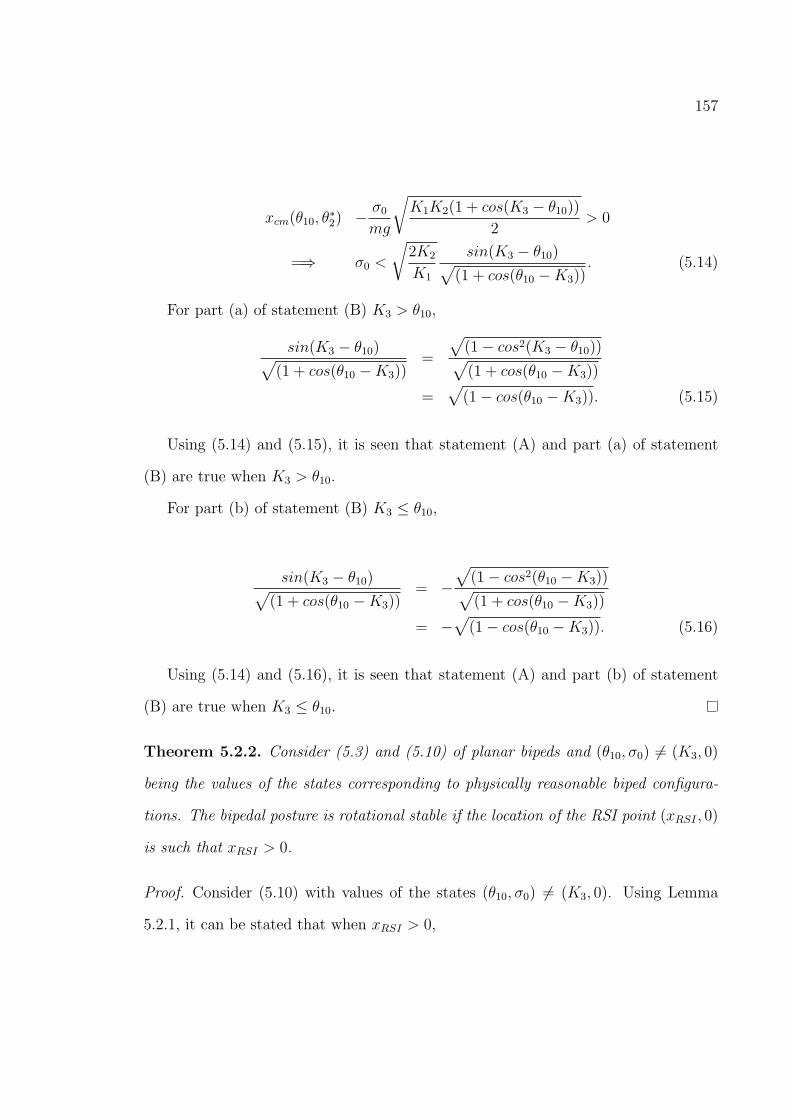
157

xcm(θ10, θ∗

2) − σ0

mg

√K1K2(1 + cos(K3 − θ10))

2> 0

=⇒ σ0 <

√2K2

K1

sin(K3 − θ10)√(1 + cos(θ10 −K3))

. (5.14)

For part (a) of statement (B) K3 > θ10,

sin(K3 − θ10)√(1 + cos(θ10 −K3))

=

√(1 − cos2(K3 − θ10))√(1 + cos(θ10 −K3))

=√

(1 − cos(θ10 −K3)). (5.15)

Using (5.14) and (5.15), it is seen that statement (A) and part (a) of statement

(B) are true when K3 > θ10.

For part (b) of statement (B) K3 ≤ θ10,

sin(K3 − θ10)√(1 + cos(θ10 −K3))

= −√

(1 − cos2(θ10 −K3))√(1 + cos(θ10 −K3))

= −√

(1 − cos(θ10 −K3)). (5.16)

Using (5.14) and (5.16), it is seen that statement (A) and part (b) of statement

(B) are true when K3 ≤ θ10.

Theorem 5.2.2. Consider (5.3) and (5.10) of planar bipeds and (θ10, σ0) 6= (K3, 0)

being the values of the states corresponding to physically reasonable biped configura-

tions. The bipedal posture is rotational stable if the location of the RSI point (xRSI , 0)

is such that xRSI > 0.

Proof. Consider (5.10) with values of the states (θ10, σ0) 6= (K3, 0). Using Lemma

5.2.1, it can be stated that when xRSI > 0,

158

(I) K3 > θ10 and σ0 <√

2K2

K1

(1 − cos(θ10 −K3))

(II) K3 ≤ θ10 and σ0 < −√

2K2

K1

(1 − cos(θ10 −K3))

Therefore, Theorem 5.2.2 can be proved if it is shown that from a given posture

with initial conditions (θ10, σ0) 6= (K3, 0), the solution vector of (5.10) reaches θ1 = 0

plane when either statement I or II is true.

From (5.10),

dσ

dθ1

=K2sin(θ1 −K3)

K1σ,

σdσ =K2

K1

sin(θ1 −K3)dθ1,

σ20

2=

σ2

2+ Eσ(θ1),

σ20 = σ2 + 2Eσ(θ1), (5.17)

where Eσ(θ1) is defined as follows:

Eσ(θ1) = −∫ θ1

θ10

K2

K1

sin(θ1 −K3)dθ1,

=K2

K1

(cos(θ1 −K3) − cos(θ10 −K3)). (5.18)

The maximum value of Eσ(θ1) in (5.18) occurs when θ1 = K3. The corresponding

maximum value is denoted by Emaxσ which is calculated by putting θ1 = K3 in (5.18).

Emaxσ =

K2

K1

(1 − cos(θ10 −K3)). (5.19)

Equation (5.17) shows that if | σ0 |>√

2Emaxσ , σ = 0 does not exists in the σ

trajectory. Because | σ0 |6>√

2Emaxσ at σ = 0. Similarly, | σ0 |<

√2Emax

σ indicates

the existence of σ = 0 i.e., zero-crossing in the σ trajectory. Depending on the values

of (θ10, σ0), there can be four possible cases with θ10 > 0 (Fig. 5.4).

159

(a) With K3 > θ10 and σ0 > 0, the trajectories of (5.10) reach θ1 = 0 plane if

there exists a zero-crossing in the σ trajectory. The zero-crossing exists when

| σ0 |<√

2Emaxσ i.e., σ0 <

√2Emax

σ for σ0 > 0.

(b) With K3 > θ10 and σ0 < 0, the trajectories of (5.10) always reach θ1 = 0 plane.

(c) With K3 ≤ θ10 and σ0 > 0, the trajectories of (5.10) never reach θ1 = 0.

(d) With K3 ≤ θ10 and σ0 < 0, the trajectories of (5.10) reach θ1 = 0 plane if there

is no zero-crossing in the σ trajectory. Zero-crossing exists if | σ0 |>√

2Emaxσ

i.e., σ0 < −√

2Emaxσ for σ0 < 0.

Cases (a) and (b) prove Theorem 5.2.2 when (I) is true while cases (c) and (d)

prove Theorem 5.2.2 when (II) is true.

5.2.2 CM criteria for Rotational Stability

Suppose (xcm(θ1, θ∗

2), ycm(θ1, θ∗

2)) = (χ, ψ) and xcm(θ10, θ∗

2) = χ0. Hence,

χ = −K2

mgsin(θ1 −K3),

χ = −ψθ1 (Time derivative),

χdχ = −χψdθ1,

χ2 = χ20 − 2

∫ θ1

θ10

χψdθ1,

χ20 = χ2 + 2Eχ, (5.20)

where Eχ =∫ θ1

θ10χψdθ1.

160

Lemma 5.2.3. Consider (5.3) and (5.10) of planar bipeds. For the states (θ10, σ0)

with (xcm(θ1, θ∗

2), ycm(θ1, θ∗

2)) = (χ, ψ) and xcm(θ10, θ∗

2) = χ0, corresponding to physi-

cally reasonable biped configurations, the following two statements are equivalent:

(A) χ0 >√

2Emaxχ

(B) σ0 <√

2K2

K1

(1 − cos(θ10 −K3))

Similarly, the following two statements are equivalent:

(C) 0 > χ0 > −√

2Emaxχ

(D) σ0 < −√

2K2

K1

(1 − cos(θ10 −K3))

where Emaxχ is the maximum value of Eχ.

Proof. As per equation (5.20), χ will not change sign if χ0 >√

2Emaxχ . When χ0 >

√2Emax

χ , it is seen from (5.13) that K3 > θ10. Hence, as χ never changes sign,

K3 > θ10 should be always true. Emaxχ occurs at θ1 = K3. However, if statement (B)

is not true, then K3 > θ10 is not true always (see Fig. 5.4 and proof of Theorem) 5.2.2.

Hence, the statement (B) is also true when (A) is true. Therefore, statement (A) and

(B) are equivalent. Similar proof is possible to show the equivalence of statement (C)

and (D).

With the states (θ10, σ0) 6= (K3, 0), corresponding to physically reasonable biped

configurations, the biped is rotational stable if either statements (A) or (C) of Lemma

5.2.3 is true. It can be noted that the such criterion on CM is equivalent to the

stability criterion mentioned in Theorem 5.2.2 (Using Lemma 5.2.1 and 5.2.3).

161

Figure 5.6: RSI point and Phase Portrait.

Remark. The two loci for σ =√

2K2

K1

(1 − cos(θ10 −K3)) and

σ = −√

2K2

K1

(1 − cos(θ10 −K3)) are shown in Fig. 5.6. xRSI > 0 in any bipedal pos-

ture corresponding to the shaded area in Fig. 5.6. Hence, the shaded area corresponds

the rotational stable postures.

WhenK3 > θ10, the value of σ0, for which σ = 0 and θ1 = K3 occur simultaneously,

corresponds to Emaxσ =

σ2

0

2(from (5.17) and (5.18)). For K3 > θ10, the minimum

value of θ10, for which the trajectory reaches θ1 = K3 plane, corresponds to Emaxχ =

12

K2

2

(mg)2sin2(K3 − θ10) (from (5.20) and (5.13)). σ0 and θ10 corresponding to Emax

σ and

Emaxχ lie on the two loci shown in Fig. 5.6.

5.2.3 Discussions on the RSI Point

Some useful notes on RSI point:

162

Figure 5.7: Rotational Stability for stationary biped.

Figure 5.8: RSI point xRSI > 0. Biped is rotational stable even if xcm(θ) < 0.

163

1. Consider the expression of xRSI in (5.12). If σ0 = 0, the stability condition

in Theorem 5.2.2 effectively leads to xcm(θ) > 0 (Fig. 5.7). Basically, this is

the GCM (Ground Projection of CM) which explains the rotational stability for

stationary biped [10]. The location of RSI point addresses the effects of the

non-zero angular momentum.

2. The magnitude of the positive xRSI indicates the degree of rotational stability.

When σ > 0, larger value of σ lessen the positive magnitude of xRSI leading to

lesser rotational stability. Actually, the positive value of σ tries to rotate the

biped counterclockwise inducing tendency to topple forward. That is reflected

in the value of xRSI . Similar explanation is possible when xcm(θ) < 0 and the

biped is rotational stable because the negative value of σ is such that xRSI > 0

(Fig. 5.8). The biped becomes ‘rotational unstable’ when xRSI 6> 0.

3. The concept of planar RSI point can be extended to three-dimensional repre-

sentation when both frontal and sagittal planes are considered (Fig. 5.1 (a),

(b)). The RSI point will have (xRSI , 0, zRSI) form in three-dimensional case.

The xRSI and zRSI can be computed independently. The constants K1, K2 and

K3 would vary in different planes. xRSI indicates degree of rotational stability

in sagittal plane while zRSI indicates that in frontal plane.

5.3 RSI Point Based Stability Criteria

The RSI-based criterion in Theorem 5.2.2 determines stability in postures with for-

ward foot-rotation and θ2 = 0. For utilizing RSI point as stability criterion during

164

biped locomotion, the RSI-based criterion in Theorem 5.2.2 is revisited in two per-

spectives: (1) rotational stability when θ2 6= 0 and (2) backward foot-rotation.

5.3.1 Gaits with θ2 6= 0

In the bipedal gaits with θ2 6= 0, the system internal dynamics becomes as (5.21) [7].

θ1 =σ

M11(θ2)− M12(θ2)

M11(θ2)θ2,

σ = −mgxcm(θ). (5.21)

For bipedal gaits with θ2 6= 0, (θ1, σ) can be solved from (5.21) at any point

of time. The rotational stability of the biped at the posture corresponding to such

(θ1, σ) solutions can be decided based on the RSI criterion mentioned in Theorem

5.2.2. If such (θ1, σ) solutions satisfy the criterion mentioned in Theorem 5.2.2, the

biped is rotationally stable at the posture at that particular time. For stability of a

particular gait, every posture of the gait and corresponding solutions of (5.21) should

be rotational stable. While utilizing the RSI criteria, the constants in (5.9) have to

be computed for every posture associated with the gait.

5.3.2 Backward foot-rotation

Consider the foot link shown in Fig. 5.9. To decide on the forward toppling we can

use the criterion mentioned in Theorem 5.2.2 with l1 = Lff in (5.2) and (5.9). If

positive value of xRSI is sufficiently large, the ankle hits the ground and the impact

might make the biped to topple backward. During backward toppling, the biped

rotates about the end-point (other than toe) of the foot-link and can be considered

165

Figure 5.9: Forward and backward foot-rotation.

like tiptoed biped about the other end-point of the foot-link.

In case of backward foot-rotation, θ1 < 0 and the phase-portrait is the mirror

image of Fig. 5.4. The expression for RSI with respect to the point of rotation during

backward foot-rotation (xbRSI) is given by (5.22) where σ′

0 is the angular momentum

about the point of rotation in backward direction and K′

1, K′

2, K′

3 are computed

from (5.9) with l1 = Lfb. σ′

0 is dependent on the nature of impact and foot/ground

compliance. Without impact σ′

0 = σ0 −mxcm(θ)(Lff + Lfb) where σ0 is the angular

momentum about toe [3]. Impact can be taken into account by modifying σ′

0 according

to the impact model [91]. The equilibrium point during backward foot-rotation is

(K′

3, 0). The condition for rotational stability is xbRSI < 0 (similar to the criterion in

Theorem 5.2.2). The relative position between xbRSI and xRSI with respect to (X,Y )

is given by (5.22).

xbRSI = xcm(θ10, θ∗

2) − (Lff + Lfb) −σ

′

0

mg

√K

′

1K′

2(1 + cos(K′

3 − θ10))

2,

=⇒ xbRSI = xRSI − (Lff + Lfb). (5.22)

166

Hence, the condition to avoid backward toppling is as per (5.23).

xbRSI < 0,

=⇒ xRSI < (Lff + Lfb),

=⇒ xRSI < foot length. (5.23)

5.3.3 Stability Criterion

Merging the conditions for both forward (Theorem 5.2.2) and backward foot-rotation

in (5.23), the overall bipedal stability condition is rewritten as (5.24). It is notable

for the computation of xRSI that the constants in (5.9) is dependent on the point of

foot-rotation during biped locomotion. Moreover, σ is the angular momentum about

the point of foot-rotation during forward and backward rotation.

Biped Stability Criteria : 0 < xRSI < foot length.

(5.24)

5.3.4 Comparison with other Ground Reference Points

RSI-based stability criterion fundamentally differs from well known ground reference

points in a number of ways. When ZMP is within the support polygon, it coincides

with the center of pressure (CP) [10]. Such postures with ZMP/CP within the support

polygon are statically stable and there is no foot-rotation. When ZMP is outside

the support polygon, it is termed as Fictitious ZMP (FZMP) [9]. The location of

ZMP/FZMP being outside the support polygon indicates that the foot is about to

167

Figure 5.10: ZMP/FRI/CP/FZMP and RSI: (a) Foot is not going to rotate. (b) Footis about to rotate. (c) Foot is rotated, and bipedal posture is rotational stable.

Figure 5.11: ZMP/FRI/CP and RSI: ZMP/CP/FRI indicate whether the foot isabout to rotate or not, RSI point indicates whether the bipedal posture will lead toa flat-foot posture or not.

168

rotate. FZMP and FRI indicates similar stability aspects of biped locomotion (Fig.

5.10). The location of FRI point indicates whether the foot is going to rotate or not.

When FRI is located within the support polygon it coincides with ZMP. All these

ground reference points investigates certain stability aspects associated with the flat-

foot bipedal posture. Location of such points indicates the possibility of foot-rotation

during locomotion. On the contrary, RSI point deals with situations when foot is

already rotated but the biped has not fallen down. The location of the RSI point

indicates whether the biped is going back to flat-foot posture or topple over (Fig.

5.11).

In flat-foot postures, ZMP and FRI use the torque generated at the toe-ground

contact point due to GRF. Such torques due to GRF becomes zero in tiptoed bipeds

because GRF acts at the point of rotation. Therefore, ZMP and FRI are not suitable

for postural stability analysis when the foot is already rotated. On the other hand, RSI

point does not use GRF in its computation and is able to analyze stability in tiptoed

bipedal postures. However, RSI is not relevant in ideal flat-foot postures. The torques

due to GRF will appear in equations (5.5) and (5.6) in flat-foot biped. Therefore,

the stability concepts associated with RSI and ZMP/FRI are complementary to each

other.


The applicability of RSI point in various scenarios associated with the biped locomo-

tion is illustrated through simulation studies and validated experimentally. We limit

our study to forward toppling, as backward toppling can be performed in a similar

way. Four cases are studied and analyzed through simulations and experimentations.

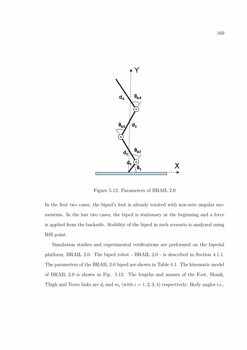
169

Figure 5.12: Parameters of BRAIL 2.0

In the first two cases, the biped’s foot is already rotated with non-zero angular mo-

mentum. In the last two cases, the biped is stationary at the beginning and a force

is applied from the backside. Stability of the biped in such scenario is analyzed using

RSI point.

Simulation studies and experimental verifications are performed on the bipedal

platform, BRAIL 2.0. The biped robot - BRAIL 2.0 - is described in Section 4.1.1.

The parameters of the BRAIL 2.0 biped are shown in Table 4.1. The kinematic model

of BRAIL 2.0 is shown in Fig. 5.12. The lengths and masses of the Foot, Shank,

Thigh and Torso links are di and mi (with i = 1, 2, 3, 4) respectively. Body angles i.e.,

170

ankle, knee and hip angles are θb = [ θb1 θb2 θb2 ]T . Biped’s absolute orientation is

θa = [ θ1 θTb ]T .

5.4.1 Simulations

Simulations are done based on the parameters shown in Table 4.1. The dynamics of

the biped is computed in the MATLAB/Simulink environment. The dynamic param-

eters are expressed in C language code by using ‘ccode’ command for faster computa-

tion and simulation. The control algorithms are simulated in Microsoft VC++ envi-

ronment using the C code of the biped-dynamics generated by MATLAB/Simulink.

Integration algorithm is based on fourth order Runge-Kutta method with a fixed step

size of 0.0001s.

Four different examples are provided to illustrate the applicability of RSI point in

stability analysis of biped locomotion. In the first example, the biped’s foot is rotated

such that xcm(θ) < 0. In this scenario, the location of GCM makes the biped to

topple forward when it is stationary. However, with negative angular momentum, the

location of the RSI point satisfies the stability criterion in Theorem 5.2.2. Therefore,

the bipedal posture is rotational stable. In the second example, the biped’s foot is

rotated but xcm(θ) > 0. In this scenario, the location of GCM makes the biped

rotational stable when it is stationary. However, with positive angular momentum,

location of RSI point is negative i.e., the biped is ‘rotational unstable’. The Biped

starts from a stationary posture in third and fourth examples. A force is applied on

the biped from the backside. Whether the biped is rotational stable (example 3) or

unstable (example 4) is investigated using RSI point.

Let us consider a bipedal posture with the body joint angles given by θb =

171

0 0.1 0.2 0.3 0.4 0.5 0.6 0.7−0.02

0

0.02

0.04

0.06

0.08

0.1

0.12

0.14

Radian

Met

er

xRSIxCM

t=0

K3

Figure 5.13: θ1 Vs. xRSI θ1 Vs. xcm and : θ10 = 0.6 rad and σ0 = −0.0289 kgm2s−1.

[ 2.3638 −1.5217 1.5286 ]T rad. With this body posture and θ1 = 0 i.e., θa =

[ 0 2.3638 −1.5217 1.5286 ]T , the location of CM is xcm(θa) = 0.0646 m and

ycm(θa) = 0.1155 m. It is noticeable that 0 < xcm(θa) < d1 which indicates that the

biped is in a statically stable posture with θ1 = 0. The values of the three constants

in (5.9) with θb = [ 2.3638 −1.5217 1.5286 ]T are K1 = 27.6501, K2 = 1.6873 and

K3 = 0.5101. Examples are shown to illustrate the effects of rotational stability on

the bipedal systems.

Example 1 (xcm(θ) < 0, but rotational stable)

Consider the posture given by θa = [ 0.6 2.3638 −1.5217 1.5286 ]T . Let, the

initial joint angular velocity is θ1 = −0.8 rad/s and the rest of the angular velocities

are zeroes. Therefore, θ10 = 0.6 and θ10 > K3 indicate that xcm(θ) < 0 i.e., the biped

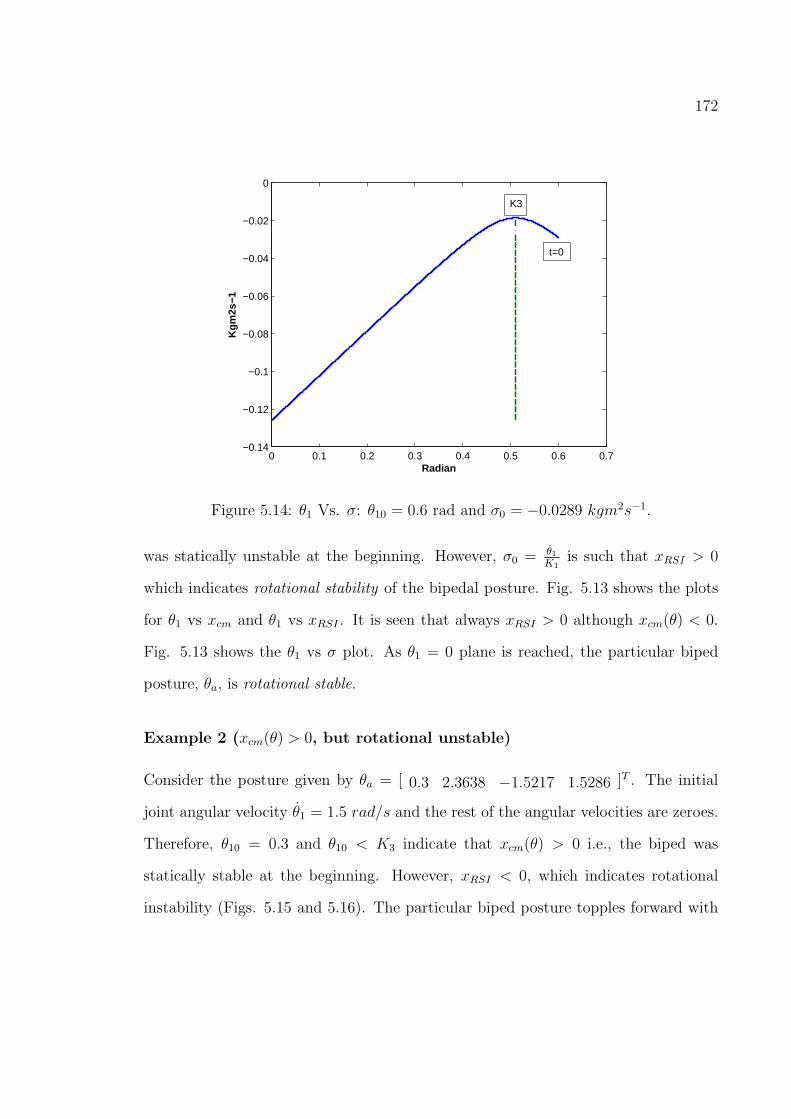
172

0 0.1 0.2 0.3 0.4 0.5 0.6 0.7−0.14

−0.12

−0.1

−0.08

−0.06

−0.04

−0.02

0

Radian

Kgm

2s−1

t=0

K3

Figure 5.14: θ1 Vs. σ: θ10 = 0.6 rad and σ0 = −0.0289 kgm2s−1.

was statically unstable at the beginning. However, σ0 = θ1K1

is such that xRSI > 0

which indicates rotational stability of the bipedal posture. Fig. 5.13 shows the plots

for θ1 vs xcm and θ1 vs xRSI . It is seen that always xRSI > 0 although xcm(θ) < 0.

Fig. 5.13 shows the θ1 vs σ plot. As θ1 = 0 plane is reached, the particular biped

posture, θa, is rotational stable.

Example 2 (xcm(θ) > 0, but rotational unstable)

Consider the posture given by θa = [ 0.3 2.3638 −1.5217 1.5286 ]T . The initial

joint angular velocity θ1 = 1.5 rad/s and the rest of the angular velocities are zeroes.

Therefore, θ10 = 0.3 and θ10 < K3 indicate that xcm(θ) > 0 i.e., the biped was

statically stable at the beginning. However, xRSI < 0, which indicates rotational

instability (Figs. 5.15 and 5.16). The particular biped posture topples forward with

173

0.5 1 1.5 2−0.3

−0.25

−0.2

−0.15

−0.1

−0.05

0

0.05

Radian

Met

er

xRSIxCM

t=0

K3

Figure 5.15: θ1 Vs. xRSI and θ1 Vs. xcm: θ10 = 0.3 rad and σ0 = 0.0542 kgm2s−1.

0.5 1 1.5 20

0.05

0.1

0.15

0.2

0.25

0.3

0.35

Radian

Kgm

2s−1

t=0

K3

Figure 5.16: θ1 Vs. σ: θ10 = 0.3 rad and σ0 = 0.0542 kgm2s−1.

174

−0.1 0 0.1 0.2 0.3 0.4 0.5 0.60

0.02

0.04

0.06

0.08

0.1

0.12

0.14

Radian

Met

er

xRSIxCM

t=0

ExternalForce

K3

t=0.26 Sec

Figure 5.17: θ1 Vs. xRSI and θ1 Vs. xcm: Pushed from the backside and rotationalstable.

time and is ‘rotational unstable’.

Example 3 (push from back and rotational stable)

The initial posture of the biped is considered as θa = [ 0 2.3638 −1.5217 1.5286 ]T

and all the angular velocities are zero. The biped is pushed from the backside by a

force of 2.6 N at a height of 40 cm for 0.26 sec (based on the experiment discussed

in section 5.4.2). It is equivalent to a torque of 2.6 × 0.4 = 1.04 Nm for 0.26 sec at

the joint between toe and ground. Hence, (5.10) is modified as (5.25). Due to the

application of the external push from the backside, the biped moves forward which

leads to θ10 = 0.2078 rad and σ0 = 0.0710 kgm2s−1.

175

−0.1 0 0.1 0.2 0.3 0.4 0.5 0.6−0.15

−0.1

−0.05

0

0.05

0.1

Radian

Kgm

2s−1

t=0.26 Sec

t=0

K3ExternalForce

Figure 5.18: θ1 Vs. σ: Pushed from the backside and rotational stable.

θ1 = K1σ,

σ = K2sin(θ1 −K3) + 1.04. (5.25)

Now, consider the posture given by θa = [ 0.2078 2.3638 −1.5217 1.5286 ]T

with σ0 = 0.0710 kgm2s−1. As xRSI > 0, the posture is rotational stable. Therefore,

the biped was able to absorb the push (Figs. 5.17 and 5.18).

Example 4 (push from back and rotational unstable)

The initial posture of the biped is considered as θa = [ 0 2.3638 −1.5217 1.5286 ]T

and all the angular velocities are zeroes. A force of 2.6 N is applied at a height of 40

cm for 0.265 sec from the backside of the biped. It is equivalent a torque of around

2.6 × 0.4 = 1.04 Nm for 0.265 sec at the joint between the toe and ground. Due to

176

0 0.2 0.4 0.6 0.8 1−0.15

−0.1

−0.05

0

0.05

0.1

Radian

Met

er

xRSIxCMt=0.265 Sec K3

ExternalForce

Figure 5.19: θ1 Vs. σ: Pushed from the backside and ‘rotational unstable’.

0 0.2 0.4 0.6 0.8 10

0.02

0.04

0.06

0.08

0.1

0.12

Radian

Kgm

2s−1

K3ExternalForce

t=0.265 Sec

Figure 5.20: θ1 Vs. σ: Pushed from the backside and ‘rotational unstable’.

177

the application of the external force from backside the biped moves forward leading

θ10 = 0.2178 rad and σ0 = 0.0735 kgm2s−1 (from (5.25)). Now, consider the posture

given by θa = [ 0.2178 2.3638 −1.5217 1.5286 ]T with σ0 = 0.0735 kgm2s−1. As

xRSI < 0, the biped topples forward due to the push (Figs. 5.19 and 5.20).

5.4.2 Experiments

The experiments were performed on the biped BRAIL 2.0 based on the examples

3 and 4. The biped’s initial posture is θa = [ 0 2.3638 −1.5217 1.5286 ]T (Fig.

5.21). All the six motors at the three joints of the both legs are rotated to the

angular positions corresponding to θb = [ 2.3638 −1.5217 1.5286 ]T and are hold

at those positions. A force is applied on it from backside and intensity of the push is

measured using force sensors. The force measurement system uses Tekscan FlexiForce

force sensors and certain linearization circuitry (details available in [99]).

The height of the point of application of the force is 40 cm above the ground. The

sensing portion of the FlexiForce sensor is placed at the point of application of force.

Force is applied with different amplitude and time duration. It is found that when a

force of 2.6 N is applied for 0.26 sec the biped can maintain rotational stability. This

validates the example 3 in simulation. When similar amount of force is applied for

0.26 − 0.30 sec the biped becomes ‘rotation unstable’. This validates the example 4

in simulation.

178

Figure 5.21: BRAIL 2.0: Push from back.

179

5.5 Conclusions

The stability aspects of biped locomotion with foot-rotation is investigated in the

article. The planar bipeds are modeled as a two-link kinematic structure with the

rotating foot being the first link and rest of the biped being modeled as an inverted

pendulum (and second link). The model is underactuated due to the absence of actu-

ation at the joint between the rotating foot and ground. Presence of underactuation

in the model leads to non-trial internal dynamics. A stability concept named rota-

tional stability is introduced to indicate the stability of the internal dynamics (5.10)

corresponding to a bipedal posture with foot-rotation. It is established that the ro-

tational stability of the bipeds is quantified by the location of the ground reference

point called ‘rotational stability index (RSI)’ point. Examples of ‘rotational sta-

ble/unstable’ bipedal configurations in different postures are illustrated in simulation

and are validated experimentally on a biped robot.

Chapter 6

Conclusions and Future Directions

6.1 Conclusions

Biped locomotion can be either flat-foot (foot-link does not loose contact with ground

surface) or with foot-rotation (foot-link rotates about toe). Presence of foot-rotation,

during biped locomotion, brings in various stability issues associated with the addi-

tional passive DOF at the joint between toe and ground. Based on the presence of

foot-rotation during locomotion, the research contributions reported in this disserta-

tion can be divided into two parts. First part of the dissertation deals with stability,

optimization and robustness of flat-foot walking gaits while the second part deals

with stability issues associated with the foot-rotation during biped locomotion.

The inverse-kinematics based walking gait is generated for a twelve DOF biped

robot. The walking gait is parameterized in terms of certain parameters i.e., Step

length, Bending-height, Maximum Lifting-height and Maximum Frontal-shifting. The

gait is optimized by finding the optimum values of the parameters considering a

tradeoff between postural stability and walking speed. ZMP is utilized as a stability

criterion and it is assumed that foot is flat during locomotion. Inverse kinematic

180

181

based gait is computed off-line and implemented on a biped robot - BRAIL 1.0. Due

to off-line computation of the inverse kinematic based gait, such gaits need further

enhancement for robustness. Stability of such gaits is further addressed when the

biped is subjected to disturbances.

An online ZMP compensation technique for disturbance rejection is proposed to

improve the biped locomotion gait. In this method, the ZMP is kept within a closer

range of the the ankle joint (‘safety zone’). Whenever the ZMP falls outside the

‘safety zone’, due to disturbances, the online compensation is activated to bring back

the ZMP location within the ‘safety zone’. The ZMP compensation method is utilized

in various applications to show its suitability to improve biped-locomotion-stability

and reject disturbances. Utilizing the compensation technique, a humanoid robot

was able to carry additional weight placed at the backside of robot, climb up or down

slopes and absorb pushes from back or front. In the compensation technique, ZMP

is utilized as stability criterion considering a flat-foot locomotion.

The later part of the dissertation deals with biped locomotion in presence of foot-

rotation. The foot being already rotated, the bipedal systems becomes underactuated

due to the additional passive DOF at the joint between toe and ground. The un-

deractuated bipedal system has two dimensional zero-dynamics submanifold of the

full order biped dynamics. For the postural stability in such scenarios where the

foot is rotated, the stability of the associated zero-dynamics plays a key role. The

stability analysis in the dissertation is mainly focused on the stability of such zero-

dynamics. Conditions are established for the stability of the zero-dynamics as well as

the underactuated bipedal dynamics (with foot-rotation).

Landing stability analysis is performed while considering jumping gait of planar

182

biped robot. Landing is considered in presence of foot rotation and is modeled as

underactuated two-link inverted pendulum. While considering the asymptotic sta-

bility of the biped’s ZD for stable landing, the foot compliance model with ground

is modeled as spring-damper. Stability conditions are established for stable landing

and, critical potential index and critical kinetic index are introduced to measure the

landing stability margin. The stability margin depends on certain properties of the

bipedal structure, foot-ground contact surface and the control parameters.

The stability conditions of biped locomotion with foot-rotation is established. The

biped with foot rotation is underactuated by one DOF due to the passive DOF at

the joint between the toe and ground, and such bipeds are modeled as underactuated

two-link inverted pendulum. The stability aspects of such configurations are indi-

cated by “rotational stability”. A ground reference point named “rotational stability

index (RSI)” point is introduced to quantify rotational stability of a biped with foot

rotation.

6.2 Future Directions

The concept of RSI point is useful to analyze stability of biped locomotion with

foot rotation. Biped (with foot) locomotion is stable irrespective of occurrence of

foot rotation if the location of RSI point satisfies the stability criterion mentioned in

Theorem 5.2.2 and section 5.3.3.

Some possible applications of RSI point might be:

• Landing stability of jumping and hopping gaits: In the landing stability analy-

sis in Chapter 4, the stability conditions are based on foot-ground compliance

183

model and certain control parameters.

When the foot is rotated, RSI point can analyze whether the biped is about to

attain a flat-foot posture (stability in Subsystem A, Fig. 4.9). However, the

concept of RSI point is not relevant in flat-foot postures. Hence, RSI point

can not explain stability in Subsystem B (Fig. 4.9). The stability of flat-foot

bipeds is analyzed by ZMP or FRI. The unification of the concepts of RSI and

ZMP/FRI is an interesting area to work on.

• Stability of walking gaits: The concept of RSI point can be applied to find out

stable walking gait with foot rotation for biped robots.

Advantage of using RSI-based stability criterion is that it takes into account the

foot-rotation during locomotion. Therefore, RSI-based criteria provides greater

stability margin than ZMP-based criteria. For example, ZMP criteria says biped

is statically unstable when ZMP is outside the foot support area because such

ZMP locations cause foot-rotation. However, the RSI-based criteria suggests

that the biped is rotational stable as long as 0 < xRSI < foot length, irrespective

of foot-rotation. Similar argument is true for FRI point as well.

• Periodicity aspects of walking, hopping and running gaits: RSI point approach

can be useful in establishing periodicity of various periodic gaits.

The existence of periodic orbits in biped locomotion can be investigated with

periodic occurrence of forward and backward foot-rotation.

Chapter 7

Author’s Publications

7.1 International Journal

1. P. Vadakkepat, Dip Goswami and Chia Meng Hwee. “Disturbance Rejection

by Online ZMP Compensation,” Robotica, Cambridge Press, vol. 26, pp. 9-17,

2007.

2. P. Vadakkepat and Dip Goswami. “Biped Locomotion: Stability, Analysis and

Control,” Int. Journal of Smart Sensing and Intelligent Systems, vol. 1, no 1,

pp 187-207, March 2008.

3. Dip Goswami, Prahlad Vadakkepat and Phung Duc Kien, “Genetic Algorithm-

based Optimal Bipedal Walking Gait Synthesis considering Tradeoff between

stability margin and Speed,” Robotica (2008).

4. Prahlad Vadakkepat, Ng Buch Sin, Dip Goswami, Zhang Rui Xiang, Tan Li

Yu, “Soccer Playing Humanoid Robots: Processing Architecture, Gait Gener-

ation and Vision System,” Robotics and Autonomous Systems (Accepted for

publication).

184

185

5. Dip Goswami, Prahlad Vadakkepat, “Jumping Gaits for Planer Biped Robots

with Stable Landing,” IEEE Transaction on Robotics (Under 2nd Review).

6. Dip Goswami, Prahlad Vadakkepat, “RSI Point: Postural Stability in Bipeds,”

IEEE Transaction on Robotics (Under Review).

7.2 International Conference

1. Vadakkepat, P and Dip Goswami, “MANUS Humanoid: A Test bed for Ad-

vanced Robotics Research,” International Conference on Emerging Mechanical

Technology Macro to Nano, ed. R. K. Mittal and N. N. Sharma (2007): 195

203 (Emerging Mechanical Technology Macro to Nano, 16 18 Feb 2007, Birla

Institute of Technology and Science, Pilani, India).

2. P. Vadakkepat and Dip Goswami, “Biped Locomotion: Stability, Analysis and

Control,” CIRAS, Palmerston North, New Zealand, 28-30 November 2007.

3. Jin Yongying, Dip Goswami, and Prahlad Vadakepat, “Walking Gait Genera-

tion for Humanoid Robot BRAIL 1.0,” CIRAS, 19-21 June 2008, Linz, Austria.

4. Burra Pavan Kumar, Dip Goswami, and Prahlad Vadakepat, “Jumping and

Hopping Robot: Development and Experimentation,” CIRAS, 19-21 June 2008,

Linz, Austria.

Bibliography

[1] J. Yamaguchi, D. Nishino, A. Takanishi, “Realization of dynamic biped walking

varying joint stiffness using antagonistic driven joints,” Proceedings of Interna-

tional Conference of Robotics and Automation, Vol. 3, pp 2022-2029 (1998).

[2] M. Ogino, Y. Katoh, M. Aono, M. Asada, K. Hosoda, “Vision-based rein-

forcement learning for humanoid behaviour generation with rhythmic walking

parameters,” Proceedings of IROS, Vol. 2, pp 1665-1671 (2003).

[3] ER Westervelt, JW Grizzle, C. Chevallerau, JH Choi, B. Morris “Feedback

control of dynamic bipedal robot locomotion,” Boca Raton : CRC Press (2007).

[4] John J. Craig, “Introduction to Robotics: Mechanics and Control,” Second Edi-

tion, Addison-Wesley Longman Publishing Co., Inc. Boston, MA, USA. 1989.

[5] K.S. Fu, R.C. Gonzalez and C.S.G. Li, “Robotics: control, sensing, vision, and

intelligence,” McGraw-Hill, New York, USA, 1987.

[6] M. Vukobratovie, B. Borovac, D. Surla and D. Stokie, “Biped Locomotion:

Dynamics, Stability, Control and Application,” Springer, 1990.

[7] C. Chevallereau, E.R. Westervelt and J. W. Grizzle, “Asymptotically Stable

Running for a Five-Link, Four-Actuator, Planar Bipedal Robot,” The Interna-

tional Journal of Robotics Research, vol. 24, no. 6, pp. 431-464, 2005.

[8] Jean-Jacques E. Slotine, Weiping Li, “Applied Nonlinear Control,” New Jersey,

1991.

186

187

[9] M. Vukobratovic and B. Borovac, “Zero Moment Point - Thirty Five Years of its

Life,” International Journal of Humanoid Robotics Vol. 1, No.1 157-173, 2004 .

[10] Ambarish Goswami, “Postural Stability of Biped Robots and the Foot-Rotation

Indicator (FRI) Point,” The International Journal of Robotics Research, vol.

18, no. 6,pp. 523-533, 1999.

[11] M.H. Raibert, Jr H.B. Brown and M. Chepponios, “Experiments in Balance

with a 3D One-legged Hopping-Machine,” International Journal of Robotic Re-

search, vol. 3, no. 2, pp 75-92, 1984.

[12] E. Koditschek and Martin Bhler, “Analysis of a Simplified Hopping Robot,”

The International Journal of Robotics Research, vol. 10, no. 6, pp. 587-605,

1991.

[13] T. Sugihara, Y. Nakamura and H. Inoue, “Real-time humanoid motion genera-

tion through ZMP manipulation based on inverted pendulum control,” ICRA,

pp. 1404 - 1409 vol.2, 11-15 May 2002.

[14] S. Kajita, F. Kanehiro, K. Kaneko, K. Fujiwara, K. Harada, K. Yokoi and H.

Hirukawa, “Biped walking pattern generation by using preview control of zero-

moment point,” IEEE International Conference on Robotics and Automation

(ICRA), pp. 1620 - 1626, vol.2, 14-19 Sept. 2003.

[15] S. Kitamura, Y. Kurematsu and M. Iwata, “Motion generation of a biped loco-

motive robot using an inverted pendulum model and neural networks,” IEEE

Conference on Decision and Control, pp. 3308 - 3312, vol.6, 5-7 Dec. 1990.

[16] Napoleon, S.Nakaura, M. Sampei, “Balance control analysis of humanoid robot

based on ZMP feedback control,” IEEE International Conference on Intelligent

Robots and System, Vol. 3, pp. 2437-2442 (2002).

188

[17] Hun-ok Lim, Y. Yamamoto and A. Takanishi, “Control to realize human-like

walking of a biped humanoid robot,” IEEE International Conference on Sys-

tems, Man, and Cybernetics, pp. 3271 - 3276, vol.5, 8-11 Oct. 2000.

[18] JH Choi, JW Grizzle, “Planar bipedal walking with foot rotation,” American

Control Conference, Vol. 7, pp. 4909- 4916 (2005).

[19] A.Goswami, “Foot rotation indicator (FRI) point: a new gait planning tool

toevaluate postural stability of biped robots,” IEEE International Conference

on Robotics and Automation, Vol. 1, pp. 47-52 (1999).

[20] Yamaguchi, J., Soga, E., Inoue, S., Takanishi, A., “Development of a bipedal

humanoid robot-control method of whole body cooperative dynamic biped walk-

ing,” Proceedings of 1999 IEEE International Conference on Robotics and Au-

tomation, Vol. 1, 10-15, 368 - 374, 1999.

[21] J. Vermeulen, B. Verrelst, D. Lefeber, P. Kool B. Vanderborght, “A real-time

joint trajectory planner for dynamic walking bipeds in the sagittal plane,”

Robotica, Volume 23, Issue 06, Nov 2005, pp 669-680.

[22] K. Hirai, M. Hirose, Y. Haikawa and T. Takenaka, “The Development of Honda

Humanoid Robot,” Proceedings of the 1998 IEEE International Conference on

Robotics and Automation, 1321-1326, 1998.

[23] N. Shiraishi, Y. Kawaida, Y. Kitamura, S. Nakaura and M. Sampei, “Vertical

jumping control of an Acrobat Robot with consideration of input timing,” Pro-

ceedings of the 41st SICE Annual Conference, vol. 4, pp. 2531 - 2536, 5-7 Aug.

2002.

[24] K. Mitobe, N. Mori N, K. Aida, Y. Nasu, “Nonlinear feedback control of a

biped walking robot,” Proceedings of 1995 IEEE International Conference on

Robotics and Automation, Vol. 3, pp 2865 - 2870 (1995).

189

[25] Garcia M., Chatterjee A., Ruina A., “Efficiency, speed, and scaling of two-

dimensional passive-dynamic walking,” Dynamics and Stability of Systems, Vol.

15, No. 2, 75-99, 2000.

[26] Steve Collins, Andy Ruina, Russ Tedrake, Martijn Wisse, “Efficient Bipedal

Robots Based on Passive Dynamic Walkers,” Science Magazine, Vol. 307, 1082-

1085, 2005.

[27] F. Yamasaki, K. Hosoda and M. Asada, “An Energy consumption based con-

trol for humanoid walking,” IEEE/RSJ International Conference on Intelligent

Robots and System (IROS), pp. 2473 - 2477, vol. 3, 30 Sept.-5 Oct. 2002.

[28] K. Ono, R. Takahashi,A. Imadu and T. Shimada, “Self-excitation control for

biped walking mechanism,” IROS, pp. 1143 - 1148, vol.2, 31 Oct.-5 Nov. 2000.

[29] Kyung-Kon Noh, Jin-Geol Kim and Uk-Youl Huh, “Stability experiment of a

biped walking robot with inverted pendulum,” 30th IEEE Annual Conference

of Industrial Electronics Society, pp. 2475 - 2479, vol. 3, 2-6 Nov. 2004.

[30] Xiuping Mu and Qiong Wu, “Synthesis of a complete sagittal gait cycle for a

five-link biped robot,” Robotica, pp 581-587, vol. 21, Issue 05, Oct 2003.

[31] A.W. Salatian and Y.F. Zheng, “Gait synthesis for a biped robot climbing

sloping surfaces using neural networks. II. Dynamic learning,” ICRA, pp. 2607

- 2611 vol.3, 12-14 May 1992.

[32] M. Cao and A. Kawamura, “A design method of neural oscillatory networks for

generation of humanoid biped walking patterns,” ICRA, pp. 2357 - 2362 vol.3,

16-20 May 1998.

[33] A. Dasgupta and Y. Nakamura,“Making feasible walking motion of humanoid

robots from human motion capture data,” ICRA, pp. 1044 - 1049 vol.2, 10-15

May 1999.

190

[34] Sang-Ho Choi, Young-Ha Choi and Jin-Geol Kim, “Optimal walking trajectory

generation for a biped robot using genetic algorithm,” IROS, pp. 1456 - 1461,

vol.3, 17-21 Oct. 1999.

[35] M.Y. Cheng and C.S. Lin, “Genetic algorithm for control design of biped loco-

motion Systems,” IEEE International Conference on Man and Cybernetics, pp.

1315 - 1320 vol.2, 22-25 Oct. 1995.

[36] Jung-Shik Kong, Bo-Hee Lee and Jin-Geol Kim, “A study on the gait generation

of a humanoid robot using genetic algorithm,” SICE 2004 Annual Conference,

pp. 187 - 191 vol.1, 4-6 Aug. 2004.

[37] F. Arakawa and T. Fukuda, “Natural motion trajectory generation of biped

locomotion robot using genetic algorithm through energy optimization,” IEEE

International Conference on Systems, Man, and Cybernetics, pp. 1495 - 1500,

vol.2, 14-17 Oct. 1996.

[38] Z. Tang, C. Zhou, Z. Sun, “Humanoid Walking Gait Optimization Using GA-

Based Neural Network,” pp. 252-261, ICNC(2) 2005.

[39] Y. Sakagami, R. Watanabec, C. Aoyama, S. Matsunaga, N. Higaki, “The intel-

ligent ASIMO: System overview and integration” Proceedings of the IEEE/RSJ

International Conference on Intelligent Robots and Systems, Switzerland. pp.

24782483, 2002.

[40] L. Righetti, A.J. Ijspeert, “Programmable Central Pattern Generators: an

application to biped locomotion control,” IEEE International Conference on

Robotics and Automation (ICRA06). Orlando, pp. 1585-1590, 2006.

[41] P. Manoonpong, T. Geng, T. Kulvicius, B. Porr, F. Wrgtter, “Adaptive, Fast

Walking in a Biped Robot under Neuronal Control and Learning,” PLoS Com-

put Biol, 3(7), e134, 2007.

191

[42] C. Capaday, “The special nature of human walking and its neural control,”

Trends Neurosci 25: 370376, 2002.

[43] J. Duysens, V. de Crommert, “Neural control of locomotion. Part 1: The central

pattern generator from cats to humans,” Gait and Posture 7: 131141, 1998.

[44] T. McGeer, “Passive dynamic walking,” International Journal of Robotics Re-

search, vol. 9, no., 2, pp. 62-82, 1990.

[45] A. J. Ijspeert, A. Crespi, D. Ryczko, J. M. Cabelguen, “From swimming to

walking with a salamander robot driven by a spinal cord model,” Science 315

(5817) 14161420, 2007.

[46] H. Kimura, Y. Fukuoka, A. H. Cohen, “Adaptive dynamic walking of a

quadruped robot on natural ground based on biological concepts,” International

Journal of Robotics Research 26 (5) 475490, 2007.

[47] P. Manoonpong, F. Pasemann, H. Roth, “Modular reactive neurocontrol for

biologically-inspired walking machines,” The International Journal of Robotics

Research, vol. 26, no. 3, pp. 301-331, 2007.

[48] R.D. Beer, R.D.Quinn, H.J. Chiel, R.E. Ritzmann, “Biologically inspired ap-

proaches to robotics: what can we learn from insects?,” Communications of the

ACM, Vol. 40, No. 3, pp. 3038, 1997.

[49] T. Geng, B. Porr, F. Wrgtter, “Fast Biped Walking with A Sensor-driven Neu-

ronal Controller and Real-time Online Learning,” The International Journal of

Robotics Research, vol. 25, no.3, pp. 243-259, 2006.

[50] WA Gruver, TT Lee, PL Jeng, “Control of a 5-link biped robot for steady

walking,” IEEE International Symposium on Intelligent Control, pp 484-489

(1998).

192

[51] L. Roussel, C.-De-Wit, A. Goswami, “Generation of energy optimal complete

gait cycles for biped robots,” IEEE International Conference on Robotics and

Automation, Vol. 3, Page(s): 2036-2041 (1998).

[52] Vibet M, “Control law decoupling for 2-D biped walking system Cotsaftis,”

IEEE Engineering in Medicine and Biology Magazine, Volume 7, Issue: 3, pp

41-45 (1988).

[53] S. Kajita, O. Matsumoto, M. Saigo, “Real-time 3D walking pattern genera-

tion for a biped robot with telescopic legs,” IEEE International Conference on

Robotics and Automation, Vol. 2, pp. 2299-2306 (2001).

[54] JS Albus, “A new approach to manipulator control: the cerebellar model articu-

lation controller (CMAC),” ASME Journal of Dynamic systems, Measurements

and Control, pp 220-227, (1975).

[55] YH Kim, FL Lewis, “Optimal design of CMAC neural-network controller for

robot manipulators,” IEEE Transactions on Systems, Man and Cybernetics:

Part C, Vol. 30, Issue 1, pp 22-31 (2000).

[56] DM Katic, MK Vukobratovic, “Highly efficient robot dynamics learning by

decomposed connectionist feedforward control structure,” IEEE Transactions

on Systems, Man and Cybernetics, Vol. 25, Issue 1, pp 145 - 158 (1995).

[57] M. Yamakita, M. Kishikawa and T. Sadahiro, “Motion control for robust land-

ing of acrobat robot,” Proc. IEEE/RSJ Int. Conf. on Intelligent Robots and

Systems, pp. 1141-1146, 2003.

[58] S. Hyon, N. Yokoyama and T. Emura, “Back handspring of a multi-link gym-

nastic robot - reference model approach,” Advanced Robotics, vol.20, no.1, pp.

93-113, 2006.

193

[59] Hun-ok Lim, Kaneshima, Y., Takanishi, A., “Online walking pattern genera-

tion for biped humanoid robot with trunk,” Proceedings of IEEE International

Conference on Robotics and Automation, Vol. 3, 11-15, 3111 - 3116, 2002 .

[60] McGeer T., “Passive walking with knees,” Proc. IEEE Int. Conf. Robotics and

Automation, Cincinnati, OH, 1640-1645, 1990.

[61] Russ Tedrake, Teresa Weirui Zhang, Ming-fai Fong, and H. Sebastian Seung,

“Actuating a Simple 3D Passive Dynamic Walker,” Proceedings of the IEEE

International Conference on Robotics and Automation (ICRA), Vol. 5, 4656-

4661, 2004.

[62] Collins, S. H., Wisse, M., Ruina, A. “A Three-Dimensional Passive-Dynamic

Walking Robot with Two Legs and Knees,” International Journal of Robotics

Research, Vol. 20, No. 2, 607-615, 2001.

[63] M.D. Mann, “The Nervous System and Behavior,” Harper and Row, Philadel-

phia, 1981.

[64] Y. Fukuoka, H. Kimura and A. H. Cohen, “Adaptive dynamic walking of a

quadruped robot on irregular terrain based on biological concepts,” Interna-

tional Journal of Robotics Research, Vol. 22, No. 3-4, 187-202 2003.

[65] Jun Nakanishi, Jun Morimoto, Gen Endo, Gordon Cheng, Stefan Schaal, Mitsuo

Kawato, “Learning from demonstration and adaptation of biped locomotion,”

Robotics and Autonomous Systems, 47, 79-91 2004.

[66] Jun Morimoto, Gordon Cheng, C. G. Atkeson, G. Zeglin, “A Simple Reinforce-

ment Learning for Biped Walking,” Proc. IEEE International Conference on

Robotics and Automation, April 2004.

[67] Jong-Hwan Kim, Dong-Han Kim Yong-Jae Kim, Kui-Hong Park, Jae-Ho Park,

Choon-Kyoung Moon, and Kiam Tian Seow, “Humanoid Robot HanSaRam:

194

Recent Progress and Developments,” Proc. International Conference on Com-

putational Intelligence, Robotics and Autonomous Systems, 2002 .

[68] R. Zhang, P. Vadakkepat and C.M. Chew, “Motion Planning for Biped Robot

Climbing Stairs,” Proceeding of FIRA Robot World Congress, Vienna, Austria

Oct 1-3, 2003 .

[69] K. Mitobe, G. Capi, Y. Nasu, “Control of walking robots based on manipulation

of the zero moment point,” Robotica Volume 18, Issue 06, Nov 2000, pp 651-657.

[70] Jong Hyeon Park, Hoam Chung, “ZMP compensation by online trajectory gen-

eration for biped robots,” ICRA 1999 10-15 Oct Volume: 4, page(s): 960-965.

[71] Shimojo, M., Araki, T., Ming, A., and Ishikawa M., “A ZMP sensor for a biped

robot,” Proceedings. 2006 Conference on International Robotics and Automa-

tion (IEEE Cat. No. 06CH37729D), 2006, pages 1200-1205.

[72] Bauby, C. E., and Kuo, A. D., “Active control of lateral balance in human

walking,” Journal of Biomechanics, 33, 1433-1440, 2000.

[73] www.tekscan.com/pdfs/FlexiforceUserManual.pdf

[74] www.hitecrcd.com/homepage/product-fs.htm

[75] M. Spong and M. Vidyasagar, “Robot Dynamics and Control,” Wiley, New

York, 1991.

[76] E.R.Westervelt, J.W.Grizzle and D.E. Koditschek, “Hybrid zero dynamics of

planar biped walkers,” IEEE Transactions on Automatic Control, vol. 48, no.

1, pp. 42- 56, Jan 2003.

[77] A. Isidori, “Nonlinear Control Systems,” Springer-Verlag New York, USA, 1995.

195

[78] S. Kajita, T. Nagasaki, K. Kaneko, K. Yokoi and K. Tanie, “A hop towards

running humanoid biped,” IEEE International Conference on Robotics and Au-

tomation, vol. 1, pp. 629-635, 2004.

[79] J. Nagasaka, K. Kuroki, Y. Suzuki, S. Itoh and Y. Yamaguchi, “Integrated mo-

tion control for walking, jumping and running on a small bipedal entertainment

robot,” IEEE International Conference on Robotics and Automation, vol. 4,

pp. 3189-3194, Apr 26-May 1, 2004.

[80] http://world.honda.com/HDTV/ASIMO/.

[81] K. Arikawa and T. Mita, “Desing of Multi-DOF Jumping Robot,” IEEE Inter-

national Conference on Robotics and Automation, pp. 3992 - 32997, 2002.

[82] S. Sakka and K. Yokoi, “Humanoid Vertical Jumping based on Force Feedback

and Inertial Forces Optimization,” IEEE International Conference on Robotics

and Automation, pp. 3752 - 3757, 18-22 April 2005.

[83] V. Nunez and N. Nadjar-Gauthier, “Control strategy for vertical jump of hu-

manoid robots,” International Conference on Intelligent Robots and Systems,

pp. 2253 - 2258, 2-6 Aug. 2005.

[84] T. Hirano, T. Sueyoshi and A. Kawamura, “Development of ROCOS (Robot

Control Simulator)-Jump of human-type biped robot by the adaptive impedance

control,” Proceedings of 6th International Workshop on 30 Advanced Motion

Control, pp. 606 - 611, April 2000.

[85] T. Mita, Sang-Ho Hyon and T.K. Nam, “Analytical time optimal control so-

lution for a two-link planar aerobot with initial angular momentum,” IEEE

Transactions on Robotics and Automation, vol. 17, no. 3, pp. 361 - 366, June

2001.

196

[86] M. Sobotka and M. Buss, “Locomotion studies for a 5DoF gymnastic robot,”

Proceedings of International Conference on Intelligent Robots and Systems, pp.

3275- 3280, August 2005.

[87] Mehdi Nikkhah, Hashem Ashrafiuon and Farbod Fahimi, “Robust control of

underactuated bipeds using sliding modes,” Robotica, vol. 25, no. 3, pp. 367-

374, May 2007.

[88] T.F. Coleman and Y. Li, “An Interior, Trust Region Approach for Nonlinear

Minimization Subject to Bounds,” SIAM Journal on Optimization, vol. 6, pp.

418-445, 1996.

[89] T.F. Coleman and Y. Li, “On the Convergence of Reflective Newton Meth-

ods for Large-Scale Nonlinear Minimization Subject to Bounds,” Mathematical

Programming, vol. 67, pp. 189-224, 1994.

[90] A. Meghdari and M. Aryanpour, “Dynamic Modeling and Analysis of the Hu-

man Jumping Process,” Journal of Intelligent and Robotic Systems, vol. 37, pp.

97-115, 2003.

[91] Yildirim Hurmuzlu and Dan B. Marghitu, “Periodic Motions of a Hopping

Robot With Vertical and Forward Motion,” The International Journal of

Robotics Research, vol. 13, no. 1, pp. 82-92, 1994.

[92] K. Mirza, M.D. Hanes and D.E. Orin, “Dynamic simulation of enveloping power

grasps ,” International Conference on Robotics and Automoation, vol. 2, pp.

430-435, 2-6 May 1993.

[93] M.S. Branicky, “Multiple Lyapunov functions and other analysis tools for

switched and hybrid systems,” IEEE Transactions on Automatic Control, vol.

43, no. 4, pp. 475-482 Apr 1998.

197

[94] B. Morris, J.W. Grizzle, “A Restricted Poincar Map for Determining Exponen-

tially Stable Periodic Orbits in Systems with Impulse Effects: Application to

Bipedal Robots,” CDC-ECC, pp. 4199- 4206, Dec. 2005.

[95] Kwang Won Sok, Manmyung Kim, Jehee Lee, “Simulating biped behaviors

from human motion data,” International Conference on Computer Graphics

and Interactive Techniques, no. 107, 2007.

[96] Marko B. Popovic, Ambarish Goswami, “Ground Reference Points in Legged

Locomotion: Definitions, Biological Trajectories and Control Implications,” Int.

Journal of Robotics Research, vol. 24, no. 12, pp. 1013-1032, 2005.

[97] Arakawa, T. Fukuda, T.,“Natural motion generation of biped locomotion robot

using hierarchical trajectory generation method consisting of GA, EP layers,”

ICRA, pp. 211-216, vol.1, 1997.

[98] Hassan K. Khalil, “Nonlinear systems,” Portland, OR, 2001.

[99] Prahlad Vadakkepat, Dip Goswami and Chia Meng Hwee, “Disturbance Rejec-

tion by Online ZMP Compensation,” Robotica, vol. 26, pp. 9-17, 2007.

[100] M. Berkemeier and R. Fearing, “Tracking fast inverted trajectories of the un-

deractuated acrobot,” IEEE Transansaction Robotics and Automatation, vol.

15, pp. 740-750, 1999.

[101] Goswami Dip, Vadakkepat Prahlad and Phung Duc Kien, “Genetic algorithm-

based optimal bipedal walking gait synthesis considering tradeoff between sta-

bility margin and speed,” Robotica (2008).

BIPED LOCOMOTION: STABILITY ANALYSIS, GAIT ... - CORE

Documents

Transcript of BIPED LOCOMOTION: STABILITY ANALYSIS, GAIT ... - CORE