The Biomechanics of Huma.n Locomotion

by

Christopher Leonard Vaughan

A Thesis Presented in Fulfilment for the Degree

Doctor of Science in Medicine

University of Cape Town

August 2009

The copyright of this thesis vests in the author. No quotation from it or information derived from it is to be published without full acknowledgement of the source. The thesis is to be used for private study or non-commercial research purposes only.

Published by the University of Cape Town (UCT) in terms of the non-exclusive license granted to UCT by the author.

Published by

University of Cape Town Faculty of Health Sciences Anzio Road Observatory 7925 South Africa

The Biomechanics of Human Locomotion

Copyright © Christopher Leonard Vaughan

All rights reserved. This book, or parts thereof, may not be reproduced in any form or by any means, electronic or mechanical, including photocopying, recording or any information storage and retrieval system now known or to be invented, without written permission from the Publisher.

National Library of South Africa Cataloguing-in-Publication Data

A catalogue record for this book is available from: The National Librarian, National Library of South Africa, PO Box 496, Cape Town 8000, South Africa.

ISBN 978-0-620-44792-8

ii

Statement Affirming Originality of Work

A list of all my publications on the biomechanics of human locomotion is presented on pages 7 to 12 of this document. Of these 60 publications, a subset of 31 has been selected and these publications - highlighted in blue - constitute the work submitted for the degree. Reference to each publication is by its number in square brackets.

I affirm that for all publications for which I am the sole author [16, 24, 25, 26, 40, 49], this is my original work. For all publications for which I am the first author and there are one or more co-authors [5, 11, 13, 19, 22, 23, 28, 29, 31, 47, 50, 51, 52, 58, 59], I affirm that I was the senior and corresponding author and wrote the first draft of the publication.

There are eight publications for which one of my postgraduate students was the first author [32, 38, 39, 42, 43, 56, 57, 60], and I affirm that these works were conceived by me and conducted under my supervision, and I was the senior and corresponding author. Finally there are two publications for which one of my scientific collaborators was the senior author [33, 44]. These publications have been included because they formed the basis for some of my further original work [11, 38, 49, 52].

Statement Affirming Submission of Work

I affirm that I have not submitted this work for an equivalent degree at this or any other university.

Christopher L Vaughan

17 August 2009

iii

Signature Removed

Acknowledgements

The material in this document has been compiled from a 3D-year career in biomechanics. There are a number of people whose support I would like to acknowledge.

First, there are my mentors: Dave Matravers at Rhodes University; Jim Hay and Jim Andrews at the University of Iowa; and Mike Whittle at Oxford University.

Second, there are colleagues who have contributed to and influenced my own ideas on human locomotion: Brian Davis, Jeremy O'Connor, Warwick Peacock, Leila Arens, Jonathan Peter, Graeme Fieggen and Willem van der Merwe at the University of Cape Town; Diane Damiano and Mark Abel at the University of Virginia; and Mark O'Malley at University College Dublin.

Third, I have been fortunate to supervise some outstanding postgraduate students: Barbara Berman, Noddy Subramanian, Monica Busse, Nelleke Langerak, Marijka Blaszczyk and Andrea Hemmerich at the University of Cape Town; Derek Wells, Francisco Sepulveda and Noel Eldridge at Clemson University; and Gary Brooking, Ken Olree, Dave Kowalk and Jeff Duncan at the University of Virginia.

Fourth, I am delighted to recognise Marian Jacobs, my Dean at the University of Cape Town, who encouraged me to submit this portfolio of publications for the degree.

Finally, I would like to acknowledge the support of my family, in particular my wife Joan, who has been with me every step of the way on this odyssey, which I have entitled The Biomechanics of Human Locomotion.

iv

Table of Contents

Cover Page ................................................................................................................... .

Statements ..................................................................................................................... iii

Acknowledgements .................................. ....... ............................................................... iv

Table of Contents ........................................................................................................... v

Synopsis of the Work...................................................................................................... 1

List of Publications by Christopher L Vaughan ............................. ,. .......... .... .......... ........ 7

Collateral Evidence of the Value of the Work................................................................. 7

Publications that Constitute the Work ..................................................... , ..... ...... ...... ..... 13

Publication [5] ...................................................................................................... 13 Publication [11] .................................................................................................... 169 Publication [13] .................................................................................................... 191 Publication [19] ., .................................................................................................. 219 Publication [22] .................................................................... ................................ 227 Publication [23] ......................................................... .......... ................................. 231 Publication [24] .................................................................................................... 241 Publication [25] .................................................................................................... 251 Publication [26] .................................................................................................... 261 Publication [28] .............................................. : ..................................................... 309 Publication [29] .................................................................... ................................ 313 Publication [31] .................................................................................................... 327 Publication [32] ............. ....................................................................................... 335 Publication [33] ................................................ ...... ......... ..................................... 345 Publication [38] ........................................................................................... ......... 355 Publication [39] .................................................................................................... 361 Publication [40] .................................................................................................... 367 Publication [42] .................................................................................................... 389 Publication [43] .................................................................................................... 397 Publication [44] ................................................................................................ , ... 405 Publication [47] .................................................................................................... 415 Publication [49] .................................................................................................... 433 Publication [50] .................................................................................................... 445 Publication [51] .................................................................................................... 451 Publication [52] ...................... .............................................................................. 465 Publication [56] .................................................................................................... 473 Publication [57] '" ................................................................................................. 479 Publication [58] .................................................................................................... 487 Publication [59] ............... ....... .............................................................................. 493 Publication [60] ...................................................... .......... .................................... 497 Publication [16] .................................................................................................... end

v

vi

SYNOPSIS OF THE WORK

My research career began at Rhodes University in 1975 when, for my BSc (Honours) degree in Applied Mathematics and Physics, I completed my thesis on a biomechanical model of a sprinter. For the past 34 years the biomechanics of human locomotion has been the major thread running through my research. In the past ten years I have added the themes of medical imaging and research policy, but it is the mechanics of the neuromuscular system, particularly as this applies to the locomotor apparatus that forms the basis of the current work.

My 60 publications on the biomechanics of human locomotion have been listed on pages 7 to 12. Of these I have selected 31 publications, highlighted in blue, that are reproduced here on pages 13 to 500. Collateral evidence that addresses the value of my contributions has also been summarized on pages 7 to 12. For the journals I have included the impact factors as defined by the Institute for Scientific Information (lSI). In addition, I have listed the number of citations provided by the lSI's Web of Science database as well as the number of citations provided by the Google Scholar database.

Within the broad spectrum of the biomechanics of human locomotion, my seminal contributions can be summarized in three separate but related areas: (1) basic theories of human locomotion; (2) impact of clinical interventions on the neuromuscular system; and (3) engineering tools for human movement scientists. Note that the numbers in square brackets refer to the references on pages 7 to 12.

Basic Theories of Human Locomotion

Based on a comprehensive analysis of the biomechanics of sprinting, I developed a mathematical model of the sprinter. I assumed that only two external forces acted on the sprinter in the horizontal direction: the horizontal component of the ground reaction driving him forward and air resistance impeding him. These forces formed the basis for a 'first order differential equation describing the sprinter's velocity. A novel device was constructed to record the runner's velocity continuously and there was good agreement between my theory and experimental data. The resulting paper was my first publication in a scholarly journal [19]. On taking up my position at UCT in 1980 I extended the model with a view to pinpointing a runner's strengths and weaknesses and to predict what his time might be for a particular distance [24]. By using a hand-held programmable calculator and readily available equipment, the model was implemented in the field [25]. Further exposure of the model was provided in a highly cited paper that I published in CRC Critical Reviews in Biomedical Engineering [26]. The value of this 30 year-old theoretical model is that it is still applicable to any class of runner, from a novice sprinter at school to the current world record holder Usain Bolt.

Despite a complex neuromuscular control system, human locomotion is characterized by smooth, regular and repeating movements. Coordinated motion thus occurs as a direct result of the cyclical activation of many leg muscles. The challenge facing the biomechanical scientist is that there are many more muscle activators than independent equations: the system is therefore mathematically indeterminate [40]. The problem may be circumvented by reducing all muscle, bone and ligament forces to a single force and torque acting across the joints of the leg. My first theoretical contributions to this problem were based on my PhD thesis and published shortly after I joined UCT in 1980. Utilizing mathematical optimization theory, I was able to demonstrate that for closed loop problems such as walking up stairs, the neuromuscular system attempts to minimize the joint torques and thus the amount of

1

muscular effort [22, 23]. I was among the first scientists to demonstrate the fX>wer of mathematical optimization to overcome the problem of indeterminacy, a technique that is now in wide use in biomechanics. Since the mathematical equations to calculate joint torques in three-dimensional space are non-trivial, I have published a full description in Dynamics of Human Gait (see pages 109 to 132 in this thesis). This book [5] constitutes my most highly cited publication with more than 300 citations (see page 7), thus making a significant contribution to the 'field.

Artificial neural networks (ANNs) were first developed in the 1950s in an effort to create a mathematical model of the information processing capabilities of the brain. I was one of the first biomechanical scientists to realize the potential of ANNs to model the human locomotor system, in particular the relationship between muscle activity, as measured by electromyography and joint torques [11, 32]. I therefore contributed to bringing the argument full circle: ANNs, originally inspired by the idea that mathematical computation oould be modelled on the brain, now had the potential to help elucidate how the central nervous system (CNS) itself functioned [49]. An important measure of the value of this work is the fact that my key publication [32] is now a citation classic, with more than 50 citations (see page 10).

It has been recognised for more than 30 years that rhythmic movements such as locomotion are produced by neuronal circuits in the mammalian spinal cord known as central pattern generators (CPGs). However, the evidence to prove that CPGs existed in humans was lacking [11, 49]. In an electromyographic study of 16 bilateral muscles during normal human walking, we were the first scientists to provide evidence to SLiPPOrt the CPG hypothesis in humans by showing that there appear to be just three fundamental patterns (or eigenvectors) needed to overcome the problem of high dimensionality: loading response, propulsion and a coordinating factor between the left and right sides of the body [33, 38].

The theory of dynamic similarity as applied to animal locomotion had its origins in the work of two 19th century naval architects [51]. According to this hypothesis, two fundamental gait parameters - step length and step frequency - can be rendered dimensionless by using a subject's leg length, thus enabling the scientist to compare the gait patterns of subjects with different heights. Late in 2004 the skeletal remains of a pygmy-sized hominin were recovered from a cave on the Indonesian island of Flores, and we applied dynamic similarity to predict how she might have walked 18,000 years ago [56]. We have also applied the hypothesis to the Autralopithecines who left their footprints at Laetoli in central Africa more than four million years ago [58]. Our findings suggest that, despite their diminutive size, these ancient hominins were capable of ranging across a wide geographical area. The value of our contribution to the theory of dynamic similarity is that we have documented how it may be applied to a wide range of problems, including: the effects of size in growing children [13, 50]; the effects of gravity when walking on the moon or planets [51]; the impact of pathology and the benefits of treatment [52, 57]; and the gait of bipedal robots [49, 51].

Large cohort studies on the gait of normal children are important for two reasons: first, they provide a database for comparison with children who are undergoing treatment [13]; and second, the developing child is an excellent model for studying neuromaturation [50]. Together with my colleagues from Charlottesville, Virginia and Cape Town, I completed two separate studies: a full three-dimensional gait analysis of the joint angles and torques of 75 infants [13]; and a second study on the temporal-distance parameters (step length and frequency) of 200 children aged 14 to 150 months [50]. We showed that when the joint torque data are scaled to account for size differences, the gait of three-year olds appears to be similar to that of adults [13]. However, a careful analysis of our temporal-distance

2

parameters based on the dynamic similarity hypothesis revealed that a child's gait changes up to an age of about five years before reaching maturity. This latter finding was modelled by a neuromaturation growth curve [50]. This then led me to propose a risk-aversion hypothesis: when a child takes its first few halting steps, its biomechanical strategy is to minimize the risk of falling [49]. The neuromaturation curve and risk-aversion hypothesis are presented in Figure 1 below, and illustrate two of the novel theories of human locomotion that I have contributed to the field of biomechanics.

0.6

en. 0.5

~ 8 0.4

~ ~ 0.3 c: o 'in 0.2 r::: Q)

E o 0.1

0.0

(a)

o

• • • •• • • •

J3 (t) = 0.45 ( 1 - e -O.05t )

50 100 150

Age (months) t

A

single limb stance time

step length

(b)

Figure 1 (a) Dimensionless velocity \3 is plotted as a function of the child's age in months. At 18 months of age \3 is equal to 0.27 and this parameter steadily increases up to about 70 months when it reaches the adult value (A) of 0.45. The data have been modelled by a neuromaturation growth curve [50] (b) A risk aversion hypothesis: when learning to walk, young infants adopt a biomechanical styrategy of minimizing risk by maintaining a shorter step length, lower cadence, wider step width and lower single-limb stance time [49].

Impact of Clinical Interventions on the Neuromuscular System

In the early 1980s, two clinicians at the Red Cross Children's Hospital in Cape Town -Warwick Peacock and Leila Arens - pioneered dorsal rhizotomy surgery for the reduction of spasticity in children with cerebral palsy. Together with my postgraduate student Barbara Berman, we conducted pre-operative and one year post-operative gait analysis studies on a cohort of 14 patients in 1985 and 1986 respectively. We demonstrated statistically significant increases in step length, knee range of motion and walking speed [28, 29]. Step frequency (also known as cadence) was virtually unchanged, however. In mid-1988, by which time I was working in the USA, I returned to Cape Town at a visiting professor and, together with Barbara Berman, we conducted a three-year follow-up study of the same cohort. Our results confirmed that knee motion had continued to improve and was approaching a nearly normal range, although cadence remained essentially unchanged [31].

On my return to Cape Town in late 1995 to take up the Hyman Goldberg Chair in Biomedical Engineering, I extended the analysis of these patients. With my postgraduate student Nivedita Subramanian, we conducted a ten-year follow-up study using gait analysis [46]. Because all the patients were now 10 years older, and many had grown considerably in height, we normalized their gait parameters using the dynamic similarity hypothesis. While

3

range of motion data for the hip and knee joints were similar to normal, dimensionless velocity, cadence and step length were all less than normal [47]. Finally, in 2005 my PhD student Nelleke Langerak tracked down all 14 patients from the original cohort and conducted a twenty-year follow-up study using two-dimensional gait analysiS. We demonstrated that the increased knee range of motion had been maintained while both temporal-distance parameters (dimensionless cadence and dimensional step length) were significantly greater at 20 years compared to the pre-operative values, leading to improved walking speed [57]. These key findings have been summarized in Figure 2 below. Our series of studies have provided vital evidence that selective dorsal rhizotomy leads to improved locomotor function that is sustained over a twenty-year period. The real value of these extraordinary follow-up studies is that, for the first time, clinicians, patients and their families have been provided with objective evidence to decide whether the benefits of rhizotomy outweigh the risks of this neurosurgical procedure.

Knee Range of MoUon (degrees)

~.------------------------------,

80 ·----

70

:~ ~ ~~ o 0

40

: ~1--(a)

Pre-op 1yr Post 3yr Post IOyr Post 20yr Post

Hlp Ra~e of Motion (degrees)

80,---------------------a=-H.-~~-yoo-n-~-.~

E8 Cerebl1tl paL$: V pt!lCienta • C).JtJ1$1"!o

70 .. -

80 ..

~ : .. 50 g~ Q 40 ~- ~~ ~8 30 . 1- -- _ ..

(b) Pre-op Iyr Post 3yr Post 10yr Post 20yrPos!

Oimelliiontess Cade~ce

0 .7 ,---------------------------------,

:: g~ g~ °e ~~ Q~ 0.4 1- - --,--- . .1. .. _ .. _-- - .. ... --

.1 -L

0.3 .-------------- - - . - . --- . - . ---- - - - - - - ---

0.2

(c) Pre-op 1yr Post 3yr Post I Oyr POSI 20yr Post

Dlmenslonl&s8 Step Length 1.1 ,---------------------------------,

BHeal!l'l'f'oo/\trol" o EJc ereb(ll! pafsyp8trenl.l

-1

(d) Pra-op 1yr Post 3yr Post IOyr Post 20yr Post

Figure 2 Boxplots comparing: (a) the knee range of motion; (b) hip range of motion; (c) dimensionless cadence; and (d) dimensionless step length for healthy controls and for patients with cerebral palsy before rhizotomy and at 1-, 3-, 10-, and 20-years postoperatively. The boxes show the first, second (median), and third quartiles, whiskers represent the minimum and maximum values, while the circles represent the outliers [57].

One of the major challenges facing clinicians who treat patients with neuromuscular disorders is that each patient presents with a very different clinical picture. Since the various functional parameters as measured by gait analysis tend to be extremely variable for a single disorder such as cerebral palsy, it is difficult to document the progress of an individual patient. With my colleague from Dublin, Mark O'Malley, we have implemented a new statistical algorithm

4

known as fuzzy clustering to analyze the temporal-distance parameters of a large cohort of children with spastic diplegia [44]. We identified five cluster centres, each representing distinct walking strategies adopted by the patients [52]. An individual patient will have membership in each of the five clusters, based on the distance from the cluster centre. After some form of clinical intervention, such as physiotherapy or surgery, the membership can change, thus providing an objective measure of improvement for the individual patient. The clinical utility and value of the technique has been demonstrated for patients undergoing both orthopaedic surgery [44, 52] and neurosurgery [51, 59].

Because the human knee is unstable and thus vulnerable to injury, the necessary stability is provided by the muscles crossing the joint together with the ligamentous structures, especially the anterior cruciate ligament (ACL). One of the techniques developed by orthopaedic surgeons to repair the torn ACL is the transplant of the middle third of the ipsilateral patellar tendon [43]. Recognizing that the knee is biomechanically challenged when ascending and descending stairs, my postgraduate students and I developed a protocol plus the necessary instrumentation and algorithms to study subjects during these activities [34, 39, 42]. In a study of patients before and after ACL reconstruction, we demonstrated that knee laxity decreased significantly while subjectively knee function also improved. However, there were significant reductions for the peak torque, power and work generated by the injured knee when climbing stairs, which were compensated for by signi'ficant increases at the contralateral ankle. Our 'findings [43] demonstrated that donor site morbidity had to be critically evaluated, while the value of this work was that it contributed to a realization among orthopaedic surgeons they had to develop alternative reconstructive techniques. A new surgical procedure - double-bundle replacement of the ACL using a harvested hamstring tendon - has in fact been developed and we have recently designed a novel approach using magnetic resonance imaging to evaluate the procedure [60].

Engineering Tools for Human Movement Scientists

In 1982, shortly after I came to UCT for the first time, I published an annotated bibliography on the biomechanics of human gait [1]. A second hardcopy edition was brought out five years later [2], while third and fourth editions were published in electronic format in 1992 and 1999 respectively [15, 18]. The 4th edition, known as GaitBib, included over 6,500 annotated references. It went far beyond PubMed and other databases such as Web of Science by including books and conference proceedings in addition to journal articles from the last one hundred years.

Although it is well accepted that the joint forces and torques are important causative parameters in human gait [40], ready access to the 3D mathematics was lacking in the literature. In 1992 I published this information in the book Dynamics of Human Gait [3], together with a software package entitled Gait Analysis Laboratory [14], available on both 5Y4" and 3W' diskettes. This was the first time such powerful tools had been made so readily available to human movement scientists. In 1999 I published a CD-ROM called GaitCD that made this technology available on the Windows platform [16]. GaitCD, which is included in an envelope at the end of this thesis, contains four separate packages: Animate; GaitBib [18], GaitBook [5]; and GaitLab [17]. Animate consists of four movies on human gait: muscle activity (see Figure 3a below); ground reaction forces; joint torques; and the integration of these three parameters. GaitBook and GaitBib have already been described above, while GaitLab is a sophisticated software package which implements the gait theory and algorithms from GaitBook. From the convenience of a personal computer, the user is able to: explore 3D data from more than 500 input files of actual patients; perform dynamic 3D animation (see

5

Figure 3b below); view all major gait parameters; and output standardized plots. The value of these engineering tools can be gauged by: the high number of citations for GaitBook (over 300, see page 7); and by the fact that over one thousand human movement scientists from around the world have been using GaiteD for the past decade.

(a) (b)

Figure 3 (a) Muscle activity during the gait cycls, as represented in the Animate software package [161 ; and (b) the GaJlLab package enables the user to study dynamic 3D animation, including the kinematics of point markers and the ground reaction forces [17}.

6

PUBLICATIONS ON THE BIOMECHANICS OF HUMAN LOCOMOTION

BY CHRISTOPHER lEONARD VAUGHAN

These 60 publications on the biomechanics of human locomotion are a subset of more than 100 publications. Those highlighted in blue are included in this submission and constitute the work submitted for the degree. Note that: IF = Impact Factor, as published by the Institute for Scientific Information (lSI); WS = number of citations in the lSI's Web of Science database; GS = number of citations in the Google Scholar database; and Page = page number where the references can be found in this thesis. Note also that the Web of Science only provides citations for refereed journal articles; it does not provide the number of citations for books, book chapters or computer software. Only journals have an Impact Factor.

BOOKS

[1] Vaughan Cl, Biomechanics of Human Gait: an Annotated Bibliography. ISBN 0 7992 04587 published by University of Cape Town, 228 pages, March 1982

[2] Vaughan Cl, Murphy GN, Du Toit LL, Biomechanics of Human Gait: an Annotated Bibliography, 2nd edition, Human Kinetics Publishers, Illinois, 230 pages, 1987

[3] Vaughan Cl, Davis BL, O'Connor JC, Dynamics of Human Gait, Human Kinetics Publishers, Illinois, 137 pages, 1992

[4] Allard P, Cappozzo A, Lundberg A, Vaughan C, Three­Dimensional Analysis of Human Locomotion, John Wiley and Sons, Sussex, England, 423 pages, 1997

[5] Vaughan Cl, Davis BL, O'Connor JC, Dynamics of Human Gait (2nd edition), ISBN 0 620 23558 6, Kiboho Publishers, Cape Town, 155 pages, 1999

BOOK CHAPTERS

[6] Vaughan Cl, "Computer simulation of human motion in sports biomechanics", Invited Chapter in Exercise and Sports Science Reviews, Vol. 12, pp. 373-416, 1984

[7] Vaughan Cl, Bowsher KA, Sussman MD, "Spasticity and gait: knee torques and muscle co-contraction", in The Diplegic Child: Evaluation and Management (ed. MD Sussman), American Academy of Orthopaedic Surgeons, Rosemont, IL, pp. 45-58, 1992

[8] Vaughan Cl, Nashman .. IH, Murr MS, "What is the normal function of tibialis posterior in human gait?", in The Diplegic Child: Evaluation and Management (ed. MD Sussman), American Academy of Orthopaedic Surgeons, Rosemont, IL, pp. 397-410, 1992

IF WS GS Page

332 13

7

[9] Vaughan Cl, Sussman MD, "Human gait: from clinical interpretation to computer simulation", Invited Chapter in Current Issues in Biomechanics (ed. M.Grabiner), Human Kinetics Publishers, Illinois, pp. 53-68, 1993

[10] Vaughan Cl, Carlson WE, Damiano DL, Abel MF, "Biomechanics of orthotic management of gait in spastic diplegia", Chapter in Lower Limb Orthotic Management of Cerebral Palsy, (ed. D Condie), International Society for Prosthetics and Orthotics, Copenhagen, Denmark, pp. 181-191,1995

[11] Vaughan Cl, Brooking GD, Olree KS, "Exploring new strategies for controlling multiple muscles in human locomotion", Chapter in Human Motion Analysis: Current Applications and Future Directions (eds. G. Harris, P. Smith), IEEE Press, New York, pp. 93-113,1996

[12] Vaughan Cl, "Neural network models of the locomotion apparatus", Chapter 13 in Three-Dimensional Analysis of Human Locomotion (eds. P Allard, A Cappozzo, A Lundberg, C Vaughan), John Wiley and Sons, Sussex, England, pp. 259-280, 1997

[13] Vaughan Cl, Damiano DL, Abel MF, "Gait of normal children and those with cerebral palsy", Chapter 16 in Three-Dimensional Analysis of Human Locomotion (eds. P Allard, A Cappozzo, A Lundberg, C Vaughan), John Wiley and Sons, Sussex, England, pp. 335-361,1997

COMPU"rER SOFTWARE

[14] Vaughan Cl, Davis BL, O'Connor JC, Gait Analysis Laboratory, an interactive package consisting of software and a computer manual entitled GaitLab, Human Kinetics Publishers, Illinois, 1992

[15] Vaughan Cl, Besser MP, Sussman MD, Bowsher KA, Biomechanics of Human Gait: An Electronic Bibliography (3rd edition), Human Kinetics Publishers, Illinois, 1992

[16] Vaughan Cl, GaitCD, a CD-ROM containing four separate packages: Animate; GaitBib; GaitBook; and GaitLab, ISBN 0 620 23561 6, Kiboho Publishers, Cape Town, 1999

[17] Vaughan Cl, Davis BL, O'Connor JC, Gait Analysis Laboratory, a Windows 95 package with a database of over 500 files on normal and pathological gait, ISBN 0 620235608, Kiboho Publishers, Cape Town, 1999

8

IF WS GS Page

169

13 191

end

IF WS GS Page

[18] Vaughan Cl, Biomechanics of Human Gait: an Electronic Bibliography (4th edition) with over 6,500 references, ISBN 0 620 23559 4, Kiboho Publishers, Cape Town, 1999

REFEREED JOURNAL ARTICLES

[19] Vaughan Cl and Matravers DR, "A biomechanical model 2.2 of the sprinter", Journal of Human Movement Studies, 3:207-213, 1977

[20] Vaughan Cl, "Biomechanics of joints and jOint replacement", Rheumatology Review, 2(1 ):4-5, 1982

[21] Vaughan Cl, Andrews JG, Hay JG, "Selection of body 2.1 segment parameters by optimization methods", ASME Journal of Biomechanical Engineering, 104(3):38-44, 1982

[22] Vaughan Cl, Hay JG, Andrews JG, "Closed loop problems 2.8 in biomechanics. Part I. A classification system", Journal of Biomechanics, 15(3):197-200, 1982

[23] Vaughan Cl, Hay JG, Andrews JG, "Closed loop problems 2.8 in biomechanics. Part II. An optimization approach", Journal of Biomechanics, 15(3):201-210, 1982

[24] Vaughan Cl, "Simulation of a sprinter. Part I. Development 1.3 of a model", International Journal of Bio-medical Computing, 14:65-74, 1983

[25] Vaughan Cl, "Simulation of a sprinter. Part II. 1.3 Implementation on a programmable calculator", International Journal of Bio-medical Computing, 14:75-83, 1983

[26] Vaughan Cl, "The biomechanics of running gait", CRC 1.1 Critical Reviews in Biomedical Engineering, 12(1): 1-48, 1984

[27] Nissan M, Davis BL, Vaughan Cl, "Segmented force plate 1.3 software package for clinical use", Computer Methods and Programs in Biomedicine, 26: 193-198, 1988

3 3 219

21 29

14 9 227

14 15 231

5 2 241

3 3 251

18 34 261

1 1

[28] Vaughan Cl, Berman B, Staudt LA, Peacock WJ, "Gait 1.2 41 39 309 analysis of cerebral palsy children before and after rhizotomy", Pediatric Neuroscience, 14(6):297-300, 1988

[29] Vaughan Cl, Berman B, Peacock WJ, Eldridge NE, "Gait analysis and rhizotomy: past experience and future considerations", Neurosurgery: State of the Art Reviews, 4(2): 445-458, 1989

12 10 313

9

IF WS GS Page

[30] Berman B, Vaughan el, Peacock WJ, "The effect of 1.4 rhizotomy on movement in patients with cerebral palsy", American Journal of Occupational Therapy, 44(6): 511-516, 1990

34 32

[31] Vaughan el, Berman B, Peacock WJ, "Cerebral palsy and 2.2 66 58 327 rhizotomy: a 3 year follow-up with gait analysis", Journal of Neurosurgery, 74: 178-184, 1991

[32] Sepulveda F, Wells D, Vaughan el, "A neural network 2.8 67 78 335 representation of electromyography and joint dynamics in human gait", Journal of Biomechanics, 26: 101-109, 1993

[33] Davis BL, Vaughan el, "Phasic behavior of EMG signals 1.9 31 40 345 during gait: use of multivariate statistics", Journal of Electromyography and Kinesiology, 3(1): 51-60,1993

[34] Besser MP, Kowalk DL, Vaughan el, "Mounting and 2.7 calibration of stairs on piezoelectric force platforms, Gait & Posture, 4(1): 231-235,1993

[35] Bowsher KA, Vaughan el, "Effect of foot-progression 2.8 angle on hip joint moments during gait", Journal of Biomechanics, 28(6):759-762, 1995

[36] Damiano DL, Kelly L, Vaughan el, "Effects of quadriceps 2.2 strengthening on crouch gait in spastic diplegia", Physical Therapy, 75(8): 658-671, 1995

8 10

11 11

73 123

[37] Damiano DL, Vaughan el, Abel MF, "Muscle response to 2.6 76 147 heavy resistance exercise in spastic cerebral palsy", Developmental Medicine and Child Neurology, 37(8):731-739, 1995

[38] Olree KS, Vaughan el, "Fundamental patterns of bilateral 1.9 31 40 355 muscle activity in human locomotion", Biological Cybernetics, 73(5): 409-414,1995

[39] Kowalk DL, Duncan JA, Vaughan el, "Abduction- 2.8 43 38 361 adduction moments at the knee during stair ascent and descent", Journal of Biomechanics, 29:383-388, 1996

[40] Vaughan el, "Are joint torques the Holy Grail of human 2.2 20 26 367 gait analysis", Human Movement Science, 15(3): 423-443, 1996

[41] Carlson WE, Vaughan el, Damiano DL, Abel MF, 1.7

10

"Orthotic management of equinus gait in spastic diplegia", American Journal of Physical Medicine and Rehabilitation, 76:219-225, 1997

32 74

IF WS GS Page

[42] Duncan JA, Kowalk DL, Vaughan el, "Six degree of 2.7 freedom joint power in stair climbing", Gait & Posture, 5(3):204-210, 1997

8 12 389

[43] Kowalk DL, Duncan JA, McCue FC, Vaughan el, 3.4 31 31 397 "Anterior cruciate ligament reconstruction and joint dynamics during stair climbing", Medicine and Science in Sports and Exercise, 29( 11): 1406-1413, 1997

[44] O'Malley MJ, Abel MF, Damiano DL, Vaughan el, "Fuzzy 2.9 25 33 405 clustering of children with cerebral palsy based on temporal-distance gait parameters, IEEE Transactions on Rehabilitation Engineering, 5: 300-309, 1997

[45] Abel MF, Juhl GA, Vaughan el, Damiano DL, "Gait 2.2 38 74 assessment of fixed ankle-foot orthoses in children with spastic diplegia", Archives of Physical Medicine and Rehabilitation, 79: 126-133, 1998

[46] Subramanian N, Vaughan el, Peter JC, Arens LJ. "Gait 2.2 35 37 before and ten years after rhizotomy in children with cerebral palsy spasticity", Journal of Neurosurgery, 88: 1014-1019, 1998

[47] Vaughan el, Subramanian N, Busse ME, "Selective 2.7 13 24 415 dorsal rhizotomy as a treatment option for children with spastic cerebral palsy", Gait and Posture, 8(1): 43-59, 1998

[48] Sadeghi H, Sadeghi S, Prince F, Allard P, Labelle H, 2.0 22 20 Vaughan el, "Functional roles of ankle and hip sagittal muscle moments in able-bodied gait", Clinical Biomechanics, 16(8):688-695, 2001

[49] Vaughan el, "Theories of bipedal gait: an odyssey", 2.8 22 37 433 Journal of Biomechanics, 36(4): 513-523, 2003

[50] Vaughan el, Langerak N, O'Malley MJ "Neuromaturation 2.2 13 15 445 of human locomotion revealed by non-dimensional scaling", Experimental Brain Research, 153: 123-127, 2003

[51] Vaughan el, O'Malley MJ "Froude and the contribution of 2.7 16 19 451 naval arc~litecture to our understanding of bipedal locomotion", Gait and Posture, 21 (3): 350-362, 2005

[52] Vaughan el, O'Malley MJ "A gait nomogram used with 2.6 fuzzy clustering to monitor functional status of children with cerebral palsy", Developmental Medicine and Child Neurology, 47(6): 377-383, 2005

6 7 465

11

IF WS GS Page

[53] Schache AG, Baker R, Vaughan Cl "Differences in lower 2.8 limb transverse plane joint moments during gait when expressed in two alternative reference frames", Journal of Biomechanics, 40(1): 9-19, 2007

[54] O'Connor CM, Thorpe SK, O'Malley MJ, Vaughan Cl 2.7 "Automatic detection of gait events using kinematic data", Gait & Posture, 25(3): 469-474, 2007

[55] Langerak NG, Lamberts RP, Fieggen AG, Peter JC, 1.4 Peacock WJ, Vaughan Cl, "Selective dorsal rhizotomy: long-term experience from Cape Town," Child's Nervous System, 23(9): 1003-1006, 2007

[56] Blaszczyk MB, Vaughan Cl "Re-interpreting the evidence 0.9 for bipedality in Homo f/oresiensis" , South African Journal of Science, 103: 409-414, 2007

[57] Langerak NG, Lamberts RP, Fieggen AG, Peter JC, van 2.2 der Merwe L, Peacock WJ, Vaughan Cl, "A prospective gait analysis study in patients with diplegic cerebral palsy 20 years after selective dorsal rhizotomy," Journal of Neurosurgery: Pediatrics, 1: 180-186, 2008

[58] Vaughan Cl, Blaszczyk MB "Dynamic similarity predicts 2.0 gait parameters for Homo floresiensis and the Laetoli hominins", American Journal of Human Biology, 20(3): 312-316,2008

[59] Vaughan Cl, Langerak NG, Lamberts RP, Fieggen AG, 2.2 Peter JC, van der Merwe L, Peacock WJ, "Selective dorsal rhizotomy and the challenge of monitoring its long-term sequelae: Response", Journal of Neurosurgery: Pediatrics, 1: 178-179,2008

[60] Hemmerich A, van der Merwe W, Vaughan Cl, 2.8 "Measuring three-dimensional knee kinematics under torsional loading", Journal of Biomechanics, 42(2): 183-186,2009

12

2 3

6 7

3 4

2 1 473

5 3 479

2 3 487

493

497

14

Dynamics of

Human Gait (Second Edition)

Christopher L Vaughan, PhD University of Cape Town

Brian L Davis, PhD Cleveland Clinic Foundation

Jeremy C O'Connor, BSe (Eng) University of Cape Town

Kiboho Publishers Cape Town, South Africa

1 5

16

South African State Library Cataloguing-in-Publication Data

Vaughan, Christopher L Dynamics of human gait I Christopher L Vaughan, Brian L Davis, Jeremy C O'Connor

Includes bibliographical references and index.

1. Gait in humans I Title 612.76

ISBN: 0-620-23558-6

ISBN: 0-620-23560-8

First published in 1992

Dynamics of Human Gait (2nd edition) by CL Vaughan, BL Davis and JC O'Connor

Gait Analysis Laboratory (2nd edition) by CL Vaughan, BL Davis and JC O'Connor

Copyright 1999 by Christopher L Vaughan

All rights reserved. Except for use in a review, the reproduction or utilisation of this work in any fonn or by any electronic, mechanical, or other means, now known or hereafter invented, including xerography, photocopying and recording, and in any information storage and retrieval system, is forbidden without the written pennission of the publisher. The software is protected by international copyright law and treaty provisions. You are authorised to make only archival copies of the software for the sole purpose of backing up your purchase and protecting it from loss.

The tenns/BM PC, Windows 95, and Acrobat Reader are trademarks of International Business Machines, Microsoft and Adobe respectively.

Editor: CD Replication: Text Layout: Software Design: Cover Design: Illustrations: Printer:

Christopher Vaughan Sonopress South Africa Roumen Georgiev and N arima Panday Jeremy O'Connor, Michelle Kuttel and Mark de Reus Christopher Vaughan and Brian Hedenskog Ron Ervin, Christopher Vaughan and Roumen Georgiev Mills Litho, Cape Town

Printed in South Africa

Kiboho Publishers P.O. Box 769 Howard Place, Western Cape 7450 South Africa http://www.kiboho.co.zalGaitCD e-mail: GaitCD@kiboho.co.za

This book is dedicated to our families:

Joan, Bronwyn and Gareth Vaughan; Tracy, Sean and Stuart Davis;

and the O'Connor Family_

17

·1 8

Contents

About Dynamics of Human Gait Vll

About Gait Analysis Laboratory ix Acknowledgments Xl

Chapter 1 In Search of the Homunculus 1 Top-Down Analysis of Gait 2 Measurements and the Inverse Approach 4 Summary 6

Chapter 2 The Three-Dimensional and Cyclic Nature of Gait 7 Periodicity of Gait 8 Parameters of Gait 12 Summary 14

Chapter 3 Integration of Anthropometry, Displacements, and Ground Reaction Forces

Body Segment Parameters Linear Kinematics Centres of Gravity Angular Kinematics Dynamics ofJoints Summary

Chapter 4 Muscle Actions Revealed Through Electromyography Back to Basics Phasic Behaviour of Muscles Relationship Between Different Muscles Summary

Chapter 5 Clinical Gait Analysis - A Case Study Experimental Methods Results and Discussion Summary

15 16 22 29 32 36 43

45 45 52 55 62

63 64 65 76

v

19

vi

·20

CONTENTS

Appendix A Dynamic Animation Sequences

Appendix B Detailed Mathematics Used in GaitLab

Appendix C Commercial Equipment for Gait Analysis

References

Index

77

83

107

133

137

About Dynamics of Human Gait

This book was created as a companion to the GaitLab software package. Our intent was to introduce gait analysis, not to provide a comprehensive guide. We try to serve readers with diverse experience and areas of interest by discussing the basics of human gait as well as some of the theoretical, biomechanical, and clinical aspects.

In chapter 1 we take you in search of the homunculus, the little being inside each of us who makes our walking patterns unique. We represent the walking human as a series of interconnected systems - neural, muscular, skeletal, mechanical, and anthropometric - that form the framework for detailed gait analysis.

The three-dimensional and cyclical nature of human gait is described in chapter 2. We also explain how many of the relevant parameters can be expressed as a function ofthe gait cycle, including kinematics (e.g., height of lateral malleolus), kinetics (e.g., vertical ground reaction force), and muscle activity (e.g., EMG of rectus femoris).

In chapter 3 we show you how to use the framework constructed in the first two chapters to integrate anthropometric, 3-D kinematic, and 3-D force plate data. For most readers this will be an important chapter - it is here that we suggest many of the conventions we believe to be lacking in three­dimensional gait analysis. Although conceptually rigorous, the mathemati­cal details are kept to a minimum to make the material accessible to all stu­dents of human motion. (For the purists interested in these details, that infor­mation is in Appendix B.)

In chapter 4 we describe the basics of electromyography (EMG) and how it reveals the actions of the various muscle groups. We discuss some of the techniques involved and then illustrate the phasic behaviour of muscles dur­ing the gait cycle and describe how these signals may be statistically analysed.

One of the purposes of this book is to help clinicians assess the gaits of their patients. Chapter 5 presents a case study of a 23 year-old-man with cerebral palsy. We have a complete set of 3-D data for him that can be processed and analyzed in GaitLab.

Beginning in Appendix A we use illustrated animation sequences to em­phasize the dynamic nature of human gait. By carefully fanning the pages of

Vll

21

Vlll

22

ABOUT DYNAMICS OF HUMAN GAIT

the appendixes, you can get a feel for the way the human body integrates muscle activity, joint moments, and ground reaction forces to produce a repeatable gait pattern. These sequences bring the walking subject to life and should provide you with new insights.

The detailed mathematics used to integrate anthropometry, kinematics, and force plate data and to generate 3-D segment orientations, and 3-D joint forces and moments are presented in Appendix B. This material, which is the basis for the mathematical routines used in GaitLab, has been included for the sake of completeness. It is intended for researchers who may choose to include some of the equations and procedures in their own work.

The various pieces of commercially available equipment that may be used in gait analysis are described and compared in Appendix C. This summary has been gleaned from the World Wide Web in late 1998 and you should be aware that the information can date quite rapidly.

Dynamics of Human Gait provides a solid foundation for those new to gait analysis, while at the same time addressing advanced mathematical tech­niques used for computer modelling and clinical study. As the first part of Gait Analysis Laboratory, the book should act as a primer for your explora­tion within the GaitLab environment. We trust you will find the material both innovative and informative.

About Gait Analysis Laboratory

Gait Analysis Laboratory has its origins in the Department of Biomedical Engineering of Groote Schuur Hospital and the University of Cape Town. It was in the early 1980s that the three of us first met to collaborate on the study of human walking. Our initial efforts were simple and crude. Our two-dimensional analysis of children with cerebral palsy and nondisabled adults was perfonned with a movie camera, followed by tedious manual digitizing of film in an awkward minicomputer environment. We concluded that others travelling this road should have access - on a personal com­puter - to material that conveys the essential three-dimensional and dy­namic nature of human gait. This package is a result of that early thinking and research. There are three parts to Gait Analysis Laboratory: this book, Dynamics oj

Human Gait, the GaitLab software, and the instruction manual on the inside cover of the CD-ROM jewel case. In the book we establish a framework of gait analysis and explain our theories and techniques. One of the notable features is the detailed animation sequence that begins in Appendix A. These walking figures are analogue counterparts to the digital animation presented in Animate, the Windows 95 software that is one of the applications in the GaiteD package. GaitLab s sizable data base lets you explore and plot more than 250 combinations of the basic parameters used in gait analysis. These can be displayed in a variety of combinations, both graphically and with stick figure animation.

We've prepared this package with the needs of all students of human move­ment in mind. Our primary objective has been to make the theory and tools of 3D gait analysis available to the person with a basic knowledge of me­chanics and anatomy and access to a personal computer equipped with Win­dows 95. In this way we believe that this package will appeal to a wide audience. In particular, the material should be of interest to the following groups:

• Students and teachers in exercise science and physiotherapy • Clinicians in orthopaedic surgery, physiotherapy, podiatry,

IX

x

24

ABOUT GAIT ANALYSIS LABORATORY

rehabilitation, neurology, and sports medicine • Researchers in biomechanics, kinesiology, biomedical engineering, and

the movement sciences in general

Whatever your specific area of interest, after working with Gait Analysis Laboratory you should have a much greater appreciation for the human lo­comotor apparatus, particularly how we all manage to coordinate move­ment in three dimensions. These powerful yet affordable tools were de­signed to provide new levels of access to the complex data generated by a modem gait analysis laboratory. By making this technology available we hope to deepen your understanding of the dynamics of human gait.

Acknowledgements

First Edition

We are grateful to all those who have enabled us to add some diversity to our book. It is a pleasure to acknowledge the assistance of Dr. Peter Cavanagh, director of the Center for Locomotion Studies (CELOS) at Pennsylvania State University, who provided the plantar pressure data used for our anima­tion sequence, and Mr. Ron Ervin, who drew the human figures used in the sequence. Dr. Andreas von Recum, professor and head of the Department ofBioengi­

neering at Clemson University, and Dr. Michael Sussman, chief of Paediatric Orthopaedics at the University of Virginia, provided facilities, financial sup­port, and substantial encouragement during the writing of the text.

The three reviewers, Dr. Murali Kadaba of Helen Hayes Hospital, Dr. Stephen Messier of Wake Forest University, and Dr. Cheryl Riegger of the University of North Carolina, gave us substantial feedback. Their many sug­gestions and their hard work and insights have helped us to make this a better book.

We are especially grateful to Mrs. Nancy Looney and Mrs. Lori White, who helped with the early preparation of the manuscript.

Appendix C, "Commercial Equipment for Gait Analysis," could not have been undertaken without the interest and cooperation ofthe companies men­tioned.

The major thrust of Gait Analysis Laboratory, the development of GaitLab, took place in June and July of 1988 in Cape Town. We especially thank Dr. George Jaros, professor and head of the Department of Biomedical Engi­neering at the University of Cape Town and Groote Schuur Hospital. He established an environment where creativity and collaboration flourished. We also acknowledge the financial support provided by the university, the hospital, and the South African Medical Research Council.

Much of the conceptual framework for Gait Analysis Laboratory was de­veloped during 1983-84 in England at the University of Oxford's Ortho­paedic Engineering Centre (OOEC). Dr. Michael Whittle, deputy director, and Dr. Ros Jefferson, mathematician, provided insight and encouragement during this time. They have maintained an interest in our work and recently shared some of their kinematic and force plate data, which are included in GaitLab. The data in chapters 3 and 5 were provided by Dr. Steven Stanhope, direc­

tor, and Mr. Tom Kepple, research scientist, of the Biomechanics Labora­tory at the National Institutes of Health in Bethesda, Maryland; and by Mr.

Xl

cy 5' - '.

Xll

26

ACKNOWLEDGMENTS

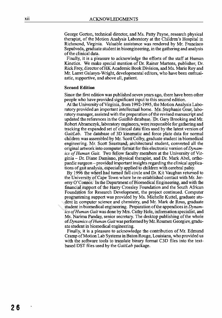
George Gorton, technical director, and Ms. Patty Payne, research physical therapist, of the Motion Analysis Laboratory at the Children's Hospital in Richmond, Virginia. Valuable assistance was rendered by Mr. Francisco Sepulveda, graduate student in bioengineering, in the gathering and analysis of the clinical data.

Finally, it is a pleasure to acknowledge the efforts of the staff at Human Kinetics. We make special mention of Dr. Rainer Martens, publisher, Dr. Rick Frey, director ofHK Academic Book Division, and Ms. Marie Roy and Mr. Larret Galasyn-Wright, developmental editors, who have been enthusi-astic, supportive, and above all, patient. .

Second Edition

Since the first edition was published seven years ago, there have been other people who have provided significant input to this second edition.

At the University of Virginia, from 1992-1995, the Motion Analysis Labo­ratory provided an important intellectual home. Ms. Stephanie Goar, labo­ratory manager, assisted with the preparation of the revised manuscript and updated the references in the GaitBib database. Dr. Gary Brooking and Mr. Robert Abramczyk, laboratory engineers, were responsible for gathering and tracking the expanded set of clinical data files used by the latest version of GaitLab. The database of 3D kinematic and force plate data for normal children was assembled by Mr. Scott Colby, graduate student in biomedical engineering. Mr. Scott Seastrand, architectural student, converted all the original artwork into computer format for this electronic version of Dynam­ics of Human Gait. Two fellow faculty members at the University of Vir­ginia - Dr. Diane Damiano, physical therapist, and Dr. Mark Abel, ortho­paedic surgeon - provided important insights regarding the clinical applica­tions of gait analysis, especially applied to children with cerebral palsy.

By 1996 the wheel had turned full circle and Dr. Kit Vaughan returned to the University of Cape Town where he re-established contact with Mr. Jer­emy O'Connor. In the Department of Biomedical Engineering, and with the financial support of the Harry Crossley Foundation and the South African Foundation for Research Development, the project continued. Computer programming support was provided by Ms. Michelle Kuttel, graduate stu­dent in computer science and chemistry, and Mr. Mark de Reus, graduate student in biomedical engineering. Preparation of the appendices in Dynam­ics of Human Gait was done by Mrs. Cathy Hole, information specialist, and Ms. Narima Panday, senior secretary. The desktop publishing ofthe whole of Dynamics of Human Gait was performed by Mr. Roumen Georgiev, gradu­ate student in biomedical engineering.

Finally, it is a pleasure to acknowledge the contribution of Mr. Edmund Cramp of Motion Lab Systems in Baton Rouge, Louisiana, who provided us with the software tools to translate binary format C3D files into the text­based DST files used by the GaitLab package.

CHAPTER!

Figure1.1 A homun­culus controls the dorsiflexors and plantar flexors of the ankle, and thus determines the pathway of the knee. Note. From Human Walking (p. 11) by V. T. Inman, R.J. Ralston, and F. Todd, 1981, Baltimore: Williams & Wilkins. Copyright 1981 by Williams & Wilkins. Reprinted by permission.

In Search of the Homunculus

Homunculus: An exceedingly minute body that according to medical scientists of the 16th and 17th centuries, was contained in a sex cell and whose preformed structure formed the basis for the human body.

Stedman's Medical Dictionary

When we think about the way in which the human body walks, the analogy of a marionette springs to mind. Perhaps the puppeteer who pulls the strings and controls our movements is a homunculus, a supreme commander of our locomo­tor program. Figure 1.1, reprinted from Inman, Ralston, and Todd (1981), illus­trates this point in a rather humorous but revealing way. Though it seems simplis­tic, we can build on this idea and create a structural framework or model that will help us to understand the way gait analysis should be performed.

27

2 DYNAMICS OF HUMAN GAIT

Top-Down Analysis of Gait Dynamics of Human Gait takes a lop-down approach to the description of human gait. The process that we are most interested in starts as a nerve impulse in the central nervous system and ends with the generation of ground reaction forces. The key feature of this approach is that it is based on cause and effect.

Sequence of Gait-Related Processes

figure 1.2 The seven components that form the functional basis for the way in which we walk. This top-down approach constitutes a cause-and-efft:cI model.

28

We need to recognise that locomotor programming occurs in supraspinal centres and involves the conversion of an idea into the pattern of muscle activity that is necessary for walking (Enoka, 1988). The neural output that results from this supraspinal programming may be thought of as a central locomotor command being transmitted to the brainstem and spinal cord. The execution of this command involves t\Vo components:

1. Activation of the lower neural centres, which subsequently establish the sequence of muscle activation patterns

2. Sensory feedback from muscles, joints, and other receptors that modifies the movements

This interaction between the central nervous system, peripheral nervous system, and musculoskeletal effector system is illustrated in Figure 1.2 (Jacobsen & Webster, 1977). For the sake of clClrity, the feedback loops have not been included in this figure. The muscles, when activated, develop tension, which in tum generates forces at, and moments across, the synovial joints.

Central nervous system

2 Peripheral nervous system

Synovial joint

Rigid link segment 5

Extemal 'o'ces 7 /

Figure 1.3 The sequence of seven events that lead to walking. No/e. This illustrdtion of a hemiplegic cerebral palsy child hlls been adapted from Gait Disorders In Childhood alld Adolescence (p. 130) by D.H. Sutherland, 1984, Baltimore: Williams & Wilkins. Copyright 1984 by Williams & Wilkins. Adapted by pennission.

fN SEARCH OF THE HOMUNCULUS 3

The joint forces and moments cause the rigid skeletal links (segments such as the tbigh, calf, foot, etc.) to move and to exert forces on the external env ironmen t.

The sequence of events that must take place for walking to occur may be summarized as follows:

1. Registration and activation of the gait conunand in the central nervous system

2. Transmission of the gait signals to the peripheral nervous system 3. Contraction of muscles that develop tension 4. Generation of forces at, and moments across, synovial joints 5. Regulationofthejoint forces and moments by the rigid skeletal segments

based on their anthropometry 6. Displacement (i.e., movement) of the segments in a manner that is recog­

nized as functional gait 7. Generation of ground reaction forces

TIlese seven links in the chain of events that result in the pattern of movement we readily recognize as human walking are illustrated in Figure 1.3.

2

3

Clinical Usefulness of the Top-Down Approach

TIle model may also be used to help us

• understand pathology • determine methods of treatment, and • decide on which methods we should llse to study patient's gait.

For example, a patient's lesion could be at the level of the central nervous system (as in cerebral palsy), in the peripheral nervous system (as in Charcot­Marie-Tooth disease), at the muscular level (as in muscular dystrophy), or in the synovial joint (as in rheumatoid arthritis). The higher the lesion, the more profound the impact on all the components lower down in the movement chain. Depending on the indications, treatment could be applied at any ofthe different levels. In the case of a "high" lesion, such as cerebral palsy, this could mean rhizotomy at tbe central nervous system level, neurectomy at the

29

30

4 DYNAMICS OF HUMAN GAIT

peripheral nervous system level, tenotomy at the muscular level, or osteotomy at the joint level. In assessing this patient's gait, we may choose to study the muscular activity, the anthropometry of the rigid link segments, the move­ments of the segments, and the ground reaction forces.

Measurements and the Inverse Approach

Figure 1.4 The inverse approach in rigid body dynamics expressed in words.

Measurements should be taken as high up in the movement chain as possible, so that the gait analyst approaches the causes of the walking pattern, not just the effects. As pointed out by Vaughan, Hay, and Andrews (1982), there are essentially two types of problems in rigid body dynamics. The ftrst is the Direct Dynamics Problem in which the forces being applied (by the homuncu­lus) to a mechanical system are known and the objective is to determine the motion that results. The second is the Inverse Dynamics Problem in which the motion of the mechanical system is defmed in precise detail and the objective is to determine the forces causing that motion. This is the approach that the gait analyst pursues. Perhaps it is now clear why the title of this ftrst chapter is "In Search ofthe Homunculus"!

The direct measurement of the forces and moments transmitted by human joints, the tension in muscle groups, and the activation of the peripheral and central nervous systems is fraught with methodological problems. That is why we in gait analysis have adopted the indirect or inverse approach. This approach is illustrated verbally in Figure 1.4 and mathematically in Figure 1.5. Note that four of the components in the movement chain - 3, electromyo­graphy; 5, anthropometry; 6, displacement of segments; and 7, ground reac­tion forces - may be readily measured by the gait analyst. These have been highlighted by slightly thicker outlines in Figure 1.4. Strictly speaking, elec­tromyography does not measure the tension in muscles, but it can give us insight into muscle activation patterns. As seen in Figure 1.5, segment an­thropometry As may be used to generate the segment masses ms, whereas segment displacements Ps may be double differentiated to yield accelerations as. Ground reaction forces F G are used with the segment masses and accelera­tions in the equations of motion which are solved in tum to give resultant joint forces and moments FJ•

Electromyography

3

5 6

4

Ground reaction forces

7

Figure 1.5 The inverse approach in rigid body dynamics expressed in mathematical symbols.

Figure 1.6 The struc­ture of the data (circles) and programs (rect­angles) used in part of GaitLab. Note the similarity in format between this figure and Figures 1.2 to 1.5.

IN SEARCH OF THE HOMUNCULUS 5

5 6 7

Many gait laboratories and analysts measure one or two of these compo­nents. Some measure all four. However, as seen in Figures 1.2 to 1.5, the key to understanding the way in which human beings walk is integration. This means that we should always strive to integrate the different components to help us gain a deeper insight into the observed gait. Good science should be aimed at emphasizing and explaining underlying causes, rather than merely observing output phenomena - the effects - in some vague and unstruc­tured manner.

Whereas Figures 1.4 and 1.5 show how the different measurements ofhu­man gait may be theoretically integrated, Figure 1.6 illustrates how we have implemented this concept in GaitLab. The four data structures on the left­electromyography (EMG), anthropometry (APM), segment kinematics (KIN), and ground reaction data from force plates (FPL) - are all based on direct measurements of the human subject. The other parameters - body segment parameters (BSP), joint positions and segment endpoints (JNT), reference frames defming segment orientations (REF), centres of gravity, their veloci-

5 6 7

31

6

Summary

32

DYNAMICS OF HUMAN GAIT

ties and accelerations (COG), joint angles as well as segment angularveloci­ties and accelerations (ANG), dynamic forces and moments at joints (DYN) - are all derived in the Process routine in GaitLab. All 10 data structures maybe viewed and (where appropriate) graphed in the Plot routine in GaitLab. The key, as emphasised earlier, is integration. Further details on running these routines are contained in the GaiteD instruction booklet.

This first chapter has given you a framework for understanding how the hu­man body moves. Although the emphasis has been on human gait, the model can be applied in a general way to all types of movement. In the next chapter we introduce you to the basics of human gait, describing its cyclic nature and how we use this periodicity in gait analysis.

CHAPTER 2

Figure 2.1 The refer­ence planes of the human body in the standard anatomical position. Note. From Human Walking (p. 34) by V. T. Inman, H.I. Ralston, and F. Todd, 1981, Baltimore: Williams & Wilkins. Copyright 1981 by Williams & Wilkins. Adapted by permission.

The Three­Dimensional and Cyclic Nature of Gait

Most textbooks on anatomy have a diagram, similar to Figure 2.1, that ex­plains the three primary planes of the hwnan body: sagittal, coronal (or fron­tal), and transverse. Unfortunately, many textbook authors (e.g., Winter, 1987) and researchers emphasize the sagittal plane and ignore the other two. Thus, the three-dimensional nature of human gait has often been overlooked. Al­though the sagittal plane is probably the most important one, where much of the movement takes place (see Figure 2.2, a), there are certain pathologies where another plane (e.g., the coronal, in the case of bilateral hip pain) would yield useful information (see Figure 2.2, a-c).

Other textbook authors (Inman et al., 1981; Sutherland, 1984;Sutherland, Olshen, Biden, & Wyatt, 1988) have considered the three-dimensional nature of human gait, but they have looked at the human walker from two or three separate

Transverse plane

Frontal Plane Sagittal plane

7

33

34

8 DYNAMICS OF HUMAN GAIT

Figure 2.2 The gait of an 8-year-old boy as seen in the three principal planes: (a) b sagittal; (b) transverse; and (c) frontal.

Figure 2.3 The walking subject projected onto the three principal planes of movement. Note. From Ruman Walking (p. 33) by V.T. Inman, R.J. Ralston, and F. Todd, 1981, Baltimore: Williams & Wilkins. Copyright 1981 by Williams & Wilkins. Adapted by permission.

a c

views (see Figure 2.3). Though this is clearly an improvement, we believe that the analysis of human gait should be truly three-dimensional: The three separate projections should be combined into a composite image, and the parameters expressed in a body-based rather than laboratory-based coordinate system. This important concept is described further in chapter 3.

z

Periodicity of Gait The act of walking has two basic requisites:

1. Periodic movement of each foot from one position of support to the next 2. Sufficient ground reaction forces, applied through the feet, to support the

body

These two elements are necessary for any form of bipedal walking to occur, no matter how distorted the pattern may be by underlying pathology (Inman et al., 1981). This periodic leg movement is the essence of the cyclic nature of human gait

Figure 2.4 illustrates the movement of a wheel from left to right. In the position at which we first see the wheel, the highlighted spoke points vertically down. (The

Figure 2.4 A rotating wheel demonstrates the cyclic nature of forward progression.

Gait Cycle

Figure 2.5 The nonnal gait cycle of an 8-year­old boy.

THE THREE DIMENSIONAL & CYCLIC NATURE OF GAIT 9

wheel is not stationary here; a "snapshot" has been taken as the spoke passes through the vertical position.) By convention, the beginning of the cycle is referred to as 0%. As the wheel continues to move from left to right, the highlighted spoke rotates in a clockwise direction. At 20% it has rotated through 72° (20% x 360°), and for each additional 20%, it advances another 72°. When the spoke returns to its original position (pointing vertically downward), the cycle is complete (this is indicated by 100%).

CUO()OQCU 0% 20% 40% 60% 80% 100%

This analogy of a wheel can be applied to human gait. When we think of someone walking, we picture a cyclic pattern of movement that is repeated over and over, step after step. Descriptions of walking are normally confmed to a single cycle, with the assumption that successive cycles are all about the same. Although this assumption is not strictly true, it is a reasonable approxi­mation for most people. Figure 2.5 illustrates a single cycle for a normal 8-year-old boy. Note that by convention, the cycle begins when one of the feet (in this case the right foot) makes contact with the ground.

1-------- Stance phase --------11-- Swing phase ----1 ~ First double + Single limb stance + Second double -4

support support

Initial Loading Mid Terminal Preswing Initial Midswing Terminal contact response stance stance swing swing

Phases. There are two main phases in the gait cycle: During stance phase, the foot is on the ground, whereas in swing phase that same foot is no longer in contact with the ground and the leg is swinging through in preparation for the next foot strike.

As seen in Figure 2.5, the stance phase may be subdivided into three sepa­rate phases:

1. First double support, when both feet are in contact with the ground 2. Single limb stance, when the left foot is swinging through and only the right

foot is in ground contact

35

36

10

Figure 2.6 The time spend on each limb during the gait cycle of a normal man and two patients with unilateral hip pain. Note. Adapted from Murray & Gore (1981).

DYNAMICS OF HUMAN GAIT

3. Second double support, when both feet are again in ground contact

Note that though the nomenclature in Figure 2.5 refers to the right side of the body, the same terminology would be applied to the left side, which for a normal person is half a cycle behind (or ahead of) the right side. Thus, first double support for the right side is second double support for the left side, and vice versa. In normal gait there is a natural symmetry between the left and right sides, but in pathological gait an asymmetrical pattern very often exists. This is graphically illustrated in Figure 2.6. Notice the symmetry in the gait of the normal subject between right and left sides in the stance (62%) and swing (38%) phases; the asymmetry in those phases in the gaits of the two patients, who spend less time bearing weight on their involved (painful) sides; and the increased cycle time for the two patients compared to that of the normal subject.

Normal man Left

_38%_62%_ ~~?%~38%~ Right

~ Stance

c=J Swing

Patient with avascular necrosis, left hip Painful limb

~~~r':~42%~ _31%_~~%_ Sound limb

Patient with osteoarthritis, left hip Painful limb

_60%~40%~ _20%_80%_

Sound limb

o 0.2 0.4 0.6 0.8 1.0 1.2 1.4 1.6 1.8 2.0

Time(s)

Events. Traditionally the gait cycle has been divided into eight events or periods, five during stance phase and three during swing. The names of these events are self-descriptive and are based on the movement of the foot, as seen in Figure 2.7. In the traditional nomenclature, the stance phase events are as follows:

1. Heel strike initiates the gait cycle and represents the point at which the body's centre of gravity is at its lowest position.

2. Foot-flat is the time when the plantar surface of the foot touches the ground. 3. Midstance occurs when the swinging (contralateral) foot passes the stance

foot and the body's centre of gravity is at its highest position. 4. Heel-off occurs as the heel loses contact with the ground and pushoff is

initiated via the triceps surae muscles, which plantar flex the ankle. 5. Toe-off terminates the stance phase as the foot leaves the ground

(Cochran, 1982).

The swing phase events are as follows:

6. Acceleration begins as soon as the foot leaves the ground and the subject activates the hip flexor muscles to accelerate the leg forward.

7. Midswing occurs when the foot passes directly beneath the

Figure 2.7 The tradi­tional nomenclature for describing eight main events, emphasising the cyclic nature of human gait.

THE THREE DIMENSIONAL & CYCLIC NATURE OF GAIT II

body, coincidental with midstance for the other foot. 8. Deceleration describes the action of the muscles as they slow the leg and

stabilize the foot in preparation for the next heel strike.

De~e~ion f£:[t Midswing jf-/ .

SWIng phase

( 40%

l (

iL~~e,strike \( \' ~oot-ftat

Stance phase 60%

\

~ v / / ( ( ~idstance AcrelerntiOn'l ~ /ii

"--- v ~I-Off Toe-off

The traditional nomenclature best describes the gait of normal subjects. How­ever, there are a number of patients with pathologies, such as ankle equinus sec­ondary to spastic cerebral palsy, whose gait cannot be described using this ap­proach. An alternative nomenclature, developed by Perry and her associates at Rancho Los Amigos Hospital in California (Cochran, 1982), is shown in the lower part of Figure 2.5. Here, too, there are eight events, but these are sufficiently general to be applied to any type of gait:

1. Initialcontact(O%) 2. Loading response (0-10%) 3. Midstance (10-30%) 4. Terminal stance (30-50%) 5. Preswing (50-60%) 6. Initial Swing (60-70%) 7. Midswing(70-85%) 8. Terminal swing (85-100%)

Distance Measures. Whereas Figures 2.5 to 2.7 emphasise the temporal as­pects of human gait, Figure 2.8 illustrates how a set offootprints can provide useful distance parameters. Stride length is the distance travelled by a person during one stride (or cycle) and can be measured as the length between the heels from one heel strike to

37

38

12 DYNAMICS OF HUMAN GAIT

1---- Left step length ---+--- Right step length ----I

Figure 2.8 A person's footprints can very often -----....-:::-c-----,-..,...,-----1

provide useful distance parameters.

1----------- Stride length ---------1

the next heel strike on the same side. Two step lengths (left plus right) make one stride length. With nonnal subjects, the two step lengths (left plus right) make one stride length. With normal subjects, the two step lengths will be approximately equal, but with certain patients (such as those illustrated in Figure 2.6), there will be an asymmetry between the left and right sides. Another useful parameter shown in Figure 2.8 is step width, which is the mediolateral distance between the feet and has a value of a few centimetres for normal subjects. For patients with balance problems, such as cerebellar ataxia or the athetoid form of cerebral palsy, the stride width can increase to as much as 15 or 20 cm (see the case study in chapter 5). Finally, the angle of the foot relative to the line of progression can also provide useful information, documenting the degree of external or internal rotation of the lower extremity during the stance phase.

Parameters of Gait The cyclic nature of human gait is a very useful feature for reporting different parameters. As you will later discover in GaitLab, there are literally hundreds of parameters that can be expressed in terms of the percent cycle. We have chosen just a few examples (displacement, ground reaction force, and muscle activity) to illustrate this point.

Displacement

Figure 2.9 The height (value in the Z direction) in metres (m) of a normal male's right malleolus as a function of the gait cycle.

Figure 2.9 shows the position of a normal male's right lateral malleolus in the Z (vertical) direction as a function of the cycle. At heel strike, the height is about 0.07 m, and it stays there for the next 40% ofthe cycle because the foot is in contact with the ground.

Normal adult male Marker Right Lateral Malleolus (m)

0.25 ,--------;-----=---,--------,---------,--'----'---_

0.20

0.15

0.10

N 0.05

0.00 '---------'----------"----------'----'------~ o 20 40 60

% Gait Cycle 80 100

THE THREE DIMENSIONAL & CYCLIC NATURE OF GAIT 13

Then, as the heel leaves the ground, the malleolus height increases steadily until right toe-off at about 60%, when its height is 0.17 m. After toe-off, the knee continues to flex, and the ankle reaches a maximum height of 0.22 m at 70% of the cycle. Thereafter, the height decreases steadily as the knee extends in preparation for the following right heel strike at 100%. This pattern will be repeated over and over, cycle after cycle, as long as the subject continues to walk on level ground.

Ground Reaction Force

Figure 2.10 The vertical ground reaction force in newtons (N) acting on a cerebral palsy adult's right foot during the gait cycle.

Muscle Activity

Figure 2.10 shows the vertical ground reaction force of a cerebral palsy adult (whose case is studied in detail in chapter 5) as a function of the gait cycle. Shortly after right heel strike, the force rises to a value over 800 newtons (N) (compared to his weight of about 700 N). By midswing this value has dropped to 400 N, which is a manifestation of his lurching manner of walking. By the beginning of the second double support phase (indicated by LHS, or left heel strike), the vertical force is back up to the level of his body weight. Thereaf­ter it decreases to zero when right toe-off occurs. During the swing phase from right toe-off to right heel strike, the force obviously remains at zero. This ground reaction force pattern is quite similar to that of a normal person except for the exaggerated drop during midstance.

Cerebral palsy adult male

1000 ,-----.-----.------~----~----

800

600

400

200

o

-200 '---------'----------'--------'-----------'-----o 20 40 60

% Gait Cycle 80 100

Muscle activity, too, can be plotted as a function of percent cycle as seen in Figure 2.11. Here the EMG of the rectus femoris for a normal female is illustrated. Notice that just after right heel strike, the EMG increases. Be­cause the rectus femoris is a hip flexor and knee extensor, but the hip and knee are extending and flexing at this time, the muscle is acting eccentrically. Dur­ing the midstance phase, the activity decreases substantially, picking up again during late stance and early swing. During this period, both the hip and knee are flexing. The rectus femoris is again reasonably quiescent in midswing, but its activity increases before the second right heel strike.

39

40

14

Figure 2.11 The electromyographic activity in microvolts (~V) of a nonnal female's right rectus femoris muscle plotted as a function of the gait cycle.

Summary

DYNAMICS OF HUMAN GAIT

Normal adult female

EMG Right Rectus Femoris (uV) 80~--

60 -----------.---!-~-- - ----------t-- --------f- ----------------!---

20 -----\: / --------~

/

-J~----------'---------------- L._---_---_---_~-_---_-_--_---_---_---~'--_--~

o 20 40 60 % Gait Cycle

80 100

Figure 2.11 provides some insight into the actions of a single muscle, but literally hundreds of muscles are active during the gait cycle. The challenge facing the central nervous system is to control simultaneously the actions of all these muscles. This is addressed further in chapter 4. Before that, however, chapter 3 teaches you how to integrate anthropometric, kinematic, and force plate data.

CHAPTER 3

Integration of Anthropometry, Displacements, and Ground Reaction Forces

In chapter 1 you learned that the gait analyst must pursue the inverse dynam­ics approach in which the motion of the mechanical system is completely speci­fied and the objective is to find the forces causing that motion. This approach is illustrated in words in Figure 1.4 and in mathematical symbols in Figure 1.5. In chapter 2 you were introduced to the three-dimensional nature of human gait. You also learned that gait is a cyclic activity and that many variables­such as displacement, ground reaction forces, and muscle activity - can be plotted as a function of the cycle. In this chapter we will show how all these measurements may be integrated to yield the resultant forces and moments acting at the joints of the lower extremities.

This chapter covers five different topics. In Body Segment Parameters, you will learn how simple anthropometric measurements, such as total body mass and calflength, can be used in regression equations to predict the masses and moments of inertia of lower extremity segments. In Linear Kinematics we show how the position of external markers attached to the skin may be used to predict the position of internal landmarks such as the joint centres. In Centres of Gravity, the joint centres are used to predict the positions of the segment centres of gravity; then, using numerical differentiation, the veloci­ties and accelerations ofthese positions are obtained. In Angular Kinematics, the anatomical joint angles are calculated, as are the angular velocities and accelerations of the segments. Finally, in Dynamics of Joints, the body seg­ment parameters, linear kinematics, centres of gravity, angular kinematics, and ground reaction forces are all integrated in the equations of motion (see Figures 1.4 and 1.5) to yield the resultant joint forces and moments.

Be aware that because we are dealing with gait analysis as a three-dimen­sional phenomenon, some of the concepts and mathematics are quite com­plex. However, our intent is that the material in this chapter be accessible to all persons who have passed a basic undergraduate course in mathematics.

15

41

42

16 DYNAMICS OF HUMAN GAIT

The challenge will be thinking in 3-D even though the diagrams are obviously plotted on a flat, 2-D page. If you need a bigger challenge, a detailed and rigorous coverage ofthe material is presented in Appendix B.

Body Segment Parameters A major concern for the gait analyst is personalising the body segment param­eters ofthe individual subject. By body segment parameters we mean

e mass in kilograms ofthe individual segments (e.g., thigh, calf, foot); e centre of gravity location of the individual segments relative to some

specified anatomical landmarks (e.g., proximal and distaljoints); and e moments of inertia of the segments about three orthogonal axes (i.e.,

axes at right angles to one another) that pass through the segment centre of gravity.

Moment of inertia is a measure of the way in which the mass is distributed about the axis of interest and has the units ofkilogramemetreemetre (kgem2

).

It therefore varies with mass and the square oflength.

Selection of Segments

Another concern is the selection of individual segments. As you will see a little later in the chapter, we have chosen six segments: thigh, calf, and foot on both the left and right sides. We are making the assumption that these are rigid segments whose dimensions (and thus their segment parameters) do not change during the motion of interest. We all know, however, that the foot is not a single rigid segment and so you should be aware that any model has some limitations. We chose a 6-segment model for simplicity (and because virtually all gait laboratories do the same), but it is possible that in the future, biomechanical models will need to be more detailed.

Problems in Estimation

In attempting to estimate the body segment parameters for an individual sub­ject, there are various approaches that can be followed. These include

e cadaver averages (Braune & Fischer, 1889; Dempster, 1955); e reaction board (Bernstein, 1967); e mathematical modelling (Hanavan, 1964; Hatze, 1980); e scans using gamma rays, axial tomography, or magnetic resonance imag­

ing (Brooks & Jacobs, 1975; Erdmann, 1989; Zatsiorsky & Seluyanov, 1985); and

e kinematic measurements (Ackland, Blanksby, & Bloomfield, 1988; Dainis, 1980; Vaughan, Andrews, & Hay, 1982).

Each of these has severe limitations. The cadaver averages are not suffi­ciently specific for individual subjects and very often only total body mass is used as a predictive variable. The reaction board technique is a long and tedious procedure which cannot estimate segment masses and centres of gravity independently. Mathematical modelling suffers from the disadvantage that too many variables (242 in the case ofHatze's model) need to be measured, thus requiring an inordinate amount of time and patience. Scanning techniques, though potentially very accurate and detailed, must be seriously questioned as a routine method because of the radiation exposure and high costs. Although they have some appeal, kinematic measurements either have not yielded re-

ANTHROPOMETRY, DISPLACEMENTS, & GROUND REACTION FORCES 17

Anthropometry

Figure 3.1 The anthro­pometric measurements of the lower extremity that are required for the prediction of body segment parameters (masses and moments of inertia).

suIts to a satisfactory degree of accuracy or require too much time (Jensen, 1986).

What is needed for estimating body segment parameters is a technique with the following features:

• Personalised for individuals • Short time required to take measurements • Inexpensive and safe • Reasonably accurate

We can describe a technique that we believe meets these criteria. Not surpris­ingly, it is based on anthropometry. Figure 3.1 illustrates the measurements that need to be made, Table 3.1 describes, in anatomical terminology, how the parameters are measured, and Table 3.2 shows the data for a normal man. (In fact, Table 3.2 contains the data for the Man.DST file used in GaitLab.)

/ Thigh length

/ Calf length

/

Maileolusl height

ASIS breadth

Midthigh circumference

Knee diameter

-----=:::::: Foot length

There are 20 measurements that need to be taken - 9 for each side of the body, plus the subject's total body mass, and the distance between the anterior superior iliac spines (ASIS). With experience, these measurements can be made in less than 10 minutes using standard tape measures and beam calipers, which are readily available. They describe, in some detail, the characteristics ofthe subject's lower extremities. The question to be answered in this: Can they be used to predict body segment parameters that are specific to the indi­vidual subject and reasonably accurate? We believe the answer is "yes".

As mentioned earlier, most of the regression equations based on cadaver data use only total body mass to predict individual segment masses. Although this will obviously provide a reasonable estimate as a first approximation, it does not take into account the variation in the shape of the individual seg­ments.

44

18 DYNAMICS OF HUMAN GAIT

Table 3.1 Description of Anthropometric Parameters and How to Measure Them

Parameter Description

Body mass Measure (on a scale accurate to 0.01 kg) the mass of subject with all clothes except underwear removed

ASIS breadth With a beam caliper, measure the horizontal distance between the anterior superior iliac spines

Thigh length With a beam caliper, measure the vertical distance between the superior point of the greater trochanter of the femur and the superior margin of the lateral tibia

Midthigh circumference With a tape perpendicular to the long axis of the leg and at a level midway between the trochanteric and tibial landmarks, measure the circumference of the thigh

Calf length With a sliding caliper, measure the vertical distance between the superior margin of the lateral tibia and the lateral malleo Ius

Calf circumference With a tape perpendicular to the long axis of the lower leg, measure the maximum circumference of the calf

Knee diameter With a spreading caliper, measure the maximum breadth of the knee across the femoral epicondyles

Foot length With a beam caliper, measure the distance from the posterior margin of the heel to the tip of the longest toe

Malleolus height With the subject standing, use a sliding caliper to measure the vertical distance from the standing surface to the lateral malleolus

Malleolus width With a sliding caliper, measure the maximum distance between the medial and lateral malleoli

Foot breadth With a beam caliper, measure the breadth across the distal ends of metatarsals I and V

Note. Adapted from Chandler et al. (1975).

Prediction of Segment Mass

We believe that individual segment masses are related not only to the subject's total body mass, but also to the dimensions of the segment of interest. Spe­cifically, because mass is equal to density times volume, the segment mass should be related to a composite parameter which has the dimensions oflength cubed and depends on the volume ofthe segment. Expressed mathematically, we are seeking a mUltiple linear regression equation for predicting segment mass which has the form

Segment mass = CI(Total body mass) + C2 (Length)3+ C3 (3.1)

where CI, C2, and C3 are regression coefficients. For our purposes, the shapes of the thigh and calf are represented by cylinders, and the shape of the foot is similar to a right pyramid. (Though a truncated cone may provide a better approximation of the thigh and calf, it requires an extra anthropometric measurement for each segment and yields only a marginal improvement in accuracy.)

(Density) Mass of cylinder = ----(Length) (CircumferenceY (3.2)

41t

ANTHROPOMETRY, DISPLACEMENTS, & GROUND REACTION FORCES 19

Figure 3.2 Lower extremity body segments and their geometric counterparts: (a) thigh; (b) calf; (c) foot.

Mass of pyramid = _1 (Density) (Width) (Height) (Length) (3.3) 3

Table 3.2 Anthropometric Data Required to Predict Body Segment Parameters for a Normal Male

Number Anthropometric measurement Value Units

1 Total body mass 64.90 kg 2 ASIS breadth 0.240 m 3 R. Thigh length 0.460 m 4 L. Thigh length 0.465 m 5 R. Midthigh circumference 0.450 m 6 L. Midthigh circumference 0.440 m 7 R. Calf length 0.430 m 8 L. Calf length 0.430 m 9 R. Calf circumference 0.365 m

10 L. Calf circumference 0.365 m 11 R. Knee diameter 0.108 m 12 L. Knee diameter 0.112 m 13 R. Foot length 0.260 m 14 L. Foot length 0.260 m 15 R. Malleolus height 0.060 m 16 L. Malleolus height 0.060 m 17 R. Malleolus width 0.074 m 18 L. Malleolus width 0.073 m 19 R. Foot breadth 0.098 m 20 L. Foot breadth 0.096 m

Figure 3.2, a-c, illustrates the three anatomical segments and their geomet­ric counterparts.

,-

a b

We assume the segment density among subjects to be invariant and then use the linear dimensions as predictors of the segment masses. We based our regression equations on six cadavers studied by Chandler, Clauser, McConville, Reynolds, and Young (1975). Although we would ideally prefer to have had more cadavers, these are the only data in the literature that are so complete. This applies not only to the anthropometric measurements (Tables 3.1 and 3.2) but also to the principal centroidal moments of inertia which are de­scribed in great detail. Based on these data in Chandler et al. (1975), we have performed multiple linear regression to yield the following equations:

46

20 DYNAMICS OF HUMAN GAIT

Mass ofthigh = (0.1032)(Total body mass) + (12. 76)(Thigh length)(Midthigh circumference)2 +(-1.023) (3.4)

Mass of calf = (0.0226)(Total body mass) + (31.33)(Calflength)(Calf circumference)2 + (0.016) (3.5)

Mass of foot = (0.0083)(Total body mass) + (254.5)(Malleolus width)(Malleolus height) (Foot length) + (-0.065) (3.6)

Using the data in Table 3.2 (Total body mass = 64.90 kg; Right ca1flength = 0.430 m; Right calf circumference = 0.365 m), Equation 3.5 yields

Mass of right calf = (0.0226)(64.90) + (31.33)(0.430)(0.365)2+0.016

= 3.28 kg

Further details on the statistical basis for these regression equations to predict mass may be found in Appendix B.

Prediction of Segment Moments of Inertia

As mentioned previously, the moment of inertia, which is a measure ofa body's resistance to angular motion, has units ofkgm2. It seems likely therefore that the moment of inertia would be related to body mass (kilogram) times a com­posite parameter which has the dimensions oflength squared (m2). Expressed mathematically, we are seeking a linear regression equation for predicting segment moment of inertia which has the form

Segment moment of inertia = C4(Total body mass)(Length)2 + C5 (3.7)

where C4 and C5 are regression coefficients. The key is to recognise that the (Length)2 parameter is based on the moment of inertia of a similarly shaped, geometric solid. A similar approach has been proposed by Yeadon and Morlock (1989). As before, the thigh and calf are similar to a cylinder and the foot is approximated by a right pyramid. Figure 3.3 shows the principal orthogonal axes for the thigh and a cylinder.

Using the mathematical definition of moment of inertia and standard calcu­lus, the following relationships can be derived:

Moment of inertia of cylinder about flexion/extension axis = 1 .

- (Mass) [(Length)2+ 0.076 (Crrcumference)2] (3.8) 12

Moment of inertia of cylinder about the abduction/adduction axis = 1

- (Mass) [(Length)2+ 0.076 (Circumference)2] (3.9) 12

ANTHROPOMETRY, DISPLACEMENTS, & GROUND REACTION FORCES 21

Figure 3.3 Principal orthogonal axes for trhe thigh and a right cylinder.

Moment of inertia of cylinder about the intemaIJextemal rotation axis =

_1_ (Mass) (Circumference)2 (3.10) 81t2

FIx/Ext

Abd/Add

..... ---- ....

InUExt InUExt

When studying these three equations, you will notice the following: Equa­tions 3.8 and 3.9 are the same, which comes from the radial symmetry of a cylinder; all three equations have the units of kgem2; the moment of inertia about the intemaIJextemal rotation axis (Equation 3.10) depends only on mass and circumference (squared) and not on the length of the cylinder. As can be seen from Equation 3.7, each of the equations provides two regression coef­ficients. There are three regression equations per segment (Equations 3.8, 3.9, and 3.10 are the examples for the thigh), and there are three separate segments - thigh, calf, and foot. This means that the regression analysis of the Chandler data will yield 2 x 3 x 3 = 18 regression coefficients. All of these are provided in Appendix B, but for the purpose of this chapter, we show one regression equation for the thigh:

Moment of inertia of thigh about the flexion/extension axis=

(0.00762)(Total body mass) x

[(Thigh lengthY + 0.076 (Midthigh circumference)2] + 0.0115 (3.11)

Again, using the data in Table 3.2 (Total body mass = 64.90 kg; Right thigh length = 0.460 m; Right midthigh circumference = 0.450 m) in the previous equation, we get

Moment of inertia of right thigh about the flexion/extension axis =

(0.00762)(64.90) x [(0.460)2 + 0.076(0.450)2] + 0.0115 = 0.1238 kgem2

(3.12)

Table 3.3, which contains the data for the Man.DST file generated in GaitLab, provides all the body segment parameters that are required for de-

47

48

22 DYNAMICS OF HUMAN GAIT

tailed 3-D gait analysis of the lower extremities. In addition to the body segment masses and moments of inertia already discussed in this section, no­tice that there are also segment centre-of-mass data. These are expressed as ratios and are based on knowing the segment endpoints for the thigh, calf, and foot. These points are between the hip and knee joints, the knee and ankle joints, and the heel and longest toe, respectively. The ratios in Table 3.3 are the means ofthe ratios in Chandler et al. (1975).

Table 3.3 Body Segment Parameter Data for Lower Extremities of a Normal Male

Segment number I 2 3 4 5 6 Segment name R. Thigh L. Thigh R. Calf L. Calf R. Foot L. Foot

Mass 6.86 6.82 3.28 3.28 0.77 0.76 CG position 0.39 0.39 0.42 0.42 0.44 0.44 (ratio proximal/distal length) Moments of inertia(kgomom) FlxlExt axis 0.1238 0.1257 0.0490 0.0490 0.0035 0.0035 Abd/ Add axis 0.1188 0.1207 0.0504 0.0504 0.0040 0.0039 IntlExt axis 0.0229 0.0220 0.0037 0.0037 0.0011 0.0011

Note. The parameters were generated from the anthropometric data of Table 3.2 using regresion equations such as 3.4 to 3.6 and 3.11.

In summary then, Table 3.1 describes how the anthropometric measure­ments should be made, Table 3.2 is an example of the 20 parameters for a male subject, and Table 3.3 shows the body segment parameters (BSPs) that are derived using the regression equations and anthropometric measurements. We think you will agree that the BSPs have been personalised by means of linear measurements that do not require much time or expensive equipment. In Appendix B, we show that these equations are also reasonably accurate and can therefore be used with some confidence.

Though we believe that our BSPs are superior to other regression equa­tions that are not dimensionally consistent (e.g., Hinrichs, 1985), it is appro­priate to put this statement into the proper perspective. The moments of inertia are really only needed to calculate the resultant joint moments (see Equation 3.30 later in this chapter). Their contribution is relatively small, par­ticularly for the internal/external rotation axis. For example, in stance phase, the contributions from the inertial terms to joint moments are very small be­cause the velocity and acceleration oflimb segments are small.

Linear Kinematics As described in the previous section on anthropometry, each of the segments ofthe lower extremity (thigh, calf, and foot) may be considered as a separate entity. Modelling the human body as a series of interconnected rigid links is a standard biomechanical approach (Apkarian, Naumann, & Cairns, 1989; Cappozzo, 1984). When studying the movement of a segment in 3-D space we need to realise that it has six degrees offreedom. This simply means that it requires six independent coordinates to describe its position in 3-D space uniquely (Greenwood, 1965). You may think of these six as being three cartesian coordinates (X,Y, and Z) and three angles of rotation, often referred to as Euler angles. In order for the gait analyst to derive these six coordi­nates, he or she needs to measure the 3-D positions of at least three noncolinear markers on each segment. The question that now arises is this: Where on the

ANTHROPOMETRY, DISPLACEMENTS, & GROUND REACTION FORCES 23

Use of Markers

Figure 3.4 The 15-marker system that uniquely defines the position of each segment

lower extremities should these markers be placed? Ideally, we want the mini­mum number of markers placed on anatomical landmarks that can be reliably located, otherwise data capture becomes tedious and prone to errors.

Some systems, such as the commercially available OrthoTrak product from Motion Analysis Corporation (see Appendix C), use up to 25 markers. We feel this is too many markers, and the use of bulky triads on each thigh and calf severely encumbers the subject. Kadaba, Ramakrishnan, and Wootten (1990) of the Helen Hayes Hospital in upstate New York proposed a marker system that uses wands or sticks about 7 to 10 cm long attached to the thighs and calves. The advantage of this approach is that the markers are easier to track in 3-D space with video-based kinematic systems, and they can (at least theoretically) provide more accurate orientation of the segment in 3-D space.

L. ASIS

R. Femoral wand 6

z

10 L. Metatarsal head II

o R. Metatarsal L. Heel

headll~ X

8

in 3-D space: (a) a Global reference frame anterior view; (b) posterior view.

b

L. Femoral wand

L. Tibial wand

L. Metatarsal 8 head II

z

o

49

50

24

Figure 3.5 The 3-D coordinates of the right lateral malleolus plotted as a function of time. There are approximately one and a half gait cycles (i.e., from right heel strike beyond the next right heel strike) in this figure, as can be seen in the Z curve.

DYNAMICS OF HUMAN GAIT

The major disadvantage is that the wands encumber the subject, and ifhe or she has a jerky gait, the wands will vibrate and move relative to the underlying skeleton. In addition, Kadaba et al. (1990) only have two markers on the foot segment. After careful consideration we have adopted the 15 marker loca­tions illustrated in Figure 3.4, a and b. This is referred to as the Helen Hayes Hospital marker set in GaitLab.

Note the position of the XYZ global reference system in Figure 3.4 with its origin at one corner of Force Plate 1. The X, Y, and Z coordinates of these 15 markers as a function oftime may then be captured with standard equipment

Table 3.4 Three-Dimensional Displacement Data of External Landmarks at Time = 0.00 s (Right Heel Strike) of a Normal Male

Number Name X(m) Y(m) Z(m)

1 R. Metatarsal head V 0.157 0.142 0.057 2 R. Heel -0.016 0.207 0.032 3 R Lateral malleolus 0.033 0.155 0.067 4 R. Tibial tubercle 0.002 0.181 0.443 5 R. Femoral epicondyle -0.055 0.136 0.509 6 R. Greater trochanter -0.207 0.082 0.880 7 R. ASIS -0.161 0.141 0.979 8 L. Metatarsal head V -0.578 0.392 0.032 9 L. Heel -0.705 0.320 0.138 10 L. Lateral malleolus -0.648 0.374 0.128 11 L. Tibial tubercle -0.383 0.341 0.396 12 L. Femoral epicondyle -0.369 0.393 0.495 13 L. Greater trochanter -0.263 0.439 0.891 14 L. ASIS -0.174 0.386 0.976 15 Sacrum -0.369 0.242 0.962

Note. The XYZ positions refer to the global coordinate system defined in Figure 3.4, al­though the position of the subject in this figure is much later in the gait cycle (approaching right toe-oft).

Normal adult male

Marker Right Lateral

Malleolus (m)

Marker Right Lateral

Malleolus (m)

Marker Right Lateral

Malleolus (m)

x

N

0.3

~ ...•..••••• 0.2

0.1

0.0 0.0 0.4 0.8

Time (s) 1.2 1.6

ANTHROPOMETRY, DISPLACEMENTS, & GROUND REACTION FORCES 25

(described in Appendix C). The data in the DST files in GaitLab were gath­ered at the Oxford Orthopaedic Engineering Centre (OOEC), the National Institutes of Health (NIH) Biomechanics Laboratory, the Richmond Children's Hospital, and the Kluge Children's Rehabilitation Center in Charlottesville, Virginia (where all laboratories use the VI CON system from Oxford Metrics). Table 3.4 shows the data for one time frame (actually the fIrst right heel strike), while Figure 3.5 is an example of X, Y, and Z coordinates of the right lateral malleolus plotted as a function oftime.

Marker Placement for Current Model

Figure 3.6 The three markers (1, 2, and 3) which define the position of the foot in 3-D space: (a) side view; (b) view from above. The uvw reference system may be used to predict the position of the ankle and toe.

One of the problems in capturing kinematic data is that we are really inter­ested in the position of the underlying skeleton, but we are only able to mea­sure the positions of external landmarks (Figure 3.4 and Table 3.4). Because most gait studies are two-dimensional and concentrate on the sagittal plane, researchers have assumed that the skeletal structure of interest lies behind the external marker. We obviously cannot do that with our 3-D marker positions, but we can use the external landmarks to predict internal positions. The 3-step strategy used to calculate the positions of the hip, knee, and ankle joints on both sides ofthe body is as follows:

1. Select three markers for the segment of interest. 2. Create an orthogonal uvw reference system based on these three mar­

kers. 3. Use prediction equations based on anthropometric measurements and

the uvw reference system to estimate the joint centre positions.

Foot. Consider the markers on the right foot as seen in Figure 3.4a. These are numbered 1, metatarsal head II; 2, heel; and 3, lateral malleolus. They are shown in more detail in Figure 3.6, a and b.

3

VFoot

a b

When creating the uvw reference system, we fIrst place the origin at Marker 3 (lateral malleolus). The three markers form a plane, and the w axis is per­pendicular to this plane. The u axis is parallel to the line between markers 2 and 1 although its origin is Marker 3. Finally, the v axis is at right angles to both u and w so that the three axes uvw form a so-called right-handed sys­tem. (To determine if a system is right-handed, point the fmgers of our right hand in the direction of the u axis, curl them toward the v axis, and your thumb should be pointing in the w direction. This is called the right-handed

51

52

26

Figure 3.7 The three markers (3, 4, and 5), which define the position of the calf in 3-D space. This is an anterior view. The uvw reference system may be used to predict the position of the knee joint.

DYNAMICS OF HUMAN GAIT

screw rule.) Now that uvw for the foot has been defined, we can use this information in prediction equations to estimate the position of the ankle and longest toe:

P Ankle = PLateral malleolus

+ 0.0 1 6(Foot length)uFoot

+ 0.392(Malleolus height) vFoot

+ 0.478(Malleolus width) wFoot

P Toe = PLateral malleolus

+ 0.742(Foot length)uFoot

+ 1.074(Malleolus height) vFoot

- 0.187(Foot breadth) wFoot

(3.13)

(3.14)

You should realise that these equations refer to the right ankle and toe. The mathematics for calculating uvw and distinguishing between the left and right sides may be found in Appendix B.

Calf. Consider the markers on the right calf as seen in Figure 3.4a (note: This segment is sometimes referred to as the shank or leg). These are numbered 3, lateral malleolus; 4, calf wand; and 5, femoral epicondyle. They appear in more detail in Figure 3.7.

\ \) Knee

WCa~

4

When creating the uvw reference system, we first place the origin at Marker 5, femoral epicondyle. The three markers form a plane, and the u axis is perpendicular to this plane. The v axis is parallel to the line between Markers 5 and 3. Finally, the 'baxis is at right angles to both u and v so that the three axes uvw form a right-handed system as before. We can now use this triad uvw for the calfto estimate the position ofthe knee joint centre based on the following prediction equation:

P Knee = PFemoral epicondyle

+ O.OOO(Knee diameter)uCalf

+ O.OOO(Knee diameter)v Calf

+ 0.500(Knee diameter)w Calf (3.15)

ANTHROPOMETRY, DISPLACEMENTS, & GROUND REACTION FORCES 27

Figure 3.8 The three markers (7, 14, and 15), which define the position of the pelvis in 3-D space: (a) lateral view; (b) anterior view. The uvw reference system may be used to predict the position of the right and left hips.

As with the ankle, this equation refers to the right knee, but the mathematics for the left knee are essentially the same (see Appendix B).

Pelvis. Consider the markers on the pelvis as seen in Figure 3.4. These are numbered 7, right anterior superior iliac spine or ASIS; 14, left ASIS; and 15, sacrum. The sacral marker is placed at the junction between the fifth lumbar vertebra and the sacrum. They appear in more detail in Figure 3.8, a and b.

Wpelvis

13

a b

When creating the uvw reference system for the pelvis, we first place the origin at Marker 15 (sacrum). The three markers form a plane, and the w axis is perpendicular to this plane. The v axis is parallel to the line between Mark­ers 7 and 14, although its origin is Marker 15. Finally, the u axis is at right angles to both v and w so that the three axes uvw form a right-handed system. Now that uvw for the pelvis has been defined, we can use this information in a prediction equation to estimate the positions of the left and right hip joints:

PHip = PSacrum

+ (O.598)(ASIS breadth)upelvis

+/- (0.344)(ASIS breadth)vpe,vis

(0.290)(ASIS breadth)wpe'vis (3.16)

The ± differentiates between the left (+) and right (-) hip joints. This method for predicting the positions ofthe hip joint centres is very similar to others in the literature (Campbell, Grabiner, Hawthorne, & Hawkins, 1988; Tylkowski, Simon, & Mansour, 1982).

Prediction of Joint Centres

Equations 3.13 to 3.16 demonstrate how it is possible to use the 3-D posi­tions of external landmarks (Table 3.4) and anthropometric data (Table 3.2) to predict the 3-D positons of internal skeletal landmarks (i.e., the joint cen­tres). The coefficients in Equations 3.13 to 3.15 have been based on direct 3D measurements of 12 normal subjects, while 3.16 is based on stereo X rays of a normal subject (Vaughan, 1983). The biomechanics literature desper­ately needs coefficients that have been derived from many subjects, both nor-

53

54

28

Figure 3.9 The 3-D coordinates of the right ankle joint while walking, plotted as a

DYNAMICS OF HUMAN GAIT

mal and abnormal. Table 3.5 shows an example of the 3-D data of the joint centres and foot endpoints from the Man.DST file in GaitLab. A single joint, the right ankle, has been plotted out in Figure 3.9 for comparison with the right lateral malleolus in Figure 3.5. Though the curves are similar, they are not identical, especially with regard to the absolute value of the Y coordinate.

Table 3.5 Three Dimensional Displacement Data of the Joint Centres and Foot Endpoints at Time= 0.00 s (Right Heel Strike) in a Normal Male

10intIPoint

R.Hip L. Hip RKnee L. Knee R. Ankle L. Ankle R. Heel L. Heel R. Toe L. Toe

X(m)

-0.193 -0.201 -0.037 -0.327 0.059

-0.610 -0.007 -0.695 0.261

-0.441

Y(m)

0.161 0.326 0.197 0.326 0.204 0.326 0.205 0.321 0.232 0.308

Z(m)

0.905 0.901 0.534 0.509 0.090 0.138 0.036 0.152 0.133 O.oI8

Note. The XYZ positions refer to the global coordinate system defined in Figure 3.4.

Normal adult male

Joint Centre

Right Ankle (m)

x

1.5

L 1.0 - ---------- - ----- ----------------------

0.5 - - _____________ c _____ • --------- - __________ _

0.0

0.25 function of time. Note Joint Centre

[ --- - -- --- -- T --- --- --- -- --- - - --- -- - --- --- ----l the similarities (and Right Ankle (m) differences) between

0.20

~ ................... . ........... . these curves and those in Figure 3.5, which are for the right lateral malleo-lus.

Joint Centre

Right Ankle (m)

>-

N

0.15

0.10

0.20

0.15

0.10

0.05

r==-~-----~----------- ------- -~-~~~~~-- -----~ L=-- -- --------- -------- --- --- -- =J 0.0 0.4 0.8

Time (s) 1.2 1.6

Determination of Segment Orientation

The final task in this section on linear kinematics is to determine the orienta­tion of each segment in 3-D space. This is done by embedding a reference system (xyz) in each segment that will define how each segment is positioned relative to the global (i.e., laboratory) reference frame XYZ. The location of each xyz reference frame is at the segment's centre of gravity. (We will de­scribe in the nex t section how this position is obtained.) Figure 3.10 illustrates how the xyz frames are derived.

ANTHROPOMETRY, DISPLACEMENTS, & GROUND REACTION FORCES 29

Figure 3.10 The segrnentreference frames (xyz) embedded at the centres of gravity of each segment. Note the segment numbering system: I, right thigh; 2, left thigh; 3, right calf; 4, left calf; 5, right foot; and 6, left foot. Refer to the text for the definition of these reference frames.

z

o

In the case of the thighs, the x axis runs from distal to proximal on a line between the knee and hip joints. The xz plane is formed by the hip joint, the thigh wand marker, and the knee joint. The y axis, by definition, is at right ankles to the xz plane and, as seen in Figure 3.10, points in an anterior direc­tion. By the right-handed screw rule (defined earlier), the z axis is perpen­dicular to x and y and points to the person's left.

For the calves, the x axis again runs from distal to proximal but on a line between the ankle and knee joints. The xz plane is formed by the knee joint, the calf wand, and the ankle joint. The y axis, by definition, is at right angles to the xz plane and, as seen in Figure 3.10, points in an anterior direction. Using the right-handed screw rule again, the z axis is perpendicular to x and y and points to the person's left. For the feet, the x axis is directed from the longest toe toward the heel marker. The xy plane is formed by the ankle joint, the heel marker, and the toe position. The z axis, by definition, is at right angles to the xy plane and points to the person's left. As seen in Figure 3.10, the y axis obtained by the right-handed screw rule (in this case z - x - y) points upward and away from the dorsal surface of the foot.

The mathematics to determine xyz for each segment relative to the global XYZ is based on standard vector algebra and is covered in full detail in Ap­pendixB.

Centres of Gravity In order to calculate the positions of segment centres of gravity (CO), we need two sets of information: the locations of the joint centres or segment endpoints (Table 3.5) and the body segment parameter data (Table 3.3).

Prediction of Segment Centre of Gravity

Using the mean data of Chandler et al. (1975) and the example shown in Figure 3.11, the following equations for predicting centre of gravity locations

55

30

Figure 3.11 The location of the centre of gravity of the right thigh, with the joint centres (hip and knee) and corresponding body segment parameters (0.39, 0.61).

DYNAMICS OF HUMAN GAIT

may be derived:

P Th" hCG = PH" + 0.39 (PKnee - P'II"P) Ig "Ip ,

P = P + 0 42 (p - P ) Calf.CG Knee • Ankle Knee

P = P + 0 44 (p - P ) Foot.CG Heel . Toe Heel

(3.17)

(3.18)

(3.19)

Velocity and Acceleration

The next task is to get the velocity and acceleration data for the segment centres of gravity (refer to Figures 1.4 and 1.5). Velocity and acceleration may be defined, in simplistic form, as follows:

Velocity = (Change in displacement)/(Change in time)

Acceleration = (Change in velocity)/(Change in time)

(3.20)

(3.21)

These two equations are simple, fmite difference equations and are part of the branch of mathematics known as numerical differentiation (Miller & Nelson, 1973). Two techniques for smoothing out noisy displacement data and per­forming numerical differentiation were presented by Vaughan (1982): a digi­tal filter and the quintic spline. Though the quintic spline can be used to good effect for both smoothing and differentiation (Wood & Jennings, 1979), the size of the computer code (i.e., the number of program lines) and its long running time precludes its use on a personal computer. For GaitLab, we have chosen to use a digital filter algorithm for smoothing displacement data, as popularised for use in biomechanics research by Pezzack, Norman, and Win­ter (1977).

Example of Centre of Gravity Data

Table 3.6 is an example of the centre of gravity data for one time frame for the

56

ANTHROPOMETRY, DISPLACEMENTS, & GROUND REACTION FORCES 31

Man.DST file in GaitLab. Choosing the centre of gravity (CG) of one seg­ment (the right foot) and one direction (Z) yields the curves seen in Figure 3.12. This figure shows how Equations 3.20 and 3.21 function. Study the position curve at the top of Figure 3.12 first. You will notice that at t = 0.0 s (heel strike), the foot's CG is slightly above zero. It drops down almost to zero and then does not change much until about 0.6 s. This period is obvi­ously when the foot is flat on the ground. At heel strike, the velocity is slightly negative because the CG is still moving downward. During foot-flat (0.1-0.6 s), the velocity is almost zero because the displacement is not changing (see Equation 3.20). The acceleration is quite large and positive just after heel strike when the foot is experiencing an upward force from the ground. Dur­ing the foot-flat phase, when the velocity is not changing much, the accelera­tion is almost zero (see Equation 3.21).

Table 3.6 Three-Dimensional Displacement, Velocities and Acceleration Data of the Segment Centres of Gravity at Time = 0.00 s (Right Heel Strike) for a Normal Male

Segment X Y Z Vx Vy Vz ~ ~ 3z

R. Thigh -0.121 0.173 0.761 0.68 -0.12 0.08 8.2 -1.3 2.6 L. Thigh -0.238 0.324 0.748 0.77 -0.09 -0.02 8.7 0.5 0.3 R. Calf 0.012 0.199 0.347 0.52 -0.05 0.00 4.0 0.6 1.4 L. Calf -0.436 0.327 0.355 0.68 0.03 0.09 9.2 -1.4 1.5 R. Foot 0.115 0.217 0.074 0.19 0.03 -0.23 -2.1 1.0 -0.8 L. Foot -0.579 0.316 0.097 0.32 0.06 0.26 6.0 0.7 3.3

Note. The XYZ positions refer to the global coordinate system defined in Figure 3.4. The

Figure 3.12 The displacement, velocity and acceleration of the right foot's centre of gravity in the Z direction as a function of time

velocities (in mls) are v x, Vy and v z' while ~, ~ and az are the accelerations (in mls2).

Normal adult male

Segment Centre

Right Foot Position (m)

Segment Centre

Right Foot Velocity (m/s)

Segment Centre Right

0.4 f~-~ 0.0 -~ ~ -- ~

! -0.4 L---0.8

/' -----:;/-,- ---

Foot Acceleration (m/s·s) 1~ C ____ ~+--o r~- ,--~ -~-\-~!-- j--

N -5 1-------10 '---

0.0 0.4 0.8 Time (s)

- - ~ - -

1.2 1.6

The next phase is heel-off to toe-off which takes place between 0.6 and

57

32 DYNAMICS OF HUMAN GAIT

0.8s. The position of the foot's CG gradually increases to about 0.15 m. The velocity increases to 0.7 mls as the heel lifts off prior to toe-off at 0.8 s. From toe-off (just after 0.8 s) to the next heel strike (just after 1.3s), there are some interesting hills and valleys in all three curves. From Equation 3.20, you can see that any time the position curve has a hill or valley (i.e., a maximum or minimum point), the velocity must be zero. Similarly, from Equation 3.21, any time the velocity curve has a hill or valley (also referred to as a turning point), the acceleration must be zero. The position curve has turning points at about 0.91, 1.15, and 1.28 s; at these same points the velocity is zero. The velocity curve has turning points at about 0.83, 1.02, 1.21, and 1.33 s, and at these points, the acceleration is zero.

Methodological Notes

As a final comment, you should be aware that the digital filter algorithm has some endpoint problems (Vaughan, 1982). This means that the algorithm has a tendency to oversmooth the first few and last few data frames, which can result in erroneous velocity and acceleration data. One way of overcoming this is to sample extra frames of data on either side of the period of interest and then ignore these extra frames after the data have been smoothed. An­other approach would be to use a different smoothing algorithm, such as a least squares quintic spline. The latter was considered for GaitLab, but the increased processing time and memory requirements mitigated against it (Vaughan, 1982).

Angular Kinematics In this section, you will learn about two different ways to express the angular orientation of the segments in 3-D space. First, we will show you how one segment is orientated relative to another - the anatomical joint angles. Sec­ond, we will define how one segment is orientated relative to the fixed global reference frame - the segment Euler angles, named after the 18th-century Swiss mathematician. The anatomical joint angles are important because the ranges of movement are of interest to clinicians (e.g., hip abduction and ad­duction, knee flexion and extension, ankle inversion and eversion). The seg­ment Euler angles are important because they are needed to define the angular velocities and angular accelerations of the segments. These latter two angular kinematic parameters are used in the equations of motion (see Figure 1.5) to calculate the joint moments.

Definition of Anatomical Joint Angles

There has been some debate as to the most appropriate method of defining joint angles so that they make sense from a traditional, anatomical point of view. We have decided that the most sensible method has been proposed by Chao (1980) and Grood and Suntay (1983). Consider the segment reference frames that were defined in Figure 3.10. Each j oint has a reference frame in the proximal and distal segments (for the hip joint, this is the pelvis and thigh; for the knee joint, the thigh and calf; for the ankle joint, the calf and foot). Joint angles are defined as a rotation of the distal segment relative to the proximal segment. The rotations may be defmed, in general, as follows:

• Flexion and extension (plus dorsiflexion and plantar flexion) take place about the mediolateral axis of the proximal segment (i.e., the z axes in Figure 3.10).

ANTHROPOMETRY, DISPLACEMENTS, & GROUND REACTION FORCES 33

Figure 3.13 The axis of rotation for the left knee. The proximal and distal reference frames are shown on the left, while the axes are highlighted on the right There are three separate ranges of motion: Flexion and extension take place about the mediolateral axis of the left thigh (z); internal and external ritation take place about the longitudinal axi of the left calf (xJ; and abduction and adduction take place about an axis that is perpendicular to both Z2 and x4.Note that these three axes do not form a right-handed triad, because Z2 and x4 are not necessarily at right angles to one another.

• Internal and external rotation take place about the longitudinal axis of the distal segment (i.e., the x axes in Figure 3.10).

• Abduction and adduction take place about a floating axis that is at right angles to both the flexion/extension and internal/external rotation axes.

These angle definitions can be a little more easily understood by referring to Figure 3.13, which illustrates the left knee.

Internal and external rotation

Flexion and extension

Abduction and adduction

The first three columns of Table 3.7 show the anatomical joint angles for t=O.OO s for the Man.DST file in GaitLab, whereas Figure 3.14 concentrates on the right hip joint. The mathematical details describing how the rotation axes of Figure 3.13 can be used to generate the data in Figure 3.14 and Table 3.7 are quite complex and are included in Appendix B.

Table 3.7 Angular Kinematics (Anatomical Joint Angles, Segment Angular Velocities and Accelerations) at Time = 0.00 s for a Normal Male

Joint! FIx! AbdJ Int! Segment Ext Add Ext Omega Omega Omega Omdot Omdot Omdot z x y z x y

R. Hip/Thigh 18.9 -5.0 -3.7 0.15 0.11 -0.08 9.3 6.5 -0.3 L. Hip/Thigh -21.8 2.1 -13.3 0.61 -0.02 0.48 3.2 15.5 5.1 R. Knee/Calf 10.4 4.1 -1.7 -0.15 0.95 0.88 5.2 82.8 12.7 L. Knee/Calf 18.9 5.1 9.0 -0.19 0.60 -1.25 21.0 -9.4 -20.3 R. AnklelFoot -7.6 -6.8 -16.8 0.03 0.40 2.57 -0.7 3.1 -1.9 L. AnklelFoot -9.7 -8.3 -19.0 -1.80 -1.18 2.16 7.3 -16.6 38.4

Note. The first three columns are the anatomical joint angles. Refer to the text and Figure 3.13 for their definitions. The middle three columns, the segment angular velocities, and the last three columns, the segment angular accelerations, are kinematic quantities derived from the segment Euler angles (refer to text and Figure 3.16) and are relative to the seg­ment reference frames (Figure 3.10).

59

60

34

Figure 3.14 The orientation of the right thigh relative to the pelvis, that is, the right hip joint angles plotted, as a function of time. Top is flexion (positive) and extension (nega­tive), middle is internal (+ve) and external rotation (-ve), and bottom is abduction (+ve) and adduction (­ve).

Figure 3.15 The three linear degrees of freedom (XR. Calt' YR. Calf

and ZR. Calf) defining the position of the right calf's centre of gravity in terms of the global reference system XYZ

DYNAMICS OF HUMAN GAIT

Normal adult male

Joint Angle

Right Hip (degrees)

Joint Angle

Right Hip (degrees)

Joint Angle

Right Hip (degrees)

z

x u:::

x w

£

x w

'0 .0 «

o

0.0

-4.0

-8.0

t'··············I···n.......! ••••••••••••. ~

0.0 0.4 0.8 Time(s)

1.2 1.6

Definition of Segment Euler Angles

Segment Euler angles play an important role in calculating segment angular velocities and accelerations. Earlier in this chapter, we discussed the need to have at least three non-colinear points on a segment to describe its position in 3-D space uniquely. Each segment (or free body) in 3-D space has six de­grees of freedom: Six independent coordinates are necessary to define the segment's position. Three of these coordinates are the X, Y, and Z positions of the segment's centre of gravity, which are illustrated for the right calf in Figure 3.15. The other three coordinates are the Euler angles and can be defined with the aid of Figure 3.16. (Your ability to think in 3-D will now be tested to the limit!) First, we move the CG of the calf so that it coincides with the origin ofthe global reference system. We do this because the position of the calf's CG has already been taken care of as seen in Figure 3.15. Second,

ANTHROPOMETRY, DISPLACEMENTS, & GROUND REACTION FORCES 35

Figure 3.16 The three angular degrees of freedom (or Euler angles

<PR.CaU' 9R.CaU' and 'l'R.calf) defining the orientation of the right calf's reference axes (xR.Call' YR.Call' and zR.Calf) relative to the global reference system XYZ. Note that the calf's CG has been moved to coincide with the origin of XYZ. The three Euler angle rotations take place in the following order: (a) <PR.calf about the Z axis; (b) 9R.calf about the line of nodes; and (c)

we define the line of nodes, which is a line at right angles to both the global reference axis Z and the calf axis ZR.CaIf,"" Third, we rotate the xyz system of the calf from the XYZ (global) system to Its actual position. The following three rotations are performed in order:

1. <I> about the Z axis 2. e about the line of nodes 3. '" about the zR.Calfaxis

These three rotations are the Euler angles and are illustrated in Figure 3.16. The particular convention that we have chosen to use - one based on the axes of rotation and their order (Zlline of nodes/z) - is that adopted by Synge and Griffith (1959) and Goldstein (1965) in their well-known texts on classical mechanics.

z

'l'R.Calf about the zR.Calf axis. The line of nodes is perpendicular to both Z and zR.Calf'

Angular Velocity and Acceleration

When the Euler angles have been calculated for each segment and at each instant in time, the angular velocities and accelerations may be derived.

Angular velocity = Function [Euler angles and their first derivatives]

Angular acceleration = Function [Euler angles and their first and second derivatives]

(3.22)

(3.23)

These equations are complex and lengthy, but have been included for the sake of completeness in Appendix B. There are a number of points that you need to be aware of, however.

1. The symbol for angular velocity is the Greek letter ro (pronounced

61

62

36 DYNAMICS OF HUMAN GAIT

"omega"). 2. The angular velocity has three components and is expressed relative to

a body-based coordinate system (xR.Cal~ y E.Cal~ zR.Calf in the case ofFigu­re 3.16) rather than the global reference trame XYZ.

3. The angular acceleration is the first derivative of angular velocity, so we use the symbol cO (pronounced "omega dot").

4. The units for angular velocity and acceleration are radians/second and radians/second2 respectively (where radian is an angular measurement and is a dimensionless ratio).

Table 3.7 has an example of segmental angular velocities and acceleration at t = 0.00 s. Figure 3.17 is a plot of angular velocities and accelerations for the right calf about its own z axis.

Dynamics of Joints So far in this chapter we have dealt only with kinematic quantites, such asdisplacement, velocity, and acceleration. As stressed in chapter 1, the kine­matics are the effects, but we are also interested in studying the dynamics, the causes of motion. We now are ready to integrate body segment parameters, linear kinematics, centres of gravity, angular kinematics, and ground reaction forces in the equations of motion (Figures 1.4 and 1.5) to yield the resultant joint forces and moments.

Measurement of Gro~nd Reaction Forces

To perform 3-D gait analysis, we must have a force plate that provides six pieces of information:

Figure 3.17 Angular velocity (top) and angular acceleration (bottom) of the right calf relative to its z axis, plotted as a function of time.

1. Force in X direction, F x 2. Force in Y direction, F y

3. Force in Z direction, F z 4. Position of resultant force in X direction, DX 5. Position of resultant force in Y direction, DY 6. Torque about Z axis, T z

Figure 3.4 shows the position of two force plates used in tandem where the origin of the global reference system XYZ is placed at the comer of Plate 1. Figure 3.18a depicts a foot on the plate, whereas Figure 3.18b shows the previously listed six pieces of information associated with the contact be­tween the foot and plate.

Normal adult male

Segment Angle

Right Calf Velocity (rad/s)

Segment Angle

N I

Right Calf Acceleration

(rad/s's)

4.0

2.0

0.0

-2.0

-4.0

100 ,------~.------~------,

N -100 I

-200 ~----~--~---~----" 0.0 0.4 0.8 1.2 1.6

Time (5)

ANTHROPOMETRY, DISPLACEMENTS, & GROUND REACTION FORCES 37

Figure 3.18 The force plate used to measure the reaction forces of the ground acting on a subject's foot: (a) view of foot and plate showing XYZ global reference frame; (b) the resultant force F R of the plate on the foot has three orthogonal components-F x' F Y' and F z' The position of this resultant force is specified by the coordinates DX and DY, and T z is the torque applied to the foot about the vertical Z axis.

Z Z

Fz

0

a b

Table 3.8 The Three-Dimensionl Force Plate Information, as Defined in Figure 3.18b, Showing the Data for Plates 1 and 2 Between 0.68 and 0.72 s

Time = 0.68 s Number Fx(N) Fy(N) Fz(N) DX(m) DY(m) Tz<Nm)

Plate 1 108 -1 645 0.196 0.204 2.774 Plate 2 0 0 0 0.000 0.000 0.000

Time = 0.70 s Number Fx(N) Fy(N) Fz(N) DX(m) DY(m) Tz<Nm)

Plate 1 117 -4 617 0.198 0.205 2.546 Plate 2 -15 30 271 0.672 0.272 0.609

Time = 0.72 s Number Fx(N) Fy(N) Fz(N) DX(m) DY(m) Tz<Nm)

Plate 1 120 -2 538 0.199 0.206 1.417 Plate 2 -79 30 352 0.677 0.274 0.159

Table 3.8 shows the ground reaction force infonnation for both plates be­tween 0.68 and 0.72 s for the Man.DST file in GaitLab. Note that at 0.68 s, all the values for Plate 2 are zero. This simply means that the subject's left foot has not yet made contact with this plate. Note too that the DX value for Plate 2 is about 0.47 m greater than that for Plate 1. This simply reflects the fact that Plate 2 is that much further from the origin of the global reference frame (refer to Figure 3.4). Note also that Fz in Plate 1 is decreasing (with increasing time) as the subject's right foot approaches toe-off. The ground reaction force data may be plotted as a function of time as seen in Figure 3.19.

There are a few observations that need to be made when studying the F x' F Y' and F z curves in this figure. The range (in newtons) for the vertical force F z is almost three times that of the fore-aft force F X' The mediolateral force F X has a range ofless than one tenth ofF z' The subject's weight is a little over 6uON, so F z' which has the characteristic double hump, exceeds body weight

64

38 DYNAMICS OF HUMAN GAIT

at two different times during the stance phase. As can be seen from all three curves, the stance phase lasts a little over

0.75 s. It should be pointed out that the male subject in this example was walking slightly slower than his normal pace (stance time is normally a little over 0.6 s). The fore-aft force F x is negative (i.e., acting in a backward or aft direction) for the first half ofthe cycle. Thereafter it becomes positive as the subject pushes off, driving backward on the plate, and, in accordance with Newton's third law of motion, experiencing a forward force. The mediolateral force F y is negative for the first 0.5 s, indicating that just after heel strike, the foot was acting on the plate in the positive Y direction (refer to Figure 3.18, and remember that all these forces - F x' F y' F z - reflect the force of the plate on the subject's foot and not vice versa). During most of the stance phase F y is positive, which means that the plate is pushing inward (or in a medial ctirection) on the subject's foot.

Calculation of Joint Forces and Moments

Figure 3.19 The fore­aft (F), mediolateral (Fy), and vertical (Fz) forces in newtons (N), acting on the subject's

Now that we have the ground reaction force data, we can go on to calculate the resultant forces and moments acting at the joints of the subject's lower extremities - ankles, knees, and hips. The mathematics to accomplish this is not trivial (Greenwood, 1965), but we provide a simple overview of some of the key steps here in this chapter, leaving the details for Appendix B. First, you need to understand the concept of a Free Body Diagram (FBD). An FBD is a diagram in which the segment or body or interest (say, the right foot) is removed (or set free) from its environment and the external forces and mo­ments acting on it are drawn in. Figure 3.20 shows an FBD for the right foot.

Normal adult male

Force Plate 1 FX (N) 100 F ---------- --- ---- --- ---- --- .. r::~ ______ -----"---- -. ----.. ---

:: ~ .::~::: ::: ::: t ::::::: :::.;:: .. : .:.::. ::: I:: ::::: ::::: ::

right foot, as a function Force Plate 1 FY (N)

lE ' , --.--~ ~ r' •• · ••.•••••• r •••••••••••••• t •••••••••••••• t··· ••••. ~~ of time. For X, a forward

force is +ve, backward is -ve; for Y to the left is +ve, to the right is -ve; and for Z, up is +ve, down is -yeo

Force Plate 1 FZ (N)

: :

600 -/- -', --- -_L L ~-- -- - - - - - - - -, - - - - - -- - - - -- - -; - - -- - - - -- - ---

400 ------ ---- ---l- ----- --------~--------- --- -- ~ ---

200 ------ ------- ~------ -- -- ---" - ---- ------- --.------- -------

o 0.0 0.4 0.8

Time (s) 1.2 1.6

ANTHROPOMETRY, DISPLACEMENTS, & GROUND REACTION FORCES 39

Figure 3.20 Free Body Diagram for the right foot during pushoff. The external forces acting on the foot are its weight W F' the resultant ground reaction F R' and the force of the calf on the foot at the ankle joint F R.Anlde The external moments acting on the foot are the ground reaction torque about the Z axis T Z' and the moment of the calf on the foot at the ankle joint MR.Ankle Note that the torque and moment are indicated as vectors with double arrow points. Compare this FBD for the right foot with Figure 3.18 and make sure you understand the similarities and differ­ences

F R.Ankle

WFoot

The next step is to apply Newton's second law of motion to each segment with the aid of the FBD. This law has two basic forms: linear and angular.

Linear: The summation of external forces acting on a segment (or free body) is equal to the rate of change of the linear momentum of the segment.

If we consider that

Linear momentum = (Mass of segment) (3.24) x (Velocity of segment CG)

and that the mass of the segment remains constant over time, the first deriva­tive of Equation 3.24 may be written as

Change in linear momentum = (Mass of segment) (3.25) x (Acceleration of segment CG)

U sing the definition for the linear form of Newton 's second law of motion and Equation 3.25 we get

L Forces = (Mass of segment) (3.26) x (Acceleration of segment CG)

Ifwe apply Equation 3.26 to the FBD in Figure 3.20, then the resulting equa­tion is

F + W + F = mass a R.Ankle Foot R R.Foot R.Foot.CG

(3.27)

40

66

DYNAMICS OF HUMAN GAIT

The only unknown in this equation is FRAnkl. The weight of the foot W F is simply its I?ass (massR.Foot' obtained froin fa~le 3.~) times the accelerati~n due to gravIty g; the ground reaction force F R IS obtamed from the force plate (Table 3.8 and Figure 3.19); the mass of the right foot massR,.Fool comes from Table 3.3; and the acceleration of the foot's centre of graVIty aRF CG was derived earlier (Table 3.6 and Figure 3.12). All this means that we'~~w have sufficient information to solve for the resultant force at the right ankle joint F Ankl. It is important to realise that this force is not simply the force of the tit'ta a~ting on the talar dome. Rather, it is the resultant of all the forces acting across the ankle, including bone, ligament, and muscular forces. To solve for all these individual forces uniquely is not possible because we do not have enough equations (Vaughan, Hay & Andrews, 1982).

The angular form of Newton's second law of motion may be stated as follows:

Angular: The summation of external moments acting on a segment (or free body) about its centre of gravity is equal to the rate of change of the angular momentum of the segment.

Expressed mathematically, and applied to the right foot of Figure 3.20, this law takes the form

L Moments = Rate of change of angular momentum of the segment

(3.28)

We take moments about the segment's CG, so the left side of Equation 3.28 is

L Moments = MR.Ankle + T z + Moment due to F R.Ankle + Moment due to F R

The right side of Equation 3.28 has the form

(3.29)

Rate of change of angular momentum = (3.30) Function [moments of inertia, angular velocity, and acceleration]

The form of this function is well established (Synge & Griffith, 1959) and is presented in full in Appendix B. Because we know the principal centroidal moments of inertia (Table 3.3) and the segmental angular velocities and accel­erations (Table 3.7), we can calculate the rate of change of angular momen­tum. The only unknown in the right side of Equation 3.29 is MI. The ground reaction torque T z is known from the force plate (see Table ~.:t, ~hich contains data for the Man.DST file used in GaitLab), the resultant force at the right ankle F R.A~I is calculated in Equation 3.27, and the ground reaction force FR is obtam~d from the force plate (Table 3.8). In addition we know that

Moment due to force = Force x Lever arm (3.31)

Because we took moments relative to the segment centre of gravity in Equa­tion 3.29, the lever arms for FRAnkl and FR are relative to the right foot's centre of gravity. We know where the foot's CG is from Table 3.6, the right

ANTHROPOMETRY, DISPLACEMENTS, & GROUND REACTION FORCES 41

ankle's position from Table 3.5, and the point of application of the ground reaction force from Table 3.8. With this information, we calculate the lever arms and hence the moments due to the proximal force at the ankle and the distal force from the ground.

U sing Equations 3.26 to 3.31, we can calculate M Ankl; F R I was calcu-lated in Equation 3.27. Now, by Newton's third law o}mdtion"(i1~o known as the law of action and reaction), if we know the force and moment exerted by the calf on the foot at the ankle, then the force and moment exerted by the foot on the calf at the ankle has the same magnitude and opposite direction. We can then apply Newton's second law (Equations 3.26 and 3.28) to the calf to solve for the resultant force and moment at the knee joint. We repeat the process for the thigh to find the force and moment at the hip joint. Just as this procedure has been applied to the right side, it can be applied to the left side, providing the foot is either airborne (in which case the ground reaction force data are zero) or in contact with a force plate (and the ground reaction force data can be measured).

Expression of Joint Forces and Moments

The resultant joint forces and moments are three-dimensional vectors. This means that they can be expressed in terms of their components. One way of doing this is to use the global reference frame XYZ as the basis for the com­ponents. The drawback of this approach, however, is that it can be difficult to relate these laboratory-based components to human subjects, particularly those who walk at an angle to the X and Y axes instead of walking parallel to the X axis as illustrated in Figure 3.4. We believe a more sensible approach is to express the forces and moments in terms of body-based coordinate systems that have some anatomical signficance. We have chosen the same axes used to define anatomical joint angles. These are as follows:

Forces

• A mediolateral force takes place along the mediolateral axis of the proxi mal segment.

• A proximal/distal force takes place along the longitudinal axis of the distal segment.

• An anterior/posterior force takes place along a floating axis that is per­pendicular to the mediolateral and longitudinal axes.

Moments

• A flexion/extension moment takes place about the mediolateral axis of the proximal segment.

• An internaVexternal rotation moment takes place about the longitudinal axis of the distal segment.

• An abduction/adduction moment takes place about a floating axis that is perpendicular to the mediolateral and longitudinal axes (see Figure 3.21).

Table 3.9 shows the resultant forces and moments expressed in terms of these components (the table contains data for the Man.DST file used in GaitLab), and Figure 3.22 concentrates on the flexion/extension moments at the right hip, knee and ankle joints. These curves compare favorably with other data in the literature (Andriacchi & Strickland, 1985; Apkarian et ai.,

68

42

Figure 3.21 The reference axes for the left knee for expressing the components of (a) the resultant force at the knee; and (b) the resultant moment at the knee. Refer to the text for further discussion of these axes.

DYNAMICS OF HUMAN GAIT

1989; Gainey et ai., 1989; Winter, 1987). In Figure 3.23 the three compo­nents of the resultant moment at the right knee joint have been plotted. You will notice that the ranges (in newton-metres, Nm) for the flexion/extension and abduction/adduction moments are of the same order of magnitude. This is an excellent example ofthe potential danger in assuming that gait is purely a two dimensional activity, and therefore casts some doubt on concepts such as the support moment proposed by Winter (1987). Note that in both Figures 3.22 and 3.23, the time axis runs from 0.00 to 1.40 s (i.e., from right heel strike to the next right heel strike). We do not have force plate information for the second right foot contact (although we do have kinematic data up to 1.68 s), so it is inappropriate to calculate joint forces and moments for the final 0.28 s.

Flexion

Proximal

Medial

Distal

Normal adult male

Figure 3.22 The flexion extension moments (in newton-metres, Nom) at the right hip, knee, and ankle joints plotted as a function of time.

Joint Dynamics Right

Knee Moment (N.m) : _:: t,j.7::~ l '. / _______________ 0_ - 0 - 1

, ----------------~-j -50

100 Joint Dynamics Right x

u::: 50 Ankle Moment (N.m)

x 0 w

-50 '-----_~_~ __ ~_~ __ ~_~ __ J

0.0 0.2 0.4 0.6 0.8 1.0 1.2 1.4 Time (s)

ANTHROPOMETRY, DISPLACEMENTS, & GROUND REACTION FORCES 43

Figure 3.23 The flexion/extension, in terna1i external rotation, and abduction/ adduction moments in newton-metres, Nom) at the right knee joint plotted as a function of time.

Summary

Normal adult male

Joint Dynamics Right )(

Knee Moment (N.m)

Joint Dynamics Right

Knee Moment (N.m)

u::

£;

x w

Joint Dynamics Right "0

-10

40 ~--------~--------~-

Knee Moment (N.m) ~ 20

-20 ~--~----~--~----~--~---~---

0.0 0.2 0.4 0.6 0.8 1.0 1.2 1.4 Time (s)

Table 3.9 The Three-Dimensional Resultant Joint Forces (F) and Moments (M) Acting at the Six Major Joints of the Lower Extremity at Time = 0.30 s

Joint F MedLat F AntPos FpnDis M FIxExt MAbdAdd MlntExt

R. Hip -10 -34 -674 6.1 49.5 3.0 L. Hip 6 -38 -111 -2.1 -0.6 -0.4 R. Knee -76 85 -599 -19.5 15.3 -0.7 L. Knee 33 -32 -7.8 -0.9 -0.2 R. Ankle -45 -568 57 17.9 1.6 -6.4 L. Ankle -6 -9 0.0 0.2 0.1

Note. The forces are in newtons, N; the moments are in newtonometres, Nom.

We have fmally reached the furthest point up the movement chain -- the joint forces and moments -- in our efforts to determine the causes of the observed movements. We cannot measure the tension in the muscles (see Figure 1.4) because there are not enough equations (such as 3.26 and 3.28) to calculate the large number of unknown muscle tensions. This state ofindeterminancy has been solved by some researchers using mathematical optimization tech­niques (Crowninshield & Brand, 1981; Davy & Audu, 1987), but their pre­dictions of individual muscle tensions have been only partially validated using electromyography. In chapter 4 you will learn some of the fundamentals of electromyography -- particularly their applications to human gait.

69

44 DYNAMICS OF HUMAN GAIT

70

CHAPTER 4

Back to Basics

Electrodes

Muscle Actions Revealed Through Electromyography

To record shape has been far easier than to understand it.

c.s. Sherrington, 1940

"The time has come to take EMG seriously." This quote from Hof (1988) suggests two things: First, there are investigators who in the past have not taken EMG seriously; and second, there are good reasons why this should no longer be the case. We do not intend to suggest that EMG is the ultimate tool for understanding human gait, but we hope that you will fmd there are some definite uses for the technique in the field oflocomotion studies.

Much of the confusion surrounding EMG analysis stems from an inad­equate understanding of what is being measured and how the signal is pro­cessed, so we discuss some basic methodological issues first. These include basic electrochemistry regarding the operation of electrodes, selection of sam­pling frequencies, and signal processing methods. Next, we review the phasic activity of the major muscle groups involved in human gait. Finally, we study how these muscles interact with one another and reveal some basic patterns using a statistical approach.

With the prospect of gaining some insight into the neuromuscular system, you may be tempted to rush in and apply any conveniently available electrode to some suitably prominent muscle belly, in the belief that anything can be made to work if you stick with it long enough. Rather than pursuing such an im­petuous approach, we believe that the necessary attention should first be paid to some basic electrochemical principles.

To begin with, you need to have some idea of what an electrode is. Basically, it is a transducer: a device that converts one form of energy into another, in

45

7 f'

72

MUSCLE ACTIONS REVEALED THROUGH ELECTROMYOGRAPHY 46

Figure 4.1 A simple half-cell

this case ionic flow into electron flow (Warner, 1972). The tenn electrode potential has been defmed as the difference between the potential inside the metal electrode and the potential at the bulk of the solution (Fried, 1973). This implies that the metal electrode cannot, by itself, be responsible for the electrode potential. Thus to prevent confusion, it is better to refer to half-cell potentials, which suggests that it is not just the electrode that is important, but the solution as well. Figure 4.1 shows a simple half-cell.

+ - - + - -

+ + - -

+ - - - + +++

./

In the half-cell shown in Figure 4.1, the metal ions tend to go into solution, and the electrolyte ions tend to combine with the metal. This results in a charge separation, which occurs in the region of the electrode and the electro­lyte boundary. Because one can think ofthis boundary as being composed of two oppositely charged sheaths, it is commonly referred to as the double layer. In the ideal case, if two electrodes made of the same metal were in contact with a solution oftheir salts (e.g., zinc in a solution of zinc sulphate), the double layers would be identical, and there would be no net potential between the two electrodes. If the metals were different, such as copper and zinc electrodes, there would be a galvanic potential between the two (Figure 4.2). In the context of measuring EMG potentials, the electrodes must be identical, because you want the measured voltage difference to be attributable to half-cell changes due only to ionic flow within the electrolyte - not to galvanic potentials.

Figure 4.2 The potential (V) between two electrodes, one made of zinc/zinc sulphate and the other of copper/ copper sulphate.

ZnS04

47 DYNAMICS OF HUMAN GAIT

The concepts of half-cell potential and the double layer are extremely im­portant for anyone working in the field of electromyography, because arti­facts in the measured voltages can result when the double layer is disturbed by movement of the electrode. Warner (1972) describes a motion artifact as a percentage disturbance of the double layer. Electrode motion is unavoidable during walking, and especially during running; but if the artifact can be re­duced somehow, the final EMG data will contain fewer errors. The easiest way to achieve minimal motion artifacts is by choosing suitable electrodes. An electrode with a half-cell potential of 1.6 V would have twice the artifact compared to an electrode with a half-cell potential of 0.8 V for an equal dis­turbance in the double layer (Warner, 1972). Typical half-cell potentials ap­pear in Table 4.1.

Table 4.1 Typical Half-Cell Potentials for Different Metals That Could Be Used for EMG Electrodes

Electrode

Zinc Tin Lead Hydrogen Silver (Ag) Platinum Gold AglAgCI

Note. Adapted from Rieger (1987).

Potential (V)

-0.760 -0.140 -0.126 0.000 0.799 1.200 1.420 0.223

It is apparent from Table 4.1 that pure silver has a half-cell potential of more than three times that of an electrode made of the same material but with a coating of silver chloride deposited on the surface. Pure silver is a poor electrode for EMG studies, because silver ions do not exist in the body nor in commonly used electrolytes. Therefore, the reaction at the boundary never reaches equilibrium. Large artifacts can also be caused by the migration of chloride ions from the body to the electrode surface. On the other hand, if the silver is coated with silver chloride, it is usual to obtain a stable half-cell po­tential of only 0.223 V. This, together with the fact that a stable equilibrium can be achieved between the chloride ions in the electrolyte and those in the body, allows EMG signals of moving subjects to be measured relatively accu­rately.

Warner (1972) describes a second possible source of artifact when measur­ing EMG signals from an exercising subject: the changes in the composition of the electrolyte resulting from the addition of sweat. Because perspiration is about 99.2% water, there will be a progressive shift in the baseline voltage as the amount of perspiration increases. A similar problem occurs in long­term studies in which the electrolyte is not completely sealed from the air and progressive drying occurs. In the latter case, crystals form and there are fewer free ions available to make up the half-cell (Warner, 1972).

To conclude this discussion of characteristics that make up a good elec­trode, it must be emphasized that the physical attachment of the electrode should be fmn enough to restrict lateral motion and electrolyte drying, yet not so firm that it hinders the movement of the subject. The electrodes should be as similar as possible, with a low half-cell potential, such as found with the

73

74

MUSCLE ACTIONS REVEALED THROUGH ELECTROMYOGRAPHY 48

Electrophysiology

Figure 4.3 A dipole moving down a volume conductor (a) is analo­gous to the action potential that travels down a nerve axon. Refer to the text for an explanation of the way that the triphasic signal (b) is generated.

Ag/ Agel combination. If these are used, they should be cleaned gently, after each application, to keep the silver chloride coating intact.

Until now, we have tacitly assumed that there is some activity under the skin that is worth measuring. At this stage it is worthwhile to consider the under­lying physiological processes that cause an electrical voltage to appear on a person's skin. Of necessity the discussion will be brief, but you are encour­aged to refer to other excellent books on this topic (Loeb & Gans, 1986; Webster, 1976).

At the risk of oversimplifying the physiological processes that result in a nerve impulse being transmitted down a nerve axon, Figure 4.3a roughly il­lustrates the form of an axon potential. In this diagram a dipole (a small object with a positive and negative charge at each end) is moving along a volume conductor. A differential amplifier records the difference between the potentials at Points A and B on the conductor. Initially there is no difference between these points, so the output from the amplifier is zero. However, as the dipole approaches Point A, this point becomes negative with respect to B, and there will be some negative output. As soon as the dipole passes A, the situation changes. Not only does Point B start to register the approaching negative charge, but Point A begins to feel the effect of the positive charge at the other end of the dipole. The result is that when the quantity A-B is ampli­fied, it is markedly positive. Finally, when Point B registers the positive end of the dipole, and Point A has returned to zero potential, the quantity A-B is slightly negative.

A B

a b

The resulting graph in Figure 4.3b is triphasic in appearance and bears some similarity to an action potential that actually traverses a nerve axon. It should be noted that a single axon leading to a muscle is responsible for the innervation of as few as 3 or as many as 2,000 individual muscle fibres (Win­ter, Rau, Kadefors, Broman, & DeLuca, 1980). A neuron and the muscle fibres that it innervates are referred to as a motor unit. Once an action poten­tial reaches a muscle fibre, it propagates proximally and distally and is termed the motor action potential, or MAP. A motor unit action potential (MUAP) is a spatiotemporal summation of MAPs for an entire motor unit. Finally, an electromyographic signal (which is the topic of interest for the rest of this chapter) is the algebraic summation of many repetitive sequences of MUAPs from all active motor units in the vicinity of the recording electrodes (Winter et al., 1980).

49 DYNAMICS OF HUMAN GAIT

It is also important to note that the commands given to a muscle do not always cause the muscle to shorten. Cavanagh (1987) notes that one of the main functions of a muscle may indeed be to act as a brake, rather than to shorten actively. This is one reason why he prefers the term muscle action to muscle contraction. In this chapter we too will use the terminology he has suggested and use eccentric and concentric action, where appropriate.

Selection of Sampling Frequency

Figure 4.4 Although this signal has a fre­quency of 30 Hz and sampling is at 60 Hz, it is still possible to get no signal. This problem is known as "aliasing."

Once you have decided to measure myoelectric signals from a muscle and have applied a suitable electrode to the surface of the skin, the issue of sam­pling frequency needs to be addressed. The importance of this issue can be seen in Figure 4.4. Ifthe actual signal has a cyclic period of 0.033 s (i.e., a frequency of 30 Hz) and you sample every 0.016 s (i.e., a frequency of 60 Hz), it is theoretically possible to record no signal at all. In passing, it is important to point out that sampling at 60 Hz is extremely inadvisable, be­cause this is the frequency at which electricity is generated in many parts of the world. It is therefore very likely that any recording would be more a reflection of the electrical fields surrounding the equipment in the laboratory than of the physiological processes within the muscle of interest. To circum­vent the problem of choosing a sampling frequency that is too low, the theo­rem of Shannon is often used as a rule of thumb: The sampling frequency should be at least twice the highest frequency of interest. According to stan­dards prepared under the auspices of the International Society of Electro­physiological Kinesiology (ISEK), the range of signal frequencies for surface EMGs is from 1 to 3,000 Hz (Winter et ai., 1980). This means that to prevent the problem of aliasing illustrated in Figure 4.4, a sampling frequency of at least 6,000 Hz may be required. In general, however, most of the power of the signal is in the range 50 to 150 Hz and certainly below 250 Hz (see Figure 4.5). For this reason a sampling frequency of 500 Hz would be more than adequate for surface EMG and will be within the capabilities of most data capturing systems presently in use.

2

1

o

-1

Sampling times -2

o 0.033 0.066 0.099 Time (seconds)

75

76

MUSCLE ACTIONS REVEALED THROUGH ELECTROMYOGRAPHY

Figure 4.5 The power in an EMG signal ploued as a function of the frequency conten!. Notice thaI indwelling electrodes have a higher frequency content. NOle. Based on data from Winter (1979).

o 200

Surface

400 600 800 Frequency (Hz)

Surface Versus Indwelling Electrodes

The electrode options available to someone wishing to collect EMG data are many and varied. You can use needle or wire electrodes (Basmajian and DeLuca, 1985) and there are other possibi lities, such as monopolar or bi po lar surface electrodes. For a comprehensive review of these and other elecrrode types, refer to the texts by Loeb and Gans (1986) and Geddes (1972). Some examples of surface electrodes are illustrated in Figure 4.6. The advantages of these electrodes are that they are simple to lise, arc noninvasive, and, if the skin surface is well prepared, will provide a good indication of the underlying muscle activity. (Preparing the skin surface requires that hair be shaved and that the dry, keratinised layer be removed by lightly abrading the skin with very fine sandpaper and then swabbing with alcohol-soaked cotton.) The disadvantage ofsurface electrodes, however, is that the activity of deep muscles cannot be monitored. Though in many Applications in gait analysis this is not a problem, there are times when a deep muscle, such as tibialis posterior, may be suspected ofsome underlying pathology (such as spastic hemiplegia with a varus foot) and only deep, indwelling electrodes can be used.

Figure 4.6 Some examples of comercially (\v<lilable surface electrodes used to capture EMG signals. These electrodes are used more often to cllpture ECG (electrocar­diographic signals, but they also work well for EMG.

51

Figure 4.7 A simple differential amplifier. The signals V I and V 2

are the input from the electrodes placed on the muscle; the signal V the output from the 0

amplifier.

DYNAMICS OF HUMAN GAIT

When using bipolar surface electrodes, it is typical to have the signals preamplified and then sent to a main differential amplifier. A possible source of confusion here is that if the amplifier measures the difference between the two signals at its input stage, the need for a separate ground electrode is not that obvious. However, the way that most differential amplifiers are designed (see Figure 4.7), a separate ground electrode is needed to ensure that the input signals are referenced in such a way that they do not exceed the limits of the amplifier. A more detailed discussion on amplifiers may be found in Loeb and Gans (1986).

if Ra = F\ Rl ~

then V = Ra [V - V ] o R 2 1

1

As mentioned earlier, one method for reducing motion artifact is to select electrodes such as the Agi Agel variety, which have low half-cell potentials. Another method of getting rid of most of these spurious signals is to take advantage of the fact that motion artifact noise is at the low end of the fre­quency spectrum (as seen in chapter 2, most gait signals repeat about once per second, i.e., one hertz). By filtering out or removing any signals with a frequency less than 20 Hz, many of the problems caused by artifacts can be reduced. Also, as indicated previously, using a notch filter to eliminate 60 Hz background noise (sometimes referred to as "mains hum") would be advis­able.

Signal Processing Methods

Some methods for processing EMG data have been recommended by ISEK (Winter et al., 1980). As seen in Figure 4.8, the raw EMG signal may be processed in a number of ways. These include

• full-wave rectification, in which the absolute value of the signal is taken; • a linear envelope detector, which consists of full-wave rectification fol­

lowed by a low-pass filter (i.e., all the high frequencies are removed); • integration of the linear envelope (taking the area under the curve) over

the period of interest; and • a simple binary threshold detector, in which the muscle is designated to

be either off or on.

77

MUSCLE ACTIONS REVEALED THROUGH ELECTROMYOGRAPHY 52

Figure 4.8 Some of the most common methods for processing the raw EMG signal. Notice that the threshold detector to determine if a muscle is on or off must be set arbitrarily. Note. Adapted from Winter (1979).

1ime

Raw signal

Rectified

Filtered

Threshold detection

Integrated

Time reset

Voltage reset

For the rest of this chapter, and in the software examples demonstrated in Chapter 5 and GaitLab, we have chosen to represent EMG signals processed by the linear envelope method.

Phasic Behaviour of Muscles

78

In Figure 2.11, you saw the EMG activity in a single muscle - a normal female's rectus femoris - plotted as a function of the gait cycle. One ofthe fascinat­ing features of human gait, however, is that the central nervous system must control many muscles simultaneously. Figure 4.9 shows the normal EMG patterns for 28 ofthe most important muscles in the lower extremities plotted as functions of the gait cycle. When you consider that this graph is for one side of the body only and that there is another set of muscles on the other side which are half a cycle out of phase, you realise just how complex the human locomotor apparatus is!

The order of muscles in Figure 4.9 has been chosen so that there appears to be a wave of muscle action that flows from left to right, that is, from heel strike through to the next heel strike. Muscles with similar phasic activity have been grouped together. This applies both to muscles with similar actions (such as tibialis anterior and extensor digitorum longus), as well as those with no immediately apparent connection (such as rectus femoris and gluteus maxi­mus).

Inman et at. (1981) introduced a novel method for illustrating the actions ofleg muscles during the gait cycle. Wooden models of the pelvis and lower limbs were constructed and arranged in an expanded and sequential series depicting a single stride. Based on photographs of these models, drawings were made, and muscle groups were superimposed on the drawing of each model at each position. Then the level of the muscle activity was indicated by colour: red, highly active; pink, intermediate; and white, quiescent. We have adapted and extended their concept in this book. Figure 4.10 shows a gait cycle from two separate views, posterior and lateral; the events are indicated using the conventions described in Figure 2.5 and 2.7. The seven major muscle groups represented in Figure 4.10 are

53

Figure 4.9 Nonnal EMG patterns for 28 of the major muscles in the lower extremities plotted as a function of the gait cycle. Note. Adapted from Bechtol (1975).

DYNAMICS OF HUMAN GAIT

1. gluteus maximus (posterior view); 2. gluteus medius (posterior and lateral views); 3. adductor magnus (posterior view); 4. quadriceps (lateral view); 5. hamstrings (posterior and lateral views); and 6. tibialis anterior (lateral view).

The shading indicates the degree of activity: black, most active; stippled, intermediate; and white, quiescent. The images in Figure 4.10 form part of the animation sequences that are the focus of Appendix A, where we will extend the concepts of Inman et al. (1981) and enable you to bring the human locomotor apparatus to life by fanning the pages of this book. In addition, these muscle activity sequences have been colour-coded and animated in GaitLab.

0% 30% 60% 100%

Vastus intermedius ~ /" -..... --Vastus lateralis ~ --Vastus medialis ~ --Rectus femoris f---..... ..,.... --" .......-Gluteus maximus ~ --... /"" Gluteus medius v---.. - 1--- /'

Gluteus minimus ~--'" Tensor fasciae latae -- -r----..... ..,.... --........ Erector spinae ~ ~ Flexor digitorum longus

./ ~ Flexor hallucis longus ,.-r--~ Gastrocnemius - .............

Peroneus brevis ---- - ........... Peroneus longus

/' -- ---........, Soleus /' -........... -nbialis posterior ------ ---- ........... Adductor longus --..... ~ ----Adductor mag nus ~ .---....... Iliopsoas -----. ~ Sartorius ..,....-- -" Extensor digitorum longus --- - ---...---Extensor hallucis longus ~ /'

.,../'"

Tibialis anterior ~ ..",- --Gracilis ~ ~ - ---Semimembranosus ~

Semitendinosus ........ ~ Biceps femoris (long) -.......... ---------Biceps femoris (short) --...... - ------E-E-- Stance phase ----::)I~EE__ Swing phase ----;.

79

MUSCLE ACTIONS REVEALED THROUGH ELECTROMYOGRAPHY 54

Heel strike Foot flat Midstance Heel-off

Figure 4.10 Posterior and lateral views of Initial contact Loading response Midstance Terminal stance seven of the major muscles of the lower extremities, showing the activity of the muscles at key phases of the gait cycle. Toe-off Acceleration Midswing Deceleration

Initial swing Preswing Midswing Terminal swing

80

55 DYNAMICS OF HUMAN GAIT

A careful study of Figures 4.9 and 4.10 allow certain generalities to be made concerning the phasic behaviour of the muscles. Most of the major muscle groups are active at or around both heel strike and toe-off (i.e., at the beginning and end of the stance and swing phases of the cycle). These are the periods of deceleration and acceleration of the legs, when body weight is transferred from one foot to the other. During midstance and midswing, most muscles (with the exception of gluteus medius and triceps surae during stance, and tibialis anterior during swing) are relatively quiescent. This is interesting because it is during these two periods (midstance and midswing) that the greatest observable movement takes place. During midstance, gluteus me­dius acts as a hip abductor to stabilise the pelvis as the contralateral leg swings through, while the triceps surae prevents excessive dorsiflexion of the ankle and then prepares to drive the person forward. During midswing, the tibialis anterior (as well as extensor digitorum longus and extensor hallucis longus) provides active dorsiflexion and thus prevents the toes from dragging on the ground. As a general rule, then, it appears that one of the principal actions of the muscles is to accelerate and decelerate the angular motions of the legs (Inman et al., 1981).

Relationship Between Different Muscles

Figure 4.11 A phase diagram of the EMG of the triceps surae plotted as a function of the EMG of the tibialis anterior, both in micro­volts (I!V). Note the L shape of the curve, which indicates that these two muscles act in a reciprocating manner (when one is active, the other is quiescent and vice versa). RTO, right toe-off; RHS, right heel strike.

Although the foregoing review considered the phasic activity of all the major muscles separately, some useful insights into the neuromuscular system can be obtained by studying the relationships that exist between different muscles. A question frequently of interest to those involved in gait analysis concerns the degree to which muscles are synergists or antagonists. There seems to be little dispute in the literature concerning the phasic behaviour of the plantar flexors and dorsiflexors of the ankle during natural walking. Mann and Hagy (1980) found that when the one group was on the other was off, a finding endorsed by Procter and Paul (1982) and Inman et al. (1981), and seen in Figures 4.9 and 4.1 O. This pattern can be demonstrated by plotting the activ­ity levels of one muscle as a function of the other, and Figure 4.11 illustrates such a graph. Note that when each muscle is highly active the other is almost quiescent.

Normal adult male

EMG of triceps

surae (IlV)

250,----------------------------,

200

150

100

50 RHS

o~----~------~------~----~ o 400 EMG of tibialis anterior (IlV)

81

MUSCLE ACTIONS REVEALED THROUGH ELECTROMYOGRAPHY 56

Figure 4.12 A phase diagram of the EMG of the rectus femoris plotted as a function of the EMG of the gluteus medius. Note that these two muscles, although they have quite different roles, are almost perfectly in phase with one another. RTO, right toe-off; RHS, right heel strike.

Figure 4.11 is based on data published by Winter (1987) and was gener­ated in GaitLab. We recommend that you experiment with all the possible combinations of pairs of muscles (note that GaitLab has data for eight muscles, so these are 28 possible pairings of different muscles). Many different forms of relationships will be found. Figure 4.12 shows that gluteus medius and rectus femoris are relatively coactive. If their activity levels increased and decreased in perfect harmony, the curve would be a straight line passing through the origin and the top right-hand corner ofthe graph. If, in addition, the slope ofthe curve was unity, it would indicate that the magnitudes at any particular instant were the same. When there is a loop in the graph (as seen in Figure 4.13), you can deduce that there is some phase lag between the two individual EMG traces. Although a graph such as that shown in Figure 4.13 may be difficult to interpret, the effort of thinking about gluteus medius and ham­strings would most likely help you gain a better understanding ofthe relation­ship between these muscles.

Normal adult male

EMG of gluteus

medius (~V)

Normal adult male

EMG of

80r-----------------------------,

60

40

20

20 40 60 80 100 EMG of rectus femoris (~V)

80.-----------------------------,

Figure 4.13 A phase hamstrings (~V) diagram of the EMG of the hamstrings plotted as 60

a function of the EMG of the gluteus medius. The large loop indicates 40 that there is a consider-able phase lag between these two muscles. RTO, right toe-off; 20 RHS, right heel strike.

20 40 60 80 100 EMG of gluteus medius (~V)

82

57 DYNAMICS OF HUMAN GAIT

Multidimensional Scaling and Muscle Mapping

Figure 4.14 Prior to perfonning multidimen-sional scaling it is necessary to detennine the coactivity between all pairs of muscles.

Although graphs such as Figures 4.11 to 4.13 allow the degree of coactivity to be easily visualized, the number of pairings becomes excessive when deal­ing with more muscles. For example, Winter (1987) listed the EMG activity for 16 muscles of the locomotor system, which would require 120 graphs. The geographer Gould (1985) used a novel way of depicting the relationships between many variables, called multidimensional scaling. (He used the tech­nique to describe the "closeness" of academic journals - by noting how many times one journal cites another - and also the relationships between all the characters of Romeo and Juliet!) His statistical technique allows one to map the location of points on a set of axes such that the distance between the points gives some indication of how close those variables are to one another. In the present context, to fmd the best two-dimensional representation of 16 points would take an extremely long time, not to mention the tediousness and frustration that would be involved. Fortunately, Gould described a computer­ised method for optimising the location of points that represent some com­plex relationship. This method involves an iterative procedure that "seeks" the best solution given some arbitrary starting configuration.

The degree of co activity between the 16 muscles that Winter (1987) listed can be determined by following the procedure outlined in Figure 4.14. Figure 4.15 illustrates the resulting muscle map and shows the relationships between all 16 muscles in muscle space. The distance between any two muscles gives an indication ofthe similarity between these muscles.

200

150 High coactivity

~ Lateral hamstrings (.!) 100 ;:;: w

50

0 0 20 40 60 80 100

200

150 Little

> coactivity .=,

100 (.!) ;:;: w

50 Lateral hamstrings

0 0 20 40 60 80 100

% Cycle

93

MUSCLE ACTIONS REVEALED THROUGH ELECTROMYOGRAPHY 58

Figure 4.15 Multidi­mensional scaling leads to a muscle map that shows the relationships between different muscle groups.

Factor Analysis

84

Biphasic space

·GMa

VL Vastus lateralis RF Rectus femoris GMa Gluteus maximus GMe Gluteus medius ES Erector spinae MG Medial gastrocnemius LG Lateral gastrocnemius PL Peroneus longus So Soleus AL Adductor longus AM Adductor mag nus Sa Sartorius EDL Extensor digitorum longus TA libialis anterior MH Medial hamstrings LH Lateral hamstrings

From the map of muscle relationships in Figure 4.15, some interesting ob­servations can be made. First, muscles with relatively low levels of EMG activity, such as gluteus maximus, sartorius, rectus femoris, and gluteus me­dius, are located toward the periphery. Conversely, muscles that are highly active, such as gastrocnemius or tibialis anterior, are much closer to the cen­tre. It is also interesting to note the various groupings of muscles. As the name triceps surae suggests, there are three calf muscles grouped together. However, it is less obvious that tibialis anterior and extensor digitorum lon­gus are associated with the hamstrings, although when you consider what happens at heel strike, this grouping does make sense: Just when the anterior calf muscles are doing their utmost to prevent the foot from slapping on the ground, the hamstrings are controlling and stabilising the hip and knee joints. Further insight into the four main groups or spaces in Figure 4.15 will be provided a little later in this chapter when we introduce you to a factor analy­sis approach.

The position of peroneus longus in Figure 4.15 indicates that it is acting as an intermediary, bridging the activities of the pre- and post-tibial muscles. This is not unexpected if one bears in mind what Winter (1987) has to say regarding the activity ofthis muscle: "The first burst appears to stabilise the ankle against foot inversion (possibly as a co-contraction to the tibialis ante­rior), and the remainder ofthe activity through to and including push-off is as a plantar flexor" (p. 54).

One of the goals of studying EMG is to discover the control processes in­volved in regulating muscular activity during gait. In other words, we want to uncover some ofthe traits of the homunculus, the "little man" responsible for coordinating our movement patterns (see Figure 1.1). Unfortunately, not much progress has been made in this regard, because neural signals cannot be measured directly and the complexity of the human nervous system far ex­ceeds any electronic or computer device. The best we can do is to analyse EMG signals using either pattern recognition algorithms (Patla, 1985) or a branch of multivariate statistics commonly known as factor analysis (Kaiser, 1961).

Of relevance to the present chapter is the question, are there some under-

59 DYNAMICS OF HUMAN GAIT

lying trends that in combination can explain all the variations in a set ofEMG traces? This question is important, because if it is found that there are fewer factors than there are muscles, the neural system may not need one program for each EMG signal. Thus, by decomposing the original data, we can ascer­tain how many independent patterns are needed to span the entire muscle space, and therefore how many EMG traces are needed to reconstruct all of the EMG patterns. Another advantage ofthis approach is that it pennits us to know, for example, how similar gluteus medius is to vastus lateralis over a variety of instances in the gait cycle. The resulting correlation between EMG patterns and the underlying factors is called the loading matrix. If two EMG signals load highly on the same factor, then their patterns are similar.

A factor analysis, using the commercially available SAS package, was con­ducted on the data published by Winter (1987) for 16leg muscles. The results of the analysis showed that only four main patterns emerged. These four patterns, or components, accounted for 91.5 % of the variance. Whether to include a fifth pattern was debatable: It only accounted for an extra 5% ofthe variance in the EMG data. By including this fifth component, the total amount of variance accounted for would obviously have been 96.5%, but we decided that 91.5% was acceptable. The question to be addressed at this stage is, What do these four factors mean from a physiological point of view? To tackle this question, we need to look at the matrix offactor loadings shown in Table 4.2.

Table 4.2 Tbe Analysis of 16 EMG Signals Using Multivariate Statistics Yields a Matrix of Loading Factors

Muscle Factor 1 Factor 2 Factor 3 Factor 4

Gluteus medius 0.17 0.03 0.98 0.02 Gluteus maximus 0.57 -0.11 0.71 0.37 Medial hamstrings 0.85 -0.26 0.19 -0.07 Lateral hamstrings 0.89 -0.10 0.35 0,13 Erector spinae 0.29 0.19 0.35 0.76 Sartorius 0.09 -0.29 0.19 0.85 Rectus femoris 0.23 0.07 0.87 0.40 Vastus lateralis 0.31 -0.01 0.89 0.29 Adductor longus 0.15 -0.14 0.18 0.93 Adductor magnus 0.27 -0.76 0.23 0.05 Tibialis anterior 0.86 -0.24 0.17 0.36 Extensor digitorum longus 0.83 -0.15 0.28 0.38 Medial gastrocnemius -0.26 0.81 0.10 -0.35 Lateral gastrocnemius -0,11 0.98 -0.01 -0.03 Soleus -0.40 0.88 0.02 -0.20 Peroneus longus 0.38 0.77 0.30 0.24

Factor Loadings - Patterns of Muscle Activity

Inspection of Table 4.2 offers some insight into how the EMG signals can be grouped. Both lateral and medial hamstrings as well as tibialis anterior and extensor digitorum longus load highly on the first factor. Thus, this factor can be thought of as describing the activity of those muscles whose peak EMG signal occurs within 5% of heel strike (i.e., 95% to 5% of the cycle). We have therefore called it the heel strike factor. The second factor describes the activity of the triceps surae and peroneus longus muscles, which are most

85

MUSCLE ACTIONS REVEALED THROUGH ELECTROMYOGRAPHY 60

Figure 4.16 The four underlying factors (or trends) for the EMG profiles of 16 leg muscles based on multivariate statistics (see Table 4.2). Note that the units have been normalised, or scaled.

86

active during mid- and tenninal stance. This factor we called the propulsion factor. Muscles that load highly on the third factor are gluteus medius, rectus femoris, vastus lateralis, and possibly gluteus maximus. The similarity be­tween these muscles is that they have peak activity levels at about 10% ofthe gait cycle, and, excepting the fIrst, all have a slight, second burst just after toe-off. These muscles can be thought of as predominantly hip and thigh stabilisers, and this factor is therefore referred to as the loading response factor. Lastly, with regard to the fourth factor, it is apparent that sartorius, adductor longus, and possibly erector spinae are correlated. The similarity between these three muscles may be difficult to imagine, but by referring to Figure 4.9, it can be seen that these muscles all have two approximately equal peaks -just after heel strike and just after toe-off. This factor has therefore been called the biphasicfactor. It is important to point out here that the heel strike factor is the most important, in the sense that it accounts for most of the variance, whereas the biphasic factor is the least important.

Further manipulation of the data (beyond what is shown in Table 4.2) yields the basic shape ofthe factor scores presented in Figure 4.16. Remember that by combining these four graphs, most of the trends in the 16 EMG traces can be described. It is interesting to compare these results with those of Patla (1985) who suggested that just four basic features were required to synthesise seven muscular activity patterns within various conditions of speed and stride length. In his analysis, the error in using only four features was 8.3%, which is similar to the error of 8.5% that our four factors have yielded. Wootten, Kadaba, and Cochran (1990a, 1 990b ) represented the linear envelope signals of 10 different muscles using a principal component analysis. They found that between 3 and 5 features (or components) were necessary to represent, and thereby reconstruct, the individual muscle patterns. Their purpose, however, was other than fInding the relationship between different muscle groups (as we have explored in this chapter).

3 3

B 2 ... 2 ~ .9

()

~ 1 Jl! 1 .;: c:::

~ 0 0

:.!Q 0 Q) ::J Q) Co

:::c -1 0 c: -1

-2 -2 0 20 40 60 80 100 0 20 40 60 80 100

% Cycle % Cycle

3 0 N 2 0 Q) ts Ul

c::: Jl! 8. 1 .2 1 Ul Ul

~ IU .t::.

C) Co .~ 0 iii "C IU 0

...J -1 -1 0 20 40 60 80 100 0 20 40 60 80 100

% Cycle % Cycle

61

Figure 4.17 TheEMG activity of four selected muscles (in 11 V), each one typical of the four basic factors shown in Figure 4.16 and Table 4.2. Note. Based on data from Winter (1987).

DYNAMICS OF HUMAN GAIT

400 (!)

(!) ::::!: ::::!: w ~ 300 ~ 200 .Q 'E lii Q) 'E 200 c: as g 100 .!!l ~ 100

III as (!)

F ~ ...J 0

20 40 60 80 100 0 20 40 60 80 100 % Cycle % Cycle

(!) 100 100 (!)

::::!: ::::!: w 80 w 80 III Q) ~

'6 60 as 60 c: Q) 'is.. E 40 III 40 III

~ ~ Q)

20 20 '5 ~ a w 0

0 20 40 60 80 100 20 40 60 80 100 % Cycle % Cycle

It is interesting to note how strongly the muscle map in Figure 4.15 ties in with the factor analysis in Table 4.2. The four factors in Table 4.2 have been represented as four spaces in Figure 4.15. If we choose a representative muscle from each of the four factors and plot its activity as a function ofthe gait cycle (see Figure 4.17), then the agreement with the factor score graphs in Figure 4.16 is remarkable. However, we must finish this discussion on the relation­ship between different muscles with a word of caution. Both the multidimen­sional scaling technique (Figures 4.14 and 4.15) and the factor analysis with multivariate statistics (Table 4.2 and Figure 4.16) were based on surface EMG from Winter (1987). Surface EMG signals are notorious for the amount of crosstalk between muscles (Inman et al., 1981; Loeb & Gans, 1986). This means, for example, that a pair of electrodes placed over the soleus will al­most certainly pick up the signal from nearby muscles, such as the two heads of the gastrocnemius, at the same time. The high degree of correlation be­tween certain muscles may therefore be a result ofthe data capture procedure rather than a true manifestation ofthe underlying neuromuscular control sys­tem. One solution to this problem would be to gather fine-wire EMG data, but the likelihood of attracting a large pool of subjects would be rather slim.

We have extended the analysis of Winter's unilateral data (Davis & Vaughan, 1993) to a bilateral analysis of 8 muscle pairs (Olree & Vaughan, 1995). Again, two fundamental factors -- loading response and propoulsion -- were estab­lished and another pattern, named the coordinating factor, was identified.

Despite the shortcoming of surface EMG, we believe that the foregoing discussion should give you a deeper appreciation ofthe control strategies that permit bipedal humans to walk in a smooth, coordinated fashion.

87

Summary

88

MUSCLE ACTIONS REVEALED THROUGH ELECTROMYOGRAPHY 62

In this chapter on electromyography, we have taken you back to the basics­explaining some fundamental electrophysiology, the importance of understand­ing electrodes, and the issues of sampling frequency plus signal processing. In Figure 4.9 you saw the actions of 28 muscles and realized just how com­plex the human locomotor apparatus is. Finally, you learned how two statisti­cal techniques - multidimensional scaling and factor analysis - can help reveal some basic patterns of interaction between muscles. In the next chap­ter, you will see how electromyography - and other gait analysis parameters - may be applied to the understanding of pathological gait.

CHAPTER 5

Clinical Gait Analysis­A Case Study

As we stated earlier, one of the purposes of this book is to introduce clinicians to the insights that gait analysis can offer when analysing the locomotor status of patients. Our clinical example is a 23-year-old man, whom we will call SI. He was born by breech delivery, and his breathing was delayed. He had abnormal motor develop­ment and began physiotherapy at the age of 13 months. By 20 months he was able to stand independently, and by 26 months he was walking. There was some dis­agreement among SI's physicans concerning his diagnosis. At age 15, the neurolo­gist described a "steppage" gait, high arched feet, weakness in the calf muscles, and depression of ankle joint reflexes. Based on electromyographic data and nerve con­duction velocity tests, the neurologist made a diagnosis ofhypertorophic peripheral neuropathy of the type Charcot-Marie-Tooth. At the same age, SI's orthopaedic surgeon diagnosed him as having cerebral palsy with evidence of athetosis and hypo­tonia. He described SI's gait as being athetoid with instability of the ankle joints and an equinus foot on the left side. Although the surgeon believed that SI had cerebral palsy, he did not rule out hereditary hypertrophic polyneuropathy as an alternative diagnosis.

The orthopaedic surgeon elected to address the unstable ankles byperfonning an arthrodesis of the subtalar joints according to the method ofLambrinudi (1927). In this procedure, a wedge of bone is excised from the plantar aspect of the head and neck of the talus. The distal sharp margin of the body of the talus is inserted into a prepared trough in the navicular. The talus is thus locked in an equinus position at the ankle joint, whereas the rest of the foot maintains the desired degree of dorsiflexion. The procedure was done fITSt on the left side and then on the right side (4 months later) when SI was 16 years old. Figure 5.1, a-h shows the pre- and post-operative X-rays of his feet. Notice the clawing of the toes and the high arch before surgery. After surgery, the bones of the feet are in a more neutral alignment, and the staples used in the arthrodesis have provided the necessary stability.

63

89

CLINICAL GAIT ANALYSIS - A CASE STUDY 64

a

Figure 5.1 X-rays of the clinical subject Sl's feet before and after surgery: right foot lateral before (a) c and after (b); left foot lateral before (c) and after (d); right foot dorsal before (e) and after(f); left foot dorsal before (g) and after (h).

e

9

Experimental Methods

Kinematic Data

90

We studied Sl's gait when he was 23 years old and a very fuctional ambulator. His only difficulties were ascending and descending stairs (a result of the weakness in his calf muscles) and walking on uneven terrain (compromised by lack of mobility in his subtalar joints). We used a simple beam caliper and flexible tape to measure the necessary anthropometric data (see Tables 3.1 and 3.2). The electromyographic, kinematic, and force plate data were all gathered simultaneously. It should be noted that Sl's EMG and force plate data were sampled at 1,000 Hz but are translated and reported in the file c1inica1.dst in GaitLab at 50 Hz. This was done to facilitate comparison with the kinematic data sampled at 50 Hz.

Fifteen spherical markers, 15 mm in diameter, were attached to Sl's body with double-sided tape according to the marlcer configuration illustrated in Figure 3.10 in Vaughan et al. (1992). A Vicon system, consisting of strobed, infrared light and five cameras operating at 50 Hz, was used to capture the 3-D kinematic data (see Ap­pendixC).

65

EMGData

Force Plate Data

DYNAMICS OF HUMAN GAIT

For the EM G, we shaved the hair from the area of interest and used surface Ag/ AgCI pregelled electrodes with the Trnnskinetics telemetry system. Only muscles on the right side were studied, and these included erector spinae, gluteus maximus, glu­teus medius, lateral hamstrings, rectus femoris, adductor longus, tibialis anterior, and triceps surae. Details on the placement of the electrodes may be found in Winter (1987). The raw EMG data were fed through a cascade of three hardware filters: fIrst-order high pass (20 Hz), third-order low pass (300 Hz), and sixth-order high pass (20 Hz) Butterworth filters. The analogue signals were sampled at 1,000 Hz and then full-wave rectified and passed through a linear envelope detector in soft­ware (see Figure 4.8).

The ground reaction forces were measured with a pair of AMTI force plates ar­ranged in tandem. Details on these devices, which monitor the six components of the ground reaction (refer to Figure 3.18), may be found in Appendix C. As mentioned, the EMG, kinematic, and force plate data were gathered simultaneously for three separate walking trials. Based on videotapes taken at the same time, we selected one representative trial for detailed analysis.

Results and Discussion All the data that we collected on SI -the anthropometry, electromyography, kine­matics and force plate - are contained in the file clinical.dst in GaitLab. Therefore, all the data and figures that we present in this chapter are available to you. Although the following data and discussion are self-contained, you are encouraged to experi­ment with GaitLab. By exploring on your own you will develop a much better appreciation of the power of3-D gait analysis.

Anthropometric Comparisons

The anthropometric and body segment parameter data for SI are shown in Tables 5.1 and 5.2. Though Sl's height (1. 7Om) and mass (69.5 kg) are normal for a young man, Table 5.1 shows some of the anthropometric measures that are a manifestation ofhis underlying pathology. Note that the circumferences ofhis right and left calves are 0.292 m and 0.319 m, respectively. The asymmetry of the two sides is quite clear, and the muscle atrophy in the calf muscles can be seen by comparing Sl's circumferences with those of the normal male's in Table 3.2. Despite a total body mass of 64.9 kg, almost 5 kg Iss than that ofSI, the normal male shows calf circum­ferences of 0.365 m. These discrepancies in the anthropometric measurements also translate into differences for the body segment parameter data (cf Tables 5.2 and 3.3). In the clinical example, the masses ofSl's right and left calves are 2.67 kg and 2.85 kg, respectively. Compare these figures with a normal man's masses of3.28 kg. Although there are fairly small differences for the moment of inertia data of the calves about the flexion/extension and abduction/adduction axes, there are substan­tial differences about the intema1!extemalaxes(cfO.0025kgm2forSI.sright calf compared to 0.0037 kgm2 for a normal man's calf). Again, these differences are explained by the atrophy in Sl's calf musculature.

91

92

CLINICAL GAIT ANALYSIS - A CASE STUDY 66

Tables 5.1 The Anthropometric Measurements for the Clinical Subject SI (Adult With Cerebral Palsy)

Number Anthropometric measurement Value Units

Total body mass 69.50 kg 2 ASIS breadth 0250 m 3 R. Thigh length 0.393 m 4 L. Thigh length 0.415 m 5 R. Midthigh circumference 0.524 m 6 L. Midthigh circumference 0.513 m 7 R. Calflength 0.405 m 8 L. Calflength 0.397 m 9 R. Calf circumference 0.292 m

10 L. Calf circumference 0.319 m II R. Knee diameter 0.II4 m 12 L. Knee diameter 0.110 m 13 R. Foot length 0.238 m 14 L. Foot length 0.243 m 15 R. Malleolus height 0.065 m 16 L. Malleolus height 0.067 m 17 R. Malleolus width 0.072 m 18 L. Malleolus width 0.066 m 19 R. Foot breadth 0.084 m 20 L. Foot breadth 0.083 m

Note. The format of this table is the same as that of Table 3.2

Table 5.2 Body Segment Parameters Generated from Table 5.1 Using Gaitmath

Segment number 2 3 4

Segment name R. Thigh L.Thigh RCalf L.Calf

Mass (kg) 7.53 7.54 2.67 2.85

CGposition 0.39 0.39 0.42 0.42 (ratio: proximal/length) Moments of inertia (kgomom)

FlxIExt axis 0.1044 0.1133 0.0462 0.0450 Abd/ Add axis 0.1003 0.1089 0.0472 0.0459

IntlExt axis 0.0319 0.0307 0.0025 0.0030

Note. The format ofthis table is the same as that of Table 3.3

Table 5.3 Temporal and Distance Parameters for the Clinical Subject SI and a Normal Male

Parameter

Cycle time (s) Cadence time (steps/min) Stride length (m) Average speed (mls)

Clinical subject SI

0.98 122.40

1.22 124

Note. These data were generated in GaitLab

5 6 R. Foot L. Foot

0.80 0.79 0.44 0.44

0.0032 0.0033

0.0036 0.0037

0.0010 0.0010

Normal man

1.30 92.30

128 0.99

67 DYNAMICS OF HUMAN GAIT

Kinematic Comparisons

Figure 5.2 The mediola-teral position (in metres, m) of the left and right heels as a function of the gait cycle: (a) clinical subject SI; (b) nonnal man.

Next, we can examine some simple kinematic measurements. Table 5.3 shows the cycle time, cadence, stride length, and average speed for our clinical example and also for a normal man. When interpreting these data, bear in mind that the man was walking quite slowly. This highlights the fact that the normal range can be fairly large. In the case of our clinical example, SI's cadence of 122.4 steps/min is slightly greater than normal (in fact, it is more like a military pace), but his stride length of 1.22 m is quite short. This combination of cadence and stride length yields a jerky type of steppage gait. Though this cannot be easily interpreted from the data in Table 5.3, it is readily apparent when viewed within GaitLab.

Cerebral palsy adult male

0.40 ,-------~~~~~~~~~~

Marker Left Heel (m)

0.30 >-

0.20

0.10 ~~~--'----~~---'---~~_--L_~-----"~~~

0.40 ,----~~--,----~~----,--~~--,-----~~--,---~

Marker Right Heel (m)

>- 0.30

0.20

0.10 0 20 40 60 80 100

a % Gait Cycle

Normal adult male

0.35

Marker Left Heel (m)

0.30

>-0.25

0.20

0.25

Marker Right Heel (m) 0.20

>-

0.15

0.10 0 20 40 60 80 100

b % Gait Cycle

93

EMG Comparisons

94

CLINICAL GAIT ANALYSIS - A CASE STUDY 68

Figure 5.2a clearly illustrates SI's balance problems, his wide base of support, and the lurching style that characterise his gait. This figure shows the positions of the left and right heels in the mediolateral (Y) direction as a function of the gait cycle. At right heel strike, the left and right heels have almost the same Y position - 0.22 m. Then as the left foot leaves the ground, it swings out laterally to the left, almost to 004 m. At left heel strike, the Y position of the heel is 0.3 7 m and the right heel is at 0.22 m, providing a 0.15 m base of support. Compare this with the base of a nonnal male in Figure 5.2b, where the heels are nevermore than 0.10 m apart. At left heel strike, the position ofSI's right heel moves about 0.07 medially. Then at right toe-off, the heel swings out laterally to the right in preparation for the next right heel strike. By viewing SI's gait within GaitLab, you will get a clear picture of the in-and-out move­ment of the feet shown in Figure 5.2a. The normal male illustrated in Figure 5.2b seems to be moving very slightly from left to right as he progresses forward. (Be aware that the curves in Figure 5.2 are based on raw, unfiltered data.)

Figures 5.3 to 5.5 provide a comparison of the EMG for our clinical subject, SI, and a normal man. Before discussing these figures, however, it is important to reiterate that the normal data were not captured from a subject but are based on Winter (1987), whereas the EMG data were gathered directly from SI. You should also be aware that it is very difficult to compare magnitudes between the two sets of graphs (i. e., the EMG values in microvolts, oq.l V), but a comparison of the phasic activity (i.e., the timing of muscle actions) is entirely valid.

From the animation of clinical.dst in GaitLab, it is evident that the clinical subject's right knee goes into slight recurvatum during the midstance phase. (This will be dis­cussed later.) Although the EMG pattems for the gluteus maximus are very similar, SI's erector spinae muscle on the right side lacks the biphasic pattern that we see for the normal man in Figure 5.3 b. The normal increase in activity during the second double support phase (from left heel strike to right toe-ofi) is missing.

One of the purposes of the erector spinae (as its name suggests) is to keep the trunk upright; it also helps to stabilise the pelvis as weight is transferred from one leg to the other. Though Figure 5.3b does not show left toe-off(LTO), it is reasonable to assume that a normal man would have good left/right symmetry. As a general rule, then, the activity in both the left and right erector spinae rises and falls during the double support phase. The EMGs from these two muscles are in perfect phase with one another (cf Figure 4.12 and accompanying discussion in chapter 4). Because we did not gather EMG for SI's left side, we cannot say what the activity of that side's erector spinae might be.

Figure 504, a and b, compares theEMG activity for the gluteus medius, ham­strings, and rectus femoris muscles. The most obvious discrepancy is in the activity of the gluteus medius during early stance, the loading response phase, when the contralateral foot (here, the left) is about to leave the ground. The sudden decrease in EMG activity in gluteus medius, a hip abductor, is almost certainly compensated for by the side-to-side lurching described earlier.

The other discrepancy in Figure 504 is one of timing in which SI's hamstrings reach their maximum activity level in midswing rather than just before and after heel strike as in a normal male. SI's hamstrings may be trying to control or decelerate the forward jerky motion at the hip (flexion) and knee (extension). The primary role of the hamstrings in normal gait is to stabilise the hip and knee at heel strike.

Figure 5.5, a and b, compares the EMG activity for the adductor longus, tibialis anterior, and triceps surae muscles. Though SI's adductor longus seems a little dys­phasic (its highest activity level is during late stance, rather than at toe-ofi), it is the

69

Figure 5.3 Muscle activity (in microvolts, J..l V) of the erector spinae and gluteus maximus plotted as a function of the gait cycle: (a) clinical subject SI; (b) normal man. Note. Normal data based on data from Winter (1987).

DYNAMICS OF HUMAN GAIT

Cerebral palsy adult male

EMG Right Erector

Spinae (~V)

EMG Right Gluteus

Maximus (~V)

a

Normal adult male

EMG Right Erector

Spinae (~V)

EMG Right Gluteus

Maximus (~V)

b

80 ~----~------------~-------------,

60

40

20

o '------------' o 20 40 60 80 100

% Gait Cycle

120 ,------~----~------~-------------~

80

40

o'---------~----~------~----~----~

60 ~----~----~------~---------

o '------------'--------'--------'---------'-- -------~

o 20 40 60 80 100 % Gait Cycle

muscles of the lower leg that show ~or discrepancies in activity when compared to normal levels. Although you have to be careful when comparing activity levels from two muscles in the same person, it is noteworthy that the EMG for a normal man's tibialis anterior reaches almost 400 11 V just after heel strike. In contrast, SI' s tibialis anterior is active throughout most of the gait cycle, but its activity level is amately the

95

96

Figure 5.4 Muscle activity (in microvolts, !lV) of the gluteus medius, hamstrings, and rectus femoris plotted as a fimction of the gait cycle: (a) clinical subject Sl; (b) nonnal man. Note. Nonnal data based on data from Winter (1987).

CLINICAL GAIT ANALYSIS - A CASE STUDY 70

Cerebral palsy adult male

EMG Right Gluteus

Medius (~V)

EMG Right

Hamstrings (~V)

EMG Right Rectus

Femoris (~V)

a

Normal adult male

EMG Right Gluteus

Medius (~V)

EMG Right

Hamstrings (~V)

EMG Right Rectus

Femoris (~V)

b

': ~'m+. ;i.:n- nn mmmn nnnmn 40 ------ ---- ! --; / -------, ----------- ----------- -----------

o ," :

o 20 40 60 80 100 % Gait Cycle

:~ •••••••••••••• -. -- ••••••••••••••••••••••••••••••••••• _ ••

o 20 40 60 80 100 % Gait Cycle

same as that of his other muscles. Pre-operatively, the neurophysiologist described this muscle as having "scarce, denervated-type muscle potentials." Despite the cor­rection of the bony deformities (seen in Figure 5.1), the underlying neural control of this muscle has probably not been changed. This point was highlighted with regard to the movement chain described in chapter 1 (cf Figure 1.2 and accompanying discussion).

71

Figure 5.5 Muscle activity (in microvolts, 1.1 V) of adductor longus, tibialis anterior, and triceps surae plotted as a function of the gait cycle: (a) clinical subject SI; (b) normal man. Note. Normal data based on data from Winter (1987).

DYNAMICS OF HUMAN GAIT

Cerebral palsy adult male

EMG Right Adductor

Longus tiN)

EMG Right Tibialis

Anterior tiN)

EMG Right Triceps

Surae (,N)

a

Normal adult male

EMG Right Adductor

Longus (J.1V)

EMG Right Tibialis

Anterior (J.1 V)

EMG Right Triceps

Surae (J.1V)

b

100 F _____ : ,~····l············(····"······f··········~······"· .... o

100

75 r=nnn nnnnnnn .... nnnnnn~ J 50 ------~- ------ -------------- ------------------ - ----

25 -------- ---------~---------------- ----------- --- - -

o o 20 40 60 80 100

% Gait Cycle

II :: It i".---- ---I

20 ------- -/--- ___ L ______ -. -: _ ---- -- ____ I

o ----,-' --- i

:~~ r---·----~--------------------- ------ ---~---- - ----------200 __________ c __ --------------------- --- -

10~ -------",~-- -------------------------------- --

:~ ~ ••.•••••••• r ••••••••• 1 ••••••• : ••• ~ ••••••••••• i •••••••••.• o ~ ~ W ~ 100

% Gait Cycle

Perhaps the most interesting feature of Figure 5.5 is the complete lack oftriceps surae signal during the pushoff phase (i.e., before left heel strike and right toe-oft). Although lacking this pushoff function, which is characteristic of normal gait, SI's triceps surae are active before and after heel strike. Nevertheless, you can recognise SI's gait without seeing him because you can hear the characteristic slapping sound ofhis feet. This is almost certainly a result of the weakness in the tibialis anterior and its inability to control the plantar flexion that occurs just after heel strike

97

98

CLINICAL GAIT ANALYSIS - A CASE STUDY 72

Kinetic Comparisons

Figure 5.6 Vertical

Figure 5.6, a and b, shows the vertical ground reaction forces experienced by the right (plate I) and left (plate 2) feet of our clinical subject, SI, and a nonnal man. Sl's patterns are not much different from nonnal. Perhaps the only real clue that these force patterns are the result of some underlying pathology are the exaggerated dips in the CUlVes during midstance. However, as indicated by Vaughan, du Toit, and Roffey (1987b), this pattern could also be produced by a nonnal person walking at a fast pace. We must emphasise again that the nonnal subject in Figure 5.6b was walking quite slowly; thus his vertical ground reaction forces are quite flat during midstance.

Cerebral palsy adult male

Force Plate 1

FZ (N)

Force Plate 2

FZ (N)

800

400

o~--------~----------~--------~

800

400

ground reaction forces (in 0

newtons, N) on the right 0.0 0.5 1.0 1.5 (Plate I) and left (Plate 2) a Time (s)

feet plotted as a function oftime: (a) clinical subject

Normal adult male SI; (b) normal man.

600

400

Force Plate 1 200 FZ (N)

0

-200

600

400 Force Plate 2

FZ (N) 200

0

-200

0.0 0.5 1.0 1.5 b Time (s)

f. ,~ .' .. ~~ .

73 DYNAMICS OF HUMAN GAIT

Ankle Joint Comparisons. In chapter 1 we stated that gait analysts should try to work as far up the movement chain as possible. We also stressed that the key to understanding a person's gait is to integrate the actions at different levels: muscular, joint, and kinematic. This is what we have done in Figures 5.7to 5.9. In Figure 5.7, a and b, we concentrate on the ankle joint. Notice that the plantar flexion and dorsiflexion angles are very similar; the only difference (and this is slight) is that S1 strikes the ground with his foot in about 100 of plantar flexion, hence the slapping action described earlier. The moments at the ankle joint are remarkably similar, with

Figure 5.7 Integration of different levels in the movement chain acting about the ankle joint. EMG (in microvolts, 11 V) of triceps surae, net ankle joint moment (in newton­metres, Nm), and ankle angle (in degrees), plotted as a function of the gait cycle: (a) clinical subject SI; (b) normal man.

Cerebral palsy adult male

EMG Right Triceps

Surae (IlV)

x Joint Dynamics Right u:::

Ankle Moment (N.m)

Joint Angle Right

Ankle (degrees)

a

Normal adult male

EMG Right Triceps

Surae (IlV)

~

Joint Dynamics Right fi: Ankle Moment (N.m)

Joint Angle Right

Ankle (degrees)

b

x w

x u:::

x w

'~ f dUi",,--- -------,-----50 --- -',-- --- ,---

2~ ,---t_-_--_-_'_--_-"--' _---_-_--_-_'_-_--~c/_--_-_\._~ ____ __'____ __

-----] ----------

I

:ff o t-- ' --------------

-30

o 20 40 60 80 100 % Gait Cycle

:~ ,--------,-------------,-~-/------- -, - - - - - - - - --]

3~ - - ~ ~~~~~~ ~ _______ //~ ~:~:: _ ~ ~ ~~~ ~~~ ~ _ _ ___ ___ -j , ___ ~ ____ ~ __ ~ ___ ~ ___ J -30 -

1: ~ _____________ ---t

-10 r-------- T ------------ --------------- I

-20 "------- -----o 20 40 60 80 100

% Gait Cycle

99

100

CLINICAL GAIT ANALYSIS - A CASE STUDY 74

a maximum plantar flexor moment of about 75 Nm during the second double sup­port in both cases. What may at first seem puzzling is this: The plantar flexor moment for SI is at its maximum at the same time that the plantar flexor muscle group, the triceps surae, is almost quiescent. How can this apparent anomaly be resolved? Because ofSI's lurching style of gait, he is able to "throw" his body forward, thus ensuring that the ground reaction force passes in front ofhis ankle joint. As you recall from Equation 3.29, the moment at the ankle joint is largely determined by the ground reaction force. If this force is anterior to (i.e., in front of) the ankle joint, it will tend to dorsiflex the foot. To overcome this action, a plantar flexor moment is generated about the ankle joint. Despite the weakness in the triceps surae, the effect ofthe arthrodesis is to prevent collapse of the subtalar joint, thus assisting with the produc­tion of a plantar flexor moment.

Knee Joint Comparisons. In Figure 5.8, a and b, we concentrate on the knee joint. At first glance, the curves for SI and a normal male appear to be quite similar. However, on closer examination you will see that in midstance Gust before left heel strike), the knee goes into recurvatum (about 10" of extension), the knee moment changes from extension to flexion, and the rectus femoris, a knee extensor, shows its maximum activity. It appears that the knee is compensating in some way for the deficiencies that SI experiences more distally around his ankle joint. With the knee snapping back into hyperextension, the rectus femoris is actively assisting this move­ment, thus endangering the posterior capsule of the knee. When the knee moment is in flexion, the ground reaction force is acting in an anterior direction. This force is trying to push the knee into further hyperextension, and to overcome this tendency, a net flexor moment must be exerted across the joint.

In Figure 5.4a, when the rectus femoris reaches its maximum value of about 50 !lV, the hamstrings are at a relatively low level- about 25!lV. As pointed out previously, you must be very careful when trying to compare these two numbers. However, a net flexor moment indicates that the flexor muscles are dominant over the extensor muscles. It is possible that the surface electrodes placed over the rectus femoris picked up a signal from the whole quadriceps group, whereas the electrodes for the hamstrings were placed laterally over the long head of the biceps femoris, excluding the contributions from semimembranosus and semitendinosus.

It is interesting that Sutherland (1984), in his book Gait Disorders in Childhood and Adolescence, presented pre-operative data on an ll-year-old girl with Char­cot-Marie-Tooth disease. She too had knee recurvatum, clasping of the toes (cf Figure 5.1), and ground reaction forces that were quite similar to normal except that the centre of pressure was concentrated in the forefoot region. Unfortunately, Sutherland did not have EMG or joint moment data on this patient.

Hip Joint Comparisons. Finally, in Figure 5.9, a and b, we concentrate on the hip joint. The general shape of the curves for gluteus maximus EMG, resultant hip joint moment, and hip angle are very similar for SI and a normal male. The only major difference is the magnitude ofSI's flexion moment during pushoff: At over 100 Nm, it is almost double a normal male's value. As with his knee joint, it is likely that this high value is in response to the problems SI has distally and to his lurching style of gait

75

Figure 5.8 Integration of different levels in the movement chain acting about the knee joint. EMG (in microvolts, Il V) of rectus femoris, net knee joint moment (in newton-metres, Nm), and knee angle (in degrees), plotted as a function of the gait cycle: (a) clinical subject SI; (b) normal man.

DYNAMICS OF HUMAN GAIT

Cerebral palsy adult male

EMG Right Rectus

Femoris (J.1 V)

Joint Dynamics Right

Knee Moment (N.m)

Joint Angle Right

Knee (degrees)

a

Normal adult male

EMG Right Rectus

Femoris (J.1V)

x u:::

x w

x u:::

x u:::

Joint Dynamics Right

Knee Moment (N.m) Jj

Joint Angle Right

Knee (degrees)

b

x u:::

--------:1 i

"------!

-:~' l-:'.· ~~~-----50 ----------,-----

, ,.: -75 --~'------~------~

-----t----- -----1 __ ':t..._

::0 rum -n u,un u] -30 ~------~------~--------~,--~

o 20 40 60 80 100 % Gait Cycle

90 ,--------,------------,----~-

60 _J __ :':',L__ ____ ------ --------- ----~~ 3: '----___ 'i~'_. ~_--_,-_--_--_-L-_ - - - - - - - - - - - - - .1

25 ,---,----,---~--

_2

05 1'1, --- - _/ _____ .--------- - ----------.---- - -----r==, -----------

Iv "JI -50 J

:2:0 ~ .••• - -•• -•..• -----••••• -.• -.- -- -------o [ ~-~--------~-+- -+- - ___ I

o 20 40 60 80 100 % Gait Cycle

Figure 5.9 Integration of different levels in the movement chain acting about the hip joint. EMG (in microvolts, IlV) of gluteus maximus, net hip joint moment (in newton­metres, Nm), and hip angle (in degrees), plotted as a function of the gait cycle: (a) clinical subject SI; (b) normal man.

Summary

102

CLINICAL GAIT ANALYSIS - A CASE STUDY 76

Cerebral palsy adult male

EMG Right Gluteus

Maximus (IN)

x Joint Dynamics Right ~ Hip Moment (N.m)

Joint Angle Right

Hip (degrees)

a

Normal adult male

EMG Right Gluteus

Maximus (J.1V)

x w

x u:::

x w

~ Joint Dynamics Right LL

Hip Moment (N.m)

Joint Angle Right

Hip (degrees)

b

x w

x u:::

x w

~ tll···········nnl

1 ~ l •. : ••••• l ••••••••••• l •• ~ ••••••• l ••••••••••• r ••••••••••• 1 -50 i . .

.~ llln[n.[n' o 20 40 60 80 100

% Gait Cycle

~ r'llilm 1 ~ l ••••. ~ ••• l ••••••••• f ••• · ••• r ••••• n n. \ ••.•••• n .1 -50 ; . .

:} t ••• ·· •• ::.l ••••••••••• \ ••••••••••• r· •••••••••• 1 ••••••••••• 1

o 20 40 60 80 100 % Gait Cycle

When you consider that Figures 5.2 to 5.9 are just a few of the many hundreds of curves that can be generated in GaitLab, you realise the potential gait analysis has to aid your understanding of movement dysfunction. We encourage you to ex­plore SI's data in more detail to elucidate both his limitations and his strengths.

APPENDIX A

Dynamic Animation Sequences

There are two sets of animation sequences - one runs from pages 77 to 131, and the other runs in reverse or­der from pages 132 to 78. Each includes one complete gait cycle, and they are identical except that the first se­quence emphasises the sagittal view, and the second emphasises the posterior view. To animate the se­quences, isolate the appendixes and place your thumb next to Frame 1 of the sequence you wish to view. Flex the book gently, then fan the pages so that the subject begins to walk. With a little practice you should be able to generate a smooth animation in either direction.

The science of gait analysis has emerged due to the inability of the human eye to measure objectively the many interrelated compo­nents of the locomotion system (Brand & Crowninshield, 1981). The word analysis comes from the Greek analyein and means ''to break up" (Webster s Ninth New Collegiate Dictionary, 1983). This is precisely what the discipline involves: using measurement techniques to separate kinematic, kinetic, and other parameters de­scribing certain aspects oflocomotion. This procedure has its mer­its for specific applications such as the evaluation of anew surgical technique: By using the tools of gait analysis one can objectively compare specific facets of a patient's walking pattern before and after surgery. In this way, it is possible to avoid making compari­sons based only on subjective ideas and recollections of how the patient used to walk

Unfortunately, by its very nature, gait analysis tends to reduce a dynamic, complex locomotion sequence to a static form, usually graphs and tables. This prevents the human eye from using its mar­vellous capabilities of global pattern recognition. This human trait, which allows a farmer to spot an injured animal in a herd and en­ables a boardsailor to select the "perfect wave," has defied attempts at duplication by computer technology. In the medical setting, the computer-generated printout accompanying an ECG trace is re-

Frame = 1 Time = O.OOs Right heel strike

71

103

Frame=28 Time = 1.08s

104

78 APPENDIX A

garded only as a guide - the final decision concerning a heart ab­nonnality is left to the cardiologist, who scans the patterns embed­ded in the ECGwavefonn.

Leonardo da Vmci once urged artists to make a "graceful coun­terbalancing and balancing in such a way that the figure shall not appear as apiece of wood" (Keele, 1983,p.174). In 1872 Leland Stanford, governor ofCalifomia, hired Eadweard Muybridge to in­vestigate the question of''unsupported transit": whether a trotting horse ever has all four feet off the ground. For his initial studies, Muybridge took a sequence of photographs, up to 25 pictures/s, that showed that the horse is completely airborne for certain time periods, which allegedly helped Stanford to win a $25,000 wager (Solomon, 1989)! From this early start, Muybridge continued his photographic analyses of the movements of humans and animals at the University of Pennsylvania. His efforts culminated in two classic volumes, Animals in Motion (1899) and The Human Figure in Motion (1901).

Early Attempts at Integrating Animation and Gait Analysis Although sequential images contain significant material for all bio­mechanics researchers, the graphic nature of a printed book cannot convey the feeling of motion. This was recognised by the great French physiologist Etienne Jules Marey who used some of the Muybridge sequences as strips for a zoetrope. Also known as ''the wheel oflife," the zoetrope had been invented in 1834 by William Homer of Bristol, England: A revolving drum with slits in its sides exploited the principle of the persistence of vision to simulate move­ment (Solomon, 1989). More recently, Cavanagh (1988), in ac­cepting the Muybridge Medal from the International Society ofBio­mechanics, animated some of the Muybridge sequences to illustrate his own work on locomotion. In 1990, the Addison Gallery in Andover, Massachusetts, took all ofMuybridge's sequences and recorded them onto a videodisk. This disk, together with its educa­tional software, has recently been made commercially available by the Voyager Company of Santa Monica, CA, and should provide students of human movement with an outstanding leamingresource.

Contributions to Our Animation Studies Our own efforts to use animation in understanding the mechanics of human gait have been influenced not only by Muybridge, but by some recent workers, too. An important contribution was made by Inman et al. (1981), who introduced a novel method for illustrating the actions ofleg muscles during the gait cycle (refer to the discus­sioninchapter4). Cavanagh,Hennig,Bunch,andMacmillan(1983) measured the pressure distribution beneath the plantar surface of the foot during walking and animated wireframe diagrams of the pressure profile, using a graphics display computer and a movie camera; as the pressure "flowed" from the rear of the foot to the front of the foot, the perspective also changed, offering the observer

APPENDIX A

some additional insights. As one of the appendixes to his PhD the­sis, van den Bogert (1989) included a software diskette that en­abled a user to run animated sequences ofa walking horse on a standard personal computer with CGA graphics. These sequences, which were generated from a computer simulation package, could be run at various speeds.

Reversal of Gait Analysis Beginning in this appendix, and continuing into the next, the process of gait analysis will be reversed and a single, static figure will be brought to life. This will be done by having you, the reader, fan the pages of the appendixes to animate our still-frame images. These animation sequences will help you gain a new appreciation of the hwnan trademark, bipedality. Note that though it is possible to make the figure walk backward, the videotape that formed the basis for these animation sequences was filmed at 25 frames/s for a total of 28 frames/cycle and a normal, forward walking pace of 1.7 mls on a treadmill.

There were two primary sources for the data superimposed on the animation sequences. These were Winter (1987) for the joint moments, electromyography, and ground reaction forces, and the Center for Locomotion Studies (CELOS) at Pennsylvania State University for the plantar pressure profiles.

Note that whereas the edges of the book have animation fig­ures for both the sagittal and frontal planes, the computer ani­mation in GaitLab shows only the sagittal view.

Sagittal Plane Motion

The four figures showing a right, sagittal plane view of the person indicate, from top to bottom,

• total body motion; • muscular activation of gluteus medius, quadriceps, hamstrings,

tibialis anterior, and triceps surae; • ground reaction forces; and • resultant joint moments.

Note that the joint moments are based on the inverse dynamics approach (Winter, 1987). The solid circles represent extension and dorsiflexion moments, whereas hollow circles represent flexion and plantar flexion moments. The radius of each circle is proportional to the magnitude of the corresponding moment, with the three joints being plotted to the same scale (cl Figures 5.7b, 5.8b, and 5.9b). A similar, icon-based approach to illustrating moments has been suggested by Loeb and Levine (1990). Greaves (1990) has also demonstrated software that overlays the 3-D ground reaction force and joint moment as a vector on an animated stick figure. We would have liked to include more muscles in our animation sequences (e.g., gluteus maximus, a hip extensor). However, we felt that there was a limit to the amount of information that could be displayed without crowding the images unnecessarily. Therefore, we must emphasise that some muscles, vitally important in human gait, have not been

79

Frame = 2 Time = 0.045

Frame=27 Time = 1.045

106

80 APPENDIX A

included here purely for reasons of space. It is said that a picture is worth a thousand words, and this is

certainly true for this animation sequence. In particUlar, pay atten­tion to the following:

• The relationship between ground reaction force and joint mo­ments - the figures illustrate the error that can be made by assuming a quasi-static situation. If the inertial contriubtions to joint moment were neglected, there would be no moments dur­ing the swing phase.

• The relationship between joint moment and muscle activation - in particular note the stabilising role of the muscles in coun­teracting the moment applied to the joints.

• The orientation of the ground reaction force - at first, the ground reaction force acts posteriorly, but later, during pushoff, it acts anteriorly.

• The ratio between stance and swing times-typically 60010:40% of the gait cycle.

Frontal Plane Motion

The four figures showing a posterior, frontal plane view of the per­son illustrate, from top to bottom,

• total body motion; • muscular activation of gluteus maximus, gluteus medius, adduc­

tor magnus, hamstrings, and gastrocnemius; • ground reaction forces; and • pressure distribution on the plantar surface of the foot.

We chose not to include frontal plane joint moments because we felt that they would clutter the figures. A few key muscles, such as tibialis anterior, were not included for the same reason. The follow­ing are points that should be noted:

• The slight, side-to-side movement of the torso as first one foot then the other is lifted off the ground. In the case of a person with weak hip abductors, this movement is far more pronounced.

• The phasic behaviour and stabilisation role of the muscles (e.g., gluteus medius activation at contralateral toe-oft).

• The relationship between ground reaction force and pressure distribution under the foot (the contour intervals are 25 kPa, or kilopascals ).

• The transfer of weight from the heel across the foot's lateral border onto the metatarsal heads, and the important role of the toes during pushoff.

It may take a while to become proficient at flipping backward and forward through these animation sequences, but when mas­tered, it should take about one second to visualise each complete gait cycle. Do not assume that by flipping through faster you can get an impression of speed walking - a person's entire stride pattern, muscle activation, ground reaction forces, and plantar pressure profile change with a change in speed. However, at least in this particular sequence, a normal male's gait can be visualised using pattern rec­ognition, unobscured by stick figures or tables of data that would be

APPENDIX A

understood only by those actively engaged in locomotion research.

Summary The animation ofhl.Ul1an gait is certainly not new, having been intro­duced by the pioneering studies ofMuybridge a century ago. What is new is the integration of the animated movement with the underly­ing causes OfhlUllan gait muscle activity, joint moments, and ground reaction forces. We believe that the sequences on these pages will bring the walking subject alive, providing you with new insights; also, we encourage you to spend time with the Animate program in GaitLab.

81

Frame = 3 Time = O.08s Right foot flat

107

82

Frame=26 Time = 1.008 Rigth deceleration

108

APPENDIX A

APPENDIXB

Detailed Mathematics U sed in GaitLab

This appendix contains the detailed mathematics that are used to process the anthropometric, kinematic, and force plate data files. These details have been incorporated in the GaitLab program. Be­cause we do not provide a listing of the source code for GaitLab, and because the material presented in chapter 3 tends to gloss over many details, we have provided all the necessary details for re­searchers of human gait in this appendix.

Like chapter 3, this appendix covers five different topics: body segment parameters; linear kinematics; centres of gravity; angular kinematics; and dynamics of joints.

Body Segment Parameters

We have chosen to use a method for predicting body segment pa­rameters that is based on simple geometric modeling combined with the anthropometric data of Chandler et al. (l975). The thighs and calves are modelled by right rectangular cylinders, whereas the feet are modelled by right rectangular pyramids. The key point to bear in mind is that our modelling process makes use of dimensional con­sistency. By this we mean that only parameters that have the com­posite units of kilograms are used to predict segment mass, and that only parameters with the composite units ofkgem2 are used to pre­dict segmental moments of inertia. We believe, for example, that it makes little sense to use only total body mass to predict segmental moments of inertia. (This was the method used by Chandler et aI., 1975.) We will show later in this section how much better our method is in predicting segment moments of inertia. Frame =4

Time = 0.12 s

83

109

84

- .--l

Frame = 28 Time = 1.085

11 0

APPENDIX B

Equations 3.1 to 3.3 describe the fonnat and rationale for gener­ating regression equations to predict segment mass based on an­thropometric data. The relevant parameters, A] through A

20, are

presented in Table B.I. (A description of how to make these mea­surements is provided in Table 3.1.) The regression equations that we derived (Equations 3.4 to 3.6 in chapter 3) are based on the six cadavers in Chandler et al. (1975) and are repeated here, for sake of completeness, in Table B.2. This table also lists the centre of gravity ratios, which are based on the mean values of the cadavers.

In equations 3.7 to 3.1 0 and Figure 3.3 we argued for regression equations to predict segmental moments of inertia that are based on body mass in kilograms (kg) times a composite parameter having the dimensions oflength squared (m2). Equation 3.11 was presented as one example (in this case, for the moment of inertia of the thigh about the flexion/extension axis) of such a regression equation. The full set of 18 equations (right and left thighs, calves, and feet, about their flexion/extension, abduction/adduction, internal/external rota­tion axes) is presented in Table B.3. In trying to understand the relevant axes, refer to Figure 3.3 and 3.10 and the following key:

FIxExt AbdAdd IntExt

z axis yaxis x axis

Table B.1 Anthropometric Data for Calculating Body Segment Parameters and for Predicting Joint Centres and Segment Endpoints

Parameter number Name

Total body mass

Anterior superior iliac spine (ASIS) breadth Right thigh length

Left thigh length

Right midthigh circumference Left midthigh circumference

Right calflength Left calflength Right calf circumference

Left calf circumference Right knee diameter Left knee diameter

Right foot length Left foot length

Right malleolus height

Left malleolus height

Right malleolus width Left malleolus width Right foot breadth

Left foot breadth

APPENDIX B

Table B.2 Equations to Predict the Masses and Centres of Gravity for the Thigh, Calf and Foot

Mass.R.Thigh=(0.1032)· Al + (12.76)· A3. AS· AS -1.023; MassLThigh =(0.1032)· Al + (12.76)· A4· A6· A6 -1.023; Mass.R.Calf=(0.0226)· Al +(31.33)· A7· A9· A9+0.016; Mass.L.Calf=(0.0226)· Al +(31.33)· A8· AID· AlD+0.OI6; Mass.R.Foot=(0.0083)· Al +(2S4.5)· AI3· AIS· AI7 -0.06S; Mass.L.Foot=(0.0083)· Al + (2S4.5) • AI4· AI6· AI8 -0.06S;

CG _ Ratio.R.Thigh = 0.39; CG_Ratio.L.Thigh=0.39; CG _ Ratio.R.Calf= 0.42; CG _ Ratio.L.Calf = 0.42; CG_Ratio.R.Foot=O.44; CG _ Ratio.L.Foot = 0.44;

Note. Al through AI8 are the anthropometric parameters defined in Table B.I. The fonnat of these equations is exactly the same as the C++ code in GaitLab.

Table B.3 Equations to Predict Moments ofInertia (I) for the Thigh, Calf, and Foot

I]lxExt.R.Thigh = 0.00762 • Al • (A3. A3 +0.076· AS· AS)+0.011S3; I]lxExt.L.Thigh = 0.00762 • Al • (A4· A4 + 0.076 • A6· A6)+0.OIIS3; I_AbdAdd.R.Thigh = 0.00726 • Al • (A3. A3 +0.076· AS· AS) +0.01 186; I_AbdAddLThigh=0.00726· Al • (A4· A4+0.076· A6· A6)+0.OII86; UntExt.R.Thigh=O.OOISI· AI· AS· AS+0.0030S; UntExt.L.Thigh=O.OOISI· AI· A6· A6+0.0030S;

I]lxExt.R.Calf=0.00347· Al • (A7· A7 + 0.076 • A9· A9) + O.OOS 11; I]lxExt.L.Calf=0.00347· Al • (A8· A8+0.076· AlD· AlD)+O.OOSII; I_AbdAdd.R.Calf=0.00387· Al • (A7· A7 +0.076· A9· A9)+0.00138; I_AbdAdd.L.Calf=0.00387· Al • (A8· A8+ 0.076· AlD· AlD)+0.00138; UntExt.R.Calf=O.OO04I· AI· A9· A9+0.00012; UntExt.L.Calf=O.OOO4I· AI· AlD· AID+0.000I2;

I]lxExt.R.Foot=0.OOO23· Al • (4· AIS· AIS+3· A13· A13)+0.OOO22; I]lxExt.L.Foot=0.OOO23· Al • (4· AI6· AI6+3· AI4· AI4) + 0.00022; I_AbdAdd.R.Foot=0.OOO2I· AI· (4 ·AI9 ·AI9+3· A13· A13)+0.00067; I_AbdAdd.L.Foot=0.0002I· AI·(4·A20·A20+3· AI4· AI4) +0.00067; UntExt.R.Foot=0.00I41 • Al ·(AIS· AIS + AI9· AI9)-0.00008; UntExt.L.Foot=0.OOI41 • Al • (AI6· AI6+ A20· A20) -0.00008;

Note. Al through A20 are the anthropometric parameters defined in Table B.I. The fonnat of these equations is exactly the same as the C++ code in GaitLab.

Because we have proposed that a gait analyst should take the time to measure 20 anthropometric parameters (fable B.1) and use these data in our regression equations (Tables B.2 and B.3), it is

8S

Frame = 5 Time =0.165 Lefttoe-off

111

86

Frame =24 Time=O.92s

112

APPENDIX B

reasonable to ask, Is there any benefit? We believe that there is a benefit in personalising the BSPs. Chandler et al. (1975) derived regression equations based only on total body mass for predicting segmental masses and moments of inertia. Their correlation coeffi­cients, which are a measure of how well their equations fitted the data, are presented in Table B.4. For comparison, our correlation coefficients are also included in this table. Because Equations 3.4 to 3 .6 (top of Table 8.2) used more than one parameter to predict segment mass (total body mass and a composite parameter repre­senting segment volume), it is necessary to calculate R' , the correla­tion coefficient adjusted to allow for shrinkage:

I (p-l) -

R' = [R2 ___ (1 _ R2)] 2 N -p

(B.1)

where N is the number of cadavers (6), P is the number of predic­tors (2), and R is the unadjusted multiple correlation coefficient (Kim & Kohout, 1975). You can see that ifp=l orN»p, thenR' =R.

Note that for each of the segment masses, the adjusted coeffi­cient was substantially better than the simple correlation coefficients of Chandler et al. (1975). Note, too, thatthe correlation coeffi­cients for the moments of inertia equations proposed in the current method were in all cases (except one) markedly higher than those of Chandler. In that one case (the moment of inertia of the thigh

Table B.4 Comparison of Met bods Used to Predict Body Segment Parameters for 6 Cadavers of Cbandler et at (1975)

(;handl~r's m~thQg QaitL!!b m~thog Correlation Correlation Adjusted

Parameter Segment Coefficient Coefficient Coefficient·

Mass Thigh 0.941 0.998 0.997 Calf 0.917 0.997 0.996 Foot 0.784 0.899 0.812

Moment of inertia Thigh F1xExt 0.865 0.901 AbdAdd 0.939 0.913 IntExt 0.876 0.932

Calf F1xExt 0.850 0.972 AbdAdd 0.821 0.962 IntExt 0.795 0.896

Foot F1xExt 0.696 0.899 AbdAdd 0.762 0.871 IntExt 0.819 0.825

"The correlation coefficients for the GaitLab method have to be adjusted for shrinkage because the equations to predict segment mass are based on more than one composite parameter. Refer to text for more detail.

APPENDIX B

about the abduction/adduction axis), our coefficient of 0.913 is still quite acceptable. It was not necessary to calculate an adjusted correlation coefficient for our moments of inertia, because only one predictor - a composite parameter having the dimension kilogram -metre -metre (kg-m2) - was used.

We believe that the evidence contained in Table B.4 provides encouraging support for our suggestion that the equations in Tables B.2 and B.3 are of benefit to the gait analyst, who can use these equations to personalise the BSPs of a subject knowing that they work extremely well with the original data from subjects whose sizes and shapes may be quite different from those of the 6 male cadav­ers of Chandler et al. (1975). The equations can be used on chil­dren or women or tall basketball players without giving unreason­able answers. The same cannot be said for regression equations, such as those proposed by Hinrichs (1985), that are not dimension­ally consistent. This important issue has been addressed by Yeadon and Morlock (1989).

Linear Kinematics

In this section we show how the 15 marker positions (see Figure 3.4 and Table B.5) may be used to accomplish two primary tasks. The first is to calculate uvw reference systems for each segment (see Figures 3.6 to 3.8) to predict the positions of joint centres and segment endpoints (see Equations 3.13 to 3.16). The second task is to use the joint centre positions and the external marker positions (Table B.5) to generate segment reference frames (xyz), which are embedded at the centres of gravity of each segment (see Figure 3.10).

Table B.S Position Numbers and Names oCExternal Marker Positions

Position number Name

Right metatarsal head II Right heel Right lateral malleolus Right tibial wand Right femoral epiconyle Right femoral wand Right anterior superior iliac spine Left metatarsal head II Left heel Left lateral malleolus Left tibial wand Left femoral epiconyle Left femoral wand Left anterior superior iliac spine Sacrum

From Figure 3.6, we may define the unit vector triad uvw for the right foot as follows:

(B.2)

87

Frame =6 Time = 0.205

113

88

Frame=23 Time = 0.88s

114

APPENDIX B

W = R.Foot (PI - P3) X (P2 - P3)

I(PI - P3) X (P2 - P3}1

VR.Foot = WR.Foot X 0R.Foot

(B.3)

(B.4)

Then, based on stereo X-rays (Vaughan, 1983), we have the fol­lowing equations:

PR.Ankle = P3 + 0.016A13 0R.Foot + 0.392AISVR.Foot (B.5)

and + 0.478AI7WR.Foot

which are the same as Equations 3.13 and 3.14. Similarly, we may calculate the unit vector triad ovw for the left foot as follows:

W = L.Foot (Ps - PIO) X (P9 - PIQ)

I(Ps - PIQ) x (P9 - Plo)1

V L.Foot = W L.Foot X 0L.Foot

(B.7)

(B.8)

(B.9)

As before, this unit vector triad may be used to estimate the follow­~

and

PL.Ankle = PIQ + 0.0 16A140L.Foot + 0.392A16VL.Foot (B.1O)

- 0.478AISWL.Foot

+ 0.187A20wL.Foot

which are similar to Equations B.5 and B.6, the main difference being that.w R.Foo points medially, whereas W L.Foot po~ts 1aternlly.

From FIgure ~. 7, we may define the unit vector tnad ovw for the right calf as follows:

° R.Calf = (P4 - Ps) X (P3 - Ps)

l(p4 - Ps) X (P3 - Ps)1

(B.12)

(B. 13)

APPENDIX B

'IIR.Calf = UR.Calf X V R.Calf (B.14)

We can now calculate the position of the right knee:

(B.15)

+ 0.500A1 J W RCalf

which is the same as Equation 3 .15. Similarly, we may calculate the unit vector triad uvw for the leftcalfas follows:

VL.Calf (P IO - P1YlpIO - Pl21 (B.16)

(P ll - P12) X (PIO-P1)

U = (B. 17) L.Cale I(P ll - P12) X (Pll- P12)1

'IIL.Calf = U L.Calf X V L.Calf (B.18)

As before, this vector triad may be used to estimate the position of the left knee:

PL.I(noo = PI2 + 0.000AI2UL.Calf + 0.000AI2vL.Calf (B.19)

- 0.500A12wL.Calf

which is similar to Equation B.15, the main difference being that w points medially, whereas W L points laterally. ~m Figure 3.8, we may define~e unit vector triad uvw for the

pelvis as follows:

Vpelvis (P14 - P7)/lp l4 - P71 (B.20)

(p7- PIS) x (P14-P1S) (B.21) WL.Calf=

1(P7- PIS) X (P14- Pls)1

upelvis = V Pelvis X W Pelvis (B.22)

This same vector triad may be used to calculate the positions of both the right and left hips:

PR.Hip PIS + 0.598~upelvis - 0.344~vpelvis

- 0.290A2 W Pelvis

PL.Hip = PIS + 0.598~upelvis + 0.344~vpelvis

- 0.290A2Wpelvis

(B.23)

(B.24)

These equations (B.23 and B.24) for predicting the position of the hip joints are very similar to others in the literature (Campbell et aI., 1988; Tylkowski et at., 1982).

"~':"."'::" . Q

'" .

~:

~

89

Frame = 7 Time = O.24s

115

90

Frame =22 Time = 0.84s Right midswing

11 6

APPENDIX B

The next task is to use the joint centre positions and external marker positions to generate segment reference frames (xyz), which are embedded at the centres of gravity of each segment (see Figure 3.10). There are a few observations that need to be made first:

IJK are the unit vectors in the XYZ directions; ijk are the unit vectors in the xyz directions.

ipelvis = W Pelvis jpelvi. = Upelvi. 1r1·=Vpl · It»e VIS e VIS

Segment 1 is the Right Thigh; Segment 2 is the Left Thigh; Segment 3 is the Right Calf; Segment 4 is the Left Calf; Segment 5 is the Right Foot; Segment 6 is the Left Foot.

The unit vector triad ijk defining the directions ofxyz in the seg­ments may be calculated as follows:

Right Thigh

Left Thigh

Right Calf

i = I

(PR.HiP - PR.Knee)

IPR.HiP - PR.Kneel

(P6 - PR.Hi~ X (PR.Knee - PR.HiP)

l(p6 - PR.HiP) X (PR.Knee - PR.HiP)1

i = 2

(PL.HiP - PL.Knee)

IpL.HiP - PL.Kneel

(PL.Knee - PL.HiP) X (p 13 - PL.HiP)

I (PL.Knee - PL.HiP) X (P13 - PL.Hip)I

i = 3

(PR.Knee - PR.Ankle)

IPR.Knee - PR.Anldel

(Ps - PR.Knee) X (PR.Ankle - PR.Knee)

I(ps- PR.Knee) X (PR.Ankle - PR.Knee)I

~ = i3 X j3

(B.25)

(B.26)

(B.27)

(B.28)

(B.29)

(B.30)

(B.31)

(B.32)

(B.33)

APPENDIX B

Left Calf

Right Foot

Left Foot

i = 4

(PL.Knee - PLAnk/e)

IPL.Knee - PLAnklel

(PL.Ankle - PL.Knee) X (P\2 - PL.Knee) j4= ----------------------

I (PL.Ank1e - PL.Knee) X (p \2 - PL.Knee)1

i = S

(P2 - PR.Toe)

Ip2 - pR.Toel

(PR.Ankle - P2) X (PR.Toe - P2)

I (PRAnkle - P2) X (PR.Toe - P2)1

i = 6

(P9 - PL.Toe)

Ip9 - pL.Toel

(PL.Ankle - P9) X (PL.Toe - P9)

I (PL.Ankle - P9) X (PL.Toe - P9)1

(B.34)

(B.35)

(B.36)

(B.37)

(B.38)

(B.39)

(B.37)

(B.38)

(B.42)

It is important to realise that although these ijk vector triads are used to define the segmental coordinate system xyz, they are actu­ally expressed in terms of the global reference system XYZ. The XYZ coordinates for the ijk vector triad of the pelvis and the six lower extremity segments are listed for time = 0.00 s in Table B.6 (which contains the data for the Man.DST file used in GaitLab).

Centres of Gravity

This section has three purposes: First, we provide the equations that are used to estimate centres of gravity based on joint centres and segment endpoints; second, we discuss the digital filter that is used to smooth raw position data; and third, we cover the finite difference theory that is the basis for perfonning numerical differen­tiation to calculate velocities and accelerations.

From Figure 3.11 and Tables 3.5 and B.2, the following equa­tions may be derived:

91

Frame =8 Time = 0.28s Right midstance

92

Frame=21 Time = 0.80s

11 8

APPENDIX B

PR.Thigh.CG = P R.Hip + 0.39 (PR.Knee - P R.HiP)

PL.Thigh.CG = P L.Hip + 0.39 (PL. Knee - PL.HiP)

PR.Calf.CG = P R.Knee + 0.42 (PR.Ankle - P R.Knee)

PL.Calf.CG = P L.Knee + 0.42 (PL.Ankle - PL.Knee)

P =p +044(p -P ) R.FooI.CG R.Heel • R.Toe R.Heel

P =p +044(p -P ) L.Foot.CG L.Heel • L.Toe L.Heel

(B.43)

(B.44)

(B.45)

(B.46)

(B.47)

(B.48)

In human movement activities such as gait, the frequency of the displacement signal is almost always less than the frequency of the noise. The purpose of a digital filter, therefore, is to filter out the high-frequency noise while allowing the low-frequency displacement signal to pass through untouched. The format of a low-pass digital filter is as follows:

x' = a x + a x + a r + b x' + b r' (B.49) n rrn r-n-J I-n-2 r n-J I- n-2

where x' refers to filtered output coordinates, x refers to raw unfil­tered coordinate data, n refers to the nth sample frame, and ao through b 2 are the filter coefficients. These filter coefficients are constants that depend on the type and order of the filter, the sam­pling frequency (i. e., the frame rate), and the cutoff frequency (i. e., how much noise should be attenuated). As can be seen from Equa­tion B.49, the filtered output x' is a weighted version of the imme­diate and past raw data, plus a ~eighted contribution of past filtered output. For the GaitLab program, the second-order low-pass Butterworth filter was used. Further details may be obtained in Radar and Gold (1967) and Winter (1979). A FORTRAN listing of the subroutine DIGFIL which implements EquationA.49 may be found in Vaughan (1982).

We pointed out in chapter 3 that the digital filter has endpoint problems, which can lead to erroneous velocities and accelerations in the first few and last few frames. One of the algorithms that does

Table B.6 Three-Dimensional Coordinates ofthe ijk Unit Vectors for Segment Reference Frames at Time = 0.00 s (Right Heel Strike) for a Normal Male

Segment ix iy ~

Pelvis -0.072 0.017 0.997 R. Thigh -0.385 -0.088 0.919 L.Thigh 0.305 -0.001 0.952 R.Calf -0.213 -0.016 0.977 L.Cal[ 0.606 0.001 0.795 R.Foot -0.936 -0.095 -0.339 L. Foot -0.884 0.043 0.465

APPENDIX B

Segment jx jy jz

Pelvis 0.996 0.053 0.071 R. Thigh 0.922 -0.008 0.386 L. Thigh 0.917 0272 -0.293 RCalf 0.977 -0.022 0.212 L.Calf 0.791 0.103 -0.603 R. Foot -0.298 -0.302 0.906 L.Foot 0.454 0309 0.835

Segment Isc ky ~

Pelvis -0.052 0.998 -0.021 R. Thigh -0.026 0.996 0.084 L. Thigh -0258 0.962 0.084 RCalf 0.Dl8 1.000 0.021 L.Calf -0.083 0.995 0.062 R. Foot -0.188 0.949 0.254 L.Foot -0.\08 0.950 -0.294

Note. The XYZ values refer to the global coordinate system defined in Fig­ure3.l0.

not have these endpoint problems is the quintic spline (Vaughan, 1982; Wood & Jennings, 1979). We had planned to offer the quintic spline as an option for smoothing and differentiating in the GaitLab software, but the size of the code and its running time precluded this option.

We have based our method for determining numerical differen­tiation on finite difference theory. Finite difference methods may be derived from Taylor series expansions (Miller & Nelson, 1973), and they provide fonnulae for calculating first and second deriva­tives of displacement -time data. The first and second derivatives (i.e., velocity and acceleration) are expressible as

dx • __ n=x= dt n

x - X n+J n-J (B.50) 2L1t

and

d1xn = X = xn+J - 2xn + xn.J

dt1 n (L1tF (B.51)

where x is an input data point, n refers to the nth sample frame, and L1t is the time between adjacent frames. Equations B.50 and B.51 are known as central difference fonnulae. Forward and backward difference fonnulae may be used for derivatives of displacement data at the beginning and end of the data set. All these fonnulae are approximations, because the time interval L1t is not infinitely small. Therefore, any noise in the input signal has a large influence on the accuracy of the derivative values. A FORTRAN listing of the sub­routine FIDIFF which implements Equations B.50 and B.51 is also included in the paper by Vaughan (1982).

93

Frame=9 Time = 0.325

94

Frame = 20 Time = 0.76 5

Right acceleration

·120

APPENDIX B

Angular Kinematics

In this section we will cover three areas: deftnition of anatomical joint angles, deftnition of segment Euler angles, and derivation of segment angular velocities and accelerations based on the Euler angles.

We stated in chapter 3 that we chose to adopt the methods pro­posed by Chao (1980) and Grood and Suntay (1983) for deftning our anatomical joint angles. Consider the segment reference frames deftned in Figure 3.10. The lower extremities have been partitioned into six pairs of segments in Figure B.I, a-f.

a

The following conventions apply to all six joints: ~Jtimal = flexion/extension axis. i

Distal = internal/external rotation axis.

I Joint = abduction/adduction axis.

I = ~ximal X ~istal Joint liz- X i I

~oxim.l Distal

a. = flexion/extension angle. ~ = abduction/adduction angle. r = internal/external rotation angle.

c

ip81vist ~k

KPelvis

R.Hip

R.Knee

b

d

(B.52)

i ~PeIvis Pelvis •

Jp81v1

LHip •

L.Knee •

APPENDIX B

e f

Figure B.l Unit vector reference frames embedded in the proximal and distal segments on either side of an anatomical joint: (a) right hip; (b) left hip; (c) right knee; (d) left knee; (e) right ankle; (f) left ankle.

Flexion is positive and extension is negative. Abduction is positive and adduction is negative. Internal rotation is positive and external rotation is negative.

Using these conventions and the unit vector triads in Figure B.1, we get the following relationships for the anatomical joint angles:

fl, H' = sin" [IR H' • ip I ' ] "'"R. Ip . Ip evlS

~R.Hip = sin-'[kpe'vis • i,]

"'RH' = -sin-I [IR H' • k,] . Ip . Ip

~.Hip = sin-'[IL.Hip • ipe'vis]

~L.Hip = -sin-'[kpe,vis • i2]

YLH, = sin-'[ILH' • Il- ] . Ip . Ip .~

. 1['1 • ] ~,Knee = -SIn- 'R,Knee .1 1

A = sin-'[k • i ] I-'R.Knee I 3 'V = -sin-I [I • Il-] IR.Knee R.Knee ~

fl, = -sin-I [I • i ] L,Knee L.Knee 2

A = -sin-I[1l- • i ] I-'L.Knee .~ 4

YL.Knee = sin-I [1L.Knee • k4]

~.Ankle = sin-I [lR.Anlde • j3]

~R,Ankle = sin-I [Js • is] YR.Ankle = -sin-I [1R.Ankle • ks]

(B.53)

(B.54)

(B.55)

(B.56)

(B.57)

(B.58)

(B.59)

(B.60)

(B.61)

(B.62)

(B.63)

(B.64)

(B.65)

(B.66)

(B.67)

~''''e

t!J ......

....... : ,:

95

=-

Frame =10 Time =0.365

12 1

.......

.......

96

Frame = 19 Time = 0.72 s

122

APPENDIX B

(XL.Ankle = sin-I [1L.Ankle • L] ~LAnk1e = -sin-I [k4 • i6]

YLAnk1e = sin-I [ILAnkle • k6]

(B.68)

(B.69)

(B.70)

Note that for the angles at the left and right ankle joints, the fol­lowing conventions apply:

(X = plantar flexion (positive) and dorsiflexion (negative) ~ = varus (positive) and valgus (negative) Y = inversion (positive) and eversion (negative)

The neutral position for determining plantar flexion and dorsiflexion is a right angle between the long axes of the calfand foot.

We showed in chapter 3 that a segment reference frame xyz may be orientated in 3-D space relative to the global reference system XYZ by means of three Euler angles. The Euler angle rotations are performed in the following order:

(a) <l> about the K axis of the global reference frame, (b) S about the line of nodes, and (c) '" about the k axis of the segment,

where the line of nodes is a unit vector defmed as

(Kxk) L=---

IKxkl (B.7l)

By way of example, Figure 3.16 has been expanded into Figure B.2, a-c, which shows each of the Euler angles for a single segment. The angles may be calculated as follows:

<l> = sin· I [(I x L)· K]

S = sin-I[(K x k)· L]

'" = sin-I[(L x i)· k]

(B.72)

(B.73)

(B.74)

Our convention for the definition of the Euler angles is based on two classical mechanics texts by Synge and Griffith (1959) and Goldstein (1965). The segment angular velocities may be obtained from the Euler angles as follows:

• • cOsegmenLX = <l>sinSsin", + Scos",

ro t = ~sin Scos ljI- 8sin '" segmen .y

ro = ~cosS + ",. segment.z

(B.75)

(B.76)

(B.77)

where the segment angular velocities (() are given relative to the seg­ment-based reference frame xyz, and the dot above the Euler angles

(e.g., ~) indicates the first derivative with respect to time (e.g., ~ ).

APPENDIX B

Bytaldngthe first derivative of Equations B.75 toB.77, we get the segment angular accelerations:

cO L = $~in8simv+ $ecos8simv (B.78) segmen x • • ••• •

+ <lnvsin8cos", + 8cos", - 8",sin", • •• ••

co t = <l>sin8cos", + <l>8cos8cos", (B.79) segmen .y • • ••• •

- <I>",sin8sin", - 8sin", - 8",cos", • •• • • ••

co t = <l>cos8 - <l>8sin8 + '" segmen .z (B.80)

The Euler angles <1>8", are smoothed using the digital filter described earlier in this chapter (Equation B.49), whereas finite difference meth­ods (Equations B.50 andB.51)maybeused to calculate first and second derivatives.

Dynamics of Joints

We are now at the stage where we can integrate all the previous sections and, using Newton's second and third laws of motion, gen­erate the resultant forces and moments acting at the lower extremity joints. In fact, we will integrate the following:

• Body segment parameters (BSP data) • Segment centres of gravity, velocities, and accelerations (COG

data) • Ground reactions from force plates (FPL data) • Joint centres and segment endpoints (JNT data) • Segment reference frames (REF data) • Segment angular velocities and accelerations (ANG data)

In performing this integration, we will follow a standard procedure of six steps for each of the segments:

1. Calculate the forces at the proximal joint using the linear form of Newton's second law.

2. Calculate the moment arms, proximal and distal, between the force application point and the segment centre of gravity.

3. Calculate the residual moment acting on the segment. 4. Calculate the rate of change of angular momentum for the seg­

ment 5. Calculate the resultant joint moment, first in the xyz system us­

ing the angular form ofNewton's second law, then in the XYZ system.

6. Convert the joint force and moment from the XYZ system to a body-based system.

It is also pertinent to point out that these six steps are performed first on the foot, then on the calf, and finally on the thigh.

97

Frame = 11 Time = 0.40s

12 ~

98

Frame = 18 Time = 0.68s

124

APPENDIX B

z

x a

8 z

b

c

Z .. Segment

x" Segment

y

y'segment

~----,Y

~----\y

Figure 8.2 The three angular degrees of freedom (or Euler angles <l>Segment'

8S'8ment ' "'segment) defining the orientation of a segment's reference axes (~egment' Y Segment' zSegment) relative to the global reference system XYZ (see Goldstein, 1965). Note that the CG has been moved to coincide with the origin ofXYZ. The three Euler angle rotations take place in the following order: (a) <l>segmem about the Z axis; (b) 8segment about the line of nodes; and (c) "'Segment about the ZSegment axis. The line of nodes is perpendicular to both the Z and zSegment axes. The primes and double primes indicate the intermediate axis positions.

APPENDIX B

Because the format for the time rate of change of angular mo­mentum is similar for all segments, angular momentum H and its first derivative Bcan be expressed in 3-D in terms of the segment reference frame:

• • H =l-:r i +

Segment L'segmenLx Segment • H . +

Segment.y JSegment (B.8l)

• Hsegment.z ~egment

The xyz components can be expressed in terms of moments ofiner­tia, angular velocities, and angular accelerations (Goldstein, 1965):

• • H =1 00 + SegmenLx Segment.lntExt Segment.x

(B.82)

(I -I )00 00 Segment.FlxExt Segment.AbdAdd Segment.z Segment.y

• • H =1 00 + Segment.y Segment.AbdAdd Segment.y (B.83)

(1 - 1 )00 00 Segment.lntExt Segment.FlxExt Segment.x SegmenLz

• • H =1 00 + Segment.z Segment.FlxExt SegmenLz

(B.84)

(I - 1 )00 00 Segment.AbdAdd Segment.lntExt SegmenLy Segment.x

Right Foot. Application of the linear form of Newton's second law to the right foot yields the following:

•• F R.Ankle.X = ~.Foot~.FOOLCG - F Platel.X

•• F =m Y -F .

R.Ankle.Y R.Foot R.Foot.CG Platel.Y

F = m (Z + 981) - F R.Ankle.Z --~.Foot R.FooLCG· Platel.Z

(B.85)

(B.86)

(B.87)

The proximal (Prx) and distal (Dis) moment arms may be calculated as follows:

and

where

PPr.<.S = PR.Ankle - PR.FOOt.CG

P Dis.S = PPlatel - PR.Foot.CG

PPlatel = DXlI + DYlJ + OK

(B.88)

(B.89)

(B.90)

(The subscript 5 indicates the right foot.) The residual (Res) mo­ment acting on the right foot is

M =T +(p xF ) Res.S Plate I Pr.<.S R.Ankle (B.9l)

and + (p. x F )

DIS.S Plate I

T Platel = 01 + OJ + T Z.Platel K (B.92)

99

Frame = 12 Time = 0.445

12 5

100

Frame = 17 Time = 0.645

12 6

APPENDIX B

The rate of change of angular momentum for the right foot may be calculated using the standardised form of Equations B.82 to B.84. Then, application of the angular analogue of Newton's second law yields

• M =H -i·M R.Anlde.x 5x 5 Res.5

• M =H -J' ·M R.Ankle.y 5y 5 Res.5

and •

M =H -k·M R.Ankle.z 5z 5 Res.5

Adding these components gives

(B.93)

(B.94)

(B.95)

M = M i + M j + M k (B.96) R.Ankle R.Ankle.x 5 R.Anlde.y 5 R.Ankle.z 5

Because iJ 5k5 are expressed in terms of the IJK (or XYZ) refer­ence system (see Table B.6), Equation B.96 expresses M~ also in terms of the XYZ system. From Equations B.85 to B.1S/, e

F =F I+F J+F K R.Anlde R.Anlde.X R.Anlde.Y R.Anlde.Z (B.97)

Equations B.97 and B.96 provide us with the resultant joint force (F) and moment (M) of the right calf acting on the right foot. These two vectors are expressed in terms of the global reference system XYZ. However, from an anatomical point of view, it makes far more sense to express the force and moment in terms of a body­based coordinate system. We have chosen to use the same coordi­nate systems that were used to calculate the anatomical joint angles (see Equations B.53 to B.70). Remember, too, that the resultant force or moment is being exerted by the proximal segment on the distal segment. Therefore, we get the following components:

F = F - i R.Anlde.PtxDis R.Ankle 5 (B.98)

F =F - k R.Ankle.MedLat R.Ankle 3 (B.99)

F = F -I R.Ankle.AntPos R.Anlde R.Ankle (B.100)

Also, M =M-i R.Anlde.InvEve R.Anlde 5 (B.101)

M =M-k R.Ankle.PlaDor R.Anlde 3 (B.I02)

M =-M-I R.Anlde.VarVal R.Ankle R.Ankle (B.103)

Right Calf, Application of the linear form ofNewton's second law to the right calf yields the following:

•• F =m Y tlF R.Knee.X R.Calr' '"F..CaU.CG R.Anlde.X

•• F =m Y tlF R.Knee.Y R.Calf R.Calf.CG R.Ankle.Y

•• F =m (Z +9.81)tlF R.Knee.Z --~.Calf\ R.Calf.CG R.Anlde.Z

(B.104)

(B.105)

(B.106)

APPENDIX B

The proximal (Prx) and distal (Dis) moment anns may be calculated as follows:

and PPrx.3 = P R.Knee - PR.Ca1f.CG

P Dis.3 = P R.Ankle - PR.CalC.CG

(B.107)

(B. 108)

where the sUbscript 3 refers to the right calf. The residual (Res) moment acting on the right calfis

M =-M -(p xF ) Res.3 R.Ankle Dis.3 R.Ankle

(B. 109)

+ (PPrx.3 X F R.Kne)

The rate of change of angular momentum for the right calf may be calculated using the standardised form of Equations B.82 to B.84. Then, application of the angular analogue of Newton's second law yields the following:

• M =H -i-M

R.Knee.x 3x 3 Res3 •

M =H - J' -M R.Knee.y 3y 3 Res3 •

M =H - Ie -M R.Knee.z 3z oJ Res3

Adding these components gives

(B.110)

(B.111)

(B.112)

Again, we can express the resultant joint force (F; Equations B.1 04 to B.106) and resultant joint moment (M; Equation B.113) in terms of a body-based coordinate system:

F = F - i R.Knee.PrxDis R.Knee 3 (B.114)

F =F-k R.Knee.Medlat R.Knee 1 (B.115)

F = F -I R.Knee.AntPos R.Knee R.Knee (B.116)

Also, M =M-i R.Knee.IntExt R.Knee 3 (B. 117)

M =M-k R.Knee.FlxExt R.Knee I (B. 118)

M =-M-I R.Knee.AbdAdd R.Knee R.Knee (B.119)

Right Thigh, Application of the linear form of Newton's second law to the right thigh yields the following:

•• F R.Hip.X = mR.ThighXR.Thigh.CG ilF R.Knee.X

•• F R.Hip.Y = ~.Thigh Y R.Thigh.CG ilF R.Knee.Y

•• F R.Hip.Z = ~.Thigh(ZR.Thigh.CG + 9.81) ilF R.Knee.Z

(B.120)

(B.121)

(B.122)

The proximal (Prx) and distal (Dis) moment anns may be calculated

101

Frame = 13 Time = 0.48s Left heel strike

12 7

102

Frame = 16 Time = 0.60s

12 8

APPENDIX B

as follows:

and PDi • .J = PRJenee - PR.Thigh.CG

(B.123)

(B.124)

where the subscript I refers to the right thigh. The residual (Res) moment acting on the right thigh is

M =-M -(p xF ) Re •. 1 R.Knee Di •. 1 R.Knee (B.125)

+ (PPrx.1 X F R.HiP)

The rate of change of angular momentum for the right thigh may be calculated using the standardised form of Equations B.82 to B.84. Then, application of the angular analogue of Newton's second law yields the following:

• M RH· = HI - i l - M Re•1 . tp.. .'

M =H-J"-M R.Hip.y Iy I Resl

• M =H - k -M

R.Hip.z Iz I Re.1

Adding these components gives

MRHi = M RH· i l + M RH· jt + M RH· kl . P . tp.X . tp.y . tp.z

Tz.p'ete1

(B.126)

(B.127)

(B.128)

(B.129)

Figure B.3 Free body diagrams for the right foot, calf, and thigh, showing the external forces acting on each segment. Note that the forces and moments at the ankle and knee joints are equal in magnitude but opposite in direction, depending on the segment concerned (Newton's third law).

APPENDIX B

We can express the resultant joint force (F; Equations B.120 to B.122) and resultant joint moment (M; Equation B.129) in terms of a body-based coordinate system:

FRH· PrxD' = F . • i l . Ip. IS R.Hlp

F R.Hip.MedLat = F R.Hip • ~elvis

F H' tP = FRH· • lRH' R. Ip.An os . Ip . Ip

Also, M =M·i R.Hip.lntExt R.Hip I

M =-M·1i-R.Hip.FlxExt R.Hip "I>elvis

M =-M·I R.Hip.AbdAdd R.Hip "It.Hip

See the right leg free body diagrams in Figure B.3.

(B.130)

(B.131)

(B. 132)

(B.133)

(B. 134)

(B.135)

Left Foot. Application of the linear form ofNewton's second law to the left foot yields the following:

•• F =m Y -F

L.Ankle.X L.Foot" L.Foot.CG Plate2.x ••

F =m Y -F L.Ankle.Y L.Foot L.Foot.CG Plate2.Y ••

F L.Ankle.Z = mL.Foot(ZL.FootCG + 9.81) - F Plate2.Z

(B. 136)

(B. 137)

(B. 138)

The proximal (Prx) and distal tDis) moment arms may be calculated as follows:

and

where

PPrx.6 = PL.Ankle - PL.Foot.CG

P Dis.6 = PPlate2 - PL.Foot.CG

PPlate2 = DX21 + DY2J + OK

(B.139)

(B.140)

(B.141)

(The subscript 6 indicates the left foot.) The residual (Res) moment acting on the left foot is

and

MRes.6 = T Plate2 + (PPrx.6 X F L.Ankle)

+ (PDis.6 X F Platel)

T Plate2 = 01 + OJ + T Z.Plate2 K

(B.142)

(B.143)

The rate of change of angular momentum for the left foot may be calculated using the standardised form of Equations B.82 to B.84. Then, application of the angular analogue of Newton's second law yields •

M =H -i·M L.Ankle.x 6x 6 Res.6

• M =H _Jo ·M

LAnkle.y 6y 6 Res.6

and •

M =H -k.M ··L.Ankle.z 6z 6 Res.6

(B. 144)

(B.145)

(B.146)

103

Frame = 14 Time =0.525

129

104

, .' ".'

Frame = 15 Time = 0.56 s Right heel-off

13 0

APPENDIX B

Adding these components gives

M =M i +M j L.Ankle L.Ankle.x 6 L.Anlde.y 6 (B.147)

+M k L.Anlcle.2 6

Again, we can express the resultant joint force (F; Equations B.136 to B.138) andresultantjointmoment(M; Equation B.147) in terms of a body-based coordinate system:

F = F - i L.Anlde.PTxDis L.Ankle 6 (B.148)

F =-F-k L.Ankle.MedLat L.Ankle 4 (B.149)

F = F -I L.Ankle.AntPos L.Ankle L.Anlde

(B.150)

Also, M =-M-i

L.Anlde.InvEve L.Anlde 6 (B.151)

M =M-k L.Anlde.PlaDor L.Ankle 4 (B.152)

M =M-I L.Anlcle.VarVal LAnkle R.Ankle (B.153)

Left Calf. Application of the linear form of Newton's second law to the left calf yields the following:

•• F =m Y IlIF

L.Knee.x L.Call"' '"L.Calf.CG L.Anlde.x ••

F =m Y IlIF L.Knee.Y ""-L.Calf L.Calf.CG L.Ankle.Y ••

F L.Knee.Z = ~CaiZL.Calf.CG + 9.81) IlIF L.Ankle.Z

(B.154)

(B.155)

(B.156)

The proximal (Prx) and distal (Dis) moment arms may be calculated as follows:

and P Dis.4 = PL.Ankle - PL.Calf.CG

(B.157)

(B.158)

where the subscript 4 refers to the left calf. The residual (Res) moment acting on the left calf is

M =-M -(p xF ) Res.4 L.Anlde Dis.4 L.Ankle (B.159)

+ (PPrx.4 X F L.Kn..)

The rate of change of angular momentum for the left calf may be calculated using the standardised form of Equations B.82 to B. 84. Then, application of the angular analogue of Newton's second law yields the following:

• MLKn = H4 - i4 - M Res4 . ee.x x

• M =H -j-M

L.Knee.y 4y 4 Res4 •

M =H - k -M L.Knee.2 42 4 Res4

(B.160)

(B.161)

(B.162)

APPENDIX B

Adding these components gives

M =M i +M j L.Knee L.Knee.. 4 L.Knee.y 4 (B.163)

+M k L.Knee.z 4

We can express the resultant joint force (F; Equations B.154 to B.156) and resultant joint moment (M; Equation B.163) in terms of a body-based coordinate system:

F = F - i L.Knee.PrxDis L.Knee 4 (B.164)

F =-F-Is L.Knee.MedLat L.Knee (B.165)

F = F -I L.Knee.AntPos L.Knee L.Knee (B. 166)

Also, M =-M-i L.Knee.lntE.t L.Knee 4

(B.167)

M =M-Is L.Knee.FlxE.t L.Knee (B.168)

~ =M-I .Knee.AbdAdd L.Knee L.Knee (B.169)

Left Thigh. Application of the linear form of Newton's second law to the left thigh yields the following:

•• F L.Hip.x = ~.Thigh~.Thigb.CG iI F L.Knee.x

•• F L.Hip.Y = mL.Thigh Y L.Thigh.CG iI F L.Knee.Y

•• F L.Hip.Z = mL.Thigh(ZL.Thigh.CG + 9.81) iI F L.Knee.Z

(B.170)

(B.171)

(B.I72)

The proximal (Prx) and distal (Dis) moment arms may be calculated as follows:

and P Di •. 2 = PL.Knee - PL.Thigh.CG

(B.173)

(B.174)

where the subscript 2 refers to the left thigh. The residual (Res) moment acting on the left thigh is

M =_M -(p xF ) Res.2 "'""L.Knee Dis.2 L.Knee (B.175)

+ (PPrx.2 X F L.Hi)

The rate of change of angular momentum for the left thigh may be calculated using the standardised form of Equations B.82 to B.84. Then, application of the angular analogue ofNewton's second law yields the following:

• M =H-i-M

L.Hip.. 2.""2 Res2 •

M =H -J·-M L.Hip.y 2y 2 Res2

• M =H -k-M L.Hip.z 2z 2 Res2

(B.176)

(B.I77)

(B.178)

105

Frame = 15 Time = 0.565 Right heel-off

1,3 1

106

Frame = 14 Time = 0.525

132

APPENDIX B

Adding these components gives

MLHO = MLHo i2 + MLHo j2+ M LH· Ie . Ip . IpoX 0 IpoY . Ip.Z·~ (B.129)

Again, we can express the resultant joint force (F; Equations B.170 to B.l72) and resultant joint moment (M; Equation B.179) in terms of a body-based coordinate system:

FL H' PrxOi = FL HO - i2 . IP. s 0 Ip

F =-F-k L.Hip.MedLat L.Hip Pelvis

FLHO A tP = FL . - lLHo . Ip. n os .Hlp . Ip

Also, M =-M-i L.Hip.lntExt L.Hip 2

M =-M-k L.Hip.FlxExt L.Hip Pelvis

ML.HiP.AbdAdd = ML.HiP - lL.HiP

See the left leg free body diagrams in Figure B.4.

TZoPlate2

(B.180)

(B.181)

(B.182)

(B.183)

(B.184)

(B.185)

Figure B.4 Free body diagrams for the left foot, calf, and thigh, showing the external forces acting on each segment. The forces and moments at the ankle and knee joints are equal in magnitude but opposite in direction, depending on the segment concerned (Newton's third law of motion).

APPENDIXC

Commercial Equipment for Gait Analysis In chapter 1 we introduced you to a framework for understanding the mechanics of human gait. The inverse dynamics approach of rigid body mechanics lets us make certain measurements and then use those data to say something about joint forces and moments and muscu1artension. By way of slightly thicker outlined rectangu­lar boxes, Figure 1.4 illustrates the four components - electromyo­graphy, anthropometry, displacement of segments, and ground re­action forces - that form the basis of this appendix. In addition, because we have stressed the importance of integration, there is also a category on software packages.

Electromyography. Loeb and Gans (1986) have written an ex­cellent book on electromyography (EMG), including names and addresses of companies. If you would like to explore EMG tech­niques and equipment in more detail, refer to this book. As will be seen from the descriptions that follow in this appendix, there are quite a few companies which have EMG equipment that will suit the needs of gait analysts.

Anthropometry. Although anthropometry may be broadly defined as the scientific measurement of the human body, in the context of gait analysis it simply means the measurement of certain features, such as total body mass or height, which enable the prediction of body segment parameters. These parameters are the segment masses and moments of inertia, the latter being a measure of the way in which the segment's mass is distributed about an axis of rotation. The simplest instruments required would be a bathroom scale and a flexible tape measure. Because such equipment is readily available, and can yield quite acceptable results, we will not review the whole field of companies that manufacture anthropometric equip­ment, but we have included information on one company (Carolina Frame = 16

Time = 0.60s

107

'133

108

Frame = 13 Time = 0.485 Left heel-strike

134

APPENDIX C

Biological Supply).

Displacement of Segments. There are many diseases of the neu­rological, muscular, and skeletal systems that manifest themselves as some form of movement dysfunction. It is not swprising, there­fore, that many companies have concentrated on developing sys­tems to measure the displacement of body segments. Two wide­ranging reviews on human movement were written by Atha (1984) and Woltring (1984), and you may refer to these papers for more detailed background information. Lanshammar (1985) has suggested that the ideal device for the measurement and analysis of human displacement data would be characterised by

• high spatial resolution, better than 1: 1 ,000; • high sampling rate, at least 1,000 frames per second; • passive, lightweight markers on the subject; • automatic marker identification; and • insensitivity to ambient light and reflections.

Developments in this field were published in the proceedings from an international meeting (Walton, 1990). These proceedings pro­vide both a historical perspective and a fascinating insight to the field, showing just how close some companies were ten years ago to realising Lanshammar's goals. It should come as no surprise, however, that there are still no commercial systems currently avail­able that meet all of the above criteria.

Ground Reaction Forces. Our interest in the forces and pres­sures acting on the soles of our feet is by no means new. Over a century ago, Marey (1886) developed one of the earliest systems to measure ground reaction forces. A fixed force plate, developed by Fenn (1930) and designed to measure forces in three orthogonal directions, has been in existence for over half a century. Today there are two essential types of commercial devices for measuring ground reaction forces: force plates, which are fixed in the ground and record the force between the ground and the plantar surface of the foot (or sole, if the subject is wearing shoes); and pressure in­soles, which are worn inside the shoe and record the pressures be­tween the plantar surface of the foot and the shoe sole. The force plate is stationary and can only record the stance phase of a single gait cycle, whereas the pressure insole moves with the subject and can record multiple steps.

Integrated Software Packages. In many ways, a good integrated software package is the glue that holds all the disparate parts of gait analysis together. It is not sufficient merely to collect data from

APPENDIX C

various instruments and then examine the results in isolation. The aim of gait analysis is to combine the data from electromyography, anthropometry, displacement of segments, and ground reaction forces in a meaningful and biomechanically sound manner. This is what we have done in our GaitLab package.

A number of companies have developed commercial products that are available foruse by the gait analyst. We provide each company's name, address, telephone and facsimile numbers, e-mail and World Wide Web addresses, product type, and a brief product descrip­tion. Our intent is not to recommend one product over another, but merely to describe the features of individual products and give you an up-to-date catalogue of the instruments that are used in gait analy­sis. Bear in mind that all companies reserve the right to change their product specifications without prior notice. This appendix was as­sembled in Apri11999 and the following World Wide Web site served as the primary source for researching individual companies and ex­tracting the relevant information.

http://members.ao1.comlBiomechYP

The information on the following companies has been assembled in alphabetical order.

Company Name: Address:

Telephone: Facsimile: e-mail: Product Type:

ADTECH RRI,Box565. Mathias, WV26812 USA + I 304 897 6878 + I 304 897 6887 adainis@hardynet.com Integrated Software Package

This company introduced a binary file format, known as C3D, which is now widely used by the gait analysis community. The ADTECH Motion Analysis Software System (AMASS) is designed to be used with video-based motion analysis systems and has the following fea­tures: corrections for nonlinearities due to lens, detector, and elec­tronics of the cameras, yielding an accuracy of I to 3 mm within a 2 m3 volume; automatic identification of3-D calibration reference markers, which allows a calibration to be performed in less than 5 minutes; automatic tracking of3-D position of markers (rather than the traditional 2-D approach for each camera), which decreases data reduction time by almost an order of magnitude; and flexible camera placement. The ADTECH Graphics (AD G) program is a general purpose software package, designed for the convenient

109

Frame = 17 Time = 0.645

135

Frame = 12 Time=044s

13 6

110 APPENDIX C

manipulation and pictorial presentation of3-D kinematic and digi­tized analogue data in C3D file format. Its major advantage is its versatility and ease of use. Although the ADG program can com­pute many kinematic variables and display them with force plate and EMG data in a single plot, it does not possess the capability of calculating kinetic data such as joint forces and moments.

Company Name:

Address:

Advanced Mechanical Technology, Incor­porated (AMTI) 176 Waltham Street Watertown, MA 02172 USA

Telephone: + 1 617 926 6700 Facsimile: + 1 627 926 5045 e-mail: instr@amtimail.com World Wide Web: http://www.amtiweb.coml Product Type: Ground Reaction Forces Description: The biomechanics force platform systems from AMTI are based on strain gauges, a mature and well-estab­lished force-transducing technology. In addition to the force plate itself, the system comes with a multichannel strain gauge amplifier and integrated software that runs on mM PC and compatible com­puters. The plate provides six outputs - the forces and moments about the orthogonal X, Y, and Z axes. The standard plate has the following features: a loading range of up to 5,000 N, resonant fre­quency of250 to 500 Hz, and a size of 0.51 m x 0.46 m x 0.08 m. Other plates with larger loading capacities, higher resonant frequen­cies, or larger areas are also available (in fact, 36 different models are available and the company also custom manufactures force plates). The major advantage of the AMTI force plate is that it provides all the ground reaction force informationnecessmy for doing a dynamic analysis oflower extremity gait. However its disadvan­tage is that it provides the resultant ground reaction force and its point of application, but provides no information on the distribution of this force (i.e., the pressure).

Company Name: Address:

Telephone: Facsimile: e-mail: World Wide Web: Product Type:

Ariel Dynamics, Incorporated 4891 Ronson Court, Suite F San Diego, CA 92111 USA + 1 6198742547 + 1 6198742549 ariel 1 @ix.netcom.com http://www.apas.coml Displacement of Segments Integrated Software

APPENDIX C

Description: The Ariel Performance Analysis System (APAS) takes advantage of consumer electronic products that are inexpensive and available off-the-shelf These include video cam­eras, video cassette recorders, frame grabbers, and personal com­puters. It is the APAS software which integrates these hardware components to produce both 2D and 3D co-ordinates of joint cen­tres. No special markers are used. While this is an advantage in that the subject is not encumbered in any way, it does mean that the points of interest have to be manually digitised. This tedious proce­dure leads to a significant amount of time being required, particu­larly if the user is performing a 3D analysis with multiple cameras and high frame rates. With the design philosophy of using standard video technology, the system is very flexible, and can be easily moved from one site to another. The APAS software not only generates displacement data but it can also generate standard gait parameters as well as incorporating data from force plates and electromyogra­phy.

Company Name: Address:

Telephone: Facsimile:

Bertec Corporation 1483 Delashmut Avenue Columbus,OH 43212 USA + 1 614421 2803 + 1 6144212811

e-mail: sales@bertec.com World Wide Web: http://www.bertec.com/ Product Type: Ground Reaction Forces Description: Bertec manufactures six standard sizes of force plates, utilising strain gauge technology and precision machined aircraft aluminium. Each force plate measures the three orthogonal components of the ground reaction force, along with the moments about the orthogonal axes. From these data it is then possible to calculate the point of application of the ground reaction force (cf Figure 3.18). Each plate consists ofa six-component load trans­ducer with built-in pre-amplifier at each of the four comers. These pre-amplifiers provide an initial gain of500, thus allowing the use of long cables (10 to 15 metres), before reaching any external amplifi­cation. This design means that a high signal-to-noise ratio can be achieved, and the force plate can be located a considerable dis­tance from the acquisition system without signal degradation. The standard size plate for gait analysis is O.4m x 0.6m x 0.08m and comes with integrated mounting feet, enabling the device to be used without the need for a special mounting plate. The maximum verti­cal force varies from 5 to 20kN (depending on the model), while the corresponding natural frequency ranges from 400 to 1800 Hz. The major advantage of the Bertec force plate is that it provides all

111

Frame = 18 Time = 0.68 s Righttoe-off

13 7

112

Frame = 11 Time = 0.40s

13 8

==IIIIIIiIIIIII ___ -=-- -=-.::::;

APPENDIX C

the ground reaction force infonnation necessary for doing a dy­namic analysis oflower extremity gait. However, its disadvantage is that while it provides the resultant ground reaction force and its point of application, it provide no infonnation on the distribution of this force (i. e. the pressure).

Company Name: Address:

Telephone: Facsimile:

B & L Engineering 3002 Dow Avenue, Suite 416 Tustin, CA 92780 USA + 1 7145059492 + 1 7145059493

e-mail: sales@bleng.com World Wide Web: ht1p:llwww.bleng.com/ Product Type: Displacement of Segments Description: The Stride Analyzer System provides a quantitative assessment of velocity, cadence, stride length, gait cycle duration, single and double limb support. It consists of: a pair of infra-red photo relays to be positioned at the beginning and end of a measured walkway; a pair of insoles that are each instrumented with four footswitches; a backpack worn around the subject's waist that records the data; a standard serial interface to download the data to a host computer; and analysis software. The major advan­tage of this entry gait analysis system is that it provides basic tempo­ral-distance parameters very rapidly and inexpensively. Its disad­vantages include: subject encumbrance; the need for multiple size insoles, particularly when studying children; and the inability to mea­sure the displacement of segments that are proximal to the feet.

Company Name: Address:

Telephone: Facsimile: e-mail: World Wide Web: bortec.html

Bortec Electronics Incorporated 7172 Sierra Morena Boulevard Calgary Alberta T3H 3G6 Canada + 1 403 686 1904 + 1 403 249 7778 bortec@cadvision.com http://www.cadvision.com/bortec/

Product Type: Electromyography Description: The AMT-8 Octopus is an EMG system designed to acquire and transmit signals, via a single thin cable, from a human subjectto a computer-based acquisition system. The stan­dard system is comprised of three main components: a patient unit with 8 pre-amplifiers plus a battery pack; the transmission cable; and a receiving unit. The patient unit includes a light weight plastic

APPENDIX C

enclosure with built-in encoding electronics and interface connec­tors for the 8 EMG pre-amplifiers plus two footswitches. The stan­dard length of the transmission cable is 10m but this can be ex­tended to 50m without any degradation in the quality of the signal. The receiving unit is a standard 19" rack mount enclosure that pro­vides 8 analogue output channels for the EMG signals and 2 digital channels for the footswitches. As with all EMG systems, there is some patient encumbrance (each amplifier has a cable length of 1 metre), especially with the "umbilical cord" that connects the sub­ject to the computer. For safety reasons, the AMT -8 Octopus makes use of optical isolation circuitry to protect the subject from electrical shocks.

Company Name: Address:

Telephone: Facsimile: e-mail: World Wide Web: Product Type:

Bioengineering Technology & Systems Via Cristoforo Columbo, 1A Corsico Milan 20094 Italy + 39 24 58751 + 39 24 5867074 bts@bts.it http://www.bts.itl Electromyography Displacements of Segments Integrated Software

Description: The TELEMG system has 8 EMG chan­nels and 6 footswitch channels. There are two alternative digital data transmission modes: through an optical fibre; and through a radio frequency link with a range of 5Om. The portable unit weighs just O.4kg, has a sampling rate of 5 kHz per channel and a 10 bit resolution, and its 9V battery provides 2 hours of continuous use. A special software package called GAITEMG is available to pro­vide quantitative comparative data for a given patient and between patients. The major components of the ELITEplus motion analyser are passive retroreflective markers (diameter from 1 mrn to 1 cm); high sensitivity video cameras and either a visible or infrared light source; a video image processor that digitises the analogue signal and recognises individual markers using a numerical "mask" algo­rithm; a computer and software to calibrate, capture, and display the data. Force platform and EMG data may be gathered simulta­neously to the kinematic data. The standard sampling rates are from 50 to 120 frames/s, and the system accuracy is claimed to be 112800 of the field view. Up to eight separate cameras can be used with the video image processor but, as with most video-based sys­tems that use passive markers, the identification of the individual markers still remains a problem that is not entirely handled by the

.....

C)'.

113

Frame = 19 Time = 0.72 5

13 9

Frame = 10 Time = 0.365

140

114

L

=-

APPENDIX C

software alone, and some user input is required. GAITELiclinic is an integrated software package that allows the simultaneous collec­tion of kinematics, force plate and EMG data. It utilises three inter­nationally defined clinical protocols, including the Helen Hayes Hos­pital marker set (cf Figure 3.4), and calculates all the clinically rel­evant parameters, including segment angles and joint dynamics. GAITELiclinic incOlporates database technology, enabling the user to document a patient's progress, and it has an automatic report facility which generates graphic documentation within minutes of test completion.

Company Name: Address:

Telephone: Facsimile:

Carolina Biological Supply Company 2700 York Road Burlington,NC 27215 USA + 1 3365840381 + 1 336 584 7686

e-mail: carolina@carolina.com World Wide Web: http://www.carolina.coml Product Type: Anthropmetry Description: The research instruments of the anthropo-metric measurement set are made of tool steel and have been spe­cifically designed for measuring stature and length of limb segments and portions oflimbs. All the scales are in metric units and have vernier adjustments for added precision. There are special calipers for measuring awkward parameters such as joint diameter or chest depth. In addition, there are skinfold thickness calipers and preci­sion flexible tape measures. The whole set comes in a durable, form­fitted storage case.

Company Name: Address:

Telephone: Facsimile: e-mail: World Wide Web: Product Type:

ChamwoodDynamics Limited 17 South Street Barrow-upon-Soar Leicestershire LE 12 8LY United Kingdom + 44 1509 620 388 + 44 1509416791 info@chamdyn.com http://www.chamdyn.coml Electromyography Displacement of Segments Integrated Software

Description: The CODA EMG system has 8 pre-am­plifier modules with integral electrodes which snap onto standard disposable silver/silver-chloride electrodes mounted on self-adhe­sive pads. These modules are connected to a beltpack which digitises

APPENDIX C

the analogue signals at a rate of 1600Hz. The raw rectified EMG signals are then transmitted in digital form to a receiver module at the host computer using infra-red telemetry. In addition, a proces­sorin the beltpack produces a linear envelope signal for each muscle and drives a visible red light emitting diodes on the pre-amplifier. This visible indication of muscle activity can be recorded on video as the patient walks. The range ofthe infra-red telemetry system is 6 metres. The COD A mpx30 motion tracking system consists of small infra-red light emitting diodes that are pulsed sequentially, and a camera that incOlporates 3 linear sensors. Sampling rates of up to 800Hz are possible and the system identifies up to 28 targets uniquely and in real-time. Patient encumbrance is minimised by the use of miniature battery packs, each of which have a unique identity so that the CODA system can always recognise the markers. The field of view is up to 6 metres and, in small volumes, the resolution of the system is O.lmm. It is possible to operate both the EMG and mpx30 systems in parallel, despite both utilising infra-red technol­ogy. For tracking bilateral movements such as human gait, it is nec­essary to acquire a second mpx30 system, increasing the cost sig­nificantly. Charnwood Dynamics also provides a Gait Analysis Pack­age that calculates all the standard parameters - joint angles and moments - and has a Report Generator which prints a sequence of graphs.

Company Name: Address:

Telephone: Facsimile: e-mail: World Wide Web: Product Type:

Columbus Instruments 950 North Hague Avenue Columbus,OH43204-2l2l USA + 1 6142760861 + 1 6142760529 sales@columbusinstruments.com http://www.colinstcoml Displacement of Segments Integrated Software

Description: The Videomex-X system, also called Biovision, is comprised of the following components: coloured mark­ers (up to twelve) to be placed on the subject; an RGB color video camera (one for 20 and two for 3D); a high-speed colour image analyser; an IBM compatible computer; and motion analysis soft­ware. It combines passive markers, which do not encumber the subject., and unique marker identification in real-time by colour-cod­ing. Sampling rate is 60 frames/s, and with the pixel resolution of 320 x 240, the system's spatial resolution is approximately 1 :500. The major advantage of these systems is the availability of the data in real-time, without the need for tedious postprocessing to track and identify markers. The disadvantages include the limited number

115

Frame = 20 Time = 0.76 5

Right acceleration

116

Frame = 9 Time = 0.32 s

142

APPENDIX C

of markers, the large size of markers (at least 2% of field-of-view width), and only two cameras for 3D, which limits you to studying one side of the body at a time. The software package derives com­mon gait parameters, such as cadence, stride length, plus maximum flexion and extension of ankle, knee and hip joints. It also provides velocities and accelerations but does not integrate force plate and kinematic data to generate joint forces and moments.

Company Name:

Address:

Telephone: Facsimile: e-mail: World Wide Web: Product Type:

Computerized Function Testing Corpora­tion(CFTC) 1725 West Harrison, Box 22 Chicago, IL 60612 USA + 13125632231 + 1 312421 5679 info@cftc.com http://www.cftc.com/ Displacement of Segments Integrated Software

Description: CFTC manufactures a product called the Gaitlink Data Acquisition System which includes 2 to 4 standard video cameras, a proprietary video digitiser board, tracking and processing software. In addition, the system also incorporates a force plate manufactured by Bertec. The processing software can facilitate a variety of protocols, including walking,jogging, stair climb­ing and chair activities. In addition to providing the hardware and software, CFTC also operates a support service with a network of satellite laboratories that gather and transmit the raw data to head­quarters for analysis and interpretation. CFTC maintains an online database of 4000 subjects who have been tested by the gait labo­ratory at the Rush Medical Center in Chicago. The satellite labora­tories are located in the USA and Japan.

Company Name: Address:

Telephone: Facsimile:

DelSys Incorporated PO Box 15734 Boston, MA 02215 USA + 16172360599 + 1 6172360549

e-mail: delsys@delsys.com World Wide Web: http://www.delsys.com/ Product Type: Electtomyogr.aphy Description: The Delsys product line consists of a two channel portable EMG system, a four channel and an eight channel system. All their systems utilise a novel parallel bar active electrode which requires no skin preparation or conductive gel. There are

APPENDIX C

two types of electrode: a two-bar differential electrode and a tbree­bar double differential electrode. The latter type is useful for reduc­ing cross-talk from adj acent muscles and for detecting identifiable motor unit action potentials from the skin surface. Delsys also pro­vides an adhesive especially designed to attach their parallel bar electrodes to the skin. Because only the 2 channel system is por­table, the Delsys systems may be limited for gait analysis unless the subjects are walking on a treadmill.

Company Name: Address:

Telephone: Facsimile:

Electronic Quantifiction, Incorporated POBox 16 Chalfont, PA 18914 USA +1 215997 1765 +1 215 997 1282

e-mail: jimwalsh@fast.net World Wide Web: http://www.gaitmatcoml Product Type: Displacement of Segments Description: The GaitMat II system has been designed to measure the temporal-distance parameters of human walking. It consists ofa mat 3.8m long, 0.6m wide and 0.03m thick. Within the mat are embedded pressure-sensitive switches arranged in 40 rows, with each row containing 256 switches. This means that the separation of switches in both the medio-lateral and longitudinal di­rections is l5mm. With a data capture rate of 100Hz, the GaitMat II automatically measures step length, stride length, base of sup­port, step time, swing time, stance time, single and double support, and average velocity. One ofthe major advantages of this entry­level gait analysis system is that it provides objective data within a matter of seconds after the subject has completed the walking trial. These data may be easily entered into a spreadsheet or database program. Its only disadvantage is its inability to measure the dis­placement of segments that are proximal to the feet.

Company Name: Address:

Footmaxx 468 Queen Street East, Suite 400 Toronto Ontario M5A IT7 Canada

Telephone: + 1 416 366 3668 Facsimile: + 1 4163668087 e-mail: webmaster@footmaxx.com World Wide Web: http://www.footmaxx.com/ Product Type: Ground Reaction Forces Description: The Footmaxx force plate consists of960 capacitance-based pressure transducers which are sampled at 30Hz.

117

Frame = 21 Time = 0.80s

143 j,

118

Frame=8 Time = 0.28s Right midstance

14 4

APPENDIX C

The company not only supplies their force plates to end-users but they also offer an orthotic manufacturing service for podiatrists. Patients walk barefoot over the plate and the 3D pressure profile is then sent, via modem, to Footmaxx. At their laboratory, the patient's file is analysed using their Metascan software and an orthotic pre­scription is specified. The orthosis is then manufactured according to the prescription and within days of the measurements, it is shipped back for the patient to use. The advantage of the F ootmaxx force plate is that the pressure data are available immediately and are easy to intetpret. The disadvantages include the low sampling rate and the lack of shear loading (anterior-posterior and mediolateral).

Company Name: Address:

Telephone: Facsimile:

Innovative Sports Training, Incorporated 3712 North Broadway, Suite 119 Chicago, IL 60613 USA + 1 773 528 1935 + 1 7735282149

e-mail: sales@innsport.com World Wide Web: http://www.innsport.com/ Product Type: Displacement of Segments Description: Innovative Sports Training (1ST) has de-signed the MotionMonitor system which includes: a personal com­puter, up to 16 six degree-of-freedom sensors, quick release sen­sor attachment cuffs, transmitter, and driving software. The sensors are based on electro-magnetic field theory and provide the 3 posi­tions and 3 angular orientations (i.e. six degrees-of-freedom) of the segment of interest in real-time. A data capture rate of 144Hz is supported. The major advantage of the MotionMonitor is that all the data are immediately available, there being no ambiguities with marker identification. On the negative side, the technology is influ­enced by the presence of metallic objects in close proximity to the sensors (such as force plates or steel girders in the floor), and sys­tem accuracy is significantly degraded. The integrated software can accommodate force plates and EMG equipment, and provides both joint angles and moments. The focus of the 1ST system is the reha­bilitation market, including the evaluation of gait.

Company Name: Address:

e-mail: World Wide Web: Product Type:

Kiboho Publishers P.O. Box 769 Howard Place Western Cape 7450 South Africa GaitCD@kiboho.co.za http://www.kiboho.co.zalGaitCD Integrated Software

APPENDIX C

Description: The GaitLab software package fonns a part of the GaiteD product from Kiboho Publishers. The first edi­tion was published by Human Kinetics (Vaughan et al., 1992), whereas the second edition is based on the updated theory pre­sented in this book Dynamics of Human Gait by Vaughan et al. (1999). GaitLab 2.0 runs on the Windows 95/9S/NT operating system and supports both the original marker set of Vaughan et al. (1992) as well as the more widely accepted Helen Hayes Hospital set ofKadaba et al. (1990). The program enables the user to ani­mate both raw and processed (joint centre) data, with pan and zoom facilities. Calculated parameters include 3 D joint angles, forces and moments, plus temporal-distance parameters. A flexible plotting window enables a variety of standard graphs to be generated. GaitLab is supplied with two large databases: over 70 nonnal chil­dren aged between 2 and 13 (Vaughan et al., 1997); and a detailed study of 11 cerebral palsy children walking with and without ankle foot orthoses (Carlson et al., 1997). The file fonnat supported is DST (data storage and translation) which is a text-based standard developed by the European Union consortium called CAMARC.

Company Name: Address:

Kistler Instrumente AG Postfach 304 Winterthur CH-S40S Switzerland

Telephone: + 41 52 224 1111 Facsimile: + 41 52 224 1414 e-mail: sales@kistler.ch World Wide Web: http://www.kistler.chl Product Type: Ground Reaction Forces Description: Kistler force plates have been commercially available for almost three decades. They are based on piezoelectric quartz transducers that are sensitive to loads in the three orthogonal directions. One of these triaxial transducers is mounted near each of the four corners of the plate, so that the device provides the following infonnation: reaction forces in the X, Y, and Z directions; the X, Y position of this resultant reaction force; and the free mo­ment about the vertical (Z) axis, as well as the moments about the X and Y axes. Because of the natural tendency of piezoelectric mate­rials to provide a decaying signal when placed under a static load, special charge amplifiers are supplied with the system. These have recently been incorporated within the transducer itself This combi­nation of transducer and amplifier provides a wide operating range (-10,000 to + 20,000 N) and yet is very sensitive (it can measure the heart rate of a person standing quietly on the plate). Depending on the plate's material (steel, aluminium, or glass) and its size, the natural frequency varies from 300 to over 1,000 Hz, which is quite

119

Frame = 22 Time = 0.84 s

120

Frame =7 Time = 0.245

"14 6

APPENDIX C

adequate for gait analysis. The standard size is 0.6 m x 0.4 m x O.lm, although larger sizes can be obtained. Kistler also manufac­tures an instrumented treadmill which incorporates force plates, as well as a system to visualise the force vector overlaid on a video image. The major advantage of the Kistler force plate is that it pro­vides all the ground reaction force information necessary for doing a dynamic analysis oflower extremity gait. However, its disadvan­tage is that although it provides the resultant ground reaction force and its point of application, it provides no information on the distri­bution of this force (i. e., the pressure).

Company Name: Address:

Mega Electronics Limited Box 1750 Savilahdentie6 Kuopio 70211 Finland

Telephone: + 358 175800977 Facsimile: + 358 17 5800978 e-mail: info@meltd.fi World Wide Web: http://www/meltd.fiI Product Type: Electromyography Description: Mega Electronics manufactures two main EMG systems. The ME300 Muscle Tester consists of a two chan­nel system which is portable. A small lightweight unit, powered by batteries, can be clipped onto a belt and will store up to 32kB of data in its own memory, with the data being transferred to a com­puter after capture by an optic cable. The ME300 is ideal for gait studies in which the focus is just on two muscles. The Mespec 4000 EMG system consists of two units, each with four channels. There are several expansions to the Mespec 4000, including a gait analysis option, and a telemetry option which permits wireless re­cording of muscle activity.

Company Name: Address:

Telephone: Facsimile:

MIE Medical Research Limited 6 Wortly Moor Road Leeds LES 12 4JF United Kingdom +44113 279 3710 + 44 113 231 0820

e-mail: enquiries@mie-uk.coml World Wide Web: http://www.mie-uk.coml Product Type: Electromyography

Displacement of Segments Integrated Software

Description: The MT8 Radio Telemetry System frees the subject from being directly wired to the recording equipment. There

APPENDIX C

are five main components: EMG preamplifiers; an g.·channel trans­mitter unit; a receiver unit; an analogue-to-digital (AID) card for connecting directly to an mM PC (or compatible) microcomputer; and a software package. The preamplifiers, with a mass of 45 g including cable and connector and supplied with gains of 1 ,000, 4000 or 8600, may be used either with the supplied electrode kit or with other commercially available, pregelled electrodes. The eight cables from the preamplifiers plug into the transmitter unit, which has a mass of 0.55 kg and is worn around the waist on a belt. The transmitter, powered by a rechargeable 9-V battery, has a line-of­sight range of greater than 150 m and may be used for applications other than EMG. An economical Gait Analysis System is also based on telemetry and thus frees the subject or patient from being "hard­wired" to the recording instrument. There are six main components: toe and heel switches; electrogoniometers for the hip, knee, and ankle joints; an 8-channel transmitter unit; a receiver unit; an ana­logue-to-digital card for connecting directly to a personal computer; and a software package for capturing and displaying the data. There are several advantages to this system: It is easy to operate; the data for a series of steps are available within minutes; other signals, such as heart rate, EMG, and foot pressure, can be transmitted simulta­neously (bearing in mind the 8-channellimitation); no speciallabo­ratory facilities, other than the computer, are required. It has some disadvantages also: It encumbers the subject; the goniometers mea­sure relative joint aQ.gles, rather than absolute joint positions: these particular goniometers are uniaxial, although, theoretically, multiaxial devices could be used. MIE also manufactures a system called Kinemetrix, based on standard infra-red video technology, to mea­sure the displacement of segments. Lightweight, reflective targets can be tracked in 2D using a single camera, or in 3D using up to six cameras which are interfaced to a standard personal computer. Like all systems based on passive targets, Kinemetrix has the disadvan­tage of not being able to identify targets uniquely. The Kinemetrix software package will calculate not only standard gait parameters such as joint angles and segment velocities, but it can integrate EMG and force platform data too.

Company Name: Address:

Telephone: Facsimile: e-mail: World Wide Web: Product Type:

Mikromak GmbH Am Wolfsmantel18 Erlangen D-91 058 Germany + 49 9131 690960 + 499131 6909618 info@mikromak.com http://www.mikromak.coml Displacement of Segments

121

Frame = 23 Time = 0.88 5

14 i

122

Frame=6 Time = 0.205

148

APPENDIX C

Description: Mikromak manufactures high-speed cam­era systems that can be used for 2D (one camera) or 3D (two cam­eras) kinematic analysis. The model 200 camera has a pixel resolu­tion of256 x 256 at all recording speeds which are selectable be­tween 50 and 220 frames per second. With a standard image buffer of80 MB of RAM, 4 seconds of data may be captured at 220 Hz. The recording time is halved when a stereo system (two cameras) is used. The model 360 operates at higher capture rates (up to 360 Hz) but sacrifices pixel resolution to 640 x 67. The WINanalyze software package can track the movement of body segments with and without markers. This is accomplished in a semi-automated fashion. The software also calculates velocities, accelerations,joint angles and, with the aid of a body model, it can also estimate the position of segment centres of mass. In addition to the high-speed cameras manufactured by Mikromak, the WINanalyze software can also be used with conventional video cameras and videotape re­corders. The advantages of the system include its high speed, es­pecially for studying impulsive activities such as heelstrike, and ver­satility' with movements being studied both indoors and outdoors. Its disadvantages include problems with the unique identification of targets, and the use of only two cameras for 3D analysis, which limits the user to studying one side of the body at a time.

Company Name: Address:

Telephone: Facsimile: e-mail: World Wide Web: Product Type:

Motion Analysis CotpOration 3617 Westwind Boulevard Santa Rosa, CA 95403 USA + 1 707 579 6500 + 1 707 526 0629 info@motionanalysis.com http://www.motionanalysis.coml Displacement of Segments Integrated Software

Description: The core hardware manufactured by Mo­tion Analysis CotpOration (MAC) is their ExpertVision Hires Sys­tem, based on multiple (up to 16) high-speed video cameras which operate up to 240 Hz. The video data can be collected simulta­neously with analogue data from force plates, EMG and other sources. The system uses passive retro-reflective targets with the 3D data being available within seconds of trial completion. Data output is in ASCII or the widely-used C3D format. MAC also pro­duces a number of software packages that have been designed for the gait analyst. These include Orthotrak, FootTrak and KinTrak. Ortho Trak, now in version II, combines 3D kinematic, force plate and EMG data to produce a complete gait report, including tempo­ral-distance parameters,joint angles, moments and powers. It also

APPENDIX C

allows the user to plot ensemble averages which can be applied to multiple trials of one patient or to larger groups. FootTrakmeasures the kinematics of the ankle, subtalar andmetatarso-phalangeal joints, and can be combined with the output from a plantar pressure sys­tem. KinTrak is a general purpose package that combines 3D ki­nematic and kinetic data, and can be customised by the user to calculate a variety of parameters. These include angles, joint mo­ments, accelerations, etc. which can be represented in graphical, tabular or stick figure form.

Company Name: Address:

Telephone: Facsimile: e-mail: World Wide Web: Product Type:

Motion Lab Systems, Incorporated 4326 Pine Park Drive Baton Rouge, LA 70809-2397 USA + 1 225 928 4248 + 12259280261 sales@emgsrus.com http://www.emgsrus.com/ Electromyography Displacement of Segments Integrated Software

Description: The MA-300 EMG devices from Motion Lab Systems come in three options: 6,10, or 16 channels. The electrodes are designed with a built-in preampflier which ensures a clean (i.e. noise-free) signal. The frequency response of the system is 20 to 2000 Hz and includes adjustable low-pass filters. The subject carries the control unit, either on a belt or a jacket, and the signals are multiplexed and transmitted to the base computer via a thin and flexible coaxial cable. This cable also carries an isolated DC supply which means that the control unit does not need batter­ies. A radio-telemetry unit is currently under development. The 16 channel EMG system has an additiona14 channels to transmit other signals (such as goniometers, electrocardiograph, respiration, en­ergy consumption, etc.). The 6 and 10 channel EMG systems also accommodate 8 foot switches. The foot switches, which are de­signed to measure standard temporal-distance parameters, are thin (0.3mm) disposable polymer film devices and come with a45mm long connecting tail. The switch itselfis available in two sizes, 18mm and 30mm diameter respectively. In addition, there are specially designed cords and cables to connect the foot switches to the con­trol unit. Besides its EMG analysis software, Motion Lab Systems also supply a number of software packages that are especially use­ful for the gait analyst. The program RData2 translates C3D files into ASCII text, including the DST format used in GaitLab. Most of the files on GaiteD were created with RData2. The program MLSviewer enables the user to view any DST file, including the

123

Frame =24 Time = 0.92 s

14.9

124

Frame=5 Time=O.16s Left toe-off

15 0

APPENDIX C

GCD (gait cycle data) files created by Vicon Clinical Manager. Demo versions ofboth RData2 and MLSviewer may be found on GaiteD. The C3D file editor program offers filtering, interpolation, and pa­rameter editing, including the creation ofC3D files from an Excel spreadsheet.

Company Name: Address:

Telephone: Facsimile:

MusculoGraphics, Incorporated 1840 Oak Avenue Evanston, IT., 60201 USA + 1 8478661882 + 1 8478661808

e-mail: info@rnuscu1ographics.com World Wide Web: http://www.muscu1ographics.coml Product Type: Integrated Software Description: The major product manufactured by Musculographics is SIMM, or Software for Interactive Musculosk­eletal Modeling. SIMM is a graphics-based package that enables the user to develop and analyse musculoskeletal models very rap­idly. The model consists of 3D solid representations of bones, muscles, ligaments and other structures. SIMM calculates the joint moments that each muscle can generate at any body position. By manipulating the model using the graphical interface, the user can quickly explore the effects of changing musculoskeletal geometry, and other model parameters, on the muscle forces and joint mo­ments. Whereas SIMM was originally designed to run on Silicon Graphics workstations, it has recently been ported to the Windows 95/98/NT platform. SIMMIGait consists ofthe standard SIMM software plus the Gait Module Option. It is designed to read in files written by movement analysis systems, such as the C3D files cre­ated by the Vicon system from Oxford Metrics. The software cre­ates a 3D animation showing body motion, muscle activity and ground reaction forces, emphasising the integration of these param­eters (cf Chapter 1).

Company Name: Address:

Telephone: Facsimile: e-mail: World Wide Web: Product Type: Description:

Northern Digital, Incorporated 103 Randall Drive Waterloo Ontario N2V 1 C5 Canada + 1 5198845142 + 1 5198845184 sales@ndigital.com http://www.ndigital.coml Displacement of Segments The Optotrak system from NDI utilises

APPENDIX C

three linear charge couple devices (CCDs) in a single instnunent. This provides both excellent spatial resolution (claimed to be better thanO.1mm) as well as high sampling rates (750 Hz for 3 targets). The targets consist of active infrared light emitting diodes which are pulsed sequentially so that as the number of targets increases the sampling rate decreases. The 3D data are available in real time and unique target identification is achieved, even when a target disap­pears from view temporarily. Because the Optotrak instnunent is calibrated in the factory by NDI, there is no need for calibration in the field prior to data capture. The Optotrak has a field of view of 34° and can track up to 256 targets, thus allowing very detailed motions to be captured. Its disadvantages include subject encum­brance by the trailing cables that strobe the targets and provide power (although an optional tether1ess controller minimises this prob­lem), and only one side of the body can be studied with a single instnunent. For tracking bilateral movements such as human gait, it is necessary to acquire a second Optotrak device, increasing the cost significantly. NDT has recently introduced a cost-effective sys­tem called Polaris which is based on two rectangular CCDs and it can track the 3D positions of either active or passive targets in real time.

Company Name: Address:

Telephone: Facsimile:

Novel GmbH Ismaningerstrasse 51 Munich 81675 Gennany + 49 89 417 7670 + 498941776799

e-mail: novel@nove1.de World Wide Web: http://www.novel.del Product Type: Ground Reaction Forces Description: Novel manufactures two systems - the Emed pressure mat and the Pedar pressure insole - that are based on the same capacitive technology and may be driven by the same integrated electronics and computer plus software. The insole has 85 separate transducer sites (each about 18 mm x 18 mm) while the pressure mat has an area of 0.36 m x 0.18 m and up to 2,048 transducer sites (each about 6 mm x 6 mm). The sampling rate is up to 100 frames/s for the two systems; the pressures are colour-coded in seven different colour values, similar to thermographic analysis, and have a numerical value between 0.02 and 1.27 MPa. Unfortu­nately, colour cannot be printed in journal articles because ofthe prohibitive cost, but this technique clearly enhances understanding and pinpoints areas of unduly high or low pressure. The advantages of these systems are the intuitive method of displaying pressure data, good spatial resolution and pressure range, simplicity of operation

---.4

125

Frame = 25 Time = 0.965

15 1

Frame=4 Time = 0125

152

126 APPENDIX C

and understanding, and the capability to switch between a pressure mat and an insole. The disadvantages are the relatively small size of the platfonn, which could lead to targeting, encwnbrance of the sub­ject by the trailing wires of the pressure insole system, and the lack of shear force infonnation (i.e., no anterior/posterioror medial/lat­eral forces).

Company Name: Address:

Telephone: Facsimile: e-mail: World Wide Web: Product Type:

Oxford Metrics, Limited 14 Minns Estate West Way Oxford 0X2 om United Kingdom + 44 1865261800 + 44 1865 240527 sales@metrics.co.uk http://www.metrics.co.uk1 Displacement of Segments Integrated Software

Description: Oxford Metrics has recently introduced the Vicon 512 system which accommodates up to 12 video cameras and is able to track the 3D position of 50 passive targets within a matter of seconds. The cameras, which operate between 50 and 240 Hz, all have a ring of infra-red light emitting diodes surrounding the lens which serve to illuminate passive retro-reflective markers (ranging in size from 4mm to over 50mm). The cameras utilise a simplified cabling system, in which the power plus video and synchronisation signals are all carried via a single cable to and from the DataStation. The 2D coordinates are transferred from there to the personal computer workstation via 100 Mbit Ethernet. In addi­tion, 64 channels of analogue data - such as force plates, EMG and foot switches-can be gathered simultaneously. Utilising pipe­line technology, the Vicon 512 system can go from data capture, to the availability of3D coordinates, and on to the running ofbiome­chanical models in a single step. There are two software packages that are designed forthe gait analyst. Vicon Clinical Manager(VCM) is a mature product, based on the Helen Hayes Hospital marker set (Kadaba et ai., 1990), that integrates kinematic and force plate data to calculate joint moments and powers (Davis et ai., 1991). It is specific to gait, and incorporates a patient database, a gait cycles window, and a report generatorprograrn called RGEN. The inputs to VCM are C3D files while the outputs are the GCD (gait cycle data) files based on the CAMARC standard. Oxford Metrics also manufactures a general purpose software package called BodyBuilder which enables the user to customise the biomechani­cal model to his or her own application.

Company Name: Address:

Telephone: Facsimile:

APPENDIX C

Peak Perfonnance Technologies 7388 South Revere Parkway, Suite 603 Englewood, CO 80112 USA + 1 303 799 8686 + 1 303 799 8690

e-mail: peakinfo@peakperfonn.com World Wide Web: http://www.peakperfonn.com/ Product Type: Displacement of Segments

Integrated Software Description: These are complete tum-key systems (i.e., everything is included, and all you need to do is "tum the key" to get the system up and running) consisting of the following three options: (1) a two-dimensional system, with video camcorder, video cas­sette recorder (VCR), video monitor, VCR controller board, per­sonal computer, graphics monitor, printer, and driving software; (2) a three-dimensional system, with additional video cameras that can be synchronized with the master camcorder, a portable VCR, a calibration frame, and appropriate 3D module software; and (3) an automatic system known as Peak Motus, with flood lights, reflec­tive markers, a proprietary hardware interface, and additional soft­ware. The temporal resolution of Peak Systems is variable de­pending on the video recording system being used. The standard system arrangement uses 60 frames/s, although the Peak System is compatible with video recording equipment that can record at a rate of up to 200 frames/so The advantages of these systems are as follows: Markers are not always required; movement can be cap­tured on videotape (even under adverse field and lighting condi­tions) and then processed by the computer at a later time; the soft­ware to process and display the kinematic infonnation is very flex­ible, creating animated stick figures for quantitative analysis. The major disadvantages are that the video-based systems require con­siderable "hands-on" from the operator to digitise the data, and so the time from capturing the movement of interest to the availability of data can be quite lengthy. Peak Motus, which can accommodate up to 6 cameras, overcomes this disadvantage when passive retro­reflective targets are attached to the subject. An analogue acquisi­tion module enables the user to gather force plate, EMG and other data that are synchronised with the kinematic data The Peak Motus Gait Analysis Module uses the Helen Hayes Hospital marker set (cf. Figure 3.4) and the algorithms to calculate joint angles, forces and moments are based on those of Vaughan et al. (1999) pub­lished in this book Dynamics of Human Gait.

127

Frame = 26 Time = 1.005 Right deceleration

153

128

Frame = 3 Time = 0.08s Right foot-flat

154

APPENDIX C

Company Name: Address:

Telephone: Facsimile: e-mail: World Wide Web: Product Type:

QualisysAB Goteborgsvagen 74 Savedalen S-43363 Sweden + 46313369400 + 46313369420 sales@qualisys.se http://www.qualisys.coml Displacement ofSegrnents Integrated Software

Description: The heart of the kinematic analysis system from Qualisys is their custom-designed camera, which is called a motion capture unit (MCV). Passive retro-reflective targets are attached to the subject and these are illuminated by infra-red diodes that surround the lens in the MCU. The light is reflected back to the MCV and the 2D locations of up to 150 targets are calculated in real time. The ProReflex systems come in two versions, the MCV 240 (operating between 1 and 240 Hz) and the MCV 1000 (oper­ating between 1 and 1000 Hz). Vp to 32 MCUs can be connected in a ring-type topology, thus providing complete coverage of any complex 3D movement, including gait. The spatial resolution is claimed to be 1 :60,000 of the field of view, and the range of the MCVs is up to 75m. This system would therefore appear to be approaching the ideal device described by Lanshammer (1985) al­though there are still problems with unique target identification. Qualisys also supplies the QGait software package which has been designed to integrate kinematic, force plate and EMG data. This includes temporal-distance parameters, as well as 3D angles and moments at the hip, knee and ankle joints. It incorporates two sets of marker configurations, one of which is the Helen Hayes Hospital set (Kadaba et al. 1990).

Company Name: Address:

Telephone: Facsimile: e-mail: World Wide Web: Product Type:

Roessing Research and Development BV POBox31O Enschede 7500 AE The Netherlands + 31534875777 + 31 534340849 rrd@rrd.n1 http://www.rnl.n1I Electromyography Ground Reaction Forces

Description: The Whisper system from RRD is a simu­lator to test surface EMG equipment. It is a stand-alone unit that connects to any EMG instrument which measures raw or smooth rectified EMG. It generates 15 seconds of digitised surface EMG

APPENDIX C

(200 m V peak-to-peak), preceded by 5 leading impulses and su­perimposed on a common mode disturbance. Dynamic response can be tested, both in the time and frequency domains. Potential users include decision makers looking to purchase EMG equip­ment, as well as clinicians and researchers wanting to verify the func­tional operation of their equipment. Another ofRRD 's products is VISIONplus which facilitates the real time visualisation on video of muscle activation patterns and the ground reaction force vector. VISIONplus is supplied in three modules: (1) Splitscreen allows up to 4 video cameras to be connected and any 2 views to be dis­played next to each other on the monitor; (2) EMG allows an 8 channel surface EMG system to be connected with bargraph dis­plays shown above the video; and (3) GRF enables a force plate system to generate the ground reaction force vector and superim­pose this on the video of the moving subject, showing both the mag­nitude and point of application of the force. All three modules can be implemented together and, with a video cassette recorder, the subject's gaitpattems can be archived for later viewing. VISIONplus implements the integration emphasised in Chapter 1 in a simple yet intuitively appealing way.

Company Name: Address:

RSscan International Lammerdries27 OlenB-2250 Belgium

Telephone: + 32 14232031 Facsimile: + 32 14231 944 e-mail: info@rsscan.com World Wide Web: http://www.rsscan.com/ Product Type: Ground Reaction Forces Description: RSscan manufactures two types of system, both known as Footscan, to measure ground reaction forces: a pres­sure plate and pressure insoles. The plates come in a width ofO.4m and lengths of 0.5, 1.0 and 2.0m. The polymer sensors are 5mm in diameter, thus providing 4 sensors per cor, and the plates are 18mm thick. The sample rate is 400 Hz and a standard personal computer (Macintosh or Windows-based) is used to capture the data. The F ootscan insoles are just 1.5mm thick and can be supplied in all shoe sizes. A sampling frequency of up to 1000 Hz is supported. Because the sensors are based on capacitative technology, which is non-linear at high pressures, RSscan also provides a calibration method based on piezoelectric sensors. Calibration can be per­fonned continuously for the pressure plates. The major advantages of this system are that the data are available in real time and the use of colour to indicate pressure levels enhances understanding. How­ever, there are some disadvantages: the accuracy of the insoles is

....... ;..:::.:::.: .. : .... :: .: .. ;::~:

129

Frame = 27 Time=1.04s

155

130

Frame:: 2 Time:: 0.04 s

15 6

APPENDIX C

unknown, the subject is encumbered by trailing cables when insoles are worn, and no shear force infonnation is provided.

Company Name: Address:

Telephone: Facsimile:

SIMI Reality Motion Systems GmbH Postfach 1518 Unterschleissheim D-85705 Gennany + 49893214590 + 498932145916

e-mail: simi@simi.com World Wide Web: http://www.simi.com! Product Type: Displacement of Segments Description: The basic philosophy of the kinematic sys-tem from SIMI is to take advantage of standard video cameras and frame grabbers. They support both 2D and 3D motion capture, the latter with up to 6 camera inputs. Frame rates between 25 and 10,000 Hz are supported., the only limitation being the video equip­ment used for recording the motion. The points of interest on the moving subject may be highlighted by reflective markers or even simple high contrast tape. Digitising of individual markers is done either manually (which can be extremely tedious if multiple targets and high frame rates are used) or in a semi-automated fashion. The analysis software allows the incorporation ofEMG and force plate data, and can also be customised to create stick figure animations and plots of parameters such as joint angles and velocities. The SIMI Phaser option enables the user to detect gait-specific param­eters such as stance and swing phase times. The major advantage of the SIMI approach is its flexibility, using standard off-the-shelf technology and enabling studies to be conducted both indoors and outdoors. However, the penalty is that the system is not turn-key, requiring considerable expertise by the end-user, which means that data throughout is quite limited.

Company Name: Address:

Skill Technologies, Incorporated 1202 East Maryland Avenue, Suite lG Phoenix, AZ 85014 USA

Telephone: + 1 602 277 7678 Facsimile: + 1 6022772326 e-mail: sales@Skilltechnologies.com World Wide Web: http://www.skilltechnologies.com! Product Type: Displacement of Segments Description: Skill Technologies supports three different motion capture models called Imperial, Phoenix and Genius. These systems capture both the 3D position (X, Y, Z) and orientation angles (pitch, yaw and roll), thus providing 6 degree-of-freedom data. The

APPENDIX C

hardware is based on electro-magnetic field theory with the trans­mitter being stationary and a sma1l receiver (15mm x IOrmn x IOrmn) attached to the body segment of interest. The Imperial and Phoenix systems link the receivers to the base station via a tethered card, whereas the Genius system is based on wireless telemetry technol­ogy. It supports up to 16 sensors each sampling at 120 Hz, and has a range of approximately 5 metres. The hardware is manufactured by two companies, Ascension Technology Corporation and Polhemus Incorporated, which have websites at

http://www.ascension-tech.coml http://www.polhemus.coml

One of the major advantages of these systems is that 3D data are available in real time and segments are uniquely identified. A disad­vantage is that metallic objects (such as force plates or steel girders in the floor and ceiling) can distort the magnetic field and degrade the accuracy. Skill Technologies has developed a calibration algo­rithm to minimise the effects oflarge metal objects. Another disad­vantage is the encumbrance of the sensors and their cables, particu­larly when the tethered systems are used.

Company Name: Address:

Telephone: Facsimile:

Tekscan,Incorporated 307 West First Street South Boston, MA 02127 USA + 1 617 464 4500 + 16174644266

e-mail: sales@tekscan.com World Wide Web: http://www.tekscan.coml Product Type: Ground Reaction Forces Description: The F-Scan system uses a fairly mature sensor technology, called force sensing resistors, that enables up to 1,000 separate sensing sites to be monitored in a thin (0.1 mrn) transducer placed inside the shoe. The transducers, which can be re-used up to 7 times, can be cut to fit the size of the patient's shoe. Though this reduces the number of sensing sites, the system has a constant distribution of approximately 4 sensors/cm2

• The trans­ducers are attached to the computer via an umbilical cord of cables, but a wireless unit will soon be released. Included with the base system are the driving software, a high-resolution colour monitor for displaying a 3D movie of foot pressure in real time, a colour printer for hard-copy printouts, and 20 transducers. The major advantages of the system are that the transducer is extremely thin, it can be customized to fit inside any shoe, which avoids the targeting problem, data are available in real time, and the use of colour for

131

Frame = 28 Time = 1.08 s

15 7

132

Frame = 1 Time=O.OOs Right heel strike

15 8

APPENDIX C

pressure levels enhances understanding. However, there are some disadvantages: The loading response is nonlinear, and because each sensing site is not separately calibrated, the accuracy of the system is unknown. However, Tekscan has recently introduced a bladder system to calibrate individual sensors. Also, the durability of the flexible transducers is unknown (although new resistive inks have improved this feature), and the subject is encumbered by trailing wires.

References

Ackland, T.R, Blanksby, B.A, & Bloomfield, 1. (1988). Inertial characteristics of adolescent male body segments. Journal of Biomechanics, 21, 319-327.

Andriacchi, T.P., & Strickland, AB. (1985). Gait analysis as a tool to assess joint kinetics. In N. Benne, AE. Engin, & K.M. Correia da Silva (Eds.), Biomechanics of normal and patho­logical human articulatingjoints (pp. 83-102). The Hague: Martinus Nijhoff.

Apkarian, 1., Naumann, S., & Cairns, B. (1989). A three-dimensional kinematic and dynamic model of the lowerlimb. Journal of Biomechanics, 22,143-155.

Atha, 1. (1984). Current techniques for measuring motion. AppliedErgonomics, 15,245-257. Basmajian, J.y', & DeLuca, c.J. (1985). Muscles alive: Their functions revealed by electromyo­

graphy. Baltimore: Williams & Wilkins. Bechtol, C.O. (1975). Nonnalhumangait. InJ.H. Bowker & C.B. Hall (Eds.), Atlas oforthotics:

American Academy of Orthopaedic Surgeons (pp. 133-143). St. Louis: Mosby. Bernstein, N. (1967). The coordination and regulation of movements. London: Pergamon Press. Brand, RA, & Crowninshield, RD. (1981). Comment on criteria for patient evaluation tools. Jour­

nalofBiomechanics, 14,655. Braune, W., & Fischer, O. (1889). Uber den Schwerpunkt des menschlichen Korpers [On the centre

of gravity of the human body]. Abhandlungen der Mathematisch - Physische Klasse der Konigl. Sachsischen Gesellschaft der Wissenschaften, 15, 561-572. (Leipzig: Hirzel)

Brooks, C.B., & Jacobs, AM. (1975). The gamma mass scanning technique for inertial anthropomet­ric measurement. Medicine and Science in Sports, 7,290-294.

Campbell, K.R, Grabiner, M.D., Hawthorne, D.L., & Hawkins, D.A (1988). The validity of hip joint center predictions from anatomical landmarks. Journal of Biomechanics, 21,860.

Cappozzo, A (1984). Gait analysis methodology. Human Movement Science, 3, 27-50. Carlson, W.E., Vaughan, C.L.,Damiano, D.L., & Abel, M.E (1997). Orthotic management of equinus

gait in spastic diplegia. American Journal of Physical Medicine and Rehabilitation. 76, 219-225.

Cavanagh, P.R (1987). On "muscle action" versus "muscle contraction. Journal of Biomechanics, 21,69.

Cavanagh, P.R (1988). Studies in the biomechanics of distance running and plantar pressure distribu­tion. In G. de Groot, AP. Hollander, P.A Huijing, & G.J. van Ingen Schenau (Eds.), Biome­chanics XI-A (pp. 3-14). Amstserdam: Free University Press.

16 0

134 REFERENCES

Cavanagh, P.R, HemUng, E.M., Bunch, RP., & Macmillan, N.H. (1983). A new device for measure­ment of pressure distribution inside the shoe. In H. Matsui & K. Kobayashi (Eds.), Biomechan­ics III-B (pp. 1089-1096). Champaign, IL: Human Kinetics.

Chandler, RE, Clauser, C.E., McConville, J.T., Reynolds, H.M., & Young, J.W. (1975). Investiga­tion of inertial properties of the human body (Aerospace Medical Research Laboratory Tech. Rep. No. 74-137). Dayton, OH: Wright-Patterson Air Force Base, AMRL. (prepared for U.S. Department of Transportation, National Highway Traffic Safety Administration, Con­tract No. DOT-HS-017-2-315-1A; National TechnicalInformation Service No. AD-A016 485)

Chao, E.Y. (1980). Justification of triaxial goniometer for the measurement of joint rotation. Journal of Biomechanics, 13,989-1006.

Cochran, G .v.B. (1982). A primer of orthopaedic biomechanics. New York: Churchhill Livingstone. Crowninshield, RD., & Brand, RA (1981). A physiologically based criterion of muscle force predic­

tion in locomotion. Journal of Biomechanics, 14,793-801. Dainis, A (1980). Whole body and segment center of mass determination from kinematic data. Journal

of Biomechanics, 13, 200. Davis, B.L., & Vaughan, C.L. (1993). Phasic behavior ofEMG signals during gait: use of multivariate

statistics. Journal of Electromyography and Kinesiology, 3,51-60. Davy, D.T., & Audu, M.L. (1987). A dynamic optimization technique for predicting muscle forces in the

swing phase of gait. Journal of Biomechanics, 20, 187-202. Dempster, W.T. (1955). Space requirements of the seated operator: Geometrical, kinematic, and

mechanical aspects of the body with special reference to the limbs (Wright Air Development Center Tech. Rep. No. 55-159). Dayton, OH: Wright-Patterson Air Force Base, WADC. (National Technical Information Service No. AD-087892)

Enoka, RM. (1988). Neuromechanical basis of kinesiology. Champaign, IL: Human Kinetics. Erdmann, W.S. (1989). Application of computerized tomography for obtaining inertia quantities of the

human trunk. Journal of Biomechanics, 22, 1100. Fenn, W.O. (1930). Work against gravity and work due to velocity changes in running. American

Journal of Physiology, 93, 433-462. Fried, I. (1973). The chemistry of electrode processes. New York: Academic Press. Gainey, le., Kadaba, M.P., Wootten, M.E., Ramakrishnan, H.K., Siris, E.S., Lindsay, R, Canfield, R,

& Cochran, G.v.B. (1989). Gait analysis of patients who have Paget disease. Journal of Bone and Joint Surgery, 71-A, 568-579.

Geddes, L.A (1972). Electrodes and the measurement of bioelectric events. New York: Wiley-Interscience.

Goldstein, H. (1965). Classical mechanics. Reading, MA:Addison-Wesley. Gould, P. (1985). The geographer at work. London: Routledge & Kegan Paul. Greaves, lO.B. (1990). Recent software developments for biomechanical assessment. In lS. Walton

(Ed.), SPIE Symposium: Vol. 1356. Mini-symposium on image-based motion measurement (pp. 8-11). Bellingham, WA: Society of Photo-Optical Instnunentation Engineering.

Greenwood, D. T. (1965). Principles of dynamics. Englewood Cliffs, NJ: Prentice Hall. Grieve, D. W. (1968). Gait patterns and the speed of walking. Biomedical Engineering, 3, 119-122. Grood, E.S., & Suntay, W.J. (1983). A joint coordinate system for the clinical description of three-

dimensional motions: Application to the knee. Journal ofBiomechanical Engineering, 105, 136-144.

Hanavan, E.P., Jr. (1964). A mathematical model of the human body (Aerospace Medical Research Laboratories Tech. Rep. No. 64-102). Dayton, OH: Wright-Patterson Air Force Base, AMRL. (NTIS No. AD 608463)

Hatze, H. (1980). A mathematical model for the computational determination of parameter values of anthropomorphic segments. Journal of Biomechanics, 13,833-843.

Hinrichs, R (1985). Regression equations to predict segmental moments of inertia from anthropometric measurements. Journal of Biomechanics, 18,621-624.

Hoff, AL. (1988). Assessment of muscle force in complex movements by EMG. In G. de Groot, AP.

REFERENCES 135

Hollander, P.A Huijing, & G. 1. van Ingen Schenau (Eds.), Biomechanics XI-A (pp. 111-117). Amsterdam: Free University Press.

Huang, H.K, & Wu, S.C. (1976). The evaluation of mass densities of the human body in vivo. Com­puters in Biology and Medicine, 6, 337-343.

Inman, Y.T., Ralston, HJ., & Todd, F. (1981). Human walking. Baltimore: Williams & Wilkins. Jacobsen, B., & Webster, J. G. (1977). Medicine and clinical engineering. Englewood Cliffs, NJ:

Prentice Hall. Jensen, RK. (1986). Body segment mass, radius, and radius of gyration properties in children. Journal

of Biomechanics, 19, 355-368. Kadaba, M.P., Ramakrishnan, H.K, & Wootten, M.E. (1990). Measurement oflower extremity kine­

matics during level walking. Journal of Orthopaedic Research, 8, 383-392. Kaiser, H.F. (1961). A note on Guttman's lower bound for the number of common factors. British

Journal of Mathematical and Statistical Psychology, 14, 1-2. Keele, K.D. (1983). Leonardo da Vinci s Elements of the Science of Man. New York: Academic

Press. Kim, 1.0., & Kohout, FJ. (1975). Multiple regression analysis: Subprogram regression. In N.H. Nie

(Ed.), Statistical packagefor the social sciences. New York: McGraw-Hill. Lambrinudi, C. (1927). New operation on drop-foot. British Journal of Surgery , 15, 193. Lanshamrnar, H. (1985). Measurement and analysis of displacement. In H. Lanshammar (Ed.), Gait

analysis in theory and practice (pp. 29-45). Uppsala, Sweden: Uppsala Universitet, UPTEC 85R.

Loeb, G .E., & Gans, C. (1986). Electromyography for experimentalists. Chicago: University of Chicago Press.

Loeb, G.E., & Levine, W.S. (1990). Linking musculoskeletal mechanics to sensorimotorneurophysiol­ogy. In 1.M. Winters & S.L.Y. Woo (Eds.), Multiple muscle systems (pp. 165-181). New York: Springer-Verlag.

Mann, RA, & Hagy,J. (1980). Biomechanics of walking, running, and sprinting. American Journal of Sports Medicine, 8, 345-350.

Marey, EJ. (1886). La machine animal. Felix A1can (Ed.), Paris. Martin, P.E., Mungiole, M., Marzke, M.W., & Longhill, J .M. (1989). The use of magnetic resonance

imaging for measuring segment inertial properties. Journal o/Biomechanics, 22, 367-376. Miller, D.I., & Nelson, R.C. (1973). Biomechanics of sport. Philadelphia: Lea & Febiger. Murray, M.P. & Gore, D.R. (1981). Gait of patients with hip pain or loss of hip joint motion. In 1. Black

& J.H. Dumbleton (Eds.), Clinical biomechanics: A case history approach. New York: Churchill Livingstone.

Olree, KS., & Vaughan, c.L. (1995). Fundamental patterns ofbilateral muscle activity in human loco­motion. Biological Cybernetics, 73, 409-414.

Patia, AE. (1985). Some characteristics ofEMG patterns during locomotion: Implications for the locomotor control process. Journal of Motor Behavior, 17, 443-461.

Pezzack, 1.C., Norman, RW., & Winter, D.A (1977). An assessment of derivative determining tech­niques used from motion analysis. Journal of Biomechanics, 10,377-382.

Procter, P., & Paul, J. (1982). Ankle joint biomechanics. Journal of Biomechanics, 15, 627-634. Radar, C.M., & Gold, B. (1967). Digital filtering design techniques in the frequency domain. Proceed-

ings of IEEE (Institute of Electrical and Electronic Engineers), 55, 149-171. Rieger, P.H. (1987). Electrochemistry. Englewood Cliffs, NJ: Prentice Hall. Solomon, C. (1989). Enchanted drawings: The history of animation. New York: Knopf. Sutherland, D.H. (1984). Gait disoroers in childhood and adolescence. Baltimore: Williams & Wilkins. Sutherland, D.H. Olshen, R.A., Biden, E.N., & Wyatt, M.P. (1988). The development of mature

walking. Oxford, England:Mac Keith Press. Synge, 1.L., & Griffith, B.A (1959). Principles of mechanics. New York: McGraw-Hill. Tylkowski, C.M., Simon, S.R., & Mansour, 1.M. (1982). Internal rotation gait in spastic cerebral palsy.

The Hip: Proceedings of 10th Open Meeting of the Hip Society, 10, 89-125. van den Bogert, A1. (1989). Computer simulation of locomotion in the horse. Doctoral dissertation

16 1

162

136 REFERENCES

OSBN 90-9003176-6), University of Utrecht, Netherlands. Vaughan, c.L. (1982). Smoothing and differentiation of displacement-time data: An application of splines

and digital filtering. International Journal 0/ Bio-Medical Computing, 13,375-386. Vaughan, c.L. (1983). Forces and moments at the hip, knee, and ankle joints. Annual Report 0/ the

Oxford Orthopaedic Engineering Centre, 10, 17-18. Vaughan, c.L., Andrews,J.G., & Hay, J.G. (1982). Selection of body segment parameters by optimi­

zation methods. Journal 0/ Biomechanical Engineering, 104,38-44. Vaughan, c.L., du Toit, L.L., & Roffey, M. (1987). Speed of walking and forces acting on the feet. In

B. Jonsson (Ed.), Biomechanics X-A (pp. 349-354). Champaign, IL: Human Kinetics Vaughan, e.L., Hay, J .G., & Andrews, J.o. (1982). Closed loop problems in biomechanics. Part 1-

A classification system. Journal o/Biomechanics, 15,197-200. Vaughan, e.L., Davis, B.L., & O'Connor, J.e. (1992). Dynamics o/Human Gait. Champaign,IL:

Human Kinetics. Vaughan, e.L., Damiano, D.L., & Abel, M.E (1997). Gait of normal children and those with cere­

bral palsy. In P. Allard, A. Cappozzo, A. Lundberg, C. Vaughan (Eds.), Three Dimensional Analysis o/Human Locomotion (pp. 335-361), Sussex: John Wiley and Sons.

Walton, J.S. (1990). SPIE Symposium: Vol. J 356. Mini-symposium on image-based motion mea­surement. Bellingham, WA: Society of Photo-Optical Instrumentation.

Warner, A. (1972). Modern biopotential electrode principles and applications. Fullerton, CA: Beckman Instnunents.

Webster, J.G. (1976). Medical instrumentation: Application and design. Madison: University of WlSCOllSin.

Webster oS Ninth New Collegiate Dictionary. (1983). Springfield, MA: Merriam-Webster. Winter, D A. (1979). Biomechanics o/human movement. New York: Wiley. Winter, D.A., Rau, G., Kadefors, R., Broman, H., & DeLuca, C.J. (1980). Units, terms, and standards

in the reporting ofEMG research. Report by the International Society ofElectrophysio1ogicai Kinesiology.

Woltring, H.J. (1984). On methodology in the study of human movement. In H.T.A. Whiting (Ed.), Human motor actions-Bernstein reassessed (pp. 35-73). Amsterdam: Elsevier.

Wood, G.A., & Jennings, L.S. (1979). On the use of spline functions for data smoothing. Journal 0/ Biomechanics, 12,477-479.

Wootten, M.E., Kadaba, M.P., & Cochran, o.VB. (1990a). Dynamic electromyography: I. Numerical representation using principal component analysis. Journal o/Orthopaedic Research, 8, 247-258.

Wootten, M.E., Kadaba, M.P., & Cochran, G.VB. (1990b). Dynamic electromyography: II. Normal patterns during gait. Journal o/Orthopaedic Research, 8, 259-265.

Yeadon, M.R., & Morlock, M. (1989). The appropriate use of regression equations for the estimation of segmental inertia parameters. Journal o/Biomechanics, 22,683-689.

Zatsiorsky, VM., & Seluyanov, V. (1985). Estimation of the mass and inertia characteristics ofthe human body by means of the best predictive regression equations. In D.A. Winter, R.W. Norman, R.P. Wells, K.c. Hayes, & A.E. Patla (Eds.), Biomechanics IX-B (pp. 233-239). Champaign, IL: Human Kinetics.

Index

A Abduction, 32, 33, 34, 42, 43, 95 Acceleration

angular, 35, 36 and calculating centres of gravity, 29-31 during gait cycle, II, 54

Action and reaction, 40 Addison Gallery (Andover, MA), 78 Adduction, 33, 34, 43, 95 Adductor longus, 53, 58, 59, 60, 65, 68, 71 Adductor magnus, 53, 58, 59 ADG (ADTECH Graphics), 109, 110 ADTECH,109 Advanced Mechanical Technology, Inc. (AMTI), 110 Aliasing, 49 AMASS (ADTECH Motion Analysis Software System), 109 Amplification, of electrode signals, 48 Anatomical position, standard, 7 Andrews, J.G., 4 Animals in Motion (Muybridge), 78 Animation sequences, dynamic, 53 Ankle. See also Foot.

of clinical subject, 73, 74 control of, I joint forces and moments at, 38, 41, 102 plantar flexion and dorsiflexion in, 32, 73, 79, 96 predicting position of joint centre, 25-26 reference frame for, 23, 28, 32, 36, 37, 41, 96

Ankle equinus, II Anterior superior iliac spines (ASIS)

breadth of, 17-19,66,84 and predicting hip joint centre, 23, 24, 27

Anthropometric Measurements Set (Carolina Biological Supply Company), 114 Anthropometry, 3, 4, 5, 15, 17, 19

of clinical subject, 64, 65, 66, 67-73, 75 equipment for, 107

Ariel Dynamics, Incorporated, I 10 Arthrodesis, 63, 74 Atha, J., 108 Avascular necrosis, 10 Axial tomography, 16

B Balance, 12, 68, 78 Bertec Corporation, III Bioengineering Technology & Systems, 113

Bipedalism, 8, 61, 79 Biphasic factor, 60 B&L Engineering, 112 Body, human

centre of gravity, 10, 16, 28, 30 mass of, 18, 19,20,39,40,65, 121 planes of, 7, 8

coronal (or frontal), 7 sagittal, 7, 8, 25, 77, 79 transverse, 7, 8

Body segment parameters, 5, 15, 16, 21 and anthropometry, 17, 18, 19,86-87 definition of, 16 GaitLab mathematics for, 83-87 prediction of segment mass, 18-20 prediction of segment moments of inertia, 20-22 problems in estimation of, 16,17 selection of segments, 16

Bortec Electronics Incorporated, 112 Bunch, R.P., 78 Butterworth filter, second-order low-pass, 92

C Cadaver averages, 16 Calf. See also Knee

centre of gravity 0, 34, 35 circumference of, 17-18 Euler angles of, 33, 35 joint dynamics of, 100-101, 104-105 length of, 17-18 markers for kinematic measurement of, 26, 87-89 orientation of, 28-29 predicting mass of, 18-20 predicting position of knee joint centre, 26

Calf circumference, 17, 18, 19,66,84 Calf length, 15, 17, 18, 19, 66, 84 Calipers

beam, 17, 18, 64 sliding, 18 special, 114 spreading, 18

Carolina Biological Supply Company, 114 Cavanagh, P.R., 49, 78 Centre for Locomotion Studies (CELOS), 79 Centres of gravity. See also Gravity, centres of Cerebellar atax ia, I 2 Cerebral Palsy

137

163

16 4

138 INDEX

impact on central nervous system, 3 measuring ground reaction force of patients with, 13 types of

athetoid form of, 12, 63 with hypotonia, 63 spastic, 11

Chandler, R.E, 18, 19,21,29,83-87 Chao, E.Y., 32, 94 Charcot-Marie-Tooth disease, 3, 63, 74 Charnwood Dynamics Limited, 114 Clauser, C.E., 19 Clinical analysis, case study for, 63-76 Cochran, G.Y.B., 10, 11, 60 Columbus Instruments, 115 Computerized Function Testing Corporation (CFTC), 116 Coronal (or frontal) plane, 7

D Deceleration, 11, 54, 55, 68, 82, 127 Delsys Incorporated, 116 Digital filter algorithm, 30, 32 Displacement

as component in walking, 3, 92 equipment for measuring, 107-118 measurement of, 4, 12, 15

Distance, measurement of, 11-12, 16-20 Dorsiflexion, 32, 55, 63, 74, 96 Double layer, 46-47 du Toit, L.L., 72

E Electrode potential, 40, 47 Electrodes

advantages and disadvantages of, 50-51 definition of, 45-48 skin surface preparation for, 50, 65 types of, 50-51

Electromyography (EMG), 5, 45-61 of clinical subject, 64, 68-71 electrochemical principles, 46-49 electrophysiology, 48-49 equipment for, 112-114, 116, 120, 128 measuring muscle activity by, 13-14 and muscle interactions, 55-61 and phasic behaviour of muscles, 52-55 sampling frequency in, 49-50 signal processing methods for, 51-52 surface versus indwelling electrodes for, 50-51

Electronic Quantification, Incorporated, 117 Electrophysiology, 48-49 Elite Motion Analyser (Bioengineering Technology & Systems), 113 EMED Systems (Novel Electronics, Inc.), 125 Equipment for gait analysis

for anthropometry, 107-114 for electromyography, 107, 112-114, 116, 120, 128 integrated software packages for, 109, 118, 124 for measuring displacement segments, 110-130 for measuring ground reaction forces, 110, III,

117, 119-129 Erector spinae, 53, 58-61, 65, 68-69 Ethernet Local Area Network, 125 Euler angles, 22, 32,-35, 94-98 Eversion, 32, 96 ExpertYision (Motion Analysis Corporation), 122 Extension, 32-34, 42, 68, 74, 79, 116 Extensor digitorum longus, 52, 53, 55, 58, 59 Extensor hallucis longus, 53, 55 External forces, as component in walking, 58-59, 61-62

F Factor analysis, 58-59, 61-62

Feedback, sensory, 2 Femoral epicondyle, 26 Fenn, W.O., 108 First double support phase, 9 Flexion, 32-34, 62, 68, 73-74, 79, 96, 116 Foot. See also Ankle; Footprints; Heel

breadth of, 17-18 centre of gravity of, 30-31, 92 and events in gait cycle Free Body Diagram (FBD) for, 38, 39 joint dynamics of, 10-11 length of, 17-19 markers for kinematic measurement of, 25-26, 91 orientation of, 29 posi tion during walking, 8, 9, II predicting mass of, 18-20 predicting position of ankle joint centre, 25-26 pressure distribution under, 80 and rotation of body, 12 slapping of, 58, 73 and torso movement, 80

Foot breadth, 17-19 Foot-flat, 10- \I, 54 Foot length, 17-19 Footmaxx, 117 Footprints, and distance measurement, II, 12 FootTrak (Motion Analysis Corporation), 23, 122 Force plates, 5,36,65,97, 108, 110-111, 118-120, 122,

126, 131 Free Body Diagram (FBD), 38, 39 Frontal Plane, See Coronal (or frontal) plane F-Scan (Tekscan), 131

G Gait (human)

clinical example of, 63-76 computer simulation of, 78-79 cyclic nature of, 8-12 dynamic animation sequences for, 77-132 equipment for analysis of, 107-132 integration of components in, 5 measurement of, 4-6, 15-43 parameters of, 12-14 pathological, 3-4, 63-76 periodicity of, 8-12 sequence of events in, 3 symmetry in, 10 as three-dimensional, 7-8 top-down analysis, 2-4

Gait analysis, science of, 77-81 Gait Analysis System (MIE Medical Research Limited), 120 Gait cycle

asymmetry in, 10-11 distance measures for, \1-\2 and EMG patterns for muscles of lower extremities,

52-54 events of, 10-11 of patients with pathologies, 12 phases of, 9-1, 80

GaitLab animated muscle sequences in, 53 Animate program of, 81 animation figures in, 79 DIGFIL subroutine in, 92 digital filter algorithm in, 30, 32 FIDIFF subroutine in, 93 integration of measurements in, 5-6 KIN files in, 5 linear envelope method of representing EMG signals

in, 52, 65

muscle interactions explored in, 55 structure of data files in, 5

Gamma ray scanning, 16 Gans, C., 48, 50, 51, 61, 107 Gastrocnemius, 53, 58, 59, 61, 80 Geddes, L.A., 50 Gluteus maximus, 53, 58-60, 65, 68-69, 74, 76, 79, 80 Gluteus medius, 53, 55-56, 58-61, 68, 70, 79, 80 Gold, B., 92 Goldstein, H, 35, 96, 98 Gould, P., 57 Gravity, centres of (CG), 15-16, 29-31

GaitLab mathematics for, 91-93 Greaves, J.O.B., 79 Griffith, B.A., 35, 40, 96 Ground reaction forces

H

as component in walking, 2, 3, 8 equipment for measuring, 111-131 measurement of, 4, 15, 36-38 orientation of, 80 relationship to joint moments, 80

Hagy, J., 55 Half-cell potentials, 46-47, 51 Hamstrings, 53, 56-59, 63, 65, 68, 70, 74, 79-80 Hay, J.G., 4, 16, 40 Heel, 25 Heel-off, 10-11, 54 Heel strike, 10, II, 54, 55, 58-60 Heel strike factor, 59, 60 Hennig, E.M., 78 Hinrichs, R., 22, 87 Hip. See also Pelvis

anatomical joint angles of, 32-34 of clinical subject, 74, 76 joint forces and moments at, 38, 40 pain in, 7, 10 predicting position of joint centre, 27, 89 reference frame for, 33, 89-90

Hip flexor muscles, 10, 13 Hip pain,

bilateral, 7 unilateral, 10

Hof, A.L., 45 Homer, William, 78 Human Figure in Motion, The (Muybridge), 78

I

INDEX 139

of clinical subject, 66-67 determination of segment orientation, 28-29 GaitLab mathematics for, 87-91 marker placement, 25-27, 87 prediction of joint centres, 27-28 use of markers, 23-24, 87

Kistler Force Plate (Kistler Instrument Corporation), 120 Kistler Instrument Corporation, 119 Knee. See also Calf

axis of rotation for, 32, 33 of clinical subject, 74, 75 diameter of, 17, 18 joint forces and moments at, 38, 40 pathway of, I predicting position of joint centre, 26, 88-89 reference axes for, 42 reference frame for, 32, 89-90

Knee diameter, 17-18 Knee extensor muscle, 13, 74

L Lambrinudi, C., 63 Lanshammar, H., 108 Lateral malleolus, 12, 18, 24-26, 28, 87 Leg. See Calf; Knee; Thigh Leonardo da Vinci, 78 Levine, W.S., 79 Linear envelope, for processing EMG signals, 51, 52, 65 Line of nodes, 35, 96, 98 Loading matrix, 59 Loading response, II, 54, 58, 60-61, 68, 132 Loading response factor, 60 Locomotion. See Gait (human); Motion; Movement, Loeb, G.E., 48, 50, 51, 61, 79, 107 Lurching, 13, 68, 74

M McConville, J.T., 19 Macmillan, N.H., 78 Magnetic resonance imaging, 16 Malleolus height, 13, 17-19,66,84 Malleolus width, 17-19, 66, 84 Mann, R.A., 55 Marey, Etienne Jules, 78, 108 Mathematical modelling, of body segment parameters,

16-17 Measurement of human gait, See also Equipment for gait

IBM PC, PC/AT, PCIXT, and PS/2 personal computers, 110,

analysis, 4-6, 15-43 MegaElectronics Limited, 120 Metatarsals, 18, 25, 80 Midstance, 10, II, 54, 55, 68 Midswing, II, 54, 55

121 Inertia. See Moments of inertia Initial contact, II, 54 Initial swing, II, 54 Inman, Y.T., 1,7,8,52-53,55,61,78 Innovative Sports Training, Incorporated, 118 International Society of Biomechanics, 78 International Society of Electrophysiological Kinesiology

(ISEK), 49, 51 Inversion, 95

K Kadaba, M.P., 23, 24, 60, 119, 126, 128 Kiboho Publishers, 118 Kinematic measurements, 16, 67

angular, 15, 32-34 definition of anatomical joint angles, 32 definition of segment Euler angles, 32, 34-35 GaitLab mathematics for, 94-97 velocity and acceleration, 35-36

linear, 15, 22-32 for clinical subject, 64-65

Midthigh circumference, 18-19, 21 MIE Medical Research Limited, 120, 121 Mikromak GmbH, 121 Moments of inertia

definition of, 16 prediction of, 20-22 relationship to ground reaction force, 80 relationship to joint force, 40-43

Morlock, M., 20, 87 Motion, Newton's laws of, 38, 39,40,41,97, 106 Motion Analysis Corporation, 23, 122 Motion artifact noise, 51 Motion Lab Systems, Incorporated, 123 Motor action potential (MAP), 48 Motor unit, 48 Motor unit action potential (MUAP), 48 Movement

as component in walking, 2, 3 direct dynamics of, 4

165

16 6

140

inverse (indirect) dynamics of, 4-6, 15, 79 MT8 Radio Telemetry System (MIE Medical Research

Limited), 120 Multidimensional scaling, 57-58, 62 Muscles

action versus contraction of, 49 as component in walking, 2-3 concentric action of, 49 eccentric action of, 49 electrophysiology of, 48-49 interaction between, 55-61 mapping of, 57 measuring activity of, 13-14 measuring tension in, 43 and muscular dystrophy, 3 phasic behaviour of, 52-55 and stability of joints, 80 as synergists versus antagonists, 55

Muscular dystrophy, 3 MusculoGraphics, Incorporated, 124 Musculoskeletal system, as component in walking, 2-3

also Muscles; Skeleton Muybridge, Eadweard, 78, 81

N National Institutes of Health (NIH) Biomechanics Labora­

tory, 25 Nerve impulses, 48 Nervous system, central

and cerebral palsy, 3 as component in walking, 2-3 and control of muscle coordination 52 and impulse for walking, 2 '

Nervous system, peripheral and Charcot-Marie-Tooth disease, 3 as component in walking, 2-3

Neurectomy, 3 Newton, Sir Isaac, 37-41, 97, 99-106 Norman, R.W., 30 Northern Digital, Inc., 124 Novel Electronics, Inc., 125 Numerical differentiation, 15, 30

o OPTOTRAK system (Northern Digital, Inc.), 124 Orientation, of body segment, 28-29 OrthoTrak (Motion Analysis Corporation), 122 Osteoarthritis, 10 Osteotomy, 4 Oxford Metrics, Limited, 126 Oxford Orthopaedic Engineering Centre (OOEC), 25

P Pathologies of human gait, See also names of individual

medical conditions and diseases, 3-4, 8, 63-76 Patla, A.E., 58, 60 Pattern recognition algorithms, 58 Paul, 1., 55 Peak Performance Technologies, Inc., 127 Peak Video Motion Measurement Systems (Peak Perf or

mance Technologies, Inc.), 127 Pelvis. See also Hip

markers for kinematic measurement of, 27, 89 predicting position of hip joint centre, 27

Peroneus longus, 53, 58, 59 Perry, 1., 11 Perspiration, 47 Pezzack, 1.C., 30 Plantar flexion32, 73, 79, 96 Pressure insoles, J 29 Preswing, 9, II, 54 Procter, P., 55

INDEX

Propulsion factor, 60

Q Quadriceps, 53, 74, 79 Quintic spline, 30, 32 Qualisys AB, 128

R Radar, C. M., 92 Ralston, H.1., I, 7, 8 Ramakrishnan, H.K., 23 Rancho Los Amigos Hospital, II Reaction boards, 16 Rectification, full-wave, 51 Rectus femoris, 13, 14, 52, 53, 56, 58-60, 65, 68, 70, 74,

75 Recurvatum, 68, 74 Reynolds, H.M., 19 Rheumatoid arthritis, 3 Rhizotomy, 3 Richmond Children's Hospital, 25 Right-handed screw rule, 25, 29 Rigid skeletal links,

assumption of rigidity for, 16 as component in walking, 2-3

Roessing Research and Development BV, 128 RotTey, M., 72 Rotation

external, 12, 21, 22, 32, 33,41, 94-96 internal, 12, 21, 22, 32, 33, 41, 94-96

RSscan International, 129

S Sacrum, 23, 24, 27, 87 Sagittal plane, 7, 25, 79 Sartorius53, 58-60 SAS statistical package, 59 Scale, bathroom, 107 Second double support phase, 9, 13, 68 Shank. See Calf Silver chloride, 47, 48 SIMI Reality Motion Systems GmbH, 130 Single limb stance phase, 9 Skeleton, indirect measurement of, 24, 25 Skill Technologies, Incorporated, 130 Software packages, integrated, 108 Soleus, 53, 58, 59, 61 Spastic hemiplegia, 50 Speed walking, 80 Stance phase, 9-12, 22, 38, 53, 108 Stanford, Leland, 78 Step width, 12 Stride length, 11-12, 60, 66, 67, 112, 116, 117 Suntay, W.1., 32, 94 Sutherland, D.H., 3, 7, 74 Sweat, 47 Swing phase, 9, 10, II, 13, 53, 80, 130 Synge, 1.L., 35, 40, 96 Synovial joints

T

as component in walking, 2-3 and rheumatoid arthritis, 3

Tape measure, 107 Tekscan, 131 Tenotomy, 4 Terminal stance, II, 54, 60 Terminal swing, II, 54 Theorem of Shannon, 49 Thigh

centre of gravity of, 29-30 joint dynamics of, 101-103, 105-106

length of, 17-18 orientation of, 28·29 predicting mass of, 18-20 predicting moments of inertia of, 20-22

Thigh length, 17-18 Threshold detector, 51-52 Tibialis anterior, 52-53, 55, 58, 59, 61, 65, 68, 71, 79, 80 Tibialis posterior, 50, 53 Tibial tubercle, 24 Todd, F., \, 7. 8 Toe-off. 10-11, 54, 55, 60 Toes, clawing of, 63 Transkinetics telemetry system, 65 Transverse plane, 7 Triceps surae. 10, 55, 58, 59, 65, 68, 71, 73, 74, 79 Turning point, 32

V Valgus, 96 van den Bogert, AJ., 79 Varus, 50, 96 Vastus lateralis, 53, 58-60

INDEX

Vaughan, C.L., 4, 16,27,30,32,40,61,64,88,92,93, 119, 127

Velocity angular, 35, 36, 40 and calculating centres of gravity, 29-32

VICON System (Oxford Metrics, Ltd), 25, 64, 124, 126 Videomex-X (Columbus Instruments), 115 Voyager Company, 78

W Walking. See Gait (human), Walking, speed, 80 Warner, A., 46, 47

141

Winter, D.A., 7, 42. 48-52, 56-59, 61, 65, 68, 69, 71, 79, 92

Woitring, H.J., 108 Wootten, M.E., 23, 60

Y Yeadon, M.R., 20, 87 Young, J.W., 19

Z Zoetrope, 78

16 7

16 8

Christopher L. Vaughan Gary D. Brooking Kenneth S. Olree

6.1. INTRODUCTION

Chapter 6

Exploring New Strategies for Controlling Multiple Muscles in Human Locomotion

Bipedal gait is an important hallmark of human evolution. Despite complex control sys­tems, human gait is characterized by smooth, regular, and repeating movements. It therefore provides an appropriate focus to elucidate the flexible control strategies used by a biolog­ical system, and moreover, there is the potential for applying these strategies to robotic design. While much is known about individual components of human locomotion, it is significant that there is no widely accepted hypothesis for how the process works. The long-term goal of our research is to develop and test an integrated theory of bipedal gait that combines computational models of the neural control and musculoskeletal effector systems.

There are three theoretical models that provide the foundation for the work described here. Basic research in the spinalized cat preparation has shown that the initiation and timing of muscle action seems to be the work of a network of interneurons in the spinal cord that provides a cyclic pattern of signals [I]. This primitive and localized circuit, which we have called a spinal oscillating network (SON), is the first theoretical model. Once the neural drive has activated the muscles, they develop tension, and the musculoskele­tal system operates in a functional milieu that is governed by the theory of Newtonian mechanics (our second model). The link between the neural control system (SON the­ory) and musculoskeletal effector system (Newtonian theory) has hardly been explored. We believe that artificial neural network (ANN) theory, especially with the incorpora­tion of biologically based design features and feedback structures, can provide this vital link.

In this chapter we first review the research literature that provides the foundation for much of our own thinking. Second, we describe three projects that integrate our most

93

16 9

170

94 Part 1 Technology

recent research. Third, we layout our research agenda for the next few years, delineating the steps that will be required to accomplish successful testing of our theoretical model of human locomotion. Finally, we consider some of the possible clinical applications of the technology and speculate on future trends in this field.

6.2. NEURAL CONTROL OF HUMAN LOCOMOTION

6.2.1. Neuronal Oscillators

Beginning with the pioneering research on mammalian walking by T. G. Brown [2], it has become increasingly evident that such rhythmic movements, both in the vertebrates and in the invertebrates, are generated by neuronal circuits that, in the isolated central nervous system (CNS), can generate neuronal activity patterns closely resembling those observed in nearly intact animals [3,4]. Rapid progress in the identification of specific neuronal oscillators that generate animal locomotor rhythms has occurred only recently, and most completely, with the investigation of the circuits underlying invertebrate movements. For example, there now exist published circuit diagrams of the neuronal oscillators underlying locomotory rhythms in leeches, insects, and marine mollusks, to name only the best de­scribed preparations [5,6]. Several of these circuits have been analyzed extensively through modeling studies [5]. In the recent past, research on vertebrate locomotor circuits has also progressed rapidly [7]. Detailed neuronal circuits that underlie vertebrate locomotion are now available for larval frogs [8] and for the lamprey [9]. S. Grillner [10] has suggested that there are a number of neuronal modules (possibly corresponding to spinal segmental levels, which he has referred to as a central pattern generator, or CPG), each of which can be made to produce a rhythmic output. He has further speculated on the unit CPG hypothesis, which suggests a very versatile motor organization, able to combine different components in a variety of ways. While an independent control of parts could be utilized, for instance, in the volitional control of independent ankle, knee, or hip movements or even individual muscle groups, activation of the entire CPG network will normally give rise to locomotion [10]. Rather than CPG, we prefer to use the concept of an SON in the current chapter.

6.2.2. Spinal Cord Circuitry

The identities of the neurons that comprise the SON remain largely unknown, but they do appear to be coextensive with interneurons that receive primary afferent input [11]. Al­though SONs can function without sensory input, this input can modify and reset the output to the alpha motoneurons [12]. Figure 6-1 illustrates the current knowledge of spinal cord circuitry: both the proprioceptive feedback and the descending commands converge on a matrix of interneurons [11]. Among these interneurons are at least some distinct subtypes with predictable input patterns (e.g., Renshaw cells, propriospinal cells, Ib inhibitory in­terneurons, reciprocal inhibitory interneurons) that allow a complex distribution of input signals [13]. We believe that this matrix of connections between the spinal interneurons, which links the sensors and actuators, can provide the necessary framework for us to build our ANN model of bipedal gait.

Chapter 6 Exploring New Strategies for Controlling Multiple Muscles in Human Locomotion

I

I " "

I " " I I

I I I I I

, I / " , I I / /

. ,,',' / /

',I " I I " ,I " (' " 'I r ,

Higher Order Commands

\

\

9S

Sensory , Feedback:

I

\ \ ,

Motor Neuron Drive

.... \,

) I I

" I " I

\ \

\ ' \ '" , ,

\ , , "

" I ~ I

Figure 6-1. Spinal integration, in which both the descending commands and proprioceptive feedback converge on a matrix of interneurons [11]. Amongthe interneurons are some distinct subtypes: Renshaw cells; propriospinal cells, Ib inhibitory interneurons, and reciprocal in­hibitory interneurons.

6.2.3. A Cause-and-Effect Model of Bipedal Gait

I

I

I

Upright bipedal gait is an important characteristic of the human condition, and yet too often this ability to walk is taken for granted. When the locomotor apparatus malfunc­tions, and walking ability is impaired, available options seldom account for the underlying

171

96

172

Part 1 Technology

complexity of the neural, muscular, and skeletal subsystems. The process of locomotor programming occurs in supraspinal centers and involves the conversion of an idea into a pattern of muscle activity that is necessary for walking [14]. The interaction between the CNS, the peripheral nervous system (PNS), and the musculoskeletal effector system is illustrated in Figure 6-2. Note that for the sake of clarity, feedback loops have not been included. The sequence of events that takes place for walking to occur, therefore, can be summarized as follows: (1) registration and activation of the gait command in the CNS; (2) transmission of the gait signals to the PNS; (3) contraction of muscles that develop ten­sion; (4) generation of forces at, and moments across, synovial joints; (5) regulation of the joint forces and moments by the rigid skeletal segments based on their anthropometry; (6) displacement (i.e., movement) of the segments in a manner that is recognized as functional gait; and (7) generation of ground reaction forces. These events are based on cause and effect. While Figure 6-2 stresses the top-down control of human gait, with the cascade of events described above, the role played by sensory feedback is vitally important and should not be overlooked.

The functional model illustrated in Figure 6-2 can be used to gain some insight into physiology, methods of analysis, and the techniques utilized to study a person's gait [15]. Dynamic gait in the bipedal robot has been successfully implemented in the United States [16] and in Japan [17], where the control strategy has been based on driving torques applied at the joints with angular feedback. The mathematical relationship between electromyography (EMG) and the musculoskeletal system awaits further elucidation, but the Newtonian model of human gait, pioneered by W. Braune and O. Fischer [18] over a century ago, has received widespread acceptance [15,19]. There are essentially two types of problems in rigid body dynamics [20]. The first is the direct dynamics problem, in which the forcing functions are known and the objective is to determine the resulting motion of the system. The second is the inverse dynamics problem, in which the motion is completely specified and the objective is to find the forcing functions causing that motion. Gait analysis normally involves this second approach, but in the research described in this chapter, we will concentrate on the direct dynamics problem. The equations to be solved are a set of coupled differential equations [21.].

6.2.4. Artificial Neural Networks

ANN theory, one example of computational neuroscience, has come about through the efforts of scientists to create a mathematical model of the information-processing capabili­ties of the human brain. The field is almost five decades old [22,23], and although there was some activity in the 1960s [24-26] it has only become widely accepted as an area of serious research endeavor with the relatively recent efforts of J. J. Hopfield [27], J. A. Anderson [28], D. E. Rumelhart el al. [29], S. Grossberg [30], and others. As the name implies, an ANN is a group of many neurons (sometimes referred to as units or processing elements) that are interconnected and distributed in layers. The operation of the network is normally divided into two different phases [31.]. First, in response to a given input stimulus, a pro­cess of changes in the synaptic weights (and other pertinent parameters) takes place. This phenomenon is called learning. The second function of an ANN is to recall, or to process an input stimulus and generate an output signal. What distinguishes one ANN mode! from another are their respective learning and recall mechanisms, the activation functions, the numbers of layers and neurons, and the distribution of connections. Robotic manipulators have utilized ANNs to replace direct dynamics algorithms [32], while applications of ANNs to study real biological systems have started to appear within the past few years [33-35].

Chapter 6 Exploring New Strategies for Controlling Multiple Muscles in Human Locomotion

1 Central Nervous System

2 Peripheral Nervous System

Muscles 3

4 Synovial Joint

Rigid Link Segment 5

Movement 6

External Forces 7

Figure 6-2. The sequence of events necessary for human locomotion to occur. (While this cause-and-effect model stresses "top down" control of human gait, the important role played by sensory feedback should not be overlooked.) This figure has been reproduced, with pennission, from C. L. Vaughan et aI. [15].

97

173

17 4

98 Part 1. Technology

6.2.5. Integra'ling the Theories

The argument has thus come full circle: ANNs, inspired by the example of the central nervous system, now have the potential to help us understand how the eNS itself functions. We believe that biologically based ANNs have the potential to provide a robust model of the oscillating and trajectory networks that control human gait. While some authors have suggested one advantage of ANNs is that hidden properties emerge when simulations are run [36], it is our contention that while the weights and interconnections store the functionality and memory of the system, they provide little insight into the overall functioning of the system. We will address this problem in our future research by developing a series of networks in smaller blocks to gain functional insight.

6.3. OUR RESEARCH FINDINGS TO DATE

There are three areas in which we have been working during the past few years that are relevant to the current chapter. These are: an ANN model of human gait using EMGs as input to the network; analyzing bilateral EMG signals with factor analysis; and developing a biologically based neuron that incorporates features lacking in current ANN designs. We describe these three projects in the following paragraphs.

6.3.1. An ANN Model of Human Gait

The basic structure of our network consisted of an array of several neurons and inter­connections between all elements from consecutive rows, as shown in Figure 6-3(a). We therefore hypothesized that input signals (EMG) could be used to predict the output signals (joint moments). The ANN was implemented with the back-propagation algorithm, which is composed of two stages: a feedforward step, where neuronal outputs are specified; and a feedback stage, where the connection weights and bias terms are updated [37,38]. The two steps are repeated for several patterns (sets of input and output values) until the difference between the network output and the expected values is below a specified tolerance value. This learning phase is illustrated in the left hand flow chart of Figure 6-3(b). In the EMG to joint moment mapping of Figure 6-3(a), the input signals are the EMG values for 16 muscles (gluteus medius and maximus, semitendinosus, biceps femoris, erector spinae, sartorius, rectus femoris, vastus lateralis, adductor longus and magnus, tibialis anterior, extensor dig­itorum longus, medial and lateral gastrocnemius, soleus, and peroneus) on the right side of the body. All training data (16 EMG and 3 joint moment patterns) were obtained from D. A. Winter [19]. Successful training of the network [left hand side of Figure 6-3(b)] took about 100,000 iterations, by which time the error (difference between actual and predicted joint moments) was below a predetermined threshold of 0.025. Simulating any abnormality took no more than a fraction of a second since all this required was a single feedforward loop [right side of Figure 6-3(b)].

Two abnormalities were simulated: a 30 percent reduction in soleus activity, and complete elimination of the rectus femoris. Figure 6-4(a) depicts the network prediction for the reduction in soleus activity during the entire gait cycle. It shows a clear decrease in plantarfiexor (extensor) ankle moment during most of the stance phase and particularly before toe-off. This agrees with what we might expect since the soleus reaches maximum

Chapter 6 Exploring New Strategies for Controlling Multiple Muscles in Human Locomotion

Input Layer

Middle Layer

Output Layer

1

1

Stimulus (EMG)

1 1

1 1 Response (Joint Moments)

(a)

Figure 6-3. (a) Basic architecture for a three-layer artificial neural network. Sixteen EMG patterns provide stimulus to the input layer of neu­rons; these are fully connected to the middle (or hidden) layer of neurons, which in tum are connected to the output layer. Response (or output) from this network is a set of three joint moments. (b) This flowchart illustrates the two important activities that take place after an artificial neural network has been built: training, shown on the left from Start to branch point I; and simulation, shown on the right from I to Stop. Both (a) and (b) have been adapted from F. Sepulveda et al. [37].

99

activity during the latter part of stance phase, between 40 percent and 60 percent of the gait cycle. Figure 6-4(b) shows the joint moment predictions for a simulated elimination of the rectus femoris, a bi-articulate muscle that acts both as a hip flexor and knee extensor. The response is an increase in hip extensor and a decrease in knee extensor moments shortly after heel-strike, which corresponds to what we might expect. Despite the apparent success of this network, a number of shortcomings still exist: There are no feedback loops; the physical arrangements of muscles are ignored; and time is not an explicit variable in the

17 5

100

17 6

Randomize synaptic weights and bias terms.

Calculate hidden layer response.

Calculate output layer response.

Compare predicted joint moments with

known values.

No

Update synaptic weights and bias terms.

(b)

Figure 6-3. (Continued)

Part] Technology

Input: modify one or more EMG input signals.

Using trained synaptic weights and bias terms,

run neural net model.

Calculate output layer response

(joint moments).

Output: numeric and

graphic results.

Yes

Stop

No

model. The speculative nature of computer simulation is both its appeal and weakness [39], but rigorous validation still tends to be an extremely difficult task [40]. Relatively few workers in the field of human gait biomechanics have attempted simulations of pathological conditions [41].

6.3.2. Bilateral EMG Signals and Factor Analysis

We have explored the application of multivariate statistical techniques to the 16 uni­lateral EMG signals presented by D. A. Winter [19] and have demonstrated that as few as 4 patterns can account for 91.5 percent of the variance in the original data set [15,42]. We rotated the eigen vectors so that they represented the most basic orthogonal features

Chapter 6 Exploring New Strategies for Controlling Multiple Muscles in Human Locomotion 101

1 ... 0 UJ

UJ c: - Q) c: - a Q) x E UJ 1 0 ::E "0 Q)

.~ "iii a E ... 1 0 z ...

0 x Q)

u::

1 a a

Normal 1 - Normal Predicted Hip - - Predicted ...

0 UJ

UJ c: - Q) c: a Q) x E UJ 1 0

::iE Knee "0 Q)

.~ "iii E a ... 1 0 z ...

0 Ankle x

Q)

u::

1 a 20 40 60 80 100 a 20 40 60

% Cycle % Cycle

(a) (b)

Figure 6-4. (a) The artificial neural network simulates a 30% reduction in soleus activity. The network predicts a reduction in the plantarflexor mo­ment at the ankle. (b) The artificial neural network simulates the elimination of rectus femoris activity. The network predicts an in­crease in the hip extensor moment in early stance, and a decrease in knee extensor moment. Both (a) and (b) have been adapted from F. Sepulveda et al. [37].

Hip

Knee

Ankle

80 100

of the original data set and could therefore be linked to specific phases of the gait cycle, thereby allowing us important physiological insights [42]. These data, which were in good agreement with other studies in the literature [43,44], suggested that in the control of human gait there are not multiple different "motor programs" for each of the many muscles of the lower limbs, but rather a few basic patterns that in some combination can describe all the necessary EMG signals.

We have recently extended this work and have gathered data for 16 bilateral EMG mus­cle signals (erector spinae, gluteus maximus, gluteus medius, rectus femoris, hamstrings, adductor magnus, tibialis anterior, and gastrocnemius on the left and right sides) on 10 sub­jects performing four distinct locomotor activities (forward walking, backward walking, ascending and descending stairs). Our analysis produced five factors for each of the four activities and accounted for at least 97.4 percent of the variance in the data [45]. Whereas previous studies, including our own [42], had shown that four factors were sufficient to represent the EMG patterns for forward walking, we believe that the introduction of a fifth factor was the result of our bilateral study. We interpreted this factor to be a coordinating factor that maintains the 180-degree phase shift between the left and right sides. The other four factors could be grouped as pairs that are shifted 180 degrees in phase. Based on the muscles that loaded most heavily on these factors, and the role of these muscles in the gait cycle [42], we interpreted them to be the loading response and propulsion factors for the left and right sides.

Figure 6-5(a) and (c) illustrate orthogonal factors 1 and 2 for forward walking, which represent loading response on the left and right sides respectively (note that the data are

17 7

102

17 8

Part 1 Technology

presented with respect to the gait cycle for the right side). The ensemble average EMG data for the rectus femoris muscles, which stabilize the hip and knee joints just after heel-strike (i.e., the loading response) have been plotted in Figure 6-5(b) and (d) for comparison pur­poses. Figure 6-5(e) and (g) illustrate orthogonal factors 3 and 4 for forward walking which represent propulsion on the left and right sides respectively. The ensemble average EMG data for the gastrocnemius muscles, which propel the body forward just before toe-off (i.e. the propulsion phase) have been plotted in Figure 6-5(f) and (h) for comparison purposes. Figure 6-5(i), the coordinating factor, shows six turning points with each maximum being followed by a corresponding minimum 50 percent later in the cycle. The right tibialis an­terior EMG, which loads highly (in a positive direction) on this factor, has been plotted in Figure 6-5(j) for comparison.

The findings presented in Figure 6-5 lend credence to our hypothesis that the central nervous system has a strategy to reduce the high dimensionality that exists in the control of multiple muscles in human gait. In fact, we have shown that the 16 muscle patterns can be represented by a mere 5 patterns. Since 4 of these patterns occur as pairs shifted by 50 percent of the cycle (loading response and propulsion), the number of patterns can be further reduced to just 3 [45].

6.3.3. Biologically Based ANN Structures

Recent studies have shown that artificial neural networks (ANNs) have great potential for both biomechanical modeling and simulation [37]. However, the success of these studies has been limited by the present ANN architectures and designs, which have many deviations from biological neurons, some of which are listed below:

1. Traditionally, the accepted functional unit for most ANN computations is the neu­ron [22], and these rigidly structured models allow for little or no variation in the characteristics of different neurons [46].

2. Input and output signals are not frequency modulated as in the biological case.

3. Biological limitations, such as fatigue and excitability of a synaptic junction, are ignored.

4. Update laws are too rigid, which results in digital goodlbad judgment of an output, rather than an analogue better/worse judgment.

5. Most ANN architectures do not allow for variations in time (Le., they are not spa-tiotemporal).

It is clear that although many of the exact features of biological systems are not yet known, much of what is known about biological neurons has been excluded from present ANNs. We have developed a biologically based neuron that incorporates many of the biological features that are lacking [47]. Figure 6-6 show s the schematic representation of two model neurons linked together to make an oscillator. The model can be described in three sections: the synapse, the neuronal output, and learning.

Biological communication is based on the action potential (AP), which is a high voltage spike lasting about 1 ms. Throughout our model, the time of the AP is used as a single unit of time (i.e., the AP lasts for one time unit). In our model, as can be seen in Figure 6-7(a), an AP arriving at a synapse causes a rise in the local synaptic voltage (synapse output signal), which is analogous to the effect of vesicles being released in the neuron. This voltage will then decay with time. The following incoming AP adds to the present local synaptic voltage. To model the synaptic fatigue, the effect that an incoming AP has on

Chapter 6 Exploring New Strategies for Controlling Multiple Muscles in Human Locomotion 103

5 CD .... 0 CJ 4 en .... ~ 3 Figure 6-5. (a) Orthogonal factor 1: lIS u.

Factor analysis yields the "'C CD 2

loading response factor for .!::l 'E

the left side. (b) Ensemble lIS "'C

average EMG data of the r:::: oS

left rectus femoris for 10 en 0

subjects, corresponding to 0 20 40 60 80 100 the loading response factor % Cycle

in Fig. 6-5(a). (c) Orthog- (e) onal factor 2: Loading re- 1.0 sponse factor for the right side. (d) Ensemble average (,!) 0.8 EMG data for the right rec- ~ w tus femoris corresponding "'C 0.6

CD to loading response factor in .!::l ,,'- ....

~ 0.4 Fig. 6-5(c). (e) Orthogonal . ... . factor 3: Propulsion factor 0

, z 0.2

for the left side. (J) Ensem- .. , ble average EMG data of the

......... - ....... . .. -- .. _ .. , .... - ... , ~.'

left gastrocnemius, corre- 20 40 60 80 100 sponding to the propulsion % Cycle

factor in Fig. 6-5(e). (j)

17

104

180

5 CD ... 0 u 4 CJ) ... ~ 3 CIS U. "0 CD 2 N

'E CIS "0 C .s

CJ)

0

1.0

(!) .08 :::iE UJ "0 .06 CD

.!::!

~ .04 0 z .02

0

Part 1

5 ~ 0 u 4 CJ) ... 0 t5 3 CIS U. "0 CD 2 N

'E CIS "0 C CIS

Ci5 0

0 20 40 60 80 100 0 20 40 60 % Cycle % Cycle

(g) (i) 1.0

(!) 0.8 ::!: UJ "0 0.6 CD

.!::!

~ 0.4 e-'

, .' '\,. , e-, ... , . .. \ , 0 , , .. "' ..... ' z 0.2 • , . ............. -_ . ee .. ....... _.

..... -.... -._--..... 0 .'

0 20 40 60 80 100 0 20 40 60 % Cycle % Cycle

(h) (j)

Figure 6-5. (Continued) (g) Orthogonal factor 4: Propulsion factor for the right side. (h) Ensemble average EMG data of the right gastrocnemius, corresponding to the propulsion factor in Fig. 6-5(g). (i) Orthogo­nal factor 5: Coordinating factor, showing six turning points, with maxima and minima shifted by 50%. (j) Ensemble average EMG data of the right tibialis anterior, which loads highly (in a positive direction) on the coordinating factor. The left tibialis anterior, not shown here, loads highly in a negative direction on this factor. These figures have been adapted from data in K. S. Olree and C. L. Vaughan [45] and have all been plotted with respect to the gait cycle for the right side.

Technology

80 100

,e ,

80 100

the synaptic strength is a function of the incoming AP's frequency, seen in Figure 6-7(b). This phenomenon exists in the biological synapse, as it has a limited number of vesicles, . which restricts the number and rate of the APs it can process. Typically, the synapse of a large motor neuron will contain approximately 1000 vesicles, of which about 200 are used for each incoming AP. These functions are not discrete quanta: the fewer vesicles that remain in storage, the lower the number of vesicles used in an AP, and hence, the smaller . the initial voltage rise. Likewise, the rate of vesicle resorption increases inversely to the number of vesicles remaining. For each time interval, the synaptic strength is mUltiplied by a weighting factor. This is analogous to the position and shape of the dendritic spines, . which have been found to efficiently prevent impulse transmission [48], and might thus be responsible for the learning function in neurons [49]. The weight is different for each

Chapter 6 Exploring New Strategies for Controlling Multiple Muscles in Human Locomotion

Action Potential (Sigmoid)

O/PIJ t

Action Potential (Sigmoid)

O/PIJ t

Figure 6-6. A schematic representation of two model neurons linked together to make an oscillator [47].

5

4

'5 3

Q. '5 0 2

1

0 0 0.05 0.10

Synapse(t)

0.15

Time (s)

(a)

0.20 0.25

Output

Strength

"* - AP

0.30

Figure 6-7. (a) Synaptic output from the model neuron, plotted as a function of time. The curve illustrates the effect of fatigue on the output of the synapse. (b) Incoming action potentials (APs), demonstrating synaptic fatigue. The parameters p and u are time constants that determine the synaptic strength, and are based on real biological neurons [47].

lOS

18 1

182

106

1.0

0.8 .s:::. i5l c 0.6 Q) .... en ()

a 0.4 ctI c >-en

0.2

a

Part 1 Technology

p = 200, 0' = 5000

~~~--------------------~====~--T1000

a 0.02 0.04

Time (5)

(b)

0.06

Figure 6-7. (Continued)

Pool

Strength .... AP

0.08

800

600 '8 ~ Q)

'0 400 .~

>

200

synapse and has a range from -1 to 1. This makes it possible to model an inhibitory input.

The adaptive or learning nature of the ANN results from being able to update the weighting factors. For temporal connections in the network, a "good" or desirable output may not be due to the present inputs of the individual synapses, but rather to the signal pattern that happened prior to the favorable output [50]. For our model this was implemented using a fatigue function of the synapse and an excitability function of the neuron. Fatigue is a direct measure of how active that synapse has been in the past; the more fatigued it is, the more it has been activated. Excitability is a measure of how active the neuron has been in the past. In order to control the modification of the weights, a performance value was added. This performance value has been implemented according to the objectives of the network.

6.4. OUR RESEARCH AGENDA FOR THE FUTURE

6.4.1. Overall Design of the System

As discussed previously, and illustrated in Figure 6-1, our current knowledge of the mammalian spinal cord proposes that both the descending commands and proprioceptive feedback signals converge on a matrix of intemeurons. G. E. Loeb et al. [11] have suggested that researchers should consider the possible matrix of connections between sensors and actuators as a blank slate, to be explored without preconceived notions. We have adapted their proposed hierarchical model of the relationship between an open-loop controller and a closed-loop regulator for motor control (Figure 6-8). We have modeled the matrix of intemeurons in the spinal cord by a cascade of three neural networks: a spinal oscillating network; a trajectory generating network; and a trajectory regulating network. Although these three networks are conceptually distinct processes from a control engineering perspec­tive, and will be implemented separately in our model, they might actually reflect different

Chapter 6 Exploring New Strategies for Controlling Multiple Muscles in Human Locomotion

Figure 6-8. A hierarchical model of the human locomotor appara-tus describes the relation­ship between an open-loop controller and closed-loop regulator. The matrix of in­temeurons in the spinal cord (cf Fig. 6-1) has been mod­eled by a cascade of three neural networks: a spinal oscillating network; a tra­jectory generating network; and a trajectory regulating network. Output from the final network is a set of 16 muscle-activation signals that serve as input to the New­tonian model of the muscu­loskeletal effector system. This figure has been adapted from the ideas proposed by G. E. Loeb et al. [11].

I

Cycle

Resetting

Phase

Resetting

Closed-Loop

Feedback

Higher Order Locomotor Commands

Spinal Oscillating Network

3 Signals

Trajectory Generating

Network

64 Signals

Trajectory Regulating

Network

16 Signals

Musculoskeletal Effector System

Final Gait Trajectories

107

I

emergent properties of the same group of intemeurons [11]. The output from the trajec­tory regulating network will be the muscle actuation signals. These serve as input to the Newtonian model of the musculoskeletal effector system. The sensory feedback from this model includes the joint angles and joint angular velocities, while each muscle group will have a sensor for combined length and velocity (Ia muscle spindle afferent), force (Ib Golgi tendon organ), and activation (efference copy via the Renshaw cell, RC). We now describe the major components of our system in more detail.

6.4.2. Design of the Spinal Oscilla'ling Network (SON)

A central goal of neuroethologists is to characterize animal behavior by describing the mechanisms whereby synaptic interactions between physiologically characterized neurons serve to control movements. To explain the neuronal origins of rhythmic movements many questions must be answered, including one that is addressed in this chapter: What is the nature of the spinal oscillator that generates the rhythmic signals? In humans, this ques­tion has not been addressed directly, as it has in the invertebrates or in lower vertebrates. However, it is significant that for the entire range of animals for which the neural origins of locomotion have been investigated, there is a single distinct mechanism that appears to generate the fundamental oscillations, namely, reciprocal inhibition between individual

108

. 184

Part 1 Technology

neurons or between pools o( nearly identical neurons. The specific central neural circuits that generate locomotor oscillations in mammals, and in particular humans, remain un· known, although the neuroanatomy and some physiology of the mammalian spinal cord is well described. We have reviewed various models of the mammalian neural locomotor . oscillator [51,52] and have chosen to base the SON on our previous studies of a biologically based ANN [47] and factor analysis of bilateral EMG [45]. In order to achieve a simple oscillator, we have combined four of the biological neurons shown in Figure 6-6 into a network. The inputs for each neuron included the outputs from all the neurons (including itself), as well as an external input. The external inputs were set to zero for all except one neuron, since its external input was used as a trigger to start the oscillations. With specified synaptic values, a constant set of weights can be calculated to ensure oscillations; i.e., one weight to cause self-inhibition, one weight to cause a strong excitatory input from its closest neighbor, and the other weights set to a low value. The output that was obtained from the four oscillating neurons is shown in Figure 6-9. Note how a single input pulse leads to a cyclic pattern of firing every unit time step from the four neurons. Using this network and weights as a starting point, and by introducing variations into synaptic val­ues, different frequency signals can be learned by training the network with the desired signal. It is our intention to train this spinal oscillating network initially with the three fundamental signals that we have established from the factor analysis study on forward walking [45].

Input Time

Neuron 1 Output

TIme

Neuron 2 Output

Time

Neuron 3 Output

Time

Neuron 4 Output

Time

Figure 6-9. A single input to a network of four biologically based neurons (cf Fig. 6-6) leads to oscillating output from each neuron. When some synaptic parameters are changed, the network can be retrained to provide osciHating outputs with different frequencies .

Chapter 6 Exploring New Strategies for Controlling Multiple Muscles in Human Locomotion

6.4.3. Design of the Trajecto,ry Generating and Regulating Networks

109

With reference to Figure 6-8, the output from the spinal oscillatinl network (SON) will be the three fundamental patterns that we identified in our previous study [45] and illustrated in Figure 6-5. These three signals will therefore serve as the input to the trajectory generating network. There will be a total of 64 output trajectories from this network:

8 joint angles

8 joint angular velocities

16 length plus velocity, signals (Ia spindles)

16 force signals (Ib Golgi tendon organs)

16 activation signals (Renshaw Cells)

As with the SON, we will use the biologically based neuron [47] as our building block for this network, which will be trained with the data generated for the Newtonian model (Section 6.4.4). The trajectory regulating network will have 128 signals as input: 64 from the trajectory generating network. and 64 via closed loop feedback (Figure 6-8). This network will also be constructed from our basic building block neuron, and it too will be trained with the data generated for the Newtonian model.

6.4.4. Design of the Newtonian Model

Our mechanical model of the bipedal walker will consist of the following:

16 muscles

7 segments 6 joints 8 angles

Erector spinae, gluteus maximus, gluteus medius, adductor magnus, ham-strings, rectus femoris, tibialis anterior, and gastrocnemius bilaterally

Upper body including pelvis plus thigh, calf, and foot, bilaterally Hip, knee, and ankle joints, bilaterally Flexion/extension and abduction/adduction at hip joints, flexion/extension

at knee joints, and plantar/dorsiflexion at ankle joints, bilaterally

We plan to build a forward dynamics model to explain how the muscles produce move­ment [20,21]. As seen from Figure 6-10, the body produces movement by transforming the neuromuscular excitations (EMG) ... EMG)6), the muscle force trajectories (FJ ... F)6) and the muscle joint torque trajectories (T)mus ... Tsmus) into joint angular accelerations (<P), velocities (<i», and displacements (4)). The relationship between the kinetics and kine­matics is given by the dynamical equations of motion (referred to as the forward mUltijoint dynamics in Figure 6-10), and we will use the same strategy for fonnulating and solving these equations as established by the group at Stanford University [21,41]. Once the model has been fonnulated, then appropriate biomechanical data (body segment parameters, seg­ment kinematics, ground reaction forces, and EMG trajectories) will be gathered. Finally, we will compute the neuromuscular excitation trajectories (EMG) ... EMG)6) that, when applied to the forward dynamics model, give the best fit to the measured data.

185

18 6

110 Part I Technology

Foward Multijoint Dynamics

EMG1 F1 (i,1 Joint Tmus <111 Muscle 1 Geometry r---;-.. r-;.

Tendon M-1(<II) I Dynamics (Moment Arms)

~ ~ - R (<II) 1: mus F16 <IIa <IIa EMG16 a

I

t I I

Figure 6-10. Forward dynamics analysis of musculoskeletal system transforms neuromuscular excitations (16 EMG signals) to provide joint an­gular acceleration, velocities, and accelerations [21].

I <111 ~

I-~

i'

6.5. CLINICAL APPLICATIONS AND FUTURE TRENDS

We are confident that we can demonstrate the applicability of the SON and trajectory generating and regulating network theories to human gait, despite there being no easy method of validation. We have been unable to find any references to work on humans who have had a complete lesion of their spinal cord, but we presume that it would be feasible (although probably not ethical) to confirm the existence of such networks in these persons. Our previous work [37,38] and that of others [11,52] give us some confidence that ANN theory will be useful in modeling SONs for human locomotion. The ability of the Newtonian model to provide appropriate sensory feedback (muscle length, joint angle, ground pressure) will be a key component in determining success. The model, which is quite speculative, will allow us to ask the "what if?" questions. By "corrupting" parts of the ANN we may be able to simulate certain conditions or pathologies. This will allow us to explore, for example, how bipedal robots accommodate uneven terrain or faulty joint actuators [16], why children with cerebral palsy walk with high levels of agonist/antagonist co-contraction [53], or why adults with osteoarthritis of the knee develop significant varus deformities [54].

Very few theories of human gait have been proposed, and those theories have not been subjected to close scrutiny [38]. We suggest that a fertile area of future research would be to test such theories both experimentally and using computer simulation techniques [55]. As proposed in this chapter, we believe that theories of human gait should not look at the musculoskeletal system in isolation, but should try to integrate the neural control system as well. Despite the promise of computer simulation as an adjunct to clinical decision making, this has yet to be accomplished. We are confident that as models become more realistic, algorithms easier to implement, and computers faster and more powerful, this promise might still be fulfilled before the year 2000. Clinicians and engineers concerned with understanding human locomotion will surely be limited only by their own imaginations.

References

[1] Perret C. Centrally generated pattern of motoneuron activity during locomotion in the cat. In: Roberts A, Roberts Beds. Neural Origin of Rhythmic Movement. Cambridge, England: Cambridge University Press; 1980:405-422.

Chapter 6 Exploring New Strategies for Controlling Multiple Muscles in Human Locomotion 111

[2] Brown TG. The intrinsic factors in the act of progression in the mammal. Proceedings of the Royal Society: London 1911;84:308-319.

[3] Bullock TH. The origins of patterned nervous discharge. Behaviour 1961;17:48-59. [4] Delcomyn F. Neural basis of rhythmic behavior in animals. Science 1980;210:492-

498. [5] Se1verston AI. Model Neural Networks and Behavior. New York, NY: Plenum Press;

1985:3-548. [6] Friesen WOo Neural control of leech movements. In: Jacklet JW ed. Neuronal and

Cellular Oscillators. New York, NY: Marcel Dekker;1989:267-316. [7] Cohen AV, Rossignol S, Grillner S. Neural Control of Rhythmic Movements in Verte­

brates. New York, NY: John Wiley & Sons Inc; 1988:500 pp. [8] Roberts A. The neurons that control axial movements in a frog embryo. Amer Zool

1989;29:53-63. [9] Gri11ner S, Wallen P, Brodin L, Lansner A. Neuronal network generating locomotory

behavior in lamprey: Circuitry, transmitters, membrane properties and simulation central pattern generators for locomotion, with special reference to vertebrates. Annual Reviews in Neuroscience 1991; 14: 169-200.

[l0] Grillner S. Neurological bases of rhythmic motor acts in vertebrates. Science 1985;228: 143-149.

[11] Loeb GE, Levine WS, He 1. Understanding sensorimotor feedback through optimal control. In: Cold Spring Harbor Symposia on Quantitative Biology, Cold Spring Harbor Laboratory Press; 1990:791-803.

[12] Conway BA, Hu1tborn H, Kiehn O. Proprioceptive input resets central locomotor rhythm in the spinal cat. Experimental Brain Research 1987;68:643.

[13] McCrea DA. Spinal cord circuitry and motor reflexes. Exercise and Sports Science Reviews 1986; 14: 105.

[14] Enoka RM. Neuromechanical Basis of Kinesiology. Champaign, Ill: Human Kinetics Publishers; 1988.

[15] Vaughan CL, Davis BL, O'Connor J. Dynamics of Human Gait, Champaign, Ill: Human Kinetics Publishers; 1992.

[16] Hemami H, Zheng YF, Hines MJ. Initiation of walk and tiptoe of a planar nine-link biped. Math Biosc 1982;61:163-189.

[17] Kato I, Fujie M, Yoshida T, Ichiyu K, Eng D. Development of the legged walking robot. Hitachi Review 1987;36(2):71-78.

[18] Braune W, Fischer O. Der Gang des Menschen, Abhandlungen der Mathematisch­physische Klasse der Kongl. Sachsischen Gesellschaft der Wissenschai¥n, Parts I to IV. Leipzig: S. Hirzel; 1895.

[19] Winter DA. The Biomechanics and Motor Control of Human Gait. Ontario, Canada: The University of Waterloo Press; 1987.

[20] Vaughan CL, Hay JG, Andrews JG. Closed loop problems in biomechanics, Parts I and II. J Biomech 1982; 15: 197-210.

[21] Zajac FE. Muscle coordination of movement: A perspective. J Biomech 1993;26(Sup­p1ement 1): 1 09-124.

[22] McCulloch WS, Pitts W. A logical calculus of the ideas immanent in nervous activity. Bull Math Biophys 1943;5:115-133.

18 7

112

18 8

Part 1 Technolo

[23] Hebb DD. The Organization of Behavior. New York, NY: John Wiley & Sons In 1949.

[24] Rosenblatt F. Principles of Neurodynamics. Washington, DC: Spartan Books; 1961. [25] Widrow B, Smith FW. Generalization and infonnation storage in networks of Ada!'

neurons. In: Yovits MC, Jacobi GT, Goldstein GD, eds. Self-Organizing Systems Washington, DC: Spartan Books; 1962.

[26] Minsky M, Papert S. Perceptrons. Cambridge, Mass: MIT Press;1969. [27] Hopfield 11. Neural networks and physical systems with emergent collective comp

tational abilities, Proc Natl Acad Sci USA 1982;79:2554-2558. [28] Anderson JA. Cognitive and psychological computation with neural models, lEE

Trans Sys Man Cyb 1983;13:799-815. [29] Rumelhart DE, Hinton GE, Williams RJ. Learning representations by back propagatio

errors. Nature 1986;323:533-536. [30] Grossberg S. ed. Neural Networks and Artificial Intelligence. Cambridge, Mass:

Press;1988. [31] Rumelhart DE, McClelland DL, and the PDP Research Group. Parallel Distribute

Processing: Explorations in the Microstructure of Cognitions. Cambridge, Mass: MIT Press; 1986.

[32] Kawato M, Furukawa K, Sizuki R. A hierarchical neural-network model for control and learning of voluntary movement. BioI Cybernet 1987;57:169-185.

[33] Zipser D, Andersen RA. A back-propagation programmed network that simulates response properties of a subset of posterior parietal neurons. Nature 1988;331 :679-684.

[34] Massane L, Bizzi E. Generation oflimb trajectories with a sequential network. Interna· tional Joint Conference on Neural Networks. New York, NY: IEEE Press; 1989;2:345-349.

[35] Wells DM, Vaughan CL. A 3-D transfonnation of a rigid link system using back propagation. International Joint Conference on Neural Networks. New York, NY: IEEE PTess;1989; 2:630.

[36] Mitchell 11, Brotchie JM, Brown GDA, Crossman AR. Modeling the funtional orga· nization of the basal ganglia: A parallel distributed processing approach. Movement Disorders 1991;6(3):189-204.

[37] Sepulveda F, Wells D, Vaughan CL. A neural network representation of electromy· ography and joint dynamics in human gait, J Biomech 1993;26:101-109.

[38] Vaughan CL, Sussman MD: Human gait: from clinical interpretation to computer simulation. In: Grabiner M ed. Current Issues in Biomechanics. Champaign, JJ1: Human Kinetics Publishers; 1993:53-68.

[39] Vaughan CL. Computer simulation of human motion in sports biomechanics. Exercise and Sports Sciences Reviews 1984;12:373-416.

[40] Panjabi M. Validation of computer models (letter). J Biomech 1979;12:238. [41] Yamaguchi GT. Perfonning whole-body simulations of gait with 3-D, dynamic mus·

culoskeletal models. In: Winters JM, Woo SLY eds. Multiple Muscle Models. New York, NY: Springer-Verlag;1990:663-679.

[42] Davis BL, Vaughan CL. Phasic behavior of EMG signals during gait: Use of multi· variate statistics. J Electromyog KinesioI1993;3(1):51-60.

Chapter 6 Exploring New Strategies for Controlling Multiple Muscles in Human Locomotion 113

[43] Patla AE. Some characteristics of EMG patterns during locomotion: Implications for the locomotor control process. J Mot Behav 1985;17:443-46l.

[44] Wootten ME, Kadaba MP, Cochran GVB. Dynamic electromyography. I. Numerical representation using principal component analysis. J Ortlwp Res 1990;8:247-258.

[45] Olree KS, Vaughan CL. Fundamental patterns of bilateral muscle activity in human locomotion. Biological Cybernetics, 1995;73(in press).

[46] Shepherd GM. The significance of real neuron architectures for neural network sim­ulations. In: Schwartz EL ed. Computational Neuroscience. Cambridge, Mass: MIT Press; 1990:84-96.

[47] Brooking GD, Vaughan CL. Control of human movement with artificial neural nets: A biologically based neuron. Proceedings of Nth International Symposium on Computer Simulation in Biomechanics. Montlignon, France; 1993:CSB 1O-l3.

[48] Koch C, and Poggio T. Electric properties of dendritic spines. Trends in NeuroScience 1 983;March:80-83.

[49] Callatay AM. Natural and Artificial Intelligence. New York, NY: North-Holland; 1992:27-109.

[50] Hecht-Nielsen R. Neurocomputing. Reading, Pa: Addison-Wesley; 1990:2-10. [51] Miller S, Scott PD. The spinal locomotor generator. Experimental Brain Research

1977;30:387-403. [52] Patla AE. Analytic approaches to the study of outputs from central pattern generators.

In: Cohen, AV, Rossignol S, Grillner S eds. Neural Control of Rhythmic Movements in Vertebrates. New York, NY: John Wiley & Sons Inc;1988:455-486.

[53] Vaughan CL, Bowsher K, Sussman MD. Spasticity and gait: knee torques and muscle co-contraction. In: Sussman MD ed. The Diplegic Child: Evaluation and Manage­ment. Rosemont, Illinois: American Academy of Orthopaedic Surgeons; 1992:45-58.

[54] Wang JW, Kuo KN, Andriacchi TP, Galante JO. The influence of walking mechan­ics and time on the results of proximal tibial osteotomy. J Bone Joint Surg Am 1990;72A( 6):905-909.

[55] Pandy MG, Berme N. Quantitative assessment of gait determinants during single stance via a three-dimentional model: 2. Pathological gait. J Biomech 1989;22: 725-733.

189

19 0

16

Gait ofNonnal Children and Those with Cerebral Palsy

CHRISTOPHER L. VAUGHAN}, DIANE L. DAMIANcY AND MARK F. ABEL 2

I University of Cape Town, Cape Town, South Africa 2University of Virginia, Charlottesville, VA, USA

NORMAL CHILDREN

INTRODUCTION

It is generally accepted that an infant will acquire the ability to sit independently at approximately 6 months, to walk without support between a year and 15 months, and to run at 18 months (Sutherland et aI., 1980). During this crucial period, and for the subsequent few years, the central nervous system (CNS) will mature in parallel with musculoskeletal growth. The child's characteristic gait pattern will be influenced by these two factors. As the child grows older, the primary gait variables-temporal distance parameters, angular kinematics and joint kinetics-will change, and it is natural to ask the question: how much of the change can be attributed to maturation and how much to growth?

This is a complex question to answer but it is nevertheless one with which most gait laboratories must grapple. Many of their patients will be children with some form of neurological deficit· and, in assessing their gait, the laboratory personnel require nonnative data for the purpose of comparison. Is it possible to standardize gait parameters so that a normal 5-year-old can be compared to a normal 12-year-old? Can a 6-year-old child with cerebral palsy be compared to a 6-year-old with no disabilities? We believe that such comparisons are indeed feasible and we will provide some supportive evidence in this first section of the chapter.

Three-dimensional Analysis of Human Locomotion. Edited by P. Allard, A. Cappozzo, A. Lundberg and C. Vaughan © 1997 John Wiley & Sons Ltd. ISBN0471 969494

191

192

336 Three-dimensional Analysis of Human Locomotion

Our approach is to scale the gait parameters to body size by adopting the approach suggested by Hof (1996). The premise on which his method is based is the simple assumption that taller people tend to walk with longer steps and lower step rates than shorter people, while heavier individuals will exert greater forces and moments than those who are lighter. When normalizing a gait parameter it is thus necessary to account for both body length and mass. Table 1 is a summary of the primary gait parameters and the formulae for creating dimensionless numbers.

By rendering the gait parameters dimensionless, we are able to factor out the effects of growth. Any differences that exist, say between normal 5- and 12-year­olds, can be attributed to CNS maturation. Similarly, when comparing patients with normals, the differences will be primarily a function of the pathology. While Sutherland (1996), who has been a pioneer in the field of paediatric gait (Sutherland, 1978 and Sutherland et aI., 1980, 1988), supports the approach of Hof (1996), he believes that it is applicable only after age 4, when CNS maturation has occurred.

TEMPORAL-DISTANCE PARAMETERS

The two fundamental temporal-distance parameters in human gait are step length I (measured in metres) and cadence or frequency f (measured 10 steps per second). They combine to form another parameter, velocity:

V= If (1)

Note that some authors (Beck et aI., 1981) prefer to use stride length (which is simply two consecutive steps, left plus right) and measure cadence in steps/min. However, equation (1) is in a simple form and the units (m/ s for velocity) are consistent. Furthermore, it is fairly straightforward to transform temporal­distance data between these two conventions.

Table 1. Gait parameters can be nonnalized and rendered dimensionless according to the approach suggested by Hof (1996)

Quantity Symbol Dimension Dimensionless number

Mass m M m' = mlmo Length I L I' = 1110 Time t T t' = tl..j(log) Frequency f T- i f' = f I ..j(gl 10) Velocity v LT- i v' = v I ..j(gl 10) Force F MLT-2 F' = Flmog Moment M ML2T2 M' = Mlmoglo Angle ¢ Already dimensionless

Note: mo = body mass; 10 = leg length (distance from greater trochanter to floor); and g = acceleration due to gravity (9.81 m/s2).

Gait of Normal Children and Those with Cerebral Palsy 337

As demonstrated by research groups based in San Diego (Sutherland et aI., 1980, 1988) and in Chicago (Beck et aI., 1981), step length increases steadily with age. Beck et al. (1981) suggested normalizing this parameter by dividing by the child's height and expressing as a percentage. Hof (1996) has argued that it makes more sense to divide by leg length. This is the approach that we used in our laboratory at the University of Virginia in a study of 75 normal children between 2 and 13 years of age. Figure I a shows the actual stride lengths (in metres) expressed as a function of age, and the increase over the 10 years is quite evident. When these data are normalized by leg length, there is no difference across the age range (Figure I b).

Actual Data 1.4

----E 1.2 ......... .t:: +-' C> c:::

1 Q) ....J Q)

"'0 ·c 0.8 +-' en ............

0.6 1 2 3 4 5 6 7 8 9 10 11 12 13

(a) Age (years)

Dimensionless Data 2.4

2.2 .t:: 2 +-' C> c:::

1.8 ............

Q) .......... " - . -- .......... ... ....J Q) 1.6 "'0 ·c ................. .. - ........... . +-' 1.4 en

1.2

1 1 2 3 4 5 6 7 8 9 10111213

(b) Age (years)

Figure 1. Stride length plotted as a function of age: (a) actual data in metres; (b) dimensionless data normalized according to Table 1. These data are based on a study of 75 normal children performed at the University of Virginia

193

194

338 Three-dimensional Analysis of Human Locomotion

In contrast to stride length, cadence decreases with age (Figure 2a). However, when this parameter is nonnalized as described in Table 1, Figure 2b shows that there is again no difference· across the age range (Zijlstra, Prokop and Berger, 1996).

Our data suggest that when children are asked to walk at their naturally selected speed, there is no statistical difference in their stride length and frequency when these parameters are nonnalized according to Hof (1996). O'Malley (1996), in re-analysing the data of Sutherland et al. (1988), has used a least squares correlation technique to nonnalize step length and frequency with respect to both age and height. He concluded that this statistical approach was more flexible than the simple nonnalization approach proposed by Beck et al. (1981) and Hof (1996), and it had the added benefit of retaining the original units. As might be expected, walking velocity will also increase with age (Figure

190 ..-... c: 'E 170 --CIl a. Q) ..... CIl 150 ......... Q) (.) c Q) 130 "C co ()

110

1

(a)

0.8

0.7

Q) 0.6 (.) c

0.5 Q) "C co 0 0.4

0.3

0.2

(b)

Actual Data

-' .

.. --. -

- .

2 3 4 5 6 7 8 9 10 11 12 13

Age (years)

Dimensionless Data

, .......... ..

._----- ......... .. .. -

1 2 3 4 5 6 7 8 9 10 11 12 13

Age (years)

Figure 2. Cadence plotted as a function of age: (a) actual data in steps/min; (b) dimensionless data nonnalized according to Table 1. These data are based on a study of 75 nonnal children perfonned at the University of Virginia

Gait ofNonnal Children and Those with Cerebral Palsy 339

3a), but, when nonnalized appropriately (Table 1 and equation 1), it too has a constant value. Note that this parameter is truly dimensionless, in contrast to some reports, which have expressed velocity in statures/so The data in Figures 1 to 3 suggest that, as far as these temporal-distance parameters are concerned, children have established a mature gait pattern by age 2.

Sutherland et al. (1980) have argued that maturation occurs only by age 4, and their thesis is bolstered by another temporal-distance parameter, the duration of single limb stance (expressed as a percentage of the gait cycle). We have reproduced their data in Figure 4, where the steady increase in this parameter from age 1 (31%) to age 4 (36%) is clearly evident. These data are in stark contrast to our own data, also plotted in Figure 4, where the single limb stance time is approximately constant at 39%. It is unclear why there is this discrepancy, but it may be related to the fact that our method for detennining the gait events

Actual Data 1.5

- 1.3 ~ E -~ 1.1 '(3 0 Q)

~." ....... ,

. .

~ ... "" .... ", ........... .

. , . ... -..... .. .. . . " .

> 0.9 , .

0.7 1 2 3 4 5 6 7 8 9 10 11 12 13

(a) Age (years)

0.8

0.7

~ 0.6 u o 0.5 Q)

> 0.4

0.3

0.2

Dimensionless Data

- <5 .... ",

., .... ,. , , . .

'.

." .' . .' . '"' ~ '"' .. -.... .... .. .. .. '"' '"

1 2 3 4 5 6 7 8 9 10 11 12 13 (b) Age (years)

Figure 3. Velocity plotted as a function of age: (a) actual data in metres/s; (b) dimensionless data normalized according to Table 1. These data are based on a study of 75 normal children performed at the University of Virginia

195

196

340 Three-dimensional Analysis of Human Locomotion

....-CD 44 (.) » (.) 42

;:f!. Current study 0

'-"

CD 40 (.) c CO 38 .. CJ)

.0 36 E "'T 34 J!2 C> c 32

C/)

1 2 3 4 5 6 7 8 9 10 11 12 13 Age (years)

Figure 4. Duration of single limb stance (expressed as a percentage of the gait cycle) plotted as a function of age. The data of Sutherland et al. (1980) have been contrasted with our own study of75 normal children performed at the University of Virginia

was based on force plate and video records, while Sutherland et al. (1980) used 16 mm movie films.

ANGULAR KINEMATICS

Joint angles, particularly those in the sagittal plane for the hip, knee and ankle, are very repeatable and readily identified gait parameters. Fortunately, they are already dimensionless and so do not need to be normalized (Table 1). Sutherland et al. (1988), in their detailed anlaysis of over 400 children, showed that the joint kinematics were very similar for 1-, 2- and 7-year-olds, although there were some subtle differences. We also studied the three-dimensional (3D) kinematics of our 75 children and have reproduced the ensemble averages for 2-, 3- and 12-year-olds in Figure 5.

A brief examination of Figure 5 reveals that the curves for these three age groups are very similar. However, a more careful study shows. that 2-year-olds have some subtle' differences, whereas the 3- and 12-year-olds are virtually indistingUishable. For the hip joint angle (Figure 5a), the 2-year-olds have about 5-10° more flexion, exhibiting a slightly exaggerated anterior pelvic tilt. For the knee joint angle (Figure 5b), the 2-year-olds have more flexion at heel strike (0% and 100%), midstance (40%) and midswing (70%). The lack of extension at heel strike and midstance may be attributed to the 2-year-old child lacking some stability. The ankle joint angle (Figure 5c) shows the 2-year-olds with slightly more dorsiflexion in stance and less plantarflexion in swing. The data in Figure 5 are consistent with those of Sutherland et al. (1980, 1988), confirming

Gait of Normal Children and Those with Cerebral Palsy

80 x u:

60 If) (1) (1)

0, 40 (1)

0

20 .... x W

0 0

(b)

20 .... 0 0

10 If) (1)

~ 0 ,

0> (1)

0

-10

m a..

-20

0 (c)

Hip angle

- - 2 year olds , ' , -.- 3 year olds " /_. -._. -12 year olds I .'

40 60

I I

% Gait cycle

I I I i

I .l I •

80

Knee angle

, , - - 2 year olds

,

_.- 3 year olds - 12 ye,ar olds

20 40 60 80 % Gait cycle

Ankle Angle

- - 2 year olds -- 3 year olds -12 year olds

20 40 60 80 % Gait Cycle

100

100

100

341

Figure 5. Angular kinematics for 2-, 3- and 12-year-olds plotted as a function of the gait cycle: (a) hip joint; (b) knee joint; and (c) ankle joint. These are ensemble curves based on a study of75 normal children performed at the University of Virginia

1 p 7

19 8

342 Three-dimensional Analysis of Human Locomotion

that 2-year-olds have joint angle patterns that are similar to older children. By age 3 the patterns are well established and essentially identical to those of teenagers and, indeed, adults (Ounpuu, Gage and Davis, 1991).

JOINT KINETICS

The resultant moments (or torques) at the hip, knee and ankle, also referred to as the joint kinetics, play an important causative role in human gait (Vaughan, Davis and O'Connor, 1992). Despite their importance, there have been very few reports in the archival literature on the joint moments for normal children, with the study by Ounpuu, Gage and Davis (1991) being a notable exception.

Ounpuu, Gage and Davis (1991) studied 31 normal children (19 females and 12 males) with no previous history of musculoskeletal problems and ranging in age from 5 to 14 (mean age of 9.6). They presented ensemble average data for electromyography, kinematics, joint moments and joint powers. We have digi­tized their data for the ankle joint moment and reproduced the curve in Figure 6. Note that Ounpuu, Gage and Davis (1991) have normalized the joint moment by dividing by body mass in kilograms.

The standard deviations in Figure 6, represented by dashed lines, suggest that there is not much variability in the ankle joint moment across the age range of 5-14 years. However, as we (Bowsher and Vaughan, 1995) and others (Ramak­rishnan et aI., 1987; Hof, 1996) have argued, when normalizing for body size, you should account for weight and segment length differences. Support for this

co 1.6 Q..

Ci 1.2 ~

E Z 0.8 -----c ~ 0.4 a

:::2: 0 L-a o -0.4

~.-

o 20 40 60 80 100

% Gait cycle

Figure 6. Ankle moment plotted as a function of the gait cycle. The curves are based on data in Ounpuu, Gage and Davis (1991) for 31 normal children (average age 9.6 years). Note: the moments have been normalized by dividing by _body mass in kilograms; the solid line is the ensemble average, while the dashed lines indicate plus and minus one standard deviation

Gait of Normal Children and Those with Cerebral Palsy 343

argument is provided in Figure 7, where the ankle moments for our 2- and 12-year-olds have been compared. In Figure 7a, the data are presented in actual units ofNm, in Figure 7b the units ofNm/kg are used (Ounpuu, Gage and Davis, 1991), while in Figure 7c we have normalized by body weight and leg length (Table 1).

In Figure 7a the difference between the 2- and 12-year-olds is quite obvious. When the ankle joint moment is normalized by body mass (Figure 7b), the difference is much less dramatic. However, a careful examination of Figures 7b and 6 reveals that our 2-year-olds have a moment pattern that is similar to the lower standard deviation ofOunpuu, Gage and Davis (1991), while the pattern of our 12-year-olds is similar to their upper standard deviation. The dimensionless ankle moment (Figure 7c) demonstrates that 2- and 12-year-olds have very similar patterns. Our dimensionless data for the hip and knee joint moments also show that infants and teenagers (and indeed adults) exhibit almost identical profiles, providing further evidence that mature gait may be established by as early as 2 years of age.

CHILDREN WITH CEREBRAL PALSY

CHARACTERIZATION IN CEREBRAL PALSY GAIT

Cerebral palsy (CP) is a broad diagnostic category, the common underlying abnormality being an injury to the CNS within the first 2 years of life. While the precise neurophysiological causes are not known, in two-thirds of cases prema­turity, anoxia, or other perinatal complications are related factors (Torfs, van der Berg and Oechsli, 1990). Although many patients may have associated cognitive or sensory deficits, the hallmark of this disorder is motor dysfunction. The vast majority of patients exhibit spasticity, which is a sign of pyramidal involvement, while a small percentage exhibit athetosis, ataxia or dystonia, which are extrapyramidal signs. The anatomical classification is based on body regions affected, such as hemiplegia, where the upper and lower extremity on one side of the body are involved, quadriplegia, where all four extremities are affected, and diplegia, where both lower extremities are involved with minimal if any deficits in the upper extremities.

Disorders of balance, tone and selective muscle control all contribute to the motor deficits seen in this population (Gage, 1991). However, virtually all children with diplegia and hemiplegia, and a small proportion of those with quadriplegia, will eventually walk with some difficulty (Molnar, 1991). The ability to walk is a primary concern for parents of a child with CP in early childhood (Bleck, 1990). Consequently, the majority of interventions provided to these children are designed to facilitate, improve or maintain this skill. Although other disabilities may take precedence in adulthood (Bleck, 1984), physical

19 9

200

344 Three-dimensional Analysis of Human Locomotion

Ankle moment (Nm)

70 IU a.. 60 - - 2 year olds

50 -12 year aids .....

40 c: CD E 30 0

:?! 20

10 ....

0 0 0

-10,

0 20 40 60 80 100 (a) % Gait cycle

Ankle moment (Nmlkg)

1.6 IU a::

1.2 - - 2 year olds - 12 year aids

.-c 0.8 Q)

E 0

:?! 0.4

, 0 ,

.... 0 0

-0.4

0 20 40 60 80 100 (b) % Gait cycle

Dimensionless ankle moment

IU a.. 0.2 - - 2 year olds

- 12 year olds ..... c Q) 0.1 E , , 0 ,

:?! ,

, 0

,

.... 0 0

-0.1

0 20 40 60 80 100 (c) % Gait cycle

Figure 7. Ankle moment plotted as a function of the gait cycle for 2- and 12-year-olds: (a) actual data in Nm; (b) data normalized by dividing by body mass in kilograms; and (c) dimensionless data normalized according to Table 1. These are ensemble curves based on a study of 75 normal children performed at the University of Virginia

Gait of Normal Children and Those with Cerebral Palsy 345

limitations are still a major concern for these individuals, and the desire to maintain ambulation persists (Harris, Abel and Damiano, 1997).

When evaluating the gait of a child or an adult with Cp, normal gait parameters are used as the standard for comparison, and therapeutic interventions are often designed to minimize the differences between normal and CP gait. However, the primary goal should not be to create a gait pattern that appears normal but rather to improve function. Persons with CP typically walk slower (Norlin and Odenrick, 1986; Abel and Damiano, 1996) and with a greater energy cost (Rose et aI., 1989; Harris, Abel and Damiano, 1997), than an age- and size-matched comparison group. They also tend to be less stable, spending proportionately greater time in single or double limb stance (Abel and Damiano, 1996). Not only are children with CP generally slower, but they also have a diminished capacity to increase their walking velocity compared to their peers and, as illustrated in Figure 8, they tend to rely on an increase in cadence to produce a greater speed (Abel and Damiano, 1996). An additional finding is that in contrast to paediatric normative values, velocity appears to decrease with age in CP (Norlin and Odenrick, 1986) in the absence of surgical intervention (Johnson, Abel and Damiano, 1997), suggesting a deterioration in gait function over time.

The functional limitations that occur in CP are the result of more specific kinematic, kinetic and EMG abnormalities that may vary considerably across patients, even those within the same diagnostic category. A major dilemma for clinicians and researchers who assess outcomes of treatments for CP has been

Q) 0.3 U c: Q) .... ~ o 0.2 -(/)

ro LL 0 -~ 0.1 .... LL c: ro Q)

~ 0

Strategies to Increase Walking Speed

p<O.OO1

Velocity

p<O.0002

Stride length

• Diplegic o Normal

NS

Cadence

Figure 8. Histogram comparing the strategy by which normal children and those with spastic diplegia increase their walking velocity (Abel and Damiano, 1996). The data have been normalized according to the method described in Table 1

201

202

346 Three-dimensional Analysis of Human Locomotion

the wide heterogeneity of patients carrying the diagnosis, and the differential responses to interventions in this population. Gait analysis has been shown to be very useful in providing a quantitative and comprehensive way to document this diversity (Damiano and Abel, 1996) and to categorize these individuals based on their ambulatory patterns (Winters, Gage and Hicks, 1987; 0 'Malley, Abel and Damiano, 1995). This information could ideally be used to examine the effects of interventions within and across more homogeneous patient subgroups.

Nearly all children with spastic diplegia have deficits at the foot and ankle and, as severity increases, the ability to exert control at the knee and hip joint is compromised. These patients typically demonstrate a toe-strike pattern with ankle equinus, a stiff, crouched position at the knees with limited stance-phase exten­sion and reduced swing-phase flexion; there is also exaggerated flexion, adduction and internal rotation at the hips. In the involved lower extremities of children with hemiplegia, distal muscles are also primarily affected, with proximal involvement seen as severity increases. These children tend to have a slight reduction in velocity, with reduced step length and stance time on the affected side. Patterns of motion include the lack of heel-strike with frequent equinovarus deformities, slight knee crouch during stance, a tendency for the hip to be positioned in more flexion and adduction (as compared to the opposite extremity), with elevation and retraction ofthe hemi-pelvis on the hemiplegic side.

Although some advances have been made in understanding the pathophysio­logy of Cp, as well as identification and prevention of some of the predisposing factors, no 'cure' exists for the primary brain lesion. All currently available therapeutic interventions therefore aim to alleviate the peripheral manifestations of this CNS disorder, and at best serve only to modify the course of this chronic disease. The most common treatments for ambulatory persons with CP include: physiotherapy; the application of orthoses; spasticity-reducing medications; neurosurgery, selective dorsal rhizotomy; and orthopaedic surgery. The advent and increasing utilization of gait analysis technology has altered clinical practice for those with access to these facilities, and has led to a dramatic increase in published research reports on the motor dysfunction seen in ambulatory CPo Gait analysis offers additional insights into the complex, 3D walking disorders in CP that are undetectable with mere visual observation (Sutherland, 1989). It is an evaluative rather than a diagnostic tool which is used in combination with other clinical measures to monitor progress over time, to help plan interventions, and to assess the outcomes of those interventions (Abel, 1995).

EFFECTIVENESS OF PHYSIOTHERAPY IN IMPROVING GAIT FUNCTION IN CEREBRAL PALSY

With rare exceptions, virtually all children diagnosed with CP receive phy­siotherapy services. Despite its prevalence, studies examining the efficacy of traditional therapy approaches have failed to demonstrate consistent beneficial

Gait of Normal Children and Those with Cerebral Palsy 347

effects (Campbell, 1990). Surprisingly few studies utilizing gait analysis as an outcome measure for assessing physical therapy interventions in CP have been published. Motion analysis methodology has been used to assess the effective­ness of physiotherapy treatments such as inhibitory casting (Bertoti, 1986; Hinderer et aI., 1988) and neurodevelopmental therapy (NDT) and ankle-foot orthoses (Embrey, Yates and Mott, 1990). In a novel experimental design, the change in the qualitative performance of a reaching task due to an NDT programme was evaluated with this technology, by quantifying the directness of the movement and the pattern of acceleration before and after the intervention (Kluzik, Fetters and Coryell, 1990). Gait analysis was also instrumental in documenting the positive effects of posterior walkers as compared to anterior ones (Logan, Byers-Hinkley and Ciccone, 1990). The posterior design encour­aged a more upright posture, which also led to improvement in joint alignment and excursion in gait.

The disappointing functional outcomes from traditional therapy approaches in CP have spurred the profession to explore alternative clinical strategies. One approach to treating motor deficits in CP that is gaining popUlarity is transcuta­neous electrical stimulation (Pape et aI., 1993). The theoretical basis underlying this treatment strategy is to apply a low-intensity stimulation to a non-spastic antagonist over a prolonged period of time in an attempt to reduce spasticity and thereby enhance motor function. While preliminary reports document positive motor outcomes, including a measurable improvement in walking ability, using standard developmental scales, published articles documenting the precise effects on gait function have not yet been forthcoming.

Another approach that was virtually ignored during the predominance of NDT, but is now experiencing a resurgence, is the use of muscle strengthening. Although weakness is recognized clinically in spastic CP (Guiliani, 1991), strength training has not been a standard practice in the physiotherapy treatment approach with these children. No evidence exists to support the current clinical prejudice against the use of resistance exercise in persons with CNS involve­ment; in fact, research findings are accumulating to the contrary. Not only are children with CP weak (Damiano, Kelly and Vaughan, 1995), but the degree of weakness has been shown to be directly related to motor function (Damiano, Vaughan and Abel, 1995; Kramer and MacPhail, 1994). The underlying patho­logy does not appear to inhibit the ability of these children to increase strength (Damiano, Kelly and Vaughan, 1995), although it is still unknown how increased peripheral strength affects force production during motor tasks. Positive out­comes from strengthening in CP include increased rate of torque production (McCubbin and Shasby, 1985), improved range of motion (Horvat, 1987) and positive gait changes such as increased energy efficiency (MacPhail and Kramer, 1995), decreased crouch and increased stride length (Damiano, Vaughan and Abel, 1995). Further impetus for the use of strengthening is that it is an additive approach to motor dysfunction, in contrast to orthopaedic surgery procedures,

20~

204

348 Three-dimensional Analysis of Human Locomotion

which improve joint excursion by reducing strength, an approach that could prove problematic in children who are already weak.

The CNS damage in spastic diplegia produces a common gait pattern characterized by excessive knee flexion in stance phase. With time, and often despite treatment, the crouched posture may result in permanent contracture of the hamstring muscles. This is manifested by an inability to extend the knee completely. The hypothesis guiding this research was that muscle imbalance at the knee was in part responsible for crouch gait, and quadriceps strengthening would alleviate the crouch by enabling the quadriceps to extend the knee. Results were anticipated to be similar to those found after surgery to lengthen the hamstring tendons, which address the muscle imbalance by decreasing strength. We therefore initiated a project to examine the degree of weakness in the muscles surrounding the knee and to determine the effect of quadriceps strengthening on both isometric force production and gait function (Damiano, Kelly and Vaughan, 1995; Damiano, Vaughan and Abel, 1995).

First, quadriceps and hamstring strength was measured, and expressed as percentage maximum muscle contraction, in 14 children with spastic diplegia and 25 normal children. All values were normalized by body weight to allow for comparisons across SUbjects. Then, the children with diplegia were entered into a 6-week quadriceps-strengthening programme. None of the children who partici­pated in the programme had a static knee flexion contracture. These studies revealed that both the hamstrings and quadriceps muscles in the children with diplegia were weaker than in normal subjects. Furthermore, significant increases in muscle strength, with reduction in crouch gait, were found as a result of the strength-training programme. Increased stride length was an additional positive change found after the 6-week training programme (Table 2). Specifically, these children showed greater knee extension in terminal swing, which elongated their stride and pre-positioned the knee in more extension prior to initial contact. No improvement in knee extension was noted in midstance, which can be explained

Table 2. Kinematic gait parameters at freely selected and fastest speeds for 14 children who participated in a strength-training programme compared to normative data for a

9-year-old child

Before After Normal (9 year)

Free Fast Free Fast Free

Velocity (m/s) 0.76 1.20 0.82 1.30 1.23 Stride length (m) 0.74 0.83 0.84 0.97 1.14 Cadence (steps/min) 119 173 120 162 128 Knee flexion at IC 32.0 33.9 26.6 30.2 3.0 Knee flexion in MS 12.7 14.4 10.7 12.2 0.0

Ie = initial contact; MS = midstance. Knee flexion in degrees. Bold type indicates significant differences between conditions (p < 0.05).

Gait of Normal Children and Those with Cerebral Palsy 349

by the fact that knee motion at this point in the cycle in controlled primarily by the plantarflexion-knee extension force couple (Gage, 1991).

While this study clearly demonstrated that strengthening is a viable treatment option in CP (Damiano, Kelly and Vaughan, 1995; Damiano, Vaughan and Abel, 1995), it only addressed one aspect of the motor dysfunction seen in this population. A comprehensive rehabilitation programme must consider the other components of the motor impairment in CP as well, such as the primary symptoms of spasticity and centrally mediated muscle imbalance, and the secondary peripheral effects, which may include limitations in passive range of motion and bony deformities. Furthermore, while gait analysis technology appears to be an ideal, objective tool for evaluating gross motor function in ambulatory individuals, it remains underutilized by the physiotherapy profession for documentation of the functional effects of therapeutic approaches in CPo

EFFECTIVENESS OF ORTHOSES IN MANAGING GAIT DISORDERS IN CEREBRAL PALSY

Approximately 70% of the children diagnosed with CP will eventually become ambulatory, and nearly all of them will receive' one, and more likely several, ankle-foot orthoses (AFOs) during their lifespan. The current standard of practice is to use orthoses as a first-line treatment for those without significant ankle joint contractures, to improve ankle-foot patterns during walking. The major goals of orthotic intervention, regardless of pathology, are: (1) to prevent deformity; (2) to support normal joint alignment and mechanics; (3) to provide variable ranges of motion; and (4) to facilitate function (Knutson and Clark, 1991). Although an orthosis may only have a direct effect on foot and ankle joint alignment, this distal control is believed to exert a positive effect on more proximal joints as well (Condie and Meadows, 1993).

Metal bracing had been employed in some patients with CP for several decades, but the use of AFOs as we know them today did not really become prevalent in this population until the 1970s. Their rapid proliferation was spurred on by the clinical popularity of inhibitory casts in the treatment of tone and alignment abnormalities in CP, and the development of mouldable plastics for in­shoe correction of dynamic deformities. This technology has improved consider­ably with the development of stronger, lighter and more flexible orthoses. New designs such as hinged and supramalleolar orthoses have emerged, along with the incorporation of more sophisticated design features, as exemplified in the more recent introduction of the 'dynamic' AFOs. However, scientific evidence for the effectiveness of orthoses for improving motor function in CP, or the relative efficacy of different designs, has not kept pace with technology.

The effects of AFOs on walking function have been studied by using both simple and more sophisticated gait analysis techniques. Using video technology alone, Powell, Silva and Grindeland (1989) showed no significant effect of AFOs

205

206

350 Three-dimensional Analysis of Human Locomotion

on cadence, velocity or stride length. Thomas, Mazur and Wright (1989) used kinematic and EMG information to evaluate 17 children with CP walking barefoot and in AFOs. They demonstrated an improvement in ankle motion for all children, and also an increase in the hip and knee motions for at least 80% of the patients. Perhaps their most interesting finding was a significant reduction in co-contraction of some muscle groups, and more phasic patterns in the tibialis anterior, gastrocnemius, vastus lateralis and medial hamstrings. They therefore speculated that these changes in muscle function decreased the energy consump­tion required for walking, a conclusion also reached by Mossberg, Linton and Friske (1990).

Condie and Meadows (1993) compared the dynamics of normal paediatric gait with that of children who have spastic diplegia with and without AFOs. They demonstrated that the use of an appropriate AFO in CP reduced the high impact forces seen in early stance with CP, while the vertical reaction forces in late stance were increased, suggesting an improved ability to support body weight and to generate push-off.

In our laboratory, we performed a study to quantify the effects of fixed AFOs on equinus gait and crouch gait in diplegic CP (Abel et aI., 1997). A cohort of 35 subjects with spastic diplegia was evaluated to assess the effectiveness of AFOs in controlling crouch gait (n = 17) and equinus gait (n = 18). Subjects were tested barefoot and in the orthoses on the same day. Our primary hypothesis was that elimination of abnormal foot contact pattern would produce more normal joint moments, enhance stability and increase stride length and velocity. Physical examination and computerized 3D motion analysis were used to determine bracing indications and effect of bracing on gait. The equinus group was characterized by equinus at foot strike and mid stance with an increased plantar­flexion moment in early stance and a typically reduced moment in late stance. The crouch group demonstrated increased excessive knee flexion and an exaggerated knee extensor moment in midstance which were associated with planovalgus foot deformities.

For the patient group as a whole, a significant increase in velocity and stride length was seen using the AFOs compared with bare feet (p < 0.003). This increase was accomplished by an increase in single limb stance time and increased excursion at the pelvis, hip and knee while anke excursion was decreased (Table 3). The effect of bracing on velocity and stride length was similar for both indications (equinus and crouch). In conclusion, compared with barefoot walking, AFOs provided better stability, improved joint alignment and thus increased walking velocity for both dynamic equinus and crouch gait patterns.

A second project examined the biomechanical effects of bilateral rigid AFOs compared to dynamic supramalleolar orthoses (SMOs) in 11 children with spastic diplegia, ranging from 4 to 11 years of age. A four-camera system was used to obtain 3D kinematic data, while two force plates provided ground

Gait of Normal Children and Those with Cerebral Palsy

Table 3. Comparison of mean values for temporal-distance and kine­matic gait parameters in bare feet and AFOs for 35 children with CP

(Abel et aI., 1997)

Velocity (m/s) Stride length (m) Cadence (steps/min) Single stance (%) Double stance (%) Stance (%) Pelvic excursion (degrees) Hip excursion (degrees) Knee excursion (degrees) Ankle excursion (degrees) Ankle position at contact (degrees) Ankle maximum (degrees) Ankle minimum (degrees)

Barefoot AFO

0.72 0.69

123.5 32.2 33.9

67.0 7.1

40.8 36.8 25.8

1.26 14.3

-9.1

0.82 0.79

121.2 35.0 30.0 65.0 8.1

45.2 42.0 13.7

6.91 15.7

2.6

Bold type indicates significant differences between conditions (p < 0.05).

351

reaction force data. An inverse dynamics approach, combining anthropometric, kinematic and force plate data, was employed to calculate joint moments and powers (Vaughan, 1996). Each child was studied in both orthoses, with order of use randomly assigned, and in shoes alone. In summary, on the positive side, the AFOs functioned successfully by limiting the range of motion at the ankle, positioning the foot appropriately prior to initial foot contact, absorbing less power following initial foot contact, and generating a larger ankle moment during push-off. From a negative point of view, the AFOs did not decrease the undesirable plantarflexion moment peak at 20% of the cycle, and their use led to a reduction in the ankle power generated during push-off (Vaughan, 1996). In contrast to the AFOs, which altered the ankle joint mechanics quite noticeably, the SMOs appeared to have elicited almost no changes at all (cf. Figure 9). This is an important finding, since SMOs are widely prescribed and, because of their cosmetic appeal, are well tolerated by patients and their families (Carlson et aI., 1995).

While research evidence suggests that orthoses are beneficial for ankle-foot deformities in Cp, not all patients benefit to the same degree; some may show equivocal results, and still others may be hampered by their use. We need to be able to predict the patient and orthotic factors that determine success prior to prescription, and also to verify improvement for an individual patient once prescribed. One limitation of a standard gait assessment is that the foot is assumed to be a rigid segment, and all motion occurring within the foot is therefore recorded as ankle motion. Dynamic plantar pressure distribution mea­surement systems provide a more accurate and precise evaluation of ankle-foot deformities and the biomechanical effects of an orthosis. The clinical importance

20 7

208

352 Three-dimensional Analysis of Human Locomotion

.~

o "0

(a)

..... c .sa 0..

..... C Cb

E 0 ~

~ .:s:: c «

11)

"-0 "0

(b)

Ankle range of motion (degrees)

15

Or---------------------~~r-----~

-5~~--~--~~--~--~~~~--~~

o

0.2

0.1

0.0

0

20 40 60 80 Percent cycle

Normali sed Ankle Moment

20 40

· .... · .. AFOs --Baseline ----- SMOs

60 80 Percent Cycle

100

100

Figure 9. Ensemble averages, based on 11 children with spastic diplegia, for (a) sagittal plane ankle angle; and (b) sagittal plane ankle moment normalized according to Table I. The three conditions illustrated are: AFOs; SMOs; and baseline, where the same shoes, but no orthoses, were worn (Vaughan, 1996)

Gait of Normal Children and Those with Cerebral Palsy 353

of analysing specific areas of pressure under the plantar surface of the foot has been well documented in diabetes (Cavanagh and Ulbrecht, 1994), and in many surgical reconstructive and revascularization procedures for the foot and ankle (Cooper and Dietz, 1995; Widhe and Bergren, 1994). Surprisingly, this techno­logy has not been applied extensively to the CP population, where virtually all individuals have distal motor involvement that leads frequently to ankle and foot deformities.

GAIT CHANGES AFTER PHARMACOLOGICAL AND NEURO­SURGICAL REDUCTION OF SPASTICITY

Pharmacologic~l interventions directly aimed at reducing spasticity in ambula­tory patients with CP are not widespread and, with the exception of intrathecal baclofen, have been shown to be minimally effective at best (Park and Owen, 1992). Botulinum-toxin A (Botox), injected intramuscularly, has been used in patients with CP and, while its most direct effect is the production of muscle weakness, it has also. been shown to be capable of reducing spasticity (Koman et aI., 1993). Reports have also documented gait improvements as a result of injections into the gastrocnemius and hamstring muscle groups in children with spastic CP (Koman et aI., 1993; Cosgrove, Corry and Graham, 1994). However, Botox has a short-lived positive effect (3-6 months) and may therefore only be a temporary solution for these patients.

For children who are ambulatory or pre-ambulatory, selective dorsal rhizotomy is a neurosurgical procedure that offers a permanent reduction in spasticity with the primary objective of facilitating or improving gait function. Ideal candidates are those who are limited in their functional mobility by spasticity, yet have sufficient underlying muscle strength and voluntary control. Other good prognos­tic indicators of success from rhizotomy include: diagnosis of spastic diplegia secondary to prematurity; intelligence within or close to the normal range; a highly motivated patient and family; and no evidence of extrapyramidal signs (Oppenheim, Staudt and Peacock, 1991). This procedure is typically performed on children less than 12 years of age, although it has also been performed in adolescence and adulthood, with one report documenting positive functional outcomes in 77% of the patients studied (Peter and Arens, 1994).

Virtually all patients show an immediate reduction in spasticity postopera­tively, as typically measured with the modified Ashworth Scale (Bohannon and Smith, 1987).~ Interestingly, improvement in muscle tone and function in parts of the body not directly affected by the surgery have been reported, with an improvement in sitting balance being especially evident (Lazareff, Mata-Acosta and Garcia Mendez, 1990). Several gait analysis studies (Cahan et aI., 1989; Boscarino et aI., 1993; Thomas et aI., 1996; Vaughan et aI., 1988; Vaughan, Berman and Peacock, 1991) have shown consistent improvements in free walking velocity, stride length, and hip and knee excursion, with a reduction in

209

210

354 Three~dimensional Analysis of Human Locomotion

cadence. Our long~tenn results have only recently become available (Subrama­nian et aI., 1997) and suggest that motor function continues to improve in these patients with age (cf. Figure 10). However, many of those studied continued to receive other interventions such as physiotherapy and orthopaedic surgery after the rhizotomy surgery.

In summary, rhizotomy effectively alleviates spasticity, which is one of the dominant negative symptoms in patients with CPO It does not create, but rather

- 80 fJ) Q)

I!! 70 0> Q)

60 1::J .......... c

50 0 :.-.:; 0 :2 40 -0

30 Q) en c 20 co 0::: Q) 10 Q) c ~ 0 (a) Pre-Op 1yr 3yr 10 yr Normal

- 30 fJ) Q) Q) I.- 25 C) Q) "0 .......... Q) 20 :J ro > 15 Q)

'0> C co 10

0::: I

1::J

~ 5 0-

::c 0 (b) Pre-Op 1yr 3yr 10 yr Normal

Figure 10. Gait analysis data: (a) knee range of motion; and (b) hip mid-range value for a long-term study of 11 children with CP who underwent selective posterior rhizotomy surgery (Vaughan et aI., 1988; Vaughan, Berman and Peacock, 1991; Subramanian et aI., 1997)

Gait of Normal Children and Those with Cerebral Palsy 355

unmasks, weakness (Guiliani, 1991). While it has been shown to improve both active and passive range of motion in the lower extremities, orthopaedic surgery is still often required to address residual or recurrent static and dynamic contractures or correct bony deformities as well to maximize outcomes. Addi­tionally, an intensive physiotherapy programme focusing on muscle strengthen­ing postoperatively has been shown to enhance the functional results of this surgery and may be responsible for some of the positive outcomes seen (McLaughlin et al., 1994).

EFFECT OF ORTHOPAEDIC SURGERY ON GAIT IN CEREBRAL PALSY

Traditionally, orthopaedic procedures in the form of tendon lengthening or bone realignment have played a central role in the treatment of deformity caused by CP (Bleck, 1987a; Park and Owen, 1992). The strong belief that surgery is beneficial underlies the fact that most children with CP in the USA and elsewhere undergo some form of orthopaedic surgery during childhood. Indica­tions for orthopaedic surgery in spastic CP include dynamic or static joint contractures which interfere with ambulation or lead to joint malalignment. The overall goal of these interventions is to improve mobility and functional independence. Surgery is invasive and involves a permanent change in the structure of muscles and/or bones, and is recommended only when the deformity is not amenable to treatment by more conservative means such as physiotherapy or bracing (Hoffer et al., 1988; Bleck, 1987a,b).

Three-dimensional gait laboratories have been acknowledged as important tools for assessment of neuromuscular disorders (Skrotsky, 1983; DeLuca, 1991; Sutherland, 1989) and we have shown that gait performance is representative of generalized gross motor function in CP (Damiano and Abel, 1996). Gait analysis provides data which are used to differentiate primary gait deviations from compensatory patterns of motion to aid in surgical decision-making. The post­operative outcome can also be quantified with this technology (Gage et al., 1984; Sutherland, 1989; Thometz, Simon and Rosenthal, 1989; Lee, Goh and Bose, 1992; Rose et al., 1993; Etnyre et al., 1993). Gage et al. (1984) used quantitative gait analysis to evaluate the outcome of multiple orthopaedic surgeries per­formed at one sitting in 20 patients. By summation of various gait parameters, they concluded that 13 patients were improved, six were unchanged and one was worse. The patients who remained unchanged postoperatively showed less severe involvement than the improved group, although no description of preoperative motor involvement was provided.

In a similar study, we have prospectively analysed 25 consecutive children with spastic diplegia undergoing mUltiple muscle-tendon lengthening to im­prove walking. All patients were assessed in our motion analysis laboratory preoperatively and at 3, 6 and 9 months postoperatively in order to monitor

211 .

21 2

356 Three-dimensional Analysis of Human Locomotion

recovery and to minimize the confounding effect of improvements in gait due solely to limb growth. In addition, the gross motor function measure (GMFM) and a comprehensive physical examination consisting of lower extremity passive range of motion were performed. The GMFM is a validated evaluation tool measuring a variety of gross motor skills ranging from lying to running and jumping (Russell et aI., 1991). We hypothesized that the improved alignment and joint excursion following surgery should be reflected by increased walking speed and stride length. Furthermore, if the weakening effect of muscle-tendon lengthening were detrimental, a deterioration of gait variables and other motor skills would be expected.

The mean number of muscle-tendon units treated on the 25 subjects was 7.0 (range 2-13) or 3.5 units per limb. As predicted, passive range of motion improved at the joints directly affected by the surgical procedure. In examining the functional outcomes (Table 4), we found significant increases in walking velocity and stride length at 9 months postoperatively, with no change in cadence. This suggests that the gait was not only faster, but more efficient postoperatively. The increased stride length resulted from different combinations of increased pelvic, hip and knee motion across subjects, and the knee position was more extended during stance, indicating better joint alignment and a more upright posture. Improvements at the individual joints were more apparent when the patients were subgrouped by procedures. For example, in the subjects who underwent gastrocnemius lengthenings, ankle motion shifted to a more normal range, with a marked reduction in the equinus positioning of the ankle that was evident preoperatively. Finally, significant improvements in the standing and walking domains of the GMFM were seen.

In conclusion, the data on surgical treatment to improve ambulation in CP indicate that the technical outcome in terms of greater passive joint range of motion is quite predictably achieved (> 90%). When examining active motion or positive functional changes in gait, it is apparent that, while most patients do

Table 4. Comparison of preoperative and postoperative gait and gross motor function measure results for 25 patients who underwent orthopaedic surgery

at the University of Virginia

9 Month' ANOVA Preop. postop. p-value

Velocity (m/s) 0.69 0.80 0.017 Cadence (steps/min) 123 125 0.735 Stride length (m) 0.66 0.75 0.001 Double support time (%) 33.2 32.3 0.992 Stance time (%) 66.4 66.7 0.809 GMFM5 46.87 49.62 0.042 GMFMtotal 79.41 80.81 0.037

Bold type indicates significant difference at p < 0.05.

Gait of Nonnal Children and Those with Cerebral Palsy 357

seem to improve in these measures, some clearly do not change, and a few may even be worse as a consequence of the weakness imposed by surgery (Figure 11). Gait analysis provides a more detailed biomechanical assessment of motion, but surgical recommendations are still dependent on the clinical skill, judgement and biases of the surgeons who utilize these data in decision-making. The resultant recommendations may span the range from no surgery, to an operation at a single joint, to simultaneous bony and soft-tissue procedures at multiple joints. Gage (1991, 1994) contends that gait analysis is essential in the orthopaedic treatment of a child with Cp, and its use has led to the development of new procedures as well as the elimination of less effective and even injurious ones. Furthennore, the gait record is far more objective than passive range of motion measurements and can be used to reappraise decisions (Abel, 1995). DeLuca (1991) and others (Lee, Goh and Bose, 1992) found that the additional information provided by gait analysis has led to the perfonnance of more effective and perhaps fewer orthopaedic procedures.

ACKNOWLEDGEMENTS

This chapter resulted from a collaboration between the three authors when they were affiliated with the University of Virginia. We gratefully acknowledge the financial support of the National Institutes of Health (RO} HD30134), the US Department of Education

200

>. 150 t.-O)

e> :::J 100 rn t.-O)

~ 50 0) 0)

ffi 0 .J::. o ?f!. -50

-100

• Velocity

o Stride length

I ndividual Patients

Figure 11. The percentage change in velocity and stride length for 25 patients who underwent orthopaedic surgery, comparing preoperative and 9-month postoperative assessments

213

214

358 Three-dimensional Analysis of Human Locomotion

(Rehabilitation Engineering Training Grant HI33P10006), and the Orthopaedic Research and Education Foundation. In particular, we would like to thank our students who assisted in gathering and analysing the data: Scott Colby, Gary Brooking, Robert Abramczyk, Jerome Watson, David Johnson, Jeff Bush, Tim Harris, Mary Beth Wiley, Kristen Bowsher, John Paul Romano, Warren Carlson, Greg Juhl and Michael Pannunzio.

REFERENCES

Abel, M. F. (1995) Letter to Editor in response to 'Gait laboratory analysis for preoperative decision making in spastic cerebral palsy: is it all that it is cracked up to be?' J. Pediatr. Orthop., 15,698-699.

Abel, M. F. and Damiano, D. L. (1996) Strategies for increasing walking speed in diplegic cerebral palsy. J. Pediatr. Orthop., 16, 753-758.

Abel, M. E, Juhl, G. A., Vaughan, C. L. and Damiano, D. L. (1997) Functional assessment of ankle foot orthoses in children with spastic diplegia. Arch. Phys. Med. Rehab. (Br.) (in press).

Beck, R. 1., Andriacchi, T. P., Kuo, K. N., Fermier, R. W. and Galante, 1. O. (1981) Changes in the gait patterns of growing children. J. Bone Joint Surg. (Am.), 63, 1452-1456.

Bertoti, D. B. (1986) Effect of short leg casting on ambulation in children with cerebral palsy. Phys. Ther., 66(10), 1522-1529.

Bleck, E. E. (1984) Where have all the CP children gone?-the needs of adults. Dev. Med. Child Neurol., 26, 669-676.

Bleck, E. E. (1990) Management of the lower extremities in children who have cerebral palsy. J. Bone Joint Surg. (Am.), 72, 140-144.

Bleck, E. E. (1987a) Special assessments and investigations. In: Orthopaedic Management in Cerebral Palsy (ed. E. E. Bleck), MacKeith Press, Philadelphia, PA, pp. 65-105.

Bleck, E. E. (1987b) Goals, treatment and management. In: Orthopaedic Management in Cerebral Palsy, (ed. E. E. Bleck), MacKeith Press, Philadelphia, PA, pp. 142-212.

Bohannon, R. W. and Smith M. B. (1987) Interrater reliability of a modified Ashworth scale of muscle spasticity. Phys. Ther., 67, 206-207.

Boscarino, L. E, Ounpuu, S., Davis, R. B., Gage, 1. R. and DeLuca, P. A. (1993) Effects of selective posterior rhizotomy on gait in children with cerebral palsy. J. Pediatr. Orthop., 13,174-179.

Bowsher, K. A. and Vaughan, C. L. (1995) Effect of foot-progression angle on hip joint moments during gait. J. Biomech., 28, 759-762.

Cahan, L. D., Adams, J. M., Perry, J. and Beeler, L. M. (1990) Instrumented gait analysis after selective dorsal rhizotomy. Dev. Med. Child Neurol., 32, 1037-1043.

Campbell, S. K. (1990) Consensus conference on the efficacy of physical therapy in the management of cerebral palsy. Pediatr. Phys. Ther., 2, 123-124.

Carlson, W. E., Damiano, D. L., Abel, M. E and Vaughan, C. L. (1995) Biomechanics of orthotic management of gait in spastic diplegia. Gait Posture, 3, 102.

Cavanagh, P. R. and Ulbrecht, J. S. (1994) Clinical plantar pressure measurement in diabetes: rationale and methodology. The Foot, 4, 123-135.

Condie, D. N. and Meadows, C. B. (1993) Ankle-foot orthoses. In: Biomechanical Basis of Orthotic Management (ed P. Bowker, D. Condie, D. Bader and D. Pratt), Butterworth­Heinemann, Oxford, pp. 99-123.

Cooper, D. M. and Dietz, E R. (1995) Treatment of idiopathic clubfeet: a thirty year follow-up note. J.BoneJointSurg. (Am.), 77(10),1477-1489.

Gait of Normal Children and Those with Cerebral Palsy 359

Cosgrove, A P., Corry, 1. S. and Graham, H. K. (1994) Botulinum toxin in the management of the lower limb in cerebral palsy. Dev. Med. Child Neurol., 36, 386-396.

Damiano, D. L. and Abel, M. F. (1996) Relationship of gait analysis to gross motor function in spastic cerebral palsy. Dev. Med. Child Neurol., 38, 389-396.

Damiano, D. L., Kelly, L. E. and Vaughan, C. L. (1995) Effects of quadriceps femoris muscle strengthening on crouch gait in children with spastic diplegia. Phys. Ther., 75(8), 658-667.

Damiano, D. L., Vaughan, C. L. and Abel, M. F. (1995) Muscle response to heavy resistance exercise in children with spastic cerebral palsy. Dev. Med. Child Neurol., 37, 731-39.

DeLuca, P. A (1991) Gait analysis in the treatment of the ambulatory child with cerebral palsy. CZin . .Drthop. Relat. Res., 64, 65-75.

Embrey, D. G., Yates, L. and Mott, D. H. (1990) Effect ofneurodevelopmental treatment and orthoses on knee flexion during gait: a single subject design. Phys. Ther., 70, 626-637.

Etnyre, B., Chambers, C. S., Scarborough, N. H. and Cain, T. E. (1993) Preoperative and postoperative assessment of surgical intervention for equinus gait in children with cerebral palsy. 1 Pediatr. Orthop., 13,24-31.

Gage, J. R. (1991) Gait Analysis in Cerebral Palsy. MacKeith Press, New York, Cam­bridge.

Gage, J. R. (1994) The role of gait analysis in the treatment of cerebral palsy. 1 Pediatr. Orthop., 14, 701-702.

Gage, J. R., Fabian, D., Hicks, R. and Tashman, S. (1984) Pre- and postoperative gait analysis in patients with spastic diplegia: a preliminary report. 1 Pediatr. Orthop., 4, 715-725.

Guiliani, C. A (1991) Dorsal rhizotomy for children with cerebral palsy: support for concepts of motor control. Phys. Ther., 71(3), 248-259.

Harris, T., Abel, M. F. and Damiano, D. L. (1997) The effect of spastic cerebral palsy on gait patterns and joint function in adults. Dev. Med. and Child Neur., 39(9), (in press).

Hinderer, K. A, Harris, S. R., Purdy, A H., Chew, D. E., Staheli, L. T., McLaughlin, J. F. and Jaffe, K. M. (1988) Effects of 'tone-reducing' vs. standard plaster casts on gait improvement of children with cerebral palsy. Dev. Med. Child Neurol., 30, 370-377.

Hof, A L. (1996) Scaling gait data to body size. Gait Posture, 4, 222-223. Hoffer, M. M., Rinsky, L., Root, L., Simon, S. R. and Sutherland, D. H. (1988)

Symposium: management of cerebral palsy in the lower extremity. Con temp. Orthop., 16, 79-111.

Horvat, M. (1987) Effects of a progressive resistance training program on an individual with spastic cerebral palsy. Am. Correct. Ther.l, 41(1), 7-11.

Johnson, D., Abel, M. F. and Damiano, D. L. (1997) The evolution of gait in childhood and adolescent cerebral palsy. 1 Pediatr. Orthop., 17(3),392-396.

Kluzik, J., Fetters, L. and Coryell, J. (1990) Quantification of control: a preliminary study of the effects of neurodevelopmental treatment on reaching in children with spastic cerebral palsy. Phys. Ther., 7, 65-78.

Knutson, L. M. and Clark, D. E. (1991) Orthotic devices for ambulation in children with cerebral palsy and myelomeningocele. Phys. Ther., 71, 947-960.

Koman, L. A, Mooney, J. F. 3rd, Smith, B., Goodman, A and Mulvaney, T. (1993) Management of cerebral palsy with botulinum-A toxin: preliminary investigation. 1 Pediatr. Orthop., 13(4),489-495.

Kramer, J. F. and MacPhail, H. E. A (1994) Relationships among measures of walking efficiency, gross motor ability and isokinetic strength in adolescents with cerebral palsy. Pediatr. Phys. Ther., 6, 3-8.

Lazareff, J. A, Mata-Acosta, A M. and Garcia Mendez, M. A. (1990) Limited posterior

21 5

21 6

360 Three-dimensional Analysis of Human Locomotion

rhizotomy for the treatment of spasticity secondary to infantile cerebral palsy: a preliminary report. Neurosurgery, 27(4), 535-538.

Lee, E. H., Goh, 1. C. H. and Bose, K (1992) Value of gait analysis in the assessment of surgery in cerebral palsy. Arch. Phys. Med. Rehabil., 73, 642-646.

Logan, L., Byers-Hinkley, K and Ciccone, C. D. (1990) Anterior versus posterior walkers: a gait analysis study. Dev. Med. Child Neurol., 32, 1044-1048.

MacPhail, H. E. A and Kramer, J. F. (1995) Effect of isokinetic strength-training on functional ability and walking efficiency in adolescents with cerebral palsy. Dey. Med. Child Neurol., 37, 763-775.

McCubbin, J. A and Shasby, G. B. (1985) Effects of isokinetic exercise on adolescents with cerebral palsy. Adapt. Phys. Activ. Q., 2, 56-64.

McLaughlin, J. F., Bjornson, K. F., Astley, S. J., Hays, R. M., Hoffinger, S. A, Armantrout, E. A. and Roberts, T. S. (1994) The role of selective dorsal rhizotomy in cerebral palsy: critical evaluation of a prospective clinical series. Dey. Med. Child Neurol., 36, 755-769.

Molnar, G. (1991) Rehabilitation in cerebral palsy. WesternJ. Med., 154(5), 569-572. Mossberg, K A, Linton, K A and Friske, K. (1990) Ankle-foot orthoses: effect on

energy expenditure of gait in spastic diplegic children. Arch. Phys. Med. Rehabil., 71, 490-494.

Norlin, R. and Odenrick, P. (1986) Development of gait in spastic children with cerebral palsy. J. Pediatr. Orthop., 6, 674-680.

O'Malley, M. 1. (1996) Nonnalization of temporal-distance parameters in pediatric gait. J. Biomech., 29(5), 619-625.

O'Malley, M. 1., Abel, M. F. and Damiano, D.L. (1995) Fuzzy clustering of temporal­distance and kinematic data for children with cerebral palsy. Gait Posture, 3, 92.

Oppenheim, W. A, Staudt, L. A and Peacock, W. J. (1991) The rationale for rhizotomy. In: The Diplegic Child (ed. M. D. Sussman), American Academy of Orthopaedic Surgery Press, Rosemont, IL, pp. 271-285.

Ounpuu, S., Gage, J. R. and Davis, R. B. (1991) Three-dimensional lower extremity joint kinetics in nonnal pediatric gait. J. Pediatr. Orthop., 11(3),341-349.

Pape, K. E., Kirsch, S. E., Galil, A, Boulton, 1. E., White, A and Chipman, M. (1993) Neuromuscular approach to the motor deficits of cerebral palsy: a pilot study. J. Pediatr. Orthop. 13(5),628-633.

Park, T. S. and Owen, 1. H. (1992) Surgical management of spastic diplegia in cerebral palsy. N Eng. J. Med., 326, 745-749.

Peter, 1. C. and Arens, L. 1. (1994) Selective posterior rhizotomy in teenagers and young adults with spastic cerebral palsy. Br. J. Neurosurg., 8, 135-139.

Powell,M. M., Silva, P. D. and Grindeland, T. (1989) Effects of two types of ankle-foot orthoses on the gait of children with spastic diplegia. Dey. Med. Child Neurol. (Suppl. 59),31(5),8-9.

Ramakrishnan, H. K, Kadaba, M. P. and Wootten, M. E. (1987) Lower extremity moments and ground reaction torque in adult gait. In: Biomechanics of Normal and Prosthetic Gait (ed. J. L. Stein), BED- Vol. 4, American Society of Mechanical Engineers, New York, pp. 87-92.

Rose, J., Gamble, J. G., Medeiros, J., Burgos, A and Haskell, W. L. (1989) Energy cost of walking in normal children and in those with cerebral palsy: comparison of heart rate and oxygen consumption. J. Pediatr. Orthop., 9, 276-279.

Rose, S. A, DeLuca, P. A, Davis, R.B., Ounpuu, S. and Gage, 1. R. (1993) Kinematic and kinetic evaluation of the ankle after lengthening of the gastrocnemius fascia in children with cerebral palsy. J. Pediatr. Orthop., 13, 727-732.

Russell, D., Rosenbaum, P., Cadman, D., Gowland, C., Hardy, S. and Jarvis, S. (1991) The

Gait ofNonnal Children and Those with Cerebral Palsy 361

gross motor function measure: a means to evaluate the effects of physical therapy. Dev. Med. Child Neurol., 31, 351-352.

Skrotsky, K. (1983) Gait analysis in cerebral palsied and nonhandicapped children. Arch. Phys. Med. Rehabil., 64, 291-295.

Subramanian, N., Vaughan, C. L., Peter, 1 C. and Arens, L. 1 (1997) Gait before and ten years after rhizotomy in children with cerebral palsy spasicity. J. Neurosurgery (in press).

Sutherland, D. H. (1978) Gait analysis in cerebral palsy. Dev. Med. Child Neurol., 20, 807-813.

Sutherland, D. H. (1984) Gait Disorders in Childhood and Adolescence. Williams & Wilkins, Baltimore, MD.

Sutherland, D. H. (1989) Gait analysis in neuromuscular diseases. In: Instructional Course Lectures, 39, pp. 333-341. American Academy of Orthopaedic Surgeons, Rosemont, IL.

Sutherland, D. H. (1996) Dimensionless gait measurements and gait maturity. Gait Posture, 4,209-211.

Sutherland, D. H., Olshen, R., Cooper, L. and Woo, S. L. Y. (1980) The development of mature gait. J. Bone Joint Surg. (Am.), 62-A, 336-353.

Sutherland, D. H., Olshen, R. A., Biden, E. N. and Wyatt, M. P. (1988) The Development of Mature Walking. MacKeith Press, London.

Thomas, S. S., Mazur, 1 M. and Wright, N. (1989) Quantitative assessment of AFOs for children with cerebral palsy. Dev. Med. Child Neurol. (Suppl. 59),31(5), 7.

Thomas, S. S., Aiona, M. D., Pierce, R. and Piatt, 1 H. (1996) Gait changes in children with spastic diplegia after selective dorsal rhizotomy. J. Pediatr. Orthop., 16, 747-752.

Thometz, 1, Simon, S. and Rosenthal, R. (1989) The effect on gait of lengthening of the medial hamstrings in cerebral palsy. J. Bone Joint Surg. (Am.), 71, 345-353.

Torfs, C. P., van der Berg, B. 1 and Oechsli, E W. (1990) Prenatal and perinatal factors in the etiology of cerebral palsy. J. Pediatr., 116, 615-619.

Vaughan, C. L. (1996) Are joint torques the Holy Grail of human gait analysis? Human Movem Sci., 15,423-443.

Vaughan, C. L., Berman, B., Staudt, L. A. and Peacock, W. 1 (1988) Gait analysis of cerebral palsy before and after rhizotomy. Paediatr. Neurosci., 14, 297-300.

Vaughan, C. L., Berman, B. and Peacock, W. 1 (1991) Cerebral palsy and rhizotomy. A three year follow up evaluation with gait analysis. J. Neurosurg., 74, 178-184.

Vaughan, C. L., Davis, B. L. and O'Connor, 1 C. (1992) Dynamics of Human Gait. Human Kinetics, Champaign, IL.

Vaughan, C. L., Carlson, W. E., Damiano, D. L. and Abel, M. E (1995) Biomechanics of orthotic management of gait in spastic diplegia. Report of a Consensus Conference on the Lower Limb Orthotic Management of Cerebral Palsy (ed. D. N. Condie), inter­national Society for Prosthetics and Orthotics, Copenhagen, pp. 181-191.

Widhe, T. and Bergren, L. ( 1994) Gait analysis and dynamic foot pressure in the assessment of untreated clubfoot. Foot Ankle Int., 15(4), 186-190.

Winters, T. E, Gage, 1 R. and Hicks, R. (1987) Gait patterns in spastic hemiplegia in children and young adults. J. Bone Joint Surg. (Am.), 69,437-441.

Zijlstra, W., Prokop, T. and Berger, W. (1996) Adaptability of leg movements during normal treadmill walking and split-belt walking in children. Gait Posture, 4,212-221.

21 7

21 8

Journal of Human Movement Studies, 1977,3,207-213

A BIOMECHANICAL MODEL OF THE SPRINTER

C.L. VAUGHAN and D.R. MATRAVERS Department of Applied Mathematics, Rhodes Un~versity, Grahamstown, Republic of South Africa.

Abstract

The relevant biomechanics of sprinting were studied and a mathematicaCmodel was developed. This model, based on the· external forces acting on the sprinter (ground reaction propelling him and air resistance' impeding him)~ describ~s ,the runner's horizontal velocity. A new device was constructed to record the . runner's velocity continuously. There is good agreement between theory and experimental data, and the model is' applicable to any class of sprinter.

Introduction

This paper arises from a comprehensive study in which the biomechanical principles of sprinting were considered. It was assumed that only two external forces act on the sprinter in the horizontal direction; these were the horizontal component of the ground reaction driving him forward, and air resistance retarding him. Various mathe­matical models were developed to describe these forces;·' and· the models· applied in· Newton's second law of motion to formulate a first order non-linear differential equation.

A device was designed and constructed to produce continuous records of the athlete's velocity in order to estimate certain parame­ters critical to the models. Four top sprinters from Rhodes University were used for the study; they were instructed to sprint at maximum effort for at least sixty metres while their velocities were recorded.

The data were analysed, the parameters evaluated and each model was completely specified. Various numerical techniques were used to solve the differential equations, and predicted velocity was c·ompared with experimental results. The optimum theoreti-

cal model was subseque·ntly chosen on the basis of the~e comparisons.

Relevant Biomechanics

For this study it is assumed that the sprinter exerts a maximum effort from the time the gUll: is fired; he subsequently achieves a certain maximum velocity and maintains this for the period of interest. It is further assumed. that the ~printer's rotation about his longitudinal and medi~l axes can be ignored; however" appreciable rotation about his transverse axis does occur and the significance of this will'be.discussed below. The athlete is thus treated as moving.in the two-dimensional sagittal plane.

[here are only tl;1ree significant external forces acting on the runner. These are the reaction of the ground RG, the athlete's W, and air resistance or drag D. The reaction RG may be resolved into two components, 'horizontal and vertical. N eitl;te.r W nor the· vertical component of RG ·are considered for the model since their i_mbalanc~ merely causes the upward or downward accelera­tion of the athlete's centre of mass. Since the aim of sprinting is to cover a certain horiz-

208 Journal of Human Movement Studies, 1977,3, 193-206

ontal distance in the shortest possible time, it is reasonable to analyse only those forces acting in the horizontal direction.

It is the horizontal component of Ro that drives the athlete forward. When the gun is fired, this component of RG assumes its maximum value. The sprinter uses a set of starting blocks and leans well forward;. he thus finds it easier to push backwards with full force and so derive a greater propulsive reaction. In addition, the athlete spends more time in contact with the ground at the start of the race (Hopper, 1973) and is therefore able to exert a greater impulse. As the athlete accelerates, he assumes a more upright position of the trunk (Dowel et aI, 1975; Hay, 1973), and RG decreases until it reaches a minimum value when maximum velocity is achieved.

The above argument is strengthened from a different point of view by certain work physiologists (Fenn, 1930), who have shown that the faster the limbs are made to move, the smaller is the drive they are able to deliver to their surroundings, in this case the ground; the horizontal component of RG must therefore decrease as' velocity Increases.

The resistance of the air D not only causes the athlete to do work which restricts his speed, but it can also impair his running position, resulting in a more upright trunk. The magnitude of D depends on various factors (Hay, 1973). It is widely accepted (Dyson, 1973; Hoerner,' 1959; Hopper, 1973), that the force due to air resistance varies as the squar!! of the velocity, provided the medium is sufficiently disturbed.

Various Mathematical Models

Based on the preceding discussion, the application of Newton II for the athlete's acceleration yields

220

dv dt

(1)

where dv/ dt is the rate of change of velocity with respect to time (i.e. acceleration), Ep the propulsive force per unit mass and Fr the resistive force per unit mass: The next step is to decide what forms Fpand Fr should take. Previous researchers (Furusawa et aI, 1927; Henry & Trafton, 1951; Keller, 1973, 1974) chose ~p to b~ constant and F r directly proportIonal to the athlete's velocity. Although these assumptions gave very satis­factory results for the' athlete's velocity, reference to the previous section indicates that the above models are not based on sound physical reasoning.

In the light of certain research and the­ories on the initial driving force of an athlete (Blader, 1968; Henry, 1952; Hopper, 1973) and based on the conclusions of the biome­chanical analysis, the following forms for F p

were chosen: linear Fp= Al - BIV; parabolic Fp= A2-.B2V~; square r.<?o! F~=A3~B3V~; hyperbolIc _F p=A4/(B4 + v) and exponentIal Fp=As e - B 5 v. In each o~ these models F starts off at some maXImum value and decreases as v increases. Reaction time is disregarded since it constitutes a small fraction ( 0.2 s) of the race time. Since the driving force must be of a discontinuous nature in practice (the sprinter is airborne for certain discrete periods of time), the models chosen for F p are therefore approxi­mations. However, the parameters Ai and Bi allow for adjustments so that the average horizontal driving force is modelled.

Since air resistance is directly propor­tional to the velocity squared, the model for Fr is simply

F = ev2 r , (2)

where C has units m . The actual air resist­ance is obtained by multiplying equation 2 by the runner's mass M. It is widely accepted (Di Prampero et aI., 1976; Hoerner, 1959; Whitt & Wilson, 1974) that air resistance can be calculated from the equation

Journal of Human Movement Studies, 1977,3,207-213 209

where Cn is the (dimensionless) drag coeffi­cient, f the density of the air, Ap the pro­jected or cross-sectional area of the runner and v his velocity. A combination of equa­tions (2) and (3) gives an expression for C:-

cnt Ap C= 2M .

(4)

Since values for the unknowns on the right hand side of equation (4) can be readily obtained, it is possible to calculate C.

Two further pieces of information are required to determine the values of the parameters Ai and Bi . When the athlete reaches his normal terminal or maximum velocity (which can be measured) his accel­eration dv/ dt is necessarily zero. Substitu­tion of the maximum velocity into equation (1) will yield a relationship between Ai and Bi. The separate values can then be deter­mined by measuring the athlete's initial acceleration at the start of the race (velocity is then zero) and again substituting into equation (1).

. Continuous velocity time device

In order to determine the parameters dis­cussed in the previous section, it was neces­sary to construct devices to record the sprinter's velocity from start to attainment of maximum velocity.

Previous methods (Furusawa et aI., 1927; Henry, 1951; Ikai, 1968; Jackson & Cooper, 1969), while yielding satisfactory results, did not give a continuous record of the athlete's velocity over the initial acceleration phase. Recent technological developments have permitted the construction of an apparatus that will record the athlete's velocity contin­uously. The method used had the advantage of not interfering with the runner's perfor­mance.

An interesting application of micro-wave technology is the 'radar' device used for measuring a motor vehicle's speed. The present device was built along similar lines

using standard laboratory equipment. The principle on which the apparatus is based, is the Doppler shifted frequency of the micro­wave beam reflected from the moving run­ner. The runner's velocity is ,given by

v= (5)

where c is the velocity of propagation of the waves (3xl0 m/ s), ~f is the so-called Dop­pler frequency, and f t is the transmitted frequency (Manchester, 1965).

S orne work has already been done on the design of micro-wave devices (Manchester, 1965) and the present apparatus was deve­loped with consideration being given to the problems peculiar to the determination of an athlete's velocity. The final layout chosen is illustrated in Figure 1.

Figure 1 The micro-wave device

Frequency-voltage converter Mixer

Graph plotter

Gunn oscillator

Frequency. meter

Wave guide /

Receiving horn

Power supply Cross-guide coupler

A metal-walled rectangular wave-guide was used; it consisted of a number of inter-' changeable sections which could be screwed firmly together. The whole unit was mounted onto a wooden baseboard so that the apparatus was portable.

221

210 Journal of Human Movement StUdies', 1977,3,207-213

With a steady voltage and current outflow from the power supply, the Gunn oscillator transmitted a constant frequency micro­wave of9.0GHzfor a maximum power of70 mW. The cross-guide coupler sampled 1% of the output power and sent it through the freq uency meter to the mixer ~The rest (99%) of Gunn output power passed out through the transmitting horn. The frequency meter was used to determine the exact value of the transmitted frequency. The mixer, consist­ing essentially of two diodes, resolved the difference between the frequencies of trans­mitted and reflected waves, this being the Doppler frequency 6.f. It was found prefer­able to use a large parabolic dish for the receiving horn since the reflected waves from a moving athlete were • scattered' .

In the next stage it was necessary to amplify the reflected power since this dec­reased as the distance of the target from the horns increased. The recording device employed was a Hewlett-Packard X-V plot­ter which required a frequency-voltage con­verting circuit. Thus the Doppler frequency 6.f, directly proportional to the runner's

TABLE I

velocity by equation 5, was converted to a voltage which was in turn used to drive the plotter's pen. The recorder was calibrated by means of a frequency generator so that the athlete's velocity could be determined. The scanning speed ofthe pen was 10 cm/ s which gave an ideal spread over the first few critical seconds of the acceleration phase.

Results and analysis

Four of Rhodes University's best sprinters were recruited for the purpose of testing the device and gathering data to estimate the parameters Ai and Bi of the theoretical models. A level grass track was used during the off-season. Details of each athlete are given in Table I while the data collected are contained in Table II. The initial acceleration was deter­mined by averaging the initial slope of ten velocity-time recordings for each athlete.

A further device, which has been used extensively before (lkai, 1968; Jackson & Cooper, 1969), was constructed: light beams were concentrated on photo-cells at a series

Athlete Age Height Mass Best 100m (years) (m) (kg) (seconds)

MF 19 1.79 84 11.1 NH 26 1.83 81 10.3 PL 22 1.80 72 10.5 CV 22 1.81 74 10.9

TABLE II

Initial Time at Velocity at Maximum Acceleration 27.5m 27.5m velocity

Athlete (mls2) (5) (mls) (mls)

MF 10.50 3.82 59.50 9.94 NH 10.26 3.83 9.30 10.12 PL 10.65 3.78 9.92 10.24 CV 10:55 3.85 9.31 9.90

222

Journal of Human Movement Studies, 1977,3,207-213 211

of timing stations, and when the beam was broken by the passage of the athlete along the track, an electrical timer was triggered on or off making it possible to measure the athlete's average verocity over short dis­tances. This device was employed to mea­sure the athlete's velocity and time at 27.5m (an extra check on the validity of each model) as well as the athlete's maximum velocity.

The subject NH is used as the example for the rest of this analysis. Previous work (Di Prampero et al., 1976; Hoerner, 1959; Shanebrook & J aszczak, 1976) suggests that

TABLE III

Model

Linear Parabolic Square Root Hyperbolic Exponential

Figure 2 Five models compared with experimental result

1/1 ...... .E->--u ,g

" > 0

6 • 0

5

4 • 3

2 ..

o o O.t. 0.8

A

10.26 m/s2 10.26 m/s2 10.26 m/s2 5.46 m2/s3

10.26 m/s2

o Parabolic

0

. Linear

Experiment o Square Root

• Exponential •

& Hyperbolic

1.2 Time/s)

the drag coefficient CD for a sprinter has a value of 1.12. For the temperature and barometric pressure conditions prevailing at Grahamstown on the day of the tests., air density is taken as 1.2 kg/ m2• Analysis of various work (Di Prampero et al., 1976; Hoerner, 1959; Shanebrook & Jaszczak, 1976) indicates that the projected area of a sprinter Ap is about 27.5% of total body area Ab where

Ab = 0.21 7Ho . 72 5 M0'1- 2 5 • (6)

H is the athlete's height in m, M his mass in kg, and Ab has units m (Vaughan & Ste-

B

0.963 S-1

Velocity after 3.83s (m/s)

0.095 m-1

3.064 m /S3/2 0.532 m/s 0.296 s/m

9.94 10.12 9.23 5.73 8.10

wart, 1976). Use of NH's height and mass plus the above values in equations 4 and 6 give him a value of C = '0.005 m2 •. From Table II, NH has an initial acceleration of 10.26 m/ s and a maximum velocity of 10.12 m/ s. These figures are then substituted in equation 1 to yield the values of Ai and Bj for the five different models. The results are presented in Table III.

Integration of equation 1 for the five different models is done numerically using the Euler and Runge-Kutta methods (Abra­mowitz & Stegun, 1968), with the aid of an HP25 programmable calculator. It is thus possible to calculate velocity as a function of time. Figure 2 is an experimental record of NH's velocity over the initiial 1.2 seconds . Also included in the figure are the predicted velocities of the five different models. It can be readily observed that the square root model gives the closest approximation to

223

212 Journal of Human Movement Studies, 1977,3,207-213

experimental data. The small irregularities ·in NH's actual velocity are almost certainly due to the braking action of his leading foot striking the ground and the discontinuous nature of the driving force. In addition, reference to Tables II and III shows that the square root model gives the best estimation of NH's velocity after 3.83 seconds. The optimum model for NH is thus

dv Ii - 2 -. dt = 10.26 - 3.064v72 - 0.005v , (7)

and Figure 3 illustrates the- full numerical solution.

Figure 3 Theoretical velocity,..time graph

12

11

iii 10 -E 9 >-

:'!:: 8 v 0 - 7 401 >

6

5

4

3

2

0 0

Discussion

5 Time (s) 10

A sprinter is not able to maintain his maxi­mum speed for an indefinite length of time. There is thus a certain point at which the model must break down. The time at which the- decrease in speed starts will depend primarily on the training and fitness of the individual athlete. Various researchers (Furusawa et al., 19f7; Ikai, 1968) have

224

shown that their subjects have a substantial fall-off in speed. However, a simple analysis of Tommy Smith's 19.5s for the straight 220 yards shows that he failed by about 4% to maintain his top speed throughout the latter part of the race. It is thus possible that for top class sprinter~ the model may hold for as much as 200 metres.

The total air drag on NH at his maximum sprinting speed is calculated from equation (3) as about 41.5 Newton. This compares quite favourably with the figures quoted by various workers (Raine, 1970; Shanebrook & J aszczak, 1976; Whitt & Wilson, 1974) for the drag on cyclists, skiers and also runners.

The mathematical model is a general one and can be applied to any class of sprinter once the necessary data have been collected;

~~ = A - Bv% - Cv2 . (8)

There is little the sprinter can do to alter the value of C. However, a large initial accelera­tion is advantageous to him, so he should work at increasing the value of the parame­ter A. Since B determines how rapidly his acceleration falls off, a small value for B will be to his advantage. In addition, if equation (8) is integrated twice (again using numerical techniques), then distance is obtained as a function oftime. It would thus be possible to predict a sprinter's time for a particular dista~ce providing he were able to maintain his maximum velocity. The model can there­fore be employed to evaluate and even improve a sprinter's performance.

References

ABRAMOWITZ M. and STEGUN lA. Handbook of Mathematical Functions. New York; Dover Publica­tions, 1968.

BLADER F.B. The Analysis of Movements and Forces in the Sprint Start. Biomechanics I, New York: Karger, 1968.

DI PRAMPERO P.E. et al. Energy Cost of Speed Skating and efficiency of work against air resistance. Journal of Applied Physiology, 1976, 40, 584-591.

DOWEL LJ. et al. A cinep18.tographical analysis of the 100 yard dash. Journal of Sports Medicine, 1975, 15,20-25.

Journal of Human Movement Studies, 1977,3,207-213 213

DYSON G.H. The Mechanics of Athletics (6th Ed.). Lon­don: University Press, 1973.

FENN W.O. Frictional and kinetic factors in the work of sprint running. American Journal of Physiology, 1930,92,583-611.

FURUSA WA K. et al. The Dynamics of Sprint Running. ProceedingsoJthe Royal Society B., 1927,102,29-42.

HAY J.G. The Biomechanics of Sports Techniques. Engle­wood Cliffs, N.J. 1973.

HENRY F.M. Force-time characteristics of the Sprint Start. Research Quarterly, 1952, 301-318.

HENRY F.M. & TRAFTON LR. The Velocity Curve of Sprint Running. Research Quarterly, 1951,409-421.

HOERNER S.F. Fluid Dynamic Drag. Midlank Park, N.J. 1959.

HOPPER B.J. The Mechanics of Human Movement, Lon­don; Crosby, Lockwood Staples, 1973.

IKAI M. Biomechanics of Sprint Running with respect to the speed curve. Biomechanics 1, New York: Karger, 1968.

JACKSON A.S. & COOPER J.M. Multiple timing system for measuring components of sprint velocity curve. Research Quarterly, 1969.587-589.

KELLER J.B. A theory of competitive running. Physics Today, 1973, September.

KELLER J.B. Optimal Velocityina Race. American Mathe­matics Monthly: 1910:" .

MANCHESTER F.D. Simple Doppler-shift apparatus using Micro-waves. American Journal of Physics, 1965, 33, 499-500.

RAINE A.E. Aerodynamics of Skiing. Science Journal, 1970, 6, 26-30.

SHANEBROOK J.R. & JASZCZAK R.D. Aerodynamic Drag Analysis ofR unners. Medical Science of Sports,

. 1976, 8, 43-45. VAUGHAN C.L. & STEWART J.M. Surface Area of Nude

and Clothed Man. Report 59/76. Chamber of Mines, Johannesburg, 1976.

WHITT F.R. & WILSON D.G. Bicycling Science. Cam­bridge Massachusetts; M.LT. Press, 1974.

Acknowledgement

The authors would like to express their thanks to the Rhodes University Physics Department for their aid in the design and construction of the micro wave device.

225

226

J. Bio_chani". Vol1~, No.3, pp. 197-200, 1982. Printed in Greal Britain.

0021-9290/82ftj30197-04 S03:00ftj Pergamon Press Ltd.

CLOSED LOOP PROBLEMS IN BIOMECHANICS. PART I-A CLASSIFICATION SYSTEM*

CHRISTOPHER L. V AUGHANt

Department of Biomedical Engineering, University of Cape Town and Groote Schuur Hospital, Observatory .7925, Cape Town, South Africa

JAMES G. HAY

Biomechanics Laboratory, "Department of Physical Education, University of Iowa, Iowa City, IA 52242, U.S.A.

and

JAMES G. ANDREWS

Division of Materials Engineering, University of Iowa, Iowa City, IA 52242, U.S.A.

Abstract-Biomechanics researchers have relied heavily on the inverse dynamics approach for calculating the rorces and torques at human joints. However, implicit in this approach is the assumption that there are sufficient independent equations of motion to uniquely determine these unknown kinetics. There exists a class of problems, commonly referred to as closed loop problems, when there are insufficient equations and indeterminacy arises. The purposes of the present paper are (1) to develop a general classification system of closed !t)op problems ror whole body movements; and (2) to identify the minimum number of force transducing devices necessary to uniquely determine joint kinetics for these problems.

The classification system is based on the human subject's interaction with his environment and with himself. Two criteria are considered: first, the number of the subject's extremities in contact with fixed external reference systems, and second, the number of closed loops formed by those extremities not in contact with fixed external systems. Different combinations of these two criteria are examined and grouped into five cases according to the degree to which the equations of motion are over-determined, determined, or under­determined. Examples are given to illustrate the concepts. It is relt that the use of this system should aid in the understanding of joint force and torque calculations, especially with regard to the under-determined cases.

INTRODUCTION

Various authors (Wells, 1967; Chao and Rim, 1973) have pointed out that there are two types of problem in rigid body dynamics. The first is the Direct Dynamics Problem in which the forcing functions applied to a mechanical system are known and the objective is to determine the resulting motion of the system (Fig. 1(a». The second is the Inverse Dynamics Problem in which the motion of the mechanical system is com­pletely specified and the objective is to find the forcing functions causing that motion (Fig. 1. (b».

The direct measurement of the forces and torques transmitted by human joints is fraught with metho­dological problems. Biomechanics researchers have therefore resorted to the inverse approach since dis­placement-time data on human movement can be obtained readily. However, implicit in this approach (Fig. 1 (b» is the assumption that there are sufficient independent equations to uniquely determine the unknown forces. Such a situation does not always exist in practice, though, and a state of indeterminacy may arise.

• Received 6 April 1981. t Please address all correspondence to Dr. C. L. Vaughan.

As a simple illustration of this problem, consider the closed loop four-bar linkage mechanism shown in Fig. 2. In this case, the system has a single degree of freedom-that is, only one angle (9) has to be known to specify a unique configuration of the mechanism. This means that there is only one independent (differential) equation of motion. However, if in­dividualdriving torques exist at two or more ofthe four revolute joints, it is impossible to solve the inverse dynamics problem and determine these torques given only the system kinematics. The concept of 'closed loop' indeterminacy illustrated in this example oCcurs in many practical applications.

The most common example of a closed loop prob­lem is the double support phase of the gait cycle. The Russian physiologist Bernstein (1967) recognised the existence of this problem and devoted some attention to its solution. More recently, various groups of researchers (Robertson and Winter, 1979; Rahmani et al. 1980; Hardt and Mann, 1980) have examined the possibility of determining joint kinetics for the double support phase using only kinematic data. (It should be pointed out that indeterminate problems can be made determinate by the use of appropriately placed transducers--e.g. a force plate in the gait example).

It is clear, therefore, that the existence of closed loop

197

22 7

22 8

198 CHRISTOPHER L. VAUGHAN, JAMES G. HAY and JAMES G. ANDREWS

(Al DIRECT DYNAMICS PROBLEM

Forces Equations

at Motion

Double

Integration

(Bl INVERSE DYNAMICS PROBLEM

Displacements Double

Differentiation

Equations

of Motion

Displacements

Forces

Fig. 1. Basic problems in rigid body dynamics.

problems has been acknowledged by some researchers. However, they have tended to concentrate on a single example-the double support phase of gait-and have made no attempts to define or categorize the various closed loop problems that arise in the course of analyzing human motion. This would appear to be a logical step to take before developing a method to solve closed loop problems. The purposes of the present paper are therefore:

(1) to develop a general classification system of closed loop problems for whole body movements; and

(2) to identify the minimum number of force trans­ducing devices necessary to uniquely determine joint kinetics for these problems.

THEORY

It is convenient to consider the human body to consist of a number of rigid body segments. For the purpose of this paper 14 segments are chosen and these are shown in Fig. 3(a): the head (1), the upper arms (2, 5), the forearms (3, 6), the hands (4, 7), the thighs (8,11), the shanks (9, 12), the feet (10, 13) and the trunk (14). While these segments are certainly not rigid in the strictest sense of the word, the deformations that do take place are typically very small when compared with the overall movements of the segments. The assumption of rigidity is therefore made since it serves to simplify the dynamical analysis considerably.

The points at which the joint forces and torques are

Fig. 2. Closed loop four-bar linkage mechanism.

(Al (B)

Fig. 3. Mechanical model chosen to represent the human body. (a) Rigid body segments. (b) Application points for

forces and torques.

considered to be applied are shown in Fig. 3(b): the neck (1), the shoulders (2, 6), the elbows (3, 7), the wrists (4, 8), the hips (10,14), the knees (11,15) and the ankles (12, 16). In addition, it is assumed that a force and torque act at knuckle III on each hand (5,9) and at each of the great toes (13, 17). This assumption is made since external forces applied to the distal segment do not generally have a fixed point of application. The reduction of the force system by equipollence to a single force and torque at a point fixed in the segment is therefore convenient.

Newton's principles of linear and angular momen­tum may be applied to each of the 14 segments to yield (Andrews, 1974):

(1)

i=I, ... ,14

(2)

where

i = subscript referring to segment number; m segment mass; i = acceleration of segment ~nter of mass; F = resultant force acting on system; A = time rate of change of angular momentum of segment about its own center of mass; and T = resultant torque abou t segmen t cen ter of mass of all ex ternal forces and torques acting on segment.

Equations (1) and (2) yield 28 vector equations of motion (or 3 x 14 = 42 scalar equations for planar motion). Since a vector force and torque may act at each of the 17 joints, there are, potentially, 34 unknown vector forcing functions (or 3 x 17 = 51 unknown scalar forcing functions for planar motion) acting on the system. In order to gain some insight into the problems of ascertaining joint forces and torques for complex biomechanicallinkage systems, the following classification system was developed.

Classification of closed loop problems 199

CLASSIFICA nON SYSTEM

When the whole body motion of a human subject is studied, his interaction both with his environment and with himself should be examined. His extremities may be in contact with a fixed external reference system (e.g. the floor), with a movable external system (e.g. a walking stick), or with himself (e.g. a hand on his hip). Consider first the number of the subject's extremities in contact with fixed external reference systems. The nomenclature adopted is non-support (NS), single support (SS), double support (DS), triple support (TS1 and quadruple support (QS). Second, the number of closed loops formed by those extremities not in contact with fixed external systems is considered-open loop (OL), single closed loop (SCL), and double closed loop (DCL). Different combinations of these two conditions are examined and grouped into five cases according to the degree to which the equations of motion describing the model's behavior are over-determined, determined, or under-determined. In each case a single example is chosen to illustrate these concepts.

Case 1

NS-OL (example: sprint running, airborne phase). Since the vector force and torque at each of four distal segment end-points (5,9, 13 and 17) must be equal to zero, the number of vector system equations increases by 4 x 2 = 8 from 28 to 36. The number of governing vector equations (36) is thus two greater than the number of vector unknowns (34), and the system is over-determined.

Case 2

(a) NS-SCL (example: diving, hands clasped to­gether). (b) SS-OL (example: walking). In the sec?nd example, there are three distal segment end-pomts where the vector forces and torques are known to be zero, so that the number of vector system equations increases by 3 x 2 = 6 from 28 to 34. The number of governing vector equations (34) is thus equal to tbe number of unknown vector forces and torques (34), and tbe associated problem is theoretically deter~ minate. (Note: only in special circumstances will such a system of equations fail to yield a unique solution. These circumstances arise when the governing system equations are singular).

Case 3

(a) NS-DCL (example: gymnastics, cowboy tucked somersault). (b) SS-SCL (example: sprint relay ex­change, hand on hip). (c) DS-OL (example: ",:a.lking). In the third example, two of the four extrenutles are unconstrained and the number of vector system equa­tions increases by 2 x 2 = 4 from 28 to 32. The number of governing vector equations (32) is thus two less than the number of unknown vector forces and torques (34). This case is therefore under-determined. In order to uniquely determine the joint forces and torques, a single force transducing device would be

required to provide two vector joint resultants and therefore two extra vector equations.

Case 4

(a) SS-DCL (example: ice-skating, hands on hips). (b) DS-SCL (example: golf swing). (c) TS-OL (ex­ample: walking with cane). In the second example, an additional link (club) becomes part ofthe system, thus increasing the number of vector equations by two from 28 to 30 and the number of unknown vector forces and torques by four (two at each hand contact) from 34 to 38. Four extra equations may be obtained by applying Newton's law of action and reaction to the 'joints' where each hand grips the club. These four equations increase the total number of vector equations of motion from 30 to 34. The total number of governing vector equations (34) is thus four less than the number of unknown vector forces and torques (38). This case is also under-determined. In order to uniquely determine the joint forces and torques, a minimum of two separate force transducing devices would be required to provide four extra vector equations.

Case 5

(a) DS-DCL (example: vertical jump take-off, both hands on hips). (b) TS-SCL (example: walking with cane, hand on hip). (c) QS (example: walking, hands holding parallel bars). In the third example, where the parallel bars are considered fixed, the number of governing vector equations (28) is six less than the number of unknown forces and torques (34). This case is again under-determined. In order to uniquely de­termine the joint forces and torques, a minimum of three separate force transducing devices would be required to provide six extra vector equations.

CASE

-A Ns-OL

2 ( A Ns·sCL ss'OL

tp r li Ns'DCL ss-sCL Ds'OL

4 ~'1tJ 55- DC L Os·sCL Ts-OL

5 t fJ f Os-DCL Ts-sCL as

Fig. 4. Classification system of whole body activities. (Ex­ample, refer to text.)

229

200 CHRISTOPHER L. VAUGHAN, JAMES G. HAY and JAMES G. ANDREWS

Table 1. Oassification system for calculation of joint forces and torques

No. of equations Case minus No. of No.offorce No. Name· unknowns devices required

NS-OL 2 0

2 NS-SCL 0 0 SS-OL

3 NS-DCL -2 SS-SCL DS-OL

4 SS-DCL -4 2 DS-SCL TS-SCL TS-OL

5 DS-DCL -6 3 TS-SCL QS

• NS = Non-Support SS = Single Support DS = Double Support TS = Triple Support

A summary of the above classification system for calculating joint forces and torques is presented in Table 1 and Fig. 4. Note that the whole body activities depicted in Fig. 4 are the same as the examples cited for each ofthe five cases above. It should also be noted that this classification system is not completely exhaustive with regard to the examples in each case. For instance, NS-TCL has not been included in Case 4 since it was felt that such an example occurred very rarely. How­ever, the five different cases do encom~ass all whole body activities, so that the system is indeed general.

230

In a previous research study (Vaughan and An­drews, 1980), use was made of the over-determinacy in Case 1 for formulating an optimization procedure to predict in vivo body segment parameters. The de­terminacy in Case 2 is well-recognized and has been used as the basis for many studies in biomechanics. The under-determined cases (3, 4 and 5) have not been studied in any great depth (except for the double support phase of gait mentioned previously) and they form the basis for another study (Vaughan et al .. 1982).

CONCLUSION

A classification system has been developed for the calculation of resultant joint forces and torques acting during whole body activities. Over-determined, de­termined and under-determined states have been iden­tified and classified in to five separate cases. The under­determined states are associated with the existence of

QS = Quadruple Support OL = Open Loop

SCL = Single Closed Loop DCL = Double Closed Loop

one or more closed loops within the system. It is felt that use of this system should aid in the understanding of joint force and torque calculations, especially with regard to under-deterrnined cases.

REFERENCES

Andrews, J. G. (1974) Biomechanical analysis of human motion. KiMsiology IV, 32-42

Bernstein, N. (1967) The Coordination and Regulation of Movements, pp. 60-113. Pergamon Press, London.

Chao, E. Y. S. and Rim, K. (1973) Application of optimization principles in determining the applied moments in human leg joints during gait. J. Biomech. 6,497-510.

Hardt, D. E. and Mann, R. W. (1980) A five body-three dimensional dynamic analysis of walking. J. Biomech. 13, 455-457.

Rahmani, S., McGhee, R. B., Weiner, F. C. and Koozekanani, S. H. (1980) Reduced order dynamic models for on-line computer analysis of human gait. Submitted for pUblication.

Robertson, D. G. E. and Winter, D. A. (1979) Estimation of ground reaction forces from kinematics and body segment parameters. Abstract, Canadian Association of Sports Sciences, Vancouver.

Vaughan, C. L and Andrews, J. G. (1980) An optimization approach to selection of body segment parameters. Pre­sented at Fourth Annual Conference American Society of Biomechanics, Burlington, Vermont.

Vaughan, C. L., Hay, 1. G. and Andrews, 1. G. (1982) Closed loop problems in biomechanics. Part II-an optimization approach. J. Biomech. IS, 201-210.

Wells, D. A. (1967) LofIrangian Dynamics, pp. 268-269. Schaum's Outline Series, McGraw-Hill, New York.

J. BiomechanUa VoL 15. No.3. pp. 201-210, 1982. Printed in Great Britain.

0021 . 9290/82/03020 I ! 0 $03.0010 Pergamon Press Ltd.

CLOSED LOOP PROBLEMS IN BIOMECHANICS. PART II-AN OPTIMIZATION APPROACH*

CHRISTOPHER L. V AUGHANt

Department of Biomedical Engineering, University of Cape Town and Groote Schuur Hospital, Observatory 7925, Cape Town, South Africa

JAMES G. HAY

Biomechanics Laboratory, Department of Physical Education, University of Iowa, Iowa City, IA 52242, U.S.A.

and

JAMES G. ANDREWS

Division of Materials Engineering, University of Iowa, Iowa City, IA 52242, U.S.A.

Ahslract-A closed loop problem in biomechanics may be defined as a problem in which there are one or more closed loops formed by the human body in contact with itself or with an external system. Under certain conditions the problem is indeterminate-the unknown forces and torques outnumber the equations. Force transducing devices, which would help solve this problem, have serious drawbacks, and existing methods are inaccurate and non-general. The purposes of the present paper are (1) to develop a general procedure for solving closed loop problems; (2) to illustrate the application of the procedure; and (3) to examine the validity of the procedure.

A mathematical optimization approach is applied to the solution ofthree different closed loop problems­walking up stairs, vertical jumping and cartwheeling. The following conclusions are drawn: (1) the method described is reasonably successful for predicting horizontal and vertical reaction forces at the distal segments although problems exist for predicting the points of application of these forces; (2) the results provide some support for the notion that the human neuromuscular mechanism attempts to minimize the joint torques and thus, to a certain degree, the amount of muscular effort; (3) in the validation procedure it is desirable to have a force device for each of the distal segments in contact with a fixed external system; and (4) the method is sufficiently general to be applied to all classes of closed loop problems.

INTRODUCTION

A closed loop problem in biomechanics may be defined as a problem in which there are one or more closed loops formed by the human body in contact with itself or with an external system. Under certain circumstances, the closed loop(s) create a problem which is under-determined-that is, there are more unknown joint forces and torques than governing equations. Closed loop problems have been previously classified (Vaughan et at .• 1982) into five separate cases: Case 1 is over-determined, Case 2 is determined, and Cases 3, 4 and 5 are under-determined. In these latter three cases the degree to which the problem is under-determined increases with the case number.

The under-determined state can normally be over­come provided sufficient force transducing devices are available to supply the data for the extra equations. However, the drawbacks associated with these devices (their cost, problems associated with 'targetting', non­avai1ability in clinical and competitive sporting situ­ations, etc.) suggested that there was a need to estimate joint kinetics using only kinematic data.

As pointed out previously (Vaughan et at., (982), there are many different examples of closed loop

Received 6 April 1981. tPlease address all correspondence to Dr. C. L. Vaughan.

201

problems that exist for whole body movements. The most common example, however, is the double sup­port phase of the gait cycle which has been studied by a number of researchers.

The Russian physiologist Bernstein (1967) devoted considerable attention to the double support phase of gait. The resultant force acting on the whole body center of mass was computed and the contribution from each foot was estimated. He discussed the backward thrust delivered by the rear foot at the beginning of double support, and the forward thrust delivered by the front foot toward the end of this period some 100-200 ms later. However, Bernstein did not appear to use a force plate, nor did he present his equations of motion. It is therefore not clear what method he used to determine the contribution from each foot.

Chao (1971) proposed a method, based on the application of mathematical optimization, to solve the inverse dynamics problem in biomechanics. The meth­od was designed to make successive improvemen ts in an initially estimated set of joint torques. These improvements were made by deriving a set of calculated displacements closer and closer to the set of measured displacements as the iterative process progressed. He studied two planar systems: a closed loop system (5-bar linkage), and an open loop system (3-bar com­pound pendulum) which modelled the lower extremity

231

232

202 CHRISTOPHER L. VAUGHAN, JAMES G. HAY and JAMES G. ANDREWS

during the swing phase of gait. His procedure had limited success in the closed loop case since con­vergence occurred only if the initial set was close to the optimal set (Chao, 1971). However, Chao and Rim (1973) reported some encouraging results for the open loop system.

Quanbury and Winter (1974), and Robertson and Winter (1979), also studied the double support phase of gait. The horizontal and vertical ground reaction forces on the foot of interest were known to be zero prior to heel strike and after toe otT (i.e. during the phase of single support on the other foot). These forces were extrapolated during the double support phase by fitting cubic polynomials to the known force values at the beginning and end of the single support phases. Center of pressure locations were estimated by fitting a cubic spline to a set of points derived from heel, ankle, ball and toe kinematics. They claimed a reasonable de~e of accuracy (maximum errors were 18% for vertical force and 14% for center of pressure) although t~e horizontal ground reaction force showed ± 38% discrepancy between measured (via force plate) and calculated (via kinematics) values.

Recently, McGhee and his associates (McGhee et aI., 1978; McGhee, 1979; Rahmani et at., 1980) have achieved partial success in attempting to overcome the closed loop problem for the double support phase of gait. They hypothesized that there was a linear transfer of the resultant horizontal and vertical ground re­action force from the back foot to the front foot during double support. They obtained acceptable results for the vertical force and point of application (maximum errors were 8% and 1S% respectively) but concluded that the linear transfer hypothesis was inappropriate for the horizontal force (maximum error was 49%). Nevertheless, the authors stated that by changing the horizontal force assumption, their model would be capable of producing joint torque estimates of suf­ficient accuracy to be of clinical value. They did not elaborate, however, on the nature of the changes they had in mind.

Hardt and Mann (1980) performed a five body three dimensional analysis of walking and used the linear transfer function of McGhee et ai. (1978) for the double support phase. They did not validate their results but merely compared the overall shape of the force-time and torque-time curves with data from other in­vestigators. As they stressed themselves, points of greatest concern were the abrupt changes which took place at toe-off and heel-strike.

The aforementioned workers studied the closed loop problem as it applied to the double support phase of gait. Their solution techniques were therefore geared specifically for this particular closed loop prob­lem. However, there are many different types of closed loop problem that exist for whole body movements (Vaughan et aI •• 1982).

In summary, a variety of different clo~ loop problems have been classified, force transducing de­vices-which would help solve these problems-

have serious drawbacks, and existing methods to solve the ~losed loop problem of double support during gait are maccurate and non-general. The purposes of the present paper are therefore: (1) to develop a general procedure for solving the various types of closed loop problems; (2) to illustrate the application of this g~~eral procedUl:e for three essentially planar acti­vlhes; and (3) to examine the validity of the procedure for these applications.

THEORY

As in Part I of this paper (Vaughan et at., 1982), the human body is considered to consist of 14 rigid segments. These are: the head (1), the upper arms (2, S), the forearms (3, 6), the hands (4, 7), the thighs (8, 11), the shanks (9,12), the feet (10,13) and the trunk (14). The joints at which forces and torques are considered to be applied are: the neck (l), the shoulders (2, 6), the elbows (3, 7), the wrists (4, 8), the hips (10, 14), the knee~ (11, 1S) and the ankles (12, 16). Externally applIed forces to the distal segments (hands and feet) do not generally have a fixed point of application. It is also possible that an external torque may be applied to these distal segments. A convenient modelling tech­nique is to reduce such a force system by equipollence to a single force and torque at a point fixed within the distal segment. For this reason it is assumed that a force and torque act at knuckle III on each hand (S, 9) and at the distal phalanx of each great toe (13, 17). These points may therefore be regarded as 'pseudo joints'.

A free body diagram of a typical segment (the right shank) is shown in Fig. 1. The inertial reference frame R : OX YZ is orientated such that the Y axis is directed vertically upward. It may be noted that the force and torque at the ankle joint ( - F 12 and - T u> are given n~gative signs. The joint force and torque acting on the distal end of each segment (except for the pseudo joints 5, 9, 13 and 17) are given negative signs in order to satisfy Newton's law of action and reaction. The location vectors d and p are directed distally and proximally respectively, while the numerical subscript is used to indicate the segment numbers.

Newton's principles of linear and angular momen­tum may be applied to segment 9 in Fig. 1 to yield (Andrews, 1974):

(1)

Tu - Tn + (P9 x Fu) - ~ x F 12) = 8 9 (2)

where a9 is the linear acceleration ofthe center of mass of segment .9 and 8 9 is the time rate of change of angular momentum of segment 9 about its own center of mass. Vector equations (1) and (2) hold for both two- and three-dimensional motion.

The rest of this paper is restricted to the case of two­dimensional motion in the vertical X Y plane of the inerti~l reference frame R :OXYZ. (This planar as­sumptIon serves to reduce the mathematical com-

Optimization in closed loop problems 203

plexity of the problem but it does not affect the generality of the solution procedure). The force (F) and torque (Tj ) at joint j may be written as:

Fj = (F Xi' F Yl' O)T

Tj = (0,0, TJ)T.

(3)

(4)

The location of the mass center of each segment is relative to the origin 0 of R : OXYZ is specified by (x", y,) and the proximal-distal orientation of the long axis of each segment i relative to the X axis of R is specified by angle (J,.. Furthermore, the moment of inertia of segment s about a transverse Z axis passing through its mass center is denoted by Is. Equations (1) and (2) may then be written in the two-dimensional scalar form as:

F XII - F XI2 = m9x9

F YI1 - F Y12 = m9(Y9 + g)

Til - T12 - PY9FXli + P X9FYll

(5)

(6)

+ dy9F xu - d X9F YU = I iJ9• (7)

Equations (5), (6) and (7) may be repeated for each of the 14 segments to yield 42 simultaneous equations which are algebraic (rather than differential) in nature if the kinematics are known. If the double support phase of gait is considered, the forces and torques at knuckle III on each hand may be set equal to zero. This provides a further set of six scalar equations:

Fx, =0

Fn=O

T, =0

FX9 =0

FY9 =0

T9 -0. (8)

All these scalar equations may be expressed in matrix form as

[A] b = B (9)

z Fig. 1. Free body diagram for segment 9 (right shank~

where [A] is a 48 x 51 matrix and contains the coefficients for the unknown forces and torques, b is a column vector of dimension 51 x 1 containing the 17 x 3 = 51 unknown scalar joint forces and torques

(F xJ' F Yj' Tjf, and B is a column vector of dimension 48 x 1 containing kinematic quantities such as on the right-hand side of equations (5), (6), (7) and (8).

Equation (9) is insoluble since the number of unknowns (51) exceeds the number of governing equations (48). This is a classic example of closed loop indeterminacy. The following optimization problem was formulated in an attempt to overcome this problem:

Find the optimal set of design variables b E R~1 that minimises the objective function

17

J(b) =:: L (AxFlfJ + A,Ft + ~.Tj) (10) j-l0

subject to equality constraints

H

",,(b) = L (Aub,) - Bi =:: 0 i = 1, ... , 48 (11 ) .=1

and inequality constraints

i=49, ... ,156. (12)

In equation (10) Ax. Ay and ~. are constant scalar weighting factors, 11".11, and v z are constant exponents, and J(b) is a scalar function of the forces and torques at the joints within the closed loop. Equation (11) is simply based on equation (9), while equation (12) provides three sets of constraints. First, it constrains the vertical ground reaction forces to be non-negative:

"'49 = - F Y13 :s; 0 ""0 = - F Y1 7 S O. (13)

Second, it constrains the point of application of the vertical ground reaction forces to lie within the length L of the foot:

""I = T13 sO

"'52 = - LFY13 - T 13 :s; 0

""3 = T17 sO

"',4=-LFY17 -T I7 sO. (14)

Third, it constrains the joint forces and torques to lie between prescribed lower and upper bounds:

"',4+. = -br + b! sO

r=I, ... ,51. (15)

The problem of choosing the proper objective function and the appropriate values for the weighting factors and exponents is a difficult one, since the correct form of J (b) cannot be known a priori. The form of J (b) in equation (10) is not completely general since it involves no coupling effects-that is, products of different joint torques, different joint forces and com­binations thereof. Many joints are 'coupled' by two­joint muscles so there may be some argument for

233

234

204 CHRISTOPHER L. VAUGHAN, JAMES G. HAY and lAMEs G. ANDREWS

considering an objective function that contains this type of cross-over effect. These effects, however, were not modelled in the present study. The particular choice of J(b) is based on an examination of the relevant literature.

Various researchers (Cappozzo et aI., 1975; Crow­ninshield et al., 1978; Crowninshield, 1978; Hardt, 1978; Pedotti et aI., 1978; Penrod et al., 1974; Seireg and Arvikar, 1975) have studied the problem (also indeterminate) of distributing joint torques among individual muscles and among various other joint structures. All of these people used an optimization approach and most ofthem attempted to minimize the individual muscle forces, reasoning that this was physiologically sound for the activities studied. Most of them were able to obtain results they judged to be reasonable from a temporal viewpoint when the optimal solution was compared with direct elec­tromyographic measurements.

Nubar and Contini (1961) hypothesized that the human body would, consciously or subconsciously, endeavor to move in such a manner as to reduce the total muscular effort to a minimum, consistent with the constraints. They defined the total muscular effort as the sum of the squares of the joint torques. While Nubar and Contini presented a numerical example to de­monstrate their method, this example was for static equilibrium and was not based on any direct measure­ments. The assumption that the resultant joint torque is equivalent to total muscular effort ignores the contributions from ligaments, joint contact friction and normal forces, and antagonistic muscle activity. While it is likely that these contributions exist, their magnitudes are generally uncertain, making the va­lidity of such an assumption difficult to assess.

Since the joint forces and torques can be either positive or negative (as opposed to muscle forces which are always assumed to be tensile and treated as being non-negative), exponents of '1% = '1, = Vz = 2 were chosen for the objective function (10). Two separate objective functions were tested. In the first, A% = Az = J.lz = 1, and in the second, A% = Ay = 0 and J.lz = 1.

The gradient projection algorithm, first introduced by Rosen (1960, 1961) and later adapted by Haug and Arora (1979), was selected for use from the available algorithms for the solution of this non-linear optimi­zation problem. This algorithm is a direct method of optimization (Haug and Arora, 1979) for which an initial estimate of the design variable vector bo must be given. (Note: it is not necessary that this initial estimate be consistent with the constraints. The gra­dient projection algorithm is designed to drive the design variables into the feasible solution space.) As is the case for most algorithms, the closer the initial estimate is to the optimal set, the faster convergence takes place. Three scalar equations-which are re­quired so that the number of equations may be increased from 48 to 51 and so that bo can therefore be computed-may be supplied in the following manner.

First, the distribu tion of the vertical ground reaction force (F y = F Y13 + FYI 7) is estimated to be appor­tioned according to

(l-ex)F y13 -exFY17 =0 (16)

where 0 ~ ex ~ 1, and where F Y13 and F Y1 7 are the vertical ground reaction forces on the right and left toes respectively. If ex = 1, then F Y17 = 0 and only the right foot is in ground contact. If ex = 0, then F Y13 = 0 and only the left foot is in ground con tact.

Second, the horizontal distance between the actual point of application of the vertical ground reaction force F Y13 and the right toe, is estimated according to

fJLF Y13 - T13 = 0 (17)

where 0 ~ fJ ~ 1, L is the length of the foot, and where T 13 is the torque at the right toe due to the vertical ground reaction force F Y13' If fJ = 1, then LF Y13 = T 13 and the point of application is the heel, while if fJ = 0, then T 13 = 0 and the point of application is the toe.

Third, the magni tude and direction of the horizon tal ground reaction force on the right foot, as a fraction of total body weight, is estimated according to

F X13 =yMg (18)

where - % ~ Y ~ %, F X13 is the horizontal ground reaction force on the right toe, and M is the total body mass.

Equations (16), (17) and (18) may be appended to equation (9) to yield

[C] bo = D (19)

which has solution

bo = [C]-1 D (20)

where bo is an initial estimate of the design variable vector b. The matrix [C] is in fact sparse (i.e. it has very few non-zero elements) so that matrix inversion can be easily accomplished.

METHODS

A single subject (height = 1.75 m, mass = 70.99 kg) was used for all trials. The selection of his body segment parameters was based on optimization me­thods (Vaughan and Andrews, 1980). The closed loop activities which he performed were different, not only with regard to the speed of movement, but also with regard to the distal segments in contact with external reference frames. Three essen tially planar activities­simulations of standard activities-were selected. These were walking up stairs, vertical jumping and cartwheeling (Fig. 2). In terms of the classification system for closed loop problems outlined in Part I of this Paper (Vaughan et aI., 1982) all three activities are examples of Case 3, Double Support-Open Loop. Case 3 indicates that the systems are under-determined with at least one force device required to determine the join t kinetics uniquely; Double Support indicates that two

Optimization in closed loop problems 205

Walking up Stairs

Vertical Jumping

~)tJtf Cartwheeling

Fig. 2. Closed loop activities studied. (Note: for the purpose of illustration the cross-sectional area of the bar has been

exaggerated. )

of the distal extremities are in contact with external systems; and Open Loop indicates that there are no closed loops formed by those extremities not in contact with external systems. There are other examples of closed loop problems in Cases ~,4 and 5 (cf. Vaughan et al., 1982) but they were not studied because it was felt that the examples of Fig. 2 were a fair rep­re~ntation.

Two separate devices were utilized for the collection offorce records. The first device was a Kistler tri-axial force platform linked on-line to a mini-computer and line-printer. The second device was a custom-built force bar made of hot rolled steel 89 cm long and 2.54 cm in diameter. The supports on which the bar was placed were of variable height to accommodate the different activities studied. Strain gauges were bonded to each end of the bar and connected, via an amplifier (which also balanced the strain gauge bridges), to an analog recording device. A Locam motion-picture camera, operating at 100 frames per seond, was used to record the motion of interest. A plan view of the experimental layout is shown in Fig. 3.

The films were digitized on a Vanguard Motion Analyzer which had an image size of 14cm x 19 em and a resolution of 0.025 mm. On average, objects viewed on the Vanguard image were 1/25 their real-life size.

A series of tests were conducted to determine which method of smoothing the raw data and performing time differentiation was most suitable for the purpose. The following methods were considered. (a) Digital filtering (Pezzack et al., 1977); (b) cubic spline (IMSL, 1975); and (c) quintic spline (Wood and Jennings, 1979). The quin tic method was selected for use because if did not have the end-point problems of the other methods. A general purpose FORTRAN program, developed by Sohoni et al. (1978) for the gradient

Walkway , ,

Wall

,

Force Plate

I Recorder I

, /

, 4.59m /

, j / / , / , / , / , / Y MOVIe Camera

IComputer I

/ /

/

/

Fig. 3. Plan view of experimental layout.

projection algorithm, was modified for the optimi­zation problem of equations (10), (11) and (12).

RESULTS AND DISCUSSION

As mentioned in the theory section, two different objective functions were used in the optimization procedure. These two functions were

17

JI(b) = L (Fh + F~j + Tn (21) j= 10

17

J 2(b) = L (T;). (22) j=IO

To gauge the relative merits of each objective function, the kinetics of the distal segment end-points in contact with fixed force transducing devices were measured and compared with predicted values. On this basis J 2

was shown to give clearly superior results to J \. For this reason, all the results presented in this section are based on objective function J 2.

Curves for (a) the horizontal forces, (b) the vertical forces and (c) the points of application of the vertical forces on both feet, with the subject walking up stairs, are presented in Figs 4-6. The tenn 'measured values' refers to recordings from the force plate or force bar. Since the force bar recorded only the horizontal and vertical bar reaction forces, the point of application of the bar reaction force on the distal segment (i.e. foot or hand) was estimated from the film of the performance. The term 'initial solution' refers to the solution ob­tained before optimization. This solution was secured with the aid of the parameters, IX, (3 and y in equations (16), (17) and (18). The term 'final solution' refers to the solution obtained after convergence of the objective function in the optimization procedure.

The sequence above the graph in each figure has five body positions. Each body position represents the position of the subject at the corresponding instant in time indicated on the horizontal scale-that is, the first position occurred at 0.00 s, the second at 0.04 s, the third at 0.08 s, the fourth at 0.12 s, and the fifth at 0.16 s.

The convention for the direction of the horizontal

2~ 5

23 6

206 CHRISTOPHER L. VAUGHAN, JAMES G. HAY and lAMES G. ANDREWS

5.-----.-----.-----.-----,

RIGHT

52 -5 • z

ILl u a:: o u..

...J « I­Z o N a:: o :E:

...... urtd valu .. IftlllAl Solulion Final Solulion

-10L----...... __ ....... __ ...L.. __ .......J

15.-----.-----,-----.-----,

MIa • .".d Valu .. InlllAl Solullon Final Solution

-5~--~----~----~--~ noo 0.04 0.08

TIME (5)

0.12 0.16

Fig. 4. Horizontal reaction force of bar (right foot) and plate (left foot) for walking up stairs.

and vertical reaction forces in Figs 4-6 is positive to the right and upward, respectively. The points of application of the vertical reaction forces (both for force plate and force bar) were measured relative to the center of the force plate.

To compare objectively how well the 'initial so­lution' approximated the 'measured values' in Figs 4-6, error estimates E were calculated according to Kennedy and Gentle (1980):

E =L' Iqy -qGldt

t1 - to (23)

where qy is the measured quantity, qG is the calculated quantity and to and t 1 are initial and final times respectively, for the period of interest.

The results are presented in Table 1 (walking up stairs~ Table 2 (vertical jumping) and Table 3 (cart­wheeling). The error estimates for the horizontal and vertical forces are expressed as a percentage of the peak-to-peak value of the measured curve, while the error estimates for the point of application are ex­pressed as a percentage of foot length (or hand width). The decision to use foot length (or hand width) as a

lir!r !r/ir!r 12

MIa.~r.d Yalu .. InitIAl Solullon Final Solution

8

RIGHT

, N 4 6"-"/-52 ,,/ , . • -".,,, / z ,.,-' ~.

ILl .~.-. u a:: ,-0 lL.

...J « u t= a:: !oJ >

LEFT

4

Nluur.d Yalu .. InillAl Solution Final Solution

0 QOO Q.04 OD8 0.12 0.16

TIME (5)

Fig. 5. Vertical reaction force of bar (right foot) and plate (left foot) for walking up stairs.

basis for evaluation was made because (a) the obvious physical significance was desirable and (b) this pro­cedure had been used previously by Rahmani et al. (1980) and a direct comparison could thus be made with their results.

In 15 of the 18 cases in Tables 1-3, the percentage error estimate for the 'final solution' is less than the percentage error estimate for the 'initial solution'. This evidence suggests that the optimization procedure has generally been successful in driving the 'initial solution' towards the 'measured values'. However, there are three cases for which the percentage error estimate of the 'final solution' is greater than the 'initial solution' and these are predictions for locations of the points of application of the bar reaction forces on the right foot or hand.

The percentage error estimates for the points of application of the 'final solution' seem large when compared with the percentage error estimates for the horizontal and vertical forces of the 'final solution'. It should be recalled, however, that these parameters are based on different denominators-for the forces the denominator is a peak-to-peak value, whereas for the point of application it is a foot length or a hand width.

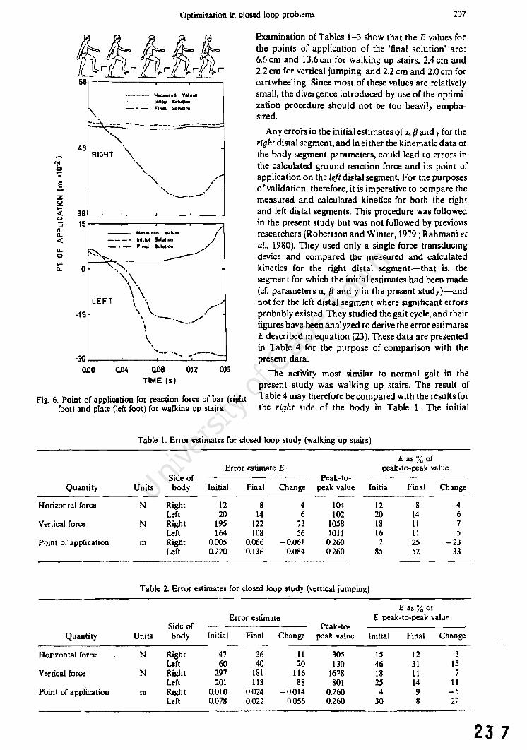
Optimization in closed loop problems 207

E -§ < ~ ...J

8: «(

IJ.. o .... 0..

_," V"I~ ... 1011101 SoIUIIon 1'., - ,- I"n"1 SoIlltIOl\

~-~\--------------------------

"'" 48 RIGHT '\

''\ '''. // "--._.-' 38~----~----~--__ ~ __ ~ 15r-----r-----.-----,-----~

o

--~ MM..u,N: Vol" ..

"

Initial Sollllion Fit tel Solution

''\\ \ . \\

LEFT I'

\ \ ,r' -15 \ '-.--./ I \ \ , ,

'-"".-.......... _-""--- ..... _--30 '--_ ........ __ ........ ___ --'-__ -.l

000 o.oa TIME (5)

Ol2 016

Examination of Tables 1-3 show that the E values for the points of application of the 'final solution' are: 6.6cm and 13.6cm for walking up stairs, 2.4cm and 2.2 em for vertical jumping, and 2.2 cm and 2.0 cm for cartwheeling. Since most of these values are relatively small, the divergence introduced by use of the optimi­zation procedure should not be too heavily empha­sized.

Any errors in the initial estimates of CI, fJ and y for the right distal segment, and in either the kinematic data or the body segment parameters, could lead to errors in the calculated ground reaction force and its point of application on the left distal segment. For the purposes of validation, therefore, it is imperative to compare the measured and calculated kinetics for both the right and left distal segments. This procedure was followed in the present study but was not followed by previous researchers (Robertson and Winter, 1919; Rahmani et ai., 1980). They used only a single force transducing device and compared the measured and calculated kinetics for the right distal segment-that is, the segment for which the initial estimates had been made (cr. parameters ex, fJ and y in the present study)-and not for the left distal segment where significant errors probably existed. They studied the gait cycle, and their figures have been analyzed to derive the error estimates E described in equation (23). These data are presented in Table 4 for the purpose of comparison with the present data.

Fig. 6. Point of application for reaction force of bar (right foot) and plate (left foot) for walking up stairs.

The activity most similar to normal gait in the present study was walking up stairs. The result of Table 4 may therefore be compared with the results for the right side of the body in Table 1. The initial

Table 1. Error estimates for closed loop study (walking up stairs)

Eas%of Error estimate E· peak-ta-peak value

Side of Peak-to-Quantity Units body Initial Final Change peak value Initial Final Change

Horizontal force N Right 12 8 4 104 12 8 4 Left 20 14 6 102 20 14 6

Vertical force N Right 195 122 73 1058 18 II 7 Left 164 108 56 1011 16 11 5

Point of application m Right 0.005 0.066 -0.061 0.260 2 25 -23 Left 0.220 0.136 0.084 0.260 85 52 33

Table 2. Error estimates for closed loop study (vertical jumping)

Eas%of Error estimate E peak-to-peak value

Side of Peak-to-Quantity Units body Initial Final Change peak value Initial Final Change

Horizontal force N Right 47 36 11 305 15 12 3 Left 60 40 20 130 46 31 15

Vertical force N Right 297 181 116 1678 18 11 7 Left 201 113 88 801 25 14 11

. POint of application m Right 0;010 0.024 -0.014 0.260 4 9 -5 Left 0.078 0.022 0.056 0.260 30 8 22

23 7

23 8

208 CHRISTOPHER L. VAUGHAN, JAMES G. HAY and JAMES G. ANDREWS

Table 3. Error estimates for closed loop study (cartwheeling)

E as % of Error estimate E peak-to-peak value

Side of Peak-to-Quantity Units body Initial Final Change peak value Initial Final Change

Horizontal force N Right 16 11 5 108 15 10 5 Left 38 27 11 101 37 27 10

Vertical force N Right 72 44 28 422 17 11 6 Left 53 30 23 269 20 11 9

Point of application m Right 0.004 0.022 -O.ot8 0.098 4 22 18 Left 0.060 0.020 0.040 0.098 61 20 41

Table 4. Error estimates for gait studies (double support phase) by different researchers

E as % of Error estimate E Peak-to-peak value peak-to-peak value

Quantity Units Robertson Rahmani Robertson Rahmani Robertson Rahmani

Horizontal force N 59 55 Vertical force N 98 64 Point of application m 0.011 0.035

percentage error estimate for the horizontal force in Table 1 is markedly better than both values in Table 4, although the value for the vertical force is slightly worse. Since each of these studies had errors in the kinetics of the foot under consideration (cf. parameters lX, p and}' in the present study), in addition to possible errors in the kinematic data and body segment para­meters, there is no way of knowing how accurate their kinetic data were for the contralateral foot. Based on the findings of the present study, it seems likely that the kinetic data for the contralateral foot, as well as the joint forces and torques within the closed loop, would have contained considerable errors.

In the present study, the percentage error estimates for the 'initial solution' of the horizontal force, vertical force and its point of application on the right distal segment (force bar) are much smaller than the cor­responding values for the left distal segment (force plate). Since these results are for the 'initial solution', the design variables do not have to be consistent with the constraints. In fact, for two of the activities (walking up stairs and cart wheeling) the point of application of the ground reaction force sometimes lies outside the distal extremity (Fig. 6). However, the effect of the optimization procedure is to drive these design vari­ables into the feasible solution space and hence decrease the percentage error estimates considerably (Tables 1-3).

The intent to be as general as possible in formulating the closed loop problem led to the distal segment end­points for each of the four extremities (i.e. points 5, 9, 13 and 17) being treated as if they were joints like all the others. As such they were included in the objective function J" of equation (22). However, if J" is to be dependent on muscular effort, there are certain con­ditions when the torque at a distal segment end-point

155 118 38 46 950 755 10 8

0.290 0.290 4 12

may be a function of the choice of that end-point position and not muscular activity per se. This issue was not addressed in the present paper but probably should be in future work.

The results presented in Figs 4-6 and Tables 1-3 indicate that by using the optimization approach, the horizontal and vertical reaction forces at the distal segments have been successfully predicted, although some errors still exist for the prediction of the points of application of these forces. These errors, although not particularly large, could have been eliminated by the use of more appropriate modelling techniques (e.g. the point of application of the vertical bar reaction force could have been fixed by an equality constraint t/lJ The objective function J ,,-the sum of the squares of resultant joint torques within the closed loop-was found to yield the better results of the two objective functions considered. It is suggested, however, that the torques at certain distal segment end-points may have to be excluded from this objective function in order that it may more closely represent muscular effort. The results obtained in this study provide some support for the notion that the human neuromuscular mechanism

. attempts to minimize the joint torques during a closed loop activity. More work is required, however, to establish the limitations, if any, that govern its use in the analysis of closed loop activities and, in partic­ular, for those activities which the subject has not encountered or practised before.

The procedure for determining an initial estimate of the joint forces and torques dealt exclusively with the closed loop problem of Case 3 (Vaughan et al., 1982). However, it is a fairly straightforward matter to extend this procedure to closed loop problems of Cases 4 and 5 which have a greater degree of indeterminacy. Where three extra scalar equations are required for planar

Optimization in closed loop problems 209

Case 3 problems in order to supply the initial estimate of the design variable vector bo, six and nine extra scalar equations would be required for planar Case 4 and 5 problems, respectively. Furthermore, the objec­tive function in equation (10) can be altered so that the summation includes those forces and torques within the extra closed loop(s). In theory then, closed loop problems of Cases 4 and 5 can be easily handled using the techniques presented here for Case 3 problems. However, a certain degree of skill and experience are required to make reasonable estimates of the para­meters IX, f3 and y for equations (16), (17) and (18). The estimation of further parameters could perhaps be troublesome, from a practical point of view.

CONCLUSIONS

(1) Application of an optimization approach to the closed loop problem in biomechanics has been re­asonably successful for predicting the horizontal and vertical reaction forces at the distal segments. Some problems exist for predicting the points of application of these forces.

(2) The results obtained in this study provide some support for the notion that the human neuromuscular mechanism attempts to minimize the joint torques­and thus to a certain degree, the amount of muscular effort-during the closed loop activities that were studied.

(3) The methods ofthe present paper are sufficiently general to be applied to all classes of the closed loop problem which are underdetermined. Since only Case 3 problems were studied in the present paper, it is suggested that Case 4 and 5 problems-which are of greater indeterminacy-should be studied in future.

REFERENCES

Andrews, J. G. (1974) Biomechanical analysis of human motion. Kinesiology IV, 32-42.

Bernstein, N. (1967) The Coordination and Regulation 0/ Movements. Pergamon Press, London.

Cappozzo, A., Leo, T. and Pedotti, A. (1975) A general computing method for the analysis of human locomotion. J. Biomech. 5, 307-320.

Chao, E. Y. S. (1971) Determination of applied forces in linkage systems with known displacements: with special application to biomechanics. Doctoral dissertation, Uni­versity of Iowa.

Chao, E. Y. S. and Rim, K. (1973) Application of optimization principles in determining the applied moments in human leg joints during gait. J. Biomech. 6, 497-510.

Crowninshield, R. D. (1978) Use of optimization techniques to predict muscle forces. J. biomech. Engng 100, 88-92.

Crowninshield, R. D., Johnston, R. c., Andrews, J. G. and Brand, R. A. (1978) A biomechanical investigation of the human hip. J. Biomech. II, 75-85.

Hardt, D. E. (1978) Determining muscle forces in the leg during normal human walking-an application and eva­luation of optimization methods. J. biomech. Engng 100, 72-78.

Hardt, D. E. and Mann, R. W. (1980) A five body-three dimensional dynamic analysis of walking. J. Biomech. 13, 455-457.

8M 15:3 - E

Haug, E. J. and Arora, J. S. (1979) Applied Optimal Design. John Wiley and Sons, New York.

International Mathematical Statistical Libraries. (1975) The I MSL Library Vols 1 and 2.

Kennedy, W. J. and Gentle, J. E. (1980) Statistical Computing. Marcel Dekker, New York.

McGhee, R. B. (1979) Mathematical models for dynamics and control of posture and gait. Paper presented at VlIth International Congress of Biomechanics, Warsaw, Poland.

McGhee, R. B., Koozekanani, S. H., Gupta, S. and Cheng, I. S. (1978) Automatic estimation of joint forces and moments in human locomotion from television data. I dent(fication and System Parameter Estimation (Edited by Rajbman, E.). North-Holland, New York.

Nubar, Y. and Contini, R. (1961) A minimum principle in biomechanics. Bull math. Biophys. 23, 377-390.

Pedotti, A., Krishnan, V. V. and Stark, L. (1978) Optimi­zation of muscle force sequencing in human locomotion. Mathl Biosci. 38, 57-76.

Penrod, D. D., Davy, D. T. and Singh, D. P. (1974) An optimization approach to tendon force analysis. J. Bio­mech.7, 123-129.

Pezzack, J. c., Norman, R. W. and Winter, D. A. (1977) An assessment of derivative determining techniques used for motion analysis. J. Biomech. 10, 377-382.

Quanbury, A. O. and Winter, D. A. (1974) Calculation of floor reaction forces from kinematic data during single, support phase of human gait. Abstract, 5th Canadian Medical and Biological Engineering Conference, Montreal.

Rahmani, S., McGhee, R. B., Weimer, F. C. and Koozek­anani, S. H. Reduced order dynamic models for online computer analysis of human gait. Submitted for pub­lication.

Robertson, D. G. E. and Winter, D. A. (1979) Estimation of ground reaction forces from kinematics and body segment parameters. Abstract, Canadian Association of Sport Sciences, Vancouver.

Rosen, J. B. (1960) The gradient projection method for nonlinear programming. Part I, linear constraints. SIAM J. appl. Math. 8, 181-217.

Rosen, J. B. (1961) The gradient projection method for nonlinear programming. Part II, nonlinear constraints. SIAM J. appl. Math. 9, 514-532.

Seireg, A. and Arvikar, R. J. (1975) The prediction of muscular load sharing and joint forces in the lower extremity during walking. J. Biomech. 8, 89-102.

Sohoni, V. N., Arora, J. S. and Haug, E. J. (1978) A general purpose non-linear programming computer code GRP based on the gradient projection method. Technical Report 41, College of Engineering, University of Iowa.

Vaughan, C. L. and Andrews, J. G. (1980) An optimization approach to selection of body parameters. Presented at the 4th Annual Conference, American Society of Bio­mechanics, Burlington, Vermont.

Vaughan, C. L., Hay, J. G. and Andrews, J. G. (1982) Closed loop problems in biomechanics. Part I-a classification system. J. Biomech. 15, 197-200.

. Wood, G. A. and Jennings, L. S. (1979) On the use of spline functions for data smoothing. J. Biomech. 12,477-479.

NOMENCLATURE

a linear acceleration (mfs2) b design variable vector containing joint forces and

torques (N, Nm) d location vector, directed distalIy (m) g acceleration due to gravity (mfs2)

subscript referring to constraint number j subscript referring to joint number I superscript referring to lower bound on b m segment mass (kg)

23 9

210 CHRISTOPHER L. VAUGHAN, JAMES G. HAY and JAMES G. ANDREWS

p location vector, directed proximally (m) L length of foot (m) q a measured or calculated quantity (N. m) M total body mass (kg) r subscript referring to design variable number 0 origin of fixed inertial reference system s subscript referring to segment number r reference system t time (s) T resultant joint torque (Nm) u superscript referring to upper bound on b V subscript referring to measured quantity q x coordinate in X direction ofR :OXYZ (m) X reference axis in orthogonal system R: OXYZ y coordinate in Y direction of R : OX YZ (m) Y reference axis in orthogonal system R : OXYZ z coordinate in Z direction ofR :OXYZ (m) Z reference axis in orthogonal system R :OXYZ [A] 48 x 51 coefficient matrix ex parameter to estimate vertical ground reaction force B 48 x 1 column vector containing kinematic quantities (VGRF) [e] 51 x 51 coefficient matrix p parameter to estimate application point of Y.GRF 0 51 x 1 column vector containing kinematic quantities y parameter to estimate horizontal ground reaction E error estimate of difference between two curves (N, m) force F resultant joint force (N) t'J exponent of force variables in J G subscript referring to calculated quantity q (j segment orientation angle (radian) H angular momentum about center of mass (kgm2/s2) 1 weighting factor of force variables in J I segment transverse centroidal moment of inertia )J. weighting factor of torque variables in J

(kgm2) v exponent of torque variables in J J objective or cost function

'" equality or inequality constraint

24 0

SIMULATION OF A SPRINTER. PART I. DEVELOPMENT OF A MODEL

C.L. VAUGHAN

Department of Biomedical Engineering, University of Cape Town and Groote Schuur Hospital, Observatory, Cape 7925 (South Africa)

(Received 15 May, 1982)

The two horizontal forces acting on a sprinter are ground reaction driving him forward and air resistance impeding him. The driving force starts ofT at a maximum value but decreases with in­crease in velocity, whereas the resisting force varies as the square of velocity. Mathematical models of these two forces have been incorporated in Newton's Second Law to yield a second order non­linear differential equation to describe the sprinter's motion. This equation may be numerically integrated, and validation of the model has shown there is good agreement between theory and experimental data. The model may be used to characterise a runner's performance (a so-called 'sprint proflle'), to pinpoint his strengths and/or weaknesses, and to predict what his time might be for a particular distance if he were able to maintain maximum velocity.

Introduction

The running gait must surely be one of man's most natural activities. It is therefore significant that man does not fully understand running, particularly from a bio­mechanical standpoint. Although research on the biomechanics of running dates back to the early Greek philosopher Aristotle, it is only in the last 50 years that mathematical modelling of a sprinter's performance using mechanical principles has been attempted (Furusawa et 01., 1927; Hill, 1927; Fenn, 1930; Henry et 01., 1951, 1952; Keller, 1973, 1974; Vaughan et 01., 1977). While all of these researchers obtained satisfactory results for predicting a sprinter's horizontal velocity, not all of them based their equations on sound mechanical reasoning (cf. Vaughan et 01., 1977).

The advent of the digital computer has given greater scope to the use of simulation models, particularly for the understanding, evaluation and improvement of human movement. The purposes of the present paper are as follows:

(I) to develop a mathematical model that simulates the horizontal forces acting on a sprinter; and

(2) to measure relevant kinematic parameters in order to validate the model.

The implementation of the model will be described in Part II of this paper. (Vaughan, 1982).

65

Int. J. Bio-Medical Computing (14) (1983) 65-74

0020-7101/83/0000-0000/$03.00 © 1983 Elsevier Scientific Publishers Ireland Ltd. Printed and Published in Ireland

241

66

supporting force

C.L. Vaughan

weight

driving force

Fig. 1. Free body diagram of external forces acting on a sprinter.

Biomechanical theory and mathematical modelling

For the purposes of this study it is assumed that a sprinter exerts his maximum effort from the time the gun is fired; he then achieves his maximum velocity and main­tains this for the period of interest. The sprinter is assumed to move in the mid-sagittal plane, so that any rotation about a longitudinal or medial axis can be ignored.

Figure 1 illustrates the external forces acting on a sprinter. These are the ground reaction force (which may be resolved into two orthogonal components, a horizontal driving force and a vertical supporting force), the athlete's weight, and air resistance. In the present model, neither the supporting force nor the weight are considered since their imbalance merely causes the upward or downward acceleration of the runner's centre of mass. The aim of sprinting is to cover a set horizontal distance in the minimum time. For this reason only the horizontal forces are considered for the purposes of the model.

Baumann (1976), Blader (1968) and Henry (1952) have all shown that the hori­zontal driving force assumes its maximum value immediately after the gun is fired. Since the sprinter is using a set of starting blocks he is able to lean well forward, pushing backward with great vigour and thereby evoking a favourable. propulsive reaction, Furthermore, the sprinter spends a greater proportion of his time in contact with the ground (Hopper, 1973) and is thus able to exert a greater impulse. Figure 2 shows the sprinter progressing from (a) the start, to (b) maximum velocity when the trunk is more upright (Dowell et al., 1975; Hay, 1978) and the driving force now

242

Sprinter's model development 67

(0 ) ( b)

Fig. 2. Forward lean of a sprinter: (a) at start of race; (b) at maximum velocity. These diagrams have been modified from Hay (1978).

assumes a minimum value because of the unfavourable body orientation. This obser­vation that the horizontal driving force decreases as the sprinter's velocity increases is strengthened by the work of Fenn (I930) and other work physiologists. They have shown that the faster muscles shorten, the smaller the force they are able to exert on their environment, in this case the ground. It is important to point out that the driving force must be of a discontinuous nature in practice since the sprinter is airborne for certain discrete periods of time (Hay et al., 1982). The above discussion is therefore a slight simplification of reality.

The magnitude of the air resistance depends on a variety of factors (Hay, 1978; Pugh, 1970, 1971). It is widely accepted however, that the force due to the air re­sistance varies as the square of the velocity, provided the air is sufficiently disturbed (Batchelor, 1967; Davies, 1980; Hoerner, 1965). The effects of air resistance are two­fold: the sprinter must do work to overcome it and thus his velocity is restricted and his trunk position is impaired.

Application of Newton's Second Law to the sprinter's centre of mass yields

Ma =Fd -Fr (1)

where M is his total body mass, a his horizontal acceleration, Fd his driving force and Fr his resisting force (air resistance). Division by M gives

(2)

where fd is his driving force per unit mass and fr is his resisting force per unit mass.

243

68 C.L. Vaughan

The question that arises is as follows: what forms should!d and fr take? As discussed above, !d starts off at some maximum value and decreases as horizontal velocity v increases. Previous research by Vaughan et al. (1977) has indicated the following form:

(3)

where A, B and a are unknown parameters. The model for!, is simply

(4)

where C is an unkno~n parameter. Equation (2) therefore becomes

(5)

When

v =0, (6)

when

~.= vmax,a = 0

so

o =A -Bva -ev.2 max max

giving

B=Av-a -ev2-Q max max (7)

Now, it is generally accepted (Batchelor, 1967; Hoerner, 1965; Pugh, 1970) that the force due to air resistance may be calculated from the equation

(8)

where CD is a dimensionless drag coefficient, p is the density of the air, and Qp is the projected or cross-sectional area of the runner. Since!, = F,/M, Eqns. (4) and (8) yield

(9)

244

Sprinter's model development 69

Previous work (Hoerner, 1965; Shanebrook et al., 1976) suggests that the drag coef­ficient CD for a sprinter has a value of 1.12. For average temperature and barometric pressure conditions (20°C and 760 mmHg) air density p may be taken as 1.2 kg/m3

.

The projected area Qp has been shown to be about 27.5% of total body aiea Qb

(Horner, 1965; Pugh, 1971; Shanebrook et al., 1976). Vaughan et. al., 1976) have suggested that Qb may be satisfactorily calculated by the modified Du Bois formula

(10)

where Hand M are total body height and mass, respectively. Substitution of these values for CD, P and Qp into Eqn. (9) yields

C = 0.0401Ho.ns M-O. S7S (11)

Equation (5) may be rewritten as

f=A -BsC¥. -CS2 (12)

and is a second order non-linear differential equation which describes the sprinter's motion (s is horizontal displacement and the dots indicate first and second time derivatives). The parameters A, Band C may be calculated from Eqns. (6), (7) and (11) provided values for ainit, vmax , H, M and Q are known. The next section of this paper will describe the methods used to measure ainit and vmax and the section there­after will describe the procedures for selecting the optimum value for Q.

Validation of theoretical model

Four university sprinters were recruited for the purpose of evaluating the mathe­matical model in Eqn. (12). Their physical characteristics are contained in Table 1. Two devices 'were constructed for the purpose of gathering the necessary kinematic data.

The first device was designed to give a continuous record of the athlete's velocity

TABLE 1

PHYSICAL CHARACTERISTICS OF SUBJECTS

Athlete Age Height Mass Best 100 m (years) (m) (kg) (s)

MF 19 1.79 84 11.1 NH 26 1.83 81 10.3 PL 22 1.80 72 10.5 KV 22 1.80 74 10.9

24 5

246

70 C.L. Vaughan

TABLE 2

KINEMATIC MEASUREMENTS AND PREDICTIONS FOR EACH ATHLETE

Predictions, indicated with an asterick*, are based on the model for which ct = 0.7

Athlete ainit vmax t 27.5 s 27.5 S~7.5 V27 •s V~7.5 t~oo (m/s2) (m/s) (s) (m) (m) (rnls) (m/s) (s)

MF 10.50 9.94 3.82 27.5 27.7 9.50 9.64 11.23 NH 10.26 10.12 3.83 27.5 27.2 9.80 9.65 11.09 PL 10.65 10.24 3.78 27.5 27.3 9.92 9.79 10.94 KV 10.55 9.90 3.85 27.5 27.2 9.31 9.51 11.26

and used micro-wave technology (Manchester, 1965; Vaughan et al., 1977) very similar to the 'radar' device used by the police for measuring a motor vehicle's speed. The slope of the initial velocity-time graph (range was limited to 20 m) could then be differentiated to yield the athlete's initial acceleration ainit for calculating A in Eqn. (6).

The second device, in which light beams were concentrated on photo-cells at a series of timing stations (25.0 m, 27.5 m, 30.0 m, 40.0 m, 45.0 m and 50.0 m) has been used quite extensively before (Ikai, 1968; Jackson et al., 1969). The variables of interest are the time and velocity at 27.5 m (t27,S' V27,s) and maximum velocity (vmax) between 40.0 m and 50.0 m. All these kinematic measurements are presented in Table 2.

The data from Tables 1 and 2 may be substituted in Eqns. (6) and (7) and (11) for the purposes of evaluating A, Band C if a value of a is selected. In a previous paper by Vaughan et al. (1977) values 0.5 and 1.0 for a were tried, but, as will now be demonstrated, the optimum lies between these values.

Integration of Eqn (12) for six different a-values was done numerically using a modification of the Taylor Series Expansion (Abramowitz et al., 1968), with the aid of a Casio FX-502P programmable calculator. It is thus possible to calculate velocity and displacement as a function of time. The following expression was calculated for each value of a

(13)

where the superscript * indicates a value predicted by the model. Figure 3 illustrates the mean value for the sum of squares of the four subjects plotted as a function of a. Quite clearly the minimum value for Eqn. (13) is obtained when a value of a = 0.7 is used. Just how well theory matches experiment can also be judged by examining Table 2.

A further check on the validity of the a = 0.7 model may be seen in Fig. 4. The continuous velocity-time record of NH for the initial 1.2 s has been compared with

Sprinter's model development

7 ,----------------------------,

6

U')

W 5 0:: « => o I, U')

~ 3

~ => 2 U')

o L-__ ~--._--~=-_.--_.--_.--~

0.5 0.6 0.7 0.8 0.9 1.0

ALPHA

71

Fig. 3. Sum of squares (cf, Eqn. (13) plotted as a function of parameter 0:. Note: these are the mean values for the four athletes, and the solid line has been 'added merely for the purpose of illustration.

three different model predictions. Again the value of ex = 0.7 give a very satisfactory approximation to experimental result.

Discussion

VI

"-E

>-I-

U 0 ...J

W >

Table 2 contains the 100-m time for each athlete predicted by the model. When it

ALPHA

7 x 1.0

0 0.7 6 • 0.5 0

5 • 0

• I,

EXPERIMENT 3

2

o *-__ ~--.---~--~--.---~------~ 0.0 0.1, 0.8

TIME (s)

1.2

Fig. 4. Experimental result (solid line) compared with predicted values for three different values of 0: for subject NH.

24 7

248

72 C.L. Vaughan

TABLE 3

PARAMETER VALUES FOR EACH ATHLETE

Based on model for which ex = 0.7

Athlete

MF NH PL KV

10.50 10.26 10.65 10.55

2.009 1.929 1.982 2.018

0.0048 0.0050 0.0053 0.0052

is considered that the data on which the models are based were gathered on a grass track during the off-season, the comparison with the best 100 m times in Table 1 is quite reasonable.

Table 3 contains the values for parameters A, Band C for each athlete based on a = 0.7. The values for NH were used to generate the data for Figs. 5 and 6. Figure 5 illustrates Fd and F, plotted as a function of velocity. At the terminal velocity (Le.

8

N 0 7 ~

• z 6

a::: w

5 I-

Z

a::: 0... 4 Vl

z 3 0

w u 2 a::: 0 lJ..

0

-1

o

~DRIVING FORCE (ground reaction)

lRESISTING FORCE

(air resistance)

, "­ , ,

"-"- , , ,

2 4 6 8 10 12 14

VELOCITY (m/s)

Fig. 5. Horizontal forces acting on the sprinter NH as a function of his velocity. These are based on Eqns. (3) and (4) where A. Band C have the values of Table 3 and ex = 0.7.

Sprinter's model development 73

12 N ~ 1/1

"- • 10 E E

~

III 8 z "- ~

E z ~ w ~

~ 6 « a:: >- w w ~ u - « -.J u 4 w 0 -.J

U -.J c.. U W VI « > 0 2

:1/1 .1/1 1/1 0 5

-2 0 2 4 6 8 10 12

TIME (s)

Fig. 6. Theoretical displacement, velocity and acceleration curves for subject NH based on Eqn. (12).

maximum velocity), Fr has a value of 42 N which compares quite favourably with the figures quoted by various workers (Raine, 1970; Sharebrook et al., 1976; Whitt et al., 1974) for the drag on cyclists, skiers and also runners.

Figure 6 shows theoretical displacement, velocity and acceleration curves. In reality a sprinter is not able to maintain his maximum speed for an indefinite length of time. The model of Eqn. (12) becomes no longer applicable as soon as the athlete's speed drops below its maximum value. The time at which the decrease in speed starts depends on the fitness and ability of the athlete. Furusawa et al. (1927) and Ikai (1968) have demonstrated that their subjects have a substantial fall-off in speed after relatively short distances. However a simple analysis of Pietro Mennea's 200-m world record indicates that this decrease in speed over the second 100 m was only a few per cent.

The model of Eqn. (12) is a general one for all sprinters and the parameters A, B and C are characterised by ainit, vmax, Hand M. There is little the sprinter can do to alter the values of Hand M - and therefore C. However, a powerful drive out of the blocks (Le. a large value for ainit) and a large maximum velocity Vmax are clearly factors which can improve through hard work and training. The model has the following uses:

(1) to characterise a runner's performance (a so-called 'sprint profIle') for com­parison throughout the season;

(2) to pinpoint where a sprinter's strengths and/or weaknesses might lie; and (3) to predict what a sprinter's time might be for a particular distance if he were

able to maintain maximum velocity.

The model developed and validated in this paper forms the basis for a further study (Vaughan, 1982) in which some of the above uses are examined.

249

25 0

74 C.L. Vaughan

References

Abramowitz, M. and Stegun, LA., Handbook of Mathematical Functions, Dover, New York, 1968. Batchelor,G.K.,AnIntroduction to Fluid Dynamics. University Press, Cambridge, 1967. Baumann, W., Kinematic and dynamic characteristics of the sprint start, in Biomechanics V-B,

P.V. Komi (ed.) University Park Press, Baltimore, 1976, pp. 194-199. Blader, F.B., The analysis of movements and forces in the sprint start, in Biomechanics I, J. Warten­

weiler, E. Jokl and M. Hebbelinck (Eds.), Karger, Basel, 1968, pp. 278-281 Davies, C.T., Effects of wind assistance and resistance on the forward motion ofa runner,!. Appl.

Physiol., 48 (1980) pp. 702-709. Dowell, L.J., Jubela, R. and Mamaliga, E., A cinematographical analysis of the 100 yard dash

during acceleration and at optimum velocity, acceleration zero, I Sports Med., 15 (1975) pp.20-25.

Fenn, W.O. Frictional and kinetic factors in the work of sprint running, Am. I. Physiol., 92 (1930) pp.583-611.

Furusawa, K., Hill, A.V. and Parkinson, J., The dynamics of sprint running, Proc. R. Soc., B102 (1927) pp. 29-42.

Hay, J.G., The Biomechanics of Sports Techniques, (2nd edn.), Prentice-Hall, Englewood Cliffs, 1978,519 pp.

Hay, J.G. and Reid, J .G., The Anatomical and Mechanical Bases of Human Motion, Prentice-Hall, Englewood Cliffs, 1982, pp. 264-265.

Henry, F.M., Force-time characteristics of the sprint start, Res. Q., 22 (1951) pp. 409-421. Hill, A.V., The air-resistance to a runner, Proc. R. Soc., DI02 (1927) pp. 380-385. Hoerner, S.F., Fluid-Dynamic Drag, S.F. Hoerner, New Jersey, 1965, pp. 3-12. Hopper, B.1., The Mechanics of Human Movement, Crosby Lockwood Staples, London, 1973,

175pp. Ikai, M., Biomechanics of sprint running with respect to the speed curve, in Biomechanics I, J.

Wartenweiler, E. Jokl and M. Hebbelinck (Eds.), Karger, Basel, 1968, pp. 282-290. Jackson, A.S. and Cooper, J.M., Multiple timing system for measuring components of sprint-

velocity curve, Res. Q., 40 (1969) pp. 857-859. Keller, J.B., A theory of competitive running,Phys. Today (1973). Keller, J.B., Optimal velocity in a race, Am. Math. Mon., 5 (1974). Manchester, F.D., Simple Doppler-shift apparatus using micro-waves, Am. I. Phys., 33 (1965)

pp.499-500. Pugh, L.G.C.E., Oxygen intake in track and treadmill running with observations on the effect of air

resistance,!. Phys., 213 (1971) pp. 255-276. Pugh, L.G.C.E., The influence of wind resistance in running and walking and the mechanical

efficiency of work against horizontal or vertical forces,!. Phys., 213 (1971) pp. 255 -276. Raine, A.E., Aerodynamics of skiing, Sci. 1.,6 (1970) pp. 26-30. Shanebrook, J.R. and Jaszczak, R.D., Aerodynamic drag analysis of runners, Med. Sci. Sports, 8

(1976) pp. 43-45. Vaughan, C.L. and Matravers, D.R., A biomechanical model of the sprinter, I. Hum. Movement

Stud., 3 (1977) pp. 207-213. Vaughan, C.L. and Stewart, J.M., Surface area of nude and clothed man, Report 59/76, Chamber

of Mines, Johannesburg, 1976, 35 pp. Vaughan, C.L. Simulation of a sprinter. Part II. Implementation on a programmable calculator,

Int. I. Bio-Med. Comput., 14 (1983) pp. 75-83. Whitt, F .R. and Wilson, D.G., Bicycling Science, M.I.T. Press, Cambridge, 1974.

SIMULATION OF A SPRINTER. PART II. IMPLEMENTATION ON A PROGRAMMABLE CALCULATOR

c.L. VAUGHAN

Department of BiomediCIJI Engineering, University of Cape Town and Groote Schuur Hospital, Observatory, Cape 7925 (South AfriCIJ)

(Received 15 May, 1982)

Although successful models have been developed to simulate a sprinter's performance, they are often complex and sophisticated, requiring a main frame environment and expensive monitor­ing equipment. These d~sadvantages preclude the wide-spread use of the models by practitioners. This paper presents a method in which the necessary data can be easily gathered - using a tape measure, six stop watches and bollards, a starting gun, and a bathroom scale. A simple algorithm is presented for calculating the parameters of a previously defined model, and implemented on hand-held programmable calculators, the Casio FX-502P and HP41C. The model calculates the sprinter's initial horizontal acceleration, maximum horizontal velocity and can be used to predict the time for any given race distance. The model can therefore be used to evaluate the sprinter's current performance as well as indicate his potential if he were able to reach and maintain maxi­mum velocity.

Introduction

As outlined in Part I of this paper (Vaughan, 1982), a sprinter's performance can be simulated by means of a mathematical model. A prime consideration when develop­ing a model should be the use to which it can be put. It may be useful for the re­searcher to understand aspects of the biomechanics of sprinting, or it may have a wider scope to the practitioner - the sprint coach - in evaluating and improving sprint performance. If sophisticated measuring equipment is required (Jackson et al., 1969; Vaughan et al., 1977) then the expense will preclude widespread use of the model by practitioners. However, if the eqUipment needed is cheap and readily avail­able then the model's potential is greatly expanded. It is with this view in mind that the present paper has been prepared.

Vaughan (1982) has shown that the following differential equation - based on Newtonian mechanics - offers a successful means for predicting a sprinter's kine­matics:

75 Int. J. Bio-Medical Computing (14) (1983) 75-83 0020-7101/83/0000-0000/$03.00 © 1983 Elsevier Scientific Publishers Ireland Ltd. Printed and Published in Ireland

(1)

251

252

76 C.L. Vaughan

where s is horizontal displacement, the dots indicate first and second derivatives with respect to time, and A, Band C are parameters unique to each sprinter's per­formance. If parameters A, Band C can be determined then Eqn. (l) can be numeri­cally integrated to yield the sprinter's horizontal displacement, velocity and accelera­tion at various times during the race. The purposes of this study therefore are

(l) to collect data on sprinters of varying ability using cheap and readily avail­able equipment;

(2) to develop a simple algorithm for calculating A, Band C; and (3) to implement and test the algorithm on a hand-held programmable calculator.

Data collection

Six sprinters of both sex and of varying ability were studied at the beginning of the athletics season. The track had a synthetic surface and was housed indoors, thus eliminating wind effects (but not of course air resistance). The equipment required was as follows

1. Tape measure 2. 6 Stop watches 3. 6 Bollards 4. Starting gun or wooden clapper 5. Bathroom scale

The tape measure was used to set up accurately six timing stations (indicated by the six bollards) at 5, 10, 15, 30,40 and 50 m. Each sprinter was instructed to sprint 'flat out' until at lea~t 60 m during which period his or her time was recorded by a timekeeper at each of the six timing stations. Mter the trial, the tape and scale were used to obtain the athlete's height and mass, respectively. All these data - in addition

TABLE 1

ANTHROPOMETRIC DATA AND MODEL PARAMETERS FOR EACH ATHLETE

Athlete's Sex Age Height Mass $max A B C initials (years) H M (m/s) (m/s2) (m 0.3S -1.3) (m- I)

(m) (kg)

JB F 15 1.68 57.0 9.1 9.2 1.86 0.0057 LC M 20 1.79 66.0 10.0 10.5 1.99 0.0055 RD M 21 1.77 67.0 9.1 14.3 2.96 0.0054 VE M 22 1.80 75.5 11.1 11.3 1.98 0.0051 KV M 28 1.80 76.5 9.1 10.7 2.19 0.0051 KW F 19 1.67 53.0 9.1 9.7 1.96 0.0059

Calculator programs for a sprinter's profile 77

TABLE 2

ATHLETE'S TIMES AT EACH STATION

Note: the best 100-m time is that recorded for the season, while all the values with an asterisk are those predicted by the model with.6.t = 0.05.

Athlete's Time initials

Sm 10 m 15 m 30m 40m SOm best 100 m (s) (s) (s) (s) (s) (s) (s)

J B 1.3 2.1 2.7 4.6 5.7 6.9 12.3 1.3* 2.1* 2.7* 4.5* 5.6* 6.7* 12.2*

LC 1.1 2.0 2.5 4.3 5.3 6.4 11.1 1.2* 2.0* 2.5* 4.2* 5.2* 6.2* 11.2*

RD 1.1 1.8 2.4 4.2 5.3 6.4 11.6 1.1* 1.8* 2.4* 4.1* 5.2* 6.3* 11.8*

VE 1.1 1.8 2.4 4.2 5.1 6.1 10.4 1.2* 1.8* 2.4* 3.9* 4.8* 5.7* 10.2*

KV 1.2 2.0 2.6 4.3 5.4 6.5 11.5 1.3* 2.0* 2.6* 4.3* 5.4* 6.5* 11.9*

KW 1.3 2.0 2.7 4.4 5.5 6.6 11.6 1.3* 2.0* 2.7* 4.4* 5.5* 6.6* 12.0*

to the model's predictions which will be discussed in a later section - have been included in Tables 1 and 2.

Each of the five items listed above are relatively inexpensive and should be readily available to most peopie involved in the coaching of sprinters.

Development of algorithm

There are essentially two types of dynamics problems: (a) the forward problem, in which the kinetics (i.e. forces and torques) are known and the differential equa­tions are solved to yield the kinematics (Le. accelerations, velocities and displace­ments); and (b) the inverse problem, in which the kinematics are known and the algebraic equations are solved to yield the kinetics (Wells, 1967). Now the majority of biomechanics problems fall into this latter category because it is normally so difficult to measure forces and torques directly (Chao et ai, 1973; Vaughan et al., 1982a).

Chao et al. (1973) argued that numerical differentation applied to experimentally

253

25 4

78 c.L. Vaughan

obtained data would magnify the inherent measurement errors. They therefore pro­posed a method for obtaining joint kinetics based on the application of mathematical optimization (steepest descent algorithm) using a modification of the direct dynamics approach. The method was designed to make successive improvements of an initially­estimated set of joint torques by driving a set of calculated displacements (obtained by numerical integration) closer and closer to the set of measured displacements as the iterative process progressed.

The algorithm proposed in the present paper is very similar to that of Chao et al. (1973) although the optimization is simplified considerably. It may be stated as follows (Haug et al., 1979): Find the optimal design variable A E R 1 that minimizes the objective function

subject to the constraints I/Iji = 1 ••• 5 where

1/11 = S'- A + BsO.7 + Cs 2 = a

1/12 = C - O.04Jt>·725 M-O .575 = a

given H, M and (ti,Si) i = 1 •.• 6

(2)

(3)

(4)

(5)

(6)

(7)

In Eqn. (2) the asterisk * indicates a displacement calculated by the model. Equation (3) is simply a rearrangement of Eqn. (1), and Eqn. (4) shows that paramater C is a function of Hand M (cf. Vaughan (1982) for more detail). Equation (5) indicates that B is a function of A, C and smax where this last unknown may be calculated simply from (ti,si) i = 4,5,6. The inequality constraints (6) and (7) ensure that A lies between A min and A max which have to be specified.

Although the gradient projection algorithm is very versatile (Haug et al., 1979) and can be readily adapted to biomechanical applications (Vaughan et al., 1982b), a much simpler iterative search was chosen for this study. This was done so that the algorithm could be accommodated on a hand-held programmable calculator.

The flow diagrams with the four separate programs BIORUN, INTEG2, RUNMOD and CALTIM are illustrated in Figs. 1-4. They have the following functions:

N <.n U'I

BIORUN

Smax = max{(S6- S5)/(t6 -t5) (55 - 5

4)/ (t

5 - t4 )

810RUN

no

BIORUN

no

finish

Fig, 1. Flow diagram for main program BIORUN which accepts anthropometric and kinematic data as input, and yields "max, A, Band Cas output.

~ S" ..,. ~ ~ c ca ~ (s> .... ~ ... "3 ;:s' ..,. ~ ... ~ "t:I C3 ~ \'Il

-.l \Q

256

80 C.L. Vaughan

(3) INTEG2

s n+, s + 5 6t + 1 56t2 n n "2

o RUNMOD

o CALTIM

no

finish

Fig. 2. Flow diagram for subroutine INTEG2 which integrates a second order differential equa­tion.

Fig. 3. Flow diagram for subroutine RUNMOD which evaluates the running model of Eqn. (1).

Fig. 4. Flow diagram for subroutine CAL TIM which calculates the time for a given distance.

BIORUN

INTEG2

RUNMOD CALTIM

This is the main controlling program, accepting all the measured data, calculating C, S max. B and the optimum value for A. This subroutine integrates a second order differential equation and is based on a Taylor Series Expansion (Abramowitz et a/., 1968). This subroutine simply evaluates the running model of Eqn. (1). This subroutine calculates the time for a given race distance.

Testing of programs

The flow diagrams of Figs. 1-4 may be incorporated on a hand-held programmable calculator, either the Casio FX-502P (approximate cost £50) or the Hewlett-Packard HP41-C (about £120). The programs for both these calculators may be obtained from the author. Athlete LC is chosen for the purpose of illustration.

Step Data

1 2 (H) 3 (M) 4 (tl) 5 (t2) 6 (t3) 7 (t4) 8 (ts) 9 (t6)

10 (A min)

11 (LlA) 12 (A max)

13 14 15 (srace)

Calculator programs for a sprinter's profile

input operation Read out ®QD 1

@ O. 1.79 @ 1.79

66.0 (ill) 5.4845 ... 1.1 (ill) 1.1 2.0 @ 2.0 2.5 @D 2.5 4.3 @ 4.3 5.3 @ 5.3 6.4 @D 10. 9.0 (ill) 9. 0.5 (ill) 0.5

12.0 (ill) 10.5 @D 1.985 .... <ill O.

100.0 @ 11.2

-03

Remark

Value for C

Smax in mls

A optimum B

trace in s

81

Steps 14 and 15 can be repeated as often as required. In step 12 about 7.5 min is required from when @D is depressed until 10.5 is displayed, and in step 15 about 5 min elapses from (ill) to the display of 11.2.

The calculated values for smax> A, Band C for each athlete are contained in Table 1, while the predicted times for each of the six timing stations plus 100 m are pre­sented in Table 2. The two parameters smax and A are simply the sprinter's maximum horizontal velocity and initial horizontal acceleration, respectively, and give a good indication of performance.

Discussion

Table 2 illustrates just how well the predicted values match the measured ones. For subjects KW and KV the agreement is very good while that for LC and VE is not so good. A further means of comparison is in graphical form as seen in Fig. 5, which is based on the data for LC.

One of the problems of this particular study was the fact that the stop watches were only accurate to 0.1 s. Since timing stations 4, 5 and 6 were separated by 10 m, the calculation of S max was limited to only three values, namely 9.1, 10.0 and 11.1 m/s. However, it is highly probable that smax did not have these exact values for each athlete. Since smax affects the value of B and hence the whole model, it is likely that better predictions could have been obtained had stop watches accurate to 0.01 s been used.

Another possible drawback of the model is the time required for the iterative process to yield A optimum and predict trace. It should be pointed out, however, that

2,5 7

25 8

82

60

E SO

I- 40 z w ~ w 30 u « -l

20 0.. Ul -0

10

0 0

• measured predicted

•

2 3

TIME (s)

c.L. Vaughan

•

5 6 7

Fig. 5. Measured (dots) and predicted (solid line) values for the horizontal displacement as a function of time for subject LC.

the FX-502P is a good 20% faster than the HP41-C, a fact which is well documented (Pountain, 1981). If the algorithm is implemented on a micro- or mini-computer then the cycle time is greatly reduced but of course portability must be sacrificed.

Based on the results presented in this paper, the following conclusions may be drawn:

(1) A mathematical model, which uses as input easily obtained displacement­time data of sprinters, has been implemented on a cheap hand-held calculator; and

(2) the output from the model gives a good indication of the sprinter's perform­ance and his potential.

References

Abramowitz, M. and Stegun, LA., Handbook of Mathematical Functions, Dover, New York, 1968.

Chao, E.Y.S. and Rim, K., Application of optimization principles in determining the applied moments in human leg joints during gait,J. Biomech., 6 (1973) pp. 497 -510.

Haug, E.J. and Arora, 1.S., Applied Optimal Design, lohn Wiley and Sons, New York, 1979. Jackson, A.S. and Cooper, 1.M., Multiple timing system for measuring components of sprint­

velocity curve, Res. Q., 40 (1969) pp. 857-859. Pountain, D., Calculator Corner,Pers. Comput. World, September (1981) p. 168. Vaughan, c.L. and Matravers, D.R., A biomechanical model of the sprinter, J. Hum Movement

Stud., 3 (1977) pp. 207 -213. Vaughan, c.L., Simulation of a sprinter. Part I. Development of a model, Int. J. Bio·Med. Comput.,

14 (1983) pp. 65-74.

Calculator programs fora sprinter's profile 83

Vaughan, c.L., Hay, J.G. and Andrews, J.G., Closed loop problems in biomechanics. Part I. A classification system, J. Biomech., 15 (1982a) pp. 197-200.

Vaughan, c.L., Andrews, J.G. and Hay, J.G., Selection of body segment parameters by optimiz­ation methods,J. Biomech. Eng., 104 (1982b) pp. 38-44.

Wells, D.A., Lagrangian Dynamics, Schaum's Outline Series, McGraw-Hill, New York, 1967.

25 9

26 0

Author:

Referee:

Volume 12, Issue 1

BIOMECHANICS OF RUNNING GAIT

Christopher L. Vaughan Department of Biomedical Engineering University of Cape Town and Groote

Schuur Hospital Cape Town, South Africa

James G. Hay Department of Physical Education University of Iowa Iowa City. Iowa

I. INTRODUCTION

On October 23, 1983 nearly 17,000 runners took part in the annual New York City marathon, a race of some 40.2 km. This simple statement demonstrates the fact that running - and particularly road running - now plays a leading role among mass-participation sports. Simultaneous with the meteoric rise in the popularity of running during the past decade, there has also been a commitment to basic research in various aspects of running. Perhaps understandably, the preponderance of this research has been of a physiological nature, with sports scientists exploring the cardiovascular and other benefits of running. But what about the biomechanical aspects? Are they too worthy of the attention of researchers? Consider a few more points related to the NYC marathon.

Over 500 of the 1100 injured runners who required medical attention - either during the race or immediately afterwards - had complaints related to pain in the lower extremities, such as blisters, strains, and sprains. I It seems likely that the etiology for many of these problems had a biomechanical foundation. Each runner who completed the race took ap­proximately 25,000 steps and on each of these steps, experienced a ground reaction force three to five times body weight. 2 The internal forces on the joint contact points and in the individual muscles were larger still - about ten times body weight. 3 This is indeed strong evidence in favor of musculoskeletal running injuries having a biomechanical etiology. Running is often considered an inexpensive sport from the equipment point of view, but consider the following statistic. If we assume that most of the runners had at least two pairs of running shoes - one for racing, the other for training - then the competitors in this race alone represented nearly $2 million worth of footwear. Since the running shoes were effectively the only manner in which the runner physically interacted with his or her envi­ronment, they clearly played a vital role in the transmission of forces to and from the ground. It is little wonder then that much of the money that has been generated by the running revolution has been channeled back into the biomechanical design of running shoes. 4 Clearly these three important topics - musculoskeletal injuries, external and internal forces, and the design of running shoes - are sufficient justification for a review chapter on the biomechanics of running gait.

It is perhaps significant that I]opular journals directed toward practitioners, i.e., the coaches and athletes, carry articles extolling the importance of a biomechanical understanding of running. These have varied from an examination of orthotic devices5 to gait analysis and running shoes, 6 and from running injuries 7 to the exploration of optimum running techniques. 8

This is an important trend since it will most likely guarantee that the research results of sports scientists find their way to the market place rather than being limited only to those who consult academic journals. Nevertheless, such articles must obviously be read with a great deal of caution, since the journalist may misinterpret the scientist's conclusions or ..

Reprinted from the CRC Critical Reviews in Biomedical Engineering. Vol. 12. I§sue I. pages 1·-48. C> 1984 by CRC Press. Inc.

261

262

2 CRC Critical Reviews in Biomedical Engineering

overemphasize certain points. Statements such as "A forward-looking handful of experts have opened the gait to analysis and their findings could revolutionize the shoe industry";6 "We have conclusive proof that some syndromes that derive in the back are the result of poor foot function";5 and "The greatest energy cost in running comes from raising the runner's center of gravity from one stride to the other"8 tend to be optimistic or, worse still, clearly wrong.

Some of the pioneers in the biomechanics of running gait have been Muybridge9 (whose major work was done before the tum of the century), Hill,1O Furusawa et aI., II Fenn,.2 and Elftman J3 (who worked during the 1920s and 1930s). During the past decade, a number of review papers have been published. 14.15 Miller presented a keynote address to the inaugural meeting of the American Society of Biomechanics in 1977 entitled' 'Biomechanics of running - what should the future hold?" .16 In this paper she focused on the progress, problems, and challenges of biomechanical research of running at that time. From a perspective stand­pomt it is appropriate at this stage of the present paper to examine some of the challenges Miller highlighted for future researchers, and see to what extent those challenges have been met.

Miller felt that analyses had been limited almost entirely to motion in the sagittal plane, because skilled running was often considered a quasiplanar activity. She argued that the third dimension could not be overlooked if a full understanding of the skill was to be achieved, especially where the role of the arms or atypical running gaits were involved. Despite the obvious technical problems of studying the human body in three dimensions, an increasing number of researchers have since taken their studies to this degree of completeness. 17-19 Although sophisticated on-line techniques for studying the movement of the human body in three dimensions such as Selspot and Vicon are available, it would appear that the traditional photographic procedures are still most widely used.6 The obvious drawback of the traditional approach is that it is extremely labor intensive: each photographic image of the runner may have anything up to 25 marker points (such as joint centers) that need to be manually digitized. There may be two or more cameras and, depending on the sampling rate, over 100 photographic images. However, when the state-of-the-art techniques overcome the problems of encumbrance (SELSPOT) and slow sampling speed (VICON), as well as the limitation of being used indoors, it is anticipated that many more studies of running will be fully three dimensional.

Miller's second point was that there should be a continuing effort to investigate individual body segment contributions to running. Although she was referring mainly to resultant joint forces and moments, she also included segmental mass moments of inertia, methods for obtaining accurate linear and angular accelerations, relationships between electromyographic (EMG) activity and muscle force, and determination of segmental energy patterns. Miller herself has done some work on joint forces and moments,20 and other workers in this field have been Mann and Sprague,zl Mann,22 and Winter. 23.24 However, it is surprising that so few studies have been conducted to measure the joint kinetics, especially if we consider the important causative role that they play. On the determination of moments of inertia which are personalized for the individual runner, a number of papers have been published,25.26 but more work needs to be done so that the procedure can be implemented reasonably quickly and yet accurately. With regard to methods for estimating accelerations from displacement­time data, Fourier series would seem to be particularly appropriate for a cyclic activity like running gait,l4.16.17 while more recently Vaughan et a1. 26.27 have shown the benefits of a least squares quintic spline. It is nevertheless pertinent that at least two or three papers on numerical differentiation have appeared in the Journal of Biomechanics for each of the past 6 years. On the question of relating EMG to muscle forces, there has been no work done specifically for human subjects running, although there has been some progress using a strain gauged buckle transducer on cats.28 This line of study is fraught with methodological

Volume 12, Issue I 3

problems, not least of which being the question of standardization of electrode techniques. It is therefore doubtful whether the next decade will see much progress on formulating appropriate EMG-force "calibration curves". Concerning segmental energy patterns, much work has certainly been done23.24.29-34 and this will be elaborated on in a later section.

Miller's final point was that the mechanics of running should not be viewed in isolation. She felt that special efforts should be made by sports scientists to communicate and undertake cooperative investigations with scientists from other disciplines. In addition to the many biomechanics researchers in physical education departments doing work on running, there are others such as podiatrists, 35 biomedical engineers ,24.36.37 physiologists,38 physical ther­apists, and orthopedic surgeons39-41 who are active in this area. Perhaps the best example of collaboration by scientists from different backgrounds is that of the sports medicine group at the University of Oregon. 42 Such collaboration, which will hopefully become even more commonplace in the future, can only be to the benefit of scientists everywhere as they share their own unique insights.

Two recent bibliographies on biomechanics43.44 listed over 300 publications on running gait up until the end of 1981. The present review is not intended as a comprehensive review of the subject matter and therefore many references have, of necessity, been excluded. Six topics, which have been judged to be the most pertinent, have been chosen for review. These are, in their order of presentation, as follows: comparison of walking and running; computer modeling and simulation; kinetics of running; running shoes; running injuries; and energy, work, and power.

II. BIOMECHANICAL COMPARISON OF WALKING AND RUNNING GAITS

A. Definitions Although a variety of definitions for biomechanics exists - both general and specific -

the one most appropriate to the present review would probably be the following: biomechanics is the science that examines both the internal and external forces acting on a human body and the effects produced by these forces.

Applied to running, an example of the internal forces could be the knee joint contact force, while the ground reaction is an example of the external forces. There is a variety of effects. These include anything from segment kinematics in the short term to painful joints in the long term.

The Oxford dictionary describes gait as "the manner of walking; bearing or carriage as one walks; manner of forward progression of a runner" .

According to Miller, 16 many people regard running as a natural extension of walking and, to a certain ex tent this is true. Intermediate between walking and running is race walking, which is defined by the International Amateur Athletic Federation2 as progression by steps so taken that unbroken contact with the ground is maintained. At each step, the advancing foot of the walker must make contact with the ground before the rear foot leaves the ground. During the period of each step in which a foot is on the ground, the leg must be straight at the knee for at least one moment, and in particular, the supporting leg must be straight in the vertically upright position.

Another few definitions for stride and step are required since these terms have not always been used consistently in the literature. 16

The stride is the basic unit of locomotion and is commonly measured from the initial ground contact of one foot to the next touch down of the same foot (e.g., ipsilateral footstrike to ipsilateral footstrike).

The step refers to that half of the stride encompassed by two consecutive footstrikes (e.g., ipsilateral footstrike to contralateral footstrike).

In normal symmetric gait, the step would simply be half of the stride. However, it is not always valid, particularly with pathological gait, to make such an assumption.

263

21; 4

4 CRC Critical Reviews in Biomedical Engineering

The stance periods for walking, race walking, and running have been illustrated in Figure 1. In progressing from walking to race walking, the subject takes longer strides in addition to using a far more vigorous arm action. What is not so obvious from Figure IB, but is graphically illustrated in Figure 10, is the marked tilting of the pelvis and shoulders and that lateral curvature of the spine required in race walking. These movements are almost certainly the result of the "straight-Ieg-through-the-vertical" rule and would appear to pre­dispose race walking athletes to injury. 45 Other features of the race walker's action include the marked hyperextension of the knee joint leading to large stresses in the posterior structures and possible long-term injury, and excessive plantar flexion at the ankle joint (in order to maintain ground contact and remain within the rules) which leads to painful Achilles tendon. 45

Although race walking may not be regarded as very efficient,2 particularly if one studies the increased electrical activity in the trunk and arm muscles,45 the vertical excursion of the center of gravity is somewhat less than that for free-speed walking (0.028 vs. 0.041 m).45.46 In progressing from race walking to running, the most obvious change is the large increase in range of motion at the hip and knee joints, a point that will be discussed later in this section.

B. Timing and Step Length The differences between walking, race walking, and running are most graphically illus­

trated by the changing time patterns of the various phases of the cycle: when the foot is in contact with the ground (stance or support phase) and when it is not in contact (swing or recovery phase). A number of researchers have published work in this area,41.45.47 and Figure 2 is a composite of their data.

We note from this figure that in normal walking, the cycle lasts about I sec and that 60% of this period is spent in the stance phase. Also of interest is the phase when both the ipsi­and contralateral feet are on the ground - the double-support phase - which lasts a little over one tenth sec. As the person progresses from walking to race walking, not only does the cycle time decrease to about 0.75 sec, but the double-support phase disappears and the person spends equal amounts of time in stance and swing. In actual fact, there should be a very short period of double stance (a few 1/100 sec is all that is necessary) so that the rules of race walking are not violated. 45 Progressing to running, the cycle time continues to decrease and we now have a period when both legs are in swing and the athlete is airborne. As the athlete runs faster still, the stance phase becomes a smaller and smaller percentage of the total cycle period.

A group of researchers from SwedenJ8.47.48 have performed a number of studies in which they have tried to understand some of the mechanisms that come into playas the person's speed of locomotion increases. They concentrated on the critical speeds between 1.5 and 3.5 m1sec when a subject is able to both walk and run. Figure 3 shows the relationship between the cycle, support, and swing phases and horizontal velocity. It is clear that in both walking and running, the subject increases velocity by decreasing the cycle time, more sharply in the case of walking. For walking, this is achieved by decreasing both support and swing time, whereas for running only support time is decreased and swing time actually increases slightly. Interestingly, the length that the body's center of mass moves during a single support phase is about 50% longer (0.9 vs. 0.6 m) in walking than in running. 47

Further insight into this question can be obtained by considering the simple equation:

(1)

in which v represents horizontal velocity; estep is step length with units of m; and f"ep is step frequency or rate with units of sec - I. With reference to Figures 2 and 3, fstep is simply the inverse of the step time. Velocity v can be increased by a variety of means: increasing either

Volume 12, Issue 1 5

WALKING

A

RACE WALKING

8

RUNNING

C

FIGURE I. Sagittal plane views of (A) walking, (8) race walking, and (C) running,2 and (D) a coronal plane view of race walking.4~

.estep or fstep or both. A few workers have studied the relationship between .estep, fstep , and velocity,'5.32 and their data have been represented in Figure 4. We see that there is a fairly linear and steep increase in .estep from 2 to 7 m/sec. Thereafter the increase is much more gradual and in fact there is little difference in the step length of a sprinter at 8 and 10 m/

26 5

6 CRC Critical Reviews in Biomedical Engineering

C

r['iCill C

0.0

RACE WALKING

FIGURE ID

o swing

70

~ 80 •

0.5

~ stance

RUN

WALK 1.5 m/s

RACE WALK 3.0 m/s

5.0 m/s

~ SPRINT

9.0 m/s

1.0 TIME (s)

FIGURE 2. Swing and stance times for different forms of locomotion. Note: I is ipsilateral and C is contralateral, and the numbers in the boxes represent the percentage of total cycle time.

sec. In contrast, fstep increases fairly gradually at the lower velocities, but between 8 and 10 m/sec the slope is much steeper. These trends lead to the obvious question: what are the limiting factors in maximum sprinting speed? The answer, however, is not so obvious. Chapman and Caidweipi ascribed the limitation in running speed to an inability of the athlete to increase the eccentric knee moment prior to foot strike. They argued that this large moment was required for the energy absorption of foot strike, but at higher speeds the moment could not be generated in a sufficiently short period of time. This apparently resulted in an inability

, to increase running speed by elevating fstep . Another factor alluded to in their paper and in the work of others l2

.36 is the limitation imposed by the force-velocity relationship of muscle.

C. Joint Angles and Electromyography One of the most popular methods for presenting angular kinematic data to have emerged

2 6 6 during the past decade has been the angle-angle diagram. 16.49.50 Figure 5 has been adapted

Volume 12, Issue 1

1.0 CYCLE \

"-O.B

"-CYCLE

0.6 Ul SUPPORT "-

W "'-::E

0.4 SWING ....... f- - ..........

SUPPORT ~

0.2

WALK RUN

0.0 0 2 3 4

VELOCITY (m/s)

FIGURE 3. Cycle, swing, and support times for walking and running as a function of horizontal velocity. (Adapted from Nilsson, J. and Thor­stenssor., A., 9th Int. Congr. Biomech., Waterloo, August 8 to 12, 1983.)

5

7

from the work of Miller l6 and shows the effect of increasing running speed on the range of motion of the knee joint and thigh (note: the knee joint angle is the angle enclosed between the thigh and the calf, whereas the thigh angle is measured relative to a fixed horizontal axis). The data were for a national-caliber female distance runner performing at three speeds: jogging (3.8 m1sec) , racing pace (5.6 m1sec) , and sprinting (7.5 m1sec). The differences between jogging and racing pace were clearly more marked than those between the racing pace and sprinting, although the increase in velocity was about the same in each case (l.8 vs. 1.9 m1sec). In going from jogging to racing pace, there was a marked increase in the range of motion of both the hip and knee joints during the swing phase (i.e., between ipsilateral toe-off and ipsilateral foots trike ). This point can be reconciled by examining Figure 4, which shows that as velocity increased from 2 to 6 m1sec, step length played a dominant role. However, from 6 to 10 m1sec, step length, which is directly related to thigh and knee range of motion, was relatively constant and step rate was dominant. Perhaps a less obvious feature of Figure 5 was the decrease in the extensionlflexion peak occurring prior to ipsilateral foots trike with the increase in running speed. Miller ascribed the purpose of this action to reduce the relative velocity of the foot with respect to the ground at initial contact and thereby attenuate both the landing shock and the braking impulse. Also of interest was the marked similarity in the patterns for the middle third of the stance period. A further observation by Miller was that the stride-to-stride variation of joint angles was less at faster running speeds.

There have been a number of workers who have studied both the joint angular kinematics and the EMG activity of the muscles crossing the joints simultaneously, 22.38.51-53 despite some reservations regarding the fruitfulness of such comparisons. 16 As Miller l6 has observed, efforts to attribute a flexion movement to electrical activity from the flexor muscles of that particular joint overlook the important role of eccentric contraction. However, it is indeed possible to check whether a muscle is acting concentrically or eccentrically by examining

267

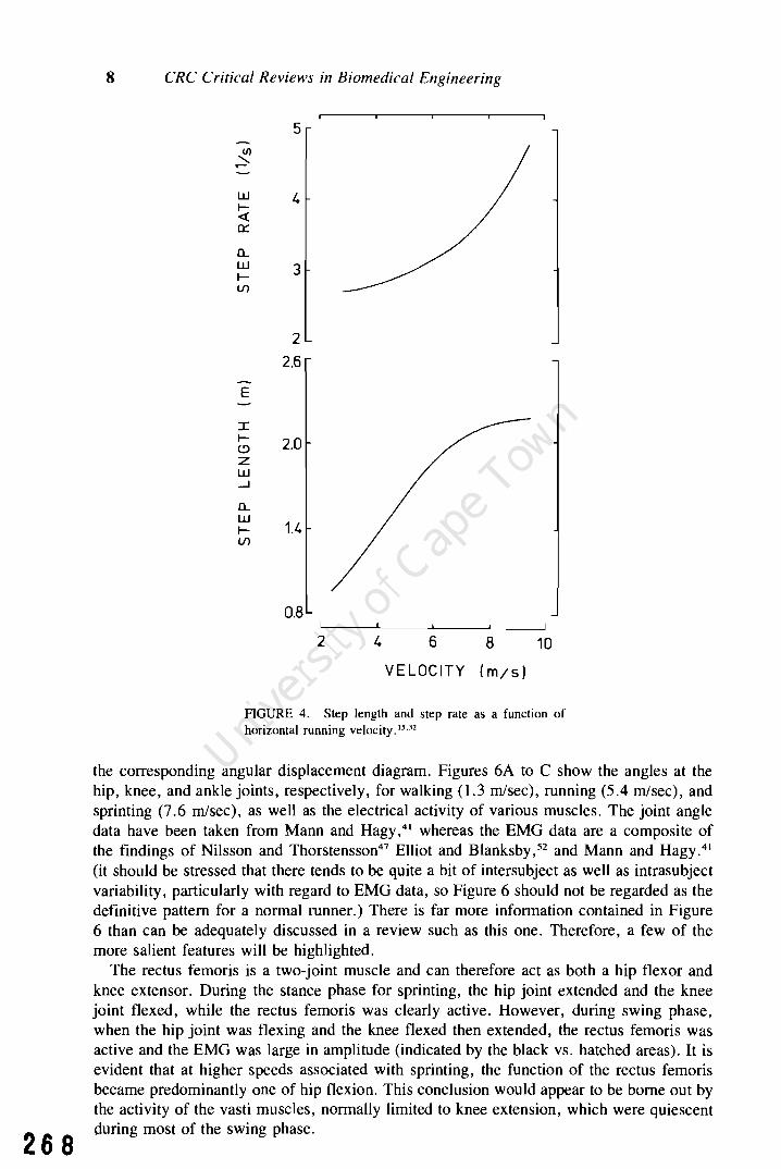
268

8 CRC Critical Reviews in Biomedical Engineering

W I­« 0:::

0.... W l­ll)

E

I l­e:> z w ~

0.... W l­ll)

5

3

2

2.6

2.0

1.4

0.8

2 4 6 8

VELOCITY (m/s)

10

FIGURE 4. Step length and step rate as a function of horizontal running velocity.'5.J2

the corresponding angular displacement diagram. Figures 6A to C show the angles at the hip, knee, and ankle joints, respectively, for walking 0.3 m/sec), running (5.4 m/sec), and sprinting (7.6 m/sec), as well as the electrical activity of various muscles. The joint angle data have been taken from Mann and Hagy,41 whereas the EMG data are a composite of the findings of Nilsson and Thorstensson47 Elliot and Blanksby,52 and Mann and Hagy.41 (it should be stressed that there tends to be quite a bit of intersubject as well as intrasubject variability, particularly with regard to EMG data, so Figure 6 should not be regarded as the definitive pattern for a normal runner.) There is far more information contained in Figure 6 than can be adequately discussed in a review such as this one. Therefore, a few of the more salient features will be highlighted.

The rectus femoris is a two-joint muscle and can therefore act as both a hip flexor and knee extensor. During the stance phase for sprinting, the hip joint extended and the knee joint flexed, while the rectus femoris was clearly active. However, during swing phase, when the hip joint was flexing and the knee flexed then extended, the rectus femoris was active and the EMG was large in amplitude (indicated by the black vs. hatched areas). It is evident that at higher speeds associated with sprinting, the function of the rectus femoris became predominantly one of hip flexion. This conclusion would appear to be borne out by the activity of the vasti muscles, normally limited to knee extension, which were quiescent during most of the swing phase.

Volume 12, Issue I 9

""0 1800

c ········3.8 m/s (}) ...... - -5.6 m/s X (})

--7.5m/s

W -..J ~

<.9 Z :

« :

W 90

0

'. w -" ... -.' z \ / + ~

\ / ~ / x IFS :--.....

o ITO -~

x • CFS ()) + CTO - 0

0

1800 270 0 360 0

extend THIGH ANGLE flex

FIGURE 5. Knee joint angle vs. thigh angle for an elite female distance runner at three different speeds. IFS, ipsilateral footstrike; ITO, ipsilateral toe-off; CFS, contralateral footstrike; CTO, contralateral toe-off. (Adapted from Miller. D. I.. Can. J. Appl. Sports Sci .. 3,229, 1978.)

The lack of knee extension during the stance phase of sprinting (see Figure 6B) was described by Mann and Hagy41 to be a result of the sprinter having insufficient time to undergo any type of shock absorption. They ascribed most of the absorption of initial ground contact forces to the slight dorsiflexion at the ankle joint seen in Figure 6C. However, other authors 16.47 have shown that this flexion/extension peak does occur in the stance phase of sprinting. In a commentary on the paper by Mann and Hagy, 41 Drez stated that the significance of their data had to be treated with caution due to the small size of the sample group, but he encouraged them to study more normal subjects and to compare these data with injured subjects. There can be no doubt that this was extremely sound advice, not only for this group of researchers, but also for all workers concerned with the biomechanics of running.

A marked difference between walking and running was evident for the control of the ankle joint. The plantar flexion following heel strike in walking (Figure 6C) was accompanied by activity in the tibialis anterior, a dorsiflexor. Later on in the stance phase when dorsiflexion occurred, the gastrocnemius, a plantar flexor, became active. In running, where touchdown normally took place towards the forefoot, dorsiflexion began immediately. This motion was accompanied by large activity in the gastrocnemius which started during the second half of the swing phase. Thus there appeared to be a change in the coordination of the calf mus­culature as the subject progressed from walking to sprinting.

While most workers have concentrated on those muscle groups that control movement in the sagittal plane, Thorstensson et al,38 and Nilsson and Thorstensson.47 have studied the erector spinae muscles which control trunk movement in the frontal plane. A comparison of walking and running may be seen in Figure 7 in which T F represents lateral trunk flexion with upward being ipsilateral,38 The basic activity of the erector spinae muscles was quite similar for walking and running, with peaks occurring bilaterally at each touchdown. How­ever, for walking, the EMG amplitude was larger for the ipsilateral muscles when the spine was moving contralaterally and vice versa. In running, the erector spinae activity became.

269

270

10 CRC Critical Reviews in Biomedical Engineering

80

x Q)

~

W -l (::>

Z « a.. I 40

"0 C Q) +-x Q)

50 % CYCLE

A

r f

r f ~-~h

9 mo

rf ~~h

9 mo

100

FIGURE 6. Angles at (A) hip, (B) knee, and (C) ankle for walking (l.3 mlsec), running (S.4 mlsec), and sprinting (7.6 mlsec).41 The EMG data41.47.s2 have three levels: blank means little or no activity, cross-hatching means moderate activity, and black indicates a large amount of activity. Muscles are abbreviated by rf, rectus femoris; h, hamstrings; g rna, gluteus maximus; v, vasti group; g, gastroc­nemius; t a, tibialis anterior. The cycle starts and finishes at ipsi­lateral heelstrike and the vertical dashed lines indicate ipsilateral toe-off.

far more symmetrical, and this was correlated with forward inclination of the trunk. Thor­stensson et al. 38 therefore argued that the function of the erector spinae was to brake lateral trunk motion in walking and forward trunk motion in running. Although the Swedish studies were limited to locomotion on a level treadmill, it may be speculated that uphill running, which requires a pronounced forward lean of the trunk, would almost certainly predispose a runner to lower back pain due to the increased load placed on the erector spinae.

The data presented in Figures 6 and 7 compare angular kinematics and EMG. As stressed by Miller,16 it would be very useful to examine angular kinetics, i.e., joint forces and moments, and EMG data simultaneously. Some pioneering work on this was done by Elliot and Blanksby, 52.53 although their studies had two shortcomings. First, they presented their moment data in discrete, digital format (i.e., tables) rather than the more easily assimilated analog format (i.e., graphs). Second, they only calculated the moments for the swing phase since they used a treadmill for their studies and could not measure ground reaction forces with a force plate. More recently, a three-dimensional analysis of resultant moments in upper extremity joints and their relationship to EMG have been reported by Hinrichs. 18 He too used a treadmill, but did not have to contend with problems of external forces associated with lower extremity studies. Interestingly, Hinrichs found that the resultant moments closely followed the EMG activity, especially at the elbow joint, and this activity increased signif­icantly with increased running speed.

D. Ground Reaction Forces Although the topic of kinetics will be covered in more depth in a later section, the ground

Volume 12, Issue] 11

120 -I SPRINT

rf

)( y (lI

0

w 0 --J IRUN C) 120 z c{

w w z rf ~

60 y

h '0 C

~ )( Ql

FIGURE 68

SPRINT

til '-0 9 '0

azm to 0

w RUN --J C)

Z c{

9 w :

--J t a ~ z c{

I-0 C 0 0 Ci

PlZlmamlllWWiuma 9

0 50 100 % CYCLE

FIGURE 6C

271

12 CRC Critical Reviews in Biomedical Engineering

ERECTOR SPINAE EMG

walk 1.5 m/s

run 2.5m/s

o 100

ipsi

contra

ipsi

contra

walk 2.5m/s

run 6.0m/s

o 100

FIGURE 7. Muscle activity in the erector spinae and the lateral trunk flexion angle T F for walking and run­ning. The cycle starts and finishes at ipsilateral heel­strike. (Adapted from Thorstensson, A., Carlson, H., Zomlefer, M. R., and Nilsson, 1., Acta Physiol. Scand., 116, 13, 1982.)

reaction forces (GRF) for walking, race walking, and running have been included here for the purpose of comparison. 2 Again, it should be realized that the data in Figure 8A to C are for a single trial of one subject - an experienced race walker - and should be studied with this point in mind.

For walking, the vertical GRF had the familiar double-humped pattern with its magnitude being just above, below, and above body weight, respectively. In race walking, this pattern disappeared and in running, there was a large initial peak about five times body weight and described by NiggS4 and others as the "passive" phase. It was described in this way because the duration of this peak was So short, about 10 to 15 msec, that the muscles did not have sufficient time to absorb the impact in an interactive manner.

The horizontal forces were smaller in magnitude, but nevertheless important in controlling the forward motion of the human locomotor apparatus. As we would expect, the subject first experienced a posterior (braking) force followed by an anterior (driving) force, with the areas under these curves, i.e., the impulse, being approximately constant. This was consistent with the impulse-momentum relationship and the fact that the subject was pro­gressing at approximately constant vecocity in each of the three figures. Although the mediolateral forces were extremely small in walking (certainly less than a quarter body weight), these forces were quite substantial in race walking. This can be understood by referring to Figure ID and noting the exaggerated movements in the frontal plane.

III. COMPUTER MODELING AND SIMULATION

A. Definitions It has been said by Miller l6 that the basic methods used to study the biomechanics of

2 7 2 running gait today differ little from the classic studies of Muybridge, 9 Furusawa et al., 11

, .

~ 2BW] z o I­u « w

posterior /

Volume 12, Issue 1 13

---- .....

-------

, ' 0:: .lBW 2

anterior .....

medial lateral

;/ ....... <::.=="'" //-'---. __ ._._._._.---'--'---.~ -l..-=:-'---'-"-"":'.

- ;;;< ~-o z :::)

o 0:: (.9 --0.15--- TIME

A

\I/~ ~ ~ ! 2BW\ vertical , o ~~~~-L~ ____ ~, ________________ ~~ ______ __

I I \

I­U « W ..!.BW 0:: 2

o Z

.:::) o 0:: ~

posterior ./ anterior

medial lateral

\ \ ---- ...

-0.15- TIME

B

FIGURE 8. Ground reaction forces for (A) walking, (B) race walking, and (C) running. (Adapted from Payne, A. H., Biomechanics VI-A, Asmussen, E. and Jorgensen, K., Eds., University Park Press, Baltimore, 1978,293.)

273

274

14 CRC Critical Reviews in Biomedical Engineering

If)

w U 0:: " 0

2BW II ('

LL II II , I

" , I

Z vertical II , 0 , \

l-II , \ I I ,

U , " « 'r" w ,,", \

0:: :)1. \

0 posterior

l i \ z anterior

'1 ::::> .lBW I. \ I

0 . 1 ."'--... \ I 0:: 2

'" I t9 medial 1· I \ /

.' .,........L---lateral \'-' I

\

I . \ \ I . I ,,,

\ . U -0.15- TIME

FIGURE 8C

Fenn, 12 and Elftman l3 performed over half a century ago. However, one big advantage which we do have with modern-day technology is the digital computer. Aside from its ability to capture and analyze raw data from a running human (e.g., a digitized movie film or a force plate record), the computer has an extremely powerful and versatile role to play in modeling and simulation. In a general treatise on the computer simulation of human motion in sports biomechanics, Vaughan55 suggested the following two definitions:

I. Computer modeling refers to the setting up of mathematical equations to describe the system of interest, the gathering of appropriate input data, and the incorporation of these equations and data in a computer program.

2. Computer simulation is reserved to mean the use of a validated computer model to carry out "experiments" on the real-world systems that have been modeled under carefull y controlled conditions.

These two definitions have been embodied in Figure 9, where A depicts the activity of computer modeling, while B is concerned with computer simulation. The steps in this procedure therefore include defining the problem, developing the mathematical model, writ­ing the computer program, determining the input values, validating the model, and per­forming simulation experiments.

(a)

modify equations and program

no

Volume 12, Issue I 15

INPUT parameter values,

boundary and intial conditions on vcriables

(b)

no

FIGURE 9. A flow chart for (a) computer modeling and (b) computer simulation. (Adapted from Vaughan. C. L.. Exercise Sports Sci. Rev .. 12, 1984.)

B. Advantages and Disadvantages It is pertinent at this stage to pose the question: "Of what use is computer simulation in

the study of running gait, and what are the possible drawbacks?" It is the exploratory nature of computer simulation that offers the greatest advantage. It is able to answer the' 'what if" questions. These include questions such as "What would be the sprinter's time for 100 m if she increased her initial acceleration by 1O%?"; "What would be the loading in the medial compartment of a marathon runner's knee if his running shoes had a larger flare?"; and "What would be the optimum race strategy for the 1500-m runner if his best 400-m time was 56 sec?". The list of questions is probably endless.

There are, in addition, other advantages to the computer simulation approach. The first is safety: the runner is saved from having to perform potentially hazardous experiments. Instead of the athlete having to wear a new and untried design of shoe orthotic (thus risking soft tissue or other injury), an experiment could be performed on the computer using the athlete's normal running pattern as input parameters. A second advantage is time: many different simulations can be done in a matter of seconds or minutes (e.g., working out different race strategies), whereas with traditional techniques hours or days would be required to achieve the same variety of choices. A third advantage is the potential to predict optimal performance: because we are able to isolate and control selected variables while others are held constant, we can pinpoint the best methods using mathematical optimization theory. A fourth advantage is cost saving: it would be much cheaper to run a series of simulations for the design of a new training shoe than to actually fabricate a range of physical models. A fifth advantage has been the development of inexpensive, yet powerful, microcomputers and programmable calculators which can be used for simulation studies down at the track. 37 The high resolution graphic displays which can be obtained with microcomputers make the simulation procedure that much easier to interpret and therefore implement.

Computer simulation is by no means a panacea for all the problems encountered in the biomechanics of running gait. 55 Perhaps its most important shortcoming is the difficulty we

27 5

276

16 CRC Critical Reviews in Biomedical Engineering

FIGURE 10. Free body diagram of the forces acting on a runner. Refer to text for details of the forces. (Adpated from Vaughan, C. L., Int. J. Bio-Med. Comput., 14, 65, 1983.)

encounter when trying to validate the computer model, a point argued succinctly by Panjabi. S6

He highlighted the dilemma of a mathematical model being validated only in a given number of known situations, and yet the main purpose of the model being to predict behavior in unknown situations. This point is particularly pertinent in biomechanics models of running gait. Vaughan and MatraversS7 showed how previous researchers ll ,s8-60 who modeled the forces acting on a sprinter used unsound physical reasoning, but nevertheless achieved reasonable predictions for the athlete's velocity-time curve. A further problem that has precluded the widespread use of computer simulation in running biomechanics has been the difficulty in translating the simulated results into a practical setting. A partial solution to this problem would be for researchers to attempt to publish two accounts of their research findings: one in a scholarly research publication, and another in an appropriate journal or lay publication where the emphasis is placed on describing the results in an easily understood and assimilable form.

Despite the obvious advantages of computer simulation in studying running gait, it is surprising how seldom this technique has been used in the past. This is particularly unusual in view of the great deal of attention that has been devoted by biomechanics and robotics researchers to simulation of walking gait. 55 The rest of this section will be devoted to those few papers that have made use of computer simulation to study running per se.

c. One Degree-of-Freedom Models The computer simulation of running using a single differential equation can best be

reviewed by studying the free body diagram of a runner as illustrated in Figure 10. The external forces acting on the runner are the ground reaction force (which may be resolved

Volume 12, Issue 1 17

into two orthogonal components, a horizontal driving force Fo, and a vertical supporting force Fs), the athlete's weight W, and air resistance FR. For the present model, neither the supporting force Fs nor the weight W has been considered, since their imbalance merely causes the upward or downward acceleration of the runner's center of mass. The aim of a race is to cover a set horizontal distance in the minimum time and for this reason only the horizontal forces are considered for the model. Note, too, that the runner is assumed to be moving in the mid-sagittal plane, so that rotation about a longitudinal or frontal axis as well as mediolateral forces have been ignored. The differential equation governing the forward motion of the runner is

dv M - = Fo - FR

dt

where M is the runner's body mass and dv/dt his rate of change of velocity.

(2)

In the early 1970s, Keller59.6o published some theoretical work on running which has

proved to be a stimulus for at least two other groups of researchers. 57.61 Although Keller did not appear to be aware of the fact, he used virtually the same reasoning as Furusawa et al. II and Henry and Trafton58 to derive the identical velocity-time equation for sprinting. With reference to Figure 10 and Equation 2, he argued that the driving force Fo should be a constant maximum for sprinting, since the runner would be attempting to exert maximum effort throughout the race. He also assumed the resisting force FR was proportional to velocity, but was uncertain whether this force was internal or external or a combination of the two. In addition, his model used equations of energy balance and calculus of variations to predict world record times for distances between 50 and 10,000 m. He achieved good agreement (the absolute errors were less than 3% in all cases), although his model did produce an unusual result: it predicted that for races longer than 291 m (which he defined as the maximum sprint distance) the runner should actually slow down during the last few meters. In order to explain this optimal race strategy, he described the analogy of a car with a limited amount of gas traveling a set distance in the shortest time, using the fuel up shortly before the end, and "freewheeling" to the finish line.

Vaughan36.37.57 has argued that the driving force Fo of Equation 2 should not be a constant maximum, but should actually decrease as the sprinter's velocity increased. This would be consistent with the experimental work of Baumann62 and others. The exact form of Fo was not a very straightforward choice since in reality it is discontinuous; during the airborne periods of sprint running (see Figure 2) neither foot is on the ground and therefore no driving force can be exerted. Another complication is that just after heel strike , Fo is actually a braking force unless the foot is moving backward faster than the runner's center of mass is moving forward at heelstrike. Nevertheless, Vaughan36 chose a form of Fo that appeared to be reasonably consistent with experimental data and also gave good predictions. In contrast to Keller, 59 Vaughan36 assumed that the air resistance force FR should vary as the square of the velocity, which would be more consistent with the accepted principles of fluid mechanics. The simulated displacement, velocity, and acceleration curves predicted by the model for an Olympic athlete are shown in Figure 11. Since a sprinter is never able to run at his maximum velocity indefinitely, there is a point at which the model must no longer be applicable. Of course the stage at which this occurs depends largely on the physical ability and state of fitness of the runner. For world-class runners such as Pietro Mennea, the 200-m record holder, their decrease in speed over the second half of a 200-m race is only a few percent. Some of the advantages of Vaughan's modeP7 were that it could be (I) applied to all classes of sprinter, both male and female; (2) used to ascertain where a sprinter's strengths and/or weakness might lie; (3) utilized to predict a sprinter's time for a given race distance; and (4) used by the coach in the field since it has been implemented with a programmable

277

278

18 CRC Critical Reviews in Biomedical Engineering

12

10 N 0 v

VI

" • E E 8

VI z "

I-

0 E z 6 w I- ::E <t 0: r w w I- U

<t 4 ..J U ..J W 0 n.. u ..J V') U w

<t > 0 2

<t > 0 0 A

-2

0 2 4 6 8 10 12

TIME (5)

FIGURE II. The simulated displacement, velocity, and acceleration curves predicted for an Olympic sprinter. (Adapted from Vaughan, C. L., Int. J. Bio-Med. Comput., 14,65, 1983.)

calculator and inexpensive equipment. Its major disadvantage was that it was limited to sprinting: since it did not attempt to model any of the physiological parameters which may have some effect on performance, it could not be applied to running distances greater than 200 m.

Senatof>l extended Keller's theory of sprint running with the ultimate goal being to achieve a better agreement between measured oxygen uptake and Keller's estimate of the maximum steady-state rate of developing energy in a runner's muscles. To do this, he allowed the resisting force FR to be proportional to some positive power n of velocity (Keller used n =

1, and Vaughan used n = 2), and the driving force Fo to vary during the race. However, his strategy for varying Fo would appear to be inconsistent with experimental findings62

since he proposed that the sprinter would need to exert larger forces as sprinting speed increased. All his data analysis and attempts at validation were performed using world­record times of races under 220 yards (201.2 m) from 1960 to 1979. He was unable to determine the optimal value for n and concluded that accurate displacement-time data (to a precision of 1 msec) for the critical start-up region (0 to 20 m) would be required.

D. EtTects of Air Resistance The effects of air resistance were modeled by Hill over half a century ago. IO The most

accepted form for FR has been

(3)

where p is the density of the air; Co is a dimensionless drag coefficient; A is the projected or cross-sectional area of the runner; and v is his velocity. 16.57.63.64 The most difficult of these parameters to evaluate is Co and some of the most useful research in this area was performed by Shanebrook and laszczak. 64 They modeled the runner using a series of con-

Volume 12, Issue I 19

jugated circular cylinders to simulate the trunk and appendages, and a sphere to simulate the head. They found that CD varied from 1.10 to 1.14 and the corresponding values for FR (at v = 10.1 mlsec) were of the order of 25 to 40 N, depending on the runner's build.

Pugh65 and more recently Kyle6J have performed simulations to predict the speed of runners traveling in groups and therefore shielding themselves against the retarding effect of air resistance. With a shielding factor of 40% and a mechanical efficiency of doing work against wind resistance of 40%, Kyle predicted a lap saving of 1.4 sec at a speed of 6.1 m/sec. At world-record pace for the mile or 1500 m, the time saving would be about 1.75 sec per lap. He therefore proposed a strategy for a national team race in which a record pace would be maintained for three laps by rotating the runners at the front while shielding the ultimate winning individual. The reason why such a formal and systematic use of pacing is not widely used at present may lie in the possibility that success in middle distance running is determined more by psychological and physiological factors rather than mechanical ones such as air resistance. Kyle's simulations nevertheless have some intriguing possibilities.

E. Multidegree-of-Freedom Model While most researchers have considered the runner to be modeled by a single degree-of­

freedom system - which obviously simplifies the mathematics considerably - Bourassa and Morel66 have recently developed a nine-segment model for simulating the human running motion. They set up their model using standard Lagrangian formulation and treated the problem as an initial value one: the resultant joint forces and moments were specified as a function of time and numerical integration was performed to yield the kinematic parameters. These authors did not generate their own input data, and since they were forced to use incomplete data from the literature, a rigorous validation could not be performed. Instead, they used an inadequate trial-and-error procedure to demonstrate the possible applications of their model. However, it is anticipated that these and other authors will validate such models properly in the future and the models should then prove to be useful in studying both the forward and the inverse problems of biomechanicsY

F. Design of Running Tracks In a somewhat different application to those studies already reviewed in this section,

McMahon and Greene68•69 used computer simulation modeling to aid them in the design of

an indoor track facility for the Harvard University track team. Their physical model of the runner's leg is illustrated in Figure 12A and consisted of a rack and pinion element connected in series with a damped spring. The role of motor commands from higher neural centers was modeled by a rack and pinion element, the stiffness of the muscles was modeled by a spring, and the force-velocity relationship of skeletal muscle and the rate-dependent sensi­tivity of the reflexes were modeled by a dashpot. The rack and pinion therefore positioned the leg prior to ground impact, setting up the hip, knee, and ankle angles. The reaction to external forces such as the runner's weight and the vertical impact of the track on the contact leg - was modeled by the deflection of the damped spring. Since the rack and pinion determined the lower extremity joint positions at the beginning and end of the ground contact phase, it therefore dictated the step length (the authors defined this as the distance the body moved forward while one foot was on the ground). The body motion during the ground contact phase was controlled by the damped spring which thus determined the ground contact time. Once a few simple items of information - the runner's mass, leg length, spring stiffness, and his step length and maximum horizontal velocity on a hard surface - had been gathered, this simplified model allowed the researchers to calculate the effect of track stiffness on step length and ground contact time. Their challenge, therefore, was to see what value of track compliance, if any, would optimize running speed (they defined this as the ratio of step length to ground contact time). They were looking for a "tuned" track which

279

280

20 CRC Critical Reviews in Biomedical Engineering

u L.

0 L.

...... "'-

.:::t. u 0 L. ...... ......

r­u « r­z o u o z ::::> o n::: (9

3.0

2.5

2.0

1.5

"0 00

A

o measurement - theory

1.0 ---------.

0.1 10 100

STIFFNESS ktrack/kman

B

FIGURE 12. (A) Model of a runner's lower extremity to represent the separate role of descending commands (rack and pinion) and muscle prop­erties plus local reflexes (damped spring). (B) Normalized ground contact time VS. normalized track stiffness. Note: both axes are plotted on a log­arithmic scale. (Adapted from McMahon, T. A. and Greene, P. R., 1. Biomech .. 12, 893, 1979.)

would maximize step length and simultaneously minimize ground contact time. The results of the simulation experiment using their theoretical model may be seen in Figure 12B, where normalized ground contact time has been plotted against normalized track stiffness. There are two points of interest in this figure. First, the measured data (which were gathered using eight subjects, a high speed movie camera, a force platform, and three types of track -foam rubber pillows, wooden track with adjustable compliance, and concrete floor) agreed rather well with the theory of the model. Second, and of particular interest, was the fact that the theory predicated a minimum ground contact time for a track with stiffness inter­mediate between the soft pillows and the hard concrete, a stiffness factor of two to four times that of the athletes. The corresponding curve for step length was very slightly elevated (compared to the hard surface) at this intermediate stiffness which meant that according to their theory, a tuned track did indeed exist. In fact, a speed enhancement of between 2 and 3% was predicted.

Volume 12, Issue 1 21

McMahon and Greene had a unique opportunity to test the validity of their model in the practical environment. An indoor track, consisting of a polyurethane top surface and a substructure made primarily of wood, was built in 1977. The substructure was designed to have a stiffness of between two and three times that of the average athlete. The authors were, perhaps understandably, enthusiastic about the effects of the new track. They presented data to show how middle distance runners, both those from Harvard and other institutions, had a speed advantage of between 2 and 3%, exactly as their model had predicted. 69 An important conclusion was that the real advantage of the tuned track was probably not speed enhancement - the opposition ran faster on it, too - but comfort and safety. On a subjective basis, it was noted that the Harvard team had experienced fewer injuries during the first year the track had been in use despite their apparently heavy training sessions. While some of the conclusions of the authors would need to be substantiated by more rigorous and long­term studies, the results of their work certainly provide encouraging evidence of the power of computer modeling and simulation. Their final remark that "no outdoor track of the optimum mechanical design has yet been built, but if it were the mile record could be improved by 7 seconds" stands as a challenge. 68 To what extent this challenge has been met in the last 5 years is not known, unfortunately.

IV. KINETICS OF RUNNING GAIT

A. Forces and Pressures Acting on the Foot As mentioned in the first section of this paper, the foot is normally the only part of a

runner's anatomy that is able to interact mechanically with the environment. It is therefore logical that in their pursuit of a better understanding of the running human, researchers have studied the ground reaction forces (Figure 8). The device which is normally used for this purpose is the force platform, one of the earliest being that of Fenn,12 and illustrated in Figure 13. Although the principles of force platforms have changed little since the time of Fenn, some of the technical details have changed radically. The springs and turnbuckles have been replaced by strain gauged or piezoelectric transducers, while the data are no longer recorded on a revolving drum but with the aid of a storage oscilloscope, magnetic tape recorder, or high-speed digital computer. Besides the early work of Fenn, other pioneers to have used force platforms to study running humans have been Tsujino,70 who described a type of "kick-board", Payne,2 and more recently Cavanagh. 71 In addition to measuring the three orthogonal forces acting on a runner's foot (vertical, posterior/anterior, and medial! lateral), illustrated in Figure 8, modem force platforms are also capable of yielding the three orthogonal moments applied by the foot. Using these six signals, it is a fairly straightforward procedure, described by Cavanagh,71 to calculate the point of application of the resultant ground reaction force. This point is sometimes also referred to as the center of pressure and has been illustrated in Figure 14. What we see from Figure 14 is that at heelstrike, this point was located laterally on the running shoe. As the stance phase progressed, the center of pressure moved towards the forefoot and medially, passed through the mid-foot region, then along the second and first metatarsals until toe off from the hallux. One might be tempted to conclude that the mid-foot region was being subjected to large loads, particularly if the resultant ground reaction force vector was also superimposed on this diagram. However, this would be a fatal mistake, as emphasized by Cavanagh and Ae.72 The problem lies in the fact that force platforms are not able to give all the individual forces being exerted by different parts of the foot or shoe, merely the resultant ground reaction force. In order to examine the forces on the foot in greater detail, Cavanagh and Ae72 used a commercial device known as the Footprint@. This device consisted of 500 individual transducer elements that rested on a photoelastic material which was filmed from below with a high-speed movie camera. Each of the metal transducer plungers produced a circular pattern, the diameter of

281

282

22 CRC Critical Reviews in Biomedical Engineering

(a)

( b) (c)

FIGURE 13. An early force platform (circa 1930) illustrating (a) the recording drum, (b) the transducer arrangement, and (c) the platform installed in a runway. (From Fenn, W.O., Am. 1. Physiol., 93,433, 1930. With permission.)

.. . .. . . . . . .. . .'y". , . • ."'"""-., . J •• • ..- r·-

--.

FIGURE 14. Center of pressure location during right foot contact for a subject running at 4.3 mlsec. (Adapted from Cavanagh, P. R., 1. Biomech., 11,487,1978.)

which was related to the applied pressure. The pressure estimate from each transducer was plotted as the component perpendicular to the plane of the shoe outline. In this manner, a continuous surface was formed where the height of the surface above the ground plane was directly proportional to pressure, as shown in Figure 15. In this figure, which is for walking, the pressure in the rear-foot region at 0.08 sec after footstrike may be compared with the pressure across the metatarsals at 0.32 sec. At times intermediate between these two, Ca­vanagh and Ae72 showed that there was little or no mid-foot loading, as would be indicated from Figure 14, but that the load was shared between the rear and forefoot. Another manner in which Cavanagh displayed these pressure profiles was in an animated movie generated by photographing a sequence of plots frame by frame. 4

•73

While it is clear from Figure 15 that plantar pressure profiles yielded useful information, the procedure nonetheless suffered from a few drawbacks. First, the method was very labor intensive, as each of about 70 transducer circles for each frame had to be manually digitized; second, it would appear that the Footprint® device behaved differently under static and

Volume 12, Issue 1 23

0.9 MPa

0.085

0.325

FIGURE I S. Pressure between the shoe and the ground at two instances of the stance phase of normal slow walking. (Adapted from Cavanagh, P. R. and Ae, M., J. Biomech., 13,69,1980.)

dynamic conditions, making calibration extremely difficult;72 third, the equipment and there­fore the subsequent display (Figure 15) only provided force information normal to the ground plane, whereas the horizontal components clearly have an important role to play (Figure 8); fourth, and perhaps most significant, the pressure that was measured existed at the ground/ shoe interface and not at the shoe/foot interface. This last point is certainly not a new one, as demonstrated by the equipment illustrated in Figure 16 and used by Marey in 1886.

More recently, pioneering work on an in-shoe pressure transducer has been done by Hennig et al. 74 and by workers at the Langer laboratories who have developed the Electro­dynograph (EDG).5 This latter device, which has been available commercially since 1982, consists of seven miniature and unobtrusive transducers that are attached to the plantar surface of each foot. The signals are analog-to-digitally converted and stored using a small microprocessor device carried by the patient. Once the patient has completed the trial of interest, the data are fed via a serial link to a second microcomputer for processing and display. It is anticipated that this and other devices will play an important part in the future understanding of foot function and in the diagnosis of lower extremity pathology.

283

24 CRC Critical Reviews in Biomedical Engineering

B. Internal Pressures

FIGURE 16. An early attempt by Marey in 1886 to monitor the pressure at the shoe/foot interface of a runner (Reproduced with permission from University Park

Press).

Grillner et al. 75 used a Millar tip pressure transducer to measure the intraabdominal pressure (lAP) intragastrically for 13 subjects. In addition, EMG activity of the abdominal muscles was recorded with surface electrodes as the subjects walked and ran on a motor-driven treadmill and force plate. They demonstrated substantial increases in pressure (a peak lAP of 20 mmHg for walking at 2.5 m/sec, and 32 mmHg while running at 5 m/sec). The increases in lAP were phasic and occurred when the vertical load on the body - indicated by the force platform - increased. The rise in lAP was also associated with increased EMG activity in the muscles of the abdominal wall, although the authors stressed that muscle activity occurred prior to footstrike. They speculated on the "shock-absorbing" capacity of the abdominal cavity and noted that an insufficiency in abdominal muscle function was one possible factor in the etiology of back pain. The inference was that patients unable to build up adequate lAP would tend to load their spines more heavily, and thus be more susceptible to back pain. However, Grillner et al. 75 did recommend that further work be done to establ ish whether runners with low back pain not only have weak abdominal muscles, but also the inability to build up adequate lAP.

McDermott et al. 76 presented the early results of a new technique, using a device which they named a solid-state transducer intracompartmental (STIC) catheter, to measure dynamic pressure changes in the anterior compartment of the calf. They studied 9 patients with exercise-induced anterior compartment syndrome and compared them with 11 asymptomatic male controls. They recorded anterior compartment pressures (ACPs) with the subjects walking and running on a treadmill. While there was no statistical difference for the control vs. the symptomatic group for walking (46 ± 12 vs. 74 ± 23 mmHg), the difference for

28 4 running (66 ± 16 vs. 106 ± 18 mmHg) was statistically significant at the 0.001 level. On

Volume 12, Issue 1 25

the basis of their findings, they argued that it was more appropriate to use functional ACPs rather than resting supine values in the diagnosis of anterior compartment syndrome, and that for running any value greater than 85 mmHg should be considered abnormal. Although the authors would have liked to measure EMGs simultaneously as was done by Grillner et al.,75 they were sufficiently satisfied with the STIC catheter technique to conclude that it provided an objective measurement for selection of patients for fasciotomy.

C. Resultant Joint Moments It is the resultant joint forces and moments that play the important causative role in human

movement, whereas the kinematics, described in the first section of this paper, are the effect. 67 For this reason, joint moments have received particular attention from biomechanics researchers over the years. In order to calculate the resultant moment acting on a segment at a particular joint, we need to know the linear and angular acceleration of the segment (i.e., kinematics), the segment's mass and principal centroidal moments of intertia (i.e., body segment parameters), and all other forces and moments acting on the segment. This is the classic inverse dynamics problem. The procedure is simplified considerably if one starts at a free-swiming distal segment, where the only other force acting besides the proximal joint force and moment is the segment weight. One can then move in a proximal direction, solving the joint forces and moments sequentially. It is for this reason that the majority of researchers have calculated moments in the ankle, knee, and hip joints of the recovery leg. The first of these was Elf tman, 13 followed more recently by Elliot and Blanksby, 52 Miller, 49 and Chapman and Caidwelpi Of course it would have been possible for these workers to have extended the analysis from the other free distal extremities and so on down to the joints of the support legY The problem with this approach would be the degradation in joint moment accuracy due to errors introduced by the segment kinematics and body segment parameters.

In a basic variation of the angle-angle diagram discussed earlier (see Figure 5), Miller49

has plotted the hip and knee moments for the recovery leg as a function of the joint angle. Figure 17 shows the data for the sound limb of a below-knee amputee running at 6.4 mJ sec. It is clearly evident from this figure that the knee musculature tended to act eccentrically throughout most of the recovery phase, whereas the hip musculature acted concentrically except for a short period prior to contralateral toe-off. Also of interest is the fact that the range of the hip moment (about 300 Nm) was considerably more than that of the knee moment (about 100 Nm). The problem with diagrams such as Figure 17, however, is that they beg the question: what happens between ipsilateral footstrike and ipsilateral toe-off, i.e., the all-important stance phase?

There have been surprisingly few researchers who have attempted to answer the above question, probably due to the problems and expense of using a force platform (especially in conjunction with a treadmill). The most notable studies to have calculated the joint moments throughout the running cycle are those of Aleshinsky and Zatsiorsky, 17 Mann and Sprague,21 Mann, 22 and Winter. 23.24

Of these studies, the most detailed was certainly that of Aleshinsky and Zatsiorsky, 17 who calculated the three-dimensional forces and moments in all major joints for walking, race walking, and sprinting. A novel feature of their paper was the superposition of the joint members on a stick-figure diagram of the subject which could be viewed from anyone of three orthogonal directions. Because the purpose of their paper was to emphasize their computational techniques, the data presented for the joint forces and moments were dis­appointingly incomplete, It is possible, however, that more comprehensive details could be found in some of their papers published in Russian.

The sprinting data of Mann21.22 and the jogging data of Winter2J.24 have been combined to yield Figure 18. In Figure 18A, where the hip moment has been plotted as a function of

285

286

26 CRC Critical Reviews in Biomedical Engineering

x 100 ())

'+-

E ito

z 0.... 0 I

l- I I

Z f

W ,

~ 0 ifs L

I-100

z - concentric - - - eccentric 0 -,

I-Z « 200 I- 100 160 220 ---l ::J

100 If)

w .-0:: cta .... ... ~.-' . ... I

/ •• /

W . Ifs I w I

l:J Z I

c: 0 ,.

()) ~ ~ _-·ito ..... • cfs /.-X ()) ' ... -~ .... .....

0 40 80 120 160

flex JOINT ANGLE (0 ) extend

FIGURE 17. The resultant moments at the hip and knee joints for the sound limb of a below-knee amputee plotted as a function of the joint angle. Note: the data points are 0.02 sec apart and the key to the different events (ito, cfs, etc.) may be found in Figure 5. (Adapted from Miller, D. I., Collected Papers on Sports Biomechanics, Wood, G. A., Ed., University of Western Australia, Perth, 1983,74.)

the running cycle, the values during the stance phase of sprinting were considerably greater than the recovery phase values. (This serves to demonstrate the inadequacy of studies which present only the recovery phase moments as in Figure 17). In comparing the hip moments for jogging and sprinting in Figure 18A, they were phasically quite similar (especially if one considers the difference in stance period), although the jogging moments did not vary much in magnitude between stance and swing. Clearly demonstrated is the importance in sprinting of the hip extensor moment just after footstrike, and the hip flexor moment just prior to toe-off. Presumably these larger moments were due to the shock absorption and vigorous push-off required by the sprinters. While the ankle moments were fairly similar for jogging and sprinting (except for the slight phase shift due to the difference in stance period) as seen in Figure 18C, the same could not be said for the knee moments of Figure 18B. In sprinting, a knee flexor moment was dominant for the first one third of the stance phase. Mann22 attributed this knee flexor dominance to the purpose of decreasing the hor­izontal (retarding) ground force immediately following footstrike. During the latter part of the stance phase, for both jogging and sprinting, the knee extensors were dominant, this being necessary to arrest the downward motion of the body (eccentric contraction) and then to produce positive horizontal and vertical velocity prior to toe-off (concentric contraction).

Volume 12, Issue 1

toe off x sprint jog Q)

..... 300 I I I

E z

100 I-Z 0 W ........ ::E '-0 100 ........

--' ::E

0...

:r: 300

\J C Q) 0 50 100 ...... x

% CYCLE Q)

A

toe off x Q)

sprint ..... 300

jog

I I

E I z

I-Z W ::E

0 0 ::E

w w z ~ 300

\J C 0 50 100 Q) ...... x % CYCLE Q)

B

FIGURE 18. The resultant joint moment at (A) hip, (B) knee, and (C) ankle joints for jogging and sprinting. These curves have been drawn from the data presented by Mann and Sprague,21 Mann,22 and Winter. 23.24

27

As Miller16 has suggested, it is normally of most relevance to discuss the joint moments in conjunction with both the joint kinematics and EMG of those muscles crossing the lower extremity joints. This can best be done by comparing Figures 6 and 18, bearing in mind that these graphs have been adapted from different studies using different sUbjects. Other interesting observations are as follows: during the stance phase of jogging, the extensor moments peaked at different times - the hip at 5%, the knee at 15%, and the ankle at 25% of the cycle; when comparing the subjects jogging, Winter24 showed the coefficient of variation was lowest for the ankle, increased for the knee, and was highest for hip; during the latter part of the recovery phase, for both jogging and sprinting, the hamstring muscle group played the dual role of active hip extensor and knee flexor; successful sprinters exerted larger hip extensor and knee flexor moments for longer periods of time, thus increasing the potential for hamstring injury. 22

287

288

28 CRC Critical Reviews in Biomedical Engineering

1Il L-

a lJ 300

E z

I- 100 z w 0 L 0 L

w --1 ::L Z <{ 300 L-

a +- 0 c a 0.

toe off

sprint jog I

I

/ ./

/ /

/

I

/'

50 % CYCLE

FIGURE 18e

D. Individual Muscle and Bone Forces

100

As demonstrated above, the resultant moments clearly give considerable insight into the mechanics of joint function. However, these moments are limited in the sense that they are the resultant of all the individual muscle, bone, and ligament moments. They therefore tell us which is the dominant muscle group, but nothing of the individual contributions to this resultant moment. The problem with trying to calculate the individual muscle and bone forces is that one runs into the question of indeterminacy: there are more unknown forces than governing equations. 67 Burdett3 has recently attempted to overcome this indeterminacy in a comprehensive study of three subjects running at 4.5 mlsec. He assigned the muscles crossing the ankle joint to five groups: plantar flexors, plantar flexors and invertors, plantar flexors and evertors, dorsi flexors and invertors, and dorsi flexors and eveI1ors. He combined three-dimensional data from cadaver dissection (to determine muscle origins and insertions) with force plate and three-dimensional movie data, and assumed that the inertial and grav­itational forces acting on the foot could be ignored. He further ignored the moments about the long axis of the foot, and assumed that only two tendons were exerting force at any instant, thereby yielding a minimum joint force. Figure 19 demonstrates the results that were obtained for the muscle and joint contact forces of one particular athlete. These forces, in the region of 10 to 13 times body weight, were clearly quite considerable and help us understand the possible problems that the runner may encounter. Despite the obvious short­comings in Burdett's procedure, particularly the absence of a partial validation using EMG, this paper has an extremely important contribution to make, and it is hoped that future papers will venture into this challenging territory. For it is only by knowing the individual soft tissue and body forces that we can truly understand the mechanical envrionment of the joints, particularly as applied to pathology.

A rather ambitious study, and one likely to create problems with human subjects com­mittees, was that performed by Lanyon et al. 77 They glued a strain gauge rosette to the anteromedial aspect of a subject's exposed tibia. They were thus able to compare strain rates and principal compressive and tensile strains for the subject walking 0.5 mlsec) and running (2.2 mlsec) with and without shoes. In general, the principal strains for running were about 50% greater than those for walking, and varied between 124 and 847 microstrain. Although the data presented in this paper should be regarded with a good deal of caution (they were from one subject only, and smaller strains were measured for increasing loads carried by the subject), this study nevertheless represents one of the very few attempts to measure in vivo forces acting on the human body while running.

A. Introduction

Volume 12, Issue 1 29

compressive I- 12 I <:)

W 3; 10

I->- U 0 «

8 0 I-CD Z

0 LL U

6 0 I-

W Z ....J 0 4 0- ...., anterior shear I- /----........ ....J ::> 2 r \... ~ / \ « "-

0 '-...

Vl « Vl 10 w U 0:: 8 0 LL

W w

6 ....J ....J U ~ Vl z ::> « ~ 4

2

0······· 0 20 40 60 80 100

% STANCE TIME

FIGURE 19. Individual muscle and bone (joint contact) forces at the ankle joint for an athlete run­ning at 4.5 m1sec. (Adapted from Burdett, R. G., Med. Sci. Sports Exercise. 14, 308, 1982.)

V. BIOMECHANICS OF RUNNING SHOES

A comprehensive review of running shoes, designed to bridge the gap between the layman and scientist, was published by Cavanagh 78 in 1980. It covered the history and evolution of the running shoe, how it was manufactured and tested, how it could help prevent injuries, and advice on choosing the correct shoe. It is strongly recommended for anyone interested in learning about running shoes.

Figure 20 illustrates the runner's primary piece of equipment: a pair of shoes. If one examines the shoes closely, it is evident that they are badly worn. This wear pattern has resulted from a number of factors: the materials of which the shoes were made, the terrain on which the runner trained, and, most importantly, the owner's running pattern. In fact, it is commonplace for runners visiting an injury clinic to take their running shoes with them as these can aid the physician in making the diagnosis and deciding upon the appropriate method of treatment. (In many cases this may include changing the type of running shoe altogether) .

289

290

30 CRC Critical Reviews in Biomedical Engineering

RGURE 20. A runner's primary piece of equipment: a pair of running shoes. These particular shoes, which are badly worn, gIve some indication of the manner in which the owner nomllilly runs.

Clearly. we cannot talk about the biomechanics of running gait without also considering research into the biomechanics of running shoes. Over the past decade, the most active and prominent researcb groups studying the interaction between runners and their shoes have been those at Pennsylvania State University ,4.74.78 Zurich,79.80 Calgary, 54.81·ft) Oregon, 84·89

and more recently at Shoe and Allied Trades Research Association (SATRA) in England,90 and Nikc (U .S.).9).9~.97 Evidence of the great interest thaI researchers have in the biome­chanics of running shoes is demonstrated by the fact that two world conferences, the first at Nijmegen. Holland. in 1982. the second al Calgary, Canada, in 1983, have dealt with only this special topic. The importance that shoe companies allach to biomechanical analysis and design of running shoes can be gauged by a number of factors. First. at least two of the leading companies have established their own running gait laboratories. costing hundreds of thousands of dollars. while many 01 hers perform research in association with independent consultants and university research institutions. 6 Second, a casual perusal of the advertising pages of running magazines will reveal marketing claims such as "to engineer exceptionaJ soling products with an expanded range of biomcchanical options". "by contouring the heel to match the radius of the average subtalar joint", and "the revolutionary material works to reduce impact force so that damaging peaks of pressure are reduced to healthy, gently rolling hills". As Cavanagh"' has highlighted, running shoe companies have ted the way in promoting research, especially on the biumechanics of running. with the aim being to produce a better running shoc - better in terms of safely, comfort, and performance.

Forthe past 9 years. a leading running magazine -Runner's World- has been conduct.ing a special survey to rank Ihe leading shoes. 91 From 1977 10 1982, this survey included a battery of objective tests perfonned by the Biomechanics Laboratory at Pennsylvania Stale University. Among the evaluations were heel and forefOOI shock absorption. upper and sole durabi lity, tlexibility. long-term impact for mid-sole longevity. rear foot control, shoe weight. and permeability. 88 Although these objective tests have now been discontinued. the subjective reports of over 10.000 runners on factors such as rear foot and forefoot impact. flexibility. sole wear and traction. shoe weight. and rear foO[ control determined, to a large extent, the

Volume 12, Issue 1 31

,-------,-,n.=..o _< satisfied

?

no satisfied

?

no satisfied ?

no sat is fied ?

no satisfied Finis~

?

FIGURE 21. A flow chart of current approaches to running shoe evaluation proposed by Cavanagh.4

ranking of the various shoes. In 1983, there were 40 different men's shoes and 30 women's shoes ranked, with a number of categories such as "pronators", "high-mileage runners", and "pregnant runners" being included. 9

! While it is now fairly well accepted that no single shoe will meet the individual needs of every runner, the Runner's World survey has played an important role in the recent evolution of the running shoe for a number of reasons: first, it has made companies aware of the significance of biomechanical research; second, it has made runners more aware of the role that the shoe can play in injury prevention and performance; and third, it has made researchers aware of some of the inadequacies in the early laboratory tests on shoes.

B. Methodology in the Assessment and Design of Running Shoes Figure 21 represents an idealized flow chart for evaluating a running shoe proposed recently

by Cavanagh,4 in which each of the eight steps may not always be followed in practice. Although the first point - establishing design criteria - may at first glance seem to be quite obvious, Cavanagh pointed out that crucial data, such as the stresses applied by the foot to the shoe, did not exist in the literature. In step 2, he emphasized the importance of laboratory tests that simulate, as nearly as possible, the actual conditions of use. Step 3, mathematical modeling, has not yet been exploited to any great extent, but as pointed out in an earlier section of the present paper, this avenue of research has tremendous potential. Once appropriate bench tests for important properties such as cushioning, flexibility, and durability have been completed, shoe researchers can assess the performance of the prototype shoe. If dissatisfied, they can loop back as far as step 1 if necessary. In step 5, biomechanical analysis of subjects running with the shoes is performed. In this way it is possible to assess the response of a particular group of runners (e.g., those with rigid feet) to the shoe. Some of these analyses will be discussed shortly. A measure of the success of any running shoe can be gauged from the feedback obtained from the runners themselves. The subjective wear tests therefore form an integral part of running shoe evaluation, as seen by the latest Runner's

291

32 CRC Critical Reviews in Biomedical Engineering

World survey. 91 Step 7, retrospective injury surveys, was deemed by Cavanagh4 to be a much underutilized tool in assessing both the causative and preventative role that shoe design could play. The final step, bench tests on worn shoes, is an important although often neglected step in running shoe evaluation. The pair of shoes illustrated in Figure 20 would certainly bear testimony to this point, but it would appear that some progress is being made towards addressing the problems of worn shoes. 90

In this keynote address, Cavanagh4 also discussed three problems with current approaches to running shoe evaluation. First, there was the dilemma of performance vs. protection. It had been established that lighter running shoes could lead to a decrease in oxygen con­sumption and this introduced a possible conflict since the lighter shoes may not have afforded sufficient protection for the runner's anatomy. Second, it was obvious that little standard­ization existed on methods of testing running shoes. The ultimate losers in this state of affairs were the running consumers themselves since they had no way of judging whether the advertising claims of the shoe company were relevant or meaningful. Third, was the problem of interindividual variability and the whole question of designating a shoe as being "safe". In looking at future directions, Cavanagh hoped that there would be progress made on: (I) acceptance of test methodology; (2) educating the consumer, preferably via a sports medicine organization; and (3) coordinating survey and research efforts to establish the relationship between shoe function and injury prevention.

The assessment of running shoes by bench tests alone has been strongly condemned by Nigg et al. 80 and Bates. 88 In a study of shoes with different hardness, Nigg et al. 80 showed that the "shock absorption" of the shoes could be assessed by two methods. First, the peak ground reaction force experienced by runners wearing the shoes and running across a force plate was measured. Second, an impact test was performed in which the acceleration of a shot dropped onto the heel of the shoe was measured with an accelerometer. These two tests gave totally different results, demonstrating the pitfalls in using only a single bench test to evaluate a particular parameter. Bates88 has provided further evidence of the inadequacies of bench testing, and has also argued persuasively that intraindividual variability and meas­urement error were problems that should be carefully addressed. 87 He recommended that the average values of at least eight and preferably ten trials of one subject were necessary in order to obtain reliable values of ground reaction forces. 86 In fairness to Cavanagh, whose group at Penn State performed the Runner's World tests, it should be pointed out that he and his associates have made significant contributions to our understanding of the interaction between the runner and his or her shoes.n -74

Bates et al. 84-86 have been strong proponents of the use of vertical and mediolateral ground reaction forces to assess running shoes. They have described in some detail how different parameters, such as peak values and impulses, from these two signals can give insight into shoe mechanics. However, one particular paper, 84 ostensibly on the design of running shoes, tells us very little about design per se, and rather more on how to partition the ground reaction force curves. Nigg54 and Nigg et al. 81 have also been a supporter of using the high impact force, which Nigg calls "active" (see Figure 8C) to evaluate the shock-absorbing properties of running shoes and the possibility of injury. It seems likely, however, that the approach followed by Burdett3 and others who have attempted to relate external ground reaction forces to internal muscle and bone forces will yield more profitable data.

In an attempt to understand stability and rear foot control, Nigg et al. 79.80 introduced a method for measuring inversion and eversion of the foot. This involved filming the runner from behind (most researchers presently use a treadmill) and measuring two angles, ~ and 'Y, illustrated in Figure 22A. These were called the Achilles tendon angle ~ and the calcaneal angle 'Y. The difference between running barefoot and using a pair of shoes is shown in Figure 23, where inversion/eversion were greater for subjects running in shoes. To what

2 9 2 extent the measurement error caused by out-of-plane movements, seen in Figure 22B, biases

Volume 12, Issue 1 33

(A) ( B)

FIGURE 22. (A) Achilles tendon angle 13 and calcaneal angle 'Y give an indication of pronation and supination. (B) These angles may be difficult to measure during the latter stages of stance when out-of-plane movements occur (Adapted from Stacoff, A. and Kaelin, X., Biomechanical Aspects of Sport Shoes and Playing Surfaces, Nigg, B. M. and Kerr, B. A., Eds., University of Calgary, Canada, 1983, 143.)

'Q...

w -.J 200

0

C)

z « z ......... 0

1800

0 z w barefoot l-

I

If) ',,'

1600

, w running shoes -.J -.J

I U « HS TO

STANCE TIME

FIGURE 23. A comparison of the Achilles tendon angle for athletes running barefoot and with running shoes. (Adapted from Nigg, B. M. and Luethi, S., Sportwissenschaft, 3, 309, 1980.)

293

294

34 CRC Critical Reviews in Biomedical Engineering

these results is not shown since there would appear to be no studies to date which have been fully three dimensional. Stacoff and Kaelin92 have used the ~ and 'Y angles to assess running shoe design and concluded that while the shoe mechanical factors contributed considerably to the amount of pronation, biomechanical and biomedical factors were relatively unknown.

Perkins and Whittaker90 addressed two extremely important aspects of running shoes: preventing wear faults, and measuring stresses in shoes during actual use. In this latter case, while admitting that conventional stress analysis was extremely difficult to perform on shoes, they managed to use a variety of methods including video images, Moire fringe, and strain gauges, to study the strain along the flex line of the sole and the stresses on the upper. It seems likely that such research will prove profitable in the future.

C. Effects of Shoes on Oxygen Demands of Running As alluded to above, the weight of a pair of running shoes can be a factor in the amount

of oxygen required by a runner (normally referred to as V02) at a given work load. Frederick et al. 95 argued that conventional oxygen uptake measurements were theoretically able to resolve differences as small as I %. Indeed, they showed that at a pace of 4.5 m/sec, the

difference in V02 for lightweight racing shoes (0.32 kg per pair) and heavier air-soled prototypes (0.46 kg per pair) was statistically significant at the 0.05 level. They attributed this finding to the remarkable repeatability of measurements made on exceptionally fit subjects. Fukuda et al. 94 studied three different shoes (0.395, 0.595, and 0.795 kg per pair, respectively) at three different speeds. They established a statistical difference (at the 0.01 level) only between the lightest and heaviest shoes and only at the intermediate speed of 3.3 m/sec. In another study, Frederick et al.'l5 took five shoes with the same mass and identical construction except for the mid-sole composition which was varied to give a range

of hardness values. They found no significant relationship between V02 and shoe hardness,

although there was a highly significant relationship between V02 and knee flexion velocity (r = 0.8) and this kinematic adaptation correlated with shoe hardness. This led the authors to speculate that the lack of correlation could be due in part to the large interindividual variations.

D. Shoe Orthotics and Cushioning During the past decade, orthotic devices specifically designed for use in running shoes

have become available via prescription. 5 These devices are now commonplace in running, with podiatrists and chiropodists leading the way in promoting their use. It is also possible to buy orthotic inserts without prescription and an example of these is illustrated in Figure 24. These particular inserts include a material known as Sorbothane which has been shown by Light et al. 96 to have excellent shock -absorbing properties at heels trike in walking, although no detailed studies would appear to have been done for running. Bates et al. 42 and Hamill et al. 89 have studied how foot orthoses modify selected aspects of lower extremity mechanics. They showed that these devices significantly reduced the period of pronation, the amount of maximum pronation, as well as the vertical force impulse. In a somewhat different study, Nigg et al. 81 investigated three types of orthotic arch support -loose inlay, glued-in inlay, and support permanently attached to the shoe - and showed that while all supports reduced the maximum ~ angle (see Figure 22), there was no difference between the three methods of support.

The effects of special types of cushioning have been studied by Clarke et al. 97 and Cavanagh and Henning. 73 The first group used an impact tester, force platform, and accelerometer measurements to examine shoes made from five different types of cushioning materials; butyl, polymeric foam ("air-sole"), and three different grades of ethyl vinyl acetate (EV A) foams. Although these soles covered a wide range of hardness, they found no correlation

Volume 12, Issue I 35

FlGURE 24. A pair of orthotic inserts which include a special shock-absorbing material called Sorbothanc.

between the vertical impulse force and hardness. Cavanagh and Hennign used the pressure distribution curves (figurc 15) to show the difference between barefoot running, and running with (I 1.3-cm-thick closed cell foam (50 durometer) attached to the plantar surface of the foot. While the foam did serve to allenuate the loads slightly, the peak pressure points under the hallux and across the metatarsal heads were still clearly visible. This finding would certainly seem to warn us that claims about cushioning material being able to "spread the load evenly" should bc regarded with caution.

VI. RUNNING INJURIES AND PATHOLOGIC GAIT

A. Introduction With the exponential growth in running, there has also been a rapid increase in lhe number

of runners seeking medical advice from orthopedic surgeons and other sports medicine physicians. 98 One surgeon specializing in the treatment of running injuries, Dr. W. G. Clancy. has been moved to comment: "Many orthopedLsts. even those interested in sports, hate to sec a runner or jogger enter their office because these injuries appear difficult to diagnose and even more difficult to treat ... Those (runners) who consistently average over 100 miles a week become an orthopedist's nightmare. "39 Nevertheless, most runners are dedi­cated and will go to extraordinary lengths to pursue their sport.

In an often-cited paper. James et aJ.3~ reported a series on 180 patients suffering from 232 conditions, 65% of the injuries occurring among long-distance runners, <,1% in sprint and middle-distance runners, 24% in joggers, and 2% in hurdlers and decathletes. They reported that the etiology of fhe various problems fell into three categories -training errors, anatomic factors, and shoes and surfaces - with the majority, about 60%, being associated with training errors. These errors were classified as being excessive mileage, intCllsc wor­kouts. rapid change in the training routine, and running on hills and hard surfaces. A breakdown of 164 of the 232 conditions into 6 categories was done and this is illustrated in Figure 25A. Quite clearly, knee pain was the most common condition. The methods of treatment used by James and colleagues to trent the runners arc shown in Pigure 25 B. From a biornechanical point of view, the load on the point of injury was decreased by advocating

295

296

36 CRC Critical Reviews in Biomedical Engineering

KNEE PAIN

SHIN SPLINTS

ACHILLES TENDINITIS

PLANTAR FASCIITIS D

STRESS FRACTURES D

ILIOTIBIAL TRACT D TENDINITIS

0 50 100

% INCIDENCE

A

TOTAL REST

REDUCED MILEAGE

ORTHOTICS

SHOE CHANGE I

STEROID INJECTION I

ANTI-I NFLAMMATORY I

SURGERY D

o 50 100

% INCIDENCE

B

FIGURE 25. (A) The etiology for a series of 164 running injuries seen by James et aJ.39 (B) The manner in which these injuries were treated.

Volume 12, Issue 1 37

either total rest or reduced mileage, while the loading was changed either by orthotics, shoe change, or surgery. Steroid injections and anti-inflammatory drugs probably did not alter the mechanics of running so much as relieve the symptoms. While orthotics are certainly not a panacea as perhaps suggested by some,99 it would appear that they are able to prevent or reduce compensatory pronation and hence reduce the loads on various foot structures and other structures more proximally. 7.39

Besides the running injuries identified by James et al. 39 and shown in Figure 25A, there are many other problems which would appear to have some sort of biomechanical etiology. These include trochanteric bursitis (most frequently seen in runners who do their training on the sides of roads and affecting the downside leg) popliteus tendonitis (resulting from running down hills),IOO various neuropathies apparently related to mechanical injury of the nerve,IOI and inflammation of the sacroiliac joints caused by incorrect foot function. 7 In this latter case, the incorrect foot function led to a tilting of the pelvis with each step, and unduly large shear stresses were produced on the sacroiliac joints. Treatment was by means of shoe orthotics with appropriate wedges and posts and stretching of certain muscle groups to allow more normal joint function. Further sound advice on the treatment of running injuries, where the emphasis was placed on understanding the biomechanics involved, was given in a symposium chaired by Clancy et al. 98.100 This included information on training errors, terrain, running footwear, and functional orthotic devices.

The term "stress fracture" probably has a different connotation for different people. To the engineer, it is the failure of a material and is associated with a high concentration of stress (force applied over an area). To the physician it is a somewhat less well-defined term. Some have regarded it as a process rather than an occurrence, an example of accelerated bone remodeling: the fracture occurs as the bone is attempting to adapt to changes in form and function. 102.103 It has been suggested that stress fractures result from unusual forces due to fatigue of surrounding muscles or perhaps to the rhythmic repetitive action of muscles on bone produced by running. 102 The sports medicine literature is replete with case histories on the diagnosis and treatment of stress fractures,103-107 but it is disappointing that few workers appear to have addressed the more fundamental issue: what conditions predispose a particular runner to stress fractures and how can these conditions be avoided?

An excellent review on Achilles tendon disorders in runners has been presented by Smart et al. 108 On the etiology of this condition, they described (at some length) the biomechanical factors. First, they pointed out that the two complex foot motions of supination and pronation are a combination of simultaneous movement at the ankle (tibiotalar), subtalar (talocalcaneal), and midtarsal (talonavicular and calcaneocuboid) joints. They defined supination as the collective movement of inversion, plantar flexion, and adduction, while the opposite motion, pronation, was the combination of eversion, dorsiflexion, and abduction. The angle ~, defined in Figure 22, represented an attempt to measure supination/pronation, and Figure 23 showed that on contact the foot first underwent pronation and then supinated during the push-off phase. Using high-speed cinematography, Smart and colleagues were able to show that prolonged pronation (due to abnormal foot function) produced a whipping action or bowstring effect in the Achilles tendon. They speculated that this action could in tum lead to microtears in the tendon. Other mechanical factors identified as playing a role in this disease were dynamic imbalance of muscles crossing the ankle joint, shoe designs which had loose fitting heel counters, narrow heel bases, inadequate heel wedges, and inflexible soles.

B. Shin Splints Although there is some controversy over the exact meaning of the term "shin splints",

it is generally accepted that the lesion may have a bone (stress fracture), vascular (ischemia), or soft tissue (myositis, fasciitis) origin. 109.110 In the past few years, there have been two

297

38 CRC Critical Reviews in Biomedical Engineering

studies that have used the J3 angle (see Figures 22 and 23) to study this condition. Gehlsen and Seger'09 studied 20 female runners, 10 being the control group with no previous history of shin splints, and the other 10 having a history of shin splints, but being asymptomatic at the time of testing. They concluded that the shin-splint subjects had greater angular dis­placement between the calcaneus and the midline of the lower leg than subjects with healthy legs, and that this angle was also affected by the speed at which the subjects were running and the footwear they were wearing. In a similar study, Viitasalo and Kvist" O looked at 35 male athletes with shin splints and compared them to 13 male controls. They too found that the Achilles tendon angle of the shin splint group was significantly greater, both at footstrike and for the range of motion to the maximally everted position. They suggested that there were structural and functional differences in the feet and ankles between healthy athletes and those with shin splints. The problem was treated in many cases by means of simple orthotic devices used to limit the excess movements in the subtalar joints, although a detailed analysis of the influence of their mode of treatment has yet to be reported.

c. Ligamentous Injuries Cain and Schwab'" have presented a detailed case study of a patient who ruptured a

posterior cruciate ligament and returned to his competitive professional sport despite the obvious instability of the knee joint. They used high-speed cinematography together with EMG to study the patient walking, jogging, and running on a treadmill. In addition, they used standard isokinetic equipment to test the strength of his quadriceps muscle group. Among their findings were (I) the quadriceps on the injured side contracted 20% longer than that on the uninjured side, starting well before heelstrike; (2) high-speed cinematography showed that the subject's tibia subluxed posteriorly during knee flexion following toe-off and reduced anteriorly during knee extension prior to heelstrike; (3) the quadriceps on the injured side - despite the disadvantage of a reduced moment arm resulting from posterior cruciate insufficiency - exerted a peak torque similar to that on the uninjured side and ranked as the third best performance for all members of his professional football team. While these results were for only one subject and should therefore be interpreted with caution, it would certainly appear that this athlete was able to compensate for the ligamentous instability during running by more vigorous muscle action. The long-term effects of such compensating mech­anism can only be speculated. It is clear that far more work needs to be undertaken in the future to elucidate further how the human body compensates for ligamentous and other soft­tissue injury.

298

Nigg et al. 82 used a force plate analysis of the ground reaction forces (vertical, antero­posterior, mediolateral) to assess 16 patients with unilateral anterior cruciate ligament in­juries. Their results showed: (1) similar vertical and anteroposterior forces in the injured and normal legs; (2) increased maximal lateral reaction forces at the beginning of foot contact in the injured leg; (3) decreased maximum lateral forces during stance phase in the injured leg; and (4) marked decrease in the maximal value of rotational friction during take-off. They proposed the hypothesis that the asymmetries in movement of subjects with unilateral anterior cruciate insufficiency were connected with the time pattern of the movement. For faster movements the subjects tended to protect and unload the affected extremity. This protection seemed to work better for the latter part of stance phase where the movement could be controlled by muscle activity than immediately following heelstrike which Nigg has defined as the passive phase. 54

D. Amputee Running Gait A group of researchers at the University of Washington have conducted a series of studies

aimed at a better understanding of the running gait patterns of lower extremity amputees. 49 ,50 They argued that although running was perhaps an activity difficult for these individuals, it

Volume 12, Issue 1 39

was nevertheless possible that such activity could hold the key to improving the quality of life for many. Enoka et al. 50 addressed the question of how the temporal and length char­acteristics of their strides were related to running speed, and what adjustments were made in the angular displacement patterns of the lower extremity segments to compensate for partial limb loss and prosthetic replacement. Six of the ten subjects studied were able to demonstrate a true running pattern (alternating periods of single support followed by an airborne phase) with the range in velocity being from 2.7 to 8.2 mlsec. Normal gait is characterized by the dominant role of step length at lower speeds and step rate at higher speeds (see Dillman,15 Fukunaga et al.,32 and Figure 4). For the amputee's intact and prosthetic steps, however, step rate assumed the major role in affecting speed throughout the range examined. The authors theorized that this was due to the amputees' unwillingness to alter step length beyond that which they perceived as being a safe limit. With regard to segmental angular displacement, Enoka et al. 50 showed that during the support phase on the prosthetic limb, the knee was maintained in an excessively straight position. They felt that such rigidity would reduce the shock absorption function of the limb and place unnatural stress on the knee, hip, and vertebral column, and was probably due to either insufficient quadriceps strength, or an attempt to avoid pressure on the quadriceps femoris tendon, or the provision of a greater feeling of security by reducing the possibility of knee buckling. They therefore called for a re-evaluation of prosthetic design to accommodate the needs of those amputees who wished to participate more actively.

Miller49 has recently reported further on the running gait of lower extremity amputees, giving the magnitudes of the ground reaction forces acting on the prosthesis. Although the magnitudes were not significantly different from the intact foot (or the loads experienced by normal runners), there were significant differences in the configuration of the force-time curves. After footstrike, there was a slower rise to maximum and prior to take-off there was a more protracted decay in the vertical reaction force below body weight, decreasing the upward velocity at take-off. Although Miller has reported joint moments during the swing phase (Figure 17), she has given no information for the corresponding data during stance. Despite the lack of detailed design criteria, prosthetic prototypes have been developed specifically for running, and the preliminary analysis of these devices does seem encouraging. 49

VII. ENERGY, WORK, AND POWER

Of all the different topics on the biomechanics of running gait, this one on mechanical energy, work, and power is undoubtedly the one where least agreement exists. The reasons for this confusion in the literature are not altogether clear, but some insight can be gleaned from a brief review of the historical development of the topic. Because the measurement of mechanical work combined with the measurement of metabolic energy consumption was thought to yield an understanding of the runner's efficiency, some of the pioneering studies were performed by people who were essentially physiologists.12.13.112.113 More recently, research in this area has been taken on by scientists in departments of physical educa­tion.34.114.115 Perhaps reflecting the emphasis of their scientific backgrounds, which were obviously predominantly physiological, none of these authors made any reference to classical mechanics or physics texts to justify their choice of equations to calculate energy, work, or power. The results, unfortunately, have been somewhat difficult to interpret. For this reason, Williams and Cavanagh34 developed a model for calculating mechanical power which would allow them to compare the effects of different assumptions by previous authors. While they showed that identical kinematic data could yield mechanical power values ranging from 273 to 1775 W, depending on the assumptions made, they were not able to make any definitive recommendations as to the most appropriate method.

It is fairly well accepted, in both the classical mechanicaPI6 and biomechanicaP9.34 lit-

299

300

40 CRC Critical Reviews in Biomedical Engineering

erature, that the correct formula for calculating segmental energy Es at a particular time is to add the potential and kinetic energies:

(4)

where the subscript s refers to the segment number; m is mass; g is the acceleration due to gravity; x and y are the horizontal and vertical displacement of the segment's center of gravity; the dots indicate first derivative with respect to time; I is the transverse centroidal moment of inertia; and w is absolute angular velocity. Note that the runner is assumed to be moving only in the sagittal plane, and that the component of potential energy due to the storage of elastic energy in the muscles and ligaments has not been included.

The data from Williams and Cavanagh34 for the Es values of the right foot, shank, and thigh and trunk of an athlete running at 3.6 m1sec have been presented in Figure 26. A few points are evident from this figure: the energy levels for the segments of the right lower extremity were least during ipsilateral stance and greatest during ipsilateral recovery as one would expect; the energy level of the trunk, with its biphasic pattern due to the potential energy contribution from the rise and fall of the trunk's center of gravity with each step, was considerably larger than those of the lower extremity segments. (It is perhaps interesting to note that Williams and Cavanagh,34 while doing a three-dimensional study with four movie cameras and quoting measurement errors to four decimal places, i.e., 1110 mm, did not apparently extend Equation 4, which is two-dimensional, to the three-dimensional for­mulation. This would have required the use of principal centroidal moments of inertia and Euler angles and their derivatives to calculate the kinetic energy of rotation. 116)

A problem arises when one wishes to calculate the work done by the whole body. It is not just a simple matter of adding the segmental energies at each time instant and then equating the change in energy to the work done. Such an approach does not take account of the transfer of energy between segments, nor the effects of positive and negative work. In fact, as highlighted by Williams and Cavanagh,34 any attempt to try and calculate the work done from energy estimates alone is likely to be fraught with problems.

It is proposed that a far more fruitful approach would be to return to first principles and examine the definition of work. As shown by Spiegel,116 if a force F acts on a body and gives it a displacement of dr, then the work done by the force on the body is defined as

dW = F· dr (5)

Similarly, the work done by a moment M acting on a body and giving it an angular displacement of de is given by

dW = M· de (6)

Power is the rate at which work is done, i.e., dW/dt, and this has led Winter23,24 to define the concepts of joint force power PFj and muscle moment power PMj as

(7)

and

(8)

where the subscript j refers to the joint of interest; Fx and Fy are the resultant horizontal and vertical forces, respectively; M is the resultant moment; and w in this case is the relative

--,

>-(9 n::: w z w

-.J « I-z W ~ (9 w I.f)

Volume 12, Issue I 41

RFS 300r---------~--~--------~--~~

RTO LFS LTO RFS

250

200 100

50

O~~~~----~------~--~~ 0.0 0.2 0.4

TIME (5)

0.6 0.8

FIGURE 26. Mean segmental energy patterns from 31 subjects running at 3.6 mlsec for the trunk and right thigh, calf. and foot. (Adapted from Williams, K. R. and Cavanagh, P. R., J. Biomech., 16, 115, 1983.)

angular velocity at the joint. This approach, which has recently been followed by Chapman and Caldwell,3o,31 would seem to offer far more chance of success than the "energy only" scheme. 34,114,115

Figure 27 shows the resultant joint moment power for a person jogging and has been adapted from Winter. 24 Because the area under a power-time graph (i.e., the integral) gives the work done, it was possible to examine the energy-absorbing and -generating roles of the different muscle groups. From Figure 27 it can be seen that while the ankle musculature appeared to be primarily energy generators (+ 56 vs. - 26 J), the knee muscles were mainly energy absorbers (+ 36 vs. - 88 J). These findings have led Winter4 to conclude, perhaps somewhat boldly, that the training protocol of joggers as well as the rehabilitation of injured runners needs to be re-evaluated. He asserted that 75% of the chronic injuries resulting from jogging (tendonitis, shin splints, stress fractures, plantar fasciitis, and chondromalacia) was related to high forces and powers that occurred at push-off, and therefore eccentric knee exercise and concentric plantarflexor training were indicated. In another paper, Winter23

superimposed the values of both the joint force and joint moment powers on a diagram of the lower extremity at different stages of the recovery phase. In this way he facilitated the visualization of energy generation, absorption, and transfer at the hip, knee, and ankle joints.

30 1

302

42 CRC Critical Reviews in Biomedical Engineering

HC TO HC

200 a..

0 -~

I

-200 a::: w ~ 0 200 a..

w I- W Z Z 0 W ~ ::E 0 ::E

I-z -400 0 -,

I-Z « 400 I--I ::)

W If) -I

W ~ a::: z 0 «

-400 0.0 0.2 0.4 0.6 0.8

TIME (5)

FIGURE 27. Resultant joint moment power (cf. Equation 7) at the hip, knee, and ankle joints for a subject jogging at 2.7 m/sec. The numbers under the curves are the areas (i.e., the integrals) and represent the work done in Joule. (Adapted from Winter, D. A., J. Biomech., 16,91,1983.)

In studying two international-class female sprinters, Chapman and CaldwelPo looked only at the recovery phase (they used a treadmill and not a force plate). Their hip and knee moment powers were similar in shape to those of Winter,24 but about five to seven times greater in magnitude, due no doubt to the differences between sprinting and jogging. They were able to provide some evidence of the dual role played by the rectus femoris and hamstring group, both two-joint muscles acting at the hip and knee joints.

Despite the degree of importance attached by some authors to the importance of energy, work, and power,23.24.34 it seems unlikely that such an approach can yield more insight than the traditional methods of angular kinematics, EMG, and joint forces and moments.

VIII. FUTURE RESEARCH DIRECTIONS

This paper has presented a review of the relevant and state-of-the-art research on the biomechanics of running gait. There have been significant advances in certain areas since a similar paper by Miller16 outlined the challenges facing researchers 6 years ago. However, there are other areas where progress has been disappointingly slow and the purpose of this section is to highlight possible future research directions .

. While the linear and angular kinematics of the running gait pattern have been studied in

Volume 12, Issue 1 43

some depth, the studies done on EMG are relatively few in number. Where possible, researchers gathering EMG data for running humans should simultaneously gather kinematic and, most importantly, kinetic data. It is of little use to look at muscle activity in isolation while these muscles are developing tension which results in joint forces and moments and ultimately movement at the joints. It is possible that EMG studies, in addition to giving fundamental insight into how we run, could also yield information concerning the etiology and prevention of certain running injuries. It is conceivable that certain kinds of muscle contractions may predispose the runner to a particular injury and perhaps EMG studies could help shed some light on this question.

Simulation is an extremely powerful tool, well recognized and accepted by engineers, but relatively unused by sports scientists. However, with the power of digital computers increasing almost as rapidly as their prices are spiraling downward, and with a number of "user-friendly" simulation packages becoming widely available, it is anticipated that future research on the biomechanics of running gait will make extensive use of computer simulation techniques.

Joint moments and individual muscle and bone forces cannot be overemphasized as an area of running research because of the vital causative role that they fulfill. To date, there have been very few studies that have studied these parameters during the all-important stance phase, and no studies appear to have been performed on injured runners. It is hoped that the research in this area will follow the pattern of walking research where the emphasis was first placed on studying the normal popUlation before progressing to pathological gait. Researchers should definitely attempt to reach beyond fundamental planar studies and begin to study running gait as it truly occurs, in three dimensions.

Shoe research is an area in which significant progress has been made during the past decade. Nevertheless, there is definitely scope for a great deal of further research, particularly where this applies to studying the interaction between the runner's foot and the shoe. While such research will obviously be faced with significant methodological challenges, it is felt that the effort will be rewarded with an improved understanding of differing foot mechanics and progress towards establishing meaningful criteria for choosing the correct shoe for a particular foot.

On the question of energy, work, and power, it is clear that future researchers in this area will have to get back to basics. They will need to define these parameters in precise, mechanical terms and steadfastly keep to these definitions when attempting to combine physiological and biomechanical data. This approach will most likely lead to a clearer understanding of a difficult topic, rather than the review-type paper of Williams and Cavanagh34

which probably left most readers more confused than when they started. There has been some mention made of various methodological devices used to study the

running human. It is likely that in the future the technology will become available to allow researchers to study the kinematic, electromyographic, and kinetic patterns of runners in their true environment (Le., on the track or road) rather than in the artificial environment of a laboratory with treadmills, short run-ups, and force plates requiring "targeting". This technology will be of benefit to many other scientists and not only those studying running gait.

Without any doubt, the research direction with the greatest growth potential is the use of biomechanics to study running injuries. Runners have the right to look to biomechanical scientists for answers to their problems. It behooves us as researchers to approach the question of running injuries in a scientific manner, content not merely to diagnose and treat, but also serious in our endeavors to seek answers to the more important issues of etiology and prevention.

303

304

44 CRC Critical Reviews in Biomedical Engineering

Selspot Selective Electronics Inc. P.O. Box 250 Valdese, N.C. 28690 U.S.A.

Vicon Oxford Dynamics 11 Nuffield Way Abingdon Oxon OXl4 1RY England

IX. ADDRESSES

Electrodynograph Langer Biomechanics Group, Inc. 21 East Industry Court Deer Park, N.Y. 11729 U.S.A.

Sorbothane P.O. Box 2 Golden Hill Lane Leyland, Preston England

Footprint Ramot Ltd Tel Aviv Israel

ACKNOWLEDGMENTS

I should like to acknowledge the following organizations and people: the S.A. Medical Research Council, the Department of National Education (Sport Advancement), and the University of Cape Town for financial assistance~ Mr. L. du Toit, Mr. J. Marcus, and Mr. B. Davis for helping to gather the many references; Mrs. H. Morgan for allowing me to photograph the running shoes and orthotics; the Oxford Orthopaedic Engineering Centre, University of Oxford, where I was spending sabbatical leave while this paper was written; the authors who sent me reprints of their research papers; and Mrs. 1. Vaughan for consid­erable assistance in the preparation of the manuscript.

REFERENCES

I. Schlein, A., Marathon medicine, Runner's World, October, 75, 1983. 2. Payne, A. H., A comparison of the ground forces in race walking with those in normal walking and

running, in Biomechanics VI-A, Asmussen, E. and Jorgensen, K., Eds., University Park Press, Baltimore, 1978. 293.

3. Burdett, R. G., Forces predicted at the ankle during running, Med. Sci. Sports Exercise, 14, 308, 1982. 4. Cavanagh, P. R" Current approaches, problems and future directions in shoe evaluation techniques,

presented at 9th Int. Congr. Biomech., Waterloo, August 8 to 12, 1983. 5. Harrold, G., Biomechanics - orthotic devices, Marathon and Distance Runner, March, 52, 1983. 6. Zonderman, J., Opening the gait to analysis, Runner's World, August, 36, 1983. 7. Chambers, M., Running on ... ,Arhlete's World, May, 60, 1983. 8. Higdon, H., Shadows on the waH, The Runner, November, 46, 198\. 9. Muybridge, E., The Human Figure in Motion, Dover, New York, 1955.

10. Hill, A. V., The air-resistance of a runner, Proc. R. Soc. Lond. Ser. B, 102,380, 1927. 11. Furusawa, K., Hill, A. V., and Parkinson, J., The dynamics of sprint running, Proc. R. Soc. Lond.

Ser. B, 102,29, 1927. 12. Fenn, W.O., Work against gravity and work due to velocity changes in running, Am. 1. Physiol., 93,

433, 1930. 13. Elftman, H., The work done by muscles in running, Am. 1. Physiol., 129,672, 1940.

Volume 12, Issue 1 45

14. James, S. L. and Brubaker, C. E., Biomechanical and neuromuscular aspects of running, Exercise Sports Sci. Rev., I, 189, 1973.

15. Dillman, C. J., Kinematic analyses of running, Exercise Sports Sci. Rev., 3, 193, 1975. 16. Miller, D. I., Biomechanics of running - what should the future hold?, Can. J. Appl. Sports Sci., 3,

229, 1978. 17. Aleshinsky, S. Y. and Zatsiorsky, V. M., Human locomotion in space analyzed biomechanically through

a multi-link chain model, J. Biomech .. 11,101,1978. 18. Hinrichs, R. N., A 3D analysis of the net moments at the shoulder and elbow joints in running and their

relationship to upper extremity EMG activity, presented at 9th Int. Congr. Biomech., Waterloo, August 8 to 12, 1983.

19. Williams, K. R., A comparison of 2D vs. 3D analyses of distance running kinematics, presented at 9th Int. Congr. Biomech., Waterloo, August 8 to 12, 1983.

20. Miller, D. I., Body segment contributions to sport skill performance: two contrasting approaches, Res. Q. Exercise Sport, 51, 219, 1980.

21. Mann, R. and Sprague, P., A kinetic analysis of the ground leg during sprint running, Res. Q. Exercise Sport, 51, 334, 1980.

22. Mann, R. V., A kinetic analysis of sprinting, Med. Sci. Sports Exercise, \3,325, 1981. 23. Winter, D. A., Energetics of human movement. II. Practical analyses and assessments, Aust. J. Sports

Sci., p. 26. 1982. 24. Winter, D. A., Moments of force and mechanical power in jogging. J. Biomech., 16,91, 1983. 25. Hatze, H., A mathematical model for the computational determination of parameter values of anthropo­

morphic segments, J. Biomech .. \3, 833, 1980. 26. Vaughan, C. L., Andrews, J. G., and Hay, J. G., Selection of body segment parameters by optimization

methods, J. Biomech. Eng., 104,38, 1982. 27. Vaughan, C. L., Smoothing and differentiation of displacement-time data, Int. J. Bio-Med. Comput., \3,

375, 1982. 28. Sherif, M. H., Gregor, R. J., Liu, L. M., Roy, R. R., and Hager, C. L., Correlation of myoelectric

activity and muscle force during selected cat treadmill locomotion. J. Biomech., 16,691, 1983. 29. Winter, D. A., Calculation and interpretation of mechanical energy of movement, Exercise Sport Sci.

Rev., 6, 183, 1978. 30. Chapman, A. E. and Caldwell, G. E., Factors determining changes in lower limb energy during swing

in treadmill running, J. Biomech., 16,69, 1983. 31. Chapman, A. E. and Caldwell, G. E., Kinetic limitations of maximal sprinting speed. J. Biomech., 16,

79, 1983. 32. Fukunaga, T., Matsuo, A., Yuasa, K., Fujimatsu, H., and Asahina, K., Effect of running velocity on

external mechanical power output, Ergonomics, 23, 123, 1980. 33. Fukunaga, T., Matsuo, A., and Ichikawa, M., Mechanical energy output and joint movements in sprint

running, Ergonomics, 24, 765, 1981. 34. Williams, K. R. and Cavanagh, P. R., A model for the calculation of mechanical power during distance

running, J. Biomech., 16, liS, 1983. 35. Subotnick, S. I., A biomechanical approach to running injuries, Ann. N.Y. Acad. Sci., 30\, 888, 1977. 36. Vaughan, C. L., Simulation of a sprinter. I. Development of a model, Int. J. Bio-Med. Comput., 14,65,

1983. 37. Vaughan, C. L., Simulation of a sprinter. II. Implementation on a programmable calculator, Int. J. Bio­

Med. Comput., 14, 75, 1983. 38. Thorstensson, A., Carlson, H., Zomlefer, M. R., and Nilsson, J., Lumbar back muscle activity in

relation to trunk movements during locomotion in man, Acta Physiol. Scand., 116, \3, 1982. 39. James, S. L., Bates, B. T., and Osternig, L. R., Injuries to runners, Am. J. Sports Med .• 6,40, 1978. 40. Mann, R. A. and Hagy, J. L., The function of the toes in walking, jogging and running, Clin. Orthopaed.

Relat. Res., 142,64, 1979. 41. Mann, R. A. and Hagy, J., Biomechanics of walking, running and sprinting, Am. J. Sports Med., 8,

345, 1980. 42. Bates, B. T., Osternig, L. R., Mason, B., and James, S. L., Foot orthotic devices to modify selected

aspects of lower extremity mechanics, Am. J. Sports Med., 7, 338, 1979. 43. Hay, J. G., A Bibliography of Biomechanics Literature, University ofIowa, 1981. 44. Vaughan, C. L., Biomechanics of Human Gait: An Annotated Bibliography. University of Cape Town,

South Africa, 1982. 45. Murray, M. P., Guten, G. N., Mollingel', L. A., and Gardner, G. M., Kinematic and electromyographic

patterns of Olympic race walkers, Am. J. Sports Med., 11,68, 1983. 46. Cavagna, G. A. and Franzetti, P., Mechanics of competition walking, J. Physiol .. 315,243,1981. 47. Nilsson, J. and Thorstensson, A., The transition from walking to running - a comparison of muscle

activity and movement patterns, presented at 9th Int. Congr. Bio-mech., Waterloo, August 8 to 12, 1983.

305

30 6

46 CRC Critical Reviews in Biomedical Engineering

48. Grillner, S., Halbertsma, J., Nilsson, J., and Thorstensson, A., The adaptation to speed in human locomotion, Brain Res., 165, 177, 1979.

49. Miller, D. I., Biomechanical considerations in lower extremity amputee running and sports perfonnance, in Collected Papers on Sports Biomechanics, Wood, G. A., Ed., University of Western Australia, Perth, 1983,74.

50. Enoka, R. M., Miller, D. I., and Burgess, E. M., Below-knee amputee running gait, Am. 1. Phys. Med., 61,66, 1982.

51. Dietz, V., Schmidtbleicher, D., and Noth, J., Neuronal mechanisms of human locomotion, 1. Neuro­physiol., 42, 1212, 1979.

52. Elliot, B. C. and Blanksby, B. A., The synchronization of muscle activity and body segment movements during a running cycle, Med. Sci. Sports, II, 322, 1979.

53. Elliot, B. C. and Blanksby, B. A., A biomechanical analysis of the male joggmg action, 1. Hum. Movement Stud., 5,42, 1979.

54. Nigg, B. M., External force measurements with sport shoes and playing surfaces, in Biomechanical Aspects of Sport Shoes and Playing Surfaces, Nigg, B. M. and Kerr, B. A., Eds., University of Calgary, Canada, 1983, II.

55. Vaughan, C. L., Computer simulation of human motion in sports biomechanics, Exercise Sports Sci. Rev., 12, 1984.

56. Panjabi, M., Validation of mathematical models, 1. Biomech., 12,238, 1979. 57. Vaughan, C. L. and Matravers, D. R., A biomechanical model of the sprinter, 1. Hum. Movement Stud.,

3,207, 1977. 58. Henry, F. M. and Trafton, I. R., The velocity curve of sprint running, Res. Q., 22,409, 1951. 59. Keller, J. B., A theory of competitive running, Phys. Today, 26, 42, 1973. 60. Keller, J. B., Optimal velocity in a race, Am. Math. Mon., 81, 474, 1974. 61. Senator, M., Extending the theory of dash running, 1. Biomech. Eng., 104, 209, 1982. 62. Baumann, W., Kinematic and dynamic characteristics of the sprint start, in Biomechanics V-B, Komi, P.

V., Ed., University Park Press, Baltimore, 1976, 194. 63. Kyle, C. R., Reduction of wind resistance and power output of racing cyclists and runners travelling in

groups, Ergonomics, 22, 387, 1979. 64. Shanebrook, J. R. and Jaszczak, R. D., Aerodynamic drag analysis of runners, Med. Sci. Sports, 8,43,

1976. 65. Pugh, L. G. C. E., The influence of wind resistance in running and walking and the mechanical efficiency

of work against horizontal or vertical forces, 1. Physiol., 213, 255, 1971. 66. Bourassa, P. A. and Morel, Y., A mathematical model for computer simulation of human running motion,

presented at 9th Int. Congr. Biomech., Waterloo, August 8 to 12, 1983. 67. Vaughan, C. L., Hay, J. G., and Andrews, J. G., Closed loop problems in biomechanics. I. A clas­

sification system, 1. Biomech., 15, 197, 1982. 68. McMahon, T. A. and Greene, P. R., The influence of track compliance on running, 1. Biomech., 12,

893, 1979. 69. McMahon, T. A. and Greene, P. R., Fast running tracks, Sci. Am., 239, 148, 1978. 70. Tsujino, A., The kick in sprint running, Kobe 1. Med. Sci., 12, I, 1966.

71. Cavanagh, P. R., A technique for averaging center of pressure paths from a force platfonn, 1. Biomech., 11,487,1978.

72. Cavanagh, P. R. and Ae, M., A technique for the display of pressure distributions beneath the foot, 1. Biomech., 13,69, 1980.

73. Cavanagh, P. R. and Hennig, E. M., Pressure distribution measurement - a review and some new observations on the effect of shoe foam materials during running, in Biomechanical Aspects of Sport Shoes and Playing Surfaces, Nigg, B. M. and Kerr, B. A., Eds., University of Calgary, Canada, 1983, 187.

74. Hennig, E. M., Cavanagh, P. R., and MacMillan, N. H., High resolution in-shoe pressure distribution measurements by piezoelectric transducers, in Human Locomotion I, Canadian Society for Biomechanics, 1980, 120.

75. Grillner, S., Nilsson, J., and Thorstensson, A., Intra-abdominal pressure changes during natural move­ments in man, Acta Physiol. Scand., 103, 275, 1978.

76. McDermott, A. G. P., Marble, A. E., Yabsley, R. H., and Phillips, B., Monitoring dynamic anterior compartment pressures during exercise, Am. 1. Sports Med., 10,83, 1982.

77. Lanyon, L. E., Hampson, W. G. J., Goodship, A. E., and Shah, J. S., Bone defonnation recorded in vivo from strain gauges attached to the human tibial shaft, Acta Orthopaed. Scand., 46, 256, 1975.

78. Cavanagh, P. R., The Running Shoe Book, Anderson World, California, 1980. 79. Nigg, B. M. and Luethi, S., Bewegungsanalysen beim Laufschuh, Sportwissenschaft, 3, 309, 1980. 80. Nigg, B. M., Denoth, J., Luethi, S., and StacotT, A., Methodological aspects of sport shoe and sport

floor analysis, presented at 8th Int. Congr. Biomech., Nagoya, July 20 to 24, 1981.

Volume 12, Issue I 47

81. Nigg, B. M., Luethi, S., Segesser, B., StacofT, A., Guidon, H.-W., and Schneider, A., Sportschuhk­orrekturen, Z. Orthopad. Grenzgebiete. 120, 34, 1982.

82. Nigg, B. M., Bell, G. D., Kiefer, G. N., Luethi, S. H., and Schachar, N. S., A quantitative assessment of the asymmetry of locomotion parameters in subjects with chronic anterior cruciate ligament injuries, presented at Can. Soc. Biomech. Conf., Kingston, Ontario, September 1982.

83. Nigg, B. M., Measurement and magnitude of loads in selected sports, presented at 9th Int. Congr. Biomech., Waterloo, August 8 to 12, 1983.

84. Bates, B. T., Osternig, L. R., Sawhill, J. A., and James, S. L., Design of running shoes, in Proc. Int. Con! Med. Devices Sports Equipment. Shoup, T. E. and Thacker, 1. G., Eds., ASME, New York, 1980.

85. Bates, B. T., Functional evaluation of footwear, in Proc. Big Ten CIC Symp. Biomech .. Cooper, J. M. and Haven, B., Eds., Indiana State Board of Health, 1981.

86. Bates, B. T., Osternig, L. R., Sawhill, J. A., and James, S. L., An assessment of subject variability, subject-shoe interaction, and the evaluation of running shoes using ground reaction force data, J. Biomech., 16, 181, 1983.

87. Bates, B. T., DeVita, P., and Kinoshita, H., The effect of intra-individual variability on sample size, in Biomechanical Aspects of Sport Shoes and Playing Surfaces, Nigg, B. M. and Kerr, B. A., Eds., Uni<versity of Calgary, Canada, 1983, 191.

88. Bates, B. T., Testing and evaluation of running shoes, presented at 9th Int. Congr. Biomech., Waterloo, August 8 to 12, 1983.

89. Hamill, J., Bates, B. T., and White, C. A., Evaluation of foot orthotic appliances using ground reaction force data, Human Locomotion /I, Canadian Society of Biomechanics, 1982, 74.

90. Perkins, P. J. and Whittaker, R. E., Improving the wear performance of sports footwear, in Biomechanical Aspects of Sport Shoes and Playing Surfaces, Nigg, B. M. and Kerr, B. A., Eds., University of Calgary, Canada, 1983, 177.

91. Anon., Ninth annual Runner's World 5-star shoe survey, Runner's World. October, 98, 1983. 92. StacofT, A. and Kaelin, X., Pronation and sport shoe design, in Biomechanical Aspects of Sport Shoes

and Playing Surfaces, Nigg, B. M. and Kerr, S. A., Eds., University of Calgary, Canada, 1983, 143. 93. Frederick, E. C., Measuring the effects of shoes and surfaces on the economy of locomotion, in Bio­

mechanical Aspects of Sport Shoes and Playing Surfaces, Nigg, B. M. and Kerr, B. A., Eds., University of Calgary, Canada, 1983,93.

94. Fukuda, H., Ohmichi, H., and Miyashita, M., Effects of shoe weight on oxygen uptake during sub­maximal running, in Biomechanical Aspects of Sport Shoes and Playing Surfaces, Nigg, B. M. and Kerr, B. A., Eds., University of Calgary, Canada, 1983, 115.

95. Frederick, E. C., Clarke, T. E., Larsen, J. L., and Cooper, L. B., The effects of shoe cushioning on the oxygen demands of running, in Biomechanical Aspects of Sport Shoes and Playing Surfaces, Nigg, B. M. and Kerr, B. A., Eds., University of Calgary, Canada, 1983, 107.

96. Light, L. H., McLellan, G. E., and Klenerman, L., Skeletal transients on heel strike in normal walking with different footwear, J. Biomech., 13,477, 1980.

97. Clarke, T. E., Frederick, E. C., and Cooper, L. B., Biomechanical measurement of running shoe cushioning properties, in Biomechanical Aspects of Sport Shoes and Playing Surfaces, Nigg, B. M. and Kerr, B. A., Eds., University of Calgary, Canada, 1983,'25.

98. Clancy, W. G., Smith, W. B., Drez, D., and Detmer, D. E., Running injuries. l. Environmental factors in running, running footwear, chronic leg pain, Am. J. Sports Med., 8, 137, 1980.

99. Marshall, R. N., Foot mechanics and joggers' injuries, N.Z. Med. J., 88, 288, 1978. 100. Clancy, W. G., Running injuries. n. Evaluation and treatment of specific injuries, Am. J. Sports Med.,

8,287, 1980. 101. Massey, E. W. and Pleet, A. B., Neuropathy in joggers, Am. J. Sports Med., 6, 209, 1978. 102. Hajek, M. R. and Noble, H. B., Stress fractures of the femoral neck in joggers, Am. J. Sports Med., 10,

112, 1982. 103. Butler, J. E., Brown, S. L., and McConnell, B. G., Subtrochanteric stress fractures in runners, Am. J.

Sports Med., 10, 228, 1982. 104. Colt, E. W. D. and Spyropoulos, E., Running and stress fractures, Br. Med. J., 706, 1979. 105. Norfray, J. F., Schlachter, L., Kernahan, W. T., Arenson, D. J., Smith, S. D., Roth, I. E., and

Schlefman, B. S., Early confirmation of stress fractures in joggers, J. Am. Med. Assoc., 243, 1647, 1980. 106. Percy, E. C. and Gamble, F. 0., An epiphyseal stress fracture.ofthe foot and shin splints in an anomalous

calf muscle in a runner, Br. J. Sports Med., 14, 110, 1980. 107. Tehranzadeh, J., Kurth, L. A., Elyaderani, M. K., and Bowers, K. D., Combined pelvic stress fracture

and avulsion of the adductor longus in a middle-distance runner, Am. J. Sports Med., 10, 108, 1982. 108. Smart, G. W., Taunton, J. E., and Clement, D. B., Achilles tendon disorders in runners - a review,

Med. Sci. Sports Exercise, 12,231, 1980. 109. Gehlsen, G. M. and Seger, A., Selected measures of angular displacement, strength, and flexibility in

subjects with and without shin splints, Res. Q. Exercise Sport, 51,478, 1980.

307

308

48 CRC Critical Reviews in Biomedical Engineering

110. Viitasalo, J. T. and Kvist, M., Some biomechanical aspects of the foot and ankle in athletes with and without shin splints, Am. J. Sports Med .. J I, 125. 1983.

1 II. Cain, T. E. and Schwab, G. H., Performance of an athlete with straight posterior knee instability, Am. J. Sports Med., 9, 203, 1981.

112. Cavagna, G. A., Saibene, F. P., and Margaria, R., Mechanical work in running, J. Appl. Physiol .. 19, 249, 1964.

113. Cavagna, G. A. and Kaneko, M., Mechanical work and efficiency in level walking and running. J. Physiol .. 268,467, 1977.

114. Komi, P. V., Ito, A., Sjodin, B., Wallenstein, R., and Karlsson, J., Muscle metabolism, lactate breaking point, and biomechanical features of endurance running, Int. J. Sports Med .. 2, 148, 1981.

115. Luhtanen, P. and Komi, P. V., Mechanical energy states during running, Eur. J. Appl. Physiol .. 38,41, 1978.

116. Spiegel, M. R., Theoretical Mechanics. Schaum Publishing, New York, 1967.

r f

Pediatr Neurosci 1988;14:297-300 © 1988 S. Karger AG, Basel

0255-7975188/0146-0297 $ 2.7510

Gait Analysis of Cerebral Palsy Children before and after Rhizotomy

Christopher L. Vaughan", Barbara Berman b, Loretta A. Staudt c, Warwick 1. Peacock c

"Department of Bioengineering, Clemson University, S.c., USA; bWest Hartford, Conn., USA; cDivision of Neurosurgery, UCLA Medical Center, Los Angeles, Calif., USA

Key Words. Gait analysis . Rhizotomy . Spastic cerebral palsy

Abstract. Over the past decade, selective posterior rhizotomy has been used successfully to reduce spasticity in patients with cerebral palsy. Although clinical evaluation of these patients revealed functional improvement follow­ing surgery, more objective analysis of the outcome of this surgery was sought. Kinematic gait analysis of 14 pa­tients with spastic cerebral palsy was performed before and after selective posterior rhizotomy. Measurements of stride length, thigh range of motion, knee range of motion, average speed of walking, and cadence were made. Statistically significant increases in stride length, thigh range and knee range were found. Average speed was in­creased and cadence was virtually unchanged. These results corroborate clinical findings of improvement in gait of spastic patients with cerebral palsy following selective posterior rhizotomy.

Introduction

Selective posterior rhizotomy has been successfully used in recent years to reduce spasticity in selected pa­tients with cerebral palsy [1,5] and is now performed at several major medical centers throughout the United States. Reduction of spasticity using posterior rhizoto­my was first performed by Foerster [2] who reported a series of 157 patients in 1913. He divided whole posteri­or spinal nerve roots from L2 to S2, sparing L4 to preserve knee extensor tone. Gros et al. [3] adapted the procedure to preserve sensation by cutting 4/ s of posterior spinal nerve rootlets. In 1978, Fasano et al. [1] described electrical stimulation of posterior nerve root­lets to selectively divide only those associated with an abnormal response in patients with cerebral palsy. Laiti­nen et al. [4] successfully used this procedure to reduce spasticity in adults with spinal cord injury or multiple sclerosis. In order to safely identify and spare the sacral roots involved in sphincter control, Peacock et al. [5] re­vised Fasano's surgical technique and encountered no

serious complications. Selective posterior rhizotomy has been recommended for purely spastic children without athetosis or severe joint contractures. Those with greater involvement in the lower extremi­ties (diplegic), who were intelligent and had some ability to walk prior to surgery appeared to benefit most [5].

The complications of spasticity in cerebral palsy have traditionally been managed by orthopedic surgery. The aim of selective posterior rhizotomy, however, is to reduce the spasticity rather than treat its complications. This should facilitate patient care and improve indepen­dent function with the aid of postoperative physical and occupational therapy. Although previous multidisci­plinary clinical evaluation of children following surgery showed dramatic improvement in certain children [5], more objective analysis of the functional outcome of this procedure has been necessary. The purpose of this paper is to report a kinematic gait analysis study on 14 spastic children before and after selective posterior rhi­zotomy.

30 9

298

THIGH

KI\IEE

Fig. 1. Sagittal plane view of marker positions at hip, knee and ankle joints and definition of thigh and knee angles.

Patients and Methods

Patient Selection The children in this study were part of a larger series of 100 pa­

tients who underwent selective posterior rhizotomy between 1981 and 1985. The availability of the gait analysis system in 1985 made it pos­sible to study 14 ambulatory spastic cerebral palsy patients before and after surgery. (Note, there were 29 patients who underwent rhi­zotomy in 1985 but only half of them were able to walk prior to sur­gery.) The age range was 2-14 years. Patients who were selected for surgery had spasticity which interfered with function; no significant athetosis, ataxia or rigidity; and no apparent weakness of the lower extremities. All of the children received therapy before and after sur­gery.

Operative Technique Under endotracheal general anesthesia without muscle relaxants,

each patient was placed prone on bolsters. A midline incision was made and limited laminectomies were performed from the second to the fifth lumbar vertebrae with preservation of the posterior facet joints. The dura was opened to expose the cauda equina. Electromyo­graphic recording electrodes were placed in major muscle groups of the lower extremities corresponding to the nerve roots tested (L2 to S2). The legs were exposed to visually monitor the motor responses in addition to EMG recording. By using anatomical landmarks and electrically stimulating anterior roots, the levels of the posterior nerve roots were accurately determined. Each of the constituent nerve rootlets were electrically stimulated using two insulated blunt microneurosurgical hooks which had been adapted for this purpose. Stimulation at a frequency of 50/s was applied at the threshold inten­sity for muscle contraction. Those rootlets associated with a response characterized by tetanic and diffused muscle contraction with a lack of inhibition were severed, and the remainder left intact.

Procedures Kinematic gait analysis was performed I or 2 days prior to surgery

and between 5 and 14 months after surgery (mean 9 months). A por­table gait analysis system encorporating a microcomputer and a Microneye digital camera (Micron Technology, Boise, Idaho) was de­veloped [6]. This allowed for postoperative evaluation of children liv­ing in distant areas. Three retroreflective markers were placed at the hip (greater trochanter of the femur), knee (lateral femoral epicon­dyle), and ankle (lateral malleolus) of each child. Two-dimensional

31 0

Vaughan/Berman/Staudt/Peacock

displacement data were recorded via the camera's light-sensitive ran­dom access memory chip which converts a planar image into a digital pattern. Analyses of the right and left lower limbs were performed separately in the sagittal plane during the child's customary gait. The sampling rate varied between 12 and 15 Hz with a maximum of 50 frames resulting in 3-4 s of data/limb. Computer programs were writ­ten to allow display of the data points as raw data, movement trajecto­ries or stick figure diagrams. In addition, the angular motion of the thigh segment and knee in the sagittal plane were calculated as a func­tion of time. Figure I illustrates the position of the markers and the definition of these angles. Time and distance parameters of cadence (number of steps per minute), stride length (the distance between two consecutive heel strikes of the same lower extremity) and average speed of walking were also computed. Statistical analysis of mean values was performed using Student's paired t test with a significance level of 0.05. Thus, each child's preoperative values (for right and left sides) were compared with his or her own postoperative values.

Results

Figure 2 shows pre- and postoperative stick figures for 1 patient, while figure 3 illustrates the thigh and knee angle/angle data generated from these stick figures. The mean pre- and postoperative values (for all 14 patients) of cadence, stride length, average speed, thigh range and knee range are given in table 1. Statistically significant increases were seen postoperatively for stride length (p=0.049), thigh range (p<O.OOOl) and knee range (p = 0.029). Stride length increased by over 200/0, thigh range by 36% and knee range by 28%. Average speed in­creased by 18% from a mean of 0.67 to 0.79 m/s (p = 0.059). The mean value for cadence was virtually unchanged in the postoperative analysis.

Table 1. Results of gait analysis following selective posterior rhi­zotomy

Parameter Before After Difference p value

Stride length, m 0.72 0.87 0.15 0.049* (0.24) (0.33)

Average speed, m/s 0.67 0.79 0.12 0.059 (0.30) (0.36)

Cadence, steps/min 109 105 -4 0.595 (34) (28)

Thigh range, degrees 15 53 14 <0.0001* (9) (9)

Knee range, degrees 39 50 11 0.029* (16) (20)

Mean values with standard deviations below in parentheses. Statistical comparison (p value) was performed using Student's paried t test. * = Statistically significant at the 0.05 level.

Gait Analysis of Cerebral Palsy Children before and after Rhizotomy 299

STICK FIGURE STICK FIGURE

BRveLWB BRveLWA II APR 85 PRE-OP 11 APR 86 POST-OP LEFT WALK LEFT WALK X RANGE • 2000 MM V RANGE • 1000 MM X RANGE • 2000 MM V RANGE • 1000 MM

STICK FIGURE STICK FIGURE

BRveRWB BRveRWA II APR 85 PRE -OP 11 APR 86 POST-OP RIGHT WALK RIGHT WALK X RANGE • 2000 MM V RANGE • 1000 MM X RANGE • 2000 MM V RANGE • 1000 MM

Fig. 2. Stick figure diagrams for I patient. Preoperative data are on the left and postoperative data are on the right. The data from the pa­tient's left-hand side are above the data from the patient's right-hand side.

BRV*LWB II APR 85 PRE-OP BRV*LWA 11 APR 86 POST-OP LEFT WALK LEFT WALK

90 90

K F K F N L N L E E E E E X E X

A 40 A 40 N N G E G E L X L X E T E T

0 0 10 10

30 EXT THIGH ANGLE FLEX 40 30 EXT THIGH ANGLE FLEX 40

BRV*RWB II APR 85 PRE-OP BRV*RWA 11 APR 86 POST-OP RIGHT WALK RIGHT WALK

90 90

K F K F N L N L E E E E E X E X

A 40 A 40 N N G E G E L X L X E T E T

Fig. 3. Thigh/knee angle/angle 0 0

diagrams for the same patient as in 10 10 figure 2. 30 EXT THIGH ANGLE FLEX 40 30 EXT THIGH ANGLE FLEX 40

Discussion

The improvement in thigh and knee ranges of motion measured postoperatively is felt to be a consequence of reduced spasticity in antagonistic muscle groups cross­ingthe hip and knee following selective posterior rhizot­omy. Although two dimensional analysis does not truly

measure only sagittal plane motion due to the contribu­tion of rotational movement, the increases in thigh and knee ranges were large (a mean increase of 36070 for the thigh and 28% for the knee) and are believed to be good estimates of the true values. The increase in range ofmo­tion appears to have contributed to the increased stride length. Although stride length is related to leg length in .

311

300

a normal individual, the mean increase of 0.15 m is un­likely to be purely a function of maturation alone, par­ticularly when accompanied by documented changes in thigh and knee range of motion. Improvement in stride length should increase the speed of walking, provided the cadence remains the same. The individual can cover greater distance with each step, but takes the same num­ber of steps per minute. The average speed of walking was increased in this group of 14 patients by 18010. Although this change was not statistically significant, increased speed is likely to be of functional importance to individual children.

According to Perry [7], stride characteristics includ­ing stride length, velocity (speed of walking) and single stance time are important in evaluating a patient's over­all walking ability. Two of these characteristics were evaluated in this study revealing improved values for both stride length and velocity with a statistically sig­nificant pre- and postoperative difference in stride length. Previous subjective clinical observations of im­provement in function and cosmesis during ambulation following selective posterior rhizotomy appear to be substantiated by these findings. Although diagnostic studies for planning patient treatment are often recom­mended for cerebral palsy patients, there is little documentation of objective pre- and posttreatment out­come for all types of cerebral palsy management. This preliminary study provides some objective evidence of the outcome of selective posterior rhizotomy for ap­propriately selected patients.

Although results presented here are encouraging in that they objectively document the functional improve­ments following selective posterior rhizotomy, they should also be interpreted with caution since our follow­up time is relatively short (mean of 9 months). There have been other objective studies [4], but here too the follow-up was relatively short (mean of months). We recognize the importance of longer follow-up and will be addressing this issue in the future.

Summary and Conclusions

A revised technique of selective posterior rhizotomy has been advocated for selected children with spastic cerebral palsy. Although the clinical evaluation of these children revealed successful reduction of spasticity and

312

Vaughan/Berman/StaudtlPeacock

improvement in function, more objective evidence was sought. A computerized two-dimensional kinematic gait study was performed on 14 ambulatory children with spastic diplegia who underwent the surgical proce­dure. Analysis of the results revealed improvements in basic gait parameters, which appears to indicate an over­all improvement in the functional ability of the children. Although there are limitations to this method of motion analysis, these early results corroborate clinical findings of improved function in spastic children following sur­gical reduction of spasticity. It is important to continue to evaluate and refine techniques of selection, surgical treatment, and postoperative therapy for this procedure. Although the potential for dramatic improvement in function exists, the outcome of the procedure is depen­dent on appropriate patient selection and management. We believe that future studies should assess three­dimensional movement, integrate kinematic, dynamic Uoint forces and torques) and electromyographic data, and evaluate energy costs with long-term follow-up.

References

I Fasano VA, Broggi G, Barolat Romana G, et al: Surgical treat­ment of spasticity in cerebral palsy. Child's Brain 1978;4:289-305.

2 Foerster 0: On the indications and results of the excision of posterior spinal nerve roots in men. Surg Gynecol Obstet 1913;16:463-474.

3 Gros C, Ouknine G, Vlahovitch B, et al: La radicotomie selective posterieure dans Ie traitement neuro-chirurgical de I'hypertonie pyramidale. Neurochirurgie 1967;13:181-195.

4 Laitinen LV, Nilsson S, Fugl-Meyer AR: Selective posterior rhi­zotomy for treatment of spasticity. J Neurosurg 1983;58: 895-899.

5 Peacock WJ, Arens LJ, Berman B: Cerebral palsy spasticity. Selective posterior rhizotomy. Pediatr Neurosci 1987;13:61-66.

6 Vaughan CL, Smith DC, Du Toit LL: Kinematic gait analysis us­ing a digital camera; in Jonsson B (ed): Biomechanics X-B. Cham­paign, Human Kinetics Publishers, 1987, pp 1041-1047.

7 Perry J: Integrated function of the lower extremity including gait analysis; in Cruess RL, Rennie WRJ (eds): Adult Orthopedics. New York, Churchill Livingstone, 1984, vol 2, pp 1161-1207.

Warwick J Peacock, MD Division of Neurosurgery UCLA Medical Center 74-137 CHS Los Angeles, CA 90024 (USA)

I

CHRISTOPHER L. VAUGHAN, PHDl BARBARA BERMAN, MSc2

WARWICK J. PEACOCK, MD3 NOEL E. ELDRIDGE, MS4

GAIT ANALYSIS AND RHIZOTOMY: PAST EXPERIENCE AND FUTURE CONSIDERATIONS

1 Department of Orthopedic Surgery

University of Virginia Charlottesville, Virginia

20ccupational Therapist West Hartford, Connecticut

3Pediatric Neurosurgery UCLA Medical Center Los Angeles

4Department of Bioengineering Clemson University Clemson, South Carolina

Reprint requests to: Chri~opherL.Vaughan,PhD

Motion Analysis Laboratory Kluge Children's Rehabilitation

Center 2270 Ivy Road Charlottesville, VA 22901

In the United States today, it is estimated that for every 200 live births, one child will be afflicted with cerebral palsy (CP). During the past decade, a new and somewhat controversial neurosurgical technique for reducing spasticity has emerged. The procedure, known as selective posterior lumbar rhizotomy (SPLR), involves the cutting of sensory nerve roots on a functional basis. While it is clear at least subjectively that patients undergoing the procedure have greatly reduced muscle tone, the long-term functional benefits of SPLR remain unproven. Based on preliminary data, our hypothesis is that SPLR surgery leads to a decrease in spasticity and thus to an improvement in locomotor function. This paper addresses two basic questions. First, what have we learned so far? We report the results of a kinematic gait analysis study of 14 children who were ambulatory prior to surgery, and compare their pre- and postoperative results with the data from 9 normal boys. Second, where do we go now? We suggest that three important areas for future research are long­term follow-up, three-dimensional studies, and an emphasis on cause-effect relationships in the locomotor apparatus.

LITERATURE REVIEW Cerebral palsy is a term applied to a

number of disabilities resulting from injury to

NEUROSURGERY: State of the Art Reviews-Vol 4, No.2, November 1989 Philadelphia, Hanley & Belfus, Inc. 445

313

31 4 '

446 VAUGHAN, BERMAN, PEACOCK, ELDRIDGE

the immature central nervous system (CNS). The complexity and diversity of CP are expressed in the Denhoff definition: " ... [cerebral palsy] is a composite of symptoms and findings resulting from cerebral dysfunction which includes within its spectrum convulsions, intellectual, perceptual and learning disorders, com­munication defects, behavioral and emotional disorders as well as disturbances in the muscle tonus, balance and coordination. ''3 The frequency of occurrence of CP is difficult to ascertain (given the wide range of disability levels), but Eiben and Crocker have stated that a fairly reasonable estimate would be 7:1000 live births.s

Cerebral palsy is generally divided into three types: spastic, athetoid, and ataxic. According to some studies, the proportion of types is about 80% spastic, 10% pure athetoid, and 10% ataxic.s Clinically, spasticity is characterized by a disharmony of muscle movements brought on by hyperactive stretch reflexes and hypertonicity of certain muscle groups. Increased tonus in these spastic muscle groups often leads to deformities of major joints such as the hips, knees, and ankles. Spastic CP patients who are able to walk may adopt an equinus (foot down) style of gait, may have internally rotated and scissoring hips, and have compensatory patterns of hip and knee flexion. In addition, they may have poor fine motor control, and their spastic responses are velocity-dependent. This chapter focuses on spastic patients, as they are the most appropriate candidates for SPLR surgery.

A thorough and wide-ranging review of the physiology of spasticity has been provided by Bishop.2 The regulation of muscle tonus throughout any portion of a locomotor cycle is achieved either directly via alpha motoneuron pathways, or indirectly via gamma-spindle reflex loop pathways. It is this balance of inhibitory and facilitatory signals onto the alpha motoneuron pool (anterior horn cells) which ultimately produces smooth coordinated motion. For brain lesions such as cerebral palsy, the inhibitory influences of the descending motor tracts are greatly reduced and motor neurons become hyperactive, resulting in a clinical picture that is recognized as spasticity.

A number of treatment strategies are used to improve the condition of the spastic CP patient, although there is no therapeutic, pharmaceutical, or surgical approach that is entirely effective. Of the noninvasive techniques, occupational and physical therapy are used extensively as a means of developing or relearning motor skills. The therapist also plays an important role in early evaluation and diagnosis of spastic CP as well as postoperative management.2 Neuro-inhibitory drugs such as procaine, alcohol and baclofen have been injected into muscles or administered intrathecally to relieve spasticity, although their effects are very short-term, lasting a few months at most.2

Orthopedic surgery has been the most widely used invasive technique to control the effects of spastic CP.20 Various surgical procedures can be used to correct problems such as forearm pronation, hip subluxation, spinal deformities (e.g., scoliosis), knee flexion contractures, and spastic equinus deformities of the foot/ ankle complex. These procedures include muscle lengthening, tendon transfers, and osteotomies. The orthopedic surgeon thus corrects developing deformities at the musculoskeletal level and does not affect the primary lesion, which lies in the central nervous system.

Two basic surgical strategies are available to the neurosurgeon in attempting to reduce spasticity: (1) neural stimulation, which acts to increase the inhibition of the upper motoneurons, and (2) ablative surgery, which acts to decrease the facilitation of the alpha motoneurons. A substantial volume of literature, much

GAIT ANALYSIS AND RHIZOTOMY 447

of it controversial, has been written about chronic electrical stimulation to the dorsal surface of the cerebellum and the dorsal columns of the spinal cord. The efficiency of this procedure is highly variable and seems to be largely dependent on the determination of which patients are most suitable.!3

The British neurophysiologist Sherrington first induced spasticity in cats by mid-brain transection in 1898.19 He then discovered that, by severing the posterior roots innervating the affected limbs, the spasticity was removed and the limb muscles were rendered flaccid. In modern physiologic terminology, the gamma-spindle reflex loop was disrupted, thereby greatly reducing facilitatory input to the anterior hom cells that regulate muscle tonus.

Foerster was the first to apply Sherrington's findings clinically, in 1913.8 He severed whole posterior nerve roots in the lumbar and cervical regions of a number of spastic CP patients. He left the L4 root intact bilaterally so that the sensory feedback was not completely lost. Foerster's clinical results did not seem to generate much excitement in the neurosurgical community, probably because of the alleged sensory loss after surgery. After further work by Gros and his colleagues9,10 20 years ago, the most widely used neurosurgical technique for reducing spasticity was developed by Fasano et al. in the 1970s, which they called functional posterior rhizotomy.6,7,9,10 Because a lack of inhibitory processes from the descending spinal tracts is considered to be the basic mechanism of spasticity, Fasano used an operative technique that involved electrically stimulating posterior rootlets at various frequencies and measuring the elec~romyographic (EMG) response in the corresponding muscle groups. Rootlets that failed to suppress stimulation at high frequencies (50 Hz) were felt to be involved in the process leading to spasticity and were therefore sectioned. The advantage of the Fasano technique is that it attempted to measure direct scientific data in order to determine abnormal spinal circuit pathways. Clinical results have been very encouraging, especially for the lower limbs. It was this functional approach of Fasano that inspired our own work in Cape Town and also that of Laitinen et al. in Sweden.!,!4-!8

The assessment of rhizotomy patients has been primarily subjective. Foerster showed photographs of a few of his patients pre- and postoperatively, and these are quite revealing, as the decreased spasticity and increased function are clearly evident. 8 Fasano et al. have an extensive series and their evaluations were essentially done on a visual basis.6 They treated 109 cases of spastic CP with SPLR and, of those patients who were able to walk prior to surgery, 63% showed improvement postoperatively. Laitinen et al. treated 7 patients who had spasticity (secondary to multiple sclerosis) with SPLR.!4 They assessed flexion/ extension strength at the knee joint with the aid of a Cybex dynamometer, and a significant increase in muscle strength and joint range of motion was demonstrated. In Cape Town we developed a method for assessing tone, joint stiffness, voluntary control of single joint motions, and functional movements (sitting, kneeling, etc.) using a standardized testing procedure.! In addition we studied the kinematics of crawling patterns in children with CP using a methodology similar to that described in the present paper.25 Sutherland has recently reported three-dimensional gait data for a spastic diplegic girl immediately prior to SPLR and then at 6 months after the operation.2! He was able to demonstrate a good improvement, particularly in knee and ankle range of movement, but unfortunately did not integrate the kinematic and force plate data to study joint forces and moments.

315

31 6

448 VAUGHAN, BERMAN, PEACOCK, ELDRIDGE

WHAT HAVE WE LEARNED SO FAR?

Materials and Methods Fourteen patients with spastic diplegic cerebral palsy (age range 2 to 14, mean

of 7.7 years) were studied before and after selective posterior lumbar rhizotomy. These 14 children (8 boys, 6 girls) were part of a larger series of more than 100 spastic patients who underwent the SPLR procedure in Cape Town between 1981 and late 1985.18 Kinematic gait analyses were performed 1 or 2 days prior to surgery and between 5 and 14 months following surgery (mean, 9 months). We anticipated having to study some of the patients in different settings (e.g., schools and two separate hospitals) in Cape Town. In addition, some children lived 1500 km away so it was unrealistic to bring them back to Cape Town for postoperative followup. We therefore set out to devise a simple and transportable gait analysis system, described below, and travelled by air to the distant centers to perform the gait analyses. Although there are some gait data on normal children, we felt that it was appropriate to gather information on normals using our own instrumentation for the purposes of comparison.21 During the flrst part of 1988 we collected data on 9 normal boys, with a mean age of 5.5 years (range, 4.5 to 6.2). In the future we expect to extend this normal database considerably by including females and by increasing the numbers and the age range.

During the past decade, powerful yet inexpensive microcomputers have become available to a greater number of scientists. With many peripheral devices being readily available for these computers and their architecture designed to facilitate interfacing, it is not surprising that microcomputer-based systems have found their way into human movement laboratories.22 We set out to develop an inexpensive system that would generate kinematic gait data within minutes of the person having completed a walking tria1.23 We based our design on the MicronEye digital camera (Micron Technology, Boise, ID), an inexpensive device (less than $300) that interfaces directly with most of the popular microcomputers (Apple II and IBM PC/XT/AT). Using a light-sensitive random access memory (RAM) chip, the camera converts a planar image into a digital pattern with a maximum pixel resolution of 128)( 256. We utilized retro­reflective material for our markers and designed a special case for our camera, which included a spot lamp and a mirror with an appropriate aperture cut from it (Fig. 1). We were able to gather the data in normal ambient lighting conditions. Special purpose computer programs were written in Assembler, BASIC (for the Apple II) and PASCAL (for the IBM PC) to capture, process, store, and display the 2-D displacement data for up to flve discrete markers. These data were available 30 seconds after the person had flnished Walking. The sampling rate varied between 12 and 15 Hz (depending on exposure time) and, with a maximum of 50 frames, we could capture about 3 to 4 seconds of data. The spatial resolution was approximately 1:300. We have used our system on more than 150 subjects, including the CP and normal children discussed in this paper.

The reflective markers were placed over the greater trochanter, just below the lateral epicondyle of the femur, and on the lateral malleolus to represent the position of the hip, knee, and ankle joints, respectively (Fig. 2). Figure 3 shows the raw data, trajectories, and stick flgure diagrams generated by our system for one of the patients prior to surgery. In addition to these plots, which give a good qualitative description of the gait pattern, we also calculated the knee and thigh angles (deflned in Fig. 2) as a function of time. When plotting these two angles

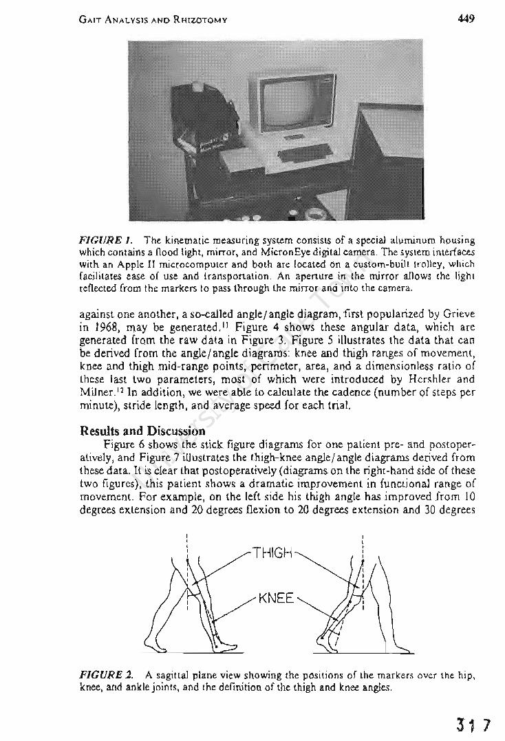
GAIT ANALYSIS AND RHIZOTOMY 449

FIGURE I. The kinematic measuring system consists of a special aluminum housing which contains a flood light, mirror, and MicronEye digital camera. The system interfaces with an Apple II microcomputer and both are located on a custom-built trolley, which facjlitates ease of use and transportation. An aperture in the mirror allows the light reflected from the markers to pass through the mirror and into the camera.

against one another, a so-called angle/ angle diagram, first popularized by Grieve in 1968, may be generated. 11 Figure 4 shows these angular data, which are generated from the raw data in Figure 3. Figure 5 illustrates the data that can be derived from the angle/ angle diagrams: knee and thigh ranges of movement, knee and thigh mid-range points, perimeter, area, and a dimensionless ratio of these last two parameters, most of which were introduced by Hershler and Milner. 12 In addition, we were able to calculate the cadence (number of steps per minute), stride length, and average speed for each trial.

Results and Discussion Figure 6 shows the stick figure diagrams for one patient pre- and postoper­

atively, and Figure 7 illustrates the thigh-knee angle/angle diagrams derived from these data. It is clear that postoperatively (diagrams on the right-hand side of these two figures), this patient shows a dramatic improvement in functional range of movement. For example, on the left side his thigh angle has improved from 10 degrees extension and 20 degrees flexion to 20 degrees extension and 30 degrees

KNEE

FIGURE 2. A sagittal plane view showing the positions of the markers over the hip, knee, and ankle joints, and the definition of the thigh and knee angles.

31 7

31 8

450 VAUGHAN, BERMAN, PEACOCK, ELDRIDGE

DATA

BRyeRWB II APR 85 PRE- OP RIGHT WALK X RANGE a 2000 MM Y RANGE • 1000 MM

• '" • • I •

.........

.,

TRAJECTORIES

BRyeRWB \I APR 85 PRE - OP RIGHT WALK X RANGE = 2000 MM y RANGE 1000 MM

STICK FIGURE

BRyeRWB \I APR 85 PRE - OP RIGHT WALK X RANGE = 2000 MM y RANGE 1000 MM

FIGURE 3. Sagittal plane data gener­ated within seconds of the patient completing a walking trial. A, Raw data points. B, Trajectories formed by joining points of the same marker. C, Stick figure diagram formed by joining points of the same frame. These are preoperative data for a single patient. Note that the horizontal (X) range is 2000 millimeters with intervals of 200 mm, and the vertical (Y) range is 1000 millimeters with l00-mm intervals.

flexion. Similarly, the knee angle has gone from 15 degrees/40 degrees to 5 degrees/65 degrees. Although the diagrams on the right of Figure 7 do approach a normal pattern (Fig. 8), the patient is still unable to achieve full knee extension during the early stance phase (refer to the stick figure diagram in Figure 6).

The reasons for this flexed-knee position at heel strike are not clear, but a number of hypotheses may be postulated. First, it is possible that the preoperative spastic patterns have been so ingrained (this boy was 14 years old at the time of surgery) that even a year after surgery (when our gait analysis was performed) the patient still lacks selective control and depends on flexor and extensor synergies for movement. Second, the SPLR procedure, while reducing spasticity, can also uncover some muscular weakness in the knee extensors postoperatively when the child can no longer utilize the spastic muscle response. It is therefore possible that this child's knee extensor mechanism was not yet sufficiently developed postop­eratively to enable full knee extension at heel strike. Third, the reduction in spasticity and increase in joint range of motion probably posed new challenges for

GAIT ANALYSIS AND RHIZOTOMY

BRyeRWB II APR 85 PRE-OP RIGHT WALK

90

K F N L E E E X

A 40 N G E L X E T

0

A 10

0 TIME (S) 2 3

BRyeRWB \I APR 85 PRE - OP RIGHT WALK

90

K F N L E E E X

A 40 N G E L X E T

c O~---------+------------~ 10~~~~~~~ __ ~ __ ~~~~

30 EXT THIGH ANGLE FLEX 40

8RY·lWA 17 APR 86 POST- OP lEFT WAlK

90~-r--~--~~--~--r---

\&1)( ~\&I " ~ ZLo.

'" \&I \&I~ Z )( 11<\&1

A

40

o ~=======~T~HIGH~R~ANG~E ===---1

10~~--~--~~--~--~~

30 EXT THIGH ANGlE FlEX 40

BRY*LWA 17 APR 86 POST-OP LEFT WALK

90~~--~---r--~--~--~--'

lUX ..JIU " ..J Z Lo. e(

IU IU~ Z x :.: IU

RATIO·.[A/P

40

O~---------+------------~ 10~~--~--~--~ __ ~ __ ~_

C 30 EXT THIGH ANGLE FLEX 40

451

BRyeRwB \I APR 85 PRE - OP RIGHT WALK

T H I G H

A N G L E

B

40

F L E X

E X T

30 0 TIME (S) 2 3

FIGURE 4. The angular data, as de­fined in Figure 2 and generated from the raw data presented in Figure 3. A, Knee angle versus time. B, Thigh angle versus time. C, Knee angle versus thigh angle. Note that in C there is a cyclic pattern (which progresses in a clockwise direction) that repeats itself. For a consistent gait pattern (as is evidenced here), each cyclic loop should be very similar from one cycle to the next.

BRY*LWA 17 APR 86 POST- OP LEFT WALK

90r-~--~---r---r---r--~--,

lUX ..JIU " ..J Z l&-e(

IU IU~ Z x :':IU

B

40

KNEE MID­RANGE POINT

Or-----------I----'---------------\ 10~~--~--~--~--~--~~

30 EXT THIGH ANGLE FLEX 40

FIGURE 5. Parameters that may be de­rived from the angle-angle diagram. I2 A, Knee and thigh ranges. B, Knee and thigh mid-range points. C, Area, perimeter, and ratio.

31 9

320

452 VAUGHAN, BERMAN, PEACOCK, ELDRIDGE

STICK FIGURE

BRV-LWfJ II APR 85 PRE -op LEFT WALK X RANGE • 2000 MM Y RANGE • 1000 MM

STICK FIGURE

BRY.RWB II APR 85 PRE -OP RIGHT WALK X RANGE • 2000 MM V RANGE • 1000 MM

STICK FIGURE

BRV_LWA 17 APR 86 POST-OP LEFT WALK X RANGE • 2000 MM Y RANGE • 1000 MM

STICK FIGURE

BRV_RWA 17 APR 86 POST-OP RIGHT WALK X RANGE • 2000 MM V RANGE • 1000 MM

FIGURE 6. Stick figure diagrams for one patient pre- and postoperatively. Preoperative data are on the left, and postoperative data are on the right. Diagrams for the patient's left-hand side are on top and for the right-hand side on the bottom.

BRV*LWB II APR 85 PRE-OP BRV*LWA 17 APR 86 POST-OP LEFT WALK LEFT WALK

90 90

K F K F N L N L E E E E E X E x

A 40 A 40 N N G E G E L X L X E T E T

0 0

10 10 30 EXT THIGH ANGLE FLEX 40 30 EXT THIGH ANGLE FLEX 40

BRV*Rwa II. APR 85 PRE-OP BRV*RWA 11 APR 86 POST-OP RIGHT WALK RIGHT WALK

90 90

K F K F N L N L E E E E E X E X

A 40 A 40 N N G E G E L X L X E T E T

0 0

10 10 30 EXT THIGH ANGLE FLEX 40 30 EXT THIGH ANGLE FLEX 40

FIGURE 7. The thigh-knee angle/angle diagrams for the same patient as in Figure 6.

GAIT ANALYSIS AND RHIZOTOMY

FIGURE 8. A thigh-knee angle/ angle diagram for a normal child. Compare this with the pre- and postopera­tive diagrams in Figure 7.

Normal Child 18 May 1987 WALKING Left side, 5 year old girl

90

K F N ~ ~ X A 40

~ E L X E T

o 10

30 EXT THIGH ANGLE

453

FL EX 40

the child to maintain his balance. He may well be compensating by flexing at the knee and thereby increasing his sense of stability. A fourth possibility is that the patient may have had a fixed joint contracture prior to SPLR.

While considerable insight can be obtained by a case study approach, it is also pertinent to pool the data for all 14 patients for comparison with the 9 normal children. The full set of data for all the children (and this includes both their left and right sides) is presented in Table 1. Cadence, while quite variable,

TABLEl. Mean Values (with Standard Deviations Below in Parentheses) of Biomechanical Parameters for the Walking Patterns of 14 Spastic Children

Before and After SPLR.

Parameter Before After Difference p Value Normal

Cadence 109 105 -4 0.595 115 (steps/min) (34) (28) (19)

Stride Length 0.72 0.87 0.15 0.049 0.90 (m) (0.24) (0.33) (0.19)

Average Speed 0.67 0.79 0.12 0.059 0.85 (m/s) (0.30) (0.36) (0.20)

Thigh Range 39 53 14 <0.0001 42 (degrees) (10) (13) (4)

Knee Range 39 50 11 0.029 61 (degrees) (16) (20) (5)

Thigh Mid-Range 15 18 3 0.154 6 Point (degrees) (9) (9) (3)

Knee Mid-Range 40 56 16 <0.0001 35 Point (degrees) (13) (11) (6)

Area 819 1300 481 0.002 1301 (degree2) (487) (637) (292)

Perimeter 133 173 40 0.001 184 (degrees) (40) (47) (52)

Ratio 0.21 0.20 -0.01 0.346 0.19 (0.03) (0.03) (0.02)

Statistical comparison (p value) was performed using Student's paired "t" test. In addition, the right-hand column contains the equivalent data for 9 normal boys (mean age of 5.5 years).

321

322

454 VAUGHAN, BERMAN, PEACOCK, ELDRIDGE

was effectively unchanged postoperatively (p = 0.595). It is well-known that, if anything, cadence decreases slightly as a child matures.20 The cadence of 115 for normal children (mean age of 5.5 years) was slightly greater than values for the children with CP. In contrast to cadence, stride length increased significantly by over 20% from 0.72 meter to 0.87 meter, approaching the normal value of 0.90 meter. The calculation was derived as follows:

Average speed = cadence x (stride length)

where cadence would be expressed in units of strides per second rather than steps per minute. The average speed also increased quite substantially (by 18%), although the statistical significance (p = 0.059) was approached but not reached.

Since walking speed is very difficult to control, depending on the person's mood and motivation on the day of testing, and can vary quite considerably (note the standard deviation of 0.20 m/ s for the normal children), one should be cautious in interpreting the modest increase in the patients' speed postoperatively. The increase in stride length can be accomplished in two ways: the child's legs grow in length, or the legs are moved through a greater range of motion.

Although the pre- and postoperative studies were performed an average of 9 months apart, we would argue that the length maturation effects, while not trivial, are certainly insufficient to provide a 0.15 meter increase in stride length. The clue to this increase is contained in the thigh range data. Here we see a 36% increase from 39 degrees to 53 degrees, with the difference being highly statistically significant (p < 0.000 1) and the postoperative value being larger than normal. The range of motion at the knee was also significantly increased, not to the degree associated with the thigh but nevertheless approaching the normal value. From a physical point of view, we can speculate that one of the effects of the SPLR procedure has been to decrease the spasticity in the hip flexor, knee flexor, hip adductor, and ankle plantar flexor muscle groups. The reduction in spasticity has enabled the patients to move their thighs and knees through a greater range of movement, thus increasing stride length and average speed.

The thigh mid-range point (Fig. 5B) was effectively unchanged (p = 0.154), whereas the knee mid-range point shifted from 40 degrees flexion to 56 degrees flexion, with the difference being highly statistically significant (p < 0.000 1) and the shift being away from the normal value. This trend was exhibited by the patient in Figures 6 and 7, and the possible reasons for the shift to knee flexion were discussed above. We believe that this point should be carefully examined in the future, particularly in a long-term study where patients can be followed for at least 2 or 3 years after surgery.

Hershler and Milner were the first to introduce the quantitative analysis of angle-angle diagrams to yield the parameters area A, perimeter P, and a dimensionless ratio JAip (Fig. 5C).12 They suggested that A, being a function of both thigh and knee angles, is expressive of the total conjoint range of angular motion experienced at the hip and knee joints during one complete gait cycle. By conjoint range they meant the mapping of all possible angle-angle points during a gait cycle. We can see from Table 1 that the patients in our study had a substantial increase in A, which was highly statistically significant (p = 0.002), with their postoperative value being almost identical to normal. They also argued that P was a measure of the coordination between the two joints during gait (assuming that area did not change). Because our patients had a substantial increase in area, it is reasonable that perimeter also increased. Hershler and

GAIT ANALYSIS AND RHIZOTOMY 455

Milnerl2 suggested that the dimensionless ratio was a quantifier of the shape of the angle-angle diagram. As seen in Table 1, our patients did not show a change in this parameter (p = 0.346), so we can conclude that the shape of the angle-angle diagram did not really change. Intuitively, this seems acceptable, particularly if we compare the left and right sides of Figure 7. The value of the ratio (0.20) is also consistent with the value found by Hershler and Milner for an adult with cerebral palsy who was implanted with a cerebellar stimulator. 12 His ratio was 0.22. The fact that our normals had a value of 0.19 suggests that the dimensionless ratio is not a very useful measure of locomotor function.

WHERE DO WE GO NOW? While we have not satisfied our original hypothesis in a rigorous manner,

we have at least provided some evidence that selective posterior lumbar rhizotomy improves the functional range in walking patterns of spastic CP children. This leads us to speculate upon where the future emphasis should lie. We believe that there are at least three important areas for studying the gait of SPLR patients in the future: (l) there should be long-term prospective studies; (2) the two-dimensional studies described above should be extended to three dimensions; and (3) we should be concerned about cause-effect relationships.

All of the 14 patients in this study were evaluated preoperatively in 1985 and followed up for postoperative assessments during 1986. The average time between assessment was just 9 months. With a procedure such as SPLR, the major concern of all interested parties-patients, families, and clinicians-is whether the apparent benefits of the operation are long term. Some of the original patients operated on by Fasano et al. are now 15 years beyond surgery.6 Although gait analysis per se was not performed preoperatively, we feel certain that videotaping (which apparently was done) has the potential to highlight the long-term benefits of SPLR.

When one studies the gait of a spastic CP child, one realizes immediately that the movement dysfunction is not confined to the sagittal plane. As pointed out by Ducroquet et al. (see Figure 9) we need to be concerned not only with the sagittal plane but with the frontal and horizontal planes as well.4 At present, three-dimensional gait analysis systems tend to be very expensive (at least $40,000) and thus are usually found in large hospitals and university laboratories. However, we hope that some of the newer technologies being driven by the robotics revolution will find their way into the smaller gait laboratories.22 These 3-D systems will be readily accessible both in terms of price and ease of use.

Finally, we need to be concentrating on cause-effect relationships in the gait cycle. When a patient walks a complex series of neural, muscular, and skeletal actions take place before we observe a movement pattern that is readily recognized as gait. This sequence of events has been simplified and illustrated in Figure 10. This model can be used to help our understanding of pathology, treatment, and, indeed, the different methods of gait analysis. In the case of cerebral palsy, the primary lesion (or pathology) is in the brain at the level of the central nervous system (Levell in Fig. 10). The way in which the lesion manifests itself is via the lower levels (2 through 5). From a treatment point of view, the neurosurgeon using .. cerebellar stimulation or SPLR is attacking the problem at Levell and attempting to approach the cause of spasticity as closely as possible. The orthopedic surgeon, performing a tendon release or osteotomy, is having an effect at Level 3 or 4. This is at least two levels below the primary lesion in the cause-effect chain.

323

324

456 VAUGHAN, BERMAN, PEACOCK, ELDRIDGE

SAGITTAL

FRONTAL

HORIZONTAL

.~- -~- .~-FIGURE 9. Human gait is a movement that should be studied in three dimensions. (Adapted from Ducroquet et al.4)

From a gait analysis point of view, the study described above concentrated on a description of the segment movements. These clearly are the end result, or effect, of the sequence of events higher up in the cause-effect chain. We believe that it is imperative for future gait studies of SPLR to move higher up in the movement chain. Specifically, electro myographic (EMG) data should be gathered simultaneously with 3-D segment movements and 3-D ground reaction fprces. These data should be integrated, using the inverse dynamics approach, to calculate the 3-D joint forces and torques. We believe that this data will yield significant insight into the neuromuscular control strategies used by a spastic patient before and after SPLR. It is also suggested that further basic research, using animal models, should be performed on SPLR. In this way it would be possible to study the activity in the central and peripheral nervous systems during locomotor activities.

CONCLUSION While posterior rhizotomy has been used as a surgical approach to reduce

spasticity for nearly 75 years, we believe that our study is the first attempt to quantify objectively the effects of this surgery on function.s Specifically, we put forward the hypothesis that SPLR leads to a decrease in spasticity and thus to

GAIT ANALYSIS AND RHIZOTOMY

Sequence of Events

1. Registration in eNS 2. Activation of PNS 3. Muscle contracts, develops force 4. Force and torque at joints 5. Segment movements and

ground reaction forces

457

2

FIGURE 10. The sequence of events in walking is outlined (left) and illustrated (right) in a cerebral palsy child with right hemiparesis. (Adapted from Sutherland).2o

an improvement in locomotor function. Insofar as increased range of movement can be thought of as an improvement in locomotor function, we have provided some evidence that our original hypothesis is true. While SPLR is certainly not a panacea, it seems to be a treatment modality with considerable promise. There are many patients around the world who suffer from the debilitating effects of spasticity and who could potentially benefit from the surgery.

We believe that future studies should be directed toward: long-term follow­up (at least 3 years); true 3-D movement assessment (to extend the 2-D work presented here); and integration of kinematic, dynamic Goint forces and torques), and electromyographic data. With an increasing number of neurosurgeons contemplating the use of SPLR in treating CP patients, it is imperative that long­term rigorous scientific studies be initiated.

ACKNOWLEDGMENTS

We should like to thank the following for their generous financial assistance: the University of Cape Town (Department of Neurosurgery), the South Mrican Medical Research Council, the Council for Scientific and Industrial Research, the Hyman Goldberg Foundation, and Clemson University (Department of Bioengineering).

REFERENCES I. Berman B, Peacock W J, Vaughan CL, Bridger RS: Assessment of patients with spastic cerebral

palsy before and after rhizotomy. Dev Med Child Neuro 29:24, 1987. 2. Bishop B: Spasticity: Its physiology and management. Parts I-IV. Phys Ther 57:371-401, 1977. 3. Denhoff E: Cerebral Palsy: The Preschool Years: Diagnosis, Treatment and Planning.

Springfield, IL, Charles C Thomas, 1967. 4. Ducroquet R, Ducroquet J, Ducroquet P: Walking and Limping. Philadelphia, J.B. Lippincott,

1968. 5. Eiben RM, Crocker AC: Cerebral palsy within the spectrum of development disabilities. In

Thompson GR, Rubin IL, Bilenker RM (eds): Comprehensive Management of Cerebral Palsy. New York, Grune & Stratton, 1983, pp 19-23.

6. Fasano VA, Broggi G, Barolat-Romana G, Squazzi A: Surgical treatment of spasticity in . cerebral palsy. Child's Brain 4:289-305, 1978.

7. Fasano VA, Barolat-Romana G, Zeme S, Squazzi A: Electrophysiological assessment of spinal circuits in spasticity by direct dorsal root stimulation. Neuro,urgery 4: 146-151, 1979.

8. Foerster 0: On the indications and results of the excision of posterior spinal nerve roots in men. Surg Gynecol Obstet 16:463-474, 1913.

325

326

458 VAUGHAN, BERMAN, PEACOCK, ELDRIDGE

9. Gros C, Ouaknine G, Vlahovitch B, Frerebeau P: La radiocotomie selective posterieure dans Ie traitement neurochirurgical de l'hypertonie pyramidale. Neurochirurgie 13:505-518, 1967.

10. Gros C, Privat JM, Benezech J, Frerebeau P: Sectorial posterior rhizotomy of surgical treatment for spasticity. Acta Neurochir (Wien) 35:181-195, 1976.

II. Grieve DW: Gait patterns and the speed of walking. Biomed Engineer 3: 119-122, 1968. 12. Hershler C, Milner M: Angle-angle diagrams in above-knee amputee and cerebral palsy gait. Am

J Phys Med 59:165-183, 1980. 13. Ivan LP, Ventureyra ECG: Chronic cerebellar stimulation in cerebral palsy. App Neurophysiol

45:51-54, 1982. 14. Laitinen LV, Nilsson S, Fugl Meyer AR: Selective posterior rhizotomy for treatment of

spasticity. J Neurosurg 58:895-899, 1983. 15. Peacock WJ, Eastman RW: The neurosurgical management of spasticity. S Afr Med J 60:849-

850, 1981. 16. Peacock WJ, Arens U: Selective posterior rhizotomy for the relief of spasticity in cerebral palsy.

S Afr Med J 63:119-124,1982. 17. Peacock WJ, Arens U, Berman B: An assessment of selective posterior rhizotomy as a procedure

for relieving spasticity in cerebral palsy. Dev Med Child NeuroI29:22, 1987. 18. Peacock WJ, Arens LJ, Berman B: Cerebral palsy spasticity. Selective posterior rhizotomy.

Pediatr Neurosci 13:61-66, 1987. 19. Sherrington CS: Decerebrate rigidity of reflex coordination of movements. J PhysioI22:319-337,

1898. 20. Sutherland DH: Gait Disorders in Childhood and Adolescence. Baltimore, Williams and

Wilkins, 1984. 21. Sutherland DH: Utilization of gait analysis for clinical decision-making in cerebral palsy.

Workshop, American Academy for Cerebral Palsy and Developmental Medicine, Boston, 1987.

22. Vaughan CL, Smart NM, Edwards BI, Kwan-Leung S: Gait Analysis on a Microbudget. In Winter D, et al (eds): Biomechanics IX-B. Champaign, IL, Human Kinetics Publishers, 1985.

23. Vaughan CL, Smith DC, du Toit LL: Kinematic Gait Analysis Using a Digital Camera. In Jonsson B (ed): Biomechanics X-B, Champaign, IL, Human Kinetics Publishers, 1987.

24. Vaughan CL, Murphy GN, du Toit LL: Biomechanics of Human Gait: An Annotated Bibliography. Champaign, IL, Human Kinetics Publishers, 1987.

25. Vaughan CL, Berman B, Peacock WJ: Kinematics of Crawling Applied to Cerebral Palsy Children Before and After Rhizotomy. In de Groat, et al (eds): Biomechanics XI. Amsterdam, Vrije Universiteit Press, 1988.

-

JNeurosurg74:178-184,1991

Cerebral palsy and rhizotomy

A 3-year follow-up evaluation with gait analysis

CHRISTOPHER L. VAUGHAN, PH.D., BARBARA BERMAN, M.Sc., AND

WARWICK J. PEAcOCK, M.D.

Department of Orthopaedic Surgery, University of Virginia, Charlottesville. Virginia. and Department of Pediatric Neurosurgery. University of California Medical Center, Los Angeles. California

...... A recent increase in the popularity of selective posterior rhizotomy for reduction of spasticity in cerebral palsy has led to a demand for more objective studies of outcome and long-term follow-up results. The authors present the results of gait analysis on 14 children with spastic cerebral palsy, who underwent selective posterior rhizotomy in 1985. Sagittal plane gait patterns w~re studied before surgery and at I and 3 years after surgery using a digital camera system. The parameters measured included the range of motion at the knee and thigh, stride length, speed of walking, and cadence. The range of motion at the knee was significantly increased at 1 year after surgery and further improved to a nearly normal range at 3 years after surgery. In contrast, postoperative measurements of thigh range exceeded normal values at I year, but decreased toward normal range at 3 years. While improvements in range of motion continued between Years I and 3, the children developed a more extended thigh and knee position, which indicated a more upright walking posture. Stride length and speed of walking also improved, while cadence remained essentially unchanged. This 3-year follow­up study, the first to examine rhizotomy using an objective approach, has provided some encouraging results regarding early functional outcome.

KEy WORDS gait dorsal root

SPASTICITY is a major problem in children with cerebral palsy. Cerebral palsy is a motor disorder due to a non progressive perinatal insult to the

developing brain. Approximately 25,000 children are born with or develop cerebral palsy in the United States each year.3 One of the neurosurgical options available for reduction of spasticity in cerebral palsy is selective posterior rhizotomy. Posterior rhizotomy for relief of spasticity was first reported in 1908 by the Germany neurosurgeon Foerster,8 although he credited Monro with similar work as early as 1904. In 1913, Foerstee reported a series of 159 patients in whom he completely divided the posterior roots from L-2 to S-2 bilaterally, but spared the L-4 roots. Although Foerster's clinical results seemed encouraging, the procedure was almost overlooked by the neurosurgical community during the next half-century. It was not until Gros, et al., 10 revised the surgical technique and divided only a portion of the sensory nerve rootlets comprising each posterior root to reduce sensory loss that .the approach became more acceptable.17 In 1978, Fasano, et al.,4.6 described the use of electromyography (EMG) during electrical

178

rhizotomy cerebral palsy

stimulation of the posterior nerve rootlets in spastic patients as the basis for selective rootlet division, and this approach was adopted by others. 12 Peacock, et al.,14-16 further modified Fasano's approach by chang­ing the operative site from the level of the conus to the cauda equina in order to ensure preservation of the lower sacral nerve roots involved in bowel and bladder control.

Within the past 4 years, there has been a major resurgence of interest in the procedure and there are now over 30 centers in North America offering this surgery.13 With the increase in patient numbers and the apparent endorsement of the procedure by some in the neurosurgical community,24 objective analysis of the long-term results becomes essential.

Foerstee and Fasano and Broggis provided SUbjective and anecdotal evidence of improvements in function following posterior rhizotomy, the latter with a IS-year follow-up period in 80 patients. Peacock, et al., IS found reduction in spasticity and improvement in function in 60 patients after selective posterior rhizotomy; follow­up evaluation up to 7 years revealed maintenance of

J. Neurosurg. / Volume 74/ February, /991

327

32 8

Gait before and 3 years after rhizotomy

functional improvements and no return of spasticity.1 In order to obtain more specific and objective data, we began routine measurement of walking and crawling patterns of patients before and after selective posterior rhizotomy.19-23 The results of approximately 1 year after surgery were reported by Vaughan, et al.,ll for 14 ambulatory patients and revealed a significant increase in thigh range, knee range, and stride length. The ca­dence was virtually unchanged and, although the speed of walking increased, the difference was nq.t statistically significant. It was concluded that rhizotomy reduced spasticity, thus allowing an increase in functional range of motion during gait which contributed to a longer stride length. These results confirmed our clinical im­pressions of gait improvement in spastic children fol­lowing the rhizotomy procedure. However, the follow­up period was not adequate for evaluation of long-term effects. The purpose of the present study is to provide an objective assessment of the gait patterns of patients undergoing selective posterior rhizotomy after a post­surgical period of 3 years, and to compare these results with those obtained after 1 year.

Clinical Material and Methods

Patient Selection The goal of the examination and selection process

was to identify those patients who were mainly handi­capped by spasticity and not the other features of cerebral palsy. Thus, clinical examination of muscle tone, reflexes, strength, range of motion, balance, and motor control was performed. Individuals with cerebral palsy who had spasticity but lacked rigidity, dystonia, athetosis, and ataxia were chosen. Because improve­ment in walking was our goal for this group of patients, it was important to ensure that they had adequate trunk control, balance, and antigravity strength, and did not have severe fixed contractures. Children with truncal hypotonia, weakness, or tendons overlengthened by previous orthopedic surgery were not considered for the procedure. Children of normal intelligence with bilat­eral lower-extremity spasticity and minimal upper-ex­tremity involvement (spastic diplegia), good trunk con­trol (ability to side sit), lower-extremity strength, and the ability to walk were considered the best candidates for the study.

Twenty-nine spastic children with cerebral palsy un­derwent selective posterior rhizotomy in 1985.2 Four­teen were able to walk prior to surgery and thus could be studied using gait analysis preoperatively and again 5 to 14 months following rhizotomy (mean 9 months). At the time of surgery, the age range was 2 to 14 years (mean 8 years). Eleven of the original 14 patients were available for reassessment in 1988 at a mean postop­erative period of 36 months. All patients received pre­operative and postoperative physical therapy. For pur­poses of comparison, gait data were also collected for nine normal children with a mean age of 5 years.

J. Neurosurg./ Volume 74/ February, 1991

Operative Technique The procedure was performed under endotracheal

general anesthesia without the use of long-acting de­polarizing agents. The patient was positioned prone with bolsters under the chest and pelvis to allow the abdominal wall to move freely and to prevent epidural vein distention. Access to the lower extremities for in­traoperative EMG and visual monitoring was ensured by careful positioning and draping of the patient. Ac­curate identification of the lumbosacral posterior roots and rootlets is difficult at the level of the conus, which is accessed using a T12-Ll laminectomy. We therefore exposed the cauda equina through laminectomies from L-2 to L-5 with careful preservation of the posterior facet joints. The posterior roots and their levels were identified by visual anatomical features with accuracy confirmed using electrical stimulation. The S-l root was usually the largest, and stimulation of its anterior root produced flexion of the knee and ankle plantar flexion. The S-2 root was significantly smaller, and ankle plantar flexion and toe flexion occurred on stim­ulation of its anterior root. The plane separating the posterior and anterior roots was clearly visualized. The posterior root was broader, flatter, and lighter in color than the anterior root. The electrical threshold for a motor response was much lower for the anterior root . than the posterior root. By counting upward from the confirmed S-l root, the L-2 root could be easily iden­tified at its dural exit point. The posterior root of L-2 was separated from the anterior root, and the two to four rootlets comprising the posterior root were stimu­lated in turn by means of two insulated microneuro­surgical hook electrodes.· The threshold for a motor response was identified using a O.I-msec square wave stimulus. A tetanic stimulus was then applied to the rootlet at 50 Hz (nonsinusoidal) for I second. The responses were monitored using EMG needle or surface electrodes.

For the patients in this study, two muscle groups were sampled simultaneously. For identification of the L2-4 rootlets electrical activity from the quadriceps and adductor muscles was sampled, and for the L5-S2 rootlets the gastrocnemius and tibialis anterior muscles were monitored. Rootlets were sectioned if they were associated with a low threshold for motor response, a sustained response beyond the I-second stimulus in­terval, or spread to inappropriate muscle groups. The recording technique has been refined since these pa­tients were treated, resulting in better selectivity and a decrease in the average number of rootlets divided. We now monitor EMG patterns from 10 muscles simulta­neously using the chart recorder of an electroenceph­alograph. t Responses are recorded from the hip ad-

* Microneurosurgical hook electrodes manufactured by Aesculap Surgical Instruments, Burlingame, California.

t Electroencephalograph manufactured by Nihon Kohden Inc., Irvine, California.

179

J

180

C. L. Vaughan, B. Berman, and W. J. Peacock

o.crem.ntel R.apo ....

B A LsftAddud0r5

Lsft_

Sulltalned Reaponu

Lsft Quadr!eeps Lsft 0uacItIeapI

l.sft_AnIe<." LaIIT __ 1or

Lei! Hamstrings LsftHamslmgS .'. 'A'''''t'

Len Gos\roalomius LeIt Gastrocnemius

RighlAddUClOrs l'I\II"'I'II~illlllil Right AdducIors

Righi Ouodriceps Right 0uacItIeapI

Right T_Anterior Right 1ibiaIis Anterior

Righi Harnstnngs ~~~" Right Hamstrings

R;ghl Gootrocnemius AightGastnx:nemius -t ' I I I I I. ,I

1 lOt. trainlOrtghtl-3roo1lM t MC..lraln Ie lefll-3 roadet

c Multlpha.1c Reapo ..... W1th Clonic Activity Dlal.1Id ConIraIaIMeI Spread

o

Lsft Quadriceps

Lsft HamSl1ings l.eII_ -......

"",

.,. ~

Righi Quad_ps

Righi TIbialis Anterio'

-----t/'"

Fa •

FIG. 1. Various electromyographic responses recorded during intraoperative electrical stimulation of the posterior rootlets using a lO-channel recording system. A: Decremental responses which are considered to be normal. B: An abnormally sustained response in the left quadriceps. C: Multiphasic clonic patterns seen in reaction to a steady stimulus. The rootlets associated with these responses are divided. D: Abnormal spread to ipsilateral hamstrings and contralateral tibialis anterior and hamstring muscles following stimulation of a left L-2 rootlet with an incremental pattern in the left hamstrings.

J. Neurosurg./ Volume 74/ February, 1991

329

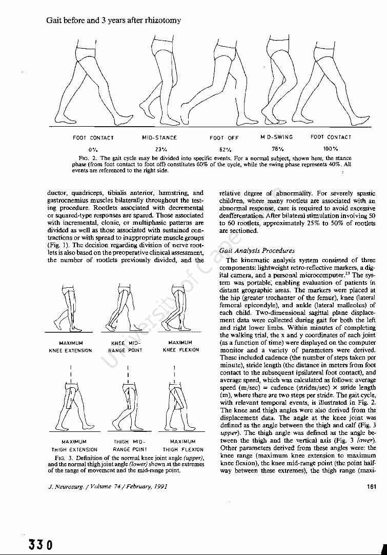
Gait before and 3 years after rhizotomy

FOOT CONTACT MID-STANCE FOOT OFF MID-SWING FOOT CONTACT

0% 23'/, 62% 78% 100"1.

FIG. 2. The gait cycle may be divided into specific events. For a normal subject, shown here, the stance phase (from foot contact to foot oft) constitutes 60% of the cycle, while the swing phase represents 40%. All events are referenced to the right side.

ductor, quadriceps, tibialis anterior, hamstring, and gastrocnemius muscles bilaterally throughout the test­ing procedure. Rootlets associated with decremental or squared-type responses are spared Those associated with incremental, clonic, or mUltiphasic patterns are divided as well as those associated with sustained con­tractions or with spread to inappropriate muscle groups (Fig. I). The decision regarding division of nerve root­lets is also based on the preoperative clinical assessment, the number of rootlets previously divided, and the

MAXIMUM

KNEE EXTENSION

MAXIMUM

THIGH EXTENSION

KNEE MID­

RANGE POINT

THIGH MID­

RANGE POINT

MAXIMUM

KNEE FLEXION

MAXIMUM

THIGH FLEXION

FIG. 3. Definition of the normal knee joint angle (upper), and the normal thighjoint angle (lower) shown at the extremes of the range of movement and the mid-range point.

J. Neurosurg. / Volume 74/ February, 1991

330

relative degree of abnormality. For severely spastic children, where many rootlets are associated with an abnormal response, care is required to avoid excessive deafferentation. After bilateral stimulation involving 50 to 60 rootlets, approximately 25% to 50% of rootlets are sectioned.

Gait Analysis Procedures

The kinematic analysis system consisted of three components: lightweight retro-reflective markers, a dig­ital camera, and a personal microcomputerP The sys­tem was portable~ enabling evaluation of patients in distant geographic areas. The markers were placed at the hip (greater trochanter of the femur), knee (lateral femoral epicondyle), and ankle (lateral malleolus) of each child. Two-dimensional sagittal plane displace­ment data were collected during gait for both the left and right lower limbs. Within minutes of completing the walking trial, the x and y coordinates of each joint (as a function of time) were displayed on the computer monitor and a variety of parameters were derived. These included cadence (the number of steps taken per minute), stride length (the distance in meters from foot contact to the subsequent ipsilateral foot contact), and average speed, which was calculated as follows: average speed (m/sec) = cadence (strides/sec) X stride length (m), where there are two steps per stride. The gait cycle, with relevant temporal events, is illustrated in Fig. 2. The knee and thigh angles were also derived from the displacement data. The angle at the knee joint was defined as the angle between the thigh and calf (Fig. 3 upper). The thigh angle was defined as the angle be­tween the thigh and the vertical axis (Fig. 3 lower). Other parameters derived from these angles were: the knee range (maximum knee extension to maximum knee flexion), the knee mid-range point (the point half­way between these extremes), the thigh range (maxi-

181

•

Normal Male

Flexion

R.Knee

Angle Ideg)

Extension

70,----------r------~------__, __ TH I GH ---;-------+

60 RANGE

SO FO

40

30

20

10

0

-10 -20

I I Thigh Mid­I Range Point

r; I

1 KNEE RANGE

I I I

Knee Mid- j Range Point

Fe

30 Extension R, Thigh Angle (deg) Flexion

FIG. 4. The knee angle plotted as a function of the thigh angle for a normal adult,9 showing the range of motion and mid-range point paramters. The curve progresses in clockwise fashion with foot contact (FC) and foot off (FO). At F-F the knee is fully extended while the thigh is maximally flexed to about 20·. During the stance phase theJhigh extends to about -20· and then flexes again after FO. The knee flexes slightly after Fe and then extends during stance until just before FO. At the beginning of the swing phase, the knee flexes to about 60· and gradually extends to O· in anticipation of Fe.

mum thigh extension to maximum thigh flexion), and the thigh mid-range point (Fig. 3). The knee and thigh ranges indicate the total arc of motion used by the individual during the gait cycle, while the mid-range points reflect the location of this movement arc within the child's available range. The angle data were also illustrated using an angle-angle diagram which was first introduced by Grieve9 (Fig. 4). Quantitative analysis of the angle-angle diagram was also performed as de­scribed by Hershler and Milner. II

The mean values for the right and left sides were determined for all of the gait variables and used for statistical analysis.

Results

For ease of understanding, the cadence, stride length, and average speed will be expressed in order as follows: pre-surgery/l year postsurgery/3 years postsurgery/nor­mal. Data for nine normal children have been included for the purpose of comparison.21 The mean results for cadence were 109/105/103/115 steps per minute. The mean stride lengths were 0.72/0.87/1.03/0.90 m, and the average speeds were 0.67/0.79/0.90/0.85 m/sec. For the patients, cadence decreased slightly during the 3 years following surgery, although the differences were not statistically significant. Stride length was signifi­cantly improved after 1 year and at 3 years increased by almost 50% from 0.72 to 1.03 m. Average speed of walking was significantly increased only after the 3-year period.

The ranges of movement at the knee and thigh (Fig. 5 upper) were substantially increased after rhizotomy.

182

C. L. Vaughan, B. Berman, and W. J. Peacock

80.----------,

60

40

20-

o

....... III """'''

Before 1 yr Aller 3 yn ACta Normal

60,-----------------, • P.1ianl

50111_'

40

30

20

10

o Befon 1 yr After 3 yTS AAer Normal

60~------------,

50

40

30

20

10

o &:(O~ I yr After 3 yn Afler Normal

20~------------,

10

o~---jl Beron: 1 yr Anu 3 yTS Mer Normal

FIG. 5. Upper: The range of motion for the knee (left) and thigh (right) in rhizotomy patients (before surgery and I and 3 years after surgery) compared with data on normal children. Lower: The mid-range point data for the knee (left) and thigh (right) in rhizotomy patients (before surgery and I and 3 years after surgery) compare~ with data on normal children. -

The thigh range was slightly less than normal preoper­atively and exceeded normal at both the 1- and 3-year follow-up examinations, although there was a slight decrease toward normal at the 3-year study. The range of knee movement was considerably limited prior to surgery, significantly improved after 1 year, and in­creased to nearly normal by 3 years after surgery. The mid-range point in knee movement was significantly increased after 1 year, indicating an excessively flexed knee position, but returned to a more normal value after 3 years (Fig. 5 lower left). The mean mid-range point for the thigh did not differ significantly from the preoperative value over the study period, although it tended to be increased at the I-year point (Fig. 5 lower right).

Discussion

Complications Postoperatively, none of the patients developed

wound complications or problems with bowel and blad­der sphincter control. In no patient could any sensory deficit be detected in the dermatomes innervated by the lumbosacral plexus; increased sensitivity to light tough was noted in all patients after surgery but resolved spontaneously within 5 to 10 days. Although the follow­up period is relatively short, there has been no clinical or radiological evidence of spinal instability or defor­mity as a result of the multiple-level lumbar laminec­tomies, probably because of careful preservation of the posterior facet joints.

Spasticity and Range of Motion The primary result of selective posterior rhizotomy

is the reduction of spasticity. This is reflected by im-

J. Neurosurg./ Volume 74/ February. 1991

Gait before and 3 years after rhizotomy

MAXIMUM KNEE EXTENSION

MAXIMUM

KNEE MID­

RANGE POINT

THIGH 10110-

MAXIMUM KNEE FLEXION

MAXIMUM

THIGH EXTENSION RANGE POtNT THIGH FLEXION

FIG. 6. Definition of the knee joint angle (upper) and thigh angle (lower) for a spastic child showing the extremes of range of movement and the mid-range point.

provement in the range of motion at the knee and thigh during gait which was maintained throughout the study period. The thigh range was initially close to normal and exceeded normal values following surgery. The knee range was quite limited preoperatively and then approached the normal range by the 3rd postoperative year. This is believed to be due to reduction in spasticity in muscles acting across two joints such as the ham­strings and rectus femoris muscles and possibly to re­duction in co-contraction of muscle groups across the hip and knee joints. This improvement in thigh and knee range has allowed patients to increase their stride length and speed of walking.

Significance of Mid-Range Points Whereas the range of motion data are probably a

measure of reduction in spasticity, the mid-range points provide insight into the degree of strength and control a patient exhibits during gait. The minimum, maxi­mum, and mid-range points of the thigh and knee for normal gait occur at specific points during the normal gait cycle (Figs. 2 and 3). These angles differ in the spastic child due to muscular co-contraction, restric­tions in range of movement, and other features of cerebral palsy such as synergistic movement patterns, weakness, and lack of motor control (Fig. 6). The increased value of the knee mid-range point after the first postoperative year was indicative of a more flexed standing posture in comparison with preoperative and

J. Neurosurg. / Volume 74/ February, 1991

332

normal studies. A flexed knee posture is often caused by weakness or lack of control of the calf musculature. The improvement in knee postUJ'e indicated by a lower knee mid-range value at 3 years suggests development of better strength and control.

Stride Length, Cadence, and Speed Improvements in range of motion appeared to be a

major factor producing increased stride length found at both the 1- and 3-year follow-up periods. Although limb growth with maturation may contribute to changes in stride length, the dramatic changes with simultane­ous increases in range of motion noted in our patients make it unlikely that this was a function of growth alone. Cadence remained relatively stable over the 3 years, but had a decreasing trend in accordance with the findings of Sutherland,18 who identified a decrease in cadence with normal maturation. The increased stride length without a significant change in cadence allowed patients to improve their average speed of walking. Speed is difficult to control, however, and can be influenced by mood or motivation. The standard deviation for speed among the normal children tested was as much as 0.20 m/sec. An increase in average speed for the patients is an important reflection of functional improvement, although the changes in range of motion are probably more direct representations of the benefits of the procedure.

Conclusions

Although posterior rhizotomy has been used as a surgical approach to reduce spasticity for over eight decades, this study is the first to examine functional outcome of an objective basis. This 3-year follow-up study, using a simple sagittal-plane gait analysis system, has provided interesting data regarding early postoper­ative outcome and development of changes over time.

The patients undergoing selective posterior rhizot­omy in this series had significant increases in knee and thigh ranges of motion with thigh range exceeding normal values and knee range approaching the norm. The mid-range points, indicative of control, initially reflected a more flexed standing posture which later improved. This suggests that patients can increase their strength and muscular control following selective p0s­

terior rhizotomy, and that physical therapy may make an important contribution to their functional improve­ment. Future prospective studies should concentrate on three-dimensional motion analysis of gait, measure­ment of energy cost, and the integration of motion, force, and EMG data. In time, long-term studies will provide clinicians with important evidence of the func­tional benefits that rhizotomy can offer the spastic patient.

Acknowledgments

The assistance of Ms. Jennifer Brink in data reduction and Dr. Peter Burrows in statistical analysis is gratefully acknowl-

183

edged. We are particularly grateful to Ms. Loretta Staudt for her valuable insight during the preparation of this manuscript

References

I. Arens lJ, Peacock WJ, Peters J: Selective posterior rhi­zotomy: a long term follow-up study. Childs Nerv Syst 5: 148-152, 1989

2. Berman B: Selective posterior rhizotomy: does it do any good? Neurosurg State Art Rev 4:431-444, 1989

3. Eiben RM, Crocker AC: Cerebral palsy within the spec­trum of development disabilities, in Thompson GH, Rubin IL, Bilenker RM (eds): Comprehensive Manage­ment of Cerebral Palsy. New York: Grune & Stratton, 1983, pp 19-23

4. Fasano VA, Barolat-Romana G, Zeme S, et al: Electro­physiological assessment of spinal circuits in spasticity by direct dorsal root stimulation. Neurosurgery 4:146-151, 1979

5. Fasano VA, Broggi G: Functional posterior rhizotomy. Neurosurg State Art Rev 4:409-412, 1989

6. Fasano VA, Broggi G, Barolat-Romana G, et al: Surgical treatment of spasticity of cerebral palsy. Childs Brain 4: 289-305, 1978

7. Foerster 0: On the indications and results of the excision of posterior spinal nerve roots in men. Surg Gynecol Obstet 16:463-474, 1913

8. Foerster 0: Uber eine neue operative methode der Behan­dlung spastischer Uihmungen mittels Resektion hinterer Riickenmarkswurzeln. Z Orthop Chir 22:203-223. 1908

9. Grieve DW: Gait patterns and the speed of walking. Biomed Engin 3: 119-122, 1968

10. Gros C, Ouaknine G, Vlahovitch B, et al: La radicotomie selective posterieure dans Ie traitement neuro-chirurgical de l'hypertonie pyramidale. Neurochirurgie 13:505-518, 1967

II. Hershler C, Milner M: Angie-angie diagrams in above­knee amputee and cerebral palsy gait. Am J Phys Med 59:165-183,1980

12. Laitinen LV, Nilsson S, Fugi-Meyer AR: Selective poste­rior rhizotomy for treatment of spasticity. J Neurosurg 58:895-899, 1983

13. Oppenheim WL: Selective posterior rhizotomy for spastic cerebral palsy: a review. Clin Orthop 253:20-29, 1990

14. Peacock WJ, Arens lJ: Selective posterior rhizotomy for

184

C. L. Vaughan, B. Berman, and W. J. Peacock

the relief of spasticity in cerebral palsy. S Afr Med J 63: 119-124,1982

15. Peacock WJ, Arens lJ, Berman B: Cerebral palsy spasti­city: selective posterior rhizotomy. Pediatr Neurosci 13: 61-66, 1987

16. Peacock WJ, Eastman RW: The neurosurgical manage­ment of spasticity. S Afr Med J 60:849-850, 1981

17. Privat JM, Benezech J, Frerebeau P, et al: Sectional posterior rhizotomy, a new technique of surgical treat­ment for spasticity. Acta Neurochir 35:181-195, 1976

18. Sutherland DH: Gait Disorders in Childhood and Adoles­cence. Baltimore: Williams & Wilkins, 1984

19. Vaughan CL, Berman B, du Toit LL, et al: Gait analysis of spastic children before and after selective lumbar rhi­zotomy. Del' Med Child NeuroI29:25, 1987

20. Vaughan CL, Berman B, Peacock WJ: Kinematics of crawling applied to cerebral palsy children before and after rhizotomy, in de Groot G, Hollander AP, Huijing PA, et al (eds): Biomechanics XI-A. Amsterdam: Vrije Universiteit Press, 1988, pp 190-196

21. Vaughan CL, Berman B, Peacock WJ, et al: Gait analysis and rhizotomy: past experience and future considerations. Neurosurg State Art Rev 4:445-458, 1989 .

22. Vaughan CL, Berman B, Staudt LA, et al: Gait analysis of cerebral palsy children before and after rhizotomy. Pediatr Neurosci 14:297-300, 1988

23. Vaughan CL, Smith DC, du Toit LL: Kinematic gait analysis using a digital camera, in Jonsson B (ed): Bio­mechanics X-B. Champaign, 01: Human Kinetics Publish­ers, 1987, pp 349-354

24. Walker ML: Comment on cerebral palsy spasticity, selec­tive posterior rhizotomy. Pediatr Neurosci 13:66, 1987

Manuscript received February 7, 1990. Accepted in final form June 18, 1990. This study was supported in part by the University of Cape

Town, the South African Medical Research Council, and Groote Schuur Hospital.

Address for Dr. Vaughan: Department of Orthopaedic Surgery, University of Virginia, Charlottesville, Virginia.

Address for Ms. Berman: Occupational Therapist, 23 Hatheway Drive, West Hartford, Connecticut.

Address reprint requests to; Warwick J. Peacock, M.D., Department of Pediatric Neurosurgery, University of Califor­nia Medical Center, Los Angeles, California 90024.

J. Neurosurg. / Volume 74/ February, 1991

333

334

J. Biomechanics Vol. 26. No.2. pp. 101-109. 1993. Printed in Great Britain

0021-9290/93 56.00 + .00 © 1993 Pergamon Pres. Ltd

A NEURAL NETWORK REPRESENTATION OF ELECTROMYOGRAPHY AND JOINT DYNAMICS IN

HUMAN GAIT

FRANCISCO SEPULVEDA,· DEREK M. WELLSt and CHRISTOPHER L. VAUGHANt§

·Department of Physiology, Catholic University of Chile, Santiago, Chile; tCenter for Complex Systems, Florida Atlantic University, Boca Raton, FL 33431, U.S.A. and tMotion Analysis Laboratory,

Department of Orthopaedic Surgery, University of Virginia, Charlottesville, VA 22908, U.S.A.

Abstract-Optimization theory and other mathematical algorithms have traditionally been used to model the relationship between muscle activity and lower-limb dynamics during human gait. We introduce here an alternative approach, based on artificial neural networks with the back-propagation algorithm, to map two different transformations: (1) EMG -> joint angles; and (2) EMG -> joint moments. Normal data for 16 muscles and three joint moments and angles (hip, knee, and ankle) were adapted from the literature [Winter (1987), The Biomechanics and Motor Control of Human Gait]. Both networks were successfully trained to map the input vector onto the output vector. The models were tested by feeding in an input vector where all 16 muscles were slightly different (20%) from the training data, and the predicted output vectors suggested that the models were valid. The trained networks were then used to perform two separate simulations: 30% reduction in soleus activity; and removal of rectus femoris. Net 2, in which electromyography was mapped onto joint moments, provided the most reasonable results, suggesting that neural networks can provide a successful platform for both biomechanical modeling and simulation. We believe that this paper has demonstrated the potential of artificial neural networks, and that further efforts should be directed towards the development oflarger training sets based on normal and pathological data.

INTRODUCTION

There is a cause-and-efl'ect sequence of events that takes place for human walking to occur, and these events may be summarized as follows: (1) registration and activation of the gait command in the central nervous system; (2) transmission of the gait signals to the peripheral nervous system; (3) contraction of muscles that develop tension, with concomitant gen­eration of electromyographic (EMG) signals; (4) gen­eration of forces at,. and moments across, synovial joints; (5) regulation of the joint forces and moments by the rigid skeletal segments based on their anthro­pometry; (6) movement of the segments in a manner that is recognized as functional gait; and (7) genera­tion of ground reaction forces (Vaughan et al., 1992). The relationship between steps (3) and (4) has been the focus of considerable research in biomechanics (Vaughan and Sussman, 1992). The basic problem, facing both the human walker and biomechanics researchers, is one of distribution (also referred to sometimes as redundancy): How are the large number of muscle forces distributed among relatively few joint moments? There have been essentially three strategies that researchers have followed in attempting to elucid­ate this question: studying the relationship between EMG and muscle force; estimating individual muscle forces by means of mathematical optimization theory;

Received in ji nal form 29 June 1992. §Author to whom correspondence should be addressed.

H)l

and trying to correlate EMG and joint moments. We will briefly review the research on these three strategies.

Inman et al. (1952) first observed changes in myo­electric signal amplitudes according to variations in the applied muscle load. Since then much work has been done to determine the degree to which EMG signal amplitudes and muscle loads are related (Bigland and Lippold, 1954; Bouisset, 1973; Komi, 1973; Milner-Brown and Stein, 1975; Hatze, 1978, Hof and van den Berg, 1977). However, the influence of muscle length, rate and type of muscle contraction, electrode design and placement (and other factors) have conspired to ensure that no definitive relation­ship has yet been found.

An acceptable mechanical description of individual muscle forces in human gait results in an indetermi­nate system of equations, which has led to the use of mathematical optimization theory (Seireg and Arvikar, 1973; Crowninshield and Brand, 1981; Davy and Audu, 1987; Pandy and Berme, 1988 a, b; Vaughanet aI., 1982; Yamaguchi, 1990). One problem is that the cost function to be minimized cannot be known a priori and may vary from person to person depending upon the demands of the task (Brand and Crowninshield, 1981). We believe that certain optim­ization algorithms have been chosen more for their mathematical convenience (Seireg and Arvikar, 1973) than physiological relevance (Crowninshield and Brand, 1981). Validation of models is important but not trivial (Panjabi, 1979) and some workers have compared their predicted muscle forces with known

335

336

(a) EMG - a - A~~~~S

(b) EMG _ ~ _ JOINT

~ MOMENTS

Fig. 1. Schematic of the neural network models: (a) hip, knee, and ankle angles are predicted from EMG of sixteen muscles (Table 1); and (b) hip, knee, and ankle moments are predicted from the EMG data All predictions are made for the right leg

displacement in the sagittal plane during the gait cycle.

EMG data (Crowninshield and Brand, 1981; Yamag­uchi, 1990). While this approach did yield some evid­ence of success for the temporal validation, it provided no basis for suggesting that the magnitudes of the muscle forces were valid. Independent in vivo corro­boration is not possible, given today's technology.

Pedotti (1977) made a qualitative investigation of EMG and joint moment correlations for the lower limbs during level walking. Although his study, which included seven muscles, was inconclusive, it did illus­trate the complexity of the problem. Olney and Winter (1985) correlated EMG to ankle and knee moments by using calibrated regression constants from cycled iso­metric contractions of six leg muscles. Their model yielded large discrepancies (more than 100% differ­ences at times) for the knee moments when compared to expected values. Hof et al. (1987) have recently presented a model where modified Hill's equations were used to predict ankle moments from EMG of the calf muscles during walking, but they too had large differences between measurement and prediction.

Despite the lack of progress to date, we believe that the third strategy has the greatest potential. We hypothesize than an artificial neural network al­gorithm will provide the successful means for correla­ting EMG and joint dynamics (Fig. 1). We will provide evidence that ours is a valid model, and we will demonstrate the model's utility by using it to stimulate the effects of altering the input muscle patterns.

ARTIFICIAL NEURAL NETWORKS

Neural computing has resulted from attempts to create a mathematical model of the information pro­cessing capabilities of the brain. In order to under­stand any particular algorithm created to date, it is necessary first to become familiar with the general properties of a neural system.

The fundamental unit of the nervous system is the neuron (Fig. 2). Typical neurons found in the central nervous system have: a nucleus, or soma, with simple processing abilities; dendrites (backward extensions) that contain connection sites, or synapses, for incom­ing units; and a forward extension called an axon, through which infonnation is carried to other neurons

DENDRITE

output = 1

m 1 + e)(p(-L:w. s.)

i =1 I I

w synaptic weight s input stimulus AF = activation function

Fig. 2. Simplified neuronal processing. Input signals from incoming neuron termina tions can either excite or inhibit the soma, depending upon the synaptic weight. A negative synaptic strength leads to inhibition of the postsynaptic neuron, whereas, a positive weight results in its relative excitation. The net effect of all inputs is integrated by the soma and processed according to the activation function. Normally, ifthe total excitation exceeds a threshold value, an appropriate output signal is sent to other neurons by means of an axon. For the sigmoid function used here, however, any

input will yield an output.

by means of an action potential (Guyton, 1986). The output from each neuron is detennined primarily by the actual nuclear processing, called the transfer or adivation function, and the net summation of incom­ing excitatory and inhibitory stimuli. The excitatory level of a connection site is also called the synaptic weight and is believed to be the variable whose adaptability ultimately detennines the behavior of a given group of neurons. A sigmoid activation function, descriptive of real biological processing, provides neuronal output (cf. Fig. 2).

An artificial neural network, as the name implies, is a group of many neurons interconnected and distribu­ted in layers, where circles are used to represent the somas and dendrites, and solid lines represent the axons (Fig. 3). The operation of any such network is divided into two different phases (Rumelhart and McClelland, 1986). First, in response to a given input stimulus, a process of changes in the synaptic weights takes place. This phenomenon is called 'learning'. The second function of a neural net is to 'recall', or to process an input stimulus and generate an output signal accordingly. What distinguishes one network model from another are their respective learning and recall mechanisms, the activation functions, the num­ber of layers and neurons, and the distribution of connections.

The field of artificial neural networks is almost five decades old (McCulloch and Pitts, 1943; Hebb, 1949), and although there was some activity in the 1960s (Rosenblatt, 1961; Wid row and Smith, 1963; Minsky and Papert, 1969), it has only become widely accepted as an area of serious research endeavor with the relatively recent efforts of Hopfield (1982), Rumelhart

A neural network representation 103

INPUT LAYER

MIDDLE LAYER

OUTPUT LAYER

STIMULUS (EMG)

RESPONSE ( JOINT ANGLES)

Fig. 3. Basic neural network architecture for model defined in Figure l(a). Excitation of the input layer yields an effect on the middle layer units as determined by the synaptic weights, signal, and activation function. The middle layer neurons then stimulate the output neurons in a similar manner, yielding the total network response. The presence of the middle layer enables the network to obtain a representation of more complex systems than it would have with only two

layers.

et al. (1986), and Grossberg (1988). Robotic manip­ulators have utilized neural networks to replace in­verse dynamics algorithms (Kawato et al., 1987), while applications of artificial neural networks to study real biological systems have appeared only within the past few years (Zipser and Andersen, 1988; Massone and Bizzi, 1989; Wells and Vaughan, 1989).

PROPOSED NEURAL NETWORK MODEL

The basic structure of the network introduced in this study consists of an array of several neurons and interconnections between all elements from consecut­ive rows (Fig. 3). The back-propagation technique is composed of two stages: a feedforward step, where neuron outputs are specified; and a feedback stage, where the connection weights and bias terms are updated. The two steps are repeated for several pat­terns (sets of input and output values) until the difference between the network output and the ex­pected values is below a specified tolerance value. This cyclic presentation of patterns is called the learning phase (and is illustrated in the left-hand flow chart of Fig. 4).

In the EMG to angle mapping [cf. Fig. 1(a)], the input signals are the EMG values for 16 muscles (Table 1). Outputs from each middle layer neuron are given by the following activation function:

1 o pJ = ---...,.----------,

1+exp ( -i~l EMGPiWjiO"j)

j = 1, 2, ... 32, (1)

where 0 is the middle layer output, EMG refers to the muscle activity input, W is a synaptic weight (or connection strength), and 0" is a bias term. The sub­script i refers to the input neuron, while j is the middle layer neuron, and p is one of the 20 patterns. Notice that EMG is the output from the first layer of neurons and serves as the input to the middle layer. The synaptic weights and bias terms are given by the

update synaptic weights & bias terms

Fig.4. Flow diagrams to represent the training of Net 1 (on the left-hand side), and utilization ofthe trained model in simulation experiments (right-hand side). This figure is based on previous work by Vaughan (1984). 337

338

Table 1. Listing of muscles included in the neural network model (Winter,

1987)

1. Gluteus medius 2. Gluteus maximus 3. Semitendinosus 4. Biceps femoris 5. Erector spinae 6. Sartorius 7. Rectus femoris 8. Vast us lateralis 9. Adductor longus

10. Adductor magnus 11. Tibialis anterior 12. Extensor digitorum longus 13. Medial gastrocnemius 14. Lateral gastrocnemius 15. Soleus 16. Peroneus longus

following equations:

W ji(n+ 1) = W ji(n) + I·Ll5 pjEMG pi'

O'j(n+ 1) =O'j(n) +J.lJpi

(2)

(3)

where n is the iteration number, and J.l is the learning rate. For n= 1, the initial values of the synaptic weights and bias terms are given random values. The error signal J pj is given by

3

Jpj =Opj(1-0pj ) L Jp~W~j' (4) ~=1

where k denotes an output neuron and J p~ is defined below. The response of an output neuron is the predicted joint angle and is given by

1 k= 1, 2,3.

(5)

The synaptic weights and bias terms are determined by

W~j(n+ 1) =w~in) +J.lJp~Opj' (6)

O'~(n+ 1) =O'~(n) +J.lJp~, (7)

while the error signals are given by

J~ =(tp~ -ANGLEp~)(ANGLE~ -ANGLE;~),

(8)

where tp~ is the training (expected) output angle for pattern p and output neuron k. The EMG to joint moment transformation makes use of a similar net [see Fig. 1 (b)], in which the EMG values from 16 muscles were used to predict the joint moments [de­fined in Fig. 5 (a)].

TRAINING. VALIDATION, AND SIMULATION

All training data (EMG, moments and angles) were obtained from Winter (1987). Twenty evenly spaced

(a)

a - ankle

h -hip

k- knee

ft '"' foot

Ig-Ieg

th - thigh

tr - trunk

(b)

JOINT MOMENTS

JOINT ANGLES

Fig. 5. (a) Joint moment definitions. The moment vectors are perpendicular to the sagittal plane. and positive magnitudes have been defined so that they cause extension at the relevant joint (b) Joint angle definitions. All angles are in the sagittal plane and have zero values for a straight. vertically oriented

leg with the foot flat on the ground.

time intervals were selected from the gait cycle of normal subjects walking at natural cadence for the training of the networks. Each pattern p, therefore, represented a 5% increment in the gait cycle. All EMG values, moments and angles were normalized between 0.1 and 0.9 according to appropriate absolute maxima and minima throughout the cycle. Normalization of the data was required because the activation function used here only yields values between zero and one. A different range for neuronal outputs could have been used by adjusting the activation function, but the present range facilitates comparison between data sets from different gait patterns. Furthermore, conver­gence of the process is much faster if the data are near the maximum derivative region, that is near 0.5, since smaller changes in synaptic weights lead to higher changes in the output [cf. equation (1)]. In fact, the existence of data too close to zero or one could require an almost infinite number of iterations for trans­formation convergence. The tolerance used was 0.025, the learning rate was set equal to 0.95, and the middle

A neural network representation 105

layer in both nets had 32 elements. These values were chosen on the basis of previous work by our own group (Wells and Vaughan, 1989). Although a larger number of hidden neurons and smaller tolerance would probably have improved network performance, this could only have been accomplished at the expense of computer time and available memory.

As outlined above, we developed two separate artificial neural network models: EMG - joint angles; and EMG _ joint moments (illustrated in Fig. 1). The back-propagation algorithm (Rumelhart et al., 1986), described in equations (1)-(8) and illustrated in the left-hand side of Fig. 4, was used to train these two networks. Since the successful training of an artificial neural network does not necessarily constitute valid­ation of the model, we addressed this issue next. The training data (both EMGs as well as joint moments and angles) were adapted from Winter (1987). These were mean data, based on more than 10 normal subjects, and the EMG patterns had large standard deviations (at least 50% of the mean value for some muscles). In contrast, the joint angle and joint moment data tended to be much less variable. To explore the issue of validity, we used the trained artificial neural network and fed in a set of EMG patterns that were all slightly different from the training set. Three separate perturbations were applied to all 16 EMG patterns of both networks: (1) addition of random noise (up to + / - 20% of original signal); (2) a constant increase of 20% and (3) a constant decrease of - 20%. It was then possible to compare the output Uoint angles and moments) of these perturbations with the data sets used to train both networks.

Finally, we performed two separate simulation ex­periments: a 30% reduction in soleus activity; and 100% reduction (i.e. complete elimination) of rectus femoris. As has been pointed out previously (Vaughan, 1984), it is important to draw a distinction between the training procedure used to develop a model (left-hand side of Fig. 4) and the simulation process (right-hand side of Fig. 4). Note that when one muscle input was changed (e.g. 30% reduction in soleus), all other muscle inputs remained the same as the training values.

RESULTS

All synaptic weights were randomized at the be­ginning of the learning process and after 1000 iter­ations the joint angles predicted by Net 1 approached the expected values [Fig. 6(a)]. At the conclusion of training there was no discernible difference between predicted and expected values [Fig. 6(b)]. Nets 1 and 2 took 54,000 and 98,000 iterations, respectively, to reach an error below the predetermined 0.025 thre­shold. (Although not presented here, the results for Net 2 were as successful as those illustrated for Net 1 and Fig. 6.) The training of the two networks took an average of 24 h of continuous running on an IBM

DURING TRAINING 1000 iterations NET 1

I --- , , e: ---0

HIP 'iii VIe: \<.ICIo 0 ....J-c.!)~ 1 z <{ -----0 ILl

KNEE ~ ....J

0 <{ :l: 1 ere: 00 z 'jC

~ ANKLE -normal

1 - - - predicted

0 0 stance 60 swing 100

(a) % CYCLE

END OF TRAINING 54000 iterations NET 1

r e: 0 HIP VI .~

ILICIo 0 ....J ... c.!): I z <{

0 ILl KNEE ~ ....J

0 <{ :l: 1 ere: 00 z .-x

~ ANKLE -normal

1 - - - predicted

0 0 stance 60 swing 100

(b) % CYCLE

Fig. 6. Example of network predictions (Net 1) during the training process: (a) 1000 iterations after initial randomiz­ation of synaptic weights; and (b) predictions after the 0.025 tolerance was reached 54,000 iterations later. Note that in (b) there is no difference between the normal (--) and predic­ted (- - -) values, indicating that we have accomplished a

successful transformation.

PC/AT with a numeric co-processor. It must be emphasized that this was the time required for the networks to be trained. This period is unrelated to the time the networks take for making the predictions themselves. In fact, use of the networks for simulating any abnormality takes no more than a fraction of a second since all this requires is a single forward pass through the network. Our results provide ample evid­ence that the neural network algorithm can be used very successfully to map an input vector of 16 muscles onto an output vector of three joint angles.

Once Nets 1 and 2 had been successfully trained, we subjected each to perturbations on all 16 input muscle signals (Table 2). Despite the + /- 20% alteration in

339

340

Table 2. Mean absolute differences (with standard deviations in parentheses) between the actual output data and the output predicted by the model for perturbations on all 16 input muscle signals. These'means and standard deviations are calculated over the 20 time increments (or patterns) of the gait cycle. Note that the moment data have been presented for a person with a mass of70 kg, while the total range values, taken from the original source of our data files (Winter, 1987), have been included for comparison.

Joint angles Joint moments (degrees) (Nm)

Perturbations Hip Knee Ankle Hip Knee Ankle

Random noise (up to + / - 20% ) 1.5 (1.3)

Constant increase (+20%) 1.9 (0.9)

Constant decrease (-20%) 2.6 ( 1.3)

Total range 33

all the input patterns, the outputs on average varied no more than + / - 4.3 0 for the knee joint angle and +/- 7.7 Nm for the ankle joint moment. Expressed as a proportion of the total range for the particular joint (64 0 for the knee and 118 Nm for the ankle moment), these differences are both less than 7%. It is well known that while EMG data tend to be quite variable, joint moments and particularly joint angles are far more consistent from subject to subject (Winter, 1987). Our data suggest that both Nets 1 and 2 are quite robust, in that slightly different input patterns (ones that the networks had never seen before) still led to very similar joint angle and moment outputs (cf. Table 2). While certainly not conclusive, we believe that the perturbation experiments reported in Table 2 provide some evidence that the models are also valid. The dilemma of validation was addressed

30·/. REDUCTION IN SOLEUS NET 1

1 --- --

c: 0

III -~ w'" 0 -1-

e>= I z .:{

Cl w KNEE N :i .:{ 0 ~ 1 c::c 00 z·-

)(

~ ANKLE -normal - - - - predicted

1 0 0 stanc. 60 swing 100

(a) % CYCLE

3.9 1.8 4.5 2.3 6.5 (2.4) (1.4) (4.3) (1.8) (5.2) 3.2 0.9 4.0 2.6 7.2

(1.8) (0.6) (4.1) (1.5) (7.2) 4.3 1.0 2.3 2.3 7.7

(2.1) (0.9) (2.2) (2.6) (7.7) 64-- 29 70 62 118

by Panjabi (1979) who argued that because a math­ematical model can only be validated in a given number of known situations, but its purpose is to predict behavior in unknown situations, no perfect validation is possible.

The network simulations for the 30% reduction in soleus activity during the entire gait cycle yielded different results for Nets 1 and 2 (Fig. 7). The response of Net 1 to the perturbation was a slight increase in ankle extension (i.e. plantarfiexion) before toe-off, at the same time that excessive knee flexion occurred [Fig. 7(a)]. This prediction seems unreasonable since a weaker soleus would probably have resulted in less plantarfiexion, given that this calf muscle's main func­tion is to plantarfiex (extend) the ankle. The output from Net 2 was a clear decrease in plantarfiexor (extensor) ankle moment during most of the stance

f ... 0

VIlli .... ~ z-~~ 0 ~

Cl w N :i .:{

~ c:: ... 0 0

z~

1

]0% REDUCTION IN SOLEUS NET 2

-normal - -- predicted HIP

o~ ________ ~~=-______ ~ 1

0r-----------~----------~ 1

ANKLE

OL--L~ __ ~~_~~_~~~~

o (b)

stanc. 60 swing

% CYCLE

100

Fig. 7. Network predictions for a simulated 30% reduction in the electromyographic signal of the soleus during the entire gait cycle. Two different simulations were based on the networks defined in Fig. 1, as follows: (a) Net 1; and (b) Net 2. The angles and moments have been normalized in the range 0-1. For the ankle, 'extension' refers to plantarflexion. The events in the gait cycle are: 0% heel strike; 60% toe off; 100%

heel strike, all for the ipsilateral foot.

A neural network representation 107

ELIMINA nON OF RECTUS FEMORIS NET 1 ELIMINATION OF RECTUS FEMORIS NET 2

r 1 -normal --- predicted HIP ...

c: 0 0 \/lUI

\/l .~ HIP .... & z-W'" w~ 0 ....l- a <.!)~ :,;: I z 1 0 « :,;:

----- KNEE 0 0 W KNEE W N N ::::.; ::::.;

? « ~ « :,;: 2: D:c: ~.~

0:: ... 0° ANKLE

~ -normal z,; - ANKLE - - - predic:ted -1 a 1 0

a stane. 60 swing 100 0 stane • 60 swing lOa (a) • ,. CYCLE (b) % CYCLE

Fig. 8. Network predictions for complete elimination of the rectus femoris. As in Fig. 7, Networks 1 and 2 were used for the predictions in (a) and (b), respectively. The angles and moments have been normalized in the range 0--1. For the ankle, 'extension' refers to plantarflexion. The events in the gait cycle are: 0% heel

strike; 60% toe off; 100% heel strike, all for the ipsilateral foot.

phase and particularly before toe-off [Fig. 7(b)]. This agrees with what we might expect since the soleus reaches maximum activity during the latter part of stance phase, between 40 and 6Q-O/o of the gait cycle. Simultaneously, an increase in hip extensor moment was predicted, which could be interpreted as an at­tempt by the artificial neural network to compensate for the abnormal soleus behavior. No obvious changes were predicted for the knee moments.

The simulated elimination of the rectus femoris, a bi-articulate muscle that acts both as a hip flexor and knee extensor, also yielded different results for Nets 1 and 2 (Fig. 8). For Net 1, there was decreased knee flexion shortly after heel-strike and during the swing phase, which would seem to be inappropriate [Fig. 8 (a)]. However, a loss of rectus femoris might also lead to instability, thus flattening out the flexion/ extension wave that normally occurs during early stance. It should be noted that the action of the vastus lateralis, also a knee extensor, was left intact (cf. Table 1). The predicted increase in ankle flexion (dorsiflex­ion) during early stance and decreased plantarflexion during early swing, times when rectus femoris is most active, may be a manifestation of the compensation by Net 1. For Net 2, elimination of rectus femoris led to an mcrease in hip extensor and a decrease in knee extensor moments shortly after heel-strike [Fig. 8 (b)]. Since rectus femoris is both a hip flexor and knee extensor, this result corresponds to what we might expect from the elimination of its activity.

DISCUSSION

In the Introduction we hypothesized that artificial neural networks would provide a successful method to

explain one of the cause-and-effect steps in human gait: the correlation between muscle actuation levels (EMG) and the moments across synovial joints. The success of the neural networks in solving the distribu­tion problem can be judged from the fact that they were able to converge (Fig. 6), that slight perturba­tions to all EMG inputs led to similar output predic­tions (Table 2), and that dramatic changes to single muscle inputs led, in the case of Net 2, to reasonable simulated predictions (Figs 7 and 8).

Despite the above interpretation of our results, it is important to note that there are several assumptions and limitations involved in the use of the present technique for mapping EMG data onto angle and moment space. We have assumed that a particular combination of muscle activities and external loads will yield only one possible set of resultant joint moments. Mapping in the opposite direction is not possible: a particular moment or joint angle pattern could be generated by an infinite combination of muscle activity patterns (Winter, 1987). One limita­tion of our procedure was that the models were trained on a single set of normal data: the mean patterns published by Winter (1987). The neural net­works, therefore, had no knowledge of normal inter­subject variability (although they tended to be quite robust as seen in Table 2), nor were they exposed to pathological gait data. A second limitation was that in normalizing the EMG patterns, we divided each muscle's level by the same denominator, which was based on the individual muscle with the largest signal (in }.tV). Since the EMG data for the 16 muscles were based on surface electrodes, where cross-talk is always a problem, the normalization procedure could poten· tially have biased a particular muscle's contribution to the overall gait pattern. Third, we did not model the

341

342

physical arrangement of muscles, force-velocity rela­tionships, or sensory feedback information, although we have previously used the neural network approach for this purpose to study reaching movements with a two segment, five degree-of-freedom, model of the upper extremity (Wells and Vaughan, 1989). Finally, our neural network model did not include temporal relationships (Le. parameters at time t + 1 are a func­tion of what happened at time t) although the learning algorithm did present the training patterns in sequen­tial order. As can be seen in equations (1)-(8~ time does not appear explicitly.

One of the reasons to build mathematical models is to use them to predict behavior (Vaughan, 1984). As reviewed in the Introduction, there have been other workers who have modeled the relationship between EMG and joint moments (Olney and Winter, 1985; Hof et al., 1987). The major shortcoming of these two models was that the authors did not set them up to explore the prediction of behavior. There was no attempts made to utilize the models to simulate the effects of changing the EMG input patterns. In con­trast, we have emphasized this feature in the model presented here (cf. Fig. 4). The speculative nature of computer simulation is both its appeal and weakness, but rigorous validation still tends to be an extremely difficult task (Panjabi, 1979). Relatively few workers in the field of human gait biomechanics have attempted simulations of pathological conditions (Yamaguchi, 1990). None, to our knowledge, have either validated or made a strong case in favor of accepting their simulations.

While a normal subject would be unlikely to experi­ence the loss of a single isolated muscle, the same cannot be said for neurologically impaired patients. The procedures of Achilles tendon lengthening and rectus femoris release are common orthopaedic ap­proaches used to treat cerebral palsy children (Bleck, 1987). There have been both applied and theoretical studies which provide indirect evidence that the joint moment predictions of our model are reasonable. Gage (1991) studied (pre- and post-operatively) the effects of an elongation of the triceps surae in a child with spastic hemiplegic cerebral palsy. This led to a dramatic reduction in the plantarflexor moment dur­ing early stance phase. Lengthening a muscle tendon is done to weaken the muscle and, while this not exactly the same as our perturbation (30% reduction in soleus), the results are comparable. We should point out, however, that this child's EMO and joint moment patterns were quite different from normal prior to surgery. Delp et aI. (1990) have developed a static simulation package which models the contributions of individual muscles to joint moments. Their model accounts for the length-tension relationships in muscle-tendon actuators, and can be used to predict the effect of weakening (i.e. lengthening) a muscle on the overall joint moment. Delp and Zajac (1992) have used the model to simulate the effects of different surgeries and their results coincide with ours: weak-

ening soleus by increasing its length 1 em leads to a 30% decrease in plantarflexor moment [ef. Fig. 7(b)]; and weakening rectus femoris by increasing its length 2 em leads to a 48% decrease in knee extensor mo­ment and a 50% decrease in hip flexor moment [cf. Fig. 8(b)]. Their results do appear to support the verisimilitude of our prediction.

There are a number of research avenues that have potential in future applications of our artificial neural networks. We could, for example, gather data on a group of spastic cerebral palsy children prior to surgery. The network could be trained on their data and then predictions made based on the type of surgery performed. The actual data gathered after surgery could be compared with the data predicted by the simulation model. In this way it would be possible to gain further insight regarding the validity of the neural network approach. Another approach would be to study a cohort of normal subjects performing slightly different locomotor tasks (e.g. ascending and descending stairs, backward walking) and train the model on these data. The emergent properties of the artificial neural network could, thus, be explored (Rumelhart and McClelland, 1986). Of the two neural networks explored in this paper (cf. Figs 1, 7 and 8), Net 2-which maps EMO joint moments-would probably have the greatest potential for further devel­opment. The joint moments simulated by Net 2 could then be used as the input to the forward dynamics problem to solve for limb trajectories (Vaughan et al., 1982).

Based on the data presented in Figs 6-8 and Table 2, and the above discussion, we believe that the following conclusions can be drawn:

(1) The neural network algorithm can be used successfully to map an input vector of 16 muscles onto an output vector of three joint angles or moments.

(2) Based on an input vector where aU 16 muscles are slightly different, the model predicts an output vector which appears to be valid.

(3) Net 2-which maps EMO-+joint moments­provides the most plausible results when changes to the muscle input data are simulated.

(4) Further work should be done with the model so that it is trained on a larger data set of both normal and pathological subjects.

Acknowledgement-This work was performed while all three authors were at Clemson University. We acknowledge the financial assistance of the Department of Bioengineering.

REFERENCES

Bigland. B. and Lippold, O. C. J. (1954) The relation between force. velocity and integrated electrical activity in human muscles. J. Physiol. 1l3, 214-224.

Bleck, E. E. (1987) Orthopaedic Management in Cerebral Palsy. MacKeith Press, Oxford.

Bouisset, S. (1973) EMG and muscle force in normal motor activities. In New Developments in EMG and Clinical

A neural network representation 109

Neuro-phy3iology (Edited by Desmedt J. E.). pp. 547-58l S. Karger. BaseL

Crowninshield. R. D. and Brand, R. A. (1981) A Physiolo­gically based criterion of muscle force prediction in loco­motion. J. Biomechanics 14. 793-80l.

Davy. D. T. and Audu, M. L. (1987) A dynamic optimization technique for predicting muscle forces in the swing phase of gajt. J. Biomechanics. 20, 187-20l.

Delp, S. L., Loan, J. P .• Hoy. M. G .• Zajac, F. li, Topp. E. L. and Rosen. J. M. (1990) An internctive graphics­based model of the lower extremity to study orthopaedU: surgical procedures. IEEE Trans. Biomed. Engng 37, 757-767.

Delp, S. L. and Zajac. F. E. (1992) Force- and moment­generating capacity of lower extremity muscles before and after tendon lengthening, Clin. Orthop. ReI. Res. (in press).

Gage, J. R. (1991) Gait Analysis in Cerebral Palsy. MacKeith Press, Oxford.

Grossberg, S. (1988) Neural Networks and Artificial In­telligence. MIT Press. Cambridge.

Guyton, A. C. (1986) Textbook of Medical Physiology, 7th Edn. W. B. Saunders, Philadelphia.

Hatze, H. (1978) A general myocybemetic control model of skeletal muscle. BioI. Cybern. 28, 143-157.

Hebb, D. D. (1949) The Organization of Behavior. Wiley, New York.

Hof, A. L. and van den Berg, J. W. (1977) Linearity between the weighted sum of the EM Gs of the human triceps surae and the total torque. J. Biomechanics. 10, 529-539.

Hof, A. L., Pronk:, C. N. A. and van Best. J. A. (1987) Comparison between EMG to force processing and kinetic analysis for the calf muscle moment in walking and stepping. J. Biomechanics. 20, 167-178.

Hopfield, J. J. (1982) Neural networks and physical systems with emergent collective computational abilities, Proc. Natn. Acad. Sci. U.S.A. 79, 2554-2558.

Inman, V. T., Ralston, H. J., Saunders, J. B., Feinstein, B. and Wright, Jr. W. B. (1952) Relation of human electromyo­gram to muscu1ar tension. Electroencephalography Clinical Neurophysiology 4, 187-194.

Kawato. M .• Furukawa, K .• and Sizuki, R. (1987) A hier­archical neural-network model for control and learning of voluntary movement. Bioi. Cybern. 57, 169-185.

Komi. P. V. (1973) Relationship between muscle tension, EMG and velocity of contraction under concentric and eccentric work. In New Developments in EMG and Clinical Neurophysiology (Edited by Desmedt, J. E.), pp. 596-606. S. Karger. Basel.

Massone. L. and Bizzi, E. (1989) Generation of limb trajec­tories with a sequential network. International Joint Con­ference on Neural Networks, Vol. 2, pp. 345-349. IEEE Press.. New York.

McCulloch, W. S. and Pitts. W. (1943) A logical calculus of the ideas imminent in nervous activity. Bull. Math. Bio­phys. '5, 115-133.

Milner-Brown, H. S. and Stein, R. B. (1975) The relation between the surface electromyogram and muscular force. J. Physiol. 246, 549-569.

Minsky. M. and Papert, S. (1969) Perceptrons. MIT Press, Cambridge.

Olney, S. J. and Winter, D. A. (1985) Predictions of knee and ankle moments of force in walking from EMG and kine­matic data. J. Biomechanics. 18, 9-20.

. Pandy. M. G. and Berme. N. (1988a) A numerical method for simulating the dynamics of human walking. J. Biomechan­ics.21, 1043-1051.

Pandy. M. G. and Berme. N. (1988b) Synthesis of human walking: planar model for single support. J. Biomechanics. 21, 1053-1060.

Panjabi, M. (1979) Validation of computer models (letter). J. Biomechanics 12, 238.

Pedotti, A. (1977) A study of motor coordination and neuromuscular activities in human locomotion. Bioi. Cy­bern. 26, 53-62.

Rosenblatt, F. (1961) Principles of Neurodynamics. Spartan Books, Washington, DC.

Rumelhart, D. E., Hinton, G. E. and Williams, R. J. (1986) Learning representations by back propagation errors. Nature 323, 533-536.

Rumelhart, D. E. and McClelland. D. L. (1986) Parallel Distributed Processing: Explorations in the Micro­structure of Cognitions. MIT Press, Cambridge.

Seireg, A. and Arvikar, R.J. (1973) A mathematical model for evaluation of forces in lower extremities of the musculos­keletal system. J. Biomechanics 6, 313-326.

Vaughan, C. L. (1984) Computer simulation of human motion in sports biomechanics. Exercise Sports Sciences Reviews 12, 373-416.

Vaughan. C. L., Davis, B. L. and O'Connor, J. C. (1992) Dynamics of Human Gait. Human J(jnetics Publishers. Champaign, IL.

Vaughan. C. L.. Hay. J. G. and Andrews, J. G. (1982) Closed loop problems in biomechanics. Parts I and II. J. Bio­mechanics 15. 197-210.

Vaughan. C. L. and Sussman, M. D.(1992) Human gait: from clinical interpretation to computer simulation. In Current Issues in Biomechanics (Edited by Grabiner, M.). Human Kinetics Publishers, Champaign, IL (in press).

Wells, D. M. and Vaughan. C. L. (1989) A 3D transformation of a rigid link system using back propagation. Interna­tional Joint Conference on Neural Networks, Vol. 2, p. 630. IEEE Press, New York.

Widrow. B. and Smith, F. W. (1963) Pattern recognition control systems. Computer and Iriformation Sciences Sym­posium Proceedings. Spartan Books, Washington, DC.

Winter, D. A. (1987) The Biomechanics and Motor Control of Human Gait. University of Waterloo Press, Ontario.

Yamaguchi. G. T. (1990) Performing whole-body simu­lations of gait with 3-D. dynamic musculoskeletal models. In Multiple Muscle Models (Edited by Winters, J. M. and Woo, S. L. Y.). pp. 663-679. Springer, New York.

Zipser, D. and Andersen, R. A. (1988) A back-propagation programmed network that simulates response properties of a subset of posterior parietal neurons. Nature 331, 679-684.

343

344

Journal of Electromyography and Kinesiology Vol. 3, No.1, pp 51-60 © 1993 Butterworth·Heinemann Ltd

Phasic Behavior of EMG Signals During Gait: Use of Multivariate Statistics

Brian L. Davis and *Christopher L. Vaughan

Department of Biomedical Engineering and Applied Therapeutics, Cleveland Clinic Foundation, Cleveland, Ohio; and ·Departments of Orthopaedics and Biomedical Engineering, University of Virginia, Charlottesville, Virginia, U.S.A.

Summary: The present study represents an attempt to ascertain whether there are some underlying trends that, in some combination, can explain all the variations in the linear envelopes of 16 EMG signals of selected leg muscles. Two kinds of analyses were performed: (a) a factor analysis of EMG data corresponding to 16 muscles of the lower limb and (b) a "multi-dimensional scaling" (MDS) procedure. The latter technique involved mapping the Carte· sian coordinates for 16 points subject to the constraint that the distance be­tween any two points reflected the degree of coactivity for the corresponding muscles. The results of these analyses showed that four factors could account for 91.5% of the variance in the original data set. These factors could be clearly demarcated on the "muscle map," tending to support the notion that there are motor "programs" for groups of muscles that have to perform a given function during locomotion. Further analysis of the loading matrix (i.e .• correlations between each EMG vector and each of the four factors) showed groups of muscles that acted in a similar manner. The muscle groups could be divided into those that act at the times of (a) heelstrike. (b) single limb loading re­sponse, (c) propulsion phase, or else (d) acted in a biphasic manner. Key Words: Muscle coordination-Biomechanics-Locomotion-Electromyogra­phy-Statistics.

One of the goals of biomechanical research is to uncover some of the control processes that are in­volved in regulating muscle activity during gait. In this regard, one of the questions frequently of inter­est to gait analysts concerns the phasic action of muscles. Although we ideally would like to measure the efferent neural signals directly, this is currently not possible. For this reason, researchers (14) have often relied on EMG signals to infer what "pro­gramming" is taking place in the central nervous system (CNS).

Measurement of the coactivation of muscles can

Accepted January 4. 1993. Address correspondence and reprint requests to Dr. B. L.

Davis. at Department of Biomedical Engineering and Applied Therapeutics (Wb3), Cleveland Clinic Foundation, 9500 Euclid Avenue. Cleveland, OH 44195. U.S.A.

help in quantifying the manner in which movement is controlled. In the present study the focus was on normal control of a well-learned movement (loco­motion). Cocontraction can be regarded as a spe­cific case of coactivity that refers to an agonist/ antagonist pair being simultaneously active. In this situation one may suspect a need to stiffen a joint [e.g., during alternating knee flexion and extension (13), or at the ankle during walking (4)]. A different situation is found when muscles spanning different joints (e.g., hamstrings and tibialis anterior) are co­active. In this case one might anticipate a need to achieve a particular kind of movement (such as dur­ing the swing phase). In the present study no dis­tinction was made between muscles crossing differ­ent joints and agonist/antagonist pairs. The focus was rather to examine overall muscle synergy by

51

345

52 B. L. DAVIS AND C. L. VAUGHAN

examining phasic similarities in a number of mus­cles of the lower limb during gait.

In the simplest case, if there was a need to know whether a pair of muscles were activated at similar instances in the gait cycle, one could plot the linear envelopes of their EMG activity on the same set of axes [similar in concept to angle-angle diagrams (8)]. The graphs depicted in Fig. 1 correspond to (a) muscles that act in unison and (b) muscles that act at different phases of the gait cycle. In the latter case, when one muscle is highly active, the other is almost quiescent. Although graphs such as these allow the degree of coactivity to be easily visual­ized, the number of pairings becomes excessive when dealing with more muscles. Winter (18) lists the EMG activity for 16 muscles of the locomotor system. In this case, 120 graphs would be needed to describe the relationships between all possible pairs of muscles.

"Multi-dimensional scaling" (MDS) is a novel way of depicting the relationships between many variables (7). This approach allows one to plot the location of points on a set of axes such that the distance between the points gives some indication of how "close" those variables are to each other.

A 200

> =1-

i 150 -§ .., ~ 100 :r: 'iii -l 50

" ~ w

00 300 400

EMG: Tibialis Anterior (!L V)

B 400

>300 ~ '" ::l

~ 200 OIl

" ~ 100 w

0 0 400

EMG: Tibialis Anterior (!LV)

FIG. 1. EMG versus EMG plots for (a) muscles that act in a synchronized" manner and (b) muscles that act at different times of the gait cycle. In the case of 16 muscles, 120 of these plots would be needed to cover all possible pairs of muscles.

J Electromyogr Kinesiol, Vol. 3, No.1, 1993

346

The process of finding the best two-dimensional representation of 16 points requires "seeking" an optimal solution given some arbitrary starting con­figuration. This iterative process has been used (7) to obtain maps showing the relationships between, inter alia, characters in plays and participants in a game of field hockey. (In the former case, two char­acters would be mapped close to each other if they spoke to each other frequently, whereas in the latter case, "closeness" was dependent on the number of times the players passed the ball to each other.) It is important to note that the scales and/or orientation of the axes are not important-if the X and Y axes are both expanded by a similar amount, the spatial relationship of the points on the map is not altered.

Factor analysis is a statistical procedure that per­mits the basic dimensions (vectors) of a matrix to be determined. In brief, the method entails (a) the de­termination of principal components (3,5,19) for a matrix (18) that, in this study, consisted of 51 rows and 16 columns of EMG data for various muscles of interest, and (b) a "factor rotation" (see Appendix) using the "varimax" criterion (9). The biomechan­ical relevance of this factor analysis is that it per­mitted muscles with similar EMG linear envelopes to be grouped together in a relatively objective man­ner. There were two "subjective" aspects of the analysis. First, a decision had to be made as to how much of the variance in the data set had to be ac­counted for. This can be likened to a Fourier anal­ysis where one uses only a few sine and cosine terms to describe the main features of cyclical data. To perfectly describe all the fluctuations in the data set may require many Fourier coefficients, and in­vestigators usually determine how much of the vari­ance they want to account for. In the case of a factor analysis, if the main features (dimensions) of a data set can be described by a few components (hence the term "principal components"), then there will be a few eigenvectors that are associated with large eigenvalues. Smaller amounts of variance (e.g., superimposed noise) will result in other eigen­vectors being associated with small eigenvalues. In this study, eigenvectors that had corresponding eigenvalues less than unity were considered to de­scribe noise (10). The second "subjective" aspect of the study was that names were given to the fac­tors that were found. This is commonly done in the area of factor analysis, and it requires some insight into what each factor could be describing. In this study, factors were mainly named according to tem­poral events during the gait cycle. Other investiga-

54 B. L. DAVIS AND C. L. VAUGHAN

map, given the distances between individual cities and all other cities. However, KYST is not limited to plotting points that are separated by measured distances, nor is it restricted to two dimensions. In this study, coactivity determined how close points were, and for simplicity, two dimensions were used to plot "muscle maps." Details regarding the the­ory of KYST, together with explanations of the KYST output are provided in (15).] In brief, the KYST algorithm attempts to define a configuration of points in such a way that the distances between pairs of points matches the relationship between the variables that those points represent. If there was perfect agreement, the so-called "stress" value (12) would be zero. (In geographical terms, this would correspond to a cartographer drawing a map that perfectly reflects the exact distances between all cities.) In the present context stress refers to the inability to map all the XY locations subject to the constraint that the distances between them corre­late perfectly with the values for the coactivity in­dices. For this reason "stress" can be thought of as a "badness-of-fit" measure (11).

Since it is difficult to be absolutely certain the KYST solution represents the best "map" (i.e., in seeking a configuration with the lowest stress value, it is possible to find a solution that has a local, rather than a global, minimum), a series of starting configurations were chosen in a random way. The expectation was that, with at least one of these con­figurations, the iterative nature of the KYST algo­rithm would result in an optimal solution being found. Furthermore, if the same solution was found irrespective of the starting configuration, there would be added reason to regard the solution as an "optimal" one. In this study, ten different starting configurations were used-one was selected by the KYST algorithm itself (a "best guess" initial con­figuration), and nine randomly selected configura­tions were chosen. Although it could be argued that more (e.g., 100 or 200) initial conditions should be tested, one can never prove that the final result rep­resents an optimal solution. However, if (a) the stress value is low, (b) all ten solutions give the same answer, and (c) the solution already yields an interpretable answer, then one can be confident that the KYST algorithm has found a reasonable map depicting the relationship between the variables.

Once a "muscle map" had been generated, the task that remained was to interpret it in a biome­chanically meaningful way. In this respect, it was of interest to know if the location of 16 points could be

J Eleclromyogr Kinesiol, Vol. 3. No.1, 1993

divided into two or more regions, with each region corresponding to a different feature or •• dimension" of the original data set. In this study a factor anal­ysis (as described in the Appendix) was used to determine various muscle groupings.

RESULTS

The results of the factor analysis showed that only four eigenvalues (see Appendix) were greater than unity. The question regarding the inclusion or exclusion of the fifth eigenvector was debatable­although its associated eigenvalue was only 0.812, it did account for an extra 5% of the variance in the EMG data. (By including the fifth component, the total amount of variance that could be accounted for would have been 96.5%). However, since (a) four components accounted for most of the vari­ance (91.5%), and (b) Kaiser (10) recommends using only eigenvalues greater than unity, the fifth factor was excluded from further consideration. The basic shape of the four factor scores are presented in Fig. 3.

Figure 4 illustrates the results of the MDS for (a) the case where the CI values were calculated using the data as provided by (18), and (b) where the CI values were determined after the linear envelopes had been normalized using Eqs. 1-4. Although both (a) and (b) depict the relationships between all six­teen muscles, the latter method has the advantage that the phasic nature of EMG signals is enhanced through the use of the normalization procedure. Su­perimposed on the XY -locations of the 16 points are four regions, each one corresponding to a different factor. What is readily apparent is that even though the locations of the points appear quite different in Fig. 4a compared with Fig. 4b, the spatial arrange­ment still permits four distinct regions to be iso­lated.

DISCUSSION

Methodology

Before discussing the relevance of the present findings to the control of locomotion, it is worth­while reviewing some issues related to (a) similari­ties between principal component analysis (PCA), factor analysis, and MDS, (b) the merits of a "va­rimax" rotation, and (c) the definition of "coactiv­ity index."

34 7

PHASIC BEHA VIOR OF EMG SIGNALS 53

tors may choose to name the factors according to the anatomical location of the muscles grouped within each factor, or some other criterion.

METHODS

In this study intersubject ensemble averages of data for 16 muscles of the lower limb were used. This data set was published by Winter (18). Two methods were used to determine a "coactivity in­dex" (CI) for all pairs of muscles. The first method (Fig. 2) entailed integrating the area common to su­perimposed linear envelopes (16). Large CI values reflected muscles that were simultaneously active, with each having high levels of EMG activity. How­ever, it was found that this definition of coactivity had a drawback in the case of some muscles (e.g., gluteus medius) which had low levels of EMG ac­tivity throughout the gait cycle. When these mus­cles were paired with others that had either moder­ate or high levels of EMG activity, the calculated value for CI was often the same. (In these cases the CI was equal to the area under the linear envelope corresponding to the muscle with low EMG levels.)

A 200,-----------------------,

Med. Hamstrings

~ Lat. Hamstrings

% Cycle 8 400,-----------------------,

~300 o > 8 .~ 200 5

20 40 60 80 100 % Cycle

FIG. 2. The coactivity index, or CI, was determined by inte­grating the overlap between the linear envelopes for pairs of muscles. The muscles in (A) demonstrate a high degree of coactivity, while in the case of (8), the small overlap results in a low CI value.

34 R

For this reason a second method for determining the CI was employed by first normalizing the EMG data. This was done according to the steps outlined in Eqs. l~.

The initial step in the normalization procedure involved obtaining the minimum value (Emin) for each set of EMG data:

Emin = MIN(Eorig(I):Eorig(51») (1)

where EOrig(I) corresponds to the first value of the EMG signal (linear envelop) and Eorig(51) corre­sponds to the last value. The reason for there being 51 datum points is that Winter (18) listed the EMG values every 2% of the gait cycle, starting at 0%, or heelstrike, and ending at 100%. (Each EMG linear envelope can be thought of as an "EMG vector" with 51 dimensions, in much the same way that the position of an object in space can be described in three dimensions.)

Once the minimum value of the linear envelope for a particular muscle had been determined, a new set of 51 EMG values was obtained. The ith entry in this new data set was given by

Enew(i) = EOrig(i) - Emin (2)

The next step in the normalization process entailed finding the maximum value of all 51 values of Enew:

Emax = MAX(EneW(I):Enew(51») (3)

Finally, the normalized data set was determined as follows:

Enorm(i) = 100 x (Enew(i»)IEmax (4)

where, as before, "i" ranged from 1 to 51. Once the data sets for all sixteen muscles had

been normalized, a new value for the CI for all pairs of muscles was calculated according to the process outlined in Fig. 2. This analysis resulted in 120 co­activity indices being generated; these CI values were then used to constrain the location of 16 points on a map.

The means by which the "best" solution was found for the XV-location of the 16 points was through the "KYST" algorithm (12,15). ["KYST" is an abbreviation for the researchers who contrib­uted to the algorithm, namely Kruskal, Young, Shepard, and Torgerson. It is one of a family of methods that can be used to plot the relationships between many variables-the most common exam­ple being the process of constructing a geographical

J Elecrromyogr Kinesiol, Vol. 3, No.1, 1993

56 B. L. DAVIS AND C. L. VAUGHAN

A Biphasic Space

Propulsion

o Hee1strike GMa

Loading Response

B Heelstrike Space

DBiPhasic Space

ESO

-------TIf o

EDL

o o

~-----,

o W

oSa

tL oPL Soo

MH AM MOo

Loading Response Space

__ ---=P-,;;r,.=o....::...;:u 1 s ion Spa c e o RF GMa

o VI.. GMe

o

FIG. 4. Results of the multidimensional scaling (MDS) pro­cedure. A: Map obtained when CI values were obtained with­out normalizing the linear envelopes of each of the 16 mus­cles. B: Map obtained when the normalization method was invoked. Note that in each case the muscles referred to in Fig. 1A are in the same region, whereas those in Fig. 1 Bare in different regions. LH, lateral hamstrings; RF, rectus fem­oris; ES, erector spinae; PL, peroneus longus; MH, medial hamstrings; VL, vastus lateral is; Sa, sartorius; LG, lateral gastrocnemius; TA, tibialis anterior; GMa, gluteus maximus; AL, adductor longus; MG, medial gastrocnemius; EDL, ex­tensor digitorum longus; GMe, gluteus medius; AM, adduc­tor magnus; So, soleus.

could not interpret individual factors in the way that Fig. 3 allows. The question as to whether a varimax rotation is the most appropriate, is one that statis­ticians have discussed previously (1). The varimax rotation (9) attempts to find the basic structure in a set of data by rotating the principal component axes (which, by definition, are orthogonal). This is done in such a way that the new positions of the axes (now called factors) are aligned with trends in the data. According to Cattell (1), orthogonality and simple structure are contradictions, and for this rea­son he advocates using rotation procedures that al­low the axes to become oblique with respect to each

J Electromyogr Kinesiol, Vol. 3, No. I, 1993

other. In this way there can be better agreement between the oblique factors and trends in the data. However, as others (14) have pointed out, basic features (factors) that are orthogonal are thus also independent of each other. In the present context, it was felt this represented a significant advantage in interpreting the results, since any factors that were obtained would represent entirely different trends in the EMG data.

Coactivity Index

In conducting the MDS procedure, some measure of the relationship between the activity of pairs of muscles was needed. Rather than develop a coac­tivity index (CI) as illustrated in Fig. 2, it might be argued that a better method of determining whether two muscles act in a similar manner is simply to examine their correlation. If the correlation coeffi­cient for muscles A & B was 0.9 but for muscles A & C, and B & C, it was close to zero, one could legitimately expect A and B to be "close" to each other and far from C. The problem with using the correlation matrix, however, is that individual en­tries are often negative. The question then is wheth­er muscles with a high negative correlation coeffi­cient are closely related or not. Moreover, in geo­graphical terms, it does not make intuitive sense to map two regions which have a negative distance between them. For this reason it was felt that the definitions of CI described in the "Methods" sec­tion were more appropriate.

Underlying Trends in EMG Signals During Locomotion

The question that has to be answered at this stage is, "What do the four factors uncovered by the fac­tor analysis represent?" To tackle this question one needs to look at the matrix of factor loadings (des­ignated by the letter" A" in the Appendix). Inspec­tion of Table I offers some insight into how the EMG signals can be grouped. [Due to the fact that three of the factors correspond to different phases of the gait cycle (heelstrike, loading response, and propulsion phases), and the fourth corresponds to muscles that act biphasically, it is felt that each fac­tor can be given an appropriate name. These names are also shown on the "map" depicted in Fig. 4.]

Both lateral and medial hamstrings as well as tib­ialis anterior and extensor digitorum longus load highly on the first factor. This factor can thus be

349

PHASIC BEHAVIOR OF EMG SIGNALS 55

A

8

3 3

... 2 ... 2

2 g v u .. .,

lot. I ~

., ~ 0 :; .. 0; c.

0

~ - I .t - I

I - 20 20 40 60 80 100 - 20 20

% Cycle

... 3 2 E '" '" 2 ~ g I .,

'" '" I ., ., ~ 0

~ ,;l 0 ., 0 er:: "' ..

.c QIl CI.

:6 -1 iii - I .. 0

...J -20 20 40 60 80 100 -2

20 0 % Cycle

Different Methods of Reducing the Dimensionality of Data Sets

Many techniques of pattern recognition have been listed in the literature (3). Some confusion has been caused by (a) the fact that some of these tech­niques are identical and yet have different names and (b) the same name has been used to describe different procedures. An example of the first of these sources of confusion is that the so-called "Karhunen-Loeve expansion" is very similar to peA (3). The only difference is that the Karhunen­Loeve expansion requires eigenvectors to be found for a covariance matrix (5,20), whereas a peA uses the correlation matrix (17). Although the theory for these methods is identical, the former was devel­oped as a means of representing continuous electri­cal signals in terms of more basic functions, whereas the latter was developed by psychologists who sought to reduce the redundancy in data sets describing the characteristics of people (e.g., height, age, etc.) (17).

An example of the same name being used to de­scribe different procedures is where factor analysis is sometimes equated with peA (17). The example given in the Appendix shows how peA can be ex­tended into a factor analysis. It should be pointed out that one of the main advantages of factor anal­ysis, is that not only are the number of basic fea-

350

C

FIG. 3 • Graphs of the four fac-tor scores. These correspond to (A) heelstrike factor, (8) loading

I •••••• 1 I I response factor, (C) propulsion 40 60 80 100 factor, and (D) biphasic factor. % Cycle (These scores correspond to

each column in the matrix Fthat is given in the Appendix,) If a muscle had an EMG linear en-

D velope that corresponded to the top left curve, for instance, It would be closely associated with the muscles that are acti-vated at, or close to, the heel-strike event.

40 60 80 100 % Cycle

tures in the data recognized, but these can be inter­preted in some meaningful way. Duda and Hart (3) describe peA as a method of accounting for the variance in a data set, whereas factor analysis ac­counts for the correlations among the features. (In the context of the present study, the peA indicated that four components are necessary to account for the variance in the data, whereas the factor analysis indicated that specific groups of muscles could be identifi ed.)

Philosophical similarities between factor analysis and MDS also exist. The former is based on angles between vectors (see Appendix), whereas the latter is based on distances between points (15). Both methods generally use Euclidean space, but it is usually easier to interpret distances between points than it is to gauge angles between vectors.

Varimax Rotation

In terms of extending a peA into a factor analysis (e.g., by performing a varimax rotation), some com­ments need to be made. By performing a regular PCA, Wootten et al. (19) found that between three and five features could adequately represent the ac­tivity of 10 muscles of the lower limb. However, since these authors did not extend their principal components analysis by rotating the factors, they

J Electromyogr Kinesiol, Vol, 3, No.1, 1993

58 B. L. DAVIS AND C. L. VAUGHAN

pertinent to note that both the factor analysis and multidimensional scaling procedures suggest there could be four independent features (related to heel­strike, propulsion, loading response, and biphasic events) that underlie the 16 original EMG linear en­velopes. DeLuca (2) has indicated that linear enve­lopes may reflect the neural input to individual mus­cles. If this is indeed the case, then the results of this study suggest that the control of natural loco­motion may entail the selection of basic programs that, in some combination, results in the muscles being activated in a particular sequence. Further research needs to be done to ascertain what effects fatigue and/or pathology have on these basic pro­grams, and whether specific pathologies result in groupings of muscles that are different to those shown in Fig. 4.

CONCLUSIONS

Both the factor analysis and the multidimensional scaling procedures that were conducted in this study showed that four distinct basic features could be identified in the EMG data presented by Winter (18). These factors accounted for 91.5% of the vari­ance in the original data set and were grouped into four distinct regions on a "muscle map." These re­sults tend to support the notion that there are motor "programs" for groups of muscles that have to per­form a given function during locomotion. The groups of muscles can be divided into those that act at the times of (a) heelstrike, (b) loading response, (c) propulsion phase, or else (d) in a biphasic man­ner.

APPENDIX

The method of factor analysis can be explained through the use of a simple example. Table Al lists some hypothetical data-notice that column C is simply the sum of the first two. One can therefore guess that in seeking some underlying (Le., more

TABLE AI. Hypothetical data corresponding to three variables measured at four instants in time

A B C

Time 1 4 0 4 Time 2 4 4 8 Time 3 0 4 4 Time 4 0 0 0 Mean 2 2 4 SD 2 2 2v2

J Electromyogr Kinesioi, Vol. 3, No.1, 1993

TABLE A2. The "standardized Z" matrix obtained

Time 1 Time 2 Time 3 Time 4

using data in Al

A

1 1

-1 -1

B

-) I 1

-I

c o 1.414 o 1.414

basic) trends, it will likely be found that there are only two "factors." Another point to note is that it seems as though there is absolutely no correlation between columns A and B.

Starting off with a 4 x 3 matrix (4 rows represent different instants in time and 3 columns represent different variables), we need to remove some vari­ation and "standardize" the matrix. This is done by subtracting from each entry in each column, the average for that column, and then dividing by the standard deviation for that column. The new matrix that is obtained is what is known as "a standardized Z-matrix," as shown in Table A2.

The next step involves finding the correlation be­tween each column and every other column. Since we have three columns, we can expect there to be six possible pairings. This is reflected in the corre­lation matrix (Fig. At) which has values of unity along the diagonal and correlation values else­where. (Note that the matrix is symmetric, which is what one would expect-the relationship between variables A and B is the same as between B and A). If the columns of Table A2 are thought of as vec­tors, then the values in the correlation matrix reflect the cosine of the angle between any two vectors (Fig. At).

In order to proceed further, one needs to find the eigenValues and their associated eigenvectors of this correlation matrix. In simple terms, an eigen­vector is an indicator of the "stretch" in vector space. The first eigenvector shows the direction of

ABC

B = 0.707 C

B FIG. A1. Graphic depiction of the correlation matrix corre-sponding to the data shown in Table A 1. Note that the cosine of the angles between variables matches the entries in the correlation table.

351

PHASIC REHA VIOR OF EMG SIGNALS 57

TABLE 1. Matrix of factor loadings showing which muscles are associated with each of the factors a

Factor Factor Factor Factor Muscle I 2 3 4

Gluteus medius 0.17 0.03 0.98 0.02 Gluteus maximus 0.57 -0.11 0.71 0.37 Medial hamstrings 0.85 -0.26 0.19 -0.07 Lateral hamstrings 0.89 -0.10 0.35 0.13 Erector spinae 0.29 0.19 0.35 0.76 Sartorius 0.09 -0.29 0.19 0.85 Rectus femoris 0.23 0.07 0.87 0.40 Vastus lateralis 0.31 -0.01 0.89 0.29 Adductor longus 0.15 -0.14 0.18 0.93 Adductor magnus 0.27 0.76 0.23 0.05 Tibialis anterior 0.86 -0.24 0.17 0.36 Extensor dig. longus 0.83 -0.15 0.28 0.38 Med. gastrocnemius -0.26 0.81 0.10 -0.35 Lat. gastrocnemius -O.ll 0.98 -0.01 -0.03 Soleus -0.40 0.88 0.02 -0.20 Peroneus longus 0.38 0.77 0.30 0.24

a With this insight some appropriate titles (e.g., heelstrike fac-tor) can be formulated.

thought of as describing the activity of those mus­cles whose peak EMG signal occurs within 5% of heels trike (Le., 95 to 5% of the cycle). The second factor describes the activity of the triceps surae and peroneus longus muscles. This factor can thus be thought of as a "propulsion" indicator. Muscles that load highly on the third factor are gluteus me­dius, rectus femoris, vastus lateralis, and possibly gluteus maximus. The similarity between these muscles is that they have peak activity levels at -10% of the gait cycle, and with the exception of the first, all have a slight second (minor) burst just after toe-off. These muscles can be thought of as predominantly hip or thigh stabilizers that act to balance the trunk during the loading response phase of gail. Lastly, with regard to the fourth factor, it is apparent that sartorius, adductor longus, and pos­sibly erector spinae are correlated. The similarity between these three muscles may be difficult to imagine, but by referring to the original data (I8), it can be ascertained that they all have two approxi­mately equal peaks-one just after heelstrike and one just after toe-off.

Results of the factor analysis can be compared with those of Patla (I4) who used a Karhunen­Loeve expansion to recognize EMG patterns. He suggested that four basic features were required to synthesize seven muscular activity patterns within various conditions of speed and stride length. In his analysis, the error in using only four features was 8.3%, similar to the error of 9.5% accepted in the present analysis.

352

From the map of muscle relationships, some in­teresting observations can be made. In Fig. 4a it can be seen that muscles with low EMG levels (gluteus maximus, sartorius, rectus femoris, and gluteus me­dius) are located toward the periphery. Conversely, muscles that are highly active such as gastrocnemi­us or tibialis anterior are much closer to the center. In Fig. 4a and b it is interesting to note the various "groupings" of muscles. As the name triceps surae suggests, there are three calf muscles grouped to­gether. However, it is less obvious that tibialis an­terior and extensor digitorum longus should be as­sociated with vastus lateralis-although when one considers what happens at heelstrike, this grouping makes sense-just when the anterior calf muscles are acting to prevent the foot from "slapping" on the ground, vastus lateralis is controlling the amount of knee flexion that occurs. Another simi­larity is present after toe-off: While tibialis anterior and extensor digitorum longus are dorsiflexing the foot to allow it to clear the ground, vastus lateralis helps to arrest the shank that is swinging backwards at this time. The position of peroneus longus in Fig. 4a and b is such that it bridges the activities of the pre- and posttibial muscles. This is not unexpected if one bears in mind what Winter (I8) has to say regarding its activity: "The first burst appears to stabilize the ankle against foot inversion (possibly as a co-contraction to the tibialis anterior), and the remainder of the activity through to and including push-off is as a plantar flexor" (p. 54).

Because Fig. 4 was generated by determining CI values for EMG signals measured with surface elec­trodes, one may suspect that cross-talk between the various muscles can account for the groupings that were found. This is certainly a distinct possibility in the case of muscles that are in close proximity (e.g., soleus and gastrocnemius or lateral and medial heads of the hamstrings). However, one cannot as­cribe the close position of hamstrings and extensor digitorum longus or vastus lateralis and gluteus maximus to this artifact. A related point is that cer­tain muscles that are in close anatomical proximity [e.g., sartorius and gluteus medius, which had elec­trodes placed 3 cm below the midpoint of the iliac crest and 8 cm distal to the anterior superior iliac spine (ASIS), respectively (I8)] are not always in the same region of the map. Thus although cross­talk undoubtedly influences the degree of coactivity between certain muscles, it does not account for the locations of the muscles shown in Fig. 4a and b.

In terms of the control of the nervous system it is

J Electromyogr Kinesiol, Vol. 3. No.1, 1993

PHASIC BEHA VIOR OF EMG SIGNALS 59

First Eigenvector

EIgenvalues <

0.707 Eigenvectors 450

(

~--'----'"

Eigenvector

2.0 1.0

- . 5 .707

1

1

-. 5 -.707

-.707 0

FIG. A2. Graphic depiction of the eigenvectors correspond­ing to each of the eigenvalues. These eigenvectors are the principal components of the original data matrix. Once they are rotated (in this case by 45°) they are known as factors.

most stretch, and the second is orthogonal to the first and indicates the second most dominant direc­tion of "stretch." There are as many eigenvectors as there are dimensions in the correlation matrix­three in this case-and they are all orthogonal. In this simple example, it can be expected that the first eigenvector will be oriented in a SW -NE direction, and the second, in a SE-NW direction. Since the stretch "into the page" is zero, there is no need for a third eigenvector. This is borne out by the third eigenvalue being zero (Fig. A2). It should be noted that the importance of determining the eigenvalues of a matrix lies in the fact that they give an indica­tion of how many vectors are redundant. Here, it is possible to see that only two dimensions are needed to fully describe all three columns. In practice, it is not likely that there will be many eigenvalues that are exactly zero.

Having ascertained that there are two dimensions in our example, it is necessary to find out more about the underlying factors that make up these di­mensions. To do this, the eigenvectors (which are the principal components of the data) must be ro­tated until they more clearly identify clusters of vectors. (It is desired that the factor "loadings," or cosines of the angles between the vectors and either of the rotated eigenvectors be as close to unity as possible.) Intuitively, one can see that if the eigen-

A B C

TABLE A3. Factor loadings obtained after performing a "varimax" rotationa

Factor 1

I o 0.707

Factor 2

o 1 0.707

a Refer to Table 1 for the results that were obtained with actual EMG data.

Time 1 Time 2 Time 3 Time 4

TABLE A4. Factor scores for the set of data given in Table Ala

A'

1 1

-1 -1

B'

-\ 1 1

-1

a Note that the entries are simply scaled versions of the data for variables A and B. Variable C can be obtained by a linear combination of A' and B'.

vectors are rotated 45°, they will line up very neatly on the two vectors shown in Fig. A2. This rotation was performed using the "varimax" criterion (9). The results shown in Table A3 are as expected-the vectors aligned along the X and Y axes each give loadings of unity on one of the factors.

Finally, having ascertained what the underlying factors are, it is of interest to know what the basic graphs are that account for the trends in the original data. This step is not that clear cut, since the so­called "factor scores" cannot be uniquely com­puted (6). However, there are a variety of ways of estimating these factor scores. One such method is to calculate the quantity

F = ZA(A'A)-l

where F is a matrix giving the basic graphs, Z is the standardized Z-matrix and A is the matrix of factor loadings (given in Table A3). In this simple case it can be found that F is the matrix given in Table A4. In other words, the underlying trends in the set of three columns given originally, are simply scaled versions of columns A' and B'. The reason for this rather uninteresting result, is that the original data set was constructed with two graphs that had no correlation whatsoever, and a third that was highly dependant on the first two. It is very unlikely that this would ever be the case with actual data col­lected in a gait laboratory.

Acknowledgment: The authors would like to acknowl­edge Dr. Peter Gould of The Pennsylvania State Univer­sity who demonstrated that MDS and factor analysis are tools that are useful to both geographers and researchers in other disciplines. This report is based on work pre­sented at the XIlth Meeting of the International Society of Biomechanics, Perth, Australia, December, 1991.

REFERENCES

I. Cattell RB. The meaning and strategic use of factor analysis. In: Handbook of Multivariate Experimental Psychology, ed

J Electromyogr Kinesiol, Vol. 3, No. I, 1993

353

60 B. L. DAVIS AND C. L. VAUGHAN

by Cattell RB, Rand McNally & Co., Chicago, pp 174-243, 1966.

2. DeLuca CJ. Physiology and mathematics of myoelectric sig­nals. IEEE Tran Biomed Eng BME-26, 313-325, 1979.

3. Duda RO, Hart PE. Pattern Recognition and Scene Analy­sis. John Wiley & Sons, New York, pp 246-256, 1973.

4. Falconer K, Winter DA. Quantitative assessment of co­contraction at the ankle joint in walking. Electromyogr Clin NeurophysioI25:135-149. 1985.

5. Fukunaga K. Introduction to Statistical Pattern Recogni­tion. Academic Press, New York, pp 225-236, 1972.

6. Harris CWo On factors and factor scores. Psychometrika 32:363-379, 1967.

7. Gould P. The Geographer at Work. Routledge and Kegan Paul, London. pp 189-207, 1985.

8. Grieve DW. The assessment of gait. Physiotherapy 56:452-460,1969.

9. Kaiser HF. The varimax criterion for analytic rotation in factor analysis. Psychometrika 23:187-200, 1958.

10. Kaiser HF. A note on Guttman's lower bound for the num­ber of common factors. Br J Math Stat Psychol14: 1-2, 1961.

11. Kruskal JB. Carroll JD. Geometric models and badness-of­fit functions. In: ed by Krishnaiah PR, Multivariate Analy­sis, vol 2, Academic Press, New York, pp 639-670, 1969.

12. Kruskal JB, Wish M. Multidimensional Scaling. Sage Pub-

lications, London, 1978. (Sage University Paper Series on Quantitative Applications in the Social Sciences, 07--001).

13. McClelland DL. Co-contraction and stretch reflex in spas­ticity during treatment with Bac1ofen. J Neurol Neurosurg Psychiatry 36:555-560, 1973.

14. Patla AE. Some characteristics of EMG patterns during lo­comotion: implications for the locomotor control process. J Motor Behav 17:443-461, 1985.

15. Schiffman SS, Reynolds ML, Young FW. Introduction to Multidimensional Scaling: Theory, Methods and Applica­tions. Academic Press, New York, 1981.

16. Vaughan CL, Davis BL, O'Connor J. Gait Analysis Labo­ratory, Human Kinetics Publishers, Champaign, Illinois, 1992.

17. Watanabe S. Pattern Recognition: Human and Mechanical. John Wiley & Sons, New York, pp 199-238, 1985.

18. Winter DA. The Biomechanics and Motor Control of Human Gait. University of Waterloo Press, Ontario, 1987.

19. Wootten ME, Kadaba MP, Cochran GV. Dynamic electro­myography. 1. Numerical representation using principal components analysis. J Orthop Res 8:247-258, 1990.

20. YoungTY, Calvert TW. Classification, Estimation and Pat­tern Recognition. American Elsevier Publishing Co., New York, pp 226-233, 1974.

ADVERTISE IN THIS JOURNAL MAKE IT WORK FOR YOU

This journal is highly specific and enables companies to advertise their product. service or event to a well defined and attentive audience within a

perfectly-tailored editorial environment.

Butterworth-Heinemann journals provide:

,-Precision targeting

- Long 'shelf life'- advertising goes on working, reinforcing your sales message

- High pass-on readership

Full details of advertisement rates, mechanical data, information on circulation and copy dates can be obtained from:

MTB Advertising, 11 Harts Gardens, Guildford, Surrey GU2 6QA UK Telephone: +44 (0) 483 578507 Fax: +44 (0) 483572678

[;]U TTERWORTH [;]E INEMANN

J Electromyogr Kinesiol. Vol. 3, No.1, 1993

3'54

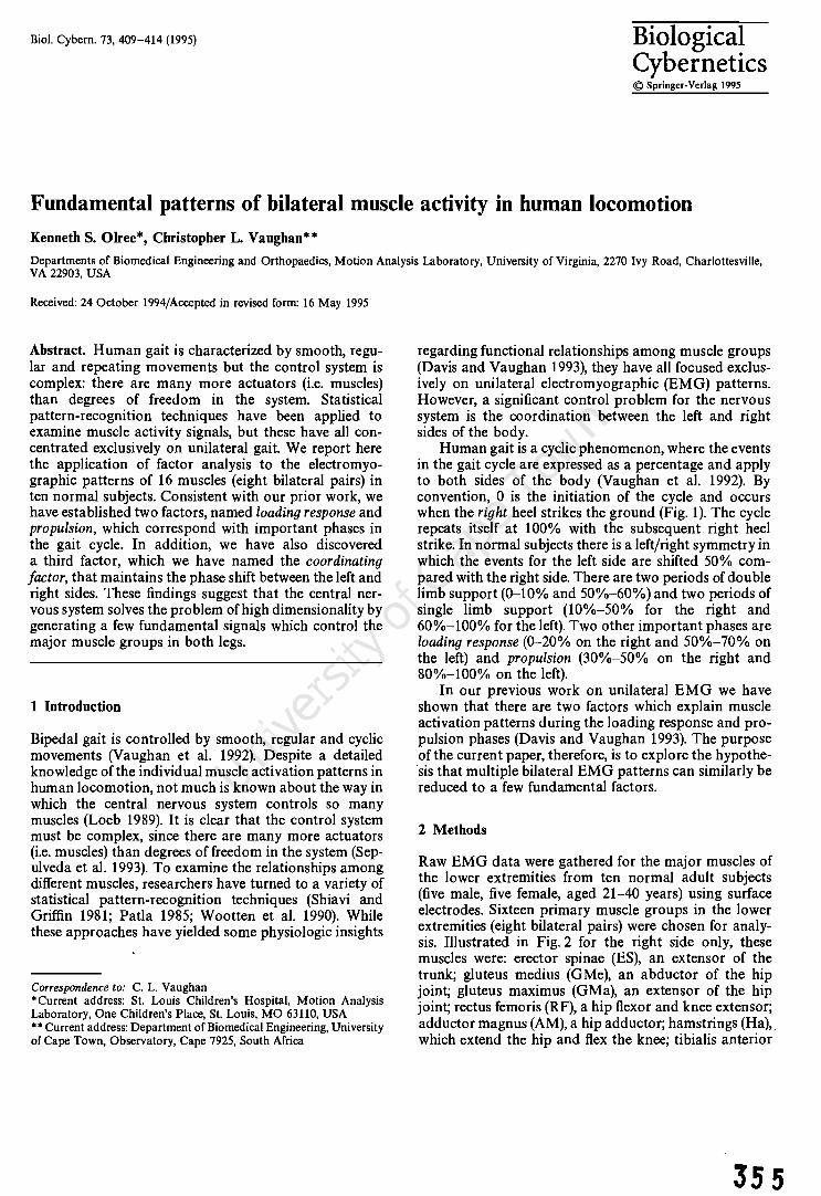
BioI. Cybern. 73, 409-414 (1995) Biological Cybernetics © Springer-Verlag 1995

Fundamental patterns of bilateral muscle activity in human locomotion

Kenneth S. Olree*, Christopher L. Vaughan"

Departments of Biomedical Engineering and Orthopaedics, Motion Analysis Laboratory, University of Virginia, 2270 Ivy Road, Charlottesville, VA 22903, USA

Received: 24 October 1994/Accepted in revised form: 16 May 1995

Abstract. Human gait is characterized by smooth, regu­lar and repeating movements but the control system is complex: there are many more actuators (i.e. muscles) than degrees of freedom in the system. Statistical pattern-recognition techniques have been applied to examine muscle activity signals, but these have all con­centrated exclusively on unilateral gait. We report here the application of factor analysis to the electromyo­graphic patterns of 16 muscles (eight bilateral pairs) in ten normal subjects. Consistent with our prior work, we have established two factors, named loading response and propulsion, which correspond with important phases in the gait cycle. In addition, we have also discovered a third factor, which we have named the coordinating factor, that maintains the phase shift between the left and right sides. These findings suggest that the central ner­vous system solves the problem of high dimensionality by generating a few fundamental signals which control the major muscle groups in both legs.

1 Introduction

Bipedal gait is controlled by smooth, regular and cyclic movements (Vaughan et al. 1992). Despite a detailed knowledge of the individual muscle activation patterns in human locomotion, not much is known about the way in which the central nervous system controls so many muscles (Loeb 1989). It is clear that the control system must be complex, since there are many more actuators (i.e. muscles) than degrees of freedom in the system (Sep­ulveda et al. 1993). To examine the relationships among different muscles, researchers have turned to a variety of statistical pattern-recognition techniques (Shiavi and Griffin 1981; Patla 1985; Wootten et al. 1990). While these approaches have yielded some physiologic insights

Correspondence to: C. L. Vaughan ·Current address: St. Louis Children's Hospital, Motion Analysis Laboratory, One Children's Place, St. Louis, MO 63110, USA ** Current address: Department of Biomedical Engineering, University of Cape Town, Observatory, Cape 7925, South Africa

regarding functional relationships among muscle groups (Davis and Vaughan 1993), they have all focused exclus­ively on unilateral electromyographic (EM G) patterns. However, a significant control problem for the nervous system is the coordination between the left and right sides of the body.

Human gait is a cyclic phenomenon, where the events in the gait cycle are expressed as a percentage and apply to both sides of the body (Vaughan et al. 1992). By convention, 0 is the initiation of the cycle and occurs when the right heel strikes the ground (Fig. 1). The cycle repeats itself at 100% with the subsequent right heel strike. In normal subjects there is a left/right symmetry in which the events for the left side are shifted 50% com­pared with the right side. There are two periods of double limb support (0-10% and 50%-60%) and two periods of single limb support (10%-50% for the right and 60%-100% for the left). Two other important phases are loading response (0-20% on the right and 50%-70% on the left) and propulsion (30%-50% on the right and 80%-100% on the left).

In our previous work on unilateral EMG we have shown that there are two factors which explain muscle activation patterns during the loading response and pro­pulsion phases (Davis and Vaughan 1993). The purpose of the current paper, therefore, is to explore the hypothe­sis that multiple bilateral EMG patterns can similarly be reduced to a few fundamental factors.

2 Methods

Raw EMG data were gathered for the major muscles of the lower extremities from ten normal adult subjects (five male, five female, aged 21-40 years) using surface electrodes. Sixteen primary muscle groups in the lower extremities (eight bilateral pairs) were chosen for analy­sis. Illustrated in Fig. 2 for the right side only, these muscles were: erector spinae (ES), an extensor of the trunk; gluteus medius (GMe), an abductor of the hip joint; gluteus maxim us (GMa), an extensor of the hip joint; rectus femoris (RF), a hip flexor and knee extensor; adductor magnus (AM), a hip adductor; hamstrings (Ha),. which extend the hip and flex the knee; tibialis anterior

355

410

\ ~/ Right Mid-Stance

Left Mid-Swing

Right Heel Off 50% Left Heel Strike

Fig. 1. Human gait is a cyclic phenomenon in which the left and right sides are 50% out of phase. The cycle starts at 0 with right heel strike and finishes at 100% with the subsequent right heel strike. Other important events are foot flat, mid-stance, heel off, toe off and mid­swing (Vaughan et al. 1992)

Erector Spinae

Gluteus Medius

Hamstrings --IM1

1M~hf6l\- Tibialis Anterior

Gastrocnemius

Fig. 2. Eight major muscle groups, shown here for the right leg, were selected for surface electromyographic (EMG) analysis

(TA), an ankle dorsiflexor; and gastrocnemius (Ga), an ankle plantar flexor and knee flexor.

Skin overlying the muscles was carefully prepared: hair was first shaved off, the outer layer of epidermal cells was abraded, and the oil and dirt were removed with an alcohol pad. Bipolar silver/silver chloride surface elec­trodes were placed over the 16 muscles with 1 em be­tween each pair of electrodes. Electrode placement was symmetric for the left and right sides of the body. Each electrode pair was attached to a light-weight preamplifier with a gain of 8000 and the amplified signal was fed into a small (0.44 kg) transmitter carried by the subject. The multiplexed signal was then telemetered, via radio waves, to a host computer. The EMG data were high-pass filtered (cut-off frequency 30 Hz) to remove motion arti­fact and each channel was sampled at 1000 Hz for a dura­tion of 4 s, thus yielding the raw signals (Fig. 3). In

356

Raw Electromyographic Signals in Human Gait

CIJ ES "C iii GMe

= GMa

~ RF Nd

Ha TA

Ga CIJ ES

"C GMe iii GMa

l: RF .2' ". .. '

a::: Nd

Ha TA

Ga ·W

RHS LHS RHS LHS RHS

1mvL 200 rna

Time

Fig. 3. An example of raw EMG patterns for one subject completing two consecutive gait cycles. RHS, right heel strike; LHS, left heel strike; ES, erector spinae; GMe, gluteus medius; GMa, gluteus maximus; RF, rectus femoris; AM, adductor magnus; Ha, hamstrings; T A, tibialis anterior; Ga, gastrocnemius

addition, a footswitch was taped to the sole of each subject's right shoe to record the gait cycle events. Each subject was instructed to walk briskly along a level path for three separate trials.

The 16 raw EMG signals were full-wave rectified, smoothed using a low-pass second-order Butterworth filter with a cut-off frequency of 3 Hz, and then nor­malized for both magnitude and time (Yang and Winter 1984). This was accomplished by scaling the EMG signal to a number between 0 and 1, based on the maximum value of the signal seen during the cycle (Davis and Vaughan 1993). Temporal normalization was based on the footswitch data and was accomplished by expressing the EMG values as a function of the gait cycle: from 0 to 100% in 2% increments (Vaughan et al. 1992). It should be pointed out that in all data shown in this paper the percent cycle is with respect to the right side. All subjects completed three trials and since each trial of 4 s consisted of two or three complete gait cycles, up to nine cycles of data were gathered. These data sets were ensemble aver­aged for each of the individual subject's 16 muscles. Finally, an ensemble average was generated for each of the 16 muscles from the averages found for each subject. To assess the repeatability of the 16 EMG patterns, both within and between subjects, a variance ratio (VR) statis­tic was computed (Hershler and Milner 1978). The data were then reduced to the appropriate format - a matrix of 51 rows of percent cycle increments by 16 columns of muscle patterns- for the application of statistical pat­tern-recognition techniques (Rummel 1970; Gorsuch 1974).

The factor analysis was based on three steps. The first step consisted of finding the correlations for all possible EMG variable pairs. This resulted in a 16 x 16 correla­tion matrix. Each correlation value measured the linear dependence of one variable on another. The second step

involved finding the eigenvalues and eigenvectors of the correlation matrix. Eigenvectors of a correlation matrix are mutually orthogonal (Rummel 1970). This means that each eigenvector represented a unique dimension in the 16 EMG activity space. The amount of variance explained by an eigenvector for a correlation matrix was found by dividing its associated eigenvalue by the num­ber of variables analyzed (Rummel 1970). Eigenvectors which represented only a trivial amount of variance were then excluded from further analysis. The third step con­sisted of orthogonally rotating the eigenvectors such that the variance explained by each eigenvector was maxi­mized for EMG variables having similar patterns of activity and minimized for patterns having dissimilar patterns. Orthogonal rotation aided an interpretation of the factor structure by grouping variables with similar patterns of activity, while keeping the factors (or rotated eigenvectors) mutually orthogonal (Basilevsky 1994). This procedure yielded the factor loading matrix. Factor scores were then computed from the original EMG data and the factor loading matrix. The factor scores for a particular factor can be interpreted as a composite variable which resembles the original variables which load most highly on its factor (Rummel 1970). Factor scores are also mutually orthogonal.

3 Results

The ensemble averages (Fig. 4) demonstrated good left/ right symmetry, low variability and excellent agreement with the previous literature on bilateral EMG (Arsenault et al. 1986; Ounpuu and Winter 1989). The variance ratios. (VRs) indicated that the data were repeatable, both within and between subjects (Table 1). Consistent with the literature, tibialis anterior and gastrocnemius were the least variable, while gluteus maxim us and adductor magnus tended to be most variable (Kadaba et al. 1989) .. When the 51 x 16 matrix of EMG signals, illustrated in the ensemble average data of Fig. 4, were subjected to factor analysis, the associated eigenvalues demonstrated that only five eigenvectors were required (Table 2). Note that the 'eigenvalue greater than one' criterion was ap­plied (Rummel 1970). In fact, these five eigenvectors ac­counted for 98.1 % of the variance in the original EMG data set of 16 muscles. When the five eigenvectors were rotated to produce five factors, and the factor scores were correlated with the original 16 EMG signals, the loading matrix yielded the results summarized in Table 3.

Gluteus medius and rectus femoris on the left side, plus erector spinae on the right side, load most heavily on factor 1. This means that a plot offactor scores for factor 1 (Fig. 5, top) will yield a curve that is very similar to the EMG signals for these muscles (Fig. 4). Factor 2 is sym­metric to factor 1: the same three muscles, but on the contralateral side, load on factor 2. Gastrocnemius on the left side, plus hamstrings on the right side, load most heavily on factor 3. As before, a plot of the factor scores (Fig. 5, middle) yields a curve that is very similar to the EMG signals for these muscles (Fig. 4). Factor 4 is sym­metric to factor 3: the same two muscles, but on the

"tI I: III

o I: II) II)

~ ~ .c "tI II)

iii u .!!.

u ~ Co III .. Cl o > E o .. .... u II)

iii "tI II)

.!::! iii E .. o Z

left

o 20 40 60 80 100 RHS LHS RHS

.. ::J

.~ .. ::!! .. ::J

5 i5 .. .~

~ .. a u ~

!I c .. .. ::!!

Right

o 20 40 80 80 100 RHS LHS RHS

Percent Cycle (for right side)

411

Fig. 4. Grand ensemble EMG signals for ten subjects, normalized in magnitude and time, as a function of the gait cycle. The continuous line represents the mean, while the dashed lines indicate plus and minus 1 standard deviation. Note in particular that there is good symmetry between the left and right sides when the 50% phase shift is taken into account; that on the basis of the standard deviations muscle patterns are very repeatable; and that each signal has one or more distinct peaks. RHS, right heel strike; LHS, left heel strike

contralateral side, load on factor 4. Tibialis anterior on the right side loads positively on factor 5 while the left tibialis anterior loads negatively (Table 2). Also loading positively on factor 5 is the right gluteus maximus. The left gluteus maximus has a relatively high negative load­ing on factor 5 but its highest loading is on factor 1. Interestingly, the right gluteus maximus also has a rela­tively high positive loading on factor 2. A plot of factor 5 (Fig. 5, bottom) yields a curve that is similar to the

357

412

Table 1. Variance ratios (VRs) for the 16 EMG patterns calculated for the gait cycle

Muscle Subject number Grand ensemble

2 3 4 5 6 7 8 9 10

Left side ES 0.09 0.13 0.18 0.60 0.17 0.26 0.28 0.08 0.13 0.10 0.29 GMe 0.04 0.15 0.28 0.23 0.33 0.31 0.06 0.29 0.15 0.41 0.38 GMa 0.18 0.29 0.23 0.29 0.22 0.30 0.15 0.29 0.28 0.30 0.64 RF 0.44 0.21 0.12 0.11 0.57 0.20 0.08 0.11 0.52 0.27 0.41 AM 0.39 0.31 0.32 0.33 0.38 0.29 0.45 0.51 0.79 0.43 0.60 Ha 0.06 0.04 0.04 0.37 0.20 0.30 0.19 0.25 0.36 0.17 0.36 TA 0.04 0.13 0.09 0.16 0.14 0.06 0.04 0.19 0.31 0.11 0.19 Ga 0.22 0.05 0.03 0.12 0.04 0.02 0.03 0.03 0.05 0.04 0.18

Right side ES 0.10 0.10 0.09 0.22 0.20 0.18 0.12 0.16 0.12 0.08 0.17 GMe 0.07 0.09 0.09 0.15 0.38 0.36 0.23 0.09 0.42 0.10 0.24 GMa 0.01 0.30 0.48 0.47 0.22 0.31 0.30 0.27 0.54 0.26 0.74 RF 0.18 0.15 0.23 0.12 0.35 0.10 0.06 0.85 0.30 0.21 0.29 AM 0.59 0.21 0.16 0.53 0.70 0.18 0.44 0.19 0.86 0.21 0.79 Ha 0.05 0.10 0.08 0.11 0.09 0.13 0.21 0.20 0.31 0.52 0.38 TA 0.15 0.10 0.14 0.30 0.27 0.27 0.05 0.16 0.10 0.10 0.30 Ga 0.06 0.04 0.03 0.08 0.11 0.02 0.04 0.08 0.06 0.04 0.15

Note that the VRs for a specific subject are based on six separate cycles while the ensemble VRs are based on the mean values for ten subjects. They are not simply the average of the VRs for the subjects. The VR statistic is a measure of repeatability: the closer the value is to zero, the greater the similarity between the curves, while a VR of 1 (or larger) signifies curves that differ greatly (Hershler and Milner 1978) ES, erector spinae; GMe, gluteus medius; GMa, gluteus maximus; RF, rectus femoris; AM, adductor magnus; Ha, hamstrings; TA, tibialis anterior; Ga, gastrocnemius

Table 2. The eigenvalue results for 16 muscles in forward walking demonstrate that five factors accounted for 98.1 % of the variance in the data

Magnitude Variance

Value 1

6.4 40.2

Value 2

4.4 27.4

Value 3

2.4 15.0

Value 4

1.5 9.4

Value 5

1.0 6.2

Total

15.7 98.1

To determine how many eigenvectors (or factors) should be retained, the 'eigenvalue greater than one' criterion was applied (Rummel 1970). This reduces the complexity of the analysis because factors which explain little variability are discarded, while the remaining factors which represent the dominant features in the original data are retained. The proportion of variance explained by each eigenvalue can be found by dividing the magnitude of the eigenvector by the number of variables analyzed, in this case 16 EMG patterns. These data indicate that the original set of EMG data can be reconstructed by a linear combination of just five factors with a mean square error of only 1.9%

EMG signals for the right tibialis anterior and gluteus maxim us (Fig. 4).

4 Discussion

The plots of the first two factor scores (Fig. 5, top) show maxima at 55% (factor 1) and 5% (factor 2) of the gait cycle. These two phases correspond to loading response on the left and right sides respectively (Fig. 1). The muscles involved serve the role of stabilizing the loco­motor apparatus just following heel strike. We thus refer to factors 1 and 2 as the loading response factors for the left and right sides respectively (Davis and Vaughan 1993).

The plots of the second two factor scores (Fig. 5, middle) show maxima at 90% (factor 3) and 40% (factor 4) of the gait cycle. These two phases correspond to propulsion of the left and right sides respectively (Fig. 1).

35 8

Since the gastrocnemius serves the role of propelling the body forward just prior to toe oft" we refer to factors 3 and 4 as the propulsion factors for the left and right sides respectively (Davis and Vaughan 1993). Also loading heavily on these factors, but in a negative direction, are the adductor magnus muscles (Table 2). We interpret a high negative loading to signify that a muscle pattern is inhibited (rather than facilitated) at that particular phase in the cycle. This suggests that the fundamental factor which controls propulsion simultaneously facilitates ip­silateral gastrocnemius and contralateral hamstrings, while inhibiting ipsilateral adductor magnus.

Factor 5 contains three maxima, and three corres­ponding minima which occur 50% later in the cycle than the maxima (Fig. 5, bottom). This observation, and the finding that tibialis anterior and gluteus maximus load highly on this factor in opposite directions for the left and right sides, suggest that the purpose of this fundamental factor is to maintain symmetry between the two sides. We

Table 3. A factor loading matrix, showing the correlation between the factor scores and the original EMG variable

Factor 1 Factor 2 Factor 3 Factor 4 Factor 5

Len side ES 0.391 0.844 0.235 0.228 0.023 GMe 0.941 - 0.104 - 0.279 0.105 0.012 GMa 0.861 0.086 - 0.233 0.119 - 0.422 RF 0.946 0.162 - 0.247 0.020 0.020 AM 0.163 - 0.103 -0.923 - 0.111 - 0.277 Ha 0.147 - 0.283 -0.272 0.890 -0.152 TA 0.514 0.091 - 0.395 0.221 -0.715 Ga - 0.145 - 0.025 0.946 - 0.189 0.188

Right side ES 0.747 0.494 0.334 0.218 0.094 GMe - 0.238 0.920 - 0.019 - 0.276 0.031 GMa 0.044 0.605 - 0.041 - 0.452 0.635 RF 0.361 0.827 0.059 -0.325 0.236 AM - 0.310 0.189 - 0.236 - 0.879 0.037 Ha - 0.445 0.303 0.773 - 0.287 - 0.098 TA -0.064 0.446 0.454 - 0.214 0.721 Ga -0.090 0.115 - 0.419 0.822 - 0.339

An orthogonal varimax rotation was used: the eigenvectors were rotated so that not only did they remain independent of one another but the correlation of the original variables with the factor scores was maximized (Basilevsky 1994). The loading matrix for the five factors shows how individual muscles load highly on specific factors. The percent variation explained by a particular factor for a muscle variable may be found by squaring the factor loading and multiplying by 100. Note that in each row the highest factor loading has been emboldened to indicate which factor is most representative of the original muscle pattern and to illustrate the symmetry in the factor loading Muscle abbreviations as in Table 1

thus refer to factor 5 as the coordinating factor. This notion of left/right symmetry may be further explored by shifting the factor scores 50% and then correlating them with the original factors (Table 4). As expected, there is a high correlation between shifted factor 1 and factor 2, as well as between shifted factor 3 and factor 4. Factor 5 correlates negatively with itself after being shifted 50% of the cycle. These findings suggest that the five factors may be further reduced to three fundamental patterns: loading response, propulsion and coordination.

Research in other vertebrates (Perret 1980) has shown that the initiation and timing of muscle action seems to be the work of a network of interneurons in the spinal cord that provides a cyclic pattern of signals (Loeb 1989). The matrix of interneurons, onto which converge both descending higher-order commands and prop­rioceptive feedback signals, may be conceptualized as a cascade of neural networks (Loeb et al. 1990). Consis­tent with the central pattern generator hypothesis (Grillner et al. 1991), a spinal oscillating network prob­ably generates the fundamental patterns of human loco­motion (Fig. 5). Once these patterns have passed through the subsequent neural networks (Loeb et al. 1990), the final output will be the muscle activation signals (Figs. 3, 4). These EMG signals provide input to the musculos­keletal apparatus which operates in a functional milieu that is governed by the theory of Newtonian mechanics (Vaughan et al. 1992). While the relationship between the EMG signals and mechanical parameters has been suc-

413

3.0

CD -,

\ en 2.0 \ c:: \ 0 \ Q. \ Factor 2 en

1.0 \ CD \ a::: \ \

C) c:: 0.0 :0 n:J 0

...J ·1.0

2.0 -, " \ , \ I \

1.0 , \

c:: Factor 4 : \

0 \

'iii I \ I :;

0.0 I

Q. I

0 I .... I

0- I I

·1.0 I , I

I

2.0

C) c:: 1.0 '+=, n:J

.!: "0 .... 0.0 0 0 U

·1.0

o 10 20 30 40 50 60 70 80 90 100

Percent Cycle

Fig. 5. Factor scores plotted as a function of the gait cycle. Factors 1 and 2 are bilaterally symmetric (Table 2) and have been plotted together, and similarly for factors 3 and 4. Factor 1 is the loading re.~ponsefactor for the left side, having a peak at about 55% of the cycle. This corresponds very closely to the EMG profiles for the left gluteus medius and rectus femoris as well as the right erector spinae in Fig. 4. Similarly, factor 2 is the loading response factor for the right side, with a peak at about 5% of the cycle and the same agreement with the EMG profiles in Fig. 4. Factor 3 is the propulsion factor for the left side with a peak at 90% of the cycle, corresponding closely to the EMG profile for the left gastrocnemius. Factor 4 is the propulsion factor for the right side, having a peak at 40% of the cycle and is in good agreement with the right gastrocnemius in Fig. 4. Factor 5 is referred to as the co· ordinating factor. It contains three maxima, and three minima which occur 50% later in the cycle than the maxima. The homologous pair of tibialis anterior and gluteus maximus load highly on this factor in opposite directions for the right and left sides (Table 3), suggesting that its purpose is to maintain left/right symmetry

cessfully modelled with artificial neural networks (Heller et al. 1993; Sepulveda et al. 1993), there has been no implementation to date of a model which incorporates the full complexity of the neural, muscular and skeletal systems in human gait (Vaughan et al. 1995). Our find­ings, which strongly suggest that the central nervous

359

414

Table 4. To illustrate the symmetry in the factors, a correlation matrix ·was created between the original factor scores and the factor scores after phase shifting by 50% of the cycle

Original Shifted factor (50% cycle) factor

Factor 1 Factor 2 Factor 3 Factor 4 Factor 5

Factor 1 0.11 Factor 2 0.92 -0.07 Factor 3 -0.13 0.25 -0.24 Factor 4 -0.26 0.09 0.87 0.02 Factor 5 0.22 0.12 -0.30 -0.33 -0.79

Note the very high correlation for shifted factor 1 and factor 2, as well as for shifted factor 3 and factor 4. Note also that factor 5 is quite highly correlated with itself (in a negative direction) after being shifted by 50% of the cycle

system solves the problem of high dimensionality by generating a few fundamental signals to control the major muscle groups in both legs, provide the basis for building a successful model of locomotor control.

Acknowledgement. This research was supported in part by a National Institutes of Health grant 1R01 HD30134.

References

Arsenault AB, Winter DA, Wells R (1986) Bilateralism of EMG profiles in human locomotion. Am J Phys Med 65:1-16

Basilevsky A (1994) Statistical factor analysis and related methods. Wiley, New York

Davis BL, Vaughan CL (1993) Phasic behavior of EMG signals during gait: use of multivariate statistics. J Electromyogr KinesioI3:51-60

Gorsuch RL (1974) Factor analysis. Saunders, Philadelphia Grillner S, Wallen P, Brodin L, Lansner A (1991) Neuronal network

generating locomotor behavior in lamprey: circuitry, transmitters, membrane properties and simulation of central pattern generators

360

for locomotion, with special reference to vertebrates. Annu Rev Neurosci 14: 169-200

Heller BW, Veltink PH, Rijkhoff NJM, Rutten WLC, Andrews BJ (1993) Reconstructing muscle activation during normal walking: a comparison of symbolic and connectionist machine learning techniques. Bioi Cybern 69:327-335

Hershler C, Milner M (1978) An optimality criterion for processing electromyographic (EMG) signals relating to human locomotion. IEEE Trans Biomed Eng 25:413-420

Kadaba MP, Ramakrishnan HK, Wootten ME, Gainey J, Gorton G, Cochran GVB (1989) Repeatability of kinematic, kinetic, and elec­tromyographic data in normal adult gait. J Orthop Res 7:849-860

Loeb GE (1989) Neural control of locomotion: how do all the data fit together? Bioscience 39: 800-804

Loeb GE, Levine WS, He J (1990) Understanding sensorimotor feed­back through optimal control. Cold Spring Harbor Symp Quant Bioi LV:791-803

Ounpuu S, Winter D (1989) Bilateral electromyographical analysis of the lower limbs during walking in normal adults. Electroen­cephalogr Clin Neurophysiol 72:429-438

Patla AE (1985) Some characteristics of EMG patterns during loco­motion: implications for the locomotor control process. J Motor Behav 17:443-461

Perret C (1980) Neural origin of rhythmic movement. Cambridge University Press, Cambridge, pp 405-422

Rummel RJ (1970) Applied factor analysis. Northwestern University Press, Evanston

Sepulveda F, Wells D, Vaughan CL (1993) A neural network repres­entation of electromyography and joint dynamics in human gait. J Biomech 26:101-109

Shiavi R, Griffin P (1981) Representing and clustering electromyo­graphic gait patterns with multivariate techniques. Med Bioi Eng Comput 19:605-611

Vaughan CL, Davis BL, O'Connor JC (1992) Dynamics of human gait. Human Kinetics, Champaign

Vaughan CL, Brooking GD, Olree KS (1995) Exploring new strategies for controlling multiple muscles in human locomotion. In: Human motion analysis: current applications and future directions. IEEE Press

Wootten ME, Kadaba MP, Cochran GVB (1990) Dynamic electro­myography I. Numerical representation using principal compon· ent analysis. J Orthop Res 8:247-258

Yang JF, Winter DA (1984) Electromyographic amplitude normaliz­ation methods: improving their sensitivity as diagnostic tools in gait analysis. Arch Phys Med Rehabil 65:517-521

~ Pergamon

0021-9290(95)00038-0

J. Biomeclumics, Vol. 29, No.3, pp. 383-388, 1996 Elsevier Science Ltd

Printed in Great Britain 0021-9290/96 SIS.OO + .00

TECHNICAL NOTE

ABDUCTION-ADDUCTION MOMENTS AT THE KNEE DURING STAIR ASCENT AND DESCENT

David L. Kowalk,* Jeffrey A. Duncant and Christopher L. Vaughan*t

Departments of ·Orthopaedics and tBiomedical Engineering, University of Virginia, Charlotteville, Virginia, U.S.A.

Abstract-To examine the relative magnitude of the knee abduction-adduction moments during stair climbing, ten normal subjects (average weight 660 N, leg length 0.962 m, height 1.74 m) were studied during repeated trials of stair ascent and descent. Data were collected using a four-camera video system and two forces plates incorporated within a flight of three stairs. The inverse dynamics approach was used to calculate internal moments at the knee, and these moments were normalized in magnitude (to percent body weight and leg length) and time (percent stance). The primary findings were: (1) knee joint moments were similar in shape and magnitude for the first and second steps during both stair ascent and descent; (2) the abduction knee moments, although comparable in magnitude (25-45 Nm), were statistically smaller than the extension moments (60-85 Nm) for stair ascent and descent; and (3) the moment patterns were exclusively abductor throughout stance, indicating that the ground reaction vector always passed medial to the knee joint center. Although the knee abduction-adduction moment is not in the primary plane of motion, its magnitude should not be ignored when trying to understand the stability and function of the knee during stair climbing.

Keywords: Knee joints; Stairs; Abduction moments.

INTRODUcnON

A novel theory of human gait posits that locomotion depends on the joint moments which are in the plane perpendicular to the intended direction of progression. Consider a man walking on level ground [Fig. l(a)]. The plane that is perpendicular to his direction of progression is the frontal plane, and the hip joint moment axes that are in this plane are the flexion-extension and internal-external rotation axes. Supporting arguments for the role of the internal-external hip rotation moments has been provided by the 'compass gait' model of Saunders et al. (1953), the 'spinal engine' theory of Gracovetsky (1985), and reciprocat­ing gait orthoses for spina bifida children (Mazur et al., 1990). Despite these studies, the vast majority of researchers in human gait have focused on the sagittal plane and emphasized the flexion-extension moments as the primary effectors of locomo­tion.

Stair climbing is of particular interest since stairs are fre­quently encountered obstacles in daily living, and require greater knee moments and ranges of motion than those required in level walking (Andriacchi et al., 1982; Andriacchi and Mikosz, 1991). To move up or down stairs, the direction of progression is up the incline and so the moments applied about axes that are in a plane at right angles to this direction should be considered: for the knee this includes both the flexion-extension and abduc­tion-adduction axes [cf. Fig. 1(b)]. While the flexion-extension moments are undoubtedly crucial, a natural question to ask is: how important are the abduction-adduction moments at the knee during stair climbing? Andriacchi et al. (1980) used a method to calculate joint moments (the cross product of the

Received in final form 24 February 1995. Address correspondence to: Dr Christopher L. Vaughan,

Department of Biomedical Engineering, University of Cape Town Observatory, Cape 7925, South Africa

383

ground reaction force vector and the joint center positional vector) which neglected contributions from inertial terms and segment weights, an approach which is subject to increasing errors in moment calculations for joints above the ankle (Wells, 1981). Furthermore, a resultant 3D joint moment must be ex­pressed in terms of anatomically relevant axes to have any functional relevance. Selection of these axes in prior bi­omechanical models (Andriacchi et al., 1982; Costigan et al., 1992, 1993) suggests there may be some scope for improvement. The purpose of this technical note, therefore, is to recommend an anatomically consistent set of axes for determining joint moments and to examine the relative magnitude of the knee abduction-adduction moments in stair climbing.

METHODS

Ten normal adults (6 male and 4 female), ranging in age from 22 to 40 years old (average weight 660 N, right leg length 0.962 m and height 1.74 m), signed an informed consent form and served as subjects. They ascended the stairs three times beginning with their right leg and three times beginning with their left. They also descended the stairs three times beginning with their right leg and three times beginning with their left. Standing slightly in front of force plate 1, subjects ascended by stepping onto steps 1, 2 and 3 with alternating feet. Subjects began stair descent on step 3, stepped down onto steps 2, 1 and then onto the floor in front of force plate 1 (cf. Fig. 1).

Kinematic data were collected at 60 Hz using a system based on four video cameras (Motion Analysis Corporation, Santa Rosa, CA). Ground reaction forces were also measured at 60 Hz using two Kistler force plates (Winterhur, Switzerland) with steps mounted onto each plate. Stairs of standard dimensions were used with a rise of 0.203 m and a run of 0.254 m.Prior to testing, the force plates were preloaded with 356 N under the lower step and 713 N under the taller step. This preloaded step system has been calibrated and tested for accuracy in a prior

361

384 Technical Note

frontal plane

(a)

Force (b) Plate 1

flexion-extension axis

Flexion and Extension

~' ~rection of

/ Progression

Fig. 1. (a) A man walking on level ground moves forward by the application of joint moments about axes that are in the plane perpendicular to the intended direction of progression. In this example, it is the frontal plane and the joint moment axes in this plane are the flexion-extension and internal-external rotation axes for the right hip. (b) Location of the steps on the force platforms and definition of the knee joint reference axes (Vaughan et al., 1992). Note that steps 1 and 2 were sensitive to reaction forces, while the ground and step 3 were not. The flexion-extension moment takes place about the mediolateral axis of the proximal segment (thigh). The internal-external rota­tion moment takes place about the longitudinal axis of the distal segment (calf). The abduction-adduction moment takes place about a floating axis that is perpendicular to the mediolateral and longitudinal axes (these axes are not normally perpendicu­lar to each other). In this paper only the flexion-extension and

abduction-adduction moments were evaluated.

study (Besser et al., 1993). Kinematic, ground reaction force and body segment parameter data were integrated using the GaitLab software (Vaughan et al., 1992), which implements the rigorous inverse dynamics approach in three dimensions, to calculate knee moments. The axes defining these moments are based on the recommendations by Grood and Suntay (1983) for joint angles: flexion-extension occurs about a medio-Iateral axis em­bedded in the thigh, internal-external rotation takes place about the longitudinal axis of the calf, and abduction-adduction oc-

362

curs about a floating axis that is perpendicular to the flexion-extension and internal-external rotation axes [cf. Fig. 1 (b)].

All 12 trials for each subject were analyzed, and the knee joint moments calculated. These moments were averaged for each subject and across all subjects with normalization to body weight and leg length and expressed as a percentage. Leg length was defined as the distance between the greater trochanter and the soles of the feet. The choice of this method for normalization was rationalized on the following basis. The units of joint mo­ments are Nm, so ideally one would like to divide by a force (in N) and a linear parameter (in meters). Heavier individuals will tend to exert larger joint moments, as will individuals with larger segment lengths. It therefore seemed logical to divide the joint moment by the body weight and leg length and express this ratio as a percentage (Ramakrishnan et aI., 1987). The convention of internal moments, with the moment being applied by the prox­imal segment on the distal segment, has been adopted (i.e. sagittal plane knee moments during the stance phase of stair climbing will be of the extension type). Some authors have calculated external moments by mUltiplying the ground reaction force by the lever arm to the joint and therefore express knee moments during stair climbing as being of the flexion type (Andriacchi et aI., 1980; Berchuck et aI., 1990; Costigan et aI., 1993).

The ensemble averages for the knee moments were further processed for statistical analysis. First, the maximum values for the extension and adduction moments were extracted for each subject. Second, knee joint angular impulses were calculated by integrating the extension and abduction moments over percent cycle. These data were then subjected to an analysis of variance (ANOVA) to test for differences at the om level of significance. Finally, variance ratios (VRs) were calculated for the knee flexion-extension and abduction-adduction moments to test for repeatability of the patterns (Hershler and Milner, 1978).

RESULTS

There were no significant differences in the maximum knee joint moments for the first step versus the second step (Table 1). For the joint impulses the only difference was for abduction during descent (Table 1). Since most gait laboratories do not have sufficient height clearance to incorporate a set of stairs with more than three steps, it is important to have established that this apparent limitation appears to have a negligible effect on the joint moments and impulses.

When comparing the direction of stair climbing, there were no differences for abduction but descent yielded greater maximum extension moments and impulses than ascent (Table 1). Whereas this difference for extension was seen early in stance phase for ascent [Fig. 2(a)], the pattern shifted for descent with the max­imum moment occurring much later in stance [Fig. 2(b)]. In contrast, the abduction moments exhibited a very similar bi­phasic pattern for both ascent and descent [Fig. 2(c) and (d)].

The maximum knee abduction moment was statistically smaller than the extension moment for both ascent and descent (fable 1, Fig. 2). In the knee joint impulse comparisons, there were no differences for stair ascent (although abduction was slightly greater for both the first and second steps) but extension was statistically greater for descent (fable 1). In general, all 10 subjects demonstrated good repeatability for both abduc­tion-adduction and flexion-extension moments for ascent and descent, with variance ratios (VRs) between 0.09 and 0.45 for the six trials (Table 2). Interestingly, the VRs were much lower for the grand ensemble data, with values between 0.11 and 0.14 (fable 2).

The moment data were normalized for the purpose of en­semble averaging and statistical comparison (Fig. 2). To facilit­ate comparison with the literature, the mean anthropometric values for the 10 subjects (height 1.74 m, weight 660 N, and leg length 0.962 m) were used to convert these data back to Nm (Fig. 3).

Technical Note

Table 1. Average values for the maximum knee moments and impulses, based on six trials by 10 subjects

Moment Impulse Direction Condition Extension Abduction Extension Abduction

Ascent First step 9.7 ( ± 2.4) 6.5 ( ± 1.2) 3.5 ( ± 1.0) 3.9 ( ± 0.9) Second step 9.4 ( ± 1.9) 6.8 ( ± 1.3) 3.1 ( ± 0.7) 4.1 (± 1.1)

Descent First step 14.0 (± 2.0) 7.6 ( ± 1.2) 6.3 ( ± 1.3) 4.4 ( ± 1.0) Second step 15.4 ( ± 2.4) 6.9 ( ± 1.5) 6.7 ( ± 1.6) 3.7 ( ± 0.9)

Ascent First step vs second step 0.339 0.206 0.017 0.075 Descent Fist step vs second step 0.044 0.041 0.161 0.002·

Ascent vs Descent 0.000· 0.020 0.000· 0.025 Ascent Extension vs abduction 0.009· 0.510 Descent Extension vs abduction 0.000· 0.008·

Note: These data, in the top portion of the table, are each followed by the standard deviations in parentheses. Note that moments are normalized to body weight and leg length and expressed as a percentage, while the impulses are the areas under the moment curves for extension and abduction (cf. Fig. 2). Statistical comparisons, utilizing analysis of variance, are shown with the p values in the bottom portion of the table. Significance was set at p < 0.01 and has been indicated by an asterisk ( .). Note that the comparisons for the last three rows are based on the first step only. These statistical comparisons were repeated for the maxima of each trial for each subject (rather than using ensemble averages) and the same results were established.

Stair Ascent: First Step Stair Ascent: First Step

12 10 r------------------,

x CD

E ~ "0

CD 0 .~ ::::!: iii E CD

CD 0 c Z ~

>C CD

;;::

(a)

x CD

E CD

"OE CDo ~::::!: as CD ECD ... C

~~ >C CD

;;::

(b)

, , \ ,

\ :8 8 '" 8 , , , 6

\ \ \

4 \ \ \ , \, , ,

0 ,

I '" ... -, , " \ ... \ I I ' ,_ .... "" ,

4 ' I' \

:/ " "'-',\ I I , \

2 I, , ' II \ \ II \ \

a --':./ \ \ ...... _----

-4 _2~~~-~~-~~-~-L-~~

0 20 40 60 80 100 (c) o M ~ 00 80 100

Percent Cycle Percent Cycle

Stair Descent: First Step Stair Descent: First Step

20 10

15 ' -, I \

I \ I , \ I ,."'" ,

10 I I '\ I I \ \

I \ \

"-', I I \ \ , , I \ \

5 I ,

I \ \ I I I \ \

I ,', , \::.- ....... I I

, '-

, I I -.................

0 ,

I ,

"0 8 .c , ,

'" I \

, , \ I

E 6 , ,

,-CD I

"C E I , -, l!lo I I

, , , :=:2 4 ' I '-,

"'CD " I, E CD I I ... c 2 I I

~~ I I I I

I I "0 / , I "0 -------------'" '/

-5 0 20 40 60 80 100

-2 0 20 40 60 80

Percent Cycle (d) Percent Cycle.

Fig. 2. Ensemble averages of knee fiexion-extension moments for the initiation step during (a) stair ascent; and (b) stair descent. Ensemble averages of the knee abduction-adduction moments for the initiation step during (c) stair ascent and (d) stair descent. The solid line represents the average of six trials for each of ten subjects. Dashed lines represent ± one standard deviation. Moments are normalized to body weight (average 660 N) and right leg length (aveage 0.962 m) and expresed as a percentage. Knee moments in Nm may be estimated by multiplying the y-axis value by a subject's weight (N) and right leg length (m), and dividing by 100. Time data have been normalized to the gait cycle with 0% being the first foot contact and

100% the subsequent contact with the same foot.

100

385

363

386

x CD

E ~ C CD E 0 ~ CD CD c:: ~

)(

CD

""

(a)

x CD

E ~ C CD E 0 ~

31 c:: ~

)(

CD

""

(b)

36 4

Technical Note

Table 2. Variance ratios (VRs) for the flexion-extension and abduction-adduction moments at the knee joint during stair ascent and descent (Hershler and Milner, 1978)

Ascent Descent

Subject Flexion-extension Abduction-adduction Flexion-extension Abduction-adduction

Nl 0.27 0.16 0.09 0.16 N2 0.25 0.14 0.16 0.13 N3 0.25 0.21 0.16 0.32 N4 0.32 0.37 0.10 0.16 N5 0.28 0.13 0.22 0.11 N6 0.19 0.11 0.18 0.19 N7 0.17 0.19 0.24 0.29 N8 0.33 0.24 0.17 0.26 N9 0.35 0.20 0.15 0.14 NI0 0.21 0.26 0.26 0.45

Grant ensemble 0.14 0.11 0.11 0.13

Note: VRs for a specific subject are based on six separate trials, while the ensemble VRs are based on the averaged moment curves for 10 subjects. They are not simply the average of the VRs for the subjects. A VR is a measure of repeatability: the closer the value is to zero, the greater the similarity between the curves, while a VR of 1 (or larger) signifies curves that differ greatly.

100

80

60

40

20

0

-20

-40

140

120

100

80

60

40

20

0

-20

-40

Stair Ascent: Comparison with Literature Stair Ascent: Comparison with Literature eo

/-·'.McFadyen :B " I

, , \ 1\1 50 , ,

, Andriacchi I I , (/ .. >.-:.~~\ E Kowalk I ,

40 \ \

ii " .... ',Andriacchi ~ \

r / \~~ \ ........... Costigan C 30

J/\~;<:/ \ CI E , 0 I

20 I

~ 1.'- ........ CI

.. CI ~ ..............

10 r c:: I Costigan ~ I , "0 "0

0 1\1

-10 0 20 40 60 80 100

(c) 0 20 40 60 80

Percent Cycle Percent Cycle

Stair Descent: Comparison with Literature Stair Descent: Comparison with Literature 50

Andriacchi "0 McFadyen " .e " \

1\1 40 I

, I E ! I 30 I I ~ I

I I C ! CI 20 I E

0 ~ 10

CD CD c:: 0 ~ \ , ., \ I .,.-.... "0 -10 \,_/ Andriacchi "0 I'll

-20 0 20 40 60 80 100 0 20 40 60 80

Percent Cycle (d) Percent Cycle

Fig. 3. Comparison of knee moment data from the literature: flexion-extension curves for (a) stair ascent and (b) stair descent; and abduction-adduction curves for (c) stair ascent and (d) stair descent. Note that Kowalk (solid line) refers to the data in the current paper where the data in Fig. 2 have been converted to units ofN m using the approach described in the figure caption. Andriacchi (dashed line) refers to the data of Andriacchi et al. (1980) and is based on a single trial for a single subject. McFadyen (dot-dashed line) refers to the data of McFadyen and Winter (1988) and is based on a single trial for a single subject (WM86). Their data, in units of Nm/kg, have been converted to N m by multiplying by the average subject mass in the current paper (67.3 kg). Costigan (dotted line) refers to the data of Costigan et al. (1992) and is based on the data for 34 subjects. Their data, also in units of Nm/kg, have been converted to Nm by multiplying by

67.3 kg.

100

100

Technical Note 387

DISCUSSION

The current data for flexion-extension moments are similar in shape and magnitude to the previously published values of Andriacchi and Mikosz (1991) for ascent and descent and McFadyen and Winter (1988) for ascent [Fig. 3(a) and (b)]. However, Costigan et al. (1993) reported a second peak in late stance for ascent [Fig. 3(a)], while McFadyen and Winter (1988) have an early peak in the stance phase for descent [Fig. 3(b)]. For the abduction moments, Andriacchi et al. (1980) reported patterns of similar magnitude to the current study for stair ascent [Fig. 3(c)] and descent [Fig. 3(a)] but the curves had quite different shapes, particularly for descent where knee adduction moments were measured [Fig. 3(d)]. For stair ascent, the abduc­tion moment data of Costigan et al. (1993) were similar in shape but the magnitude was approximately 50% of the maximum value for the current study [Fig. 3(c)]. It should be emphasized that Andriacchi et al. (1980) and McFadyen and Winter (1988) reported their curves for a single trial of a single subject, while the curves in Costigan et al. (1993) and the current study were based on an ensemble average of multiple subjects.

The discrepancies between the knee joint moments of Andriacchi et al. (1980) and McFadyen and Winter (1988) and the current study highlight the inherent danger when using a single subject's data as representative of the group. This is particularly pertinent for the abduction data during descent [Fig.3(d)] where the data of Andriacchi et al. (1980) suggest that a knee adduction moment was required in early and late stance. This implies the loading of structures (e.g. collateral ligaments) on the medial side of the knee since the ground reaction force vector must have passed lateral to the knee joint center. The data in the current study, with low standard deviations in early and late stance [Fig. 2(c) and (d)], suggest that normal subjects did not exert knee adduction moments. A possible source of difference was the axis that Andriacchi et al. (1980) chose for abduction-adduction: a vector perpendicular to the long axis of the tibia that rotates with the internal and external rotation of the tibia about its long axis. During the range of motion seen in stair climbing, this rotation can be as much as 20°. This 'coup­ling' effect has previously been shown to introduce significant errors for knee kinematics (Ramakrisnan and Kadaba, 1991) and probably has a similar effect for the joint moments. Another source of confusion relates to the data of Costigan and col­leagues: in a prior methodological paper, the moments were expressed relative to a global coordinate system (Costigan et al., 1992), but a more recent paper, on which the data in Fig. 3 were based, reported the data as 'fixed body moments' (Costigan et al., 1993). The precise axis for the abduction-adduction mo­ments was not defined, however.

The most important parameters affecting the accuracy of the joint moment data are the vectors defining the flexion-extension and abduction-adduction axes (Grood and Suntay, 1983; Vaughan et al., 1992), and the point of application plus line of action for the ground reaction force (Besser et al., 1993). The relatively low standard deviations for the joint moment data (Table 1, Fig. 2), and the good repeatability as demonstrated by the low variance ratios (Table 2), suggest that errors were kept to a minimum in this study. The lateral knee marker plays an important role in defining the knee joint center and therefore influences the location of both the flexion-extension and abduc­tion-adduction axes. Because the bony prominence of the fem­oral epicondyle and proximal fibula could be readily palpated, the knee marker was reliably located. While inertial contribu­tions to joint moments were important during the swing phase [up to 20% of the peak-to-peak range may be observed in Fig. 2(a)], their effect during stance phase was found to be essentially negligible. The repeatability of the knee joint moments as meas­ured by the variance ratio (VR) statistic (cf. Table 2) was in good agreement with the values of 0.13 to 0.35 reported by Bowsher and Vaughan (1995) for hip joint moments in level walking. These findings strengthen the argument for normalizing joint moments by dividing by body weight and leg length (Rama­krishnan et al., 1987).

To move up or down stairs requires the production of mo­ments at the hip, knee and ankle joints. While the sagittal plane (i.e. flexion-extension) moments are intuitively the most impor­tant, the abduction-adduction moments also play an importnat role at the knee, providing both propulsion and mediolateral stability. The structures that must normally provide the knee abduction moment, which results because the ground reaction force passes medial to the knee joint center, include the lateral collateral ligament and the ilio-tibial band. The magnitUde of the abduction moment casts doubt on the utility of the 'support moment' concept which assumes that only sagittal plane mo­ments are functionally relevant for stair climbing (McFadyen and Winter, 1988). While the abduction moments were statist­ically smaller than the extension moments, there were 'two per­iods-late stance in stair ascent and early stance in stair de­scent-when the extension moment was close to zero but the abduction moment had a value between 25 and 40 Nm.

Acknowledgements-This research was supported in part by an NIH Orthopaedic Research Training Grant T32 AR07482 (DLK), a United States Department of Education Rehabilita­tion Engineering Training Grant H133Pl0006-92 (JAD), and a National Institutes of Health Grant ROL HD30134 (CLV).

REFERENCES

Andriacchi, T. P., Andersson, G. B. 1., Fermier, R. W., Stern, D. and Galante, 1. O. (1980) A study of lower limb mechanics during stair-climbing. J. Bone Jt Surg. 62-A, 749-757.

Andriacchi, T. P., Galante, 1. O. and Fermier, R. W. (1982) The influence of total knee-replacement design on walking and stair-climbing. J. Bone Jt Surg. 64-A, 1328-1335.

Andriacchi, T. P. and Mikosz R. P. (1991) Musculoskeletal dynamics, locomotion and clinical applications. In Basic Or­thopaedic Biomechanics (Edited by V. C. Mow and W. C. Hayes), pp. 51-92. Raven Press, New York.

Berchuck, M., Andriacchi, T. P., Bach, B. R. and Reider, B. (1990) Gait adaptations by patients who have a deficient anterior cruciate ligament. J. Bone Jt Surg. 7loA, 871-877.

Besser, M. P., Kowalk, D. L. and Vaughan, C. L. (1993) Mounting and calibration of stairs on piezoelectric force platforms. Gait Posture 1, 231-235.

Bowsher, K. A. and Vaughan, C. L. (1995) Effect offoot-progres­sion angle on hip joint moments during gait. J. Biomechanics 28,759-762.

Costigan, P. A., Wyss, U. P., Deluzio, K. and Li, 1. (1992) Semiautomatic three-dimensional knee motion assessment system. Med. Bioi. Engng Comput. 30, 343-350.

Costigan, P. A., Wyss, U. P., Li, J., Cooke, T. V. D. and Olney, S. J. (1993) Forces and moments at the knee during stair­c1i~bing. Proc. XIVth Congr. Int. Society of Biomechanics, Pans, France, pp. 288-289.

Gracovetsky, S. (1985) An hypothesis for the role of the spine in human locomotion: a challenge to current thinking, J. Bio­med. Engng 7, 205-2L6.

Grood, E. S. and Suntay. W. J. (1983) A joint coordinate system for the clinical description of three-dimensional motions: ap­plication to the knee, J. Biomech. Engng 105, 136-144.

Hershler, C. and Milner, M. (1978) An optimality criterion for processing electromyographic (EMG) signals relating to hu­man locomotion, IEEE Trans. Biomed. Engng 25, 413-420.

McFadyen, B. 1. and Winter, D. A. (1988) An integrated bio­mechanical analysis of normal stair ascent and descent. J. Biomechanics 21, 733-744.

Mazur,1. M., Sienko-Thomas, S., Wright, N. and Cummings, R. 1. (1990) Swing-through vs. reciprocating gait patterns in patients with thoracic-level spina bifida. ZeitschriJt for Kin­derchirurgie 45 (supp!.), 1 : 23-25.

Ramakrishnan, H. K., Kadaba, M. P. and Wootten, M. E. (1987)

36.1\

388 Technical Note

Lower extremity joint moments and ground reaction torque in adult gait. In Biomechanics of Normal and Prosthetic Gait, pp. 87-92. American Society of Mechanical Engineers BED-4jDsc-7.

Ramakrishnan, H. K. and Kadaba, M. P. (1991) On the estima­tion of joint kinematics during gait. J. Biomechanics 24, 969-977.

Saunders, 1. B. Inman, V. T. and Eberhart, H. D. (1953) The

366

major determinants in normal and pathological gait. J. Bone Jt Surg. 35-A, 543-559.

Vaughan, C. L., Davis, B. L. and O'Connor, J. C. (1992) Gait Analysis Laboratory. Human Kinetics Publishers, Cham­paign.

Wells, R. (1981) The projection of the ground reaction force as a predictor of internal joint moments, Bull. Prosthetics Res. 18,15-19.

~ ~ ~

ELSEVIER Human Movement Science 15 (1996) 423-443

HUMAN MOVEMENT SCIE~t~E

Are joint torques the Holy Grail of human gait analysis?

Christopher L. Vaughan *

Department of Biomedical Engineering, University of Cape Town, Observatory, Cape Town 7925, South Africa

Abstract

Despite complex control systems, human gait is characterised by smooth, regular and repeating movements. Such coordinated motion occurs as a direct result of the cyclical activation of many leg muscles. It is the tension in these muscles that serves as the direct cause of the kinematic patterns that we observe and recognise as locomotion. The challenge facing biomechanists, however, is that there are many more muscle activators than independent equations defining the system. This leads to the classic indeterminate problem. Engineers have circumvented this problem by means of a mechanical ruse: all muscle, bone and ligament forces are reduced to a single (vector) resultant joint force and torque. Using an inverse dynamics approach, the joint torques may be estimated and it has been proposed that they are the causative factors that help biomechanists understand how gait is achieved. This is the approach that we followed at the University of Virginia over the past 5 years. In this paper, we will review the data from our own studies, exploring both the advantages and disadvantages of the joint torque approach. Our target populations have included: normal children; cerebral palsy children with orthoses; ankle inver­sion-eversion in level gait; knee abduction-adduction in stair climbing; and athletes with tom anterior cruciate ligaments. While this quest should be an interesting journey, offering a few fleeting glimpses of biomechanical insight, our final destination does not yield the Holy Grail.

PsyC/NFO classification: 3300

Keywords: Human gait; Locomotion; Joint torque

• E-mail: kvaughan@anat.uct.ac.za, Tel.: +2721 4066544, Fax: +27 21 4483291.

0167-9457/96/$15.00 Copyright © 1996 Elsevier Science B.V. All rights reserved. PII SO 167-9457(96)00009-7

3R 7

424 c.L. Vaughan / Human Movement Science 15 (1996) 423-443

1. Introduction

Human gait is characterised by smooth, regular and repeating movements. The apparent simplicity of movement masks complex underlying control mecha­nisms represented by the nervous, muscular and skeletal systems. This leads to the obvious question.

1.1. How do we walk?

The process of locomotor programming occurs in supraspinal centres and involves the conversion of an idea into a pattern of muscle activity that is necessary for walking (Enoka, 1988). The interaction between the central nervous system (CNS), the peripheral nervous system (PNS), and the muscu­loskeletal effector system is crucial for successful movement. The sequence of events that take place for walking to occur may be summarised as follows: 1. registration and activation of the gait command in the CNS, 2. transmission of the gait signals to the PNS, 3. contraction of muscles that develop tension, 4. generation of forces at, and torques across, synovial joints, 5. regulation of joint forces and torques by the rigid skeletal segments based on

their anthropometry, 6. displacement (i.e., movement) of the segments in a manner that is recognised

as functional gait, 7. generation of ground reaction forces.

These events are based on cause and effect (Vaughan et aI., 1992). While the cascade described above stresses the top-down control of human gait, the role played by sensory feedback is vitally important and should not be overlooked (Loeb et aI., 1990).

The coordinated motion occurs as a direct result of the cyclical activation of many leg muscles and it is the tension in these muscles that serves as the direct cause of the kinematic patterns that we observe and recognise as locomotion. It is therefore not surprising that biomechanists have tended to focus on the loads generated by the muscles and sustained by the bones in their efforts to understand the nature of human motion. As illustrated in Fig. 1, a reasonable question to ask might be: what happens at the ankle joint during push off?

1.2. A free body diagram of the foot

A standard approach in mechanics is to draw a free body diagram. This means that the system of interest - in this case the foot - is freed from its

368

c.L. Vaughan / Human Movement Science 15 (1996) 423-443 425

What happens at the

ankle joint during push off ?

Fig. 1. During the push off phase of the gait cycle, the muscles crossing the ankle joint are helping to propel the body forward. It is reasonable to wonder about the mechanical environment of the structures at the ankle joint complex and the role that each might play in propulsion.

surroundings and all the external forces acting on the foot are drawn in as vectors (Fig. 2). These forces include the weight of the foot (WF ), the horizontal and vertical ground reaction forces (F x and F y), the bony forces of the calf acting on the foot (Ffibula and Ftibia), and the many muscle forces (FAchilles,

F peronei' Ftibialis posterior' Ftibialis anterio)· Note that, for the sake of convenience, the forces exerted by the ligaments and other soft tissues (such as the skin) have been ignored.

F Tibialis posterior

FFibUla

Fig. 2. A free body diagram of the foot, in which all the external forces acting of the foot are identified, is the first step in understanding the mechanical environment. The plethora of muscle and bone forces means that there are too many unknowns (see Section 1.3 for discussion).

369

426 c.L. Vaughan / Human Movement Science 15 (1996) 423-443

1.3. The indeterminate problem

While the weight of the foot can be estimated and the ground reaction forces can be accurately measured by means of a force plate, the bone and muscle forces are all unknown. Since they cannot be readily or, indeed ethically, measured with in vivo transducers, the question that arises is whether they can be calculated from these other known quantities. For a single body such as the foot, there are only 3 independent equations of motion in 2D (and 6 equations in 3D). Since the bone and muscle forces are vector quantities, indicated by the bold notation, there will be 12 unknowns in a 2D analysis and 18 unknowns in a 3D analysis. There are obviously too many unknowns for the number of independent equations and the system is said to be indeterminate (Vaughan et aI., 1982).

1.4. The inverse dynamics approach and joint torques

There are 3 main strategies that may be employed to overcome this state of indeterminacy. First, the number of unknowns can be reduced. For example, it may be assumed that only one of the muscles - such as the Achilles tendon - is exerting a force and the two bone-on-bone forces can be reduced to a single force. This decreases the number of unknowns to 4 in 2D (and 6 in 3D), yielding a tractable solution. However, there will be numerous occasions, confirmed by electromyographic data, when there is simultaneous activity of more than one muscle group. A second strategy that has been adopted is the use of mathematical optimization theory (Crowninshield and Brand, 1981). Here, the unknown forces are treated as design variables, and the task is to seek those design variables that minimise a cost function such as segmental energy of the foot or ankle joint power, subject to certain constraints which are simply the equations of motion. The problem with this strategy is that the cost function cannot be known a priori and the resulting muscle and bone force predictions can never be fully validated (Collins, 1995). The third and final strategy to circumvent the indeterminate problem is to use a mechanical ruse: all muscle, bone and ligament forces crossing the ankle joint are reduced to a single (vector) resultant force FA and torque TN As illustrated in Fig. 3 for the 2D case, there are sufficient equations (3) to solve for the 3 scalar unknowns (FAx' FAy' TA ).

Strictly speaking, the 3 equations are ordinary second-order differential equa­tions. In the forward dynamics approach, the forces and torques are used as input and the equations are solved (typically numerically) to yield the movement of the system of interest (in this case the foot). However, this assumes that the

370

c.L. Vaughan / Human Movement Science 15 (1996) 423-443 427

Fy + FAY - WF = mFYFcg

FXd1 + Fyd2 - FAxd3 - F Ayd4 + TA = IFuF

Fig. 3. Free body diagram of the foot. Resultant force and torque at ankle. The many muscle and bone forces at the ankle joint (cf. Fig. 2) may be reduced to a single (vector) force and torque. In the 2D case illustrated here, the 3 equations of motion (based on the standard Newtonian formulation) are sufficient to solve for the 3 unknowns FAx' FAy and TA .

ankle joint force and torque are known as a function of time. This is seldom the case in biomechanics. The movements are measured (xFcg ' YFcg and (XF)' as are the segmental anthropometry (mF and IF) and lever arms (d!, d2 , d3 and d4 ).

Instead of being differential equations, the equations are now algebraic in form and it is a simple matter to solve for the unknowns (FAx, FAY' TA). This is the inverse dynamics approach and it is one of the most common in biomechanics research. Note that I regard the terms 'torque' and 'moment' as synonymous. While 'torque' will be used consistently throughout the text, some of the figures, which have been reproduced from other publications, will include the word 'moment'.

1.5. The potential importance of 3D joint torques

The Holy Grail was reputed to be the cup used at the Last Supper and is a symbol of 12th and 13th century legends (Grolier' s Encyclopaedia, 1995). It was sought by the knights of King Arthur in several mediaeval romances. The search for the Holy Grail was an epic struggle, and only heroes who were free from sin - such as Sir Galahad - were successful in their quest. You might reasonably ask: what has this got to do with joint torques? Well, just as the ancient knights considered the Holy Grail to be something well worth struggling to find, so too have modern-day biomechanists expended significant effort trying to measure joint torques. As highlighted above in Section 1.1, the joint torques may be considered the cause of the resulting movements. By studying the

371

428 c.L. Vaughan / Human Movement Science 15 (1996) 423-443

causes, biomechanists have believed that they will come to understand why and how aberrant movements occur.

2. Joint torques in human gait

Joint torques may be thought of as the resultant effect of the forces exerted by the muscles crossing a joint. By convention, in this paper I will refer to internal joint torques, where the proximal segment (e.g., the calf in Fig. 3) exerts a torque on the distal segment (the foot in Fig. 3). While joint torques can be exerted voluntarily merely by contracting the muscles, they are typically exerted in reaction to some external forces. These external forces may be gravity and, as is the case in human gait, ground reaction forces during the stance phase (Figs. 2 and 3).

The magnitude and direction of joint torques can be largely established by examining the magnitude of the ground reaction force (GRF) and its line of action relative to the individual joints (cf. Fig. 4). I say 'largely' even though the rigorous inverse dynamics approach (Fig. 3) requires inertial parameters to be taken into account (Wells, 1981). In walking, the contributions by the weights and accelerations are quite small and so the joint torque can be estimated, as a first approximation, by multiplying the GRF and the perpendicular distance from its line of action to the joint centre (in vector notation, this is simply referred to as r X F).

To illustrate the application of 3D joint torques, I have chosen to summarise 5 projects that cover both normal and pathological gait: (1) normal children; (2)

Fig. 4. The ground reaction force vector plotted with respect to the hip, knee and ankle joint centres during 5 important phases of the gait cycle. These phases are: heel strike, foot flat, midstance, heel off, and toe off. Note that the length of the vector is scaled so that body height equals body weight. Note too that the line of action of the GRF relative to the joint centre determines if the torque is flexor or extensor (see Section 2.1 for discussion).

372

c.L. Vaughan / Human Mouel11enf Science 15 (1996) 423-443 429

cerebral palsy children and orthoses; (3) ankle inversion-eversion in level gait; (4) knee abduction-adduction and stair climbing; and (5) anterior cruciate ligament instability.

2.1. Normal children

The stance phase in normal human gait is often divided into 5 events - heel strike, foot flat, midstance, heel off and toe off - which are illustrated in Fig. 4. Just after heel strike, the GRF passes anterior to the hip joint and posterior to the knee and ankle joints. This leads to extensor torques at the hip and knee joints and a dorsiflexor ankle torque. At foot flat, the GRF is greater than body weight in magnitude and it now passes significantly anterior to the hip, through the knee and is anterior to the ankle joint centre. This leads to a large hip extensor torque, zero torque at the knee and an ankle plantar flexor torque. At midstance, the GRF diminishes in magnitude and passes through the hip and anterior to the knee and ankle. The hip torque is therefore zero, the knee torque is flexor and, because of the large lever arm, the ankle plantar flexor torque is quite large. At heel off, the GRF increases to greater than body weight again and now passes posterior to the hip (leading to a flexor torque), posterior to the knee (leading to an extensor torque) and is still anterior to the ankle (which results in a large plantar flexor torque). Finally, just before toe off, the GRF's magnitude de­creases significantly, but its line of action is still posterior to the hip and knee and anterior to the ankle. The joint torques therefore decrease in magnitude and retain their direction when compared to heel off.

Many clinical gait laboratories around the world have chosen to emphasize locomotor disorders in children. While there have been some databases on normal children published in the peer-reviewed literature (Ounpuu et aI., 1991), there are two main drawbacks: such information tends to be specific to a laboratory and its particular inverse dynamics model; and it is difficult to get computer copies of these databases for comparison and plotting purposes. We at the University of Virginia therefore chose to undertake our own 3D analysis of 75 normal children, aged between 2 and 13 years. The data were processed using the Vicon Clinical Manager software package (Oxford Metrics, Oxford, UK) which implements a standard 3D inverse dynamics approach to calculate joint torques. The data in Fig. 5 are the ensemble averages of the sagittal plane torques at the hip, knee and ankle joints for 5 10-year-old children.

When studying these curves, there are a few pertinent observations that should be made. First, the magnitude of the maximum ankle torque is larger than the hip which in turn is larger than the knee. Second, the ankle data tend to

373

430 c.L. Vaughan/ Human Movement Science 15 (1996) 423-443

Normalized Hip Moment (Nm/kg)

0.8 (a) x CD

0.4 -at: CD CD

~E 0 as 0 E~ ~ c. 0._

-0.4 ZI x ~ -0.8

-1.2 0 20 40 60 80 100

Percent Cycle

Normalized Knee Moment (Nm/kg) 0.6 ,-------------------,

I \ (b) x CD 0.4

x g -0.4

-0.6 '--__ ----'---___ ~ __ _'__ ___ L__ __ __.J

o 20 40 60 80 100

Percent Cycle

Normalized Ankle Moment (Nm/kg) 1.6 ,---------------------,

t: as a. 1.2 C

"0 CD

~ E := 0 0.8 as~

E CD 032 Z ~ 0.4

, I

, I

(c)

o ~~-------~~=-----------1 '- -

o 20 40 60 80 100

Percent Cycle

Fig. 5. Ensemble averages, based on 3 trials each for 5 lO-year-old children, of the sagittal plane torques (moments) at the major lower extremity joints: (a) hip; (b) knee; and (c) ankle. Note that the torques have been normalised by dividing the values in Nm by body mass in kg and that the dashed lines indicate one standard deviation. These are internal joint torques in which the proximal segment exerts its effect on the distal segment.

374

c.L. Vaughan / Human Movement Science 15 (1996) 423-443 431

be much less variable (as indicated by the dashed standard deviation lines) than either the hip or knee data. Third, the hip and ankle joint torques are much simpler curves than the knee torque which tends to 'wobble' about the zero axis. Finally, the magnitudes and directions of the torques in Fig. 5 are consistent with the simple r X F analysis of Fig. 4. It should be noted that these data have been normalised to body weight and are therefore very similar to the curves for normal adults. However, since a torque has both a force and lever arm component, it may reasonably be argued that normalisation should also include a length parameter (Ramakrishnan et aI., 1987). It turns out that this is particularly important when trying to understand the patterns for very young children who are less than 3 years of age.

2.2. Cerebral palsy children and orthoses

Cerebral palsy (CP) is a disorder of the central nervous system with a variety of causes. Spastic diplegia is the most prevalent form of CP and there has been a proportional increase in its numbers over the past 3 decades (Bleck, 1987). A number of treatment modalities are used to improve the function of the child with spastic CP: physiotherapy, orthoses, orthopaedic surgery, neurosurgery and neuro-inhibitory drugs. The orthotic approach, because it is conservative, has a certain appeal. Since some health care centres charge in excess of US$1000 for a pair of orthoses, it is imperative that their efficacy be carefully scrutinised. The fixed ankle foot orthosis (AFO) crosses the ankle joint and controls equinus (drop foot) by preventing, or severely limiting, ankle plantar flexion throughout the gait cycle. The supramalleolar orthosis (SMO) does not restrict ankle motion per se, but it has been theorised that the SMO improves ankle motion through control of the foot and diminution of the extensor reflex (Cusick, 1988). The goal of this project was to use the inverse dynamics approach to examine how walking with either an AFO or SMO differed from walking with no orthotic aid (Carlson et aI., 1996).

Gait analyses were performed on 11 children with spastic diplegia, utilizing a standard 3D system. Ensemble averages of time-distance, kinematic and kinetic parameters were obtained for each condition, and a repeated measures analysis of variance was performed (p < 0.05). As might have been expected, the AFOs significantly reduced total ankle excursion and increased the dorsiflexion angle at foot strike (Fig. 6a). Not surprisingly, SMOs did not restrict ankle range of motion (Fig. 6a). When the joint torques were studied, AFOs increased the peak plantar flexor torque significantly when compared to SMOs and baseline (Fig. 6b). However, the maximum values were still less than those for normal

375

432

376

C.L Vaughan I Human Movement Science 15 (1996) 423-443

1/1 ... o "0

15

Ankle Range of Motion (degrees)

(a) ...... >/\ ..

~--,.

.­.­/.

O~-------------+~~--~

20 40 60 80 100 Percent Cycle

Normalised Ankle Moment (Nm/kg)

2.0

c: (b) ~ ·······AFOS

1.5 Baseline ----·SMOs

c: Q> 1.0 E 0 ~

.9! 0.5 .x

c: «

0.0 'iii ... 0 "0

-0.5 0 20 40 60 BO 100

Percent Cycle

Normalised Ankle Power (W/kg)

2 r-~-.~--.-~-r~--~~-'

~ (C) ...... ·AFOs Baseline

1/1 .Cl CI

'..-----SMOs \ \ \ ! , \ \ \ \

_1L-~-L~~L-~~~~~~

o 20 40 60 80 lOO Percent Cycle

c.L. Vaughan / Human Movement Science 15 (1996) 423-443 433

Eversion

Fig. 7. The ankle joint complex may be represented as a universal joint (Wright et aI., 1964). In this model, the plantar-dorsiflexion and inversion-eversion axes intersect and are perpendicular to each other. In addition to the angles measured about these axes, it is also possible to think of torques being generated about the axes. It should be noted that it is possible to have a universal joint in which the axes do not intersect and are non-orthogonal. Such a joint could represent, for example, the tibiotalar and subtalar joints.

age-matched children and the curves were also different in shape. Whereas the normal ankle plantar flexor moment increased steadily to a peak at 55% of the cycle (Fig. 5c), there was an extra peak at 15% for the children with CP (Fig. 6b). This extra peak was a direct result of the equinus position of the foot at initial contact but the use of the orthosis did not correct the problem. Interest­ingly, the use of an AFO led to a decrease in ankle joint power generated at push-off because the ankle angular velocity was decreased, while the SMO had no effect (Fig. 6c). Our general conclusion is that although neither brace changed stride length and walking speed, the AFOs did offer some benefits to the child with spastic diplegia (better foot position at heel strike, greater ankle torque at push off), while the SMOs appeared to have very little measurable effect.

2.3. Ankle inversion / eversion in level gait

Wright et al. (1964) devised an electrogoniometric system in which the two axes were manually aligned with the tibiotalar and subtalar joint axes. They showed that the kinematics of the ankle joint complex could be modelled as a reciprocating universal joint (Fig. 7), a finding recently confirmed by Scott and Winter (1991), and we speculated that this theory might also apply to the joint

ho __________________________________________________________ __ Fig. 6. Ensemble averages, based on II children with spastic diplegia, for: (a) sagittal plane ankle angle; (b) sagittal plane ankle torque (moment); and (c) ankle joint power. The 3 conditions illustrated are: ankle foot orthoses (AFOs); supramalleolar orthoses (SMOs); and baseline where the same shoes, but no orthoses, were worn. Note that the torques and powers have been normalised by dividing through by body mass.

377

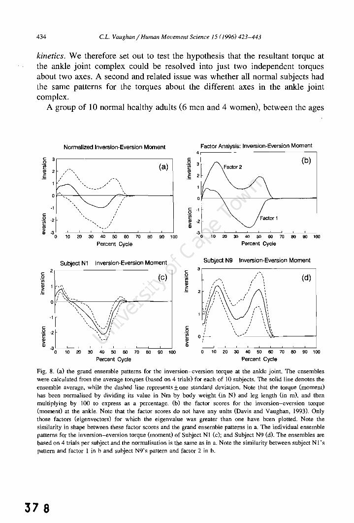
434 c.L. Vaughan / Human Movement Science 15 (1996) 423-443

kinetics. We therefore set out to test the hypothesis that the resultant torque at the ankle joint complex could be resolved into just two independent torques about two axes. A second and related issue was whether all normal subjects had the same patterns for the torques about the different axes in the ankle joint complex.

A group of 10 normal healthy adults (6 men and 4 women), between the ages

Normalized Inversion-Eversion Moment

§ 3,------------------------------,

.~ (Cl) ~ 2 ,/-,\ .!: ;' \

; " ......

·1 c: .~ ·2 (jj

, , , "

,,- '\ / ,

-' , ~ , , ,

, , ,

I

, , I ,

~ ·3~-~--~~--_L __ L_ ____ ~ __ L-_L~

o 10 20 30 40 50 60 70 80 90 100

Percent Cycle

Subject N1 Inversion-Eversion Moment 2 c:

(C) 0 .~

(I) 1 ,,, , > .!:

0

-1

c: 0 :L .~

(I)

~ 0 10 20 30 40 50 60 70 80 90 100

Percent Cycle

Factor Analysis: Inversion-Eversion Moment

c: o .~

.~

4

(b)

o~--~~----------~----------~

§ ·1 ~ 'i!! l ~ .2 L ~ L[ __ L-_L __ ~~ __ -L __ L--L __ ~~

o 10 20 30 40 50 60 70 80 90 100

Percent Cycle

Subject N9 Inversion-Eversion Moment

c: 3 0 (d) .~

(I) > .!: 2

c: 0 .~

0 (I)

~ 0 10 20 30 40 50 60 70 80 90 100

Percent Cycle

Fig. 8. (a) the grand ensemble patterns for the inversion-eversion torque at the ankle joint. The ensembles were calculated from the average torques (based on 4 trials) for each of 10 subjects. The solid line denotes the ensemble average, while the dashed line represents ± one standard deviation. Note that the torque (moment) has been normalised by dividing its value in Nm by body weight (in N) and leg length (in m), and then mUltiplying by 100 to express as a percentage. (b) the factor scores for the inversion-eversion torque (moment) at the ankle. Note that the factor scores do not have any units (Davis and Vaughan, 1993). Only those factors (eigenvectors) for which the eigenvalue was greater than one have been plotted. Note the similarity in shape between these factor scores and the grand ensemble patterns in a. The individual ensemble patterns for the inversion-eversion torque (moment) of Subject Nl (c); and Subject N9 (d). The ensembles are based on 4 trials per subject and the normalisation is the same as in a. Note the similarity between subject Nl 's pattern and factor 1 in b and subject N9's pattern and factor 2 in b.

37 8

c.L. Vaughan/ Human Movement Science 15 (J996) 423-443 435

of 22 and 53 years, were studied using the standard inverse dynamics approach (Vaughan et aI., 1992). When the resultant ankle torque was resolved into components, the plantar-dorsiflexion torque was extremely repeatable and essentially identical to the pattern for normal children (Fig. 5c). The inversion­eversion pattern was much more variable, however (Fig. 8a). Factor analysis, a technique in which just a few eigenvectors are used to represent complex patterns (Olree and Vaughan, 1995), was applied to the joint torques. All 10 subjects loaded strongly on a single factor for plantar-dorsiflexion which explained almost 96% of the variance in the original data. For the inversion­eversion torque, the data were more variable (Fig. 8a), and two factors were needed to explain over 91 % of the variance: 7 subjects loaded heavily on factor 1 while 3 subjects loaded heavily on factor 2. As pointed out by Davis and Vaughan (1993), one of the powerful features of factor analysis is that the eigenvectors may be rotated orthogonally, so that the factor scores can be presented in a form that has physiological meaning (Fig. 8b). These scores were then compared with the ensemble average data (Fig. 8a) and the similarity in the patterns was quite striking. The patterns for factors 1 and 2 were very similar to the standard deviation curves. Further evidence of the insight that factor scores provide may be explored by plotting individual subject torque patterns. For example, in the loading matrix subject N 1 loaded heavily on factor 1 while subject N9 loaded heavily on factor 2. The ensemble average of the inversion­eversion torque for Nl (Fig. 8c) was very similar in shape to factor 1 (Fig. 8b), while the curve for N9 (Fig. 8d) was very similar in shape to factor 2 (Fig. 8b).

The sinusoidal patterns for the plantar-dorsiflexion torques (Fig. 5c) and inversion-eversion torques (Fig. 8a) do appear to lend some credence to the reciprocating universal joint theory. However, the fact that the plantar flexion torque is an order of magnitude greater than the inversion-eversion torque, the considerable variability in the latter's pattern, and the existence of other non-trivial components of the torque (e.g., pronation-supination), weakens the argument in favour of the theory. Factor analysis has shown that normal subjects may be classified as either predominantly evertors (Fig. 8c) or invertors (Fig. 8d).

2.4. Knee abduction / adduction in stair climbing

Stair climbing is of particular interest since stairs are frequently encountered obstacles in daily living, and require greater knee torques and ranges of motion than those utilised in level walking (Andriacchi et aI., 1982). Whilst the flexion-extension torques are undoubtedly crucial, a natural question to ask is:

379

436 c.L. Vaughan / Human Movement Science J 5 (J996) 423-443

Force Plate 1

Flexion and Extension

%J' ~rection of / Progression

Fig. 9. Location of 3 steps over two force platforms and definition of the knee joint reference axes. Note that steps 1 and 2 were sensitive to reaction forces while the ground and step 3 were not. The flexion-extension torque takes place about the mediolateral axis of the proximal segment (thigh). while the internal-external rotation torque takes place about the longitudinal axis of the distal segment (calf). The abduction-adduction torque is exerted about a floating axis that is perpendicular to the mediolateral and longitudinal axes (Vaughan et al.. 1992). This figure has been reproduced from Kowalk et al. (1996a) with permission.

how important are the abduction-adduction torques at the knee during stair climbing? We suspected that the magnitudes of these frontal plane torques were functionally important and designed an experiment to explore this notion (Kowalk et aI., 1996a).

Ten normal adults (6 male and 4 female), ranging in age from 22 to 40 years, ascended a set of stairs, 3 times beginning with their right leg and 3 times beginning with their left. Ground reaction forces were measured with two force plates and steps mounted onto each plate (Fig. 9). Stairs of standard dimension, having a rise of 0.203 m and a run of 0.254 m, were used. The force plates were preloaded with 356 N under the lower step and 713 N under the taller step prior to data capture, using a previously tested approach (Besser et aI., 1993). The GRF data were integrated with 3D kinematic data in an inverse dynamics approach to yield the resultant torque at the knee joint. These torques were normalized in magnitude (to percent body weight and leg length) and time (percent stance).

As might be expected, the knee torque was primarily in the extensor direction, reaching a normalised value of almost 10 (percent body weight and leg length) during the early part of stance phase (Fig. lOa). This normalised value can be converted back into standard torque units of Nm if you multiply by

380

c.L. Vaughan / Human Movement Science 15 (1996) 423-443

12

x Ql

8 'E Ql

"0 E Ql 0 .~ ~ 4 iti Ql E Ql 0 C Z ~

x 0 Ql

;;:::::

-4 0

"0

10 r

.0 8 <ll

'E 6 Ql

"0 E Ql 0 ~~ 4 <ll Ql E Ql .... c

2 ~~ "0

0 "0 <ll

-2 0

Stair Ascent: First Step

(a)

, , I

, I

20 40 60 80 100

Percent Cycle

Stair Ascent: First Step

,~,

I ' I ' I \

, r....." .... - "-I I '\ \ ' \ I I '- ,_......... \ J, \ \

I ", \ I I - .... __ .... - ........ , \

\ \ \ \ \ \ \ \

(b) I

\ \ """"------ ... -----

20 40 60 80 100 Percent Cycle

437

Fig. 10. Ensemble averages for the initiation step during stair ascent for: (a) flexion-extension torque; and (b) abduction-adduction torque. The solid line represents the average of 6 trials for each of 10 subjects, while dashed lines represent ± one standard deviation. Torques (moments) have been normalised to body weight (average 660 N) and right leg length (average 0.962 m) and expressed as a percentage. Knee torques in Nm may be estimated by multiplying the y-axis value by a subject's weight (N) and right leg length (m), and dividing by 100. Time data have also been normalised to the gait cycle with 0% being the first foot contact and 100% the subsequent contact with the same foot. These figures have been reproduced from Kowalk et al. (I996a) with permission.

body weight (660 N) and leg length (0.962 m) and divide by 100. This yields a maximum extensor torque of 65 Nm. In contrast to the sinusoidal pattern for flexion-extension, the abduction-adduction torque was biphasic in shape and exclusively abductor in direction throughout the stance phase (Fig. lOb). This latter point clearly indicates that the line of action of the GRF was always directed medial to the knee joint centre. The maximum normalised magnitude of 6 translates into 35 Nm which was statistically smaller than the 65 Nm extensor torque. Although the flexion-extension torques were clearly the most important,

381

438 C.L. Vaughan / Human Movement Science 15 (1996) 423-443

the abduction-adduction torques also played a vital role at the knee, providing both propulsion (to ascend the stairs) and mediolateral stability. The structures that must normally provide the knee abduction torque include the lateral collateral ligament and the iliotibial band. This magnitude of the abduction torque casts doubt on the utility of the 'support moment' concept which assumes that only sagittal plane torques are functionally relevant for stair climbing (McFadyen and Winter, 1988). Although the abduction torques were statistically smaller that than the extensor torques (cf. Fig. lOa and b), there was a period in late stance when the extensor torque was close to zero, but the abductor torque had a value of 25 Nm.

2.5. Anterior cruciate ligament instability

Anterior cruciate ligament (ACL) injuries are the most common ligamentous injury of the knee. The ACL is an important structure which provides mechani­cal support to the knee, preventing anterior displacement of the tibia on the femur and hyperextension of the knee joint. Previous studies by Berchuck et aI. (1990) have shown that ACL-deficient patients exert decreased knee extension torques during level walking (also known as 'quadriceps avoidance' gait), but no studies had evaluated biomechanical changes during stair climbing following ACL reconstruction. We studied 10 normal subjects (cf. Section 2.4 and 8 ACL patients who were evaluated both pre- and postoperatively with a mean follow-up of 6 months (Kowalk et aI., 1996b). All patients underwent arthroscopic ACL reconstruction using middle third bone-patellar tendon-bone autograft (O'Brien et aI., 1991).

For each of the 3 subject groups (normals, patients pre-operatively, and patients postoperatively), kinematic and force plate data were collected and analysed to calculate joint angles, torques, powers and work. These data were ensemble averaged and statistically analysed using repeated measures analysis of variance with a significance level set at 0.05. Anterior-posterior knee laxity decreased from 7.9 mm to 5.8 mm postoperatively (compared with 4.4 mm for the uninjured knees) while subjective knee function also improved following ACL reconstruction with the score increasing from 70.4 to 88.5 (compared with 96.1 for the uninjured knees). These data clearly suggested that the surgery was a success. However, the joint torque data told a different story.

Pre-coperatively, there were no statistically significant differences in biome­chanical parameters between patients' ACL-deficient and intact sides and the normal subjects. Postoperatively, however, statistically significant reductions were seen in the peak extensor torque (90 vs. 23 Nm), power (181 vs. 84 W)

382

c.L. Vaughan / Human Movement Science 15(1996) 423-443

)( III

C III E 0 ~

"C III .~ iii E 0 z

)( CD

;;::

)( III

C III E 0 ~

"C

.~ iii E 0 z

)( III

;;::

Knee Flexion - Extension Moment (Donor Side)

10

8

6

4

2

0

-2

-4

-6 0 20 40

-- Nonnal Pre-Op

........ Post-Op

60 80

Percent Cycle

(a)

100

Knee Flexion - Extension Moment (Non-Donor Side)

10

8

6

4

2

0

-2

-4

-6 0 20 40

---- Nonnal (b) Pre-Op

........ Post-Op

60 80

Percent Cycle

100

439

Fig. 11. Ensemble averages of knee flexion-extension torques during stair ascent for: (a) the donor side; and (b) the non-donor side. The solid lines represent the average of 6 trials for each of the normal subjects (cf. Section 2.4). Dashed lines are the pre-operative data and dotted lines are the postoperative data and represent the average of 6 trials for each of 8 ACL-deficient patients. Torques (moments) have been normalised to body weight and leg length and expressed as a percentage. Torques in Nm may be estimated by multiplying the y-axis value by a subject's weight (in N) and leg length (in m) and dividing by 100. Note that the average values for the subjects were: normals, 645 Nand 0.96 m; patients pre-operatively, 886 Nand 1.07 m; and patients postoperatively, 914 Nand 1.07 m.

383

440 c.L. Vaughan / Human Movement Science 15 (1996) 423-443

and work performed (28 vs. - 7 1) at the knee from which the graft had been harvested (Fig. 11). This was accommodated by significant increases in excur­sion, torque and power at the contralateral ankle joint. As seen in Fig. 9, at the same time that the ipsilateral (left) knee must generate a large extensor torque to raise the body, the contralateral (right) ankle can provide assistance by generat­ing a plantar flexor torque. These findings have important clinical implications. They show that while the ACL reconstructions were successful in restoring anterior-posterior knee stability, the decrease in knee torque generated postoper­atively by the donor knee suggests that donor site morbidity (removal of the middle third of the patellar tendon) may need to be critically evaluated over a long-term period.

3. Concluding remarks

The title of this paper is a provocative one: are joint torques the Holy Grail of human gait analysis? Has our quest led to some biomechanical insight? These questions demand an answer. In reviewing the 5 projects where 3D joint torques have been studied, we have learned: that normal children generate large and repeatable torques at the ankle joint while the knee torques tend to be much smaller and more variable; that children with cerebral palsy derive some benefit from wearing an ankle foot orthosis because it allows them to exert slightly greater plantar flexion torques during push off; that in level gait, normal adults exhibit two distinct types of inversion-eversion torque patterns about the long axis of the foot; that in climbing stairs, the knee abductor torques are quite large and contribute to both propulsion and mediolateral stability; and that patients with anterior cruciate ligament insufficiency, despite the apparent success of the ipsilateral patellar tendon autograft, exert smaller knee extensor torques at the donor knee. Most of these insights could probably not have been predicted without the benefit of a rigorous 3D inverse dynamics approach. Lest we be too enthusiastic about the utility of joint torques, a few words of caution are probably in order.

3.1. Sources of error

Like all measurements which involve biological phenomena, joirit torques are ~­

subject to a variety of sources of error. The equations of motion in Fig., 3 ". provide a good starting point. The unknowns are the joint force components (FAx' FAy) and the joint torque TA. The parameters which must be measured or

, l-

384

c.L. Vaughan / Human Movement Science 15 (1996) 423-443 441

estimated include the segmental anthropometry (mF and IF)' the accelerations (xFcg ' YFcg and O-F)' the lever arms (d p d2 , d3 and d 4 ) and the ground reaction forces (F x' F y). While the ground reaction forces make a significant contribu­tion to the joint torques (cf. Fig. 4 and Section 2.1, they are also the most reliable and accurate. Segmental anthropometry (typically generated by regres­sion equations based on cadavers) and the accelerations (based on numerical differentiation of noisy displacement data) are notorious for their inaccuracy, but they fortunately do not make major contributions to the joint torques. This leaves the lever arms which are very sensitive to marker placement on the skin surface and the biomechanical model chosen to estimate joint centres. As seen in the third equation of Fig. 3, the lever arms are the multipliers of the ground reaction and joint forces, and so they have an important impact on the accuracy of the joint torque values. It is therefore not surprising that distal torques tend to be more repeatable than proximal torques (Fig. 5), and sagittal plane torques are more repeatable than frontal or transverse plane torques (cf. Figs. 5 and 8a).

3.2. Role of antagonistic muscle activity

As described in Section 1.4, joint torques are a ruse or mathematical convenience: they serve as a substitute for all the muscles crossing a joint. They are, in fact, the resultant of all the muscles. This means that it is possible to have a zero torque if the agonist and antagonist muscles are quiescent or if they are contracting equally hard. In other words, there is not a unique one-to-one relationship between joint torque (e.g., knee extensor) and the muscles generat­ing that torque (the quadriceps).

3.3. Future goals

While this quest has been an interesting journey, and has off~red a few fleeting glimpses of biomechanical insight, I do not believe that the destination so far reached has yielded the Holy Grail. There are further odysseys that must be pursued. These include: an uncertainty analysis (Cappozzo et aI., 1975; Davis, 1992) using partial derivatives and a large variety of real gait data; a combination of the inverse dynamics approach and simultaneous electromyo­graphic studies, thus addressing the issue of antagonistic muscle activity; implementation of improved biomechanical models of the human body, thereby minimising the errors introduced by measurement; and finally, a concerted effort should be made to combine forward and inverse dynamics approaches to gain further understanding qf the complexities underlying human locomotion.

385

442 c.L. Vaughan / Human Movement Science 15 (1996) 423-443

Acknowledgements

This work was supported in part by grants from the National Institutes of Health (ROI HD30134, T32 AR07482) and the US Department of Education (Rehabilitation Engineering Training Grant H133PI0006-92). In addition, I gratefully acknowledge the assistance and input of my colleagues at the Univer­sity of Virginia: Stephanie Goar, Scott Colby, Warren Carlson, Diane Damiano, Mark Abel, Jodi Nashman, Dave Kowalk, and Jeff Duncan.

References

Andriacchi, T.P., J.O. Galante and R.W. Fermier, 1982. The influence of total knee-replacement design on walking and stair climbing. Journal of Bone and Joint Surgery 64A, 1328-1335.

Berchuck, M., T.P. Andriacchi, RR Bach and R Reider, 1990. Gait adaptations by patients who have a deficient anterior cruciate ligament. Journal of Bone and Joint Surgery 72A, 871-877.

Besser, M.P., D.L. Kowalk and e.L. Vaughan, 1993. Mounting and calibration of stairs on piezoelectric force platforms. Gait and Posture I, 231-235.

Bleck, E.E., 1987. Spastic diplegia: orthopaedic management in cerebral palsy. In: E.E. Bleck (ed.), Clinics in Developmental Medicine (pp. 99-282). Philadelphia: Lippincott ..

Cappozzo, A., T. Leo and A. Pedotti, 1975. A general computing method for the analysis of human locomotion, Journal of Biomechanics 8, 307-320.

Carlson, W.E., e.L. Vaughan, D.L. Damiano and M.F. Abel, 1996. Orthotic management of equinus gait in spastic diplegia. Archives of Physical Medicine and Rehabilitation, in review.

Collins, J.1., 1995. The redundant nature of locomotor optimization laws. Journal of Biomechanics 28, 251-267.

Crowninshield, RD. and RA. Brand, 1981. A physiologically based criterion of muscle force prediction in locomotion. Journal of Biomechanics 14, 793-80 I.

Cusick, RD., 1988. Managing foot deformity in children with neuromotor disorders. Physical Therapy 68, 1903-1912.

Davis, RL., 1992. Uncertainty in calculating joint moments during gait. Proceedings of Eighth Meeting of the European Society of Biomechanics, Rome, Italy.

Davis, B.L. and e.L. Vaughan, 1993. Phasic behavior of EMG signals during gait: use of multi-variate statistics, Journal of Electromyography and Kinesiology 3, 51-60.

Enoka, RM., 1988. Neuromechanical Basis of Kinesiology. Champaign, IL: Human Kinetics. Grolier's Encyclopaedia, 1995. CD-ROM. Chicago, IL: Grolier Electronic Publishing. Kowalk, D.L., J.A. Duncan and e.L. Vaughan, 1996a. Abduction-adduction moments at the knee during stair

ascent and descent, Journal of Biomechanics 29, 383-388. Kowalk, D.L., J.A. Duncan, F.e. McCue and c.L. Vaughan, 1996b. Anterior cruciate ligament reconstruction

and knee dynamics during stair climbing, Medicine and Science in Sports and Exercise, in review. Loeb, G.E., W.S. Levine and J. He, 1990. Understanding sensorimotor feedback through optimal control. Cold

Spring Harbor Symposia on Quantitative Biology (pp. 791-803). Cold Spring Harbor, NY: Cold Spring Harbor Laboratory Press.

McFadyen, B.1. and D.A. Winter, 1988. An integrated biomechanical analysis of normal stair ascent and descent, Journal of Biomechanics 21, 733-744.

O'Brien, S.1., RF. Warren, H. Pavlov, R Panariello and T.L. Wickiewicz, 1991. Reconstruction of the chronically insufficient anterior cruciate ligament with the central third of the patellar tendon, Journal of Bone and Joint Surgery 73, 278-286.

386

c.L. Vaughan / Human Movement Science 15 (1996) 423-443 443

Ounpuu, S., lR. Gage and R.B. Davis, 1991. Three-dimensional lower extremity joint kinetics in normal pediatric gait, Journal of Pediatric Orthopaedics 11,341-349.

Olree, K.S. and e.L. Vaughan, 1995. Fundamental patterns of bilateral muscle activity in human locomotion, Biological Cybernetics 73, 409-414.

Ramakrishnan, H.K., M.P. Kadaba and M.E. Wootten, 1987. Lower extremity joint moments and ground reaction torque in adult gait, Biomechanics of Normal and Prosthetic Gait, ASME BED-4, 87-92.

Scott, S.H. and D.A. Winter, 1991. Talocrural and talocalcaneal joint kinematics and kinetics during stance phase of walking, Journal of Biomechanics 24, 743-752.

Vaughan, e.L., lG. Hay and J.G. Andrews, 1982. Closed loop problems in biomechanics. Part I. A classification system, Journal of Biomechanics 15, 197-200.

Vaughan, e.L., B.L. Davis and J.e. O'Connor, 1992. Dynamics of Human Gait. Champaign, IL: Human Kinetics.

Wells, R., 1981. The projection of the ground reaction force as a predictor of internal joint moments, Bulletin of Prosthetics Research 18, 15-19.

Wright, D.G., S.M. Desai and W.H. Henderson, 1964. Action of the subtalar and ankle joint complex during the stance phase of walking, Journal of Bone and Joint Surgery 46A, 361-382.

387

388

r

ELSEVIER Gait & Posture 5 (1997) 204-210

Six degree of freedom joint power in stair climbing

Jeffrey A. Duncana, David L. Kowalkb

, Christopher L. Vaughan*c

°Biomet Inc .• Warsaw. IN. USA b Department of Orthopaedics. Unil1ersity of Virginia. Charlottesville. VA. USA

"Department of Biomedical Engineering. University of Cape Town. Obserllatory. Cape 7925. South Africa

Received 20 October 1994; accepted 13 February 1996

Abstract

In the past, joint power has most often been calculated as the product of the sagittal plane joint moment and the sagittal plane joint angular velocity, thus modelling the joint as a simple one degree of freedom (DOF) hinge. More recently three DOF power has been calculated by taking the scalar product of the net joint moment and the angular velocity of the joint, thus modelling the joint as a ball and socket joint. We introduce a six DOF approach for calculating joint power, an approach which allows three degrees of rotational freedom, as well as three degrees of translational freedom, thus implementing a rigorous definition of true mechanical power. We established that for the hip joint during stair ascent, three DOF power was significantly greater than six DOF power (by as much as 60 W/lcg), while for stair descent, one DOF power was significantly less than six DOF power (by up to 45 W/lcg). On the basis of the total work done in raising the body up a set of stairs (weight x height), the six DOF approach provided more accurate results than either the one or three DOF models. We also showed that six DOF power data were as repeatable as joint moments, with variance ratios between 0.13 and 0.20. While these findings are certainly not the definitive word, they do offer some guidance regarding the effect that certain assumptions have when calculating joint power in three dimensions.

Keywords: Joint power; Work; Stairs

1. Introduction

Almost 70 years ago Fenn [I] evaluated power and work by studying the movements of the centre of mass and the limbs relative to the centre of mass during run­ning and sprinting. Since then, the two principal methods have been segmental energy changes and joint power.

Segmental energy change is one way to calculate the amount of work performed on a body [2-10]. A 'pseudowork' method, based on the sum of the absolute changes of the potential, rotational kinetic and transla­tional kinetic energy [2-5], overestimates the work per­formed because it does not allow for energy transfer between or within segments. Another method uses estimates for the amount of elastic storage [6-9], but

• Corresponding author. Tel.: +27214066544; fax: +27214483291; e-mail: kvaughan@anat.uct.ac.za.

0966-6362/97/$17.00 © 1997 Elsevier Science B.V. All rights reserved PH S0966-6362(96)01086-7

none of these procedures has ever produced acceptable results [10].

In more recent years, the instantaneous power has been calculated by multiplying the joint angular velocity by the moment acting across that joint [11-17], and the work done can then be calculated by finding the area under the power-time curve [18]. Most researchers, with one notable exception [19], have included only the sagit­tal plane angular velocity and moment in their calcula­tion of joint power, thus underestimating the power because motions in the non-sagittal planes, as well as translation within the joints, were not included. This is a one degree of freedom (DOF) approach in which the joint is modelled as a simple hinge. An approach cur­rently used clinically [20] is to calculate the joint power by taking the scalar product of the net joint moment and angular velocity, thus calculating the rotational three DOF power and modelling the joint as a ball and socket joint. While Buzcek and his colleagues [19] used a six

389

390

J.A. Duncan et al. I Gait &: Posture 5 (1997) 204-2/0 205

degree of freedom (DOF) model for joint power, they presented their results as three planar graphs. This is misleading since power, by definition, is a scalar quanti­ty and should be presented as a single curve.

Van Ingen Schenau and Cavanagh [21] commented that "studies do not seem to exist where the power cal­culations ... are based on the definition of power, as can be found in textbooks on mechanics." The purpose of this technical note is to introduce true six DOF joint power and to contrast the data with one and three DOF values for stair climbing.

2. Methods

The true mechanics of power and work are based on the work-energy equation. This equation simply states that the amount of work performed on a body is equal to the change in all forms of energy acting on that body. The equation can then be differentiated so that power is equal to the rate of change of energy acting on the body. The two methods presented for calculating work and power - changes in segmental energy and joint power - are simply the two sides of the above equation. How­ever, not all the terms on the energy side can be calculated yet, because the elastic storage and strain energy of the human body are not properly understood [21]. This leaves the joint power side of the equation which, if completely and accurately calculated, will ade­quately define the power and work within the system.

Power is defined as:

Power=M. ",+F·" (1)

where M is a moment acting on a body, '" is the angular velocity of the body, F is the force acting on a body and " is the linear velocity of the point of application of the force [18] (boldface terms refer to vector quantities and the dot indicates a scalar product). Power can be calculated for each segment on either side of the joint and their sum is the joint power. This leaves eight par­ameters that are needed to calculate the joint power:

10int Power = Mp..oximal • "'proximal + Fproximal • "proximal

(2)

where the subscripts refer to either the proximal or distal segments comprising the joint. Eq. 2 makes only one assumption about the joint: the multiple insertions of the muscle tendons and ligamentous structures can be grouped into a single force and a single moment acting about a specific point. The choice of that point is ar­bitrary the resultant force would be the same whereas the resultant moment would be different and has no effect on the power calculation for that segment. If the point chosen is the instantaneous centre of rotation of

the joint, then Fproximal = -Fdistab "proximal = "dislJI" and joint force does not contribute to joint power. This is the basis for the one and three DOF approaches. However, instantaneous centres of joint rotation cannot be reliably calculated from standard motion data, and an alternative strategy has to be explored.

We have chosen as our point of reference the joint centre which is a fixed point in each segment. It will only coincide with the instantaneous joint centre of rotation for a perfect spherical (ball-and-socket) or revolute (hinge) joint. We therefore assumed that the joint centre could be independently estimated from the proximal and distal segments. At any given instant in time, these two points may be assumed to be coincident. Then, by

Newton III, Mproximal = -MciislJIl and Fproximal = -Fdislah but "proximal and "dislJll will not normally be equal (unless the joint centre coincides with the centre of rotation). With these assumptions, Eq. 2 can be simplified to

10int Power = M • ("'dislJIl -- "'proximal)

+ F . ("distal - "proximal) (3)

All of these terms must be calculated with respect to the same reference frame in order for the scalar product to be valid. The global reference frame is the most logical choice for a reference frame since joint powers contain two segments in their calculation and the global frame is the only frame common to both segments. The forces and moments can be calculated using standard in­verse dynamics approaches [22], leaving only four par­ameters to be calculated: the angular velocities of the segments, "'proximal and "'distah and the velocities of the points of application of the joint force, "proximal and "distal' These kinematic parameters may be obtained using well-established 3D algorithms [22].

To calculate the joint centres, one set of prediction equations came from the work of Vaughan and his colleagues [22] (cf. equations A13, Al6 and Al8 in the Appendix), while the second set was based on the other segment which comprises the joint (cf. equations Al4, A 15 and AI7). The second set was determined using the first set of prediction equations as a basis, and gathering data on normal adults who stood in the anatomical posi­tion. Based on the notation in the Appendix, Eq. 3 may be written for the right hip, knee and ankle joints.

loint Powerri&hl hip =

Mri&hl hip . ("'ri&hl Ihi&h -- "'pelvis)

+ F ri&hl hip . (" ri&hl hip Ihi&h -- "ri&hl hip pelviS> (4)

10int PoWerri&hlknec = Mri&hl knee . ("'ri&hl shank -- "'ri&hl Ihi&h)

+ Fri&hl knee . ("ri&hl knee shank -- "ri&hl knee Ihi&h) (5)

39"

206 JA. Duncan et aJ.1 Gait & Posture 5 (1997) 204-210

A ~elvis

Pright ASIS( " ,)------4,.......;;........;;........,;......:....-{,;

B c PheeJ

ipelViS "k.root Pthigh

Fis. 1 (A) Pelvic and right thigh markers and reference frames. The ilk reference frame corresponds to that defined in equations A I through A6. (8) Right shank markers and reference frame. The ilk reference frame corresponds to that defined in equations A7 through A9. (C) Right foot markers and reference frame. The iJk reference frame corresponds to that defined in equations AIO through A12.

Joint Powerript ankle =

Mript ankle • (Calript foot - Calript stumt>

+ F ript ankle • (VriPI ankle fOOl - VriPI ankle shank) (6)

Gait analysis was conducted on to normal subjects (six male, four female, ages 22-40, mass 65.8 :::I::: 11.9 kg). Each subject ascended and descended a staircase which consisted of three steps (22 em rise, 25 cm run) six times: three trials beginning with the right leg and three with the left (25]. Kinematic and force plate data were collected and analyzed to calculate one, three and six OOF joint power, while the area under the power-time curves was calculated to determine the amount of work performed. The data were pooled and statistical analysis

Table I

using repeated measures MANOV A (P < 0.05) was per­formed to test for a significant difference between the groups. Repeatability of the one, three and six DOF joint power approaches was tested using a variance ratio (VR) statistic (24].

3. Results

Six OOF power was significantly different from both one and three OOF power for stair ascent and stair de­scent (Table I, Fig. 2). The work calculated from the six OOF power curve was also significantly different from the one and three OOF curves for stair ascent and stair descent (Table 2).

The statistical method compared only the overall

Maximwn and minimwn joint power (W/kg) throughout the gait cycle for one, three and six degree of freedom (ooF) models show that both one and three ooF models signiflClllltly differ from the six ooF model

Parameter looF 300F 600F

Max Min Max Min Max Min

Hip ascending 1.45 (: 0.37) -0.58 (: 0.08) 2.16· (: 0.30) .... !5S .. (: 0.09) 1.56 (: 0.36) -0.65 (: 0.11) Knee ascending 1.47 (: 0.29) -0.75 (: 0.13) 1.79 (: 0.30) -0.79 (: 0.15) 1.59(: 0.41) -0.79 (: 0.17)

Ankle ascending 3.07 (: 0.78) -0.22 (: 0.08) 2.98 (: 0.81) -0.28 (: 0.10) 3.16 (: 0.78) -0.26 (: 0.10) Hip descending 0.47· (: US) .... 14·(: US) 0.86 (: 0.30) -0.66 (: 0.20) 0.75 (: 0.23) -0.65 (: 0.17) Knee descending 1.32 (: 1.34) -2.93 (: 1.80) 1.55 (: 1.56) -3.03 (: 1.93) 1.54 (: 1.53) -3.28 (: 1.96) Ankle descending 2.35 (: 1.08) -2.50 (: 1.17) 2.42 (: 1.19) -2.82 (: 1.52) 2.66 (: 1.14) -2.77 (: 1.52)

Mean and standard deviation are shown with signiftcant (P < 0.05) differences between oee" and six ooF power or tbree b and six ooF power; positive values = power generated; negative values = power absorbed.

392

J A. Duncan el af. I Gail & Poslure 5 (1997) 204-210 207

A 3 ,----_H-'-.ip_Jo=--in:.:...t P,--,o-,-,wC'-er.:..:A::..:sc:.:::en:::.d::::ing~S::.::ta::::ir.:..s __ ---; B Knee Joint Power Ascending Stairs C 3 2

-OneOOF - - - Three OOF

··Six OOF c: CI> co

c: .. '"

c: g:. 2

-OneOOF - - - Three OOF ······SixOOF

'" 1 ~ '" .. ~

'" ~ iii ~

0

'" ~ .. ~

'" 0 .0

'" '" il '" 0 .0

'" .. ,. ...... -

-1 -1 -1 0 20 40 60 80 100 0 20 40 60 80 100 0 20 40 60 80 100

Percent Cycle Percent Cycle Percent Cycle

0 0.8

Hip Joint Power Descending Stairs E Knee Joint Power Descending Stairs F 3

Ankle Joint Power Descending Stairs

c: 0.6 .. '" 0.4

'" ~ 0.2 '" .. ~ 0

"

'" -0.2 .0

'" -0.4

-0.6 0 20 40

(\, !: " ,. " J

I

-OneOOF - - - Three OOF

·Six OOF

60 80

c: CI>

'" co ~ '" '" ~

'" .0

'"

100

0 c: 2 .. co

co

~ 0 '" '" -1 ~ -1

'" .0

'" -2

-2 -3

0 20 40 60 80 100 0 20 40 60 80 100 Percent Cycle Percent Cycle Percent Cycle

Fig. 2. Power curves, nonnalised to body mass (W/kg) for: (A) hip joint ascending stairs; (B) knee joint ascending stairs; (C) ankle joint ascending stairs; (0) hip joint descending stairs; (E) knee joint descending stairs; and (F) ankle joint descending stairs. The solid line represents sagittal plane one degree of freedom (OOF) power, the dashed line represents three OOF power, while the dotted line represents six OOF power. Note: gen = power generated; abs = power absorbed.

maximum and minimum for the gait cycle. Assuming six DOF power to provide the 'correct' values, it was found that one DOF power almost always underestimates the amount of power and could underestimate the power by as much as 92% (Fig. 2d). Three DOF power, on the other hand, underestimates power by as much as 40010 (Fig. 2e), overestimates power by as much as 40010 (Fig. 2a), and has additional turning points (Fig. 2d).

Table 2 Joint work (J/kg) throughout the gait cycle for one, three and six degree of freedom (OOF) joint power models show that both one and three OOF models differ significantly from the six OOF model

Parameter IOOF 300F 600F

Hip ascending 0.43 0.73· 0.52 (:i: 0.12) (:i: 0.14) (:i: 0.13)

Knee ascending o.n" 0.36· 0.26 (:i: 0.10) (:i: 0.(9) (:i: 0.09)

Ankle ascending 0.43 0.44· 0.42 (:i: 0.10) (:i: 0.11) (:i: 0.11)

Hip descending 0.13" 0.10· 0.05 (:i: 0.03) (:i: 0.04) (:i: 0.07)

Knee descending -0.45" -O.y. -0.65 (:i: 0.48) (:i: 0.!!7) (:i: 0.60)

Ankle descending -0.06" -O.O!!· 0.01 (:i: 0.11) (:i: 0.11) (:i: 0.20)

Mean and standard deviation are shown with significant (P < 0.05) differences between 0." and six OOF or tbreeb and six OOF.

The variance ratios calculated for one, three and six DOF power (fable 3) are similar to those for the kine­matics and moments, showing that power is as repeatable as many gait parameters that are currently used. The six DOF values are approximately the same as the one and three DOF values, suggesting that six OOF power is as repeatable as either one or three OOF power.

4. Discussion

The purpose of this technical note was to introduce true six DOF joint power for stair climbing and to con­trast the data with one and three DOF values. We have presented the method and equations by which six DOF can be calculated. This approach, while it has removed the major assumptions currently used by most resear­chers and clinical programs, still suffers from a number of drawbacks. First, to predict a joint centre with some confidence, three points are normally needed on the seg­ment of interest. Since we have only two markers on the thigh (Fig. tal, we had to incorporate a pelvic marker to estimate the hip joint centre (equation At4). Clearly this is not ideal. However, we were faced with a decision of utilising either an existing IS-marker set that is well accepted in gait analysis laboratories [23], or adding extra markers to the thigh (e.g. over the greater

393

208 lA. Duncan <t al.1 Gait & Posture 5 (1997) 204-210

Table 3 Inter-subject Variance Ratios (VRs) at the hip, knee and ankle for joint powers, angles and moments for stair ascent and descent. VRs are a measure of repeatability: the closer the value is to zero the more similar the values, while the closer the values are to I (or larger) the more greatly the values differ [24\

Parameter Hip Knee

Ascent Descent Ascent

I DOF power 0.15 0.47 0.10 3 DOF power 0.10 0.30 0.07 6 DOF power 0.17 0.34 0.13 Flexion/extension angle 0.04 0.14 0.03 Abduction/adduction angle 0.37 0.64 0.75 IntemaVextemai angle 0.83 0.83 0.67 Flexion/extension moment 0.09 0.11 0.14 Abduction/adduction moment 0.09 0.10 0.11 IntemaVextemai moment 0.07 0.35 0.13

trochanters). We chose the first approach so that our methods would be backwardly compatible with the large installed database of patient files in clinical gait labora­tories.

Second, there are various artifacts - such as skin movement - that could have atTected our data. While this is true of all data currently gathered in clinical gait laboratories, and probably contributed to the variability in both the kinematic and kinetic parameters (Table 3), the results are comparable to other findings in the litera­ture. For example, the variance ratios for the hip joint moments found by Bowsher and Vaughan [26] were 0.13 (flexion-extension), 0.25 (abduction-adduction) and 0.35 (internal-external rotation) for level walking. The cor­responding values in the current study (Table 3) tend to be considerably smaller, particularly for stair ascent. It is not surprising that the stair descent VRs tended to be greater, given the variability in foot placement when walking down a set of steps.

The one OOF joint power corresponded well with those presented by McFadyen and Winter [17]. There were ditTerences in the absolute peaks for some of the joints, however. The curves presented by McFadyen and Winter represented only one subject while those presented here are the ensemble average for 10 subjects (Fig. 2). Since the curves represent ditTerent subject samples, the ditTerences were not felt to be important. There are no six OOF curves available in the literature and so no comparison is possible. The importance of using the six DOF approach can be seen by examining the work of McFadyen and Winter [17]. They concluded that the hip is not involved in absorbing energy during stair descent which is consistent with the one DOF curve. However, when the six OOF curves are studied it is seen that nearly 11% of all energy absorbed during stair descent is absorbed at the hip (Fig. 2d). Clearly a more rigorous approach is necessary for correct inter­pretation of power curves and the associated work done during stair climbing.

394

Ankle

Descent Ascent Descent

0.85 0.20 0.41 0.85 0.21 0.43 0.80 0.20 0.41 0.05 0.13 0.11 0.85 0.52 0.72 0.66 0.99 0.99 0.11 0.10 0.12 0.13 0.75 0.87 0.18 0.21 0.24

We have shown that for the hip, six OOF power is significantly less than three DOF power for stair ascent and significantly greater than one OOF power during stair descent (Table I). Furthermore, all six OOF joint work values are significantly less than the three DOF values at all the joints for both ascent and descent (Table 2). These findings beg the questions: which approach should be used by clinicians and researchers? Is six OOF joint power more 'accurate' than three OOF joint power estimates? Some insight into these questions can be gleaned by clowoser analysis of the work data in Table 2. The total work performed by a human subject when raising his or her body up a set of stairs is the summa­tion of the work done at the six major joints of the lower extremities (hips, knees and ankles on both sides of the body). Assuming left-right symmetry [27], the values for stair ascent from Table 2 are 3.06 J/kg for three DOF and 2.40 J/kg for six DOF. These data should be com­pared with the target of 2.25 J/kg which is based on the height of the step (0.23 m) and the acceleration due to gravity (9.8 mls2). Note that the units of J/kg are the same as m2/s 2• On the basis of this comparison, the six DOF joint power approach would appear to provide a more acceptable estimate of total work than the three DOF approach. While these findings are certainly not the definitive word, they do otTer some guidance regar­ding the etTect that certain assumptions have when calculating joint power in three dimensions.

Acknowledgement

This work was supported in part by grants from the US Department of Education under a Rehabilitation Engineering Training Grant H133PI0006-92 (JAO), and the National Institutes of Health T32 AR 7482 (OLK), ROJ H030134 (CLV), when the three authors worked together at the University of Virginia's Motion Analysis Laboratory .

lA. Duncan et 0/.1 Gait & Posture 5 (1997) 204-210 209

Appendix A

For the sake of completeness, should anyone wish to implement our six DOF approach, the full set of predic­tion equations are reproduced in this Appendix. The pre­diction equations for the right hand side are presented with respect to the ijk unit vector segment reference

frames defined in equations A I through A 12 and represented in Fig. la-c. The marker positions (p) are with reference to a modified Helen Hayes marker set [23].

In equations A13 through AIS the joint centres are subscripted first by the joint centre and then by the seg­ment on which the joint centre calculations are based.

• PJefi ASIS - Pright ASIS Jpelvis = I I

PJefi ASIS - Pright ASIS

(Pright ASIS - PJefi ASIS) x (PJefi ASIS - PsacrunJ kpelvis = I I

(Pright ASIS - PJefi ASIS) x (PJefi ASIS - PsacrunJ

ipelvis = ipelvis X kpelvis

• Pright knee - Pright ASIS Jrigh t thigh =

iright thigh =

I Pright knee - Pright ASIS I

(Pright thigh - Pright ASIS) X (Pright knee - Pright ASIS)

I (Pright thigh - Pright ASIS) X (Pright knee - Pright ASIS) I

knght thigh = iright thigh X iright thigh

• Pright malleolus - Pright knee Jright shank = I I

Pright malleolus - Pright knee

(Pright shank - Pright knee) X (Pright malleolus - Pright knee) iright shank = I I

(Pright shank - Pright knee) X (Pright malleolus - Pright knee)

knght shank = iright shank X jright shank

iright foot =

kright foot =

Pright 2nd metatarsal head - Pright heel

I Pright 2nd metatarsal head - Pright heel I

(Pright 2nd metatarsal head - Pright malleolus) X (Pright heel - Pright ankle)

I (Pright 2nd metatarsal head - Pright malleolus) X (Pright heel - Pright ankle) I

iright foot = kright foot X iright foot

Pright hip pelvis = Psacrum + 0.59S (ASIS breadth)ipelvis - 0.344 (ASIS breadth)ipelvis - 0.290 (ASIS breadth)kpelvis

Pright hip thigh = Pright ASIS - 0.120 (right thigh circumference)iright thigh + 0.167 (right thigh lengh)iright thigh + 0.092 (ASIS breadth)kright thigh

Pright knee thigh = Pright knee - 0.015 (right thigh length)iright thigh + 0.500 (right knee diameter)kright thigh

(AI)

(A2)

(A3)

(A4)

(A5)

(A6)

(A7)

(AS)

(A9)

(AIO)

(All)

(AI2)

(AI3)

(AI4)

(AI5)

395

210 JA. Duncan et al.1 Gait &: Posture 5 (1997) 204-210

Pright knee shank = Pright knee + 0.500 (right knee diameter)krigh, mank (AI6)

Pright ankle shank = Pript malleolus - 0.015 (right shank circumference)iright shank

- 0.052 (right shank lengh)Jrigh' shank

(AI7)

+ 0.470 (right malleolus diameter)kright shank

Pright ankle foot = Pright malleolus + O. 742 (~ght foot length)i~t f'!<lt + 1.074 (nght malleolus helght)Jright foot

- 0.187 (right foot breadth)kright foot

(AI8)

References

[I) Fenn W. Work against gravity and work due to velocity changes in running. Am J PhysioJl930; 93: 433-462.

[2J Gregor R, Kirkendall D. Performance efllciency of world class female marathon runners. In: Asmussen E and Jorgensen K, cds. Biomechanics VI-B. Baltimore, MD: University Park Press. 1978: 40-45.

[3) Norman R, Sharratt M, Pe7.:zack J, Noble E. A re-examination of the mechanical efllciency of horizontal treadmill running. In: Komi P, ed. Biomechanics V-B. Baltimore, MD: University Park Press, 1976: 87-93.

[4) Luhtanen P, Komi P. Mechanical energy states during running Eur J Appl Physiol1978; 38: 41-48.

[5] Luhtanen P, Komi P. Force-, power-, and elasticity-velocity relationships in walking, running. and jumping. Eur J Appl Physiol 1980; 44(3): 279-289.

[6) Asmussen E, Bonde-Petersen F. Apparent ef1lciency and storage of elastic energy in human muscles during exercise. Acta Physiol Scand 1974; 92: 537-545.

(7] Cavagna G, Saibene F, Margaria R. Mechanical work in run­ning. J Appl Physioll964; 18: 1-9.

[8] Cavagna G, Komarek L, Mazzoleni S. The mechanics of sprint running. J Physiol1971; 217: 709-721.

(9] Thys H, Faragginana T, Margaria R. Utilization of muscle elasticity in exercise. J AppJ PhysioI1972; 32: 491-494.

[IOJ Williams K, Cavanagh P. A model for the calculation of mechanical power during distance running. J Biomech 1983; 16(2): 115-128.

[IIJ Winter DA, Quanbury AO, Reimer GO. Instantaneous energy and power Dow in normal human gait. In: Komi PV, cd. Bio­mechanics V-A. Baltimore, MD: University Park Press, 1978; 40-45.

(12] Winter DA. Calculation and interpretation of mechanical energy of movement. Exercise Sport Sci Rev 1978,6: 183-201.

113] Winter DA. Energy generation and absorption at the ankle and knee during fast, natural, and slow cadences. CJin Orthop Relat Res 1983; 175: 147-154.

396

(14) Winter DA, White SC. Cause-efTect correlations of variables of gait. In: Jonsson B, ed. Biomechanics X·A. Champaign, IL: Human Kinetics Publishers, 1987: 363-368.

[IS) Winter DA. The Biomechanics and Motor Control of Human Gait. Waterloo, Ontario, Canada: University of Waterloo Press, 1987.

[16) Andriacchi TP, Anderson GDJ, Fermier RW, Stem D. Galante JO. A study of lower limb mechanics during stair-climbing. J Bone Jt Surg 1980; 62·A(5): 749-757.

[17] McFadyen BJ, Winter DA. An integrated biomechanical analy­sis of normal stair ascent and descent. J Biomech 1988; 21(9): 733-744.

[l8J McGill OJ, King WW. Engineering Mechanics, An Introduction to Dynamics. Boston. MA: PWS·King, 1989.

(19] Buczek FL, Kepple TM. Siegel KL, Stanhope SJ. Translational and rotational joint power terms in a six degree-of·freedom model of the normal ankle complex. J Biomech 1994; 27(12): 1447-1457.

[20] Vicon Clinical Manager software. Oxford, United Kingdom: Oxford Metrics Ltd.

[21) van Ingen Schenau G, Cavanagh P. Power equations in endurance sports. J Biomech 1990; 23(9): 865-881.

(22J Vaughan C, Davis B, O'Connor J. Dynamics of Human Gait. Champaip, IL: Human Kinetics Publishers, 1992.

[23) Kadaba M, Ramakrishnan H, Wootten M, Gainey J. Gorton G, Cochran G. Repeatability of kinematic. kinetic, and elec­tromyographic data in normal adult gait. J Orthop Res 1990; 7: 849-860.

(24] Hershler C, Milner M. An optimality criterion for processing e1ectromyographic (EMG) signals relating to human locomo­tion. IEEE Trans Biomed Eng 1978; 25: 413-420.

[25] Besser M. Kowalk DL, Vaughan CL. Mounting and calibration of stairs on piezoelectric force platforms. Gait Posture 1993; I: 231-235.

(26J Bowsher KA. Vaughan CL. Effect of foot-progression angle on hip joint moments during gait. J Biomech 1995; 28(6): 759-762.

[27] Kowalk DL, Duncan JA. Vaughan CL. Abduction-adduction moments at the knee during stair ascent and descent. J Biomech 1996; 29(3): 383-388.

Anterior cruciate ligament reconstruction and joint dynamics during stair climbing

DAVID L. KOW ALK, JEFFREY A. DUNCAN, FRANK C. McCUE m, and CHRISTOPHER L. VAUGHAN

Departments of Orthopaedics and Biomedical Engineering, University of Virginia, Charlottesville, VA; and Department of Biomedical Engineering, University of Cape Town, Cape Town, SOUTH AFRICA

ABSTRACT KOWALl(, D. L., J. A. DUNCAN, F. C. McCUE m, and C. L. VAUGHAN. Anterior cruciate ligament reconstruction and joint dy­namics during stair climbing. Med. Sci. Sports Exerc., Vol. 29, No. II, pp. 1406-1413, 1997. Athletes with anterior cruciate ligament (ACL) deficiencies exert decreased knee extension moments during level walking (quadriceps avoidance gait), and yet within a few months of ACL reconstruction they are often expected to return to competitive sport. To investigate this issue further, 10 normal subjects and seven ACL deficient patients were evaluated both pre- and post-operatively (mean follow-up of 6 months), and each performed multiple trials ascending a staircase which consisted of three steps. Bilateral joint angles, moments, powers, and work were measured and the data were ensemble averaged and statistically analyzed (repeated measures ANOV A with significance level set at 0.05). Anterior-posterior knee laxity decreased significantly (from 7.9 mm to 5.8 mm) while subjec­tive knee function also improved following ACL reconstruction (knee score increased from 70.4 to 88.5). Pre-operatively, there were no statistically significant differences in biomechanical parameters be­tween the patients' ACL-deficient and intact sides and the normal subjects. Post-operatively, however, statistically significant reductions were seen for the peak moment (91.9 vs 22.5 Nm), power (181 vs 84 W), and work performed (28.0 vs -5.6 J) at the injured knee, which was also the knee from which the patellar tendon graft had been harvested. These reductions were accommodated by significant in­creases in excursion, moment, and power at the contralateral ankle joint. The results indicate that while the ACL reconstructions were successful in restoring anterior-posterior knee stability, the decrease in knee power and work performed post-operatively by the injured (i.e., donor) knee suggests that donor site morbidity may need to be criti­cally evaluated over a long-term period.

KNEE BIOMECHANICS, GAIT ANALYSIS, ORTHOPAEDIC SURGERY

A nterior cruciate ligament (ACL) injuries are the most common ligament injury of the knee (18). The ACL provides constraint to prevent anterior

displacement of the tibia on the femur and is thought to be especially important for anterior-posterior stability when the knee is flexed (22). Noyes et al. (23,24) found

019S·913119?n911·1406S3.00I0 MEDICINE & SCIENCE IN SPORTS & EXERCISe. Copyright C 1997 by the American College of Sports Medicine

Submitted for poblication February 1996.

Accepted for poblication July 1997.

1406

that approximately one-third of ACL deficient patients were able to improve knee functi~n following rehabili­tation with few subsequent (or no) symptoms during activities of daily living or recreational activity. One­third of their patients showed no improvement with re­habilitation, and the final third, despite therapy, had worsening of their symptoms of knee instability. This finding suggests that some patients were able to develop compensatory adaptations to accommodate their lack of intrinsic knee stability while others were not (19). Ra­diographic changes of degenerative joint disease have been demonstrated following ACL disruption (12,18) which correlates with the patients' continued participa­tion in strenuous activity and symptoms of giving way. For this reason, it is common for orthopaedic surgeons to recommend surgical reconstruction for patients with a tom ACL.

Several surgical procedures have been developed to restore stability to the ACL deficient knee including bone-patellar tendon-bone autograft (26), semitendinosus tendon autograft (10), iliotibial band autograft (15,29,37), cadaveric patellar tendon allograft (31), syn­thetic replacement (9,17,32,36), and extra-articular re­construction (3,6,8). While all these procedures provide some increase in knee stability, few have been evaluated objectively to determine whether dynamic knee function is improved. It is significant that a recent issue of Clinical Orthopaedics and Related Research (No. 325, 1996) devoted 13 papers to failed ACL surgery.

ACL deficient patients have been studied in the sagittal plane during level walking, jogging, and stair climbing (2,4). These studies demonstrated a decrease in knee e?Ctension moments in ACL deficient patients during level walking and jogging where peak knee moments occurred at 200 and 40° of knee flexion, respectively. The pattern was termed a "quadriceps avoidance gait," where patients exhibited a net internal flexion moment, and was elicited during activities where the knee was loaded in only a few degrees of flexion and where quadriceps activity produced an anterior drawer force on the proxi-

39 7

ACL REPAIR AND BIOMECHANICS OF STAIR CLIMBING

mal tibia and strain in the ACL. These studies also demonstrated that peak external knee moments were ac­tually higher in ACL deficient patients than in normals during stair ascent (2,4). No data were presented, how­ever, for knee moments following ACL reconstruction.

This finding of larger moments across the ACL defi­cient knee during stair ascent may at first appear to be counter-intuitive, since the biomechanical demands of stair climbing (20,21) might seem more likely to elicit a quadriceps avoidance gait The purpose of this study, therefore, was to examine the adaptations at the hips, knees, and ankles in ACL deficient patients and to de­termine whether these patterns returned toward normal following surgical reconstruction. Specifically, the fol­lowing hypotheses were tested: 1) Pre-operatively, there would be a significant reduction (compared with normal) in the moment, power, and work generated by the ACL deficient knee when ascending stairs; and 2) Post-oper­atively, there would be no significant difference (com­pared with normal) in the joint kinetics.

MATERIALS AND METHODS

Subjects. Gait analysis was conducted on 10 normal healthy adults (six males and four females, ages 22-40 yr), and seven unilateral ACL deficient patients (five males and two females, ages 18-38 yr) both pre-opera­tively and post-operatively. Patients were selected pre­operatively from the orthopaedic clinic of one of the authors (FCM) with the selection criteria being that the subject have no significant musculoskeletal injuries or deformity involving either lower extremity other than the ACL deficient knee and that he/she have the ability to ascend stairs without the use of a railing. The testing protocol was approved by the university's review board, and informed consent was obtained from each subject before testing.

Knee evaluation. All seven patients had unilateral ACL tears, conftrmed by clinical exam and magnetic resonance imaging. No other ligamentous instability was noted on clinical exam. Four of the seven patients had tears of the posterior hom of the medial meniscus. while the others had no meniscal injury. Knee laxity was mea­sured using a KT -1000 Knee Ligament Arthrometer (MedMetric Corp, San Diego, CA) with 89 N (20 lb) of anterior pull. Only five of the seven patients had KT-1000 testing performed both pre- and post-operatively since the device was not always available at the time of testing. Subjective knee function was rated pre- and post­operatively using the rating system developed by Harter et al. (11).

Surgical procedure. All patients underwent arthro­scopic ACL reconstruction using middle third bone-pa­tellar tendon-bone autograft (25) performed by the same surgeon (FCM). In each of the seven patients, primary ACL reconstruction was performed with the patellar ten-

398

Official Journal of the American College of Sports Medicine 1407

don harvested from the ipsilateral knee (Le., the injured knee). Following reconstruction, all subjects were reha­bilitated with the same protocol. Post-operative testing was not done until at least 12 wk following reconstruc­tion (range 3.2 to 11.3 months, mean 6.0 months). While some authors have advocated an accelerated rehabilita­tion protocol in which patients return to light sports as early as the eighth week after surgery (30), 12 wk is normally considered the earliest period for resumption of exercise by most clinicians (27). Patients are normally allowed to resume competitive athletic activity after the sixth post-operative month (16). All patients in the present study were actively involved in exercise at the time of their evaluation, although only two had returned to competitive athletics.

Gait analysis. Each of the normal subjects. as well as the ACL deficient and ACL reconstructed patients. as­cended a set of stairs barefoot. at a freely selected speed, a total of six times: three times beginning with the right foot and three times beginning with the left. The staircase consisted of three steps (23 cm rise, 25 cm run) which were attached to two force plates, with pre-loading and calibration of the staircase performed according to pre­viously established guidelines (5). For each of the three subject groups (normals, patients pre-operatively, and patients post-operatively), kinematic data were collected using a four-camera system from Motion Analysis Cor­poration (Santa Rosa, CA) while ground reaction forces were gathered with Kistler force plates (Winterthur, Switzerland). All these data were sampled at 60 Hz and subsequently analyzed to calculate joint angles, mo­ments, powers, and work using well-accepted biome­chanical techniques (7,20,34). The joint moments were calculated as internal moments, that is, the action of the proximal segment on the distal segment (20,21) in con­trast to other workers in the field (1,2,4) who have adopted the external moment convention. Moments, usu­ally expressed in units of Nm, were normalized to body weight (BW) and leg length (LL) and expressed as a percentage (20). Both power and work were normalized to body mass (note that the body mass and leg length means were: normals, 65.8 kg and 0.96 m; patients pre­operatively, 90.4 kg and 1.07 m; and patients post-oper­atively, 93.3 kg and 1.07 m).

Statistical analysis. Bilateral knee laxity and subjec­tive knee function data were collected for the patients pre- and post-operatively. In addition, bilateral kinematic (maximum joint excursion) and kinetic (maximum joint moment, power, and work) parameters were gathered for the hip, knee, and ankle joints of the normal control subjects and the patients pre- and post-operatively. For the normal subjects, the data for the left and right sides were pooled, the decision being based on a prior study where bilateral symmetry was shown (20). Since the

1408 Official .Ioumal of the American College of Sports Medicine

objective was to evaluate the effects of surgery, statistical comparison was made between the injured knees (i.e., the ACL reconstructed knees) and the intact knees. To facil­itate the interpretation of the data, the following compar­isons were made:

[1] Normal vs injured pre-operatively [2] Normal vs intact pre-operatively [3] Injured vs intact pre-operatively [4] Injured pre-operatively vs injured post-operatively [5] Intact pre-operatively vs intact post-operatively [6] Injured vs intact post-operatively [7] Normal vs injured post-operatively [8] Normal vs intact post-operatively

A factorial repeated-measures ANOV A was used to determine these comparisons. The statistical package used for all analyses was SPSSIPC+ for IBM-compatible computers (SPSS, Chicago, n..) and the significance level was set at 0.05. A prior study (20) indicated that despite the relatively low number of subjects (10 normal controls and 7 patients), there would be sufficient statistical power in the kinematic and kinetic data to allow adequate com­parison. In fact, based on a preliminary analysis of the data from the current study, with a desired power of 0.8 the phi coefficient was greater than 1.0 for each of the 12 parameters, indicating that the sample size was adequate. The variance ratio statistic (13) was used to confIrm that the data were consistent across trials.

MEDICINE AND SCIENCE IN SPORTS AND EXERCISE

RESULTS

Knee evaluation. A significant difference was found in knee laxity for the injured leg pre- and post-operatively (P < 0.01), with all five recorded values decreasing, from a mean of 7.9 rom to 5.8 rom. These results were con­sistent with the subjective findings that the surgeries were successful and knee stability and function had improved (knee score 70.4 pre-operatively vs 88.5 post-operative­ly).

Pre-operative comparison. Before surgery there were no statistical differences for any of the parameters when the donor and nondonor knees were compared with normal (cf. comparisons [1] and [2] in Table 1). (Note that statistically significant differences in Table 1 have been highlighted by adding an asterisk to the mean value while the superscripts [1] through [8] indicate the rele­vant comparison). Furthermore, there were also no dif­ferences between the injured and intact knees pre-oper­atively (comparison [3D. Thus, despite the instability resulting from ACL deficiency (a Lachman value of 7.9 rom for the injured knees and 4.4 rom for the intact knees), the patients' stair climbing gait was kinematically and dynamically symmetric before surgery. These statis­tical findings (Table 1) may be verified by studying the mean data for the joint powers (Figs. 1, 2, and 3) which are plotted throughout the gait cycle. The data have been separated according to side: (a) injured and (b) intact,

TABLE 1. Ensemble averages (and SD) for 10 normals and 7 ACL patients during stair ascent.

Patients Pre-operatively Post-operatively

Parameter Joint Normals Inlured Intact Injured Intact

Excursion (degrees) Hip 59.1 (3.2) 58.5 (6.1) 63.8 (7.0) 63.6 (4.5) 58.6 (2.2) Knee 81.8 (4.8) 80.6 (9.6) 87.8 (6.5) 85.9 (7.6) 83.1 (6.5) Ankle 33.8 (2.9) 41.8 (13.7) 33.6 (7.4) 35.2 (6.4) 41.0 (10.1)

Moment (%BWxLL) Hip 10.5 (2.1) 10.5 (2.1) 10.2 (1.9) 11.4 (1.6) 9.9 (2.1) Knee 9.0[7)· (2.0) 9.714]' (2.9) 7.9 (3.0) 2.314116][71' (1.3) 6.716)' (2.9) Ankle 12.7 (1.8) 11.0 (2.3) 11.8 (1.6) 12.6 (1.5) 13.6 (1.9)

Power (W·kg -') Hip 1.6 (0.4) 2.0 (0.7) 1.8 (0.6) 1.9 (0.8) 1.7 (0.5) Knee 1.6(7)' (0.4) 2.0141 ' (0.7) 1.8 (0.7) 0.914116117) • (0.3) 1.616)' (0.5) Ankle 3.218). (0.8) 2.7 (0.6) 2.815)' (0.6) 3.016)' (0.6) 4.215118))8]. (1.4)

Work (J.kg-') Hip 0.44 (0.11) 0.55 (0.36) 0.51 (0.35) 0.53 (0.27) 0.60 (0.25) Knee 0.2217). (0.08) 0.3114). (0.26) 0.22 (0.24) -0.06(4))8))7)' (0.16) 0.2818). (0.11) Ankle 0.35 (0.09) 0.35 (0.12) 0.33 (0.08) 0.35 (0.16) 0.44 (0.27)

• I ndicates significant differences. Excursion refers to the angular range of motion during one gait cycle (ct. Fig. 1). Moments, usually expressed in units of Nm, are normalized to body weight (BW) and leg length (LL) and expressed as a percentage. Both power and work have been normalized to body mass. Note that the body mass and leg length means are: normals, 65.8 kg and 0.96 m; patients pre-operatively, 90.4 kg and 1.07 m; and patients post-operatively, 93.3 kg and 1.07 m. Statistical comparison was done using repeated measures ANOVA with significance set at P <0.05. [1] Normal vs injured pre-operatively. [2] Normal vs intact pre-operatively. [3] Injured vs intact pre-operatively. [4] Injured pre-operatively vs injured post-operatively. [5] Intact pre-operatively vs intact post-operatively. [6] Injured vs intact post-operatively. [7] Normal vs injured post-operatively. [8] Normal vs intact post-operatively.

399

ACL REPAIR AND BIOMECHANICS OF STAIR CLIMBING

40 0

A

B

c: ~ 1.5

Cl ..I<:

1.0

~ .... 0.5 Q)

~

Hip Power (Injured Side)

Normal Pre-Op Post-Op

a. 0.0 i---------'-'~_:___...z:."'----__\\,O-_+_I

~ -0.5 I'll

-1. 0 '----~__'_ _ _'__---'-_.L...___'__'---'-____'_

c: ~ 1.5

Cl ..I<:

1.0

~ .... 0.5 Q)

~

o 20 40 60 80

Percent Cycle

Hip Power (Intact Side)

Normal Pre-Op Post-Op

100

a. 0.0 f-----"""""~~7-"------>rt_-f__i

~ -0.5 I'll

-1 . 0 '~~---'_~--l._-'----'-_.L...----'----"'----..J o 20 40 60 80 100

Percent Cycle

Figure l-ElISemble averages of hip power during stair ascent for (a) the injured side, and (b) the intact side. The solid lines represent the average of six trials for each of 10 normal subjects. Dashed lines are the pre-operative data and dotted lines are the post-operative data and represent the average of six trials for eacb of seven ACL deficient patients. Powers are nonnalized to body mass in kg. Note that the average values for the subjects are: nonnals, 65.8 kg; patients pre­operatively, 90.4 kg; and patients post-operatively, 93.3 kg.

with the curves for the normal subjects plotted in a solid line and pre-operative curves indicated by a dashed line.

Post-operative comparison. After surgery the most important finding was a statistically significant reduction in the knee moment, power, and work at the injured knee

Official Journal of the American College of Sports Medicine 1409

(comparison [4]). The maximum knee moment decreased from a normalized value of 9.7 to 2.3 (91.9 to 22.5 Nm when scaled for body weight and leg length), the knee power decreased from 2.0 to 0.9 W·kg- I

, and the knee work dropped from 0.31 to -0.06 J·kg- l (cf. Table 1,

A

B

Knee Power (Injured Side)

c: ~ 1.5

r\ \ \ \ \ \ \

1.0 \ ~ \

~ \ .... 0.5 \ Q) \

-- Normal Pre-Op

............. Post-Op

~ \ a. 0.0 F'-----'.,.....-\-\.:..---+.,..c;~'7.---....,c.~

~ -0.5 I'll

-1. 0 '-----~-----L _ _'__--'-_'__--L---'-_.l..._--'--------.J

c: ~ 1.5

Cl ..I<:

1.0

~ .... 0.5 Q)

~ o

o 20 40 60 80

Percent Cycle

Knee Power (Intact Side)

Normal Pre-Op Post-Op

100

a. 0.0 F'----*---".."""'-:;.~~...,.,..,...--....,c:>-~

~ -0.5 I'll

-1 . 0 '-----~_L-~_L---'--_-'----'--_-'----'--____' o 20 40 60 80 100

Percent Cycle

Figure 2-ElISemble averages of knee power during stair ascent for (a) the injured side, and (h) the intact side. The solid lines represent the average of six trials for each of 10 normal suhjects. Dashed lines are the pre-operative data and dotted lines are the post-operative data and represent the average of six trials for each of seven ACL deficieut patients. Powers are nonnalized to body mass in kg. Note that the average values for the subjects are: nonnals, 65.8 kg; patients pre­operatively, 90.4 kg; and patients post-operatively, 93.3 kg.

1410 Official Journal of the American College of Sports Medicine

A

4.0 .

c: 3.5 OJ Cl

3.0

C; 2.5

~ 2.0 .... OJ 1.5 == 0 a. 1.0

0.5 III .0 m

0.0

-D.5 0

B

4.0

c: 3.5 OJ Cl

3.0

C; 2.5

~ 2.0 .... OJ 1.5 == 0 a. 1.0

0.5 III .0 m

0.0

-0.5 0

Ankle Power (Injured Side)

20

Normal Pre-Op Post-Op

40 60

Percent Cycle

Ankle Power (Intact Side)

Normal Pre-Op

.............. Post-Op

20 40 60

Percent Cycle

80

80

100

100

Figure 3-Ensemble averages of ankle power during stair ascent for (a) tbe injured side, and (b) tbe intact side. The solid lines represent tbe average of six trials for each of 10 normal subjects.. Dashed lines are tbe pre-operative data and dotted lines are the post-operative data and represent the average of six trials for each of seven ACL deficient patients.. Powers are normalized to body mass in kg. Note tbat tbe average values for the subjects are: normals, 65.8 kg; patients pre­operatively, 90.4 kg; and patients post-operatively, 93.3 kg.

Figs. 2a and 4). Note that post-operative data have been plotted in a dotted line.

Caution should be exercised when comparing the max­imum data in Table 1 with the ensemble average curves

MEDICINE AND SCIENCE IN SPORTS AND EXERCISE

in Figures 1 through 3. The data in Table 1 are based on the average of the individual maxima, wherever these occur in the gait cycle. When the data are ensemble averaged to produce Figures 1 through 3, the effect is to attenuate the contribution of peaks that occur at slightly different times. For example, the power at the injured knee post-operatively is reported as 0.9 W'kg- 1 in Table 1, whereas the equivalent value in Figure 2a is closer to 0.7 W·kg- l

.

Simultaneous with the reduction in kinetic parameters for the injured knee, there were also significant changes in some parameters for the intact side post-operatively (comparison [5]). These occurred at the ankle joint. There was a statistically significant increase in ankle joint power from 2.8 to 4.4 W'kg- 1 (cf. Table 1, Fig. 3b). Although not statistically significant, ankle excursion increased from 33.6 to 41.0 degrees, while ankle joint moment increased from a normalized value of 11.8 to 13.6 (111.9 to 133.1 Nm when scaled for body weight and leg length).

Given these changes at the injured knee and the ankle joint of the intact side, it is not surprising that there would be considerable asymmetry post-operatively (comparison [6]): the knee joint values on the injured side tended to be significantly smaller while the ankle joint values on the intact side were significantly greater (Table 1). When comparing the post-operative data with normal, the knee joint parameters on the injured side were reduced: the moment from 9.0 to 2.3, the power from 1.6 to 0.9 W'kg- 1

, and the work from 0.22 to - 0.06 Hg- 1 (com­parison [7]).

Compensatory strategies in stair ascent. The to­tal work performed by a human subject when raising his

Joint Work Ascending Stairs

3.0

2.5

Hip2 2.0

Knee 2

Jf 1.5 Ankle 2 --(Q Q) :;

1.0 0 Hip 1 -:>

0.5 Knee 1

Ankle 1 0.0

Pre-Op Post-Op Normal -0.5

Figure 4-Work done by tbe six m~or joints of tbe lower extremities to raise tbe Whole body up one 0.23 m step. Note tbat for tbe normal subjects, 1 Bnd 2 refer to tbe left and right sides of the body, while for the patients pre- and post-operatively. 1 refers to the injured side and 2 to the intact side.

401

ACL REPAIR AND BIOMECHANICS OF STAIR CUMBING

or her body up a set of stairs is the summation of the work done at the six major joints of the lower extremity (hips, knees, and ankles on both sides of the body). The mean values of Table I have been combined and illustrate that the total work done by the normal subjects is the same as by the patients pre- and post-operatively when normal­ized to body mass (Fig. 4). The mean value between 2.0 and 2.5 ]'kg- 1 is based on the height of the stair (0.23 m) and the acceleration owing to gravity (9.8 m·s- 2

). Note that units of Jokg- 1 are the same as m2/s2

. In Figure 4, when the pre- and post-operative joint work data are compared, the contribution from the injured knee (knee 1) is dramatically reduced. In fact, it has a negative value, indicating power absorption. To accommodate for this lack of contribution from the injured knee, the work generated by the intact ankle and hip were increased.

402

DISCUSSION

Evaluation of hypotheses. The purpose of this snidy was to determine whether ACL deficient patients placed higher loads across their injured knee during stair climb­ing as indicated in previous studies (2,4) and to ascertain whether their stair climbing patterns returned toward normal following surgical reconstruction. Specifically, it was hypothesized that patients' knee joint moments, power, and work would be significantly less than normal pre-operatively but that these parameters would return to normal levels post-operatively. As highlighted in the results section, quite the opposite was found (cf. Table 1). Pre-operatively, there were no statistically significant differences in biomechanical parameters, but post-oper­atively there was a significant reduction in knee joint moment, power, and work on the injured (or operated) side.

Pre-operative comparison. The first question that needs to be addressed is: why do ACL deficient patients demonstrate a quadriceps avoidance gait in level walking (2,4) but not when ascending stairs? After all, the loads placed on the structures around the knee joint are far greater in stair climbing than in level walking (20,21). The answer perhaps lies in the possibility that the ACL helps to provide anterior-posterior stability by resisting an anterior drawer force on the proximal tibia, and this force's magnitude and direction are directly related to the ground reaction force vector. During the stance phase of normal level walking, the ground force has a direction which oscillates about the knee joint center: first anterior, then posterior, and finally anterior just before push-off. By Newton's law of action and reaction, there must therefore be a net flexor moment, then extensor and finally a flexor moment (35). The extensor moment at the knee is generated by the quadriceps muscles. The back­ward horizontal ground reaction force in early to mid­stance produces a forward shearing force between distal femur and proximal tibia which serves to simulate a

Official Journal of the American College of Sports Medicine 1411

Controlled Weight Forward Foot Lowering Acceplance Pull-Up Continuance Foot-Off Clearance

Figure S-Six of the important phases that occur in the gait cycle for stair ascenL Note that the beginning of the cycle (0% in Figs. 1 through 3) actually occurs at right foot contact, which is between controlled lowering and weight acceptance. Foot-off occurs at approximately 60% of the cycle while the subsequent foot contact denotes 100%.

Lachman test and so an ACL deficient person will try to minimize the extensor moment by ensuring that the ground reaction vector passes anterior to the knee joint center. In contrast, the climbing of stairs generates ground reaction forces that are primarily vertically di­rected (cf. Fig. 5) and the shearing forces between femur and tibia are probably minimized, possibly reducing the need for quadriceps avoidance.

Post-operative comparison. The second question that needs to be addressed is: why do patients post­operatively demonstrate a reduction in knee joint moment and power on the injured (operated) side despite the decrease in joint laxity and subjective improvement in knee function? As has been pointed out, the knee exten­sor moments required to ascend a set of stairs tend to be much greater than for level walking (1,21). It is the quadriceps muscle group, with the tension being trans­mitted through the patellar tendon, that generates this large extensor moment. Since the operative procedure harvests the ACL replacement from the patellar tendon (25), it is probably reasonable to assume that the tendon's force-generating capacity will be affected. Rubinstein et al. (28) found decreases in knee extensor strength post­operatively (69% of normal at 6 wk) which returned to 93% of normal by 1 yr. Tibone et al. (33) also demon­strated knee extensor weakness; however, in their sub­jects strength only returned to 85% by 2 yr. Inman et al. (14) demonstrated a persistent "partial quadriceps avoid­ance gait" during level walking in their subjects who were evaluated 8-12 months post-operatively. Since the patients in the present study were evaluated at 3.2 to 11.3 months post-operatively, it is possible that the acute effects of the reconstruction are still present, but follow­ing a longer rehabilitation period these effects will dis­appear.

Compensatory strategies in stair ascent. Despite the reduction in the moment, power, and work exerted at the injured (operated) knee, all the subjects were able to negotiate a set of stairs quite successfully 6 months after

•

1412 Official Joumal of the American College of Sports Medicine

surgery. Their strategy was to generate an increased power at the contralateral ankle. The maximum knee extensor moment and power occurred between 10 and 20% of the cycle and this was also the point at which the injured values were significantly reduced (cf. Fig. 2a). At the equivalent time in the gait cycle-60-70% for the contralateral (intact) side is the same as 10-20% for the ipsilateral (injured) side-the contralateral ankle moment and power were at their maximum values (Fig. 3b). The intact ankle therefore assisted the injured knee at this crucial phase between weight acceptance and pull-up (Fig. 5). This compensatory strategy has been summa­rized in Figure 4 which illustrates the contribution of each joint to the total work required to ascend one stair.

Future directions. The current findings suggest that, at least in the short-term period of 6 months after surgery, donor site morbidity with the patellar tendon autograft may compromise knee joint function. Unresolved is the question of whether this altered function will persist over a longer-term period as suggested by Tibone et al. (33) or whether the patellar tendon might heal sufficiently and so facilitate a return to normal function. This is an important

REFERENCES

1. ANDRIACCHI, T. P., G. B. J. ANDERSSON, R. W. FERMIER, D. STERN, and J. O. GALANTE. A study of lower-limb mechanics during stair-climbing. J. Bone Joint Surg. 62-A:749-757, 1980.

2. ANDRlAcon, T. P. Dynamics of paIhologica1 motion: applied to the anterior cruciate deficient knee. 1. Biomech. 23(Suppll):99-105, 1990.

3. ARNOLD, J. A. A lateral extra-articular tenodesis for anterior cru­ciate ligament deficiency of the knee. Orthop. Clin. N. Am. 16: 213-222, 1985.

4. BERCHUCK, M., T. P. ANDRIACCHI, B. R. BACH, and B. REmER. Gait adaptations by patients who have a deficient anterior cruciate ligament. J. Bone Joint Surg. 72-A: 871-877, 1990.

5. BESSER, M. P., D. L. KOWALK, and C. L. VAUGHAN. Mounting and calibration of stairs on piezoelectric force platforms. Gait Posture 1:231-235, 1993.

6. CARSON, W. G. Extra-articular reconstruction of the anterior cru­ciate ligament: lateral procedures. Orthop. Clin. N. Am.16:191-211, 1985.

7. DUNCAN, J. A., D. L. KOWALK, and C. L. VAUGHAN. Six degree of freedom joint power in stair climbing. Gait Posture, 5:204-210, 1997.

8. EwsON, A. E. Distal iliotibial band transfer for anterolateral rotatory instability of the knee. J. Bone Joint Surg. 61-A:330-337, 1979.

9. GLOUSMAN, R., C. SHIELDS, R. KERLAN, F. JOBE, S. LOMBARDO, L. YOCUM, J. TmoNE, and R. GAMBARDELLA. Gore-Tex prosthetic ligament in anterior cruciate deficient knees. Am. J. Sports Med. 16:321-326, 1988.

10. GoMEZ-CASIRESANA, F. B., M. N. BASTOS, and C. G. SACRISTAN. Semitendinosus Kennedy ligament augmentation device for anterior cruciate ligament reconstruction. Clin. Orthop. 283:21-33, 1992.

11. HARTER, R. A., L. R. OSTERNIG, K. M. SINGER, S. L. JAMES, R. L. LARSON, and D. C. JONES. Long-term evaluation of knee stability and function following surgical reconstruction for anterior cruciate ligament insufficiency. Am. J. Sports Med. 16:434-443, 1988.

12. HAzEL, W. A., J. A. RAND, and B. F. MORREY. Results of menis­cectomy in the knee with anterior cruciate ligament deficiency. Clin. Orthop. 292:232-238, 1993.

13. HERSHLER, c., and M. MILNER. An optimality criterion for process­ing electromyographic (EMG) signals relating to human locomo­tion. IEEE Trans. Biomed. Eng. 25:413-420, 1978.

MEDICINE AND SCIENCE IN SPORTS AND EXERCISE -

finding because autogenous patellar tendon grafts are standard orthopaedic practice for ACL deficient patients who are permitted to return to competitive athletics 6 months after surgery (26). Another issue not addressed in this study is whether the diminution in knee joint function for stair climbing would translate to other activities which might require large extensor moments (2). Future studies should certainly focus on the long-term sequelae of ACL reconstruction by patellar tendon autograft and also contrast this operative approach with other methods of reconstruction.

The authors acknowledge the advice on statistical analysis pro­vided by Dr. Sedick Isaacs.

This work was supported in part by grants from the National Institutes of Health R01 HD30134, T32 AR07482, and the US De­partment of Education under a Rehabilitation Engineering Training Grant H 133P1 0006 -92. No benefits in any form have been received or will be received from a commercial party related directly or indirectly to the subject of this article.

Address for correspondence: Dr. Christopher Vaughan, Hyman Gold­berg Professor of Biomedical Engineering, University of Cape Town, Observatory, Cape 7925, South Africa E-mail: kvaughan@anat.uctac.za

14. INMAN, W. S., J. M. TIMONEY, P. M. QUESADA, P. F. SHARKEY, H. B. SKINNER, R. L. BARRACK, and A. H. ALExANDER. The effect of anterior cruciate ligament reconstruction on gait. Can temp. Or­thop. 30:209-212, 1995.

15. INSALL, J., D. JOSEPH, P. AGl.IETIl, and R. CAMPBEll. Bone-block iliotibial-band transfer for anterior cruciate insufficiency. J. Bone Joint Surg. 63-A:560-569, 1981.

16. JAUREGUrro J. W., and L. E. PAULOS. Why grafts fail. Clin. Orthop. 325:25-41, 1996.

17. JENKINS, D. H. R., and B. McKIBBIN. The rate of flexible carbon­fibre implants as tendon and ligament substitutes in clinical prac­tice.1. Bone Joint Surg. 62-B:497-499, 1980.

18. JOHNSON, R. J. The anterior cruciate ligament problem. Clin. Or­thop. 172:14-18, 1983.

19. KANNus, P., M. JARVINEN, and T. FINLAND. Conservatively treated tears of the anterior cruciate ligament. J. Bone Joint Surg. 69-A: 1007-1012, 1987.

20. KOWALK, D. L., J. A. DUNCAN, and C. L. VAUGHAN. Abduction­adduction moments at the knee during stair ascent and descent. J. Biomech. 29:383-388, 1996.

21. McFADYEN, B. J., and D. A. WINTER. An integrated biomechanical analysis of normal stair ascent and descent. J. Biomech. 21:733-744, 1988.

22. MOORE, K. L. Clinically Oriented Anatomy, Baltimore: Williams & Wilkins, 1992.

23. NoYES, F. R., P. A. MOOAR, D. S. MAlTHEWS, and D. L. BUTLER. The symptomatic anterior cruciate-deficient knee. Part I: The long-term functional disability in athletically active individuals. J. Bone Joint Surg. 65A:154-162, 1983.

24. NoYES, F. R., D. S. MATIHEWS, P. A. MOOAR, and E. S. GROOD. The symptomatic anterior cruciate-deficient knee. Part II: The results of rehabilitation, activity modification, and counseling on func­tional disability. J. Bone Joint Surg. 65A:163-174, 1983.

25. O'BRIEN, S. J., R. F. WARREN, H. PAVLOV, R. PANARIELLO, and T. L. WICKIEWlCZ. Reconstruction of the chronically insufficient anterior cruciate ligament with the central third of the patellar ligament. J. Bone Joint Surg. 73A:278-286, 1991.

26. O'NEIll., D. B. ArthroscopicalJy assisted reconstruction of the anterior cruciate ligament. J. Bone Joint Surg. 78A:803-813, 19%.

403

ACL REPAIR AND BIOMECHANICS OF STAIR CUMBING

27. PAULOS, L. E., and J. STllRN. Rehabilitation after anterior ctUciate ligament surgery. TIt£: Anterior Cruciate Ligament: Current and Future Concepts, D.W. Jackson (ed.). New York: Raven Press, pp. 381-395, 1993.

28. RtmINSTElN, R. A .• K.. D. SHBLIIOUltNI!, C. D. VANMETm!., J. C. McCARROLL, and A. C. REmo. Isolaled autogenous bone-patellar tendon-bone graft site morbidity. Am. J. Sports Med. 22:324-327, 1994.

404

29. Scurr, W. N., and P. M. SCHOSClllllM. Intra-articular transfer of the iliotibial muscle-tendon unit. Clin. OrtJwp. 172:97-101, 1983.

30. SBWlOUltNl!, K.. D., and P. Nm. Accelerated rehabilitation after anterior ctUciate ligament reconstruction. Am. J. Sports Med. 18: 292-299, 1990.

31. SHlNO, K.., T. KIMuRA, H. HIROSE, M. l'loUE, and K. DNo. Recon­struction of the anterior ctUciate ligament by allogenic tendon graft. 1. Bone Joint Surg. 68B:739-746, 1986.

Official Journal of the American College of Sports Medicine 1413

32. STRUM, G. M., and R. L. LARsoN. Clinical experience and early results of carbon fiber augmentation of anterior cruciate recon­struction of the knee. Clin. Orthop. 96:124-138, 1985.

33. TIsoN!;, J. E., and T. J. Amica. A biomechanical analysis of anterior cruciate ligament reconstruction with the patellar tendon. Am. J. Sports Med. 16:332-335, 1988.

34. VAUGHAN, C. L., B. L. DAVIS. and 1. C. O'CONNOR. Dyru:unics of HW1III1I Gait, Clampaign, IL: Human Kinetics, 1992.

35. VAUGHAN, C. L. Are joint torques the Holy Grail of human gait analysis? Hum. Movement Sci. 15:423-443, 1996.

36. WOODS, G. W. Synthetics in anterior cruciate ligament reconstruc­tion: A review. Orthop. Clin. N. Am.16:227-235, 1985.

37. YOST, J. G., K. CHBKOFSIIT, P. SCHOSClllllM, P. NOLAN, H. SLOVIN. and W. N. SCOTT. Intraanicular iliotibial band reconstruction for anterior cruciate ligament insufficiency. Am. J. Sports Med. 9: 220-224, 1981.

300 IEEE TRANSACJ10NS ON REHABILITATION ENGINEERING. VOL. 5. NO.4. DECEMBER 1997

Fuzzy Clustering of Children with Cerebral Palsy Based on Tenlporal-Distance Gait Paranleters

Mark J. O'Malley, Senior Member, IEEE, Mark F. Abel, Diane L. Damiano, and Christopher L. (Kit) Vaughan, Member, IEEE

Abstract-Temporal-distance parameters for 88 children with the spastic diplegia form of cerebral palsy (CP) are grouped using the fuzzy clustering paradigm. The two features chosen for clustering are stride length and cadence which are normalized for age and leg length using a model based on a population of 68 neurologically intact children. Using information provided by the neurologically intact population and cluster vaUdity techniques, five clusters for the children with cerebral palsy are identified. The five cluster centers represent distinct walking strategies adopted by children with cerebral palsy. Utilizing just four easily obtained parameters-sbide length, cadence, leg length and age-and a small number of simple equations, it is possible to classify any child with spastic diplegia and to generate an individual's membership values for each of the five clusters. The clinical utility of the fuzzy clustering approach is demonstrated with pre- and post-operative test data for subjects with cerebral palsy (one neurosurgical and one orthopaedic) where changes in membership of the five clusters provide an objective technique for measuring improvemenL This approach can be adopted to study other clinical entities where different duster centers would be established using the algorithm provided here.

Index Terms-Cerebral palsy, clustering, fuzzy, gait.

I. INTRODUCTION

A MBULATORY abilities and gait patterns vary in cerebral palsy [1]. Attempts to classify these children based

on ambulatory function and gait measurements have been primarily qualitative [2], [3] and are therefore of limited scientific relevance. Many treatments are designed to improve gait patterns in children with cerebral palsy (CP), but due to the heterogeneity of children with this diagnosis, evaluation of treatment effects in this population is problematic [4], [5]. Therefore, the need exists for a quantitative, objective technique to clearly identify (or differentiate) subgroups of children with CP in order to assess the outcome of surgical or therapeutic interventions.

Gait analyzes produce kinematic, kinetic and electromyo­graphic (EMG) measurements of human walking [6]. Pattern

Manuscript received March 31, 1997; revised September 23, 1997. This work was supported in part by grants from Fulbright Ireland, Forbairt, the National Institutes of Health (HD30134), and the Orthopaedic Research and Education Foundation.

M. J. O'Malley is with the Department of Electronic and Electrical Engineering, University College, Dublin 4, Ireland.

M. F. Abel and D. L. Damiano are with the The Motion Analysis Laboratory, Kluge Children's Rehabilitation Center, University of Virginia, Charlottesville, VA 22903 USA.

C. L. Vaughan is with the Department of Biomedical Engineering, Univer­sity of Cape Town, South Africa.

Publisher Item Identifier S 1063-6528(97)09041-1.

recognition techniques have been employed to characterize normal and pathological gait patterns using various sets of these gait parameters 'as feature vectors. Several researchers have used supervised techniques where groups are defined a priori and the data are analyzed to give quantitative mecha­nisms which will correlate with these groupings, e.g., discrim­inant analysis. Tibarewala and Ganguli [7] selected eight gait parameters including total velocity change and total time for the acceleration and deceleration phase of gait for each leg in 67 subjects. Basic differences in the patterns associated with different types of subjects were noted and these differences were exploited by using discriminant analysis to differentiate groups defined a priori. In a similar approach, Richardson and Brubaker [8] used Fourier analysis of time series data to obtain an individual's gait signature and discriminant analysis was shown to be capable of identifying gender and velocity based on differences among individuals. One of the earliest attempts at quantitative supervised pattern recognition applied to electromyographic recordings (EMG) can be attributed to Bekey et al. [9] where botlt normal and pathological gaits are considered. The activity information (on or off) for six muscles, swing or stance, was represented in a 12-element binary vector and the results of discriminant analysis with 11 sets of data for training and 19 sets for testing were presented.

Other researchers have used descriptive and subjective techniques to establish groupings. In order to identify clinical subgroups in cerebral palsy, Winters et al. [2] examined sagittal plane kinematic and EMG data for 46 children with spastic hemiplegia, and presented four descriptive patterns of involvement, progressing from distal to proximal as severity increased. However, these authors did not demonstrate that the gait data correlated statistically with the groupings. Kadaba et al. [10] used a more quantitative approach with 30 children di­agnosed with spastic diplegia. Here again kinematics were the selected parameters, with principal component analysis being employed for dimension reduction. Twelve features resulted and these were clustered using a stepwise K -means clustering algorithm where the number of clusters was chosen arbitrarily (i.e., no cluster validity) and no less than ten subgroups were identified from the 30 subjects. Interestingly, both Wmters et al. [2] and Kadaba et al. [10] relied most heavily on kinematic data for classification purposes. However, temporal-distance parameters are perhaps more fundamental [11], and should therefore be considered when differentiating gait patterns. Lastly, several purely descriptive classification schemes based primarily on ambulatory ability have been developed and

1063-6528/97$10.00 © 1997 IEEE

405

O'MALLEY .1 al.: FUZZY CLUSTERING OF CHILDREN WITH CP

utilized with patients with other motor disorders. Hoffer and colleagues [3] grouped children with myelomeningocele into one of three levels, the first two of which were ambulatory and the third included patients who were unable to ambulate. Damiano and Abel [12] utilized a similar classification in chil­dren with CP which added a third ambulatory level between the first and second levels of the Hoffer classification. Perry and co-authors [13] developed a six level ambulatory classi­fication scheme to differentiate locomotor ability in patients who were recovering from strokes.

The purpose of the present study was to use temporal­distance parameters with the fuzzy clustering technique to ob­jectively· group the ambulation of neurologically intact children and those with cerebral palsy. Unlike the previous techniques [2], [3], [7]-[10], [12], [13] the groupings were not established a priori nor was the technique descriptive or SUbjective. The advantages of the fuzzy clustering technique is that it allows multiple memberships of groups. These groups are not defined a priori and the changes in memberships pre- and postoperatively can be utilized by clinicians as an objective measure of improvement. In addition, the cluster centers will provide biomechanical insight and help to identify the different walking strategies adopted by children with CPo

II. GAIT MEASUREMENTS AND FEATURE SELECTION

A. Gait Measurements

Eighty eight children with the spastic diplegia form of cerebral palsy (ranging from 2 to 20 years with a mean of 9.9 years), and a neurologically intact control group of 68 children (ranging from 2 to 13 years with a mean of 7.1 years) with no history of motor pathology, were evaluated in the Motion Analysis Laboratory at the University of Virginia. Each child performed at least three walking trials at a freely selected and comfortable walking speed. Temporal-distance and kinematic data were collected on all children with a six­camera Vicon system (Oxford Metrics, Oxford, England). All data were processed through Vicon Clinical Manager (Version 1.21) software. The data for each child are ensemble averages of at least three trials, with values for the right and left sides averaged. For nonnalization purposes, each child's leg length was recorded. Leg length was measured segmentally (distance from the greater trochanter to femoral epicondyle, plus distance to medial malleolus, plus distance to plantar surface of foot).

B. Feature Selection

The demand for a large number of samples grows expo­nentially with the dimensionality of the feature space. This limitation is related to what Bellman calls the "curse of dimensionality" and imposes a restriction on the number of features that should be selected [14]. The dimension of the feature space was chosen to be two. This corresponds with a commonly accepted heuristic that the number of samples (88 and 68 in this case) should equal approximately ten to the power of the dimension of the feature space [15] (i.e., 102 = 100).

406

301

The two features. chosen were stride length and cadence. These two parameters are favored by biomechanists and healthcare professionals because of ease of interpretation and clinical utility. Choosing these two temporal-distance parameters can be partially justified by Damiano and Abel [12] where it was found that temporal-distance parameters, such as stride length and cadence, were more sensitive indicators of the degree of motor involvement among children with CP than parameters such as kinematics which focused on single joints. Stride length and cadence are considered to be fundamental gait parameters [11]. Stride length is a composite measure of the functional ranges of motion at the joints of the lower extremity, while cadence is a measure of the central nervous system's ability to modulate reciprocal leg movements. As such they are statistically independent when normalized for leg length and age [16].

III. MATHEMATICAL ALGORITHMS

A. Normalization for Age and Leg Length

One of the major difficulties in using the temporal-distance parameters to differentiate gait patterns in children is the effect of age and leg length [17]. In order to have a reasonable number of samples, it is necessary to collect data from children of many different ages and leg lengths and therefore a proper normalization technique is required. Also, there is a time difference between the gathering of data for a child who is being assessed pre- and postoperatively and for proper comparison a normalization technique is an imperative. Recently, a comprehensive technique for the normalization of gait parameters for age and leg length has been developed [16], [18]. One of the advantages of this technique is that it allows the normalization of a data set using a model based on the data set itself or a model based on a reference data set. Here, there are two data sets, 68 neurologically intact children in a control group and 88 children with CPo The control group was normalized using a model based on themselves. The children with CP are normalized using the model for the control group. Using this approach, any trends in the neurologically intact children for leg length and age are removed. For the children with CP any trends that would be expected in a neurologically intact population are removed, thus leaving any pathological trends [19]. This would not be achieved if the children with CP were normalized using a model based on themselves.

For the control group stride length was normalized with respect to leg length according to

(1)

where NSLN is the normalized stride length of the control group children, SLN is the stride length of the control group children, LLN is the leg length of the control group children, ao, al,' .. ak are the parameters of the kth order polynomial model which describes the stride lengthlleg length relationship for the control group children and SLN is the average stride length of the control group children.

302 IEEE TRANSACfIONS ON REHABn.rrATION ENGINEERING. VOL. S. NO.4. DECEMBER 1997

For children with CP the stride length was normalized with respect to leg length according to

where NSLcp is the normalized stride length of the children with CP, SLcp is the stride length of the children with CP and LLcp is the leg length of the children with CPo

For the control group children cadence was nonnalized with respect to age according to

where NCAD N is the normalized cadence of the control group children, CAD N is the cadence of the control group children, AGEN is the age of the control group children, bo, b1 ,···, b" are the parameters of the kth order polynomial model which describes the cadence/age relationship for the control group children and CAD N is the average cadence of the control group children.

For the children with CP cadence was normalized with respect to age according to

NCADcp = CADcp - (bo + b1AGEcp + b2(AGEcp)2 " --+ .. ·+b,,(AGEcp) )+CADN (4)

where NCADcp is the nonnalized cadence of the children with CP, CADcp is the cadence of the children with CP and AGEcp is the age of the children with CPo

B. Scaling

Since the fuzzy technique to be employed for clustering uses the Euclidean distance (10) as a measure of similar­ity (dissimilarity), scaling each feature vector to have unity variance is prudent and thereby avoids the possibility of one feature dominating simply due to large numerical values. This scaling step follows normalization and precedes the clustering algorithm. For stride length it is given as

SNSL = SFSLNSL (5)

where SNSL is the scaled, normalized stride length, SFSL is the scaling factor for stride length and NSL is the normalized stride length.

For cadence the scaling procedure is given as

SNCAD = SFcAoNCAD (6)

where SNCAD is the scaled, normalized cadence, SFcAo is the scaling factor for cadence and NCAD is the normalized cadence.

C. Clustering

The fuzzy clustering paradigm [20] is used here as it allows for a subject to have graded membership of several groups which is particularly suited to children with CP [21]. This condition encompasses a very wide range of symptoms and

patients may fall along a continuum rather than in well­defined clinical groups. Fuzzy clustering differs from hard clustering in that each individual has a degree of membership of each cluster, rather than complete membership of a single cluster. The fuzzy approach is much more informative and realistic as most objects typically have a strongest membership of one group but share attributes of many groups. A child may therefore exhibit walking behavior which would identify himlher with several groups. Also, since gait parameters and walking strategies vary considerably among children [22], the interpretation of the fuzzy clustering results would be far more robust than hard clustering techniques.

The fuzzy K -means algorithm is based on the minimization of the following objective function with respect to U, a fuzzy K-partition of the data set, and to Va set of K centroids

N K

Jq(U, V) = L ~)uij)qd2(Xj, Vi) K <N (7) j=1i=1

where q is any number greater than one, Xj is the jth m­dimensional feature vector, Vi is the centroid of the ith cluster, Uij is the degree of membership of Xj in the ith cluster, d2(Xj, Vi) is any inner product metric (distance between Xj and Vi), N is the number of data points and K is the number of clusters. The parameter q is the weighting exponent for Uij and controls the "fuzziness" of the resulting clusters [23].

Fuzzy clustering was carried out through the following iterative steps.

a) Choose primary centroids Vi (initial estimates). b) Compute the degree of membership of all feature vectors

in all the clusters

[

1 ] 1/{q-l)

U .. - d2(Xj, Vi) (8) '1 - K [ 1 ] 1/{q-1) .

{; d2(Xj, V,,)

c) Note: r;~1 Uij = I, i.e., the sum of the degrees of memberships in the K clusters for each feature vector equals one.

d) Compute the new centroids (Vi)

e)

N

L(Uij)qXj , j=1 Vi = -N:-:----

L(Uij)q j=1

(9)

and update the degree of membership Uij to Uij accord­ing to step b).

K N

if L L (Uij - Uij ) 2 < e stop, otherwise go to step c) i=1 j=1

where E: > 0 is a tolerance value which indicates conver­gence.

407

O'MALLEY ~I al.: FUZZY CLUSTERING OF CHnDREN WITH CP

TABLE I DATA FOR 68 NEUROLOGICAlLY INTACT CIIIlJ)REN (THE CONTROL GROUP)

133.92 122.82 121.56 160.02

. 8 129.66 1.18 120.78 l.ll 128.94

15 1.03 119.70 16 0.94 142.62 17 l.00 128.76 18 0.95 149.64 19 0.95 149.64 20 0.95 142.80 21 1.28 125.04 0.60 22 0.94 129.12 0.56 23 1.33 123.18 0.67 24 1.05 116.88 0.60 25 1.25 117.90 0.79 26 1.01 126.54 0.53 27 1.07 135.78 0.64 28 0.72 144.90 0.40 29 1.05 104.88 0.61 30 1.08 160.02 0.59

0.67 32 0.98 0.57 33 1.08 0.70 34 0.76 0.34 35 1.22 0.67

I 36 0.97 0.59 37 1.14 0.73 38 0.71 0.41 39 1.19 0.57 40 1.21 0.68 41 0.95 0.42 42· 0.96 0.58 431 1.04 0.65 44 0.89 0.44

This algorithm. if initialized at different starting points (initial estimates of Vt), may well converge to different lo­cal minima of the objective function [24], [25]. Therefore. the algorithm should be initialized at random positions, run multiple times and the best global solution should be chosen.

IV. REsULTS

The stride length and cadence data for the 68 neurologically intact children (the control group) and the 88 children with the spastic diplegia fonn of CP are given in Tables I and II, respectively. Included also are the ages and leg length for all subjects so that the data can be nonnalized with respect to

these parameters.

A. Normalization and Scaling

Fig. 1 shows the raw stride length and cadence data for the 68 neurologically intact children (control group) and the 88 children with CPo A first-order polynomial model based on the

40 8

303

TABLE I (Continued.) DATA FOR 68 NEUROLOGICAllY INTACT CHlLOREN (THE CONTROL GROUP)

.42 0.57 0.61 0.52

132.90 0.60 58 0.94 120.30 0.52 59 1.01 130.38 0.63

.60 0.78 165.00 0.40

. 61 0.94 157.44 0.47

.62 0.80 161.88 0.42 163 1.22 136.92 0.71

64. 1.37 120.30 0.80 65 1.00 142.50 0.62 66 1.24 119.52 0.72 61 1.20 116.76 0.73 68 1.38 124.68 0.64

control group data (Table Ill), was used to normalize the stride length with respect to the leg length. Due to the reciprocal nature of the cadence/age relationship [16], a second-order polynomial model based. on the control data (Table Ill), was deemed more appropriate to normalize cadence with respect to age. Fig. 2 shows the normalized stride length and cadence data for the 68 children in the neurologically intact control group and the 88 children with CPo Prior to clustering, the nonnalized data for the children with CP is scaled according to (5) and (6) using the scaling factors given in Table m.

B. Clustering

The Fuzzy K-means algorithm requires the choice of a "fuzziness" factor (q > 1). For q = 1 the algorithm produces a hard partition and for large q every subject becomes an equal member of all clusters, regardless of any structure in the data. The value of q = 2 is a compromise and is used here [20]. The Euclidean distance was used for the inner product metric

d2(Xj, Vt) = (Xj - Vt)T A(Xj - Vt) (10)

where A equals the identity matrix and the tolerance value for testing for convergence was e = 10-4 •

It is known a priori that the neurologically intact children fonn a logical grouping around a single cluster center (SLN = 1.02, CADN = 136.84) and they are therefore excluded from the CP clustering procedure. However, this cluster center represents neurologically intact and the clustering algorithm is modified after step c) so that this cluster center is always an output of the clustering algorithm. This means that the children with CP will always have a membership value for the neurologically intact control group. Under this modification the algorithm always converged and this is illustrated by Fig. 3.

The fuzzy clustering algorithm seeks to divide up a data set in a feature space into K -partitions where the number K is an input Cluster validity techniques attempt to answer the

304 IEEE TRANSAcnONS ON REHABILITATION ENGINEERING, VOL. 5. NO.4. DECEMBER 1997

TABLE IT TABLE II (Continued.) DATA FOR 88 CHILDREN WITH THE SPASTIC DIPLEGIA FORM OF CEREBRAL PAlSY DATA FOR 88 CHILDREN WITH nIE SPASTIC DIPLEGIA FORM OF CEREBRAL PALSY

stride length (m cadence (steps/min) lei!: lenlZ1h (m I a5!:e (vears) 1 0.85 108.30 0.88 13 2 0.77 101.46 0.73 8 3 0.94 87.72 0.83 15 4 0.86 90.18 0.90 18 5 0.93 122.40 0.75 11 6 0.44 143.16 0.66 7 7 0.99 117.00 0.94 16 8 0.69 125.40 0.70 15 9 0.59 154.92 0.59 12 10 1.01 158.40 0.67 10 11 0.92 131.82 0.63 12 12 0.50 128.00 0.71 10 13 0.93 116.82 0.87 15 14 0.31 65.16 0.49 5 15 0.58 179.52 0.54 6 16 0.90 144.06 0.63 7 17 0.91 161.58 0.73 10 18 1.09 107.70 0.89 13 19 0.92 97.80 0.79 16 20 0.76 102.50 0.71 11 21 1.08 111.72 0.90 20 22 0.84 83.82 0.86 18 23 0.87 118.26 0.71 11 24 0.99 115.80 0.79 12 25 0.72 128.03 0.78 10 26 0.85 164.52 0.64 9 27 0.48 210.24 0.49 5 28 0.52 172.98 0.41 6 29 0.90 159.78 0.64 8

130 0.62 152.64 0.45 3 31 0.48 156.00 0.63 7 32 0.82 144.66 0.69 8 33 0.75 135.00 0.69 8 34 0.74 178.02 0.58 7 35 0.85 129.72 0.65 7 36 0.98 128.00 0.81 10 37 0.67 137.88 0.61 7 38 0.71 161.00 0.51 5 39 0.81 129.12 0.63 8 40 0.86 96.72 0.75 11 41 0.70 155.00 0.47 4 42 0.83 142.32 0.77 16 43 0.83 148.92 0.59 7 44 0.92 134.34 0.61 9 45 1.02 131.10 0.84 16 46 0.96 139.32 0.73 10

question of how many clusters most likely exist within a given data set [26]. In general, a valid number of clusters is one where the similarity between cluster members is as large as possible while the similarity between cluster centers is as small as possible. There is no evidence to suggest that children will fall into well defined groupings even if a large representative sample in an ideal feature space could be obtained.

The neurologically intact children in the control group are distinctive and define one cluster center. The control group has a normalized stride length standard deviation of 0.096 m and a normalized cadence standard deviation of 10.98 steps/min (Fig. 2). The group of children with CP has a normalized stride length standard deviation of 0.17 m and a normalized cadence standard deviation of 29.24 steps/min (Fig. 2). Hypothesising that each cluster center for the children with CP should cover approximately the same distribution as a cluster center for the control group, the number of cluster centers for the children

47 0.70 148.38 0.53 5 48 0.77 147.90 0.56 6 49 1.25 144.24 0.78 10 50 0.44 103.00 0.72 9 51 0.87 107.22 0.75 10 52 0.55 142.14 0.69 9 53 1.20 118.44 0.79 17 54 0.94 88.86 0.77 16 55 0.71 88.86 0.88 19 56 0.48 81.90 0.66 11 57 0.77 119.04 0.50 7 58 0.75 73.20 0.80 15 59 0.76 89.34 0.75 II 60 0.80 107.04 0.74 16 61 0.84 114.84 0.74 15 62 0.97 83.76 0.74 13 63 0.84 117.00 0.77 12 64 0.44 152.52 0.41 2 65 0.46 185.58 0.45 4 66 0.60 145.32 0.49 3 67 0.67 157.20 0.54 7 68 0.57 88.50 0.76 12 69 0.34 69.36 0.51 6 70 0.93 93.66 0.75 11 71 0.52 89.00 0.73 14 72 0.80 105.24 0.58 8 73 0.50 128.70 0.45 3 74 0.62 81.30 0.69 11 75 0.52 91.32 0.60 9 76 0.46 129.69 0.71 11 77 0.75 99.42 0.71 15 78 0.50 56.94 0.52 9 79 0.77 61.38 0.88 18 80 0.90 98.22 0.52 7 81 0.43 129.06 0.47 4 82 0.81 97.32 0.79 12 83 0.35 96.78 0.47 5 84 0.67 114.42 0.51 4 85 0.32 69.60 0.51 5 86 0.66 141.30 0.45 4 87 0.46 64.02 0.44 3 88 0.46 122.46 0.68 10

with CP may be estimated as

K = ( 0.17) (29.24) = .7 0.096 10.98 4

which, when rounded up to the nearest integer value, gives five. Additionally, Fig. 4 shows cluster validity using the hard Separation index D, which is a maximum for valid clusters [27] and it has a local maximum at five clusters. Although not conclusive, this analysis suggests that five is the most valid number of clusters.

Fig. 5 shows the resulting five cluster centers VI, V2, V3, V4, and V5 appropriately reverse scaled according to (5) and (6) using the scaling factors given in Table III. Their values are tabulated in Table IV. Also shown in Fig. 5 are the normalized data for the children with CP and four constant velocity contours. These constant velocity contours are 25, 50, 75, and 100% respectively, of the control group's normalized average velocity (i.e., 1.02 m x 136.84 steps/min or 1.16 mls). It should be noted that for the results illustrated in Fig. 5, the value of the objective function at convergence is J(Xj, Vi) = 25.49 (Fig. 3). However, running the algorithm

40 9

O'MALLEY el aI.: FUZZY CLUSTERING OF CHILDREN WlTII CP

TABLE ill STRIDE LENGTHILEG LENG1l! MODEL COfFfICJENTS, CADENCE/AGE

MODEL COfFfIClENTS AND STRIDE LENG1l!, CADENCE SCALING FACTORS. THE S11lIDE LENG1l! AND CADENCE SCAUNG FACTOR ARE 1lIE REcIPROCAL OF 1lIE STANDARD DEVIATION OF TIlE NoRMALIZED

STRIDE LENG1l! AND CADENCE DATA FOR 1lIE 88 CIflLDREN WITH CP

220

200

leo

160

~ i 140 a. .. :!12O

~ -8100 .. u

eo ++

:1 +

~.2

ao 0.28 (m)

a, 1.31

SL N 1.02 (m)

bo 174.07 (steps/olin)

bl -7.04 (steps/min.yr)

b2 0.22 (stepS/min.yr')

CADN 136.84 (steps/min)

SFSL 5.88

SF CAD 0.034

+ +:.1 .po:, + • •

+ + + +

* +

+ +. +... :. ~ 1-t.+:-+, ••

+ +,.... + + • ;:: ~~ ~. I,. .

+ :t+ ':'.", "',':' + * ++ • +

+1:t+++++

+ + + '* +

0.4 0.6 0.8 1.2 SIrida length (m)

.'

Fig. 1. Raw stride length and cadence data for children with CP (+) and neurologically intact control group (.). The group of children with CP has a stride length standard deviation of 0.21 m and a cadence standard deviation of 31.49 steps/min. The control group has a stride length standard deviation of 0.18 m and a cadence standard deviation of 15.81 steps/min.

20 times, where it was initialized at random positions on each occasion, resulted in 15 solutions with J(Xj, Vi) = 25.49 and 5 solutions with J(Xj, Vi) = 26.78.

C. Test Data

Test data which were not part of the original data, is now introduced (Table V). There are four subjects: A and B are neurologically intact children while C and D are children with the spastic diplegia form of CPo Both these subjects with CP were studied before and after surgery. Subject C had the neurosurgical procedure dorsal rhizotomy [28]. She was 8 years of age prior to surgery (CI) and she was then studied at one year (C2) and three years post-surgery (C3). Subject D underwent orthopaedic surgery which consisted of

410

220

200

leo

160

:£ + +

i 140 + + ..

:!120 8

"+ 1100 u

eo

60

40

20 0.2

+, .' .. + ++ ••• I.

+ + ++ + + + -t..+ +. ', •• 1 I'l:' . ++++ 4+++ •• +.'::' ... \., ••••••

+ + + + + •• \0 •• .' 4 ..,. • + •• ~ ..

+ + + + + +++

+ + +

0.4

++ + ++

+

0.6 0.8 1.2 Stride length (m)

305

Fig. 2. Normalized stride length and cadence for children with CP (+) and neurologically intact control group (.). Stride length is normalized with respect to leg length using a first-order polynomial model (Table ill) derived from the control group. Cadence is nonnalized with respect to age using a second-order polynomial model (Table ill) derived from the control group. The group of children with CP has a normalized stride length standard deviation of 0.17 m and a nOnnalized cadence standard deviation of 29.24 steps/min. The control group has a normalized stride length standard deviation of 0.096 m and a nonnalized cadence standard deviation of 10.98 steps/min.

38r---~---.--~---.----r---.----r---r---,

34 5> ~ .!i32 ~ IL

~30

i 28

26

fterations

Fig. 3. Convergence of objective function leU, V) using the fuzzy cluster­ing algorithm with the scaled. nonnalized data for the children with CP and the number of cluster centers K = 5.

lengthening of the medial hamstrings and the gastrocnemius muscles bilaterally and releases of the adductor and gracilis muscles, also bilaterally. He was three years of age prior to surgery (Dl) and he was then studied one year (D2) and two years postsurgery (D3).

The test data are normalized for age and leg length using the parameters in Table III and (2) and (4) and these data points are plotted on Figs. 6 and 7 along with the five cluster centers (Table IV). The normalized test data and the five cluster centers were then scaled using the parameters in Table III and (5) and (6). The memberships for the test data are calculated using (8) and (10) and the results for subject C and D are plotted in Figs. 8 and 9. The membership for the

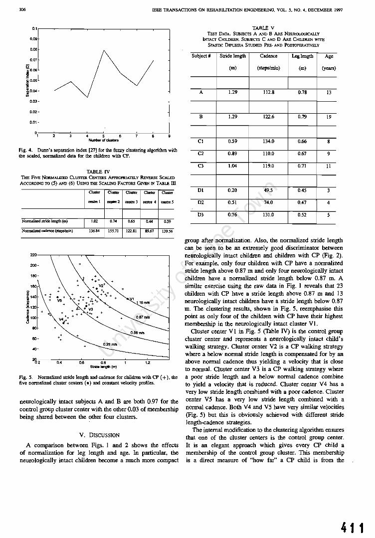
306 IEEE TRANSACTIONS ON REHABll.ITATION ENGINEERING. VOL. S. NO.4, DECEMBER 1997

O.I,--.---,....---.------,r----,-----,---.---

0.09

0.08

0.07

0.03

0.02

°1·~-~2~-~3~-~4r--~5--~6--~-~8-~9 NIMItJer 01 clusters

Fig. 4. Dunn's separation index [27] for the fuzzy clustering algorithm with the scaled, normaJized data for the children with CP.

TABLE IV THE FIVE NORMALIZED CLUsrER CENTERS APPROPRIATELY REvERsE SCALED

ACCORDING TO (5) AND (6) USING TIlE SCALING FAcTORS GIVEN IN TABU: ill

Normalised stride length (m)

Normalised cadence (st.epslmin)

200

180

s ~ 140 j ~120

~ ~ 100

80

60

40

+ + +

Cluster

"""be I

1.02

136.84

CIUS1er C1US1er Cluster Cluster

cea1Ie2 centn: 3 c:en1Ie 4 centn: 5

0.74 0.65 0.44 0.39

155.71 122.81 89.67 139.56

~~~--~--~r_-~~--~--~---0.2 0.4 0.6 0.8 12 S1ride I8ngIh (m)

Fig. 5. NormaJized stride length and cadence for children with CP (+), the five normalized cluster centers (.) and constant velocity profiles.

neurologically intact subjects A and B are both 0.97 for the control group cluster center with the other 0.03 of membership being shared between the other four clusters.

V. DISCUSSION

A comparison between Figs. I and 2 shows the effects of normalization for leg length and age. In particular, the neurologically intact children become a much more compact

TABLE V TEsT DATA. SUBJECTS A AND B ARE NEUROLOGICALLY

OOACI' CHn.DREN. SUBJECTS C AND 0 ARE CHn.DREN WITII SPASTIC DIPLEGIA STUDIED PRE- AND POSTOPERATIVELY

Subject # Stride length Cadence Leg length Age

(m) (steps/min) (m) (years)

A 1.29 112.8 0.78 13

B 1.29 122.6 0.79 19

C1 0.59 134.0 0.66 8

C2 0.89 110.0 0.67 9

C3 1.04 119.0 0.71 11

01 0.20 49.5 0.45 3

02 0.51 74.0 0.47 4

D3 0.76 131.0 0.52 5

group after normalization. Also, the normalized stride length can be seen to be an extremely good discriminator between neurologically intact children and children with CP (Fig. 2). For example, only four children with CP have a normalized stride length above 0.87 m and only four neurologically intact children have a normalized stride length below 0.87 m. A similar exercise using the raw data in Fig. I reveals that 23 children with CP have a stride length above 0.87 m and 13 neurologically intact children have a stride length below 0.87 m. The clustering results, shown in Fig. 5, reemphasise this point as only four of the children with CP have their highest membership in the neurologically intact cluster VI.

Cluster center V I in Fig. 5 (Table IV) is the control group cluster center and represents a neurologically intact child's wal1cing strategy. Cluster center V2 is a CP wal1cing strategy where a below normal stride length is compensated for by an above normal cadence thus yielding a velocity that is close to normal. Cluster center V3 is a CP walking strategy where a poor stride length and a below normal cadence combine to yield a velocity that is reduced. Cluster center V 4 has a very low stride length combined with a poor cadence. Cluster center V5 has a very low stride length combined with a normal cadence. Both V4 and V5 have very similar velocities (Fig. 5) but this is obviously achieved with different stride length-cadence strategies.

The internal modification to the clustering algorithm ensures that one of the cluster centers is the control group center. It is an elegant approach which gives every CP child a membership of the control group cluster. This membership is a direct measure of "how far" a CP child is from the

411

O'MALLEY e/ al.: FUZZY CLUSTERING OF CHILDREN WITH CP

60

40

~7-----~----~-----7~----~----~----~ 0.2 0.4 0.6 O.B 1.2

Stride length (m)

Fig. 6. The five normalized cluster centers (.), constant velocity profiles, two test subjects A and B (neurologically intact), and the test subject C (with CP) at eight years (Cl), nine years (C2), and II years (C3).

220

200

160

:& ~ 140 Q.

!! .!!.120

~ -8100 .. (.)

60

60

40 01 • 2<6.2 0.4 0.6 O.S 1.2

Stride length (m)

Fig. 7. The five normalized cluster centers (.), constant velocity profiles and the test subject D (with CP) at three years (D1), four years (D2) and five years (03).

control group. When the chiidren with CP are clustered with an external modification, where the control group cluster center is added after algorithm convergence and membership values are recalculated, very similar results are obtained.

Wong et al. [29] used a Kth nearest neighbor clustering paradigm (i.e., hard clustering), to group 128 CP subjects. No normalization for leg length and/or age was carried out and no less than a tenth-order featUre space was employed, thereby violating Bellman's guidelines on dimensionality. ln our opinion these two shortcomings severely limit the utility of their work.

The age range for the neurologically intact children is from 2 to 13 years and for the children with CP is from 2 to 20 years. This mismatch in age ranges is not ideal, particularly when the model derived from the neurologically intact children's data is being used to normalize the children with CPo However, since the stride length/leg length and cadence/age relationships are

412

307

1.00r-----------------------------------~

0.80 -1-------------------108 Years f--------------j l!1l9 Years I

.9- 0.60 t-----------f?1r-------1

.r:: f!! CD .c E CD :!: 0.40 t-----------------Ul:11t-----------1

0.20

0.00 Cluster 1 Cluster 2 Cluster 3 Cluster 4 Cluster 5

Fig. 8. Membership changes for subject C, from preoperatively (eight years) to postoperatively (nine and 13 years).

1.00 ,----------------------------...,

0.60

.9- 0.60 ~

I!! 1: E .,

1'03 Years I 04 Years .SYears,

.-.-------------------------1

~ 0.40 t--------------------=

0.20

0.00 C~1 ~2 CI'-3 C~4 CluslBr5

Fig. 9. Membership changes for subject D, from preoperatively (three years) to postoperatively (four and five years).

monotonic, the inherent extrapolation is acceptable. Indeed, in the test data, subject B is a 19 year old healthy subject and after normalization sits almost on top of the control group cluster center (Fig. 6) with a membership value of 0.97, therefore indicating the validity of the extrapolated model. Other techniques could be used to normalize the dati. [30]. However, they would be incapable of removing trends, expected in the neurologically intact population, from the data of the children with CPo

The real power and utility of the fuzzy clustering approach introduced in this paper is demonstrated with the data for the test subjects (Tables V, Figs. 6-9). The two neurologically intact subjects A and B have different ages and genders (a 13-year old male and a 19-year old female, respectively) and yet they both fall very close to the control group cluster center VI in Fig. 6.

Subject C is a girl with spastic diplegia. At eight years of age her highest membership was in cluster V5 (Figs. 6 and

IEEE lltANSALnONS ON REHABILITATION ENOINEERJl'lG. VOL. 5. NO. 4. DECEMBER 1m

8). She then underwent a dorsa! rbi7..0tomy procedure and her gait was re-evaluated one and three years later [28J. Her poinl on the stride length-cadence diagram has shifted from C I to C2 (one year postsurgery), where It is close to cluster V3, and finally to C3 (Ihree years postsurgery) where she has moved closer to clusters V I and V 2. It is clear thai her gai I improved afler surgery and continued to move toward the neurologically intact control group three years later.

Subject 0 is II boy with spastic diplegia. At ] years of age his highest membership was in cluster V4 (Figs. 7 and 9). He then underwent an orthopaedic procedure and his gait was reevaluated one and two years later. At one year postsurgery his point on the stride length- cadence diagram has shifted from 0 I to D2 which is closer to the control group cluster center VI (Fig. 7) but his highest membership is sLill in cluster V4 (Fig. 9). At two years postsurgery his point on the stride length-cadence diagram has shifted from 02 to 03 which is moving closer to VI. V2. and V3. This movement and his membe~hip v8..lues (Fig. 9) clearly demonstrale an improvement in his gail velocicy. £nterestingly, he has achieved this by increasiog both stride Jength and cadence.

We believe that our fuzzy clustering approach has important implications for outcome-based research. Utilizing just four easily obtained paramelers-stride length, cadence, leg length and age-it is possible to classify any child with spasLic diplegia. Using (2) and (4) and the coefficients in Table ill, the ' data may be normalized to generate a point on the stride length-cadence diagram (Fig. 6). Then, employing the scaling faclors ITable ill and (5) and (6») and cluster centers (Table IV) and (8) and (to), it is possible to generate an individual's membership values for each of the five clusters. This demonstrates the utility of fuzzy clustering and contrasts wilh the more subjective (descriptive) techniques [2], [3J, [12), [13) which are not capable of quantifying change and where groups are defined a priori. This approach can be adopted to study other clinical entities (e,g. stroke or osteoanhritis) where different cluster centers would be establisherl using the algorithm provided here.

REFERENCES

[II J. G . Gage. GOI/ IIl101YJi.< '" Cerebrol Pal.,y. New York: MacKctlh. 1991 .

(2) T. F. Winler~. J .. G . Gase. and R. Hicks. "Gail paLlctnS in .pasrie hemiplegia ill chiJdreb and yoong adults," J. Joint Bon~ Su'g., vol. 69A. pp. 437-441. 1987.

131 M. M. Hoffer. E. Feiwell, R. PetTY, R. J. Perry. and C. Bonnett.. "Functional ambulation ill patienLS with myelomeningocele:' J. Bone Join! Surg .. "01. S5. pp. 1)"1-148. 1973.

(41 H. G. WaIlS. """Gail laboratory anl)"'is for preopc:l"3UVt de.:i.sion making in spastic cerebral palsy' 15 il all iI'S cracL.:ed up 10 be ?:. J. PIl~diOJr. Or/hop .. vol. 14. pp. "103-704. 1994.

151 J. G. Gage. "The role of gail aoruysis in the crealrnenl of ~rebfljl palsy:' J. Paedial. Onhop .. vol. 14. pp. 701-702, 1994 .

[61 c. L Vaughan. B. L Davis. and J. C. O·Connor. D)"nLJmic.~ of HU/TIM Gai,. Cbam[)llign. tL Human Kinetics. 1992.

[7) O. N. TIbarewala and S. Ganguli. "Panem recognition in 13Chogn.phic gail records of nonnal and lower el!lremity handlC<lpped human sub­jecu.~ J. BiD"'ed. &g., vol. 4, pp. 23~240. 1982.

(8J D. Richardson. 3lId C. Brubaker. ~liullWl gail quanli6caLion and p31.lem rccognitioll." Biomu:1uur.. N ·)'. "~lJj.$on and JOIl1cnsen, Eds.. Cham. paign, JL: Human Kinematics. 1978.!'P. 198-3~.

(9J G. A. BeU)·. C. Chang, J. Peny, and M. }Joffe>, "P!IICm recognilion of mulLiple EMG sigoals app~erl 10 the description of human gail," PrO(:. IEEE, vol. 65, pp. 674-681. 1977.

[l0) M. P. Kad.\ba. H. K. Ramakri.<hoan. 0 Jacob<. M. E. Woou~n. C. Chambers. C. Scvboroug/l. and)3 Goode.. "Quantilllliye gail U1alysis: pan ern rec.ognlliun in spA.<;{ic diple~ia." in PfV(. 61h AM"' . Eos, CCI15I Cii" . Goll Anal. Conf.. Michigan Slate Univ .. East Lansing. M I, 1990. pp. 9-12.

[II] V. T . Inman. H. J. Ralston. and F. Todd. f/,vrwn Walking . Baltimore, MD: Willialm and Wilkins. 1981.

(I:!I D. L. Damiano and M. F. Abel. "Re)auonship of gaic anOllysis to grou mOlor functIon in cerebral palsy:' De~lop. Mcd. Child NeuroL. vol. 38, pp. 389-396. 1996.

II3J J. Perry, M. Garrell, J. K. Grooley, and S. J. Mulroy. ' 'Classlficalion of wallUng handicap in the s:roke populaLion:' Sirek vol . 26, pp. 9!!2-989, 199~ .

(14J R. O. Duda. and P. £. Han. Pal/ern CI4.uificolio" and Sc~ne Anolyis. New York: Wiley, 1973.

IISJ R. J. Marks. "Verbal comm""!.:' inA TUlOriDl Cou,u 0/1 A11'ificial NeUfal Ncr ... orkJ w;tll ,A.ppl. to Power SY11., I£.E:£ Power Eng. Soc. Wintel MWi(lg. BalIlmOf"C, MO, 11' 112.(). Jan 1996.

[16J M. /. O'Malley, "Normaliution of cemporal-di<cBnce panunelen; in paodlatric gait." J. 8io_chon.. Yol. 29. pp. 619-625. /996.

117J D. H. Suthtrland. R A. Olshen. E. N. Riden. and M. P. WyBLI, The D~lop"'e'" 0/ Malure WaLb'tlg. Mac Keith Press. 1988.

[18) M. J. O'Malley. "Letter 10 !be: Editor, Aulhor"~ Ruponse.. Nornlali"-Olion of !empor31-<lislBtlcc paramet= in paodiatric gail." I. B;o",~c:han.. vol. 30. pp. 301-302. 1997.

[19J R. D. Sleve/UOO. R. P. Hayes. L. V. CaIU. and J. A. Blackman, "Oinical com:lates of line.1T grIlWlb In children will> cerebral palsy." Develop. Med Child NeuroL. vol. 36. !'P. 135-142. 1994.

[20J J. C. Bez.dck and S. K. Pal, Fulr,Y Models fa' POI/em R~cognil;on. Ne .... York: IEEE Press. 1992.

[211 M. 1. O'Malley. M. F. Abel. and D. L. DamiMo, "FuZ.2:)l cluslering . of temporel-di.lance pBTame(ers and kinem~lic data for ccrclJral palsy children," Gail and Poslure. vol. 3. p. 92. 1995

Inl f, N. Todd, L. W. UmOreul. S. R. Slonncr, M. E. Johanson. R Helens. R. S. A. Moran. and R. K. Ashky, ~Varialions in the gait of n()!'lTlal ch.ildren:· J. 8"",e Jow Surg .. vol. 71 A. pp. 196-204, 1989.

(23) J. C. Be2.dek.. Pacrem R«ogfUlintl ""ith Fuu:y Db)e,"/;'" Fu"c:liofl A/go­rilhm... New York: Plenum. 1981.

[lA J __ . "'A convergence theorem (Clr the fuzzy !SODATA clustering algori!hm.~ IE££ TrnflS. paC/em Anal. Machinz lnulL. vol 2. pp. I-S. 1900.

[25) J. C. Bezddr.. R. Hall1away. M. J. Sabia. and W. T. Tuclce:r. "Coo"e!' gence the.ol)l (or fuz:zy C-mean&: counl.ereJ81lIpl~ and repairs:' IEEE TrorlS. SYJI. Man Cybem .. vol. 17, pp. 873-877. 1987.

[26J R. C. Dubes. 4How many cluslers ase be~(?-3Jl e~perilIl~nl:' Pattern Recos .. vol 20. pp. 64S-¢63. 1987.

[27J J. C. Dunn. "Well ~paraled clusters amJ opumaJ tuuy panilions," J. CyNm.. vol. 4. pp. 95-104, 1974.

(2Jl] Co L. Vaushan . B. 8elTTW1, and W. 1. Pe2Cock, """Gail !II1aJy.i. and rhilolomy . A three year foll()W-up evaluation .... ilh gait analysis:' J. Ncurolurg ., "01. 74. pp. 17&-1&4. )991.

\29) M. A. Wong. S. ·Simon. and R A. DIsheR. "SllIti,ticaJ analys;' of gail palle.mS of pe:rs<ms with cerebral pally.~ Slac. M~d.. \'01. 2, pp. 34S-354, 1983.

[30) A. L. Hof. "Scaling gail data to body .iz.c,"" Gait and Pas/un:. vol. 4. pp. 222-223. 1996.

Mar)< O'Malley (SM '9S) rece.iv~tI the B.E. and Ph.D. deg.teeS in electrical engineering (rom Ihe National Univ=ily of Irel8f\d in 1983 and 1987, respecti vel y.

Afic{ one year working in (he industry on Euro­pean Sp.cc Ag~cy projects. he joined the academic staff as a J..ej;lurer in the Departmem of EleclJnJ1jc and Electrical Engineering a! UruVeriJly College Dublin. ireland. Hi~ r=cch Interests lICe modellOg and control " .. ilb applications in biomedical engi­neering and po""a ~ystems He it; th. loint Head

o( the Rehabilitation EngJac:ering 1.;o001"ll101)' al the National Rcllabilitallon Hospital. Dun J...aoire..lreland . J.n !994, he was awarded a Fulbrighc Fellowship and sUb$cquenrly spent seven months as an Re.<CMCh Fellow in th~ De{lanmcnl of Onllopacdic Surgery alllle University of Virginia. CharlottesvlUe.

O·MJIIl.l..EY tr oJ.: FlJ2ZY CLlJSTERING OF CHruJREN WITH CP

.. ~

•• i'Ji ... . r!.

~ '. -AI .. I.~.r· .

cucbraJ piliy.

Mark F. Abel received the M.D. degree from Th[8Jlt Uni Yc:rSicy , New Orleans.. LA. in 1982 He then wenl 00 10 complell: orthopaedic surgery and pediauic onhopaedic special!}' craini ng al llIe Uni· ven;ly of California. San Diego.

Currenlly. he is an Associale Professor of Or· Ihopaedic:s and Pediatrics at the University of Vir· gini", Ch:>tlollCSvllle. He is al<o the Medicol Direc· lOr of the instirulion'S Motion Analy~is l..1bol"3lorr. The cmph.asu of hi, r=arch is On the clinic.a.i application of treacmems for cerebral palsy. hip

Diane L Dwtiaao received the M.S. degree in pliysical therapy from Du~ University, Durham, NC. in 1979, aad the Ph.D. degree In biom.:chanics irom the Univeaily of Vtrginia. CharlonesviUe. in 1993.

She h.a.I ren years of clinic.al experience io pedi. amc pliys.ical therapy. Sbe is currently all AssiSUlDI Professor of Onhopae;lics and R~h Direcl.or of the Molion Aa.alyu. l....:I.boralOry al Univcrs.icy of Virginia. Owlollcsvi!Je. He( rese.ucli focuses on muscle performance IUld functional oUlComes in

Dr. Damiano has recdved five mltional =h award.: two from I"" American Academy of Cerebral Palsy. IWO from the Americn Phy.lica.l Thetllpy A>S(ICialion. and mOSt recently lhc presllglQUS Elbel HauslTWJ OinicaJ R~;".uch Scholars Award from th~ Uniled Cerebral Palsy.

414

309

Christopber L (KJ I) Va aghan eM' 87) gradua led wjlb a first cl.us honors aod leceived !he degJeC In physiC':l and applied mathem&lic5 from Rhod~ Univen;ity, in 1975. bdore receiving Ihe Ph.D. degree in musculoslc.elel<ll biomechanics from lh. University of Iowa, Iowa City, in 1980.

He did a postdocloral fellowsh.ip in onhopaedic engineering at Ox.ford University. U.K .. in 1983 and open! the years 1986-1995 in the U.S .. where he was Professor of Onhop.cdics ""d Biomedical Engi­neering at the Univen;ity of Virginia, Charlottesville.

He i, c\ll'Te1l11y th~ Hym"" Goldberg Professor and Chairman of Biomedical Engineering a! !he Univ~lly of Cape Town. South Africa., w~~re his research is focused on the biomech.anics of human gail.

ELSEVIER Gait and Posture 8 (1998) 43-59

Review article

Selective dorsal rhizotomy as a treatment option for children with spastic cerebral palsy

Christopher L. Vaughan a,*, Nivedita Subramanian b, Monica E. Busse a

K Department of Biomedical Engineering, University of Cape Town, Observatory, Western Cape 7925, South Africa b Department of Physiology and Neuroscience, Sackler Institute of Biomedical Sciences, New York University, Nell' York, USA

Accepted 23 April 1998

Abstract

Cerebral palsy is the most common motor disorder originating in childhood and spasticity is the most frequent manifestation. The treatment strategies to reduce spasticity and thereby ameliorate the attendant gait abnormalities have included physiotherapy, orthoses, antispastic medications, orthopaedic surgery and neurosurgery. Of these, the neurosurgical procedure known as selective dorsal rhizotomy has gained widespread exposure, and indeed acceptance, over the past two decades, despite there being some controversy as to its efficacy. In this paper we review: cerebral palsy, including classification and treatment; selective dorsal rhizotomy, including historical background, patient selection, operative procedure, clinical outcome and complications; and gait analysis studies, including temporal-distance parameters, joint kinematics, normalisation for growth, and long-term follow-up. Both the short-term (I year) and long-term (10 years) evidence has demonstrated that selective dorsal rhizotomy not only reduces spasticity but it also provides lasting functional benefits as measured by improved range of motion during gait. Rhizotomy is not a panacea for children with spastic diplegia but it is an important treatment option for the clinician to consider. © 1998 Elsevier Science B.V. All rights reserved.

Keywords: Cerebral palsy; Spasticity; Neurosurgery; Gait

1. Introduction

Cerebral palsy is the most common motor disorder originating in childhood [1] and spasticity is the most frequent manifestation [2]. Although many children with cerebral palsy may have cognitive and sensory deficits, the hallmark of the disorder is motor dysfunc­tion [3]. Over 50% will have spasticity in the lower extremities (known as spastic diplegia) and movement will be compromised at the ankle, knee and hip joints. Despite these deficits, the majority of children with spastic diplegia will learn to walk although this will be at a later age compared to their peers who develop

• Corresponding author. Tel.: + 27 21 4066238; fax: + 27 21 4483291; e-mail: kvaughan@anat.uct.ac.za

0966-6362/98/$19.00 © 1998 Elsevier Science B.V. All rights reserved. PH S0966-6362(98)00018-6

normally [4]. Not surprisingly, all parents place a major emphasis on the ability of their children to develop the necessary motor skills to walk. The child with spastic diplegia will usually have a walking pattern that may include scissoring of the legs, internal rotation of the thighs, an equinus ankle at foot contact, and there is frequently exaggerated knee flexion (so-called crouch gait) in stance [5]. Parents have turned to clinicians for treatment strategies to ameliorate the gait abnormali­ties, and these strategies have included physiotherapy, orthoses, antispastic medications, orthopaedic surgery and neurosurgery [6]. Of these, the neurosurgical proce­dure known as selective dorsal rhizotomy has gained widespread exposure, and indeed acceptance, over the past two decades, despite there being some controversy. as to its efficacy [7]. In this paper we will review:

41 5

44 C.L. Vaughan el al./ Gail and Posture 8 (1998) 43-59

cerebral palsy, including classification and treatment; selective dorsal rhizotomy, including historical back­ground, patient selection, operative procedure, clinical outcome and complications; and gait analysis studies, including temporal-distance parameters, joint kinemat­ics, normalisation for growth, and long-term follow-up. Finally, we will make some concluding remarks about the future role that rhizotomy will have as a treatment option for children with cerebral palsy.

2. Cerebral palsy

Cerebral palsy is the term applied to a group of conditions characterised mainly by motor disability re­sulting from a non-progressive, permanent insult to the developing nervous system. The cause of insult, which may be pre-, ante- or post-natal, can result from dam­age to an otherwise normally developing system or can be due to the abnormal development of the nervous system itself [8]. Spasticity is a consequence of an insult to the motor control area of the cerebral cortex. Cere­bral palsy, or Little's disease as it was initially known, was first described by an English orthopaedist, William 1. Little, who attributed it to difficult birth. He put forward the hypothesis that spasticity was due to neonatal brain damage. The term 'cerebral palsy' itself was coined by Sir William Osler in 1888 in his review of 151 cases, most of whom were subjects with spastic diplegia. Sigmund Freud in 1897 associated spastic diplegia with premature birth in his treatises on the classification of cerebral palsy [8]. Freud also was the first to emphasise that observed symptoms could arise from a variety of causes and that the disorder itself could be classified into subgroups or types [9].

2.1. Classification

It is difficult to classify cerebral palsy precisely into individual categories but three distinct physiological types are usually seen. These are the spastic (80'% of all cerebral palsy cases), the athetoid (15%) and the ataxic (5%) types, though cerebral palsy can exist as a combi­nation of two types [2].

The spastic type of cerebral palsy is characterised by motor dysfunction including hypertonicity of the 'clasp knife' variety in the affected muscles. When these spas­tic muscles are stretched, they respond in an exagger­ated manner by contracting and blocking the movement. Other characteristics include increased ten­don jerks and clonus. Patients with spastic cerebral palsy also display abnormal postures associated with the anti-gravity muscles, namely the extensors in the legs and flexors in the arm. Fear, excitement or anxiety may bring about changes in hypertonicity and posture due to increased muscle tension. Selective, voluntary

416

motion, though laboured, is often present [10]. Spastic­ity is a physical sign of an upper motor neuron lesion and involves damage to the pyramidal tracts [11].

The athetoid type of cerebral palsy is characterised by uncontrollable purposeless movements which may be writhing, jerky, tremor, swiping or totally random patterns. This kind of motion is increased by excite­ment, insecurity and decreased by fatigue, fever, drowsiness or if the subject's attention is deeply held. Voluntary motion is possible with an initial delay be­fore the motion is begun. The involuntary movement may partially or entirely disrupt willed motion, making it appear uncoordinated. There may be fluctuations of muscle tone occurring with swings in mood or emo­tions. The diagnosis of athetosis is difficult to make before the age of 2 years at which time the disorder of involuntary movement begins to emerge. Due to mini­mal damage to the cerebral cortex (the extra-pyramidal system is jnvolved), people with athetosis tend to pos­sess normal intelligence compared to those with spastic­ity, although mental defects do occur. People with athetosis are often observed to have 'drive' and outgo­ing personalities [10].

The ataxic type of cerebral palsy is characterised by poor fixation of the head, trunk, shoulders and pelvic girdle, while voluntary movements are clumsy and un­coordinated. The affected individual tends to over­reach or under-reach for an object, suffering from dysmetria and accompanied sometimes by intention tremors. People with ataxia usually display hypotonia and a purely ataxic case is quite rare [10].

Insult to the various areas of the precentral gyrus of the motor cortex results in the topographical distribu­tion of neuromotor impairments in cerebral palsy [9]. Topographically, cerebral palsy may be classified into 'quadriplegia' (where all four limbs are affected), 'diple­gia' (involvement of four limbs with the legs being more affected than the arms), 'paraplegia' (involvement of both legs), 'hemiplegia' (involvement of one side of the body) and 'monoplegia', a rare case where one limb is affected [10].

Spasticity may be defined as a velocity dependent response to passive muscle stretch [12]. It may be assessed in several ways, including simple clinical tools such as the modified Ashworth scale [13,14] and more sophisticated measurement equipment such as the isoki­netic dynamometer [12]. When spastic muscles are pas­sively stretched, they can restrain, totally block or even reverse the movement. However, the relationship be­tween spasticity and voluntary movement is not well understood. Patients with spasticity also have centrally­mediated muscle imbalance which tends to favour the hip flexors and adductors, hamstrings and ankle plantarflexors. In time the overactivity can lead to muscle shortening [4]. Selective motor control is im­paired to varying degrees, with distal control more affected than proximal.

c.L. Vaughan et al. / Gait and Posture 8 (1998) 43-59 45

In discussing the causes of cerebral palsy, it is possi­ble to classify these into developmental abnormalities and traumatic injuries inflicted on the normally devel­oping brain. One of the most important consequences of ischaemia in the vulnerable arterial zones close to the ventricular wall is periventricular leukomalacia, which is seen as necrotic patches in the periventricular white matter adjacent to the external angles of the lateral ventricles [8]. This has been verified by conducting MRI studies of patients with spastic cerebral palsy who have undergone selective posterior rhizotomy [15]. The le­sions may evolve into periventricular cavities sur­rounded by glial scar tissues with calcified fibres, resulting in thinning of the white matter in the corpus callosum and centrum semi ovale and also in the expan­sion of the lateral ventricles.

2.2. Treatment

Spasticity may be alleviated using both surgical and non-surgical techniques. Non-surgical methods such as physiotherapy and occupational therapy aim to min­imise the influence of spasticity on voluntary move­ments by teaching the patient new postures and movement patterns. Administration of physiotherapy differs with age [16], although an important aim is to maintain range of motion and slow the progressive muscle tightness in spastic cerebral palsy. There has been no direct evidence for the efficacy of physiother­apy alone in the management of cerebral palsy, al­though when coupled with surgical techniques as a part of post-operative care and rehabilitation, the adminis­tration of physiotherapy is thought to be indispensable [17].

A number of muscle relaxant drugs have been used to reduce spasticity, albeit with temporary relief. Some of the most commonly used drugs are: (i) Diazepam, a GABA (gamma-aminobutyric acid) analogue which in­hibits the release of excitatory neurotransmitters and thereby acts as a muscle relaxant; (ii) Dantrolene, which acts directly on skeletal muscle by inhibiting the release of calcium from the sarcoplasmic reticulum and thereby decreases the force of muscle contraction and produces muscle weakness [6]; and (iii) Baclofen, an­other GABA analogue, which inhibits transmitter re­lease by competitive inhibition of neurotransmitters at the spinal level [18]. However, the oral administration of antispastic drugs is marginally effective in reducing spasticity, due to the limited ability of the drugs to penetrate the blood-brain barrier [6]. Another proce­dure introduced in the past few years is the administra­tion of Botulinum-A toxin (Botox) injections directly into the affected muscles. This reduces overactivity in spastic muscles for about 3-6 months with no apparent adverse side effects [19]. Very recently, the insertion of an intrathecal baclofen pump has received a lot of

attention, with the suggestion that the need for subse­quent orthopaedic surgery may be reduced [20].

Surgical methods currently in use may be classified into orthopaedic and neurosurgical procedures. Ortho­paedic surgery includes three types of surgery on mus­cles and tendons, namely: release, lengthening and transfer [21]. Appropriate surgery is performed depend­ing upon the affected muscle. There are four common procedures. First, distal hamstring lengthening surgery aims to eliminate crouched gait pattern, and may min­imise internal rotation gait [22]. This procedure may be performed in conjunction with rectus femoris transfer which helps to minimise the 'stiff knee posture in swing phase of gait, thereby increasing the knee range of motion [23]. Second, Achilles tendon lengthening cor­rects ankle equinus [24]. A variation of this procedure is the gastrocnemius-soleus lengthening which is done when the soleus muscle does not display significant contracture [25]. Third, tendon transfers are commonly performed for correction of varus foot deformities and include the split anterior and posterior tibial tendon transfers, procedures by which the lateral half of the tendon is moved to the cuboid and peroneus brevis respectively, creating a balanced yoke on the foot and thereby neutralising the varus pull of the tendons [26]. The choice of procedure is dependent on the dysphasic muscle that produces the deformity [27]. Fourth, surgery may also be performed at the hip to alleviate the consequences of cerebral palsy, namely complica­tions such as spasticity and hip dislocations which arise from a combination of factors, including spastic muscle imbalance. Orthopaedic procedures performed include: psoas recession over the brim of the pelvis to address hip flexor spasticity [28]; femoral and pelvic osteotomies [29,30], the primary reconstructive procedures for bony deformity; resection arthroplasty to treat total body involved patients in whom there is severe erosion of the articular cartilage and gross incongruity of the femoral head and acetabulum as a consequence of prolonged dislocation [4,29,31]; and, very rarely and somewhat controversially, total hip arthroplasty [32], which is most effective on patients with no evident contralateral subluxation or dislocation of the hip [4].

Although alternative techniques such as selective pe­ripheral neurotomies where peripheral nerves are inter­rupted using microscopic techniques have been partially successful [33], the most prevalent neurosurgical proce­dure currently performed for the reduction of spasticity is selective dorsal rhizotomy. This will be reviewed in the following section. Selective dorsal rhizotomy ad­dresses the functional complications that arise from spasticity. It cannot address pre-existing conditions such as bony abnormalities (e.g. internal femoral tor­sion) and muscle contractures in the older child. In a retrospective study of 178 children (54 aged 2-4 years, and 124 aged 5-19 years at the time of surgery),·

417

46 c.L. Vaughan el a/. / Gail and POSlUre 8 (1998) 43-59

Chicoine et al. [34] showed that early rhizotomy re­duced the need for orthopaedic surgery for heel cord, hamstring and adductor releases. However, there was no difference between the two groups for femoral os­teotomies, iliopsoas releases and ankle/foot operations. It has thus been recognised that a combination of orthopaedic and neurosurgical procedures, appropriate for the individual child, is required.

3. Selective dorsal rhizotomy

3.1. Historical background

The original concept of rhizotomy or 'cutting roots' is credited to Dr c.L. Dana of New York who recom­mended this operation and it was first performed by Robert Abbe in 1888 for the relief of pain in a case of ascending neuritis [35]. Dorsal (i.e. sensory) root rhizo­tomies were first performed by Dr Otfrid Foerster, a German neurosurgeon, in 1908. He described 159 cases of which 88 were cases of 'congenital spastic paraplegia' [35]. The technique he adopted was the division of the entire dorsal sensory roots from L2 to S2, excluding either L4 or L5 to preserve knee extensor tone. Foerster distinguished the ventral and dorsal nerve roots and identified the roots associated with knee extensors via electrical stimulation [36]. He also emphasised the iden­tification of spastic cases as opposed to athetosis and paralysis and reported improved results in patients with lower extremity involvement. These criteria are still very much in consideration when selecting patients in the current era [37]. The procedure fell into disuse over the next six decades following Foerster's pioneering work due to difficulties with sensory loss that resulted from extensive and indiscriminate sectioning of the dorsal roots. During this period spasticity was treated by ventral root rhizotomy which brought about muscle atrophy, or by destructive procedures like cordotomy or myelotomy [38], in which the side effects were often more noteworthy than the benefits of the procedure [39].

Gros et al. [40] revised Foerster's procedure by sec­tioning only a fraction of the rootlets, and thus preserv­ing sensation. They further refined the technique by electrically stimulating each of the rootlets, thereby mapping out those related to essential muscles like the quadriceps, and abdominal and pelvic supporters which were left intact. Those muscles that showed abnormal action in the electromyography (EMG) recordings, and were thought to cause spasticity, were then 'released' by sacrificing their respective sensory rootlets [II].

Fasano et ill. [41] discovered that some rootlets, when stimulated with impulses of a certain frequency, re­sponded with a brief localised contraction whereas oth­ers showed a continuous prolonged contraction which

41 8

spread to other muscles, an abnormal phenomenon linked with those muscles associated with spasticity. These rootlets were then sectioned. This technique re­lieved spasticity without compromising sensation. It was later applied to a group of adults suffering from multiple sclerosis and spinal cord injuries with positive results [42].

The Fasano procedure, initially performed in the region of the conus medullaris, was modified by Pea­cock in 1981 [43,44]. He shifted the site of rhizotomy to the region of the cauda equina, thus facilitating easier separation of the ventral and dorsal roots and identifi­cation of individual rootlets. When Peacock moved from Cape Town to Los Angeles in the mid-1980s, this is the technique which he introduced to many neurosur­gical centres in North America and was widely adopted for the treatment of spasticity in the child with cerebral palsy [6,45]. More recently, in an effort to reduce the problems of lumbar instability [46], some surgeons have adopted a more limited laminectomy at the level of the conus as advocated by Park [47]. There is also some controversy as to the number of rootlets that should be sectioned, where less than 25% can lead to limited functional gains [48].

3.2. Patient selection

The primary objectives of selective dorsal rhizotomy are to improve locomotor function in a spastic individ­ual or to ease daily handling and care in the case of a non-ambulatory child with severe quadriplegia. Candi­dates may either be classified as ambulators who are capable of maintaining and improving functional abili­ties upon alIeviation of spasticity, or those patients who have been severely affected by cerebral palsy to the extent that they are non-ambulatory and care taking becomes difficult. Most patients in this second category tend to be intellectually handicapped [44].

The ideal candidate for selective dorsal rhizotomy would be a mobile and motivated child with normal or near-normal intelligence who is attempting to improve his/her gait pattern [37]. Although these children are usually less than 12 years of age, the procedure has been performed on teenagers, yielding a reduction in tone with positive functional outcomes in 77% of the cases [49]. Selection criteria for the procedure include: (i) premature birth, where the children are usually identified by the age of I year and display an initial hypotonicity that progresses to pure spasticity; (ii) good underlying strength, along with trunk and motor con­trol (some children use their spasticity to compensate for lack of support from the anti-gravity muscles and rhizotomy in such a case could be detrimental); and (iii) absence of rigidity, dystonia, athetosis and ataxia. Since these conditions are not brought about by damage to the motor cortex, patients will not usually benefit from rhizotomy [37].

C.L. Vaughan et al. / Gait and Posture 8 (1998) 43-59 47

Evaluation of trunk musculature, head control and equilibrium responses may be accomplished with the Rancho Los Amigos Hospital test of upright motor control [50]. Prospective candidates for rhizotomy are evaluated thoroughly by a team which normally con­sists of a paediatric neurologist, a paediatric neurosur­geon, an orthopaedic surgeon, a paediatric psychologist, paediatric physiotherapists and occupa­tional therapists [51]. Their task is to determine crucial factors such as compromised muscle groups and to give the surgical team complete detailed pre-operative infor­mation on which the eventual pattern of surgery will be based.

The issue of appropriate patient selection cannot be overemphasised [52]. Contra-indications include: (i) in­volvement of extra-pyramidal system (athetosis); (ii) underlying muscle weakness; (iii) lack of access to post-operative physiotherapy; (iv) lack of motivation on the part of patients and parents; and (v) spastic hemiplegia, where the children are considered too mildly involved to benefit from rhizotomy [53]. The risks of inappropriate decision-making are significant, with possible negative outcomes including long-term weakness post-operatively, and loss of postural support due to reduction in tone. The pre-operative identifica­tion of underlying muscle strength versus how tone contributes to standing posture and trunk stability re­quires a thorough evaluation by a knowledgeable clini­cian such as a physiotherapist [36].

3.3. Operative procedure

The patient is placed prone on the operating table with bolsters under the pelvis and chest to allow free movement of the abdominal wall. This also prevents epidural vein distension and reduces bleeding [36]. A general endotracheal anaesthesia is administered using agents such as halothane, fentanyl or nitrous oxide without the use of muscle relaxants which might affect intra-operative EMG monitoring [45]. Using the poste­rior superior iliac spines as reference, the lumbosacral spinous processes are marked to the level of the L4 spine. A midline laminectomy, in which case a sub-pe­riosteal dissection is used to allow for bone formation from the intact periosteum after closure, or laminotomy (where the bone is sutured back into place) is then performed from L2 to L5 [36], though some surgeons include Ll as well [54]. The addition of this level carries a certain amount of risk since it ventures close to the thoracic region. On the other hand, Lazareff et al. [55] have shown positive results with an L5 to SI laminectomy.

Before the dura is opened, care should be taken to ensure haemostasis in the muscular layer since the presence of blood in the spinal canal can impede the procedure by making root identification and manage-

ment more difficult. This also occurs when the dura is accidentally opened during laminectomy, causing blood to leak into the sub-arachnoid space and the loss of cerebro-spinal fluid, leading to the adherence of clots to the roots and possible spinal canal collapse [56]. Once the dura is opened, the nerve root levels are confirmed using electrical stimulation by eliciting motor responses from the ventral roots of SI and S2. The ventral roots are then separated from the dorsal roots from L2 to S I with the help of a magnifier. The threshold voltage is determined by stimulating the dorsal root of L2 using microsurgical blunt hook electrodes. The posterior root is then subdivided into a number of rootlets, usually about 40-50 for a typical bilateral case. Each one of these is stimulated with a O.l-ms pulse at 10 V. The voltage is gradually increased until a response is seen on the EMG. The EMG response to a non-sinusoidal stimulus of 50 Hz is noted. Roots giving rise to abnor­mal patterns are then sectioned, while those showing normal responses are spared. Examples of abnormal responses as defined by Fasano et al. [41] are: (i) an incremental amplitude EMG response; (ii) muscles re­sponding to stimulation of nerve roots not connected to it; and (iii) a continued tetanic contraction response even after the stimulus is removed [48].

Variations on this procedure, such as shifting the site of excision just caudal to the conus medullaris [6], have been proposed with the claim of reducing motor weak­ness in intensity after selective dorsal rhizotomy. How­ever, sufficient evidence is still lacking to support this approach. Inclusion of the S2 rootlet (involving plantar flexion), though not performed in all cases due to possible complications with incontinence, has been shown to reduce plantar flexor spasticity significantly [57]. It should be mentioned that there is some variabil­ity among neurosurgeons in the method of selecting which rootlets and the number to cut and these deci­sions will obviously have an impact on the functional outcome. Furthermore, some surgeons replace the spinous processes while those who do not run the risk of post-operative instability of the lower spine [46].

3.4. Clinical outcome

Selective dorsal rhizotomy is a surgical procedure done under general anaesthesia with a low mortality risk. All patients undergoing this procedure have shown a reduction in their muscle tone to varying extents and a concomitant improvement in their functional move­ments and gait. The change in spasticity is usually graded according to the modified Ashworth - Bohannon scale, which is summarised in Table I [58]. Results showing reduction of spasticity conducted at various centres around the world [55,58-60] have been graphi-cally summarised in Figs. I and 2. .

419

48 C.L. Vaughan et al. / Gait and Posture 8 (1998) 43-59

Table I St.andardised scale for grading spasticity [13,14]

Score Definition

o Hypotonic: Floppy. Muscle tone less than normal. I Normal: No increase in muscle tone. 2 Mild: Slight increase in muscle tone. Minimal resistance

to movement through less than half the range. 3 Moderate: Increase in muscle tone through most of the

range of motion but the affected part is easily moved. 4 Severe: Considerable increase in tone and passive move­

ment difficult.

Fig. I (a and b) indicate there is a definite shift towards decreased spasticity after surgery, implying that rhizotomy has an almost immediate effect in re­ducing increased muscle tone. An interesting finding by

PI. Flexors

III

g. Quadriceps e (!)

CD U ~ Hamstrings

:::i

Adductors

o

Lazareff et al. [55] was that despite operating on a very small section of the lumbar area (only rootlets at the level of L4, L5 and Sl were subject to deafferentation), muscles not directly innervated by these segments­such as the hip flexors and some upper limb muscles (deltoid, biceps and the wrist flexors)-showed a reduc­tion in spasticity. As can be seen from Fig. 2(a and b), there is a drastic reduction in spasticity in the muscle groups involved. In terms of functional improvements, this would mean a more normal posture when the patient is sitting or standing. The lowering of tone in the hamstrings and rectus femoris reduces crouch gait, enabling the individual to adopt a more upright pos­ture. This reduction in crouch, together with decreased spasticity in the adductors, reduces scissoring of the legs displayed by children with cerebral palsy. Improvement

2

EI Before Surgery

• Afte r Surge ry

3 4

(a) Degree of Spasticity

PI. Flexors

(/) Quadriceps Q, :::J 0 ... (!) Hamstrings CD U III :::J

:::i Adductors

Hlp Flexors

(b)

0 2 3

Degree of Spasticity

EI Before Surgery

• Afte r Su rge ry

4 5

Fig. I. Degree of spasticity before and after surgery: (a) Peacock and Staudt [58]; (b) Abbott et al. [59] based on the modified Ashworth scale [13,14].

420

c.L. Vaughan et al. /Gait and Posture 8 (1998) 43-59 49

20r-------------------------------------------,

J!J c G)

16

~ 12 D.. .... o ... .x 8 E :::J Z

4

o L-__________ _

Hypotonic Nonnal Mild

13 Before Surgery

.After Surgery

Moderate Severe

(a) Degree of Spasticity

30r---------------------------------------~

25

J!J c CD 20 ~

[!J Before Surgery

• After Surgery

1\1 D.. '0 15 ... .x E 10 :::J Z

5

o .L.-______ ----' .........

Hypotonic Nonnal Mild Moderate Severe

(b) Degree of Spasticity

Fig. 2. Degree of spasticity before and after surgery: (a) Berman et al. [60]; and (b) Lazareff et al. [55] based on the modified Ashworth scale [13,14].

of spasticity in the hip flexors can have mixed conse­quences. While the person may be able to stand more upright in due course, it may also reduce trunk control since some children use spasticity to compensate for lack of support from the anti-gravity muscles [37]. Decreased spasticity in the plantar flexors results in reduction of equinus gait [55].

The aspect of spasticity reduction most clinically relevant to physiotherapists and occupational therapists is the improvement of functional capacities like sitting, standing, kneeling and walking. There have been a number of positive results published in this area and these are tabulated in Table 2. The data listed includes only those patients classified as ambulatory. Post-oper­ative evaluation in these cases was conducted in a time

period ranging from 4 months to 10 years after surgery and not all patients were evaluated for each of the tasks listed. In addition, some of these patients may have been studied more than once by the same group of authors. While the overall improvement of functional abilities, especially sitting, is noteworthy, it can be seen that some of these children may lose their ability to stand and walk immediately after surgery. This can probably be attributed to loosening of the hip flexors where the children had learned to use their spasticity to compensate for the weakness of the anti-gravity mus­cles. A very important aspect of the outcome evaluation of selective dorsal rhizotomy is gait analysis of these children pre- and post-operatively which will be re~

viewed in greater depth in Section 4.

421

50 c.L. Vaughan et al. / Gait and Posture 8 (1998) 43-59

Table 2 The percentage of patients who experienced functional improvement after dorsal posterior rhizotomy

Study No. of Subjects Sitting Standing Walking Crawling

+ NC + NC + NC + NC

Peacock and Arens [44] 7 83% 17% 0% 7J% 14% 14% 100% 0% 0% 60% 40% 0% Peacock et al. [61] 40 98% 2% 0% 88% 8% 3% 87% 8% 3% 98% 2% 0% Berman et al. [60] 29 66% 34% 0% 52% 48% 0% 52% 48% 0% 41% 59% 0% Peacock and Staudt [58] 16 lOO% 0% 0% 88% 0% 12% lOO% 0% 0% 66% 0% 33% Peter and Arens [62] IlO 79% 21% 0% 72% 26% 2% 88% 11% 1% Not tested Peter and Arens [49] 30 70% 30% 0% 57% 40% 3% 86% 0% 0% Not tested

Note: not all patients were evaluated for each of the different activities and some appear in more than one of the studies. +, better; NC, no change; -, worse.

3.5. Complications

Despite the fact that selective dorsal rhizotomy is deemed to be a successful neuro-surgical procedure, various complications may occur as a result of essential secondary procedures performed at the same time. The most notable of these is spinal abnormality brought about by the laminectomy performed in order to allow access to the dorsal roots. Peter et al. [46] examined 55 children who underwent selective posterior rhizotomy and found that spinal abnormalities were present in 23 patients. An extensive lO-year follow-up study on 163 children revealed that 20% developed spondylolysis or spondylolisthesis [63]. One functional outcome of this problem is the increased lordosis and the increased anterior pelvic tilt during gait [64]. Residual spasticity after selective dorsal rhizotomy has been reported in a study conducted at the New York University Medical Center, although this particular finding may be partly attributed to some roots with abnormal responses being left intact, the exact reason for this is not yet known [65]. Another problem that has been identified is the progressive subluxation of the hips secondary to rhizo­tomy [66] although this is a function of patient selec­tion. Other complications, some of which are directly related to the procedure itself, include bronchospasms, pneumonia, bladder and bowel dysfunction, post-oper­ative pain and sensory alteration. These complications can be avoided by identifying candidates who are at risk and administering suitable remedies [67].

4. Gait analysis studies

While selective dorsal rhizotomy is intended to re­duce spasticity in the child with cerebral palsy, the expectation is that the surgery will also lead to func­tional benefits. Tests such as the gross motor function measure (GMFM) are designed to monitor different activities (lying, rolling, sitting, crawling, kneeling, standing, walking, running and jumping) that are im-

422

portant in a child's motor development [3,48], but computerised gait analysis is the accepted objective method for measuring functional status [5,68]. Ten years ago our own group in Cape Town was the first to study the effects of rhizotomy with gait analysis [69], but in the subsequent decade a substantive body of knowledge has been published in the archival literature [3,7,58,60,64,70-78]. These papers will be reviewed in the current section under the topic headings of: tempo­ral-distance parameters; joint kinematics; normalisation for growth; and long-term follow-up.

4.1. Temporal-distance parameters

The two fundamental gait parameters are stride length, measured in metres, and cadence, normally expressed as steps per minute [73]. Their product, with suitable scaling for units, produces the subject's veloc­ity, measured in metres per second. There are five groups who have published the short-term (8-12 months) effects of rhizotomy on temporal-distance parameters: Cape Town [69,76]; Los Angeles [70-72]; Seattle [3]; Portland [74,75]; and Newington [64]. These data have been summarised in Table 3.

Although the 16 subjects in the paper by Abel et al. [3] increased their stride length on average by 0.06 m, this was not statistically significant. However, in all the other studies the subjects' stride length I year after surgery was significantly increased (Table 3). While it might be argued that the stride length increase could be a result of natural growth, Boscarino et al. [64] nor­malised by leg length and still showed a significant increase. Cadence decreases with age in the normal child [78] and for the rhizotomy patients, most studies showed a slight decrease (Table 3). Only in the case of the independent ambulators of Boscarino et al. [64] was the decrease significant. The findings for velocity were equivocal: some showed a significant increase [70-72,74] while others showed no change [3,64,69,74,76]. In the latter case, the increase in stride length was offset by the decrease in cadence.

..... '" """

Table 3 Comparison of temporal-distance parameters in short-term gait analysis studies on rhizotomy patients

Authors Vaughan et al. Cahan et al. Abel et al. [3) Thomas et at [74] Thomas et al. [74] Boscarino et al. [64] Bosacarino et al. [64] [69,76] [70-72] (independent) (dependent) (independent) (dependent)

Number of patients 14 14 16 13 13 II 8 Follow-up (months) 9 8.3 12.2 12 12 12 II Mean age (years) 7.7 6.5 5.9 6.3 6.3 5.5 6.3

Velocity (m/s) Before 0.67 0.62 0.56 0.78 0.51 IA" 0.6a

After 0.79 0.77· 0.55 0.98* 0.50 IA" 0.7'

Cadence (steps/min) Before 109 105 113 134 105 140 90 After 105 106 99 136 91 124* 85

Stride length (m) Before 0.72 0.68 0.56 0.67 0.56 1.26a 0.84" After 0.87· 0.88· 0.62 0.84* 0.66* 1.39'* 0.97'*

Note that Boscarino et al. [64] and Thomas et at {74] have divided their subjects into independent (left-hand column) and dependent ambulators (right-hand column). Note too" that Boscarino et aL [64] normalised velocity and stride length by dividing by each subject's leg length and that * indicates significant difference between before and after for p<0.05 .

~ t'"

~ o!il § ~ l:I :-""-il ;:;..

§ ""-~ i:1. I:: ~

"" -:::: \Q

~ e I

~

'"

52 c.L. Vaughan el al. / Gait and Posture 8 (1998) 43-59

The results for the short-term temporal-distance parameters leave two important questions unresolved: (i) How much of the change can be attributed to natural growth rather than the surgical intervention?; and (ii) What are the long-term effects of the surgery on functional outcome? These questions will be addressed in Section 4.3 and Section 4.4, respectively.

4.2. Joint kinematics

In order to achieve the increase in stride length shown in Table 3, subjects must move their limbs through a greater range of motion. This means that the angles at the hip, knee and ankle joints should provide some insight as to the strategies used by subjects after rhizotomy when their muscles have been freed from the constraints of spasticity. While some have argued that three-dimensional (3D) kinematics have the potential to yield important insights when evaluating children with cerebral palsy [74], the reality is that sagittal plane joint angles provide the most compelling evidence to support the contention that rhizotomy leads to an improvement in gait function.

(a) l5 "0 30

en Ql

l!! []) Ql

:!:!. Ql Cl

/ c « Ql

:>< c \ « /

-30 ,,-. co c.

a 25 50 75 100 % Gait Cycle

(b) x "" 60

en Ql

l!! []) Ql

:!:!. 30 Ql "-Cl c « Ql Ql C

\ ~

a )( Ql

a 25 50 75 100

% Gail Cycle

Fig. 3. Sagittal plane angles for a single subject pre-operatively (dot-dash line) compared with I year post-operatively (solid line) and a normal cohort (dashed line): (a) knee; and (b) ankle. Note: these graphs have been adapted from Thomas et al. [75].

424

Fig. 3(a and b) depict the knee flexion-extension and ankle dorsi-plantar flexion angles for a single subject before and I year after rhizotomy [75]. Also shown on the graphs are normal data curves. It is immediately evident that post-surgery the subject exhibits a pattern that is much closer to normal. While the range of motion at both the knee and ankle are within normal limits post-opera­tively, there are a few subtle differences: the 15° knee flexion at initial foot contact; the 5° knee hyper-exten­sion at mid-stance (at 45% of the gait cycle); and the equinus position of foot (15° ankle plantar flexion) during the swing phase (from 60 to 100% of the gait cycle).

While Fig. 3 focuses on just one subject, it is appro­priate to summarise the ensemble average data from multiple studies. This is accomplished in Table 4 where the short-term results from four sites-Cape Town [69,76], Los Angeles [58], Newington [64] and Portland [74,75]-have been presented. Note that these are sagit­tal plane kinematics and because the authors did not all measure the same set of parameters Table 4 is, of necessity, quite sparse. In most cases, however, each parameter was measured by at least two different centres.

The general consensus was that all subjects, except the dependent ambulators of Boscarino et al. [64], had a statistically significant increase in range of motion at both the hip and knee joints. While Thomas et al. [74,75] found no increase in the ankle range of motion, there was a shift in where the range occurred: both independent and dependent ambulators had a more dorsiflexed position in mid-stance [64,74,75]. Vaughan et al. [69,76] were also interested in where the range of motion occurred for the hip and knee joints. Their mid-range value parameter showed an increase post-op­eratively for both the hip and knee, with the knee being statistically significant. In fact, the values moved away from normal, suggesting that while the patients' total range of motion was improved, their hip and knee joints were in a more flexed (i.e. crouched) position. This important finding will be explored in more depth in Section 4.4 where the long-term outcomes are reviewed.

Boscarino et al. [64] found a significant increase post-operatively in the mean anterior pelvic tilt angle for their independent ambulator group. This negative finding is obviously of some concern and may result from muscle imbalance around the pelvis or perhaps to surgical technique (i.e. whether or not the spinous processes are returned at the end of surgery). It would appear that a five-level laminectomy in the lumbosacral region can lead to spondylolysis, lordosis and increased joint mobility [63].

oI:ora I\)

c.n

Table 4 of joint kinematics in short-term gait analysis studies on rhizotomy patients

Authors Vaughan et al. Peacock and Boscarino et al. [64] Boscarino et al. [64] Thomas et al. [74] Thomas et al. [74] Thomas et aL [69,76] Staudt [58] (independent) (dependent) (independent) (dependent) [75]

Number of patients 14 18 II 8 13 13 23 (months) 9 8.9 12 II 12 12 12

Mean age (years) 7.7 5.9 5.5 6.3 6.3 6.3 6.4

Pelvic range of motion Before 10 8 9 8 9 After 8* 11* 10 10 10

Hip range of motion Before 39 46.7 45 47 After 53* 51.1 * 52* 51

Hip mid-range value Before 15 After 18

Maximum hip extension in stance Before 8 9 6 8 7 After 6 10 1· 0* 2*

Knee range of motion Before 39 47.6 49 48 45 After 50* 60.0· 57· 61* 54*

Knee mid-range value Before 40 After 56·

Knee flexion at foot contact Before 32 39 After 28· 40

Ankle range of motion Before 38 37 38 After 35 41 38

Maximum dorsi-flexion in stance Before 0 -7 0 -12 -6 After 10* 9* 13" 8* 10*

Note that Boscarino et al. (64) and Thomas et al. [74] have divided their subjects into independent (left-hand column) and dependent ambulators (right-hand column) and that * indicates significant difference between before and after for p<0.05.

0 r-.

~ ~ ;:,-

'" ::: ~

'" ,.... "-

~ '" ::: "'-"'t1 c '" ;:-... " 0()

'"'" ~ '0 ~

t I ~

VI ....,

54 c.L. Vaughan et al.! Gait and Posture 8 (/998) 43-59

220.----r--.---.----r __ ----~--------._------._------~

200

180

c ~ 140 V1

~ !!..120 • V3 * C2

* A 1.16 m/s

g ~ 100 (\J

u • V4

80

60

40

20~------~------~~------~------~--------~------~ 0.2 0.4 0.6 0.8 1.2

(a) Stride length (m)

1.00

0.80

~ 0.60 ~ Gl ..c E ~ 0.40

1

08 Years 09 Years .11 years

,-

r------

r------

0.20 r------

J r-- r------

0.00 ld I rT1II r--. Cluster 1 Cluster 2 Cluster 3 Cluster 4 Cluster 5

(b)

Fig. 4. (a) Five normalised cluster centres VI through to V5 (represented by solid dots), constant velocity profiles, two normal test subjects A and B, and a child with cerebral palsy C before surgery at 8 years of age (CI), I year after surgery (C2) and at 3 years after surgery (C3). Note that the stride length and cadence have been scaled and normalised [73]. (b) Membership changes for the same subject C at the three different ages. Both diagrams have been reproduced with permission from the publishers [73].

4.3. Normalisation for growth

One of the important challenges facing researchers who perform longitudinal studies on children is what to do about growth and maturation. If a child's gait parameters change, you are never sure if the changes result from growth or the intervention (such as rhizo­tomy). While some researchers have normalised gait parameters such as stride length by leg length [64], there are other gait parameters, such as velocity and joint moments, which have been normalised inappropriately [78]. Quite recently Hof [79] has proposed a method of

426

normalisation that is both dimensionally consistent and biomechanically sensible. It is also easy to use, requir­ing only the subject's leg length and body mass, and we have applied Hofs approach to both normal children [78] and also to long-term evaluation of rhizotomy [7,78]. This study forms the basis for Section 4.4.

Another normalisation approach has been intro­duced by O'Malley et al. [73], in which a statistical technique based on leg length and age was applied to a group of 68 normal children and 88 children with cerebral palsy. Using just two gait parameters (or fea­tures)-stride length and cadence-a fuzzy clustering

c.L. Vaughan et al. / Gait and Posture 8 (1998) 43 - 59 55

0.6

~ 0.5 'u 0 Qj 0.4 > VI VI

0.3 Q)

c: 0 'iii 0.2 c:: Q)

E is 0.1

0.0· Pre-Op 1yr 3yr 10 yr Nannal

(a)

0.7 1.0

.r:. -CI c:: 0.8 Q)

...J C. $ 0.6 en

Q) 0.6 (J c:: Q) 0.5 '0 III () VI 0.4

VI VI

VI Q)

Q) 0.4 c: c: 0.3

0 0 'iii c::

'iii c:: 0.2 Q)

Q) 0.2 E is

E is 0.1

0.0 0.0

3yr 10 yr Nannal Pre-Op 1yr 3yr 10 yr Nannal (c) (b)

Pre-Op 1 yr

Fig. 5. Dimensionless temporal-distance parameters: (a) velocity; (b) cadence; and (c) step length, for II subjects before rhizotomy, and at I, 3 and 10 years after surgery compared with normal controls [7]. Note that the parameters have all been normalised according to Hof [79].

technique was used to produce five cluster centres: V I, being normal, through to VS. Once these clusters had been established, it was then possible to use test data which were not part of the original data set. Three subjects were studied: A and B were neurologically intact, while e had spastic diplegia. In fact she was part of our original rhizotomy projects [69,77]. She was 8 years of age prior to surgery (e I) and she was then studied at I year (e2) and 3 years post-surgery (e3).

After our subject's data and those of the normal children A and B had been appropriately normalised [73], they were plotted on the cadence-stride length chart as seen in Fig. 4(a). Note that, as expected, A and B were located very close to the normal cluster VI. In contrast, before surgery subject el was very close to cluster VS (the short stride length/high cadence strategy). One year after the rhizotomy she moved closer to normal (e2) and at 3 years post-operatively she was closer still to normal (e3). This shift is also dramatically illustrated in Fig. 4(b) where her membership of each cluster is presented. We believe that this clustering technique, based on a rigorous normalisation algorithm, is a powerful tool to perform longitudinal studies on individual patients, whatever the intervention [73].

4.4. Long-term follow-up

Until recently, the only long-term studies (i.e. greater than S years) on the efficacy of rhizotomy were subjec­tive studies published by the Italian [80] and South African [62] groups. Although our own 3 year data had shown some interesting changes between I and 3 years [77], there was a real need to understand the long-term functional implications of selective dorsal rhizotomy. We review here our most recent 10 year gait data on II children who underwent surgery in 1985 [7,78].

Because of the problems with growth highlighted in Section 4.3 above, we normalised velocity, cadence and step length according to Hof [79]. Our mean data are presented in Fig. S(a-c). In the case of step length (Fig. S(c)) there is a steady increase after surgery so that after 3 years the subjects were within the normal range. Between 3 and I 0 years the step length decreased slightly, although it was statistically no different from normal. We speculated that the small decrease may have resulted from the fact that five of the II subjects were videotaped in a confined room that was not conducive to attaining a standard gait [7]. Perhaps the most interesting temporal-distance parameter was the dimen-

42 7

56 c.L. Vaughan et al. /Gait and Posture 8 (1998) 43-59

~ 80 ,------------------------------------, I/)

.Q)

~ 70 Cl Q) ~ 60 c: o 50 :g ~ 40 '0 Q) 30 Cl

Iii 20 0:::: m 10 c: ~ 0

(a) Pre-Op 1yr 3yr 10 yr Nonnal

70.----------------------------------,

i ~ 60

~ ~ 50 c o :g 40

~

'0 30

Q)

g> 20 <U

0:::: 10 0. I o

(b) Pre-Op 1yr 3yr 10 yr Nonnal

~ 70 .,--------------------------------------,

~ Cl 60 Q)

~ 50 Q) :J (ij 40 > ~ 30 c: <U

-6 20 :E Q) 10 Q) c: ~ 0

(c) Pre-Op 1yr 3yr 10 yr Nonnal

30 .----------------------------------, ~ I/) Q)

~ 25 Cl Q)

~ Q) 20 :J (ij > 15 Q) Cl c: ~ 10

-C

:E 5 0. I

o

(d) Pre-Op 1yr 3yr 10 yr Nonnal

Fig. 6. Sagittal plane joint kinematics: (a) knee range of motion; (b) hip range of motion; (c) knee mid-range value; and (d) hip mid-range value, for II subjects before rhizotomy, and at I, 3 and 10 years after surgery compared with normal controls [7].

sionless cadence which was unchanged by the surgery and was always significantly less than normal (Fig. 5(b)). Although the neural mechanisms underlying spasticity in cerebral palsy are poorly understood, it is presumed that brain damage leads to a loss of supraspinal inhibition of the activity in the spinal stretch reflex [6]. Rhizotomy attacks the problem at the level of the spinal cord by reducing the amount of afferent reflex activity but does not address the primary lesion which resides in the brain. Since cadence is likely to be centrally mediated, rhizotomy probably has a limited influence on this parameter [7]. While dimen­sionless velocity increased after surgery, as seen in Fig. 5(a), it is not surprising that the patients failed to achieve the normal level, given their reduced cadence.

Joint angles are well-established by the age of 3 years [78] and since they do not have to be normalised for growth they can be compared across the age span. Our long-term ranges of motion and mid-range values for the knee and hip joints are presented in Fig. 6(a-d). At 10 years after surgery, both knee and hip ranges of motion are within normal limits (Fig. 6(a and b)). The gains seen at 1 year (Table 4) have therefore been

428

maintained. The more interesting data, however, are the mid-range values. These parameters are particularly relevant for spastic diplegia because they are a measure of the degree of crouch gait [7]. For both the knee and hip the values are significantly elevated pre-operatively (Fig. 6(c and d)). At 1 year after surgery they are further elevated (Table 4), suggesting that the patients are worse off. It is possible that this 'collapsed' position is a function of the muscle weakness that is often unmasked immediately post-operatively [12]. After surgery the mid-range values steadily decreased so that by 10 years they were within normal limits. This reduc­tion in crouch was achieved at the same time that the ranges of motion were retained (Fig. 6(a and b)).

5. Concluding remarks

When rhizotomy was first introduced in North America over 10 years ago, it was regarded with a degree of skepticism by some clinicians who demanded objective evidence of the procedure's efficacy and safety. It was suggested that rhizotomy should be com-

c.L. Vaughan et al. / Gait and Posture 8 (/998) 43-59 57

pared to more traditional therapeutic interventions such as physiotherapy [48] and orthopaedic surgery [3] but the reality is that there are tremendous obstacles to be overcome in designing a scientifically rigorous protocol: few clinicians, or indeed families, would be willing to subject children to a randomised trial involving two radically different surgical approaches.

The importance of physiotherapy in the early years after rhizotomy has been emphasised [81], as has the muscle weakness that is unmasked [12]. It is quite possible that the positive changes seen in the knee and hip mid-range values between I and 3 years (Fig. 6( c and d» were a direct result of the physiotherapy re­ceived by our subjects. While physiotherapists have tended to avoid muscle strengthening exercises in chil­dren with cerebral palsy, recent evidence suggests that children with spastic diplegia cannot only increase quadriceps strength significantly, but this gain in knee extensor function also improves the swing phase of gait [82]. It is thus quite conceivable that patients scheduled for rhizotomy should undergo appropriate muscle­strengthening exercises before surgery. They would then be well-placed to derive maximum post-operative benefit once the spasticity has been removed.

The evidence reviewed in this paper has demon­strated that selective dorsal rhizotomy can lead to some improvement in locomotor function but it is not a panacea for children with spastic diplegia. It is simply one treatment option that in the right child can lead to significant long-term functional benefits.

Acknowledgements

We would like to acknowledge the financial assis­tance of the Harry Crossley Foundation and to thank South African Airways and Air India for providing airline tickets for one of the authors (N. Subramanian) to travel around South Africa to videotape some of the patients. We are grateful to the patients and their families for their willingness to participate in our long­term follow-up study, and we acknowledge the thought­ful comments by Diane Damiano and Mark Abel of the University of Virginia.

References

[II Molnar GE. Rehabilitation in cerebral palsy. West J Med 1991; 154( 5): 569-72.

[2] Eiben RM, Crocker Ae. Cerebral palsy within the spectrum of developmental disabilities. In: Thompson G, Rubin IL, Bilenker RM, editors. Comprehensive Management of Cerebral Palsy. New York: Grune and Stratton Publishing, 1983: 19-24.

[3] Abel MF, Damiano DL, McLaughlin JF, Song KM, Graubert CS, Bjornson KF. Comparison of functional outcomes from

orthopaedic and neurosurgical interventions in spastic diplegia. Neurosurgical Focus, ISSN 1092-0684, 1998;4(1):article 2.

[4] Bleck EE. Orthopaedic Management in Cerebral Palsy. London: MacKeith Press, 1987.

[5] Gage JR. An overview of normal and cerebral palsy gait. Neurosurg State Art Rev 1989;4(2):379-401.

[6] Park TS, Owen JH. Surgical management of spastic diplegia in cerebral palsy. New Engl J Med 1992;326(11):745-9.

[7] Subramanian N, Vaughan CL, Peter JC, Arens LJ. Gait before and ten years after rhizotomy in children with cerbral palsy spasticity. J Neurosurg 1998;88(6):1014-9.

[8] Blasco P. Pathology of cerebral palsy. In: Sussman M, editor. The Diplegic Child. Rosemont, IL: American Academy of Or­thopaedic Surgeons, 1991:3-20.

[9] Hardy Je. Cerebral Palsy. Englewood Cliffs, NJ: Prentice-Hall, 1983.

[10] Levitt S. Treatment of Cerebral Palsy and Motor Delay. Lon­don: Blackwell, 1977.

[II] Gros e. Spasticity: clinical classification and surgical treatment. In: Krayenbiihl H, editor. Advances and Technical Standards in Neurosurgery, vol. 6. Vienna: Springer, 1979:55-97.

[12] Engsberg JR, Olree KS, Ross SA, Park TS. Spasticity and strength changes as a function of selective dorsal rhizotomy. Neurosurgical Focus, ISSN 1092-0684, 1998;4(1 ):article 4.

[J3] Ashworth B. Preliminary trial of carisoprodol in multiple sclero­sis. Practitioner 1964;192:540-2.

[14] Bohannon RW, Smith MB. Interrater reliability of a modified Ashworth scale of muscle spasticity. Phys Ther 1987;67:206-7.

[15] Park TS, Phillips LH, Tomer Je. Magnetic resonance imaging in selective dorsal rhizotomy for cerebral palsy. Neurosurg State Art Rev 1989;4(2):485-95.

[l6] Cassidy-Conway M, Zawacki RM. Physical therapy. In: Thomp­son G, Rubin IL, Bilenker RM, editors. Comprehensive Man­agement of Cerebral Palsy. New York: Grune and Stratton Publishing, 1983:193-204.

[17] Campbell SK. Expected outcomes of physical therapy for chil­dren with cerebral palsy: the evidence and the challenge. In: Sussman M, editor. The Diplegic Child. Rosemont, IL: Ameri­can Academy of Orthopaedic Surgeons, 1991:221-227.

[l8] Blackman JA, Reed MD, Roberts CD. Muscle relaxant drugs for children with cerebral palsy. In: Sussman M, editor. The Diplegic Child. Rosemont, IL: American Academy of Ortho­paedic Surgeons, 1991 :229-240.

[l9] Koman LA, Mooney JF, Smith B, Goodman A, Mulvaney T. Management of cerebral palsy with Botulinum-A toxin: pre­liminary investigation. J Pediatr Orthop 1993;13(4):489-95.

[20] Gerszten PC, Albright AL, Johnstone GF. Intrathecal baclofen infusion and subsequent orthopaedic surgery in patients with spastic cerebral palsy. Neurosurgical Focus, ISSN 1092-0684, 1998;4(1 ):article 3.

[21] Moseley CF. Physiologic effects of soft tissue surgery. In: Suss­man M, editor. The Diplegic Child. Rosemont, IL: American Academy of Orthopaedic Surgeons, 1991 :259-269.

[22] Root L. Distal hamstring surgery in cerebral palsy. In: Sussman M, editor. The Diplegic Child. Rosemont, IL: American Academy of Orthopaedic Surgeons, 1991 :309-315.

[23] Gage JR. Distal hamstring lengthening/release and rectus femoris transfer. In: Sussman M, editor. The Diplegic Child. Rosemont, IL: American Academy of Orthopaedic Surgeons, 1991:317-336.

[24] Rosenthal RK, Simon SR. The vulpius gastrocnemius-soleus lengthening. In: Sussman M, editor. The Diplegic Child. Rose­mont, IL: American Academy of Orthopaedic Surgeons, 1991 :355-364.

[25] Simon SR, Ryan A W. Biomechanical/neurophysiologic factors related to surgical correction of equinus deformity. In: Sussman M, editor. The Diplegic Child. Rosemont, IL: America,n Academy of Orthopaedic Surgeons, 1991:365-381.

429

58 C.L. Vaughan et al. / Gait and Posture 8 (1998) 43-59

[26] Roehr B, Lyne ED. Split anterior tibial tendon transfer. In: Sussman M, editor. The Diplegic Child. Rosemont, IL: American Academy of Orthopaedic Surgeons, 1991 :411-415.

[27] Green NE. Split posterior tibial tendon transfer: the universal procedure. In: Sussman M, editor. The Diplegic Child. Rose­mont, IL: American Academy of Orthopaedic Surgeons, 1991:417-426.

[28] Patrick lH. Techniques of psoas tenotomy and rectus femoris transfer: "new" operations for cerebral palsy diplegia-a new description. 1 Paediatr Orthop (Br) 1996;5(4):242-64.

[29] Sherk HH, Pasquareillo PD, Doherty 1. Hip dislocation in cerebral palsy. Selection for treatment. Dev Med Child Neurol 1983;25(6):738-46.

[30] Tylkowski CM, Rosenthal RK, Simon SR. Proximal femoral osteotomy in cerebral palsy. Clin Orthop Relat Res 1980; 151: 183-92.

[31] Koffman M. Proximal femoral resection or total hip replacement in severely diabled cerebral-spastic patients. Orthop Clin North Am 1981 ;12(1):91- 100.

[32] Root L, Goss lR, Mendes 1. The treatment of the painful hip in cerebral palsy by total hip replacement or hip arthrodesis. 1 Bone 10int Surg 1986;68A(4):590-8.

[33] Sindou M, Abdennabi B, Sharkey P. Microsurgical selective procedures in peripheral nerves and the posterior root spinal cord junction for spasticity. Appl Neurophysiol 1985;48:97-104.

[34] Chicoine MR, Park TS, Kaufman BA. Selective dorsal rhizotomy and rates of orthopedic surgery in children with spastic cerebral palsy. 1 Neurosurg 1997;86:34-9.

[35] Foerster O. On the indications and results of the excision of posterior nerve roots m men. Surg Gynecol Obstet 1913;16(5):463-74.

[36] Peacock Wl, Staudt LA. Spasticity in cerebral palsy and the selective posterior rhizotomy procedure. 1 Child Neurol 1990;5: 179-85.

[37] Oppenheim WL, Staudt LA, Peacock Wl. The rationale for rhizotomy. In: Sussman M, editor. The Diplegic Child. Rose­mont, IL: American Academy of Orthopaedic Surgeons, 1991:271-286.

[38] Yamada S, Perot PL, Ducker lB, Lockard I. Myelotomy for control of mass spasms in paraplegia. 1 Neurosurg 1976;45:683-91.

[39] Albright AL. Selective posterior rhizotomies for spasticity in children. 1 Prosthetics Orthotics 1988;2( 1):54- 8.

[40] Gros C, Ouaknine G, Vlahovitch B. Frerebeau, La radicotomie selective posterieure dans Ie traitment neuro-chirurgical de I'hy­pertonie pymidale. Neuro-Chirurgie 1967; 13:505-18.

[41] Fasano VA, Barolat Romana G, Ivaldi A, Sguazzi A. La radico­tomie posterieure fonctionnelle dans Ie traitement de la spasticite cerebrale. Neuro-Chirurgie 1976;22(1 ):23-34.

[42] Laitinen LV, Nilsson S, Fugl-Meyer AR. Selective posterior rhizotomy for treatment of spasticity. 1 Neurosurg 1983;58:895-9.

[43] Peacock Wl, Eastman RW. The neurosurgical management of spasticity. S Afr Med 1 1981;29:849-50.

[44] Peacock Wl, Arens LJ. Selective posterior rhizotomy for the relief of spasticity in cerebral palsy. S Afr Med 1 1982;62: 119-24.

[45] Oppenheim WL. Selective posterior rhizotomy for spastic cere­bral palsy. Clin Orthop Relat Res 1990;253:20-9.

[46] Peter lC, Hoffman EB, Arens LJ, Peacock Wl. Incidence of spinal deformity in children after multiple level laminectomy for selective posterior rhizotomy. Child's Nerv Syst 1990;6:30-2.

[47] Park TS. Selective dorsal rhizotomy for the spasticity of cerebral palsy. In: Rengachary SS, Wilkins RH, editors. Neurosurgical Operative Atlas, vol. 4. Park Ridge, IL: American Association of Neurological Surgeons, 1995: 183-190.

[48] McLaughlin IF, Bjornson KF, Astley Sl, Hays RM, Hoffinger SA, Armantrout EA, Roberts TS. The role of selective dorsal

430

rhizotomy in cerebral palsy. Critical evaluation of a prospective clinical series. Dev Med Child Neurol 1994;36:755-69.

[49] Peter lC, Arens LJ. Selective posterior lumbosacral rhizotomy in teenagers and young adults with spastic cerebral palsy. Br 1 Neurosurg 1994;8: 135-9.

[50] Montgomery 1, Gillis MK, Winstein C. Physical Therapy Man­agement of Patients with Hemiplegia Secondary to Cerebrovascu­lar Accident. Downey, CA: Professional Staff Association of Rancho Amigos Hospital, 1983.

[51] Abbott R, Forem SL, 10hann M. Selective posterior rhizotomy for the treatment of spasticity, a review. Child's Nerv Syst 1989;5:337-46.

[52] Arens LJ, Peacock Wl, Peter 1. Selective posterior lumbar rhizotomy: criteria for selection of cases. Physiotherapy 1989;45(4):97-9.

[53] Dudgeon Bl, Libby AK, McLaughlin IF, Hays RM, Bjornson KF, Roberts TS. Prospective measurement of functional changes after selective dorsal rhizotomy. Arch Phys Med Rehabil 1994;75:46-53.

[54] Gaskill SK, Wilkins K, Martin AE. Selective posterior rhizotomy to treat spasticity associated with cerebral palsy: a critical review. Tex Med 1992;88(6):68-71.

[55] Lazareff lA, Mata-Acosta AM, Garcia Mendez MA. Limited selective posterior rhizotomy for the treatment of spasticity secondary to infantile cerebral palsy: A preliminary report. Neu­rosurgery 1990;27(4):535-8.

[56] Schijman E, Erro MG, Mean NV. Selective posterior rhizotomy; experience of 30 cases. Child's Nerv Syst 1993;9:474-6.

[57] Lang FF, Deletis V, Cohen HW, Velasquez L, Abbott R. Inclusion of the S2 dorsal rootlets in functional posterior rhizo­tomy for spasticity in children with cerebral palsy. Neurosurgery 1994;34(5):847 -53.

[58] Peacock Wl, Staudt LA. Functional outcomes following selective posterior rhizotomy in children with cerebral palsy. 1 Neurosurg 1991;74:380-5.

[59] Abbott R, 10hann-Murphy M, Shiminski-Maher T, Quartermain D, Forem SL, Gold JT, Epstein Fl. Selective dorsal rhizotomy: outcome and complications in treating spastic cerebral palsy. Neurosurgery 1993;33(5):851-7.

[60] Berman B, Vaughan CL, Peacock Wl. The effect ofrhizotomy on movement in patients with cerebral palsy. Am 1 Occup Ther 1990;44(6):511-6.

[61] Peacock Wl, Arens LJ, Berman B. Cerebral palsy, spasticity, selective posterior rhizotomy. Pediatr Neurosurg 1987; 13:61-6.

[62] Peter lC, Arens LJ. Selective posterior lumbosacral rhizotomy for the management of cerebral palsy spasticity. A 10 year experience. S Afr Med 1 1993;83:745-7.

[63] Peter lC, Hoffman EB, Arens LJ. Spondylolysis and spondylolis­thesis after five level lumbosacral laminectomy for selective posterior rhizotomy. Child's Nerv Syst 1993;9:285-8.

[64] Boscarino LF, Ounpuu S, Davis RB, Gage lR, DeLuca PA. Effects of selective posterior rhizotomy on gait in children with cerebral palsy. 1 Pediatr Orthop 1993;13:174-9.

[65] Morota N, Abbott R, Kofler M, Epstein Fl, Cohen H. Residual spaslIclty after posterior rhizotomy. Child's Nerv Syst 1995;11:161-5.

[66] Greene WB, Dietz FR, Goldberg Ml, Gross RH, Miller F, Sussman MD. Rapid progression of hip subluxation in cerebral palsy after selective posterior rhizotomy. 1 Paediatr Orthop 1991;11:494-7.

[67] Abbott R. Complications with selective posterior rhizotomy. Pediatr Neurosurg 1992;18:43-7.

[68] Vaughan CL, Davis BL, O'Connor lC. Dynamics of Human Gait. Champaign, IL: Human Kinetics Publishers, 1992.

[69] Vaughan CL, Berman B, Staudt LA, Peacock Wl. Gait analysis of cerebral palsy children before and after rhizotomy. Pediatr Neurosci 1988; 14(6):297 - 300.

C.L. Vaughan et a/. / Gait and Posture 8 (1998) 43-59 59

[70) Adams 1, Cahan LD, Perry 1, Beeler LM. Foot contact pattern following selective dorsal rhizotomy. Pediatr Neurosurg 1995;23:76-81.

[71) Cahan L, Adams 1M, Beeler L, Perry 1. Clinical electrophysio­logic and kinesiologic observations in selective dorsal rhizotomy in cerebral palsy. Neurosurg State Art Rev 1989;4(2):477-84.

[72) Cahan LD, Adams 1M, Perry 1, Beeler LM. Instrumented gait analysis after selective dorsal rhizotomy. Dev Med Child Neu­rol 1990;32:1037-43.

[73) O'Malley M1, Abel MF, Damiano DL, Vaughan CL. Fuzzy clustering of children with cerebral palsy based on temporal­distance gait parameters. IEEE Trans Rehabil Eng 1997;5(4):300-9.

[74] Thomas SS, Aiona MD, Pierce R, Piatt 1H. Gait changes in children with spastic diplegia after selective dorsal rhizotomy. 1 Pediatr Orthop 1996;16:747-52.

[75) Thomas SS, Aiona MD, Buckon CE, Piatt 1H. Does gait continue to improve 2 years after selective dorsal rhizotomy? 1 Pediatr Orthop 1997;17:387-91.

[76) Vaughan CL, Berman B, Peacock W1, Eldridge NE. Gait anal­ysis and rhizotomy: past experiences and future considerations. Neurosurg State Art Rev 1989;4(2):445-57.

[77) Vaughan CL, Berman B, Peacock W1. Cerebral palsy and rhi­zotomy. A three year follow up evaluation with gait analysis. 1 Neurosurg 1991 ;74: 178-84.

[78] Vaughan CL, Damiano DL, Abel MF. Gait of normal children and those with cerebral palsy. In: Allard p. Cappozzo A. Lund­berg A, Vaughan CL, editors. Three-dimensional Analysis of Human Locomotion. Chichester: Wiley, 1998:335-361.

[79] Hof AL. Scaling gait data to body size. Gait Posture 1996;4:222-3.

[80] Fasano VA, Broggi G. Functional posterior rhizotomy. Neuro­surg State Art Rev 1989;4(2):409-12.

[81] Irwin-Carruthers SH, Davids LM, van Rensburg CK, Ma­gasina V, Scott D. Early physiotherapy in selective posterior rhizotomy. Physiotherapy 1985;41(2):44-9.

[82) Damiano DL, Kelly LE, Vaughan CL. Effects of quadriceps strengthening on crouch gait in children with spastic diplegia. Phys Ther 1995;75(8):658-71.

431

432

JOURNAL OF

BIOMECHANICS

ELSEVIER Journal of Biomechanics 36 (2003) 513-523 www.elsevier.comllocate/jbiomech

Keynote Lecture XVIIIth ISB, Ziirich, Switzerland, 2001

Theories of bipedal walking: an odyssey * Christopher L. Vaughan*

www.JBiomech.com

Department of Human Biology, Faculty of Health Sciences, University of Cape Town, Observatory 7925, South Africa

Accepted II November 2002

Abstract

In this paper six theories of bipedal walking, and the evidence in support of the theories, are reviewed. They include: evolution, minimising energy consumption, maturation in children, central pattern generators, linking control and effect, and robots on two legs. Specifically, the six theories posit that: (I) bipedalism is the fundamental evolutionary adaptation that sets hominids-and therefore humans-apart from other primates; (2) locomotion is the translation of the centre of gravity along a pathway requiring the least expenditure of energy; (3) when a young child takes its first few halting steps, his or her biomechanical strategy is to minimise the risk of falling; (4) a dedicated network of interneurons in the spinal cord generates the rhythm and cyclic pattern of electromyographic signals that give rise to bipedal gait; (5) bipedal locomotion is generated through global entrainment of the neural system on the one hand, and the musculoskeletal system plus environment on the other; and (6) powered dynamic gait in a bipedal robot can be realised only through a strategy which is based on stability and real-time feedback control. The published record suggests that each of the theories has some measure of support. However, it is important to note that there are other important theories of locomotion which have not been covered in this review. Despite such omissions, this odyssey has explored the wide spectrum of bipedal walking, from its origins through to the integration of the nervous, muscular and skeletal systems. © 2003 Published by Elsevier Science Ltd.

Keywords: Gait theories; Bipedal walking

1. Introduction

Upright bipedal walking is an important hallmark of the human condition. Despite a highly complex neural control system, human gait is characterised by smooth, regular and repeating movements. The sequence of events that takes place for walking to occur may be summarised as follows: registration and activation of the gait command within the central nervous system; transmission of the gait signals to the peripheral nervous system; contraction of muscles that develop tension; generation of forces at, and moments across, synovial joints; regulation of the joint forces and moments by the rigid skeletal segments based on their anthropometry; movement of the segments in a manner that is recognised as functional gait; and generation of ground

-Cl This paper was presented in part as the Presidential Lecture at the XVIIIth Congress of the International Society of Biomechanics in Zurich, Switzerland, 13 July 2001.

·Corresponding author. Tel.: + 27-21-406-6238; fax: + 27-21-448-7226.

E-mail address:kvaughan@cormack.uct.ac.za (C.L. Vaughan).

0021-9290/03/$-see front matter © 2003 Published by Elsevier Science Ltd. doi: 10.10 16/S0021-9290(02)00419-0

reaction forces (Vaughan et ai., 1999). In parallel with this temporal cascade of events-which are based on cause and effect-the sensory feedback system provides real-time information that influences the gait pattern. Despite there being well in excess of 7000 published references on the biomechanics of human gait (Vaugh­an, 1999), only a handful of papers have considered the underlying theories of bipedal walking. The purpose of this review paper, this odyssey, is to consider six theories of bipedal walking and to explore the evidence in support of the theories.

2. Evolution

Bipedalism is the fundamental evolutionary adaptation that sets hominids-and therefore humans-apart from other primates

It was the Roman historian Pliny the Elder who in 75 AD is reputed to have said "Ex Africa semper aliquid novi" which means "Always something new out of. Africa". While he was most probably referring to the

433

514 C L VQU<)'I!m J )OIl1710{ of BlOmedJ{lfllU 36 (JOG3) 5}1· 523

sirange and unusual Jnimals brought from the dark c.:ontinen r, he could nol have known Iluli his own anceslors had waJked 0111 of the Rift Valley in Af6ca ova 200,000 yc:ar.s DC (Lewin. 1993). This area, commonly referred (0 ;)S the Cradle of Humankind. w;t., [he Scene of so mc ex Iraordinary archaeological discoveries during !III.: 20th cen tll ry.

Perrlaps the most remarkable of these discoveries occurred in 1976 when Mary Leakey exposed the fossilised footprints of human ancestors in L(leIOII, East A frica (Leakey and [-lay, 1079). The footpri IllS were formed 3.7 million years ago by at least two hominiJ~ walking side-by-side over wet volcanic ash (cf. Fig. I). These trails show thai one hominid was larger than the other but, despite the difference in their size, their gaits ;tppeared to he in phase, suggesting lh,H they mr:ly even have been walking arm in arm. A careful 3D photo­grammetric analysis of the footprints revealed that there was probably a third hominid who followed in the larger of the two set:. 'If prints (Riithcr. 1996). The age of these footprints proved that bipedalism existed at least a million years hefore stone tools and the development of a lurge brain, Ihus sClIling one of (he major isslle~ of contention in palaeoan t hI opology (Leakcy and \ViI Iker, 19(7).

While the footprints a I Laetoli provided incon lrover­tib(c eVIdence ror the existence of hiped<llism in hUman ancestors. they did not answer (he fundamental question of why or how this form of locomotion evolved. One strategy that has been employed to seek an answer to t hesc: questions has been [0 study the bipedal gait of

non-h lIman prima res (Prosl, 1980). Tardieu et aL (1993) compured the g[lilS of a 9-year-old chimpanzee and a 3-year-old child. They bypothesised that one of I he necessary changes dming the evolution of human bipedalism would be the progressive reduction in the displacement of the whole body centre of gravity. Utilising 3D volumelric measurements of rhe body segments, based on fini (e elemenr modelling. they concluded that rhe trajectory of a human's mass centre was distingulshed from that of the chimpanzee not hy a lowel movemenr amplil ude bllt by phasic synchronisa­tion of the: transverse and vertical displacements. Using cine-f<ldiography, JenkInS (1972) showed that bipedal chimpanzees walk with a femur that is more abducted and flexed than humans. The adducted angulation of the femur allows both human~ :rnrl AlIslra/opilhecus aj"I"­enxis (an e;)rly hominid, with "Lucy" having the most complete record of locomotor morphology) to place the feet directly beneath the whole body centre of gravity, providing a smoother. more efficient gail (Jenkins, 1972; leWin, 1993).

While there have been studies based on energetic analysis (Rodman and McHenry, L9RQ, Steudel, 1996) as well as neural control (Dunbar et aL, 1986) to try and under.stl:lnd the evolution of bipedalism, one of the most biornechanically insightful approaches has been re­ported hy Crompton el 31 (1998). Using the bones or Lucy in a detailed compUler simulation, they showed that erect gait (bellt-hip and bent-knee) was unlikely to ha ve c:volved because of the ext ra energy required (cf FIg. 2). Whatever the reasons. it is clear Ihal

~._. ~'r-{,~r A:,{~i ;~'-"':)l rn'!i '~..il~~'!~~ ': ••.• " t., .. ; .,' 'JJ-~, " .. r;i', '1. ".. ~ .. ~ ":~~~ .' "~' . '0 , I :t .. 'Ii,~ , ,"; .' , (r~~ . . ". ,·,·1 l' .~.,.,,~ :' /:j!/~f ," ~ tl~' \~ .[(. I • ( • .f, :~t~.

flJr,· ". ~., ',' '. J ' .• ' '\'41 '! .

;1 ". I,' ~j •

( :~, .' .. "" '1' ~ .~i. "1 .1(' . 'f,~. '. 4 '.,: ~~ ."

..., • 4 ,',\. .... . •• , .I" .... ! h' '\ .. '·0.< ., , . " " ; .' . <, 0 ; r., I~' r:'~~ ;, . ," .. :\ . \' .. ' . ~.~~ . ". _., ' .' . ... ' , U.:' o,;~M·-,\"

\ .

"!"", ". ~. , .... , I

... r· ,,~, ) .. ' ; , " .

, .

• 0 ,.,,~ . / 1. .... ' \ ,. '

I 'o f o!!;'.' '~Io,l','~ , Ft, t II" I • •• '.'.. - ' I

I ' " '. 0, . ,. f,r· ~ '._'~ , "f~ . , ". " .

,I!t(,· '; ! "r'~ "

.'0( " ..,.: /~ ..... _ .:

fig I. Fo"-Silisc:ti footprints 81 Ul"loti In Tan:zanin, made J.7 million year~ ago by biped~1 homlods (Leakey and J-tay. 1979). Photographs reproduced by pernusslon of W(;BH Boslon and John R.:adc:r

434

c.L. Vaughan / Journal of Biomechanics 36 (2003) 5/3-523 515

Fig. 2. Computer-simulated animation of "bent-hip bent-knee" walking by an early hominid Australopithecus aferensis, a form of gait requiring extra energy (Crompton et aI., 1998). Note that MSW=mid-swing; HS=heel strike; and MST=mid-stance, the different phases of the gait cycle.

knuckle-walking African apes and humans share a common ancestor, with bipedalism being a specialised evolutionary adaptation (Lewin, 1993; Richmond and Strait, 2000).

3. Minimising energy consumption

Locomotion is the translation of the centre of gravity along a pathway requiring the least expenditure of energy

The celebrated Irish playwright George Bernard Shaw commented that "There are only two qualities in the world: efficiency and inefficiency, and only two sorts of people: the efficient and the inefficient" (Shaw, 1904). This comment resonates with Fig. 1 in Saunders et al. (1953) where a young boy, holding a piece of chalk against his body at approximately the level of his centre of gravity, scribbles a smooth wavy line on a plate glass window as he walks parallel to it. It was this group from San Francisco which proposed the theory of minimising energy consumption. They started with the concept that human walking could be represented, in a minimal configuration, by a pelvis and two stiff legs that allowed only flexion and extension at the hip joints, a so-called "compass gait". This model obviously produced a jerky, undulating gait. The subsequent addition of six deter­minants-pelvic rotation, pelvic tilt, knee flexion during stance, knee and ankle interactions, and lateral dis­placement of the pelvis--converted this gait into a smooth sinusoidal pattern (Saunders et aI., 1953). They postulated that the pathological loss of two or more of

these determinants would lead to a threefold increase in energy consumption.

The biomechanics group at the University of Cali­fornia (San Francisco and Berkeley) did further pioneering work in which they explored the relationship between the basic variables of walking: step length, step rate, and metabolic energy expenditure (Ralston, 1958; Zarrugh et aI., 1974). They demonstrated that indivi­duals select a walking speed-the product of step length and step rate-so as to minimise the metabolic energy expended per unit distance travelled. Joint torques, which provide a measure of muscle activity and thus energy consumption, can in the absence of large inertial contributions be estimated as the vector product of the ground reaction force and the moment arm to the joint centre (Vaughan, 1996). As illustrated in Fig. 3, the line of action of the ground reaction force passes close to the ankle, knee and hip joints of the stance limb, thus minimising the joint torques (Alexander, 1992).

The theory of the six determinants by Saunders et al. (1953), which was based on a simple kinematic argu­ment, had a certain logical appeal and has been repeated, almost as proven fact, in subsequent publica­tions (Inman et aI., 1981; Vaughan and Sussman, 1993). However, about 15 years ago Pandy and Berme (1988, 1989) began to test the theory, utilising computer simulation techniques, and most recently Anderson and Pandy (200 I a, b) have built a remarkable model of bipedal gait based on dynamic optimisation. The human body was modelled as a 10-segment, 23 degree of freedom 3D linkage driven by 54 muscle actuators. The optimisation problem was to solve for the control variables-the muscle excitation patterns-subject to

435

516 c.L. Vaughan I Journal of Biomechanics 36 (2003) 513-523

Fig. 3. The ground reaction force (GRF) vector plotted with respect to the hip, knee and ankle joints (Vaughan, 1996). The joint torques (or moments), estimated as the cross product of the force and the lever arms, are minimised because the GRF passes close to the joint centres (Alexander, 1992).

the constraint equations (which were generalised dis­placements and velocities plus dynamic equations for the skeletal and muscle forces) in order to minimise the cost function which was the total metabolic energy consumed divided by the displacement of the centre of gravity during one gait cycle. Without any a priori knowledge the model predicted joint torques and muscle activation patterns in good agreement with experimental data (cf. Fig. 4).

4. Maturation in children

When a young child takes its first few halting steps, his or her biomechanical strategy is to minimise the risk of falling

This theory is perhaps best encapsulated in the rhyme by children's author AA Milne: "Whenever I walk in a London street, I'm ever so careful to watch my feet" (Milne, 1924). The speaker was Milne's son Christopher Robin who was determined to step on the squares lest he incur the wrath of the imaginary bears. The whimsy of children's poetry leads to the question: what are the scientific factors that contribute to the development of a mature gait pattern in children?

It is generally accepted that an infant will acquire the ability to sit independently at approximately 6 months, to walk without support between a year and 15 months, and to run at 18 months (Sutherland et aI., 1980). During this crucial period, and for the subsequent few years, the child's central nervous system (CNS) will mature in parallel with musculoskeletal growth. These two factors-CNS maturation and muscuoloskeletal growth-will influence the child's characteristic gait pattern (Vaughan et aI., 1997).

436

As the child grows older, the primary gait variables will change: the width of the walking base gradually diminishes, reciprocal arm-swinging becomes apparent, cadence decreases, while step length, walking velocity and single-limb stance all increase (Beck et aI., 1981; Preis et aI., 1997; Sutherland et aI., 1980; Wheelwright et aI., 1993). These changes beg the question: how much of the change can be attributed to CNS maturation and how much to growth of the muscles and long bones? By rendering the gait parameters dimensionless, it should be possible to factor out the effects of growth. Any residual differences that exist, say between 5- and 12-year olds, can then be attributed to CNS maturation alone (Vaughan et aI., 1997).

Various methods for scaling (or normalising) chil­dren's gait parameters have been proposed, including statistical detrending (O'Malley, 1996) and division by body height (Beck et aI., 1981). Hof (1996) has proposed a method that renders all parameters dimensionless. His method is based on the simple assumption that taller people tend to walk with longer steps and lower step rates than shorter people, while heavier individuals will exert greater forces and moments than those who are lighter (Hof and Zijlstra, 1997). We have applied this scaling method to a cohort of 204 children aged between 14 and 169 months (1-14 years) and concentrated on four fundamental gait parameters: step length, cadence, step width and single-limb stance time (Langerak et aI., 2001; Vaughan et aI., 2001). These scaled (dimension­less) parameters change between 14 and 60 months but are invariant after 80 months of age (cf. Fig. 5). Scaled step length, cadence and single-limb stance time all increase, while step width decreases, suggesting that the child becomes more confident-and therefore willing to take more risks-as the CNS matures. These data provide support for a risk aversion hypothesis, in which

c.L. Vaughan / Journal of Biomechanics 36 (2003) 513-523 517

1651

GAS

SOL

PFEV

o 20 40 60 80 100 % Gait Cycle

Fig. 4. Forces generated by muscles crossing the ankle joint are derived by optimisation theory (minimim energy consumption) and compared to actual electromyographic activity (Anderson and Pandy, 200Ia). Note that the vertical scale is in Newton while GAS = gastrocnemius, SOL = soleus, and PFEV = peroneus brevis and longus.

Scaled Gait Parameters 0.8

0.7 Step length In (I) ::J

0.6 Cii > Cadence In In (I) 0.5 c: 0 Single limb stance '00 c:

0.4 (I)

E is

0.3 Step width

0.2 +---,-----.----.----,-----.----.----.----1 o 20 40 60 80 100 120 140 160

Age (months)

Fig. 5. Fundamental gait parameters, scaled according to Hof (1996), change during the first 6 years (72 months) of life and are thereafter invariant with age (Vaughan et a\., 200\).

the young infant seeks to minimise the risk of falling by maintaining a shorter step length, lower cadence, wider step width and lower single-limb stance time (cf. Fig. 6).

5. Central pattern generators

A dedicated network of interneurons in the spinal cord generates the rhythm and cyclic pattern of electromyo­graphic signals that give rise to bipedal gait

Francis Crick, who in 1962 shared the Nobel Prize for co-discovering the structure of deoxyribonucleic acid (DNA) and subsequently turned his attention to neuroscience, said "I myself find it difficult at times to

avoid the idea of the homunculus-a little man directing it all. As Lewis Carroll's Alice might have phrased it, you're nothing but a pack of neurons" (Voll, 1994). In the context of human locomotion, this statement conjures up the image of the little man, illustrated in Fig. 1.9 on page II of the book by Inman et al. (1981), controlling the actions of the tibialis anterior and triceps surae muscles during the stance phase of the gait cycle.

Beginning with the pioneering research on mamma­lian walking almost a century ago by Brown (1911), it has become increasingly evident that rhythmic move­ments such as locomotion are generated by neuronal circuits that, in the isolated CNS, can generate neural activity patterns which closely resemble those observed in nearly intact animals (Delcomyn, 1980). Grillner (1985) suggested that there are a number of neuronal modules, which he referred to as central pattern generators (CPGs), that can be made to produce a rhythmic output. He further speculated on the unit CPG hypothesis, suggesting a versatile motor organisation able to combine different components in a variety of ways. Although detailed circuits that underlie vertebrate locomotion are now available for larval frogs and the lamprey (Vaughan et aI., 1996), is there evidence to prove that CPGs exist in humans?

In a review of gait after spinal cord injury (SCI), Pinter and Dimitrijevic (1999) have provided two examples for the existence of the CPG in humans. In the case of incomplete SCI, the human lumbar cord isolated from brain influence can be trained to respond with rhythmic, locomotor-like EMG activity to periph­eral afferents which are activated by externally induced stepping movements where the subject was suspended over a moving treadmill (cf. Fig. 7a). They also

518 c.L. Vaughan I Journal of Biomechanics 36 (2003) 513-523

Risk Aversion Hypothesis

single limb stance time

~ step width <E<~--~)~ step length

Fig. 6. When learning to walk, young infants adopt a biomechanical strategy of minimising risk by maintaining a shorter step length, lower cadence, wider step width and lower single-limb stance time (Langerak et a\., 2001). The gait parameters have been scaled according to Hof (I996).

Brain

Incomplete SCI

Locomotor CPG

SCS ~ .. 20-60 Hz ~;.

1-10V •

Brain

Complete SCI

Locomotor CPG

Fig. 7. Stepping movements, providing evidence of a central pattern generator (CPG), can be induced in patients with spinal cord injury (SCI) using: (a) mechanical stimulation via a treadmill; and (b) spinal cord stimulation or SCS (Pinter and Dimitrijevic, 1999).

conducted a study on six subjects with complete long­standing SCI in which an electrical train of stimuli were applied epidurally over the second lumbar segment of the spinal cord (cf. Fig. 7b). This stimulation induced rhythmic, alternating stance and swing phases of the lower limbs (Dimitrijevic et ai., 1998).

Olree and Vaughan (1995) performed a principal components (or factor) analysis on the EMG patterns of

438

16 muscles (eight bilateral pairs) in ten normal subjects. They established two primary factors, named loading response and propulsion, which correspond with impor­tant phases in the gait cycle (cf. Fig. 8). They also discovered a third factor, which they called the coordinating factor, that appeared to maintain the phase shift between the left and right legs. Their findings suggest that the CNS solves the problem of high

CL. Vaughan I Journal of Biomechanics 36 (2003) 513-523 519

Propulsion Factor 3 r--------------,------------~

2

-1

• Factor 3

- Factor 4

% Gait Cycle

Fig. 8. Eigenvectors, or factor analysis scores, plotted as a function of the gait cycle (Olree and Vaughan, 1995). Factors 3 and 4 are the propulsion factors and correspond closely to the electromyographic signals of the left and right gastrocnemius muscles, respectively.

dimensionality by generating just a few fundamental signals which control all the major muscle groups in both legs. There have been other recent studies utilising EMG in both infants and adults that have provided support for the hypothesis that a single locomotor CPG controls both forward and backward walking (Lamb and Yang, 2000; van Deursen et aI., 1998).

6. Linking control and effect

Bipedal locomotion is generated through global en­trainment of the neural system on the one hand, and the musculoskeletal system plus environment on the other

Charles Scott Sherrington, who won a Nobel Prize for his contributions to neuroscience in 1932, said "Swiftly the brain becomes an enchanted loom, where millions of flashing shuttles weave a dissolving pattern, always a meaningful pattern though never an abiding one; a shifting harmony of sub-patterns" (Sherrington, 1941). This analogy between the functioning of the brain and a machine was a mathematical construct described almost 60 years ago by McCulloch and Pitts (1943). They pioneered the field of artificial neural networks (ANNs) and, although there was some activity in the 1960s (Rosenblatt, 1961; Minsky and Papert, 1969), ANNs only became widely accepted as an area of serious research endeavour during the 1980s with the efforts of Hopfield (1982), Anderson (1983), Rumelhart et aL (1986) and others. As the name implies, an ANN is a group of many neurons (or processing elements) that are interconnected and distributed in layers. An ANN normally operates in two states: learning, where a process of changes in the synaptic weights occurs; and recall, where an input stimulus generates an output signal (Rumelhart et aI., 1986).

While ANNs were originally utilised in pattern recognition problems, their application to the study of real biological systems began to appear in the early 1990s (Srinivasan et aI., 1992. Sepulveda et aI., 1993). The argument had thus come full circle: ANNs, inspired by the example of the central nervous system, now had the potential to help elucidate how the CNS itself functioned (Vaughan, 1997). Sepulveda et aL (1993) built an ANN in which 16 EMG signals were used as the input signals and three joint torques were generated as output. Once the network had been successfully trained, a series of simulations were conducted. A 30% reduction in the magnitude of the soleus EMG led to a significant reduction in the plantar flexor moment at the ankle joint (cf. Fig. 9), a prediction that is consistent with our understanding of ankle biomechanics. Recognising the potential of ANNs to control muscle activation pat­terns, Popovic et al. (1993) developed a network which they tested on chronic spinalised cats. Other researchers have built on this basic science platform and have used ANN models and functional electrical stimulation to rehabilitate the gait of human subjects (Graupe and Kordylewski, 1995; Sepulveda and Cliquet, 1995).

While the aforementioned models linked the con­troller (neural system) and the effector (mechanical system), they lacked true integration with feedback influencing the real-time performance of the model (Vaughan, 1997). One of the most intriguing models of bipedal walking is that developed by Taga et al. (1991). A pair of CPGs, modelled by an ANN, controlled the muscles of the trunk plus the left and right hip, knee and ankle joints. Their biped consisted of eight segments, 10 degrees of freedom and 19 muscle actuators. A series of

i -- normal -_. predicted

HIP (; .,

(f) C .... ------- --. .... Q)

z';( 0 ~Q) If-------=:::::::::::::::::::..-----...-4 o :2 Cl w N ::::i <t: :::i: a:: 0'" z~

Q) ;;:

1

KNEE

o~-----------------------------", 1

OL--L __ ~_L __ L__L __ L-_L __ L__L~

o 20 40 60 80 100

PERCENT CYCLE

Fig. 9. An artificial neural network, designed to link 16 electromyo­graphic signals and three joint moments, predicts the effect of a 30% reduction in the soleus activity (cf. dashed line), showing a significant decrease in the plantar flexor moment at the ankle during the push-off phase (Sepulveda et al., 1993). .

439

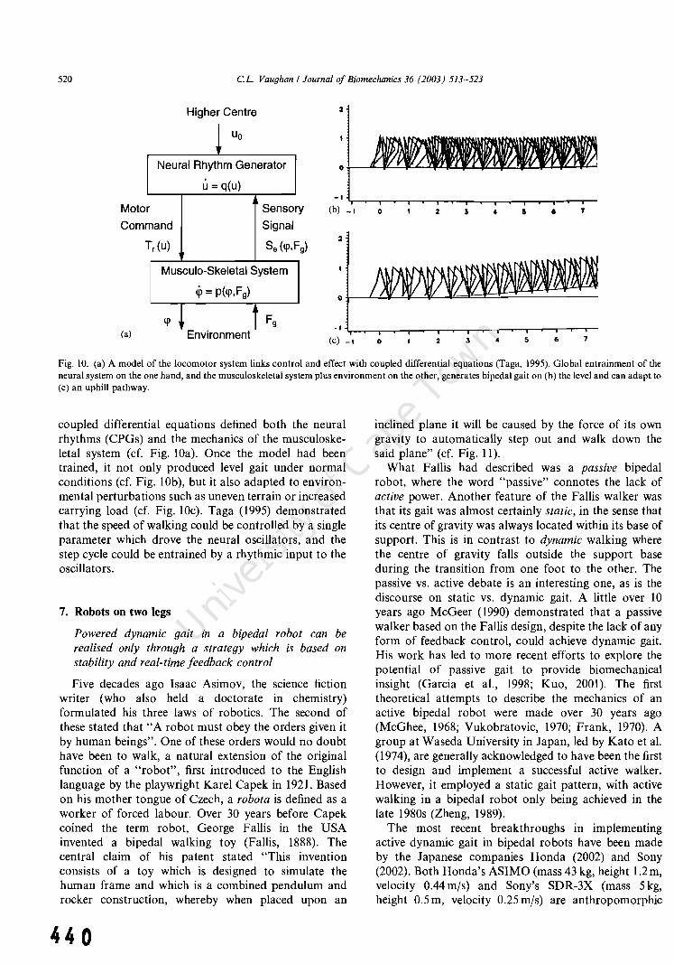
520 c.L. Vaughan I Journal of Biomechanics 36 (2003) 513-523

Higher Centre

~ Uo

I\leural Rhythm Generator

r Mota

Com mand

u = q(u}

Sensa

Signal

ry

Tr(u} Se (q>,F

Musculo-Skeletal System

q, = p(q>, F g)

2

q> * t Fg (a) Environment -I~~-r~-,~~.-~,-~-r-r-,-'~r-r-.-

(c) _I o 2 3 4 5 6 7

Fig. 10. (a) A model of the locomotor system links control and effect with coupled differential equations (Taga, 1995). Global entrainment of the neural system on the one hand, and the musculoskeletal system plus environment on the other, generates bipedal gait on (b) the level and can adapt to (c) an uphill pathway.

coupled differential equations defined both the neural rhythms (CPGs) and the mechanics of the musculoske­letal system (cf. Fig. lOa). Once the model had been trained, it not only produced level gait under normal conditions (cf. Fig. lOb), but it also adapted to environ­mental perturbations such as uneven terrain or increased carrying load (cf. Fig. IOc). Taga (1995) demonstrated that the speed of walking could be controlled by a single parameter which drove the neural oscillators, and the step cycle could be entrained by a rhythmic input to the oscillators.

7. Robots on two legs

Powered dynamic gait in a bipedal robot can be realised only through a strategy which is based on stability and real-time feedback control

Five decades ago Isaac Asimov, the science fiction writer (who also held a doctorate in chemistry) formulated his three laws of robotics. The second of these stated that "A robot must obey the orders given it by human beings". One of these orders would no doubt have been to walk, a natural extension of the original function of a "robot", first introduced to the English language by the playwright Karel Capek in 1921. Based on his mother tongue of Czech, a robota is defined as a worker of forced labour. Over 30 years before Capek coined the term robot, George Fallis in the USA invented a bipedal walking toy (Fallis, 1888). The central claim of his patent stated "This invention consists of a toy which is designed to simulate the human frame and which is a combined pendulum and rocker construction, whereby when placed upon an

440

inclined plane it will be caused by the force of its own gravity to automatically step out and walk down the said plane" (cf. Fig. 11).

What Fallis had described was a passive bipedal robot, where the word "passive" connotes the lack of active power. Another feature of the Fallis walker was that its gait was almost certainly static, in the sense that its centre of gravity was always located within its base of support. This is in contrast to dynamic walking where the centre of gravity falls outside the support base during the transition from one foot to the other. The passive vs. active debate is an interesting one, as is the discourse on static vs. dynamic gait. A little over 10 years ago McGeer (1990) demonstrated that a passive walker based on the Fallis design, despite the lack of any form of feedback control, could achieve dynamic gait. His work has led to more recent efforts to explore the potential of passive gait to provide biomechanica1 insight (Garcia et ai., 1998; Kuo, 2001). The first theoretical attempts to describe the mechanics of an active bipedal robot were made over 30 years ago (McGhee, 1968; Vukobratovic, 1970; Frank, 1970). A group at Waseda University in Japan, led by Kato et al. (1974), are generally acknowledged to have been the first to design and implement a successful active walker. However, it employed a static gait pattern, with active walking in a bipedal robot only being achieved in the late 1980s (Zheng, 1989).

The most recent breakthroughs in implementing active dynamic gait in bipedal robots have been made by the Japanese companies Honda (2002) and Sony (2002). Both Honda's ASIMO (mass 43 kg, height 1.2 m, velocity 0.44mjs) and Sony's SDR-3X (mass 5 kg, height 0.5 m, velocity 0.25 mjs) are anthropomorphic

0. T_ tHL!S _,LfTlI 1fT

hkU.M I.~ l ,. l&U

Fig. II. The first three drawings or the patent by Falli, (1888) demonstrating how 11 hiredal toy is able to walk when powewl only by gravity Reproduced wIth the permission or the United SI~ICS P~lcnl and Trademark Office. 1 am indebted to Andy Ruina or Cornell University whose research group made the palent ava.ilabh: on their web-sile

Fis.. 12. Two Rlllhropomorphic biped;ll robots, each with 24 degrees oi freedom, th~t dcmonsltate powered dynamic gail utilising rcal-llme feedback control: (a) ASIMO manufactured by Honda (2002); and (b) SDR-3X manufactured by Sony (2002). Both photographs have been reproduced with the pennission of the re~peclive compames

robots with 24 degrees of freedom (ef. Fig. 12). Both have joint torque actuators, sophisticated feedback via accelerometers and rale sensors, plus an onboard computer to provide real-time eontro\. As is evident from videos of the robots, their gait --which includes stair climbing-is not only stable but very similar to that of humans whom they have been designed to mimic. To be sure, robots on two legs have come a long way since F:.tllis· invention in the late 19th cent ury.

8. Concluding remarks

There are, of course, other important theories of locomotion that have not been considered in tbis review. These include: Ihe dynamic similarity hypothesis, where the Froude Ilumber-the dimensionless ratio of velocity

squared to the product orleg length and the acceleration due to gra vity-is constant (Alexander and Jaycs, 1983); lhc theory of the spinal engine. which posits that the lumbar spine is the key structure necessary for land­based locomotion. wilh the pelvis being driven hy the spine (Gracovctsky, 1985); and dynamic systems theory, which postulates tllat new fomls of behaviour-such as infant locomotion-will emerge from the cooperative interactions of multiple components within a task context (Thelen and Ulrich, 1991). Despite these omissions. the odyssey has covered a wide spectrum, from the evolution of hipedal walking through to the integration of the nervous, muscular, and skeletal systems.

While it is highly unlikely that a single. unifying theory of bipedal walking exists, there ;He interel'ling ways in which the six theories reviewcxl in this paper

44 1

522 c.L. Vaughan I Journal of Biomechanics 36 (2003) 513-523

overlap with one another. For example, the risk aversion hypothesis proposed for the maturation of gait in young infants (cf. Fig. 6) explains the historical development of an active bipedal robot, in moving from a static to a dynamic mode of walking. In addition, the central pattern generator theory has been included by Taga (1995) in his theory linking control and effect, while it should also be feasible to extend his model so that it incorporates the minimum energy consumption features of the model by Anderson and Pandy (2001a). With the computational resources available today, large-scale models of the human body can be used to produce realistic simulations of bipedal walking that are an order of magnitude more complex than those produced just a decade ago (Pandy, 2001).

Acknowledgements

I gratefully acknowledge the financial support of The Wellcome Trust, the South African Medical Research Council, and the National Research Foundation.

References

Alexander, R.M., 1992. The Human Machine. Columbia University Press, New York, pp. 176.

Alexander, R.M., Jayes, A.S., 1983. A, dynamic similarity hypothesis for the gaits of quadrupedal mammals. Journal of Zoology (London) 202, 577-582.

Anderson, J.A., 1983. Cognitive and psychological computation with neural models. IEEE Transactions on Systems, Man and Cyber· netics, 13,799-815.

Anderson, F.e., Pandy, M.G., 2001a. Static and dynamic optimization solutions for gait are practically equivalent. Journal of Biomecha­nics 34, 153-161.

Anderson, F.e., Pandy, M.G., 2001b. Dynamic optimization of human walking. Journal of Biomechanical Engineering 123 (5), 381-390.

Beck, R.1., Andriacchi, T.P., Kuo, K.N., Fermier, R.W., Galante, J .0., 1981. Changes in gait patterns of growing children. Journal of Bone and Joint Surgery 63-A (9), 1452-1457.

Brown, T.G., 1911. The intrinsic factors in the act of progression in the mammal. Proceedings of the Royal Society: London 84, 308-319.

Crompton, R.H., Yu, L., Weijie, W., Gunther, M., Savage, R., 1998. The mechanical effectiveness of erect and "bent-hip, bent-knee" bipedal walking in Australopithecus afarensis. Journal of Human Evolution 35 (I), 55-74.

Delcomyn, F., 1980. Neural basis of rhythmic behavior in animals. Science 210, 492-498.

Dimitrijevic, M.R., Gerasimenko, Y., Pinter, M.M., 1998. Effect of reduced afferent input on lumbar CPG in spinal cord injury subjects. Society for Neuroscience 24, 623-624.

Dunbar, D.C., Horak, F.B., MacPherson, J.M., Rushmer, D.S., 1986. Neural control of quadrupedal and bipedal stance: implications for the evolution of erect posture. American Journal of Physical Anthropology 69 (I), 93-105.

Fallis, G.T., 1888. Walking toy. United States Patent Number 376,588, Washington, DC.

442

Frank, A.A., 1970. An approach to the dynamic analysis and synthesis of biped locomotion machines. Medical and Biological Engineering 8,465-476.

Garcia, M., Chatterjee, A., Ruina, A., Coleman, M., 1998. The simplest walking model: stability, complexity, and scaling. Journal of Biomechanical Engineering 120 (2), 281-288.

Gracovetsky, S., 1985. An hypothesis for the role of the spine in human locomotion: a challenge to current thinking. Journal of Biomedical Engineering 7, 205-216.

Graupe, D., Kordylewski, H., 1995. Artificial neural network control of FES in patients for patient responsive ambulation. IEEE Transactions on Biomedical Engineering 42 (7), 699-707.

Grillner, S., 1985. Neurological bases of rhythmic motor acts in vertebrates. Science 228, 143-149.

Hof, A.L., 1996. Scaling gait data to body size. Gait & Posture 4, 222-223.

Hof, A.L., Zijlstra, W., 1997. Comment on "Normalization of temporal-distance parameters in pediatric gait". Journal of Biomechanics 30 (3), 299-302.

Honda, 2002. Humanoid robot. http://world.honda.com/robot/ Hopfield, J.1., 1982. Neural networks and physical systems with

emergent collective computational abilities. Proceedings of the National Academy of Sciences of the USA 79, 2554--2558.

Inman, V.T., Ralston, H.1., Todd, F., 1981. Human Walking. Williams and Wilkins, Baltimore, pp. 154.

Jenkins, F.A., 1972. Chimpanzee bipedalism: cineradiographic analysis and implications for the evolution of gait. Science 178 (63), 877-879.

Kato, I., Ohteru, S., Kobayashi, H., Shirai, K., Uchiyama, A., 1974. Information-power machine with senses and limbs. In: Theory and Practice of Robots and Manipulation. Springer, New York, pp. 11-24.

Kuo, A.D., 2001. A simple model of bipedal walking predicts the preferred speed-step length relationship. Journal of Biomechanical Engineering. 123 (3), 264--269.

Lamb, T., Yang, J.F., 2000. Could different directions of infant stepping be controlled by the same locomotor central pattern generator? Journal of Neurophysiology 83 (5), 2814--2824.

Langerak, N., Leskens, H., Deib, G., Martinez, F., Vaughan, e.L., 2001. At what age is a child's gait mature? In: Miiller, R., Gerber, H., Stacoff, A. (Eds.), Proceedings of XVIIIth Congress of International Society of Biomechanics. Ziirich, Switzerland, pp. 25-26.

Leakey, M.D., Hay, R.L., 1979. Pliocene footprints in the Laetolil Beds at Laetoli northern Tanzania. Nature 278,317-323.

Leakey, M., Walker, A., 1997. Early hominid fossils from Africa. Scientific American 276 (6), 74--79.

Lewin, R., 1993. The Origin of Modern Humans. Scientific American Library, New York, pp. 204.

McCulloch, W.S., Pitts, W., 1943. A logical calculus of the ideas immanent in nervous activity. Bulletin of Mathematical Biophysics 5, 115-133.

McGeer, T., 1990. Passive dynamic walking. International Journal of Robotics Research 9, 62-82.

McGhee, R., 1968. Some finite state aspects of legged locomotion. Mathematical Biosciences 2, 67-84.

Milne, A.A., 1924. Lines and squares. In: When We Were Very Young. Methuen Children's Books, London.

Minsky, M., Papert, S., 1969. Perceptrons. MIT Press, Cambridge, MA.

Olree, K.S., Vaughan, e.L., 1995. Fundamental patterns of bilateral muscle activity in human locomotion. Biological Cybernetics 73 (5),409-414.

O'Malley, M.1., 1996. Normalization of temporal-distance parameters in pediatric gait. Journal of Biomechanics 29 (5), 619-625.

Pandy, M.G., 2001. Computer modeling and simulation of human movement. Annual Reviews in Biomedical Engineering 3,245-273.

CL. Vaughan I Journal of Biomechanics 36 (2003) 513-523 523

Pandy, M.G., Berme, N., 1988. A numerical method for simulating the dynamics of human walking. Journal of Biomechanics 21, 1043-1051.

Pandy, M.G., Berme, N., 1989. Quantitative assessment of gait determinants during single stance via a three-dimensional model: I. Normal gait. Journal of Biomechanics 22, 725-733.

Pinter, M.M., Dimitrijevic, M.R., 1999. Gait after spinal cord injury and the central pattern generator for locomotion. Spinal Cord 37 (8),531-537.

Popovic, D.B., Stein, R.B., Jovanovic, K.L., Dai, R., Kostov, A., Armstrong, W.W., 1993. Sensory nerve recording for closed-loop control to restore motor functions. IEEE Transctions on Biome­dical Engineering 40 (10), 1024-1031.

Preis, S., Klemms, A., Muller, K., 1997. Gait analysis by measuring ground reaction forces in children: changes to an adaptive gait pattern between the ages of one and five years. Developmental Medicine and Child Neurology 9 (4), 228-233.

Prost, J.H., 1980. Origin of bipedalism. American Journal of Physical Anthropology 52 (2), 175-189.

Ralston, H.J., 1958. Energy-speed relation and optimal speed during level walking. Internationale Zeitschrift fUr angewandte Physiolo­gie 17, 277-283.

Richmond, B.G., Strait, D.S., 2000. Evidence that humans evolved from a knuckle-walking ancestor. Nature 404, 382-385.

Rodman, P.S., McHenry, H.M., 1980. Bioenergetics and the origin of hominid bipedalism. American Journal of Physical Anthropology 52 (I), 103-106.

Rosenblatt, F., 1961. Principles of Neurodynamics. Spartan Books, Washington, DC.

Rumelhart, D.E., Hinton, G.E., Williams, .R.J., 1986. Learning representations by back propagation errors. Nature 323, 533-536.

RUther, H., 1996. Part IX. Report on the photogrammetric field campaign. In: Laetoli Project: Conservation of the Hominid Trackway Site at Laetoli, Tanzania, Getty Conservation Institute, New York, pp. 66--105.

Saunders, J.B., Inman, V.T., Eberhart, H.D., 1953. The major determinants in normal and pathological gait. Journal of Bone and Joint Surgery 35-A, 543-558.

Sepulveda, F., Cliquet, A., 1995. An artificial neural system for closed loop control of locomotion produced via neuromuscular stimula­tion. Artificial Organs 19 (3), 231-237.

Sepulveda, F., Wells, D., Vaughan, C.L., 1993. A neural network representation of electromyography and joint dynamics in human gait. Journal of Biomechanics 26, 101-109.

Shaw, G.B., 1904. Act IV. John Bull's Other Island, Constable London.

Sherrington, C.S., 1941. Man on his nature. The Gifford Lectures, MacMillan, New York, p. 178.

Sony, 2002. Sony develops small biped entertainment robot. http:// www.sony.co.jp/en/

Srinivasan, S., Gander, R.E., Wood, H.C., 1992. A movement pattern generator model using artificial neural networks. IEEE Transac­tions in Biomedical Engineering 39 (7), 716--722.

Steudel, K., 1996. Limb morphology bipedal gait and the energetics of hominid locomotion. American Journal of Physical Anthropology 99 (2), 345-355.

Sutherland, D.H., Olshen, R., Cooper, L., Woo, S.L., 1980. The development of mature gait. Journal of Bone and Joint Surgery 62 (3), 336-353.

Taga, G., 1995. A model of the neuro-musculo-skeletal system for human locomotion. I. Emergence of basic gait. Biological Cybernetics 73 (2), 97-111.

Taga, G., Yamaguchi, Y., Shimuzu, H., 1991. Self-organized control of bipedal locomotion by neural oscillators in unpredictable environment. Biological Cybernetics 65 (3), 147-159.

Tardieu, c., Aurengo, A., Tardieu, B., 1993. New method of 3D analysis of bipedal locomotion for the study of displacements of the body and body-parts centers of mass in man and non-human primates: evolutionary framework. American Journal of Physical Anthropology 90 (4), 455-476.

Thelen, E., Ulrich, B.D., 1991. Hidden skills: a dynamic systems analysis of treadmill stepping during the first year. Monographs of the Society for Research in Child Development 56 (I), 1-104.

van Deursen, R.W., Flynn, T.W., McCrory, J.L., Morag, E., 1998. Does a single control mechanism exist for both forward and backward walking? Gait & Posture 7 (3), 214-224.

Vaughan, c.L., 1996. Are joint torques the Holy Grail of human gait analysis? Human Movement Science 15,423-443.

Vaughan, C.L., 1997. Neural network models of the locomotor apparatus. In: Allard, P., Cappozzo, A., Lundberg, A., Vaughan, C.L. (Eds.), Three-dimensional Analysis of Human Locomotion. Wiley, Chichester, UK, pp. 259-280.

Vaughan, C.L., 1999. Biomechanics of Human Gait: an electronic bibliography, 4th Edition, ISBN 0620235594, Kiboho Publishers, Cape Town.

Vaughan, C.L., Brooking, G.D., Olree, K.S., 1996. Exploring new strategies for controlling multiple muscles in human locomotion. In: Harris, G.F., Smith, P.A. (Eds.), Human Motion Analysis. Current Applications and Future Directions. IEEE Press, New York, NY, pp. 93-113.

Vaughan, c.L., Damiano, D.L., Abel, M.F., 1997. Gait of normal children and those with cerebral palsy. In: Allard, P., Cappozzo, A., Lundberg, A., Vaughan, C.L. (Eds.), Three-dimensional Analysis of Human Locomotion. Wiley, Chichester, UK, pp. 335--361.

Vaughan, c.L., Davis, B.L., O'Connor, J.c., 1999. Dynamics of Human Gait, 2nd Edition, Kiboho Publishers, Cape Town, pp. 155.

Vaughan, C.L., Langerak, N., Deib, G., Leskens, H., Martinez, F., 200 I. The acquisition of mature gait patterns in children. In: Proceedings of IX Congresso Brasileiro de Biomecanica. Gramado, Brazil, pp. 9-13.

Vaughan, C.L., Sussman, M.D., 1993. Human gait: from clinical interpretation to computer simulation. In: Grabiner, M.D. (Ed.), Current Issues in Biomechanics. Human Kinetics, Champaign, IL, pp.53-68.

VolI, D., 1994. Soul searching with Francis Crick. Omni Magazine 16 (2), 46--53.

Vukobratovic, M., 1970. On the stability of biped locomotion. IEEE Transactions on Biomedical Engineering 17 (I), 25-36.

Wheelwright, E.F., Minns, R.A., Law, H.T., Elton, R.A., 1993. Temporal and spatial parameters of gait in children. I: Normal control data. Developmental Medicine and Child Neurology 35, 102-113.

Zarrugh, M.Y., Todd, F.N., Ralston, H.J., 1974. Optimisation of energy expenditure during level walking. European Journal of Applied Physiology 33, 293-306.

Zheng, Y.F., 1989. Acceleration compensation for biped robots to reject external disturbances. IEEE Transactions on Systems, Man, and Cybernetics 19 (I), 74-84.

443

444

Exp Brain Res (2003) 153: 123-127 DOl 10.1007/s00221-003-1635-x

Christopher L. Vaughan· Nelleke G. Langerak . Mark J. OMalley

Neuromaturation of human locomotion revealed by non-dimensional scaling

Received: 16 June 2003 I Accepted: I August 2003 I Published online: 12 September 2003 © Springer-Verlag 2003

Abstract When two fundamental gait parameters-step length and step frequency-are scaled non-dimensionally, thereby accounting for increases in a childs physical size, ontogenetic changes in the locomotor control strategy are revealed. We believe dimensionless velocity 13, the product of dimensionless step length and frequency, serves as a measure of neural development. It increases from the age of 18 months and reaches a plateau between 50 and 90 months, attaining the adult value of 0.45. Based on a study of 200 children, our fmdings lend support to a theory that posits a neuromaturation growth curve with the form: f3 (t)=0.45 (l-e -o.05~ where t is the age in months and 0.05 is the growth coefficient.

Keywords Growth curve . Ontogeny· Children . Gait . Velocity· Mathematical model

Introduction

It has been argued that innate pattern generators in the spinal cord produce infant stepping in the fIrst few weeks oflife (Lamb and Yang 2000) and these generators are also

C. L. Vaughan (C8J) . N. G. Langerak. MRC/uCT Medical Imaging Research Unit, Department of Human Biology, Faculty of Health Sciences, University of Cape Town, 7925 Observatory, Western Cape, South Africa e-mail: kvaughan@cormack.uct.ac.za Tel.: +27-21-4066238 Fax: +27-21-4487226

N. G. Langerak Department of Physiology, University of Nijmegen Medical Center, 6500 HB Nijmegen, The Netherlands

Present address: C. L. Vaughan· M. J. OMalley Department of Electronic and Electrical Engineering, University College Dublin, Belfield 4, Dublin, Ireland

responsible for the basic locomotor rhythm in adults (pinter and Dimitrijevic 1999). During the ontogenetic phase of independent human locomotion, beginning at 10-18 months of age, two separate but parallel forms of growth occur (DeJaeger et al. 2001): the infants physical size, its mass and height, increases (Sutherland et al. 1980); and specifIc neural circuits develop during ontog­eny and transform the infants locomotor pattern (Forssberg 1985). The bipedal plantargrade gait of humans is unique, contrasting with the patterns of quadrupeds and non­human primates, in which the temporal activity of the muscles differs quite markedly (F orssberg 1992). The footprints left in the volcanic ash at Laetoli in Africa by hominids 3 million years ago indicate that they walked with a marked heel-strike at initial ground contact and utilized push-off during the end of the stance phase (Forssberg 1992). These ancient data have been used to compare the walking patterns of fossil hominids to that of modern children (Alexander 1984). Because bipedal locomotion is a quintessential feature of human evolution, it provides a rich experimental platform to explore a topic such as ontogeny and the consequences of size change (Koehl 2000).

The objective of this study was to understand the locomotor control strategy adopted by young children during the acquisition of bipedal gait. We hypothesized that non-dimensional scaling would account for physical growth, thereby yielding new insights into the process of neuromaturation.

Materials and methods

The subjects for this study were 200 normal children (102 boys and 98 girls) aged between 14 and 160 months (i.e. 1-13 years) who were recruited from pre-schools and elementary schools in Cape Town. The parents or legal guardians of aU children signed a formal consent prior to participation in the project, having read through a protocol that was approved by the Human Subjects Committee of the University of Cape Town. The focus was on younger children, with 125 being under the age of 80 months. In addition, 15 normal adults (8 men and 7 women) were also studied for comparison

124

purposes and they were deliberately chosen with a wide range in statures: from 1.59 m up to 2.01 m in height. Prior to the actual gait analysis, a series of anthropometric parameters were measured, the most important of which was the leg length. This was estimated as

. the height of the greater trochanter above the ground when standing upright (Sutherland 1997).

We monitored the locomotion during level walking by means of a six-camera video system (Vaughan et al. 1999). The XYZ coordinates of four small targets, located on the heels and over the 2nd metatarsal heads of the left and right feet, were measured as a function of time (Fig. 1 a). The data capture rate was 120 Hz, yielding a temporal resolution of 0.0083 s, while the spatial accuracy was 5 mm, both of which were sufficient to assess the subtle locomotor strategies employed by young children during ontogeny.

Each child walked at his or her own self-selected pace in the positive X direction (Fig. I a). Between two and four gait cycles per walking trial were captured and three trials per subject were gathered. Key temporal events for sequential gait cycles-foot contact and toe off for both right and left feet-were identified on a frame-by-frame basis, from which the fundamental temporal­distance parameters of step length and step frequency were derived (Vaughan et al. 1999). Step length was measured in metres as the horizontal distance, in the direction of progression, between the right and left heels at sequential foot contacts. Step frequency was measured in steps per second as the inverse of the time between sequential contacts of the right and left feet. The data for an individual subject were averaged across the gait cycles in each trial and across the three trials.

Results

As expected, step length increased with age, from less than 0.2 m at 14 months, to over 0.6 m at 150 months (Fig. 2a). In contrast, step frequency decreased over the same age range, from as high as 3.0 steps/s to approximately

, ,.c" ••

z . :., ~.

>, --. f'

• ...,K y

a b

Fig. 1 a Location of four retro-reflective spherical targets on the feet of a young child. The three-dimensional (3D) coordinates of these targets, 20 mm in diameter and placed on the heels and over the second metatarsal heads, were measured by a six-camera video system operating at 120 Hz (Vaughan et al. 1999). Each child walked at his or her own self-selected pace in the positive X direction. The 3D kinematic data were used to identify key events for each gait cycle (foot contact and toe off for both feet), and then the temporal-distance parameters of step length and step frequency were derived. b Bipedal gait is a cyclic activity that may be modelled by the action of an inverted pendulum (McMahon and Bonner 1983). The leg length is equivalent to the length of the pendulum, and the hip joint follows a pathway along the arc of a circle centered on the foot (Alexander 1992). This simple model provides the basis for non-dimensional scaling of the temporal­distance gait parameters of step length and step frequency to render them dimensionless (Hof 1996)

44 6

2.0 steps/s for the older children (Fig. 2b). These results are consistent with the fmdings of other researchers (Sutherland et al. 1980; Beck et al. 1981). Now, the changes in these fundamental gait parameters that occurred during this period between 14 and 160 months resulted from two separate but parallel forms of growth: the childs height and mass (i.e. its physical size) increased (Sutherland et al. 1980); and specific neural circuits developed through the process of synaptogenesis as neuromaturation took place (Forssberg 1985). Although some authors believe that walking experience should be considered a third developmental factor (Adolph et al. 2003), we propose that the parallel effects of musculo­skeletal growth and neuromaturation can be separated through a process of non-dimensional scaling.

Non-dimensional scaling

While a rigorous statistical technique, based on detrending and simultaneous normalization, has been proposed (OMalley 1996), this method tends to mask the neuroma­turation process (Sutherland 1997). A non-dimensional scaling approach, based on the similarity between bipedal gait and an inverted pendulum, has been adopted (Alex­ander 1992; McMahon and Bonner 1983). The distance travelled by a pendulum along its arc is equal to the product of the pendulum length and the angle (measured in radians) subtended by the arc (Fig. lb). For equal angles, the step length would be directly proportional to leg length and so this is a widely accepted scaling method:

A = SL/LL (1)

where A is the dimensionless step length, SL is step length in metres and LL is leg length, also measured in metres (Hof 1996; Vaughan et al. 1997). The period (or cycle time) for a simple pendulum is equal to 2n(L/g)1I2 where L is the pendulum length in metres and g is the acceleration due to gravity, 9.8 mls2

• This approach leads to the equation for scaling step frequency:

({i = SF /(g/LL)1/2 (2)

where <p is the dimensionless step frequency, and SF is step frequency in steps/s, while g and LL are as defmed above (Hof 1996). The step length and step frequency data presented in Fig. 2a, b were scaled non-dimensionally according to Eqs. 1 and 2. We assumed that such scaling would account for all the musculoskeletal growth, with any residual differences being explained by maturation of the nervous system.

After the temporal-distance parameters had been scaled, the data for the 200 children were grouped into 6-month epochs and averaged. There were 24 epochs in all, beginning at 18 months (children aged 14-20 months), and continuing on to 24 months (ages 21-27 months), 36 months, etc., and ending at 156 months (ages 153-160 months). There were at least 10 children in each of the

0.9

0.8

0.7 • . . .,..-.. :: 'lJ'" '\. g 0.6 • ..,.. 2' ,.

~ 0.5 .. ;Ii]~. · <: .. . !l 0.4 aff· D. . ~, ...... II) 0.3 Zii •••• 0.2 • 0.1

0.0

0 50 100 150

a Age (months)

3.5

• • i" 3.0 -". .. .' .. ... D. .. , ... ~ .e

.!!!.- 2.5 .. J •• ~ . ~ .. ~ . .. : .. , <: ~ . ... " ... II) :: .... ,., or..-' .. .;~ 'r 6- 2.0

at -. . . • " .. • D. II)

1.5 Zii

1.0

0 50 100 150

b Age (months)

Fig. 2a-d The temporal-distance parameters for 200 young children are plotted as a function of their age in months. These parameters are: a step length; and b step frequency. The step length, measured in metres, increases with age while the step frequency, measured as the number of steps per second, tends to decrease with increasing age (Sutherland et al. 1980; Beck et al. 1982). The step frequency data tend to be slightly more variable than step length, particularly for the younger children (Sutherland et al. 1980). The dimensionless temporal-distance parameters for 200 young children were clustered into 6-month epochs, beginning at age 18 months, and the average value for each epoch was calculated. c Dimension­less step frequency <p is plotted as a function of dimensionless step

first 6 epochs. Dimensionless step frequency q:> has been expressed as a function of dimensionless step length A (Fig. 2c). At age 18 months both parameters have low values, with the data point being located at (0.57 ± 0.06, 0.47 ± 0.05), where A = 0.57 and q:> = 0.47. As age increased both these dimensionless parameters steadily increased (Adolph et al. 2003; Hof and Zijlstra 1997; Sutherland 1997), taking on values of (0.63 ± 0.06, 0.52 ± 0.04) at 24 months, (0.66 ± 0.05, 0.53 ± 0.05) at 30 months, (0.70 ± 0.06, 0.54 ± 0.03) at 36 months and (0.73 ± 0.05, 0.55 ± 0.05) at 42 months (Fig. 2c).

The mean data for the adults were calculated as A = 0.75 ± 0.06 and q:> = 0.60 ± 0.04 and have been plotted on the same graph as the children (cf. black square indicated by the letter A in Fig. 2c). It is clear that from about age 50 months onwards, the childrens data are clustered in the vicinity of the adult data point, and these fmdings are consistent with the values presented by Stansfield et al.

125

0.70 -e->-~ 0.65 CD :J I:T at 0.60 D.

~ 0.55 III III CD 1: 0.50 0 ';;; <: II)

E 0.45 C

0.40

0.50 0.55 0.80 0.85 0.70 0.75 0.80

C Dimensionless Step Length A

0.6

CO- 0.5 >- A "" 8 0.4 ~ <II 0.3 <II Q)

C 0 0.2 'iii C Q) ~ (I) = 0.45(1 - e -I).M'l E 0.1 is

0.0

0 50 100 150

d Age (months) t

length A. Each dot represents a 6-month epoch and the numbers next to the dots indicate the age in months (from 18 to 42 months). The isocurves are plots of dimensionless velocity j3 (where j3 = A x <p), with the values ranging from 0.25 to 0.50. The small square located at (0.75, 0.60), and identified by the letter A, is the mean value for 15 adults. d Dimensionless velocity (3 is plotted as a function of the childs age in months. At 18 months of age /3 is equal to 0.27 and this parameter steadily increases up to about 70 months when it reaches the adult value of 0.45, indicated by the small square with the letter A on the right-hand axis. These data have been modelled by a neuromaturation growth curve where the dimensionless velocity at maturity /3", = 0.45, and the growth coefficient k = 0.05 month- 1

(2003) in a longitudinal study of children aged 5-12 years. The shift in the dimensionless parameters from (0.57, 0.47) at 18 months up towards the cluster centered on (0.75,0.60) provides an indication of the neuromaturation that occurs during ontogeny, beginning with the early phase of independent walking. Such an analysis has also been used to demonstrate that children with cerebral palsy who undergo surgical treatment tend to approach the normal cluster (OMalley et al. 1997). Dimensionless step length and frequency can be combined to yield dimen­sionless velocity f3

{3=)..xrp (3)

which has been plotted as a series of isocurves in Fig. 2c, with j3 ranging in value from 0.25 to 0.50. Combining Eqs. 1-3 yields

44 7

126

f3 = V/(g X LL)l/2

where V is the velocity in mls and is equal to SL x SF. Equation 4 expresses dimensionless velocity 13 as the square root of the Froude number, a parameter that has been extensively used in locomotion studies (Alexander 1984; Hof and Zijlstra 1997).

The Froude number, which is central to the dynamic similarity hypothesis of Alexander and Jayes (1983), allows us to answer the question whether young infants walk in a dynamically similar manner to older children and adults. We therefore propose that dimensionless velocity 13, which is a composite of the fundamental gait parameters A and cp, is well suited to serve as a measure of neuromaturation. When plotted as a function of age, 13 starts out with a value of 0.27 at 18 months and then increases steadily up to about 70 months when it reaches the adult value of 0.45 (Fig. 2d).

of genetically predetermined neural networks exists at the (4) onset, and development proceeds with selection on the

basis of afferent signals generated during movement (Forssberg 1999). When a young infant takes its first few halting steps, its biomechanical strategy is to minimize the risk of falling (Vaughan 2003). Then, during ontogeny, strength increases, postural constraints become less dom­inant (Muir 2000) and mediolateral stability improves (Yaguramaki and Kimura 2002). Development proceeds by the selection of the most favourable neural networks (Forssberg 1999) so that the variability in muscle activa­tion decreases, co-contraction is diminished, and the adult pattern emerges (Okamoto et al. 2003).

A mathematical model

The data in Fig. 2d are consistent with a growth curve first described by von Bertalanffy (1938) and there exists a standard differential equation in physics which represents the simplest possible description of the approach to an equilibrium:

df3/dt = k(f3oo - f3(t)) (5)

in which the positive constant k is a growth coefficient, 1300 is the dimensionless velocity at maturity, and t is the time in months. If we assume that (3 = 0 at t = 0 (i.e. at birth), which is a reasonable assumption, then the solution to the first order differential Eq. 5 is

(6)

Since (300 = 0.45, k can be determined by minimizing the sum of squared differences using the /3 data in Fig. 2d. The value for k is 0.05, yielding our neuromaturation growth curve for the ontogeny of human locomotion:

In Eq. 7, the growth coefficient k varies slightly from individual to individual and is a measure of the rate at which a normal childs gait approaches the adult pattern (i.e. when 1300 = 0.45). The growth curve can also be applied to dimensionless step length and step frequency, where Aoo = 0.75 and CPoo = 0.60 respectively (c£ Fig. 2c), and for both parameters the growth coefficient k = 0.08. For a disorder such as cerebral palsy, where there are neurodevelopmental delays, both k and 1300 will have lower values. This occurs despite neurosurgical interventions such as dorsal rhizotomy for which non-dimensional scaling has been applied to understand the long-term implications of both the disorder and its treatment (Subramanian et al. 1998). While dimensionless step length A can approach normal values in these patients, dimensionless step frequency cp is not altered by age or surgery (Vaughan et al. 1998). Since cp is an indirect measure of the central pattern generator, this suggests that in cerebral palsy there may be limited opportunities to select favourable neural networks (Forssberg 1999).

The solution to the growth curve (c£ Eq. 7 and Fig. 2d) assumes that /3 = 0 at age 0 (Le. at birth). Since it has been shown that even in the early weeks of life young neonates, if properly supported, are able to take spontaneous steps (Yang et al. 1998), this assumption is probably a slight simplification. It is also likely that other growth curves, for which /3 ::/= 0 when t = 0, could explain the data just as well as Eq. 7. This equation is similar in form to a general growth equation that has been derived from first principles and is based on the conservation of metabolic energy, allometric scaling, and the energetic cost of producing and

f3(t) = 0.45(1 _ e-O.05l )

Discussion

(7) maintaining cells (West et al. 2001). Whether a neural growth equation can be similarly derived from first principles remains to be explored. What we have shown is that non-dimensional scaling of Velocity has yielded a measure of neuromaturation, and thus revealed some insight regarding the ontogeny of human locomotion.

According to dynamical systems theory, movement patterns do not arise from the maturation of neural centres or central pattern generators but instead new behaviour emerges through self-organization (Thelen et al. 1987; Jeng et al. 1997). This theory has been challenged, on the basis that it provides limited insight regarding the neural control of motor development, and an alternative theory, based on neuronal group selection, has been proposed (Forssberg 1999; Sporns and Edelman 1993): a repertoire

448

Acknowledgements We thank Gerard Deib, Harmen Leskens and Fernando Martinez for their assistance in gathering and analyzing the data. We also acknowledge the financial assistance of The Well come Trust, the Medical Research Council of South Africa, and Stichting Nijrneegs Universiteits Fonds. Christopher Vaughan was an Ernest Walton Fellow, funded by Science Foundation Ireland, when this work was completed.

References

Adolph KE, Vereijken B, Shrout PE (2003) What changes in infant walking and why. Child Dev 74:475-497

Alexander RM (1984) Stride length and speed for adults children and fossil hominids. Am J Phys Anthropol 63:23-27 '

Alexander RM (1992) Exploring biomechanics. Animals in motion. Scientific American Library, New York

Alexander RM, Jayes AS (1983) A dynamic similarity hypothesis for the gaits of quadrupedal mammals. J Zool 201 :135-152

Beck RJ, And:iacc~i TP, Ku~ KN, F~rmier RW, Galante JO (1981) Changes m galt patterns m growmg children. J Bone Joint Surg 63A: 1452-1457

DeJaeger D, ~ille~s PA, Heglund NC (2001) The energy cost of walkmg m children. Eur J PhysioI441:538-543

Forssberg ,H (1985) Ontogeny of human locomotor control. l. Infant steppmg, supported locomotion and transition to independent locomotion. Exp Brain Res 57:480-493

Forssberg H (1992) Evolution of plantigrade gait: is there a neuronal correlate? Dev Med Child Neurol 34:920--925

Forssberg H (1999) Neural control of human motor development Curr Opin Neurobiol 9:676-{)82

Hof AL (1996) Scaling gait data to body size. Gait Posture 4'222-223 .

Hof ~, Zijlstra W (1997) Comment on normalization of ternporal­distance parameters in pediatric gait. J Biomech 30:299

Jeng. SF, ~iao HF, Lai JS, Hou JW (1997) Optimization of walking m chIldren. Med Sci Sports Exerc 29:370--376

Koehl MAR (2.000) Consequences of size change during ontogeny and evolution. In: Brown JR, West GB (eds) Scaling in biology. Oxford University Press, New York, pp 67-86

Lamb T, Yang JF (2000) Could different directions of infant stepping be controlled by the same locomotor central pattern generator? J Neurophysiol 83:2814-2824

McMahon TA, Bonner IT (1983) On size and life. Scientific American Library, New York

Muir GD ~2000) Early ontogeny of locomotor behaviour: a companson between altricial and precocial animals. Brain Res Bull 53:719-726

Okamoto T, Okamoto K, Andrew PD (2003) Electromyographic developmental changes in one individual from newborn stepping to mature walking. Gait Posture 17: 18-27

OMalley MJ (1996) Normalization of temporal-distance parameters in pediatric gait. J Biomech 29:619-625

127

OMalley MJ, Abel MF, Damiano DL, Vaughan CL (1997) Fuzzy c~ustering ~f children with cerebral palsy based on temporal­

. dIstance ~al~ I?~a~eters. IEEE Trans Rehabil Eng 5:300--309 Pmter MM, Drrmtnjevlc MR (1999) Gait after spinal cord injury and

the central pattern generator for locomotion. Spinal Cord 37:531-537

Sporns 0, Edelman GM (1993) Solving Bernsteins problem: a proposal for the development of coordinated movement by selection. Child Dev 64:960--981

Stansfield BW, Hillman SJ, Hazlewood ME, Lawson AM, Mann AM, Louden IR, Robb JE (2003) Normalisation of gait in children. Gait Posture 17:81-87

Subramanian N, Vaughan CL, Peter JC, Arens LJ (1998) Gait before and t.el! years after rhizotomy in children with cerebral palsy spasticity. J Neurosurg 88:1014-1019

Sutherland D (1997) The development of mature gait. Gait Posture 6:163-170

Sutherland DH, Olshen R, Cooper L, Woo SL (1980) The development of mature gait. J Bone Joint Surg 62A:336-353

Thelen E, .Ska.la K, "Selso JAS (19~7) The dynamic nature of early coordmatlOn: eVidence from bilateral leg movements in young infants. Dev Psychobiol 23:179-186

Vaug~ CL (2003) Theories of bipedal walking: an odyssey. J Blomech 36:513-523

Vaughan CL, Damiano DL, Abel MF (1997) Gait of normal children and those with cerebral palsy. In: Allard P, Cappozzo A, Lundberg A, Vaughan CL (eds) Three-dimensional analysis of human locomotion. John Wiley, Chichester, pp 335-361

Vaughan CL, Su~ramanian .N, Bus~e ME (1998) Rhizotomy as a treatment optIon for chIldren With cerebral palsy. Gait Posture 8:43-59

Vaughan CL, Davis BL, OConnor J (1999) Dynamics of human gait. Kiboho Publishers, Cape Town

von BertalanfIy L (1938) A quantitative theory of organic growth. Hum BioI 10:181-213

West GB, Brown JR, Enquist BJ (2001) A general model for ontogenetic growth. Nature 403:628-631

Yaguramaki N, Kimura T (2002) Acquirement of stability and mobility in infant gait. Gait Posture 16:69--77

Yang JF, Stephens MJ, Vishram R (l998) Infant . g: a method to study the sensory control of human wa . J Physiol 507:927-937

450

Available online at www.sciencedirect.com

.CI~"C. @DIR~CT.

ELSEVIER Gait and Posture 21 (2005) 350-362 www.elsevier.com/locate/gaitpost

Review

Froude and the contribution of naval architecture to our understanding of bipedal locomotion *

Christopher L. Vaughan a,b,*, Mark J. O'Malleyb

• MRC/uCT Medical Imaging Research Unit, Department of Human Biology, Faculty of Health Sciences, University of Cape Town, Observatory, Western Cape 7925, South Africa

b Department of Electronic and Electrical Engineering, University College Dublin, Beljield, Dublin 4, Ireland

Accepted 12 January 2004

Abstract

It is fascinating to think that the ideas of two 19th century naval architects could offer useful insights for 21 st century scientists contemplating the exploration of our planetary system or monitoring the long-term effects of a neurosurgical procedure on gait. The Froude number, defined as Fr = v2/gL, where v is velocity, g is gravitational acceleration and L is a characteristic linear dimension (such as leg length), has found widespread application in the biomechanics of bipedailocomotion. This review of two parameters, Fr and dimensionless velocity f3 = (Fr)I/2, that have served as the criterion for dynamic similarity, has been arranged in two parts: (I) historical development, including the contributions by William Froude and his son Edmund, two ship designers who lived more than 130 years ago, the classic insights of D' Arcy Wentworth Thompson who, in his magnum opus On Growth and Form, espoused the connection between mathematics and biology, and the pioneering efforts of Robert McNeill Alexander, who popularised the application of Fr to animal locomotion; and (II) selected applications, including a comparison of walking for people of different heights, exploring the effects of different gravitational fields on human locomotion, establishing the impact of pathology and the benefits of treatment, and understanding the walking patterns of bipedal robots. Although not all applications of Fr to locomotion have been covered, the review offers an important historical context for all researchers of bipedal gait, and extends the idea of dimensionless scaling of gait parameters. © 2004 Elsevier B.Y. All rights reserved.

Keywords: Froude number; Gait; Dynamic similarity; Walking; Size; Gravity; Children

1. Introduction

Bipedalism is the fundamental evolutionary adaptation that sets hominids-and therefore humans-apart from other primates [1]. A toddling infant, taking its first few halting steps on the living room carpet, uses essentially the same walking pattern as a 2 m tall adult striding down the road [2]. However, it is not only humans who utilise bipedalism as their primary mode of terrestrial locomotion; prehistoric dinosaurs, some of which had a height of over 5 m, used a running gait [3], while the hopping crow stands less than 0.3 m tall [4]. This leads to the obvious question: how do we compare the gait patterns of all these different animals? The

1:< This paper was presented in part as a keynote lecture at the 7th annual conference of the Gait and Clinical Movement Analysis Society in Chattanooga, Tennessee on 18 April 2002 .

• Corresponding author. Tel.: +27-21-406-6235; fax: +27-21-448-7226.

E-mail address:kvaughan@corrnack.uct.ac.za (C.L. Vaughan).

0966-6362/$ - see front matter. © 2004 Elsevier B .V. All rights reserved. doi:lO.lOI6/j.gaitpost.2004.01.011

answer lies in the field of physical similarity and dimensional analysis [5]. It was the naval architect William Froude who, 130 years ago, introduced a non-dimensional parameter that served as the criterion for dynamic similarity when compar­ing boats of different hull lengths [6]. This parameter, now known as the Froude number or Fr, is equal to v2/gL where v is velocity, g is gravitational acceleration, and L is a char­acteristic length (in nautical engineering, the hull length). This review of the contribution of naval architecture-the Froude number-to our understanding of bipedal locomo­tion has been compiled in two parts, numbered I and II, and seven sections, numbered 2.1-3.4.

2. Part I: historical development

2.1. William and Edmund Froude

William Froude was born in Devon, England in 1810 and studied classics and mathematics at Oxford University (cf.

451

CL V/l/l!!ha~. MJ. O'M"lky I GOil OIld pu,lur~ 2/(2005) .150-362 1~1

(a) (b)

Fig l. (a) WillJam Froude (l810--1879) and (b) his third ,00 Robcn Edmund Froud. (1S46-192-l). RopmduC1Xl with the f'<'nnt:<.<ion of Ru.<..;cll [7J.

Fig. I a ) Following gradualion he worked in the field of civil engineering. a..~siSling lsambard Kingdom Brund with Ihe huilding of the Bristol and Ex:eter Railway in 1838. By 1846, he had retired from full time employment to run the family estates but it was also an opportunity to tum his alieni ion to the sea and ships that had always exercised iI

special fascinalion for him [7]. His work was influenced by a particularly expen~ive mistake [8]. Froude h~d been consulted by his old boss Rrunel and the mistake involved lhe design of a huge iron-clad ocelln liner. the Great £asfern, which was the largest ship in the world at that time. Even Ihough the designers had included paddle wheels and a screw propeller, as well a.s auxiliary sails (Fig. 2a), the sheer size of the ship meant that it had insufficient power. Its speed was ,,0 slow that there was no way the ship could eelrTI enough to poy for the cost of its fuel [8 [. a significant shortcoming, sinl:c the GreM Easlern laid the undersea telegraph cable bel ween Co. Kerry, Ireland and Newfoundland, Canada in 1l:!69, linking the continents of Europe Ilnd North America for Ihe tirSI lime. Although Froude wa.., involved wilh the engineering of Ihe Great E.llSlern in only a minor capacity, he clc~rly apprecIated how poorly naval archilects in the mid-19th century underSlood wave resistance and the effect., of size.

Froudc' ~ ow n approach to science. and indeed reI igion, is ~ummed up in a phrase thai he often quoted: "Our sacred duty [is] 10 doubt each and every proposilion PUI to us in­cluding our own" r9). He turned his anention 10 experimen­t;tlion in the River Dart on two sCelle models. called R(lven and Swan, in which he demonstrated that there was no ide.al form and that performance varied with speed. With this ev­idence he persll<lded the government to fund the building in the early 1870s of a lowing tank, almost 100 m long. across the road from his house. With the as..~islance of his third son Robert Edmund (Fig. I b), born in 1846, he W~~ able 10 lOW his models at a known speed through still waler us-

452

ing a steam-powen-d winch that pulled the carriage along a track suspended over the tonk (Fig. 2b). The drag foree acting on the models was monitored by a custom-designed dynamometer [10].

What Froude observed was that large and small models of geometrically similar hulls produced different wave pallerns when lOwed at the same speed (Fig. 2c). However. if the larger hull was pulled al greater speeds, there was a speed at whkh lhe wave pallem~ were ne.llrly identical. This occurreo when the rOlio of Ihe velocity squared 10 the huH length was the same for both large and small hulls. He had thu~ demonstrated that geometrically similar hulls would also be dynamicnlly similar. in tenns of wave resistance, when this ratio-now known as the Froude number-was constant. In his olVn words [6J:

That "Law of Comparison" is thaI if the speeds of the ships are proponional to the square roots of their dimenSIons, their resistances at those speeds will be as the cubes of their dimensions.

From 1873 unlit his deClth in 1879 in Simonstown. a naval base near Cape Town, South AfriclI (Fig. 3), William Froudc puhlished many papers in journals such as Nalure Ill) and in other scholarly publicalions [6 .1 0 .1 2) . After the passing of his father. Edmund conlinued the family tradition of re;earch on hydrodynamics, publishing hi~

own findings on wave-making resislance of ships. and inlroducing the analogy of a simple pendulum [1 3]. He W;[S also lliell known for having recommended the suit­able dimensions of screw propellers [141. By the time of Edmund's own death in 1924, lhe father and son hnd left nn indelible legacy -between them they pub­lished 34 papers in the Transactions oj the InstilllliDIi oj Naval ArchileCls - with every ship in the world to­day owing its pelformance to their insights and steadfast endc.;l vour.

C L. VII;l~Jl(ln, !oJ J. O'MrdJ", I Gail "",J Pf)~I/lTr '] J (?OO5 J J50-.i1l2

(a)

(b)

(e)

FiS , 2 , (~) 'rne Grl'lll EaSIUII wus ~ ship which convinced William rroude Ih~1 naval archilecL< 01 Ihe mid-19th ccmu!)' did nul und..,aanu " 'ave ,.,islanc-, and {he clTec{~ of ~ize , Rep,oduc,d wilh the permi,«,on of (he Manlime Mu,<cum, Vaicnti. 1<land. Co, KelT)'. Ireland (b) The lowing \nn~ bUIll by Willirun Froude in lhe carl y I 870s \Vhen: he conducled hydrodynomic experimenl, 00 scalc modcl~, Reproduccd wilh lhe pcnnission or Ru.,o;c ll 171. (C) WilJi~m Froudc conducled c<pcrimenll< on Ihc re.isla.nC'e of m(ldel ho~~ or <.IiO'erenl length'_ nllowing him In s{udy dlvel,!:ins b"\\1 wa,-es 11 21 Reproduced w uh permi<.<ion of Ihe Ruyal Inslliulion o{ Naval ArchJICCls,

453

C.L. Vnuglllln, MJ. O',I!IDliry / G"jl and Post",." 21 (2(05)J5()"J6: 353

FIg. 3. William Froude's grn,-c'lOne in Slmon~lown, a n~vnl b"", ncar C~rc Town, with the nrsl autilor (CLV) <lnndin!( ncarby.

2 2 _ D'Arc)' WenlwQrlh Thompson

Whi Ie the Froudes had concentrated on the movement of ships, it was the polymath D'An:y Wentworth Thomp."<ln who first recognised Ihe connection between the Froude number and animal locomotion, although his derivation of Froude'_~ Law was based on skin friclion and did not ac­knowledge the interaction between gravity and inertia. Born in Edinburgh, Scotland in 1860, he won prizes for the Clas­~ics. Greek. mathematics and modern languages in his final yenr of high school (15]. After beginning hi~ medical stud­ies It Edinburgh University, he switched to science at Cam­bridge University, earning a BA in zoology in 1883. The fol­lowing year Thompson wa~ appointed Professor at Dundee (bter incorpor;)ted within the University of Sf. Andrews) and occupIed this chair until his death In 1948, a remarkable record of 64 years (Fig. 4), Thompson pos..'CSsOO II unique set of skills: he was a Greek 5cholar, a biologist and a math· cma(ici:Ul. Although he was a prOlific writer, publishing al­most 300 scientific micles and books [16J, he is be~t known for his famous book On Growth and Form, first published in 1917 [17). His primary thesis was that all living creatures could only be properly understood in tcrm~ of pure math­ematics. These arguments were advMced in beautiful prose that was a pleasure to read with poetry in thc sentences [18).

Thompson's understanding of the relRlionship between scale, Froude and bipedal locomotion are be~t revealed in

4

Fig. 4. D'Arcy Wenl"'or~, Thomp"on (I R60--1 948) , aUlhor of 0" G10w,II am' Form 1171 Rcproduc<:ti With the pcrmi<<lon of O'Connor and Raben.

son 1151_

three quotations that have been extracted from his magnum opus 011 Gro .... th ilJld Form [17 J, On page 17, he introduces the concept of dynamic similarity:

For sf'o/I! hll~ a very marked effect upon phy.~ical phe. nomena, and the effect of scale constitutes what is known as the principle of similitude, or of dynamical similarity.

This statement form~ tbe basis for a discussion on the strength of a muscle and the resistllnce of a bone to crush­ing stress, both of which vary with their cross-sedion~, In considering Ihe movement of terreslrial animals, living un­der the direct action of gravity, he argues that there is D limit to the size of an l:lnimal. with an elephant approaching the I i mit. Then on page 23 Thom pson introduces the ana logy be­tween two dynamically similar animals and two steam"hip~ nnd their propulsion:

In two similar and closely related animab, as also in two steam engines. the law is bound to hold that the rate of working musl tend to vary with the square of the lin· ear dimensions, according to Froude's Law of steam,hip compnrison.

He explores the movement of birds and fish through a fluid medium nnd shows thtl! by applying Froudc's Law their velocities squared ~re proportional to a linear dimension (e.g. Ihe animal's length). Finally, on page 30, he comp:lres bipedal walking plltlems by means of a pendulum model:

354 CL. Vaughan, MJ. O'Malley / Gait and Posture 21 (2005) 350--362

Fig. 5. The tiny inhabitants of Lilliput await the revival of Captain Lemuel Gulliver, in a scene from Jonathan Swift's book, Gulliver's Travels, which was first published in 1726. The different-sized characters in this classic inspired Thompson [)7J to apply Froude's Law to compare their stride lengths.

Now let two individuals walk in a similar fashion with a similar angle of swing. The arc through which the leg swings will vary as the length of the leg, but the time of the swing will vary as the square root of the pendulum length. Therefore the velocity will also vary as the square root of the length of the leg.

In a later abridged edition of On Growth and Form, which John Tyler Bonner had the temerity to edit [18], an illustra­tion of a simple pendulum was included, and the step lengths of characters from Jonathan Swift's book Gulliver's Trav­els (Fig. 5) were compared. The inhabitants of Lilliput and Brobdingnag, with heights of 0.15 and 20m, respectively, would have had step lengths of 0.06 m and 8.4 m on the ba­sis of geometric similarity. By extending Thompson's argu­ment, and applying Froude's Law and dynamic similarity to the inhabitants, we see that they would have had walking ve­locities of 0.29 and 3.3 mis, respectively. These values can be compared to Captain Lemuel Gulliver's height of 1.8 m, a step length of 0.76 m and walking velocity of 1.2 mls.

2.3. Robert McNeill Alexander

Despite the widespread impact of Thompson's book [17], the legacy of the Froudes and their contribution to the understanding of scale and propUlsion in biology lay dor­mant for decades. The one person who changed that and so popularised the application of the Froude number to animal locomotion was Robert McNeill Alexander, Professor of Zoology at the University of Leeds. Through the publication of his books on biomechanics [19-22], his book chapters

that arose from special conferences on animal locomotion [23-26], and most importantly his articles in high impact journals [3,4,27-36], Alexander has ensured that the Froude number can now take its rightful place as an important parameter for us to employ when studying bipedal gait.

It all started in 1976 with a study to estimate the speeds of dinosaurs [27]. Because there were reasonably well-documented dinosaur tracks from which stride lengths could be measured (Fig. 6), Alexander used observations of living animals, including humans, and applied these to dinosaurs. He argued that the movements of animals of geometrically similar form but of different sizes would be dynamically similar when they moved with the same Froude number Fr = v2/gL, where L was the height of the hip joint above the ground. He also posited that geometrically similar movements required equal values of the relative stride length, the dimensionless ratio AIL, where A was the stride length (Fig. 6). Then, based on data from mammals as diverse as jirds (a type of gerbil), men and horses, he plotted Fr as a function of AIL on logarithmic coordinates and established the empirical relationship

A -=2.3(v2/gL)0.3 (1) L

And this equation could then be rewritten as

v=0.25g°.5 A1.67 L-1.I7 (2)

Since g was known (9.8 m/s2), while A could be measured directly from the dinosaur footprints and L estimated from intact dinosaur skeletons, v could be readily calculated. The estimated speeds were rather low, between 1.0 and 3.6 mis,

455

456

C.L. Vaughan, MJ. O'Malley / Gait and Posture 21 (2005) 350-362 355

A­stride length

Fig. 6. Alexander [27] showed that it was possible to estimate the running speed v of a dinosaur, with hip height L and a stride length of). (calculated from the fossil record and preserved footprints respectively), using the Froude number data for contemporary animals. Adapted with permission from reference [3].

but it was difficult to know if the tracks were made when the dinosaurs were walking or running [27]. Others used Alexander's approach [37], and a new track site showed that some dinosaurs probably achieved speeds of up to 11 mls [38]. While Alexander continued to refine the relationship between relative stride length and Fr (Fig. 7a), the release of

7 6 • Various quadrupeds

.c 5 Humans c;, 0

c 4 t::" Kangaroos j1

Q) 'C 3 .~

Q) • • . 2: 2 • (ij Qi 0::

the movie Jurassic Park in the early 1990s led to further de­bate about the maximum speed at which a bipedal dinosaur could run [36,39]. Using arguments based on Froude num­bers [3,27] as well as bone strength [3,40], Alexander con­cluded [36] that Tyrannosaurus rex was probably not very good at chasing Jeeps!

0.1 0.2 (a)

0.5 2 Froude Number

20

0·5

Q) 04 u c ~

03 & 'C Q) 0·2 UI <11 .c c.. 0·1

00 0·1 0·3 3 10 30

(b) Froude Number

Fig. 7. (a) Relationship between relative stride length AIL and the Froude number v2/gL for bipeds (kangaroos and humans) and quadrupeds [3], with the curve through the data represented in Eq. (I) (note the logarithmic scale on each axis). (b) Phase difference between the forefeet versus the Froude number for quadrupedal mammals, with a logarithmic scale on the horizontal axis. These graphs have been adapted with permission from references [3,31] respectively.

356 CL. Vaughan, MJ. O'Malley / Gait and Posture 21 (2005) 350-362

One of Alexander's most highly cited articles was his dy­namic similarity hypothesis [31]. He noted that the galloping movements of cats and rhinoceroses are remarkably similar even though the animals are so different [22], and postu­lated five dynamic similarity criteria: (1) each leg has the same phase relationship; (2) corresponding feet have equal duty factors (% of cycle in ground contact); (3) relative (i.e. dimensionless) stride lengths are equal; (4) forces on corre­sponding feet are equal multiples of body weight; and (5) power outputs are proportional to body weight times speed. He hypothesised, and provided the necessary experimental evidence to demonstrate, that animals meet these five cri­teria when they travel at speeds that translate to equal val­ues of Fr [31]. Evidence in support of criterion 3 has been presented in Fig. 7a, while the data for criterion 2 may be seen in Fig. 7b. At Fr values below 2, the phase differences lie between 0.4 and 0.5, and the animals utilise symmetri­cal gaits such as walking, trotting and pacing. There is an abrupt transition at Fr values between 2 and 3, and above 3 the animals use asymmetrical gaits such as cantering and galloping. Although Alexander developed the dynamic sim­ilarity hypothesis for quadrupedal animals [31], it may also be applied to bipedal gait [33].

3. Part II: selected applications

3.1. Effects of size

As indicated above in Section 2.1, D' Arcy Thompson used the Froude number to compare the walking speeds of different sized characters in Gulliver' s Travels. This is clearly one of the major benefits of the Froude number, with the primary application being in the study of children's gait [1,2,32,41-44]. Alexander [32] showed that when dimen­sionless stride length was plotted as a function of dimen­sionless speed {J where

{J = v/(gL)1/2 = (Fr)1/2 (3)

then data for children aged over 4 years were the same as adults. He used this empirical relationship to predict the walking speeds for two small hominids (with estimated heights of 1.19 and 1.39 m) who left their footprints in vol­canic ash at Laetoli in East Africa 3.7 million years ago [1]. Alexander estimated the speeds to be 0.64 and 0.75 mis, re­spectively, which corresponds to modem humans walking in small towns [32]. Minetti and his colleagues have stud­ied two other groups that have short statures: Pygmies from West Africa [45,46]; and pituitary dwarfs suffering from growth hormone deficiency [46,47]. This latter group will be described later in Section 3.3 when the effects of pathology and treatment are considered.

Minetti et al. [45] simultaneously measured oxygen con­sumption and kinematics for Pygmy adults (height 1.53 ± 0.04m) and Caucasian adults (height 1.77 ± 0.04m) walk­ing and running on a treadmill. They showed that for walk-

ing, the metabolic power (oxygen consumption per kilogram per minute) was the same for both groups when expressed as a function of Fr. For running, however, they discovered that the Pygmies had a lower metabolic cost, suggesting that the two groups probably did not run in a dynamically sim­ilar fashion. Saibene and Minetti [46] combined the walk­ing data for children aged 1-12 years [48] with that of the Pygmy adults and plotted the recovery of mechanical en­ergy (expressed as a percentage) as a function of Fr. They demonstrated that, despite the size differences in the sub­jects, all the data could be fitted by a single curve with a peak energy recovery value of 65% at the same Froude number (Fr = 0.25), which represents the optimal walking speed for all humans.

When the fundamental gait parameters (step length, step frequency, single limb stance time, and step width) are ren­dered dimensionless according to the method advocated by Hof [49], these parameters change during the first 6 years of a child's life [1,41,42]. Thereafter, they are invariant, with the values for 7 year olds, teenagers and adults be­ing the same [41]. This finding has been referred to by Vaughan [1] as a risk aversion hypothesis: when a child takes its first few halting steps, its biomechanical strategy is to minimise the risk of falling. Vaughan et al. [50] have argued that when step length and step frequency are scaled non-dimensionally, they account for increases in a child's physical size (i.e. biomechanical changes) and any residual changes in the fundamental locomotor parameters reveal on­togentic development. They posited that dimensionless ve­locity {J (Eq. (3», which is the product of dimensionless step length and frequency, serves as a measure of neural devel­opment. All three parameters increased from the age of 18 months and reached maturity (i.e. adult values) between 50 and 90 months (Fig. 8a). Based on a study of 200 children, the findings of Vaughan et al. [50] lend support to a theory that posits a neuromaturation growth curve:

{J(t) = 0.45(1 - e-O.05t ) (4)

where t is the child's age in months, 0.45 is the adult value for {J, and 0.05 is the growth coefficient (Fig. 8b).

3.2. Effects of gravity

Five years before Neil Armstrong took his first historic steps on the moon in 1969, scientists were already intrigued by the problems that could face humans walking in a sub­gravity environment [51]. The Apollo missions of the early 1970s then provided the impetus for further exploration of the mechanics of locomotion when the gravitational ac­celeration has a magnitude that is either smaller or greater than that on Earth. Since gravity appears explicitly in the Froude number equation, where Fr is equal to v2/gL, it lends itself very well to the purpose of testing the dynamic similarity hypothesis for different values of g [46,52-57]. If we compare the same subject (i.e. the leg length L is con-

457

C.L. Vaughan, MJ. O'Malley I Gait and Posture 21 (2005) 350-362 357

>. 0 c Q)

Q)

Q)

en en Q)

C 0 'iii c Q)

E 0

()

co.. ~ "[j a Qj > !/l !/l Q)

c: a 'iii c Q)

E 0

()

o. a

0.65

0.60

0.55

0.50

0.45

0.40 u.... ......................... o...L.t;:....~ ........ u..J. ........ ..o.;Jo,I,..&...I~

0.50 0.55 0.60 0.65 O. a O. 5 O. a Dimensionless t e engt h

0.6,--------------,

0.5

0.4

0.3

0.2

0.1

0.0 a 50 100 150

Age (months) t

Fig. 8. The dimensionless temporal-distance parameters for 200 young children were clustered into 6-month epochs, beginning at age 18 months, and the average value for each epoch was calculated [50]. (a) Dimension­less step frequency is plotted as a function of dimensionless step length. The numbers next to the dots indicate the age in months, the isocurves are plots of dimensionless velocity fJ, and the small square A is the mean value for 15 adults. (b) Dimensionless velocity fJ is plotted as a func­tion of the child's age in months. At 18 months of age, fJ is equal to 0.27 and this parameter steadily increases up to about 60 months when it reaches the adult value of 0.45. These data have been modelled by a neu­romaturation growth curve where the dimensionless velocity at maturity fJoo = 0.45, and the growth coefficient k = 0.05 per month. Reproduced with the permission of Springer-Verlag, publishers of Experimental Brain Research [501.

458

stant) walking on different planets, and assume the Froude numbers are equal, then

[

gplanet ] 1/2 Vplanet = Vearth -­

gearth (5)

There are two basic methods for simulating hypogravity. The first technique involves the subject either walking or running on a treadmill while his torso is suspended (e.g. on a bicycle saddle) via a system of cables and pulleys [51,58]. An almost constant vertical force, in the opposite direction to the gravity vector, thus unloads the subject and enables the researchers to simulate values of the ratio gplanetlgearth

2.0

u;-S 1.5

J 1.0 CI c 0 Kram at al. [52) ;i

~ • Griffin at aI. [54) 0.5 • Cavagna et aL [59. 60]

/j. Margaria & Cavagna 1511

0.0 0.0 0.5 1.0 1.5 2.0

gplanet / geanh

Fig. 9. Walking speed plotted as a function of gravity, which is expressed as a fraction of the Earth's gravity, for a human with leg length L = 0.92 m [46,56,57J. The three theoretical curves (Eq. (5» represent optimal walking speed (Fr = 0.25), walk-to-run transition speed (Fr = 0.5), and the physical limit of walking (Fr = 1.0). The experimental data of Cavagna and co-workers [51,59,6OJ and Kram and colleagues [52,54J have been superimposed on these curves. Modified from the publications by Minetti and co-workers [46,56,57J.

between 0.1 and 1.0 [52-551. The one drawback of this method is that the four limbs are not strictly unweighted [46]. The second technique, which can simulate both hypo­and hyper-gravity, is based on aeroplanes flying along a parabolic trajectory [59,60]. While all the body segments experience the same gravitational acceleration, this method has the drawback that the time available to perfonn the lo­comotor experiments is limited to between 20 and 30 s [46].

Minetti and co-workers [46,56,57] have utilised Eq. (5) and plotted theoretical curves of walking speed as a func­tion of the gravity ratio (Fig. 9). These three curves repre­sent the prediction of dynamic similarity where leg length L equals 0.92 m and three separate Froude numbers are plot­ted: Fr = 0.25 (optimal walking speed); Fr = 0.5 (the walk-to-run transition speed); and Fr = 1.0 (physical limit of walking, after which subject becomes airborne). Super­imposed on these curves are the experimental data of Cav­agna and co-workers [51,59,60] and Kram and co-workers [52,54]. As can be seen in Fig. 9, there is generally good agreement between the dynamic similarity theory and ex­periment [46,57].

On Earth, an average man will have an optimal speed of walking of 1.5 mls and a walk-to-run transition speed of 2.0mls. On the Moon, which has a gravity about 0.16 times that of Earth, the corresponding speeds would be about 0.40 times that on Earth (i.e. the square root of 0.16 from Eq. (5)), or 0.6 and 0.8 mis, respectively (cf. Fig. 9). These values were predicted by Margaria and Cavagna 40 years ago [51], although not using the Froude number approach [57]. The difficulty that astronauts had in trying to walk at terrestrial

358 CL. Vaughan, MJ. O'Malley / Gait and Posture 21 (2005) 350--362

speeds on the Moon was evident from the footage of skip­ping gaits seen on television and debriefings of the Apollo missions [61]. Cavagna et al. [59,60] simulated the gravita­tional field on Mars (0.40 times the Earth) and hyper-gravity of 1.5 times the Earth (between Neptune's value of 1.13 times Earth's gravity and Jupiter's value of 2.4) and again their optimal speeds are in good agreement with theory, the filled circles in Fig. 9 (note: Jupiter is not shown because it is beyond the illustrated scale for the horizontal axis). Interest­ingly, as the ratio gplanet1gearth increases beyond 1.0, so the distance between the curves for optimal speed (Fr = 0.25) and the waJk-to-run transition (Fr = 0.5) increases, suggest­ing that an astronaut exploring Jupiter would have a greater range of possible walking speeds available to him [57,60].

3.3. Impact of pathology and benefits of treatment

One of the obvious clinical manifestations in adult pa­tients with childhood-onset growth hormone deficiency (GHD) is shortness of stature, in addition to reduced maxi­mal isometric muscle strength and muscle size [46]. Saibene and Minetti [46] compared GHD patients (average height 1.45 ± 0.07 m) with normal age-matched controls (average height 1.76 ± 0.04m) walking and running on a treadmill. They showed that when metabolic cost and energy recov­ery were plotted as a function of Fr for walking, the two groups exhibited responses that were dynamically similar, demonstrating a substantial "normality" in this group of childhood-onset GHD patients [46].

An important challenge facing researchers who perform longitudinal studies on paediatric populations with neu­rological and orthopaedic disorders (e.g. cerebral palsy, congenital hip dysplasia) is to control or account for growth and maturation [62]. This is a vitally important topic when long-term follow-up studies are conducted to try and un­derstand the natural history and outcome of treatment [63]. As highlighted in Section 3.1 of this paper, dimensionless velocity {3, which is the square root of Fr (Eq. (3)), pro­vides a convenient parameter for comparing the gait of different-sized children [1,50].

An alternative normalisation approach was introduced by O'Malley et al. [64,65], in which a statistical technique based on leg length was applied to a group of 68 normal children and 88 children with the spastic diplegic form of cerebral palsy. Using just two gait parameters (also known as features)-stride length and cadence-a fuzzy clustering technique was used to produce five cluster centres [65]. These data have been re-analysed using non-dimensional scaling [50], rather than statistical de trending [64], and Fig. 10 illustrates the normal cluster (VI) as well as four other clusters (V2 to V5) that characterise the children with cerebral palsy. Note that every child will have a membership in each cluster, with the magnitude depending on the Eu­clidian distance from the cluster centre [65], and the smaller the dimensionless velocity {3, the more disabled the child [62]. Note too that clusters V2 to V5 not only correspond

0.7 >-u c: CD :::::I CT 0.6 tJ! LL 0.. $ en 0.5

~ CD C .2 0.4 Ul c: CD E

C5 0.3

0.3 0.4 0.5 0.6 0.7 0.8 0.9 1.0

Dimensionless Step Length

Fig. 10. Five dimensionless cluster centres VI through V5 (represented by solid dots), constant dimensionless velocity isocurves (cf. Fig. 8a). two normal test subjects A and B. and a child with cerebral palsy C before neurosurgery at 8 years of age (el). and then at I year (C2). 3 years (e3) and 10 years (e4) after surgery [62.651.

with a particular velocity but this dimensionless velocity can be achieved by different combinations of dimensionless step length and frequency (cf. Figs. 8a and 10).

The Froude number has utility not only to assess the impact of pathologies such as cerebral palsy and GHD, but also to track the benefits of treatment. In the case of selec­tive dorsal rhizotomy, a neurosurgical technique designed to reduce spasticity in children with cerebral palsy, there was a pressing need to understand the long-term functional impli­cations of this radical and somewhat controversial procedure [62]. Subramanian et al. [66] performed gait analysis 10 years after surgery for 11 patients who had also been eval­uated pre-operatively and at 1 and 3 years post-operatively. Most of the children were less than 12 years of age when they underwent the rhizotomy (the youngest in fact was aged 2 years) so that they had grown considerably in stature during the intervening decade. While the joint kinematics could be easily compared [66], Vaughan et al. [62] have scaled the temporal-distance parameters- step length, step frequency and velocity-to render them dimensionless (Fig. 11). In the case of dimensionless velocity {3 and di­mensionless step length, there was a steady increase up to 3 years after surgery with a slight decrease thereafter. Per­haps the most interesting parameter was the dimensionless step frequency that was unchanged by the surgery and was always significantly less than normal.

As seen in Fig. 10, the real power of the fuzzy clustering approach is that it allows the progress of individual children to be monitored [62,65]. The data for two neurologically in­tact subjects A and B, who have different ages and genders (a 13-year-old male and a 19-year-old female, respectively) and were not part of the original data set of 68 normal chil­dren, both fell close to the control group cluster at VI. Sub­ject C had spastic diplegia and was part of the Cape Town

45 9

C L VOl/glllln . MJ. O"Mollry I GO;I ond POSIure 21 (1005) 350-362 359

~ t .O c;, (a) c: OJ 08 ..J 0. ~

cii 0.6 Vl III OJ 0 .4 C

.2 11\ <: 0 .2 ~ Ci

00 Pre-Op tyr 3 yr tOyr Normal

,... 0.7 '-' (b) c: ~ 0.6 a III 0.5 u: :;- 0.4 ii3

0 .3 '" '" ~ 0.2 c: ,2 '" 0.1 c:

~ 0 .0 is Pr&-Op 1'1' 3yr IOyr NOrmal

O.S i?:- (cl

'8 0.5 q;

0.4 > ::!

0.3 .9l c: .Q

02 ~ ~ 0.1 is

0 .0 Pro.()p tyr .lyr to yr Noonlll

Fig II . Dlmt'n ~ion lc Icmporal·dist:m~e p:uamcl~"'. (a) step length; (b) <ICp irc'lucncy: :l1ld (el velociry . for II $ubjcclS before rhizolomy. ~n~ al I. 1 and 10 )'C'lr~ arref sur~ery comp~n:d with normal control~ 1(6). These /i.<;urc:s hlY~ ~n ~d.lplod from Vaugh~n el 'II. [62].

rh izotomy study (62.661 but was not one of the 88 cerebral palsy children from the Virginia study 165 ). She was 8 years of age prior to surgery (C I) and \VlIS then studied at I year (C2) . 3 years (C3) and JO yenr.; (C4) post-surgery. Before surgery subject CI was very close to cluster V5 . the short step length and high cadence stntegy, with a dimensionless velocity equal to 0.26 (Fr = 0.068). Thcrenfter. ~e moved progr.:ss illcly closer to nomlal. a position which was main­tained a decade after her original surgery. by which time she was a young woman of 18 .

3.4. Bipedal robots

In the late 19(h century. George Fallis invented a bipedal walking toy. for which the central claim of his patent stated "TIlis invention consists of a toy which is designed to sim· ul ate the human frame ami which is a combined pendu­lum and rocker construction. whereby when placed upon

460

an inclined plane il will be caused by (he force of its own gravity (0 automatically step out and walk down the ~aid plane" (67]. What Fallis had described was a passive bipedal robot (i .e. it lncked actille power) and. because its centre of gravity wa~ always within its base of support. the gait was static (in dynamic walking the centre of gravilY falls out­side the support ba~e during the transition from one foot to the other) . These contrasting approaches to the design of bipedal robots-passive versus acti ve and stalic versus dynamic - has led to an interesting debate [' J and , as high­I'tghled by Vaughan and Verrijzer r 681. the Froude number can shed some light on this SUbject.

Active bipedal robots were first described theoretical ly over three decades ago [69- 71] . with a group at Waseda Univer.;ity in Japiln building the first successful active walker [72] . It employed a stalic gait pattern. with active dynamic walking only bt:ing :lchieved in the late 1980s (73.74]. McGeer [75 .76J demonstrated that a passive walker bnsed on the Fallis design could 3chieve dynamic gait de­spite the lack of any feedbllck control. His pioneering work ha.~ led to more recent effons 10 explore the potential of pas­sive dynamic gail to yield biomechanical insights [77-791. Collins et Ill. [79J have built a three-dimensional passive robot (ma~s = 4.8 kg . height = 0.85 m) that walks down a 5 m ramp with a slop~ of 3~ (Fig. 12a). Furusho and Sano [741 built one of the first active dynamic robots (mass = 25 kg. height = 0.97 m) . The mo!;t recent developments in implementing active dynamic gait in bipedal robots have been made by two Japanese companies: Honda's AS1MO (mass = 43 kg. height = 1.2 m) [ 0 1 and Sony's SDR-3X (mass = 5 kg, height = 0.5 rn) 181) are both anthropomor­phic robots wilh 24° of freedom (f ig. 12b). Although the pa.~si\'e robots are clearly more energy efficient than their actively powered counterparts. their dynamic similarity with human walking is much less certain [6 ].

McGeer [761 provided Ihe necessary dala for his 2D pas­sive walker (u = 0.56 mls. L = 0.80 m. fi = 0.20) while Collins et aL [79] reported simibr values for their 3D walker (u = 0.51 mls . L = 0.82m. j3 = 0.18) . Futusho and Sano (741 also provided the relevanl dalA for their active dynamic robot (I) = 0. 18 mis, L = 0.6 m, /3 = 0 .07) . Ba~d on the technical speCifications published on the World Widc Web sites for the Honda 180] and Sony (811 roboLS. we hllve es­tablished the corresponding data for ASTMO (u = 0 .44 mls. L = 0.67 m. f:I = 0 .17) and SDR-3X (u = 0 .25 m/s. L = 0.28 m. ~ = 0.15)_ The dimensionless velocity f3 has been plotted as a function of leg lenglh L for these five robots in Fig. 13. While it is clear that the passive walker.; have dimen­sionless velocities ·- and therefore Froude numbers ··-thar are slighlly larger than the two act i v~ly powered robOls manu­factured by Honda and Sony. all these value~ must be seen in perspeclive. A comparison of the ~ vnlues for normal chil ­dren and adults (Fig. lb) with the /3 vulues for these active and passive robots (Fig . 13) dcmon~lrntes thnl their gait is not dynamically similar to that of adu~t humans whom they have been designed to nlimic . In fact . from a developmen-

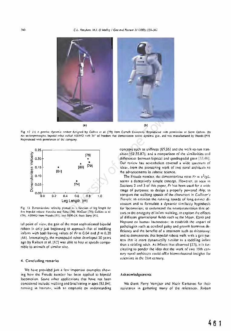
C L, Va/lkhan. MJ. O'Mallt')' J Gau "TId PO,</Uff' 21 (200j) )j()..)6)

(a) (b)

Fig . 12. (a) A pm;.,;ve dynamic ,"3lkcr dc<i~n~d by Collins el al . /79J from Cornell UnivCJ">lly. Reprodu~o:<J will> pcnn;«ion QI Srcw Co)IIII,'. (b)

An onlhropomorphic b'pcdnl robo. cDIIO<I ASIMO wllh 24" of freedom Ihsi demo"slnllCS RClive dynomJC gail .• nd wa, manufa<."1ured by Honda I. ~O I

R~produced wilh penni.slon of lhe comp.1ny,

0.25 ?:-

[76) '8 0.20 • Qi • > • (79) Cfl 0.15 • [eO} If}

[81] ~ c 0.10 .Q If} • c: <I> 0.05 [74J .S D

0.00 0.0 0,2 0.4 0,6 0,8 1.0

Leg Length (m)

Fig, 13. Dimen.,;onl",.' velneily pinned .liS a funclion 01 leg \c.ng'h for live bipedal robolS: Furushu and ~unu [741: McGce. 1761: Coli in, el al. l7~J. ASIMO from Honda 1801: nnd SDR-3X from Sony I II.

tal point of view, ule gait of the most sophisticated bipedal robots is only jus.! beginning to approacll that of toddling infant~ w~th both having values (If Fr = 0.04 and f3 = 0.20 loHI. Interestingly. th~ monopedal robot developed 20 years ago by Raiben et al. [8- 1 wa~ able to hop at speeds compa­rable to animals of simil'H ~izc.

4. Concluding remarks

We have provided jwa a few important examples show­ing how lIle Froudc number has been applied to bipedal locomotion, Some other Clpplications that have not been considered include: walking and brachiating in apes [83,84); running in humans. with an emphasis on undegtanding

concepts such as stiffness 18:1.861 and the walk-to-run Iran­sition 152.55,871; and a comparison of the similarities and differences between bipedal and quadrupedal guns 133.461. Our review has ncvcrth.eless covered a wide spectrum of ideas, rrom the pioneering work of two naval archilt:ct~ to the advancements in robotic science.

The froude number. Ihc dimensionless ralio Fr = v2/gL. seems a deceptively siJllple concept. However. as secn \1\

Sections 2 and 3 of this paper. Fr has been used for a lVid~ range of purposes: to design a properly powered .<hip; to compare the walking speeds of the characteT!; in Gu'h\'er's Travels: to e.~(imate the running speeds of long-extinct di­nosaOT!; and to formulate a dynamic similanty hypothesis for locomotion; to understand the neuromaturation thaI OC'

curs in lhe ontogeny of infHnt walking; to explore the effects of different gravitational field~ such as the Moon, E:l11h and Neptune on human locomotion: to eSlablish thc Impact of pathologies such as cerebral palsy and growlh hormolle de· ficiency and the benefits of a treatment such as rhizotolllY; and to demonslrate that bipedal robots walk with :J gait pat· rem that is more dynamically similar 10 a toddling infant than a s.u·iding adult. As Mi neui has observed (57]. it is fas­cinating to ponder the idea that the work of two 19th cen­tury nav;}! :lrchiro>.Cl.<; could offer biomechanic.'ll insighl~ fOf Sl:jen tists in the 21 st century.

Ack nowlerlgemenlS

We lhank Ferry Venijz.er and Nazir Karbanee for their assistance in g:lIhering many of the referenl:e~, Rober1

461

CL. Vaughan, MJ. O'Malley I Gait and Posture 21 (2005)350--362 361

Saunders, head librarian at the Royal Institution of Naval Architects in London, provided copies of the original papers by William and Edmund Froude, while Phil Russell and David Brown provided us with information, photographs and insights into the Froude family. Neill Alexander gen­erously provided vital feedback and historical context. We also acknowledge the financial assistance of The Wellcome Trust and the Medical Research Council of South Africa. One of us (CLV) held an Ernest Walton Fellowship, funded by Science Foundation Ireland, when this paper was written.

References

[I J Vaughan CL. Theories of bipedal gait: an odyssey. I Biomech 2003 ;36:513-23.

[2J Vaughan CL, Damiano DL, Abel MF. Gait of normal children and those with cerebral palsy. In: Allard P, Cappozzo A, Lundberg A, Vaughan CL, editors. Three-dimensional analysis of human locomo­tion. Chichester: 10hn Wiley and Sons; 1997. p. 335-{;1.

[3J Alexander RM. How dinosaurs ran. Sci Am 1991;264(4):62-8. [4J Hayes G, Alexander RM. The hopping gaits of crows (Corvidae)

and other bipeds. I Zool 1983;200:205-13. [5J Duncan WI. Physical similarity and dimensional analysis. London:

Edward Arnold; 1953. [6J Froude W. On useful displacement as limited by weight of structure

and of propulsive power. Trans Inst Naval Architects 1874;15:148-55.

[7J Russell P. In: Froude W, editor. Navies in transition, last ac­cessed via the Internet on 12 August 2003 at http://www.btinternet. coml~philipr/froude.htm.

[8J McMahon TA, Bonner JT. On size and life. New York: Scientific American Library; 1983.

[9J Brown D. In: Froude W, Newman IH, editors. A sacred duty to doubt. Paper presented to the Royal Institution of Naval Architects, London; 21 September 1998.

[lO] Froude W. On the comparative resistances of long ships of several types. Trans Inst Naval Architects 1876;17:181-8.

111 J Froude W. The theory of "stream lines" in relation to the resistance of ships. Nature 1875;13:50-2.

[12] Froude W. Experiments upon the effect produced on the wave-making resistance of ships by length of parallel middle body. Trans Inst Naval Architects 1877;18:77-97.

[13 J Froude RE. On the leading phenomena of the wave-making resistance of ships. Trans Inst Naval Architects 1881;22:220-45.

[14] Froude RE. A description of a method of investigation of screw propeller efficiency. Trans Inst Naval Architects 1883;24:231-55.

[15] O'Connor J], Robertson EF. D'Arcy Wentworth Thompson, accessed 12 August 2003 at http://www-groups.dcs.st-and.ac.ukJ~history/

Mathematicians/Thompsonj)' Arcy.html. [16J Bushnell GH. A list of the published writings of D'Arcy Wentworth

Thompson. In: Clark WELG, Medawar PB, editors. Essays on growth and form; 1945. p. 386-400.

[17J Thompson DW. On growth and form. Cambridge: Cambridge Uni­versity Press; 1917.

[18] Bonner IT. Lives of a biologist: adventures in a century of extraor­dinary science. Cambridge, MA: Harvard University Press; 2002. p. 17-21.

119] Alexander RM. Locomotion in animals. Glasgow: Blackie & Son; 1982. p. 81-113.

[20J Alexander RM. Animal mechanics. 2nd ed. Oxford: Blackwell; 1983. p. 33-6.

[21 J Alexander RM. Elastic mechanisms in animal movement. Cambridge: Cambridge University Press; 1988. p. 121-5.

462

[22] Alexander RM. Exploring biomechanics. Animals in motion. New York: Scientific American Library; 1992. p. 36-40.

[23] Alexander RM. Terrestrial locomotion. In: Alexander RM, Goldspink G, editors. Mechanics and energetics of animal locomotion. London: Chapman and Hall; 1977. p. 168-203.

[24] Alexander RM. Mechanics and scaling of terrestrial locomotion. In: Pedley Tl, editor. Scale effects in animal locomotion. London: Academic Press; 1977. p. 93-110.

[25] Alexander RM. The mechanics of walking. In: Elder HY, Trueman ER, editors. Aspects of animal motion. Cambridge: Cambridge Uni­versity Press; 1980. p. 221-35.

[26J Alexander RM. Basic mechanics. Mechanics of animal locomotion. In: Alexander RM, editor. Advances in comparative and environ­mental physiology, vol. 11. Berlin: Springer-Verlag; 1992. p. 1-15.

[27] Alexander RM. Estimates of speeds of dinosaurs. Nature 1976;261:129-30.

[28] Alexander RM, Langman VA, layes AS. Fast locomotion of some African ungulates. I Zool 1977;183:291-300.

[29] Alexander RM. Estimates of energy cost for quadrupedal running gaits. I ZQol 1980;190:155-92.

[30] Alexander RM. Optimum walking techniques for quadrupeds and bipeds. I Zool 1980;192:97-117.

[31] Alexander RM, layes AS. A dynamic similarity hypothesis for the gaits of quadrupedal mammals. I Zool 1983;201:135-52.

[32J Alexander RM. Stride length and speed for adults, children, and fossil hominids. Am I Phys Anthropol 1984;63 :23-7.

[33J Alexander RM. The gaits of bipedal and quadrupedal animals. Int I Robot Res 1984;3(2):49-59.

[34] Alexander RM. Optimization and gaits in the locomotion of verte­brates. Physiol Rev 1989;69(4):1199-227.

[35] Alexander RM. Energy-saving mechanisms in walking and running. I Exp Bioi 1991;160:55-{;9.

[36] Alexander RM. Tyrannosaurus on the run. Nature 1996;379:121. [37] Thulborn RA. Estimated speed of a giant bipedal dinosaur. Nature

1981 ;292:273-4. [38] Farlow 10. Estimates of dinosaur speeds from a new trackway site

in Texas. Nature 1981;294:747-8. [39] Hutchinson lR, Garcia M. Tyrannosaurus was not a fast runner.

Nature 2002;415:1018-21. [40] Farlow 10, Smith MB, Robinson 1M. Body mass, bone "strength

indicator", and cursorial potential of Tyrannosaurus rex. I Vertebrate Paleontol 1995;15:713-25.

[41] Hof AL, Zijlstra W. Comment on normalization of temporal-distance parameters in pediatric gait. I Biomech 1997;30:299.

[42] Sutherland D. The development of mature gait. Gait Posture 1997;6:163-70.

[43] Pierrynowski MR, Galea V. Enhancing the ability of gait analyses to differentiate between groups: scaling gait data to body size. Gait Posture 2001;13:193-201.

[44] Stansfield BW, Hillman Sl, Hazlewood ME, Lawson AM, Mann AM, Loudon lR, et al. Normalization of gait data in children. Gait Posture 2003;17:81-7.

[45] Minetti AE, Saibene F, Ardigo LP, Atchou G, Schena F, Ferretti G. Pygmy locomotion. Eur I Appl Physiol 1994;68:285-90.

[46] Saibene F, Minetti AE. Biomechanical and physiological aspects of legged locomotion in humans. Eur I Appl Physiol 2003;88:297-316.

[47] Minetti AE, Ardigo LP, Saibene F, Ferrero S, Sartorio A. Mechanical and metabolic profile of locomotion in adults with childhood-onset GH deficiency. Eur I Endocrinol 2000;142:35-41.

[48J Delaeger D, Willems PA, Heglund NC. The cost of walking in children. Eur I Physiol 2001 ;441 :538-43.

[49J Hof AL. Scaling gait data to body size. Gait Posture 1996;4:222-3. [50] Vaughan CL, Langerak N, O'Malley MI. Neuromaturation of human

locomotion revealed by non-dimensional scaling. Exp Brain Res 2003;153:123-7.

[51] Margaria R, Cavagna C. Human locomotion in sUbgravity. Aerospace Med 1964;35:1140-6.

362 CL. Vaughan. MJ. O'Malley I Gait and Posture 21 (20OS) 350-362

[52] Kram R. Domingo A. Ferris DP. Effect of reduced gravity on the preferred walk-run transition speed. J Exp BioI 1997;200:821-6.

[53] Donelan JM. Kram R. The effect of reduced gravity on the kinematics of human walking: a test of the dynamic similarity hypothesis for locomotion. J Exp BioI 1997;200:3193-201.

[54] Griffin TM. Tolani NA. Kram R. Walking in simulated grav­ity: mechanical energy fluctuations and exchange. J Appl Physiol 1999;86:383-90.

[55] Donelan JM. Kram R. Exploring dynamic similarity in human run­ning using simulated reduced gravity. J Exp BioI 2000;203(16):2405-15.

[56] Minetti AE. Invariant aspects of human locomotion in different gravitational environments. Acta Astronaut 2001 ;49(3-10): 191-8.

[57] Minetti AE. Walking on other planets. Nature 2001;409:467-9. [58] He J. Kram R, McMahon TA. Mechanics of running under simulated

low gravity. J Appl Physiol 1990;71(3):863-70. [59] Cavagna GA, Willems PA, Heglund NC. Walking on Mars. Nature

1998;393:636. [60] Cavagna GA, Willems PA, Heglund NC. The role of gravity in human

walking: pendular energy exchange, external work and optimal speed. J Physiol (Lond) 2000;528:657-68.

[61] Minetti AE. The biomechanics of skipping gaits: a third locomotion paradigm. Proc R Soc Lond BioI 1998;265:1227-35.

[62] Vaughan CL, Subramanian N, Busse ME. Selective dorsal rhizotomy as a treatment option for children with spastic cerebral palsy. Gait Posture 1998;8:43-59.

[63] Weinstein SL. Long-term follow-up of pediatric orthopaedic condi­tions. Natural history and outcomes of treatment. J Bone Joint Surg 2ooo;82-A:980-9O.

[64] O'Malley MJ. Normalization of temporal-distance parameters in pe­diatric gait. J Biomech 1996;29:619-25.

[65] O'Malley MJ, Abel MF, Damiano DL, Vaughan CL. Fuzzy cluster­ing of children with cerebral palsy based on temporal-distance gait parameters. IEEE Trans Rehabil Eng 1997;5:300-9.

[66] Subramanian N, Vaughan CL, Peter JC, Arens U. Gait before and ten years after rhizotomy in children with cerebral palsy spasticity. J Neurosurg 1998;88: 1014-9.

[67] Fallis GT. Walking toy. United States Patent Number 376,588, Wash­ington, DC; 1888.

[68] Vaughan CL, Verrijzer F. Exploring dynamic similarity in the gait of children and bipedal robots by means of the Froude number. In: Proceedings of the 7th Annual Meeting of the Gait and Clinical Movement Analysis Society, Chattanooga, USA; April 2002. Pub­lished at http://www.utc.edu/gait2oo2/abstracts/vaughan.pdf.

[69] McGhee R. Some finite state aspects of legged locomotion. Math Biosci 1968;2:67-84.

[70] Frank AA. An approach to the dynamic analysis and synthesis of biped locomotion machines. Med BioI Eng 1970;8:465-76.

[71] Vukobratovic M. On the stability of biped locomotion. IEEE Trans Biomed Eng 1970;17:25-36.

[72] Kato I, Ohteru S, Kobayashi H, Shirai K, Uchiyama A. Information-power machine with senses and limbs. Theory and prac­tice of robots and manipulation. New York: Springer-Verlag; 1974. p. 11-24.

[73] Zheng YF. Acceleration compensation for biped robots to re­ject external disturbances. IEEE Trans Syst Man Cybern 1989;19: 74-84.

[74] Furusho J, Sano A. Sensor-based control of a nine-link biped. Int J Robot Res 1990;9:83-98.

[75] McGeer T. Passive dynamic walking. Int J Robot Res 1990;9:62-82. [76] McGeer T. Principles of walking and running. In: Alexander RM,

editor. Mechanics of animal locomotion. Advances in comparative and environmental physiology, vol. II. Berlin: Springer-Verlag; 1992. p. 113-39.

[77] Garcia M, Chatterjee A, Ruina A, Coleman M. The simplest walking model: stability, complexity, and scaling. J Biomech Eng 1998;120:281-8.

[78] Kuo AD. Stabilization of lateral motion in passive dynamic walking. Int J Robot Res 1999;18:917-30.

[79] Collins SH, Wisse M, Ruina A. A three-dimensional passive-{]ynamic walking robot with two legs and knees. Int J Robot Res 200 I ;20:607-15.

[80] Honda. Humanoid robot, accessed 12 August 2003 at http://world. honda.com! ASIMOI.

[81] Sony. Sony develops small biped entertainment robot, last ac­cessed on 12 August 2003 at http://www.sony.netlSonylnfo/News/ Press/2oooll/OO'{)57E2/.

[82] Raibert MH, Brown HB, Chepponis M. Experiments in balance with a 3D one-legged hopping machine. Int J Robot Res 1984;3(2):75-92.

[83] Aerts P, van Damme R, van Elsacker L, Duchene V. Spatio-temporal gait characteristics of the hind-limb cycles during VOluntary bipedal and quadrupedal walking in Bonobos (Pan paniscus). Am J Phys AnthropoI2ooo;III:503-17.

[84] Chang YH, Bertram JE, Lee DV. External forces and torques gen­erated by the brachiating white-handed gibbon (Hylobates lar). Am J Phys Anthropol 2000;113(2):201-16.

[85] McMahon TA, Cheng Gc. The mechanics of running: how does stiffness couple with speed? J Biomech 1990;23(Suppl 1):65-78.

[86] Farley CT, Glasheen J, McMahon TA. Running springs: speed and animal size. J Exp BioI 1993;185:71-86.

[87] Hreljac A. Effects of physical characteristics on the gait transition speed during human locomotion. Hum Mov Sci 1995;14:205-16.

464

A gait nomogram used with fuzzy clustering to monitor functional status of children and young adults with cere bral palsy

Christopher L Vaughan* PhD, Department of Human Biology, University of Cape Town, South Africa; Mark J O'Malley PhD, Department of Electronic and Electrical Engineering, University College Dublin, Ireland.

"Correspondence to first author at Medical Research CouncillUniversity of Cape Town Medical Imaging Research Unit, Department of Human Biology, Faculty of Health SCiences, University of Cape Town, Observatory, Western Cape 7925, South Africa. E-mail: kvaughan@cormack.uct.ac.za

We have developed a gait nomogram based on dynamic similarity to characterize and compare neuromuscular function. We used temporal-distance data based on 669 normal participants (age range 5 to 98 years), and 78 children and young adults with spastic diplegia (43 males, 35 females; mean age lOy 8mo, standard deviation 3y llmo, range 5 to 2Oy), all of whom were independent ambulators. A new statistical algorithm known as fuzzy clustering was implemented and five cluster centres were identified, each representing distinct walking strategies adopted by children with cerebral palsy. Using just three easily obtained parameters - leg length in metres, stride length in metres, and cadence in steps per minute - our program calculates a child's dimensionless step length and step frequency, generates the individual's membership values for each of the five clusters, and plots the gait nomogram. The clinical utility of our approach has been demonstrated for two test participants with spastic diplegia, using pre- and postoperative data (one neurosurgical and one orthopaedic), where changes in membership ofthe five clusters provide objective measures of improvement in their neuromuscular function.

In the past two decades a varietyoftreatments have emerged to address the functional problems of children with cerebral palsy (CP), and specifically those with spastic diplegia. These have included: selective dorsal rhizotomy (peacock and Arens 1982); prescription of ankle-foot orthoses (Rosenthal 1984) ; continuous infusion ofbaclofen intrathecally through a pump (Albright et al. 1991); simultaneous multi-level orthopaedic surgery (Nene et al. 1993); injection of botulinum toxin at the neuromuscular junction (Cosgrove et al. 1994); and selective strengthening of lower extremity muscles (Damiano et al. 1995). In all of these procedures, an important expectation, of the patients, their families, and the clinicians involved, is an improvement in neuromuscular function, in particular the child's ability to walk. It is, therefore, not surprising that gait analysis has been strongly advocated as an adjunct in the treatment of children with CP (Gage 1994; Morton 1999), although some clinicians have expressed doubts about the efficacy of gait studies for preoperative decision-making (Watts 1994). Because CP is such a heterogeneous motor dis­order, evaluation of treatment effects in this population tends to be problematic. We believe that there is a need for a simple yet quantitative and objective method to differentiate sub­groups of children with spastic diplegia so that the outcome of surgical or therapeutic interventions may be assessed.

Gait analysis laboratories provide kinematic, kinetic, and electromyographic (EMG) measurements of human walking. In fact, it is possible to generate hundreds of different para­meters from a single trial based on just one individual (Vaughan et al. 1999). The challenge is to determine which gait parameters provide a faithful measure of neuromuscular function, and then to use pattern recognition techniques to characterize both normal and pathological gait using these parameters as feature vectors. Wong et al. (1983) grouped 128 participants with CP using a nearest-neighbour cluster­ing algOrithm but they did not account for participants' size, and their use of 10 gait parameters violated Bellman's guide­lines on dimensionality (Duda and Hart 1973). Winters et al. (1987) used a subjective technique based on descriptions of kinematic and EMG data to allocate 46 children with spas­tic hemiplegia into four groups, progressing from distal to proximal as severity increased. However, they failed to demonstrate a statistical correlation between the data and the groupings. Kadaba et al. (1990) classified 30 children diagnosed with spastic diplegia using kinematic data, where the number of clusters (10) was chosen arbitrarily; although their 12 feature vectors for 30 participants far exceeded Bellman's guidelines (Duda and Hart 1973). Another tech­nique proposed by Olshen et al. (1989) was Fourier coeffi­cients combined with bootstrap analysis but this approach has been found to have limited application by other researchers.

The Gross Motor Function Measure has gained wide­spread acceptance in the field because it is a clinical tool that is both reliable and valid for objectively documenting severi­ty of the gross motor functional status of a child with CP (Russell et al. 1989,2000). A classification system generated from the GMFM scores provides a means for rank-ordering the severity of CP based on age-matched clinical descriptors (Palisano et al. 1997), and has been used in a meta-analysis to demonstrate functional improvement in 90 children treat- . ed by selective dorsal rhizotomy (Mclaughlin et al. 2002). Damiano andAbel (1996), ina studyof32 children with spastic CP (26 with diplegia, six with hemiplegia), have reported a

DevelopmentalMedtcine & Chtld Neurology 2005, 47: 377-383 377

465

statistically significant relation between the GMFM score and the gait variables of stride length (normalized for leg length in metres) and cadence (in steps per minute). We believe that these temporal-<iistance parameters are per­haps the most fundamental of all gait parameters (Inman et al. 1981), and we have previously used them with a fuzzy clustering algorithm to classify 88 children with CP into five groups (O'Malley et al. 1997). The purpose of the present study was to introduce a simple gait nomogram based on the dynamic similarity hypothesis and non-dimensional scaling (Vaughan and O'Malley 2005), and to show how fuzzy clus­tering of two fundamental gait parameters allows the func­tional status of children with CP to be monitored.

Method DYNAMIC SIMIIARIlY

Based on the similarity between bipedal gait and a swinging pendulum (Alexander 1992, Hof 1996), step length - which is equal to half the stride length - is directly proportional to leg length, yielding the dimensionless ratio:

(1)

where SLd is the dimensionless step length, SL is step length in metres, and LL is leg length, also measured in metres (Hof 1996, Vaughan et al. 1997). The period, or cycle time, for a simple pendulum is equal to 2rr(L/g)'l" where L is the pendu­lum length in metres andg is the acceleration due to gravity (9.8m/S2). This approach leads to the equation for scaling step frequency:

(2)

where SF d is the dimensionless step frequency, and SF is step frequency in steps per second (equal to cadence in steps per minute divided by 60), while g and LL are as defined above (Hof 1996). Dimensionless step length and frequency can be multiplied together to yield dimensionless velocity v d:

vd=SLdxSFd, (3)

while Equations 1 to 3 can be combined to yield:

Vd = v/(gxLL) I\, (4)

where v is the velocity in metres per second and is equal to SLxSF. Alexander and]ayes (1983) posited that the Froude number, Fr=v2/(gxLL), will be the same for gaits that are dynamically similar. Equation 4 simply expresses dimension­less velocity v d as the square root of the Froude number. By using dimensionless data for step length SLd and step frequency SF d we have shown that the gait of children older than 60 months (Le. at least 5y) is dynamically similar to that ofteenagers and adults (Vaughan et al. 2003). For normal children between the ages of 18 and 48 months, the dimensionless parameters SLd' SF d' and v d steadily increase, reaching a plateau by 60 months of age when neuromaturation appears to be com­plete (Vaughan 2003, Vaughan et al. 2003).

NORMALS

Based on our dynamic similarity findings for the gait of normal participants of at least 5 years of age (Vaughan et al. 1997, 2003) we decided to pool our own data from previous studies. These included 53 children from the University ofVrrginia, Vrrginia, USA (O'Malleyet al. 1997), and data gathered at the University of Cape Town, Western Cape, South Africa: 120 young chil-

378 DevelopmentalMedicine & Child Neurology 2005, 47: 377-383

466

dren (Vaughan et al. 2003); 12 teenagers and adolescents (Subramanian et al. 1998); and 15 adults (Vaughan et al. 2003). These 200 participants were added to data from the literature: 282 adults from Auvinet et al. (2002); 25 adults from Sekiya and Nagasaki (1998); 16 children from Stansfield et al. (2003); 14 children and 12 adults from Stolze et al. (1997); and 120 chil­dren from Sutherland et al. (1988), yielding 669 normal partic­ipants. The stride (or step) length in metres and the cadence in steps per minute were scaled according to Equations 1 and 2 to yield dimensionless step length SLd and step frequency SF d' while Equation 3 yielded dimensionless velocity v d' For two of the studies (Sekiya and Nagasaki 1998, Auvinet et al. 2002) the authors provided the height of their adult participants, but not leg length, and so leg length was calculated as 52.6% of height, a value based on the adult data ofYaughan et al. (2003).

PATIENTS

There were 78 children and young adults with the spastic diplegia form of Cp, ranging in age from 5 to 20 years with a mean of 10 years 8 months, evaluated in the Motion Analysis Laboratory at the University of Yirginia. Ethical approval was granted by the university's Institutional Review Board, and parents or guardians of the children signed an informed con­sent form. They were a subset of the same cohort that we have previously reported (O'Malleyet al. 1997) with the removal of 10 children aged 2, 3, and 4 years. We chose to exclude these patients to make our sample comparable to the normal partic­ipants because dynamic similarity holds for children aged not less than 5 years (Vaughan et al. 2003). Each child performed three walking trials at a freely selected walking speed. We assumed this pace to be optimal, using the least amount of energy per unit of distance travelled (Zarrugh et al. 1974, De] aeger et al. 2001). Three-dimensional kinematic data were collected at 60Hz with a six-camera Vicon system (Oxford Metrics, Oxford, UK) while the Yicon Clinical Manager soft­ware package yielded the temporal-<iistance parameters of stride length and cadence. The data for each child were ensem­ble averages of the three trials, with values for the left and right sides averaged. Leg length was measured as the segmental sum of three distances when standing upright: greater trochanter to femoral epicondyle, distance to lateral malleolus, and dis­tance to plantar surface of foot. This anthropometric measure­mentwas used to scale step length and frequency according to Equations 1 and 2.

FUZZY CLUSTERING

As indicated above, our number of samples (Le. patients with CP) was equal to 78. We need to ask the question: how many gait parameters will allow us to characterize the neuromus­cular status of these children? Bellman's 'curse of dimension­ality' imposes a restriction on the number of feature vectors (Le. gait parameters) to be selected: 10 raised to the power of the number of feature vectors should approximately equal the number of samples (Duda and Hart 1973). Note that since 102 = 100, which approximately equals the number of patients (78), we have therefore chosen two feature vectors: dimensionless step length and dimensionless step frequency. These two fundamental parameters (Inman et al. 1981) are sensitive indicators of neuromuscular function in children with CP (Damiano and Abel 1996). Step length may be con­sidered a compOSite measure of the functional range of motion at the lower extremity joints, whereas step frequency

is a measure of the central nervous system's ability to modu­late reciprocal leg movements. In addition, the two parame­ters are statistically independent of one another (O'Malley 1996, Auvinet et at. 2002), thus strengthening their ability to separate different grou ps of participants.

We have chosen to implement a fuzzy clustering algorithm because it allows an individual participant to have graded membership of several groups (Bezdek and Pal 1992). Because patients with CP have a wide range of clinical mani­festations, it is most likely that they will fall along a continu­um rather than into a single well-defined group or cluster, this being the primary attribute of hard clustering. Because it is known a priori that neurologically intact individuals (both children and adults) form a logical grouping around a Single cluster centre, the algorithm was modified so that the normal centre was always an output of the clustering process for children with CP (O'Malley et at. 1997). The fuzzy clustering algorithm, based on mathematical optimization, seeks to divide up the data set or feature space (i.e. dimensionless step frequency vs dimensionless step length) into K parti­tions or clusters, where K is an input to the algorithm (O'Malley et al. 1997). We used cluster validity techniques to establish the optimal value for K (Dubes 1987).

A further output of our algorithm is the degree of mem­bership that a specific patient has in each of theK cluster cen­tres. It is a measure of the Euclidian distance from the cluster centre to the patient's point on the SF d versus SLd plane, with the degree of membership being inversely proportional to the distance (Le. the closer a patient is to a cluster, the greater the membership). The sum of the degrees of membership in the K clusters is equal to 1 (O'Malley et al. 1997).

TEST DATA

We have included test data that were not part of the original data set for either normal participants or the 78 children with CPo While the gait of the children with CP may have changed over time, we did not want to use training data to illustrate the utility of the algorithm. There were four test participants: A and B were neurologically unimpaired children (a male aged By and a female aged 19y respectively), whereas partic­ipants C and D both had spastic diplegia and were studied before and after surgery. Participant C had the neurological procedure of selective dorsal rhizotomy performed when she was 8 years old (Vaughan et at. 1988). She was evaluated by gait analysis preoperatively and then postoperatively at 1, 3 (Vaughan et at. 1991), and 10 years (Subramanian et at. 1998). These four times have been designated C1, C2, C3, and C4 respectively. Participant D underwent orthopaedic surgery that consisted of bilateral release of the hip adductor and gracilis muscles, with bilateral lengthening of the medial hamstrings and gastrocnemius muscles. He was three years of age before surgery (D1) and he was then studied at one year (D2) and two years (D3) after surgery (O'Malleyet at. 1997). Although this patient was younger than 5 years, the age at which normal children attain a mature gait pattern (Sutherland et al. 1980, Beck et at. 1981, Vaughan 2003), we have included him for illustration. His data need to be inter­preted with caution, however. For each of the children we measured leg length (in metres), stride length (in metres), and cadence (in steps per minute).

Results Data for 669 normal participants are given in Table I, and

Table I: Data for 669 normal participants adapted from the literature. Dimensionless parameters calculated from Equations 1 to 3, means and standard deviations weighted according to number of participants in each study. Data provide a basis for normal cluster centre VI (Table ill and Fig. 1)

Authors n Age range (y) Dimensionless Dimensionless Dimensionless step length step frequency velocity

Auvinet et al. (2002) 282 20-98 0.832 0.603 0.501 O'Malley et al. (1997) 53 5-13 0.901 0.545 0.491 Sekiya and Nagasaki (1998) 25 19-32 0.804 0.528 0.425 Stansfield et al. (2003) 16 5-12 0.867 0.571 0.495 Stolze et al. (1997) 14 6-7 0.853 0.512 0.437 Stolze et al. (1997) 12 22-35 0.868 0.583 0.506 Subramanian et al. (1998) 12 12-23 0.783 0.560 0.438 Suthecland etal. (1988) 120 5-7 0.786 0.594 0.467 Vaughan et al. (2003) 120 5-13 0.754 0.594 0.448 Vaughan et al. (2003) 15 23-51 0.773 0.582 0.450

Weighted mean 0.814 0.588 0.478 Weighted standard deviation 0.041 0.023 0.025

Table II: Mean (SD) data for children with spastic diplegia. Participants are a subset of a previously studied cohort of 88 children (O'Malley et al.1997), all children (n=78) were at least 5 years old. Dimensionless parameters calculated using Equations 1 to 3. Full set of data can be obtained from first author (eLV) or derived from Table I in O'Malley et a1. (1997)

Agey

10.7 (3.9)

Leglengthm Stride length m Cadence steps/min

0.691 (0.120) 0.761 (0.207) 119.0 (31.1)

Dimensionless step length

0.552 (0.132)

Dimensionless step frequency

0.521 (0.123)

Dimensionless velocity

0.294 (0.109)

A Gait Nomogram and Fuzzy Clustering for Individuals with CP Christopher L Vaughan andMarkJ O'Malley 379

467

are based on our previous research (O'Malley et al. 1997, Subramanian et al. 1998, Vaughan et al. 2003) as well as other publications in the literature (Sutherland et al. 1988, Stolze et al. 1997, Sekiya and Nagasaki 1998, Auvinet et al. 2002, Stansfield et al. 2003). The full age range from 5 to 98 years was included, and dimensionless step length, frequency, and velocity have been reported. Weighted means and standard deviations (SDs) for Sid' SF d' and vd were 0.814 (SD 0.041), 0.588 (SDO.023), and 0.478 (SDO.025) respectively.

Data for 78 children with spastic diplegia are given in Table II. Participants were aged from 5 to 20 years and their leg length, stride length, and cadence have been reported. Based on equations 1, 2, and 3, the dimensionless parameters were derived. The means and SDs for Sid' SFd, and vd were 0.552 (SDO.132), 0.521 (SDO.123), and 0.294 (SDO.I09) respec­tively. Each of these was less than normal (Table I) and, as would be expected, the data were quite variable.

Using the normal weighted means of Sid=0.814 and SFd=0.588 as the first cluster centre, the fuzzy clustering

Table m: Five cluster centres identified by fuzzy clustering algorithm using dimensionless step length and step frequency data (Tables I and ll). VI, normal participants; V2 to V5 children with spastic diplegia. Dimensionless velocity was calculated from Equation 3

Cluster Dimensionless Dimensionless Dimensionless centre step length step frequency velocity

VI 0.814 0.588 0.478

V2 0.630 0.604 0.381

V3 0.557 0.463 0.258

V4 0.391 0.598 0.234

V5 0.391 0.340 0.133

0.1 0 .1 0.2 0.3 0.4 0.5 0.6 0.7 0.8 0.9

Dimensionless step length

Figure 1: Gait nomogram showing data/or children with spastic diplegia (e) and five cluster centres (0). Contours illustrate constant dimensionless velocity and were generated by Equation 3.

380 Developmental Medicine & Child Neurology 2005, 47: 377-383

46 8

algorithm was applied to the Sid and SF d data for the chil­dren with CP in Table II. First, we had to establish the optimal number of clusters or partitions, K. In general, a valid num­ber of dusters is one where the similarity between cluster mem­bers is as large as possible while the Similarity between cluster centres is as small as possible. Using a hard separa­tion index (Dunn 1974), we established that the most valid number of dusters was five (Dubes 1987, O'Malley et al. 1997). Figure 1 shows the resulting five cluster centres VI, V2, V3, V4, and V5, with the Sid and SFd data for the 78 children with CPO The actual values for the five cluster centres are given in Table III. Figure 1 is a gait nomogram in which contours, or isocurves, for dimensionless velocity have also been plotted. These constant velocity contours represent values of v d rang­ing from 0.05 to 0.9, with normal being located at approxi­matelyO.5.

The data for the four test participants are reported in Table Iv, and include age, leg length, stride length, cadence, dimensionless step length Sid' dimensionless step frequen­cy SF d' and dimensionless velOCity v d' The dimensionless test data have been plotted in Figure 2 with the five cluster cen­tres (Table III). The cluster membership values for the test data were calculated (O'Malley et al. 1997) and the results for partiCipants C and D have been plotted in Figures 3 and 4. The memberships of the neurologically intact participants A and B for the normal cluster centre were 0.86 and 0.99 respectively, with the balance of membership being shared among the other four clusters.

Discussion Only one of the participants with CP had a dimensionless step length greater than the normal value of 0.814, whereas just eight of the patients had their highest membership in the nor­mal cluster VI (Fig. 1). 1\vo of these had dimensionless velocity values of approximately 0.5, suggesting that their gait patterns

0.1 0.1 0.2 0.3 0.4 0.5 0.6 0.7 O.B 0.9

Dimensionless step length

Figure 2: Gait nomogram showing data/or/our test participants (-),five cluster centres (0), and constant velocity contours. Participants A and B were normal controls, participants C and D had spastic diplegia and underwent neurosurgery and orthopaedic surgery respectively (see Table lV).

were dynamically similar to nonnal. Given the evidence of the link between GMFM scores and fundamental gait parameters (Damiano andAbeI1996), it seems reasonable to conclude that they had good neuromuscular function. In contrast, there were three patients with dimensionless velOCity values less than 0.1 and it is likely that their GMFM scores, and therefore their neu­romuscular function, would have been very low indeed.

Cluster centre VI (Fig. 1, Table III) represents a nonnal par­ticipant's strategy for walking at his or her optimal speed. The other four cluster centres provide some insight into the walking strategies that a child with CP might adopt. Cluster centre V2 is a CP walking strategy wherein a below nonnal step length is compensated for by a step frequency that is slightly greater than normal, yielding a dimensionless velOCity ofO.381, which is rea­sonably close to nonnal. Cluster centre V3 is a CP walking strate­gywhere a poor step length and a below nonnal step frequency combine to yield a reduced velocity of 0.258. Cluster centre

V4 has a similar velOCity of 0.234 but this is achieved with a strategy that is qUite different: an extremely low step length in combination with a step frequency that is essentially nonnal, suggesting that V4 may be considered an improvement and therefore slightly 'beuer' than V3. Cluster centre V5 has an extremely low step length which, when combined with a poor step frequency, yields a velocity of just 0.133. FinaUy, it is of interest to compare the CP walking strategies with the imma­ture patterns of healthy toddlers without disability (Vaughan et al. 2003). An 18-month-old infant has vd =0.267 (with SLd=0.572 and SF d=0.467) whereas a 30-month-old child has vd=0.351 (with SLd=0.664 andSFd=0.529).

The real power and applicability of our fuzzy clustering approach is demonstrated with the test participant data (Table Iv, Figs 2 to 4), although in time we would want to doc­ument a much larger clinical group. The two nonnal partici­pants, A and B, had different ages and sex (a 13-year-old male

Table IV: Test data. Participants A and B were neurologically intact children, whereas participants C and D were children with spastic diplegia who were studied pre- and postoperatively (Vaughan et a1.1988, 1991, 1998; O'Malley et al.1997)

Participant

A B Cl C2 C3 C4 Dl D2 D3

Q.

1: l!! 4l .c E 4l

::E 0.4

Age(y)

13 19 8 9

11 18 3 4 5

• Preop.

• ty postop.

D 3y postop.

D tOy postop.

o -t-"-L.....IIIII"-r-V1 V2

Leg length (m)

0.78 0.79 0.66 0.67 0.71 0.74 0.45 0.47 0.52

V3

Cluster number

Stride length (m)

1.29 1.29 0.59 0.89 1.04 1.02 0.20 0.51 0.76

V4 V5

Figure 3: Participant C has membership values for each of the five cluster centres (V1-5). These values changedfrom preoperatively (C1), to 1 year (C2), 3 years (C3), and 10 years postoperatively (C4). Membership values at anyone time (e.g. preoperatively) must add up to 1.

Cadence Dimensionless (steps/min) step length

112.8 0.827 122.6 0.816 134.0 0.447 110.0 0.664 119.0 0.732 113.5 0.689 49.5 0.222 74.0 0.543

131.0 0.731

1.0

• Preop .

0.8 8 ty postop.

~ 0.6 l!! 4l .c E 4l

::E 0.4

0.2

o

D 2y postop.

V1 V2

Dimensionless Dimensionless step frequency velocity

0.530 0.438 0.580 0.473 0.579 0.259 0.479 0.318 0.534 0.391 0.520 0.358 0.177 0.039 0.270 0.146 0.503 0.367

V3 V4 V5

Cluster number

Figure 4: Participant D has membership values for each of the five cluster centres (V1-5). These values changed from preoperatively (D1), to 1 year (D2), and 2 years postoperatively (D3). Membership values at anyone time (e.g. preoperatively) must add up to 1.

A Gait Nomogram and Fuzzy Clustering for Individuals with CP Christopher L Vaughan andMarkJ 0 'Malley 381

46 9

and a 19-year-old female respectively) and yet they both fell very close to the normal control group at cluster centre VI (see Tables I and Iv, Fig. 2). In addition, they both had mem­bership values in VI that were greater than 0.86.

Participant C was a female with spastic diplegia. When she was eight years of age her highest membership was in cluster V4 (Figs 2 and 3). She then underwent a selective dorsal rhizo­tomy procedure and her gait was re-evaluated 1, 3, and 10 years later (Vaughan et aI. 1988, 1991, 1998). Her location on the gait nomogram shifted from Cl to C2 (one year post­surgery), where it was then close to cluster centre V3. At three years postsurgery (C3) she moved closer to clusters V2 and VI, a position that was generally maintained 10 years after the surgery (C4), although there was slight deterioration in her functional status. As indicated by the movement from Cl to C4 on the gait nomogram (Fig. 2) and the changes in her mem­bership (Fig. 3), she migrated towards the normal values, clearly demonstrating the functional benefits of the surgery.

Participant D was a boy with spastic diplegia. At 3 years of age his highest membership was in clusterV5 (Figs 2 and 4). He then underwent an orthopaedic procedure and his gait was re-evaluated one and two years later. At one year postsurgery his point on the gait nomogram shifted from Dl to D2, which was in the direction of the normal cluster centre VI (Fig. 2) although his highest membership was still in cluster V5 (Fig. 4). At two years postsurgery his location on the gait nomogram had moved from D2 to D3, and was approaching cluster centres VI, V2, and V3. This movement and the change in his membership values (Fig. 4) clearly demonstrate an improvement in his veloci­ty, achieved with a strategy of increasing both step length and frequency (Table IV). The data for this young child should be interpreted with caution, however. He was 3 years old before surgery, an age at which normal children have not yet achieved mature gait patterns (Hof and Zijlstra 1997, Sutherland 1997, Vaughan 2003). At 3 years of age the dimensionless velocity for normal children has a value of 0.38, increasing to 0.43 at 4 years and only approaching the adult value ofO.478 at 5 years (Vaughan et aI. 2003). In the case of participant D, the changes in his gait pattern from Dl to D3 were a measure of both neu­romaturation (Forssberg 1992) as well as the effects of his soft­tissue surgery.

The concept of a gait nomogram based on stride length, cadence, and walking speed was first introduced byTodd et aI. (1989). Its use was unfortunately limited, probably because the interpretation was not particularly intuitive, and it has not been adopted by clinicians who evaluate neuromuscular func­tion in children. We believe that our gait nomogram, based on dimensionless scaling of step length and frequency, when combined with our fuzzy clustering algorithm (Figs 1 and 2) has important implications for outcome-based research. By measuring just three easily obtained parameters - one anthro­pometric and two temporal-distance - it is possible to classify the gait of any child with spastic diplegia. It is not necessary to use sophisticated three-dimensional gait analysis tools to gather these parameters: a stopwatch, tape measure, and tal­cum powder will suffice. However, we acknowledge that clinicians will still want to measure some variables (e.g. knee joint angle) that demonstrate the specific effect of a particU­lar management (e.g hamstring release).

To facilitate the implementation of our gait nomogram we have included the source code, written in the ubiquitous computer language MATLAB (The MathWorks, Natick, MA,

382 Developmental Medicine & Child Neurology 2005, 47: 377-383

~70

USA), as an appendix to this paper. The user needs to enter just three parameters - leg length in metres, stride length in metres, and cadence in steps per minute - and the program calculates the dimensionless parameters of step length SLd ,

step frequency SF d' and velocity v d' and then generates plots for the gait nomogram and membership values (Figs 2 to 4). Clinicians can thus use this nomogram to compare an individ­ual with CP with the database of all patients (Fig. 1), and to monitor change over time as a result of treatment (Fig. 2). In future, we would like to use a non-intervention group ofchil­dren with CP Oohnson et aI. 1997) to see whether their non­dimensional parameters change over time. Our fuzzy clus­tering algorithm could be adopted to study other clinical disorders (e.g. spina bifida) where different cluster centres would be established (O'Malley et aI. 1997).

DOl: 1O.1017;S0012162205000745

Accepted for publication 2nd August 2004.

Acknowledgements We acknowledge the financial assistance of the Wellcome Trust, the Medical Research Council of South Africa, and the National Research Foundation of South Africa. Christopher Vaughan held an Ernest Walton Fellowship, funded by Science Foundation Ireland, when this work was done.

References Albright AL, Cervi A, Singletary J. (1991) Intrathecal baclofen for

spasticity in cerebral palsy.] Am MedAss 265: 141S-1422. Alexander RM. (1992) Exploring Biomechanics: Animals in Motion.

New York: Scientific American Library. p 36-40. Alexander RM, Jayes AS. (1983) A dynamic similarity hypothesis for

the gaits of quadrupedal mammals.] Zool201: 135-152. Auvinet B, Berrut G, Touzard C, Moute! L, Collet N, Chaleil D,

Barrey E. (2002) Reference data for normal subjects obtained with an acce!erometric device. Gatt Posture 16: 124-134.

BeckRJ, Andriacchi TP, Kuo KN, FermierRW, GalanteJO. (1981) Changes in gait patterns in growing children.] Bonejoint Surg Am63: 1452-1457.

BezdekJC, Pal SK. (1992) Fuzzy Modelsfor Pattern Recognition. New York: Insitute for Electrical and Electronics Engineers Press.

Cosgrove AP, Corry IS, Graham HK. (1994) Botulinum toxin in the management of the lower limb in cerebral palsy. Dev Med Chtld Neurol36: 386-396.

Damiano DL, Vaughan CL, Abel MF. (1995) Muscle response to heavy resistance exercise in children with spastic cerebral palsy. DevMed Child Neurol 37: 731-739.

Damiano DL, Abel MF. (1996) Relation of gait analysis to gross motor function in cerebral palsy. Dev Med Child Neurol38: 389-396.

DeJaeger D, Willems PA, Heglund NC. (2001) The energy cost of walking in children. Eur j Physiol441: 53S-543.

Dubes RC. (1987) How many clusters are best? An experiment. Pattern Recog 20: 645-663.

Duda RO, Hart PE. (1973) Pattern Classification and Scene Analysis. New York: Wiley.

DunnJC. (1974) Well separated clusters and optimal fuzzy partitions.]Cybernet4: 95-104.

Forssberg H. (1992) Evolution of plantigrade gait: is there a neuronal correlate? Dev Med Child Neurol34: 920-925.

Gage JR. (1994) The role of gait analysis in the treatment of cerebral palsy.j PediatrOrthop 14: 701-702.

Hof AL. (1996) Scaling gait data to Ixxty size. Gait Posture 4: 222-223. HofAL, Zijlstra W. (1997) Comment on 'Nonnalization of temporal­

distance parameters in pediatric gait' .] Biomech 30: 299. (Letter) Johnson DC, Damiano DL, Abel MF. (1997) The evolution of gait

in childhood and adolescent cerebral palsy.j Pediatr Orthop 17: 392-396.

Inman VT, Ralston HJ, Todd F. (1981) Human Walking. Baltimore: Williams and Wilkins. p 22-29.

KadabaMp, Ramakrishnan HK,Jacobs 0, Wootten ME, Chambers C, Scarborough C, Goode B. (1990) Quantitative gait analysis: pattern recognition in spastic diplegia. In Soutas-little RW, editor. Proceedings of 6th Annual East Coast Clinical Gait Laboratory Conference, East Lansing, Michigan. East Lansing, Michigan: Michigan State University. p 9-12.

Mclaughlin J, Bjornson K, Temkin N, Steinbok P, Wright V, Reiner A, Robens T, Drake J, O'Donnell M, Rosenbaum P, Barber J, Ferrel A. (2002) Selective dorsal rhizotomy: meta-analysis ofthree randomized controlled trials. Dev Med Child Neurol 44: 17-25.

Monon R. (1999) New surgical interventions for cerebral palsy and the place of gait analysis. Dev Med Child Neurol 41: 424-428.

Nene AV, Evans GA, PatrickJH. (1993) Simultaneous multiple operations for spastic diplegia. Outcome and functional assessment of walking in 18 patients.] Bone]oint Surg Br 75: 488-494.

Olshen RA, Biden EN, Wyatt MP, Sutherland DH. (1989) Gait analysis and the bootstrap.Ann Stat17: 1419-1440.

O'Malley MJ. (1996) Normalization of temporal-distance parameters in pediatric gait.] Biomech 29: 619-625.

O'Malley MJ, Abel MF, Damiano DL, Vaughan CL. (1997) Fuzzy clustering of children with cerebral palsy based on temporal--distance gait parameters. IEEE Trans Rehabil Eng 5: 300-309.

Palisano R, Rosenbaump'WollterS, Russell 0, WoodE, Galuppi B. (1997) Devt:lopmentand reliability of a system to classify gross motor function in children with cerebral palsy. DevMed ChildNeurol 39: 214-223.

Peacock WJ, Arens LJ. (1982) Selective posterior rhizotomy for the relief of spasticity in cerebral palsy. S Afr Med] 62: 119-124.

Rosenthal RK. (1984) The use of onhotics in foot and ankle problems in cerebral palsy. FootAnkle 4: 195--200.

Russell OJ, Rosenbaum PL, Cadman DT, Gowland C, Hardy S,Jarvis S. (1989) The Gross Motor Function Measure: a means to evaluate the effects of physical therapy. Dev Med Child Neurol 31: 341-352.

Russell OJ, Avery LM, Rosenbaum PL, Raina PS, Wollter SO, Palisano RJ. (2000) Improved scaling of the Gross Motor Function Measure for children with cerebral palsy: evidence of reliability and validity. Phys Ther 80: 873-885.

SekiyaN, Nagasaki H. (1998) Reproducibility of the walking patterns of normal young adults: test-retest reliability of the walk ratio (step-lengthlstep-rate). Gait Posture 7: 225--227.

Stansfield BW, Hillman SJ, Hazlewood ME, Lawson AM, Mann AM, Louden IR, Robb JE. (2003) Normalisation of gait in children. Gait Posture 17: 81-87.

Stolze H, Kuhtz-BuschbeckJp, MondwurfC, Boczek-Funcke A, J6hnk K, Deuschl G, Illen M. (1997) Gait analysis during treadmill and overground locomotion in children and adults. Electroencephalogr CUn Neurophysiol 105: 490-497.

Subramanian N, Vaughan CL, Peter JC, Arens LJ. (1998) Gait before and ten years after rhizotomy in children with cerebral palsy spasticity.] Neurosurg 88: 1014-1019.

Sutherland D. (1997) The development of marure gait. Gait Posture 6: 163-170.

Sutherland DH, Olshen R, Cooper L, Woo SL. (1980) The development of marure gait.] Bone]oint SurgAm 62: 336-353.

Sutherland DH, Olshen RA, Biden EN, Wyatt MP, editors. (1988) The Development of Mature Walking. Clinics in Developmental Medicine No. 104/105. London: Mac Keith Press.

Todd FN, Lamoreux LW, Skinner SR, Johanson ME, St Helen R, Moran SA, Ashley RK. (1989) Variations in the gait of normal children. A graph applicable to the documentation of abnormalities.] Bone]oint SurgAm 71: 196-204.

Vaughan CL. (2003) Theories of bipedal walking: an odyssey. ] Biomech 36: 513-523.

Vaughan CL, Berman B, Staudt LA, PeacockWJ. (1988) Gait analysis of cerebral palsy children before and after rhizotomy. Pediatr Neurosci 14: 297-300.

Vaughan CL, Berman B, PeacockWJ. (1991) Gait analysis and rhizotomy. A three year follow-up evaluation with gait analysis. ]Neurosurg74: 178-184.

Vaughan CL, Damiano DL, Abel MF. (1997) Gait of normal children and those with cerebral palsy. In: Allard P, Cappozzo A, Lundberg A, Vaughan CL, editors. Three-dimensional Analysis of Human Locomotion. Chichester: John WIley. p 335-361.

Vaughan CL, Subramanian N, Busse ME. (1998) Rhizotomy as a treatment option for children with cerebral palsy. Gait Posture 8: 43-59.

Vaughan CL, Davis BL, O'Connor J. (1999) Dynamics of Human Gait. Cape Town: Kiboho. p 15--43.

Vaughan CL, Langerak N, O'Malley MJ. (2003) Neuromaruration of human locomotion revealed by non-dimensional scaling. Exp Brain Res 53: 123-127.

Vaughan CL, O'Malley MJ. (2005) Froude and the contribution of naval architecture to our understanding of bipedal locomotion. Gait Posture 21: 350-362.

Watts HG. (1994) Gait laboratory analysis for preoperative decision making in cerebral palsy: is it all that it is cracked up to be? ] Pediatr Orthop 14: 703-704.

Wmters TF, Gage JG, Hicks R. (1987) Gait patterns in spastic hemiplegia in children and young adults.] Bone]oint Surg Am 69: 437-441.

Wong MA, Simon S, Olshen RA. (1983) Statistical analysis of gait patterns of persons with cerebral palsy. Stat Medicine 2: 345-354.

Zarrugh YF, Todd FN, Ralston HJ. (1974) Optimisation of energy expendirure during level walking. Eur] Appl Physiol 33: 293-306.

Appendix

% This program calculates the dimensionless gait parameters % and then plots a gait nomogram and membership bar chan % First, enter the raw data LL = input CEnter leg length (in metres) '); StrideLength = inputCEnter stride length (in metres) '}; Cadence = inputCEnter cadence (in steps per minute) '}; % Calculate the dimensionless parameters SL = O.5*StrideLength; lamda subject = SULL; SF = Cadence/60; phi_subject = SF/(sqn(9.81/LL»; beta_subject = lamda_subject*phi_subject; % Assign cluster centre values V(l, 1) =0.814; V(1,2)=0.588; V(2, 1)=0.630; V(2,2) =0.604; V(3,1)=0.557; V(3,2)=0.463; V(4, 1)=0.391; V(4,2) =0.598; V(5, 1) =0.391; V(5,2)=0.340; % Calculate the subject's membership in each cluster sum =0.0; fork=1:5

distance(k)= l/«(lamda_subject-V(k,l» ~ 2 + (phi_subject­V(k,2» ~ 2);

sum=sum +distance(k); end

fork=1:5 membership(k) = distance(k)/sum; end

% Generate constant velocity contours forj=1:100

lamda(l,j) = j/100; phi (1,j) =0 .05;1amda(1,j); fori=2:10

lamda(i,j) = j/100; phi(i,j} = (i-1)/(10*lamda(i,J)); end end % Plot subject data, cluster centres, contours and axes plot (lamda _ subject, phi_ subject, 'ks' ,V (:,1) ,V(: ,2), 'ko') ; hold fori=1:10 plot(lamda(i,:) ,phi (i,:), 'k-'); end axis([0.11.00.11.0]) xlabelCDimensionless Step Length') ylabelCDimensionless Step Frequency') % Plot labels for cluster centres and contours text(0.80,0.56, 'VI'); text(0.62,0.57, 'V2'); text(0.55,0.43, 'V3'); text(0.38,0.57, 'V4'); text(0.38,0.31, 'V5'); text(0.13,0.43,'0.05'); text(0.16,0. 70, '0.1'); text(0.24,0.88, '0.2'); text(0.32,0.97,'0.3'); text(0.43,0.97,'0.4'); text(0.53,0.97,'0.5'); text(0.63,0.97,'0.6'); text(0.74,0.97,'0.7'); text(0.84,0.97,'0.8');text(0.94,0.97,'0.9'); % Plot membership bar chan figure bar( membership); axis([060 1]) xlabelCCluster Number') ylabel('Membership')

A Gait Nomogram and Fuzzy Clustering for Individuals with CP Christopher L Vaughan andMark] 0 'Malley 383

471

472

,

Research Letters South African Journal of Science 103, September/October 2007 409

Re-interpreting the evidence for bipedality In Homo floresiensis

Maria B. Blaszczyk* and Christopher L. Vaughan**

The unveiling In October 2004 of the remains of a pygmy-sized homlnln recovered from a cave on the island of Flores, Indonesia, sparked an intense series of debates within the palaeoanthro­pology community. The discoverers diagnosed It to be a new species of Homo, which they called Homo floresiensis, and they interpreted the postcranial morphology as being 'consistent with human-like obligate bipedalism'. We have examined the morphology with the aim of determining whether biomechanlcal evidence supports the claim that this hominln-known as LB1-was indeed habitually bipedal. LB1's Innominate bone differs from that of modern humans through the marked lateral flaring of the ilium, while her femur has a small head and a relatively long neck. Although these features are also found in australopitheclnes and are commonly regarded as 'primitive' traits, we concluded that none would have prevented her from exhibiting an efficient, bipedal gait. Having established that LB1 walked on two legs, we employed the principle of dynamic similarity to speculate how she might have walked. Assuming the galt of LB1 was dynamically similar to that of modern Homo sapiens, we used known dimensionless parameters, together with her leg length (0.55 m), to estimate her fundamental gait parameters: step length = 0.45 m, step frequency = 2.48 steps/second and speed = 1.11 m/s. Our review has provided insights regarding the way in which LB1 and her fellow diminutive homlnins walked aboutthe Island of Flores over 18000 years ago.

Introduction One of the key traits that separate hominins from all other

primates is the habitual use of a bipedal gait. Humans are the only extant species in the hominin group, and our bipedality is the most distinctive adaptation from our closest living relatives, the anthropoid apes. I, 2 This single characteristic is seen to be such a defining feature that skeletal adaptations to bipedalism are frequently used to identify our extinct hominin ancestors and relatives, and attempts at classification of these extinct species are often made on the basis of these adaptations. Wood and Collard,3 for example, have proposed that the fossil hominins be divided into two groups on the basis of locomotor inferences that have been made from their postcranial morphol­ogies. The first group displayed a form of terrestrial bipedalism combined with an ability to climb proficiently, thus employing a mixed strategy, and include Praeanthropus, Australopithecus, and Homo habiUs. The second group, consisting of Homo erectus, Homo ergaster, Homo heidelbergensis and Homo neanderthalensis, was com­mitted to modern human-like terrestrial bipedalism, with a very limited arboreal facility. Wood and Collard3 furthermore argued that a fossil species should be included in the Homo genus only if it met the criteria of fa postcranial skeleton whose functional morphology is consistent with modern human-like obligate

'Department of Human Biology. FacuRy of HeaRh Sciences, University of Cape Town, Observatory 7925, South Africa. I AuthOr for correspondence. E-mail: kitvaughan@uct.ac.za

bipedalism', and, on this basis, concluded that Homo habilis should be excluded from the genus. More recent analyses of the approximately 6-million-year-old Orrorin tugenensis fossils have, however, found this species' femur to be morpholOgically more like that of modern humans than australopithecines,' which led Pickford et aU to conclude that Orrorin was a habitual biped. If this deduction is correct, the story of the evolution of bipedalism and its place in classificatory schemes is likely to change.

The unveiling in October 2004 of the remains of a pygmy-sized hominin recovered from a cave on the island of Flores, Indonesia, has sparked an intense series of debates, and the issue of how to classify the specimen is one of the major controversies.6-9 In describing the skeleton, catalogued as LB1, Brown et al. lo diag­nosed it to be a new species of Homo, and thus gave it the name Homo floresiensis. Although many experts support the taxonomic decision of Brown and his colleagues, others have challenged their interpretation and offered alternative theories.s These include the view that the primitive characteristics of LB1's anat­omy suggest an ancestor such as Homo habilis, or that it might perhaps be an offshoot of Australopithecus.6

So what led Brown and colleagues to place LB1 in the genus Homo? Although they acknowledged that the LBI skeleton showed a mosaic of primitive and derived traits, and were impressed by the characteristics LB 1 shared with early hominins such as the australopithecines, they concluded that 'the facial and dental proportions, postcranial anatomy consistent with human-like obligate bipedalism, and a masticatory apparatus most similar in relative size and function to modern humans all support assignment to the genus Homo.'lo The recreation of the LB1 skeleton in the illustrative pose in National Geographic ll is cer­tainly suggestive of a bipedal gait (see Fig. 1). The interpretation of the postcranial morphology as being 'consistent with human­like obligate bipedalism' is thus one of the major pillars upon which the claim by Brown et al. lO rests.

Features of the postcranial skeleton of Homo floresiensis The recovery ofthe LB1 skeleton took place during an archaeo­

logical excavation at Liang Bua, Flores, in September 2003.12 The recovered elements of the postcranial skeleton included a fairly complete right leg and left innominate bone of the pelvis and less complete left leg, hands and feet. The vertebral column, sacrum, scapulae, clavicles and ribs were represented only by fragments, while the arms were reported more recently.13

Describing the postcranial elements, Brown et al. lO noted that, 'in common with all bipedal hominins, the iliac blade is short and wide.' That is where their discussion of LB1's bipedality began and ended. They went on to describe the marked lateral flare of the ilium, whose blade would have projected more laterally relative to the plane of the acetabulum than in modern humans (Fig. 2), before going on to discuss the anatomy of the femur (Fig. 3). They asserted that the femur's overall anatomy was most consistent with the broad range of variation found in Homo sapiens, with, for example, strong development of the inter­trochanteric crest as is characteristically found in our species.1O

However, they also described the biomechanical neck length of the femur (55.5 mm) as being long relative to the femoral head diameter (31.5 mm), a feature of the australopithecines and early Homo (Table 1). They noted that several indices of femoral size and shape-the relationship between femoral head size and mid shaft circumference (66 mm), and femoral length (280 mm)" and sub-trochanteric shaft size (525 mm2)-fell within the chimpanzee and australopithecine range of variation.10

,14 Their description of the tibia showed that the rela tionship between the midshaft cross section (347 mm2

) and the length of the tibia

473

410 South African Journal of Science 103, September/October 2007 Research Letters

100

50 em

o Fig. 1. The reoovered bones 01 Homo 1I0I8siensis have been assembled in IhlS loromotor pose by an artist, clearly suggesting thai La1 displayed a human-like bipedal gal\. This rigure has been redrawn 'rom the original ~'()Iour illustrallon In National Geogrnphic. II

(235 mm) was in the chimpanzee range of variation, and distinct from Homo.

1n <1ddition to structural characteristics related to requirements of bipedality, some of the most obvious differences between human and ape skeletons are 'proportionaJ differences, involv­ing not only the relative lengths of the long bones and trunk but also bone girth and joint surfact' size directly reflecting the different requirements of weight transfer through human and ape 5keletons'.J5 It is somewhat surprising that Brown cI a/.IO did not consider these proportions in thei r discussion on LB l' s mode of locomotion. As several of the indices characterizing LB l' s lower limb fall within the australopithecine and chimpanzee range of variation (Table 1), might it not follow that LBI's loco­motor mode shared features with those predicted for australo­pithecines, or even those displayed by chimpanzees? What is the relative importllnce of these and other morphological features in predicting a species' mode of locomotion? A comparison o( the biomechanica I characteristics of bipeda lity and q uadrupeda lism and their respective morpholOgical indicators in modem humans ilnd our closest living relatives are hrlpful in answering these queslions.

Morphological indicators of arboreal and bipedal locomotion Quadrupedalism is the most common mode of locomotion

among primates, although they certainly display a wide array of

474

locomotor behaviours. Apes are, however, largely arboreal and thus the basic mechanical conditions of climbing in trees can be related to their skeletal anatomy.' The most obvious require­ment for a bipedal gait is an upright posture, which in turn requires that the centre of mass (CoM) of the body remain directly over the rectangular area formed by the supporting feet. This explains, for example, why chimpanzees, when walk­ing bipedally, do so with a bent-hip;bent-knee (BHBK) gait." A BHBK gait is fatiguing if significant distances are walked,'7 whereas the 'stiff-legged' gait of humans allows for an effective exchange of gravitational potentiill and kinetic energy, which minimizes energy consumption.'~·IO Morphological features that allow extension of the lower limb joints during locomotioll, such as the lumbar lordosis, are consequently seen to be indicators of a bipedal gait.

The ape pelvis displays several features common to other quadrupeds, such as ischial corpora that are elongated, and ilial blades that lie mostly in the coronal plane. lLI The ape's long ischium is adapted to power the hip in extension by giving the hamstrings a long moment arm, while the lengthened ilium provides gluteus medius and minimus with great fibre length, which is mechanically advantageous for quadrupedallocomo· tion and during climbing.' In contrast, the human pelvisis short, squat and basin-shaped. The human ilium is unique among primates by virtue of the fact thi:lt it is wider than it is high,') thus eliminating any restrictive contact between the ilia and the lower lumbar vertebrae:!ll and facilitating bipedal posture. Anotherexdusively human feature is the greater sciatic notch on the sacral margin of the ilium, created by retroflexion of the ilium, and resulting in a far gre<lter angle between the ilium and the ischium than that seen in apes. This allows the trunk to be held upright without compromising the biomechanical relation­ship between the ischium and the femur."

Differences in the morphology of the femur in humans ,md apes include the degree of obliquity of the femoral shaft, its mediolateral curvature and cortical thickness, and the relative size of the femoral condyles. The latter three parameters reflect the difference in weight transfer during quadrupedal versus bjpedallocomotion.'~ In humans the knee joint is closer to the mid-line of the body, and placement of the feet facilitates a smoother and more efficient gait.'5.16.:!1

Indicators of bipeclality In the fossil record One of the big debates in pa[aeoanthropology has centred on

the locomotor mode of australopithecines, with the Auslra­

lopithecus ajarellsis specimen AL-288-I, commonly known as 'Lucy', being particularly extensively studied because her loeo­motor anatomy is reasonably intact.:!l Numerous studies have pointed out that the morphology of the pelvic and lower limb bones of Al/slmlopilhcClL5 present a mosaic pattern of feaI ures.2'-1..'

They retain some primitive, ape-like traits, such as short lower limbs and relatively small lower limb and vertebral joints, but also have derived, more human-like features associated with bipedalism, including short, laterally facing iliac blades and valgus knees. In addition, AJls/ralopilhcclIs displays unique features not found in either apes or humans, such as an excep­tionally wide and laterally flared pelvis.JII The debates regarding the locomotor mode of AI/51 mlopill1cCl/5 are many, the literature is extensive, and a comprehensive review of these debatE'S thus falls outside the scope of this paper. Certain areas of lhe debate are, however, relevant to the present discussion. As Brownel a/"· have pointed out, the poslcranial skeleton of LSI, like that of AL-288-1, 'combines a mosaic of primitive, unique and derived features: and the two sp€cimens share certain morphological

Research LeHers South African Journal of Sclence 103, SeptemoerJOctober 2007 411

10

5 em

o

fig.2 Comparison 01 the lefllnnomrnal9 bone from LB 1 (above) wilh a modemadullfemale Homo saoi8fl$ (below) This figure has been redrawn from the original black a I'd white phOlograoM in Nalur8. ro

features, such as a broad pelvis with lateral (Janng of the ilium dnd a l()n~ neck of femur in relation to femoral head diameter (Figs 2 and 3). These latter two features are often regarded as 'primitive' and have frequently been cited as evidence o( incom­plete bipedal adaptalion in australopithecines,%l,l.l and an assess­ment ot their implications for locomotion is thus required .

A sJnaU femoral head in relation to the femoral neck length has commonly be .. n assumed to result in excessively high hip-joint stresses in bipedal stallce, which would not be compatible with habitual bipedalism. Lovejoy eI ilL" challenged this assumption by means of a biomechanical analysis of the stMic force and relative joint stress thilt would hJve acted on the femoral head of one australopithecine. Sts-14, as compared 10 that of the average of 2.0 Amerindians. The femoral head of Sts-14 is missing. but it was possible to make inferences from the femoral neck. They calculated the ratio of femoral head stress in Homu sapiells to that in Sts-14 to be 2.03 when nomlalized for total body weight. Thus, a smilll femOTill heild does not necessarily le,ld to high stresses; it is only one of the fllclors governing (orces within the total pelvi-femorill complex." The same can be said for other features: inter-acetabular distance alone does not predict joint reaction force,; the extent of lateral Oaring of the ilia ilnd the femoral neck also need to be considered. An increal'e in either of these tl\lO factors will result in an increased lateral biomechanical lever arm, tel1ding to reduce joint stresses. The biomechanical evidence therefore supports the assertion that morphological features such as tilteral Oaring of the ilia and long femoral necks are not evidence of inefficient bipedalism in AlLSlmlopil"C(II~;

rather, if considered as a whole, they can be indic~ live of a human-like bipedal gail.

Another feature of AuslmlopilhcC/ls that is sometimes cited as being reflective of an inefficient gilit is short legs. Some anthro­pologists have equilted short legs with incrCi\sed energy expen­diture because a grE'aler stride length, m~dc pos.sible by longer limbs, will lead to reduced cadence for a given velocity.'" This means that the leg swings less often, so power requirements decrease, and less energy is used. As Kramer and Eck'" have pointed Ollt, however, stride length is only one aspect governing energy expenditure . Longer legs may decrease cadencE' for a given velocity, but they also have a higher mass mCllnt'nt of inertia and as 1I result the power required in each step is increased, so i I does no tau tomaticall '! follow lha tlengthening of the lower limb decreases power requirements. Steudel~' found no significant relationship between cost of locomotion versus limb length in 21 species o( mammals, includ ing walkillb ,1nu running in humans, while more recent data sllggest thntlol)ger legs increase daily energy expenditure (DEE) in hominins. with the DEE for H . ertXlllS estimilted to be 84% greater than that of Aristmiopitheclis. "

The case for blpedallty In Homo fforesiensis A cursory glace at the short. SCluat innominate bone uf LI~l,

with its curved, ventr~l!y extending iliac blades (Fig. 2), i~

enough to convince most people With a basic knowled ge of comparative anatomy that this hominin walked on t·wo legs. The ilium displays all of the ll1ilir1 cha filcteristics that distinguish the

475

412 South African Journal of SCience 103, September/October 2007 Research Letters

pelves of the Hominidae from those of their quaurupedal primate reliltives: shortness, in­crCJse in breadth, and retroflexion to create the gre<lter sciatic notch.r} These unique mor­phulogical charilcters have aU been shown to be specific ildaptalions to bipedalism.

What i~ less obviollS from 1.Bl's locomotor aniltomy is the type of bipedality and the degree to which it was displayed. LB1's innominate bone differs frum thilt of modern hum,ms through the marked lateral flaring of j Is ilium (Fig. 2), and her femur has a smaU head and a relatively long neck (Fig. 3). She also has relatively short l~, ;lnd the pmpor­tions of many of the characters of her lower limb bones fall within the chimpanzee and australopithecine range of variation (fable 1). Do these differences accordingly mean that the flDrc~lcJlsi5 gait was signific.antly different from that of sapiells? Not necessarily.

-. Proportional differenceS in long bones,

which are traditionillly studied through indi­ces, are used to characterize a spf'Cies and their relationships to othl'r spe'Cies (Table t). For example, the humerofemoral index (ratio of lengths of humerus to femur) among the hIgher primates demonsl.rates that humans hove unusuaUy long lower limbs, and apes unusuaHy short ones, in relation to Ihl'ir upper timbs, whereas arboreal Old World monkeys hilve iI more or less isometric rela­

Ftg_ 3. Anterior and posterior views of the righl temur and tibra from La 1. showing cross sections of the femoral neck and mldshafl. and the tibial midshafL ThiS figure has been redlawn from the original black and while photograph in N8Iure.'0

tionship. r' In this respect, arboreal quadrupedal monkeys re­semble bipedal humans more closely than they do arboreal quadrupedill apes. Therefore, proportional differences in long bone$, while commonly used in functional interpretations o( interspecies relationships, cannot in and of themselves be good predictors of locomotor mooe. The same is true of the length of lower limb bones in relation to the rest of the body; L51's legs aT(' short, but this would not have precluded her from having dis­played an efficient bipedal gait. As we have argued and as Kr"mer and Eck"" have pOinted out, because shorter legs require less power than do longer ones, to posit that short legs represent ,II) incomplete adaptation to bipedal gait is not tenable.

Lastly, we turn to the so-called 'primitive' features of un's postCTilnial morphology. her broild pelviS and her femur with long neck dnd small h€'ad (Figs 2 and 3). If these features are interpreted from a purely comparative point of view, one might be led to expect that [.131's gait was distinct from that of modem

humans-that is, differences in locomotor anatomy are consistent with differences i.n gait. This line of analysis might be carried even further, leading one to postulate that, as humans arc the exemplar of efficient bipedalism among primates and their anatomy will rellect this, any deviation will tend to signal a less efficient gait. 'v¥hen scrutinized rigorously, however, these kinds of assumptions do not always hold water.:.l A good exam­ple is the debunking of the myth that a smaUer femoral head au­tomatically means higher hip-joint strt'sses. On the contrary, a careful biomechanical analysis revealed that smaller heads can exist in combination. with lower hip-joint stresses thiln those found in modem humans.'"

The above example demonstrates the dangers of interpreting morphological features in isolation. Wide hips have been seen as a poor adaptation to bipedalism because they would increase hi p joint reaction forces. ll That wider hips as 11 featu re by them­selves would do this is true, as they increase the lever arm at

Table I Comparison of anlhropomelric data (Or (our dlffersnt speC1es: a mooorn human femate. Homo sapiens; a modem great ape. the chimpanzee (Pen frogIDdyfes); AuSlralOPllhecus; and Homo fioreSJ6f1SJS. the specimen lB,. The Indices have been complied Irom a variety of sources.'O,IJ---15.>J For Aus/rB/opi/hecu5. most of the Indices are for the specimen AL·288·'." e>eceP! lor Ihe temoral neck Ind&x. whIch Is based on SIS-\4." and bicondylar angle which is based on Al-129·1," The humerolemoraJ iOOax for AusrralOpilhecus is an es~male based on incomplete humen and fem~ra. Tho definillonS for the parBmatars are lisleD below,

Patamelers Homo sapiens

Humerofemorallndex 709 ~ 3.4 Crulal indfll( 76,2 ",00 Femoral neel< rndex f5 f Femoral robuSlrcrly 18.0-22.8 Tibial robuSlicrly 19,8--22.7 Blcondylar angle (0) 10.5 i: 2.4

Hum~rofemorai ",dex _ I()O • (humeralletlgth~lemo,.,.tlengtn)

ClUml 'nee> - 100 ~ {lIb,.llan9Ih)l{lemorallengrh). Femoral neel< ,ndex - 100 • {biomech.ntc~1 length ollerno,.,.1 neck)l(lemorSIIMglI'l, Femoral IObusliclly - 100 w {ferno,.1 mrd·snalt circumlerar>ee)lf'emorall8l1glh) nbi.1 'OOuSI,city M 100 x (ubial m,d-shaff c,(Cumferencal/{liballenglhl.

PErn Iroglodytes Aus/ralopilhecus

102,6 ± 3,7 85,9 8Q.d ± 2.0 03,6

16.9 22.7-27.5 23.5 21.4-26.1 23.8

1.0" 1,9 15.0

8icondyiar angie ~ anllie Ihal shaff 01 the lemur makeS wilh the VEin!:.r wilen 1M two lamo",t condyl~. ora r~inq on a hori7onlBIlevei surface

476

HDmo flores/ensls

868 83,9 19.8 23.6 2B.1 14.0

Research Letters South African Journal of Science 103, September/October 2007 413

which body weight operates. But wide hips are not an isolated feature of LBl's anatomy-they are found co-existing with a marked lateral iliac flare and long neck of femur, two features which tend to act in the opposite direction to bring down reaction forces. When we consider the features of LB l' s pelvis in relation to each other rather than in isolation, therefore, we can see that none of them would have prevented her from exhibiting an efficient, habitual, bipedal gait. Perhaps Kramer and Eck29

have accorded the big differentiating features their most likely significance, with arguments for another hominin's habitual bipedality: 'australopithecines like AL-288-1 were proficient bipeds not despite their short legs and wide pelves but, rather, because of them'. The same could be said of LB1.

Estimating plausible gait parameters for Homo floresiensis

Having established that LBI walked on two legs, it is reasonable to ask how she walked. To assist in this endeavour, Vaughan and Blaszczyk33 have employed the principle of dynamic similarity, an extension of geometric similarity (where one object is made identical to another by multiplying all lengths by a constant factor). In dynamic similarity, all lengths, times and forces are multiplied by separate constants. In bipedal locomotion, two different systems exhibit dynamic similarity when they walk with equal Froude numbers (Fr),

Fr = if/gLL, (1)

where v is the speed of walking in mis, g is the gravitational acceleration (9.81 m/s2) and LL is the leg length in metres.34 The Froude number has been adapted from naval architecture and allows the comparison of locomotion in different-sized bipeds.35

It follows that the independent gait parameters step length (SL) and step frequency (SF) may be normalized to yield dimension­less parameters

1 = SULL

and tp = SF/(g/LL)V"

(2)

(3)

where the product of dimensionless step length (1) and dimensionless step frequency (tp) combine to yield dimensionless speed f3 (= 1 x tp)36 and the substitution of Equations (2) and (3) yields the square root of the Froude number:

f3 = v/(gLL)Y' . (4)

Equations (2), (3) and (4) enable us to gain key insights regard­ing plausible gait parameters for LB1. Based on a sample of 669 normal subjects, ranging in age from children aged 5 all the way up to elderly adults in their 90s, we have shown that the dimensionless parameters for dynamically similar gait have values of 1 = 0.814 ± 0.041, tp = 0.588 ± 0.023, and f3 = 0.478 ± 0.025.35 These values may be contrasted with data for children younger than 5 during neuromaturation,36 or children with cerebral palsy evaluated before and after surgery.37

Vaughan and Blaszczyk33 argue that the anthropometric indices of H. f/oresiensis and H. sapiens support the assertion that the locomotor morphologies of these two species are geometri­cally similar, and they have assumed that the gait of LBI was dynamically similar to that of modern Homo sapiens. This makes it possible to add the length of LBl's femur (280 mm) and tibia (235 mm) as provided by Brown et al.,10 plus an estimate of her malleolar height (35 mm), to yield a leg length LL = 0.55 m. Equations (2), (3) and (4) then yield values of SL = 0.45 ± 0.02 m, SF = 2.48 ± 0.10 steps/second, and v = 1.11 ± 0.06 m/s (Fig. 4).

For purposes of comparison, the same equations may be applied to the fossilized footprints discovered in Laetoli, East

0.1

:g2.5

l a. 2

! ~ c: ~ 1.5

I cp pfe-op

0.50.'---0c'--0""'--2 _--L..._---L-_----' __ '--_-'--=~ __

.1 . 0.3 0.4 0.5 06 0.7 08 0.9 Step length (m)

Fig. 4. A gait nomogram, where actual parameters-step frequency in steps! second and step length in metres-have been plotted against one another and the isocurves represent actual walking speeds, ranging from 0.1 to 2.2 m/s. The isocurves are simply based on the relationship between speed, step frequency and step length (v= SF x SL). Equations (2), (3) and (4) have been used to calculate the fundamental gait parameters for a tali Homo sapiens (THS), Homo f/oresiensis (LB1) and the two tracks at Laetoli.33

•3IHO Also illustrated are the neuromaturation

data for normal toddling infants aged 18 and 36 months,36 plus a child with cerebral palsy seen before and after orthopaedic surgery."

Africa by Leakey and Hay,38 which were formed in wet volcanic ash almost 4 million years ago by two hominins. 18 Charteris et al. 39

reported the step lengths (SL) of the two tracks as 0.387 m and 0.472 m. By assuming dynamic similarity for the gait ofthese two australopithecines,33 Equation (2) yields leg length (LL) and then Equation (3) provides an estimate of step frequency (SF). As seen in Fig. 4, the values for LBllie between those for the two Laetoli hominins. Also included in Fig. 4 are values for a tall Homo sapiens (height of 2.01 m and LL = 1.028 m), two cohorts of normal children at age 18 and 36 months,!8 and a child with cerebral palsy seen before and after surgery.37 The tall Homo sapiens with LL = 1.028 m has a longer step length (SL = 0.89 m), a lower step frequency (SF = 1.85 steps/s), and a much greater walking speed (v = 1.63 m/s) than LBI and the Laetoli hominins.33

The values for the walking speeds of the Laetoli hominins (1.03 and 1.14 m/s) were greater than the values predicted by Charteris et aP9 and Alexander,40 although a more recent analysis based on evolutionary robotics has predicted speeds for these australopithecines in excess of 1.0 m/S!I In the case of LBl, her anthropometric indices are very similar to the Australopithecus afarensis specimen AL-288-1 ('Lucy'), but somewhat different from a modern female Homo sapiens (Table 1). While these differ­ences cannot be ignored, especially when applying dynamic similarity theory, Crompton et a/. 17 have demonstrated that Lucy's gait would have been comparable to that of modern humans.

Although the theory of dynamic similarity has been success­fully applied across several different species,34.35 some authors have concluded that Froude number corrections are not adequate predictors of the mass-specific cost of transport!2 Despite such findings, we believe it is quite plausible that LBl, with a height estimated to be approximately 1.06 m,1O walked efficiently at a speed of just more than 1.0 m/S.33

Concluding remarks The island of Flores is approximately 350 km long from west t-o

east, 80 km at its widest point from north to south, and occupies

477

414 South African Journal of Science 103, September/October 2007 Research Letters

an area of 14 300 km2 (ref. 11), which is approximately the same size as the state of Connecticut in the U.s. If LBI had walked at her natural speed, it would have taken her about 88 hours to traverse the length of the island, assuming continuous walking along a straight and flat path. By comparison, the tall Homo sapiens in Fig. 4 would have taken approximately 64 hours to cover the same course, that is, about a day less than LBI.

Interestingly, the discoverers of LBI have postulated that the Homo f/oresiensis species may have arisen from an ancestral population of Homo erectus and that their long-term isolation on Flores resulted in endemic dwarfing.lO,n Speed of walking is proportional to the square root of leg length [see Equation (4)], but energy expenditure for walking at a particular speed is proportional to body massY Since body mass is proportional to volume (for a particular density), energy utilization is roughly proportional to the cube of leg length. This suggests that a reduc­tion in size resulting from dwarfism would have had a far more dramatic impact on energy consumption than on walking speed. Thus, a shorter LL may have slightly curtailed LBI's ranging behaviour (a 27% reduction in walking speed compared to tall Homo sapiens), but this would have been more than offset by the significantly lower calorie requirements (an 85% reduc­tion in energy expenditure compared to tall Homo sapiens).

Dynamic similarity is not an exact science,34,35 but it does nevertheless provide us with some insights regarding the way in which LBI and her fellow pygmy-sized hominins might have walked about the island of Flores over 18 000 years ago.

We gratefully acknowledge the financial support of the Medical Research Council and National Research Foundation of South Africa, and the Wellcome Trust of Great Britain. Annelie O'Hagen drew the skeletal illustrations in Figs 1-3.

Received 2 August. Accepted 4 October 2JXJ7.

1. Preuschoft H. (2004). Mechanisms for the acquisition of habitual bipedality: are there biomechanical reasons for the acquisition of upright bipedal posture? ]. Anat. 204, 363-384.

2. Robinson J.T. (1972). Early Hominid Posture and Locomotion. University of Chicago Press, Chicago.

3. Wood B.A. and Collard M. (1999). The human genus. Science 284, 6~71. 4. Sawada Y., Pickford M., Senut B., Itaya T., Hyodo M., Miura T., Kashine e.,

Chujo T. and Fujii H. (2002). The age of Orrorin tugenensis, an early hominid from the Tugen Hills, Kenya. C. R. Pelleval. 1,293-303.

5. Pickford M., Senut B., Gommery D. and Treil J. (2002). Bipedalism in Orrorin tuge/tensis revealed by its femora. C. R. Pelleval. 1, 191-203.

6. Wong K. (2005). The littlest human. Sci. Am. 292(2),40-49. 7. Dalton R. (2004). Little lady of Hores forces rethink of human evolution. Nature

431,1029. 8. Balter M. (2005). Small but smart? Hores hominid shows signs of advanced

brain. Science 307, 1386-1389. 9. Lahr M.M. and Foley R (2004). Human evolution writ small. Nature 431,

1043-1044. 10. Brown P., Sutikna T., Morwood M.J., Soejono R.P., Jatmiko, Saptomo E.W and

Due R.A. (2004). A new small-bodied hominin from the Late Pleistocene of Hores, Indonesia. Nature 431, 105~ 1061.

11. Morwood M., Sutikna T. and Roberts R. (2005). The people time forgot. National Geographic April, 2-15.

12. Morwood M,J., Soejono RP., Roberts R.G., Sutinka T., Tumey e.S.M., Saptomo E. Wand Due R.A. (2004). Archaeology and age of anew hominin from Hores in eastern Indonesia. Nature 431,1087-1091.

13. Morwood M,J., Brown P., Jatmiko, Sutinka T., Saptomo E.W, Westaway K.E., Due R.A., Roberts R.G., Maeda T., Wasisto S. and Djubiantono T. (2005). Further evidence for small-bodied hominins from the Late Pleistocene of Hores,

478

Indonesia. Nature 437,1012-1017. 14. Haeusler M. and McHenry H.M. (2004). Body proportions of Homo ltabilis

reviewed.]. Hum. Evol. 46, 433-465. 15. Aiello L.e. and Dean M.e. (1990). An Introduction to Human Evolutionary Anat­

omy. Academic, London. 16. Jenkins EA.). (1972). Chimpanzee bipedalism: cineradiographic analysis and

implications for the evolution of gait. Science 178, 877-{j79. 17. Crompton R.H., Li Y., Wang W, Gunther, M.M. and Savage R. (1998). The

mechanical effectiveness of erect and bent-hip, bent-knee bipedal walking in Australopithecus ajarensis. J. Hum. Evol. 35, 5~74.

18. Vaughan e.L. (2003). Theories of bipedal walking: an odyssey. ]. Biomech. 36, 513-523.

19. Cavagna G.A., Heglund N.e. and Taylor e.R. (1977). Mechanical work in terrestrial locomotion: two basic mechanisms for minimizing energy expendi­ture. Am.]. Physiol. 233,243-261.

20. Lovejoy e.O. (2005). The natural history of human gait and posture I: Back and pelvis. Gait Posture 21, 9~ 112.

21. Schmitt D. (2003). Insights into the evolution of human bipedalism from experimental studies of humans and other primates.]. Exp. Bioi. 206, 1437-1448.

22. Johanson D.e., Lovejoy e.O., Kimbel WH., White T.D., Ward S.c, Bush M.B., Latimer B.L. and Coppens Y. (1982). Morphology of the Pliocene partial hominid skeleton (AL 288-1) from the Hadar Formation, Ethiopia. Am.]. Phys. Anthropol. 57,403-451.

23. Berge e. (1994). How did the autralopithecines walk? A biomechanicalstudy of the hip and thigh in Auslralopithecus ajarensis.]. Hum. Evol. 26,259-273.

24. Stern J. and Susman R. (1983). The locomotor anatomy of Australopititecus ajarensis. Am. ]. Phys. Anthropol. 60, 279-317.

25. Ward e.v. (2002). Interpreting posture and locomotion of Australopithecus ajarensis: Where do we stand? Yrbk Phys. Anthropol. 45, 18~215.

26. Rak Y. (1991). Lucy's pelvis anatomy, its role in bipedal gait.]. Hum. Evol. 20, 273-290.

27. Lovejoy e.O., Heiple KG. and Burnstein A.H. (1973). The gait of Australo­pithecus. Am.]. Phys, Allthropol. 38, 757-780.

28. Jungers WL. (1982). Lucy's limbs: skeletal allometry and locomotion in Australopithecus ajarensis. Nature 297, 676-678.

29. Kramer P.A. and Eck G.G. (2000). Locomotor energetics and leg length in hominid bipedality.]. Hum. Evol. 38, 651-{;66.

30. Steudel K (1996). Limb morphology, bipedal gai t, and the energetics of hominid locomotion. Am. J. Phys. Anthropol. 99, 34~356.

31. Steudel-Numbers KL. (2006). Energetics in Homo erectus and other early hominins: the consequences of increased lower-limb length. ]. Hum. Evol. 51, 44~53.

32. Hunt K.D. (1994). The evolution of human bipedality: ecology and functional morphology. ]. Hum. Evol. 26, 183-202.

33. Vaughan e.L. and Blaszczyk M.B. (in press). Dynamic similarity predicts gait parameters for Homo jloresiensis and the Laetoli hominins. Am. ]. Hum. BioI.

34. Alexander R.M. (1976). Estimates of speeds of dinosaurs. Nature 261, 129-130. 35. Vaughan e.L. and O'Malley M.J. (2005). Froude and the contribution of naval

architecture to our understanding of bipedal locomotion. Gait Posture 21, 350-362.

36. Vaughan e.L., Langerak N.G. and O'Malley M.J. (2003). Neuromaturation of human locomotion revealed by non-dimensional scaling. Exp. Brain Res. 153, 123-127.

37. Vaughan e.L. and O'Malley M.J. (2005). A gait nomogram used with fuzzy clustering to monitor functional status of children and young adults with cerebral palsy. Oev. Med. Child Neurol. 47, 377-383.

38. Leakey M.D. and Hay R.L. (1979). Pliocene footprints in the Laetoli beds at Laetoli, northern Tanzania. Nature 278, 317-323.

39. Charteris L Wall J.e. and Nottrodt J.W (1982). Pliocene hominid gait: new interpretations based on available footprint data from Laetoli. Am. ]. Phys. Anthropo/. 58,133-144.

40. Alexander R.M. (1984). Stride length and speed for adults, children, and fossil hominids. Am. ]. Phys. Anthopol. 63, 23-27.

41. Sellers WI., Cain G.M., Wang Wand Crompton R.H. (2005). Stride lengths, speeds and energy costs in walking of Australopithecus ajarensis: using evolutionary robotics to predict locomotion of early human ancestors.]. R. Soc. Interface 2, 431-441.

42. Steudel-Numbers KL. and Weaver T.D. (2006). Froude number corrections in anthropological studies. Am.]. Phys. Anthopol. 131,27-32.

43. Zarrugh M.Y., Todd EN. and Ralston H.J. (1974). Optimisation of energy expenditure during level walking. Eur. J. Appl. Physiol. 33,293-306.

J Neurosurg Pediatrics 1: 180--186, 2008 See the corresponding editorials in this issue, p 177 and pp 178-179.

A prospective gait analysis study in patients with diplegic cerebral palsy 20 years after selective dorsal rhizotomy

NELLEKE G. LANGERAK, M.Sc.,1 ROBERT P. LAMBERTS, M.Sc.,1 A. GRAmM FIEGGEN, F.C.S.,l JONATmN C. PETER, F.R.C.S.,2 LIZE VAN DER MERWE, PH.D.,3 WARWICK J. PEACOCK, F.R.C.S.,4 AND CHRISTOPHER L. VAUGmN, PH.D.I

IMedical Research CouncillUniversity of Cape Town Medical Imaging Research Unit, Department of Human Biology, Faculty of Health Sciences, University of Cape Town, Observatory, Western Cape; 2Department of Paediatric Neurosurgery, Red Cross Children's Hospital, Rondebosch, Western Cape; 3Biostatistics Unit, South African Medical Research Council, Tygerberg, Western Cape, South Africa; and 4Department of Neurological Surgery, University of California San Francisco, California

Object. Selective dorsal rhizotomy (SOR) has been widely performed for the reduction of spasticity in patients with cerebral palsy during the past 2 decades. The objective of this study was to determine whether the surgery has yield­ed long-term functional benefits for these patients.

Metlwds. The authors present results from a prospective 20-year follow-up study of locomotor function in 13 pa­tients who underwent an SOR in 1985. For comparison, we also present gait data for 48 age-matched healthy controls (12 at each of 4 time points). Patients were studied preoperatively and then at 1,3, 10, and 20 years after surgery. Study participants were recorded in the sagittal plane while walking using a digital video camera, and 6 standard gait param­eters were measured.

Results. In this group of patients 20 years after surgery, knee range of motion (ROM) was on average 12° greater than preoperative values (p < 0.(01). Hip ROM before surgery was no different from that in the healthy control group. This parameter increased markedly immediately after surgery (p < 0.(01) but had returned to normal after 20 years. The knee and hip midrange values-a measure of the degree of "collapse" due to muscle weakness after surgery-had returned to preoperative levels after 20 years, although they were respectively II and 8° greater than those in healthy controls. Both temporal-distance parameters (dimensionless cadence and dimensionless step length) were significant­ly greater at 20 years than preoperative values (cadence, p = 0.003; step length, p = 0.02), leading to improved walk­ing speed.

Conclusions. Twenty years after undergoing SOR, our patients showed improved locomotor function compared with their preoperative status. (DOl: JO.3171/PED/2008/1/3/180)

KEy WORDS • cerebral palsy • gait analysis • long-teno follow-up • range of motion • selective dorsal rhizotomy

THE prevalence of CP has risen from 1.5 per 1000 live births in the 1960s to the current rate of 2.5 per 1000 live births in developed countries.24 In addition, there

is increased longevity in the adult CP population.2o Although CP is a complex neurological condition resulting from a nonprogressive lesion in the developing brain,4 adults with CP experience secondary complications and accelerated im­painnents. L8 Because 80% of CP cases have spasticity as the primary abnonnality,30 which can lead to secondary abnor­malities such as muscle contractures, II it is important to use insight when treating this condition. Treatment strategies for CP spasticity have included physical therapy, orthotic de-

vices, oral pharmacological intervention, parenteral medica­tion, and surgery.2.L2.L9.33,35 Only the intrathecal baclofen pump and SDR interfere directly with the primary abnonnality of spasticity in CP by attempting to restore the balance of spinal circuits. 11,33

Selective dorsal rhizotomy was first perfonned by Foer­sterlO in the early 1900s and modified in the 1960s by Gros et al. L3 In the 1970s Fasano and colleagues9 further refmed the procedure by cutting the posterior rootlets on the basis of intraoperative functional electrical stimulation of leg muscles. Peacock et al.26,27 refmed this method in the 1980s by exposing the cauda equina to identify dorsal rootlets·at their exit foramina. Despite some controversy regarding its efficacy,2L SDR has gained widespread acceptance over the past 2 decades.2,11,25.32,33 In a recent review, Steinbok32 con-

Abbreviations used in this paper: CP = cerebral palsy; ROM = range of motion; SOR = selective dorsal rhizotomy.

180 J. Neurosurg.: Pediatrics / Volume 1/ March 2008

47 Q

Twenty-year study of gait in cerebral palsy after rhizotomy

cluded that there was strong evidence of decreased lower limb spasticity, increased lower limb ROM (without loss of muscle strength), and a moderate degree of improvement in activities of daily living after SDR for spastic CPo Although a large number of studies support the efficacy of SDR in reducing spasticity and improving function, most of these are based on assessments performed within 1 to 5 years af­ter surgery. Our own research, based on a prospective study of Dr. Peacock's patients at 1, 3, and 10 years after surgery, has provided evidence to show that lasting functional ben­efits (as measured by improved gait) can be obtained with SDR when patients with CP become adolescents and young adults.5.22.34.36-38

Given the large number of patients with CP who have undergone SDR in the past 2 decades, it is clearly impera­tive that the clinical community is given objective and com­pelling evidence of the long-term sequelae of the SD R pro­cedure when these patients become adults. In this paper, we present results from a prospective 20-year follow-up study of 13 patients who received SDR surgery in 1985, with a particular focus on their gait data.

Clinical Materials and Methods

This study was approved by the Human Ethics Commit­tee at the University of Cape Town, and each participant signed an informed consent form. In addition, the patients with CP completed a questionnaire that recorded other inter­ventions, amount of physical therapy, problems with daily activities, and their personal feelings about the outcome of the SDR procedure.

Twenty-nine children with CP underwent SDR in 1985. Selection for surgery was based on the following criteria: 1) exhibition of spasticity; 2) absence of athetosis; 3) absence of significant underlying muscle weakness; and 4) access to postoperative therapy. Fourteen of the 29 children were able to walk (4 household ambulators and 10 independent ambu­lators) and participated in the first study comparing pre­operative and I-year postoperative gait analysis data.5.37,38 Eleven of these 14 patients were available and participated in the 3- and to-year follow-up studies.22,34,36,40 We located all 14 original patients in early 2005, and each was willing to participate in this reassessment. One of the 14 patients had severe muscle weakness and was not able to walk inde­pendently; for this reason, she was excluded from the study. Two patients were able to walk using a device-l using a

crutch and the other using a cane.22 The mean age of the 13 patients who participated in the 20-year follow-up study during 2005 was 27.3 years (range 22-34 years). For pur­poses of comparison, gait analysis was also performed on a group of 12 age-matched healthy controls who had a mean age of 27.8 years (range 22-34 years). Table 1 provides an overview of the groups that participated in the different studies.

Selective Dorsal Rhizotomy

All children underwent operations performed by Dr. Pea­cock at the Red Cross Children's Hospital in Cape Town, South Mrica. Each patient received endotracheal general anesthesia (without the use of long-acting neuromuscular blocking agents), and was then placed in a prone position with bolsters under the chest and pelvis. Limited laminec­tomies were performed from L-2 to S-I, exposing the cauda equina with preservation of the posterior facet joints. The dorsal roots were separated from the anterior roots. For the electromyographic recordings, electrodes were placed in major muscle groups of the lower extremities, correspond­ing to the nerve rootlets tested. A 50-Hz train of stimuli was applied at the threshold intensity for muscular contraction and those dorsal nerve rootlets associated with a normal response were left intact, whereas those associated with an abnormal response were divided.

Gait Evaluation

Our 2D kinematic gait analysis system consisted of light­weight retroreflective markers, a linear calibration standard, and a portable digital video camera (DCR-TRV80E, Sony). Although it would have been preferable to study all patients in the same laboratory, the cost of transportation precluded this option. Two researchers (N.G.L. and R.P.L.) drove by car with all the equipment throughout South Africa to visit 8 of the 13 patients with CP in their hometowns. The gait data were captured in a dimmed room with a walkway of at least 11 meters, similar to our laboratory in Cape Town. Three markers were placed at the hip (greater trochanter of the femur), knee (lateral femoral epicondyle), and ankle (lateral malleolus of the distal fibula) of each individual. These markers reflect the light transmitted by an infrared light source on top of the camera. Separate analyses of the right and left lower limbs were performed in the sagittal plane. The patient was required to walk barefoot, without any orthoses, at his or her normal pace in a plane perpen-

TABLE 1

Characteristics of patients included in the 20-year follow-up study*

Study Group Name No. of Patients Sex (FIM) Mean Age in Yrs (range) Source

preop OCP 13 5/8 7.3 (2-14) Vaughan et aI., 1988, 1989 1-yr postop 1 CP 13 5/8 8.3 (3-15) Vaughan et ai" 1988, 1989

0-1 HCt 12 517 7.5 (2-12) Vaughan et aI., 1997 3-yr postop 3CP 10 4/6 9.7 (5-17) Vaughan et aI., 1991

3HC 12 517 9.2 (5-13) Vaughan et aI., 1997 10-yr postop 10 CP 10 4/6 16.1 (12-22) Subramanian et aI., 1998

IOHC 12 6/6 19.3 (14--22) Subramanian et aI., 1998 20-yr postop 20CP 13 5/8 27.3 (22-34) present study

20HC 12 517 27.8 (22-34) present study

* HC = healthy control. t The same group of 12 healthy controls was used for the preoperative and I-year postoperative comparisons,

1. Neurosurg.: Pediatrics / Volume 1/ March 2008 181

480

N. G. Langerak et al.

TABLE 2

Adjusted differences in means and probability values for 6 gail parameters *

Preop (0 CP group) as Reference Healthy Controls as Reference

Gait Parameter Measuret 1 CP 3CP IOCP 20CP OCP 1 CP 3CP IOCP 20CP

knee ROM (0) 13 12.1 14.0 12.4 12.1 -15.9 -2.8 3.7 -4.0 -9.3 P value <0.001 <0.001 <0.001 <0.001 0.002 0.64 0.23 0.09 <0.001

hip ROM n 13 14.9 8.6 4.6 3.9 -5.4 10.0 4.1 2.1 3.4 p value <0.001 0.003 0.01 0.04 0.07 <0.001 0.07 0.39 0.07

knee midrange value (0) 13 16.8 4.1 -2.6 4.4 2.4 20.0 9.4 5.6 10.9 P value <0.001 0.21 0.41 0.07 0.55 <0.001 0.03 0.03 <0.001

hip midrange value (0) 13 4.0 0.0 -4.0 -2.7 9.5 13.8 10.0 8.7 7.6 P value 0.03 1.00 0.07 0.11 0.004 <0.001 <0.001 0.001 <0.001

dimensionless cadence 13 -0.01 0.01 0.01 0.07 -0.09 -0.11 -0.07 -0.09 -0.06 p value 0.61 0.72 0.73 0.003 0.04 0.002 0.06 0.02 0.005

dimensionless step length 13 0.13 0.24 0.05 0.07 -0.24 -0.11 0.02 -0.18 -0.10 p value <0.001 <0.001 0.18 0.02 <0.001 0.09 0.58 0.001 0.002

* Adjusted for age, sex, side, and repeated measures. t 13 is calculated as the difference between the means of the gait parameters (mean of the group of interest subtracted from the mean

of the reference group).

dicular to the camera's optical axis. The data obtained from the camera were then analyzed digitally using customized software for gait analysis. Through suitable calibration and scaling, the x and y coordinates of the joints were obtained in real units (meters) as a function of time (sample rate of 25 Hz). From these data it was possible to calculate all rel­evant gait parameters.

Outcome Measures

As in our previous pre- and postoperative studies, the gait parameters included angular kinematic data and temporal­distance parameters. The angle at the knee joint was defmed as the angle between the thigh and the calf, whereas the hip angle was defined as the angle between the thigh and the vertical axis. Hip and knee midrange values were defined as the point halfway between the extremes of extension and flexion.34.36 The temporal-distance parameters included ca­dence (or step frequency, the number of steps per second) and step length (the distance in meters between 2 consecu­tive heel strikes [left-to-right or right-to-left]).

When performing a longitudinal study on children it is important to account for the way that study participants grow and mature. Angular kinematic data do not change af­ter a child reaches the age of 3 years and so these parameters are comparable in all follow-up studies. In contrast, tempo­ral-distance parameters change as a child ages and so it is necessary to normalize these parameters for the effects of growth.3J Hof1s recommended that temporal-distance param­eters could be normalized by leg length, converting cadence and step length into dimensionless units as follows:

dimensionless cadence = (cadence)/[g/(leg length)]l12 dimensionless step length = (step length)/(leg length)

The letter "g" in these equations represents the accelera-tion due to gravity (9.81 rnIsecond2), leg length is measured in meters (the distance from the greater trochanter to the ground), cadence is measured in steps per second, and step length is measured in meters. IS We were in possession of leg length measurements for the preoperative and the 1-,3-, 10-, and 20-year postoperative studies, and could apply this nor­malization method to our measurements. This method en-

182

abled us to compare patients with themselves (over the 20 years of the study) and with the age-matched healthy con­trols.

Statistical Analysis

Boxplots were used to graphically summarize the ob­served data. We performed 2 sets of comparisons: measure­ments at 1, 3, 10, and 20 years after an SDR (the groups of interest) were compared with preoperative gait parameters and also with measurements from age-matched healthy control groups (the reference groups). For each gait param­eter and comparison, we present the effect size (13), and the corresponding probability value. The 13 value reported is the difference between the means of the gait parameters (mean of the group of interest subtracted from the mean of the reference group), adjusted for age, sex, and side, as well as for repeated measures on each patient. The age we ad­justed for is the age at the time of the operation (in the com­parison with preoperative measurements) and current age (for comparison with healthy control groups). Individual linear mixed-effects models were used for all comparisons.

Results

One of the 13 patients had conflicting feelings about the benefits of the SDR operation. All patients received intense physical therapy at school pre- and postoperatively, where­as more than half of the group also received orthopedic sur­gery (tendon lengthening of the rectus femoris, hamstring, or Achilles, or osteotomy in the lower limb or foot) after SDR. Some of the patient cohort suffered from back pain, and all had relatively poor balance. Eleven of the 13 patients were either working or studying at college, and none had any problems with activities of daily living.

The results of this study are based on 13 patients with CPo of whom 3 were missing in the 3- and 10-year follow­up studies (Table 1). Table 2 shows the estimated adjusted differences between the subject groups and the reference groups (13 value) and corresponding p values.

Angular Kinematics

Knee and Hip ROM. Knee ROM of the patients with CP

1. Neurosurg.: Pediatrics / Volume 1/ March 2008

Twenty-year study of gait in cerebral palsy afler rhizotomy

was . on average, 15.90 less than that of the healthy control group before surgery (p :: 0.002). This ROM improved sig­nificanlly (p < 0.00]) at I, 3, 10, and 20 years after the operation. The greatest difference (14.0°) was found 3 years ofter surgery. This mean was 3.70 greaLer than thaI of the healthy control group, although this difference wa~ not sig­nificant (p = 0.23; Table 2).

llle mean hip ROM was the only parnmetcr that was not signi.ficantly different from the healthy control group before surgery. One year postoperatively. mean hip ROM had in­creased by 14.90 (p < 0.001) and was 10.00 greater than the mean in the healthy volunLeer group (p < 0.001). The data (Fig. I and Table 2) show that after the initial large increase the mean hip ROM values decreased and approached the he:llthy control group values with no statistically significant di tTerences.

Midrange Vailles. The knee and hip midrnnge values of the paticnl.~ with CP showed a similar trend in the years fol­lowing surgery (Fig. 2). Preoperatively, both parameters were greater in the CP group than in the healthy control group, although only the hip midrange value of 9S' was sIgnificantly different (p = 0.(04). One-year postoperative­ly, there was a significant increase in borh midrange values (knee: 16.8°, p < 0.001; hip: 4.0", p = 0.03; Tnhle 2). These values then improved, as indicated by a decrease iII values closer to that of the healthy control groups (Fig . 2), although they remained stalislically greater (Table 2).

Temporal-Disfance Parumefers

The dimensionless cadence of patients with CP did not change significantly after SDR. except at 20 yean; after sur­gery when there was a 0.07 mean increase compared with preoperative values (p = 0.003). Dimensionless cadence for patients was consistently less than that for healthy wlltrols (Table 2. and Fig. 3).

The boxplots of dimensionless step length (fig. 3) and knee ROM (Fig. I) show similar trends for patients with CP. One year after surgery there was a significant improvement of 0.13 (p < 0.00 I) compared with the preoperative value with a further signiticant increase (0.24) at 3 years (p < 0.00 I). followed by a slight deterioration at 10 and 20 year> LIfter su rgely. A Ithough the step length viLIues of the 10- and 20-year follow-up studies are smaller than in the 3-year study and significantly different from the heallhy control groups. there is still a sigllificant benefil of 0.07 al 20 years afler surgery compared with preoperntive values (p = 0.02, Table 2).

Discussion

Our study of patients with CP who underwent SDR in 1985 has shown that although the greatest gains were made dUling the fiN 3 years after surgery. 20 years later the pa­tients with CP still demonslrnted on i mprovemellt in their gait patten! compared with preoperative valucs. Ths result is in accordance with our IO-year follow-up study data, in which we objecti vely demonstrated the contribution of SDR to functional benefits, as measured by improved gait.n~

Anglliar Kinemntics

PallenlS with spastic CP demonstrate greater muscle stiff­ness. than control groUpS.B When these patients undergo an

1. Neumsurg.: Pedimrics I l'o/ltInt: II March 2008

482

Koe-6 Rarge of Motion (degrees)

90 .-------------------------------------~

80

30

20 1 Pre-op Iyr Post 3yrPost 1 Oyr POsl 20yr Posl

Hip RIl r'"Q 01 Molion (dogrees) 80 r-------------------------~=_--------_.

70

60

50

Pre-op lyr Post 3y" Post

~'II1T"""u"" CAfDOOlI pall),p.tenllo

0UtI1on

lOY' POsl 20yr Post

FIG. I. Box.plot comparing knee (upper) and hip (lower) ROM values for patients wilh CP and healthy controls, before SDR (Pre­op) and at 1-.3-. 10-. and 20-years postoper:Juvely (Post). In all liS ' urcs the bmes show the flfSL. second (median). and third quartiles; IVhiskers reprc.~nI the minimum and maximum values. excluding outliers; and circles represent the ou[Jiers.

SDR, studies have shown that this spastic reduction will be maintained for at least 4 years.'·· I7.13.1.~ Diplegic patients have a smaller ROM than persons without spasticiry'" and this will increase after SDRY Our series of follow-up studies have shown that this increase is most pronounced in the ftrst 3 years after surgcry,lUoO.JO during the imponanl ye."\t"S of growth, and may le<lJ indirectly to fewer conLractures. As the patients became older, our 10- and 20-year follOW-lip studies showed slightly decreased ROM for the hip and knee (Fig. I).

The typical walking pattern for patients with CP and spa.~­tic diplegia is a crouch gail, which results in a high midrange value for the hip. One yem after an SDR, a "collapsed" gait panem is o~rved, with a significant increase in midrange values for both the knee 31ld the hip (Fig. 2). One fe<lSOn for this negative side effect could be posLoperative muscle weak­ness in the lower extremities. Alternatively, we hypothesize: that this change in gait mechanics could also be the result of lum bar hyperiordosis. which leads to increased hi p flexion to maintain a patient'S center of gravity over the base of sup­port.

183

KnIMI Mld-Range Value (degAM!s) 60

70

60

@ ~~ ~ 1 Y' POSl 31' Post 10yf Post 20yr POSI

Hip Mid-Range Value (degrtl )

40 r-------------------------~~--------_. ElH"'rryCO<l~ E3C4otob,1I! pal'YP~ "" • Ou-..

30

Pre-op 1 yr POt\ 31' Post IOyr Post 20yr Post

FIG. 2. Boxp)ot comparing knee (upper) and hip (lower) mid­range value.~ for palicnlS with CP and healthy C{)nlrOls, before SDR and a\ 1-.3-. )C).., and 2O-years po.'(toperntively.

Temporal· Distance Parameters

Damiano and Abel6 showed that cadence is correlated with muscle snength in the lower extremities. In general. muscle strength in patients with CP is less than that of healthy con­trols, which may be why the number of steps per mi.nute i& reduced. The outlier i.n dimensionless cadence repre..~nted a single patient (Fig. 3). She and her mother reported i.n the questionnaire that, although she received intensive physical therapy posroperalively, she continued to suffer from muscle weakl\ess. Although her cadence increased slighdy at 10 and 20 years after surgery, this increase was probably not a result of increased muscle strength but rather because she was walking with II C11Jtch.

In contrast to cadence, step length is not correlated with muscle strength. ,J but is related to joint excursion, which is reduced in patients with CP compared with healthy COIl­

troIs. 1.1 In our 20-year follow-up srudy, the change., in kne.e ROM corresponded with the changes in dimensionless step length (Figs. I and 3).

Gait ill Adults with CP

Andersson and Mattsson3 and Jahnsen nnd colleagues"

184

N. G. Langerak el aJ.

Dimenslo S5 Caden;e

07 ,----------------------------------,

:: g g 0.4

0.3

0.2 • I

P,e~ lyr Post Jyr Post I~POSI 20)'" Post

Dimemlorless Step Length

1.1 r---- -------------------------,

1.0

0.9

08

0.7

0.6

0.5

0 .4

Pre-op 1yr Post 3yr Post Oyr Post 20yr Post

FIG. 3. Boxplot comparing dimcns.ionles~ cadeJ)cc (uppt'rJ and dimcn.~ionless SLep lwgth (I(Jlver) values r()r patienlc; with CP and hCClithy comTOIs. before S DR and at )", )" ) 0-. and 20-ycar.; JXlS(()~ t.'14livcly"

huve published questionnaire data regarding the locomotor skills of adults with CPo Their groups consisted of 77 and 145 patieJ\ts with diplegic CP, respecti vely. and they showed that 30 to 40% of the pauents were able to walk withuut sup­pen, although 20% always 1I~ a wheelchair. Both STUdies showed that 75% of their patients demonstrated decreased walking abiliry between 15 and 34 years of age. Although we have to consider that our group size was much smaller (14 patients), we demonstrated that 20 years after an SRD. at a mean age of27.3 ye:m, II of our patients (79%) walked without support and only I (7%) was confined to a wheel· chai r.

Limiting Factors

Founeen patients with CP participated in uur studies. which provided sufficient power for me statistical analysis; howcver, the research sample should ideally be much largo er for our findings to have widespread applicability. In ad­dition. 3 of the L4 patients were missing for the 3- and 10-year follow-up srudies, and we had 10 exclude I of the 14 because she was not able I(l walk. independently 20 yem after surgery. Because of me reduced sample size. we were

1. N(!urosurg.: Pediatrics / Volume} / March 2008

Twenty-year study of gait in cerebral palsy after rhizotomy

unable to account for confounding factors such as orthope­dic surgery and back pain.

The healthy control groups for the various postopera­tive studies did not consist of the same study participants, whereas the CP patient group did. In our analysis, we used the appropriate statistical methods to factor in this discrep­ancy. Ideally, we should also have had a single control group consisting of patients with CP who did not undergo SDR in 1985. This was not ethically possible, however, and for that reason we used age-matched healthy controls. There is also a dearth of published gait data for adults with Cp, making it difficult to compare our patients at 20 years after surgery.

Conclusions

Since new information on SDR was obtained in Cape Town in the early 1980s, few centers have had the opportu­nity to perform long-term studies. We conclude that 20 years after our patients underwent SDR, they continue to show an improvement in their gait patterns compared with preoperative levels. Although we cannot predict how these patterns might have looked without this operative proce­dure, we can assume that the patients would continue to have experienced spasticity and deterioration from secon­dary abnormalities, such as contractures. In addition to the positive locomotor benefits of SDR 20 years after surgery, some concerns remain about spinal instability.29 We believe it is necessary to conduct further detailed research about these factors, thus affirming the importance of long-term clinical follow-up studies.

Acknowledgment

We thank Dr. Peter Verkoeijen, of the Department of Psychology at Erasmus University in Rotterdam, for providing valuable assis­tance in the evaluation of the data.

References

I. Abel MF, Damiano DL, Gilgannon M, Carmines D, Kang HG, Bennett BC, et al: Biomechanical changes in gait following se­lective dorsal rhizotomy. J Neurosurg 102 (2 Suppl): 157-162, 2005

2. Aiona MD, Sussman MD: Treatment of spastic diplegia in patients with cerebral palsy: Part II. J Pediatr Orthop B 13:S 13-S38, 2004

3. Andersson C, Mattsson E: Adults with cerebral palsy: a survey describing problems, needs, and resources, with special empha­sis on locomotion. Dev Med Child NeuroI43:76-82, 2001

4. Bax M, Goldstein M, Rosenbaum P, Leviton A, Paneth N, Dan B, et al: Proposed definition and classification of cerebral palsy, April 2005. Dev Med Child Neurol 47:571-576, 2005

5. Bennan B, Vaughan CL, Peacock WJ: The effect of rhizotomy on movement in patients with cerebral palsy. Am J Occup Ther 44: 511-516,1990

6. Damiano DL, Abel MF: Functional outcomes of strength training in spastic cerebral palsy. Arch Phys Med Rehabil79:119-125, 1998

7. Damiano DL, Laws E, Carmines DV, Abel MF: Relationship of spasticity to knee angular velocity and motion during gait in ce­rebral palsy. Gait Posture 23: 1-8, 2006

8. Damiano DL, Quinlivan J, Owen BF, Shaffrey M, Abel MF: Spas­ticity versus strength in cerebral palsy: relationships among invol­untary resistance, voluntary torque, and motor function. Eur J Neurol8 (5 Suppl):40-49, 2001

9. Fasano VA, Barolat-Romana G, Ivaldi A, Sguazzi A: [Func-

1. Neurosurg.: Pediatrics / Volume 1/ March 2008

484

tional posterior radiculotomy in the treatment of cerebral spas­ticity: perioperative electric stimulation of posterior roots and its use in the choice of roots to be sectioned.] Neurochirurgie 22:23-34, 1976 (Fr)

10. Foerster 0: On the indications and results of the excision of pos­terior nerve roots in men. Surg Gynecol Obstetr 6:463-474, 1913

11. Gage JR (ed): An overview of treatment, in The Treatment of Gait Problems in Cerebral Palsy. London: Mac Keith Press, 2004, pp 238-244

12. Goldstein M: The treatment of cerebral palsy: what we know, what we don't know. J Pediatr 45 (2 Suppl):S42-S46, 2004

13. Gros C, Ouaknine G, Vlahovitch B, Frerebeau P: [Selective pos­terior radicotomy in the neurosurgical treatment of pyramidal hy­pertension.] Neurochirurgie 13:505-518, 1967 (Fr)

14. Gul SM, Steinbok P, McLeod K: Long-tenn outcome after se­lective posterior rhizotomy in children with spastic cerebral pal­sy. Pediatr Neurosurg 31:84-95, 1999

15. Hof AL: Scaling gait data to body size. Gait Posture 4:222-223, 1996

16. Jahnsen R, Villien L, Egeland T, Stanghelle JK, Holm I: Loco­motion skills in adults with cerebral palsy. Clin Rehabil 18: 309-316,2004

17. Kim DS, Choi JU, Yang KH, Park CI: Selective posterior rhi­zotomy in children with cerebral palsy: a lO-year experience. Childs Nerv Syst 17:556-562, 2001

18. Klingbeil H, Baer HR, Wilson PE: Aging with a disability. Arch Phys Med Rehabil85 (7 Suppl):S68-S73, 2004

19. Koman LA, Smith BP, Shilt JS: Cerebral palsy. Lancet 363: 1619-1631,2004

20. Krigger KW: Cerebral palsy: an overview. Am Fam Physician 73:91-100, 2006

21. Landau WM, Hunt CC: Surgical management of spastic diple­gia. N Engl J Med 327:566-568,1992

22. Langerak NG, Lamberts RP, Fieggen AG, Peter JC, Peacock WJ, Vaughan CL: Selective dorsal rhizotomy: long-tenn experience from Cape Town. Childs Nerv Syst 23:1003-1006,2007

23. MittaI S, Farmer JP, Al-Atassi B, Gibis J, Kennedy E, Galli C, et al: Long-tenn functional outcome after selective posterior rhizot­omy. J Neurosurg 97:315-325,2002

24. Odding E, Roebroeck ME, Stam HJ: The epidemiology of cere­bral palsy: incidence, impainnents and risk factors. Disabil Re­habil28:183-191,2006

25. Park TS, Owen JH: Surgical management of spastic diplegia in cerebral palsy. N Eng! J Med 326:745-749, 1992

26. Peacock WJ, Arens U: Selective posterior rhizotomy for the relief of spasticity in cerebral palsy. S Afr Med J 62: 119-124, 1982

27. Peacock WJ, Eastman RW: The neurosurgical management of spasticity. S Afr Med J 60:849-850, 1981

28. Peter JC, Arens U: Selective posterior lumbosacral rhizotomy for the management of cerebral palsy spasticity. A lO-year ex­perience. S Afr Med J 83:745-747, 1993

29. Peter JC, Hoffman EB, Arens U: Spondylolysis and spondylo­listhesis after five-level lumbosacral laminectomy for selective posterior rhizotomy in cerebral palsy. Childs Nerv Syst 9:285-288, 1993

30. Stanley E, Blair E, Albennan E: How common are the cerebral palsies?, in Cerebral Palsies: Epidemiology and Causal Path­ways. London: MacKeith Press, 2000, pp 14-21

31. Stansfield BW, Hillman SJ, Hazlewood ME, Lawson AM, Mann AM, Loudon IR, et al: Nonnalisation of gait data in children. Gait Posture 17:81-87, 2003

32. Steinbok P: Outcomes after selective dorsal rhizotomy for spas­tic cerebral palsy. Childs Nerv Syst 17:1-18, 2001

33. Steinbok P: Selection of treatment modalities in children with spastic cerebral palsy. Neurosurg Focus 21(2):E4, 2006

34. Subramanian N, Vaughan CL, Peter JC, Arens LJ: Gait before and 10 years after rhizotomy in children with cerebral palsy spas­ticity. J Neurosurg 88:1014-1019, 1998

185

35. Sussman MD, Aiona MD: Treatment of spastic diplegia in pa­tients with cerebral palsy. J Pediatr Orthop B 13:S1-S12, 2004

36. Vaughan CL, Berman B, Peacock WJ: Cerebral palsy and rhi­zotomy. A 3-year follow-up evaluation with gait analysis. J Neurosurg 74:178-184,1991

37. Vaughan CL, Berman B, Peacock WJ, Eldridge NE: Gait analy­sis and rhizotomy: past experience and future considerations. Neurosurg State Art Rev 4:445-458, 1989

38. Vaughan CL, Berman B, Staudt LA, Peacock WJ: Gait analysis of cerebral palsy children before and after rhizotomy. Pediatr Neurosci 14:297-300, 1988

39. Vaughan CL, Damiano D, Abel MF: Gait of normal children and those with cerebral palsy, in Allard P, Cappozzo, Lundberg A, et al (eds): Three-DimensionaJ AnaJysis of Human Locomotion. Sussex, England: John Wiley & Sons, 1997, pp 335-361

40. Vaughan CL, Subramanian N, Busse ME: Selective dorsal rhi­zotomy as a treatment option for children with spastic cerebral palsy. Gait Posture 8:43-59, 1998

186

N. G. Langerak et al.

41. Wren TA, Rethlefsen S, Kay RM: Prevalence of specific gait abnormalities in children with cerebral palsy: influence of cere­bral palsy subtype, age, and previous surgery. J Pediatr Or­thop 25:79-83, 2005

Manuscript submitted September 18,2007. Accepted November 13, 2007. This work was supported by funds from the Science Foundation

Ireland, the South African Medical Research Council, and the Uni­versity of Cape Town to Dr. Vaughan.

Address correspondence to: Christopher L. Vaughan, Ph.D., MRCI UeT Medical Imaging Research Unit, Department of Human Biol­ogy, Faculty of Health Sciences, University of Cape Town, Observa­tory, Western Cape 7925, South Africa. email: kit.vaughan@uct.ac.za

J. Neurosurg.: Pediatrics / Volume 1/ March 2008

486

AMERICAN JOURNAL OF HUMAN BIOLOGY 20:312-316 (2008)

Original Research Article

Dynamic Similarity Predicts Gait Parameters for Homo floresiensis and the Laetoli hominins

CHRISTOPHER L. VAUGHAN' AND MARIA B. BLASZCZTI{ Department of Human Biology, Faculty of Health Sciences, University of Cape Thwn Observatory, Western Cape 7925, South Africa

ABSTRACT Late in 2004, the skeletal remains of a pygmy-sized hominin recovered from a cave on the Indonesian island of Flores were first documented, with the authors concluding that the "postcranial anatomy [was] consistent with human-like obligate bipedalism" (Brown et al. [2004]: Nature 431:1055-1061). We have assumed that Homo flore­siensis, who was estimated to be 18,000-years-old, walked with a gait pattern that was dynamically similar to modem man. The dynamic similarity hypothesis was also applied to the Australopithecines that left their footprints at Laetoli 4-million-years ago. According to this hypothesis, dimensionless gait parameters can be used in combination with known leg length or step length to calculate velocity of bipedal locomotion. We have gathered data on 20 extant modem humans to calculate the standard estimates of error when predicting gait parameters. We predict that the Homo flore­siensis specimen walked at a velocity of 1.11 ::!::: 0.14 mls. For the Laetoli footprints, the velocity for Track 1 was esti­mated to be 1.03 ::!::: 0.12 mls and for Track 2 to be 1.14 ::!::: 0.12 mls. These latter values for Australopithecines are greater than prior analyses, but are in good agreement with more recent work based on evolutionary robotics. Since modern man walks at 1.44 ::!::: 0.14 mis, our results suggest that, despite their diminutive size, these ancient hominins were capa-ble of ranging across a wide geographical area. Am. J. Hum. Biol. 20:312-316, 2008. © 2008 Wiley-Liss, Inc.

Late in 2004, the skeletal remains of a pygmy-sized hom­inin that had been recovered from a cave on the Indonesian island of Flores were first documented in the scientific lit­erature (Brown et al., 2004; Morwood et al., 2004). These publications generated considerable interest, as well as some controversy, with regard to how the specimen should be classified (Balter, 2005; Dalton, 2004; Lahr and Foley, 2004; Wong, 2005). The original discoverers of the skele­ton, catalogued as LB1, postulated that their discovery constituted a new species of Homo which they named Homo floresiensis (Brown et al., 2004). While some experts agreed with this taxonomic classification, there were others who challenged the decision and provided alterna­tive interpretations (Balter, 2005). Some believed that LB l's primitive traits were more consistent with H. habilis or even an offshoot of Australopithecus (Wong, 2005). Others were of the opinion that LB1 might even have been a microcephalic individual (Eckhardt et al., 2005; Martin et al., 2006), although a careful mapping of LB1's brain using an endocast analysis (Falk et al., 2005), and the sub­sequent publication of further diminutive specimens from the same site (Morwood et al., 2005a), would appear to sup­port the classification of a new species.

In their original description, Brown et al. (2004) con­cluded that the "postcranial anatomy [was] consistent with human-like obligate bipedalism." A rigorous inter­pretation of LB1's morphological features supports the conclusion that she walked on two legs. However, given that she and her fellow diminutive hominins ranged across the island of Flores-an area of ~14,300 km2-it seems reasonable to ask how she might have walked more than 18,000-years-ago. Specifically, we ask: how much of an impact would short limbs have had on bipedal speeds and what were the implications of slower preferred speeds? It is the purpose of our article to answer these questions, to estimate plausible gait parameters for H. floresiensis, and to compare these parameters to the Laetoli footprints.

© 2008 Wiley-Liss, Inc.

METHODS Theory of dynamic similarity

'Ib assist us in this endeavor we have employed the theory of dynamic similarity (Alexander, 1976), which is an extension of geometric similarity (where an object can be made identical to another object by multiplying all lengths by a constant factor). In dynamic similarity it is necessary to multiply all lengths, times and forces by sep­arate constants. In bipedal locomotion two different sys­tems exhibit dynamic similarity when they walk with equal Froude numbers, Fr

Fr = v2/gLL (1)

where v is the speed of walking in mis, g is the accelera­tion due to gravity (9.81 mls2

), and LL is the leg length in meters (Vaughan and O'Malley, 2005a). The speed v is made up of two fundamental (i.e. independent) gait pa­rameters: step length SL, measured in meters, and step frequency SF, measured in steps/s, so that

v = SL x SF (2)

Based on the principle of dynamic similarity, SL and SF can be scaled to yield dimensionless parameters

Contract grant sponsors: The Medical Research Council, The National Research Foundation of South Africa, The Wellcome Trust of Great Britain.

'Correspondence to: Christopher L. Vaughan, Faculty of Health Scien­ces, MRCIUCT Medical Imaging Research Unit, University of Cape Thwn Observatory, Western Cape 7925, South Africa. E-mail: kit.vaughan@uct.ac.za

Received 31 January 2007; Revision received 17 June 2007; Accepted 25 July 2007

DOl 10.100Vajhb.20721 Published online 10 January 2008 in Wiley InterScience (www.interscience.

wiley.com).

487

GAIT FOR HOMO FLORESIENSIS AND LAETOLI HOMININS 313

TABLE 1. Dimensionless gait parameters ..1., ({I, and (3 for different groups of Homo sapiens subjects

Subjects

669 normal subjects 18-month-old infants 36-month-old infants CP child pre-op CP child post-op

Dimensionless step length (,1.)

0.81" 0.04 0.57:': 0.06 0.70:': 0.06

0.22 0.73

Dimensionless step frequency (rp)

0.59:': 0.02 0.47:': 0.05 0.54:': 0.03

0.18 0.50

Dimensionless velocity «(3)

0.48:': 0.03 0.27:': 0.06 0.38:': 0.05

0.04 0.37

The data for the 669 normal subjects have been adapted from the literature and the values ..1. = 0.81, 'P = 0.59, and P = 0.48 constitute dynamically similar gait (Vaughan and O'Malley, 2005b). The data for the 18- and 36-month old infants are based on 10 subjects in each cohort and constitute dynamically different gait pat­terns (Vaughan et al., 2003). The data for the cerebral palsy (ep) child seen pre- and postoperatively also constitute dynamically different gait patterns (Vaughan and O'Malley,2005b).

~ 0.4 Q)

C .~ 0.3 c Q)

80.2 o CP pre-op

0'0.1 0.2 0.3 0.4 0.5 0.6 0.7 0.8 0.9 Dimensionless Step Length A

Fig. 1. A gait nomogram, where dimensionless step frequency has been plotted against dimensionless step length and the contours, or isocurves, represent dimensionless speed which ranges from 0.05 to 0.7. Note that DSG = dynamically similar gait (Vaughan et al., 2003; Vaughan and O'Malley, 2005a; 2005b), while the other data represent normal toddling infants 18 and 36 months old (Vaughan et aI., 2003), plus a child with cerebral palsy seen before and after orthopaedic sur­gery (Vaughan and O'Malley; 2005b).

;. = SL/LL (3)

and

cp = SF/(g/LL)1/2 (4)

where A. is dimensionless step length and </> is dimension­less step frequency (Vaughan et aI., 2003). As with Eq. (2), dimensionless speed fJ is calculated from the product of step length and step frequency

(5)

And substitution ofEqs. (3) and (4) yields

fJ = v/(gLL)1/2 (6)

which, as seen from Eq. (1), is simply the square root of the Froude number. These six equations enable us to gain valuable insight regarding the most plausible gait param­eters for LBI and other bipeds from the fossil record (Alexander, 1976) if we assume these bipeds walked at

488

their preferred speeds with kinematics that were similar to modern H. sapiens.

We have previously shown that children over the age of 5 years, all the way up to adults in their 90s, walk with a gait that is dynamically similar (Vaughan and O'Malley, 2005a). Based on a sample of 669 normal subjects, the dimensionless parameters for dynamically similar gait (DSG) have values of A. = 0.81 ± 0.04, </> = 0.59 ± 0.02, and fJ = 0.48 ± 0.03 (Table 1). As illustrated in Figure 1, and summarized in Table 1, these parameters differ con­siderably when compared with normal toddling infants of 18 and 36 months of age studied during the period of neu­romaturation (Vaughan et aI., 2003) or a child with cere­bral palsy (CP) evaluated before and after surgery (Vaughan and O'Malley, 2005b). Since DSG exists for equal Froude numbers [Eq. (1)], and dimensionless veloc­ity fJ is the square root ofthe Froude number [Eq. (6)], the gait patterns for the 18- and 36-month-old infants (fJ = 0.27 and 0.38) and the CP child studied pre- and postoper­atively (fJ = 0.04 and 0.37) are dynamically different when compared with the DSG pattern of Figure 1 (fJ = 0.48).

Variables recorded

To gain some insight regarding the general applicability of the DSG model to extinct hominins, we have gathered new data for 20 normal extant subjects who were not a subset of the 669 normal subjects used to establish the DSG parameters (Table 1). The subjects were 20 normal humans (10 male and 10 female) who were deliberately chosen to vary greatly in age and stature. They or, in the case of children, their parents signed a formal consent prior to participation in the project. The protocol was approved by the Human Ethics Committee of the Univer­sity of Cape Town. Prior to the gait analysis, three anthro­pometric parameters were measured: greater trochanter to lateral epicondyle of the knee; lateral epicondyle to lat­eral malleolus; and height of the malleolus above the ground. Their sum constituted the leg length.

We monitored the subjects' locomotion during level walking by means of a six-camera video system (Vaughan et al., 2003). The three-dimensional coordinates of spheri­cal targets, located on the heels and over the 2nd metatar­sal heads of both feet, were measured as a function of time. The frame rate ofthe cameras was 120 Hz (temporal resolution = 0.0083 s) while the spatial accuracy was 5 mm. Each subject was instructed to walk at his or her self-selected (i.e. preferred) pace while being filmed. Between two and four gait cycles per walking trial were captured and three separate trials per subject were ana­lyzed. The key temporal events for both left and right

American Journal of Human Biology

314 C.L. VAUGHAN AND M.B. BLASZCZYK

TABLE 2. Anthropometric data and temporal·distance gait parameters for 20 extant modern human subjects

Height Leg length Step length step frequency Velocity Dimensionless Dimensionless Dimensionless Subject (m) (m) (m) (steps/s) (mls) step length (A) step frequency (<p) velocity (p)

1 1.79 0.915 0.655 2.033 1.33 0.716 0.621 0.445 2 1.63 0.840 0.670 2.068 1.39 0.798 0.605 0.483 3 1.66 0.869 0.700 1.905 1.33 0.806 0.567 0.457 4 1.83 0.920 0.725 1.935 1.40 0.788 0.593 0.467 5 1.74 0.950 0.830 2.143 1.78 0.874 0.667 0.583 6 1.64 0.893 0.645 2.068 1.33 0.722 0.624 0.451 7 1.60 0.892 0.690 1.765 1.22 0.774 0.532 0.412 8 1.85 1.001 0.735 1.765 1.30 0.734 0.564 0.414 9 2.01 1.028 0.885 1.847 1.63 0.861 0.598 0.515

10 1.83 0.975 0.770 1.935 1.49 0.790 0.610 0.482 11 1.69 0.859 0.720 1.792 1.29 0.838 0.530 0.444 12 1.80 0.918 0.735 1.792 1.32 0.801 0.548 0.439 13 1.48 0.855 0.700 2.127 1.49 0.819 0.628 0.514 14 1.50 0.905 0.640 2.038 1.30 0.707 0.619 0.438 15 1.37 0.800 0.700 2.313 1.62 0.875 0.660 0.578 16 1.11 0.601 0.465 2.496 1.16 0.775 0.617 0.478 17 1.12 0.600 0.430 2.383 1.02 0.717 0.589 0.422 18 1.10 0.585 0.445 2.508 1.12 0.761 0.613 0.466 19 1.33 0.775 0.555 2.329 1.29 0.716 0.655 0.469 20 1.07 0.502 0.425 2.617 1.11 0.847 0.592 0.501 Mean 1.56 0.834 0.656 2.093 1.347 0.786 0.602 0.473 S.D. 0.29 0.149 0.130 0.267 0.187 0.053 0.039 0.044

The gait data are the means for 6 to 12 trials per subject. Dimensionless gait parameters are based on Eqs (3), (4), and (5).

TABLE 3. The DSG dimensionless parameters (A = 0.81, r/> = 0.59, and (3 = 0.48) have been applied to the 20 extant subjects of Table 2

Prediction

SL from LL (m) SF from LL (steps/s) u from LL (mls) LL from SL (m) SF from SL (steps/s) u from SL (mls)

95% confidence interval

0.089 0.146 0.142 0.099 0.146 0.121

Their measured leg length (LL) and step length (SL) values have been used in Eqs. (3), (4), and (6) to predict step length, step frequency and velocity. The dif­ferences between these predictions and the measured values have been used to calculate the standard estimate of error (SEE). Assuming a 95% level of confi­dence, the SEE values have been combined with the number of subjects (20) to yield 95% Confidence Intervals (Smith, 1996).

feet-initial foot contact and toe off-were identified and two fundamental gait parameters, step length and step frequency, were calculated. Step length was measured as the horizontal distance, in the direction of progression, between the right and left heels at sequential foot con­tacts. Step frequency was measured as the inverse of the time between sequential contacts ofthe right and left feet.

RESULTS

Applying dynamic similarity to modern Homo sapiens

Our 20 human subjects varied greatly in age (6-53 years), height (1.07-2.01 m), and leg length (0.502-1.028 m). Not surprisingly, as seen in Table 2, there was consider­able variability in step length (0.43-0.89 m), step fre­quency (1.77-2.62 steps/s), and velocity (1.02-1.63 mls). However, with the insertion of leg length in Eqs. (3), (4), and (6), the dimensionless parameters were much less vari­able (A. = 0.79 ± 0.05,4> = 0.60 ± 0.04, and P = 0.47 ± 0.04) and they compare favorably with the DSG patterns (cf. Ta­ble 1). We then used the DSG dimensionless parameters (A. = 0.81, 4> = 0.59, and P = 0.48), together with the meas­ured parameters for the 20 extant subjects (LL, SL, SF, and v in Table 2), to calculate 95% confidence intervals for pre­dicting step length, step frequency, and velocity (Table 3).

American Journal of Human Biology

This variation among individuals in our human sample will provide some insight when considering our fossil estimates.

Applying dynamic similarity to Homo floresiensis and the Laetoli footprints

Ifwe assume the gait of LBI was dynamically similar to that of modern H. sapiens, then we can use the dimension­less parameters for DSG, together with her leg length, to estimate actual fundamental gait parameters. We can add the length of her femur (280 mm) and tibia (235 mm) as provided by Brown et al. (2004), plus an estimate of the height of her malleolus (36 mm), to give a leg length ofLL = 0.551 m. This estimate, which is necessary since Brown et al. (2004) did not report this parameter, is based on the average data for our infants and children (Vaughan et al., 2003) for whom the malleolus height was established to be 7% of the length of the femur plus tibia. Equations (3), (4), and (6) then yield the values of SL = 0.45 m, SF = 2.48 steps/s, and v = 1.11 mls (Fig. 2). Based on the 95% confi­dence interval for velocity predicted by LL (Table 3), the walking velocity for LBI lies in the range 0.97-1.25 mls (while her step length is in the range 0.36-0.54 m, and her step frequency lies between 2.33 and 2.63 steps/s). These values may be compared with other examples from the archaeological record, as well as the data for infants, pathological examples such as CP, and a tall modern man (Fig. 2).

The fossilized footprints found by Leakey and Hay (1979) in Laetoli, East Mrica, were formed 3.7-million­years ago by at least two hominins walking side-by-side over wet volcanic ash (Ruther, 1996; Vaughan, 2003). The step lengths of these two tracks at Laetoli have been measured as 0.387 and 0.472 m (Charteris et al., 1982). These step lengths may be inserted in Eq. (3) and leg length LL can be estimated for the two tracks (0.475 and 0.580 m, respectively), assuming DSG and with A. = 0.81. The gait velocity v can then be calculated from Eq. (6) with P = 0.48. For Track 1, v = 1.03 ± 0.12 mls and for Track 2, v = 1.14 ± 0.12 mis, where the 95% confidence

489

GAIT FOR HOMO FLORESIENS/S AND LAETOL/ HOMINtNS 315

:0 c: 8 2.5 Q)

~ a. ~ 2.0

>­u c: ~ 1.5 r:J ~ U.

~ 1.0 (j)

0.1

0.50.0 0.1 0.2 0.3 0.4 0.5 0.6 0.7 0.8 0.9

Step Length (m)

Fig. 2. A gait nomogram, where actual parameters-step frequency in steps/second and step length in meters-have been plotted against one another and the isocurves represent actual walking speeds, rang­ing from 0.1 to 2.2 mls. Note that the DSG values from Figure 1 have been combined with Eqs. (3) and (4) to calculate the fundamental gait parameters for H. floresiensis (LB1) and the two tracks at Laetoli (Leakey and Hay, 1979; Charteris et ai., 1982; Alexander, 1984).

intervals are based on velocity predicted by SL (Table 3). As seen in Figure 2, the values for LB11ie between those for the two Laetoli hominins which are generally accepted to have been Australopithecines (Sellers et al., 2005).

For purposes of illustrative comparison, we have selected a tall modern man (with a height of 2.01 m) who was subject number 9 in our follow-up study (Table 2). With LL = 1.028 m, he has a longer step length (SL = 0.89 m), a lower step frequency (SF = 1.85 steps/s), and much greater walking speed (u = 1.63 mls) than our early ances­tors. LB1, with an estimated height (stature) of about 1.0 m (Brown et aI., 2004), is not much taller than a modern 36-month-old infant (height of 0.9 m and LL = 0047 m) but is predicted to have had a greater step length and speed of walking (Fig. 2). In fact, LBl's actual gait parameters (Fig. 2) are very similar to our three 6-year-old children (Subjects 16, 18, and 20 in Table 2).

DISCUSSION

In applying dynamic similarity theory to bipedallocomo­tion we have assumed the subjects were all walking at their preferred (i.e. energetically optimal) speeds. What if this assumption were not true for LB1? How might she have walked? Figure 1 provides a clue. During development, from the onset of walking until ",60 months of age (i.e. 5 years), the gait of infants is significantly different from that ofteenagers and adults. This difference is ascribed to the effects of neuromaturation (Vaughan et aI., 2003). In Figure 1, the patterns for developmentally mature gait (Le. DSG) and the developing gait of 18- and 36-month-old infants lie approximately on a diagonal. Instead of exhibit­ing a pattern in the vicinity of DSG, LB1 may have lacked the necessary neurodevelopment and so might have been closer to the 36-month-old infant with dimensionless veloc­ity fJ = 004 (). = 0.72, 1> = 0.56). This would translate into a walking speed of 0.93 mls (SL = 0040 m, SF = 2.34 steps/s), a value that lies just outside the 95% confidence interval.

In the case of the Laetoli hominins, the footprints were made in wet volcanic ash (Leakey and Hay, 1979). Since they may have been walking more cautiously, their gait might not have been dynamically similar to modern man.

490

On this basis, it might therefore be argued that our esti­mates for walking speed of 1.03-1.14 mls are too high. Charteris et al. (1982) and Alexander (1984) estimated values for walking speed between 0.56 to 0.75 mls. How­ever, both these authors predicted walking speed on the basis of height (stature) and this in turn was estimated from foot length (estimated to be 15.5% of height). Since Australopithecines had relatively longer toes (Ward, 2002), the predictions for height by Charteris et al. (1982) and Alexander (1984)-1.19 m for the maker of Track 1 and 1.39 m for Track 2-may well had been an overesti­mation. This would in turn have led to lower estimates for walking speed. A more recent analysis based on evolution­ary robotics, an algorithm that creates gait patterns de novo by optimizing muscular efficiency, has predicted speeds for the Laetoli tracks in excess of 1.0 mls (Sellers et aI., 2005). The authors concluded that their predictions conflicted with the suggestion that Australopithecus afar­ensis used a "shuffling" gait, but instead indicated that the species was a fully competent biped. Our data would appear to support their conclusion.

The dynamic similarity model assumes geometric similar­ity of the underlying morphology. LBl's anthropometric indices (humerofemoral = 86.7 and crural = 83.9) are simi­lar to the Australopithecine specimen AL-288-1 known as Lucy (values of 85.9 and 83.6, respectively) but somewhat larger than values for modern Homo sapiens (70.9 ± 304 and 78.2 ± 0.8) (Aiello and Dean, 1990; Brown et al., 2004; Haeusler and McHenry, 2004). There are other indices com­paring H. sapiens and H. floresiensis, such as femoral neck index (15.1 vs. 19.8), femoral robusticity (22.8 vs. 23.6), and bicondylar angle (10.5° vs. 14.0°), to support the argument that the two species are geometrically similar (Morwood et al., 2005a). Green et al. (2007) have used a Monte Carlo approach to show that the limb-size proportions in A. afar­ensis are similar to those of human and significantly differ­ent from the great apes. Drapeau and Ward (2007) have recently demonstrated that individual limb segment lengths can be independently modified by selection, thus supporting the argument that the length of one segment cannot always be used to infer the length of others.

Using computer-based biomechanical simulation, Crompton et al. (1998) have shown that the gait of Lucy would have been very comparable with modern humans and she was unlikely to have walked with an energetically inefficient bent-hip bent-knee pattern. The theory of dynamic similarity applied to locomotion requires just a single anthropometric parameter-leg length-as the fun­damental measure oflength. Although the theory has been successfully applied across different species (Alexander, 1976; Vaughan and O'Malley, 2005a), some authors have concluded that Froude number corrections do not adequately predict the mass-specific cost of transport (Steudel-Numbers and Weaver, 2006). Despite such find­ings, we believe it is quite plausible that LB1 walked effi­ciently at a speed of just over 1 mls.

We have used SL, rather than LL, to estimate the walk­ing speed of the Laetoli hominins (Fig. 2). This required us to combine Eqs. (3) and (6) to yield

u = fJ(gSL/ ).)1/2 = 5.76(SL)I/2 (7)

While we are mindful of the cumulative effect of a sequence of confidence intervals when predicting parame-

American Journal of Human Biology

316 C.L VAUGHAN AND M.B. BLASZCZYK

ters (Smith, 1996), we are reassured by the analysis of our extant data (cf. Table 3) which shows the velocity pre­dicted by SL has a lower confidence interval (0.121 mls) than when LL is used as the predictor (0.142 mls),

We return to our original question: how much of an impact would short limbs have had on bipedal speeds and what were the implications of slower preferred speeds? The island of Flores is ,,-,350-km long from west to east and 80 km from north to south at its widest point (Morwood et al., 2005b). At her natural speed of 1.11 :!: 0.14 mis, it would have taken LB1 about 88 h (range 78-100 h), walking continuously, to traverse the length of the island. This of course assumes a flat and straight path, neither of which are consistent with the terrain of Flores, and it seems unlikely that LB1 would have ranged over the entire island, or if she did, not at one time. Since mod­ern man walks at 1.44 :!: 0.14 mis, it would take about 68 h (range 62 to 75 h) to cover the same distance, i.e. about a day less than LB1.

The discoverers of H. /laresiensis have speculated that the species might have arisen from an ancestral popula­tion of H. erectus and that their long-term isolation on the island led to endemic dwarfing (Brown et al., 2004; Lomo­lino, 1985; Pianka, 1974). Because speed of walking is pro­portional to the square root of leg length [see Eq. (6)], while energy expenditure for walking at a particular speed is proportional to the cube of leg length (Zarrugh et al., 1974), a reduction in size resulting from dwarfing would have had a far greater impact on energy utilization than on walking speed. So, while a shorter LL might have slightly curtailed LBl's ranging behavior, this would have been more than offset by the significant reduction in calo­rie intake. Previous studies of the daily energy expendi­ture (DEE) in hominin fossils have combined both locomo­tion and nonlocomotion costs. Recent data suggest that leg length has a significant impact, with DEE for H. erec­tus being 84% greater than that of Australopithecus (Steudel-Numbers, 2006).

While dynamic similarity is not an exact science (Alexander, 1984; Vaughan and O'Malley, 2005a), it does nevertheless provide us with some insights regarding the way in which LB1 and her fellow pygmy-sized hominins walked about the island of Flores over 18,000-years ago. It has also allowed us to reconsider the gait parameters of the Autralopithecines who made the tracks at Laetoli almost 4-million-years ago.

LITERATURE CITED

Aiello L, Dean C. 1990. An introduction to human evolutionary anatomy. London: Academic Press. p 244-274.

Alexander HM. 1976. Estimates of speeds of dinosaurs. Nature 261:129-130.

Alexander HM. 1984. Stride length and speed for adults, children, and fos­sil hominids. Am J Phys AnthopoI63:23-27.

Balter M. 2005. Small but smart? Flores hominid shows signs of advanced brain. Science 307:1386-1389.

Brown P, Sutikna T, Morwood MJ, Soejono RP, Jatmiko, Saptomo EW, Due RE. 2004. A new small-bodied hominin from the Late Pleistocene of Flores, Indonesia. Nature 431: 1 055-1 061.

American Journal of HUTrUln Biology

Charteris J, Wall JC, Nottrodt JW. 1982. Pliocene hominid gait: new inter­pretations based on available footprint data from Laetoli. Am J Phys AnthopoI58:133-144.

Crompton RH, Li Y, Wang W, Gunther MM, Savage R. 1998. The mechani· cal effectiveness of erect and bent-hip, bent-knee bipedal walking in Australopithecus afarensis. J Hum Evol 35:55-74.

Dalton R. 2004. Little lady of Flores forces rethink of human evolution. Nature 431:1029.

Drapeau MSM, Ward Cv. 2007. Forelimb segment length proportions in extant hominoids andAustrolopithecus, Am J Phys AnthopoI132:327-343.

Eckhardt RH, Kuperavage A, Sommer HJ, Galik K. 2005. Short stature or tall story? Hypothesis and imagination in body size reconstruction of LBI from Flores, Indonesia. Proceedings of XXth Congress of Interna­tional Society of Biomechanics, Cleveland, Ohio, p 913.

Falk D, Hildeboldt C, Smith K, Morwood MJ, Sutikna T, Brown P, Jatmiko, Saptomo EW, Brunsden B, Prior F. 2005. The brain of LBl, Homo flore· 8wn8is. Science 308:242-245.

Green DJ, Gordon AD, Richmond BG. 2007. Limb-size proportions in Austrnlopithecus afarensis and Australopithecus africanus. J Hum Evol 52:187-200.

Haeusler M, McHenry HM. 2004. Body proportions of Homo habilis reviewed. J Hum EvoI46:433-465.

Lahr MM, Foley R. 2004. Human evolution writ small. Nature 431:1043-1044.

Leakey MD, Hay RL. 1979. Pliocene footprints in the Laetolil beds at Lae­toli, northern Tanzania. Nature 278:317-323.

Lomolino MV. 1985. Body size of animals on islands: the island rule re­examined. American Naturalist 125:310-316.

Martin RD, MacLamon AM, Phillips JL, Dobyns WB. 2006. Flores hominid: new species or microcephalic dwarf? Anat Record 288A:1123-1145.

Morwood MJ, Soejono RP, Roberts RG, Sutikna T, Turney CSM, Westaway KE, Rink WJ, Zhao JX, van den Bergh GD, Due RA, Hobbs DR, Moore MW, Bird MI, Fifield LK. 2004. Archaeology and age of a new hominin from Flores in eastern Indonesia. Nature 431:1087-1091.

Morwood MJ, Brown P, Jatmiko ,Sutinka T, Saptomo EW, Westaway KE, Due RA, Roberts RG, Maeda T, Wasisto S, Djubiantono T. 2005a. Fur· ther evidence for small-bodied hominins from the Late Pleistocene of Flores, Indonesia. Nature 437:1012-1017.

Morwood M, Sutikna T, Roberts R. 2oo5b. The people time forgot. Nat Geogr April:2-15.

Pianka ER. 1974. Evolutionary ecology. New York: Harper and Row. 356 pp.

Ruther H. 1996. Part IX. Report on the photogrammetric field campaign. In: Laetoli Project: conservation of the hominid trackway site at Laetoli, Tanzania. New York: Getty Conservation Institute. p 66-105.

Sellers WI, Cain GM, Wang W, Crompton RH. 2005. Stride lengths, speeds and energy costs in walking of Austrolopithecus afarensis: using evolu­tionary robotics to predict locomotion of early human ancestors. J R Soc Interface 2:431-441.

Smith RJ. 1996. Biology and body size in human evolution. Statistical in­ference misspplied. Curr AnthropoI37:451-481.

Steudel-Numbers KL. 2006. Energetics in Homo erectus and other early hominins: the consequences of increased lower-limb length. J Hum Evol 51:445-453.

Steudel-Numbers K, Weaver TD. 2006. Froude number corrections in an­thropological studies. Am J Phys AnthropoI131:27-32.

Vaughan CL. 2003. Theories of bipedal walking: an odyssey. J Biomech 36:513-523.

Vaughan CL, Langerak NG, O'Malley MJ. 2003. Neuromaturation of human locomotion revealed by non·dimensional scaling. Exp Brain Res 153:123-127.

Vaughan CL, O'Malley MJ. 2oo5a. Froude and the contribution of naval architecture to our understanding of bipedal locomotion. Gait Posture 21:350-362.

Vaughan CL, O'Malley MJ. 2005b. A gait nomogram used with fuzzy clus­tering to monitor functional status of children and young adults with cerebral palsy. Dev Med Child NeuroI47:377-383.

Ward CV. 2002. Interpreting the posture and locomotion of Australopithi· cus aferensis: where do we stand? Yrbk Phys AnthropoI45:185-215.

Wong K. 2005. The littlest human. Sci Am 292:40-49. Zarrugh MY, 'Ibdd FN, Ralston HJ. 1974. Optimisation of energy expendi­

ture during level walking. Eur J App PhysioI33:293-306.

491

492

See the corresponding editorial and article in this issue, pp 178-179 and pp 180-186.

Editorial

J Neurosurg Pediatrics 1:177, 2008

Selective dorsal rhizotomy

JACK R. ENGSBERG, PH.D.,. AND TAE SUNG PARK, M.D.2

I Program in Occupational Therapy and 2Department of Neurological Surgery. Washington University, St. Louis Children's Hospital, St. Louis, Missouri

In this issue of the Journal of Neurosurgery: Pediatrics, Langerak and colleagues report on the gait status of a group of patients with spastic diplegia cerebral palsy (CP) who underwent selective dorsal rhizotomy (SDR) in childhood 20 years ago in Cape Town, South Africa. The authors have previously reported on the gait status of the same cohort of patients at I, 3, and 10 years after SDR.

This report is remarkable from 4 perspectives. First, the investigators were able to locate all 14 of the original pa­tients and obtain approval for collecting data 20 years later. The approval and data collection undoubtedly were possible because of the investigators' ability to bring the gait analy­sis system directly to the patients' location instead of hav­ing the patients come to the laboratory. Hence, the simple 1-camera system with 3 surface markers provided an avenue of data collection that would not have been possible with a multicamera, complex marker set.

The second perspective is that significant improvements from the preoperative measure have persisted over the 20-year period. These improvements include knee and hip an­gular kinematics as well as cadence and step length mea­surements. An age-matched sample of healthy controls without disability was used to assess improvement. A short­coming of the study is that data were not also collected from a control group with spastic diplegia CPO Ideally, such a group could have been followed-up in parallel to the SDR group, but a group selected in a similar manner to the group without disability would have also been helpful by provid­ing another level of comparison.

The third perspective is that the investigators have estab­lished a standard of improvement for future studies reporting on the long-term changes from SDR or any other intervention performed in children with CP. The results point to the need for developing gait progression curves similar to those exist-

J. Neurosurg.: Pediatrics I Volume 1 I March 2008

ing for the Gross Motor Function Measure. l These curves de­scribe the expected changes for the Gross Motor Function Measure over time according to different Gross Motor Func­tion Classification System levels. They provide an excellent reference from which to judge intervention efficacy.

The fourth perspective is that gait limitations associated with CP do not disappear as the child becomes an adult, yet most gait research focuses solely on children with CPo Be­cause adulthood lasts much longer than childhood, future research should focus on the gait characteristics of adults with CP as well as investigate interventions that could im­prove their gait and overall quality of life.

It should be noted that the authors did not go into great detail regarding other existing data. For example, prior to surgery on the original 14 patients, 4 were household am­bulators and 10 were independent ambulators. At 20 years postoperatively, 1 patient was unable to walk independent­ly, 1 walked with a crutch, and I used a cane. It would have been interesting to compare the current walking ability of these patients with their preoperative ability. It would also have been interesting to note any relationships that may have existed between pre- and postoperative gait status and subsequent orthopedic surgeries.

Langerak and colleagues are to be congratulated for their outstanding work. They have added to the body of knowl­edge in this area in an unprecedented and significant way. (DOl: 1O.3171IPED1200811131177)

Reference

I. Russell OJ, Rosenbaum PL, Cadman DT, Gowland C, Hardy S; . Jarvis S: The gross motor function measure: a means to evalu­ate the effects of physical therapy. Dev Med Chlld Neurol31: 341-352, 1989

177

493

See the corresponding editorial and article in this issue, p 177 and pp 180-186.

Editorial

J Neurosurg Pediatrics 1:178-179, 2008

Selective dorsal rhizotomy and the challenge of monitoring its long-term sequelae

A. LELAND ALBRIGHT, M.D.

Department of Neurosurgery, University of Wisconsin Health Center, Madison, Wisconsin

Langerak and colleagues report sagittal gait analysis data from 13 patients with diplegic cerebral palsy (CP) who un­derwent selective dorsal rhizotomy (SDR) 20 years ago, and conclude that the patients' gait was improved compared with their preoperative status. They evaluated the hip and knee angle, the hip and knee midrange angle, and the ca­dence and step length, adjusted for patient size. Knee range of motion was 120 greater than the preoperative range; hip range of motion was normal preoperatively and at 20 years. Knee and hip midrange values were similar preoperatively and at 20 years, and 8-110 greater than in normal controls. Cadence and stride length were significantly improved at 20 years.

It is difficult, if not impossible, to evaluate the effects of an operation 20 years later if the operation is performed on adolescent children who get variable postoperative physio­therapy, who cooperate with the physiotherapy to different degrees, who have different musculoskeletal contractures preoperatively, and whose postoperative orthopedic manage­ment varies considerably. The authors note that more than half of their 13 patients received orthopedic surgery postop­eratively, surgery that included lengthening of the rectus fe­moris, hamstrings, and Achilles tendon. Those operations would be expected to increase the knee angle, the knee mid­range angle, and, often, to increase step length. Unfortunate­ly, fewer than half of the 13 patients did not undergo ortho­pedic operations, a number too small from which to draw meaningful conclusions.

I sympathize with the authors' desire to obtain long-term data about the effects of lumbar rhizotomies, but do not be­lieve the present data teach us much, given the multiple con­founding variables. Other long-term data are needed, such as the long-term effect of SDR on spasticity and on muscu­loskeletal deformities such as scoliosis and hip migration.

178

494

REsPONSE: We thank Drs. Albright, Engsberg, and Park for their insightful remarks about our paper on the group of 14 patients with spastic diplegic CP who underwent SDR in Cape Town more than 20 years ago. We were very interest­ed to read their comments, particularly because they and their colleagues in Madison, Pittsburgh, and St. Louis have made significant contributions to our knowledge of allevi­ating spasticity in children with CP.l,3,4

Dr. Albright has commented that it is difficult to evaluate the effects of an operation if patients subsequently receive variable postoperative interventions such as orthopedic sur­gery. We acknowledge that the presence of confounding factors and the low patient sample size does make it diffi­cult for us to conclude with statistical certainty that the long­term benefits resulted from the SDR alone. We would ar­gue, however, that it is indeed possible to attribute most of the benefits after 20 years to the original surgery. We should point out that only 4 of our patients « one third) received subsequent tendon lengthening procedures that might have influenced knee kinematics and step length. Furthermore, it would have been unethical to withhold other interventions after the original neurosurgery.

Drs. Engsberg and Park have commented that we could have gone into greater detail regarding the data for our pa­tients, and they are correct. We have written a companion paper to this study that is currently in review with the jour­nal Developmental Medicine & Child Neurology, in which we have focused on the functional performance of these 14 patients. Our outcome measures were related to the 3 di­mensions of the International Classification of Functioning, Disability and Health model: 1) abnormalities in body struc­ture and function: muscle tone, joint stiffness, and voluntary movements; 2) limitations in activity: functional movement assessments; and 3) restrictions in participation: activities of

1. Neurosurg.: Pediatrics / Volume 1/ March 2008

Editorial

>- 0.8· g ~ 07 ~ ~ 0.6 .!l (f)

~ c o ·iii c: <I)

E o

04

1

03i

I 02 1'

I

I 0.1 !

0.1

(1

V5 '--------~~

-----------------

0.2 0.3 0.4 0.5 0.6 0.7 0.8 0.9 1.0 Dimensionless Step Length

FIG. 1. Gait nomogram that plots dimensionless step frequency (SFd) against dimensionless step length (SLd). Five cluster centers (open circles) are shown, based on healthy controls (VI) and pa­tients with spastic diplegia (V2-V5), together with the mean data for our patients who underwent SDR (black circles) at 5 different time points (preoperatively [Pre], and at 1, 3, 10, and 20 years post­operatively). The contours illustrate constant dimensionless veloci­ty (vd) and were generated by the equation Vd = SFd X SL..

daily living, assessed using a questionnaire. This second pa­per is also a prospective study in that we were able to build on the methodology established by Berman and associates.2

We were unfortunately unable to apply the Gross Motor Function Measure because this instrument was only devel­oped in the late 1980s,5 well after our cohort of patients had undergone operations. It should be pointed out, though, that the Gross Motor Function Measure was originally designed for children, whereas our cohort was between 22 and 33 years of age when we evaluated them in 2005.

Drs. Engsberg and Park have also suggested that there is a need for gait progression curves. We agree with their sug­gestion, and believe that our gait nomogram provided here (Fig. 1) may to some extent fulfill this need. The nomo­gram shows dimensionless step frequency plotted against dimensionless step length. There are 5 clusters represented: VI is for healthy controls, whereas V2-V5 represent dif­ferent gait strategies used by patients with spastic diplegia.6

Also plotted in Fig. 1 are the gait progression data, repre­senting the mean values for our patients who underwent SDR (preoperatively, and then at 1,3, 10, and 20 years after surgery). Figure 1 shows that at 3 years postoperatively the mean values are closest to VI, the cluster center for healthy controls; at 10 years, they have regressed slightly towards V3; but by 20 years, they are moving back toward V2 and Vi. This nomogram can be particularly useful when track­ing the gait strategies of an individual patient over time, or to judge progress after surgery.

1. Neurosurg.: Pediatrics I Volume 1 I March 2008

In conclusion, it is our hope that this long-term follow-up study will encourage other research groups to publish their own fmdings of similar cohorts whose surgery was per­formed in the 1 980s and 1990s. Although SDR is certainly not a panacea for the treatment of spastic diplegia in pa­tients with CPo our evidence suggests that the procedure has produced benefits that are long lasting. We are currently conducting a study on the long-term effects of SDR on spi­nal stability in 3 cohorts: patients with spastic diplegia who underwent operations at least 10 years ago; age-matched patients with spastic diplegia who never received SDR; and age-matched healthy controls. We would also urge those investigative groups with long-term follow-up data on other interventions in this patient population-such as the baclo­fen pump and botulinum toxin-to contribute their findings to the literature. After all, it is only by subjecting all inter­ventions to the scrutiny of peer review that we can provide clinicians and the patients they treat, with the necessary evi­dence to pursue a particular course of treatment. (DOl: 10.317IIPED/2()()8!1131178)

CHRISTOPHER L. VAUGHAN, PH.D. NELLEKE G. LANGERAK, M.Sc.

ROBERT P. LAMBERTS, M.Sc. University of Cape Town

Western Cape, South Africa A. GRAHAM FIEGGEN, F.C.S.

JONATHAN C. PETER, F.R.C.S. Red Cross Children's Hospital

Western Cape, South Africa LIZE v AN DER MERWE, PH.D.

South African Medical Research Council Western Cape, South Africa

WARWICK J. PEACOCK, F.R.C.S. University of California, San Francisco

San Francisco, California

References

1. Albright AL: Intrathecal baclofen for childhood hypertonia. Childs Nerv Syst 23:971-979,2007

2. Berman B, Vaughan CL, Peacock WJ: The effect of rhizotomy on movement in patients with cerebral palsy. Am J Occup Ther 44: 511-516, 1990

3. Engsberg JR, Ross SA, Collins DR, PaIk TS: Effect of selective dorsal rhizotomy in the treatment of children with cerebral palsy. J Neurosurg 105 (1 Suppl):8--l5, 2006

4. Park TS, Owen JH: Surgical management of spastic diplegia in cerebral palsy. N Eng! J Med 326:745-749, 1992

5. Russell DJ, Rosenbaum PL, Cadman DT, Gowland C, Hardy S, Jarvis S: The gross motor function measure: a means to evalu­ate the effects of physical therapy. Dev Med Child Neurol 31: 341-352, 1989

6. Vaughan CL, O'Malley MJ: A gait nomogram used with fuzzy clustering to monitor functional status of children and young adults with cerebral palsy. Dev Med Child Neurol 47:377-383, 2005

179

495

496

Inurml or 8Iorn.cl'lan,,; 42 (20091 18J-186

- -----.. - --Conlenu list5 aya ilable 81 ScienceDlroct

Journal of Biomecharrics journal home pege: www.e isey io r.com/lo c tei jbiomf!ch

#ww.JBio mecn .. co m

Shon communication

Measuring three-dimensional knee kinematics under torsional loading

A. Hemmerich~. w. van der Merwe b• C.L Vaughan .l..

4

• Deporrmenl of Human Biology. Unl"""lIy of Co(}t To"",,, South Ajnra • Sporu ~I.ncc OrrhoplJ<dlcs Clinie, Co"," Thwrt. SOlllh A/rico

--------- - - - --

ARTICLE INFO ABSTRACT

kndt ~ Istory: ,t.ccq>tM 14 Oc1obt-r 2008

Ke>""",,lf: ~u~on'l ~n," .. loxiry M'.1gnC"lir rrsoniincc Hy'U.pnJ: (MRJ) ll'" ", -rl,rncn.lion.1 ()o) kine",",II" EQuipn\~nl d=sn Rcpe.lIAbBity of ({"mil,.

Excessive knee joilll I.lxJty is olien u>ed .lS an Ind Ica lo r of joint cll.sedsr or Injury. Clinical .l~ssmeO I dl"Vices dr .. currently IImiled 10 dnrerior-po~rerior drawer m.asurem~nt'. while roals used 10 measure movement i" the rr-m.ining degree'S of f"",dOm ~re eilh .. r Inv"sive Or prone 10 soft ri.sue aneraCI. Th" objective of [his work was. therefort'o to develop J methodology whereby in viV() kr.p,· Joint klncrndllcs could be measured I» Ihr..., dimen .• ions under tOl""SlOrl.l1 loadmg whil~ 11 ill mJintaining a non - i" v~,iv~

procedure. A device designed 10 admimster.1 <ubject-normalized 10rQue In me rr .. ruverse pl~ l\c of the knee was <('CUrely faslened 10 the OUler fume of .In open mdgnetic fC!onanCe Imdging (MRI ) rnagnN. Low resolution 3D Tl-welghred images (6.25 mm slice rhickness) were gener.1led by lhe Ool T"sla MRI scanner in less thAn 3 min while th~ joinl Wd.5 under lo;od. The )0 im3ge volume was Ihen shapE'­m;!lcll~d to .. high fC«Ilution imdge volume (I.S6mm sli~ thickness) scanned in • no-load PO<iIlOIL Thre~-d i men5jondl rOldtions and ITa nsla lJon< of the (ibla with respect 10 lhe femur were oic"ul""d by (omp~r)ng rhe trJnsform'lion mnrices before and "fter torque was appl.ed. Result! from six <L,~j.cl' showed thai Ihls technique w3, repe"tdble over five Irial5 wllh th~ knee In eXlended and flexed posiliom. Dirrer~nus in r .. nge of rolalion we", shown toelween subjeeu and bc!Wffn knee posi!lons suggesling Ihal lhis merhodology h.ls sufficient utilily for funh...- dpplicauon ,n cl,mcal studlf'<.

I. Introdurtion

Rorationallaxity of the knee i~ one aspect hy which to diagnose knee pdthology ilnd to ev,lluace surgicaJ tre~lrne,,!. such as anterior crUCloolre ligament (AC!.) reconstruction (Ceorgoulis et aI., 2 003. 2005 : Ka n;] moM ~'r , I.. 2000; Koh er ai., 200S: I..og, n el ~L. 2004: Mannel taL 2004 : Musahl e al.. 2007: Sropp et aI. , 2004; Tashm.m e[ aL. 2004; V,litl et JL. 2002: Yamamoto e[ .. I .... 2004: Zafragni ni et 4'1.. 2000). Seve rol I metl10ds for measunng in vivo knee ol nd <lll kle joint kinemolties in rhree (hmensions (3D) have now been developed using medical imdging tcchnlQul"s ( B ingh~m .lnd U. 2006: Fe llows ~t al .. 2005b: Kupper er a l" 2007: Siegler e[ al~ 2005: Tashman and Ander t, 2003 ; Udupa t"t al.. 1998; Van Slot Jan er ~I. . 2006 ). These studies were less inv.ls l.ve than coldaveric studies using bicortical pins. dod results from these studies were found to be more accur~te th.ln previous in vivo mel hods of me.lsurement th,.\( used e~lemal devices or skin markers prone l() soft tissue aITefa" (Bingham and U. 20015: Fellows 1'1 ,d .. 200Sb; Koh et ;I i,. 2005: Kupper et ~ I.. 2007; Siegler et a1.. 2005: T.ashmJn dnd Ande rs!. 2003: lJdupa P. t aL. 1998 : Van Sinl Jan et .1.1. . 2006).

• COlT<',pondi 118 .u I her. T~I . 02 7 ] I 406 6235. E·mall add,es..s: "' I LV ,H~2 h ,m l.JCI , ~l C.Z ll (CL \l .1l 1 ~~h ;1I11 .

0021 9290/1 -,u (ronl monrr ;:; 2008 EI<"";~r ud "II right; IC'~. dol: 10 .10 !GIl J~ ion "'cll .~003 .1 0.02 1

·0 2008 fl"vier Lid. All nghts rcserved.

h~ this study . .l method was dl'veloped by which [0 medSUi"f' 6 degr~ of freedom tibiofellloral knee kinernJtic5 in vivo while the joint was subjected 10 scallc \Orsion~1 IO.lding_ Our /irst nhjf'(tive. therefore. Wo1S to design d nd bu ild a device th~t would JPply a known [orslonJI load to a SUbJ~t'5 kn~ at lIuidhle degrN'~ of knee flexion while being 5Cdn ned using m~gnetic resona nee imolging (MR1): Ihe imag~ of the knee ill the torqued position could Ihen be ose-d to measure rotational and translational motion or the joint both accuratt'ly dnd non-invdsively. The next objective WJ5 to dett:rmine the rcpeatdbillly of this methodology with torQues dPplied in inteTl'dl ~nd exrem~1 rotation and wilh the knCC' in full extension and 30-' of flexion. The with; n-subject variability associated with tibial rotation under the different loading conditions would then demonstr~(e thl' potennal or the system to provide resullS that are cliniCdlly relevant.

2. Pdethod.

2.1. rOrs:'D~lll 'Olldmg tlPparo(~

Tht IOf!iiQn,11 IOddjng appJlf.tlUS. W.<IS fllCll.lnlC'd to the O?c-n-MRI wrirrll fc1bl~

with Jluminium ~Iid~ r~Bt pcrmimng, l'dJU!UmC"tll or flexlon-(!'){l('"rn:lon Jr'\d JbdUCl!oft-~dduCljnn .ngks (f~ I). A plostlc boo! wa. llJnnITll"d Ie Ihr ",r.lloft b.ljof V1.a t:;t.lCfi,dOl l t twnn!:"Js- I,hilll PNmined (oof ptlSi rloll ltlg !OWArd Ihr kl1C"C c'(u! Ip, ~' h!i(1er sllbject' l.1bt ~net' Io.aflng drn("{" w.u rorarr-d -"bout rhr p''';l:nr IClbie ro p~rmll i~ng nf 111(' cornrJl"tc rdl knee.

49 7

184 A Hemrnuich f l 01. / foamal of 8lomechanic< 42 (2009) 183-186

Fig. 1. Knee loading device with s"bj~crs ~ ~t 30" o( nexion. Figure inserr Shows boot in (ully cxtended poiltion with <lide r~lls (A and B) (or n""iOn-txlen­sion dod varus-valgus .djustm.or depending on subJect's position. in ,ddirion [0

internal-enemal rorallon b><e (C).

The aDP.:>ra[Us w., d~signed [0 prrmlt [otllue about only Ihe long ""is of the IIbia while the other S degr~ o( freedom were fixed al Ihe disral end o( rhe shank. With rhe (ooc and shank rigidly conneacd io [iw boor. [he forces applied [0 [he distal end of [he boor were tr.lnsmitted 10 the k~ joint via Ihe [ibi •. Full fOcarionJI freedom {ould be achiev~d Jt ehe hip and ITJrulalion was limiled by liz,lmen[ <tlffnes; and joint mcctldnicl only; [hacfore. rOlalions and ' .. nslarions ar Ihe knee ils"lf were possibl~.

In order to comp~re results becween individuJls and subject groups. a <fC

torque was appll~d 10 each knee being examined. The olpplted lorque was normal,zed 10 body mass ~ccording 10 Ihe follOWing equalion:

T = O.OSM ... I 25 (I)

whe", TIS lhe .:>pplied tOl<jue in N m and M refer, co Ihe subjec", m ... , in kg. Thi, equJ.[lon w.a:s based on data from the liter.llure in .1ddlciQn co pttor daUi in which Ihe median of a range of lorque value< corresponding 10 ~rceplions of minimum ro maximum con,fort levels was recorded (Vagi el ,)\.. 2002: BI.nKevoort ;lnd Hui.<ke, . 19%; M.,nnL'l O[ "I.. 10G4: Ka l)dtnori et ,)1 .. 1000).

The magnitude of Ihe Jpplied torque w.s measured by rulling a commerci.ll spring sCJle n:mneClcd 10 Ihe PE'rimerer of lhe roulion disc of the boor vi~ a Ihin cord. The lQ.ld measur<>:<! by lhe " .. Ie was men con~erred to, lorque ~alue l>a.sed on the di,unce from Ihe cenl,." of rotanon to the point of applicarion of load (i.e. the radius of Ihe lIlulian di<c).

2.2. In vivo repeotob,Jiry srudy

A repc.lIability 5ludy W~S underUken 10 mc.sure lhe variJbilily of knee jOint kinem.lics under [orsionalload. T~e protocol. which WaS approved by Ihe HUm.ln Eth ics Comm,nee o( rhe Universiry of cape Town. was repeared Hve limes by a. ,ingle IOve,ng,lIor on one knee of each subject in a flexed and excended p05inon. InfOfTlled consent WdS given bY ~ne fem.le dnd live male subjeCts (age 29.3 ± 3.6 ye.",. heighl 17S.0± 8.6cm. m~ss 72 .0 ± 13.0kg) prior lodal. (olle((\on. SubjeCis hJd no h,slory of injUry for Ihe knee 10inr of inlcresl. A minimum of 011<> day was gill"" berw""n ~ach trill (or e~(h subjecr. excepr for Subjecl 2 whose ~ve rrials were conducced ovO( two dJys due to rime consrrainrs. Jnrrac1ass colTeJJliOIl coefficienlS (ICC) were calculaced for range of rOLlcion dalJ in both eXlended and flexed Imee pClSlcions.

nu~ime",ional (3D) TI-weighted tfdNverse images wich ~ 256.256 malrlx .nd pIxel s,ze 0[0.703 mm were dCQuired using -l 0.2 Tesi. dediate-d open­MR 'ystem (E-SL.ln XQ. Esaare. Ir,ly). The Jxia! plJ.ne WdS chosen for Ihis sequence as it was che one with che gre.lesr degree of knee motion under (Oniono( IOdding • • md found to h"~ Ihe greatest ~ccuracy when ffiE'Jsunng JOlanon (Fellows <-I JI.. 20(50). A high resolution SCln in a neutral knee posilion genera red 90 conuguo"" sliCe< of I.S6mm Ihid,ne« for a 14cm field-<1f-view. ThIS 10 image volum~ was ~cquired In JUst over 10 min . Four low resoiurions sc.rtS (22 slices of 6.25 mm Ihickness) re<juiring only 2 min 50 s were I~k~n wllh lhe subiecr's knee under load: inlernally and exccrnally tarqued with Ihe kr.~ in full e>Ctel",on as well as incem"lIy and exrernally tOl'QUW with the knee ~I 30' of flexion.

The 30 models of Ihe knee were gener.>ced from (he MR imdg~ scanned in e.eh posliion using • commerci~1 segmenl.lion softwan: package (MimicsThi . Mdte",li"". Belgium) and expelled as point cloud models to M~llabThi. An iterative dosest poinrs algorithm bJ.Sed on [he melhod of fellows et al. (2005a) w.s used to regiS!er Ihe poines oflhe high tesolulion (unloaded) model segments 10 Ihose of each .s,oci.led low resolullon (torqUf'd) model. 8y shape ma,chlOg Ihe [,igh and low resolution model of each segment. it< posinon and orienration could

498

be aecurJrely det~nnin~d without requiring a long MRI SCMI in a rorqued position . whkh could cau," discomforl 10 ~ subject. Tr..lf..formalion mal rice! represeotins the rotalions and rraMlalions frnm Ihe hIgh 10 low rt solulion models were recorded (or born [h~ tIbia and femur : the final posilions o( Ih~ lil.>i. u~der lhe fOUf condition. of IOrsionall().lding were [hen (akulal~d w1th respecr ro the femul in Ihe unloade-d neueral P<l~ilion .

LOC.l1 coordinat" systpms (lCS) were defined by identifying seveul .n.llomical landmarks on th .. high resolution 30 models of the distal altd proximall'llds of the femur and lib .... resp«tivdy (fig. 2). LAndmat1< posilion was verified usmg [he associated olll,ogon.1 MR images. ll,c-se 3D posillon data wcre Ihen exported inlo Mallab™ to c,lcubte th~ lCS. By using Ihe trans{ormalion matrices delermined in the shape·marching procedure. con.i,rene lCS could be identified in Ih .. low resolullon models. Clinic.l df'Scriplions of rotation and tran,lat,on followed the LOl'lVCnlion developed by Crood .nd Sunt ay (1983 J. The y~XI' of the righl femur ""tended from th. latelal to the medLaI [pmorJI epicondyle with the origin ,t itl midpoint. (For the left kne.: che direclion was r~versed.) A temporary I -axis was norm,,1 10 lhe pl"ne deAne<l by lhe most anlerior and posterior pomts of me medial femor~1 condyle and the moll polleriur point on tI,e laleral cond~le. The femoral ~-..1xis in Ihe poSierior-.lnlerior dire<:lion was defined a! perpendicul>r (0

rhe y-axis and d lemporary ,,·axis. Th~ W)Sl-Plllduct of the. · and y-axes genetalN the final I-axi,.

The origin of the libial coordinat" system was located 10 [he middle of the medial pl.lIe.u, since Ihe axis of (olatlon extends through this PQsilion for Ihe nex.iOl> range of 10· -SlY (McPher~on e[ al .. 2005). The libidl 1'-,;.is extended from Ihe late,,1 to mediallibial plateau mid'points for Ihc riShl knee and wa. l'e\Iersed for t~ lefl. The mid·poin.s of me medi.1 dnd Idter.1 platNLlS were defined as the most distal poinl in .he central _"" of each plaleau .nd could eadly be idcnllfied on the JD model. The "-axis was detinpd as nonnal to rhe plane of cont"cl 01 the femoral condyles. i.e. the tibial plateau. The plane was defined .. having the previously described pOints on Ihe medial and IUeral I,bial pl~teJ\ls as well as Ihe mosl anlerior point on the mos: proximal slice of lhe tibial medial condyle. The x-axis of Ihe libi. in the po<CNior .... nll'rio .. diltttion was .. Iculated as th~ cross-product of che y . • nd Z-axes.

To see If ~ariJbiliry in knee kin~mali{s was .I~oci.led wilh knee morphology rather than Ihe shape-tn.1lching algorilhrn and to I,mlt any inaccuracy ~s<OC'~lcd wich rite illVestigaror's chosen .nalomic.\llandm.arks. high resolullon MR im~&~ were <c~nned for each triol for Subj<'<t L From each hIgh resoludon knee <can. 3D models were {",.ced .nd l~ndtn.1t1<s were identified to build rhe I.CS for each segmenl. for these five lrials. Ihe "'~~tabil itY of Ihe identinealion of the knee la.ndmart<s was measured and che effur an me overall knee kinemarin In the torqued posilions WdS detennincd .

3. Results

Standard deviations in all three planes for all landmarks identified on the five neutral scans for Subject 1 were found to be less rhan 2 mm. excepr for the landmark on the amerior surface of the mediill tibial plateau where the standard deviation in the medial-lateral direcrion was 2.2 mm. The effect of the I.andmark position variabiliry on the overall values of tibial rotarion was minimal (Fig. 3).

Mean ranges of tibial rotation for the six subjects varied berween 11.6" and 32.2< for rhe exrended position and 17.2" and 28.8° for the flexed position: standard deviations over the five (rials for external and internal rotations were consistently less rh<ln 2.5" (T<lble 1). fCC-values for the range of rotation were 0.99 and 0.93 in the extended and flexed knee positions. respectively.

4. Discussion

[n chis study. a merhodology was developed to measure 3D knee joint laxiry under tOrsional loading and tested in vivo at full extension and 30" of flexion . The non-invasive MRI ]>ermined accurate measurement of the underlying bone. rhereby avoiding skin motion artefact. Repeatability resulrs from six subjects showed that knee kinemaTics were subject specific. even in healthy individuals.

The effects on the overall knee kinematics of Subject 1 due co the use of only one versus the complete set of five neutral scans were minimal (Fig. 3) since rhe greatest variations in landmark position were in directions chat did not affect (he orientation of

A. Hfmm~ricl! or a/./ Journal of BiomechaniCS 4) (2009) IB3- ISG IllS

a b

Fig. 2. Antcnor and DlX.crior vil'WS of the 3D models of !he righ! (emur ~nd ribi~ wilh .n'I"mical I.nd"",r.s. flex,oo-~.rc,,<ion. inlern.I-eJ(I~rndl rol.""n, .,oct abdu(lion-~dduClion ((ladling) """'5 arc shown in red, yellow, dnd purple. rcspectlvriy.

30.0

i 25,0

i 20.0 :g.

J 15.0 «

~ 10.0

/l ~.O

0.0

EJrta,n~ Position

CJ 1 Neutrel Scan • S Neutral Scana

External Torque

Internal Torque

Range 01 Rotatlon

fleQd Poaitlon

Extemal Torque

In\emel Torque

Range 01 RotatiOfl

Fig. J. Me~n.nd <I""d.!rd d."ialion of absolute tibi.1 rol.tion dnglo (Oegtel'.,) under ext~rnal and internal lorqu. I,,",dtng for Subject t ming one vers", five orulr.1 ~ .... 11S

in exlendC'd ~nd flexed I"',irion ..

Table 1 Mean .nd st.ndard Oevi,\lian a/libial rolatioo angles under tnrsionAl lo.,dlns; (ronv",'ion: external po,im'c; imem,,1 11'''8<',;0.) and "118" of lib,.1 rOl."on tor So< subjects in .><1ended ~nd flexed !>OJlIiom bd«<l ao five 5<'15 of dau.

Subj. Appl. lorq. Kne.:: .l<w"lded

Ext.lorq. Int.lo.q, !tang.

Mean SO Meln SO MeAn

3.9 7,7 0.9 -5.5 0.9 13.2 2 5.] 26,7 1.5 -5.5 0.8 32,2 J 45 6,(j 0.7 -S.O 1.6 I \.6 '1 4.7 9.2 0.6 -12.B 2.4 22,0 5 5.0 4.9 1.3 -8.6 1.3 13,5 5 5,8 7.8 \.8 -7 .1 1.6 14.9

the segment ilxe~. The limited field of view of rhe MRI scanner lUdY have cOllllibuted to inconsistent landmark position as landmarks ar rhe proximal end of the tibia were less prominent than thf' distal end. Howevl'r. differt'nces in ml'an knee kinematics undf'r specific loading conditions bNwel'n subjects were sub-

Kne-e OC'l<ed 30

Exl. torq. lor. IOrq. Range

SO Me.n SO Mean SO MNn SO

0.9 6.9 1.2 -\6.3 2,3 23.2 2.8 L7 19.9 1.9 -8,8 11 28.8 2.5 \.7 9.0 \.4 -8.2 22 17.2 2.4 2.8 B.7 1.2 -\4.7 15 23.4 2.6 2.2 2.8 10 -21.4 \.8 24.2 1.2 2.\ 5.7 0.9 - 17.8 o.s 23.4 1.4

sl.1ntial (Table I ~ We therefore concluded that using only one high rf'solution neutral scan to analyse all five [rials would be i1cceptable for each of rhe remaining subjects.

OUf study showed clinically rt'levant differl'nces in the degree of knee rotation under four rotational loading conditions. All

186 A Hemmerich et al./ Journal of Biomechanics 42 (2009) 183-186

subjects demonstrated an increase in internal rotation with the knee flexed (Table 1), which agreed with the findings of Kanamori et al. (2000) and Musahl et al. (2007). Although standard deviations for each subject were greater than those reported by Musahl et al. (2007), their study used invasive bicortical pins on cadavers for a 'best case scenario: The large disparity in tibial rotation values in this study, in addition to smaller individual standard deviations versus those reported by Kanamori et al. (2000) for 12 cadaveric knees, indicated that variation across a subject group was more substantial than within repeated trials of an individual. The high ICC-values calculated for the range of rotation suggest excellent agreement of the data over the different testing days; however, these results should be interpreted with caution as they are based on a limited number of subjects.

The high level of precision demonstrated by this methodology despite the decreased MRI scan time could be attributed to the normalized torque values and individualized bone segment­matching protocol. This non-invasive, subject-specific methodol­ogy is consequently valuable for further in vivo research on rotational knee laxity, especially involving patients having pain associated with joint pathology.

Conflict of interest statement

None declared.

Acknowledgements

Financial support for this project was provided by the Natural Sciences and Engineering Research Council of Canada and the National Research Foundation of South Africa. The authors would like to acknowledge Charles Harris, lekraam Fakier, Melissa Dagnin, Merle Neethling du Toit, and Christopher Ball for their contribu­tions on the device design as well as data collection and processing.

References

Bingham. J .. Li. G., 2006. Optimized image matching method for determining in­vivo TKA kinematics with a dual-onhogonal fluoroscopic imaging system. Journal of Biomechanical Engineering 128, 588-595.

Blankevoon. L.. Huiskes. R., 1996. A mechanism for rotation restraints in the knee joint. Journal of Onhopaedic Research 14, 676-679.

Fellows. R .. Hill, N .. Gill. H .. Macintyre, N., Harrison, M., Ellis, R., Wilson, D., 2005a. Magnetic resonance imaging for in vivo assessment of three-dimensional patellar tracking. Journal of Biomechanics 38, 1643-1652.

FellowS, R.A .. Hill. N.A.. Macintyre. N.J .. Harrison. M.M .. Ellis, R.E .. Wilson. D.R., 2005b. Repeatability of a novel technique for in vivo measurement of three­dimensional patellar tracking using magnetic resonance imaging. Journal of Magnetic Resonance Imaging 22. 145-153.

500

Georgoulis, A, Papadonikolakis, A, Papageorgiou. C .. Mitsou. A, Stergiou, N .• 2003. Three-dimensional tibiofemoral kinematics of the anterior cruciate ligament­deficient and reconstructed knee during walking. American Journal of Spons Medicine 31, 75-79.

Georgoulis, A. Ristanis. S .. Moraiti, c., Mitsou, A, Bernard, M., Stergiou. N .. 2005. Three-dimensional kinematics of the tibiofemoral joint in ACL-deficient and reconstructed patients shows increased tibial rotation. Operative Techniques in Onhopaedics 15. 49-56.

Grood. E .• Suntay. W .• 1983. A joint coordinate system for the clinical description of three-dimensional motions: application to the knee. Journal of Biomechanical Engineering 105. 136-144.

Kanamori, A., Woo, S.L-Y., Ma, 8., Zeminski,J., Rudy, T.W., Li, G., Livesay, G.A .. 2000. The forces in the anterior cruciate ligament and knee kinematics during a simulated pivot shift test: a human cadaveric study using robotic technology. Anhroscopy 16, 633-639.

Kupper,J .. Leitz-Ramage. B .. Corr, D .. Han. D .• Ronsky.J., 2007. Measuring knee joint laxity: a review of applicable models and the need for new approaches to minimize variability. Clinical Biomechnics 22, 1-13.

• KQh, J.5.. Nagai. T., Motojima. S., Sell, T.C., Lephan, S.M., 2005. Concepts and measurement of in vivo tibiofemoral kinematics. Opererative Techniques in Onhopaedics IS, 43-48.

Legan, M., Williams, A, Lavelle, J., Gedroyc, W .. Freeman, M .. 2004. What really happens during the lachman test? A dynamic MRI analysis of tibiofemoral motion. American Journal of Spons Medicine 32, 369-375.

Mannel, H., Marin, E, Claes, L, Durselen, L, 2004. Anterior cruciate ligament rupture translates the axes of motion within the knee. Clinical Biomechanics 19,130-135.

McPherson, A, Karrholm, J., Pinskerova, V., Sosna, A, Manelli, S., 2005. Imaging knee position using MRI RSA/CT and 3D digitisation. Journal of Biomechanics 38. 263-268.

Musahl, V., Bell, K., Tsai, A .. Costic, R., Allaire, R., Zantop. T .. lrrgang. J., Fu, F .. 2007. Development of a simple device for measurement of rotational knee laxity. Knee Surgery Spons Traumatology Anhroscopy 15. 1009-1012.

ScoPP. J., Jasper. L, Belkoff Ill., S .. Moorman, c., 2004. The effect of oblique femoral tunnel placement on rotational constraint of the knee reconstructed using patellar tendon autografts. Anhroscopy 20. 294-299.

Siegler, A, Udupa, J., Ringleb, S., lmhauser, c., Hirsch, 8., Odhner, D .. Saha, P., Okereke, E., Roach, N.. 2005. Mechanics of the ankle and subtalar joints revealed through a 3D quasi-static stress mri technique. Journal of Biomecha­nics 38. 567-578.

Tashman, S., Anderst, W., 2003. In-vivo measurement of dynamic joint motion using high speed biplane radiography and CT: application to canine ACL deficiency. Journal of Biomechanical Engineering 125,238-245.

Tashman. S .. Collon. D .. Anderson, K .. Kolowich. p .. Anderst, W .. 2004. Abnormal rotational knee motion during running after anterior cruciate ligament reconstruction. American Journal of Spons Medicine 32. 975-983.

Udupa. J .. Hirsch. B .. Hillstrom. H .. Bauer. G .. Kneeland. J .. 1998. Analsysis of in vivo 3-D internal kinematics of the joints of the foot. IEEE Transactions on Biomedical Engineering 45, 1387-1396.

Van Sint Jan, S .. Patrck. S .. Feipel. V .. Scbzack. S .. Rooze. M .. Sholukha. V .. 2006. In vivo registration of both electrogoniometry and medical imaging: develop­ment and application on the ankle joint complex. IEEE Transactions on Biomedical Engineering 53, 759-762.

Yagi. M .. Wong, E .. Kanamori, A .. Debski. R .. Fu. F .. Woo. S .. 2002. Biomechanical analysis of an anatomic anterior cruciate ligament reconstruction. American Journal of spons Medicine 30, 660-666.

Yamamoto, Y., Hsu. W., Woo, S., Scyoc, A.V .. Takakura. Y., Debski, R .• 2004. Knee stability and graft function after anterior cruciate ligament reconstruction: a comparison of a lateral and an anatomical femoral tunnel placement. American Journal of Spons Medicine 32, 1825-1832.

Zaffagnini. S., Manelli. S .. Fakioni, B .. Motta. M .. Marcacci, M .. 2000. Rotational laxity after anterior cruciate ligament injury by kinematic evaluation of clinical tests. Journal of Medical Engineering & Technology 24, 230-236.