western cape - CORE

MODELING AND REGULATING

HYDROSALINITY DYNAMICS IN THE

SANDSPRUIT RIVER CATCHMENT

(WESTERN CAPE)

By Richard DH Bugan

Dissertation Presented for the Degree of Doctor of Philosophy in the Faculty of Agrisciences at Stellenbosch

University

Supervisor: Dr WP de Clercq Co-Supervisor: Dr N Jovanovic

April 2014

ii

Scenes from the Sandspruit Catchment

Stellenbosch University http://scholar.sun.ac.za

iii

Declaration By submitting this dissertation electronically, I declare that the entirety of the work contained therein is my own, original work, that I am the sole author thereof (save to the extent explicitly otherwise stated), that reproduction and publication thereof by Stellenbosch University will not infringe any third party rights and that I have not previously in its entirety or in part submitted it for obtaining any qualification. This dissertation includes four (4) original papers which have been published in, or which are in the process of being submitted to, peer reviewed journals. The development and writing of the papers (published and unpublished) were the principal responsibility of myself. Signature of candidate: ……………………………………………………… Date: ……………………………….. Copyright 2014 Stellenbosch UniversityAll rights reserved


iv

Abstract Bugan, R.D.H. Modelling and regulating hydrosalinity dynamics in the Sandspruit River catchment (Western Cape). PhD dissertation, Stellenbosch University. The presence and impacts of dryland salinity are increasingly become evident in the semi-arid Western Cape. This may have serious consequences for a region which has already been classified as water scarce. This dissertation is a first attempt at providing a methodology for regulating the hydrosalinity dynamics in a catchment affected by dryland salinity, i.e. the Sandspruit catchment, through the use of a distributed hydrological model. It documents the entire hydrological modelling process, i.e. the progression from data collection to model application. A review of previous work has revealed that salinisation is a result of land use change from perennial indigenous deep rooted vegetation to annual shallow rooted cropping systems. This has altered the water and salinity dynamics in the catchment resulting in the mobilisation of stored salts and subsequently the salinisation of land and water resources. The identification of dryland salinity mitigation measures requires thorough knowledge of the water and salinity dynamics of the study area. A detailed water balance and conceptual flow model was calculated and developed for the Sandspruit catchment. The annual streamflow and precipitation ranged between 0.026 mm a-1 - 75.401 mm a-1 and 351 and 655 mm a-1 (averaging at 473 mm a-

1), respectively. Evapotranspiration was found to be the dominant component of the water balance, as it comprises, on average, 94% of precipitation. Streamflow is interpreted to be driven by quickflow, i.e. overland flow and interflow, with minimal contribution from groundwater. Quantification of the catchment scale salinity fluxes indicated the Sandspruit catchment is in a state of salt depletion, i.e. salt output exceeds salt input. The total salt input to and output from the Sandspruit catchment ranged between 2 261 - 3 684 t Catchment-1 and 12 671 t a-1 - 21 409 t a-1, respectively. Knowledge of the spatial distribution of salt storage is essential for identifying target areas to implement mitigation measures. A correlation between the salinity of sediment samples collected during borehole drilling and the groundwater EC (r2 = 0.75) allowed for the point data of salt storage to be interpolated. Interpolated salt storage ranged between 3 t ha-1 and 674 t ha-1, exhibiting generally increasing storage with decreasing ground elevation. The quantified water and salinity fluxes formed the basis for the application of the JAMS/J2000-NaCl hydrological model in the Sandspruit catchment. The model was able to adequately simulate the hydrology of the catchment, exhibiting a daily Nash-Sutcliffe Efficiency of 0.61. The simulated and observed salt outputs exhibited discrepancies at daily scale but were comparable at an annual scale. Recharge control, through the introduction of deep rooted perennial species, has been identified as the dominant measure to mitigate the impacts of dryland salinity. The effect of various land use change scenarios on the catchment hydrosalinity balance was evaluated with the JAMS/J2000-NaCl model. The simulated hydrosalinity balance exhibited sensitivity to land use change, with rooting depth being the main factor, and the spatial distribution of vegetation. Re-vegetation with Mixed forests, Evergreen forests and Range Brush were most effective in reducing salt leaching, when the “salinity hotspots” were targeted for re-vegetation (Scenario 3). This re-vegetation strategy resulted in an almost 50% reduction in catchment salt output. Overall, the results of the scenario simulations provided evidence for the consideration of re-vegetation strategies as a dryland salinity mitigation measure in the Sandspruit catchment. The importance of a targeted approach was also highlighted, i.e. mitigation measures should be implemented in areas which exhibit a high salt storage.


v

Uittreksel Die teenwoordigheid en impak van droëland versouting word duideliker in die halfdor Wes-Kaap. Dit kan ernstige gevolge inhou vir die streek wat reeds as ‘n waterskaars area geklassifiseer is. Hierdie verhandeling is ‘n poging om ‘n metode vir die regulering van waterversoutingsdinamiek in ‘n opvangsgebied wat deur verbrakking van grond geaffekteer is, i.e. die Sandspruit opvangsgebied, te bepaal deur gebruik te maak van ‘n verspreide hidrologiese model. Dit dokumenteer die volledige hidrologiese modeleringsproses, i.e. vanaf die versameling van data tot die aanwending van die model. ‘n Oorsig van vorige studies bevestig dat versouting ‘n gevolg is van die verandering vanaf meerjarige inheemse plantegroei met diep wortelstelsels tot die verbouing van gewasse met vlak wortelstelsels. Dit het ‘n verandering in die water en versoutingsdinamiek in die opvangsgebied tot gevolg gehad in soverre dat dit die mobilisering van versamelde soute en gevolglike versouting van die grond en waterbronne tot gevolg gehad het. Die identifikasie van maatreëls om droëland versouting te verminder, vereis ‘n deeglike kennis van die water- en versoutingsdinamiek van die studie gebied. ‘n Gedetailleerde waterbalans en konseptuele vloeimodel was bereken vir die Sandspruit opvangsgebied. Die jaarlikse stroomvloei en neerslag varieer tussen 0.026 - 75.401 mm a-1 en 351 - 655 mm a-1 (gemiddeld 473 mm a-1), onderskeidelik. Dit is bevind dat evapotranspirasie die dominante komponent is van die waterbalans, aangesien dit 94% uitmaak van die neerslag. Stroomvloei word aangedryf deur snelvloei, i.e oppervlakvloei en deurvloei met minimale bydrae van grondwater. Die omvang van die opvangsgebied se soutgehalte het aangedui dat die Sandspruit opvangsgebied tans ‘n toestand van soutvermindering ondervind, i.e. sout invloei word oorskrei deur sout uitvloei. Die totale sout in- en uitvloei in die Sandspruit opvangsgebied het gewissel tussen 2 261 - 3 684 t Opvangsgebied-1 en 12 671 - 21 409 t a-1 onderskeidelik. Kennis van die ruimtelike verspreiding van opbou van soute in die grond is belangrik om areas te identifiseer vir die toepassing van voorsorgmaatreëls. ‘n Korrelasie tussen die soutinhoud van sediment monsters wat versamel is tydens die boor van boorgate en die grondwater EC (r2 = 0.75) het die interpolasie van puntdata waar sout aansamel toegelaat. Hierdie interpolasie van sout aansameling het gewissel tussen 3 t ha-1 and 674 t ha-1 en bewys ‘n algemeen verhoogde opbou met vermindering in grond elevasie. Die hoeveelheidsbepaling van water en die versoutings roetering vorm die basis vir die aanwending van die JAMS/J2000-NaCl hidrologiese model in die Sandspruit opvangsgebied. Die model het ‘n geskikte simulasie van die hidrologie van die opvangsgebied geimplimenteer, en het ‘n daaglikse Nash-Sutcliffe Efficiency van 0.61 getoon. Die gesimuleerde en waargenome sout afvoer het teenstrydighede getoon t.o.v daaglike metings maar was verenigbaar op ‘n jaarlikse skaal. Aanvullingsbeheer deur die aanplanting van meerjarige spesies met diep wortelstelsels is geidentifiseer as ‘n oorwegende maatreël om die impak van verbrakking van grond teë te werk. Die effek van verskeie veranderde grondgebuike op die balans van die opvangsgebied se hidro-soutgehalte is geëvalueer met die JAMS/J2000-NaCl model. Die balans van gesimuleerde hidro-saliniteit het ‘n sensitiwiteit t.o.v veranderde grondgebruik getoon, met die diepte van wortelstels as die hoof faktor, asook die ruimtelike verspreiding van plantegroei. Hervestiging van verskeie tipes bome, meerjarige bome en “Range Brush” was die effektiefste t.o.v die vermindering in sout uitloging waar die soutgraad konsentrasie areas ge-oormerk was vir hervestiging van plantegroei (Scenario 3). Die strategie van hervestinging het ‘n afname van 50% in versouting in die opvangsgebied getoon. In die geheel het die resultate van die simulasies genoegsame bewys gelewer dat ‘n strategie van hervestiging en groei as ‘n voorsorg maatreël kan dien om droëland versouting in die Sandspruit


vi

opvangsgebied teen te werk. Die belangrikeid daarvan om ‘n geteikende benadering te volg is benadruk, i.e. voorsorg maatreëls kan toegepas word in areas met hoë soutgehalte.


vii

Acknowledgements Thanks so much to my supervisors Dr Willem de Clercq and Dr Nebo Jovanovic for the guidance, support and motivation. Our relationship was initiated during my undergraduate studies and this relationship has played a major role in not only my professional development, but has also benefitted me in my everyday life. I would also like to particularly thank Dr Jörg Helmschrot and Dr Manfred Fink for the support and constant willingness to share insight. I look forward to many more years of collaboration with all of you. I would also like to express my sincere thanks to: The Water Research Commission (WRC), National Research Foundation (NRF), Council for Scientific and Industrial Research (CSIR) and the German Federal Ministry of Education and Research (BMBF) for providing research funding. The Department of Water Affairs (DWA) for funding the extensive borehole drilling programme in the Sandspruit catchment. The Agricultural Research Council (ARC)-Institute for Soil Climate and Water (ISCW) and the DWA for maintaining the climate and streamflow monitoring stations and for providing data. The farmers Jerry Damp (Zwavelberg and Oudekraal), Ben Mostert (Oranjeskraal), Johan Mostert (Oranjeskraal), Neil Hannekom (Uitvlug) and KS Koch (Malansdam) for allowing us to establish experimental sites on their farms and for providing insight into the environmental conditions. The School of Bioresources Engineering and Environmental Hydrology (University of KwaZulu-Natal) for conducting the stable isotope analysis. Louisa Van der Merwe (CSIR, Information Services) for assisting with the translation of the abstract. The team at the Friedrich Schiller University of Jena (Germany), particularly Thomas Steudel, Hendrik Göhmann and Christiaan Fischer, for assistance with hydrological modelling issues and for being such welcoming hosts during exchange visits. Friends and colleagues within the Water Competency Area (CSIR) for their support during this PhD study. All my friends, who have always provided encouragement during my studies. Thanks to my family; especially my parents, Richard and Maureen, my siblings, nephew and niece; for their love, warmth and support over all these years. To my wife, Tersia, for walking this journey with me, for always believing in me and for your unfailing support.


viii

Acronyms and Abbreviations ACRU Agricultural Council Research Unit ARC Agricultural Research Council API Application programming Interface AVE Absolute Volume Error BC2C Biophysical Capacity 2 Change BMBF German Federal Ministry of Education and Research CMA Catchment Management Agencies DEM Digital Elevation Model DWA Department of Water Affairs DWAF Department of Water Affairs and Forestry EC Electrical Conductivity ET Evapotranspiration GFS Groundwater Flow Systems GMWL Global Meteoric Water Line GWC Gravimetric Water Content HRU Hydrological Response Units IDW Inverse Distance Weighting IOA Index of Agreement IWR Institute for Water Research JAMS Jena Adaptable Modelling System LAI Leaf Area Index LMWL Local Meteoric Water Line LPS Large Pore Storage mamsl meters above mean sea level MDBC Murray Darling Basin Commission MDBMC Murray Darling Basin Ministerial Council MGA Malmesbury Group Aquifer MPS Medium Pore Storage NGDB National Groundwater Database NRF National Research Foundation NSE Nash-Sutcliffe Efficiency NWRS2 National Water Resources Strategy 2 PET Potential Evapotranspiration RMSE Root Mean Square Error SANS South African National Standards SBI Salt Balance Index SCE Shuffle Complex Evolution SER Salt Export Ratio SSC Small Scale Catchment SPATSIM Spatial and Time Series Information Modelling SWAT Soil Water Assessment Tool TDS Total Dissolved Salts TMG Table Mountain Group TSI Total Salt Input TWI Topographic Wetness Index VTI Variable Time Interval


ix

VWC Volumetric Water Content WMA Water Management Area WRC Water Research Commission


x

Contents Declaration _______________________________________________________________________ iii Abstract _________________________________________________________________________ iv Uittreksel ________________________________________________________________________ v Acknowledgements ________________________________________________________________ vii Acronyms and Abbreviations ________________________________________________________ viii List of Figures ___________________________________________________________________ xiii List of Tables ____________________________________________________________________ xvi

1. INTRODUCTION _____________________________________________ 19

2. LITERATURE REVIEW ________________________________________ 26

2.1 Dryland Salinity ____________________________________________________________ 26 2.1.1 Sources of Salt ________________________________________________________ 28 2.1.2 Factors which Contribute to Dryland Salinity____________________________________ 29 2.1.3 Investigations in Australia ________________________________________________ 31 2.1.4 Salinity Investigations in the Western Cape (South Africa) ___________________________ 34

2.2 The Impacts of Dryland Salinity _______________________________________________ 36 2.3 Assessing the Hazards and Risks Posed by Dryland Salinity ________________________ 38 2.4 Managing Dryland Salinity ___________________________________________________ 39 2.5 Hydrological Modelling as a Catchment Scale Dryland Salinity Management Tool ________ 45

2.5.1 Model Parameterisation, Calibration and Validation ______________________________ 46 2.5.2 Salinity Management Models Applied in Australia _______________________________ 47

2.6 Hydrological Modelling: Southern Africa _________________________________________ 50 2.6.1 Challenges Faced ______________________________________________________ 50 2.6.2 Hydrological Models Applied in Southern Africa _________________________________ 51

2.7 Conclusions ______________________________________________________________ 58 2.8 References _______________________________________________________________ 59

3. A CONCEPTUAL WATER BALANCE MODEL OF THE SANDSPRUIT CATCHMENT _______________________________________________ 68

3.1 Introduction _______________________________________________________________ 68 3.2 Study Area _______________________________________________________________ 69

3.2.1 Location ____________________________________________________________ 69 3.2.2 Topography and Land Use ________________________________________________ 69 3.2.3 Climate ____________________________________________________________ 69 3.2.4 Soils_______________________________________________________________ 70 3.2.5 Geology _____________________________________________________________ 70 3.2.6 Hydrology ___________________________________________________________ 74 3.2.7 Hydrogeology _________________________________________________________ 74

3.3 The Catchment Water Balance ________________________________________________ 76 3.4 Methodology ______________________________________________________________ 78

3.4.1 Precipitation _________________________________________________________ 78 3.4.2 Streamflow __________________________________________________________ 78 3.4.3 Stable Isotopes ________________________________________________________ 80 3.4.4 Groundwater Recharge ___________________________________________________ 80 3.4.5 Evapotranspiration _____________________________________________________ 81 3.4.6 Soil Water Storage _____________________________________________________ 82 3.4.7 Water Balance Modelling _________________________________________________ 82

3.5 Results and Discussion _____________________________________________________ 83


xi

3.6 Conclusions ______________________________________________________________ 92 3.7 References _______________________________________________________________ 93

4. QUANTIFICATION OF THE SALINITY FLUXES IN THE SANDSPRUIT CATCHMENT _______________________________________________ 97

4.1 Introduction _______________________________________________________________ 97 4.2 Theory and Methodology ___________________________________________________ 100

4.2.1 Salt Input ___________________________________________________________ 100 4.2.2 Measuring Soil Salinity __________________________________________________ 101 4.2.3 Salt Storage __________________________________________________________ 103 4.2.4 Spatial Variability in Salt Storage __________________________________________ 105 4.2.5 Salt Output __________________________________________________________ 105 4.2.6 Catchment Salt Balance __________________________________________________ 106

4.3 Results and Discussion ____________________________________________________ 107

4.3.1 Salt Input ___________________________________________________________ 107 4.3.2 Soil Salinity _________________________________________________________ 107 4.3.3 Salt Storage __________________________________________________________ 108 4.3.4 Spatial Variability in Salt Storage __________________________________________ 108 4.3.5 Salt Output __________________________________________________________ 110 4.3.6 Catchment Salt Balance __________________________________________________ 111

4.4 Conclusions _____________________________________________________________ 111 4.5 References ______________________________________________________________ 111

5. HYDROSALINITY MODEL APPLICATION IN THE SANDSPRUIT CATCHMENT: JAMS/J2000–NACL _____________________________ 114

5.1 Introduction ______________________________________________________________ 114 5.2 Model Selection __________________________________________________________ 116 5.3 The Conceptualization of Hydrological and Salinisation Processes ___________________ 118 5.4 Model Description: JAMS/J2000 ______________________________________________ 119

5.4.1 Spatial Representation of the Catchment _______________________________________ 120 5.4.2 Hydrological Processes ___________________________________________________ 120 5.4.3 JAMS/J2000-NaCl ___________________________________________________ 123

5.5 Model Set-up _____________________________________________________________ 131 5.5.1 Input Data __________________________________________________________ 132 5.5.2 Model Parameterisation __________________________________________________ 142 5.5.3 Model Calibration _____________________________________________________ 144

5.6 Model Results ____________________________________________________________ 149 5.7 Conclusions _____________________________________________________________ 156 5.8 References ______________________________________________________________ 158

6. SIMULATING THE EFFECTS OF LAND USE CHANGE ON THE HYDROSALINITY BALANCE OF THE SANDSPRUIT CATCHMENT: DRYLAND SALINITY MANAGEMENT ____________________________________ 163

6.1 Introduction ______________________________________________________________ 163 6.2 Current Salinity Status and Future Targets _____________________________________ 165 6.3 Water and Salt Balance: Current Land Use _____________________________________ 166 6.4 Land Use Change Scenarios ________________________________________________ 169 6.5 Scenario Simulation Results _________________________________________________ 174 6.6 Conclusions _____________________________________________________________ 181 6.7 References ______________________________________________________________ 181

7. SYNTHESIS ________________________________________________ 184


xii

7.1 Summary of Key Findings ___________________________________________________ 184 7.1.1 Review of Previous Work Pertaining to Dryland Salinity - Chapter 2, Objective (a) __________ 184 7.1.2 Hydrological Dynamics in the Sandspruit Catchment - Chapter 3, Objective (b) and (c) ________ 185 7.1.3 Salinity Fluxes and Regolith Salt Storage in the Sandspruit Catchment - Chapter 4; Objective (b), (c), (d) 186 7.1.4 Hydrosalinity Model Application in the Sandspruit Catchment - Chapter 5, Objective (e) _______ 186 7.1.5 Dryland Salinity Mitigation: Scenario Simulations - Chapter 6, Objective (f) _______________ 188

7.2 Conclusions _____________________________________________________________ 189 7.3 Recommendations for Further Research _______________________________________ 189 7.4 References ______________________________________________________________ 191

APPENDIX A ____________________________________________________ 192

APPENDIX B ____________________________________________________ 209

APPENDIX C ____________________________________________________ 216


xiii

List of Figures Figure 1.1. The locality of the study area in the Western Cape. ................................................... 21

Figure 2.1. The general mechanism with which dryland salinity occurs in Australia (reproduced

from Gilfedder et al., 1999) ................................................................................................... 27

Figure 2.2. A flat landscape does not allow for the rapid flow of groundwater and surface water.

Consequently, any accumulated salts are washed away slowly (reproduced from Office of

Environment and Heritage, 2011a). ...................................................................................... 30

Figure 2.3. A narrowing of the width or a reduction in basement depth at the catchment outlet are

common restrictions to surface water and groundwater outflow (reproduced from Office of

Environment and Heritage, 2011a). ...................................................................................... 31

Figure 2.4. A schematic diagram of the CATSALT model (reproduced from Vaze et al., 2004). 49

Figure 2.5. Flow diagram illustrating the structure of the monthly Pitman model ....................... 52

Figure 2.6. Pitman model parameters (reproduced from Hughes, 2004a). .................................. 53

Figure 2.7. Flow diagram illustrating the structure of the VTI model (reproduced from Hughes,

1995). ..................................................................................................................................... 57

Figure 3.1. The location of the Sandspruit catchment in the Western Cape. ................................ 70

Figure 3.2. Geological map of the Sandspruit catchment. ............................................................ 72

Figure 3.3. Location of the drilling transects (T) in the Sandspruit catchment (reproduced from

Jovanovic et al., 2009). ......................................................................................................... 73

Figure 3.4. The general geological succession in the Sandspruit catchment. The strata symbols

are explained by the lithology (reproduced from Jovanovic et al., 2009). ............................ 75

Figure 3.5. The groundwater potentiometric surface across the Sandspruit catchment. The

interpreted direction of groundwater flow is also shown. ..................................................... 77

Figure 3.6. Climate gauging stations used in this investigation. ................................................... 79

Figure 3.7. The correlation of annual precipitation and runoff in the Sandspruit catchment. ...... 84

Figure 3.8. Environmental isotope concentrations in groundwater samples collected in the upper,

mid- and lower reaches of the Sandspruit catchment, and river water samples plotted

together with GMWL and LMWL. ....................................................................................... 86

Figure 3.9. Simulated and observed streamflow for the Sandspruit catchment (Mar – Oct 2009).

............................................................................................................................................... 89

Figure 3.10. The components of simulated streamflow (RD1 – overland flow, RD2- interflow

from the soil horizon, RG1- interflow from the weathered horizon, RG2 – groundwater

flow). ..................................................................................................................................... 89


xiv

Figure 3.11. Conceptual flow model for the Sandspruit Catchment. ............................................ 91

Figure 3.12. Long term groundwater level data. ........................................................................... 92

Figure 4.1. Major towns (red) and selected streamflow salinity gauges (blue) in the Berg River

catchment. .............................................................................................................................. 98

Figure 4.2. The streamflow salinity recorded at stations G1H020, G1H036 and G1H023 on the

Berg River. ............................................................................................................................ 99

Figure 4.3. The location of the boreholes in the Sandspruit catchment. ..................................... 102

Figure 4.4. Streamflow volume and EC measured during the period June 2007 to 2010. .......... 106

Figure 4.5. Interpolated regolith salt storage (t ha-1) in the Sandspruit catchment. .................... 110

Figure 5.1. The conceptualization of hydrological and salinisation processes in the Sandspruit

catchment (reproduced from Flügel, 1995) ......................................................................... 119

Figure 5.2. The concept of the J2000 soil water module (reproduced from Krause, 2002). ....... 122

Figure 5.3. The concept of the JAMS/J2000-NaCl model (modified from Steudel et al., 2013;

Krause et al., 2009). ............................................................................................................ 124

Figure 5.4. The concept of the J2000 contour bank module (reproduced from Steudel et al.,

2013). ................................................................................................................................... 131

Figure 5.5. Conceptualisation of flow around the contour banks. .............................................. 131

Figure 5.6. The dominant soil forms in Sandspruit catchment (reproduced from Gorgens and de

Clercq, 2006). ...................................................................................................................... 133

Figure 5.7. Land use in the Sandspruit catchment (reproduced from CSIR and ARC, 2005). ... 134

Figure 5.8. The climate stations within the vicinity of the Sandspruit catchment. ..................... 135

Figure 5.9. Monthly precipitation totals recorded during the calibration and validation periods.

............................................................................................................................................. 137

Figure 5.10. Double-mass curve of precipitation data recorded at the Zwavelberg and Sandspruit

stations. ................................................................................................................................ 138

Figure 5.11. Streamflow data quality codes during the period 01/01/2009 – 31/12/2011. ......... 139

Figure 5.12. The annual runoff coefficient for the Sandspruit catchment. ................................. 140

Figure 5.13. The correlation between annual rainfall and runoff in the Sandspruit catchment. . 140

Figure 5.14. Double-mass curve of runoff data and the catchment average precipitation data .. 141

Figure 5.15. The Graphical User Interface of the JAMS/J2000-NaCl hydrological model. ....... 145

Figure 5.16. Observed and simulated catchment runoff. ............................................................ 152

Figure 5.17. Simulated catchment precipitation. ......................................................................... 153

Figure 5.18. The spatial distribution of the annual average catchment precipitation. ................ 153

Figure 5.19. Components of simulated runoff. ........................................................................... 154


xv

Figure 5.20. Simulated soil water storage dynamics. .................................................................. 155

Figure 5.21. Observed and simulated catchment inorganic salt output. ...................................... 156

Figure 6.1. The salinity of the Sandspruit River. ........................................................................ 166

Figure 6.2. Observed and simulated catchment runoff. .............................................................. 167

Figure 6.3. Observed and simulated catchment inorganic salt output. ........................................ 168

Figure 6.4. Delineated HRUs for the Sandspruit catchment. The riparian zones utilised within

Scenario 1 is also shown. .................................................................................................... 170

Figure 6.5. HRUs which contain contour banks in the Sandspruit catchment. ........................... 171

Figure 6.6. Interpolated regolith salt storage (t ha-1) in the Sandspruit catchment. .................... 173

Figure 6.7. HRUs which exhibit a mean salt storage > 100 t ha-1. .............................................. 174

Figure 6.8. Results of Scenario 1. ............................................................................................... 178

Figure 6.9. Results of Scenario 2. ............................................................................................... 179

Figure 6.10. Results of Scenario 3. ............................................................................................. 180


xvi

List of Tables

Table 2-1 Factors Which Contribute to the Development of Dryland Salinity (Office of

Environment and Heritage, 2011a) ....................................................................................... 29

Table 2-2 Areas at Risk from Shallow Water Tables or with a High Salinity Hazard by State

(Australia) (National Land and Water Resources Audit , 2001) ........................................... 33

Table 2-3 The Salinity Level at Which Production Starts to Decline for Some Common Crop and

Pasture Plants (Maas and Hoffman, 1977) ............................................................................ 37

Table 2-4 Tree and Shrub Species for Saline Areas (Office of Environment and Heritage, 2011b)

............................................................................................................................................... 41

Table 2-5 Pasture Species for Saline Areas (Office of Environment and Heritage, 2011b) ......... 43

Table 2-6 the Characteristics of Halophyte Species Selected for Potential Dryland Salinity

Management .......................................................................................................................... 44

Table 2-7 The Major Salinity Models and Decision Support Tools Being Applied in Australia

(Littleboy et al., 2003) ........................................................................................................... 48

Table 2-8 Simulation Results for Model Applications in the Buffelspruit Catchment (Hughes,

2004a) .................................................................................................................................... 54

Table 2-9 Simulation Results for Model Applications in the Friedenau Catchment (Hughes,

1995) ...................................................................................................................................... 55

Table 2-10 Simulation Results for Model Application in the Mosetse Catchment (Hughes, 1995)

............................................................................................................................................... 57

Table 3-1 The Location of the Boreholes Which Were Drilled in the Sandspruit Catchment ...... 73

Table 3-2 Available Precipitation Data (mm) ............................................................................... 83

Table 3-3 Annual Streamflow Volumes ....................................................................................... 84

Table 3-4 Calculated Potential Evapotranspiration (mm) ............................................................. 86

Table 3-5 Catchment Actual ET (mm) .......................................................................................... 87

Table 3-6 Groundwater Recharge Estimates ................................................................................. 88

Table 3-7 Results of Water Balance Simulations (Mar – Oct 2009) for the Sandspruit Catchment

............................................................................................................................................... 89

Table 3-8 Components of the Simulated Water Balance (Mar – Oct 2009) for the Sandspruit

Catchment .............................................................................................................................. 90

Table 4-1 Total Salt Input (TSI) to the Sandspruit Catchment (de Clercq et al., 2010) ............. 101

Table 4-2 Description of Sampling Sites .................................................................................... 101

Table 4-3 Common Methods With Which to Measure Soil Salinity .......................................... 103


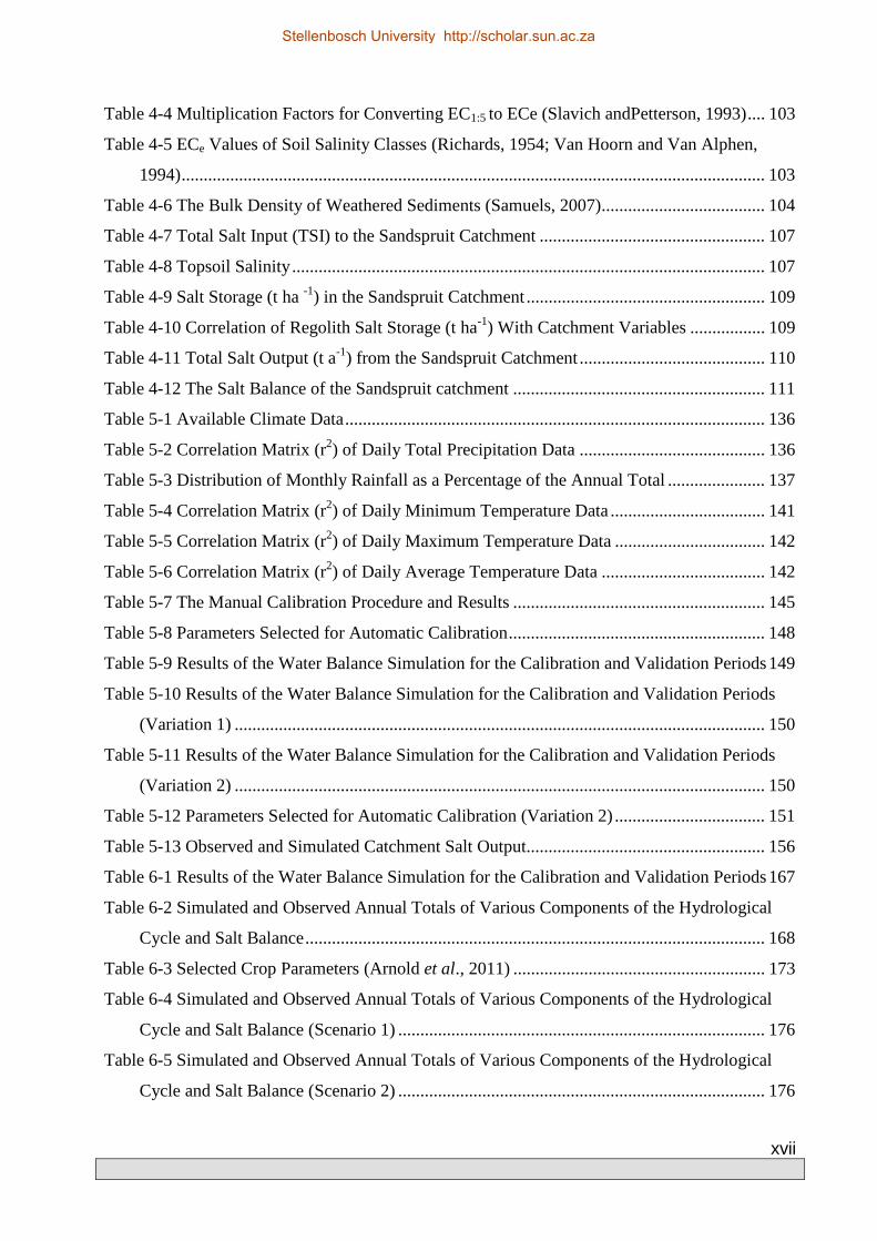
xvii

Table 4-4 Multiplication Factors for Converting EC1:5 to ECe (Slavich andPetterson, 1993) .... 103

Table 4-5 ECe Values of Soil Salinity Classes (Richards, 1954; Van Hoorn and Van Alphen,

1994) .................................................................................................................................... 103

Table 4-6 The Bulk Density of Weathered Sediments (Samuels, 2007) ..................................... 104

Table 4-7 Total Salt Input (TSI) to the Sandspruit Catchment ................................................... 107

Table 4-8 Topsoil Salinity ........................................................................................................... 107

Table 4-9 Salt Storage (t ha -1) in the Sandspruit Catchment ...................................................... 109

Table 4-10 Correlation of Regolith Salt Storage (t ha-1) With Catchment Variables ................. 109

Table 4-11 Total Salt Output (t a-1) from the Sandspruit Catchment .......................................... 110

Table 4-12 The Salt Balance of the Sandspruit catchment ......................................................... 111

Table 5-1 Available Climate Data ............................................................................................... 136

Table 5-2 Correlation Matrix (r2) of Daily Total Precipitation Data .......................................... 136

Table 5-3 Distribution of Monthly Rainfall as a Percentage of the Annual Total ...................... 137

Table 5-4 Correlation Matrix (r2) of Daily Minimum Temperature Data ................................... 141

Table 5-5 Correlation Matrix (r2) of Daily Maximum Temperature Data .................................. 142

Table 5-6 Correlation Matrix (r2) of Daily Average Temperature Data ..................................... 142

Table 5-7 The Manual Calibration Procedure and Results ......................................................... 145

Table 5-8 Parameters Selected for Automatic Calibration .......................................................... 148

Table 5-9 Results of the Water Balance Simulation for the Calibration and Validation Periods 149

Table 5-10 Results of the Water Balance Simulation for the Calibration and Validation Periods

(Variation 1) ........................................................................................................................ 150


(Variation 2) ........................................................................................................................ 150

Table 5-12 Parameters Selected for Automatic Calibration (Variation 2) .................................. 151

Table 5-13 Observed and Simulated Catchment Salt Output ...................................................... 156

Table 6-1 Results of the Water Balance Simulation for the Calibration and Validation Periods 167

Table 6-2 Simulated and Observed Annual Totals of Various Components of the Hydrological

Cycle and Salt Balance ........................................................................................................ 168

Table 6-3 Selected Crop Parameters (Arnold et al., 2011) ......................................................... 173


Cycle and Salt Balance (Scenario 1) ................................................................................... 176




xviii




19

1. INTRODUCTION

The freshwater resources of South Africa are experiencing increasing pressure as a result of increased abstraction, agricultural and economic development, habitat destruction and population increase. Additionally, the impending impacts of climate change are expected to exacerbate the problem, particularly in the western/south-western regions of the country. In addition to quantity, there are also significant water quality challenges in South Africa. The main contributors to water quality problems are (Nkondo et al., 2012):

• Mining (acidity and increased metals content). • Urban development (salinity, nutrients and microbiological). • Industrial activities (chemicals and toxins). • Agriculture activities (sediment, nutrients, agro‐chemicals and salinity).

Salinity has particularly been identified as one of the main water quality problems in South Africa (DWAF, 1986). Effective management of the already scarce freshwater resources, in the complex physical, social and economic environment which characterizes South Africa, is therefore imperative. Water resource quality and quantity issues are often interrelated and therefore need to be addressed in an integrated manner. The South African National Water Resources Strategy 2 (NWRS 2; Nkondo et al., 2012) calls for the protection, use, development, conservation, management and control of water resources in South Africa. The NWRS 2 not only considers water for human consumption, agricultural development and economic growth, but also considers the needs of the biophysical environment, i.e. it calls for a site-specific river discharge to be maintained to support ecological functioning. In South Africa, water resources management occurs at a Water Management Area (WMA) scale. The country has been divided into 9 WMAs, the boundaries of which consider catchment and aquifer boundaries, financial viability, stakeholder participation and equity considerations (Nkondo et al., 2012). These WMAs are managed by Catchment Management Agencies (CMAs), who are responsible for the integrated water resources management in their respective WMA. Currently there, is a drive in the water resources management sector to equip these CMAs with tools, which allow for scientifically based and integrated management of the freshwater resources in South Africa at a catchment scale. In this regard, distributed hydrological modelling has particularly been highlighted as having potential to satisfy these requirements. This work evaluates the use of a distributed hydrological model as a catchment scale water and salinity management tool in a tributary catchment of the Berg-Olifants WMA. It documents the entire hydrological modelling process, i.e. the progression from data collection to model application.

1.1 Background

The Berg River is a valuable source of freshwater to the Western Cape (Figure 1.1). It is a source of water to the Greater Cape Town area, the West Coast region (Saldanha), the irrigated agricultural sector as well as the numerous ecosystems dependant on the river system. The combined impoundments of the Riviersonderend-Berg River system currently contribute more than 80% of the total annual water yield, i.e. 450 million m3, required by the Greater Cape Town


20

and West Coast regions (Gorgens and de Clercq, 2006). Water quality degradation however poses a significant threat to this resource. The Berg River (Figure 1.1) has been exhibiting a trend of increasing salt levels since the 1960s (DWAF, 1993), particularly along the mid- to lower-reaches. This is a cause for major concern due to the social, economic and ecological significance of the Berg River. The increase in salt levels may be attributed to the clearing of natural vegetation (Renosterveld) to make way for cultivated lands and pastures, thereby altering the water balance and mobilizing salts stored in the regolith. This process is termed dryland salinisation and is evident throughout the wheatlands of the Swartland and Overberg regions in the Western Cape. The salts may either be a product of the weathering of rock or it may be brought into the landscape, from the ocean, by rain or wind. Any attempt to maintain water of a suitable quality could be doomed to fail if the prognosis for further decantation of salts from the catchment regolith into tributaries of the Berg River and options for managing this remain unknown. Dryland salinisation has been well studied and documented in Australia. Due to similarities in climate, soils, natural salt levels in the regolith, topography and land use practices (Fey and de Clercq, 2004), the Australian scenario may be valuable in terms of understanding the dynamics of the process in the Western Cape. In Australia it is interpreted that the introduced farming systems generally use less water and resultantly larger volumes of runoff are produced and/or larger amounts of rainfall recharge the groundwater system. An increase in recharge produces a rise in the water table. The groundwater dissolves and mobilizes salts that were stored above the “old” water table in the previously unsaturated regolith, transporting the salts toward the land surface. This produces an increase in soil, and eventually stream, salinity (Greiner, 1998; Walker et al., 1999; Acworth and Jankowski, 2001). The dynamics and mechanisms of the process however differ in the semi-arid Western Cape, when compared to that which dominantly occurs in Australia. Observations made within the Sandspruit catchment, a tributary catchment of the Berg River, suggest that increased groundwater recharge is evident, however the potentiometric surface does not intersect the ground surface. In certain areas of the catchment the potentiometric surface is less than 2 m below ground level in winter. At such depths, capillary action can mobilise water and salts towards the soil surface. Additionally, soil evaporation and evapotranspiration concentrate salts in the upper layers of the soil profile. As shallow lateral subsurface fluxes (throughflow) is the dominant streamflow contributing component in the Sandspruit catchment (Bugan et al., 2012a), it is also interpreted to be the dominant mechanism with which salt is mobilised towards lower valley locations and surface water bodies. (Bugan et al., 2012b) reported that salt storage in the Sandspruit catchment increases with decreasing ground elevation, i.e. it is higher in the valleys and downstream parts of the catchment. This is interpreted to be a function of salt leaching in the hilltops and salt accumulation in the valleys. Land use change has been identified as the dominant approach to mitigate the impacts of and control dryland salinisation (Greiner, 1998; McFarlane and Williamson, 2002; Walker et al., 2002). This has mainly been achieved through a change from annual agricultural cropping systems to perennial vegetation which exhibits a higher evaporative demand. This reduces groundwater recharge/infiltration and the subsequent mobilisation of stored salts.


21

1.2 Study Area

This research was conducted in a significantly saline tributary catchment (a result of dryland salinity) of the Berg River, i.e. the Sandspruit catchment (Figure 1.1). For a detailed description of the locality and physiography of the Sandspruit catchment, the reader is referred to Chapter 3.

Figure 1.1. The locality of the study area in the Western Cape.

1.3 Problem Statement

Due to the social, economic and ecological significance of the Berg River, it is essential that research be conducted in order to establish appropriate land uses and management practices that would reduce the salinisation of the Berg River. Extensive previous research has been conducted to understand the process and dynamics of the salinisation of dryland areas in the Western Cape. However, these investigations were primarily conducted at a field scale as opposed to the


22

catchment scale. A need therefore exists to comprehend and quantify the process at a catchment scale. Additionally, these investigations did not focus on the identification and implementation of potential mitigation measures to improve the water quality of the Sandspruit River, and subsequently the Berg River. Dryland salinity may be classified as non-point source pollution. Many modelling approaches only consider point sources. Thus, these would not be able to adequately represent the salinity dynamics in catchments affected by dryland salinity. The quantification of salts stored and released from individual hydrological units represents information that could provide the basis for hydrological and agro-hydro-chemical modelling of salt redistribution in the catchment. This information would also enable models to be effectively adapted to develop the appropriate criteria for regulating land use and consequently salt mobilisation.

1.4 Aims and Objectives of the Research

The specific objectives of this research are: (a) To study the characteristics and causes of spatial and temporal dynamics of water cycle

components and inorganic salt fluxes in the Sandspruit catchment. (b) To quantify the regolith salt storage and establish its spatial distribution in the Sandspruit

catchment. (c) To evaluate the use of a distributed hydrological and salinity model as a catchment scale

water (quantity and salinity) resources management tool. (d) To quantify the effects of alternative land uses on the catchment scale water and salinity

dynamics.

1.5 Thesis Statement

In light of the above (Section 1.3 and Section 1.4), the concise thesis of this work is to demonstrate that non-point source pollution models can be successfully used to simulate the effects of dryland salinity and to identify mitigation measures. This thesis statement may however be sub-divided according to the following:

(a) To comprehend and quantify all biophysical processes which effect the manifestation and dynamics of dryland salinisation at a catchment scale:

• As the catchment scale is often considered as appropriate for management, a need exists for the up scaling of the results of the numerous local/farm scale studies pertaining to dryland salinity in the Western Cape. This will also facilitate the extrapolation of the methodology and results to catchments which exhibit similar physiographic conditions.

(b) To develop the methodology to facilitate the quantification of the catchment scale distributed regolith salt storage.

• Dryland salinity may be categorised as non-point source pollution. The distributed regolith salt storage therefore needs to be quantified as it will be used as input data for modelling purposes.

• It will also allow for a target approach where mitigation measures are concerned as areas of high salt storage will be identified.

(c) To develop a salinity module to facilitate the simulation of inorganic salt fluxes at a catchment scale.


23

• Many catchment scale water quality models are only able to consider point sources of pollution. Due to the nature of dryland salinity (non-point source pollution) the need exists for the development of process modules to adequately simulate this process.

(d) To evaluate the effect of alternative land use practices on the hydrosalinity dynamics in the Sandspruit catchment.

• Land use change has extensively been used as a dryland salinity mitigation measure in Australia. However, due to different mechanisms of occurrence its potential for use in the Western Cape needs to be evaluated.

The most important contributions to science arising from this dissertation are:

• The development of a methodology to simulate catchment scale water and salt fluxes, which considers distributed regolith salt storage. This methodology may be applicable to other hydrological modelling packages.

• The development of a methodology to quantify the distributed regolith salt storage. The methodology and results may be extrapolated to areas which exhibit similar physiographic conditions.

• The identification of potential dryland salinity mitigation measures. The appropriate application of these mitigation measures may have a significant impact on the water quality in areas affected by dryland salinity.

1.6 Definition of Terms and Concepts

Hydrosalinity dynamics refers to variations in water volumes and inorganic salt concentrations, masses and rates of mobilisation. In the context of this dissertation these dynamics may occur either in surface water, groundwater, precipitation or soil. Regulating hydrosalinity dynamics refers to practices at hydrological unit scale that will reduce the precipitation of salts at the soil surface and the consequent mobilisation of these salts by overland flow, throughflow and baseflow. This may include alternative land use practices. These practices aim to regulate the mobilisation of salts.

1.7 Outline of the Dissertation

This dissertation is organised into 7 Chapters. This chapter (Chapter 1) presents the background information, the formulation of the problem statement, the aims and objectives of the research, as well as the thesis statement. Chapter 2 presents a comprehensive review of previously published work pertaining to the mechanisms of occurrence of dryland salinity and its dynamics. The bulk of the literature emanate from investigations conducted within Australia, where dryland salinity has reached epic proportions in terms of its impact and spatial extent of occurrence. Similarities in climate, topography, geology and land use practices however suggest that the extensive knowledge base developed within Australia, may be very useful to investigations conducted within South Africa, and particularly to those conducted within the semi-arid Western Cape. A review of hydrological models which have been applied in southern Africa is also presented, thus evaluating their potential for use in this study. Chapters 3, 4, 5 and 6 present the scientific papers responding to the objectives of this study. A detailed conceptual water balance and flow model is presented for the Sandspruit catchment in


24

Chapter 3. This work aims to identify the dominant components of the water balance as well as the dominant streamflow generation components. Common theoretical equations are utilised. Stable isotope analysis and a distributed hydrological model are used to conduct hydrography separation. The water balance and conceptual flow model will form the basis for the application of distributed hydrological modelling in the Sandspruit catchment and the development of salinity management strategies. Chapter 4 presents the methodology for and results of the quantification of the salinity fluxes in the Sandspruit catchment. This included the quantification of salt storage (in the regolith and underlying shale), salt input (rainfall) and salt output (in runoff). The quantification of salinity fluxes at the catchment scale is an initial step and integral part of developing dryland salinity mitigation measures. It is an important component of identifying the current salinity status and trend in the catchment, i.e. a state of salt depletion/accumulation or accumulation/depletion rates. Additionally, it will also generate data which will facilitate the calibration and validation of salinity management models. Ultimately however, it provides an indication of the severity of the salinity problem in an area. It is envisaged that this information may be used to classify the land according to the levels of salinity present, provide a guide and framework for the prioritisation of areas for intervention and the choice and implementation of salinity management options. In Chapter 5, the applicability of the JAMS/J2000-NaCl hydrosalinity model as a catchment scale water and salinity management tool in the semi-arid Sandspruit catchment is evaluated. The modelling exercise aims to represent the processes relating to the movement of water and salt from subsurface landscape stores to the land surface and/or to surface water systems. A detailed description of the model is provided, including all process modules and data requirements. The available input data are also discussed. The results of the modelling exercise are also presented. Land use change has been identified as the dominant approach to mitigate the impacts of and control dryland salinisation. In Chapter 6, the effects of alternative land use/management scenarios on the water and salt fluxes in the Sandspruit catchment are evaluated. The JAMS/J2000-NaCl hydrosalinity model was used to conduct the scenario simulations. In Chapter 7 the overall findings of the research are discussed. Additionally, recommendations are also presented.

1.8 References

ACWORTH, R.I. and JANKOWSKI, J., 2001. Salt source for dryland salinity - evidence from an upland catchment on the Southern Tablelands of New South Wales. Australian Journal of Soil Research, 39, pp. 12-25.

BUGAN, R.D.H., JOVANOVIC, N.Z. and DE CLERCQ, W.P., 2012a. The water balance of a seasonal stream in the semi-arid Western Cape (South Africa). Water SA, 38(2), pp. 201-212.

BUGAN, R.D.H., JOVANOVIC, N.Z., FINK, M., STEUDEL, T. and PFENNIG, B., 2012b. Sandspruit Hydrosalinity Modeling. WRC project K5/1849, Deliverable 27. Stellenbosch: Council for Scientific and Industrial Research.

DWAF, 1993. Hydrology of the Berg River basin. Prepared by Berg, R.R. of Ninham Shand in association with BKS Inc. as part of the Western Cape System Analysis. Report No PG000/00/2491. Pretoria: DWAF.


25

DWAF, 1986. Management of the water resources of the Republic of South Africa. Pretoria: Department of Water Affairs and Forestry.

FEY, M.V. and DE CLERCQ, W.P., 2004. Dryland salinity impacts on Western Cape rivers. Report No 1342/1/04. Pretoria: Water Research Commission.

GORGENS, A.H.M. and DE CLERCQ, W.P., 2006. Research on Berg River Water Management. Summary of water quality information system and soil quality studies. Report No 252/06. Pretoria: Water Research Commission.

GREINER, R., 1998. Catchment management for dryland salinity control: model analysis for the Liverpool Plains in New South Wales. Lyneham, Australia: CSIRO Publishing.

MCFARLANE, D.J. and WILLIAMSON, D.R., 2002. An overview of water logging and salinity in southwestern Australia as related to the 'Ucarro' experimental catchment. Agricultural Water Management, 53, pp. 5-29.

NKONDO, M.N., VAN ZYL, F.C., KEURIS, H. and SCHREINER, B., 2012. Draft national water resources strategy 2 (NWRS-2). Version 1: Comprehensive. Pretoria: Department of Water Affairs.

WALKER, G., GILFEDDER, M. and WILLIAMS, J., 1999. Effectiveness of current farming systems in the control of dryland salinity. Adelaide, Australia: CSIRO Publishing.

WALKER, G. et al. 2002. Estimating impacts of changed land use on recharge: review of modelling and other approaches appropriate for management of dryland salinity. Springer Berlin / Heidelberg. Available from: <http://dx.doi.org/10.1007/s10040-001-0181-5>.


26

2. LITERATURE REVIEW

2.1 Dryland Salinity

The occurrence of dryland salinity has been documented throughout the semi-arid regions of the world. In humid and sub-humid areas, where rainfall is sufficient, salinity is of little concern because rainfall is able to leach out accumulated salts (Lamsal et al., 1999). The salinisation of dryland areas has been studied extensively in Australia and to a lesser extent in countries such as South Africa and Argentina. It occurs in dryland areas, i.e. non-irrigated and may be a result of natural soil/regolith salinity and/or from increased groundwater recharge and/or reduced discharge. Salinity may generally be defined as the accumulation of salt in land and water to a concentration that adversely impacts the natural and/or built environments. Dryland salinity possesses the potential to cause extensive environmental degradation, i.e. to flora and fauna, to aquatic and terrestrial ecosystems, to agricultural crops and pastures, to water supplies and to infrastructure. Its occurrence is generally characterized by the appearance of bare salty patches in the landscape, a decline in vegetation cover density, the appearance of salt tolerant species and/or the salinisation of water resources (Greiner, 1998; Walker et al., 1999). It is generally caused by human activities, which alter the hydrological balance of the landscape through the removal of indigenous vegetation to make way for cultivated lands and pastures. According to Eamus et al. (2006) dryland salinity is best interpreted as a change in the hydrological balance of the landscape arising from changes in the ecology of the landscape. In Australia, dryland salinity has assumed epic proportions in its spatial, economic and ecological impact (Eamus et al., 2006). The problem arises as a result of the introduced farming systems using less water, i.e. lower evapotranspiration rates, than the indigenous vegetation (Hatton and Nulsen, 1999). Resultantly, larger volumes of runoff are produced, increased interflow may occur and/or larger amounts of rainfall recharge the groundwater system. The increases in runoff may be immediately discernible, however the impacts associated with increased recharge may take decades to centuries to be fully expressed (Smitt et al., 2003). An increase in recharge produces a rise in the water table (Figure 2.1). According to Peck and Hurle (1973) recharge under annual crops and pastures are typically two orders of magnitude larger than that under indigenous vegetation. Rising groundwater tables dissolves and mobilizes salts that were stored above the old water table in the previously unsaturated regolith and brings them to the surface (Herron et al., 2003; Greiner and Cacho, 2001). The water table does not need to intersect the land surface to cause dryland salinity. When groundwater levels reach a critical depth, i.e. 1 – 2 m below ground level, water can be mobilised to the surface through capillary action (Office of Environment and Heritage, 2011a). Soil evaporation and evapotranspiration also concentrate these salts in the upper layers of the soil profile, adversely affecting vegetation growth (Herron et al., 2003). Peck and Williamson (1987) demonstrated that, in catchments experimentally cleared for agriculture, piezometric surfaces were observed to move upwards at rates up to 2.6 m a-1 in response to increased recharge. The timing of the effects of a large-scale land use change on the catchment water yield is dependent on the groundwater characteristics. This timing is very important, especially when looking at the physical and economic viability of a range of possible management options, since groundwater discharge is the process, which mobilises salt to the land surface and to surface water bodies (Smitt et al., 2003). Catchments affected by dryland salinity typically also exhibit saline groundwater. However, there may be long time delays between any change in land use and the subsequent changes in salinity (Smitt et al., 2003). This salinity is


27

typically very strongly correlated with Cl- (Bennetts et al., 2006) and increases in a downstream direction, thereby exacerbating salinisation in groundwater discharge zones (Salama et al., 1999). Salinised land often develops in lower valley locations and at breaks of slope, however, topography alone is not sufficient to predict the location of salinised areas (Barrett-Lennard and Nulsen, 1989). Salt may be mobilised by overland flow, by lateral sub-surface seepage or by groundwater eventually ending up in rivers or other water features (National Land and Water Resources Audit, 2009). In some places the lateral flow of saline water to low points in the landscape and subsequent evaporation of this water has led to the formation of saline scalds especially in arid and semi-arid zones (Eamus et al., 2006). According to Clarke et al. (1998) major faults explain the location of areas of dryland salinity not explained by topography. The underlying mechanism is hydraulic conductivity variations, i.e. it is observed to be 2.9 to 5.9 times higher inside the fault zone when compared to outside. Minimal studies pertaining to the effects of regional geological features, such as major faults, on spatial variations in hydraulic conductivity and the impacts that this has on groundwater flow and hence the development of dryland salinity have however been conducted. Other factors should however not be excluded when attempting to understand spatial patterns of dryland salinity, i.e. geomorphology, regolith thickness and degree of clearing (Clarke et al., 1998).

Figure 2.1. The general mechanism with which dryland salinity occurs in Australia (reproduced from

Gilfedder et al., 1999) Dryland salinisation may become a considerable cost to a country’s economy and a cause of significant environmental degradation. Not only does salinity degrade productive agricultural land and streams, it also corrodes metals, increases water purification costs and/or reduces the usability of water. Dryland salinity affects land and water resources on site, e.g. at the farm scale, but also elsewhere in the catchment (downstream). On farms salinity damages infrastructure, salinises water resources, causes loss of farm flora and fauna and loss of shelter and shade.


28

Salinity also has a major impact on public resources such as water supplies, thereby affecting sources of drinking water and irrigation (National Land and Water Resources Audit, 2009). Eamus et al. (2006) estimates the cost associated with lost agricultural produce and damage to infrastructure in the Murray-Darling Basin, Australia’s largest river, to be in the order of $250 million. According to Bennett et al. (1997), as cited by Greiner and Cacho (2001), the costs associated with dryland salinity in Australia is estimated to be in the order of $270 million/year, comprising agricultural, infrastructure and environmental costs of $130 million, $100 million and $40 million respectively. Dryland salinisation has been increasingly recognised as one of the main land and water degradation issues in southern Australia (MDBMC, 1999). While there is general consensus concerning the magnitude of the problem, deliberation still occurs about the way to manage the problem. This is due to the wide range of processes leading to salinisation and also to the economics of dryland salinity which has not been well integrated with biophysical studies (Baker et al., 2001). It is however distinctly apparent that more land and rivers will become more saline unless a plan which helps manages and control dryland salinity is developed and implemented (MDBMC, 1999).

2.1.1 Sources of Salt

A diverse range of inorganic salts may cause dryland salinity, which includes sodium, calcium, magnesium, potassium, chloride, sulphate, bicarbonate and carbonate ions (Office of Environment and Heritage, 2011a). The occurrence of salt in the landscape may be as a result of weathering, deposition by rain, aeolian deposition and the release of connate salts. Weathering Weathering is the process which describes the decomposition of minerals in the rock and the subsequent release of soluble ions that combine to form salts. The type of ions released is a function of the type of rock being weathered. For significant weathering to occur, a continuous flow of new water from recharge should occur (Office of Environment and Heritage, 2011a). Rain Water and Aeolian Deposits A possible explanation for the occurrence of salts in a landscape is the combination of a semi-arid climate with close proximity to the ocean. Rainfall and wind can transport salts of marine origin and deposit them on land and in surface waters. Ocean spray may also be a significant contributor of salts to the landscape. Rainwater generally has a salt concentration of 10-30 mg L-1. Assuming a total annual rainfall of approximately 500 mm, then this equates to 150 kg of salt per hectare per year (150 kg ha-1 yr-1). A large proportion of the deposited salts are washed directly into surface water systems (Office of Environment and Heritage, 2011a). Hingston and Gailitis (1976) reported that the annual accumulation rate of salt, i.e. mainly sodium and chloride, in the wheat belt of Western Australia was 100-250 kg ha-1 in high rainfall coastal areas and approximately 10-20 kg ha-1 300 km inland. Chapman (1966) presented similar findings. He stated that in south-west Africa, it occurs that salts are blown in from the sea over centuries and deposited inland (aeolian salts). According to Bresler et al (1982) the atmospheric salt composition changes with increasing distance from the coast. Absolute Cl- and Na+ concentrations in the rainfall decrease as the air mass moves further inland. Hatton and Nulsen (1999) suggest that salts in the unsaturated zone are dominantly of atmospheric origin. Strong winds may also transport significant quantities of salt, producing aeolian derived salt deposits, which particularly occur in coastal areas. Erosion of such deposits may mobilise salts into waterways (Office of Environment and Heritage, 2011a).


29

Connate Salts Certain fine grained geological units, e.g. shale and siltstone, which were deposited under marine conditions, may contain large quantities of salt that may be dissolved into the groundwater system. Resultantly, groundwater associated with such rock types are commonly of a poor quality, especially where there has not been fracturing, uplifting and/or flushing (Office of Environment and Heritage, 2011a).

2.1.2 Factors which Contribute to Dryland Salinity

According to Bennett (1998) the biophysical properties causing dryland salinity are generally well understood and relate to the induced hydrological imbalance. The successful implementation of management action requires careful assessment of the relative significance of these interconnected biophysical factors, which are region dependant. These factors include:

• Climate and soil type; • The size, geology and topography of the catchment; • The depth of the water table and the groundwater salinity across the catchment; • The catchment salt store in the saturated and unsaturated zones; • The spatial extent of dryland salinity and its position in the landscape; • Land use options, and economic/social/political constraints and factors.

Many areas in Australia are naturally saline as a result of a combination of biophysical factors (Office of Environment and Heritage, 2011a):

• Ancient climatic conditions and a geological history, which has generated and stored high levels of inorganic salts;

• The current semi-arid/arid climate and relatively flat topography which are conducive to salt accumulation and concentration in specific locations;

• Long-term climate trends causing dynamic groundwater levels and salt mobilisation.

The Office of Environment and Heritage (2011a) also highlighted the contribution of these biophysical factors to the development of dryland salinity through a series of illustrations. These are represented in Table 2-1 and Figures 2.2 - 2.3.

Table 2-1 Factors Which Contribute to the Development of Dryland Salinity (Office of Environment and Heritage, 2011a)

Factor Description Result Figure

Climate A semi-arid/ arid climate where the rate of evaporation greatly exceeds precipitation

Salt accumulation

Topography A flat landscapes results in slow surface water and

groundwater flow Accumulated salts are washed

away slowly Figure

2.2

Catchment outlet size

A narrowing of the width or a reduction in basement depth at the catchment outlet are common

restrictions to surface water and groundwater outflow

Accumulated salts are washed away slowly

Figure 2.3


30

Figure 2.2. A flat landscape does not allow for the rapid flow of groundwater and surface water. Consequently, any accumulated salts are washed away slowly (reproduced from Office of Environment and Heritage, 2011a).


31

Figure 2.3. A narrowing of the width or a reduction in basement depth at the catchment outlet are common restrictions to surface water and groundwater outflow (reproduced from Office of Environment and Heritage, 2011a).

2.1.3 Investigations in Australia

Dryland salinity has received extensive attention, particularly in Australia, where its occurrence is widespread. The Australian Dryland Salinity Assessment 2000 Report (National Land and Water Resources Audit, 2009) compiled state scaled assessments of the presence and potential for development of dryland salinity. The potential for development is determined based on information regarding shallow groundwater tables and land use practices. The results of this assessment indicate that the area of land with a high potential to develop dryland salinity exceeds 5.5 million ha. This area further has the potential to increase to 17 million ha by 2050. Currently, the total area of land adversely impacted by dryland salinity in Australia is approximately 2.5 million ha. The most important factors which affect salinisation are the physio-chemical properties of the soil, water management practices, topography, the depth of the water table, the quality of shallow groundwater and climatic conditions (Lamsal et al., 1999). The increase in land salinisation, a result of land clearing for agriculture has been accompanied by increasing trends in the salinity of water resources in the south-west of Western Australia. The current


32

salinity for various south-western streams is above 800 mg L-1, resulting in them being unsuitable for drinking purposes (McFarlane and Williamson, 2002). Eamus et al. (2006) conceptualized 3 ways by which clearing of natural vegetation causes dryland salinisation:

• Tree clearing increases local groundwater recharge, causing water tables to rise directly under the cleared land, mobilizing salts towards the surface;

• In a local hillslope system, increased recharge in combination with increased overland flow may cause saline groundwater levels to develop vertically, but also to flow and accumulate downslope (compounded by the accumulation of overland flow);

• In regional systems, such as those associated with the majority of salinized land in Western Australia, broad valley lands are salinizing through a complex combination of the processes at large scales, i.e. increased recharge, the rise of saline water tables, large regional flood events caused by increased overland flow from cleared hillslopes, and increased hydraulic gradients from evolving groundwater levels under cleared, adjacent hillslopes.

According to Office of Environment and Heritage (2011a) the introduction of European farming systems in Australia has altered the distribution of vegetation types across the landscape, introducing agricultural crops as a replacement to indigenous species. The introduced annual crops and pastures, e.g. wheat and clover, generally have a shallow root system and exhibit an annual water use pattern. Alternatively, perennial indigenous vegetation is deep rooted and requires water for growth throughout the year. Additionally, indigenous vegetation also has the capacity to increase growth rates in response to rainfall events. Both these characteristics limit groundwater recharge rates (Office of Environment and Heritage, 2011a). According to Williamson (1998), as cited by McFarlane and Williamson (2002), there are three basic requirements for the salinisation of soil and streamflow to occur:

• A store of salt in the regolith ranging from 50-5000 t ha-1 in a region which experiences 320-1400 mm of rainfall per annum, respectively;

• A supply of water to mobilize the salt. Groundwater recharge should range between 4-10% of rainfall;

• A mechanism by which the salt is redistributed to specific locations in the landscape, e.g. rivers, where it causes degradation. The hydrogeological properties of the regolith influence these water transmitting mechanisms.

Peck and Hatton (2003) investigated the salinity and discharge of salts from catchments in Australia. They stated that top soils (0–0.2 m depth) are said to be saline if the saturated extract exhibits an electrical conductivity (EC) of approximately 4 dS m-1, which is the criteria for saline soil used by the US Salinity Laboratory (Peck and Hatton, 2003) and which is also used in many countries. When the salt concentration in the root zone exceeds the tolerance limits of the crop, crop growth may be negatively affected (American Society of Civil Engineers, 1990; Karim et al., 1990; Somani, 1991; Mondal et al., 2000). At such a degree of salinity, plant growth is restricted even though enough water may be present in the root zone (American Society of Civil Engineers, 1990; Karim et al., 1990; Somani, 1991; Mondal et al., 2000). Peck and Hurle (1973) as cited by Peck and Hatton (2003), used stream gauging and rainfall records, and measurements of the salinity of rainfall to estimate the chloride balance of catchment areas in southwest Australia that remained under natural forest vegetation or had been partly cleared and developed for dryland agriculture. They showed that in partly farmed areas,


33

the total chloride input was 3-21 times lower than the total chloride output. For comparative reasons this ratio was measured in uncleared catchments, where a balance between the input and output of chloride was observed. McFarlane and Williamson (2002) studied the nature, extent and consequences of water logging and dryland salinisation in the agricultural areas of Southern Australia. It was reported that there are basic requirements for the development of saline and waterlogged areas within the specific geology and geomorphology of the region. According to McFarlane and Williamson (2002) water logging and salinity are a result of changes in the inputs, outputs and storage of water and salts caused by the reduced water use by annual crops and pastures, which have replaced the indigenous vegetation. Rising water levels and waterlogging provide a transport mechanism for salt from deeper saline aquifers to the soil surface where concentration through evaporation results in salt accumulation on the soil surface and in the rooting zone. Downgradient increases in groundwater salinity occur in a variety of groundwater systems within Australia (Bennetts et al., 2006; Salama et al., 1993). This increase in salinity may be explained through a combination of evaporation in discharge zones and dissolution of connate salts. Cartwright et al. (2004) suggests that considerable salt concentration by evaporation may occur in groundwater discharge zones in Australia, with minimal contribution from connate salts and evaporates. The majority of Australian studies suggest that the increase in groundwater salinity is a result of the clearing of indigenous vegetation, thereby increasing recharge, which either leaches salts from salt deposits in the vadose zone downwards (Leaney et al., 2003) or causes the water table to rise, dissolving salts in the process. Water-rock interactions also influence the composition of groundwater and hence groundwater salinity. Its relative effects can by estimated by comparing the median groundwater composition with that of local rainfall, using the chemically inert species Cl-. National Land and Water Resources Audit (2001) compiled future dryland salinity risk and hazard estimates. The results indicate that area of agricultural and pastoral land currently affected by dryland salinity (5.7 million hectares) would increase to 17 million hectares by 2050 in the absence of effective management. The results of these estimates at the state scale are shown in Table 2-2. The areas which exhibit the greatest risk are South Australia (Murray-Darling Basin), Victoria, New South Wales and the agricultural areas of south-west Western Australia. These estimates were however derived using limited data, and particularly the lack of groundwater data was a major limitation.

Table 2-2 Areas at Risk from Shallow Water Tables or with a High Salinity Hazard by State (Australia) (National Land and Water Resources Audit , 2001)

State 1998 – 2000 (ha) 2050 (ha) Western Australia 4 363 000 8 800 000

Victoria 670 000 3 110 000 South Australia 390 000 600 000

New South Wales 181 000 1 300 000 Tasmania 54 000 90 000

Queensland not assessed 3 100 000

Total 5 658 000 17 000 000 Pannell and Ewing (2006) is however of the opinion that the results from the National Land and Water Resources Audit (National Land and Water Resources Audit, 2001) is a substantially over estimation of the areas of land that are or will be actually affected by dryland salinity. The identification of the areas at risk was a function of the groundwater table depth. Areas which


34

exhibit a groundwater table depth less than 2 m or between 2 m and 5 m were interpreted to be at risk. However, Pannell and Ewing (2006) suggests that within the land meeting this criterion only a proportion will suffer reduced productivity from the effects of salinity. Ferdowsian et al. (1996) estimated that the current area in Western Australia where plant growth is affected by salinity is approximately 1.8 million ha, which is less than 50% of the land area interpreted to be at risk (National Land and Water Resources Audit, 2001). Regardless, there is no doubt that the impacts are very extensive, and will become more so (Pannell and Ewing, 2006).

2.1.4 Salinity Investigations in the Western Cape (South Africa)

The phenomenon of dryland salinity in the Western Cape (South Africa) was first investigated by Malherbe (1953). However the issue has recently (1990’s) received widespread attention due to the pronounced salinisation of the Berg River. This has culminated in a series of Water Research Commission (WRC) projects, aimed to understand and address the issue. Malherbe (1953) identified the presence of fossil salts as a cause of dryland salinity. Fossil salts are salts deposited in marine sediments of ancient seas. These sediments are buried, lithified, then uplifted and become parent material for the soil. Evaporation of groundwater concentrates these salts at the surface thereby degrading the soil. The present hard pans and soils of the North- western coastal area of the Western Cape developed as a result of inland sea water intrusion (Malherbe, 1953). Sedimentary rocks in South Africa (e.g. Dwyka Series, the Malmesbury shale and the Enon conglomerate) are rich in soluble salts, which if weathered to soil material may cause an accumulation of salts under low rainfall conditions (Malherbe, 1953). These salts may remain in the original soils resulting in the area becoming saline. During the wet winter, flood and seepage water transport salts from the higher- to lower-lying areas where the water evaporates and the salts are left to concentrate at the soil surface. The salts in the districts of Malmesbury and Picketberg in the Western Cape are believed to have originated from the sea as well as from the weathering of the underlying bedrock (Malherbe, 1953). According to Fourie (1976), the West Coast of South Africa is a semi-arid region in which dryland salinity is expected. The Department of Water Affairs (DWA) has monitored the water quality in the Berg River since the mid-1970s. Natural soil salinity has been identified as a source of salts affecting the water quality of the Berg River (Fourie and Steer, 1971; Fourie and Görgens, 1977). Fourie (1976) assessed the salinity of the Berg River in 1976 by focusing on certain Berg River tributaries and reported them to exhibit elevated salt concentrations. Fourie and Görgens (1977) investigated the mineralization of the Berg River and it was reported that the salinity increase of the river could be the result of increasing irrigation practices along the river. Flügel (1995) extensively studied river salinisation due to dryland agriculture between 1985 and 1986 in the 150 km2 catchment of the Sandspruit River, a tributary of the Berg River. Water bodies within the catchment were investigated with the aim of identifying and quantifying their salinity dynamics. Flügel (1995) reported that dryland agriculture contributed to river salinisation based on the findings that the bulk annual atmospheric deposition accounted for only a third of the total salt output for 1986. The mean annual rainfall in the Sandspruit River catchment area is approximately 400 mm a-1, and was reported to have a salt concentration of 37 mg L-1. Sodium and chloride, transported by wind and rain from the Atlantic Ocean, were reported to be the dominant ions. Flügel (1995) stated that the balance of the total salt output was delivered by groundwater and interflow from the weathered shale and the soils within the catchment.


35

Görgens and de Clercq (2006) assessed the influence of irrigation return-flow on the water quality of the Berg River and it was reported that its contribution to the salt levels in the Berg River was minimal when compared to the consequences of dryland salinisation. A need for considerable improvement of monitoring systems for point and non-point source pollution in the Berg River catchment was highlighted. Fey and de Clercq (2004) undertook a pilot study to determine whether a more extensive investigation is required of dryland agricultural impacts on river salinity in the Berg River catchment. It was reported that dryland salinity is extensive and that it is likely to have a significant impact on the water quality of the Berg River. Extensive patchiness in croplands, especially in wheat fields, which dominate the land use in the Berg River catchment, was identified. Ground truthing of these patches confirmed that they are associated with soil salinity. The soils were found to be sufficiently saline to affect wheat growth. The findings of this study suggested the need for a more detailed survey of salt distribution in the soils, regolith, and ground- and surface waters coupled with a fundamental study of salt mobilisation in response to climate, topography and land use practice in a small scale catchment. The results would serve as a prelude to extrapolation and calculation of the extent of the problem through hydrological modelling. de Clercq et al. (2010) and Bugan (2008) investigated the hydrosalinity dynamics in the soil and vadose zone of a small scale catchment (SSC), i.e. Goedertrou, exhibiting evidence of dryland salinity and which is representative of semi-arid conditions in the Berg River catchment. The study not only examined salt sources and storage but also groundwater fluxes and catchment runoff with the view of informing future large-scale modelling and to guide the development of on-farm management practices. An experimental site was also established at Voëlvlei Dam to allow for a comparison of hydrology and salt balances to be made between winter wheat and restored Renosterveld. Monitoring and modelling of runoff under different vegetation scenarios (winter-wheat and Renosterveld) suggested that land use changes have a potential impact on salt release from the regolith into surface water. Salt and water discharge into the Berg River was also monitored at the medium scale Sandspruit catchment (de Clercq et al., 2010). This study has provided valuable information concerning the water and salt fluxes in overland flow and the vadose zone from different land uses. de Clercq et al. (2010) also suggested that the salts inducing salinisation of areas in the Berg River catchment are of marine origin as opposed to being products of rock weathering. Aqueous extraction of various regional Malmesbury shale powders provided evidence that these contribute insufficient quantities of inorganic salts to account for those discharging from catchments such as the Sandspruit. Resultantly it was interpreted that the salts present in the regolith have accumulated meteorically over a long period. This contradicts an initial theory that the salts are contributed from rocks, which are of marine origin. de Clercq et al. (2010) also calculated the input and output of salts from the Sandspruit catchment, a significantly saline tributary of the Berg River. The net salt discharge (a maximum of 20 000 tons a-1, however averaging at 6 700 tons a-1) when calculated per unit area of the catchment is close to 0.5 ton ha-1 a-1. The chemical signature of the discharge reflected a marine origin as the salts, i.e. chloride, sulphate and bicarbonate, concentrations match those of seawater. de Clercq et al. (2010) suggest that the salts discharging from catchments such as the Sandspruit have accumulated aerially over a long period during which either the climate was more arid and/or there was a vegetation cover (renosterveld and, before that, a speculated Olea-Rhus savanna) with a larger water use potential when compared to wheat. Recommendations from the study highlighted a need for continued monitoring in order to describe typical salinity patterns in


36

similar environments, to inform hydrological models and to establish management measures and guidelines.

2.2 The Impacts of Dryland Salinity

Dryland salinity may have significant long term impacts. These impacts may broadly be categorised as on-site impacts and off-site impacts. On-site impacts are generally associated with the salinisation of land and water and are clearly visible and quantifiable. Off-site impacts are a result of increased water salinisation and sediment loads and are much less visible and quantifiable (Office of Environment and Heritage, 2011a). The on-site impacts may include (Office of Environment and Heritage, 2011a):

• Waterlogging of soils and groundwater discharge (seepage, springs and baseflow to streams);

• The accumulation of salt in the soil and the associated toxicity; • A decline in the vegetation cover density and a change in the vegetation towards

increasingly salt and waterlogging tolerant species; • The degradation of the soil structure, the formation of dispersive sodic soils, poor soil

drainage and hard packing of soil surfaces; • The decline and loss of productive land; • Increased soil erosion and the subsequent loss of fertile top soil and the formation of

erosion features (e.g. gullies); • An increase in groundwater salinity; • The degradation of surface water quality as a result of increased salt and sediment load.

The off-site impacts may include (Office of Environment and Heritage, 2011a):

• A decline in downstream biodiversity;

• The deterioration of the health of riparian, aquatic and groundwater dependant ecosystems;

• The degradation of water quality resulting in it being unfit for human consumption, irrigation, stock watering and industry;

• Damage to downstream infrastructure, e.g. buildings, roads and pipes.

Soil salinisation is reported to reduce the potential yield of salt-sensitive crops and pastures by more than 10%, however reductions of 50% are common in areas where salinity is combined with water logging and sodicity (McFarlane and Williamson, 2002). High salinity soil-water is evident in the root zone in many Australian catchments, and the link between saline soil-water and high transpiration rates is well established (Leaney et al., 2003). Initially, many plants suffer from the effects of waterlogging, as their roots can no longer take up oxygen. Gradually, the toxic effects of salt accumulation in the root zone also affect vegetation health. As the level of salinity increases, salt tolerant species begin to succeed those that are more salt sensitive (Office of Environment and Heritage, 2011a). Eamus et al. (2006) also states that excessive salt concentrations within the plant root zone causes reduced seed germination, reduced growth, reduced yield and eventually plant death. According to Murray et al. (2003), salinity at the landscape scale affects the ecosystem species composition, ecosystem structure, net primary productivity and biodiversity.


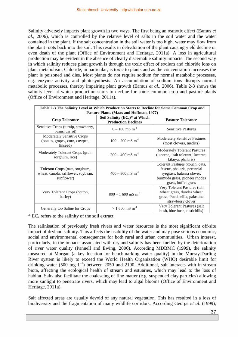
37

Salinity adversely impacts plant growth in two ways. The first being an osmotic effect (Eamus et al., 2006), which is controlled by the relative level of salts in the soil water and the water contained in the plant. If the salt concentration in the soil water is too high, water may flow from the plant roots back into the soil. This results in dehydration of the plant causing yield decline or even death of the plant (Office of Environment and Heritage, 2011a). A loss in agricultural production may be evident in the absence of clearly discernable salinity impacts. The second way in which salinity reduces plant growth is through the toxic effect of sodium and chloride ions on plant metabolism. Chloride, in particular, is toxic to plants and as the concentration increases the plant is poisoned and dies. Most plants do not require sodium for normal metabolic processes, e.g. enzyme activity and photosynthesis. An accumulation of sodium ions disrupts normal metabolic processes, thereby impairing plant growth (Eamus et al., 2006). Table 2-3 shows the salinity level at which production starts to decline for some common crop and pasture plants (Office of Environment and Heritage, 2011a).

Table 2-3 The Salinity Level at Which Production Starts to Decline for Some Common Crop and Pasture Plants (Maas and Hoffman, 1977)

Crop Tolerance Soil Salinity (ECe)* at Which

Production Declines Pasture Tolerance

Sensitive Crops (turnip, strawberry, beans, carrot)

0 – 100 mS m-1 Sensitive Pastures

Moderately Sensitive Crops (potato, grapes, corn, cowpea,

linseed) 100 – 200 mS m-1

Moderately Sensitive Pastures (most clovers, medics)

Moderately Tolerant Crops (grain sorghum, rice)

200 – 400 mS m-1 Moderately Tolerant Pastures

(lucerne, ‘salt tolerant’ lucerne, kikuya, phalaris)

Tolerant Crops (oats, sorghum, wheat, canola, safflower, soybean,

sunflower) 400 – 800 mS m-1

Tolerant Pastures (couch, oats, fescue, phalaris, perennial ryegrass, balansa clover,

burmuda grass, pioneer rhodes grass, buffel grass

Very Tolerant Crops (cotton, barley)

800 – 1 600 mS m-1

Very Tolerant Pastures (tall wheat grass, dundas wheat grass, Puccinellia, palastine

strawberry clover

Generally too Saline for Crops > 1 600 mS m-1 Very Tolerant Pastures (salt bush, blue bush, distichilis)

* ECe refers to the salinity of the soil extract The salinisation of previously fresh rivers and water resources is the most significant off-site impact of dryland salinity. This affects the usability of the water and may pose serious economic, social and environmental consequences for both rural and urban communities. Urban interest, particularly, in the impacts associated with dryland salinity has been fuelled by the deterioration of river water quality (Pannell and Ewing, 2006). According MDBMC (1999), the salinity measured at Morgan (a key location for benchmarking water quality) in the Murray-Darling River system is likely to exceed the World Health Organization (WHO) desirable limit for drinking water (500 mg L-1) between 2050 and 2100. Additional, salt interacts with in-stream biota, affecting the ecological health of stream and estuaries, which may lead to the loss of habitat. Salts also facilitate the coalescing of fine matter (e.g. suspended clay particles) allowing more sunlight to penetrate rivers, which may lead to algal blooms (Office of Environment and Heritage, 2011a). Salt affected areas are usually devoid of any natural vegetation. This has resulted in a loss of biodiversity and the fragmentation of many wildlife corridors. According George et al. (1999),


38

without the implementation of management measures, most or all of the damp land and woodland communities will be lost to salinity in Western Australia. Infrastructure is also at risk to the effects of dryland salinity. Typical impacts include a decline in the lifespan of roads and pavements and the corrosion and destruction of bitumen, concrete and brick structures. According to (National Land and Water Resources Audit, 2001), assets at high risk from shallow saline water tables by 2050 will include 67 000 km of road, 5 100 km of rail and 220 towns.

2.3 Assessing the Hazards and Risks Posed by Dryland Salinity

The most important factors controlling the salinity hazard and risk for a particular catchment is climate, catchment shape, hydrogeology, soils and land use. Knowledge of these allows for the estimation of the potential timeframe, severity and size of area that might be affected by dryland salinity (Office of Environment and Heritage, 2011a). According to Powell (2004) assessing the salinity risk is the first step in any strategic decision-making by producers and advisors. It also facilitates the clarification of the nature of the salinity, i.e. whether it is land salinisation or stream salinisation. Salinity hazard and salinity risk are measures of the propensity of a landscape’s biophysical characteristics, combined with its management, to express salinity (Office of Environment and Heritage, 2011a). Littleboy et al. (2003) defines salinity hazard as the inherent landscape or catchment characteristics that predispose a particular area to the development of salinity. These physical characteristics include:

• Climate (long-term average rainfall and evaporation)

• Topography • Catchment shape

• Groundwater properties (e.g. storage capacity, groundwater levels and groundwater salinity)

• Geology • Geomorphology • Drainage or surface flow characteristics

• Regolith thickness and type

• Soil attributes • Soil stores in the vadose zone

The salinity risk is a measure of the likelihood of salinity occurring as a result of the interactions between land use, water balance, climate and other activities (Littleboy et al., 2003). Essentially, it is the likelihood of the salinity hazard being realised. It is a factor of the salinity hazard and the temporally variable conditions which affect the salinity processes (Office of Environment and Heritage, 2011a). The salinity risk provides a good indication of whether salinisation will occur, as well as the potential location, severity and the expected extent (Office of Environment and Heritage, 2011a). Salinity risk factors include:

• Short-term extreme climatic events; • Land use; • The condition of the vegetation; • The condition of the soil

Salinity mitigation measures should target changes in land use and management that are likely to have the greatest influence on the salinity risk of a landscape at a particular time (Office of


39

Environment and Heritage, 2011a). The salinity risk is the biggest factor determining whether salinisation will occur. Determining the relative salinity hazard and risk is a useful measure to inform the selection and implementation timing of potential mitigation measures. It also allows for the comparison and ranking of areas for priority management.

2.4 Managing Dryland Salinity

It is clear that management options are needed to mitigate dryland salinity (Smitt et al., 2003). Managers are required to answer questions pertaining to salinity targets, the costs of salinity and how management options will vary according to landscape and catchment land uses (Dawes et al., 2004). Dryland salinisation poses a serious challenge to land and water managers at both local and regional scales. Eamus et al. (2006) states that the conceptual models for how the clearing of natural scrubland translates into salinized land and water varies greatly and these variations have major implications for management strategies. According to Greiner (1998) the following aspects need to be addressed when developing a catchment management strategy for salinity:

• The preferred options for land use change • The scale of land use change required • Suitable locations to apply land use change • The degree of salinisation which is economically reasonable • How are the costs of salinity and its control shared across the catchment

In addition, management strategies should also take geological variations into account to be effective (Clarke et al., 1998). According to Williamson (1998), as cited by McFarlane and Williamson (2002), rehabilitation requires control of only one of the three basic requirements (see Section 1.1.3) for the salinisation of soil and streamflow to occur. However, where management is only partially effective, a suitable control should be identified within the other two factors. The removal of stored salt would take hundreds to thousands of years and thus this is not considered a feasible option. A logical approach for long term control is to manage the cause and restrict groundwater recharge across the landscape. According to McFarlane and Williamson (2002) recharge control has been the dominant approach to reducing dryland salinisation in Australia for the past 40 years. This approach focuses on altering the type, distribution and rooting depth of vegetation by using plants suited to productive growth in seasons of high evaporative demand. Landholders generally accept the notion that land use change is necessary for controlling water tables and salinisation (Greiner, 1998). However, unless catchment managers and landholders are aware of the environmental consequences of land use change as well as the economic dimensions of the problem and the trade-offs involved, then land use change for water table control is unlikely to be implemented. A further impediment to this management option is that landowners in the recharge areas of the catchment have no motive to reduce groundwater accessions because they are not exposed to the costs associated with the salinisation (Greiner, 1998). Walker et al. (2002) is also of the opinion that to manage dryland salinity, knowledge of the effects of land use change on groundwater recharge is required. There are various techniques available for comparing groundwater recharge under different land uses. These include soil tracer methods which, although they are good in terms of replication and remote field sites, are subject


40

to spatial variability. Lysimeters are also good for comparison, however their use in drier areas and on sloping land is a challenge. The availability of soil water data allows for the use of agronomic water balance studies, which with the aid of a soil-vegetation model may be used to estimate long-term deep drainage (Walker et al., 2002). The analysis of specific land-use scenarios, e.g. perenniality, and root and leaf area dynamics requires the use of complex models, which require complex and extensive data for calibration. To achieve salinity targets, changes in land use and land management practices as well as the implementation of engineering works are required to reduce the export and mobilisation of salts from catchments affected by dryland salinity (Herron et al., 2003). Alley cropping is regarded as a suitable management option as it will allow the agriculture to be continued in the bays between the rows. However this method would require as much perennial, preferably deep rooted, vegetation as possible in the bays to achieve the required recharge reductions. (Greiner, 1998) suggests that dryland plains should be subjected to opportunity cropping and reduced fallow rotations and that perennial pastures should be re-introduced in all areas of the catchment. According to Hatton and Nulsen (1999), ecosystem mimicry may be regarded as a useful concept in the development of management methods for minimising the impact of inorganic salts on land and water resources in southern Australia. Pannell and Ewing (2006) suggests that the main action to prevent groundwater tables from rising is the establishment of perennial plants, either herbaceous (pastures or crops) or woody (trees and shrubs). Perennial pastures can be placed anywhere in the catchment. Ideally, a mixture of warm and cool season plants will ensure that water is used for active growth all year round. Where these saline water tables are already shallow, farmers still have the option of planting salt tolerant species, e.g. saltbush. Angus et al. (2001) suggests that lucerne pastures and improved crop management can result in greater use of rainfall than annual pastures, fallows, and poorly managed crops. The tactical use of lucerne-based pastures in sequence with well-managed crops can help with the dewatering of the soil and reduce or eliminate the risk of increased groundwater recharge. Farmers may not be able to reduce the salinisation process when land use management options require high levels of investment with little or delayed return, as is the case with tree plantations (Greiner, 1996). Widespread re-afforestation of farmland is unlikely for economic reasons as it would reduce farm incomes (Crosbie et al., 2008). Agroforestry has however been proposed for certain areas, which requires the introduction of woody perennials either as crop rotations, alley crops or plantation blocks (Lefroy and Stirzaker, 1999). At a local scale, i.e. farm scale, the introduction of tree belts have reduced recharge and increased interception of laterally flowing shallow groundwater (White et al., 2002). Trees should be placed where groundwater needs to be intercepted as the root systems of pasture plants are generally too shallow to access this water. Trees use the most water in a limited area, whereas pastures use less water but over a greater area (Office of Environment and Heritage, 2011b). Groundwater use by plantation blocks shows large variation, i.e. between 700 mm a-1 under favourable conditions to almost nothing on hypersaline groundwater (Benyon et al., 2006). Catchment scale applications have shown to result in lower water tables, reduced areas of water logging and a reduction in salt export (Crosbie et al., 2007). Selecting the most suitable areas to plant trees for salinity control requires extensive knowledge of the hydrology of the catchment (Stirzaker et al., 1999). Blocks of trees planted on groundwater discharge sites have been observed to decrease the groundwater level, however it may result in the concentration of salts in the rooting zone (Heupeman, 1999). In certain cases this has resulted


41

in a reversal of the hydraulic gradient at the site, preventing any mechanism of salt export and consequently limiting the lifespan of the tree block. (Office of Environment and Heritage, 2011b) presented several tree and shrub species which may be suitable for recharge control in saline areas, which are presented in Table 2-4. The species presented in Table 2-4 may be used as a reference when selecting a mix of salt tolerant trees and shrubs suitable for planting on saline sites. Planting a combination of species across a site reduces the risk of failure and enhances the biodiversity and shelter benefits achievable from the planting.

Table 2-4 Tree and Shrub Species for Saline Areas (Office of Environment and Heritage, 2011b)

Botanical Name Common

Name

Class 1: 200 – 400 mS m-1

(slightly saline)

Class 2: 400 – 800 mS m-1 (moderately

saline)

Class 3: 800 mS m-1

(very saline)

Class 4: 1600 mS

m-1 (highly saline)

Uses Origin

Acacia mearnsii Green wattle × × A, C, F Australia

Acacia melanoxylon

Black wood × × A, E, F Australia

Acacia salicina # Willow wattle × × × A, G

Australia

Acacia saligna # Orange Wattle × × × G, F

Australia

Acacia stenophylla

River cooba × × × A, C, D, G Australia

Atriplex spp # Saltbush × × × × G Australia

Casuarina cunninghamiana

River she oak × × × A, C, F

Australia

Casuarina glauca *

Swamp she oak × × × × A, C, H

Australia

Casuarina obesa WA swamp

oak × × × × A Australia

Eucalyptus astringens #

Brown mallet × × A, C, F

Australia

Eucalyptus camaldulensis *

River red gum × × × A, C, E, F

Australia

Eucalyptus camphora #

Swamp gum × × A, C Australia

Eucalyptus cladocalyx #

Sugar gum × × A, B, E, G Australia

Eucalyptus kondinensis

Stocking gum × × × ×

Australia

Eucalyptus largiflorens #

Black box × × × A, C, F Australia

Eucalyptus leucoxylon #

Yellow gum × × × A, C, E Australia

Eucalyptus melliodora

Yellow box × × A, C, E, F Australia

Eucalyptus microtheca #

Coolibah × × × A, C, F Australia

Eucalyptus occidentalis *#

Flat top yate × × × A, C, F Australia

Eucalyptus ovata Swamp gum × A, C, E, F Australia

Eucalyptus sargentii #

Sergeants mallet × × × ×

Australia

Eucalyptus sideroxylon

Iron bark × × A, C, E, F Australia

Eucalyptus spathulata

Swamp mallet × × ×

Australia


42

Botanical Name Common

Name

Class 1: 200 – 400 mS m-1

(slightly saline)

Class 2: 400 – 800 mS m-1 (moderately

saline)

Class 3: 800 mS m-1

(very saline)

Class 4: 1600 mS

m-1 (highly saline)

Uses Origin

Eucalyptus tereticornis #

Forest blue gum × × × A, C, E, F

Australia

Eucalyptus viminalis

Manna gum × F, E Australia

Maireana brevifolia

Blue bush × × × × G Australia

Melaleuca halmaturorum

Swamp paper bark × × × × A

Australia

Tamarix aphylla Athol tree × × × × A Africa,

Middle East and Asia

Uses column: A – Firewood, B – Preserved Posts, C – Durable Posts, D – Pulpwood (> 600 mm annual rainfall), E – Sawlogs (> 500 mm annual rainfall), F – Honey/pollen/attractive to bees, G - Fodder

# - Denotes provenance variation with species; * - Denotes frost susceptibility According to Walker et al. (1999) many of the best management practices for current agricultural systems cannot induce hydrological conditions at a catchment scale to be similar to that prevailing under indigenous vegetation. Restoring the native vegetation by regeneration or replanting lowers water tables locally, but field evidence suggests that this restoration needs to be extensive for it to have regional effects. Herron et al. (2003) also concluded from results of large scale modelling exercises that vast portions of the landscape will be required to be re-afforested if significant changes to in stream salinity and salt loads are to be achieved. Rehabilitation of saline land could be expected to include the application of a variety of both biological and engineering options within a social and economic framework. The control of water movement in aquifers can be achieved using appropriate drainage options to prevent groundwater rise and discharge at the soil surface (Greiner, 1998). In areas where the asset to be preserved is extremely valuable and an efficient method of disposal exists, then it is likely that pumps and drains will form part of the salinity management system. Studies conducted within the Murray-Darling basin (Australia) have shown that the targeting of hot spot areas to reduce salt exports have the potential to significantly influence salt exports. The extent of the influence is dependent on the magnitude of the difference in groundwater salinity concentrations between hot spot areas and the rest of the catchment, as well as the proportion of the catchment that the hot spot areas occupy (MDBC, 2001). Where differences in groundwater salinities between hot spot areas and the remainder of the catchment are small, variations in salt exports will mainly be dependent on the area of the catchment replanted to trees, and not the salinity of the higher salt exporting areas within the catchment (MDBC, 2001). Soil plays an important role in salinity management as it is the physical buffer between rainfall and groundwater recharge (Office of Environment and Heritage, 2011a). Healthy soils promote water retention and support active plant growth, thereby reducing groundwater recharge rates. It is thus necessary to improve soil health to minimise the occurrence of dryland salinity. Improved soil health may be achieved through (Office of Environment and Heritage, 2011a):

• Land use systems that maintain groundcover throughout the year, e.g. perennial crops and pastures


43

• Increased soil biological activity and improved soil organic matter concentrations through the use of organic wastes

Vegetation has been identified as a significant component of any dryland salinity prevention and/or mitigation action plan. The type of vegetation and its placement can be used to restore or maintain the water balance in a catchment (Office of Environment and Heritage, 2011b). Annual crops use limited annual rainfall and their water use is limited to the growing season. Perennial crops, however, like indigenous trees use water all year round with most of it occurring during the warm season (Office of Environment and Heritage, 2011b). Crops, pastures, fodder shrubs and trees can all be grown in saline areas, however the correct management actions are required. Some plants are very salt tolerant while others are sensitive even to low concentrations. The correct species choice for salinity management is a function of the location of planting (Office of Environment and Heritage, 2011b). The effective use of vegetation in salinity management requires continuous management to promote growth and water use. The salt tolerance of a specific crop is a function of its ability to extract water from salinised soils. The salt tolerance limit for crops and most trees is approximately 100 mS m-1 (1 dS m-1) (Eamus et al., 2006). Certain tree species, e.g. Casuarina cunninghamiana and Eucalyptus camaldulensis are regarded as being relatively salt tolerant and can flourish in soil salinities of up to 150 mS m-1. Saltbush, a halophyte, is also reported to be tolerant to high salt levels (Eamus et al., 2006). Halophytes are plant species that grow naturally in saline and alkaline soils, semi-arid areas, coastal estuaries and marshes. Areas with high salt concentrations in the upper soil profile are also sometimes associated with the occurrence of Chenopod shrubland. Chenopod (saltbush) shrublands occur extensively in the arid zones of Australia, covering approximately 7% of the mainland. Two important genera are Atriplex (saltbush) and Maireana (bluebush). Chenopod shrublands are common to alkaline or saline soils or in saline depressions (Eamus et al., 2006). Barley and date trees are also considered to be highly tolerant to salinity and marginal halophytes (Maas and Hoffman, 1977). Office of Environment and Heritage (2011b) recommended salt tolerant pasture species for different classes of saline soil (Table 2-5). It was recommended to select a combination of grasses and clovers based on rainfall (amount and season), degree and extent of water logging, soil pH and soil fertility.

Table 2-5 Pasture Species for Saline Areas (Office of Environment and Heritage, 2011b)

Species Sowing Rate

(kg ha-1) Salt

Tolerance

Water Logging

Tolerance

Summer Drought

Tolerance

Acidity Tolerance (low pH)

Rainfall Range (mm) *

Phalaris 2 Moderate Moderate High

(dormant) Sensitive 550 – 750

Tall Wheat Grass

4-6 6-10 *

Moderate Moderate Moderate Moderately

Tolerant 400 – 500

Perennial Ryegrass

0.5 Low Moderate Low Moderately

Tolerant 700 – 800

Fescue 4 Low to

Moderate High Low

Moderately Tolerant

750

Puccinella 2-4 Moderate High Low Sensitive 400 – 500 Makarikari

Grass 2-4

Low to Moderate

High High Moderate 450

Lucerne 0.5-3 Low Low Low to

Moderate Sensitive 375 – 450

Rhodes Grass 1-4 Moderate Low to

Moderate Moderate Tolerant 500


44

Species Sowing Rate

(kg ha-1) Salt

Tolerance

Water Logging

Tolerance

Summer Drought

Tolerance

Acidity Tolerance (low pH)

Rainfall Range (mm) *

Subclover 2-3 Low to

Moderate Low to

Moderate High

Moderately Tolerant

500

Balansa Clover

0.5-1 Low High High Moderately

Tolerant 550

Strawberry Clover

1-2 Moderate Moderate Low Sensitive 600 – 650

White Clover 0.5-3 Low Moderate Low Low to

Moderate 700 – 775

Lotus 1-2 Moderate High Low Tolerant 900 * Areas with summer waterlogging may take species with higher rainfall requirements Jovanovic et al. (2009) also studied halophyte species which hold potential for use in dryland salinity management. They are presented in Table 2-6.

Table 2-6 the Characteristics of Halophyte Species Selected for Potential Dryland Salinity Management Species Common name Use Origin Characteristics Atriplex

nummularia1 Old man salt

bush Forage bush Australia

Semi-arid regions, frost resistant, requires deep soils

Distichlis palmeri2 Nipa grass Grain grass for food Mexico It can absorb sea water

Batis maritime 3 Saltwort

Ornamental succulent shrub, leaves are edible, manufacture of glass and soap, oil, herbal medicine

Coastal areas of Americas

It grows in sandy coastal salt marshes, can endure soil

waterlogging

Suaeda esteroa4 Estuary sea-blite Succulent shrub California It grows in coastal salt

marshes Atriplex

dimorphostegia5 - Annual herb Asia

It grows in desert dunes and alluvial fans

Suaeda arcuata6 - Annual herb Asia - Gamanthus

gamacarpus7 - Annual herb Asia

It grows in saline depressions

Plantago coronopus8

Buck's horn plantain

Leaf vegetable Asia -

Avicennia marina9

Grey or white mangrove

Perennial shrub or tree East Africa, South Asia, Australia

Intertidal zones of estuaries

Salicornia spp.10 Glasswort,

pickleweed and marsh samphire

Succulent forage herb, edible, manufacture of glass

and soap, oil

U.S., Europe, South Africa

and South Asia

It grows in salt marshes, on beaches and among

mangroves Panicum

virgatum11 Switchgrass Perennial forage grass North America It dominates in grasslands

Kochia scoparia12

Poor man’s alfalfa

Annual forage bush Asia Semi-arid regions and low

fertility soils 1http://www.biodiversityexplorer.org/plants/amaranthaceae/atriplex_nummularia.htm, accessed on 27 July 2009

2 http://en.wikipedia.org/wiki/Distichlis_palmeri, accessed on 27 July 2009 3 http://www.fs.fed.us/global/iitf/pdf/shrubs/Batis%20maritima.pdf, accessed on 27 July 2009

4 http://en.wikipedia.org/wiki/Suaeda_esteroa, accessed on 27 July 2009 5 http://www.efloras.org/florataxon.aspx?flora_id=2 and taxon_id=200006771, accessed on 27 July 2009 6 http://www.efloras.org/florataxon.aspx?flora_id=2 and taxon_id=200006941, accessed on 27 July 2009 7 http://www.fao.org/ag/AGP/AGPC/doc/Counprof/Uzbekistan/uzbekistan.htm, accessed on 27 July 2009

8 http://en.wikipedia.org/wiki/Plantago_coronopus, accessed on 27 July 2009 9 http://en.wikipedia.org/wiki/Avicennia_marina, accessed on 27 July 2009

10http://en.wikipedia.org/wiki/Salicornia, accessed on 29 July 2009 11http://en.wikipedia.org/wiki/Switchgrass, accessed on 29 July 2009

12http://www.hort.purdue.edu/newcrop/afcm/kochia.html, accessed on 30 June 2009


45

2.5 Hydrological Modelling as a Catchment Scale Dryland Salinity Management Tool

A prerequisite for salinity management is modelling of the impacts of land use change on water yields, salt export, and aquifer response times (Tuteja et al., 2004). The use of distributed hydrological models can facilitate a quantitative analysis of the impacts of climate and land use change on a catchment’s hydrosalinity fluxes. It will also allow for the representation of system dynamics and complex hydrological processes (Tuteja et al., 2004). Hydrological models are mathematical representations of the processes involved in the transformation of meteorological inputs, e.g. precipitation, solar radiation and/or wind speed, through surface and subsurface transfers of water and energy into hydrological outputs, e.g. streamflow, soil moisture content and/or groundwater level fluctuations (Hughes, 2004b). They are required partly because it is impractical to monitor streamflow or groundwater at a sufficiently representative number of points to provide officials with the information needed to quantify the availability of natural resources. They are also required because human activities constantly modify the natural environment and it is essential to be able to obtain estimates of the impacts these modifications may have on the availability of water resources (Hughes, 2004b). Everson (2001) suggests that optimising the water yield from catchments is becoming an essential component in catchment management. Computer simulations of the water balance is an essential tool in the design of agricultural and urban water supply systems, flood estimations, management of rural water resources for allocation and use, management of stormwater and wastewater in urban areas and management of aquatic ecosystems. There are various types of catchment scale deterministic hydrological models. Generally, they may be distinguished by the temporal and spatial resolutions allowed for and the detail included in the representation of watershed processes. The models may be distinguished as:

• Models which use a high resolution time interval, are fully distributed and incorporate detailed representations of catchment hydrological processes using algorithms based on physical laws. These models require more input data and are generally suitable for application in ungauged basins.

• Models which operate on a more coarse time scale (e.g. monthly), are lumped or semi-distributed and which represent watershed processes as conceptual storages linked by empirical transfer functions. These models have less stringent data requirements and generally make use of historical streamflow data for calibration.

Each model type is only applicable in certain conditions, which is dependent upon data availability, the required accuracy and resolution of simulation results and the time resources available for the application (Hughes, 1995). According to Beven (1985), as cited by Ajami et al. (2004), the main advantages of distributed models are the spatially distributed nature of their inputs and the use of physically based parameter values. Surface hydrology models, alone, are not able to adequately explain patterns of stream salinity (Vaze et al., 2004). Salt stores in the landscape need to be linked to surface, subsurface and groundwater flow processes to represent how salt enters the stream. As such, the water balance needs to be sufficiently distributed to capture the heterogeneity of the salt store and mobilisation processes (Vaze et al., 2004). Land-use-induced changes to groundwater recharge will exhibit a lagged response, depending on the properties of the groundwater flow systems (Vaze et al., 2004). This is likely to affect the extent of discharge patterns over time and therefore salt mobilisation and washoff.


46

2.5.1 Model Parameterisation, Calibration and Validation

Distributed catchment scale hydrological models generally encompass numerous model parameters and the modeller thus requires extensive knowledge of the study area or extensive modelling experience to make valid estimates of these parameters. Many hydrological models incorporate a priori parameter estimation techniques, however, these have not been fully validated through testing using retrospective hydrometeorological data and corresponding land surface characteristics data (Duan et al., 2006). Duan et al. (2006) further states that there is a considerable degree of uncertainty associated with parameters obtained using current a priori techniques. According to Breuer et al. (2009), the majority of model parameters should be assessable from catchment information. The available data from field investigations, e.g. geological information from borehole logs, data from pumping tests, soil maps and analysis (texture, density and/or retention curves) and/or vegetation maps should be used to define spatial model parameters. When treating a catchment as an open system and looking at the process driving mechanisms, it becomes evident that the system behaviour is controlled by input and property variables which are highly heterogeneous (Bongartz, 2003). Understanding the variability in catchment responses resulting from the spatial and/or temporal variability of climate, topography, soils and vegetation is a challenging issue facing hydrology (Jothityangkoon et al., 2001). According to Hughes (2008), any development of hydrological models should be based on a thorough conceptual understanding of the processes being simulated and supported by quantitative information that can be used to parameterise a model for a specific application. Reliable simulation results can only be obtained if parameter values for processes being considered are known with some accuracy (Eckhardt et al., 2003). Parameter uncertainty significantly depends on the catchment studied and data aspects in addition to the model structure (Merz and Blöschl, 2004). In general parameters may vary spatially, so they may be unique to each watershed or to a grid point, with some even exhibiting temporal variation (Duan et al., 2006). In addition, there may also be uncertainties associated with the data used for calibration and validation which may arise from various sources, including the measurement equipment, the sampling procedure followed and the use of point measurement to represent grid/modelling unit averages (Madsen, 2000). Parameterisation may also be associated with scaling problems, i.e. differences between the measurement scale, model grid scale and the scale at which the basic algorithmic descriptions are derived (Madsen, 2003). A rigorous parameterisation process is essential to avoid methodological problems in the subsequent phases of model calibration and validation (Andersen et al., 2001). In general, the results of a priori parameter estimation are further refined through manual calibration which is carried out by the modeller. According to Eckhardt and Arnold (2001), the success of manual calibration relies on the experience of the modeller and their knowledge of the basic approaches and interactions of the model. In manual calibration a trial-and-error parameter adjustment is made. In this case, the goodness-of-fit of the calibrated model is basically based on a visual judgement by comparing the simulated and observed hydrographs (Madsen, 2000). A manual calibration is therefore always subjective to some extent and may be very time consuming. Model parameterisation and model calibration is generally an iterative process. If calibration results in poorly defined parameters, the parameterisation should be reconsidered. In automatic calibration, parameters are adjusted automatically according to a specific search scheme for optimisation of certain calibration criteria (objective functions). The process is repeated until a specific stopping criterion is satisfied, e.g. maximum number of model


47

evaluations, convergence of the objective functions, or convergence of the parameter set (Madsen, 2003). According to Beven (1996), as cited by Andersen et al. (2001), variation of all parameters of a distributed model during calibration may result in over-parameterisation which may affect the credibility of the model simulations. Thus it is important to conduct a thorough parameterisation procedure to assess the majority of parameter values directly or indirectly from field data in an objective way, thereby identifying a minimum number of parameters to be adjusted through automatic calibration ((Refsgaard, 1997; as cited by Andersen et al. , 2001). In the initial model parameterisation process, sensitivity analysis can be conducted to investigate the sensitivity of model responses to certain parameters, thereby identifying those which should be further refined by automatic calibration (Madsen, 2003). In a multi-objective context, model calibration can in general be performed on the basis of, (a) multi-variable measurements, e.g. groundwater levels, streamflow and/or water content in the unsaturated zone; (b) multi-site measurements, i.e. several measurement sites of same variable distributed within the catchment; and (c) multi-response modes, i.e. objective functions that measure various responses of hydrological processes such as, e.g. the water balance, peak flows and/or low flows (Madsen, 2003). Model validation tests whether a model is accurately representing reality (Littleboy et al., 2003). Model validation improves confidence in the model itself (structure and algorithms), as well as in the parameterisation of the model. Traditionally, model validation was carried out by comparing simulation results with a measured and independent data set that was not used for model development, calibration or parameterisation. However, it should be borne in mind that no model can be completely validated because there is insufficient data available to completely validate a model for all climates, land uses, soils, geologies and groundwater systems (Littleboy et al., 2003). As a result of limitations in data available for model validation, (Littleboy et al., 2003) proposed alternatives:

• Cross-validation of models is possible when a diversity of conceptually different models is applied to predict the same output. Confidence in model outputs are improved if simulation results are similar for all models;

• A qualitative assessment of simulation results may be undertaken by an independent expert.

2.5.2 Salinity Management Models Applied in Australia

Computer models are increasingly being used to facilitate the development and implementation of salinity management strategies in Australia (Littleboy et al., 2003). These models allow for any impacts associated with strategies to be assessed, and allow for the quantification of the outcomes of implementation. Salinity models may be used for:

• Audit analyses (predicting future salinity trends and areas of land salinisation)

• The identification of “hot spots” pertaining to stream and landscape salinity

• Ranking areas for investment into managing dryland salinity

• Implementation and monitoring

There is a wide range of modelling techniques and approaches used in Australia, to improve the management and comprehension of dryland salinity. The diversity in available models is generally a function of the differences in the way that salinity is expressed and recognized in the environment (Littleboy et al., 2003). This is generally a result of differences in the scale and


48

nature of hydrogeological process causing dryland salinity. Broadly, biophysical salinity modelling in Australia may be classified into 4 groups, i.e. salinity hazard models, trend models, scenario models and river basin models. The major modelling tools currently being applied in Australia are presented in Table 2-7.

Table 2-7 The Major Salinity Models and Decision Support Tools Being Applied in Australia (Littleboy et al., 2003)

Category/Model Area Focus Summary Salinity Hazard

BRS Australia Landscape Composite index of climate and soil properties

Queensland Murray-Darling

Basin (QLD) Landscape

Composite index of recharge potential, discharge sensitivity and salt stores

Trend

MDBC Audit Murray-Darling

Basin Stream

Coupled rising groundwater model with current stream salinity trends to estimate future stream EC and salt

loads

NLWRA Australia Landscape Identification of current and future areas of shallow

water tables. Linked to impact assessment on agriculture, urban and infrastructure

Scenario

BC2C Murray-Darling

Basin Stream

Simulates regional scale impacts of afforestation and other land use changes on mean annual water yield,

recharge and stream salinity

CATSALT Sub-catchment Stream Assesses the impacts of land use change in a catchment

on daily water yields and salt loads exported from a catchment

MODFLOW Catchment to

Regional Groundwater

Evaluates the impacts of management options on aquifer behaviour including the effects of abstraction and

dynamic recharge due to land use change

FLOWTUBE Catchment Groundwater Examines the effects of a range of recharge and discharge options on catchment groundwater

River Basin

IQQM River Valleys

(NSW) Stream

A salt transport model coupled to the NSW water allocation model (IQQM) to rote salt through river

networks

REALM River Valleys

(Victoria) Stream

A salt transport model coupled to the Victorian water allocation model (REALM) to rote salt through river

networks Decision Support

LUOS Property to Catchment

Property Planning

Evaluates the impacts of land use change at a site on water yields and salt loads exported from the catchment

SALSA Regional Regional Planning

Compares the costs of alternative land use scenarios in the Murray-Darling Basin

The majority of salinity modelling techniques has been developed to conduct scenario simulations, thereby evaluating the impacts of different management scenarios on hydrosalinity fluxes. A scenario may represent a land use option, a land management change or an engineering solution (Littleboy et al., 2003). Each scenario is modelled over a fixed period of climatic data, with the differences between each being used to quantify the impacts of the scenario on the water balance, catchment hydrology and salinity (Littleboy et al., 2003). Scenario models are generally applied at the sub-catchment to catchment scale. The Biophysical Capacity to Change (BC2C) model predicts the regional scale impacts of land use change on the mean annual catchment stream flow, groundwater recharge and stream salinity (Littleboy et al., 2003). BC2C couples a downward water balance modelling approach with


49

groundwater response using groundwater flow systems (GFS) mapping to provide hydrogeological and salinity parameters (Gilfedder et al., 2009). BC2C disaggregates spatially into GFS, simulates land use impacts on the water yield, partitions hydrology into recharge and runoff and predicts salt exports. Littleboy et al. (2003) is however of the opinion that outputs from BC2C are “first-cut” estimates. CATSALT is a quasi-physical model, developed to couple landscape salinisation and stream salinity (Tuteja et al., 2004). The model operates on a daily time step and includes three modules, i.e. SMAR (a lumped conceptual rainfall runoff model), a runoff distribution component based on land use and topography, and a salt mobilisation and washoff component. SMAR adopts a distributed approach to account for current land use and to incorporate the effects of land use change. CATSALT evaluates the impacts of land use changes in a catchment on water yields, salt loads and salinities exported from a catchment (Littleboy et al., 2003). A schematic diagram of the CATSALT model is presented in Figure 2.4.

Figure 2.4. A schematic diagram of the CATSALT model (reproduced from Vaze et al., 2004).

FLOWTUBE and MODFLOW are the main groundwater models used for salinity modelling in Australia (Littleboy et al., 2003). FLOWTUBE, a one-dimensional, one- or two-layered numerical groundwater flow model, is able to assess long-term trends in groundwater levels, and estimate rates of groundwater level rise and the temporal scale of groundwater movement. The model adopts a mass balance approach, solving changes in hydraulic head induced by recharge and discharge fluxes, and lateral transfers described by Darcy’s Law in the direction of flow (Vaze et al., 2004). Essentially, it provides preliminary estimates of the impacts of land use change on the average groundwater levels in a GFS and the times to transition from one equilibrium state to another (Littleboy et al., 2003). Outputs from FLOWTUBE include a transect of hydraulic heads. MODFLOW is a two-dimensional model of groundwater flow. In terms of land use change, it is used to evaluate the effects of management options (e.g. abstraction patterns and/or recharge dynamics) on aquifer behaviour (Littleboy et al., 2003).


50

2.6 Hydrological Modelling: Southern Africa

Water is a significant natural resource in southern Africa, due to its limited availability. Additionally, the highly variable nature of a large proportion of the region’s water resources puts emphasis on the need for continuous monitoring of hydrological system components and their interactions (Helmschrot and Flügel, 2002). Hydrological modelling in the southern African region has developed against a background of a high degree of spatial and temporal variability in hydrometeorological processes (Everson, 2001), a general lack of available data and limited financial and personnel resources (Hughes, 2008). In addition, water resource utilisation and land use changes which are likely to affect natural hydrological processes are poorly documented in many areas. This makes it difficult to calibrate and validate hydrological simulation results against historical data (Hughes, 2008). The development and successful application of hydrological models in the region has been adversely affected by (Hughes, 2008):

• High temporal and spatial variability in hydrometeorological variables and resulting streamflow

• A lack of sufficiently long or continuous records of rainfall (and other hydrometeorological variables) and streamflow

• Inadequate records of land use changes and both temporal and spatial variations in water utilisation

• A lack of quantitative understanding of the mechanisms of some important hydrological processes, e.g. channel transmission losses and surface-groundwater interactions

• A lack of capacity in some regions

According to Hughes (2008) arid and semi-arid catchments exhibit a high degree of spatial variability in rainfall during individual storm events. Resultantly, developing generalisations about runoff generation patterns can be a challenge, even at small scale, i.e. up to 10 km2. At larger scales, additional factors such as permeable channel beds, high rates of evaporation and a lack of antecedent baseflow contribute to complex spatial variability in streamflow. Gorgens and Boroto (2003), as cited by Hughes (2008), highlighted the importance of channel transmission losses as one of the most important processes in the water balance in semi-arid catchments. Both pool storage and streamflow are subject to infiltration into the channel beds and banks of the river, the amount of which is highly dependent upon the characteristics of the soil or geological material.

2.6.1 Challenges Faced

Rainfall Data Constraints Rainfall-runoff models are particularly sensitive to the rainfall input and any errors in rainfall estimates are amplified in streamflow simulations. This implies that the success of hydrological modelling studies, largely depends on the accuracy of the rainfall data, both temporally and spatially, and the manner in which this data is processed in the model (Schulze, 1995). According to Hughes (2008), the spatial variability of the occurrence and depth of rainfall in semi-arid regions, especially over short periods, coupled with sparse monitoring networks, inhibits the efficiency of quantifying the main water inputs. In addition most rainfall records are only available at daily scales, making it difficult to define the real rainfall intensity characteristics, which are interpreted to be significant in semi-arid runoff generation processes (Hughes, 1995).


51

The potential exists for improving the spatial detail of rainfall inputs through satellite derived estimates, however if it is to be used in conjunction with long term records the two sources have to be checked for consistency. Evaporation Data Constraints Generally, the availability of evaporation data is far worse than for rainfall data (Hughes, 2008). As evapotranspiration is interpreted to be the second largest component of the water balance in semi-arid catchments, this could potentially be a major factor for hydrological modelling. However, Hughes (2008) suggests that for many semi-arid rainfall events, the generation of runoff is less dependent upon the antecedent moisture storage properties (which is affected by evaporative losses) than on rainfall intensity patterns and soil surface conditions. Evaporation data could be a determining factor in quantification of channel losses through direct evaporation or transpiration from riparian vegetation. Streamflow Data Constraints For the majority of hydrological modelling applications, streamflow data is essential for calibration and testing the validity of the model formulation. South Africa generally has a good monitoring network in the semi-arid regions, making use of either weir or flume structures. However, semi-arid regions are characterised by extreme flows and few gauging approaches can quantify these accurately (Hughes, 2008). Water Abstraction and Land Use Information Information availability pertaining to dams exhibits some variability. Small farm dams are interpreted to have a significant impact on the streamflow characteristics of semi-arid catchments and there is generally little data available pertaining to their storage capacities. Information pertaining to major dams is more freely available (Hughes, 2008).

2.6.2 Hydrological Models Applied in Southern Africa

Generally, models that have been developed within the southern African region have been moderately detailed ‘conceptual’ type models, with numerous parameters. The traditional approach to application has been the manual calibration of parameters using observed data and the use of regionalised parameter sets for use in ungauged catchments (Hughes, 2008). The type of model that is the best to use is dictated by the purpose of applying the model and the type of information available (Hughes, 2004a). According to Hughes (2008), any development of hydrological models should be based on a thorough conceptual understanding of the processes being simulated and supported by quantitative information that can be used to parameterise a model for a specific application. Pitman/WRSM90 Model Wilk and Hughes (2002) suggest that this model has been more widely applied within the southern African region than any other hydrological model. However, problems have arisen with its use in arid areas (Hughes, 1995). It was developed in the 1970s (Pitman, 1973) and was designed for water resource assessment purposes in managed catchments. It is a conceptual model consisting of storages linked by functions designed to represent the dominant hydrological processes evident at the catchment scale. The model accounts for the following processes: interception, impervious area runoff, catchment absorption and surface runoff, soil and groundwater runoff and evaporative losses (Hughes, 1996). The data requirements for the Pitman


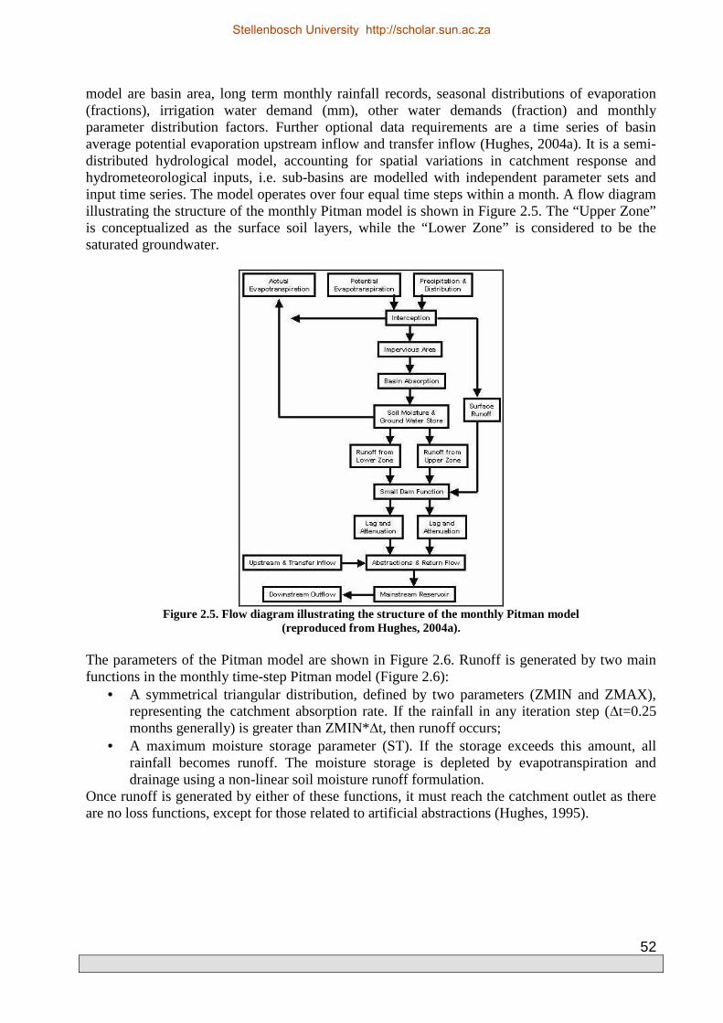
52

model are basin area, long term monthly rainfall records, seasonal distributions of evaporation (fractions), irrigation water demand (mm), other water demands (fraction) and monthly parameter distribution factors. Further optional data requirements are a time series of basin average potential evaporation upstream inflow and transfer inflow (Hughes, 2004a). It is a semi-distributed hydrological model, accounting for spatial variations in catchment response and hydrometeorological inputs, i.e. sub-basins are modelled with independent parameter sets and input time series. The model operates over four equal time steps within a month. A flow diagram illustrating the structure of the monthly Pitman model is shown in Figure 2.5. The “Upper Zone” is conceptualized as the surface soil layers, while the “Lower Zone” is considered to be the saturated groundwater.

Figure 2.5. Flow diagram illustrating the structure of the monthly Pitman model

(reproduced from Hughes, 2004a). The parameters of the Pitman model are shown in Figure 2.6. Runoff is generated by two main functions in the monthly time-step Pitman model (Figure 2.6):

• A symmetrical triangular distribution, defined by two parameters (ZMIN and ZMAX), representing the catchment absorption rate. If the rainfall in any iteration step (∆t=0.25 months generally) is greater than ZMIN*∆t, then runoff occurs;

• A maximum moisture storage parameter (ST). If the storage exceeds this amount, all rainfall becomes runoff. The moisture storage is depleted by evapotranspiration and drainage using a non-linear soil moisture runoff formulation.

Once runoff is generated by either of these functions, it must reach the catchment outlet as there are no loss functions, except for those related to artificial abstractions (Hughes, 1995).


53

Figure 2.6. Pitman model parameters (reproduced from Hughes, 2004a).

Current versions of the model incorporate the effects of abstractions by distributed farm dams, direct abstractions from the river, as well as major storage dams at the outlet of each sub-area (Hughes, 1996). ‘Dummy’ dams representing the loss storage and evaporating area have sometimes been incorporated into the model to account for the effects of channel transmission losses (Görgens and Boroto ,2003; as cited by Hughes, 2008). Midgeley et al. (1994) developed parameter estimation guidelines for the Pitman model through the WR90 study, in which the model was applied to catchments in South Africa, Lesotho and Swaziland. These guidelines can be used for parameter estimation for most climate regions in southern Africa, but should be refined where data is available. Since the original development, the Pitman model has been subjected to numerous revisions. Hughes (2004a) added explicit groundwater recharge and discharge functions to the model structure. These new components aimed to realistically account for groundwater flow in a catchment. The modified groundwater version incorporates 24 parameters, with 14 of these typically being established a priori or through initial calibration runs (Hughes, 2004a). Resultantly, only 10 parameters remain for calibration. In semi-arid areas however, the calibration procedure generally focuses on the catchment adsorption function (3 parameters), the maximum size of the soil moisture storage and the channel loss parameter (Hughes, 2008). Hughes (2004a) compared the performance of the groundwater version of the Pitman model and the original version in the 581 km2 Buffelspruit catchment, a tributary of the Komati River (Mpumalanga, South Africa). Most parameter values were the same for both models. Both models performed poorly, but Hughes (2004a) attributed this to the quality of the rainfall input data. The mean annual groundwater recharge simulated by the revised Pitman model was 42 mm/4.8% of mean annual rainfall, which is within the range of recharge reported for the area (Bedenkamp et al., 1995). The mean annual groundwater contribution to streamflow (% of total


54

flow) estimated by the model was 28% which was comparable with the 31% estimated by Baron et al. (1998). The revised model was however found to be more difficult to calibrate due to the larger number of parameters. The variables with which model performance were evaluated is shown in Table 2-8.

Table 2-8 Simulation Results for Model Applications in the Buffelspruit Catchment (Hughes, 2004a)

Simulated Pitman Model (original): Coefficient of efficiency

Coefficient of determination (R2)

0.200 0.434

Pitman Model (groundwater model): Coefficient of efficiency

Coefficient of determination (R2)

0.205 0.446

Hughes (1997), as cited by Hughes (2008) suggests that the model is more applied and exhibits better results in humid and temperate areas, when compared to arid regions. This is interpreted to be a result of the poor accounting of spatial variation in rainfall inputs that is typical in semi-arid and arid regions, the inability to account for temporal distribution of rainfall within a month and the simplistic method with which runoff generation is simulated (Hughes, 1995). NAMROM Model According to Mostert et al. (1993), as cited by Hughes (2008), this model was designed specifically for application in Namibian catchments. It is a semi-distributed model, designed to incorporate issues pertaining to the dynamic, non-seasonal, vegetation cover conditions, as well as channel transmission losses to alluvial aquifers. It has not been applied outside Namibia and therefore its general applicability is largely untested. The model adopts a single equation for total effective precipitation, in which four parameters are used, i.e. antecedent weighting factor (seasonally varying), initial loss, sub-catchment loss factor and loss exponent. The antecedent weighting factor is included in the calculation of a runoff coefficient applied to the monthly rainfall time series. The weighting factor being a function of the rainfall observed in the three previous seasons. A regression equation is formulated for observed runoff and total effective precipitation. Thus, the model is more of a statistical regression type model with weighting parameters having some perceived physical meaning (Hughes, 2008). Hughes (1995) applied the original Pitman model, a modified version of the Pitman model incorporating a dynamic vegetation cover routine and the NAMROM model to the 212 km2 Friedenau catchment, situated to the west of Windhoek (Namibia). Including components related to dynamic vegetation cover were interpreted to have a beneficial effect on the simulation results. Improved vegetation cover is assumed to facilitate increased infiltration of rainfall or runoff. Variations in vegetation cover densities were interpreted to be driven by rainfall. The results of the model applications are shown in Table 2-9. Improvements were evident after the inclusion of the dynamic vegetation response routine, however the Pitman model still performed poorly in this catchment. A problem which is common to semi-arid regions was experienced, where certain events are grossly over-estimated and others under-estimated. Hughes (1995) suggests that the better performance of the NAMROM model could be attributed to the inclusion of a transmission loss routine in the model structure.


55

Table 2-9 Simulation Results for Model Applications in the Friedenau Catchment (Hughes, 1995)

Year Rainfall (mm) Observed

Streamflow (ml)

Simulated Streamflow (ml) Original Pitman

model Modified Pitman

model NAMROM

1973/74 763 6100 13 883 11 050 6 340 1974/75 426 220 942 172 470 1975/76 583 740 8 906 5 240 1 110 ACRU Model ACRU (Agricultural Council Research Unit) is a product of the Bioresources and Environmental Engineering Hydrology School of the University of KwaZulu-Natal (Schulze, 1995). The model was developed as a simple decision making tool for agrohydrological problems. The model may be applied in ungauged catchments as certain parameters may be estimated through default relationships with measurable catchment properties, i.e. soils, vegetation or management practices (Schulze, 2000). ACRU has dominantly been applied in the temperate and humid regions of South Africa, frequently investigating the impacts of various land use changes, e.g. commercial afforestation (Hughes, 2008) as well as being used for water resource assessments (Everson, 2001) and irrigation supply (Dent, 1998). Evidence documenting successful semi-arid applications is not easily obtainable (Hughes, 2008). ACRU is a physical conceptual hydrological model that conceives a one-dimensional system in which processes are included in discrete time units. The model represents the soil’s ability to store and transmit water, while vegetation water use is modelled using hydrological variables. The generation of stormflow is based on the assumption that, after initial abstractions, runoff is a function of the rainfall amount and the soil water deficit from a critical depth of soil. The soil water deficit antecedent to a rainfall event is simulated by ACRU’s multi-layer water budgeting routines on a daily time scale. Stormflow is divided into quickflow and delayed flow, resulting in varying temporal responses at the catchment outlet. The “lag” being dependant on soil properties, basin size, slope and the density of the drainage network. The model requires input data of rainfall, maximum temperature, minimum temperature, A-pan, leaf area index, incoming radiation flux density (MJm-2day-1), relative humidity (%) and wind run (kmday-1). The model operates on a daily time step and has numerous parameters which require quantification (Everson, 2001; Hughes, 2008). For a detailed description of ACRU, the reader is referred to Schulze (1995). Everson (2001), aimed to develop an understanding of the water balance of a first order grassland catchment, located in the northern part of the Natal Drakensberg Park, in order to develop or improve existing hydrological models and to identify or quantify the principal factors (meteorological, plant and soil) controlling the process of water loss in grasslands. The performance of ACRU (Schulze, 1995) was also evaluated. Results from ACRU illustrated a good agreement between observed and simulated streamflow, i.e. a coefficient of agreement of 0.87 and a correlation coefficient of 0.80. In general, ACRU under-estimated streamflow by 15 %, performing reasonably well in the average rainfall and dry years. The biggest deviation from observed streamflow records was observed in the wet years. Everson (2001) concluded that the under-estimation evident in wet years might be a result of ACRU’s inability to account for subsurface soil water flow in a catchment. Kamish et al. (2008) used a modified version of ACRU, i.e. ACRUSalinity (Teweldebrhan, 2003), to simulate the daily catchment runoff as well as TDS concentrations and TDS loads for various sub-catchments of the Berg River (Western Cape). ACRUSalinity, in general, produced reasonably representative simulated flow outputs, however the simulated TDS concentrations


56

required considerable calibration, especially for the highly saline catchments. The results from the semi-arid Sandspruit catchment, a significantly saline tributary of the Berg River, showed that the simulated flows were not comparable with observed flow. Kamish et al. (2008) however suggested that a finer delineation of the catchment could possibly result in a better simulated flow series. Observed flows were over-estimated by approximately 32 % in the Sandspruit catchment. Unacceptable values for ‘R2’ and the coefficient of efficiency of 0.45 and 0.18 were obtained, respectively. The Sandspruit catchment naturally produces high TDS concentrations during the winter months when previously dissolved salts are mobilized. The salinity validation of daily TDS concentration was illustrated on an exceedance basis. The results showed that for TDS concentrations above 5000 mgL-1, the simulated exceedance percentage is representative of the exceedance percentage displayed by the observed record. Below 5000 mgL-1, the simulated exceedance percentage at any given TDS value is under-estimated by approximately 18 %. Kamish et al. (2008) concluded that the patterns of salinity production and mobilisation observed in the highly saline sub-catchments of the Berg River can be accurately simulated using the current module for salinity generation and mobilisation. VTI Model The Variable Time Interval (VTI) model is a product of the Institute for Water Research (IWR), Rhodes University (Hughes and Sami, 1994). It is a semi-distributed daily time step model, but can be run at shorter time steps (between 5 minutes and 1 day) of assumed high process activity (based on thresholds of rainfall intensity) given that rainfall data is available at the required temporal scale (Hughes, 1996). The model includes routines to simulate interception loss, infiltration and infiltration excess runoff, soil moisture dynamics in a two layer soil, saturation excess and saturation interflow runoff, groundwater recharge, springflow and groundwater rise and channel transmission losses (Hughes, 1996). Allowance is also made for abstractions from small farm dams or the river itself. The main moisture accounting routines are quite complex with numerous feedback mechanisms. A transmission loss routine is also incorporated, enabling water that has reached the channel to be re-infiltrated if sufficient capacity exists in the transmission loss storage zone (Hughes, 1995). A flow diagram illustrating the structure of the VTI model is shown in Figure 2.7. The model aims to account for all processes interpreted to be significant to semi-arid environments and thus is relatively complex with numerous parameters. Initial parameter estimates can however be obtained from relatively simple indices of catchment parameters, e.g. soil, geology and vegetation (Hughes, 1996). More than 35 parameters are required for each sub-catchment of the spatial distribution system. The successful application of the model requires detailed knowledge of its structure, a detailed conceptual understanding of the dominant runoff generation mechanisms in the basin, as well as good quality climate input data (Hughes, 2008).


57

Figure 2.7. Flow diagram illustrating the structure of the VTI model (reproduced from Hughes, 1995).

Hughes (1995) applied the daily VTI model and the monthly Pitman model to the Mosetse catchment (Botswana) to investigate whether simulated daily flows aggregated into monthly volumes could provide a better representation of the observed monthly time series than the Pitman model. The simulation results are shown in Table 2-10. The VTI model exhibited reasonable daily results, given the data constraints in the area, and more than acceptable monthly results.

Table 2-10 Simulation Results for Model Application in the Mosetse Catchment (Hughes, 1995)

Observed Simulated VTI model (daily flows): Coefficient of efficiency Mean discharge (m3 s-1)

Standard deviation of daily flows (m3 s-1)

1.21 8.18

0.42 1.17 7.03

VTI model (monthly flows): Coefficient of efficiency Mean discharge (m3 s-1)


2.99 11.36

0.74 3.06 10.38

Pitman model (monthly flows): Coefficient of efficiency Mean discharge (m3 s-1)


2.99 11.36

0.43 3.37 15.31

SPATSIM SPATSIM (Spatial and Time Series Information Modelling) is a product of the IWR (Hughes, 2002). This package makes use of an ESRI Map Objects spatial front end, linked to a database table structure, for data storage and access and includes links to a number of hydrological and water resource estimation models (Hughes, 2008). The package also includes data preparation


58

and analysis functionality. SPATSIM has been adopted as the core modelling environment to be used for the update of the South African water resource information system (WR90; Midgeley et al., 1994).

2.7 Conclusions

A comprehensive review of previously published work pertaining to the mechanisms of occurrence of dryland salinity and its dynamics is presented. The bulk of the literature emanate from investigations conducted within Australia, where dryland salinity has reached epic proportions in terms of its impact and spatial extent of occurrence. Similarities in climate, topography, geology and/or land use practices however suggest that the extensive knowledge base developed within Australia, may be very useful to investigations conducted within South Africa, and particularly to those conducted within the semi-arid Western Cape. Based on the results of investigations conducted within Australia and observations made by Flügel (1995), Fey and de Clercq (2004), de Clercq et al. (2010), Bugan (2008) and Bugan et al. (2012a) the manifestation of dryland salinity in the mid- to lower Berg catchment, including the Sandspruit catchment, is a result of the clearing of the perennial deep-rooted Renosterveld to make way for annual shallow-rooted winter wheat and summer pasture. As the annual winter-wheat and summer pasture has a lower water use potential than Renosterveld, more water is available to mobilise stored salts toward the soil surface, and/or to lower valley locations and to water bodies. The dynamics of the process may however be different in the semi-arid Western Cape, when compared to that which dominantly occurs in Australia. In Australia the removal of indigenous vegetation results in increased groundwater recharge, mobilising salts which were stored in the previously unsaturated regolith towards the surface. The water table may intersect the land surface, where salts are precipitated subsequent to evaporation/evapotranspiration. Observations made within the Sandspruit catchment, suggest that increased groundwater recharge is evident, however the potentiometric surface does not intersect the ground surface. In certain areas of the catchment the potentiometric surface is less than 2 m below ground level in winter. At such depths, capillary action can mobilise water and salts towards the soil surface. Additionally, soil evaporation and evapotranspiration can also concentrate salts in the upper layers of the soil profile. As shallow lateral subsurface fluxes (throughflow) is the dominant streamflow contributing component in the Sandspruit catchment (Bugan et al., 2012a), it is also interpreted to be the dominant mechanism with which salt is mobilised towards lower valley locations and surface water bodies. Bugan et al., 2012b reported that salt storage in the Sandspruit catchment increases with decreasing ground elevation, i.e. it is higher in the valleys and downstream parts of the catchment. This is interpreted to be a function of salt leaching in the hilltops and salt accumulation in the valleys. Several investigations (Greiner , 1998 and Walker et al., 1999) suggest that bare salty patches, a decline in vegetation cover density and/or the degradation of groundwater/surface water quality is evidence for the occurrence of dryland salinity. Fey and de Clercq (2004) and de Clercq et al. (2010) reported that extensive patchiness in croplands, especially in wheat fields, which dominate the land use in the mid- to lower Berg River catchment, occur. Ground truthing of these patches confirmed that they are associated with soil salinity, of sufficient concentration to affect wheat growth. These saline soils are reported to be contributing to the salinisation of water resources, e.g. in the mid- to lower Berg catchment (Fourie, 1976; Fourie and Steer, 1971; Fourie and Görgens, 1977; de Clercq et al., 2010). Saline groundwater may also be a result of dryland salinity, and this salinity is frequently strongly correlated with Cl- (Bennetts et al., 2006). The groundwater EC in the downstream areas of the Sandspruit catchment reaches 2 200 mS m-1


59

(Jovanovic et al., 2011). The chemical speciation of groundwater in the catchment is dominated by Na+ and Cl- (Jovanovic et al., 2011). The occurrence of salt in the landscape is reported to generally be a function of rock weathering, aerial deposition by wind and/or rain and proximity to the ocean. Malmesbury Shale, which dominates the geological characterisation of the Sandspruit catchment, is rich in soluble salts, which if weathered to soil material may cause an accumulation of salts under low rainfall conditions (Malherbe, 1953). Additionally, Flügel (1995) reported that the mean annual rainfall in the Sandspruit catchment is approximately 400 mm a-1, and that it exhibits an average salt concentration of 37 mg L-1. Sodium and chloride, transported by wind and rain from the Atlantic Ocean, were reported to be the dominant ions. This low annual rainfall quantity (semi-arid climate) and the rainfall dynamics (intensity and frequency) does not allow for the salts to be flushed out of the catchment, and thus salt accumulation occurs. Recharge control has been the dominant mechanism to control and mitigate the impacts of dryland salinisation in Australia for the past 40 years (McFarlane and Williamson, 2002). This generally involves altering the type, distribution and rooting depth of the vegetation through using perennial plants that are suited to productive growth in seasons of high evaporative demand. Hydrological modelling has frequently been used to evaluate the effectiveness of dryland salinity mitigation measures. This has mainly been achieved through evaluating the effects of different land management scenarios on the catchment hydrosalinity fluxes. The models range in complexity and their use is generally a function of data availability and the objective of the investigation. A scenario may represent a land use option, a land management change or an engineering solution (Littleboy et al., 2003). Each scenario is modelled over a fixed period of climatic data, with the differences between each being used to quantify the impacts of the scenario on the water balance, catchment hydrology and salinity (Littleboy et al., 2003). A review of hydrological models, which are being applied in southern Africa, is presented. The models range in complexity, temporal scales of application and/or data requirements. The main aim of conducting the review was to identify which models are dominantly applied and for which purposes. Hydrological modelling in the southern African region has developed against a background of a high degree of spatial and temporal variability in hydrometeorological processes (Everson, 2001), a general lack of available data and limited financial and personnel resources (Hughes, 2008). Thus, the type of model that is the best to use is dictated by the purpose of applying the model and the type of information available (Hughes, 2004a). The general consensus is also that, model performance is significantly better in humid and temperate regions when compared to arid and semi-arid areas. The review has provided valuable information, in terms of model selection criteria and potential sources of error associated with climate input data, particularly in semi-arid areas.

2.8 References

AJAMI, N.K., GUPTA, H., WAGENER, T. and SOROOSHIAN, S., 2004. Calibration of a semi-distributed hydrological model for streamflow estimation along a river system. Journal of Hydrology, 298, pp. 112-135. AMERICAN SOCIETY OF CIVIL ENGINEERS (ASCE), 1990. Agricultural Salinity Assessment and Mangagement. 71. New York, USA: ASCE manuals and reports on engineering practice.


60

ANDERSEN, J., REFSGAARD, J.C. and JENSEN, K.H., 2001. Distributed hydrological modelling of the Senegal River basin - model construction and validation. Journal of Hydrology, 247, pp. 200-214. ANGUS, J.F., GAULT, R.R., PEOPLES, M.B., STAPPER, M. and VAN HERWAARDEN, A.F., 2001. Soil water extraction by dryland crops. annual pastures and lucerne in south-eastern Australia. Australian Journal of Agricultural Research, 52, pp. 183-192. BAKER, P., PLEASE, P., CORAM, J., DAWES, W., BOND, W., STAUFFACHER, M., GILFEDDER, M., PROBERT, M., HUTH, N., GAYDON, D., KEATING, B., MOORE, A., SIMPSON, R., SALMON, L. and STEFANSKI, A., 2001. Assessment of Salinity Management Options for Upper Billabong Creek Catchment, NSW: Groundwater and Farming Systems Water Balance Modelling. Canberra: Bureau of Rural Sciences. BARON, J., SEWARD, P. and SEYMOUR, A., 1998. The groundwater harvest potential mao of the Republic of South Africa. Technical Report No GH3917. Pretoria: Directorate of Geohydrology, Department of Water Affairs and Forestry. BARRETT-LENNARD, E.G. and NULSEN, R.A., 1989. Dryland soil salinity - cure, containment or catastrophe, 5th Australian Agronomic Conference, 1989 1989, Australian Society of Agronomy pp304-311. BEDENKAMP, D.B., BOTHA, L.J., VAN TONDER, G.J. and VAN RENSBURG, H.J., 1995. Manual on quantitative estimation of groundwater recharge and aquifer storativity. Report No TT73/95. Pretoria: Water Research Commission. BENNETT, B., 1998. Dealing with Dryland Salinity. ECOS, 98, pp. 9-28. BENNETT, J., BLAMEY, R. and MORRISON, M., 1997. Valuing damage to South Australian wetlands using the contingent valuation method. Report No 13/97. Canberra: Land and Water resources research and Development Corporation. BENNETTS, D.A., WEBB, J.A., STONE, D.J.M. and HILL, D.M., 2006. Understanding the salnisation processes for groundwater in an area of south-eastern Australia, using hydrochemical and isotopic evidence. Journal of Hydrology, 323, pp. 178-192. BENYON, R.G., THEIVEYANATHAN, S. and DOODY, T.M., 2006. Impacts of tree plantations on groundwater in south-astern Australia. Australian Journal of Botany, 54, pp. 181-192. BEVEN, K., 1996. Response to comments on 'A discussion of distributed hydrological modelling' by Refsgaard et al. In: M.B. ABBOTT and J.C. REFSGAARD, eds, Distributed hydrological modelling. Dordrecht: Kluwer, pp. 289-295. BEVEN, K., 1985. Distributed models. In: M.G. ANDERSON and T.P. BURT, eds, Hydrological forecasting. New York: Wiley, pp. 405-435. BONGARTZ, K., 2003. Applying different spatial distribution and modelling concepts in three nested mesoscale catchments of Germany. Physics and Chemistry of the Earth, 28, pp. 1343-1349.


61

BRESLER, E., MCNEAL, B.L. and CARTER, E.L., 1982. Saline and sodic soils. New York: Springer-Verlag. BREUER, L., HUISMAN, J.A., WILLEMS, P., BORMANN, H., BRONSTERT, A., CROKE, B.F.W., FREDE, H., GRÄFF, T., HUBRECHTS, L., JAKEMAN, A.J., KITE, G., LANINI, J., LEAVESLEY, G., LETTENMAIER, D.P., LINDSTRÖM, G., SEIBERT, J., SIVAPALAN, M. and VINEY, N.R., 2009. Assessing the impact of land use change on hydrology by ensemble modelling (LUCHEM). 1: Model intercomparison with current land use. Advances in Water Resources, 32, pp. 129-146. BUGAN, R.D.H., 2008. Hydrosalinity fluxes in a small scale catchment of the Berg River (Western Cape), University of the Western Cape. BUGAN, R.D.H., JOVANOVIC, N.Z. and DE CLERCQ, W.P., 2012a. The water balance of a seasonal stream in the semi-arid Western Cape (South Africa). Water SA, 38(2), pp. 201-212. BUGAN, R.D.H., JOVANOVIC, N.Z., FINK, M., STEUDEL, T. and PFENNIG, B., 2012b. Sandspruit Hydrosalinity Modeling. WRC project K5/1849, Deliverable 27. Stellenbosch: Council for Scientific and Industrial Research. CARTWRIGHT, I., WEAVER, T.R., FULTON, S., NICHOL, C., REID, M. and CHENG, X., 2004. Hydrochemical and isotopic constraints on the origins of dryland salinity, Murray basin, Victoria, Australia. Applied Geochemistry, 19, pp. 1233-1254. CHAPMAN, V.J., 1966. Vegetation and salinity. In: H. BOYKO, ed, Salinity and Aridity: New Approaches to Old Problems. The Hague: Dr. W. Junk Publishers, . CLARKE, C.J., GEORGE, R.J., BELL, R.W. and HOBBS, R.J., 1998. Major faults and the development of dryland salinity in the western wheatbelt of Western Australia. Hydrology and Earth System Science, 2(1), pp. 77-91. CROSBIE, R.S., HUGHES, J.D., FRIEND, J. and BALDWIN, B.J., 2007. Monitoring the hydrological impact of land use change in a small agricultural catchment affected by dryland salinity in central NSW, Australia. Agricultural Water Management, 88, pp. 43-53. CROSBIE, R.S., WILSON, B., HUGHES, J.D., MCCULLOCH, C. and KING, W.M., 2008. A comparison of the water use of tree belts and pasture in recharge and discharge zones in a saline catchment in the Central West of NSW, Australia. Agricultural Water Management, 95, pp. 211-223. DAWES, W.R., GILFEDDER, M., WALKER, G.R. and EVANS, W.R., 2004. Biophysical modelling of catchment-scale surface water and groundwater response to land-use change. Mathematics and Computers in Simulation, 64(1), pp. 3-12. DE CLERCQ, W.P., JOVANOVIC, N.Z. and FEY, M.V., 2010. Land use impacts on salinity in Berg River water. Report No K5/1503. Pretoria: Water Research Commission. DENT, M.C., 1998. Estimating crop water requirements for irrigation planning in southern Africa. Agricultural Engineering South Africa, 20, pp. 7-19.


62

DUAN, Q., SCHAAKE, J., ANDRÉASSIAN, V., FRANKS, S., GOTETI, G., GUPTA, H.V., GUSEV, Y.M., HABETS, F., HALL, A., HAY, L., HOGUE, T., HUANG, M., LEAVESLEY, G., LIANG, X., NASONOVA, O.N., NOILHAN, J., OUDIN, L., SOROOSHIAN, S., WAGENER, T. and WOOD, E.F., 2006. Model parameter estimation experiment (MOPEX): An overview of science strategy and major results from the second and third workshops. Journal of Hydrology, 320, pp. 3-17. EAMUS, D., HATTON, T., COOK, P. and COLVIN, C., 2006. Ecohydrology: vegetation function, water and resource management. Australia: CSIRO Publishing. ECKHARDT, K. and ARNOLD, J.G., 2001. Technical note: Automatic calibration of a distributed catchment model. Journal of Hydrology, 251, pp. 103-109. ECKHARDT, K., BREUER, L. and FREDE, H., 2003. Parameter uncertainty and the significance of simulated land use change effects. Journal of Hydrology, 273, pp. 164-176. EVERSON, C.S., 2001. The water balance of a first order catchment in the montane grasslands of South Africa. Journal of Hydrology, 241(1-2), pp. 110-123. FERDOWSIAN, R., GEORGE, R., LEWIS, F., MCFARLANE, D., SHORT, R. and SPEED, R., 1996. The Extent of Dryland Salinity in Western Australia, Proceedings of the 4th National Conference and Workshop on the Productive use and Rehabilitation of Saline Land, Albany, Western Australia, 25 - 30 March 1996, pp89-97. FEY, M.V. and DE CLERCQ, W.P., 2004. Dryland salinity impacts on Western Cape rivers. Report No 1342/1/04. Pretoria: Water Research Commission. FLÜGEL, W., 1995. River salinity due to dryland agriculture in the Western Cape Province, Republic of South Africa. Environmental International, 21, pp. 679-686. FOURIE, J.M. 1976. Mineralization of Western Cape rives. PhD edn. Stellenbosch: University of Stellenbosch. FOURIE, J.M. and GORGENS, A.H.M., 1977. Mineralization studies of the Berg River (1974-1976). Report No 334. Pretoria: Council for Scientific and Industrial Research. FOURIE, J.M. and STEER, A.G., 1971. Water quality survey of the Berg River for the period 1963-1970. Research report to the Provincial Administration of the Cape of Good Hope. National Institure of Water Research. GEORGE, R., CLARKE, C., HATTON, T., REGGIANI, P., HERBERT, A., RUPRECHT, J., BOWMAN, S. and KEIGHERY, G., 1999. The Effect of Recharge Management on the Extent of Dryland Salinity, Flood Risk and Biodiversity in Western Australia. Preliminary Computer Modelling, Assessment and Financial Analysis Perth: Unpublished report to State Salinity Council of Western Australia. GILFEDDER, M., WALKER, G. and WILLIAMS, J., 1999. Effectiveness of current farming systems in the control of dryland salinity. Australia: CSIRO Publishing.


63

GILFEDDER, M., WALKER, G.R., DAWES, W.R. and STENSON, M.P., 2009. Prioritisation approach for estimating the biophysical impacts of land-use change on stream flow and salt export at a catchment scale. Environmental Modelling and Software, 24(2), pp. 262-269. GORGENS, A.H.M. and BOROTO, J., 2003. Limpopo River: an overview of alternative methods for estimating transmission losses, Hydrology of Mediterranean and Semi-Arid regions, 2003 2003, IAHS. GORGENS, A.H.M. and DE CLERCQ, W.P., 2006. Research on Berg River Water Management. Summary of water quality information system and soil quality studies. Report No 252/06. Pretoria: Water Research Commission. GREINER, R., 1998. Catchment management for dryland salinity control: model analysis for the Liverpool Plains in New South Wales. Lyneham, Australia: CSIRO Publishing. GREINER, R., 1996. SMAC: spatial optimisation model for analysing catchment management. Environmental Software, 11(1-3), pp. 159-165. GREINER, R. and CACHO, O., 2001. On the efficient use of a catchments's land and water resources: dryland salinisation in Australia. Ecological Economics, 38, pp. 441-458. HATTON, T.J. and NULSEN, R.A., 1999. Towards achieving functional ecosystem mimicry with respect to water cycling in southern Australian agriculture. Agroforestry Systems, 45(1-3), pp. 203-214. HELMSCHROT, J. and FLÜGEL, W., 2002. Land use characterization and change detection analysis for hydrological model parameterisation of large scale afforested areas using remote sensing. Physics and Chemistry of the Earth, 27, pp. 711-718. HERRON, N., DAVIS, R., DAWES, W. and EVANS, R., 2003. Modelling the impacts of strategic tree planting on salt loads and flows in the Macquarie River Catchment, NSW, Australia. Journal of Environmental Hydrology, 68, pp. 37-50. HEUPEMAN, A., 1999. Hydraulic gradient reversal by trees in shallow water table areas and repercussions for the sustainability of tree-growing systems. Agricultural Water Management, 39, pp. 153-167. HINGSTON, F.J. and GAILITIS, V., 1976. The geographic variation of salt precipitated over Western Australia. Australian Journal of Soil Research, 14, pp. 319-335. HUGHES, D.A., 2008. Modelling semi-arid and arid hydrology and water resources - The southern African experience. In: H. WHEATER, S. SOROOSHIAN and K.D. SHARMA, eds, Hydrological Modelling in Arid and semi-Arid Areas, IHP International Hydrology Series. Cambridge University Press, . HUGHES, D.A., 2004a. Incorporating groundwater recharge and discharge functions into an existing monthly rainfall-runof model. Hydrological Sciences, 49(2), pp. 297-311. HUGHES, D.A., 2004b. Three decades of hydrological modelling research in South Africa. South African Journal of Science, 100, pp. 638-642.


64

HUGHES, D.A., 2002. The development of an information modelling system for regional water resource assessments, Proc. of the 4th international conference on FRIEND, 2002, IAHS Publication No 274 pp43-49. HUGHES, D.A., 1997. Southern African FRIEND - The application of rainfall-runoff models in SADC region. report No 235/1/97. Pretoria: Water Research Commission. HUGHES, D.A., 1996. Southern African FRIEND. Rainfall-runoff moodelling, Hydrology of Mediterranean and semi-Arid Regions, 1996, . HUGHES, D.A., 1995. Monthly rainfall-runoff models applied to arid and semi-arid catchments for water resource estimation purposes. Hydrological Sciences, 40(6), pp. 751-769. HUGHES, D.A. and SAMI, K., 1994. A semi-distributed, variable time interval model of catchment hydrology - structure and parameter estimation procedures. Journal of Hydrology, 155(265), pp. 291. JOTHITYANGKOON, C., SIVAPALAN, M. and FARMER, D.L., 2001. Process controls of water balance variability in a large semi-arid catchment: downward approach to hydrological model development. Journal of Hydrology, 254, pp. 174-198. JOVANOVIC, N.Z., BUGAN, R.D.H. and SOLTAU, L.S., 2009. Report detailing boreholes in the Sandspruit Catchment. Deliverable 10, WRC Project K5/1849. Stellenbosch: CSIR, Natural Resources and the Environment. JOVANOVIC, N.Z., ISRAEL, S., PETERSEN, C., BUGAN, R.D.H., TREDOUX, G., DE CLERCQ, W.P., VERMEULEN, T., ROSE, R., CONRAD, J. and DEMLIE, M., 2011. Optimised Monitoring of Groundwater - Surface Water - Atmospheric Parameters for Enhanced Decision-Making at a Local Scale WRC Report No. 1846/1/11. Pretoria: Water Research Commission. KAMISH, W., ROSSOUW, J.N., GORGENS, A.H.M. and CLARKE, F., 2008. Improvements to the ACRUSalinity model and upgrading of the Berg River water quality information system. Report No 1301/1/08. Pretoria: Water Research Commission. KARIM, Z., HUSSAIN, S.G. and AHMED, M., 1990. Salinity problems and crop intensification in the coastal regions of Bangladesh. Soils Publication No 33. Bangladesh: Soils and Irrigation Division, BARC. LAMSAL, K., PAUDYAL, G.N. and SAEED, M., 1999. Model for assessing impact of salinity on soil water availability and crop yield. Agricultural Water Management, 41(1), pp. 57-70. LEANEY, F.W., HERCZEG, A.L. and WALKER, G.R., 2003. Salinisation of a fresh palaeo-ground water resource by enhanced recharge. Ground Water, 41(1), pp. 84-92. LEFROY, E.C. and STIRZAKER, R.J., 1999. Agroforestry for water management in the cropping zone of southern Australia. Agroforestry Systems, 45, pp. 277-302.


65

LITTLEBOY, M., VERTESSY, R. and LAWRENCE, P., 2003. An Overview of Modelling Techniques and Decission Support Systems and their Apllication for Managing Salinity in Australia, 9th National PUR$L Conference, 29 September - 2 October 2003 2003, . MAAS, E.V. and HOFFMAN, G.J., 1977. Crop salt tolerance, current assessment. Journal of Irrigation and Drainage, 103, pp. 115-134. MADSEN, H., 2003. Parameter estimation in distributed hydrological catchment modelling using automatic calibration with multiple objectives. Advances in Water Resources, 26, pp. 206-216. MADSEN, H., 2000. Automatic calibration of a conceptual rainfall-runoff model using multiple objectives. Journal of Hydrology, 235, pp. 276-288. MALHERBE, I.D.V., 1953. Soil fertility. London: Oxford University Press. MCFARLANE, D.J. and WILLIAMSON, D.R., 2002. An overview of water logging and salinity in southwestern Australia as related to the 'Ucarro' experimental catchment. Agricultural Water Management, 53, pp. 5-29. MDBMC, 1999. The Salinity Audit of the Murray-Darling Basin: a 100 Year Perspective. Canberra, ACT: Murray-Darling Basin Ministerial Council. MERZ, R. and BLÖSCHL, G., 2004. Regionalisation of catchment model parameters. Journal of Hydrology, 287, pp. 95-123. MIDGELEY, D.C., PITMAN, W.V. and MIDDLETON, B.J., 1994. Surface water resources of South Africa 1990. Volumes 1-6. Report No 298/1.1/94 - 298/6.1/94. Pretoria: Water Research Commission. MONDAL, M.K., BHUIYAN, S.I. and FRANCO, D.T., 2000. Soil salinity reduction and prediction of salt dynamics in the coastal ricelands of Bangladesh. Agricultural Water Management, 47, pp. 9-23. MOSTERT, A.C., MCKENNZIE, R.S. and CRERAR, S.E., 1993. A rainfall/runoff model for ephemeral rivers in an arid or semi-arid environment, Proc. 6th South African National Hydrology Symposium, 1993, pp219-224. MURRAY, B.R., ZEPPEL, M.J.B., HOSE, G.C. and EAMUS, D., 2003. Groundwater-dependent ecosystems in Australia: It's more than just water for rivers. Ecological Management and restoration, 4, pp. 110-113. MURRAY-DARLING BASIN COMMISSION (MDBC), 2001. Basin Salinity Management Strategy 2001 - 2015. Canberra: Murray-Darling Basin Ministerial Council. NATIONAL LAND AND WATER RESOURCES AUDIT, 15 June 2009, 2009-last update, australian dryland salinity assessment 2001: extent, impacts, processes, monitoring and managment options [Homepage of National Land and Water Resources Audit], [Online]. Available: http://www.anra.gov.au/topics/salinity/pubs/national/salinity_contents.html [June/14, 2010].


66

NATIONAL LAND AND WATER RESOURCES AUDIT, 2001. Australian Dryland Salinity Assessment 2000. Canberra, ACT: Natiional Land and Water Resources Audit. OFFICE OF ENVIRONMENT AND HERITAGE, 2011a. Book 1 Dryland Salinity: The Basics. New South Wales, Australia: Department of Premier and Cabinet, NSW Government. OFFICE OF ENVIRONMENT AND HERITAGE, 2011b. Book 4 Dryland Salinity: Productive Use of Saline Land and Water. New South Wales, Australia: Department of Premier and Cabinet, NSW Government. PANNELL, D.J. and EWING, M.A., 2006. Managing secondary dryland salinity: options and challenges. Agricultural Water Management, 80, pp. 41-56. PECK, A.J. and HATTON, T., 2003. Salinity and the discharge of salts from catchments in Australia. Journal of Hydrology, 272, pp. 191-202. PECK, A.J. and HURLE, D.H., 1973. Chloride balance of some farmed and forested catchments in southwestern Australia. Water Resources Research, 9, pp. 648-657. PECK, A.J. and WILLIAMSON, D.R., 1987. Effects of forest clearing on groundwater. Journal of Hydrology, 94, pp. 47-66. PITMAN, W.V., 1973. A mathematical model for generating monthly flows from meteorological data in South Africa. Report No 2/73. South Africa: Hydrological Research Unit, University of Witwatersrand. POWELL, J., 2004. Dryland Salinity: On-Farm Decisions and Catchment Outcomes. A Guide for Leading Producers and Advisors. PX 040 651. Canberra, ACT: Land and Water Australia. REFSGAARD, J.C., 1997. Parameterisation, calibration and validation of distributed hydrological models. Journal of Hydrology, 198, pp. 69-97. SALAMA, R.B., OTTO, C.J. and FITZPATRICK, R.W., 1999. Contributions of groundwater conditions to soil and water salinisation. Hydrogeology Journal, 7, pp. 46-64. SALAMA, R.B., WELLS, A.S.M., FARRINGTON, P. and BARTLE, G.A., 1993. The chemical evolution of groundwater in the aquifer system of the Yilgarin Craton of western Australia. Perth: CSIRO Division of Water Resources. SCHULZE, R.E., 2000. Modelling hydrological responses to land use and climate change: A southern African perspective. Ambio, 29, pp. 12-22. SCHULZE, R.E., 1995. Hydrology and agrohydrology. A text to accompany the ACRU 3.00 Agrohydrological Modelling System. Report No TT69/65. Pretoria: Water Research Commission. SMITT, C., GILFEDDER, M., DAWES, W., PETHERAM, C. and WALKER, G., 2003. Modelling the Effectiveness of Recharge Reduction for Salinity Management. 06/03. Canberra, ACT: Murray-Darling Basin Commission.


67

SOMANI, L.L., 1991. Crop production with saline water. Vyas Nagar, India: Agro Botanical Publishers. STIRZAKER, R.J., COOK, F.J. and KNIGHT, J.H., 1999. Where to plant trees on cropping land for control of dryland salinity: some approximate solutions. Agricultural Water Management, 39, pp. 115-133. TEWELDEBRHAN, A.T. 2003. The hydrosalinity module of ACRU Agrohydrological Modelling System (ACRUSalinity) - Module Development and Evaluation. Submitted in partial fullfillment of the requirements for the degree of MSc in Hydrology edn. Pietermaritzburg: School of Bioresources, Engineering and Environmental Hydrology, University of Natal. TUTEJA, N.K., VAZE, J., MURPHY, B. and BEALE, G., 2004. CLASS: Catchment scale multiple-landuse atmosphere soil water solute transport model. Technical Report 04/12. New South Wales, Australia: Department of Infrastructure, Planning and Natural Resources. VAZE, J., BARNETT, P., BEALE, G., DAWES, W., EVANS, R., TUTEJA, N.K., MURPHY, B., GEEVES, G. and MILLER, M., 2004. Modelling the effects of land-use change on water and salt delivery from a catchment affected by dryland salinity in south-east Australia. Hydrological Processes, 18(9), pp. 1613-1637. WALKER, G., GILFEDDER, M. and WILLIAMS, J., 1999. Effectiveness of current farming systems in the control of dryland salinity. Adelaide, Australia: CSIRO Publishing. WALKER, G. et al. 2002. Estimating impacts of changed land use on recharge: review of modelling and other approaches appropriate for management of dryland salinity. Springer Berlin /Heidelberg. Available from: <http://dx.doi.org/10.1007/s10040-001-0181-5>. WHITE, D.A., DUNIN, F.X., TURNER, N.C., WARD, B.H. and GALBRAITH, J.H., 2002. Water use by contour-planted belts of trees comprised of four Eucalyptus species. Agricultural Water Management, 53, pp. 133-152. WILK, J. and HUGHES, D.A., 2002. Calibrating a rainfall-runoff model for a catchment with limited data. Hydrological Sciences, 47(1), pp. 3-17. WILLIAMSON, D.R., 1998. Land degradation processes and water quality effects, water logging and salinity. In: J. WILLIAMS, R.A. HOOK and H.L. GASCOIGNE, eds, Farming Action-Catchment Reaction, the Effect of Dry-land Farming on the Natural Environment. Collingwood, Victoria: CSIRO Publishing, pp. 162-190.


68

3. A CONCEPTUAL WATER BALANCE MODEL OF THE SANDSPRUIT CATCHMENT 1

3.1 Introduction

The quantification of a catchment’s water yield is a fundamental problem in hydrology, particularly the volume of water available at the catchment outlet over a fixed time period (Poncea and Shetty, 1995). The catchment water balance issue is even more fundamental under the impacts of significant human-induced land use change. Optimising the water yield from catchments within South Africa has become an essential component of catchment management as increased pressure is being placed on the country’s water resources, primarily due to population growth and inadequate management of the resource. Hydrological modelling has been identified as an essential tool for effective catchment management. Both physically-based hydrological models and simple conceptual water balance models are useful tools to address a range of hydrological problems (Xu, 1999). Conceptual water balance models provide insight into the hydrological processes within catchments (Everson, 2001), and are regarded as being essential for the development and improvement of physically-based hydrological models. Conceptual models do not take into account the detailed geometry and small–scale variability of catchments, but rather consider the catchment as an ensemble of interconnected conceptual storages (Jothityangkoon et al., 2001). In addition, they allow for the identification or quantification of the principal factors (meteorological, plant and/or soil), which control the processes of water loss. They also allow for the generation of synthetic sequences of hydrological data for various purposes including water resources design and management (Xu, 1999). A lack of capacity and inadequate infrastructure does however mean that detailed information pertaining to all the terms of the water balance equation is rarely available to catchment hydrologists (Everson, 2001). The semi-arid Western Cape province of South Africa has recently received much attention (de Clercq et al., 2010; Fey and de Clercq, 2004) due to areas, particularly the Swartland region, increasingly exhibiting evidence of dryland salinity. This does not only pose a potential threat to the freshwater resources in the area, i.e. the Berg River, but also to the agricultural industry. The Swartland is regarded as the “bread basket” of the country due to the extensive wheat cultivation in the area. The Sandspruit River, a tributary of the Berg River, has particularly been impacted by dryland salinisation, exhibiting deteriorating water quality. The river has been observed to exhibit water quality, which is unfit for domestic supply or irrigation for much of the rainy season (de Clercq et al., 2010). It is thus essential to

1 BUGAN, R.D.H., JOVANOVIC, N.Z. and DE CLERCQ, W.P., 2012. The water balance of a seasonal stream in the semi-arid Western Cape (South Africa). Water SA, 38(2), pp. 201-212. JOVANOVIC, N.Z., ISRAEL, S., PETERSEN, C., BUGAN, R.D.H., TREDOUX, G., DE CLERCQ, W.P., VERMEULEN, T., ROSE, R., CONRAD, J. and DEMLIE, M., 2011. Optimised Monitoring of Groundwater - Surface Water - Atmospheric Parameters for Enhanced Decision-Making at a Local Scale. WRC Report No. 1846/1/11. Pretoria: Water Research Commission.


69

identify the main hydrological drivers within the catchment to develop effective dryland salinity management strategies. The need to address salinity has highlighted the importance of understanding the fundamental hydrological processes that underpin all water resource and land use issues (Hughes et al., 2007). Ward (1972) suggests that clearly detailed investigations should be aimed initially at an improved understanding of hydrological processes within the catchment. The aim of this investigation was to calculate and develop a detailed water balance and conceptual flow model for the Sandspruit catchment for the period 1990 to 2010 on a winter rainfall water year (1 April – 31 March) basis. This would allow for the identification of the dominant hydrological drivers in the catchment as well as the dominant flow contributors to streamflow. This balance was based on physical data gathered during previous Water Research Commission (WRC) projects (de Clercq et al., 2010 and Fey and de Clercq, 2004), current WRC projects, weather stations managed by the Agricultural Research Council (ARC) as well as Department of Water Affairs (DWA) streamflow data. A detailed description of the study area, i.e. the Sandspruit catchment, is also provided.

3.2 Study Area

3.2.1 Location

The Sandspruit catchment, which forms part of quaternary catchment G10J, is located in the Western Cape province of South Africa, approximately 80 km north-east of Cape Town (Figure 3.1). Major towns in the area are Malmesbury, Riebeek-Wes and Moorreesburg. The Sandspruit catchment is regarded as a medium sized catchment. It is a seasonal stream, i.e. it only flows between the months of June and November, exhibiting a catchment area of approximately 152 km2.

3.2.1 Topography and Land Use

The topography of the catchment is relatively flat, exhibiting a gently undulating surface. The elevation ranges between 900 mamsl in the higher elevated southerly parts (Kasteelberg) of the catchment to 40 mamsl in the lower elevation areas (north-west). The average topographic gradient across the catchment is 0.013. Land use in the Sandspruit catchment is dominated by cultivated lands and pastures. The catchment falls within the “bread basket” of South Africa and thus agriculture is dominated by wheat cultivation. However the growing of lupins and canola is not uncommon. Farmers in the area generally follow a three year planting rotation, i.e. cultivation only occurs every 3rd year. Lands are left fallow between planting rotations and used for grazing. Soil erosion is minimized through the use of man-made anti erosion contours, which are evident throughout the catchment.

3.2.1 Climate

The Berg River catchment experiences a Mediterranean climate with warm dry summers and cool wet winters. Rainfall is of a cyclonic nature, extending normally over a few days with significant periods of clear weather in between. Little rain falls during summer, with the rainy season extending from April through to October. Precipitation is generally in the form of


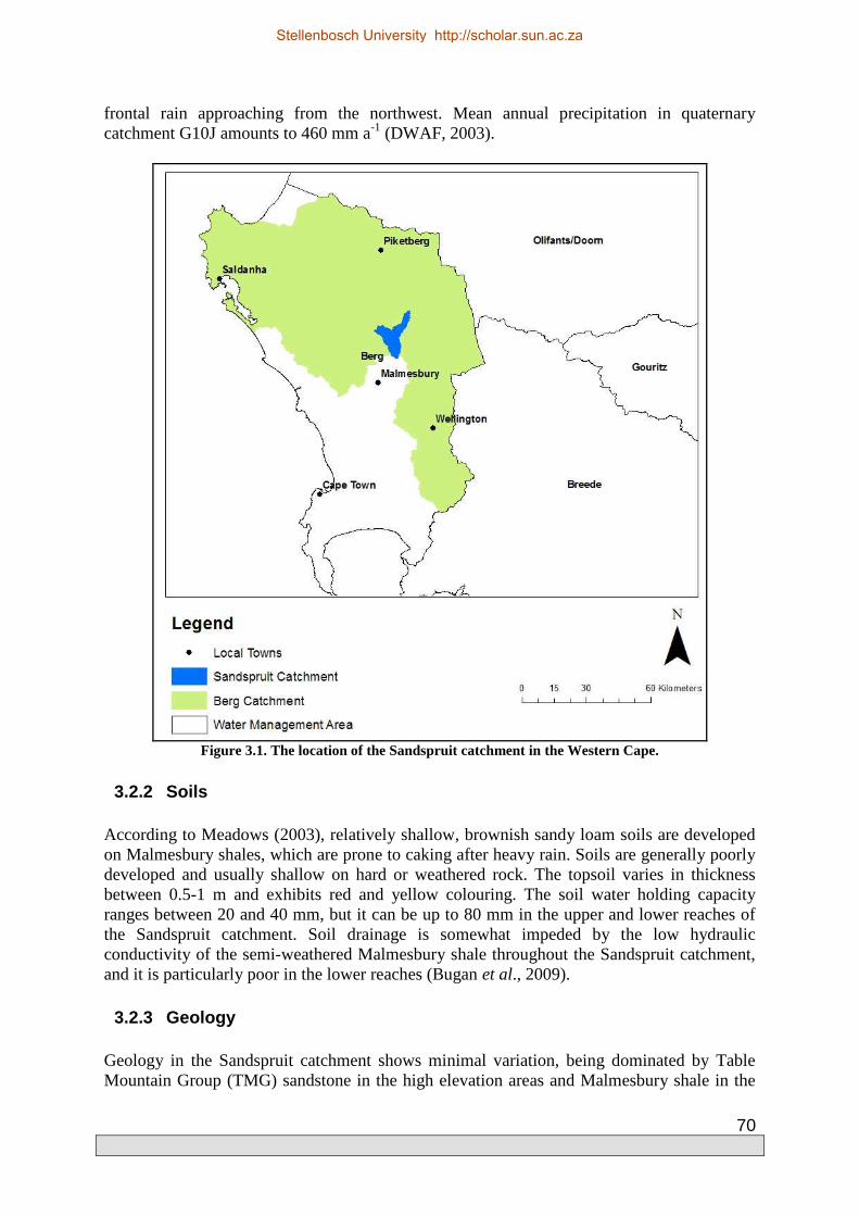
70

frontal rain approaching from the northwest. Mean annual precipitation in quaternary catchment G10J amounts to 460 mm a-1 (DWAF, 2003).

Figure 3.1. The location of the Sandspruit catchment in the Western Cape.

3.2.2 Soils

According to Meadows (2003), relatively shallow, brownish sandy loam soils are developed on Malmesbury shales, which are prone to caking after heavy rain. Soils are generally poorly developed and usually shallow on hard or weathered rock. The topsoil varies in thickness between 0.5-1 m and exhibits red and yellow colouring. The soil water holding capacity ranges between 20 and 40 mm, but it can be up to 80 mm in the upper and lower reaches of the Sandspruit catchment. Soil drainage is somewhat impeded by the low hydraulic conductivity of the semi-weathered Malmesbury shale throughout the Sandspruit catchment, and it is particularly poor in the lower reaches (Bugan et al., 2009).

3.2.3 Geology

Geology in the Sandspruit catchment shows minimal variation, being dominated by Table Mountain Group (TMG) sandstone in the high elevation areas and Malmesbury shale in the


71

mid to low elevation parts (Figure 3.2). An alluvium cover is also evident, which increases in thickness towards the lower elevation areas of the catchment. The TMG is represented by Kasteelberg (900 mamsl). It is a light-grey quartzitic sandstone outcrop, exhibiting thin siltstone, shale and polymictic conglomerate beds. It is interpreted to be part of the Peninsula Formation. The remainder of the watershed is dominated by the Malmesbury Group shales. These are represented by low grade metamorphic rocks such as phyllitic shale, quartz and sericrete schist, siltstone, sandstone and greywacke (Meyer, 2001). It is interpreted to be part of the Moorreesburg Formation. Field investigations have however revealed that there are granite hills, essentially granite plutons intruded into the Malmesbury Group, which are surrounded by clay soils typically derived from weathered granite (Anchor Environmental and Freshwater Consulting Group, 2007). The alluvium cover is represented by fine sediment, which may be characterised as loam and sandy loam. Jovanovic et al. (2009) undertook an extensive borehole drilling exercise in the Sandspruit catchment to study the geology, depth to groundwater and groundwater quality. Three transects were identified as drilling sites, which are representative of the upper-, mid- and lower-reaches of the Sandspruit River respectively (Figure 3.3). The transects were also sited so as to be representative of the geological variability in the catchment (Figure 3.2). Eleven boreholes were drilled across Transect 1 in an area dominated by TMG sandstones (Kasteelberg) as well as Malmesbury shale. It should be noted, however, that the boreholes drilled at this site did not intersect any TMG sandstones. Transect 2, represented by 3 boreholes, is located in a Malmesbury shale dominated environment. Transect 3, represented by 5 boreholes, is also located in a Malmesbury shale dominated environment, however a deeper/thicker alluvium cover exists here. After completion of these transects, two additional transects were drilled, i.e. transects 4 and 5, represented by 3 and 4 boreholes respectively. Table 3-1, lists all the boreholes which were drilled in the Sandspruit catchment.


72

Figure 3.2. Geological map of the Sandspruit catchment.


73

Figure 3.3. Location of the drilling transects (T) in the Sandspruit catchment (reproduced from Jovanovic

et al., 2009).

Table 3-1 The Location of the Boreholes Which Were Drilled in the Sandspruit Catchment Transect (Farm) Borehole No Latitude (S) Longitude (E) Altitude (mamsl)

1 (Zwavelberg)

ZB001 -33.35245 18.81108 309 ZB002 -33.34896 18.81472 278 ZB003 -33.34921 18.81642 272 ZB003a -33.34921 18.81642 272 ZB004 -33.35187 18.82455 361 ZB004a -33.35187 18.82455 361 ZB0051 -33.35187 18.82457 361 ZB006 -33.35279 18.81962 303 ZB006a -33.35284 18.81973 303 ZB007 -33.34745 18.81996 303 ZB007a -33.34745 18.81996 303

2 (Oranjeskraal) OK001 -33.25959 18.80986 107 OK002 -33.25757 18.80806 118 OK003 -33.25256 18.80997 125

3 (Uitvlugt)

UV001 -33.19636 18.86041 70 UV002 -33.19873 18.86535 62 UV003 -33.20017 18.86819 64 UV004 -33.20425 18.87108 81 UV005 -33.19855 18.85466 119

4 (Oudekraal) OKR1 -33.34023 18.80592 219 OKR1a -33.34023 18.80592 219 OKR2 -33.33972 18.80619 219


74

Transect (Farm) Borehole No Latitude (S) Longitude (E) Altitude (mamsl)

5 (Malansdam)

MD1 -33.27970 18.75520 231 MD1a -33.27970 18.75520 231 MD2 -33.28504 18.77325 144 MD2a -33.28504 18.77325 144

1Logged, but not used for research and monitoring Boreholes marked with “a” are shallow boreholes adjacent to a deep borehole

Results from the investigation by Jovanovic et al. (2009) indicated that the catchment geology is characterised by an alluvium cover (yellow/brown sand/silt), which increases in thickness downstream, overlaying Malmesbury shale (grey/ dark grey). The alluvium cover is composed of sandy material with differing boulder contents as well as exhibiting clay layering. During the time of drilling moist and saturated horizons, were also observed within this alluvium cover (Jovanovic et al., 2009). Water strikes generally occurred at the interface between the alluvium cover and Malmesbury shale. The typical geological succession evident in the catchment is illustrated for UV003 (Table 3-1) in Figure 3.4. The borehole logs for the boreholes drilled at Transects 1-3 (Figure 3.3) in the Sandspruit catchment are presented in Appendix A. Borehole logs were constructed using Borehole Logging Version 1.0 (Jia and Xu, 2009).

3.2.4 Hydrology

The Sandspruit River is a seasonal stream with streamflow mainly occurring between the months of June and November. Streamflow at the catchment outlet is gauged with a crump weir. Methods such as velocity measurements, backwater calculations and slope-area are used to calibrate these stations for high flows (DWAF, 2008). Water abstraction from the Sandspruit River is minimal, due to its inadequate quality, and thus observed records are interpreted to be natural streamflow. According to Middleton and Bailey (2009) runoff in quaternary catchment G10J ranges between 10 and 20 mm a-1. Anchor Environmental and Freshwater Consulting Group (2007) reports naturalised mean annual runoff for the Sandspruit catchment to be 6 m3 s-1. If it is assumed that groundwater discharges into rivers in areas where the water table is within 2.5 m of the surface (Anchor Environmental and Freshwater Consulting Group, 2007), then it is deduced that the Sandspruit River is generally influent in character, i.e. water is discharged from the river into the groundwater system.

3.2.5 Hydrogeology

The Malmesbury Group Aquifer (MGA) is the main aquifer system in the study area. It is classified as a Minor Aquifer System (Parsons, 1995). These are defined as fractured or potentially fractured rocks that do not have a high primary permeability, or other formations of variable permeability. Secondary aquifers attribute their water-bearing properties to weathering, fracturing and faulting processes. However, the argillaceous nature of most of the rock and poor groundwater quality, limit the exploitation potential of these aquifers. A borehole yield analysis indicated that 32% of boreholes yield less than 0.5 L s-1 and 11% yield more than 5 L s-1 (Meyer, 2001). Although these aquifers seldom produce large quantities of water, they are important both for local supplies and in supplying baseflow to rivers. They also have a moderate vulnerability to pollution (Parsons, 1995). Recharge in semi-arid regions are generally episodic, thus only occurring during intense rainfall events or during periods of prolonged rainfall. Recharge is reported to be 71 mm a-1 around Kasteelberg and 69 mm a-1 in the rest of quaternary catchment G10J (Vegter, 1995).


75

X HY V

Layer No.

StrataThick

(m)Elev. (m)

Depth (m)

Lithology Remark

1 Q 1 63 1

Coarse sand. Red to yellow and purple. Friable aggregates.

Dry. Grassed area.

2 Q 8 55 9Light brown very fine sand to clay. Moist.

3 Q 10 45 19

Very light brown, pale-whiteish very fine sand to clay. Almost dry.

4 MS 2 43 21Light grey with light brown fraction clay. Moist.

5 MS 3 40 24 Grey shale, powdery. Moist.

6 MS 7 33 31 Grey shale, gravelly. Wet.

7 MS 5 28 36 Grey shale, slurry.

Water strike (borehole overflowed at about 4 L/min, 0.34-0.97 L/s at V-notch with salinity 18.7-21 dS/m).

8 MS 6 22 42Charcoal clay, gravelly, brown fractions, slurry. Water strike.

Well ID

UV003 Well Log: Lithology and ConstructionSandspruit

Drilling method: Rotary pneumatic Contract No.

18.86819-33.20017

Scale

20090520

64

20090519

6200

75Surface

Elevation (m)Diameter (mm)

Coordinate

Column map

Well depth (m) 42 Commencing date

Casing depth (m) 30 Ending date

Figure 3.4. The general geological succession in the Sandspruit catchment. The strata symbols are

explained by the lithology (reproduced from Jovanovic et al., 2009).


76

Groundwater quality in the catchment is dominantly a function of lithology, in addition to residence time and rainfall (recharge). Groundwater generally exhibits a NaCl character and an EC ranging between 33 mS m-1 and 2 060 mS m-1 (Jovanovic et al., 2009). Cl- is by far the dominant anion, particularly in the mid- and lower reaches of the catchment. Groundwater level data gathered during this investigation and data from the National Groundwater Database (NGDB), allowed for a potentiometric surface within the catchment to be interpolated, via Inverse Distance Weighting (IDW). The potentiometric surface ranges between 0.10 – 43.35 mbgl (meters below ground level). The interpolated potentiometric surface is presented in Figure 3.5. Groundwater flow is expected to occur perpendicular to equipotential lines. The interpreted direction of groundwater flow is shown in Figure 3.5. Groundwater flows in a north to north-westerly direction in the southern parts and in a north easterly direction in the northern parts of the catchment. The contrasting direction of flow in the western and north-western parts of the catchment suggests that a groundwater divide could exist in this area.

3.3 The Catchment Water Balance

The water balance of a catchment is a deterministic relationship between the water balance components that are random variables in time and space, with usually unknown probability distributions (Everson, 2001). Rainfall is the independent input variable, which is transformed in the hydrological cycle into the dependant output variables, i.e. evaporation/evapotranspiration, streamflow and change in soil storage. To enable mathematical prediction of the hydrological variables some simplifications are required. The most practical method is the use of the deterministic approach of applying the macroscopic version of the continuity equation. The various continuous water movement processes of the water cycle are lumped over fixed time intervals and areas and related by the water balance equation. The volumetric water balance (mm a-1) per unit area is expressed in various formats (Everson, 2001; Eagleson, 1978; Poncea and Shetty, 1995; L'vovich, 1979; Beven and O' Connell, 1983; Ward, 1972). Its common form is: P – Ea +/– SS = Q (3.1) Where P is the precipitation, Ea the actual evaporation, SS the subsurface storage and Q is the streamflow. All variables, except P, are influenced by subsurface water, which is generally not measured. This problem is managed with the assumption that there is no net change in subsurface water storage over extended periods, i.e. a year or more. If the period of observation is a year and expected values are substituted, the change in storage may be regarded as negligible (Everson, 2001; Beven and O' Connell, 1983) and the average annual water balance equation expressed as: P – Ea = Q (3.2) If the water balance equation can be solved, then it is plausible that measurements or estimations of the individual components of the water balance are accurate. Additionally, the catchment may then be regarded as a water tight hydrological unit. This essentially means that all precipitation falling within the topographical drainage divide leaves the catchment via the main river or as evapotranspiration and that there is no consistent net gain or loss of water by soil water or groundwater seepage.


77

The computation of the catchment water balance may include all components of the hydrological cycle and thus exhibits varying degrees of complexity. The degree of complexity is often dependant on data availability and the aims of the investigation/study. Precipitation is a very important input to the water balance equation, and should thus be represented as accurately as possible. If a reliable, complete and representative rainfall record is available within a catchment/sub-catchment then the application of interpolation techniques is not required. However, if the catchment exhibits variable rainfall distributions, it is generally required to apply a spatial distribution procedure to estimate representative rainfall amounts.

Figure 3.5. The groundwater potentiometric surface across the Sandspruit catchment. The interpreted

direction of groundwater flow is also shown.


78

3.4 Methodology

There are several methods currently applied in South Africa to compute the components of the catchment water balance and the components of streamflow. Some of these have been applied at the quaternary catchment scale, Water Management Area (WMA) scale and even national scale. It was envisaged to compute, or account for, all components of the water balance as well as the components of streamflow. The following methods as well as data from previous investigations were used to calculate the water balance and conceptualize a flow model for the Sandspruit catchment.

3.4.1 Precipitation

The Sandspruit catchment is characterised by a semi-arid climate, where long dry summers and cool wet winters prevail. All precipitation occurs as rainfall. Annual rainfall exhibits a range between 300 and 400 mm, being dominated by long duration and low intensity frontal rainfall between the months of April and October (de Clercq et al., 2010). Annual catchment rainfall amounts were calculated by averaging available annual rainfall data. The rain gauge network in the vicinity of the study area consists of 7 gauges (Figure 3.6). The ARC manages 4 of these gauges, all of which are located outside of the catchment within a distance of 30 km. As rainfall in semi-arid regions usually exhibits large spatial variation, 3 additional gauges were installed inside the catchment during this investigation (February 2009). These gauges were located so as to be representative of different elevation ranges within the catchment, i.e. the upper-, mid- and lower-reaches.

3.4.2 Streamflow

Daily average streamflow (m3 s-1) has been recorded at DWA station G1H043 (Figure 3.3) since the mid 1980’s and this data was used in this investigation. To develop a detailed conceptual flow model of the catchment, knowledge of the dominant contributors to catchment streamflow was required. Data in this respect were gathered from previous investigations and by using the following methods: Baseflow Baseflow is a non-process related term for low amplitude, high frequency flow in a surface water body (Parsons and Wentzel, 2007). Herold’s method of hydrograph separation is a commonly applied technique in South Africa, for calculating the groundwater contribution to streamflow, i.e. baseflow. The method suggests that the current groundwater component results from the combined effect of decay of previous groundwater discharge and previous streamflow increase (Xu et al., 2002). Vegter (1995) quantified the baseflow, using the Herold method, in quaternary catchment G10J to be 94 mm a-1. Schulze (1997) quantified baseflow to be 0.93 mm a-1 and Hughes et al. (2003) calculated it to be 12.11 mm a-1. Infiltration and Overland Flow de Clercq et al. (2010) undertook extensive local-scale studies concerning infiltration rates and overland flow in the vicinity of the study area. Double-ring infiltrometers and rainfall-simulators were used to study the relationship between infiltration (rate and volume) and overland flow. The characteristics of infiltration and overland flow were interpreted to be a function of land use and cultivation practices. In summer, soils are compacted with minimal


79

vegetative covering which significantly limits infiltration, thereby increasing overland flow. In winter, shallow cultivation and preferential flow paths created by root channels facilitate infiltration and reduce overland flow. The fairly dense nature of winter wheat, the dominant land use in the study area, further impedes overland flow rates and volumes. Infiltrating water is interpreted to move downward or laterally if a layer of low permeability is encountered. Similar physiographic conditions in the Sandspruit catchment suggest that infiltration and overland flow could exhibit similar characteristics as that observed by de Clercq et al. (2010). However, land use is not entirely dominated by wheat during winter. Due to the crop rotation method used by farmers, some areas are left fallow and used for grazing. This is likely to also influence the apportionment of infiltration and overland flow.

Figure 3.6. Climate gauging stations used in this investigation.


80

3.4.3 Stable Isotopes

Environmental isotopes are commonly used in hydrological studies, e.g. investigating timescales associated with water flow, tracing water and pollutants and identifying sources and processes. The stable isotopes ratios of deuterium (2H) and oxygen- 18 (18O) are particularly useful in determining the dominant flow contributors (overland flow, interflow or baseflow) to a water body (Rice and Hornberger, 1998). These isotopes are indicative of the processes to which the water has been subjected in the course of the water cycle (Clarke and Fritz, 1997). Oxygen- 18 and deuterium analysis refers to stable isotope ratio of 18O/16O and 2H/1H in the water molecule respectively (Weaver et al., 2007). The stable isotope concentrations are enriched (increased) in waters that have been subjected to evaporation after precipitation. Alternatively direct recharge from rainfall commonly has a depleted stable isotope concentration. For a description of this methodology, data interpretation techniques and sampling protocol the reader is referred to Bredenkamp et al. (1995) and Weaver et al. (2007). Oxygen- 18 and deuterium were analysed for in groundwater and surface water (Sandspruit River) samples collected in September 2010. The sampling protocol outlined by Weaver et al. (2007) was followed.

3.4.4 Groundwater Recharge

Groundwater recharge can vary significantly across a catchment, both spatially and temporally, particularly so in the more arid parts of the country (DWAF, 2006; Parsons, 1994 and Simmers, 1998). The simplest method used to extrapolate point recharge estimates is through the use of empirical formulas, which equate recharge as a proportion of precipitation. These empirical formulas however assume recharge to be a constant percentage of rainfall. A benefit of rainfall–recharge approaches is that they may be applied without detailed data sets and with limited local recharge studies for verification. The approach however is generic and does not account for physical water cycle processes. DWAF (2006) reviewed the results of numerous recharge studies. These were grouped according to the type of study (e.g. recharge values obtained from catchment baseflow studies), internationally where similar climatological and geohydrological conditions exist, investigations conducted in southern Africa and investigations by Beekman et al. (1996). The data were used to develop the “Woodford” trend line (Equation 3.3) which was used to compute a national direct recharge map. Y = 0.0001X2 + 6Exp-16X -8Exp-13 (3.3) Where, Y is recharge (mm a-1) and X is mean annual precipitation (mm a-1). The equation developed by Beekman et al. (1996) from recharge studies conducted in Botswana: Y = 148LnX - 880 (3.4) The chloride mass balance method (Eriksson and Khumakasem, 1969) is also commonly used to estimate groundwater recharge. It is based on a simple theoretical equation: Y = X x ClP / Clgw (3.5)


81

Where, Y is groundwater recharge (mm a-1), X is mean annual precipitation (mm a-1), ClP is the chloride concentration in rain water (mg L -1) and Clgw is the chloride concentration in groundwater (mg L -1). The chloride mass balance method assumes steady state between the chloride flux at the surface and the chloride flux beneath the ET and mixing zone, and therefore does not consider atmospheric deposition or other sources of chloride. Groundwater recharge was calculated using Equations 3.3, 3.4 and 3.5. These equations were used as they are commonly used in South Africa. Additionally, a range of equations were used as a large degree of uncertainty is commonly associated with groundwater recharge estimation methods. Thus, these could provide a range of acceptable groundwater recharge estimates.

3.4.5 Evapotranspiration

Evapotranspiration (ET) is regarded as an important process across a wide range of disciplines including ecology, hydrology and meteorology (Wilson et al., 2001). Evaporation potential plays a limited role in the hydrological processes of the high rainfall areas as water availability exceeds the evaporative demand, but dominates these processes in the semi-arid areas of the southern, low latitudes (Alexander, 1985). The catchment water balance provides a single integrated assessment of annual ET for a specific area, with the ability to account for annual variability depending on rainfall and vegetation. If actual ET is calculated with the water balance equation, as a residual, it is assumed that deep losses of water, e.g. groundwater recharge, are negligible and that the soil water content is identical at the start and end of the hydrological year, i.e. 1 April and 31 March respectively. This assumption may be justified through the presence of impervious layers, minimal faulting or the absence of preferential flow paths in the study area, which minimise deep drainage (Everson, 2001). Alexander (1985) states that areas located between latitudes 200 S and 400 S are characterized by high incident solar radiation and consequently high evaporation losses, which greatly reduce the proportion of the rainfall contributing to river flow. In South Africa approximately 8.6% of precipitation is converted to streamflow (Alexander, 1985). The balance being lost through evapotranspiration, groundwater recharge and/or groundwater losses. Quaternary catchment G10J is reported to exhibit a potential ET range between 1 500 and 1 700 mm a-1 (Midgeley et al., 1994). Allen et al. (1998) developed a series of equations for calculating the grass reference ET (ET0) based on the Penman-Monteith equation. This provides a reliable estimate of the catchment reference ET based on readily available data from Automatic Weather Stations. Reference ET can then be converted to potential ET (PET) by using a crop coefficient. PET is the amount of water that could be evaporated and transpired if there were sufficient water available. Semi-arid areas are generally regarded as being water stressed and thus PET is not representative of the actual ET. To convert PET to actual ET a stress coefficient is used. The potential ET, for the Moorreesberg and Landau stations (Figure 3.6), was calculated using the method described by Allen et al. (1998) and crop factor estimated by de Clercq et al. (2010). de Clercq et al. (2010) derived the crop factor during selected window periods (summer and winter) for winter wheat and bare soil/wheat stubble, which are the dominant land uses in the catchment. A daily crop factor was calculated using linear regression analysis of the daily crop factor derived by de Clercq et al. (2010) and the day of year (R2 = 0.85). The crop factor, for a combination of winter wheat and bare soil/wheat stubble, ranged


82

between 0.43 and 1.23, averaging at 0.83. The ARC also calculates ET0 using data collected at the De Hoek and Langgewens stations (Figure 3.6), which were also converted to PET. As a stress coefficient was not available, the catchment actual ET was calculated as a residual using a modified version of the common form of the water balance equation, i.e. Ea = P – SS – Q.

3.4.6 Soil Water Storage

Bugan (2008) logged soil water at a site representative of the mid- to lower-reaches of the Sandspruit catchment. Although it is located outside the study area, this site exhibits similar soils, climate and geology. Variation in the volumetric water content (VWC) on samples collected and observed from logger data suggests that minimal variation occurs, at an annual scale (Bugan, 2008). At an annual scale, variations of less than 0.1 m m-1 were observed, which are interpreted to be negligible.

3.4.7 Water Balance Modelling

Water balance models are essential decision making tools in water resources assessments, commonly being used to quantify a catchment’s water balance. These are essentially based on variations of the water balance equation. They range in complexity from lumped (does not consider variations in physiographic conditions) to fully distributed (considers pixel scale variations in physiographic conditions) models. Through calibration of known variables and components these models also allow for the quantification of more complex components of the water balance. An additional function of certain water balance models is the ability to perform hydrograph separation, which was the aim of application in this investigation. The model chosen for application was the JAMS/J2000 (Krause, 2002) model. The JAMS/J2000 model is a distributed parameter hydrological model, which simulates the water balance in large catchments (Krause, 2002). It simulates the water balance in a spatially distributed process orientated manner, with the model core focussing on methods of runoff generation and concentration. Three process levels may be distinguished inside JAMS/J2000: (1) Processes concerning the spatial and temporal distribution of the climate input data, (2) Processes of runoff generation (infiltration excess and saturation excess), and (3) Processes controlling runoff concentration and flood routing. An approach which delineates the basin based on topographic features is adopted. A GIS overlay technique is used, where grid files (elevation, slope, aspect, land use, soil and geology) are overlain producing hydrologically homogenous units in the basin, i.e. hydrological response units (HRU) approach, which are units that are assumed to behave hydrologically similar. The daily input data requirements include precipitation, minimum and maximum temperature, wind speed, relative humidity and sunshine duration. The model provides capabilities for the spatial distribution (IDW) of point measured input data across the watershed. These methods of spatial distribution are based on vertical and horizontal variations of parameters throughout the catchment (Krause, 2002). The model is able to simulate interception, ET, snow accumulation and ablation, horizontally differentiated soil water and groundwater dynamics, distributed runoff generation and flood routing in the catchment’s river network. For a detailed description of the model the reader is referred to Chapter 5.


83

The JAMS/J2000 model was set-up for the Sandspruit catchment for the 2009 winter season (March-October 2009). The main aim of model application was hydrograph separation and the identification of the dominant flow contributors to streamflow. Input data were gathered from the climate gauging stations shown in Figure 3.6. The model was calibrated using data collected and observations made during this investigation and by de Cercq et al. (2010).

3.5 Results and Discussion

The precipitation per water year is shown in Table 3-2. Catchment annual rainfall varied between 351 and 655 mm a-1, averaging at 473 mm a-1.

Table 3-2 Available Precipitation Data (mm) Water Year

De Hoek

Langgewens Moorreesberg Goedertrou Sandspruit Oranjeskraal Zwavelberg Average

1990 597 409 392 466 1991 755 471 493 573 1992 644 389 409 481 1993 554 458 404 472 1994 438 360 388 395 1995 620 321 383 441 1996 793 502 538 611 1997 468 294 290 351 1998 518 357 401 425 1999 645 372 375 464 2000 471 302 334 369 2001 838 544 526 636 2002 618 416 393 476 2003 494 297 288 360 2004 476 388 301 388 2005 505 358 330 398 2006 695 474 527 436 533 2007 854 678 626 460 655 2008 844 482 538 406 323 519 2009 577 407 477 319 391 494 444

Average 620 414 421 473

MIN 438 294 288 351 MAX 854 678 626 655

STDEV 136 94 95 91

Annual streamflow volumes, per water year, measured at station G1H043 are shown in Table 3-3. Annual streamflow in the catchment during the period of observation was variable, ranging between 0.004 Mm3 a-1 and 11.641 Mm3 a-1 and this is also reflected in the standard deviation. Streamflow also exhibited high variability between water years. During the period of observation, on average 6.5% of rainfall was converted to streamflow. This is lower than the average of 8.6% for South Africa suggested by Alexander (1985). The correlation of annual streamflow to average annual rainfall (Figure 3.7) yielded poor results, i.e. r2 < 0.4 However, it should be noted that this correlation dominantly utilises rainfall data from stations located outside the catchment (Figure 3.6), which may not be representative of rainfall inside the catchment. Due to the limited data from stations located inside the catchment, the correlation could not be performed with only stations located inside the catchment.


84

R² = 0.374

300

400

500

600

700

0 10 20 30 40 50 60 70 80

Pre

cipi

tatio

n (m

m)

Runoff (mm)

Figure 3.7. The correlation of annual precipitation and runoff in the Sandspruit catchment.

Table 3-3 Annual Streamflow Volumes

Water Year

Mm3 a-1 mm a-1

1990 11.461 75.401 1991 10.078 66.303 1992 8.026 52.803 1993 11.221 73.822 1994 6.983 45.941 1995 1.192 7.842 1996 9.175 60.362 1997 2.032 13.368 1998 1.320 8.684 1999 0.538 3.539 2000 0.008 0.053 2001 7.347 48.336 2002 1.568 10.316 2003 0.066 0.434 2004 0.004 0.026 2005 0.082 0.539 2006 3.208 21.105 2007 8.727 57.414 2008 4.117 27.086 2009 5.605 36.875 Sum 92.758 610.250 Average 4.638 30.513 MIN 0.004 0.026 MAX 11.461 75.401 STDEV 4.135 27.203


85

The strongly seasonal nature of the Sandspruit River and the depth of the water table suggests that the contribution to streamflow from baseflow is minimal, leaning towards negligible in average and below average rainfall years. Evidence gathered from literature (de Clercq et al., 2010 and Jovanovic et al., 2009) and during this investigation suggests that the Sandspruit River is sustained by quickflow, i.e. overland flow, interflow in the soil profile and direct rainfall. The results of the isotope study are shown in Figure 3.8. The Sandspruit samples represent surface water samples whilst the rest represent groundwater samples. The GMWL, representing the world average and a LMWL derived from rainfall sampled at Tulbagh (Diamond and Harris, 1993) located approximately 30 km east of the catchment, is also shown. Generally, samples which plot in the left/bottom left of the graph exhibit a depleted stable isotope signature as opposed to those which plot in the right/top right which exhibit an enriched signature. The shift from depleted to enriched signatures is indicative of water being subject to evaporation. The results indicate that groundwater sampled at Zwavelberg (upper-reaches) exhibits a depleted signature, providing evidence that this is the source/recharge area in the catchment and that recharge is immediate. This is also expected due to the favourable recharge conditions evident at Zwavelberg, i.e. exposed bedrock, minimal soil covering, higher rainfall and the fractured nature of the TMG. The remainder of the groundwater samples (mid- to lower-reaches) plot below the LMWL and along an imaginary Evaporation Line. The Evaporation Line represents waters subjected to evaporation after precipitation occurred. This is expected as the PET is approximately 2-3 times greater than the catchment average precipitation. This also indicates that groundwater recharge in the vicinity of these boreholes is delayed and indirect. The samples which plot along the LMWL have undergone minimal or negligible enrichment by evaporation. Also, samples which exhibit high deuterium and oxygen-18 concentrations are interpreted to be representative of a mixture of evaporated and more recent rain water. Surface water samples generally exhibit an enriched stable isotope signature, which is similar to that observed in groundwater sampled in the mid- and lower-reaches of the catchment. This indicates that the dominant flow contributor is through subsurface flow, i.e. interflow and to a lesser extent baseflow.


86

Figure 3.8. Environmental isotope concentrations in groundwater samples collected in the upper, mid- and lower reaches of the Sandspruit catchment, and river water samples plotted together with GMWL

and LMWL. The computed PET values, on a water year basis, are shown in Table 3-4. Data for the 2009 water year is not complete.

Table 3-4 Calculated Potential Evapotranspiration (mm)

Water Year

Moorreesberg Landau De

Hoek Langgewens Average

1990 1255 1219 1237 1991 1232 1225 1229 1992 1180 1130 1155 1993 1287 1145 1216 1994 1264 1065 1165 1995 1207 1040 1124 1996 1116 978 1047 1997 1199 1010 1105 1998 1213 983 1098 1999 1249 1050 1150 2000 1238 1038 1138 2001 1235 952 1094 2002 1289 857 1073 2003 1284 924 1104 2004 1349 1002 1176 2005 1313 979 1146 2006 1337 1044 1164 1182 2007 2076 1050 1001 1057 1296 2008 1742 553 1134 1093 1131

Average 1319 1013 1151

MIN 1116 553 1047 MAX 2076 1225 1296

STDEV 222 145 62


87

Using a modified version of Equation 1, the catchment actual ET can be calculated (Table 3-5). According to Ward (1972), an assumption that changes in storage are negligible would be valid for an extended time period, i.e. ≥ 3 years. A reduction of the observation period increases the relative importance of the moisture storages within the catchment. The calculated actual ET is presented in Table 3-5. During the period of observation, the catchment actual ET accounts for, on average, approximately 94% of the water balance. Using the yearly average PET (Table 3-4) the stress factor was back-calculated (actual ET/PET) and ranged between 0.30 and 0.54. This range of stress factor values may be applicable to similar semi-arid environments. The stress factor correlated well with catchment average rainfall (r2 = 0.76).

Table 3-5 Catchment Actual ET (mm)

Water Year

Actual ET Actual ET

(% of rainfall)

Stress Factor

1990 390.60 83.82 0.32 1991 506.70 88.43 0.41 1992 428.20 89.02 0.37 1993 398.18 84.36 0.33 1994 349.06 88.37 0.30 1995 433.16 98.22 0.39 1996 550.64 90.12 0.53 1997 337.63 96.19 0.31 1998 416.32 97.96 0.38 1999 460.46 99.24 0.40 2000 368.95 99.99 0.32 2001 587.66 92.40 0.54 2002 465.68 97.83 0.43 2003 359.57 99.88 0.33 2004 387.97 99.99 0.33 2005 397.46 99.86 0.35 2006 511.90 96.04 0.43 2007 597.59 91.23 0.46 2008 491.91 94.78 0.43 2009 407.13 91.69

Average 442.34 93.97 0.39

MIN 337.63 83.82 0.30 MAX 597.59 99.99 0.54

STDEV 77.11 5.33 0.07

Groundwater recharge was calculated using Equations 3.3 and 3.4. The results are presented in Table 3-6. Equations 3.3 and 3.4 yielded average estimates of 23 mm a-1 and 29 mm a-1 respectively. Large discrepancies were observed between the results from the two methods when rainfall was significantly below or above the mean annual average.


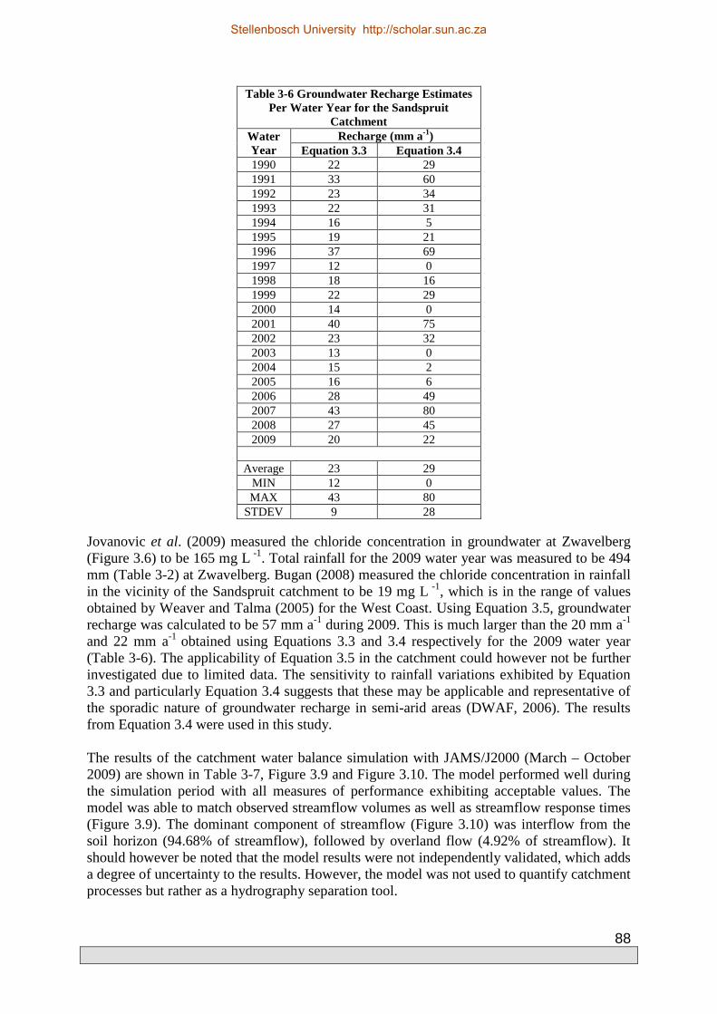
88

Table 3-6 Groundwater Recharge Estimates Per Water Year for the Sandspruit

Catchment Water Year

Recharge (mm a-1) Equation 3.3 Equation 3.4

1990 22 29 1991 33 60 1992 23 34 1993 22 31 1994 16 5 1995 19 21 1996 37 69 1997 12 0 1998 18 16 1999 22 29 2000 14 0 2001 40 75 2002 23 32 2003 13 0 2004 15 2 2005 16 6 2006 28 49 2007 43 80 2008 27 45 2009 20 22

Average 23 29

MIN 12 0 MAX 43 80

STDEV 9 28 Jovanovic et al. (2009) measured the chloride concentration in groundwater at Zwavelberg (Figure 3.6) to be 165 mg L -1. Total rainfall for the 2009 water year was measured to be 494 mm (Table 3-2) at Zwavelberg. Bugan (2008) measured the chloride concentration in rainfall in the vicinity of the Sandspruit catchment to be 19 mg L -1, which is in the range of values obtained by Weaver and Talma (2005) for the West Coast. Using Equation 3.5, groundwater recharge was calculated to be 57 mm a-1 during 2009. This is much larger than the 20 mm a-1 and 22 mm a-1 obtained using Equations 3.3 and 3.4 respectively for the 2009 water year (Table 3-6). The applicability of Equation 3.5 in the catchment could however not be further investigated due to limited data. The sensitivity to rainfall variations exhibited by Equation 3.3 and particularly Equation 3.4 suggests that these may be applicable and representative of the sporadic nature of groundwater recharge in semi-arid areas (DWAF, 2006). The results from Equation 3.4 were used in this study. The results of the catchment water balance simulation with JAMS/J2000 (March – October 2009) are shown in Table 3-7, Figure 3.9 and Figure 3.10. The model performed well during the simulation period with all measures of performance exhibiting acceptable values. The model was able to match observed streamflow volumes as well as streamflow response times (Figure 3.9). The dominant component of streamflow (Figure 3.10) was interflow from the soil horizon (94.68% of streamflow), followed by overland flow (4.92% of streamflow). It should however be noted that the model results were not independently validated, which adds a degree of uncertainty to the results. However, the model was not used to quantify catchment processes but rather as a hydrography separation tool.


89

Table 3-7 Results of Water Balance Simulations (Mar – Oct 2009) for the Sandspruit Catchment

Performance Measure

Result Nash-Sutcliffe Efficiency (NSE) 0.85 Coefficient of Determination (r2) 0.85 Absolute Volume Error (AVE) 0.33 m3 s-1

Root Mean Square Error (RMSE) 0.35

Figure 3.9. Simulated and observed streamflow for the Sandspruit catchment (Mar – Oct 2009).

Figure 3.10. The components of simulated streamflow (RD1 – overland flow, RD2- interflow from the soil

horizon, RG1- interflow from the weathered horizon, RG2 – groundwater flow).


90

The components for the simulated water balance are shown in Table 3-8. Equation 3.1 cannot be solved for the simulation results indicating that there are losses from the catchment, i.e. 17.94 mm. This may be attributed to changes in soil moisture storage over the simulation period.

Table 3-8 Components of the Simulated Water Balance (Mar – Oct 2009) for the Sandspruit Catchment

Component Simulated value (mm simulation period -1)

Precipitation 307.21 Potential ET 653.07 Actual ET 256.98

Simulated Streamflow 32.29 Observed Streamflow 32.48

RD1 1.59 RD2 30.57 RG1 0.13 RG2 0

Data gathered during this investigation allowed for a conceptual flow model to be developed for the Sandspruit catchment (Figure 3.11). The catchment receives 473 mm a-1 precipitation on average (Table 3-2). Higher rainfall was recorded in the upper reaches of the catchment (494 mm a-1 at the foot of Kasteelberg), where groundwater recharge mainly occurs through the Sandstone fractured rock system, compared to the lower reaches (321 mm a-1 at DWA station No. G1H043). Streamflow at DWA gauge G1H043 is measured to be approximately 30 mm a-1 (Table 3-3). Evapotranspiration makes up the remainder of the water balance (443 mm a-1), assuming there are no other losses of water, e.g. regional groundwater losses directly through discharge into the Berg River. Soil water and groundwater storage are negligible components of the water balance over extended periods of observation. Seasonal fluctuations of the groundwater potentiometric surface in the catchment measured in boreholes (Jovanovic et al., 2009) suggest that evaporation impacts the groundwater table, and that a seasonal groundwater recharge-discharge mechanism exists. This seasonal behaviour is exhibited in Figure 3.12, which presents the hourly automatically recorded and manually measured groundwater levels at ZB004 and UV005 (Table 3-1, Figure 3.3). The seasonal nature of the stream and the depth of the water table suggested that the regional groundwater contribution to streamflow is minimal, leaning towards negligible. Streamflow is driven by quickflow, which comprises overland flow and especially interflow from the alluvium cover. Temporary seasonal perched water tables occur at the interface of the alluvium cover and Malmesbury shale with low permeability (Jovanovic et al., 2009). Infiltration is facilitated by preferential pathways created by root channels (winter wheat) as well as the minimization of overland flow rates by the dense wheat cover (de Cercq et al., 2010). In addition, man-made anti-erosion contours that are common in the area represent micro-areas where overland flow of water is barraged and water infiltrates. The dominant contribution to the stream hydrograph is therefore interflow, originating from the recharge of temporary groundwater tables in winter. This contribution generally occurs until November, about two months after the end of the rainy season. As groundwater recharge and discharge is less than streamflow (30 mm a-1), the historic values of groundwater recharge of 69-71 mm a-

1 estimated by Vegter (1995) for quaternary catchment G10J appear to be overestimated (assuming no other groundwater losses occur). The percentage contributions to the hydrograph components (Figure 3.11) were estimated using the JAMS/J2000 hydrological


91

model. It should be noted that the model results were not independently validated. In this study, groundwater recharge was calculated to be 29 mm a-1 on average. However, this is mainly recharge to temporary winter water tables which contribute to interflow.

Figure 3.11. Conceptual flow model for the Sandspruit Catchment.

Isotope analyses (Figure 3.8) indicate that groundwater, in particular in the mid- and lower reaches of the catchment, was subject to evaporation before recharge took place. This is the same water that discharges and predominantly contributes to the stream. The poor correlation between average annual streamflow and average rainfall (r2 < 0.4) suggests that a variety of factors may influence streamflow, e.g. rainfall distribution, cropping systems and/or evapotranspiration. Streamflow is therefore more dependent on the rainfall distribution in time and water use than on annual rainfall.


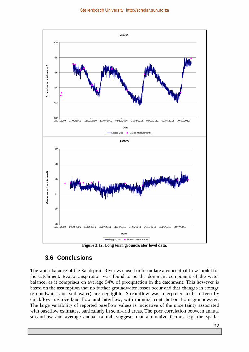
92

350

352

354

356

358

360

17/04/2009 14/09/2009 11/02/2010 11/07/2010 08/12/2010 07/05/2011 04/10/2011 02/03/2012 30/07/2012

Gro

undw

ater

Lev

el (

mam

sl)

Date

ZB004

Logged Data Manual Measurements

70

72

74

76

78

80

17/04/2009 14/09/2009 11/02/2010 11/07/2010 08/12/2010 07/05/2011 04/10/2011 02/03/2012 30/07/2012

Gro

undw

ater

Lev

el (

mam

sl)

Date

UV005

Logged Data Manual Measurements Figure 3.12. Long term groundwater level data.

3.6 Conclusions

The water balance of the Sandspruit River was used to formulate a conceptual flow model for the catchment. Evapotranspiration was found to be the dominant component of the water balance, as it comprises on average 94% of precipitation in the catchment. This however is based on the assumption that no further groundwater losses occur and that changes in storage (groundwater and soil water) are negligible. Streamflow was interpreted to be driven by quickflow, i.e. overland flow and interflow, with minimal contribution from groundwater. The large variability of reported baseflow values is indicative of the uncertainty associated with baseflow estimates, particularly in semi-arid areas. The poor correlation between annual streamflow and average annual rainfall suggests that alternative factors, e.g. the spatial


93

distribution of winter wheat, the temporal distribution of rainfall, rainfall intensities, soil moisture and/or climatic variables (temperature), exert a greater influence on streamflow. It should however be noted that the correlation between annual streamflow and average annual rainfall dominantly utilises rainfall data from stations located outside the catchment (Figure 3.6), which may not be representative of rainfall inside the catchment. Measured streamflow also correlates poorly with calculated actual ET (Table 3-5, r2 = 0.13). Correlations of observed streamflow (for both above and below average precipitation years) with average rainfall and actual ET were also poor. Everson (2001) is of the opinion that when rainfall is lower than ET, excess water, even in wetter years, is still not sufficient to satisfy the PET and will resultantly not influence streamflow volumes. Streamflow is more dependent on the rainfall distribution in time rather than on the annual volume. These poor correlations could also be a result of inadequate spatial monitoring of climatic variables, particularly rainfall. Unfortunately the data record from stations located inside the catchment (Figure 3.6) is not sufficiently long to investigate this. Additionally, errors in measurements should also be considered as a factor. The water balance and conceptual flow model will form the basis for the application of distributed hydrological modelling in the Sandspruit catchment and the development of salinity management strategies. The application of distributed hydrological models could be used to further investigate and validate results of this investigation, i.e. quantifying baseflow, groundwater recharge and observed streamflow volumes in particular. It is also interpreted that results, e.g. ET estimates, methods to quantify groundwater recharge and/or hydrograph separation, from this investigation could potentially be extrapolated to other semi-arid areas.

3.7 References

ALEXANDER WJR (1985) Hydrology of low latitude Southern Hemisphere land masses. Hydrobiologia 125 75-83.

ALLEN RG, PEREIRA LS and RAES D (1998) Crop evaporation: guidelines for computing crop water requirements. Irrigation and Drainage Paper No 56, Rome, Italy.

ANCHOR ENVIRONMENTAL and FRESHWATER CONSULTING GROUP (2007) Berg River baseline monitoring programme. Final report - Volume 5: Synthesis. DWAF Report No. P WMA 19/G10/00/2107, Department of Water Affairs and Forestry, Pretoria.

BEEKMAN H, GIESKE A and SELAOLO ET (1996) GRES: Groundwater recharge studies in Botswana 1987-1996. Botswana J. Earth Sci 3 1-17.

BEVEN KJ and O' CONNELL PE (1983) General report on water balance computation techniques, New Approaches in Water Balance Computations, August 1983. IAHS Publ 148 41-46.

BREDENKAMP DB, BOTHA LJ, VAN TONDER GJ and VAN RENSBURG HJ (1995) Manual on quantitative estimation of groundwater recharge and aquifer storativity. Report No 73/95, Water Research Commission, Pretoria.

BUGAN RDH (2008) Hydrosalinity fluxes in a small scale catchment of the Berg River (Western Cape). University of the Western Cape, Cape Town.


94

BUGAN RDH, JOVANOVIC NZ, DE CLERCQ WP, HELMSCHROT J, FLÜGEL W and LEAVESLEY GH (2009) A comparitive analysis of the PRMS and J2000 hydrological models applied to the Sandspruit Catchment (Western Cape, South Africa). In: CA BREBBIA, NZ JOVANOVIC and E TIEZZI, eds, Management of Natural resources, Sustainable Development and Ecological Hazards 2 edn. WIT Press,Southampton, 391-402 pp.

CLARKE ID and FRITZ P (1997) Environmental isotopes in hydrogeology. Lewis Publishers, Boca Reton, New York.

DE CLERCQ WP, JOVANOVIC NZ and FEY MV (2010) Land use impacts on salinity in Berg River water. Report No K5/1503, Water Research Commission, Pretoria.

DIAMOND R and HARRIS C (1997) Oxygen and hydrogen isotope composition of Western Cape meteoric water. S. Afr. J. Sci 93 371 -374.

DWAF, 3 September 2008, 2008-last update, hydrological services [Homepage of Department of Water Affairs and Forestry], [Online]. Available: http://www.dwaf.gov.za/hydrology/ [27 May 2010].

DWAF (2006) Groundwater Resource Assessment II: Final report. Task 3a: Recharge. Department of Water Affairs and Forestry, Pretoria.

DWAF (2003) Berg River Baseline Monitoring Project. Description of Geohydrological Conditions. Groundwater Atlas. Department of Water Affairs and Forestry, Pretoria.

EAGLESON PS (1978) Climate, soil and vegetation. Water Resour Res 14 (5) 705-776.

ERIKSSON E and KHUNALASEM V (1969) Chloride concentrations in groundwater, recharge rate and rate of deposition of chloride in the Israel coastal plain. J Hydrol 7 178-197.

EVERSON CS (2001) The water balance of a first order catchment in the montane grasslands of South Africa. J Hydrol 241 110-123.

FEY MV and DE CLERCQ WP (2004) Dryland salinity impacts on Western Cape rivers. Report No 1342/1/04. Water Research Commission, Pretoria.

HUGHES DA, HANNART P and WATKINS D (2003) Continuous baseflow separation from time series of daily and monthly streamflow data. Water SA 29 (1) 43-48.

HUGHES JD, KHAN S, CROSBIE RS, HELLIWELL S and MICHALK DL (2007) Runoff and solute mobilization processes in a semiarid headwater catchment. Water Resour Res 43 15.

JIA, H. & XU, Y. 2009. Borehole Logging Version 1.0. Pretoria: Water Research Commission.

JOTHITYANGKOON C, SIVAPALAN M and FARMER DL (2001) Process controls of water balance variability in a large semi-arid catchment: downward approach to hydrological model development. J Hydrol 254 174-198.


95

JOVANOVIC NZ, BUGAN RDH and SOLTAU LS (2009) Report detailing boreholes in the Sandspruit Catchment. Deliverable 10, WRC Project K5/1849. CSIR, Natural Resources and the Environment, Stellenbosch.

KRAUSE P (2002) Quantifying the impact of land use changes on the water balance of large catchments using the J2000 Model. Phys Chem Earth 27 663-673.

L'VOVICH MI (1979) World water resources and their future. American Geophysical Union, Washington DC.

MEADOWS ME (2003) Soil erosion in the Swartland, Western Cape Province, South Africa: implications of past and present policy and practice. Environ Sci Policy 6 17-28.

MEYER PS (2001) An explanation of the 1:500 000 general hydrogeological map Cape Town 3317. Department of Water Affairs and Forestry, Pretoria.

MIDDLETON BJ and BAILEY AK (2009) Water resources of South Africa, 2005 study (WR2005). Report No TT 380/08, Water Research Commission, Pretoria.

MIDGELEY DC, PITMAN WV and MIDDLETON BJ (1994) Surface water resources of South Africa 1990. Volumes 1-6. Report No 298/1.1/94 - 298/6.1/94, Water Research Commission, Pretoria.

PARSONS R (1994) A review of approaches and methodologies for determining leachate generation at waste disposal sites and groundwater recharge. Report No. 564/1/94, Water Research Commission, Pretoria.

PARSONS R and WENTZEL J (2007) Groundwater Resource Directed Measures Manual. Report No TT 299/07, Water Research Commission, Pretoria.

PARSONS RP (1995) A South African aquifer system management classification. Report No 77/95, Water Research Commission, Pretoria.

PONCEA VM and SHETTY AV (1995) A conceptual model of catchment water balance: 1. Formulation and calibration. J Hydrol 173 (1-4) 27-40.

RICE K and HORNBERGER GM (1998) Comparison of hydrochemical tracers to estimate source contributions to peak flow in a small, forested headwater catchment. Water Resour Res 34 1755-1766.

SCHULZE RE (1997) South African atlas of agrohydrology and -climatology. Report No TT82/96, Water Research Commission, Pretoria.

SIMMERS I (1998) Groundwater recharge: an overview of estimation problems and recent developments. In: NS ROBINS, ed, Groundwater Pollution, Aquifer Recharge and Vulnerability. 130 edn. Geological Society, London, 107-115 pp.

VEGTER JR (1995) An explanation of a set of national groundwater maps. Report No TT 74/95, Water Research Commission, Pretoria.


96

VEGTER JR and PITMAN WV (2003) Recharge and Streamflow. In: Y XU and H BEEKMAN, eds, Groundwater recharge estimation in Southern Africa. Cape Town: UNESCO Paris, 109-122 pp.

WARD RC (1972) Checks on the water balance of a small catchment. Nord Hydrol 3 44-63.

WEAVER JMC and TALMA AS (2005) Cumulative rainfall collectors – A tool for assessing

groundwater recharge. Water SA 31 (3) 283-290.

WEAVER JMC, CAVÉ L and TALMA AS (2007) Groundwater Sampling (second edition). Report No TT 303/07, Water Research Commission, Pretoria.

WILSON KB, HANSON PJ, MULHOLLAND PJ, BALDOCCHI DD and WULLSCHLEGER SD (2001) A comparison of methods for determining forest evapotranspiration and its components: sap-flow, soil water budget, eddy covariance and catchment water balance. Agric For Meteorol 106 (2) 153-168.

XU C (1999) Estimation of parameters of a conceptual water balance model for ungauged catchments. Water Resour Manage 13 353-368.

XU Y, TITUS R, HOLNESS SD, ZHANG J and VAN TONDER GJ (2002) A hydrogeomorphological approach to quantification of groundwater discharge to streams in South Africa. Water SA 28 (4) 375-380.


97

4. QUANTIFICATION OF THE SALINITY FLUXES IN THE SANDSPRUIT CATCHMENT 2

4.1 Introduction

Soil and stream salinisation is a major environmental problem occurring in many parts of the world. It reduces the fertility of landscapes impacting agricultural activities and degrades water quality resulting in it being unfit for domestic, recreational, agricultural and/or industrial use. This results in significant economic losses and water supply issues. The salinisation of soils and water resources may either be a natural phenomenon (primary salinity) or a result of anthropogenic activities (secondary salinity). Primary salinity is associated with the release of salts through the weathering of naturally saline rocks and/or deposition by climatic controls (aeolian or rainfall deposition). Climatic controls are largely a function of proximity to the coast. Human-induced or secondary salinisation may either be a function of the direct addition of saline water, e.g. industrial effluent and/or saline irrigation water, to the landscape and/or water resources or it may be a result of a change in the water balance (quantity and dynamics) of a catchment causing the mobilisation of stored salts (dryland/non-irrigated salinity). Dryland/non-irrigated salinity commonly occurs as a result of changes in land use (indigenous vegetation to agriculture and/or pasture) and management which cause a change in the water and salt balance of the landscape consequently mobilizing stored salts. Salinity has long been identified as one of the main water quality problems in South Africa (DWAF, 1986). Many rivers exhibit high salinities, which is either a result of the naturally saline geology in which the rivers flow (Lerotholi, 2005) or a result of anthropogenic activities. The Berg River which is located in the Western Cape is an example of a river which has been exhibiting an increasing trend in salinity levels, particularly in the mid- to lower-reaches. The Berg River is a pivotal source of freshwater to Cape Town, the agricultural sector, the industrialized town of Saldanha and the instream ecology. To illustrate this salinity increase, the long term salinity of selected stations in the Berg River catchment (Figure 4.1) is graphically displayed in Figure 4.2. The data were soured from the Department of Water Affairs (DWA). Station G1H020 is located downstream of Paarl (Figure 4.1) and is representative of the water quality in the upstream sections of the Berg River. Stations G1H036 and G1H023 (Figure 4.1) are representative of the mid-stream and downstream sections of the river respectively. A significant salinity increase is observed from

2 BUGAN, R.D.H., JOVANOVIC, N.Z., DE CLERCQ, W.P., FLÜGEL, W-A., HELMSCHROT, J., FINK, M. and KRALISCH, S. Dryland Salinity Management in the Semi-Arid Western Cape (South Africa). XXV IUGG General Assembly Earth on the Edge: Science for a Sustainable Planet, 28 June–7 July 2011, Melbourne, Australia.

DE CLERCQ, W.P., JOVANOVIC, N.Z., BUGAN, R.D.H., MASHIMBIYE, E. and DU TOIT, T., in progress. Management of human induced salinization in the Berg River catchment and development of criteria for regulating agricultural land use in terms of salt generating capacity. Pretoria: Water Research Commission.


98

station G1H020 towards station G1H023 (Figure 4.2). The increased streamflow salinity recorded at G1H023 is not influenced by oceanic salts as it is located approximately 20 km upstream of the Berg River estuary at Velddrif (Figure 4.1). This salinity increase exhibited at G1H036 and G1H023 is interpreted to not only be a function of a change in the geological environment (G1H020 is located in an area dominated by Table Mountain Group sandstones, whereas G1H036 and G1H023 are located in areas dominated by Malmesbury Shale) but also a change in land use.

Figure 4.1. Major towns (red) and selected streamflow salinity gauges (blue) in the Berg River catchment. Consequently, a cycle of research projects was initiated to comprehend the cause and dynamics of the salinisation in the catchment. It was reported that, in addition to the occurrence of naturally saline geology, the increase in salinity observed in the Berg River may also be attributed to dryland salinisation (Fey and de Clercq, 2004; de Clercq et al., 2010; Flügel, 1995). According to de Clercq et al. (2010) changes in land use over the last century or more, from extensive pastoral use to intensive cropping, has triggered the same process of salt decantation that is so widespread in Australia (Acworth and Jankowski, 2001; Clarke et al., 2002; Crosbie et al., 2007; Peck and Hatton, 2003). The Sandspruit catchment, a tributary of the Berg River, has particularly been impacted by dryland salinity (de Clercq et al., 2010). According to Flügel (1995) the total salt output from the Sandspruit catchment, a tributary of the Berg River, in 1986 was 8 052 t, of which a third may be accounted for by atmospheric deposition. The change in land use has changed the water balance in the catchment resulting in the mobilisation of stored salts. In addition, the semi-arid climate (low rainfall and high potential evapotranspiration rates) in the Western Cape limits the capacity to

N

Not to scale


99

drain salt and water and consequently causes the accumulation of salt in the soil and groundwater. Pegram and Görgens (2001) also identified salinity increases in the Breede River, which is also a significant resource in the Western Cape.

0.0

5.0

10.0

15.0

20.0

25.0

30.0

35.0

40.0

45.0

50.0

01/1967 01/1972 01/1977 01/1982 01/1987 01/1992 01/1997 01/2002 01/2007 01/2012

EC

(m

S/m

)

Date

G1H020

0.0

12.0

24.0

36.0

48.0

60.0

72.0

84.0

96.0

108.0

120.0

01/1982 01/1987 01/1992 01/1997 01/2002 01/2007 01/2012

EC

(m

S/m

)

Date

G1H036

0.0

80.0

160.0

240.0

320.0

400.0

480.0

560.0

640.0

720.0

800.0

01/1982 01/1987 01/1992 01/1997 01/2002 01/2007 01/2012

EC

(m

S/m

)

Date

G1H023

Figure 4.2. The streamflow salinity recorded at stations G1H020, G1H036 and G1H023 on the Berg

River.


100

The quantification of salinity fluxes at the catchment scale is an initial step and integral part of developing dryland salinity mitigation measures. It is an important component of identifying the current salinity status and trend in the catchment, i.e. a state of salt depletion/accumulation and/or rates of accumulation/depletion. Additionally, it will also generate data which will facilitate the calibration and validation of salinity management models. Ultimately however, it provides an indication of the severity of the salinity problem in an area. The objective of this study was to quantify the salinity fluxes in the 152 km2 Sandspruit catchment. This included the quantification of salt storage (in the regolith and underlying shale), salt input (rainfall) and salt output (in runoff). Salt storage was quantified on a spatially distributed basis with the aim of identifying salt load ‘hotspots’. It is envisaged that this information may be used to classify the land according to the levels of salinity present, provide a guide and framework for the prioritisation of areas for intervention and the choice and implementation of salinity management options. The investigation was conducted for the period 2007 - 2010, thus studying four rainfall seasons.

4.2 Theory and Methodology

The Sandspruit catchment is located in the mid- to lower-reaches of the Berg catchment, an area which stores large quantities of soluble inorganic salts in the regolith. The change in land use, from indigenous vegetation to agriculture, has altered the water balance (changes in evapotranspiration and infiltration/recharge dynamics) causing the mobilisation of these salts and the subsequent salinisation of soils, groundwater and streams. Salt output is interpreted to be well in excess of salt input and considered to be mainly mobilised by interflow, as interflow from the soil horizon is the dominant contributor to streamflow (94.68% of streamflow (Bugan et al., 2012). As evapotranspiration exceeds precipitation throughout most of the year, leaching of salts is likely to be limited and soluble salts accumulate in the soil horizon. During rainfall events, the resultant runoff and infiltration periodically flush these salts throughout the landscape and into rivers.

4.2.1 Salt Input

The main source of salt input to the Sandspruit catchment occurs via rainfall. As dryland farming is mainly practiced, the potential for salt input to occur via irrigation with saline water is minimal. Salt input may also occur via dry aeolian deposition, due to the proximity to the coast, however due to the low volumes associated with this mechanism and the complexity of quantifying it, it was not considered in this investigation. Salt input to a catchment from rainfall may be quantified using the equation (Jolly et al., 1997): TSI = R * CA * SFC (4.1) Where TSI is the Total Salt Input (kg CA-1), R is the Rainfall (mm), CA is the Catchment Area (km2) and SFC is the Salt Fall Concentration (mg L-1). The salinity of rainfall was not monitored during this study, however data in this regard are available from previous investigations. Flügel (1995) estimated the Sandspruit catchment to receive approximately 440 mm a-1 (mean), and this rainfall to have a salt concentration ranging between 14 and 125 mg L-1, averaging at 37 mg L-1. Sodium and chloride transported by wind from the Atlantic Ocean were the dominant ions. Due to the unavailability of recent rainfall salinity data it is assumed that the data presented by Flügel (1995) is still valid.


101

Flügel's (1995) estimate equates to 2 475 t (0.2 t ha-1) on average. de Clercq et al. (2010) estimated the salt input to the Sandspruit catchment for the period 1981 – 2007. The results are presented in Table 4-1.

Table 4-1 Total Salt Input (TSI) to the Sandspruit Catchment (de Clercq et al., 2010)

Year Rainfall (mm)

TSI (t CA -1)

TSI (t ha-1)

Year Rainfall (mm)

TSI (t CA -1)

TSI (t ha-1)

1981 495 2785 0.18 1995 485 2727 0.18 1982 600 3374 0.22 1996 768 4321 0.28 1983 486 2731 0.18 1997 419 2355 0.15 1984 680 3824 0.25 1998 575 3233 0.21 1985 666 3746 0.25 1999 472 2655 0.17 1986 473 2662 0.18 2000 333 1873 0.12 1987 573 3223 0.21 2001 751 4222 0.28 1988 475 2670 0.18 2002 588 3306 0.22 1989 648 3642 0.24 2003 394 2213 0.15 1990 562 3160 0.21 2004 467 2626 0.17 1991 556 3128 0.21 2005 409 2298 0.15 1992 647 3639 0.24 2006 570 3203 0.21 1993 377 2120 0.14 2007 660 3710 0.24 1994 504 2836 0.19

The total salt input for the 2007 – 2010 rainfall seasons was quantified using average rainfall values calculated by Bugan et al. (2012), and the average rainfall salt concentration derived by Flügel (1995).

4.2.2 Measuring Soil Salinity

During April-June 2009, 26 boreholes were drilled throughout the Sandspruit catchment (Figure 4.3). The coordinates of the boreholes are presented in Table 3-1 (Chapter 3). Drilling sites were spatially distributed so as to be representative of geological and topographic variation within the catchment. The Rotary Percussion method was used to drill the boreholes and collect samples. The depth of drilling was determined by the depth to groundwater and the depth to consolidated hard rock (Malmesbury Shale). In some cases, boreholes were drilled deeper so as to investigate whether further water strikes would be intersected within the shale. Borehole site characteristics are summarized in Table 4-2.

Table 4-2 Description of Sampling Sites

Sampling Site

Ground Elevation (mamsl)

Date Drilled

Drilling Depth (m)

Depth to Hard Rock

(m)

Potentiometric Head (mamsl) *

Reason Stopped

Zwavelberg ZB001 309 09/05/2009 12 11 Dry Hard rock reached ZB002 278 09/05/2009 18 9 270.20 Hard rock reached

ZB003 272 27/04/2009 120 11 263.16 No intersection of deeper water table


ZB005 361 24/04/2009 14 13 355.95 Hard rock reached


ZB006A 07/05/2009 11 11 297.08 Hard rock reached


ZB007A 303 08/05/2009 12 12 Dry Hard rock reached


102

Sampling Site


Date Drilled

Drilling Depth (m)

Depth to Hard Rock

(m)

Potentiometric Head (mamsl) *

Reason Stopped

Oranjeskraal

OK001 107 11/05/2009 103 8 101.07 No intersection of deeper water table

OK002 118 13/05/2009 30 29 107.24 Hard rock reached OK003 125 14/05/2009 36 29 Blocked Hard rock reached

Uitvlug UV001 70 21/05/2009 72 69 56.14 Hard rock reached

UV002 62 18/05/2009 30 15 60.28 No intersection of deeper water table

UV003 64 13/05/2009 42 22 Artesian No intersection of deeper water table

UV004 81 20/05/2009 45 30 76 No intersection of deeper water table

UV005 119 22/05/2009 120 53 75.37 No intersection of deeper water table

* 31/01/2011-01/02/2011

Figure 4.3. The location of the boreholes in the Sandspruit catchment.

The salinity of soil is generally measured by drawing salts from the soil into solution and measuring the salinity of the solution. The different methods with which soil salinity may be measured are presented in Table 4-3. During borehole drilling, sediment samples were collected at 1 m intervals. The samples were sealed in sampling bags and used to measure soil water content. Sub-samples were subsequently used to prepare 1:5 solid:solution extracts (Allison et al., 1954) and the resulting solution was used to measure EC1:5 (mS m-1). Sampling and testing soil is an accurate method of measuring salt levels and can also determine whether factors, other than


103

salinity, are affecting an area. The EC1:5 was then converted to the ECe (EC of the soil extract) using a multiplication factor (Slavich and Petterson, 1993; Table 4-4). The salinity of the topsoil (0 – 0.5 m) was then assessed according to the salinity classes proposed by Richards (1954) and Van Hoorn and Van Alphen (1994), which is presented in Table 4-5.

Table 4-3 Common Methods With Which to Measure Soil Salinity Measurement

Symbol Soil Solution/Soil

Measurement Description

EC 1:5 Soil:water solution

1 part soil: 5 parts water Does not take soil texture into account

ECe Soil ECe refers to the EC of the soil extract

Takes soil texture into account Is determined by multiplying the EC1:5 by a soil texture factor

ECse Soil

ECse refers to the EC of the saturated extract Laboratory method used to determine soil chemistry

Measures water extracted from a soil:water paste This measurement is approximately the same as ECe

Table 4-4 Multiplication Factors for Converting EC1:5 to ECe (Slavich andPetterson, 1993)

Soil Field Texture

Description Conversion

Factor

Sands

Very little or no coherence

17 Cannot be rolled into a stable ball

Individual sand grains adhere to the fingers

Loams

Can be rolled into a thick thread but will break before it is 3-4 mm thick

10 Soil ball is easy to manipulate and has a smooth spongy feel

with no obvious sandiness

Clay Loams Can be easily rolled to a thread 3-4 mm thick but with a number

of fractures along the length 9 Plastic like soil, capable of being moulded into a stable shape

Light Clays Can be rolled to a thread 3-4 mm thick without fractures

8 Some resistance to rolling out Plasticity evident, smooth feel

Medium Clays

Handles like plasticine

7 Forms rods without fractures

Some resistance to ribboning shear Ribbons to 7.5 cm or more

Table 4-5 ECe Values of Soil Salinity Classes (Richards,

1954; Van Hoorn and Van Alphen, 1994)

Class Salinity Class

ECe (mS m-1)

Non-saline 0 < 200 Slightly Saline 1 200 – 400

Moderately Saline 2 400 – 800 Very Saline 3 800 – 1600

Highly Saline 4 > 1600

4.2.3 Salt Storage

The sediment samples collected during borehole drilling, which were used to prepare 1:5 solid:solution extracts, were also used to quantify the salt storage in the catchment. The EC results of the 1:5 solid:solution extracts are, however, not a true representation of field


104

conditions due to the diluting effect of the added water in the preparation of the 1:5 solid:solution extracts. This diluting effect was accounted for using the following process:

• As the mass of water is 5 times the mass of soil, the soil sample is said to have a water content of 500% in gravimetric terms. The gravimetric water content (GWC) is thus 5 g water per 1 g soil.

• The GWC may then be converted into volumetric water content (VWC) using the soil bulk density. As disturbed samples were collected, it was not possible to measure porosity, density and hydraulic properties. However, the bulk density of the regolith was measured on drilling cores collected in a catchment adjacent to the Sandspruit exhibiting similar physical conditions (Samuels, 2007). The cores exhibited similar geological layering (sequence) to that observed in the Sandspruit catchment. The results are presented in Table 4-6, which represent the average bulk density of three cores.

• A dilution factor may then be obtained for each sample by dividing the VWC of the solid:solution extracts by the actual VWC. EC measured on 1:5 solid:solution extracts were then multiplied by this dilution factor to obtain true EC values.

• The Total Dissolved Salts (TDS) was then inferred from the EC using results from regression (R2 = 0.90) analysis performed by (Bugan, 2008), i.e. TDS (mg L-1) = 534.91 * EC (dS m-1) – 12.655.

Table 4-6 The Bulk Density of Weathered

Sediments (Samuels, 2007) Layer Description Bulk Density (g cm-3)

1 Topsoil 1.253

2 Sandy

Loam soil 1.494

3 Clayey soil 1.410

4 Malmesbury

Shale 1.516

The TDS concentrations of the sediment solution was used to calculate the salt storage in t ha-

1. These data represented model inputs for the simulation of inorganic salt fluxes as well as allowed the identification of areas of maximum salt storage in the catchment. Salt storage (t ha-1) from TDS (mg L-1water) may be quantified using the following equations: Calculate the soil mass (kg ha-1;White, 2006),

M = T*Db*105 (4.2)

Where M is the Soil Mass (kg ha-1), T is the Thickness of the horizon (cm) and Db the Bulk Density (g cm-3). Calculate the soil salt concentration (mg salt kg-1 soil),

Cs = Cw x GWC (4.3)

Where Cs is the Soil Salt Concentration (mg salt kg-1 soil), Cw is the Water Salt Concentration (mg L-1 water) and GWC is the Gravimetric Water Content (kg kg-1). Calculate the salt mass (kg ha-1),


105

SC = Cs*M /106 (4.4)

Where SC is the Salt Mass (kg salt ha -1), Cs is the Soil Salt Concentration (mg salt kg -1 soil) and M is the Soil Mass (kg soil ha -1).

4.2.4 Spatial Variability in Salt Storage

Salt stores occur in areas which are conducive to the accumulation of water and salts. Knowledge of the spatial distribution of salt storage in the catchment is essential for salinity management, particulary the implementation of distributed salt balance models. As salt storage is usually quantified on a point basis (t ha-1), interpolation methods are used to distribute these data across a catchment. Flügel (1995) suggested that salt distribution in the Sandspruit catchment is a function of the topographic location. Cox et al. (1999) was also of the opinion that spatial variability in salt storage is evident to dominantly be a function of elevation. The topographic wetness index (TWI), which combines local upslope contributing area and slope, is also commonly used to quantify topographical controls on hydrological processes (Sorensen et al., 2005). Point data of regolith salt storage was correlated with ground elevation and the TWI to investigate whether this relationship could be used to interpolate the data. As a further measure, groundwater EC, which is well defined across the catchment, was also correlated with regolith salt storage.

4.2.5 Salt Output

The total salt output from a catchment may be quantified using streamflow quantity and salinity datasets, i.e. the salt load is equal to the product of the streamflow (m3 s-1) and the corresponding stream water salinity (TDS, mg L-1). The salinity of the Sandspruit River is being monitored with an electronic EC sensor, hourly, from June 2007. Data were missing for the period 06/06/2009 – 30/07/2009 due to sensor malfunction. The sensor is located at the Sandspruit gauging weir (G1H043), for which streamflow quantity (m3 s-1) data are available for the period May 1980 to present. This station is maintained by the DWA. The electronic EC sensor produced readings in mV, which were calibrated using streamflow EC readings recorded with a hand-held EC meter during field visits. Grab samples were also collected and the EC analyzed in the laboratory. The calibration was assumed to be linear, i.e. EC (mS m-1) = 0.886* daily average mV - 218.99; R2 = 0.72. Periods for which mV data were missing, were filled using a correlation (R2 = 0.68) with streamflow, i.e. Salt Output (t d-1) = 169.49 * Streamflow (m3 s-1) + 26.743. The streamflow (m3 s-1) and logged EC data for the period of observation are shown in Figure 4.4.


106

0

200

400

600

800

1000

1200

1400

1600

1800

2000

0

2

4

6

8

10

12

14

28/04/2007 03/01/2008 09/09/2008 17/05/2009 22/01/2010 29/09/2010

EC

(m

S/

m)

Str

ea

mfl

ow

(m

3s-1

)

Date

streamflow EC

Figure 4.4. Streamflow volume and EC measured during the period June 2007 to 2010.

The salt output from the Sandspruit catchment was quantified using the equation (Verhoff et al., 1982): SL = TDS * Q * 1000 L m-3 / 1x106 mg kg-1 (4.5) Where SL is the Salt Load (kg s-1), TDS is the Total Dissolved Solids (mg L-1) and Q is the discharge (m3 s-1). The TDS was inferred from EC using the conversion TDS (mg L-1) = EC (mS m-1) * 6.5 (DWAF, 1996), which is commonly used in South Africa.

4.2.6 Catchment Salt Balance

The catchment salt balance, i.e. salt output/input (O/I) ratio, is a key indicator for a catchment that is undergoing salinisation (Williamson, 1998). Prior to the clearing of indigenous vegetation, the O/I ratio may be considered to be at equilibrium (Peck and Hurle, 1973), which does not imply that it is equal but that it is stable. Clearing of the indigenous vegetation may result in output exceeding input, or increased output. The rate of migration back to a state of equilibrium is dependent on the leaching rate and the magnitude of the salt stores (Jolly et al., 2001). In catchments with a mean annual rainfall of less than 500 mm, the time required to restore the salt equilibrium is expected to be of the order of 100s to 10 000s of years depending on rainfall, hydrogeological conditions, salt storage, catchment size and the amount of vegetation clearance (Jolly et al., 2001). The salt mass balance approach has been used with some success to predict the effect of upstream catchment land use on salinity. Generally, a favourable salt balance (mass out ≥ mass in) is considered necessary for sustainable agriculture (Thayalakumaran et al., 2007). The salt balance may be represented by (Wilcox, 1963):

M in – Mout = (dM/dt) (4.6)


107

Where Min and Mout are the mass per unit time of salt input and output respectively and dM/dt is the rate of change in mass in the system. This equation implies that equilibrium, in terms of salt, is achieved when there is no change in the mass of salt in the system, i.e. dM/dt is zero. The salt balance of a system that has a net accumulation of salt is considered at risk from salinisation of land and water resources (Thayalakumaran et al., 2007). Two additional terms are also used to describe the salt balance, i.e. the salt balance index (SBI) and salt export ratio (SER) (Peck and Hurle, 1973; Wilcox, 1963; Gilfedder et al., 1999). These are defined by the salt output from a given hydrological volume and time period, divided by the salt input. The system is in equilibrium when the SBI or SER equals 1. The system is in a state of salt accumulation when the SBI or SER <1, as opposed to a state of salt depletion when the SBI or SER >1 (Thayalakumaran et al., 2007).

4.3 Results and Discussion

4.3.1 Salt Input

The total salt input to the Sandspruit catchment during the period of observation is shown in Table 4-7. Rainfall was assumed to exhibit a TDS concentration of 37 mg L-1. Average catchment rainfall was obtained from Bugan et al. (2012). The salt input was therefore a function of rainfall amount as variable rainfall chemistry data were not available. The TSI ranged between 2261 and 3684 t CA-1.

Table 4-7 Total Salt Input (TSI) to the Sandspruit Catchment

Year Rainfall (mm a-1)

TSI (t CA -1) TSI (t ha-1)

2007 655 3684 0.24 2008 519 2919 0.19 2009 444 2497 0.16 2010 402 2261 0.15

4.3.2 Soil Salinity

The salinity of the topsoil samples (0 – 0.5 m) collected during borehole drilling (Figure 4.3) is presented in Table 4-8. The EC1:5 were converted to ECe using a multiplication factor (Slavich and Petterson, 1993), which is based on soil textural analysis. The results indicate that the majority of the topsoil samples may be classified as non-saline (Van Hoorn and Van Alphen , 1994). However, two samples which were sampled in the downstream parts of the catchment (Uitvlug, Figure 4.1) may be classified as very saline (Van Hoorn and Van Alphen, 1994). This may be indicative of the influence of topography on soil salinisation processes.

Table 4-8 Topsoil Salinity Sampling

Site EC1:5

(mS m-1) Multiplication

Factor ECe

(mS m-1) Salinity Class

Zwavelberg ZB001 8.20 10 82 0/non-saline ZB002 6.20 10 62 0/non-saline ZB004 5 9 45 0/non-saline ZB005 3.3 9 29.70 0/non-saline


108

Sampling Site

EC1:5

(mS m-1) Multiplication

Factor ECe

(mS m-1) Salinity Class

ZB006A 2.75 10 27.50 0/non-saline ZB007 7.10 17 120.70 0/non-saline

ZB007A 14.80 17 251.60 1/slightly saline Oranjeskraal

OK001 6.80 10 68 0/non-saline OK002 2.50 10 25 0/non-saline OK003 7.40 10 74 0/non-saline

Uitvlug UV001 11.20 10 112 0/non-saline UV002 170.00 9 1530 3/very saline UV003 97.00 10 970 3/very saline UV004 27 10 270 1/slightly saline UV005 5.20 10 52 0/non-saline

4.3.3 Salt Storage

The regolith salt storage, measured at each borehole is presented in Table 4-9. The regolith is defined as the layer of loose, heterogeneous material which overlies hard rock (soil zone and vadose zone). The salt storage ranged between 15 t ha-1 and 922 t ha-1. The salt storage is dominantly a function of the depth of the profile as well as elevation, i.e. the regolith salt storage generally increased with decreasing ground elevation. Profiles located at Uitvlug (downstream in the catchment) exhibited elevated salt concentrations indicating that a salinity ‘hot spot’ may be located there. It should however be noted that this quantification technique incorporates a degree of uncertainty, which is mainly associated with the bulk density values. The estimates used in this quantification are from samples collected at a different site and at different depths.

4.3.4 Spatial Variability in Salt Storage

The point data of regolith salt storage was correlated with ground elevation (mamsl), the catchment TWI, and groundwater EC to identify relationships with which to interpolate the data. The coefficients of determination of the correlation analysis are presented in Table 4-10. The correlations were also evaluated using the Spearman’s rank correlation coefficient (Rs; Sorensen et al., 2005). Rs is a measure of the statistical dependance between two variables. If there are no repeated data values, a perfect Rs of +1 or −1 occurs when each of the variables is a perfect monotone function of the other. The sign of Rs indicates the direction of association between X (the independent variable) and Y (the dependent variable). If Y tends to increase when X increases, the Rs is positive. If Y tends to decrease when X increases, the Rs is negative. Salt storage did not correlate well with elevation. This is interpreted to be due to the fact that the borehole locations did not sufficiently account for elevation variations in the catchment, i.e. the borehole transects (Figure 4.3) were essentially drilled across three elevation zones/bands. Also, as the TWI incorporates elevation, the inadequate representation of elevation variation affected this correlation. Regolith salt storage correlated well with groundwater EC (mS m-1), exhibiting a coefficent of determination of 0.75.


109

Table 4-9 Salt Storage (t ha -1) in the Sandspruit Catchment

Site Borehole No

Soil Zone Salt Storage (t ha -1)

Soil Zone Profile Depth (m)

Regolith Salt Storage (t ha -1)

Regolith Profile Depth

(m)

Zwavelberg

ZB001 8 3 28 11

ZB002 14 4 23 9

ZB003 8 2 52 11

ZB004 4 4 15 19

ZB005 4 4 16 13

ZB006 38 12 40 16

ZB006A 5 3 21 11

ZB007 4 2 75 15

ZB007A 8 2 97 12

Oranjeskraal

OK001 4 2 18 8

OK002 4 3 79 29

OK003 10 4 39 29

Uitvlug

UV001 8 3 349 69

UV002 168 3 922 15

UV003 55 2 519 22

UV004 211 16 341 30

UV005 45 18 97 53

Table 4-10 Correlation of Regolith Salt Storage (t ha-1) With Catchment Variables

Groundwater EC (mS m-1)

*


TWI

r2 0.75 0.41 0.07 Rs 0.72 -0.76 -0.21

* Groundwater samples collected in September 2010 The correlation between groundwater EC (mS m-1) and regolith salt storage (t ha-1) may be described by the equation: salt storage (t ha-1) = 0.3269 (groundwater EC mS m-1) + 1.4292 (4.7) This correlation was used to interpolate salt storage across the catchment (Figure 4.5), by making use of additional historic groundwater EC data that were gathered from the National Groundwater Database (NGDB) of the DWA. According to Bennetts et al. (2006) this strong correlation is expected as saline groundwater may be a result of dryland salinity/high soil salinity. Interpolated regolith salt storage ranged between 3 t ha-1 and 674 t ha-1. The data also indicate that storage increases with decreasing ground elevation, i.e. in a north-easterly direction. Salt storage is expected to be lower in the hilltops, due to salt leaching and higher in the valleys due to salt accumulation. The spatially-averaged regolith salt storage in the Sandspruit catchment is 110 t ha-1. Due to the interpolation procedure and the historic nature of the groundwater EC data, these results incorporate uncertainty. They should thus not be considered as absolute values, but rather as estimates of salt storage. Even though these results may not be taken as absolute values, the identification of areas of high salt storage also holds important implications for water resources management and land use planning. It enables resource managers to make informed decisions in terms of vegetation


110

distribution/planting strategies and the locations for the implementation of salinity management measures

Figure 4.5. Interpolated regolith salt storage (t ha-1) in the Sandspruit catchment.

4.3.5 Salt Output

The total annual export of salt from the catchment was calculated using the catchment discharge and streamflow salinity datasets (Equation 4.5). The results are presented in Table 4-11. During the period of observation the salt output from the Sandspruit catchment ranged between 12 671 t a-1 and 21 409 t a-1. The salt output is expected to be dominantly a function of discharge, i.e. rainfall amounts.

Table 4-11 Total Salt Output (t a-1) from the Sandspruit Catchment Year Rainfall (mm) Discharge (mm) Salt Output (t a-

1) 2007 655 32 16 890 2008 519 27 12 671 2009 444 37 21 409 2010 402 15 14 599


111

4.3.6 Catchment Salt Balance

The catchment salt balance, i.e. salt output/input (O/I) ratio is presented in Table 4-12. The rate of change in mass of the system (dM/dt) and the SBI/SER indicate that the Sandspruit catchment is in a state of salt depletion, i.e. salt output exceeds salt input.

Table 4-12 The Salt Balance of the Sandspruit catchment

Year dM/dt (t a-1) SBI/SER

2007 - 13 206 4.6 2008 -9 752 4.3 2009 -18 912 8.6 2010 -12 872 8.5

4.4 Conclusions

The TSI to the catchment from rainfall ranged between 1727 and 3684 t CA-1. The salt input was calculated as a function of rainfall amount as variable rainfall chemistry data were not available. Topsoil samples gathered during borehole drilling may generally be regarded as non-saline, exhibiting an ECe < 200 mS m-1. However, two samples gathered at Uitvlug, which is located in the downstream parts of the catchment (Figure 4.1) exhibited elevated ECe (800 – 1600 mS m-1) and may thus be classified as very saline. This provides evidence for the influence of topographic controls on salinisation processes. The salt storage in the regolith ranged between 15 t ha-1 and 922 t ha-1 and a salinity “hot spot” was identified in the lower reaches of the catchment. The point data of regolith salt storage were correlated with ground elevation (mamsl), the catchment TWI, and groundwater EC to identify relationships with which to interpolate these data. Regolith salt storage correlated well with groundwater EC (mS m-1), exhibiting a coefficent of determination of 0.75. Interpolated regolith salt storage ranged between 3 t ha-1 and 674 t ha-1, exhibiting generally increasing storage with decreasing ground elevation. The average regolith salt storage in the Sandspruit catchment is 110 t ha-1. During the period of observation the salt output from the Sandspruit catchment ranged between 12 671 t a-1 and 21 409 t a-1. The rate of change in salt mass of the system and the SBI/SER indicated that the Sandspruit catchment is in a state of salt depletion, i.e. salt output exceeds salt input. The input data and parameters required for calibration and validation of a semi-distributed hydrosalinity model have been calculated.

4.5 References

ACWORTH, R.I. and JANKOWSKI, J., 2001. Salt source for dryland salinity - evidence from an upland catchment on the Southern Tablelands of New South Wales. Australian Journal of Soil Research, 39, pp. 12-25.

ALLISON, L.E., BERNSTEIN, L., BOWER, C.A., BROWN, J.W., FIREMAN, M., HATCHER, J.T., HAYWARD, H.E., PEARSON, G.A., REEVE, R.C., RICHARDS, L.A. and WILCOX, L.V., 1954. Diagnosis and improvement of saline and alkali soils. Agricultural Handbook No. 60 edn. United States Department of Agriculture.

BENNETTS, D.A., WEBB, J.A., STONE, D.J.M. and HILL, D.M., 2006. Understanding the salnisation processes for groundwater in an area of south-eastern Australia, using hydrochemical and isotopic evidence. Journal of Hydrology, 323, pp. 178-192.


112

BUGAN, R.D.H., 2008. Hydrosalinity fluxes in a small scale catchment of the Berg River (Western Cape), University of the Western Cape.

BUGAN, R.D.H., JOVANOVIC, N.Z. and DE CLERCQ, W.P., 2012. The water balance of a seasonal stream in the semi-arid Western Cape (South Africa). Water SA, 38(2), pp. 201-212.

CLARKE, C.J., GEORGE, R.J., BELL, R.W. and HATTON, T.J., 2002. Dryland salinity in south-western Australia: its origins, remedies and future research directions. Australian Journal of Soil Research, 40, pp. 93-113.

COX, J., DAVIES, P. and SPOUNCER, L., 1999. Water and soil degradation in the Keynes Catchment, South Australia. Technical Report 40/99. Australia: CSIRO Land and Water.

CROSBIE, R.S., HUGHES, J.D., FRIEND, J. and BALDWIN, B.J., 2007. Monitoring the hydrological impact of land use change in a small agricultural catchment affected by dryland salinity in central NSW, Australia. Agricultural Water Management, 88, pp. 43-53.

DE CLERCQ, W.P., JOVANOVIC, N.Z. and FEY, M.V., 2010. Land use impacts on salinity in Berg River water. Report No K5/1503. Pretoria: Water Research Commission.

DWAF, 1986. Management of the water resources of the Republic of South Africa. Pretoria: Department of Water Affairs and Forestry.

DWAF, 1996. South African water quality guidelines (second edition). Volume 4 agricultural use: irrigation. Pretoria: Department of Water Affairs and Forrestry.


FLÜGEL, W., 1995. River salinity due to dryland agriculture in the Western Cape Province, Republic of South Africa. Environmental International, 21, pp. 679-686.

GILFEDDER, M., WALKER, G. and WILLIAMS, J., 1999. Effectiveness of current farming systems in the control of dryland salinity. Australia: CSIRO Publishing.

JOLLY, I.D., DOWLING, T.I., ZHANG, L., WILLIAMSON, D.R. and WALKER, G.R., 1997. Water and salt balances of the catchments of the Murray-Darling Basin. Technical Report 37/97. Australia: CSIRO Land and Water.

JOLLY, I.D., WILLIAMSON, D.R., GILFEDDER, M., WALKER, G.R., MORTON, R., ROBINSON, G., JONES, H., ZHANG, L., DOWLING, T.I., DYCE, P., NATHAN, R.J., NANDAKUMAR, N., CLARKE, R. and MCNEIL, V., 2001. Historical stream salinity trends and catchment salt balances in the Murray_darling basin, Australia. Marine and Freshwater Research, 52, pp. 53-63.

LEROTHOLI, S. 2005. The role of salinity as an abiotic driver of ecological condition in a rural agricultural catchment. MSc edn. Grahamstown, South Africa: Rhodes University.

PECK, A.J. and HURLE, D.H., 1973. Chloride balance of some farmed and forested catchments in southwestern Australia. Water Resources Research, 9, pp. 648-657.


113

PECK, A.J. and HATTON, T., 2003. Salinity and the discharge of salts from catchments in Australia. Journal of Hydrology, 272, pp. 191-202.

PEGRAM, G.C. and GORGENS, A.H.M., 2001. A guide to non-point source assessment. Report No TT 142/01. Pretoria: Water Research Commission.

RICHARDS, L.A., 1954. Diagnosis and Improvement of Saline and Alkali soils. Agricultural Handbook No. 60. USA: USDA.

SAMUELS, D. 2007. Hydraulic properties of the vadose zone at two typical sites in the Western Cape for the assessment of groundwater vulnerability to pollution. M.Sc edn. Bellville: University of the Western Cape.

SLAVICH, P.G. and PETTERSON, G.H., 1993. Estimating the electrical conductivity of saturated paste extracts from 1:5 soil, water suspensions and texture. Soil Research, 31(1), pp. 73-81.

SORENSEN, R., ZINKO, U. and SEIBERT, J., 2005. On the calculation of the topographic wetness index: evaluation of different methods based on field observations. Hydrology and Earth System Science, 2, pp. 1807-1834.

THAYALAKUMARAN, T., BETHUNE, M.G. and MCMAHON, T.A., 2007. Achieving a salt balance—Should it be a management objective? Agricultural Water Management, 92(1-2), pp. 1-12.

VAN HOORN, J.W. and VAN ALPHEN, H.A., 1994. Salinity Control. In: H.P. RITZEMA, ed, Drainage Principles and Application. 2nd, Pubilcation 16 edn. Wageningen, The Netherlands: ILRI, .

VERHOFF, F.H., YAKSICH, S.M. and MELFI, D.A., 1982. An analysis of total phosphorous transport in river systems. Hydrobiologia, 91, pp. 241-252.

WHITE, R.E., 2006. Principles and practice of soil science: the soil as a natural resource. fourth edn. Victoria, Australia: Blackwell Publishing.

WILCOX, L.V., 1963. Salt balance and leaching requirement in irrigated lands. 1290.

WILLIAMSON, D.R., 1998. Land degradation processes and water quality effects, water logging and salinity. In: J. WILLIAMS, R.A. HOOK and H.L. GASCOIGNE, eds, Farming Action-Catchment Reaction, the Effect of Dry-land Farming on the Natural Environment. Collingwood, Victoria: CSIRO Publishing, pp. 162-190.


114

5. HYDROSALINITY MODEL APPLICATION IN THE SANDSPRUIT CATCHMENT: JAMS/J2000–NACL 3

5.1 Introduction

Hydrological modeling has in recent years become essential for effective and holistic management (quality and quantity) of water resources at a catchment scale. It enables officials and scientists to address a variety of engineering and environmental problems, e.g. assessing anthropogenic impacts on water resources, evaluating the assurance of water supply, assessing the impacts associated with land use change and/or forecasting floods. The use of distributed hydrological models can facilitate a quantitative analysis of the impacts of climate and land use change on a catchment’s water and solute fluxes. Many salt mobilisation models aim to predict the impacts of land use change on surface and groundwater contributions of water and salt to catchment stream flow (Gilfedder and Littleboy, undated). According to Bari and Smetten, (2006), in order to predict the impact of land use change, it is necessary to manipulate the evapotranspiration parameters to mimic the desired change in the water balance. Conceptually, salt stores may be mobilised by changes in the partitioning of rainfall into overland flow, through flow, recharge and evaporative components (Bari and Smetten, 2006). Additionally, mobilisation may also occur when water pathways intercept stored salts. These pathways vary both within and between catchments and can operate across a range of spatial and temporal scales. Thus there is a range of methods for partitioning rainfall into these pathways and for dealing with the interaction of these pathways with stored salts (Gilfedder and Littleboy, undated). Salt mobilisation modeling approaches exhibit ranges in complexity, data requirements, scales of application

3 BUGAN, R.D.H., JOVANOVIC, N.Z., DE CLERCQ, W.P., HELMSCHROT, J., FLÜGEL, W. and LEAVESLEY, G.H. 2009. A comparative analysis of the PRMS and J2000 hydrological models applied to the Sandspruit Catchment (Western Cape, South Africa). In: C.A. BREBBIA, N.Z. JOVANOVIC and E. TIEZZI, eds, Management of Natural resources, Sustainable Development and Ecological Hazards 2 edn. Southampton: WIT Press, pp. 391-402.

BUGAN, R.D.H. and JOVANOVIC, N.Z. 2010. Integrated catchment modelling in a semi-arid area. CSIR 3rd Biennial Conference: Science Real and Relevant, CSIR International Convention Centre, 30 August-1 September 2010, Pretoria, South Africa.

DE CLERCQ, W.P., JOVANOVIC, N.Z., BUGAN, R.D.H., MASHIMBIYE, E. and DU TOIT, T., in progress. Management of human induced salinization in the Berg River catchment and development of criteria for regulating agricultural land use in terms of salt generating capacity. Pretoria: Water Research Commission.

STEUDEL, T., BUGAN, R.D.H., KIPKA, H., PFENNIG, B., FINK, M., DE CLERCQ, W.P., FLÜGEL, W. and HELMSCHROT, J. 2013. Implementing contour bank farming practices into the J2000 model to improve hydrological and erosion modelling in semi-arid Western Cape Province of South Africa. Hydrology Research.


115

and may also focus on a particular salt mobilisation process at the expense of others. Heterogeneity in geology, land use and climate increases the complexity of salinity modeling and thus a thorough understanding of catchment physical processes is required. The rate of salt export from a catchment is a function of rainfall, hydrogeological conditions, salt storage, catchment size, vegetation and land use (Jolly et al., 2001). A fundamental difference between salt mobilisation models is the manner in which they spatially represent the catchment, i.e. lumped, generalised or distributed. The applicability of each model depends on the scale at which the output is required and the scale of the management options which are used as input. At the simplest scale, a lumped bucket model assumes spatial homogeneity in hydrologic properties using a single set of parameters to represent water stores and fluxes of water between stores. Evapotranspiration is estimated using spatially averaged parameters across all land uses in the modeled area (Bari and Smetten, 2006). Generalised or distributed catchment models have multiple independent or hydrologically-linked areas and use a range of sub-models to perform their water partitioning. The accuracy and reliability of modeling results is directly proportional to a model’s ability to accurately represent the dominant salt mobilisation processes evident in a catchment. These processes may exhibit large spatial variation and they are dominantly a function of the catchment physical characteristics, e.g. soil, geology, climate, topography, vegetation and/or land use. Salt mobilisation generally occurs via overland flow (solute washoff), vertical hydrosalinity fluxes that occur via infiltration (with soil phase-water solution interactions), through flow (lateral subsurface hydrosalinity fluxes) and groundwater flow. According to Wasson (1998) solute washoff, along with leaching, is the most direct process involved in the salinisation of water resources. The inorganic salts may either be transported as solutes or they may be adsorbed to suspended sediment particles. The solute component is influenced by precipitation and overland flow, whilst adsorbed salts are linked to sediment transport (Johanson, 1983). Vertical water fluxes in the soil profile are generally simulated using tipping bucket (cascading) models, which are based on soil-specific field capacity levels. Current models generally simulate salt fluxes using the convection-dispersion equation. This technique includes salt movement by convection, mechanical dispersion due to variations in velocity through pores of different size, and diffusion, which is controlled by concentration gradients. The movement of contaminants in the unsaturated zone is controlled by infiltration, which is governed by large suction gradients between the wetting front and dry media. Throughflow, along impermeable or semi-permeable layers may be simulated based on empirical water redistribution fractions. Alternatively, Richard’s equation which incorporates convective-dispersive solute flux may be applied, if gradients of water pressure heads and concentrations are known (Schulze, 1995). The ability to simulate groundwater pathways is an important aspect of salt mobilisation models, as groundwater discharge is often a mechanism for salt generation to streams (Bari and Smetten, 2006). Catchment groundwater may be treated as a single store with an associated delay function, i.e. a lumped approach. Spatially variable approaches (generalized or distributed) may use numerous stores for each modelled entity, which is also able to simulate recharge and then discharge to the stream using a storage-discharge relationship (Bari and Smetten, 2006). Bari and Smetten (2006) are of the opinion that improved catchment scale hydrosalinity modelling requires:

• Improvement in the mapping of regolith salt storage and geological structures. This enables the identification of water flow paths and salt store intersection zones and shows accumulation of salt.


116

• Matching model complexity to data complexity and the complexity of the modelling excercise.

• Improved disaggregation/conceptualisation of catchments (both surface and sub-surface), enabling better spatial connectivity.

The scarcity of significant water resources and increased water demand in the Western Cape, which is largely a function of a predominantly semi-arid climate, population increase and socio-economic development, highlights the need for the implementation of effective water resources management initiatives. The objective of this study was thus to evaluate the applicability of the JAMS/J2000-NaCl hydrosalinity model as a catchment scale water and salinity management tool in the semi-arid Sandspruit catchment, where the development of agricultural production areas in the catchment has resulted in the salinisation of land and water resources. The salinisation of water resources in the Western Cape has over the past decade, particularly, attracted numerous investigations due to the importance of water and salinity management. This modeling exercise aims to represent the processes relating to the movement of water and salt from subsurface landscape stores to the land surface and/or to surface water systems. The results of a series of detailed field studies, which were aimed at understanding the manifestation and dynamics of dryland salinity in the Sandspruit catchment (Flügel, 1995; Fey and de Clercq, 2004; Bugan, 2008; de Clercq et al., 2010; Bugan et al., 2012; de Clercq et al., in progress) provide the basis for this investigation. The motivation for the use of a hydrosalinity model is provided by the complexity of salinisation problems, which dictates that field studies alone are often not sufficient to unravel the nature of the underlying processes.

5.2 Model Selection

Chapter 2 provides a review of hydrological models, which have been applied in southern Africa. These range in complexity, temporal and spatial scales of application and/or data requirements, and have generally been developed for region specific applications or to address a specific environmental problem. The review also reveals reduced application in arid/semi-arid environments. Based on the results of previous investigations (Flügel, 1995; Fey and de Clercq, 2004; Bugan, 2008; de Clercq et al., 2010; Bugan et al., 2012; de Clercq et al., in progress) in addition to information gathered from international literature the successful simulation of hydrosalinity fluxes in the Sandspruit catchment requires the following key criteria to be satisfied:

• Distributed catchment properties (geology, land use/vegetation, soil, topography, hydrology and hydrogeology) and distributed climatic inputs (rainfall and temperature) need to be considered.

• The heterogeneity of salt storage and the salt mobilisation processes need to be accounted for. Considering distributed regolith salt storage will facilitate the identification of ‘hot spots’ pertaining to stream and landscape salinity. In addition, it will allow for the ranking of areas for investment into managing dryland salinity.

• The model should be able to simulate surface, subsurface (unsaturated zone) and groundwater flow processes as salt stores may be mobilised by changes in the partitioning of rainfall into overland flow, through flow, recharge and evaporative components.


117

• The model should incorporate the functionality to easily conduct land use/climate change scenario simulations, which have been identified as a useful measure to assess the efficiency of dryland salinity mitigation measures. Thus, the model should also incorporate additional and suitable, from a dryland management perspective, land use and/or management options.

• The model should be able to manipulate the evapotranspiration parameters to mimic the desired change in the water balance resulting from land use change.

Based on these criteria, particularly the consideration of distributed regolith salt storage, the hydrological models presented in Chapter 2 would not be suitable for application in this study. This highlighted the need for evaluating models which have been applied in other countries/regions or for the development of new models/additional model components. The consideration of the application of the JAMS/J2000 hydrological model (Krause, 2002) initially stemmed from a National Research Foundation (NRF)/German Federal Ministry of Education and Research (BMBF) bi-lateral agreement, entered into by Stellenbosch University and the model developers at Friedrich-Schiller University (Jena, Germany). This agreement was also fuelled by a study conducted by (Flügel, 1995) in the Sandspruit catchment. An evaluation of the JAMS/J2000 model (Krause, 2002) revealed that the model accounts for many of the processes required for suitable hydrosalinity modelling, i.e. distributed catchment properties and climatic inputs, the simulation of surface and subsurface flow processes, and the ability to easily conduct scenario simulations. This agreement then facilitated the development of any components which would be required to adequately simulate the hydrosalinity fluxes in the Sandspruit catchment. Bugan et al. (2009) first evaluated the applicability of the JAMS/J2000 semi-distributed hydrological model (Krause, 2002) in the semi-arid Sandspruit catchment. The study concluded that the model was able to match the timing of seasonal hydrograph responses, however it was not able to match annual discharge volumes. Annual discharge was overestimated in certain cases and underestimated in others. The JAMS/J2000 model exhibited a daily Nash-Sutcliffe Efficiency (NSE) of below 0.4. Bugan et al. (2009) attributed the poor model performance primarily to the inability of the model to simulate the effects of the anti-erosion contours on the catchment water balance. These contours are designed to restrict overland flow, thereby reducing soil erosion and thus to accurately simulate the water balance of the catchment, this effect needs to be accounted for. In a subsequent study, Steudel et al. (2013) applied a modified version, through the addition of a contour bank module, of the process-based JAMS/J2000 model in the Sandspruit catchment. It was reported that the implementation of the contour bank module improved the model performance significantly, i.e. an increase in the daily NSE from 0.47 (original version) to 0.65 (modified version) was observed. Steudel et al. (2013) concluded that the implementation of a contour bank module is a requirement for distributed hydrological and erosion modeling approaches in areas characterized by contour bank farming. To satisfy the salinity modeling requirement of this investigation, a salinity module was developed for the model version documented by Steudel et al. (2013). The module facilitates the simulation of inorganic salt fluxes in overland flow, throughflow and groundwater flow. It also accounts for the spatial variability in salt storage and exhibits sensitivity to land use change and vegetation types. It is envisaged that the methodology adopted and results from this investigation may be applicable to the entire Berg catchment, as well as other catchments which exhibit similar physiographic conditions.


118

5.3 The Conceptualization of Hydrological and Salinisation Processes

For a detailed description of the study area, the reader should refer to Chapter 3. The conceptualization of the hydrological and salinisation processes in the Sandspruit catchment is informed by studies conducted by Flügel (1995), Bugan et al. (2009) and Bugan et al. (2012). Flügel (1995) identified a distinct difference between the hydrosalinity dynamics evident in the summer and winter half years (Figure 5.1). The winter rainfall season is generally initiated in April/May. This initial rainfall wets the shallow soils occurring on hillslopes, which is subsequently saturated by rainfall in July/August. This saturation initiates overland flow and interflow processes. During winter, rainfall on the slopes also recharges a shallow perched aquifer and the regional fractured shale aquifer which causes the rise of groundwater levels. Although these soils exhibit low infiltration capacities, the vegetation roots are interpreted to act as a preferential pathway in winter thereby facilitating groundwater recharge (Bugan et al., 2012; Bugan et al., 2009). The rise in groundwater levels is particularly evident along the valley floor and produces baseflow in the Sandspruit River. Salts from these recharge areas are leached from the soils and weathered shale. These are mobilised by interflow towards the lower valley locations and eventually into the Sandspruit River. Soils located on the slopes are thus less saline than those located along the valley floor. (Bugan et al., 2012; Bugan et al., 2009) supports this theory stating that streamflow is driven by interflow in the layers above the Malmesbury Shale. The high evapotranspiration rates in the summer months, depletes soil water. Salts are resultantly transported upward by capillary rise and are subsequently precipitated in the vadose zone and on the soil surface. Baseflow generally terminates around October/November.


119

Figure 5.1. The conceptualization of hydrological and salinisation processes in the Sandspruit catchment

(reproduced from Flügel, 1995)

5.4 Model Description: JAMS/J2000

JAMS/J2000 is a meso- to macro-scale hydrological model developed at the Friedrich-Schiller University Jena (Germany). JAMS/J2000 simulates the water balance in large river basins, i.e. typically larger than 1000 km2. It simulates the hydrological cycle in a spatially distributed process-orientated manner, with the model core focusing on methods of runoff generation and concentration. The model accounts for the heterogeneity of a catchment’s environmental parameters (Krause, 2002). J2000 is housed inside the Jena Adaptable Modelling System (JAMS), which is a modular structured environmental modelling framework and is thus referred to as JAMS/J2000. JAMS is able to couple components at the single process implementation level and the modular approach enables the division of system routines from the scientific parts. Single hydrological processes are implemented as encapsulated process modules. Due to its modular design JAMS models can easily be adapted to new problems by exchanging single process components with newly implemented ones. The functionality of the system includes basic data input and output, application and communication of single model components and an application programming interface (API) for the implementation of the scientific methods in the form of encapsulated programme modules (Kralisch and Krause, 2006). The benefits of the system include the ability for model developers to concentrate on only the implementation of the most suitable scientific methods and consistency of the model interface and environment.


120

5.4.1 Spatial Representation of the Catchment

JAMS/J2000 adopts a distributed modelling approach, subdividing the catchment into Hydrological Response Units (HRUs; Flügel, 1996). HRUs are defined as distributed, heterogeneously structured entities having a common climate, land use and underlying pedo-topo-geological associations controlling their hydrological transport dynamics (Flügel, 1996). They characterize spatial variability of hydrological dynamics through disaggregation of the landscape into sub-areas. HRUs are topologically connected model entities (Wolf et al., 2009). The HRU regionalisation concept is realised by the intersection of landscape parameters such as topography, land use, soils and geology (Wolf et al., 2009). Each HRU has associated properties (e.g. soil, topographic and hydrogeological) that are used as inputs in model parameterization.

5.4.2 Hydrological Processes

The JAMS/J2000 model is able to simulate interception, evapotranspiration, snow accumulation and ablation, horizontally differentiated soil water and groundwater dynamics, distributed runoff generation and flood routing in the catchment’s river network (Krause et al., 2006). The hydrological processes are implemented as individual encapsulated program modules (Krause, 2002). These modules are supplied by the modelling framework, i.e. JAMS, with the data they require and are returning output back to the modelling system for on-going processing in subsequent modules. Only process applicable to the semi-arid conditions in the Sandspruit catchment will be discussed here. Interception Module The interception module allows for the calculation of the net precipitation as a function of the field precipitation, incorporating particular vegetation covers and their annual development, i.e. the net precipitation is the difference between field precipitation and the interception storage capacity. Thus, net precipitation only occurs when the maximum interception storage capacity of the vegetation is exceeded (FSU, 2013). Any precipitation exceeding the maximum interception storage capacity is passed as throughfall to the following module. The interception module utilises a simplified storage approach after Dickinson (1984). This algorithm calculates the maximum interception storage capacity of the vegetation as a product of the leaf area index (LAI) and a specific storage value. The specific storage value is also a function of the intercepted precipitation type, i.e the maximum interception capacity of snow is noticeably higher than of liquid precipitation (Krause, 2002). Interception storage may only be depleted by evaporation. The interception module does not consider stemflow, Additionally, the module assumes the daily rainfall to be concentrated as one event only. Whether this assumption is considered to be valid depends on the typical patterns and distribution of daily rainfall. If the rainfall occurs over a concentrated period over a hour or so, it is likely that the model will over-estimate interception losses. Evapotranspiration Module Potential evapotranspiration (PET) is calculated according to the Penman–Monteith equation (Allen et al., 1998) in several steps. The input required by the Penman–Monteith equation is provided by climate input data and the parameters of the specific vegetation class of each HRU. The calculation of PET considers physical constraints (e.g. temperature and wind speed) as well as vegetation specific parameters (e.g. aerodynamic resistance, bulk resistance and effective height). The seasonal dynamics of these vegetation parameters are derived by continuous functions, which are extrapolated from discrete values obtained from various


121

literature sources (Krause, 2002). J2000 also incorporates algorithms to calculate missing climatic input data, e.g. net radiation balance, real and saturated vapor pressure, heat fluxes and absolute humidity. During the simulation the actual evapotranspiration is calculated using the PET and the actual soil moisture, using either a linear or non-linear relationship. Soil Water Module The JAMS/J2000 soil water module (Figure 5.2) represents the soil zone as a regulation and distribution system, interacting with numerous other process modules (Steudel et al., 2013). The module is structured according to process units (infiltration and evapotranspiration) and storage units [middle pore storage (MPS), large pore storage (LPS) and depression storage; FSU, 2013]. Infiltration is the first process considered in the soil water module. The infiltration capacity is estimated using an empirical method, considering the antecedent soil moisture conditions and the maximum infiltration rate (threshold). Three different threshold values for the maximum infiltration capacity (mm d-1) can be set by the user, i.e. maximum summer infiltration capacity, maximum infiltration capacity for snow covered HRUs and maximum winter infiltration capacity (HRUs devoid of snow). During the simulation, these values are multiplied with the relative saturation of the soil water storages resulting in a maximum infiltration rate (mm d-1). When this threshold value is exceeded, the surplus water contributes to depression storage from where it can be infiltrated or produces overland flow. Overland flow occurs when the storage capacity of the depression storage is exceeded (dependent on the slope of the HRU). In the model, this overland flow is referred to as Runoff Direct 1 (RD1). Rainfall on impervious areas also contributes to RD1 (Krause, 2002). To simulate water movement in the unsaturated soil zone, the module implements a storage concept based on two different compartments, i.e. MPS and LPS. The MPS describes the water storage dynamics of the middle pore sizes (diameter of 0.2 – 50 µm), in which water is held against gravity. Water is only drained from the MPS via an active tension. The LPS describes the water storage dynamics of the large and macro-pores (> 50 µm). The LPSs are not able to hold water against gravity and are considered to be the source for any vertical or horizontal water flows. The storage capacity of the MPS and LPS is a function of soil conditions (soil type, compactness, humus and clay content) and the effective rooting depth of the vegetation. The distribution of infiltrated water between the MPS and LPS is calculated using the relative saturation of the MPS as an indicator. The greater the water storage in the MPS, the less water it receives and vice versa. The MPS is also depleted by transpiration. The outflow from the LPS is calculated by a non-linear relationship, taking the relative saturation of the storage into account (Steudel et al., 2013). The outflow is split into horizontal component Runoff Direct 2 (RD2), which is interflow from the unsaturated soil zone, and the vertical components (deep percolation and evapotranspiration). This split is a function of topographic (e.g. slope) and soil (e.g. soil depth and/or hydraulic conductivity) properties (Krause, 2002; Steudel et al., 2013).


122

Figure 5.2. The concept of the J2000 soil water module (reproduced from Krause, 2002).

Groundwater Module The groundwater module incorporates two storages, for each HRU, representing the shallower weathering zone and a deeper aquifer. The upper groundwater reservoir (RG1) is characterised by loose weathered material with high permeability and the lower groundwater reservoir (RG2) is characterised by fractures and clefts of the bedrock. The water received via percolation, is distributed amongst these storages, depending on slope and a calibration parameter. Output from the groundwater module occurs via two components, i.e. a fast output component/slow interflow (RG2) and baseflow (RG2). Water may also be transferred to the unsaturated zone via capillary action. The parameterisation of the groundwater reservoirs requires the definition of the maximum storage capacity of the upper and the lower groundwater reservoirs as well as retention coefficients (FSU, 2013). Runoff Concentration and Routing After the simulation of the runoff generation processes, at the HRU scale, the runoff concentration (a lateral routing scheme), groundwater balance and flood routing in the river channels is simulated (Krause, 2002). Runoff concentration is calculated based on a multi-dimensional linkage of HRUs, in a manner which allows for each HRU to receive water from multiple HRUs (Pfennig et al., 2009a). This multi-dimensional approach (Pfennig and Wolf, 2007) connects each runoff component generated in a HRU to a receiving HRU or to a receiving stream reach. The flood routing inside the channel network is simulated by connecting the channel storages, which receive water from the topologically connected HRUs. The flow velocity is calculated inside the channel using the Manning-Strickler equation (Krause, 2002). Thus, the travel time inside the channel is mainly controlled by a roughness coefficient. The outflow from each channel segment is transferred as inflow to the downstream channel segment. The contribution from each channel segment is accumulated at the catchment outlet, i.e. catchment runoff.


123

5.4.3 JAMS/J2000-NaCl

JAMS/J2000-NaCl (Figure 5.3) was developed as a modification of JAMS/J2000-S (Fink et al., 2007; Bende-Michl et al., 2007; Krause et al., 2009; Department of Geoinformatics, Hydrology and Modelling, 2011) and the model version documented by Steudel et al. (2013). JAMS/J2000-NaCl was developed with the aim of facilitating spatially distributed simulation of water and inorganic salt fluxes at the catchment scale, through the addition of a salinity module. It also includes modules for the simulation of land use management. It was envisaged that the model shows sensitivity to land use and land management at the HRU scale. JAMS/J2000-S is a combination of the distributed model J2000 and the semi-distributive nitrogen transport routines of the Soil Water Assessment Tool (SWAT, (Arnold et al., 1998). JAMS/J2000-S simulates the water and nutrient dynamics in catchments which exhibit nutrient problems (Fink et al., 2007). The additional components in JAMS/J2000-S compared to the standard version include soil temperature, soil nitrogen balance, land use management, plant growth as well as the groundwater nitrogen balance. JAMS/J2000-NaCl is essentially the mass balance component of JAMS/J2000-S due to the conservative nature of inorganic salts as opposed to the reactive nature of nutrients. Thus, certain components which describe the input of nutrient, as well as all of the reactive and transformation processes of nutrients were omitted during the development of JAMS/J2000-NaCl. The contour bank module developed by Steudel et al. (2013) and Pfennig et al. (2009b) was incorporated into JAMS/J2000-NaCl. The concept of the JAMS/J2000-NaCl model is presented in Figure 5.3. This section will only describe the modules, which were not addressed in Section 5.4.2.


124

Figure 5.3. The concept of the JAMS/J2000-NaCl model (modified from Steudel et al., 2013; Krause et al., 2009).


125

Land Use Management Module The functionality of the land use management module is in accordance with that of the SWAT model (Arnold et al., 1998). This module allows for the representation of annual crop rotations and the implementation of management operations, e.g. sowing, controlling the plant growth cycle, harvesting and tillage practices. The planting operation initiates plant growth and can be used to assign a time of planting for agricultural crops or the initiation of plant growth (Neitsch et al., 2011). The harvesting function controls plant biomass removal on user specified dates. This may either be through a harvest without killing method or a harvest and kill method. The harvest without killing method, uses a plant harvesting index to control the amount of biomass removed. After plant biomass is removed in a harvesting operation, the plants leaf area index (LAI) is adjusted accordingly. The harvest and kill operation stops plant growth. The amount of biomass removed, according to the plant harvest index, is regarded as being the yield. The remaining fraction of plant biomass is converted to organic residue on the soil surface (Neitsch et al., 2011). Additionally, a kill operation is also available which stops all plant growth and converts all plant biomass to organic residue. Plant Growth Module The plant growth module controls plant development using daily accumulated heat units, biomass development algorithms, a harvest index and plant growth inhibitors, e.g. temperature, water availability and salt stress (Neitsch et al., 2011). The timing of land use management operations also controls plant growth. Salinity Module The salinity module allows for the spatially distributed simulation of water and inorganic salt fluxes at the catchment scale. The salinity module allows for the simulation of numerous processes:

• Inorganic salt input via rainfall • Inorganic salt redistribution via evaporation • Inorganic salt redistribution via transpiration as plant uptake, salt removal with

harvest and salt recirculation with decaying plant residues • Mass transport with soil water movement, overland flow and groundwater

This section will provide a description of these processes. The descriptions and equations presented below are a modified version of those presented by the Department of Geoinformatics, Hydrology and Modelling (2011). The salinity of rainfall may have a significant impact on a catchment’s hydrosalinity balance, particularly in areas in close proximity to the coastline. The total catchment scale salt input is a function of the rainfall amount, the catchment area and the rainfall salt concentration (see Chapter 4.2.1). The salinity module accounts for the salinity of rainfall through the implementation of a deposition factor. This deposition factor assumes that 1 mm rain deposits a fixed kg ha-1 of salt on the topsoil. Flügel (1995) estimated the rainfall in the Sandspruit catchment to have a salt concentration ranging between 14 and 125 mg L-1, averaging at 37 mg L-1. The module does not consider variations in rainfall salinity which is known to occur, particularly with distance from the coastline. Additionally, the salinity module does not consider dry aeolian deposition of salt. Subsurface salt movement may either be downward or upward, depending on the direction of soil water movement. Downward salt movement occurs as a result of the infiltration of water from the topsoil to underlying soil horizons and to the groundwater reservoir. On the other hand, upward movement may occur as a result of evaporation/evapotranspiration.


126

The upward flux of saline soil water via evaporation/evapotranspiration is represented in the model using the equation:

(5.1)

Where: NaClupmove = the amount of salt transported by evaporation from each horizon (kg NaCl ha-1) NaClPool = soil salt pool (kg NaCl ha-1) aEvap = actual evapotranspiration from the horizon (mm) actLPS = actual large pore storage of the horizon (mm) actMPS = actual middle pore storage of the horizon (mm) stoFPS = fine pore storage of the horizon (mm) The stoFPS may be defined as the soil water storage/content just above plant wilting point. This storage is however not available to plants for uptake. During this upward flux the salt load moves from lower horizons through to the overlying horizons. It is a function of the actual evapotranspiration and the moisture storages in the respective soil horizons. The model however does not account for the subsequent deposition of salts in the topsoil/on the soil surface as a result of evaporation. For the simulation of the mass transport of salt by water, the salt concentration of this mobile water is required. The amount of mobile water is a function of the soil water storages and the water distribution between soil horizons/water leaving the soil horizons. Movement between the soil water storages is according to that described in the soil water module (Section 5.4.2). The total amount of water in the soil storages is calculated using the equation:

(5.2) Where: soilwater = total soil water (mm) actLPS = actual large pore storage of the horizon (mm) actMPS = actual middle pore storage of the horizon (mm) stoFPS = fine pore storage of the horizon (mm) The total amount of mobile soil water is calculated using the equation: for soil horizon = 1

(5.3)

or

for i > soil horizon < n (5.4)

or

for soil horizon = n (5.5)


127

Where: mobilewater = amount of mobile water (mm) RD1out = runoff direct 1 (mm) BNaCl = percolation coefficient (default value = 0.2) RD2out = runoff direct 2 (mm) hperco = percolation to deeper soil horizons or groundwater (mm) horbyinfilt = infiltration that passes to deeper soil horizon in a time step, thereby passing the actual soil horizon (mm) diffout = water that leaves the soil layer horizon via diffusion (mm) i = actual soil horizon n = number of soil horizons To calculate the amount of salt which is mobilised with water, the inorganic salt concentration of the mobile water is required. This concentration is multiplied by the volume of mobile water to obtain the mass of inorganic salt lost. The inorganic salt concentration of the mobile soil water is calculated using the equation:

(5.6)

Where: concNaClmobile = inorganic salt concentration of the mobile water (kg NaCl ha-1 x mm) NaClPool = soil salt pool (kg NaCl ha-1) θnit = fraction of the pore volume from which anions are excluded (due to dominantly positive charge of the clay mineral, default value = 0.05) mobilewater = amount of mobile water (mm) soilwater = total soil water (mm) The amount of salt uptake by plants is a function of the salt concentration in soil water (Equation 5.6) and the transpiration rate. The plants store the salt until they are harvested and resultantly the salt is removed from the field with the harvested material. The residues that stay on the field decay and release the stored salt on the soil surface according to the decay rate. The effect of water percolating to deeper horizon, during a time step, is accounted for with the parameter infil concfactor. This parameter influences the degree of interaction of the percolating water with the soil matrix. Alternatively, it also controls the extent to which percolating water bypasses deeper layers via macro pores.

(5.7) Where: horbyinfilt = infiltrated water that percolates to deeper horizons during a time step, thereby passing through the actual layer (mm) infil concfactor = bypass parameter (mm) i = actual soil horizon n = number of soil horizons


128

In some cases, the percolation of water to deeper horizons may be exceeded by the rainfall infiltration rate. This results in the “ponding” of water until eventually soil saturation is reached. The model is not able to account for the upward fluc of salt which may result from this process, The inorganic salt load in the runoff components is calculated as a function of the inorganic salt concentration of the mobile water (concNaClmobile). The inorganic salt concentration of RD1 is only influenced by soil horizon 1, whereas the concentration in RD2 is influenced by all soil horizons. The inorganic salt concentrations in RD1 and RD2 are represented with the equations:

(5.8)

(5.9) Where: NaClRD1 = inorganic salt load in RD1 (kg NaCl ha-1) BNaCl = percolation coefficient (default value = 0.2) RD1out = runoff direct 1 (mm) cocnNaClmobile = inorganic salt concentration of the mobile water (kg NaCl ha-1 x mm) NaClRD2 = inorganic salt load in RD2 (kg NaCl ha-1) RD2out = runoff direct 2 (mm) The percolation coefficient (BNaCl) represents the interaction between RD1 and the soil matrix of the topsoil (soil horizon 1), thereby influencing the inorganic salt concentration of RD1. Percolation of saline water also occurs to the groundwater reservoir, which is represented with the equation:

(5.10) Where: NaClperco = salt load in the percolating water (kg NaCl ha-1) horbyinfilt = infiltrated water that percolates to deeper horizons during a time step, thereby passing through the actual layer (mm) hperco = percolation to deeper soil layers or groundwater (mm) cocnNaClmobile = inorganic salt concentration of the mobile water (kg NaCl ha-1 x mm) Salt may also be mobilised via diffusion, i.e. water movement that occurs due to potential gradients. The amount of diffusion is calculated with the equation: for wldiff > 0

(5.11) for wldiff < 0 (5.12) Where: diffoutNaCl = salt in the diffusion water (kg NaCl ha-1) wldiff = diffusion water (mm)


129

cocnNaClmobile = inorganic salt concentration of the mobile water (kg NaCl ha-1 x mm) i = actual soil horizon Diffusion may either occur upward or downward. A negative value denotes downward movement, whereas a positive value denotes upward movement. The soil salt pool (NaClPool) is also affected by diffusion:

(5.13)

(5.14) Where: NaClPool = soil salt pool (kg NaCl ha-1) diffoutNaCl = salt in the diffusion water (kg NaCl ha-1) i = actual soil horizon The salinity dynamics which occur in the groundwater reservoirs (RG1 and RG2) is in accordance with the standard JAMS/J2000 model (Krause, 2002). The water and salt load are allocated to the two reservoirs via percolation, with the partitioning being a factor of the slope and a calibration parameter. Salt output from the reservoirs occurs proportionally and analogues to the water. An attenuation factor is also utilised to delay the change in the salt storage proportions in the reservoirs. This factor represents the mixing and diffusion processes in the aquifer. Contour Bank Module Steudel et al. (2013) applied an enhanced version of the JAMS/J2000 model (Krause, 2002) for the simulation of the hydrological and erosion dynamics in the Sandspruit catchment. This was essentially facilitated through the addition of a contour bank module. The contour banks were considered in the delineation and routing of HRUs. The presence of contour banks was defined to be a function of land use and slope, i.e. only HRUs where the land use was agriculture and which exhibited a mean slope between 6 and 18% were assigned contour banks. The distance between contour banks was calculated to be a function of the mean HRU slope (Tarboton, 1997) and site specific conditions (Mathee, 1984). This was further modified by Pfennig et al. (2009b), who developed the equation: V = 0.5 * S + 0.5 (5.15) Where V is the distance between neighbouring contour banks (m) and S is the mean HRU slope (%). If contour banks are present in a specific HRU, the mean HRU slope length was divided by the number of segments resulting from contour lines crossing each specific HRU. The contour bank module addressed water storage at the contour banks and its dynamics (inflow and outflow). The conceptual understanding of the contour bank module is illustrated in Figure 5.4. The storage volume is dependent on the contour length per HRU (which is calculated during the pre-processing and depends on site specific conditions), the contour width and a predefined catchment-specific mean height of the contour bank wall. The specific width of the contour bank wall is calculated as a trigonometric function of the mean HRU slope (γ), bank angles (α and β) and the wall height (Figure 5.4 a). The main inflows into this storage are surface runoff (RD1), interflow (RD2) and shallow groundwater flow (RG2, Figure 5.4 b). It should however be noted shallow groundwater flow do not always contribute


130

to the storage at the contour bank depending on the soil depth and the depth of the trench. This only occurs where the contour bank intersects the groundwater reservoir. During each simulation time step, overland flow (RD1) is routed into the contour bank storage. If this storage is exceeded, the excess is routed to the downstream HRU. The proportion of interflow (RD2) which contributes to the contour bank storage is a function of the actual interflow (RD2act) and a gradient. This gradient is defined as the difference between the water level of the intermittently saturated soil zone interacting with the trench (WLT) and the total water level depth of the intermittently saturated soil zone (WLSZ, Figure 5.4 b). Outflow from the contour bank storage may occur via infiltration, percolation and/or concentrated contour bank outflow. Additionally, water stored at the contour banks may also be channelled to a corresponding stream segment. The contour banks module developed by Steudel et al. (2013) was designed to be compatible with a lumped (single layered) soil water module. However, representative simulation of hydrosalinity fluxes requires a layered soil water module to facilitate improved simulation of the different flow components (overland flow and interflow). Additionally, a layered soil water module allows for vertical variability in salt storage (per soil layer) which was representative of field conditions. Interface modules were therefore developed, which sum the inflow of water and salt from different layers into one layer before it reaches the contour bank, essentially creating a lumped soil water module. The water and salt fluxes are distributed proportionally after being subjected to the processes in the contour bank module (Figure 5.5).


131

Figure 5.4. The concept of the J2000 contour bank module (reproduced from Steudel et al., 2013).

Figure 5.5. Conceptualisation of flow around the contour banks.

5.5 Model Set-up

The JAMS/J2000-NaCl model operates on a daily time step. The model was set-up for the period 1 January 2000 – 31 December 2011. The simulation period may be subdivided according to:

• Model initialisation (1 January 2000 – 31 December 2008) • Model calibration (1 January 2009 – 31 December 2010) • Model validation (1 January 2011 – 31 December 2011)


132

The short calibration and validation periods are a result of limited data availability, i.e. data from all climate stations (Table 5-1) are only available for the period 17/02/2009 – 31 December 2011.

5.5.1 Input Data

Spatial Data For the delineation of HRUs the model requires data pertaining to the topography (Digital Elevation Model, DEM), land use, soils and geology. These were obtained from the following sources:

• Soils - Görgens, A.H.M. and de Clercq, W.P. 2006. Summary of Water Quality Information System and soil quality studies: Research on Berg River water management. WRC Report No TT252/06, Water Research Commission, Pretoria.

• Geology - Visser, D. 1989. Explanation of the 1:1 000 000 geological map, fourth edition, 1984: The geology of the Republic of South Africa, Transkei, Bophuthatswana, Venda, Ciskei and the Kingdoms of Lesotho and Swaziland. Geological Survey, Pretoria.

• Land Use - CSIR and ARC. 2005. National land cover: raster data set. Council for Scientific and Industrial Research, Pretoria.

• DEM – USGS. 2003. Shuttle Radar Topography Mission (SRTM), 90 m resolution. United States Geological Survey, USA.

Soils within the catchment (Figure 5.6) are shallow and poorly developed with soil thicknesses between 0.5 and 1 m (Bugan et al., 2009). Almost 70% of the catchment area is dominated by the lithic Glenrosa soil form which is highly erodible. These soils develop predominantly on the substrates of the Malmesbury Group and Table Mountain Group rocks (Gorgens and de Clercq, 2006). The Dundee soil form dominantly occurs along the streambed of the Sandspruit River. These soils exhibit variability in terms of depth, i.e. shallow and deep deposits (alluvial material). Flooding has resulted in stratification of this soil form, i.e. variations in texture, colour and thickness. The northern parts of the river bed are characterised by moderately deep, wet and saline duplex soils of the Estcourt soil form. The north-eastern parts of the catchment are dominated by the soils of the Swartland soil form, which develop as a result of the weathering of the Malmesbury shales. These soils have a high agricultural potential. Minor occurrences of the colluvial soils of the Oakleaf form are evident in the northern and eastern parts of the catchment (Lambrechts, 2007). Geology in the Sandspruit catchment shows minimal variation, being dominated by Table Mountain Group (TMG) sandstone in the high elevation areas and Malmesbury shale in the mid to low elevation parts (Figure 3.2). An alluvium cover is also evident, which increases in thickness towards the lower elevation areas of the catchment. Land use (Figure 5.7) in the Sandspruit catchment is dominated by cultivated lands and pastures (approximately 145 km2). The catchment falls within the “bread basket” of South Africa and thus agriculture is dominated by wheat cultivation. However the growing of lupins and canola is not uncommon. Farmers in the area generally follow a three year planting rotation, i.e. cultivation only occurs every 3rd year. Lands are left fallow between planting rotations and used for grazing. Soil erosion is minimized through the use of man-made anti erosion contours, which are evident throughout the catchment.


133

Figure 5.6. The dominant soil forms in Sandspruit catchment (reproduced from Gorgens and de Clercq,

2006). The topography of the catchment is relatively flat, exhibiting a gently undulating surface. The elevation ranges between 900 mamsl in the higher elevated southerly parts (Kasteelberg) of the catchment to 40 mamsl in the lower elevation areas (north-west). The average topographic gradient across the catchment is 0.013.


134

Figure 5.7. Land use in the Sandspruit catchment (reproduced from CSIR and ARC, 2005).

Climate Data The model requires daily values of precipitation (mm), minimum and maximum air temperature ( , wind speed (m s-1), relative humidity (%) and sunshine hours (h). In addition, the model also requires observed runoff data with which to evaluate the simulation results. The model utilises regionalisation methods to spatially distribute these point measurements. These methods scrutinise the vertical (e.g. the inversely proportional relationship between temperature and elevation) and horizontal (horizontal variation of rainfall) variability of each data set during a time step (Krause, 2002). The vertical variability is calculated as a function of a linear regression relationship between the station elevation and the parameter value. If the coefficient of determination of this relationship is in excess of a user defined threshold, then the parameter values are corrected to the elevations of the HRUs by the gradient of the regression line. This method is however only employed for data values which are highly influenced by elevation. Horizontal variations are accounted for through the use of an Inverse Distance Weighted (IDW) method. The conjunctive use of these regionalisation methods produces parameter values for each day and HRU (Krause, 2002). Climate input data are available from numerous stations located inside and in close proximity to the Sandspruit catchment (Figure 5.8). Daily runoff data (m3 s-1) are also available for station G1H043 (Figure 5.7). These stations are managed by the Agricultural Research Council (ARC) and the Department of Water Affairs (DWA) in South Africa. The data which


135

are available from each station, as well as the length of the data record, are presented in Table 5-1.

Figure 5.8. The climate stations within the vicinity of the Sandspruit catchment.


136

P – precipitation, TMin – minimum temperature, TMax – maximum temperature, WS – wind speed, RH – relative humidity, SH – sunshine hours The Sandspruit station malfunctioned on 27/09/2010. Precipitation data for the period 29/09/2010 to 31/12/2011 were filled using a regression relationship with the Zwavelberg station (R2 = 0.67). When no precipitation was recorded at Zwavelberg it was assumed that none occurred at Sandspruit. To allow for an extended model initialisation period, climate data for the period 01/01/2000 – 12/06/2007 (Sandspruit) and 01/01/2000 – 16/02/2009 (Oranjeskraal and Zwavelberg) were calculated using regression analysis. The climate data, for the calibration and validation periods, were checked for homogeneity and consistency. The correlation matrix for the precipitation data are presented in Table 5-2. The spatial precipitation distribution in this region is interpreted to be a function of both the topography and the distance from the coastline (east-west). The monitoring of precipitation at the Zwavelberg, Oranjeskraal and Sandspruit stations (Figure 5.8) is interpreted to account for the topographic variation, whereas that monitored at Langgewens and Voëlvlei (Figure 5.8) accounts for the east-west variation. The acceptable correlation of precipitation data recorded at Langgewens, Sandspruit, Oranjeskraal and Zwavelberg is due to the proximity of the stations. The precipitation data recorded at the Voelvlei station also correlates well with that recorded at Oranjeskraal. The influence of proximity is also evident in the poor correlations of the De Hoek and Moorreesberg stations with the rest of the climate stations. The De Hoek station is also located in a mountainous area which could be influencing the precipitation data recorded here. The influence of the use of different combinations of precipitations stations will be evaluated on model results.

Table 5-2 Correlation Matrix (r 2) of Daily Total Precipitation Data

Elev

(mamsl) DH LW MB SP OK ZB VV

De Hoek 126 0.39 0.16 0.35 0.32 0.34 0.35 Langgewens 191 0.38 0.63 0.77 0.78 0.53 Moorreesberg 199 0.20 0.26 0.26 0.25

Sandspruit 42 0.66 0.80 0.20 Oranjeskraal 118 0.81 0.62 Zwavelberg 278 0.56

Voëlvlei 72 DH – De Hoek, LW – Langgewens, MB – Moorreesberg, SP – Sandspruit, OK – Oranjeskraal, ZB – Zwavelberg, VV – Voëlvlei The monthly precipitation totals (average of all available of data) are presented in Figure 5.9. The rainfall season is generally initiated in April and continues to September/October each year.

Table 5-1 Available Climate Data Climate Station

Lat Long Elev (mamsl)

Parameter Data Record Length

P

(mm) TMin ( )

TMax ( )

WS (m s-1)

RH(%)

SH (h)

De Hoek -33.1500 19.0333 126 * * 01/01/1987 – 31/12/2011 Langgewens -33.2833 18.7000 191 * * * 01/01/1987 – 31/12/2011 Moorreesberg -33.1500 18.6833 199 * * * * * * 01/01/1987 – 31/12/2011

Sandspruit -33.1611 18.8922 42 * * * 13/06/2007 – 27/09/2010 Oranjeskraal -33.2576 18.8081 118 * * * 17/02/2009 – 31/12/2011 Zwavelberg -33.3490 18.8147 278 * * * 17/02/2009 – 31/12/2011

Voëlvlei -33.3418 19.0411 72 * 01/01/1987 – 31/12/2011 Landau -33.5778 18.9679 126 * * 01/01/1987 – 31/12/2011


137

Rainfall does occur during the summer months, which are generally a result of convective storms. The seasonal rainfall pattern, in terms of monthly total distribution, generally follows a similar pattern (Figure 5.9 and Table 5-3). An outlier was however observed in May 2010, when 135.6 mm were recorded. No significant variation in the monthly rainfall (%) distribution (Table 5-3) was observed.

0

20

40

60

80

100

120

140

01/2009 06/2009 11/2009 04/2010 09/2010 02/2011 07/2011 12/2011

Pre

cip

ita

tio

n (

mm

)

Date

Precipitation

Figure 5.9. Monthly precipitation totals recorded during the calibration and validation periods.

Table 5-3 Distribution of Monthly Rainfall as a Percentage of the Annual Total

Month (%)

Annual Total

(mm) 1 2 3 4 5 6 7 8 9 10 11 12

2009 468.1 0.4 4.5 0.3 5.2 17.8 19.8 15.0 11.3 6.0 3.1 16.1 0.5 2010 421.1 0.1 4.4 1.7 5.0 32.2 16.2 9.0 11.9 3.6 8.0 5.4 2.5 2011 397.9 3.5 0.2 2.5 6.5 20.7 24.5 8.7 13.0 6.6 6.0 5.7 2.2 Double-mass curves are also commonly used to check the consistency of many kinds of hydrologic data. The technique compares data from different stations, thus being able to adjust, amongst others, inconsistent precipitation data. The graph of the cumulative data of one variable versus the cumulative data of a related variable is a straight line so long as the relation between the variables is a fixed ratio. Breaks in the double-mass curve of such variables are caused by changes in the relation between the variables. These changes may be due to changes in the method of data collection or to physical changes that affect the relation (Searcy and Hardison, 1960). Results of the double-mass curve analysis of precipitation data recorded during the calibration and validation period are presented in Figure 5.10 and in Appendix B. Generally, the double-mass curves for all datasets exhibit a similar pattern/trend to that which is evident in Figure 5.10. No clearly discernible evidence is apparent which indicates inconsistency in the datasets. Small scale variations, i.e. breaks, are interpreted to be a function of the spatial (topographic and east-west) variations in precipitation.


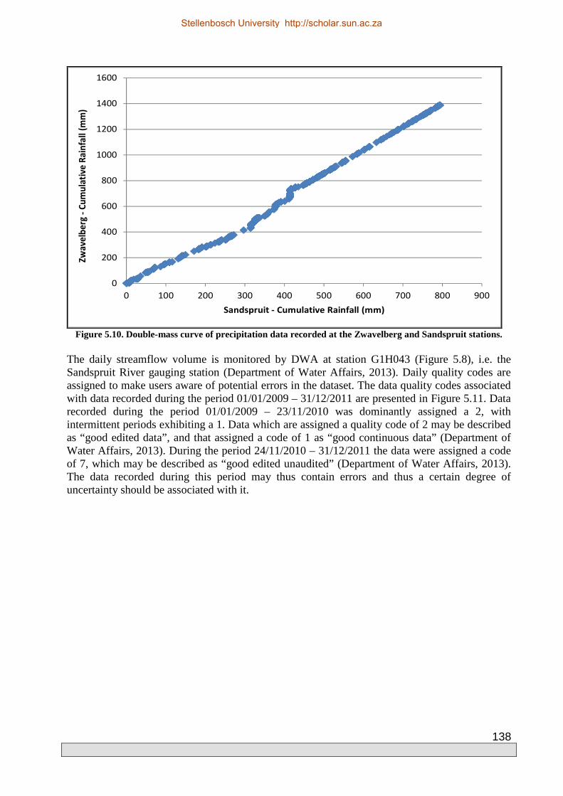
138

0

200

400

600

800

1000

1200

1400

1600

0 100 200 300 400 500 600 700 800 900

Zwa

velb

erg

-C

um

ula

tive

Ra

infa

ll (m

m)

Sandspruit - Cumulative Rainfall (mm)

Figure 5.10. Double-mass curve of precipitation data recorded at the Zwavelberg and Sandspruit stations.

The daily streamflow volume is monitored by DWA at station G1H043 (Figure 5.8), i.e. the Sandspruit River gauging station (Department of Water Affairs, 2013). Daily quality codes are assigned to make users aware of potential errors in the dataset. The data quality codes associated with data recorded during the period 01/01/2009 – 31/12/2011 are presented in Figure 5.11. Data recorded during the period 01/01/2009 – 23/11/2010 was dominantly assigned a 2, with intermittent periods exhibiting a 1. Data which are assigned a quality code of 2 may be described as “good edited data”, and that assigned a code of 1 as “good continuous data” (Department of Water Affairs, 2013). During the period 24/11/2010 – 31/12/2011 the data were assigned a code of 7, which may be described as “good edited unaudited” (Department of Water Affairs, 2013). The data recorded during this period may thus contain errors and thus a certain degree of uncertainty should be associated with it.


139

0

1

2

3

4

5

6

7

8

01/01/2009 30/06/2009 27/12/2009 25/06/2010 22/12/2010 20/06/2011 17/12/2011

Figure 5.11. Streamflow data quality codes during the period 01/01/2009 – 31/12/2011. The quantification of the runoff coefficient for a catchment is a useful measure to identify errors in observed data and also to gauge the replicability of a catchments hydrological processes. The annual runoff coefficient for the Sandspruit catchment was calculated for the period 1987 – 2011. The runoff coefficient (K) is an analysis of the rainfall-runoff relationship, which is based on actual, simultaneous measurements of both rainfall and runoff. It is defined by the division of the runoff by the corresponding rainfall both expressed as depth over catchment area (mm): K = Runoff (mm)/Rainfall (mm) (5.17) The long term catchment annual rainfall was calculated as the average of rainfall data recorded at De Hoek, Langgewens, Moorreesberg and Voëlvlei (Outside Stations, Figure 5.8) and as an average of data collected at all stations, i.e. all stations which record precipitation (Table 5-1). The calculated runoff coefficients are presented in Figure 5.12. Overall, the Sandspruit catchment exhibits a runoff coefficient of < 0.2. According to Gan et al. (1997) the hydrological processes in catchments which exhibit a runoff coefficient of 0.2 or less, such as the Sandspruit, are more difficult to simulate than wet catchments or catchments with relatively high streamflow/rainfall ratios. This is due to the former exhibiting more complex and variable hydrological processes than the latter. The ratio was significantly low in 2011, i.e. 0.006. Although not significant, in terms of magnitude, the advantage of installing rainfall stations inside the catchment is evident in the increase in the runoff coefficient in 2009 and 2010 (All Stations, Figure 5.12).


140

0

0.02

0.04

0.06

0.08

0.1

0.12

0.14

0.16

0.18

1987 1989 1991 1993 1995 1997 1999 2001 2003 2005 2007 2009 2011

Ru

no

ff C

oef

fici

ent

Year

Outside Stations All Stations

Figure 5.12. The annual runoff coefficient for the Sandspruit catchment. Catchment average rainfall was also correlated with runoff, which exhibited a poor result (r2 = 0.33). This may indicate that runoff is more dependent on the spatial distribution of rainfall than on annual totals. The results are presented in Figure 5.13.

R² = 0.3333

0

10

20

30

40

50

60

70

80

250 300 350 400 450 500 550 600 650 700 750 800

Ru

no

ff (

mm

)

Rainfall (mm)

Outside Stations All Stations

Figure 5.13. The correlation between annual rainfall and runoff in the Sandspruit catchment.


141

The double-mass curve technique may also be used to compare the cumulative data of one variable with a pattern (several stations) of the cumulative data of related variables (Searcy and Hardison, 1960), e.g. runoff and catchment average precipitation. Results of the double-mass curve analysis of runoff and catchment average precipitation data recorded during the calibration and validation periods are presented in Figure 5.14. During the calibration and validation periods 5 periods of runoff are evident. The pronounced break in the dataset during the period 06/06/2009 – 20/10/2009 is a result of a delayed rainfall- runoff response, i.e. the increased runoff was recorded a day after a pronounced rainfall event. The response of runoff to rainfall is clearly evident during 2009 and 2010. However, during 2011, the slope of the curve is markedly different. This may be a result of a pronounced change in precipitation characteristics, i.e. intensity and duration. Alternatively, it may be a result of errors in the recorded runoff.

0

20

40

60

80

100

120

0 200 400 600 800 1000 1200 1400

G1

H0

43

-C

um

ula

tive

Ru

no

ff (

m3/s

)

Cumulative Catchment Average Rainfall (mm)

06/06/2009 - 20/10/2009

08/11/2009 - 08/12/2009

13/05/2010 - 26/10/2010

18/06/2011 - 25/07/2011

31/07/2011 - 24/09/2011

No Runoff

Figure 5.14. Double-mass curve of runoff data and the catchment average precipitation data

The correlation matrices for the temperature data are presented in Table 5-4, Table 5-5 and Table 5-6. A strong correlation was observed between the temperature data recorded at all stations.

Table 5-4 Correlation Matrix (r 2) of Daily Minimum Temperature Data

Elev

(mamsl) LD MB ZB OK SP

Landau 126 0.88 0.73 0.87 0.89 Moorreesberg 199 0.77 0.91 0.79 Zwavelberg 278 0.83 0.65 Oranjeskraal 118 0.83 Sandspruit 42

LD – Landau, MB – Moorreesberg, ZB – Zwavelberg, OK – Oranjeskraal, SP – Sandspruit


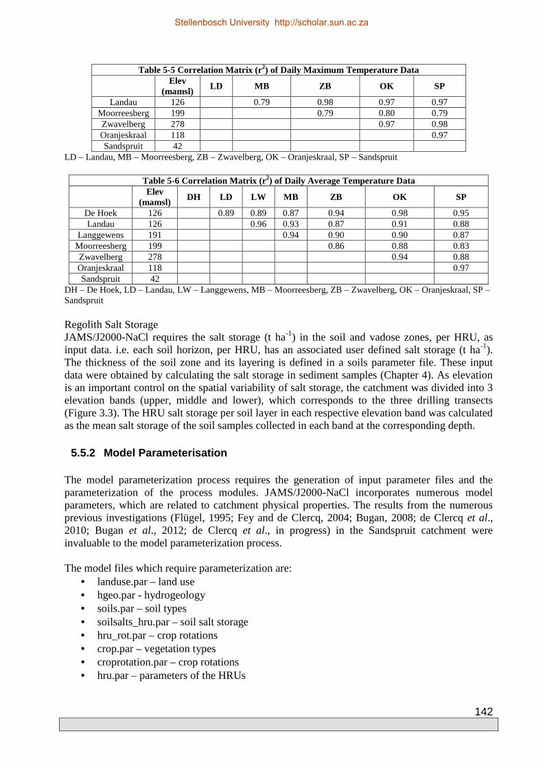
142

Table 5-5 Correlation Matrix (r 2) of Daily Maximum Temperature Data

Elev

(mamsl) LD MB ZB OK SP

Landau 126 0.79 0.98 0.97 0.97 Moorreesberg 199 0.79 0.80 0.79 Zwavelberg 278 0.97 0.98 Oranjeskraal 118 0.97 Sandspruit 42

LD – Landau, MB – Moorreesberg, ZB – Zwavelberg, OK – Oranjeskraal, SP – Sandspruit

Table 5-6 Correlation Matrix (r 2) of Daily Average Temperature Data

Elev

(mamsl) DH LD LW MB ZB OK SP

De Hoek 126 0.89 0.89 0.87 0.94 0.98 0.95 Landau 126 0.96 0.93 0.87 0.91 0.88

Langgewens 191 0.94 0.90 0.90 0.87 Moorreesberg 199 0.86 0.88 0.83 Zwavelberg 278 0.94 0.88 Oranjeskraal 118 0.97 Sandspruit 42

DH – De Hoek, LD – Landau, LW – Langgewens, MB – Moorreesberg, ZB – Zwavelberg, OK – Oranjeskraal, SP – Sandspruit Regolith Salt Storage JAMS/J2000-NaCl requires the salt storage (t ha-1) in the soil and vadose zones, per HRU, as input data. i.e. each soil horizon, per HRU, has an associated user defined salt storage (t ha-1). The thickness of the soil zone and its layering is defined in a soils parameter file. These input data were obtained by calculating the salt storage in sediment samples (Chapter 4). As elevation is an important control on the spatial variability of salt storage, the catchment was divided into 3 elevation bands (upper, middle and lower), which corresponds to the three drilling transects (Figure 3.3). The HRU salt storage per soil layer in each respective elevation band was calculated as the mean salt storage of the soil samples collected in each band at the corresponding depth.

5.5.2 Model Parameterisation

The model parameterization process requires the generation of input parameter files and the parameterization of the process modules. JAMS/J2000-NaCl incorporates numerous model parameters, which are related to catchment physical properties. The results from the numerous previous investigations (Flügel, 1995; Fey and de Clercq, 2004; Bugan, 2008; de Clercq et al., 2010; Bugan et al., 2012; de Clercq et al., in progress) in the Sandspruit catchment were invaluable to the model parameterization process. The model files which require parameterization are:

• landuse.par – land use • hgeo.par - hydrogeology • soils.par – soil types • soilsalts_hru.par – soil salt storage • hru_rot.par – crop rotations • crop.par – vegetation types • croprotation.par – crop rotations • hru.par – parameters of the HRUs


143

Each land use/land cover has its own ID and is associated to one or more HRUs: • 1 - Impervious area > 80 % • 2 - Impervious area < 80 % • 3 - Pasture and Meadows • 4 - Coniferous forest • 5 - Deciduous forest • 6 - Mixed Forest • 7 - Arable farm land (also crop land) • 8 - Struik (shrub) • 9 - Wetland • 10 - Open areas • 11 - Water bodies

The file landuse.par requires the following parameters for each land use:

• Albedo • Minimum surface resistance for water-saturated soil (January to December) • LAI (from the beginning to the end of the vegetation period) • Effective height of vegetation (from the beginning to the end of the vegetation period) • Root depth • Sealed grade of soil surface

The file hgeo.par requires the following parameters, which represent hydrogeological properties of one or more HRUs:

• Maximum storage capacity of the upper ground-water reservoir (RG1) • Maximum storage capacity of the lower ground-water reservoir (RG2) • Storage coefficient of the upper ground-water reservoir (RG1) • Storage coefficient of the lower ground-water reservoir (RG2)

The file soils.par requires the following parameters, which represent the soil properties of one or more HRUs:

• Thickness of soil • Minimum permeability coefficient • Depth of the horizon above the horizon with the smallest permeability coefficient • Maximum permeability coefficient • Boolean variable that allows (1) or restricts (0) capillary rise • Air capacity • Usable field capacity • Usable field capacity per decimeter of profile depth

The file soilsalts_hru.par requires the following per HRU:

• Soil ID • The salt storage (t ha-1) of each soil layer

The file hru_rot.par requires the following per HRU:

• Crop rotation ID

The file croprotation.par requires the following per HRU: • Crop rotation ID


144

• Crop ID per year of simulation. The model incorporates numerous crop types which are listed in the crop.par file. The available crop types are presented in Appendix C.

The file hru.par includes the following parameters per HRU: • Coordinates of the centroid point • Mean surface elevation • Area • Slope • Aspect • Flow length • Soil ID (linked to soils.par file) • Land use ID (linked to landuse.par file) • Hydrogeology ID (linked to hgeo.par file) • Salt ID (linked to soilsalts_hru.par)

JAMS/J2000-NaCl also incorporates additional land management functionality (till.par and lmArable.par). This allows for the incorporation of tillage practices and times, harvesting methods and times.

5.5.3 Model Calibration

The accurate parameterization of environmental models is a critical component of their successful application. The direct determination of parameter values is however often not feasible as they lack clear physical meaning or due to the costs associated with field measurements (Fischer et al., 2009). Thus, the estimation of model parameter values is often a process whereby model response is compared to observed data in a trial and error process. The user adjusts model parameters within a specific range at pre-defined intervals and this may be done manually or using automatic techniques. Janssen and Heuberger (1995) recommend that the model calibration process combines both manual and automatic techniques. A comparison of the simulated and observed streamflow is often used to evaluate the process. It is usually suggested that, if possible, calibration first be performed on an annual basis, before progressing to a monthly and eventually daily time interval. It is also recommended that the calibration process follow a model initialisation period, during which model parameters are assumed to adjust to reasonable starting values. The length of this initialisation period and the subsequent calibration period is dependent on the availability of input data and the objective of the study. The criteria which were used to evaluate the model performance during the calibration process were the Absolute Volume Error (AVE), the Nash-Sutcliffe Efficiency (Nash and Sutcliffe, 1970), the coefficient of determination (r2) and the Index of Agreement (IOA; Willmott, 1981). This is in accordance with recommendations made by Janssen and Heuberger (1995), Krause et al. (2005) and Wagener et al. (2003). Manual Calibration Manual model calibration is a process whereby the user manually adjusts model parameters within a specific range at pre-defined intervals. During this process the user also identifies which parameters exert the greatest influence on simulation outputs, i.e. sensitivity analysis. These sensitive parameters are subsequently used in an automatic calibration process.


145

Besides being able to manually edit the text files with input parameters (Chapter 5.5.2) and variables, the interface of the model (Figure 5.15) allows the user to fine tune the calibration by changing certain parameters. The parameters were adjusted using a trial and error process with the objective being to compare simulated and observed runoff. The parameters were adjusted within a justifiable range and at certain intervals, until optimal efficiencies of model performance (statistical indicators) were observed. The manual calibration process is illustrated in Table 5-7.

Figure 5.15. The Graphical User Interface of the JAMS/J2000-NaCl hydrological model.

Table 5-7 The Manual Calibration Procedure and Results

Variable Definition Values range

in the calibration

Interval used in the calibration

End value

J2KNaClSoilLayer

Beta_NaCl Percolation coefficient for

inorganic salt 0 - 1 0.1 0.2

Deposition factor (kg ha-1) Inorganic salt rainfall

deposition factor per mm rainfall

0 – 1.5 0.1 0.8*

Radiation Tab Longitude of time-zone

center (dec. °) - - - 18

East or West of Greenwich - - - East Daily or hourly time steps - - - Daily Parameter a for Angstroem

formula - - -

0.25 (default)

Parameter b for Angstroem formula

- - - 0.5 (default)


146


in the calibration


End value

Interception Tab

a_rain Maximum storage capacity of the interception storage per m2 of leaf area for rain

0 - 10 0.5 0.15

J2KProcessLayeredSoilWater Tab

soilMaxDPS (mm) Maximum depression

storage capacity 0 - 10 1 3

soilPolRed Polynomial reduction

coefficient for the computation of actual ET

0 - 100 5 80

soilLinRed Linear reduction coefficient for the computation of actual

ET 0 - 10 1

0 (PolRed or LinRed are alternatives; PolRed was

used)

soilMaxInfSummer (mm) Maximum infiltration in the

summer half year 0 - 200 5 30

soilMaxInfWinter (mm) Maximum infiltration in the

winter half year 0 - 200 5 70

soilImpGT80 Relative infiltration capacity of areas with a sealed grade

> 80% 0 - 1 0.05 0.25

soilImpLT80 Relative infiltration capacity of areas with a sealed grade

< 80% 0 - 1 0.05 0.75

soilDistMPSLPS Calibration coefficient for allocation of infiltration to

LPS and MPS 0 - 10 1 5

soilDiffMPSLPS Calibration coefficient for diffusion amount of MPS to

LPS 0 - 10 0.05 0.6

soilOutLPS Calibration coefficient for

outflow from the LPS 1 - 10 1 9

soilLatVertLPS

Calibration coefficient for allocation of LPS runoff to

lateral (interflow) and vertical (percolation)

components

0 - 10 0.5 10

soilMaxPerc (mm) Maximum percolation in the

time step 0 - 2000 1 14

geoMaxPerc (mm) Maximum percolation in the

time step (into semi-consolidated rock)

0 - 2000 2 2

soilConcRD1 Recession coefficient for

overland flow 0 - 10 1 10


interflow 0 - 10 1 9

kdiff_layer Layer MPS diffusion factor 0 - 10 0.1 0.1

BetaW Water use distribution

parameter for transpiration 0 - 100 10 10

J2KProcessGroundwater Tab

initRG1 Initial groundwater storage in RG1

0 - 1 0.1 0

initRG2 Initial groundwater storage in RG2

0 - 1 0.1 0


147


in the calibration


End value

gwRG1RG2dist Calibration coefficient for water allocation to percolation

0 - 10 1 1

gwRG1Fact Factor for runoff contribution from RG1

0 - 10 0.5 2


0 - 10 0.5 4.5

gwCapRise Capillary rise coefficient 0 - 1 0.1 0.4

NaCl_concRG1 Initial salt concentration in

RG1 per HRU 0 – 10 1 1

NaCl_concRG2 Initial salt concentration in

RG2 per HRU 0 - 10 1 1

J2KProcessreachRouting Tab flowRouteTA Flood routing coefficient 0 - 100 10 10

* Based on the rainfall salt concentration range (14 - 125 mg L-1) presented by Flügel (1995) and the annual total rainfall presented in Table 5-3, the deposition factor ranges between 0.13 and 1.5. The “Regionalisation” tab (Figure 5.15) is used to access a screen where information pertaining to the regionalisation of weather variables is entered:

• Number of closest stations for regionalization: Number (n) of stations that are used for the calculation of the climate input values of an HRU.

• Power of inverse distance weighting (IDW) function for regionalization. A higher power results in less influence from distant points and vice versa. The most commonly used value is 2.

• Elevation correction on/off: Activation of the elevation correction. • r-sqr threshold for elevation correction: Threshold for elevation correction of data. If the

coefficient of determination of the regression relationship between the station values and the elevations of the station is less than the threshold, no elevation correction is carried out.

These settings can be determined for each input variable (i.e. minimum temperature, maximum temperature, mean air temperature, precipitation, absolute humidity and sunshine duration) individually. Automatic Calibration Automatic model calibration of the JAMS/J2000-NaCl model is supported by a semi-automated assistant that guides the user through the calibration procedure, i.e. OPTAS (Fischer et al., 2009). OPTAS runs on a computing cluster of the Department of Geoinformatics, Hydrology and Modelling at the Friedrich Schiller University Jena (Germany). This does not occupy any local computing resources and allows a calibration of up to four models at the same time. A list of all available parameters for calibration is available, from which the user should make a selection. A list of objective functions (e.g. Nash-Sutcliffe Efficiency) is also available. The user can either select a single criterion or several criteria. When selecting several criteria, a multi-criteria optimization problem is created which differs significantly from a (common) one-criterion optimization problem regarding its solution characteristics. OPTAS incorporates several optimization methods. The Shuffle Complex Evolution (SCE; Duan et al., 1992) method was employed in this study. The SCE method was developed especially for parameter optimization applications in hydrological models. The method has illustrated its


148

effectiveness, robustness and efficiency in numerous studies, particularly in the field of hydrology (Fischer et al., 2011). The SCE method handles the optimization problem as a natural evolutionary process (Fischer et al., 2009). The SCE method is described by Fischer et al. (2009) as a population of samples, which each represent one solution. The population may be divided into complexes that evolve independently. New samples are created through the formation of new sub-complexes. The new samples, however, need to satisfy certain criteria before they are added to the population whereby they are superseding the current “worst” sample. After some iteration, the complexes are joined. The process of complex segmentation and new sub-complex formation is repeated until no further improvement of the sample “goodness of fit” can be achieved. The SCE algorithm exhibits good convergence for a variety of problems, i.e. a sufficient number of model iterations has a fairly high probability to converge to a global optimum (Fischer et al., 2009). The commonly used “goodness-of-fit” measure, i.e. NSE (Duan et al., 2006) between observed and simulated values was used to evaluate model performance (objective function).

The automatic calibration process was run for the period 01/01/2000 to 31/12/2010. The period 01/01/2000 – 31/12/2008 was used as an initialization period and the period 01/01/2009 – 31/12/2010 was used as the calibration period. The manual calibration processes identified 18 parameters which have a significant influence on model results (Table 5.7), which were subsequently used in the automatic calibration process. The parameter ranges used in the automatic calibration process is also shown in Table 5-8.

Table 5-8 Parameters Selected for Automatic Calibration


in the calibration

Starting value

End value


0 - 10 0.15 0.26


storage capacity 0 - 10 3 4.26



0 - 100 80 74.47


winter half year 0 - 200 70 89.86


< 80% 0 - 1 0.75 0.75


outflow from the LPS 1 - 10 9 9.02

soilLatVertLPS



components

0 - 10 10 9.34


time step 0 – 2000 14 306.55



0 - 2000 2 173.03


overland flow 0 - 10 10 9.80


interflow 0 - 10 9 7.19



149


in the calibration

Starting value

End value


0 - 1 1 0.90


0 – 10 2 3.00


0 - 10 4.5 3.20

gwCapRise Capillary rise coefficient 0 - 1 0.40 0.47 flowRouteTA Flood routing coefficient 0 - 100 10 1.38 cbWallhoehe Contour bank height (m) 0 - 1 0.64 0.62

5.6 Model Results

The model performance was evaluated using the following criteria: • The NSE is a commonly used measure. Values for NSE vary from negative infinity to 1.

A value of 1 indicates a perfect fit between observed and simulated data, while a value < 0 implies that the simulated value is (on average) a poorer predictor than the long-term average of the observations. The NSE criterion is often criticized due to the fact that the differences between the observed and simulated values are calculated as squared values. Thus, larger values are strongly over-estimated, while lower values are neglected (Legates and McCabe, 1999). This leads to an overestimation of model performance during peak flows and an underestimation during low flow conditions. A NSE of 0.4 – 0.6 is classified as satisfactory and a value > 0.6 is classified as good.

• The AVE provides the absolute difference between the observed and simulated value. Thus, a lower AVE is more desirable as opposed to a higher value.

• The coefficient of determination (r2) is defined as the squared value of the coefficient of correlation (Krause et al., 2005). It is also commonly defined as the squared ratio between the covariance and the multiplied standard deviations of the observed and simulated values (Krause, 2005). The coefficient of determination ranges between 0 (no correlation) and 1 (perfect fit). It should however be used with caution as a model which frequently over-or under-predicts may still exhibit an acceptable r2 value.

• The IOA (Willmott, 1981) aims to overcome the insensitivity of the NSE and r2 to differences in the observed and simulated means and variances (Legates and McCabe, 1999). The IOA, as with the NSE, is also very sensitive to peak flows and insensitive to low flows. The IOA ranges between 0-1, with a value of 0 representing no correlation and 1 a perfect fit. A value > 0.60 is regarded as representing a good fit between observed and simulated values.

The efficiency criteria of the water balance simulation for the calibration and validation periods are presented in Table 5-9. In terms of the model performance evaluation criteria, the model exhibits good results during the calibration period, i.e. a good correlation between the daily simulated and observed streamflow volumes were observed.

Table 5-9 Results of the Water Balance Simulation for the Calibration and Validation Periods Performance Criteria 2009 2010 2009 and 2010 2011

NSE 0.58 0.22 0.55 negative AVE (mm) 13.22 28.69 41.92 57.90

rsq 0.67 0.60 0.57 0.27 IOA 0.70 0.58 0.66 0.12


150

The effects of the use of different variations of rainfall stations on model results were also evaluated. Two configurations were considered, i.e. the exclusion of rainfall data recorded at De Hoek and Moorreesberg (Variation 1, Table 5-2) and only the use of rainfall data recorded inside the Sandspruit catchment (Zwavelberg, Oranjeskraal and Sandspruit; Variation 2; Table 5-2). The automatic calibration process was repeated to consider this variation in precipitation data. The results are presented in Table 5-10 and Table 5-11. The improvement in model performance, resulting from the omission of rainfall data recorded at De Hoek and Moorreesberg (Table 5-10) is clearly discernible. Thus it is not always appropriate to include all available data as the effect of orographic rainfall and the spatial variation of rainfall should be considered. The use of only rainfall data measured within the Sandspruit catchment resulted in further, although not significant, improvement in model performance. This improvement is not evident in the average, considering both 2009 and 2010, but rather in the increased stability of the performance evaluation criteria over 2009 and 2010.

Table 5-10 Results of the Water Balance Simulation for the Calibration and Validation Periods (Variation 1)

Performance Criteria

2009 2010 2009 and

2010 2011


rsq 0.73 0.62 0.65 0.26 IOA 0.69 0.55 0.65 0.11

Table 5-11 Results of the Water Balance Simulation for the Calibration and Validation

Periods (Variation 2) Performance

Criteria 2009 2010

2009 and 2010

2011


rsq 0.66 0.63 0.64 0.27 IOA 0.69 0.61 0.67 0.11

Considering the results presented in Table 5-9, Table 5-10 and Table 5-11 it was decided to use the configuration producing results in Table 5-11, i.e. only utilizing rainfall data measured at Zwavelberg, Oranjeskraal and Sandspruit (Variation 2), for further analysis. The results of the automatic calibration process for this configuration are presented in Table 5-12. The model results discussed further, relate to that produced from Variation 2. The observed and simulated streamflow are presented in Figure 5.16. During the calibration period, good correspondence between observed and simulated runoff was observed (Figure 5.16), in terms of temporal runoff dynamics. The model is able to represent the timing of initiation of increased runoff during winter. High peaks in the simulated runoff data set correspond well with that of the observed runoff and pronounced rainfall events (Figure 5.17). In general, the model under-estimated runoff volumes during extreme rainfall events. The model was however not able to entirely replicate the ephemeral characteristic of the Sandspruit River, as baseflow was simulated during the summer months. This baseflow was generally in the order of 0.025 – 0.2 m3 s-1. The model also produced streamflow in response to pronounced rainfall events during summer, which is not evident in the observed streamflow data set.


151

The dominance of evapotranspiration, in terms of the catchment water balance was well replicated by the model as it amounted to more than 80% of the annual rainfall. This is in accordance with results presented by Bugan et al. (2012). During the main rainfall season, i.e. April to September, 67% (2009), 86% (2010) and 89% (2011) of the annual total simulated runoff was recorded. The rainfall season extended to November in 2009, during which 24% of the annual total simulated runoff occurred. The spatial distribution of rainfall, i.e. the average annual (2009 – 2011) rainfall per HRU, is illustrated in Figure 5.18. The model was able to accurately replicate the effects of topography and distance from the coastline on rainfall distribution (Figure 5.18). The model was not able to accurately replicate the water balance of the Sandspruit catchment during the validation period. This creates uncertainty, in terms of the model’s ability to accurately replicate reality. This is often a result of calibrated parameter values, which are not necessarily physically relevant. However, the evidence provided in Figure 5.11, Figure 5.12 and Figure 5.14 also suggest that the observed streamflow data collected in 2011 contains errors. Operator inefficiency, equipment failure, changing rating tables or poor calibration of gauging weirs are all problems which are frequently encountered with streamflow records (Kienzle et al., 1997). Additionally, the variation in runoff dynamics observed in 2011 is not a result of variations in the temporal distribution of rainfall (Figure 5.9 and Table 5-3). Thus, it is uncertain whether the poor model performance during the validation period is a result of irrelevant model parameters/unsuitable model structure or due to errors in the observed runoff data set.

Table 5-12 Parameters Selected for Automatic Calibration (Variation 2)


in the calibration

Starting value

End value


0 - 10 0.15 0.42


storage capacity 0 - 10 3 5.25



0 - 100 80 55.54


winter half year 0 - 200 70 99.31


< 80% 0 - 1 0.75 0.86


outflow from the LPS 1 - 10 9 8.45

soilLatVertLPS



components

0 - 10 10 7.96


time step 0 – 2000 14 1257.19



0 - 2000 2 481.10


overland flow 0 - 10 10 9.53


interflow 0 - 10 9 5.86


152


in the calibration

Starting value

End value



0 - 1 1 0.73


0 – 10 2 0.78


0 - 10 4.5 3.51

gwCapRise Capillary rise coefficient 0 - 1 0.40 0.38 flowRouteTA Flood routing coefficient 0 - 100 10 1.25 cbWallhoehe Contour bank height (m) 0 - 1 0.64 0.62

The dominant component of simulated runoff was RD2 (Figure 5.18) which is interflow within the unsaturated zone. This is in accordance with observations made by Bugan et al. (2012) and Flügel (1995). In terms of proportion, this is followed by shallow groundwater flow (RG1). Minimal contributions from surface runoff (RD1) also occurred. Over the entire simulation period (2009 – 2011) the proportions of contribution to streamflow from the different components were:

• RD1 (surface runoff) – 6% • RD2 (interflow within the unsaturated zone) – 70% • RG1 (shallow groundwater flow) – 21% • RG2 (baseflow) – 3%

0

1

2

3

4

5

6

7

8

9

10

01/2009 05/2009 09/2009 01/2010 05/2010 09/2010 01/2011 05/2011 09/2011

Ru

no

ff (

m3/s

)

Date

Runoff Plot

Observed Runoff Simulated Runoff

Figure 5.16. Observed and simulated catchment runoff.


153

0

5

10

15

20

25

30

35

01/2009 05/2009 09/2009 01/2010 05/2010 09/2010 01/2011 05/2011 09/2011

Pre

cip

ita

tio

n (

mm

)

Date

Precipitation

Figure 5.17. Simulated catchment precipitation.

Figure 5.18. The spatial distribution of the annual average catchment precipitation.


154

The simulated catchment runoff significantly increases during May. Rainfall and saturation of the soil initiates overland flow (RD1, Figure 5.19) and interflow (RD2, Figure 5.19) processes. The dominance of interflow (RD2) as a streamflow contributor is illustrated by its strong correlation with simulated runoff (Figure 5.16) and the catchment soil water storage dynamics (Figure 5.20). Recharge of the shallow perched and regional aquifer produces shallow groundwater flow, i.e RG1 (Figure 5.19). The contribution of RG1 to streamflow is particularly evident during the latter parts of the rainfall season. Simulated streamflow response during the dry summer months (Figure 5.16) is interpreted to be a result of persistent soil moisture during these months (Figure 5.20), particularly in the LPS. Observations by Bugan (2008) and Bugan et al. (2012) however suggest that these soil moisture reservoirs are depleted during the summer months. This discrepancy has also produced the pronounced AVE, as presented in Table 5-11.

0.0

0.5

1.0

1.5

2.0

2.5

01/2009 05/2009 09/2009 01/2010 05/2010 09/2010 01/2011 05/2011 09/2011

Ru

no

ff (

mm

)

Date

Runoff Components Plot

RD1 RD2 RG1 RG2

Figure 5.19. Components of simulated runoff.


155

0

1

01/2009 05/2009 09/2009 01/2010 05/2010 09/2010 01/2011 05/2011 09/2011

Re

lati

ve

So

il S

atu

rati

on

Date

Soil Water Storage

Middle Pore Storage (MPS) Large Pore Storage (LPS)

Figure 5.20. Simulated soil water storage dynamics.

The observed and simulated inorganic salt output from the catchment (t d-1) is presented in Figure 5.21. The observed data set was quantified using streamflow quantity and salinity datasets, i.e. the salt load is equal to the product of the streamflow (m3 s-1) and the corresponding stream water salinity (TDS, mg L-1). The salinity of the Sandspruit River was monitored with an electronic EC sensor, hourly, from June 2007 to October 2010. Data were missing for the period 06/06/2009 – 30/07/2009 due to sensor malfunction. The sensor is located at the Sandspruit gauging weir (G1H043, Figure 5.8), for which streamflow quantity (m3 s-1) data are available for the period May 1980 to present. This station is maintained by the DWA. The electronic EC sensor produced readings in mV, which were calibrated using streamflow EC readings recorded with a hand-held EC meter during field visits. Grab samples were also collected and the EC analyzed in the laboratory. The calibration was assumed to be linear, i.e. EC (mS m-1) = 0.886* daily average mV - 218.99; r2 = 0.72. Periods for which mV data were missing, were filled using a correlation (r2 = 0.68) with streamflow, i.e. Salt Output (t d-1) = 169.49 * Streamflow (m3 s-1) + 26.743. This correlation was also used to produce catchment salt output in 2011. As the salt output and runoff are directly related the discrepancies between observed and simulated runoff dynamics are also evident in Figure 5.21. The initiation of increased salt output during winter corresponds well between the observed and simulated datasets. However, pronounced differences in the magnitude of the peaks are evident during winter. This is interpreted to be due to the model’s inability to accurately replicate the extreme runoff events in winter. Additionally, the simulated baseflow which occurs in the dry summer months (Figure 5.16) significantly affects the simulated salt output. The results are presented at an annual scale in Table 5-13. The data are within the same order of magnitude, when analyzed at an annual scale. Thus, for this reason and due to the discrepancies observed at a daily scale (Figure 5.21) it is suggested that the simulated catchment salt output of the JAMS/J2000–NaCl model only be utilized at an annual scale.


156

0

200

400

600

800

1000

1200

1400

1600

01/2009 05/2009 09/2009 01/2010 05/2010 09/2010 01/2011 05/2011 09/2011

Sa

lt O

utp

ut

(t d

-1)

Date

Catchment Salt Output

Observed Simulated

Figure 5.21. Observed and simulated catchment inorganic salt output.

Table 5-13 Observed and Simulated Catchment Salt Output Year Observed (t a-1) Simulated (t a-1) 2009 21 409 23 242 2010 14 599 10 601 2011 3 259 9 063

5.7 Conclusions

The use of distributed hydrological models can facilitate a quantitative analysis of the impacts of climate and land use change on a catchment’s water and solute fluxes. The objective of this study was to evaluate the applicability of the JAMS/J2000-NaCl hydrosalinity model as a catchment scale water and salinity management tool in the semi-arid Sandspruit catchment, where the development of agricultural production areas in the catchment has resulted in the salinisation of land and water resources. JAMS/J2000-NaCl is a meso- to macro-scale hydrological model, which simulates the water and salinity balance in river basins. It simulates hydrosalinity processes in a spatially distributed process-orientated manner. The JAMS/J2000-NaCl model was selected for application based on numerous criteria, which include:

• The representation of distributed catchment properties as well as distributed climatic inputs.

• The ability to account for the heterogeneity of salt storage and the salt mobilisation processes.

• The ability to simulate surface, subsurface (unsaturated zone) and groundwater flow processes.

• The ability to simulate the effects of contour banks on the catchment hydrosalinity dynamics.

A close working relationship with the model developers at the Friedrich-Schiller University (Jena, Germany) allowed for the incorporation of additional process components in the model.


157

JAMS/J2000-NaCl requires daily climatic input data (precipitation, minimum and maximum air temperature, wind speed, relative humidity and sunshine hours) as well as spatial input data (DEM, land use, soils and geology) for the delineation of HRUs. In addition, the model also requires observed runoff data with which to evaluate the simulation results. For the simulation of inorganic salt fluxes, the model requires distributed regolith salt storage as well as the salt concentration of rainfall. The salinity module allows for the simulation of numerous processes:

• Inorganic salt input via rainfall. • Inorganic salt redistribution via evaporation. • Mass transport with soil water movement, overland flow and groundwater.

The climate data were checked for homogeneity and consistency using linear regression analysis and double-mass curves. The correlation matrix revealed that the correlation of precipitation data measured at different stations is dominantly a function of topography and the distance from the coastline. Thus, the influence of the use of different combinations of precipitations stations were evaluated on model results. Results of the double-mass curve analysis of precipitation data generally exhibit a similar pattern/trend. No clearly discernible evidence is apparent which indicates inconsistency in the datasets. The quantification of the runoff coefficient for a catchment is a useful measure to gauge the replicability of a catchments hydrological processes. Overall, the Sandspruit catchment exhibits a runoff coefficient of < 0.2. According to Gan et al. (1997) the hydrological processes in catchments which exhibit a runoff coefficient of 0.2 or less, such as the Sandspruit, are more difficult to simulate than wet catchments or catchments with relatively high streamflow/rainfall ratios. The double-mass curve analysis of runoff and catchment average precipitation data was also performed. During the calibration and validation periods, 5 periods of runoff are evident. This analysis revealed pronounced breaks as well as clearly discernible differences in the slope of the rainfall-runoff curve from 2009 to 2011. This may be a result of a pronounced change in precipitation characteristics, i.e. intensity and duration. Alternatively, it may be a result of errors in the recorded runoff. The accurate parameterization of environmental models is a critical component of their successful application. The model parameterization process requires the generation of input parameter files and the parameterization of the process modules. JAMS/J2000-NaCl incorporates numerous model parameters, which are related to catchment physical properties. The results from the numerous previous investigations conducted in the Sandspruit catchment were invaluable to the model parameterization process. The model calibration process combined both manual and automatic techniques. A comparison of the simulated and observed streamflow was used to evaluate the process. In terms of the model performance evaluation criteria, the model exhibited good results during the calibration period. The effects of the use of different variations of rainfall stations on model results were also evaluated. A significant improvement of model performance was observed when only precipitation data recorded inside the catchment was used. During the calibration period, good correspondence between observed and simulated runoff was observed, in terms of temporal runoff dynamics. However, the model generally under-estimated runoff volumes during extreme rainfall events. The model was also not able to entirely replicate the ephemeral characteristic of the Sandspruit River, as baseflow was simulated during the summer months. The model was not able to accurately replicate the water balance of the Sandspruit catchment during the validation period. This creates uncertainty, in terms of the model’s ability to accurately replicate reality. Significantly reduced model performance during the validation period is often a result of calibrated parameter values, which are not necessarily


158

physically relevant. However, the evidence provided in Figure 5.11, Figure 5.12 and Figure 5.14 also suggest that the observed streamflow data collected in 2011 contains errors. Thus, it is uncertain whether the poor model performance during the validation period is a result of irrelevant model parameters/unsuitable model structure or due to errors in the observed runoff data set. It is also more appropriate to validate a hydrological model over an extended period, incorporating both wet and dry years. This could however not be done due to limited data availability. The discrepancy between the observed and simulated runoff is also evident in the comparison of the observed and simulated inorganic salt output from the catchment. The initiation of increased salt output during winter corresponds well between the observed and simulated datasets. However, pronounced differences in the magnitude of the peaks are evident during winter. At an annual scale, the observed and simulated catchment salt output is within the same order of magnitude. Overall, the results of the hydrosalinity process-based modeling of the Sandspruit catchment with the JAMS/J2000-NaCl model indicates that potential exists for the model to be used as a water and salinity management tool in the catchment. Results of the simulation of salinity fluxes should however only be evaluated at an annual scale. The model may be utilized as a catchment management tool to study the following:

• Assess the effects of alternative land use (different vegetation types, alternative crop rotation cycles and/or varying spatial distributions of vegetation) on the catchment water and salinity balance.

• Assess the effects of alternative land management practices (soil management/tillage practices and/or alternative contour bank construction techniques and distribution methodologies) on the catchment water and salinity balance.

• Evaluate potential impacts of climate change (increased/decreased temperature and/or alternative rainfall characteristics).

• Study the effects of water abstraction on the catchment water and salinity dynamics.

5.8 References

ALLEN, R.G., PEREIRA, L.S. and RAES, D., 1998. Crop evaporation: guidelines for computing crop water requirements. Irrigation and Drainage Paper No 56. Rome, Italy: UN FAO.

ARNOLD, J.G., SRINIVASAN, R., MUTTIAH, R. and WILLIAMS, J., 1998. Large area hydrologic modelling and assessment. Part I, Model development. Journal of American Water resources Association, 34(1), pp. 73-89.

BARI, M.A. and SMETTEN, K.R.J., 2006. A daily salt balance model for stream salinity generation processes following partial clearing from forest to pasture. Hydrology and Earth System Science, 10, pp. 519-534.

BENDE-MICHL, U., KEMNITZ, J., HELMSCHROT, J., KRAUSE, P., CRESSWELL, H., KRALISCH, S., FINK, M. and FLÜGEL, W., 2007. Supporting natural resources management in Tasmania through spatially distributed solute modelling with JAMS/J2000-S, MODSIM 2007 International Congress on Modelling and Simulation, 2007 2007, Modelling and Simulation Society of Australia and New Zealand pp2354-2360.


159



BUGAN, R.D.H., JOVANOVIC, N.Z., DE CLERCQ, W.P., HELMSCHROT, J., FLÜGEL, W. and LEAVESLEY, G.H., 2009. A comparative analysis of the PRMS and J2000 hydrological models applied to the Sandspruit Catchment (Western Cape, South Africa). In: C.A. BREBBIA, N.Z. JOVANOVIC and E. TIEZZI, eds, Management of Natural resources, Sustainable Development and Ecological Hazards 2 edn. Southampton: WIT Press, pp. 391-402.

CSIR & ARC. 2005. National land cover: raster data set. Pretoria, South Africa: Council for Scientific and Industrial Research.

DE CLERCQ, W.P., JOVANOVIC, N.Z., BUGAN, R.D.H., MASHIMBIYE, E. and DU TOIT, T., in progress. Management of human induced salinisation in the Berg River catchment and development of criteria for regulating agricultural land use in terms of salt generating capacity. Pretoria: Water Research Commission.

DE CLERCQ, W.P., JOVANOVIC, N.Z. and FEY, M.V., 2010. Land use impacts on salinity in Berg River water. Report No K5/1503. Pretoria: Water Research Commission.

DEPARTMENT OF GEOINFORMATICS, HYDROLOGY AND MODELLING, 30 November 2011, 2011-last update, water and nutrient balance model J2000-S [Homepage of Friedrich Schiller University (Jena, Germany)], [Online]. Available: http://jams.uni-jena.de/ilmswiki/index.php/Water_and_Nutrient_Balance_Model_J2000-S [February 7, 2012].

DEPARTMENT OF WATER AFFAIRS, 1 March 2013, 2013-last update, resource quality services water quality data exploration tool [Homepage of Department of Water Affairs], [Online]. Available: http://www.dwaf.gov.za/iwqs/wms/data/000key.asp [04/17, 2013].

DICKINSON, R.E., 1984. Modelling evapotranspiration for three-dimensional global climate models. In: J.E. HANSEN and T. TAKAHASI, eds, Climate processes and climate sensitivity. Washington DC: pp. 58-72.

DUAN, Q., SCHAAKE, J., ANDRÉASSIAN, V., FRANKS, S., GOTETI, G., GUPTA, H.V., GUSEV, Y.M., HABETS, F., HALL, A., HAY, L., HOGUE, T., HUANG, M., LEAVESLEY, G., LIANG, X., NASONOVA, O.N., NOILHAN, J., OUDIN, L., SOROOSHIAN, S., WAGENER, T. and WOOD, E.F., 2006. Model parameter estimation experiment (MOPEX): An overview of science strategy and major results from the second and third workshops. Journal of Hydrology, 320, pp. 3-17.

DUAN, Q., SOROOSHIAN, S. and GUPTA, V., 1992. Effective and efficient global optimization for conceptual rainfallrunoff models Water Resources Research, 28(4), pp. 1015-1031.



160

FINK, M., KRAUSE, P., KRALISCH, S., BENDE-MICHL, U. and FLÜGEL, W., 2007. Development and application of the modelling system J2000-S for the EU-water framework directive. Advances in Geosciences, 11, pp. 123-130.

FISCHER, C., KRALISCH, S., KRAUSE, P., FINK, M. and FLÜGEL, W., 2009. Calibration of hydrological model parameters with the JAMS framework, 18th World IMACS / MODSIM Congress, 13 - 17 July 2009 2009, pp866-872.

FISCHER, C., KRALISCH. S., KRAUSE, P. and FLÜGEL, W., 2011. A two-stage strategy for efficient and effective calibration of distributed hydrological models, Models - Repositories of Knowledge (Modelcare 2011), September 2011 2011, pp1-8.

FLÜGEL, W., 1996. Hydrological Response Units (HRUs) as modeling entities for hydrological river basin simulation and their methodological potential for modeling complex environmental process systems. Results from the Sieg catchment. Die Erde, 127, pp. 43-62.

FLÜGEL, W., 1995. River salinity due to dryland agriculture in the Western Cape Province, Republic of South Africa. Environmental International, 21, pp. 679-686.

FSU, 18 May 2013, 2013-last update, ILMSWIKI: hydrological model J2000 [Homepage of Friedrich-Schiller University], [Online]. Available: http://jams.uni-jena.de/ilmswiki/index.php/Hydrological_Model_J2000 [August 19, 2013].

GAN, T.Y., DLAMINI, E.M. and BIFTU, G.F., 1997. Effects of model complexity and structure, data quality, and objective functions on hydrologic modelling. Journal of Hydrology, 192, pp. 81-103.

GILFEDDER, M. and LITTLEBOY, M., undated. An overview of catchment-scale salt mobilisation models, 2nd International Salinity Forum. Salinity, water and society-global issues, local action, undated, .

GORGENS, A.H.M. and DE CLERCQ, W.P., 2006. Research on Berg River Water Management. Summary of water quality information system and soil quality studies. Report No 252/06. Pretoria: Water Research Commission.

JANSSEN, P.H.M. and HEUBERGER, P.S.C., 1995. Calibration of process-orientated models. Ecological Modelling, 83, pp. 55-66.

JOHANSON, R.C., 1983. New mathematical modeling system. In: R.L. SWANN and A. ESCHENROEDER, eds, Fate of chemicals in the environment: Compartmental and multimedia models for predictions. Washington, USA: American Chemical Society, pp. 125-147.

JOLLY, I.D., WILLIAMSON, D.R., GILFEDDER, M., WALKER, G.R., MORTON, R., ROBINSON, G., JONES, H., ZHANG, L., DOWLING, T.I., DYCE, P., NATHAN, R.J., NANDAKUMAR, N., CLARKE, R. and MCNEIL, V., 2001. Historical stream salinity trends and catchment salt balances in the Murray_darling basin, Australia. Marine and Freshwater Research, 52, pp. 53-63.

KIENZLE, S.W., LORENTZ, S.A. and SCHULZE, R.E., 1997. Hydrology and water quality of the Mgeni catchment. Report No TT87/97, Water Research Commission, Pretoria.


161

KRALISCH. S. and KRAUSE, P., 2006. JAMS – A framework for natural resource model development and application, VOINOV. A., JAKEMAN. A. and RIZZOLI. A.E., eds. In: Proceedings of the iEMSs Third Biannual Meeting “Summit on Environmental Modeling and Software”, 2006 2006, International Environmental Modeling and Software Society pp6.

KRAUSE, P., 2002. Quantifying the impact of land use changes on the water balance of large catchments using the J2000 model. Physics and Chemistry of the Earth, 27, pp. 663-673.

KRAUSE, P., BÄSE, F., BENDE-MICHL, U., FINK, M., FLÜGEL, W. and PFENNIG, B., 2006. Multiscale investigations in a mesoscale catchment – hydrological modelling in the Gera catchment. Advances in Geosciences, 9, pp. 53-61.

KRAUSE, P., BENDE-MICHL, U., FINK, M., HELMSCHROT, J., KRALISCH, S. and KUNNE, A., 2009. Parameter sensitivity analysis of the JAMS/J2000-S model to improve water and nutrient transport proceses simulation - a case study for the Duck catchment in Tasmania, R. ANDERSEN, R.D. BRADDOCK and L.T.H. NEWHAM, eds. In: 18th World IMACS Congress and MODSIM09 13 - 17 July 2009 2009, International Congress on Modelling and Simulation pp3179-3186.

KRAUSE, P., BOYLE, D. and BASE, F., 2005. Comparison of different efficiency criteria for hydrological model assessment. Advances in Geosciences, 5, pp. 89-97.

LAMBRECHTS, J.J.N., 2007. Proposed construction of a new cement factory and extension to the existing mining operation in Riebeek-West, Western Cape. Agricultural Assessment. Stellenbosch, South Africa: Department of Soil Science, Stellenbosch University.

LEGATES, D.R. and MCCABE, G.J., 1999. Evaluating the use of “goodness-of-fit” Measures in hydrologic and hydroclimatic model validation. Water Resources Research, 35(1), pp. 233-241.

MATHEE, J. A. LA G., 1984. Beskerming van bewerkte landerye. National Soil Conservation Manual. Chapter 8. Pretoria, South Africa: Directorate of Agricultural Engineering and Water Supply.

NASH, J.E. and SUTCLIFFE, J.V., 1970. River flow forecasting through conceptual models. Part I-A: Discussion of principles. Journal of Hydrology, 10, pp. 282-292.

NEITSCH, S.L., ARNOLD, J.G., KINIRY, J.R. and WILLIAMS, J.R., 2011. Soil and Water Assessment Tool Theoretical Documentation Version 2009. TR-406. Texas: Texas Water Resources Institute.

PFENNIG, B., KIPKA, H., WOLF, M., FINK, M., KRAUSE, P. and FLÜGEL, W., 2009a. Development of an extended routing scheme in reference to consideration of multi-dimensional flow relations between hydrological model entities R.S. ANDERSSEN, R.D. BRADDOCK and L.T.H. NEWHAM, eds. In: 18th World IMACS / MODSIM Congress. 17-17 July 2009a, Modelling and Simulation Society of Australia and New Zealand and International Association for Mathematics and Computers in Simulation pp1972-1978.

PFENNIG, B., KIPKA, H., WOLF, M., FINK, M., KRAUSE, P. and FLÜGEL, W., 2009b. Development of an extended routing scheme in reference to consideration of multi-dimensional flow relations between hydrological model entities. In: R.S. ANDERSSEN, R.D. BRADDOCK


162

and L.T.H. NEWHAM, eds, 18th World IMACS Congress and MODSIM09 International Congress on Modelling and Simulation. Modelling and Simulation Society of Australia and New Zealand and International Association for Mathematics and Computers in Simulation, pp. 1972-1978.

PFENNIG, B. and WOLF, M., 2007. Extraction of process based topographic model units using SRTM elevation data for Prediction in Ungauged Basins (PUB) in different landscapes , L. OXLEY and D. KULASIRI, eds. In: MODSIM 2007: International Congress on modelling and Simulation, December 2007 2007, Modelling and Simulation Society of Australia and New Zealand pp685-691.

SCHULZE, R.E., 1995. Hydrology and agrohydrology. A text to accompany the ACRU 3.00 Agrohydrological Modelling System. Report No TT69/65. Pretoria: Water Research Commission.

SEARCY, J.K. and HARDISON, C.H., 1960. Double-Mass Curves. Manual of Hydrology: Part 1, General Surface-Water Techniques. Water Supply Paper 1541-B. USA: Geological Survey.

STEUDEL, T., BUGAN, R.D.H., KIPKA, H., PFENNIG, B., FINK, M., DE CLERCQ, W.P., FLÜGEL, W. and HELMSCHROT, J., 2013. Implementing contour bank farming practices into the J2000 model to improve hydrological and erosion modelling in semi-arid Western Cape Province of South Africa. Hydrology Research.

TARBOTON, D.G., 1997. A new method for the determination of flow direction and upslope area in grid digital elevation models. Water Resources Research, 5(1), pp. 81-100.

WAGENER, T., MCINTYRE, N., LEES, J., WHEATER, H.S. and GUPTA, H., 2003. Towards reduced uncertainty in conceptual rainfall-runoff modelling: Dynamic identifibility analysis. Hydrological Processes, 17, pp. 455-476.

WASSON, R.J., 1998. Dryland farming, erosion and stream sediments - the problem of catchment scale. In: J. WILLIAMS, A.H. ROSEMARY, L. HESTER and L. GASCOIGNE, eds, Farming action - Catchment reaction - the effect of dryland farming on the natural environment. Collingwood, Australia: CSIRO Publishing, pp. 215-228.

WILLMOTT, C.J., 1981. On the validation of models. Physical Geography, 2, pp. 184-194.

WOLF., M., PFENNIG, B., KRAUSE, P. and FLÜGEL, W., 2009. Delineation of topographic process entities using SRTM for hydrological modelling 18th World IMACS / MODSIM Congress, 13-17 July 2009 2009, pp2021-2027.


163

6. SIMULATING THE EFFECTS OF LAND USE CHANGE ON THE HYDROSALINITY BALANCE OF THE SANDSPRUIT CATCHMENT: DRYLAND SALINITY MANAGEMENT 4

6.1 Introduction

The successful management of dryland salinity requires that both the causes and symptoms be addressed. There are various potential management options, which in combination, can account for variations in climate, soils, hydrology and agricultural practices. The implementation of a potential management option should consider the social and economic needs of the community as well as the environmental conditions. The benefits of rehabilitating saline land include (Office of Environment and Heritage, 2011):

• Minimizing the spread of salinity, thereby reducing the area of land affected; • Increased agricultural production by replacing annual species with more productive

perennial species; • Reducing soil erosion by maintaining ground cover; • Decreased topsoil salinity by reducing evaporation and evapotranspiration; • Improved site aesthetics and value; • Reduced saline overland flow into surface water bodies; • Reducing saline discharge by using salt and/or waterlogging tolerant trees and pasture

Office of Environment and Heritage (2011) also listed several factors which influence the feasibility of implementing effective mitigation actions:

• Biophysical possibility, i.e. certain land management practices have specific biophysical requirements to be effective;

• Social acceptability, i.e. proposed land management options should be socially acceptable to land managers and the community;

• The availability of skills to implement and manage the mitigation measure; • Economic viability, i.e. management practices should be affordable to land managers; • Regulatory controls

Recharge control has been identified as the dominant approach to mitigate the impacts of and control dryland salinisation (McFarlane and Williamson, 2002; Greiner, 1998; Walker et al., 2002). This has mainly been achieved through land use change from annual agricultural cropping

4 BUGAN, R.D.H., FINK, M., JOVANOVIC, N.Z., DE CLERCQ, W., HELMSCHROT, J., STEUDEL, T., PFENNING, B. and FISCHER, C. 2013. Land Use Management: A Dryland Salinity Mitigation Measure (Western Cape, South Africa). International Interdisciplinary Conference on Land use and Water Quality: Reducing the Effects of Agriculture. The Hague, the Netherlands, 10 - 13 June 2013.

DE CLERCQ, W.P., BUGAN, R.D.H., JOVANOVIC, N.Z., VISSER, T., DE VILLIERS, J. and SMITERS, J., In review. Implementation of salinity and water management tools for the Berg and Breede catchments in the Western Cape. Human-induced impacts on water quality and quantity. WRC K5/2063.


164

systems to perennial vegetation which exhibits a high evaporative demand. This reduces groundwater recharge/infiltration and the subsequent mobilisation of stored salts. Hydrological models have been the main tool with which to evaluate the effects of land use change scenarios on water yields, salt export and aquifer response times at the catchment scale. A scenario may represent a land use option, a land management change or an engineering solution (Littleboy et al., 2003). Each scenario is modelled over a fixed period of climatic data, with the differences between each being used to quantify the impacts of the scenario on the water balance, catchment hydrology and salinity (Littleboy et al., 2003). Vaze et al. (2004) investigated the effects of land use change scenarios based on increased perennial pasture and tree cover in areas which exhibited high leakage and saline discharge rates in the 1 550 km2 Boorowa River catchment (south-eastern Australia). The main aim was to quantify downstream impacts as a result of the reduction in flow and salt export. The study, unlike conventional salinity studies that focus on groundwater alone, explored surface and groundwater interactions with salt stores and the stream. The quasi-physical semi-distributed model, i.e. CATSALT, was used to simulate runoff and salt fluxes from different source areas. The FLOWTUBE groundwater model was used to simulate the long-term impacts of land use change on groundwater discharge. CATSALT was able to satisfactorily model the daily observed streamflow and salt load at the catchment outlet. The analysis of various land use change scenarios however indicated that changing annual cropping areas to perennial pastures is unlikely to result in a significant improvement of the water quality in the catchment. A land use change in approximately 20% of the high recharge and high saline discharge areas to tree cover, would be required to reduce stream salinity by 15 mS m-1 from its current salinity level. Although a 20% increase in tree cover in these areas showed the greatest reduction in salt load and salinity for the least loss of water yield for the catchment, it is also likely that a much smaller tree cover increase is responsible for most of this effect. Optimising the tree planting area in relation to specific recharge/discharge areas could maximise the salt reduction benefit while maintaining fresher flows and more dilution (Vaze et al., 2004). The results of the FLOWTUBE simulations indicate that areas which exhibit increased recharge could re-equilibrate in approximately 20 years at the catchment scale, and approximately 15 years for individual hillslopes. Gilfedder et al. (2009) is of the opinion that predicting the impacts of land use change on streamflow and stream salt export is hampered by the availability of detailed measured data, particularly with regard to hydrogeological information. Thus a relatively simple modelling framework was developed which is able to utilise generally available broad data sets such as topography, rainfall/climate and geology. The Biophysical Capacity to Change (BC2C) model combines a downward/top-down water balance modelling approach, with groundwater response using groundwater flow systems (GFS) mapping to provide hydrogeological and salinity parameters, into a spatial model for simulating the impacts of variations in woody vegetation cover across large areas (Gilfedder et al., 2009). Gilfedder et al. (2009) applied BC2C in the Murrumbidgee catchment (south-eastern Australia) and the simulation results were compared to observed streamflow and salinity data recorded at 14 gauging stations. The model exhibited favourable results and provide a useful starting point for analysing the impacts of land use change on streamflow and salt load. Additionally, it will assist catchment managers in identifying areas where more detailed investigations are required. The aim of this investigation was to identify land use/management scenarios that would minimise the impacts of dryland salinisation on water resources in the Sandspruit catchment. The JAMS/J2000-NaCl hydrosalinity model was used to investigate the effect of various land use


165

change scenarios on the catchment scale water and salt balance of the Sandspruit catchment. The different land use scenarios were selected based on the following:

• To maximise the salt reduction benefit; • To minimise the impact on the catchment water yield;

6.2 Current Salinity Status and Future Targets

Continuous streamflow and salinity data, which are recorded at the catchment outlet, are available for the periods 1985-current and June 2007-October 2010 respectively. Additionally, the Department of Water Affairs (DWA) has been collecting grab samples since 1980, which are being used to assess the water quality. The data are presented in Figure 6.1. Analysis of the DWA electrical conductivity (EC) data indicates that the average salinity of the Sandspruit river is 813 mS m-1 (5 285 mg L-1), ranging between 4 mS m-1 and 1 780 mS m-1. For reference purposes the guideline salinity values for the potential water uses most applicable to the Sandspruit catchment is also shown. The drinking water quality guideline (SANS 241:2005, 2005) dictates that the maximum allowable limit is 370 mS m-1 and that the consumption period may not exceed 7 years. (Department of Water Affairs and Forestry, 1996a) suggests that at salinities in excess of 540 mS m-1 the water may still be used for irrigation of selected crops provided sound irrigation management is practised and yield decreases are acceptable. However, the management and soil requirements become increasingly restrictive and the likelihood of sustainable irrigation decreases rapidly (Department of Water Affairs and Forestry, 1996a). The water quality guideline associated with livestock watering (Department of Water Affairs and Forestry, 1996b) suggests that at salinities in excess of 1 077 mS m-1, beef production will in all likelihood decline significantly. Cows should survive and recover when offered water with suitable salinity levels, provided exposure is not too long. For sheep to exhibit a similar effect, the salinity of water used for livestock watering should be in the range of 2 000 mS m-1 (Department of Water Affairs and Forestry, 1996b). The water quality data of the Sandspruit River dictates that it is unfit as a source of drinking water and for irrigation purposes. It may be used for livestock watering, however, cows in particular should be monitored for any negative effects. It should however be borne in mind that the data characterise the water quality at the catchment outlet and thus represent the total amount of salts accumulated from various sources at various points in the catchment. Thus the water quality may be markedly different in the upstream parts of the river.


166

0

400

800

1200

1600

2000

01/01/1980 23/06/1985 14/12/1990 05/06/1996 26/11/2001 19/05/2007

EC

(m

S/m

)

Date

Logged EC DWA EC Sheep

Drinking Water

Livestock Watering: Cows

Irrigation

Livestock Watering: Sheep

Figure 6.1. The salinity of the Sandspruit River.

Future salinity targets are mainly a function of water use requirements. As abstraction from the Sandspruit River is minimal to negligible, particularly in the downstream areas, the water quality is of little concern in the catchment and thus it is difficult to set salinity targets. However, significant amounts of salts are contributed to the Berg River, which may be of concern to downstream water users, e.g. Saldanha and the in stream ecology. Thus, future salinity targets (maximum allowable salt output) for the Sandspruit River is mainly a function of the dilution capacity of the Berg River. At this stage, the main aim is to reduce salt output through land use/management change without significantly impacting the agricultural sector.

6.3 Water and Salt Balance: Current Land Use

The catchment scale water and salt balance was simulated under current land use conditions for the period 1 January 2009 – 31 December 2011 with the JAMS/J2000-NaCl semi-distributed hydrological model. For a full description of the model, model set-up, calibration, efficiency criteria and model results the reader should refer to Chapter 5. For ease of reference selected model results are presented and discussed below. The model efficiency criteria are presented in Table 6-1. In terms of the model performance evaluation criteria, the model exhibits good results during the calibration period (2009 and 2010), i.e. good correlations between the daily simulated and observed streamflow volumes were observed (Figure 6.2). This was particularly in terms of the temporal runoff dynamics. The model is able to represent the timing of initiation of increased runoff during winter. High peaks in the simulated runoff data set correspond well with that of the observed runoff and pronounced rainfall events. The dominant component of simulated runoff was RD2 (Figure 5.18) which is interflow within the unsaturated zone. In general, the model under-estimated runoff volumes during extreme rainfall events. The model was however not able to entirely replicate the


167

ephemeral characteristic of the Sandspruit River, as baseflow was simulated during the summer months. The dominance of evapotranspiration, in terms of the catchment water balance was well replicated by the model as it amounted to more than 80% of the annual rainfall. The model was not able to accurately replicate the water balance of the Sandspruit catchment during the validation period (2011, Table 6-1). This creates uncertainty, in terms of the model’s ability to accurately replicate reality. This is often a result of calibrated parameter values, which are not necessarily physically relevant. However, the evidence provided in Figure 5.11, Figure 5.12 and Figure 5.14 also suggest that the observed streamflow data collected in 2011 contains errors. Thus, it is uncertain whether the poor model performance during the validation period is a result of irrelevant model parameters/unsuitable model structure or due to errors in the observed runoff data set.


Performance Criteria

2009 2010 2009 and

2010 2011


rsq 0.66 0.63 0.63 0.27 IOA 0.69 0.61 0.67 0.11

The observed and simulated inorganic salt output from the catchment (t d-1) is presented in Figure 6.3. As the salt output and runoff are directly related the discrepancies observed between observed and simulated runoff dynamics are also evident in Figure 6.3. The initiation of increased salt output during winter corresponds well between the observed and simulated datasets. However, pronounced differences in the magnitude of the peaks are evident during winter, which is interpreted to be a result of the under-estimation of runoff volumes during extreme rainfall events. Additionally, the simulated baseflow which occurs in the dry summer months (Figure 6.2) significantly affects the simulated salt output.

0

1

2

3

4

5

6

7

8

9

10

01/2009 05/2009 09/2009 01/2010 05/2010 09/2010 01/2011 05/2011 09/2011

Ru

no

ff (

m3/s

)

Date

Runoff Plot

Observed Runoff Simulated Runoff

Figure 6.2. Observed and simulated catchment runoff.


168

0

200

400

600

800

1000

1200

1400

1600

01/2009 05/2009 09/2009 01/2010 05/2010 09/2010 01/2011 05/2011 09/2011

Sa

lt O

utp

ut

(t d

-1)

Date

Catchment Salt Output

Observed Simulated

Figure 6.3. Observed and simulated catchment inorganic salt output.

The simulated and observed annual totals associated with various parts of the hydrological cycle and the salinity balance during the calibration and validation period are presented in Table 6-2. The simulated and observed catchment precipitation was generally of the same order of magnitude. Simulated catchment actual evapotranspiration ranged between 84 – 95% of the simulated precipitation, which is in accordance with estimates made by Bugan et al. (2012). Pronounced discrepancies in the magnitude were observed between the annual simulated and observed runoff in 2011. The simulated and observed catchment scale salt outputs are within the same order of magnitude, when analysed at an annual scale. There was a good correlation between the annual simulated and observed salt output in 2009 and 2010 which is interpreted to be a function of the good correlation between the simulated and observed runoff. The reduced observed salt output in 2011 is interpreted to be a result of the discrepancies observed during the model validation period.

Table 6-2 Simulated and Observed Annual Totals of Various Components of the Hydrological Cycle and Salt Balance

Year Simulated Observed

Precipitation*

(mm a-1)

Actual Evapotranspiration

(mm a-1)

Runoff (mm a-1)

Salt Output (t a-1)

Precipitation (mm a-1)

Runoff (mm a-1)

Salt Output (t a-1)

2009 441.23 364.79 50.71 23 242 380.70 36.87 21 409 2010 385.98 353.02 28.97 10 601 311.33 15.88 14 599 2011 411.38 334.62 39.73 9 063 374.30 2.50 3 259

* Represents the annual total of the Inverse Distance Weighted (IDW) catchment precipitation Due to the discrepancies observed at a daily scale (Figure 6.3) it is suggested that the simulated catchment salt output of the JAMS/J2000–NaCl model only be utilized at an annual scale. The results presented here provide a reference for the assessment of the impacts of land use/management change on the catchment water and salt balance. These results may not be appropriate to be used as absolute values but may be used as reference to assess the potential changes which may be observed.


169

6.4 Land Use Change Scenarios

Complete re-vegetation may be considered feasible in higher rainfall catchments, where improved water quality is the main aim. However, such a planting strategy is impractical in lower rainfall areas, e.g. Sandspruit catchment, due to the need to maintain cereal cropping. It is thus necessary to consider methods of integrating deep rooted vegetation/trees with agriculture that allow agricultural production to continue whilst also improving the water quality. The premise of this system is that the belts of deep rooted vegetation will intercept surface and groundwater before they salinize the valleys. Roots will have to exploit adjacent cropped soils to several meters lateral extent and also deplete soil water to several meters depth. During a WRC Project K5/2063 workshop (de Clercq et al. , In review), i.e. Tools for Water Managers – Scenarios in Land Use, on 14 February 2013 several hydrological modelling scenarios were identified, which are aimed at mitigating the impacts of dryland salinity. Members of the project team, stakeholders and members of the project steering committee were present at the workshop. These scenarios were reviewed and agreed upon during a WRC Project K5/2063 Reference Group meeting (de Clercq et al., In review) on 13 March 2013. The aim of the scenario simulations is to evaluate the impact of the different land use/vegetation strategies on the catchment-scale water and salt balance. The hydrological modelling scenarios include: Scenario 1: Simulating the effects of alternative land use/vegetation types in riparian zones. The functionality of the JAMS/J2000-NaCl model allows for the land use/management practiced in individual Hydrological Response Units (HRUs, Figure 6.4), located along the Sandspruit River to be modified. These HRUs are assumed to represent the riparian zone. HRUs are units within which the hydrological responses are assumed to be homogenous. The HRU map for the Sandspruit catchment as well as those which are located within the riparian zone is shown in Figure 6.4. Scenario 2: Simulating the effects of alternative land use/vegetation types in HRUs which contain contour banks. The use of man-made anti erosion contour banks are widespread throughout the Sandspruit catchment. These contour banks are interpreted to significantly impact the hydrosalinity dynamics in the catchment. The effect of alternative land use/management practices in individual HRUs, which contain contour banks (Figure 6.5), is evaluated. Scenario 3: Simulating the effects of alternative land use/vegetation types in areas which exhibit a high salt storage in the regolith zone. A regolith salt storage map was developed for the Sandspruit catchment by correlating point data of calculated regolith salt storage and interpolated groundwater salinity (Chapter 4, Figure 6.6). This map facilitated the identification of areas which exhibit high salt storage, which are primarily located in lower valley locations. The effect of alternative land use/management practices in individual HRUs, located in areas which exhibit high (mean > 100 t ha-1) regolith salt storage (Figure 6.7) was evaluated.


170

Figure 6.4. Delineated HRUs for the Sandspruit catchment. The riparian zones utilised within Scenario 1 is

also shown.


171

Figure 6.5. HRUs which contain contour banks in the Sandspruit catchment.

There are 100 different crops incorporated into the JAMS/J2000-NaCl hydrological model, which are presented in Appendix C. These land use options and associated parameters were adopted from the SWAT model (Arnold et al., 2011). The aim of the scenario simulations is evaluating the effects of different crops, as well as different spatial distributions of these, on the water and salt balance in the Sandspruit catchment. The scenarios were formulated to replace the less water-use efficient land uses with more water-use efficient ones, so as to reduce the leakage rates and in turn the salt loads. At this stage the effects on agricultural production and stakeholder (farmers and/or catchment managers) acceptance were not considered. However, these would play a vital role in the implementation of any salinity management strategy which incorporates land use change. The integration of woody perennials and/or perennial shrubs and grasses into farming systems is often advocated as a method of reducing recharge and remediating dryland salinity (Robinson et al., 2004). The spatial distribution and depth, to which roots penetrate the soil, may exert a large degree of control on the water fluxes to the atmosphere and the groundwater (Canadell et al., 1996). Root-soil interactions in the rhizosphere influence the quantity of water being transported to and from the vadose zone. Based on this and lessons learnt, primarily from Australian case


172

studies, the crops (from those available in the JAMS/J2000-NaCl model) which could be utilised in salinity management strategies include:

• Mixed forests • Evergreen forests • Range brush • Pasture

It should however be noted that Mixed Forest and Evergreen Forest species may not necessarily survive the environmental conditions evident in the Sandspruit catchment. The parameter sets associated with these species are assumed to be similar to that of Eucalyptus species. These species and their associated parameter sets were used because data are not available for tree species suitable for Sandspruit conditions.

Mixed forests may be classified as multi-specific and heterogeneous (Porté and Bartelink, 2002). It is commonly characterised by the presence of coniferous forests and broad-leafed deciduous forests, or by the presence of two or more dominant tree species. This species diversity is expected to result in more comprehensive water use patterns, i.e. from both deep (tap root systems) and shallow (lateral root systems) soil layers. The seasonal leaf loss of the deciduous species may however reduce the water use efficiency of the forest. Mixed forests also generally occur in regions which receive precipitation in excess of 600 mm a-1. The semi-arid conditions in the Sandspruit catchment may thus limit its growth and water use efficiency. Evergreen forests retain their green foliage throughout the year. These forests thus abstract water all year round. Evergreen forests occur in tropical regions (Broadleef Evergreens) and in temperate regions (Coniferous Evergreens). The Coniferous Evergreens are thus more suited to the climatic conditions evident in the Sandspruit catchment. These are regarded as being hardy trees that can withstand sandy, rocky and various poor quality soils. Additionally, it can also withstand drought. Range brush vegetation is a vegetation type which is dominated by shrubs. It may be a stable vegetation type, occurring in a region over an extended period, or a transitional community that occurs temporarily as a consequence of fire. It commonly occurs in deserts or areas characterised by a Mediterranean climate. The water use characteristics of the Range brush vegetation is interpreted to be similar to that of Renosterveld, which is endemic to the Western Cape. Renosteveld was removed in the Sandspruit catchment to make way for cultivated lands and pastures. The re-introduction of Renosterveld should thus revert the catchment water balance to that which was evident under natural conditions. Renosterveld is able to abstract shallow soil water in winter and deeper groundwater during the dry summer months. This characteristic minimizes the formation of perched water tables in winter and maintains a deeper groundwater level, thereby reducing salt mobilisation. Pasture may be defined as land used for grazing. The vegetation of pasture land is dominantly grass. The grasses generally grow and actively transpire throughout the year. Although these grasses exhibit a shallow rooting depth, the dense surface vegetation covering generally reduces overland flow volumes and the associated inorganic salts. It is envisaged that these crops would minimise leakage and also the mobilisation of stored salts. Selected parameters associated with these crop types are presented in Table 6-3.


173

Figure 6.6. Interpolated regolith salt storage (t ha-1) in the Sandspruit catchment.

Table 6-3 Selected Crop Parameters (Arnold et al., 2011)

Crop Name

Classification Rooting Depth

(m)

Maximum Canopy Height

(m)

Optimal Temp.

for Plant

Growth (oC)

Mixed Forest

Tree 2 24 15

Evergreen Forest

Tree 2.5 25 15

Range Brush

Tree 2 1 25

Pasture Perennial

Vegetation 0.8 0.9 21


174

Figure 6.7. HRUs which exhibit a mean salt storage > 100 t ha-1.

6.5 Scenario Simulation Results

The results of the scenario simulations are presented in Table 6-4 – Table 6-6 and in Figures 6.8, 6.9 and 6.10. For comparative purposes, the results of the “real world” simulation (reference data) are also presented. The reference data is characterised by a winter wheat (0.5 m rooting depth) and fallow (summer pasture; 0.8 m rooting depth) rotation, i.e. winter wheat is cultivated every third year. The land is generally left fallow for two years to somewhat regenerate soil fertility and for re-growth of previously cultivated grasses (e.g. wheat or medic grass) for pasture. The sensitivity of the JAMS/J2000-NaCl hydrological model to different crop types (with rooting depth being the dominant factor) as well as different spatial distribution of these crops is clearly evident. The impact of different crop types on the catchment water balance generally exhibited a similar pattern. As expected, the deeper rooted crop types exhibited higher annual evapotranspiration rates, and hence reduced annual runoff, when compared to the shallower rooted species. This is interpreted to be due to the fact that these deeper rooted species are able to utilise soil water from both the shallower and deeper soil layers, in contrast to the shallower rooted species which only utilises soil water from the shallow soil layers. As is evident in Figure


175

5.19, interflow is the dominant component of runoff. This interflow occurs in the shallow soil layers. The results from previous experiments (de Clercq et al., 2010) indicate that these shallow soil layers may remain saturated for extensive periods during winter, thus being a source of water to these shallow rooted and deep rooted crop types. Results from previous investigations (de Clercq et al., in progress) have shown that certain deep rooted vegetation species, e.g Renosterveld, have adapted to abstract water from shallow soil layers (lateral root system) and deeper soil layers (tap root system). The impact of the different crop types on the catchment salt balance has also been exhibited. The deeper root species exert a greater influence, i.e. reduction, on the catchment salt balance. These crop types abstract water from the soil horizons where salt mobilisation dominantly occurs. Previous investigations (de Clercq et al., 2010; Jovanovic et al., 2009) have shown that a perched water table occurs at the interface of the sand/silt cover and the Malmesbury Shale. This zone is also commonly associated with high salt storage. The deeper rooted crop types are able to abstract water from this zone, thereby minimising salt mobilisation. Additionally, according to Bugan (2008) a difference in vegetation cover density causes different volumes of runoff and different amounts of salt mobilisation. Uncultivated (bare) soil and less densely planted soil produced more runoff when compared to densely planted areas, under the same conditions. Consequently larger volumes of salt are mobilized from the areas that produce more runoff. The deeper rooted species, i.e. Mixed Forest, Evergreen Forest and Range Brush, generally exerts a similar influence on the catchment water and salt balance. These species are most effective in minimising salt mobilisation when the lower more saline parts of the catchment are re-vegetated (Scenario 3, Table 6-6, and Figure 6.10). This was not a function of the total percentage of area re-vegetated (Figure 6.7) as this area was less than that utilised in Scenario 2 (Figure 6.5). The re-vegetation of the lower more saline areas of the catchment resulted in a 49%, 47% and 47% reduction in catchment salt output in 2009, when utilising the Mixed Forest, Evergreen Forest and Range Brush species respectively. The re-vegetation of contour banks (Table 6.5 and Figure 6.9) was also effective in reducing the catchment salt output. The re-vegetation of contour banks with the Mixed Forest, Evergreen Forest and Range Brush species resulted in a 14%, 15% and 13% reduction in the catchment salt output in 2009 respectively. The results of Scenario 1 (Table 6-4 and Figure 6.8) were much closer to those observed under reference conditions. This indicates that the re-vegetation of riparian zones with these vegetation types may not be effective in controlling the leaching of stored salts in the Sandspruit catchment.


176

Table 6-4 Simulated and Observed Annual Totals of Various

Components of the Hydrological Cycle and Salt Balance (Scenario 1)

Selected Crop

Year Actual

Evapotranspiration (mm a-1)

Runoff (mm a-1)

Salt Output (t a-1)

Reference Data

2009 364.79 50.71 23 242 2010 353.02 28.97 10 601 2011 334.62 39.73 9 063

Mixed Forest

2009 370.46 47.65 19 645 2010 363.69 26.53 9 544 2011 339.88 37.64 8 792

Evergreen Forest

2009 370.24 47.71 19 692 2010 363.36 26.61 9 587 2011 339.61 37.72 8 895

Range Brush

2009 369.55 48.21 19 597 2010 363.26 26.79 9 489 2011 339.01 37.96 8 768

Pasture 2009 364.27 50.35 25 475 2010 357.42 28.10 12 304 2011 338.76 38.47 9 129



Selected Crop

Year Actual


Runoff (mm a-1)

Salt Output (t a-1)

Reference Data

2009 364.79 50.71 23 242 2010 353.02 28.97 10 601 2011 334.62 39.73 9 063

Mixed Forest

2009 374.97 44.97 19 895 2010 375.42 25.29 8 460 2011 344.74 35.04 7 376

Evergreen Forest

2009 374.11 46.03 19 862 2010 373.17 26.32 8 487 2011 344.09 35.94 7 424

Range Brush

2009 372.52 47.05 20 123 2010 373.84 26.41 8 520 2011 342.32 36.62 7 407

Pasture 2009 363.08 49.83 25 820 2010 363.78 26.58 11 527 2011 344.47 35.77 8 911


177



Selected Crop

Year Actual


Runoff (mm a-1)

Salt Output (t a-1)

Reference Data

2009 364.79 50.71 23 242 2010 353.02 28.97 10 601 2011 334.62 39.73 9 063

Mixed Forest

2009 368.42 47.95 11 895 2010 360.87 27.58 5 446 2011 339.62 38.17 5 187

Evergreen Forest

2009 367.78 48.34 12 307 2010 360.23 27.95 5 640 2011 338.95 38.51 5 333

Range Brush

2009 367.72 48.77 12 252 2010 360.51 27.98 5 771 2011 338.43 38.71 5 436

Pasture 2009 363.72 50.11 30 269 2010 357.72 28.16 14 510 2011 339.56 38.17 7 718


178

330.00

340.00

350.00

360.00

370.00

380.00

Reference Data Mixed Forest Evergreen Forest Range Brush Pasture

Act

ua

l E

va

po

tra

nsp

ira

tio

n (

mm

/a)

2009 2010 2011

25.00

30.00

35.00

40.00

45.00

50.00

55.00


Ru

no

ff (

mm

/a)

2009 2010 2011

2000

6000

10000

14000

18000

22000

26000

30000


Sa

lt O

utp

ut

(t/a

)

2009 2010 2011

Figure 6.8. Results of Scenario 1.


179

330.00

340.00

350.00

360.00

370.00

380.00


Act

ua

l E

va

po

tra

nsp

ira

tio

n (

mm

/a)

2009 2010 2011

25.00

30.00

35.00

40.00

45.00

50.00

55.00


Ru

no

ff (

mm

/a)

2009 2010 2011

2000

6000

10000

14000

18000

22000

26000

30000


Sa

lt O

utp

ut

(t/a

)

2009 2010 2011



180

330.00

340.00

350.00

360.00

370.00

380.00


Act

ua

l E

va

po

tra

nsp

ira

tio

n (

mm

/a)

2009 2010 2011

25.00

30.00

35.00

40.00

45.00

50.00

55.00


Ru

no

ff (

mm

/a)

2009 2010 2011

2000

6000

10000

14000

18000

22000

26000

30000


Sa

lt O

utp

ut

(t/a

)

2009 2010 2011



181

6.6 Conclusions

Hydrological models have been the main tool with which to evaluate the effects of land use change scenarios on water yields, salt export and aquifer response times at the catchment scale. This investigation aimed to evaluate the impacts of a change in vegetation type, as well as different spatial distributions of vegetation, on the hydrosalinity balance of the Sandspruit catchment using the JAMS/J2000-NaCl hydrological model. The JAMS/J2000-NaCl exhibited acceptable model performance efficiencies during the calibration period, however model performance significantly deteriorated during the validation period. This may either be due to inappropriate model parameters which do not replicate reality, model structure issues or due to errors in the observed runoff data set. This creates uncertainty in terms of the applicability if the model in the Sandspruit catchment. It is therefore suggested that the results of the scenario simulations be used as reference values only and not absolute values. It may be used to assess the potential impacts of any scenarios. Three re-vegetation strategies were considered, i.e. the re-vegetation of riparian areas (Scenario 1, Figure 6.4), contour banks (Scenario 2, Figure 6.5) and the salinity “hot spots” in the catchment (Scenario 3, Figure 6.7). The salt and water balance simulated with JAMS/J2000-NaCl exhibited sensitivity to land use change, with rooting depth being the main factor, and the spatial distribution of vegetation. The introduced crop types impacted the simulated water balance in a similar manner. The deeper rooted crop types exhibited higher annual evapotranspiration rates, and hence reduced annual runoff, when compared to the shallower rooted species. This is due to the deeper rooted species being able to abstract soil water from both the shallower and deeper soil layers, in contrast to the shallower rooted species which only utilises soil water from the shallow soil layers. Re-vegetation with the deeper rooted species, i.e. Mixed Forest, Evergreen Forest and Range Brush, had the greatest impact on the hydrosalinity balance in the Sandspruit catchment. These species were most effective in reducing salt leaching, when the “salinity hotspots” were targeted for re-vegetation (Scenario 3, Figure 6.7 and Figure 6.10). In 2009, this re-vegetation strategy resulted in an almost 50% reduction in catchment salt output. The re-vegetation of HRUs which contain contour banks (Scenario 2, Table 6.5 and Figure 6.9) with the deep rooted species also affected the catchment salt output. This scenario resulted in about a 15% reduction in salt output in 2009. The results of Scenario 1 were of the same order of magnitude as that observed under reference conditions and thus this scenario was ineffective in reducing salt leaching. It should however be noted that some of the species (Mixed Forest and Evergreen Forest) used in the scenario simulations may not survive the environmental conditions evident in the Sandspruit catchment. These species are however interpreted to exhibit the same characteristics of a Eucalyptus species. The results of the scenario simulations indicate that the use of deep rooted vegetation to control dryland salinity may be considered in the Sandspruit catchment. The importance of a targeted approach was also highlighted, i.e. mitigation measures should be implemented in areas which exhibit a high salt storage in the soil regolith.

6.7 References

ARNOLD, J.G., KINIRY, J.R., SRINIVASAN, R., WILLIAMS, J.R., HANEY, E.B. and NEITSCH, S.L., 2011. Soil and Water Assessment Tool Input/Output File Documentation Version 2009. Technical Report No 365. Texas, USA: Texas A&M University System.


182



CANADELL, J., JACKSON, R.B., EHLERINGER, J.B., MOONEY, H.A., SALA, O.E. and SCHULZE, E. 1996. Maximum rooting depth of vegetation types at the global scale. Oecologia, 108(4), pp. 583-595.

DE CLERCQ, W.P., BUGAN, R.D.H., JOVANOVIC, N.Z., VISSER, T., DE VILLIERS, J. and SMITERS, J., In review. Implementation of salinity and water management tools for the Berg and Breede catchments in the Western Cape. Human-induced impacts on water quality and quantity. WRC K5/2063.

DE CLERCQ, W.P., JOVANOVIC, N.Z., BUGAN, R.D.H., MASHIMBIYE, E. and DU TOIT, T., in progress. Management of human induced salinisation in the Berg River catchment and development of criteria for regulating agricultural land use in terms of salt generating capacity. Pretoria: Water Research Commission.

DEPARTMENT OF WATER AFFAIRS AND FORESTRY, 1996a. South African Water Quality Guidelines (second edition). Volume 4: Agricultural Use: Irrigation. Pretoria: Department of Water Affairs and Forestry.

DEPARTMENT OF WATER AFFAIRS AND FORESTRY, 1996b. South African Water Quality Guidelines (second edition). Volume 5: Agricultural Use: Livestock Watering. Pretoria: Department of Water Affairs and Forestry.

GILFEDDER, M., WALKER, G.R., DAWES, W.R. and STENSON, M.P., 2009. Prioritisation approach for estimating the biophysical impacts of land-use change on stream flow and salt export at a catchment scale. Environmental Modelling & Software, 24(2), pp. 262-269.

GREINER, R., 1998. Catchment management for dryland salinity control: model analysis for the Liverpool Plains in New South Wales. Lyneham, Australia: CSIRO Publishing.

JOVANOVIC, N.Z., BUGAN, R.D.H. and SOLTAU, L.S., 2009. Report detailing boreholes in the Sandspruit Catchment. Deliverable 10, WRC Project K5/1849. Stellenbosch: CSIR, Natural Resources and the Environment.

LITTLEBOY, M., VERTESSY, R. and LAWRENCE, P., 2003. An Overview of Modelling Techniques and Decission Support Systems and their Apllication for Managing Salinity in Australia, 9th National PUR$L Conference, 29 September - 2 October 2003 2003, .

MCFARLANE, D.J. and WILLIAMSON, D.R., 2002. An overview of water logging and salinity in southwestern Australia as related to the 'Ucarro' experimental catchment. Agricultural Water Management, 53, pp. 5-29.

OFFICE OF ENVIRONMENT AND HERITAGE, 2011. Book 4 Dryland Salinity: Productive Use of Saline Land and Water. New South Wales, Australia: Department of Premier and Cabinet, NSW Government.


183

PORTÉ, A. and BARTELINK, H.H., 2002. Modelling mixed forest growth: a review of models for forest management. Ecological Modelling, 150(1–2), pp. 141-188.

ROBINSON, N., HARPER, R.J., SMETTEM, K.R.J. and MCGRATH, J.F., 2004. Tree Placement Strategies for Salinity Control in Dryland Farming Systems of Southern Australia, ISCO 2004 - 13th International Soil Conservation Organisation Conference – Conserving Soil and Water for Society: Sharing Solutions, July 2004.

SANS 241:2005, 2005. South African national Standard. Drinking Water. Pretoria: Standards South Africa.

VAZE, J., BARNETT, P., BEALE, G., DAWES, W., EVANS, R., TUTEJA, N.K., MURPHY, B., GEEVES, G. and MILLER, M., 2004. Modelling the effects of land-use change on water and salt delivery from a catchment affected by dryland salinity in south-east Australia. Hydrological Processes, 18(9), pp. 1613-1637.

WALKER, G. et al. 2002. Estimating impacts of changed land use on recharge: review of modelling and other approaches appropriate for management of dryland salinity. Springer Berlin / Heidelberg. Available from: <http://dx.doi.org/10.1007/s10040-001-0181-5>.


184

7. SYNTHESIS

This dissertation represents a first attempt at recommending catchment scale mitigation measures to reduce the impacts of dryland salinity on the water resources of the semi-arid Western Cape (South Africa). The methodology applied and results from this investigation potentially have direct implications for water resources management in the Berg and Breede catchments in the Western Cape. The dissertation also demonstrates that non-point source pollution models can be successfully used to simulate the effects of dryland salinity and may also be used to identify mitigation measures. In addition, the importance of comprehensive data collection to the modelling process is highlighted.

7.1 Summary of Key Findings

Six (6) objectives were set to realize the overall goal of this study. The key findings, as they relate to the objectives of the study, are outlined in the following subsections.

7.1.1 Review of Previous Work Pertaining to Dryland Salinity - Chapter 2

A comprehensive review of previously published work pertaining to the mechanisms of occurrence of dryland salinity, consequences of dryland salinity and potential mitigation measures is presented. The majority of the literature was produced from investigations conducted within Australia, where dryland salinity is a major environmental degradation issue. Similarities in physiographic conditions suggest that the extensive knowledge base developed within Australia, may be applicable to investigations conducted within South Africa. Based on the results of investigations conducted within Australia and observations made by Flügel (1995), Fey and de Clercq (2004), de Clercq et al. (2010), Bugan (2008) and Bugan et al. (2012a) the occurrence of dryland salinity in the mid- to lower Berg catchment, including the Sandspruit catchment, is a result of the clearing of the perennial deep-rooted Renosterveld to make way for annual shallow-rooted winter wheat and summer pasture. The change in vegetation has altered the water balance and dynamics of water flow, i.e. more water is available to mobilise stored salts toward the soil surface, and/or to lower valley locations and to water bodies. Stored salts are mainly mobilised by shallow lateral subsurface fluxes (throughflow). The occurrence of salt in the landscape is reported to be a result of rock weathering, aerial deposition by wind and/or rain and proximity to the ocean. Malmesbury Shale, which dominates the geological characterisation of the Sandspruit catchment, is rich in soluble salts, which if weathered to soil material may cause an accumulation of salts under low rainfall conditions (Malherbe, 1953). Dryland salinity may have significant long term impacts. These impacts may broadly be categorised as on-site impacts (e.g. accumulation of salt in the soil, decreasing vegetation cover density and/or increasing groundwater and surface water salinity) and off-site impacts (e.g. decreasing downstream biodiversity and/or damage to downstream infrastructure). Controlling the amount of water infiltration (recharge) has been the dominant measure with which to mitigate the impacts of dryland salinity in Australia (McFarlane and Williamson, 2002).


185

This is achieved through a change from annual shallow rooted species to deeper rooted perennial species. The effectiveness of potential mitigation measures are commonly evaluated through the use of hydrological models. The models allow for the evaluation of the effects of a change of vegetation cover on the catchment hydrosalinity fluxes. An extensive review of hydrological models, which have been/are being applied in southern Africa, is also presented. The main aim of conducting the review was to identify which models are dominantly applied and for which purposes. The review has provided valuable information, in terms of model selection criteria and potential sources of error associated with climate input data, particularly in semi-arid areas.

7.1.2 Hydrological Dynamics in the Sandspruit Catchment - Chapter 3, Objective (a)

A detailed water balance and conceptual flow model was calculated and developed for the Sandspruit catchment for the period 1990 to 2010. The Sandspruit River contributes significantly to the salinisation of the mid- to lower-reaches of the Berg River and thus the hydrological drivers need to be quantified and conceptualised in order to develop salinity management strategies. Various components of the water balance, i.e. precipitation, evapotranspiration (ET), streamflow and groundwater recharge, were monitored and quantified. Common theoretical equations were utilised. In addition, stable environmental isotopes and water balance modelling were used to perform hydrograph separation as well as to quantify components of the water balance. Annual streamflow in the catchment during the period of observation was variable, ranging between 0.026 mm a-1 and 75.401 mm a-1. This variation was also evident with the catchment annual rainfall, which ranged between 351 and 655 mm a-1, averaging at 473 mm a-1. On average, 6.5% of rainfall was converted to streamflow during the period of observation. Evapotranspiration was found to be the dominant component of the water balance, as it comprises, on average, 94% of precipitation in the catchment. Groundwater recharge was calculated to average at 29 mm a-1. The catchment water balance (Equation 3.1 and 3.2) is closed, i.e. adds up to 100%, if it is assumed no further groundwater losses occur and that changes in storage (groundwater and soil water) are negligible. The water balance model (JAMS/J2000) performed well during the simulation period with all measures of performance exhibiting acceptable values. Simulation results indicate that streamflow is driven by interflow from the soil horizon (94.68% of streamflow), followed by overland flow (4.92% of streamflow). These results, together with the physiographic conditions evident in the catchment, were used to develop a conceptual flow model. Streamflow is interpreted to be driven by quickflow, i.e. overland flow and interflow, with minimal contribution from groundwater, and is also more dependent on the rainfall distribution in time rather than on the annual volume. The correlation between average annual streamflow and average rainfall was observed to be poor, suggesting that alternative factors, e.g. the spatial distribution of winter wheat and/or the temporal distribution of rainfall, exert a greater influence on streamflow. Results from this investigation, e.g. ET estimates, methods to quantify groundwater recharge and/or hydrograph separation, could potentially be extrapolated to other semi-arid areas.


186

7.1.3 Salinity Fluxes and Regolith Salt Storage in the Sandspruit Catchment - Chapter 4; Objective (b)

The success of any dryland salinity mitigation strategy is highly dependent on the comprehension and quantification of catchment salinity fluxes. The salt storage (in the regolith and underlying shales), salt input (rainfall) and salt output (in runoff) were quantified for the Sandspruit catchment. The main source of salt input to the Sandspruit catchment occurs via rainfall. The salinity of rainfall was not monitored during this study, however Flügel (1995) reported the rainfall in the Sandspruit catchment to have a salt concentration ranging between 14 and 125 mg L-1, averaging at 37 mg L-1. Using an average concentration of 37 mg L-1 and the catchment average rainfall estimates derived by Bugan et al. (2012), the total salt input to the Sandspruit catchment ranges between 2 261 and 3 684 t Catchment Area-1. The total salt output from a catchment may be quantified using streamflow quantity and salinity datasets. The salinity of the Sandspruit River was monitored with an electronic EC sensor, hourly, from June 2007. The sensor is located at the Sandspruit gauging weir (G1H043), for which streamflow quantity (m3 s-1) data are available. During the period of observation the salt output from the Sandspruit catchment ranged between 12 671 t a-1 and 21 409 t a-1. The salt output is expected to be dominantly a function of streamflow discharge. Sediment samples collected during the drilling of 26 boreholes across the Sandspruit catchment were used to quantify the regolith salt storage. The regolith salt storage ranged between 15 t ha-1 and 922 t ha-1. The salt storage is dominantly a function of the elevation of the sampling location, i.e. the regolith salt storage generally increased with decreasing ground elevation. Sampling profiles located in the downstream parts of the catchment exhibited elevated salt concentrations indicating that a salinity ‘hot spot’ may be located there. Knowledge of the spatial distribution of salt storage in the catchment is essential for salinity management. Salt stores occur in areas which are conducive to the accumulation of water and salts. Point data of regolith salt storage was correlated with ground elevation, the Topographic Wetness Index (TWI) and groundwater elctrical conductivity (EC) to investigate whether this relationship could be used to interpolate the data. Regolith salt storage only correlated well with groundwater EC (mS m-1), exhibiting a coefficent of determination of 0.75. Interpolated regolith salt storage ranged between 3 t ha-1 and 674 t ha-1, exhibiting generally increasing storage with decreasing ground elevation. The average regolith salt storage in the Sandspruit catchment is 110 t ha-1. The interpolated salt storage however incorporates a degree of uncertainty due to the interpolation method. Additionally the data used in the salt storage calculations may also incorporate errors. The salt storage may therefore not be regarded as exact values, but rather as salt storage ranges or it may give an indication of magnitude.

7.1.4 Hydrosalinity Model Application in the Sandspruit Catchment - Chapter 5, Objective (c)

The objective of this component of the study was to evaluate the applicability of the JAMS/J2000-NaCl hydrosalinity model as a catchment scale water and salinity management tool in the semi-arid Sandspruit catchment. The water balance and conceptual flow model formed the


187

basis for the application of a distributed hydrological model in the Sandspruit catchment and for the development of salinity management strategies. The salinity fluxes and regolith salt storage provided the input data and parameters required for calibration and validation of the salinity modelling components. The modeling exercise aimed to represent the processes relating to the movement of water and salt from subsurface landscape stores to the land surface and/or to surface water systems. In Chapter 2, a review of hydrological models which have been applied in southern Africa was presented. The successful simulation of catchment scale hydrosalinity fluxes requires that certain key criteria be satisfied. These included accounting for distributed catchment properties and climatic inputs, spatially variable salt storage and/or salt mobilisation processes. Considering these key criteria, the hydrological models presented in Chapter 2 would not be suitable for application in this study. This led to the consideration of the application of the JAMS/J2000 hydrological model (Krause, 2002). JAMS/J2000 is a meso- to macro-scale hydrological model and simulates the water balance in large river basins. It simulates the hydrological cycle in a spatially distributed process-orientated manner, accounting for the heterogeneity of a catchment’s environmental parameters (Krause, 2002). To satisfy the salinity modeling requirement of this investigation, a salinity module was developed for the JAMS/J2000 model, thereby creating the JAMS/J2000-NaCl model. The model was able to account for all processes of the catchment salt balance, adopting a mass balance approach. It also accounted for the spatial variability in salt storage. The model was set-up for the period 1 January 2000 – 31 December 2011. The simulation period was subdivided according to:

• Model initialisation (1 January 2000 – 31 December 2008) • Model calibration (1 January 2009 – 31 December 2010) • Model validation (1 January 2011 – 31 December 2011)

The short calibration and validation periods were a result of limited data availability. In terms of the model performance evaluation criteria, the model exhibited good results during the calibration period (2009 – 2010). A good fit between observed and simulated runoff was observed, in terms of temporal runoff dynamics. Extreme peaks in the simulated runoff data set corresponded well with that of the observed runoff and pronounced rainfall events. In general, however, the model under-estimated runoff volumes during extreme rainfall events. The model was not able to entirely replicate the ephemeral characteristic of the Sandspruit River, as baseflow was simulated during the summer months. The model was not able to accurately replicate the water balance of the Sandspruit catchment during 2011, i.e. the validation period. This creates uncertainty, in terms of the model’s ability to accurately replicate reality. This is often a result of calibrated parameter values, which are not necessarily physically relevant. However, the evidence provided in Figure 5.11, Figure 5.12 and Figure 5.14 also suggest that the observed streamflow data collected in 2011 contains errors. Thus, it is uncertain whether the poor model performance during the validation period is a result of irrelevant model parameters/unsuitable model structure or due to errors in the observed runoff data set. The discrepancy between the observed and simulated runoff was also evident in the comparison of the observed and simulated inorganic salt output from the catchment. The initiation of increased salt output during winter corresponded well between the observed and simulated datasets. However, pronounced differences in the magnitude of the peaks were evident during


188

winter. At an annual scale, the observed and simulated catchment salt output was within the same order of magnitude. Overall, the results of the hydrosalinity modeling of the Sandspruit catchment with the JAMS/J2000-NaCl model indicated that potential exists for the model to be used as a water and salinity management tool in the catchment. Results of the simulation of salinity fluxes should however only be evaluated at an annual scale.

7.1.5 Dryland Salinity Mitigation: Scenario Simulations - Chapter 6, Objective (d)

The aim of this component of investigation was to identify land use/management scenarios that would reduce the impacts of dryland salinisation on water resources in the Sandspruit catchment. The effect of various land use change scenarios on the catchment hydrosalinity balance was evaluated with the JAMS/J2000-NaCl model. Due to uncertainties associated with model performance, particularly during the validation period, these results only provide a reference for the assessment of the impacts of land use/management change on the catchment water and salt balance. These results may not be appropriate to be used as absolute values but may be used as reference to assess the potential changes which may be observed. Three re-vegetation scenarios were considered:

• The re-vegetation of riparian areas, i.e. Scenario 1 • The re-vegetation of HRUs which contain contour banks, i.e. Scenario 2 • The re-vegetation of salinity hotspots in the catchment, i.e. Scenario 3

JAMS/J2000-NaCl incorporates numerous crop types. The scenarios aimed to replace the low water-use of annual crops and pastures with high water-use perennial deep rooted species. Based on this and lessons learnt, primarily from Australian case studies, the land uses (from those available in the JAMS/J2000-NaCl model) which could be utilised in salinity management strategies include:

• Mixed forests • Evergreen forests • Range brush • Pasture

The hydrosalinity balance simulated with JAMS/J2000-NaCl exhibited sensitivity to land use change, with rooting depth being the main factor, and the spatial distribution of vegetation. Re-vegetation with Mixed forests, Evergreen forests and Range Brush exerted a greater influence on the hydrosalinity balance when compared to the Pasture species. This is due to the former exhibiting a greater rooting depth. These species were most effective in reducing salt leaching, when the “salinity hotspots” were targeted for re-vegetation (Scenario 3). In 2009, this re-vegetation strategy resulted in an almost 50% reduction in catchment salt output. It should however be noted that some of the species (Mixed Forest and Evergreen Forest) used in the scenario simulations may not survive the environmental conditions evident in the Sandspruit catchment. These species are however interpreted to exhibit the same characteristics of a Eucalyptus species. These were used due to the unavailability of parameter data sets for species suited to the environmental conditions evident in the catchment.


189

The results of the scenario simulations provide evidence for the consideration of re-vegetation strategies as a dryland salinity mitigation measure in the Sandspruit catchment. The importance of a targeted approach was also highlighted, i.e. mitigation measures should be implemented in areas which exhibit a high salt storage in the soil regolith.

7.2 Conclusions

In this dissertation, the dynamics and quantities of the biophysical processes which affect the development and dynamics of dryland salinisation at the catchment scale were investigated. It has followed a methodological process, identifying all the data, information and tools required to identify potential dryland salinity mitigation measures. The objectives of the study (Chapter 1) have been achieved through the detailed investigations conducted in Chapters 2 – 6. In short, these may be summarised as follows:

• Quantify catchment scale hydrological fluxes (precipitation, evapotranspiration, streamflow and groundwater recharge) and the dominant streamflow contribution components

• Quantify the catchment scale salinity fluxes (input and output) and spatially distributed salt storage in the soil and vadose zone

• Identify catchment scale water resources management tools which are able to represent the water and salinity dynamics of the catchment. These tools were also able to facilitate the identification of mitigation measures, e.g. land use change and/or engineering solutions.

The methodology followed provided a mechanism which enable water resource managers to identify salinity mitigation measures for catchments which exhibit similar physiographic conditions. The quantification of the regolith salt storage represents data which were previously not available for the Western Cape. These data were very important in identifying areas to implement salinity management strategies. A salinity module has also been developed for the JAMS/J2000 model, creating the JAMS/J2000-NaCl model. JAMS/J2000-NaCl was developed specifically to simulate the processes related to dryland salinisation in the semi-arid Western Cape. A review of existing models which have been applied in southern Africa has revealed that this functionality was previously not available. An additional novelty of this work is that it has been the first to identify potential dryland salinity mitigation measures for the Western Cape. These measures ultimately aim to control the spread of dryland salinity and hence to improve soil and water quality. Evidence has been provided which shows that the re-introduction of the deep rooted perennial vegetation, e,g, Renosterveld, at strategic locations (salinity “hot spots”) significantly reduces the catchment salt output in streamflow.

7.3 Recommendations for Further Research

This research has provided a first attempt at identifying dryland salinity mitigation measures. Prior to implementing the mitigation measures it is however recommended that the following subject areas be refined through further studies:


190

• Further validation of the model is required to increase the confidence in the model results. It is recommended that this incorporate both wet and dry years to evaluate its performance across a range of hydrological conditions.

• The salinity of rainfall needs to be monitored as well as its spatial distribution to

accurately quantify the salt input to the catchment.

• Field-scale/modelling unit scale re-vegetation investigations are required, i.e. to further validate the model results. This essentially involves quantifying the field scale/modelling unit water and salt output under current conditions and subsequently quantifying the water and salt output after the introduction of deep rooted perennial species. This type of investigation will also allow for age, in terms of increasing root depth, of the re-introduced species and the salt output to be correlated.

• An appropriate methodology needs to be established for the re-introduction of deep rooted perennials, including Renosterveld. This may include studies pertaining to planting densities and/or landscape location. The effect of re-introducing Renosterveld on the biodiversity of the area also needs to be studied.

• The re-vegetation strategies (Chapter 6) suggest that significantly large areas of the

catchment be re-vegetated which could negatively affect the agricultural sector. It is thus recommended, that research be conducted in order to further optimise the re-vegetation strategies, i.e. identify the optimal catchment area as well the spatial distribution, to be re-vegetated in order to achieve salinity management targets. Socio-economic studies are required to investigate the potential impacts of re-vegetation strategies on the agricultural sector. The agricultural sector may be hesitant to implement these strategies as it may result in the loss of productive agricultural land and farm income.

• The methodology for quantifying spatially distributed salt storage (Chapter 4) may in most cases not be economically feasible due to the costs associated with drilling boreholes. It may thus be very useful to identify alternative methodologies. The increasing availability of remote sensing products holds great potential in this regard. These often provide cost effective ways of quantifying environmental parameters. Mashimbye (2013) studied the potential for salinity mapping using remote sensing products in the Berg River catchment. Thus it is recommended that this study form the basis for any study which attempts to quantify soil salt storage using remote sensing products. The data presented in this study may be utilised to validate the data from the remote sensing products.

• The scenario simulations utilises Evergreen and Mixed Forest species which may not necessarily survive the conditions of the Sandspruit catchment. These species were used due to the availability of parameter datasets. It is therefore recommended that research be conducted in order to quantify the required parameters to allow for the utilisation of tree species which are suited to the conditions in the Sandspruit catchment.

• The spatial distribution of cultivated lands and pastures is particularly dynamic in the Sandspruit catchment. Farmers generally follow a crop-rotation cycle, where fields are cultivated every 3rd year and left fallow in-between. The currently available land use map


191

(Chapter 5) does not distinguish between cultivated lands and pastures. In addition, the location of cultivated lands and pastures are also not considered, as these change from year to year. In this study this dynamic was not accounted for. This may significantly affect the catchment hydrosalinity dynamics and thus it is recommended that it be considered in further catchment scale hydrosalinity studies. This dynamic vegetation characteristic of the area may be represented through the use of suitable remote sensing products.

7.4 References

BUGAN, R.D.H., 2008. Hydrosalinity fluxes in a small scale catchment of the Berg River (Western Cape), University of the Western Cape. BUGAN, R.D.H., JOVANOVIC, N.Z. and DE CLERCQ, W.P., 2012. The water balance of a seasonal stream in the semi-arid Western Cape (South Africa). Water SA, 38(2), pp. 201-212. DE CLERCQ, W.P., JOVANOVIC, N.Z. and FEY, M.V., 2010. Land use impacts on salinity in Berg River water. Report No K5/1503. Pretoria: Water Research Commission. FEY, M.V. and DE CLERCQ, W.P., 2004. Dryland, salinity impacts on Western Cape rivers. Report No 1342/1/04. Pretoria: Water Research Commission. FLÜGEL, W., 1995. River salinity due to dryland agriculture in the Western Cape Province, Republic of South Africa. Environmental International, 21, pp. 679-686. KRAUSE, P., 2002. Quantifying the impact of land use changes on the water balance of large catchments using the J2000 model. Physics and Chemistry of the Earth, 27, pp. 663-673. MALHERBE, I.D.V., 1953. Soil fertility. London: Oxford University Press. MCFARLANE, D.J. and WILLIAMSON, D.R., 2002. An overview of water logging and salinity in southwestern Australia as related to the 'Ucarro' experimental catchment. Agricultural Water Management, 53, pp. 5-29.

MASHIMBIYE, E.Z. 2013. Remote sensing of salt-affected soils. PhD edn. Stellenbosch, South Africa: Stellenbosch University.


192

APPENDIX A

X HY V

Layer No.

StrataThick

(m)Elev. (m)

Depth (m)

Lithology Remark

1 Q 2 307 2 Light reddish sand. Very fine.

2 Q 8 299 10Light brown sand. Very fine. Grey shale chips.

3 MS 2 297 12 Grey shale. Shale fragments.

Well ID

ZB001 Well Log: Lithology and ConstructionSandspruit


18.81108-33.35245

Scale

20090509

309

20090509

6150

75Surface


Coordinate

Column map




193

X HY V

Layer No.

StrataThick

(m)Elev. (m)

Depth (m)

Lithology Remark

1 Q 3 275 3 Brown sand. Wet.

2 Q 1 274 4 Light brown grey sand.

3 Q 2 272 6Yellow sand, reddish. Sizeable quartzite chips.

4 Q 7 265 13 Yellow pale fine sand.

5 MS 1 264 14Mixture of yellow pale fine sand and grey shale.

6 MS 4 260 18Grey shale. Fragments of grey shale.

Well ID



18.81472-33.34896

Scale

20090509

278

20090509

6150

75Surface


Coordinate

Column map




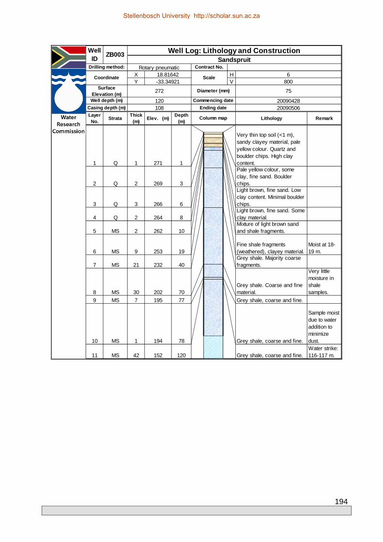
194

X HY V

Layer No.

StrataThick

(m)Elev. (m)

Depth (m)

Lithology Remark

1 Q 1 271 1

Very thin top soil (<1 m), sandy clayey material, pale yellow colour. Quartz and boulder chips. High clay content.

2 Q 2 269 3

Pale yellow colour, some clay, fine sand. Boulder chips.

3 Q 3 266 6

Light brown, fine sand. Low clay content. Minimal boulder chips.

4 Q 2 264 8Light brown, fine sand. Some clay material.

5 MS 2 262 10Mixture of light brown sand and shale fragments.

6 MS 9 253 19Fine shale fragments (weathered), clayey material.

Moist at 18-19 m.

7 MS 21 232 40Grey shale. Majority coarse fragments.

8 MS 30 202 70Grey shale. Coarse and fine material.

Very little moisture in shale samples.

9 MS 7 195 77 Grey shale, coarse and fine.

10 MS 1 194 78 Grey shale, coarse and fine.

Sample moist due to water addition to minimize dust.

11 MS 42 152 120 Grey shale, coarse and fine.Water strike: 116-117 m.

Well ID



18.81642-33.34921

Scale

20090506

272

20090428

6800

75Surface


Coordinate

Column map




195

X HY V

Layer No.

StrataThick

(m)Elev. (m)

Depth (m)

Lithology Remark

1 Q 1 271 1

Very thin top soil (<1 m), sandy clayey material, pale yellow colour. Quartz and boulder chips. High clay content.

2 Q 2 269 3

Pale yellow colour, some clay, fine sand. Boulder chips.

3 Q 3 266 6

Light brown, fine sand. Low clay content. Minimal boulder chips.

4 Q 2 264 8Light brown, fine sand. Some clay material.

5 MS 2 262 10Mixture of light brown sand and shale fragments.

6 MS 2 260 12Fine shale fragments (weathered), clayey material.

Well ID

ZB003a Well Log: Lithology and ConstructionSandspruit


18.81642-33.34921

Scale

20090506

272

20090506

6100

75Surface


Coordinate

Column map




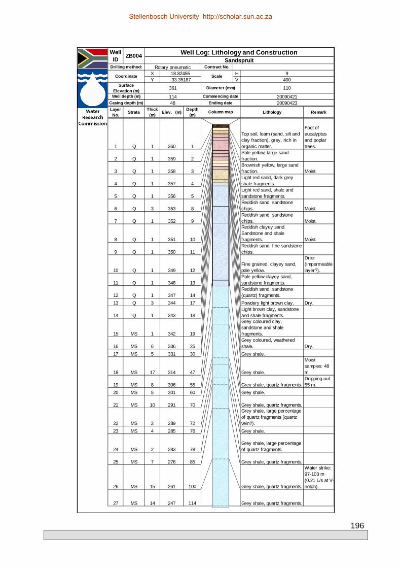
196

X HY V

Layer No.

StrataThick

(m)Elev. (m)

Depth (m)

Lithology Remark

1 Q 1 360 1

Top soil, loam (sand, silt and clay fraction), grey, rich in organic matter.

Foot of eucalyptus and poplar trees.

2 Q 1 359 2Pale yellow, large sand fraction.

3 Q 1 358 3Brownish yellow, large sand fraction. Moist.

4 Q 1 357 4Light red sand, dark grey shale fragments.

5 Q 1 356 5Light red sand, shale and sandstone fragments.

6 Q 3 353 8Reddish sand, sandstone chips. Moist.

7 Q 1 352 9Reddish sand, sandstone chips. Moist.

8 Q 1 351 10

Reddish clayey sand. Sandstone and shale fragments. Moist.

9 Q 1 350 11Reddish sand, fine sandstone chips.

10 Q 1 349 12Fine grained, clayey sand, pale yellow.

Drier (impermeable layer?).

11 Q 1 348 13Pale yellow clayey sand, sandstone fragments.

12 Q 1 347 14Reddish sand, sandstone (quartz) fragments.

13 Q 3 344 17 Powdery light brown clay. Dry.

14 Q 1 343 18Light brown clay, sandstone and shale fragments.

15 MS 1 342 19

Grey coloured clay, sandstone and shale fragments.

16 MS 6 336 25Grey coloured, weathered shale. Dry.

17 MS 5 331 30 Grey shale.


Moist samples: 48 m.

19 MS 8 306 55 Grey shale, quartz fragments.Dripping out: 55 m.


21 MS 10 291 70 Grey shale, quartz fragments.

22 MS 2 289 72

Grey shale, large percentage of quartz fragments (quartz vein?).


24 MS 2 283 78Grey shale, large percentage of quartz fragments.



Water strike: 97-103 m (0.21 L/s at V-notch).


Well ID



18.82455-33.35187

Scale

20090423

361

20090421

9400

110Surface


Coordinate

Column map




197

X HY V

Layer No.

StrataThick

(m)Elev. (m)

Depth (m)

Lithology Remark

1 Q 1 360 1Top soil, loamy, pale yellow colour, sandstone fragments.

2 Q 1 359 2Reddish sand, sandstone, coarse. Dry.

3 Q 1 358 3Red sand, sandstone, coarse.

4 Q 1 357 4Red sand, coarse, sandstone. Moist.

5 Q 1 356 5Red sand, sandstone, coarse. Moist.

6 Q 3 353 8Red sand, sandstone, coarse. Moist.

7 Q 2 351 10Red/brown sand, coarse, sandstone chips. Moist.

8 Q 2 349 12Clayey sand, sandstone chips. Very moist.

9 Q 3 346 15 Powdery light brown clay. Dry.

Well ID



18.82457-33.35187

Scale

20090424

361

20090423

10100

110Surface


Coordinate

Column map




198

X HY V

Layer No.

StrataThick

(m)Elev. (m)

Depth (m)

Lithology Remark

1 Q 5 298 5 Alluvial sand.

2 Q 6 292 11Light brown fine sand, sandstone (boulder) chips.

3 MS 4 288 15Grey/olive fine clayey sand, shale fragments.


5 MS 105 178 125 Grey shale.

6 MS 10 168 135Grey shale, coarser material, sand and shale mixture.

7 MS 16 152 151 Fine clay, grey shale.


Well ID



18.81962-33.35279

Scale

20090425

303

20090424

61001

75Surface


Coordinate

Column map




199

X HY V

Layer No.

StrataThick

(m)Elev. (m)

Depth (m)

Lithology Remark

1 Q 1 302 1 Alluvial sand. Light brown.Rich in roots. Dry.

2 Q 1 301 2 Alluvial sand. Light brown. Dry.

3 Q 1 300 3

Alluvial sand, yellow-red-purple shale fragments. A few quartzitic boulder chips. Brown-red colour. Moist.

4 MS 2 298 5

Grey/olive clay mixed with smaller portion of light brown sand, Very few soft shale fragments. Moist.

5 MS 2 296 7 Grey/olive clay, powdery.

6 MS 3 293 10Grey/olive clay, very soft shale fragments. Moist.

7 MS 2 291 12Grey/olive clay, very soft shale fragments.

Wet. No water strike, Throughflow borehole.

Well ID



18.81973-33.35284

Scale

20090507

303

20090507

6100

75Surface


Coordinate

Column map




200

X HY V

Layer No.

StrataThick

(m)Elev. (m)

Depth (m)

Lithology Remark

1 Q 1 302 1

Red coarse sand with gravelly fraction, some quartzite chips. Dry.

2 Q 2 300 3

Yellow very fine sand, a few boulder chips, some clay and silt. Dry.

3 Q 1 299 4

Light yellow very fine sand, a few boulder chips, some clay and silt. Dry.

4 Q 2 297 6Yellow very fine sand, some clay and silt. Dry.

5 Q 1 296 7Reddish very fine sand, some clay and silt. Dry.

6 Q 2 294 9Yellow very fine sand, some clay and silt. Dry.

7 Q 4 290 13Yellow-whiteish very fine sand, some silt and clay. Dry.

8 Q 1 289 14Mixture of pale sand, reddish sand and grey shale. Dry.

9 MS 1 288 15

Grey shale with some pale and reddish sand. Some grey shale chips. Dry.

10 MS 1 287 16Predominantly grey and dark shale. Coarse chips of shale. Moist.

11 MS 1 286 17 Grey shale. Coarse chips. Moist.

12 MS 35 251 52 Grey shale, coarse chips. Partially wet.

13 MS 12 239 64Grey shale, very coarse chips. Partially wet.

14 MS 3 236 67 Grey shale, coarse chips. Wet.

15 MS 8 228 75Grey shale, very coarse chips.


16 MS 3 225 78Grey shale, very coarse chips. Wet.

Well ID



18.81996-33.34745

Scale

20090508

303

20090508

6400

75Surface


Coordinate

Column map




201

X HY V

Layer No.

StrataThick

(m)Elev. (m)

Depth (m)

Lithology Remark

1 Q 1 302 1 Yellow-reddish sand. Dry.

2 Q 4 298 5Yellow-reddish very fine sand, some clay and silt. Moist.

3 Q 3 295 8Yellow-pale very fine sand, some silt and clay. Moist.

4 Q 2 293 10Brown very fine sand, some clay and silt. Moist.

5 Q 2 291 12Light brown very fine sand, some clay and silt. Moist.

Well ID



18.81996-33.34745

Scale

20090508

303

20090508

6100

75Surface


Coordinate

Column map




202

X HY V

Layer No.

StrataThick

(m)Elev. (m)

Depth (m)

Lithology Remark

1 Q 1 106 1Yellow-white sand. Quartzite chips. Dry.

2 Q 1 105 2Yellow-red sand. Quartzite chips. Dry.

3 Q 1 104 3 Yellow pale very fine sand. Moist.

4 Q 1 103 4 Light brown very fine sand. Moist.

5 Q 1 102 5Yellow pale very fine sand. Some quartzite chips. Moist.

6 Q 1 101 6Dark brown loam. Some soft chips. Wet.

7 Q 1 100 7Light brown pale loam. Some soft chips. Moist.

8 Q 1 99 8

Predominantly light brown pale loam mixed with grey shale. Grey shale fragments. Moist.

9 MS 4 95 12

Predominantly grey shale mixed with light brown pale loam. Grey shale fragments, some of them big. Moist.

10 MS 2 93 14Grey shale. Grey shale fragments. Wet.

11 MS 2 91 16 Grey shale.Water strike: 15-16 m.

12 MS 1 90 17Grey shale. Grey shale fragments. Wet.

13 MS 1 89 18Grey shale. Grey shale fragments. Partially wet.

14 MS 1 88 19Grey shale and occasional brown fragments. Wet.

15 MS 1 87 20Grey shale and occasional brown fragments. Moist.

16 MS 41 46 61Grey shale and occasional brown fragments. Dry.

17 MS 7 39 68Grey shale and occasional brown fragments. Wet.

18 MS 4 35 72Grey shale and occasional brown fragments. Very wet.

19 MS 4 31 76Grey shale and occasional brown fragments. Partially wet.

20 MS 27 4 103Grey shale and occasional brown fragments.

Water pumped to soften shale.

Well ID

OK001 Well Log: Lithology and ConstructionSandspruit


18.80986-33.25959

Scale

20090511

107

20090510

6400

75Surface


Coordinate

Column map




203

X HY V

Layer No.

StrataThick

(m)Elev. (m)

Depth (m)

Lithology Remark

1 Q 1 117 1

Reddish sand, boulder (sandstone chips), fine grained sand, roots.

2 Q 1 116 2

Reddish brown sand, boulder chips, quartz chips, fine grained sand.

3 Q 1 115 3

Yellowish brown fine grained sand with loam, boulder chips.

4 Q 1 114 4

Yellowish brown fine grained sand with loam, quartz and boulder chips.

5 Q 1 113 5Yellow brown loamy sand with boulder chips.

6 Q 3 110 8Yellow brown loamy sand with boulder chips.

7 Q 1 109 9Loam, some clay, few boulder chips. Moist.

8 Q 1 108 10Fine grained sand with some loam, fine boulder chips.

9 Q 1 107 11Pale, fine grained sand with loam and fine chips. Moist.

10 Q 3 104 14Orange brown loamy sand, with pale loam, small chips. Moist.

11 Q 2 102 16 Light brown, loamy sand. Moist.

12 Q 4 98 20Brown/dark brown loamy sand. Moist.

13 Q 1 97 21Brown/light brown fine sand, small chips.


14 Q 3 94 24High clay content, dark brown, shale chips.

15 Q 1 93 25Clayey sand, brown with shale.

16 MS 4 89 29

Brown/yellow coarse sand with shale chips, quartzitic sand.


Well ID



18.80806-33.25757

Scale

20090513

118

20090513

680

75Surface


Coordinate

Column map




204

X HY V

Layer No.

StrataThick

(m)Elev. (m)

Depth (m)

Lithology Remark

1 Q 1 124 1Coarse red sand with boulders and quartz chips.

2 Q 2 122 3

Silty sand, orange brown with boulder and sandstone chips, some clay.

3 Q 4 118 7Orange silty sand, boulder chips.

4 Q 2 116 9Orange silty sand, minimal boulder chips.

5 Q 4 112 13Orange silty sand, minimal boulder chips, some clay.

6 Q 6 106 19Yellow orange silty sand, shale chips. Moist.

7 Q 1 105 20Yellow brown coarse sand, sandstone and shale chips.

8 Q 5 100 25Pale yellow silty sand, shale and boulder chips.

9 Q 4 96 29Pale fine to coarse sand, shale chips.


Water strikes at 29-30 m and 34-35 m (not large enough to measure on V-notch).

Well ID



18.80997-33.25256

Scale

20090514

125

20090514

680

75Surface


Coordinate

Column map




205

X HY V

Layer No.

StrataThick

(m)Elev. (m)

Depth (m)

Lithology Remark

1 Q 2 68 2Red yellow-pale sand. Small fragments.

Many roots in the top 1 m from grassland. Moist.

2 Q 18 50 20

Light yellow very fine sand, some silt and clay fractions. Powdery. Moist.

3 Q 8 42 28

Light yellow very fine sand, some silt and clay fractions. Powdery. Moist.

4 Q 13 29 41

Light yellow very fine sand, some silt and more clay fractions. Powdery. Moist.

5 Q 2 27 43Light yellow fine sand, high clay content.

Moist. Collapsing from 40 m on,

6 Q 10 17 53

Saturated light yellow fine sand with high clay content, some coarse sand present.

7 MS 7 10 60

Brown to dark brown saturated fine sand, high clay content, shale chips.

8 MS 8 2 68

Brown to dark brown saturated fine sand, clay, grey to dark grey shale chips.

Water strike: 62 m (0.52 L/s at V-notch) and samples remained saturated to the bottom.

9 MS 4 -2 72Dark grey (charcoal colour) shale chips.

Well ID



18.86041-33.19636

Scale

20090522

70

20090521

6400

75Surface


Coordinate

Column map




206

X HY V

Layer No.

StrataThick

(m)Elev. (m)

Depth (m)

Lithology Remark

1 Q 1 61 1Brown sand. Small percentage clay. Wet.

2 Q 1 60 2Brown sand with bigger percentage clay. Wet.

3 Q 2 58 4Brown-grey loam with yellow and grey spots. Wet.

4 Q 2 56 6Brown-grey loam with yellow and grey spots. Very wet.

5 Q 2 54 8Grey clay with considerable brown sand fraction.

6 MS 5 49 13Grey clay with occasional brown sand fraction. Wet.

7 MS 1 48 14Grey clay with small brown sand fraction. Saturated.

8 MS 5 43 19 Grey shale. Wet.

9 MS 1 42 20Grey shale with small brown sand fraction. Saturated.

10 MS 2 40 22Grey shale with small brown sand fraction. Very wet.


Water strike: 23-30 (0.88 L/s at V-notch).

12 MS 5 32 30 Gravelly charcoal clay. Water strike.

Well ID



18.86535-33.19873

Scale

20090519

62

20090518

6200

75Surface


Coordinate

Column map




207

X HY V

Layer No.

StrataThick

(m)Elev. (m)

Depth (m)

Lithology Remark

1 Q 1 80 1Red sand to very fine sand, some clay, friable aggregates

Moist. Bare spot surrounded by renosterveld bushes.

2 Q 14 66 15Red sand to very fine sand and clay, friable aggregates. Moist.

3 Q 2 64 17Yellow-pale reddish very fine sand. Moist.

4 Q 7 57 24 Yellow-pale very fine sand. Moist.

5 Q 2 55 26Yellow-pale reddish very fine sand to clay. Moist.

6 Q 1 54 27

Yellow-pale to grey olive very fine sand to clay. Muddy reddish intrusions. Gley process visible. Moist.

7 MS 2 52 29Light grey to light brown olive clay. Gley process visible. Moist.

8 MS 1 51 30 Grey to dark grey clay. Moist.

9 MS 6 45 36Dark grey charcoal, predominantly clay. Moist.

10 MS 6 39 42 Grey slurry, a few chips.

Water strike: 38-48 m (0.38-1.26 L/s at V-notch).

11 MS 3 36 45

Grey slurry, dark chips, some big quartzite chips and stones. Water strike.

Well ID



18.87108-33.20425

Scale

20090520

81

20090520

6200

75Surface


Coordinate

Column map




208

X HY V

Layer No.

StrataThick

(m)Elev. (m)

Depth (m)

Lithology Remark

1 Q 55 64 55 Sand.

2 MS 65 -1 120 Shale.


Well ID



18.85466-33.19855

Scale

20090524

119

20090523

61001

75Surface


Coordinate

Column map




209

APPENDIX B

0

200

400

600

800

1000

1200

1400

1600

1800

0 200 400 600 800 1000 1200 1400

De

Ho

ek

-C

um

ula

tiv

e R

ain

fall

(m

m)

Langgewens - Cumulative Rainfall (mm)

0

200

400

600

800

1000

1200

1400

1600

1800

0 200 400 600 800 1000 1200 1400

De

Ho

ek

-C

um

ula

tiv

e R

ain

fall

(m

m)

Moorreesberg - Cumulative Rainfall (mm)

0

200

400

600

800

1000

1200

1400

1600

1800

0 200 400 600 800 1000 1200 1400 1600 1800

De

Ho

ek

-C

um

ula

tiv

e R

ain

fall

(m

m)

Voëlvlei - Cumulative Rainfall (mm)


210

0

200

400

600

800

1000

1200

1400

1600

1800

0 200 400 600 800 1000 1200 1400 1600

De

Ho

ek

-C

um

ula

tiv

e R

ain

fall

(m

m)

Zwavelberg - Cumulative Rainfall (mm)

0

200

400

600

800

1000

1200

1400

1600

1800

0 200 400 600 800 1000 1200

De

Ho

ek

-C

um

ula

tiv

e R

ain

fall

(m

m)

Oranjeskraal - Cumulative Rainfall (mm)

0

200

400

600

800

1000

1200

1400

1600

1800

0 100 200 300 400 500 600 700 800 900

De

Ho

ek

-C

um

ula

tiv

e R

ain

fall

(m

m)

Sandspruit - Cumulative Rainfall (mm)


211

0

200

400

600

800

1000

1200

1400

0 200 400 600 800 1000 1200 1400

Lan

gg

ew

en

s -

Cu

mu

lati

ve

Ra

infa

ll (

mm

)

Moorreesberg - Cumulative Rainfall (mm)

0

200

400

600

800

1000

1200

1400

0 200 400 600 800 1000 1200 1400 1600 1800

Lan

gg

ew

en

s -

Cu

mu

lati

ve

Ra

infa

ll (

mm

)

Voëlvlei - Cumulative Rainfall (mm)

0

200

400

600

800

1000

1200

1400

0 200 400 600 800 1000 1200 1400 1600

Lan

gg

ew

en

s -

Cu

mu

lati

ve

Ra

infa

ll (

mm

)

Zwavelberg- Cumulative Rainfall (mm)


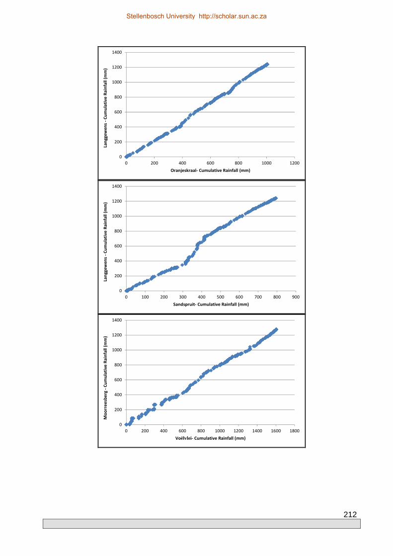
212

0

200

400

600

800

1000

1200

1400

0 200 400 600 800 1000 1200

Lan

gg

ew

en

s -

Cu

mu

lati

ve

Ra

infa

ll (

mm

)

Oranjeskraal- Cumulative Rainfall (mm)

0

200

400

600

800

1000

1200

1400

0 100 200 300 400 500 600 700 800 900

Lan

gg

ew

en

s -

Cu

mu

lati

ve

Ra

infa

ll (

mm

)

Sandspruit- Cumulative Rainfall (mm)

0

200

400

600

800

1000

1200

1400

0 200 400 600 800 1000 1200 1400 1600 1800

Mo

orr

ee

sbe

rg -

Cu

mu

lati

ve

Ra

infa

ll (

mm

)

Voëlvlei- Cumulative Rainfall (mm)


213

0

200

400

600

800

1000

1200

1400

0 200 400 600 800 1000 1200 1400 1600

Mo

orr

ee

sbe

rg -

Cu

mu

lati

ve

Ra

infa

ll (

mm

)


0

200

400

600

800

1000

1200

1400

0 200 400 600 800 1000 1200

Mo

orr

ee

sbe

rg -

Cu

mu

lati

ve

Ra

infa

ll (

mm

)


0

200

400

600

800

1000

1200

1400

0 100 200 300 400 500 600 700 800 900

Mo

orr

ee

sbe

rg -

Cu

mu

lati

ve

Ra

infa

ll (

mm

)



214

0

200

400

600

800

1000

1200

1400

1600

1800

0 200 400 600 800 1000 1200 1400 1600

Voël

vlei

-C

um

ula

tiv

e R

ain

fall

(m

m)


0

200

400

600

800

1000

1200

1400

1600

1800

0 200 400 600 800 1000 1200

Voël

vlei

-C

um

ula

tiv

e R

ain

fall

(m

m)


0

200

400

600

800

1000

1200

1400

1600

1800

0 100 200 300 400 500 600 700 800 900

Voël

vlei

-C

um

ula

tiv

e R

ain

fall

(m

m)



215

0

200

400

600

800

1000

1200

1400

1600

0 200 400 600 800 1000 1200

Zw

av

elb

erg

-C

um

ula

tiv

e R

ain

fall

(m

m)


0

200

400

600

800

1000

1200

1400

1600

0 100 200 300 400 500 600 700 800 900

Zw

av

elb

erg

-C

um

ula

tiv

e R

ain

fall

(m

m)


0

200

400

600

800

1000

1200

0 100 200 300 400 500 600 700 800 900

Ora

nje

skra

al

-C

um

ula

tiv

e R

ain

fall

(m

m)



216

APPENDIX C

Land Use/Type Options Available in the JAMS/J2000-NaCl Hydrological Model Crop Name Crop Name Crop Name Crop Name

Agricultural Land-Generic Sugarcane Indian grass Spring Canola-Argentine Agricultural Land-Row Crops Spring Wheat Alfalfa Asparagus

Agricultural Land-Close-grown Winter Wheat Sugar Beet Broccoli Orchard Durum Wheat Red Clover Cabbage

Hay Rye Alsike Clover Cauliflower Forest-Mixed Spring Barley Soybean Celery

Forest-Deciduous Oats Cowpeas Head Lettuce Forest-Evergreen Winter Rye Mung Beans Spinach Wetlands-Mixed Pearl Millet(Hirse) Lima Beans Green Beans

Wetlands-Forested Timothy Lentils Cucumber Wetlands-Non-Forested Smooth Bromegrass Kleegrass Eggplant

Pasture Meadow Bromegrass Field Peas Cantaloupe

Summer Pasture Tall Fescue Garden or Canning

Peas Winter Rape

Winter Pasture Kentucky Bluegrass Sesbania Ackergras Range-Grasses Bermudagrass Flax Bell Pepper

Range-Brush Crested Wheatgrass Upland Cotton-harv

w/ stripper Strawberry

Triticale Western Wheatgrass Upland Cotton-harv

w/ picker Tomato

Water Slender Wheatgrass Tobacco Apple

Corn Italian (Annual)

Ryegrass Sugarbeet Pine

Corn Silage Russian Wildrye Potato Oak Sweet Corn Altai Wildrye Sweetpotato Poplar

Eastern Gamagrass Sideoats Grama Carrot Winter Barley Grain Sorghum Big Bluestem Onion Urban Areas Sorghum Hay Little Bluestem Sunflower Phacelia Johnsongrass Alamo Switchgrass Spring Canola-Polish Corn Silage (undersown)


western cape - CORE

Documents

Transcript of western cape - CORE