CAPE PENINSULA UNIVERSITY OF TECHNOLOGY - CORE
146
CAPE PENINSULA UNIVERSITY OF TECHNOLOGY DEPARTMENT OF MECHANICAL ENGINEERING FACULTY OF ENGINEERING Remote Monitoring and Evaluation of a Photovoltaic (PV) Groundwater Pumping System By Selbourne Rapoone Makhomo In partial fulfilment of the requirements of the Master's Degree in Technology (Mtech) Under the supervision of Mr. I1yas Omar and Prof. Eugene Cairn cross NOVEMBER 2005
-
Upload
khangminh22 -
Category
Documents
-
view
3 -
download
0
Transcript of CAPE PENINSULA UNIVERSITY OF TECHNOLOGY - CORE

CAPE PENINSULAUNIVERSITY OF TECHNOLOGY
DEPARTMENT OF MECHANICAL ENGINEERING
FACULTY OF ENGINEERING
Remote Monitoring and Evaluation of a Photovoltaic (PV)
Groundwater Pumping System
By
Selbourne Rapoone Makhomo
In partial fulfilment of the requirements of the Master's Degree in
Technology (Mtech)
Under the supervision of
Mr. I1yas Omar and Prof. Eugene Cairncross
NOVEMBER 2005

Declaration
DECLARATION
1
I, the undersigned, hereby declare that the dissertation presented here is my own work and the
opinions contained herein are my own and do not necessarily reflect those of the Cape
Peninsula University of Technology. All references used have been accurately reported.
Name: ?i:0:-::!??.~.f(...r:-!..f:: t1f.?.tH?~1.D
Signature:~ .
Date: ?:.7.. ((~/t:.~ , .

Abstract
ABSTRACT
11
Potable water, and especially the accessibility to it, is an essential part of everyday life. Of
particular note, is the challenge that residents of remote rural African villages face in order to
gain access to this basic requirement. Specifically, the rural areas in the Northern Cape
(Province north of Cape Town) region in South Africa is one such example that illustrates
this problem very well. In order to address the requirements for drinkable water, various
types of water pumping technologies have been used. Up to now, the two competing water
pumping systems, diesel and photovoltaic (PV), have been the primary technologies deployed
in selected sites in the Northern Cape.
The manual data collection of water pumping system data in the Northern Cape is fraught
with impracticalities such as travel costs and requirements for skilled personnel. Therefore, as
a preliminary step to accelerate development and testing, a local experimental laboratory PV
water pumping rig was set-up within the Department of Mechanical Engineering at the Cape
University of Technology. A short-term analysis was performed over a period of three weeks
on the rig and the experimental results indicated the following: array efficiency of 16.3%,
system efficiency of 15.0% and an average system efficiency of 1.47%. However, the results
do indicate that long-term monitoring of PV water pumping systems can be suitable in
serving to determine dynamic system performance and system life cycle costs.
The purpose of this project is two-fold - firstly, to present the results on the work done on the
experimental PV system. Additionally, due to the specific challenges of limited
communications infrastructure in the rural Northern Cape regions, the report presents the
telemetry method employed for the remote monitoring of the proposed water pumping
systems in the Northern Cape as well as monitoring results. The complete hardware and
software set-up of the experimental system has been presented in the report as well as the
present work done in order to move from the laboratory to the actual field implementation.
The remotely monitored field results taken over a period of two months show an array
efficiency of 3.0%, a system efficiency of 32.0% and an overall system efficiency of 1.3%.
The array and overall efficiencies are lower than expected due to the pump operating at off
design conditions (3.6m3/day). If the pump were operating at near-design conditions
(20m3/day), the array and overall efficiencies would be high as 20.0% and 4.0% respectively.

Abstract 111
A PV water pumping 15-year life cycle cost analysis has indicated a unit water cost of
R15.08/m3 or 1.5 cents/! and an energy cost of 30 cents/m4• A diesel15-year life cycle cost
analysis has indicated a unit water cost of R3.12/m3 or 0.31 centsll and an energy cost of 9
cents/m4• If near-design conditions were assumed for the PV system the costs would be 0.27
cents/! and 5.4 cents/m4 respectively.
The fmdings of this study do support the existing body of evidence, which indicates that PV
pumping can be competitive with diesel water pumping under specific head and flow
conditions. However, the results obtained in this text are short-term results, making it difficult
to make valid judgements with regard to how this system behaves in the long run. Yet the
socio-institutional implementation strategies are crucial to the techno-economic success of
actual pumping schemes. Even if diesel generators or other conventional pumping systems
may appear to be cheaper on a life cycle cost comparison, it might be preferable to go for a
PV system because of the operational advantages. Future work will evaluate a larger number
of systems and eventually record long-term results which will be used to assess the reliability
and functionality of the systems.

AcknowledgementS
ACKNO'VLEDGE~ffiNTS
iv
The author wishes to thank the following persons and institutions for their valuable
contribution towards the completion of this work.
Q Mr I Omar, the supervisor, deserves valuable credit for the efforts he put towards the
compilation of this report. His assistance and advice during the various stages of this report
are highly appreciated.
Q Prof. E Caimcross, the co-supervisor, also deserves valuable credit by thorough reading
and helpful comments he offered.
Q Ms R Ziegler, is thanked for editing and proof-reading.
Q Peninsula Technikon and the Cape Peninsula University of Technology are also thanked
for the fmancial support they provided me for the entire study period. The Technikon also
provided me with the testing facility.
Q Allpower, Shell Renewables and Total Energie SA, for their donation of some of the
water pumps, modules and controllers.
Q lagon Witkowsky, his assistance on the monitoring side has been helpful and is highly
appreciated. The information and comments he provided were so helpful - I enjoyed our
interaction.
Q Thanks to my parents for their patience, encouragement and fmancial support during
difficult times.
Q Finally, to my colleagues at the Department of Mechanical Engineering for their
assistance and support during the preparation of this work.

Contents page
TABLE OF CONTENTS
Contents
Declaration
Abstract
Acknowledgements
Table of contents
List of figures
List of tables
Abbreviations and list of symbols
CHAPTER 1: INTRODUCTION
1.1. Background/awareness of the problem
1.2. Purpose and scope of the project
1.3. Significance of the project
1.4. Objectives of the project
1.5. Report strnctnre
v
Page
I
11
IV
V
IX
xn
xiii
1
I
2
3
3
4
CHAPTER 2: REVIEW OF REMOTE MONITORING FOR GROUND WATER PV
PUMPING SYSTEM (pVPS) 7
2.1. The concept 'remote monitoring system' 7
2.1.1. Data transmission using low earth orbit (LEO) satellite 13
2.1.2. Data transmission using a telephone line/cellular phone 14
2.1.3. Data transmission using a radio 14
2.1.4. Data transmission using direct connection 15
2.2. Technical considerations ofa Photovoltaic water pumping system (PVWPS) 15
2.2.1. PVarray 15
2.2.2. The power conditioning device 16
2.2.3. Motor/pump Irnit 17
2.3. Economic considerations ofPVWPS 18
2.3.1. Life cycle costing 19
2.4. Social aspects ofPVWPS 23

Contents page VI
CHAPTER 3: LABORATORY WORK AND PRELThflNARY TESTS 25
3.1. Existing PV system 25
3.1.1. PVarray 26
3.1.2. Pump Master 27
3.1.3. Motor/pump unit 28
3.2. Identification of data acquisition equipment 29
3.2.1. Datalogger 30
3.2.2. Digital flow transmitter 32
3.2.3. Digital pressure transmitter 33
3.2.4. Anemometer 34
3.2.5. Pyranometer 34
3.2.6. DC power supply 35
3.2.7. A day/night switch 36
3.3. Presentation ofresults 38
3.3.1. Temperature versus time 41
3.3.2. Array, converter and pump power versus time 41
3.3.3. Head versus time 42
3.3.4. Flow rate versus time 43
3.3.5. Irradiance power versus time 43
3.3.6. Array efficiency versus irradiance 44
3.3.7. Converter efficiency versus time 45
3.3.8. System efficiency versus time 45
3.3.9. Pump efficiency versus time 46
3.3.10. Overall efficiency versus time 47
3.4. Experimental observations and conclusions 47
CHAPTER 4: FIELDWORK AND TESTS 49
4.1. Site description (Lepelsfontein) 49
4.2. System description 50
4.2.1. Solar panels 51
4.2.2. The Grundfos DC/AC inverter 52
4.2.3. Pump 52
4.3. Rooifontein 53
4.4. Telemetry hardware and configuration 53

Contents page
4.4.1. Flow & pressure transmitters
4.4.2. Pyranometer
4.4.3. Solar panel
4.4.4. Data logger
4.4.5. HF modem (The Aerocomm Data Transceiver)
4.4.6. GSM modem (Samba GSMlGPRS & Tango modems)
CHAPTER 5: FIELD RESULTS Ac"ID ANALYSIS
5.1. On-site results & discussion
5.2. Remote monitoring experiences & results
5.2.1. Array & pump power versus time
5.2.2. Temperature versus time
5.2.3. Array efficiency versus irradiance
5.2.4. System efficiency versus time
5.2.5. Overall efficiency versus time
5.3. Cost analysis
5.3.1. Life cycle costing
5.3.2. Unit water cost
5.3.3. Costs ofPV pumping system
5.3.4. Costs of diesel pumping system
5.4. Comparative assessment of the two water pumping technologies
CHAPTER 6: CONCLUSIONS
6.1. PV and diesel pumping
6.2. Remote monitoring
6.3. Concluding comments
BmLIOGRAPHY
APPENDICES
APPENDIX A: Data sheets of experimental hardware
APPENDIX B: Data sheets of field hardware
APPENDIX C: Data acquisition data sheets
APPENDIX D: Experimental results
APPENDIX E: Field results
vii
54
55
56
57
58
58
62
62
67
68
68
69
70
70
73
73
73
74
75
80
83
83
87
87
89
94
95
99
106
III
113

Contents page
APPENDIX F: Field maps
APPENDIX G: Field pictures
viii
125
128

List offigures
Figure 1.1:
Figure 2.1:
Figure 2.2:
Figure 2.3:
Figure 2.4:
Figure 2.5:
Figure 2.6:
Figure 2.7:
Figure 2.8:
Figure 2.9:
Figure 2.10:
LIST OF FIGURES
Schematic diagram of data transmission to the computer
Block diagram ofthe PVP and the primary data acquisition system
Network architecture
Data-acquisition architectures for RES systems
Test facility for PV-diesel hybrid energy systems
Data transmission using Satellite
I-V curve of a module
PV versus diesel pumping system
Life cycle costs (Rlm4) ofPV & diesel versus time (years)
Life cycle costs (R) ofPV & diesel versus time (years)
Relative costs of PV & diesel
ix
3
8
9
10
11
13
17
20
21
22
22
Figure 3.1: Layout ofphotovoltaic pumping system in the Thermodynamics laboratory 26
Figure 3.2: 75 W x 3 WA Siemens modules 27
Figure 3.3: WaterMax Pump master 28
Figure 3.4: Installation of motor/pump unit 29
Figure 3.5: Data Taker DT605 30
Figure 3.6: Digital flow transmitter 32
Figure 3.7: Tronic line pressure transmitter 33
Figure 3.8: Anemometer 34
Figure 3.9: Pyranometer (LI-200SZ) 35
Figure 3.IO(a):Internal day/night switch 36
Figure 3.1O(b):External day/night switch 36
Figure 3.11: Configurations of transducer connections to the datalogger 37
Figure 3.12: The need for instantaneous readings 40
Figure 3.13: Temperature versus time 41
Figure 3.14: Array, converter & pump power versus time 42
Figure 3.15: Head versus time 42
Figure 3.16: Flow rate versus time 43
Figure 3.17: Irradiance power 43
Figure 3.18: Array efficiency versus irradiance 44

List offigllres X
Figure 3.19: Converter efficiency versus time 45
Figure 3.20: Pump efficiency versus time 46
Figure 3.21: System efficiency versus time 46
Figure 3.22: Overall efficiency versus time 47
Figure 4.1: Rainwater storage tanks 49
Figure 4.2: Water flow diagram from the pump to the end user 50
Figure 4.3: Set of Liselo & Helios PV panels 52
Figure 4.4: Gmndfos inverter 52
Figure 4.5(a): Diesel engine 53
Figure 4.5(b): Pump inside a borehole 53
Figure 4.6: Telemetry system configuration 54
Figure 4.7: Flow & pressure transmitters 55
Figure 4.8: Pyranometer 56
Figure 4.9: Solar panel 57
Figure 4.10: A data logger & a charge controller 57
Figure 4.11: The Aerocom Data Transceiver 58
Figure 4.12: The Falcom Samba GPRS/GPS modem 58
Figure 4.13(a):Tango modem 59
Figure 4. 13(b):Tango with antenna 59
Figure 4.14: An actual telemetry set-up 59
Figure 4.15: A transmitting RF antenna at the pump station 60
Figure 5.1: Rooifontein diesel pump data Jan '95 - Sep '01 65
Figure 5.2: Lepelsfontein solar pump data Jan '95 - Dec '97 66
Figure 5.3: Screen print of results downloaded from the data logger 67
Figure 5.4: Array & pump power versus time 68
Figure 5.5: Temperature versus time 68
Figure 5.6: Array efficiency versus irradiance 69
Figure 5.7: System efficiency versus time 70
Figure 5.8: Overall efficiency versus time 71
Figure 5.9: PV life cycle cost breakdown 76
Figure 5.10: Diesel life cycle cost breakdown 76
Figure 5.11: Initial & operating costs of PV & diesel pumping 77

List offigures
Figure 5.12:
Figure 5.13:
Figure 5.14:
Figure 5.15:
Life cycle costs of PV & diesel pumping
PV & diesel costs comparisons
PV actual & diesel systems cumulative & energy costs
PV predicted & diesel systems cumulative & energy costs
Xl
77
78
78
79

List oftables XlI
LIST OF TABLES
Table 2.1:
Table 3.1:
Table 3.2:
Table 3.3:
Summary of field PV & diesel water pumping
Specifications of WA Siemens modules
Three different sources that may be used to power a data taker
Measured parameters of the PV pumping system
21
26
31
39
Table 4.1:
Table 4.2:
Table 4.3:
Comparisons between Peninsula Technikon and Lepelsfontein PV systems 5I
Specifications ofLiselo and Helios solar panels at Lepelsfontein 51
Specifications WA Siemens module 56
Table 5.1: Summary of PV and diesel water pumping systems in Lepelsfontein and
Rooifontein respectively 62
Table 5.2: Data sheet of Lepelsfontein settlement 63
Table 5.3: Summary of results of Rooifontein diesel water pumping 64
Table 5.4: Summary ofresults ofLepelsfontein PV water pumping 66
Table 5.5: PV initial costs 74
Table 5.6: Replacement, maintenance and operating costs ofPV pumping 74
Table 5.7: Replacement, maintenance and operating costs of diesel pumping 75
Table 5.8: Diesel set initial costs 75
Table 5.9: Summary of the three water pumping life cycle costs 75
Table 5.10: Data used for solar pumping cost comparison 79
Table 5.11: Data used for diesel pumping cost comparison 80
Table 5.12: Summary of unit water and pumping costs for PV & diesel 81
Table 6.1:
Table 6.2:
Summary ofPV & diesel life cycle, unit & pumping costs
Summary of experimental & filed results
84
86

Abbreviations
CPUT
PV
PVWPS
DAS
DAE
MPPT
STC
LED
LCC
LEO
RF
GSM
CRF
RV
Wp
R
c
UWC
EC
Symbols
H,
Ht
Tamb
Q
p
g
G
ABBREVIATIONS AND LIST OF SYMBOLS
Cape Peninsula University of Technology
Photovoltaic
Photovoltaic water pumping system
Data acquisition system
Data acquisition equipment
Maximum power point tracker
Standard test conditions
Light emitting diode
Life cycle costs
Low earth orbit
Radio frequency
Global System for Mobile Communications
Capital recovery factor
Residual value
peak power generated by PV panels (W)
South African currency
cents(IOO cents=Rl)
Unit water cost in rand per cubic meter (Rlml)
Energy/pumping cost (Rlm4)
Units
static head m
total head m
ambient temperature QC
water flow rate ml/s
density kg/ml
gravitational acceleration 9.81 mls2
module current A
module voltage V
converter current A
converter voltage V
irradiance W/m2
XlU

XlV
A area of the modules m2
Pirr irradiance power W
Parr array power W
Peon converter power W
TlAnay array efficiency %
llConvener converter efficiency %
11 System system efficiency %
TlOveral1 overall efficiency %

Chapter I
Chapter 1
INTRODUCTION
Introduction 1
1.1. BACKGROUND/AWARENESS OF THE PROBLEM
The provision of adequate water supplies to households in underdeveloped rural areas
remains a crucial area of concern in South Africa. In a vast and relatively dry country like
South Africa, the satisfaction of basic water needs is for many people, a daily struggle (Omar
& Law, 1991:1). This leads to poor living conditions and, in extreme cases, the migration of
the rural population to urban centres (Arab et ai, 1999:191). Considering the importance of
clean, disease-free water in all fundamental human activities, there can be no doubt that lack
of an adequate water supply acts as a major constraint to the development of rural
communities. It is therefore important to design a system that will assist in providing clean,
disease-free water in sufficient quantities at an affordable cost.
The rural regions of the Northern Cape are good examples of areas facing this problem.
Therefore, in order to facilitate the collection of potable water, various types of water
pumping technologies have been employed in the past. Photovoltaic (PV) and diesel
groundwater pumping systems have been used successfully in most cases, to supply rural
communities in the Northern Cape with drinkable water. Although both pumping
technologies have their merits, there still exists a need to perform a thorough long-term field
study ofPV systems in the rural Northern Cape regions.
To date, the degree of acceptance ofphotovoltaic solar water pumping systems by the users is
very low. There are several factors which have inhibited the widespread implementation of
these systems. These include high initial cost, lack of awareness and technical expertise, lack

Chapter 1 Introduction 2
of sufficient knowledge on the daily output of these systems (predictability) and a history of
failures. A number of solar water pumping systems were installed in various areas around the
world. However, most of these systems have experienced problems, mainly because these
were not properly sized (Jafar, 2000:86).
As an attempt to test and assess the reliability and capabilities of the PV system, a research
project was initiated at Cape Peninsula University of Technology (CPUT) in the
Thermodynamics laboratory of the department of Mechanical Engineering. The project is
divided into two phases. Phase I involves the testing, monitoring and data evaluation from
the laboratory tests. Phase 2 is concerned mainly with evaluating available data from the two
water pumping systems installed in the Northern Cape (PV & diesel). Data is to be
transmitted from the pumping system to the microcomputer via a wireless link between the
two stations (plant & base station).
1.2. PURPOSE AND SCOPE OF THE PROJECT
The purpose of this research is to monitor and evaluate two PV water pumping systems, one
system is installed in the Thermodynamics laboratory in the department of Mechanical
Engineering, CPUT and the other system is in Lepelsfontein, a small village in the Northern
Cape. It is also the purpose of the research to show that a remote monitoring system can be
used for monitoring performance and to show that the system is cost effective. Available
results from the diesel water pumping system in Rooifontein will also be used and be
compared with the PV results to determine the life cycle costs of two systems. Monitoring
here refers to accessing data from the PV plant to the computer using a wireless link. The
wireless link involves data acquisition equipment (DAE) incorporating necessary software
and hardware. Then available data from the computer will be analyzed and evaluated. Data
referred to here are the following parameters; flow rate, pressure, wind speed, irradiance,
voltage and current generated by the panels. Evaluation involves technical, economic,
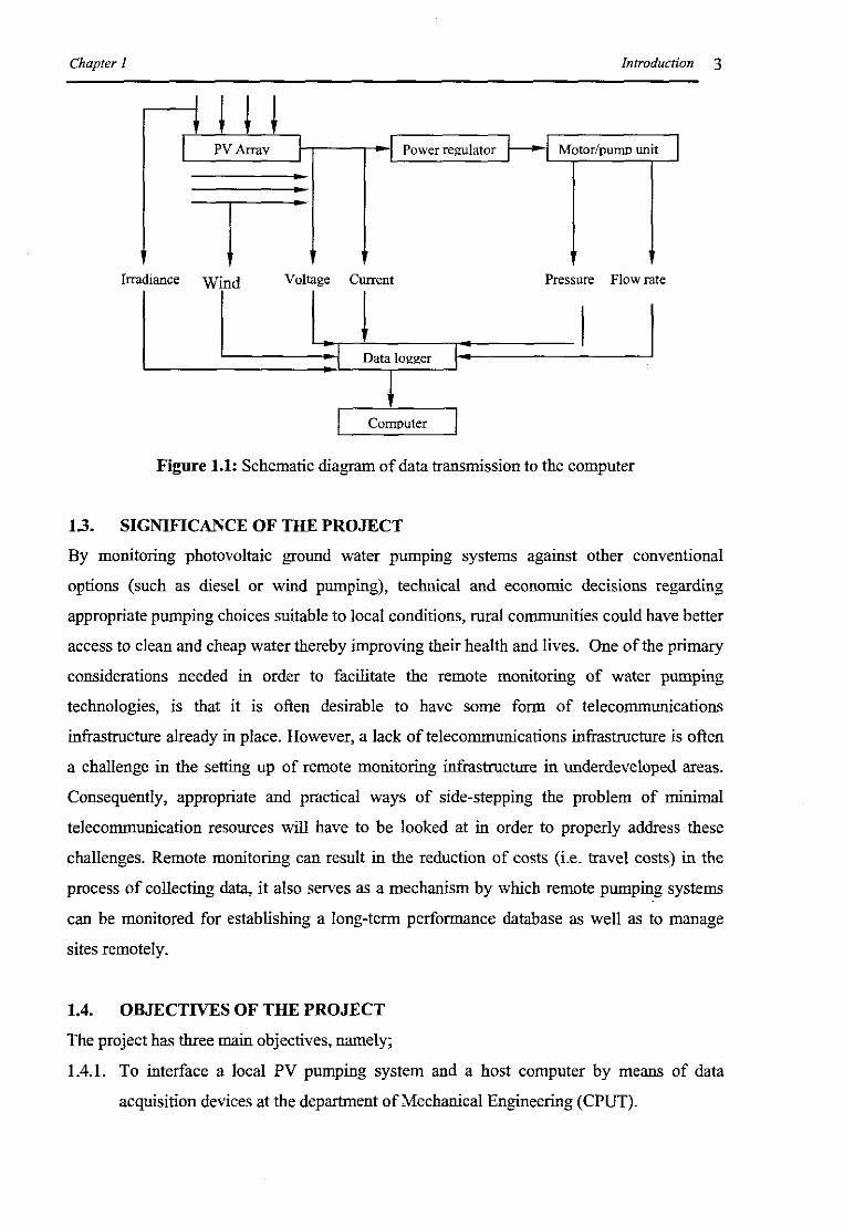
institutional and social aspects of the PV pumping system. Figure 1.1 shows a line diagram
of an existing PV system with the necessary data acquisition equipment. Data from the
system is directly transmitted to the data logger which changes the mechanical signals from
the transducers to readable electrical quantities. A power supply is provided to change AC to
DC.
Chapter 1
, ,,I-r---,-..-j, Power regulator
..•
Introduction 3
Motor/pump unit I
Irradiance Wind Voltage Current
~Pressure Flow rate
IData logger I
Computer
Figure 1.1: Schematic diagram of data transmission to the computer
1.3. SIGNIFICANCE OF THE PROJECT
By monitoring photovoltaic ground water pumping systems against other conventional
options (such as diesel or wind pumping), technical and economic decisions regarding
appropriate pumping choices suitable to local conditions, rural communities could have better
access to clean and cheap water thereby improving their health and lives. One of the primary
considerations needed in order to facilitate the remote monitoring of water pumping
technologies, is that it is often desirable to have some form of telecommunications
infrastructure already in place. However, a lack of telecommunications infrastructure is often
a challenge in the setting up of remote monitoring infrastructure in underdeveloped areas.
Consequently, appropriate and practical ways of side-stepping the problem of minimal
telecommunication resources will have to be looked at in order to properly address these
challenges. Remote monitoring can result in the reduction of costs (i.e. travel costS) in the
process of collecting data, it also serves as a mechanism by which remote pumping systems
can be monitored for establishing a long-term performance database as well as to manage
sites remotely.
1.4. OBJECTIVES OF THE PROJECT
The project has three main objectives, namely;
IA.I. To interface a local PV pumping system and a host computer by means of data
acquisition devices at the department ofMechanical Engineering (CPUT).

Chapter 1 Introduction 4
1.4.2. To establish a communication link between the Lepelsfontein PV system and a local
ground receiving station at the CPUT.
1.4.3. To compare PV water pumping with diesel water pumping field results and make
some valid conclusions. The obtained results will assist in:
o The analysis of technical aspects of the system (determining system and sub
system efficiencies).
D The study of economic aspects (determining the true life cycle costs to establish
the relative merits of each method ofpumping).
1.5. REPORT STRUCTURE
The remainder of this report is structured as follows:
1.5.1. CHAPTER 2
This chapter presents a literature survey on remote monitoring systems for PV ground water
pumping system. The first section defines the concept 'remote monitoring system'. It
reviews the work done in this particular field as well as the problems that could be
encountered.
The next section introduces various methods that can be used to transmit data from the PV
plants to the receiving stations. The methods which are dealt with here are satellite
transmission, telephone line transmission, direct transmission, radio & modem transmission
and cell phone transmission. Section 2.3 illustrates the economic aspects of this option (PV)
of water pumping. Cost comparisons are made, but more important is the illustration of the
non-financial considerations that make PV the preferred choice as a power source for
pumping application.
Section 2.2 gives insight into the technical aspects of the PV system. This summarizes the
most important aspects related to stand-alone PV components. This includes an introduction
to PV components and stand-alone systems, but also considers issues related to quality, safety
and maintenance of the systems. The [mal section of this chapter demonstrates the
importance of user involvement in all stages of the project cycle. It focuses on those
applications where the success of the technology will depend not only on its own merits, but
also on how well this technology has interacted with the people who daily depend on the PV
equipment.
Chapter I Introduction 5
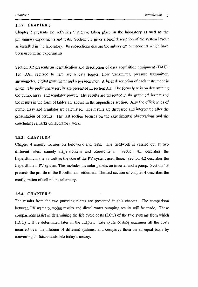
1.5.2. CHAPTER 3
Chapter 3 presents the activities that have taken place in the laboratory as well as the
preliminary experiments and tests. Section 3.1 gives a brief description of the system layout
as installed in the laboratory. Its subsections discuss the subsystem components which have
been used in the experiments.
Section 3.2 presents an identification and description of data acquisition equipment (DAE).
The DAE referred to here are a data logger, flow transmitter, pressure transmitter,
anemometer, digital multimeter and a pyranometer. A brief description of each instrument is
given. The preliminary results are presented in section 3.3. The focus here is on determining
the pump, array, and regulator power. The results are presented in the graphical format and
the results in the form oftables are shown in the appendices section. Also the efficiencies of
pump, array and regulator are calculated. The results are discussed and interpreted after the
presentation of results. The last section focuses on the experimental observations and the
concluding remarks on laboratory work.
1.5.3. CHAPTER 4
Chapter 4 mainly focuses on fieldwork and tests. The fieldwork is carried out at two
different sites, namely Lepelsfontein and Rooifontein. Section 4.1 describes the
Lepelsfontein site as well as the size of the PV system used there. Section 4.2 describes the
Lepelsfontein PV system. This includes the solar panels, an inverter and a pump. Section 4.3
presents the profile of the Rooifontein settlement. The last section of chapter 4 describes the
configuration of cell phone telemetry.
1.5.4. CHAPTER 5
The results from the two pumping plants are presented in this chapter. The comparison
between PV water pumping results and diesel water pumping results will be made. These
comparisons assist in determining the life cycle costs (LCC) of the two systems from which
(LCC) will be determined later in the chapter. Life cycle costing examines all the costs
incurred over the lifetime of different systems, and compares them on an equal basis by
converting all future costs into today's money.

Chapter i introduction 6
1.5.5. CHAPTER 6
Chapter 6 is the concluding chapter. It presents the conclusions on the laboratory work as
well as the fieldwork. Finally, the overall concluding remarks are made as to the success of
the project.

Chapter 2 Review O/Remote Monitoring For Ground Water PVPS 7
Chapter 2
REVIEW OF REMOTE MONITORING FOR GROUND
WATER PV PUMPING SYSTEMS (PVPS)
2.1. THE CONCEPT 'REMOTE MONITORING SYSTEM'
Photovoltaic water pumping system performance incorporating remote monitoring is an area
that has not been widely researched in South Africa. Nevertheless, remote monitoring
systems for ground water supply have been operating in a few African countries and
elsewhere (Benghanem, 1998). In South Africa, several PV projects are underway and most
of them do not incorporate data acquisition devices. The major obstacles in these systems as
illustrated by Scholle (1994:1), are, advanced technological requirements and their associated
costs. Scholle's data acquisition system consisted of a data logger, signal conditioning,
transducers and a computer. The primary data acquisition system used for the main test
period (over five months) was capable of logging a number of steady state parameters
simultaneously. The secondary data acquisition unit was available for one week. It was
capable of sampling two signals at a time and had a very large bandwidth. One of the
problems Scholle outlined is the limitation of the signal processing units. The interface
circuitry might be limited in terms of range and bandwidth. He also made an uncertainty
analysis of the acquired data for each parameter and mentioned the problems encountered in
his work. Scholle's data acquisition system was local to the system. Figure 2.1 overleaf
shows Scholle's block diagram of the PV pumping and the primary data acquisition system
(DAS).

Chapter 2 Review OfRemote Monitoring For Ground Water PVPS 8
..........-Interface
Electronics
Controller
.--
PVArray
Figure 2.1: Block diagram ofthe PVP and the primary data acquisition ssystem (Scholle,
1994:67)
Benghanem et ai, (1998) developed a PV water pumping system, which incorporated data
acquisition equipment, and it was installed in Algeria. Due to the high cost of setting up and
maintaining a large number of data acquisition systems for the PV water pumping systems,
the authors developed a real time system based on a central microcomputer used as a micro
server, with a relatively low cost. They designed a universal data acquisition system for
Algeria with available components and easy accessibility from a central server. They have
shown three possible connections in which each can transmit data from a PV station to a
microcomputer. The first connection is modem based, the second direct RS232C port
connection and the third was VHF radio. Each of the three connections have pros and cons
so careful selection should be made with respect to the area to be used. From the system's
results they could:
• Determine component reliability
• Obtain information on performance degradation
• And evaluate the experimental design methods in the future.
Figure 2.2 shows the basic architecture of the measurement system for several stations. The
configuration considered is composed of a number of micro-systems, which allow the
acquisition ofmeteorological data and specific PV data.

Chapter 2 Review OfRemote Monitoring For Ground Water PVPS 9
Modem connectionPVPWSl Microsystem 1
,
~ Microsystem 2Direct ~
Microcomputer IPVPWS2
Connection~
PVPWSn Microsystem n VHF connection
Figure 2.2: Network architecture (Benghanem et ai, 1998:394)
This acquisition system is seen to be economical and compatible with any personal computer.
This configuration also allows interested parties to access information on the Internet.
Koutrolis et al (2003) developed an integrated computer-based system for renewable energy
source (RES). The system consisted of a set of sensors for measuring both meteorological
(e.g. temperature, humidity etc.) and electrical parameters (photovoltaics, voltage and current
etc.). The collected data were fIrst conditioned using precision electronic circuits and then
interfaced to a PC using a data-acquisition card. The LABVlEW program was used to further
process, display and store the collected data on the PC disk. The confIguration of data
acquisition architectures for RES systems is shown in fIgure 2.3 overleaf.

Chapter 2 Review O/Remote Monitoring For Ground Water PVPS 10
(a)
"'C1lther
0Sen~n
! ! ! !
r - ;.., R,S-~'l!Data-logging
~ Llnit
PC j l R5-1..'2
RESl'LA.'>T
Ruor-din~
l.-rfl1ilwh:~
T tmfl'(Tar'lI"l:
B;;&I'"ilQltl,.-ic rrriun:
(b)
rw~~i.1
0L..._..:~:~~~~l.'\'o\.TIU"IiAl... "'•...•......
I:-;STRL-:\!£:S:TS ~..\'lIOX.-\L
{;S.~,_p Ilfl&& C"'*_ J~STllt-")'lE~TS 1"(;\ 5101;1-.....~rPCI-6U2JE
h..J.o\Q CARD 'I
C...nectm- IIIJ1'l;kPC
....• i"'
U)brldPboto,'olrllk/
~I.ftrfa(~ "'~..tfi(T &- RES "log Get1t"ntorEkattriiK:- / op:h:tl.oJl .Cin:um 1\hmir.lJrhtt:. xlIlStJn . S~'mm
(e)
Figure 2.3: Data-acquisition architectures for RES systems (Koutrolis et a12003:141)
The above architecture has the advantages of rapid development and flexibility in the case of
changes, while it can be easily extended for controlling the RES system operation.
A test facility was installed by Wichert et al (200 I), at the Centre for Renewable Energy
Systems Technology (Australia) to quantify the potential for performance improvements of
photovoltaic-diesel (PV-diesel) hybrid energy systems. The research facility is part of the
cooperative program to develop improved power conditioning systems for the provision of
electricity in remote areas. A customized control interface was developed using the control

Chapter 2 Review OfRemote Monitoring For Ground Water PVPS 11
and data acquisition software, LabVIEW. The graphical user-interface supports the
automatic or manual definition of control parameters, which allows the system designer to
apply optimal control methods for the management of PV-diesel hybrid energy systems.
Refer to figure 2.4 below for a configuration of PV-diesel hybrid energy systems.
rrccnirg
In-.-l"'"eAlIb.,,-! Tettlp""~
,+-c",------,--' Rrnrrrtn:~
,
Figure 2.4: Test facility for PV-diesel hybrid energy systems (Wichert et al2001:3l3)
The developed graphical control environment implements the following tasks:
o Continuous acquisition ofweather data (5 min average data, 5 s sampling rate)
o Continuous acquisition of system performance data (5 min average data, 10 s sampling
rate)
o Graphical display of actual performance and predicted operation of the test system.
Recent work shows that Algeria is one of the African countries where PV water pumping
technology is used. Arab et al (1998) conducted a study on performance of PV water
pumping systems and the aim of the work was to analyze the performance of different
photovoltaic water pumping systems. They developed a simulation program to obtain
generator-pump configurations for a given installation site as well as a daily load profile. The
program assisted in predicting the PV pumping system performance by taking into account
the different parameters of the system and its geographic location.

Chapter 2 Review O/Remote Monitoring For Ground Water PVPS 12
In the past decade, the Commission of the European Communities (CEC) has been
instrumental in initiating, implementing, and coordinating the photovoltaic technology
activities amongst its 12 member countries (Imamura et aI, 1992:13). Several articles have
been published on monitoring the performance of PV plants. The most common devices in
use for monitoring PV plants are; modems, satellites and radios. Imamura et al (1992), claim
that a key problem in the past has been the unreliability of continuous operation of the data
acquisition systems because of their many serial elements, more complex computers, and
mechanical data recording devices. One way of improving the reliability of data collection is
to use parallel or redundant data acquisition devices for important parameters which one may
not want to lose because of computer or data logger failure.
Another telemetry technology designed by Virtual technologies called Virtu-WelFM•
Wireless remote monitoring can be an option for monitoring purposes. It allows wirelessly
monitoring of pumps, tank levels, water flows etc (http://www.virtualtechnologiesltd.com).
Virtu-Well™ sends alarms via digital pager and email within five minutes of an event.
Importantly, all systems are solar powered, for installation simplicity and superior reliability.
However, they can be custom configured for AC power and requires no special software.
The two disadvantages of this design are; it is only effective for distances not longer than 160
kilometers and it can only iog data after every five minutes of the event.
Hamza et al (1995) developed a monitoring system where two pumps which were driven by
two sets of solar panels (M-51 & M-53 Arco Solar modules) were monitored. For each of
these pumps, solar radiation in the plane of the PV array, ambient temperature, PV array
voltage and current, water discharge and water delivery pressure were monitored using a data
logger. The results of pump performance showed that their performance was 10-25% less
than predicted by the manufacturer's literature.
Perez et al (2001) investigated the capability of satellite remote sensing to monitor the
performance of ground-based photovoltaic (PV) arrays. A comparison between the actual
output of PV power plants and satellite-simulated output estimated at six climatically distinct
locations was presented. Results showed that the satellite resource could be an effective
means of simulating the performance of PV systems and of detecting potential problems with
PV power plants.

Chapter 2 Review OfRemote Monitoring For Ground Water PVPS 13
2.1.1. DATA TRANSMISSION USING LOW EARTH ORBIT (LEO) SATELLITE
In remote monitoring systems for photovoltaic ground water pumping applications, a low
orbit satellite is viewed as an option/alternative in communicating/linking with a ground
station and a transceiver, despite some disadvantages that can make this option less viable. A
satellite is basically any object that revolves around a planet in a circular or elliptical path.
The path a satellite follows is an orbit. Satellites have been in use for several years io
commercial communications. A satellite is basically used to transmit the signals from the
ground station to the transceiver or vice versa. Several systems (fibre optics for example)
have been designed recently to replace the satellites due to the disadvantages associated with
their operation. Figure 2.5 below shows an example of a data flow diagram. It shows data
transmission from a remote data collection platform io the field to a hand-held unit.
Remote Data CollectionPlatform in the field
~
I Satellite dish I•Digital Direct Readout
Ground Station
•I Computer
Figure 2.5: Data transmission using a satellite
(http://www.sutron..comlproducts/applicationslHydroServicesDiagram.HTM)
A problem with these Low Earth Orbit (LEO) satellites is that they orbit the Earth in an hour
or two, so they are only over a particular ground station for a few mioutes. The higher the
altitude of a satellite, the further it has to travel to circle the Earth and the longer it takes for
one orbit. Satellite communications have lost some of their advantages over wire with the
advent of fibre optics. In situations where optical fibres are available, they offer the cheapest
communications solution because of their wide bandwidth. Satellites will maintain a niche in
providing communications where it is too expensive to run a fibre and in mobile applications
(such as ships at sea). Satellite broadcast delivery can work if the cost of the ground station
can be kept lower than the cost of running and renting a line (along with its associated
electronics) to the user.

Chapter 2 Review O/Remote Monitoring For Ground Water PVPS 14
2.1.2. DATA TRANSMISSION USING A TELEPHOl'i'E LINE/CELLULAR PHONE
Recent developments in mobile communication and personal computer teclmology have laid
a new foundation for mobile computing. Performance of the data communication system as
seen by an application program is a fundamental factor when communication infrastructure at
the application layer is designed. Telephone/cellular phone data transmission is the most
common and preferred means of transmitting information from one point to another.
The cellular phone system makes it possible to interrogate a data logger and remote telemetry
unit (RTU) when no telephone line is available at the site. This is especially useful when the
logging system is temporary or must be moved regularly. Cellular telephone telemetry offers
an economical and convenient means of conducting remote, monitoring, and for acquiring
data between two distant stations. Cellular-phone based monitoring systems offer the
advantage of data acquisition and communication with remote sites via computer dial-up
from any location where telephone service is available. Two-way communication also allows
remote modification of data recording parameters, alert threshold values, and communication
parameters as conditions change. Automatic dial-out on detection of an alert condition
provides immediate notification to pre-defined pager numbers, and monthly service and
airtime costs are low, making long-term monitoring and remote acquisition of data recorded
on the order of hours or minutes quite cost effective (available @
http://gsa.confex.com/gsa/2002AM/finalprogram/abstract41604.htm).
2.1.3. DATA TRANSMISSION USING A RADIO
In its broadest sense, telemetry can be defmed as the and science of conveying information
from one location to another. With radio telemetry, radio signals are utilized to convey that
information. Radio systems are often the ideal method to pass data between remote sites and
a central facility. This is especially true in remote areas not served by telephone or cellular
systems. Field stations and repeater stations can be located to allow communication over
long distances and rough terrain. The maximum distance between any two communicating
stations is approximately 24 km and must be line of sight (unobstructed by mountains, large
buildings, etc.). Longer distances and rough terrain may require intermediate repeater
station(s). Hardware required for radio frequency (RF) data transmission includes antennae
and radio modems. Power for the RF stations is provided by lead-acid batteries which can be
charged with either solar or grid.

Chapter 2 Review O/Remote Monitoring For Ground Water PVPS IS
2.1.4. DATA TRANSMISSION USING DIRECT CONNECTION
This is the most cost effective technology of data transmission from one station to another.
Direct connection is used for systems with multiple sensors and control sites within small
areas. There are two types ofconnections viz.:
Cl Direct connections for distances less than 100 meters.
Cl Short haul modems using either two or four-wire connection, typically used for distances
to three kilometers (www.sutron.comlproducts/telemetry/directconnect.htmw).
It is therefore evident that direct connections will not be suitable for data transmission
between two distant stations.
2.2. TECHNICAL CONSIDERATIONS OF A PHOTOVOLTAIC WATER
PUMPING SYSTEM (pVWPS)
From a technical point of view, photovoltaic technology is relatively simple. However, there
are still some other crucial steps that must be taken at both the design and the installation
stages. This section will summarize the most important aspects related to stand-alone PV
systems.
There are three types of stand-alone systems depending on whether they use battery storage
or auxiliary power source. The three types are:
Cl PV-direct - because it powers the load directly without using any battery. This system
has the simplest configuration and is normally used either for applications that are not critical
and match the availability of sunlight, such as in water pumping.
Cl PV with battery - this system includes storage that allows the load to be powered when
the PV array cannot supply power directly (e.g. at night and during periods oflow sunlight.
D PV-hybrid - includes systems that rely on other renewable energy such as wind or hydro
to complement the local solar resource. This type uses batteries too, for short-term variations
of sunlight conditions.
A PV system comprises three mam subsystems namely; PV array, power conditioning
equipment and a motor/pump unit. They are described as follows:
2.2.1. PV ARRAY
A photovoltaic module consists of a number of solar cells electrically connected to each other
and mounted in a support structure or frame. Modules are designed to supply electricity at a
certain voltage (commonly l2V), the current produced is directly dependant on how light
strikes the modules. Although one module is often sufficient for many power needs, two or
Chapter 2 Review O/Remote Monitoring For Ground Water PVPS 16
more modules can be wired together to form an array. In general, the larger the area of a
module or array, the more electricity that will be produced. According to Nyman, (2000: 28),
photovoltaic array with reflectors converted only 11% of the solar energy received into
electrical energy.
Photovoltaic modules and arrays produce direct-current (DC) electricity. They can be
connected in both series and parallel electrical arrangements to produce any required voltage
and current combination. PV modules are in three main types: mono-crystalline, poly
crystalline and amorphous. Mono-crystalline panels have an efficiency ranging between 14
21 % and are manufacturer guaranteed for 20 - 25 years. Poly-crystalline panels have an
efficiency of about 12% and are manufacturer guaranteed for 15 - 20 years. Amorphous
panels have an efficiency of about 5% and a guarantee of 5 - 10 years. Their relative costs
(http://www.solarbuzz.com/ModulePrices.htm. 04/07/2005) are 3.68, 3.71 and 3.36 US
dollars per peak Watt (Wp) respectively.
2.2.2. THE POWER CONDITIONING DEVICE
Matching devices are used so that systems will operate at optimum power, matching the
electrical characteristics of the load and the array. Both PV arrays and electric motors
operate most effectively with certain voltage and current characteristics, but it may be
difficult to obtain a good match between them. For this reason it is often worthwhile to use
some type of power conditioning. In most cases the use of power conditioning equipment
implies a power loss (typically 5%), and additional cost. There are two types of power
conditioning devices. The flfst is the DC/DC converter which draws power at a constant
voltage for all irradiances, and then chops or boosts the voltage as required by the system.
The better DC/DC converters monitor cell temperature because the Peak Power Curve moves
sideways as the temperature of the cell changes. They then set the input accordingly.
Overleaf (figure 2.6) is an I-V curve of a module.

Chapter 2 Review OfRemote Monitoring For Ground Water PVPS 17
PERFOR\IAN CES
3 lKWlm2
0.5KW1m2
O.8KWlnC
I
0.5
ii 2
.L~-_~ _
0f---5.,--m--,,-~,=;;j
I=(V) TI 2S'C AM:15
Figure 2.6: I-V curve ofa module (TSP 1000 pumping manual)
The second type is the Maximum Power Point Tracker (MPPT) which monitors the power
delivered by the array and adjusts the apparent impedance of the system to maximize this
power. If the power increases the MPPT continues to adjust the apparent impedance in the
same direction; if the power decreases it changes direction. Good DCIDC converters and
MPPT deliver about 90 to 96% of the power that they receive. Another function of power
conditioners is to safeguard the utility network system and its personnel from possible harm
during repairs. The requirements of power conditioners generally depend on the type of
system they are integrated with and the applications of that system.
For AC applications, power conditioning is often accomplished with regulators, which
control output at some constant level of voltage and include an inverter that converts the
direct current generated by the PV array into alternating current.
2.2.3. MOTOR/PUMP UNIT
In some cases it is feasible to utilize off-the-shelf, mass-produced motors. However, some
manufacturers have developed specialized motors with an above average efficiency to
minimize overall system costs. The motor/pump system operates in a different way to a
conventional motor because the power supply varies as the incident solar energy changes.
Most motors are designed for maximum efficiency at certain voltage/current characteristics,
and performance can drop off quickly from this operating point. In a solar powered system,
the motor/pump must be able to work fairly efficiently over a range of voltage and current
Chapter 2 Review O/Remote Monitoring For Ground Water PVPS 18
levels. Although these specialized motors cost more than conventional motors, this is
outweighed by the cost saving in terms of the number of PV modules required.
The cost of the motor is a small fraction of the array's cost: so to minimize the cost of the
whole system one would prefer a more efficient motor to a cheaper one. The motor must be
reliable for a remote site. Although AC motors are cheaper and more readily available they
need current inversion. This may reduce the efficiency of the system as well as its reliability
by adding another component. AC motors are also less efficient than DC motors unless they
use power matching with variable frequency as well as variable voltage. Until AC systems
have proved their reliability and efficiency it is safer to use DC motors.
Permanent magnet DC motors should be used so that no power is wasted by an
electromagnet. Even though the brushes need to be changed, brushed motors are preferable
to brushless motors. This is because brusWess motors are less efficient and require electronic
circuits with the resulting loss in reliability. According to Gosnell, (1991 :57), a DC system
can be used rather than AC system because:
• The electronics for DC power maximizers are simpler and thus more reliable than for AC
power maximizers.
• The efficiency of the DC motor is better because AC maximizers that track both
frequency and voltage are not easily available.
• The power loss in the DC maximizers themselves is less than in AC maximizers.
Pump performance is heavily dependant on the assumptions made at the design stage
regarding solar and water resource characteristics. Careful account has to be taken of the
variations in solar input to the array, the static water level in the well and water demand.
Failure to do this has resulted in many systems being undersized so that they fail to meet the
demand, or excessively oversized, with associated additional capital cost (Hill, 1989:47).
2.3. ECONOMIC CONSIDERATIONS OF PVWPS
This section reviews economic aspects of different energy options in relation to their scale
and costs. The concept of life cycle costing is introduced and its importance for photovoltaic
water pumping is discussed.

Chapter 2
2.3.1. LIFE CYCLE COSTING
Review OfRemote Monitoring For Ground Water PVPS 19
RV
(l+rY
The initial cost is only one element in the overall economics of a system. Some Iype of
economic assessment is required to determine which system from a number of choices will
give the best value for money in the longer run, either for the customer or for the economy as
a whole. The economics of PV and other renewable energy technologies are rather different
to those of conventional small power systems, in that:
IJ The capital cost of the equipment is relatively high, especially for larger plants.
IJ The running costs are low and there are no fuel costs.
IJ The output of the system depends on its location.
IJ The output of the system depends on the load pattern.
IJ The reliability is high.
When comparing PV with a diesel generating set, the high initial costs of the fonner make
PV look unattractive at first sight. However, the picture often changes with an appreciation of
the longer-tenn economic picture. This normally is achieved through the method of life cycle
costing. Life cycle costing examines all the costs incurred over the lifetime of different
systems, and compares them on an equal basis by converting all future costs into today's
money. This method is known as a discounted life cycle cost analysis: the result is levelised
cost. Life cycle costing enables one to appreciate how the various costs involved over a
period of time can be simplified into a fixed annual or monthly cost. The fonnula for LCC is
as follows (Yaron et ai, 1994:62);
LCC=C +t CnC n=o(l+r)"
Where:
Cc = initial capital cost (capital, labour, administration cost)
Cn = operating cost (operation, and maintenance cost, fuel, tax and interest) in year n
n = time period (year)
r = discount rate
t = total life ofproject (years)
RV = residual value
If the annual operating costs are constant, the above fonnula can be simplified to:
LCC=C +~_ RVC CRF (l+rY

Chapter 2
where CRF (capital
Review OfRemote Monitoring For Ground Water PVPS 20
rrecovery factor) = ------,-
l-(1+r)-1
Figure 2.7 below clearly shows the economics of PV compared to village diesel pump and
commercial pump.
12000
10000
't:l= 8000coe:,-'" 6000Q...'t:l...~
4000"===-<: 2000
0
50 3124
m1050 2700
o Village diesel pump. Commercial farm diesel pump 0 PV pump
Figure 2.7: PV versus diesel pumping system (Yaron et ai, 1994:63)
The results obtained in the figure above demonstrate the clear economic superiority of PV
water pumping up to a level close to 200Om4/day. Moreover, in an isolated village, PV
pumping is viable until levels of 300Om4/day (Yaron et ai, 1994:64). Energy & Development
Group, (1996), presented their results obtained from two water pumping systems, one in
Kamassies, the other in Rooifontein (pV & diesel respectively) as in table 2.1. The idea here
was to assess how life cycle costing can assist in demonstrating how long-term information
from a pumping system can be used to determine unit water costs (Rlm3) and pumping costs
(Rim4). It is also to indicate the viability of PV water pumping compared to diesel water
pumpmg.

Chapter 2 Review OfRemote Monitoring For Ground Water PVPS 21
Table 2.1: Surmnary of field PV & diesel water pumping (EDG, 1996).
Site Kamassies RooifonteinCommunity Size(persons) 330 550PVorDiesel PV DieselInstall date 1994 1993System size 740 Wp array 10.3 kWDesi2D volume (m'/dav) 10 30Total head (m) 30 36Total volume pumped (m') 8383 18720Averal!e volume pumped (m'/dav) 16 21Averal!e m4 pumped (m4/day) 486 764Averaee volume per capita (l/caD) 49 39Initial cost of system (R) R66,405 R63,68IOperatine costs RI,III R43,937Total cost (R) R67,516 RI07,618Unit water cost (Rim4) RO,268 RO,16015 year life-cycle cost estimate (R) R80,005 R224,25315 year unit cost estimate (Rim') RO,029 RO,052
The above results can be further presented graphically in order to make comparisons betweenPV and diesel systems and the following figures were created. The diesel cost in this studywas RI.92/l (SAPIA annual report web page accessed @http://www.mbendi.com/sapialpubs/2002ARep/Arepa14.htm. 26/0612005).
PV & DIESEL VS TIME (YEARS)
0.6'-~ 05
~ 0.4'" cpv8 0.3
" - ,.- cDIESEL! 0.2 ~ -0- nl:;; - -" 0.10-
0
0 5 10 15 20
TIME (YEARS)
Figure 2.8: Life cycle costs (RIm") ofPV & diesel versus time (years)
Figure 2.8 shows the energy costs in Rim" (m" = flow rate in m3 x head in m, this gives an
indication of the energy input for pumping) of PV and diesel pumping and the following
conclusions can be made from the results.

Chapter 2 Rf?View O/Remote Monitoring For Ground Water PVPS 22
o After 5 years of the project initiation, pumping costs of PV are higher than that of diesel
pumpmg.
o As time increases beyond 5 years, the accumulative pumping costs of diesel seem to
increase tremendously and in 20 years time the pumping costs of diesel will double that of
PV.
o The above results show how PV can be competitive to diesel after a certain period of
time.
--
~
-r ~rl I r,
PV & DIESEL VS lIME (YEARS)
~!=" 250000
'"o 200000uIol 150000,.Ju 100000;,.u 50000'"~- 0,.J
o 5 10
TIME (YFARS)
15 20
fDPVl~
Figure 2.9: Life cycle costs (R) of PV& diesel versus time (years)
Figure 2.9 illustrates the life cycle costs in rands of PV and diesel over a period of 20 years. It
shows how much diesel pumping will cost after 20 years and it is far more than PV pumping
due to operating and maintenance costs (0 & M).
Relative costs (I & 0) of PV & diesel
150000
g 100000
'"....'"= 5()()()()U
0
0 5 IQ
Time (years)
I_PVDDiesell
15 20
Figure 2.10: Relative costs of PV & diesel

Chapter 2 Re<1ew OfRemote Monitoring For Ground Water PVPS 23
The figure above shows the relative costs of PV versus diesel over a period of 20 years.
Initial (D costs of PV are slightly higher than that of diesel. After 10 years, the costs of diesel
are far more than the costs of pv. This is due to high operating and maintenance costs of
diesel pumping, therefore this makes PV more economical and viable compared to diesel
pumping. A further aspect that needs consideration is the relative reliability or operating
factor of PV versus diesel systems. Remote monitoring of these systems is vital as it can
inform how these systems are behaving in-situ; a further benefit is the possibility of remote
control and corrective action. This is to highlight that the pumping technology need not be
selected on the basis of initial costs only, but on true life cycle costs (I and 0 & M). In areas
where PV have entered into competition with diesel-driven pumps, their comparatively high
initial costs are offset by the achieved savings on fuel and reduced maintenance expenditures.
One aspect of this study is to make as many economic comparisons as possible using PV and
diesel energy technologies to prove the most cost-effective technology under different
operating conditions ofload, flow rate, geographic location, etc.
2.4. SOCIAL ASPECTS OF PVPWS
PV water pumps have found wide social acceptance, particularly in villages which previously
had to pump water by hand (Hill, 1989:47). However, PV pumping systems, being a new
technology, need continuing institutional support to enable them to be successfully integrated
into the rural communities that stand to benefit. There are three main areas where
institutional support is particularly needed:
o At the planning and procurement stage
o For administering the operation
o Maintenance and spare parts.
At the planning stage, it is important to involve the local community from the outset and
encourage them to organize a management committee. The local costs should be raised
locally, either in cash or in direct labour.
The local organization must then be assisted to organIZe appropriate arrangements for
distributing the water and levying charges. It is helpful to appoint a keeper or operator to
watch over the system and he/she will need to be given basic training in routine maintenance
and simple trouble-shooting.
Chapter 2 Review OfRemote Monitoring For Ground Water PVPS 24
With good design and the installation of the latest types of systems, system reliability could
be good. However, there will inevitably be faults arising from time to time which cannot be
fIxed by the users. Good communication between the site and the source of support are
desirable, but it has to be recognized that in many rural areas the necessary infrastructure
simply is not available.
As has been stated, the point of this study is to make as many economic comparisons as
possible using PV and diesel energy technologies to prove the most cost-effective
technology, the next chapter presents laboratory work as well as the preliminary tests
conducted on a PV rig at CPUT. The system will be briefly described as well as data
acquisition equipment (DAE) in place. The available results will be presented, analysed and
conclusions be made.

Chapter 3
Chapter 3
Laboratory work andpreliminary tests 25
LABORATORY WORK AND PRELIMINARY TESTS
3.1. EXISTING PV SYSTEM
The fIrst PV water pumping system was installed in 2001. The system was installed adjacent
to the Thermodynamics laboratory, in the department of Mechanical Engineering, CPUT.
The system comprised three subsystems; a set of three PV modules mounted onto an
adjustable structure that can be tilted at angles of 100, 300 and 60°. The second subsystem
was the DC/DC power-matching converter employed to match the maximum power points of
the PV array with the I-V load line of the DC electric motor. It is an electronically controlled
circuit which monitors the maximum power points of a PV system to the I-V curve of the
connected load over the widest possible range.
The third subsystem was a motor/pump unit. The motor used was a 4" permanent magnet
submersible DC motor. These 4" motors have been specifIcally designed for permanent
submersible and important operations. The pump used was the progressing cavity (Mono)
type. Unlike the conventional borehole pump which uses centrifugal force as the energy to
displace water, this concept uses the progressing cavity to draw water up through it. This
kind of pump has the features of being capable of very high pressure and cooling by water
circulation around the stator. The water was pumped from a 4000 1drum through a 40 mm
diameter PVC pipe and discharged at a height of 4.6 m. Some distance away from the pump
outlet was a BSPTF 40 mm throttling gate valve. Adjacent to the gate valve was a pressure
transmitter. A digital transmitter was situated above the pressure transmitter.
The solar panel model nsed was PW 1000 l2-24V, bi-glass series, Polycrystalline. The
modules, power converter and motor/pump unit were donated by Total Energie South Africa

Chapter 3 Laboratory work and preliminary tests 26
(TENESA). The system installed in 2002 was similar to the 2001 system except, the new
modules, power regulator and a motor/pump unit. The section below will elaborate on each
of the components that form the recent system. Figure 3.1 below shows the configuration of
the PV system as installed adjacent to the Thermodynamics laboratory.
Figure 3.1: Layout of photovoltaic pumping system in the Thermodynamics laboratory
3.1.1. PV ARRAY
The modules, power regulator and motor/pump unit used for the recent installation were
Allpower WaterMax equipment. The module type is Waterhog A (WA) Siemens modules
75W x 3. These modules cater for daily flow rates of between 2000 and 6838 litres at 0-80
m. 75 W modules are recommended to ensure that the flow rates indicated are in fact
achieved. The specifications of the modules are seen in table 3.1 below.
Table 3.1: Specifications ofWA Siemens modules
Warranty Years Item Watts Peak Amps Peak volts Size (mm)
25 SP-75 75 4.4 17 1200x527x34

Chapter 3 Laboratory work and preliminary tests 27
The three modules are connected in senes as to give maximum voltage at maximum
irradiance. They are mounted onto an adjustable structure that can be tilted at different
angles as shown in figure 3.2 below. The modules are mounted in such a way that the trees
and other objects cannot obstruct them.
Figure 3.2: 75W x 3 WA Siemens modules
3.1.2. PUMP MASTER
A controller or current booster is an electronic device used with most solar pumps, it acts like
an automatic transmission, helping the pump to start and not to stall in weak sunlight. The
power controller draws power at constant voltage for all irradiances and regulates voltage as
required by the system.
A PV array is a constant current type device. A 75-Watt panel is specified to deliver 4.4
amps at 17 volts. PV controllers essentially connect the PV array directly to the battery when
the battery is not at a high state of charge. When this 75-Watt panel is connected directly to a
battery charging at 12 volts, the PV panel still provides about the same current. Because PV
output is lower, it can only deliver 53 W to the battery. This wastes 22 W of available power.
In order to avoid these losses, the PV pump can be connected directly to power controller and
water pumped during the day can be stored in a tank so that water can be used when there is

Chapter 3 Laboratory work and preliminary tests 28
not enough radiation to run the pump. The figure below shows the power regulator (pump
Master).
Figure 3.3: Watermax Pump Master
3.1.3. MOTORiPUMP UNIT
The WATERMAX range of pumps are positive displacement submersible pumps constructed
of high quality bronze and stainless steel, 95/113/144 mm in diameter respectively, weighing
9/12/19 kg and having a 19/25/32 mm outlet. It can be run off at variety of solar module
configurations. Maximum total head depends on the solar module choice and pump
selection, but can vary between 20 m to 150 m. Multiple pumps can also be installed down
the same well or borehole. The pump used in this test weighs 12 kg, has an outlet of 25 mm
and diameter of 114 mm. Some of the Watermax pump features are as follow;
o WaterMax pumps are serviceable
o Maintenance friendly
o Has a silent operation and is therefore environmentally friendly
o Can run on as little as ID Watts
o Simplicity is the key feature
o Fitted with an equalizing diaphragm to compensate for submergence pressures, allowing
early start-up and improving performance
o Can run dry without water in the pump chamber

Chapter 3 Laboratory work and preliminary tests 29
1:1 Makes use of sealed bearings obtainable at any bearing dealer and thus no oil lubrication
on any components which wear with time.
The installation of the pump inside the drum is shown in figure 3.4 below. The pump is fitted
inside a galvanized bracket to provide stability when in operation.
Figure 3.4: Installation of motor/pump unit
3.2. IDENTIFICATION OF DATA ACQUISITION EQUIPMENT
The purpose of data acquisition systems is to accept all the data outputs from vanous
auxiliary sensors of photovoltaic water pumping system or other monitoring installation,
displaying the data on a computer. The main point of configuring the system is to define the
order and format of the data to be digitally recorded.
During data acquisition, the system should supply various modes of monitoring the real-time
system performance, error and problem reporting, etc. The next section introduces data
acquisition devices that have been used for the preliminary tests that have been conducted in
the laboratory.

Chapter 3
3.2.1. DATA LOGGER
Laboratory work and preliminary tests 30
Traditionally, data acquisition has been defmed as the regular collection of data - scanning
sensors, taking instantaneous measurements, and then feeding these to a recorder or
computer.
Data logging has two possible definitions:
)- It is considered to be making a permanent record of data that has been collected: printing
or plotting it, writing it on a sheet of paper, storing it on a computer's hard disk or in
electronic memory.
~ Data logging is also perceived as the total operation of collecting data and making a
permanent record of it.
Data loggers have features which provide users, with a variety of requirements and
experience, a method of high quality mobile and stationary data acquisition and storage. The
DATATAKER 605 used in this project is a small self-contained unit, designed primarily for
remote, unattended operation. The 605 models can become a fully functional laboratory data
acquisition instrument when a keyboard and monitor are attached to its built-in I/O ports.
Data can be printed out or plotted in a variety of formats. Ifdesired the raw or analyzed data
can be provided on a computer diskette, via e-mail, or on a secure Internet ftp site. The data
taker 605 is a laboratory quality data acquisition instrument designed for either portable,
remote, unattended operation, or as part of a laboratory set-up. Figure 3.5 below shows a
DATATAKER605model
Figure 3.5: Data Taker DT605 (http://www.datataker.com/products/dt605zoom.html)

Chapter 3 Laboratory work andpreliminary tests 31
Each data logger in the data Taker range has a number of characteristics that differentiates it
from other models. This section describes the characteristics ofDT 605.
• 10 Analog and 7 digital channels
• Relay Multiplexer (±lOO input)
• Isolated COMS Port
• Efficient switch mode supply
• Channel expansion socket
Table 3.2: Three different sources that may be used to power a data taker
Source Range +Terminal -Terminal
AC 9-18Vac AC/DC- AC/DC-
AC 11-28Vdc AC/DC- Gnd
9Valkaline 6.2-l0Vdc AIkaline+ Bat.-
battery
6V Gel Cell 5.6-8Vdc Lead + Bat.-
battery
Analog inputs
• 10 differential or 30 single euded, or any mix
• Switchable attenuator that allows high voltage measurement
• Sampling rates 25 samples/sec
• Channels have 500 volt isolation while not being read
• Input impedance 1 MO, or>100 MO selectable
• Common mode range ±3.5 VDC, ±IOOVDC attenuators on
• Common mode rejection >90 db (I 10 db typical)
• Series mode line rejection >35 db

Chapter 3 Laboratory work and preliminary tests 32
• Sensor excitation of 4.5 V, 250f.1l\ or 2.500rnA each channel
• Full, half and quarter bridges, voltage or current excitation
• Multiplexer type: relay
3.2.2. DIGITAL FLOW TRANSMITTER
The flow rate also changes with respect to change in level of irradiance and therefore
affecting the voltage variation. The device employed to monitor the flow rate is a digital
flow transmitter with a built-in flow transducer. The paddle-wheel flow transmitter for
continuous flow measurement and batch control is specifically designed for use in neutral and
aggressive, solid-free liquids. The transmitter is made of a compact fitting and an electronic
module quickly and easily connected together by a bayonet. The model used for the
demonstration is 8035 plastic INLINE manufactured by Burkert Easy Fluid Control
Systems. This plastic-fitting design ensures simple installation of the transmitters into all
pipes from 15 to 50 mm diameter. The transmitter component converts the measured signal
and displays the actual value. The output signals are provided via a 4-pole cable plug. The
flow transmitter can be installed in either horizontal or vertical pipes. The transmitter 8035
can receive an optional power supply 2301115 VAC and is also available with 9 VDC battery
power supply.
Figure 3.6: Digital flow transmitter
Chapter 3 Laboratory work and preliminary tests 33
The operation of the transmitter is smooth, but it has to be calibrated correctly to give
accurate readings.
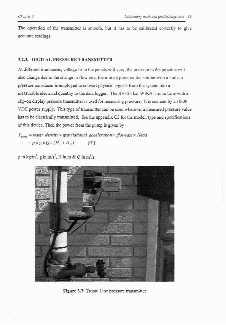
3.2.3. DIGITAL PRESSURE TRANSMITTER
At different irradiances, voltage from the panels will vary, the pressure in the pipeline will
also change due to the change in flow rate, therefore a pressure transmitter with a built-in
pressure transducer is employed to convert physical signals from the system into a
measurable electrical quantity to the data logger. The SI 0-25 bar WIKA Tronic Line with a
clip-on display pressure transmitter is used for measuring pressure. It is sourced by a 10-30
VDC power supply. This type of transmitter can be used wherever a measured pressure value
has to be electrically transmitted. See the appendix C3 for the model, type and specifications
of this device. Then the power from the pump is given by
Pp~p =water density x gravitational acceleration x jlowrate x Head
= pxgxQx(H, +Hd ) [W]
Figure 3.7: Tronic Line pressure transmitter

Chapter 3
3.2.4. ANEMOMETER
Laboratory work and preliminary tests 34
The speed of wind is another variable that needs to be monitored as it has an impact on the
absorption of heat by the panels. The device used for this particular application is an
anemometer. It detects the wind speed as well as the direction of wind. The working
procedure of this device is the as the above devices. The figure below shows the anemometer
used.
Figure 3.8: An anemometer
3.2.5. PYRANOMETER (LI-200SZ)
The LI-200SZ is an instrument for measuring solar radiation received from a whole
hemisphere. It is suitable for measuring global sun plus sky radiation. Solar radiation varies
significantly among geographical regions, season, and time of the day. Often, the most
required measurement is the energy flux density of both direct beam and diffuse sky radiation
passing through a horizontal plane of known unit area (i.e. global sun plus sky radiation).
The LI-COR pyranometer may be handheld or mounted at any required angle; provided that
reflected radiation is not a significant portion of the total. The sensor and the vertical edge of
the diffuser must be kept clean in order to maintain appropriate cosine correction. For
operation, the cable of the LI-200SZ pyranometer sensor is terminated with the two bare
leads of the coaxial cable. This allows the LI-200SZ to be used with the six current channels
of the LI-lOOO Data logger located on the screw down terminals to the 1000-05 terminal
block, and the 1000-06 AC terminal block. The shield of coaxial cable is positive and the
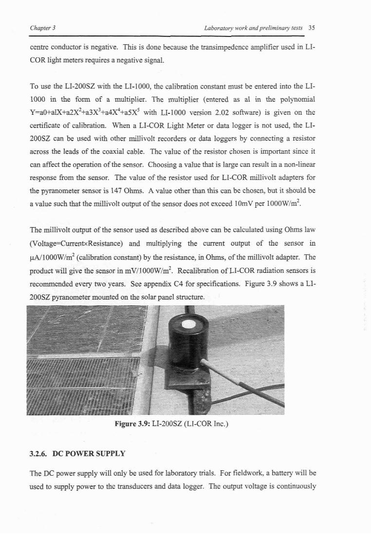
Chapter 3 Laboratory work and preliminary tests 35
centre conductor is negative. This is done because the transimpedence amplifier used in LI
COR light meters requires a negative signal.
To use the LI-200SZ with the LI-lOOO, the calibration constant must be entered into the LI
1000 in the form of a multiplier. The multiplier (entered as al in the polynomial
Y=aO+alX+a2X2+a3X3+a4X4+a5X5 with LI-lOOO version 2.02 software) is given on the
certificate of calibration. When a LI-COR Light Meter or data logger is not used, the LI
200SZ can be used with other millivolt recorders or data loggers by connecting a resistor
across the leads of the coaxial cable. The value of the resistor chosen is important since it
can affect the operation of the sensor. Choosing a value that is large can result in a non-linear
response from the sensor. The value of the resistor used for LI-COR miIlivolt adapters for
the pyranometer sensor is 147 Ohms. A value other than this can be chosen, but it should be
a value such that the millivolt output of the sensor does not exceed IOmV per 1000W/m2•
The millivolt output of the sensor used as descrihed above can be calculated using Ohms law
(Voltage=CurrentxResistance) and multiplying the current output of the sensor in
flAIIOOOW/m2 (calibration constant) by the resistance, in Ohms, of the miIlivolt adapter. The
product will give the sensor in mV/IOOOW/m2• Recalibration ofLI-COR radiation sensors is
recommended every two years. See appendix C4 for specifications. Figure 3.9 shows a LI
200SZ pyranometer mounted on the solar panel structure.
Figure 3.9: LI-200SZ (LI-COR Inc.)
3.2.6. DC POWER SUPPLY
The DC power supply will only be used for laboratory trials. For fieldwork, a battery will be
used to supply power to the transducers and data logger. The output voltage is continuously

Chapter 3 Laboratory work and preliminary tests 36
adjustable between 0 rating voltage in one range by means of a coarse and fine potentiometer,
the load current may have value from 0 rating current and adjusted by means of a coarse and
fine potentiometer. Both outputs can accurately read on voltmeter and ammeter. Both
stability and ripple are extremely good to meet the requirements of modem circuit design.
The unit can be used as either constant voltage or current source. This device is employed to
power a pressure transmitter, flow transmitter and a DATATAKER.
3.2.7. ADAYINlGHTSWITCH
As an experimental trial, the datalogger was set to sample at half hour intervals. Additionally,
the time window of interest is from sunrise to sunset, since this is when the PV system is
operational. A locally designed day/night sensor is used to control the state of the acquisition,
depending on the lighting conditions. Figure 3.10 (a) & (b) below show the internal and
external pictures of a day/night switches respectively.
To sensor in ~g 3.1O(b) Threshold control
Figure 3.10 (a): Internal day/night switch
switch
Figure 3.10 (b): External day/night
The diagram overleaf (figure 3.11) shows the pattern of voltage flow from the panels to the
data logger and motor/pump with necessary resistors and fuses to control the amount of
voltage/current to the data logger.

Chapter 3 Laboratory work andpreliminary tests 37
t-__-,._---1_-n+Vcc (I5VDC)
lOO Oluru;
4... .20mA
+ Ch. 1
- [Currentloop]
~--I-r-_-L~
Ch. 4
[Current]
Ch. 2
[Voltage]
Ch. 3
[Temp]
+
+
+E----~
Pyranometer
Type K Thermocouple
F
lOO Ohms
+Vcc (15VDC)
Flow-rate meter
B
CC
•RI ~ IMOhm Ch. 7+[Voltage]
R2 "" 100 Ohms.E
•RI~IMOhm
+ Ch. 8
[Voltage]R2 ~ 100 Ohms
+Vcc (l5VDC)
..!:::-"~'"---B
0.33 Ohms @25W
SolarPanel
Master
=rJ=:~E0.1 Ohms @ IOW
I---F
D
Figure 3.11: Configuration of transducers connections to the data logger
Once the data logger and Pumpmaster are in operation, they can be subjected to many
conditions that they may not have been designed for. Figure 3.11 illustrates how the
Pumpmaster and the data logger are protected against undesired conditions. These two
devices can be protected against lightning since the panels are a good receiver of lightning.
The data logger is also protected against over-voltage by using the fuse. This fuse will blow
if the panels generate the threshold current that would exceed the expected current. The most

Chapter 3 Laboratory work and preliminary tests 38
effective method to avoid over-voltage damage is by use of an over-voltage crowbar (but it
has not been used in this test).
3.3. PRESENTATION OF RESULTS
The results presented in this section will not be used as a basis to test the reliability of the
system, but to determine the efficiencies of the system and components. The components
referred to here are: solar panels, Pumpmaster and motor/pump unit. Therefore, array power
refers to power generated by the panels, regulator power refers to power to run the pump and
hydraulic power is power delivered by the pump at a certain head. The formulae given below
will be used to calculate the above parameters.
Useful equations
Array input
Power efficiency of any component is given by power out divided by power in. The power
into the array is the product of the irradiance and the area of the array. The area is known and
so ouly the irradiance needs to be measured. The power out is given by the product of the
array voltage and the array current.
P'"adiM" = plane of array irradiance x array area. 2 . 2GmW/m andAmm
= GpOA xA [W]
Array output
P =array current x array voltage= I in Amps and V in Volts
=1= xV= [W]
Converter output
pca" = converter current x converter voltage
= I ca" x Vca" [W]
Power of the converter is the product ofvoltage from the converter and current from theconverter.
Motor/pump output
Pp,mp = water density x gravitational acceleration x flowrate x Head
=pxgxQx(H, +Hd ) [W]
The pump power output is the product ofwater density p (kglm\ gravitational acceleration g
(m1s\ flow rate Q(m3/s), total head H (dynamic head + static head).

Chapter 3
Overall Efficiency
P'7", = P pump x 100 [%]
irradiance
Laboratory work and preliminary tests 39
The overall efficiency of the system is the power out of the system divided by the power into
the system. In this case, power out of the system is given by pump power (Ppump) and power
into the system is given by irradiance power.
System Efficiency
Ppump'7,uhm =--x 100 [%]. P
=
System efficiency is power generated by the pump divided by power generated by the array.
Component Efficiency
pn =~xIOO'Icomp P...
Svstem parameters
[%]
Table 3.3: Measured parameters of the PV pumping system
ABBREVIATIONS UNITS PARAMETERSGpOA W/mL Plane of arrav irradianceI arr A Array currentVarr V Array voltageIcon A Converter currentV ean V Converter voltageQ mj/s Flow rateHs m Static headp kPa Pressure
li<I m Dynamic headTa °C Ambient temperature
All these parameters were interfaced to the data logger. The data logger supports eight
analogue channels and four digital channels. The channels are read continuously and
averages for each channel are computed for each minute. The length of the log period is set
by the user. The information is recorded in the internal memory of the data logger. At the

Chapter 3 Laboratory work andpreliminary tests 40
end of each test or series of tests, this data can then be transferred onto the memory of a
personal computer for analysis.
The efficiencies of some of the components of the system vary with irradiance. So in order to
model the operation of the components accurately it is necessary to get instantaneous
readings rather than readings averaged over half an hour, for example. This is illustrated by
the graph below.
A series ofreadings atchanging irradiance
Average of readings giveserror of about 5%
60 1r--:---:--:-----------------,Actual valueal600 W/m' -----::::::="..~t--.....----<.-.--.....--
0+-.-.~--r-___,--~-~-_.,.._-___,--~___1
300 400 450 500 600 650 700 750 800
Irradiance (W/m2)
Figure 3.12: Hypothetical system efficiency versus irradiance (Gosnell, 1991:69)
The graph shows a hypothetical set of readings for efficiency versus irradiance. As can be.
seen if the readings are averaged a value is found which is well below the actual value of the
efficiency at that time. So it can be deduced that the log period needs to be kept as short as
possible to model the operation of the components accurately.
The experimental results are presented in the section. Data was captured at time intervals of
30 minutes. Relevant manufacturers' pump performance curves are presented in appendix
A3 andA4.

Chapter 3 Laboratory work andpreliminary tests 41
3.3.1. TEMPERATURE VERSUS TIME
The graph below shows a relationship between ambient temperature and time. Medium
temperatures are during the day and therefore would result in medium solar intensities. This
is good for the solar panels to produce electrical energy, but high solar intensities have a
negative impact on production of energy, as increase in the temperature of the PV modules
due to solar heating lowers the PV conversion efficiency (Chandratilleke, 1986:59).
Temperature vs Time25
Day 1 Day 2 Day 3 Day 4 Day 5 Day 620
.....= 15-.......c-S 10...
"'" 5
0
11 :00 11 :00 10-:,0 10:00 10:00 10:00Start time: 07:00 - end time: 18:00 daily
TIme (hrs)
Figure 3.13: Temperature versus time (24/08/04 - 30/08/04)
3.3.2. ARRAY, CONVERTER & PUMP POWER VERSUS TIME
Figure 3.14 overleaf shows the graphical results of power generated by the panels, power to
the pump/converter power and power generated by the pump over a different time of the day.
The graphs show notable variations of array, converter and pump power. The relationship
between array power and converter power is very close and this is because of the efficient
converter. All the three powers drop drastically in the event of cloud cover and when the
levels of irradiances become low. The pump power does not appear to be affected much by
the small fluctuations of the array power except at night when irradiance is zero. This is
because the Pumpmaster draws power at constant voltage for all irradiances and regulates
voltage as required by the system. One would expect to see an increase in pump power as
array power increases and a decrease in pump power as array power decreases. However,
because of the Pumpmaster's operation, this is not necessarily so. The maximum array power
output for this test is 120 W with a corresponding converter power of 118 W at 879 W/m2•
The efficiency of the converter with these results at this time is 97%. The maximum
efficiency of75 W module at 1000 W/m2, with an area of 0.632m2
, is 11.9% (manufacturer).

Chapler3 Laboratory work and preliminary tests 42
From the obtained results, the efficiency of the array was calculated to be 16.3%. This value
seems to be reasonable taking into account the fact that this experiment was conducted in
winter when the levels of irradiance were quite low.
Array, Pump & Converter power vs Time
140 I I I I I I~
oi!:l~ 120 bo.. --,,"I .~ 1 ""'" 1 I I
'., 1 ~I ~I~ 1- 1 I\~ ....Q.~ 100 I I 1 T 1 :rS ~ I I 1 1" Q IDCl. Q. I I I....
60 1 I>,'"co 1:: 1
~... '" 40... .. Day I I Day 2 Day 3 Day 4 I Day 5 Day 6« =Q 20 I IU V V 'U ~ 'U "0
11:00 11:00 10:30 10:00 10:00 10:00lime (24hn)
Stut:07:OOI-Array pl1..~r -Pump (X)wer - Con~rter PJMr rEnd: 18:00
Figure 3.14: Array, pump & converter power versus time (24/08/04 - 30108104)
3.3.3. HEAD VERSUS TIME
The following figure shows a plot of dynamic head with respect to time of the day. Head
varies with the pressure created by the pump. The higher the pressure, the more the head will
mcrease. Here head ranges between 4.8 m and 5.5 In.
Bead vs rune
Day 6
10:0010:00
I Day 5I1
10:00
Thne(24Bn)
Day 3
10:3011:00
Day 2
Start time: 07:00 - end time:: 18:00 daily
5.6 -r--~------,r-----.-----.-----'------'
5.5
5.4
5.3
85.2~
"t:l 5.1co=50
4.9 I
4.8 I4.7 1
14.6 .frmcrrmmnTmT<rrmm-.nTnn~nTIT<rrm,",,",TnT<nTITnTIT<rrmm-.n""":'TmT<rrmTnn=
11:00
Figure 3.15: Head versus time (24/08/04 - 30108104)

Chapter 3 Laboratory l1c-'ork andpreliminary tests 43
3.3.4. FLOW RATE VERSUS TIME
The trend of flow rate versus time is increasing flow with increasing irradiance, viz flow
increases from early moming to around midday, after which flow drops towards sunset. This
is as expected because flow is proportional to incoming energy.
Flow rate vs Time
II Day 3 I Day4
IIII Day 5 Day 6
,I, ,I
10:30 10:00 10:00 10:00Time (24Hrs)
Figure 3.16: Flow rate versus time (24108/04 - 30108/04)
3.3.4. IRRADIANCE POWER VERSUS TIME
Irradiance power is directly proportional to the product of solar radiation (W1m2) and the
surface area of the solar panels. It means that as the irradiance increases, irradiance power
will also increase while the surface area will be constant.
Irradiance power vs Time
Day 6
3000 ~--~--~~--~---~---~--------,
~- 2500..0>:: 20000c:.0> 1500
'"=eo 1000:aeo
500..Day 1..-
10:0010:0010:00
ime (24hrs)
10:3011:00
o-k~""";',.,.,.,.,."""=n":""-~~"";'~~~;"""~~"";',.",,,~rnrrI
11:00
Start time: 07:00 - end time: 18:00 daily
Figure 3.17: Irradiance power versus time (24/08/04 - 30108104)

Chapter 3 Laboratory work and preliminary tests 44
33.6. ARRAY EFFICIENCY VERSUS IRRADIANCE
The array efficiency is dependant on several conditions such as solar irradiance, ambient
temperature, and wind speed. The variables defIning the operating condition are irradiance,
cell temperature, absolute air mass, and solar angle-of-incidence on the array. The maximum
peak DC power (119.5 kW) measured is considerably less than the nominal 224.4 W
nameplate rating of the installed system. There are several reasons - all expected: The power
production performance of the PV modules is fairly dependent on the array temperature. The
higher the panel temperature, the lower the solar to electric conversion efficiency. The
Siemens modules installed experienced a 0.4% drop in their nominal energy conversion
efficiency for each degree centigrade which the arrays are warmer than 25°C.
The obtained maximum effIciency of 16.3% is quite reasonable and this effIciency is likely to
decrease in summer due to higher operating temperature, therefore it is acceptable to
conclude that the modules are effIcient basing that conclusion on the manufacturer's
specifIcations. Heliotronics (2004: 4) also reports that the solar panels can only capture about
10-20% of the energy ID sunlight. Sarkar et al (accessed @
http//fsec.ucf.eduledliasee/isree/sarkar-water.pdf, 22/06/2005) reported an array
(monocrystalline) effIciency of 13%, Hamakwa (1986:415) obtained the maximum array
(Amorphous) efficiency of 6-7 % and Helikson et al (1991:4) reported an array effIciency of
11%.
Array efficiency vs Irradiance18
16~
';t. -----~ 14
~=";:; 12
= /"";;-10/'....
<: 8
6212 337 471 584 658 764 859 900
Irradiance (WIm)
Figure 3.18: Array effIciency versus irradiance (24/08/04 - 30/08/04)

Chapter 3 Laboratory work and preliminary tests 45
3.3.7. CONVERTER EFFICIENCY VERSUS TIME
Converter efficiency is the ratio of power generated by the solar panels and power driving the
pump. The converter is one of the efficient components of the PV water pumping system.
Here the average converter efficiency is 97%. Other researchers such as Helikson et al
(1991:4) reported a converter efficiency of 96%. Sippola et al (2002:2) recorded converter
efficiencies of 83%, 86% and 93% and Makhomo (2001 :40) obtained an efficiency of 88%.
Converter Efficiency vs Time
120 -,---r-,-----"r----,-,---r-,---r-,-----,Day 1 1 Day 2 1 Day 3 1 Day 4 I Day 5 I Day 6
~ 100 1-'...........-l;L..--......._.",Ir-_,.....~1 ;1 .../'11 ~ IJ';:;80 I Y<:'- 1 1 1 1 I~ 1 1 1 1 I.. 60... 1 I I I I1: 1 I I I I1: 40 I 1 1 I I§ 1 1 1 1 I
U 20 1 1 1 1 I1 I I 1 1
10:0010:0010:30 10:00
Time (hrs)
o-J,.,.,~,.".,~~~,""",o=~~""",,~~~,,,.,.,-nmCTfT~~~~,~,,.".",-m
11:00 11:00
Start time: 07:00 ~ end time: 18:00
Figure 3.19: Converter efficiency versus time (24/08/04 - 30/08/04)
3.3.8. PUMP EFFICIENCY VERSUS TIME
The punip efficiency is the ratio between the hydraulic power (pgHQ) and the electrical
power (VI) of the converter. The difference between pump efficiency and system efficiency
here will not be that much due to the high efficiency of the converter (97%). The value of
pump efficiency reflects the efficiencies: dc-de converter, motor and pump. The mean
subsystem efficiency is 15% (motor & pump). This value is below the expected range of 25
- 45% for Mono pumps according to Harnza et al (1995:495). Helikson et al (1991) also
reported a pump efficiency of 44%. If a DC motor efficiency is assumed to be 45% and
mono pump efficiency of 71% according to Hadi (2003:38) then the overall motor/pump
efficiency will be 32%.

Chapter 3 Laboratory work and preliminary tests 46
Pump Efficiency ,"15 TIme
Day 6
10:00
Day 5
10:0010:00
TIme (24hrs)
20 -,---,-----.-------.------,------.----,
1816
~
~ 14.~ 12 ~V'\,""'\
I<: I\~ 10 I
E" 8 :cC 6 I
4 I2 I
o -hn==!n'=~=nITrrm=rrm=~rrm=rrmk=mn=rr\_nTnTrrm=rrni
11:00 11:00 10:30Start time: 07:00 - end time: 18:00 daily
Figure 3.20: Pump efficiency versus time (24/08/04 - 30/08/04)
3.3.9. SYSTEM EFFICIENCY VERSUS TIME
System efficiency is directly proportional to power generated by the pump and inversely
proportional to power generated by the panels. It is clear that system efficiency is dependent
on voltage and current from the panels, system head as well as the flow rate. The maximum
system efficiency obtained was 17%. The most probable cause of this is that the pump was
operating at a low head (about 5m), viz at low heads efficiency is low, but increases with
increasing head (see appendix A4).
Systemll1iciencyvs TIme
Day 6
10:0010:0010:00
TIme(24hrs)
Day 3
10:30
Day 2
11:00
Start time: 07:00 - end time: 18:00 daily
18,---,----,------,,-----,----,.-----,16 Day 1
;., 14
'"~ 12<lE 10
'"e 8'"1;; 6;>,
'" 4
2
Okrrm""""TnTCM"rm-rrrrm""",=rc=rrm-nTn-m-n-rrmc=rrrrrrmTrrn-'-';;TnT~nTrr,.,j
11:00
Figure 3.21: System efficiency versus time (24/08/04 - 30/08/04)

Chapter 3
3.3.10. OVERALL EFFICIENCY VERSUS TIME
Laboratory work andpreliminary tests 47
The overall efficiency of the system is determined by the hydraulic power and power from
the sun (irradiance power). The graph below shows the efficiencies ranging between 0.4%
and 1.8%. The average overall efficiency was obtained to be 1.47%.
~rall £fficiency \5 TIme I2.01
,.,
1.8 Day 1 Day 2 Day 3 Day 4 Day 5 Day 61.6
'"'" lA=I'~ 1.2lE
'"l 1.0;; 0.8...... 0.60
004
0.2
0.011:00 11:00 10:30 10:00 10:00 10:00
Start time: 07:00 - end time: 18:00 daily TIme (hrs)
Figure 3.22: Overall efficiency versus time (24/08/04 - 30/08/04)
3.4. EXPERIMENTAL OBSERVATIONS AND CONCLUSIONS
From the above results, the mean efficiencies of the three subsystems are as follow:
o Array efficiency 16.3%
o System efficiency 15.0%
o Overall efficiency 1.47%
Some of these efficiencies are quite encouraging (especially array efficiencies) considering
the fact that the tests were performed in winter when there are low levels of irradiance. There
were some discrepancies in the results which might have been caused by the operating
conditions of the whole system. These are some of the notable conditions:
• Operating point of pump - As mentioned in section 3.3.9, the pump is not operating at
a reasonable head, with a significant loss in efficiency. If it had been operating at higher
head (5Om for example) as is normal in a borehole pump, pump efficiency would alter to
about 35% (see appendix A4).
• Season - The season will also have an impact on overall results. The temperatures were
very low in the Cape Peninsula on the days on which the experiments were conducted. This
experiment was conducted in late August.

Chapter 3 Laboratory work and preliminary tests 48
There are no valid judgements that can be made at this stage on these short-term results.
Long-term results can enable us to perform valid assessments as to whether this system is
reliable or not, so it is important to have enough data to check if the system is behaving
consistently over a period of time and to obtain information about its performance over the
whole range of irradiance levels. The overall experimental results are quite encouraging and
the progress up to this stage is promising.
It would be important to talk of the accuracy of the data acquisition system (transducers,
interface and data logger) because the accuracy for the transducers and the error sources in
the components of the signal conditioning are available from data sheets. The collected data
though, should be expressed on the basis of uncertainty. The reason for this is that the
calibration of the data acquisition system is not based on the comparison to known values, but
is compared to other measuring devices that have a particular accuracy.
However, the overall experiment was carried out quite successfully despite some problems
encountered during the process. The lessonslknowledge learned out of this work will be of
great importance when applying this information to the actual site. The next logical step is to
develop the same experiment to the actual site.
The next chapter presents the fieldwork on two villages namely Lepelsfontein and
Rooifontein. The results of the two villages will be for comparative purposes and
determination of life cycle costs of the competing systems (PV and diesel pumping). More
attention will be on the results that have been collected for a long time (two years for
example).
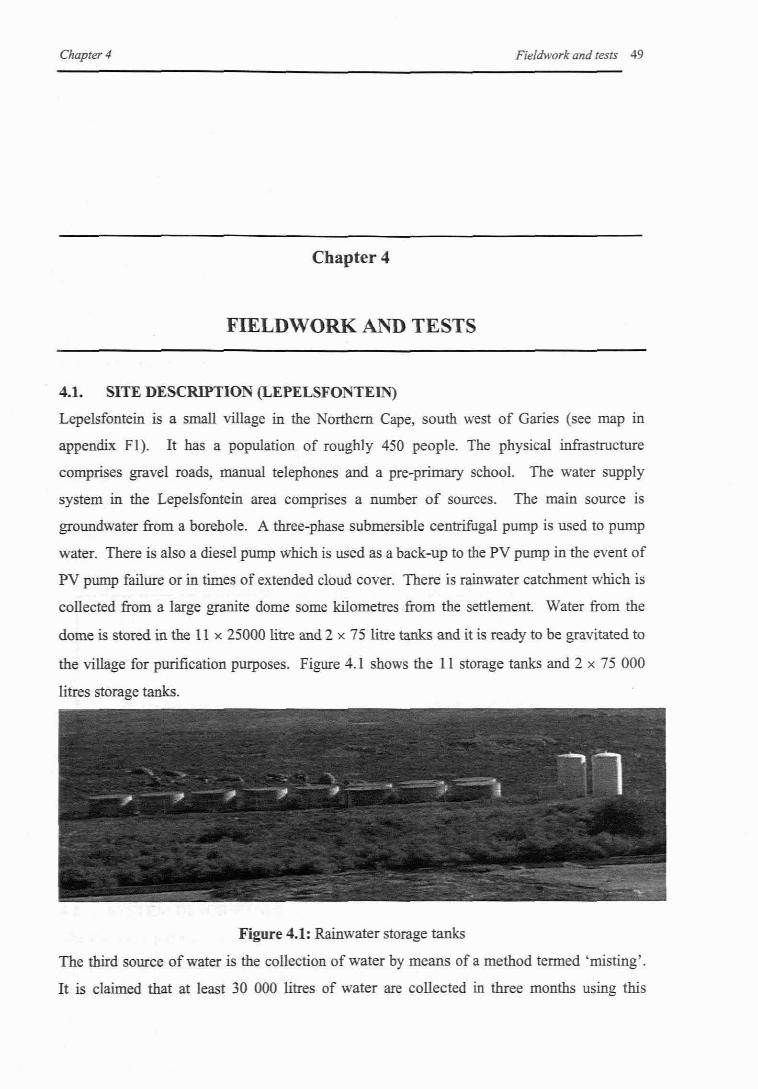
Chaprer4
Cbapter4
FIELDWORK AND TESTS
Fieldwork and tests 49
4.1. SITE DESCRIPTION (LEPELSFONTEIN)
Lepelsfontein is a small village in the Northern Cape, south west of Garies (see map in
appendix Fl). It has a population of roughly 450 people. The physical infrastructure
comprises gravel roads, manual telephones and a pre-primary school. The water supply
system in the Lepelsfontein area comprises a number of sources. The main source is
groundwater from a borehole. A three-phase submersible centrifugal pump is used to pump
water. There is also a diesel pump which is used as a back-up to the PV pump in the event of
PV pump failure or in times of extended cloud cover. There is rainwater catchment which is
collected from a large granite dome some kilometres from the settlement. Water from the
dome is stored in the II x 25000 litre and 2 x 75 litre tanks and it is ready to be gravitated to
the village for purification purposes. Figure 4.1 shows the II storage tanks and 2 x 75 000
litres storage tanks.
Figure 4.1: Rainwater storage tanks
The third source of water is the collection of water by means of a method termed 'misting'.
It is claimed that at least 30 000 litres of water are collected in three months using this

Chapter 4 Fieldwork and tests 50
method. The latter was an experimental system, but has become non-functional due to
breakage of the net and collection gutters.
The PV system is situated about 2 km to the south west of Lepelsfontein village. The PV
pump operates seven days a week. A diesel pump becomes operational only when the PV
pump does not work (when it is faulty or being maintained or extended cloud cover). Water
is pumped to 2 storage tanks located in the village. Each storage tank has a capacity of 30
000 litres. Water from storage tanks is gravitated to a diesel pump located at about 300 m
down the hill. The purirying/desalinating chemicals are added before water is pumped to the
supply tanks. Water has to be desalinated as it is claimed that the sea, which is about 10 km
to the south east of the settlement, affects the quality of underground water and therefore it is
not readily available for consumption. A total dissolved solids content of around 1380 mg/l
was measured in 2001 (Toens & Vennote, 2001: 59).
There are four supply tanks of 10 000 litres each located at about 400 m from the diesel pump
house uphill. Water from the supply tank is gravitated to the village and is accessed through
standpipes. Figure 4.2 below shows a line diagram of water flow from the pump to the end
user.
PV water pump
Supply tanks
IStandpipes
Stora~e tanks
I---------- Diesel pump (desalination)
Figure 4.2: Water flow diagram from the pump to the end user
4.2. SYSTEM DESCRIPTION
The PV water pumping set-up at Lepelsfontein comprises three subsystems namely, a set of
PV panels, an inverter and a three phase-centrifugal pump. Table 4.1 below illustrates
comparisons between the PV system installed at CPUT and Lepelsfontein system.

Chapter 4
Table 4.1: Comparisons between CPUT and Lepelsfontein PV systems
Fieldwork and tests 51
CPUT Lepelsfontein
Array size 225Wp 1.72 kWp
Converter/inverter Converter (DC/DC) Inverter (DC/AC)
Pnmp DC submersible mono pump AC centrifugal pump
4.2.1. SOLAR PANELS
There are two sets of solar panels used to power a three phase centrifugal pump located about
IO m away from the pump. A first set ofpanels consists of 20 panels manufactured by Liselo
Solar. The second set of panels consists of 4 Helios Power panels all connected in series.
Table 4.2 below shows the specifications of the two sets of solar panels. Figure 4.3 overleaf
shows the field configuration of two sets of solar panels.
Table 4.2: Specifications of He1ios and Liselo solar panels at Lepelsfontein (detailed
specifications in appendix B1 & B2 respectively).
•• Liselo Solar
Peak Volts (V) Peak Amps (A) Watts (W) Size (cm) Guarantee (years)
17.28 4.4 75 1215(L)x540(W)x60(D) 20
Hellos Power
Peak Volts (V) Peak Amps (A) Watts (W) Size (cm) Guarantee (years)
16.66 3 55 750(L) x 524(W) x 34(D) 25

Chaprer4 Fieldwork and tests 52
Figure 4.3: Sets of Liselo and HeIios PV panels
4.2.2. THE GRUNDFOS DClAC INVERTER
Inverters are used to transform DC power into three-phase AC power. This three-phase
inverter is developed by Grundfos. The model of this inverter is Solartronic SA 1500. The
specifications of the inverter are available in appendix B3.
Figure 4.4: Grundfos inverter
4.2.3. PUMP
An SP2A-I3 Grundfos centrifugal pump was used for pumping water. The design flow rate
ranges between 0.2-2 m3fh, total head of 52 m, maximum current 2.35 A, maxinJUm power

Chapter 4 Fieldwork and tests 53
0.55 kW and voltage ranging between 3x380 - 400 - 415 V. The pump curve can be seen in
appendix 84.
43. ROOIFONTEIN
Rooifontein is located 90 km southeast of Springbok (see map in appendix F3), roughly 2 km
south of Kamassies and has automatic exchange telephones, a primary school and two shops.
The population is approximately 550 people in 100 households. The main forms of economic
activity are limited to employment in the Provincial Roads Department, migrant labour at
Kleinsee diamond mine and livestock farming.
Until the mid 1980's, the community of Rooifontein was dependant on a wind pump
extracting water from the dry Buffelsrivier riverbed. Later two diesel powered water pumps
were replaced in 1993 by a Lister genset installation which is currently in operation. Water is
sourced from a caisson well in the dry riverbed. All the households have standpipes. The
geographic location of the abstraction point is N 30°06'57.1", E 018°28'73.4", latitude
30.6571 and longitude 18.28734. Figures 4.5 (a) & (b) show a Rooifontein diesel engine and
pump inside a borehole respectively.
•• I· " .
/n/~1
Figure 4.5(a): Diesel engine Figure 4.5(b): Pump inside borehole
4.4. TELEMETRY HARDWARE AND CONFIGURAnON
Cellular phone data transmission is the most common and preferred means of transmitting
information from one point to another. The cellular phone system makes it possible to
interrogate a data logger and remote telemetry unit (RTU) when no telephone line is available
at the site. Figure 4.6 overleaf shows the configuration of the cellular phone telemetry setup
that is used in Lepelsfontein for data acquisition. The use of satellite for data transmission
was initially considered but it seemed to be too costly and LEO satellite communication was

Chapter 4 Fieldwork and tests 54
found to be unreliable with a high monthly subscription. The latter will be revisited when
more sites are monitored as the project develops over the next 5 years.
The information from the site will be transmitted by means of a set of modems which are in
series and are intenaced to the RS232 port of a data logger. The information from the data
logger is transmitted to the HF modem by means of RS232 intenace. An antenna from the
HF modem transmits the signals to another antenna which is connnected to the HF modem
located some distance uphill. The HF modem is intenaced to a GSM by means of RS232.
An antenna is ready to transmit the information to another GSM modem which is on the
receiving station at CPUTo Then this GSM modem is intenaced to a computer. Information
from the computer can be accessed by means of a LABVIEW program and the user sets the
length of logging and transmission.
i GSMModem
Stage 2
RS23
TD A Nl;ll\llTTTTNr:'.
Stage I
RS23
I Data !ol!l!er I
I-----------------------------------------~-------------------------------------------------, :,,,,GSM :
,,,,,,,,,,,,,,,,,, ', '_____________________________________________________________________ ; 1
Stage 3
; ••••~••••••••• _ •• _._ ••• ·0•••••••••••••••••••••••_ •••••• 0 •••••• _ ••••••••• ·'_0
: . <.GSM RECEIVINGI • Computer
f ~ GSMModem RS23 • [QI =1
Figure 4.6: Telemetry system configuration
4.4.1. FLOW AND PRESSURE TRANSMITTERS
NOTE: Some ofthe data acquisition devices used for experimental tests were also used/or
field tests therefore the applications and descriptions of those devices are the same. Those
descriptions will be the same as in section 3.2.

Chapter 4 Fieldwork and tests 55
Figure 4.7 below shows the set-up of digital flow and pressure transmitters in the pipeline at
Lepelsfontein PV water pumping station. The two transmitters have built-in transducers that
measure and convert mechanical quantities into readable electrical quantities. The data from
the two transmitters is transmitted to a data logger for storage and analysis purposes. A 12
VDC battery sources both transmitters. The flow transmitter model used in this experiment is
8032 brass INLINE manufactured by Burkert Easy Fluid Control Systems. The diameter
of the transmitter is 50 mm and the output signal is 4 - 20 mA. The S10-25 bar WIKA Tronic
Line pressure transmitter is the model used to measure pressure. The output signal of the
pressure transmitter is 4 - 20 mA.
Figure 4.7: Flow and pressure transmitters
4.4.2. PYRANOMETER
The LI-200SZ pyranometer is an instrument used for measuring solar radiation received from
a whole hemisphere. It is mounted onto a solar panel structure in such a way that the trees
and other objects cannot obstruct it. To use the LI-200SZ with the LI-IOOO, the calibration
constant must be entered into the LI-I 000 in the form of a multiplier. The multiplier (entered
as al in the polynomial. Y=aO+alX+a2X2+a3X3+a4x4+a5X5 with LI-IOOO version 2.02
software) is given on the certificate of calibration.
When a LI-COR Light Meter or data logger is not used, the LI-200SZ can be used with other
millivolt recorders or data loggers by connecting a resistor across the leads of the coaxial
cable. The value of the resistor chosen is important since it can affect the operation of the
sensor. Choosing a value that is large can result in a non-linear response from the sensor.
The value of the resistor used for LI-eOR millivolt adapters for pyranometer sensor is 147

Chapter 4 Fieldwork and tests 56
Ohms. A value other than this can be chosen, but it should be a value such that the millivolt
output of the sensor does not exceed IOmV per IOOOW1m2 The millivolt output of the sensor
used as described above can be calculated using Ohms law CVoltage=CurrentxResistance)
and multiplying the current output of the sensor in J.1A/1000W/m2 (calibration constant) by
the resistance, in Ohms, of the millivolt adapter. The product will give the sensor in
mV/1OOOW/m2• Recalibration ofLI-COR radiation sensors is recommended every two years.
See appendix C4 for specifications.
Figure 4.8: A pyranometer
4.43. SOLAR PANEL
A solar panel shown in figure 4.9 overleaf is used to charge a 12 VDC battery, which is used
to supply voltage to flow, and pressure transmitters, data logger and an HF modem. The
voltage from the solar panel is regulated by a charge controller to prevent overcharging of a
battery. The specifications of this solar panel are shown in table 4.3 below.
Table 43: Specifications ofWA Siemens module
Warranty Years Item Watts Peak Amps Peak volts Size (mm)
25 SP-75 75 4.4 17 1200x527x34

Chapter 4 FieldwQrk and tests 57
Figure 4.9: A solar panel
4.4.4. DATA LOGGER
The signals from the sensors are transferred by wire, to an instrument which conditions,
amplifies, measures, scales, processes, displays and stores the sensor signals. This is the Data
Acquisition instrument (data logger). It takes instantaneous measurements, stores
measurements and then feeds these to a laptop or a computer, but in this case it sends data to
an HF modem (Aerocomm Data Transceiver). The captured information assists in
determining;
• Efficiency of the system
• Performance of the system
• Reliability of the system
The model used in this demonstration is DATATAKER 605. The specifications of this
device are in appendix Cl.
Figure 4.10: Adata logger and a charge controller
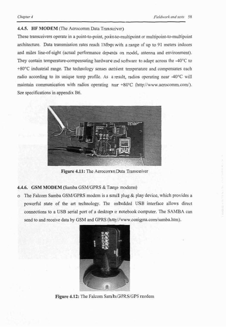
Chapter 4 Fieldwork and tests 58
4.4.5. HF MODEM (The Aerocomm Data TraI1SCeiver)
These transceivers operate in a point-to-point, point-to-multipoint or multipoint-to-multipoint
architecture. Data transmission rates reach IMbps with a range of up to 9I meters indoors
and miles line-of-sight (actual performance depends on model, antenna and environment).
They contain temperature-compensating hardware and software to adapt across the -40°C to
+80°C industrial range. The technology senses ambient temperature and compensates each
radio according to its unique temp profile. As a result, radios operating near -40°C will
maintain communication with radios operating near +80°C (http://www.aerocomm.com/).
See specifications in appendix B6.
Figure 4.11: The AerocoIIllD Data Transceiver
4.4.6. GSM MODEM (Samba GSMlGPRS & Tango modems)
o The Falcom Samba GSMlGPRS modem is a SlIla!l plug & play device, which provides a
powerful state of the art technology. The embedded USE interface allows d,irect
connections to a USB serial port of a desktop or notebook computer. The SAMBA can
send to and receive data by GSM and GPRS (I1ttpJ/www.conigma.comlsarnba.htm).
Figure 4.12: The Falcom SamllaGPRS/GPS modem

Chapter 4 Fieldwork and tests 59
o The FALCOM TANGO is a plug & play Dual Band GSMlGPRS device for direct and
easy connection to any terminal equipment that is able to handle attention-eommands
(AT) for modem control. The TANGO concept offers two RS232 interfaces, audio
interface, car voltage range power supply (http://wwwJalcom.de/txt-produkte-tango
k.html).
Antenna
9 pin serial port
!
Figure 4.13(a): Tango modem
DC powerSupply
Figure 4.13(b): Tango with antenna
Figure 4.14: An actual telemetry set-up

Chapter 4 Fieldwork and tests 60
Figure 4.14 shows a picture of a transmitting station located about 200 m away from the
Lepelsfontein water pump station. The coordinates of the water pump station are: S
31°01'50.9", EOI7°51'50.8" with an elevation of 192 m. The coordinates of the
transmitting station are: S 31°01'49.2", E 017"51'44.0" with an elevation of 234 m. The
figure shows two antennas fixed adjacent to the solar panel. The RF antenna faces the
direction of the PV station, receiving information from a transmitting RF antenna connected
to the RF modem which is interfaced to the data logger. The other antenna is a GSM antenna
facing in another direction to the RF antenna. This antenna is transmits the information from
the GSM modem to the nearest Vodacom (GSM service provider) transmitting service
station. The white box underneath the solar panel has enclosed the two modems (RF &
GSM). A solar panel is used to charge a 12V battery which will in turn supply power to the
two modems. A charge controller has been used to regulate voltage from the solar panel to
the battery. A battery is enclosed in the black cage shown in the picture. Figure 4.15 below
shows an RF antenna at the pump station and it faces in the direction of RF antenna shown in
figure 4.14.
Figure 4.15: A transmitting RF antenoa at the pump station
This cellular telemetry system that has been put in place seemed to be working well even
though the security of the whole equipment remain a matter of concern. It is however, very
unlikely that the equipment can be vandalised considering the distance between the village
and the pump station. The involvement of the community in this kind of project can be
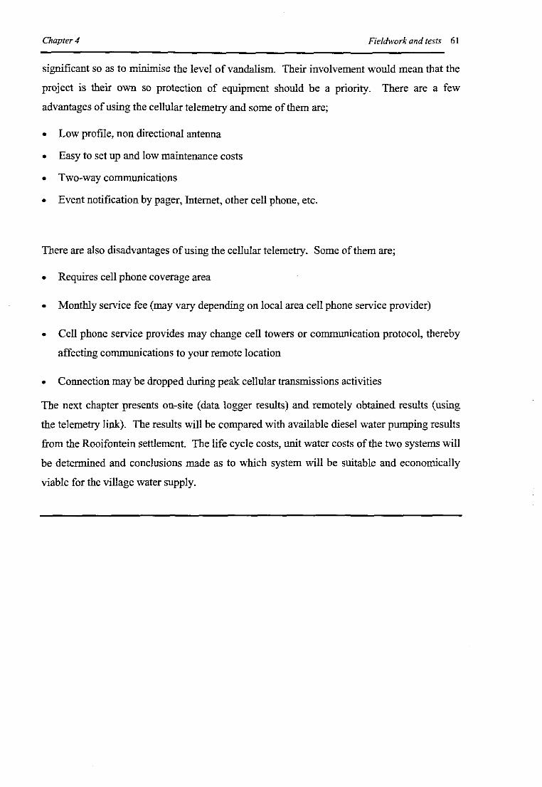
Chapter 4 Fieldwork and tests 61
significant so as to minimise the level of vandalism. Their involvement would mean that the
project is their own so protection of equipment should be a priority. There are a few
advantages ofusing the cellular telemetry and some of them are;
• Low profile, non directional antenna
• Easy to set up and low maintenance costs
• Two-way communications
• Event notification by pager, Internet, other cell phone, etc.
There are also disadvantages ofusing the cellular telemetry. Some of them are;
• Requires cell phone coverage area
• Monthly service fee (may vary depending on local area cell phone service provider)
• Cell phone service provides may change cell towers or communication protocol, thereby
affecting communications to your remote location
• Connection may be dropped during peak cellular transmissions activities
The next chapter presents on-site (data logger results) and remotely obtained results (using
the telemetry link). The results will be compared with available diesel water pumping results
from the Rooifontein settlement. The life cycle costs, unit water costs of the two systems will
be determined and conclusions made as to which system will be suitable and economically
viable for the village water supply.
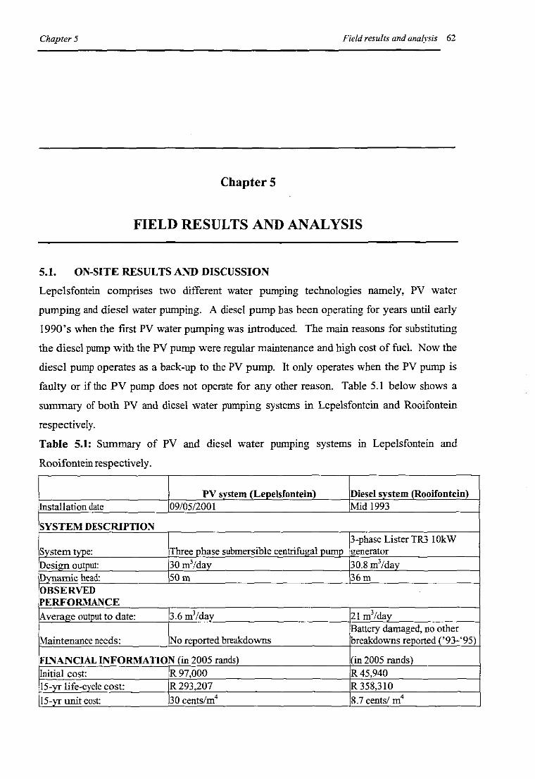
Chapter 5 Field results and analysis 62
ChapterS
FIELD RESULTS AND ANALYSIS
5.1. ON-SITE RESULTS AND DISCUSSION
Lepelsfontein comprises two different water pumping technologies namely, PV water
pumping and diesel water pumping. A diesel pump has been operating for years until early
1990's when the first PV water pumping was introduced. The main reasons for substituting
the diesel pump with the PV pump were regular maintenance and high cost of fuel. Now the
diesel pump operates as a back-up to the PV pump. It only operates when the PV pump is
faulty or if the PV pump does not operate for any other reason. Table 5.1 below shows a
summary of both PV and diesel water pumping systems in Lepelsfontein and Rooifontein
respectively.
Table 5.1: Summary of PV and diesel water pumpmg systems m Lepelsfontein and
Rooifontein respectively.
PV system (Lepelsfontein) Diesel sYstem (Rooifontein)Installation date 09/05/2001 Mid 1993
SYSTEM DESCRIPTION3-phase Lister TR3 IOkW
Svstem type: Three phase submersible centrifugal PumP o-enerator
Design output: 30 m3/dav 30.8 m3/davDynamic head: 50m 36mOBSERVEDPERFORMANCEAverage output to date: 3.6 m3/dav 21 m3/dav
Battery damaged, no otherMaintenance needs: No reported breakdowns breakdowns reported ('93-'95)
FINANCIAL INFORMATION (in 2005 rands) (in 2005 rands)Initial cost: R97,000 R45,94015-yr life-cycle cost: R293,207 R358,31O15-vr unit cost: 30 cents/m4 8.7 cents/ rn'

Chapter 5 Field results and analysis 63
Table 5.2: Data sheet of Lepelsfontein settlement.
Borehole mformation
DATA SHEET: LEPELSFOl'.'TEIN .
Descriotion of settlement and services Other senicesPopulation: 450 persons Few telenhonesEconomic activities: farming Pre-primary school
No electricitvWater supply: Ground water from boreholes 1 shop
[Mobile clinic (every two weeks)
Water uses: domestic
Storage: 4 storage tanks of 10 000 litres each
SOLAR WATER PUMPTechnical descriptionInstallation date: 9/5/2001Dynamic head: 50mDescription: Three-ohase submersible centrifugal oumnSpecifications: 1.72 kWn arrav (20x75Wn and 4x55Wn)
DCIAC inverterSolartronic SA 1500
Design performance: 30 m3/dayOhserved performance: 3.6 m3/dayMaximum output to date 12.1 m3/dav (May 2001)
Total output to end '04 5184m3
Average output to end '04: 3.6 m3/dayMaintenance: No maintenance recordedAvailability of data:Flow data actual - formal records availableSystem installed recently, so limited operation and maintenance informationComments:As the diesel pump has mainly been used as a backup, it is difficult to compare it with pumpingsystems which operate full-time, and costs are likely to be higher for this system.Coordinates:
Depth ofborehole:
Pump depth:
S 31°01'49.2", E 017°51'44.0"
146m
112m
Water level in the borehole: 35 m
Borehole yield: 4.2 Vs
The graph shown in figure 5.1 (p. 65) shows the five-year results from Rooifontein diesel
pumping system (lan '95 - Sep '01). The information provided in this report, for
Rooifontein in particular, includes the following parameters; amount of rain for each month

Chapter 5 Field results and analysis 64
(mm), water pumped per month (kl), average water level and water consumption
(I/person/day). The summary of the annual average results of Rooifontein diesel water
pumping are shown in table 5.3 below. The results show an average rainfall of 1.6 cm in
1997, with corresponding average pumped volume of 918 m3, average borehole water level
of -7.47 m and the consumption of 56 I/person/day. This increase in water consumption can
be caused by various reasons such as the amount of rainfall in that particular year, amount of
water pumped, the level of water in the borehole or the increased population in that year
(Toens & Vennote, 2001). See appendix El for more results.
Table 5.3: Summary ofresults ofRooifontein diesel water pumping (Jan '95 - Sep '01)
Rooifontein Borehole Information.
Year Average Average Annual Average Annual Average Annual
Annual Water pumped (Id) Water level (m) Consumption (IIper/day)
Rainfall (cm)
'95 1.3 904 -12.57 55
'96 1.5 870 -10.65 54
'97 1.6 918 -7.47 56
'98 0.3 940 -6.86 57.9
'99 1.05 843 -6.96 51.9
'00 0.96 954 -7.43 58.7
'01 1.3 1024 -8.44 63.11
The following discussions are based on figure 5.1 overleaf:
o Volume of water pumped - The graph shows inconsistent volume ofwater pumped for a
three-year period with notably high volumes in summer. The maximum volume recorded is
inDec '95 and is 1480m3•
o Water consumption - The graph of water consumption (I/person/day) behaves fairly
consistently for the three-year trial. One can also notice a slightly higher consumption in
summer. This might be as a result of lack of rain during that period as can be seen from the
graph. The population of Rooifontein at the time of data collection is not given but the
average consumption of each person per day is calculated to be 55 I/per/day in '95, 54
I/per/day in '96 and 56 I/per/day in '97. In September 2001, the consumption was 63
I/per/day.
o Rainfall - The purpose of showing rainfall figures here is to show how water
consumption behaves with respect to rainfall. It is evident from the graph that water

Chapter 5 Field results and anaZvsis 65
consumption is high in periods of no rain. The graph does not clearly show the relationship
between water consumption and amount of rain.
D Level of water in the borehole - The level of borehole water is seen to be decreasing as
time goes on. This graph behaves inconsistently for the whole trial period. One can observe
that the amount of rain has a little impact on the level of water in the borehole. One might
expect to see a similar trend of water level graph and the volume of water pumped, but it is
not the case in this illustration. There is no observable relationship between level of water in
the borehole and other parameters explained above.
Rooifontein Diesel Pnmp Data
."-10 1i-<:•-15 ~
-20
Months Jan '95 - Se '01
·IRainfall--Consurnption Waterlevel
Figure 5.1: Rooifontein diesel pump data Jan '95 - Sep '01 (Toens & Vennote RK,
2001:42)
The main difference between Lepelsfontein PV water pumping system and Rooifontein diesel
water pumping system is that the output of the latter is higher than the former. This can be
seen in annual average volumes from table 5.3 and 5.4. The annual average volume of water
pumped in Lepelsfontein ranges between 94 and 169 m3 while Rooifontein recorded average
values ranging between 904 and 918 m3• There are no previous records on water
consumption for the Lepelsfontein system, except for real data since the monitoring system
has been in place (Dec, 2004 onwards).

Chapter 5 Field results and analysis 66
Table 5.4: Summary of annual results ofLepelsfontein PV water pumping (Jan '95 -Sep '01)
Lepelsfontein Borehole Information
Year Average Average Water Average AverageRainfall (cm) pumped(kl) Water level (m) Consumption (lIper/day)
'95 2 169 -35.59 No records
'96 1.9 169 -35.99 No records'97 1.5 94 -36.28 No records'98 0.3 940 -32.97 No records'99 1.4 318 -34.19 No records'00 1.2 210 -34.92 No records'01 2.1 196 -35.26 No records
The followmg diSCUSSIOns are based on figure 5.2 below
o Volume of water pumped - The maximum volume of water recorded in September '95
is 260 m3• April and May '97 do not have records on amount of water pumped. The reason
for this is not known, but one might think the readings were not recorded or the pump was
not in operation.
o Water consumption - There are no records made in Lepelsfontein in this trial period.
o Rainfall - There are seven months in three years when there was no rain at all. The
graph does not show any relationship between rainfall and other parameters.
o Level of water in the borehole - The graph of borehole water level behaves fairly
consistently over this assessment period. Water level is ranging between -34 and -37 m with
no sudden drop/increase observed.
Lepelfootein Solar Pump Data (Jao '95 - Sep '01)
_rainfall_waterpumped --waterlevel
Figure 5.2: Lepelsfontein solar pump data Jan '95 - Sep '01 (Toens & Vennote B.K,
2001:58)

Chapter 5 Field results and analysis 67
5.2. REMOTE MONITORING EXPERIENCES & RESULTS
To prove the reliability and validity of data from the system, acquired data was compared to
data from the Aquimon database and the overlapping of data was about 97%. The difference
here was that the data logger could not give accurate data when a particular variable was
zero. For example, when the flow rate or solar radiation was zero, the data logger recorded a
negative value which cannot be true, as flow rate cannot be negative. Despite this problem,
there were no other operational problems encountered during the monitoring period.
The results presented in this section are obtained from Lepelsfontein PV water pumping
system. The data logger captured the information from the 03112/04 to 02/02/05. The results
shown below are the results captured only when the pump was in operation. The results
captured at night and when the pump was not in operation were omitted. The print screen
shown in figure 5.3 below shows the format ofresults downJoaded from the computer. These
results were then changed to spreadsheet format to produce the graphs that fol1ow. The first
numbers (512751600) in the highlighted area represent time, the second (28.729) data logger
internal temperature, the third (4.2731) flow rate in mi11iamps, the fourth (4.8275) pressure in
mi11iamps, the fifth (25.483) ambient temperature, the sixth (2.8682) irradiance (multiplying
factor is 200), seventh (1.1407) voltage from the solar panels (multiplying factor is 101) and
the eighth (1.5571) is shunt voltage.
ATOKATOKATS01000
OKATD<07265S8S39>
NO C.!.lUUE3ATD<0726SS6S3~;>
CCEN;;;CT 9600E~a~S13D85668,12:w~hannellist error w:E,O,S1303S568,iO;-command errorw ;
D,O,S130S567~,O:I,O,42~79: [~eqnesced ~he t1me - 11:1~am]
n a 513085685 O:!O 5938: r '~9ted ~he date - 05 A ril 2005D,O,512751fiOo,1;A,a,28.72914.2731,~.8275,ZS.433,2.8682,1.1407,1.5571:
DrO,512755200,~:AsO,JO.Z~7,4.608J,5.Z863zZ6.608,~.ZS3~,l.Z2Z1,Z.2533:
D,O,51275S600,1:A,O,32.004,4.4670,4.S9S1,26.862,3.2437.1.2071,1.7618:D,-.O"_51276?!lOQ,, t:A..o 0,31,'•.12,6,,:'1 "4030, 4,,2,2,SlI'Z5 .. 911.l1 ..98601' 1. ZS27l 0 .. 99100:_>
Figure 5.3: Screen print ofresults downJoaded from the data logger

Chopter5 Field results and analysis 68
5.2.1. ARRAY & PUMP POWER VERSUS TIM:E
The figure below shows an array and hydraulic power with respect to time. The relationship
between the two graphs is clearly seen here. The increase in array power results in increase
in hydraulic power. This is because higher irradiance generates more power and that power
increases the amount of water pumped
16:00
--Array power --Pumppower I16:00 16:00 16:00 16:00 16:00
Time (hrs)
lOO
50
O-h,.~~~~"""':'~~~;"""'~""""';~~~"';"'~~~
07:00
Start 07:00End: 18:00
400
t 350~
8. 300c.. 250e~
= ~200l'-o_
all 150>.......«
Figure 5.4: Array & pump power versus time (07/12/2004 - 13/12/2004)
5.2.2. TEl\IPERATURE VERSUS TIM:E
The following plot indicates ambient temperature over the monitoring period of six days.
16:0016:0016:0016:0016:0016:00
Temperature vs Time..............•-._ - _.... , ,...•....- ,..Day I , Day2 ,Day3 ,Day4 ,Day5 , Day6 ,
, , '~1 ,
, t/:~. r--!I, I ,V I, , , I, , , ,, I , ,, I I ,, I I ,
45
40
35f 30=f 25..c.. 20e~ 15
10
5
O+rrTTT~""'~~A.rrnCTTT,J,.,.TTTTTTrrf,TTT~""h-rCTTOTTT"'O""
07:00
Start time: 07:00 - end time: 18:00 daily Time (hrs)
Figure 5.5: Temperature versus time (07/12/2004 - 13/12/2004)

ChapleT 5 Field results and analysis 68
5.2.1. ARRAY & PUMP POWER VERSUS TIME
The figure below shows an array and hydraulic power with respect to time. The relationship
between the two graphs is clearly seen here. The increase in array power results in increase
in hydraulic power. This is because higher irradiance generates more power and that power
increases the amount of water pumped
Array & Pump power vs Time
16:00
Day 6Day 5Day 3 ,Day 4,IIIIIII
--Arraypo_. --Pumppo_r I
I Day2I,,,,I
16:00 16:00 16:00 16:00 16:00Time (Ius)
4OO-r----.,----.,---r----,.------,---,---,t 350 Day 1
~ 3000.0. 250S~
= ~200""-0Cl 150»:: 100
~ 50 i_---.L----.':..--.......,'1oj:..---.!.......--....\J~~- .....:!...O.j..,..,.~crr:~~.......:.~~~~~,.......;~~~,..:,..,~~~
07:00
Start: 07:00End: 18:00
Figure 5.4: Array & pump power versus time (07/12/2004 - 13/12/2004)
5.2.2. TEMPERATURE VERSUS TIME
The following plot indicates ambient temperature over the monitoring period of six days.
Temperature vs Time
16:0016:0016:00 16:00
Time (hrs)
16:00
45 ~--......----.------....----.-------r-----,--;40 Day I
35
30
25
20
15
10
5
O-h-~~..-A-~~~.\-,...,~~-.'n~~~k~~...,.4~~~-.Jr....,
07:00 16:00
Start time: 07:00 - cnd time: 18:00 daily
~B......0.S.....
Figure 5.5: Temperature versus time (07/12/2004 - 13/12/2004)

Chapter 5
5.2.3. ARRAY EFFICIENCY VERSUS IRRADIANCE
Field results and analysis 69
Efficiency of an array is the amount of solar energy the module can convert into electrical
energy. Figure 5.6 below shows the efficiency of the array at different times of the trial
period. The array efficiency is dependant on several factors such as; time of day, weather
conditions, wind speed, and irradiance as well as the temperature of the array. The maximum
array efficiency obtained was 3.9%. The obtained efficiency of 3.0% is quite low and the
discrepancy of the results at high solar intensities is in part attributed to the temperature
effects of solar cells at elevated cell temperatures. These high temperatures increase the
irradiance power thus having a negative impact on array power generation. Another major
factor which may affect the efficiency of the array, is the motor/pump efficiency. If the
motor/pump draws a certain power (IxV) to pump water, even if the array can generate more
power, the motor/pump will only draw the required power. This concept brings into play the
question of system matching. It is either that the system is oversized or the pump itself is
faulty. If the assumed optimum efficiency point of the pump is considered, the expected
array efficiency of 52% can be taken, which will affect the overall system efficiency
proportionately. At the operating condition of 2.6 m3/day, the efficiency is as low as 15%
(see appendix B5).
Array efficiency vs Irradiance
3.4~
~ 3.2 ---- -----.....,;;., 3
./'"='" 2.8
/'""<j.-0::: 2.6
/''";;.,eo: 2.4/'....
2.2-<: /2
320 417 513 618 708 868 905 976 1004 1023 1037 1053
Irradiance C\Vlm2)
Figure 5.6: Array efficiency versus irradiance (07/12/2004 - 13/12/2004)

Chapter 5 Field results and analysis 70
5.2.4. SYSTEM EFFICIENCY VERSUS TIME
System efficiency is directly proportional to power generated by the pump and inversely
proportional to power generated by the panels. It is clear that system efficiency is dependent
on voltage and current from the panels, system head as well as the flow rate. An average
system efficiency of a 6-day trial has been calculated to be 32%. This value can be
acceptable considering the fact that the pump head is 50m and Hamza et at (1995:495)
reports a system efficiency of 30% and 36% of two villages using Grundfos centrifugal
pumps. It is evident that the system efficiency increases or decreases at the same time with
system head and flow.
System Efficiency vs Time
16:00 16:00
Day 5 Day 6Day 4
16:00 16:00
Time (24hrs)
I Day3
16:00
I Day2
16:00Start time: 07:00 -end time: 18:00 daily
80 -,----,----,----.----.,---....--...."~ 70 Day 1~';: 60...§ 50
";;;is 40... 30
E20I'"tllO
O+n-rr;.,...,..,.,..,..,.,...,..,-rr;,..,.,.,...,..,-rr;-rr-,.,.....~-rr-",..n-rMTMTcrl-,..,.,.,.,..,..r;.,.J\-M
07:00
Figure 5.7: System efficiency versus time (07!l2/2004 - 13/12/2004)
5.2.5. OVERALL EFFICIENCY VERSUS TIME
The overall efficiency of the system is detennined by the power delivered by the pump and
power from the sun (irradiance power). The graph overleaf shows the efficiencies ranging to
a maximum of 3.2%, which is acceptable when one considers an overall system efficiency of
3% and 4% from the Intermediate Technology Development Group manual, (Accessed @
http://www.itdg.org/docs/technical information servicefsolar pv wateroumps.pdf,
page 6, 24/05/2005).

Chapter 5 Field results and analysis 7l
Overall Efficiency vs Time
16:0016:0016:00 16:00
Time (24hrs)
16:0016:00
Start time: 07:00 - end time: 18:00 daily
3.0,----"----,,,----..--,---..--.---..--,--,,-,~ Day I ,Day 2 I Day 3 1 Day 4 I Day 5 J Day 6 ,~2.5 , , , I I I~
... 1 1 , 1 J, 1
... 2.0 , I I I 1\ 1§ 'I I I 1\ I
,~1.5 : : :l, : .:\ :>ol 1.0 /\ "', .( y " I I \ I.e \......,/,1\ / '\ ,/': i 1\ !' ,~ ....~,r I ...~J I '~,,~~" I \"-~ I " Io 0.5 , I I I I ,- I
I , , 1 , ,0.0 +n..,.,..,-rn"";""-rn.,...,...,..,.,.;..,..,...,..,..,...,..,...,...;..,...,~.....,.,""";...,..,..,..,..,...,-r-;""':"'..,.,..,-r-;-rr,,..,-1
07:00
Fignre 5.8: Overall efficiency versus time (07/12/2004 - 13/12/2004)
From the above results, the average efficiencies of the three subsystems are as follow:
o Array efficiency (3.0%)
o System efficiency (32.0%)
o Overall efficiency (1.3%)
If all the components were operating at their design conditions, then the following results are
expected:
• Array efficiency (20%)
• System efficiency (30 - 40%)
• Overall efficiency (4%)
The efficiency of the array is quite low considering the fact that the tests were perfonned in
summer when there are high levels of irradiance. There were some discrepancies in the
results which might have been caused by the operating conditions of the whole system. One
notable discrepancy is the efficiency of the pump. If one considers the technical
specifications of the pump as well as the pumping history of this pump, it is evident that the
pump was not operating according to its design specifications. It also raises a question of
reliability as this pump was installed in 200 I. However, there are several naturally occurring
processes that can contribute to deterioration of a borehole and pumping system. Following
is a list of three of the most common causes. Three common causes of deterioration - Sand,
Minerals, and Bio-fouling

Chapter 5 Field results and ana~vsis 72
• Sand Production - Most wells pump some amount of sand, but over time or with an
increase in the amount of sand entering the system the following may occur. Impellers
can become worn to a point at which they are no longer able to lift the same amount of
water as initially pumped. The sand that is pulled into the well can cause blockage in the
surrounding gravel pack reducing the well's ability to pull in water. Sand pumping may
also cause cavern-like formations behind the screen and/or gravel pack settling, both of
which can cause failure ofthe well itself.
• Mineral Encrustation - Groundwater contains various levels of different minerals. The
types of minerals are dependent upon the location and geology of the area where the well
is located. Naturally occurring acid in groundwater keeps the minerals in solution. As
the water is pumped from the well, the minerals precipitate out of the water and collect,
forming a hard-scale build up on the pump, pump casing, and screen. As the scale
increases, the ability of the pump to pull water into the casing and deliver it to ground
level is reduced.
• Bio-fouling from Bacteria - Bacteria naturally occur in every well. The bacteria feed on
iron particles in the soil and on those of the well casing and screen. If enough bacteria
are present, they can form a bacterial fIlm inside the well casing and screen, and even
plug the surrounding pores of the soil. This bacterial fIlm reduces the capacity of the
borehole.
Deterioration of a system's output may be a symptom of various natural causes. Sand
production, mineral encrustation, and bio-fouling due to bacteria can cause worn parts,
clogged equipment and even borehole failure.
While a pump test every few years will keep tabs on the overall performance of the pump, it
is also a good idea to consider having a borehole rehabilitated as necessary. How often a
borehole should be rehabilitated depends on length of service of the borehole and a decrease
in its specific capacity.
There are no valid judgements that can be made at this stage with regard to these short-term
results. Long-term results can assist in performing valid assessments as to whether this
system is reliable or not, so it is important to have enough data to check if the system behaves
consistently over a period of time and to obtain information about its performance over the
whole range of irradiance levels.

Chapter 5
5.3. COST ANALYSIS
Field results and analysis 73
(5.1)
This section evaluates the cost of the PV and diesel water pumping systems. This cost is
calculated over a base period of 15 years and it includes all anticipated future costs that will
be incurred. Included in the analysis, is a prediction of unit and pumping costs if design
conditions were achieved, i.e. flow of 20 m3/day.
5.3.1. LIFE CYCLE COSTING
Life cycle cost analysis (LCC) gives the total cost of PV system. It includes all expenses
incurred over the life of the system. There are two reasons to do an LCC analysis: to compare
different power options, and to determine the most cost-effective system designs. The LCC
includes the initial capital cost, the installation cost, the annual maintenance cost and
replacement costs. In most cases, the operation costs of a PV system are zero since it does
not require any fuel, but the remuneration of a pump caretaker will be taken as an operating
cost. All the future costs are reduced to their present value by a rate which is equivalent to
the opportunity cost of the capital investment. This rate is referred to as the real discount rate
(dr) which can be taken to be the difference between the interest rate and the inflation rate.
The present value (PVal) is calculated as follows: PVal =C x [_1_]"l+dr
Where C is the cost in terms of today's money COS) which is being incurred n years from the
SL SL
present. Then, the LCC is calculated as follows: LCC = Cinitial + Cimtall + LM + LR (5.2)n=! n=l
Where Cinitial and C,n<tall are the initial and installation costs respectively. M and R are
maintenance and replacement costs respectively. The assumptions for the LCC are that the
interest and the inflation rte remain constant, that the rate of escalation is zero and that the
maintenance and replacement costs have been correctly assessed. Real discount rate will be
assumed to be 10% and the project lifetime to be 25 years (Cowan, 1992).
5.3.2. UNIT WATER COST
The unit water cost is useful when two water-pumping technologies are compared in terms of
cost. The unit water cost takes the cost of the system and water delivered into account. The
units are in cents/m3• In order to evaluate the unit water cost the life cycle cost has to be
[(1 .)SL .]. . +1 XI
amortIsed mto annual amounts first. Therefore P = LCC x ( .)SL1+1 -1
(5.3)

Chapter 5 Field results and analysis 74
Where P is the amortised annual amount, SL is the project lifetime and i is the interest rate.
The real interest rate is taken to be the same as the real discount rate used equation 5.1. The
unit water cost [cents/m3] is calculated by: Unit water cost = P (5.4)
Qvohmnual
Where Qvol:annual is the total amount of water pumped per year in m3• In cases where two
systems are not delivering the water at the same static head the unit water cost can be stated
as centslm4 where the unit water cost as calculated in equation 5.4 is divided by the static
head (Cowan, 1992).
5.3.3. COSTS OF PV PUMPING SYSTEM
Table 5.5: PV initial costs
Lepelsfontein ('04 costs) Cost(R) Percentage (0/0) of Source
All costs include 14% VAT total.
Solar panels (20 x RI,600) 36,480 34 Actual data
Solar pauels (4 x R2,300) 10,488 10 Actual data
Inverter SA 1500 (I x R8,031) 9,155.34 9 Actual data
Cables, pipes & fittings 16,518.60 16 Actual data
SP2A-15 Grundfos pump (I x R6,196) 7,063.44 7 Actual data
Labour, installation & commissioning 8,400 8 Actual data
Supply tanks (4 x R3,700) 13,912 13 Actual data
Delivery & installation of supply tanks 4,000 4 Actual data
TOTAL 106,017.38 100
Table 5.6: Replacement, maintenance and operating costs of PV pumping
Lepelsfontein ('04 costs) Cost(R) Percentage (%) of Source!
total ..Replacement costs 11,000 35 Estimated
Maintenance costs 2,805.21 9 Estimated
Operating costs 18,000 57 Estimated
TOTAL 31,805.21 100
Smce the rnstallatIOn of the PV system, there have been mmor replacements and mamtenance
and they have constituted a small percentage towards the capital costs.
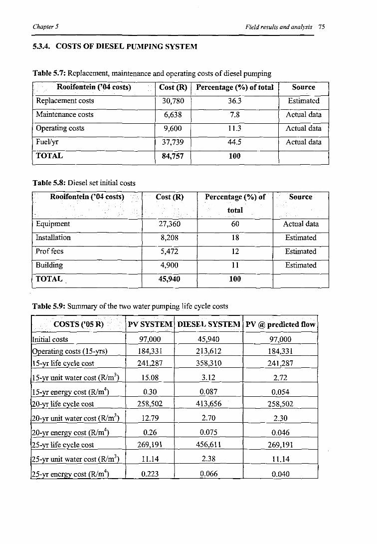
Chapter 5
5.3.4. COSTS OF DIESEL PUMPING SYSTEM
Field results and analysis 75
Table 5.7: Replacement, maintenance and operating costs of diesel pumping
Rooifontein ('04 costs) Cost (R) I Percentage (%) oftotal SourceI
Replacement costs 30,780 36.3 Estimated
Maintenance costs 6,638 7.8 Actual data
Operating costs 9,600 11.3 Actual data
Fuellyr 37,739 44.5 Actual data
TOTAL 84,757 100
Table 5.8: Diesel set initial costs
Rooifontein ('04 costs) ••••• I Cost(R) Percentage (%) of Source
total.
Equipment 27,360 60 Actual data
Installation 8,208 18 Estimated
Proffees 5,472 12 Estimated
Building 4,900 11 Estimated
TOTAL 45,940 100
Table 5.9: Summary of the two water pumping life cycle costs
.COSTS ('05 R) PV SYSTEM DIESEL SYSTEM PV @ predicted flow
Initial costs 97,000 45,940 97,000
Operatinl! costs (l5-yrs) 184,331 213,612 184,331
15-yr life cycle cost 241,287 358,310 241,287
15-yr uoit water cost (Rlm3) 15.08 3.12 2.72
15-yr ener/lY cost (Rlm4) 0.30 0.087 0.054
!:W-vr life cycle cost 258,502 413,656 258,502
20-vr uoit water cost (Rlm3) 12.79 2.70 2.30
20-vr enerl!Y cost (RJm4) 0.26 0.075 0.046
125-vr life cycle cost 269,191 456,611 269,191
125-vr uoit water cost (Rlm3) 11.l4 2.38 11.14
25-yr energy cost (Rim4) 0.223 0.066 0.040

Chapter 5 Field results and analysis 76
While the capital costs of PV systems are two to three times higher than those of diesel
systems, operating costs are typically low, as repair and maintenance are minimal and there
are no fuel costs. Refer to figure 5.9 below.
PV life cycle cost breakdown
Capital
77%
Repair &
maintenance10%
Figure 5.9: PV life cycle cost breakdown
The main problem in diesel systems is the high fuel and replacement costs as seen in figure
5.10 below. It is the high operating costs that discourage the use of diesel systems.
Diesel life cycle cost breakdown
Operator10%
-~--
Capital45%
Repair &maintenance
7%
Fuel38%
Figure 5.10: Diesel life cycle cost breakdown

Chapter 5 Field results and analysis 77
Figure 5. I I below shows the relative costs of PV versus diesel over periods of 15, 20 and 25
years. Initial costs of PV are higher than that of diesel from early stages of the systems'
operation. This is due to high operating and maintenance costs of diesel pumping, therefore
this makes PV more economical and viable compared to diesel pumping.
Relative costs 0 & 0) of PV & Diesel
400000.,-----------------------,350000 +------------~~----300000 +----_------
g 250000 +---~ 200000 +-~_~
c5 15000010000050000o J.----.L__
15 20Years
25
!DPV.DieseII
Figure 5.11: Initial & operating costs ofPV & diesel
Figure 5.12 illustrates the life cycle costs in rands ofPV and diesel over periods of 15,20 and
25 years. It shows how much diesel pumping will cost after 25 years and it is far more than
PV pumping due to operating and maintenance costs. Also evident are the relative costs if
the PV system was to operate at design conditions, showing significantly lower costs than
diesel.
LIFE CYCLE COSTS
500000
400000
'" 300000-'"QU 200000
100000
0
15 20 25Years
DPV • Diesel
Figure 5.12: Life cycle costs ofPV & diesel

Chapter 5 Field results CUld analysis 78
It is evident from the plot below that PV initial costs are about twice higher than those of
diesel system. PV enjoys low maintenance and replacement costs.
COSTS COMPAltISONS
120000 ,..--------- ---,
100000+-~~-----------------~
80000:la 60000
40000
20000
o+-~~~~-.L-~'-'----~--=---~==..c...~~
Initial Replacement Operating Maintenance
I PV Diesel IFigure 5.13: PV & diesel pumping costs comparisons
The life cycle cost analysis of the PV pumping system indicates that the average pumping
costs over 25 years are likely to be below 22 cents/m', while pumping costs of diesel are
likely to be below 7 cents/m' when the pump operates at 3.6m3/day.
PVactual & Diesel water pumping costs
5<XXXXl~-----------------..... 245<XXXl 1.8
4<XXXXl 1.6
35tXXXJ - _.. 1.4 =1.2 ~-... ~
1 >. ECllii:
0.8 t-c
15<XXXl 0.6 '"
IlXXXXJ .... 0.4
~L~---:::::::::::::::;::;:::;:::;:::;:::;:::;::::;::::;:::;;:::::;::;:::;::::;:::;:::;;;J ~2
2345678910111213141516171819202122232425
Years
...... .. PV cum cosu- PV actual energy costs
Diesel cum costsDiesel energy costs
Figure 5.14: PV actual & diesel systems cumulative and energy costs

Chapter 5 Field result. and analysis 79
However, if the pump operated at its optimum design conditions (20m3/day), then the
pumping costs ofPV would reduce to 4 cents/m', 43% less than that of diesel.
PV predicted & Diesel water pumping costs
0.3
0.25
0.2
0.1515000')1<XXXXl 0.1
5000') 0.05
o +-r-r--.-r-r_T--.~r_T__r_~._T___._._.,.,___.~~-r__r+ 0
5000Xl -,--------------------r 0.4
45000') 0.35400000
35000')
123456789101I1213141516171819202122232425Years
. - - .. PV cum eMU- PV Jredicted energy C0515
--Diesel cum costs- - Diesel energy C0515
Figure 5.15: PV predicted & diesel systems cumulative and energy costs
Tables 5.10 and 5.11 show a data used for comparing PV and diesel systems.
Table 5.10: Data used for solar pumping cost comparison
PV PUMP CHARACTERISTICS
Depth of water supply, head (m) 50
Annual average daily water demand (m'/day) 3.6
PV array peak power (kWp) 1.7
PV pumping system availability (%) 99
PVarray life (years) 25
Pump life (year) IS
Real discount rate (%) 5.2
PV unit costs (RIm') (15 years) 15.08

Chapter 5
Table 5.11: Data used for diesel pumping cost comparison
Field results and analysis 80
DIESEL PUMP CHARACTERISTICS
Depth of water supply, head (m) 36
Annual average daily water demand (mj/day) 21
Diesel generator power rating (kW) 10.3
Average load factor (%) 80
Diesel fuel cost (RIlitre) 3.12
Diesel pump availability (%) 97
Diesel gen-set life (years) 25
Real discount rate (%) 5.2
Diesel unit costs (Rim') (15 years) 3.12
5.4. COMPARATIVE ASSESSMENT OF THE TWO WATER PUMPINGTECHNOLOGIES
The specific water pumping cost is the main criterion for an appraisal of different pumping
technologies. This is the cost incurred by a pumping system, taking investment costs as well
as running costs into account, to supply one cubic meter per day at a pumping head of one
meter. They are expressed in R per m4. The costs have been calculated on the basis of
annuities, using a country-specific, inflation-adjusted calculatory interest rate (5.2%), and
taking into account the service life of the respective component (i.e. 15 years). The specific
water pumping costs depend not only on the pumping head but also on a number of other
site-specific parameters, which must be accounted for. This makes it difficult to apply the
results to other sites and to make generally applicable assertions regarding economic
efficiency. The main parameters in question include:
• System output
• Solar irradiance
• The discount factor
• And useful life of individUal system components
The objective of this section is to make a comparative life cycle analysis of the efficiency and
cost of diesel and solar pumping technologies. Specifically, it aims to estimate the cost of
pumping water per cubic meter using diesel and solar-power technologies over the life cycle
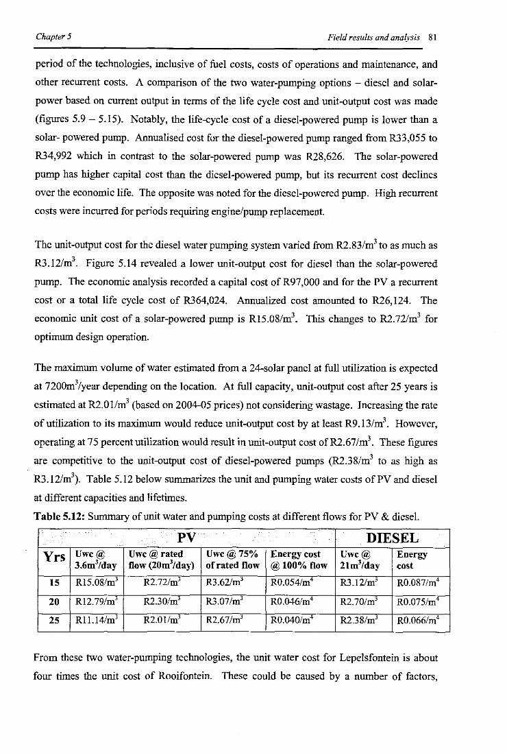
Chapter 5 Field results and ana(vsis 81
period of the technologies, inclusive of fuel costs, costs of operations and maintenance, and
other recurrent costs. A comparison of the two water-pumping options - diesel and solar
power based on current output in terms of the life cycle cost and unit-output cost was made
(figures 5.9 - 5.15). Notably, the life-cycle cost of a diesel-powered pump is lower than a
solar- powered pump. Annualised cost for the diesel-powered pump ranged from R33,055 to
R34,992 which in contrast to the solar-powered pump was R28,626. The solar-powered
pump has higher capital cost than the diesel-powered pump, but its recurrent cost declines
over the economic life. The opposite was noted for the diesel-powered pump. High recurrent
costs were incurred for periods requiring engine/pump replacement.
The unit-output cost for the diesel water pumping system varied from R2.83/m3 to as much as
R3.12/m3. Figure 5.14 revealed a lower unit-output cost for diesel than the solar-powered
pump. The economic analysis recorded a capital cost of R97,000 and for the PV a recurrent
cost or a total life cycle cost of R364,024. Annualized cost amounted to R26,124. The
economic unit cost of a solar-powered pump is RI5.08/m3• This changes to R2.72/m3 for
optimum design operation.
The maximum volume of water estimated from a 24-solar panel at full utilization is expected
at 7200m3/year depending on the location. At full capacity, unit-output cost after 25 years is
estimated at R2.0l/m3 (based on 2004-05 prices) not considering wastage. Increasing the rate
of utilization to its maximum would reduce unit-output cost by at least R9.13/m3. However,
operating at75 percent utilization would result in unit-output cost ofR2.67/m3• These figures
are competitive to the unit-output cost of diesel-powered pumps (R2.38/m3 to as high as
R3.12/m\ Table 5.12 below summarizes the unit and pumping water costs ofPV and diesel
at different capacities and lifetimes.
Table 5.12: Summary ofunit water and pumping costs at different flows for PV & diesel.
PV DIESELYrs Uwc@ Uwc@rated Uwc@75% Energy cost Uwc@ Energy
3.6m3/day flow (20m3/day) of rated flow @lOO%flow 21m3/day cost
15 R15.08/m3 R2.72/m3 R3.62/m3 RO.054/m4 R3.12/m3 RO.087/m4
20 R12.79/m3 R2.30/m3 R3.07/m3 RO.046/m4 RZ.70/m3 RO.075/m4
25 Rl1.14/m3 R2.0I/m3 RZ.67/m' RO.040/m4 RZ.38/m' RO.066/m4
From these two water-pumping technologies, the unit water cost for Lepelsfontein is about
four times the unit cost of Rooifontein. These could be caused by a number of factors,

Chapter 5 Field results and analysis 82
including a high capital cost for Lepelsfontein, very low pump output as well as high
operating costs (salary of a pump caretaker). The pumping costs for Lepelsfontein are about
three times higher than those of Rooifontein. In contrast, the unit water cost is 90% that of
diesel and the pumping cost is about 60% that of diesel when the design conditions for PV
are assumed.
Chapter 6 is the concluding chapter. It presents the conclusions on the laboratory work as
well as the fieldwork. Finally, the overall concluding remarks are made as to the success of
the project.

Conclusions 83
Chapter 6
CONCLUSIONS
This chapter summarizes and concludes all the main issues emerging from the previous
chapters. This chapter is structured into four sections. Section 6.1 presents general
conclusions on PV and diesel water pumping. Section 6.2 summarizes the remote monitoring
system. The last section (section 6.3) concludes the entire report.
6.1. PV AND DIESEL PUMPL"lG
The findings ofthis study support the existing body of evidence, which indicates that PV has
a place in rural water supply. The increasing number of PV water pumping systems clearly
shows that the acceptance of PV technology in this sector is high. The main problem with
PV pumps has been their high initial cost, but with cheaper PV modules coming onto the
market and with improved system designs, this does not constitute such a barrier. The
upgrading of the PV system in Lepelsfontein improved the output of the system even though
the performance of the system has drastically deteriorated recently.
The introduction of PV water pumping systems in remote areas has discouraged the use of
diesel water pumping. It is evident that diesel engines can deliver high flow rates even at
high heads, but the costs of fuel, cost of maintenance, pollution and other obstacles make this
technology less preferred. The 15-year life cycle cost indicated a unit water cost of R3.121m3
and an energy cost of 9 cents/m4• The 25-year life cycle cost indicated a pumping cost of 7
cents/m4, 43% higher than that of PV. This is because of high operating and maintenance
costs of diesel and a higher pumping head of the PV system.

Conclusions 84
6.1.1. ECONOMIC ASPECTS
It is not possible to generalise about the economic viability of PV systems. Each application
has to be considered on its merits, taking into account local conditions and the cost of
alternatives. Although PV systems have high initial costs, they require no fuel and very little
maintenance and should last many years. In many remote areas, diesel generators, the main
alternative to PV generators, would be impractical due to fuel supply costs and uncertainties,
plus the problems associated with maintenance and the supply of spare parts. In water
pumping, PV water pumps may be cost competitive with diesel pumps for applications where
the flow is low and the head is low to medium. The analysis is sensitive to the cost of diesel
fuel and the life expectancy of the diesel pump. PV pumps are more likely to be viable for
village water supply where social benefits are high. Even if diesel generators may appear to
be cheaper on a life cycle cost comparison, it might be preferable to go for a PV system
because of their operational advantages. Table 6.1 shows a summary of pumping water costs
ofPV and diesel over a period of 15, 20 and 25 years.
Table 6.1: Summary ofPV and diesel life cycle (LCC), unit (UWC) and pumping (EC) costs
.. PV.
DIESELYrs LCC UWC@ UWC@ EC@ EC@ LCC UWC@ EC@
(R) 3.6m3/day 20m3/day 3.6m3/day 20m3/day (R) 21m3/day 21m3/day
15 293207 RI5.08/m3 R2.72/m3 RO.302fm4 RO.054/m4 358310 R3.12/m3 RO.087/m4
20 331390 RI2.79/m3 R2.30/m3 RO.2561m4 RO.046Im4 413656 R2.70/m3 RO.075/m4
25 361024 Rl1.141m3 R2.0l/m3 RO.223/m4 RO.040/m4 456611 R2.38Im3 RO.0661m4
6.1.2. TECHNOLOGICAL ASPECTS
Experimental experience: It would be important to talk of the accuracy of the data
acquisition system (transducers, interface and data logger) because the accuracy of the
transducers and the error sources in the components of the signal conditioning are available
from data sheets. The collected data though, should be expressed on the basis of uncertainty.
The reason for this is that the calibration of the data acquisition system is not based on the
comparison to known values, but is compared to other measuring devices that have a
particular accuracy. There were no serious technical problems encountered during the
experiments and the experience gained from these experiments was very useful when
conducting field experiments.

Conclusions 85
Field experience: The efficiencies shown in table 6.2 overleaf are a summary of
experimental and field results obtained from two PV water-pumping systems (laboratory &
field respectively). The average efficiency of the array was found to be 3% for a two-month
monitoring period. This output is below the manufacturer's specifications. This might have
been caused by several conditions such as: high solar intensities that contributed to the
temperature effects of solar cells at elevated cell temperatures (increase in the temperature of
the PV modules due to solar heating, lowers the PV conversion efficiency), dust that
accumulates on the PV panels can also reduce the output of the panels (it should be noted that
the array's structure is not projected at any height - the top part of the structure is projected at
about half a meter - see figure 4.8). Bullwinkel and Hopkinson (1981) reported a 10%
decrease in PV array output after 3 years of field operation due to soil accumulation on the
array and degradation of system components.
It is also a possibility that the panels are gradually beginning to be less efficient considering
their installation date (1991). The use of tracking PV arrays can be used to improve the
performance of the panels in theory, but experience has shown that at remote sites where
maintenance is difficult to provide, the extra complexity is not warranted.
The average system efficiency is calculated to be 32% for the monitoring period of two
months. The results show that the pump operated at only 12% of its design volume. One
cause for the pump or motor to be less effective can be overloading due to sediments in the
water or tight bearings. The primary reason is attributable to the operating efficiency of the
solar panels (3%).
Pump performance is heavily dependant on the assumptions made at the design stage
regarding solar and water resource characteristics. Careful account has to be taken of the
variations in solar input to the array, the static water level in the well and the water demand.
Failure to do this can result in systems being undersized so that they fail to meet the demand,
or excessively oversized, with associated additional capital cost. This system was upgraded
in 2001. The pump was replaced and additional solar panels (4x55 W) were installed. Table
6.1 below shows a summary of experimental and field results.

Conclusions 86
Table 6.2: Summary of experimental and field results
Experimental results Field results .
Maximum Average Design Maximum Average Design
Array efficiency 17.3% 16.3% 20% 4% 3% 20%
System efficiency 17% 15% 32% 74% 32% 30-40%
Overall efficiency 1.8% 1.47% 6% 3.2% 1.3% 4%
6.1.3. SOCIAL ASPECTS
Experience from Lepelsfontein settlement has shown that the users now generally welcome
the PV system which is in operation, provided that they be involved at an early stage in the
planning process and have been given basic instruction on how to operate the system and
carry out routine maintenance. No vandalism and theft have been reported to date and almost
all the users know that they have to protect the system. If the community is fully involved in
the development ofprojects like this, it is more likely that the community will take care of the
installation and protect it against theft. Problems arise when a system is set down in the field
by a research organization and the local people are expected to use it without any real
appreciation of what is involved and without proper arrangements for follow-up. A system
caretaker was appointed from the village to take care of the system's daily operation.
6.1.4. INSTITUTIONAL ASPECTS
There has been no consistent planning and project management of water supply in the
Northern Cape area, partly due to many different institutions involved in this field.
Implementation has thus been unplanned. The fallout of this is that there appears to have
been no systematic approach in terms of system design, sizing and quality, and consequently
the water supply level has sometimes been lower than expected. This is partly as a result of
inadequate technical knowledge of PV systems amongst the institutions commissioning their
installation, but the fact that the systems have been operating reliably to date is a reflection of
the maturity of the technology and the integrity of the suppliers. The Karniesberg
municipality later came in and took control of water supply in Lepelsfontein settlement and
funding the upgrading of the existing project through the Consolidated Municipal
Infrastructure Prograrmne (CMIP). Consulting engineers (Bouwer and Viljoen, Springbok,
SA) did all the design work:.

Conclusions 87
6.1.5. CO~CLUSIONS
The technical, economic social and institutional factors associated with each application need
to be carefully considered before any general conclusion can be made regarding the viability
of photovoltaic water pumping. Obtaining reliable data on the perfonnance of many PV
systems is not easy and hence hampers the evaluation of the economic prospects. It is also
not easy to evaluate the economic prospects, as many systems have not been in operation
long enough to yield sufficient data on component lifetimes and replacement costs.
6.2. REMOTE MONITORING
The initial objective of this research was to establish a communication link between the
Lepelsfontein PV system and a local ground receiving station at the Cape Peninsula
University of Technology. That communication link was established and is operational. The
capital and construction costs of this system were low. However, operation cost (airtime)
seemed to be high, but it depended on how often and when data was downloaded from the
data logger. The infonnation provided by this system was used to;
• Determine component reliability
• Obtain information on perfonnance degradation
• Comparatively evaluate different water pumping technologies
• And determine life cycle costs of the system.
The results from the PV station are now available and they can be downloaded at an
operator's will. Long-tenn tests can also be perfonned and the results of these tests will be
documented in future reports. Future work is aimed at expanding this technology to other
regions of interest. An ultimate objective of this work is to develop a real time system based
on a central microcomputer used as a micro-server, with a relatively low cost. A real time
system will capture and measure specific data from several stations. It is important to
conduct feasibility studies in order to select an appropriate communications technology for a
specific village.
6.3. CONCLUDING COMMENTS
As an attempt to monitor the PV groundwater pumping systems in the remote areas of the
Northern Cape Province, logical steps were followed until the fmal system became
operational. The first step was to build a test rig to conduct laboratory assessments and

Conclusions 88
preliminary tests. These experiments were done in preparation for the set up of the telemetry
link requjred for transmission of logged PV water pump data. The preparations went quite
well despite a long time taken to set up the equipment.
The next step was to construct a real time monitoring system, but prior to the construction,
telemetry equipment was tested in laboratory. The installation of the system took two days.
The system was tested at the base station and data was downloaded. In conclusion, the
objectives of the research were achieved. This is an initial step of the on-going process of
monitoring the water pumping systems in the Northern Cape.

Bibliography and references
BIBLIOGRAPHY
89
Ameur S, Laghrouche M & Adane: Monitoring a greenhouse using a microcontroller-based
meteorological data acquisition system, Renewable Energy 24(2001) 19-30.
Arab A H & ChenIo F., Performance ofPV water pumping systems International journal on
Renewable Energy 18 (2) (1999) 191-204, Pergamon Press, Oxford.
Barlow R, McNelis B & Derrick A., Solar Pumping, An introduction and update on the
Technology, Performance, Costs, and Economics, Intermediate Technology Publications and
The World Bank,Washington D.C., 1993.
Benghanem M, Hadj Arab A & Mukadam K., Data acquisition system for photovoltaic water
pumps, International journal on Renewable Energy 17 (1999) 385-396, Pergamon Press,
Oxford.
BuIIwinkeI H.J & Hopkinson R.F: Three-year performance study ofthe Mead, Nebreska, 25
kWp photovoltaic power system, Proc. 1981 Annual Meeting American Section of the
International Solar Energy Society, Vo!. 4.2, pp. 1239-1243 (1981).
Burkert Easy Fluid Control Systems Manual
ChandratiIleke T. T & Ho J. C: A study ofa photovoltaic array for water pumping, Solar &
Wind Technology, Vo!. 3, Issue I, pp59-71, 1986.

Bibliography and references 90
Cowan W.D (Ed): RAPS design manual, Vol I, Energy for Development Research Centre,
University of Cape Town, Cape Town, 1992.
Energy & Development Group: Evaluation of diesel and PV water pumping systems in
Namaqualand, Noordhoek, Cape Town, September, 1996.
Gosnell R.J., Photovoltaic water pumping: A case study in Kwazulu, Energy for Development
Research Centre, Energy Research Institute, University of Cape Town, 1991.
GTZ, 1995: International Programme for Field Testing ofPhotovoltaic Water Pumps - Final
PVP Conference (27/1195 - 01/12/95). Deutsche Gesellschaft fur Technissche
Zusammenarbedit (GTZ) GmbH, Eschbom.
Hadi H: Course ofIntelligent Mechanical Systems Engineering, A Dissertation Submitted to
the Faculty of Kochi University of Technology in Partial Fulfl1ment of the Requirement for
the degree of Doctor (Philosophy), August 2003.
Hamza A.A & Taha A.l: Performance of submersible PV solar pumping systems under
conditions in the Sudan, Renewable Energy, Vo!. 6, No. 5-6, pp. 491-495, 1995
Helikson H.J, Haman D.Z & Baird C.D: Pumping Water for Irrigation Using Solar Energy,
Florida Cooperative Extension Service, University of Florida, 1991.
Heliotronics: Solar Learning Lab™User's Guide, Inc, Hingham, 2004.
Hession P.J & Bonwick W.J: Digital data gathering for solar energy measurement, Solar
Energy 30 (1983) 441-446, Pergamon Press, Oxford.
Hill R., Applications ofphotovoltaics. Adam Hilger, England, 1989.
Imamura M.S, Helm P, & Palz W.: Photovoltaic System Technology, H S Stephens &
Associates, Bedford, England, 1992.

Bibliography and references 91
Jafar M., A model for small-scale photovoltaic solar water pumping, Renewable Energy 19
(l) (2000) 85-90, Elsevier Science.
Koutrolis E & Kalaitzakis K: Development of an integrated data-acquisition system for
renewable energy sources system monitoring, Renewable Energy 28(2003) 139-152.
Lasnier F, Ang G. T, Lwin S.K & Hemasuk T,. Photovoltaic Tests and Instrumentation,
Pumping system, Asian Institute of Technology, Thailand, 1988.
Loois G & Hemert V. B., Stand-alone photovoltaic applications. James & James LTD, UK,
1999.
Makhomo S.: Installation, commissioning and preliminary testing of a photovoltaic water
pumping system, unpublished B.Tech thesis, Peninsula Technikon, South Africa, 2001.
Mukaro R, Carelse X.F & Olumekor L: First peiformance analysis of a silicon-cell
microcontroller-based solar radiation monitoring system, Solar Energy Vo!. 63, No. 5, pp.
313-321,1998.
Omar I. & Law S.: Energy Alternatives for the supply of water in Namaqualand, Energy
Research Institute, University of Cape Town, 1991.
Omar, I & Makhomo, S.: Energy alternatives for water pumping in mral areas - Using a
case study approach, Proceedings of the 10th Domestic Use of Energy Conference, Cape
Technikon, South Africa, 2002.
Omar, I & Makhomo, S.: Remote monitoring system for Photovoltaic groundwater pumping
in remote areas, Proceedings of the 11 th Domestic Use of Energy Conference, Cape
Technikon., South Africa, 2003.
Oparaku O.V.: Rural area power supply in Nigeria: A cost comparison of the photovoltaic,
diesel/gasoline generator and grid utility options. Renewable Energy 28 (2003) 2089-2098,
Pergamon Press, Oxford.

Bibliography and references
Ovies S: Personal Communication, Lepelsfontein water pump caretaker, 2004/05.
92
Perez R, Kmiecik M, Herig C & Renne D.: Remote Monitoring of PV Performance using
Geostationary Satellites, Solar Energy Vo!. 71, No. 4, pp. 255-261, 2001, Pergamon Press,
Oxford.
Photovoltaic Systems: Power for a new
http://www.cimat.com/buyerguide/power.html. (06/03/03).
era, available @
South African Petroleum Industry Association (SAPIA) annual report 2002, (Sapia annual
report web page accessed @
http://www.mbendLcom/sapia/pubs/2002ARep/Arepa14.htm. 26/06/2005).
Sarkar M. A. R, Obaidullah M, Mahmud Z & Martinac I: Solar PV Submersible Water
Pumping for Small Scale Use in Bangladesh, Bangladesh University of Engineering &
Technology, Dhaka, Bangladesh (accessed @ http//fsec.ucf.eduledliasee/isree/sarkar
water.pdf,22/06/2005».
Scholle A.: Evaluation of two prototype three phase photovoltaic water pumping systems,
Energy for Development Research Centre, Energy Research Institute, University of Cape
Town, 1994.
Seutloali T.: Laboratory testing and evaluation of a photovoltaic water pumping system,
unpublished B.Tech thesis, Peninsula Technikon, South Africa.
Sippola M & Sepponen R: DC/DC Converter technology for distributed telecom and
microprocessor power systems - a literature review, Applied Electronics laboratory, Helsinki
University of Technology, 2002.
System Performance Monitoring Services, available @
http://www.us.schott.com/apc/english/productslinstrumentation/#data, (05/03/03).

Bibliography and references 93
Solar (photovoltaic) Water Pumping Intermediate Technology Development Group, web
document available @
http://www.itdg.org/docs/technical information service/solar pv waterpumps.pdf,
Toens & Vennote.: Grondwater Monitenng en Bestuur van Waterstelsels in Namaqualand,
Provinsiale Administrasie van die Provinse Noord-Kaap, Wynberg, 2001.
Virtu-Well wireless remote monitoring, web page available @
http://www.virtualtechnologiesltd.com/PDFsNirtu-WeIIITMl.pdf, (06/01/04).
Wilshaw A.R, Pearsall N.M & Hill R: Installation and operation ofthe first city centre PV
monitoring station in the United Kingdom, Solar Energy Vol. 59, Nos. 1-3, pp. 19-26, 1997.
Witchert B, Dymond M, Lawrence W & Friese T: Development of a test facility for
photovoltaic-diesel hybrid energy systems, Renewable Energy, 22(2001) 19-30.
Yaron G, Irving F.T & Jansson S, 1994: Solar Energy For Rural Communities (The Case in
Namibia), Intermediate Technology Publications, University ofNamibia.

APPENDICES
Appendix A: Data sheets ofexperimental hardware
Appendix B: Data sheets of field hardware
Appendix C: Data acquisition data sheets
Appendix D: Experimental results
Appendix E: Field results
Appendix F: Field maps
Appendix G: Field pictures
95
99
106
111
113
125
128
94

Appendix A: Data sheets ofexperimental hardware
AI: Daily performance charts ofwatennax WA
95
IElectrical Parameters ~~~S~P7=5~~==I~~~~-;
I12V !6V I 11
IMaximilD1power rating IrPmax~~.~.~~.Ir[W-.-a~tt~s]-.-~1-75~.~~~--'--'~-~~I'-.--~--i
IMinimum power rating Irp~m~in==~lr[\~IV~att~S~]==~170 IIRated current IrIm~p=~=I[AmPS] 14.4 18.8 I~-~--'I
I-R-at~ed~V-o~lta~g~e-~===lvmp [(VOltS] 1~17~.0--~18.5 II~Sh-O~~~C~ir~CU~i~tc-urr-..~en~t~..=~.~.IISC ![AInPS] 14.8 1=9.~6-.•=·==~r-1~.===~"
IOpen circuit voltage Ivoc 1(Volts] .·'21.7 110.9 I
IPhysical Parameters .1.. .1INumberofseriesceIIs. L. 136IL~e~n~gth~...===============I[mm](in) 1~12~0~0~(4~7~.3~)======1
1Width . ...I[mrn](in) ... [527 (20.8) ..
rID~ep~th=(=w=/o=bo=x=)~..=~~=====~=.=..=.[[mm] (in) 1=34=(=1.=3)=..=====_1
[weiglit l[kgJ(lbs)._!7.6 (16.7)
Iw~..~a~r=ra~n~ty~..===============~L 1=.=========~IIPower>=o90%ofmininlUrn power ([Years]. . .1 10
!Power >=0 80% ofD1inimum power I[Years] 1~25=========~1

Appendix A: Data sheets ofexperimental iUlrdware
A1: Daily performance charts ofwatermax WA
96
2 X SOW 2 X 751/>1 3 )( SOW 3 X 75W 4 )( 60W 4 X 75W
TOTAL MO DU LES MODULES MODULES MODULES MODULES MODULES
HEAD (SERIES) (SERIES) (SERIES) (SERIES) (SERIES) (SERIES)
L1TR ESI LIT RESI L1TRESI L1TRESI L1TRESI L1TR ESI
DAY DAY DAY DAY DAY DAY
6Dm 2047 2197 3460 4017 4452
70m 1887 2412 2660 3882 4452 4933
60m 2270 2777 3123 4304 4866 5414
50m 2653 3142 3586 4726 5320 5695
40m 3036 3507 4048 5148 5754 6376
30m 3419 3872 4512 5570 6188 6857
20m 3802 4237 4975 5~92 6622 7338
10m 4165 4602 5436 6414 7056 7619
Om 4570 4970 5904 6636 7490 63]0
OAIL'" FLOWRATESAJiE FOR FIJinlARRAY:&O\1L't
T<J"T,Al • EA.D ~IDAI L'1 FLOW ~TE&l : F li:orl1ll WATER UV I< L TO POI YT 0 F I) E LN ER....

AppendLt A: Data sheets ofexperimental hardware
A3: DC performance charts of watermax WA pump
97
..~ ,'" .\f:; :':: .."!,~~~J~'~7::Y·:
. . ..>/;'." , :, 'F c'[ "'.'~ . ;"
64V 60V 55V 4SV 36V 32V 2~V
TOTAL A MPS LIT RES! AM PS LITRES! AM PS L~RES! A WPS LITRES! A~ PS LITRE S! AW PS A MPSHEA 0 HOUR HOUR HOUR HOUR HOUR LITRES! L ITR ESIH
HOUR OUR
80m 4.8 G85 Hi8 G40 4.oG 800 4.0 020 '.46 370 4.53 310 4 . .49 225
70m 420 710 420 GGO 4.14 610 '.11 535 4.02 380 4.07 330 4.13 23G
80m 3.90 720 3.77 G80 3.7A 830 3.71 000 3.64 400 3.80 340 3.88 240
50m 3.55 740 3.40 G95 3.35 650 3.31 565 3.24 410 3.20 350 3.23 250
'Om 3.16 760 2.88 ?l0 3.88 660 2.81 515 2.S1 420 2.S1 360 2.14 260
30m 2.7. 780 2.0G 725 2.50 875 2.54- 535 2.43 430 2.38 370 2.31 270
20m 2.30 780 2.17 750 2.13 700 2.12 610 2.04 450 1.97 360 I.S2 260
10m 1.6S 610 1.71 775 1.72 715 1.69 620 1.62 460 1.57 '00 1.47 265
Om 1.55 850 1.~2 800 1.38 720 1.32 SOD 1.21 460 1.16 '20 1.04 290
OTHER SOLAR MODULE CONFIGURATIONS ARE POSSIBLE - CONSULT
MANUFACTURERS

Appendi~ A: Data sheets ofexperimental hardware 98
A4: DC performance and efficiency curve of watermax WA pump
Pump perfunnance cun'e
10
25 17="20 0<:;
E15 "'"
5
--"'"'--.."
80 70 60 50 40 30Head (m)
20 10 o
---Pumpperfonnance curve - - Efficiency

Appendi, B: Data Sheets offield hardware
HI: Specifications ofHelios PVmodules
.F7~~~-:~r~~r*~a:-;:~~t=¥~·-.-"'_f---t~i·;:-;-~-~~~-~~~~~~ '".... :;';' ii '0 ;;",::~
&""'- "','-'. -""/-:=;'-"";";:::&;_::'"
NEW GENERATION OF PHOTOVOLTAIC MODULES
99
Th" phctovoltaic modul.-. Hsao ha"e b~n designed for th€ rlJalelectrification, data survey. telecommunication and specialapplications. Thanks to th~ ",,",satlllty, main charnctNistic of th~
Hellos modules, th.-y are very appreciated and used either in thedeveloping countries or in the European ma rkets. The recentintKXJuc~cnof 1he high eftic;"ncy cell. 1-t.l1ax@> in monocrystdllinesilicon, has highly increased their performance.At the typical battery operating "oltdge 02-13 Volts) the I-Max®tecmology, developed by Hellos for the high efficiency modules,allows to obtdin. differently comparing with the tradlticnal modules,a high increase of 1he ClJrent i1 0-17%). Such characteristic makesthese rr>:ldules p"rricularrl sulmble for stand alone systems withbarteriE-s. Made by 36 high E-fflciency cells I-Max® 165 x S8mm inrnonocr;'StaDine silicon. these modules have b~n designed in orderto work under the toughest opera~ve and environmental comitions.The Helios modules have been long lasting proven of a typicala"erage lifetime of more than 30 years"Furthermore every single cell and module produced ha"e beenseveral times tested and checked throughout the manufacturingprocess.Interconnections between modules are easy. practical andoptimized fer all configu",~on voltages.R.obust construction and hea'l.'Y duty anodized aluminium framedesign makes this module su~able secure, simple and fast to beinstalled in many situations.
H59IlISOW • 55\'1
Guaranteed power:o. 110% 25 yearsRelative humidity up to 100%Dimensions 750 " 524" 34 ± 1mmWeight Kg. 4,60Tolerance on technical data: ± 10%
(E
ELECTRICAL SPECIFICATIONS (at 100mWlcm', 25"C, AM 1,5)MODULE H5BO
. ~"'_lWpl Wan. 50 Watts 551-short ~'liCI:ireJrt-\~ ~t.ll"1PS 3.50 Amps 3.80r ap.'cF.:llir~\Voc) .cm 2ll.ao IjQIt.~-- 2~.90
i Vohage at milllimtlm p:JNer l'.'mp) hhs 16.66 \iolts , 6,57r-CUfrelll at-maJ,JrTPJ m p::tNer a-mp)~~- Amps . -3:oo~---ki6~-'-'-~---'-~-3:3Q~
!-typ~-C~'_ atb:.rtt;;Y;;;;e.-;,;;;-.;;;lUll"11-2.SVlT--A;;;~-~------3:i5--T-A;;;p$ -~----- 3.4[NOCF1NoiiiJ,fq>ef<l!illg celltempemtJrei'-~:-'C~--~--- :ui1--' -----.c-- 43±2-! CMn~of "loc ·.."it~ ttmp=i"im.re .,~ mV,""C -:00 m\'Y*C .~)
\M"" Io1I<Jng or surf,,,,, p-essure r'm2 ~oo f20Q Om" eqtW' r'm2 2400 f200 Om" equi\ljHailstQfle Impilct resistance 24mm ~ 00 km,i! 24mm at 80-km~1l--Sttlrage:arldo~ngtemperat~ lie da.-iJJ:a+96 IC fsom-4!lm .... 95Ma;ocimlJT1 s)'stem lidtage Vdt5 000 Vdts 600

Appendix B: Data Sheets offield hardware
B2: Specifications of LiseIo PV modules
JI'!!'!!]USELO 75W (ARXQ75)MONOCRYSTAWNE PHOTOVOLTAICSOLAR PlOOll.E CATASHEET
lOO
Use-Io Solar Modules provide:• Olltimurn solar power cooverson• Hi;Jh mechanical SJeng1tl• Quick. !Eecure mounting• Ef::ctJical cortinuITt under eX'".reme tem;::erature conc!ino,15
Cell Matffial & Configurrtion : Optical EfficiencyEach mo-jure contains hign qualitj slicon cens, in strings of cells connec~ed in series. Indi\lidual cells are hated wf'"ll a patentedanti·rene:tive :oating forenhance-d optical cOlpling and maximum efficiency.
Module Construction: ReliabmtyCells are laminated:n Ettrjlene Vinyl Aceti!e (EVA). and sandw ched betNeen high transMi3sion. imp;:;ct resistant glass, anc a moistureresi3tant Te-:::tlar bac'ing. Lamination in EVA facntates tt1ermal expansion, :Jro"ices mJistur= protection and ensu'es tr/ stability cnd et~ctric31insulation.
Frame Construction: Mechanical RobustnessModules have robUst, extruded anccised aluminium hmes, capable of wthstaOOing \",-ind IJads af up to 20Dkmil"our. A thin layer of sifJconsea ant is appl ed be.r....een the frame and the rrodule, providing a fur-ller tarrier against hLmidit/, 35 ,,-ell as a cushion against impact andthermal expansJon_
Electrical Connection: P;otec:ion & ConjnuitYModules :are supplie::J wr.r a wc~erproof 1P65 junction box with sealed screw lid:, 2Qmm knockout holes and compression glam3 for externalelectrical power cable feeds. Bectrical connecJon in the junctioo om: is directly into screw terminals en the printed cir·:uit board con~ainlng
pro1ectl·oJE t::y~ass diodes.
Physical Mounting ~ Speed & SecurityModules are rrDunted in j:osincn via slotted holes on the frame. This provlces qLick, secure fiXing of modules to the suoporting structure_
Warranty: Continucus OperationModules have a tfPicaf design life 0120 years cnd are sU~liedwfth 3; 20 year limited power output warrant,.
ELEClRI::AL & MECHAN CAL SPECIFICATIONS
Ch;racteisticNunber of Cells
Cell Type
Module Size
Jun:ton Box
Noniilal Module Vdtage
Typical P,.k Power\I'p
Voltage; Open Circ'Jit Voc
Curcl1t : Short Circu t Ise
Voltage: Peak Power VC;!
Curent : Peak Power Ipp
Module MassNOCTTemperaJJre Coefficient cfVoc
Ternperaiure Coeffident d Ise
Hailstone Resistance
Urit
mm
V
V
AV
A
1\1·C
mv...·CrnV,'C
~J1lIl1
lISELO 75W UODULE (ARX075)36Mono 125x125mm
. 1215 (L) x 540 [W) >60 (D)
Standard IP6: cov€r12
7596
2124
466
17.284.40
8.2:] (8.£6 with c;;rcboard pacJo:aging)
45
-79
1.5
25mm diamatsr @ SOkm.h
Note: All :jata is based on measurerrents nade under $'"..andard Test CondJtions {STCI of insolathn of 1000 \Na:t&rn'" (1 Sun) at a spectraldistibutiOn of AM' 1.5 and a eel tempera~ureof 25"C, and may -'ary by up to 1n%._
LlSELO (PTY) LIDMant.1adurers & Djstribuors of Photovoltaic MOOUles and systens
57 Aaidina Crescent, Gate.....ay Industrial Park, Ce-ntUliol, South Africa.PO Box 52669. Wierda ?3--<1l, 014~, South Afiica.
Tel:+271266'-660-t Fax: +-2712 651-7155E-Mail: [email protected]
ISO 9002

Appendix B: Data Sheets offield hardware
B3: The SA-I 500 pump controller
Water Pumps
Grundfos
101
SunWize'TtCHHOLOQl,Ea
SA·15<10The Gn.mcllos 001'1 dr'Oct SP line cl ...-ata l:U1lDS shoukl be wnsidefoo t>y anwne "'ho ....llnls 10do the job right Ihe first time. The pumps are a stanless steel centrifugal design with nodiaPhr"llffi" 10 replace and a water-cooled motor.
The Solar pump '500 'eties operates from a sola' array of 7 or BmMules In series~ fo 2000wafts. TIltS _as ea"! pump water!tonl a ma><l" um ooptll cl 650 feet Co,nmon applleat"ns forthis series 01 the GruOOfos Sola Pump 1,00 are can:p~<lld wata systems, Ivestoek watering.~rigatbn, end larger oorr.munity wata systems.
TheSA-1500 controler is a pump controlJa- and an lmerter. There ere many pump contrrnfeatures in the controller sudl as maxirntrn pc:M'er p:Jint tracking, low water sensing, and floatswitch lenninats. This cmlroller takes the DC __er fro... the sdir array end iwerts ~ to 63 VN:.,3 phase for the p""p motors.
AccessOrffls:Contact your deal... for the accessories 10 eompl>te your wet... pumping systems.• A solar a-ra'1 tracker, using a tracker OIl a water pumping system may .,crease your water
",eduction up to 25~• Sli:rn~ pt.rnp c.:tJIa • Root .switches. • Sow mocftjes
VolIAge Paw.. Row Ra. Total v..tIc3l WeVdSOlAR PWP l!il10 PUWS VIJC Current Wp Cl'IoI lift Cm feel) \lb.) USRI'
ooo.t502S SPI M8 105 ID 120 HA 2000 H,9 328106$ 39.9 1)1,315.00
0'..31~ SP1.5h-21 100ID 120 1~ 2000 71'12 262tom :rT 1)1,290.00~~00..315015 SP2A-15 105 ID 120 1~ 2000 711>20 164tom !\I.S 1)1,199.00 me
100ID 120 = 1)1 ,\12.00 "'..,10315010 51'3 MO 1~ 2000 IHl~ 981D2:lO ~~11875(.05 SPa A-5 105 10 120 1~ 2000 4()" 140 71D 92 32.9 1)1,112.00 :;:m
07315003 SPI4h-J 100ID 120 1~ 2000 8011>180 71D 49 42.1 1)1,224.00 ts:cmrnIOllBl
S25100 5.\1500 ConI1llII!r 1051D 120 1~ 2000 9.7 1)1 ,558.00
CAIllE TBl~'IIWIOIl m115()99 C:l!>1e tennifl:ltbll<il ,,'-sock $126.00
6M.:b l5trJSi:r.!ic.6tM~"9'"

Appendix B: Data Sheets offield hardware
B4: Technical details of SP 2A centrifugal pump
102
Company name: GRUNDFOS NSCreated by: Joseph MokgwammePhone: '2711 579-4800Fax: +2711455-6066Dale: 23/0612005
70
DescriptionProduct' name:Product No;EANnwnber::
ValueSP 2A-1309001K135708601051302
H SP 2A-13(m) -- - . - -~------ - -- -- b;'~1~44 m'lh
--- ~-----_.. __._-----_.- H = 63 m -------,----.Es = 0-5847 kV\'hIma
Tedmical:Speed fur pump data:Rated f.ow::Rated head:Curve tolerance:Pump No:Stages:Model:Valve:
2900 rpm2m",'h52mISO 9906 Annex A0900001313ApUmp with built-in non-retum vat"e
60 -
50
40
20 ------------/- _
M.aterials:Material, pump:
Material, impeller:
Installation:Size, pu.'Up outletMotor diameter:
Liquid:1\.'.ax rJquid t at D. 15 rnlsec:
Stainless steel1.4301 DIN \'V.-Nr.304 AlSIStainless steel1.4301 DIN W_...~r.304AJSIStainless stBeIl_,BOl DIN W_-Nr.304AJSI
Rp 11/44indl
4Q·C
30 --~---
10
00 0.2 0.4 0.6 08P
(k\\~
0.3
0.6
_Eta pump = 47.5%Eta pump+motor = 293 %
1.2 14 1.6 1.8 2 2.2 24Q(m"!h)
Electrical data:Mmor !:ype:Applic. motor.P2:J\1ains frequency:Rated: 'Vol+~ge:
Starting met~Rated currentCos phi - power factor:Raterlspeo<l:Endosum class (lEe 34-5)·Insulation class (!Ee 85):Motor protec.:Th..."'m1a1 p.rowe:8uHt-in temp. transmitter::.Plugs mot cable:""""No:OtheB:Net weightG~weig,'1t
Shipping volume:
MS4J2GRUNDFOS(155 kW5Ql-iz3;le 33O-40Q...415 V~ect-orHjne
2,00-220-2,35 AO.7M.64-0.602850-200Q-2870 rpm,P58BNONEelite-malno279192003
10.9kg12.7 kg0011 m"
04
0.2P2-522W
Q P1 - MS W
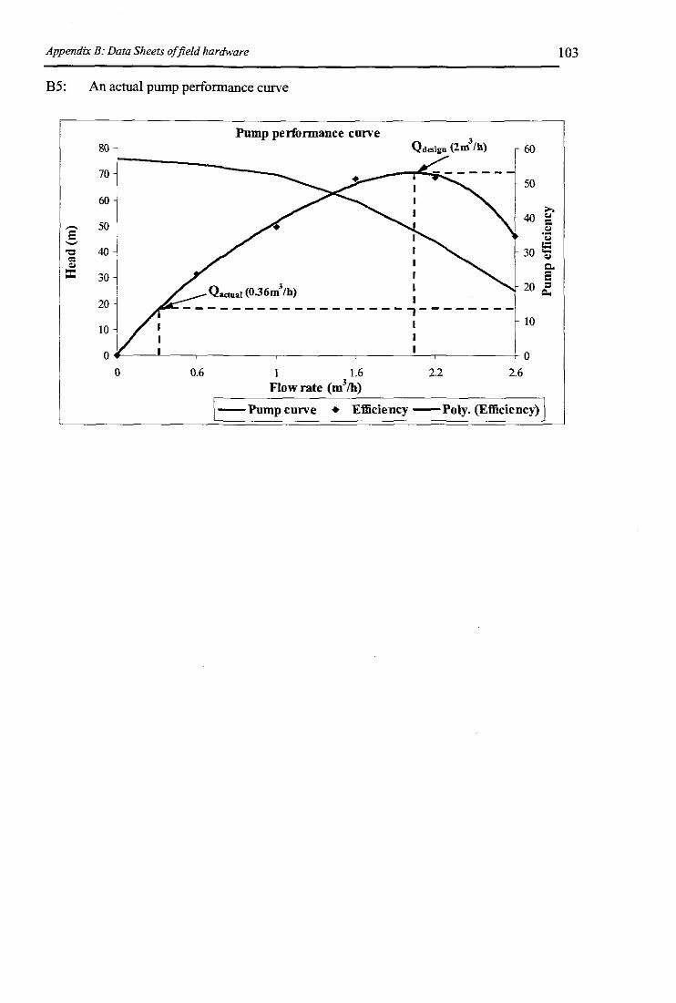
Appendix B: Data Sheets offield harmllare 103
B5: An actual pump performance curve
3Qd",'gn (lm Ih)
1 1.6Flow rate (m3/h)
Pump performance curve
0.6
1-Pump curve + Efficiency - Poly. (Efficiency) \

Appendix B: Data Sheets offield hardware
B6: The specifications ofAerocomrn (AC4486) Transceiver
104
Performance AC4486-5 AC4486-500 (pending)
Interface 20-uin mini connector 20-nin mini connector
Serial Data Rate Up to 115.2 Kbps Up to 115.2 Kbps
Power Draw (typical) 35 mA TX/30mARX TBD
Channels Uut02 Up to 2
SecuriN One-byte svstem ID One-byte svstem ID
Radio Frequency AC4486-5 AC4486-500 (pending)
Frequency Band 869.7 - 870.0 MHz 869.40 - 869.65 MHz(software-selectable) (EU5mW) (EU500mW)
Modulation FSK FSK
Output Power 5mWfixed 5 mW - 500 mW variable(wl 3dBi antenna) (100% duty cycle) (l0% duty cycle)
Voltage 3.3V - 5.5V 3.3V nominal +1-2%, +1-30mV
Sensitivity-96dBm -96dBm(@ full RF data rate)
Range (typical, depends on Up to 3,000 feet Up to 20 milesantenna and environment) (914 m) (32 km)
EmironmentaI AC4486-5 AC4486-500 (pending)
Temperature -40° to +80°C -40° to +80°C
Humidity 10%- 90% 10% - 90%
Physical AC4486-5 AC4486-500 (pending)
DimDimensions 1.65 x 1.90 x 0.20 inches 1.65 x 1.90 x 0.20 inches(4.2 x 4.8 x 0.5 cm) (4.2 x 4.8 x 0.5 cm)
Weight <0.70z«20g) < 0.7 oz « 20 g)
Antenna Connector MMCX jack or integrated antenna MMCXjack
Certification AC4486-5 AC4486-500 (pending)
Approvals CE Approvals pending.
Meets all safety and emissions
SafetyMeets all safety and emissions requirements but requires
requirements. separation from the end-user toadhere to safety standards.

Appendix B: Data Sheets offield hardware 105
B7: The specifications of Samba GSMlGPRS modem
other feahKesSM. FD. LD. MC RC. ON. ME +SIM phone
book mancgemenlFixed cfa[ll1g number. SIM too'kit elms 2511\1. net",'C!1< cnd service provider rocksReal time dockAIann mo,'lQgemenl
UCS 2charactersef management
Basic featuresTelephcny ITCH/FS) cnd emergency cans;
full role. enhanced fuU rate. half ralecnd adap~ve mui:i rote (M~R). duo' tonerrnJJ freqL.'ef1CY furdon (DTMF)
SMS IGSM ond GPRS mode): fext and PDU.
paill to poinf MTand MO. SMS troadcaslGSM cicu~ dota feot'Jres: ITon5p<.Tent and ron
ironspcrent!JP 10 960:) bps. goop 3: d:Jss 1.cIO£i 2. olernate speech and fax. M\lP 2
GPRS packet dala features:data dowrlbk transler: max. 85.6 'Kbps;
data up!ink transfer. max. 428 !<bp..<;
cO(f.l1g schemes CS-l 10 CS-4WAP comp!ianrond compfantwith SMG 31
GSM supplcmcntay services: can iorw'arding.
cm barring. mulf;party. call waifi.ng andca] hold. co[ng Ene identity. amiceofcharge. USSD. dosed user group
E1eclrical chcroclerislicsPower supply: +5VDC (trOl.Jg<'1 USB portl
GenefolTr'-Bond GS,'NGPRS modem
E-GS.\,1900 I DCSI&'XlI PCSI900 MHzCIc,--s 4 !2WI !or EG5M900Cia,; 1(IWj!orOCSI800/PCSl900Sma!f .size and low power consumption
Voce.SMSFax and data tronm1ission wTihout exta hcro\v::reinterno!3 VSlM interlaceEasy remote control by AT commands for
dedicated cppkmionsf'Jry type approved accorcflng to
GSM phase 2+ specfficaiionfury shie'ded cnd ready-to-use
Physical characterislicsDimensions: ILxWxH)
88.7mmx37.6mmx 12.6 mmWeight:79gNormal range fempera!lire: -2O"C to +55"CRestricted operation:
-2S'C io -!JOC cnd +SYC 10 +7O"C
InterfacesSingle antenna interlaceInferno! $l.IoJ, interfooo: 3VonlyUS8serial [nkHeadset jo-.'i:Frrmv.ue upgrade:
over USB lnte1fcce cnd SlM cerd

Appendix C: Data acquisition data sheets 106
Cl: Specifications of DATA TAKER 605
TfnIperature• n~"!1OOCwpl'I1P"'B.C. D. E.G.J.I.N. R.S~I v.ilhcolCJun<1i'"ffiI1lIl"IlSJ'<fl and \ine:lrWJjon.
• P!JJJnum tmls. «-0.00385 &0.OO3916!l·n~c.3D1RSlst1·1\1<:k<1 RIDs. a..o.OO500lfl/Orc. an] !1'<lsl"""-".• Cow< RIDs. «-o.OO39U'nrc. JrI)' res&ll>:e.• Therm!sto<s.YellowS~Y5I 4llliI "'fie<..• SemJcondud0r5. AD5!lO.lM335. UI3-l and I.MlS.
T"mle ;lnd D31e• Re>oJo,lOIl 1sea>r>i,ttur.l<)' 2 Sl'«JI1d!jd:ly.• D"'e inDD·1.!1\!)lYi. MU1lD/ll1T. d:rr nuniler;and deem• Ume In HIiJ,C,l5S.SKorulsSSSSS;nl declmJ! boo[ HRllHl• ~ 3Jto-inrr"""wng lntmnl'lnkn (second. mill"'. hour ;)I
,hm} loruse in"'luencing.:Jl.lrms. Gllcul:lllOllS. elC.
• Real.~dock U'>l'd hr SGm s:heWling.!beonllim. slamd1Ia. alann timing and in calculJ rions.
Digital Outputs• ~ mtMos cornp"tJb"'~ 0.1"'" chJnnolsror 5'\1Icb€d
outputs. rehy clJ{I[Io!.31:mn annundftJn, sensu< "'P!"'n• Open colleclm lines. ""eel 10+ 30\1lC (? 200tn....• DigJlJl «"f'l'S.mwtb the digitJilnfd~• 3lllJs. ds;Jbyb.lck~ ;nj beeperon the diSPb! JU"l• £xp:>trJon by <'Xt<>rJUI mo<Mes.
~ lJnib R""olu,;::25,(.))') m. I~V
±250.00 m\' IC\JV±2500.0 ID" IllOiJ\%100.00 V IOmV=02500 m~ 200n.'::tZ.500 m~ 11'-'±ZiOO ...\ IIJIL'
Ally rang.e IIlA010100 Permll O.OI'1C10.000 Ohms 05m£100.00 Ohm.<; 5rnUJOO.O Ohms SOrn!:
70000 Ohms 500m!0.110300.000.0 Hz 0.0018
:?>O.OOO I!); pSer IpS·250.010 lBOO.O DegC 0.1%·~!Olllo 3200.0 Degf 0.1%
-104 10 104 wm Ippru
.10510105 wm IDppn
.!O6 1O loG wm lOOpp0.,,1 StlIe Ill~> 15 Sl:lte I
0.00 ID 1.00 Sol. 0.010[065535 Coon!' I()to 655lS (WIllS I
0<<1 Sue I
Digl1JI BitDi:lilJI R~e{4 blIs)DIgibI A'ierage
Temper.llUre
frequenqPeri«l
Ranges'nl'" T,pr
DCCUJmIr1nternJ1 ShulllS
4-20lllHoopR05IS4UICe
DC ,olege
Th. DJt:ltlk..-305;md603 an> mlcroproc""",r~ t>ou.rypo'/.ered dJt3log.,~ '.<hI;: hmrosurelnJAllS from ",o<I_r types.AroIoglnplll cl..."""" Jr. reJar IIJIlltipe>:ed. prmi<ing hlgb...vlllt>g.m-easorrmml r:l!l?~(ornm:m mode nnge;m:i toJer.JtesLug... "1lhsl.1n~ "'Juges th:ul fuwker 5OO.nI 600.Ibt1~n IJltludes=ir:>llunctlom. r:>lculJtiorn:llld:lE'lISOr dJbr.1tion fun i$ :stated in boltery lal<ed RUI .nIrtmot:lbJ. Dk'Il1OlJC3rds. Almnsc. be"" (or allc~1s.The~605 has:.I lnlegrJI dlsfby;md k!1P>d.Sullob1etors<lentilk. indu5lrlal:u>d pdJlit ulillly ~pt:lla1lons.
AI1;llog Inputs• ID diJl€n>nllJ! or 30s~ ended. Qn be U'>l'd in anyl!lll..• fxp=;ionby e<I€IlI.Jlnolules"iIh III dill€fel1lbl or 3Oslng!e
ended =I<lg IIlJ'lI ch:me". &I:nimum rv.o modules supp<ll'Ied.• Au,ocalibr.Jting.nIOUJor.mging. 4 <!«:Jdl?s.• ReIOlution 13 bu (illS slgn. lilY.• 5:lmplirJgr~.. ZSs:llJlpks!Sl'Cond.• !"'ur-mb<'ller1h:m 0.15% o!lull sr""'-• !lnezllj better th:m 0.05"0·lnpullmpe<bntemn.or >lOOMn~le.• Common mode onge:dOO\llC.• InpuI"itfurandIngroltJges 101"amlog dDnneIs
• U_l«Lod <h;nr).'1s •± l.5E\llC lor 1()pS·±500;1lC lor 50rID·±IOO;1lC <oo_ly
• Selecte<lckmtls .± lOO;1lC colllino>uSly• Common mode njectlon >rodJ.lllldb I)'picl• Series tOO<ie lJne> r<'jertiOll >lSdb• 5eIIsor <:'(Cb"n ci SV. Z50Op.\ er l.500mA each <bmnel.• 4. 3 .nil \\ire resistance. RID:md ,hi'rmiSlOr nrosarretlI<'I:.• fulLJuI!:lnd qwrterbn:lges. mltJge Of CUITenI emtltion.• Reby multiple.ter.
Digital Inputs• ~ TIValOSCOl!lfO'ibltdigitJlinpll ch:Jrnlel>l:Jr~stJIe. b!'".
ffiDlS >Dd 10... spe<rl 00II1llets I0H:t.16 bit.pr~le.• DlgitIIlnpw slnn,itIJ digltJI outpul dl:ll1llds.• l"JXlllSiOn by exl€lll.JllIlOdules.• 3high 'IJ"-"l CO'UJJl€lS. IIHzIlOl1ll.1lly. <lI' l~lHz oplio'DII!
J6b•.~I•.• AIulo:J cbaRnels :>loo read di,,"iIOI !Ue. us..- deIirohle threshold.

Appendix C: Data acquisition data sheets 107
Network Communications• RS.J85. y;jd",rur crxr,etIng prclocol.• COIlO'frOO It!, "'1st,J p3Jr.1lmlIwru 1000 n>M'S,• Up io 321o:k'"E!fS GlD be in;] I1:Ir.nker nl't"Aoor1(. ~iIh 01lf" OOSi.
Power Supply• Voqe 9-1 SW: or 11- 2H'DC""mi po_.• Mains p<J\w,dfrom 12>',(;DC mJins,dJjxor.• JuJlOOJ:J1k::1!1y S<'Ie<1S k..p<J_ sondb!' (sleep) modo.• Cuma drJ\\' lZOmI IlOIDlJ! p<J'oI'erIIlOd<'. 4OCm~ v,hP.n dtlfJ
lntrnnlbJIII'f), d'iOp.\ Imr po_ (sl.ep) mode.·lnI€rnJll.2Ah gel cell hJtter} redl3rg,d by exterml p""""• Appro<imJre botrl'f) lie foe dlferent sdJ'iLles ond b'IIeIJ SiZ<
Ml'Cbanlral Spedficatlon• R1Jffi<I "",<Lt", rolJSllU(1jon~ powder COOI,d Sleel• C;][J be u:;ed dlrroly. Of hoosed III fl.'ed Of pon:lble encmures• L'ngth 270nun (10.5 inciEs), \\1drh IfOmm (U indl."S).• Height 85rnm (33 kJche,;) \\ilhm trfllDIJ r.rrd Inserted.• Height 105mm (1.2 me,",,) "'!lh,m?fIlOI)' c;lId _n,d.• W,;gbr 2.4Kg.• Signalli(J CornctloD by ,.,..,..1ermInJ!s.• Ojx1:lllng temperJill'e -20 to 70 °C. humidity 95~~
Acceswrief> locloded• 1l0i24O\.'\[1J1JllJ:>lln€ IJO'Ier:xlJptoc• l.2Ahgel eelllnterm1!XJ1tery.• RS232 COOlIWDiGrtIo1ls c;ili., for IDW" and compotlbl",.• GeIlillgStlrtedMJJltlJ! >od U.,r's M.nJ:tl• ileTern1id rn::ace pocl<;t,,,,, for IBM'" and compatibles.
Options• Clt:lnoel 'XjIIIt:S!OD In<>dules with 10 diff,raruo!i30 single md,mog lnptIl>, JIld 20 dgItJIlnput>, llId 10 dlgilJI QUtpl15.
• Portable C1IlJ cose. cbmsl"n rEslgn. \\''"'''IJm1 OPE7, NIMi·lo:lusrrbl qualliy sWendo=es (fP6'i, IDa 5).• ,t!,h rednrg:JbIe gel cell or 17Ah olktn.. b:lllell'• &lKDataraler IJlflI1UIj canLslores 16,000 rEadings.• 25!iK fuiltaker lllemo<J canl. stores81.000 ...~• 5121 PCMCH 1Ilf'll1000canl. stores 170.000 reading>.• lM PlJ,ICU memO!} card, sI<res 340.000 rwn&,.• PCMCU IIH'IIDIJ canl;rl,ptoc• MeIIlOI} C3Id m.len.• Com:ruroiotlom 001£ fir .\W.MadJtosh"".• DeCipher Plus so!l'l,,,. pock:Jge for IBM'" Jlld eornp;tlibles.
Ordering• DJtltJlmwltlt dispby Droll5• !J:rtaJJker"ithOOl dispby DT'Al5• Clt:lnoel"'lpJIIS.ion 1OO<Lt, ([fJ• Prnable ClIlY cos, PE• SruJIl indu5!J'bl eIldClSllre SlI• l",ge indu.stti.1f enclOlUre liE• SruJIl irldu5trW Clbin" SlC• &lK IJataraler IJlflI1UIj card MC.(i4• 256KDalatakerlllWlOI]Card MC·256• 512XPCMCl~mernOf}rnrd MC·512P'lMPIJ,n~mernorJcnrd MC10Z4P• PCMCU melllOlJ canl ;rl,ptor MC·ADP• MernCllj' Card Rrotler -RS232 Interlaco MC-RS• MernCllj' Card Rrotler -CetJlfonir:s 11lIerlace MC-RP
Scanning Input Channels• 11mm'dl:lte "'Jnschedul2. ""' include 0"" or m"", cllJnne3.• 4repetiIlI'escan scnedules. CJJIlJK1udeOllO orOXlfl' cJnnnels.• TlJIle lu<e:l ~itllDcremen1li ri I S«.11llh I oouror 1d:lr.• E,.em bJsed <cJImitlg 011 dlgitll or roIJOter ch.wleI ",erns .• PoIIlused~ iniIlJIed by host requ£SlS.• CoruIitiIlllJl scJlllliI1ll\tIile ""JdglJI infAJlls~
Dala SGlling• !lrt:I ,,:Id from input ch1nneIs ill.erms 01eleetrid UllilS ClJl he
=led to ~eert:rg units. All <llb lllillIipIIJ:Ition l> lbrn pemrmedou Ihe scJ!ed dJlJ.
• Up 1020 defiKlbl.lineJ 5jDIl~ ded1ml ""'!'Ec<><JnlllJl'"• Up to 20defiKJble poI;mo1ll1Jl5,!mm IsI 10 5th order.• Other [onrnof.,osorcab'bcaJrn Clll he irqlIetllffileclusing
m3IIlerrot!CJ1 €IJlfffiIDlIS.
Data Manipulation• S!Jl~ dJiJ iudu1lng '''J:ll!,'' >t!lJ<Ud ooi::llon. mlDimum
and 1I1JIlnum \\Ith die and time rimln and mIlL and inlegr.J!.• De~ role ri dell:1 (diEemtiJl) and hrtegd 1Jm,.,.,.=.• ffistc.gr:un. vAlh dEfinJlJle nunJher ri cl""'"• E."IJf",,"on eclJ:rtIon~ clnnnel t!XI Jru1 ron<.tJms. QfilMleli<:.
logll:;i mtd rebJlJrJJI ~.1og.1tlg, and iXher fumloos.
Alarms• Alarms for mor1rorltig ~ut chdllIle3 for high and kJ", ohtm
iMIde Jod outlirle ri r:lflge JlJrnL Viih dffidle s?tpoints.• Alarms can he conlbinedby Ar.D,OllandXORopetaJ=• OpIIowl delay period before Jfioulofrnnge conditionis
cooslder.d J Iru. o!:Jr.n. or""""'l'COlliicl3ro atr1lererovelJ'.• ,\brms can s'li1lch digid ou!puts &dtlp!Jj· p;metlIDs. returD''''
10 the basl. trig,,""f sCJJUlitlg. Jlld exentle fl:n:IJ];er cOllllllJllds.
Data StlJGlge• Il.Jrll'f)blCkedinlemJ!R.~i ..oresup., 13.650reulin~• R€IOOI:IIJI. memo!)' cords. stor'IlJ'IO :>IO.OOOreadiJl;l.• SIilci<<lI1ddrcuJarOOlfer (",,,"wrile) d1n ~oJ:ll!,l'rnodes.
• No dJiJ 1= ,,1>:'11 mi'lOOfJ e:trds ore exchJng?<!.• SI""" dJ.I:l "'" be ret!Jflled for indl1'irltd SlJllIIlngschedrJl<s,
and for sel'ctlbJe dJte and tkne periods.
Data Fonnat• .'.ll <llb In ASCilllOOlIng polnlfi:<€d p<J1ItI Of exponenllJl follllJ!S.• !lrt:I tltmJIis u.",. coofigur:t1lI' for ch:mel id'l1tilic3tiOn. dJTJ
resoltioon. tIniIs"" om delitrir""• SElectliJle b05l COIIllJUtE!' am fomJJl \\11h IJ;.tfirectiollJl error
dE\roIonl"otllCol.• Comp;llibJe with spreaislre>. gqDi< JlI! stJtisticalpxbg~ .re:.• Comp;rtibJe",lib IlXJ>I romput= nrxletrn. GHlm, JlI! satelli1e.
Progr.mIDling• Allpr~i' bj 5lmpIe 1koctij1lW commands. which",.
enreredfrom 0 host ooroplller,i:l tll!1 saIaIinl<lfac,.• CDI1lII11lIlls ""' b' p<o-ffi:orded ilOO a melllQl} cord. >Dd these
are aJt01IDlldlyex_ed lih""""" m"""" C3Id ls _rted.
Display and KeJPad (mOOS only)• rm type, 2WI 16cb=cr~hJddJr.:JI~.• IJlsrOls chonnel rb:t. JlJrmSl:llUS ondSJSlffillllfortroliOll.• :; key kennlfor dispbr selection. scrolling. to::klighL• Kojp:td also prond. 1user M:rohle fmdioD k'l"• HIlls, beeper and lLshing Indlght flU'iJe~fir ahrrrK
Host Communications• RS232, full durie:<. "\150 SIlJ'1"CIS R-"423• 300.1200. Z400 and 9600 """d. ""lrcbselecrabl€.• Bl-tfirecrlooJl XO!!'l1lfF prolQfoL• CcmpalibJe willl mmpoters.l'rrlliiok rncxlGm.,.mme ground
lffiIlIo:I;jfs, sl'fl3l fI1n'Er~ ete:.
s:liripG~ mebJ_b """y
(OlDlnnOusly
IlJ1lnu1'15 mimJres
1hour
LZAliCol ColIIlarlKy
5i1o..,fS12 dJj,60dJj,110 d:ris
11 Afi Allcilio(B3.IFry3dJrs
160 dJj,SVOdJj.1I00d:Jj,

Appendix C: Data acquisition data sheets
C2: Specifications of flow transntitter
Digital Flow Tran~mitter
for continuous flow measurement and batch control
Technical data
108
Type 8035Plastic-INLlNE
General dataPipe diameterMeasuring ranges
Fluid temperature
Ambient temperatureStorage'temperaturePressure ratingMax. fluid pressureEnclosure
Measuring rangeAccuracy
Repeatability
Display
FittingSensor holdeiPaddle-wheelAxis and beatingO~rin9S
HousingFront plate foH
from ON 15 to ON 50 (112- to 2-)as from 1 IJrnin (ON1S pipe. 0.1 m/s flow velocity)as from 0.3 gpm (1!2~ pipe, 0.3 fps ttow velocity)
PVDF: 0 to 100"C (32 to 212~F)
PP: 0 to ao·c (32 to 176'F)PVC: 0 to 60"C (32 to 140"'F)o to 60"C (32 to 140~F)
~10 to ao'c {14 to 176'F)PN 10, 6 bar 1235 psi)IP 65
0,1 to 10 m/s (0.3 to 32.8 fps).< 1% within 0.5 10 mls (1.6 to 32.8 fps) r)<;; 5% Within 0,3 0.5 mfs (La to 1.6 fps) n0.4% of measured value n15 l( 60 mm. 8-digit leD-display. alphanumeric,15 segments, 9 mm large
PVC / pp I PVOFPVC I pp I pvDFPVOFceramlcFPM standardPCpotyester
(1 In reference conditions (water, 2trC, ideal installation)
Specific data Flow TransmirterVOltage supply 12...30 VOC
Option: 1151230 VAC power supplyOutput sign.al 4...20 mALoad max. 900 U at 30V
mal{. 500 Q at 24Vmax. 100 0 at 15Vmal(, 800 n with power supply 115/230 VAC
Pulse output Open collector NPN and PNP. 0...30 V, 100 mA, protectedOption: relay Reed closing 0.' sec.• opening depending on flow rate 0.1 sec. min.mal(. 34 V. 0.2 A.
Relay output (option) 2 relays. freely programmable. 3 A. 230 V
Specific data Flow SwitchVoltage supply
Re(a~ output
12...30 VOCOption: 115/230 VAC power supplyfr~y programmable, 3 A, 230 "
Digital inputSDigital outpu1Relay output
Spec:ific data Batch ControJlerVoltage supply 12...30 VDC
Option: 115/230 VAC power supply4. i...,puts. 5...30 VOC
1 i.nput, Open collector NPN and PNP, 0.•.30 V. 100 mA. protected2 relays. freely prog-rammable, 3 A. 230 V
Specific data Stand Alone (Battery)Voltage supply 9 vac battery supplyAutonomy 3._4 years with lithium batteries
1...2 years with standard batteri-es

Appendix C: Data acquisition data sheets 109
C3: Specifications ofpressure transmitter
2. EleIttrlscher Anschluss IWirlng I Branchement eJectrlq
2-Lel1ers'/1ll1! 12-w1nl_1SystOm& It 2.fi1s 3-lellenIystem1_ system 1SystOm& /l3-fiIs
® ® OlN.c3650S~
DIN 43 650 DkJ9~0lN43:6S0
® -=-=-=
@ ~<'l3~, 4-p:Igr.a~Mr2111
i....o:ci.'TvJ:dUg4~
~Ml2..'""~
1-0: ~~"&-
~r~-'~~ U,,~ '"
f .~ ..; 'l"!'~~ ws. {21
[!'! s;gr.al , S9"I de """"
~ CETransmitter S 10
0_•• 10 ...... ... 20 ItJA
~DC1.",.... 1+ 2-
N ft&3g110
.,!!~-~.--- •Hiifr"~/~,,~j~
5 f: fabrik-Nr. f~ No. i No. Woep *". ErzoorPs-Nr... ProdIJd No. i cooe At1Jde
3. Z"b.hiir I AA"",_:lrieiessl AcceuoIres
G-1.2~l·weld-en ac\aptOtJI&t'l'mse asouder
Gl." ~f3ad41iw!.eJd-onadaptor terrmase it souder
Gl,'2m1Q.-:Jichtungi'~J"'~ toliqUe
G"Ii"l~!~ng/Wl~lofi(J.le
G 1.22~ rnax- .400 t:ar!Throttle. max. C bar IG 1.-2 Rat:m;d. arro'r,maL 400 bar-
00-
,,
11 922991192264
90920999092161
1604791
90 91262

Figure S. L1·200SZ Spewnl Re,ponif<: Curve.
'iEI"r~mffif'~mmm !lmrr. TiIlFin)ffiffi3 ~~!t I!g ffi[~~im\fi i,W ~!rn~;j w,ljli~
.."'lili~I~1 '~
j
~±'.~h~::'~ ~'\1·'''''''·
I
!
I
SI'I':CIFICATIOSS
C.Ubr.tloo: Calibraled ugaln,' an Epploy Preci'ion SpeclralPyrnnomeler (PSP) undor nalarol daylight condition,. Ab,olule elTor underOlese conditions), ± 5'l> maximum,lyplcally± 3%.S.n'IlI.lIy, Typically gO IJA per 1000 W m·l•L1n.arlly, Ma,imum devloUon of 1% up 10 3000 W m·2.Stability: <± 2% c1l""80 ovcr' 1 yClll period.Respon,e Time' 10 lJS.Temperalurr Dependence: ± 0.1 S% per ere maximum.Cosine Corrtctlon: Cosine corrc.cled up to 800 angle of incidence.Azimuth: <± 1% error over 3600 at 450 elevolion.Tilt: No errcr induced from oricntntion.DNcelor: High stability 'i1icon pholOvollaic del""IOr (blue enhanced).Sensor Ilouslng, WeatherproOf anodized aluminum case with acrylicdiffuscr ond slllinles. ,:eel 1Imdwaro.Size, 2.38 010. , 2.5-1 cm H (0.94" , La").Weight: 28 g (l oz.).Accessories: 20035 ~founling and Levering Filllure.Cubl. Lenglh: 3 me"'rs (10 ft) standutd. U·200SZ·50; SO fl.
nI ~
~ '"6..~>;'
0 f)~ t?'" "~
'" ~'" ~'"'g, s:t'"' ;"...... 0,
~n 1}0?" "'"'1:l "'"1 "";;
~
~ ! a a a a •............o
JtrNO<IrJtI INln'" JNT.>tlJ4

Appendix D: Experimental results III
Experimental results 24/08/04 - 30/08/04)PUll 1nl P. Mot
Uate 'l'ime 1~low Irradiance MoVol Vol Press T.mp t.mp Shnt Shnt IIdYII III Plrr Parr Peon PlIlIlI\n I£ll'arr f:Ucun (msvs l~nuver E[[pu
8/24/2004 11:00 17,7 762 83,9 84.3 3,1 18,0 21.9 0,14 0,14 0,0 5,0 2256 117 114 14,5 5,2 97,3 12.4 n.6 12,7
8/24/2004 1/ :30 18,1 821 84.3 84,6 16.5 18,2 22,2 0,14 0,14 0,2 5,1 2430 117 114 15,2 4,8 97,4 12,9 0,6 13,2
8/24/2004 12;00f-4~
8(,6 83,6 83,9 9,0 18,4 22.4 0,14 0,14 0,1 5,1 2564 1/7 114 14.4 4,5 98,1 12,3 0,6 12,6
8/24/2004 12:30 17,8 890 83,7 84,1 0,9 18,6 22,6 0,13 0,13 0,0 5,0 2635 112 110 14,5 4,2 98.4 13,0 0,5 13,2
8/24/2004 13;00 17,0 901 83,6 83,9 0,0 18,8 22,8 0,14 0,13 0,0 5,0 2666 114 112 13,8 4,3 97,9 12,0 0,5 12,3
8/24/2004 13:30 17.4 887 83,9 84,2 18,3 19.0 23,0 0,13 0,13 0,2 5,1 2626 114 III 14,7 4.3 97,7 12,9 0.6 13,2
8/24/2004 14;00 17,7 857 83,8 84,3 5,7 19,1 23,2 0,13 0,13 0,1 5,0 2536 113 III 14.5 4.4 98.4 12,9 0,6 13,1
8/24/2004 14:30 16,8 808 84,5 84,8 0,0 19,3 23,3 0,13 0,13 0,0 5,0 2393 113 109 13,6 4,7 96.5 12,1 0,6 12,5
8124120114 15 :Illl 17,8 745 84,2 84.6 6,1 19,5 23.4 1l,14 0,14 0,1 5,1l 2206 1/6 114 14,6 5.3 98,1 12,6 0,7 12,8
8/24/2004 15:30 17,6 665 84,0 84,3 0,5 19,6 23,5 0,13 0,13 0,0 5,0 1969 112 110 14,3 5,7 97,5 12,7 0,7 13,0
8/24/2004 I (,;{jlJ 17,5 568 83,7 83,9 0,0 19,3 23,5 0,13 0,13 0,0 5,0 1681 III 108 14,2 6,6 97,3 12,7 0,8 13,1
8/24/2004 16;30 17,3 460 82,0 82.4 0,5 19,0 23,4 0,13 0,13 0,0 5,0 1363 III 109 14,0 8,1 98,3 12,7 1.0 12,98/24/2004 17;00 10,8 329 50,6 50,8 10.4 18,8 23,3 0,11 0,11 0,1 5,1 974 56 54 8,9 5,7 96.5 16,0 0,9 16.6
8/25/2004 8:30 7,2 212 34,7 43,9 30,3 15,7 20,2 0,11 0,14 0,3 5,3 628 50 48 6,2 7,9 96.6 12.4 1.0 12,98/25/2004 9:00 15.4 338 78.0 78.4 0,0 16,0 20,3 0,14 0,14 0,0 5,0 999 113 110 12,5 11 ,3 97,3 11.1 1.3 11.48/25/2004 9:30 17,0 471 81.5 81.9 15,8 16,5 20,6 0,14 0,14 0,2 5,1 1395 115 1/3 14,2 8.3 98.4 12.4 1.0 12,68/25/2004 10:00 16,8 585 82,9 83,1 0,0 16,9 20,9 0,13 0,13 0,0 5,0 1731 1/2 110 13,6 6,5 98,7 12,2 0,8 12,38/25/2004 10:30 17,7 698 83.0 83.4 0,0 17,2 21.2 0,14 0,14 0,0 5,0 2065 115 113 14,3 5,6 97,8 12,5 0,7 12,78/25/2004 11:00 15,5 658 82,0 82,3 0,0 17,5 21.4 0,13 0,13 0,0 5,0 1949 109 109 ~- 5,6 99.9 11.5 0,6 11.68/25/2004 11:30 17,6 879 85,9 86.2 2,0 17,7 21.7 0,14 0,14 0,0 5,0 2601 120 118 14,3 4,6 98,5 12,0 0,6 12,28/25/2004 12:00 17,2 871 83,3 83,6 15,5 17,9 21.9 0,13 0,13 0,2 5,1 2579 112 III 14.4 4,3 98.8 12,9 0,6 13,08/25/2004 12;30 17,2 896 83,5 83,7 14,1 18.1 22.1 0,13 0,13 Il.l 5,1 2653 113 \08 14.3 4.2 96.3 12,7 0,5 13,28/25/2004 13:00 17,5 901 83.4 83.6 11.2 18.3 22.3 0.13 0,13 0.1 5.1 2666 III 108 14,6 4.2 96.9 13.1 0.5 13,58/25/2004 13:30 17.0 885 84.1 84.4 0.0 18.4 22.5 0,13 0.13 0.0 5.0 2620 113 110 13,7 4.3 97.7 12.2 0,5 12.58/25/2004 14:00 17.5 858 83.4 83.8 5.2 18,5 22.7 0,13 0.13 0.1 5.0 2539 112 109 14.4 4.4 97.2 12.9 0.6 13,28/25/2004 14:30 17, I 812 84,1 84.2 0.0 18.7 22.8 0,14 0.13 0,0 5.0 2403 114 III 13,9 4.7 97.5 12.2 0,6 12.58/25/2004 15:00 17.3 751 83.8 84,1 0.0 18.9 22,9 0.13 0,13 0.0 5,0 2223 111 110 14,0 5,0 98.7 12.6 0,6 12.78/25/2004 15:30 17,3 624 83,6 84.0 5.9 18,9 23.0 0,13 0.13 0.1 5.0 1847 113 109 14.2 6.1 96.4 12,6 0.8 13.18/25/2004 16:00 16.9 471 82.7 83.0 14.4 18.7 23,1 0.13 0,13 0,1 5.1 1393 110 109 14,1 7.9 98.7 12.8 1.0 12.98/25/2004 16;30 17,1 471 82,1 82.5 16,7 18.6 23.0 0.13 0.13 0,2 5, I 1393 109 108 14.3 7.8 98.8 13.1 1.0 13,3812512004 17:00 111.8 333 50.4 50,7 11.3 \8.5 22.9 O. \ \ 0.11 0.1 5.\ 937 56 55 8.9 5,6 99.0 16.1 0.9 16,28/25/2004 17;30 3.8 182 19.6 43.7 34.2 18.2 22.7 0,06 0.11 0.3 5.3 540 28 22 3.3 5.2 79.0 11.8 0.6 14,98/26/2004 8:30 6.9 202 33.4 43.8 38,5 15.3 19.8 0.11 0.13 0.4 5.4 598 47 45 6.1 7.9 95.4 12.9 1.0 13,58/2(,/2004 9:0{) 13.7 306 69.2 69.6 33.7 15,6 20.0 0.16 0,16 0.3 5.3 907 110 108 11.9 12,1 98.5 10.8 1.3 11.08/26/2004 9:30 15,6 457 81.7 82,0 0,0 16.3 20.3 0,14 0.14 0.0 5,0 1353 112 1/2 12.6 8.3 99.4 11.3 0,9 11.38/26/2004 10;00 17.3 568 83.1 83.5 14.4 16.6 20,6 0.14 0.14 0.1 5.1 1680 116 114 14.4 6.9 98.4 12.4 0.9 12.68/26/2004 10:30 17,2 663 83.9 84.0 0,0 16.9 20.9 0.13 0,13 0,0 5,0 1963 113 112 13.9 5.8 99,2 12,3 0,7 12.48/26/2004 11:00 17.5 744 83.7 84.0 14.5 17.2 21.2 0,14 0.14 0.1 5,1 2202 115 114 14.6 5.2 99.3 12.7 0.7 12,8

Appendix D: Experimental results 112
17,51.816.916.3 99.915.25.5 2666 120 1180.50.224.9 0.221.086.2 53,885.9Mllx: 18.1 901Fluw in lIrnIrrodillncc in W/m2
Motor voltage in VoltsPunc' voltage in VoltsI)ressurc in kPaPuncl sllu'1t voltage in VoltsTotal head in meters('1 ..1' Irradhtncc power in WattsPm array power in WattsPCOII cOllverter power in WattsPllllm/l pump power in WattsEffu arrayellicicncyEffc converter ct1'icicncyEITp pump efficiencyElTs system cflicicncyEcru overall efficiency
8/28/2004 16:00 16.9 564 79.4 79.6 18.4 20,9 24.7 0.13 0,13 0.2 5.1 1670 104 99 14,2 6.2 95.9 13,7 0.9 14.38/28/2004 16:30 16,2 452 78,3 78.5 1.4 20,8 24,7 0.13 0.12 0,0 5.0 1338 lOO 96 13.2 7.5 96.0 13.2 1.0 13.78/2812004 17:00 10,3 332 48.5 48.7 17.1 20.7 24,7 0,11 0,10 0,2 5.1 982 52 51 8.7 5,3 97.6 16.7 0,9 17.18/29/2004 8:30 2,2 53 16.7 43.9 33.9 18.0 22.4 0,06 0.11 0.3 5.3 156 25 19 2.0 16.3 75,0 7,7 1.2 10,28/29/2004 9:00 6.3 148 30.7 43,9 34.9 18.0 22.4 0.10 0.13 0.4 5.3 439 43 40 5,5 9.8 92.2 12.7 1.3 13.88/29/2004 9:30 5.9 122 27,7 43,8 36.9 18.3 22.5 0.09 0.13 0.4 5.3 360 39 35 5,1 10.7 89.9 13.3 1.4 14.78/29/2004 10:00 16.1 419 80.7 81.1 9.0 18,6 22,6 0,15 0.14 0.1 5.1 1241 118 117 13.3 9,5 98.7 11.3 1.1 11.48/2912004 10:30 \6.8 570 81.4 81.8 10.2 19.0 22.8 0.13 0.13 0.1 5,\ 1688 109 lU9 13.9 6.5 99.8 \2.8 0,8 12.88/29/2004 I1 :00 17,1 632 81.2 81.4 17.6 19.2 23.0 0.13 0.13 0.2 5.1 1872 109 107 14,4 5.8 98.2 13.2 0.8 13.48/2912004 11:30 15, I 315 72.2 72.5 1.7 19.3 23.2 0.12 0.12 0.0 5.0 934 89 88 12.3 9,5 98.8 13,8 1.3 13.98/29/2004 12:00 17.0 875 80.4 80.7 17.5 19,7 23.5 0.13 0.13 0,2 5.1 2590 108 105 14.3 4,2 97.1 13,2 0.6 13.68/29/2004 12:30 16.7 612 80.0 80.3 12,7 19,9 23,7 0,13 0.12 0.1 5,1 1811 105 lOO 13,9 5,8 95,1 13.3 0,8 14.08/29/2004 13:00 16.4 76R 79.5 79.8 6.1 20.3 24.0 0.13 0.13 0.1 5,0 2274 104 103 13,4 4.6 99.0 13.0 0.6 13, I8/2W2004 13:30 16,0 845 82.4 82.7 0,0 20.5 24.2 0.13 0,13 0.0 5.0 2502 107 105 12.9 4.3 97.7 12,0 0.5 12.38/2912004 14:00 17,1 797 82.4 82,8 8,0 20.6 24.4 0.13 0.13 0.1 5,0 2360 110 107 14.1 4.7 97.4 12.8 0,6 13.28/29/2004 14:30 15.4 806 81.1 81.5 0.0 20.6 24,5 0.13 0.13 0.0 5.0 2384 104 102 12,5 4.3 98.8 12.0 0.5 12,2812912004 \ 5:\lO 16.8 734 80.9 81.4 7.\ 20.8 24,6 0.13 0.13 0.1 5.0 2172 105 104 13.9 4.8 98.5 13.2 0.6 13,48/29/2004 15:30 16.8 642 80,7 81.0 4.1 21.0 24.8 0.13 0.13 0.0 5.0 1901 104 102 13.7 5,5 98.2 13,2 0.7 13.48/2W2004 16:00 16.9 543 80,8 81.1 9,2 21.0 24.9 0.13 0,13 0,1 5.1 1609 106 101 14.0 6,6 95,9 13.2 0.9 13.88/29/2004 16:30 16.5 435 78,6 79.0 11.5 20.9 24.9 0,13 0.12 0.1 5,1 1287 101 96 13,7 7.8 95.7 13.6 1.1 14,38/29/2004 17:00 10.4 314 48.5 48.7 16,/ 20.9 24.9 0,11 0.10 0.2 5.1 931 52 50 8.7 5.6 96.9 16.9 0.9 17.48/3012004 11:00 4,0 64 19,9 43,7 36.2 19.1 23.0 0.06 0.12 0.4 5.3 190 28 23 3.4 14.8 82.4 12.3 1.8 14.98/30/2004 11:30 7.5 188 36,5 43.9 34.6 19.3 23.2 0.12 0.14 0,4 5.3 558 52 50 6.5 9.2 96.2 12.6 1.2 13.1_. " .... .. - . - - • F •• . . .- -

Appendix E: Field results
Cost analysis to date (2001- 2004)
Total present worth of system
Recurrent Costs
Maintenance
Present worth
Operating Costs
Present worth
Total cost
Annual levelised cost
Unit water cost to date (2001-2004)
=R98,940
=R970/year
=Ax [1-(1 +i)-n ]/i
= 970 x [1- (1 + 0.052)-"]/0.052
= R3,424
= R18,000/year
= 18,000x [1-(1 + 0.052)-, ]/0.052
=R63,532
=RI65,896
= 165,896x[(1 +0.052)' x 0.052](1+0.052)' -1
= R46,967
114
Unit water cost (UWC) to date
Energy cost
Total cost to date=-----------Total volume pumped to date
165,896:0
5,184
:0 R32.00/m3
:0 3.2 cents/l
unit water cost
- total head (static head + head losses + friction losses)
32.00
50
:0 RO.64/m'
= 64 cents/m'

Appendix E: Field results
Cost analysis for 15 years (PV)
Initial costs
Recurrent Costs
Maintenance
Present worth
Operating Costs
Present worth
Total cost
Annual levelised cost
Unit water cost for 15 years
Unit water cost (UWC)
Energy cost
Il5
=R98,940
=R970/year
= Ax [1-(1 +i)-n\li
= 970 x[1- (1 + 0.052r1']/0.052
=R9,934
= RI8,000/year
= 18,000 x[1- (1 + 0.052r15 ]/0.052
=RI94,265
=R293,207
=LCC x[(l+i)SL Xi](l+i)SL -1
= 293,207X[(1 +0.052)" x 0.052](1 + 0.052)15 -1
=R28,626
Annual levelised cost
Q vol:anDual
293,207
3.6x 360x 15
=R15.08/m 3
= 1.5 cents/l
unit water cost
total head (static head + head losses + friction losses)
=15.08
= R0.30/m 4
= 30 cents/m 4

Appendix E: Field results
Cost analysis for 20 years
Total present worth of system
Recurrent Costs
Maintenance
Present worth
Operating Costs
Present worth
Total cost
Annual levelised cost
Unit water cost for 20 years
Unit water cost (OWC)
Energy cost
116
=R98,940
= R970/year
=Ax [1-(1 + i)-n ]/i
= 970 x [1- (1 + 0.052) -20 )/0.052
= Rll,886
= R18,000/year
= 18,000 x 11-(1 + 0.052)-20 )/0.052
=R220,564
=R327,762
1 89 [(1 + 0.052)'" x 0.052]= 33,3 x -'----;----'---:c:;;---
(1+0.052)'" -1
=R27,045
QVOI:1UIDUal
= ---=3:.-3....:.1,3.:..c8:..:.9--=3.6x 360x 20
=R12.79/m'
= 1.3 centsll
unit water cost
= total head (static head + head losses + friction losses)
=12.79
= RO.25/m 4
= 26cents/m 4

Appendix E: Field results
Cost analysis for 25 years
Total present worth of system
Recurrent Costs
Maintenance
Present worth
Operating Costs
Present worth
Total cost
Annual levelised cost
Unit water cost for 25 years
Unit water cost (UWC)
Energy cost
117
=R98,940
=R970/year
= Ax [1-(1 +i)-n]/i
= 970 x[1- (1 + 0.052) -25]/0.052
= R13,401
= R18,000/year
= 18,000x[1- (1 + 0.052)-25]/0.052
=R248,683
=R361,023
= 361,023 x[(1 + 0.052)25 x 0.052](1 + 0.052)25 -1
=R26,124
Annual levelised cost
Q voblDDUal
= ---:3,--6-,1,,--02-::.3_3.6x 360x 25
= Rl1.14/m3
== 1.1 centsll
unit water cost
total head (static head + head losses + friction losses)
== 11.14
== RO.22/m 4
= 22 cents/m 4

Appendix E: Field results
APPENDIX El (b) DIESEL PUMP LIFE CYCLE COSTS CALCULATIONS
118
Period of analysis (n)
Discount rate
Capital Costs/initial costs
Replacement Costs
Total present worth of system
Recurrent Costs
Maintenance
Present worth
Operating Costs
Present worth
Total cost
Annual levelised cost •
Unit water cost for 15 years (diesel)
Unit water cost (UWC)
= 15 years
=5.2%
=R45,940
= R30,780
= R76,720
= R6,638/year
= Ax [1-(1 +i)-n Ili
= 6,638 x [1- (1 + 0.052) ~151/0.052
=R67,978
= R20,859/year
= 20,859 x [1-(1 + 0.052r15 ]/0.052
=R213,612
=R358,310
= LCCX[ (l+i)5L Xi](l+i)SL -1
= 358,310X[(1 +0.052)15 X0.052](1 +0.052Y' -1
=R34,992
Annual levelised cost=--------Q vo):aonual
358,310=
21 x 365x 15
=R3.11/m 3
= 0.31 centsll
Energy costunit water cost
total head (static head + head losses + friction losses)
=3.11
=RO.086/m 4
= 8.6 centslm4

Appendix E: Field results
Cost analysis for 20 years
Total present worth of system
Recurrent Costs
Maintenance
Present worth
OperatingCosts
Present worth
Total cost
Annuallevelised cost
Unit water cost for 20 years (diesel)
Unit water cost (UWC)
= R76,720
= R6,6381year
= Ax [I - (I + i)- n]/i
= 6,638 x [I - (I + 0.052f20]10.052
=R81,339
= R20,859Iyear
= 20,859 x [I -(I +0.052f20]/O.052
= R255,597
= R413,656
= 413,656 x[(I + 0.052)20 x 0.052](I + 0.052)20 - I
= R33,753
Annual levelised cost
Q vol:annuaJ
413,656
119
21x 365x 20
=R2.69/m3
=0.27 centsll
Energy costunit water cost
total head (static head + head losses + friction losses)
=2.69
= RO.075/m·
= 7.5 cents/m'

Appendix E: Field results
Cost analysis for 25 years (diesel)
Total present worth of system
Recnrrent Costs
Maintenance
Present worth
Operating Costs
Present worth
Total cost
Annual levelised cost
Unit water cost for 25 years (diesel)
Unit water cost (UWC)
=R76,720
= R6,638/year
= Ax [1-(1 +i)- n]/i
= 6,638x [1-(1 +O.05W25 J/0.052
= R91,709
= R20,859/year
= 20,859 x[1- (1 + 0.052)-25 )/0.052
=R288,182
=R456,611
= 456,611 x[(1 + 0.052)25 ~ 0.052](1 + 0.052)_5 -1
= R33,055
Annual levelised cost
Q vol:anllual
456,611
120
21x365x25
=R2.38/m3
= 0.24 centsll
Energy costunit water cost
total head (static head + head losses + friction losses)
=2.38
= RO.066/m 4
= 6.6 cents/m 4

Appendix E: Field results 121
COST ANALYSIS OF PV ACTUAL (3.6m3/day) AND DIESEL WATER PUMPINGSYSTEMS (unit & water pumping costs)
~ffi-M"~01":' ~m ; ECi'Y I'>.IC', OH\~ ',,,PW "::ce' . uwc . EeC--"-,,,-.. _i.1 98940' 18970 I 18032 116972 90.256 1.805 76720 27497 26138 102858 13.419 0.3732 98940 18970 35173 134113 51.741 1.035 76720 27497 50984 127704 8.330 0.2313 98940 18970 51467 150407 38.685 0.774 76720 27497 74601 151321 6.581 0.1834 98940 18970 66955 165895 32.001 0.640 76720 27497 97052 173772 5.668 0.1575 98940 18970 81678 180618 27.873 0.557 76720 27497 118392 195112 5.091 0.1416 98940 18970 95673 194613 25.027 0.501 76720 27497 138678 215398 4.684 0.1307 98940 18970 108976 207916 22.918 0.458 76720 27497 157961 234681 4.374 0.1218 98940 18970 121622 220562 21.773 0.425 76720 27497 176291 253011 4.126 0.1159 98940 18970 133643 232583 19.940 0.399 76720 27497 193715 270435 3.920 0.10910 98940 18970 145069 244009 18.828 0.377 76720 27497 210277 286997 3.744 0.10411 98940 18970 155931 254871 17.878 0.358 76720 27497 226021 302741 3.591 0.10012 98940 18970 166255 265195 17.052 0.341 76720 27497 240987 317707 3.454 0.09613 98940 18970 176070 275010 16.323 0.326 76720 27497 255213 331933 3.331 0.09314 98940 18970 185399 284339 15.671 0.313 76720 27497 268736 345456 3.219 0.08915 98940 18970 194267 293207 15.083 0.302 76720 27497 281590 358310 3.116 0.08716 98940 18970 I 202697 301637 14.547 0.291 76720 27497 293809 370529 3.021 0.08417 98940 18970 210710 309650 14.055 0.281 76720 27497 305424 382144 2.933 0.08118 98940 18970 218327 317267 13.600 0.272 76720 27497 316465 393185 2.850 0.07919 98940 18970 225567 324507 13.179 0.264 76720 27497 326960 403680 2.772 0.07720 98940 18970 232450 331390 12.785 0.256 76720 27497 336936 413656 2.698 0.07521 98940 18970 238992 337932 12.417 0.248 76720 27497 346419 423139 2.629 0.07322 98940 18970 245211 344151 12.070 0.241 76720 27497 355434 432154 2.563 0.07123 98940 18970 251123 350063 11.744 0.235 76720 27497 364003 440723 2.500 0.06924 98940 18970 256742 355682 11.435 0.229 76720 27497 372148 448868 2.440 0.06825 98940 18970 262084 361024 1L143 0.223 76720 27497 379891 456611 2.383 0.066
LEGEND:
I'.:;~V'Vactual pumping costs, ,:'- i.Diese1 pumping costs
IC: Initial co,ts in RandsO+R: Operating & Replacement costs In RandsPW: Total present worth of life cycle costs In RandsCC: Cumulative costs In Rands
U\YC: Unit water costs in Rlm3
EC: Energy costs In RIm'

Appendix E: Field results
COST ANALYSIS OF PV PREDICTED (20m3/day) AND DIESEL WATERPUMPING SYSTEMS (unit & water pumping costs)
122
~J(f\Yib~ r1fOiifi~.illp~t ~1:tWb'iJy'E:Cl' le Oi-lil 'PW' k' ", 'UWC'cc·I 98940 18970 18032 1I6972 16.024 I 0.325 I 76720 27497 26138 102858 13A192 98940 18970 35173 1341I3 9.313 0.186 76720 27497 50984 127704 8.3303 98940 18970 51467 150407 6.963 0.139 76720 27497 74601 151321 6.5814 98940 18970 66955 165895 5.760 0.1I5 76720 27497 97052 173772 5.6685 98940 18970 81678 180618 5.017 0.100 76720 27497 1I8392 195112 5.0916 98940 18970 95673 194613 4.505 0.090 76720 27497 138678 215398 4.6847 98940 18970 , 108976 207916 4.125 0.083 76720 27497 157961 234681 4.3748 98940 18970 121622 220562 3.829 0.077 76720 27497 176291 25301I 4.1269 98940 18970 133643 232583 3.589 0.072 76720 27497 193715 270435 3.92010 98940 18970 145069 244009 3.389 0.068 76720 27497 210277 286997 3.7441I 98940 18970 155931 254871 3.218 0.064 76720 27497 226021 302741 3.59112 98940 18970 166255 265195 3.069 0.061 76720 27497 240987 317707 3.45413 98940 18970 176070 275010 2.938 0.0591 76720 27497 255213 331933 3.33114 98940 18970 185399 284339 2.821 0.056 76720 27497 268736 345456 3.219IS 98940 18970 194267 293207 2.715 0.054 76720 27497 281590 358310 3.1I616 98940 18970 202697 301637 2.618 0.052 76720 27497 293809 370529 3.02117 98940 18970 210710 309650 2.530 0.051 76720 27497 305424 382144 2.93318 98940 18970 218327 317267 2.448 0.049 76720 27497 316465 393185 2.85019 98940 18970 225567 324507 2.372 0.047 76720 27497 326960 403680 2.77220 98940 18970 232450 331390 2.301 0.046 76720 27497 336936 413656 2.69821 98940 18970 238992 337932 2.235 0.045 76720 27497 346419 423139 2.62922 98940 18970 245211 344151 2.173 0.043 76720 27497 355434 432154 2.56323 98940 18970 1251I23 350063 2.114 0.042 76720 27497 364003 440723 2.50024 98940 18970 256742 355682 2.058 0.041 76720 27497 372148 448868 2.44025 98940 18970 262084 361024 2.006 0.040 76720 27497 379891 45661I 2.383
LEGEND:
li?~.'PVpredicted pumping costs_~~\i$ni.esel pumping costs
IC: Initial costs in RandsO+R: Operating & Replacement costs in RandsPW: Total present worth of life cycle costs in RandsCC: Cumulative costs in Rands
UWC: Unit water costs in Rim'
EC: Energy costs in Rim'

Appendix g. Field results 123
• I~I"" I~,'~"~., \"" , ...., .... vv 1 l '.n , ...., .... V"·,
inl I' I'uncl shunlJ)l1ll' Timc tcmll nuw rJI'CSSllrl~ lClI1l' SOlllf Irrlld I hi: An'u \'nll Vul \"ollat!c Cutl'cul 11th IltfJl I'nrr Piuc 1'lJlllIIlJ Ellan Erfsn El'l'unl'
12!712004 7:0O:{)O 315 4,H I 434 28,5 2.50 501 50 9.432 J ,23 124.4 OJ2(J O,l)HX OA4 ~O.4 122.9 4724 JlJ.7 2.(1()2 J2 O.H
1217120lJ4 8:()O:(]O 343 4.4(\ 424 30,} (,(IU no 50 lJA32 \, IS 1(5,9 1l.2h7 \J,B Iq 0,43 50A 93.8 31WJ %.K 3, Ill!.) ?,') \.2
12!7120(J4 9:()O:()() 3.ll 545 4.115 30,11 4,03 S07 50 \).432 1.14 115.5 O.70H 2.14CJ (1.49 50.5 247.9 7610 45,0 3257 IX 06
121712004 10:(JO:(J() 322 5.72 5,06 llJ,3 5.01 100l 50 9432 1 16 117.5 O,7l)l) 2420 0.52 505 284 " lJ4eJ.7 ,\7,3 lOIO 17 os1217!2\l\l'\ I \:00\)0 30") 572 524 2'il,(l 5.17 Hl34 50 94:'1 1.l7 11 R0 0.107 2.537 0.53 50.S 29 l)4 'Y755 473 :tOCJl} Ir, 0.5
121712004 12:0000 31.1l 5.73 5.26 2l),O s,or; 1012 50 9.432 1. I\} 119.7 (UDR 2539 0,54 50,5 3D3,\} l)S4lJ ,\73 3 lRo Ir, OS _.121712()O4 13:(JO:(J[J 3 I R 5.65 5.11 2l), I 4,53 9(j(j 50 9432 I 17 11 R.3 0715 2,257 0.52 50.5 267.1 115,12 4(17 3126 17 (l,.'i
12!712(){J4 l'I:(J9~ 291\ 54f1 4.H4 10.1 3/i7 735 50 9.432 1,20 [20,S ()fi22 1.IlR(j 049 50,) 227,7 (l92 l ) ,15,2 12H7 211 07 --121712U04 15:0{):OO 32.3 SOl) 4.32 30.5 2.57 513 50 9.412 1.19 1202 0.407 1.234 0.44 50.4- 14S:1 4H4J 420 3 0(12 2H Ol) ---J 2171200·1 !(,JlI):O(J 34.7 3.9.1 3.(12 30,2 [,35 270 50 9.432 1.21 122.1 0,140 0423 037 50.4 5l,6 2544 J23 2,O)!) (13 IJ
12/S/2004 70000 31.1 4.74 4,27 28.5 2A4 48l) 50 l).432 128 12H.H 0.30] O.91l) (J.44 50.4 ~~,3 4(11 I .19. I 2,5(l7 33 O,X-----12/H/2[)o4 lI:{]O:(){) 34A 5.34 4f13 31A 3,54 70S 50 9,4.12 1.22 123.6 0,527 1.597 0.47 50,S 197.5 (1(182 ,14.1 2 ll55 22 07
12/8!2004 l)',nO',O{l 34.7 5.6(\ H3 J2.1 4A2 &K4 SO 9.4 3-2 I.IH \ 1\1.,4 \UN5 2,106 0.'1-9 50.5 25\\,4 IB4\ '\(1.7 3,0\\2 19 Il.{l
12/8/2004 10:{Jo:OO 35.4 5.73 5,12 31.8 4.% 99] 50 9.432 1.19 [20,6 0.777 2356 0.52 50.5 284,1 li362 47,3 30]5 17 0.5
12/S/2[)04 11:00:{JO 331 5.77 5.16 30,4 5.16 103 I 50 9.432 1.16 117.6 0.1\44 2.5511 0.53 50,5 ]O(),l) 9727 47,6 3.m'l 16 0,5
\21~f2\\\lq \2:\lIJ,Oll 32.6 5.77 5.17 10,0 5.02 lno" 5n 9'D2 I.IR 11l).1 0,826 2,501 05] 50,S 2l)R.l 9470 47.6 3.148 1(, 05
12/R/20f)4 13:(J(l:()(1 323 5f15 50 I )0.3 4.52 905 50 9.432 1 19 120,5 074.3 2252 n,5l 50.5 2714 8534 4(1,7 3 IHJ 17 n.S
12/H/200,1 14:00:00 316 54H 4.74 32.1 3.68 T16 50 9.412 1.19 120.5 0617 1.8(Jl) 04R 50,5 225,2 6939 ,15,2 3,246 20 07
12/1l/2()[H 15:00:00 342 5 13 425 322 2,57 514 5U 9.432 1.21 122,(i 0,400 1.212 OA3 50,4 14X(i 41149 423 )OfJ4 2H ()lJ
12/R!2004 lfi:(JO:[)O 35,5 3.l}3 3,60 319 135 27() 50 9.432 I 19 119,7 0,140 (J,426 0,37 50.4 510 2543 32,3 2.004 (1.1 I 3
12/l)/200,1 7:oo.{J0 342 478 420 31.H 2.41 4R5 50 l).432 1.21 122,3 (J..1()9 0,937 0.43 50A 1145 4575 ~9.4 2,503 34 ()l)
12/lJ/2004 H:OO:OO 37.8 5.21 4.65 35.3 .l53 707 50 9.432 1.18 IIRI 0.504 1.527 0.47 50.5 Ix I,2 66(,5 ,B,O 2,719 2,1 O,{1- -~- --~-
12NI2004 lJ:OO:OO 37.5 5,55 4.74 34,] 4.40 H80 50 lJAJ2 1.15 115.7 0.674 2.043 0,48 50.5 23(1.4 113(JO ,IS.H 2,1I4R 19 0,6
12/912004 IO:()O:OO 35,8 5.70 4,74 32.6 4.98 4% 50 9,41,2 1.12 113.5 0777 2..155 \\AlI 51t5 267,2 9395 47,\\ 2.l'IH IR 0,5
12NI2004 11:0():()0 HO 5.77 4}1'1 11.3 5.18 1037 50 9.432 1.13 114.6 0.838 2.5,10 04lJ 50.5 290.lJ 9777 47/, 2.97(, 1(, 0,5-----J2/l)/2[)()4 12:0(]:O() 33.l) 5,HO 4,93 31.2 5JlJ IOOrl 50 l),432 1.1G I n,G (J,Hn 2.509 0.50 50.5 2lJ5.2 94 l) I 47.lJ J,IIO 16 0,5
12f9f21l\)4 13:\\O:\lO 3],8 573 4H3 ,31.5 4.52 905 50 9.'fJ2 1.17 118.5 {),738 2,2]6 0.49 50.5 265.1 11534 473 3,lmi IH 0,6
~~/2()O4 14:{I0:00 32.5 5.4fl 454 JJ.8 3.70 740 50 9432 I 17 11 R.O O,(i!7 1,IW} 0.4(1 50,5 220,5 6lJIlI 452 3 158 21 0,(1
12/9/2004 15:(J0:()() J(1,(j 5,24 403 35.5 2.02 523 50 9432 120 121.3 (J.402 1.219 0.41 50.4 147,9 4l)]6 412 2.9% 29 (l,l)
12N!2()O'1 I(dJ():OO 39.3 391 3.59 HI 1.37 275 50 9.432 1.13 114.4 0.152 0,462 037 511.4 .52,8 2591 324 2.0.1 1) (,1 I 212/111l2OfH 6:00:{lO 27 I 3,92 3,90 24.7 169 33R 511 9.432 ---2J!.? IN,9 0.2 [5 Ofl52 fl.'!O 50.4 587 31flll ]23 1,1l40 55 10-12/10/20CH 7:(Jo:()o 2R.0 3.92 H7 25.7 1,07 215 50 9.432 1.27 128,0 (I 112 11338 OJ9 511A 433 2025 J23 2,141) 75 1,6J2/1(l/2()(j4 11:00.00 113 531 451 30.6 3.47 694 50 9432 1.17 IIHA O,51fJ 1.5(i5 o.4r} 50.5 185.4 fi549 'D,lI 2,100 24 07
12/10/2004 l):OO:O\l 35.1 5.59 4.cd JJ.o 4.38 87(, 50 9.432 1.13 113.7 0,675 2,044 0.47 50.5 2324 8261 46.1 2RI3 211 O,Cl

Appendix E: Field results 124
12/10!2004 [0:00:00 35.2 5.73 4.75 32.0 4.93 985 50 9.432 1.14 115.6 0.761 2.30(j 0.48 50.5 266.7 9293 47.3 2.869 18 0.5
1211 0/2004 11:00:00 34.1 5.70 4.82 31.9 5.14 1027 50 9.432 1.13 114.4 0.816 2.473 0.49 50.5 282.9 9687 47.1 2.921 17 0.5
12/10/2004 12:00:00 34.6 5.77 4.76 31.8 4.99 998 50 9.432 1.14 114.8 0.807 2.444 0,49 50.5 280.5 9411 47.6 2.981 17 0.5
12/10/2004 1):00:00 34.3 5.70 4.73 31.7 4.50 900 50 9.432 1.17 118.2 0.733 2.223 0.48 50.5 262.6 8488 47.0 3.094 18 0.6
12110/2004 14:0():(JO 32.8 5.55 4.53 32.9 3.68 735 50 9.432 1.18 119.1 0.615 1.864 0.46 50.5 222.1 6937 45.8 3.202 21 0.7
12/1012004 15:0o:\}\) 34.2 5.16 4.11.) 33.1 2.61 521 50 9.432 1.19 119.9 0.420 1.273 0.43 50.4 152.6 4914 42.6 3.105 28 0.9
1211012004 [6:00:00 37.6 3.93 3.59 33.0 1.40 279 50 9.432 1.18 119.0 0.152 0.461 0.37 50.4 54.8 2632 32.4 2.083 59 1.2
12/11/2004 1:00:00 36,3 4.75 4.17 34.3 2.40 480 50 9.432 .1.18 118.9 0.318 0.%2 0.43 50.4 114.4 4523 39.1 2.5JO 34 0.9
12/11/2004 8:00:00 40.6 5.28 4.53 38.1 3.51 702 50 9.432 1.16 117.0 0.518 1.569 0.46 50.5 183.6 6622 43.6 2.772 24 0.7
12111/2004 9:00:00 42.9 5.46 4.94 39.1 4.41 882 50 9.432 1.13 114.2 0.680 2.061 0.50 50.5 235.4 8317 45.1 2.831 19 0.5
12111/2004 10;00:00 39.5 5.56 4,95 36.3 4.96 991 50 9.432 1.12 112.7 0.767 2.324 0.50 50.5 261.8 9351 45.9 HOO 18 0.5
12/11/2004 11:00:00 38.1 5.63 4.93 35.9 5.16 1031 50 9.432 1.09 109.7 0.819 2.483 0.50 50.5 272.5 9728 46.5 2.801 17 0.5
12/11/2004 12:00:00 38.3 5.63 4.93 35.5 5.04 1009 50 9.432 1.12 112.7 0.814 2.467 0.50 50.5 278.1 9515 46.5 2,1)22 17 0.5
12/11/2004 \3:OIUIU 37,4 5.59 4.81 34.8 4.52 903 50 9.432 1.12 11J,4 0.740 2.243 0.49 50.5 254.5 8520 46.2 2.987 18 0.5
12/11/2004 14:00:00 35.4 5.45 4.60 36.2 3.70 739 50 9.432 1.16 117.0 0.608 1.843 0.47 50.5 215.6 6971 45.0 3.093 21 0.6
12111/2004 [5:00:00 37.6 5.17 4.17 37.2 2.62 524 50 9.432 1.17 117.8 0.426 1.292 0.43 50.4 152.2 4944 42.6 3.078 28 0.9
12111/2004 16:00:(JO 41.4 3.93 3.62 37.5 1.39 278 50 9.432 1.13 114.2 0.155 0.471 0.37 50.4 53.7 2620 32.4 2.051 60 1.2
12/1212004 5:00:fJO 24.4 3.92 3.88 22.3 0.65 130 50 9.432 1.00 101.2 0.011 0,462 0.40 50.4 46.7 1226 32.3 3.812 69 2.6
12112/2004 7:00:00 26.5 3.93 3.89 24.6 0.80 160 50 9.432 \.06 107.2 0.141 0,428 0,40 50,4 45.9 1511 32.3 3.039 70 2.1
12112/2004 K:OO:O(J 29.6 4.75 4.05 28.1 1.82 365 50 9.432 1.20 121.0 0.294 0.892 0.41 50.4 107.9 3442 39.1 3.IJ5 36 1.1
12/12/2004 9:00:00 30.4 5.94 4.85 30.6 6.20 1240 50 9.432 1.10 111.3 0.979 2.968 0.49 50.5 330.5 11699 49.0 2.825 15 0.4
12fll(2004 10:00',00 34.9 5.73 S.OO 32.3 5.23 lOSS 50 9,432 1.16 117,4 0.830 2.515 0.51 50.5 295.2 9952 47.3 2.966 16 0.5
12/12/2004 11:00:00 34.2 5.77 5.16 32.2 5.93 1187 50 9.432 1.12 113.3 0.923 2.796 0.53 50.5 316.8 11194 47.7 2.830 IS 0.4
12/12/2004 12:(JI):OO 35,0 5.98 5.02 32.2 5.90 1180 50 9.432 1.14 115.3 0.974 2.950 0.51 50.5 340.2 11125 49,4 3.058 IS 0.4
12/1212004 1):00:00 34.1 5.62 4.95 31.7 4.59 918 50 9.432 1.16 117.6 0.738 2.238 0.50 50.5 263.1 8658 46.4 3.038 18 0.512112/2004 14;OO:O(J 31.9 5.52 4.79 32.8 3.91 782 50 9.432 1.16 116.8 0,662 2.007 0,49 50.5 234.4 7373 45,6 3.179 19 0.6
12112/2004 15:00:00 33.8 4.99 4.29 33.0 2.44 488 50 9.432 1.17 118.0 OA08 1.238 0,44 50.4 146.1 4605 41.2 3.m 28 0.9
12/12!2004 16:00:00 36.7 3.93 3.66 32.6 1.35 269 50 9,432 1.19 120.4 0.148 0.449 0.37 50.4 54.1 2538 32.4 2.13 I 60 1.J12/IJ/2004 6:00:00 28.7 3.93 3.92 27.3 1.69 339 50 9.432 0.93 93.9 0.223 0.676 0.40 50,4 63.4 3194 32.4 1.985 51 1.012/13(2004 7',O(};(J0 32.7 4.95 4.33 30.7 2.58 516 50 9,432 1.16 117.6 0,393 1.192 0.44 50,4 140.3 4R69 40.9 2.880 29 0.812/14/2004 16:00:0(} 33,6 3.93 3.98 29.5 1.45 290 50 9.432 1.23 124.2 0.143 0.433 0.41 50.4 53.8 2739 32.4 1,963 60 1.2
12115/2004 5:00:00 22.8 3.92 3.97 20.3 1.90 380 50 9.432 1.10 111.2 0.245 0.742 0.40 50.4 82.6 3584 32.3 2.304 39 0.912/1512U04 7:{)O:OO 29.3 4.67 4.30 27.3 2.38 476 50 9.432 1.29 130.4 0.290 0.878 0,44 50.4 114.5 4488 38.5 2.552 34 0.912/15/2004 8:00:(}O 33.5 5.27 4.76 )0.5 3.47 693 50 9.432 1.22 123.2 0.518 1.569 0.48 50.5 193.3 6540 43.5 2.956 23 0.712/1512004 9:00:00 34.6 5.59 4.98 32.1 4.36 872 50 9.432 1.17 118.5 0.689 2.088 0.51 50.5 247.4 8228 46.2 3.006 19 0.61211512004 JO:OO:(Jo 35.2 5.66 5.18 32.2 4.91 981 50 9.432 1.17 118.3 0.797 2.414 0.53 50.5 285.5 9254 46.8 3.085 16 0.5

Appendix F: Field /IIaps 126
F2: Lepelsfontein Map
•.'
x"'-:\.~
;'1 1~1 1'.\,1 ~,·.1. -... I '"11 •.-_., '''l-
'~·'·-H,,'.\ -- ~'. ,... ~''.:,r.-::lo 4~ 300 30'. -wroot '\. .
Maljlesfontel!ll ..... I~
-~ ~"----~llpr.. n ;L-
(' I \_.~y1~J<"" ~,
) CA~~J • .'l/J .~~-~>M:'./~ ~(
\ / \ .\r /l ~
(T' f'.~;'!<\-'~t}",~-- ,~>. .' : 1 l)I ' -~ ,~ l: .
\. k' .:. \ r~\./ ~'-"
.\.." • J' ~ , ......"". _ ,} J\'"
...1 ,.1'.1' .- ~',
':,\
enO"Elt1b'ElSl"1 -:;';",/I De Kru1 \ /~O"kI N 0 T"I E ~~c APE ~
spee1fn, an,. "oak. J ..-r~ \::' \:t'<, I, -r \ \ "J /'" ,,.' r-1 Ii I. , .... \\.J , ' • ' ...., ,
_,__.~ ! "-: -~ ,R~\~ldam ·BI SbOkho~k'LJilnob .. r<;j' ._~. ) " Gal'fes " '" " /.
'~~:- ,I I "N~rllls" " " -,
) ". ~ak" .,;~-~ " 'f ./I::z-.t ,, { ..)... I /
'I' J ::-:"'~ ~} "'..I ~ • ,,1 " ." ..
~f ': _c; __, fl~~>_-~f':;'--"<'-"""( , .:. ':\ "",;~ "\ .' ,( __ • '._lVakfon,t,Elfn/y\ ,..' 'S" ,,:.\ --',---~:;A:-..... :'>-C~' !~. / ._-
"-.~, ' \'l I -
", \ • '1 l'I'. ,," • • )
I L. /' r
• ~~~_CJC'--P'?H:t:erfontirll'l f
," ,,: '""' /,\" \.)•l

Appelldix F: Field 1I1«{)S 127
F3: Rooifontein Map
o
,,-:.
I .. ,,_,<>
"-,'.. ~ ~ ... •• J '~~._ .",;"'1.J~._'-
" .('.J
I~
"
~..,.....,...-:.,:--'N :1:'
"
j
-'..
~ A p/~\
/,/ ,~. ~"'-., "I...~\ -----.. ~ .I
'. 1.:/ "":' t.L /-~_ \ . 'c.,ofb.;!i'k·"" ><:_ '''\' J kiss
",W-'T£ ,," '" " J•"" ",;;;'.. ." .____ 0" , 'X~. ", ., ""cv t ",~ .. ..-;, y ~(':( "i~~. .i" ~.~ '.;,"
._. "" ,)\.0"",~ ,.". /' \ :" :.•• :<' '. A·~ " ,..... ~7 ) ." "",""_,,," ,,/ ",' ":"'i,'" ,,<'/ ' ,"".I _ ~ . • ,.,. ',: ,.1·
/. .:, / _ ..l .." . ".. "."/ . ,..... ,- I . .\ .. .:)
(
, .... ,.. .•",;~ .' . \ ;7.-- . o... ..' :) ,_. I
';'.1, "",,',,"'/ (( J", J ;\ ;'f..... ,.• ·.1 " "I"l .' ,, /.,.-,' ", ;:'., ..•. - .:.. . .,:' \.... \
I"....~.. .~" ·N I /l" ,.,.
J
. . ..... \ .,,'" . .1 ,/,~!<.
. / "', .'.. '.. {' Buch'uf "" .(' ... ~' (-'~" ~9 "'-ln1" .d...... 1 ",,\.~ , .,' ."'._.- __ .i'~"I.... i

Appe"di.t G: Field piC:lIIres
Gl: Rooifontein diesel engine
G3: Lepelsfontein village
G2: Rooifontein engine house lUld borehole
G4: Lepelsfolltein PV system plant
128

Appendix G: Field pictures
GS: Old configurations of flow & pressure transmitters
G7: IllStallation of data acquisition devices
G6: Work in progress to install the new hardware
GS: The conunissioning of the system
129

Appel/dix G: Field piell/res
G9: Picture of hardware towards completion
G1l: The PV module charging the battery
GIO: The bonding of the pyranometer
G12: Data logger, charge controller & a battery
130

Appendix G: Field pic/llres
G13: Tango GSM modem with an aerial (experimental testing)
G15: A data logger and a transceiver (experimental testing)
131
G14: AerocomJ11 data transceiver (experimental testing)
G16: The Falcom Samba GPRS/GPS modem (experimental testing)

Appemlix G: Field pictures
G17: Construction phase of the transmi tting station GI8: Installation period
132
G19: Commissioning of the system G20: Appearance of the system when it is completed