CONTROL AND ANALYSIS OF SOFT BODY LOCOMOTION ON A ROBOTIC PLATFORM

by

AKHIL KANDHARI

Submitted in partial fulfillment of the requirements

for the degree of Doctor of Philosophy

Dissertation Advisor: Roger D. Quinn

Department of Mechanical and Aerospace Engineering

CASE WESTERN RESERVE UNIVERSITY

May, 2020

ii

CASE WESTERN RESERVE UNIVERSITY

SCHOOL OF GRADUATE STUDIES

We hereby approve the dissertation of

Akhil Kandhari

Candidate for the degree of Doctor of Philosophy*.

Professor Roger D. Quinn, Committee Chair

Professor Kathryn A. Daltorio, Committee Member

Professor Hillel J. Chiel, Committee Member

Professor Robert Gao, Committee Member

January 10, 2020

*We also certify that written approval has been obtained

for any proprietary material contained therein.

iii

For my parents:

Vinny and Anand

iv

Contents List of Tables .................................................................................................................... vii

List of Figures .................................................................................................................. viii

Acknowledgements ............................................................................................................ xi Abstract ............................................................................................................................. xii

1. Introduction ..................................................................................................................... 1

1.1 Background and Significance.................................................................................... 2

1.2 Peristaltic Locomotion .............................................................................................. 4 1.3 Worm-like robots ...................................................................................................... 6

1.4 Outline and Contributions of this Dissertation .......................................................... 8

2. Compliant Modular-Mesh Worm-like Robot ............................................................... 10

2.1 Introduction ............................................................................................................. 11 2.2 Robot Design ........................................................................................................... 12

2.2.1 Bi-directional actuation .................................................................................... 12

2.2.2. Mesh structure ................................................................................................. 14

2.2.3. Electronics and control .................................................................................... 16

2.3. Methods and Results .............................................................................................. 17 2.3.1 Characterization of segments ............................................................................ 18

2.3.2 Locomotion performance ................................................................................. 20

2.4. Discussion .............................................................................................................. 22

3. Stiffness properties affecting worm like-robot turning and straight-line locomotion .. 25 3.1. Introduction ............................................................................................................ 26

3.2. CMMWorm-S Robot Design ................................................................................. 27

3.3. Electronics and Control .......................................................................................... 32

3.4. Methods and Results .............................................................................................. 35 3.4.1 Characterization of Stiffness ............................................................................ 36

3.4.2 Robot Locomotion Performance as a Function of Stiffness ............................. 45

3.5 Discussion ............................................................................................................... 53

4. Design and Actuation of Fabric-based Worm-like Robot ............................................ 60 4.1 Introduction ............................................................................................................. 61

4.2 Robot Design ........................................................................................................... 64

4.2.1 FabricWorm ...................................................................................................... 67

v

4.2.2 MiniFabricWorm .............................................................................................. 70

4.2.3 Electronics and Control .................................................................................... 72

4.3. Stiffness Characterization and Performance Comparison ...................................... 73 4.3.1. Diameter-length coupling ratio ........................................................................ 73

4.3.2. Longitudinal stiffness ...................................................................................... 75

4.3.3. Bending stiffness ............................................................................................. 76

4.3.4. Robot speed ..................................................................................................... 79 4.4. Conclusions and Future Work ................................................................................ 81

5. Analysis for minimizing COT and maximizing velocity .............................................. 86

5.1. Introduction ............................................................................................................ 87

5.2. Results .................................................................................................................... 89 5.2.1 Template Model: An idealized soft worm with no slip .................................... 89

5.2.2 Calculating Velocity ......................................................................................... 93

5.2.3 Limiting Effects of Soft Segment Deformation ............................................... 94

5.2.4 Cost of Transport as a Function of Waveform, Geometrical Properties and Poisson’s Ratio .......................................................................................................... 96

5.2.5 Structural implications of analysis: How current worm-like robots couple length and diameter ................................................................................................... 97

5.2.6 Implication of analysis for actuation: Artificial muscles for fast, compact and precise movements .................................................................................................. 100

5.2.7 Implications of analysis for waveform control: Effective gait patterns for locomotion ............................................................................................................... 104

5.2.8 Velocity-Optimal and COT-Optimal Waves .................................................. 106

5.3 Conclusion and Discussion ................................................................................... 112

5.4 Materials and Methods .......................................................................................... 115 5.4.1 Capturing earthworm data .............................................................................. 115

5.4.2 Velocity and cost of transport calculation for Compliant Modular Mesh Worm Robot ....................................................................................................................... 116

6. Design and Control of turning in worm like robots: The geometry of slip elimination control ......................................................................................................................... 118

6.1 Introduction ........................................................................................................... 119

6.2 Model .................................................................................................................... 123 6.2.1 Assumptions ................................................................................................... 123

6.2.2 Trapezoid Segment Model .............................................................................. 125

vi

6.2.3 Problem Scope ................................................................................................ 128

6.3 Implications of Non-Periodic Waveforms ............................................................ 128

6.3.1 The Special Case of Straight Line Motion ..................................................... 129

6.3.2 A single non-periodic wave may not be able to reorient a straightened body to face a new direction in the same straight configuration .......................................... 130

6.3.3 Except when the body has uniform constant curvature, SEC waves will change as they travel down body ......................................................................................... 132

6.4 Calculating SEC Waves ........................................................................................ 134

6.5 Simulation Results................................................................................................. 138

6.5.1 Successive waves with the same initial reach ................................................ 139 6.5.2 Orienting to a desired direction ...................................................................... 142

6.6 Robot Result .......................................................................................................... 145

6.6.1 Periodic wave to compare with Non-Periodic Wave ...................................... 148

6.6.2 Robot Experimental Results ........................................................................... 151 6.7 Discussion and Conclusions .................................................................................. 155

7. Distributed sensing for worm-like robots to increase locomotion efficiency ............. 161

7.1 Introduction ........................................................................................................... 162

7.2 Background ........................................................................................................... 163 7.3 Robot design .......................................................................................................... 164

7.4 Electronics and control .......................................................................................... 167

7.5 Experimental Methods and Results .................................................................. 168

7.5.1 Single Segment in Pipe ................................................................................... 168 7.5.2 Locomotion between Parallel Substrates ........................................................ 171

7.6 Conclusions ........................................................................................................... 176

8. Discussion and Future Directions ............................................................................... 178

8.1 Design of Soft Worm-like Robots ......................................................................... 179 8.2 Control ................................................................................................................... 182

Appendix A ..................................................................................................................... 185

Appendix B ..................................................................................................................... 186

B.1 Velocity Calculation ............................................................................................. 186

B.2 Cost of Transport Calculation............................................................................... 188 Bibliography ................................................................................................................... 192

vii

List of Tables

Table 3.1: Properties of the three mesh-tubes used for testing purposes …………..…....35

Table 3.2: Rhombus stiffness measured from the slope of the linear fit ………………....38

Table 3.3: Summary of segment stiffness properties for different configurations ............47

Table 4.1 Summary of structural comparison ………………………………..……..…...72

Table 5.1: Wave properties and corresponding ideal velocity and COT…………….....108

viii

List of Figures

Figure 1.1: An illustration of peristaltic locomotion……………………………..………. 5

Figure 1.2: Softworm is a robot made of continuously deformable mesh…...……..……. 7

Figure 2.1: Compliant Modular Mesh Worm (CMMWorm) robot ………………………12

Figure 2.2: Mesh of the CMMWorm robot laid flat on a surface ………….……………. 13

Figure 2.3: A single segment of CMMWorm……………………………………………. 14

Figure 2.4: The mesh rhombuses are joined at hinge joint vertex pieces………………... 15

Figure 2.5: height-width coupling of an earthworm and CMMWorm……………..…… 19

Figure 2.6: Waves propagate from right to left and progress through six states………... 20

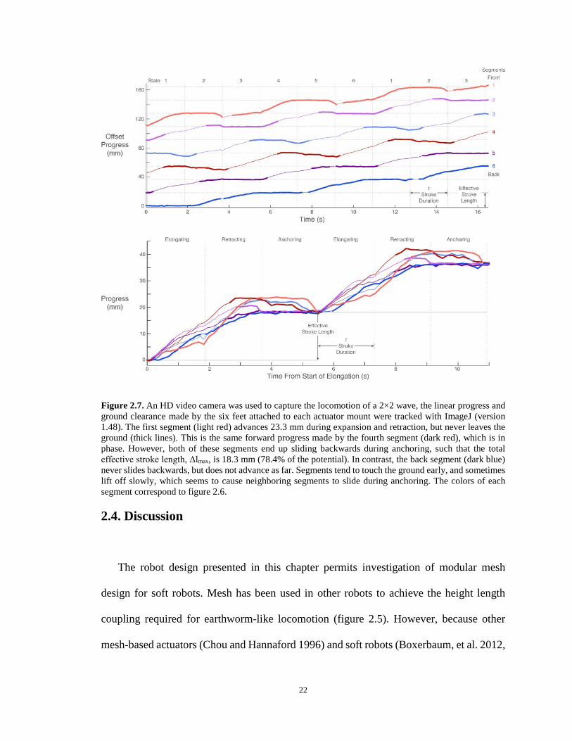
Figure 2.7: HD video camera was used to capture the locomotion of a 2×2 wave…….... 22

Figure 3.1: Compliant Modular Mesh Worm-Steering (CMMWorm-S)………..……… 28

Figure 3.2: A single segment of the CMMWorm-S…………………………………..….30

Figure 3.3: The mesh of the CMMWorm-S is composed of vertex pieces……………… 31

Figure 3.4: Turning mechanism schematic as seen from the transverse view…………… 34

Figure 3.5: Diagrams showing a segment with different configurations………………… 36

Figure 3.6: Change in width (∆w) of a rhombus as a force is applied…………………... 37

Figure 3.7: Change in length of an isolated segment as a tensile force…………………. 40

Figure 3.8: Longitudinal segment stiffness for each configuration……………………… 41

Figure 3.9: Change in height of an isolated segment when a compressive force...……… 42

Figure 3.10: Circumferential stiffness as measured………………………………........... 43

Figure 3.11: Experimental Young’s modulus measured………………………………… 46

Figure 3.12: Forward progress per peristaltic cycle……………………………………... 48

ix

Figure 3.13: Video stills of the CMMWorm-S robot turning……………………………. 50

Figure 3.14: Angle by which the robot turns per peristaltic cycle………………………. 52

Figure 3.15: Summary of design criteria………………………………………………… 57

Figure 4.1: Worm-like robots’ segments………………………………………………... 63

Figure 4.2: Structure of chosen fabric, captured by a microscope………………………. 66

Figure 4.3: Layout of fabric for assembly of fabricworm……………………………….. 67

Figure 4.4: FabricWorm during a peristaltic wave………………………………............ 69

Figure 4.5: Front and side view of FabricWorm fully expanded………………………... 69

Figure 4.6: MiniFabricWorm consists of no rigid components in the structure………… 70

Figure 4.7: Coupling ratio, which is the relationship between the change in length……. 75

Figure 4.8: Change in length of a single segment when a force is applied……………… 77

Figure 4.9: Change in angle of the robot as a moment is applied………………….......... 78

Figure 4.10: Images demonstrating the bending limits of these two robots……….......... 79

Figure 4.11: Robot speed normalized by diameter………………………………………. 80

Figure 5.1: Recent worm-like robots……………………………………………………. 89

Figure 5.2: Waveform diagram showing moving and anchoring segments…………….. 92

Figure 5.3: Commonly used structures in peristaltic devices……………………………100

Figure 5.4: Actuation schemes of peristaltic devices found in literature………………. 103

Figure 5.5: Schematic of different waveforms commonly used………………….......... 105

Figure 5.6: An example of cost of transport associated with waveform…………......... 109

Figure 5.7: Cost of transport for a peristaltic robot………………………………......... 111

Figure 5.8: Ratio of number of moving segments to anchoring segments…………….. 112

Figure 6.1: A key property of worm-like locomotion…………………………….......... 125

x

Figure 6.2: The body of a worm-like robot is represented using trapezoids…………… 127

Figure 6.3: A worm-like robot will have limits on the possible shapes……………….. 127

Figure 6.4: Balancing a pair of elongating and retracting segments…………………… 130

Figure 6.5: The reachable space of the front segment…………………………….......... 134

Figure 6.6: Some areas of the reachable space do not permit…………………….......... 136

Figure 6.7: If pairs of segments are controlled…………………………………………. 138

Figure 6.8: A pair of trapezoid segments can move together…………………………… 138

Figure 6.9: Diagram of paired extension and retraction……………………………….. 140

Figure 6.10: The non-periodic SEC control wave is determined………………………. 144

Figure 6.11: An example simulation trial is shown with NPW………………………… 146

Figure 6.12: Overhead view of Compliant Modular Mesh Worm with Steering............ 147

Figure 6.13: Schematic extracted from the simulation for periodic 2×1 wave………… 150

Figure 6.14: Trajectories for periodic and non-periodic waveform……………………. 154

Figure 6.15: Distance between simulation predicted position and actual position………155

Figure 7.1: Distributed-Sensing Compliant Worm robot (DiSCo-Worm)………………165

Figure 7.2: Sensor configuration of a single segment placed flat on a surface………….166

Figure 7.3: Expansion of a single segment within a pipe……………………………… 170

Figure 7.4: DiSCO-Worm locomoting through two parallel horizontal surfaces……….172

Figure 7.5: Data recorded from the 2nd segment using the closed-loop controller...........174

Figure 7.6: Comparison between open-loop and closed-loop controller…………..........175

Figure A1: Free body diagram of a vertex piece, showing the forces…………………. 185

Figure B1: Schematic depicting a total of n segments……………………………..……186

xi

Acknowledgements

This work would not have been possible without the support of countless friends,

family, and colleagues. Most of all, I thank my parents for getting me where I am today. I

owe almost as much to my advisors, Roger Quinn and Kathryn Daltorio, who have guided

me and been patient mentors throughout my graduate career. My co-advisor, Hillel Chiel,

has shared his enthusiasm, and attention to detail.

I would like to thank Andrew de Salle Horchler for his friendship, creativity, guidance

and mentoring that got me involved with this project. I would like to thank Kenneth Moses,

Ronald Leibach, Fletcher Young, Debnath Maji and Alexandra Cornell for their friendship

and for many engaging discussions about design and control of the current iteration of

worm-like robots. My other co-authors and friends Richard Bachman, Yifan Wang, Yifan

Huang, Anna Mehringer and Kayla Andersen, who made invaluable contributions to this

work. Finally, I would like to thank Robert Gao, Joseph Mansour, Cenk Çavuşoğlu, Gary

Wnek and Stuart Rowan and all members of the Biologically Inspired Robotics Laboratory,

past and present.

This work was funded by National Science Foundation (NSF) research grant IIS-

1065489 and Grant No. NSF #1743475

xii

Control and Analysis of Soft Body Locomotion on a Robotic Platform

Abstract

by

AKHIL KANDHARI

Earthworms locomote using traveling waves of segment contraction and expansion, which when

symmetric, result in straight-line locomotion and when biased result in turning. The mechanics of

the soft body permit a large range of possible body shapes which both comply with the environment

and contribute to directed locomotion. Inspired by earthworms, a new platform: Compliant

Modular Mesh Worm robot (CMMWorm) is presented to study this type of locomotion. Using this

platform as the basis for evaluation, I show that locomotion efficiency is sensitive to body stiffness.

Furthermore, using simplified beam theory, I demonstrate the power required for peristaltic

locomotion is related to the geometrical properties, structural properties and gait pattern of the

robot. The analyses of peristaltic locomotion demonstrate energetic losses to frictional slip is the

key reason for loss of power efficiency. By representing segments as isosceles trapezoids with

reasonable ranges of motion, I determine control waves that in simulation do not require slip. I

apply the resulting control wave on our robotic platform that leads to a decrease in prediction error,

improving kinematic motion prediction for planning. To mimic the ability of an earthworm to adapt

to external perturbations, I equipped the CMMWorm with pressure and stretch sensors for

improving locomotion efficiency in constrained environments. I show that using a closed-loop

controller helps eliminate slip in constrained environments thereby increasing locomotion

efficiency. These analyses can help in the development of design criteria and control for future soft

robotic peristaltic devices.

1

Chapter 1 Introduction

2

1.1 Background and Significance

Inspired by Biology, researchers have been mimicking the multi-functionality,

adaptability and locomotion-efficiency of biological organisms on robotic platforms. Most

biological organisms use their body compliance to interact with their environment.

Capturing the softness and body compliance of such biological organisms and applying it

on robotic platforms has led to the evolution of the field of soft-robotics (Rus and Tolley

2015).

In contrast to conventional rigid robots, soft robots are made using compliant materials

that allows the structure to passively adapt to its surrounding environment (Trivedi, et al.

2008, Kim, et al. 2013). Constrained environments like tunnels pose a challenge to robotic

locomotion, because of unpredictable environments. Soft robots can take advantage of

traction at multiple contact surfaces and improve adaptability and locomotion efficiency in

such environments. Developing soft robots that are adaptable, has also helped in improving

multi-functionality of robotic devices. For instance, a soft gripper is capable of grasping a

variety of different objects without requiring a dedicated control scheme or complex

sensory arrays (Shintake, et al. 2018). A traditional gripper, like a robotic hand, requires

sensory feedback and a controller to continually monitor its output forces and adjust its

grasping kinematics and kinetics in real time to ensure the target object is securely grasped.

In comparison, the soft gripper relies on its inherent compliance to solve this issue.

3

Soft-bodied robots inspired by soft-bodied animals, such as worms, slugs, caterpillars

and leeches have many applications, such as inspection of pipes (it could navigate through

a network of pipes to detect leaks), search and rescue (the robot could crawl through

rubbles), exploration, and medical applications (endoscopy and colonoscopy). Although a

relatively new field, soft robotics has found many researchers developing new robots and

controllers that find usefulness in various fields (Trivedi, et al. 2008, Kim, et al. 2013,

Lipson 2014, Rus and Tolley 2015). These robots have large number of kinematically

redundant degrees of freedom and are termed hyper-redundant (Chirikjian and Burdick

1991, Trivedi, et al. 2008). On a robotic platform these degrees of freedom may be actuated

using a variety of methods including, but not limited to, shape memory alloys

(Vaidyanathan, et al. 2000, Seok, et al. 2013, Mazzolai, et al. 2012, Umedachi and Trimmer

2014), pneumatics (Mangan, et al. 2002, Onal, et al. 2011, Tolley, et al. 2014), hydraulics

(Katzschman, et al. 2014), electroactive polymers (Jung, et al. 2006, Carpi, et al. 2010),

and cables (Boxerbaum, et al. 2010, Renda, et al. 2012, Jones and Walker 2006, Horchler,

et al. 2015a).

In particular, peristaltic locomotion is promising. Over 50 robots inspired by earthworm

have been created. Unlike legged designs, each segment of the body is radially symmetric

and approximately identical, which makes it convenient for modular design at various

length scales. Instead of discrete feet, worm robots can use their entire body surface for

traction, which can be increased by material softness. As a result, worm-like robots have

been suggested for many soft robotic applications, such as search and rescue operations

(Trimmer, et al. 2006), underground exploration (Bertetto and Ruggiu 2001, Omori, et al.

2009, Tanaka, et al. 2014) pipe inspection (Ikeuchi, et al. 2012, Harigaya, et al. 2013) and

4

medical procedures like endoscopy and colonoscopy (Mangan, et al. 2002, Dario, et al.

2004, Wang and Yan 2007). This dissertation addresses several open areas of design,

control and analysis of soft worm-like locomotion.

1.2 Peristaltic Locomotion

The soft-bodied common earthworm, Lumbricus terrestris, can bend and contort its

body to navigate its terrain and squeeze into narrow, constrained spaces. At the same time,

the earthworm can exert forces radially and laterally against its environment to break up

compacted soil, create and enlarge burrows, and resist extraction from its burrows by

predators. These abilities exhibited by an earthworm make it an interesting animal to mimic

on a robotic platform.

The above listed behaviors are possible due to the segmented body of an earthworm.

These segments are composed of a set of longitudinal and circumferential muscles. The

hydrostatic coupling (Chiel, et al. 1992) in the segment allows it to extend longitudinally

while contracting circumferentially and vice-versa. A wave of radial contraction coupled

with longitudinal extension travels down the body (figure 1.1), moving the body in the

opposite direction of the wave’s travel. This kind of locomotion, referred to as peristalsis

(Gray and Lissmann 1938), allows the earthworm to navigate through its environment. The

coupling between the length and diameter of a segment (Chiel, et al. 1992) allows the

longer contracted segments to lift off the ground while the circumferentially expanded

segments rest on the ground to anchor forward motion (Kanu, et al. 2015).

5

Figure 1.1 An illustration from Gray and Lissmann, 1938 of worm peristalsis. Rearwards travelling waves (down) create a forward progression (up) over time (horizontal axis). Note that while the head appears to slip backwards it is likely not ever touching the ground. In contrast, the segments along the rest of the body do not slip backwards. The progression of given segments is shown by wavy lines from left to right. (B) Adapted from J. A. Thomson, 1916, showing the cross sectional view of the earthworm’s segment. The circumferential muscle seen in red along the periphery of the segment helps in contraction and elongation along the length of the segment. The Longitudinal muscles contract the segment causing expansion in the radial direction

During the crawling movements of the earthworms, sensory feedback provides the

animal with an ability to adapt to different types of environmental perturbations that may

occur (Mituzani, et al. 2004). The importance of sensory feedback for maintaining

rhythmic crawling motions has been established (Gray and Lissmann 1938).

Mechanosensory organs and stretch, touch, and pressure receptors are the feedback sources

in earthworms (Mill 1982). Due to the flexibility in the earthworm’s body, it is unable to

sense its posture from only stretch receptors (Mituzani, et al. 2004). However, the sensory

input activities from the setae allows it to adapt to its environment and crawl smoothly even

on rough surfaces.

6

1.3 Worm-like robots

Many different worm-like robots have been constructed (Mangan, et al. 2002,

Vaidyanathan, et al. 2000, Boxerbaum, et al. 2010, Trivedi, et al. 2008, Dario, et al. 2004,

Seok, et al. 2013, Horchler, et al. 2015a). Coordinating the actuation of multiple degrees

of freedom on a compliant body is challenging. (Tesch, et al. 2009, Transeth, et al. 2009).

Implementing properties of a soft body on a robotic platform has been simplified by

reducing or grouping the degrees of freedom (Menciassi 2004, Lee 2010), and/or by

replacing continuously deformable soft bodies with rigid joints (Wang 2007, Omori 2009).

These have adverse effects on the flexibility and performance of the robot. Backward slip,

which is a commonly observed problem in all robots attempting peristaltic motion has

given insight to the importance of friction in this mode of locomotion (Alexander 2003,

Menciassi 2004, Zimmermann 2007, Zarrouk 2010).

The Biologically Inspired Robotics Laboratory models peristaltic locomotion with

robot prototypes. The first was an underwater shape memory alloy robot with a hydrostatic

skeleton (Vaidyanathan, et al 2000). This robot used nitinol wires to actuate and had a

maximum speed of 0.6 cm/sec or 2.5 body lengths per minute. This was followed by a

wormlike robot that used long artificial muscles in series (Mangan, et al. 2002). The

artificial muscle consisted of a braided mesh that had a coupling between the length and

diameter of each segment, such that extension along the length would radially contract a

segment, and radial expansion would cause the segment to contract along the length. This

robot had a lot of backward slip, or had difficulty progressing forward when an obstacle

landed between the actuators. Softworm (Boxerbaum, et al. 2010, 2012) used a continuous

7

mesh of helically-wrapped tubes, pinned at the intersections to form rhombuses with a

fixed side length (figure 1.2), but a changing aspect ratio. The changing aspect ratios of the

mesh rhombuses caused the length and diameter of the robot body to change inversely,

similar to the hydrostatic length-diameter coupling in worms (Quillin 1998, Dorgan 2010,

Kanu, et al. 2015).

The compliance of mesh-based designs permits the bodies to bend and adapt to the

environment and actuator forces. This allows the diameter of the mesh tube to vary along

the length of the body, in contrast to the rigid linkages used in other mechanisms. The

simplicity of a compliant mesh body design means that the body of the robot can be very

durable and can continue to operate even after being crushed, as demonstrated by Seok, et

al. 2013. These properties of mesh-based structures gave way to the current generation of

earthworm-like robots in the Biorobotics Lab.

Figure 1.2 Softworm is a robot made of continuously deformable mesh that interpolates the positions of circumferential cables spaced at intervals along the long axis. As the cables are pulled, the diameter (height) decreases and the mesh expands in the longitudinal direction. A return spring combined with the mesh bending stiffness ensures the segments return to a rest length following actuation. A single drive motor turning a cam at the posterior of the robot generates smooth waves of cable tension offset by fixed angles around the cam. Softworm can travel at six-body lengths per minute (4m/min).

8

1.4 Outline and Contributions of this Dissertation

This dissertation addresses several open areas of peristaltic locomotion that could help

designers decide fundamental questions about actuation, structure, control and sensing for

soft peristaltic devices. Chapter 2 presents the design and performance of Compliant

Modular Mesh Worm robot, a cable driven worm-like robot, where each segment is

individually actuated using a servomotor. The modularity of the mesh allows for

interchanging compliant components of the structure, thereby altering the overall stiffness.

This chapter lays the groundwork for the development of peristaltic robot’s discussed

throughout the dissertation and how compliance, friction and control affect overall

efficiency during peristaltic locomotion.

Chapter 3 presents the next iteration of Compliant Modular Mesh worm robot that is

capable of steering. The robot is used as a platform to answer fundamental questions of

how different components of the structure affects overall stiffness along orthogonal

directions. Furthermore, I show how overall stiffness along orthogonal directions affects

straight-line and turning locomotion. Finally, in order to generalize the design criteria in

this chapter, I present a guideline based on experimental results of how orthogonal

stiffnesses should be related to body scale in order to permit intended soft body

deformation for locomotion with a mesh body.

Chapter 4 presents a worm-like robot that incorporates fabric in the structure. In this

chapter I show how fabric can replace traditional structural and compliant elements in an

earthworm-like robot to achieve comparable performance with fewer mechanical parts. I

directly compare a nonfabric-based design (CMMWorm) with a fabric-based design,

9

demonstrating peristaltic locomotion on substrates with different coefficients of static

friction.

In chapter 5, I consider an idealized locomoting earthworm model that does not need

to slip but takes into account effects of actuation and deformation, providing a template for

understanding peristaltic locomotion. By employing simplifying assumptions, I

demonstrate how worm-like robots can be constructed of any stiffness material with

sufficient effective Poisson’s ratio and actuation energy density. Furthermore, for a given

robot length, either velocity or energy efficiency can be optimized. The analysis shown in

this chapter is supported both by experiments on our robot and by a review of worm robots

in the literature.

A kinematic model of the Compliant Modular Mesh Worm with steering is presented

in Chapter 6. Using a simplified 2D model, in simulation I demonstrate the constraints that

are required for allowing peristaltic locomotion without slip. Furthermore, I implement the

kinematic constraints derived using this simple geometry on our mesh based worm-like

robot to demonstrate improvement in turning locomotion by increasing predictability.

In chapter 7, I assess the added value of sensors on a soft robotic platform. To do so, I

developed the new worm-like robot with force sensitive pressure sensors (to detect external

constraints) and stretch sensors (to detect internal state). Using this platform, I implement

a closed-loop control on a soft worm-like robot for better understanding the mechanics of

peristaltic locomotion in constrained environments.

Chapter 8 discusses future directions for the main themes of this work. Improvement

to the current iterations of the robots presented throughout this dissertation in terms of

design and control that will help in developing truly soft robots of the future.

10

Chapter 2 Compliant Modular-Mesh Worm-like Robot

This chapter was originally published as:

Horchler, A.D., Kandhari, A., Daltorio, K.A., Moses, K.C., Ryan, J.C., Stultz, K.A., Kanu, E.N., Andersen, K.B., Kershaw, J.A., Bachmann, R.J. and Chiel, H.J., 2015. Peristaltic locomotion of a modular mesh-based worm robot: precision, compliance, and friction. Soft Robotics, 2(4), pp.135-145.

Edits have been made in order to solely focus on the design and control of the robot and not all results from the publication are present in this thesis.

11

2.1 Introduction

Mimicking and better understanding the way an earthworm uses its many segments

will help in designing new soft robots for a wide variety of applications. For better

understanding the control and dynamics of such a robot platform, we develop a new type

of robot: Compliant Modular Mesh Worm (CMMWorm). The robot’s body utilizes a

compliant mesh that couples decreases in diameter with increases in length. The function

of the mesh parallels the hydrostatic skeleton of an earthworm. Because of this diameter-

length coupling, as waves of radial contraction travel down the cylindrical body, the robot

advances along ground or in pipes with peristaltic locomotion. The mesh consists of

rhombuses whose sides are polycarbonate rods or nylon tubes. The vertices of the mesh

are 3-D printed and permit pin-joint rotation of the rhombus sides. Each segment of the

robot is individually controlled using a smart servo actuator attached to cables for both

longitudinal and circumferential actuations. The modular mesh enables the robot to achieve

a large strain range comparable to that of an earthworm.

In this chapter we investigate the mechanics of soft peristaltic locomotion in a novel

compliant modular mesh worm robot, CMMWorm (figure 2.1) controlled with precise

mechanical actuators and cables at each segment. The segment and component modularity

of our robot’s discretized mesh facilitates the critical tuning of local stiffness. The progress

and ground clearance of individual segments is tracked and speeds for different wave

shapes and friction coefficients are compared. These results suggest design and control

insights for future soft worm-like robots, including the importance of lifting segments off

12

the ground and how stiffness, precision, or friction can be designed or adjusted to reduce

slip.

2.2 Robot Design

2.2.1 Bi-directional actuation

In order to investigate terrain-adaptive peristaltic locomotion, CMMWorm required

actuation and sensing at many points along its length. For this purpose, Robotis Dynamixel

MX-64T actuators are used at each of the segments. These “smart actuators” have position,

speed, and load sensing capabilities.

In previous mesh-based robots, segment diameter has been actuated by tensioning

circumferential cables (Boxerbaum, et al. 2012) or coiled shape memory actuators (Seok,

et al. 2013) in conjunction with longitudinal compliance to return segments to their

maximum diameter. CMMWorm uses two pairs of Kevlar® cables to actuate each segment

allowing one mesh-mounted Dynamixel actuator to act bi-directionally. Spooling in the

circumferential cables simultaneously spools out the longitudinal cables and vice versa.

Figure 2.1 Compliant Modular Mesh Worm (CMMWorm) robot with six modular individually controlled segments moving on a flat surface. The length of the robot as pictures is 119 cm.

13

When shortened, the two circumferential cables, like the circular muscle layer of an

earthworm (Gray and Lissmann 1938), elongate the segment while decreasing its diameter.

Similarly, like longitudinal muscles, the longitudinal cables reduce segment length while

increasing segment diameter.

Figure 2.2 Mesh of the CMMWorm robot laid flat on a surface during assembly. The longitudinal and circumferential cable placement for one segment is highlighted in red and blue, respectively. Three-ply Kevlar® cable is used. Nylon tube (translucent) and polycarbonate rod (highlighted in orange) links connect the vertex pieces. Tension springs are mounted atop the actuator to keep the circumferential cable taut during actuation. Side springs to increase the stiffness of the segment for a more uniform distribution of forces throughout the segment. C: circumferential vertex, 45: longitudinal 45 vertex, 135: longitudinal 135 vertex, TO: tie-off vertex, M: actuator mount, S: half inter-contact length, ls: segment length, hR: rhombus height, lR: rhombus length, L: rhombus side length.

14

Figure 2.3 A single segment of CMMWorm fully expanded (left) and fully contracted (right). The circumferential cable tensioning springs are visible above the black Dynamixel actuator.

The longitudinal and circumferential cable lengths are proportional to the mesh rhombus

lengths and heights, respectively (figure 2.2). The circumferential cables cross each

rhombus height, following the circumference of the robot. The longitudinal cables zig-zag

to cross each rhombus length by following along the links. Because of the nonlinear

(Pythagorean) relationship between rhombus length and height, linear tension springs

attached between the actuators and the circumferential cables keep these cables taut over

the expansion-contraction cycle (figure 2.3).

2.2.2. Mesh structure

Rather than long continuous fibers, as in MeshWorm (Seok, et al. 2013) and Softworm

(Boxerbaum, et al. 2012), our robot is comprised of short “links” of flexible tubing or rod

secured by quick connect air hose fittings that are connected via rigid “vertex” pieces – the

white 3-D printed parts in figures 2.1 and 2.3 (shown in detail in Fig. 2.4). The 3.18 mm ×

1.85 mm (0.125" × 0.073", outer × inner diameter) nylon tubes and 3.18 mm (0.125")

diameter polycarbonate rods are both cut to a length of 48 ±0.25 mm. Like the connecting

15

caps in Softworm (Boxerbaum, et al. 2012), the role of the vertex pieces is to join sections

of tubing or rod so as to prevent relative translation, but allow relative rotation and permit

attachment and routing of the actuating cables. The shape of the vertex pieces also limits

both the minimum and maximum possible diameter of a segment (12.6 cm and 20.6 cm

measured from the side, respectively). The minimum diameter is constrained by the

actuators within the mesh. The included angle (see figure 2.2) ranges between 50º and 110º,

which allows for greater contractions in diameter than our previous robot (Boxerbaum, et

al. 2012). Elastomer feet are affixed to each vertex piece (visible in figures 2.1 and 2.3) to

increase friction with substrates of interest.

To create an easily modifiable, modular robot, Legris™ push-in fittings were chosen

to connect the vertex pieces with the flexible tubing or rod links. The fittings were

purchased as equal straight unions (part number 3106 53 00), cut in two, machined flat,

and epoxied into the vertex pieces (figure 2.4A). The Legris™ fittings allow

interchangeable segments to be assembled individually and connected at a later time. This

modularity also allows links with different lengths and material properties to be easily

tested.

Figure 2.4. The mesh rhombuses are joined at hinge joint vertex pieces, such as the circumferential vertex (A), which have slots to insert the actuating cables and Legris™ fittings to securely hold lengths of tube or rod. The actuator mount vertex (B) also houses a spool on which the longitudinal and circumferential cables are wound in opposite directions. The vertex pieces were 3-D printed in Acrylonitrile butadiene styrene (ABS) on a Stratasys Fortus 400mc FDM (fused deposition modeling) machine, (0.010" slice height, ±0.005" tolerance).

16

Each segment of the robot is comprised of 18 vertex pieces of five different types:

circumferential (figure 2.4A), longitudinal 45, longitudinal 135, tie-off, and actuator mount

(figure 2.4B). Each vertex piece has a straight slot on its top, enabling easy insertion and

removal of cables, facilitating assembly (figure 2.4A). The longitudinal 45 and 135 have

internal radii for the longitudinal actuator cables to pass through them at approximately 45º

and 135º, respectively. The circumferential vertex pieces have a hole for a circumferential

cable, in addition to a pass-through for a longitudinal cable.

The circumferential cables are tied to the upper spool affixed to the actuator (see

figure 2.4B) and pass through the circumferential vertex pieces (figure 2.4A) on each side

before being tied-off and tensioned at the top-most circumferential vertex (figure 2.2, see

also figure 2.3). The longitudinal cables are tied to the lower spool (figure2.4B) and emerge

together from a single hole on the actuator mount vertex before splitting and “zigzagging”

through eight vertex pieces, ending at the two tie-off vertex pieces (figure 2.2).

2.2.3. Electronics and control

The Dynamixel MX-64T actuators for each of the six segments are connected via a

serial bus that supplies power from a linear DC power supply (off-board power) and

permits communication with a microcontroller. The MX-64T actuators have a 12-bit, 360º

absolute encoder and use a PID algorithm to control position, speed, or load. The sensory

capability of these actuators allows for control and data logging without additional sensors

directly attached to the mesh.

A single Robotis OpenCM9.04 microcontroller (32-bit ARM Cortex-M3,

STM32F103CB, 72 MHz) is used for control. This small (66.5 mm × 26.9 mm, 11.1 g)

17

board is mounted to the side of the actuator at the end of the robot. The OpenCM9.04 is

configured to communicate with the MX-64T actuators at 3 MBps without requiring

additional high-speed serial communication circuitry. Programming of the microcontroller

and data logging are performed over a USB connection to a PC.

Our open source DynamixelQ library for the OpenCM9.04 microcontroller enables

high-speed and robust communication with AX and MX series Dynamixel actuators. The

library has syntax to facilitate reading from and writing to multiple actuators

simultaneously.

A time-based control scheme generates waves along the length of the robot to produce

locomotion on the ground. Pairs of actuators configured in speed control mode are

simultaneously commanded to move in opposite directions at their maximum speed for

fixed stroke durations, τ. The next set of actuators in the wave sequence is activated

immediately after the previous stroke duration terminates (see the Locomotion

performance sub-section below for further detail on the specific wave patterns used).

2.3. Methods and Results

The use of multiple actuators allows for different segments of CMMWorm to achieve

different diameters by smoothly deforming the mesh body (figure 2.1). For a six-segment

bi-directionally-actuated robot, the maximum forward speed was 25.8 cm/min on a

plywood surface. The total weight of the assembled six-segment CMMWorm is 2.08 kg.

Each segment weighs 317 g (including one 126 g actuator). The front and back segments

include an additional ring of rhombuses to attain a more uniform shape, which adds 83.1 g

18

to each. The length of a six-segment CMMWorm ranges from 103 cm fully retracted to

134 cm fully elongated, while the corresponding diameters, measured form the side, range

from 20.6 cm to 12.6 cm, respectively.

2.3.1 Characterization of segments

Height-Length Coupling

Like earthworms (figure 2.5A), individual rhombuses (figure 2.5B), and individual

segments (figure 2.5C) have a coupling mechanism such that increases in length cause

decreases in height. In the earthworm, the height (vertical dimension) versus the length

(along the worm’s longitudinal axis) of one segment was tracked via video as the animal

crawled over flat ground. Assuming the worm has a cylindrical cross-section with diameter

equal to height, the height and length can be related via an isovolumetric relationship about

a calculated average volume (figure 2.5A). In the robot, these relationships were

characterized by measuring the straight-line distances between particular vertex feet of an

isolated segment (a cylinder three rhombuses long and six rhombuses around, which is

only actuated at a single ring).

Stiffness

The modular construction and versatility of the Legris™ connectors in CMMWorm

allowed different stiffness elements to be tested, resulting in the configuration presented

here. The flexibility of the nylon tubes permits adjacent segments to achieve different

diameters. However, each rhombus around the circumference of the segment needs to

extend and contract together (figure2.5B).

19

To better transmit the actuated mesh changes around the circumference, the robot has

side springs, Teflon® sheathes, and stiffer polycarbonate rods for the middle and upper

rhombuses that form each actuated ring (figure 2.2, highlighted in orange). The lower

rhombuses undergo greater deformation (visible figure 2.5B as farther from the red curve)

due to supporting more weight and interfacing with the actuators, and thus benefit from the

flexible tubing. As a result, the differences in rhombus length and height culminate in

differences in segment length and height (figure 2.5C). The stiffness of an isolated segment

Figure 2.5. (A) One segment (11-th from anterior) of an earthworm was tracked as the animal crawled over flat ground. The height (vertical dimension) versus the length (along the worm’s longitudinal axis) were tracked with ImageJ (version 1.48, National Institutes of Health) throughout one extension and retraction cycle. Due to the error (±0.4 mm horizontally, ±0.06 mm vertically), the data was smoothed with a five-point moving average. Assuming the worm has a cylindrical cross-section with diameter equal to height, the height and length can be related via an isovolumetric relationship about a calculated average volume. (B) Individual rhombuses of our mesh robot change aspect ratio following an approximately Pythagorean relationship, assuming constant rhombus side length (L = 2.65 cm). To verify this, the rhombus lengths and heights on an isolated individual segment were measured. To obtain these data precisely, the actuator position was advanced in small increments, pausing at each step to allow for measurements of the rhombus lengths and heights from foot-to-foot. In a ring about each actuator, each segment has six rhombuses (two along the bottom, two in the middle, and two at the top), which were averaged in pairs. The height and length are normalized by twice the rhombus side length (the maximum length or height possible for a rigid rhombus). The cable tension at the top and bottom segments results in larger effective hypotenuses because the bottom of the connectors pull inward. The side springs on the middle rhombuses (Fig. 2.2) counteract this effect, which is why the middle rhombuses follow closer to the red line. (C) Individual rhombus changes culminate in height changes for the robot segment. Here, the robot diameter is plotted against the lower rhombus length times 1.5 to get the approximate length of a single segment. This results in segments whose length-wise elongation is coupled with vertical contraction, like a material with a positive Poisson’s ratio.

20

was characterized at an intermediate diameter by applying increasing compressive force

over a length range of 47 mm. The longitudinal stiffness, k, (the slope of the

force/deformation line) was found to be 0.29 N/mm.

2.3.2 Locomotion performance

Three wave patterns, denoted p×n, where p is the integer number of segments per wave

(including spacer segments) and n is the integer number of waves along the body (and the

number of simultaneously active actuator pairs), were used for locomotion (Fig. 2.6). A

single or double two-segment wave (2×1 and 2×2) and a longer three-segment wave (3×1),

in which a suspended “spacer” segment at maximum elongation separates a pair of

elongating and retracting segments, were evaluated

Figure 2.6. Waves propagate from right to left and progress through six states. As a result, the worm robot traverses from left to right. The 2×1 wave actuates two segments at any given time. This waveform travels one stroke length per cycle (six states). The 2×2 wave contains two instances of a wave that each actuate two segments at a time. The 3×1 wave actuates two segments separated by a suspended “spacer” segment at maximum elongation. The 2×2 and 3×1 waves progress two stroke lengths each cycle. Equation (2) can be derived from this figure by comparing the advancement of each segment and assuming that they transition sequentially to and from Δlmax in one period τ.

21

An HD video camera was used to capture the locomotion of the robot undergoing a

2×2 wave. The locations of the six feet attached to the actuator mounts (figure 2.2) of the

robot were tracked (figure 2.7, top). Unlike the case of a rigid robot (Zarrouk, et al. 2010),

each foot’s motion is different. Ideally, each segment would lift off from the ground at the

start of its elongation and begin advancing in the air. Next, during retraction, the foot would

advance with the same slope (i.e., speed), touching the ground just as anchoring begins.

During anchoring, the segment would maintain position (a flat line). A further source of

variation in the segments is that the terminal segments (front and back) cannot lift up as

high (because they are slightly heavier and supported only on one end). Note that, while

different segments can behave differently over time, in the context of the wave, patterns of

progress and contact are consistent from cycle to cycle. Since tracking the first segment

shows a pattern of advancing the maximum stroke and then sliding backwards, which is

similar to the case for rigid robots in compliant tubes (Zarrouk and Shoham 2012) or

imperfectly coordinated simulations (Daltorio, et al. 2013), the analysis can be simplified

by tracking only the front foot.

Finally, many different trials were run on three substrates: plywood (µs = 0.91),

laminate top desk (µs = 0.76) and silicone parchment (µs = 0.62). Greater friction typically

resulted in greater speeds. Both the 2×2 and the 3×1 waves on the desk surface resulted in

speeds of approximately 3.5 mm/s. While the speed for the 2×1 waveform on the plywood

was 2mm/s. As the amplitudes of the waves are increased, the advance per step increases

up to a point. Since the actuators were controlled at constant speed, the stroke durations, τ,

also increased, resulting in plateauing in total speed.

22

Figure 2.7. An HD video camera was used to capture the locomotion of a 2×2 wave, the linear progress and ground clearance made by the six feet attached to each actuator mount were tracked with ImageJ (version 1.48). The first segment (light red) advances 23.3 mm during expansion and retraction, but never leaves the ground (thick lines). This is the same forward progress made by the fourth segment (dark red), which is in phase. However, both of these segments end up sliding backwards during anchoring, such that the total effective stroke length, Δlmax, is 18.3 mm (78.4% of the potential). In contrast, the back segment (dark blue) never slides backwards, but does not advance as far. Segments tend to touch the ground early, and sometimes lift off slowly, which seems to cause neighboring segments to slide during anchoring. The colors of each segment correspond to figure 2.6.

2.4. Discussion

The robot design presented in this chapter permits investigation of modular mesh

design for soft robots. Mesh has been used in other robots to achieve the height length

coupling required for earthworm-like locomotion (figure 2.5). However, because other

mesh-based actuators (Chou and Hannaford 1996) and soft robots (Boxerbaum, et al. 2012,

23

Mangan, et al. 2002, Seok, et al. 2013) use continuous wrapped fibers or tubes, adjustments

often require refabricating the mesh structure from scratch. The design of CMMWorm’s

vertex pieces allows the stiffness and dimensions of the mesh to be modularly adjusted.

The robot is modular on many levels: different segments can be controlled in different

patterns (figure 2.6), different rhombuses can have different stiffnesses (by attaching the

side springs, see figure 2.2), and different rhombus sides can have different bending

stiffnesses (e.g., rods versus tubes).

CMMWorm faces some of the hallmark challenges of soft robotics (Kim, et al. 2013,

Lipson, 2014). Nonlinear strain and hysteresis is evident in the actuation length curves

shown in figure 2.5. Unlike other worm robots that have reported lower speeds at higher

friction coefficients (Onal, et al. 2012, Zarrouk and Shoham 2012), CMMWorm moves

faster as µs increases, which means that slip is not essential for operation. This may be

important for applications in which high shear could result in damage (e.g., endoscopy) or

inefficiency (e.g., autonomous exploration).

Development of CMMWorm lays the groundwork for further understanding peristaltic

locomotion on a robotic platform. Extrapolating from the idea shown in this chapter, in the

following chapters, we improve the robot in terms of design and functionality. We include

steering in the next iteration of the CMMWorm robot (Chapter 3). Compliance and

structural modularity of CMMWorm allow us to develop stiffness-based design criteria for

peristaltic devices (Chapter 3 and 4). Hyper-redundant robot design allows us to analyze

and optimize gait patterns for peristaltic locomotion (Chapter 5). Using kinematic models

of CMMWorm, we improve straight-line and turning peristaltic locomotion efficiency on

flat surfaces (Chapter 6). Furthermore, we add an array of sensors along the length of our

24

robot to improve efficiency of peristaltic locomotion in constrained environments (Chapter

7).

25

Chapter 3 Stiffness properties affecting worm like-robot turning and straight-line locomotion

This chapter was originally published as:

Kandhari, A., Huang, Y., Daltorio, K.A., Chiel, H.J. and Quinn, R.D., 2018. Body stiffness in orthogonal directions oppositely affects worm-like robot turning and straight-line locomotion. Bioinspiration & biomimetics, 13(2), p.026003.

26

3.1. Introduction

Developing soft-bodied robots capable of animal-like locomotion is a challenging

problem and biological insights could be valuable for both mechanical design and control

strategies. Soft-bodied animals, such as earthworms, can locomote in diverse

environments. Their soft bodies allow them to squeeze through confined spaces, comply

with their environment and make sharp turns. Duplicating these behaviors for robotics

would be valuable in constrained-space applications (such as burrowing, exploration and

search and rescue).

Whereas worm-like peristalsis has been shown to be effective for forward locomotion

in worm-inspired robots (Boxerbaum, et al. 2010, Seok, et al. 2013, Horchler, et al 2015a),

effective navigation in real-world environments requires being able to make volitional

turns. Earthworms and other soft-bodied animals most commonly turn their bodies by small

angles by forming low amplitude bends along their body lengths (Kim et al 2011). Adding

steering to a worm robot permits volitional control and allows for movement in more

complex environments. Soft-bodied robots achieve turning in different ways. For example,

earthworm-inspired robots have turned by varying segment lengths using servomotors,

(Omori et al 2008), by using shape memory alloys (SMA) that bend the segment about

pivot points (Umedachi and Trimmer 2014), or by adding additional SMAs along the

longitudinal axis (Seok et al 2013).

Previous investigators have not explored the relationship between body stiffness,

circumferential stiffness and the efficiency of locomotion and turning. In this chapter, we

explore worm-inspired biomechanical and control strategies for forward locomotion and

27

turning using peristalsis in a new robotic platform. In particular, we empirically determine

the relative roles of circumferential, longitudinal and bending stiffness for forward

locomotion and turning. Based on these measurements, we present a stiffness model that

can be used in the design of future soft robots.

To investigate worm-like turning in a soft-bodied robot, we designed and constructed

a new robot: Compliant Modular Mesh Worm with Steering (CMMWorm-S). Unlike its

predecessor, CMMWorm-O (Chapter 2, Horchler et al 2015a), this new robot has two

motors in each of its six segments that allow for differential strain in a segment, which

results in turning of the robot. The new robot’s modularity allows us to easily interchange

components to alter the stiffness of the robot. To understand how the compliant

components affect longitudinal, circumferential and bending stiffness, tubes of different

bending stiffness values and return springs of different stiffnessess are implemented and

the gross stiffness properties of the robot are measured. Peristaltic locomotion tests are also

conducted on flat ground for both straight-line locomotion and turning to analyze how

different stiffness values affect performance of worm robots. We now report that greater

bending stiffness improves turning locomotion, whereas greater circumferential stiffness

speeds straight-line locomotion.

3.2. CMMWorm-S Robot Design

CMMWorm-S (figure 3.1) has two motors (instead of the one in our previous robot) in

each of its six segments to allow for differential peristalsis.

28

Figure 3.1: Compliant Modular Mesh Worm-Steering (CMMWorm-S) in an arc-like configuration. Each segment includes two actuators that allow bending for turning. The various components of the robot mesh are labelled.

The basic configuration and circumference of CMMWorm-S are similar to our previous

worm-like robot CMMWorm-O, a cable actuated, multi-segmented soft robot (Horchler et

al 2015a). In CMMWorm-O each segment was actuated by a single servomotor so that

different segments of the robot can achieve different diameters, smoothly deforming the

mesh body. CMMWorm-O’s mesh is comprised of short “links” of flexible tubing or rod,

secured by quick-connect air hose fittings that were embedded in rigid vertex pieces. The

vertex pieces were 3-D printed and their role is to join sections of tubing or rod to prevent

relative translation, but allowed relative rotation and permitted attachment and routing of

the actuating cables. A motor driven circumferential cable, like the circumferential muscle

of the earthworm’s segment, was used to contract the segment’s diameter. Linear springs

along the length of the segment passively returned the segment to its initial maximum

diameter state on the removal of the actuation load. CMMWorm-S improves on the design

of its predecessor in terms of locomotion capabilities, mechanical robustness, and reduced

mass.

29

The addition of more actuated degrees of freedom allows volitional turning. Each

segment of CMMWorm-S is actuated by two smaller Robotis Dynamixel AX-18A

servomotors. These actuators are 50% faster as compared to the MX-64T actuators used in

the CMMWorm-O robot (97 rpm at 12V as opposed to 63 rpm at 12V), allowing the robot

to move faster. Each actuator controls one-half of a segment, i.e. three rhombuses, whereas

in CMMWorm-O each actuator controls a whole ring of six rhombuses around the diameter

of a segment. The mesh deforms circumferentially according to the amount of cable

spooled in by the actuator.

For straight locomotion, both segment motors operate equally and evenly extend both

halves of a segment, increasing the length symmetrically. This extension of each segment

during one cycle of a peristaltic wave is defined as the stroke length. To cause the robot to

turn, actuators of a segment spool in different cable lengths, thereby causing a segment to

extend non-uniformly. This concept was demonstrated in Softworm (Boxerbaum, et al.

2012) where the tension in the cables was passively biased along the length of the robot. In

CMMWorm-S, the segment half opposite to the direction of the turn extends more in order

to cover a larger distance. For example, if the robot has to turn left, the right side of the

robot needs to cover a larger distance as compared to the left side. This difference in the

amount of cable spooled in can be achieved in two ways: one side may contract for a longer

time period, while keeping the speed of both actuators constant, or the speed of actuation

may be different between the two actuators while keeping the duration of actuation

constant.

30

Figure 3.2: A single segment of the CMMWorm-S (A-D) indicating the segment contraction-expansion cycle and CMMWorm-O (E-F). (A) The two circumferential cables highlighted in blue and red actuated by two different servomotors when spooled equally, allows the segment to contract in diameter (B) while extending in length (C). Springs along the length of the segment return the segment to its maximum diameter as shown in D as the cable is spooled out. (E) A single actuator in CMMWorm-O controls a single cable and hence does not permit differential spooling of cables. (F) Expanded side view of CMMWorm-O.

31

Figure 3.3: The mesh of the CMMWorm-S is composed of vertex pieces that allow easy connection of tubes. The vertex piece is composed of the tube union that firmly holds the tubes in place, the twist on cap that clasps the tubes down inside the tube union, a stainless steel eyelet for the passage of the actuation cable and a rubber foot that helps in traction during locomotion. The tube union and twist on caps are 3-D printed separately in acrylonitrile butadiene styrene on a Stratasys Fortus 400mc FDM (fused deposition modeling) machine with 0.245 mm (0.010”) slice height ±0.127 mm (0.005”) tolerance. The vertexes permit rotation about the axis through the screw.

The improved modular design of CMMWorm-S gives us the opportunity to exchange

components and test for different and softer stiffness properties. The new design

incorporates smaller vertex pieces without push-in Legris™ fittings. The quick connect

Legris fittings used on CMMWorm-O were expensive, bulky and had to be machined and

epoxied into the vertex pieces. The size and rigidity of the vertex pieces is a limiting factor

in reducing the stiffness of the robot. In CMMWorm-O, high stiffness springs and stiff

mesh tubes had to be used to maintain maximum diameter and a uniform shape due to

bulky vertex pieces. The new design of the vertex pieces (figure 3.3) incorporates

unidirectional teeth inside the tube union, and a twist on cap to clasp the tubes inside the

vertex pieces. This design change replaces the Legris fittings and ensures that the tubes do

not slip out during motion of the robot. Due to the smaller size of the vertex pieces, the

32

robot can incorporate softer tubes and softer linear springs, thereby decreasing the overall

stiffness of the robot.

In CMMWorm-O, the actuation cable passed through slots in the vertex pieces causing

a large amount of friction acting on the cables. This lead to cable wear and frequent

breakdowns. The cables in CMMWorm-S pass through stainless steel eyelets threaded into

the vertex pieces. Eyelets have helped in reducing friction, thereby reducing uneven

deformation and frequent cable breakage.

These design changes were necessary to conduct the research presented in this chapter.

CMMWorm-S is able to locomote forward and turn via peristalsis and its components can

be easily exchanged and its stiffness can be reduced as compared to CMMWorm-O.

Furthermore, the mass of the new robot is 37% less than CMMWorm-O. These

improvements allowed us to perform empirical studies into the relationships between

component, segment and body stiffness versus forward and turning locomotion.

3.3. Electronics and Control

CMMWorm-S is actuated by twelve Dynamixel AX-18A servomotors that incorporate

sensors for feedback control. These actuators are connected through a serial bus. In order

to reduce voltage drop, the actuators are connected in two parallel chains comprising six

actuators on each side. Each chain of actuators is connected to a microcontroller, which is

powered by an off-board DC power supply. The AX-18A actuators have a 300˚ encoder

along with position, speed, and load feedback capabilities. The actuators’ sensory

capabilities allow data logging without the need for additional sensors on the robot

(Kandhari et al. 2016).

33

A single Robotis OpenCM9.04 microcontroller (32-bit ARM cortex-M3,

STM32F103CB, 72MHz) is used for control. The microcontroller is mounted on the side

of an actuator at the end of the robot. It communicates with the AX-18A actuators at

1MBps. Programming of the microcontroller and data logging are performed over a USB

to PC connection.

Our open source DynamixelQ library for the Open CM9.04 microcontroller enables

high-speed communication with AX and MX series Dynamixel actuators. The library has

syntax that allows reading and writing to multiple actuators simultaneously.

A time-based control scheme generates waves along the length of the robot to produce

locomotion. For all the tests performed throughout this chapter a 3×1 wave (where 3

represents the number of segments per wave, including suspended segments, and 1 the

number of waves along the body) was used (Chapter 2). The 3×1 wave has two pairs of

segments working in conjunction, as one segment expands in diameter, the other contracts.

Between both active segments is a contracted inactive (suspended) segment referred to as

the spacer segment. Thus, at any given time, four actuators are active within CMMWorm-

S. The actuators are configured to speed-control mode and are simultaneously commanded

to move at a specified speed, with maximum torque for a fixed duration. The next set of

actuators in the wave sequence are activated immediately after the previous duration

terminates. For straight-line locomotion, all four actuators are controlled at the same speed.

In contrast, for turning, the actuators controlling the side opposite of the direction of the

turn are controlled at speeds greater than the actuators on the inner side for the same

duration. The difference between the speeds of these actuators is referred to as the bias.

This allows the outer side to extend by a greater distance as compared to the inner side. All

34

the turning experiments were carried out with a 75% bias, i.e. the rpm of the inner actuator

were 75% slower than the outer actuator.

𝐁𝐁𝐁𝐁𝐁𝐁𝐁𝐁 =𝐎𝐎𝐎𝐎𝐎𝐎𝐎𝐎𝐎𝐎 𝐁𝐁𝐚𝐚𝐎𝐎𝐎𝐎𝐁𝐁𝐎𝐎𝐚𝐚𝐎𝐎 𝐁𝐁𝐬𝐬𝐎𝐎𝐎𝐎𝐬𝐬 − 𝐈𝐈𝐈𝐈𝐈𝐈𝐎𝐎𝐎𝐎 𝐁𝐁𝐚𝐚𝐎𝐎𝐎𝐎𝐁𝐁𝐎𝐎𝐚𝐚𝐎𝐎 𝐁𝐁𝐬𝐬𝐎𝐎𝐎𝐎𝐬𝐬

𝐎𝐎𝐎𝐎𝐎𝐎𝐎𝐎𝐎𝐎 𝐁𝐁𝐚𝐚𝐎𝐎𝐎𝐎𝐁𝐁𝐎𝐎𝐚𝐚𝐎𝐎 𝐁𝐁𝐬𝐬𝐎𝐎𝐎𝐎𝐬𝐬 (𝟑𝟑.𝟏𝟏)

Figure 3.4: Turning mechanism schematic as seen from the transverse view, as the cables are spooled in with a uniform bias, the segment contraction is uneven causing each segment to expand unevenly. The outer side contracts more than the inner side and that causes the robot to turn. Between a contracting and expanding segment is an inactive contracted segment referred to as the “spaces segment”. Note: due to friction and slip, the robot does not turn by such large angles as shown in the schematic.

35

3.4. Methods and Results

We empirically characterized the properties and performance of the robot using

components of different stiffness. Three types of flexible tubes of varying internal diameter

and material (table 3.1) are used to vary the mesh-tube stiffness. The other compliant

components of the mesh are the springs that help return the segment to its expanded state

after the actuation load has been removed. Two different springs were used with stiffness

values of 0.45 N/cm and 1 N/cm. The springs are attached along the length of the segment

between rhombuses. Springs of equal stiffnesses are attached on both sides such that the

stiffness properties on either side of a segment are uniform. Figure 3.5 defines the different

configurations of springs used in order to obtain different return forces on the segment.

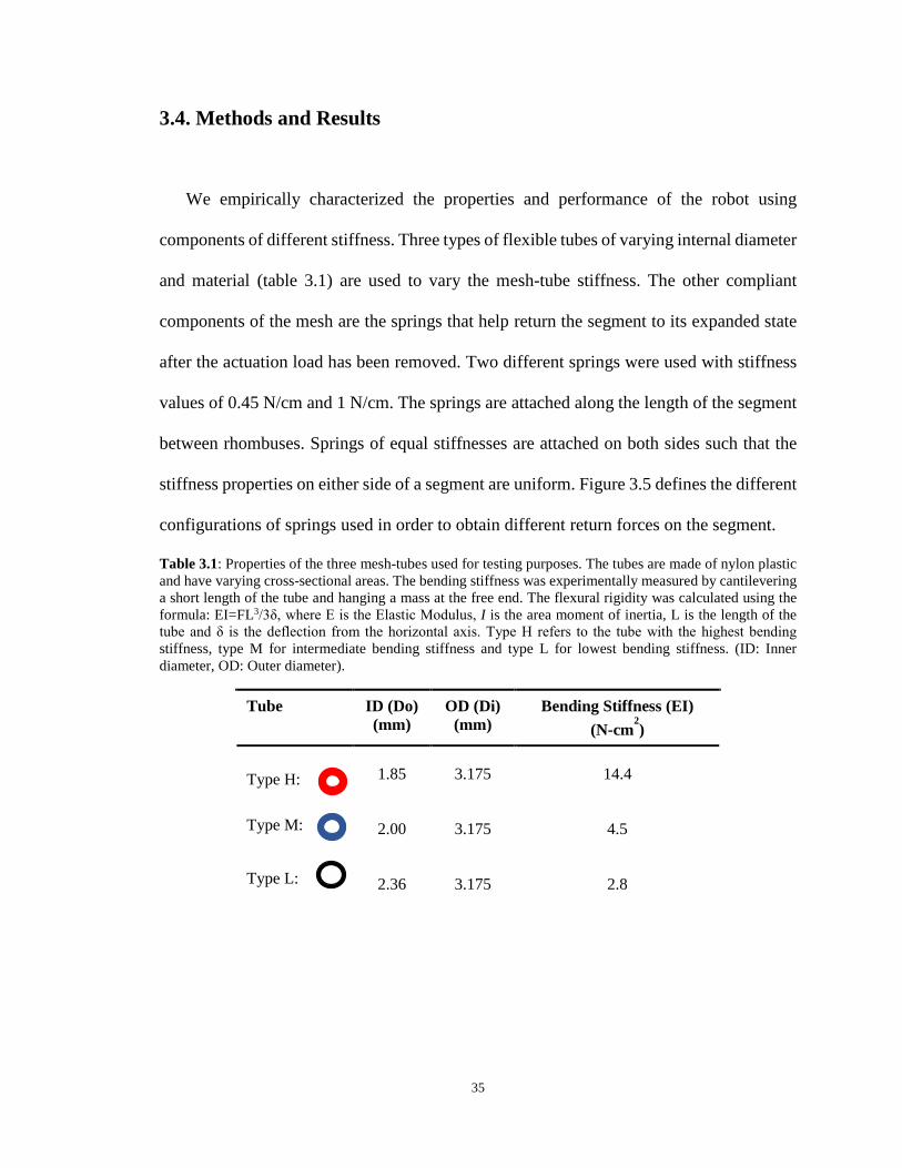
Table 3.1: Properties of the three mesh-tubes used for testing purposes. The tubes are made of nylon plastic and have varying cross-sectional areas. The bending stiffness was experimentally measured by cantilevering a short length of the tube and hanging a mass at the free end. The flexural rigidity was calculated using the formula: EI=FL3/3δ, where E is the Elastic Modulus, I is the area moment of inertia, L is the length of the tube and δ is the deflection from the horizontal axis. Type H refers to the tube with the highest bending stiffness, type M for intermediate bending stiffness and type L for lowest bending stiffness. (ID: Inner diameter, OD: Outer diameter).

Tube ID (Do) (mm)

OD (Di) (mm)

Bending Stiffness (EI) (N-cm

2)

Type H: 1.85 3.175 14.4

Type M: 2.00 3.175 4.5

Type L: 2.36 3.175 2.8

36

Figure 3.5: Diagrams showing a segment with different configurations of return springs used in testing. Springs are coil extension spring with stiffness 0.45N/cm and 1N/cm that are attached along the length of the segment, providing a return force after the actuation load is removed. The springs are symmetrically attached around the segment (A) 2×0.45N/cm, (B) 4×0.45N/cm, (C) 6×0.45N/cm and (D) 4×0.45+2×1 N/cm.

3.4.1 Characterization of Stiffness

Characterization of stiffness of an individual rhombus

To better understand the kinematics and the softness of our mesh-based robot, we first

extracted a single rhombus with a return spring and subjected it to a longitudinal force

while measuring the change in length (figure 3.6). The rhombus is composed of four vertex

pieces connected via tubes or “links” and a linear spring attached along the diagonal of the

rhombus, providing a force to return the rhombus to its initial rest state. In a completely

rigid mechanism, the rhombus would extend until the included angle between the vertex

pieces reached its maximum limits (rigid contact between components of the vertices).

However, in the case of a rhombus with flexible tubing, it can bend further: it is capable of

bending until an upper limit is reached (maximum bending of links as shown in figure 3.6:

see appendix A1). This test was used to quantify the effect that flexible tubes have on the

stiffness of an individual rhombus.

37

Figure 3.6 Change in width (∆w) of a rhombus as a force is applied along the diagonal of an isolated rhombus in a planar setting for three tube types and two springs (0.45N/cm for A and 1N/cm for B). The total change in width without tube deformation is 5.85 cm. Beyond that, the tubes start to bend inwards, deforming the rhombus as shown. The total change in width up to 5.85 cm is expected to be linear and due to the return force of the spring only. Beyond this, the bending and longitudinal stiffness of the tubes cause the force to increase with a sharp change in slope of the curve (stiffness). Each tube then acts like a spring, with spring stiffness Kt. The stiffness of tube type L is the least, so that maximum deformation is observed. Tube deformation decreases with an increase in tube stiffness as seen in both A and B. A linear fit up to 6 cm (linear working zone) is used to find the stiffness of the rhombus with different components.

Based on the kinematic constraints of the vertices, the total extension possible without

bending the tubes is approximately 6 cm. Beyond that, the tubes are loaded in tension and

in bending moment. Thus, they start to bend and the rhombus stiffens but not infinitely as

would be the case if the tubes were rigid.

This characterization of the stiffness of an individual rhombus leads to the conclusion

that the spring stiffness is the main factor determining the stiffness of the rhombus in the

longitudinal direction in the robot’s normal operating range (table 3.2). Beyond this, links

are in tension and bending as shown in figure 3.4, increasing the rhombus width, even

though the vertex pieces have reached their maximum included angle limits.

38

Table 3.2: Rhombus stiffness measured from the slope of the linear fit as shown in figure 3.6. Measured rhombus stiffness is compared to the stiffness of the individual spring for different tube types, showing the contribution of the tubes towards the stiffness of an individual rhombus. Measured rhombus stiffness is similar to the stiffness of the spring for the case of Figure 3.6A but as the spring stiffness increases, the tubes add to the overall rhombus stiffness (figure 3.6B).

Tube Spring Stiffness

(N/cm) Calculated Stiffness

(N/cm)

Type H 0.45 0.49

1.00 1.25

Type M 0.45 0.45

1.00 1.12

Type L 0.45 0.45

1.00 1.09

Characterization of stiffness of a segment

The results from individual rhombus stiffness help in predicting the stiffness of a

segment of the robot. The segment is radially symmetric and has three stiffness

components: (a) longitudinal stiffness due to tensile forces applied along the length of the

segment, (b) circumferential stiffness due to compressive forces applied perpendicular to

the length of the segment and (c) bending stiffness due to different diameters between

adjacent segments (straight-line locomotion) or within the same segment (turning).

We measured the contribution of each component of the mesh to the stiffness of a

segment. To do so, an isolated segment was subjected to forces in both longitudinal and

circumferential directions, while measuring the changes in longitudinal length and

39

circumferential height, respectively. To measure the bending stiffness, the deflection of a

vertically loaded cantilevered segment was measured from a horizontal line.

Longitudinal Stiffness

We measured the longitudinal stiffness of a segment constructed with tubes of differing

stiffnesses (figure 3.5). A segment is composed of six rhombuses connected in a ring-like

pattern. When subjected to a tensile force along its length, the segment extends in length

while contracting in diameter (similar to hydrostatic coupling observed in earthworms). A

tensile force up to 12N was applied in increments of 2N, and the change in segment length

was measured. The resultant plot allows calculation of the stiffness (slope of the curve) of

a segment along its longitudinal axis and comparison of the result to a stiffness calculated

from the expected rhombus stiffness (longitudinal return springs connected in parallel =

Ks, see Table 3.2).

40

Figure 3.7: Change in length of an isolated segment as a tensile force was applied for four different spring stiffness configurations (figure 3.5). The colored dashed lines are the predicted stiffness of the segment based on the calculated rhombus stiffness (table 3.2). The slope of the gray dashed line is the equivalent stiffness of the return springs attached in the segment, i.e. Ks, the sum of the stiffnesses of each of the longitudinal return springs in that segment for the four different configurations shown in Figure 3.5. Red, blue and black solid lines join the experimentally measured points. The region of the curve up to an extension of 6 cm is used to estimate the longitudinal stiffness of the segment. In case of configuration D (Ks = 3.8 N/cm, maximum extension = 3.6 cm), the entire curve is used to estimate the stiffness of the segment. Note that in the first configuration, predicted and actual values are very similar but for the other configurations the predicted values are less accurate.

As observed in the case of a rhombus, the main factor determining a segment’s

longitudinal stiffness is the sum of the segment’s longitudinal return springs (Ks, see figure

3.8). Increasing the stiffness of the return springs increases the longitudinal stiffness of the

segment. In addition, similar to the case of the rhombus, links with higher bending stiffness

resulted in higher segment stiffness. However, the measured stiffness of the segment is

lower than the predicted stiffness; this difference is due to the links bending out of plane

when connected in a ring-like pattern.

41

Figure 3.8: Longitudinal segment stiffness for each configuration as measured from figure 3.7 compared to the predicted stiffness (solid lines) from the rhombus model and the stiffness of the return springs (gray dashed line). The measured longitudinal stiffness is less than the predicted stiffness for each tube type from the rhombus model due to the bending of the links when connected in a ring-like structure. The measured longitudinal stiffness is thus a function of both tube bending stiffness and return spring stiffness. The colored dashed line indicates a quadratic fit for each tube type. The return springs have a major contribution towards the longitudinal stiffness, as there is a noticeable difference between the longitudinal stiffness of different configurations (vertical dashed lines). The difference in stiffness values for different tubes for the same configuration is very small compared to different spring configurations (figure 3.5). The predicted value for tube types M and L overlay the spring stiffness line up to 2.7 N/cm.

Circumferential Stiffness

Appropriate circumferential stiffness is also important for peristaltic locomotion of a

worm robot. If the robot were too compliant, then on actuation, the mesh would deform

unevenly causing locomotion to be less efficient. On the other hand, if it is too stiff, the

motors could not deform it within and between segments and the robot could not move.

Therefore, an efficient robot must strike a balance between these extreme limits. The

42

structure must be compliant enough to bend and deform evenly while being able to

maintain structural integrity. We measured circumferential stiffness by applying a

compressive force normal to the length of the robot.

The circumferential compressive stiffness of the segment is dependent on the stiffness

of the links more than it is on the stiffness of the return springs (figure 9). When a

compressive force is applied on the segment, tubes with larger bending stiffness resist

deflection to a greater extent. Tubes with lower bending stiffness comply with the load

more easily. There is a noticeable difference between the segment’s circumferential

Figure 3.9: Change in height of an isolated segment when a compressive force was applied radially for different longitudinal spring configurations (figure 5). The maximum compression in height is approximately 13 cm, where the top of the segment is in contact with the actuators. The curve becomes vertical at approximately 13 cm as further deformation is not possible. A linear fit to the curve from 0 cm to 13 cm was used to estimate the circumferential stiffness of a segment. For tube types M and L, maximum deflection is observed with the application of a minimum of approximately 4.5 N (all configurations), while for tube type H, maximum deflection is not attained with applied load as large as 9.5 N.

43

stiffness for tube type H, the stiffest tube, as compared to segments with the other tubes

(figure 3.10).

There is an upper limit to the circumferential stiffness of a segment as the return spring

stiffness increases (figure 3.10). Beyond that limit, if the return spring stiffness is increased,

the segment cannot maintain the height-width coupling. The links are unable to transfer the

decrease in height to an increase in length. Instead, the segment undergoes the phenomenon

of “barreling” due to compressive loads. The cross-sectional shape of the segment changes

from circular to oval. The higher the tube stiffness, the more resistant the segment is to

barreling. Thus, a down-facing parabolic function was observed in the plot of

circumferential vs. return spring stiffness as Ks was increased.

Figure 3.10: Circumferential stiffness as measured from figure 3.9 shows a non-linear relationship between circumferential stiffness and return spring stiffness. A downward parabolic curve (quadratic fit) was observed as the spring stiffness increased in each case. There is a noticeable difference between the circumferential stiffness of tube type H and the others due to its larger bending stiffness. However, the difference between the other tube types is small.

44

Bending Stiffness

The worm robot body’s bending stiffness is also important for its performance. During

peristaltic locomotion, adjacent segments achieve different diameters. Bending stiffness

provides a measure of the ability of a contracted segment to support itself between

expanded anchoring segments. Thus, bending stiffness can reduce frictional drag.

Bending stiffness of the robot is measured by cantilevering segments. Multiple

segments of the six segment robot are supported on a table and one or two segments are

cantilevered at the end of the table. The cantilevered segments bend due to their own

weight, which is assumed to be evenly distributed along their length. The deflection along

the length allows us to calculate the Young’s or elastic modulus (E) and the bending

stiffness of the robot. Young’s modulus is measured using the equation:

𝑬𝑬 =𝑾𝑾𝑳𝑳𝟒𝟒

𝟖𝟖𝟖𝟖𝟖𝟖(𝟑𝟑.𝟐𝟐)

where W is the distributed load per unit length, L is length, δ is deflection from the

horizontal axis and I is the area moment of inertia.

As can be seen in figure 3.11, the elastic modulus depends on the tube-link bending

stiffness and the return spring stiffness. The elastic modulus of a segment increases with

increasing link bending stiffness and more so with greater return spring stiffness. The

elastic modulus also increases with return spring stiffness. However, beyond a maximum,

for softer tubes M and L, increasing the return spring stiffness causes the bending stiffness

to decrease. As the tube stiffness increases, the resistance to uneven deformation increases.

However, on further increasing spring stiffness, the tubes can no longer resist the force and

start to bend and contort non-uniformly. The tubes kink or bend out of plane such that the

45

return springs undergo minimum elongation. Thus, both return springs and link stiffness

affect a segment’s bending stiffness. Interestingly, although the robot includes some

relatively rigid components, its elastic modulus is in the range of soft materials.

Summary of Stiffness Properties

Table 3.3 summarizes segment longitudinal, circumferential and bending stiffness for

different tube and return spring stiffness values and configurations. The link stiffness

strongly affects the circumferential stiffness, whereas return spring stiffness most strongly

affects longitudinal stiffness. The bending stiffness follows a similar pattern to that of the

circumferential stiffness. Greater link bending stiffness results in greater bending and

circumferential stiffness of the segment; beyond a maximum value, increasing the return

spring stiffness causes the bending stiffness to decrease.

3.4.2 Robot Locomotion Performance as a Function of Stiffness

With a better understanding of the stiffness properties of the robot from the above

studies, we analyzed the performance of the robot as a function of stiffness. Videos from

the transverse view were recorded for both straight-line locomotion and turning. All

experiments were recorded with the robot crawling on wood (µs = 0.85) in order to reduce

the effect of slip.

Straight-Line Locomotion

Figure 12 illustrates that the robot achieved greater speed with stiffer tube-links.

The robot made increasingly greater forward progress per peristaltic cycle as the tube

stiffness was increased from Type L to Type M to Type H tubes. We attribute this speed

difference to two observations. First, uneven deformation was observed with less stiff

46

tubes. The stiffer tubes allow better transfer of forces along the rhombus mesh. As the tube

stiffness decreases, the tubes closer to the actuator bend easily and do so rather than

transferring forces evenly throughout the mesh. Thus, progress per peristaltic wave

decreases as the stiffness of the tubes decrease. Another important factor for efficient

locomotion is the ability of adjacent fully expanded segments to lift contracted segments

as the contracted segments advance. Greater bending stiffness of the tubes allows lifting of

contracted segments instead of dragging them. In the case of softer links, both uneven

deformation of tubes and the inability of anchoring segments to lift adjacent contracted

segments led to poor overall forward progress.

Figure 3.11: Experimental Young’s modulus measured for the six-segmented CMMWorm-S. Young’s modulus is measured using the equation E=WL4/(8δI), where W is the distributed load per unit length, L is length, δ is deflection from the horizontal axis and I is the area moment of inertia. Although composed of relatively rigid components, Young’s modulus of our robot lies in the range comparable to soft material.

47

Table 3.3: Summary of segment stiffness properties for different configurations.

Tube

Return Spring

Stiffness (Ks) (N/cm )

Longitudinal Stiffness (Kl)

(N/cm )

Circumferential Stiffness(Kc)

(N/cm )

Bending Stiffness

(Kb = EI/L3)

(N/cm)

Type H 0.90 0.73 0.80 2.36 1.80 1.51 1.03 2.43 2.70 1.99 1.07 3.10 3.80 3.78 1.09 3.87

Type M 0.90 0.72 0.35 0.32 1.80 1.32 0.43 0.76 2.70 1.88 0.51 0.94 3.80 3.26 0.50 0.89

Type L 0.90 0.63 0.33 0.33 1.80 1.13 0.37 0.50 2.70 1.73 0.38 0.50 3.80 3.14 0.34 0.45

48

Figure 3.12: Forward progress per peristaltic cycle (N=12) for each configuration was measured and compared. Forward progress was measured by commanding the actuators to run at zero bias at 70 rpm. A video from the transverse view was taken for each run. Frames were extracted at the end of each cycle and ImageJ (version 1.48, National Institute of Health) was used to measure the progress made per peristaltic cycle. The robot made greater forward progress with stiffer tubes.

A comparison of speed in figure 3.12 for different segment configurations suggests

three trends. First, a larger variation was observed in the first configuration (Figure 5A, Ks

= 0.9 N/cm). This is because the return spring force is not sufficient to expand the segment

to its original maximum diameter once the actuation load is removed. That is, after

extension, the overall robot length elongates and tends to lose efficiency due to the inability

of the segments to return to their maximum diameters. Second, as the spring stiffness

increases, the actuators require more force to contract a segment to its minimum diameter,

and due to the actuators limitations they fail to do so when the return spring stiffness is

greater than 1.8 N/cm, thereby decreasing the overall achievable progress (stroke length).

49

Third, forward locomotion strongly depends on the bending stiffness of the links. For all

return spring stiffnesses tried, links with higher bending stiffness had better performance.

However, while the tubes need to be sufficiently stiff in order to transfer forces and lift

adjacent segments, they need to be soft enough to be deformed by the motors and to be

connected in a ring-like pattern and deform evenly as the wave travels down the body.

Turning

Experiments were performed to determine the turning performance of the robot (figure

3.13) in terms of its mean angle turned (figure 3.14A) and progress made (figure 3.14B)

per peristaltic cycle. The actuators were run at 75% bias (inner actuator speed = 18 rpm,

outer actuator speed = 70 rpm). The angle turned was determined by measuring the angle

between straight lines drawn from the actuators of the first segment to the actuators of the

last segment before and after each cycle. Progress made while turning was measured by

multiplying the angle by which the robot turned and the radius of curvature about a fixed

turning point. The product is the arc length, which is defined as the progress made while

turning.

50

Figure 3.13: Video stills of the CMMWorm-S robot turning on a wooden surface. Each still corresponds to the beginning of a new peristaltic cycle.

While turning, the halves of a segment must be capable of achieving different

longitudinal elongations. Thus, the segment should be soft enough to achieve different

lengths on either side (length bias), while being stiff enough to have a sufficient stroke

length. Links with the highest bending stiffness (type H) had maximum angle turned per

peristaltic cycle as compared to the other types (figure 3.14A). Even though segments with

51

the softer tubes were capable of achieving different elongation on their sides, the overall

extension was less than for the stiffer tubes.

The angle by which the robot turns follows the same trend as the bending stiffness of

the robot (figure 3.14A). As return spring stiffness increases in the case of stiffer links,

higher turning angles are achieved. In the case of links with lower bending stiffness, the

angle turned per peristaltic cycle reaches a maximum and starts to decrease with increasing

return spring stiffness. The reasoning is the same as for bending stiffness: The ability of

the links to resist uneven deformation decreases with increasing return spring stiffness.

This causes the links to kink and bend out of plane, thereby decreasing the extension. This

decrease in extension causes the robot to turn by smaller angles.

Measuring the robot’s progress along an arc while turning allows us to plan a path the

robot might take while navigating around obstacles. We want to be able to optimize the

robot’s path. Thus, we measure the forward progress the robot makes while turning with

respect to different stiffness configurations (figure 3.14B). Similar to straight-line

locomotion and turning, performance with tube type H is better compared with types M or

L. As the stiffness of the springs is increased, the progress made while turning increases

and then decreases beyond a maximum.

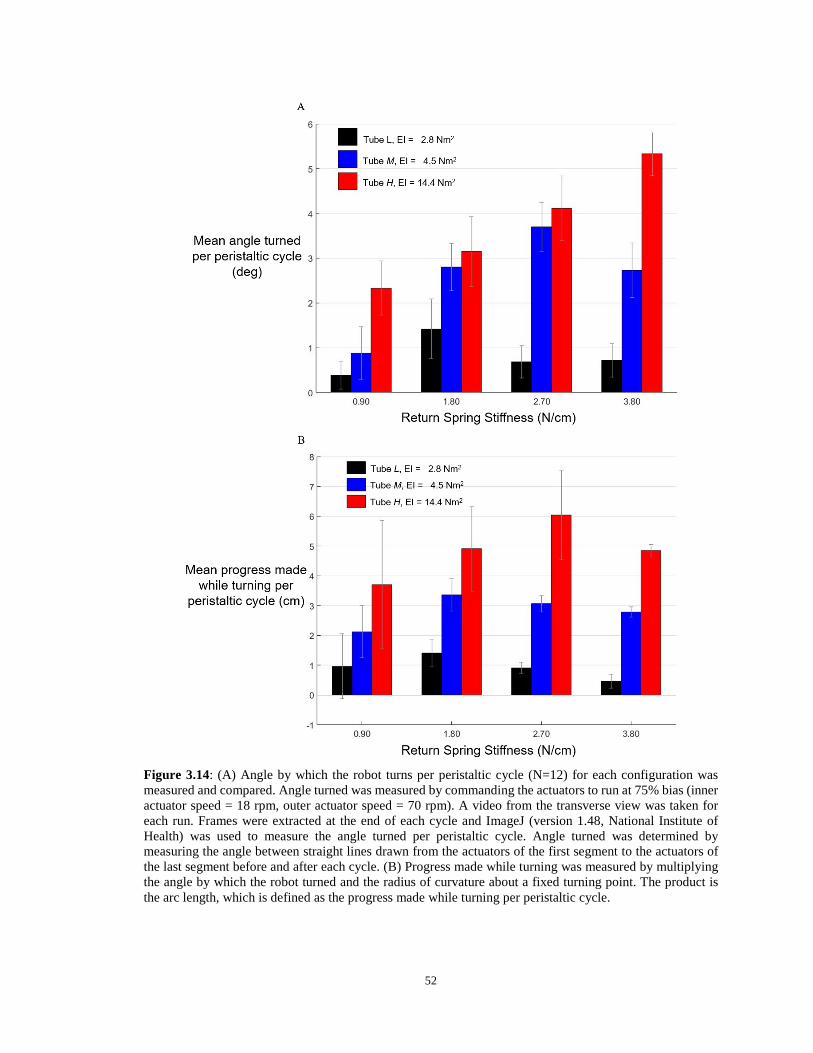
52

Figure 3.14: (A) Angle by which the robot turns per peristaltic cycle (N=12) for each configuration was measured and compared. Angle turned was measured by commanding the actuators to run at 75% bias (inner actuator speed = 18 rpm, outer actuator speed = 70 rpm). A video from the transverse view was taken for each run. Frames were extracted at the end of each cycle and ImageJ (version 1.48, National Institute of Health) was used to measure the angle turned per peristaltic cycle. Angle turned was determined by measuring the angle between straight lines drawn from the actuators of the first segment to the actuators of the last segment before and after each cycle. (B) Progress made while turning was measured by multiplying the angle by which the robot turned and the radius of curvature about a fixed turning point. The product is the arc length, which is defined as the progress made while turning per peristaltic cycle.

53

3.5 Discussion

The Compliant Modular Mesh Worm robot with Steering (CMMWorm-S) is a mesh-

based robot that uses motor driven cables for actuation. The mesh, composed of 3D printed

rigid vertex pieces and flexible tubes, allows interchanging of its components to vary the

stiffness of the robot. CMMWorm-S is capable of an entirely new volitional movement,

turning, because of the addition of two actuators per segment. Presence of two actuators

allows segments to differentially lengthen and shorten, thereby causing turning motion. It

is a significant advance over the original robot (CMMWorm-O) that our group had

previously developed and described (Chapter 2). Because the previous robot was only

capable of straight-line locomotion, it was not possible for us to study the trade-offs on

different behaviors as functions of stiffness of different components. In this chapter, we

advance in the design and control of a robot capable of multiple behaviors which has not

been previously described in the literature. Our results suggest that for CMMWorm-S,

increasing circumferential stiffening speeds forward locomotion and increasing its bending

stiffness increases its turning angle.

We first examined the effects of tube-link stiffness and return spring stiffness on a

single rhombus. For a single rhombus, the resultant stiffness is highly dependent on the

return spring stiffness. The longitudinal stiffness of the rhombus is directly proportional to

the return spring stiffness, as one would expect from rigid-link mechanism analysis. The

tubes connecting the vertex pieces have very little effect on the rhombus stiffness until a

limit is reached after which the resultant stiffness greatly increases but not infinitely, as it

would with rigid links.

54

Next, we examined the effects of tube stiffness and return spring stiffness on the

longitudinal, circumferential and bending stiffness of an individual segment. Longitudinal

stiffness of a segment is strongly dependent on the return spring stiffness. The stiffness

along the length of the segment increases as the return spring stiffness increases.

Longitudinal stiffness of the segment is, however, less than the predicted equivalent

stiffness of rhombuses connected in parallel in a ring-like structure due to the bending of

the tubes. An upward parabolic relation is observed for longitudinal stiffness as the return

spring stiffness increases. On the other hand, circumferential and bending stiffness of the

segment is proportional to the bending stiffness of the links. Increasing the bending

stiffness of the links resulted in higher circumferential and bending stiffness. On increasing

the return spring stiffness, beyond a maximum, the circumferential and bending stiffness

decrease due to uneven deformation of tubes. A downward parabolic relation is observed

for both circumferential and bending stiffness. This implies that the return spring stiffness

has an optimal based on the structure: It has to be strong enough to return the segment to

the original shape but weak relative to the link bending.

We examined the effects of longitudinal, circumferential and bending stiffness of the

body on forward locomotion and turning. For our design, the stiffer mesh tubes and return

springs resulted in greater forward progress and turning angle per peristaltic cycle.

However, in general, fabricating a stiffer robot will not ensure better performance. The

ability of the CMMWorm-S to be compliant, and adapt to its surroundings depends on the

softness of its tubes. On the other hand, if the tubes are too soft, they undergo uneven

deformation and result in inefficient locomotion. This is an important design trade-off.

55

In straight-line locomotion, circumferential stiffness is most critical. Greater

circumferential stiffness leads to greater forward progress per peristaltic cycle (figure

3.12). Greater circumferential stiffness was achieved by using links with greater bending

stiffness to connect the vertex pieces. Tubes with greater bending stiffness allow more

uniform transfer of forces throughout the segment. These tubes also help in maintaining

the overall rigidity of the structure during locomotion. However, if the links are too stiff in

bending, connecting the rhombuses in a ring-like structure will be difficult. Large bending

stiffness of the links will also result in greater coupling between adjacent segments, thus

inhibiting neighboring segments from achieving different diameters.

For turning, bending stiffness is most critical. Higher bending stiffness leads to a higher

angle turned per peristaltic cycle (figure 3.14). Bending stiffness is strongly dependent on

the bending stiffness of the links similar to circumferential stiffness. However, as the

stiffness of the return springs increases, bending stiffness of the robot decreases. Higher

bending stiffness helps in achieving a more robust structure. However, if the bending

stiffness is too high, it is more difficult to achieve a uniform deformation given actuator

strength and structural integrity of the mesh. Bending stiffness should be small enough to

allow each side of a segment to achieve different lengths for turning. Nevertheless, if the

bending stiffness of the robot is too soft, the segment will be unable to elongate during

peristaltic locomotion thus resulting in little forward progress.

To improve overall locomotion with compliant bodies, our work suggests the following

design principles. First, reduced robot mass allows for the use of more compliant (less stiff)

components. Lighter weight segments allow links with smaller bending stiffness to lift

segments and avoid dragging them as the robot advances. Greater segment mass requires

56

stiffer links to allow segments to be lifted. Second, the return springs should not be so stiff

that a large amount of actuator force is required to extend the segment and should not be

too soft such that the return springs are incapable of returning the segment to its maximum

diameter during contraction. In other words, the return spring stiffness should be small

enough to allow the segment to undergo maximum extension when acted upon by the

actuators and some external resistive force and large enough to return the segment to its

maximum diameter rest state.

In order to generalize the above design criteria, we propose a guideline based on the

experimental results in this chapter. In order to permit the intended soft body deformations

for locomotion with a mesh body, the stiffnesses should be related to the body scale as:

𝒎𝒎𝒎𝒎𝒎𝒎𝑳𝑳𝒎𝒎𝜟𝜟

<𝑲𝑲𝒄𝒄𝑲𝑲𝒃𝒃

𝑲𝑲𝒍𝒍(𝟑𝟑.𝟑𝟑)

where m is segment mass, g is acceleration due to gravity, ∆L is maximum change in

segment length for the structure, ∆A is maximum change in segment cross sectional area

for the structure (cross sectional area at maximum diameter – cross sectional area at

minimum diameter), Kc is circumferential stiffness, Kl is longitudinal stiffness and Kb is

the bending stiffness. This single equation expresses that the weight (mg) is supported by

the circumferential stiffness (Kc), a large stroke length (∆L) is permitted by low

longitudinal stiffness (Kl), and higher bending stiffness keeps moving segments from

dragging on the ground especially if the change in area is small. Thus, the goal is to design

a structure to optimize the stiffness ratio (KcKb/Kl) to permit larger stroke lengths and

payloads with less dramatic changes in radius. Our mesh robot accomplishes (3.3) for every

57

configuration and tube stiffness. However, for the worst performing assemblies, the ratio

of the right to left side is about 1. While for the best performing assemblies, the ratio is

approximately 30. Beyond this we see a decrease in performance (figure 3.15,

configuration A, tube type H), suggesting there is a maximum limit beyond which

performance starts to decrease.

Biologists have predicted that earthworm body stiffness (resistance to extension) is

constant as a function of body mass (Quillin 1999). Since peristaltic locomotion is based

on changes in dimensions of the body, longitudinal and circumferential body wall strains

are highly dependent on body length. Quillin (1999) observed that large earthworms were

crawling at greater absolute speeds compared to smaller earthworms due to longer stroke

Figure 3.15: Summary of design criteria as shown in Equation 3.3. The horizontal dashed line indicates the minimum equivalent stiffness (KcKb/Kl) based on mass, change in segment length and change in cross-sectional area (mg∆L/∆A) for peristaltic locomotion for the CMMWorm-S. Tube type ‘L’, configuration D has an equivalent stiffness of 0.05 N/cm, thus exhibits uneven deformation and poor performance. The other configurations for all tube types are above the desired equivalent stiffness causing increased efficiency in straight-line locomotion.

58

lengths. We hypothesize that earthworms rely on circumferential body wall strain during

straight-line locomotion and bending stiffness during turning. Experiments directed

towards measuring body stiffness of earthworms and correlating measured stiffness

parameters to worm locomotion will give roboticists a better insight on the parameters

required for the development of future peristaltic robots.

Researchers have defined soft robots as composed primarily of materials with moduli

in the range of that of soft biological materials (less than 109 Pascals) (Rus and Tolley

2015). Implementing properties of a soft body on a robotic platform has been simplified

by reducing or grouping degrees of freedom (Menciassi et al. 2004, Lee et al. 2010), and/or

by replacing continuously deformable soft bodies with rigid joints (Wang and Yan 2007,

Omori et al. 2009). The CMMWorm-S uses 3-D printed rigid vertex pieces as pin-joints to

simplify some of the challenges faced in soft-robotics (Kim et al. 2009, Lipson 2014). Even

though the structure of this robot includes some relatively rigid pieces, the effective elastic

modulus (0.08×104 - 0.65×104 Pascals) for the robot lies well within the range of soft-

robotics. However, for a truly soft robot to achieve its potential, all hardware used (sensors,

actuation, computation, power and communication) must be embedded within the soft body

of the robot, resulting in smarter materials (Rus and Tolley 2015).

CMMWorm-S experiences nonlinear strain during locomotion due to nonlinear

stiffness (figure 3.8 and figure 3.10). An inherent problem observed during locomotion is

the physical phenomena of hysteresis. As observed in figure 3.12, the speed of a softer

body is slower than a more rigid structure. The lack of a strong enough return force

(springs) or high structural rigidity that allows even contraction throughout the segment

causes a difference in the rate of contraction and expansion. This leads to a loss in

59

efficiency during locomotion. In future work, through model-based analysis we can

characterize this phenomenon and can develop control schemes that might reduce the effect

of hysteresis during locomotion.

In future work, we will also examine the relationship between turning and friction to

allow the robot to turn efficiently on surfaces with different coefficients of friction.

Throughout this chapter, we tested turning on a surface with a large coefficient of friction.

During turning, the robot experiences slip in the lateral direction. Slip has efficiency costs

(Daltorio et al 2013), but we have found that through model-based calibration, slip can be

reduced (Huang et al 2017) or even eliminated by making the control waves configuration-

dependent (Chapter 6). The robot presented in this chapter will be ideal for exploring the

effect of body softness in new responsive gaits for turning, obstacle avoidance, and

confined environments.

60

Chapter 4 Design and Actuation of Fabric-based Worm-like Robot This chapter was originally published as:

Kandhari, A., Mehringer, A., Chiel, H.J., Quinn, R.D. and Daltorio, K.A., 2019. Design and Actuation of a Fabric-Based Worm-Like Robot. Biomimetics, 4(1), p.13.

61

4.1 Introduction

The growing field of soft robotics demonstrates the mechanical and algorithmic

advantages of using compliant materials (Kim, et al. 2013, Tolley, et al. 2014). Low

modulus polymers allow robots to bend in ways that conventional robots cannot (Carpi, et

al. 2010). This enables robots to better accommodate human interaction and perform

delicate operations. Furthermore, soft materials better mimic biology, allowing robotic

platforms to imitate animals such as octopi (Kim, et al 2013, Mazzolai, et al. 2012, Renda,

et al 2012), caterpillars (Umedachi and Trimmer 2014), snails (Chan, et al. 2007), and

earthworms (Boxerbaum, et al 2012, Seok, et al 2013, Tanaka, et al 2014, Wang and Yan

2007) as presented in this chapter.

Textiles can be key materials for future soft robots. A wide variety of fabrics are

available that can provide advantageous weight, flexibility, strength, and cost properties

(Coyle, et al. 2007). Fabric has been used in wearable robotic devices that could provide

active assistance during walking (Park, et al. 2014, Quinlivan, et al. 2017), such as robotic

gloves for hand assistive applications (Cappello, et al. 2018, Yap, et al. 2016), or have

sensors embedded for monitoring electrophysiological information from the human body

(Jung, et al. 2014, Inaba, et al. 1996, Stoppa and Chiolerio 2014, Case, et al. 2016, Kim, et

al. 2015). Fabric embedded with shape memory materials could be useful for an active joint

stability brace on human fingers because it can change stiffness (Chenal, et al. 2014).

Pneumatic actuators embedded with fabric have been used to turn inanimate objects into

multifunctional robots (Booth, et al. 2018). New approaches to replacing structural

elements with textiles will be critical for these and other applications.

62

In this chapter, we will show how fabric can replace traditional structural and compliant

elements in an earthworm-like robot to achieve comparable performance with fewer

mechanical parts. We directly compare a nonfabric-based design with a fabric-based

design, demonstrating peristaltic locomotion on substrates with different coefficients of

static friction.

The robots we present take their inspiration from earthworms. Earthworms are

particularly skilled at navigating through confined spaces, complying with their

surroundings, and burrowing. Earthworms use their segmented body to locomote. Each

segment of an earthworm consists of a set of longitudinal and circumferential muscles. The

hydrostatic coupling (Chiel, et al. 1992) allows the segment to extend longitudinally while

contracting in diameter and vice versa. Earthworms travel by means of waves of muscular

contractions called peristalsis (Gray and Lissmann 1938), which causes the segments of

the body to sequentially elongate and shorten in length, generating locomotion in the

direction opposite to that of the muscular contractions. During peristalsis, the

circumferentially expanded segments anchor the body allowing contracting segments to

advance. Mimicking this type of locomotion on a robotic platform would be valuable in

navigating constrained environments.

Many worm-like robots have been constructed (Boxerbaum, et al. 2012, Horchler, et

al. 2015, Kandhari, et al. 2018a, Dario, et al. 2004). The Compliant Modular Mesh Worm

robots (CMMWorm-Original and CMMWorm-Steering (CMMWorm-S; figure 4.1))

developed by our group (Chapter 2 and Chapter 3) are modular multisegmented, cable

actuated soft robots. Both CMMWorm robots have a mesh structure held together with

three-dimensional (3D) printed rigid components referred to as vertex pieces. Vertex pieces

63

are connected with short links of flexible nylon tubes that allow relative rotation and

prevent relative translation. A cable running along the circumference of each segment is

actuated by either one (CMMWorm-Original) or two (CMMWorm-S) servomotors, similar

to the circumferential muscle of an earthworm’s segment. As an actuator rotates, it spools

in cable, thereby contracting the diameter of the segment. Linear springs are placed along

the length of the segment that extend as the segment contracts in diameter. As the actuator

spools out cable, the springs passively return the segment to its maximum diameter state,

based on the amount of cable spooled out, similar to the longitudinal muscles of an

earthworm’s segment.

Figure 4.1 Our previous worm-like robots’ segments mimic worm segments with a cylindrical mesh held together with 3D printed vertex pieces and linear springs. Single segment of Compliant Modular Mesh Worm-Steering robot (CMMWorm-S) which has two AX-18A actuators and 22 3D printed rigid components (vertex pieces). The vertex pieces are connected using flexible nylon tubes. The linear springs placed along the length of the segment passively return the segment to its maximum diameter. The CMMWorm-S has redesigned 3D printed vertex pieces which replace the commercial quick-connect fittings used to connect tubes in the first iteration. The 3D printed components are printed in acrylonitrile butadiene styrene on a Stratasys Fortus 400 mc FDM (fused deposition modeling) machine with 0.245 mm slice height.

Here, we present the structure of two fabric-based worm-like robots. Like earthworms

and our prior robot CMMWorm, the body structures achieve locomotion by coupling radial

expansion with longitudinal contraction. The FabricWorm, with a maximum diameter of

64

21 cm, has a mesh structure consisting of one third the number of rigid components (vertex

pieces), as compared to CMMWorm, and nylon tubes encased within two layers of

stretchable fabric. The MiniFabricWorm, with a maximum diameter of 12.5 cm, has a mesh

structure consisting of nylon tubes encased within two layers of stretchable fabric and no

rigid vertex pieces. This chapter describes the diameter–length coupling ratio, stiffness

properties, and speed achieved by the two robots on different substrates with different

coefficients of static friction. We report that the maximum speed achieved by FabricWorm

is 33 cm/min (0.49 body-lengths/min) and that of MiniFabricWorm is 13.8 cm/min (0.25

body-lengths/min). The highest speed for both robots was achieved on linoleum tiles with

a coefficient of static friction of 0.36 for MiniFabricWorm and 0.43 for FabricWorm. We

also compare the performance of these robots to their nonfabric counterparts, which to the

best of our knowledge is unique to the present work.

4.2 Robot Design

A design goal of this work is to reduce the number of rigid components in our prior

worm robots (Softworm, Compliant Modular Mesh Worm Robot-Original and Compliant

Modular Mesh Worm Robot with Steering). These rigid components limit the

deformability of the robots. Our first fabric-based robot, FabricWorm, eliminated many of

the 3D printed vertex pieces that held the mesh together and the linear springs. Our second

version, MiniFabricWorm, is smaller and eliminated all the 3D printed vertex pieces of the

mesh, leaving only the actuators as rigid components.

In both versions, two layers of stretchable fabric are sewn together around flexible

tubes that intersect in a mesh pattern of rhombuses. The fabric compliance provides the

65

spring return force that counters the cable actuation, eliminating the need for springs. The

sleeves created by the fabric hold the mesh together, reducing (in the case of FabricWorm)

and eliminating (in the case of MiniFabric Worm) the need for the pin joints created by the

vertex pieces. The flexibility of the fabric allows large elastic deformation of the mesh

structure, where an increase in length is coupled with a decrease in diameter (similar to the

hydrostatic coupling observed in earthworms).

Fabric selection is critical. Fabric elasticity can come either from elastic composite

fibers or from the way the fabric combines those fibers; for example, knits permit greater

stretch than weaves (Mehringer, et al. 2017, Poincloux, et al. 2018). For FabricWorm and

MiniFabricWorm, we used a knitted cotton fabric that was made of 97% cotton and 3%

spandex. We used a knitted cotton fabric, since these can achieve large, recoverable

deformations with a strain of around 300% (Mehringer, et al. 2017). The selected fabric

has anisotropic stiffness properties (figure 4.2), which we used to provide recovery forces.

Two pieces of fabric stitched together have a stiffness of 9 N/cm along its stiff direction

(referred to as knit side) and 1 N/cm along its soft direction (referred to as knit warp).

Fabric has negligible bending stiffness, but the “stretchability” can be directly compared

to linear spring stiffness (ranged between 0.9 N/cm to 3.8 N/cm for the CMMWorm

robots). The stiffer crosswise direction was aligned with the circumferential direction of

the body, as the fabric provides the passive restoring force to return segments to the

maximum (un-actuated) diameter. This eliminates the need for longitudinal springs used

in previous iterations (Chapter 2 and Chapter 3).

66

Figure 4.2: (A) Structure of chosen fabric, captured by a microscope with 100x magnification. Top left is the fabric in its undeformed state, top right shows stretch along the knit warp side (stiffness = 1 N/cm) and bottom panel shows stretch along knit side (stiffness = 9N/cm). (B) Change in length of fabric as a force is applied along the knit side and knit warp. The slope of the linear fit for the two curves is the stiffness of the material along orthogonal directions. Dimension of fabric tested was 2.54 cm × 2.54 cm.

The mesh of flexible tubes is integrated into the fabric to give the structure a compliant

worm-like shape. Without fabric, the flexible tubes alone are not capable of returning to

the maximum diameter state after circumferential deformation. Conversely, without the

tubes, the fabric alone does not hold a cylindrical shape under gravity, nor can it be

contracted uniformly. For FabricWorm, tubes of length 18.5 cm are connected using 3D

printed rigid vertex pieces that were used in CMMWorm. Nylon tubes with different

bending stiffness properties were used to test FabricWorm. A stiffer tube with wall

thickness of 0.66mm with bending stiffness (EI, where E is Young’s modulus and I is area

moment of inertia) of 14.4 N cm2 and a softer tube with wall thickness of 0.4 mm with

bending stiffness (EI) of 2.8 N cm2. On the other hand, MiniFabricWorm lacks any rigid

components in its structure, i.e., the structure does not consist of any vertex pieces. The

entire structure is composed of tubes spiraled along the entire length of the robot embedded

within the fabric. The tube used has a wall thickness of 0.635 mm and a bending stiffness

of 32.64 N cm2. The assembly of both robots is discussed below.

67

4.2.1 FabricWorm

Two 80 cm × 70 cm rectangles were cut out of the fabric, with the 70 cm length in the

direction of the stretch. A template using tubes and vertex pieces was assembled and placed

on the fabric to create an outline of sleeves through which the tubes would pass (Connolly,

et al. 2015). The two fabric pieces were then sewed along these lines with all purpose thread

on a Husqvarna Viking Opal 650 sewing machine using a straight stitch, while making sure

no strain was introduced during this process. This resulted in sleeves to encase the tubing

(figure 4.3) (Mehringer 2017). Once the tubes are inserted inside the sewn sleeves, the

structure is rolled into a cylindrical shape and the two edges of the fabric are joined using

sew-on snaps on the top. The sew-on snaps allow for easy access to inner components

(vertex pieces or cables) for assembly and repair purposes

Figure 4.3: (A) The lines drawn on one layer of fabric serve as a guide for sewing sleeves for the tubing to pass through. The pink dots show where the vertex pieces will be placed and the placement of the actuators for a six segments robot is marked. (B) The tubes are fed through the sleeves and the actuation cable is fed through the vertex pieces. The vertex pieces are also encased within the two layers of fabric. (C) Tubing used shown without the fabric. Note: the vertex pieces shown in this figure are from the first iteration of Compliant Modular Mesh worm robot, while Figure 1 shows the second iteration of the Compliant Modular Mesh Worm robot, i.e. Compliant Modular Mesh Worm with Steering (CMMWorm-S). CMMWorm-S has redesigned 3D printed vertex pieces that replaces the commercial quick-connect fittings used to connect tubes in the first iteration.

68

The rhombus pattern of the mesh causes the length-width coupling that creates a change

in diameter in response to a change in length. The included angle of the rhombus (the

sewing angle of the sleeves) is based on the limits of the rigid vertex pieces, allowing

maximum range of motion. The final assembly of FabricWorm consists of one-third the

number of rigid pieces (48 as compared to 132) when compared to its predecessor

Compliant Modular Mesh Worm robot. Each segment consists of six rigid components,

one actuator mount and five vertex pieces. The actuator mount houses the Robotis MX-

64T actuator. A cable running along the circumference of the segment is actuated by the

motor, allowing circumferential contraction (causing longitudinal extension). As the cable

is unspooled, the fabric around the mesh passively expands the diameter of the segment,

based on the amount of cable unspooled until it reaches its maximum possible diameter

(rest state). A sequential circumferential contraction and expansion of connected segments

allows the robot to locomote in a direction opposite to the direction of the contraction-

extension wave.

Fully assembled FabricWorm (figure 4.4) (Mehringer 2017) has six segments with six

actuators and a total of 48 3-D printed components. The total robot weighs 1.61 kg and has

a rest length of 67 cm. The maximum diameter is 21 cm and the robot is capable of

deforming to 60% of its maximum diameter (Figure 4.5) (Mehringer 2017). The fabric

worm body is deformable and is capable of being bent in a semi-circular shape.

69

Figure 4.4: FabricWorm during a peristaltic wave; the various components of the structure are labelled. The sleeves through which the tubes pass can be seen on the inside of the fabric. The total length of FabricWorm in its rest state is 67 cm.

Figure 4.5: (A) Front view of FabricWorm fully expanded. The actuation cable is highlighted (black hexagon drawn over cable for visibility). (B) As the actuation cable (smaller black hexagon) is spooled-in, the robot contracts in diameter. (C) Side view of fully expanded FabricWorm. (D) Side view of fully contracted FabricWorm.

70

4.2.2 MiniFabricWorm

MiniFabricWorm (figure 4.6) builds on the the design of FabricWorm, but simplifies

it. In contrast, its maximum diameter is smaller compared to FabricWorm (12.5 cm as

compared to 21 cm). Miniaturization of FabricWorm was limited by the presence of 3D

printed rigid pieces in the structure. Thus, MiniFabricWorm does not include any rigid

pieces in the structure. The design of MiniFabricWorm includes 2 layers of fabric sewn

together just as with FabricWorm to create sleeves for tubing. Instead of having sections

of tubes connect to vertex pieces, there are 12 longer tubes helically fed throughout the

entire length of the robot. The assembly of MiniFabricWorm is the same as FabricWorm

(figure 4.3), without the use of vertex pieces to join sections of tubing. The intersections

of the tubing in the sewn fabric sleeves replace the vertex pieces. Each segment consists of

only one rigid piece: the actuator mount. Actuator mounts are held inside the fabric

integrated mesh by being sewed through the fabric.

Figure 4.6: MiniFabricWorm consists of no rigid components in the structure. The sleeves through which tubes pass are visible. The length of MiniFabricWorm in its rest state is 55cm.

71

MiniFabricWorm uses smaller Dynamixel AX-18A actuators that are housed within

the actuator mounts. Cables attached to the actuator are sewn through the fabric across the

circumference of the segment and secured to buttons that are sewn on the top of the body.

The working principle is the same as FabricWorm: as the cable is spooled in, the segment

decreases in diameter and as the cable is spooled out, the fabric allows circumferential

expansion, based on the amount of cable spooled out.

MiniFabricWorm uses tubes of higher bending stiffness compared to the stiffest tubes

used in FabricWorm (bending stiffness of 32.64 N-cm2 compared to 14.4 N-cm2). The

reason is that when tubes of lower bending stiffnes were used, the robot failed to locomote,

due to the softness of its structure i.e., the structure was too compliant and did not cause

the robot to move. Replacing tubes within the mesh with higher bending stiffness tubes

increased the bending stiffness and circumferential stiffness of the robot based on Chapter

3. This allowed the robot to move.

MiniFabricWorm fully assembled is a 5 segment worm-like robot with only one rigid

component (actuator mount) within the structure. The robot weighs 580 grams with a

maximum diameter of 12.5 cm and minimum diameter of 10.2 cm. The total length of the

robot in its rest state is 55 cm. The structural comparison of CMMWorm-S, FabricWorm

and MiniFabricWorm is summarized in table 4.1.

The Fabric worm robots, compared to their non-fabric counterparts (CMMWorm-O

and CMMWorm-S), are much faster to fabricate and assemble due to the greatly reduced

number of parts. It is much faster to sew together two pieces of fabric than to 3D print an

additional 84 vertex pieces. Furthermore, the manual assembly process is a significant cost

72

and time factor. Fabric based robots were faster to assemble because of the elimination of

14 (for FabricWorm) to 22 (for MiniFabricWorm) vertex pieces per segment. The fabric

counterparts also do not require the attachment of discrete longitudinal springs.

Furthermore, each vertex piece costs $1.70 at standard 3D printing rates of $0.6/cm3 at

CWRU’s public maker space. The fabric, which cost approximately $12/m2 at JoAnn

Fabrics, is a cost saving solution.

Table 4.4: Summary of structural comparison between CMMWorm-S, FabricWorm and MiniFabricWorm.

CMMWorm-S FabricWorm MiniFabricWorm

Mesh mass (grams)* 650 854 305

Number of rigid pieces in structure

132 48 0

Number of segments 6 6 5

Largest diameter (cm) 21 21 12.5

Total contracted length (cm)

103 67 55

* Mass of entire robot’s mesh without actuators

4.2.3 Electronics and Control

FabricWorm and MiniFabricWorm were actuated by Dynamixel MX-64T and

Dynamixel AX-18A actuators, respectively. These actuators were connected to a single

Robotis Open CM9.04 microcontroller. Programming of the microcontroller and data

logging were performed over a USB to PC connection. We used our open source

DynamixelQ library for the Open CM9.04 microcontroller that allows high-speed

communication with AX and MX series Dynamixel actuators.

73

A time-based control scheme generates waves along the length of the robot to produce

locomotion. Both FabricWorm and MiniFabricWorm used a 3×1 wave pattern (where 3

represents the number of segments per wave and 1 the number of waves along the body,

following the convention in [9,10]). At any given time, one segment is contracting in

diameter and one is expanding, with an inactive spacer segment in between. After sufficient

time has passed for contraction and retraction, (1.8 seconds for FabricWorm and 0.9

seconds for MiniFabricWorm), allowing the contracting segment to achieve minimum

diameter and retracting segment to achieve maximum diameter, the wave shifts down the

body, resulting in forward motion.

4.3. Stiffness Characterization and Performance Comparison

We empirically characterized the properties and resulting performance of both robots.

For FabricWorm, two types of tubes with different bending stiffness properties were used

to determine robot properties. We determined robot properties for both robots in terms of

diameter-length coupling ratio, longitudinal stiffness, bending stiffness and robot speed on

substrates with different coefficients of static friction.

4.3.1. Diameter-length coupling ratio

To determine how change in diameter will be translated to a change in length, a

coupling ratio was evaluated for both robots. This made it possible to understand how well

the mesh can translate forces within the structure, allowing longitudinal extension and

causing locomotion. If a change in diameter does not induce a sufficient change in length

due to the structure being too soft or too stiff, the robot will not be able to move. In case of

74

a fabric integrated mesh, it is important to see if the fabric allows simultaneous changes in

length and diameter (figure 4.7).

To measure the coupling ratio for FabricWorm, the front two segments were contracted

and the change in diameter and length were noted for both versions of FabricWorm (with

stiff and soft tubes). The change in length was divided by two for change in segment length.

For MiniFabricWorm, all five segments were contracted and the change in diameter and

length was noted. Length was divided by five for change in segment length. Measuring the

coupling ratio of the robots is a quality indicator of how well the robot will move based on

the structural components and stiffness.

In MiniFabricWorm, the coupling ratio was 0.68. The change in diameter for

MiniFabricWorm could not exceed 2.3 cm, as the presence of actuator limits further

contraction. In FabricWorm with stiff tubes, the coupling ratio for a single segment was

0.82, whereas with soft tubes it was 0.19. The low coupling ratio of 0.19 is due to the low

bending stiffness of the tubing. During locomotion testing, FabricWorm with these low

bending stiffness tubes was unable to locomote, because as the segments were actuated,

the tubes buckled and kinked instead of extending the segments in length. The compliance

of the structure absorbs the actuation locally rather than transmitting force to the rest of the

structure. Hence, all locomotion testing for FabricWorm was done with the stiff tubes.

CMMWorm-S has the highest coupling ratio of 0.92. Although our goal was to make the

robot as soft as possible, this data shows that there is a limit to how soft the structure can

be for locomotion using this design.

75

Figure 4.7: Coupling ratio, which is the relationship between the change in length of a segment and the change in diameter of a segment for MiniFabricWorm (blue line), FabricWorm with soft tubes (red line) and FabricWorm with stiff tubes (gray line).MiniFabricWorm (blue line) has a coupling ratio of 0.68, whereas FabricWorm with stiff tubes has a coupling ratio of 0.82. CMMWorm (black line) has the highest coupling ratio of 0.92. A large coupling ratio will result in better longitudinal extension allowing larger stroke lengths per peristaltic wave. CMMWorm is capable of contracting by 32% of its maximum diameter while extending by 37% of its initial segment length, whereas MiniFabricWorm and FabricWorm with stiff tubes both contract by 20% of their initial diameter and extend by 16% and 31% of their initial segment length, respectively.

4.3.2. Longitudinal stiffness

Longitudinal stiffness of the robot was measured by securing one end of the robot and

applying incrementally increasing loads to the other end while measuring extension of the

robot. The slope of the regression line between displacement and force is the measured

longitudinal stiffness (Figure 4.8).

The stiffness of a segment of FabricWorm is 8.5 N-cm-1 when the mesh consists of soft

tubes and 9.9 N-cm-1 when the mesh is composed of stiff tubes. For MiniFabricWorm, the

longitudinal stiffness was 11.8 N-cm-1.

76

Figure 4.8 shows that the main factor determining the longitudinal stiffness of a

segment is the stiffness of the fabric along its knit side, and thus all the FabricWorm

stiffnesses are similar. The tubes, however, also add to the overall longitudinal stiffness; as

a consequence, MiniFabricWorm, which had the tubes of highest bending stiffness, had the

highest longitudinal stiffness, followed by FabricWorm with stiff tubes and FabricWorm

with soft tubes. FabricWorm with soft tubes exhibits uneven deformation beyond an

extension of 1 cm as the tubes started to buckle. As the fabric is responsible for

circumferential expansion of the segment on removal of the actuation force, a higher

stiffness fabric will cause an increase in the longitudinal stiffness of the segment.

In comparison to CMMWorm-S, the stretched fabric makes the robot stiffer. That is

because the stiffness of the fabric itself is stiffer than the springs used in the CMMWorm-

S robot. The total spring stiffness on CMMWorm-S was 1.8 N-cm-1 and overall stiffness

of the segment is 1.5 N-cm-1. Similarly. all the stiffnesses of the Fabric Worm robots are

similar to the stiffnesses of the fabric, and the small differences in these values are due to

the different tubes used in the structure.

4.3.3. Bending stiffness

Bending stiffness of the robot provides a quantitative measure of the ability of a

contracted segment to support itself between expanded anchoring segments. A peristaltic

robot with a higher bending stiffness will be capable of lifting its adjacent contracted

segments off the ground during longitudinal extension. As segments are lifted during

locomotion, frictional resistance decreases compared to when segments are dragged along

the substrate, thereby improving locomotion. Bending stiffness (figure 4.9) determines the

overall compliance of the structure and depends on the fabric, the tubes, the rigid

77

components (if present) and the included angle of the rhombus patterns, i.e. a fully

stretched robot has a lower bending stiffness compared to a fully compressed robot.

Figure 4.8: Change in length of a single segment when a force is applied along the length of the segment. The slope of the linear fit (dashed lines) of the curves is used to estimate the longitudinal stiffness of the segment.

On increasing the applied moment, the change in angle follows a downward parabolic

trend for FabricWorm and upward parabolic trend for MiniFabricWorm. This difference is

due to the fact that FabricWorm has rigid components present in the structure and applying

moment beyond a threshold might cause failure at these points of rigid contacts. Thus, a

moment of up to only 1.4 N-m was applied for FabricWorm. However, due to the absence

of any rigid vertex pieces in MiniFabricWorm, a larger moment could be applied without

any points of failure (breaking of the rigid components) and a larger change in bending

angle was observed. Overall, within its working region, CMMWorm has the highest

78

bending stiffness followed by FabricWorm with stiff tubes then FabricWorm with soft

tubes. Due to the absence of rigid components, MiniFabricWorm has the least bending

stiffness in the operating range, making it the most compliant robot amongst the different

iterations designed by our group (Boxerbaum, et al. 2012 Horchler, et al. 2015 Kandhari,

et al. 2018a) (Figure 4.10).

Figure 4.9: Change in angle of the robot as a moment is applied at the end of the robot. Both robots follow a non-linear trend. Joint angle of the rhombus structure is an important factor causing the non-linear trend. Joint angle decreases with increasing bending stiffness, thereby decreasing bending capability when rigid components are present. Moment that can be applied on MiniFabricWorm is larger compared to FabricWorm due to the absence of rigid components in the mesh.

79

Figure 4.10: Images demonstrating the bending limits of these two robots. (A) FabricWorm bent in a semicircle (~180̊) due to the flexibility of the body. In this photo, a string holds the ends together to maintain this position. The robot is not capable of bending any farther due to the presence of rigid components. (B) MiniFabricWorm in a circular configuration (~360̊). Due to the absence of rigid components in the mesh, the robot is capable of achieving this position. Further bending causes the actuator mounts within the robot to interfere with one another.

4.3.4. Robot speed

Finally, we compared the speed of the robots in straight-line locomotion (figure 4.11).

For FabricWorm, tests were performed using only stiff tubes, since it did not locomote

with the soft tubes because of the structure being too compliant. MiniFabricWorm and

FabricWorm were tested on surfaces with different coefficients of static friction (in

ascending order): linoleum tile, plywood and carpet. Videos from the sagittal view were

taken and Tracker software (Version 4.11.0, Open Source Physics) was used to analyze the

distance moved over multiple peristaltic cycles for both robots.

The robots achieved greater speeds with stiffer tubes and on substrates with the least

coefficient of static friction (linoleum tiles). MiniFabricWorm achieved a maximum speed

of 13.8 cm/min (0.25 body-lengths/min) on linoleum tile followed by 11.7 cm/min (0.21

body-lengths/min) on plywood and only 4 cm/min on carpet (0.07 body-lengths/min).

FabricWorm achieved a maximum speed of 33 cm/min (0.49 body-lengths/min) on

linoleum tile, 31.2 cm/min (0.46 body-lengths/min) on plywood and 28.8 cm/min (0.43

80

body-lengths/min) on carpet. The limiting factor for speed is the change in diameter that

causes a change in length. For MiniFabricWorm, the maximum change in diameter is 2.3

cm (18% of maximum diameter) and change in length is 0.8 cm. For FabricWorm,

maximum change in diameter is 4.3 cm (20% of maximum diameter) and change in length

is 3.8 cm. MiniFabricWorm, due to its smaller diameter and change in segment length, has

a smaller stroke length (extension of each segment during one cycle of peristaltic wave);

thus, in figure 11, we normalize the speed with maximum diameter.

Figure 4.11: Robot speed normalized by diameter for FabricWorm with stiff tubes (gray) and MiniFabricWorm (blue). A video was taken from the sagittal view and Tracker software was used to measure the progress made over time for both robots on substrates with different coefficients of friction (indicated on top of each bar). Note: The MiniFabricWorm robot was run three times over multiple wave cycles on linoleum tile and wood, and twice on carpet. The result shown above is the average speed over the number of trials.

Both robots experience slip in the forward and backward directions, and thus the speed

decreases as the coefficient of friction increases. MiniFabricWorm on carpet makes little

81

forward progress, because the carpet prevents the robot from moving forward: the fabric

and carpet interact such that the robot gets stuck with each kernel of the carpet, thereby

hindering forward locomotion. In contrast, for MiniFabricWorm, even without any rigid

vertex pieces in the structure, the mesh integrated fabric is capable of transmitting forces

such that the segment contracts uniformly, thereby causing longitudinal extension. On

removal of the actuation forces, the fabric allows for circumferential contraction that causes

the robot to move forward.

4.4. Conclusions and Future Work

We have shown that a mesh can be integrated into a compliant fabric to form a structure

that, when actuated, can mimic worm-like peristaltic locomotion. The fabric can secure the

mesh so that it holds its shape during actuation. Moreover, the stretchable fabric can

provide restoring forces, eliminating the need for other restoring springs. The stiffness of

the fabric is nine times greater along its knit warp direction than along its knit side

direction. We align the stiff side along the circumference of the robot, so that it aids in

passively returning the segment to its maximum diameter state as the actuation force is

removed. As a result, compared to our prior robots, fewer rigid pieces are required.

Specifically, FabricWorm uses 36% of the vertex pieces of CMMWorm, and

MiniFabricWorm uses no vertex pieces at all in the mesh.

In our experience, reducing the number of rigid parts makes the mechanical design

more robust. Our group has been improving the 3D printed connectors for modular worm

robots for more than five years to achieve greater mechanical robustness, low weight, and

low cost. The FabricWorm robots further advance the soft robotic paradigm: softer

connections are less brittle, weigh less, and cost less.

82

Overall bending stiffness is key to performance. In Chapter 3 we demonstrated that

reducing spring stiffness or using tubes with lower bending stiffness reduces stiffness

properties. However, the structure is not capable of maintaining its cylindrical shape if

tubes of lower bending stiffness are used. During locomotion, the softer tubes bend and

kink easily and are thus unable to transfer forces uniformly along the segment causing

uneven deformation, thereby hindering locomotion.

In Chapter 3 we developed design criteria for peristalsis. We demonstrated that the

ratio of the expansion of a peristaltic robot to its contraction should be less than the

capability of the segment to resist those changes. In other words, there exists limits

depending on the mass of the robot and the extent to which the robot segment can change

in diameter and length, that correlates to how soft the structure can be. If the structure of

the robot is too soft, all the actuation energy will be lost due to the compliance of the robot.

In contrast, if the structure is too rigid, the robot will be unable to deform. Both these

conditions will prohibit the robot from locomoting. Thus, for the case of MiniFabricWorm,

we used nylon tubes with higher bending stiffness such that the robot could deform

uniformly, allowing peristaltic locomotion.

When performance of FabricWorm and MiniFabricWorm are compared with their

predecessors, the advantages of fabric as a construction material are clear. Absence of rigid

components reduces the overall bending stiffness of the two robots compared to the

previous generation robots that our group had developed (approximate values -

CMMWorm-S: 3.68 Nm/rad, FabricWorm: 2.3 Nm/rad and MiniFabricWorm: 1.8

Nm/rad). Bending stiffness could be further decreased by increasing the length of the

flexible tubes used. Pitch and spacing of the flexible tubes is inversely proportional to the

83

bending stiffness. Integrating fabric in the mesh reduces the number of rigid components

present in the structure that allows FabricWorm, and to a greater degree MiniFabricWorm,

to bend and recover from large body bending.

Furthermore, we show that by selecting appropriate tube stiffness, locomotion can be

achieved even with this much softer fabric mesh. The first key to locomotion is sufficient

coupling ratio, (change in length vs. change in diameter). A low coupling ratio (such as

0.19 with soft tubes in FabricWorm) results in uneven deformations and poor locomotion.

When stiffer tubes are used, the coupling ratio increases to 0.82, which permits locomotion.

Even without the vertices, MiniFabricWorm achieves a coupling ratio of 0.68, allowing

locomotion. This is comparable with coupling ratio of earthworms of 0.66 (Horchler, et al.

2015) and 0.92 (Kandhari, et al. 2018a) for CMMWorm robots.

We have previously hypothesized that low longitudinal stiffness can be valuable for

eliminating slip if segments are imprecise (Horchler, et al. 2015), and then shown that in

practice high longitudinal stiffness increases the speed of worm-like mesh robots (Chapter

3). Here we show that the longitudinal stiffness of the segment is highly dependent on the

stiffness of the fabric that is aligned along the circumference of the segment. In our case,

the stiffer, knit side was aligned along the circumference of the robot. Hence, the

longitudinal stiffness values of the segment were comparable to the stiffness of the fabric.

We examined the speed of these two robots in straight-line locomotion on substrates

with different coefficients of friction. Due to its higher coupling ratio, FabricWorm can

achieve a maximum speed of 33 cm/min on linoleum tile whereas MiniFabricWorm can

achieve a maximum speed of 13.8 cm/min on the same substrate. Normalized by diameter,

the speeds are comparable 1.6 min-1 for FabricWorm as compared 1.38 min-1 for

84

MiniFabricWorm. These speeds are also similar to CMMWorm and CMMWorm-S, which

have speeds of 25 cm/min (0.24 body-lengths/min) and 72 cm/min (0.92 body-

lengths/min), respectively. The higher speed of CMMWorm-S as compared to

FabricWorm is due to a higher coupling ratio and the use of faster actuators (97 rpm vs 63

rpm at 12V). Actuator speed along with backward slip and compliance of structure are

factors that limit robot speed.

This design enables future worm-like robots to utilize other advantages of fabric skin.

The fabric skin protects the interior from debris. The skin is a surface upon which friction-

altering surface treatments (anisotropic friction worm-like setae) can be affixed. Fabric

integrated mesh is light, highly flexible and cheap to manufacture. The robot breaks less

frequently, as compared to its predecessors, largely due to the reduction of breakable

components. However, inherent limitations such as maximum strain before rupture,

hysteresis, toughness and fatigue still need to be better understood in future work (Bauer,

et al. 2014). Fabric skins may help traverse rough surfaces by deflecting entanglements, or

they may catch or tear on protrusions. In future work, fabric with self-healing properties

(Gaddes, et al. 2016), water resistance, and embedded sensing and actuation could be

especially valuable for worm robots.

To move toward understanding locomotion where the robot has to execute sharper

turns, squeeze through narrow constraints, burrow or travel on delicate surfaces, future

versions of the robot will have more and potentially different types of actuation. Turning

is essential, and will require left and right actuation. We have previously shown that low

bending stiffness is correlated with slower turning. However, eliminating slip in turning

may permit better turning with lower bending stiffnes. Structural stiffness and actuation

85

can work together to exert radial and axial forces for constrained space applications like

burrowing. Novel actuation can change weight distribution and allow for greater

deformability. In all these applications, the characterizations provided here can provide

baseline comparisons for future designs.

86

Chapter 5 Analysis for minimizing COT and maximizing velocity This chapter is currently under review as:

Kandhari, A., Chiel, H.J., Quinn, R.D. and Daltorio, K.A., An Analysis of Peristaltic Locomotion for Maximizing Velocity or Minimizing Cost of Transport for Worm-like Robots

87

5.1. Introduction

Worm robots are deceptively simple, making them a promising and interesting type of

soft robot. Despite it’s apparent simplicity, design of worm-like robots remains nontrivial.

Although over 50 worm-like mobile robots have been implemented, several challenges

have been identified, including stiffness optimization (Kim, et al 2006, Kandhari, et al

2018a), loss of power efficiency due to slip (Boxerbaum, et al. 2012, Daltorio, et al. 2013)

and precise control of soft segments which may vary both in their fabrication and over time

(Horchler, et al. 2015). However, throughout the animal kingdom, peristaltic locomotion

is ubiquitous (for example, in larval stages and in adults (Gjorgjieva, et al. 2013), and some

worm-like organisms are capable of rapid movements (Zoran and Drewes 1988) and

precise movements (Albrecht and Bargmann 2011). In contrast, it is entirely possible to

construct a series of worm-like segments that, when assembled, do not locomote

satisfactorily. Both structural properties and gait selection are key to coordinated

locomotion. Often it is possible to empirically optimize segment structure or control to

improve results, but an analytical guide could help designers to decide fundamental

questions about actuation, structure, control and sensing for soft peristaltic devices.

Here, we clarify how the essential characteristics in peristaltic-locomotion (actuation,

control and softness) contribute to the design of worm-like robots. Previously, textbook

models of worm locomotion claimed that the ratio of moving to anchoring segments is

limited by differences in forward and backward friction coefficients (Alexander 2003).

This would explain observations of biological earthworms in which about equal number of

segments are moving and anchoring at any given time. However, by requiring slip against

anisotropic friction, this explanation contradicts experience with engineered worm robots,

88

which often have minimal anchoring segments and use isotropic friction. Isotropic friction

allows a robot to reverse its direction and extract itself from the environment. Minimizing

anchoring increases speed. Thus, more accurate design constraints are needed for robotics

applications.

Instead of assuming slip under a uniform weight distribution, we consider an idealized

locomoting earthworm model that does not need to slip as it moves and accounts for effects

of actuation and deformation, providing a template for understanding peristaltic

locomotion with two-dimensional analysis. By employing simplifying assumptions, we

demonstrate how worm-like robots can be constructed of any stiffness material with

sufficient effective Poisson’s ratio and actuation energy density. Furthermore, for a given

robot length, either velocity or energy efficiency can be optimized. Moving fewer segments

at once decreases cost of transport but also decreases speed. While previous robots have

been optimized for speed, future robots may need to take into account energy costs. Also,

for the first time, we have an alternative explanation for earthworm observations: perhaps

they are balancing speed and cost of transport.

The idealized template analysis we present below is supported by experiments on our

robot and by a review of worm robots in the literature. To our knowledge, a dedicated

comparative review of worm robots is lacking, even though worm robots are mentioned in

multiple soft robotics reviews (Lee, et al 2017, Rus and Tolley 2015, Kim, et al. 2013). We

show that there are many possible design implementations, but that each of them can be

characterized by the parameters suggested by this analysis in terms of structure, actuation

scheme, and control.

89

Figure 5.1 Recent worm-like robots. (A) Meshworm (Seok, et al. 2013), an expandable nylon mesh using shape memory alloy (Nitinol) for actuation. (B) Peristaltic micro robot composed of silicone bellows that is capable of deforming using Nitinol and undergoes the “two-anchor method” of peristaltic locomotion (Kim, et al. 2006). (C) Softworm (Boxerbaum, et al. 2012), a cable actuated peristaltic robot made of flexible cables and pinned joints. (D) A modular worm-like robot (Nemitz, et al. 2016), which utilizes voice coils, connected by flexible silicone membranes for actuation. (E) A peristaltic crawling robot actuated using servomotor and a fabric-integrated-mesh (Kandhari, et al 2019b). (F) Soft, worm-like robot which models the putative earthworm anchoring mechanism by combining kirigami skin with radially expanding pneumatic actuators (Liu, et al. 2019). (G) Compliant Modular Mesh Worm with Steering (CMMWorm-S) (Kandhari, et al. 2018a), a cable actuated modular worm-like robot capable of turning.

5.2. Results

5.2.1 Template Model: An idealized soft worm with no slip

Earthworms are completely soft with no rigid internal skeleton or exoskeleton. Instead,

they maintain their structure with fluid-filled coelom segments that function as a

hydrostatic skeleton (Chiel, et al. 1992). The hydrostatic skeleton provides a constant

volume constraint, such that increases in length cause decreases in radius and vice versa.

Circumferential and longitudinal muscles change both segment diameter and length.

Sequential extension and expansion of the segments along the length result in peristaltic

locomotion, in the opposite direction of the wave’s travel (Gray and Lissmann 1938).

An idealized model of an earthworm provides a template (figure 5.2) for understanding

peristaltic locomotion in the sagittal plane. Generalized template models that are anchored

by more detailed models have been valuable for other types of biologically-inspired

locomotion (Full and Koditschek 1999). This analysis is pertinent to earthworm robots but

will not apply to worm-like robots that swim like C. elegans (Boyle,et al. 2012), locomote

90

using clamping feet akin to caterpillar crochets (Lin and Trimmer, 2010, Trimmer, et al.

2006), grow like a vine (Hawkes, et al. 2017) or undulate like a salamander (Ijspreet, et al.

2007). Specifically, unlike these examples, we will assume that the body of our idealized

earthworm uses only axial extension to move and only radial expansion to contact the

ground. Rigid rectilinear locomotion like a snake (Marvi, et al. 2013, Onal and Rus 2012)

is similar, but snakes have a skeleton and are relatively rigid whereas this analysis accounts

for soft body deformation (figure 5.2C).

Structurally, we will assume each segment is a hollow cylinder whose properties can

be characterized with properties including Young’s modulus (E), Poisson’s ratio (𝜗𝜗), and

density (ρ). We will call maximum radius segments “anchoring” segments because they

contact the substrate (either flat ground or the interior of a confined space like the inside of

a pipe). For simplicity, we assume each segment is independently actuated with constant

rate (±�̇�𝐿).

The control of an earthworm is defined by the numbers of moving versus anchoring

segments and their spatial relationship to each other, which define the waveform shape

(figure 5.2B). Assuming accurate control, segments move in waves with pairs of expanding

and contracting segments (black and light blue segments in figure 5.2A, respectively) such

that anchoring segments need not move relative to the ground (Horchler, et al 2015,

Boxerbaum, et al. 2012).

Eliminating slip is an important constraint which we have applied to steering and

responsive peristalsis (Kandhari, et al. 2018b, Kandhari, et al 2019b), but which is unlike

R. McNeill Alexander’s prior model. In his seminal 2003 book on the cost of transport of

various types of animal locomotion, there is a tacit assumption that an earthworm’s weight

91

is uniformly distributed and each segment moves by dragging along the ground. Thus when

a group of segments extend, the body moves forward only if the number of moving

segments slides forward more easily than the anchoring segments would slide backward.

Thus, the number of segments that can be in motion at any time is limited by the ratio of

coefficient of friction in the backward direction to the summation of coefficients of friction

in the backward and forward directions. The setae on the surface of the earthworm could

be assisting in inducing anisotropic friction properties in order to prevent backward slip. If

not, the ratio of moving segments is limited to about 50% which seems reasonable based

on earthworm unpublished observations. However, we have theorized that peristaltic

locomotion can be as efficient as a rolling wheel – where no energy is lost due to slip

(Boxerbaum, et al. 2012). In a robot, this can be implemented by lifting segments so that

as they move, they are not in contact with the ground, thereby completely eliminating work

done against ground friction (figure 5.2B) as long as extension and retraction have matched

rates, i.e., the rate of circumferential contraction is equal to the rate of circumferential

expansion for a pair of moving segments (Daltorio, et al. 2013).

Under these assumptions, we will explore the relationships between parameters. We

demonstrate how to find the relationship for body speed (v) as a function of actuation rate

of a single segment (𝑙𝑙)̇ and waveform properties (number of waves: w, number of moving

segments per wave: m and number of bridged segments: b).

92

Figure 5.2 The waveform is defined by a traveling wave of segments which can be in any of the four states (1) fully expanded anchoring segment, (2) fully contracted bridged segment, (3) circumferentially expanding or (4) circumferentially contracting segment. (A) Diagram of a multi-segment worm robot with two group of four anchoring segments, separated by eight moving segments. The three contracting segments each increase in length by the constant rate, �̇�𝐿, and the three expanding segments each decrease in length by −�̇�𝐿, thus, distance between anchor points is constant and the anchor points do not slip. (B) The actuated shape of the segments will reflect the progress of the contraction and on the real robot some smoothing is observed. (C) Finally, soft segments also deform due to gravity. The front cantilever segments bend (y) and the anchoring segments compress (d) due to the weight of the body. (D) For example, our worm robot, Compliant Modular Mesh Worm Robot (CMMWorm), is shown in a wave where four segments are moving (two contracting and two expanding) and two segments are anchoring. The first segment is cantilevered and the anchoring segments undergo compression due to their weight plus the weight of the moving segments.

93

5.2.2 Calculating Velocity

We take the approach of prior publications and calculate expected robot velocity,

noting that this will be an upper bound on measured velocity since slip, unintentional

turning, and imprecision can decrease velocity. Boxerbaum et al., 2012 defined velocity of

a continuous peristaltic robot as a function of velocity of the wave as it travels along the

length of the body and maximum structural strain. Fang et al., 2015 defined velocity of the

robot as a function of the number of moving segments and the rate of stroke of a robot

segment, assuming no bridging segments. Fang et al. specifies that there should be at least

one anchoring segment and that for every circumferentially expanding segment there

should be a circumferentially contracting segment. Thus, the number of moving segments

is always even. Seok et al., 2013 defined velocity for the number of moving segments, m

= 1 or 2 as a function of length change of each segment, number of waves and frequency

of waves. Horchler et al., 2015 defined velocity as a function of wave patterns and rate of

change of length of a segment, but did not distinguish between bridged segments and

moving segments. The actual robot achieves 75% of this predicted velocity (Horchler, et

al. 2015).

Here, we define a velocity expression for arbitrary waveform parameters m, b, w and

n. We assume a no-slip condition. Thus, between noncontiguous anchoring segments, there

must exist at least one pair of actuating segments (i.e., m ≥ 2). For simplicity, we will

assume that all segments change length at the same rate, �̇�𝐿 = ∆𝐿𝐿/∆𝑡𝑡. Thus, m must always

be even. In other words, for every contracting segment there must exist an expanding

segment, both actuating at the same rate so that anchoring segments need not slip. The ideal

velocity of the robot, videal, of a peristaltic robot without slip is directly proportional to the

94

square of the number of moving segments, m (Appendix I) and the number of waves, w,

traveling within the robot, and the rate of change of length of a segment, �̇�𝐿.

𝑣𝑣𝑖𝑖𝑖𝑖𝑖𝑖𝑖𝑖𝑖𝑖 =𝑤𝑤𝑤𝑤(𝑤𝑤 + 2𝑏𝑏)

4𝑛𝑛�̇�𝐿 (5.1)

where b is the total number of bridged segments between a pair of moving segments within

one wave and n is the total number of segments in the robot.

The ideal velocity equation shows that a high velocity can be achieved with more

moving segments and fewer anchoring segments. However, all the segments cannot be

moving at once because then the robot would rely on isotropic friction (and might not be

able to extricate itself by moving backwards). A key constraint we use is that not more than

half of the segments can be moving in a single wave (or else the robot would tip on flat

ground when the wave begins). However, even if tipping does not occur, soft deformation

can limit the number of moving segments.

5.2.3 Limiting Effects of Soft Segment Deformation

Softness is an essential advantage of worm robots, but segment compliance can

adversely affect movement. Specifically, in this section we look at how compliance affects

the robot’s ability to lift segments off the ground, which is important for preventing work

against friction via slip (Boxerbaum, et al. 2012, Daltorio, et al. 2013, Horchler, et al.

2015). In order for moving segments to rise off the ground the change in radius (∆𝑅𝑅) due

to actuation must be larger than vertical deformations of the centerline.

We consider two types of vertical deformations (figure 5.2C). First, there is the effect

of the bending of the unsupported segments, 𝑦𝑦. This is worst at the anterior and posterior

95

of the robot when the whole wave (m+b segments) is cantilevered from the body. The

second type of deformation in the vertical direction comes from compression of the

anchoring segments, 𝑑𝑑, as they support the weight of the body, including segments that are

off the ground. It is this second effect that turns out to be most important for worm robots

with fewer segments. Combining these two, we can state

|∆𝑅𝑅| > 𝑦𝑦 + 𝑑𝑑 (5.2)

In order to use simplified beam theory to approximate these deformations, we make

some key assumptions. First, the segments are modeled as thin cylindrical shells. Second,

all segments are assumed to have the same mass. Third, each segment has uniform

anisotropic Young’s modulus, i.e., Young’s modulus Ec for circumferential deformation is

not equal to Young’s modulus El for longitudinal deformation. We approximate the

cantilevered front segments as a cantilever beam under a uniform load due to segment

weight to determine the deformation y. The beam bending between two anchors is much

less than this amount because those segments are supported at both ends.

Furthermore, for the case of small deformations, ∆R can be approximated as

|∆𝑅𝑅| ≈ 𝜗𝜗𝑅𝑅∆𝑙𝑙𝐿𝐿

(5.3)

Where 𝜗𝜗 is Poissons’ ratio, R is radius, ∆l is change in segment length and L is segment

length. Substituting equation 5.3 in equation 5.2, we find the following limitation

(Appendix B.2)

𝜗𝜗𝑅𝑅𝐿𝐿∆𝑙𝑙 >

(𝑤𝑤 + 𝑏𝑏)4𝑤𝑤𝑠𝑠𝑖𝑖𝑠𝑠𝑔𝑔𝐿𝐿3

8𝐸𝐸𝐸𝐸𝑅𝑅3𝑡𝑡+

𝑤𝑤𝑠𝑠𝑖𝑖𝑠𝑠𝑔𝑔 𝑛𝑛�𝑛𝑛 − 𝑤𝑤(𝑤𝑤 + 𝑏𝑏)�

(𝑅𝑅)3

2𝐸𝐸(𝐿𝐿𝑡𝑡3 )(5.4)

96

where m is the number of segments in a single wave, b is the number of segments bridged

between a pair of moving segments, mseg is the mass of a single segment, g is acceleration

due to gravity, E is Young’s modulus, R is the radius of the segment, t is the thickness of

the segment and w is the total number of waves traveling down the length of the robot.

5.2.4 Cost of Transport as a Function of Waveform, Geometrical Properties and Poisson’s Ratio

A common metric to characterize actuators is how much power is output normalized

by weight. Here, we neglect kinetic energy because most worm robots are relatively slow

and we neglect frictional losses because we are assuming perfect control eliminates slip.

Thus, we can approximate the required power output by determining the strain energy. If

the primary energy cost is directly proportional to the change in length, assuming the

structure to have linear elasticity, strain energy is:

𝑈𝑈 =12𝑉𝑉𝐸𝐸𝑖𝑖𝜀𝜀2 (5.5)

Where V is the volume of the segment, El is its Young’s modulus in the longitudinal

direction and ε is the strain in the deformed segment. The actuators must exert at least this

much energy (plus more to overcome mechanical inefficiencies). We are assuming that this

energy is not recovered when the structure is released based on our experience with worm

robots. Thus, normalizing by time and segment weight, the power to weight ratio will be

limited by

P > 𝑉𝑉𝐸𝐸𝑖𝑖𝜀𝜀2

2𝑤𝑤𝑠𝑠𝑖𝑖𝑠𝑠𝑔𝑔∆𝑇𝑇(5.6)

97

Where mseg is a segment mass, ∆T is change in time and g is acceleration due to gravity.

Assuming a segment has uniform density, we substitute (5.6) into (5.4) which determines

how much segments have to move to lift off the ground. After simplifying, we obtain

𝐶𝐶𝐶𝐶𝑇𝑇 = 𝑃𝑃

𝑣𝑣𝑖𝑖𝑖𝑖𝑖𝑖𝑖𝑖𝑖𝑖>

1𝜗𝜗𝐸𝐸𝑖𝑖𝐸𝐸𝑐𝑐�𝑛𝑛(𝑤𝑤 + 𝑏𝑏)4

2𝑤𝑤𝑤𝑤(𝑤𝑤 + 2𝑏𝑏) �𝑅𝑅𝐿𝐿�−3

+2𝐸𝐸𝑛𝑛2

𝑤𝑤𝑤𝑤(𝑤𝑤 + 2𝑏𝑏)�𝑛𝑛 − 𝑤𝑤(𝑤𝑤 + 𝑏𝑏)��𝑅𝑅𝐿𝐿��𝑅𝑅𝑡𝑡�2� (5.7)

The ratio of power to velocity (P/υideal) is equal to the cost of transport (COT), a

common metric in robots, which is defined by the energy expenditure per unit mass per

distance traveled. Thus, equation (5.7) shows how the power requirements of peristaltic

locomotion are fundamentally limited by desired speed (𝑣𝑣𝑖𝑖𝑖𝑖𝑖𝑖𝑖𝑖𝑖𝑖) as well as the geometry

and material properties of the segments (characterized by 𝜗𝜗, 𝑅𝑅, 𝐿𝐿, 𝑡𝑡 and 𝐸𝐸𝑙𝑙𝐸𝐸𝑐𝑐

), the actuation

(which will determine 𝐸𝐸𝑖𝑖 and �̇�𝐿) and the waveform (which is characterized by 𝑛𝑛, 𝑤𝑤, 𝑏𝑏, and

𝑤𝑤). We discuss how these parameters relate to existing robots in the following sections.

5.2.5 Structural implications of analysis: How current worm-like robots couple length and diameter

This analysis (especially equations 5.4 and 5.7) show the importance of maximizing

Poisson’s ratio, 𝜗𝜗. If the constraint of equation (5.4) is not met, the robot will have to slip

along the ground unless some other way of actuating anchoring is used, potentially

doubling the number of actuators on the robot. If the constraint of equation (5.7) is not met,

the robot will not have sufficient power to deform itself at the desired rate.

Bending Cost of Transport Factor

Compression Cost of Transport Factor

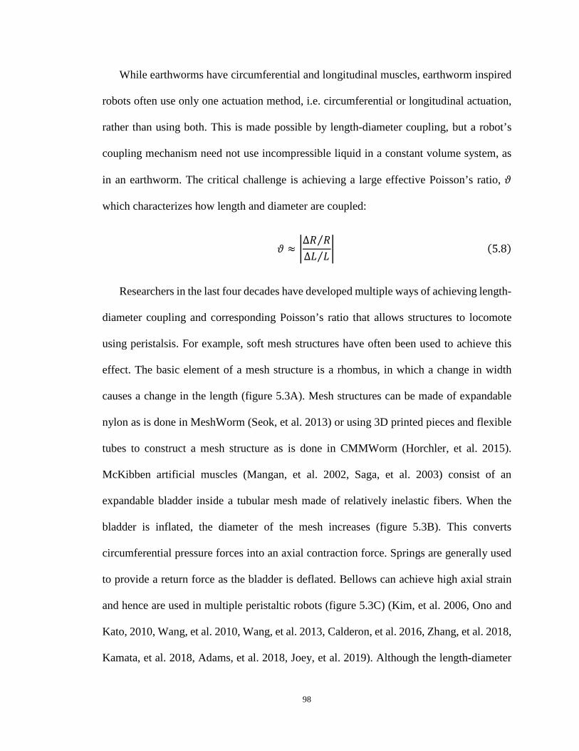
98

While earthworms have circumferential and longitudinal muscles, earthworm inspired

robots often use only one actuation method, i.e. circumferential or longitudinal actuation,

rather than using both. This is made possible by length-diameter coupling, but a robot’s

coupling mechanism need not use incompressible liquid in a constant volume system, as

in an earthworm. The critical challenge is achieving a large effective Poisson’s ratio, 𝜗𝜗

which characterizes how length and diameter are coupled:

𝜗𝜗 ≈ �∆𝑅𝑅 𝑅𝑅⁄∆𝐿𝐿 𝐿𝐿⁄

� (5.8)

Researchers in the last four decades have developed multiple ways of achieving length-

diameter coupling and corresponding Poisson’s ratio that allows structures to locomote

using peristalsis. For example, soft mesh structures have often been used to achieve this

effect. The basic element of a mesh structure is a rhombus, in which a change in width

causes a change in the length (figure 5.3A). Mesh structures can be made of expandable

nylon as is done in MeshWorm (Seok, et al. 2013) or using 3D printed pieces and flexible

tubes to construct a mesh structure as is done in CMMWorm (Horchler, et al. 2015).

McKibben artificial muscles (Mangan, et al. 2002, Saga, et al. 2003) consist of an

expandable bladder inside a tubular mesh made of relatively inelastic fibers. When the

bladder is inflated, the diameter of the mesh increases (figure 5.3B). This converts

circumferential pressure forces into an axial contraction force. Springs are generally used

to provide a return force as the bladder is deflated. Bellows can achieve high axial strain

and hence are used in multiple peristaltic robots (figure 5.3C) (Kim, et al. 2006, Ono and

Kato, 2010, Wang, et al. 2010, Wang, et al. 2013, Calderon, et al. 2016, Zhang, et al. 2018,

Kamata, et al. 2018, Adams, et al. 2018, Joey, et al. 2019). Although the length-diameter

99

coupling is low in bellow structures, due to the scalability and simple actuation techniques,

these structures have been commonly used, especially as the middle segment in two-anchor

worm robots, which are discussed below.

It is important to note that 𝜗𝜗 in equation 5.7 is the effective Poisson’s ratio of the entire

structure. Thus, while a material’s Poisson’s ratio is limited to range between -0.5 to 0.5,

metamaterials and structural linkages can have higher effective Poisson’s ratios. For

example, the effective Poisson’s ratio for our mesh robot, CMMWorm is 1.4 (Horchler, et

al. 2015). Using the simplified equation above, the approximate Poisson ratio for PEW-

RO (Nakamura, et al. 2008) is 2.9 and for Meshworm (Seok, et al. 2013) is 4. In many

origami and kirigami structures, positive or negative Poisson’s ratios can be designed

(Onal, et al. 2012). Note that when Poisson’s ratio is negative, the structure is auxetic

(Evans and Alderson, 2000), and in that case the waves travel in the same direction as the

body travels (Onal, et al. 2012).

100

Figure 5.3 The body structure enables segments to change length horizontally, while often changing in diameter (vertical) as well. Three of the most common segment structures are shown in their rest and actuated states. (A) Mesh structures rely on rhombuses with constant side length, and can be actuated using servomotors, shape memory alloys or other actuation schemes. (B) Pneumatic artificial muscles (PAMs) lengthen when the pneumatic bladder is pressurized using air. PAMs are either used in pairs or require a passive mechanism, like springs (not shown in figure) to return to their natural state when the bladder is depressurized. (C) Bellow structures are capable of large axial strain but small circumferential strain. The bellows are made of flexible materials like rubber or silicone and extend longitudinally when actuated.

5.2.6 Implication of analysis for actuation: Artificial muscles for fast, compact and precise movements

Actuation choices are critical for peristaltic robots, which are known for their large

number of kinematically-redundant degrees of freedom (Trivedi, et al. 2008). The more

degrees of freedom, the more actuators need to be compactly stored in the small form

factor. Thus, the robot’s compliance, mass, speed and efficiency largely depend on the

actuators used.

Typically, if segment stiffness is sufficient, the actuators need only pull one way and

the passive compliance of the structure acts as a return spring. Turning (Kandhari, et al.

2018a) or climbing (Andersen, et al. 2018) requires additional actuators. Reduced actuation

as in (Boxerbaum, et al. 2012, Zarrouk, et al. 2010, Winstone, et al. 2016) can enable

101

peristaltic locomotion with a single actuator for the whole robot. However, in such cases,

the robot is less modular and cannot adapt its gait as needed.

Traditional actuators can be used but can be heavy and difficult to integrate with a

compliant segment structure. For example, servomotors can tighten cables around the

diameter or zig-zagged along the length (Horchler, et al. 2015). These are easy to control,

have a high energy density and a rapid response time. However, they are typically heavy

blocks that interrupt the smooth body structure and cause limitations in structural

compliance and geometrical limits. Pneumatic pressure can be used to change segment

shapes (Mangan, et al. 2002, Liu, et al. 2019, Calderon, et al. 2016, Qi, et al. 2015, Fang,

et al. 2017, Aydin, et al. 2018, Mano, et al. 2018, Ortiz, et al. 2019), but require

compressors. On-board compressors are typically rigid and compressing gas in inefficient.

Wehner, et al. compare pneumatic energy sources for soft robotic application and provide

a framework to support the design of untethered pneumatic soft robots. Pneumatic systems,

however, are less resistant to punctures and high temperatures.

Thus, worm robots are often some of the first body designs to test new soft actuators.

Shape memory alloys (SMA) are soft and light, and are therefore common in worm robots

and worm robot skins (Kim, et al. 2006, Seok, et al. 2013, Andersen, et al. 2018). A major

advantage highlighted by Seok’s SMA controlled worm, is that the entire soft body is

resilient to damage such as being stepped on or hit with a hammer (Seok, et al. 2013).

When heated, SMA can decrease diameter (Seok, et al. 2013) or length (Andersen, et al.

2018), and the segment returns to its original shape when cooled. This can be slow.

Furthermore, in our experience, it can be challenging to precisely pair heating and cooling

rates.

102

Developing novel soft actuators that can replace their metallic counterparts is of broad

interest (Elango and Faudzi 2015, Hines, et al. 2017, Miriyev, et al. 2017). The use of

polymers and other softer actuators, such as hydrogels and bio-hybrid actuators for worm

robots has seen remarkable growth in the last few years (Zhao, et al. 2014, Mikanohara, et

al. 2014, Webster-Wood et al, 2017, Okay 2009, Mirfakhrai, et al. 2007, White and Broer

2015, Liu, et al. 2007). These actuators might be able to avoid the problems with heat

actuation by responding to light, chemical concentration or electrical current (Michal, et

al. 2015). A major drawback of these soft actuators is their inability to produce large force,

which means the structure of the body has to be correspondingly soft. However, soft

actuators promise to improve in terms of speed, reliability, power consumption, robustness

and ability to be easily integrated within the structure.

103

Figure 5.4. Peristaltic devices have been described with many different actuators. (A) Each actuator type consists of material with a characteristic Young’s modulus. (B) The most popular actuation schemes are pneumatic actuators, shape memory alloys and servomotors. Robot speed normalized by body lengths is not correlated with body stiffness – there are fast robots for stiff piezoelectric actuators and for liquid metal actuators. The colors in (B) correspond to the Young’s modulus as shown in (A). Each symbol represents a robot using the particular type of actuation scheme. Triangle, square and rhombus symbols differentiate the type of waveform the robot uses for locomotion. Note the break in the Y axis between 7 and 20.

104

5.2.7 Implications of analysis for waveform control: Effective gait patterns for locomotion

The shape of the peristaltic waveform can be altered for speed (equation 5.1) or

efficiency (equation 5.7). Each segment can be in one of the four possible states:

Circumferentially expanded (anchoring), circumferentially contracted (bridging),

expanding in diameter, or contracting in diameter (see figure 5.2). We call the spatial

pattern of these states the “waveform”. Just as a legged robot might have many possible

gaits depending on the number of legs, a worm-like robot can be controlled with different

waveforms depending on the total number of segments in the structure (n). We define each

gait by the number of moving segments per wave (m), number of waves traveling down

the length of the body (w) and number of bridging segments between expanding and

contracting segments (b). The waveform determines the speed and efficiency of peristaltic

devices.

In the literature, there are several different categorizations of waveforms for worm-like

robots (Ortiz, et al. 2019, Zhao, et al. 2014, Horchler, et al. 2015). The resting or initial

state can be circumferentially contracted (figure 5.5Ai-ii) or expanded (figure 5.5Aiii-iv).

In either case, the segments can be controlled with a complete transition or with traveling

waves, depending whether a new wave starts before the previous one finishes. In the case

of traveling waves, the number of moving segments is constant if there are enough

segments to fit the entire pattern. Figure 5.5Aiv is most similar to our robot, CMMWorm,

and is the type of robot for which will we will consider optimization.

However, there are many robots that use a two anchor waveform (figure 5.5B) in which

the middle segment is never designed to anchor. This allows independent design for

105

anchoring segments and expanding segments. Instead of having a wave of radial

contraction travel down the length of the body, the robot locomotes by discretely expanding

and contracting in diameter, and extending and retracing in length. Segments capable of

circumferential strain are capable of anchoring, whereas the segments capable of

longitudinal strain are used for forward motion. The minimum number of segments

required for this type of locomotion is three, and additional pairs of segments can be added.

Figure 5.5 There are different types of waveforms commonly used in peristaltic devices. (A) If there are large number of segments (in this case shown with six, and with positive Poisson’s ratio), the original resting state can be either circumferentially contracted (I and II) or expanded (III and IV). In both cases, either all segments can actuate before any segments return to resting state (I and III) or a traveling anchor can be

106

generated with a constant number of anchoring segments (II, shown with 1 anchor, and IV, shown with 4 anchors). (B) Two-anchor waveforms have three “segments” but the muddle and ends have different functions, and thus a coupling ratio is not required. The middle segments only extend in length, and need never anchor. The ends need only anchor and release (not extend).

5.2.8 Velocity-Optimal and COT-Optimal Waves

What is the best waveform shape for a particular robot? This analysis allows us to

supplement empirical results with theoretical optima for either speed or cost of transport

(COT). Note that because we made many simplifying assumptions (no slip, segments are

uniform thin hollow cylinders, small deformations, perfectly controllable segments), the

relative contributions of bending vs compression vs other types of energy expenditure

might be different for specific designs. However, the general location of the optimal

waveforms should be preserved even if precise deformation calculations vary.

First, consider a short (n = 6) worm robot like our robot CMMWorm. There are three

possible gaits that meet the constraints above (shown in Table 5.I). We previously called

these 2×1, 2×2, and 3×1 (Horchler, et al. 2015), where the first number represents the total

number of moving segments per wave (m+b) and the second is the number of waves along

the body (w). For n = 6, in all cases m = 2, but there may either be one wave with a bridge

segment (3×1, w = 1, b = 1), or one or two waves without a bridge segment (2×1 or 2×2, w

= 1 or 2, b = 0). Previously, we showed that the 3×1 and the 2×2 waves were expected to

be equally fast. Here, we extract geometrical and structural properties from our robot

CMMWorm, where R/L = 0.5, R/t = 30 and the Poisson’s ratio = 1.4. Additionally,

CMMWorm has anisotropic Young’s modulus, i.e., the effective Young’s modulus in the

longitudinal direction is not the same as that in the circumferential direction; the actual

ratio is Ec/El = 3×104. Inserting these numbers into inequality (5.7), we calculated the

robot’s COT for these three different waveforms. Next, we empirically measured the COT

107

for the same waveforms in our robot as described in the materials and methods section of

this chapter and compared it to our calculated COT. These results are shown in Table 5.1.

Our analysis correctly predicts that the 3×1 wave is more energetically efficient, followed

by the 2×2 wave, followed closely by the 2×1 wave.

It is not surprising that the measured COT is much higher than the theoretical minimum

predictions. The analysis predicts the minimum required power that must be input to the

robot for it to move at the desired speed. However, the measurements are electrical input

to the servomotors. Thus, the measurements include losses in the motors and transmissions,

cable friction, ground-mesh-interactions (Horchler, et al. 2015), and electronics, which we

expect are substantial. In fact, the actuators consume power even when not actuating the

robot. These effects cause a large increase in the measured cost of transport and is the main

source of difference between the predicted and measured COT. It may be possible to further

decrease COT by optimizing ∆𝐿𝐿 for different waveforms (equation 5.4), or changing other

parameters (equation 5.7).

Next, we show that a difference in speed optimal (figure 5.6A) and energy optimal

(figure 5.6B) gaits persists in longer worm robots by considering all possible waveforms

for n = 100. In this case, the number of moving segments can vary between 2 and 50 for a

single wave. The maximum no-slip velocity occurs with 2 waves with 49 segments moving

(case c: 24 pairs of actuating segments and 1 bridged segment, which leaves only 2

anchoring segments) when the velocity would be 12 times the segment strain rate.

However, the cost of transport of such a wave is 71.9, which is relatively high. The most

efficient waveform would have 10 waves with 6 moving segments each wave (case a). This

waveform has only 60% of the segments moving, and thus a speed approximately equal to

108

the segment strain rate. However, the actuators would only need to overcome the segment

stiffness required to keep fewer segments aloft. Between these two waveforms is case b in

figure 5.6, which is an approximation of the waveform of an earthworm. Earthworms move

approximately 48% of their segments (according to our observations) with one or two

waves traveling down the length of the body. For a 100 segments worm, that would

correspond to 2 waves of 24 moving segments.

Table 5.1 Wave properties and corresponding ideal velocity and cost of transport for the different waveforms for a 6 segment robot. A still from the waveform is shown in the first row and below that wave properties and bending and compression COT factors. �̇�𝐿 for CMMWorm is 3.33 cm/sec.

Total number of segments (n) 6 6 6

Moving segments per wave (m) 2 2 2

Bridged segments (b) 0 1 0

Number of waves (w) 1 1 2

Anchoring segments 4 3 2

Ideal velocity normalized by �̇�𝐿 0.166 �̇�𝐿 0.33 �̇�𝐿 0.33 �̇�𝐿

Calculated ideal velocity (cm/s) 0.55 1.1 1.1

Measured velocity (cm/s) 0.36 0.79 0.77 Bending COT factor 0.015 0.04 0.007

Compression COT factor 1.72 1.14 1.72

Total Predicted Minimum Required COT 1.735 1.18 1.727

Measured COT* 67.7 30.8 59.7 *Average electrical power input to the robot divided by velocity.

109

Figure 5.6 For a given number of segments, in this case 100, we calculate the velocity (A) and the cost of transport (B) for all possible waveform combinations. The waveform using least cost of transport and waveform with maximum velocity are highlighted by a black box (case a and case c, respectively). For minimum cost of transport, the waveform is 10 waves of 6 moving segments each wave. The ratio of moving segments to anchoring segments is 1.5. While for maximum velocity the waveform is 2 waves of 49 moving segments each wave. The ratio of moving to anchoring segments is 49. From our observations, earthworms move approximately half their segments using one or two waves (case b). Here there are 2 waves of 24 moving segments each wave. The ratio of moving to anchoring segments is 0.92.

To generalize for arbitrary numbers of segments, we perform this energy optimization

for each worm length from n = 4 (the minimum) to 150. In figure 5.7A, the optimal power

requirements are dominated by compression cost at low segment numbers, but the bending

cost increases for higher numbers. The optimal total cost of transport is high when the

number of total segments is low; as the number of segments increases, the cost of transport

decreases and is almost constant as the number of segments increases beyond 10. The

optimal 10 segment worm waveform is shown: It has one wave that travels down the body

with 5 moving segments (1 bridge, two expanding and two contracting). The other five

segments are stationary anchoring segments.

110

The specific gait pattern corresponding to the minimum cost of transport for each robot

length is shown in figure 5.7B and 5.7C. With less than 12 segments, the energetic optimal

waveform is 1 wave with the size of the wave increasing (more moving segments per

wave). For robots with more segments, additional waves should be added, with about 5 or

6 segments moving in each wave. (Note that when the number of moving segments is odd,

a bridge is need (b =1); otherwise, when the number of moving segments is even, b = 0).

Thus, we can compare the percentage of moving segments for waveforms optimized

based on velocity (Equation 5.1) and cost of transport (Equation 5.7) in figure 5.7D. As the

number of segments increases beyond 12, the percentage of moving segments for velocity

optimization is between 90-98% whereas for energy optimization, the percentage is

between 50-70%. This suggests an explanation for why earthworms (red dot) have so many

anchoring segments – the faster waveforms require much more energy.

As the total number of segments increases, the ratio becomes greater than one; that is,

the number of moving segments is greater than the number of anchoring segments. Figure

5.7E emphasizes the velocity for energy optimized waveforms, although velocity for

energy optimized waveforms is less than velocity optimized waveforms (energy optimized

velocity ranges between 0.2 – 1.0 × segment strain rate as compared to 0.2 - 18 × segment

strain rate), the cost of transport for the energy-optimized waveforms is much lower (COT

for energy optimized waveforms is less than 1 and COT for velocity optimized waveforms

can reach 250).

In figure 5.8, we compare ideal velocity as a function of number of moving segments,

optimal cost of transport and waveforms for published peristaltic robots. It seems likely

that most of these robots are designed for maximum speed, since peristalsis can be a slow

111

form of locomotion. As described earlier, for fewer numbers of segments, higher velocity

is achieved when there are more moving segments; however, this might not be the most

energy efficient waveform.

Figure 5.7 (A) The best cost of transport for a peristaltic robot decreases as the number of segments increase until leveling off at approximately 0.8 after 10 segments. Orange line shows compression cost of transport

112

factor and purple shows bending cost of transport factor. The summation of both these factors is the total cost of transport (black line). Bending cost of transport is always smaller than compression cost of transport since the number of segments that are being cantilevered at the beginning of the wave are always few. (B & C) Waveform parameters that result in best COT above are shown. As the number of segments increases, it is suggested that the number of moving segments be limited and the number of waves increase, allowing small cantilevers yet large numbers of moving segments. The maximum number of moving segments is 6 in a single wave which is constant beyond 48 segments; however, the number of waves continues to increase from 5 to 15. (D) Thus, the percentage of moving segments for energy-optimized waveforms (black line) is much lower than for the velocity optimized waveforms (blue lines), especially as the number of segments increases. We also show percentage of moving segments for earthworms in this case, where we took measurements from 3 different worms with total number of segments (n) = 142, 147 and 144. The number of moving segments for each case was m+b = 70, 67 and 64, respectively. (E) Ideal velocity for velocity optimal waveform (blue line) ranges between 0.2�̇�𝐿 to 18�̇�𝐿 and goes beyond 2 as the number of segments increases beyond 20, whereas for the COT-optimal waveform (black-line) the velocity stops increasing just under 1�̇�𝐿.

Figure 5.8 This plot shows the different velocities that can be achieved by changing the number of moving segments. Gray boxes indicate waveforms where the cantilevered segments will tip on flat ground as the number of moving segments in a single wave is more than half the total number of segments. Black boxes indicate that locomotion will require anisotropic friction. The black line is the energy optimized waveform. Peristaltic robots in existing literature are indicated by red dots. For example, red dots for number of segments, n = 6 and maximum segments moving at once w(m+b) = 3, are our robots, CMMWorm (Horchler, et al. 2015), CMMWorm-S (Kandhari, et al. 2018a) and FabricWorm (Mehringer, et al. 2017). Note: in those cases, in which the ratio of moving segments to anchoring segments is not constant, i.e., complete transition method (Figures 5.5Ai and 5.5Aiii), we consider the ratio of maximum number of moving segments to minimum number of anchoring segments.

5.3 Conclusion and Discussion

113

After characterizing over 50 worm robot designs (see examples in figure 5.1), we

developed a template model (figure 5.2). Assuming perfect segment control and no slip,

the theoretical speed of the idealized model (Eq. 5.1) is limited by the rate of extension of

a segment and the number of moving segments that can be lifted off the ground. To achieve

peristaltic locomotion without slipping, the physical constraint of lifting the segments off

the ground must be met. Specifically, radial deformation must exceed the vertical bending

of cantilevered moving segments in addition to vertical compression of anchoring segments

(figure 5.2C). Waveforms with many moving segments concentrate body weight on a few

anchoring segments, which then undergo greater vertical compression, and thus will have

to further extend those moving segments to not drag on the ground. Similarly, more moving

segments will have to be further cantilevered from anchoring segments, and thus will also

require greater extension to counteract bending deformation (Equation 5.4).

Approximations are found for each of these bending and compression terms, based on

assuming that each segment can be modeled as a uniform thin cylinder of length L, radius

R, and thickness t and with anisotropic Young’s Modulus. The bending term is proportional

to (𝑅𝑅𝐿𝐿

)−3 and the compression term is proportional to 𝑅𝑅𝐿𝐿 times 𝑅𝑅

𝑡𝑡. Since R/L ranges from 0.1

to 1 for the robots in the literature and the thickness must always be less than the radius,

the compression term dominates the overall cost of transport as compared to the bending

term.

The model highlights three key design choices for a peristaltic robot. First, a segment

structure with a nonzero effective Poisson’s ratio is needed, which has been achieved in

various ways (figure 5.3). Second, actuators capable of causing longitudinal or

circumferential strain are needed. We show that at least nine types of actuators have been

114

used in the literature (figure 5.4). The actuation determines the mass and greatly affects the

overall stiffness (Young’s Modulus) of the robot and also can be characterized by speed

and power-to-weight-ratio. Finally, a worm robot requires the choice of a waveform shape

for control. While several different wave types have been used (figure 5.5), we propose a

unified characterization based on the number of moving segments per wave, the number of

waves, and any bridging segments in the wave (see Table 5.1 for the complete list of

possible examples for n = 6).

Based on these fundamental concepts, we developed an expression for the required

power-to-weight output of the segment actuators (Equation 5.7). The power is proportional

to velocity, and inversely proportional to Poisson’s ratio. Furthermore, the power

expression also includes geometric and waveform terms, which means that energetically

optimal waveforms can be found for various geometries (figure 5.6). Thus, such waveforms

may provide a guide for future robots, which may increase the number of segments to

increase speed or reduce power-to-weight requirements (figure 5.7). Power-optimal

waveforms have fewer moving segments and more anchoring segments than speed-optimal

waveforms, and most current worm robots are between speed optimal and power optimal

curves (figure 5. 8). Worm robots with larger numbers of segments will be increasingly

possible with improved techniques for fabricating large Poisson’s ratio segment structure

and with novel actuation materials with high power-to-weight ratios.

We note that this analysis does not constrain the Young’s modulus to a particular

optimum value. This suggests that robots capable of peristaltic locomotion can be made

out of any convenient materials, soft or hard. In our experience, it is relatively easier to

work with stiffer materials (Kandhari, et al. 2018a) because they tend to be easier to control,

115

but if the actuator power-to-weight ratio is too small, actuation may not be possible. While

developing a robot, researchers can use the analytical guide developed in this chapter to

calculate waveform properties that might be most efficient given geometrical properties,

or can calculate geometrical properties given various waveform properties that might help

with the initial design of the structure. Although current robots often use feedforward

control for gaits, ultimately maintaining low cost of transport for uneven terrain will require

feedback. Earthworms have a rich range of sensors and their behavior is dominated by

feedback: Mechanosensory organs and stretch, touch and pressure receptors along the

length of the body allows earthworms to locomote in constrained environments and burrow

(Mill 1982). While there are many worm-like robots, contact sensing has not been explored

for most of them. In simulation, we have shown that a worm-like robot can be more

efficient in crawling through constrained environments with contact sensing (Daltorio, et

al. 2013). In Chapter 8, we demonstrate that by implementing force sensors along the

circumference of the mesh structure of our robot, DiSCo-Worm (Distributed Sensing

Compliant Worm robot), slip can be reduced while moving in constrained environments

(Kandhari, et al. 2018b). However, the use of traditional sensors like force sensitive

resistors, stretch sensors and inertial measurement units hinder the deformable

characteristics of soft robots. Therefore, researchers are developing soft sensors (Park, et

al. 2012) and sensors that are embedded within soft materials that will allow the structure

to retain its flexibility while achieving accurate control.

5.4 Materials and Methods

5.4.1 Capturing earthworm data

116

Large, living earthworms (Lumbricus terrestris) were ordered from Carolina Biological

Supply Company. Multiple videos of earthworm locomotion were recorded from the

transverse view using an HD camera (Canon Vixia HF G30, 59.94 fps). From these sets of

videos, three videos with three different earthworms (in which the earthworms moved

mostly in a straight line) were chosen for counting the number of total segments and

number of moving segments during peristaltic locomotion. Sections of the earthworms

were marked with non-toxic paint to make counting of segments easier. Tracker video

analysis software (Version 4.11.0, Open Source Physics, https://physlets.org/tracker/) was

used to analyze the videos. Anchoring and moving segments were distinguished by visually

observing, frame-by-frame, whether a segment moved or not. If the position of a segment

moved over the span of 5 frames (0.1 seconds) we considered the segment to move. At

each instant, we would calculate the number of moving segments during locomotion. Stills

from the videos were extracted to count the total number of segments for each case.

5.4.2 Velocity and cost of transport calculation for Compliant Modular Mesh Worm Robot

Compliant Modular Mesh Worm Robot is a cable actuated soft robot, composed of

nylon tubes and 3-D printed pin-joints (Horchler, et al. 2015). The robot consists of six

segments; each segment is actuated using two Dynamixel® XL430-W250-T actuators.

Cable from each actuator wraps around half the circumference of the segment. As the

actuators rotate, cables along the circumference of the segment are uniformly spooled in,

thus allowing the mesh-like structure to contract in diameter and extend in length. Linear

springs along the length of the segment passively return the segment to its maximum

diameter as the cable is spooled out by the actuators. If both actuators rotate at the same

117

speed for the same duration, the segment contracts uniformly. If the actuators rotate at

different speeds, the bias in the amount of cable spooled in by the left versus right half,

will allow the robot to turn. In this chapter, we focus only on straight-line locomotion. The

actuators are controlled using an Open CM 9.04 microcontroller that allows programming

of the actuators.

The actuators can be programmed to set the sequence in which the segments contract

and expand. For this chapter, we explored the 3×1, 2×1 and 2×2 waveforms (as defined in

the Results section). The experiments with CMMWorm were carried out on linoleum tile

and a DC power supply was used to power the actuators. The actuators were supplied with

a constant voltage of 12V and varying current as required by the actuators. The average

electrical power for all three waveforms over 5-6 waves was measured and at the end the

distance travelled in each case was measured. Cost of transport was calculated by dividing

the measured average power consumption from the DC power supply by the distance

traveled by the robot.

118

Chapter 6 Design and Control of turning in worm like robots: The geometry of slip elimination control This chapter was originally published as:

Kandhari, A., Wang, Y., Chiel, H.J. and Daltorio, K.A., 2019. Turning in Worm-Like Robots: The Geometry of Slip Elimination Suggests Nonperiodic Waves. Soft robotics.

119

6.1 Introduction

Mobile soft robots inspired by earthworms could have applications in medicine, search

and rescue and infrastructure inspection. Soft body locomotion (Menciassi, et al. 2004,

Umedachi and Trimmer 2014, Kim, et al. 2006) depends only on body deformation rather

than the use of wheels or legs which might break, slip or get caught in tight spaces.

However, in order to move in the desired direction, waves of extension and retraction must

be coordinated as they travel along the body (Daltorio, et al. 2013). Currently, most worm

robots work best traveling in straight lines on flat surfaces or completely constrained pipes.

To make soft worm-like robots navigate in 3D applications, a control theory for segment

coordination during turning is needed.

A defining feature of earthworm-like robots is mechanical coupling between segment

diameter and segment length (Horchler, et al. 2015). When increasing diameter decreases

length (and vice versa), this type of locomotion can be thought of as positive Poisson’s

ratio peristalsis (which we will abbreviate as 3P). 3P coupling can be achieved either by a

constant volume fluid constraint (as in an earthworm’s hydrostatic skeleton (Chiel, et al.

1992)) or by mechanical linkages (such as braided meshes Mangan, et al. 2002, Seok, et

al. 2013), pinned mesh rhombuses (Boxerbaum, et al. 2012, Kandhari, et al. 2018a,

Mehringer, et al. 2017), or curved springs (Omori, et al. 2009)). Origami segments can

have positive or negative effective Poisson’s ratio, depending on the fold pattern (Onal, et

al. 2013, Fang, et al. 2017). Note that this analysis will focus on positive Poisson’s ratio

(3P) structures; for a negative Poisson’s ratio, however, the traveling waves would go in

the other direction (from tail to head rather than head to tail for forward motion) (Tanaka,

120

et al. 2011). The advantage of 3P coupling is that it reduces the number of required

actuators by mechanically linking the ground contact status of a particular segment of the

body to the extension of that segment, as a single actuator is capable of causing an

extension in length while contraction in diameter and vice-verse.

In 3P locomotion, segments of the body that have the largest diameter (and thus shortest

length) will be so-called “anchoring segments” (Daltorio, et al. 2013, Tanak, et al. 2011).

The larger-diameter anchoring segments press against the inner circumference of the pipe

or against the floor. The smaller-diameter segments do not contact at all. This is in contrast

to some models of snake-robot crawling (Liljeback, et al. 2012) where the weight is

assumed to be supported evenly at all segments (Alexander, 2013) – an assumption that

may not be true in all animals (Tang, et al. 2017, Marvi, et al. 2013).

The frictional cost of transport (COT) for worm-like locomotion is determined by

energetic losses to frictional slip (Alexander, 2013). Without the 3P constraint, the

segments would not lift off the ground and, thus, all motion would require irreversible

energy loss to sliding friction. As a result, the frictional cost of transport (the work done

against friction per weight and distance) would be equal to the friction coefficient

(Alexander, 2013) (COT = E/mgd, where energy due to friction, E = µkmgd, m is mass, g

is acceleration due to gravity, µk is the friction coefficient and d is displacement), which

can be high for a soft robot in a constrained space. However, we have recently shown that

with 3P coupling and kinematic coordination, anchoring segments need not slip and thus

the frictional COT can approach 0 – similar to a rolling wheel (Boxerbaum, et al. 2010,

Boxerbaum, et al. 2012). For straight line 3P locomotion, slip can be eliminated by

coordinating the segments such that the rate of lengthwise elongation and retraction are

121

equal between noncontiguous anchors (Daltorio, et al. 2013). Backward locomotion can be

achieved by reversing the direction of the waves of elongation/retraction. For uneven

ground, waves can be modified based on sensed ground contact forces (Daltorio, et al.

2013, Kandhari, et al. 2018a, Kandhari, et al. 2018b) so as not to increase frictional COT.

Slip is a critical metric to minimize for several reasons. Uncoordinated control is not

only inefficient, it can also be ineffective (e.g., the segments may change shape but not

lead to robot progress). Slip can cause damage to delicate substrates (e.g. in medical

applications). Furthermore, focusing on the geometric (kinematic) constraints is more

generalizable to different robots and different substrate friction than kinetic models (which

will require stiffness, deformation, and contact force models).

To change direction without increase in frictional COT, slip-mitigating turning

constraints need to be developed for worm robots, analogous to Ackermann steering

constraints for wheeled robots. Current worm-like robots typically neglect this, often

limiting control policy searches to periodic waveforms, and significant slip is observed

(Mangan, et al. 2002, Seok, et al. 2013, Boxerbaum, et al. 2012, Omori, et al. 2009, Aydin,

et al. 2018). Not only is energy wasted, but also the motion is difficult to predict. In one

example, with the same turning control policy, the robot’s head moved left on high friction

surfaces and right on low friction surfaces (Kandhari and Daltorio 2018).

The geometry of control for slip reduction provides a theoretical basis for control

design, which can augment current approaches based on empirical trials (Omori, et al.

2008), genetic algorithms (Mirletz, et al. 2015), or fitting from animal data (Gong, et al.

2016). While rigid snake robots can be controlled for obstacle-exploitation (Transeth, et al.

2008, Liljeback, et al. 2011), in order to similarly plan for worm-like robots, the 3P

122

constraints should also be considered. This chapter demonstrates that without slip, multiple

waves of non-uniform, non-periodic control are required to change the body orientation for

an abstract 3P robot. We will call such control policies Non-Periodic Waveforms (NPW).

While other models of worm-like locomotion have focused on dynamics (Zimmermann

and Zeidis 2007), substrate compliance (Zarrouk and Shoham 2012), backward vs. forward

locomotion (Tanaka, et al. 2011), or contact-responsive timing (Daltorio, et al. 2013), to

our knowledge, this is the first model to focus on the theory of slip reduction for turning

gaits for a generic worm-like robot. In simulation, a general trapezoid model is developed

and some turning strategies for anterior segments are provided as a first step towards

developing full planning solutions for more detailed models (Huang, et al. 2017). On our

robot (Kandhari, et al. 2018a), we show that by using kinematic constraints derived using

this simple geometry, slip can be reduced using a NPW. Thus, NPW results in more

predictable turning motions than the naïve periodic waveforms we and others have used

previously (Seok, et al. 2013, Aydin, et al. 2018, Kandhari and Daltorio 2018, Omori, et

al. 2008). Specifically, kinematic models can predict the NPW controlled-position of our

robot Compliant Modular Mesh Worm with Steering (CMMWorm-S) with positional error

of less than 50% of the initial body diameter per cycle, whereas, if a periodic wave is used,

the positional error averages 160% of the body diameter per cycle. These positional errors

are calculated by measuring the distance between the simulated trajectory and actual robot

trajectory over 3 trials of 19 peristaltic cycles for each segment. The approximately tripled

error in the periodic wave trials is due to forced slip and associated soft body deformation,

which can be eliminated with the kinematic models presented in this chapter.

123

6.2 Model

We will make some simplifying assumptions to develop a simple segment model with

only two variables per segment (left and right side lengths) that will be applicable to

different body designs such as those actuated with cables (Horchler, et al. 2015,

Boxerbaum, et al. 2012), pneumatic pressure (Mangan, et al. 2002, Adams, et al. 2018),

and shape memory alloy wires (Seok, et al. 2013, Andersen, et al. 2018). Note that the goal

of the model is not to accurately describe all aspects of robot body motion in real

environments, but rather to understand the general implications of imposing a no-slip

constraint. We will show in the subsequent sections that this simple model can contribute

towards more predictable turning.

6.2.1 Assumptions

First, by assuming that each segment contacts the ground and anchors after retracting

as much as possible, the body can be modeled in the 2D plane of the turn (without

calculating vertical positions of segments). We assume that the diameter of the body can

be considered constant for the purposes of calculating distances between contact points.

The 3P diameter decrease need only be enough to raise the moving body segments off the

ground, and narrowing the diameter too much can result in excess bending due to gravity.

For our robot, a decrease in diameter is coupled with increase in length; however, even if

the diameter decreases noticeably (as in figure 6.1, which is exaggerated), the important

part of the shape is the relative location and angle of the anchoring segments, which are

affected less because the anchoring segment’s diameter is larger. In other words, side

124

lengths between variable diameter rings are approximated using side lengths between

constant diameter rings. A more accurate model would require an expression for the length-

diameter coupling relationship (which might be nonlinear for a particular robot) as well as

appropriate intersegmental smoothing. Since the number of free parameters (right and left

side lengths) would be the same, it is more general and simpler geometrically to use the

isosceles trapezoid segments here with leg length equal to the nominal diameter. Later

work may include a transformation into more robot-specific quadrilaterals.

The second simplification is that the effect of the actuators can be modeled

independently from each other. In other words, for our worm-like robot, contraction of a

segment affects the dimensions of adjacent segments (figure 6.1). We have shown,

however, that when the body is a continuous mesh, the actuation effects can be linearized

and separated into independent local changes (Huang, et al. 2017) and thus the body can

be considered in discrete segments for the purpose of control.

This model applies to other actuation schemes for 3P segments that both elongate and

bend. In this chapter, we will refer to the soft body as turning left or right, but this model

could also be applied to other directions (e.g. vertical bending to climb up walls).

125

Figure 6.1. A key property of worm-like 3P locomotion is that the short segments contact the ground, whereas the long segments do not. Here an example 3D cylindrical mesh in which radial strain is -40% of longitudinal strain (Poisson’s ratio = 0.4) is shown. At the center of each segment is a ring (red ring) which can change diameter slightly (gray rings) as the left and right side lengths change. The mesh shape shown is constructed with two intermediate rings along piece-wise arcs with interpolated diameters between each pair of actuated rings, connected in a helical pattern. The isosceles trapezoid projection is shown below. For our latest mesh robots, the minimum number of segments that can be raised off the ground is two adjacent turning segments and three straight segments. The remaining segments contact the ground beneath the actuators with shortest length, indicated with filled gray circles. In this chapter, the trapezoids around those points will be considered anchoring segments.

6.2.2 Trapezoid Segment Model

The relationship between basis length and bending angle 𝛽𝛽 can be found with geometry.

Each segment is a trapezoid with left-side length 𝑤𝑤L, the right-side length 𝑤𝑤R, and the

trapezoid legs are the constant diameter 𝑑𝑑 as shown in Fig. 2. Thus:

12(𝑤𝑤R − 𝑤𝑤L) = 𝑑𝑑 cos𝛽𝛽 (6.1)

A trapezoid representation of the body is exact if the centerline follows a series of

126

piecewise tangent arcs at the actuator. Note that trapezoids are a more convenient

representation because, in the default straight positions, they have equal base side lengths

rather than the infinite radii of curvature. When finite, the radius of curvature for the center

is the average of the left and right curve radii (𝑟𝑟L and 𝑟𝑟R). The curve radii are related by

geometry to the trapezoid parameters by:

|𝑟𝑟L − 𝑟𝑟R| = 𝑑𝑑

𝑟𝑟L cos𝛽𝛽 =𝑤𝑤L

2(6.2)

𝑟𝑟R cos𝛽𝛽 = 𝑤𝑤R/2

The included arc angle, 𝜃𝜃, of each of these curves also defines isosceles triangles as

shown in figure 6.2. Since the sum of all the included angles in a triangle is equal to 180°:

𝜃𝜃2

+ 𝛽𝛽 = 90° (6.3)

The limits of segment deformation will have important effects on the way the robot

turns. To better visualize deformation, here we allow the segment to elongate to 100% of

its initial length. Furthermore, the initial short segment length is set equal to the nominal

diameter. Thus, after normalization by the diameter, the initial configuration of a segment

is the 1×1 square at the lower left corner of figure 6.3 and we assume each segment can be

controlled to achieve any of the trapezoid shapes within the bounds in figure 6.3. These

bounds were determined by extending one side (left or right side) of a single segment of

our worm-like robot, Compliant Modular Mesh Worm robot with Steering (CMMWorm-

S) while keeping the other side length constant and measuring the side lengths of the

127

segment. The configuration space represents the dimensions a single segment of the

CMMWorm-S can achieve, normalized by diameter.

Figure 6.2. The body of a worm-like robot is represented using a series of trapezoids (heavy lines), which could alternatively be represented using a series of arcs (shaded gray). wL and wR are the leg lengths and d is the nominal diameter.

Figure 6.3: A worm-like robot, like our robot CMMWorm-S, will have limits on the possible shapes of a single segment. For the simulated examples shown here, the trapezoid segments must be within these bounds, which are generous for the worm robot in13. Diagrams of the trapezoids represented by the boundary dots are shown near the border. wR/d and wL/d are the right and left trapezoid base lengths respectively, normalized by diameter.

128

6.2.3 Problem Scope

This model will be used to search for control waveforms that balance elongation and

retraction of segments such that slip motions at the anchoring segments are not generated.

Specifically, we will focus on waves for which two segments are moving at once (one

elongating and one retracting). This type of wave is referred to as a 2×1 non-periodic

waveform, where, as a segment is extending in length, an adjacent segment is shortening

in length. In our robots, increasing the number of segments per wave (e.g. 3×1 with a

suspended segment between contracting and retracting segments) can cause some segments

to drag along the ground when extended. For expediency, subsequent waves can begin

before the first wave reaches the end of the body (for example 2×2 waves), but for clarity

here only one wave at a time will be shown on the body.

6.3 Implications of Non-Periodic Waveforms

First, this section demonstrates that slip elimination control (SEC) for straight line

locomotion can be achieved with symmetric, periodic waves, as we have previously used.

However, we show that, for turning, SEC may not result in straightening the body after a

single wave, and waveforms need to change as they travel along the length of the body.

Such waveforms will need to be calculated via the method of the next section based on the

changing robot configuration and are hence referred to as Non-Periodic Waveforms

(NPWs).

129

6.3.1 The Special Case of Straight Line Motion

Straight line 3P forward locomotion is achieved with waves of elongation and

retraction that travel in the opposite direction as the moving robot. As a given segment

elongates, a posterior segment retracts at the same rate, increasing the average progress of

both segments. Thus, the SEC constraint of no slip condition is satisfied as long as

elongation and retraction rates between anchoring segments are equal.

Furthermore, because the elongating segment can elongate until it reaches the starting

length of the paired retracting segment, and vice versa (figure 6.4A), the same waveform

can be applied to the next pair of segments. In other words: the control waveform need not

change as it travels down the body. Moreover, this is true for all segments after a wave

passes down the body. As a result, subsequent waves can be identical to the initial wave.

Next, we will show that these waveform properties do not hold for all turning waves for

example (figure 6.4C, when the posterior and anterior segments of the body are oriented at

90̊ from each other), although they can hold for the special case of turns in which the body

lies along an arc with constant radius (figure 6.4B).

130

Figure 6.4. Balancing a pair of elongating and retracting isosceles trapezoid segments (white) such that the anchoring segments (in gray) do not move. Arrow on top indicates direction of motion. Segments marked R are retracting in length, while segments marked E are elongating in length. A pair of segments retracting and elongating in length are shown for (a) straight line motion (b) when the body lies along an arc with constant radius, (c) when the posterior and anterior of the body are oriented 90° from each other. The grey segments are anchoring segments and do not move as the retracting and elongating segments change states.

6.3.2 A single non-periodic wave may not be able to reorient a straightened

body to face a new direction in the same straight configuration

A key characteristic of the bending of the robot is how much a single wave can change

the orientation of a segment. We consider this for the first segment of the robot from an

initially straight configuration. Subsequent segment will follow the same pattern, i.e., for

some positions of the anterior segments, geometrically reachable positions required from

the posterior segments might fall outside of their respective reachable space, which will

cause these segments to slip.

When the first segment returns to its shortest shape and contacts the ground, the

131

configuration of the second segment (the second segment “reach”) will determine the

contact position of the first segment, i.e., the center point of the front of the first segment.

The reachable space of the first segment from an initially straight configuration with a two-

segment wave is shown in figure 6.5.

After the first segment is at its maximum diameter, it becomes an anchoring segment

and the third segment can begin extending while the second segment contracts. Thus,

subsequent segments will be able to reach a translated reachable space by extending from

their posterior anchoring segments (until the last 2 segments that can be cantilevered).

If we want to reorient the robot, i.e. have it facing a different direction in the same

straight configuration as the original, we can determine the necessary location of each

segment by measuring backwards from the front segment’s initial reach. But if that location

is outside in the translated reachable space for that segment, an anchoring segment will

have to slip. In our example, the x-y reachable space limits eliminate many of the most

extreme turns (black crosses, figure 6.6). But even where the x and y coordinates of the

required location lies within the reachable space, the orientation may not lie within the

reachable configuration space. In fact, the orientation constraints interfere for all but the

straight-line motions. This would mean that a point (for example a small foot) at the center

of the segment might be able to stay in the same place for initial reaches that are represented

by red dots in figure 6.6, but that point and the body around it would have to rotate.

Thus, especially for long soft bodies, such as worms, or for segments with limited range

of motion, there will not be a SEC wave that can completely reorient the straight body. In

other words, the configuration of the posterior segments will require the reach of these

segments to be outside their respective reachable kinematic configurations, hence

132

necessitating slip. If slip is not permitted or possible, after one wave, the body will be in

different shape for the next wave.

6.3.3 Except when the body has uniform constant curvature, SEC waves will

change as they travel down body

If the final shape of the retracting segment is the initial shape of the elongating segment

(and vice versa), there is a symmetry that simplifies the control waveforms (as in straight

line locomotion). Because the relative geometry is the same before and after the wave has

passed, subsequent waves can be identical to the first wave. However, this is only possible

if the two outer edges of the elongating and retracting segments are mirror symmetric. If

they are not mirror symmetric, as in figure 6.4B and in figure 6.7A and 6.7B, the initial

and final relative positions of the anchoring segments will be different, necessitating slip.

Note that not every mirror transformation corresponds to a pair of possible segments. In

figure 6.7C, a line of symmetry was found but the associated segment pair is not a

trapezoid, and outside the segment configuration space.

In order for the first and last segment shapes to match without slip, both trapezoids in

the moving pair must have the same center of curvature point (and therefore the same radii),

and that center of curvature must lie on the mirror symmetry line, as in figure 6.7D. In this

case, the short and long trapezoids will have different included arc angle, 𝜃𝜃 (figure 6.8,

where θ1 ≠ θ2), which can be gradually equalized and then reversed without requiring

anchor segments to slip. A consequence of this constraint is that there is no matched pair

of trapezoids that includes exactly one rectangle: either both trapezoids must be rectangles

or neither can be rectangles. If segment one (S1) is a rectangle (A) and segment 2 (S2) is a

133

non-rectangular trapezoid (B) at the beginning of a wave, it will not be possible for S2 to

have shape A and S1 to have shape B at the end of the wave.

As the wave travels down the body, this mirror symmetry must be true for each pair of

anchors if subsequent waves are to be identical. For example, in figure 6.7D, the second

and fifth segments are mirror symmetric (while third segment contracts and fourth

expands), but when the wave moves to anchor the third and sixth segments they are not

mirror symmetric. As a result, there exists no constant-shape phase-shifted traveling wave

(periodic wave) that can reorient rectangular segments in one orientation to rectangular

segments in another orientation.

This reveals a second special case of locomotion – if and only if all the segments in the

body have the same center of curvature point, the SEC waves can be repeated identically

and do not need to change amplitudes as they travel down the body. Just as the total of the

two lengths remain constant as one increases and the other decreases for straight line

locomotion (figure 6.4A), the total of the two arc angles remains constant in a constant

curvature turn (figure 6.4B). At every intermediate position, a trapezoid is defined by one

segment with an increasing arc angle and one with a decreasing arc angle.

Non-periodic waves must be used to eliminate slip for non-constant curvature turns.

For example, non-periodic waves are necessary when transitioning from a straight line to

a turn or in the middle of a turn, when some segments are straight, as in figure 6.4C. Such

non-periodic SEC waves are described in the following section.

134

Figure 6.5: The reachable space of the front segment assuming only two segments can be cantilevered off the ground, and the range of motion of a segment is as described by the configuration limits in figure 6.3. The reachable space has three dimensions (x and y position, and angle). Two projections of this space are shown: (top) x and y and (bottom) y and angle turned by the first segment due to the kinematic reach of the second segment. Both x and y positions in (a) and (b) are normalized by diameter and hence are dimensionless.

6.4 Calculating SEC Waves

As the geometry above shows, SEC waves for arbitrary body configurations will be a

function of the changing body shape: different for each wave in time and for each segment

in the body. The front and rear segment waveforms are the least constrained since they

135

have anchors only on one side during elongation and retraction. Here, they are elongated

slightly and returned to square initial conditions. The nontrivial calculation of SEC

waveforms begins at the second segment.

As described above, the initial second segment “reach” defines the anchoring position

of the first segment. The choice of initial reach is described below.

Between anchoring segments, the moving segments are controlled such that the

anchoring segments do not need to slip. We formulate the problem as determining four

degrees of freedom (𝑤𝑤R1, 𝑤𝑤L1, 𝑤𝑤R2, and 𝑤𝑤L2) such that the anchoring segments are

stationary. Formally, the black dots in figure 6.8 maintain their positions by satisfying the

following three constraints:

1. The total length of the two trapezoids, 𝑠𝑠L, in figure 6.8, must be constant over time.

Applying the cosine rule to the triangle defined by the left bases of the trapezoids and the

line between them:

(𝑠𝑠𝐿𝐿)2 = (𝑤𝑤L1)2 + (𝑤𝑤L2)2 − 2𝑤𝑤L1 𝑤𝑤L2 cos𝐵𝐵 (6.4)

where 𝐵𝐵 is the angle between the bases of the adjacent trapezoids (𝛽𝛽1 + 𝛽𝛽2) and (𝑠𝑠𝐿𝐿)2 is

constant

2. The total bending angle of the two trapezoids (angle Ω in figure 6.8) is constant

3. The relative orientations of the two anchoring segments must be constant. Thus, the

sum of the included arc angles 𝜃𝜃1 + 𝜃𝜃2 in figure 6.8 must be constant. Since the isosceles

triangle that corresponds to each isosceles trapezoid must have interior angles that sum to

180°, a constant 𝜃𝜃1 + 𝜃𝜃2 implies a constant 𝛽𝛽1 + 𝛽𝛽2

With four degrees of freedom and three constraints, there is a 1D set of solutions. Thus,

136

from one trapezoid base (e.g. 𝑤𝑤L1, which would start from an initial position and increase

until a stopping condition is reached) the other three (𝑤𝑤R1, 𝑤𝑤R2, and 𝑤𝑤L2) can be uniquely

determined.

Figure 6.6. Some areas of the reachable space do not permit the body to straighten out again after one wave without slip. In particular, slip without rotation is only possible for essentially straight line motion. Schematics shown at right demonstrate how straightening the segments after choosing different points for the first segment reach, within the configuration space, will cause posterior segments (third segment in this case) to slip.

First, to get 𝑤𝑤L2 from 𝑤𝑤L1, Equation (4) can be solved using the quadratic formula. The

values of the constants 𝑠𝑠𝐿𝐿 and 𝐵𝐵 can be inserted from the starting conditions. Then the

individual trapezoid acute angles 𝛽𝛽1 and 𝛽𝛽2 can be found through the sine rule because

𝑤𝑤L2sin𝐵𝐵 = 𝑠𝑠𝐿𝐿 sin 𝛾𝛾, where 𝛾𝛾 = 𝛽𝛽1 − Ω, as in figure 6.8. 𝑤𝑤L2 can be found from:

137

sin(𝛽𝛽1 − Ω) = 𝑤𝑤L2sin𝐵𝐵𝑠𝑠𝐿𝐿

(6.5)

Once 𝛽𝛽1 is determined from (5), 𝐵𝐵 − 𝛽𝛽1 = 𝛽𝛽2. Then equation (1) can be used to find

the right base lengths for the trapezoids (𝑤𝑤R1, 𝑤𝑤R2). The choice of initial reach of the first

segment, which along with initial configuration, determines all the constants (sL, Ω and B),

is discussed in the next section.

As shown for straight-line locomotion (Huang, et al. 2017), the rates of contraction and

retraction can be estimated using equation 6.4. Since the total length of the two trapezoids

(sL) must be constant over time, taking the derivative of equation 6.4, we can derive the

rate at which the left side lengths must change in order to keep the total length constant.

On differentiating and simplifying we derive the following relation:

𝑤𝑤L1(̇ 𝑤𝑤L1 − 𝑤𝑤L2 cos𝐵𝐵) = −𝑤𝑤L2̇ (𝑤𝑤L2 − 𝑤𝑤L1 cos𝐵𝐵) (6.6)

where, 𝑤𝑤L1 ̇ and 𝑤𝑤L2 ̇ are the rate of change of left side lengths of adjacent segments. 𝑆𝑆L ̇ and

𝐵𝐵 ̇ are zero since both these values are assumed to be constant.

However, in this chapter we focus on geometric analysis of left and right side lengths

and not the rate of change of these side lengths. The rate of change is actuation based and

is not considered at this point.

138

Figure 6.7. If pairs of segments are controlled so that the short segment reaches the same shape as the long segment, and vice versa, it is clear from the overlaid initial and final configuration that slip will occur for (a) and (b) but not for (c) and (d) because of the mirror symmetry about the dotted blue line.

Figure 6.8. A pair of trapezoid segments can move together, one elongating and one retracting, without necessitating slip of neighboring segments if the black dots do not move relative to each other. In the text, the geometry of non-periodic waves is calculated from the parameters shown.

6.5 Simulation Results

The result of these calculations is a set of non-periodic waveforms that eliminates slip

by coordinating pairs of actuating segments while keeping designated anchoring segments

stationary. An example pair of segments are shown in figure 6.9. This pair-wise segment

expansion and retraction will be extended to non-periodic waves (NPW) that travel down

139

the body.

To generate the control wave for a whole body with a given initial shape, two design

choices remain: the initial reach of the second segment (which determines direction) and

the final conditions before transitioning to actuate the next pair (which determines segment

step length). To permit as much motion as possible, the latter is determined by the limits

of the configuration space (figure 6.9B). A portion of the resulting control is shown in

figure 6.9C.

6.5.1 Successive waves with the same initial reach

The control wave is uniquely determined by the actions of the front of the robot,

specifically the reach of the second segment. First, we consider a simple control design that

always uses the same second segment reach. In figure 6.10, a 6-segment robot begins from

a straight body configuration (six 1×1 squares), and a constant second segment initial reach

is chosen. Four example initial reaches are shown: each left side length is set to the

maximum (2 times the initial length), the right initial side lengths are (a) 0.9, (b) 1.325, (c)

1.6 and (d) 2.0. Note that (d) is the straight-line case where both side lengths are 2 times

the initial length. In the first column, the shape of the body before and after a single wave

are shown in thick gray and thin black lines respectively. A small amount of progress is

visible everywhere except the head (because the head progress occurred during the initial

reach and was held constant during non-periodic waves). If the same initial reach is chosen

from that configuration and so forth for each successive configuration, the blue dotted path

is followed. The second column shows the path and an example robot body over the first

100 waves. The converged shape of the path is shown in the third column.

140

Figure 6.9. (a) Diagram of paired extension and retraction with the initial configuration in gray and the final in black. The trapezoid side lengths of segments 2 and 3 are varied such that the only edge that moves is the one between segments 2 and 3. At each configuration during the transition, both segment 2 and 3 are isosceles trapezoids. (b) As viewed in the configuration space from figure. 6.3, the segments stop when one of them (in this case segment 2) reaches the boundary of the configuration space. (c) As viewed in the time domain, the mean extensions (the increase in length) intersect and the side length differences (a measure of the segment bending) change more gradually. Control input refers to the changing of the trapezoid lengths normalized by diameter (d); it is a dimensionless input that depends on the mean extension of the segment and the side length difference.

As the examples show, a result of always choosing the same second segment reach over

multiple waves can be either convergence to a constant curvature path (figure 6.10B&C)

or a gradual decrease in motion magnitude ending in a stall in which subsequent segments

cannot progress (figure 6.10A). The reason is that over multiple waves a navigation

maneuver will change the body shape as well as its position and orientation. Since the

magnitude of motion is limited by the initial conditions of each segment within the

configuration space, the effect of the initial reach depends on the body configuration. Thus,

it is possible to choose a second segment initial reach that in combination with the initial

configuration of the third segment, permit little or no paired elongation and retraction

between the second and third segments. In such a case, all the posterior segments will have

141

nowhere to extend because they have reached the limit of their range of motion in the

previous wave and the wave will be stalled (as a result, the blue and gray lines overlap

exactly in figure 6.10A, final column). To advance, another less extreme reach would have

to be used at the second segment.

In the figure 6.10E, the entire space of possible initial reaches is explored. Three

hundred waves were passed along an initially straight body in order to see the convergence

properties of all possible combinations of left turning waves (𝑤𝑤R ≥ 𝑤𝑤L) at 0.025

resolution. The first panel shows how much distance the head moves at the 300th wave.

The progress can be seen as the distance between the blue dots in the path of the robots in

the above panels. The second panel shows the change in angular orientation after the 300th

wave. The examples shown in the above panels are labeled as points on the right extreme

of the plot.

This demonstrates that the stall conditions occur for turns that are too tight.

Specifically, initial reaches that are within the dark blue triangle at the lower right of the

range of motion decrease in progress over time.

Alternately, for many conditions, the segment configurations converge to a constant

curvature path which permits consistent turning. If the side lengths are nearly equal, greater

progress per wave is possible with less turning (figure 6.10B). A middle strategy of

extending one side length to about a midpoint of the range while extending the other side

length all the way results in a stable reorienting turn (figure 6.10C, represented by the

diamond in figure 6.10E)

142

6.5.2 Orienting to a desired direction

An important goal for steering a worm-like robot would be to orient to a particular

direction. For example, the robot may need to follow a compass direction or a light source

to find an exit. An efficient policy is needed that changes the body from traveling straight

in one direction to traveling straight in another direction without turning too tightly (which

can have diminishing progress per wave as is shown in figure 6.10A).

A solution is a stable reorienting turn combined with a head stabilization algorithm. As

shown in figure 6.11, to turn 90°, the example simulated robot used the initial reach from

figure 6.10C (long side extended to 2, short side to 1.325), until the second segment initial

reach was able to orient the front segment to 90° from the original orientation. In this case,

that new orientation occurred after 7 waves. Subsequent initial reaches were calculated to

always orient the front segment (the head) to face 90° while extending the second segment

as much as possible.

Specifically, the head stabilizing initial second segment trapezoid side lengths are

calculated as follows. First the difference in angle between the posterior edge of the second

segment (𝛼𝛼2𝑝𝑝) and the desired angle of the anterior edge (𝛼𝛼2𝑖𝑖𝑖𝑖) is determined. In our case,

𝛼𝛼2𝑝𝑝 is measured from geometry of the trapezoid edge and 𝛼𝛼2𝑖𝑖𝑖𝑖 is 0° for a left 90° turn. The

second trapezoid must have included arc angle, 𝜃𝜃, equal to this difference. Using equation

(6.3), the included trapezoid angle, 𝛽𝛽, can be found from 𝜃𝜃. Then from 𝛽𝛽, the difference in

side lengths (𝑤𝑤R − 𝑤𝑤L) = ∆𝑤𝑤 is found from (6.1). Thus, for a left turn, the second segment

side lengths (𝑤𝑤R2 and 𝑤𝑤L2) can be found from:

143

𝛽𝛽 = 90° −(𝛼𝛼2𝑝𝑝 − 𝛼𝛼2𝑖𝑖𝑖𝑖)

2

∆𝑤𝑤 = 2𝑑𝑑 cos𝛽𝛽

𝑤𝑤R2 = 𝑤𝑤max (6.7)

𝑤𝑤L2 = max (𝑤𝑤max − |∆𝑤𝑤|,𝑤𝑤SRT)

where 𝑑𝑑 = 1, 𝑤𝑤max = 2, and the stable reorienting turn side length is 𝑤𝑤SRT = 1.325.

A result of the SEC and range of motion limitations is that stabilizing to a new head

orientation can take many waves. In our example, turning a six-segment worm by 90̊ can

take over 50 peristaltic waves before all segments are reoriented towards the new direction.

Aligning the front edge in a particular head direction requires that the x coordinate of the

path varies slightly at first. Furthermore, in order to maintain a particular front segment

angle, the body may have small bends or kinks. With this heuristic algorithm, after 7 waves

the stable reorienting turn can align the head to face 90° from the original direction. After

15 SEC waves, the body is approximately aligned in the new direction and the path is

straight. After 50 SEC waves, the kinks in the body straighten out and the motion converges

to straight line motion in the new direction. Note that several other turning controls were

tried (tighter turn steering, wagon handle steering, using smaller reaches (for which the

right-side length was not at its maximum)); all these alternatives induced oscillations. The

approach presented in equation (6.7) is shown because it has a good balance of tight turning

and smooth path (in blue), as shown in figure 6.11A.

144

Figure 6.10. The non-periodic SEC control wave is determined from initial shape of the second segment from the front (light blue) within the body (gray). The final shape after a single SEC wave (black) will advance the posterior segments as much as possible while holding the head stationary at that position. For a-d, x-axis indicates the forward position of the model normalized by diameter (x/d) and the y-axis indicates the lateral position normalized by diameter (y/d). The blue path indicates the progression of the midpoint of the front edge of the first segment. Each column shows the final orientation of the worm-model after 1, 100

145

and 200 waves respectively. For tight turns (a), it is possible that continuing with the same reach results in smaller and smaller steps (as evidenced by blue dots spacing getting closer and closer and eventually stalling), whereas for other types of turns (b) a stable reorienting turn, and (c) a shallower turn, the path converges to a circular arc. The difference in the paths of (b) and (c) indicates a different trajectory followed due to different first segment kinematic reach. In straight line locomotion (d), the progress per wave is the greatest (as evidenced by the difference between the gray initial shape and black final shape). (e) Here we show the results of using the complete range of possible second segment reaches. The steady state progress and turning of the above examples are shown within the context of the configuration space (long side length represents the trapezoid side that extends more longitudinally, whereas the short side length is the length of the shorter side of the trapezoid). It can be seen that below a certain line, progress will stall (region of zero progress in the bottom corners), e.g., example (a) represented by the circle. The fastest motion will be to walk in a straight line (d) represented by an upward triangle. The fastest way to reorient will be at the maximum of the graph at the right (represented by the diamond). In the range between the two, trade-offs between forward progress and turning can be made (for example (c), represented by the left triangle). An initial reach with long side length less than 2 will result in smaller motions per wave. Note: the first step for (a) takes into account the entire range of motion of the first segment based on the kinematic configuration of the second segment; hence, the turn made during the first wave is large.

6.6 Robot Result

We validate the performance of the non-periodic waveforms (NPW) by applying them

to an earthworm inspired soft-bodied robot, Compliant Modular Mesh Worm with Steering

(CMMWorm-S) (figure 6.12). CMMWorm-S is a cable-actuated, multi-segmented soft

robot. The locomotion of this robot depends on the material deformation of a series of

flexible nylon tubes, held in a mesh configuration with 3D printed vertex pieces. Even

though the structure of this robot includes rigid components, the effective elastic modulus

for the robot lies well within the range of soft robotics (0.5 × 104 Pascals). In our previous

paper (Kandhari, et al. 2018a), we have shown that turning angle largely depends on the

bending stiffness of the body, which is due to the flexibility of the nylon tubes used in the

mesh.

146

Figure 6.11. An example simulation trial is shown with NPW control for a 90° turn (𝛼𝛼2𝑖𝑖𝑖𝑖 = 0°). (a) Starting with the initial reach determined above, and then, when possible, keeping the front of the robot facing parallel to the y-axis, the path of the robot and the initial and final states of the body for waves 1,5,10,15, and 50 are shown. The SEC waveforms are shown (b) in detail for the first 10 waves and (c) over the full 50 waves. Control input refers to the changing of the trapezoid lengths normalized by diameter (d); it is a dimensionless input that depends on the mean extension of the segment and the side length difference. The solid black line is the mean extension of the segment’s two side lengths 1

2(𝑤𝑤R+𝑤𝑤L) − 𝑑𝑑 and indicates the elongation of the

147

segment. Each segment of the body elongates and retracts once per wave. The amplitude of elongation gradually increases to the full limit of the range of motion. The dotted lines with circles are the difference in side lengths (𝑤𝑤R − 𝑤𝑤L) which indicate the bending of the segments. This changes more gradually, with damped oscillations that converge to zero when the body is straight at the new orientation.

Each segment of the CMMWorm-S is actuated using two actuators (Dynamixel AX-

18A actuators) controlling either the left or right side of a segment. Each actuator controls

a cable that runs along half the circumference of the segment. On actuation, cables are

spooled in, contracting the segment in diameter and extending it in length. To produce

turning motion, different cable lengths are spooled in by the two actuators within a

segment, causing one side to extend more than the other, which in turn induces the robot

to bend. The gait pattern can be changed by varying the longitudinal extensions of each

side, based on the configuration space. The diameter of the robot ranges between 22 cm to

12 cm, depending on segment state.

Figure 12. Overhead view of Compliant Modular Mesh Worm with Steering in a bent configuration. Schematic of six segments projected in the 2-D plane is shown. Each segment includes two actuators (black) that change left and right segment side lengths.

148

6.6.1 Periodic wave to compare with Non-Periodic Wave

We implemented the non-periodic waveform on the CMMWorm-S robot and compared

its performance with a naïve periodic waveform. For linear waves, we had defined a time-

based control wave that involved 2 actuating segments (one extending in length and the

other shortening) and traveled down the body one at a time (a so-called 2×1 wave). To go

straight, the extension and shortening rates were equal on left and right, keeping each

segment left-right symmetric. To turn, we decreased the actuation speed on one side (from

70 rpm to 18 rpm) for both extension and retraction. This causes segments to bend during

actuation due to unequal spooling of cables on left and right side of a particular segment.

After longitudinal extension, the contracted segment expands in diameter until it returns to

its initial anchoring state (maximum diameter). This pattern is the same for all segments,

i.e., all inner actuators rotate at 18 rpm and all outer actuators rotate at 70 rpm for 1.9

seconds duration, first in one direction and then in reverse. Thus, the control waveform is

periodic (repeating for each cycle) and uniform (the same for each segment, phase shifted).

This is a natural choice for a turning controller; however, as discussed in (Kandhari and

Daltorio, 2018), significant slip is observed and whether the front of the body moved left

or right depended on the surface friction.

We also simulated the periodic 2×1 waveform (figure 6.13) using isosceles trapezoids

using similar assumptions to the SEC model above. Unlike the NPW, the periodic wave

has to slip at some point on the body and so we needed to add a slip assumption. Based on

observations of the robot, the side of the robot with the fewest anchoring (max diameter)

segments slips the most. For example, if segment one is an anchoring segment, segment

149

two and three are a pair of actuated segments (segment two expanding in diameter and

segment three contracting) and segments four, five and six are anchoring segments, then in

order to maintain the periodicity, segment one will experience slip. If there are the same

number of anchoring segments at front and back, both sides are allowed to slip in a way

that minimizes total slip (see figure 6.13).

The NPW similar to figure 6.11 was implemented on the robot with a few minor

changes. The simulated model does not account for the motion of the first and last

segments. Therefore, in the robot, the first segment was controlled to extend in length with

maximum bias (difference between left and right side lengths) and the last segment was

controlled to extend with zero bias (no difference in right and left side length) and 50%

mean extension, i.e., the left and right sides were extended uniformly to 50% of maximum

extension. This allowed the last segment to be cantilevered and prevented it from dragging.

Control input for segments two through five were based on the control input developed

using the 2-D model as shown in figure 6.11B. On the actual robot, the interconnected

segments did not achieve the full range of motion in figure 6.4 because of coupling between

segments. Therefore, the waveform in figure 6.11B was modified to accommodate a

smaller amplitude wave. To calibrate this wave, a single segment was measured after

different actuation speeds over the state duration (1.9 seconds). A linear regression was

used to determine the actuation speeds to achieve the desired segment side lengths.

150

Figure 6.13. Schematic extracted from the simulation for periodic 2×1 wave (left) and non-periodic waveform (right). The robot in both cases is turning left. The segments of the robot are projected as isosceles trapezoids. For each state of the wave, a segment can be either extending in length (blue trapezoids), contracting in length (grey trapezoids) or anchoring (white trapezoids). For a pair of actuating segments, longitudinal extension and contraction is constant for each state for periodic waveform and varies for non-periodic waveform. For the periodic waveform, to maintain these shapes, some segments that are supposed to anchor must slip (orange trapezoids). For example, in state 4 of the periodic wave, no anchoring segment is present, since in order to achieve the configuration all segments experience slip. For the 2×1 wave, the segments that slip are shown in the figure and the corresponding distance experienced by a point (denoted by Si, where i indicates segment number) that slips within a segment is shown. The arrows within the segments for periodic waveforms show the direction and magnitude of slip of the center of the segment from the previous state. The non-periodic waveform shown is the first wave, starting from an initially straight position. Note that subsequent NPW waves will have different initial configurations because the ending state and starting state are different and the segments do not expand to maximum diameter during expansion states.

151

6.6.2 Robot Experimental Results

Experiments were performed for the two control policies (periodic and non-periodic

waveforms) on linoleum tile with a coefficient of static friction (µs) of 0.55. Videos from

the overhead view were recorded for three trials of nineteen peristaltic waves each. Videos

were analyzed using ImageJ (Ver. 1.51j8, National Institute of Health) and Tracker

software (Version 4.11.0) to measure the angle turned by the robot after each peristaltic

cycle while tracking the trajectory of each segment. Performance of the robot was

measured by angle turned per peristaltic cycle and precision of the path followed by each

segment of the robot compared to the path followed by the 2-D models (supplementary

videos provided show the robot turning overlaid with the 2-D model for periodic and non-

periodic waveforms).

We compared the angle turned by the robot with the predicted angle turned by the 2-D

model for periodic and non-periodic waves. For simulation in both cases, the robot was

targeted to turn by 90̊; however, while testing, we limited the number of peristaltic waves

to 19 instead of an angle-based end point. The angle turned is the angle between the original

body orientation and the line segment between the first and last segment actuators after

each cycle. After 19 peristaltic waves, the 2×1 periodic wave resulted in a turn of 76˚ in

simulation and 57˚ on the robot. The non-periodic waveform turned by 34˚ in simulation

and 39˚ on the robot after 19 peristaltic waves. These results show that the angle prediction

error is less for the NPW: with the NPW, the robot turned only 14% more than predicted,

whereas with the periodic wave, the robot turned 25% less than predicted. Periodic waves,

however, achieve a higher turning angle due to all segments turning with maximum

152

capability, whereas for NPW the segments are constrained in order to restrict any anchoring

segments from slipping.

The trajectories for all six segments of the robot were tracked using Tracker, providing

insight into segment slip that results in imprecise locomotion (figure 6.14). For simulated

NPW (figure 6.14C), the segment trajectories overlap because the anchoring points are

holding position. For the simulated periodic waves (figure 6.14A), the segment trajectories

do not overlap but are spaced apart due to lateral slip, perpendicular to the direction of

motion. In experimental trials of the periodic waves (figure 6.14B), the lateral slip tends to

move the robot further in the opposite direction of the turn than predicted (i.e. the robot is

turning right but slip causes translation to the left). This translation is caused in part by the

posterior segments tending to “whip out” of their predicted trajectories, and then become

anchors. In the NPW, this translation is less, as can be seen on the y-axis. After 19

peristaltic waves, the periodic wave moves left 20.4 cm, with an error of 80% relative to

the predicted movement, whereas the NPW moves 29.16 cm, with a 13% error relative to

the predicted movement. The asymmetric placements of the actuators along the length of

the robot causes an uneven mass distribution between segments. During turning motion,

this uneven mass distribution causes the robot to roll about its longitudinal axis. The lateral

movements are amplified by the ability of the body to roll, which is not captured by the

trapezoidal model. The robot trajectories show a saw-tooth motion. When we look at the

details for a particular segment, we can see that the segment moves in different directions

in the different phases in figure 6.13. For example, in the 4th segment of the NPW, the

predicted forward progress per wave starts out small and straight, but the anterior adjacent

segments are turning. Because of the mesh structure, segments are not completely

153

independent, unlike the simulation. This makes it difficult for the robot to achieve the

desired SEC shape, which causes slip during anchoring. This slip is large relative to the

progress during extension and contraction for the posterior segments, but smaller for the

anterior segments.

We calculated the error between the actual robot path and the paths predicted with

minimal slip (for the periodic waveform) or no slip conditions (for the non-periodic

waveform). We compared the trajectories of the 2-D model and actual robot data by

recording the root mean squared error of the Euclidean distance between the center points

of each segment after each wave (figure 6.15). Results show that NPW follows the

predicted trajectory with one-third the total error of a periodic waveform (averaging 46%

as compared to 160% of the maximum segment diameter per wave). The posterior

segments in NPW tend to have more error (37% of maximum segment diameter for front

three segments and 55% of maximum segment diameter for rear three segments) than the

predicted path as observed in the trajectory in figure 6.14. This is due to the end segment

moving outward, as described above. For the periodic waveform, the overall error is more

for all segments as compared to the NPW. Posterior segments for the 2×1 periodic

waveform, however, have less error when compared to the anterior segments (166% versus

150% of maximum segment diameter) because the front segments are required to slip more

(as in figure 6.13, segment 1 slips at minimum 8.4+8.6 cm = 17.0 cm, whereas segment 6

slips 2.2+8.5 cm = 10.7 cm).

154

Figure 6.14. Trajectories for each segment for (A) 2-D periodic model, (B) robot using periodic waveform, (C) 2-D non-periodic model and (D) robot using non-periodic waveform. (A) The model is allowed to experience minimal slip to maintain periodicity and hence each segment follows a trajectory that does not overlap with the trajectories of other segments. In (C) the trajectories overlap, which is a necessary condition to eliminate slip using kinematic constraints. The trajectories from all six segments in (B) show that the trajectories do not overlap; rather they experience a lateral slip (upwards) instead of following the expected trajectory. For NPW in (D) some trajectories overlap for brief periods but the posterior segments experience more lateral slip as compared to the anterior segments. The saw-tooth projections in (B) and (D) are caused when an adjacent segment is contracting or expanding circumferentially; due to coupling between segments, the neighboring anchoring segment moves. (Supplementary Video 1 is used to plot the trajectories for (C) and (D), and Supplementary Video 2 is used for (A) and (B)). Note: the axes limits are different for the plots for better visualization of the progress made.

155

Figure 6.15. For each of the six robot segments, the distance between simulation predicted position and actual position at each state in Fig. 13 is averaged over 3 trials with 19 wave cycles each. The non-periodic wave (orange bars) has less prediction error (difference between model-predicted and measured segment location) than the periodic wave (blue bars), indicating less slip and thus more predictable movements for non-periodic waveforms.

6.7 Discussion and Conclusions

It might be naively assumed that a worm-like robot can be turned incrementally using

an analytically optimal periodic wave. In this chapter, the geometrical analysis

demonstrates that no such wave exists without slip – except for the trivial cases of straight-

line locomotion or turning when the robot body is already bent in a uniform-curvature arc.

Neglecting slip in control design results not only in wasted energy, but also results in

qualitatively different behaviors as a function of the substrate coefficient of friction (Aydin,

et al. 2018). This chapter analyzes the theoretical geometry required for slip elimination in

planned worm-like robot paths.

For worm-like robots, simple path planning approaches do not apply. First, worm and

snake-like robots are redundant (the number of independently actuated DOF is greater than

156

the state variables of the end effector), even hyper-redundant (because almost all the

different actuators in a chain could advance the head in the same way, especially if friction

is anisotropic) (Chirikjian and Burdick, 1995). Second, in some turning applications, the

body shape in the environment matters as much as the head position. In that case, the

combination of constraints (3P, SEC, and segment limits) leave only two independently

controllable DOF of the robot (left and right initial second segment side lengths) – which

means that the problem becomes non-holonomic (the number of state variables for the body

including configuration and position is greater than the number of controllable DOF).

Neither non-holonomic nor redundant robots can use traditional inverse kinematic

manipulator planning, although there are computational approaches based on neural

networks (Zhang, et al. 2017) or hierarchical optimization (Yuan 2017).

The presented theoretical approach may be valuable for path planning. The advantage

of soft-bodied robots is to be able to go into challenging constrained places. Overhead

motion tracking is unlikely to be available. We envision the robot having to traverse various

terrains, possibly re-planning as it goes. For example, to squeeze into a narrow tunnel from

a smooth surface may require careful realignment of the body at a specific location. Being

able to plan this motion can save power and decrease response time. Especially for many

segmented worm-like robots, it would be wasteful and frustrating to have to back up and

“re-park” for small lateral translations. Since slip is unpredictable, understanding the

constraints to eliminate it can improve accuracy of such plans. Understanding the reachable

space, the types of possible paths, and the format of the necessary control waves is an

essential first step.

This work shows how a turning worm-like robot can be modeled as a series of

157

trapezoids (figure 6.1 and figure 6.2), which advance in pairs such that their neighboring

segments are stationary anchors (figure 6.4). For a reasonable range of motion (figure 6.3),

the reachable space of the head segment is determined (figure 6.5). However, for many of

the points in that reachable space, slip is required for the rest of the robot to straighten out

behind the head in a straight configuration because the straightened positions of subsequent

segments are outside their own reachable spaces (figure 6.6). Thus, straightening in a new

orientation without slip will require several control waves. Furthermore, when two moving

segments are elongating and retracting, equivalent shape changes can be achieved without

slip if and only if their edges are mirror symmetric and they share the same center of

curvature (figure 6.7). Thus, unless all the segments on the body have the same center of

curvature in initial and final configurations, the waves that control turning will not be

phase-shifted periodic functions; rather, they will change as they propagate down the body.

This implies that rather than seeking a single waveform that can travel down the body

and be repeated for subsequent turning, it may be valuable to consider a soft-bodied control

strategy that is responsive to the body’s configuration in the environment. The nominal

control will be a non-periodic wave (NPW). Based on the geometric constraints (figure

6.8), these waves can be calculated (e.g., figure 6.9). from a particular choice of second

segment reach. If the same reach is repeated, the motion either converges to a constant

radius turn or stalls in a tightly curled shape (figure 6.10). To orient to a particular direction,

head orientation stabilization can be used to calculate waves that converge to straight line

motion in a new direction (figure 6.11).

We applied the non-periodic waveform to our soft-robot, Compliant Modular Mesh

worm robot with Steering (CMMWorm-S) (figure 6.12). For comparison, we also

158

simulated and applied a periodic 2x1 waveform, which we expected to slip (figure 6.13).

When the predicted and measured turn angle and body position (figure 6.14) are measured,

we see that the robot in fact slips even more that the minimum amount predicted, which

results in larger prediction error for the periodic wave than for the non-periodic wave

control (figure 6.15).

We note that even though the non-periodic wave was calculated from a geometric “slip

elimination” constraint, the robot can still be observed to slip relative to the theoretical

position. For both periodic and non-periodic waveforms, the robot experiences slip that the

model does not capture. To accurately predict these slips, more detailed modeling is

required, likely of both the robot itself and of the environment. Continuous soft body

modeling may account for segment inertia, interdependent soft deformation of adjacent

segments, and segment diameter variation. Coulomb friction modeling, terramechanics and

new contact models are likely critical for modeling slip patterns on these and more diverse

terrains. Such detailed robophysics models are making it increasingly possible to model

and predict how a robot will behave on a particular surface (Aguilar, et al. 2016). These

approaches can be important in correcting the specific errors that may accumulate along

the body during turning locomotion.

In contrast to detailed physical modeling, the contribution of this chapter is a template

that makes minimal assumptions about specific segment or environment kinetics. The goal

is not to accurately predict slip (which requires assumptions specific to the robot and

substrate) but rather to better understand how to reduce slip. Our work provides kinematic

limits of peristaltic robots based on geometric constraints and an analytical control solution.

Our robot results validate our approach by reducing slip. Despite imperfect control inherent

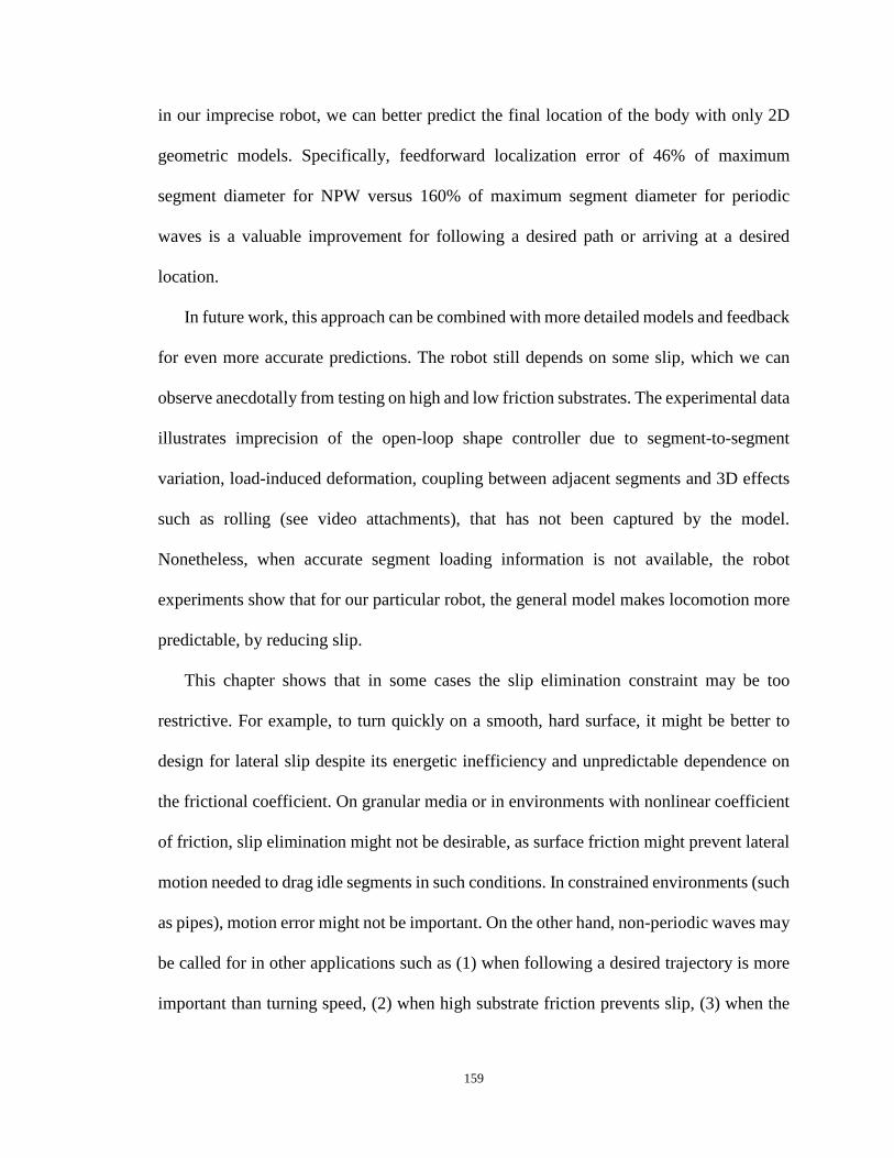
159

in our imprecise robot, we can better predict the final location of the body with only 2D

geometric models. Specifically, feedforward localization error of 46% of maximum

segment diameter for NPW versus 160% of maximum segment diameter for periodic

waves is a valuable improvement for following a desired path or arriving at a desired

location.

In future work, this approach can be combined with more detailed models and feedback

for even more accurate predictions. The robot still depends on some slip, which we can

observe anecdotally from testing on high and low friction substrates. The experimental data

illustrates imprecision of the open-loop shape controller due to segment-to-segment

variation, load-induced deformation, coupling between adjacent segments and 3D effects

such as rolling (see video attachments), that has not been captured by the model.

Nonetheless, when accurate segment loading information is not available, the robot

experiments show that for our particular robot, the general model makes locomotion more

predictable, by reducing slip.

This chapter shows that in some cases the slip elimination constraint may be too

restrictive. For example, to turn quickly on a smooth, hard surface, it might be better to

design for lateral slip despite its energetic inefficiency and unpredictable dependence on

the frictional coefficient. On granular media or in environments with nonlinear coefficient

of friction, slip elimination might not be desirable, as surface friction might prevent lateral

motion needed to drag idle segments in such conditions. In constrained environments (such

as pipes), motion error might not be important. On the other hand, non-periodic waves may

be called for in other applications such as (1) when following a desired trajectory is more

important than turning speed, (2) when high substrate friction prevents slip, (3) when the

160

environment could be damaged by shear forces, as in medical applications, or (4) motion

in open spaces such as moving towards a given goal where following a trajectory is

important. In these applications, understanding the limitations of slip elimination control

is essential for planning multiple waves to reach a desired location and configuration.

The geometrical analysis presented here establishes limits of possible no slip behavior

and will help robot designers relate segment range of motion and bending stiffness to slip

requirements and turning speeds. In future work, we will be able to extend our modeling

and control efforts to arrive at specific targets over a range of surfaces with varying

frictional properties with optimal cost or minimal number of waves.

161

Chapter 7 Distributed sensing for worm-like robots to increase locomotion efficiency This chapter was originally published as:

Kandhari, A., Stover, M.C., Jayachandran, P.R., Rollins, A., Chiel, H.J., Quinn, R.D. and Daltorio, K.A., 2018, July. Distributed Sensing for Soft Worm Robot Reduces Slip for Locomotion in Confined Environments. In Conference on Biomimetic and Biohybrid Systems (pp. 236-248). Springer, Cham.

162

7.1 Introduction

Compliant or “soft” robots that can undergo large deformations are promising because

of their ability to passively adapt their shape to the environment (for example in grasping

an arbitrary object (Rateni, et al. 2015)), store collision energy (for example in running legs

(Altendorfer, et al. 2001)), and recover from damage (for example bouncing back into

shape after being compressed (Seok, et al. 2013)). There are many instances where

performance is improved by compliance, but often the cost of compliance is uncertainty.

As sensor technology improves, it is possible to put tactile sensors in new places and with

softer materials. However, the value of such sensors for soft-body locomotion is not yet

established.

To assess the added value of such sensors, we have built a new worm-like robot with a

total of 49 sensors and 12 actuators. Unlike our previous Compliant Modular Mesh Worm

Robot which relied only on smart servomotors to control the diameter of each segment and

infer ground contact (Kandhari, et al. 2016), here each segment diameter is controlled

independently on the left and right side, contact pressures are measured directly with force-

resistive sensors, and stretch sensors assess body shape.

While there have been many other worm-like robots (Boxerbaum, et al. 2012, Seok, et

al. 2013, Horchler, et al. 2015, Trivedi, et al. 2008), contact sensing has not been explored

in most cases. Thus, this platform is valuable for (1) implementing closed-loop control for

constrained environments, (2) better understanding mechanics of peristaltic locomotion in

animals and robots, (3) determining critical requirements for sensor operation and

placement, and (4) in future work, validating simulations (Huang, et al. 2017) of modular

soft bodies.

163

In this chapter we discover that (a) the forward progress under open loop control is

largely due to slip, (b) the actuators work harder and longer in open loop, wasting energy

and risking damage to structure and actuation cables, and (c) the movements of the closed

loop robot incur less slip, which is a key cause of imprecision.

7.2 Background

Soft-bodied invertebrates such as earthworms can access constrained environments by

contorting their bodies in order to comply with their surroundings. The multi-segmented

body of an earthworm incorporates circumferential and longitudinal muscles. Due to

hydrostatic coupling, activation of a segment’s circumferential muscles causes it to

contract in diameter while extending in length, whereas activation of longitudinal muscles

causes the segment to shorten in length and expand in diameter (Chiel, et al. 1992).

Peristaltic waves of segment contractions and expansions along the length of the

earthworm’s body (Gray and Lissmann, 1938) cause the soft-bodied animal to locomote.

This coupling between the length and diameter of a segment (Chiel, et al. 1992) allows the

longer contracted segments to lift off the ground while the circumferentially expanded

segments rest on the ground to anchor forward locomotion (Kanu, et al. 2015). While

complying with their surroundings, earthworms are also capable of exerting forces radially

and laterally against their environment to break up compacted soil, create and enlarge

burrows, and resist extraction from their burrows by predators.

During peristaltic locomotion, sensory feedback allows the animal to adapt to

environmental perturbations (Mizutani, et al. 2004). Sensory feedback from various

mechanosensory organs and stretch, touch, and pressure receptors (Mill 1982) allow the

animal to maintain rhythmic peristaltic locomotion by modulating motor patterns (Gray

164

and Lissmann, 1938). Setae, present on the body of the earthworm, serve as

mechanoreceptors that allow it to adapt to its environment and crawl smoothly even on

rough surfaces (Mizutani, et al. 2004).

Soft-bodied robots have been shown to be mobile in constrained-space applications

(Ikeuchi, et al. 2012, Trimmer, et al. 2006, Bertetto and Ruggiu 2001, Tanaka, et al. 2014).

In simulation, we have shown that a worm-like robot can be more efficient in crawling

through constrained environments with contact sensing (Daltorio, et al. 2013). Specifically,

we have shown that a worm-like robot crawling through a narrowing in a pipe will exert

more energy because the segments lose energy to friction and slip. However, if ground

contact forces can be sensed, the Cost of Transport (COT) can be reduced. This chapter is

the first step in implementing such a controller on a physical robot.

7.3 Robot design

Our Distributed-Sensing Compliant Worm robot (DiSCo-Worm) (figure 7.1) has a

modularly assembled soft mesh body, like our previous robot CMMWorm. The mesh of

the robot consists of short “links” of flexible tubing connected via 3-D printed “vertex

pieces”, that allow relative rotation. Links of tubes and vertex pieces are assembled to form

a rhombus, such that rotation of the vertex pieces will cause the aspect ratio of a rhombus

to change. These rhombuses are connected in a ring-like structure to form a segment.

Each of the six modular segments has two actuators, one for each half of the segment

(Kandhari, et al. 2018a). Connected to each actuator spool, a cable travels halfway around

the circumference of the segment, either controlling the left or the right half of the segment.

The actuators spool in the cable causing the segment to contract in diameter, while

165

extending in length, equivalent to the circumferential muscles in earthworms. The diameter

of the segment is constrained by the amount of cable spooled in. Longitudinal springs

placed along the length of each segment perform similarly to the longitudinal muscle of an

earthworm’s body. On removal of the circumferential actuation force that causes the robot

to decrease in diameter, these longitudinal springs return the segment to the maximum

diameter as the circumferential cable is spooled out. Sequential actuation of the segments

causes a wave of circumferential contractions and expansions to travel down the length of

the body. This results in peristaltic locomotion opposite to the direction of the wave’s

travel.

Figure 7.1. Distributed-Sensing Compliant Worm robot (DiSCo-Worm) during a peristaltic wave on flat surface. The various components of the robot mesh including the sensors and actuators are labelled.

Unlike other worm robots, DiSCo-Worm incorporates a suite of pressure and stretch

sensors along the surface of its body. This network of distributed sensors allows the robot

to sense external perturbations and constraints, while keeping track of its own

configuration. Each sensor works independently. Each segment incorporates six Force

Sensing Resistors® (FSR-402) and two flexible stretch sensors. The FSR-402 sensors are

166

placed on each vertex piece around the circumference of each segment (Figure 2), in order

to detect external loads that may act on the robot radially (for example, from the inner

surface of a pipe). FSR sensors exhibit a decrease in resistance with increase in force

applied to the 14.7mm active area of the sensor. This decrease in resistance corresponds to

external loads the robot experiences.

Because the readings from the FSR sensors are independent of segment position, we

also added conductive stretch sensors that run along the length of the segments (one on

each side). As the segment extends in length, the resistance of the stretch sensors increases,

directly correlated to the extended length of the segment. Because the radius of a segment

is kinematically constrained to decrease with length, these sensors indicate the shape of the

segment.

Figure 7.2. Sensor configuration of a single segment placed flat on a surface. The FSR sensors are marked by circles around them. Stretch sensors are highlighted in red. UR: Upper Right, LR: Lower Right, UL: Upper Left, LL: Lower Left, T: Top, B: Bottom. Left and right vertex pieces join to form the ring-like structure and anterior and posterior segments are connected to the vertex pieces at the top and bottom of the figure.

167

To detect objects in the robot’s path, the first segment is specialized with the addition

of an HC-SR04 ultrasonic distance-measuring sensor. This allows the robot to respond to

obstacles in the robot’s path.

DiSCo-Worm thus has distributed sensing: Each of the six segments has eight sensors

and the first segment has an ultrasonic sensor, for a total of forty-nine sensors to determine

its configuration and environment.

7.4 Electronics and control

DiSCo-Worm is actuated by twelve Dynamixel AX-18A actuators connected to an

ArbotiX-M microcontroller. The actuators are powered using an off-board DC power

supply at a constant voltage of 11.8V. All forty-nine sensors are wired back to an off-board

Mayhew Labs MUX Shield II connected to the ArbotiX-M microcontroller. The MUX

Shield II allows the ArbotiX-M microcontroller to extend its total number of analog ports

from 8 to 53.

A 3×1 waveform, where 3 represents the number of segments per wave (including

inactive suspended segments) and 1 represents the number of waves along the body, was

used for all tests throughout this chapter. The 3×1 wave consists of an expanding segment,

a contracting segment and an inactive suspended (contracted) segment between the two

active segments. The active actuators are commanded to move at a specified speed with

maximum torque. All other inactive segments during a wave are expanded to their

maximum allowable diameter, for anchoring. An open-loop time-based control is

compared to a closed-loop control scheme where both controllers always maintain this

pattern.

168

With open-loop (time-based) control, actuators are configured to move for a fixed

duration. This duration is based on the time it takes for a segment to contract to its minimum

possible diameter of 13 cm from its maximum (initial) diameter of 22 cm at a constant

actuator speed. The next set of actuators in the wave sequence are activated immediately

after the previous duration terminates.

With closed-loop control, speeds are the same but the duration is limited by the forces

measured at the FSRs (during radial expansion) and the extension measured with the

conductive stretch sensors (during radial contraction). The microcontroller interprets the

data from the sensors to control the actuators such that an expanding segment is

commanded to move until a preset force threshold value is reached. The preset was

established via single-segment testing to achieve a desired normal force. A contracting

segment is commanded to move until a preset stretch sensor threshold value is reached,

correlating to its maximum allowable extension. In this control scheme, the two segments

are actuated independently. If a contracting or expanding segment reaches its threshold

value first, the segment stops and waits for its corresponding active segment to stop. The

next set of actuators are activated once both segments in the previous wave sequence stop.

In case an external threshold is not reached (no external constraint), a time-based threshold

is set in order to stop the expanding segment once it reaches its maximum diameter.

7.5 Experimental Methods and Results

7.5.1 Single Segment in Pipe

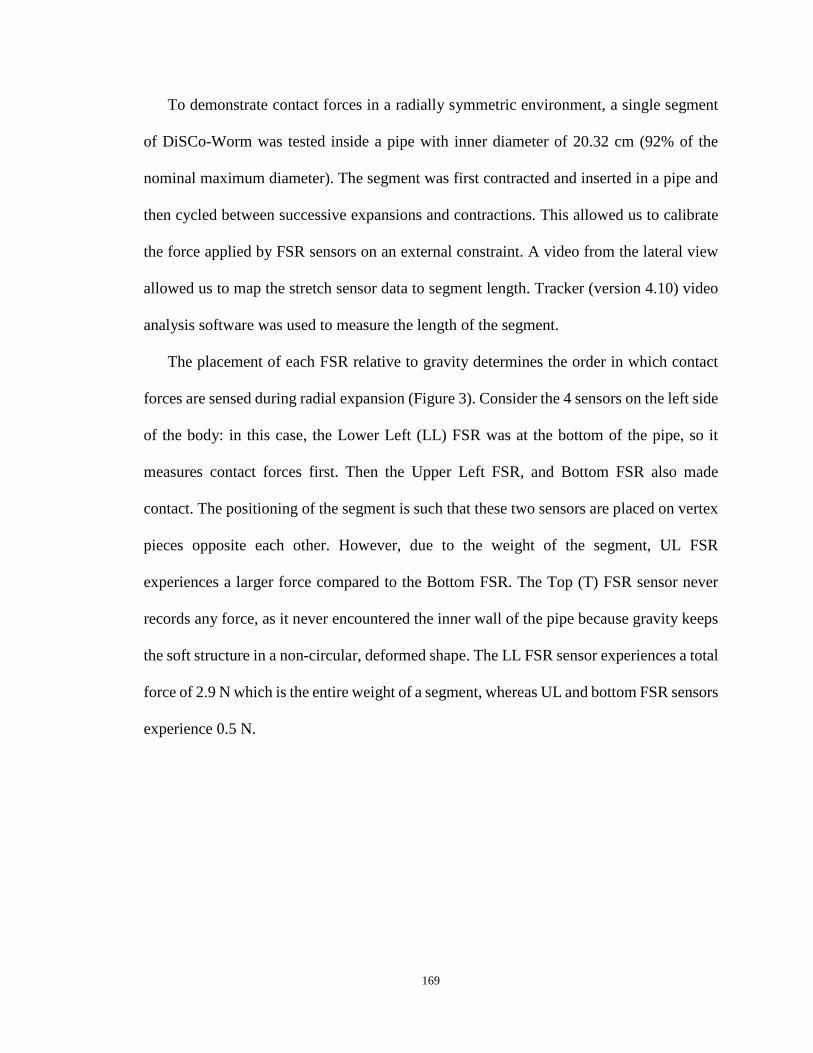
169

To demonstrate contact forces in a radially symmetric environment, a single segment

of DiSCo-Worm was tested inside a pipe with inner diameter of 20.32 cm (92% of the

nominal maximum diameter). The segment was first contracted and inserted in a pipe and

then cycled between successive expansions and contractions. This allowed us to calibrate

the force applied by FSR sensors on an external constraint. A video from the lateral view

allowed us to map the stretch sensor data to segment length. Tracker (version 4.10) video

analysis software was used to measure the length of the segment.

The placement of each FSR relative to gravity determines the order in which contact

forces are sensed during radial expansion (Figure 3). Consider the 4 sensors on the left side

of the body: in this case, the Lower Left (LL) FSR was at the bottom of the pipe, so it

measures contact forces first. Then the Upper Left FSR, and Bottom FSR also made

contact. The positioning of the segment is such that these two sensors are placed on vertex

pieces opposite each other. However, due to the weight of the segment, UL FSR

experiences a larger force compared to the Bottom FSR. The Top (T) FSR sensor never

records any force, as it never encountered the inner wall of the pipe because gravity keeps

the soft structure in a non-circular, deformed shape. The LL FSR sensor experiences a total

force of 2.9 N which is the entire weight of a segment, whereas UL and bottom FSR sensors

experience 0.5 N.

170

Figure 7.3. Expansion of a single segment within a pipe of 20.32 cm inner diameter (orientation of the segment when placed within the pipe is shown on top). (A) FSR readings from four pressure sensors along the circumference of the segment indicate the segment encountering the inner wall of the pipe. The segment diagram on top shows the placement of the sensors around the circumference when viewed from a transverse view. Lower Left sensor shows large force readings on the onset of segment expansion. On completion of expansion, the three FSR readings (Bottom, Upper Left and Lower Left) indicate continuous contact with the inner wall of the pipe until contraction starts at which point no radial force is applied on these sensors. (B) Stretch sensor measurement from both right and left side of the segment shows an increase in resistance as the segment begins to extend in length. The offset between the two stretch sensors is due to the initial lengths of the sensors being different. During operation, we subtract the current reading from the reading obtained at maximum possible extension. (C) Measured side length of the segment using video analysis indicating the expansion and contraction cycle aligned with sensory data.

171

Stretch sensors are more accurate during radial contraction than during extension,

which suits our need to limit contraction. During radial contraction, as the segment length

increases, the values recorded from these sensors also increase. Since the segment

uniformly contracts and expands, both these sensors exhibit a similar trend. However, on

segment expansion, the values do not directly correlate to segment length. This is because

the sensors have a few resistive artifacts (i.e., hysteresis). When stretched into position and

released, the resistance slightly increases upon release, and decays exponentially to its

resting resistive values. Figure 3 shows that the stretch sensor values start to decay during

the suspension phase while the length of the segment is still constant.

7.5.2 Locomotion between Parallel Substrates

DiSCo-Worm with all six segments and 49 sensors locomoted between two parallel

wooden surfaces set 16 cm apart (72% of initial maximum diameter (figure 7.4)), using

both open-loop and closed-loop control schemes. Results from these tests are summarized

in this section.

During closed loop control, the sensors stop expansion after contact (figure 7.5A). Note

that between two parallel constraints, the figure shows that only the top and bottom sensors

contact the ground. The threshold set (dashed lines, figure 7.5A) indicate when the top or

bottom have sufficient normal force to stop further expansion and allow anchoring of the

segment. The bottom FSR sensor placed directly underneath the actuator mount

experiences a high normal force, due to the weight of the segment resting on it. During

expansion, on coming in contact with the constraint, the normal force on the Top FSR

sensor increases the set threshold, thereby stopping any further expansion of the segment.

It can be observed that during contraction and the suspended phase of the wave, the sensor

172

reading for the bottom sensor indicates no contact with the ground. In contrast, during the

anchoring phase of the peristaltic cycle, the bottom sensor measures large values,

indicating the anchoring phase.

The bottom FSR sensor exerts a force of 2.3 N (80% of segment weight); compliance

between adjacent segments prevents the segment from exerting 100% of its weight on the

surface. The top FSR sensor experiences a maximum force of 1.0 N which quickly

decreases due to motion of the other segments.

Figure 7.4. DiSCO-Worm locomoting through two parallel horizontal wooden surfaces. The distance between the two surfaces was set at 16 cm. Both the open-loop controller and closed-loop controller were tested in the same constrained environment.

Stretch receptors indicate increase in resistive values when the segment undergoes

contraction (figure 7.5B). The threshold for the stretch sensors indicates when the segment

reaches maximum longitudinal extension with some allowance. On reaching this preset

threshold, the contraction phase of the actuation is stopped. During the expansion phase,

the resistive values of the stretch sensors decay to their initial values, similar to the case of

a single segment.

173

Actuator positions logged using the actuators encoder allow for tracking all four phases

of the 3×1 peristaltic cycle (expansion, anchoring, contraction, suspension) and aligning

with sensory feedback information.

How does limiting the duration of each step affect behavior? In 50 seconds, the closed

loop control resulted in 5.04 cm progress over 7 peristaltic waves, whereas the open loop

controller resulted in 10.43 cm over 5 peristaltic waves. Thus, as a result of the feedback

control, the robot takes smaller steps adapting to its environment with an overall speed of

48% of the open loop speed. Although the open-loop movements are faster, they are less

precise, as we describe below.

During open-loop control, there is a large amount of slip in both forward and backward

directions. Slip occurs when segments move during anchoring phases. Slip is measured at

the contact point using video analysis. For the open-loop controller, the segment slipped

backward by 8.67 cm. If no backward slip had occurred, the total forward progress of the

segment using an open-loop controller would have been 19.1cm. Using the closed-loop

controller, the robot experienced backward slip of 6.70 cm, so there is less backward slip.

Most of the backward slip, in both cases, was experienced during the contraction and

suspension phase of the peristaltic cycle. Although both control schemes have high

backward slip, forward slip in the case of open-loop control is higher than that of closed-

loop control. With open-loop control, the robot progressed by approximately 6.10 cm

during its anchoring phase. In contrast, the closed-loop controller did not progress

noticeably during its anchoring phase. The maximum longitudinal extension in both cases

was similar, but due to forward slip, segments in open-loop control contribute to larger

progress.

174

Figure 7.5. Data recorded from the 2nd segment using the closed-loop controller as the robot was allowed to locomote between two parallel horizontal surfaces. (A) Sensory information from the Top and Bottom FSR indicating when the robot came in contact with the external constraint. The robot rests on ground so the bottom FSR reading is high when the segment is anchoring. The segment then contracts until it is completely lifted away from the ground (all FSR for that segment read zero). Then the segment expands causing the bottom and also the top FSR sensors to make contact with the substrates (both top and bottom FSR show contact forces). Due to the compliance of the structure, as the adjacent segments move, the top sensor loses contact, thus exhibiting no contact during the anchoring phase. The dashed orange and blue line indicates the preset force threshold for the closed-loop controller for the Bottom and Top FSR respectively. (B) Data from stretch sensor indicates longitudinal extension of the segment during contraction phase. Stretch sensor’s resistance increases with an increase in length. The maximum extension that the stretch sensor experiences is set to zero. At zero, the contracting segment is at its minimum possible diameter. Negative values indicate the length of the stretch sensor is shorter than its maximum extension. Zero indicates that the segment has reached its maximum extension and any further extension can cause the robot to break. By setting the maximum extension, we eliminate any pre-existing discrepancies between stretch sensors (the offset observed between the left and right side in Figure 3). (C) Actuator position logged aligned with sensor data showing the four different phases of the peristaltic 3×1. The expansion and contraction phase are highlighted.

175

Figure 7.6. Comparison between (A) open-loop and (B) closed-loop controller. On the left Y-axis is the forward progress, measured using video tracking software, of the second segment during peristaltic locomotion (Note the scale difference in both figures (A) and (B)). Right Y-axis indicates the spool position of the actuator of that segment. Gray boxes are aligned with the spool position indicating anchoring phase. The angle by which the actuators rotate from contraction phase to expansion phase is indicated beside the gray boxes. Overall, in a span of 50 seconds, the total forward progress achieved by the open-loop controller is 10.43cm in 5 complete waves. In contrast, for the closed loop-controller, forward progress is 5.04cm by the end of the anchor phase of the 7th peristaltic wave.

For some applications, slip in any direction is undesirable as it leads to imprecise

control. Out of the total progress made by the open-loop controller, 58% was due to slip in

the forward direction (at a time that the segment should have been anchoring). During slip,

the upper and bottom surface of the segment was in continuous contact with the external

176

constraint. If there was no forward slip, the robot would have progressed by 4.3 cm for the

open-loop controller.

This soft robot shows the ability to alter its gait pattern in accordance to its environment

using a closed-loop controller. With open loop control, the motors continue to rotate even

after coming in contact with an external constraint. The actuators rotate for approximately

545˚ in the open-loop controller. For the closed-loop controller, on encountering an

external constraint, the actuators stop rotating, thereby causing no further expansion.

During this time, the actuators rotate between 459˚ - 500˚. The reduction in degrees rotated

causes the peristaltic cycle to move faster, by shortening the time duration of each cycle.

The adaptability of the closed-loop controller to its external environment leads to

coordinated motion that wastes less energy.

7.6 Conclusions

In this chapter we discover that in a constrained environment (a) the forward progress

under open-loop control is largely due to slip, (b) the actuators work harder and longer in

open loop, wasting energy and risking damage to the structure and actuation cables, and

(c) the movements of the closed loop robot incur less slip which is a key cause of

imprecision during locomotion. However, the robot’s overall speed is slowed relative to

open loop control, in part due to the reduction in forward slip. With sensors, DiSCo-Worm

is capable of reducing slip in both the forward and backward direction.

The FSR data will help to improve the closed loop control for soft robots in future

work. From figure 7.5A, blue line, the contact forces decrease after initial contact. Whether

177

this is due to structural interdependence of segments or multi-time scale dynamics, this

work demonstrates that an anchoring-state force controller will be necessary to prevent

early cut-off of soft expansion. Conversely, without such a controller, designing the

segment structure for compliance might be a higher priority than developing sensors. On

the other hand, in our simulated worm-like robot, the gains in performance were very small

unless the phasing of the segments was permitted to adapt (Daltorio, et al. 2013).

From figure 7.6, it can be observed that, for the open loop controller, most of the

forward progress for the 2nd segment occurred during the anchoring phase of the wave

(58% of the total 10.43 cm). Thus, instead of the segment lifting and progressing forward,

the segment drags along the upper and lower surface of the external constraints. For the

closed-loop controller, minimal slip was observed during the anchoring phase of peristaltic

locomotion (~0). However, the segment did experience a large amount of backward slip

during its contraction phase. An improved controller could solve this problem. In figure

7.6, a drift in actuator positions is observed in the closed-loop controller due to inaccuracies

in stretch sensors during contraction. We can reduce these sensor inaccuracies using signal

processing techniques. Furthermore, it may be valuable to be able to sense shear force in

order to detect slip (Umedachi, et al. 2016).

This work suggests the type of sensors that are valuable for reducing positional

uncertainty in worm like motion. Sensory feedback can also protect the robot from damage.

Due to continuous rotation, there have been instances where the excess actuation tangles

the cable, causing the cable to break. The closed-loop control prevents this from happening.

With the sensory feedback, we can develop control that is more precise and allows the

robot to navigate through various constrained environments.

178

Chapter 8 Discussion and Future Directions

179

8.1 Design of Soft Worm-like Robots

In this dissertation, I demonstrate the design of soft earthworm-like robots capable of

peristaltic locomotion. In chapter 2, I introduced Compliant Modular Mesh Worm robot, a

cable actuated, multi-segmented earthworm-like robot capable of soft-body deformations

allowing it to move on flat surfaces. In chapter 3, I correlated body stiffness to straight-line

and turning locomotion. With FabricWorm and MiniFabricWorm, in chapter 4, I

demonstrated how rigid components in the structure can be replaced with compliant

components and still be capable of locomotion. The next step is to make changes to the

design of the robot to improve the overall robustness and performance of the structure.

There are many avenues for improving design of the current iteration of the mesh worm

robot. The 3-D printed vertex pieces are bulky and affect the overall compliance of the

robot. With the design of FabricWorm we show that the structure could have fewer pieces

and still retain its structural rigidity in order to undergo peristaltic locomotion. The next

generation of CMMWorm robot could implement softer components onto the structure, the

3D printed vertex pieces could be printed using soft material that is possible using

Stereolithography printing techniques. In this, the printer is capable of curing a polymer

that can be compliant in nature, for example Agilus© material for the Object printer. This

will help in reducing the mass of the 3D printed vertex pieces and making it easier to

integrate with the compliant structure. Furthermore, in the current iteration we use stainless

steel eyelets and 3D printed actuator mount through which the Kevlar cables pass. There

is still some amount of friction the cables undergo, that causes them to wear over time and

eventually break. This can be fixed with some changes to the actuator mount, in future

iterations the cables would potentially undergo less friction if they never came in contact

180

with the edges of the actuator mount. In future iteration of the robot, small roller bearings

could be used for the cables to pass over, thereby reducing friction.

In the latest iterations of the mesh structure, we are using the Dynamixel AX-18A

actuators. Although these actuators can provide more than sufficient torque, they have a

low baud rate and imprecise control. The actuator has a 300˚ encoder which makes position

control inaccurate when passing through the dead zone (60˚). To overcome this issue, the

program to run the actuators had to accommodate any inaccuracies that may occur, making

the runtime for the program longer. Recently, Dynamixel launched a new actuator,

Dynamixel XL430-W250-T, that is equipped with a 360˚ encoder and a higher baud rate.

The presence of a 360˚ encoder allows for more precise position and velocity control

methods.

The force resistive sensors are directly stuck onto the rubber feet in the current iteration

of DiSCoWorm. It may be possible to redesign the vertex pieces such that the force sensors

can be incorporated within the vertex pieces and the rubber feet can be added on top of the

sensors to assist in traction, without hindering the performance of the sensors. Additionally,

the rubber feet can be replaced with 3-D printed rubber like material that would permit

testing of feet with anisotropic friction properties and provide the same functionality as

setae in preventing slip. Preliminary testing with DiSCoWorm shows that the force sensors

show a change in force readings if undergoing slip, adding an inertial measurement unit

(IMU) on each segment can assist in detecting motion of anchoring segments. In other

words, if an anchoring segment undergoes any motion, it is slipping, in this case the change

in force sensor readings coupled with IMU readings can convey forward or backward slip.

181

Another area of research that we are going towards is the development of completely

soft robots. In this case the structure, actuator and sensors will be made of completely

compliant materials. All iterations of worm robots presented here have been soft bodied

with hard actuating components (servomotors). We in collaboration with the department

of Macromolecular Sciences at Case Western Reserve University and University of

Chicago are currently researching and developing soft actuators that will replace the

traditional rigid actuators within the soft structure. To this end, I have had the advantage

of working with polymer researchers who are supported by the NSF PIRE grant which is

developing materials specifically for use in soft robotics. Currently they have developed

prototype soft actuators using liquid crystal elastomers (LCE). LCE’s are shape memory

polymers and behave similar to shape memory alloys (NiTiNOL), i.e., the have a forced

shape but when heated above 60˚ C change to a memorized shape. Addition of these

actuators on a mesh like structure will replace the traditionally used actuators thereby

maximizing compliance and reducing weight.

Future work in developing worm-like robots is towards making these robots smaller

(approximately 1 inch in diameter) and more compliant. Using LCE as actuators, we have

started developing a truly soft worm-like robot. In its current iteration, rings of LCE are

wrapped around a braided nylon mesh (2.54 cm in diameter). Using a heat gun, the LCE

rings are heated in sequence. On heating, the LCE rings contract in diameter, thereby

contracting the diameter of the nylon mesh. As the nylon mesh contracts in diameter, it

extends in length. On cooling, the nylon mesh expands to its maximum diameter state,

expanding the LCE ring. This method of manual heating is difficult to control and therefore

leads to imprecise peristaltic locomotion. Adding flexible, controllable heating element,

182

such as those commercially available from Omega™ and Tempco®, can be integrated in

the actuator. For successful integration, the heating element must be compliant enough to

handle the strains produced during actuation and must not require a large amount of power

to operate. However, high powered, flexible, and lightweight power sources are not yet

commercially available so power consumption must be limited to levels a commercially

available portable battery can supply. This requires altering the chemistry of the material

to be more sensitive to stimuli until an acceptable power consumption level/efficiency is

reached. Collaborators on the PIRE grant are working together until the material and

mechanical design produce peristaltic locomotion when operated at an acceptable power

consumption level.

8.2 Control

Throughout chapter 2-6 we have discussed peristaltic locomotion on a robotic platform

using a feedforward controller. In chapter 6, I presented a kinematic model of the robot

that improved turning by 66% and in chapter 7 I present a design where sensors were

incorporated in the structure and a very basic feedback controller was tested to reduce slip

during peristaltic locomotion. The next step is to develop more complex control algorithms

for generating and maintaining friction against the ground with the goal of navigating more

challenging constrained surfaces.

With a physical robot, exploring all the options in terms of environments is next to

impossible, but simulating the robot to further analyze effects of friction during peristaltic

locomotion in constrained environments is relatively easier. A dynamic simulation of an

earthworm-like robot using the design criteria presented in chapter 3 and chapter 5 can

183

make peristaltic locomotion more efficient on a robotic platform. The current simulation is

limited to pipe-like environments and does not account for turning, coupling between

segments and gravity (compression and cantilevering of segments). The next iteration of

DiSCoWorm with its array of sensors can help refining and validating the simulation

model.

The demonstrated challenges in eliminating and predicting slip also provide a novel

argument for controlling soft robotics with force control. Exploring control architecture

that enables worm-like robots for navigating constrained environments and reaching tasks

autonomously is one of the key areas of future work. For this purpose, an architecture

equipped with Recurrent Neural Network (RNN) with Reinforcement Learning (RL) could

be used. RNNs work when a target is known, based on these final target values the

controller is trained to achieve the best parameters such that it can generalize in different

situations as it achieves the target. In our case the target is to make forward progress in an

efficient way without slipping. There is no way to evaluate the performance of a given

controller without knowing what the final objective is. This is where reinforcement

learning comes in the control architecture. Reinforcement learning will help optimize the

neural network to choose the best possible output based on the reward function. These

rewards will be based on progress with minimal slip. In this case instead of sending back a

loss function where the network is trying to find the minima, the reward function will be

back propagated and the network will try to maximize the reward that can be obtained. It’s

a point based system where the reward decides on the future actions that needs to be taken

by the controller.

184

An environment can be set up in simulation which the robot can learn to explore using

an RNN equipped with reinforcement learning. The environment will include obstacles

which will trigger the sensors of the robot and to which it has to react in order to obtain

forward motion. There will be multiple training environments which will help the robot

model learn how to navigate efficiently with a reward based scheme. This way it will learn

to generalize on how to react in a situation where similar inputs are received. In the testing

environment during exploration it will choose which segments to contract or expand and

the bias required in order to turn.

Future worm robots are needed especially for confined spaces, a challenging terrain for

other types of robots. The anchoring segments may need to take advantage of more than

just radial expansion but also perhaps anisotropic or changing friction coefficient. The

robots will also need to have responsive turning behaviors in order to climb over and

around obstacles. The body stiffness may be critical for terrain adaptation or it may be

secondary to other environment-specific design criteria. There still remain many design

challenges in making soft robots smaller, more autonomous and more responsive – and

ultimately more like biological earthworms.

185

Appendix A

As the rigid vertex piece composing the rhombus reaches its maximum limit, the tubes start

to act like springs causing a sharp change in the slope of the measured extension.

Figure A1: Free body diagram of a vertex piece, showing the forces acting on the right node once the maximum limit angles are reached. Fs is the force due to the spring, while Ft is the force exerted by the tube as if it were a spring. Total extension of the spring (stiffness Ks) is x. L is the rhombus side length and θ is the half-included angle of the rhombus sides.

Total force in horizontal direction:

𝐹𝐹ℎ𝑜𝑜𝑜𝑜𝑖𝑖𝑜𝑜𝑜𝑜𝑜𝑜𝑡𝑡𝑖𝑖𝑖𝑖 = 𝐹𝐹𝑠𝑠 + 2𝐹𝐹𝑡𝑡 cos 𝜃𝜃 (𝐴𝐴1)

Where, 𝐹𝐹𝑠𝑠 = 𝐾𝐾𝑠𝑠𝑥𝑥2

, 𝐹𝐹𝑡𝑡 = 𝐾𝐾𝑡𝑡𝑥𝑥2

and cos 𝜃𝜃 = 𝑥𝑥2𝐿𝐿

Therefore, total force in horizontal direction:

𝐹𝐹ℎ𝑜𝑜𝑜𝑜𝑖𝑖𝑜𝑜𝑜𝑜𝑜𝑜𝑡𝑡𝑖𝑖𝑖𝑖 = 𝐾𝐾𝑠𝑠𝑥𝑥2

+ 𝐾𝐾𝑡𝑡𝑥𝑥2

2𝐿𝐿 (𝐴𝐴2)

186

Appendix B

B.1 Velocity Calculation

Let there be a total of n segments, where between two anchoring let there be a total of 𝑤𝑤 2�

circumferentially contracting segments, b bridged segments and 𝑤𝑤 2� circumferentially

expanding segment. The mass of each segment is mseg.

Figure B1. Schematic depicting a total of n segments, where a total of 𝑤𝑤 2⁄ segments are contracting in diameter, m/2 segments are expanding in diameter and b segments are bridged between the contracting and expanding segments. The length of each contracting segments is lc, expanding segments is le and bridged segment is lb. For locomotion without slip the anchoring segment are at their maximum diameter and do not move.

The position of the center of mass (COM) is defined as:

𝐶𝐶𝐶𝐶𝐶𝐶 =

�12 𝐿𝐿𝑐𝑐 + 32 𝐿𝐿𝑐𝑐 + ⋯+

�2 �𝑤𝑤2 � − 1�2 𝐿𝐿𝑐𝑐� +

��𝑤𝑤2 𝐿𝐿𝑐𝑐 + 12 𝐿𝐿𝑏𝑏� + �𝑤𝑤2 𝐿𝐿𝑐𝑐 + 3

2 𝐿𝐿𝑏𝑏� + ⋯+ �𝑤𝑤2 𝐿𝐿𝑐𝑐 + (2𝑏𝑏 − 1)2 𝐿𝐿𝑏𝑏��

+ ��𝑤𝑤2 𝐿𝐿𝑐𝑐 + 𝑏𝑏𝐿𝐿𝑏𝑏 + 12 𝐿𝐿𝑖𝑖� + �𝑤𝑤2 𝐿𝐿𝑐𝑐 + 𝑏𝑏𝐿𝐿𝑏𝑏 + 3

2 𝐿𝐿𝑖𝑖� + �𝑤𝑤2 𝐿𝐿𝑐𝑐 + 𝑏𝑏𝐿𝐿𝑏𝑏 +�2 �𝑤𝑤2 � − 1�

2 𝐿𝐿𝑖𝑖��

𝑛𝑛 (𝐵𝐵1.1)

187

Taking derivatives of the length L with respect to time, the velocity of the center of mass

is:

𝑣𝑣𝐶𝐶𝐶𝐶𝐶𝐶 =

�12 �̇�𝐿𝑐𝑐 + 32 �̇�𝐿𝑐𝑐 + ⋯+

�2 �𝑤𝑤2 � − 1�2 �̇�𝐿𝑐𝑐� +

��𝑤𝑤2 �̇�𝐿𝑐𝑐 + 12 �̇�𝐿𝑏𝑏�+ �𝑤𝑤2 �̇�𝐿𝑐𝑐 + 3

2 �̇�𝐿𝑏𝑏� + ⋯+ �𝑤𝑤2 �̇�𝐿𝑐𝑐 + (2𝑏𝑏 − 1)2 �̇�𝐿𝑏𝑏�� +

��𝑤𝑤2 �̇�𝐿𝑐𝑐 + 𝑏𝑏�̇�𝐿𝑏𝑏 + 12 �̇�𝐿𝑖𝑖� + �𝑤𝑤2 �̇�𝐿𝑐𝑐 + 𝑏𝑏�̇�𝐿𝑏𝑏 + 3

2 �̇�𝐿𝑖𝑖� + �𝑤𝑤2 �̇�𝐿𝑐𝑐 + 𝑏𝑏�̇�𝐿𝑏𝑏 +�2 �𝑤𝑤2 � − 1�

2 �̇�𝐿𝑖𝑖��

𝑛𝑛(𝐵𝐵1.2)

The length of the bridged segment does not change over time and for our case the rate of

circumferential expansion is equal to the rate of circumferential contractions.

∴ �̇�𝐿𝑐𝑐 = −�̇�𝐿𝑖𝑖 = �̇�𝐿 (𝐵𝐵1.3)

Simplifying equation (B1.2), we get

𝑣𝑣𝐶𝐶𝐶𝐶𝐶𝐶 =

�12 �̇�𝐿𝑐𝑐 + 32 �̇�𝐿𝑐𝑐 + ⋯+

�2 �𝑤𝑤2 � − 1�2 �̇�𝐿𝑐𝑐� +

��𝑤𝑤2 �̇�𝐿𝑐𝑐� + �𝑤𝑤2 �̇�𝐿𝑐𝑐� + ⋯+ �𝑤𝑤2 �̇�𝐿𝑐𝑐�� +

��𝑤𝑤2 �̇�𝐿𝑐𝑐 −12 �̇�𝐿𝑐𝑐� + �𝑤𝑤2 �̇�𝐿𝑐𝑐 −

32 �̇�𝐿𝑐𝑐� + �𝑤𝑤2 �̇�𝐿𝑐𝑐 −

�2 �𝑤𝑤2 � − 1�2 �̇�𝐿𝑐𝑐��

𝑛𝑛(𝐵𝐵1.4)

𝑣𝑣𝐶𝐶𝐶𝐶𝐶𝐶 =𝑏𝑏 �𝑤𝑤2 � �̇�𝐿 + 𝑤𝑤

2 ��𝑤𝑤2 �̇�𝐿��𝑛𝑛

(𝐵𝐵1.5)

188

𝑣𝑣𝐶𝐶𝐶𝐶𝐶𝐶 =𝑤𝑤(𝑤𝑤 + 2𝑏𝑏)

4𝑛𝑛�̇�𝐿 (𝐵𝐵1.6)

For multiple waves traveling within the body, anchoring segments would not move and

the ideal velocity of the body is multiplied by the number of waves.

∴ 𝑣𝑣𝑖𝑖𝑖𝑖𝑖𝑖𝑖𝑖𝑖𝑖 =𝑤𝑤𝑤𝑤(𝑤𝑤 + 2𝑏𝑏)

4𝑛𝑛�̇�𝐿 (𝐵𝐵1.7)

B.2 Cost of Transport Calculation

|∆𝑅𝑅| > 𝑦𝑦 + 𝑑𝑑 (𝐵𝐵2.1)

Where y is deformation due to cantilever of segments

𝑦𝑦 =(𝑤𝑤 + 𝑏𝑏)4𝑤𝑤𝑠𝑠𝑖𝑖𝑠𝑠𝑔𝑔𝐿𝐿3

8𝐸𝐸𝐸𝐸(𝐵𝐵2.2)

I is the moment of inertia for a thin cylinder

𝐸𝐸 = 𝐸𝐸𝑅𝑅3𝑡𝑡 (𝐵𝐵2.3)

∴ 𝑦𝑦 =(𝑤𝑤 + 𝑏𝑏)4𝑤𝑤𝑠𝑠𝑖𝑖𝑠𝑠𝑔𝑔𝐿𝐿3

8𝐸𝐸𝐸𝐸𝑅𝑅3𝑡𝑡(𝐵𝐵2.4)

d is the compression on the anchoring segments due to the weight of the entire structure

𝑑𝑑 =𝑤𝑤𝑠𝑠𝑖𝑖𝑠𝑠𝑔𝑔 𝑛𝑛

�𝑛𝑛 − 𝑤𝑤(𝑤𝑤 + 𝑏𝑏)�(𝑅𝑅)3

24𝐸𝐸𝐸𝐸(𝐵𝐵2.5)

I is the moment of inertia for a thin rod in this case

𝐸𝐸 = 1

12𝐿𝐿𝑡𝑡3 (𝐵𝐵2.6)

189

∴ 𝑑𝑑 =𝑤𝑤𝑠𝑠𝑖𝑖𝑠𝑠𝑔𝑔 𝑛𝑛

�𝑛𝑛 − 𝑤𝑤(𝑤𝑤 + 𝑏𝑏)�(𝑅𝑅)3

2𝐸𝐸(𝐿𝐿𝑡𝑡3 )(𝐵𝐵2.7)

For the case of small deformations, ∆R can be simplified as

|∆𝑅𝑅| ≈ 𝜗𝜗𝑅𝑅∆𝑙𝑙𝐿𝐿

(𝐵𝐵2.8)

𝜗𝜗𝑅𝑅∆𝑙𝑙𝐿𝐿

> (𝑤𝑤 + 𝑏𝑏)4𝑤𝑤𝑠𝑠𝑖𝑖𝑠𝑠𝑔𝑔𝐿𝐿3

8𝐸𝐸𝐸𝐸𝑅𝑅3𝑡𝑡+

𝑤𝑤𝑠𝑠𝑖𝑖𝑠𝑠𝑔𝑔 𝑛𝑛�𝑛𝑛 − 𝑤𝑤(𝑤𝑤 + 𝑏𝑏)�

(𝑅𝑅)3

2𝐸𝐸(𝐿𝐿𝑡𝑡3 )(𝐵𝐵2.9)

𝜗𝜗𝑅𝑅∆𝑙𝑙𝐿𝐿

> 𝑤𝑤𝑠𝑠𝑖𝑖𝑠𝑠𝑔𝑔𝐸𝐸𝑡𝑡

�(𝑤𝑤 + 𝑏𝑏)4𝐿𝐿3

8𝐸𝐸𝑅𝑅3+

𝑛𝑛�𝑛𝑛 − 𝑤𝑤(𝑤𝑤 + 𝑏𝑏)�

(𝑅𝑅)3

2(𝐿𝐿𝑡𝑡2 )� (𝐵𝐵2.10)

𝜗𝜗𝑅𝑅𝐸𝐸𝑡𝑡∆𝑙𝑙𝑤𝑤𝑠𝑠𝑖𝑖𝑠𝑠𝑔𝑔𝐿𝐿

> �(𝑤𝑤 + 𝑏𝑏)4𝐿𝐿3

8𝐸𝐸𝑅𝑅3+

𝑛𝑛�𝑛𝑛 − 𝑤𝑤(𝑤𝑤 + 𝑏𝑏)�

(𝑅𝑅)3

2(𝐿𝐿𝑡𝑡2 )� (𝐵𝐵2.11)

Note: E in equation (11) is Young’s modulus along the circumferential axis, and is

denoted as 𝐸𝐸𝑐𝑐 in the following steps.

Energy in a linear elastic structure

𝑈𝑈 =12𝑉𝑉𝐸𝐸𝑖𝑖𝜀𝜀2 (𝐵𝐵2.12)

Where V is volume and 𝐸𝐸𝑖𝑖 is Young’s modulus along longitudinal axis.

Assuming P to be power by weight ratio, P can be written as

P = 𝑉𝑉𝐸𝐸𝑖𝑖𝜀𝜀2

2𝑤𝑤𝑠𝑠𝑖𝑖𝑠𝑠𝑔𝑔∆𝑇𝑇(𝐵𝐵2.13)

190

Substituting E into the LHS of equation 11 and substituting V for a thin cylinder = 2𝐸𝐸𝑅𝑅𝐿𝐿𝑡𝑡

and 𝜀𝜀 = ∆𝑙𝑙/𝐿𝐿

𝜗𝜗𝑅𝑅𝑡𝑡∆𝑙𝑙𝐸𝐸𝑐𝑐𝑤𝑤𝑠𝑠𝑖𝑖𝑠𝑠𝑔𝑔𝐿𝐿

2𝑤𝑤𝑠𝑠𝑖𝑖𝑠𝑠𝑔𝑔∆𝑇𝑇𝑃𝑃𝑉𝑉𝜀𝜀2𝐸𝐸𝑖𝑖

=𝜗𝜗𝑅𝑅𝑡𝑡∆𝑙𝑙𝐸𝐸𝑐𝑐𝑤𝑤𝑠𝑠𝑖𝑖𝑠𝑠𝑔𝑔𝐿𝐿

2𝑤𝑤𝑠𝑠𝑖𝑖𝑠𝑠𝑔𝑔∆𝑡𝑡𝑃𝑃𝐿𝐿2

2𝐸𝐸𝑅𝑅𝐿𝐿𝑡𝑡∆𝑙𝑙2𝐸𝐸𝑖𝑖=𝜗𝜗∆𝑇𝑇𝑃𝑃𝐸𝐸∆𝑙𝑙

𝐸𝐸𝑐𝑐𝐸𝐸𝑖𝑖

(𝐵𝐵2.14)

∴𝜗𝜗∆𝑇𝑇𝑃𝑃𝐸𝐸∆𝑙𝑙

𝐸𝐸𝑐𝑐𝐸𝐸𝑖𝑖

> �(𝑤𝑤 + 𝑏𝑏)4𝐿𝐿3

8𝐸𝐸𝑅𝑅3+

𝑛𝑛�𝑛𝑛 − 𝑤𝑤(𝑤𝑤 + 𝑏𝑏)�

(𝑅𝑅)3

2(𝐿𝐿𝑡𝑡2 )� (𝐵𝐵2.15)

Multiplying and dividing the RHS by Videal

𝑣𝑣𝑖𝑖𝑖𝑖𝑖𝑖𝑖𝑖𝑖𝑖 =𝑤𝑤𝑤𝑤(𝑤𝑤 + 2𝑏𝑏)

4𝑛𝑛�̇�𝐿 (𝐵𝐵2.16)

𝜗𝜗𝑃𝑃𝐸𝐸�̇�𝐿

𝐸𝐸𝑐𝑐𝐸𝐸𝑖𝑖

> �(𝑤𝑤 + 𝑏𝑏)4𝐿𝐿3

8𝐸𝐸𝑅𝑅3+

𝑛𝑛�𝑛𝑛 − 𝑤𝑤(𝑤𝑤 + 𝑏𝑏)�

(𝑅𝑅)3

2(𝐿𝐿𝑡𝑡2 )� �

𝑣𝑣𝑖𝑖𝑖𝑖𝑖𝑖𝑖𝑖𝑖𝑖𝑤𝑤𝑤𝑤(𝑤𝑤 + 2𝑏𝑏)

4𝑛𝑛 �̇�𝐿� (𝐵𝐵2.17)

𝜗𝜗𝑃𝑃𝑣𝑣𝑖𝑖𝑖𝑖𝑖𝑖𝑖𝑖𝑖𝑖

>1

𝐸𝐸𝑐𝑐𝐸𝐸𝑖𝑖��𝑛𝑛(𝑤𝑤 + 𝑏𝑏)4𝐿𝐿3

2𝑅𝑅3+

2𝑛𝑛2𝐸𝐸�𝑛𝑛 − 𝑤𝑤(𝑤𝑤 + 𝑏𝑏)�

(𝑅𝑅)3

(𝐿𝐿𝑡𝑡2 )� �

1𝑤𝑤𝑤𝑤(𝑤𝑤 + 2𝑏𝑏)�

(𝐵𝐵2.18)

191

𝐶𝐶𝐶𝐶𝑇𝑇 >1

𝜗𝜗 𝐸𝐸𝑐𝑐𝐸𝐸𝑖𝑖

�𝑛𝑛(𝑤𝑤 + 𝑏𝑏)4

2𝑤𝑤𝑤𝑤(𝑤𝑤 + 2𝑏𝑏) �𝑅𝑅𝐿𝐿�−3

+2𝐸𝐸𝑛𝑛2

𝑤𝑤𝑤𝑤(𝑤𝑤 + 2𝑏𝑏)�𝑛𝑛 − 𝑤𝑤(𝑤𝑤 + 𝑏𝑏)��𝑅𝑅𝐿𝐿� �𝑅𝑅𝑡𝑡�2

� (𝐵𝐵2.19)

192

Bibliography

Adams, W., Sridar, S., Thalman, C.M., Copenhaver, B., Elsaad, H. and Polygerinos, P., 2018, April. Water

pipe robot utilizing soft inflatable actuators. In 2018 IEEE International Conference on Soft Robotics

(RoboSoft) (pp. 321-326). IEEE.

Aguilar, J., Zhang, T., Qian, F., Kingsbury, M., McInroe, B., Mazouchova, N., Li, C., Maladen, R., Gong,

C., Travers, M. and Hatton, R.L., 2016. A review on locomotion robophysics: the study of movement at

the intersection of robotics, soft matter and dynamical systems. Reports on Progress in Physics, 79(11),

p.110001.

Albrecht, D.R. and Bargmann, C.I., 2011. High-content behavioral analysis of Caenorhabditis elegans in

precise spatiotemporal chemical environments. Nature methods, 8(7), p.599.

Alexander, R.M., 2003. Principles of animal locomotion. Princeton University Press.

Altendorfer, R., Moore, N., Komsuoglu, H., Buehler, M., Brown, H.B., McMordie, D., Saranli, U., Full, R.

and Koditschek, D.E., 2001. Rhex: A biologically inspired hexapod runner. Autonomous Robots, 11(3),

pp.207-213.

Andersen, K.B., Kandhari, A., Chiel, H.J., Quinn, R.D. and Daltorio, K.A., 2018, July. A Nitinol-Actuated

Worm Robot Bends for Turning and Climbing Obstacles. In Conference on Biomimetic and Biohybrid

Systems (pp. 6-10). Springer, Cham.

Aydin, Y.O., Molnar, J.L., Goldman, D.I. and Hammond, F.L., 2018, April. Design of a soft robophysical

earthworm model. In 2018 IEEE International Conference on Soft Robotics (RoboSoft) (pp. 83-87).

IEEE.

Bauer, S., Bauer‐Gogonea, S., Graz, I., Kaltenbrunner, M., Keplinger, C. and Schwödiauer, R., 2014. 25th

anniversary article: a soft future: from robots and sensor skin to energy harvesters. Advanced

Materials, 26(1), pp.149-162.

Bertetto, A.M. and Ruggiu, M., 2001, July. In-pipe inch-worm pneumatic flexible robot. In 2001

IEEE/ASME International Conference on Advanced Intelligent Mechatronics. Proceedings (Cat. No.

01TH8556) (Vol. 2, pp. 1226-1231). IEEE.

Booth, J.W., Shah, D., Case, J.C., White, E.L., Yuen, M.C., Cyr-Choiniere, O. and Kramer-Bottiglio, R.,

2018. OmniSkins: Robotic skins that turn inanimate objects into multifunctional robots. Science

Robotics, 3(22), p.eaat1853.

193

Boxerbaum, A.S., Chiel, H.J. and Quinn, R.D., 2010, May. A new theory and methods for creating peristaltic

motion in a robotic platform. In 2010 IEEE International Conference on Robotics and Automation (pp.

1221-1227). IEEE.

Boxerbaum, A.S., Horchler, A.D., Shaw, K.M., Chiel, H.J. and Quinn, R.D., 2012, May. Worms, waves and

robots. In 2012 IEEE International Conference on Robotics and Automation (pp. 3537-3538). IEEE.

Boyle, J.H., Berri, S. and Cohen, N., 2012. Gait modulation in C. elegans: an integrated neuromechanical

model. Frontiers in computational neuroscience, 6, p.10.

Calderón, A.A., Ugalde, J.C., Zagal, J.C. and Pérez-Arancibia, N.O., 2016, December. Design, fabrication

and control of a multi-material-multi-actuator soft robot inspired by burrowing worms. In 2016 IEEE

International Conference on Robotics and Biomimetics (ROBIO) (pp. 31-38). IEEE.

Cappello, L., Galloway, K.C., Sanan, S., Wagner, D.A., Granberry, R., Engelhardt, S., Haufe, F.L., Peisner,

J.D. and Walsh, C.J., 2018. Exploiting textile mechanical anisotropy for fabric-based pneumatic

actuators. Soft robotics, 5(5), pp.662-674.

Carpi, F., Menon, C. and De Rossi, D., 2009. Electroactive elastomeric actuator for all-polymer linear

peristaltic pumps. IEEE/ASME Transactions on mechatronics, 15(3), pp.460-470.

Case JC, Yuen MC, Mohammed M, Kramer RK. Sensor Skins: An Overview. J. Rogers, R. Gharrari & D.-

H. Kim (Eds.), In Stretchable Bioelectronics for Medical Devices and Systems. New York, NY:

Springer. 2016;173-191.

Chan, B., Ji, S., Koveal, C., & Hosoi, A.E. (2007). Mechanical Devices for Snail-like Locomotion. J Intellig

Mater Syst Struct. 18 111–116.

Chiel, H.J., Crago, P., Mansour, J.M. and Hathi, K., 1992. Biomechanics of a muscular hydrostat: a model

of lapping by a reptilian tongue. Biological cybernetics, 67(5), pp.403-415.

Chirikjian, G.S. and Burdick, J.W., 1991. Hyper-redundant robot mechanisms and their applications.

Chirikjian, G.S. and Burdick, J.W., 1995. The kinematics of hyper-redundant robot locomotion. IEEE

transactions on robotics and automation, 11(6), pp.781-793.

Chou, C.P. and Hannaford, B., 1996. Measurement and modeling of McKibben pneumatic artificial

muscles. IEEE Transactions on robotics and automation, 12(1), pp.90-102.

Connolly, F., Polygerinos, P., Walsh, C.J. and Bertoldi, K., 2015. Mechanical programming of soft actuators

by varying fiber angle. Soft Robotics, 2(1), pp.26-32.

Coyle S, Wu Y, Lau K, De Rossi D, Wallace G, Diamond D. Smart nanotextiles: A review of materials and

applications. MRS BULLETIN. 2007; 32(5):434-42.

194

Daltorio, K.A., Boxerbaum, A.S., Horchler, A.D., Shaw, K.M., Chiel, H.J. and Quinn, R.D., 2013. Efficient

worm-like locomotion: slip and control of soft-bodied peristaltic robots. Bioinspiration &

biomimetics, 8(3), p.035003.

Dario, P., Ciarletta, P., Menciassi, A. and Kim, B., 2004. Modeling and experimental validation of the

locomotion of endoscopic robots in the colon. The International Journal of Robotics Research, 23(4-5),

pp.549-556.

Dorgan, K.M., 2010. Environmental constraints on the mechanics of crawling and burrowing using

hydrostatic skeletons. Experimental Mechanics, 50(9), pp.1373-1381.

Elango, N. and Faudzi, A.A.M., 2015. A review article: investigations on soft materials for soft robot

manipulations. The International Journal of Advanced Manufacturing Technology, 80(5-8), pp.1027-

1037.

Evans, K.E. and Alderson, A., 2000. Auxetic materials: functional materials and structures from lateral

thinking!. Advanced materials, 12(9), pp.617-628.

Fang, H., Wang, C., Li, S., Wang, K.W. and Xu, J., 2015. A comprehensive study on the locomotion

characteristics of a metameric earthworm-like robot. Multibody System Dynamics, 35(2), pp.153-177.

Fang, H., Zhang, Y. and Wang, K.W., 2017. Origami-based earthworm-like locomotion

robots. Bioinspiration & biomimetics, 12(6), p.065003.

Full, R.J. and Koditschek, D.E., 1999. Templates and anchors: neuromechanical hypotheses of legged

locomotion on land. Journal of experimental biology, 202(23), pp.3325-3332

Gaddes D, Jung H, Pena-Francesch A, Dion G, Tadigadapa S, Dressick W, et al. Self-Healing Textile:

Enzyme Encapsulated Layer-by-Layer Structural Proteins. ACS Applied Materials & Interfaces. 2016;

8(31):20371-8.

Gjorgjieva, J., Berni, J., Evers, J.F. and Eglen, S., 2013. Neural circuits for peristaltic wave propagation in

crawling Drosophila larvae: analysis and modeling. Frontiers in computational neuroscience, 7, p.24.

Gong, C., Travers, M.J., Astley, H.C., Li, L., Mendelson, J.R., Goldman, D.I. and Choset, H., 2016.

Kinematic gait synthesis for snake robots. The International Journal of Robotics Research, 35(1-3),

pp.100-113.

Gray J and Lissmann H W 1938 Studies in Animal Locomotion VII. Locomotory Reflexes in the Earthworm

J. Exp. Biol. 15 506–17.

Harigaya, K., Adachi, K., Yanagida, T., Yokojima, M. and Nakamura, T., 2013, March. Development of a

peristaltic crawling robot for sewer pipe inspection. In 2013 IEEE International Conference on

Mechatronics (ICM) (pp. 267-272). IEEE.

195

Hawkes, E.W., Blumenschein, L.H., Greer, J.D. and Okamura, A.M., 2017. A soft robot that navigates its

environment through growth. Science Robotics, 2(8), p.eaan3028.

Hines, L., Petersen, K., Lum, G.Z. and Sitti, M., 2017. Soft actuators for small‐scale robotics. Advanced

materials, 29(13), p.1603483.

Horchler, A.D., Kandhari, A., Daltorio, K.A., Moses, K.C., Andersen, K.B., Bunnelle, H., Kershaw, J., Tavel,

W.H., Bachmann, R.J., Chiel, H.J. and Quinn, R.D., 2015, July. Worm-like robotic locomotion with a

compliant modular mesh. In Conference on Biomimetic and Biohybrid Systems (pp. 26-37). Springer,

Cham.

Huang, Y., Kandhari, A., Chiel, H.J., Quinn, R.D. and Daltorio, K.A., 2017, December. Slip reduction

controls of mesh-body worm robot developed from a mathematical model. In 2017 IEEE International

Conference on Robotics and Biomimetics (ROBIO) (pp. 1474-1479). IEEE.

Ijspeert A J, Crespi A, Ryczko D and Cabelguen J-M 2007 From swimming to walking with a salamander

robot driven by a spinal cord model Science 315 1416–20.

Ikeuchi, M., Nakamura, T. and Matsubara, D., 2012, October. Development of an in-pipe inspection robot

for narrow pipes and elbows using pneumatic artificial muscles. In 2012 IEEE/RSJ International

Conference on Intelligent Robots and Systems (pp. 926-931). IEEE.

Inaba, M., Hoshino, Y., Nagasaka, K., Ninomiya, T., Kagami, S. and Inoue, H., 1996, November. A full-

body tactile sensor suit using electrically conductive fabric and strings. In Intelligent Robots and

Systems' 96, IROS 96, Proceedings of the 1996 IEEE/RSJ International Conference on (Vol. 2, pp. 450-

457). IEEE.

Joey, Z.G., Calderón, A.A., Chang, L. and Pérez-Arancibia, N.O., 2019. An earthworm-inspired friction-

controlled soft robot capable of bidirectional locomotion. Bioinspiration & biomimetics, 14(3),

p.036004.

Jones, B.A. and Walker, I.D., 2006. Kinematics for multisection continuum robots. IEEE Transactions on

Robotics, 22(1), pp.43-55.

Jung K, Koo J C, Nam J-D, Lee Y K and Choi H R 2007 Artificial annelid robot driven by soft actuators

Bioinspir. Biomim. 2(2) S42–S49.

Jung, S., Lee, J., Hyeon, T., Lee, M. and Kim, D.H., 2014. Fabric‐based integrated energy devices for

wearable activity monitors. Advanced Materials, 26(36), pp.6329-6334.

Kamata, M., Tachibana, K., Tanise, Y., Kawaguchi, T., Yamada, Y. and Nakamura, T., 2018, August.

Proposal of One-inch Pipe Inspection Robot “PI-RO I”. In 2018 7th IEEE International Conference on

Biomedical Robotics and Biomechatronics (Biorob) (pp. 1315-1320). IEEE.

196

Kandhari, A., Horchler, A.D., Zucker, G.S., Daltorio, K.A., Chiel, H.J. and Quinn, R.D., 2016, July. Sensing

contact constraints in a worm-like robot by detecting load anomalies. In Conference on Biomimetic and

Biohybrid Systems (pp. 97-106). Springer, Cham.

Kandhari, A., Huang, Y., Daltorio, K.A., Chiel, H.J. and Quinn, R.D., 2018a. Body stiffness in orthogonal directions oppositely affects worm-like robot turning and straight-line locomotion. Bioinspiration & biomimetics, 13(2), p.026003.

Kandhari, A., Stover, M.C., Jayachandran, P.R., Rollins, A., Chiel, H.J., Quinn, R.D. and Daltorio, K.A.,

2018b, July. Distributed Sensing for Soft Worm Robot Reduces Slip for Locomotion in Confined

Environments. In Conference on Biomimetic and Biohybrid Systems (pp. 236-248). Springer, Cham.

Kandhari, A., Wang, Y., Chiel, H.J. and Daltorio, K.A., 2019a. Turning in Worm-Like Robots: The Geometry

of Slip Elimination Suggests Nonperiodic Waves. Soft robotics.

Kandhari, A., Mehringer, A., Chiel, H.J., Quinn, R.D. and Daltorio, K.A., 2019b. Design and Actuation of a Fabric-Based Worm-Like Robot. Biomimetics, 4(1), p.13.

Kanu, E.N., Daltorio, K.A., Quinn, R.D. and Chiel, H.J., 2015, July. Correlating kinetics and kinematics of

earthworm peristaltic locomotion. In Conference on Biomimetic and Biohybrid Systems (pp. 92-96).

Springer, Cham.

Kim, B., Lee, M.G., Lee, Y.P., Kim, Y. and Lee, G., 2006. An earthworm-like micro robot using shape

memory alloy actuator. Sensors and Actuators A: Physical, 125(2), pp.429-437.

Kim, D., Park, S., Mahadevan, L. and Shin, J.H., 2011. The shallow turn of a worm. Journal of Experimental

Biology, 214(9), pp.1554-1559.

Kim, S., Laschi, C. and Trimmer, B., 2013. Soft robotics: a bioinspired evolution in robotics. Trends in

biotechnology, 31(5), pp.287-294.

Lee, C., Kim, M., Kim, Y.J., Hong, N., Ryu, S., Kim, H.J. and Kim, S., 2017. Soft robot review. International

Journal of Control, Automation and Systems, 15(1), pp.3-15.

Lee, E., Yang, J., Jolda, M. and Wood, R., 2010. Cellular slime mold robot. In the International Conference

on Robotics and Automation Workshop, Modular Robots: State of the Art (pp. 30-35).

Liljeback, P., Pettersen, K.Y., Stavdahl, Ø. and Gravdahl, J.T., 2011. Experimental investigation of obstacle-

aided locomotion with a snake robot. IEEE Transactions on Robotics, 27(4), pp.792-800.

Liljebäck, P., Pettersen, K.Y., Stavdahl, Ø. and Gravdahl, J.T., 2012. A review on modelling,

implementation, and control of snake robots. Robotics and Autonomous systems, 60(1), pp.29-40.

Lin H T and Trimmer B 2010 The substrate as a skeleton: ground reaction forces from a soft-bodied legged

animal J. Exp. Biol. 213 1133–42. Proc. Int. Symp. on Technology and the Mine Problem 1–10.

197

Lipson, H., 2014. Challenges and opportunities for design, simulation, and fabrication of soft robots. Soft

Robotics, 1(1), pp.21-27.

Liu, B., Ozkan-Aydin, Y., Goldman, D.I. and Hammond, F.L., 2019, April. Kirigami Skin Improves Soft

Earthworm Robot Anchoring and Locomotion Under Cohesive Soil. In 2019 2nd IEEE International

Conference on Soft Robotics (RoboSoft)(pp. 828-833). IEEE.

Liu, C., Qin, H. and Mather, P.T., 2007. Review of progress in shape-memory polymers. Journal of materials

chemistry, 17(16), pp.1543-1558.

Mangan, E.V., Kingsley, D.A., Quinn, R.D. and Chiel, H.J., 2002, May. Development of a peristaltic

endoscope. In Proceedings 2002 IEEE International Conference on Robotics and Automation (Cat. No.

02CH37292) (Vol. 1, pp. 347-352). IEEE.

Mano, Y., Ishikawa, R., Yamada, Y. and Nakamura, T., 2018, July. Development of Contraction Force

Control System of Peristaltic Crawling Robot for Sewer Pipe Inspection. In 2018 IEEE/ASME

International Conference on Advanced Intelligent Mechatronics (AIM) (pp. 936-941). IEEE.

Marchese, A.D., Onal, C.D. and Rus, D., 2014. Autonomous soft robotic fish capable of escape maneuvers

using fluidic elastomer actuators. Soft Robotics, 1(1), pp.75-87.

Marvi, H., Bridges, J. and Hu, D.L., 2013. Snakes mimic earthworms: propulsion using rectilinear travelling

waves. Journal of the Royal Society Interface, 10(84), p.20130188.

Mazzolai, B., Margheri, L., Cianchetti, M., Dario, P. and Laschi, C., 2012. Soft-robotic arm inspired by the

octopus: II. From artificial requirements to innovative technological solutions. Bioinspiration &

biomimetics, 7(2), p.025005.

Mehringer, A., Kandhari, A., Chiel, H., Quinn, R. and Daltorio, K., 2017, July. An integrated compliant

fabric skin softens, lightens, and simplifies a mesh robot. In Conference on Biomimetic and Biohybrid

Systems (pp. 315-327). Springer, Cham.

Mehringer, A.G., 2017. Fabricworm: A biologically-inspired robot that demonstrates structural advantages

of a soft exterior for peristaltic locomotion (MS Thesis, Case Western Reserve University).

Menciassi, A., Gorini, S., Pernorio, G. and Dario, P., 2004, April. A SMA actuated artificial earthworm.

In IEEE International Conference on Robotics and Automation, 2004. Proceedings. ICRA'04.

2004 (Vol. 4, pp. 3282-3287). IEEE.

Michal, B.T., McKenzie, B.M., Felder, S.E. and Rowan, S.J., 2015. Metallo-, thermo-, and photoresponsive

shape memory and actuating liquid crystalline elastomers. Macromolecules, 48(10), pp.3239-3246.

Mikanohara, T., Maeda, S., Hara, Y. and Hashimoto, S., 2014. Peristaltic motion of tubular gel driven by

acid-autocatalytic reaction. Advanced Robotics, 28(7), pp.457-465.

198

Mill, P.J., 1982. Recent developments in earthworm neurobiology. Comparative Biochemistry and

Physiology Part A: Physiology, 73(4), pp.641-661.

Mirfakhrai, T., Madden, J.D. and Baughman, R.H., 2007. Polymer artificial muscles. Materials today, 10(4),

pp.30-38.

Miriyev, A., Stack, K. and Lipson, H., 2017. Soft material for soft actuators. Nature communications, 8(1),

p.596.

Mirletz, B.T., Bhandal, P., Adams, R.D., Agogino, A.K., Quinn, R.D. and SunSpiral, V., 2015. Goal-directed

cpg-based control for tensegrity spines with many degrees of freedom traversing irregular terrain. Soft

Robotics, 2(4), pp.165-176.

Mizutani, K., Shimoi, T., Ogawa, H., Kitamura, Y. and Oka, K., 2004. Modulation of motor patterns by

sensory feedback during earthworm locomotion. Neuroscience research, 48(4), pp.457-462.

Nakamura, T. and Iwanaga, T., 2008, May. Locomotion strategy for a peristaltic crawling robot in a 2-

dimensional space. In 2008 IEEE International Conference on Robotics and Automation (pp. 238-243).

IEEE.

Nemitz, M.P., Mihaylov, P., Barraclough, T.W., Ross, D. and Stokes, A.A., 2016. Using voice coils to actuate

modular soft robots: wormbot, an example. Soft robotics, 3(4), pp.198-204.

Okay, O., 2009. General properties of hydrogels. In Hydrogel sensors and actuators (pp. 1-14). Springer,

Berlin, Heidelberg.

Omori, H., Hayakawa, T. and Nakamura, T., 2008, September. Locomotion and turning patterns of a

peristaltic crawling earthworm robot composed of flexible units. Proc. IEEE/RSJ International

Conference on Intelligent Robots and Systems, pp. 1630-1635.

Omori, H., Nakamura, T. and Yada, T., 2009. An underground explorer robot based on peristaltic crawling

of earthworms. Industrial Robot: An International Journal, 36(4), pp.358-364.

Onal C D and Rus D 2012 A modular approach to soft robots Proc. IEEE RAS and EMBS Int. Conf. on

Biomedical Robotics and Biomechatronics pp 1038–45

Onal, C.D., Wood, R.J. and Rus, D., 2012. An origami-inspired approach to worm robots. IEEE/ASME

Transactions on Mechatronics, 18(2), pp.430-438.

Onal, C.D., Chen, X., Whitesides, G.M. and Rus, D., 2017. Soft mobile robots with on-board chemical

pressure generation. In Robotics Research (pp. 525-540). Springer, Cham.

Ono, M. and Kato, S., 2010. A study of an earthworm type inspection robot movable in long

pipes. International Journal of Advanced Robotic Systems, 7(1), p.2.

199

Ortiz, D., Gravish, N. and Tolley, M.T., 2019. Soft Robot Actuation Strategies for Locomotion in Granular

Substrates. IEEE Robotics and Automation Letters, 4(3), pp.2630-2636.

Park, Y.L., Chen, B.R. and Wood, R.J., 2012. Design and fabrication of soft artificial skin using embedded

microchannels and liquid conductors. IEEE Sensors Journal, 12(8), pp.2711-2718.

Park, Y.L., Santos, J., Galloway, K.G., Goldfield, E.C. and Wood, R.J., 2014, May. A soft wearable robotic

device for active knee motions using flat pneumatic artificial muscles. In Robotics and Automation

(ICRA), 2014 IEEE International Conference on (pp. 4805-4810). IEEE.

Poincloux, S., Adda-Bedia, M. and Lechenault, F., 2018. Geometry and elasticity of a knitted fabric. Physical

Review X, 8(2), p.021075.

Qi, Q., Teng, Y. and Li, X., 2015, August. Design and characteristic study of a pneumatically actuated

earthworm-like soft robot. In 2015 International Conference on Fluid Power and Mechatronics

(FPM) (pp. 435-439). IEEE.

Quillin, K.J., 1998. Ontogenetic scaling of hydrostatic skeletons: geometric, static stress and dynamic stress

scaling of the earthworm Lumbricus terrestris. Journal of Experimental Biology, 201(12), pp.1871-1883.

Quinlivan BT, Lee S, Malcolm, P, Rossi DM, Grimmer M, Siviy C, Karavas N, Wagner D, Asbeck A,

Galiana I, Walsh CJ. Assistance magnitude versus metabolic cost reductions for a tethered multiarticular

soft exosuit. Science Robotics, vol. 2, no. 2, 2017.

Rateni, G., Cianchetti, M., Ciuti, G., Menciassi, A. and Laschi, C., 2015. Design and development of a soft

robotic gripper for manipulation in minimally invasive surgery: a proof of concept. Meccanica, 50(11),

pp.2855-2863.

Renda, F., Cianchetti, M., Giorelli, M., Arienti, A. and Laschi, C., 2012. A 3D steady-state model of a tendon-

driven continuum soft manipulator inspired by the octopus arm. Bioinspiration & biomimetics, 7(2),

p.025006.

Rus, D. and Tolley, M.T., 2015. Design, fabrication and control of soft robots. Nature, 521(7553), pp.467.

Saga, N., Nakamura, T. and Ueda, S., 2003, July. Study on peristaltic crawling robot using artificial muscle

actuator. In Proceedings 2003 IEEE/ASME International Conference on Advanced Intelligent

Mechatronics (AIM 2003) (Vol. 1, pp. 679-684). IEEE.

Seok, S., Onal, C.D., Cho, K.J., Wood, R.J., Rus, D. and Kim, S., 2012. Meshworm: a peristaltic soft robot

with antagonistic nickel titanium coil actuators. IEEE/ASME Transactions on mechatronics, 18(5),

pp.1485-1497.

Shintake, J., Cacucciolo, V., Floreano, D. and Shea, H., 2018. Soft robotic grippers. Advanced

Materials, 30(29), p.1707035.

200

Stoppa, M. and Chiolerio, A., 2014. Wearable electronics and smart textiles: a critical review. sensors, 14(7),

pp.11957-11992.

Tanaka, Y., Ito, K., Nakagaki, T. and Kobayashi, R., 2011. Mechanics of peristaltic locomotion and role of

anchoring. Journal of the Royal Society Interface, 9(67), pp.222-233.

Tanaka, T., Harigaya, K. and Nakamura, T., 2014, July. Development of a peristaltic crawling robot for long-

distance inspection of sewer pipes. In 2014 IEEE/ASME International Conference on Advanced

Intelligent Mechatronics (pp. 1552-1557). IEEE.

Tang, W., Xie, S., Li, H., Yang, Y. and Luo, J., 2017. The influence of lifting behavior on energy efficiency

in rectilinear locomotion. Archive of Applied Mechanics, 87(1), pp.1-13.

Tesch, M., Lipkin, K., Brown, I., Hatton, R., Peck, A., Rembisz, J. and Choset, H., 2009. Parameterized and

scripted gaits for modular snake robots. Advanced Robotics, 23(9), pp.1131-1158.

Tolley, M.T., Shepherd, R.F., Mosadegh, B., Galloway, K.C., Wehner, M., Karpelson, M., Wood, R.J. and

Whitesides, G.M., 2014. A resilient, untethered soft robot. Soft robotics, 1(3), pp.213-223.

Transeth, A.A., Leine, R.I., Glocker, C., Pettersen, K.Y. and Liljebäck, P., 2008. Snake robot obstacle-aided

locomotion: Modeling, simulations, and experiments. IEEE Transactions on Robotics, 24(1), pp.88-104.

Transeth, A.A., Pettersen, K.Y. and Liljebäck, P., 2009. A survey on snake robot modeling and

locomotion. Robotica, 27(7), pp.999-1015.

Trimmer, B.A., Takesian, A.E., Sweet, B.M., Rogers, C.B., Hake, D.C. and Rogers, D.J., 2006, May.

Caterpillar locomotion: a new model for soft-bodied climbing and burrowing robots. In 7th International

Symposium on Technology and the Mine Problem (Vol. 1, pp. 1-10). Monterey, CA: Mine Warfare

Association.

Trivedi, D., Rahn, C.D., Kier, W.M. and Walker, I.D., 2008. Soft robotics: Biological inspiration, state of

the art, and future research. Applied bionics and biomechanics, 5(3), pp.99-117.

Umedachi, T. and Trimmer, B.A., 2014, May. Design of a 3D-printed soft robot with posture and steering

control. In 2014 IEEE International Conference on Robotics and Automation (ICRA) (pp. 2874-2879).

IEEE.

Vaidyanathan, R., Chiel, H.J. and Quinn, R.D., 2000. A hydrostatic robot for marine applications. Robotics

and Autonomous Systems, 30(1-2), pp.103-113.

Wang, K. and Yan, G., 2007. Micro robot prototype for colonoscopy and in vitro experiments. Journal of

medical engineering & technology, 31(1), pp.24-28.

201

Wang, K., Wang, Z., Zhou, Y. and Yan, G., 2010, December. Squirm robot with full bellow skin for

colonoscopy. In 2010 IEEE International Conference on Robotics and Biomimetics(pp. 53-57). IEEE.

Wang, K., Ge, Y. and Jin, X., 2013, December. A micro soft robot using inner air transferring for

colonoscopy. In 2013 IEEE International Conference on Robotics and Biomimetics (ROBIO) (pp. 1556-

1561). IEEE.

Webster-Wood, V.A., Akkus, O., Gurkan, U.A., Chiel, H.J. and Quinn, R.D., 2017. Organismal engineering:

Toward a robotic taxonomic key for devices using organic materials. Science robotics, 2(12),

p.eaap9281.

Wehner, M., Tolley, M.T., Mengüç, Y., Park, Y.L., Mozeika, A., Ding, Y., Onal, C., Shepherd, R.F.,

Whitesides, G.M. and Wood, R.J., 2014. Pneumatic energy sources for autonomous and wearable soft

robotics. Soft robotics, 1(4), pp.263-274.

White, T.J. and Broer, D.J., 2015. Programmable and adaptive mechanics with liquid crystal polymer

networks and elastomers. Nature materials, 14(11), pp.1087-1098.

Winstone, B., Pipe, T., Melhuish, C., Callaway, M., Etoundi, A.C. and Dogramadzi, S., 2016, June. Single

motor actuated peristaltic wave generator for a soft bodied worm robot. In 2016 6th IEEE International

Conference on Biomedical Robotics and Biomechatronics (BioRob) (pp. 449-456). IEEE.

Yao, Y.Y. and Liu, J., 2017. A polarized liquid metal worm squeezing across a localized irregular gap. Rsc

Advances, 7(18), pp.11049-11056.

Yap, H.K., Ang, B.W., Lim, J.H., Goh, J.C. and Yeow, C.H., 2016, May. A fabric-regulated soft robotic

glove with user intent detection using EMG and RFID for hand assistive application. In Robotics and

Automation (ICRA), 2016 IEEE International Conference on (pp. 3537-3542). IEEE.

Yuan, J., 2017. Hierarchical Motion Planning for Multisteering Tractor–Trailer Mobile Robots with On-Axle

Hitching. IEEE/ASME Transactions on Mechatronics, 22(4), pp.1652-1662.

Zarrouk, D., Sharf, I. and Shoham, M., 2010, May. Analysis of earthworm-like robotic locomotion on

compliant surfaces. In 2010 IEEE International Conference on Robotics and Automation (pp. 1574-

1579). IEEE.

Zarrouk, D. and Shoham, M., 2012. Analysis and design of one degree of freedom worm robots for

locomotion on rigid and compliant terrain. Journal of Mechanical Design, 134(2), p.021010.

Zhang, Z., Zheng, L., Yu, J., Li, Y. and Yu, Z., 2017. Three recurrent neural networks and three numerical

methods for solving a repetitive motion planning scheme of redundant robot manipulators. IEEE/ASME

Transactions on Mechatronics, 22(3), pp.1423-1434.

202

Zhang, X., Pan, T., Heung, H.L., Chiu, P.W.Y. and Li, Z., 2018, October. A Biomimetic Soft Robot for

Inspecting Pipeline with Significant Diameter Variation. In 2018 IEEE/RSJ International Conference on

Intelligent Robots and Systems (IROS) (pp. 7486-7491). IEEE.

Zhao, J., Niu, J., Liu, L. and Yu, J., 2014, March. A soft creeping robot actuated by dielectric elastomer.

In Electroactive Polymer Actuators and Devices (EAPAD) 2014(Vol. 9056, p. 905608). International

Society for Optics and Photonics.

Zimmermann, K. and Zeidis, I., 2007. Worm-like locomotion as a problem of nonlinear dynamics. Journal

of Theoretical and Applied Mechanics, 45, pp.179-187.

Zoran, M.J. and Drewes, C.D., 1988. The rapid tail withdrawal reflex of the tubificid worm, Branchiura

sowerbyi. Journal of Experimental Biology, 137(1), pp.487-500.