Foot placementin robotic bipedal locomotion

Foot placementin robotic bipedal locomotion

Proefschrift

ter verkrijging van de graad van doctoraan de Technische Universiteit Delft,

op gezag van de Rector Magnificus, prof. ir. K.C.A.M. Luyben,voorzitter van het College voor Promoties

in het openbaar te verdedigen op dinsdag 13 maart 2012 om 15:00 uurdoor

Tomas de Boer

werktuigkundig ingenieurgeboren te Kortenhoef

Dit proefschrift is goedgekeurd door de promotor:

Prof. dr. F.C.T. van der Helm

Samenstelling promotiecommissie:

Rector Magnificus voorzitterProf. dr. F.C.T. van der Helm Technische Universiteit Delft, promotorDr. ir. M. Wisse Technische Universiteit Delft, copromotorProf. dr. H. Nijmeijer Technische Universiteit EindhovenProf. dr. J.H. van Dieën Vrije Universiteit AmsterdamProf. dr. ir. H. van der Kooij Technische Universiteit DelftDr. ir. A.L. Hof Rijksuniversiteit GroningenDr. J.E. Pratt Institute for Human and Machine Cognition,

USAProf. dr. ir. P.P. Jonker Technische Universiteit Delft, reservelid

Dit onderzoek is financieel mogelijk gemaakt door de Europese Commissie onderFramework Programme 6 (contract FP6-2005-IST-61-045301-STP).

A digital copy of this thesis can be downloaded from http://repository.tudelft.nl.

ISBN 978-94-6169-211-5DOI 10.4233/uuid:795fa8f5-84a0-4673-810c-a8265e29791c

Contents in brief

Summary xiii

1. Introduction 1

2. Background 11

3. Capturability-based analysis and control of legged loco-motion: theory and application to three simple gait models 21

4. Foot placement control: step location and step timeas a function of the desired walking gait 63

5. Mechanical analysis of the preferred strategy selection inhuman stumble recovery. 83

6. Robot prototype: design 101

7. Robot prototype: capturability based control 123

8. Robot prototype: performance 163

9. Discussion, conclusions and future directions 177

References 195

Acknowledgements 211

Samenvatting 213

Curriculum vitae 217

Contents

Summary xiii

1. Introduction 11.1 Motivation 21.2 Problem statement 31.3 Research focus 51.4 Goal 71.5 Approach 81.6 Thesis outline 9

2. Background 112.1 Introduction 122.2 Zero Moment Point 122.3 Limit Cycle Walking 152.4 Hybrid Zero Dynamics 162.5 Decoupled control 172.6 Conclusion 20

3. Capturability-based analysis and control of legged locomotion:theory and application to three simple gait models 213.1 Introduction 223.2 Background 233.3 Capturability framework 263.4 Three simple gait models 283.5 3D-LIPM with point foot 29

3.5.1 Equations of motion 303.5.2 Allowable control inputs 313.5.3 Dimensional analysis 323.5.4 Instantaneous capture point 323.5.5 Instantaneous capture point dynamics 343.5.6 Capturability 353.5.7 Capture regions 37

3.6 3D-LIPM with finite-sized foot 393.6.1 Equations of motion 393.6.2 Allowable control inputs 413.6.3 Dimensional analysis 413.6.4 Equivalent constant center of pressure 42

viii Contents

3.6.5 Capturability 433.6.6 Capture regions 45

3.7 3D-LIPM with finite-sized foot and reaction mass 463.7.1 Equations of motion 473.7.2 Allowable control inputs 493.7.3 Dimensional analysis 493.7.4 Effect of the hip torque profile 503.7.5 Capturability 513.7.6 Capture regions 54

3.8 Capturability comparison 553.9 Discussion 57

3.9.1 Simple models 573.9.2 Robustness metrics 593.9.3 More complex models 593.9.4 Capturability for a specific control system 593.9.5 Capturability and Viability 603.9.6 Future work 60

3.10 Conclusion 61

4. Foot placement control: step location and step timeas a function of the desired walking gait 634.1 Introduction 644.2 Model description 65

4.2.1 Equations of motion 664.2.2 Stepping constraints 68

4.3 Walking gait 694.4 Control problem 694.5 Dynamic Foot Placement controller 73

4.5.1 0-step strategy 734.5.2 1-step strategy 734.5.3 2-step strategy 754.5.4 (N > 2)-step strategy 76

4.6 Control performance 764.6.1 Number of steps 764.6.2 Time response 78

4.7 Discussion 794.8 Conclusion 81

Contents ix

5. Mechanical analysis of the preferred strategy selection in humanstumble recovery. 835.1 Introduction 845.2 Models and simulation methods 85

5.2.1 The walking models 875.2.2 The induced stumble 895.2.3 The recovery 905.2.4 The hypothesized cost of recovery 92

5.3 Results 935.3.1 Recovery of the simple model 935.3.2 Recovery of the complex models 945.3.3 Increased obstruction duration 945.3.4 Multiple-step recovery 945.3.5 Hypothesized cost measures 96

5.4 Discussion 975.5 Conclusion 100

6. Robot prototype: design 1016.1 Introduction 1026.2 Robot evolution 1026.3 Mechanics 105

6.3.1 Actuation 1066.3.2 Actuator implementation in robot design 111

6.4 Electronics 1166.4.1 Computing 1166.4.2 Sensors 1166.4.3 Power supply 117

6.5 Software 1176.6 Conclusion 120

7. Robot prototype: capturability based control 1237.1 Introduction 1247.2 Background 1257.3 Description of M2V2 Robot 1277.4 Simulation environment 1287.5 Control tasks 130

7.5.1 Balancing 1307.5.2 Walking 130

7.6 Control concepts 130

x Contents

7.6.1 Capturability-based control using an approximate model 1307.6.2 Force control 1317.6.3 Virtual model control 132

7.7 Controller implementation 1327.7.1 State machine 1347.7.2 Capture region calculator 1357.7.3 Desired footstep calculator 1387.7.4 Swing sub-controller 1397.7.5 Stance sub-controller 142

7.8 Results 1497.8.1 Balancing task 1497.8.2 Walking task 149

7.9 Discussion and future work 1537.9.1 Using simple models for complex robots 1537.9.2 1-step versus N-step capture regions 1557.9.3 Capturability margin 1557.9.4 Estimation of center of mass position and velocity 1567.9.5 Uneven ground 1567.9.6 Controlling velocity versus coming to a stop 1577.9.7 Cross-over steps 1577.9.8 Virtual toe points and center of pressure 1577.9.9 Foot placement speed and accuracy 1587.9.10 Application to other robots 158

7.10 Conclusion 158

8. Robot prototype: performance 1638.1 Introduction 1648.2 Two-legged balancing 1648.3 Single-legged balancing 1658.4 Foot placement 1678.5 Push recovery by stepping 1698.6 Discussion 169

8.6.1 Force controllability 1718.6.2 Foot placement 1718.6.3 Mechanics 1728.6.4 Electronics 1748.6.5 Software 175

8.7 Acknowledgements 175

Contents xi

9. Discussion, conclusions and future directions 1779.1 Introduction 1789.2 Recapitulation 178

9.2.1 Foot placement and robustness 1789.2.2 Foot placement and versatility 1799.2.3 Foot placement and energy-efficiency 180

9.3 General discussion 1809.3.1 On the effectiveness of foot placement 1809.3.2 On the availability of foot placement 1819.3.3 On the energetic cost of foot placement 1829.3.4 On the accuracy of foot placement 183

9.4 Conclusions 1899.4.1 Research questions 1899.4.2 General conclusions 190

9.5 Future directions 1919.5.1 On the mechanics of walking 1919.5.2 On the control of walking 192

References 195

Acknowledgements 211

Samenvatting 213

Curriculum vitae 217

Summary

Human walking is remarkably robust, versatile and energy-efficient: humans havethe ability to handle large unexpected disturbances, perform a wide variety of gaitsand consume little energy. A bipedal walking robot that performs well on all ofthese aspects has not yet been developed. Some robots are versatile, others areenergy-efficient, and none are robust since all robots often lose balance. This lack ofperformance impedes their applicability in daily life. Also, it indicates that the funda-mental principles of walking are not adequately understood. The goal of this thesisis to increase the understanding of the mechanics and control of bipedal locomotionand thereby increase the performance of robotic bipedal locomotion. This increasedunderstanding will also be useful for the development of robotic devices that can helppeople with a decreased ambulatory ability or that can augment the performance ofable-bodied persons.

Bipedal locomotion is in essence about the ability to maintain control over the posi-tion and velocity of the body’s center of mass (CoM). This requires controlling theforces that act on the CoM through the foot. The contact forces between the footand the ground can be manipulated to some extent through ankle torques or upperbody motions, but are mostly determined by the location of the foot relative to theCoM. The limited influence that ankle torques and upper body motions have on thecontact forces and consequently on the CoM is best illustrated when one tries toremain balanced on one foot without taking a step. When slightly perturbed, balanceis quickly lost and a step must be taken to prevent a fall. This demonstrates thatbalance control in walking relies on adequate control of foot placement (i.e., thelocation and timing of a step), which therefore is our main focus in the control ofrobotic gait.

The focus on foot placement control is different from other popular control ap-proaches in robotics. In ZMP-based control, one typically adjusts the robot’s stateto achieve a predefined foot placement. In Limit Cycle Walking, passive systemdynamics mostly determine foot placement. This thesis presents foot placementstrategies that can be adapted both in step time and step location, are an explicitfunction between the initial robot state and the desired future robot state, and arecomputationally relatively inexpensive to allow for real-time application on the robot.The contributions of this thesis to bipedal walking research are: a theoretical fra-mework, simulation studies, and prototype experiments. These contributions provideinsight in how foot placement control can improve the robustness, versatility andenergy-efficiency of bipedal gait.

xiv Summary

Regarding robustness, this thesis introduces the theoretical framework of capturabi-lity to analyze or synthesize actions that can prevent a fall. Fall avoidance is analyzedby considering N-step capturability: the system’s ability to eventually come to a stopwithout falling by taking N or fewer steps, given its dynamics and actuation limits.Low-dimensional gait models are used to approximate capturability of complex sys-tems. It is shown how foot placement, ankle torques and upper body motions affectthe CoM motion and contribute to N-step capturability. N-step capture regionscan be projected on the floor: these define where the system can step to remaincapturable. The size of these regions can be used as a robustness metric.

Regarding versatility, this thesis derives foot placement strategies that enable thesystem to evolve from the initial state to a desired future state in a minimal numberof steps. Simulations on simple gait models demonstrate how these foot placementstrategies can be used to change walking speed or walking direction.

Regarding energy-efficiency, we learn that simple gait models demonstrate human-like foot placement strategies in response to a stumble when optimizing for eitherone of the following cost measures for foot placement: peak torque, power, impulse,and torque divided by time. For robotic control, these results indicate that actua-tor limitations should be taken into account in the execution and planning of footplacement strategies.

Regarding robot experiments, we integrate the concepts from the capturability fra-mework into the control of a robot. The low-dimensional gait models are shown tobe useful for the robust control of a complex robot. The model takes only the CoMdynamics with respect to the center of pressure (CoP) into account. The applica-tion of this model together with force-based control strategies lead to robust robotbehavior: upright postural balance is maintained when the robot is pushed and oneof the feet is placed on a moving platform. Successful application is also shown forsingle legged balancing with compensatory stepping to regain balance after a pushand (simulated) walking.

The main conclusion is that analyzing walking control as a combination of decou-pled and low dimensional control tasks allows us to derive simple and useful controlheuristics for the control of a complex bipedal robot. We find that the key controltask is foot placement, which mostly determines the system’s CoM motion by defi-ning possible CoP locations. We can approximate the set of possible foot placementstrategies that will not lead to a fall. This set specifies the bounds to which footplacement strategies can be adjusted to achieve more versatile or energy-efficientbehavior.

1Introduction

2 Chapter 1

1.1 Motivation

This thesis investigates the control and mechanics of walking, aiming to advance thestate-of-the-art in bipedal walking robots. This research intends to contribute to thecreation of human-like robots that can one day support humans in their daily life.A common motivation for biped robot research is that the human-like appearanceof these robots is best suited to interact with people and the environments that arespecifically designed for the human morphology.

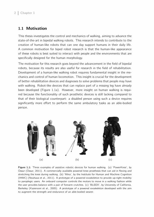
The motivation for this research goes beyond the advancement in the field of bipedalrobots, because its results are also useful for research in the field of rehabilitation.Development of a human-like walking robot requires fundamental insight in the me-chanics and control of human locomotion. This insight is crucial for the developmentof better rehabilitation devices and diagnoses to solve problems that people may havewith walking. Robot-like devices that can replace part of a missing leg have alreadybeen developed (Figure 1.1a). However, more insight on human walking is requi-red because the functionality of such prosthetic devices is still lacking compared tothat of their biological counterpart: a disabled person using such a device requiressignificantly more effort to perform the same ambulatory tasks as an able-bodiedperson.

(a) (b) (c)

Figure 1.1: Three examples of assistive robotic devices for human walking. (a) ‘PowerKnee’, byÖssur (Össur, 2011). A commercially available powered knee prosthesis that can aid in flexing andstretching the knee during walking. (b) ‘Mina’, by the Institute for Human and Machine Cognition(IHMC) (Neuhaus et al., 2011). A prototype of a powered exoskeleton to provide up-right mobilityto paraplegic users. An onboard computer controls the motors to move in a walking fashion whilethe user provides balance with a pair of forearm crutches. (c) ‘BLEEX’, by University of California,Berkeley (Kazerooni et al., 2005). A prototype of a powered exoskeleton developed with the aimto augment the strength and endurance of an able-bodied wearer.

Introduction 3

Recently, a growing number of advanced orthoses (Dollar and Herr, 2008), or exoske-letons, are being developed. These “wearable robots” fit closely to the body and workin concert with the operator’s movement. These devices use hardware and controlschemes derived from bipedal robot research to assist a person with a decreased am-bulatory ability (Figure 1.1b) or augment the performance of an able-bodied wearer(Figure 1.1c). Just as for bipedal robots, greater understanding of human locomo-tion, morphology and control is required before these devices can be made robust,efficient, safe and thereby truly functional.

1.2 Problem statement

The walking performance of robots can be evaluated on three important aspects:

- robustness, i.e., the ability to handle large unexpected disturbances;

- versatility, i.e., the ability to perform a range of different gaits;

- energy-efficiency, i.e., the ability to consume little energy.

After about 40 years of research on walking robots, there is no bipedal robot thatperforms well on all of these aspects. The human outperforms its robotic counterpartby far. Figure 1.2 illustrates the performance of current bipedal robots relative tothe human. One can see that a robot performs typically well on only one of threeaspects. There even seems to exist a clear trade-off. For example, passive limitcycle walkers are energy-efficient but are neither versatile nor robust. Powered limitcycle walkers that incorporate passive-dynamic concepts into their design, such asDenise (Wisse et al., 2007) or Flame (Hobbelen and De Boer, 2008), quickly becomeless energy-efficient for a relative small gain in robustness or versatility. Versatilerobots that can negotiate stairs, make turns and change walking speed, such asAsimo (Honda, 2011), are typically neither energy-efficient nor capable of handlingunexpected disturbances. And a robot such as Petman (Boston Dynamics, 2011) isrobust, but not energy-efficient since it relies on an a several horse-power engine todrive an off-board hydraulic pump.

Especially the low level of robustness of bipedal robots (i.e., they fall often) impedestheir applicability in everyday environments. The poor robotic walking performanceindicates that the fundamental principles of human walking are not adequately un-derstood. It is simply not true that creating a bipedal walking robot which performswell in terms of versatility, energy-efficiency and robustness is only a matter of inte-gration of existing technology or knowledge.

4 Chapter 1

energy-efficiency

robustness

versatility

Figure 1.2: A schematic representation of the performance of various bipedal robots (consideredto be representative for a larger group of robots). The performance of the robot is evaluated interms of energy-efficiency, versatility and robustness, relative to the human. More information onthe mentioned robots and their control methodology can be found in Chapter 2. As a measurefor energy-efficiency we use the specific mechanical cost of transport (as reported in Collins et al.(2005)). Robustness is measured by the robot’s demonstrated ability to withstand unexpectedperturbations in different magnitude and directions. Versatility gives an indication of the robot’sability to change walking velocity, change walking direction, walk sideways or walk on slopes or stairs.Due to the lack of robot data and the not well-defined performance measures, this illustration issubjective and has no other intention but to give an impression of the current robot performance.

Introduction 5

1.3 Research focus

There is currently no bipedal robot that is simultaneously robust, versatile and energy-efficient because of the following two reasons.

Firstly, controlling walking can be considered difficult, since the dynamics of wal-king are non-linear and high-dimensional. Also, the dynamics are a hybrid betweencontinuous dynamics during the single support phase and discrete collision dynamicsat foot impact or locking of the knee. Moreover, the walking system is essentiallyunstable since it is most of the time supported by only one leg. Stabilizing this uns-table system requires interaction with the ground through the feet, but the feet canonly push on the ground, not pull. Thus, the control of walking is difficult not onlybecause the dynamics are complex but also because the control authority over thesystem is limited.

Secondly, the walking performance is not only determined by the control of thesystem, but also by the mechanics. All the physical properties of the bipedal system(e.g., geometry, stiffness, mass, inertia) and its limitations (e.g., finite torque outputor sensing resolution) influence the walking performance. Thus, besides controlissues, there are also hardware issues to consider.

To overcome the above-mentioned problems, we look at the fundamental principlesof walking. This reduces dimensionality of the walking problem and leads to valuableinsight. In essence, walking is about progressing to a desired location while preventinga fall. A fall obviously is potentially very harmful for the system. Preventing a fallis related to the ability to maintain control over the global position and velocity ofthe system, represented by the position and velocity of the system’s center of mass(CoM). The CoM dynamics are a direct result of the gravitational force and thecontact forces with the environment that act on the CoM. The relation between theCoM dynamics and the contact forces with the ground during walking is schematicallyshown in Figure 1.3.

We focus on three basic control strategies that can be used to manipulate the in-teraction forces with the ground. These control strategies involve the use of ankletorques, angular momentum around the CoM or a step. The way these strategiesinfluence the interaction forces with the ground to control the CoM motion is illus-trated in Figure 1.4 for the example task of single-legged upright balancing. Theamount of control authority that these strategies have over the CoM are dependenton many system parameters such as foot size, peak joint torque, joint range of mo-tion, mass distribution, etc. A thorough analysis on this matter follows in Chapter 3.However, when performing the balancing tasks as illustrated in Figure 1.4, one easily

6 Chapter 1

force

CoM

CoP

≈

≈0.25 m

250 N

Figure 1.3: Walking is in essence the result of the forces that act on the center of mass (CoM). Thisfigure illustrates the evolution of the center of mass and the ground reaction force vector (GRF)during walking (side and overhead view). The GRF is the net force vector of the forces that theground applies on the foot. Its point of application is the center of pressure (CoP). The GRF datais obtained during a single walking trial at approximately 1 ms1.

(1) (2) (3)

push

jointtorque

virtual forcegroundreaction force

“ankle strategy”nominal situation “hip strategy” “stepping strategy”

CoM

CoP

Figure 1.4: Three basic balancing strategies (Horak and Nashner, 1986; Maki and McIlroy, 1997)used during bipedal locomotion, illustrated during the task of single-legged balancing. The balancestrategies manipulate the ground reaction force vector (GRF) to control the horizontal center ofmass (CoM) motion. For upright balance, the CoM is on average above the point of application ofthe GRF, i.e., the center of pressure (CoP). (1) Ankle torques manipulate the CoP location. TheGRF still acts along the line between the CoP and CoM. (2) Upper-body motions (e.g., throughhip torques) change the direction of the GRF, generating torque around the CoM and resulting inangular momentum around the CoM. The equivalence of this is a virtual GRF that passes throughthe CoM and acts at the Centroidal Moment Pivot point (Popovic et al., 2005). As a result, aforward lunge of the trunk results in a backward motion of the CoM with respect to the foot. (3)A step changes the base of support and offers new candidate CoP locations.

Introduction 7

gets an indication of the control authority of each strategy. When standing on onefoot, try to recover from a small push by taking a step. Now try to recover by usingonly ankle torques. Finally, try to recover using only upper body motions (by disablingthe ankle strategy by standing only on the ball of the foot). The ability to control theCoM motion decreases for each subsequent balancing task. Though ankle torquesand angular momentum around the CoM can manipulate the interaction forces tosome extent, the interaction forces are to a large extent simply determined by theposition of the foot on the ground relative to the CoM. Consequently, the evolutionof the CoM over time is mostly dictated by the location and the timing of a step.Or, in other words, balance control during walking is dictated by foot placement. Soto prevent a fall, adequate foot placement is essential and therefore the main topicof this research.

1.4 Goal

The goal of this thesis is to improve the performance of robotic bipedal locomo-tion in terms of robustness, versatility and energy-efficiency, by increasing the un-derstanding of the mechanics and control of foot placement. Since versatility andenergy-efficiency are only relevant when the robot can prevent a fall, a strong focuslies on the robustness of gait. This thesis aims to achieve this goal by answering thefollowing three research questions (illustrated in the figures below).

1. Regarding robustness: how can we determine where and when the foot shouldbe placed to prevent a fall?

2. Regarding versatility: how can we determine where and when the foot shouldbe placed to enable the system to evolve from its initial state to any desiredfuture state?

3. Regarding energy-efficiency: how do actuator limitations influence foot place-ment strategies?

safe step regionfor step time a

state X

1. regarding robustness 2. regarding versatility 3. regarding energy-efficiency

state Y

?

8 Chapter 1

1.5 Approach

Since foot placement is such an essential part of walking, control of foot placementhas often been addressed in research on bipedal robots (see Chapter 2 for a thoroughreview).

However, generally, foot placement is interpreted inadequately. For ‘Zero MomentPoint’-based control (Vukobratovic and Borovac, 2004), foot placement locationsare predefined and the robot’s configuration is adapted to achieve these locations.Forcefully applying such precomputed foot placement locations constrains the robot’smotion significantly and limits its robustness against unexpected disturbances. ForLimit Cycle Walking (Hobbelen and Wisse, 2007b), foot placement is controlledimplicitly and mostly the result of passive swing-leg dynamics with only low levels ofcontrol. Though the resulting foot placement is adapted to the robot’s state andcan even reject small disturbances (Wisse et al., 2005a), these implicit strategies donot indicate where and when to place the foot in case of larger disturbances.

To improve the robot’s performance, foot placement control should be adaptive andexplicit. Adaptive, so that the time and location of the step can be adjusted. Explicit,so that foot placement is a function of the current robot state and the desired futuresystem state. We contend that adaptive and explicit foot placement strategies arethe only way to remove the apparent trade-off between robustness, versatility andenergy-efficiency in robotic bipedal locomotion.

To derive control strategies for foot placement, simple gait models will be used sincethey reduce the dimensionality of the problem. As demonstrated in the previoussections, looking only at the CoM dynamics relative to the CoP can be an insightfulapproach to study the fundamentals of balance control.

As mentioned earlier, walking is not only a matter of control but also a matter ofmechanics. To gain insight in both these aspects of walking, a new humanoid robotnamed ‘TUlip’ was developed. By trying to re-invent walking on a robot, insightis gained in which problems are most relevant in walking and which solutions aremost effective. This may offer candidate hypotheses on the mechanics and controlof human locomotion, since human-like robots obey the same laws of physics ashumans do. Similarly, hypotheses on human walking can be made more plausiblewhen shown effective on a real robot.

This thesis builds upon the work of other researchers and merges and extends differentapproaches on bipedal walking. The work is influenced by the Limit Cycle Walkingapproach (Hobbelen and Wisse, 2007b), as this approach successfully demonstratesthat minor control actions on a step-to-step basis can already be sufficient to stabilize

Introduction 9

walking. Also, the research in this thesis adopts a view on walking that is inspired bythe work of Raibert (1986) and Pratt (2000b), where the walking problem is viewedas a collection of decoupled tasks, with an essential task being the control of theCoM motion through foot placement. Part of the research described in this thesis(Chapter 3 and 7) is the result of collaborative research with Pratt and colleagues.

1.6 Thesis outline

The thesis is structured as follows.

Chapter 2 gives a review of relevant research on foot placement in robotic bipedalwalking.

Chapter 3 addresses the first question raised: how can we determine where and whenthe foot should be placed to prevent a fall? The chapter introduces the capturabilityframework to analyze or synthesize actions that can prevent a fall. Fall avoidanceis analyzed by focusing on the system’s ability to eventually come to a stop withoutfalling by taking a given number of steps. The framework is applied to three simplegait models to approximate capturability for complex legged systems. The analysiscan be used to construct capture regions on the ground to which a bipedal systemcan step and prevent a fall.

Chapter 4 addresses the second question raised: how can we determine where andwhen the foot should be placed to enable the system to evolve from its initial state toany desired future state? Foot placement strategies are derived using a simple gaitmodel that accounts for the most essential dynamics of a legged system: the CoMdynamics with respect to the CoP. A controller is presented that outputs desiredfoot placement strategies to reach any desired state or gait within a finite numberof steps. The performance is demonstrated in simulation.

Chapter 5 addresses the third question raised: how do actuator limitations influencefoot placement strategies? The cost of foot placement is studied in human-likerecovery strategies following a stumble. The hypothesis is that human-like steppingstrategies are the result of a minimization of cost of recovery. A simulation studyevaluates five hypothetical measures for cost of recovery.

Chapter 6, 7 and 8 present and evaluate the developed robotic prototype TUlip, itscontrol algorithm and the resulting performance.

Chapter 9 presents a discussion of the research presented in this thesis and givessuggestions for future work.

10 Chapter 1

Note that Chapters 3-5, 7, and part of Chapter 6 are written as separate papers thathave been submitted or accepted for international conferences or journals.

Note that Chapter 3 and 7 are the result of collaborative research. Chapter 3 is anextension of previous published work of Jerry Pratt and colleagues. The descriptionof the capturability framework is the result of collaborative work of all authors. Theauthor of this thesis contributed to the application of the capturability framework tothe presented gait models and thereby enabling the synthesises of N-step capture re-gions for any N > 0. Also, he developed the Matlab GUI together with Twan Koolenwhich verified and fueled our theoretical insight in the instantaneous capture pointdynamics. Chapter 7 bundles and extends previous control algorithms as publishedby Jerry Pratt and colleagues. The author of this thesis contributed mostly to thewriting and structuring of the paper and to the verification of the developed controlalgorithms by implementating them on TUlip.

Supplemental to Chapter 8 are three videos of robot experiments of which videostills are included in the chapter. The videos are available at the website of the DelftBiorobotics Laboratory: http://dbl.tudelft.nl. When entering the website, click on‘walking robots’ and subsequently on ‘TUlip’. Also, supplemental to Chapter 3 and 4,two Matlab graphical user interfaces can be downloaded. These user interfaces allowthe user to manipulate the control inputs of the gait models presented in Chapter 3and 4 and reproduce all presented results.

2Background

12 Chapter 2

2.1 Introduction

This chapter reviews relevant research on control of robotic locomotion. A broadspectrum of control approaches exist, with many approaches having elements incommon. An attempt is made to categorize these approaches into four fundamentallydifferent control methodologies or paradigms. Each of these paradigms is reviewedand special attention is paid to the role of foot placement control within theseparadigms. Following the approach described in Chapter 1, we review whether footplacement control is:

- adaptive, i.e., both step time and step location can be changed;

- explicit, i.e., a function of the initial robot state and the desired future robotstate;

- computationally relatively inexpensive, so that it can be run online on the robot.

Sections 2.2 to 2.5 describe the four control paradigms: Zero Moment Point, LimitCycle Walking, Hybrid Zero Dynamics and Decoupled control. Section 2.6 concludesthat all the above-mentioned aspects are found in the Decoupled control approach.

2.2 Zero Moment Point

Probably the most popular control approach to achieve bipedal locomotion is basedon the Zero Moment Point (ZMP) (Vukobratovic and Borovac, 2004; Vukobratovicand Juricic, 1969). The ZMP can be described as the location on the ground aboutwhich the sum of all the moments of the active forces between the foot and therobot equals zero. Thus, it effectively reduces the ground reaction force distributionfor single support or for double support to a single point. For flat foot contact on ahorizontal floor, the ZMP location is equal to the Center of Pressure (Popovic et al.,2005). Though the ZMP is just an indicator of the robot state and potentially usefulin many bipedal control approaches, its name has become a byword for a specificcontrol approach and also a specific group of bipedal robots.

Control approaches that are specifically based on the ZMP are characterized bysatisfaction of the constraint that the ZMP is strictly within the support polygon(i.e., the convex hull that encloses the foot or feet that are on the ground). Thisensures that the stance foot remains firmly planted on the floor. The distancebetween the ZMP and the edge of the support polygon is interpreted as a measureof stability (Goswami, 1999). Offline computations are used to synthesize a gait for

Background 13

x

ZMPdesCoP

..

α

α

f(α)

f(α) f(α)

(a) (b) (c) (d)

Figure 2.1: Four models that are frequently used in the analysis and control of bipedal gait andcan be considered representative for the different control approaches described in this chapter. (a)Table-cart model (Kajita et al., 2003) used in ZMP-based control. CoM motion is calculated thatprevents the table (i.e., robot) from tipping and ZMP at a prescribed desired location. (b) Simplestwalking model (Garcia et al., 1998) used in Limit Cycle Walking control. Planar uncontrolled modelthat walks down a shallow slope, powered by gravity. (c) Planar 5-link model used in walking controlbased on Hybrid Zero Dynamics and Virtual Constraints (Westervelt et al., 2003). All link motionsare a function of the state of the unactuated stance ankle. (d) Linear Inverted Pendulum Model(Kajita and Tanie, 1991). Used offline for generation of ZMP-based robotic gait (Kajita et al.,2002), but also used online for adaptive foot placement strategies (Pratt and Tedrake, 2006).

which the ZMP stays away from the support edges while satisfying predefined gaitproperties such as desired foot step locations or gait speed (Huang et al., 2001; Kajitaet al., 2003). Complex multi-body dynamical models (Huang et al., 1999; Kagamiet al., 2002; Nishtwaki et al., 1999) or more simple inverted pendulum type models(Figure 2.1a,d) can be used to generate joint trajectories and reference trajectoriesfor the ZMP and the center of mass (CoM). These reference trajectories are thentracked by local joint controllers on the robot. ZMP-based gait typically results ina characteristic walk with flat feet and bent knees, which is required to keep fullcontrol authority over the evolution of the ZMP and CoM.

Bipedal robots that make use of the ZMP-based control approach are typically advan-ced robots with a humanlike morphology as depicted in Figure 2.2. The developmentof these robots is not solely focused on the ability to walk, but also on tasks thatuse machine vision, robotic manipulation and artificial intelligence. With the ZMPconstraint satisfied, a designer can create a wide variety of desired robotic motionsthat can be tracked on the robot. This has lead to an impressive variety of robotictasks that were demonstrated, from climbing stairs (Hirai et al., 1998) to pushing awheelchair along (Sakata et al., 2004).

14 Chapter 2

(a) (b) (c)

Figure 2.2: Three humanoid robots relying on ZMP-based control for walking. (a) ‘ASIMO’, fromHonda (Honda, 2011). (b) ‘REEM-B’ from PAL-Robotics (Tellez et al., 2008). (c) ‘HRP-4C’ fromthe National Institute of Advanced Industrial Science and Technology (AIST) (Kaneko et al., 2009).

There are numerous drawbacks to ZMP-based control algorithms. Firstly, requiringflat foot contact and bent knees typically results in poor energy-efficiency. Secondly,using precomputed walking gaits results in poor robustness to unexpected distur-bances. Consequently, recent research has been focused on the development ofmethods that enable real-time adaptation of the reference trajectories in responseto large disturbances (Diedam et al., 2008; Morisawa et al., 2010; Nishiwaki andKagami, 2010). Despite this effort, the fundamental limitation remains that ZMP-based control is not applicable in situations where the robot loses flat foot contactwith the ground. In this situation, the ZMP is non-existent (or virtual as definedby Vukobratovic and Borovac, 2004) and gives no information on how to remainbalanced. This makes it hard to synthesize motions where the foot can rotate withrespect to the ground, which is required to achieve human-like gait or handle une-ven terrain. We consider ZMP-based control too restrictive to achieve human-likewalking performance.

Note that these limitations detract nothing from the fact that the ZMP (more pre-cisely: the center of pressure) is a valuable reference point in bipedal locomotion.However, the robot’s configuration should not be adapted to achieve a predefinedZMP location. Instead, the ZMP location should be adapted to the robot’s confi-guration. The ZMP location is directly related to the forces that act on the centerof mass (as will also be shown in Chapter 3) and is therefore an input (and not anoutput) of the most essential control problem of bipedal gait: controlling the centerof mass dynamics.

Background 15

2.3 Limit Cycle Walking

Opposite from the highly controlled ZMP-based approach is the Limit Cycle Walkingapproach (Hobbelen and Wisse, 2007b) that originates from the observation that astable bipedal gait is not necessarily only a matter of actuation and control, but alsoa matter of the biped’s mechanical design being naturally conducive to walking. Thiswas the result of the work of McGeer (1990a), who demonstrated that a 2D (i.e.,planar) unactuated mechanism could obtain a cyclic gait when walking on a gentledownhill slope. This cyclic motion is powered only by gravity and locally stable in thesense that small perturbations are rejected naturally: a change in walking velocitynaturally results in a change in energy dissipation at the next step which can stabilizethe gait. For a small set of initial states, the gait naturally converges to a stablelimit cycle.

McGeer’s work lead to the development of a wide variety of passive mechanisms andmodels, for example with knees (Figure 2.3a), a torso (Wisse et al., 2004), or thosethat are capable of running (Owaki et al., 2010) or performing a three-dimensionalstable walking gait (depicted in Figure 2.3b). The concept was also extended toactuated bipedal walking on level ground and robotic prototypes were developed ofvarying complexity, for example the bipeds depicted in Figure 2.3c-d. The generalprinciple remained intact, being that the robot dynamics were still dominated by the

(a) (b) (c) (d)

Figure 2.3: Four bipeds relying on passive system dynamics to achieve a cyclic walking gait. (a)Cornell University’s copy of McGeer’s planar passive dynamic walker with knees (McGeer, 1990b).(b) Passive walker with knees and counterswinging arms (Collins et al., 2001). (c) ‘Denise’ fromDelft University of Technology (Wisse et al., 2007). (d) ‘Flame’ from Delft University of Technology(Hobbelen and De Boer, 2008).

16 Chapter 2

natural dynamics of the limbs and only minimal actuation was applied to sustain acyclic gait. Consequently, the resulting robotic gait can be characterized as energy-efficient and consists of smooth and life-like motions.

Analyzing or proving cyclic stability for a complex biped is not straightforward. The-refore, control algorithms for the actuated Limit Cycle Walkers are often based ondynamic principles of a simple planar gait model, typically the Simplest Walking Mo-del (Figure 2.1b) or an extension thereof. This low-dimensional model allows for astability analysis using Poincaré maps, where the model’s cyclic motion is analyzedon a step-to-step basis. This modeling approach is used to gain insight in how aparameter variation at one point in the gait cycle affects the model’s state over thecourse of one or multiple steps. Parameter studies on this model revealed funda-mental principles in the dynamics of bipedal walking, for example concerning walkingenergetics (Kuo, 2007 and references therein) or walking robustness (Hobbelen andWisse, 2008a,b).

However, transferring the insights gained from the simple planar walking model tocontrol algorithms for a complex biped is challenging. There can be knowledge onhow a parameter change in a certain direction can for example improve the walkingrobustness, but translating this knowledge to a control setting for a specific bipedis not straightforward. The performance of these robots relies heavily on manualtuning of the control parameters and careful tuning of the mechanical structure ofthe robot (e.g., experimenting with joint stiffness or foot shape). The lack of state-dependent feedback mechanisms makes their performance typically unreliable. Themost important stabilizing mechanism, foot placement, is left mostly as a result ofthe swing leg dynamics, which makes these robots very sensitive to changes in theenvironment or mechanical structure.

2.4 Hybrid Zero Dynamics

The Limit Cycle Walking approach demonstrates how challenging it can be to obtaina periodic gait for a complex bipedal robot, let alone prove that the robotic motionsasymptotically converge to a stable limit cycle. A way of dealing with this is descri-bed by the method of Virtual Constraints and Hybrid Zero Dynamics (Grizzle et al.,2001; Westervelt et al., 2003). Feedback controllers that enforce virtual constraintson the system are designed. These virtual constraints effectively reduce the num-ber of degrees of freedom of walking to one. The motions of all the robotic linksbecome a function of this single degree of freedom: the stance leg ankle which isleft unactuated. Using an accurate robot model (Figure 2.1c) and offline optimiza-tion techniques, joint motions are sought that ensure a provably stable periodic gait.

Background 17

Walking was achieved for the planar bipeds (Chevallereau et al., 2003; Plestan et al.,2003; Sreenath et al., 2010) depicted in Figure 2.4 and in 3D for simulated bipeds(Chevallereau et al., 2009).

The resulting gait is time invariant, which means that the foot placement locationsare fixed and the time of foot placement is a function of the forward progression ofthe robot with respect to its ankle. The robustness of the gait is determined by theability of the actuators to keep enforcing the constraints through high-gain feedback,even in the presence of disturbances (Sreenath et al., 2010; Westervelt et al., 2004).It remains challenging to extend these methods to allow for actuated ankles, gaitswith a non-instantaneous double stance phase and non periodic gaits with adaptivefoot placement strategies (Grizzle et al., 2010; Sabourin and Bruneau, 2005).

(a) (b)

Figure 2.4: Two planar bipeds relying on Virtual Constraints and Hybrid Zero Dynamics for walking.(a) ‘Rabbit’ from Centre National de Recherche Scientifique (CNRS) and the University of Michigan(Chevallereau et al., 2003). (b) ‘MABLE’ from the University of Michigan in collaboration withCarnegie Mellon University (CMU) (Grizzle et al., 2009).

2.5 Decoupled control

Another way to reduce the dimensionality of bipedal walking is to view the walkingtask as a collection of several decoupled tasks, each of lower dimensionality. Anoverview is given of various decoupled control methods.

Raibert (1986) decoupled the control of running by control of hopping height, bodyorientation and velocity. The velocity was controlled using simple foot placement

18 Chapter 2

strategies: the foot was placed forward, backward, or on the ‘neutral point’ torespectively decelerate, accelerate or maintain the same velocity. During the stancephase, hopping height was controlled by leg extension and the body orientation wascontrolled using hip torques.

Simple approximate rules proved effective for robust robotic running and resultedin impressive robot performance on several robots, for example for the one-leggedhopper depicted in Figure 2.5a. Pratt and Pratt (1998) used a the same controldecomposition for planar walking plus additional controllers for swing leg placement,and support transition (for the robot depicted in Figure 2.5b). Again, robust roboticperformance was achieved using only approximate control rules for foot placement(e.g., ‘increase the nominal stride length as the robot walks faster’). However, inthis case the robot velocity was not solely regulated by foot placement but also byjoint torques during single and double support.

(a) (b)

Figure 2.5: Robots relying on decoupled control for locomotion. (a) ‘3D One-Leg Hopper’ by Mas-sachusetts Institute of Technology (MIT) (Raibert, 1986). (b) ‘Spring Flamingo’ by MassachusettsInstitute of Technology (MIT) (Pratt and Pratt, 1998).

The results of Raibert, Pratt and their colleagues illustrate that simple approximatefoot placement strategies, typically derived from simple dynamic models, can resultin robust bipedal locomotion. However, the effectiveness of these approximate rulesis typically dependent on a few factors. They can require proper tuning of theircontrol variables, either manual or automated. Also, approximate foot placementrules rely either on (a) the rapid succession of consecutive (stabilizing) steps to dealwith the inherent mismatch between the approximated effect and true effect on therobot dynamics. This is typically only possible for well engineered, heavily actuatedrobots. Or, on (b) the existence of additional stabilizing mechanisms (e.g., ankletorques and hip torques) that together achieve the intended robotic motion.

Background 19

Later, Pratt et al. (2006) introduced a more analytical and model-based approach toderive rules for velocity control through foot placement. The simple linear invertedpendulum model (introduced by Kajita and Tanie (1991) and depicted in Figure 2.1d)was used to derive the ‘capture point’. This point gives an approximation of the steplocation for which stepping there will allow a robot to come to a stop. It usesonly information about the position and velocity of the center of mass of the robot.Adjusting the foot placement location relative to the capture point yields a velocitycontrol mechanism analogous to the neutral point of Raibert. The capture pointwas used in the control of foot placement in simulated robots to balance, recoverfrom pushes and step on desired stepping stones (Pratt and Tedrake, 2006; Rebulaet al., 2007). Recently, very similar reference points were derived using non-linearpendulum dynamics with impact dynamics (Stephens, 2007b; Wight et al., 2008)and were shown to be useful step indicators for push recovery on a humanoid robot(Stephens, 2007b; Stephens and Atkeson, 2010) or walking for a planar biped (Wight,2008).

Recently, the decoupled control of bipedal locomotion has also been extended to thedomain of physics-based character animations (Coros et al., 2010; De Lasa, 2010; Yinet al., 2007). Again, bipedal locomotion control is decoupled in separate control tasksof which explicit control of foot placement is one and derived from the same linear ornon-linear inverted pendulum model. Decoupled control of walking was shown to begeneralizable across a wide variety of gaits and simulated characters, and shown towork in the presence of disturbances or while the character is performing secondarytasks. Since the proposed walking controllers have a lot of common elements withcontrollers found in real robots, they can serve as an inspiration for (or indicationof) future robotic behavior.

The above mentioned research suggests that simple gait models that model only thecenter of mass dynamics can be used effectively to synthesize robust foot placementstrategies. This is also suggested by biomechanical studies, where such simple model-based laws were found to be good predictors of human foot placement (Hof, 2008;Hof et al., 2010; Millard et al., 2009; Townsend, 1985). These findings motivate theapproach chosen in this research. A large part of the research builds upon the notionof the capture point and extends it to the concept of ‘capturability’. This conceptis applied to various 3D gait models of varying complexity. It is demonstrated howthese models can be used in the control of various walking gaits, or upright balancewith and without reactive stepping to remain balanced.

20 Chapter 2

2.6 Conclusion

Four distinct control paradigms in the control of robotic bipedal locomotion wereevaluated based on their potential to synthesize robust, versatile and energy-efficientgait. We contend that human-like walking performance can only be achieved by footplacement strategies that are adaptive, explicitly formulated and computationallyachievable in real-time.

In the Zero Moment Point control paradigm, the center of mass dynamics withrespect to the center of pressure (or ZMP) location is controlled explicitly. However,the CoM dynamics are typically adapted to achieve a precalculated ZMP trajectoryinstead of adapting the ZMP location to the current CoM dynamics. This limitsthe applicability of ZMP-based control to situations where the CoM motion deviatessignificantly from the nominal motion, for example in case of walking in the presenceof perturbations or over uneven terrain. Foot placement in the Limit Cycle Walkingparadigm is naturally adaptive to the robot’s state, but controlled implicitly since itis mostly the result of the passive dynamics of the system. This approach is typicallyonly practical for periodic unperturbed walking gaits.

The Hybrid Zero Dynamics paradigm relies heavily on complex offline optimizationsto obtain a stable gait. For this gait, all the joints (and therefore also foot placement)are an explicit function of the stance ankle state. The step time is automaticallyadjusted based on the forward progression of the robot. However, this methodologyonly works if the robot can conform to the single prescribed gait and if the robot haspointy feet. Extending this method to more complex 3D bipeds and complex terrainsis challenging.

For decoupled control, the high dimensional walking task is viewed as a collectionof several decoupled tasks of lower dimensionality. Foot placement is considereda key task and controlled explicitly. The low dimensionality of each task allows forsimple modeling and online adaptation to the robot state. We consider this approachcurrently the most promising for the synthesis of robust, versatile and energy-efficientgait.

3Capturability-Based Analysis

and Control of LeggedLocomotion:

Theory and Application toThree Simple Gait Models

T. Koolen, T. de Boer, J. Rebula, A. Goswami, J. PrattSubmitted to International Journal of Robotic research, 2011

22 Chapter 3

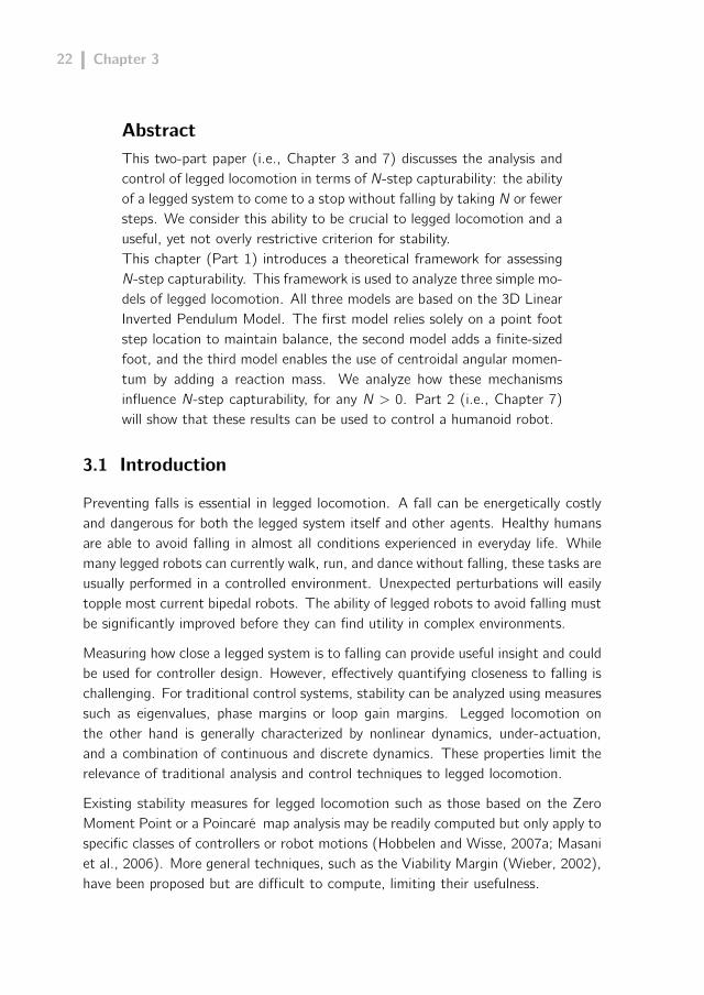
AbstractThis two-part paper (i.e., Chapter 3 and 7) discusses the analysis andcontrol of legged locomotion in terms of N-step capturability: the abilityof a legged system to come to a stop without falling by taking N or fewersteps. We consider this ability to be crucial to legged locomotion and auseful, yet not overly restrictive criterion for stability.This chapter (Part 1) introduces a theoretical framework for assessingN-step capturability. This framework is used to analyze three simple mo-dels of legged locomotion. All three models are based on the 3D LinearInverted Pendulum Model. The first model relies solely on a point footstep location to maintain balance, the second model adds a finite-sizedfoot, and the third model enables the use of centroidal angular momen-tum by adding a reaction mass. We analyze how these mechanismsinfluence N-step capturability, for any N > 0. Part 2 (i.e., Chapter 7)will show that these results can be used to control a humanoid robot.

3.1 Introduction

Preventing falls is essential in legged locomotion. A fall can be energetically costlyand dangerous for both the legged system itself and other agents. Healthy humansare able to avoid falling in almost all conditions experienced in everyday life. Whilemany legged robots can currently walk, run, and dance without falling, these tasks areusually performed in a controlled environment. Unexpected perturbations will easilytopple most current bipedal robots. The ability of legged robots to avoid falling mustbe significantly improved before they can find utility in complex environments.

Measuring how close a legged system is to falling can provide useful insight and couldbe used for controller design. However, effectively quantifying closeness to falling ischallenging. For traditional control systems, stability can be analyzed using measuressuch as eigenvalues, phase margins or loop gain margins. Legged locomotion onthe other hand is generally characterized by nonlinear dynamics, under-actuation,and a combination of continuous and discrete dynamics. These properties limit therelevance of traditional analysis and control techniques to legged locomotion.

Existing stability measures for legged locomotion such as those based on the ZeroMoment Point or a Poincaré map analysis may be readily computed but only apply tospecific classes of controllers or robot motions (Hobbelen and Wisse, 2007a; Masaniet al., 2006). More general techniques, such as the Viability Margin (Wieber, 2002),have been proposed but are difficult to compute, limiting their usefulness.

Capturability: theory and application to simple gait models 23

This leads us to propose the analysis of legged locomotion based on N-step captura-bility, which we informally define as the ability of a system to come to a stop withoutfalling by taking N or fewer steps, given its dynamics and actuation limits. N-stepcapturability offers measures that are applicable to a large class of robot motions,including non-periodic locomotion over rough terrain with impassable regions, and itdoes not require a specific control system design. N-step capturability may be readilyapproximated, and it is useful in controller design.

Both preventing a fall and coming to a stop require adequate foot placement as aresult of the ground reaction force constraints that are typical to legged locomotion.We will focus extensively on this aspect of legged locomotion using the N-step cap-ture region, the set of points to which a legged system in a given state can step tobecome (N − 1)-step capturable. A new measure of capturability in a given state,termed the N-step capturability margin, is then naturally defined as the size of theN-step capture region. Additionally, we will introduce the d∞ capturability level,which allows a general, state-independent capturability comparison between simplegait models.

The remainder of this first part is structured as follows. Section 3.2 provides asurvey of relevant literature. Section 3.3 contains definitions of the various conceptsthat constitute the N-step capturability framework. In Sections 3.4 through 3.7 weapply the capturability framework to three simple gait models based on the LinearInverted Pendulum Model (Kajita et al., 2001; Kajita and Tanie, 1991). For thesesimple gait models, we can exactly compute capturability. Section 3.8 introducesthe two capturability measures and compares the simple gait models in terms ofthese measures. A discussion is provided in Section 3.9, and we conclude the part inSection 7.10.

In Part 2 (i.e., Chapter 7) of the paper, we demonstrate the utility of the capturabilityframework by using the results of the simple gait models to control and analyzebalancing and walking motions of a 3D bipedal robot with two 6-degree-of-freedomlegs.

3.2 Background

The question “how stable is a given legged system?" has been the subject of muchresearch and debate, in both robotics and biomechanics. We will now present previouswork attempting to answer this question, including previous work on capturability.

The Zero Moment Point (ZMP) is often used as an aid in control development,with the constraint that it must remain in the interior of the base of support of

24 Chapter 3

a legged robot. A common ZMP control method is to maintain the ZMP alonga precomputed reference trajectory (Vukobratovic and Stepanenko, 1972). Duringwalking, the error between the actual and desired ZMP can be used as a measure ofthe error between the current and desired state of the robot (Okumura et al., 2003).The repeatability of the gait can also be used as an error measure (Vukobratovicand Stepanenko, 1972). One drawback to following a precomputed trajectory isthe inability of the robot to recover from a large unexpected push. Further workhas expanded the ZMP method to include step placement adjustment in reaction todisturbances (Morisawa et al., 2009; Nishiwaki and Kagami, 2010), but there is nomeasure of the ability of the robot to reactively avoid a fall when following a givenpreplanned ZMP trajectory. In addition, the ZMP requires significant modificationto apply to non-flat terrain (Wieber, 2002) or dynamic gait with a foot that rotateson the ground.

Poincaré maps have been used to measure the local stability of periodic gaits, andto induce periodic gaits of real robots using reference trajectories (Morimoto et al.,2005). Based on Poincaré Map analysis, the Gait Sensitivity Norm (Hobbelen andWisse, 2007a) provides a measure of robustness for limit cycle walkers (Hobbelen andWisse, 2007b) and has been shown to correlate well with the disturbance rejectioncapabilities of simulated planar walkers. The Gait Sensitivity Norm is calculated asthe sensitivity of a given gait measure, such as step time, to a given disturbancetype, such as a step-down in terrain, using a simulated model or experimental data.Another Poincaré map method based on Floquet multipliers has been used to analyzethe stability of human walking gaits (Dingwell et al., 2001). However, Poincaré mapanalysis assumes cyclic gait to yield a measure of stability. In addition, it requires alinearization at a given point in the gait cycle, which limits the applicability of themethod to large disturbances between steps where the linearization fails to captureessential dynamics of the motion (Dingwell et al., 2001).

Poincaré map analysis has also been applied to the case of passive limit cycle wal-kers under stochastic environmental perturbations (Byl and Tedrake, 2008), withoutlinearizing the system around the fixed point, yielding a probabilistic basin of attrac-tion. The stability of a walker is described with a mean first passage time, whichis the expected number of steps before failure, given a set of statistics for the sto-chastic environmental disturbance. However, this method assumes an approximatelyperiodic gait, and does not apply to large general disturbances such as a significantpush. Poincaré map analysis has been extended to control a walker in acyclic desiredgaits, by applying linear control based on a continuous family of Poincaré maps alongthe entire trajectory (Manchester et al., 2009). This control method can provide ameasure of robustness about the desired trajectory, but it does not consider the

Capturability: theory and application to simple gait models 25

robustness of the desired trajectory itself.

The concepts of Virtual Constraints and Hybrid Zero Dynamics have been used toobtain and prove asymptotic stability of periodic motions for walking robots (Che-vallereau et al., 2003). Introducing Virtual Constraints reduces the dimensionality ofthe walking system under consideration by choosing a single desired gait, allowing atractable stability analysis. However, if actuator limitations render the robot inca-pable of maintaining the Virtual Constraints after a large perturbation, it is possible afall could be avoided only by changing the desired trajectory to alter foot placementand use of angular momentum.

The Foot Placement Estimator, like the present work, considers the footstep locationto be of primary importance and can be used both to control and to analyze bipedalsystems (Wight et al., 2008). For a simple planar biped that maintains a rigid A-frame configuration, the Foot Placement Estimator demarcates the range of footplacement locations that will result in a statically standing system. This approach isquite similar to ours, though it is unclear how to extend this method to more generalsystems.

Wieber (2002) uses the concept of viability theory (Aubin, 1991) to reason aboutthe subset of state space in which the legged system must be maintained to avoidfalling. He shows a Lyapunov stability analysis for standing on non-flat terrain givena balance control law. However, the standing assumption precludes the use of thismethod in walking, and it provides no information on choosing step locations to avoidfalling. Capturability is closely related to viability theory, but focuses on states whichare most relevant to normal walking and also provides a method to explicitly computeacceptable regions to step.

In previous work, we have implicitly used the concept of capturability to developthe notion of capture points, the places on the ground to step that will allow alegged robot to come to a stop. We have used capture points based on simplemodels to control complex models, including a simulation of M2V2, a 12 degree offreedom humanoid robot. We have designed controllers that balance, recover frompushes, and walk across randomly placed stepping stones (Pratt and Tedrake, 2006;Rebula et al., 2007). Some of these capture point-based control methods were alsoimplemented on the physical M2V2 (Pratt et al., 2009). We will extend the conceptof capture points, applying the theory to general legged systems, considering multiplesteps and providing a more complete analysis of the ability of a legged system tocome to a stop.

26 Chapter 3

3.3 Capturability framework

Consider a class of hybrid dynamic systems that have dynamics described by

x = f (x , u) if hi(x) 6= 0 (3.1a)

x ← gi(x) if hi(x) = 0 (3.1b)

u ∈ U(x) (3.1c)

for i ∈ I ⊂ N. Here, x is the state of the system and u is the system’s control input,which is confined to the state-dependent set of allowable control inputs U(x). Whenthe system state lies on a switching surface, such that hi(x) = 0, the discrete jumpdynamics reset the state to gi(x) instantaneously. An evolution of this system is asolution to (3.1a) and (3.1b) for some input satisfying (3.1c).

For this analysis, we assume that some part of state space must be avoided at allcost – a set of failed states. For a bipedal robot, this set could comprise all statesfor which the robot has fallen. The viability kernel, described in (Aubin, 1991; Aubinet al., 2002) and introduced into the field of legged locomotion in (Wieber, 2000,2002), is the set of all states from which these failed states can be avoided. Thatis, for every initial state in the viability kernel, there exists at least one evolutionthat never ends up in a failed state. As long as the system state remains within theviability kernel, the system is viable.

The viability concept arises quite naturally and can be seen as a very generic andunrestrictive definition of ‘stability’ for a dynamic system. However, determining theviability kernel is generally analytically intractable, and approximation is computatio-nally expensive (Wieber, 2002). In addition, it is not trivial to synthesize a controllerbased solely on the viability kernel, even if it were given. This motivates the use ofmore restrictive definitions of stability. N-step capturability adds the restriction thatthe system should be able to come to a stop by taking N or fewer steps, resulting inthe following definition:

Definition 1 (N-step capturable). Let Xfailed denote a set of failed states associatedwith a hybrid dynamic system defined by (3.1). A state x0 of this system is N-stepcapturable with respect to Xfailed, for N ∈ N, if and only if there exists at leastone evolution starting at x0 that contains N or fewer crossings of switching surfaces(steps), and never reaches Xfailed.

Similar to the viability kernel and the viable-capture basin (Aubin et al., 2002), wedefine an N-step viable-capture basin as the set of all N-step capturable states. The

Capturability: theory and application to simple gait models 27

viability kernel

captured states

1-step viable-capture basin

∞ -step viable-capture basinfailed states

(a)(b)

(d)

(c)

(e)

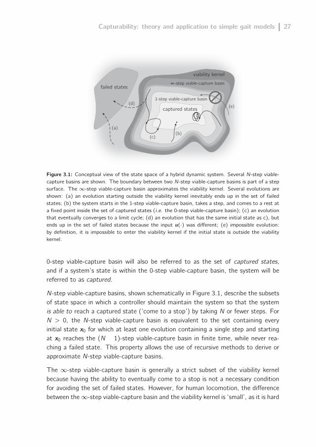
Figure 3.1: Conceptual view of the state space of a hybrid dynamic system. Several N-step viable-capture basins are shown. The boundary between two N-step viable-capture basins is part of a stepsurface. The ∞-step viable-capture basin approximates the viability kernel. Several evolutions areshown: (a) an evolution starting outside the viability kernel inevitably ends up in the set of failedstates; (b) the system starts in the 1-step viable-capture basin, takes a step, and comes to a rest ata fixed point inside the set of captured states (i.e. the 0-step viable-capture basin); (c) an evolutionthat eventually converges to a limit cycle; (d) an evolution that has the same initial state as c), butends up in the set of failed states because the input u(·) was different; (e) impossible evolution:by definition, it is impossible to enter the viability kernel if the initial state is outside the viabilitykernel.

0-step viable-capture basin will also be referred to as the set of captured states,and if a system’s state is within the 0-step viable-capture basin, the system will bereferred to as captured.

N-step viable-capture basins, shown schematically in Figure 3.1, describe the subsetsof state space in which a controller should maintain the system so that the systemis able to reach a captured state (‘come to a stop’) by taking N or fewer steps. ForN > 0, the N-step viable-capture basin is equivalent to the set containing everyinitial state x0 for which at least one evolution containing a single step and startingat x0 reaches the (N 1)-step viable-capture basin in finite time, while never rea-ching a failed state. This property allows the use of recursive methods to derive orapproximate N-step viable-capture basins.

The ∞-step viable-capture basin is generally a strict subset of the viability kernelbecause having the ability to eventually come to a stop is not a necessary conditionfor avoiding the set of failed states. However, for human locomotion, the differencebetween the∞-step viable-capture basin and the viability kernel is ‘small’, as it is hard

28 Chapter 3

to imagine a state in which a human can avoid falling, but cannot eventually cometo a captured state. A notable exception is a purely passive walker(McGeer, 1990a),for which walking persists in an infinite limit cycle with no possibility of coming to astop. In fact, an infinitely repeatable gait has been found for a simulated 3D passivewalking model that has no captured states (Coleman et al., 2001).

A problem that N-step viable-capture basins share with the viability kernel is that theydo not provide a direct means of controller design. This motivates the introductionof N-step capture points and N-step capture regions. While viable-capture basinsspecify capturability in terms of state space, capture points and capture regions aredefined in Euclidean space, and describe the places where the system can step toreach a captured state. This information can for example be used to determinefuture step locations, to be used in a control algorithm for a bipedal robot.

We encode step locations using contact reference points. Each body that is allowedto come in contact with the environment during normal operation is assigned a singlecontact reference point, which is fixed with respect to the contacting body. Contactreference points provide a convenient, low-dimensional way of referring to the positionof a contacting body, and allow us to define the N-step capture points and N-stepcapture regions as follows:

Definition 2 (N-step capture point, region). Let x0 be the state of a hybrid dynamicsystem defined by (3.1), with an associated set of failed states Xfailed. A point r isan N-step capture point for this system, for N > 0, if and only if there exists at leastone evolution starting at x0 that contains one step, never reaches Xfailed, reaches an(N − 1)-step capturable state, and places a contact reference point at r at the timeof the step. The N-step capture region is the set of all N-step capture points.

A conceptual visualization of N-step capture regions is shown in Figure 3.2.

3.4 Three simple gait models

Legged locomotion can be difficult to analyze and control due to the dynamic com-plexity of a legged system. Simple gait models permit tractable and insightful analysisand control of walking. We present three models for which it is possible to determineN-step viable-capture basins and capture regions in closed form. The results can beused as approximations for more complex legged systems and prove useful in theircontrol.

To illustrate the results obtained in this research, a Matlab graphical user interface(GUI) was created that allows the user to manipulate the control inputs for all models

Capturability: theory and application to simple gait models 29

(c) (b) (a) N-step capture regions

N = 1N = 2

N = ∞

Figure 3.2: (a) A conceptual representation of the N-step capture regions for a human in a capturedstate (standing at rest). (b) N-step capture regions for a running human. The capture regions havedecreased in size and have shifted, as compared to (a). (c) N-step capture regions for the samestate as b), but with sparse footholds (e.g., stepping stones in a pond). The set of failed states haschanged, which is reflected in the capture regions.

described in this paper, while the N-step capture regions are dynamically updated.This GUI is included as Multimedia Extension 1.

All three models are based on the 3D Linear Inverted PendulumModel (3D-LIPM) (Ka-jita et al., 2001; Kajita and Tanie, 1991), which comprises a single point massmaintained on a plane by a variable-length leg link. The complexity of the presen-ted models increases incrementally. To each subsequent model, another stabilizingmechanism is added. These mechanisms are generally considered fundamental indealing with disturbances, both in the biomechanics and robotics literature (Abdal-lah and Goswami, 2005; Guihard and Gorce, 2002; Horak and Nashner, 1986; Hyonet al., 2007; Nenchev and Nishio, 2008; Stephens, 2007b).

The first model (Section 3.5) relies solely on point foot placement to come to a stop.The second model (Section 3.6) is obtained by adding a finite-sized foot and ankleactuation to the first model, enabling modulation of the Center of Pressure (CoP).The third model (Section 3.7) extends the second by the addition of a reaction massand hip actuation, enabling the human-like use of rapid trunk (van der Burg et al.,2005; Horak and Nashner, 1986) or arm motions (Pijnappels et al., 2010; Roos et al.,2008).

3.5 3D-LIPM with point foot

The 3D Linear Inverted Pendulum Model, described by Kajita et al. (Kajita et al.,2001; Kajita and Tanie, 1991) and depicted in Figure 3.3, comprises a point mass

30 Chapter 3

êxêy

êz

g

rankle

z0

Pr

f

rm

Figure 3.3: Schematic representation of the 3D-LIPM with point foot. The model comprises apoint foot at position rankle, a point mass at position r with mass m and a massless telescopingleg link with an actuator that exerts a force f on the point mass that keeps it at constant heightz0. The projection matrix P projects the point mass location onto the xy -plane. The gravitationalacceleration vector is g.

with position r at the end of a telescoping massless mechanism (representing theleg), which is in contact with the flat ground. The point mass is kept on a horizontalplane by suitable generalized forces in the mechanism. Torques may be exerted atthe base of the pendulum. For this first model, however, we set all torques at thebase to zero. Hence, the base of the pendulum can be seen as a point foot, withposition rankle. Foot position changes, which occur when a step is taken, are assumedinstantaneous, and have no instantaneous effect on the position and velocity of thepoint mass.

Following the capturability framework introduced in Section 3.3, we treat the 3D-LIPM with point foot as a hybrid dynamic system, with dynamics that will be derivedin Section 3.5.1. Its control input is the point foot position. We define a set ofallowable values for this control input, described in Section 3.5.2. The point ranklewill be the contact reference point for all models in this paper. Changing the locationof the point foot is considered crossing a step surface. The set of failed states for allsimple models presented in this paper comprises all states for which ‖r − rankle‖ → ∞as t →∞, for any allowable control input.

3.5.1 Equations of motion

The equations of motion for the body mass are

mr = f +mg (3.2)

Capturability: theory and application to simple gait models 31

where m is the mass, r =(x y z

)Tis the position of the center of mass (CoM),

expressed in an inertial frame, f =(fx fy fz

)Tis the actuator force acting on the

point mass and g =(

0 0 −g)T

is the gravitational acceleration vector.

A moment balance for the massless link shows that

− (r − rankle)× f = (3.3)

where rankle =(xankle yankle 0

)Tis the location of the ankle.

If z = 0 initially, the point mass will stay at z = z0 if z = 0. Using (3.2), we findfz = mg. This can be substituted into (3.3) to find the forces fx and fy ,

fx = mω20(x − xankle)

fy = mω20(y − yankle)

where ω0 =√

gz0

is the reciprocal of the time constant for the 3D-LIPM.

The equations of motion, (3.2), can now be rewritten as

r = ω20(P r − rankle) (3.4)

where P =(

1 0 00 1 00 0 0

)projects r onto the xy -plane.

Note that the equations of motion are linear. This linearity is what makes the modelvaluable as an analysis and design tool, as it allows us to make closed form predictions.In addition, the equations are decoupled and represent the same dynamics in the x-and y -directions. Each of the first two rows of (3.4) describes a separate 2D-LIPMwith point foot. Therefore, results obtained for the 2D model can readily be extendedto the 3D model.

3.5.2 Allowable control inputs

We introduce two constraints on the stepping capabilities of the model. First, weintroduce an upper limit on step length, i.e., the distance between subsequent anklelocations. This maximum step length is denoted lmax and is assumed to be constant;it does not depend on the CoM location r. Second, we introduce a lower limit to thetime between steps (ankle location changes), ∆ts, which models swing leg dynamics.

32 Chapter 3

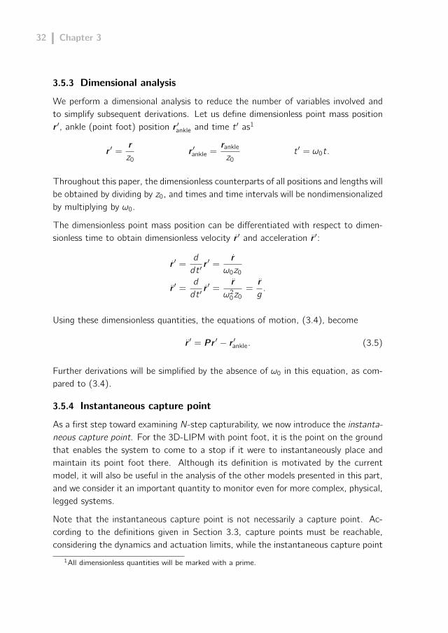
3.5.3 Dimensional analysis

We perform a dimensional analysis to reduce the number of variables involved andto simplify subsequent derivations. Let us define dimensionless point mass positionr ′, ankle (point foot) position r ′ankle and time t ′ as1

r ′ =r

z0r ′ankle =

ranklez0

t ′ = ω0t.

Throughout this paper, the dimensionless counterparts of all positions and lengths willbe obtained by dividing by z0, and times and time intervals will be nondimensionalizedby multiplying by ω0.

The dimensionless point mass position can be differentiated with respect to dimen-sionless time to obtain dimensionless velocity r ′ and acceleration r ′:

r ′ =d

dt ′r ′ =

r

ω0z0

r ′ =d

dt ′r ′ =

r

ω20z0

=r

g.

Using these dimensionless quantities, the equations of motion, (3.4), become

r ′ = P r ′ − r ′ankle. (3.5)

Further derivations will be simplified by the absence of ω0 in this equation, as com-pared to (3.4).

3.5.4 Instantaneous capture point

As a first step toward examining N-step capturability, we now introduce the instanta-neous capture point. For the 3D-LIPM with point foot, it is the point on the groundthat enables the system to come to a stop if it were to instantaneously place andmaintain its point foot there. Although its definition is motivated by the currentmodel, it will also be useful in the analysis of the other models presented in this part,and we consider it an important quantity to monitor even for more complex, physical,legged systems.

Note that the instantaneous capture point is not necessarily a capture point. Ac-cording to the definitions given in Section 3.3, capture points must be reachable,considering the dynamics and actuation limits, while the instantaneous capture point

1All dimensionless quantities will be marked with a prime.

Capturability: theory and application to simple gait models 33

does not take into account the step time or step length constraints as defined in Sec-tion 3.5.2.

The location of the instantaneous capture point can be computed from energy consi-derations. For a given constant foot position, we can interpret the first two rowsof (3.5) as the descriptions of two decoupled mass-spring systems, each with unitmass and negative unit stiffness. Dimensionless orbital energies (Kajita et al., 2001;Kajita and Tanie, 1991), E′LIP,x and E′LIP,y , are then defined as the Hamiltonians ofthese systems:

E′LIP,x =1

2x ′2 −

1

2(x ′ − x ′ankle)2 (3.6a)

E′LIP,y =1

2y ′2 −

1

2(y ′ − y ′ankle)2. (3.6b)

Since Hamiltonians are conserved quantities, so are the orbital energies.

The orbital energy for a direction determines the behavior of the 3D-LIPM in thatdirection when the CoM is moving toward the foot. Considering the x ′-direction forexample, three cases of interest arise:

1. E′LIP,x > 0. The orbital energy is sufficient to let x ′ reach x ′ankle, after which x′

continues to accelerate away from x ′ankle.

2. E′LIP,x < 0. x ′ reverses direction before x ′ reaches x ′ankle.

3. E′LIP,x = 0. x ′ comes to a rest exactly at x ′ankle.

We can solve for a foot location that results in either desired orbital energies or,equivalently, a desired velocity vector at a given value of r ′ (Kajita et al., 2001; Kajitaand Tanie, 1991). To determine the instantaneous capture point, we are interestedin the foot placement required to obtain zero orbital energy in each direction. Solving(3.6) for r ′ankle and choosing the solution for which the point mass moves toward thepoint foot shows that the dimensionless version of the instantaneous capture point(Pratt and Tedrake, 2006) is

r ′ic = P r ′ + r ′ (3.7)

or, in terms of the original physical quantities:

ric = P r +r

ω0. (3.8)

This quantity was independently described by Hof et al. (Hof, 2008; Hof et al., 2007,2005) and named the Extrapolated Center of Mass. It was shown to have significantties to balancing and walking in human test subjects.

34 Chapter 3

3.5.5 Instantaneous capture point dynamics

If the point foot is not instantaneously placed at the instantaneous capture point,the instantaneous capture point will move. We will now analyze this motion. Theresults of this analysis are depicted graphically in Figure 3.4. The dynamics thatdescribe the motion of the instantaneous capture point on the ground can be derivedby reformulating the dimensionless equations of motion in state space form. Thestate space model is based on the x ′-dynamics only (i.e., the first row of (3.5), a2D-LIPM), but the derivations can readily be extended to both directions, as notedin Section 3.5.1. The first row of (3.5) is rewritten in state space form as(

x ′

x ′

)=

(0 1

1 0

)︸ ︷︷ ︸

A

(x ′

x ′

)+

(0

−1

)︸ ︷︷ ︸

B

x ′ankle. (3.9)

The state matrix A has eigenvalues λ1,2 = ±1 and corresponding eigenvectors

V =(v1 v2

)=

1

2

(1 1

1 −1

).

The eigendata show that there is a saddle point with one stable and one unstableeigenvector. The state matrix can be diagonalized using the similarity transformationT = V −1, which results in the new state vector(

x ′1

x ′2

)=

(1 1

1 −1

)︸ ︷︷ ︸

T

(x ′

x ′

). (3.10)

The new state x ′1 is identical to the instantaneous capture point x ′ic, and x′2 is the

point reflection of the instantaneous capture point across the projection of the pointmass onto the ground. The diagonalized state space model is(

x ′1

x ′2

)=

(1 0

0 −1

)︸ ︷︷ ︸

TAT−1

(x ′1

x ′2

)+

(−1

1

)︸ ︷︷ ︸TB

x ′ankle. (3.11)

The diagonal state matrix TAT−1 shows that the model’s instantaneous capturepoint dynamics are first order. State x ′1 = x ′ic corresponds to the unstable eigenvalue+1 and is thus of primary interest in stabilizing the system.

These derivations can be repeated for the y ′-direction, so that the first row of (3.11)can be extended to

r ′ic = r ′ic − r ′ankle. (3.12)

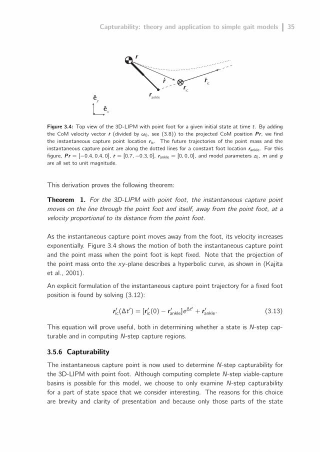
Capturability: theory and application to simple gait models 35

êy

êx

rankle

r

.r .ricric

Figure 3.4: Top view of the 3D-LIPM with point foot for a given initial state at time t. By addingthe CoM velocity vector r (divided by ω0, see (3.8)) to the projected CoM position P r, we findthe instantaneous capture point location ric. The future trajectories of the point mass and theinstantaneous capture point are along the dotted lines for a constant foot location rankle. For thisfigure, P r = [−0.4, 0.4, 0], r = [0.7,−0.3, 0], rankle = [0, 0, 0], and model parameters z0, m and gare all set to unit magnitude.

This derivation proves the following theorem:

Theorem 1. For the 3D-LIPM with point foot, the instantaneous capture pointmoves on the line through the point foot and itself, away from the point foot, at avelocity proportional to its distance from the point foot.

As the instantaneous capture point moves away from the foot, its velocity increasesexponentially. Figure 3.4 shows the motion of both the instantaneous capture pointand the point mass when the point foot is kept fixed. Note that the projection ofthe point mass onto the xy -plane describes a hyperbolic curve, as shown in (Kajitaet al., 2001).

An explicit formulation of the instantaneous capture point trajectory for a fixed footposition is found by solving (3.12):

r ′ic(∆t ′) = [r ′ic(0)− r ′ankle]e∆t ′ + r ′ankle. (3.13)

This equation will prove useful, both in determining whether a state is N-step cap-turable and in computing N-step capture regions.

3.5.6 Capturability

The instantaneous capture point is now used to determine N-step capturability forthe 3D-LIPM with point foot. Although computing complete N-step viable-capturebasins is possible for this model, we choose to only examine N-step capturabilityfor a part of state space that we consider interesting. The reasons for this choiceare brevity and clarity of presentation and because only those parts of the state

36 Chapter 3

space need to be considered to compute the N-step capture regions and relatedcapturability measures. For the current model in particular, we will only considerthose states for which the model has just taken a step. Denoting the time at whichthe previous step has been taking t ′s,prev, we set t ′ = t ′s,prev = 0.

For the 3D-LIPM with point foot, N-step capturability for these states can be fullydescribed in terms of the initial distance between the contact reference point andthe instantaneous capture point,

∥∥r ′ic(0)− r ′ankle∥∥. The maximum distance for which

the state is still N-step capturable will be denoted d ′N . Figure 3.5 shows an evolutionthat captures the model in the minimum number of steps and the values of d ′N forfive values of N. We now proceed to determine these d ′N , first for N = 0 and thenfor the general case.

0-step capturability

The requirement for 0-step capturability follows directly from the definition of theinstantaneous capture point, which shows that the model is 0-step capturable if andonly if the instantaneous capture point coincides with the point foot location. Therequirement for 0-step capturability is thus

∥∥r ′ic(0)− r ′ankle∥∥ ≤ d ′0, with d

′0 = 0 for

this model. If this requirement is not met, then ‖r − rankle‖ → ∞ as t →∞ for anyevolution that contains no steps.

N-step capturability

For higher N, N-step capturability requires being able to reach an (N − 1)-stepcapturable state using an evolution that contains only a single step. This is possibleif and only if the distance between the foot and the instantaneous capture point,evaluated at the earliest possible step time, ∆ts, is such that there exists a step ofallowable length that makes the model (N − 1)-step capturable:

‖r ′ic(∆t ′s)− r ′ankle‖ ≤ d ′N−1 + l ′max. (3.14)

Using (3.13), this can be rewritten as

‖r ′ic(0)− r ′ankle‖ ≤ (d ′N−1 + l ′max)e−∆t ′s = d ′N (3.15)

which leads to a recursive expression for d ′N :

d ′N = (d ′N−1 + l ′max)e−∆t ′s , d ′0 = 0. (3.16)

The maximum distance for N-step capturability, d ′N , follows a converging geometricseries, since

d ′N+1 − d ′N = (d ′N − d ′N−1)e−∆t ′s , ∀N ≥ 1.

Capturability: theory and application to simple gait models 37

1.0

1.5

d∞

d2

d3

d1

d0

|| ric - rankle ||

time0 1 Δts 2 Δts 3 Δts

lmax

lmax

< lmax

discrete step

continu

ous d

ynamics

Figure 3.5: N-step capturability for the 3D-LIPM with point foot, characterized using the valuesof dN (shown for N ∈ 0 . . . 3,∞). The quantity dN is the maximum distance between theinstantaneous capture point and the ankle, evaluated at step time, for which the model is N-stepcapturable. An example initial state is shown, which is 3-step capturable. Note that this state isdifferent from the state depicted in Figure 3.4. Because the initial state is not 1-step capturable, thedistance between the ankle and instantaneous capture point at ∆ts is larger than lmax. A first stepof length lmax towards the instantaneous capture point results in a discrete jump in the distancebetween the instantaneous capture point and the ankle. A second step is required to make thestate 1-step capturable, and a third step is required to reach a captured state. Note that the dNlevels only describe capturability just after a step has been taken: capturability is not in any wayreduced during the continuous evolution of the dynamics. For this figure, ∆ts and lmax are set tounit magnitude.

The ratio of the geometric series, exp(−∆t ′s) = exp(−√g/z0∆ts), can be interpreted

as a measure of the dynamic mobility of the legged system. The ratio is a dimen-sionless quantity that takes a value in the interval [0, 1) if the minimum step timeis strictly positive. Hence, the series d ′N converges. Moreover, notice that beingallowed to take more steps to come to a stop suffers from diminishing returns. Thenature of the series allows the requirement for ∞-step capturability to be computedin closed form:

d ′∞ = d ′0 +

∞∑N=0

[d ′N+1 − d ′N

](3.17a)

= l ′maxe−∆t ′s

1− e−∆t ′s(3.17b)

since d ′0 = 0 for the 3D-LIPM with point foot.

3.5.7 Capture regions

The N-step capture regions for the 3D-LIPM with point foot are shown in Figure3.6 for an example state. The values of d ′N obtained in the previous section will beused to determine these N-step capture regions in three steps:

38 Chapter 3

1. determine the instantaneous capture point location at the minimum step time;

2. determine the set of possible instantaneous capture point locations before thefirst step is taken;

3. construct a series of nested regions around this set of possible instantaneouscapture point locations.

Instantaneous capture point location after the earliest possible step time

The legged system will come to a stop if it steps to the instantaneous capture point.However, stepping is only possible after the minimum step time has passed. Hence,we first determine where the (future) instantaneous capture point will be at the firstpossible time at which a step can be taken. This point is readily found by substituting∆t ′ = ∆t ′s into (3.13).

êy

êx

rankle

ric(0)ric(∆ts)

N -

step

cap

ture

reg

ions

N = 2N = 1

N = 4

N = 3N = ∞

d1

d∞

lmax

Figure 3.6: Top view of the 3D-LIPM with point foot and N-step capture regions, for the samestate as shown in Figure 3.4. Additional to the information in Figure 3.4, this figure gives aschematic representation of the N-step capture regions for N ∈ 1 . . . 4,∞. Before the first step,the instantaneous capture point ric will move away from the point foot, rankle, on the dashed line.The set of possible future instantaneous capture point locations for which the minimum step timehas passed is the ray starting at ric(∆ts) and pointing along the dashed line, away from the pointfoot. N-step capture regions are then found as the sets of points within a distance of dN−1 to theray, as long as they lie inside the maximum step length circle. For this figure, model parameters ∆ts

and lmax are set to unit magnitude.

Capturability: theory and application to simple gait models 39

Possible instantaneous capture point locations before the first step is taken

If a step is not taken at the earliest possible time, the instantaneous capture pointwill just keep moving farther away from the point foot, as shown by Theorem 1.Therefore, the set of possible future instantaneous capture point locations at t ′ ≥ ∆t ′sis a ray starting at r ′ic(∆t ′s) which points away from r ′ankle.

Nested regions

N-step capture regions for N ∈ [1,∞] can be found using this ray and the expressionfor d ′N in (3.16). After taking a single step to an N-step capture point, the leggedsystem’s state should be (N−1)-step capturable. Step locations that put the leggedsystem in such a state are readily found using (3.16): all points within a distanceof d ′N−1 to a possible instantaneous capture point at t ′ ≥ ∆t ′s are N-step capturepoints, provided that the legged system can reach those points given the maximumstep length constraint.2 This results in the nested regions depicted in Figure 3.6.

Note that finding the 1-step capture region is especially simple. Since d ′0 = 0, thestep of finding points with distance d ′N−1 to the ray simply results in the ray itself.The 1-step capture region is then the part of the ray that is inside the maximumstep length circle.

3.6 3D-LIPM with finite-sized foot

In this section, we extend the 3D-LIPM with point foot by making the foot sizefinite. The finite-sized foot articulates with the leg at a 2-DoF ankle joint, andis assumed massless. At the ankle, torques may be applied in the pitch and rolldirections. However, the torques are limited in such a way that the foot does notstart to rotate with respect to the ground. The foot orientation (about the z-axis,i.e. the yaw direction) may be chosen arbitrarily when a step is taken. The model isshown in Figure 3.7.

3.6.1 Equations of motion

Only slight modifications to the derivation of the equations of motion for the 3D-LIPM are necessary. Equation (3.2) also applies to this model. Adding controllableankle torques τankle,x and τankle,y and a reaction torque τankle,z changes the momentbalance of the massless leg link, (3.3), to

− (r − rankle)× f + τankle = (3.18)

2A point that cannot be reached can never be an N-step capture point.

40 Chapter 3

êxêy

êz

g

Base of Support

anklerankle

z0

Pr

f

rm

τ

Figure 3.7: The 3D-LIPM with finite-sized foot, obtained by extending the 3D-LIPM with pointfoot (Figure 3.3) by a finite-sized foot and the ability to apply ankle torques τankle.

where τankle =(τankle,x τankle,y τankle,z

)Tis the ankle torque and rankle is now the

projection of the ankle joint onto the ground.

As before, fz = mg due to the model constraint z = 0, and we find the actuatorforces fx , fy and the reaction torque τankle,z from (3.18):

fx =mω20(x − xankle) +

τankle,yz0

fy =mω20(y − yankle)−

τankle,xz0

τankle,z =−τankle,xz0

(x − xankle)

−τankle,yz0

(y − yankle).

The equations of motion can then be derived by substituting this into (3.2), resultingin

r = ω20(P r − rCoP) (3.19)

where rCoP is the location of the CoP, given by

rCoP = rankle + ∆rCoP,

∆rCoP = −1

mg

τankle,y

−τankle,x0

= −τankle × ez

mg.

Capturability: theory and application to simple gait models 41

The fact that this is the CoP for this model follows readily from a moment balancefor the foot, considering that the ankle torques are such that the foot does not rotatewith respect to the ground, by model definition.

Comparing (3.19) to (3.4) clearly shows that the dynamics are essentially unchanged.The only difference is that it is now possible to displace the CoP without taking astep. Hence, the results of Section 3.5.5 are still valid if rankle is replaced by rCoP.

The dynamics of our 3D-LIPM with finite-sized foot are the same as those of theoriginal 3D-LIPM by Kajita et al. (2001), where the virtual inputs are interpreted ascomponents of an ankle torque vector, expressed in a ground-fixed frame.

3.6.2 Allowable control inputs

The step length and step time limits as defined for the 3D-LIPM with point foot inSection 3.5.2 also apply to the 3D-LIPM with finite-sized foot.3 We augment theseallowable control inputs by specifying limits on the ankle torques. The allowable ankletorques are easiest to describe in terms of their resulting CoP location. To fulfill therequirement that the foot must not rotate about its edge, rCoP must be kept insidethe base of support.4

When a step is taken, the foot orientation may be chosen without restriction.

3.6.3 Dimensional analysis

In addition to the dimensionless quantities defined for the 3D-LIPM with point footin Section 3.5.3, we define dimensionless ankle torque τ ′ankle as

τ ′ankle =τankle

mω20z

20

.

The dimensionless counterpart of the CoP is then

r ′CoP =rCoPz0

= r ′ankle − τ ′ankle × ez

and the equations of motion reduce to

r ′ = P r ′ − r ′CoP. (3.20)

Replacing r ′ankle by r′CoP, (3.12) becomes

r ′ic = r ′ic − r ′CoP (3.21)3Note that the ankle location is still used as the reference point for determining step length.4To be precise, rCoP is the foot rotation indicator (Goswami, 1999), which must be kept inside

the base of support to prevent foot rotation. If it is inside the base of support, then the CoPcoincides with the foot rotation indicator; hence we have chosen the notation rCoP.

42 Chapter 3

and for a constant CoP, (3.13) becomes

r ′ic(∆t ′) = [r ′ic(0)− r ′CoP]e∆t ′ + r ′CoP. (3.22)

3.6.4 Equivalent constant center of pressure

To find the capture region for this model, the effect of a time-varying CoP must beinvestigated.

Suppose a time-varying CoP causes the instantaneous capture point to move from aninitial position to a final position in a certain time interval. The equivalent constantCoP is the point where the CoP could have been held constant, while it would stillmove the instantaneous capture point from the initial position to the final positionin the same time interval.5

We can use (3.22) to compute the equivalent constant CoP as

r ′CoP,eq =r ′ic(∆t ′)− r ′ic(0)e∆t ′

1− e∆t ′(3.23)

Let us now examine the equivalent constant CoP for a piecewise constant CoPtrajectory. Suppose the CoP is initially located at r ′CoP,0, and is kept there for ∆t ′0.Subsequently, it is changed to r ′CoP,1 and kept there for ∆t ′1. The final instantaneouscapture point position is found by applying (3.22) twice:

r ′ic(∆t ′0) = [r ′ic(0)− r ′CoP,0]e∆t ′0 + r ′CoP,0

r ′ic(∆t ′0 + ∆t ′1) = [r ′ic(∆t ′0)− r ′CoP,1]e∆t ′1 + r ′CoP,1(3.24)

Solving (3.23) and (3.24) for r ′CoP,eq (with ∆t ′ = ∆t ′0 + ∆t ′1), we find

r ′CoP,eq = (1− w ′)r ′CoP,0 + w ′r ′CoP,1 (3.25)

where

w ′ =e∆t ′1 − 1

e∆t ′0+∆t ′1 − 1

The dimensionless scalar w ′ lies in the interval [0, 1] because both ∆t ′0 and ∆t ′1 arenonnegative. The equivalent constant CoP is thus a weighted average of the twoindividual CoPs, where the weighting factors depend only on the time intervals. Thisstatement can be generalized to any number of CoP changes and, in the limit, evento continuously varying CoPs, thus proving the following theorem:

5The equivalent constant CoP is only equivalent in terms of instantaneous capture point motionand not necessarily in terms of other parts of the state.

Capturability: theory and application to simple gait models 43

Theorem 2. For the 3D-LIPM with finite-sized foot, the equivalent constant CoPis a weighted average of the CoP as a function of time.

The time-varying CoP must always be inside the base of support, which is a convexset. By definition, a weighted average of elements of a convex set must also be inthe convex set. Therefore:

Corollary 1. If the base of support of the 3D-LIPM with finite-sized foot is constant,then the equivalent constant CoP for any realizable instantaneous capture pointtrajectory lies within the base of support.

Theorem 2 and Corollary 1 greatly simplify the analysis of capturability and captureregions, since only constant CoP positions within the base of support have to beconsidered in our subsequent derivations.

Equation (3.25) reveals some interesting properties of computing the equivalentconstant CoP for a piecewise constant CoP trajectory:

- distributivity over addition: adding a constant offset to the individual CoPlocations results in an equivalent constant CoP that is offset by the sameamount;

- associativity: when computing the equivalent constant CoP for a sequence ofthree individual CoP locations, the order of evaluation of the composition doesnot matter;

- non-commutativity: when computing an equivalent constant CoP for a se-quence of individual CoP locations, the order of the sequence being composeddoes matter.

3.6.5 Capturability

The instantaneous capture point and equivalent constant CoP concepts are now usedto determine capturability for the 3D-LIPM with finite-sized foot.

0-step capturability

We first analyze 0-step capturability. We can replace the point foot position by theCoP in Theorem 1 because the model dynamics are equivalent if the ankle positionis replaced by CoP. Hence, the instantaneous capture point diverges away from theCoP. Since the base of support is a convex set and cannot change if no step is taken,a corollary of that theorem is:

Corollary 2. Once the instantaneous capture point of the 3D-LIPM with finite-sizedfoot is outside the base of support, it is impossible to move it back inside withouttaking a step.

44 Chapter 3

Since a captured state can only be reached when the CoP can be made to coincidewith the instantaneous capture point, Corollary 2 shows that the 3D-LIPM withfinite-sized foot is 0-step capturable if and only if the instantaneous capture point isinside the base of support.

N-step capturability

For higher N, capturability is analyzed in much the same way as for the 3D-LIPMwith point foot. For the same reasons as mentioned in Section 3.5.6, we will notcompute complete N-step viable-capture basins. For this model we restrict theanalysis to states at which a step has just been taken and for which the foot isoptimally oriented, in the sense that the distance between the border of the baseof support and the instantaneous capture point is minimized, given a fixed anklelocation.6 For these states, capturability can again be expressed in terms of thedistance

∥∥r ′ic(0)− r ′ankle∥∥.

The strategy that brings the model to a halt in as few steps as possible comprisesstepping as soon as possible in the direction of the instantaneous capture point andalways maintaining the CoP as close to the instantaneous capture point as possible.

The CoP should be placed at the point on the edge of the base of support thatis closest to the instantaneous capture point. Due to the assumption of optimalorientation, this point also has the greatest distance to the ankle. This greatestdistance will be denoted rmax and is normalized as r ′max = rmax/z0. The requirementfor 0-step capturability thus becomes

‖r ′ic(0)− r ′ankle‖ ≤ r ′max = d ′0.

Similar to Section 3.5.6, we can now start at (3.14) and arrive at formulas for d ′Nand d ′∞:

d ′N = (l ′max − r ′max + d ′N−1)e−∆t ′s

+ r ′max, N ≥ 1 (3.26a)

d ′∞ = l ′maxe−∆t ′s

1− e−∆t ′s+ r ′max. (3.26b)

It is seen that the difference between d ′∞ for the model with point foot and d ′∞ forthe model with finite-sized foot is simply the normalized maximum distance betweenthe contact reference point and the edge of the foot, r ′max.

6Informally speaking: the foot is optimally oriented when the toes point in the direction of theinstantaneous capture point. See Figure 3.8.

Capturability: theory and application to simple gait models 45

3.6.6 Capture regions

The N-step capture regions for the 3D-LIPM with finite-sized foot are shown inFigure 3.8. The analysis follows the same steps as in Section 3.5.7.

Possible instantaneous capture point locations at earliest possible step time

Due to the possibility of placing the CoP at any location in the base of support,there is now more than one location where the instantaneous capture point can beat the first time that a step can be taken, i.e. at ∆t ′s. Theorem 2 and Corollary1 reveal that only constant CoP positions within the base of support need to beconsidered in this analysis. To find the set of possible instantaneous capture pointlocations at ∆t ′s, we apply (3.22) and scan through all possible CoP locations inthe base of support. Examining (3.22) shows that this set of possible instantaneous

êy

êx

rmax

rmaxBase of Support

rCoP

ric(∆ts )

1

1

2

2

3

3

N = 1

Figure 3.8: Top view of the 3D-LIPM with finite-sized foot, showing the N-step capture regions.The figure is an extension of Figure 3.6: rankle, r and r are identical. We have omitted the labelsshown in Figure 3.6 to avoid cluttering. CoP locations 1 and 3 are just in line of sight of ric(t)

and determine to which locations the instantaneous capture point may be directed (dashed lines).CoP location 2 is closest to ric(t) and results in the closest possible location of ric(∆ts). The setof all possible instantaneous capture point locations at ∆ts is a scaled point reflection of the baseof support across the instantaneous capture point (dash-dotted lines), as demonstrated by exampleCoP locations 1 to 3 and corresponding capture point locations 1 to 3. To obtain the N-stepcapture regions, the region of possible instantaneous capture point locations before the first step istaken is surrounded by bands of width d ′N , given by (3.26a). For this figure, rmax = 0.2.

46 Chapter 3

capture point locations is a scaled point reflection of the base of support across theinstantaneous capture point as shown in Figure 3.8.

Possible instantaneous capture point locations before the first step is taken

If a step is not taken at the earliest possible time, the instantaneous capture pointwill be pushed farther and farther away by the CoP. Since the CoP can only liewithin the base of support, the instantaneous capture point can only be pushed inthe directions allowed by Theorem 1 (with point foot replaced by CoP), resultingin the wedge-shaped region of possible instantaneous capture point locations shownin Figure 3.8. Note that this region is bounded by the ‘lines of sight’ from theinstantaneous capture point to the base of support (dashed lines in Figure 3.8).

Nested regions

To find the N-step capture regions, we follow the same procedure as in Section3.5.7, that is, we create nested regions around the region of possible instantaneouscapture point locations. This time, the greatest allowed distance to the possibleinstantaneous capture point locations is computed using (3.26a) instead of (3.16).This method assumes that the foot orientation will be chosen optimally when thestep is taken. Note that for this model, d ′0 = r ′max > 0, as opposed to the previousmodel. Discarding points that are outside the maximum step length circle results inthe final N-step capture regions for this model.

3.7 3D-LIPM with finite-sized foot and reaction mass

We now extend the 3D-LIPM with finite-sized foot by modeling not just a point‘body’ mass at the end of the leg, but a rigid body possessing a non-zero massmoment of inertia. Actuators in the hip can exert torques on this reaction mass inall directions, enabling lunging motions in 3D. The model, depicted in Figure 3.9,is a 3D version of the Linear Inverted Pendulum plus Flywheel Model presented in(Pratt et al., 2006). It can also be considered a linear version of the Reaction MassPendulum (Lee and Goswami, 2007) with a constant mass moment of inertia.

To make the analysis tractable, we specify several constraints. We place limits onthe allowable angle of the reaction mass with respect to the vertical axis. At thestart of our analysis, we assume that both this angle and the angular velocity of thebody are zero. Hip torques can be used to accelerate the reaction mass, but mustbe followed by decelerating torques to prevent the reaction mass from exceeding itsangle limit. Furthermore, we assume that the robot can only lunge once, in only onedirection, similar to a human using a single impulsive lunging response in an attempt

Capturability: theory and application to simple gait models 47

êxêy

êz

g

Base of Support

τanklerankle

z0

Pr

f

Reaction Mass

Figure 3.9: The 3D-LIPM with finite-sized foot and reaction mass. The 3D-LIPM with finite-sizedfoot (Figure 3.7) is extended with a non-zero mass moment of inertia tensor J and the ability toapply hip torques τhip to obtain the 3D-LIPM with finite-sized foot and reaction mass.

to regain balance after a severe perturbation. Besides angle limits, we place limits onthe allowable hip torque. The hip torque component around the z-axis is determinedby the requirement of no yaw of the reaction mass. This requirement makes theequations of motion linear. For the horizontal torque components, we assume abang-bang input profile, as used in (Stephens, 2007a,b). We assume in the analysisthat the execution time of the profile is less than the minimum step time and thatthe CoP is held constant while the torque profile is executed.

3.7.1 Equations of motion

The equations of motion for the reaction mass are

mr = f +mg (3.27a)

Jω = τhip ω × (Jω) (3.27b)

where ω =(ωx ωy ωz

)Tis the angular velocity vector of the upper body, expres-

sed in the inertial reference frame, τhip =(τhip,x τhip,y τhip,z

)Tis the hip torque

vector, J is the mass moment of inertia in the body-fixed frame, and m, r, f and gare as defined in Section 3.5.1.

Assuming that ωz = 0, that τhip,z is such that ωz = 0, and that J is diagonal,

48 Chapter 3

(3.27b) can be rewritten as

Jxx ωx = τhip,x

Jyy ωy = τhip,y

0 = τhip,z + (Jxx − Jyy )ωxωy .

This last equation specifies the hip torque about the z-axis that is required to keepthe reaction mass from yawing. Note that no hip torque about the z-axis is requiredif Jxx = Jyy .

The moment balance for the massless leg link is

− (r − rankle)× f − τhip + τankle = . (3.28)

Keeping the mass at z = z0 means that fz = mg, as before. This fact and (3.28)can be used to find the reaction forces fx and fy , and the ankle torque τankle,z :

fx = mω20(x − xCoP)−

τhip,yz0

fy = mω20(y − yCoP) +

τhip,xz0

τankle,z =τhip,x − τankle,x

z0(x − xankle) +

τhip,y − τankle,yz0

(y − yankle) + τhip,z .

We can now rewrite (3.27) to obtain the equations of motion,

r = ω20(P r − rCMP) (3.29a)

ω = J−1Pτhip (3.29b)

where r, ω0 and P are as defined in Section 3.5.1, and

rCMP = rCoP + ∆rCMP, (3.30a)

∆rCMP =1

mg

τhip,y

−τhip,x0

=τhip × ezmg

. (3.30b)

The point rCMP is the Centroidal Moment Pivot (CMP) as defined in (Popovic et al.,2005). Here we have used the fact that the CoP is equal to the Zero Moment Pointwhen the ground is flat and horizontal (Popovic et al., 2005).

The equations of motion are again linear. Note the similarity to the equations ofmotion for the previous models, which allows us to reuse most results obtained forthose models if the CoP is replaced by the CMP.

Capturability: theory and application to simple gait models 49

3.7.2 Allowable control inputs

The actuation limits of the 3D-LIPM with finite-sized foot are extended to includethe hip torque profile. The set of allowable hip torque profiles is the set of bang-bangtorque profiles for which the torque and angle limits are not exceeded at any time.Any allowable torque profile can be written as

Pτhip = τhipeτ [u(t)− 2u(t − ∆tRM) + u(t − 2∆tRM)] (3.31)

where τhip is the torque magnitude, eτ is the torque direction, u(·) is the Heavisidestep function, and ∆tRM is the duration of each torque ‘bang’. The hip torquemagnitude is limited as τhip ≤ τhip,max.

To comply with model assumptions, the angular velocity of the reaction mass mustbe zero both before and after the application of the hip torque profile, so both bangsmust have equal duration. For a 2D version of the presented model, (Stephens,2007b) and (Pratt et al., 2006) have shown that this duration has a maximum value

∆tRM,max =√Jθmax/τhip (3.32)

given the scalar mass moment of inertia J, the angle limit θmax with respect tovertical, and the hip torque τhip. The appropriate scalar inertia value for the modelpresented here can be obtained from the mass moment of inertia tensor and thetorque direction as J = eTτ Jeτ .

3.7.3 Dimensional analysis

Additional dimensionless quantities are needed to nondimensionalize the equationsof motion. We define the dimensionless mass moment of inertia J ′, angular velocityω′, and hip torque τ ′hip as

J ′ =J

mz20

ω′ =J ′ω

ω0τ ′hip =

τhip

mω20z

20

.

The dimensionless angular velocity ω′ is differentiated with respect to dimensionlesstime t ′ to obtain dimensionless angular acceleration:

ω′ =d

dt ′ω′ =

J ′ω

ω20

.

The dimensionless version of the CMP is

r ′CMP =rCMP

z0= r ′CoP + ∆r ′CMP (3.33a)

∆r ′CMP = τ ′hip × ez . (3.33b)

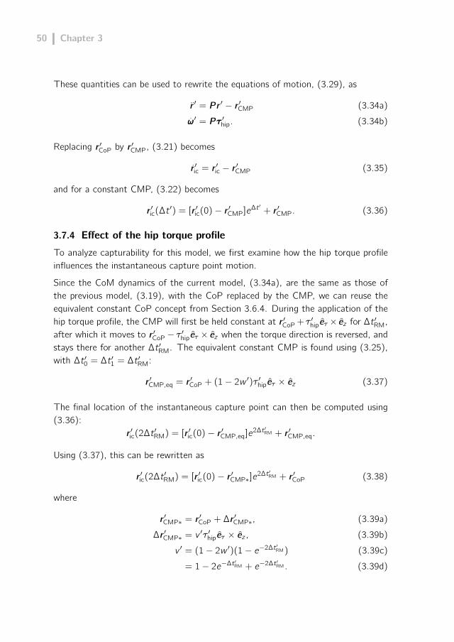
50 Chapter 3

These quantities can be used to rewrite the equations of motion, (3.29), as

r ′ = P r ′ − r ′CMP (3.34a)

ω′ = Pτ ′hip. (3.34b)

Replacing r ′CoP by r ′CMP, (3.21) becomes

r ′ic = r ′ic − r ′CMP (3.35)

and for a constant CMP, (3.22) becomes

r ′ic(∆t ′) = [r ′ic(0)− r ′CMP]e∆t ′ + r ′CMP. (3.36)

3.7.4 Effect of the hip torque profile

To analyze capturability for this model, we first examine how the hip torque profileinfluences the instantaneous capture point motion.

Since the CoM dynamics of the current model, (3.34a), are the same as those ofthe previous model, (3.19), with the CoP replaced by the CMP, we can reuse theequivalent constant CoP concept from Section 3.6.4. During the application of thehip torque profile, the CMP will first be held constant at r ′CoP +τ ′hipeτ × ez for ∆t ′RM,after which it moves to r ′CoP− τ ′hipeτ × ez when the torque direction is reversed, andstays there for another ∆t ′RM. The equivalent constant CMP is found using (3.25),with ∆t ′0 = ∆t ′1 = ∆t ′RM:

r ′CMP,eq = r ′CoP + (1− 2w ′)τ ′hipeτ × ez (3.37)

The final location of the instantaneous capture point can then be computed using(3.36):

r ′ic(2∆t ′RM) = [r ′ic(0)− r ′CMP,eq]e2∆t ′RM + r ′CMP,eq.

Using (3.37), this can be rewritten as

r ′ic(2∆t ′RM) = [r ′ic(0)− r ′CMP∗]e2∆t ′RM + r ′CoP (3.38)

where

r ′CMP∗ = r ′CoP + ∆r ′CMP∗, (3.39a)

∆r ′CMP∗ = v ′τ ′hipeτ × ez , (3.39b)

v ′ = (1− 2w ′)(1− e−2∆t ′RM) (3.39c)

= 1− 2e−∆t ′RM + e−2∆t ′RM . (3.39d)

Capturability: theory and application to simple gait models 51

The vector ∆r ′CMP∗ expresses the influence of the hip torque profile on the instanta-neous capture point motion. The scalar v ′ can be shown to monotonically increasefrom 0 to 1 for ∆t ′RM > 0.

Equation (3.38) shows that the norm of ∆r ′CMP∗ must be maximized to gain a maximaleffect of the hip torque profile on the final instantaneous capture point location. Itcan be shown that

‖∆r ′CMP∗‖max = ‖∆r ′CMP∗‖τ ′hip=τ ′hip,max. (3.40)

That is, even though increasing hip torque τ ′hip reduces the allowed torque duration∆t ′RM according to (3.32), the linear term in (3.39b) outweighs the reduced value ofv ′.

3.7.5 Capturability

The results from Section 3.7.4 will now be used to investigate capturability.

0-step capturability

With a reaction mass, the model can be 0-step capturable even if the instantaneouscapture point is not initially located inside the base of support. Rather, the require-ment for 0-step capturability is that the instantaneous capture point should be insidethe base of support after the application of the torque profile. To determine whichstates are 0-step capturable, we examine a boundary case for which the instanta-neous capture point can only just be pushed from outside the base of support backto its edge (see Figure 3.10).

For this boundary case, it is best to place the CoP as close to the initial instantaneouscapture point as possible, thus minimizing its rate of divergence. As the instantaneouscapture point needs to be pushed back to the boundary of the base of support andthe optimal CoP location is the closest point on that boundary, we have r ′ic(2∆t ′RM) =

r ′CoP. The hip torque profile should always be applied as soon as possible to be mosteffective, since waiting longer simply results in an initial instantaneous capture pointlocation that is farther removed from the foot. Using this information together with(3.39a) and (3.38), we obtain

r ′CoP = [r ′ic(0)− r ′CoP − ∆r ′CMP∗]e2∆t ′RM + r ′CoP

∴ ‖r ′ic(0)− r ′CoP‖max = ‖∆r ′CMP∗‖max

for the boundary case. Since the hip torque may be exerted in any direction and theCoP may be anywhere inside the base of support, the system is 0-step capturable inthe general case if and only if the initial distance between the instantaneous capturepoint and the base of support is smaller than or equal to

∥∥∆r ′CMP∗∥∥max.

52 Chapter 3

rankle

(a)

(b)

rCMP

ric(0)

||ΔrCMP*||max

rCoP

rmax ||ΔrCMP||max

rCMP,eq

rCoP = ric(2ΔtRM)ric(ΔtRM)rCMP

||ΔrCMP||max

rCMP,eq

Figure 3.10: Instantaneous capture point motion during the hip torque profile, for the boundary casedescribed in Section 3.7.5. (a) t ∈ [0,∆tRM): during the first half of the hip torque profile, the CMPmaximally pushes the instantaneous capture point inside the base of support. (b) t ∈ [∆tRM, 2∆tRM]:during the ‘payback phase’, the CMP must be placed in the opposite direction to stop the spinningmotion of the reaction mass. The net effect is that the instantaneous capture point ends up on theboundary of the base of support at 2∆t ′RM, exactly at the CoP. Note that the figure shows a specialcase where the foot is optimally oriented.

N-step capturability

For N-step capturability, we restrict the analysis to states in which a step has justbeen taken, the foot is optimally oriented, and the reaction mass starts in the uprightposition.

For these states, the strategy that brings the model to a stop in as few steps aspossible consists of stepping as soon as possible, choosing the CoP location as closeas possible to the initial instantaneous capture point and lunging as soon and as hardas possible in the direction of the initial instantaneous capture point.

While this strategy is being executed, r ′ic, r′CoP, r

′CMP, and r

′ankle are all on the same

line due to optimal orientation of the foot (as in Figure 3.10). The requirement for0-step capturability can thus be simplified for these states and written in terms ofthe distance to the contact reference point r ′ankle as

‖r ′ic(0)− r ′ankle‖ ≤ r ′max + ‖∆r ′CMP∗‖max = d ′0. (3.41)

The limit of capturability for N = 1 is calculated as follows. At the end of the

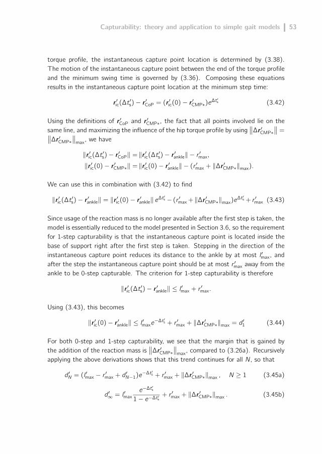
Capturability: theory and application to simple gait models 53

torque profile, the instantaneous capture point location is determined by (3.38).The motion of the instantaneous capture point between the end of the torque profileand the minimum swing time is governed by (3.36). Composing these equationsresults in the instantaneous capture point location at the minimum step time:

r ′ic(∆t ′s)− r ′CoP = (r ′ic(0)− r ′CMP∗)e∆t ′s (3.42)

Using the definitions of r ′CoP and r ′CMP∗, the fact that all points involved lie on thesame line, and maximizing the influence of the hip torque profile by using

∥∥∆r ′CMP∗∥∥ =∥∥∆r ′CMP∗

∥∥max, we have

‖r ′ic(∆t ′s)− r ′CoP‖ = ‖r ′ic(∆t ′s)− r ′ankle‖ − r ′max,

‖r ′ic(0)− r ′CMP∗‖ = ‖r ′ic(0)− r ′ankle‖ − (r ′max + ‖∆r ′CMP∗‖max).

We can use this in combination with (3.42) to find

‖r ′ic(∆t ′s)− r ′ankle‖ = ‖r ′ic(0)− r ′ankle‖ e∆t ′s − (r ′max + ‖∆r ′CMP∗‖max)e∆t ′s + r ′max (3.43)

Since usage of the reaction mass is no longer available after the first step is taken, themodel is essentially reduced to the model presented in Section 3.6, so the requirementfor 1-step capturability is that the instantaneous capture point is located inside thebase of support right after the first step is taken. Stepping in the direction of theinstantaneous capture point reduces its distance to the ankle by at most l ′max, andafter the step the instantaneous capture point should be at most r ′max away from theankle to be 0-step capturable. The criterion for 1-step capturability is therefore

‖r ′ic(∆t ′s)− r ′ankle‖ ≤ l ′max + r ′max.

Using (3.43), this becomes

‖r ′ic(0)− r ′ankle‖ ≤ l ′maxe−∆t ′s + r ′max + ‖∆r ′CMP∗‖max = d ′1 (3.44)

For both 0-step and 1-step capturability, we see that the margin that is gained bythe addition of the reaction mass is

∥∥∆r ′CMP∗∥∥max, compared to (3.26a). Recursively

applying the above derivations shows that this trend continues for all N, so that

d ′N = (l ′max − r ′max + d ′N−1)e−∆t ′s + r ′max + ‖∆r ′CMP∗‖max , N ≥ 1 (3.45a)

d ′∞ = l ′maxe−∆t ′s

1− e−∆t ′s+ r ′max + ‖∆r ′CMP∗‖max . (3.45b)

54 Chapter 3

3.7.6 Capture regions

The N-step capture regions for the 3D-LIPM with finite-sized foot and reaction massare shown in Figure 3.11 and are derived as follows.

Possible instantaneous capture point locations at earliest possible step time

Similar to the previous models, the first step to finding the capture regions is to findthe set of possible future instantaneous capture point locations at time ∆t ′s. Thedifference that the reaction mass makes is found by rewriting (3.38) as

r ′ic(∆t ′s) = r ′ic(∆t ′s)|τ ′hip=0 − ∆r ′CMP∗e∆t ′s (3.46)

where r ′ic(∆t ′s)∣∣τ ′hip=0

is the instantaneous capture point location at ∆t ′s when no hip

torque is applied, that is, when ∆r ′CMP∗ = 0, for which the model reduces to the

êy

êx

rmax

δ

Reaction Mass

A

B

C

N =

1

Figure 3.11: Top view of the 3D-LIPM with finite-sized foot and reaction mass, with a schematicrepresentation of the N-step capture regions. The figure is an extension of Figure 3.8: stateparameters rankle, r and r are identical. We have omitted labels that were already shown in Figure3.8 to avoid cluttering. The geometric construction is as follows. 1) find region A as described inFigure 3.8 and find region B by offsetting region A by δ; 2) use the lines of sight from the base ofsupport to find region C; 3) find the capture regions by offsetting region C by the values of dN from(3.26a). For this figure, τhip,max is set to 0.5 and θmax = 1/8, which results in a total lunge time(2∆tRM,max) of 1.

Capturability: theory and application to simple gait models 55

model without reaction mass. Taking the hip torque limit into account results in∥∥∥ r ′ic(∆t ′s)|τ ′hip=0 − r′ic(∆t ′s)

∥∥∥ ≤ δwhere

δ = ‖∆r ′CMP∗‖max e∆t ′s .

Therefore, the set of possible instantaneous capture point locations at time ∆t ′sconsists of all points that lie at most δ away from possible instantaneous capturepoint locations at ∆t ′s for the model without reaction mass (see Section 3.6.6).

Possible instantaneous capture point locations after the earliest possible steptime

After the application of the hip torque profile, the CMP will coincide with theCoP, and the instantaneous capture point will move on a line through itself andthe CoP. Bounds on reachable instantaneous capture point locations are thereforefound exactly as in Section 3.6.6, by constructing lines of sight (shown as the dashedlines in Figure 3.11) from the base of support to the set of possible instantaneouscapture point locations at ∆t ′s.

Nested regions

Finally, we can construct capture regions exactly as in Section 3.6.6. After the firststep is taken, no hip torque is applied anymore and the model essentially reduces tothe 3D-LIPM with finite-sized foot. We should hence construct nested regions aroundthe set of possible future instantaneous capture point locations using the values ofd ′N for the LIPM without reaction mass, i.e., those calculated using (3.26a), not theones from (3.45a). The effect of the reaction mass is already incorporated in the setof possible instantaneous capture point locations at the earliest possible step time.

3.8 Capturability comparison

For all three models, we determined which states in a subset of state space are N-step capturable, and derived descriptions of the N-step capture regions. The N-stepcapture regions of Figure 3.6, 3.8 and 3.11 clearly showed that an increase in thenumber of possible stabilizing mechanisms leads to an increase in capture region size.This result implies that there is more freedom to choose foot placements that keepthe model capturable, or we could say that the ‘level of capturability’ increases.

For a specific state, the area of the N-step capture region can be used as a measureof capturability. We call this the N-step capturability margin. This metric expresses

56 Chapter 3

+ finite-sized foot + reaction mass

+ finite-sized foot

point foot

0.62 m2

1.65 m22.21 m2

Figure 3.12: Superimposed ∞-step capture regions of all three models, as previously presented inFigure 3.6, 3.8 and 3.11. The sizes of the ∞-step capture regions, i.e. the ∞-step capturabilitymargins, are shown.

how close a specific state of a system is to not being N-step capturable. It alsogives an indication of the input deviations and disturbances that are allowed whileexecuting a given evolution. A small size of the ∞-step capture region, for example,indicates that a small disturbance will likely make the legged system fall.

In the previous sections, we graphically depicted the influence of the various mo-del parameters on the ∞-step capture region for a given initial state. Figure 3.12combines these results and displays the size of the three ∞-step capture regions.Parameters were set to estimated anthropomorphic values, as presented in Appendix3.10. For the selected initial state, the addition of a finite-sized foot caused the ∞-step capturability margin to increase by 160%. Another increase of 30% was foundfor the addition of the reaction mass.

Instead of considering a specific state, we can also consider the capturability of a mo-del in general. The d∞ capturability level, which was computed for all three models,gives an indication of the overall legged-system stability and allows a comparison. Interms of the original physical quantities, d∞ for the 3D-LIPM with finite-sized footand reaction mass is expressed as

d∞ = lmaxe−ω0∆ts

1− e−ω0∆ts︸ ︷︷ ︸3D-LIPM, Section 3.5

+ rmax︸︷︷︸3D-LIPM,Section 3.6

+τhip,max

mω20z0

[1− 2e−ω0∆tRM,max + e−2ω0∆tRM,max ]︸ ︷︷ ︸3D-LIPM, Section 3.7

. (3.47)

Capturability: theory and application to simple gait models 57

For the model with point foot, d∞ = 0.431 using anthropometric parameters. Addinga finite-sized base of support results in d∞ = 0.631, and an additional reaction massresults in d∞ = 0.664.

3.9 Discussion

3.9.1 Simple models

To analyze capturability for the three presented walking models, we made extensiveuse of the instantaneous capture point, which is determined only by the CoM positionand velocity. This gave us a dimensionally-reduced description of the dynamics of thethree models. We showed how this resulted in relatively simple and comprehensibleexpressions, and enabled calculation and visualization of capture regions and viable-capture basins.

The three models revealed the relation between the location of the point foot, theCoP and the CMP in the analysis of capturability. Despite time variant inputs,the dynamics of the instantaneous capture point remains easy to predict for allthree models: the instantaneous capture point diverges away from the CMP along astraight line at a velocity proportional to the distance to the CMP. The CMP reducesto the CoP if no reaction mass is present or actuated. The CoP reduces to the pointfoot location if the base of support is infinitesimally small.

The LIPM with point foot suggests that in order to remain capturable, the foot shouldbe placed sufficiently quickly in the direction of the instantaneous capture point. Thissimple stepping strategy was used to create a variety of stable locomotion patternsin simulation (Pratt and Tedrake, 2006; Yin et al., 2007) and was also found tobe a good predictor of stable foot placement locations in the analysis of humanwalking (Hof, 2008; Hof et al., 2010; Millard et al., 2009; Townsend, 1985).

The analysis for the LIPM with finite-sized foot introduced the equivalent constantCoP, which greatly simplifies the analysis of the presented models. This equivalentconstant CoP is a useful analysis tool and can also be applied to robot control, asdemonstrated recently (Englsberger et al., 2011).

The LIPM with finite-sized foot and reaction mass showed that lunging as soon aspossible in the direction of the instantaneous capture point maximizes the level ofcapturability. We conjecture that bang-bang control achieves the maximal influenceon instantaneous capture point motion if lunging is constrained by angle and torquelimits. Note that in general it is not straightforward to relate the effect of theangular momentum generated by the simple reaction mass to the effect generated

58 Chapter 3

by all individual links of a complex multibody system (Lee and Goswami, 2007; Orinand Goswami, 2008). However, this simple model still demonstrates the conceptualcontribution of angular momentum to the stability of locomotion.

The influence of each stabilizing mechanism on the capturability of each model wasdemonstrated by (3.47). The values of d∞ obtained for human parameters suggestthat, not surprisingly, the ability to perform rapid steps is most important to remaincapturable. This suggestion is also expressed by the metric being most sensitiveto changes in minimum step time. A variation in minimum step time can be com-pensated by another stabilizing mechanism to retain the same level of capturability.However, a 10% increase in step duration already requires a 17% longer step or a30% longer foot. For humans, selection of the appropriate step speed and lengthmay be a trade-off between the required muscle strength to perform a quick step(Smeesters et al., 2001; Thelen et al., 1997) and the perceived level of stability orsafety of the selected step length (Hsiao-Wecksler and Robinovitch, 2007; Maki andMcIlroy, 1999; Weerdesteyn et al., 2005).

The use of the three presented simple models as a representation of legged loco-motion has a number of limitations. The models discard many aspects of leggedlocomotion. Height variations of the CoM during legged locomotion were not consi-dered. Internal forces generated by lunging or swing leg dynamics were discarded.Slippage or losses at the change of support were not considered. The existence ofa double support phase in case of walking was also not taken into account. Conse-quently, using these simple models to approximate the capturability of a real robotwill lead to discrepancies between the approximated and true values.

Furthermore, the limitations on the stabilizing control inputs were modeled simplis-tically. For example, consider the limitations on the stepping performance of themodel. Stepping speed was constrained by enforcing a constant minimum step time,independent of the step location. Step location was constrained by limiting the maxi-mum step length, irrespective of the current CoM position or direction of motion.The expressions for capturability in this paper rely strongly on these simplisticallymodeled limitations.

We see an advantage in the simplicity of the presented models however. Comparablestudies demonstrated that making the models even slightly more complex can resultin expressions that are less comprehensible and require numerical methods to besolved (Pratt and Drakunov, 2007; Wight et al., 2008). This decreases understandingand increases the computational burden. Although the models are very elementary,they are still useful for the analysis and control of legged locomotion.

Capturability: theory and application to simple gait models 59

3.9.2 Robustness metrics

We introduced the N-step capturability margin, which expresses the level of captu-rability for a single state and takes both the position and velocity of the CoM intoaccount. Human subject studies already demonstrated that the CoM position andvelocity in relation to the base of support is a good indicator of the ability to main-tain balance and the number of steps required to do so (Aftab et al., 2010; Hsiaoand Robinovitch, 2001; Maki and McIlroy, 1999; Pai and Patton, 1997; Pai et al.,1998). Hof et al. (2005) were the first to formally define the distance between theinstantaneous capture point (which these authors call the ‘extrapolated CoM’) andthe base of support as a ‘margin of stability’. We see an advantage to using ourmetrics, since they take the effects and limits of the stabilizing control inputs (footplacement, ankle torque and hip torque) into account.

3.9.3 More complex models

Although we were able to perform a complete capturability analysis for three simplemodels, it remains an open issue to find a more generally applicable analytical me-thod, or even a numerical algorithm. A possible numerical algorithm could start witha small set of states that are known to be captured, such as default standing posi-tions. This set can then be expanded by finding initial states in its neighborhood forwhich there exist evolutions that reach the set and contain no steps. Subsequently,sets of N-step capturable states can be found recursively by searching for statesfrom which it is possible to reach an (N − 1)-step capturable state in a single step.While this algorithm is conceptually simple, it is likely computationally prohibitive fora complex system. In addition, including the full state of the system requires know-ledge of all relevant environment information, such as the ground profile and contactcharacteristics. Encoding the entire environment for all time is prohibitive in general.Also note that for a system with regions of chaotic dynamics, the capturability maybe uncomputable, as determining whether a state is in an N-step viable-capture basinmay be undecidable (Sipser, 2005).

3.9.4 Capturability for a specific control system

The capturability analysis presented in this part took both the dynamics and actuationlimits of the legged system into account, while no specific control law was assumeda priori. This approach allows us to make some strong conclusions concerning cap-turability. For example, if there is no ∞-step capture region, then it is impossible tomake the legged system come to a stop without falling, no matter what control lawis used. Another approach could be to assume an existing controller and determinecapturability given that controller. We can also assume a partial controller, such as

60 Chapter 3

one that provides balance and swing leg control and takes a target step location asan input. Such a controller might have internal state, which must be incorporatedinto the robot state x , but the range of actuator inputs to consider can be redu-ced, simplifying capturability analysis of the partially controlled system. We haveused this approach to greatly reduce the actuation dimensionality of a lower bodyhumanoid, admitting a machine learning solution for finding 1-step capture regionsin simulation (Rebula et al., 2007). We also use such a parameterized controller forthe robot in Part 2 (i.e., Chapter 7).

3.9.5 Capturability and Viability

Preventing a fall is important for legged locomotion. A maximally robust controlsystem would prevent falls for all states in which preventing a fall is possible. However,designing such a control system may be impractical. Instead, we design stabilizingcontrol systems using techniques and analysis tools which prevent falls for a subsetof the theoretically possible states. We believe that focusing on preventing falls overa set of N-step capturable states will lead to robust control systems and that as Nincreases the states which are subsequently considered become less and less commonand relevant. In addition, it is likely that analysis and control is computationally lesscomplex for small N than for large N.

We hypothesize that nearly all human legged locomotion takes place in a 3-step viablecapture basin and that all 3D bipedal robot locomotion demonstrated to date likelyfalls in a 2-step viable capture basin. Therefore, considering N-step capturabilityinstead of viability focuses on the states from which it is the least difficult to avoida fall. For large N, it may be best to just take the fall and switch to an emergencyfalling controller to protect the legged system and surrounding environment.

3.9.6 Future work

While the simple gait models presented in this part all pertain to bipedal walking,the concepts introduced in this paper can be applied to a wide range of walking andrunning legged systems, with any number of legs. One main area of future work isto generate walking and running models of increased complexity, develop algorithmsfor determining their capturability, and use the results to improve the robustness oflegged robots. For humanoid walking robots, we are currently investigating modelsthat incorporate uneven terrain, and consider the use of arms for pushing on wallsand grabbing handrails in order to increase robustness.

Capturability: theory and application to simple gait models 61

3.10 Conclusion

In this paper we introduced and defined N-step capturability, and demonstrated cap-turability analysis on three simple gait models. The main strength of capturabilityanalysis lies in the explicit focus on avoiding a fall in a global sense, while consideringthe computationally simpler issue of the ability to come to a stop in a given numberof steps.

By projecting N-step capturable states to the ground using contact reference points,we can generate capture regions which define appropriate foot placement, explicitlyproviding practical control information and leading to the N-step capturability margin,a useful robustness metric.

In Part 2 (i.e., Chapter 7) we will show that the exact solutions to the simple modelsin this part can be successfully used as approximations for control of a lower bodyhumanoid.

Acknowledgements

The authors gratefully acknowledge helpful discussions with D. Karssen, whose ideascontributed to the work. We would like to thank E. Westervelt for his helpful com-ments.

Appendix

Graphical user interface

A Matlab graphical user interface is created that illustrates N-step capture regions.This GUI can be downloaded from http://dbl.tudelft.nl.

Anthropomorphic model parameters

We estimated anthropomorphic model parameters for the 3D-LIPM with finite sizefoot and reaction mass, see Table 3.1. Mass and length parameters are based on atypical human 1.75 m tall and with a mass of 70 kg. Gait parameters are based onexperimental studies on human trip recovery.

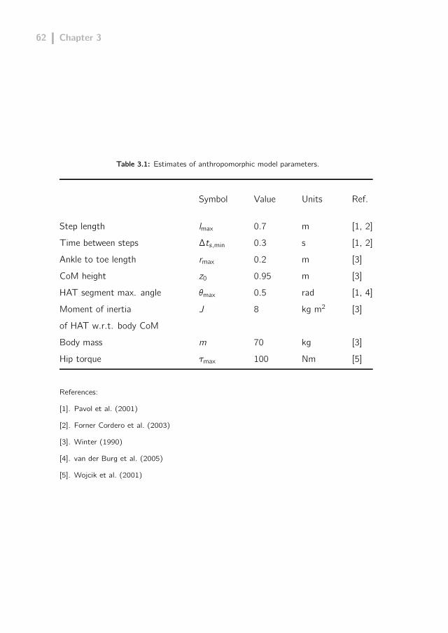
62 Chapter 3

Table 3.1: Estimates of anthropomorphic model parameters.

Symbol Value Units Ref.

Step length lmax 0.7 m [1, 2]

Time between steps ∆ts,min 0.3 s [1, 2]

Ankle to toe length rmax 0.2 m [3]

CoM height z0 0.95 m [3]

HAT segment max. angle θmax 0.5 rad [1, 4]

Moment of inertia J 8 kg m2 [3]

of HAT w.r.t. body CoM

Body mass m 70 kg [3]

Hip torque τmax 100 Nm [5]

References:

[1]. Pavol et al. (2001)

[2]. Forner Cordero et al. (2003)

[3]. Winter (1990)

[4]. van der Burg et al. (2005)

[5]. Wojcik et al. (2001)

4Foot Placement control:

Step Location and Step Timeas a Function of the Desired

Walking Gait

T. de Boer, J.G.D. Karssen, M. WisseSubmitted to Robotica, 2011

64 Chapter 4

AbstractWe present a foot placement controller for walking bipedal robots, whichoutputs the appropriate step location and step time to obtain a desiredwalking gait from every feasible system state. The step location and steptime are determined by approximating the robot dynamics with the 3DLinear Inverted Pendulum Model and analytically solving the constraintequations. The performance of the controller is tested in a simulationstudy. The results of this study show that the controller can get thesystem to a desired gait cycle from every feasible state within a finitenumber of steps.

4.1 Introduction

Generating a robust bipedal gait causes a difficult control problem. The center ofmass velocity can be controlled by the center of pressure location, but the supportpolygon imposes a constraint on this location. Especially during single support, thesupport polygon is small, which results in a system that resembles a highly unstableinverted pendulum. For the system to remain stable, an appropriate new step hasto be selected. This step determines possible future center of pressure locations.Consequently, deciding when and where to place a step is essential to control thecenter of mass and thereby obtain a robust walking gait.

Biomechanical studies found that stable step locations can be predicted based onsimple inverted pendulum dynamics, and center of mass position and velocity infor-mation (Hof et al., 2005; Millard et al., 2009; Townsend, 1985). Pratt et al. (2006)expanded this finding to robotic control and introduced the capture point. The es-sence of this step indicator (or very similar ones (Hof et al., 2005; Wight et al.,2008)) is that stepping on the indicated point will allow the robot to come to a stop.The concept of the capture point is powerful and can be used to readily predict stepregions for which the system has the ability to come to a stop or will inevitably fall(see Chapter 3).

Using the capture point to generate walking gait is less straightforward, since thisobviously requires a non-zero forward speed. Walking controllers that step a constantoffset away from the capture point have been suggested (Hof, 2008; Kajita et al.,2001; Pratt et al., 2011; Wight, 2008). This “constant offset control” approachseems logical since stepping ahead or behind the indicated point will in general causethe legged system to decelerate or accelerate respectively. Several implementations

Foot placement control 65

of this control approach were demonstrated (Coros et al., 2010; Kajita et al., 2001;Pratt et al., 2011; Wight et al., 2008).

However, the constant offset control approach has three significant shortcomings,which we will demonstrate in this paper. These are: (1) The desired gait will only bereached in infinite time. This can be problematic because the system may not haverecovered from a perturbation before a new perturbation occurs. (2) The controllerwill only work for a limited set of all feasible system states. This limits the ability tomaintain stable in the presence of large perturbations. (3) The controller assumesa constant step time. This reduces the possible step strategies and therefore limitsthe control performance.

In this paper, we will present a novel method that overcomes these shortcomings. Weintroduce a controller, which we will refer to as Dynamic Foot Placement controller,which gives a direct relation between the desired system state and the required steptime and step location to reach that state within a finite number of steps. Thecontroller is derived using the linear inverted pendulum model. The simple nature ofthis model results in simple control rules which allow for real-time implementation ona real robot. We will demonstrate the effectiveness of our proposed foot placementcontroller and show that the controller can be used to obtain a desired cyclic walkinggait from any feasible system state.

To illustrate the performance of the Dynamic Foot Placement controller, a Matlabgraphical user interface (GUI) was created. It allows the user to manipulate thestate of the linear inverted pendulum model and the desired walking gait that shouldbe obtained by the foot placement controller. The GUI can be downloaded onhttp://dbl.tudelft.nl.

This paper is organized as follows. Section 4.2 presents the model, followed by adescription of the walking gait in Section 4.3. A formal description of the intendedcontrol problem is given in Section 4.4. Section 4.5 describes the principle of opera-tion of the Dynamic Foot Placement controller, followed by a comparison betweenthe constant offset control approach and our proposed controller in Section 4.6.

4.2 Model description

To obtain simple control strategies, we use a simple model to approximate the dy-namics of a bipedal robot: the 3D Linear Inverted Pendulum Model as depicted inFigure 4.1(Kajita and Tanie, 1991). This model is widely used to synthesize controlstrategies for bipedal robots (Kajita et al., 2001; Kajita and Tanie, 1991) and toanalyze human locomotion (Hof, 2008; Hof et al., 2005).

66 Chapter 4

g

êy

êx

êz

z0

y

x

m

point foot

telescopic leg

center of mass

Figure 4.1: Schematic representation of the 3D-LIPM (Kajita and Tanie, 1991). The model com-prises a point foot, a point mass with mass m at position (x, y , z) with respect to a local referenceframe located at the point foot and a massless telescoping leg that keeps the point mass at theconstant height z = z0. The gravitational acceleration vector is g = (0, 0,−g)T . The state of themodel is uniquely described by the set of state variables q = (x, y , x , y)T .

The model comprises a point mass and a telescoping massless leg that is in contactwith the ground. The extensible leg applies an appropriate force at the point massto keep it at a constant height from the ground. The leg has a point foot, whichcan not apply torques on the ground.

4.2.1 Equations of motion

The state of the model is uniquely described by the set of state variables

q =

(p

p

), with p =

(x

y

),

with x and y representing the position of the point mass with respect to a localreference frame located at the point foot. The dynamics of the model consist ofone part that describes the stance phase and one part that describes the transitionfrom one stance phase to the next. Figure 4.2 shows the dynamics of the model inx-direction for an example walking motion that consists of two stance phases andtwo steps.

The stance phase dynamics are continuous and described by:

p = ω20p, (4.1)

Foot placement control 67

0 1 2Time [s]

3-1

0

1

0 1 2Time [s]

3-1

0

1

Loca

l pos

ition

x-d

irect

ion

x

Velo

city

x-d

irect

ion

x.

. .

.

..

-0.5

-0.5

-1-1

0

0

0.5

0.5

1

1

Velo

city

x-d

irect

ion

x.

Local position x-direction x

(a)

(b) (c)

S1

S0

S0,x S1,x

t1

t0

q1,f

q0,i

x0,i x0,f

x1,i x2,i

x1,f

q0,fd∞

d∞

x = -x .ω0

q2,i

q1,i

t0 t1 t0 t1

x0,i

x0,f

x1,ix2,i

x1,f

Figure 4.2: Dynamics of the 3D-LIPM in x-direction (with g and z0 of unit magnitude) for anexample initial state q = (0.6, y ,0.5, y)T . The model’s state is shown in state space in (a) andin the time domain in (b) and (c). For the state space plot, the boxed model pictures illustrate themodel’s configuration for the four quadrants of the plot. Continuous dynamics describe the evolutionof initial state q0,i to state q0,f over time t0. The transition dynamics describe the instantaneouschange of state q0,f to state q1,i due to step S0. This sequence is repeated for consecutive stancephases and steps. Any state that lies on the line x = x

ω0will make the model come to a stop in

x-direction, i.e., limt→∞ x = 0 (i.e., the instantaneous capture point defined by Pratt et al., 2006).The model can only come to a stop for initial states qn,i that lie inside the ∞-step viable-capturebasin (dashed lines labeled d∞, see Chapter 3) due to the imposed stepping constraints, as describedin Section 4.2.2.

68 Chapter 4

with ω0 =√

gz0, for which g is the gravitational constant and z0 the height of the

point mass. Solving (4.1) results in a closed form solution for the stance phasedynamics,

pn,f = pn,i cosh(ω0tn) +pn,iω0

sinh(ω0tn) (4.2a)

pn,f = pn,iω0 sinh(ω0tn) + pn,i cosh(ω0tn). (4.2b)

where tn is the duration of the stance phase and subscript i and f refer to the initialand final model state respectively of a stance phase, which is indexed with subscriptn, with n ∈ N0.

The transition dynamics are instantaneous and describe the changes in foot positionsthat occur when taking a step. It is assumed that a step has no instantaneous effecton the velocity of the point mass. The instantaneous state change is given by:

pn+1,i = pn,f − Sn (4.3a)

pn+1,i = pn,f , (4.3b)

where Sn = (Sn,x , Sn,y )T describes the step size in x- and y -direction.

4.2.2 Stepping constraints

To model the limitations of a real robot, we impose two stepping constraints on themodel as introduced in Chapter 3. First, we model actuator saturation on a realrobot by introducing a lower limit on the time between foot location changes:

tn ≥ tmin. (4.4)

Second, we model the limited kinematic workspace of a real robot by introducing anupper limit on step length, i.e., the distance between subsequent point foot locations:

‖Sn‖ ≤ lmax. (4.5)

Due to these constraints, the model can only operate in a subset of the state space.The subset consist of all states for which the model has the ability to come to a stop.For states outside of this subset the model will accelerate without the possibility todecelerate. The subset is spanned by model states qn,i that lie within the ∞-stepviable-capture basin as introduced in Chapter 3 and is given by∥∥∥∥ps +

piω0

∥∥∥∥ < lmax

eω0tmin − 1= d∞. (4.6)

In Figure 4.2, the basin boundary is indicated by the dashed lines labeled d∞.

Foot placement control 69

4.3 Walking gait

Our proposed foot placement controller has the ability to bring the model to anydesired feasible state. In this paper, we select a more practical application of thecontroller by bringing the model to a state that is part of a desired walking gait. Thisrequires that the model should not only arrive at the desired state, but should alsobe capable of maintaining the desired gait cycle. This requires a passed minimumstep time when the gait cycle requires another step to be taken.

The desired gait cycle is set to a humanlike two-step cyclic gait with an alternatingleft and right step. If the model has obtained the desired gait cycle, then

q* = qn+2 = qn, (4.7)

with corresponding step time t* = tn+2 = tn. The step size of the desired gait cycleis,

Sn =

(S*x

S*y (−1)n

), (4.8)

with x and y being the forward and lateral direction of movement respectively.

The control objective is a desired state within the gait cycle. For this paper, weselect the state at the end of the stance phase as a reference state within the gaitcycle:

q*f =

x*f

y*f

x*f

y*f

=

12S

*x

12S

*y (−1)n

12ω0S

*x coth( 1

2ω0t*)

12ω0S

*y tanh( 1

2ω0t*)(−1)n

. (4.9)

For all figures throughout this paper, we use an example desired gait cycle, whichis depicted in Figure 4.3. For this gait cycle t* = 1.5, S*

x = 0.75 and S*y = 0.3.

These three parameters uniquely describe the gait cycle and set the average forwardvelocity to S*

x/t* = 0.5. We set the model parameters g, z0, lmax and tmin to unit

magnitude.

4.4 Control problem

To let the model reach the desired state q*f within the gait cycle, the controller canadjust the step time tn as well as the step location Sn,x and Sn,y over a finite number

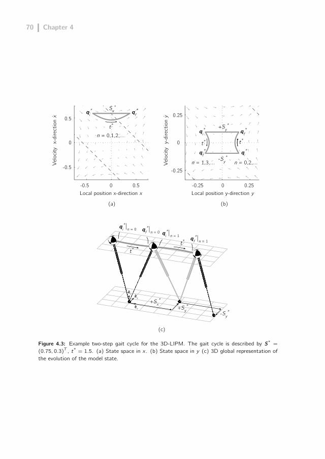
70 Chapter 4

+Sy*

-0.5

-0.5

0

0

0.5

0.5

-0.25

0

0.25

Local position x-direction x-0.25 0 0.25Local position y-direction y

Velo

city

x-d

irect

ion

x.

Velo

city

y-d

irect

ion

y.

n = 0,1,2,...

n = 1,3,... n = 0,2,...

qi*

qi*|n = 0

qi*|n = 1

qf*|n = 0

qf*|n = 1

qi*

qi*

Sx*

+Sy*

-Sy*

-Sy*

+Sx*

qf*

qf*

qf*

t*

t*t*

t*t*

êy

êx

(a) (b)

(c)

êz

Figure 4.3: Example two-step gait cycle for the 3D-LIPM. The gait cycle is described by S* =

(0.75, 0.3)T , t* = 1.5. (a) State space in x . (b) State space in y (c) 3D global representation ofthe evolution of the model state.

Foot placement control 71

of N steps, while satisfying the stepping constraints (Section 4.2.2). This results inthe following formal description of the control problem:

f (q0,i , t0, . . . , tN ,S0, . . . ,SN−1) = q*f (4.10a)

tn ≥ tmin for n = 0 . . . N (4.10b)

‖Sn‖ ≤ lmax for n = 0 . . . N − 1 (4.10c)

in which function f gives the state of the system after the Nth step. This functioncan be derived from (4.2) and (4.3) and is given by:

f (q0,i , t0, . . . , tN ,S0, . . . ,SN−1) =p0,i cosh(ω0T (N)) + p0,i

ω0sinh(ω0T (N))

−∑N−1

i=0 Si cosh(ω0(T (N)− T (i)))

p0,iω0 sinh(ω0T (N)) + p0,i cosh(ω0T (N))

−∑N−1

i=0 Siω0 sinh(ω0(T (N)− T (i)))

with T (i) =

i∑n=0

tn. (4.11)

There are many combinations of step locations, step sizes, and total number of stepsfor which the model will reach the desired gait cycle. We have chosen an approachwhere we minimize the required number of steps, for two reasons. First, because incase of a disturbance, it is beneficial to quickly return to the desired gait cycle in asmall number of steps to in order to withstand a possible new disturbance. Second,making a step is potentially costly. Using many steps may be disadvantageous froman energetic point of view and always involves risk: any step can be misplaced.

Finding a controller that satisfies the control problem (4.10) for a minimal numberof steps N can be done using numerical optimization methods. However, the non-deterministic nature of these optimization methods makes it unattractive for real-time implementation on a robot.

Therefore, we adopt a different approach to synthesize a foot placement controller.We start by checking if there is a solution to the control problem for N = 0. If thereis no solution, we repeat the procedure after an incremental increase of N. For eachN, the problem that needs to be solved is different, since N determines the numberof free (control) parameters and constraints (see Table 4.1). For example, a 1-stepstrategy has four free parameters and four equality constraints making this a fullyconstrained problem.

In the next section, we will show that our approach leads to an overall foot place-ment controller that consists of multiple simple closed-form solutions. The proposedcontroller solves the control problem for any number of steps.

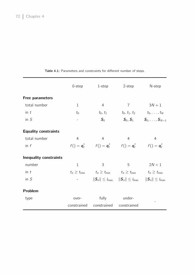
72 Chapter 4

Table 4.1: Parameters and constraints for different number of steps.

0-step 1-step 2-step N-step

Free parameters

total number 1 4 7 3N + 1

in t t0 t0, t1 t0, t1, t2 t0, . . . , tN

in S - S0 S0,S1 S0, . . . ,SN−1

Equality constraints

total number 4 4 4 4

in f f () = q*f f () = q*f f () = q*f f () = q*f

Inequality constraints

number 1 3 5 2N + 1

in t tn ≥ tmin tn ≥ tmin tn ≥ tmin tn ≥ tmin

in S - ‖Sn‖ ≤ lmax ‖Sn‖ ≤ lmax ‖Sn‖ ≤ lmax

Problem

type over- fully under--

constrained constrained constrained

Foot placement control 73

4.5 Dynamic Foot Placement controller

The Dynamic Foot Placement controller outputs the next step location and steptime, expressed in terms of the control parameters Sx,n, Sy,n and tn. We will deriveexpressions for these control parameters for each initial model state. The foot pla-cement controller consists of four N-step strategies with N = 0, 1, 2, (N > 2). EachN-step strategy will result in an (N − 1)-step strategy up to a 0-step strategy, asdemonstrated for an example 3-step strategy in Figure 4.4.

4.5.1 0-step strategy

If the initial state is already on the gait cycle or will arrive at the gait cycle withouttaking a step, then the following should hold:

q0,f = q*f ∧ t0 ≥ tmin. (4.12)

The control parameters are then given by S0,x = S*x , S0,y = S*

y and

t0 = ω0−1 log

x*f +√x*2f + ω2

0x20,i − x2

0,i

ω0x0,i + x0,i

, (4.13)

which is found by solving (4.12) for t in which q0,f is given by (4.2).

4.5.2 1-step strategy

The 1-step strategy is fully constrained (Table 4.1), which means that a uniquesolution exists for the control parameters Sx,0, Sy,0, t0 and t1. To derive an expressionfor these parameters it is important to acknowledge the following: since a step hasno instantaneous effect on the model velocities, we know that the velocities in the x-and y -direction at the moment of the step should match the velocities of the desiredgait cycle at some instant of the gait.

To further clarify this fact, let us consider the model velocities p shown in the phasespace diagram depicted in Figure 4.4(b). Here, we see a 1-step strategy that is part ofa 3-step strategy. We see that, going from a 1-step strategy to a 0-step strategy, thephase space trajectory of the model velocities intersects the phase space trajectoryof the possible gait-cycle velocities. At the instant that the velocities match, a stepis taken and the model evolves to the state q*f .

Consequently, for a 1-step strategy to be feasible, an intersection p0,f = p1,i shouldoccur. This means that the following expression, based on (4.2b), should hold,

p0,iω0 sinh(ω0t0) + p0,i cosh(ω0t0) = p*f ω0 sinh(ω0(−t1)) + p*f cosh(ω0(−t1)).

(4.14)

74 Chapter 4

t0 t1 t2t3

t*

p*f

p0,i

S*

S0

(a)

2-step strategy

1-step strategy

0-stepstrategy

3-step strategy

p1,f.

p2,i.

=

p0,f.

p1,i.

=

p2,f.

p3,i.

=

p3,f.

pf*.

pi*.

p0,i.

=

Velocity x-direction x.

Velo

city

y-di

rect

ion

y.

0.2-0.3

-0.15

0

0.15

0.3

0.4 0.6 0.8

(b)

Figure 4.4: Example 3-step strategy of the model in initial state q0,i to the desired stateq*f part of the desired gait cycle (highlighted by the thick grey line). The initial state isq0,i = (0.25, 0.58, 0.65,0.30)T . All step constraints described in Section 4.2.2 are satisfied.(a) 3D global representation of the evolution of state component p. (b) The evolution of thevelocities in x- and y -direction, i.e., state component p. Black dots indicate the states just after astep.

Foot placement control 75

This expression can be solved to find the stance phase durations t0 and t1. We omitthe expressions for t0 and t1 because of their length.

With the known stance phase durations t0 and t1, we can also derive the expressionfor the step size S0 from (4.2a) and (4.3a),

S0 = p0,f − p1,i , with (4.15)

p0,f = p0,i cosh(ω0t0) +p0,i

ω0sinh(ω0t0)

p1,i = p*f cosh(−ω0t1) +p*fω0

sinh(−ω0t1).

The last part of the 1-step strategy is to check if the found step durations t0 and t1and step size S0 are within the stepping constraints, (4.4) and (4.5). If this is notthe case, the 2-step strategy should be considered.

4.5.3 2-step strategy

A 2-step strategy is underconstrained (Table 4.1), meaning that multiple solutionscan exist for the available control parameters S0, S1 and stance durations t0, t1 andt2. The constraint equation (4.11) in case of a 2-step strategy becomes

f (q0,i , t0, t1, t2,S0,S1) = q*f . (4.16)

Solving (4.16) for S0, S1 results in

S0 = −(p0,i

ω0cosh (ω0 (t0 + t1)) + p0,i sinh (ω0 (t0 + t1))

− p*fω0

cosh (ω0t2) + p*f sinh (ω0t2))

1sinh(ω0t1)

(4.17)

S1 =(− p*f

ω0cosh (ω0 (t1 + t2)) + p*f sinh (ω0 (t1 + t2))

+ p0,i

ω0cosh (ω0t0) + p0,i sinh (ω0t0)

)1

sinh(ω0t1) .(4.18)

We can set three of the seven free control parameters (Table 4.1) and thereby derivea value for all parameters. An example option would be to set all stance durations t0,t1 and t2 to tmin, which we have done for the visualization of the control performancein Section 4.6. Though this approach might result in a stepping strategy that doesnot use the absolute minimum number of steps for some model states, Section 4.6demonstrates that the overall performance of the controller is still close to optimal.

76 Chapter 4

4.5.4 (N > 2)-step strategy

For all model states that cannot evolve to the gait cycle using N-step strategies forN ≤ 2, we adopt a single step strategy. Though more suited stepping strategiesfor N > 2 can be derived, these were found to be complex and result in a negligibleincrease in stepping performance.

The model state should quickly be brought to a region in state space for which N-step strategies for N ≤ 2 do apply, consequently tn is set to tmin. A correspondingeffective step location is a point at an offset from the instantaneous capture point(Pratt et al., 2006) and was introduced as part of the constant offset controller,explained in (Hof, 2008):

Sn = p +p

ω0+

−S*x

eω0t*−1

S*y (−1)n

eω0t*

+1

. (4.19)

If this point is not within reach due to stepping constraints, we step on the instan-taneous capture point or maximally towards this point if it is also out of reach.

4.6 Control performance

In the previous section, we introduced the Dynamic Foot Placement controller. In thissection, we discuss the performance of this controller. The performance is discussedin terms of the numbers of steps it takes to reach the desired gait cycle (Section4.6.1) and the time response (Section 4.6.2).

4.6.1 Number of steps

The goal of the Dynamic Foot Placement controller is to get the model to the desiredgait cycle from every possible initial state with the least number of steps. We checkhow well the controller reaches this goal by comparing the required number of stepsto the absolute minimal number of steps required. The numerical method used todetermine the absolute minimal number of steps is explained in the appendix. Weshow the results for the special case of 2D walking, in which S*

y = 0, y = 0 and y = 0.We use this special case, because for this case the results can easily be visualized ina graph, since the state space is only 2-dimensional instead of 4-dimensional for thecase of 3D walking.

Figure 4.5(c) shows the absolute minimal number of steps needed to get to thedesired gait cycle for a set of initial states. It shows that it is possible to get tothe desired gait cycle from all initial states within the ∞-step viable-capture basin.

Foot placement control 77

(a) Minimal possible

(b) Dynamic Foot Placement control

(c) Constant Offset control

-1

-0.5

0

0.5

1

-1 -0.5 0 0.5 1Local position x-direction x

Num

ber o

f ste

ps

0

1

2

3

4

5

6

> 6

Velo

city

x-d

irect

ion

x.

Figure 4.5: State space in the x-direction with the number of steps it takes to reach the desiredgait cycle as a function of the initial state. The desired gait cycle is highlighted by the thick greylines. (a) shows the absolute minimal number of steps it takes to reach the desired gait cycle. (b)and (c) show the number of steps takes for respectively the Dynamic Foot Placement controllerand the constant offset controller. For constant offset controller, we define that the gait cycle isreached as the difference with the gait cycle is less than 10−3. The black line in (b) and (c) is anexample path for both controllers with an initial state (xs, xs) = (0.6,−0.5).

78 Chapter 4

Time t

Constant Offset Control

Dynamic Foot Placment Control

Velo

city

x-d

irect

ion

x.

0 2 4 6 8 10

0 2 4 6 8 10

0.2

0.4

0.6

0.2

0.4

0.6

Figure 4.6: The convergence of the velocity in x-direction to the desired limit cycle for the DynamicFoot Placement controller and the constant offset controller. The desired gait cycle is indicated bythe thick grey lines.

Figure 4.5(b-c) show the number of steps that it takes to get to the desired gaitcycle for respectively the Dynamic Foot Placement controller and the constant offsetcontroller. The number of steps for the Dynamic Foot Placement controller is almostequal to the absolute minimal number of steps. Only for initial states close to thelower d∞ boundary, the number of steps is one higher for some initial conditions.The number of steps of the constant offset controller is in theory infinite sincethe convergence is asymptotical. However for this test, we assume that the gaitcycle is reached when the difference with the gait cycle is less than 10−3. With thisassumption, the number of steps for the constant offset controller is still much higherthan the minimal number of steps. In addition, there is a large range of initial statesthat are within the ∞-step viable-capture basin, but do not reach the desired gaitcycle using the constant offset controller.

4.6.2 Time response

Figure 4.6 shows an example of how the velocity in x-direction evolves to the desiredgait cycle from a disturbed state for both the Dynamic Foot Placement controllerand the constant offset controller. The velocity in x-direction is representative for allthe four state variables in q. For the Dynamic Foot Placement controller, the stateevolves to the desired gait cycle within a finite number of steps. For the constantoffset controller, the state converges asymptotically to the desired gait cycle. Thismeans that the gait cycle will only be reached if time goes to infinity.

Foot placement control 79

4.7 Discussion

The goal of this study is to synthesize a general foot placement controller, whichcan predict an appropriate step location and step time that will bring a bipedal robotto any desired gait cycle in a minimal number of steps. To arrive at comprehensiblecontrol strategies, we used a simple gait model and adopted an incremental approachto solve the control problem. The use of this approach and the model has its benefitsbut also introduces some limitations.

Incrementally solving the control problem for different N allowed us to derive closed-form expressions for the control parameters. These expressions give direct insightin the relation between the walking objective (in this case a desired walking gait ina minimal number of steps) and the foot placement control (step time and steplocation) that is required to reach this objective. We demonstrated that a total ofonly four step strategies was required to effectively bring the model to the desiredgait cycle from any feasible model state.

Another benefit from this approach is that the walking objective does not have tobe a gait cycle per se. A high-level controller can use the Dynamic Foot Placementcontroller to track a desired gait pattern, which could include reaching a standstill,changing the walking speed (Figure 4.7), making a turn (Figure 4.8) or reaching any

Sx* = 0.75

t* = 1.5

Sx* = 0.75

t* = 1

Time t0 2 4 6 8 10

Velo

city

x-d

irect

ion

x.

0.4

0.5

0.6

0.9

0.8

0.7

Figure 4.7: Simulation results of a change in walking speed using the Dynamic Foot Placementcontroller. A speed change is achieved by changing the desired gait parameters. For the depictedspeed change, the desired speed S*x/t* is changed from 0.5 to 0.75. The new desired speed isreached within three steps after the desired speed change.

80 Chapter 4

α 45o= α 45o=êy êx

êz

êy

êx

êz

Figure 4.8: Simulation results of a change in walking direction using the Dynamic Foot Placementcontroller. A change in walking direction is achieved by rotating the local coordinate frame in thex-y plane over an angle α. The depicted 90 turn is in this case achieved by rotating the coordinateframe over 45 after the first step and again 45 after the second step.

other desired system state.

A limitation of the approach is that we optimized our controller to a minimum numberof steps, though other optimization criteria might also be relevant. Other relevantoptimization criteria could be, for example, minimization of the time required toreach the state or minimization of the amount of mechanical work required by theactuators. In the near future, we plan to study how the foot placement strategiesare influenced by the selected optimization criterion or by combinations of criteria.

Though the 3D-LIPM enabled us to derive these simple stepping strategies, it isa very simplistic representation of a real robot. By modeling only center of massdynamics and not taking impact dynamics into account, we neglect many dynamicaspects of true dynamic walking. However, we believe it can be succesfully applied tocontrol a complex biped robot, similar to the successful application of the 3D-LIPMin the walking and balancing algorithms of the twelve-degree-of-freedom biped robotM2V2 (Chapter 7). It should not be attempted to forcefully mimic the 3D-LIPMdynamics on the complex biped, as is typically done for ‘Zero Moment Point’-basedcontrol approaches (Kajita et al., 2003). The evolution of the complex biped willinevitably deviate from the evolution that is predicted by the simple model. Thesimple nature of Dynamic Foot Placement controller allows for real-time executionon the robot, which allows the controller to continuously adapt to the current stateof the robot. The output of the Dynamic Foot Placement controller can be usedas an approximation for an adequate step time and step location for the real robot.Biomechanical studies (Hof et al., 2005, 2010) have shown that such simple footplacement approximations, based on simple inverted pendulum models, show good

Foot placement control 81

correlation with human foot placement strategies.

4.8 Conclusion

In this paper, we presented the Dynamic Foot Placement controller: a controller thatoutputs the next step location and step time based on the desired gait cycle and thecurrent state of the system. We investigated the performance of this controllerin a simulation study and shown that it can get the model to a desired gait cyclefrom every feasible state within a finite number of steps. In addition, we comparedthe performance of the Dynamic Foot Placement controller to the frequently usedconstant offset controller. We showed that the Dynamic Foot Placement controlleroutperforms the constant offset controller, in both the number of steps it takes toreach the desired gait as well as the size of the region in state space for which it canreach the desired gait.

Appendix

Minimal number of steps

Figure 4.5a shows the absolute minimal number of steps it takes to reach the desiredcyclic gait. In this section, we describe the numerical method used to determinethe absolute minimal number of steps. The method determines iteratively the setof states AN for which it is possible to reach the desired gait cycle within N stepsbased on the set AN−1. Two steps are taken to get AN from AN−1. First, setAN−1 is expanded to BN by adding all states that can reach AN−1 by making astep with a step size smaller or equal than the maximal step size lmax. Next, AN isdetermined as all states that will reach a state in set BN with t ≥ tmin. The first setB0 is equal to the final state in gait cycle q*f . In pseudocode this process looks asfollows:

for N = 0 to maximal number of steps doif N = 0 thenBN ⇐ q∗f elseBN ⇐ q : q − (ST , 0, 0)T ∈ AN−1 with ‖S‖ ≤ lmaxend ifAN ⇐ q : g(q, t) ∈ BN with t ≥ tminend for

in which g() represents the stance phase dynamics as given in (4.2).

5Mechanical analysis of the

preferred strategy selection inhuman stumble recovery.

T. de Boer, M. Wisse, F.C.T. van der HelmJournal of Biomechanical Engineering, 2010

84 Chapter 5

AbstractWe use simple walking models, based on mechanical principles, to studythe preferred strategy selection in human stumble recovery. Humanstypically apply an elevating strategy in response to a stumble in earlyand midswing, for which the perturbed step is lengthened in a continua-tion of the original step. A lowering strategy is executed for stumblesoccurring at mid or late swing, for which the perturbed swing foot isimmediately placed on the ground and the recovery is executed in thesubsequent step. There is no clear understanding of why either strategyis preferred over the other. We hypothesize that the human strategypreference is the result of an attempt to minimize the cost of success-ful recovery. We evaluate five hypothesized measures for recovery cost,focusing on the energetic cost of active recovery limb placement. Wedetermine all hypothesized cost measures as a function of the chosenrecovery strategy and the timing of the stumble during gait. Minimiza-tion of the cost measures based on the required torque, impulse, powerand torque/time, results in a humanlike strategy preference. The costmeasure based on swing work does not predict a favorable strategy asa function of the gait phase.

5.1 Introduction

Humans show a remarkable ability to regain balance after large perturbations duringgait, such as a stumble due to swing leg blockage. Experimental studies (Dietzet al., 1986; Eng et al., 1994; Forner Cordero et al., 2003; Grabiner et al., 1993;Schillings et al., 1996) have induced stumbles during gait to study the recoveryactions that humans employ to regain balance. These studies have shown that therecovery actions following the induced stumble can be categorized into the followingstrategies: an elevating (or reaching)strategy, where the perturbed foot is liftedand the step lengthened in a continuation of the original step, or a lowering strategy,where the perturbed swing foot is immediately placed on the ground and the recoverystep is executed by the contra lateral limb during the next step (Eng et al., 1994).

The kinematic and neuromotor responses for the lowering and elevating recoverystrategy are well characterized (Dietz et al., 1986; Grabiner et al., 1993; Pavol et al.,2001; Schillings et al., 1999). It was found that the strategy preference depends onthe timing of the induced stumble during gait (Pavol et al., 2001). For early swingperturbations (occurring at 5% to 25% of the step time) subjects show an elevatingstrategy. For perturbations in midswing (30% to55%), both lowering and elevating

Stumble recovery 85

strategies occur. In late swing (55% to 75%),subjects perform a lowering strategy(Schillings et al., 2000). However, there is very little understanding of why eitherstrategy could be favorable at a certain gait phase (Forner Cordero et al., 2005). Itis not clear which factors influence a subjects decision to prefer one recovery over theother (Schillings et al., 2000; Weerdesteyn et al., 2005). We believe that the primaryreason to prefer one strategy over the other is based on mechanical principles.

When considering the mechanics of stumble recovery, the role of the recovery limb iscrucial. Independent of the employed strategy, balance recovery relies on the ability torapidly perform a recovery step. Surely, postural responses such as control of the arms(Roos et al., 2008), trunk (van der Burg et al., 2005), or the support limb (Pijnappelset al., 2004) also contribute to balance recovery. But the timing, speed and lengthof the recovery step determine if the newly created base of support is effective instopping the forward acceleration of the body (van den Bogert et al., 2002; Hsiao-Wecksler and Robinovitch, 2007; Maki and McIlroy, 1999). The ability to performsuch a rapid recovery is dependent on muscular performance. Slower and weakermuscular responses, associated with muscular aging effects, can significantly decreasethe recovery ability (Hsiao-Wecksler, 2008; Pijnappels et al., 2008; Smeesters et al.,2001; Thelen et al., 1997; Wojcik et al., 2001). Older human subjects rely more oftenthan young subjects on multiple steps to recover (Luchies et al., 1994; McIlroy andMaki, 1996). These findings demonstrate that the limb dynamics and the requiredmuscular performance strongly influence the success of the recovery. We hypothesizethat the human strategy preference is based on an attempt to minimize the cost ofsuccessful recovery. Since this success depends on the muscular strength required toplace the recovery leg, we hypothesize that the recovery cost is proportional to therequired peak torque for rapid swing leg placement.

To study if strategy selection can be based on recovery cost minimization, we adopt asimulation approach where we use a simple, inverted pendulum type, walking model.We use this walking model to assess how the employed strategy and the timing ofthe stumble influence the required peak torque to perform a rapid recovery step.Furthermore, we validate if the mechanical principles of the simple model can berepresentative to human stumble recovery by using more physically realistic walkingmodels, multiple recovery steps, and different hypothesized measures to describe thecost of recovery.

5.2 Models and simulation methods

We simulated human stumble recovery in the following straightforward way. Wesubjected the simple walking model to a stumble at all phases of the gait cycle, from

86 Chapter 5

g

γ

mm

M

L

Lt

(a) Simplest walking model

(b) Straight-legged anthropomorphic model

(c) Kneed anthropomorphic model

Ls

wR

cR

R

ct

wt

ws

cs

Figure 5.1: Three dynamic walking models capable of showing passive cyclic gait on slope γ. Allmodels are extended with hip and knee (if applicable) actuation to recover from a stumble. Hipactuation produces a torque that acts on the swing and stance leg. Knee actuation produces atorque that acts on the swing leg thigh and shank. (a) The simplest walking model by Garcia et al.(1998). All variables are described in non-dimensional terms, with the leg length L, hip mass M,and gravitational constant g as base units. Foot mass m is infinitesimally small compared to thehip mass. (b) The straight-legged equivalent of the kneed anthropomorphic model in (c), adoptedfrom McGeer (1990a). Both models have anthropomorphically distributed mass and a point massat the hip that represents the torso. See Table 5.1 for the model parameter description and values.

Stumble recovery 87

0% to 100% of the step. The stumble was induced by instantaneously blocking andreleasing the forward swing foot motion. The stumble triggered simplified loweringand elevating strategies that used a constant hip flexion torque to power the recoveryleg. We recorded the required recovery torque as a function of the gait phase andthe employed strategy.

Furthermore, we tested if the mechanical principles revealed by the simple modelchanged when we used more complex simulation methods. We simulated stumble re-covery using two anthropomorphic walking models, a more physically realistic stumbleimplementation and multiple recovery steps. Finally, we evaluated four other hypo-thesized measures to describe the cost of recovery.

5.2.1 The walking models

A total of three walking models were used throughout this simulation study. Allmodels showed a cyclic passive dynamic gait when powered only by gravity usinga slight downhill slope. We extended these passive walking models with actuationin the hip joint and knee joint (if present), but this addition was only used when arecovery action was required in response to a stumble.

To reveal the very fundamental principles of stumble recovery, we primarily used the“simplest walking model” (Garcia et al., 1998) (Figure 5.1a). This irreducibly simplewalking model was based purely on mechanical principles. Despite its simple nature,the dynamic principles of this model have proven to provide useful insight into prin-ciples of human gait (Hobbelen and Wisse, 2008a; Kuo, 2001, 2002). Furthermore,similar simple models were found to adequately describe the dynamics of the humanbody during balance recovery (van den Bogert et al., 2002; Hsiao and Robinovitch,1999; Maki and McIlroy, 1999). It consisted of two rigid links, connected by a fric-tionless rotational joint at the hip. Point masses were located at the hip and at thefeet. The masses at the feet were infinitesimally small compared to the mass atthe hip, which resulted in a dynamic motion of the hip that is not influenced by theswing leg dynamics. The dynamics of this model were very simple, comprehensibleand required little computational power.

To test if this simple model could be representative for human stumble recovery, wevalidated the results on two complex models that were more physically realistic. Weused the straight-legged and kneed anthropomorphic models adopted from McGeer(1990a) (Figure 5.1(b,c)). These models had identical geometry and anthropomor-phically distributed mass, but the kneed anthropomorphic model also included a kneejoint and knee latch. This latch prevented knee hyperextension and locked the kneewhen fully extended during the end of the swing phase and throughout stance. The

88 Chapter 5

models comprised a point mass at the hip that represented the upper body, legsconsisting of a thigh and shank and curved feet that were offset forward of theshank.

For all models, we used dimensionless variables scaled with the overall massM,extendedleg length L and gravitational acceleration g. This resulted in time displayed in

√L/g

and torque as a fraction of MgL. The model parameters for both anthropomorphicmodels are given in Table 5.1.

The segment angles for a single step of the cyclic gait of all three walking modelsare shown in Figure 5.2. The simulation of a step consisted of continuous motion ofboth legs in between heel strikes, followed by a discrete velocity change due to theknee stop collision at full extension (for the kneed model) and the heelstrike collisionat the end of the swing phase. Both events were modeled as a fully plastic (noslip, no bounce) instantaneous impact. After the knee stop collision, the simulationprogressed with a straight swing leg. Heelstrike collision was triggered when the

Table 5.1: Model parameter description and values for both anthropomorphic models as shown inFigure 5.1(b,c) (identical to McGeer (1990a)). Mass parameters are presented as a fraction of thetotal body mass M, length parameters as a fraction of the extended total leg length L.

Model Parameter Symbol Value

Length of thigh mt 0.46

Length of shank ms 0.54

Mass at hip mh 0.676

Mass of thigh mt 0.100

Mass of shank ms 0.062

Vert. offset thigh center of mass (CoM) ct 0.2000

Vert. offset shank CoM cs 0.2372

Vert. offset foot center cr 0.3332

Hor. offset thigh CoM wt 0

Hor. offset shank CoM ws 0.0379

Hor. offset foot center wr 0.0675

Foot radius R 0.2

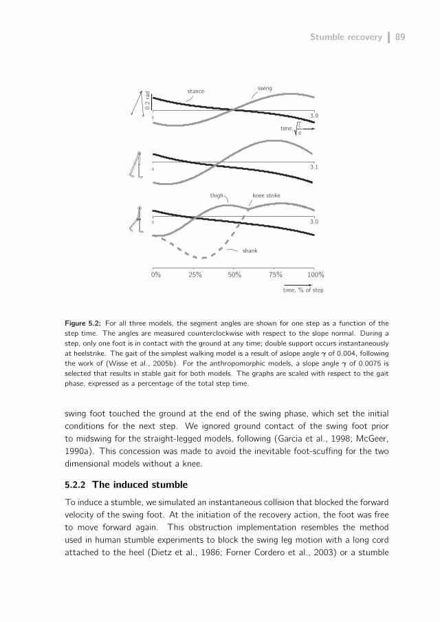
Stumble recovery 89

100%50% 75%25%0%

time, % of step

0.2

rad

swing

thigh knee strike

shank

stance

0 3.0

3.1

3.9

0

0

time, Lg

Figure 5.2: For all three models, the segment angles are shown for one step as a function of thestep time. The angles are measured counterclockwise with respect to the slope normal. During astep, only one foot is in contact with the ground at any time; double support occurs instantaneouslyat heelstrike. The gait of the simplest walking model is a result of aslope angle γ of 0.004, followingthe work of (Wisse et al., 2005b). For the anthropomorphic models, a slope angle γ of 0.0075 isselected that results in stable gait for both models. The graphs are scaled with respect to the gaitphase, expressed as a percentage of the total step time.

swing foot touched the ground at the end of the swing phase, which set the initialconditions for the next step. We ignored ground contact of the swing foot priorto midswing for the straight-legged models, following (Garcia et al., 1998; McGeer,1990a). This concession was made to avoid the inevitable foot-scuffing for the twodimensional models without a knee.

5.2.2 The induced stumble

To induce a stumble, we simulated an instantaneous collision that blocked the forwardvelocity of the swing foot. At the initiation of the recovery action, the foot was freeto move forward again. This obstruction implementation resembles the methodused in human stumble experiments to block the swing leg motion with a long cordattached to the heel (Dietz et al., 1986; Forner Cordero et al., 2003) or a stumble

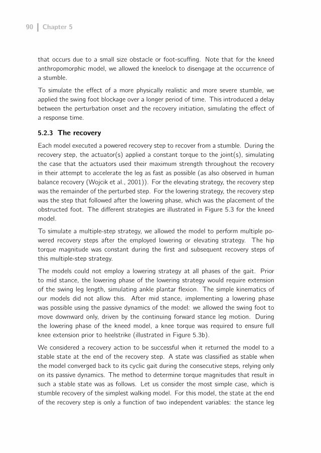
90 Chapter 5

that occurs due to a small size obstacle or foot-scuffing. Note that for the kneedanthropomorphic model, we allowed the kneelock to disengage at the occurrence ofa stumble.

To simulate the effect of a more physically realistic and more severe stumble, weapplied the swing foot blockage over a longer period of time. This introduced a delaybetween the perturbation onset and the recovery initiation, simulating the effect ofa response time.

5.2.3 The recovery

Each model executed a powered recovery step to recover from a stumble. During therecovery step, the actuator(s) applied a constant torque to the joint(s), simulatingthe case that the actuators used their maximum strength throughout the recoveryin their attempt to accelerate the leg as fast as possible (as also observed in humanbalance recovery (Wojcik et al., 2001)). For the elevating strategy, the recovery stepwas the remainder of the perturbed step. For the lowering strategy, the recovery stepwas the step that followed after the lowering phase, which was the placement of theobstructed foot. The different strategies are illustrated in Figure 5.3 for the kneedmodel.

To simulate a multiple-step strategy, we allowed the model to perform multiple po-wered recovery steps after the employed lowering or elevating strategy. The hiptorque magnitude was constant during the first and subsequent recovery steps ofthis multiple-step strategy.

The models could not employ a lowering strategy at all phases of the gait. Priorto mid stance, the lowering phase of the lowering strategy would require extensionof the swing leg length, simulating ankle plantar flexion. The simple kinematics ofour models did not allow this. After mid stance, implementing a lowering phasewas possible using the passive dynamics of the model: we allowed the swing foot tomove downward only, driven by the continuing forward stance leg motion. Duringthe lowering phase of the kneed model, a knee torque was required to ensure fullknee extension prior to heelstrike (illustrated in Figure 5.3b).

We considered a recovery action to be successful when it returned the model to astable state at the end of the recovery step. A state was classified as stable whenthe model converged back to its cyclic gait during the consecutive steps, relying onlyon its passive dynamics. The method to determine torque magnitudes that result insuch a stable state was as follows. Let us consider the most simple case, which isstumble recovery of the simplest walking model. For this model, the state at the endof the recovery step is only a function of two independent variables: the stance leg

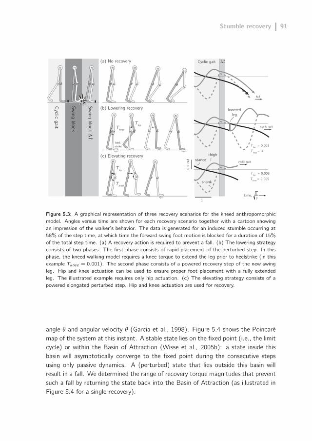
Stumble recovery 91

(a) No recovery

Swing block

Swing block ∆t

Cyclic gait

(b) Lowering recovery

(c) Elevating recovery

∆t

1

thighcyclic gait

loweredleg

Cyclic gait

shank

stance

0.2

rad

cyclic gait

fall

time, Lg

Thip = 0.003Tknee = 0

Thip = 0.008Tknee = 0.005

Thip

Tknee

Tknee

Thip

heel-strike

Figure 5.3: A graphical representation of three recovery scenarios for the kneed anthropomorphicmodel. Angles versus time are shown for each recovery scenario together with a cartoon showingan impression of the walker’s behavior. The data is generated for an induced stumble occurring at58% of the step time, at which time the forward swing foot motion is blocked for a duration of 15%of the total step time. (a) A recovery action is required to prevent a fall. (b) The lowering strategyconsists of two phases: The first phase consists of rapid placement of the perturbed step. In thisphase, the kneed walking model requires a knee torque to extend the leg prior to heelstrike (in thisexample Tknee = 0.001). The second phase consists of a powered recovery step of the new swingleg. Hip and knee actuation can be used to ensure proper foot placement with a fully extendedleg. The illustrated example requires only hip actuation. (c) The elevating strategy consists of apowered elongated perturbed step. Hip and knee actuation are used for recovery.

angle θ and angular velocity θ (Garcia et al., 1998). Figure 5.4 shows the Poincarémap of the system at this instant. A stable state lies on the fixed point (i.e., the limitcycle) or within the Basin of Attraction (Wisse et al., 2005b): a state inside thisbasin will asymptotically converge to the fixed point during the consecutive stepsusing only passive dynamics. A (perturbed) state that lies outside this basin willresult in a fall. We determined the range of recovery torque magnitudes that preventsuch a fall by returning the state back into the Basin of Attraction (as illustrated inFigure 5.4 for a single recovery).

92 Chapter 5

0.0

0.0- 0.7

0.7

[rad/s]

[rad]

[rad]

[rad]

θ

.

θ

fall backward

BoA

fixed point

fall forward [rad]0 0.6

−0.05

0.01

.

θ

θ + θ

BoA

min. T

max. T1

2

45

3

perturbed stateoutside BoA

recoveries

Figure 5.4: The Poincaré section for the simplest walking model just after heelstrike, for a slope angleof γ = 0.004 (Wisse et al., 2005b). The failure modes, Basin of Attraction (BoA) and fixed point(star at (θ, θ) = (0.1534,0.1516)) are shown. The right graph shows an enlarged and shearedsection which better visualizes the Basin of Attraction. A single lowering recovery is shown. Swingfoot blockage results in a shortened step: The state of the model can now be represented by pointnumber 1. The walker would fall forward if no recovery step would be performed. Recovery torquescan place the state back towards the fixed point (point 3) or just within the Basin of Attraction(point 2 and 4), or lead to a fall if the torque magnitude is too large (point 5) or small. After asuccessful recovery, the model will passively converge back to its cyclic gait in the subsequent steps.

5.2.4 The hypothesized cost of recovery

We considered a total of five hypothetical cost measures for the case of stumblerecovery. The selected measures were typically used in evaluation of energetic costof muscle activity in human walking (Alexander, 1989; Kuo, 2001).

We hypothesized that the recovery cost was proportional to the required peak re-covery torque for swing leg placement (i.e., the magnitude of the required constantrecovery torque). Another possibility was that recovery cost was proportional tothe torque divided by the duration that the torque is applied, since it was found tocorrelate well with the energetic cost of forced swinging of the swing leg in humanwalking (Kuo, 2001), in human running (Kram and Taylor, 1990) or in isolated swin-ging of the leg in an experimental setup (Doke and Kuo, 2007). We also studiedproportionality to the integral of the torque over the duration, i.e. the impulse (Kuo,2001). Furthermore, we determined the required peak power for successful recovery,assuming that not only peak torque is important, but also peak angular velocity ofthe swing leg. Finally, we evaluated proportionality to a combination of positive andnegative swing work.

Stumble recovery 93

5.3 Results

5.3.1 Recovery of the simple model

For the simplest walking model, Figure 5.5 shows all possible torque magnitudes thatresult in successful recovery from a stumble at different gait phases. The modelrecovered passively from stumbles occurring in early and late swing. A recoveryaction was required for stumbles induced between approximately 20% to 80% of thestep time. At approximately 65% percent, the model required the largest recoverytorque for the elevating strategy. At this gait phase, the swing foot velocity priorto the blockage was relatively high (85% of its maximum velocity) and the recoverytime of the perturbed step was relatively small (6% of the nominal step time), which

0. 1

0. 2

0. 3

no recovery torquerequired

no recovery torquerequired

elevating

lowering

1

234

5

no s

tum

ble

0 20 40 60 80 1000

hip

torq

ue, T

hip

Occurence of swing foot blockage [at % of steptime]

Figure 5.5: Stumble recovery for the simplest walking model (slope angle γ = 0.004) using anelevating and lowering strategy. Both contour maps indicate the torque magnitudes that resultin successful recovery from an instantaneous swing foot blockage. The horizontal axis shows thetiming of the induced stumble during a step, from swing initiation (at 0% of the step time) toheelstrike (at 100% of the step time). Just before heelstrike, no stumbles can be induced by swingfoot blockage because the model shows a negative foot velocity. The vertical axis shows the appliedconstant hip recovery torque. The solid black lines represent recoveries where the recovered stateends up onto (or closest to) the fixed point. To explain the graph, five points are shown thatrepresent different lowering recoveries in response to a stumble at approximately 65% of the step.All recoveries employ different recovery torque magnitudes. (Corresponding points can be found inFigure 5.4). If the applied recovery torque is too low (1) or too high (5), the model will fall withinthe current or the consecutive steps. Minimal (2) or maximal (4) successful recovery torque willjust result in recovery. If the applied recovery torque is just right (3), the model state returns onto(or closest to) the fixed point.

94 Chapter 5

resulted in a high required recovery torque.

In contrast to the elevating strategy, the minimum torque requirement for the lo-wering strategy decreased as the timing of the induced stumble moved from mid tolate swing. This can be explained by the fact that the length of the aborted stepincreased when the timing of the induced stumble approached the nominal step time.This longer step resulted in a lower stance leg velocity during the next step, whichin its turn decreased the required recovery torque.

5.3.2 Recovery of the complex models

Figure 5.6 shows the recovery torque requirements for both anthropomorphic models.The increased complexity of both models lead to less smooth contour maps comparedto the simplest walking model. The straight-legged model appeared to be susceptiveto failure due to foot-scuffing just after midswing (which was not ignored, contraryto foot-scuffing prior to midswing). For the kneed model, we clearly observed theinfluence of the knee joint and its latch.

The results showed quantitative differences in the required recovery torque betweenthe simple and more complex walking models. The difference in model geometryand mass distribution lead to different torque requirements, as expected. However,substantial qualitative similarities were observed. Again, we observed that the mostchallenging stumbles were around midswing and that the predicted recovery cost forlate swing stumbles was lower for the lowering strategy compared to the elevatingstrategies.

5.3.3 Increased obstruction duration

We obstructed the forward swing foot motion over longer periods of time. Anexample case is shown in Figure 5.7. The longer duration of the perturbation re-sulted in a decreased time to recover, which in turn resulted in an increased torquerequirement. However, the relative difference in torque requirement between the twostrategies remained.

The duration of an elevating recovery was typically shorter compared to a loweringstrategy 5.3. Therefore, the influence of the longer perturbation duration on thetotal recovery time was more significant for the elevating strategy compared to thelowering strategy.

5.3.4 Multiple-step recovery

Figure 5.8 shows an example case of successful two-step recoveries for the simplestwalking model. Both contour plots showed a division into two branches: one branch

Stumble recovery 95

Occurence of swing foot blockage [at % of steptime]

hip

torq

ue, T

hip

hip

torq

ue, T

hip

(b)

(a)

Occurence of swing foot blockage [at % of steptime]

no s

tum

ble

0.002

0.004

0.006

0.008

0 20 40 60 80 1000

2e-3

2e-3

0

0

4e-3

6e-3

knee strike in nominal gait

0 20 40 60 80 1000

0.002

0.004

0.006

0.008

falls due tofootscuff

no s

tum

ble

elevatinglowering

Figure 5.6: Stumble recovery for the anthropomorphic walking models (slope angle γ = 0.0075)using an elevating and lowering strategy. The two superimposed contour maps indicate the torquemagnitudes that result in successful recovery from an instantaneous swing foot blockage, as inFigure 5.5. (a) For the straight-legged model, the minimal amount of ground clearance of theswing foot frequently lead to failed stumble recovery due to foot scuffing. (b) For the kneed model,knee actuation may be required to stretch the leg prior to heelstrike. Patches, bounded by whiteis curves, indicate the recoveries that have equal knee torque requirements. The numbers in whiteindicate the magnitude of the required knee torque. The lowering phase of the lowering strategyrequired a constant torque of (Tknee = 0.001).

was characterized by recovery torques that were mostly higher than the single steprecovery torques and one branch was characterized by torques that were mostlylower. The higher recovery torques of the upper branch represented an overpoweredrecovery which resulted in a large maximum swing leg angle during the recovery step.The lower branches showed lower torques than the previous “single-step” strategiesand are therefore most relevant in this study on cost minimization.

Multiple-step strategies over more then two steps resulted in almost identical results:increasing in the allowed number of steps to recover did not result in a furtherdecrease in the required recovery torque. For both the multiple-step lowering strategy

96 Chapter 5

0 20 40 60 80 1000

0.002

0.004

0.006

0.008

0.01

Occurence of swing foot blockage [at % of steptime]

hip

torq

ue, T

hip

hip

torq

ue, T

hip

(b)

(a)

0 20 40 60 80 1000

0.1

0.2

0.3

Occurence of swing foot blockage [at % of steptime]

blockage during 15% of step time instantaneous

blockage

0

6e-3

8e-3

5e-3

2e-3

4e-30

1e-3

6e-3

Figure 5.7: Example recovery scenario in response to a swing foot obstruction applied for a durationof 15% of the step time. (a) For the simplest walking model, as Figure 5.5. The effect of the delaybetween the perturbation onset and recovery initiation is shown in comparison to an instantaneousblockage. For clarity, we only present torque magnitudes for recovery towards the fixed point. (b)For the kneed anthropomorphic model, as Figure 5.6b.

and the multiple-step elevating strategy, the required recovery torque magnitude isclose to the magnitude of the single-step lowering strategy.

5.3.5 Hypothesized cost measures

The results from the simplest walking model were used to calculate all hypotheticalmeasures for cost of recovery. Figure 5.9a shows the peak torque profiles derivedfrom Figure 5.5. As expected, the cost proportional to the torque divided by burstduration (Figure 5.9b) increased for short burst durations, as observed for the ele-vating recovery towards late swing. In contrast to that, the cost proportional tothe integral of force over time logically decreased for short burst durations (Figure5.9c). The hypothesized cost measure proportional to peak power (Figure 5.9d)showed a clear slope change for the elevating strategy in late swing. This was dueto a transition from a positive to a negative directed velocity of the recovery leg,since the effect of the gravitational moment acting on the leg increased for larger legangles towards late swing. This also caused an increase of negative swing work forthe elevating strategy in late swing (Figure 5.9e). All but the cost proportional toswing work predicted a favorable lowering strategy from mid to late swing. Focusing

Stumble recovery 97

0 20 40 60 80 1000

0.1

0.2

0.3

0 20 40 60 80 1000

0.1

0.2

0.3

multiple-step loweringsingle-step lowering

high torquebranch

low torquebranch

multiple-step elevatingsingle-step elevating

high torquebranch

low torquebranch

Occurence of swing foot blockage [at % of steptime]

hip

torq

ue, T

hip

hip

torq

ue, T

hip

(b)

(a)

Occurence of swing foot blockage [at % of steptime]

Figure 5.8: Multiple-step recovery for the simplest walking model. The contour map of a two-stepstrategy is superimposed on the contour map of the corresponding single-step strategy from Figure5.5. The vertical axis shows the applied constant torque that is applied to the hip during the firstrecovery step and the following step. The contour map has different branches, for recoveries thathave a higher or lower torque requirement compared to the single-step recoveries.

on the positive swing work (when assuming a higher energetic cost for positive workcompared to negative work (Abbott et al., 1952)), the cost of recovery proportionalto swing work did not show a clear favorable strategy.

5.4 Discussion

The purpose of our research was to study if the human strategy preference in stumblerecovery is based on cost minimization, which we assumed to be proportional to therequired peak torque for recovery.

All three walking models show that the required recovery torque to overcome stumblesinduced in early swing is relatively low (or even zero). Stumbles occurring at mid-swing are most demanding (which is in agreement with human stumble experiments(Forner Cordero et al., 2003)). At this point, the elevating and lowering strategy arefairly similar in their torque requirement. For late swing stumbles, the torque of alowering strategy is significantly lower compared to an elevating strategy.

A humanlike strategy preference emerges if the models would always execute thestrategy that minimizes recovery cost based on the required recovery torque. This

98 Chapter 5

0

0.2

0.4

0 20 40 60 80 100

0

0.01

0.02

0.03

0 20 40 60 80 100

Swin

g wo

rk

pos. work elev.neg. work elev.pos. work low.neg. work low.

Occurence of swing foot blockage [at % of steptime]

Peak

torq

ue |T

hip|

0 20 40 60 80 1000

0.02

0.04

0.06

Peak

pow

er

0

0.2

0.4

0 20 40 60 80 100

Impu

lse |T

hip| ∆t

0

0.5

1

0 20 40 60 80 100Tor

que

over

tim

e|T

hip| / ∆

t

elevating lowering

(a)

(b)

(c)

(d)

(e)

|Thi

p| |

|.|T

hip|

Figure 5.9: Hypothetical measures for cost of recovery for the simplest walking model, as a functionof the strategy and timing of the stumble. Cost of recovery hypothetically proportional to: (a) Theabsolute magnitude of peak recovery torque. (b) The torque divided by the duration of the recovery∆t. (c) The torque integrated over the duration of the recovery step, i.e. the impulse. (d) Thepeak recovery torque multiplied by the maximum of the recovery leg angular velocity θ. (e) Theamount of swing work performed: the torque multiplied by the angular displacement of the swingleg.

Stumble recovery 99

also holds for the cost models based on proportionality to impulse, torque divided bytime and power. The hypothesized measure based on swing work does not show aclear advantageous strategy. However, we have reason to suspect that a measurebased on swing work alone is not a good cost model for rapid swing leg placement.Doke and Kuo (Doke et al., 2005; Doke and Kuo, 2007) showed that the energeticcost of swing leg motions is a function of swing work, but mostly dominated bycost in proportion with torque, and in inverse proportion to duration of torque forincreasing swing leg speed. Our cost measures based on torque and torque durationshow a very significant difference between both strategies. We therefore reason thatstrategy selection in stumble recovery may indeed be based on cost minimization.Based on this simulation study, we cannot determine which measure describes thecost of active swing leg placement best.

The relative simple nature of our models defines their strengths and limitations. Alimitation is that the kinematics and dynamics of our walking models are too simpleto give a realistic approximation of the real magnitude of the hypothesized cost mea-sures. We can only predict the relative cost difference for the different strategies andstumble occurrences. Furthermore, the measures are all based on a single variable,i.e. hip torque for hip flexion, to realize swing leg placement. In reality, this is acombined effect of multiple mechanisms that all contribute to adequate placementof the recovery leg. These for example include knee extension, ankle plantar flexion(Pijnappels et al., 2004), arm movements (Roos et al., 2008) and trunk movements(van der Burg et al., 2005). Inclusion of all these individual mechanisms will lead toimproved estimates for the hypothesized recovery costs. It will also allow us to studytheir contribution to the success or failure of the recovery. Inclusion of the kneejoint already revealed more humanlike failure modes compared to the straight-leggedmodels, which could only fall due to wrong recovery leg placement. Inducing a severestumble on the kneed model revealed that recovery could only be achieved using arecovery leg that had a flexed knee, since the hip height at the end of the recoverywas significantly decreased. Allowing such a recovery introduces failure mechanismssuch as recovery limb buckling and improper support limb loading, which are bothimportant failure mechanisms in human stumble recovery (Pavol et al., 2001).

The strength of the models is that they allow us to consider limb kinematics anddynamics during the unperturbed and perturbed gait, which is different from othermodels used in balance recovery studies (van den Bogert et al., 2002; Hsiao andRobinovitch, 1999; Maki and McIlroy, 1999). This gives us the possibility to de-monstrate the relation between the timing of the perturbation, the reaction time,the employed strategy, the required strength and the stability of the recovery. The-refore, we believe our simulation study provides a valuable first approach towards a

100 Chapter 5

clear understanding of the fundamental principles of stumble recovery. The modelsmay also be helpful in creating more insight in the mechanisms specifically related toage-related declines in recovery ability. For example, our simulation results showeda significant reduction in the required recovery torque for a multiple-step elevatingstrategy in late swing compared to the single-step elevating strategy. This suggeststhat execution of a multiple-step recovery is required when the actuator strengthis insufficient to perform a single step elevating recovery. This may be related tothe observed behavior of human subjects when regaining standing balance using anelevating type step in response to an induced forward fall: older human subjectsrely more often than young subjects on a multiple-step recovery, which was concep-tually associated with muscular aging effects (Luchies et al., 1994; McIlroy and Maki,1996).

5.5 Conclusion

Simple walking models are used to study if the preferred strategy selection in humanstumble recovery is based on an attempt to minimize recovery cost. The hypotheticalcost measures for swing leg placement proportional to the required peak torque,power, impulse, and torque divided by time, predict a humanlike strategy preferenceas a function of the gait phase. The cost measure proportional to swing work doesnot predict a favorable strategy as a function of the gait phase. We reason that thecost of rapid swing leg placement is likely dominated by the cost of producing torque,rather than swing work. Therefore, the results suggest that the preferred strategyselection in human stumble recovery is based on an attempt to minimize recoverycost.

Appendix

All simulation models of this research can be downloaded on the website of the DelftBiorobotics Laboratory. When entering the website, click on ‘walking robots’ andsubsequently on ‘TUlip’.

Acknowledgements

We thank S.H. Collins and two anonymous reviewers for editorial and technical com-ments. The work presented in this article has been carried out with financial supportfrom the Commission of the European Union, within Framework Programme 6, RTDprogramme IST, under contract no. FP6-2005-IST-61-045301-STP.

6Robot prototype: design

Parts of this chapter have previously been published in:

D. Hobbelen, T. de Boer, M. Wisse,“System overview of bipedal robots Flame and TUlip: Tailor-made forLimit Cycle Walking”, Proceedings of the International Conference on

Intelligent Robots and Systems, 2008

102 Chapter 6

6.1 Introduction

Balance control is in essence about the ability to control the forces that act onthe CoM by controlling the CoP with respect to the CoM. This ability obviouslydepends on both the controller of the system and the mechanics of the system. Thischapter considers the mechanical aspect of walking and presents the newly developedhumanoid robot prototype ‘TUlip’ (depicted in Figure 6.1).

Previous chapters have demonstrated how balance can be controlled by the steppingstrategy, ankle strategy and hip strategy. These strategies requires accurate andfast positioning of the swing foot and the ability to control joint torques in order tocontrol the center of pressure location underneath the stance foot. Logically, therealization of robotic hardware that can demonstrate these capabilities has been ourpriority in this research.

However, it has to be taken into account that the initial design of TUlip was notrealized with these requirements in mind. The initial design was based on the ex-perience and knowledge gained through research on Limit Cycle Walking (Hobbelenand Wisse, 2007b). Unfortunately, the initial ideas on the control and mechanics ofwalking that followed from this Limit Cycle Walking approach lead to unsatisfactoryperformance when applied to TUlip. This result lead to a radical change in our viewon the control and mechanics of walking and therefore made us change the adoptedresearch approach (of which the result can be read in this thesis). Consequently, thedesign of TUlip was also changed during the research period pertaining to this thesis.

This chapter starts with an overview of the evolution of the design of TUlip inSection 6.2, describing how the design has changed and why. In Sections 6.3 to 6.5,a detailed overview of the current robot hardware is given in terms of the mechanics,electronics and software. Special attention is paid to the actuator design and theleg design, since their design is most important for the ability to control balance inbipedal locomotion.

Since the overall performance of the system depends on the implemented controller,Chapter 7 presents the developed control algorithms. Chapter 8 presents severalrobot experiments and evaluates the overall robot performance.

6.2 Robot evolution

The development of TUlip started in 2006, at the onset of the research described inthis thesis. Its initial design was tailor-made for Limit-Cycle Walking (Hobbelen andDe Boer, 2008). This approach has been used for the analysis and control of walking

Robot prototype: design 103

Figure 6.1: Design and realization of the humanoid robot TUlip (year 2008).

in the Delft Biorobotics Laboratory since 1995. The experience gained through thedevelopment of about ten walking robot prototypes (Delft Biorobotics Laboratory,2011) provided a basis for the design of TUlip. The design of TUlip shares manyfeatures with its predecessor Flame (Hobbelen and De Boer, 2008). The point ofdeparture was to develop a robot that had a mechanical structure that was naturallyconducive to walking and required only low levels on control for stabilization. Thisapproach had already lead to life-like and energy-efficient cyclic gait on previous pro-totypes (Hobbelen and Wisse, 2007b; Wisse et al., 2007). The idea was to synthesizecontrollers that would intervene in this energy-efficient gait in case disturbances oc-curred or when more versatile, aperiodic behavior would be desired. To stimulate thedevelopment in this direction, the goal was set to successfully compete in the robo-tic soccer competition of RoboCup (RoboCup, 2011). The concepts of the LimitCycle Walking approach, as well as the participation in robot soccer matches, haveinfluenced the design of TUlip in the following way.

A key concept of the Limit Cycle Walking approach is to exploit the potentially sta-bilizing properties of the passive (i.e., unactuated) dynamics of the robotic system.Based on this concept, we chose to implement compliant force/torque controllableactuators in TUlip which allow for a passive swing leg motion (through zero torquecontrol). Also, the lateral stance phase motion was made passive through the appli-

104 Chapter 6

cation of a passive-compliant ankle roll joint.

Competing in robotic soccer games requires robots to be truly advanced. As afirst step towards this goal, effort was put into making TUlip autonomous, andlightweight and mechanically robust to survive a fall. Also, we selected a human-likejoint configuration and range of motion for the legs to enable versatile behaviors,such as steering, kicking a ball and standing up when fallen down. Robotic socceralso requires enough processing power to support a software architecture for controlsoftware, vision processing, world modeling, and decision making.

In 2008, TUlip became operational. Two other copies were also realized and adoptedas research platforms by the other technical universities in the Netherlands, EindhovenUniversity of Technology and the University of Twente. Despite combined effort, astable walking gait was not achieved for any of the prototypes. After lots of tuning,the best walking performance was achieved in 2009 (Figure 6.2), which still requiredoperator intervention to prevent a fall.

After these disappointing results, we decided to completely overhaul the robot, bothin hardware and in software. In short, this involved the following. Regarding themechanics, the repeatability, predictability and controllability of the behavior had tobe increased, for example by reducing friction, play, and elasticity, and by thorough

Figure 6.2: Images showing TUlip performing a stride of a cyclic walking gait (Takahashi, 2009).The closeness of the operator gives away that small interventions are required every few steps toprevent a fall. Images are stills from the video visible on the Delft Biorobotics Laboratory website(Delft Biorobotics Laboratory, 2011).

Robot prototype: design 105

system identification, and calibration. Regarding the electronics, some of the am-plifiers were replaced for more powerful ones and the allowed motor current wasincreased (above the rated current) to increase the motor performance. Regardingthe software, effort was put into the development of software that could log, mo-nitor and modify variables on the robot in real-time to allow for better debuggingand tuning. Regarding the control software, a shift was made towards the controlapproach described in this thesis. Limit Cycle Walking control offered no feedbackmechanisms to asses the gait robustness, which offered no systematic approach (buttrial and error) to improve the gait. Also, the control consisted of multiple joint ba-sed controllers that were tuned without having a clear understanding of their effecton the rest of the system. Therefore, we chose to start the design of controllersbased on relevant state indicators such as the CoP and the location and the velocityof the CoM, and to controllers that control multiple joints and take the kinematicsof the whole system into account (see Chapter 7 for more information).

The above described evolutionary process of the robot demonstrates not only thatworking with real robot hardware can be time consuming. It also demonstrates thevalue of this prototype within this research and the impact it had on the project.Working with the robot has given us insight in the relevant issues in the mechanicsand control of walking, both for robots and for humans.

All together, the current realization of TUlip can be considered an innovative bipedalrobot prototype. The large scale application of force controllable actuators in its legssets it apart from many of the currently existing humanoids and offers implementationof novel force-based control approaches. Only few humanoid robots have similarabilities, such as the Sarcos robot (Raytheon Sarcos, 2011), the M2V2 robot (Prattet al., 2009) and the recently developed DLR-biped (Ott et al., 2010) and the cCub(Tsagarakis et al., 2011).

6.3 Mechanics

For the mechanical design, the initial design requirements were as follows:

- application of actuators that offer force control and position control;

- low mass moment of inertia of the legs with respect to the upper-boy, enablingfast swing leg; motions

- human-like leg morphology, enabling human-like versatile behavior;

- low overall weight, enabling low power motors that consume little energy.

106 Chapter 6

The resulting mechanics are now described, with a strong focus on the design of theactuators and their implementation in the robotic structure.

6.3.1 Actuation

The main choice of actuation for the robot was series elastic actuation, introduced byPratt and Williamson (1995) and successfully implemented in various other roboticapplications (Pratt et al., 2001; Veneman et al., 2006). Series elastic actuationcomprises a motor which connects to the joint through a compliant elastic element.This system is selected because of the following properties.

Firstly, measuring the elongation of the compliant element allows for determiningand controlling the amount of force/torque that is exerted by the motor on thejoint. The used control scheme is schematically shown in Figure 6.3. Initially, theability to control joint torque was deemed necessary because the control of zerojoint torque can leave the passive dynamics of the system intact and thus enable theproper application of Limit Cycle Walking control. Currently, we believe force controlis most beneficial for balance control because it allows for control of the interactionforces with the environment to regulate the CoM motion.

Jm-1 s-1 s-1

s

k

force controller

series elastic force control

motor springpositioncontroller

C2 C1

φm.. φm

.

... .

.

τm,d

τj, d.τj, e

τj, d τj,e φm

φj

φj

φj, d φj, e

φj, d ϕj, e τj

τj-

-

-

-

+

-

-

Figure 6.3: Control scheme of a series elastic actuator as used in TUlip. A motor (with inertia Jm,angle φm and input torque τm) is connected to the joint (index ‘j’) through a compliant elementwith stiffness k. The spring torque τj acting on the load is proportional to the measured differencebetween the motor angle φm and joint angle φj. The torque applied to the joint is controlled bya feedback and feedforward controller that outputs the desired input motor torque (i.e., current)based on the error between the current joint torque and the desired torque τj,d,τj,d. The desiredjoint torque can be set by a high level force controller (e.g., a Virtual Model Controller as describedin Chapter 7) or a position controller. The latter is shown as an example: the inner force controlleruses the output of an outer position controller as an input.

Robot prototype: design 107

Secondly, series elastic actuation is shock tolerant. When impacts occur in the robot(and this does happen frequently in walking), the series elasticity protects the motorand especially the gears in the gearbox.

Finally, series elastic actuation enables measurement of the energy/torque on thejoint level, excluding the energy consumed by the motor. This allows us to comparetorque/energy of our gait with other robotic or human gait, irrespective of the motortype used.

The following paragraphs will describe how the concept of series elastic actuation isimplemented in TUlip and present its performance.

Realization of series elastic actuation

Motor selection

In the series elastic actuation system, we chose to use a common geared brushed DCmotor. The use of electric DC motors generally allows high control bandwidth withrelatively little system overhead. In comparison to pneumatic or hydraulic actuatorsthis makes the electric motor an attractive candidate for an autonomous robot. Theapplication of a geared motor instead of direct drive is chosen because in case ofdirect drive the magnitude of the desired torques in our robots would require a heavymotor with overly high power rating. Typically, a geared motor has a low force fidelityand high impedance, due to a high reflected inertia and damping/friction. However,through the integration of the motor in the series elastic actuation system, theseundesirable property can be solved. The low output impedance of the series elasticactuator is illustrated in the frequency domain in Figure 6.4 and in the time domainin Figure 6.5. The dynamic effects of the motor inertia and gearhead friction arenearly invisible at the output of the series elastic actuator.

The power and gear head ratio of the geared DC motors is selected based on priorexperience with the robot Flame (Hobbelen and De Boer, 2008). The motor speci-fications are shown in Table 6.1 on page 121.

Compliant element selection

We chose to connect the DC motor to the joint using linear springs in series withsteel cables. This configuration showed satisfactory performance on other roboticprototypes (Hobbelen and De Boer, 2008; Hobbelen and Wisse, 2008b; Venemanet al., 2006), while being mechanically relatively simple. Furthermore, the use ofcables offered the possibility to place the actuator at a different location and orien-tation than the joint axis, which facilitated the design of a leg with a relatively lowmoment of inertia, as will be described in the next section.

108 Chapter 6

-100

-50

0

50

100

150

mag

nitu

de [d

B]

10 -1 100 101 10 2 103

10-1 100 101 10 2 103

0

90

180

phas

e [d

eg]

Frequency [Hz]

without series elastic actuation(only geared electric motor)

with series elastic actuation increasing seriescompliance

increasing seriescompliance

Figure 6.4: Modeled output impedance of an actuator with and without the presence of a serieselastic element plus active torque controller controlling zero torque. The geared electric motordynamics are modeled by the motor input torque/current together with a reflected inertia anddamping. The torque controller is a proportional-derivative controller. System parameters andcontroller parameters are matched with the real robot parameters for the hip pitch joint. Inputsignal is a joint oscillation at 1 Hz with an amplitude of 1 rad. Impedance of the series elasticactuator (dashed and solid line) is approximately 35 dB (about a factor of 50) lower at all frequenciescompared to the geared motor (dotted line). Using a more compliant element (instead of a typicallystiff torque sensor) results in a lower actuator impedance at high (uncontrolled) frequencies anda decrease in phase lead (i.e., less ‘damping’ added by the actuator). Figure from Hobbelen andDe Boer (2008).

0 10

0

0.4

-0.4time [s]hi

p pi

tch

join

t an

gle

[rad]

0 10

0

0.4

-0.4time [s] 0 10

0

0.4

-0.4time [s]

(a) (b) (c)

Figure 6.5: Measured hip pitch joint motion during swinging of a leg. (a) passive leg swing withactuators disconnected from joint (b) leg swing with a geared electric motor connected to the jointwith series elastic element plus active controller that actively controls zero torque. (c) leg ‘swing’with a geared motor directly connected to the joint; severely influencing the unactuated swing legmotion. Figure from Hobbelen and De Boer (2008).

Robot prototype: design 109

motor pulley

geared motor

spring unit(see right)

steel cable

steel cable

bolt + nut

spring thread fitting

tension springcable end fitting

cylinder

piston

compression spring

joint encoder

joint pulley

motor encoder

(a) (b)

Figure 6.6: Implementation of series elastic actuation in the knee joint of TUlip. (a) By measuringthe difference in orientation of the encoder on the motor and joint side, the extension of the springand steel cables can be determined, which is a measure for the torque exerted on the joint. (b) Acut-away view of the used ‘spring unit’, which consists of a high-stiffness tension spring in series witha low-stiffness compression spring with a mechanically constrained maximum compression (whichserves as a tension spring with a constrained maximum extension but is easier to implement). Properoperation of the series elastic actuator requires the application of a preloading force (through the useof the bolt) that will just drive the piston down in the cylinder and fully compresses the compressionspring (as explained in 6.7).

The compliant element that is used is a compliant unit, referred to as ‘spring unit’,that comprises a tension spring and a compression spring. Figure 6.6 shows anexample implementation of a series elastic actuator in TUlip. The reason why thesespring units are used is as follows. In the initial design of TUlip, normal tensionssprings were used as series elastic elements. To prevent cables from going slackand potentially come off the pulley when the motor applies torque on the system,a preload is required on the system. This preload is determined by the maximallyallowed joint torque, as explained in Figure 6.7. This maximally allowed joint torque

110 Chapter 6

has over the years been increased beyond the original design specifications to fulfillthe need for higher joint torques during certain motions (e.g., from 8 to 15 Nm forthe knee joint). The result was that the preloading force increased (from 450 to 900N) and caused friction and wear of the cables. This hampers actuator performance,as is demonstrated by the frequency response measurement of the initial series elasticactuator Figure 6.8. The coherence measurement shows a generally low coherencewhich suggests non-linear system behavior due to the presence of friction. Applicationof the spring unit can solve this problem by reducing the required preload and therebyreduce the friction. The required preload of the spring unit was selected to be 75 Nto overcome the internal prestress in the spring coil of the large tension spring. Thefrequency response measurement of Figure 6.9 shows a significant improvement ofthe coherence measurement.

Actuator performance

Figure 6.9 shows that the torque controllable bandwidth of the series elastic actuatorin the knee joint lies between 10-15 Hz for torques up to 5 Nm and approximately5-10 Hz for torques between 5-12 Nm. The bandwidth decreases for higher torqueamplitudes since motor saturation occurs for high-speed and large spring deflections.This demonstrates a disadvantage of the series elasticity: the low stiffness of the ele-ment between the joint and the motor forms a limitation on the torque and positioncontrol bandwidth that can be obtained on the joints. However, this is not neces-sarily a problem since gait stability does not necessarily require high-speed torque orposition control (which is also demonstrated by the walking robot Flame that has acomparable control bandwidth (Hobbelen and De Boer, 2008)).

The resolution of the force measurement depends on the resolution of the encoders,the transmission reduction and the stiffness of the deflecting elements. In the caseof the knee joint, encoders are used on the motor and joint side that have 2000 and30000 counts per revolution respectively. The reduction of the planetary gearheadis 111:1 and the reduction of the pulley system is 1.4:1. The stiffness of the largetension spring and small compression spring are 81 kN/m and 7.9 kN/m respectively.With the current selection of springs, the elasticity of the steel cables is not negligible.The stiffness of the steel cable is 64.5 kN/m per meter cable with about 0.3 m ofcable used on each side of the pulley. This results in an equivalent rotational stiffnessaround the joint of about 25 Nm/rad. The resulting smallest resolvable torque is5 ·10−3 Nm with a maximum output torque of 15 Nm, which gives a dynamical rangeof maximally 3000:1.

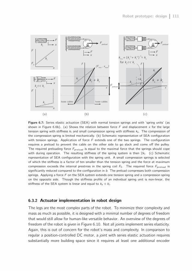
Robot prototype: design 111

Fx

x x

F(Fmax , xmax)

Fx

F

F0

F0

x

F

kl

kl

kl

kl kl + kl ks + kl

kl+s = (ks-1+ kl

-1) ≈ ks -1

≈ks

ks

ksks<< kl

for ks<< kl

F

Fpreload

Fpreload

x

Fx

Fx

Fpreload

(a) (b) (c)

loose cablesloose cables

Figure 6.7: Series elastic actuation (SEA) with normal tension springs and with ‘spring units’ (asshown in Figure 6.6b). (a) Shows the relation between force F and displacement x for the largetension spring with stiffness kl and small compression spring with stiffness ks . The compression ofthe compression spring is limited mechanically. (b) Schematic representation of SEA configurationwith tension springs. Application of force F extends one of the two springs. The configurationrequires a preload to prevent the cable on the other side to go slack and come off the pulley.The required preloading force Fpreload is equal to the maximal force that the springs should copewith during operation. The resulting stiffness of the spring system is then 2kl . (c) Schematicrepresentation of SEA configuration with the spring unit. A small compression springs is selectedof which the stiffness is a factor of ten smaller than the tension spring and the force at maximumcompression exceeds the internal prestress in the spring coil F0. The required force Fpreload issignificantly reduced compared to the configuration in b. The preload compresses both compressionsprings. Applying a force F on the SEA system extends one tension spring and a compression springon the opposite side. Though the stiffness profile of an individual spring unit is non-linear, thestiffness of the SEA system is linear and equal to ks + kl .

6.3.2 Actuator implementation in robot design

The legs are the most complex parts of the robot. To minimize their complexity andmass as much as possible, it is designed with a minimal number of degrees of freedomthat would still allow for human-like versatile behavior. An overview of the degrees offreedom of the robot is given in Figure 6.10. Not all joints implement series elasticity.Again, this is out of concern for the robot’s mass and complexity. In comparison toregular a position-controlled DC motor, a joint with series elastic actuation requiressubstantially more building space since it requires at least one additional encoder

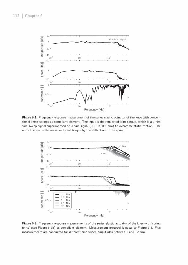
112 Chapter 6

10-1 100 101

10-1 100 101

10-1 100 101

0

0

0

0.5

1

phas

e [d

eg]

mag

nitu

de [d

B]co

here

nce

[-]

-200

200

20

-20

-40

Frequency [Hz]

1Nm input signal

Figure 6.8: Frequency response measurement of the series elastic actuator of the knee with conven-tional linear springs as compliant element. The input is the requested joint torque, which is a 1 Nmsine sweep signal superimposed on a sine signal (0.5 Hz, 0.1 Nm) to overcome static friction. Theoutput signal is the measured joint torque by the deflection of the spring.

10-1 100 101

10-1 100 101

10-1 100 101

0

0

0

0.5

1

phas

e [d

eg]

mag

nitu

de [d

B]co

here

nce

[-]

-200

200

20

-20

-40

Frequency [Hz]

1 Nm NmNm Nm Nm

2.55 7.512

1 Nm

12 Nm

Figure 6.9: Frequency response measurements of the series elastic actuator of the knee with ‘springunits’ (see Figure 6.6b) as compliant element. Measurement protocol is equal to Figure 6.8. Fivemeasurements are conducted for different sine sweep amplitudes between 1 and 12 Nm.

Robot prototype: design 113

z

yaw

hip

knee

anklepitch

roll

yx

SEA

non SEA

Figure 6.10: Degrees of freedom of TUlip. TUlip has a total of 12 degrees of freedom in the legsand two degrees of freedom (pitch and yaw) in the head which are not shown.

and additional springs. Therefore, series elastic actuation was only applied in thosejoints that were considered to have most benefit from its implementation: the jointsthat have a highly dynamic (fast) motion during walking and those that are in directcontact with the ground. This comes down to all but the hip yaw joint and hip rolljoint. In the initial realization of TUlip, an even more simple design approach waschosen: the ankle roll joint was left unactuated and two tension springs were usedto create a mechanically adjustable ankle roll stiffness. Though this implementationwas found practical in periodic straight-line walking (Hobbelen and De Boer, 2008;Wisse et al., 2007, 2006), it was quickly found that controllability of the ankle rolltorque was desired to achieve more versatile behavior.

Figure 6.11 shows the current implementation of all the actuators in the robotic leg.For all series elastic actuated joints, we have placed the actuators high up in theleg and body to minimize the mass at the end of the legs. The actuator for theankle pitch joint was placed in the upper body and is connected to the joint througha Bowden cable drive. This enables active plantarflexion of the ankle and passivedorsiflexion through a return spring. This positioning of the actuators effectivelyreduces the mass moment of inertia of the legs with respect to the hip joint, whichenables faster swing-leg motion. A naturally fast swing-leg motion is desirable forrapid foot placement strategies to prevent a fall and can also decrease energy use(Kuo, 2002). The resulting mass moment of inertia of both the legs with respect to

114 Chapter 6

hip yaw motor

ankle pitch motor

hip roll motor

hip pitch motor

spring unit

spring unit

knee pitch motor

steel cable

ankle roll motor

tension spring (ankle pitch)

bowden cable(ankle pitch)

tension spring(ankle pitch return spring)

x

yz

yaw

pitch

roll

Figure 6.11: Design of the hip and left leg of TUlip (year 2011) without protective covers.

Robot prototype: design 115

the hip is about 60% of the mass moment of inertia of the upper body with respectto the hip. This can be considered low when comparing this to the human case, forwhich this is 75% (Winter, 1990).

Kinematic data of the leg is shown in Figure 6.12. The leg was placed slightly tothe side of the pelvis/trunk of the robot to allow for a large range of motion of thehip pitch and hip roll joints 1. This large range of motion was required to be able todemonstrate the necessary skills for the RoboCup competition: standing up from alying position, kicking a ball, and performing a split for goalkeeping.

The design of the upper body is rather straightforward as can be seen in Figure 6.1.The structure of the trunk is stiff, lightweight and simple and houses all the elec-tronics. The arms (which currently only have esthetic value) and head are actuatedthrough simple Dynamixel servomotors. The total robot’s mass and joint layout areshown in Table 6.1 on page 121.

yx

z

yx

z

y

x

z

-20o20o

-30o90o

ankle roll-25o25o

ankle pitch

knee pitch

hip pitchhip roll

275

mm

320

mm

127 mm 186 mm

57 mm 75 mm

47 m

m

-90o60o

hip yaw

70o-70o

-1o140o

Figure 6.12: Joint range of motion and main dimensions of the hip and left leg of TUlip (year 2011).The total length of the robot is approximately 130 cm.

1The range of motion of the hip pitch joint has been reduced in 2011 from [−140, 90] to [−90, 60]

(as shown in Figure 6.12) to accommodate for longer springs in the series elastic actuator.

116 Chapter 6

6.4 Electronics

For the electronic architecture, the initial design requirements were as follows:

- preferably the use of proven, off-the-shelf technology to prevent inevitable bugsin custom made components;

- preferably the use of components with low mass and small volume;

- separate power circuitry for low power electronics and high power motors toprevent interaction.

An overview of the resulting design is given below.

6.4.1 Computing

All the sensors and actuators are connected to a single on-board computer that doesall the computing. Distributed control may have been favorable from a weight pointof view since locally placed controller boards can reduce the number of power cablesand sensor cables significantly. However, at the time available distributed control-ler boards were not yet small and powerful enough for these robotic applications.The selected central computer is a Diamond Systems 1GHz, 512MB SDRAM Po-seidon single board computer (Diamond Systems, 2011) with EPIC form factor. Toexpand the I/O capabilities of the Poseidon board, two Mesa 4I65 Anything-I/Ocards (MESA, 2011) are stacked onto its PC104-Plus bus. The FPGA’s on thesecards (Xilinx Spartan-II 200k gate) are programmed to count encoder pulses andcommunicate with the Elmo Whistle digital servo amplifiers (Elmo Motion Control,2011).

6.4.2 Sensors

Rotary encoders are mounted on each motor shaft. These Maxon encoders of typeHEDS 5540 have 500 pulses per revolution. All actuators with series elasticity have asecond rotary encoder placed on the joint axis, a Scancon 2RMHF (Scancon, 2011)incremental encoder with 7500 pulses per revolution corresponding to a resolutionof 2 · 10−4 rad (approximately 0.01 deg). Though incremental encoders requireinitialization, these encoders are preferred over absolute encoders because of theirhigh resolution. Lower resolution encoders were found to output non-smooth velocitysignals at low angular joint velocities, which significantly limits the amount of dampingthat can be added to the system through velocity based control.

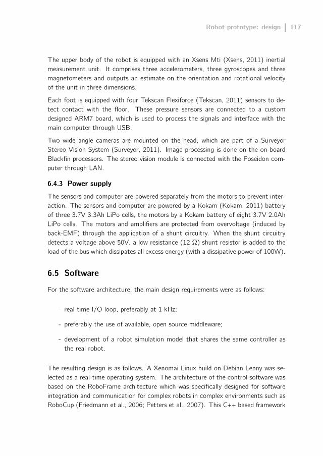
Robot prototype: design 117

The upper body of the robot is equipped with an Xsens Mti (Xsens, 2011) inertialmeasurement unit. It comprises three accelerometers, three gyroscopes and threemagnetometers and outputs an estimate on the orientation and rotational velocityof the unit in three dimensions.

Each foot is equipped with four Tekscan Flexiforce (Tekscan, 2011) sensors to de-tect contact with the floor. These pressure sensors are connected to a customdesigned ARM7 board, which is used to process the signals and interface with themain computer through USB.

Two wide angle cameras are mounted on the head, which are part of a SurveyorStereo Vision System (Surveyor, 2011). Image processing is done on the on-boardBlackfin processors. The stereo vision module is connected with the Poseidon com-puter through LAN.

6.4.3 Power supply

The sensors and computer are powered separately from the motors to prevent inter-action. The sensors and computer are powered by a Kokam (Kokam, 2011) batteryof three 3.7V 3.3Ah LiPo cells, the motors by a Kokam battery of eight 3.7V 2.0AhLiPo cells. The motors and amplifiers are protected from overvoltage (induced byback-EMF) through the application of a shunt circuitry. When the shunt circuitrydetects a voltage above 50V, a low resistance (12 Ω) shunt resistor is added to theload of the bus which dissipates all excess energy (with a dissipative power of 100W).

6.5 Software

For the software architecture, the main design requirements were as follows:

- real-time I/O loop, preferably at 1 kHz;

- preferably the use of available, open source middleware;

- development of a robot simulation model that shares the same controller asthe real robot.

The resulting design is as follows. A Xenomai Linux build on Debian Lenny was se-lected as a real-time operating system. The architecture of the control software wasbased on the RoboFrame architecture which was specifically designed for softwareintegration and communication for complex robots in complex environments such asRoboCup (Friedmann et al., 2006; Petters et al., 2007). This C++ based framework

118 Chapter 6

provides a number of services to robot control applications, such as module manage-ment, timers, intra and inter-process communication and monitoring and debuggingfacilities. Various modules were programmed within the RoboFrame application (Ro-boApp, see Figure 6.13), such as modules related to motion control, vision, worldmodeling, communication and soccer-strategy.

Within RoboFrame’s RoboGUI, a graphical user interface was created that can beused to monitor and log robot data or modify control parameters. Multiple instancesof this user interface can run on other Windows or Linux platforms and communicatewith the RoboApp. Since RoboFrame has no native support for real-time platforms,all real-time control was done in a separate process outside RoboFrame which inter-faces with an adapter module inside RoboFrame. This RoboFrame module acceptscommands from other modules (e.g., soccer-strategy) and relays these to the real-time process. Data from the real-time process can be sent back through the adapterto be used by any of the other RoboFrame modules.

The real-time control algorithm consists of different layers. The bottom layer consistsof hardware drivers that interface with the I/O ports on the Poseidon and Mesa cards.The TUlip Hardware Abstraction Layer (HAL) provides abstracted access to the ro-bot hardware. All platform dependencies, such as device registers, memory locationsor bus accesses were stored in the TUlipHAL layer. The software layer above TUli-pHAL, TUlip Motion Control (MC), communicates with the hardware objects onlythough abstract hardware objects and is, consequently, more immune to hardwarechanges. As a result, controlling the real robot or controlling the simulated robotis defined by the interface with either real objects or simulated objects through theabstract objects of TUlipHAL. This is similar to the approach adopted by Kanehiroet al. (2004) and Pratt et al. (2009).

TUlipMC implements all the control algorithms. It consists of a hierarchical sta-temachine that switches between behavioral states (e.g., walking, kicking a ball,balancing) and their behavioral substates (for example for walking: “single stance,left is swing leg”). The statemachine is responsible for the timely update of robotinputs and outputs, and handles event based transits between the different behavioral(sub)states. A detailed description of the various states that were implemented inthe statemachine is given in Chapter 7. The statemachine is set to run at 1 kHz,for which the load on the computer’s processor is about 35%.

The software architecture is designed in such a way that the control algorithms withinTUlipMC can also be directly used to control a model of the robot. When working insimulation, TUlipMC gets input data from simulated sensors and outputs to simulatedmotors. This architecture is chosen to speed up the development and evaluation of

Robot prototype: design 119

RoboFrame (non real-time)

RoboApp

TUlipMC

Statemachine

Hardware interface

Controllers

Joints

Motion Control (real-time)

Real TUlip Simulated TUlip

State

Real

SubState

ActuatorSensor

Simulated

ActuatorSensor

SubState

SubState ...

PID ...

hip y ...

World model

Strategy

...

Vision

Motion control

RoboGUI

TUlipHAL

Drivers TCP/IP

1 left foot - --

2 CoP - -(0.0,1.0,1.0)

3 left_vtp - -(1.0,1.0,1.4)

4 right_vtp - -(0.0,2.0,2.3)

5 right_vtp - -(0.0,2.0,2.3)

6 T_ankle -12.0 12.00.0

7 T_ankle -12.0 12.0

8 T_knee -12.0 12.0

9 T_hipx -12.0 12.0

10 T_hipz -12.0

0.1

2.0

0.0

1.0 12.0

Figure 6.13: Schematic overview of the software architecture used to operate TUlip.

120 Chapter 6

new control concepts and behaviors without having to deal with hardware issues.The model is created using the 20sim software package (Controllab Products B.V.,2011; Kemp, 2010). It consists of a full multi-body model of the robot with the samemechanical properties as the real robot. Physical contact with the environment canbe simulated for the feet, the ‘hands’, and the ’elbows’ through the application ofeither Kelvin Voight, or Hunt-Crossley models. Motor dynamics and friction arecurrently not included in the simulation to limit the model’s complexity.

6.6 Conclusion

We could say that the design of TUlip is satisfactory as most of the design require-ments were met. The desirable low mass moment of inertia of the legs was realized,the electronics were found to be reliable, and the software was found to functionproperly. Furthermore, the overall weight of the robot was indeed relatively low, lessthan 20 kg for a 1.3 m tall robot (see Figure 6.14).

However, many of the design requirements were based on estimates and experiencerather than trustworthy research, as the purpose of the robot was to validate theseestimates. The resulting performance of the robot will be evaluated in Chapter 8.

cabling

printed circuit boards

sensors

actuators

frame

12%

16%4%

31%

37%

Figure 6.14: Weight allocation of the robot TUlip, with a total mass of 19.8 kg.

Acknowledgements

The development of the TUlip prototypes could not have been done without the helpof the many students and staff that have contributed through the DutchRoboticsfoundation (DutchRobotics, 2011).

Robot prototype: design 121

Tab

le6.

1:TUlip’smechanicalsystem

properties

(year20

11).

Eachrowrepresents

ajointanditsassociated

rigid

body.In

thecoordinate

system

,xisforward,yisto

theleft,andzisup.The

right

legisamirror

imageof

theleft

leg(L).

Allmotorsare24

V60

WRE30

Maxon

motors;

the

transm

ission

reduction(gearheadplus

pulleyratio)

isgivenforeach

joint.

Offsetfrom

Parent[m

]CoM

offset[m

]

Joint

Rigid

body

Parent

xy

zReduction

Mass[kg]

xy

z

root

trunk

N/A

--

--

10.8

0.06

0.0

-0.020

Lhipyaw

LhipXmotor

root

0.085

0.075

-0.392

1:86

0.61

-0.009

0.0

0.007

Lhiproll

LhipYaxle

Lhipyaw

0.0

0.0

-0.071

1:190

0.08

0.0

0.0

0.0

Lhippitch

Lthigh

Lhiproll

0.0

0.038

-0.04

1:222

2.14

0.005

0.030

-0.097

Lknee

Lshank

Lhippitch

0.0

0.0

-0.275

1:155

1.02

0.038

0.019

-0.150

Lanklepitch

Lankle

Lknee

0.0

0.0

-0.32

1:325

0.08

0.0

0.0

0.0

Lankleroll

Lfoot

Lanklepitch

0.0

0.0

0.0

1:286

0.37

0.035

0.010

0.010

7Robot prototype: capturability

based control

Integral copy of:

J. Pratt, T. Koolen, T. de Boer, J. Rebula, S. Cotton, J. Carff, M.Johnson, P. Neuhaus

Submitted as “Capturability-Based Analysis and Control of LeggedLocomotion: Part 2, Application to M2V2, a Lower Body Humanoid” to

International Journal of Robotic research, 2011

Note:

This chapter is realized in strong collaboration with the Institute for Human andMachine Cognition in Florida, USA. It describes a robotic control algorithm based onthe concept of capturability. Its application is presented for IHMC’s force-controllablerobot M2V2 but also applies to TUlip. There are some notable differences. Theswing leg controller in TUlip is based on inverse kinematics and does not use inversedynamics. Also, walking with the presented algorithm has not (yet) been successfullydemonstrated on TUlip. Chapter 8 presents the results obtained with TUlip.

124 Chapter 7

AbstractThis two-part paper (i.e., Chapter 3 and 7) discusses the analysis andcontrol of legged locomotion in terms of N-step capturability: the abilityof a legged system to come to a stop without falling by taking N or fewersteps. We consider this ability to be crucial to legged locomotion and auseful, yet not overly restrictive criterion for stability.Part 1 (i.e., Chapter 3) introduced the N-step capturability frameworkand showed how to obtain capture regions and control sequences forsimplified gait models. In Part 2, we describe an algorithm that usesthese results as approximations to control a humanoid robot. The maincontributions of this part are 1) step location adjustment using the 1-step capture region, 2) novel instantaneous capture point control stra-tegies, and 3) an experimental evaluation of the 1-step capturabilitymargin. The presented algorithm was tested using M2V2, a 3D force-controlled humanoid robot with 12 actuated degrees of freedom in thelegs, both in simulation and in physical experiments. The physical robotwas able to recover from forward and sideways pushes of up to 21 Nswhile balancing on one leg and stepping to regain balance. The simu-lated robot was able to recover from sideways pushes of up to 15 Nswhile walking, and walked across randomly placed stepping stones.

7.1 Introduction

Making humanoid robots useful in complex environments requires attaining good dis-turbance rejection properties while performing other tasks, such as walking. Currentrobots have not sufficiently demonstrated this ability. In Part 1 (i.e., Chapter 3),we proposed to approach this problem using the concept of N-step capturability,informally defined as the ability to come to a stop in N steps or fewer. We provi-ded a capturability analysis of three simplified gait models. This chapter presentscapturability-based control algorithms for balancing and walking that are robust topushes and unexpected ground variations. In the presented control algorithms, wemake use of the concepts derived in the previous part of this two-part paper. Thesecontrol algorithms were implemented on M2V2, a force controlled 3D lower bodyhumanoid with two 6 DoF legs.

The three main areas of contribution of this part are:

1. step location adjustment using an approximated 1-step capture region, basedon the 3D Linear Inverted Pendulum Model (3D-LIPM) with finite-sized foot;

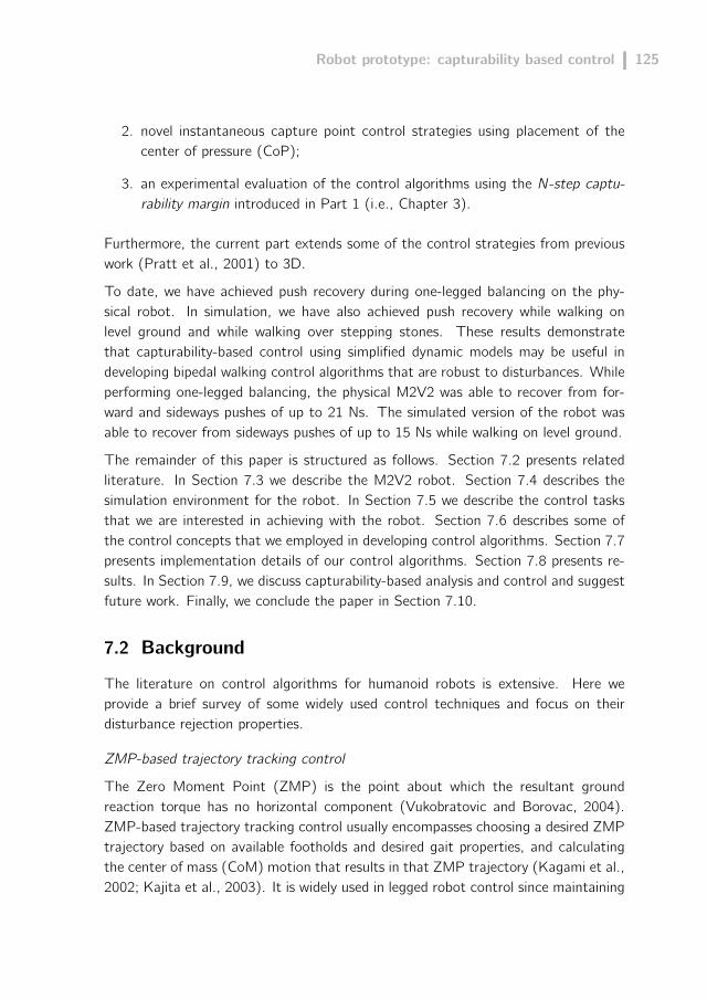
Robot prototype: capturability based control 125

2. novel instantaneous capture point control strategies using placement of thecenter of pressure (CoP);

3. an experimental evaluation of the control algorithms using the N-step captu-rability margin introduced in Part 1 (i.e., Chapter 3).

Furthermore, the current part extends some of the control strategies from previouswork (Pratt et al., 2001) to 3D.

To date, we have achieved push recovery during one-legged balancing on the phy-sical robot. In simulation, we have also achieved push recovery while walking onlevel ground and while walking over stepping stones. These results demonstratethat capturability-based control using simplified dynamic models may be useful indeveloping bipedal walking control algorithms that are robust to disturbances. Whileperforming one-legged balancing, the physical M2V2 was able to recover from for-ward and sideways pushes of up to 21 Ns. The simulated version of the robot wasable to recover from sideways pushes of up to 15 Ns while walking on level ground.

The remainder of this paper is structured as follows. Section 7.2 presents relatedliterature. In Section 7.3 we describe the M2V2 robot. Section 7.4 describes thesimulation environment for the robot. In Section 7.5 we describe the control tasksthat we are interested in achieving with the robot. Section 7.6 describes some ofthe control concepts that we employed in developing control algorithms. Section 7.7presents implementation details of our control algorithms. Section 7.8 presents re-sults. In Section 7.9, we discuss capturability-based analysis and control and suggestfuture work. Finally, we conclude the paper in Section 7.10.

7.2 Background

The literature on control algorithms for humanoid robots is extensive. Here weprovide a brief survey of some widely used control techniques and focus on theirdisturbance rejection properties.

ZMP-based trajectory tracking control

The Zero Moment Point (ZMP) is the point about which the resultant groundreaction torque has no horizontal component (Vukobratovic and Borovac, 2004).ZMP-based trajectory tracking control usually encompasses choosing a desired ZMPtrajectory based on available footholds and desired gait properties, and calculatingthe center of mass (CoM) motion that results in that ZMP trajectory (Kagami et al.,2002; Kajita et al., 2003). It is widely used in legged robot control since maintaining

126 Chapter 7

the ZMP strictly inside the support polygon at all times guarantees that it is physi-cally possible to track the reference joint trajectories using conventional control tools.The distance from the ZMP to the edge of the support polygon can be used as ameasure of robustness. Modifying the reference ZMP trajectory online has also beenexplored, including both small local ZMP changes and larger step placement changes(Nishiwaki and Kagami, 2010). Another ZMP control approach treats the ZMP asa control input, which is manipulated to produce a desired motion of the CoM. Forexample, central pattern generators have been used to calculate the reference ZMPtrajectory to produce walking (Sugihara, 2010).

Typical ZMP-based gait generation techniques cannot be used to generate gaits forwhich the stance foot rolls from heel to toe, as observed in fast human walking. Thislimitation is due to the ZMP needing to be inside the support polygon to meet theZMP stability criterion (Vukobratovic and Borovac, 2004). However, when the robotrotates about an edge of its support foot, the area of the support polygon decreasesto too small of a value to provide robustness against small modeling errors. Also,the reference joint trajectories themselves might lead the robot to a fall by design,even if the ZMP is kept inside the support polygon at all times. Hence, the ZMPcriterion is not a necessary condition to avoid falling (Pratt and Tedrake, 2006).In addition, the ZMP criterion is not applicable to non-flat terrain (Wieber, 2002).Most importantly for the present work, ZMP analysis does not answer the crucialquestion of where to step to recover from large disturbances.

Passive Dynamics Based Control

Another approach to walking control explicitly relies upon the passive behavior of therobot’s mechanical components. Straight-line periodic walking has been demonstra-ted for purely passive devices walking down a slope (Collins et al., 2001; McGeer,1990a). Adding limited actuation to machines designed for passive walking can yielda controlled, efficient gait (Collins et al., 2005). Rejection of small disturbances hasbeen shown for planar walkers under limited control (Kuo, 1999; Tan et al., 2010), aswell as locally stable gaits with purely reflexive control (Geng et al., 2006). A majorfocus of our current work is endowing robots with the ability to recover from distur-bances large enough to require significant actuation, so we cannot rely on passivedynamics alone to avoid falling.

Hybrid Zero dynamics

Another approach to locomotion control identifies relationships between the degreesof freedom of a robot that lead to a steady gait (Westervelt et al., 2003). Theserelationships are then enforced by a feedback controller, yielding a locally stable,

Robot prototype: capturability based control 127

periodic gait. This method has been shown to be able to cope with moderatelyrough terrain (Sreenath et al., 2010) (Westervelt et al., 2004). More recently, thismethod has been used to generate three dimensional walking (Chevallereau et al.,2009). However, it requires off-line computation of a repetitive gait, and thereforeit currently has no mechanism for explicitly handling rough terrain with impassableareas. Also, it is still unclear how a robot using this method will handle large pushesthat significantly disturb the state of the machine from the preplanned gait.

Compliant Strategies for Force Controllable Robots

Force controllable robots have lead to the development of compliant control stra-tegies. Virtual model control and other intuitive control strategies were used onthe 2D walking robot Spring Flamingo (Pratt et al., 2001). Coros et al. (2010)combine Jacobian transpose control, joint space PD control, and gravity compensa-tion with step planning based on an inverted pendulum model to obtain a walkingcontroller that works for a range of simulated characters, while performing secondarytasks. Stephens and Atkeson (Stephens and Atkeson, 2010) introduced an algorithmthat combines joint PD control, virtual model control and Dynamic Balance ForceControl. Dynamic Balance Force Control is an inverse dynamics approach based onthe contact forces obtained from a CoM planner. Hyon and Cheng (2007) achieveddisturbance rejection using a passivity-based controller, later complemented by CoMcontrol using a Dynamic Balancer (Hyon et al., 2009).

Compliant strategies can enhance the robustness of a walking algorithm since theyfocus on interaction forces with the environment to achieve higher level goals, insteadof relying on high gain position control and extremely accurate ground models toachieve perfect kinematic trajectories. The presented work also uses a compliantcontrol strategy.

7.3 Description of M2V2 Robot

M2V2 (see Figure 7.1) is a lower body humanoid with two 6 DoF legs (Pratt et al.,2009). There are three degrees of freedom at each hip, one at each knee, and two ateach ankle. See the Appendix for approximate inertia parameters and joint offsets,which we use in the simulation model. It is a second generation redesign of M2, arobot developed at the MIT Leg Laboratory (Paluska, 2000; Pratt, 2000a).

Each degree of freedom is driven by an identical force controllable Series Elastic Ac-tuator (SEA) (Pratt and Williamson, 1995; Pratt and Pratt, 1998). These actuatorsuse a spring in series between the drive train and the load. By measuring the springdeflection, the force exerted by the actuator can be measured. Using a feedback

128 Chapter 7

Figure 7.1: M2V2, a 3D force-controllable humanoid robot with twelve actuated degrees of freedom.

controller, the actuator force can be controlled accurately. For M2V2, each actuatorcan produce a force of up to 1.3 kN, with a smallest resolvable force of approxima-tely 4.4 N, giving it a 300 : 1 dynamic range. The force controllable bandwidth ofeach actuator is approximately 40 Hz. M2V2 has two U.S. Digital EM1-0-500 linearencoders and LIN-500 encoder strips at each Series Elastic Actuator, one to measureposition and one to measure spring deflection.

Onboard computation is provided by a PC104 with a dual core Pentium-M processor.Sensor reading is done by several AccesIO 104-Quad8 encoder input boards. Desiredcurrent is output as a PWM signal through two Real Time Devices 6816 PWMboards. Body orientation and angular rate are measured using a MicroStrain 3DM-GX3-25 inertial measurement unit. Current control is provided through twelve CopleyControls Accelnet module ACM-180-20 amplifiers. The PC104, I/O cards, andcurrent amplifiers are all located in the body of the robot.

A custom designed push stick equipped with a digital Loadstar ILoad Pro load cellwas constructed for measuring pushing forces applied to the robot. This load cell isconnected to to the robot to eliminate data synchronization issues, but the controlalgorithm does not have access to its output.

7.4 Simulation environment

We have developed a simulation model of M2V2 using the Yobotics SimulationConstruction Set (Yobotics, Inc, 2011). This software package allows for rigid body

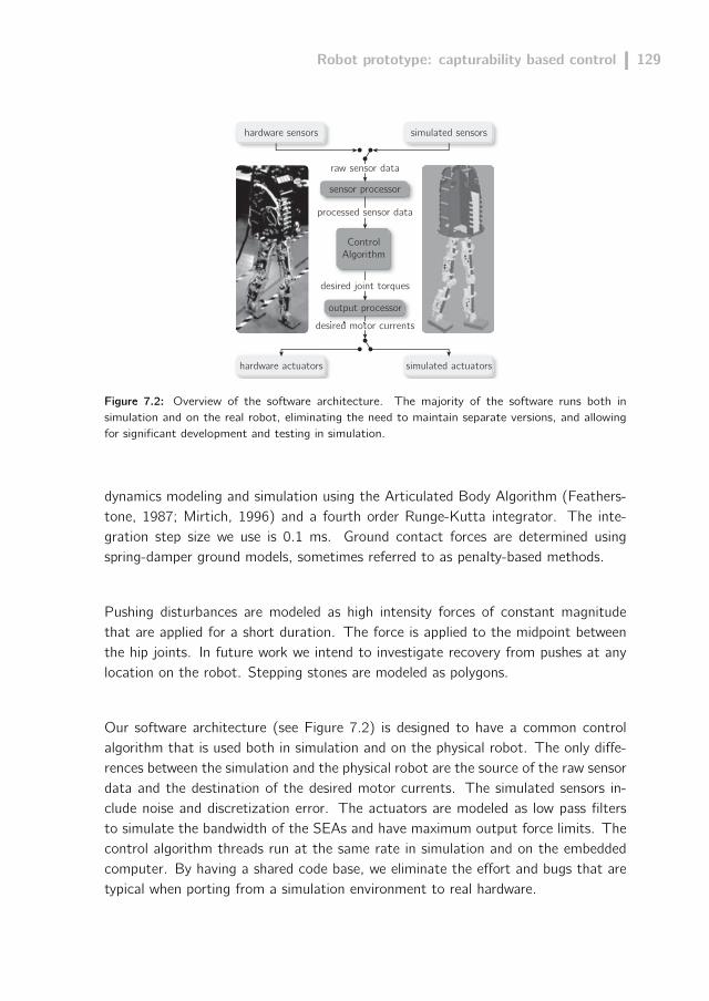
Robot prototype: capturability based control 129

hardware sensors simulated sensors

raw sensor data

sensor processor

processed sensor data

hardware actuators simulated actuators

desired motor currentsdesired mot r currentsoutput processor

desired joint torques

ControlAlgorithm

Figure 7.2: Overview of the software architecture. The majority of the software runs both insimulation and on the real robot, eliminating the need to maintain separate versions, and allowingfor significant development and testing in simulation.

dynamics modeling and simulation using the Articulated Body Algorithm (Feathers-tone, 1987; Mirtich, 1996) and a fourth order Runge-Kutta integrator. The inte-gration step size we use is 0.1 ms. Ground contact forces are determined usingspring-damper ground models, sometimes referred to as penalty-based methods.

Pushing disturbances are modeled as high intensity forces of constant magnitudethat are applied for a short duration. The force is applied to the midpoint betweenthe hip joints. In future work we intend to investigate recovery from pushes at anylocation on the robot. Stepping stones are modeled as polygons.

Our software architecture (see Figure 7.2) is designed to have a common controlalgorithm that is used both in simulation and on the physical robot. The only diffe-rences between the simulation and the physical robot are the source of the raw sensordata and the destination of the desired motor currents. The simulated sensors in-clude noise and discretization error. The actuators are modeled as low pass filtersto simulate the bandwidth of the SEAs and have maximum output force limits. Thecontrol algorithm threads run at the same rate in simulation and on the embeddedcomputer. By having a shared code base, we eliminate the effort and bugs that aretypical when porting from a simulation environment to real hardware.

130 Chapter 7

7.5 Control tasks

The controller was designed for two separate control tasks: 1) balancing on one legand 2) walking. These tasks require slightly different implementations of some ofthe modules in the controller, although the main control algorithm is the same.

7.5.1 Balancing

Balancing on one leg (subsequently called ‘balancing’) entails going from a doublesupport configuration to single support, and remaining in single support for as longas possible. If the robot is significantly perturbed while in single support, it will needto take a step to prevent a fall. Possible disturbances include pushes of significantmagnitude and, to a lesser extent, sensor and actuator imperfections. Pushes of amagnitude requiring the robot to take a step will be assumed to have a directionthat does not require a cross-over step. For example, if the robot is balancing on itsleft leg, then significant pushes could be directed forward, backward or to the right,but not to the left. Balancing was chosen as a precursor to walking because it ischallenging and requires good foot placement, but it is not as difficult as walking sincesustained forward progression is not required. To date we have achieved balancingon the physical robot, recovering from forward and sideways pushes up to 21 Ns.

7.5.2 Walking

The walking task requires the robot to move forward and be able to change walkingdirection. In addition, the controller needs to be able to handle walking over steppingstones. To date, walking on flat ground without pushes has been achieved on thephysical robot. Walking in the presence of pushes up to 15 Ns and walking overstepping stones have been achieved in simulation.

7.6 Control concepts

This section describes three key concepts we use in our control strategies, regardlessof the control task. These concepts are 1) capturability-based control using anapproximate model, 2) force control and 3) virtual model control.

7.6.1 Capturability-based control using an approximate model

We consider bipedal locomotion to be an inherently robust control problem, whichdoes not require great accuracy in controller design. This motivates our use ofan approximate model. Out of the three simplified gait models described in Part1 (i.e., Chapter 3), we have chosen to use the 3D-LIPM with finite-sized foot forapproximations. See Section 7.9.1 for the motivation for this choice. We base our

Robot prototype: capturability based control 131

control strategy on the instantaneous capture point and the approximated 1-stepcapture region. Although no guarantees on capturability can be made for the robotusing this approximation, we have found that it works well in practice.

Considering the 3D-LIPM with finite-sized foot, the instantaneous capture pointis the point on the ground where the CoP should be placed instantaneously andmaintained to come to a rest with the CoM directly above the CoP. We do notspecify a desired CoM trajectory; instead, desired instantaneous capture point pathsare used as a basis for control. The linear dynamics of the instantaneous capturepoint allows us to find a desired CoP location within the base of support that ‘pushes’the instantaneous capture point along the desired path.

For the balancing task, we determine whether taking a step is necessary based onwhether the instantaneous capture point has left the base of support (see Corollary 2in Chapter 3 and (Pratt et al., 2006)). For both control tasks described in this part,the controller will attempt to step to a desired step location in the 1-step captureregion. If the robot is disturbed significantly in mid-swing, the desired step locationwill be adjusted so that it always lies in the 1-step capture region. Section 7.9.2provides a discussion on why we chose to base the controller on the 1-step captureregion, as opposed to using an N-step capture region with N > 1.

7.6.2 Force control

Force controllable actuators allow a biped to walk smoothly and naturally. Theseactuators allow for compliant control methods that are forgiving to external forcesand unknown terrain. Traditionally, many humanoid robots use high-gain positioncontrol to track prescribed joint trajectories using non-backdrivable actuators. Thisapproach typically requires near perfect knowledge of the terrain, a near perfectdynamic model of the robot, and no external forces. When pushed or encounteringunexpected terrain, these robots may no longer be able to follow the prescribed jointtrajectories, and either a new trajectory must be computed on the fly, or the robotfalls.1

Our control approach avoids the use of joint trajectory tracking for the stance leg.Instead, we use low-impedance feedback controllers that control the fundamentalaspects of walking (foot placement and body height, orientation and speed), ratherthan attempting to rigidly control each degree of freedom. Force control providessome robustness to rough terrain since the exact foot/ground contact configuration

1Trajectory tracking bipedal robots often use compliant foot pads, force sensors, and real timemodification of ankle trajectories to control the CoP location. This technique essentially convertsthe ankle actuators to lower impedance force controllable actuators.

132 Chapter 7

is less important than the interaction forces between the feet and the ground. Inaddition, force controllable actuators simplify control of the CoP location, and allowcompliant control techniques, such as virtual model control.

7.6.3 Virtual model control

Virtual model control is a tool that allows a designer to control a robot by choosingvirtual components, such as springs and dampers, to intuitively achieve task goals(Chen et al., 2001; Hu et al., 1998, 1999; Pratt et al., 2001). Once these com-ponents are chosen, the kinematic model of the system and additional user definedconstraints allow direct calculation of the joint actuation required to simulate theeffect of the desired components.

For example, in previous work on Spring Turkey, a planar walking robot with 4 actua-ted degrees of freedom, we decomposed the requirements of walking and designedsimple virtual components to achieve each one (Pratt et al., 2001). CoM height wasmaintained by a virtual vertical spring-damper “granny walker” and forward travel wasachieved with a virtual “track bunny” with constant forward velocity connected tothe robot’s body by a virtual horizontal damper. The joint actuation was calcula-ted using the transpose of a Jacobian that spans the joints between two virtuallycontrolled points. While kinematic singularities remove degrees of freedom from thepossible actuation, the joint torques for the remaining degrees of freedom can stillbe calculated. Similar techniques were used in the control of Spring Flamingo, aplanar walker with 6 actuated degrees of freedom. Virtual model control is used inthe control of M2V2 to maintain CoM height and body orientation, and to achieveapproximate CoP control.

7.7 Controller implementation

We now present a detailed description of the balancing and walking controller. Thecontroller’s input is comprised of joint angles and angular velocities, and the orien-tation and orientation rates of the upper body. The controller’s output is comprisedof desired torques at each joint. The controller consists of five main parts:

1. the state machine, which keeps track of the gait phase for each leg and acts asa supervisory system that calls the appropriate lower level routines (see Section7.7.1),

2. the capture region calculator, which determines the instantaneous capturepoint and the 1-step capture region (see Section 7.7.2),

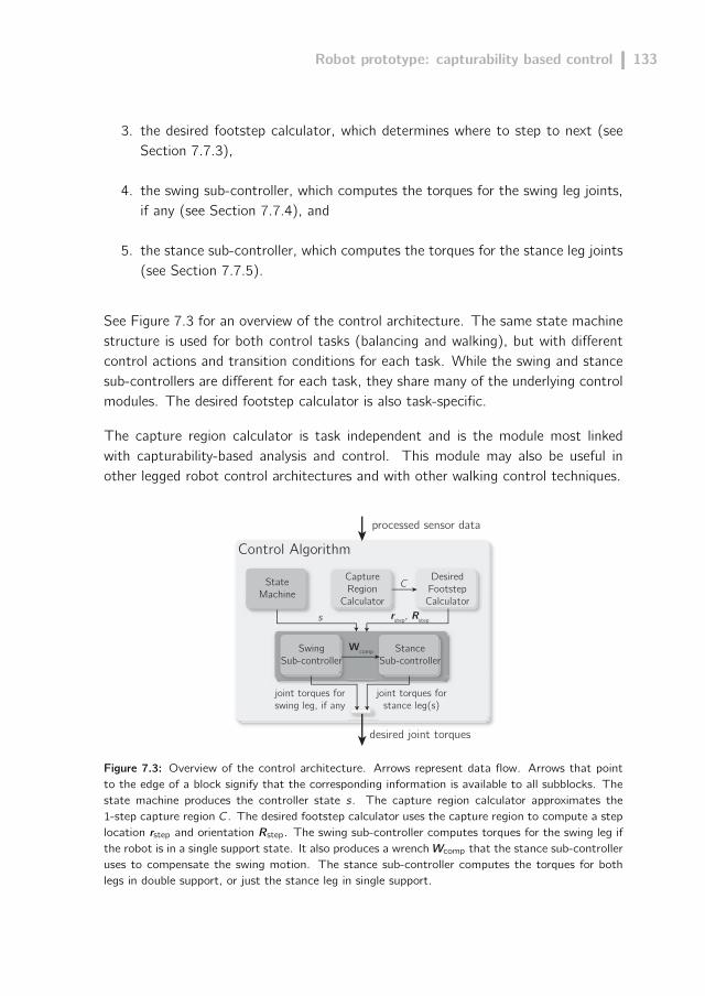
Robot prototype: capturability based control 133

3. the desired footstep calculator, which determines where to step to next (seeSection 7.7.3),

4. the swing sub-controller, which computes the torques for the swing leg joints,if any (see Section 7.7.4), and

5. the stance sub-controller, which computes the torques for the stance leg joints(see Section 7.7.5).

See Figure 7.3 for an overview of the control architecture. The same state machinestructure is used for both control tasks (balancing and walking), but with differentcontrol actions and transition conditions for each task. While the swing and stancesub-controllers are different for each task, they share many of the underlying controlmodules. The desired footstep calculator is also task-specific.

The capture region calculator is task independent and is the module most linkedwith capturability-based analysis and control. This module may also be useful inother legged robot control architectures and with other walking control techniques.

StateMachine

DesiredFootstepCalculator

desired joint torques

joint torques forswing leg, if any

joint torques forstance leg(s)

Control Algorithm

s rstep, Rstep

Wcomp

CaptureRegion

CalculatorC

processed sensor data

StanceSub-controller

SwingSub-controller

Figure 7.3: Overview of the control architecture. Arrows represent data flow. Arrows that pointto the edge of a block signify that the corresponding information is available to all subblocks. Thestate machine produces the controller state s. The capture region calculator approximates the1-step capture region C. The desired footstep calculator uses the capture region to compute a steplocation rstep and orientation Rstep. The swing sub-controller computes torques for the swing leg ifthe robot is in a single support state. It also produces a wrench Wcomp that the stance sub-controlleruses to compensate the swing motion. The stance sub-controller computes the torques for bothlegs in double support, or just the stance leg in single support.

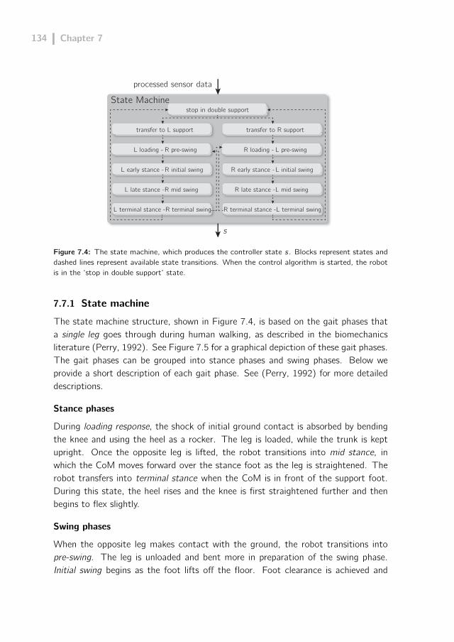
134 Chapter 7

stop in double support

transfer to L support

processed sensor data

s

L loading - R pre-swing

L early stance -R initial swing

L late stance -R mid swing

L terminal stance -R terminal swing

transfer to R support

R loading - L pre-swing

R early stance -L initial swing

R late stance -L mid swing

R terminal stance -L terminal swing

State Machine

Figure 7.4: The state machine, which produces the controller state s. Blocks represent states anddashed lines represent available state transitions. When the control algorithm is started, the robotis in the ‘stop in double support’ state.

7.7.1 State machine

The state machine structure, shown in Figure 7.4, is based on the gait phases thata single leg goes through during human walking, as described in the biomechanicsliterature (Perry, 1992). See Figure 7.5 for a graphical depiction of these gait phases.The gait phases can be grouped into stance phases and swing phases. Below weprovide a short description of each gait phase. See (Perry, 1992) for more detaileddescriptions.

Stance phases

During loading response, the shock of initial ground contact is absorbed by bendingthe knee and using the heel as a rocker. The leg is loaded, while the trunk is keptupright. Once the opposite leg is lifted, the robot transitions into mid stance, inwhich the CoM moves forward over the stance foot as the leg is straightened. Therobot transfers into terminal stance when the CoM is in front of the support foot.During this state, the heel rises and the knee is first straightened further and thenbegins to flex slightly.

Swing phases

When the opposite leg makes contact with the ground, the robot transitions intopre-swing. The leg is unloaded and bent more in preparation of the swing phase.Initial swing begins as the foot lifts off the floor. Foot clearance is achieved and

Robot prototype: capturability based control 135

Loading Response Early Mid Stance Late Mid Stance Terminal Stance Initial Swing Mid Swing Terminal SwingPre-Swing

Figure 7.5: The gait phases upon which the state machine is based. The labels correspond to thephase of the highlighted right leg. Adapted from (Perry, 1992), which describes the phases of gaitfor human walking.

the leg is swung forward. When the swinging limb is opposite the stance limb, therobot enters mid swing. The hip is flexed further and the knee is allowed to extendin response to gravity. Finally, the robot transitions into terminal swing, in which theknee is extended as limb advancement is completed.

Transitions between gait phases for the right leg are directly coupled to those for theleft leg. The states shown in Figure 7.4 were hence created by combining one gaitphase for the left leg and one gait phase for the right leg, e.g. ‘left early stance -right initial swing’. In addition to the eight walking states, there is also a state inwhich the robot is stopped in double support and states in which weight is transferredto one leg, allowing the robot to start from a stop.

While this state machine is based on walking, it is easily adapted to one-leggedbalance, through appropriate selection of control actions in each state and transitionconditions between states.

7.7.2 Capture region calculator

The capture region calculator approximates the 1-step capture region C, the set oflocations where the contact reference point, a chosen point on each foot, may beplaced at the next step so that the robot is able to reach a captured state. The al-gorithm is based on the capturability analysis of the 3D-LIPM with finite-sized foot,as presented in Part 1 (i.e. Chapter 3), and we refer to that part for the under-lying theory; here we only present the implementation details of the capture regioncalculator. See Algorithm 1 for pseudocode. Figure 7.6 describes the algorithmgraphically.

The algorithm can handle limitations on where the CoP may be placed by specifyingallowable CoP regions, represented as a set of polygons, denoted A = A0, A1, . . . .

136 Chapter 7

The allowable CoP regions may be used to model stepping stones, as well as to avoidcross-over steps and overlapping footsteps.

Algorithm 1 1-step capture region calculator

Input: S, r , r , A, ts,min, t, rmax, lmax

1: ric ⇐ P r +√

z0

g r

2: CP ⇐ A

3: if ¬pointInPolygon(S, ric) then4: Q = (q0, . . . , qn)⇐ visibleVertices(S, ric)

5: for i = 0 to n do6: pi ⇐ [ric − qi ]ets,min−t + qi

7: end for8: CP ⇐ bound(CP , p0, ric)

9: CP ⇐ bound(CP , ric, pn)

10: for i = 1 to n do11: CP ⇐ bound(CP , pi−1, pi)

12: end for13: end if14: return (CP , rmax, lmax)

Algorithm 1 assumes that the orientation of the swing foot may be chosen withoutlimitation, which means that the maximum distance rmax from the contact referencepoint to the edge of the foot polygon (see Figure 7.7) fully specifies which contactreference point locations allow a given CoP location to be attained. We furtherspecify a maximum step length lmax, defined as the maximum distance betweensubsequent contact reference point locations.

The output of the algorithm is a tuple (CP , rmax, lmax), consisting of a set of polygonsCP , the maximum offset distance to these polygons rmax, and the maximum distanceto the contact reference point lmax. The basic idea of the algorithm is to determinethe set of polygons CP consisting of the parts of A where the instantaneous capturepoint may be located when a step is taken, so that the CoP may be placed thereafter the step, letting the robot reach a captured state. The capture region C isthen found by determining allowable contact reference point locations that enablethe CoP to be placed inside CP as shown in Figure 7.7.

In Algorithm 1, S is the current support polygon represented as a clockwise orderedsequence of vertices, r is the CoM position, ts,min is the estimated earliest time atwhich a step can be taken, t is the current time, rmax is the maximum distance

Robot prototype: capturability based control 137

A1

A0

A2

r .rq0

q1

q2ric

8

9

11a

11b

CP

p0

p1

p2

Figure 7.6: Graphical depiction of Algorithm 1. The instantaneous capture point ric is first calculated(line 1). The ordered set of support polygon vertices that are visible from the instantaneous capturepoint, (q0, q1, q2) is then determined (line 4), as well as the corresponding possible locations of theinstantaneous capture point at ts,min, (p0, p1, p2) (lines 5–7). The set of polygons CP is finallydetermined by bounding the set of allowable CoP regions, A, using the lines denoted 8, 9, 11a and11b in the figure. The numbers correspond to line numbers in Algorithm 1.

C

ric CP

r max

rmax

contact reference point

rmax

lmax

Figure 7.7: The 1-step capture region C, as found by 1) offsetting the set of polygons CP by rmax,and 2) intersecting the result with a disk of radius lmax and the contact reference point as its centerto take the maximum step length constraint into account. Note that for this figure, the centroidof the foot was chosen as the contact reference point.

138 Chapter 7

from the contact reference point to the edge of the support polygon, and lmax is themaximum step length, as measured from the contact reference point.

Line 1 in the algorithm is the instantaneous capture point definition, (8) in Part 1.Line 6 describes the instantaneous capture point motion for a constant CoP andoriginates from (22) in Part 1.

The function pointInPolygon(X, p) determines whether point p is contained withinthe polygon defined by the sequence of vertices X.

Function visibleVertices(X, p) computes a clockwise ordered sequence of verticesQ = (q0, . . . , qn) taken from X that ‘can be seen’ from p, in the sense that a linesegment starting from p and pointing to qi does not intersect the polygon spannedby X. The first element of the returned sequence is the rightmost visible vertex asseen from p, and the last element is the leftmost.

The function bound(P, r0, r1) takes a set of polygons P and returns a modified versionof P , where each individual polygon is intersected with a half-plane containing allpoints to the right of a boundary line through r0 and r1. Note that the order of thearguments r0 and r1 determines the ‘direction’ of the boundary line and hence thedirection of the half-plane. This function is used to cut off parts of the allowableCoP regions to which the instantaneous capture point may not be directed or whichare not reachable given the minimum step time.

Note that if the current support foot is only partially placed inside the allowable CoPregions A, the support polygon S is the intersection of the foot polygon and A, andAlgorithm 1 can be used without modification. Furthermore, note that if there arelimits on allowable foot orientations, the step of offsetting the set of polygons CP byrmax should be replaced by convolving the allowable configurations of the swing footpolygon about CP .

7.7.3 Desired footstep calculator

The desired footstep calculator (see Figure 7.8) determines the desired positionof the swing ankle rstep and orientation of the swing foot Rstep at the end of theupcoming step. The desired position and orientation are expressed in a frame fixedto the support foot. Because footstep planning depends greatly on the controltask, we have created two separate implementations of this module: one for thebalancing task and another for the walking task. The general pattern used for bothimplementations is to choose a desired initial footstep (rstep,init,Rstep,init) at the startof the swing phase and adjust it during the swing phase if necessary, for example ifthe robot is significantly perturbed, to obtain the final output (rstep,Rstep).

Robot prototype: capturability based control 139

Balancing

The desired footstep calculator for the balancing task is a minimal implementation.The initial desired step location is computed using a fixed step length lstep in thedirection of the instantaneous capture point:

rstep,init = rankle + lstepric − rankle‖ric − rankle‖

(7.1)

where rankle is the position of the stance foot ankle. The initial foot orientation ischosen to be the same as the stance foot orientation and is never adjusted. Thedirection in which the robot steps is adjusted by recomputing (7.1) during the first0.1 s after the instantaneous capture point has left the foot polygon. After that itremains fixed for the remainder of swing.

Walking

The desired footstep for the walking task is chosen in such a way that forwardprogression is made, while the robot remains 1-step capturable. The initial steplength is determined by multiplying the desired walking velocity by a proportionalgain, while the initial step width is set to a constant value. On flat ground, thestep height is set to zero but may be changed to any feasible desired value whennecessary, for instance to climb a slope. Footstep yaw is set equal to the desiredwalking direction. Footstep pitch and roll are set to zero on flat ground but may beused to walk on rough terrain to reduce the need for compliance in the ankle joint.

If the initial desired step location ceases to be within the capture region by a desiredmargin at any instant during the swing phase, an adjusted desired step location iscomputed by projecting the initial location inside the 1-step capture region by thedesired margin. The orientation is not adjusted.

7.7.4 Swing sub-controller

The task of the swing sub-controller (see Figure 7.9) is to compute the desiredtorques for the swing leg joints. It accomodates changes in the desired step location,obtained from the desired step location calculator, on the fly. The controller containsa trajectory generator for the position and orientation of the swing foot, which isused to compute desired joint angles, velocities and accelerations through inversekinematics. The trajectory is tracked using inverse dynamics augmented by PDposition control in joint space.

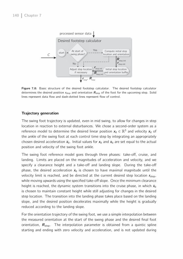
140 Chapter 7

Desired footstep calculator

Yes

CAt start of

swing phase?Compute initial step

location and orientationstart

Adjust step locationif necessary

Initial step locationand orientation buffer

processed sensor data

rstep, Rstep

rstep,initrstep,init

Rstep,init

Rstep,initNo

Figure 7.8: Basic structure of the desired footstep calculator. The desired footstep calculatordetermines the desired position rstep and orientation Rstep of the foot for the upcoming step. Solidlines represent data flow and dash-dotted lines represent flow of control.

Trajectory generation

The swing foot trajectory is updated, even in mid swing, to allow for changes in steplocation in reaction to external disturbances. We chose a second-order system as areference model to determine the desired linear position xd ∈ R3 and velocity xd ofthe ankle of the swing foot at each control time step by integrating an appropriatelychosen desired acceleration xd. Initial values for xd and xd are set equal to the actualposition and velocity of the swing foot ankle.

The swing foot reference model goes through three phases: take-off, cruise, andlanding. Limits are placed on the magnitudes of acceleration and velocity, and wespecify a clearance height and a take-off and landing slope. During the take-offphase, the desired acceleration xd is chosen to have maximal magnitude until thevelocity limit is reached, and be directed at the current desired step location rstep,while moving upwards using the specified take-off slope. Once the minimum clearanceheight is reached, the dynamic system transitions into the cruise phase, in which xdis chosen to maintain constant height while still adjusting for changes in the desiredstep location. The transition into the landing phase takes place based on the landingslope, and the desired position decelerates maximally while the height is graduallyreduced according to the landing slope.

For the orientation trajectory of the swing foot, we use a simple interpolation betweenthe measured orientation at the start of the swing phase and the desired final footorientation, Rstep. The interpolation parameter is obtained from a quintic splinestarting and ending with zero velocity and acceleration, and is not updated during

Robot prototype: capturability based control 141

Swing Sub-controllerSwing Sub-controllerrealtime

trajectorygenerator

joint levelPD control

inversekinematics

inversedynamics

τPD τID

xd, ẋd, ẍd Rd, d, d.

qd..qd, qd

. Wcomp

joint torques forswing leg, if any

s processed sensor data

rstep, Rstep

Figure 7.9: Swing sub-controller. A real-time trajectory generator computes the desired position,linear velocity and acceleration (xd, xd, xd respectively), as well as the desired orientation, angularvelocity and angular acceleration (Rd, ωd, ωd respectively), expressed in world frame. Inverse kine-matics is used to translate this trajectory from Euclidean space to desired joint positions, velocitiesand accelerations (qd, qd and qd respectively). This information is used by an inverse dynamicsalgorithm, which computes pin joint torques τid and an upper body compensation wrench Wcomp,used by the stance sub-controller. The output τPD of a joint-space PD controller is added to τIDto obtain the swing leg joint torques.

the step.

Position control

The desired position and orientation of the swing foot at every control time stepare used to compute the corresponding joint angles of the swing leg using inversekinematics. The desired linear and angular velocity and acceleration of the swing footspecify corresponding desired joint velocities and accelerations through the inverseof the swing leg Jacobian. Problems due to the singularity that occurs when theknee is stretched are circumvented by gradually scaling the desired joint velocitiesand accelerations back to zero (that is, using pure damping) based on the value ofthe Jacobian determinant.

An inverse dynamics algorithm (Featherstone, 2008), augmented by PD positioncontrol in joint space is used to compute the desired torques for the swing leg joints.We exclude the stance leg joints in computing the inverse dynamics. The desiredspatial acceleration of the upper body is set to zero. In addition to the torquesacross the swing leg pin joints, the inverse dynamics algorithm also returns a wrenchthat should be exerted across the ‘floating joint’ that connects the upper body to theworld to achieve the desired zero spatial acceleration. This wrench will be used in the

142 Chapter 7

stance sub-controller as a feed-forward term to compensate the swing leg torquesand reduce upper body oscillations.

Previously, we have also implemented a virtual model control-based swing sub-controller, but the current implementation outperforms the virtual model controlimplementation in terms of accuracy and swing speed, which we consider to be keyingredients for dynamic walking and push recovery.

7.7.5 Stance sub-controller

The stance sub-controller controls balance by computing desired torques for thestance leg(s). The goals of the stance sub-controller are to control 1) instantaneouscapture point location, 2) upper body orientation, and 3) upper body height. Thestance sub-controller is an implementation of virtual model control. For each stanceleg, it computes a desired wrench on the upper body, to be exerted by the leg,that satisfies these control goals. Jacobian transpose control is then used to findcorresponding desired leg torques. The stance sub-controller consists of multiplecontrol modules, as shown in Figure 7.10. The following sections will describe thesemodules in more detail.

Upper body height control module

The upper body height control module regulates the upper body height by determiningthe net vertical force, fz , that the legs should exert on the upper body. In doublesupport, fz is set to a constant value that slightly overcompensates the estimatedgravitational force acting on the entire robot, simulating a virtual constant forcespring. In single support, fz is set to the weight of the stance leg and the bodyplus the z-component of the force from the swing leg compensation wrench Wcomp,cancelling out some of the dynamic effects due to the swing leg motion.

Upper body orientation control module

The upper body orientation control module determines a desired torque τ that thelegs should exert on the upper body. It is used to control the orientation of the upperbody with respect to the world (as perceived by the inertial measurement unit). Thedesired pitch of the upper body is constant and set to zero. Both the desired yaw andthe desired roll depend on the gait phase and state of the support leg. Yawing androlling are used to obtain a longer reach for the swing leg and to make the gait lookmore humanlike. In addition, the desired yaw also depends on the desired walkingdirection.

The desired upper body torque is computed using PD control on the roll, pitch andyaw corresponding to the rotation matrix that describes the orientation of the actual

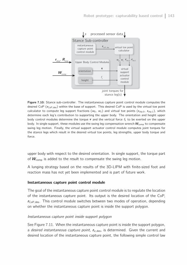
Robot prototype: capturability based control 143

orientation

Stance Sub-controller

τ

fz

joint torques for stance leg(s)

virtualsupportactuatorcontrolmoduleheight

Upper Body Control Modulesw0, w1

rvtp,0, rvtp,1

virtual toe pointcalculator

rCoP, desinstantaneouscapture point

control module

rstep, Rstep

Wcomp

s processed sensor data

Figure 7.10: Stance sub-controller. The instantaneous capture point control module computes thedesired CoP (rCoP,des) within the base of support. This desired CoP is used by the virtual toe pointcalculator to compute leg support fractions (w0, w1) and virtual toe points (rvtp,0, rvtp,1), whichdetermine each leg’s contribution to supporting the upper body. The orientation and height upperbody control modules determine the torque τ and the vertical force fz to be exerted on the upperbody. In single support, these modules use the swing leg compensation wrenchWcomp to compensateswing leg motion. Finally, the virtual support actuator control module computes joint torques forthe stance legs which result in the desired virtual toe points, leg strengths, upper body torque andforce.

upper body with respect to the desired orientation. In single support, the torque partof Wcomp is added to the result to compensate the swing leg motion.

A lunging strategy based on the results of the 3D-LIPM with finite-sized foot andreaction mass has not yet been implemented and is part of future work.

Instantaneous capture point control module

The goal of the instantaneous capture point control module is to regulate the locationof the instantaneous capture point. Its output is the desired location of the CoP,rCoP,des. This control module switches between two modes of operation, dependingon whether the instantaneous capture point is inside the support polygon.

Instantaneous capture point inside support polygon

See Figure 7.11. When the instantaneous capture point is inside the support polygon,a desired instantaneous capture point, ric,des, is determined. Given the current anddesired location of the instantaneous capture point, the following simple control law

144 Chapter 7

is used to obtain the tentative location of the desired CoP, rCoP,des:

rCoP,des = ric + kic(ric − ric,des) (7.2)

where kic is the proportional gain. This proportional control law is motivated bythe linear instantaneous capture point dynamics for the 3D-LIPM with finite-sizedfoot described in Part 1. If rCoP,des lies inside the support polygon, then the finaloutput of this control module is rCoP,des = rCoP,des. Otherwise, rCoP,des is obtainedby projecting rCoP,des to the edge of the support polygon along a line through ricand ric,des, as shown in Figure 7.11b.2 The idea behind this control law is that theinstantaneous capture point is always pushed away from the CoP, and hence towardsthe desired instantaneous capture point.

The desired instantaneous capture point is determined as a function of the stateand the control task. For the balancing task, the desired instantaneous capturepoint coincides with the centroid of the support polygon during the double supportstate. When the robot is commanded to start balancing on one leg, the desiredinstantaneous capture point is moved to the centroid of the upcoming support foot,where it remains as long as the robot is able to maintain its balance without ta-king a step. This location maximizes robustness against external disturbances fromunknown directions.

For the walking task, the desired instantaneous capture point is located near the toesof the leading foot during the double support states, promoting forward motion. Atthe start of the swing phase, the desired capture point is moved outside the stancefoot in the direction of the upcoming step location.

Instantaneous capture point outside support polygon

See Figure 7.12. The instantaneous capture point will move outside the supportpolygon if the robot is pushed significantly, or because it has been driven outsidethe stance foot polygon during the walking task. When ric is outside the supportpolygon, it is not possible to track a desired instantaneous capture point location,since the instantaneous capture point will always exponentially diverge away from thestance foot. We therefore only control the direction in which it diverges away fromthe foot. This is done by specifying a guide line, Lg, and choosing the desired CoPsuch that the instantaneous capture point is kept along this guide line.

2In practice, we use a slightly smaller support polygon when projecting the tentative desired CoP,to prevent the feet from tipping at times when this is not desired. The use of a smaller supportpolygon is necessary because of unmodeled dynamics, inability to perfectly track the desired CoP,and model uncertainty.

Robot prototype: capturability based control 145

ric,des

(b)

rCoP,des

ric

ric,des

rCoP,des

ric

(a)

rCoP,des

_

S S

Figure 7.11: Action of the instantaneous capture point control module when ric is inside the supportpolygon S. (a) the tentative desired CoP rCoP,des, as determined using (7.2), is inside the supportpolygon, so it coincides with the final output rCoP,des. (b) rCoP,des is outside the support polygonand is projected onto its edge to obtain rCoP,des.

plannedstep location

S

rCoP,des

ric

Lg

Lc

d(Lg, ric)

kic d(Lg, ric)

∆x

∆ycontact

reference point

Figure 7.12: Action of the instantaneous capture point control module when ric is outside thesupport polygon S. The guide line Lg passes through the contact reference point on the supportfoot and a point ∆x in front and ∆y inside of the contact reference point for the planned footsteplocation, see (7.3). The control line Lc is parallel to the guide line; the distance between the twois determined by (7.4). The desired CoP is chosen as the intersection of Lc and S.

We define the guide line by two points. The first is the contact reference point onthe support foot. The second is a point ∆x in front and ∆y to the inside of thecontact reference point for the planned footstep, with

∆x = kxxvdes,x (7.3a)

∆y = kxy |vdes,x | (7.3b)

where kxx and kxy are positive gains and vdes,x is the desired average velocity ofthe robot in the forward direction, in a frame oriented to match the planned steplocation. The effect of this simple control law is that the instantaneous capture pointis pushed forward and to the inside of the upcoming support foot as desired forward

146 Chapter 7

velocity is increased.

Given the guide line and the instantaneous capture point location, a second line,called the control line, is defined. The control line is parallel to the guide line. Thedistance d(Lg, Lc) between the guide line Lg and the control line Lc is set to beproportional to the distance between the guide line and the instantaneous capturepoint, d(Lg, ric):

d(Lg, Lc) = kicd(Lg, ric) (7.4)

where kic is a positive gain.

Finally, the desired CoP is computed by finding the intersection of the stance footpolygon and the control line that is closest to ric. If there are no intersections, thesupport polygon vertex closest to the control line is used. The control law (7.4)causes the instantaneous capture point to be pushed back onto the guide line aftera deviation.

Virtual toe point calculator

The virtual toe point calculator uses the desired CoP to compute a virtual toe point(VTP) and a leg support fraction for each leg(Pratt and Pratt, 1998). ControllingVTP locations and leg support fractions results in approximate control of the overallCoP of the robot.

The virtual toe point of a foot is the point about which no torque is commandedin the horizontal plane. VTPs are similar to the centers of pressure for each foot,except that a VTP is a commanded quantity, not a measured one, and is only basedon a static analysis. Details on how the VTPs are used are given in Section 7.7.5.

In single support, the VTP for the stance leg is placed at the location of the desiredCoP. In double support, we use a heuristic based on geometric relations, depictedand explained in Figure 7.13, to determine VTPs rvtp,0 and rvtp,1 in such a way thatthe desired CoP and both VTPs lie on one line.

The leg support fractions are two scalars, denoted w0 and w1, such that w0 +w1 = 1

and w0, w1 ∈ [0, 1]. A leg support fraction wi describes the fraction of the desiredtorque τ and vertical force fz to be exerted by stance leg i ∈ 0, 1. The distancesbetween the VTPs and the overall desired CoP determine the leg support fractions:

wi =‖rCoP,des − rvtp,1−i‖‖rvtp,0 − rvtp,1‖

, i ∈ 0, 1 (7.5)

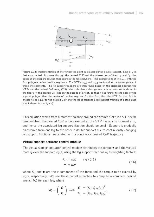
Robot prototype: capturability based control 147

w1

w0

1.0

0.5

1.0

0.5

rvtp,0 rvtp,1rCoP,des

L1

L2

Lvtp

Figure 7.13: Implementation of the virtual toe point calculator during double support. Line Lvtp isfirst constructed. It passes through the desired CoP and the intersection of lines L1 and L2, theedges of the support polygon that connect the foot polygons. The intersections of line Lvtp with thefoot polygons define two line segments. The VTPs rvtp,0 and rvtp,1 are found as the center points ofthese line segments. The leg support fractions are then found based on the distances between theVTPs and the desired CoP using (7.5), which also has a clear geometric interpretation as shown inthe figure. If the desired CoP lies on the outside of a foot, so that it lies farther to the edge of thesupport polygon than the center of the line segment for that foot, then the VTP for that foot ischosen to be equal to the desired CoP and the leg is assigned a leg support fraction of 1 (this caseis not shown in the figure).

This equation stems from a moment balance around the desired CoP: if a VTP is farremoved from the desired CoP, a force exerted at this VTP has a large moment arm,and hence the associated leg support fraction should be small. Support is graduallytransferred from one leg to the other in double support due to continuously changingleg support fractions, associated with a continuous desired CoP trajectory.

Virtual support actuator control module

The virtual support actuator control module distributes the torque τ and the verticalforce fz over the support leg(s) using the leg support fractions wi as weighting factors:

fz,i = wi fz i ∈ 0, 1τi = wiτ

(7.6)

where fz,i and τi are the z-component of the force and the torque to be exerted byleg i , respectively. We use these partial wrenches to compute a complete desiredwrench Wi for each leg, where

Wi =

(fi

τi

)with

fi = (fx,i , fy,i , fz,i)T

τi = (τx,i , τy,i , τz,i)T .

(7.7)

148 Chapter 7

The remaining x- and y -components of the force fi for each leg are computed usingthe virtual toe points. The virtual toe point constraint, which requires that no torqueshould be applied about either horizontal axis at the virtual toe point, can be enforcedas follows. We consider the virtual toe point for a foot to be the intersection of theaxes of two virtual pin joints, located on the sole of the foot. Their orthogonal axesof rotation lie in the plane of the foot. The virtual pin joints do not exist on thephysical robot, but provide a simple way of computing fx,i and fy,i since the torquesacross these joints should be zero. The virtual pin joints come after the real jointsof the robot in the kinematic chain from upper body to foot. Their rotation anglesare set to zero, but their location on the foot changes in time, depending on thelocation of the virtual toe point. We use τvtp,i ∈ R2 to denote the vector of virtualjoint torques exerted at the virtual pin joints for stance leg i . A static analysis resultsin

τvtp,i = JTvtp,iWi . (7.8)

In this equation, Jvtp,i ∈ R6×2 is the Jacobian that maps the joint velocities of thevirtual pin joints to the twist of the foot with respect to a virtual body attached‘after’ the virtual pin joints in the kinematic chain, expressed in an upper body-fixedframe.

Splitting the Jacobian Jvtp,i into a 2× 2 block Jvtp,i ,2×2 and a 4× 2 block Jvtp,i ,4×2

and using (7.7), we can rewrite (7.8) as

τvtp,i = JTvtp,i ,2×2

(fx,i

fy,i

)+ JTvtp,i ,4×2

(fz,i

τi

). (7.9)

We require that the torques at a leg’s virtual toe point be zero. We can hence solve(7.9) to find the values of fx,i and fy,i :(

fx,i

fy,i

)= −J−Tvtp,i ,2×2J

Tvtp,i ,2×4

(fz

τi

)(7.10)

The matrix JTvtp,i ,2×2 is invertible as long as the following two conditions hold: 1) thez-coordinate of the origin of the upper body, expressed in the foot-fixed frame, is notzero, and 2) the z-axis of the upper body-fixed frame does not lie in the horizontalplane of the foot-fixed frame. These conditions are always satisfied during normaloperation.

Now that fx,i and fy,i are also known, we know the complete wrenchWi to be exertedon the upper body by stance leg i , and we can use a different Jacobian, Jleg,i ∈ R6×6

Robot prototype: capturability based control 149

to find the joint torques τleg,i :

τleg,i = JTleg,iWi , (7.11)

where Jleg,i maps the joint velocities of the real joints of leg i to the twist of theupper body with respect to the foot, expressed in the upper body-fixed frame.

Computing fx,i and fy,i based on virtual toe points instead of specifying these forcesdirectly has as an advantage that virtual toe points are closely related to the CoP,which plays a major role in the instantaneous capture point dynamics described inChapter 3. This relation to the CoP also means that limits due to the finite-sizedsupport polygon are straight-forward to accomodate. We simply make sure that eachfoot’s virtual toe point lies inside its convex polygon.

7.8 Results

This section presents results obtained for both the balancing task and the walkingtask. Balancing and walking without pushes was achieved on the real M2V2 robot.Walking while recovering from pushes and walking over stepping stones was achievedon the simulated M2V2 robot. Note that figures are labeled either [REAL] if thedata is from the physical robot or [SIM] if from the simulated robot. See Extension1 for a video of results from both real-world experiments and simulations.

In this section, we evaluate the N-step capturability margin proposed in Part 1, thatis, the area of the N-step capture region. Here we use N = 1 since the presentedalgorithm is based on remaining 1-step capturable.

7.8.1 Balancing task

On the real M2V2 robot we achieved balancing on one leg and recovering fromsideways and forward pushes. Figure 7.14 shows time-elapsed images of M2V2 reco-vering from a push. Figure 7.15 shows the norm of the disturbance force, as recordedfrom the push stick, and the 1-step capturability margin. We see that the robot wasable to recover from pushes of approximately 21 Ns.

7.8.2 Walking task

On the real M2V2 robot we achieved flat ground walking without disturbances. Onthe simulated M2V2 robot we achieved walking while recovering from pushes andwalking over stepping stones.

Figure 7.16 shows time elapsed images of M2V2 walking on flat ground. For thiswalk, the robot uses a constant step length and width. During the walk, the capture

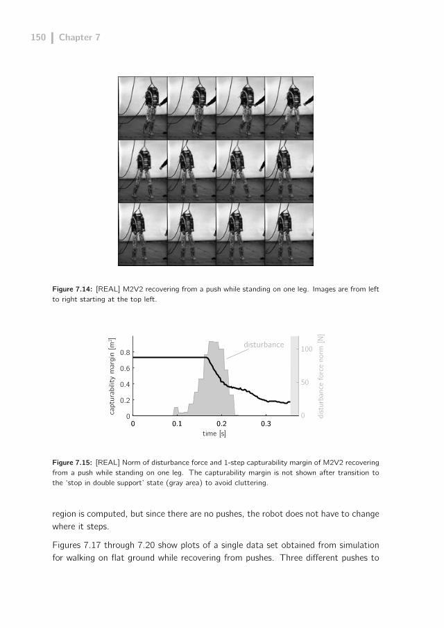
150 Chapter 7

Figure 7.14: [REAL] M2V2 recovering from a push while standing on one leg. Images are from leftto right starting at the top left.

0 0.1 0.2 0.30

50

100

time [s]

dist

urba

nce

forc

e no

rm [N

]

capt

urab

ility

mar

gin

[m2 ]

0 0.1 0.2 0.30

0.2

0.4

0.6

0.8disturbance

Figure 7.15: [REAL] Norm of disturbance force and 1-step capturability margin of M2V2 recoveringfrom a push while standing on one leg. The capturability margin is not shown after transition tothe ‘stop in double support’ state (gray area) to avoid cluttering.

region is computed, but since there are no pushes, the robot does not have to changewhere it steps.

Figures 7.17 through 7.20 show plots of a single data set obtained from simulationfor walking on flat ground while recovering from pushes. Three different pushes to

Robot prototype: capturability based control 151

Figure 7.16: [REAL] M2V2 robot walking on flat ground. Images are from left to right startingat the top left. In this walk, the robot uses a constant step length of 0.35 m and a constant stepwidth of 0.20 m. The average walking velocity is 0.21m/s.

0 2 4 6 8 10 12 140

50

100

150

200

250

300

time [s]

late

ral d

istur

banc

e fo

rce

[N]

0 2 4 6 8 10 12 14−0.4

−0.2

0

0.2

0.4

late

ral C

oM v

elocit

y [m

/s] disturbance

Figure 7.17: [SIM] Lateral velocity and disturbances of the M2V2 simulation while recovering frompushes during walking. After each push, the lateral CoM velocity increases by up to 0.44 m/s.

the left occur at approximately 4, 8.5, and 13 seconds. These pushes are modeledas forces applied to the midpoint between the hip joints and are 300 N in magnitudefor a duration of 0.05 seconds. This corresponds to an impulse of 15 Ns. Note thatpushes were to the left while the left foot was swinging. Pushes to the opposite sidewould require either a cross-over step or two quick steps, both of which are more

152 Chapter 7

(a)

(b)desired heading

Figure 7.18: [SIM] Robot as it walks while being pushed laterally to the left every second step. (a)Side view. Trajectories of the ankles are indicated with dashed lines. (b) Overhead view. Actualankle trajectories connect the sequence of footprints for each foot. The instantaneous capture pointtrajectory is indicated with a dashed line.

difficult to achieve and are an area of future work.

Figure 7.17 shows the sideways pushes applied to the M2V2 simulation, and theresulting change in velocity while recovering to pushes during walking. Since thepushes were mostly to the side, the change in lateral velocity is more prominent thanforward velocity. After each push we see that the robot recovers with one step.

Figure 7.18 shows side and overhead views of the robot. Each time a push occurs,the robot steps to the left to recover from the push. Also plotted in the overheadview are the instantaneous capture point trajectory and the trajectory of each ankle.

Figure 7.19 shows the 1-step capturability margin during walking of the M2V2 simula-tion while recovering from pushes. We see that the capturability margin significantlydecreases after each of the 3 pushes, corresponding to the decrease in area of thecapture region as seen in Figure 7.20.

Figure 7.20 shows a time-lapsed overhead view of the robot. In the first two framesthe capture region is relatively large during the beginning of swing. The robot isthen pushed between the first and second frame, decreasing the size of the captureregion and requiring the robot to choose a different place to step. In frames 3-6 therobot steps further to the left than originally intended, landing in the 1-step captureregion, and successfully recovering from the push.

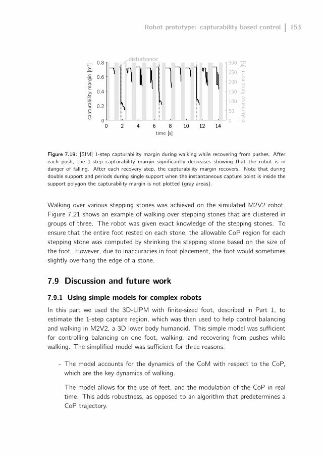
Robot prototype: capturability based control 153

0 2 4 6 8 10 12 140

50

100

150

200

250

300

time [s]

dist

urba

nce

forc

e no

rm [N

]

capt

urab

ility

mar

gin

[m2 ]

0 2 4 6 8 10 12 140

0.2

0.4

0.6

0.8 disturbance

Figure 7.19: [SIM] 1-step capturability margin during walking while recovering from pushes. Aftereach push, the 1-step capturability margin significantly decreases showing that the robot is indanger of falling. After each recovery step, the capturability margin recovers. Note that duringdouble support and periods during single support when the instantaneous capture point is inside thesupport polygon the capturability margin is not plotted (gray areas).

Walking over various stepping stones was achieved on the simulated M2V2 robot.Figure 7.21 shows an example of walking over stepping stones that are clustered ingroups of three. The robot was given exact knowledge of the stepping stones. Toensure that the entire foot rested on each stone, the allowable CoP region for eachstepping stone was computed by shrinking the stepping stone based on the size ofthe foot. However, due to inaccuracies in foot placement, the foot would sometimesslightly overhang the edge of a stone.

7.9 Discussion and future work

7.9.1 Using simple models for complex robots

In this part we used the 3D-LIPM with finite-sized foot, described in Part 1, toestimate the 1-step capture region, which was then used to help control balancingand walking in M2V2, a 3D lower body humanoid. This simple model was sufficientfor controlling balancing on one foot, walking, and recovering from pushes whilewalking. The simplified model was sufficient for three reasons:

- The model accounts for the dynamics of the CoM with respect to the CoP,which are the key dynamics of walking.

- The model allows for the use of feet, and the modulation of the CoP in realtime. This adds robustness, as opposed to an algorithm that predetermines aCoP trajectory.

154 Chapter 7

C

C

C C

C C

center of masscenter of mass velocityinstantaneous capture point

initial step locationadjusted step location

stance foot (right)swing foot (left)

capture regionC

t = 0.00 t = 0.12

t = 0.24 t = 0.36

t = 0.48 t = 0.60

Figure 7.20: [SIM] Time-lapse overhead view of the robot during the walking task, showing onestep. The robot is perturbed laterally at the start of the step (t = 0).

- The 1-step capture region is relatively large for moderate speed walking. The-refore, there is a large degree of robustness to modeling errors.

The presented control algorithms did not exploit angular momentum of the upperbody as a means of control. As we start to address more challenging tasks, likewalking over rough terrain and over narrow beams, we will likely need to use morecomplex models for computing capture regions and developing control strategies. InPart 1, we analyzed the 3D-LIPM with finite-sized foot and reaction mass. Thismodel should be useful in control when upper body angular momentum is used toprevent falling. In future work we will use this model and will investigate other strate-gies for using multi-joint upper body angular momentum in walking and disturbancerecovery.

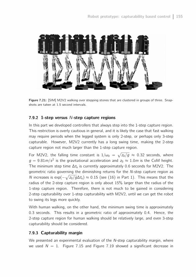
Robot prototype: capturability based control 155

Figure 7.21: [SIM] M2V2 walking over stepping stones that are clustered in groups of three. Snap-shots are taken at 1.5 second intervals.

7.9.2 1-step versus N-step capture regions

In this part we developed controllers that always step into the 1-step capture region.This restriction is overly cautious in general, and it is likely the case that fast walkingmay require periods when the legged system is only 2-step, or perhaps only 3-stepcapturable. However, M2V2 currently has a long swing time, making the 2-stepcapture region not much larger than the 1-step capture region.

For M2V2, the falling time constant is 1/ω0 =√z0/g ≈ 0.32 seconds, where

g = 9.81m/s2 is the gravitational acceleration and z0 ≈ 1.0m is the CoM height.The minimum step time ∆ts is currently approximately 0.6 seconds for M2V2. Thegeometric ratio governing the diminishing returns for the N-step capture region asN increases is exp(−

√z0/g∆ts) ≈ 0.15 (see (16) in Part 1). This means that the

radius of the 2-step capture region is only about 15% larger than the radius of the1-step capture region. Therefore, there is not much to be gained in considering2-step capturability over 1-step capturability with M2V2, until we can get the robotto swing its legs more quickly.

With human walking, on the other hand, the minimum swing time is approximately0.3 seconds. This results in a geometric ratio of approximately 0.4. Hence, the2-step capture region for human walking should be relatively large, and even 3-stepcapturability should be considered.

7.9.3 Capturability margin

We presented an experimental evaluation of the N-step capturability margin, wherewe used N = 1. Figure 7.15 and Figure 7.19 showed a significant decrease in

156 Chapter 7

this capturability margin when the robot was perturbed, as expected. For both thebalancing task and the walking task, the capturability margin recovered completelyafter taking one step.

According to the theoretical considerations presented in Part 1, the capturabilitymargin should never increase unless a step is taken or an external force is exerted onthe robot. Any other increases in capturability margin are due to modeling errors,sensor noise and lack of exact knowledge about when the swing foot hits the ground.

7.9.4 Estimation of center of mass position and velocity

The algorithm presented, like most feedback control algorithms for bipedal walking,relies on a good estimation of the CoM location and velocity, particularly in thehorizontal plane. Obtaining such an estimate on a physical robot is difficult forseveral reasons.

Knowing the CoM projection on the ground requires knowing which way is down. Asmall error in the perceived orientation of the body can result in a significant error inthe CoM projection. For example, if the CoM is at a height of 1 meter and there isa 0.01 radian error in the body orientation, that will result in approximately a 10 mmerror of the CoM on the ground. For 3D robots, orientation is typically determinedusing an inertial measurement unit (IMU), and therefore having a good IMU andrelated sensor processing is important.

Using leg kinematics to estimate the CoM velocity has the problem that one mustassume that the foot is not moving. However, if the foot is slipping, this assumptionwill make the CoM seem to be moving in the opposite direction. On the other hand,integrating an accelerometer to estimate velocity has the problem of error accumu-lation. For M2V2 we have used a combination of leg kinematics and accelerometermeasurements. We have not yet determined how accurately our CoM velocity esti-mate is, but we believe we can do much better and therefore improve performanceon the physical robot.

7.9.5 Uneven ground

Both the models presented in Part 1 and the control algorithm presented in Part 2 as-sumed flat ground. We have performed some preliminary simulations with moderateslopes and relatively small steps, and so far it appears that the same models are appli-cable to these types of terrain. However, for large slopes and steps, and very roughground, the models will likely need to be expanded and further control strategieswill need to be developed. In addition, we still need to develop capturability-basedmodels and control strategies for situations where hands can push against walls or

Robot prototype: capturability based control 157

hold handrails, or where feet can be on different slopes. In these cases concepts likeforce closure will need to be taken into account, rather than only using the CoP.

7.9.6 Controlling velocity versus coming to a stop

Capturability measures the ability of a legged system to come to a stop in N stepsor fewer. However, we are not usually interested in coming to a stop, but rathermaintaining an average speed. Even though capturability is based on the ability tocome to a stop, using tools based on capturability does not require the legged systemto come to a stop. Instead, capturability only specifies bounds on what is permissible.Within these bounds, there is ample room for such things as controlling velocity, forexample by CoP or foot placement.

7.9.7 Cross-over steps

In this study, we only considered pushes during single support which did not requirea cross-over step. Cross-over steps are challenging for a number of reasons. Theswinging leg needs to make sure to not contact the support leg. To do that, the pathof the leg may be longer, requiring longer swing time. Also, the length of the stepwill be smaller than it can be when the leg swings to the outside. An alternative isto quickly step straight down with the currently swinging leg and then quickly swingthe other leg to prevent a fall. This two-step recovery strategy requires extra timeto execute and for significant pushes will likely only be successful for robots with arelatively short swing time, on the order of how fast humans can swing their legs.

7.9.8 Virtual toe points and center of pressure

The presented control algorithm relies on the use of virtual toe points to tracka desired CoP. Virtual toe points can be interpreted as the attachment points ofvirtual actuators on the feet, and each virtual toe point is used to gain approximatecontrol of each individual foot’s CoP. The virtual toe point and a foot’s CoP willbe theoretically identical if the robot is in single support, the vertical force of thevirtual actuator equals the weight of the robot, and the vertical acceleration is zero.In simulation, the two points always remain close (within a few cm) during singlesupport. During double support, there can be a large error between the desired andactual CoP, particularly when one of the legs is stretched. For example, if the hindleg is completely stretched, and the desired CoP is on the heel of the hind leg, thenthe virtual actuator on the hind leg will be assigned a large leg support fraction.However, since the leg is straight, the actual joint torques that the virtual actuatorproduces will be small, and the CoP will be located more forward than desired.

158 Chapter 7

One way to obtain a better match between the desired and actual CoP is to keepthe knees of the robot bent to avoid losing kinematic range. However, we wish toavoid that solution since human walking does not rely on bent knees and becauseit requires unnecessarily high torques at the knees. Another solution, which we willinvestigate in future work, is to use toe off on the rear leg to better control theCoP during double support. Currently, some toe off occurs at the end of the stride,but it is simply the result of the dynamics of the walk, rather than the result of anintentional control action.

7.9.9 Foot placement speed and accuracy

In this paper, we showed how foot placement can be used to regain balance after apush. Doing so requires a fast swing that is accurate enough to make the foot landin the capture region. However, due to the use of SEAs with very compliant springs,we have had difficulty to quickly and accurately swing the leg. Although SEAs enablecompliant control, they can make joint position trajectory tracking challenging. Webelieve that we can achieve the same favorable compliant control characteristics andbetter tracking by increasing the stiffness of the series springs. On the other hand,we also believe that swing can be performed in a more compliant manner, determinedmostly by the passive pendulum dynamics of the leg, as opposed to using traditionalhigh-gain trajectory tracking. Determining swing strategies that allow for fast andaccurate steps while exploiting the natural dynamics of the leg is an area of futurework.

7.9.10 Application to other robots

We believe that capturability concepts can be applied to the analysis and controlof other legged systems. Estimating capture regions and determining capturability-based robustness metrics should be possible for all legged systems. While we advocatecompliant force control for legged robots, most of the techniques described in thispaper should also apply to high-gain position trajectory tracking robots. Steppingstrategies that take the capture region into account should be applicable to any robotthat can change where it steps on-the-fly. Control of the instantaneous capture pointshould be applicable to any robot that can control its CoP location on the ground.We are currently expanding the algorithms presented in this paper and working towardtheir application on several different humanoid robot platforms.

7.10 Conclusion

This paper showed an application of the N-step capturability framework to a 12-DoFbipedal robot. The main contributions of this part were step location adjustment

Robot prototype: capturability based control 159

using the 1-step capture region and instantaneous capture point control by CoPplacement, which are key ingredients to the presented control algorithm. In addition,the 1-step capturability margin was experimentally evaluated.

Acknowledgements

The authors would like to thank A. Goswami and E. Westervelt for their helpfulcomments.

M2V2 is a second generation version of the M2 robot, developed by G. Pratt, D.Paluska, J. Pratt, and D. Robinson at the MIT Leg Laboratory. M2V2 was designedby B. Krupp, V. Ragusila, I. Olaru, T. Craig, and J. Pratt. M2V2 electronics andinterface software was designed by G. Watkins, S. Emami, T. Hutcheson, J. Pratt,J. Smith, and S. Nayak. M2V2 was assembled and maintained by T. Craig and J.Taylor. The force sensing push stick used in push recovery experiments on M2V2was designed and constructed by J. Joyner.

A team at Bucknell University, led by S. Shooter and K. Buffinton, have designedimproved feet and a vision head for the robot. Students involved include M. Kandler,D. Snyder, L. Markison, J. Ricci and C. Hubicki.

Various low-level control modules for M2V2 were developed by C. Shake, N. vanNieuwenhuizen, F. Cañas, D. Garg, S. Tamadoni, R. van Doesburgh, T. Koolen,J. Pratt, M. Johnson, and P. Neuhaus. A team from NASA JSC, consisting of J.Braman, D. Gooding, S. Tamblyn, M. Goza and A. Hulse, has also contributed inthis area.

M2V2 filming and video editing was performed by W. Howell. Part acquisition andlab management was performed by B. Layton.

Simulation Software and user interfaces were improved by J. Carff, M. Fortenberry,D. Reyes Duran, G. Barr, B. Waxler, and P. DeMonaco.

Appendix

Robot parameters

Table 7.1 shows the joint layout and inertia parameters of M2V2. Each row repre-sents a joint and its associated rigid body. We use a coordinate system in which x isforward, y is to the left, and z is up. Note that the bottom 6 rows represent the leftleg joints and masses (marked with the letter ‘L’). The right leg is a mirror imageof the left leg, and thus is identical to the left leg except for the y values, which are

160 Chapter 7

all the additive inverse. For Pin-type joints, the letter following “Pin” refers to therotational axis that the joint is aligned with.

Robot prototype: capturability based control 161

Tab

le7.

1:Robot

jointandmasslayout.

Offsetfrom

Parent[m

]COM

offset[m

]Mom

entof

Inertia[kgm

2]

Joint

Parent

xy

zJointType

Mass[kg]

xy

zI xx

I yy

I zz

Root

N/A

0.0

0.0

0.0

Floating

24.0

0.0

0.0

0.0

2.756

2.756

0.380

Lhipyaw

root

0.0

0.092

-0.381

Pin-Z

0.2

0.0

0.0

0.0

5.3E

-45.3E

-45.3E

-4

Lhiproll

Lhipyaw

0.0

0.0

0.0

Pin-X

0.0

0.0

0.0

0.0

0.0

0.0

0.0

Lhippitch

Lhiproll

0.0

0.0

-0.029

Pin-Y

4.6

-0.0318

0.006

-0.229

0.044

0.044

0.004

Lknee

Lhippitch

0.0

0.0

-0.450

Pin-Y

4.3

-0.025

0.0

-0.229

0.054

0.054

0.003

Lanklepitch

Lknee

0.0

0.0

-0.467

Pin-Y

0.11

0.0

0.0

0.0

2.6E

-42.6E

-42.6E

-4

Lankleroll

Lanklepitch

0.0

0.0

0.0

Pin-X

0.727

0.0127

0.0

-0.051

3.63E-4

0.002

0.002

8Robot prototype: performance

164 Chapter 8

8.1 Introduction

This chapter presents and evaluates the performance of the robot prototype TUlipintroduced in Chapter 6 with the implemented control algorithms described in Chap-ter 7. We tested the performance of the robot on various aspects that we considerimportant to achieve a robust gait. These aspects have been discussed separately inearlier chapters; a short overview is given below.

- center of mass control through control of the center of pressure location;

- control of the center of pressure location through force controllable joints;

- compliant control of the force controllable joints to achieve natural robustnessto unknown terrain or external perturbations;

- joint control through high-level task-based control of essential tasks in bipedallocomotion (e.g., body height, orientation and speed, foot placement control,center of pressure control);

- adaptive, fast and accurate foot placement.

We tested the robot on these five aspects by conducting several experiments, whichare two-legged balancing, single-legged balancing, foot placement and single-leggedbalancing with foot placement to recover from a push.

Results of walking experiments are not included in this chapter since we found thatthe foot placement performance is currently not sufficiently accurate and fast toachieve a robust walking gait. Possible solutions are discussed in Section 8.6 whichevaluates the robot hardware and software.

8.2 Two-legged balancing

First, we tested the ability to control the center of pressure location and thereby thecenter of mass. The robot was commanded to remain balanced on two feet withslightly bent knees while being pushed from the side and back. The active controllerwas the stance-sub controller described in Section 7.7.5 which controlled the upperbody height, orientation, and instantaneous capture point location through controlof the center of pressure location (by controlling the virtual toe points). Results ofthis experiment are shown in Figure 8.1. The figure shows how the virtual toe pointsand support fractions are adjusted to achieve the desired center of pressure locationand drive the instantaneous capture point back towards the desired instantaneous

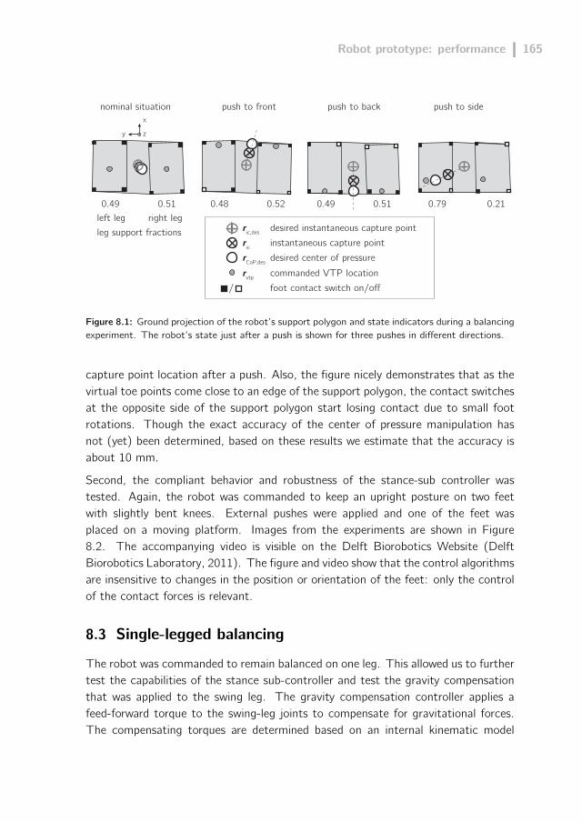
Robot prototype: performance 165

y

x

z

nominal situation push to front push to back push to side

rvtp

ric,des desired instantaneous capture point

rCoP,des

foot contact switch on/off

ric

commanded VTP locationdesired center of pressureinstantaneous capture point

/

0.49 0.51 0.48 0.52 0.49 0.51 0.79 0.21

leg support fractionsleft leg right leg

Figure 8.1: Ground projection of the robot’s support polygon and state indicators during a balancingexperiment. The robot’s state just after a push is shown for three pushes in different directions.

capture point location after a push. Also, the figure nicely demonstrates that as thevirtual toe points come close to an edge of the support polygon, the contact switchesat the opposite side of the support polygon start losing contact due to small footrotations. Though the exact accuracy of the center of pressure manipulation hasnot (yet) been determined, based on these results we estimate that the accuracy isabout 10 mm.

Second, the compliant behavior and robustness of the stance-sub controller wastested. Again, the robot was commanded to keep an upright posture on two feetwith slightly bent knees. External pushes were applied and one of the feet wasplaced on a moving platform. Images from the experiments are shown in Figure8.2. The accompanying video is visible on the Delft Biorobotics Website (DelftBiorobotics Laboratory, 2011). The figure and video show that the control algorithmsare insensitive to changes in the position or orientation of the feet: only the controlof the contact forces is relevant.

8.3 Single-legged balancing

The robot was commanded to remain balanced on one leg. This allowed us to furthertest the capabilities of the stance sub-controller and test the gravity compensationthat was applied to the swing leg. The gravity compensation controller applies afeed-forward torque to the swing-leg joints to compensate for gravitational forces.The compensating torques are determined based on an internal kinematic model

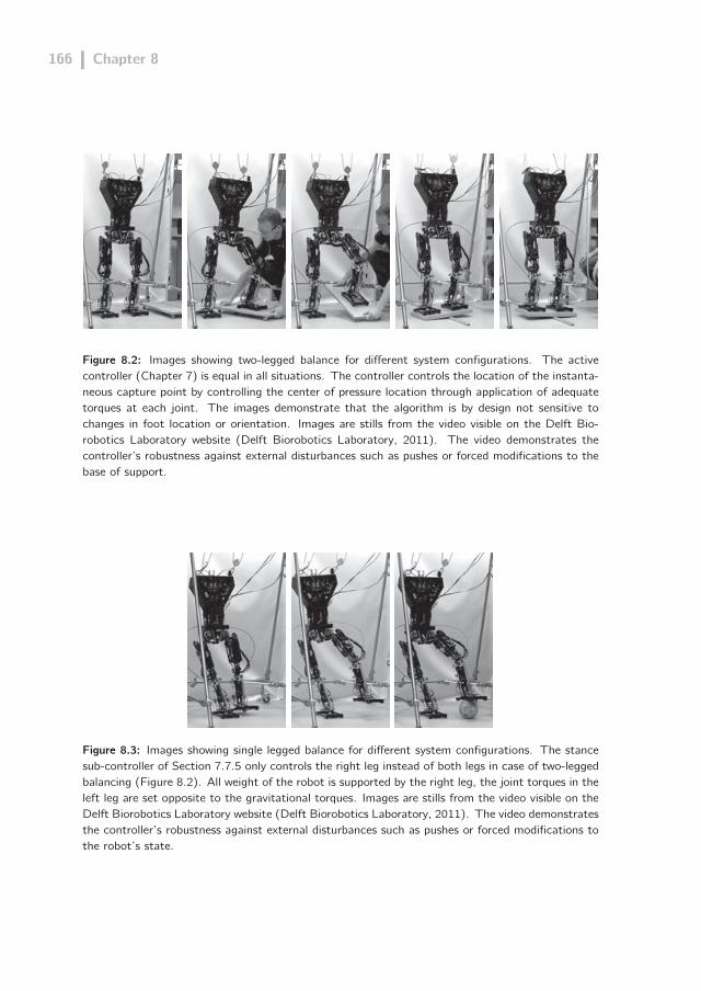
166 Chapter 8

Figure 8.2: Images showing two-legged balance for different system configurations. The activecontroller (Chapter 7) is equal in all situations. The controller controls the location of the instanta-neous capture point by controlling the center of pressure location through application of adequatetorques at each joint. The images demonstrate that the algorithm is by design not sensitive tochanges in foot location or orientation. Images are stills from the video visible on the Delft Bio-robotics Laboratory website (Delft Biorobotics Laboratory, 2011). The video demonstrates thecontroller’s robustness against external disturbances such as pushes or forced modifications to thebase of support.

Figure 8.3: Images showing single legged balance for different system configurations. The stancesub-controller of Section 7.7.5 only controls the right leg instead of both legs in case of two-leggedbalancing (Figure 8.2). All weight of the robot is supported by the right leg, the joint torques in theleft leg are set opposite to the gravitational torques. Images are stills from the video visible on theDelft Biorobotics Laboratory website (Delft Biorobotics Laboratory, 2011). The video demonstratesthe controller’s robustness against external disturbances such as pushes or forced modifications tothe robot’s state.

Robot prototype: performance 167

and the measured direction of the gravitational acceleration vector. The results areshown in Figure 8.3 and the accompanying video (see Delft Biorobotics Laboratory,2011). The figure and video demonstrate how the robot remains balanced on oneleg when the posture of the robot is changed. The gravity compensation workedsufficiently which validated the accuracy of the robot’s internal kinematic model.

8.4 Foot placement

The attainable speed and accuracy of foot placement were determined.

First, the robot was commanded to swing the leg forward over a distance of 650mm within 1 second. The swing leg trajectory was generated using a trajectorygenerator based on inverse kinematics. Inputs for the generator were three desiredfoot configurations: the foot position and orientation at the start of the step, atthe end of the step and at one point in between. The foot position and orientationin between was selected in such a way that the toe would not scuff the floor inmid-swing. Outputs of the generator were the reference joint positions and jointvelocities. These outputs were obtained by creating a smooth path in joint-spacethat would satisfy the three reference input configurations. The reference positionsand velocities were tracked by digital PID position control in the joints (see Figure6.3).

Kinematic data from a single step is shown in Figure 8.4 that illustrates the footplacement performance of TUlip in the forward direction. The tracking performanceof the system was found to be poor: the error between the real foot position anddesired foot position easily grew to about 150 mm along the trajectory. The finalpositional error was typically about 50 mm. The results demonstrate that the serieselastic actuators proved incapable of accurately tracking the given reference trajec-tory. Section 8.6 discusses the causes of this problem and describes the research wehave initiated to solve this problem.

Second, the robot was commanded to swing the leg to the side over a distance of350 mm within 1 second. The resulting accuracy was about 15 mm (partly becausethe hip roll joint is not actuated through a series elastic actuator, contrary to the hippitch joint). Gearbox play in the hip roll actuator did initially introduce an inaccuracyof about 40 mm in the lateral foot position, but this could be compensated for insoftware since the stepping motion was unidirectional.

The accuracy and repeatability of foot placement have to be improved, especiallyin the forward direction, before the robot can perform a robust walking gait. Thelateral foot placement performance did prove to be sufficient to test the robot’s

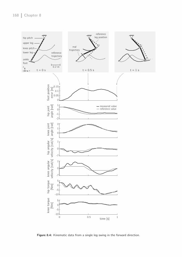
168 Chapter 8

0.2 m

lower leg

hip pitch

knee pitch

anklefoot

upper leg

referencetrajectory

measured value

realtrajectory

referenceleg position

10.5

t = 0.5 st = 0 s t = 1 s

time [s]

knee

ang

ular

velo

city

[rad/

s]hi

p an

gular

velo

city

[rad/

s]kn

ee jo

int

angl

e [ra

d]hi

p jo

int

angl

e [ra

d]

0

-7

0

0

7

-7

7

12

0

-2

01

-1

foot

pos

ition

erro

r [m

]

0

0.10.15

0.05

reference value

-10

05

-5

-10

05

-5

knee

tor

que

[Nm

]hi

p to

rque

[Nm

]

zxy

Figure 8.4: Kinematic data from a single leg swing in the forward direction.

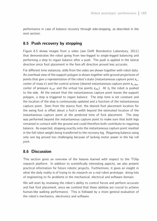
Robot prototype: performance 169

performance in case of balance recovery through side-stepping, as described in thenext section.

8.5 Push recovery by stepping

Figure 8.5 shows images from a video (see Delft Biorobotics Laboratory, 2011)that demonstrates the robot going from two-legged to single-legged balancing andperforming a step to regain balance after a push. The push is applied in the lateraldirection since foot placement in the fore-aft direction proved less accurate.

For different time instances, stills from the video are shown together with robot data.An overhead view of the support polygon is shown together with ground projections ofpoints that give a representation of the robot’s state (instantaneous capture point ric,center of mass r) and the control actions (desired instantaneous capture point ric,des,center of pressure rCoP and the virtual toe points rvtp). At t0 the robot is pushedto the side. At the instant that the instantaneous capture point leaves the supportpolygon, a step is triggered to regain balance. The step time is set constant andthe location of the step is continuously updated and a function of the instantaneouscapture point. Seen from the stance foot, the desired foot placement location forthe swing foot is offset about a foot’s width beyond the estimated location of theinstantaneous capture point at the predicted time of foot placement. The stepwas performed beyond the instantaneous capture point to make sure that both legsremained in contact with the ground and could therefore both contribute to regainingbalance. As expected, stepping exactly onto the instantaneous capture point resultedin the full robot weight being transferred to the recovery leg. Regaining balance usingonly one leg proved too challenging because of lacking motor power in the hip rolljoint.

8.6 Discussion

This section gives an overview of the lessons learned with respect to the TUlipresearch platform. In addition to scientifically interesting aspects, we also presentpractical information for future robotic projects. Furthermore, it gives an insight inwhat the daily reality is of trying to do research on a real robot prototype: doing lotsof engineering to fix problems in the mechanical, electrical and software domain.

We will start by reviewing the robot’s ability to control forces and perform accurateand fast foot placement, since we contend that these abilities are crucial to achievehuman-like walking performance. This is followed by a more general evaluation ofthe robot’s mechanics, electronics and software.

170 Chapter 8

rvtp

ric,des

rCoP,des

r

ric

stance footswing foot

direction of push(estimated)

desired steplocation

y

xt0 [s]

start push

t0 + 0.20

initiate step

t0 + 0.55s

halfway step

t0 + 0.90

foot impact

t0 + 1.15

max. CoMexcursion

t0 + 1.50

steady state

Figure 8.5: Example result of a step to regain balance after a push. The step is directed towardsthe predicted instantaneous capture point at the predicted time of foot impact.

Robot prototype: performance 171

8.6.1 Force controllability

The benefit of force based control with respect to robust balance control was de-monstrated by the balancing experiments presented in this chapter. Force controloffered the ability to control the contact forces between the foot and the ground,which made the system insensitive for the exact position and orientation of the foot.Also, the low impedance of the series elastic actuator made the system forgiving toexternal perturbations: the robot’s posture could be easily changed by the operatorwithout leading to a fall of the robot.

However, the intrinsically low impedance of the employed series elastic actuator didhamper fast and accurate trajectory tracking of joint positions. The resulting lowforce controllable bandwidth of the actuators resulted in poor tracking performancewhen using conventional high-gain feedback control. Increasing the tracking perfor-mance would require a well designed feedforward signal. For non repetitive motions,designing such a feedforward signal would require an accurate dynamic model (e.g.,see Randazzo et al., 2011). In order not to depend too much on such potentiallycomplex models, we believe that future robots are best served with series elastic ac-tuators with a higher series stiffness. To compensate for the resulting loss in shocktolerance, a low-stiffness element could be placed in the foot. This configurationwould result in an intrinsically high shock tolerance at the foot and moderate shocktolerance for impacts occurring elsewhere on the body. In the future, new conceptsof variable impedance actuators might also be developed that have an acceptable po-wer to weight ratio and thereby have added value over constant impedance actuators(van Ham et al., 2007; Hurst et al., 2004; Schiavi et al., 2008; Wolf and Hirzinger,2008).

Furthermore, for future robots we see benefit in using a concept of series elasticactuation that requires no pre-loading force. The pre-loading force in the actuatorsof TUlip affected the whole chain of components between the actuator and the joint.This resulted in friction and wear of the components. Though a concept can be usedwhere the pre-load affects only the springs (e.g., see Pratt and Williamson, 1995),it is also possible to use an elastic element that requires no pre-load. For example,a compliant element with an angular stiffness such as a double spiral spring (Lagodaet al., 2010), torsion bar (Pratt and Williamson, 1995) or the motor gearhead itself(Neuhaus et al., 2011).

8.6.2 Foot placement

The robot’s limited ability to perform fast and accurate foot placement should besolved in mechanics and in software.

172 Chapter 8

Regarding the mechanics, besides the above-mentioned issues with the series elas-tic actuators, we found that gearbox play (about 1 degree for TUlip’s planetarygearheads) had a significant effect on the accuracy of foot placement. Differenttransmission concepts should be used on future robots that have less play, such asspindle drives or harmonic drives.

Regarding the software, a swing leg controller that generates swing leg trajectoriesbased on inverse kinematics is simple to implement, but the generated joint trajec-tory can be far from optimal. We strive to use control methods that can generatea swing leg trajectory while taking system limitations into account (e.g., minimalfoot clearance, maximum torque change). We aim not to optimize these controltrajectories offline and simply play them back on the robot, but to optimize themonline. We are investigating the use of model predictive control online, which alsouses feedback of the real swing leg to account for modeling errors or disturbances.

8.6.3 Mechanics

The improvements made to the robot mechanics were mainly to improve the robust-ness, repeatability and controllability of the system.

Robustness

The robustness of the mechanical structure was improved. The strength of someof the components sometimes proved insufficient, as can be expected for a robotdesign where the focus has been on keeping the mechanical structure as light aspossible. Especially in the case of unexpected and abrupt robot behaviors, compo-nents regularly broke or were damaged. A seemingly easy solution is off course toprevent these actions from occurring in the first place. Testing control algorithms insimulation or limiting output torques or angular velocities of course helps. However,robot behavior can remain hard to comprehend and non-intuitive as it involves manydimensions, especially in the case of control algorithms that control multiple joints.Moreover, issues with the robot’s simulation model (see Section 8.6.5) made testingof new control algorithms hard. Therefore, most of the time, a slightly unsatisfac-tory and potentially deficient solution was chosen by replacing the broken part for are-designed part and preventing the same destructive robot behavior from occurringagain. Furthermore, more mechanical fuses and stops were added to the system toprevent damage. None of the newly designed parts lead to functional changes of therobot nor did it lead to new scientific insight. It does however illustrate how timeconsuming research on a real robot can be.

To improve the ease of servicing the robot and keeping it operational, we see greatbenefit from using more modular structural units in the robot. For example, modular

Robot prototype: performance 173

actuator units. TUlip has many series elastic actuators which are all conceptuallythe same but mechanically different. This requires different control tools for eachactuator and hampers quick repairs to the robot because of the many different com-ponents which are typically too costly to all keep on stock. A modular unit can solvethese problems. Modular actuator modules at each joint can come at the cost ofbeing less tailored to the specific needs of that joint and might result in a suboptimalrobot performance. However, the exact needs for a specific joint are not always welldefined, especially for a completely new robot prototype. Having thoroughly testedand well characterized actuator modules that are potentially slightly suboptimal canstill be preferable. The experience is that the robot can only serve as a true researchplatform for walking experiments if the hardware is robust and easy to maintain.Otherwise, it will serve as a platform that can only be used to demonstrate a proofof concept, which is unfortunately the case for TUlip and maybe even for most ofthe humanoid robot platforms that currently exist.

Repeatability

The repeatability of the robot behavior was initially insufficient and had to be impro-ved: executing the same foot placement strategy one day or the next day could leadto a significant difference in the resulting robot behavior. The main cause of this waspoor force-fidelity of the series elastic actuators, caused by friction in the drivetrainand the inadequate initialization of the actuators at the startup of the robot. Theseissues are discussed below.

Friction in a series elastic actuator is not necessarily harmful for its ability to accura-tely control joint torque: frictional losses between the geared motor and the elasticelement are compensated because the true elements’ deflection is fed back to thetorque controller. Consequently, the force-fidelity of the geared motor can be low.However, due to the initially high pre-loading force in the series elastic system ofTUlip, viscous and coulomb friction was found between the elastic element and thejoint. These frictional losses are not measured and therefore do affect the perfor-mance of the actuator. This issue was solved by lowering the pre-loading force onthe system by replacing the tension springs with ‘spring units’ (Figure 6.7) and byreplacing the sleeve bearings in the idler pulleys (Figure 6.6) with ball bearings.

The initialization of the robot comprises the calibration of the incremental jointand motor encoders. Especially the series elastic actuators rely heavily on accuratecalibration of these encoders, since the difference between the measured joint angleand measured motor angle directly determines the measured joint torque. At therobot startup, there typically is a nonzero joint torque since the elastic elementstypically have a nonzero deflection due to friction in the actuator (resulting in a poor

174 Chapter 8

backdrivability of the actuator). Proper initialization should determine the joint angleand motor angle that correspond to a zero joint torque.

Initially, the robot was initialized using a dynamic process. The robot was hungupright and the series elastic actuated joints were swung to the front and to theback by applying an equal but opposite motor current in both directions. The jointencoders were calibrated when the index pulse was detected, which corresponded to aknown joint angle. The motor encoders were calibrated based on the difference in themaximal measured joint angle in both directions. This difference was assumed to becaused by play in the gearbox and an initially present joint torque. Given the measureddifference, an assumed zero position of the motor encoder was estimated. However,the repeatability of this calibration proved to be poor. Therefore, a mechanicalcalibration rig was constructed to solve this issue. The calibration rig fixes the robotjoints at known angles. At the same time, we applied a sinusoidal signal to the motorof the series elastic actuators. Any initially present joint torque could be accuratelydetected since it resulted in a difference in the measured maximal motor angle inboth directions.

Controllability

The controllability of the system was improved by adding ankle actuation in the ankleroll joint. Though the effect of lateral ankle actuation remains limited due to thesmall foot width that allows for relatively low maximum torques, creating versatilemotions with a mechanically fixed ankle stiffness and equilibrium position provedimpractical.

8.6.4 Electronics

Hardly any modifications have been made to the electronics. Since almost all theelectronic components were high-end off-the-shelf components, only small problemsarose with the electronics of TUlip.

The only concern of the current electronic architecture is its weight. The electroniccomponents contribute to about 32% of the total weight of TUlip (Figure 6.14),which is very significant. About 40% of the weight of the electronics consists ofcables running from the central computer to all the sensors and actuators. With therecent advancements in the development of small and powerful motor control boards,distributed control for future humanoid robots seems preferable. Their ability to dosensor processing locally reduces the amount of cables significantly. This reduction iseven larger for controller boards that can operate in a daisy chain. Also, their abilityto do motor control alleviates the central computer from this control tasks.

Robot prototype: performance 175

8.6.5 Software

Besides the large effort that was put into the development of new control software,a lot of effort was also put into the development of tools to visualize, log and tunerobot parameters. These tools enable the analysis of experimental data offline ormodify robot behavior on the fly, which proved necessary to design advanced motioncontrollers. Though the added value of these tools is obvious, development of thesetools proved less obvious since it required communication from the real-time softwarethrough the non-real-time software to an external computer.

The overall software architecture functioned adequately, mainly because the wholecontrol software architecture was custom-made and could therefore be made to fitour needs. On the one hand, we were satisfied with our custom-made software sinceit offered great flexibility and therefore was a good match for a research project. Onthe other hand, the lack of skilled people to develop all the custom-made softwaresignificantly slowed down the research progress. This practical issue should be takeninto account in future robotic projects, especially for robotic research on a university,where the throughput of people is typically high and the experience typically low.Using control software such as The Mathworks MATLAB or National InstrumentsLabVIEW might be better suited in that case. Conversely, the community of peoplethat create and share custom made robotic applications has grown rapidly over thepast years with a good example being the Robot Operating System ROS (ROS,2011).

The lack of manpower also resulted in simulation software that did not functionas intended. Around 2008, a first simulation model of the robot was realized thatcould be controlled through TUlipMC. However, the computation time was relativelylong: in the order of 20 minutes for a few steps. This limited the practical use of thesimulation model as a tool to quickly test and debug control software. Unfortunately,we lacked manpower to find the causes and solutions of this long simulation time.Consequently, we mostly used the real robot as a test platform.

8.7 Acknowledgements

The author would like to thank the many students and staff working within theDutchRobotics foundation (DutchRobotics, 2011) for their contribution to the de-velopment of TUlip and thank Jerry Pratt from IHMC for helpful tips and codesharing with respect to the implementation of Virtual Model Control (Pratt et al.,2001) on TUlip.

9Discussion, conclusions and

future directions

178 Chapter 9

9.1 Introduction

The goal of this thesis was stated as follows.

The goal of this thesis is to improve the performance of robotic bipedal loco-motion in terms of robustness, versatility and energy-efficiency, by increasingthe understanding of the mechanics and control of foot placement. Since ver-satility and energy-efficiency are only relevant when the robot can prevent afall, a strong focus lies on the robustness of gait.

To achieve this goal, three specific research questions were formulated concerningfoot placement and robustness, versatility and energy-efficiency respectively:

1. Regarding robustness: how can we determine where and when the foot shouldbe placed to prevent a fall?

2. Regarding versatility: how can we determine where and when the foot shouldbe placed to enable the system to evolve from its initial state to any desiredfuture state?

3. Regarding energy-efficiency: how do actuator limitations influence foot place-ment strategies?

This chapter starts with a section that summarizes the main findings on foot place-ment with respect to robustness, versatility and energy-efficiency. This is followedby a more general discussion on the role of foot placement in bipedal locomotion.Finally, we state the main conclusions of this research and give directions for futureresearch.

9.2 Recapitulation

9.2.1 Foot placement and robustness

The most generic and unrestrictive definition of stability for a legged system is ‘toavoid falling’, described by the concept of viability (Aubin, 1991; Wieber, 2002).However, establishing which states are viable is generally computationally expensive,which causes this concept to be of limited practical value for controller synthesisfor bipedal locomotion. Therefore, this thesis introduced the theoretical frameworkof capturability (Chapter 3). Capturability was shown to effectively approximateviability, to be computable for simple models and to be valuable for the analysis andcontrol of bipedal locomotion. Characteristic to the capturability framework is thatit analyzes fall avoidance by considering N-step capturability: the system’s ability

Discussion, conclusions and future directions 179

to eventually come to a stop without falling by taking N or fewer steps, given itsdynamics and actuation limits. The number of steps required to come to a stop isused as a measure of how close the legged system is to falling.

Computing N-step capturability for a simple model of a complex bipedal systemprovided valuable insight for the analysis and the control of the complex system.We used the 3D Linear Inverted Pendulum Model, which models the most essentialdynamics of a bipedal system: the dynamics of the CoM with respect to the CoP.Extending the model with a foot and reaction mass allowed us to derive how ankletorques and upper body motions affect the CoM dynamics and contribute to N-stepcapturability. N-step capture regions were constructed on the ground that providedpractical information on where and when to place the foot to prevent a fall. Thesize of these regions gives a measure of capturability of the system’s state and is auseful robustness metric, termed the N-step capturability margin. The introducedd∞ capturability level provides a state-independent measure of the capturability ofthe system.

The usefulness of the capturability framework was demonstrated by its successfulintegration in the control algorithm of two complex bipedal robots (Chapter 7 - 8).

9.2.2 Foot placement and versatility

The previous chapters presented how balance strategies can influence the CoM mo-tion. These balance strategies can not only be used to prevent a fall, but also forachieving a wide variety of gaits. The capturability framework allowed the construc-tion of N-step capture regions that indicated feasible stepping regions. The effectof a candidate CoP location within these regions could be directly derived by loo-king at its location relative to the instantaneous capture point location: the CoMwould asymptotically converge to the line spanned by the CoP location and the ins-tantaneous capture point location. The distance between the CoP location and theinstantaneous capture point determined at what rate the instantaneous capture pointmoved away from the CoP location. Chapter 4 presented a foot placement controllerthat explicitly derived foot placement strategies given a desired future state. Thesefindings provided simple and useful control heuristics for the control of robotic bi-pedal locomotion. Chapter 8 presented robotic single-legged balancing, two-leggedbalancing, and push recovery. It was also demonstrated how the derived foot place-ment strategies can lead to more versatile behavior such as walking while changingwalking speed, changing walking direction and navigating over stepping stones.

180 Chapter 9

9.2.3 Foot placement and energy-efficiency

Previous chapters studied how system limitations in general can affect foot placementand thereby balance. The capturability analysis of Chapter 3 demonstrated howsystem constraints such as maximal step length and minimal step time affect thecapturability of a system. Since balance control is dictated by foot placement, suchconstraints determine to a large extent the system’s capturability. Chapter 5 analyzedin more detail how actuator limitations can influence the execution and planning offoot placement. We studied the observed relation in human stumble recovery betweenthe employed stepping strategy and the timing of the stumble in the gait phase. Wefound that simple gait models demonstrate human-like foot placement strategies inresponse to a stumble when optimizing for either one of the following cost measuresfor foot placement: peak torque, power, impulse, and torque divided by time.

9.3 General discussion

This general discussion addresses how foot placement control in robotic bipedal lo-comotion relates to: (1) the objective of an overall increase of robustness, versatilityand energy-efficiency. (2) the control of the other balancing strategies, i.e., ankletorques and upper-body motions. Both issues are discussed by the evaluation offour fundamental properties of foot placement that determine the actual role of footplacement in bipedal locomotion: its effectiveness, availability, energetic cost andaccuracy.

9.3.1 On the effectiveness of foot placement

With the application of the capturability framework to the simple gait models presen-ted in Chapter 3, a quantification of the effectiveness of the stepping strategy, anklestrategy and hip strategy is possible. The effectiveness of a strategy can be analyzedbased on the amount of control that it has over the CoM motion, represented by theinstantaneous capture point. This amount can be quantified in terms of its contribu-tion to the d∞ capturability level of a system or the N-step capturability of a givensystem state. In Section 3.8 it was approximated that foot placement determinesfor at least 65% the d∞ capturability level of a human (versus 30% for the anklestrategy and 5% for the hip strategy). The analysis can be applied to a wide rangeof legged systems and legged locomotion scenarios. For example, consider the caseof one-legged balancing given in the introduction of this thesis (Figure 1.4, page 6).To be capturable using only the ankle strategy, the instantaneous capture point ismaximally at the edges of the base of support, where the CoP can just be placed. Fora human, the CoP location can be adjusted over approximately 45 mm in the frontal

Discussion, conclusions and future directions 181

plane (Hof et al., 2007; Hoogvliet et al., 1997; King and Zatsiorsky, 2002) and over200 mm in the fore-aft direction (Winter, 1990). Using only the hip strategy, thegait model with reaction mass predicts that violent upper-body motions can only en-sure capturability if the instantaneous capture point lies not more than approximately40 mm outside the base of support. This corresponds well with observations fromhuman balance studies (Hof, 2007; Horak and Nashner, 1986; Otten, 1999). Usingonly the stepping strategy, the instantaneous capture point is maximally a step sizeaway from the stance ankle to become captured in one step, which is typically about700 mm for a human. As expected, these results confirm that foot placement is themost powerful balancing strategy for control of the CoM motion.

9.3.2 On the availability of foot placement

Since foot placement control has the largest control over the CoM motion, balancecontrol in the presence of large disturbances clearly relies mostly on foot placement.Though foot placement is powerful as a control mechanism, it is conversely onlyavailable at the occurrence of the next step. Thus, as the walking speed goes tozero and step time to infinity, balance control relies solely on the ankle and hipstrategies. What does this mean for the control of walking? How should the threestrategies interact during the control of unperturbed walking at a comfortable walkingspeed?

When relying only on foot placement for balance control, the stance phase becomesa purely ballistic phase. Any inaccuracy in foot placement results in a deviation fromthe desired CoM position and velocity at the end of the stance phase. The 3D-LIPMplus foot placement controller derived in Chapter 4 allows for predictions on howdeviations from the desired CoM motion should be corrected for by the next step.For a typical human walking gait (step time 0.55 s, step length 700 mm, step width120 mm and the reciprocal of the characteristic frequency ω0 = 3 rad s−1 (Donelanet al., 2002)), a lateral inward offset from the nominal step location requires themagnitude of the next step to be a factor of 3 larger in the outward direction toarrive back at the desired nominal CoM motion. This demonstrates how small errorsat the beginning of the stance phase are magnified at the end of the stance phase.

However, this does not necessarily lead to instability, as long as foot placement isadjusted based on the deviated CoM position and velocity. The CoM may divergequickly from the nominal motion, but a single well placed step can instantaneouslyreduce or eliminate the CoM deviation. In this way, each step corrects the deviationof the CoM motion that was introduced by the previous step. The capturabilityanalysis can be used to get an indication of an acceptable step inaccuracy. For theabove mentioned human walking gait (assuming a constant step time and no ankle

182 Chapter 9

or hip torques), the 3D-LIPM model predicts that the nominal motion is 1-stepcapturable and that a step location inaccuracy of more than 35 mm can cause thesystem to become 2-step capturable. The foot placement controller of Chapter 4 canstill cope with such step inaccuracies by adjusting the next step location (with about100 mm). The resulting gait then does resemble a ‘drunk’ walk with large variationsin the average forward and lateral velocity between steps. Instead of relying solely onfoot placement to correct CoM motion deviations, the ankle strategy can be used.The continuous availability of the ankle strategy allows for continuous correctionsto the CoM motion, as was shown graphically in Figure 3.8. Foot placement canprovide gross control and ankle torques a fine tuning, as was found for human walking(Hof et al., 2007, 2010). Due to the smaller foot width than length, the amount ofcontrol that the ankle strategy has over the CoM is less in the lateral direction thanthe fore-aft direction. This implies that for lateral balance step accuracy is moreimportant than for sagittal balance. This may explain that the absolute lateral stepvariability in human walking is larger than the fore-aft step variability (28±3 mmversus 16±3 mm, Bauby and Kuo, 2000).

The relatively low amount of control over the CoM of the hip strategy makes thisstrategy a less attractive control strategy in normal walking. Humans tend to usethis strategy only in case of balancing tasks with limited footholds or in case of severeperturbations such as a stumble (Otten, 1999; Pijnappels et al., 2010; Popovic et al.,2005).

These results suggest that walking control only through foot placement is possible,but will result in a larger (than necessary) step variability to compensate for stepinaccuracies. Foot placement control is preferably accompanied by the continuouslyavailable ankle strategy to fine-tune the CoM motion. The hip strategy can be usedfor the same purpose.

9.3.3 On the energetic cost of foot placement

To achieve an energy-efficient gait, the energetic cost of the stepping strategy, anklestrategy and hip strategy should be taken into account. Kuo (1999) studied thework-related energetic cost to actively stabilize the lateral motion of a passive wal-king model using these three strategies. When the model is perturbed, the energeticcost of stabilization through ankle torques or upper body motions increases quadrati-cally with the perturbation magnitude. The energetic cost of lateral foot placementadjustment was found to increase linearly with the perturbation magnitude. Adjust-ments in foot placement requires only minor changes to the swing-leg motion whilehaving a large effect on the CoM motion. This result suggests that foot placementcontrol is not only preferable over the other control strategies because of its high

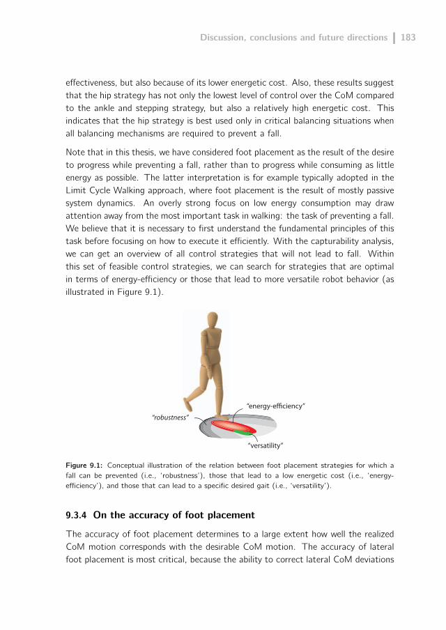
Discussion, conclusions and future directions 183

effectiveness, but also because of its lower energetic cost. Also, these results suggestthat the hip strategy has not only the lowest level of control over the CoM comparedto the ankle and stepping strategy, but also a relatively high energetic cost. Thisindicates that the hip strategy is best used only in critical balancing situations whenall balancing mechanisms are required to prevent a fall.

Note that in this thesis, we have considered foot placement as the result of the desireto progress while preventing a fall, rather than to progress while consuming as littleenergy as possible. The latter interpretation is for example typically adopted in theLimit Cycle Walking approach, where foot placement is the result of mostly passivesystem dynamics. An overly strong focus on low energy consumption may drawattention away from the most important task in walking: the task of preventing a fall.We believe that it is necessary to first understand the fundamental principles of thistask before focusing on how to execute it efficiently. With the capturability analysis,we can get an overview of all control strategies that will not lead to fall. Withinthis set of feasible control strategies, we can search for strategies that are optimalin terms of energy-efficiency or those that lead to more versatile robot behavior (asillustrated in Figure 9.1).

“robustness”

“energy-eciency”

“versatility”

Figure 9.1: Conceptual illustration of the relation between foot placement strategies for which afall can be prevented (i.e., ‘robustness’), those that lead to a low energetic cost (i.e., ‘energy-efficiency’), and those that can lead to a specific desired gait (i.e., ‘versatility’).

9.3.4 On the accuracy of foot placement

The accuracy of foot placement determines to a large extent how well the realizedCoM motion corresponds with the desirable CoM motion. The accuracy of lateralfoot placement is most critical, because the ability to correct lateral CoM deviations

184 Chapter 9

through the use of the ankle strategy is very limited. To achieve a human-like lateralstep variability (28 mm on average) in robotic walking, we estimate that the CoPlocation should be controlled at an accuracy of at least 9 mm (based on the above-mentioned ‘error amplification factor’ of 3). The initial foot placement location(described by the ‘contact reference point’ page 28) determines the possible CoPlocations that can be achieved and can therefore not be too far off from the desiredCoP location. It can be maximally located at a distance that is equal to the largestdistance between the contact reference point and the edge of the base of support.However, this configuration severely constrains the amount of CoP modulation thatcan be achieved through the ankle strategy, since the CoP is located at the borderof the base of support. A more preferable situation would be to place the contactreference point at a distance from the desired CoP that is about a quarter of the widthof the base of support. This allows for CoP modulation in all directions through theuse of ankle torques, e.g., in case of small perturbations. For a human morphology,this would correspond to a foot placement accuracy of about 10 mm.

But how to achieve that the foot (or CoP) arrives there and then, at the right locationand at the right time? And, what is the right location and the right time? Thesetwo questions reflect the essence of the control of walking: the adequate planningand execution of foot placement strategies. These two aspects of foot placementcan not be analyzed separately from each other, but are related. The execution offoot placement is for example constrained by system limitations (e.g., actuator peaktorque, kinematic range) that should be taken into account when planning adequatefoot placement strategies. Thus, adequate planning and execution of foot placementcan be the result of a complex relation between various factors, e.g., the availablelevel of actuation, sensing, state estimation and modeling. The following paragraphswill describe what insight this thesis has given us in all the factors that influence theoverall foot placement accuracy.

On the accurate planning of foot placement

This section discusses issues related to the modeling and sensing that contribute tothe overall accuracy of foot placement.

Modeling

We have derived foot placement strategies from low-dimensional linear gait models.How good is this model? We contend that for normal walking, balance control is low-dimensional, and sufficiently accurately modeled by the simple gait model because ofseveral reasons. Firstly, balance can be well analyzed by focusing only on the CoMdynamics with respect to the CoP location. Secondly, modeling the system as a

Discussion, conclusions and future directions 185

linear inverted pendulum is acceptable since the angular excursions of the pendulumare small (< 20 degrees) and the true vertical displacement of the CoM in normalhuman walking is typically only 35 mm (Gard et al., 2004). Finally, the model wasshown as a good predictor of human foot placement locations: Hof (2008) foundthat for lateral balance the CoP location at initial foot contact is a fixed offset fromthe instantaneous capture point location with a standard deviation of only 7 mm.A very similar analysis on sagittal balance found a standard deviation of 17 mm inthe fore-aft direction (Millard et al., 2009). Also, a benefit of the low-dimensionalmodel is that it can be continuously updated on the robot such that the planned footplacement strategy smoothly adapts to the state of the system.

Nevertheless, using a simple model to predict foot placement locations may resultin a CoM motion that deviates from the desired or predicted path. Rebula et al.(2007) studied how well the instantaneous capture point approximated by the 3D-Linear Inverted Pendulum Model corresponds to the actual instantaneous capturepoint of a complex robot model. The modeled robot is commanded to step towardsthe approximated instantaneous capture point and it is analyzed if the robot reachesa captured state. If this is not the case, the desired step location is changed basedon a learning algorithm. The reported offsets between the desired step locationsbased on the 3D-LIPM approximations and that on learning are in the order of 30mm. However, it is not clear if these offsets compensate for errors introduced by theuse of the simple 3D-LIPM. The reported offsets may also compensate for the errorsintroduced by the implemented controller that executes foot placement. This studyagain illustrates that planning and execution of foot placement are closely related.

We expect that in the case of moderate walking speeds, modeling errors introducedby the 3D-LIPM can easily be compensated for by ankle torques or by adaptation ofthe next foot placement. This situation may change for balance control when thesystem is 2 or 3-step capturable, for example due to a large perturbation. In this case,rapid actions are required to prevent a fall and system limitations consequently startto play a role. Control based on linear models may not be optimal or does not havethe intended effect. However, one could reason that optimality and predictability arenot that important in more extreme situations. Simple reflexive control strategies(such as ‘step as fast as you can in the direction of the approximated instantaneouscapture point’) may not be optimal but still effective in preventing a fall. Similarly, theinitial response to a perturbation in human walking also seems of a simple reflexivenature and was shown to be adapted and tailored to the specific perturbation when itwas applied multiple times (Marigold and Patla, 2002; Nieuwenhuijzen et al., 2000).Ideally, such learning mechanisms are also incorporated in future balance controlmechanisms.

186 Chapter 9

Another relevant issue to discuss is the existence of two apparently conflicting findingsregarding the adequate planning of foot placement strategies. In Chapter 4 of thisthesis, we derived explicit foot placement strategies that allow a system to evolvefrom its current state to a desired future state. This desired stated was assumed tobe four-dimensional: the desired CoM position and velocity with respect to the CoPlocation in both the sagittal and the lateral plane were considered. Then, an adequatestep time and an adequate step location were derived that would have the correcteffect on all of these four dimensions. However, studies on foot placement in humanwalking found that the control of foot placement can be decomposed in two two-dimensional problems (Bauby and Kuo, 2000; Kuo, 1999; Townsend, 1985). Thelateral and forward dynamics were found to be largely decoupled. This decoupledcontrol approach was also successfully implemented on simulated and real bipeds(Hobbelen and Wisse, 2009; Kajita et al., 2001; Pratt and Pratt, 1999). How canthese apparently conflicting findings be explained?

The decoupled view on foot placement control can be seen as a special case of whatreally is a coupled 4D problem. A decoupled approach is only possible for a constantstep time. For that special case, a step width and step length can be independentlyselected which eventually will result in the desired state. A candidate approach isstepping at a constant offset away from the instantaneous capture point, where thesystem state converges to the desired state as the number of steps goes to infinity(see Chapter 4). When releasing the constraint of a constant step time, steppingstrategies can be found that converge to the desired state within a fixed number ofsteps.

We can imagine that, for normal human or robotic walking, sustaining a constantstep time can be beneficial. This does not require enforcing motions on the swing legthat are potentially far off from the passive leg dynamics. The level of control canbe low and mostly equal for each step. Only in case of severe perturbations duringwalking do humans seem to adjust their nominal step time (van Dieën et al., 2007;Forner Cordero et al., 2003; Hof et al., 2010). It would be interesting to study howhumans select their step time and step location relative to the instantaneous capturepoint and CoP location during more versatile behavior, such as navigating throughan indoor environment. To our knowledge, such a study has not yet been conducted.

Sensing

Related to the accurate planning of foot placement is the required level of sensingthat is necessary for accurate state estimation of the robot and its internal model.The accuracy of the foot placement relies on the accuracy of the estimate of the CoMposition and velocity. Also, it requires estimations on where the CoP is underneath

Discussion, conclusions and future directions 187

the stance foot or where the swing foot is relative to the ground. We contend thatthe resolution, accuracy or update rate of modern sensors is not hampering roboticperformance. Angle sensors easily achieve resolutions of 2·10−4 rad (1·10−2 degrees)and inertial measurement units have an angular accuracy of about 2 · 10−2 rad (1degree) at an update rate of 250 Hz. However, there are two issues regarding sensingthat require attention.

Firstly, the kinematic chain from the stance foot to the swing foot is long, easilyconsisting of 12 degrees of freedom. Any unmeasured elasticity or play in one of thedegrees of freedom can cause significant deviations in the estimate of the state ofthe swing foot relative to the stance foot. This proved to be really problematic forthe control of TUlip. Gearbox play and compliance of structural components in thehip resulted in an inaccuracy of approximately 40 mm in the estimation of the lateralposition of both feet.

Secondly, state estimation of the robot state with respect to the environment isnot straightforward. To estimate the CoM velocity with respect to the ground,combined information is required from kinematic data and accelerometer data (toprevent errors due to a slipping stance foot or an accumulating integration error ofaccelerometer data). Often, we have used intuition to find filter parameters withouthaving good knowledge on how well the measured CoM velocity approximates thetrue CoM velocity. These issues require more attention in future research.

On the accurate execution of foot placement

Accurate and fast swing leg motions are essential for the ability to handle largedisturbances. The question is how to achieve this for a bipedal robot?

Since the execution of foot placement seems to be all about accurately controllingthe position of the swing foot, a logical choice would be to use stiff position controlledjoints and use high feedback control. However, position controlled joints are typicallynot shock tolerant due to their high impedance. Consequently, structural damagemay occur. Also, controlling the forces that act on the CoM throughout the stancephase is not straightforward with position controlled joints. Therefore, we see benefitin using series elasticity and force control. Not only can it be beneficial during thestance phase. During the swing phase, compliant series elasticity can decouple theactuator dynamics from the structural leg dynamics, which offers simple modelingand easy control of the leg as if a perfect torque source with controllable stiffnessis connected to the joint. Also, controlling forces is the most elementary way tocontrol motion and offers optimization of the motion in terms of energy-efficiency.

188 Chapter 9

However, for fast changing motions, compliant series elastic actuators are far from aperfect torque source with controllable stiffness. Fast motions require large torques,which require large deflections of the compliant element, which subsequently re-quire large actuator motions. The result is that actuator limitations are quicklyreached. Consequently, compliant series elasticity (like implemented on TUlip) of-fers high-fidelity force control for moderate bandwidth but hampers fast and accuratetrajectory tracking of joint positions.

A straightforward solution would be to increase the power of the motors to be ableto enforce desired swing leg motions without reaching actuator limitations. Thisdoes obviously come at the cost of added weight and more energy use. However,fast and accurate swing leg motion does not necessarily require high power motorsand high feedback gains. More ‘intelligent’ control can compensate for the lack ofmotor power. The swing leg control could be based on an accurate dynamical mo-del of the swing leg (including actuators, compliant elements, transmissions) whichenables the addition of feedforward control that can significantly improve the tra-cking performance (e.g., see Park et al., 2011). High levels of feedforward control infoot placement execution is perhaps most similar to the human case, where limitedmuscle power and muscle activation latencies do not allow for high-speed motionadaptations. Fast compensatory stepping reactions in humans were found only to bealtered during the preparational and initial phase of the swing phase and immutableduring the rest of the swing phase (Tripp et al., 2004). Humans demonstrate thatdespite actuator latencies, accurate execution foot placement can still be achieved(standard deviation of 6 mm, Hof et al., 2010).

We see most potential in series elastic actuators with increased series stiffness, sa-crificing force control accuracy in favor of force control bandwidth. The increasedintrinsic impedance (i.e., the impedance at a frequency above the controller band-width) may decrease the shock tolerance, but this could be solved by adding a morecompliant series element between the ankle joint and the floor. It should be notedthat advancements are also made in the field of robotic actuators with variable intrin-sic impedance (e.g., Eiberger et al. (2010) and references therein), but their currentlow power to weight ratio of these actuators is limiting their application in bipedalrobots.

The above-mentioned results illustrate the many factors that influence the accuracyof the planning of foot placement and/or the accuracy of the execution of footplacement and thereby determine the overall foot placement accuracy. This thesisdescribed how the capturability framework can be used for accurate planning of footplacement. Accurate execution of these strategies is required to achieve robust

Discussion, conclusions and future directions 189

robotic bipedal gait. This was already demonstrated on a simulated robot but itremains a challenge to achieve this on the real robot prototype TUlip.

9.4 Conclusions

This section presents the main conclusions regarding the posed research questionand more general conclusions.

9.4.1 Research questions

- Regarding robustness: how can we determine where and when the foot shouldbe placed to prevent a fall?

The timing and location of a step which can prevent a fall can be derived by analyzingthe system’s ability to come to a stop without falling by taking N or fewer steps.Simple models were used to approximate this ability. These models considered theeffect of balance mechanisms on the center of mass position and velocity. This meansthat they considered the effect of ankle torques, centroidal angular momentum andfoot placement on the instantaneous capture point. The resulting approximations ofthese simple models were shown to be sufficiently accurate for balance control of acomplex bipedal robot.

- Regarding versatility: how can we determine where and when the foot shouldbe placed to enable the system to evolve from its initial state to any desiredfuture state?

The timing and location of a step which allow a system to evolve to a desired futurestate can be derived by using a dimensionally-reduced model of the system. We useda simple model that considered only the most fundamental dynamics of walking: theCoM dynamics with respect to the CoP. Because of this low-dimensional view, wecould explicitly calculate the required step locations and step times for the systemto evolve to the desired future state.

- Regarding energy-efficiency: how do actuator limitations influence foot place-ment strategies?

Firstly, actuator limitations influence foot placement by directly determining theachievable minimum step time. The minimum step time and maximum step lengthdetermine to a large extent the system’s ability to prevent a fall. Secondly, simplegait models predict that actuator limitations influence human foot placement stra-tegy selection, and not only foot placement strategy execution. Shortening of a

190 Chapter 9

perturbed step is suggested to be energetically advantageous compared to the elon-gation of the perturbed step in case the perturbation occurs after mid-swing. Theopposite is true for a perturbation that occurs before mid-swing.

9.4.2 General conclusions

The capturability framework provides a unified and practical approach to the analysisand control of robust bipedal locomotion because:

a. The capturability analysis considers the relevant subset of the viability kernel.In other words, when analyzing fall avoidance by considering the ability to cometo a stop in given number of steps without falling, all plausible and commonstates of bipedal locomotion are considered.

b. The capturability analysis is theoretically not limited to a particular leggedsystem, a controller, a specific motion, a local stability indicator, or an envi-ronment.

c. N-step capturable states can be projected onto the ground to create N-stepcapture regions, which

- conveniently visualize capturability;- provide practical information for controller synthesis;- lead to the N-step capturability margin, which quantifies capturabilityand provides a measure of robustness.

A low-dimensional and decoupled view on the control of walking offers:

a. The use of simple gait models that only take the dynamics of the center ofmass with respect to the contact forces between the foot and the ground intoaccount.

b. The possibility to approximate the whole-body dynamics of a complex system.Approximations reveal that the system’s instantaneous capture point divergesaway from the centroidal moment pivot point (or center of pressure locationin case of zero centroidal angular momentum). It moves away along a straightline at a velocity proportional to the distance to the centroidal moment pivotpoint.

c. Approximations that are shown useful for the synthesis of control strategiesfor a complex bipedal robot in case of

- single-legged balancing during mild postural perturbations;- single-legged balancing with compensatory stepping in case of large per-turbations;

- two-legged balancing while the robot is being pushed and one of the feetis placed on a moving platform;

Discussion, conclusions and future directions 191

- walking in simulation.

9.5 Future directions

Previous chapters have presented new insight in the mechanics and control of bipedallocomotion. This section discusses future directions in this field of research.

9.5.1 On the mechanics of walking

TUlip was tailored for Limit Cycle Walking: series elastic actuators with low powerand high compliance were used in combination with low levels of control. Thiscombination of mechanics and control may be well-suited for periodic walking gaits atmoderate speed but it turned out that this combination was less suitable for executionof aperiodic motions. Unfortunately, committing to a specific control methodology inbipedal robot research typically means committing to a specific hardware architectureand vice versa.

In order to properly study the mechanics and control of human-like bipedal walking,there is a strong need for a more versatile bipedal robotic research platform. Arobotic platform that can not just be exclusively used for a single proof of concept,but one that can be used for research on a large variety of control ideas. The robotshould be robust and easy to maintain and should therefore be able to operate overmultiple trials. We see the following possibilities to achieve this.

The research platform should (initially) not be made autonomous. Of course, tryingto match the human functionality in an autonomous human-like machine is an in-teresting challenge (e.g., illustrated by the RoboCup competition) and makes oneappreciate the human body. However, to truly advance in the field of research onbipedal locomotion, the system’s autonomy constrains it in too many ways. It shouldbe tethered so that it can use off-board computing and off-board power supply.

Off-board computing does not only save weight but mostly offers more computingpower, which is anticipated to speed up the research progress. It means not havingto deal with a lack of memory, processing power or supported software.

Off-board power also saves weight and offers the implementation of more powerfulactuators. We believe that a surplus of actuator power is essential for a future roboticprototype. Though humans perfectly well demonstrate that high power actuatorsare not necessary for walking, we believe that powerful actuators will quickly lead tomore understanding of human walking. Taking away actuator limitations allows usto ‘cheat’: we can design walking controllers that are far from optimal or human-likebut at least result in a stable gait. From this point on, the control approach can be

192 Chapter 9

optimized to arrive at a more human-like gait with only low levels of control. Thisis different from an approach with low-power actuators that immediately requirescomplex control algorithms to get the robot operational at all.

Compare our proposed approach to the approach one adopts to learn to ride a bicyclewithout using the handle bars. One learns how to ride a bicycle as a child with thehelp of training wheels. Training wheels are used to prevent a fall, which allows oneto simplify biking (‘cheat’). This way the focus lies on the control of the pedalsand steering. The support of the training wheels can be gradually reduced aftertraining. Once the control is sufficiently mastered, complex upper-body motions canbe learned to control the bicycle without use of the hands. Trying to achieve thesame skill without such a gradual learning process, but by trial and error, is probablythe slowest and most frustrating path to success.

So, we see great benefit from a robot that is specifically designed to achieve human-like swing-leg speeds and human-like foot placement accuracy through powerful force-controllable actuators. To our knowledge, there is no description in literature of abipedal robot that is designed with these requirements in mind (though we suspect(since this information is classified) that Petman (Boston Dynamics, 2011) is a goodfirst example of this).

9.5.2 On the control of walking

The findings in this thesis suggest that walking control only through foot placementis possible, but preferably accompanied by ankle strategies and possibly hip strategies.Nevertheless, since balance control is dictated by foot placement, a possible point ofdeparture for the synthesis of a robust walking gait is the control of foot placementonly. As a start, the CoP shift through active ankle control could be emulatedby locking the ankle joint and using a slightly curved foot shape or by using a flatfoot with an ankle with a fixed stiffness as demonstrated by Wisse et al. (2006).Also, we could start of by selecting a walking gait with a relatively small step time,which decreases the possible deviations from the desired CoM motion. Once walkingis achieved through adequate foot placement control, one can start experimentingwith the use of ankle torques and upper body motions to increase the gait robustnessand fine-tune the walking motion.

To further increase the robustness of walking, there is potentially one stabilizingmechanism that can be used which is not considered in this thesis: ankle push-offwith the trailing leg during and preceding the double stance phase. A study on planarwalking models (Hobbelen and Wisse, 2008a) suggests that regulating the amountof push-off can improve the recovery from perturbations during gait by influencing

Discussion, conclusions and future directions 193

the CoM motion in the fore-aft direction. Biomechanical studies show that impulsiveankle push-off can also be used to elevate the body after severe perturbations andthereby provide time and clearance for proper positioning of the recovery limb andrestrain the angular momentum of the upper body (Pijnappels et al., 2004, 2005).Little is known about how to control ankle push-off in three-dimensional walking,during aperiodic gaits or in case of disturbances. Further research on this subjectseems desirable. Omission of ankle push-off in our presented analysis implies thatour view on possible stabilizing strategies is perhaps a bit conservative.

Once a robust gait is achieved, a relevant next step would be to focus on the ener-getic cost of walking. The Limit Cycle Walking approach presented various controlconcepts which were beneficial for the energy-efficiency of walking. For example,the energetic cost of walking could be reduced by exploiting the natural dynamicsof the swing leg or by employing ankle push-off with the stance ankle just beforethe swing foot touches the ground (Hobbelen, 2008). These control concepts couldbe integrated into the control algorithms presented in this thesis. However, integra-tion of these concepts should not be attempted without a clear understanding ofhow they affect the capturability of the system. The capturability analysis specifieswhich control actions are will not lead to a fall and are therefore permissible. Weare currently exploring ways to minimize the energetic cost of foot placement for agiven foot placement strategy provided by the capturability analysis. We aim to usea simple swing leg model in combination with model predictive control online on therobot that can minimize the energetic cost of foot placement for a given step timeand step location. A next step would be to not only optimize the execution of footplacement in terms of energetic cost, but also the planning of foot placement.

References

Abbott, B.C., Bigland, B., and Ritchie, J.M. (1952), “The physiological cost ofnegative work”, The Journal of Physiology, 117(3), p. 380.

Abdallah, M. and Goswami, A. (2005), “A Biomechanically Motivated Two-PhaseStrategy for Biped Upright Balance Control”, Proceedings of IEEE InternationalConference on Robotics and Automation, pp. 1996–2001.

Aftab, Z., Wieber, P.B., and Robert, T. (2010), “Comparison of Capture Point esti-mation with human foot placement : Applicability and Limitations”, . Proceedingsof 5èmes Journées Nationales de la Robotique Humanoïde.

Alexander, R.M. (1989), “Optimization and gaits in the locomotion of vertebrates”,Physiological Reviews, 69(1199-1227), pp. 29–64.

Aubin, J.P. (1991), Viability theory, Birkhäuser, Boston, MA.Aubin, J.P., Lygeros, J., Quincampoix, M., Sastry, S., and Seube, N. (2002), “Im-pulse Differential Inclusions: A Viability Approach to Hybrid Systems”, IEEE Tran-sactions on Automatic Control, 47(1), pp. 2–20.

Bauby, C.E. and Kuo, A.D. (2000), “Active control of lateral balance in humanwalking”, Journal of Biomechanics, 33(11), pp. 1433–1440.

van den Bogert, A.J., Pavol, M.J., and Grabiner, M.D. (2002), “Response time ismore important than walking speed for the ability of older adults to avoid a fallafter a trip”, Journal of Biomechanics, 35(2), pp. 199–205.

Boston Dynamics (2011), “PETMAN - BigDog gets a Big Brother”, . website.http://www.bostondynamics.com/robot_petman.html

van der Burg, J.C.E., Pijnappels, M., and van Dieën, J.H. (2005), “Out-of-planetrunk movements and trunk muscle activity after a trip during walking”, Experi-mental Brain Research, 165(3), pp. 407–412.

Byl, K. and Tedrake, R. (2008), “Metastable walking on stochastically rough terrain”,Proceedings of Robotics: Science and Systems IV.

Chen, J., Cheng, J., and Yu, G. (2001), “Virtual model control of a quadrupedwalking robot”, Journal of Shanghai Jiaotong University, 35(12), pp. 1771–1775.

Chevallereau, C., Abba, G., Aoustin, Y., Plestan, F., Westervelt, E.R., Canudas-de-Wit, C., and Grizzle, J.W. (2003), “RABBIT: a testbed for advanced controltheory”, IEEE Control Systems Magazine, 23(5), pp. 57–79.

Chevallereau, C., Grizzle, J.W., and Shih, C. (2009), “Asymptotically Stable Walkingof a Five-Link Underactuated 3-D Bipedal Robot”, IEEE Transactions on Robotics,25(1), pp. 37–50.

Coleman, M.J., Garcia, M., Mombaur, K., and Ruina, A. (2001), “Prediction ofstable walking for a toy that cannot stand”, Physical Review E, 64(2), p. 022901.

196 References

Collins, S.H., Ruina, A., Tedrake, R., and Wisse, M. (2005), “Efficient BipedalRobots Based on Passive-Dynamic Walkers”, Science, 307(5712), pp. 1082–1085.

Collins, S.H., Wisse, M., and Ruina, A. (2001), “A Three-Dimensional Passive-Dynamic Walking Robot with Two Legs and Knees”, International Journal of Ro-botic Research,, 20(7), pp. 607–615.

Controllab Products B.V. (2011), “20-sim”, . website.http://www.20sim.com

Coros, S., Beaudoin, P., and van de Panne, M. (2010), “Generalized biped walkingcontrol”, Proceedings of SIGGRAPH, pp. 1–9. ACM Press, New York, NY, USA.

De Lasa, M. (2010), “Feature-Based Control for Physics-Based Character Anima-tion”, , Ph.D. thesis, University of Toronto.

Delft Biorobotics Laboratory (2011), “DBL homepage”, . website.http://dbl.tudelft.nl

Diamond Systems (2011), “Poseidon EPIC SBC”, . website.http://www.diamondsystems.com/products/poseidon

Diedam, H., Dimitrov, D., Wieber, P.B., Mombaur, K., and Diehl, M. (2008), “On-line walking gait generation with adaptive foot positioning through linear modelpredictive control”, Proceedings of IEEE/RSJ International Conference on Intelli-gent Robots and Systems, pp. 1121–1126.

van Dieën, J.H., Spanjaard, M., Konemann, R., Bron, L., and Pijnappels, M. (2007),“Balance control in stepping down expected and unexpected level changes”, Journalof Biomechanics, 40(16), pp. 3641–3649.

Dietz, V., Quintern, J., Boos, G., and Berger, W. (1986), “Obstruction of theswing phase during gait: phase-dependent bilateral leg muscle coordination”, BrainResearch, 384(1), pp. 166–169.

Dingwell, J.B., Cusumano, J.P., Cavanagh, P.R., and Sternad, D. (2001), “LocalDynamic Stability Versus Kinematic Variability of Continuous Overground andTreadmill Walking”, Journal of Biomechanics Engineering, 123(1), pp. 27–32.

Doke, J., Donelan, J.M., and Kuo, A.D. (2005), “Mechanics and energetics of swin-ging the human leg”, Journal of Experimental Biology, 208(3), p. 439.

Doke, J. and Kuo, A.D. (2007), “Energetic cost of producing cyclic muscle force,rather than work, to swing the human leg”, Journal of Experimental Biology,210(13), p. 2390.

Dollar, A.M. and Herr, H. (2008), “Lower extremity exoskeletons and active orthoses:Challenges andstate-of-the-art”, IEEE Transactions on Robotics, 24(1), pp. 144–158.

Donelan, J.M., Kram, R., and Kuo, A.D. (2002), “Mechanical work for step-to-steptransitions is a major determinant of the metabolic cost of human walking”, Journal

References 197

of Experimental Biology, 205(23), pp. 3717–3727.DutchRobotics (2011), “Homepage of DutchRobotics”, . website.http://www.dutchrobotics.net

Eiberger, O., Haddadin, S., Weis, M., Albu-Schaffer, A., and Hirzinger, G. (2010),“On joint design with intrinsic variable compliance: Derivation of the DLR QA-joint”, Proceedings of IEEE International Conference on Robotics and Automation,pp. 1687–1694.

Elmo Motion Control (2011), “Whistle: Highly compact and intelligent digital servodrive”, . website.http://www.elmomc.com/products/whistle-digital-servo-drive-main.htm

Eng, J.J., Winter, D.A., and Patla, A.E. (1994), “Strategies for recovery from atrip in early and late swing during human walking”, Experimental Brain Research,102(2), pp. 339–349.

Englsberger, J., Ott, C., Roa, M.A., Albu-Schäffer, A., and Hirzinger, G. (2011), “Bi-pedal walking control based on Capture Point dynamics”, Proceedings of IEEE/RSJInternational Conference on Intelligent Robots and Systems.

Featherstone, R. (1987), Robot dynamics algorithms, Kluwer Academic Publishers,Norwell, MA, USA.

Featherstone, R. (2008), Rigid body dynamics algorithms, Springer US, Boston, MA,USA.

Forner Cordero, A., Koopman, H., and van der Helm, F.C.T. (2003), “Multiple-stepstrategies to recover from stumbling perturbations”, Gait & Posture, 18(1), pp.47–59.

Forner Cordero, A., Koopman, H.F., and van der Helm, F.C.T. (2005), “Energyanalysis of human stumbling: the limitations of recovery”, Gait & Posture, 21, pp.243–254.

Friedmann, M., Kiener, J., Petters, S., Thhomas, D., and von Stryk, O. (2006),“Modular software architecture for teams of cooperating, heterogeneous robots”,Proceedings of IEEE International Conference on Robotics and Biomimetics, pp.613–618.

Garcia, M., Chatterjee, A., Ruina, A., and Coleman, M. (1998), “The simplestwalking model: Stability, complexity, and scaling”, ASME Journal of BiomechanicalEngineering, 120, pp. 281–288.

Gard, S.A., Miff, S.C., and Kuo, A.D. (2004), “Comparison of kinematic and kineticmethods for computing the vertical motion of the body center of mass duringwalking”, Human movement science, 22(6), pp. 597–610.

Geng, T., Porr, B., and Wörgötter, F. (2006), “Coupling of neural computation withphysical computation for stable dynamic biped walking control”, Neural Comput.,

198 References

18(5), pp. 1156–1196.Goswami, A. (1999), “Postural stability of biped robots and the foot rotation indica-tor (FRI) point”, International Journal of Robotic Research, 18(6), pp. 523–533.

Grabiner, M.D., Koh, T.J., Lundin, T.M., and Jahnigen, D.W. (1993), “Kinematicsof recovery from a stumble”, The Journal of Gerontology, 48(3), p. M97.

Grizzle, J., Hurst, J., Morris, B., Park, H.W., and Sreenath, K. (2009), “MABEL, anew robotic bipedal walker and runner”, IEEE American Control Conference, pp.2030–2036.

Grizzle, J.W., Abba, G., and Plestan, F. (2001), “Asymptotically stable walking forbiped robots: Analysis via systems with impulse effects”, Transactions on Auto-matic Control, 46(1), pp. 51–64.

Grizzle, J.W., Chevallereau, C., Ames, A.D., and Sinnet, R.W. (2010), “3D bipe-dal robotic walking: Models, feedback control, and open problems”, NOLCOS,Bologna, Italy.

Guihard, M. and Gorce, P. (2002), “Dynamic control of bipeds using ankle andhip strategies”, Proceedings of IEEE/RSJ International Conference on IntelligentRobots and Systems, volume 3.

van Ham, R., Vanderborght, B., van Damme, M., Verrelst, B., and Lefeber, D.(2007), “MACCEPA, the mechanically adjustable compliance and controllableequilibrium position actuator: Design and implementation in a biped robot”, Ro-botics and Autonomous Systems, 55(10), pp. 761–768.

Hirai, K., Hirose, M., Haikawa, Y., and Takenaka, T. (1998), “The development ofHonda humanoid robot”, Proceedings of IEEE International Conference on Robo-tics and Automation, volume 2, pp. 1321–1326.

Hobbelen, D.G.E. (2008), “Limit Cycle Walking”, , Ph.D. thesis, Delft University ofTechnology.

Hobbelen, D.G.E. and De Boer, T. (2008), “System overview of bipedal robots Flameand TUlip: Tailor-made for Limit Cycle Walking”, Proceedings of InternationalConference on Intelligent Robots and Systems, pp. 2486–2491.

Hobbelen, D.G.E. and Wisse, M. (2007a), “A Disturbance Rejection Measure forLimit Cycle Walkers: The Gait Sensitivity Norm”, IEEE Transactions on Robotics,23(6), pp. 1213–1224.

Hobbelen, D.G.E. and Wisse, M. (2007b), “Limit Cycle Walking”, M. Hackel, edi-tor, Humanoid Robots, Human-like Machines, chapter 14, pp. 277–294. ITechEducation and Publishing, Vienna, Austria.

Hobbelen, D.G.E. and Wisse, M. (2008a), “Ankle Actuation for Limit Cycle Walkers”,The International Journal of Robotics Research, 27(6), pp. 709–735.

Hobbelen, D.G.E. and Wisse, M. (2008b), “Swing-Leg Retraction for Limit Cycle

References 199

Walkers Improves Disturbance Rejection”, IEEE Transactions on Robotics, 24(2),pp. 377–389.

Hobbelen, D.G.E. and Wisse, M. (2009), “Active Lateral Foot Placement for 3D Sta-bilization of a Limit Cycle Walker Prototype”, International Journal on HumanoidRobotics, 6(1), pp. 93–116.

Hof, A.L. (2007), “The equations of motion for a standing human reveal three me-chanisms for balance”, Journal of Biomechanics, 40(2), pp. 451 – 457.

Hof, A.L. (2008), “The ’extrapolated center of mass’ concept suggests a simplecontrol of balance in walking”, Human Movement Science, 27(1), pp. 112–125.

Hof, A.L., van Bockel, R.M., Schoppen, T., and Postema, K. (2007), “Control oflateral balance in walking: Experimental findings in normal subjects and above-kneeamputees”, Gait & Posture, 25(2), pp. 250–258.

Hof, A.L., Gazendam, M.G.J., and Sinke, W.E. (2005), “The condition for dynamicstability”, Journal of Biomechanics, 38(1), pp. 1–8.

Hof, A.L., Vermerris, S.M., and Gjaltema, W.A. (2010), “Balance responses tolateral perturbations in human treadmill walking”, Journal of Experimental Biology,213, pp. 2655–2664.

Honda (2011), “Asimo - the world’s most advanced humanoid robot”, . website.http://asimo.honda.com/

Hoogvliet, P., van Duyl, W.A., de Bakker, J.V., Mulder, P.G.H., and Stam, H.J.(1997), “A model for the relation between the displacement of the ankle and thecenter of pressure in the frontal plane, during one-leg stance”, Gait & Posture,6(1), pp. 39–49.

Horak, F.B. and Nashner, L.M. (1986), “Central programming of postural move-ments: adaptation to altered support-surface configurations”, Journal of Neuro-physiology, 55(6), p. 1369.

Hsiao, E.T. and Robinovitch, S.N. (1999), “Biomechanical influences on balancerecovery by stepping”, Journal of Biomechanics, 32(10), pp. 1099–1106.

Hsiao, E.T. and Robinovitch, S.N. (2001), “Elderly subjects’ ability to recover ba-lance with a single backward step associates with body configuration at stepcontact”, Journal of Gerontology Series A: Biological Sciences and MedicalSciences, 56(1), pp. M42–47.

Hsiao-Wecksler, E.T. (2008), “Biomechanical and age-related differences in balancerecovery using the tether-release method”, Journal of Electromyography and Ki-nesiology, 18(2), pp. 179–187.

Hsiao-Wecksler, E.T. and Robinovitch, S.N. (2007), “The effect of step lengthon young and elderly women’s ability to recover balance”, Clinical Biomechanics,22(5), pp. 574–580.

200 References

Hu, J.J., Pratt, J.E., Chew, C.M., Herr, H.M., and Pratt, G.A. (1998), “Adaptivevirtual model control of a bipedal walking robot”, Proceedings of IEEE InternationalJoint Symp. Intell. Syst., pp. 245–251.

Hu, J.J., Pratt, J.E., Chew, C.M., Herr, H.M., and Pratt, G.A. (1999), “Virtualmodel based adaptive dynamic control of a biped walking robot”, InternationalJournal of Artificial Intelligence Tools, 8(3), pp. 337–348.

Huang, Q., Kajita, S., Koyachi, N., Kaneko, K., Yokoi, K., Arai, H., Komoriya, K.,and Tanie, K. (1999), “A high stability, smooth walking pattern for a biped ro-bot”, Proceedings of IEEE International Conference on Robotics and Automation,volume 1, pp. 65–71.

Huang, Q., Yokoi, K., Kajita, S., Kaneko, K., Arai, H., Koyachi, N., and Tanie,K. (2001), “Planning walking patterns for a biped robot”, IEEE Transactions onRobotics and Automation, 17(3), pp. 280–289.

Hurst, J.W., Chestnutt, J.E., and Rizzi, A.A. (2004), “An actuator with physicallyvariable stiffness for highly dynamic legged locomotion”, Proceedings of IEEE In-ternational Conference on Robotics and Automation, volume 5, pp. 4662–4667.

Hyon, S.H. and Cheng, G. (2007), “Disturbance Rejection for Biped Humanoids”,Proceedings of IEEE International Conference on Robotics and Automation, pp.2668–2675. IEEE.

Hyon, S.H., Hale, J.G., and Cheng, G. (2007), “Full-Body Compliant Human-Humanoid Interaction: Balancing in the Presence of Unknown External Forces”,IEEE Transactions on Robotics, 23(5), pp. 884–898.

Hyon, S.H., Osu, R., and Otaka, Y. (2009), “Integration of multi-level posturalbalancing on humanoid robots”, Proceedings of IEEE International Conference onRobotics and Automation, pp. 1549–1556. IEEE.

Kagami, S., Kitagawa, T., Nishiwaki, K., Sugihara, T., Inaba, M., and Inoue, H.(2002), “A Fast Dynamically Equilibrated Walking Trajectory Generation Methodof Humanoid Robot”, Journal of Autonomous Robots, 12(1), pp. 71–82.

Kajita, S., Kanehiro, F., Kaneko, K., Fujiwara, K., Harada, K., and Yokoi, K. (2003),“Biped walking pattern generation by using preview control of zero-moment point”,Proceedings of IEEE International Conference on Robotics and Automation, pp.1620–1626.

Kajita, S., Kanehiro, F., Kaneko, K., Fujiwara, K., Yokoi, K., and Hirukawa, H.(2002), “A realtime pattern generator for biped walking”, Proceedings of IEEEInternational Conference on Robotics and Automation, volume 1, pp. 31–37.

Kajita, S., Kanehiro, F., Kaneko, K., Yokoi, K., and Hirukawa, H. (2001), “The3D Linear Inverted Pendulum Mode: A simple modeling for a biped walking pat-tern generation”, Proceedings of IEEE/RSJ International Conference on Intelligent

References 201

Robots and Systems, volume 1, pp. 239–246.Kajita, S. and Tanie, K. (1991), “Study of dynamic biped locomotion on ruggedterrain—derivation and application of the linear inverted pendulum mode—”, Pro-ceedings of IEEE International Conference on Robotics and Automation, volume 2,pp. 1405–1411. IEEE Comput. Soc. Press.

Kanehiro, F., Hirukawa, H., and Kajita, S. (2004), “OpenHRP: Open architecturehumanoid robotics platform”, The International Journal of Robotics Research,23(2), p. 155.

Kaneko, K., Kanehiro, F., Morisawa, M., Miura, K., Nakaoka, S., and Kajita, S.(2009), “Cybernetic human HRP-4C”, Proceedings of IEEE-RAS InternationalConference on Humanoid Robots, pp. 7–14.

Kazerooni, H., Racine, J.L., Huang, L., and Steger, R. (2005), “On the control of theberkeley lower extremity exoskeleton (BLEEX)”, Proceedings of IEEE InternationalConference on Robotics and Automation, pp. 4353–4360.

Kemp, M. (2010), “Humanoid robot TUlip: modeling and control of advanced be-haviors”, BSc project thesis 026CE2010, University of Twente.

King, D.L. and Zatsiorsky, V.M. (2002), “Periods of extreme ankle displacementduring one-legged standing”, Gait & Posture, 15(2), pp. 172–179.

Kokam (2011), “Superior Lithium Polymer Battery (SLPB)”, . website.http://www.kokam.com/english/product/battery_main.html

Kram, R. and Taylor, C. (1990), “Energetics of running: a new perspective”, Nature,346(6281), pp. 265–267.

Kuo, A. (2001), “A simple model of bipedal walking predicts the preferred speed-steplength relationship”, Journal of Biomechanical Engineering, 123, p. 264.

Kuo, A. (2002), “Energetics of Actively Powered Locomotion Using the SimplestWalking Model”, Journal of Biomechanical Engineering, 124, p. 113.

Kuo, A.D. (1999), “Stabilization of Lateral Motion in Passive Dynamic Walking”,International Journal of Robotic Research, 18(9), pp. 917–930.

Kuo, A.D. (2007), “The six determinants of gait and the inverted pendulum analogy:A dynamic walking perspective”, Human Movement Science, 26(4), pp. 617–656.

Lagoda, C., Schouten, A.C., Stienen, A.H.A., Hekman, E.E.G., and van der Kooij,H. (2010), “Design of an electric series elastic actuated joint for robotic gaitrehabilitation training”, Proceedings of International Conference on BiomedicalRobotics and Biomechatronics, pp. 21 –26.

Lee, S.H. and Goswami, A. (2007), “Reaction mass pendulum (RMP): An explicitmodel for centroidal angular momentum of humanoid robots”, Proceedings of IEEEInternational Conference on Robotics and Automation, pp. 4667–4672. IEEE.

Luchies, C.W., Alexander, N.B., Schultz, A.B., and Ashton-Miller, J. (1994), “Step-

202 References

ping responses of young and old adults to postural disturbances: kinematics ”,Journal of the American Geriatrics Society, 42(5), p. 506.

Maki, B.E. and McIlroy, W.E. (1997), “The role of limb movements in maintainingupright stance: the "change-in-support" strategy”, Physical Therapy, 77(5), pp.488–507.

Maki, B.E. and McIlroy, W.E. (1999), “The control of foot placement during com-pensatory stepping reactions: does speed of response take precedence over stabi-lity?”, IEEE Transactions on Rehabilitation Engineering, 7(1), pp. 80–90.

Manchester, I.R., Mettin, U., Iida, F., and Tedrake, R. (2009), “Stable dynamicwalking over rough terrain: Theory and experiment”, Proceedings of InternationalSympomsium on Robotic Research.

Marigold, D.S. and Patla, A.E. (2002), “Strategies for dynamic stability during loco-motion on a slippery surface: effects of prior experience and knowledge”, Journalof Neurophysiology, 88(1), p. 339.

Masani, K., Vette, A.H., and Popovic, M.R. (2006), “Controlling balance duringquiet standing: Proportional and derivative controller generates preceding motorcommand to body sway position observed in experiments”, Gait & Posture, 23(2),pp. 164–172.

McGeer, T. (1990a), “Passive dynamic walking”, The International Journal of Robo-tics Research, 9(2), p. 62.

McGeer, T. (1990b), “Passive walking with knees”, Proceedings of IEEE InternationalConference on Robotics and Automation, pp. 1640–1645.

McIlroy, W.E. and Maki, B.E. (1996), “Age-related changes in compensatory step-ping in response to unpredictable perturbations”, Journal of Gerontology Series A:Biological Sciences and Medical Sciences, 51(6), pp. 289–296.

MESA (2011), “MESA motion control cards”, . website.http://www.mesanet.com/motioncardinfo.html

Millard, M., Wight, D.L., McPhee, J., Kubica, E.G., and Wang, D.W.L. (2009), “Hu-man Foot Placement and Balance in the Sagittal Plane”, Journal of BiomechanicalEngineering, 131(12), p. 121001.

Mirtich, B.V. (1996), “Impulse-based dynamic simulation of rigid body systems”, ,Ph.D. thesis, University of California, Berkeley.

Morimoto, J., Nakanishi, J., Endo, G., Cheng, G., Atkeson, C.G., and Zeglin, G.(2005), “Poincaré-Map-Based Reinforcement Learning For Biped Walking”, Pro-ceedings of IEEE International Conference on Robotics and Automation, pp. 2381–2386.

Morisawa, M., Harada, K., Kajita, S., Kaneko, K., Sola, J., Yoshida, E., Mansard,N., Yokoi, K., and Laumond, J.P. (2009), “Reactive stepping to prevent falling

References 203

for humanoids”, Proceedings of IEEE-RAS International Conference on HumanoidRobots, pp. 528–534. IEEE.

Morisawa, M., Kanehiro, F., Kaneko, K., Mansard, N., Sola, J., Yoshida, E., Yo-koi, K., and Laumond, J. (2010), “Combining suppression of the disturbance andreactive stepping for recovering balance”, Proceedings of IEEE International Confe-rence on Intelligent Robots and Systems, pp. 3150–3156.

Nenchev, D.N. and Nishio, A. (2008), “Ankle and hip strategies for balance recoveryof a biped subjected to an impact”, Robotica, 26(05), pp. 643–653.

Neuhaus, P.D., Noorden, J.H., Craig, T.J., Torres, T., Kirschbaum, J., and Pratt,J.E. (2011), “Design and evaluation of Mina: A robotic orthosis for paraplegics”,Proceedings of International Conference on Rehabilitation Robotics, pp. 1 –8.

Nieuwenhuijzen, P., Schillings, A., van Galen, G., and Duysens, J. (2000), “Modula-tion of the startle response during human gait”, Journal of Neurophysiology, 84(1),p. 65.

Nishiwaki, K. and Kagami, S. (2010), “Strategies for Adjusting the ZMP ReferenceTrajectory for Maintaining Balance in Humanoid Walking”, Proceedings of IEEEInternational Conference on Robotics and Automation, pp. 4230–4236.

Nishtwaki, K., Nagasaka, K., Inaba, M., and Inoue, H. (1999), “Generation of reactivestepping motion for a humanoid by dynamically stable mixture of pre-designedmotions”, Conference Proceedings of IEEE International Conference on Systems,Man, and Cybernetics, volume 6, pp. 902–907.

Okumura, Y., Tawara, T., Endo, K., Furuta, T., and Shimizu, M. (2003), “RealtimeZMP compensation for biped walking robot using adaptive inertia force control”,Proceedings of IEEE/RSJ International Conference on Intelligent Robots and Sys-tems, volume 1, pp. 335–339.

Orin, D.E. and Goswami, A. (2008), “Centroidal Momentum Matrix of a humanoidrobot: Structure and properties”, Proceedings of IEEE/RSJ International Confe-rence on Intelligent Robots and Systems, pp. 653–659.

Össur (2011), “Website, Bionic Technology by Össur”, .http://www.ossur.com

Ott, C., Baumgartner, C., Mayr, J., Fuchs, M., Burger, R., Lee, D., Eiberger, O.,Albu-Schaffer, A., Grebenstein, M., and Hirzinger, G. (2010), “Development of abiped robot with torque controlled joints”, Proceedings of IEEE-RAS InternationalConference on Humanoid Robots, pp. 167–173.

Otten, E. (1999), “Balancing on a narrow ridge: biomechanics and control”, Philoso-phical Transactions of the Royal Society of London. Series B: Biological Sciences,354(1385), p. 869.

Owaki, D., Koyama, M., Yamaguchi, S., Kubo, S., and Ishiguro, A. (2010), “A

204 References

two-dimensional passive dynamic running biped with knees”, Proceedings of IEEEInternational Conference on Robotics and Automation, pp. 5237 –5242.

Pai, Y.C. and Patton, J. (1997), “Center of mass velocity-position predictions forbalance control”, Journal of Biomechanics, 30(4), pp. 347–354.

Pai, Y.C., Rogers, M.W., Patton, J., Cain, T.D., and Hanke, T.A. (1998), “Staticversus dynamic predictions of protective stepping following waist-pull perturbationsin young and older adults”, Journal of Biomechanics, 31(12), pp. 1111–1118.

Paluska, D.J. (2000), “Design of a Humanoid Biped for Walking Research”, , M.eng. thesis, Massachusetts Institute of Technology.

Park, H.W., Sreenath, K., Hurst, J.W., and Grizzle, J.W. (2011), “Identification ofa Bipedal Robot with a Compliant Drivetrain”, IEEE Control Systems, 31(2), pp.63 –88.

Pavol, M.J., Owings, T.M., Foley, K.T., and Grabiner, M.D. (2001), “Mechanismsleading to a fall from an induced trip in healthy older adults”, Journal of Geronto-logy Series A: Biological Sciences and Medical Sciences, 56(7), pp. M428–437.

Perry, J. (1992), Gait Analysis: Normal and Pathological Function, Slack, Thorofare,NJ, USA.

Petters, S., Thomas, D., and Von Stryk, O. (2007), “Roboframe - a modular softwareframework for lightweight autonomous robots”, Proceedings of Workshop on Mea-sures and Procedures for the Evaluation of Robot Architectures and Middlewareof the International Conference on Intelligent Robots and Systems. Citeseer.

Pijnappels, M., Bobbert, M., and van Dieën, J. (2004), “Contribution of the supportlimb in control of angular momentum after tripping”, Journal of Biomechanics,37(12), pp. 1811–1818.

Pijnappels, M., Bobbert, M.F., and van Dieën, J.H. (2005), “How early reactions inthe support limb contribute to balance recovery after tripping”, Journal of Biome-chanics, 38, pp. 627–634.

Pijnappels, M., Kingma, I., Wezenberg, D., and Reurink, G andvan Dieën, J.H.(2010), “Armed against falls: the contribution of arm movements to balancerecovery after tripping”, Experimental Brain Research, 201(4), pp. 689–699.

Pijnappels, M., Reeves, N., Maganaris, C., and van Dieën, J. (2008), “Trippingwithout falling; lower limb strength, a limitation for balance recovery and a targetfor training in the elderly”, Journal of Electromyography and Kinesiology, 18(2),pp. 188–196.

Plestan, F., Grizzle, J.W., Westervelt, E.R., and Abba, G. (2003), “Stable walkingof a 7-DOF biped robot”, IEEE Transactions on Robotics and Automation, 19(4),pp. 653–668.

Popovic, M.B., Goswami, A., and Herr, H.M. (2005), “Ground Reference Points in

References 205

Legged Locomotion: Definitions, Biological Trajectories and Control Implications”,International Journal of Robotic Research, 24(12), pp. 1013–1032.

Pratt, G.A. (2000a), “Legged Robots at MIT: what’s new since Raibert?”, IEEERobotics and Automation Magazine, 7(3), pp. 15–19.

Pratt, G.A. and Williamson, M.M. (1995), “Series elastic actuators”, Proceedings ofIEEE International Conference on Intelligent Robots and Systems, volume 1, pp.399–406.

Pratt, J.E. (2000b), “Exploiting Inherent Robustness and Natural Dynamics in theControl of Bipedal Walking Robots”, , Ph.D. thesis, Massachusetts Institute ofTechnology.

Pratt, J.E., Carff, J., Drakunov, S.V., and Goswami, A. (2006), “Capture Point: AStep toward Humanoid Push Recovery”, Proceedings of IEEE-RAS InternationalConference on Humanoid Robots, pp. 200–207. IEEE.

Pratt, J.E., Chew, C.M., Torres, A., Dilworth, P., and Pratt, G.A. (2001), “Virtualmodel control: an intuitive approach for bipedal locomotion”, International Journalof Robotic Research, 20(2), pp. 129–143.

Pratt, J.E. and Drakunov, S.V. (2007), “Derivation and Application of a ConservedOrbital Energy for the Inverted Pendulum Bipedal Walking Model”, Proceedingsof IEEE International Conference on Robotics and Automation.

Pratt, J.E., Koolen, T., De Boer, T., Rebula, J., Cotton, S., Carff, J., Johnson,M., and Neuhaus, P. (2011), “Capturability-Based Analysis and Control of LeggedLocomotion, Part 3: Application to M2V2, a Lower Body Humanoid”, Submittedfor publication.

Pratt, J.E., Krupp, B., Ragusila, V., Rebula, J., Koolen, T., van Nieuwenhuizen, N.,Shake, C., Craig, T., Taylor, J., Watkins, G., Neuhaus, P., Johnson, M., Shooter,S., Buffinton, K., Canas, F., Carff, J., and Howell, W. (2009), “The Yobotics-IHMC Lower Body Humanoid Robot”, Proceedings of International Conference onIntelligent Robots and Systems, pp. 410 –411.

Pratt, J.E. and Pratt, G. (1999), “Exploiting natural dynamics in the control ofa 3d bipedal walking simulation”, Proceedings of of International Conference onClimbing and Walking Robots (CLAWAR99).

Pratt, J.E. and Pratt, G.A. (1998), “Intuitive control of a planar bipedal walking ro-bot”, Proceedings of IEEE International Conference on Robotics and Automation,volume 3, pp. 2014–2021.

Pratt, J.E. and Tedrake, R. (2006), “Velocity-Based Stability Margins for Fast Bipe-dal Walking”, M. Diehl and K. Mombaur, editors, Fast Motions in Biomechanicsand Robotics, volume 340 of Lecture Notes in Control and Information Sciences,chapter 14, pp. 299–324. Springer Berlin Heidelberg.

206 References

Raibert, M.H. (1986), Legged robots that balance, Massachusetts Institute of Tech-nology.

Randazzo, M., Fumagalli, M., Nori, F., Natale, L., Metta, G., and Sandini, G. (2011),“A comparison between joint level torque sensing and proximal F/T sensor torqueestimation: implementation on the iCub”, Proceedings of International Conferenceon Intelligent Robots and Systems.

Raytheon Sarcos (2011), “www.raytheon.com”, . website.http://www.raytheon.com

Rebula, J.R., Cañas, F., Pratt, J.E., and Goswami, A. (2007), “Learning cap-ture points for humanoid push recovery”, Proceedings of IEEE-RAS InternationalConference on Humanoid Robots.

RoboCup (2011), “RoboCup, pushing the state-of-the-art”, . website.http://www.robocup.org/

Roos, P.E., McGuigan, M.P., Kerwin, D.G., and Trewartha, G. (2008), “The role ofarm movement in early trip recovery in younger and older adults”, Gait & Posture,27(2), pp. 352–356.

ROS (2011), “Robot Operating System ROS”, . website.http://www.ros.org/wiki/

Sabourin, C. and Bruneau, O. (2005), “Robustness of the dynamic walk of a bipedrobot subjected to disturbing external forces by using CMAC neural networks”,Robotics and Autonomous Systems, 51(2-3), pp. 81 – 99.

Sakata, K., Inoue, K., Takubo, T., Arai, T., and Mae, Y. (2004), “Wheelchairuser support system using humanoid robots: system concept and experiments onpushing wheelchair”, SICE Annual Conference, volume 2, pp. 1650–1655.

Scancon (2011), “Mini hollow shaft encoder”, . website.http://www.scancon.dk/scancon/upload/2RMHF.pdf

Schiavi, R., Grioli, G., Sen, S., and Bicchi, A. (2008), “VSA-II: A novel prototype ofvariable stiffness actuator for safe and performing robots interacting with humans”,Proceedings of IEEE International Conference on Robotics and Automation, pp.2171–2176.

Schillings, A., van Wezel, B., and Duysens, J. (1996), “Mechanically induced stum-bling during human treadmill walking”, Journal of Neuroscience Methods, 67(1),pp. 11–17.

Schillings, A., van Wezel, B., Mulder, T., and Duysens, J. (1999), “Widespread short-latency stretch reflexes and their modulation during stumbling over obstacles”,Brain research, 816(2), pp. 480–486.

Schillings, A., van Wezel, B., Mulder, T., and Duysens, J. (2000), “Muscular Res-ponses and Movement Strategies During Stumbling Over Obstacles”, Journal of

References 207

Neurophysiology, 83(4), pp. 2093–2102.Sipser, M. (2005), Introduction to the Theory of Computation, Course Technology.Smeesters, C., Hayes, W.C., and McMahon, T.A. (2001), “The threshold trip du-ration for which recovery is no longer possible is associated with strength andreaction time”, Journal of Biomechanics, 34(5), pp. 589–595.

Sreenath, K., Park, H.W., Poulakakis, I., and Grizzle, J. (2010), “A compliant hybridzero dynamics controller for stable, efficient and fast bipedal walking on MABEL”,International Journal of Robotics Research, -, pp. –, published online.

Stephens, B.J. (2007a), “Humanoid push recovery”, Proceedings of IEEE-RAS In-ternational Conference on Humanoid Robots, pp. 589–595. IEEE.

Stephens, B.J. (2007b), “Integral control of humanoid balance”, Proceedings ofIEEE/RSJ International Conference on Intelligent Robots and Systems, pp. 4020–4027. IEEE.

Stephens, B.J. and Atkeson, C.G. (2010), “Dynamic balance force control for com-pliant humanoid robots”, Proceedings of IEEE/RSJ International Conference onIntelligent Robots and Systems.

Sugihara, T. (2010), “Consistent Biped Step Control with COM-ZMP Oscillation Ba-sed on Successive Phase Estimation in Dynamics Morphing”, Proceedings of IEEEInternational Conference on Robotics and Automation, pp. 4224–4229. IEEE.

Surveyor (2011), “Surveyor Stereo Vision System (SVS)”, . website.http://www.surveyor.com/stereo/

Takahashi, Y. (2009), “Systematic controller design for limit cycle walking”, , Mscthesis, Delft University of Technology.

Tan, F., Fu, C., and Chen, K. (2010), “Biped blind walking on changing slope withreflex control system”, Proceedings of IEEE International Conference on Roboticsand Automation, pp. 1709–1714.

Tekscan (2011), “FlexiForce Load and Force Sensors and Systems”, . website.http://www.tekscan.com/flexiforce.html

Tellez, R., Ferro, F., Garcia, S., Gomez, E., Jorge, E., Mora, D., Pinyol, D., Oliver,J., Torres, O., Velazquez, J. et al. (2008), “Reem-B: An autonomous lightweighthuman-size humanoid robot”, Proceedings of IEEE-RAS International conferenceon Humanoid Robots, pp. 462–8.

Thelen, D.G., Wojcik, L.A., Schultz, A.B., and Ashton-Miller, James A andAlexan-der, N.B. (1997), “Age differences in using a rapid step to regain balance duringa forward fall”, Journal of Gerontology Series A: Biological Sciences and MedicalSciences, 52(1), pp. M8–13.

Townsend, M.A. (1985), “Biped gait stabilization via foot placement”, Journal ofBiomechanics, 18(1), pp. 21–38.

208 References

Tripp, B.P., McIlroy, W.E., and Maki, B.E. (2004), “Online mutability of step di-rection during rapid stepping reactions evoked by postural perturbation”, NeuralSystems and Rehabilitation Engineering, IEEE Transactions on, 12(1), pp. 140–152.

Tsagarakis, N.G., Li, Z., Saglia, J., and Caldwell, D.G. (2011), “The design ofthe lower body of the compliant humanoid robot ŞcCubŤ”, Proceedings of IEEEInternational Conference on Robotics and Automation, pp. 2035–2040.

Veneman, J.F., Ekkelenkamp, R., Kruidhof, R., van Der Helm, F.C.T., and vanDer Kooij, H. (2006), “A series elastic-and bowden-cable-based actuation systemfor use as torque actuator in exoskeleton-type robots”, The International Journalof Robotics Research, 25(3), p. 261.

Vukobratovic, M. and Borovac, B. (2004), “Zero-Moment Point — Thirty Five Yearsof its Life”, International Journal of Robotic Research, 1(1), pp. 157–173.

Vukobratovic, M. and Juricic, D. (1969), “Contribution to the Synthesis of BipedGait”, IEEE Transactions on Biomedical Engineering, BME-16(1), pp. 1 –6.

Vukobratovic, M. and Stepanenko, J. (1972), “On the stability of anthropomorphicsystems”, Math. Biosci., 15, pp. 1–37.

Weerdesteyn, V., Nienhuis, B., Mulder, T., and Duysens, J. (2005), “Older womenstrongly prefer stride lengthening to shortening in avoiding obstacles”, Experimen-tal Brain Research, 161(1), pp. 39–46.

Westervelt, E., Grizzle, J., and Koditschek, D.E. (2003), “Hybrid zero dynamics ofplanar biped walkers”, Transactions on Automatic Control, 48(1), pp. 42–56.

Westervelt, E.R., Buche, G., and Grizzle, J.W. (2004), “Experimental Validation ofa Framework for the Design of Controllers that Induce Stable Walking in PlanarBipeds”, International Journal of Robotic Research, 23(6), pp. 559–582.

Wieber, P.B. (2000), “Constrained dynamics and parametrized control in biped wal-king”, Proceedings of International Symp. Math. Th. Netw. Syst. SIAM, PerpignanFrance.

Wieber, P.B. (2002), “On the stability of walking systems”, Proceedings of Interna-tional Workshop Humanoid Hum. Friendly Robot., pp. 53–59. Tsukuba, Japan.

Wight, D.L. (2008), “A Foot Placement Strategy for Robust Bipedal Gait Control”,, Ph.D. thesis, University of Waterloo.

Wight, D.L., Kubica, E.G., and Wang, D.W.L. (2008), “Introduction of the Foot Pla-cement Estimator: A Dynamic Measure of Balance for Bipedal Robotics”, Journalof Computational Nonlinear Dynamics, 3(1), 011009.

Winter, D.A. (1990), Biomechanics and Motor Control of Human Movement, Wiley,2nd edition.

Wisse, M., Atkeson, C.G., and Kloimwieder, D.K. (2005a), “Swing leg retraction

References 209

helps biped walking stability”, Proceedings of IEEE-RAS International conferenceon Humanoid Robots.

Wisse, M., Feliksdal, G., Frankenhuyzen, J., and Moyer, B. (2007), “Passive-basedwalking robot-Denise, a simple, efficient, and lightweight biped”, IEEE Roboticsand Automation Magazine, 14(2), pp. 52–62.

Wisse, M., Hobbelen, D.G.E., Rotteveel, R.J.J., Anderson, S.O., and Zeglin, G.J.(2006), “Ankle springs instead of arc-shaped feet for passive dynamic walkers”,Proceedings of IEEE-RAS International Conference on Humanoid Robots, pp.110–116.

Wisse, M., Schwab, A., and van Der Helm, F. (2004), “Passive dynamic walkingmodel with upper body”, Robotica, 22(06), pp. 681–688.

Wisse, M., Schwab, A.L., van der Linde, R.Q., and van der Helm, F.C.T. (2005b),“How to keep from falling forward: elementary swing leg action for passive dynamicwalkers”, IEEE Transactions on Robotics, 21(3), pp. 393–401.

Wojcik, L.A., Thelen, D.G., Schultz, A.B., Ashton-Miller, J.A., and Alexander, N.B.(2001), “Age and gender differences in peak lower extremity joint torques andranges of motion used during single-step balance recovery from a forward fall”,Journal of Biomechanics, 34(1), pp. 67–73.

Wolf, S. and Hirzinger, G. (2008), “A new variable stiffness design: Matching require-ments of the next robot generation”, Proceedings of IEEE International Conferenceon Robotics and Automation, pp. 1741–1746.

Xsens (2011), “Miniature Attitude and Heading Sensor”, . website.http://www.xsens.com/en/general/mti

Yin, K., Loken, K., and van de Panne, M. (2007), “SIMBICON: Simple Biped Loco-motion Control”, Proceedings of SIGGRAPH, p. 105. ACM Press, New York, NY,USA.

Yobotics, Inc (2011), “Yobotics Home. Legged Robots, Simulation, Actuators.”, .website.http://www.yobotics.com/

Acknowledgements

Research on such a multi-disciplinary topic a robotics is not possible without the helpof many.

I would like to thank my supervisor Martijn Wisse. The development of a new robothas been an enormous adventure and without your enthusiasm and optimism wewould not have come this far. Thank you for the great cooperation. Thanks as wellto Frans van der Helm, my promotor. Although you were more distantly involved, italways was motivating and inspiring to talk, either at the office or on the bike.

Throughout the years I have had the pleasure to work with many people. In the firstplace, a lot of people have contributed to the development of TUlip. I would like tothank every student that has contributed to this research through the DutchRoboticsfoundation. I have continuously been amazed about how much enthusiasm a robotcan arouse with people. I would like to mention several people specifically, as theyhave played a crucial role in the development of TUlip: Tim van Bentum, JohannesBertens, Mehdi Chitchian, Jeroen Fransman, Bram Hendriksen, Philip Heijkoop, Gijsvan der Hoorn, Sebastiaan Kiemel, Twan Koolen, Jesper Smith, Arjan Smorenberg,Yutaro Takahashi, Erik de Vries. You have all contributed to this thesis by helpingout with numerous different things, from designing parts to developing software andfinding interested students or sponsors. I have greatly enjoyed working with you andlearned a lot. I would also like to thank Guus Liqui Lung, Eelko van Breda, BorisLenseigne en Jan van Frankenhuyzen from the DBL lab for their contribution. Thanksalso to Henk Neijmeijer, Thom Warmerdam, Dragan Kostic, Edwin Dertien, Gijs vanOort and Stefano Stramigioli from Eindhoven and Twente for their enthusiasm andsupport of the DutchRobotics initiative. Also, I would like to thank Jerry Pratt, TwanKoolen and John Rebula for the many very interesting Skype meetings. After twoand a half years we might get the two papers published after all!

Additionally, I would like to thank my colleagues at the DBL lab for the great am-biance and the enjoyable lunches. My roommates Wietse van Dijk en Shiqian Wangfor the exchanging of ideas about human and robotic walking. A big thanks to Erikand Daniël for the good times at work and outside the workplace, it has been great!

Finally, I would like to thank my parents, my sisters, my girlfriend and my friends fortheir support and encouragement.

Thank you all. It was a grand adventure!

Samenvatting

Voetplaatsing tijdens robotisch tweebenig voortbewegen

Menselijk lopen is opmerkelijk robuust, veelzijdig en efficient: mensen hebben hetvermogen om grote onverwachte verstoringen op te vangen, een grote variëteit aanloopbewegingen uit te voeren en om daarbij weinig energie te verbruiken. Een twee-benige lopende robot die op al deze vlakken goed presteert is nog niet ontwikkeld.Sommige robots zijn in staat veelzijdige loopbewegingen uit te voeren, andere zijnefficient; geen enkele robot is robuust: alle robots verliezen vaak hun balans. Degebrekkige loopprestatie van robots bellemert hun toepasbaarheid in het dagelijksleven. Ook illustreert het dat de fundamentele beginselen van lopen niet goed wor-den begrepen. Het doel van dit proefschrift is om het begrip van de mechanica enaansturing van lopen te vergroten en om daarmee de prestatie van robotisch twee-benig lopen te vergroten. Een groter begrip is tevens nodig voor de ontwikkeling vanrobotische apparaten die mensen met een verminderd loopvermogen helpen of die deloopprestatie van valide personen verbeteren.

Lopen gaat in essentie over het vermogen de positie en snelheid van het massamiddel-punt van het lichaam te kunnen sturen. Sturing van het massamiddelpunt vereist hetregelen van de krachten die via de voet uitgeoefend worden op het massamiddelpunt.De krachten die door het contact van de voet met de grond worden uitgeoefendkunnen tot op zekere hoogte gemanipuleerd worden door krachten in de enkel en be-wegingen van het bovenlichaam, maar worden bovenal bepaald door de plaatsing vande voet ten opzichte van het massamiddelpunt. De beperkte invloed die de enkel enhet bovenlichaam hebben op de contactkrachten en daarmee het massamiddelpuntworden het best geillustreerd als men probeert te balanceren op één voet zonder eenstap te nemen. Bij een kleine verstoring raakt men uit balans en moet er een stapgenomen worden om een val te voorkomen. Dit laat zien dat balans houden tijdenshet lopen afhankelijk is van de regeling van voetplaatsing (het plaatsen en timen vaneen stap). We concentreren ons daarom vooral op voetplaatsing bij het aansturenvan robotische loopbewegingen.

Door deze focus onderscheidt dit onderzoek zich van andere onderzoeken in de ro-botica. Bij het aansturen van lopen gebaseerd op ‘Zero Moment Point’ wordt detoestand van de robot aangepast om een vooraf bepaalde voetplaatsing te bereiken.In Limit Cycle Walking wordt de voetplaatsing voornamelijk bepaald door passievesysteemdynamica. Dit proefschrift presenteert voetplaatsingstrategieën waarvan detijd en plaats aangepast kunnen worden, die een expliciete functie zijn tussen deinitiële toestand van de robot en de gewenste toestand van de robot en die relatief

214 Samenvatting

weinig rekenkracht vereisen en daardoor real-time toepasbaar zijn op de robot. Debijdrage van dit proefschrift aan het onderzoek naar tweebenig lopen bestaat uit: eentheoretisch kader, simulatiestudies en experimenten op een robot prototype. Dezebijdrage geeft inzicht in hoe sturing van voetplaatsing de robuustheid, veelzijdigheiden efficiëntie van een tweebenige loopbeweging kan vergroten.

Met betrekking op het onderzoek naar robuustheid wordt het theoretisch kader vancapturability geintroduceerd om acties die een val kunnen voorkomen te analyserenof synthetiseren. Het vermijden van een val wordt geanalyseerd door N-step captu-rability : het vermogen van het systeem om uiteindelijk tot stilstand te komen zonderte vallen door middel van het nemen van N of minder stappen, met inachtneming vanzijn dynamica en actuatorlimieten. Met gebruik van simpele loopmodellen wordt eeninschatting gemaakt van de capturability van complexe modellen. Zo wordt geillus-treerd hoe voetplaatsing, enkelkrachten en bewegingen van het bovenlichaam hetmassamiddelpunt beïnvloeden en bijdragen aan N-step capturability. N-step captureregions, die aangeven waar het systeem kan stappen om de mogelijkheid van totstilstand komen te behouden, kunnen op de grond afgebeeld worden. Het oppervlakvan deze gebieden kan gebruikt worden als een maat voor robuustheid.

Met betrekking op het onderzoek naar veelzijdigheid worden voetplaatsingstrategieëngeformuleerd die het mogelijk maken voor het systeem om zijn toestand in een zo kleinmogelijk aantal stappen te laten evolueren naar de gewenste toestand. Simulatiesmet simpele modellen laten zien hoe deze voetplaatsingstrategieën gebruikt kunnenworden om de loopsnelheid of looprichting te veranderen.

Met betrekking tot het onderzoek naar efficiëntie worden door simpele loopmodel-len menselijke voetplaatsingstategieën na struikelen vertoond wanneer voetplaatsinggeoptimaliseerd wordt naar één van de volgende kostfuncties: maximaal koppel, ver-mogen, impuls, en koppel gedeeld door tijd. Met betrekking tot robotische aansturingimpliceren deze resultaten dat actuatorlimieten in acht genomen moeten worden bijzowel het uitvoeren als het plannen van voetplaatsingstrategieën.

Met betrekking tot het uitvoeren van robotische experimenten zijn de concepten vanhet ’capturability’ kader geïntegreerd in de aansturing van een robot. Het gebruikvan een simpel (laagdimensionaal) loopmodel is nuttig gebleken voor het robuust re-gelen van een robot. Een dergelijk model houdt alleen rekening met de dynamica vanhet massamiddelpunt ten opzichte van het drukpunt onder de voet. De toepassingvan dit model, samen met de op krachten gebaseerde aansturingsstrategieën leidentot robuust robot gedrag: balans blijft behouden wanneer de robot staat en geduwdwordt terwijl één van de voeten op een bewegend oppervlak wordt geplaats. Suc-cesvolle toepassing wordt ook getoond met betrekking tot balanceren op één been

Samenvatting 215

en het nemen van stappen om een duw te compenseren en balans te behouden, en(gesimuleerd) lopen.

De voornaamste conclusie is dat het analyseren van lopen als een combinatie vanontkoppelde en laagdimensionale taken, simpele en nuttige aansturings-regels kun-nen verschaffen voor het aansturen van robotisch tweebenig lopen. De belangrijksteaansturingstaak in lopen is het regelen van de positie en snelheid van het massamid-delpunt door voetplaatsing. Deze laagdimensionale opvatting van lopen maakt hetafleiden van voetplaatsingstrategieën mogelijk die ervoor zorgen het systeem een valkan voorkomen. Deze set van robuuste voetplaatsingstrategieën geven de grenzenaan waarbinnen voetplaatsing aangepast kan worden om meer veelzijdig en efficiëntgedrag te bereiken.

Curriculum vitae

October 24, 1981

Born in Kortenhoef, the Netherlands.

1999-2006

M.Sc. study Mechanical Engineering at Eindhoven University of Technology, Eind-hoven, the Netherlands. Graduated at the Control Systems Technology group. Finalproject conducted at Philips Research, titled ‘Laboratory Study on Needle-TissueInteraction: Towards the Development of an Instrument for Automatic Venipunc-ture’. The project concerned the mechatronic design and development of a prototypeinstrument for automatic venipuncture.

2006-2012

Ph.D. study at Mechanical engineering at Delft University of Technology, Delft, theNetherlands. Department of Biomechanical Engineering. The thesis project was tit-led ‘Foot placement; in robotic bipedal locomotion’ and concerned the developmentand control of a humanoid robot.