HAL Id: tel-01625020https://tel.archives-ouvertes.fr/tel-01625020

Submitted on 27 Oct 2017

HAL is a multi-disciplinary open accessarchive for the deposit and dissemination of sci-entific research documents, whether they are pub-lished or not. The documents may come fromteaching and research institutions in France orabroad, or from public or private research centers.

L’archive ouverte pluridisciplinaire HAL, estdestinée au dépôt et à la diffusion de documentsscientifiques de niveau recherche, publiés ou non,émanant des établissements d’enseignement et derecherche français ou étrangers, des laboratoirespublics ou privés.

Analyse de la locomotion humaine : exploitation despropriétés de cyclostationnarité des signaux

Firas Zakaria

To cite this version:Firas Zakaria. Analyse de la locomotion humaine : exploitation des propriétés de cyclostationnaritédes signaux. Biomechanics [physics.med-ph]. Université Jean Monnet - Saint-Etienne; UniversitéLibanaise, 2015. English. �NNT : 2015STET4019�. �tel-01625020�

THESEEN COTUTELLE

pour obtenir le grade de

DOCTEUR EN SCIENCE DE L’INGENIEUR

de

L’UNIVERSITE JEAN MONNET DE SAINT-ETIENNE,FRANCE

Specialite

Image, Vision, Signal

et

PhD EN GENIE

de

L’UNIVERSITE LIBANAISE- ECOLE DOCTORALE DES SCIENCES ET DE

TECHNOLOGIE

Specialite

GENIE BIOMEDICALE

PAR

ZAKARIA Firas

ANALYSE DE LA LOCOMOTION HUMAINE: EXPLOITATION DES

PROPRIETES DE CYCLOSTATIONNARITE DES SIGNAUX

Soutenue publiquement le 21 Decembre 2015, devant le jury compose de:

M. EL BADAOUI Professeur a l’UJM, Saint-Etienne Co-directeur

M. KHALIL Professeur a U. Libanaise Co-directeur

K. KHALIL Professeur a U. Libanaise Directeur

F. GUILLET Professeur a l’UJM, Saint-Etienne Directeur

Z. ABU-FARAJ Professeur a AUST-Liban Rapporteur

Ph. RAVIER MCF et HDR a U. d’Orleans Rapporteur

M. EL BADAOUI EL NAJJAR Professeur a U. Lille 1-France Examinateur

A. RAAD MCF a U. Libanaise Examinateur

1

HUMAN LOCOMOTION ANALYSIS: EXPLOITATION OF

CYCLOSTATIONARITY PROPERTIES OF SIGNALS

A THESIS

submitted in partial fulfillment of the requirements for the degree of

Doctor of Philosophy In Engineering

at

LEBANESE UNIVERSITY- DOCTORAL SCHOOL OF SCIENCE AND

TECHNOLOGY- AZM CENTER FOR RESEARCH IN BIOTECHNOLOGY AND

ITS APPLICATIONS

under a Cotutelle arrangement with

UNIVERSITY OF LYON, JEAN MONNET SAINT-ETIENNE UNIVERSITY,

LASPI, FRANCE

BY

ZAKARIA Firas

BEIRUT, DECEMBER 21, 2015

ZAKARIA FIRAS, 2015

2

Cette licence Creative Commons signifie quil est permis de diffuser, dimprimer ou de

sauvegarder sur un autre support une partie ou la totalit de cette uvre condition de

mentionner lauteur, que ces utilisations soient faites des fins non commerciales et que

le contenu de luvre nait pas t modifi.

3

JURY presentation

The present dissertation has been evaluated by the jury members :

Pr. Khaled KHALIL, thesis director, Lebanese University (Faculty of Engineering)

Pr. Franois GUILLET, thesis director, Jean Monnet Saint Etienne University (LASPI)

Pr. Mohamad KHALIL, co-director, Lebanese University (AZM center- EDST)

Pr. Mohamed EL BADAOUI, co-director, Jean Monnet Saint Etienne University (LASPI)

Pr. Ziad ABU-FARAJ, Reviewer/Rapporteur, American University of Science and Tech-

nology, AUST

Pr. Philippe ravier, Reviewer/Rapporteur, University of Orleans

Pr. Maan EL BADAOUI EL NAJJAR, Examiner, Lille1 University-France

Dr. Amani RAAD, Examiner, Lebanese University, Faculty of Engineering

The thesis was funded by the Agence Universitaire de la Francophonie (AUF). We

appreciatively acknowledge their financial support. We also appreciate the financial aid

given by the Rhne-Alpes International Cooperation and Mobilities (CMIRA). Also, we

gratefully thank the CHU of Saint-Etienne for providing us with the database.

4

5

Acknowledgements

First, and before i begin to write this manuscript, i would like with sincere gratitude

to thank everyone who encourages me to complete my studies and pave the way to my

success.

I express my sincere appreciation to the committee members Mr. Philippe RAVIER,

Master conference and HDR in the university of Orleans, Mr. Ziad ABU-FARAJ Pro-

fessor at the American university of science and technology- Lebanon, Mr. Maan EL-

BADAOUI EL-NAJJAR professor at Lille1 university in france, and to M. Amani RAAD

master conference to the Lebanese university, for having accepted to judge this research

work as rapporteurs and examiners on the jury.

A profound thanks to my supervisors ”Prof. Mohamed EL BADAOUI & Prof. Mohamed

KHALIL” who played a pivotal role to complete this project. I would like also to thank

them for their welcome, patience, guidance, encouragement and for the information they

have provided.

Special thanks to my directors Prof. Franois GUILLET & Prof. Khaled KHALIL

whose goals always aim for our success and advancement. Also, i thank them for their

acceptance and encouragement to press ahead with this project despite its importance

and difficulty.

Foremost, we would like to acknowledge the Agence universitaire de la Francophonie

(AUF) for their financial support, for which we are truly grateful. We also appreciate

the financial aid given by the Rhone-Alpes International Cooperation and Mobilities

(CMIRA).

Precious thanks to Dr. Hatim AbdelHamid for his support and assistance with the

English language corrections.

My thanks also go to my colleagues Sofiane MAIZ and Mourad LAMRAOUI, for re-

viewing my writing and offering ideas and opinions about the study.

Thanks also go to my friends and colleagues Mahmoud KADDOUR, Youssof TRA-

BULSI, Khaled SAFI, Ahmad MHEICH, Donald ROTIMBO, Abdelahad CHRAIBI,

Malek MASMOUDI, Thameur KIDAR, Claude TOULOUSE and Mohamad TELID-

JENE for their support and for the good times we spent together during these years.

Its great to have friends like you joining my way and life.

Finally, my deepest gratitude goes to my parents for their continuing support, encourage-

ment and inspiration throughout my studies. I hope for all of them an eternal happiness,

health and continuous donation.

i

ii

ii

Contents

Acknowledgements i

List of Figures vi

List of Tables ix

Abbreviations x

Abstract 1

Abstract in french 3

Context global et objectif final 5

Global context and objectives 8

1 GENERALITIES ON THE ANALYSIS OF HUMAN LOCOMOTION 16

1.1 Introduction to human locomotion study . . . . . . . . . . . . . . . . . . . 17

1.2 Preface . . . . . . . . . . . . . . . . . . . . . . . . . . . . . . . . . . . . . 18

1.3 Human gait analysis . . . . . . . . . . . . . . . . . . . . . . . . . . . . . . 20

1.3.1 Age pathologic study (study of neurodegenerative diseases in el-derly patients) . . . . . . . . . . . . . . . . . . . . . . . . . . . . . 20

1.3.2 Age related study . . . . . . . . . . . . . . . . . . . . . . . . . . . 23

1.3.2.1 Falling of elderly . . . . . . . . . . . . . . . . . . . . . . . 23

1.3.2.2 Fall related statistics . . . . . . . . . . . . . . . . . . . . 24

1.3.2.3 Walking cycle . . . . . . . . . . . . . . . . . . . . . . . . 25

1.3.2.4 Dual task performance . . . . . . . . . . . . . . . . . . . 26

1.3.3 Analysis techniques: state-of-the-art for gait analysis . . . . . . . . 28

1.3.3.1 Observational and 3D gait analysis . . . . . . . . . . . . . 29

1.3.3.2 Gait and postural stability . . . . . . . . . . . . . . . . . 29

1.3.3.3 Stride to stride variability (Temporal/spatial parameters) 29

1.3.3.4 Alterations in gait dynamics and detrended fluctuationanalysis (DFA) . . . . . . . . . . . . . . . . . . . . . . . . 31

1.4 Biomechanics of running and muscle fatigue . . . . . . . . . . . . . . . . . 32

1.4.1 Study related to muscle fatigue (sports fatigue) . . . . . . . . . . . 32

1.4.2 Analysis techniques: state-of-the-art for fatigue analysis . . . . . . 34

1.4.2.1 Surface electromyography (EMG) . . . . . . . . . . . . . 34

1.4.2.2 Changes in ground reaction force signals . . . . . . . . . 35

iii

Contents iv

1.5 Conclusion . . . . . . . . . . . . . . . . . . . . . . . . . . . . . . . . . . . 39

2 PROPOSED ADVANCED TECHNIQUES AND PROCESSING TOOLS 41

2.1 Introduction . . . . . . . . . . . . . . . . . . . . . . . . . . . . . . . . . . . 42

2.2 Cyclostationarity (CS): history, definitions and properties . . . . . . . . . 43

2.2.1 Cyclostationarity history . . . . . . . . . . . . . . . . . . . . . . . 43

2.2.2 Cyclostationary signals: definitions and properties . . . . . . . . . 44

2.2.3 Orders of cyclostationarity . . . . . . . . . . . . . . . . . . . . . . 45

2.2.4 Cyclostationarity descriptors of second order . . . . . . . . . . . . 46

2.2.5 Envelope analysis . . . . . . . . . . . . . . . . . . . . . . . . . . . . 48

2.2.6 Review of cyclostationary modulation types . . . . . . . . . . . . . 48

2.2.7 Degree of cyclostationarity (DCS) . . . . . . . . . . . . . . . . . . 51

2.3 Review of existing source separation techniques . . . . . . . . . . . . . . . 52

2.3.1 FastICA algorithm . . . . . . . . . . . . . . . . . . . . . . . . . . . 53

2.3.2 MCA concept . . . . . . . . . . . . . . . . . . . . . . . . . . . . . . 55

2.4 Deterministic component cancellation methods . . . . . . . . . . . . . . . 58

2.4.1 Cepstral editing procedure . . . . . . . . . . . . . . . . . . . . . . . 59

2.5 Conclusion . . . . . . . . . . . . . . . . . . . . . . . . . . . . . . . . . . . 59

3 CYCLOSTATIONARY ANALYSIS OF WALKING SIGNALS 61

3.1 Introduction . . . . . . . . . . . . . . . . . . . . . . . . . . . . . . . . . . . 62

3.2 Design of acquisition system . . . . . . . . . . . . . . . . . . . . . . . . . . 62

3.3 Kurtosis (proposed indicator of cyclostationarity) . . . . . . . . . . . . . . 64

3.4 Cyclostationarity characters of walking signals . . . . . . . . . . . . . . . 69

3.5 Methodology . . . . . . . . . . . . . . . . . . . . . . . . . . . . . . . . . . 70

3.6 Cyclic correlation with different walking conditions . . . . . . . . . . . . . 73

3.7 Cyclic correlation between fallers and non-fallers . . . . . . . . . . . . . . 75

3.8 Results summary . . . . . . . . . . . . . . . . . . . . . . . . . . . . . . . . 76

3.9 Results comparison . . . . . . . . . . . . . . . . . . . . . . . . . . . . . . . 78

3.10 Conclusion . . . . . . . . . . . . . . . . . . . . . . . . . . . . . . . . . . . 79

4 SOURCE SEPARATION FOR THE ANALYSIS AND PROCESSINGOF GRF SIGNALS 86

4.1 Introduction to passive and active peaks . . . . . . . . . . . . . . . . . . . 87

4.2 Methodology and taxonomy . . . . . . . . . . . . . . . . . . . . . . . . . . 88

4.2.1 Data Acquisition . . . . . . . . . . . . . . . . . . . . . . . . . . . . 88

4.2.2 VGRF signal analysis . . . . . . . . . . . . . . . . . . . . . . . . . 90

4.2.3 Proposed Methodology . . . . . . . . . . . . . . . . . . . . . . . . . 92

4.3 Results and discussion . . . . . . . . . . . . . . . . . . . . . . . . . . . . . 103

4.3.1 Cyclostationary analysis . . . . . . . . . . . . . . . . . . . . . . . 107

4.3.2 Comparison with BSS Techniques . . . . . . . . . . . . . . . . . . 109

4.3.3 Performance study . . . . . . . . . . . . . . . . . . . . . . . . . . . 110

4.4 Fatigue study (evolution of CS parameters with time during the 24 hoursof running) . . . . . . . . . . . . . . . . . . . . . . . . . . . . . . . . . . . 111

4.5 Conclusion . . . . . . . . . . . . . . . . . . . . . . . . . . . . . . . . . . . 121

5 FIRST- AND SECOND-ORDER CYCLOSTATIONARY SIGNAL SEP-ARATION USING MORPHOLOGICAL COMPONENT ANALYSIS122

iv

Contents v

5.1 Introduction . . . . . . . . . . . . . . . . . . . . . . . . . . . . . . . . . . . 123

5.2 Sparse representation and MCA . . . . . . . . . . . . . . . . . . . . . . . . 123

5.3 Methodology (MCACS2 model) . . . . . . . . . . . . . . . . . . . . . . . . 126

5.3.1 Proposition of new dictionary for sparse representation modeling . 127

5.4 Simulation study . . . . . . . . . . . . . . . . . . . . . . . . . . . . . . . . 134

5.5 Application on real biomechanical data . . . . . . . . . . . . . . . . . . . 136

5.5.1 Data description . . . . . . . . . . . . . . . . . . . . . . . . . . . . 136

5.5.2 MCACS2 based analysis of VGRF . . . . . . . . . . . . . . . . . . 137

5.6 Conclusion . . . . . . . . . . . . . . . . . . . . . . . . . . . . . . . . . . . 141

6 THE RANDOM SLOPE MODULATION: A NEW CYCLOSTATION-ARITY MODEL 142

6.1 Introduction . . . . . . . . . . . . . . . . . . . . . . . . . . . . . . . . . . . 143

6.2 The proposed RSM model . . . . . . . . . . . . . . . . . . . . . . . . . . . 146

6.3 Application on the ground reaction force signals . . . . . . . . . . . . . . . 149

6.4 Results . . . . . . . . . . . . . . . . . . . . . . . . . . . . . . . . . . . . . . 152

6.5 Polynomial with random coefficients . . . . . . . . . . . . . . . . . . . . . 154

6.6 Conclusion . . . . . . . . . . . . . . . . . . . . . . . . . . . . . . . . . . . 157

General Conclusion 159

A Appendix A 165

B Appendix B 167

Bibliography 168

v

List of Figures

1.1 Neurodegenerative diseases. . . . . . . . . . . . . . . . . . . . . . . . . . . 19

1.2 Swing time series from a patient with PD and a normal subject underusual walking conditions (the variability is larger in the patient with PD)[1]. . . . . . . . . . . . . . . . . . . . . . . . . . . . . . . . . . . . . . . . . 22

1.3 Gait cycle phases during walking [2] . . . . . . . . . . . . . . . . . . . . . 26

1.4 stride time variability in fallers and non-fallers. . . . . . . . . . . . . . . . 32

1.5 gait speed doesn’t change in fallers and non-fallers, while the stride timevariability is significantly increased in fallers (results from [1]). . . . . . . 32

1.6 (a) VGRF active (propulsive force) and passive (impact force) peaks. . . . 37

2.1 Cyclostationarity phenomenon . . . . . . . . . . . . . . . . . . . . . . . . 44

2.2 Space representation of a cyclostationary process . . . . . . . . . . . . . . 47

2.3 cyclic autocorrelation function (in linear scale) of a signal modulated inamplitude. . . . . . . . . . . . . . . . . . . . . . . . . . . . . . . . . . . . . 50

2.4 DCS of the model s(t) = n(t) ∗ (1 + cos(2πf0t)) with n(t) a guassianrandom signal n(t)→ N(0, σ2) and f0 = 20Hz. . . . . . . . . . . . . . . . 51

2.5 Cepstral editing procedure algorithm [3] (FFT is the Fourier transformand IFFT is the inverse Fourier transform). . . . . . . . . . . . . . . . . . 60

3.1 data acquisition system . . . . . . . . . . . . . . . . . . . . . . . . . . . . 63

3.2 Walking signal (18 seconds) registred by SMTEC system . . . . . . . . . . 64

3.3 CS model. . . . . . . . . . . . . . . . . . . . . . . . . . . . . . . . . . . . . 66

3.4 Cyclic autocorrelation function of z(t). . . . . . . . . . . . . . . . . . . . . 66

3.5 empirical relationship between Kurtosis and DCS. . . . . . . . . . . . . . 67

3.6 relationship between Kurtosis and SDCS (from database presented insection 3.2). . . . . . . . . . . . . . . . . . . . . . . . . . . . . . . . . . . . 67

3.7 block diagram of the proposed methodology. . . . . . . . . . . . . . . . . . 70

3.8 FFT of the original and synchronized signal. . . . . . . . . . . . . . . . . . 71

3.9 temporal signal and CS2 component (residual signal). . . . . . . . . . . . 72

3.10 Envelope analysis of the CS2 component of a walking signal. . . . . . . . 72

3.11 The mean cyclic autocorrelation functions for each task (a) MS (b) MD(c) MF. . . . . . . . . . . . . . . . . . . . . . . . . . . . . . . . . . . . . . 80

3.12 mean cyclic autocorrelation function, Female, Non-Fallers (MF). . . . . . 81

3.13 mean cyclic autocorrelation function, Female, Fallers (MF). . . . . . . . . 82

3.14 mean cyclic autocorrelation function, Men, non-Fallers (MF). . . . . . . . 83

3.15 mean cyclic autocorrelation function, Men, Fallers (MF). . . . . . . . . . . 84

3.16 stride to stride variablitity: differences between simple walking and walk-ing with verbal fluency task in one elderly patient. . . . . . . . . . . . . . 85

vi

List of Figures vii

3.17 stride to stride variablitity: differences between simple walking and walk-ing in dual tasks. . . . . . . . . . . . . . . . . . . . . . . . . . . . . . . . . 85

4.1 Treadmill with runner on it and example of measured signal.. . . . . . . . 90

4.2 foot kinematics for two foot strikes (a) rear-foot strike (b) fore-foot strike 91

4.3 Synchronous mean and synchronous variance of a VGRF signal. . . . . . . 93

4.4 Proposed Methodology. . . . . . . . . . . . . . . . . . . . . . . . . . . . . 94

4.5 True minimum and maximum detection. . . . . . . . . . . . . . . . . . . 94

4.6 (a) Measured waveforms of equation 4.4 (b) estimated active component(c) separated passive component. . . . . . . . . . . . . . . . . . . . . . . 96

4.7 The RLSFF algorithm. . . . . . . . . . . . . . . . . . . . . . . . . . . . . . 99

4.8 (a)GRF original signal (rear-foot strike) (b)separated active (signal inblue) and passive peaks(signal in red) using the proposed Gaussian de-composition with non-linear least square method. . . . . . . . . . . . . . . 104

4.9 The spectre of (a) active and (b) passive components. . . . . . . . . . . . 104

4.10 Separated active and passive components (rear-foot strike) using the RLSFFmethod . . . . . . . . . . . . . . . . . . . . . . . . . . . . . . . . . . . . . 105

4.11 GRF signal (fore-foot strike) . . . . . . . . . . . . . . . . . . . . . . . . . 105

4.12 separated active and passive components (fore-foot strike) . . . . . . . . . 105

4.13 Envelope spectrum of passive signal . . . . . . . . . . . . . . . . . . . . . 106

4.14 The spectra of CS2 components (the residual signal) (a) using CEPmethod (b) using time synchronous average method. . . . . . . . . . . . . 106

4.15 Spectre of both CS1 (dashed lines) and CS2 components (solid line) ofthe passive signal using CEP. . . . . . . . . . . . . . . . . . . . . . . . . . 106

4.16 (a) Residual signal and its (b) spectrum. (c) squared signal and its (d)spectrum. . . . . . . . . . . . . . . . . . . . . . . . . . . . . . . . . . . . . 108

4.17 Cyclic autocorrelation function of the residual signal. . . . . . . . . . . . . 108

4.18 Results found by Sabri et.al [1, 2] (a) separation results using the JADEapproach (b) separation results using the AJD approach. . . . . . . . . . . 109

4.19 Performance of the proposed methods vs. JADE BSS method, effect ofvarying SNR from 1 to 50dB on the LMSE for each method . . . . . . . . 110

4.20 PSD variation after 2 hours and 24 hours of running (red signal). . . . . . 111

4.21 A runners cyclic frequency evolution with time. . . . . . . . . . . . . . . . 112

4.22 (a) Cyclic frequency evolution with time: difference between median (re-sults were averaged over the 10 subjects) (b) P-value becomes significantafter 12 hours of continuous running (95%-99% significance). . . . . . . . 112

4.23 Cyclic correlation after (a) 2 hours, (b) 12 hours and (c) 24 hours of running.114

4.24 Integrated cyclic frequency of CS2 component (after 2 hr, 12 hr and 24hours of running). . . . . . . . . . . . . . . . . . . . . . . . . . . . . . . . 115

4.25 Normalized integrated cyclic correlation at the cyclic frequency v = 0 for2 subjects . . . . . . . . . . . . . . . . . . . . . . . . . . . . . . . . . . . . 117

4.26 Normalized integrated cyclic correlation at the first cyclic frequency α1

for 2 subjects . . . . . . . . . . . . . . . . . . . . . . . . . . . . . . . . . . 118

4.27 Difference between median of the degree of cyclostationarity and kurtosis(1) after 2 hours (2) after 12hours (3) after 24 hours of running. . . . . . 119

5.1 (a) Signal in the time domain. (b) Signal in the discrete cosine transformdomain presenting sparse behavior, where most of the coefficients arenearly zero and just one sharp peak is significant. . . . . . . . . . . . . . . 126

vii

List of Figures viii

5.2 Envelope spectrum (analysis and synthesis path). . . . . . . . . . . . . . 129

5.3 analysis and synthesis path for ”pulses with random amplitudes on aperiodic schedule”, i.e. PAM signal . . . . . . . . . . . . . . . . . . . . . 130

5.4 analysis and synthesis path for a periodically modulated stationary noise,i.e. AM signal . . . . . . . . . . . . . . . . . . . . . . . . . . . . . . . . . 130

5.5 Phase modulated signal, the phase of sinusoid is gaussian white process . 131

5.6 (a) Cyclostationary signal in the original domain (b) envelope spectrumcoefficient (c) sparse coefficients (after hard thresholding). . . . . . . . . . 132

5.7 MCACS2 algorithm. . . . . . . . . . . . . . . . . . . . . . . . . . . . . . . 132

5.8 Simulated data: (a) the original signal, (b) the observed periodic part,(c) the CS2 part. . . . . . . . . . . . . . . . . . . . . . . . . . . . . . . . . 135

5.9 (a) VGRF active (propulsive force) and passive (impact force) peaks. . . 137

5.10 MCACS2 based separation of a VGRF signal: (a) original VGRF signal,(b) CS1 components, (c) CS2 components. . . . . . . . . . . . . . . . . . 140

5.11 spectral characteristics of the estimated components. (a) Power spectraldensity of the original VGRF signal, (b) spectrum of CS1 components,(c)spectrum of CS2 components. . . . . . . . . . . . . . . . . . . . . . . . 140

6.1 Random variation of passive peaks each gait cycle . . . . . . . . . . . . . 144

6.2 X(t) is a trapezoid signal with random slope modulation. S”(t) is thesecond derivative (T: Constant cyclic period) . . . . . . . . . . . . . . . . 147

6.3 Slope variance of 2 simulated data: one with low slope variation andanother with high slope variation . . . . . . . . . . . . . . . . . . . . . . . 148

6.4 cyclic autocorrelation function for a small variance . . . . . . . . . . . . . 148

6.5 cyclic autocorrelation function for a big variance . . . . . . . . . . . . . . 149

6.6 A GRF peak before and after fatigue . . . . . . . . . . . . . . . . . . . . . 150

6.7 proposed methodology . . . . . . . . . . . . . . . . . . . . . . . . . . . . . 151

6.8 Curve fitting (polynomial of degree 6) . . . . . . . . . . . . . . . . . . . . 151

6.9 Slope variation for one subject after 2 h (in blue) and after 24 h (in red)of running. it appears that there exist some differences in slope variationafter 2 h and after 24 h of running that is before and after fatigue. . . . . 153

6.10 The difference between the medians of the Slope variance after 2hours1

and after 24hours2 of running (The median of 10 subjects). Notice thesignificant changes observed between the two groups. . . . . . . . . . . . 154

6.11 Polynomial curve between ”true-min” and maximum of the passive peak . 155

6.12 Figure represents median for 10 subjects after 2hours1 and after 24hours2

of running. The red part is the median, the blue edges of the box are the25th and 75th percentiles. Coeff a, b, c, d, e, and f are the coefficientsvariance of the 6th degree polynomial. . . . . . . . . . . . . . . . . . . . . 155

6.13 Polynomial curve between ”true-min” and the minimum of the passive peak156

6.14 Figure represents median for 10 subjects after 2hours1 and after 24hours2

of running. The red part is the median, the blue edges of the box are the25th and 75th percentiles. Coeff a, b, c, d, e, and f are the coefficientsvariance of the 6th degree polynomial. . . . . . . . . . . . . . . . . . . . . 157

6.15 Values represent means for 10 subjects ± standard deviation. . . . . . . . 157

6.16 VGRF slopes analysis . . . . . . . . . . . . . . . . . . . . . . . . . . . . . 164

viii

List of Tables

1.1 Causes of falls in elderly adults: summary of 12 studies that carefullyevaluated elderly persons after a fall and specified a most likely cause.b: Mean percentage calculated from the 3,628 falls in the 12 studies. c:Ranges indicate the percentage reported in each of the 12 studies. d:Thiscategory includes arthritis, acute illness, drugs, alcohol, pain, epilepsyand falling from bed. . . . . . . . . . . . . . . . . . . . . . . . . . . . . . . 24

1.2 The key Temporal/spatial parameters and their definitions . . . . . . . . 30

3.1 parameters changes in young subjects . . . . . . . . . . . . . . . . . . . . 74

3.2 Parameters changes between elderly fallers and non-fallers in two walkingconditions . . . . . . . . . . . . . . . . . . . . . . . . . . . . . . . . . . . . 74

3.3 database . . . . . . . . . . . . . . . . . . . . . . . . . . . . . . . . . . . . . 75

3.4 Non-Fallers vs. Fallers (Female)- Mean±std over 21 fallers and 64 non-fallers . . . . . . . . . . . . . . . . . . . . . . . . . . . . . . . . . . . . . . 78

3.5 Non-Fallers (Male)- Mean±std over 118 patients . . . . . . . . . . . . . . 78

4.1 Results obtained by the proposed parameters. Such parameters evolvedsignificantly (P < 0.05) from the 2nd hour until the end of running. . . . 120

ix

Abbreviations

AJD Approximate Joint Diagonalization

BSS Blind Source Separation

CDC Center for Disease Control and prevention

CEP Cepstral Editing Procedure

CS Cyclostationarity

CS1 Cyclostationarity of order 1

CS2 Cyclostationarity of order 2

CAF Cyclic Autocorrelation Function

DCS Degree of Cyclostationarity

DFA Detrended Fluctuation Analysis

EMG Electromyography

EVD Eigenvalue Decomposition

LPE Exercise Pysiology Laboratory

MCA Morphological Component Analysis

PD Parkinson Disease

RMS Root Mean Square

SDA Stabilogram Diffusion Analysis

SCD Spectral Correlation Density

SES Squared Envelope Spectrum

SOBI Second- Order Blind Identification

STFT Short Time Fourier Transform

SVD Singular Value Decomposition

TSA Time Synchronous Average

VGRF Vertical Ground Reaction Force

WHO World Health Organization

x

Abstract

The research work presented in this dissertation, involves the development of novel

methodologies and methods, for the exploitation of cyclostationarity properties and for

the treatment of ground reaction force signals, recorded during walking and running.

We are especially interested in the analysis of human locomotion in three fields of inter-

est: a study relating to pathology, a study directly related to age, and a study of muscle

fatigue. Indeed, the detection of risk of falling among the elderly for the prevention of

falls is of major concern. This is because falling on the one hand leads to a large number

of deaths and secondly, resulting in higher costs of public health.

Study the muscle fatigue in particular has occupied taken a big share out of this re-

search due to the importance of such events like strenuous level of sports. Research

and development of new methods and indicators in the field of signal processing for

better characterizing the human locomotion, would allow interesting advances in the

aforementioned issues.

The complexity of GRF signals is defined by the neuromuscular system which generates

this signal. Improved knowledge of this system requires developing source separation

methods and advanced signal processing tools to better describe the system under con-

sideration. Indeed, we will endeavor to show in this dissertation that GRF signals can

be modeled within an enlarged cyclostationary framework. The GRF signal components

(active and passive contribution) are separated by means of new source separation tech-

niques. This modeling opens new perspectives for the decomposition and identification

of individual sources.

1

On the other hand, we exploit the cyclostationary characters of signals in the context

of Morphological component analysis (MCA) method. Such algorithm enables us to

successfully separate the first and second order components of the signals under consid-

eration.

Finally, we provide a new model useful for studying and characterizing cyclostationarity.

It presents the impact of random slope variation on the cyclic spectrum of the signal. We

call this model the random slope modulation (RSM). We apply this model for studying

biomechanical signals where we consider the slope as a specic measure extracted from

the vertical ground reaction forces. The results show that the slope and polynomial

random coefficients of passive peaks can play important role and provide interesting

information concerning fatigue and concerning running / walking performance.

Resume

Les travaux presentes dans ce memoire visent a developper de nouvelles methodes

qui exploitent les proprietes de cyclostationnarite pour traiter des signaux de force de

reaction du sol enregistrees au cours de la marche et la course a pied.

Nous nous interessons a l’analyse de la locomotion humaine dans trois domaines d’etudes:

une etude liee a la pathologie, une deuxieme liee directement a l’age et une troisieme

relative a la fatigue. En effet, la detection du risque de chute chez les personnes agees

pour fin de prevention contre la chute constitue un enjeu majeur, car cette chute entraine

d’une part un nombre de deces important et d’autres part se traduit par un cout elevee

de la sante publique.

Par ailleurs, l’etude de la fatigue musculaire en particulier pour l’amelioration des per-

formances des sportifs de haut niveau a fait l’objet de nombreux travaux de recherche &

developpement. La recherche et le developpement de nouvelles methodes et d’indicateurs

dans le domaine de traitement de signal dans le but de caracteriser la locomotive hu-

maine, permettrait des avancees interessantes dans les enjeux evoques ci-dessus.

La complexite des signaux GRF est definie par le systeme neuromusculaire qui genere

ce signal. Une meilleure connaissance de ce systeme necessite le developpement des

methodes de separation de sources et des outils avances de traitement du signal pour

mieux decrire le systeme considere. En effet, nous montrons dans cette these que les

signaux GRF peuvent etre modelises dans un cadre cyclostationnaire elargi. Les com-

posantes de signal GRF (contribution active et passive) sont separees par de nouvelles

techniques de separation de sources. Cette modelisation ouvre de nouvelles perspectives

pour la decomposition et identification des sources individuelles.

3

D’autre part, on exploite les caracteres cyclostationnaire des signaux dans le cadre de la

methode d’analyse en composantes morphologique (MCA). Cet algorithme nous permet

de separer avec succes les composantes d’ordre 1 et d’ordre 2 des signaux consideres.

Finalement, nous nous proposons un nouveau modele utile pour l’etude et la car-

acterisation de cyclostationnarite. Il presente l’effet de la variation aleatoire de la pente

sur le spectre du signal cyclique. Nous appelons ce modele (modele cyclostationnaire a

pente aleatoire). Nous appliquons ce modele pour l’etude des signaux biomecaniques ou

nous considerons la pente comme une mesure specifique extraite des forces de reaction

du sol. Les resultats montrent que la pente et les polynomes a coefficients aleatoires

du pic passive peuvent jouer un role important et fournir des informations interessantes

concernant la fatigue et concernant la performance de marche et course a pied.

Contexte global et objectif final

Dans le cadre de cette these, nous nous interesserons a l’analyse de la locomotion

humaine et cela pour 3 domaines d’etudes: Etude liee a la pathologie, etude liee di-

rectement a l’age, etude de la fatigue musculaire. En effet, la detection du risque de

chute chez les personnes agees et par consequent la prevention est un enjeu majeur, car

cette chute entraine dune part un nombre de deces important et dautre part se traduit

par un cout eleve de la sante publique. Par ailleurs, l’etude de la fatigue musculaire en

particulier pour l’amelioration des performances des sportifs a fait l’objet de nombreux

travaux de recherche & developpement. La recherche et le developpement de nouvelles

methodes ou des indicateurs dans le domaine de traitement de signaux permettant de

mieux caracteriser la locomotion humaine, permettrait des avancees interessantes dans

les enjeux evoques ci-dessus.

Un premier travail de these a porte sur l’etude et la caracterisation de la marche a pied

chez une population de personnes agees, avec une etude originale et tres prometteuse

pour le traitement des signaux de marche. Cette approche utilise des outils de traitement

du signal avances et notamment la modelisation cyclostationnaire. Le cadre original de

la Cyclostationnarite nous a permis de mettre en evidence la variabilite et l’irregularite

traduites par la presence de la Cyclostationnarite d’ordre 2 (CS2) dans les signaux de

marche. En effet, un des objectifs lors de l’analyse des composantes CS2 est de proposer

et de developper des nouvelles methodes ou des indicateurs concernant la partie CS2

qui pourrait clairement souligner et differencier les troubles dans les signaux de marche.

Quantifier de tels parametres de la marche peut aider a l’identification precoce de la

chute des personnes agees, ainsi qu’a la caracterisation de quelques troubles et maladies

5

moteurs et/ou neuro-moteurs fortement liees a la marche.

Un second travail, a conduit a developper et a tester des outils de traitement du

signal pour caracteriser les foulees d’un coureur a partir de signaux de force verticale

(signaux GRF- forces de reaction verticales du sol) preleves sur un tapis de course a

pieds. L’objectif est dans ce cas l’etude de la fatigue musculaire. Le signal de force ver-

ticale sont composees de deux parties : un pic actif representant la force de propulsion

en plus d’un pic passif qui represente la force d’impact. Les recherches ont montre que

la fatigue reside dans l’information contenue dans les pics passifs du signal GRF. Le pic

passif (force d’impact) est provoque par la collision du talon avec le sol. Les changements

dans cette force d’impact pourraient etre un facteur indiquant une reaction majeure du

muscle qui peut refleter l’etat et la performance due a la fatigue.

Ces deux types de travaux se rejoignent et entrent dans le cadre plus global de l’analyse

des signaux biomecaniques. Il constitue un champ d’etude interessant, complementaire

aux travaux menes dans le cadre biomedical et l’analyse de signaux physiologiques,

electrocardiogramme electromyogramme electroencephalogramme,..

Nous nous sommes concentres sur le traitement des signaux biomecaniques dans le

but de separation de source dont l’objectif est de separer la contribution des composants

actifs (la force de propulsion) et les composants passifs (la force de contact talon sol).

Nous chercherons a exploiter les signaux du GRF grace a des methodes de separation des

sources afin de separer les composants actifs (force propulsive) et passifs (force d’impact).

Resume succinct de la problematique et des objectifs fixes

• Etude et caracterisation de la marche a pied chez une population de personnes

agees au moyen d’outils adaptes de traitement du signal.

• Analyse et caracterisation des signaux de course a pied (signaux GRF) chez des

sportifs de haut niveau au moyen d’outils de traitement du signal.

• Utilisation de la modelisation cyclostationnaire pour le traitement des tels signaux.

• Mise en evidence de la variabilite et de l’irregularite traduites par la presence de

la cyclostationnarite d’ordre 2 (CS2) des signaux de marche. (Comparaison entre

les chuteurs et les non-chuteurs en utilisant les parametres cyclostationnaires et

faire comparaison avec les parametres statistiques).

• Developpement de nouveaux indicateurs concernant la partie CS2, pouvant claire-

ment souligner et differencier les troubles chez les personnes agees.

• Caracterisation de quelques troubles moteurs/ neuro-moteurs et maladies forte-

ment liee a la marche (chute des personnes agees).

• Proposition des nouveaux indicateurs pour la caracterisation des signaux GRF et

la detection de la fatigue musculaire.

• Proposition de la methode d’analyse en composantes morphologique pour la separation

des composantes cyclostationnaires d’ordre 1 et d’ordre 2.

• Proposition d’un nouveau modele pour la caracterisation des signaux cyclostation-

naire a pente aleatoire.

Global context and objectives

Human walking is an activity whose integrity is based on complex mechanisms for

maintaining and for coordination between balance and movement of the body. The

walking of human, from child to the elderly is very difficult to analyze because of the

variability of displacements of individuals. The age, weight, sex, and other parameters

affect the walking conditions and therefore directly affect the analysis results.

There exist two approaches to study such a complex system as the human walk-

ing which is a combination of innate, issued from millions of years of evolutions, and

of apprenticeship. The first approach consists of observing the effects of walking on

variables which are easily measured and principally associated to a descriptive model.

Such methods are useful in many applications such as those of biomechanics: analysis

of motion, measurement of performance, pathology characterization, re-education, etc..

The second approach is that of neuroscience and is considered to be more explanatory.

It focuses on the supposed causes of displacement, in order to improve knowledge on the

functioning of the brain, central nervous system and sensory-motor system, etc. This

leads to a better understanding of associated pathologies. The first approach naturally

requires the study of Human Walking, and particularly the case of population of aged

people who are often subjected to numerous motor/motor-neuron dysfunctions.

Our first objective is based on the study of human walking, and particularly the case

of population of aged people who are most often subjected to numerous motor and/or

motor-neuron dysfunctions.

8

The quantification of the spatio-temporal walking parameters can help early identifi-

cation and early prediction of elderly that are prone to falling. Such quantification can

also aid in the characterization of some potential mobility troubles and diseases directly

related to walking. The examination of walking characteristics of elderly people increases

our understanding of the nature of the movement in this population and contributes to

perusal of better preventive interventions. For example it has been demonstrated that

specific changes related to walking such that the increased variability of walking as well

the increased stride length, are reliable indicators of a falling elderly. Consequently, it

becomes very important to study the walking pattern in the elderly in order to better

characterize the mechanism and then offer reliable and specific parameters that describe

different types of movement/motor-neuron disorders. Other neurological troubles that

could be studied by the treatment and diagnosis of walking signals are for example the

Alzheimer disease, Parkinson disease, .and many other diseases.

There have been numerous studies involving research and development, for detecting

falls exhibited by the elderly. Considering that the prevention of a falling elderly is

much more complex to address and estimate, very little research has been done. In fact

research is often strictly limited resourceful medical organizations that have specialized

clinical tools. Human locomotion, particularly Walking is defined by sequences of cyclic

and repeated gestures. The variability of such sequences can reveal information about

drive failure and motor / motor-neuron disorders. Studying and exploiting the Cyclo-

stationary (CS) properties of such sequences, offers a complementary way to quantify

human locomotion and its changes with progressing aging and the development of dis-

eases. This quantization may provide an insight into the neural function and the neural

control of walking which would be altered by changes associated with aging and the

presence of certain diseases.

Our first work focused on the study and characterization of walking in an elderly

population, with an original and promising study for the treatment of walking signals.

This approach uses advanced signal processing tools and in particular the cyclostation-

ary modeling. The original framework of cyclostationnarity allowed us to highlight the

variability and the irregularity resulted in the presence of the cyclostationnarity of order

2 (CS2) in walking signals. Indeed, one of the objectives during the analysis of the CS2

components is to propose and develop new methodologies or indicators for the CS2 part;

that could clearly highlight and differentiate between walking disorders signals. Quan-

tifying such parameters of walking can help to early identification of falling of elderly,

as well as the characterization of some disorders and neuro-motor diseases...

The original framework of cyclostationnarity could also bring information about GRF

signals variability taken during running. The original framework of cyclostationnarity

could allow us to highlight the variability and to assess changes in the muscles fatigue...

Thus, another important challenge in biomechanics is to assess changes in the muscles

fatigue during human locomotion. Fatigue could be experienced in pathological states

(i.e., muscular or neurological disease) or in everyday physical exercise. Analysis of hu-

man locomotion disorders can also bring useful information concerning clinical diagnosis,

sport gestures evaluation, rehabilitation, etc. This has opened up opportunities in the

fields of sport biomechanics, which is dependent on advances in the technology avail-

able to explore human locomotion. For instance, some researches have examined the

effects of ultra-marathon running on injuries, muscle damage and inflammation, and on

neuromuscular fatigue. In recent years, ultra-marathon running has become increasingly

popular in many countries around the world. The ability to run for long hours has played

a role in human evolution. It is known that the etiology of fatigue depends upon the

exercise under consideration. In order to characterize and find a full description of the

fatigue and its effects on the human locomotion mechanics, and to extract the relevant

parameters and information for diagnosis, we have investigated the changes in running

mechanics. More specifically, the ground reaction force (GRF) manifestations of fatigue,

has been investigated by using advanced signal processing tools. GRF signals are com-

posed of two parts: an active peak representing the propulsive force and a passive peak

that represents the impact force. The impact force might be a major factor indicating

the reaction of muscle, that may reflects the fatigue state and performance of the muscle.

These two works fall within the broader framework of analysis of biomechanical

signals. It is a field of interesting study, complementary to the works in the biomedical

field and analysis of physiological signals, electrocardiogram, electromyogram, electroen-

cephalogram...

Structure of the thesis

Chapter 1 provides generalities on the analysis of human locomotion. It is dedicated

to the study of neurodegenerative diseases in elderly patients such as the Parkinson dis-

ease, the Alzheimer disease, and the falling of elderly. It also presents a study on the

muscle fatigue. Chapter 1 presents also some previous analysis techniques: observational

and 3D gait analysis, analysis of spatio-temporal parameters, electromyography studies,

and studies of vertical ground reaction force signals.

The analysis and treatment of human locomotion sequences, are demonstrated, and

have proved that such processes are cyclostationary. Therfore, chapter 2 presents some

theoretical background on cyclostationnarity. It provides a summary on the basic prin-

ciples and equations of cyclostationarity (CS) and its indicators. The Cyclostationarity

of signals can estimate some descriptors, which will be used for the detection of falling

of elderly and for the measurement and estimation of muscle fatigue.

Some other techniques used within the framework of our thesis (such as Blind source

separation methods) are also presented in this chapter.

In chapter 3, we suggest that Kurtosis provides a good indicator of CS, and we show

empirically the existence of a relationship between the Kurtosis and the known indica-

tor of CS; specifically the degree of cyclostationarity (DCS). An empirical study on the

biomechanics of locomotion is performed with the objective of using it as supportive

evidence of that relationship.

In chapter 3, As part of the collaboration between LASPI and CHU of Saint Eti-

enne, we decided to focus on certain advanced signal processing theory and methods, to

study very complex phenomena of human walking, which is often subject to numerous

motor and / or motor-neurons malfunctions, such as in the case of the falling elderly

population, that often has serious and severe consequences. Furthermore, we examined

the effects on walking in elderly subjects in three task conditions: (a) single task (MS)

and (b) dual task: walking by performing a fluency task (MF) and (c) walking while

backward counting (MD). The results show that the conditions of walking impacted the

Cyclostationarity and its known indicator: the cyclic autocorrelation function. Such

indicator also evolved between fallers and non-fallers and between the fallers who have

history of falls and those who haven’t.

In chapter 4, we focus on the treatment of biomechanical signals for the purpose

of GRF components separation where the aim is to separate the contribution of the

active components and the passive components. For this reason, we proposed a new

algorithm, based on the Gaussian decomposition and non-linear least squares method

that will achieve the desired goal. Another proposed method is based on the recursive

least squares with forgetting factor (RLSFF). The results indicate the good performance

of this proposed algorithm for separating both active and passive components. A com-

parison will be also made with the reults obtained by blind source separation techniques

(BSS) such as: JADE, AJD,...

The separated passive signal is then proved to contain a mixture of a deterministic

phenomenon and a stationary random phenomenon, where both phenomena are sepa-

rated using the cepstral editing procedure (CEP) method. CEP is applied after signal

synchronization using method with maximization of the inter-correlation function. The

random part is then proved to be cyclostationary of the order 2. A real application

examined the biomechanical changes occurring in the GRF signals of ten experienced

ultra- runners during 24 hours of continuous running. The aim was to characterize and

better understand the mechanical phenomena behind the GRF signals behavior and also

to analyze and characterize the runners step in order to quantify the degree of fatigue.

This could allow a better characterization and a full innovative description of the dif-

ferent fatigue states of a runner. Moreover, some parameters are introduced which were

measured in these subjects during the 24 hours of running, such as the cyclic autocor-

relation function, the cyclic frequency and the energy of the integrated autocorrelation

function at alpha equal to zero and at the cyclic frequency =1. The results quantify

the changes induced by runners over time, where after an extreme ultra-long duration

Chapter 1

of running, could lead to significant insights into the evolution of fatigue.

In chapter 5, we exploit the CS characters of signals in the context of morphological

component analysis (MCA) method. We are interested in the separation of CS1 and

CS2 sources. We exploit the cyclostationarity of signals for creating new dictionaries in

order to separate between the CS components within the MCA framework. Moreover,

we propose a new MCACS2 algorithm composed of two dictionaries; each specialized

in sparsifying and representing a CS component. This algorithm provides a new way

to estimate CS sources using the sparse decomposition problem. The method repre-

sents the signal by a mixed overcomplete dictionary. The periodic structure (first-order

cyclostationarity or CS1) is represented by means of the discrete cosine transform dic-

tionary, while the random part of the signal (second-order cyclostationarity or CS2) is

represented by means of a new dictionary based on the envelope spectrum of the signal.

Each dictionary is associated with an analysis and synthesis path. Successful CS1/CS2

component separation is important to effectively analyze a CS signal. We illustrate the

efficiency and performance of the MCACS2 algorithm when applied to simulated signals

as well as to real biomechanical signals. The results proved that such an algorithm

enables to successfully separate the first- and second-order components of the signals

under consideration.

In chapter 6, we provide a new model useful for studying and characterizing cyclosta-

tionarity. It presents the impact of random slope variation on the cyclic spectrum of the

signal. We call such model the random slope modulation (RSM). We apply this model

for studying biomechanical signals where we consider the slope as a specific measure

extracted from the vertical ground reaction forces. The slope is random and different

for every peak. This randomness introduces a cyclostationarity of order 2. We obtain a

signal with random phenomenon (i.e., the slope that vary randomly) but repeated peri-

odically. For such signals, the origin of cyclostationarity might come from the random

variation of the slope. The results show that the slope can play an important role and

provide interesting information concerning fatigue and concerning running / walking

performance.

13

Chapter 1

Finally, we end up with a conclusion on the overall results for each path of study,

before presenting the research perspectives associated with this work.

14

Chapter 1

GENERALITIES ON THE

ANALYSIS OF HUMAN

LOCOMOTION

Contents

1.1 Introduction to human locomotion study . . . . . . . . . . . 17

1.2 Preface . . . . . . . . . . . . . . . . . . . . . . . . . . . . . . . . 18

1.3 Human gait analysis . . . . . . . . . . . . . . . . . . . . . . . . 20

1.3.1 Age pathologic study (study of neurodegenerative diseases in

elderly patients) . . . . . . . . . . . . . . . . . . . . . . . . . . 20

1.3.2 Age related study . . . . . . . . . . . . . . . . . . . . . . . . . 23

1.3.3 Analysis techniques: state-of-the-art for gait analysis . . . . . . 28

1.4 Biomechanics of running and muscle fatigue . . . . . . . . . 32

1.4.1 Study related to muscle fatigue (sports fatigue) . . . . . . . . . 32

1.4.2 Analysis techniques: state-of-the-art for fatigue analysis . . . . 34

1.5 Conclusion . . . . . . . . . . . . . . . . . . . . . . . . . . . . . 39

16

Chapter 1

1.1 Introduction to human locomotion study

Human gait is remarkable. The healthy locomotor system integrates input from

the motor cortex, cerebellum, and the basal ganglia, as well as feedback from visual,

vestibular and proprioceptive sensors to produce carefully controlled motor commands

that result in coordinated muscle firings and limb movements. When everything is work-

ing properly, this multi-level neural control system produces a stable gait and a highly

consistent walking pattern.

Human locomotion takes advantage of the interaction of internal and external

forces and is accomplished through the action of neuro-musculo-skeletal system. In

both healthy and pathological locomotion, it is possible to take measurements to study

the various effects and manifestations of locomotion that either directly or indirectly

mirror the function of neuro-musculo-skeletal system.

The measurement of human locomotion is viewed in a broad sense. That is detection,

acquisition, and collection of respective quantitative data.

Further development of human locomotion measurement systems was characterized

by an ever greater influence of technology and engineering. In the 1970s, through the

introduction of digital computers, measurement procedures were automatized to a sig-

nificant degree, becoming more efficient. The development of the fields of semiconductor

physics, electronics, measurement techniques, automatic control, telemetry video, and

computing graphics continuously contributed to new solutions of measurement, evalua-

tion and diagnostics of locomotion. Development in this field was also marked by the

formation of international professional societies such as: the journal of biomechanics,

the journal of biomechanical engineering, Human movement science, etc,..

In literature, three distinct subsets of physical variables are included when measuring

locomotion: kinematic data, which describe movement geometry, forces and moments

that are exerted when the body and its surrounding interact, and bioelectric changes

associated with skeletal muscle activity. Each can provide a comprehensive picture of

17

Chapter 1

such phenomenon [4].

In measurements of healthy locomotion, one area of research encompasses the broad

spectrum of sports activities. Data obtained by measuring structures in sporting move-

ment may be important from the standpoint of acquiring proper technique, corrections

of errors in technique, optimization of the training process, etc..

Bionics was also an interesting area of research, in which human movement might

represent a model for designing locomotion automata and robots.

In research laboratories around the world, work is being done in highly interdisciplinary

spirit, incorporating biology and engineering. Physiology, biomechanics, kinesiology,

robotics, ergonomics, neuroscience, all merge in this endeavor. The objective is to solve

problems such as the design of artificial skeletal muscles, the construction of mobile

robots, the construction of intelligent prostheses, etc.. These issues are relevant to

biomedical, military and consumer industries.

1.2 Preface

Close examination reveals complex fluctuations in the gait pattern, even under

constant environmental conditions. In the past, these fluctuations were generally con-

sidered to be ˝noiseand something to be ignored and filtered out of any analysis. Work

over the past two decades has demonstrated that this alleged noise actually conveys

important information [5]. These fluctuations and their changes over time during a walk

gait dynamics may be useful in understanding the motor control of gait, in quantifying

pathologic and age-related alterations in the locomotor control system, and in augment-

ing objective measurement of mobility and functional status. Indeed, alterations in gait

dynamics may help to determine disease severity, and medication utility, and to ob-

jectively document improvements in response to therapeutic interventions, above and

beyond what can be gleaned from measures based on the typical stride.

18

Chapter 1

Just like there are many approaches to the study of gait, so too there are many

ways of measuring the within-subject stride-to-stride changes in gait. These include ac-

celerometers, gyroscopes, goniometers, and video-based marker systems. Each of these

approaches has advantages and disadvantages.

Searching for new parameters for better characterizing such fluctuations is very im-

portant since all available parameters are not sufficient and lack of certainty and not

sensitive enough to simply differentiate between fallers and non-fallers and to character-

ize muscle fatigue.

Therefore, the walking of human, from child to the elderly is very difficult to analyze

because of the variability of displacements of individuals. The age, weight, sex, and other

parameters affect the walking conditions and therefore directly affect the analysis results.

Generally, in the analysis of human locomotion, we have three fields of interest:

a study relating to pathology, a study directly related to age, and a study related to

muscle fatigue (Figure 1.1).

Figure 1.1: Neurodegenerative diseases.

19

Chapter 1

First of all, this chapter presents the following points:

• An age pathologic study i.e., a review on neurodegenerative diseases such as:

Alzheimer, and Parkinson.

• An age related study i.e., a study of falls in the elderly for quantifying fall risk and

gait instability.

• A study of sports fatigue (because, apart from age, individual characteristics and

practice of sports cause muscle fatigue and thus affect the locomotion perfor-

mance).

Secondly, this chapter reviews the recording and measurement issues associated with

previous approaches and techniques. We also present the importance of the measurement

of human locomotion sequences for the processes and treatment of human locomotion

disorders. The variability of these sequences can reveal information of abilities or motor

skill failure.

1.3 Human gait analysis

Analysis of the human gait is the subject of many research projects at the present time.

In this section, we present an age pathologic study (i.e., a review on neurodegenerative

diseases such as: Alzheimer, and Parkinson) in addition to an age related study (i.e., a

study of falls in the elderly for quantifying fall risk and gait instability). We also review

previous and emerging approaches and techniques used in the analysis of human gait.

1.3.1 Age pathologic study (study of neurodegenerative diseases in

elderly patients)

Aging is resulting from pathologies in the central nervous system, muscles, and other

skeletal elements [6, 7]. The observation of human locomotion should take into account

the age of the observed subject.

20

Chapter 1

According to the world health organization (WHO), worldwide, the number of persons

over 60 years is growing faster than any other age group. The number of this age group

was estimated to be 688 million in 2006, projected to grow to almost two billions by

2050 [8].

For information, in Lebanon, a demographic study for the population in 2004, showed

that the proportion of the elderly population (> than 65 years) increased by 6.7% up to

7.4% and it is expected that this proportion will reach 10.2% by 2025 [9]. The numbers

of prevalence and incidence of falling vary considerably from one study to another, also

whether the fall is single or repeated.

Aging is accompanied by physiological changes associated with the nervous and mus-

culoskeletal systems. These include diminished nerve conduction velocity, loss of mo-

torneurons, decreased reflexes, reduced proprioception, and decreased muscle strength,

as well as decreased central processing capabilities [10].

We mention here some neurodegenerative disease of the central nervous system:

the Huntingtons disease, the Parkinsons disease, and the Alzheimer disease. These dis-

eases are incurable and debilitating, conditions that result in progressive degeneration

and death of nerve cells. This causes problems with movement, or mental functioning

(called dementias). These diseases are also factors commonly contribute to falls.

Alzheimer’s is a type of dementia that causes problems with memory, thinking and

behavior. Cautious gait is seen in early Alzheimer’s disease. Changes to gait may be

subtle at first, presenting initially with a reduction in the speed and stride of walk-

ing. Balance disturbance, short-stepping gait and apraxia increase with the severity

of disease. Frontal gait disorder is also more common in Alzheimer’s disease patients

(Alzheimer association alz.org). In Alzheimer’s disease there is early disturbance in gait,

with unsteadiness and frequent falls. More details about gait and balance in senile de-

mentia of Alzheimers type can be found in the following references [11–15].

21

Chapter 1

Changes in gait, such as slower walking or a more variable stride and rhythm, may

be early signs of mental impairments that can develop into Alzheimer’s before such

changes can be seen on neuropsychological tests. A cluster of studies presented at the

2012 Alzheimer’s Association’s International Conference (AAIC) in Canada, are the first

to link physical changes to the disease [16]. The researchers suggest changes in walking

pattern may start to show even before cognitive impairments appear. These studies

suggest that observing and measuring gait changes could be a valuable tool for signaling

the need for further cognitive evaluation.

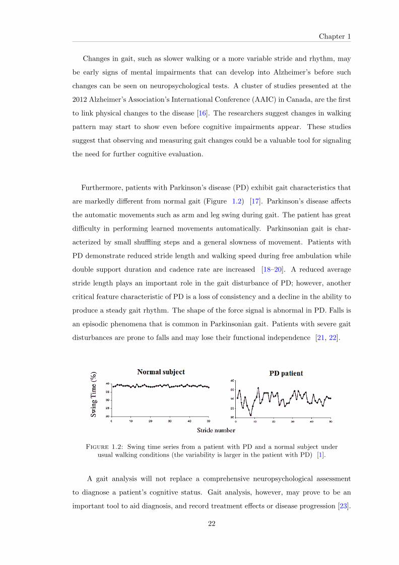
Furthermore, patients with Parkinson’s disease (PD) exhibit gait characteristics that

are markedly different from normal gait (Figure 1.2) [17]. Parkinson’s disease affects

the automatic movements such as arm and leg swing during gait. The patient has great

difficulty in performing learned movements automatically. Parkinsonian gait is char-

acterized by small shuffling steps and a general slowness of movement. Patients with

PD demonstrate reduced stride length and walking speed during free ambulation while

double support duration and cadence rate are increased [18–20]. A reduced average

stride length plays an important role in the gait disturbance of PD; however, another

critical feature characteristic of PD is a loss of consistency and a decline in the ability to

produce a steady gait rhythm. The shape of the force signal is abnormal in PD. Falls is

an episodic phenomena that is common in Parkinsonian gait. Patients with severe gait

disturbances are prone to falls and may lose their functional independence [21, 22].

Figure 1.2: Swing time series from a patient with PD and a normal subject underusual walking conditions (the variability is larger in the patient with PD) [1].

A gait analysis will not replace a comprehensive neuropsychological assessment

to diagnose a patient’s cognitive status. Gait analysis, however, may prove to be an

important tool to aid diagnosis, and record treatment effects or disease progression [23].

22

Chapter 1

1.3.2 Age related study

Aging is also accompanied by behavioral and kinematic changes and often

result in balance perturbation and impaired locomotion. The main consequence of aging

associated with deficits in locomotion is the falling. With advancing age, the risk of falls

increases with not only consequences of physical damage but also psychological and

social consequences.

1.3.2.1 Falling of elderly

Falls in the elderly are a major public health problem due to both their frequency

and their medical and social consequences. According to the World health organiza-

tion (WHO), fall is defined as ”the action of falling to the ground inadvertently, with

the inability to correct in due time and is determined by circumstances involving mul-

tiple factors that affect stability” [8]. According to a definition by the international

classification of diseases (ICD 9), fall is defined as ”any event in which the person is

unintentionally on the ground or on any other lower level”, this may include an event

during which the person lies on the ground, stumbles down the stairs, slips or loses

balance and strikes an object (table, bed...) [24]. According to Gibson et al. [25]: the

fall would be defined as ”an involuntary attraction to the ground which has high costs

consequences”.

Falls are the most common accidents in the elderly over 65 years. Fall prevalence

increases with age. Many studies have attempted to identify the risk factors in groups

at high risk of falling. Several predisposing factors that affect the ability to walk and

contribute to falling were cited such as: muscle weakness [26], impairments in gait and

balance problems [27–30], a previous fall [31], medications, cognition, musculoskeletal

problems and various pathological processes, including cardiovascular and neurological

causes. Falls is also caused by age associated diseases like the Parkinsons disease [32]

and Alzheimer.

In a study about the causes and risk factors of falls, adapted from [33], there are

many distinct causes for falls in old people, as listed in Table 1.1 , which summarizes

23

Chapter 1

data from 12 of the largest retrospective studies of falls among older persons living in a

variety of settings. Note that accidental and gait/balance disorders causes are the most

frequently, accounting for 20-50% in most series. So, balance and gait impairments in

older people increase the risk of falls.

Table 1.1: Causes of falls in elderly adults: summary of 12 studies that carefullyevaluated elderly persons after a fall and specified a most likely cause.b: Mean percentage calculated from the 3,628 falls in the 12 studies.c: Ranges indicate the percentage reported in each of the 12 studies.

d:This category includes arthritis, acute illness, drugs, alcohol, pain, epilepsy and fallingfrom bed.

Cause Mean percentageb (%) rangec (%)

’Accident’/ environment-related 31 1-53Gait/balance disorders or weakness 17 4-39Dizziness/vertigo 13 0-30Drop attack 9 0-52Confusion 5 0-14Postural hypotension 3 0-24Visual disorder 2 0-5Syncope 0.3 0-3other specified causesd 15 2-39unknown 5 0-21

1.3.2.2 Fall related statistics

The elderly tend to fall more often at home (78%) and at night and less often

on roads and public places (16%). In more than two thirds of cases (69%), the elderly

fall when walking. About 35% of people aged between 65 and 79 falls at least once a

year, and about half of those aged more than 80 fall one or many times per year. The

phenomenon of fall is often recurrent and it is estimated that 50% of fallers made at least

two falls per year [34]. Note that the fall is among the leading causes of hospitalization

in geriatric services. 10-20% of fallers result in injury, hospitalization and/or death [33].

The first fall is still a major event for the elderly. Compared to a subject that never

fell, the risk of recurrence after a first fall is multiplied by 20 and the mortality by 4.

Falling happen at any time of life but the severity of fall increases with advancing age

and reduced mobility of the individual.

24

Chapter 1

Falls are major health problems with significant economic and social ramifications.

Even when the immediate results are less dramatic, falls can have important impacts,

bringing about self-imposed mobility restrictions, fear of falling, and dependency. Falls

are also independent causes of institutionalization and mortality in older adults.

Different questionnaires and studies have quantified the importance of falls among the

elderly and support the relevance of our research. In France, falls are the leading cause

of death among people over the age of 65 where the statistics found that for this pop-

ulation there are over 400,000 fallers per year causing about 12,000 deaths [Le Figaro.fr].

According to the World Health Organization (WHO), in 2002, it is estimated that,

around the world, about 391,000 people died due to falling. So, falls is the second main

cause of death by involuntary accidents, immediately following on road traffic accidents.

Europe and the Western Pacific region combined account for nearly 60 % of the total

number of fall-related deaths worldwide.

The estimate of the financial cost of falls is very difficult, however it is a substantial

cost which varies from one country to another. In 2013, the direct medical costs of

older adult falls were $34 billion [35, 36]. The average cost of hospitalization for fall

related injury for people 65 year and older range from US$ 6646 in Ireland to US$ 17

483 in the USA. According to the world health organization, these costs are projected

to increase to US$ 240 billion by year 2040. For information, in Lebanon, there are no

official numbers determining the socio-economic costs of falling.

For a better understanding of human locomotion, a description of the walking cycle

will be presented in the next section.

1.3.2.3 Walking cycle

Walking is a complex task that engages the use of brain, spinal cord, peripheral

nerves, muscles, bones and joints. Studying human walking typically involves comput-

erized and instrumented measurement of the movement patterns that make up walking.

25

Chapter 1

It can facilitate the comparison between pathological and normal gait [37].

The walking cycle is the period from initial contact of one foot to the next initial

contact of the same foot [38–40]. In normal walking, there are two phases of gait stance

and swing. During one gait cycle in walking, the stance phase represents 60% of the

cycle while the swing phase represents the remaining 40%. Stride length is the distance

between successive initial contacts of the same foot (Figure 1.3). Step length is the

distance from initial contact of one foot to initial contact of the opposite foot [40]. The

duration of gait cycle fluctuates from one stride to the next in a complex manner. In

the normal gait pattern, complex fluctuations of unknown origin appear [41]. From a

neurophysiological control viewpoint, this behavior is of interest because it signifies the

presence of long-term dependence. They may be a consequence of peripheral input or

lower motorneuron control, or they may be related to higher nervous system centers that

control walking rhythm [10]. In elderly people, the variability and fluctuations increase

and is simply attributable to random fluctuations.

Figure 1.3: Gait cycle phases during walking [2]

1.3.2.4 Dual task performance

Human walking is an automated motor task controlled by subcortical brain regions.

Automaticity implies that gait can be performed without attention. Attention can be

thought of as the ability to focus cognitive resources and to selectively process certain

information from the environment [42]. Attention is said to be divided whenever an

26

Chapter 1

individual is processing more than one source of information at a time or performing

more than one task at a time. It is the executive function which coordinates allocation

of attention to different tasks during, daily life, allowing choices to be made about use

or storage of information and allowing division of attention between tasks if necessary

[43].

Dual task is part of executive function and is strongly related to divided attention.

So, gait disturbances are linked to alterations in executive function and attention.

Dual-task related gait changes are new way to assess age-associated change in gait

[43]. The attentional demands during locomotion vary depending on the complexity of

the task and the type of secondary task being performed. Recent works [43–45] high-

light the involvement of attentional resources in gait, using a dual − task methodology

in which performance on attention-demanding tasks such as spoken verbal response and

walking is compared when they are performed separately and concurrently.

The verbal fluency and backward counting tasks are frequently used to grab atten-

tion as a dual-task paradigm. Not away from this, walking changes is not an automatic

process but strongly highlight attention demanding task paradigm. But the rhythmic

stepping mechanism of walking remains less clearer, with only few and contradictory

published results in the literature [46, 47]. Dual task execution and fall risk have been

linked together by studies that tried to assess the rate of fall prediction while doing

another task. Many studies have clarified the usefulness of assessments of dual task

performance for fall prediction [1, 48]. The dual-task paradigm has been largely used to

test for the risk of falls and to better understand the link between mild cognitive decline

and variation in gait.

The study of gait variability under dual-task is still representing a new challenge for

the clinicians because such variability is an important fall predictor in elderly. Dual-task

related gait changes could also provide useful information about relationship between

gait disorders and cognitive decline [11].

27

Chapter 1

1.3.3 Analysis techniques: state-of-the-art for gait analysis

For all aged people, a multifactorial evaluation is necessary and will put in place

an early intervention with several areas of support:

• Vitals (Weight, Height, orthostatic blood pressure and Pulse).

• Affective/cognitive (Dementia, Depression, Fear of Falling).

• Musculoskeletal (joint, swelling, deformity, instability).

• Neurological (reflexes, coordination, sensation, cerebellar, vestibular, sensory &

proprioception)

• Lifestyle (nutrition, physical activities, intellectual activity, persons isolation, com-

fortable shoes providing good stability)

• Drug prescriptions

• Walking disorders and gait & balance performance testing.

Examination of fallers and falls prediction need assessment of bone strength, heart as-

sessments (echocardiography), acute and chronic medical problems, brain imaging (CT

scan or MRI), memory testing, physical assessment, evaluation of home safety.. One

important assessment also is the study of changes and fluctuations during a walk- gait

dynamics that may be useful to understand the alterations in the locomotor control

system. This may help to determine the fall risk and to provide insight into the neural

control of locomotion. Gait analysis can be used by health care professionals as its one

of the easiest and least expensive method of analysis.

Previous gait analysis techniques were used in literature; we mention here the most

important: the observational and 3D gait analysis; the stride-to-stride variability and

quantification of temporal/spatial parameters; the alterations in gait dynamics and De-

terended fluctuation analysis (DFA); the Electromyography (EMG) records; and the

analysis of ground reaction force signals.

28

Chapter 1

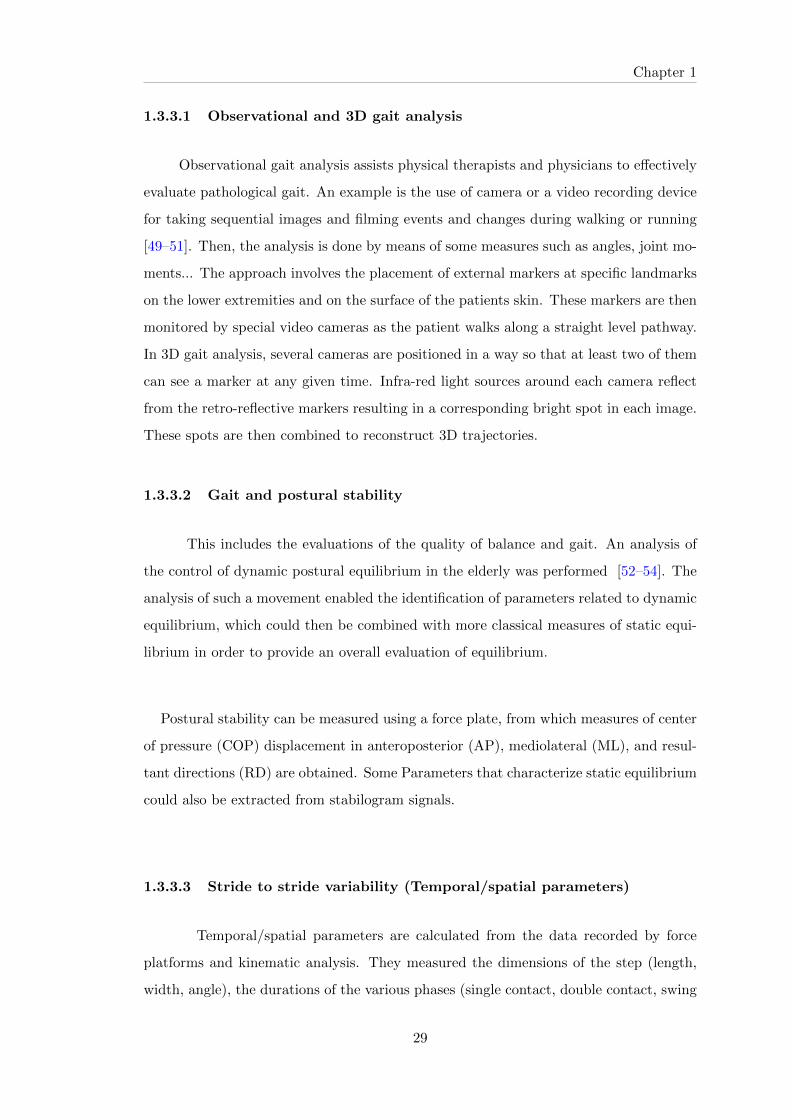
1.3.3.1 Observational and 3D gait analysis

Observational gait analysis assists physical therapists and physicians to effectively

evaluate pathological gait. An example is the use of camera or a video recording device

for taking sequential images and filming events and changes during walking or running

[49–51]. Then, the analysis is done by means of some measures such as angles, joint mo-

ments... The approach involves the placement of external markers at specific landmarks

on the lower extremities and on the surface of the patients skin. These markers are then

monitored by special video cameras as the patient walks along a straight level pathway.

In 3D gait analysis, several cameras are positioned in a way so that at least two of them

can see a marker at any given time. Infra-red light sources around each camera reflect

from the retro-reflective markers resulting in a corresponding bright spot in each image.

These spots are then combined to reconstruct 3D trajectories.

1.3.3.2 Gait and postural stability

This includes the evaluations of the quality of balance and gait. An analysis of

the control of dynamic postural equilibrium in the elderly was performed [52–54]. The

analysis of such a movement enabled the identification of parameters related to dynamic

equilibrium, which could then be combined with more classical measures of static equi-

librium in order to provide an overall evaluation of equilibrium.

Postural stability can be measured using a force plate, from which measures of center

of pressure (COP) displacement in anteroposterior (AP), mediolateral (ML), and resul-

tant directions (RD) are obtained. Some Parameters that characterize static equilibrium

could also be extracted from stabilogram signals.

1.3.3.3 Stride to stride variability (Temporal/spatial parameters)

Temporal/spatial parameters are calculated from the data recorded by force

platforms and kinematic analysis. They measured the dimensions of the step (length,

width, angle), the durations of the various phases (single contact, double contact, swing

29

Chapter 1

phase), walking speed, cadence, the supporting forces. Table 1.2 summarizes the key

parameters and their definitions.

The evolution of angular values can also be measured in the pelvis, hip, knee and an-

kle/foot in three planes, sagittal, frontal and transverse.

Table 1.2: The key Temporal/spatial parameters and their definitions

Index Definition

Velocity Walked distance time (e.g m/s)

Cadence Number of steps in a given time (e.g. steps per minute)

Step length The distance covered during the swing phase of a given leg(e.g. the distance between a toe off and the next heel strikeof the same leg)

Stride length The distance covered during a given gait cycle (e.g. thedistance between two consecutive heel strikes of the sameleg). It is also the summation of the distances of two steps(left and right)

Step width The distance between the two feet at the perpendicular axisto the walking direction for a given step

Step height The maximum distance between the forefoot and groundduring the swing time

Symmetry The ratio between the step lengths of the two legs

Spatial/temporal variability The coefficient of variation of spatio temporal indices

Coordination The timing of leg activation with respect to the other onewithin a gait cycle

Many researches and studies of gait dynamics and characteristics have concentrated

on stride-to-stride variability and on the treatment of the following parameters: the

cadence, the speed, the mean values and coefficients of variation of stride velocity, stride

time and stride length among healthy young adults, among elderly as well as among dif-

ferent pathological diseases (Parkinson disease, Huntington disease). These quantitative

measures can also be useful clinically.

Hausdorff demonstrated that the alterations in gait dynamics has meaning and is

useful for assessing fall risk and for distinguishing between fallers and non-fallers [1, 55].

The results showed that the stride time variability was significantly larger in the fallers

compared to both the young adult and elderly participants. So the relatively increased

30

Chapter 1

stride-to stride variability as well the increased stride length may reflect an unsteady gait

that predisposes to falls and thus could be considered as reliable indicators to identify

the potential risk of falling.

1.3.3.4 Alterations in gait dynamics and detrended fluctuation analysis

(DFA)

Some parameters linked to underlying physiological control systems have been iden-

tified to contain information related to long-term correlations and self-similarity. One

of these parameters is the Hurst exponent (H), which can be estimated using several

methods: rescaled range analysis (R/S), detrended fluctuation analysis (DFA) [56], and

stabilogram diffusion analysis (SDA) [57, 58].

J. Hausdorff has used the Detrended fluctuation analysis (DFA) which measures the

degree to which one stride interval is correlated with previous and subsequent intervals

over different time scales. DFA is a method based on the analysis of the relationship

between the mean magnitude of fluctuations in the series and the length of the intervals

over which these fluctuations are observed. He has demonstrated that the stride interval

time series exhibits long-range, self-similar correlations.

According to J. Hausdorff [1], the alterations in gait dynamics may help to determine

disease severity, medication utility, and fall risk, and may be useful in providing insight

into the neural control of locomotion and for enhancing functional assessment of aging,

chronic disease, and their impact on mobility. His study indicates that the measures of

gait dynamics may provide a useful index of gait instability and fall risk in older adults.

Gait instability measures were significantly increased in those who subsequently fell com-

pared to those who did not (Figure 1.4 and 1.5). Although both elderly groups had

similar walking speed and muscle strength, the elderly fallers had significant increases

in stride variance and reduced long-range, fractal dependence. Perhaps, relatively in-

creased stride-to-stride variability may reflect an unsteady gait that predisposes to falls.

31

Chapter 1

Figure 1.4: stride time variability in fallers and non-fallers.

Figure 1.5: gait speed doesn’t change in fallers and non-fallers, while the stride timevariability is significantly increased in fallers (results from [1]).

In the next section, running mechanics and exercise-related fatigue are treated with

highlight on the state-of-the-art of previous analysis techniques used for fatigue analysis.

1.4 Biomechanics of running and muscle fatigue

1.4.1 Study related to muscle fatigue (sports fatigue)

Neuromuscular fatigue is an exercise-related decrease in the maximal voluntary

force or power of a muscle or muscle group, whether or not the task can be sustained.

This potentially involves processes at all levels of the motor pathway from the brain to

skeletal muscle. The physiological processes involved in muscle force generation extend

to the whole neuromuscular system. Many different factors may underlie and be involved

in the expression of neuromuscular fatigue. The appearance of neuromuscular fatigue

is associated with changes in central or peripheral mechanisms. Interactions between

these mechanisms lead to a cascade of events which accelerate or decrease the muscles

force generation capacity [59].

32

Chapter 1

Running and walking for extreme durations, i.e. the so-called ultra-marathons, have

become increasingly popular in the last few years throughout the world, particularly in

the USA and Europe. Researches have examined the effects of classic ultra-marathon

running on injuries and muscle damage [60, 61], biochemical changes [62, 63] and neu-

romuscular fatigue [64, 65].

Studies have shown that the mechanism underlying fatigue depends on the activity

being performed also the intensity and duration of the activity are probably among

the most important factors. Studies have been focusing on the origin of muscle fatigue

after extreme long duration exercises lasting several hours and have been argued that a

significant amount of fatigue may occur after prolonged exercise. Investigating fatigue in

ultra-marathons is a major occasion to study human physiology as it is stretched towards

it endurance limits. Its only in recent years that few studies having being dedicated to

this very unusual exercise. Following are some studies which cover this: [64–72]. In

reference [66], the authors have confirmed that central fatigue would be the principal

explanation for neuromuscular fatigue during a 24 hr. running exercise. Therefore, we

can reasonably suggest that extreme ultra long duration of exercise may induce fatigue.

G. Y. Millet et al. made a study to examine the physiological and biomechanical

changes occurring in a subject after running 8,500 km in 161 days (i.e. 52.8 km daily).

Marked and consistent modifications in running pattern were shown in the kinematic,

dynamics of the running step and mechanical work data from PRE to POST at all

speeds. While contact time was not modified, the subject did re-organize his running

pattern toward that of a lower aerial time and a higher duty factor, therefore leading to

a higher step frequency [73].

G. Y. Millet et al. made also a study on the Neuromuscular Consequences of an

Extreme Mountain Ultra-Marathon over two weeks: a 166-km mountain ultra-marathon

(MUM) with 9500 m of positive and negative elevation change. Significant modifications

in markers of muscle damage and inflammation were observed. Moderate to large reduc-

tions in maximal compound muscle action potential amplitude, high-frequency doublet

force, and low frequency fatigue (index of excitation-contraction coupling alteration)

were also observed [74].

33

Chapter 1

In the section that follows, previous analysis techniques of fatigue will be discussed

along with the known measured parameters.

1.4.2 Analysis techniques: state-of-the-art for fatigue analysis

1.4.2.1 Surface electromyography (EMG)

Surface electromyography is a noninvasive method allowing the exploration of

muscle activity and the monitoring of physiological functioning [75]. During the last 30

years, it became a diagnostic tool for the study of muscle function, of fatigue, and other

nervous disorders. It is used in clinical applications and in sports domain. These surface

electrodes are frequently used to record the electrical activity of muscles during walking

and running. Several types of surface electrodes are available, with different shapes and

dimensions. These electrodes require the use of gel to improve the conductivity. Elec-

trodes (surface or thread) are then connected to a recorder. Current systems can record

from up to 16 muscles simultaneously. The mode of transmission of data is done via

telemetry.

Surface EMG parameters such as: the RMS (Root mean square), the mean frequency

and median frequency have been conventionally used to quantify muscle fatigue [76–78].

Indeed, it is known that the RMS increases with fatigue while the other two parameters

decrease linearly with the conduction velocity of action potential which decreases with

fatigue installation [79, 80].

Time/frequency tools have been also used to quantify the instantaneous evolution of

EMG frequency characteristics and to determine where the evolution is located in time.

Moreover, during dynamic contraction, the force changes, muscle length and electrodes

position with respect to active motor units in addition to the recruitment strategy and

discharge of motor units induce non-stationarity and sudden variation in the frequency

content of EMG [81]. One of the first tools used in time / frequency analysis is the short

time Fourier transform (STFT) which consists of calculating the Fourier transform on

successive and short intervals of time. Other tools are the Wigner-ville transform and

34

Chapter 1

wavelet transform which also allow us to follow the evolution of frequency content of a

signal with time. This analysis domain proved its efficiency for the treatment of EMG

surface signals obtained in dynamic conditions.

When the mechanical parameters vary too much, the evolutionary process of EMG

parameters is difficult to observe.

Later, advanced signal processing tools (cyclostationarity) have been also applied

on EMG surface signals [81, 82]. This technique provides additional information for

studying the evolution of spectral components with time. This approach is applicable

because EMG signals contain cyclic components. This approach calculates significant

frequencies from EMG signal to locate the neuromuscular activity. In a study performed

by El Hajj Dib [83], the spectral coherence was proven to be influenced by the regularity

of discharge of motor units.

1.4.2.2 Changes in ground reaction force signals

Previously, many attempts have been made to characterize human locomotion.

Many researches studied extensively the various aspects of ground reaction forces (GRF)

during walking and running [84–88]. There are many reasons why the study of GRF

is important beyond providing insight into the basic mechanism of human locomotion.

GRF are typically broken into three types: anterior-posterior, horizontal, and vertical.

The vertical GRF has received the most attention in comparisons among others.

The vertical ground reaction force exerted by men walking or running has been

accounted to analyze the various forms of human performance, to quantify impacts, to

calculate mechanical energy fluctuations, to understand propulsion, to compute muscle

forces, to quantify the muscle fatigue.

The changes in ground reaction force (GRF) signals could be measured and mod-

eled in order to indicate the function of various physiological subsystems. Indeed, the

35

Chapter 1

treatment of such signals during a biomechanical study of running could enable doctors

to extract parameters for numerous study and analysis (kinematics analysis, machine

works, mechanical characteristics of lower limbs, impacts analysis...). Previously, there

have been various studies concentrating on the analysis of Ground reaction force signals.

We named a few: [73, 88–92].

For example, H. Elftman [93] and Andriacchi et al. [94] have managed some aspects

of the ground reaction forces and made a detailed analysis of the kinematics of walking

and the dynamics of the human leg in walking providing information concerning muscle

function and gait abnormalities. Stan James [95, 96] has exhibited a large study and a

great understanding of the biomechanics of running. The works of Cavanagh et al. [84]

and W. Fenn [97] have treated the GRF values and patterns changes that occur during

distance running. T. Novacheck [98] detailed the literature regarding the biomechanics

of running and Lieberman et al. [99] conducted a study of the foot strike patterns and

collision forces to compare barefoot and shod runners. Gerlach et al. [90] investigated

how the GRF changed with fatigue as induced by an exhaustive treadmill run in female

runners. J. Gottschall [89] investigated the normal and parallel GRF during downhill

and uphill running. Also, Christina et al. demonstrated the effect of localized muscle

fatigue on vertical GRFs and ankle joint motion during running in [91]. And Mikaela

Boham et al. assessed the effects of functional fatigue on ground reaction forces of a

Jump, Land, and cut task [92].

As shown in (figure 1.6), GRF signals are usually composed of two distinct peaks: an

active force peak representing the propulsive force in addition to a passive force peak rep-

resenting the impact force. The impact force is mainly passively generated and is due to

the deceleration of the body mass at the instant of touch down. It represents the initial

impact between the body and the ground at initial heel contact. It is determined by the

effective mass of the body, the velocity and leg stiffness. It is attenuated by the heel pad

and shoe wear and could be modified by the passive characteristics of the running sur-

face. It is always smaller and of shorter duration than the propulsive force (active peak).

The second peak i.e. the active muscle force corresponds to the point when the energy

36

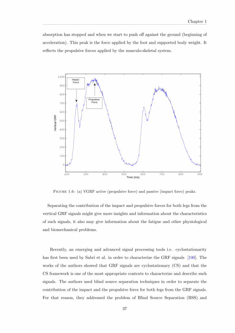
Chapter 1

absorption has stopped and when we start to push off against the ground (beginning of

acceleration). This peak is the force applied by the foot and supported body weight. It

reflects the propulsive forces applied by the musculo-skeletal system.

200 300 400 500 600 700 800 900

0

100

200

300

400

500

600

700

800

900

1000

Time (ms)

Ver

tical

GR

F

Impact Force

Propulsive Force

Figure 1.6: (a) VGRF active (propulsive force) and passive (impact force) peaks.

Separating the contribution of the impact and propulsive forces for both legs from the

vertical GRF signals might give more insights and information about the characteristics

of such signals, it also may give information about the fatigue and other physiological

and biomechanical problems.

Recently, an emerging and advanced signal processing tools i.e. cyclostationarity

has first been used by Sabri et al. in order to characterize the GRF signals [100]. The

works of the authors showed that GRF signals are cyclostationary (CS) and that the

CS framework is one of the most appropriate contexts to characterize and describe such

signals. The authors used blind source separation techniques in order to separate the

contribution of the impact and the propulsive force for both legs from the GRF signals.

For that reason, they addressed the problem of Blind Source Separation (BSS) and

37

Chapter 1

blind MIMO system identification using second order cyclic statistics. They tested some

existing instantaneous BSS methods that use different assumption on the source sig-

nals. Sabri et al. worked on different approaches: SVD (Singular Value Decomposition)

and EVD (Eigenvalue Decomposition) based approach, PDLC (the diagonalization of a

positive definite linear combination) and the AJD (Approximate Joint Diagonalization)

based approach. The AJD based approach was able to completely separate the impact

forces but not the propulsive forces of GRF signals. The propulsive forces of both steps

are not completely separated [101–103].

Sabri et al. then considered the following BSS methods [103]: SOBI (Second-Order

Blind Identification) [104], CycloSOBI [105] and JADE [106], for GRF signals sepa-

ration. The approaches based on second order statistics (SOBI and CycloSOBI) failed

to properly separate the contributions of each step. Only the JADE method, which is

based on the HOS, produced fair results. It should be noted that these works could not

find a good solution or an approach to achieve the main objective. Furthermore, the

work done did not thoroughly delve into the study of fatigue.

Even though these methods have resulted in some practical applications, these studies

have at least highlighted the concept of the signature on which our methodology is based.

Despite the advances made, there are a number of challenges still remaining. Also, in

order to obtain the best possible results, it will be necessary to have large quantities of

clinical data.

Before presenting the practical part, the physical signal processing and the results,

it is important to review the different works encountered in the literature of cyclosta-

tionarity analysis and its applications in different domains, including biomechanics. In

this literature review, we are interested in various methods of signal processing (in gen-

eral) and the theory of ”cyclostationarity” in particular. In addition, we are interested

in source separation techniques for the separation of GRF signals components.

38

Chapter 1

1.5 Conclusion

In this chapter, we made a study on human locomotion, falling of elderly, and fatigue.

We presented previous approaches to the study of gait, also many ways of measuring the

within-subject stride-to-stride changes. We concluded that searching for new parameters

for better characterizing gait fluctuations is very important since all available parameters

are not sufficient and lack of certainty and not sensitive enough to simply differentiate

between fallers and non-fallers.

39

Chapter 2

PROPOSED ADVANCED

TECHNIQUES AND

PROCESSING TOOLS

Contents

2.1 Introduction . . . . . . . . . . . . . . . . . . . . . . . . . . . . 42

2.2 Cyclostationarity (CS): history, definitions and properties . 43

2.2.1 Cyclostationarity history . . . . . . . . . . . . . . . . . . . . . 43

2.2.2 Cyclostationary signals: definitions and properties . . . . . . . 44

2.2.3 Orders of cyclostationarity . . . . . . . . . . . . . . . . . . . . 45

2.2.4 Cyclostationarity descriptors of second order . . . . . . . . . . 46

2.2.5 Envelope analysis . . . . . . . . . . . . . . . . . . . . . . . . . . 48

2.2.6 Review of cyclostationary modulation types . . . . . . . . . . . 48

2.2.7 Degree of cyclostationarity (DCS) . . . . . . . . . . . . . . . . 51

2.3 Review of existing source separation techniques . . . . . . . 52

2.3.1 FastICA algorithm . . . . . . . . . . . . . . . . . . . . . . . . . 53

2.3.2 MCA concept . . . . . . . . . . . . . . . . . . . . . . . . . . . . 55

2.4 Deterministic component cancellation methods . . . . . . . 58

2.4.1 Cepstral editing procedure . . . . . . . . . . . . . . . . . . . . . 59

2.5 Conclusion . . . . . . . . . . . . . . . . . . . . . . . . . . . . . 59

41

Chapter 2

In this chapter, we present the theory of cyclostationary process. We also present

an empirical and mathematical relationship between the kurtosis and degree of cyclo-

stationarity. We review also some existing source separation techniques.

2.1 Introduction

The stochastic approach is convenient to model signals from physical processes. A

real stochastic process is a collection of random signals representing the evolution of

random variables over time. The first studied stochastic processes are the stationary

processes. They are easy to measure and characterize because their statistical moments

are constant.

The classical methods of signal processing address the signals from a stationary view-

point. It appears in reality that the majority of biomechanical signals are inherently

non-stationary due to the evolutionary phenomena that generate them. It turns out

that some of the information they convey is precisely this non-stationarity. Although

it is somewhat a simpler treatment, the assumption of stationarity is unable to reveal

certain information. In turn, Cyclostationarity allows showing this information to the

random or deterministic phenomena, specific cases of non-stationarity. In this context,

it will be possible to add to the traditional indicators, an additional dimension reflecting

the cyclical evolution. The existence of this cyclical evolution leads naturally to exploit

the cyclostationarity of these signals, i.e. the periodicity of statistical parameters. So,

the extension of the tools from the stationary case to those of cyclostationary case al-

lows the apprehension of the characteristics of these signals by integrating an additional

dimension.

Stationary signals are analyzed with time-invariant correlations, or with frequency-

domain analysis (power spectral density). However, cyclostationary signals and generally

non-stationary signals include four variables: time, lag, cyclic frequency and carrier fre-

quency.

42

Chapter 2

2.2 Cyclostationarity (CS): history, definitions and prop-

erties

2.2.1 Cyclostationarity history

First of all, we review the different works encountered in the literature of cyclostation-

ary signal processing and its applications in different domains, including biomechanics.

Historically, the idea of cyclostationarity first appeared in 1958 by Bennett [107] who

worked with the development of synchronization algorithms for the communication sys-

tems. In 1959, Gudzenko [108] presented a study on the non-parametric spectral esti-

mation of cyclostationary signals. In the early 1960s, Gladyshev [109, 110] introduced

the concept of periodically and almost periodically correlated random processes.

Later, the works of W. Gardner, Spooner and G.B. Giannakis [111–115] have con-

tributed significantly to the concept, theory and applications of cyclostationarity in the

engineering community. They have been largely contributed in the comprehension of

cyclostationnarity. Gardner applied the CS process in the field of telecommunications

and derived numerous models useful for studying and characterizing cyclostationarity .

Fundamental contributions in the field of cyclostationarity were also reported by Izzo

and Napolitano [116–123].

In the last two decades, cyclostationarity has led to important breakthroughs in different

domains and breached the classical approaches of signal processing i.e. stationarity. For

instance, it was expanded to the field of mechanics by Antoni et al. [124–128], Randall

et al. [129], Lamraoui et al. [130, 131] and others. Recently CS was extended to the

field of biomechanics by Piscione et al. [132]; Cao et al. [133]; Sabri et al. [101], El

Badaoui & Bonnardot [134] and Maiz et al. [5, 135–137].

Cyclostationarity improve the precision and reliability of algorithms existing in a noisy

environment. It also yields to get interesting results in blind source separation [104,

126, 138].

43

Chapter 2

2.2.2 Cyclostationary signals: definitions and properties

A large number of non-stationary processes exhibit a structure in the variation of their

parameters. When this structure is periodic, the Cyclostationary process is endorsed

and adopted, i.e. a process whose statistical properties cyclically vary with respect to

time or with respect to some generic variables. CS contains hidden periodicities and so

it is not periodic in the strict sense, but some of its statistical properties are periodic as

the probability density or energy.

More clearly, a CS signal is a coupling of a periodic phenomenon (Cyclostationarity of

order 1 or CS1) and a stationary random phenomenon (Cyclostationarity of order 2 or

CS2) (Figure 2.1). This gives us a fixed periodic structure called cyclic correlation. Such

a structure allows us to show the presence or absence of hidden periodicities by means

of the cyclic autocorrelation function.

Figure 2.1: Cyclostationarity phenomenon

Generally, the essence of cyclostationarity is that sine waves could be generated from

random data by applying nonlinear transformations. As a result, a signal is CS of order

n if and only if one could find a certain nonlinear transformation of order of a signal

which will generate additive finite amplitude sinusoidal components, and that results in

spectral lines.

Notice that it is rare that biomechanical systems produce signals that are purely cyclo-

stationary for a given order. Yet, they are a combination of several orders of cyclosta-

tionarity.

44

Chapter 2

2.2.3 Orders of cyclostationarity

The works of Gardner & Spooner [112] revealed the existence of two levels of

cyclostationarity:

A. Cyclostationarity of order 1 (CS1)

The first order moment of a process Sk[t] corresponds to the mean ms[t] of its realiza-

tions ms[t] = E{Sk[t]}. A process is said to be cyclostationary of first order if its first

order moment is periodic with period T :

mS [t] = mS [t+ T ] ∀t ∈ Z (2.1)

The first order moment is periodic and so accepts Fourier series decomposition:

mS [t] =∑k∈Z

mkSe

j2πfkt (2.2)

mkS are the Fourier coefficients of mS [t] in the discrete frequencies fk = k

T

B. Cyclostationarity of order 2 (CS2)

A random process Sk[t] is said to be cyclostationary of second order if the second order

moment (Autocorrelation function) is periodic of period T :

CS [t, τ ] = CS [t+ T, τ ] = E{S[t+ τ ]S∗[t− τ ]} ∀t ∈ Z (2.3)

The instantaneous autocorrelation function is periodic and so admits a Fourier series

expansion given by:

45

Chapter 2

CS [t, τ ] =∑vk∈A

CAFS [vk, τ ]ej2πvkt (2.4)

In this decomposition, v is called the cyclic frequency,A : {vk = kT , k ∈ Z} is the set

of cyclic frequencies. CAFS [vk, τ ] are called the cyclic autocorrelation function (CAF)

given by:

CAFS [vk, τ ] = limT−→∞

1

T

T−1∑t=0

CS [t, τ ]e−j2πvkt (2.5)

This function is continuous in variable τ and discrete in variable v . It is non-zero in

some v 6= 0 . In case of stationarity, the cyclic autocorrelation function is zero for all

frequencies v 6= 0 . Indeed, at v = 0 , the cyclic autocorrelation function is exactly

the classical autocorrelation function. This property of cyclostationary model makes it

important in many applications including telecommunications and biomechanics.

2.2.4 Cyclostationarity descriptors of second order

CS signals can be described in terms of the cyclic autocorrelation function (CAF) and

its Fourier transform, the cyclic spectrum or spectral correlation density function (SCD).

The SCD constitutes a complex second order statistical description of a CS waveform.

The SCD is given by:

SCDS [vk, f ] = FTτ{CAFS [vk, τ ]} =+∞∑

τ=−∞CAFS [vk, τ ]e−j2πfkτ (2.6)

SCDS [vk, f ]

6= 0 if vk = kT , ∀k ∈ Z

0 else.(2.7)

In this equation, v is referred to as the cyclic frequency i.e. the frequency of second order

periodicity and f is called the spectrum or carrier frequency. If the signal is cyclosta-

tionary then the cycle spectrum contains harmonics of the fundamental cycle frequency.

46

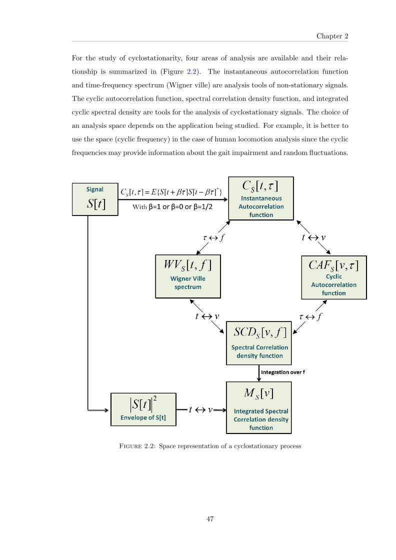
Chapter 2

For the study of cyclostationarity, four areas of analysis are available and their rela-

tionship is summarized in (Figure 2.2). The instantaneous autocorrelation function

and time-frequency spectrum (Wigner ville) are analysis tools of non-stationary signals.

The cyclic autocorrelation function, spectral correlation density function, and integrated

cyclic spectral density are tools for the analysis of cyclostationary signals. The choice of

an analysis space depends on the application being studied. For example, it is better to

use the space (cyclic frequency) in the case of human locomotion analysis since the cyclic

frequencies may provide information about the gait impairment and random fluctuations.

Figure 2.2: Space representation of a cyclostationary process

47

Chapter 2

2.2.5 Envelope analysis

Randall and Antoni [129] proved the importance to study the cyclic spectral density

integrated over f . R. Randall et al. have proven an equivalence between the integrated

cyclic spectral density (SCD) (the SCD given by eq. 2.6) and the envelope spectrum. So,

the envelope analysis can well replace the SCD. This relationship between the integrated

spectral correlation and envelope analysis allows to directly use the latter to characterize

the CS2 behavior of a signal. Indeed, the envelope analysis represents a projection of

the spectral correlation on the cyclic frequencies axis v. The result of the relationship

between the integrated SCD and the envelope for a CS signal is written as:

EnvS [v] = limT→∞

1

T

∫ T/2

−T/2E[s(t)2

]e−j2πvtdt, (2.8)

EnvS [v] =

∫RSCDx(v, f)df (2.9)

s(t) represents the temporal stochastic signal (CS2) and v is the discrete set of cyclic

frequencies.

2.2.6 Review of cyclostationary modulation types

Every CS process can be represented as a coupling of periodically modulated part

together with a random stationary part. The periods of CS in modulated signals may

correspond to carrier frequencies, repetition or pulse rates, time division multiplexing

rates...

Here, we present a review of some interesting examples of modulation types that produce

Cyclostationary waveforms i.e. waveforms with mixtures of periodicity and randomness.

These examples have received great attention in literature.

1) Periodically modulated stationary noise (noise with periodically varying

characteristics):

48

Chapter 2

This model can be written as:

S[t] = n[t]P [t] (2.10)

Where the random process n(t) is a stationary white noise, and P(t) is periodic with

period T. An example is the Amplitude modulation waveform (AM) where P(t) is given

by:

P [t] = cos(2πf0t+ φ) (2.11)

Such model has the following CAF (Figure 2.3) and SCD functions [139]:

CAFS [v, τ ] =1

2Cn(τ) cos(2πf0t)δ(v) +

1

4Cn(τ)

[ej2φ0δ(v − 2f0) + e−j2φ0δ(v + 2f0)

](2.12)

SCDS [v, f ] =1

4

[Sn(f + f0)δ(v) + Sn(f − f0)δ(v) + Sn(f)e−j2φ0δ(v + 2f0) + Sn(f)ej2φ0δ(v − 2f0)

](2.13)

Sn(f) and Cn(τ) are the power spectrum and autocorrelation function of n(t). CAFS [v, τ ]

and SCDS [v, f ] are the cyclic autocorrelation function and the spectral correlation den-

sity function respectively. CAFS [v, τ ] and SCDS [v, f ] are non-zero for {v = 0andv =

±2f0}. S(t) is cyclostationary with cyclic period 12f0

.

2) Pulses with random amplitudes on a periodic schedule

This model can be written as:

S(t) =∑k

Pkw(t− kT ) (2.14)

49

Chapter 2

Figure 2.3: cyclic autocorrelation function (in linear scale) of a signal modulated inamplitude.

The model includes for example the real pulse amplitude modulated signal (PAM) where

w(t) is a pulse signal defined on the interval (−T/2,T/2), and Pk is a zero mean station-

ary discrete time signal with unity power [139].

The SCD of such model is given by:

SCDS [v, f ] =1

T 20

W (f +v

2)W ∗(f − v

2)

+∞∑k,m=−∞

SCDv+ m

T0pk

[f − m

2T0− k

T0] (2.15)

3) Pulses on periodic schedule with randomly jittered timing

This model incorporates pulse timing jitter and can be written in the following form:

S(t) =∑k

Pkw(t− kT − εk) (2.16)

50

Chapter 2

Where its cyclic spectrum can be presented as:

SCDS [v, f ] = W (f +v

2)W ∗(f − v

2)∑β

∫ +∞

−∞SCD

v−βpk

[f − v]SCDβ

wdv (2.17)

2.2.7 Degree of cyclostationarity (DCS)

The DCS is first described by Zivanovic & Gardner [140]. It is a suitable measure of

the degree of non-stationarity for stochastic processes that exhibit CS. We can define

it as the distance from the closest stationary process having a similar power spectral

density. DCS quantifies the CS energy of s(t) at the frequency v (Figure 2.4). The

Cyclic frequency having non-zero energy on the cyclic statistics of order 2 is an indicator

determining the presence of a CS signal. So this parameter is essential for the detection

of a CS signal. For a given cyclic frequency v, DCS is defined as:

DCSvS =

∑τ |CAFS [v, τ ]|2∑τ |CAFS [0, τ ]|2

(2.18)

SDCSS =∑v

DCSvS (2.19)

Figure 2.4: DCS of the model s(t) = n(t) ∗ (1 + cos(2πf0t)) with n(t) a guassianrandom signal n(t)→ N(0, σ2) and f0 = 20Hz.

51

Chapter 2

2.3 Review of existing source separation techniques

In the following chapters, we are interested in source separation techniques for the sep-

aration of GRF signals components as well as for the separation of CS1 and CS2.

In this section, it is important to make a review of the existing source separation tech-

niques and their importance in signal processing applications.

Source separation techniques are considered to be among the most important signal pro-

cessing tools in terms of research and applications in various fields and domains (e.g.,

vibration signals and diagnosis, biomechanical signals, biomedical signals, telecommuni-

cation signals, etc.). Over the past few years, a great interest has been given to source

separation of processes excited by cyclostationary (CS) inputs. Research has been fo-

cused on disentangling periodic components out from non-deterministic ones so that each

component could be extracted and analyzed individually. The following are some studies

which cover this in different domains and applications: [5, 101, 103, 104, 125, 141–143].

Here we provide an example in the domain of mechanics and monitoring of rotating

machinery. For instance, in case of fatigue or appearance of faults, mechanical machines

do not produce stationary signals. They exhibit cyclostationarity, i.e., they experience

nonstationary behaviors composed of a coupling of periodicity and some degree of ran-

domness and noise. The defects can be detected in this nonstationary part of signal.

The study of the cyclostationarity of vibratory signals allows to take into account the

random effect that can be produced between each machine tool revolution. Furthermore,

we provide another example in the domain of biomechanics and human locomotion anal-

ysis. For example, muscle fatigue adversely impacts the mechanical efficiency of muscle

work, so the cyclic and repeated gestures that characterize human locomotion are also

affected. In other words, the cyclic properties of human locomotion experience some

degree of randomness. Previous analysis and treatment of such sequences are demon-

strated and have proven that such processes are CS [100, 137].

52

Chapter 2

Priestley [144] states that it is possible to decompose any nonstationary process into its

periodic and nondeterministic parts. Also, signals analysis has greater efficiency if pe-

riodic components could be separated from stochastic ones. Thus, the obvious need for

methods dedicated to such separation led researchers to propose several algorithms and

techniques. Moreover, it is necessary that the sources to be retrieved contain some kind

of diversity (e.g., decorrelated sources, independent sources, sources with morphological

diversity, etc.). Here we mention some of the most efficient and popular techniques in

the CS domain.

Some authors have used classical blind source separation (BSS) techniques such as the

following: the independent component analysis method (ICA) based on the strong as-

sumption of statistical independence of sources [145], the FastICA algorithm [146], the

JADE method [106] and SOBI [104]. Another method is the CycloSOBI method [105]

which is a combination of SOBI and SCORE [147] algorithms. CycloSOBI exploits the

temporal coherence and cyclostationarity of source signals. However, in general, classical

BSS methods necessitate the use of different sensors and few of them require knowledge

of the number of sources. Also, most BSS algorithms assume a greater number of sources

than the number of mixtures. In addition, classical BSS methods fail in separating from

the signal the pure second-order CS (CS2) component.

2.3.1 FastICA algorithm

FastICA is a known fixed-point ICA algorithm. It is easy to use and there are no step-

size parameters to choose. The algorithm blindly extracts all non-Gaussian independent

source signals regardless of their probability distributions.

This technique is based on running the ICA (independent component analysis) algorithm

many times with different initial values or bootstrap samples, and then looking at the

clustering of the estimated components in the signal space. Basically, each tight cluster

corresponds to a component that can be considered reliable. Reliability has algorithmic

and statistical aspects [146].

53

Chapter 2

Therefore, given the ICA model

x = AS =[aT1 , a

T2 , . . . , a

TN

][s1, s2, . . . , sN ]; T : the transpose of the matrix

of independent sources s and a mixing matrix A we run the algorithm M-times on the

data X = [x1x2 . . . xN ] consisting of N-samples and k-dimensional vectors. For each run

the data is bootstrapped and the algorithm starts with new random initial conditions.

Then we choose the clusters that best fits to the natural structure of the data.

ICASSO is a software for investigating the reliability of ICA estimates by clustering and

visualization.

Here, the ICASSO algorithm is just used to compare the estimates of some runs of

FastICA and to provide additional information on the reliability and robustness of es-

timation. Then, the estimated source signals corresponding to the active and passive

sources are clearly retrieved even in repeated experiments.

In general, the BSS algorithms give different components when run several times, so it is

important to choose the ones are to be taken seriously. We used the ICAASO algorithm,

which is based on the FastICA method, as a visualization method for investigating the

relations between estimates and estimating the clustering of sources in the signal space.

Reliable estimates correspond to tight clusters, and unreliable ones to points which do

not belong to any such cluster. ICASSO algorithm provides also a tool for getting a

detailed look into the clustering results and relations between the clusters and individual

estimates.

The ICASSO algorithm that is based on FastICA is composed of the following steps:

• Centering and whitening the data.

• Parameters selection for the estimation algorithm.

54

Chapter 2

• Running ICA many times with different bootstrapped datasets and different initial

values.

• Clustering the estimates.

• Interactive visualization application.

• Retrieving the estimates belonging to certain clusters.

2.3.2 MCA concept

Furthermore, big attention has been given in the last decade to the sparsity and Mor-

phological diversity. This technique was first presented in Bobin et al. (2006) [148] as

a source separation tool to decompose a signal or image into superposed contributions

from different sources. The idea to decompose a signal into its morphological compo-

nents is an important issue in image and signal processing. sparsity has emerged as one

of the important concepts in different signal-processing applications (restoration, feature

extraction, source separation, compression, etc.). This wider range allows more flexibil-

ity in signal representation and adaptivity to its morphological content and entails more

effectiveness in many signal-processing tasks.

The Morphological component analysis technique (MCA) is a useful and effective method

to decompose and model a signal with different morphologies. The known independent

component analysis method (ICA) assumes the sources are non-Gaussian and statis-

tically independent, whereas the MCA method assumes that for each morphological

source, there exists a basis function allowing its construction using a sparse representa-

tion. Therefore, MCA decomposes the signal with respect to a given dictionary, which

is a set of atoms used to decompose the signal.

MCA can be used to separate signal components, to denoise a signal, to remove artifacts

and to detect anomalies in signals (mechanical signals: e.g., gear signals, ). A detailed

description of this method is given as follows:

The original signal S is modeled as a linear combination of K morphological sources

(sk)k=1...K . Each morphological source is represented sparsely in a particular dictionary

55

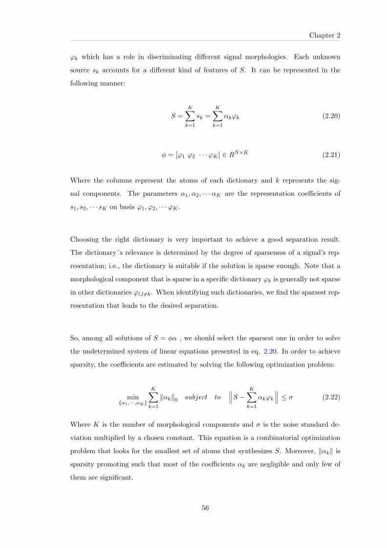
Chapter 2

ϕk which has a role in discriminating different signal morphologies. Each unknown

source sk accounts for a different kind of features of S. It can be represented in the

following manner:

S =

K∑k=1

sk =

K∑k=1

αkϕk (2.20)

φ = [ϕ1 ϕ2 · · ·ϕK ] ∈ RN×K (2.21)

Where the columns represent the atoms of each dictionary and k represents the sig-

nal components. The parameters α1, α2, · · ·αK are the representation coefficients of

s1, s2, · · · sK on basis ϕ1, ϕ2, · · ·ϕK .

Choosing the right dictionary is very important to achieve a good separation result.

The dictionary´s relevance is determined by the degree of sparseness of a signal’s rep-

resentation; i.e., the dictionary is suitable if the solution is sparse enough. Note that a

morphological component that is sparse in a specific dictionary ϕk is generally not sparse

in other dictionaries ϕl,l 6=k. When identifying such dictionaries, we find the sparsest rep-

resentation that leads to the desired separation.

So, among all solutions of S = φα , we should select the sparsest one in order to solve

the undetermined system of linear equations presented in eq. 2.20. In order to achieve

sparsity, the coefficients are estimated by solving the following optimization problem:

min{α1,··· ,αK}

K∑k=1

‖αk‖0 subject towwwS − K∑

k=1

αkϕk

www ≤ σ (2.22)

Where K is the number of morphological components and σ is the noise standard de-

viation multiplied by a chosen constant. This equation is a combinatorial optimization

problem that looks for the smallest set of atoms that synthesizes S. Moreover, ‖αk‖ is

sparsity promoting such that most of the coefficients αk are negligible and only few of

them are significant.

56

Chapter 2

Substituting the l0 norm by the l1 sparsity measure, as motivated by recent results in

Bobin et al (2008) [149], the alternative convex minimization problem becomes:

min{Φ1,··· ,ΦK}

λ

K∑k=1

‖αk‖l1 +wwwS − K∑

k=1

Φk

www2

l2with Φk = αkϕk (2.23)

In this case, the sparseness is measured by the l1 norm, which is simply the sum of

the absolute value of the entries in a vector. The l1 norm promotes the sparsity of the

decomposition of each component [150]. The number λ is the regularization parameter.

It decreases through iterations until it reaches its final value λmin which corresponds to

the targeted level of regularization.

When the sparsest representations are obtained, the signal components separation is

performed. The success of MCA relies on the incoherence between sub-dictionaries.

Each sub-dictionary should lead to sparse representations of the corresponding signal

component [151].

The steps of the MCA algorithm are summarized as follows:

1. The choice of parameters: the signal S, the dictionary ϕk, the number of iterations,

stopping threshold, the threshold update schedule and the initial threshold.

2. At each iteration:

–For k = 1 . . .K

• Compute marginal residuals Rk = S − αkϕk.

• Estimate the coefficients αk of sk with a hard thresholding.

• Update kth component by reconstruction from the selected coefficients αk:

sk = ϕkαk

–Update the threshold according to a given strategy (linear or exponential de-

crease).

57

Chapter 2

3. Stop when the threshold is higher than a given lower bound (depends in particular

on the noise standard deviation).

So, the MCA algorithm performs at first a step of computation of the coefficients αk

followed by an update of the component sk . These two steps depend on the nature of

the dictionary. At each iteration, the most salient content of each morphological compo-

nent is iteratively computed. These estimates are then progressively refined depending

on the given stopping threshold and threshold update schedule.

More information about this algorithm can be found in references [150] and [152].

Attention has been also given to the proposition of deterministic component cancella-

tion methods that exploit cyclic statistics, in time or frequency domain. Such methods

include the time synchronous averaging technique (TSA) [153], the cepstral editing

procedure (CEP) [3], the adaptive noise cancellation method (ANC) [154], the self-

adaptive noise cancellation method (SANC) [155], and the noise cancellation frequency

domain algorithm [156]. The nondeterministic process is then calculated by subtract-

ing the periodic part from the actual signal. This process includes stochastic random

variables and noise.

2.4 Deterministic component cancellation methods

Time-synchronous averaging (TSA) and Cepstral editing procedure (CEP) are two meth-

ods developed earlier and give some advantages when compared to others. TSA is gen-

erally used more for data with no or small speed fluctuations.

CEP is used in chapter 4 for separating the components of the passive signal. CEP

extracts the periodic components i.e., the first-order CS phenomenon (CS1). CEP is

discussed in details in the following sub-section.

58

Chapter 2

2.4.1 Cepstral editing procedure

Cepstral editing procedure is a very simple algorithm and it is able to provide compact

information easy to interpret. CEP is based on the cepstrum, which collects all period-

icity in the log spectrum into a small number of components which can then be edited

to remove selected families. CEP does not need an order tracking as long as the speed

variation is limited. It is based on the cepstrum of the signal that efficiently collects

spectral components that are uniformly spaced, that is, both harmonics and modulation

sidebands. Cepstrum is the inverse Fourier transform of the log spectrum. ; It is defined

as:

S(t) = TF−1{Ln|S(f)|}

with S(f) = TF{s(t)} and TF is the Fourier transform.

And S(f) = A(f)exp(j φ(f))

In terms of its amplitude and phase.

Note that the real cepstrum uses both amplitude and phase to return to the time domain.

A schematic diagram of the CEP for removing all deterministic parts is shown in Figure

2.5.

2.5 Conclusion

In this chapter, many methods have been presented to be used for the analysis of GRF

signals. We presented the theoretical background behind cyclostationarity and its in-

dicators and properties, with examples of validation. Some BSS techniques were also

presented in addition to the morphological component analysis method and a determinis-

tic component cancellation method. We applied these methods on GRF data for human

locomotion analysis, also for separation of different GRF components and sources. The

results obtained will be presented in the next chapters.

Next chapter presents the walking signals analysis with cyclostationary approach, with

a target to characterize human walking and to estimate the potential risk of fall.

59

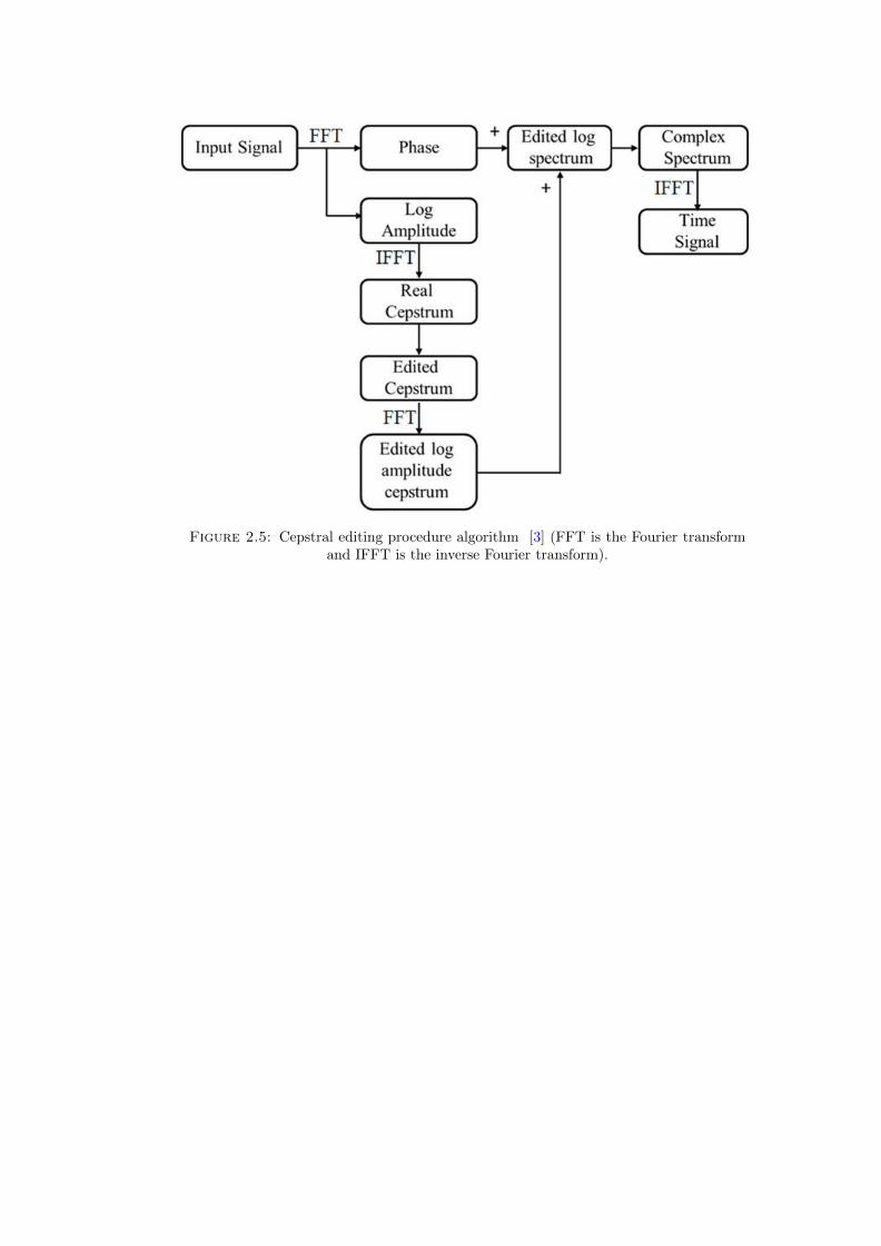
Figure 2.5: Cepstral editing procedure algorithm [3] (FFT is the Fourier transformand IFFT is the inverse Fourier transform).

Chapter 3

CYCLOSTATIONARY

ANALYSIS OF WALKING

SIGNALS

Contents

3.1 Introduction . . . . . . . . . . . . . . . . . . . . . . . . . . . . 62

3.2 Design of acquisition system . . . . . . . . . . . . . . . . . . . 62

3.3 Kurtosis (proposed indicator of cyclostationarity) . . . . . . 64

3.4 Cyclostationarity characters of walking signals . . . . . . . . 69

3.5 Methodology . . . . . . . . . . . . . . . . . . . . . . . . . . . . 70

3.6 Cyclic correlation with different walking conditions . . . . . 73

3.7 Cyclic correlation between fallers and non-fallers . . . . . . 75

3.8 Results summary . . . . . . . . . . . . . . . . . . . . . . . . . . 76

3.9 Results comparison . . . . . . . . . . . . . . . . . . . . . . . . 78

3.10 Conclusion . . . . . . . . . . . . . . . . . . . . . . . . . . . . . 79

61

Chapter 3

In this chapter, we highlight the particular interest of cyclostationarity, inherent in

biomechanical signals, for the detection of falls in elderly people. We verify and deter-

mine the cyclostationary properties of the signals under consideration.

3.1 Introduction

The right choice of signal processing tools in locomotion analysis necessitates a priori

knowledge on the signal being processed. In this chapter, we treat the signal as a stochas-

tic quantity, whose variance (i.e. energy, squared value) varies cyclically as a function of

time. We will try to adapt the theory of cyclostationary signal processing to the human

locomotion analysis. We exploit the properties of cyclostationarity for the detection and

estimation of the risk of falls in the elderly. Cyclostationarity allows the analysis of both

periodic and random behavior of signals. In walking signals, the periodic phenomenon

is related to the stride cycle while the random character could be related to the random

fluctuation from a stride to another. We verify the presence of CS2 (cyclostationarity

of order 2) which is simply attributable to variability and random fluctuations during

walking. In elderly people who are prone to falling, the variability and fluctuations

increase and thus the CS2 increases and is simply attributable to random fluctuations

and the increasing variance located in the heel contact.

3.2 Design of acquisition system

In this chapter, we analyze the data from the original series of the study by the LPE

and CHU of Jean Monnet St-Etienne University which conducted a recording experi-

ment of walking in various approaches providing important data particularly suited to

the analysis of walking.

The database is recorded and generated using The SMTEC electronic Footswitches sys-

tem. This system provides a continuous and simultaneous measurement of temporal

step parameters for a long distance and a long period.

62

Chapter 3

A pair of innersoles (with different sizes) fitted inside the subjects shoes. Each innersole

contains two independent footswitches placed at the heel and the toe, which are linked

to a portable data logger worn at the waist (Figure 3.1). A pressure of above 40g/cm2

activates the sensors and defines the state of contact. The first contact is defined by the

activation of the heel sensors and the last contact corresponds to the time when the toe

sensor goes off. According to the manufacturer, the data is sampled from footswitches

at 100 Hz which allows a temporal resolution of 10 ms.

After each walking trial, data were transferred from the data logger to a personal portable

computer via an interface cable for analysis and storage. The data was processed using

specific SMTEC software. The system recorded four independent signals (one signal for

the left heel and one for the right, and two others for the left and right toe). An example

of Left heel signals is shown in Figure 3.2.

Figure 3.1: data acquisition system

The user-friendliness of this device and its very low cost compared with other solutions

enables its use on a routine, simple and systematic basis. The system enabled gait to be

measured in an automated fashion without any encumbering attachments. Such features

63

Chapter 3

Figure 3.2: Walking signal (18 seconds) registred by SMTEC system

make this system a viable option for clinical use.

To eliminate or reduce the factors that influence the values of the recorded measure-

ments, some preliminary rules as: proper lighting, the use of normal shoes and a quiet

area without any external stimulation have been respected before starting the experi-

ment. Yet, patients should walk for a sufficient distance of at least 20 meters in straight

line with always a test trial before starting the measurements. The acquisitions were

made at a constant rate of normal walking. In addition, participants were asked to walk

in dual task conditions.

Over 500 elderly subjects, all healthy, were participated in this study at the Hospital

University of Saint Etienne.

For each subject and for each condition, there exists 4 signals recorded from 4 sensors.

So, in total, we have about 6000 signals for analysis.

3.3 Kurtosis (proposed indicator of cyclostationarity)

Relationship between kurtosis and DCS (empirical framework)

64

Chapter 3

Kurtosis is a measure of the ”peakedness” of a probability distribution, defined as the

fourth cumulant divided by the square of the variance of the probability distribution.

Kurt =C4

C22

=E[(y(t)−my)4

]E [(y(t)−m)2]2

=1T

∫ T0 [yc(t)]

4 dt

(σ2y)

2(3.1)

If the signal is a Gaussian and is random, then the exact theoretical value of its kurtosis

is equal to 3. For a non-Gaussian signal with time history peaks being more probable,

the Kurtosis becomes much greater than 3.

The kurtosis could be used to establish an effective statistical test to identify abrupt

changes in signals, such as those that characterize malfunctions and disorders. Using

Kurtosis in signal processing is very simple and easy to implement, and results in de-

creasing processing times since we are working in the temporal domain.

We suggest that Kurtosis provides a strong indicator of CS. In this part, we show em-

pirically the existence of a relationship between the Kurtosis and the known indicator

of CS; specifically the degree of cyclostationarity (DCS). An empirical study on the

biomechanics of locomotion is performed with the objective of using it as supportive

evidence of that relationship.

In order to study the possible relationship between DCS and Kurtosis, we began treating

simulated data using the following CS model:

z(t) = s(t).p(t)

p(t) = 1 + square(2πf0t, γ)

with γ = T0/T the duty cycle.

Where s(t) is the white noise stationary random component and p(t) is a periodic de-

terministic signal, T is the period of the function and T0 is the pulse duration (Figure

3.3). The CS properties of this signal is shown in figure 3.4.

65

Chapter 3

Figure 3.3: CS model.

−30−20

−100

1020

30

−10

−5

0

5

100

0.5

1

1.5

2

Cyclic frequency " α "

Cyclic Correlation " Linear scale "

TimeLag " τ "

Cyc

lic C

orr

elat

ion

Figure 3.4: Cyclic autocorrelation function of z(t).

We assessed the DCS and Kurtosis for different duty cycles, in order to modify the

DCS. The relation between DCS and kurtosis is plotted in Figure 3.5. shown below.

This figure clearly shows the existence of the relation between both parameters. The

kurtosis increases with the DCS. This means that the kurtosis may be considered as an

indicator of cyclostationarity.

66

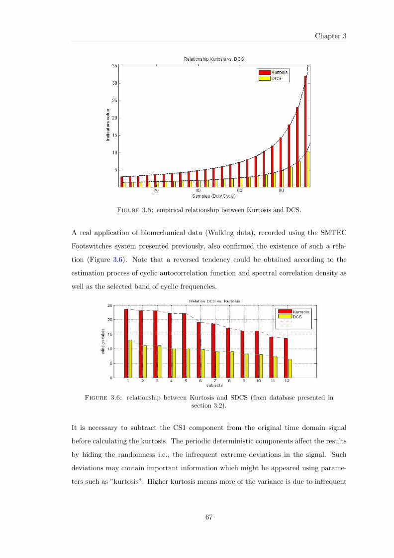
Chapter 3

Figure 3.5: empirical relationship between Kurtosis and DCS.

A real application of biomechanical data (Walking data), recorded using the SMTEC

Footswitches system presented previously, also confirmed the existence of such a rela-

tion (Figure 3.6). Note that a reversed tendency could be obtained according to the

estimation process of cyclic autocorrelation function and spectral correlation density as

well as the selected band of cyclic frequencies.

Figure 3.6: relationship between Kurtosis and SDCS (from database presented insection 3.2).

It is necessary to subtract the CS1 component from the original time domain signal

before calculating the kurtosis. The periodic deterministic components affect the results

by hiding the randomness i.e., the infrequent extreme deviations in the signal. Such

deviations may contain important information which might be appeared using parame-

ters such as ”kurtosis”. Higher kurtosis means more of the variance is due to infrequent

67

Chapter 3

extreme deviations.

Thus, the Kurtosis is computed on CS2 estimated components and is suggested to be

a useful indicator of cyclostationarity. It is a temporal indicator, and can be easily

calculated and implemented. The empirical applications on simulated as well as actual

signals obtained from candidates highlight the relationship between kurtosis and DCS

and thus put it forward as a real and major analytical tool.

The theoretical link between Kurtosis and degree of cyclostationarity is given as follows:

According to Randall et al (2001) [129], the envelope analysis is given by the following

equation:

Mxx[v] =

∫RSCDx(v, f)df = lim

T→∞

1

T

∫ T/2

−T/2E[x(t)2

]e−j2πvtdt, (3.2)

According to Borghesani et al (2014) [157], the squares envelope spectrum (SES) is

given by the following equation:

SESx[k] = |DFT{|x(t)|2}|2 (3.3)

Borghesani et al. proved an analytical relationship between the SES and the kurtosis

of the corresponding analytic signal. They demonstrated that the sum of the peaks in

the SES corresponds to the 4th order moment. more details are presented in Appendix

A.

Kurt =

∑k SESx(k)

RMS4x

(3.4)

Therefore, from equations 3.2 and 3.4, one can find the analytical relationship between

kurtosis and SCD.

SES could be written as follows:

68

Chapter 3

SESx[v] = |Mxx(v)|2 = |∫RSCDx(v, f)df |2 (3.5)

So, the kurtosis becomes:

Kurt =

∑Nv=0 SESx(v)

RMS4x

=

∑Nv=0 |

∫R SCDx(v, f)df |2

RMS4x

(3.6)

SES is in the frequency domain and RMS4x is the fourth power of the root mean square

(RMS) of the analytic filtered signal and is equal to constant.

From definition 3.6 and the definition of DCS in Appendix B, we can obtain the following

equation:

SDCS ≥ Kurt.RMS4x∫

R |Sx[0, f ]|2df(3.7)

3.4 Cyclostationarity characters of walking signals

This aspect is explored by exploiting the cyclical character of Walking signals and

the possibility of its combination with a random character introducing variability. We

took cyclostationarity (CS) as a model for further study of these signals.

In general, walking signals could be treated as sequences of repeated and cyclic gestures.

Walking signals are the combination of a cyclic character (which is the stride cycle) and

a stationary random character which introduces the step variability that is unique for

each individual. Given the cyclostationary nature of these signals we are particularly

interested in CS for a deep and profound study of such process. As presented in the

previous chapter, the CS signals are persistent random waveforms having statistical pa-

rameters that vary periodically with time. These signals are not generally deterministic

but random in their waveform generated by mechanical or cyclic gestures. The general

model of walking signals could be represented as the following:

69

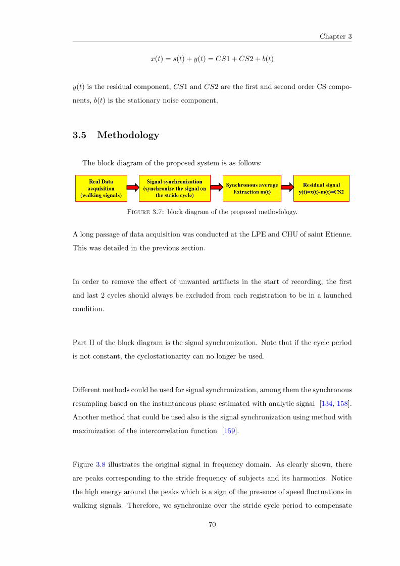
Chapter 3

x(t) = s(t) + y(t) = CS1 + CS2 + b(t)

y(t) is the residual component, CS1 and CS2 are the first and second order CS compo-

nents, b(t) is the stationary noise component.

3.5 Methodology

The block diagram of the proposed system is as follows:

Figure 3.7: block diagram of the proposed methodology.

A long passage of data acquisition was conducted at the LPE and CHU of saint Etienne.

This was detailed in the previous section.

In order to remove the effect of unwanted artifacts in the start of recording, the first

and last 2 cycles should always be excluded from each registration to be in a launched

condition.

Part II of the block diagram is the signal synchronization. Note that if the cycle period

is not constant, the cyclostationarity can no longer be used.

Different methods could be used for signal synchronization, among them the synchronous

resampling based on the instantaneous phase estimated with analytic signal [134, 158].

Another method that could be used also is the signal synchronization using method with

maximization of the intercorrelation function [159].

Figure 3.8 illustrates the original signal in frequency domain. As clearly shown, there

are peaks corresponding to the stride frequency of subjects and its harmonics. Notice

the high energy around the peaks which is a sign of the presence of speed fluctuations in

walking signals. Therefore, we synchronize over the stride cycle period to compensate

70

Chapter 3

the speed fluctuation and obtain a synchronized signal with respect to the stride. The

FFT of the synchronized signal is shown in Figure 3.8. We note clearly the differences.

The peaks here are very clear and very narrow in comparison with the FFT of the orig-

inal signal.

Figure 3.8: FFT of the original and synchronized signal.

To estimate the properties of CS2 after signal synchronization, its primarily necessary to

proceed with the extraction of CS1 components. The first tool to extract this periodic

component is the time synchronous averaging technique which can be calculated using

the following equation [160]:

mTx (t) =

1

N

N−1∑k=0

x(t+ k.T ) (3.8)

where T is the cyclic period and is accurately estimated following the previous step of

signal synchronization.

The residual signal (Figure 3.9) is then obtained by just removing that quantity from

the original signal. The residual signal is now given by:

71

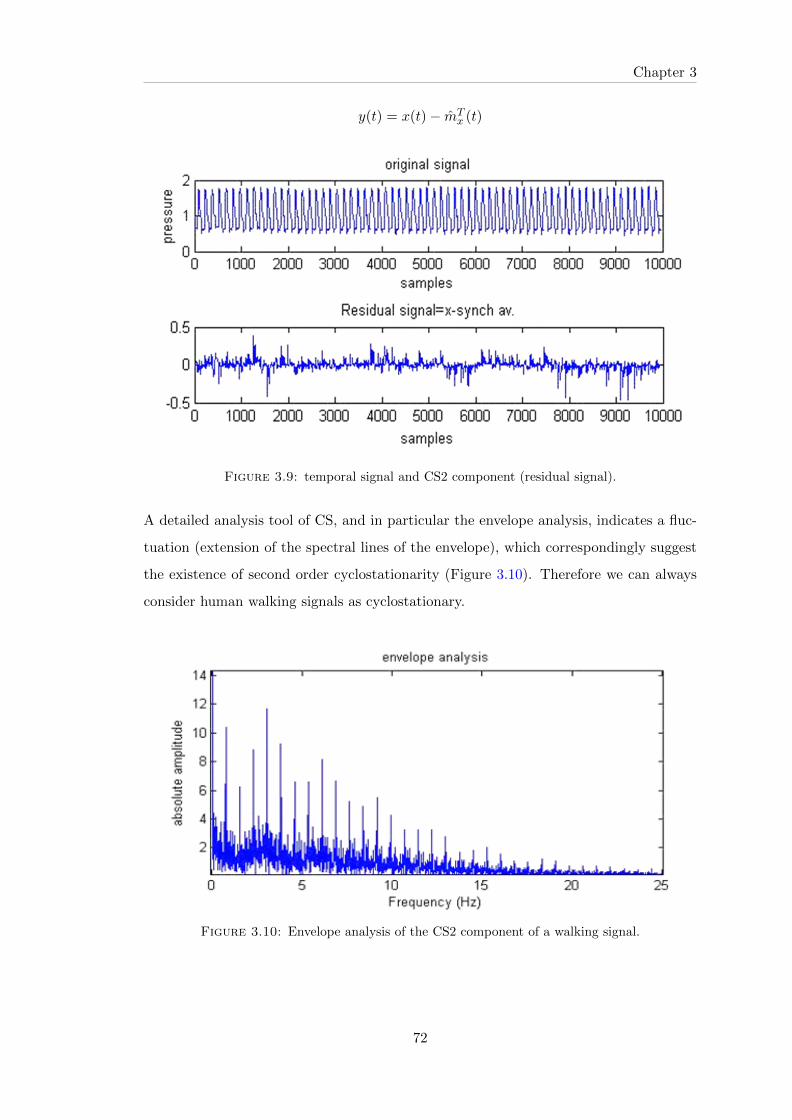
Chapter 3

y(t) = x(t)− mTx (t)

Figure 3.9: temporal signal and CS2 component (residual signal).

A detailed analysis tool of CS, and in particular the envelope analysis, indicates a fluc-

tuation (extension of the spectral lines of the envelope), which correspondingly suggest

the existence of second order cyclostationarity (Figure 3.10). Therefore we can always

consider human walking signals as cyclostationary.

Figure 3.10: Envelope analysis of the CS2 component of a walking signal.

72

Chapter 3

3.6 Cyclic correlation with different walking conditions

In this section, we examine the effects on walking in elderly subjects in three task

conditions:

• Single task (simple walking MS).

• Walking while counting backward one by one from 50 (MD).

• Walking while performing a fluency task (MF) (Walking while pronouncing the

names of animals).

Patients were asked to do as best as possible the two tasks at the same time.

The analysis tools of cyclostationarity were previously introduced in chapter 2. In the

following results, the cyclic autocorrelation function was calculated on the residual signal

(CS2 signal) i.e., after removing the periodic deterministic component from the original

CS signal. Equation 2.5 is used for the calculation.

As shown in Figure 3.11, the results varied when elderly performed a secondary dual

task during walking. This suggests the existence of an untapped paradigm, where the

walking-rhythmic stepping mechanism and the collecting patterns are not being con-

sidered as an automatic process. The results clearly show that the cyclic correlation is

greater for both MF and MD than MS. Therefore, the CS2 in MF is greater than CS2

in MD than CS2 in MS.

In short, it is evident from the CS analysis that in the case of dual task conditions, sub-

jects show a higher elevated peak (i.e. variability), a larger base and higher frequencies.

This phenomenon is stronger in case of MF over MD.

In general, the results of this study demonstrate the significant effects of executive func-

tion, attention and dual tasking on walking stability. Furthermore, they explain why

73

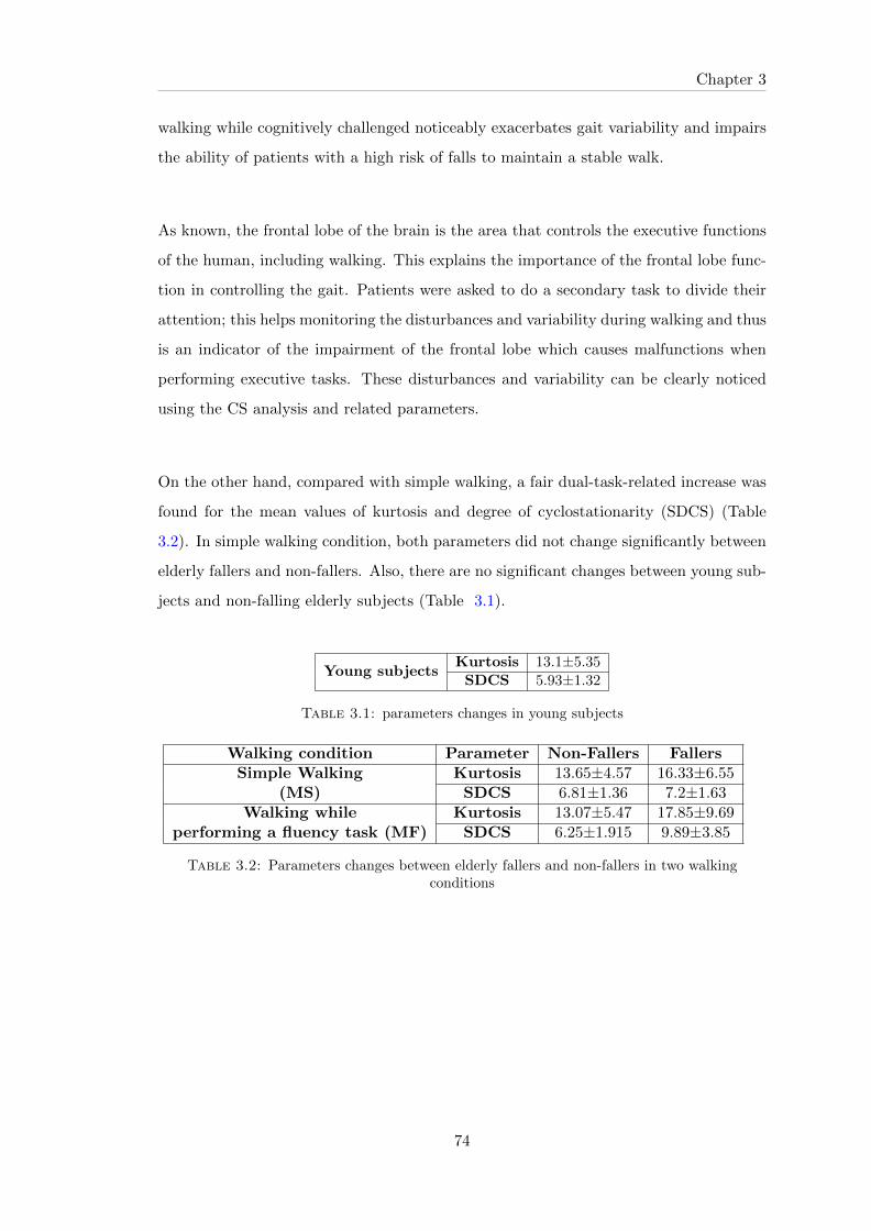
Chapter 3

walking while cognitively challenged noticeably exacerbates gait variability and impairs

the ability of patients with a high risk of falls to maintain a stable walk.

As known, the frontal lobe of the brain is the area that controls the executive functions

of the human, including walking. This explains the importance of the frontal lobe func-

tion in controlling the gait. Patients were asked to do a secondary task to divide their

attention; this helps monitoring the disturbances and variability during walking and thus

is an indicator of the impairment of the frontal lobe which causes malfunctions when

performing executive tasks. These disturbances and variability can be clearly noticed

using the CS analysis and related parameters.

On the other hand, compared with simple walking, a fair dual-task-related increase was

found for the mean values of kurtosis and degree of cyclostationarity (SDCS) (Table

3.2). In simple walking condition, both parameters did not change significantly between

elderly fallers and non-fallers. Also, there are no significant changes between young sub-

jects and non-falling elderly subjects (Table 3.1).

Young subjectsKurtosis 13.1±5.35SDCS 5.93±1.32

Table 3.1: parameters changes in young subjects

Walking condition Parameter Non-Fallers FallersSimple Walking

(MS)Kurtosis 13.65±4.57 16.33±6.55SDCS 6.81±1.36 7.2±1.63

Walking whileperforming a fluency task (MF)

Kurtosis 13.07±5.47 17.85±9.69SDCS 6.25±1.915 9.89±3.85

Table 3.2: Parameters changes between elderly fallers and non-fallers in two walkingconditions

74

Chapter 3

3.7 Cyclic correlation between fallers and non-fallers

We will push the study further by applying it to faller subjects with history of falls

and to non-fallers with no history. For more discernment and consistency, we will study

the male subjects on one side and the female subjects on another. The various informa-

tion acquired through questionnaires before or after recording the walking signals, the

medical examinations and the acquisitions with three conditions (MS: simple walking,

MD: walking with counting and MF: walking with verbal fluency ) were regrouped into a

single database containing the works of a decade of various practitioners and researchers

working on this topic. We obtain 284 feasible signals comprising 125 men and 159 women

distributed as follows (Table 3.3):

To better distinguish between the two classical groups of fallers and non-fallers, we

decided to segregate between the elderly fallers with a history of falling and the elderly

non-fallers without a history of falling & vice versa. Further distinction was achieved by

categorization of the elderly into male or female individuals.

Sexe FallersHistoryof Falls

Number

Male No Yes 27

Male Yes Yes 4

Male Yes No 3

Male No No 91

Female No Yes 67

Female Yes Yes 21

Female Yes No 7

Female No No 64

Table 3.3: database

To simplify the results, the curves obtained with the cyclic autocorrelation function

were calculated using different signals belonging to the same category and then averaged

together. Only the two sensors located at the heel of the foot were taken into account,

the reason being as mentioned before, it is at the heel that when striking the ground,

that more residues are obtained. To better distinguish the phenomenon of variability

in dual-tasks, we opted to work with only verbal fluency (MF), as the results obtained

clearly highlight the distinct differences between the non-fallers and fallers (Figure 3.12

75

Chapter 3

and 3.13), in both the case of male & female subjects. Following are the results we

obtained for females:

The results highlight two very important features. First of all, the amplitude of the

curve at the cyclic frequency v = 0 is doubled for women fallers. It increases from 0.035

to nearly 0.07 for the latter. Secondly, the fundamental frequency and its harmonics are

much higher in the case of fallers and this reflects a random walking i.e. a much more

random character of walking in female fallers.

The same for men: the non-fallers have random characters of walking which are much

less important than the fallers (Figure 3.14 and 3.15). However, for v = 0, the cyclic

autocorrelation function of fallers is twice bigger than that of non-fallers (a value of 0.02

for non-fallers and almost 0.05 for fallers). Same results can also be noticed for harmonic

frequencies.

Notice also a significant increase in the number of harmonics between non-faller and

faller female (Figure 3.12 and 3.13), and a slight increase in the number of harmonics

between non-faller and faller male(Figure 3.14 and 3.15).

3.8 Results summary

284 subjects (125 men and 159 women) were analyzed using an advanced signal pro-

cessing tools i.e. the cyclostationarity. The results in this paper showed an overview

of the capabilities of the cyclostationarity applied to human gait to detect ”flaws” and

estimate potential risk of falls in an elderly population.

Many subjects with history of falls were analyzed using the CS indicators in three

different walking conditions. The results stipulated give insight that the Cyclostation-

ary indicator (cyclic correlation) shows significant variation when performing secondary

tasks. These results may provide information for the evaluation of falling elderly. This

76

Chapter 3

means that such tasks could be useful reference factors for fall prediction.

The differences between fallers and non- fallers are quite significant in case of male and

female individuals. From a current review of several tens of seconds and basing on our

tools of signal processing (cyclostationarity), it is possible now to put forward a fast

and reliable indicator to estimate the potential risk of falls in the elderly. Thus, fall sig-

nals are clearly impacting cyclostationarity. This relationship between fallers and cyclic

correlation should take into account the sex. Finally, we note that the analysis of Cy-

clostationarity may have practical utility and benefits in biomechanical and neurological

diagnosis.

77

Chapter 3

3.9 Results comparison

A study of the stride to stride variability is done on the same database. The results

are summarized in tables 3.4, 3.5 and Figures 3.16 and 3.17. Among older adults, the

measures of stride variability were significantly increased in fallers. The stride to stride

variability is doubled for women fallers. No significant differences between male and

female. The results clearly shown that the stride to stride variability is greater for both

MF and MD than MS.

These results are quite similar to the results obtained by the cyclostationary approach,

with an advantage to CS approach for differentiating between male and female walking.

Non-Fallers Female Fallers FemaleMS MD MF MS MD MF

Variance ofStride to stridevariablility

21.5±26 43±40 38±42 17±10 57±37 70±50

Mean ofStride to stridevariablility

131±11 140±15 143±19 129±11 140±15 149±23

Table 3.4: Non-Fallers vs. Fallers (Female)- Mean±std over 21 fallers and 64 non-fallers

Non-Fallers MaleMS MD MF

Variance ofStride to stridevariablility

23.5±21 46.9±27 49.6±24

Mean ofStride to stridevariablility

137±7 153±18 156±20

Table 3.5: Non-Fallers (Male)- Mean±std over 118 patients

78

Chapter 3

3.10 Conclusion

The study described in this chapter generally used force sensitive insoles placed inside

the participant’s shoes. One advantage of this approach is that the recording system

is completely ambulatory; study participants can be assessed in clinical settings and

’real-life’ environments without having to make their way to ’gait labs’ or other sites

with special equipment. In general, in the study described above, pressure-sensitive

footswitches were used, one footswitch under the heel and one other under the toe.

In this chapter, we proved a relationship between the kurtosis and degree of cyclosta-

tionarity (DCS). This means that kurtosis provides a new indicator od CS.

We also presented the analysis of human walking signals. The chapter has put in evidence

the cyclostationary character of these signals. The cyclostationary analysis has proved to

be very appropriate to study the variability and random fluctuations during walking. An

experimental device led to the acquisition of GRF signals in different walking conditions.

The experiments were done by the LPE and CHU of Saint Etienne. The analysis of

data examined the effects of dual task paradigms on walking changes, also confirmed

the importance of such signals for estimating falls risk in the elderly. This revealed that

the changes in CS parameters could be related to dual task, falls and attention. This

determines that dual task and walking changes and fall prediction are solemnly involved

or related to attention.

79

Chapter 3

Figure 3.11: The mean cyclic autocorrelation functions for each task (a) MS (b) MD(c) MF.

80

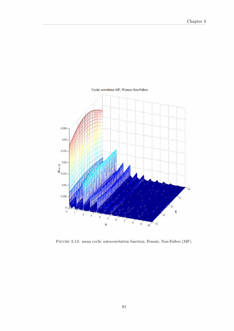
Chapter 3

Figure 3.12: mean cyclic autocorrelation function, Female, Non-Fallers (MF).

81

Chapter 3

Figure 3.13: mean cyclic autocorrelation function, Female, Fallers (MF).

82

Chapter 3

Figure 3.14: mean cyclic autocorrelation function, Men, non-Fallers (MF).

83

Chapter 3

Figure 3.15: mean cyclic autocorrelation function, Men, Fallers (MF).

84

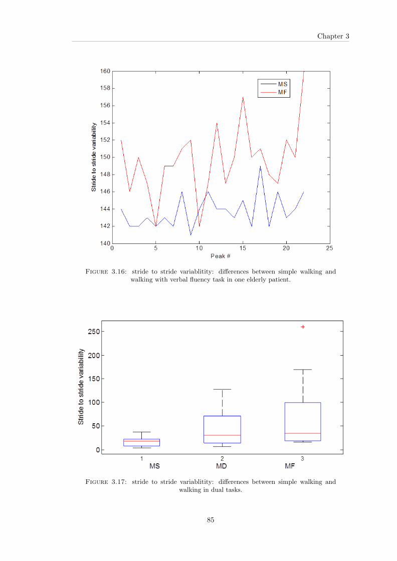
Chapter 3

Figure 3.16: stride to stride variablitity: differences between simple walking andwalking with verbal fluency task in one elderly patient.

Figure 3.17: stride to stride variablitity: differences between simple walking andwalking in dual tasks.

85

Chapter 4

SOURCE SEPARATION FOR

THE ANALYSIS AND

PROCESSING OF GRF

SIGNALS

Contents

4.1 Introduction to passive and active peaks . . . . . . . . . . . 87

4.2 Methodology and taxonomy . . . . . . . . . . . . . . . . . . . 88

4.2.1 Data Acquisition . . . . . . . . . . . . . . . . . . . . . . . . . . 88

4.2.2 VGRF signal analysis . . . . . . . . . . . . . . . . . . . . . . . 90

4.2.3 Proposed Methodology . . . . . . . . . . . . . . . . . . . . . . . 92

4.3 Results and discussion . . . . . . . . . . . . . . . . . . . . . . 103

4.3.1 Cyclostationary analysis . . . . . . . . . . . . . . . . . . . . . 107

4.3.2 Comparison with BSS Techniques . . . . . . . . . . . . . . . . 109

4.3.3 Performance study . . . . . . . . . . . . . . . . . . . . . . . . . 110

4.4 Fatigue study (evolution of CS parameters with time during

the 24 hours of running) . . . . . . . . . . . . . . . . . . . . . 111

4.5 Conclusion . . . . . . . . . . . . . . . . . . . . . . . . . . . . . 121

86

Chapter 4

4.1 Introduction to passive and active peaks

Ground reaction force (GRF) signals are usually composed of two distinct peaks: an

active force peak representing the propulsive force in addition to a passive force peak

representing the impact force. The impact force is mainly passively generated and is due

to the deceleration of the body mass at the instant of touch down. This implies that at

least part of the energy was transferred passively into the bone-ligament system. Thus,

the impact force is a major factor indicating the reaction of muscle that may reflect the

fatigue state and performance of the muscle. To study the variations in GRF signals

with time during running, we have to separate the active and passive contributions. The

results of separation will allow researchers and investigators to extract parameters for

the biomechanical study of running.

In this chapter, the treatment of such biomechanical signals obtained by experienced

ultra-long distance runners is done in two steps:

The first step focuses on the treatment of biomechanical signals for the purpose of com-

ponents separation. The aim here is to separate the contribution of the active compo-

nents (propulsive force) and the passive components (the impact force) from the ground

reaction force signals coming from high level professional runners (during 24 hours of

continuous running). For this reason, we proposed a new method that achieves the

desired goal. We named it: the Gaussian decomposition with non-linear least square

method. Another proposed method i.e., the recursive least square with forgetting factor

algorithm (RLSFF) can be used for the same purpose. In addition, we make comparison

with the results obtained using BSS algorithms such as: JADE, SOBI, and CycloSOBI.

The second step consists of testing some indicators and parameters that contribute to

better understand and characterize the mechanical phenomena behind the GRF signals.

These parameters were evaluated every 2 hours over the 24 hour treadmill run. The

results prove that the cyclic autocorrelation function and the cyclic frequency increases

and evolves significantly with time i.e., during the 24 hours of running.

87

Chapter 4

Furthermore, the integrated cyclic correlation is treated where two new indicators are

induced: these are the energy when the cyclic frequency v = 0 (Pv0) and the energy of

the first cyclic frequency (the step frequency Pv1). They were found to evolve signifi-

cantly with time during running. In addition, we assessed the degree of cyclostationarity

(DCS) and kurtosis after 2 hr and 24 hr of running. The results showed that the pro-

posed parameters seemed to be clearly affected by fatigue following fatiguing exercise.

This evolution may give an informative insight into the fatigue state of runners and may

give insights into its evolution.

This chapter is organized as follows: in the first section, we detail and describe the

work and the proposed methodology and taxonomy. Section 2 presents the results

and discussions. Section 3 analyzes and characterizes the GRF signals by means of

stationary and cyclostationary indicators i.e., it quantifies the changes in running by

means of cyclostationarity and proposed indicators.

4.2 Methodology and taxonomy

4.2.1 Data Acquisition

The experimental paradigm was carried out at the exercise physiology laboratory

(LPE) of Jean Monnet Saint-Etienne University, France. It was directly controlled by

physicians and biomechanists. The Measurements were made on an instrumented tread-

mill dynamometer equipped with embedded accelerometer sensors. This treadmill was

designed by A. Belli et al [88]. The design and potential of such system are described

in details in [88]. Full information on the physiological characteristics of subjects is de-

tailed in [71]. The machine allows the measurement of Ground Reaction Force (GRF)

signals during a run on the treadmill; also it allows fast recording and analysis of vertical

GRF from a large number of steps at a constant velocity.

The description of subjects, measurement procedures and measurement system are sum-

marized as follows:

88

Chapter 4

• 10 healthy male runners volunteered for the study. They all had high training

experience and are considered as ultra-runners.

• The experiment consisted of running for 24 hours continuously.

• A measurement period of 20 seconds and a short rest period with appropriate

drink and food intakes were done every 2 hours.

• The runners reported no injury or problems at the time of experiment.

• The data is carried out in the time domain.

• With this treadmill, the signals are sampled at 1000 Hz.

• The speed of the treadmill was set to 10 km/h during both the 24 hr run and the

measurements performed.

Figure 4.1 shows the treadmill with a runner on it and example of measured signal for

two consecutive steps. The treadmill is composed of accelerometer sensors placed at the

four corners of the carpet. Such a signal is composed of two distinct parts: a passive

peak (impact force) and an active peak (the propulsive force). The stride time duration

is defined as the time elapsed between two impacts on the ground of the same foot.

First of all, the passive peak (impact force) represents the initial impact between the

body and the ground at initial heel contact. It’s determined by the effective mass of

the body, the velocity and leg stiffness. The active peak is the force applied by the foot

and supported body weight during running. It reflects the propulsive forces applied by

the musculo-skeletal system. Notice that it is larger than the passive peak. This peak

matches the changes in body weight.

Approximately 80% of runners are rear-foot strikers. The remainders are characterized

as mid-foot and fore-foot strikers. Runners who forefoot strikes have lower impact forces

than runners who heel strike (Figure 4.2). For runners who forefoot strikes, they have

lower impact forces and may have no impact transients.

The first step in the next section focuses on the treatment of biomechanical signals

for the purpose of source separation where the aim is to separate the contribution of

89

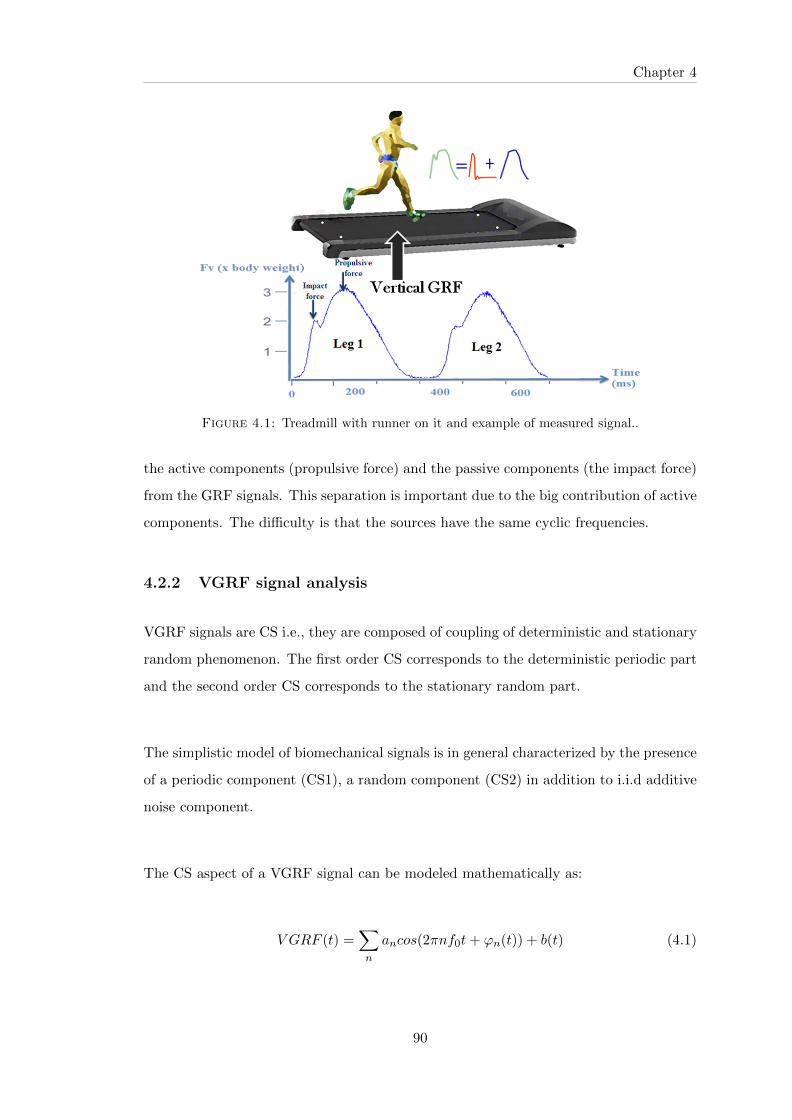
Chapter 4

Figure 4.1: Treadmill with runner on it and example of measured signal..

the active components (propulsive force) and the passive components (the impact force)

from the GRF signals. This separation is important due to the big contribution of active

components. The difficulty is that the sources have the same cyclic frequencies.

4.2.2 VGRF signal analysis

VGRF signals are CS i.e., they are composed of coupling of deterministic and stationary

random phenomenon. The first order CS corresponds to the deterministic periodic part

and the second order CS corresponds to the stationary random part.

The simplistic model of biomechanical signals is in general characterized by the presence

of a periodic component (CS1), a random component (CS2) in addition to i.i.d additive

noise component.

The CS aspect of a VGRF signal can be modeled mathematically as:

V GRF (t) =∑n

ancos(2πnf0t+ ϕn(t)) + b(t) (4.1)

90

Chapter 4

Figure 4.2: foot kinematics for two foot strikes (a) rear-foot strike (b) fore-foot strike

This equation presents the nature of cyclic variations of a VGRF signal [100]. Where

ϕ(t) represents the randomness which varies cyclically. ϕ(t) is very small (≤ 1 rd/s)

and is random, Gaussian and has a mean equal to zero. b(t) is the i.i.d. random noise.

f0 is the step frequency. an is the amplitude representing principally the runner’s weight.

ϕ(t) is very small, and thus eq. 4.1 can be simplified to the following:

V GRF (t) =

∞∑n=0

ancos(2πnf0t)−∞∑n=0

anϕn(t)sin(2πnf0t) + b(t) (4.2)

{ancos(2πnf0t)} represents the CS of order 1, and {anϕn(t)sin(2πnf0t)} represents the

CS part of order 2. To characterize the variability from stride to another, we have to go

91

Chapter 4

through the CS 2, which is included as part of passive component.

Synchronous mean and synchronous variance:

The synchronous mean consists in resynchronizing the VGRF signal using the corre-

lation function estimated between the stride cycles, then, synchronously averaging the

cycles according to the cyclic frequency where the cycle is being taken to be equal to

the stride period.

The synchronous variance is calculated using the envelope analysis of the signal. How-

ever it requires a good estimation of the synchronous mean that needs full information

about the cyclic frequency. As a result, to estimate the most accurate cyclic period and

to remove the low speed fluctuations in order to make the cyclic period constant, signal

synchronization is used. We can make use of two different synchronization procedures:

the synchronization method with maximization of the intercorrelation function [130] or

signal synchronization by means of angular resampling [134].

By calculating the synchronous mean and synchronous variance of the VGRF signal

(Figure 4.3), we notice that the first-order CS corresponds to the synchronous mean

i.e. it can identify the deterministic periodic contribution of each leg. In addition, the

second-order CS corresponds to the synchronous variance that visualizes the random

character of the VGRF signals.

Figure 4.3 clearly shows that the active and passive peaks could be represented by the

synchronous mean and synchronous variance respectively. These are the motivations

behind the separation of active and passive components.

4.2.3 Proposed Methodology

The block diagram illustrated in Figure 4.4 describes the proposed algorithm and

system methodology. The first step in this proposal puts emphasis on the detection of

92

Chapter 4

Figure 4.3: Synchronous mean and synchronous variance of a VGRF signal.

true minimum and true maximum of the original signal; this helps in the separation

of the active and passive components in the next step. The second step of the block

diagram addresses the issue of separating the active and the passive peaks of the GRFs

signals. The third step synchronizes the signal on the stride cycle to remove the low

speed fluctuations in order to ameliorate the separation of passive signal’s components

using cepstral editing procedure (CEP). The results of CEP separation will be compared

to those obtained using the time synchronous averaging technique. Finally, some pa-

rameters suited to GRF signals analysis are proposed.

I) Detection of true minimum and maximum:

Figure 4.5 discloses in detail the mathematical method of the estimation of the true

minimum and maximum. First the signal is normalized and denoised by means of the

wavelet decomposition. Then, the global maximum and minimum are found using the

derivative methods (first and second derivatives) while the false points are removed. The

true minima are the accurate location of minimum edge points which can be detected

using a comparison method. In the comparison method, simply, starting from the global

minimum point, we compare the next series of points to the current point. The corre-

sponding minimum position is precised when the series of points continue to increase

without decreasing. The position with the minimum edge point is defined as the true

93

Chapter 4

Figure 4.4: Proposed Methodology.

minimum. The global minima and true minima are plotted as red and black stars on

Figure 4. The true minimum will be used in the next step to separate the right and left

leg as well to separate the active and passive components.

Figure 4.5: True minimum and maximum detection.

94

Chapter 4

II-a) Separation of active and passive peaks:

The second part of the block diagram addresses the issue of separating the active and

the passive peaks of the GRFs signals. To achieve such a goal, a new method is proposed

for this aim. We named such method: the Gaussian decomposition with non-linear least

square method.

The GRF signals can be modeled written as:

X(t) = Xp(t) +Xa(t) (4.3)

Where Xa(t) is the active component and Xp(t) is the passive component of the GRF

signal. Consider the hypothesis that both components are independent and mutually

uncorrelated. Moreover, the primary goal is to separate these two components. And to

do so, we have to extract the active component Xa(t) for each step.

The method is based on the assumption that the variation around an active peak follows

a Gaussian distribution. This can be expressed as:

Xa(t) = a1e−(

(f(t+δ1(t))−b1)c1

)2+ ε1(t)

+ a2e−(

(f(t−T+δ2(t))−b2)c1

)2+ ε2(t)

+ ..... (4.4)

+ aNe−(

(f(t−(N−1)T+δN (t))−bN )

cN)2

+ εN (t)

Xa(t) =N∑n=1

ane−(

(f(t−(n−1)T+δn(t))−bn)cn

)2 + Σ(t)

f(t) are the instants where the different Gaussians are minimal. They represent the

samples from the observations, i.e., the GRF signal which constitutes the sum of active

and passive peaks. The goal is to search in this signal the parameters of the Gaussian.

95

Chapter 4

f(t) shows the samples of the nth Gaussian determined between two successive mini-

mums. It is centered in bn and has (cn/2) standard deviation (Figure 4.6). For the nth

Gaussian, f(t) is comprised between Tn−1 and Tn. T0 is the first true min determined by

the min-max algorithm (Figure 4.5). bn is the center of nth Gaussian (the zero reference

corresponds to the first true min), δn(t) corresponds to fluctuation of the mean period

(T1 + ...TN )/N . Xa(t) is the estimated active component of the GRF signal; εn(t) is the

error of each step. The separation of active and passive peaks is illustrated nicely by

way of the example shown in Figure 4.6b and 4.6c.

Figure 4.6: (a) Measured waveforms of equation 4.4 (b) estimated active component(c) separated passive component.

For the assessment of quadratic errors and in order to obtain best-fit values of the pa-

rameters to approximate the real signal, the coefficients an, bn, and cn are optimized

using the non-linear least squares method.

Consider a set of m data points of X(t) function (x1, y1), (x2, y2), ..., (xm, ym), and a

curve (Gaussian model function):

96

Chapter 4

yi = Xa(xi, an, bn, cn),

an = (a1, a2, ...aN ), bn = (b1, b2, ...bN ), and cn = (c1, c2, ...cN )

It is desired to find the vectors (an, bn, cn) of parameters such that the curve fits best

the given data in the least squares sense, that is, the sum of squares

S =m∑i=1

r2i (4.5)

is minimized, where the residuals (errors) ri are given by:

ri = yi − yi for i = 1, 2, ...,m. (4.6)

Where yi are the observed responses and yi is the functional portion of the model.

The minimum sum of squared residuals S is reached when the gradient is zero (necessary

condition). Since the problem is formulated with n parameters, so there are 3∗N normal

equations:

∂S

∂aj= 2

m∑i=1

ri∂ri∂aj

= 0(j = 1, ..., n)

∂S

∂bj= 2

m∑i=1

ri∂ri∂bj

= 0(j = 1, ..., n) (4.7)

∂S

∂cj= 2

m∑i=1

ri∂ri∂cj

= 0(j = 1, ..., n)

After generating the modified Gaussianity for each leg (i.e. after generating the active

peak of each step), the residual signal (i.e. the signal containing the passive peaks) is

calculated as the difference between the original signal and the fits.

Xp(t) = X(t)− Xa(t) (4.8)

This method was proposed since the active part closely resembles a Gaussian function.

This can be clearly seen in Figure 4.6.

97

Chapter 4

II-b) Separation of active and passive peaks using the RLSFF method:

The objective now is to make use of the CS character and RLSFF algorithm (Recursive

Least-Squares Algorithm with Variable Forgetting Factor) in order to separate the con-

tribution of active and passive peaks. This method will also provide good separation

results similar to the first proposed method.

RLSFF Method presentation

The resampling depending on spectral distribution of signal components represents the

first stage of preprocessing. The resampling factor was set to the value of 2. Notice that

without resampling, the separation will not be achieved.

This part of the methodology consists of applying the recursive least squares with for-

getting factor algorithm in order to separate the VGRF signal’s components.

The forgetting factor is a correction factor which is directly proportional to the error and

it gives exponentially less weight to older error samples. The forgetting factor specifies

the measurement window relevant for parameter estimation. Setting λ = 1 corresponds

to ”no forgetting” and estimating constant coefficients. Setting λ < 1 implies that

past measurements are less significant for parameter estimation and can be ”forgotten”.

λ < 1 was set to estimate time-varying coefficients.

The least-squares algorithm aims at minimizing the sum of the squares of the difference

between the desired signal and the model filter output. When new samples of the input

signals are received at every iteration, the solution for the least-squares problem could

be computed in recursive form resulting in the recursive least-squares algorithm (RLS).

The RLS algorithm pursues fast convergence also has very good performance when

working in time-varying domain. The objective here is to choose the coefficients of the

adaptive filter such that the output signal y(k), during the period of observation, will

98

Chapter 4

match the desired signal as closely as possible in the least-squares sense. The minimiza-

tion process requires information of the input signal. Also, the objective function we

seek to minimize is periodic.

Given the set of input samples {x(1), x(2), ., x(N)} that represent the normalized GRF

signal, we build a set of desired response {d(1), d(2), , d(N)}. RLS estimates the filter

coefficients, needed to convert the input signal into the desired signal. The desired sig-

nal must have the same data type and dimensions as the input signal. The RLSFF

algorithm is executed in the following manner:

Figure 4.7: The RLSFF algorithm.

Where n is the current time index, x(n) is the vector of input samples at step n, h(n) is

the vector of filter-tap estimates at step n, ξ(n) is the estimation error at step n, d(n)

is the desired signal at step n and λ is the forgetting factor (or weighting factor). λ

reduces the influence of old data and usually taking the form (0 < λ < 1). When λ = 1,

we have the ordinary least squares method.

The first step is to define the filter order m, the forgetting factor λ, and to initialize:

h(n) = 0; x(k) = 0; d(k) = 0; and P (0) = I (identity matrix). Then, the following

equations are computed:

99

Chapter 4

Filter order: ξ(n) = d(n)− hT (n− 1)x(n)

The Kalman gain vector: K(n) =λ−1P (n− 1)x(n)

1 + λ−1xT (n)P (n− 1)x(n)

Update the Coefficients: hT (n) = hT (n− 1) +K(n)ξ∗(n)

The inverse of the correlation matrix of x(n): P (n) = λ−1P (n− 1)

−λ−1K(n)xT (n)P (n− 1)

The filtered output: d(n) = hT (n− 1)x(n)

One important factor affects extremely the results of separation. This is the forgetting

factor λ. This factor gives great estimation of both components at the order of approx-

imately 99.4%. In future works, one could use iterative optimization methods in order

to choose the best values of the filter order and forgetting factor.

d(n) is the estimated output signal that represents the active component.

The passive component r(n) is calculated by just subtracting the active component from

the original signal:

r(n) = x(n)− d(n)

III) Synchronization of passive signal

The cyclic period of GRF signals varies around an average value because of the low

speed fluctuations that characterize the human locomotion. Signal synchronization is

used to remove the low speed fluctuations in order to make the cyclic period constant.

We used the synchronization method with maximization of the inter-correlation function.

100

Chapter 4

This method requires the presence of a recurring cycle in the whole pattern. It involves

measuring the delay for each cycle relative to a cycle taken as reference from the maxi-

mum of the intercorrelation function [159]. This delay is then compensated for in the

frequency domain by applying on the cycle an all-pass filter or phase shifter. The latter

has a constant gain of 0 dB and a linear phase. The method steps are summarized as

follows:

1. Determine the cyclic period to be able to cut the signal in cycles: T = floor(Fs/Fe)

Where T is the number of points per cycle, Fs is the sampling frequency, Fe: the

step frequency.

2. Measure the delay of the Kth block with the reference block using the intercorre-

lation function:

Rsr = E{sn+mr∗n}

where E{.} is the expected value operator. s and r are stationary random processes

with length N. s = sk is the Kth block and r = rk is the reference block.

N = QT, Q an integer of cycle

1 ≤ m ≤ 2N − 1 and 0 ≤ n ≤ N −m− 1

dk = F(Rsr)

F :function which estimates the delays of blocks relative to a reference block.

3. Compensate the delays in the frequency domain

sk =

∫ ∞−∞

S(f)ej2πdkfdf,

101

Chapter 4

IV) Cepstral editing procedure

After separating both active and passive components comes the third part of the

methodology that addresses the issue of separating the components of the passive signal.

To estimate the properties of second order CS phenomenon (CS2), its primarily neces-

sary after signal synchronization to proceed with the extraction of the first order CS

phenomenon (CS1) of the passive signal. The tool used to extract this periodic com-

ponent P(t) is the cepstral editing procedure (CEP) method that removes the selected

family of harmonics from the time signal. The residual signal R(t) is then obtained by

just removing that quantity from the original signal (passive signal).

R(t) = Xp(t)− P(t) (4.9)

Moreover, the result will be compared to those of time-synchronous averaging (TSA)

method.

Now we have separated the active and passive components and then found the CS2

residues of the passive signal using CEP. The final part of our algorithm is about the

extraction of cyclostationary parameters and fatigue analysis.

V) Cyclostationary Parameters and Fatigue

This part includes a study of the cyclic frequency, the DCS, the kurtosis, the cyclic

autocorrelation function and integrated cyclic correlation of the CS2 signal. This will

be done in order to measure their evolution with time during the extreme ultra long

duration of running. Such evolution may be useful for studying and detecting Fatigue.

102

Chapter 4

4.3 Results and discussion

From Figure 4.8a., it is important to notice the big contribution of active peaks. Note

that the contribution of active components is higher than that of passive components.

Such components don’t contain mainly the same information. Consequently, the need

arises to do a separation of their components in order to improve the treatment and

analysis of GRF signals.

The results of the proposed method are shown in Figure 4.8b. It should be noted how

well the separations of active and passive components are. And the advantage of such a

method is certainly the maneuverability to separate the active from passive peaks of all

steps.

Figure 4.9 illustrates the spectrum for both components. Notice that the active signal

is a purely periodic signal and that the spectrum of passive signal has rich frequency

components containing most of the information required. Furthermore, the kurtosis are

equal to 1.6 for the signal of active components and 8 for the signal of passive compo-

nents.

The envelope spectrum of passive signal (Figure 4.13) shows a mixture of a periodic

phenomenon and a stationary random phenomenon. It is important to separate these

two components in order to improve the analysis and treatment of such signals. Figure

4.14 proves the efficiency of CEP to separate the random phenomenon. Figure 4.15 il-

lustrates the power spectral densities of both periodic and random components. Noting

that the separation by CEP method outperforms when compared to the results obtained

by the time synchronous averaging technique (Figure 4.14b).

103

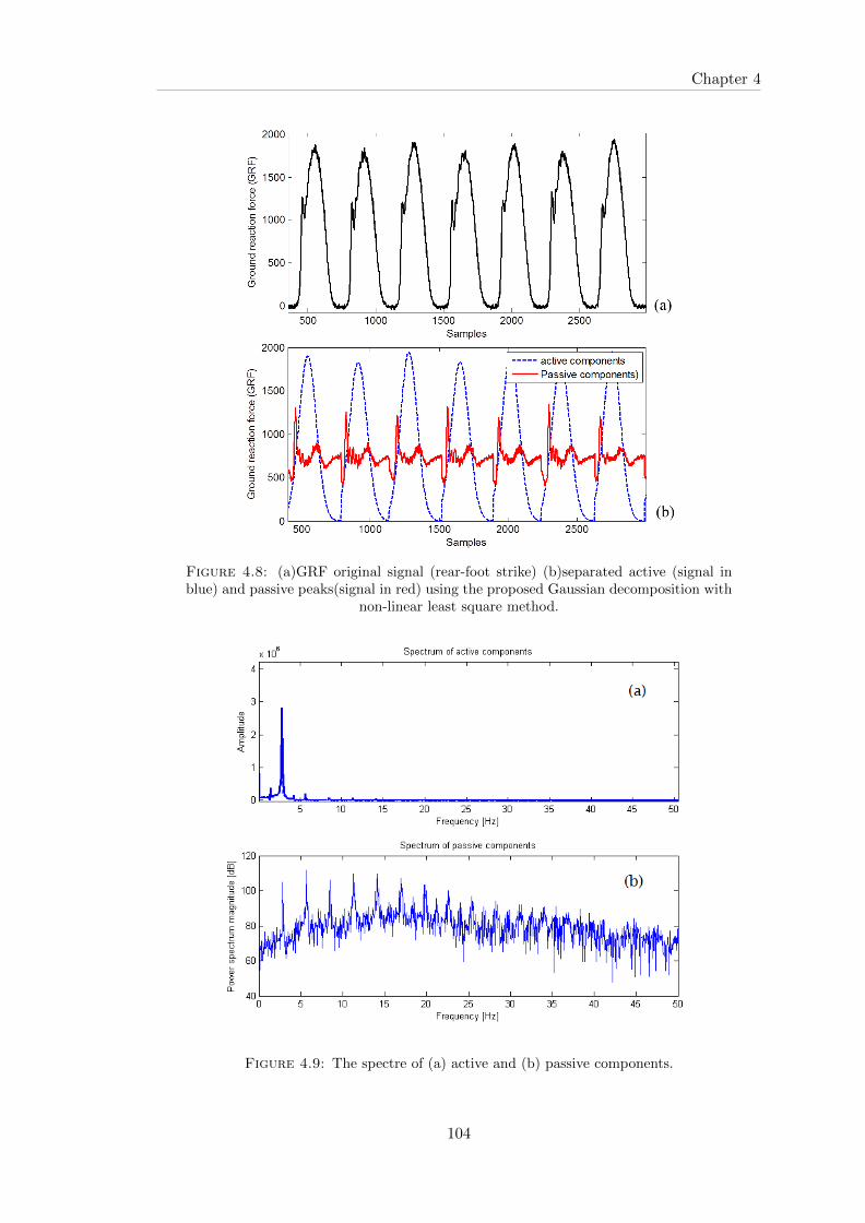
Chapter 4

Figure 4.8: (a)GRF original signal (rear-foot strike) (b)separated active (signal inblue) and passive peaks(signal in red) using the proposed Gaussian decomposition with

non-linear least square method.

Figure 4.9: The spectre of (a) active and (b) passive components.

104

Chapter 4

Figure 4.10: Separated active and passive components (rear-foot strike) using theRLSFF method

Figure 4.11: GRF signal (fore-foot strike)

Figure 4.12: separated active and passive components (fore-foot strike)

105

Chapter 4

0 5 10 15 20 25 30 35 40 45 5090

100

110

120

130

140

150

160

170

Pow

er s

pect

rum

mag

nitu

de [d

B]

Frequency [Hz]

Figure 4.13: Envelope spectrum of passive signal

Figure 4.14: The spectra of CS2 components (the residual signal) (a) using CEPmethod (b) using time synchronous average method.

Figure 4.15: Spectre of both CS1 (dashed lines) and CS2 components (solid line) ofthe passive signal using CEP.

106

Chapter 4

4.3.1 Cyclostationary analysis

The cyclostationarity appears when there is a periodicity in the properties of mean

(order 1) and in the energetic properties (order 2). Now, we will demonstrate that the

residual signals are cyclostationary.

As shown in Figure 4.16b, the deterministic phenomenon of the residual signal is nil

and its spectrum presents no cyclic frequencies. However, squaring such signal (Figure

4.16c) produces periodic components and its squared envelope spectrum reveals cyclic

frequencies of the hidden periodicities of the passive signal (Figure 4.16d). Figure 4.17

illustrates the cyclic autocorrelation function of the residual signal. The Spectre resolu-

tion is of 2.7Hz along the axis of cyclic frequency . It is clear that the cyclic correlation

has a discrete structure along the axis . Remember that the spectral lines generated by

a quadratic transformation in time are related to the cyclostationarity of order 2 and are

described by the cyclic autocorrelation function. In other words, the signal is correlated

with a delayed version of itself shifted by certain frequencies. Accordingly, it is possible

to assert that such signals contain a contribution of second order related to the step

frequency. Consequently, the residual component is obviously a pure cyclostationary

signal of order 2 (CS2).

The cyclostationary character is characterized by a coupling between a periodic

phenomenon and another random phenomenon. The random character is probably due

to several things: the random variation of the runners speed and other physiological and

mechanical changes.

107

Chapter 4

Figure 4.16: (a) Residual signal and its (b) spectrum. (c) squared signal and its (d)spectrum.

Figure 4.17: Cyclic autocorrelation function of the residual signal.

108

Chapter 4

4.3.2 Comparison with BSS Techniques

In another study, blind source separation techniques were tested on our biomechan-

ical database with the aim of separating the main sources (active and passive sources)

and characterizing the GRF signals. The results are compared with that obtained by

Sabri.et.al. [101, 102] who applied BSS techniques such as: SOBI, CycloSOBI and

JADE (Figure 4.18).

Figure 4.18: Results found by Sabri et.al [1, 2] (a) separation results using the JADEapproach (b) separation results using the AJD approach.

After exhausting the most efficient and known techniques of blind source separation,

the results of Sabri et al. have proven that such techniques will not yield a good sepa-

ration of the active and passive components of the GRF signals. Therefore it becomes

imperative to seek alternative methods and algorithms that may lead to achieving our

goals far from the BSS. Consequently, one new algorithm was proposed in this article.

This algorithm is based on the Gaussianity decomposition and non-linear least square

fitting technique. This technique has shown good results and good separation of GRFs

components. It is clear that the proposed methodology is superior in term of separating

the active and passive components of GRF signals.

109

Chapter 4

4.3.3 Performance study

Some simulation experiments are provided, showing the good performance of the meth-

ods. We used the least mean square error (LMSE) as a performance indicator. LMSE

is a common measure of estimator quality. It measures the quality of the reconstructed

signal. Here, we study the variation of LMSE with signal to noise ratio. We examined

the effects of increasing noise on the performance of methods.

As described in section 4.2, the treadmill is composed of 12 accelerometer sensors placed

at the four corners of the carpet. A VGRF signal is a linear combination of 4 sensors

placed at the four corners of the carpet. For the gaussian and RLSFF method, each

time we increase the SNR in the VGRF signal recorded during running and we calculate

the LMSE indicator. For the BSS methods, we use the 4 sensors (i.e., four sources).

As the CS1 is the most dominant part in the signal, thus making an LMS between the

original signal and the estimated CS1 components with different methods, this can be

considered as a performance indicator. A smaller LMSE means higher performance.

It seems clear that the proposed methods are more robust in the extraction of active

components with advantage of Gaussian method over the RLSFF method.

Figure 4.19: Performance of the proposed methods vs. JADE BSS method, effect ofvarying SNR from 1 to 50dB on the LMSE for each method

110

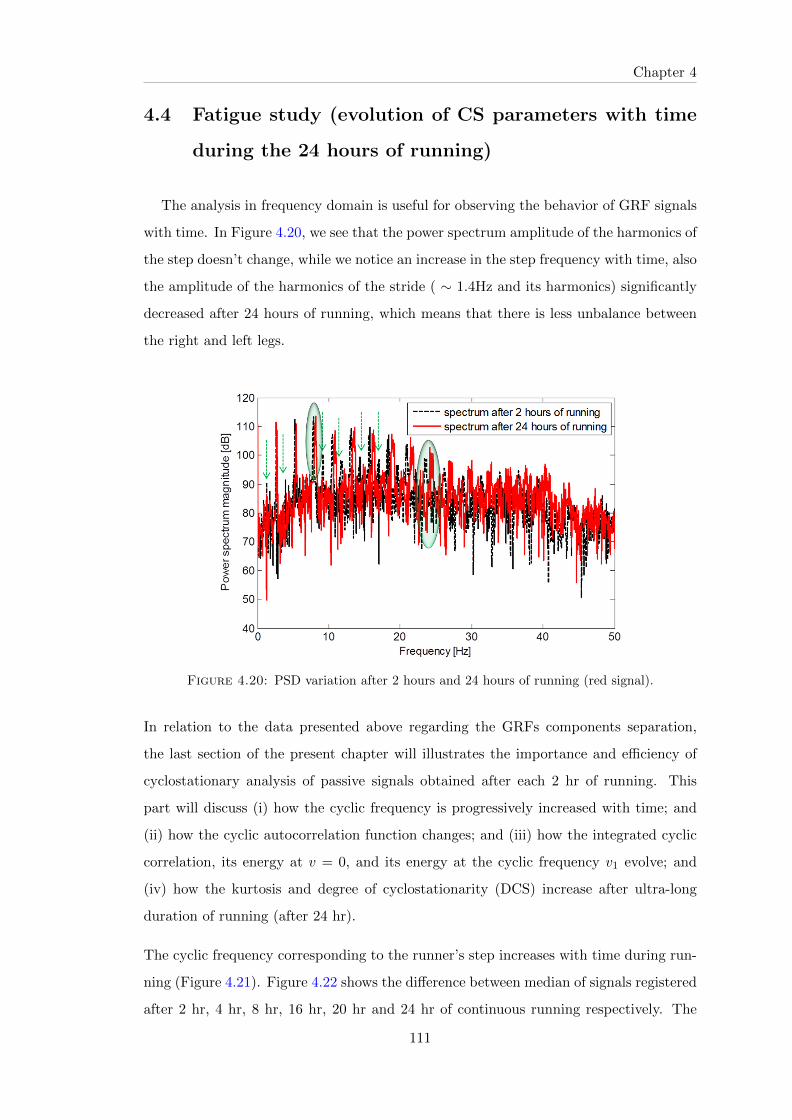
Chapter 4

4.4 Fatigue study (evolution of CS parameters with time

during the 24 hours of running)

The analysis in frequency domain is useful for observing the behavior of GRF signals

with time. In Figure 4.20, we see that the power spectrum amplitude of the harmonics of

the step doesn’t change, while we notice an increase in the step frequency with time, also

the amplitude of the harmonics of the stride ( ∼ 1.4Hz and its harmonics) significantly

decreased after 24 hours of running, which means that there is less unbalance between

the right and left legs.

Figure 4.20: PSD variation after 2 hours and 24 hours of running (red signal).

In relation to the data presented above regarding the GRFs components separation,

the last section of the present chapter will illustrates the importance and efficiency of

cyclostationary analysis of passive signals obtained after each 2 hr of running. This

part will discuss (i) how the cyclic frequency is progressively increased with time; and

(ii) how the cyclic autocorrelation function changes; and (iii) how the integrated cyclic

correlation, its energy at v = 0, and its energy at the cyclic frequency v1 evolve; and

(iv) how the kurtosis and degree of cyclostationarity (DCS) increase after ultra-long

duration of running (after 24 hr).

The cyclic frequency corresponding to the runner’s step increases with time during run-

ning (Figure 4.21). Figure 4.22 shows the difference between median of signals registered

after 2 hr, 4 hr, 8 hr, 16 hr, 20 hr and 24 hr of continuous running respectively. The

111

Chapter 4

increase in cyclic frequency means higher step variability, i.e. the runner is getting tired

and so the frequency of his steps becomes more random. So, running continuously for

24 hours increases the random phenomenon significantly. The difference becomes sig-

nificant after 10 hours of running, where it can be seen that P=0.015 after 24 hours of

running. So, the step frequency significantly increased (P < 0.05) with higher level of

fatigue.

Figure 4.21: A runners cyclic frequency evolution with time.

Figure 4.22: (a) Cyclic frequency evolution with time: difference between median(results were averaged over the 10 subjects) (b) P-value becomes significant after 12

hours of continuous running (95%-99% significance).

Figures 4.23 and 4.24 show respectively the cyclic autocorrelation function and inte-

grated cyclic correlation of one subject for T=2 hr, T=12 hr and T=24 hr. The results

presented in these figures also confirm that the cyclic correlation is significantly influ-

enced by the variations during time. The data on the harmonics of the cyclic frequencies

are very important since it may comprise information on the fatigue state of the runner.

As shown, the results highlight 2 features. First of all, the amplitude at v = 0 is doubled

112

Chapter 4

for signals recorded at T=24 hr. The cyclic correlation increases from 1000 at T=2 hr to

1700 (at T=12 hr) to nearly 2200 at T=24 hr. Secondly, the fundamental frequency i.e.

the step frequency and its harmonics are higher after 24 hr of running and this reflects

an unbalance i.e. much more random character of running. The cyclic frequency v ∼ 3

Hz corresponds to the step frequency of the runner.

The energy at v = 0, as well as at the cyclic frequency and its harmonics for T=24 hr,

have higher significance levels than at T=12 hr. Moreover, at v = 0; P=0.0036. At

v = 1; P=0.0052. At v = 2; P=0.0053 and at v = 3; P=0.0327.

One more novel and important finding is that the parameters Pv0 (the energies at v = 0)

and Pv1 (the energies of the first cyclic frequency) evolve significantly with time during

running. Thus, such parameters could be good and more direct determinants of fatigue.

The following graphs show the normalized energy tracking with time. We have obtained

two different forms of evolution (Figures 4.25 and 4.26).

1-It can be observed that the energies at v = 0 (Pv0) as well as the energy of the cyclic

frequency (Pv1) both increases with level running until a stable state is reached.

2-Also it can be noticed that the cyclic frequency energy increases linearly with respect

to time. After 10 hours of continuous running, the energy stays nearly stable for another

10 hours and a significant increase is noticed after a long time of running (after 24 hours).

After long duration of continuous running, the level of muscle fatigue increases and thus

the runners locomotion becomes low stable, this instability appears by hidden random

components periodic at the period of the step. The more the runner become fatigued the

more becomes important the cyclic frequency energy. Consequently, cyclostationarity

offers an indisputable advantage in studying biomechanical signals.

The kurtosis and degree of cyclostationarity (DCS) could also be considered as useful

indicators. Both indicators are twice bigger after 24 hours than after 2 hours of running

113

Chapter 4

Figure 4.23: Cyclic correlation after (a) 2 hours, (b) 12 hours and (c) 24 hours ofrunning.

114

Chapter 4

Figure 4.24: Integrated cyclic frequency of CS2 component (after 2 hr, 12 hr and 24hours of running).

115

Chapter 4

(Figure 4.27). The kurtosis increased from 8 to nearly 16 and the DCS increased from

15 to nearly 30 after 24 hr.

Table 4.1 summarized the different results obtained by the proposed parameters. Such

parameters evolved significantly (P < 0.05) from the 2nd hour until the end of running.

116

Chapter 4

Figure 4.25: Normalized integrated cyclic correlation at the cyclic frequency v = 0for 2 subjects

117

Chapter 4

Figure 4.26: Normalized integrated cyclic correlation at the first cyclic frequency α1

for 2 subjects

118

Chapter 4

Figure 4.27: Difference between median of the degree of cyclostationarity and kurtosis(1) after 2 hours (2) after 12hours (3) after 24 hours of running.

119

Chapter 4

Table 4.1: Results obtained by the proposed parameters. Such parameters evolvedsignificantly (P < 0.05) from the 2nd hour until the end of running.

ParameterPRE fatigue (after2 hoursof running)

(Mean+std)

POST fatigue (after24 hours of running)

(Mean+std)

P-value(t-test)

Cyclic frequency (v) 2.7±0.09 3±0.1 0.015

P v0 (x 104) 1.3±0.35 2.4±0.6 0.0036

P v1 (x 104) 0.89±0.17 1.75±0.6 0.0052

P v2 (x 104) 0.64±0.12 1.32±0.51 0.0053

P v3 (x 104) 0.47±0.16 0.85±0.38 0.0327

Kurtosis 8.7±1.5 13.6±1.6 0.0023

Degree ofcyclostationarity

(SDCS)14.6±3.6 23.5±6.3 0.003

120

Chapter 4

4.5 Conclusion

The GRF (active and passive) components were separated using a new proposed method,

based on the Gaussian decomposition and non-linear least squares method. Another pro-

posed method is based on the recursive least squares with forgetting factor (RLSFF).

The results indicated the good performance of these algorithms over BSS techniques.

The passive component was proved to be the part which contains the important infor-

mation in a GRF signal. The active component is more periodic. The passive signal is

cyclostationary. The CEP was used for separating its CS1 and CS2 sources. Although

we were able to make a study based on cyclostationary parameters on the CS2 part of

passive signal. The results were able to quantify the changes induced by runners over

time, where after an extreme ultra-long duration of running, gave significant results.

This could lead to significant insights into the evolution of fatigue.

The next chapter provides a new approach for separating CS1/CS2 components in the

context of sparsity and morphological diversity. And then an original model of CS was

proposed for the analysis of passive peaks (It analyzes the random variation of the slope

and of the polynomial coefficients of passive peaks).

121

Chapter 5

FIRST- AND SECOND-ORDER

CYCLOSTATIONARY SIGNAL

SEPARATION USING

MORPHOLOGICAL

COMPONENT ANALYSIS

Contents

5.1 Introduction . . . . . . . . . . . . . . . . . . . . . . . . . . . . 123

5.2 Sparse representation and MCA . . . . . . . . . . . . . . . . 123

5.3 Methodology (MCACS2 model) . . . . . . . . . . . . . . . . 126

5.3.1 Proposition of new dictionary for sparse representation modeling127

5.4 Simulation study . . . . . . . . . . . . . . . . . . . . . . . . . . 134

5.5 Application on real biomechanical data . . . . . . . . . . . . 136

5.5.1 Data description . . . . . . . . . . . . . . . . . . . . . . . . . . 136

5.5.2 MCACS2 based analysis of VGRF . . . . . . . . . . . . . . . . 137

5.6 Conclusion . . . . . . . . . . . . . . . . . . . . . . . . . . . . . 141

122

Chapter 5

5.1 Introduction

The aim of this chapter is to present a new approach for exploiting the CS character

of signals. This approach is built on the sparsity and morphological component analysis

method and uses only one sensor measurement. The idea is to decompose the CS1 and

CS2 mixture of a CS signal based on its morphological diversity.

Such a method could provide important results and implications when applied to CS

signals, where the aim is always to separate the contribution of periodic and random

components. In addition, despite extensive research having being dedicated to study CS

signals, there have been no studies that exploit the cyclostationarity character of signals

in the morphological component analysis framework. This is the motivation behind this

proposed method.

The chapter is organized into six sections. First of all, we describe the concept of sparsity

(parsimony) and morphological diversity. We also explain how sparsity helps in the sep-

aration of sources. Then, we describe the new methodology used for separating between

the periodic (CS1) and random (CS2) sources by means of one sensor measurement.

This methodology is based on morphological component analysis, where each source is

sparsely represented by a special dictionary. The CS2 component is sparsely represented

by a new proposed dictionary derived from envelope spectrum analysis. Next, a simula-

tion study is performed in order to validate the proposed new method. Moreover, a real

biomechanical data application is presented. Finally, we wrap up with the conclusion.

5.2 Sparse representation and MCA

Before presenting the new methodology, it is important to describe the concept of

sparsity (parsimony) and morphological diversity. We also present briefly the state of

the art.

123

Chapter 5

Sparse signals are negligible everywhere except on few significant terms with which the

information representing the signal is reconstructed. In the literature, different algo-

rithms have been used to search for the sparsest representation of a signal or image.

The most known are the pursuit algorithms (matching pursuit [161] and basis pursuit

[162]), focal underdetermined system solver [163], and MCA.

An example of sparse signal is given in Figure 5.1. Figure 5.1a shows the signal in the

time domain and Figure 5.1b in the discrete cosine transform (DCT) domain. It can be

immediately noted that Figure 5.1b presents sparse behavior, where most of the coeffi-

cients are nearly zero and just one sharp peak is significant.

The DCT and other transform domains (such as the wavelet transform, the STFT, the

Fourier transform, etc.) contain information localized at different frequency bands. Ba-

sically, it is logical to assume that only a few large coefficients contain information about

the underlying signal. The other coefficients can be assigned to the noise or other sources

that corrupt the transform coefficients. Therefore, for any modication of the coefficients,

and for selecting the signicant coefficients, many thresholding and shrinkage methods

have been proposed in the last decade. Among them, hard thresholding, is certainly the

most well known.

Hard thresholding [150, 164] is a known procedure to remove negligible and non-

significant coefficients. This killing procedure is related to a given threshold that de-

pends on the noise standard deviation. It consists of setting to zero all coefficients whose

magnitude is less than a threshold:

α = HardThresholding(α) =

α if |α| ≥ thresh

0 otherwise(5.1)

Equation 5.2 summarizes the application of sparse representation of signals. First of all,

a transform analysis operator (T) such as the DCT is applied to the original data (S),

next a nonlinear estimation rule (hard thresholding ς) is applied to the coefficients, then

the inverse transform (R) is computed to get an estimate S.

124

Chapter 5

S = Rς(TS) (5.2)

MCA is first presented in Bobin et al. [148] as a source separation tool to decompose

a signal or image into superposed contributions from different sources. The idea to de-

compose a signal into its morphological components is an important issue in image and

signal processing. MCA was firstly used in applications of image processing for image

recognition, denoising, compression and separation [150].

MCA provides a useful and effective method to decompose and model a signal with

different morphologies. The known independent component analysis method (ICA) as-

sumes the sources are non-Gaussian and statistically independent, whereas the MCA

method assumes that for each morphological source, there exists a dictionary (or basis

function) allowing its construction using a sparse representation. Therefore, MCA de-

composes the signal with respect to a given dictionary, which is a set of atoms used to

decompose the signal.

A list of possible dictionaries that might be used within the MCA are signal dependent

basis functions such as the following: the Fourier transform, the short time Fourier trans-

form (STFT), the discrete cosine transform (DCT) or local DCT, the wavelet transforms,

the ridgelet and curvelet algorithms (for 2D images) and the Karhunen Love transform

(KLT). Additional information can be found in references [150] and [165].

Learning algorithms is another way to construct an effective dictionary [165]. The

contribution of such methods is to perform updates of both the dictionary atoms and

its associated sparse coefficients (i.e., updating the parameters of the transform). Some

methods include the singular value decomposition (K-SVD), the method of optimal di-

rection (MOD), and the principal component analysis (PCA).

A dictionary design heavily depends on a number of key items: the choice of dictionary

parameters, the performance and adaptability on the source. Consequently, dictionary

125

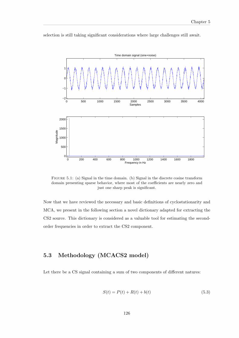
Chapter 5

selection is still taking significant considerations where large challenges still await.

0 500 1000 1500 2000 2500 3000 3500 4000−2

−1

0

1

Time domain signal (sine+noise)

Samples

0 200 400 600 800 1000 1200 1400 1600 18000

500

1000

1500

2000

Frequency in Hz

Mag

nitu

de

Figure 5.1: (a) Signal in the time domain. (b) Signal in the discrete cosine transformdomain presenting sparse behavior, where most of the coefficients are nearly zero and

just one sharp peak is significant.

Now that we have reviewed the necessary and basic definitions of cyclostationarity and

MCA, we present in the following section a novel dictionary adapted for extracting the

CS2 source. This dictionary is considered as a valuable tool for estimating the second-

order frequencies in order to extract the CS2 component.

5.3 Methodology (MCACS2 model)

Let there be a CS signal containing a sum of two components of different natures:

S(t) = P (t) +R(t) + b(t) (5.3)

126

Chapter 5

such that: P (t) and R(t) represent a CS1 and CS2 component respectively. b(t) is an

additive white noise, stationary and independent of R(t) . Separating these contribu-

tions is possible if we have a sparse representation of each underlying component. Our

methodology is based on the dictionaries that we create using the cyclostationarity con-

cept. In this section, we present a new dictionary for sparse representation modeling,

and we apply it with the MCA algorithm.

5.3.1 Proposition of new dictionary for sparse representation modeling

Over the past few years, researchers gave significant attention to developing general

overcomplete dictionaries for representing a signal; interestingly for signal and image

recognition, denoising and compression, etc. The reader is encouraged to refer to refer-

ences [148, 150, 164, 166].

Note that synthetizing a sparse signal amounts to finding the best dictionary that rep-

resents the signal.

To extract the first-order and second-order components of a CS process, we need special

dictionaries. In our framework, to represent the first-order deterministic components, we

used the DCT dictionary. The DCT is appropriate for sparse representation of smooth

and periodic behaviors; it also has the advantage of producing noncomplex coefficients.

The DCT transform of is defined by the following:

DCT (n) = c(n)

K∑k=1

s(k)cos

(π(2k − 1)(n− 1)

2K

), n = 1, 2, · · ·K (5.4)

Where, K is the length of s , and

c(n) =

1√K

n = 1√2/K 2 ≤ n ≤ K

(5.5)

127

Chapter 5

s is the input, n is the index of the output coefficient being calculated, K is the number

of elements being transformed and c is a scaling function.

In this research work, we were interested in a new original issue which has not been

explored so far in the literature. We aimed to find a dictionary that could well repre-

sent the second-order purely stochastic process. Consequently, for representing such a

process, we propose a new and simple dictionary adequate for one-dimensional signals.

This dictionary is based on the envelope spectrum analysis of a signal.

This envelope dictionary (Env) describes the signal in the second-order moments. The

results derived from the Env represent the components associated with CS2 cyclic fre-

quencies.

Generally, the envelope spectrum calculates the coefficients Envs(v) of the Fourier trans-

form of the expected squared magnitude of the temporal signal.

Previously, Randall et al [129] had proven an equivalence between the integrated cyclic

spectral density (the SCD given by eq. 2.6) and the envelope spectrum. So, the envelope

analysis can well replace the SCD. This relationship between the integrated spectral cor-

relation and envelope analysis allows to directly use the latter to characterize the CS2

behavior of a signal. Indeed, the envelope analysis represents a projection of the spectral

correlation density on the cyclic frequencies axis . The result of the relationship between

the integrated SCD and the envelope for a CS signal is written as follows [129]:

EnvS [v] = limT→∞

1

T

∫ T/2

−T/2|s(t)|2e−j2πvtdt, (5.6)

EnvS [v] =

∫RSCDS(v, f)df (5.7)

s(t) represents the temporal stochastic signal (CS2) and v is the discrete set of cyclic

frequencies.

128

Chapter 5

By combining both dictionaries (DCT and Env), we can well represent time series sig-

nals containing CS1 and CS2 components.

Generally, a dictionary is associated with an analysis and synthesis path. The analysis

path can be easily calculated directly by means of equation 5.6, while the synthesis path

represents the opposite conversion. The synthesis path is estimated by applying an in-

verse Fourier transform (IFFT) followed by the square root of coefficients. Figure 5.2

shows the block diagram for the envelope spectrum (Env) / inverse envelope spectrum

function. The red peaks represent the envelope spectrum using the estimator given by

equation (5.6).

Figure 5.2: Envelope spectrum (analysis and synthesis path).

Next, we provide some simulation examples to prove the efficiency of the proposed Enve-

lope dictionary. Figures 5.3, 5.4 and 5.5 illustrate the analyzed and synthetized signals

of three different simulation studies after applying the Envelope dictionary (Env). Fig-

ure 5.3 presents the analysis and synthesis path for ”pulses with random amplitudes on

a periodic schedule”, i.e. PAM signal. Figure 5.4 presents the result for a periodically

modulated stationary noise signal, i.e. an AM signal. Figure 5.5 presents the result for

a phase modulated signal, where the phase of sinusoid is gaussian white process.

These figures have verified the passage from the coefficients of the envelope to the signal.

note that the important information needed are well synthetized.

129

Chapter 5

0 500 1000 1500 2000 2500 3000 3500 40000

0.2

0.4

0.6

0.8

1original signal

Samples

0 500 1000 1500 2000 2500 3000 3500 40000

0.2

0.4

0.6

0.8synthesized signal

Samples

Am

plitu

de

Figure 5.3: analysis and synthesis path for ”pulses with random amplitudes on aperiodic schedule”, i.e. PAM signal

0 500 1000 1500 2000 2500 3000 3500 4000

−0.4

−0.3

−0.2

−0.1

0

0.1

0.2

0.3

0.4

0.5

Samples

original AM signalsynthesized signal

Figure 5.4: analysis and synthesis path for a periodically modulated stationary noise,i.e. AM signal

Consequently, the envelope spectrum dictionary plays a role of a discriminant between

CS parts, preferring the CS2 component over the other parts. Thus, a new dictionary is

built by exploiting the CS2 character of signals. This dictionary would be very effective

130

Chapter 5

500 1000 1500 20000

0.5

1

1.5

2

2.5

3

3.5

Samples

Am

plitu

de

original phase modulatedsignalsynthesized signal

Figure 5.5: Phase modulated signal, the phase of sinusoid is gaussian white process

at representing the CS2 component. It makes use of the significant coefficients offered

by the cyclic frequencies which are of high interest.

An example is shown in Figure 5.6, which illustrates a CS signal in the time domain and

its coefficients calculated by means of the envelope spectrum transform (Figure 5.6b) in

addition to the sparse coefficients obtained after hard thresholding (Figure 5.6c).

As a result, we propose the MCACS2 algorithm which is based on special dictionaries

suitable to the analysis of CS processes. The MCACS2 algorithm consists of an iterative

thresholding scheme presented as follows (Figure 5.7):

In our study, we aimed at separating the CS1and CS2 components of a CS signal. So,

such signal can be represented by a linear combination of two morphological components.

S = α1ϕ1 + α2ϕ2 (5.8)

131

Chapter 5

0 500 1000 1500 2000 2500 3000 3500 4000

−0.4

−0.2

0

0.2

0.4

Cyclostationary signal in time domain

Samples #

0 100 200 300 400 500

0

5

10

15Envelope Spectrum Coefficients

Frequency [Hz]

Am

plitu

de

0 100 200 300 400 500

0

5

10

15Sparse Coefficients (After HardThresholding)

Frequency [Hz]A

mpl

itude

Figure 5.6: (a) Cyclostationary signal in the original domain (b) envelope spectrumcoefficient (c) sparse coefficients (after hard thresholding).

Figure 5.7: MCACS2 algorithm.

132

Chapter 5

ϕ1 and ϕ2 were previously defined in chapter 2 (page 54)

The algorithm included three parts. First we initialized the parameters (the initial and

stopping thresholds), the total iteration number and the controlling parameters (thresh-

old update schedule). Then we got into the iterative procedure.

In the iterative procedure, we attempted to solve equation 2.23. The procedure con-

sisted of decomposing S over the transform ϕ (we obtained α), hard thresholding the

obtained component coefficients ( α = HardTHresh(α) ), and finally reconstructing

the source from the estimated coefficients α, i.e., s = ϕα . Note that the estimates

were progressively refined as the threshold evolved toward minimum; i.e., the threshold

should decrease with the iterations according to a linear or exponential decrease. Each

source was supposed to be sparsely described in its corresponding dictionary.

The algorithm depended on three important parameters:

1. The initial and stopping thresholds (regularization parameter).

2. The number of iterations.

3. The threshold update schedule (linear and exponential decrease), i.e., varying the

threshold by decreasing it linearly or exponentially.

To date, there are no specific tools for choosing the best parameters. They are still open

questions primordial to explore in the future.

However, according to Starck et al [150], the choice of the stopping threshold is done

according to the standard deviation of the noise contained in the signal. The WGN

standard deviation is estimated using the median absolute deviation (MAD) strategy

given by the following equation [150]:

σ = MAD(wf )/0.6745 = median

(|wf −median(wf )|

)/0.6745 (5.9)

Stopping criterion: λ ≤ t.σ (t is a constant)

133

Chapter 5

Where wf are the orthogonal wavelet coefficients of S at the finest scale. Moreover, t

has been chosen in the sense that it leads to good and accurate separation.

According to Starck et al [150], the exponentially decreasing strategy of threshold is

advised. Also, we had chosen a number of iterations big enough to obtain the estimates.

In the next section, a simulation study is performed to study the performance of the

CS1 and CS2 estimation component using the proposed MCACS2 method. Also, we

apply such a method to real signals coming from biomechanics.

5.4 Simulation study

As a first step, we need to validate the proposed method by a simulation study. There-

fore, we took a synthetic signal S(t) composed of a sum of noisy sinusoid and a random

pulse amplitude modulation (rPAM). The sinusoid represented the CS1 component,

while the rPAM represented the CS2 part. The mathematical model of S(t) can be

written as follows:

S(t) = P (t) +R(t) + b(t)

S(t) = CS1(t) + CS2(t)

where P (t) = sin(2πt/T ) + b(t) & R(t) =∑

n αnδ(t− nT )

P (t) is the CS1 and R(t) is the CS2. b(t) is a stationary white noise and independent

of R(t). αn is a random permutation. So, R(t) is a sparse vector containing random

permutations repeated periodically with period T.

αn is uniform, and its probability density function is given as follows:

pdfα(n) = { 1

k2 − k1}; k1 ≤ n ≤ k2 (5.10)

134

Chapter 5

with mean equal to 12(k1 + k2) and variance σ2 = 1

12(k2 − k1)2. In the simulated signal,

we used k1 = 0 and k2 = 20 .

The sinusoid had a period T = 0.05ms, which corresponded to a frequency f0 = 20Hz.

The sampling frequency was equal to 1000Hz. A part of the signal is shown in Figure

5.8a. This synthetic signal was CS at both orders 1 and 2.

Returning to the separation problem, the signal under study was analyzed with the

MCACS2 method. This separation gave rise to two components. The first one was a

purely periodic and smooth component (Figure 5.8b), so it represented the CS1 part of

the simulated signal. On the other hand, Figure 5.8c shows a second component which

was very different from the first and which represented contributions of second-order.

It seems that the method was robust in the detection and extraction of CS1 and CS2

components.

400 450 500 550 600 650 700 750

−4

−2

0

2

4

(a) Synthetic signal

Samples #

400 500 600 700

−4

−2

0

2

4

(b) CS1 components

400 500 600 700

0.5

1

1.5

2

(c) CS2 components

Figure 5.8: Simulated data: (a) the original signal, (b) the observed periodic part,(c) the CS2 part.

135

Chapter 5

5.5 Application on real biomechanical data

After the validation study of the proposed MCACS2 method, we applied our new ap-

proach on real data in an experimental analysis of biomechanical signals. An interesting

separation problem is the one related to the separation of the vertical ground reaction

forces (VGRF) components. In a VGRF signal, the CS1 part can be assigned to the

active components representing the propulsive force; whereas the CS2 part is related

to the passive components that represents the impact force (see Figure 5.9). One may

notice that the latter actually contains most of the information we are attempting to

analyze. The impact force is the major factor indicating the reaction of muscle, that

may reflect the fatigue state and performance of the muscle. For instance, after fatigue,

changes in the impact force can be masked by the very important contribution of peri-

odic parts; therefore, the need for separation.

The proposed MCACS2 method can be opted for the use in separation of periodic and

random components of VGRF signals. By taking advantage of information found in the

CS2 part, this could allow a better analysis and characterization of the runners fatigue

during time. Also, it could lead to a fully innovative description of human locomotion

mechanics during running.

5.5.1 Data description

As described previously, the database is composed of 120 GRF signals recorded from

10 experienced ultrarunners during an extreme ultra-long duration of running. The

subjects were asked to run 24 h continuously with a short rest period every 2 h. A

measurement period of 20 s was done every 2 h.

The CS aspect of these signals was modeled mathematically as follows:

S(t) = P (t) +R(t) + b(t)

136

Chapter 5

200 300 400 500 600 700 800 900

0

100

200

300

400

500

600

700

800

900

1000

Time (ms)

Ver

tical

GR

F

Impact Force

Propulsive Force

Figure 5.9: (a) VGRF active (propulsive force) and passive (impact force) peaks.

P (t) is the periodic deterministic part and R(t) the CS2 part.

Note that the model proposed in the simulation study is adequate with GRF signals.

5.5.2 MCACS2 based analysis of VGRF

Now, we apply our method to these real biomechanical signals. In our framework, the

parameters chosen are summarized as follows:

1. According to references [150] and [149], we chose to set the number of iterations

to Niter = 100.

2. The stopping threshold ≤ t.σnoise, where the standard deviation of noise was

estimated from the data and t is a constant greater than 100.

3. Exponentially decreasing schedule of threshold (according to reference [150]).

137

Chapter 5

Notice that too small number of iterations leads to a bad separation; while a large

number of iterations is computationally expensive. Experiments have shown that the

optimum number of iterations depends on the data set used in the application (typically

hundreds) [149]. So, a good thresholding strategy should provide a fast decomposition

with the least number of iterations.

Furthermore, the stopping threshold had been chosen in the sense that it leads to good,

accurate and adaptive separation. Also, the simplicity of the exponentially decreasing

schedule of threshold is an advantage and it gives good results [150].

Using the separation algorithm described previously, a VGRF signal is decomposed in

the dictionary (DCT+ Env). Figure 5.10 presents a sample of the VGRF signal in the

time domain and shows both the CS1 and CS2 separated sources. Figure 5.11 illustrates

the power spectral density (PSD) of the original VGRF signal and both the power spec-

tral densities of CS1 and CS2 components.

Figure 5.10b shows a component having a clear repetitive pattern which happens to be

periodic at order 1. On the other hand, Figure 5.10c shows a component which is very

different from the first and having a random character, including hidden information in

its structure. Figure 5.11 highlights the difference between the various components by

a frequency spectrum analysis.

For such a signal, the PSD (Figure 5.11) highlights the presence of two clearly separated

sources. The first source is dominated by CS1 components and may be linked to the

running cycle and mostly contains the propulsive force contribution. The second source

is mainly composed of CS2 random components and may be related to the fluctuations

or increasing variance located during the stance phase (during which the foot is in con-

tact with the ground). Hence, the evolution of CS2 source may lead to understand the

slight changes that can help in the diagnosis of exercise performance and muscle fatigue.

138

Chapter 5

In Figures 5.10 and 5.11, we demonstrate that the proposed approach is capable of sepa-

rating the CS1 and CS2 parts from the vertical ground reaction force signals. The DCT

seems to be a good dictionary for the extraction of periodicity. The Env brings a robust

solution in the estimation of cyclostationarity of order 2.

The MCACS2 method is verified for morphologically diverse cyclostationarity sources.

The proposed method was shown to gain considerable attention in the domain of cyclo-

stationarity and blind source separation.

Therefore, we can interpret the results as follows: if we have information about the data

and underlying components, our results show that the separation of such components is

possible using the sparsity and morphological diversity. Moreover, selecting the signifi-

cant coefficients obtained by the different transforms is the key issue to separate out the

contribution of each source.

The advantage of the developed envelope spectrum dictionary is exhibited by the main

coefficients required to represent the random behavior (CS2 behavior) in a CS signal.

The real challenge of MCACS2 algorithm lies in determining the CS1 and CS2 sources

using specific dictionaries (DCT and envelope spectrum dictionaries, respectively). The

CS aspect of VGRF signals has been taken into consideration because it is a key point

when choosing and adapting a dictionary. This proposed method can become an inter-

esting tool for accelerating and enhancing adaptability in future dictionary structures

for CS analysis.

139

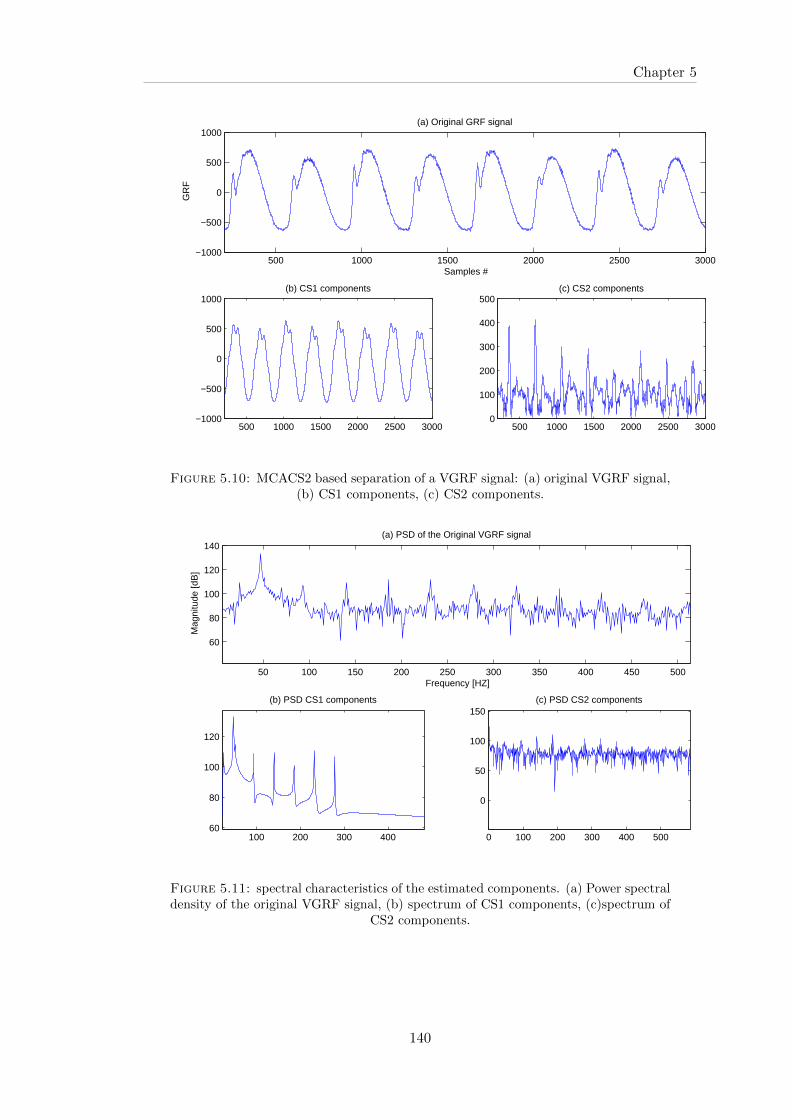
Chapter 5

500 1000 1500 2000 2500 3000−1000

−500

0

500

1000(a) Original GRF signal

Samples #

GR

F

500 1000 1500 2000 2500 3000−1000

−500

0

500

1000(b) CS1 components

500 1000 1500 2000 2500 30000

100

200

300

400

500(c) CS2 components

Figure 5.10: MCACS2 based separation of a VGRF signal: (a) original VGRF signal,(b) CS1 components, (c) CS2 components.

50 100 150 200 250 300 350 400 450 500

60

80

100

120

140(a) PSD of the Original VGRF signal

Frequency [HZ]

Mag

nitu

de [d

B]

100 200 300 40060

80

100

120

(b) PSD CS1 components

0 100 200 300 400 500

0

50

100

150(c) PSD CS2 components

Figure 5.11: spectral characteristics of the estimated components. (a) Power spectraldensity of the original VGRF signal, (b) spectrum of CS1 components, (c)spectrum of

CS2 components.

140

Chapter 5

5.6 Conclusion

In this chapter, the concept of sparsity and morphological component analysis was used

for the separation of cyclostationary components (CS1/CS2) in a signal. A new dictio-

nary based on the envelope spectrum of the signal was proposed to extract the cyclosta-

tionarity of order 2. The performance of the so called ”MCACS2 algorithm” was proved

when applied to simulated and real GRF signals. Such algorithm provides additional

way for the exploitation of cyclostationarity and it may be useful in other domain of

applications.

The next chapter treated the GRF signals in a slightly different way. Since the passive

component was proved to be the part that contains information, the chapter proposes

a new model of CS and some original indicators, i.e. the random variation of the slope

and polynomials coefficients of passive peaks.

141

Chapter 6

THE RANDOM SLOPE

MODULATION: A NEW

CYCLOSTATIONARITY

MODEL

Contents

6.1 Introduction . . . . . . . . . . . . . . . . . . . . . . . . . . . . 143

6.2 The proposed RSM model . . . . . . . . . . . . . . . . . . . . 146

6.3 Application on the ground reaction force signals . . . . . . 149

6.4 Results . . . . . . . . . . . . . . . . . . . . . . . . . . . . . . . . 152

6.5 Polynomial with random coefficients . . . . . . . . . . . . . . 154

6.6 Conclusion . . . . . . . . . . . . . . . . . . . . . . . . . . . . . 157

142

Chapter 6

Sports and physical activities cause different effects within the body systems. They may

affect the equilibrium of the internal environment. As a result, sooner or later sensa-

tions of exhaustion and fatigue may occur. The harmful effects depend on the type of

exercise. The relationship between physical exercise and muscle fatigue has particularly

attracted attention by many researchers for more than a century. Such a relationship is

very complex and still needs further research.

The slope has important implications in the signal processing domain. A polynomial

with random coefficients may also give important implications in signal processing. In

this dissertation, we consider the slope and random coefficients of the passive polynomial

(impact force) as specific measures extracted from the vertical ground reaction forces.

Such coefficients are random and different for every gait cycle (Figure 6.1). This ran-

domness introduces a cyclostationarity of order 2.

In general, the human locomotion is defined by sequences of cyclic and repeated ges-

tures. So, we have a CS process represented as a coupling of a periodic part (running

cycle) together with a random stationary part (random coefficients). For such signals,

the origin of cyclostationarity might come from the random variation of the polynomial

coefficients of the passive peak. The results show that the slope and polynomial ran-

dom coefficients of the passive peak can play an important role and provide interesting

information concerning fatigue and concerning running and walking performance.

6.1 Introduction

Spectral analysis is an efficient and adequate description of a signal. Its basic pur-

pose is to decompose the function into spectral components, i.e., into sum of weighted

sinusoidal functions. If the statistical parameters of a signal such as the mean and au-

tocovariance functions fluctuate periodically with time, then the process is said to be

cyclostationary (CS). There are numerous models used in telecommunication and in in-

dustrial and control systems that result in CS processes. Module signals including the

143

Chapter 6

0 50 100 150 200 250 300 350

0

200

400

600

800

1000V

ertic

al G

RF

Passive

Active

First ground contact Last ground

contact

Figure 6.1: Random variation of passive peaks each gait cycle

amplitude modulated signals (AM), frequency modulated signals (FM), phase modu-

lated signals (PM), pulse amplitude modulated signals (PAM), etc., have particularly

maintained attention because they have interesting properties consisting of a specific

spectral correlation density function.

Every CS process can be represented as a coupling of a periodically modulated part

together with a random stationary part. The periods of CS in modulated signals may

correspond to carrier frequencies, repetition or pulse rates, time division multiplexing

rates... Some interesting examples of the types of modulation that produce CS wave-

forms, i.e., waveforms with mixtures of periodicity and randomness are: the periodically

modulated stationary noise (noise with periodically varying characteristics); pulses with

random amplitudes on a periodic schedule; and pulses on a periodic schedule with ran-

domly jittered timing,... These examples have received great attention in literature.

144

Chapter 6

In the previous chapters, we investigated the vertical ground reaction forces dur-

ing ultra-running to study muscle fatigue and to calculate the mechanical fluctuations

with time. Our results hypothesized that the randomness in both impact and active

force peaks would increase with time, i.e., with the degree of fatigue. This randomness

and fluctuations could be monitored by the 2nd order cyclostationarity analysis and by

means of many proposed indicators discussed in (section 4.4).

Combined with our previous studies and results attained, we now add an additional

indicator i.e., the random variation of the slope and the random variation of polynomial

coefficients of the impact force.

In this chapter, we present a new modulation type producing CS. This model may

be used to characterize signals with random slopes and is referred to as ”the random

slope modulation (RSM)”. With this model, it is possible to extract information about

the CS properties and structure of the signals. For many real CS signals, the origin of

cyclostationarity might come from the random variation of the slope.

The CS properties of the proposed model (RSM) can be suitably exploited to analyze

biomechanical signals such as signals recorded during human walking and running, since

these signals were proved to be CS. The CS nature of biomechanical signals was treated

and characterized in the previous chapters. We suggested that the runner’s fatigue may

be associated with the frequency signatures of second-order characteristics of the VGRF

signals.

In this chapter, our aim was to treat the CS properties of biomechanical signals in

a slightly different way. The slope has important implications in the signal processing

domain. Here, we consider it as a specific measure extracted from the VGRF signals.

We were interested to measure its value and to monitor its evolution with time. For such

signals, we can explain the origin of CS by the random variation of the slope. The latter

may play an important role and provide interesting information concerning fatigue and

145

Chapter 6

concerning running and walking performance.

6.2 The proposed RSM model

Based on results in Chapter 4 and 5, we hypothesized that the randomness in both

impact and active force peaks would increase with time running, i.e., with the degree

of fatigue. Additionally, we could predict and monitor these changes by means of many

proposed indicators (CS based indicators- see section 4.4). We anticipated that the

passive component changes with time running and is significantly different before and

after fatigue.

What we need to accomplish in this chapter is to provide a new model useful for

studying and characterizing cyclostationarity. Such a model may be quite valuable for

studying numerous mechanical and biomechanical signals. We consider a new example

of modulation type. We will study the impact of random slope variation on the cyclic

spectrum of a CS signal.

Modulating a signal simply means to vary one parameter of the signal. In this section,

we vary each time the first slope of a trapezoid. Moreover, the signal model is a trape-

zoid repeated periodically, but the slope of its first lateral side is generated randomly.

So, we obtain a CS signal composed of a coupling of periodic and random phenomena.

The slope is random and different for every peak. This randomness introduces a cyclo-

stationarity of order 2. In this section, experimentations are performed using various

values of slope variance.

Therefore, we consider a trapezoid signal having a slope that is modulated randomly

(Figure 6.2). We change the first slope of the trapezoid randomly to simulate the walking

and running signal. Such signal could be expressed by the following signal model:

S”(t) =∑k

pk{δ(t− kT )− δ(t− kT − τk)} =d2X(t)

dt2(6.1)

146

Chapter 6

Here, we used the second derivative of the proposed signal so the signal can be more

readily modeled and analyzed. It also exhibits how much change occurs in the first slope.

{τi} is set to be an independent and identically distributed (i.i.d.) random stationary

sequence consisting of random variables produced every T s. We interpret these variables

as the time samples of a random waveform. τi are normally distributed ∼ N(µi, σi), and

are confined within the interval 0 ≤ τi ≤ τ2 . The slopes are given by:

p1 =A

τ1; p2 =

A

τ2; p3 =

A

τ3; .... pi =

A

τi; ∞ ≥ pi ≥

2A

T

δ(t) is the Kronecker delta . It’s an indicator vector (for each t) having one element

equal to unity and the rest equal to zero, and k = 0,±1,±2, ...

It can be noticed that if pk is stationary in the strict sense, then S”(t) is generally CS.

It is a random slope CS signal with the fundamental cycle 1T .

Figure 6.2: X(t) is a trapezoid signal with random slope modulation. S”(t) is thesecond derivative (T: Constant cyclic period)

Figure 6.3 presents the slopes of 2 simulated data such that one has low slope variation

and another has high slope variation. For each case, we want to analyse the cyclic

spectrum of the second derivative of the original trapezoids .

147

Chapter 6

0 5 10 15 20 25 30 35 400

5

10

15

20

25

Cycle #

Slo

pe

Low variationBig variation

Figure 6.3: Slope variance of 2 simulated data: one with low slope variation andanother with high slope variation

Knowledge of the cyclic spectrum or spectral correlation density function for specific

modulation types is important in performing evaluation and detection of different signal

processing systems and in characterizing random processes that are CS. Figure 6.4 and

6.5 represent the magnitude plot of the cyclic autocorrelation functions of S”(t), as a

function of α and τ , calculated for different slope variances. The results show that the

cyclic correlation increases for higher slope variance, also the fundamental frequency and

its harmonics are higher. So, the slope could be used as a new indicator of CS.

Figure 6.4: cyclic autocorrelation function for a small variance

148

Chapter 6

Figure 6.5: cyclic autocorrelation function for a big variance

6.3 Application on the ground reaction force signals

A ground reaction force (GRF) sample is presented in Figure 6.6. A typical GRF peak

obtained during running is composed of two different parts: a passive peak representing

the impact force and an active peak representing the propulsive force. The impact force

(passive components) results from the collision of the heel with the ground. It reaches

its maximum (Passive peak) in 50 ms after the first contact (half the stance phase).

Changes in the impact force might be a major factor indicating the reaction of muscles

that may reflect the fatigue state and performance of the muscles. Such parameters are

statistically associated with performance and does not mean that these two variables

are causally related.

The passive peaks carry information on the random part in the signal while the active

peaks are more impulsive.

In the previous chapters, we investigated the vertical ground reaction forces during

ultra-running. Our rationale was that these force data would aid in the understanding

of muscle fatigue and performance and in calculating mechanical fluctuations with time.

Combined with our previous studies and results, we now add an additional indicator

i.e., the random variation of the slope and of the polynomial coefficients of the impact

149

Chapter 6

Figure 6.6: A GRF peak before and after fatigue

force. Our impact force data suggests that running substantially increases the random-

ness and polynomial variations.

Therefore, to study muscle fatigue, our research showed that this may lie in the

information contained in the passive peak of VGRF signals. In this chapter, we pro-

pose a method based on the analysis of the slope and random polynomial coefficients

which characterize the passive peak. Our main objective is to examine the biomechan-

ical changes during a very long running exercise. Also, to study how such parameters

have changed over time.

The slope has important implications in the signal processing domain. Here, we

consider this parameter as specific measure extracted from the VGRF signals. We were

interested in measuring its value and to monitor its evolution with time. It may play an

150

Chapter 6

important role and provide interesting information concerning fatigue and concerning

running and walking performance (evaluating pathological and aging walking patterns).

Figure 6.7 represents the proposed methodology used to calculate the coefficients of

the polynomial representing the passive peak of the signal. The first step consists of

normalizing and denoising the signal by means of the wavelet method. In the second

step, we calculate the global minimum and maximum, then find the true minimum using

a comparison method presented previously in chapter 4.

Figure 6.7: proposed methodology

Figure 6.8: Curve fitting (polynomial of degree 6)

151

Chapter 6

Next, we try to find the curve that has the best fit to the passive peak and that passes

through the maximum number of points (Figure 6.8). We found that the polynomial of

degree 6 is the best. Then, for calculating the coefficients of polynomial function, we

consider an algebraic polynomial given by the following equation:

Pn(t) = a0 + a1t+ a2t2 + a3t

3 + ...+ antn =

n∑j=0

ajtj (6.2)

With random coefficients aj , j=0,1,2...n.

{aj}nj=0 is a sequence of independent identically distributed random variables which is

cyclostationary. its defined on R.

a1 is the slope to be analyzed in the next section. This slope value measures the sensi-

tivity or rate of change in VGRF as a result of a change in time. It is calculated as the

rate of change of the impact force.

6.4 Results

In this section, we analyzed the data from the original series of the study by the exercise

physiology laboratory (LPE) of Jean Monnet St-Etienne University which conducted a

recording experiment providing data suited to the analysis of running performance and

fatigue. The database was described in the previous chapters.

The slope was determined in each gait cycle, and then the variance of these slopes was

calculated.

We aim to quantify the variation in GRF signals with time after 2 h and after 24 h of

running. In Figure 6.9, it appears that there exist some differences in slope variation

after 2 h and after 24 h of running that is before and after fatigue.

In Figure 6.10, we calculate the medians (of 10 subjects) of the slope variance after 2

h and after 24 h of running. Notice the significant changes observed between the two

152

Chapter 6

groups.

Compared to level running, the slopes increase with time running and were dramatically

larger after 24 h running (POST fatigue). These results were obtained from 10 subjects.

Figure 6.9: Slope variation for one subject after 2 h (in blue) and after 24 h (in red)of running. it appears that there exist some differences in slope variation after 2 h and

after 24 h of running that is before and after fatigue.

153

Chapter 6

Figure 6.10: The difference between the medians of the Slope variance after 2hours1

and after 24hours2 of running (The median of 10 subjects). Notice the significantchanges observed between the two groups.

6.5 Polynomial with random coefficients

The polynomial with random coefficients may also shed light onto important impli-

cations in signal processing. The analysis of all random coefficients of the polynomial,

is also an interesting field of study.

Our polynomial of degree 6 can be written as follows:

Pn(t) = a+ bt+ ct2 + dt3 + et4 + ft5

First of all, we calculated the polynomial coefficients (coefficients a, b, c, d, e, and f)

between ”true-min” and ”Max. passive” and that for each cycle of the VGRF signal

(Figure 6.11). We then estimated the variance of each coefficient vector.

Figure 6.12 presents the median of the variance of each coefficient vector after 2hours1

and after 24hours2 of running. We identified a slight increase in the variance of all

coefficients after 24hours2 of running i.e., in post fatigue.

154

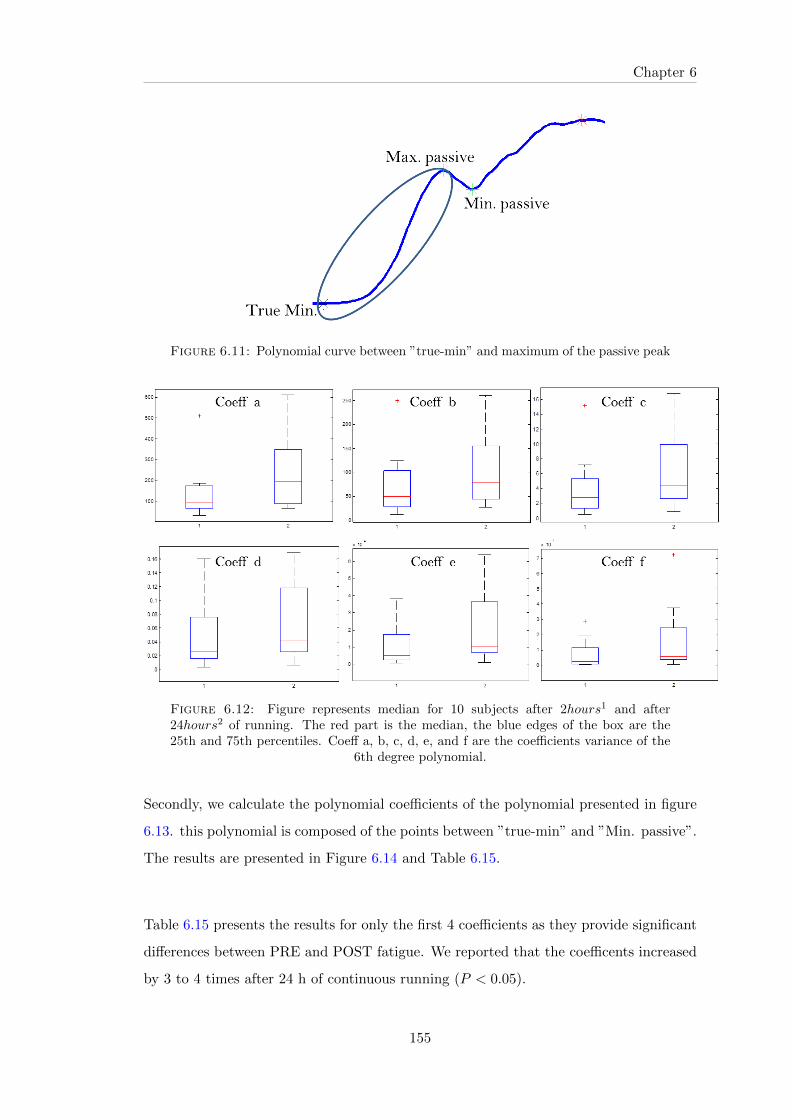
Chapter 6

Figure 6.11: Polynomial curve between ”true-min” and maximum of the passive peak

Figure 6.12: Figure represents median for 10 subjects after 2hours1 and after24hours2 of running. The red part is the median, the blue edges of the box are the25th and 75th percentiles. Coeff a, b, c, d, e, and f are the coefficients variance of the

6th degree polynomial.

Secondly, we calculate the polynomial coefficients of the polynomial presented in figure

6.13. this polynomial is composed of the points between ”true-min” and ”Min. passive”.

The results are presented in Figure 6.14 and Table 6.15.

Table 6.15 presents the results for only the first 4 coefficients as they provide significant

differences between PRE and POST fatigue. We reported that the coefficents increased

by 3 to 4 times after 24 h of continuous running (P < 0.05).

155

Chapter 6

In addition, we performed Welch’s t-test to analyze the differences between PRE and

POST fatigue. Significance was defined as P < 0.05. The tests revealed a significant

result.

Overall, our results, are better than the studies of the past ([84, 86])

Figure 6.13: Polynomial curve between ”true-min” and the minimum of the passivepeak

Table 6.15 presents the results obtained for all coefficients. The average and standard

deviation are calculated for 10 subjects.

156

Chapter 6

Figure 6.14: Figure represents median for 10 subjects after 2hours1 and after24hours2 of running. The red part is the median, the blue edges of the box are the25th and 75th percentiles. Coeff a, b, c, d, e, and f are the coefficients variance of the

6th degree polynomial.

Figure 6.15: Values represent means for 10 subjects ± standard deviation.

6.6 Conclusion

The previous chapters proved that the passive peaks of GRF signals contain the random-

ness or CS2 sources, i.e. they contain useful information to be extracted using specific

parameters.

In this chapter, we provided a new cyclostationary model called ”Random slope modu-

lation” or ”cyclostationary signals with random slopes”. This model has put in evidence

a new CS indicator that is the random variation of the slope of passive peaks. This ran-

domness introduced a cyclostationarity of order 2. Results proved that such an indicator

157

evolved significantly with time during running, so it seemed to be clearly affected by

fatigue following fatiguing exercise. The random variation of the polynomial coefficients

of passive peaks also significantly varied with time during running.

These original model and indicators provide new insight, and open new perspectives and

new possibilities for simple analysis of fatigue and falling of elderly.

General Conclusion and

perspectives

In this chapter, we give a detailed outline and summary of the contents of chapters III,

IV, V and VI which comprise the body of this thesis.

Following this summary, we suggest several topics for further research.

1. Chapter III

The results in this chapter showed an overview of the capabilities of the cyclostationarity

applied to human gait to detect ”flaws” and estimate potential risk of falls in an elderly

population.

Many subjects with history of falls were analyzed using the CS indicators in three

different walking conditions. The results stipulated give insight that the Cyclostation-

ary indicator (cyclic correlation) shows significant variation when performing secondary

tasks. These results may provide information for the evaluation of falling elderly. This

means that such tasks could be useful reference factors for fall prediction.

The differences between fallers and non- fallers are quite significant in case of male and

female individuals. From a current review of several tens of seconds and basing on our

tools of signal processing (cyclostationarity), it is possible now to put forward a fast

and reliable indicator to estimate the potential risk of falls in the elderly. Thus, fall sig-

nals are clearly impacting cyclostationarity. This relationship between fallers and cyclic

159

correlation should take into account the sex. Finally, we note that the analysis of Cy-

clostationarity may have practical utility and benefits in biomechanical and neurological

diagnosis.

2. Chapter IV

The original contribution of our proposed approach lies in solving the separation problem

of active and passive components of GRF signals, as well as in introducing new indicators

and parameters that may monitor the evolution fatigue. The database used was recorded

from 10 experienced subjects considered as high level sports and ultra-runners during

24 hours of continuous running. These are the data of the study done by the faculty of

medicine of Jean Monnet St-Etienne University which conducted a recording experiment

of running providing important data particularly suited to the analysis of fatigue as well

as to characterize and understand the mechanical phenomena behind the GRF signals

behavior. Four important conclusions can be obtained from the results stipulated in this

article:

(1) This paper presents a new procedure based on a Gaussian decomposition and non-

linear least squares method. The proposed methodology has been introduced to separate

the active and passive components of GRF signals. The results indicate the good per-

formance of the proposed algorithm for separating both active (propulsive force) and

passive (impact force) signals.

(2) A comparison is made with another proposed BSS based approach i.e. the JADE and

AJD algorithms. The comparison with these methods proved that the new methodology

outperforms in terms of GRF components separation.

(3) The separated passive signals are proved to be cyclostationary of order 2 (CS2).

There is an advantage of using cyclostationary analysis to investigate changes with time

during an extreme ultra long duration of running. Thus, modeling the passive signals

by a Cyclostationary signal may give information about the fatigue of the rider through

a cyclic spectral analysis.

(4) The proposed approach expands the prospects of the diagnosis of fatigue, subse-

quently; we have proposed several indicators that characterize running and could moni-

tor the evolution of fatigue. We introduced several indicators and follow their evolution

with time: the changes in step frequency, in the cyclic autocorrelation function, in the

integrated cyclic correlation (energy at v = 0 and at the step frequency (v1) and in the

kurtosis and degree of cyclostationarity (DCS).

The results presented proved the effectiveness of the proposed features to the character-

ization of running linked to ultra-endurance performance in a group of runners during

a 24-h treadmill run. Ultra-endurance performance can lead to weight loss, chronic fa-

tigue, and impaired physical performance.

3. Chapter V

In this chapter, we exploited the CS character of signals in the context of MCA. We

created a new dictionary with the aim of separating the cyclostationarity components

using the MCA method.

We presented a general decomposition framework for CS signals using the morphological

diversity. Within this framework, the MCACS2 algorithm was proposed. We showed

that such algorithm can be very useful to decompose a CS signal into its periodic and

random sources. The periodic components that are widely spread in a CS signal can be

represented by means of the DCT basis. The CS2 part can be sparsely represented by

means of the proposed dictionary which is based on the envelope spectrum analysis.

We analyzed the proposed approach and demonstrated the results on synthetic signals

and its application on real biomechanical signals. The latter consists of real biomechan-

ical data collected from high level runners subjected to 24 h of continuous running.

3. Chapter VI

Human fatigue studies stretches back many decades and still a significant part of medical

discourse. The purpose of this chapter was to examine the possible relationship between

fatigue development in long-distance running, and the accompanying changes in the

passive force peak (impact variables). The random variation of the slope at the passive

peak was proved to be the origin of CS of order 2 in the signal. This is considered a very

important finding to the introduction of a new indicator of CS, which is very simple and

easy to calculate i.e. the slope of passive peak (the slope of the polynomial between the

true minimum and maximum of the passive peak). This puts forth evidence of a new

CS model called ”the random slope modulation”. In addition, a question arises whether

from such an indicator, can the fatigue be estimated. Furthermore, signals recorded

from 10 experienced runners over a 24 h period were treated in order to examine the

changes during long distance running. The results showed that the proposed parameter

seemed to vary with time during ultra-long running. These changes could be directly

related to fatigue.

Perspectives

First of all, it is important to develop additional indicators of fall to differentiate fallers

and non-fallers. Moreover, its necessary to create a robust mathematical model to char-

acterize walking signals.

Secondly, we need to apply the proposed approaches and indicators of chapter 4 to a

larger database for the aim of classification in order to test their performance. This

may be done with artificial neural network and other means of the artificial intelligence.

Other scenarios could also be discussed in further applications to characterize human

locomotion in general (i.e. human running and walking) and to estimate the muscle

fatigue.

Thirdly, the choices of MCA parameters are still subject to questions essential for ex-

ploration in future works. Hence, we need to search for specific tools for choosing the

best parameters. Such tools may result in simpler and high performance algorithms.

For instance, we can use the mean squared error in order to minimize the number of

iterations. An important consideration also is the estimation and optimization of the

stopping criterion as well as the threshold. For solving these problems, we can use for

example some statistical resampling and bootstrap methods.

An interesting extension of chapter 5 is to apply the proposed MCACS2 method on me-

chanical and rotating machines, bearing vibration signals, and machine tools vibratory

signals...

Moreover, the vertical component of the VGRF signal quickly rises and falls, forming

the passive peak, then more slowly increases to a second peak at mid-stance, termed

the active peak, before decreasing prior to toe-off (Figure 6.16). One can benefit from

these changes and calculate the slope and polynomial coefficients for the different poly-

nomials. Four slopes could be calculated and analyzed (see Figure 6.16) for monitoring

the VGRF signals before and after fatigue. Also four polynomial coefficients could be

calculated and analyzed

The analysis of all random coefficients of each polynomial, is also an interesting field to

study.

Additionally, modeling analysis of random polynomials signals is also very interesting

for future studies.

Figure 6.16: VGRF slopes analysis

In future works, we are planning to reinforce our study by a mathematical model i.e.,

to find a robust mathematical model that proves the validity of a new CS model called:

Random Slope Modulation.

An interesting approach is to apply our model (RSM model)to the database of the el-

derly. This was presented in chapter 3 for studying the falling of elderly. This may

provide important results in terms of fall detection.

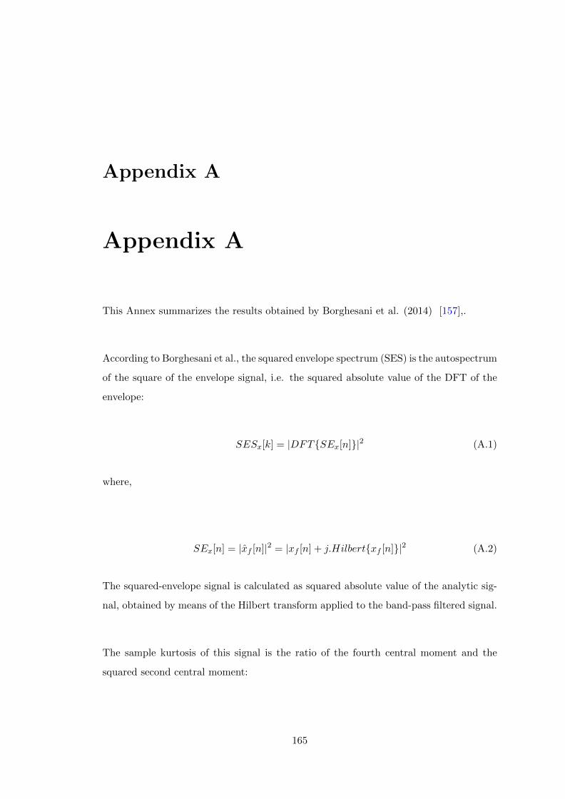
Appendix A

Appendix A

This Annex summarizes the results obtained by Borghesani et al. (2014) [157],.

According to Borghesani et al., the squared envelope spectrum (SES) is the autospectrum

of the square of the envelope signal, i.e. the squared absolute value of the DFT of the

envelope:

SESx[k] = |DFT{SEx[n]}|2 (A.1)

where,

SEx[n] = |xf [n]|2 = |xf [n] + j.Hilbert{xf [n]}|2 (A.2)

The squared-envelope signal is calculated as squared absolute value of the analytic sig-

nal, obtained by means of the Hilbert transform applied to the band-pass filtered signal.

The sample kurtosis of this signal is the ratio of the fourth central moment and the

squared second central moment:

165

Kurt =M4{xf [n]}{M2{xf [n]}}2

(A.3)

Where,

M4{xf [n]} =1

N

N∑n=1

{SEf [n]}2 = SESx[k](Parseval′stheorem) (A.4)

With,

SESx[k] =∑

k |DFT{SEf [n]}|2

Thus,

M4{x[n]} =h−l∑k=0

SESl,h[k] (A.5)

This considers that SES is non-zero only in the range of cyclic frequencies 0 ≤ k ≤ h− l

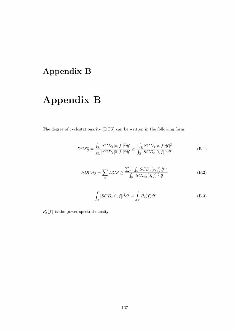
Appendix B

Appendix B

The degree of cyclostationarity (DCS) can be written in the following form:

DCSvS =

∫R |SCDx[v, f ]|2df∫R |SCDx[0, f ]|2df

≥|∫R SCDx[v, f ]df |2∫R |SCDx[0, f ]|2df

(B.1)

SDCSS =∑v

DCS ≥∑

v |∫R SCDx[v, f ]df |2∫

R |SCDx[0, f ]|2df(B.2)

∫R|SCDx[0, f ]|2df =

∫RPx(f)df (B.3)

Px(f) is the power spectral density.

167

Bibliography

[1] Jeffrey M Hausdorff. Gait dynamics, fractals and falls: finding meaning in the

stride-to-stride fluctuations of human walking. Human movement science, 26(4):

555–589, 2007.

[2] Eric Viel. La marche humaine, la course et le saut: biomecanique, explorations,

normes et dysfonctionnements, volume 9. Elsevier Masson, 2000.

[3] Robert B Randall and Nader Sawalhi. A new method for separating discrete

components from a signal. Sound and Vibration, 45(5):6, 2011.

[4] Aurelio Cappozzo. Measurement of human locomotion, vladimir medved; crc press

llc, boca raton, fl, 2001, pp. 255, isbn 0-8493-7675-0, 2003.

[5] Sofiane Maiz, Frederic Bonnardot, Jacek Leskow, Anna Dudek, et al. Determinis-

tic/cyclostationary signal separation using bootstrap. In Adaptation and Learning

in Control and Signal Processing, volume 11, pages 641–646, 2013.

[6] Serge Duckett et al. Pathology of the aging human nervous system. Oxford Uni-

versity Press US, 2001.

[7] Richard W Besdine, Difu Wu, et al. Aging of the human nervous system: what

do we know? Medicine and Health Rhode Island, 91(5):161, 2008.

[8] World Health Organization. Ageing and Life Course Unit. WHO global report on

falls prevention in older age. World Health Organization, 2008.

[9] Naufal H. Prospects of aging in lebanon and potential implications for health and

social policies. Annual meeting of the Lebanese Epidemiological Association on the

Epidemiology of Aging in Lebanon and the Eastern Mediterranean, 2011.

168

[10] Jeffrey M Hausdorff, Susan L Mitchell, Renee Firtion, Chung-Kang Peng, Merit E

Cudkowicz, Jeanne Y Wei, and Ary L Goldberger. Altered fractal dynamics of gait:

reduced stride-interval correlations with aging and huntingtons disease. Journal

of applied physiology, 82(1):262–269, 1997.

[11] Susan W Muir, Mark Speechley, Jennie Wells, Michael Borrie, Karen Gopaul,

and Manuel Montero-Odasso. Gait assessment in mild cognitive impairment and

alzheimer’s disease: the effect of dual-task challenges across the cognitive spec-

trum. Gait & posture, 35(1):96–100, 2012.

[12] Richard Camicioli, Diane Howieson, Suzanne Lehman, and Jeffrey Kaye. Talking

while walking the effect of a dual task in aging and alzheimer’s disease. Neurology,

48(4):955–958, 1997.

[13] Takashi Nakamura, Kenichi Meguro, Hideki Yamazaki, Hideyuki Okuzumi, Atushi

Tanaka, Ayumu Horikawa, Keiichiro Yamaguchi, Naofumi Katsuyama, Masao

Nakano, Hiroyuki Aral, et al. Postural and gait disturbance correlated with de-

creased frontal cerebral blood flow in alzheimer disease. Alzheimer Disease &

Associated Disorders, 11(3):132–139, 1997.

[14] Henriet Visser. Gait and balance in senile dementia of alzheimer’s type. Age and

ageing, 12(4):296–301, 1983.

[15] Pamela L Sheridan, Judi Solomont, Neil Kowall, and Jeffrey M Hausdorff. Influ-

ence of executive function on locomotor function: divided attention increases gait

variability in alzheimer’s disease. Journal of the American Geriatrics Society, 51

(11):1633–1637, 2003.

[16] Alzheimer’s Association et al. Basics of Alzheimer’s Disease: What it is and what

you can do. Alzheimer’s Association, 2012.

[17] Rossitza Baltadjieva, Nir Giladi, Leor Gruendlinger, Chava Peretz, and Jeffrey M

Hausdorff. Marked alterations in the gait timing and rhythmicity of patients with

de novo parkinson’s disease. European Journal of Neuroscience, 24(6):1815–1820,

2006.

[18] Roberta de Melo Roiz, Enio Walker Azevedo Cacho, Manoela Macedo Pazinatto,

Julia Guimaraes Reis, Alberto Cliquet Jr, and Elizabeth Barasnevicius-Quagliato.

Gait analysis comparing parkinson’s disease with healthy elderly subjects. Ar-

quivos de neuro-psiquiatria, 68(1):81–86, 2010.

[19] G Kemoun, E Watelain, L Defebvre, JD Guieu, and A Destee. [postural strategies

and falls in elderly and in parkinsonism]. In Annales de readaptation et de medecine

physique: revue scientifique de la Societe francaise de reeducation fonctionnelle de

readaptation et de medecine physique, volume 45, pages 485–492, 2002.

[20] Olivier Blin, Anne-Marie Ferrandez, and Georges Serratrice. Quantitative analysis

of gait in parkinson patients: increased variability of stride length. Journal of the

neurological sciences, 98(1):91–97, 1990.

[21] Bastiaan R Bloem, Yvette AM Grimbergen, Monique Cramer, Mirjam Willemsen,

and Aeilko H Zwinderman. Prospective assessment of falls in parkinson’s disease.

Journal of neurology, 248(11):950–958, 2001.

[22] Bastiaan R Bloem, JP Van Vugt, and Dennis J Beckley. Postural instability and

falls in parkinson’s disease. Advances in neurology, 87:209, 2001.

[23] Joe Verghese, Cuiling Wang, Richard B Lipton, Roee Holtzer, and Xiaonan Xue.

Quantitative gait dysfunction and risk of cognitive decline and dementia. Journal

of Neurology, Neurosurgery & Psychiatry, 78(9):929–935, 2007.

[24] World Health Organization. Manual of the international statistical classification

of diseases, injuries, and causes of death, volume 2. World Health Organization,

1975.

[25] Mary Jo Gibson, Robert O Andres, B Isaacs, T Radebaugh, and J Wormpetersen.

The prevention of falls in later life-a report of the kellogg-international-work-group

on the prevention of falls by the elderly. Danish medical bulletin, 34:1–24, 1987.

[26] Laurence Z Rubenstein and Karen R Josephson. The epidemiology of falls and

syncope. Clinics in geriatric medicine, 18(2):141–158, 2002.

[27] Sandra G Brauer, Yvonne R Burns, and Prudence Galley. A prospective study

of laboratory and clinical measures of postural stability to predict community-

dwelling fallers. The Journals of Gerontology Series A: Biological Sciences and

Medical Sciences, 55(8):M469–M476, 2000.

[28] Michel Raıche, Rejean Hebert, Francois Prince, and Helene Corriveau. Screening

older adults at risk of falling with the tinetti balance scale. The Lancet, 356(9234):

1001–1002, 2000.

[29] Mary E Tinetti, Mark Speechley, and Sandra F Ginter. Risk factors for falls among

elderly persons living in the community. New England journal of medicine, 319

(26):1701–1707, 1988.

[30] Bruno J Vellas, Sharon J Wayne, Linda Romero, Richard N Baumgartner, Lau-

rence Z Rubenstein, and Philip J Garry. One-leg balance is an important predictor

of injurious falls in older persons. Journal of the American Geriatrics Society, 45

(6):735–738, 1997.

[31] AM Tromp, SMF Pluijm, JH Smit, DJH Deeg, LM Bouter, and PTAM Lips.

Fall-risk screening test: a prospective study on predictors for falls in community-

dwelling elderly. Journal of clinical epidemiology, 54(8):837–844, 2001.

[32] BH Wood, JA Bilclough, A Bowron, and RW Walker. Incidence and prediction

of falls in parkinson’s disease: a prospective multidisciplinary study. Journal of

Neurology, Neurosurgery & Psychiatry, 72(6):721–725, 2002.

[33] Laurence Z Rubenstein. Falls in older people: epidemiology, risk factors and

strategies for prevention. Age and ageing, 35(suppl 2):ii37–ii41, 2006.

[34] CW Burt and LA Fingerhut. Injury visits to hospital emergency departments.

United States, 5, 1992.

[35] Judy A Stevens, Phaedra S Corso, Eric A Finkelstein, and Ted R Miller. The costs

of fatal and non-fatal falls among older adults. Injury prevention, 12(5):290–295,

2006.

[36] Centers for Disease Control, Prevention (CDC), et al. National center for injury

prevention and control. Inventory of services and funding sources for programs

designed to prevent violence against women: Introduction, page 14, 2000.

[37] David A Winter. Biomechanics and motor control of human gait: normal, elderly

and pathological. 1991.

[38] DH Sutherland, KR Kaufman, and JR Moitoza. Kinematics of normal human

walking. Human walking, pages 23–44, 1994.

[39] David H Sutherland. The evolution of clinical gait analysis: Part ii kinematics.

Gait & posture, 16(2):159–179, 2002.

[40] Jacquelin Perry, Jon R Davids, et al. Gait analysis: normal and pathological

function. Journal of Pediatric Orthopaedics, 12(6):815, 1992.

[41] Jeffrey M Hausdorff, CK Peng, ZVI Ladin, Jeanne Y Wei, and Ary L Goldberger.

Is walking a random walk? evidence for long-range correlations in stride interval

of human gait. Journal of Applied Physiology, 78(1):349–358, 1995.

[42] Olivier Beauchet and G Berrut. [gait and dual-task: definition, interest, and

perspectives in the elderly]. Psychologie & neuropsychiatrie du vieillissement, 4

(3):215–225, 2006.

[43] Galit Yogev-Seligmann, Jeffrey M Hausdorff, and Nir Giladi. The role of executive

function and attention in gait. Movement disorders, 23(3):329–342, 2008.

[44] Galit Yogev, Nir Giladi, Chava Peretz, Shmuel Springer, Ely S Simon, and Jef-

frey M Hausdorff. Dual tasking, gait rhythmicity, and parkinson’s disease: which

aspects of gait are attention demanding? European Journal of Neuroscience, 22

(5):1248–1256, 2005.

[45] John H Hollman, Francine M Kovash, Jared J Kubik, and Rachel A Linbo. Age-

related differences in spatiotemporal markers of gait stability during dual task

walking. Gait & posture, 26(1):113–119, 2007.

[46] Y Lajoie, N Teasdale, C Bard, and M Fleury. Attentional demands for static and

dynamic equilibrium. Experimental brain research, 97(1):139–144, 1993.

[47] Penny C Grabiner, S Tina Biswas, and Mark D Grabiner. Age-related changes in

spatial and temporal gait variables. Archives of physical medicine and rehabilita-

tion, 82(1):31–35, 2001.

[48] Tomomi Yamada and Fujiko Someya. Is dual task performance the most useful fac-

tor for fall prediction? Journal of the Tsuruma Health Science Society Kanazawa

University, 35(1):19–25, 2011.

[49] Christopher Kirtley. Clinical gait analysis: theory and practice. Elsevier Health

Sciences, 2006.

[50] Paul Allard, Aurelio Cappozzo, Arne Lundberg, and Christopher Vaughan. Three-

dimensional analysis of human locomotion. John Wiley & Sons, Inc., 1998.

[51] Roy B Davis, Sylvia Ounpuu, Dennis Tyburski, and James R Gage. A gait analysis

data collection and reduction technique. Human movement science, 10(5):575–587,

1991.

[52] Stephen R Lord, Russell D Clark, and Ian W Webster. Postural stability and asso-

ciated physiological factors in a population of aged persons. Journal of gerontology,

46(3):M69–M76, 1991.

[53] Purushottam B Thapa, Patricia Gideon, Kelly G Brockman, Randy L Fought,

and Wayne A Ray. Clinical and biomechanical measures of balance fall predictors

in ambulatory nursing home residents. The Journals of Gerontology Series A:

Biological Sciences and Medical Sciences, 51(5):M239–M246, 1996.

[54] David J Hewson, Jacques Duchene, Francois Charpillet, Jamal Saboune, Valerie

Michel-Pellegrino, Hassan Amoud, Michel Doussot, Jean Paysant, Anne Boyer,

and Jean-Yves Hogrel. The parachute project: remote monitoring of posture and

gait for fall prevention. EURASIP Journal on Applied Signal Processing, 2007(1):

109–109, 2007.

[55] Jeffrey M Hausdorff. Gait variability: methods, modeling and meaning. Journal

of neuroengineering and rehabilitation, 2(19):0003–2, 2005.

[56] C-K Peng, Shlomo Havlin, H Eugene Stanley, and Ary L Goldberger. Quantifi-

cation of scaling exponents and crossover phenomena in nonstationary heartbeat

time series. Chaos: An Interdisciplinary Journal of Nonlinear Science, 5(1):82–87,

1995.

[57] James J Collins and Carlo J De Luca. Open-loop and closed-loop control of

posture: a random-walk analysis of center-of-pressure trajectories. Experimental

brain research, 95(2):308–318, 1993.

[58] Didier Delignleres, Thibault Deschamps, Alexandre Legros, and Nicolas Caillou.

A methodological note on nonlinear time series analysis: is the open-and closed-

loop model of collins and de luca (1993) a statistical artifact? Journal of motor

behavior, 35(1):86–96, 2003.

[59] S Boyas and A Guevel. Neuromuscular fatigue in healthy muscle: underlying fac-

tors and adaptation mechanisms. Annals of physical and rehabilitation medicine,

54(2):88–108, 2011.

[60] LM Holtzhausen, Timothy David Noakes, Bettina Kroning, Maene de Klerk, Mimi

Roberts, and Robin Emsley. Clinical and biochemical characteristics of collapsed

ultra-marathon runners. Medicine and science in sports and exercise, 26(9):1095–

1101, 1994.

[61] Hyo Jeong Kim, Yoon Hee Lee, and Chang Keun Kim. Biomarkers of muscle and

cartilage damage and inflammation during a 200 km run. European journal of

applied physiology, 99(4):443–447, 2007.

[62] TD Noakes and JW Carter. The responses of plasma biochemical parameters to a

56-km race in novice and experienced ultra-marathon runners. European journal

of applied physiology and occupational physiology, 49(2):179–186, 1982.

[63] Kristian Overgaard, Tue Lindstrøm, Thorsten Ingemann-Hansen, and Torben

Clausen. Membrane leakage and increased content of na+-k+ pumps and ca2+ in

human muscle after a 100-km run. Journal of Applied Physiology, 92(5):1891–1898,

2002.

[64] GY Millet, R Lepers, NA Maffiuletti, N Babault, V Martin, and G Lattier. Al-

terations of neuromuscular function after an ultramarathon. Journal of applied

physiology, 92(2):486–492, 2002.

[65] Nicolas Place, Romuald Lepers, Galle Deley, and Guillaume Y Millet. Time course

of neuromuscular alterations during a prolonged running exercise. Medicine and

science in sports and exercise, 36:1347–1356, 2004.

[66] Vincent Martin, Hugo Kerherve, Laurent A Messonnier, Jean-Claude Banfi, Andre

Geyssant, Regis Bonnefoy, Leonard Feasson, and Guillaume Y Millet. Central and

peripheral contributions to neuromuscular fatigue induced by a 24-h treadmill run.

Journal of applied physiology, 108(5):1224–1233, 2010.

[67] J Mark Davis and Stephen P Bailey. Possible mechanisms of central nervous

system fatigue during exercise. Medicine and science in sports and exercise, 29(1):

45–57, 1997.

[68] Jean-Benoit Morin, Pierre Samozino, and Guillaume Y Millet. Changes in running

kinematics, kinetics, and spring-mass behavior over a 24-h run. Med Sci Sports

Exerc, 43(5):829–836, 2011.

[69] Guillaume Y Millet, Vincent Martin, Gregory Lattier, and Yves Ballay. Mecha-

nisms contributing to knee extensor strength loss after prolonged running exercise.

Journal of Applied Physiology, 94(1):193–198, 2003.

[70] Guillaume Y Millet and Romuald Lepers. Alterations of neuromuscular function

after prolonged running, cycling and skiing exercises. Sports Medicine, 34(2):105–

116, 2004.

[71] GY Millet, JC Banfi, H Kerherve, JB Morin, L Vincent, C Estrade, A Geyssant,

and L Feasson. Physiological and biological factors associated with a 24 h tread-

mill ultra-marathon performance. Scandinavian journal of medicine & science in

sports, 21(1):54–61, 2011.

[72] Michael W Whittle. Generation and attenuation of transient impulsive forces

beneath the foot: a review. Gait & posture, 10(3):264–275, 1999.

[73] Guillaume Y Millet, Jean-Benoıt Morin, Francis Degache, Pascal Edouard,

Leonard Feasson, Julien Verney, and Roger Oullion. Running from paris to bei-

jing: biomechanical and physiological consequences. European journal of applied

physiology, 107(6):731–738, 2009.

[74] Guillaume Y Millet, Katja Tomazin, Samuel Verges, Christopher Vincent, Regis

Bonnefoy, Renee-Claude Boisson, Laurent Gergele, Leonard Feasson, and Vincent

Martin. Neuromuscular consequences of an extreme mountain ultra-marathon.

PLoS One, 6(2):e17059, 2011.

[75] Carlo J De Luca. The use of surface electromyography in biomechanics. Journal

of applied biomechanics, 13:135–163, 1997.

[76] Hanne Christensen, Karen Søgaard, Bente R Jensen, Lotte Finsen, and Gisela

Sjøgaard. Intramuscular and surface emg power spectrum from dynamic and static

contractions. Journal of Electromyography and Kinesiology, 5(1):27–36, 1995.

[77] RG Edwards and OCJ Lippold. The relation between force and integrated electri-

cal activity in fatigued muscle. The Journal of physiology, 132(3):677–681, 1956.

[78] Richard HT Edwards. Human muscle function and fatigue. In Human muscle fa-

tigue: physiological mechanisms, volume 82, pages 1–18. Pitman Medical London,

1981.

[79] JS Petrofsky. Frequency and amplitude analysis of the emg during exercise on

the bicycle ergometer. European Journal of Applied Physiology and Occupational

Physiology, 41(1):1–15, 1979.

[80] Mario Cifrek, Vladimir Medved, Stanko Tonkovic, and Sasa Ostojic. Surface emg

based muscle fatigue evaluation in biomechanics. Clinical Biomechanics, 24(4):

327–340, 2009.

[81] Marco Knaflitz and Paolo Bonato. Time-frequency methods applied to muscle

fatigue assessment during dynamic contractions. Journal of Electromyography and

Kinesiology, 9(5):337–350, 1999.

[82] I El Hajj Dib, J Piscione, Jerome Antoni, D Gamet, and C Marque. Cyclic spectral

analysis of surface electromyogram to characterise oscillations in the motor system:

a simulation study. In EMBEC’05, 2005.

[83] Imad El Hajj Dib. Analyse et modelisation de l’EMG et de la fatigue musculaire

lors de mouvements dynamiques cycliques. PhD thesis, Compiegne, 2006.

[84] Peter R Cavanagh and Mario A Lafortune. Ground reaction forces in distance

running. Journal of biomechanics, 13(5):397–406, 1980.

[85] Giannis Giakas and Vasilios Baltzopoulos. Time and frequency domain analy-

sis of ground reaction forces during walking: an investigation of variability and

symmetry. Gait & Posture, 5(3):189–197, 1997.

[86] Carolyn F Munro, Doris I Miller, and Andrew J Fuglevand. Ground reaction forces

in running: a reexamination. Journal of biomechanics, 20(2):147–155, 1987.

[87] Johnny Nilsson and Alf Thorstensson. Ground reaction forces at different speeds

of human walking and running. Acta Physiologica Scandinavica, 136(2):217–227,

1989.

[88] Alain Belli, Phong Bui, Antoine Berger, Andre Geyssant, and Jean-Rene Lacour.

A treadmill ergometer for three-dimensional ground reaction forces measurement

during walking. Journal of biomechanics, 34(1):105–112, 2001.

[89] Jinger S Gottschall and Rodger Kram. Ground reaction forces during downhill

and uphill running. Journal of biomechanics, 38(3):445–452, 2005.

[90] Kristen E Gerlach, Scott C White, Harold W Burton, Joan M Dorn, John J Leddy,

and Peter J Horvath. Kinetic changes with fatigue and relationship to injury in

female runners. Medicine and science in sports and exercise, 37(4):657–663, 2005.

[91] Kathryn A Christina, Scott C White, and Louise A Gilchrist. Effect of localized

muscle fatigue on vertical ground reaction forces and ankle joint motion during

running. Human movement science, 20(3):257–276, 2001.

[92] Mikaela Boham, Mark DeBeliso, Chad Harris, Ronald Pfeiffer, John McChesney,

and Joseph M Berning. The effects of functional fatigue on ground reaction forces

of a jump, land, and cut task. International Journal of Science and Engineering

Investigations, 2013.

[93] Herbert Elftman. Forces and energy changes in the leg during walking. Am J

Physiol, 125(2):339–56, 1939.

[94] TP Andriacchi, JA Ogle, and JO Galante. Walking speed as a basis for normal

and abnormal gait measurements. Journal of biomechanics, 10(4):261–268, 1977.

[95] SL James and CE Brubaker. Biomechanics of running. The Orthopedic Clinics of

North America, 4(3):605, 1973.

[96] Peter R Cavanagh. Biomechanics of Distance Running. ERIC, 1990.

[97] Wallace O Fenn. Work against gravity and work due to velocity changes in running.

American Journal of Physiology–Legacy Content, 93(2):433–462, 1930.

[98] Tom F Novacheck. The biomechanics of running. Gait & posture, 7(1):77–95, 1998.

[99] Daniel E Lieberman, Madhusudhan Venkadesan, William A Werbel, Adam I

Daoud, Susan DAndrea, Irene S Davis, Robert Ojiambo MangEni, and Yannis

Pitsiladis. Foot strike patterns and collision forces in habitually barefoot versus

shod runners. Nature, 463(7280):531–535, 2010.

[100] Khalid Sabri, Mohamed El Badaoui, Francois Guillet, Alain Belli, Guillaume Mil-

let, and Jean Benoit Morin. Cyclostationary modeling of ground reaction force

signals. Signal Processing, 90(4):1146–1152, 2010.

[101] Khalid Sabri, Mohamed El Badaoui, Francois Guillet, A Belli, and G Millet. Blind

source separation based on cyclic spectra: Application to biomechanical signals.

In Signal Processing Conference, 2008 16th European, pages 1–5. IEEE, 2008.

[102] Khalid Sabri, Mohamed El Badaoui, Francois Guillet, A Adib, and Driss Abouta-

jdine. Blind mimo system identification based on second-order cyclic statistics: A

frequency domain approach. In ISIVC, page 0, 2011.

[103] Khalid Sabri, Mohamed El Badaoui, and Francois Guillet. Blind separation of

ground reaction force signals. Applied Mathematical Sciences, 6(53):2605–2624,

2012.

[104] Adel Belouchrani, Karim Abed-Meraim, Jean-Francois Cardoso, and Eric

Moulines. A blind source separation technique using second-order statistics. Signal

Processing, IEEE Transactions on, 45(2):434–444, 1997.

[105] Alexander Ypma, Amir Leshem, and Robert PW Duin. Blind separation of rotat-

ing machine sources: bilinear forms and convolutive mixtures. Neurocomputing,

49(1):349–368, 2002.

[106] Jean-Francois Cardoso and Antoine Souloumiac. Blind beamforming for non-

gaussian signals. In IEE Proceedings F (Radar and Signal Processing), volume

140, pages 362–370. IET, 1993.

[107] WR Bennett. Statistics of regenerative digital transmission. Bell System Technical

Journal, 37(6):1501–1542, 1958.

[108] LI Gudzenko. On periodic nonstationary processes (in russian). Radio Eng. Elec-

tron. Phys., 4(6):220–224, 1959.

[109] E Gladyshev. Periodically correlated random sequences. Dokladt Akademii Nauk

SSSR, 137(5):1026, 1961.

[110] EG Gladyshev. Periodically and almost-periodically correlated random processes

with a continuous time parameter. Theory of Probability & Its Applications, 8(2):

173–177, 1963.

[111] William A Gardner. An introduction to cyclostationary signals. Cyclostationarity

in communications and signal processing, pages 1–90, 1994.

[112] Chad M Spooner and William Gardner. The cumulant theory of cyclostationary

time-series: part ii-development and applications. IEEE Transactions on Signal

Processing, 42(12):3409–3429, 1994.

[113] Chad M Spooner. An overview of recent developments in cyclostationary signal

processing,”. In Proc. of the second workshop on cyclostationary signals, Monterey,

CA, 1994.

[114] Guotong Zhou and Georgios Giannakis. On estimating random amplitude-

modulated harmonics using higher order spectra. Oceanic Engineering, IEEE

Journal of, 19(4):529–539, 1994.

[115] Erchin Serpedin, Flaviu Panduru, Ilkay Sarı, and Georgios B Giannakis. Bibliog-

raphy on cyclostationarity. Signal Processing, 85(12):2233–2303, 2005.

[116] Luciano Izzo and Antonio Napolitano. Higher-order cyclostationarity properties

of sampled time-series. Signal Processing, 54(3):303–307, 1996.

[117] Luciano Izzo and Antonio Napolitano. Time-frequency representations of gener-

alized almost-cyclostationary signals. In 16 Colloque sur le traitement du signal

et des images, FRA, 1997. GRETSI, Groupe dEtudes du Traitement du Signal et

des Images, 1997.

[118] Luciano Izzo and Antonio Napolitano. The higher order theory of generalized

almost-cyclostationary time series. Signal Processing, IEEE Transactions on, 46

(11):2975–2989, 1998.

[119] Luciano Izzo and Antonio Napolitano. Sampling of generalized almost-

cyclostationary signals. Signal Processing, IEEE Transactions on, 51(6):1546–

1556, 2003.

[120] Antonio Napolitano. Cyclic higher-order statistics: input/output relations for

discrete-and continuous-time mimo linear almost-periodically time-variant sys-

tems. Signal processing, 42(2):147–166, 1995.

[121] Antonio Napolitano and Chad M Spooner. Cyclic spectral analysis of continuous-

phase modulated signals. Signal Processing, IEEE Transactions on, 49(1):30–44,

2001.

[122] Antonio Napolitano. Generalized almost-cyclostationary processes and spectrally

correlated processes: Two extensions of the class of the almost-cyclostationary

processes. In Signal Processing and its Applications, 2007. ISSPA 2007. 9th In-

ternational Symposium on, pages 1–6. IEEE, 2007.

[123] Antonio Napolitano. Discrete-time estimation of second-order statistics of gener-

alized almost-cyclostationary processes. Signal Processing, IEEE Transactions on,

57(5):1670–1688, 2009.

[124] J Antoni, J Daniere, and F Guillet. Effective vibration analysis of ic engines using

cyclostationarity. part ia methodology for condition monitoring. Journal of sound

and vibration, 257(5):815–837, 2002.

[125] Jerome Antoni, Frederic Bonnardot, A Raad, and Mohamed El Badaoui. Cyclo-

stationary modelling of rotating machine vibration signals. Mechanical systems

and signal processing, 18(6):1285–1314, 2004.

[126] Jerome Antoni, Francois Guillet, Mohamed El Badaoui, and Frederic Bonnardot.

Blind separation of convolved cyclostationary processes. Signal processing, 85(1):

51–66, 2005.

[127] Jerome Antoni. Cyclic spectral analysis in practice. Mechanical Systems and

Signal Processing, 21(2):597–630, 2007.

[128] Jerome Antoni. Cyclostationarity by examples. Mechanical Systems and Signal

Processing, 23(4):987–1036, 2009.

[129] Robert B Randall, Jerome Antoni, and S Chobsaard. The relationship between

spectral correlation and envelope analysis in the diagnostics of bearing faults and

other cyclostationary machine signals. Mechanical systems and signal processing,

15(5):945–962, 2001.

[130] M Lamraoui, M Thomas, M El Badaoui, I Zaghbani, and V Songmene. New indi-

cators based on cyclostationarity approach for machining monitoring. Proceedings

of Surveillance, 6:1–27, 2011.

[131] M Lamraoui, M Thomas, M El Badaoui, and F Girardin. Cyclostationarity anal-

ysis of instantaneous angular speeds for monitoring chatter in high speed milling.

In IECON 2012-38th Annual Conference on IEEE Industrial Electronics Society,

pages 3868–3873. IEEE, 2012.

[132] J Piscione, Jerome Antoni, and D Gamet. Cyclic spectral analysis of surface

electromyogram for characterisation of oscillatory activity in the motor system

during maximal isometric shoulder flexion. Journal of Biomechanics, 39:S97, 2006.

[133] Hua Caohua, Imad El Hajj Dib, Jerome Antoni, and Catherine Marque. Analysis

of muscular fatigue during cyclic dynamic movement. In Engineering in Medicine

and Biology Society, 2007. EMBS 2007. 29th Annual International Conference of

the IEEE, pages 1880–1883. IEEE, 2007.

[134] Frederic Bonnardot, Mohamed El Badaoui, RB Randall, J Daniere, and Francois

Guillet. Use of the acceleration signal of a gearbox in order to perform angu-

lar resampling (with limited speed fluctuation). Mechanical Systems and Signal

Processing, 19(4):766–785, 2005.

[135] Sofiane Maiz, Mohamed El Badaoui, Jacek Leskow, and Christine Serviere.

Subsampling-based method for testing cyclostationarity: Application to biome-

chanical signals. In Systems, Signal Processing and their Applications (WoSSPA),

2013 8th International Workshop on, pages 273–278. IEEE, 2013.

[136] Anna E Dudek, Sofiane Maiz, and Mohamed Elbadaoui. Generalized seasonal

block bootstrap in frequency analysis of cyclostationary signals. Signal Processing,

104:358–368, 2014.

[137] Sofiane Maiz, Mohamed Elbadaoui, Frederic Bonnardot, and Christine Serviere.

New second order cyclostationary analysis and application to the detection and

characterization of a runner s fatigue. Signal Processing, 102:188–200, 2014.

[138] K Ait Sghir, Mohamed El Badaoui, Marc Thomas, Francois Guillet, Mhamed

Bakrim, and Driss Aboutajdine. Parametric blind identification of the transfer

function from vibration measurements based on second order cyclostationarity. In

International congress on sound and vibration, page 0, 2011.

[139] William Gardner et al. Spectral correlation of modulated signals: Part i–analog

modulation. Communications, IEEE Transactions on, 35(6):584–594, 1987.

[140] Goran D Zivanovic and William A Gardner. Degrees of cyclostationarity and their

application to signal detection and estimation. Signal processing, 22(3):287–297,

1991.

[141] Frederic Bonnardot, RB Randall, and Francois Guillet. Extraction of second-order

cyclostationary sourcesapplication to vibration analysis. Mechanical Systems and

Signal Processing, 19(6):1230–1244, 2005.

[142] William Gardner et al. Cyclic wiener filtering: theory and method. Communica-

tions, IEEE Transactions on, 41(1):151–163, 1993.

[143] Roger Boustany and Jerome Antoni. A subspace method for the blind extraction

of a cyclostationary source: Application to rolling element bearing diagnostics.

Mechanical Systems and Signal Processing, 19(6):1245–1259, 2005.

[144] Maurice Bertram Priestley. Spectral analysis and time series. 1981.

[145] Pierre Comon. Independent component analysis, a new concept? Signal processing,

36(3):287–314, 1994.

[146] Johan Himberg and Aapo Hyvarinen. Icasso: software for investigating the re-

liability of ica estimates by clustering and visualization. In Neural Networks for

Signal Processing, 2003. NNSP’03. 2003 IEEE 13th Workshop on, pages 259–268.

IEEE, 2003.

[147] Brain G Agee, Stephan V Schell, William Gardner, et al. Spectral self-coherence

restoral: A new approach to blind adaptive signal extraction using antenna arrays.

Proceedings of the IEEE, 78(4):753–767, 1990.

[148] Jerome Bobin, Yassir Moudden, Jean-Luc Starck, and Michael Elad. Morpho-

logical diversity and source separation. Signal Processing Letters, IEEE, 13(7):

409–412, 2006.

[149] Jerome Bobin, Jean-Luc Starck, Yassir Moudden, and Mohamed Jalal Fadili. Blind

source separation: The sparsity revolution. Advances in Imaging and Electron

Physics, 152(1):221–302, 2008.

[150] Jean-Luc Starck, Fionn Murtagh, and Jalal M Fadili. Sparse image and signal pro-

cessing: wavelets, curvelets, morphological diversity. Cambridge university press,

2010.

[151] Wei Wang, Wenchao Chen, Wencheng Liu, Jin Xu, Jinghuai Gao, et al. Abrupt

feature extraction via the combination of sparse representations. In 2011 SEG

Annual Meeting. Society of Exploration Geophysicists, 2011.

[152] Jalal M Fadili, Jean-Luc Starck, Michael Elad, and David L Donoho. Mcalab: Re-

producible research in signal and image decomposition and inpainting. Computing

in science & engineering, (1):44–63, 2009.

[153] PD McFadden. A revised model for the extraction of periodic waveforms by time

domain averaging. Mechanical Systems and Signal Processing, 1(1):83–95, 1987.

[154] Bernard Widrow, John R Glover Jr, John M McCool, John Kaunitz, Charles S

Williams, Robert H Hearn, James R Zeidler, Eugene Dong Jr, and Robert C

Goodlin. Adaptive noise cancelling: Principles and applications. Proceedings of

the IEEE, 63(12):1692–1716, 1975.

[155] J Antoni and RB Randall. Unsupervised noise cancellation for vibration signals:

part i evaluation of adaptive algorithms. Mechanical Systems and Signal Process-

ing, 18(1):89–101, 2004.

[156] J Antoni and RB Randall. Unsupervised noise cancellation for vibration signals:

part ii a novel frequency-domain algorithm. Mechanical Systems and Signal Pro-

cessing, 18(1):103–117, 2004.

[157] P Borghesani, P Pennacchi, and S Chatterton. The relationship between kurtosis-

and envelope-based indexes for the diagnostic of rolling element bearings. Me-

chanical Systems and Signal Processing, 43(1):25–43, 2014.

[158] F Bonnardot, RB Randall, J Antoni, and F Guillet. Enhanced unsupervised

noise cancellation using angular resampling for planetary bearing fault diagnosis.

International journal of acoustics and vibration, 9(2):51–60, 2004.

[159] M Lamraoui, M Thomas, M El Badaoui, I Zaghbani, and V Songmene. The an-

gular kurtosis and power: new tools for machining monitoring. The International

Symposium on Dynamic Problems of Mechanics, 2011.

[160] William A Gardner. The spectral correlation theory of cyclostationary time-series.

Signal processing, 11(1):13–36, 1986.

[161] Stephane G Mallat and Zhifeng Zhang. Matching pursuits with time-frequency

dictionaries. Signal Processing, IEEE Transactions on, 41(12):3397–3415, 1993.

[162] Scott Shaobing Chen, David L Donoho, and Michael A Saunders. Atomic de-

composition by basis pursuit. SIAM journal on scientific computing, 20(1):33–61,

1998.

[163] Irina F Gorodnitsky and Bhaskar D Rao. Sparse signal reconstruction from limited

data using focuss: A re-weighted minimum norm algorithm. Signal Processing,

IEEE Transactions on, 45(3):600–616, 1997.

[164] Jerome Bobin, Jean-Luc Starck, Jalal M Fadili, Yassir Moudden, and David L

Donoho. Morphological component analysis: An adaptive thresholding strategy.

Image Processing, IEEE Transactions on, 16(11):2675–2681, 2007.

[165] Ron Rubinstein, Alfred M Bruckstein, and Michael Elad. Dictionaries for sparse

representation modeling. Proceedings of the IEEE, 98(6):1045–1057, 2010.

[166] Jean-Luc Starck, Jalal Fadili, and Fionn Murtagh. The undecimated wavelet

decomposition and its reconstruction. Image Processing, IEEE Transactions on,

16(2):297–309, 2007.