Structural aspects of stochastic mechanics and stochastic field theory
50
PHYSICS REPORTS (Review Section of Physics Letters) 77, No. 3 (1981) 263—312. North-Holland Publishing Company Structural Aspects of Stochastic Mechanics and Stochastic Field Theory’~ 2~ Francesco GUERRA Islituto Matematico Guido Castelnuovo, Universith di Roma, Italy Scuola di Perfezionamento in Fisica, Universitd di Roma, Italy U.E.R. Scientifique de Luminy, Université d’Aix-Marseille, Centre de Physique Théorique, CNRS, Marseille, France Contents: 0. Introduction 263 7. Comparison with Euclidean quantum field theory 296 1. The Hamilton—Jacobi fluid 267 8. Perturbation of stochastic differential equations 301 2. The Madelung fluid 271 9. Applications to the anharmonic oscillator and to interac- 3. Stochastic differential equations 273 ting fields 306 4. Stochastic mechanics 282 10. Extensions of stochastic mechanics. The spinning particle 308 5. Time reversal invariance 286 11. Conclusions and outlook 309 6. Simple examples 290 References 311 0. Introduction It is well known that the theory of Feynman Path Integral [1, 2] provides a most attractive formulation of quantum mechanics and relativistic quantum field theory. Based on earlier investigations by Dirac, Fock and others, this theory translates in quantum mechanical terms the classical interpretation of time evolution as the unfolding of successive canonical contact transformations acting on the configuration space of a mechanical system. As a consequence of the Heisenberg indetermination principle classical trajectories, satisfying the canonical equations of motion, are replaced by random trajectories, each giving a contribution to quantum mechanical probability amplitudes with a complex weight related to the action functional. It is important to remark that the Feynman path integral theory gives a completely independent and self contained formulation of quantum mechanics, which is equivalent to the standard formulations of Schrödinger and Heisenberg and allows, at least in principle, direct extensions to the frontiers of actual research in the meaning of quantization, for example in the direction of local gauge quantum field theory and quantum gravity. Moreover the Path Integral theory gives a straightforward understanding of the semiclassical limit, in the cases where Planck’s constant h can be considered negligible with respect to the typical actions involved in a particular phenomenon, and consequently provides a remarkable interpretation of the variational principles of classical mechanics via a stationary phase mechanism. ‘tBased on lectures given at the workshop “Stochastic Differential Equations in Physics”, June 15—28, 1980, Centre de Physique des Houches, Ecole de Physique Théorique, Les Houches, France, and at the “Scuola di Perfezionamento in Fisica”, of the University of Rome, for the a.y. 1979—80. 2>Research supported in part by CNR and MPI. 0 370-1573/81/0000—0000/$10.0O © 1981 North-Holland Publishing Company
-
Upload
independent -
Category
Documents
-
view
16 -
download
0
Transcript of Structural aspects of stochastic mechanics and stochastic field theory

PHYSICSREPORTS(Review Sectionof PhysicsLetters)77, No.3 (1981) 263—312. North-Holland PublishingCompany
Structural Aspectsof StochasticMechanics and Stochastic Field Theory’~2~
FrancescoGUERRAIslituto Matematico Guido Castelnuovo,Universithdi Roma,Italy
Scuola di Perfezionamentoin Fisica, Universitd di Roma,ItalyU.E.R.Scientifique de Luminy, Universitéd’Aix-Marseille, Centre de Physique Théorique, CNRS, Marseille, France
Contents:
0. Introduction 263 7. Comparisonwith Euclideanquantumfield theory 2961. The Hamilton—Jacobifluid 267 8. Perturbationof stochasticdifferential equations 3012. The Madelungfluid 271 9. Applicationsto theanharmonicoscillator and to interac-3. Stochasticdifferentialequations 273 ting fields 3064. Stochasticmechanics 282 10. Extensionsof stochasticmechanics.The spinningparticle 3085. Time reversalinvariance 286 11. Conclusionsandoutlook 3096. Simpleexamples 290 References 311
0. Introduction
It is well known that the theory of Feynman Path Integral [1,2] provides a most attractiveformulation of quantummechanicsandrelativistic quantumfield theory.
Based on earlier investigationsby Dirac, Fock and others, this theory translatesin quantummechanicaltermsthe classicalinterpretationof time evolution as the unfoldingof successivecanonicalcontacttransformationsactingon the configurationspaceof a mechanicalsystem.As aconsequenceofthe Heisenbergindeterminationprinciple classical trajectories,satisfying the canonical equationsofmotion, are replaced by random trajectories,each giving a contribution to quantum mechanicalprobability amplitudeswith a complexweightrelatedto the action functional.
It is importantto remarkthat the Feynmanpathintegraltheory gives a completelyindependentandself containedformulation of quantummechanics,which is equivalentto the standardformulationsofSchrödingerandHeisenbergandallows,at least in principle,direct extensionsto the frontiers of actualresearchin the meaningof quantization,for example in the direction of local gaugequantumfieldtheory andquantumgravity.
Moreoverthe PathIntegral theory gives a straightforwardunderstandingof the semiclassicallimit, inthe caseswherePlanck’s constanth can be considerednegligible with respectto the typical actionsinvolved in a particular phenomenon,and consequentlyprovidesa remarkableinterpretationof thevariationalprinciplesof classicalmechanicsvia a stationaryphasemechanism.
‘tBasedon lecturesgiven at the workshop“StochasticDifferential Equationsin Physics”,June15—28, 1980,Centre de Physiquedes Houches,Ecole de PhysiqueThéorique,Les Houches,France,and at the “Scuola di Perfezionamentoin Fisica”, of the University of Rome,for the a.y.1979—80.
2>Researchsupportedin part by CNR and MPI.
0 370-1573/81/0000—0000/$10.0O© 1981 North-HollandPublishingCompany

264 New stochasticmethodsin physics
While the physical aspectsof the Path Integral theory, in the variousfields of research,have beenratherwell understoodsince the beginning [1] and havebeenclarified during the following develop-ments[2], so that presentlythis theory is an extremelyuseful tool bothin quantumstatisticalmechanics(see for example[3]) and quantumfield theory (seefor example [4]), on the other hand a completeunderstandingand clarification of its mathematicalbasis has beenlacking for manyyears.It is only inrecent times, due to the concentratedefforts of researcherssharinguncommonabilities both in thephysical understandingof problemsand in the mathematicalcontrol of difficult techniques,that acompletelysatisfactory mathematicalinterpretation of the FeynmanPath Integral theory has beenproduced.We refer to the seriesof papers[5] by DeWitt-Moretteand the monograph[6] by Albeverioand Høegh-Krohnfor acompleteaccountof the generalideas,methodsandtechniques.
Here we would like to stressthat the searchfor a propermathematicalfoundation of a physicaltheory doesnot meanonly a concessionto the quest for aestheticbeautyandclarity but is intendedtomeetan essentialphysical requirement.In fact, as it is unconceivablethat realistictheoriesof statisticalmechanicsor quantumfields mayhavesimple explicit solutions,in anycaseit will be necessaryto resortto approximatemethodsin order to extractphysicalinformations from a proposedtheoreticalscheme,at variouslevelsof approximation.Herethe mathematicalcontrol of the theory plays a crucial role, firstof all in order to assurea priori the existenceof the objectswe are trying to calculate approximately,then to allow estimateson the proposedapproximationandthe neglectedterms. Only in this way thereliability of the resultscan be appreciatedin the frame of a real physicalmeaning.Thereforerigorousmathematicalmethods in theoretical physics must serve the primary physical needsof providingexistenceproofs, a priori boundsfor physical quantitiesandobjective waysof estimatingthe probableerrorsmadein approximatecalculations.
Fromthis point of view theFeynmanPath Integral theory,supplementedby the latest mathematicalcontributionsof [5,6] and relateddevelopments,seemsto provide a really powerful schemefor theconceptualunderstandingandpracticalhandlingof quantummechanicalmodels.
Once a successful theoretical scheme has been found it is conceivable that it is possible toreformulate its structure in equivalent terms but in different forms in order to isolate, in the mostconvenientway, someof its aspectsandeventuallyfind the road to successivedevelopments.
The objective of theselecturesis to present,in a conciseandselfcontainedway, a reformulationofthe path integraltheory in the form of a new theory called stochasticmechanics,originally proposedbyFenyes[7] andKershaw[8], neatlyformulatedby Nelson [9] andsuccessivelyextendedby many authors(seefor example[10,ii, 121) also in the field theory case[13,14].
Unfortunately stochastic mechanicsis not a well known theory, partly becauseof the stigmahistorically attachedto any statementfalling underthe suspicionof openingthe way to hiddenvariablesin quantummechanics,partly becauseits main motivationscould be foundonly in a full appreciationofthe so called “Euclideanrevolution” of the years1971—72 in constructivequantumfield theory (see[15]for an account).As a matterof fact the “Euclideanrevolution” was really a “stochasticrevolution” andin any case,dueto the ratherhardmathematicalapparatusof constructivequantumfield theory,it didnot havean immediatestrong anddirect influencein theoreticalphysics.
The main purposeof theselectures is to give a partial contributionto remedythis situation. Byleavingaside(andin any caseto the professionals)any philosophicalaspectof the problem.we assumea strictly pragmaticpoint of view and presentthe general structureof stochasticmechanicsand itsrelationswith quantummechanics,with emphasison the developmentstoward stochasticfield theoryandits relationswith quantumfield theory.
Our main motivation,as will be shownin the following, restson the idea that stochasticmechanicsis

F. Guerra. Structuralaspectsof stochasticmechanicsandstochasticfield theory 265
a very simple andclean theory,with enormouspossibilitiesof physical andmathematicaleffectivenessin the exploration of propertiesof quantummechanicalsystems,especiallywhen a large number ofdegreesof freedomis involved, as the experienceof the Euclideanmethodsin constructivequantumfield theory has shown.
Comparedwith the FeynmanPathIntegral theory stochasticmechanicspreservesthe idea of randomtrajectoriesfor the configurationaldegreesof freedomof the mechanicalsystem,but interpretstheserandom trajectoriesas effective trajectoriesof well defined stochasticprocesses,satisfying stochasticdifferentialequationsof the typewell known in statisticalmechanicsandcontrol theory.The evolutionof the randomprocessesis ruled by a stochasticversionof the Newton secondprinciple of dynamicsproposedby Nelson [9]. The link with quantummechanicsis providedby the proof that the distributionof the relevant physical observablesat each time is identical in stochasticmechanicsand quantummechanics,as a consequenceof the respectivetime evolutionequations.
The main advantageof stochasticmechanics,from the point of view of mathematicalcontrol, reliesin the possibility of exploiting the well developedmathematicalmethodsof probability theory andstochasticprocesses.In particular the functional integrals involved hereare integralsin the classicalsenseof the word, in some infinite dimensionalprobability measurespace,with all possibilities ofestimatesand limiting proceduresof the measuretheory,while Feynmanpath integrals require verydelicate new definitions [5,6] and do not sharein generalsomeof the useful propertiesof ordinaryintegrals(but seealso [16]).
Obviously there is a price to pay for the easiermathematicalcontrol, in particular the physicalii~terpretationis more involved. In fact Feynmanpath integrals give direct expressionsto quantummechanicalprobability amplitudesandthereforedefinedirectly the unitary time evolution Hamiltoniangroup exp(—itH). On the other hand stochasticmechanicsdeals with randomprocessesand in thetypical casesthe relevantfunctional integralsgive the definition of a probability transition semigroupexp(—IH), whereH can beinterpretedas the quantummechanicalHamiltonian.
Therefore the two formulations,onebasedon Feynmanpath integralsand the other on stochasticdifferentialequations,shouldnot be seenasmutually exclusiveor in competitionbut can be consideredas complementary.Different problemscan bebestdiscussedandsolved in oneor the otherformulation.The full clarification of the deepconnectionbetweenthe two approacheswill be a major step towardabetter understandingof the physical foundationsof quantummechanics.
It is also worthwhile to stress,evenat the qualitativelevel of this introduction,a peculiar aspectofstochasticmechanics,which is at the basis of typical misunderstandingand unjustifiedcriticism. Whilewe refer to section 5 for a full discussion,let us now remark that a very natural objectionarises inconnectionwith any proposalof exploiting stochasticprocessesfor the formulation of a theoreticalschemerelatedto quantummechanics.The objectioncan be phrasedas follows. “Stochasticprocessesare typical expressionsof diffusion phenomenaand therefore share a substantial time irreversiblecharacter,while quantummechanicsis time reversibleandthereforecannot haveanythingto do withstochasticprocesses”.Accordingto this objectionthewhole field of applicationof the theoryof randomprocessesto physical problemsis put into a very interestingconceptualand historicalprespective.Infact after all the main openproblem of statisticalmechanicsis still the problem of fully understandinghow a time reversible(quantumor classical)dynamicsat the microscopiclevel can give rise, at themacroscopicobservationallevel, to the time irreversible dissipative aspectsof the phenomenologicalequationsof heattransfer,viscosity, etc. But as far as stochasticmechanicsis concernedthe answertothe objection is very straightforward.In fact, as it will be explainedin a more detailedway in thefollowing, the time irreversiblecharacterof the phenomenologicalstochastic differential equations,

266 New stochasticmethodsin physics
describingdissipativeeffectsas for examplethe Langevin equation,is strictly relatedto the fact that thedrift coefficientsappearingin the equationshavea well definedexpressiondependingon the physicalenvironment,in particular on the externalfields acting on the system.This preventsthe possibilityoftransformingthe stochasticdifferential equationsunder time reversalso to preservetheir qualitativemeaning.In fact the transformeddrift coefficientswould acquire under time reversalunacceptableforms alsodependingon the dynamicalstateof the system.This is at the basisof the time irreversiblecharacterof the diffusion equationsdescribingdissipativeprocesses.On the contrary, as will be shownin the following, the drift coefficientsof the stochasticdifferential equationsin stochasticmechanicshavea genuinedynamicalmeaningandtransformcovariantly undertime reversal.Thereforethe wholeschemeof stochasticmechanicsis time reversibleas it should be.
The contentof theselecturesis organizedas follows.In section 1 we recall somebasicfacts aboutthe Hamilton—Jacobiformulationof classicalmechanics.
This frame will give a very smooth starting point for the introduction of the general structureofstochasticmechanics.In the Hamilton—Jacobitheory classicalmechanicsis representedin the form of akind of hydrodynamicalscheme,which allows a particle interpretationby its very structure.It is verywell known that quantummechanicsin the Schrödingerrepresentationcan also be given a kind ofhydrodynamicalformal aspect,very similar to Hamilton—Jacobitheory, through a suitablerecastingofthe Schrodingerequation.This highly non linear hydrodynamicalpicture, originally due to Madelung[17], is briefly reviewedin section2.
There havebeen many attemptsto give a particle interpretationto the Madelung fluid, see forexample[18]. From this point of view Nelson stochasticmechanicscan also be seenas a proposalofparticle interpretation for the Madelung fluid, but basedon the random trajectoriesof stochasticprocessesandnot on the deterministictrajectoriesof classicalmechanics.
In section 3 we collect someof the propertiesof stochasticdifferential equationswhich will beexploited in the following. We refer to the “stepping stone” in this volume [19] for a more generalbackgroundon probability theory andstochasticdifferential equations.
Section 4 is devotedto the generalproposedstructureof stochasticmechanics.We introduce thekinematicaland dynamicalassumptions,verify the particle implementationof the Madelung fluid andestablishthe connectionwith quantummechanics.
In the nextsection5 time reversalinvarianceis discussedin somedetail in order to fully convincethereader that phenomenadescribedby stochasticdifferential equationsmay sharethe property of timereversalinvariance,contrarily to a rathercommonbelief.
In section6 we introducesomevery simpleconcreteexamples,rangingfrom the harmonicoscillatorto the free scalarfield andthe electromagneticfield. A comparisonwith Euclideanfield theory is madein section 7. In particular we discussthe apparentloss of relativistic covariancein the passagefromclassicalfield theory to stochasticfield theory.
In order to introduce more interestingexampleswe need someresults coming from the generaltheory of perturbationof stochasticdifferentialequations.Theseare briefly collectedin section8.
Section 9 is partly devotedto the study of the ground stateprocessof the anharmonicoscillator,exploiting the resultsof 8. The extensionto the caseof interactingquantumfield theory is alsobrieflysketched.Finally we give a very short accountof the generalresultsobtainedin the frameof stochasticfield theory in the pastyears.
Some extensionsof stochasticmechanics,in particular to systemson a non flat manifold, are brieflymentionedin section 10, which is partly devotedto the incorporationof spin into stochasticmechanics.
Finally section 11 is devotedto the conclusionsanda brief outlook aboutfuture developments.

F. Guerra. Structuralaspectsof stochasticmechanicsand stochasticfield theory 267
We would like to recall here explicitly that our treatmentwill be rather simple minded andpedagogical,without any pretensionof completenessof argumentsor particularmathematicalelegance.This is not a reviewaboutpresentstatusof stochasticmechanics(which surelywould beworth to write),but is meantonly as an introductionto a not well known but fascinating field of research,centeredaboutapplicationsof the theory of stochasticdifferential equationsto problemsof quantummechanicsand quantumfield theory.
In conclusionthe authorwould like to thank Cécile DeWitt-MoretteandDavid Elworthyfor the nicehospitality at Les Houches,in the majesticsurroundingsof Mount Blanc, and all participantsfor thewarm, friendly andfruitful atmosphereat the workshop.
Also thanksaredueto the Directorof the “Scuoladi Perfezionamentoin Fisica” of the University ofRome,Prof. Giovanni Jona-Lasinio,and all staff andstudentsfor the opportunityof lecturing in averystimulatingenvironment.
Finally we thank Prof. M. Mebkhout andProf. J.M. Souriaufor their kind hospitality at the U.E.R.Scientifique de Luminy andthe Centrede PhysiqueThéoriqueof Marseille.
The essentialunderstandingby the author of the topics reportedin this review has been madepossibleby several discussionsand contacts,on theseand relatedsubjects,with many peopleduringmanyyears.In particularspecialthanksgo to Arthur S. WightmanandEdward Nelson for their greatdirect or indirect help.
I. The Hamilton—Jacobi fluid
In this section we give a short review of the well known Hamilton—Jacobiformulation of classicalmechanics[20]. Our purposeis to recall the main featuresof a general frame, which allows a verynatural introductionof the conceptsof stochasticmechanics.
For the sakeof simplicity we considera classicaldynamicalsystemwith n degreesof freedomandconfigurationspacegiven by the EuclideanspaceR”. Thereforethe momentumspaceis alsogiven byR~.We could considermoregeneralcaseswherethe configurationspaceis a Riemannmanifold, in factstochasticmechanicshas beenextendedalso to this case[10,12]. But we prefer, at this introductorylevel, to treat only the simpler case,so that the main line of reasoningis not disturbedby additionalmetric andtopologicalconsiderations.
We call respectivelyx and y genericpoints in configuration and momentumspace,deservingtheusual q(t),p(t) to specificationsof an actualtrajectoryas functionsof the time t.
If H = H(y, x; t) is the Hamiltonian, supposedsufficiently regular, then the canonical Hamiltonequationsof motion can be written as
f q(t) = (V~H)(p(t), q(t); t)t15(t) —(V~.H’)(,p(t), q(t); t) , (1)
where the dot is time differentiation as usual,V~H= (V~H)(y, x; t), V~H= (V~H)(y, x; t) are thegradientswith respectto y and x of the Hamilton function. Thesegradientsmust be evaluatedat theparticularpoint (p(t), q(t)) of phasespaceR’~x R” occupiedby thetrajectory at time t.
After specificationof the initial conditionsat time to
p(to) = yo, q(t0) = xo, (2)

26S New stochasticmethodsin physics
the integrationof (1) gives the trajectory in phasespace
p(t) = p(y~,x0 t) , q(t) = q(yo, x0 t) . (3)
This procedureexpressesthe deterministiccontentof classicalmechanics.Later on time reversalconsiderationswill play a relevantrole. Let us define herethe time reversal
transformationT
T: t-*t’=—t,
(4)
y~y’=—y,
andassumethat the Hamiltonianis invariant
H(y’, x’; t’) = H(y, x; t). (5)
Thenit is immediateto see,startingfrom (1) andtheir time invertedcounterpart,that if (3) is asolutionof (1) with initial conditions(2) then
p’(t’) = —p(t) , q’(t’) = q(t) (6)
is alsoa solutionof the equationsof motion,wherenow t’ plays the role of time parameter,but with theinverted initial conditions
p’(t~)= Yo , q’(t~)= x0 . (7)
Let usnow introducethe Hamilton—Jacobiequation
a~S+H(VS,x;t)=0 (8)
for the unknownfunction S = S(x, t), x E R~, t E R.
We considerthe initial valueproblemfor S satisfying (8) andsubjectto the initial condition
S(x,to)=So(x), xER~. (9)
In order to avoid any risk of confusion let us stressthat herewe are not interestedin a completeintegralof (8), butweinterpret(8), (9) in theframeof aninitial valueproblemfor theunknownS.Obviouslyin generalwe cannotassurethe existenceof a globalsolution(i.e. at all times),but if
5o is smoothenoughthenfor eachregion of configurationspaceS will bedefinedfor someinterval after t
0 till the time whensingularitieswill eventuallydevelop[20].
Let us supposethat someS satisfying (8) hasbeenfound. Then it is very well known that we candeterminecompletely a trajectory in phasespace, satisfying the canonical equations(1), by onlyspecifying the initial configurationq(to) = x0. From this point of view somegiven S definesa wholefamily of trajectorieseachcharacterizedby the initial configuration alone.

F. Guerra, Structuralaspectsof stochasticmechanicsand stochasticfield theory 269
Let us recall briefly the simple stepsof the procedure,this will be helpful when we introducetheanalogousbut morecomplicatedstochasticstructureof section4.
For a given S introducethe momentumfield
p(x, t) = (VS) (x, t) (10)
and the velocity field
v(x, t) = (V~II)(p(x, t), x; t) , (11)
andconsiderthe first order differentialsystem
q(t) = v(q(t), t) , (12)
with initial condition
q(to)=xo. (13)
Suppose(12), (13) hasbeensolved,from (10) define
p(t) = p(q(t), t) = (VS) (q(t), t) . (14)
Then it is immediately seenthat the point in phasespace(p(t), q(t)) follows a trajectorysatisfying theHamilton equations(1). The proof is at the heartof the Hamilton—Jacobitheory andcan be found inany text on classicalmechanics(seefor example[20]).
Insteadof consideringeachsingle trajectory,specifiedby the initial condition(13), for somegiven 5,we can also considera continuousdistributionof trajectories,with associateddensityin configurationspacegiven by somep(x, t). In fact starting from the Liouville equation
+ V~fi. V5H — V~15. V~H= 0 (15)
for the densityj5(x, y; t) in phasespace,we can considerthe Ansatz
~(x, y; t) = p(x, t) ~(y — VS(x, t)) (16)
which forces the momentum to assumethe Hamilton—Jacobi specification at all times. By directsubstitutionof (16) in (15) and exploitation of (8), (10), (11) we verify immediately that, for a given Ssolutionof (8), the Ansatz (16) satisfies(15) providedthe densityp is subjectto the continuityequation
3~p+V(pv)=O, (17)
wherev is definedin (10), (11).We definethe Hamilton—Jacobifluid as a mechanicalsystemliving in configurationspace,described
by two fields, the Hamilton—Jacobi function S(x, t) and the density p(x, t), and evolving in timeaccordingto (8) and(17).
270 New stochasticmethodsin physics
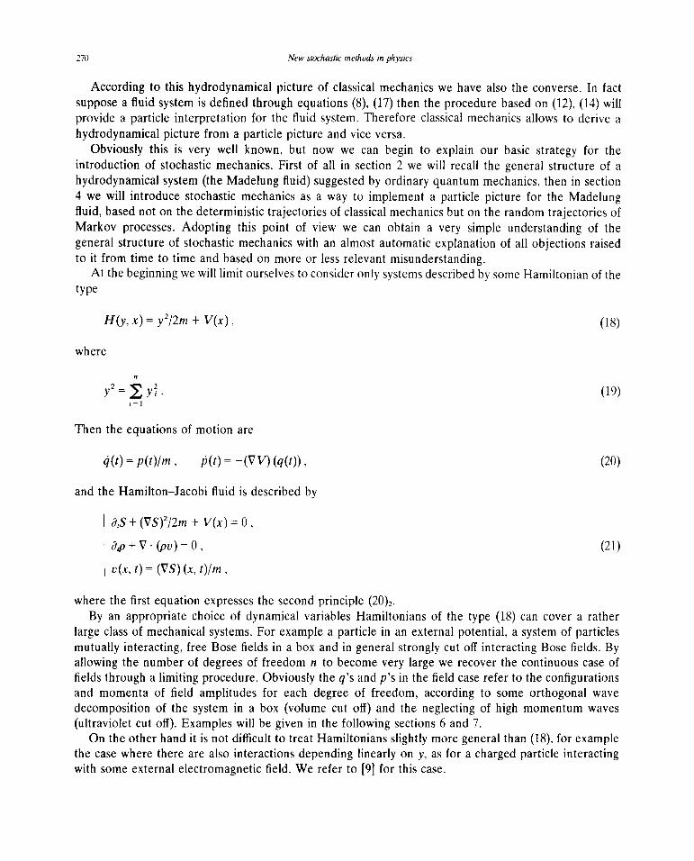
According to this hydrodynamicalpicture of classicalmechanicswe havealso the converse.In factsupposea fluid systemis definedthrough equations(8), (17) then the procedurebasedon (12), (14) willprovide a particle interpretationfor the fluid system.Thereforeclassical mechanicsallows to derive ahydrodynamicalpicturefrom a particlepicture andvice versa.
Obviously this is very well known, but now we can begin to explain our basic strategyfor theintroductionof stochasticmechanics.First of all in section2 we will recall the generalstructureof ahydrodynamicalsystem(the Madelungfluid) suggestedby ordinary quantummechanics,thenin section4 we will introducestochasticmechanicsas a way to implementa particle picture for the Madelungfluid, basednot on the deterministictrajectoriesof classicalmechanicsbut on the randomtrajectoriesofMarkov processes.Adopting this point of view we can obtain a very simple understandingof thegeneralstructureof stochasticmechanicswith an almost automaticexplanationof all objectionsraisedto it from time to time and basedon more or lessrelevantmisunderstanding.
At thebeginningwewill limit ourselvesto consideronly systemsdescribedby someHamiltonianof thetype
H(y,x)=y2/2m+ V(x), (18)
where
y2=~y~ (19)
Then the equationsof motion are
q(t) = p(t)/m , j~(t)= —(VV) (q(t)), (20)
andthe Hamilton—Jacobifluid is describedby
~9~S+ (VS)2/2m + V(x) = 0,
8,p+V(pv)=0, (21)
v(x, t) = (VS) (x, t)/m,
wherethe first equationexpressesthe secondprinciple (20)2.By an appropriatechoice of dynamicalvariablesHamiltoniansof the type (18) can cover a rather
largeclassof mechanicalsystems.For examplea particlein an externalpotential,a systemof particlesmutually interacting,free Bose fields in a box andin generalstrongly cut off interactingBose fields. Byallowing the numberof degreesof freedom n to becomevery largewe recoverthe continuouscaseoffields througha limiting procedure.Obviouslythe q’s andp’s in the field caserefer to the configurationsand momentaof field amplitudesfor each degreeof freedom, accordingto someorthogonalwavedecompositionof the systemin a box (volume cut off) and the neglectingof high momentumwaves(ultraviolet cut off). Exampleswill be given in the following sections6 and7.
On the otherhand it is not difficult to treatHamiltoniansslightly moregeneralthan(18), for examplethe casewherethereare alsointeractionsdependinglinearly on y, as for a chargedparticle interactingwith someexternalelectromagneticfield. We refer to [9] for this case.

F. Guerra, Structuralaspectsof stochasticmechanicsand stochasticfield theory 271
For the systemsconsideredin this sectionwe can alsogive a Lagrangianformulation insteadof theHamiltonianone. In particularin the case(18) we havethe Lagrangian
L(q, q) = mq2/2— V(q) (22)
and Euler—Lagrangeequationsof motion
m ~(t) = —(VV)(q(t)), (23)
which arethe particlecounterpartof the hydrodynamicalequations(21).Finally let us remark that we are talking of a particle picture even when we deal with systems
containingmanyparticlesor evenfield systems.Clearly we keeptheword “particle” havingin mind thepoint representationin phasespaceor configurationspace,asopposedto a continuoushydrodynamicalrepresentationas describedfor example by (21). Particle picture and fluid picture are connectedasexplainedbefore.Our objective will be to give a particle interpretationalso for somesystemsmoregeneralthan (21).
Let us endthis sectionwith the following basicremark.The possibilityof giving a particlepictureforfluid equations,as for example (21), basedon deterministic trajectoriesrests on the fact that theequationfor S is decoupledfrom that for p. In fact the equationfor p is simply a continuityequation,expressingthe local conservationof the fluid, while the equationfor S, of the first order in time, allowsthe introductionof particle trajectoriesidentified with its characteristiclines, as is well knownfrom thetheory of first orderpartial differentialequations[21]andthe generaldiscussionof the Hamilton—Jacobiequationin classicalmechanics.
2. The Madelung fluid
A simple non linear recastingof the standardSchrodingerequationallows the introductionof ahydrodynamicalsystemvery similar to (21). This was noticedalreadyby Madelung[17]at the beginningof wave mechanicsand can be considereda usefulgeneralframefor the discussionof the semiclassicallimit of quantummechanics.
The SchrOdingerequationassociatedto the Hamiltonian(18) is
ihö4i = —h2 zXt/i/2m + Vt/i, (24)
where i/i = i/i(x, t) is the wavefunction in L2(R~,dx) andz~is the Laplacian in W2. For all regionswhere
t/i doesnot becomezerowe can putt/i(x, t) = exp(R(x, t) + iS(x, t)/h), (25)
whereR andS arereal functions.If we substitute(25) in (24), divide by tfr andconsiderthe imaginary partwe get
= —(h2/2m)(i~aS/h+ 2VR . VS/h). (26)

272 Newstochasticmethodsin physics
Introducing the velocity field
v(x, t) = (VS) (x, t)/m (27)
and the density
p(x, t) = t/i(x, t)12 = exp(2R(x,t)), (28)
then we can identify (26) with the continuityequation
9~p+V(pv)=0. (29)
On the otherhandthe realpart in the Schrödingerequationgives
—3~S= —(h2/2m)(i~R+ VR ‘VR — (VS)2/h2)+ V. (30)
If we notice that
V(expR)=VR(expR),
~(expR) = (~R+ (VR)2) (expR), (31)
then (30) is shownto be equivalentto
3~S+ (VS)212m+ V— (h 2/2m)(~expR)/(exp R) = 0. (32)
We call Madelung fluid the hydrodynamicalsystem describedby (32), (29), (27). The analogy with(21) is striking, but it must be noticed that, while (21) has beenderived from the particle picture ofclassicalmechanics,on the other hand(32), (29), (27) are only a formal mathematicalconsequenceof(24) andno immediateparticleinterpretationis available.Thereare manypapersin the literaturetryingto reacha particle picture for the Madelungfluid basedon the idea of deterministictrajectoriesin aneffectivepotential W of the type
W = V— (h2/2m)(~expR)/(expR), (33)
but the mysteriousnature of the “quantum mechanicalpotential” subtractedto V in the r.h.s., inparticularits dependenceon the density,preventeda naturalandacceptablesolutionalong this line.
In fact we will show, following Nelson [9], that a naturalandstraightforwardparticle interpretationof the Madelung fluid is indeed possible,but only by allowing a randomcharacterto the underlyingtrajectories.In the semiclassicallimit h —~0 the randomnessdisappearsandthetrajectoriesbecomethoseof the classical theory, while the Madelung fluid, through the vanishing of the quantumpotential,reducesto the Hamilton—Jacobifluid.
Notice that we are only telling that a particlepictureis possibleandare absolutelynot claiming thatparticlesandtrajectoriesreally exist in the physicalsense.This questioncannotbe settledin the frameof the presentday understandingof quantummechanics.In fact since in any caseour starting point is

F. Guerra. Structuralaspectsof stochasticmechanicsand stochasticfield theory 273
Schrödingerequation(24), which doesnot containtrajectories,it is clear that the particlepictureis onlyan additionalconstructionandsomenew information of physical natureis necessaryin order to assureor exclude the existenceof actual randomtrajectories.
This remark led somecritics of stochasticmechanicsto deny the usefulnessof the conceptof theunderlyingstochasticprocesswhich arisesin the particle pictureof the Madelungfluid andthereforeofthe Schrödingerequation.In particular the claim was made that since all physics is containedin theSchrodingerequationit is not necessaryto introducecomplicatedstochasticprocesseswhich do not addanything to our knowledgeof the physical problem. This claim is only an additional proof of the factthat no real understandingof quantummechanicsis possiblewithout consideringthe largerframe ofquantumfield theory.As a matter of fact the whole experienceof constructivequantumfield theory(seefor example[15]) showsthat it is almost impossibleto get effective rigorousmathematicalcontrolon the Schrödingerequationfor quantumfield theoretical models, especiallywith respect to theproblemof the infinitevolume limit. On theotherhandnontrivial examplesof quantumfieldssatisfyingallWightman axioms[22]havebeenconstructed(seefor example[15])by usingas essentialtool stochasticprocessesfor fields of the typeconsideredin stochasticmechanics.
Also from the point of view of extractinginformationsfrom modelsof quantumfield theory,throughnumericaltechniquesof MonteCarlo type,stochasticmethodshavebeenshownto be extremelypowerful(seefor example[23]).
Therealsituationis thereforeexactlytheoppositeto whatthecriticsclaim:stochasticmethodsareusefulboth from a mathematicalandphenomenologicalpoint of view.
On the otherhand it is also attractivefrom a conceptualpointof view to havea simple generalandunified formulation of quantumand classicalmechanicsbasedon the theory of stochasticprocesses,whoserandomtrajectoriesbecomedeterministicin the classicallimit.
From this whole discussionit is clear that we do not departfrom standardquantummechanics,weonly introduce stochasticmechanicsas an equivalentuseful generalscheme.There is no “stochasticinterpretation”of quantummechanicsdifferent from the standardone. As a matter of fact stochasticmechanicscan be seensimply as a reformulationof quantummechanicsin termsof the languageofstochasticprocesses.But the essentialphysical core of quantummechanicsis kept unchanged,with allits peculiaraspectsandits successin the interpretationof physicalphenomena.
Let us now go back to the Madelungfluid and noticethat its defining equations(32), (29), (27) arecompletelyequivalentto the Schrödingerequation(24). Clearly it is easier to handlethe linear (24)ratherthan the non linear (32), (29), hut theremaybe caseswherethe non linear natureof (32) makeseasiertheanalysisof physicalproperties.For exampleJona-Lasinioandcoworkers[24] havegiven verynice resultson the semiclassicallimit and the propertiesof thequantumground statestarting from (32).
In the following we will assumethe Madelung fluid as a given hydrodynamicalsystem and willprovidea particlepicturefor it basedon stochasticprocesses.Somepropertiesof stochasticdifferentialequationswill be our basictools. We refer to [19] in this volume for a generaltreatment.In the nextsectionwe recall somepropertiesof direct use in the following.
3. Stochasticdifferential equations
Let us consider a system whose state at each time is completely specified by a point ~ in then-dimensionalR’~andassumea deterministicevolution

274 Newstochasticmethodsin physics
~(t) = b(~(t),t), (34)
where b(x, t) is someassignedvectorfield in R” which may dependon external fields acting on thesystem.Underappropriatesmoothnessconditionson b, for given initial conditions
(35)
thereis a uniquesolutionto (34).An exampleof deterministicevolution, as expressedby (34), (35), is given by the Hamiltoniansystem
(1).In generalthereis no completecontrol on the externalforcesor it happensthat (34) is derivedform
an approximationwhere some degreesof freedom have been neglected.A wide body of physicalexperience,ranging from statisticalmechanics,to astrophysicsand control theory (seefor examplethecollectedpapersin [25]) shows that in many casesa suitablemodification of the dynamics (34) givesgood results,providedwe takecareof all effectscoming from externalfields and neglecteddegreesoffreedomin the form of somephenomenologicallydeterminedrandomdisturbanceactingon the systemduring its evolution.
The simplestcaseis when we introducea Brownianmotion w(t) as a randomprocesscharacterizedby a transitionprobability
p(x, t; x’, t’) = (4irr’(t — t’))’2 exp(—(x— x’)2/4~(t— t’)) , t � t’ , (36)
wherev is somearbitrarydiffusion coefficient.The physical meaning of p is that p(x, t; x’, t’) dx representsthe probability that the particle
performingBrownianmotion will reachat time t the volume dx aroundx if it startedfrom the point x’at the initial time t’.
Clearly we haveas initial condition
lim p(x, t; x’, t’) = ô(x — x’) , (37)f It’
moreoverthe diffusion equationof parabolictype(heatequation)is satisfied
3(p v&~p. (38)
Thecoherenceof the physicalinterpretationof p is assuredby the normalizationcondition
Jp(x, t;x’, t’)dx = 1, (39)
moreoveras a consequenceof the spacetime translationsymmetryof (38), (37) we have
p(x, t; x’, t’) = p(x — x’, t — t’; 0,0). (40)
Sincethe diffusion developsin each time interval without rememberingthe positionsoccupiedat earlier

F. Guerra, Structuralaspectsof stochasticmechanicsand stochasticfield theory 275
times (Markov property)we havethe Kolmogorov condition
Jp(x, t; x’, t’) = Jp(x, t; x”, t”) p(x”, t”; x’, t’) dx”, (41)
for any t” such that t’ ~ t” � t.If we call w(t) the randomposition occupiedby the particle at time t, then the knowledgeof the
transition probability (36) allows us to give meaningto all correlationsof functions of the processprovided the initial distributionp(x, t0), at some initial time t0, for w(t0) is known. In fact by denotingE(...) the expectationsWe have
E(F(w(to),...,w(t~)))= JF(xo, ... , x~)p(x~, t~x~_1,t~_1). . . p(x1, t1 x~j,t0) p(xo, t0) dx0 ... dx~
(42)
for to~t~~�t~.
In particular for the densityat time t we have
p(x, t) = Jp(x, t; xo, to)p(xo, t0) dx0, (43)
so that also p(x, t) satisfies the samediffusion equation(38)
3~p=v~p, (44)
with initial condition given in generalby
lim p(x, t) = p(x, t’). (45)t I r’
In the following we will exploit the Brownian process w(t) as a random noise acting on someotherwisedeterministicevolution of the type(34), then only the differencesw(t) — w(t’), t’ < t, will playa role, so that the distributionof w(t) becomesirrelevantwhile the transitionprobability (36) keepsitscentralposition. In fact exploiting (42) wecan easilycalculatethe following averages
E(w(t) — w(t’)) = 0, (46)
E((w(t) — w(t’))(,) (w(t) — ~v(t’))U))= 802v(t— t’) , t � t’
wherex(1) denotesthe ith componentof the point x in R’1. For the infinitesimal interval (t, t+ dt),
dt > 0, we write (46) in the symbolicway
E(dw(t))= 0, E(dw(1)(t) dw0)(t))= 2i’ö~ dt, (47)
dw(t)= w(t+dt)— w(t).
In order to introduce a random disturbance on the evolution of ~(t) first of all we promote~(t) to a

276 New stochasticmethodsin physics
stochasticprocesswith densityp(x, t) and transition probability p(x, t; x’, t’) still satisfying (37), (39),(41), (43), (45). The physicalmeaningof p andp is still given by (42), with w replacedby ~, while ingeneral the simple expression (36) and the condition (40) do not hold. Our dynamical assumptions willprovide the diffusion equationreplacing(38), (44).
During the infinitesimal time interval (1, t + dt), dt > 0, according to (34) the increments of ~ in termsof the drift b will be given by
d~(t)=b(~(t),t)dt, (48)
with the definition
d~(t)= ~(t + dt) — ~(t). (49)
Obviously (48), (49) are symbolic notations,written according to the standardconventionof appliedsciencesof interpreting differentials as incrementsand symbolic relationsamongdifferentials as theanalogousrelationsamongincrementsholding up to secondorder terms.
If we perturb the deterministicdynamics(48) through a randomterm with properties(47), then weareled to consider~(t) as a stochasticprocessand to replace(48) with
d~(t)= b(÷)(~(t),t) dt + dw(t) , (50)
whereb(±)(x,t) is somegiven (non random)field in W2 and dw(t) is definedaccordingto (47).There is a large body of literature (see [19] and referencesquoted there)dealing with the proper
mathematicaldefinition of (50) andthe conditionsfor the existenceand uniquenessof solutions.But asfar as physical applicationsare concerned,as in control theory, statistical mechanicsand stochasticmechanics,then the following immediate intuitive meaning of (50) is completely sufficient. Let ussupposethat the field b(+)(x, t) has been given and that we are willing to follow the evolution of ~(t)during a time interval (t
0, to + T). Let us split this time interval into n parts through the valuest~,t1, ... , t~= t0+ T, so that eachtime interval t1+1 — t1 is smallenough,anddefinefor someinitial given~ (x0 could alsobe randomwith somegiven distributionp(x~~,t0) in R”)
= x0,
= ~(t0)+ b(+)(~(t~),t0)(t1 — t0) + w(t1) — w(t0) , (51)
= ~(t~_1)+ b(+)(~(t,,l),t~_1)(t~— t~_1)+ w(t~)— w(t~~1).The differencesw(t1÷1)—w(t1), accordingto (36), (46), areindependentGaussianrandomvariableswith
meanzero andcovariance
E((w(t1÷1)— W(t1))()(W(tJ±l)— w(t)))(E’)) = ~~~2z.’(t1+1— t1) , (52)
therefore(51) define a sequenceof randompoints (~(t0),~(t1) ~(t~)), accordingto the outcomeofeachw(t~+1)—w(t~),j0,l n—i.
The propermathematicalinterpretationof (50) is got in the limit when n —~ ~ and the largestof— t,, tendsto zero. But in any case,t~~(t) denotesa physicalobservable,we must take into account

F Guerra, Structuralaspectsof stochasticmechanicsand stochasticfield theory 277
the unavoidableexperimentalerrorson the position~(t) and the time t, thereforethe essentialphysicalcontentof (50) is alreadyreachedif eachpartial time interval is smallenoughaccordingto the physicalconditions. Therefore the physical interpretation of stochastic differential equations parallels thetreatment of ordinary differential equations through finite difference methods. Since subroutines, giving(almost) random sequences of independent Gaussian variables, are easily available in the programlibraries of large computers, then stochastic differential equations can be easily solvedon computers,tothe desired order of approximation, exploiting recursive methods based on (51) or their generalizations(see for example [26]).
The system (51) showsclearly that ~(t) evolves at each time independentlyfrom the valuesassumedatearlier times, thereforethe Markov property is preservedand the Kolmogorov equation(41) for thetransitionprobability still holds.
At this point we find it important to warn the readeragainst the possibletroublesfor the properinterpretation of stochastic differential equations coming from an unfortunatestandardpractice(foundin the phenomenological literature) of writing (50) in the apparently equivalent form
~(t) = b(+)(~(t),t) + A(t) , (53)
where A(t) is some white noise, i.e. a process with covariance given by delta functions ~(t — t’). In fact,due to the singular nature of A(t), eq. (53), as it stands,is highly ambiguous, while (50), with thespecifications(47), is not. This can beeasily understoodif we realize,for example,that the substitutionof dw’(t) = w(t) — w(t — dt) in placeof dw(t) in (50) leads to a completely different process ~‘(t), as theanalog of (51) for dw’ and the relevanceof second order terms dw dw show. Since (53) cannotdistinguish between dw and dw’ its ambiguity is clear. A consistent fraction of papers, on physicalapplications of stochastic differential equations, deals explicitly or implicitly with the differentwaysofsolving ambiguities coming from (53). The use of the correct form (50) avoids any need to work on suchproblems.
Let us now find the replacement of the equations(38), (44) for the transition probability p and thedensity p of the process~(t) whose time evolution is ruled by (50). Consider the time interval (t, t + z~t),z~t>0. Taking into account that, according to (50), the increment of ~ is the sum of a deterministicpartb(+) dt and a randompart dw, we can write, neglecting terms beyond first order in z~t
p(y,t + i~t;x, t) ~Po(fl, ~t; 0,0), (54)
wherex andy are the positionsat times t and t + ~t,
y~x+b(+)(x,t)~t+?J, (55)
~ is the increment w(t + ~t) — w(t) andPa is definedby (36). Eliminating ~ in (54) through (55) we have
p(y,t + ~t; x, t) =~po(y— x — b(+)(x, t) ~t, z~t;0,0), (56)
so we can verify that p satisfies (37) in the limit ~t —* 0 since Po does. On the other hand by subtracting— x) to both sides of (56), dividing by z~tand letting ~t —~0 we find
t9t’p(y, t’; x, t)l~.1= ~ — x)— b(±)(x,t) V~8(y— x). (57)

278 Newstochasticmethodsin physics
Sincethe representation(Si) showsclearly that (41) and (43) continue to hold, if we takethe derivative9~of (41) andlet t”—* t exploiting (57) we immediatelyget the Fokker—Planckequation
t9,p(x, t; x’, t’) = —V.. . (b(÷)(x,t) p(x, t; x’, t’)) + ii ~..p(x,t; x’, t’) , (58)
which is the generalizationof (38) to the casewhenthe drift b(~)is differentfrom zero.Analogouslyforthe densityp(x, t) of the process~(t) we get
9~(x,t) = —V~ (b(÷)(x,t) p(x, t)) + p ~ p(x, t), (59)
as (43) and(58) show. (59) is the counterpartof (44).Herewe would like to warn the readeraboutpossibleconfusionarising from the fact that both the
transitionprobability and the densitysatisfy the sameequation(58), (59). This confusionhasbeenoneof the sourcesof furtherunjustifiedcriticism to the generalstructureof stochasticmechanics,as we willshow in the following. As a matter of fact any risk of confusion disappearsif the deepdifferencebetweenthe physical meaningof p and p is taken into proper account.In fact p and p are linkedthrough (43) andthe initial conditionfor p is (37) while for p it is (45). It must alsobe noticedthat theknowledgeof the transitionprobability p doesnot determinethe densityp which in fact dependsonsomespecifiedinitial condition.
Let usnow introduce,following Nelson [9], a usefulgeneralizationof the conceptof substantialtimederivativeof hydrodynamicsto the stochasticcase.For a systemwith deterministicevolution, as givenby (34), the substantialtime derivativeof a smoothfield F(x, t) is a new field (DF)(x, t) definedby
(DF)(x, t) = lim (i.~t)’[F(~(t+ i.~t),t + ~t) — F(~(t),~ , (60)A t=O
where~(t+ z~t)is the positionat time t + ~t of a particleevolving accordingto (34) with initial positionattime t given by ~(t) = x. Sinceto first order in ~t we have
F(~(t+ st), ~t) 9~F~t + VF~b ~t, (61)
then, as is well known, the definition (60) gives
(DF)(x, t) = (3~F)(x,t) + b(x, t)~(V~F)(x,t). (62)
For the physical interpretation we remark that (62) gives the rate of change in time for theobservable F as measured through a device moving along the flux lines with velocity b in each point.
For the descriptionof kinematicalanddynamicalpropertiesof randomprocessesit will be usefulto~trya generalizationof (60) in the casewhen ~(t) is a stochasticprocess.Then we cannot exploit (60)directly becausethe Brownianmotion in (50) doesnot allow ~(t) andF(~(t))to be differentiable,but wemust introduce some smoothing procedure in order to tame the strong irregularities on randomtrajectories.This can be easily achievedby the use of conditionalexpectationswhich fix the value of~(t) at x andaverageover all possiblevaluesof ~(t + At). We must alsotake into accountthat positiveor negative values of At in the stochasticanalog of (60) will give in generaldifferent results, as aconsequenceof the remarksfollowing (53).
F. Guerra, Structuralaspectsof stochasticmechanicsand stochasticfield theory 279
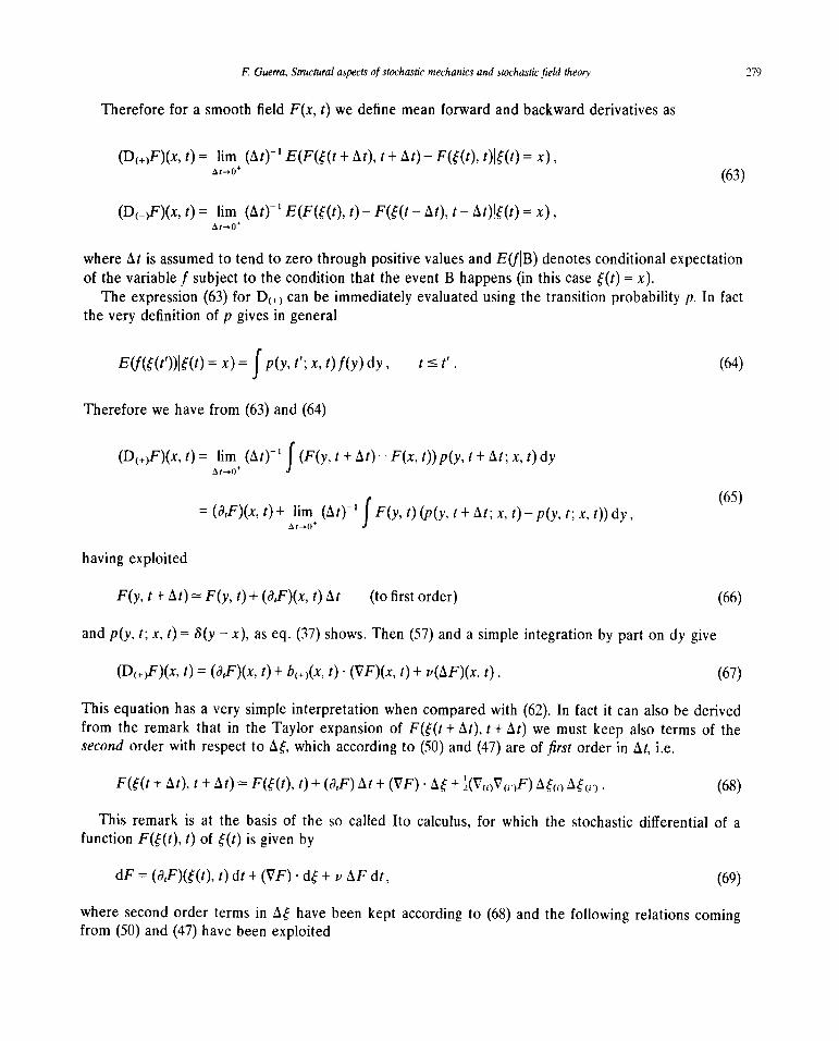
Thereforefor a smoothfield F(x, t) we definemeanforward andbackwardderivativesas
(D(±}F)(x,t) = lim (At)’ E(F(~(t+ At), t + At) — F(~(t),t)I~(t)=At-.O~ (63)
(D(_)F)(x, t) = lim (At)’ E(F(~(t),t) — F(~(t— At), t — At)~(t)
whereAt is assumedto tendto zerothrough positivevaluesandE(JIB) denotesconditionalexpectationof the variablef subjectto the condition that the eventB happens(in this case~(t) = x).
The expression(63) for D(±)can be immediatelyevaluatedusingthe transitionprobability p. In factthe very definition of p gives in general
E(f(~(t’))I~(t)= x) = Jp(y, t’; x, t) f(y) dy, t ~ t’. (64)
Thereforewe havefrom (63) and (64)
(D(+)F)(x, t) = lim (At)’ J (F(y, t + At) - F(x, t))p(y, t + At; x, t) dyA t—.O~
(65)= (3,F)(x, t)+ lim (At)1 JF(y, t)(p(y, t+ At; x, t)—p(y, t; x, t))dy,
At-.0
havingexploited
F(y, t + At) F(y, t) + (ö,F)(x, t) At (to first order) (66)
andp(y, t; x, t) = 5(y — x), as eq. (37) shows.Then(57) anda simple integrationby part on dy give
(D1+>F)(x, t) = (t9,F)(x, t) + b(+)(x, t) . (VF)(x, t) + p(AF)(x,t) . (67)
This equationhasa very simple interpretationwhen comparedwith (62). In fact it can also be derivedfrom the remark that in the Taylor expansionof F(~(t+ At), t + At) we must keepalso termsof thesecondorderwith respectto A~,which accordingto (50) and (47) areof first order in At, i.e.
F(~(t+ At), t + At) F(~(t),t) + (o,F) At + (VF). A~+ ~(V(I)V(I.)F)A~(~)A~(~’). (68)
This remark is at the basis of the so called Ito calculus,for which the stochasticdifferential of a
functionF(~(t),t) of ~(t) is given bydF= (8~F)(~(t),t) dt + (VF) . d~+ ~‘ AF dt, (69)
wheresecondorder terms in A~havebeenkept accordingto (68) and the following relationscomingfrom (SO) and (47) havebeenexploited

280 New stochasticmethodsin physics
A~(1)A~111 Aw(I) Aw(I) 2v6,~At. (70)
Notice that crosstermsof the type
b(÷)AtAw (71)
do not contributein (69) becausetheyarenot of first order in At, in fact their squaresare of order (At)3
as (47) shows.If we put F(x, t) = x(E), for eachcomponenti, in (67) we get the vectorrelation
(D(÷)~)(x,t) = b(+)(x, t), (72)
generalizingthe analogous
(D~)(x,t) = b(x, t) (73)
coming from (34), (62).It is importantto remarkthat the expression(67) is completelyequivalentto (57), which impliesthe
basic (58). Therefore we can assumeany of the expressions(SO), (57), (58), (67) as the completespecificationof the process.
Now we can derive the explicit expressionof D(_) definedin (63). Let us noticethat for smoothF andG the following holds
E(F(~(t),t) G(~(t),t)) = E(F(~(t),t) (D(÷)G)(~(t),t)) + E((D()F)(~(t),t) G(~(t),t)). (74)
The proof is very simple. In fact using as a shorthandnotation F(t) F(~(t),t) andanalogouslyfor Gwe can write
E(F(t) G(t))= lim (At)’ E(F(t + At) G(t + At) - F(t) G(t)), (75)
dt At-.O~
but we havealso
F(t + At) G(t + At) = F(t)(G(t+ At) — G(t))+ (F(t + At) — F(t)) G(t + At). (76)
Sincethe generalpropertiesof conditionalexpectationsgive the identity
E(F(t) (G(t + At) — G(t))) = F(F(t) E(G(t + At)— G(t)I~(t))) (77)
the first term in the r.h.s. of (76) substitutedin (75) gives the first term in the r.h.s. of (74) (recall thedefinition (63)), analogouslythe otherterm in (76) completes(74).
ObviouslyF andG play a symmetricrole in (74), we couldthereforewrite the r.h.s.by interchangingF and G or equivalently (+) and(—).
By definition of the densityp of the processwe havefor genericF andG

F. Guerra, Structuralaspectsof stochasticmechanicsand stochasticfield theory 281
E(F(~(t),t) G(~(t),t)) = JF(x, t) G(x, t) p(x, t) dx, (78)
thereforeperforming the time derivativein. (74) underthe integralsign andexploiting (78), (67) we canwrite (74) in the equivalentform
J(~F)(x,t) G(x, t) p(x, t) dx + JF(x, t) (31G)(x,t) p(x, t) dx + JF(x, t) G(x, t) (a~p)(x,t) dx
= f F(x, t) [(a,G)(x, t) + b(+)(x, t)~(VG)(x, t) + v(AG)(x, t)] p(x, t) dx
+ J (D~)(x,t) G(x, t) p(x, t) dx. (79)
Integrationby parton the term coming from D(±)Gshowsthat if (79) musthold for any Gthenwe musthave
8~Fp+ F3~p= —V~ (,pFb(+))+ ii A(pF)+ (D(~F)p. (80)
In particular for F 1 we have81F = 0, D(~F = 0 from (63) andtherefore(80) becomes
(t9~p)(x,t) = —V . (p(x, t) b(+)(x, t)) + v(Ap)(x,t) . (81)
This is nothingbut (59) derivedin an alternativeway.On the otherhandsubstitutionof (81) in (80) for a generalF gives immediately,if we areallowedto
divide by p,
(D(~F)(x,t) = (t9~F)(x,t) + b()(x, t)~(VF)(x, t) — v(AF)(x,t), (82)
where the vector field b() is definedby
b()(x, t) = b(±)(x,t) — 2v(Vp)(x, t)/p(x, t). (83)
Therefore(82), (83) providethe wantedexplicit expressionfor D(~.)as definedin (63).Notice alsothat
(D(~)(x,t) = b()(x, t) (84)
is the backwardcounterpartof (72). It is convenientto define
D = ~(D(+) + D(_)), SD = ~(D(+) — D(_)), (85)
so that
D(±)=D±SD, (86)
and also

282 New stochasticmethodsin physics
b(x, t) = ~(b(÷)(x,t) + b(....)(x, t)) , (Sb)(x,t) = ~(b(+)(x,t) — b()(x, t)) , (87)
b(±)(x,t) = b(x,t) ±(Sb)(x,t). (88)
Then(69) and (82) give
(DF)(x, t) = (9~F)(x,t) + b(x, t) . (VF)(x, t) , (89)
which should be directly comparedwith (62) (notice that D and b in (62) and (89) havedifferentmeanings).
We havealso
(SDF)(x, t) = (Sb)(x,t)~(VF)(x, t) + v(AF)(x, t). (90)
Taking into account(83) and(87) the Fokker—Planckequationfor p given by (59) can be written in
the form of a continuity equation(8,p)(x, t) = —V . (p(x, t) b(x, t)) (91)
which can bedirectly comparedwith (17). The local conservationequation(91) is strictly connectedwiththe continuity in time of the randomtrajectories,as (50), (47) show.
A superficial comparisonof (91) with (59) would suggestthe disappearanceof the diffusion partdependingon ii. This led someauthorsto remarkthat no real diffusion can exist if the densityp satisfiesa continuityequationof the type(91). But the remark is incorrectsincebasedon the alreadymentionedconfusionbetweenthe two similar equations(58) and (59).
In fact thereis absenceof diffusion only if the term containingthe Laplaciandoesnot appearin (58),but we can alwayslet it disappearfrom (59) if we define b through (87) and(83), so that (91) holds.
This endsour generaldiscussionof the basic conceptsof stochasticdifferential equationswhich willbe employed in the following. While we limited ourselvesto a very simple minded approach,basedmoreon physicalintuition ratherthan rigorousmathematics,we must recallthat the theory of stochasticdifferentialequationsis a well developedmathematicaldiscipline,as expoundedin the “steppingstone”[19] and referencesquotedthere. We believethat it would be very helpful, for the developmentofresearchin theoreticalandappliedphysics,to let a working knowledgeof it enterinto the basictrainingof peopleapproachingthesefields, as now is customaryfor differentialandintegral calculus.
4. Stochasticmechanics
This section is the main core of our review. Here we introducethe basic general structureofstochasticmechanics.
Our starting point is given by the Madelungfluid as definedby (32), (29), (27). Our objectiveis togive a particle picture for this fluid in the same sense as (20) give a particle picture for theHamilton—Jacobifluid (21). Since the density p enters in an essentialway into the dynamicsas (32)shows comparedto (21),, it is clear that no picture basedon deterministic trajectoriesis possible.

F. Guerra. Structuralaspectsof stochasticmechanicsand stochasticfield theory 283
Thereforewe promotethe particlepositionq(t), attachedto the Madelungfluid, to a stochasticMarkovprocesstaking values on the configurationspaceR”, characterizedby a densityp(x, t), which will beassumedto coincidewith that appearingin (29), anda probabilitytransitionp(x, t; x’, t’). Notice that toeach solution of the Madelung fluid (equivalently of the Schrodingerequation)we associatesomestochasticprocessq(t), different solutions(andthereforedifferentquantumstates)giverise to differentMarkovprocesses,eachwith its own densityandtransitionprobability. Sincea misunderstandingof thispoint has been at the origin of other unjustified criticism to stochasticmechanics,let us remark thatherethe situationis very similar to the classicalcase.Once aparticularsolutionof theHamilton—Jacobiequation (8) has been given, then by the only choice of the initial point q(t0) we can determinecompletelythe trajectory.There is no conflict with the fact that both q(to) andp(to) arenecessarytodeterminea trajectoryin phasespace,becausethe function S definesthe impulsein eachpoint through(10). Therefore the dynamical content carried by p(t) is transferredto S, and if S is given thentrajectoriesq(t) in configurationspaceareuniquely determinedby the initial condition.
Oncewe havedecidedto associatea stochasticMarkov processto eachstateof the Madelungfluidwith the samedensity,we must specify kinematicaland dynamicalpropertiesof the processin such away that we can assurethe coherenceof the assumptions.
Our first condition is given by the assumptionthat q(t) satisfiesa stochasticdifferential equationoftype (SO), which now wewrite in the form
dq(t)= v(±)(q(t),t) dt + dw(t). (92)
Clearly this mustbe understoodas the analogof (12). We alsoassumethe existenceof a scalarfunctionS(+)(x, t) such that for the vectorfield V(+) we have
v(+)(x, t) = (VS(±))(x,t), (93)
in completeanalogywith (21)3. Additional dynamicalassumptionson V(±)andS(+) will be madelater,for the momentweconsiderthem as given.
In orderto definecompletely(92) we mustspecifythe diffusion coefficient of dw as appearingin (47).This will introducesomefundamentalconstantin the theory.This constantis interpretedas an intrinsicpropertyof the randommediumperturbingthe positionof the particle.Sincewe do not know the originof the Brownian motion in (92) we must proceedphenomenologically.Nelson’s choice for a Hamil-tonianof type (18) was the following
2i’ = h/rn, (94)
whereh is h/2ir (h Planck’sconstant).Otherchoicesarepossibleas shownby Davidsonin [27],but thenthe following dynamicalequations
(105), (112) must be modified from their simple form in order to fully recoverthe propertiesof theMadelungfluid. Thereforeuntil a physical explanationfor the origin of the Brownianmotion in (92) isfound, we assume(94).
Following the reasoningleadingto (72), (83), (84) we can write
(D(±)q)(x,t) = v(±)(x,t) (95)

284 New stochasticmethodsin physics
as the averagedstochasticanalogof (12), with V(_) given by
v()(x, t) = v(+)(x, t) — (Vp)(x,t)/p(x, t),
V(-)(X, t) = I (VS())(x, t), (96)
S(..)(x, t) = S(+)(x, t) — h log p(x, t)
We alsohaveas in (67), (82), (89), (90)
(D(±~F)(x, t) = (0,F)(x, t) + v(±)(x,t)~(VF)(x, t) ± (AF)(x, t) (97)
(DF)(x, t) = (3,F)(x,t) + v(x, t) . (VF)(x, t), (98)
(SDF)(x, t) = (Sv)(x,t) . (VF)(x, t) + ~- (AF)(x, t), (99)
where
v = + V(-)) = -~- VS, (100)
Sv=~(v(+)-V(~))z~V(SS), (101)
S(x, t) = ~(S1+1(x,t) + S()(x, t)) , (102)
(SS)(x, t) = ~(S(+)(x,t) — S()(x, t)) = ~hlog p(x, t) = 11 R(x, t) . (103)
Clearly also the continuityequationholds
(a,p)(x,t) = —V (p(x, t) v(x, t)). (104)
Comparisonwith (27), (29) and(100), (102)forcesus to identify the functionS definedby (102)with thatintroducedin (25). In this way two of the threeequationsdefining the Madelungfluid, and precisely(29), (27), havebeenabsorbedinto our stochasticscheme.We needonly give a stochasticinterpretationto (32). Since the analogue(21), is strictly relatedto the secondprinciple of dynamicsas expressedby(20)2, it is clear that also (32) must be in someway relatedto a stochasticversion of Newton secondprinciple.In fact let us define, following Nelson,the accelerationfield a(x, t) in the smoothedsymmetricform
a(x, t) = ~((D(÷)D() + D()D(+))q)(x, t). (105)
Notice that from (86) it follows
+ D()D(±))= DD — SD SD. (106)

F Guerra. Structuralaspectsof stochasticmechanicsand stochasticfield theory 285
Since (97), (100), (101)show
(D1±1q)(x,t) = v(±)(x,t) (asin (72), (84)) (107)
(Dq)(x, t)= v(x, t)=-~—VS, (108)
(SDq)(x,t) = Sv(x,t) = -~-VR, (109)
wehaveimmediatelyfrom (105) and (106)
m a(x, t) = 8,VS+ (v . V)VS— h(Sv . V)VR —~-—A(VR). (110)
Througha simple rearrangementof terms,exploiting (101) and(103)we finally get the following purelykinematicalexpression
rn a(x, t)= ~ (lii)
Obviously in the classjcal case the last term containing h2 is missing, we see that it has a purely
kinematicalorigin coming from the definition (105).Our last assumption is that Newton second principle of dynamics, as expressedby (20)2 or
equivalentlyin hydrodynamicalform
m a(x, t) = —(VV)(x), (112)
continuesto hold but with the classicalaccelerationin (112)replacedby the stochasticcounterpartgiven
by (111). Thenas a consequenceof (111) and(112) we have,neglectinganunessentialconstantfield,
3,S+~(VS)2_.(Ae1~)e~=_V(x), (113)
which is nothing but the first equation(32) of the Madelungfluid. No additional “quantummechanicalpotential” is necessary.
The analogy with the classical caseis complete. In fact if we define, in the classical case,theaccelerationfield accordingto
a(x, t) = (Dv)(x, t), (114)
wherev is given by (21)3 andD is the transportderivative(60), (62), thenwe get
a(x, t) = (81v)(x, t) + v(x, t) . (Vv)(x, t) = v(a~s+ ~ (VS)2). (115)
Thereforethe secondprinciple (112) is completely equivalent to the Hamilton—Jacobi (21),.

286 New stochasticmethodsin physics
Analogously in stochasticmechanicswe havethat the secondprinciple (112), with the stochasticdefinition (111) of meanacceleration,is equivalentto the first equation(32) of the Madelungfluid.
This shows that we havegiven a particle picture for the Madelungfluid basedon two stochasticassumptions,one of kinematicalnatureexpressedby (92), the otherof dynamicalnatureexpressedby(111), (112). We hopethat the line of presentationwe havechosen,heavily basedon the analogywiththe Hamilton—Jacobiformalismof section 1, will helpto dissolvethe mystery andconsequentsuspicionsurroundingthe stochasticmechanicspictureof a quantumsystem.
It is alsoimportantto remarkthat we couldproceedin the oppositeway. In fact we can postulatethegeneralstructureof stochasticmechanicsasintroducedin thissectionandderivefromit theMadelungfluid.This showsthat stochasticmechanicsis an independenttheory in its own right.
Clearlythe distributiondensityof stochasticmechanicsp(x, t) keepstime after time the samevaluesas in quantummechanics.All operationalstatementscan be translatedinto scatteringdataexpressiblein terms of p. Thereforethe two theoriescannotbe distinguishedat the operationallevel. They aredifferent picturesof a uniquetheory describingquantumphenomena.
For the sakeof simplicity herewe haveconsideredonly very simple systemsof canonicaltype (18),but we can easily generalizeour presentationto morecomplicatedcases.
Interactionsdependingon the velocity (asfor examplethe caseof a chargedparticlemoving in somemagnetic field) can be easily considered(see directly [9]). Also canonical systemswith non flatconfigurationmanifoldhavebeenconsideredin [10,11, 12].
Non relativistic spinningparticles (also with half integerspin) havebeentreatedin [10,28].We will briefly touchupon theseextensionsof stochasticmechanicsin section10.In the nextsectionwe discussthe problemof time reversalinvariance.
5. Time reversal invariance
As we haveanticipatedin the introductiontime reversalplaysavery importantrole. In fact sinceit isgenerallyfelt that stochasticdifferential equationsdescribedissipativetime irreversiblephenomena,anaturalobjectionarisesagainst a stochasticformulation of quantummechanics,which is an essentiallytimereversibletheory.
First of all it is important to realize in which sensestochasticdifferential equationsfor dissipativeprocessesof statisticalmechanicsdo not sharetime reversalinvariance.
Let us thereforeconsidera simple model.Thetime evolutionof a macroscopicparticlewith positionx(t) and velocity v(t), immersedin a fluid at temperatureT, is well representedby the Langevinequations
dx(t)= v(t)dt, (116)
dv(t)= -~- F(x(t), v(t), t) dt — f3 v(t) dt+ dw(t), (117)
which are a slight generalizationof (SO) when the random disturbanceaffects only somedynamicalvariables(herethe velocity). In the r.h.s. of (117)the secondprinciple of dynamicsis expressedat threelevelsof approximation.In fact F is the externalforce acting on the particle, independentlyof themedium. If we disregardthe terms with /3 and dw, we assumethat the dynamicalbehaviorof the

F. Guerra. Structuralaspectsof stochasticmechanicsandstochasticfield theory 287
particleis not affectedby the medium(zero orderapproximation).The termwith /3 takesinto accountthe friction acting on the particle asa resultof the unbalancedimpactsof surroundingparticlesby effectof the motion with respectto the medium(supposedat rest on the average).Finally the termdw takesinto account,in the simplestpossibleway, randomfluctuationsin the numberof impactswith respecttothe averagevaluegiving rise to friction.
Now we perform a time inversiontransformationsimilar to (4)
T: t-*t’=—t,
x(t)—* x’(t’) = x(t) , (118)
v(t)—* v’(t’) = —v(t).
We can ask what kind of equationsaresatisfiedby the new process{x’(t’), v’(t’)} in function of thetime t’.
Clearly (116) keepsits form
dx’(t’) = v’(t’) dt’ , (119)
while (117) undergoes a dramaticchangeto the form
dv’(t’) = —1—F’(x’(t’), v’(t’), t’) dt’ — /3 v’(t’) dt’ + dw’(t’) , (120)
where dw’(t’) is definedsimilarly to dw(t) but F’ is expressed as
v’, t’) = -1—F(x, v, t)+ /3v’ — /3v — 2vV~log p, (121)
wherep(x, v, t) is the densityof the process{x(t), v(t)}.In order to prove (121) let us remark that for a smooth field G(x,v, t) on phase space, as a
consequenceof (116), (117) and(67) (for the dependenceon v) and (62) (for the dependenceon x), wehavefor the meanforwardderivative
(D(+)G)(x, v, t)
= lim (At)-’ E(G(x(t+ At), v(t+ At), t + At) — G(x(t), v(t), t)Ix(t) = x, v(t) = v)
= o~G+ v V..G+(nr’F—/3v)~V~G+pA~G. (122)
Therefore(120)is provenif we can showthat (118) implies for any G’
(D(÷)G’)(x’,v’, t’) = 8~.G’ + v’ V~.G’+(rn 1F’ — /3v’) . V~G’+ ii A~G’, (123)
with F’ given by (121)(recall that, asremarkedin section3, theexpressionof D(±)definescompletelythestochasticdifferentialequationof the process).

288 Newstochasticmethodsin physics
Becauseof the definition (118) the densityp’ of the time reversedprocesssatisfies
p’(x’, v’, t’) = p(x, v, t) (124)
with
t’ = —t, x’ = x, v’ = —v (in agreementwith (118)). (125)
For any smoothG(x, v, t) we defineG’ as
G’(x’, v’, t’) = G(x,v, t) (126)
and evaluatethe r.h.s. of (123). We have
(D(+)G’)(x’, v’ t’)
= lim (At’)—’ E(G’(x’(t’+ At’) v’(t’ + At’) t’ + At’) — G’(x’(t’) v’(t’) t’)~x’(t’)= x’ v’(t’) = v’)
= (At)1 E(G(x(t — At), v(t — At), t — At) — G(x(t), v(t), t)Ix(t) = x, v(t) = v)
= — (D()G)(x, v, t), . (127)
where we have employedthe definitions of D(±)and the transformations(118), (125), (126). As insection 3 we derived (82), (83) from (74), herewe can easily prove (recall that x is not affectedbyBrownianmotion!)
(D(_)G)(x, v, t) = 3~G+v V~G+(rn’F— /3v —2vV~logp) . V~G—v AUG. (128)
As a consequenceof (125)we have
a, = —a~, V~= Vi., V~ = —V~, A~= A~. (129)
Therefore,taking into account(126), substituting (128) into (127) we have for D(+)G’ the expression(123)with F’ given by (121).
Our result shows that in general the time inverted processstill satisfies a stochasticdifferentialequationbut with anew drift, as given in our caseby (121).
If we assumetime reversalinvarianceof the zeroorderdynamicsas expressedby
F(x, v, t) = F(x’, —v’, t’) , (130)
supplementing(118), we verify immediatelythat for /3 = 0, v = 0 the equation(120) is nothingbut thetime invertedof (117).
But if /3 > 0, p = 0, then the time inverted equation (120) has completelydifferent featureswithrespectto (117), in fact the changeof sign in the termcontaining/3 lets absurd solutions appearin zero

F. Guerra, Structuralaspectsof stochasticmechanicsand stochasticfield theory 289
externalfield with continuousexplosiveselfacceleration.If also v > 0 then the drift doesnot dependonly on the actualvaluesof the processbut also on the densitydistributionp, as (121) shows.
In conclusionthe stochasticdifferentialequationsof dissipativeprocessesareconsideredto be timeirreversible because,under time reversal, the drifts of the naturalphysical form appearingin (117)transformin generalinto drifts of unnaturalphysicalform as given by (121).
Clearlythis remark doesnot apply to the processesconsideredin stochasticmechanicsas introducedin the previoussection.Here indeeddrifts are to be consideredas dynamical variables,there is no“natural” form for them and the time inverted ones are also acceptable.This is the reasonwhy astochasticschemecan sharetime reversalinvarianceproperties.
Let usnow give somedetailsabouttime inversionin stochasticmechanics.First of all let us recall that undertime reversalthe wavefunction associatedto the Hamiltonian(18)
andsatisfyingthe equation(24) transformsas
t—*t’=—t, x—*x’=x, a~—~a,=—a,, ~ A~-+A~.=A~, (131)
t/i(x, t)—* t/i’(x’, t’) = tp*(x t)
Clearly (24) is invariant under (131) andwe have
iha,.~’= — A~’+ V(x’) t/,’. (132)
Analogouslythe quantitiesS, R, p, v appearingin the Madelungfluid (27), (28), (29), (32) transformas
S(x, t)-* S’(x’, t’) = —S(x, t),
R(x, t)—* R’(x’, t’) = R(x, t)
p(x, t)-~p’(x’,t’) = p(x, t),
v(x, t)—+ v’(x’, t’) = —v(x,t) . (133)
Onecan immediatelyverify that the definingequations(27), (29), (32) aretime reversalinvariant.Let usnow considerthe stochasticprocessq(t) introducedin section4 anddefinedby the equations
(92), (112) andrelatedones.Undertime reversalwe have
t-~’t’ = —t, q(t)—* q’(t’)= q(t), x —~ x’ = x,
at~at,=—at, ~ ~ (134)
By the sameprocedureemployedin the derivationof (120), (121) from (117), we can easilyshow thatthe transformedprocessq’(t’) satisfiesthe time inverted counterpartof (92) expressedin the form
dq’(t’) v(±)(q(t),t’) dt’ + dw’(t’) , (135)
wheredw’(t’) is definedas dw(t) and
v(±)(x,t’)= _(v(+)(x, t)——V~logp(x, t)), (136)

29() New stochasticmethodsin physics
(comparewith the expressionin (121), but recall (118) as opposedto (134)). Then(98) allows us to write
v(±)(x,t)—* v(±)(x,t’) = —v(~)(x,t), (137)
S(±)(x,t)—~S~±)(x’,t’) = —S(~)(x,t).
Clearly (137) arecompatiblewith (133). Notice also
Sv(x,t)—* Sv’(x’, t’) = Sv(x,t), (138)
to be comparedto (137), and (133)4.As in (127) we havealsoin general
(D(±)G’)(x’,t’) = —(D(..)G)(x,t) (139)
with
G’(x’, t’) = G(x, t) . (140)
In conclusionthe overall picture given by stochasticmechanics,for the mechanicalsystemswe haveconsidered,sharesthe propertyof time reversalinvariance.
Stochasticdifferential equationsof type (92) go into similar equations(135) for the time invertedprocess.Drifts transformas in (137). No contradictionarisesbecausedrifts, in contrastto the caseof adissipativeprocessas (117), havea dynamicalmeaning,as (115) shows,so that no a priori qualitativefeaturesareto beimposedon them.
A stochasticversionof quantumdissipativeprocesseshasbeengiven in [29].
6. Simpleexamples
In this sectionwe give some examplesof random processesintroduced by stochastic mechanicstaking in considerationsimple systemsof harmonicoscillators.
For a onedimensionaloscillator the Hamiltonian
H=p2!2rn +~rnw2q2 (141)
implies the equationsof motion
q=p!m, ji=—rnw2q, (142)
with generalsolution
q(t) = q
0 cos wt + sinwt,
p(t) = p0cos i~ot— mwqosin wt, (143)
where(qo,p~)areinitial conditionsat t = 0.

F. Guerra. Structuralaspectsof stochasticmechanicsand stochasticfield theory 291
The associatedSchrödingerequationfor t/’ = t/J(x, t), x E R,
iha~p= —f-— a~/i+ ~mw2x2t/i (144)
admits, as is well known, an overcompletefamily of solutions given by the coherentstates, eachassociatedto a given solution{q~,(t),p~,(t)}of (142) in the form (143).
The coherentstatesare
i/l(x, t) = (2~o-)“~ exp[_ ~— (x — q~,(t))2+ k xp~,(t)— ~ p~,(t)q~,(t)— i ~j-t] (145)
where
= h/2rnw. (146)
We will determinethe stochasticprocessq(t) associatedto eachcoherentstate.First of all let usnoticethat from (145) we havefor the densityp andthe function S definedin (28), (25)
p(x, t) = (2iro”2 exp[_ ~— (x — qc,(t))2], (147)
S(x, t) = x p~,(t)— ~p~,(t)q~,(t)— ~hwt. (148)
The configurational distribution (147) is a Gaussianwith mean q~,(t)and covariancegiven by cr.
Thereforefor the Schrödingeroperatorq~
(qst/s)(x,t) = x t/’(x, t) , (149)
we havethat the expectationvaluesin the statecit aregiven by
(t/’, qst/’~’ = q~,(t),
(~,(qs - (~,qs~))2~) = u. (150)
Thedefinitions (100}—(103) andthe given p andS allow us to write
v(x, t) =
Sv(x,t) = —w(x — q~,(t)) (151)
V(±)(X,t) = —~—p~,(t)~ w(x —
Thereforethe stochasticdifferentialequationfor the processq(t) is given by the analogof (92)
dq(t)= [~—p~1(t)— o(q(t)— qci(t))] dt + dw(t) . (152)

292 Newstochasticmethodsin physics
It is very easyto solve this equation.In fact introducethe processqo(t) definedby
q(t) = q~1(t)+ q0(t) . (153)
Then since (147) is the distribution for q(t) we havethat
po(x)= (2iro~”2exp[—x2/2cr] (154)
is the distribution for qo(t).On the otherhandsubstitutionof (153)in (152) gives
dq0(t)= —q0(t)dt+ dw. (155)
Thereforewe seethat qo(t) is the process associated to the ground state of (144)
t/so(x,t)= (2iTuY’~’4exp[_f-—i~t]~ (1S6)
and that each processq(t) associatedto any coherentstate(145) can be expressedin terms of qo(t)through(153). Obviouslythis is a specialpropertyof harmonicsystems.In order to constructprocessesfor moregeneralsystemswe will needmorerefined techniques,aswill beexplainedin sections8 and9.
Thereforeour task is now reducedto study (155) with invariant distribution (154). The Fokker—Planckequation(58) for the transitionprobabilityp of q0 is
a,p(x, t; x’, t’) = w3..(xp(x,t; x’, t’)) + ~— a~p(x,t; x’, t’). (157)
It can be easilysolvedin the form
p(x, t; x’, t’) = (2i~&(t — t’))~’2exp[_ 2&(t— t’) (x — exp{—w(t — t’)} x~)2], (158)
with
— t’) = cr(1 — exp{—2a(t— t’)}) , t � t’ . (159)
The Gaussiannatureof (154), (159) showsthat qo(t) is a GaussianMarkov processwith averagesgivenby
E(qo(t)) = f x po(x)dx = 0,
E(qo(t)qo(t’)) = Jxp(x, t; x’, t’) x’ po(x’) dx dx’ (160)
=o-exp[—w(t—t’)], t�t’.

F. Guerra, Structuralaspectsof stochasticmechanicsand stochasticfield theory 293
For generict, t’ (160)~can be written as
E(qo(t)qo(t’)) = (hl2mw) exp[—wlt — t’I]. (161)
Higher orderevencorrelationsaregiven by the recursiveexpression
E(qo(t,)qo(t2)~~~qo(t2~))= j=2 E(qo(t,)qo(tj)) E(qo(/1)” q0(~.)~’~), (162)
while odd correlationsvanish.Thesearegeneralpropertiesof Gaussianprocesses.Thereforethe processassociatedto the groundstateis completelydefinedby (161), it is a Gaussian
Markov processknown as Ornstein—Uhlenbeckprocess[19].For a more generalharmonicsystemwe can proceedas aboveby splitting it, through appropriate
linear canonicaltransformations,into independentonedimensionalharmonicoscillators,eachof whichcan be subject to the stochasticquantizationas explainedbefore.This procedurefor examplecan beappliedto afree field, enclosingit into a largefinite box andexpandinginto somecompleteorthonormalsystem.The free field is thenreducedto a collection of independentharmonicoscillators.
As a simple examplewe can takea free scalarfield [13] with Hamiltonian(we put h = c = 1)
H = ~J [(3,~)2+ (V~)2+ m~o2]dx, xE R3, (163)
andequationsof motion
a~p—A~~+rn~=0. (164)
It is convenientto considerour systemenclosedin alargebut finite box (2 with appropriateboundaryconditions.At the endwe will let the box (1 invade all three dimensionalspace.We denoteby
n = 0, 1, 2,..., a completesystem of real orthonormal functions in 12, which are eigen-functionsof the LaplacianA in 12 with the chosenboundaryconditions.Thereforewe have
J u~(x)u~.(x)dx = S,~. (normalization),
~ u~(x)u~(x’)= S~(x— x’) (completeness), (165)
Au~(x)= —k~u~(x),
whereS~is the deltafunction in the volume (1 andwe assumethat for the given boundaryconditionsk~�O.
In the infinite volume limit we haveobviously
Sts(x—x’)—~5(x—x’)=—~sJexp[ik (x—x’)]dk. (166)

294 New stochasticmethodsin physics
Now we expand~(x, t), x E 12, in the form
~(x, t) = ~ u,,(x) q,,(t), (167)
where q,,(t) are independentconfigurational coordinateseach satisfying the equationsof motion ofsomeharmonicoscillator
t~,,(t)+w~q,,(t)=O, w~=m~+k~, (168)
with Hamiltoniangiven by
H,, =~p2,,+~w2,,q,,2. (169)
The {q,,(t)} can be promotedto stochasticprocessesaccordingto the procedureexplainedbefore in thissection.In particularfor the groundstate,accordingto (161)wherewe mustput h = 1, m = 1, w —*
we havethat the q,, areindependentGaussianMarkov processeswith averagesgiven by
E(q,,(t))= 0, E(q,,(t)q,,(t’)) = S,,,,’(2w,,)’ exp[—w,,~t— t’I] . (170)
Consequently (167) tells us that also ~(x, t) is promotedto a GaussianMarkov processwith averages
E(~(x,t)) = 0 , E(~(x,t) ~(x’, t’)) = ~ u,,(x) u,,(x’) (2w,,)~exp[—w,,It — t’I] , (171)
in the finite box (2.
In the limit 12 —* R3 exploiting (165), (166) we can write the covarianceof ~ in the form
E(~(x,t) ~(x’, t’)) = (2~~J exp{ik . (x — x’)} exp{_Vk2+ rn~It— t’I} / dk 2’ (172)
2vk +m0
Let usnow seehowthe stochasticdifferentialequationsarewritten. In a finite box we havefor the q,,(t)
dq,,(t)= —w,,q,,(t)dt+dw,,, (173)
as a counterpartof (155), heredw,, is normalizedas
iw,, dw,,= S,,,,dt. (174)
If we substitute(173) into (167) andgo to the infinite volume limit thenwe get thestochasticdifferential
equationfor the field
d~p(x,t)= —V—As + rn~~‘(x,t)dt+ dw(x, t), (17S)
where
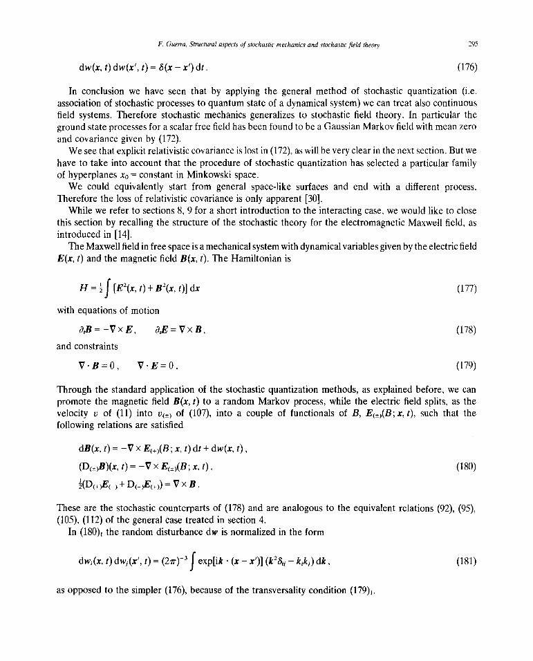
F. Guerra, Structuralaspectsof stochasticmechanicsand stochasticfield theory 295
dw(x, t) dw(x’, t) = S(x— x’) dt, (176)
In conclusionwe haveseenthat by applying the general method of stochasticquantization(i.e.associationof stochasticprocessesto quantumstateof a dynamicalsystem)we can treatalsocontinuousfield systems.Thereforestochasticmechanicsgeneralizesto stochasticfield theory. In particular theground state processes for a scalar free field has been found to be a Gaussian Markov field with mean zeroand covariance given by (172).
Wesee that explicit relativistic covariance is lost in (172), as will be very clear in the next section. But wehaveto take into accountthat the procedureof stochasticquantizationhasselecteda particularfamilyof hyperplanesx0 = constantin Minkowski space.
We could equivalently start from general space-likesurfaces and end with a different process.Thereforethe lossof relativistic covarianceis only apparent[30].
While we refer to sections8, 9 for a short introductionto the interactingcase,we would like to closethis sectionby recallingthe structureof the stochastictheory for the electromagneticMaxwell field, asintroducedin [14].
The Maxwell field in free space is a mechanicalsystemwith dynamicalvariablesgivenby theelectricfieldE(x, t) andthe magneticfield B(x, t). TheHamiltonian is
H = ~J [E2(x,t) + B2(x, t)] dx (177)
with equationsof motion
a~B=—VxE, a,E=VxB, (178)
andconstraints
V’B=O, VE=O. (179)
Throughthe standardapplication of the stochasticquantizationmethods,as explainedbefore,we canpromotethe magneticfield B(x, t) to a randomMarkov process,while the electric field splits, as thevelocity v of (11) into V(±)of (107), into a couple of functionals of B, E(±)(B;x, t), such that thefollowing relationsaresatisfied
dB(x,t) = —v x E(±)(B;x, t) dt + dw(x, t),
(D(±)B)(x,t) = —v X E(±)(B;x, t), (180)
~(D(÷)E(_)+D(~E(÷))= V x B.
Thesearethe stochasticcounterpartsof (178) and areanalogousto the equivalentrelations(92), (9S),(lOS), (112) of the generalcasetreatedin section4.
In (180), the randomdisturbancedw is normalizedin the form
dw~(x,t) dw1(x’, t) = (2ir)
3 J exp[ik . (x — x’)] (k250 — k1k1)dk, (181)
as opposedto the simpler (176), becauseof the transversalitycondition (179)~.

296 New stochasticmethodsin physics
If we in particularchosethe groundstatethenthe field B reducesto a Gaussianrandomprocesswithmeanzero andappropriatecovariance(we must refer to [14]for moredetails).
In the next section we comparethe processesobtainedherefor harmonicsystemswith thoseof theEuclideanfield theory.
For a well developed theory of stochastic differential equations for fields we refer to [31] andreferences mentioned there.
7. Comparison with Euclidean quantum field theory
Euclideanquantumfield theory is basedon the idea of replacingthe usualdescriptionof quantumfields in Minkowski space-timewith a descriptionin someauxiliary Euclideanspace.
Procedures based on this idea were rather commonin quantumfield theory during the fifties, seeforexamplethe treatmentgiven by Wick [32] of the Bethe—Salpeterequation.But Schwingerconsideredthe proposalof the Euclideanformulationin a morecomprehensiveway as a “possibleavenuefor thefuture developmentof quantumfield theory” [33].The correspondencebetweenthe two formulations,onein Minkowski space-timethe otherin Euclideanspace,can beobtained,in the simplestway, fromthe vacuum expectation values of products of quantumfields, making an analyticcontinuationfrom thepoints of physical Minkowski space-time to the points of complex space-time where the spatialcoordinatesarereal andthe time coordinateis purely imaginary(Schwingerpoints).The possibilityofthis analyticcontinuationis basedon firm physical groundssincethe work of Wightman andfollowers[22],on the generalstructureof quantumfield theory (seealso[15]).
The resulting Euclidean theory is described in terms of the so called Schwinger functions, which areessentially the Wightman functions evaluated at the Schwinger points. The basic covariance group ofthe Euclideantheory is given by the inhomogeneousEuclideangroup (rotations and translations)asopposed to the Poincaré group (rotations, boosts, translations) of the Minkowski theory. The obviousstructuralsimplification comesfrom the replacementof the indefinite metric of the Lorentzgroup(withthe relateddifficult hyperbolic problem)with the symmetricpositive definite metric of the orthogonalgroup (with the relatedmore manageableelliptic problem). Furtherdecisive progresswas made bySymanzik (see[34] and referencesthere). He realizedthat the Euclideantheory is characterizedby afield structure (Euclidean fields) with well defined dynamical properties. In the Boson case theEuclideanfields are naturally definedas commutativerandomvariablesandtheir dynamicalstructuresharesa stronganalogywith classicalstatisticalmechanics,as was convincingly shown by Symanzik insome particular cases.Finally in 1971 Nelson [35] isolated the crucial Markov property as peculiarlocality property of the Euclideanfields andestablisheda rigorousEuclideancovariantFeynman—Kacpath integral formula. Moreover he solved the main conceptualproblem left open by Symanzik,i.e.howto reconstructa Wightmanfield theory from a given Euclideanfield theory.In this way by the jointefforts of Symanzik and Nelson in few yearsthe Euclideanformulation reacheda very solid physicaland mathematicallevel of development.
The impact of Euclideanmethodson the advancementof the constructivequantumfield theoryprogramof Glimm and Jaffeand their followers [36,37] was very strong.In few yearsvery deepresultswere proven, in particular about the existenceand propertiesof quantumfields in two and threespace-timedimensions(seesection9 for ashort review andreferences).
Let us see the basic ideasof Euclideanquantumfield theory at work in a very simple case.Morecomplicatedcaseswill beconsideredin the following in the frameof stochasticfield theory.
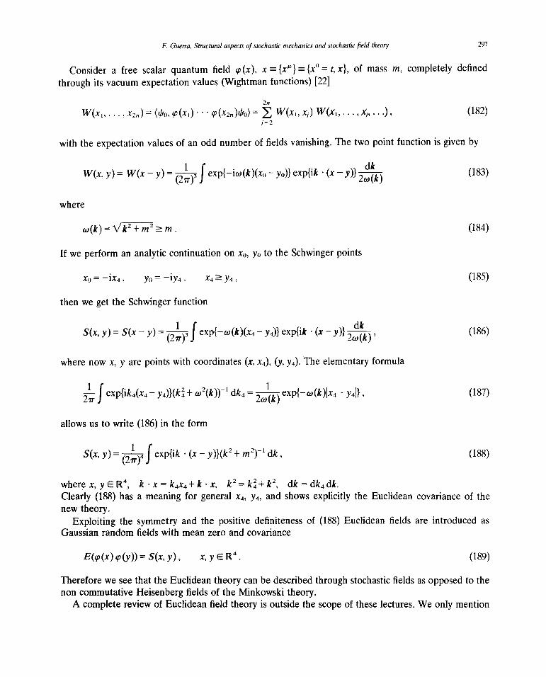
F. Guerra. Structuralaspectsof stochasticmechanicsand stochasticfield theory 297
Considera free scalar quantumfield ~(x), x {xe~} {x°= t, x}, of mass m, completelydefinedthrough its vacuumexpectationvalues (Wightmanfunctions)[22]
W(x, r2,,) = (t/io, ~(x,)~ . . ~(x~,,)çfro)= j2 W(x,, x1) W(X,,. . . ,X1,...)’ (182)
with the expectation values of an odd number of fields vanishing. The two point function is given by
W(x, y) = W(x — y) = (2)~ J exp{—iw(k)(xo— yo)} exp{ik . (x — ~ 2w(k) (183)
where
w(k)Vk2+rn2�m. (184)
If we perform an analytic continuation on x0, Yo to the Schwinger points
x0=—ix4, y0=—iy4, x4�y4, (185)
thenwe get the Schwingerfunction
S(x,y) = S(x — y) = j~-~—~J exp{—w(k)(x4— ~ exp{ik . — ~ 2w(k)’ (186)
wherenow x, y are pointswith coordinates(x, x4), (y, y4). The elementaryformula
~Jexp{ik~(x~— y4)}(k~+ w2(k))’ dk
4 = 2w(k)exp{-w(k)jx4- y4j}, (187)
allows us to write (186) in the form
S(x, y) = ~~)4 J exp{ik . (x — y)}(k2 + rn2)’ dk, (188)
wherex,yER4, k ~x=k4x4+kx, k
2=k~+k2, dk—dk4dk.
Clearly (188) hasa meaningfor generalx4, y4, and shows explicitly the Euclideancovarianceof thenew theory.
Exploiting the symmetry and the positive definitenessof (188) Euclideanfields are introduced asGaussianrandomfields with meanzeroandcovariance
E(p(x)i’p(y))=S(x,y), x,yER4. (189)
Thereforewe seethat the Euclideantheory can bedescribedthroughstochasticfields as opposedto thenoncommutativeHeisenbergfields of the Minkowski theory.
A complete review of Euclidean field theory is outside the scope of these lectures. Weonly mention

298 New stochasticmethodsin physics
that Euclideanfree fields can be easily constructedalso in more complicatedcases(see for example[38]),while for the interacting fields one can performthe analytic continuationon the Feynmanpathintegralrepresentation.We refer to [35,39,40,41] for a completetreatmentof the basicideasinvolvedin the transitionfrom the interactingMinkowski fields to the interactingEuclideanfields.
Herewe would like to emphasizethe surprisingcorrespondencebetweenthe randomfields obtainedin the frameof the Euclideanstrategy,as explainedbefore,and the randomfields constructedin theframe of stochastic mechanics, as explained in the previous section. This correspondence was first shownin [13] andholds alsoin the interactingcaseas will be explainedin section9.
First of all let us remark that by exploiting (187) in (188) we can write the covarianceof theEuclideanfields definedin (189) in the form
E(~(x4, x) ~(y4,y)) = (2)~ f exp{—u(k)1x4 — y4~}exp{ik (x — ~ 2w(k)’ (190)
A direct comparison with (172) allows us to realize that the random field ~(x4,x) defined in Euclideanfield theory coincides with the random field ~(x, t) associatedto the ground state, according tostochastic mechanics, provided we take t = x4. Sincethe two fields areessentiallythesamefrom now onwe will completelyidentify them and will call stochasticfield theory the generaltheoreticalschemeenclosing both Euclidean field theory and stochastic mechanics of fields.
This identification extends to more complicated cases. See for example [14]for the Maxwell field andsection 9 for the interacting fields.
At first sight this identification looksvery surprising,becauseafter all it seemsthat the labelsx4 andt haveacompletelydifferentmeaning.In fact t comingfrom stochasticmechanicsstandsfor the physicaltime parameter,while x4 of Euclideantheory comesfrom an analytic continuationof the physicaltimeat imaginary values, as (185) shows. But we must remark that the meaning of parameters appearing inthe expressionsof physical quantitiesis strictly connectedwith the propertiesof thesequantities,inparticular with the equationsthey satisfy. In order to help to realize the meaningof the proposedidentification we can offer the following elementaryexample, which at first sight shows the samedifficulties but whose complete understanding is very simple.
Consider a heat equation of type (38), x E R3, and its elementary solution (36) satisfying the initial
condition(37). Thereis no doubt aboutthe meaningof t, t’ as values of physical time.On the otherhandconsiderthe Schrodingerequation(24) for a free particle(x E D~~)
iha~/i= — Art/i. (191)
Its elementarysolutionK(x, t; x’, t’), t � t’, satisfying the initial condition
lim K(x, t; x’, t’) = S(x — x’) , (192)t It’
is given by
/ m \~2 Iim(x — x’)21K(x, t; x’, t ~ = ~2irhi(t — t’)) exp~2h(t— t’) j’ (193)

F. Guerra. Structuralaspectsof stochasticmechanicsand stochasticfield theory 299
Herealsothereis no doubt that tin (191), (193) is physicaltime. Neverthelessafterthe position (94) werealizeimmediatelythat the elementarysolution (36) of the heatequationand(193) of theSchrödinger,eventhough they are both expressedin termsof physical time, can be obtainedonefrom eachotherthrough analytic continuationof the type (185) and identification of x4, x~with t, t’. Thereforethereshould be no surprisewhen we see that the correlation functionsof stochasticfields can be obtainedthrough analyticcontinuationin time of correlationfunctionsof quantumfields, becausethis is exactlythe casefor (36), (193) whereno troublearisesin the interpretation.
We havethus verified, in the elementarycase of the free field, the strong connectionbetweenEuclideantheory andstochastictheory up to the pointof identification.
For the sake of completenesslet us give also the explicit connectionin the caseof the harmonicoscillator.The onedimensionalharmonicoscillatoris not so muchof interestin itself but becauseit is theprototypeof free andinteracting(Bose)fields, and thereforeit is avery usefulmodel for the purposeofillustration.
We introduceHeisenbergposition operatorsqH(t) for the harmonicoscillatorwith groundstate t/’0.According to well known ideas,mutuatedfrom quantumfield theory [22],the wholephysicalcontentofthe theory can beexpressedthroughthe time correlationfunctions
l~V(t,,... , t~)= (I/tO, qu(t,) . . . qH(tX)I/IO) . (194)
Becauseof the symmetry of the ground statethe W vanish for s odd, while for s even they can beexpressedrecursivelyin a form analogousto (182)
W(t,, ... , t~,,)= ~ W(t,, ~) WV,, ... , 4...). (195)
Thetwo point function in (195) is given by
W(t, t’) = (I/’~,qH(t) qH(t’) I/to) = exp{—iw(t — t’)} . (196)
It is immediatelyseenthat aformal analyticcontinuationin time allows usto go from (196) to (161)andvice versa.Notice that in (196)and(161) t, t’ havethe samephysicalmeaningas time parameters,just asfor (172)and(193), but themeaningof qH(t) in (196) andqo(t) in (161)is deeplydifferent. In fact qH(t) isa quantum Heisenbergfield, while qo(t) is a random process.Only at zero separationtimes, i.e.
= = t5, we have that (194) and (162) are identical. In general at each fixed time the randomprocessesof stochasticmechanicscoincide with the Heisenbergfields of quantummechanics,but atdifferent times theyaredifferent andhavedifferent correlations.
It is alsoclear that the knowledgeof (161), (162) allows the reconstructionof (195), (196), thereforethe randomprocessesof stochasticmechanicsdefinecompletelythe quantumstructure.
It is alsoimportant to remarkhereexplicitely that the only knowledgeof the groundstateprocessofstochasticmechanicsis sufficient for the reconstructionof the wholestructureof quantummechanicsforthe given system.We give heresomedetailsaboutthis fact, which in the caseof theharmonicoscillatoris completelyelementarybut extendsto morecomplicatedcasesandis of paramountimportancefor thephysicalapplicationsof stochasticmechanicsand stochasticfield theory,becausegroundstateprocessescan be easilyconstructedthroughfunctional integrationas will beshown in section9.

300 New stochasticmethodsin physics
Supposethat the groundstateprocessq0(t) for the harmonicoscillatorhasbeengiven as definedby(160), (161), (162).Let (0, 1, ~) bethe probability spacewhereqo(t) is realized(see[19]).The u-algebra.X of eventsin 0 is generatedby the elementaryevents(cylinder sets)
A(a,, t,; ... ; a~,t~)= {q(t1) <a,, ... , q(t~)< a5}, (197)
t,�”~t5, a1ER.
Obviously the probability of occurrenceof the eventA is given explicitly by
j J p(x5,t~x~,,t~,)”~p(x2,t2x,,t,)p(x,,t,)dx,~ (198)
wherep is the transitionprobability in (158).Let ~ £, .~�, be respectivelythe u-algebrasgeneratedby qo(t’) for t’ ~ t, t’ = t, t’ � t (past, present
and future with respectto t) andE�,,E~,E�, the associatedconditionalexpectations.Then Markovproperty(mutual independenceof pastandfuture conditionallyto the present)can be simplyexpressedas
E�~E�1=E�,E~,=E,. (199)
Let us now derive the quantum mechanical quantitiesfrom the process.First of all we haveimmediately,becauseof the translation invarianceof the transitionprobability and correlation func-tions, that all Hilbert spaces~ = L
2(0, £,, ~t) are isomorphic, moreover each can be isometricallyidentified with the physicalHilbert space~ = L2(R, dx), wheredx is the Lebesguemeasurein R. In factanyelementin .~ can be approximatedthrough polynomialsP(q(t)) of the processat time t, and theclaimedisomorphismis given explicitly by
~ P(q(t))4-~P(x)\/po(x)E ~, (200)
wherepo is the groundstatedensity (154).The proof is very simple. Oneneedsonly to showthat for polynomialsP and0 we have
(P(q(t)), Q(q(t)))g~,= E(P(q(t))* Q(q(t)))
= JP(x)* 0(x)po(x)dx = (P(x) \/po(x), 0(x) \/po(x))L2(R.dX). (201)
But (201) follows from (160), (161), (162) and (154)through elementarydirectcomputation.Notice thatthe absenceof nodesin p0 is essentialfor the meaningof (200).We can think of 3~asa subspaceof ~ asL2(Q, £, ~t) andinterpret(200) as an isometricembeddingJ~of~Winto ~ with image ~. The adjointJ~is a map from ~ to ~‘, it involves firstly a projectionfrom ~ to~, then the identificationof ~ with ~ through (200)
J,: ~ (202)
J’~: ~

F. Guerra, Structuralaspectsofstochasticmechanicsand stochasticfield theory 301
Obviouslywehavealso
on~,(203)J~J,~=E1 on~,
whereE, is the conditionalexpectationappearingin (199).Finally we can easilyconstructthe Hamiltonian. In fact an explicit calculationshowsimmediately
.j~j,.= exp[_ ~- t— t’~H0] on ~W, (204)
whereH0 is the quantumHamiltonian of the free harmonicoscillator.Thereforewe haveseenhow all quantummechanicalpropertiesare containedin the ground state
process(at leastin this elementarycase,but the procedurecan be generalized).In the next sectionswe attack the problemof constructingthe randomprocessesassociatedto more
complicatedsystems.
8. Perturbation of stochasticdifferential equations
In section6 we havegiven the explicit constructionof somesimple examplesof randomprocessesarising in stochasticmechanics.Theseexampleswere directly basedon the harmonicoscillatoror therelated free fields. Clearly physical applicationsrequire more complicatedsystems,as anharmonicoscillatorsand interactingfields. Obviouslythereis no hopeto get explicit expressionsfor the solutionsof thesemore complicatedmodels.Fortunatelythe generaltheory of stochasticdifferential equationscomesto help andallows us to get, through a simple chainof arguments,ratherdirect expressionsforthe correlationfunctionsof the randomprocessesassociatedto the groundstatesof thesemoregeneralsystems. The essentialtool will be given by functional integration of probabilistic type, whosemathematicalcontrol is rathereasy.
It is our purposeto give the essentialelementsof the whole argument,stressingthe main physicalideashere involved. But for a rigorous treatmentof the relevantaspectsof the theory of stochasticdifferential equationsemployed in our discussion,we must refer to the “stepping stone” or thespecializedliterature[42].
Let usconsidera stochasticdifferentialequationin R’t
dq(t)= v(±)(q(t),t)dt + dw(t) (205)
with
dw(~)(t)dw(~’)(t)= S~dt. (206)
We assumeto have obtained complete control on (205) (as for the examplesof section 6). Theprocessq(t) is realizedin a probability space(0,1~,p.), so that for theexpectationswe have
E(F(q(t1) q(t5))) = J F(q(t1) q(t5))dp. , (207)

302 New stochasticmethodsin physics
where we still denoteby q(t) in the r.h.s. the sample path expressionsof the process(the dummyintegrationvariablespecifyingthe pathsin 0 is suppressedin our notation).
Supposenow that we areinterestedin a new process~(t), satisfyinga different stochasticdifferentialequation
dc~(t)= v(+)(q(t), t) dt + dw(t), (208)
with a new drift ~(x, t), x E R~,and the same randomdisturbancedw as in (205). Under favourablecircumstanceswe can expressthe processc~in termsof q in avery direct way. Thecentralidea is to tryto realize the new process~(t) in the sameprobability space(0, .~) of q(t), thereforewith the samesample paths, but choosing a new measureji (insteadof p.), which gives in general differentprobabilitiesto the samepaths.In this casewewould have
E(F(q(t,), ... , q(t5))) = J F(q(t~),... ,q(t~))dii, (209)
in placeof (207) (recall the meaningof q(t) in the r.h.s. assamplepath functions!). In order to show thatan explicit representationof type (209) is possible in somecaseswe decideto follow the processq(t)from someinitial time t0 = 0 (for simplicity) till time T, thereforefor t wehave0 = t0 ~ t � T We alsoassumethatthereisafunction11(x)� 0, x E R”, suchthattheinitial distributionof thenewprocesst~(t)canbe given accordingto
E(F(~(O)))= E(F(q(O)) 112(q(O))) (210)
for any smoothF(x).Let usnow introducea measure~, definedon the u-algebra1(0, T) generatedby q(t), 0 � t s
d~= 122(q(0))exp[J a~dw -~ Ja~t] dp., (211)
where a = a(x, t) is some given (sufficiently regular) vector function in R”. The stochastic integralappearingin (211) is defined in [19]. We only recall herethat for a stepvector function f definedby
f(x, t)= ~(x)X1(t) (212)
where
11 t1_1�t<t~otherwise, 0= t0<t,<... <t~= T, (213)
the stochasticintegralmustbe definedas

F. Guerra, Structuralaspectsofstochasticmechanicsand stochasticfield theory 303
TJ~.dw = ~f1(q(t1)) . (w(t1±i)- w(t~)), (214)
in coherencewith the forwardnatureof dw in (208).For generalvectorfields, as appearingin (211), stochasticintegralscan bedefinedstartingfrom (214)
through appropriatelimiting procedures.If we substitute(211) into (209)we get, at leastin theinterval 0 s t ~ T, the specificationof a random
process~(t). It is easy to verify that the assumption(211) satisfies all compatibility requirements,moreoverc~definedin (209), (211) hasinitial distribution(210) andsatisfiesthe equation(208)with driftV(±)given by
V(+)(X, t) = v(÷)(x,t) + a(x, t). (215)
The proof is very simple. For the compatibilitywe haveto verify that if T’ < T then (209) and (211),
with T replacedby T’, definethe samet~(t)for 0 � t � T’ as the original (209), (211). This is true if
E(o,r’) exp[J a dw — ~ J a~dt] = 1 (216)
(notice that the additivepropertiesof the integral imply factorizationof the exponential),whereE(o,T’)is conditionalexpectationwith respectto the u-algebra1(0, T’) generatedby q(t) for 0 � t ~ T’. But(216) is simply provennoticing that for any small interval (t, t + dt) we have
t+d: t+df
E1exp[ J adw—~ J a2dt]~1, (217)
up to the first order in dt. In fact expandingthe exponentialswe have
E~[(1 + a(q(t),t) . dw + ~(a . dw)2+ O((dt)2)) ‘ (1 — ~ dt + O((dt)2))]= 1 + O((dt)2) . (218)
For theinitial conditionwe haveimmediatelythat (210)follows from (209), (211)if (216)is takenintoaccount.
In order to verify (208), (215) the readerwill convincehimself that it is enoughto show
E(F(q(t)) d4(I)(t)) = E(F(~(t))t~(+)(~)(~(t),t)) dt, (219)
for anysmoothF and0 � t � T.But (209), (211)and the Markov propertyexpressthe r.h.s. of (219) in the form
,±dt
E(112(q(O))F(q(t)) exp[ ...] dq(i)(t))
t t±dt
= E((12(q(O))F(q(t))exp[J ...] Et(exp[ J .] dqo~(t))), (220)
304 New stochasticmethodsin physics
with obviousmeaningof the shorthandnotations.But
t+dt
Et(exp[ J (a . dw — ~a2dt)] dq(I)(t))
= E,((1+ a dw + ~(a . dw)2+ . . ~)(1— ~a2dt + . . ~)dq~)= (v(±)(I) + a(1))dt + O((dt)
2), (221)
therefore(220)coincideswith ther.h.s.of (219)andthe expressions(215) of the newdrift i3(+, is verified.In conclusion the fonnulae (209), (211) give the completesolution of the stochasticdifferential
equation(208), with initial condition (210), in termsof the referenceprocessq(t) supposedcompletelyknown.
For the application of the theory sketchedhere to the study of processesarising in stochasticmechanics,the key ingredientis basedon the fact that when the field a in (211) is the gradient of ascalarthenthis formulasimplifies considerably.In fact let usassume
a(x, t) = (Vp) (x, t), (222)
thentheIto formula(seethesteppingstone)gives usthefollowing expressionfor thestochasticdifferentialof ~‘p(recall that dueto (205), (206)secondorderderivativesin x arecontributionsof first order in time)
= ô,ç’ dt + V~. dq + ~ dt. (223)
Replacingdq in (223) with (205)we get
a~dw—~a2dt=dço—Wdt (224)
with
W= D(÷)~+ ~(V~)2, (225)
whereD(±)is definedin (67) (recall that herewehaveput 2v = 1 for simplicity, as comparisonof (206)with (47) shows).
In this way we see that the stochasticintegral appearingin (211) disappearsand we can write,exploiting (224),
d/3 = 112(q(O))exp[~(q(T),T)- ~(q(O),0)— J W(q(t), t) dt] dp., (226)
valid for O�ts T.The condition (222) is surely satisfiedin stochasticmechanicsbecausea, accordingto (215), is the
differencebetweentwo different forward drift coefficientsandeachof them is a gradient (recall (92),(93)).Thereforelet ussupposethat for a given systemunderpotentialV we havecompletelyspecifieda

F. Guerra. Structuralaspectsof stochasticmechanicsand stochasticfield theory 305
random processq(t) according to the generalproceduresof stochasticmechanics.Let us changethepotentialfrom V to V andlet ~ be a newprocessassociatedto the modifiedsystem.If we call R, 5, R,5, the quantities in (100)—(103) associatedto the two systems,we can write, for the purposeofapplicationof formula (226) (putting h = 1, m = 1 for simplicity)
V(±)~v+SvV(R+S),
V(±)~j3+Sii=V(R+S), (227)
a = — V(+) = V(1~— R + S— S)= V~,
tp R—R+S—S,
122 = exp{2(1~— R)}. (228)
If we exploit the equations(26), (32) for the partial time derivatives 3,(R, 1~,S,~) in D(±)~for theexpression(225) of W, then after an elementarybut very long calculationwe can write W, definedin(225) andappearingin (226), in the form
W = A\/p/\/~5-V- A\/p/\/p+ V. (229)
Clearly for general V, V evenif p is completelyknown (as for examplefor the groundstateof theharmonicoscillator) it is very difficult to evaluate,t5. But if we are interestedonly in ground stateprocesses(andwe havefoundevidenceat the endof section7 that they areenoughto reconstructthewhole quantum mechanicalcontent!) then the eigenvalueequationfor \‘p allows us to derive aconsiderablesimplification. In fact wehave
V - ~AVp/Vp = E, V - ~AV,5/V,5= E (230)
(recall that we haveput /1 = 1, m = 1). Thereforefrom (229)we have
W=V—E—(V—E). (231)
After substitutionof (227), (228), (231) into (226) wefinally get
dp. = Q(q(O))exp[_ J (~(q(t))-V(q(t))) dt] fl(q(T)) exp{T(E- E)} dp.0, (232)
which is nothingbut a versionof the Feynman—Kacformula [19,15].The whole procedureadoptedin this section,in particularthe exploitation of (26), (32), showsthat
formula (232) synthetizesall kinematicaland dynamicalassumptionsmadeabout the nature of therandomprocessesintroducedby stochasticmechanics.
Formula(232) is the starting point for the applicationsof the nextsection.Very suggestiveinterpretationsof (232) andrelatedexpressionscan be found in [43] and[44].

306 Newstochasticmethodsin physics
9. Applications to the anharmonic oscillator and to interacting fields
We haveseen in section6 that for the harmonicoscillatorwith Hamiltonian(141) the ground stateprocessqo(t) is defined through (160), (161). Let us considernow the anharmonicoscillatorobtainedaddingto (141) and(144) a quarticinteractionof the type
V(x)= gx4, (233)
so that we have in particular for the groundstatewavefunction I/i~(x)with energy E
Echo= — a~+ ~mw2x2~h0+ gx
4~0. (234)
Let usconsiderthe processq(t) associatedto this groundstate.First of all we write
çlJo(x) = (1(x) \/po(x), (235)
wherePo is the time invariant ground statedistribution for the free process.Then the general theory sketchedin the previoussection allows us immediately to expressthe
measurep. associatedto theprocess q(t) in termsof the measurep.0 of the freeprocessq~(t).In fact wehavefor the interval 0 � t ~ T
= fl(qo(O))exp{_~ Jq~(t)dt} f1(q0(T))exp{~(E - E0)} dp.~, (236)
whereE and E0 are the ground stateenergiesof the anharmonicandharmoniccaserespectively.Ingeneralfor any smoothfunction F we have
E(F(q(t,) q(t5)))
tS+ T
= E(Q(qo(to))exp[_ f J q~(t)dt] f1(qo(to+ T)) F(qo(to) qo(ti)))exp{~(E — E0)}~ (237)
where(t0, t0+ T) is any intervalcontainingall t, ,...,t~.The interest of formula (237) is clear. It gives an explicit expressionfor the ground state process
of the interactingsystem.Also in this casethe knowledgeof the ground stateprocessallows to deriveall quantummechanicalpropertiesof the system,exploiting the sameprocedureoutlined around(200),(204).
On the otherhandalso in this caseit can beshown that the stochasticcorrelationfunctions
E(q(t,) . . . q(t,))
as expressedthrough (237), can be related to the vacuumexpectationvalues of Heisenbergoperatorsthrough analyticcontinuationas in the free field case(see[40, iS]).

F. Guerra, Structuralaspectsof stochasticmechanicsand stochasticfield theory 307
Finally we would like to point out that the explicit expressionsof (1 andE arenot necessaryin orderto write the l.h.s. of (237). In fact, by use of transfermatrix techniques(see[15] and [40]), it can beeasily shown that by putting 12(x)= 1 in (237), normalizing the r.h.s. so that E(1)= 1, and lettingt0—* —~ and t0+ T—~+°~then the resulting expressionin the r.h.s. will be convergent to the writtenexpressionin terms of 11 and E. Thereforeall correlationfunctions of the processcan be obtainedthrough a limiting procedurewell knownin statisticalmechanicsandbasedon the infinite volume limitof Boltzmann—Gibbsstates(for a general introduction to modernrigorous statistical mechanicssee[45]).
From this point of view (237) is extremelysuggestive.It showsin a sensethat stochasticmechanicshasa structurevery similar to a kind of classicalstatisticalmechanicssystemwhoseelementaryobjectsaretrajectoriesdistributed in probability accordingto a Boltzmann—Gibbsfactor exp(—U), expressedintermsof the interactionpotential.
This analogycarriesalso to the field case(see[40]).A completeaccountof the applicationsof stochasticmethodsto constructivequantumfield theory,in
the frameof the so calledEuclideanstrategy,is unfortunatelywell beyondthe scopeof theselectures,whose main purposeis only to provide an introduction to the conceptualfoundationsand generalstructureof stochasticmechanics.We must thereforerefer to [37,15,40] and papersmentionedtherefor acompletetreatment.
Here we would like only to stressthat the generalmethodsof section8 apply also to interactingfields.
Let us recall the exampleof the free field, as introducedin section6 by confining the system in afinite spatialbox and making the waveexpansion(167). If we addan interactionof the type
H,= gJco4(x)dx (238)
to the free Hamiltonian(163) andkeeponly a large but finite numberof degreesof freedom(ultravioletcutoff) we get a multidimensionalanharmonicoscillator for which a treatmentalongthe lines of theprevioustwo sectionsis still possible.Then we still havea formula like (237) generalizedto the fieldcase(the Feynman—Kac—Nelsonformula, see [39,40]).
In this cut off casewe also havethat the ground statefield processis related to quantumfieldsthrough a procedureof analyticcontinuation.Thereforethe processprovided by stochasticmechanicsfor the groundstatecoincides,alsoin the interactingcase,with the processintroducedby the Euclideanstrategy. In this way stochasticfield theory and Euclideanfield theory merge completely,with greatconceptualsimplification, becausestochasticfield theory can be introducedindependentlyin the frameof generalstochasticmechanics.
Stochasticmethods,with their intrinsic possibilityof handling functional integralsaccordingto therules of ordinary integrals,havebeenextremelysuccessful.In fact thereis a large amount of resultsabout interactingquantumfields obtainedthrough the Euclideanstrategy.Clearly the main technicalproblems are related with the removal of the spatial box cut off, the control of the ultravioletdivergenciesand the reconstructionof the standardquantumfield theory dealingwith Wightman fieldsfrom theresulting Euclideantheory.
Herewe would like to recall only someof the main results,in order to give an ideaof the lines alongwhich researchdevelopedin the pastyears.Shortly after the introductionof the Euclideanmethodsthe first proof was given about the existenceof non trivial models in two-dimensionalspace-time
308 New stochasticmethodsin physics
satisfying all Wightman axioms [46], then extendedalso to strongly coupled fields [39,40]. Theusefulnessof methodsbasedon the analogy with statistical mechanicswas also firmly established[40,15]. The results on the existenceof non trivial modelswere extendedalso to threedimensionalspace-time[47,48]. The rigorous proof of occurrenceof spontaneoussymmetry breaking followed[49,50]. RecentlyEuclideanmethodshavebeenalso employedfor the studyof gaugefield theory [51].
10. Extensionsof stochasticmechanics.The spinning particle
Stochasticmechanicshas been extendedto generalLagrangian systemswith configuration spacegiven by a Riemannianmanifold [10,11, 12]. Here delicate problemsmust be solvedconcerningthedefinition of meanforward and backwardderivatives.The most interestingaspectof this extensionisgiven by the blending of characteristicfeaturesof stochasticprocesseson one side and differentialgeometryon the other side. In particular the ability of stochasticprocessesto “see” secondordereffects of geometricnatureis clearly exhibitedin the relevanceof geodesiccorrectionsto the paralleldisplacementof vectorfields alongrandomdiffusing trajectories,as explainedin [12].
Another interestingoutcomeof the extensionof stochasticmechanicsto Riemannmanifolds is thetreatmentof stochasticspinningparticles[28]. It is usuallystatedthat functionalintegralscan not takeinto accountspin onehalf particlesbecausethesesystemsdo not haveclassicalcounterpart.In fact if weare willing to include spin one half particles into stochasticmechanicswe must find some adequateclassicalsystem,whosestochasticquantization,alongthe lines of section6 or their generalizationto nonflat manifoldsas given in [12],gives processessuitablefor the descriptionof theseparticles.Fortunatelythis can be doneas was explainedin [12],seealso [10] and [11]for earlier relatedwork.
Motivatedby the ideasput forwardin [52] and[53],we assumethat the classicalconfigurationspaceof a non relativistic spinningparticle is given by R3 x SU(2). Clearly R3 describesthe translationaldegreesof freedom,so that we must justify the choiceof SU(2) in placeof the moretraditional rotationgroup SO(3) for the descriptionof the inner rotational degreesof freedom. Notice that SU(2) is theuniversalcovering groupof SO(3). For the sakeof simplicity let us considera rigid body, with a fixedpoint, topologically connectedto otherdistant fixed bodiesthrough elastic strings (threeor more). Bythe very definition of coveringgroupwe immediately realizethat the position of the body is given bySU(2) if we takeinto accountnot only the “geometricposition”, given by customaryEuleranglesandthereforeSO(3), but alsothe topologicalstateof entanglementof all stringsconnectedwith the body.For examplea rotation of 2ir aroundsomeaxis producessuperpositionsof the strings which cannotbetopologically disentangledwithout breakingthem.A further rotation of 2ir aroundthe sameaxis (for atotal of 4ir) will produceadditionalsuperpositions,but now the stringscan be disentangled.Thereforeafter a rotationof 41T the body acquiresa position topologically equivalentto the initial one.This is aconsequenceof the doublevaluednatureof the covering.We can give a ratherconvincingjustificationto the assumptionthat theentanglementwith the surroundingsis essentialfor thecompletespecificationof the innerdegreesof freedomof a particle. In fact if we think of the particle as someconcentrationofexcitationstatesof afield, thenthe “tails” of the field, extendingto infinity, canbe thoughtasprovidingthe topologicalentanglement.
Thereforewe may assumethat the rotational degreesof freedomare given by SU(2). Throughthestochasticquantizationprocedurewe are led to considerstochasticprocessestaking values on R~xSU(2) and evolving under the action of somerandom disturbanceand a given electromagneticfield.

F. Guerra. Structuralaspectsofstochasticmechanicsand stochasticfield theory 309
Thereforewe havea descriptionof the spinningparticleinsidea stochasticframework.In particularthequantumwavefunction I/i of our systemwill be a function on R3x SU(2) and the Schrödingerequationin absenceof electromagneticfields reads
ihö,~/t=—~h2AI/t, I/iasI/i(x,g;t), xER3, gESU(2), (239)
whereA is theLaplacianon R3 x SU(2), involving constantsrelatedto the massandthe inertial momentof the body. Obviously if there is some electromagneticfield then the equationmust be modifiedaccordingto the well known gaugeinvariant prescription,so that the translationaldegreesof freedominteractthrough the electricchargeandthe rotationalones throughthe magneticmoment.
In order to give to (239) andits analogwith electromagneticinteractiona morefamiliar aspect,it isconvenientto makean expansionof the wave function in terms of a completeorthonormalset of SU(2),as given by the matrix elements R’m,,, of all irreducible representations,j = 0, ~,1,...; m,m’ =
—j, —j + 1 j, then we have
I/ic(x, g; t) = ~ R2,~,,,(g)I/i~,,.(x,t), (240)j,m,m
and the Schrödingerequationsplits (see [28]) into independentPauli-likeequationsfor eachspin j inthe form
= C’°I~/) — B ~ i ~241I ‘t’ mm’ ‘t’ mm’ p mm “p m ‘rn’
whereC°~is an energyoperatoracting only on the translationaldegreesof freedom,p. is the magneticmoment of the particle,B the externalmagnetic field and £ are appropriaterotation matrices, forexample~ = 0 (this is the caseof a spinlessstate),,~(t/2) = a (the Pauli matrices,for spin onehalf),etc.
We would like to stressthat thereare associatedrandomprocessesbeyond(239), (241), so that inparticularfunctional integrationtechniquesof the typeexplainedin section8 can be employed.
This showsthat half integerspinningparticlesarewithin the scopeof a stochasticformulation,withthe consequentpossibilityof methodsbasedon Feynman—Kacrigorous functionalintegrals.
The generalizationto the relativistic caseis still open. Clearly processeson SL(2, C), the universalcoveringof the Lorentz group, should play acentralrole. A generalanalysiswith preliminary resultsappearsin [11], we believethat also ideasput forward in [54] and[55] could be useful.
11. Conclusionsand outlook
In this reviewwe havetried to give an elementaryintroductionto the generalstructureof stochasticmechanicsas related to quantummechanics.Surely the information containedhere is partial andinadequate.Only a good working practice, free of ideological prejudices,could convince anyreaderaboutthe beautyandthe usefulnessof thistheory,characterizedby its powerful synthesisof manyideasof functional path integration, Euclidean methods and stochastic methods, in the frame of fewdynamicalassumptions.

310 New stochasticmethodsin physics
We would like to conclude this review with a short account of the two main open conceptualproblemsof stochasticmechanics.The first relatedto canonicaltransformations,the secondto Fermistatistics.
An important feature of stochasticmechanics,as we haveintroducedit in the pastsections,is thatthe relevantrandomprocesseshavealwaysbeendefinedas taking valueson the configurationspaceofthe dynamical system.This procedureselectsthe configuration spaceas playing a special role, incontrastwith classicalmechanicsand quantummechanicswhereall constituentsof phasespacehavesimilar roles. In particular in quantum mechanicswe can select any complete set of compatibleobservablesat fixed time in order to specify completelythe quantumstateof the system.Onecan shiftfrom one representationto the otherthrough a unitary transformation(for examplediagonalizingtheposition or the momentum).Thereforewhat is relevant about the dynamical structureof quantummechanicsis not the Schrödingerequationin oneparticular representationbut the possibilityof goingfrom one representationto the other through unitary transformations,which preservethe physicalcontent of the theory and transform covariantly all dynamical properties(in particular the timeevolution).
The situation is analogousin classical mechanicswhere the whole structure is covariant undercanonicaltransformations.
Clearly unitary (canonical)transformationsin quantum(classical)mechanicsshould be replacedbymeasure preserving transformations in stochastic mechanics. But a full discussion of covariancepropertiesfor the wholedynamicalscheme,insidethe stochasticframework,is still missing.This wouldallow to considerin particularalsoprocessesin momentumspace.But thegeneralobjectivewould be toconstructa comprehensivestochasticschemewhere different representationscould be selected,eachcontaining random processesfor some sets of observables(configurations,momenta,etc.) and allconnectedthrough measurepreservingtransformations.This would also help in the study of therelativistic covarianceof the stochasticfields constructedin section6.
Thereforewe believethat the problem of the generalcovariancepropertiesof stochasticdynamicsshould be carefully considered in the future research in this field. Wehope to report soon on somepreliminary resultsin this direction.
The other problemis how to incorporateFermi statisticsinto stochasticmechanics.Clearly thiswould beimportant firstly for theconceptualreasonof giving unified treatmentto all kind of fields, butin particular for the possibility of exploiting the powerful methodsof stochasticintegrationboth formathematicalcontrol andfor numericalinvestigations.Unfortunatelyall treatmentsgiven sofar employGrassmannvariablesin formal functional integralsor in Euclideanfield theory, in a context very farfrom a stochasticframe. Clearly herethe problem is to find, in the absenceof a direct classicalstartingpoint, a convenientconfigurationspacewheresuitablerandomprocessescould give modelsfor Fermistatistics.Preliminaryresultsare given in [56],whereit is foundthat, just as Gaussianrandomprocessesplay a role for the harmonicoscillatorand thereforefor the Bose fields, so randomwalks on the twoelementgroup Z2 = (—1, 1) seemto play the samerole for Fermi oscillatorsand thereforefor Fermifields. But surely the questionof understandingFermi statisticsin the frame of stochasticmechanicsdeservesvery careful investigations.
In conclusionwe can seethat stochasticmechanics,after someyearsof oblivion, undertherefreshingimpact of the applicationof probabilistic methodsin Euclideanfield theory is growing into a generaltheoreticalscheme,whosepossibilitiesof physical insight andsynthetizingpowerwe areperhapsonlybeginningto understand.

F. Guerra, Structuralaspectsof stochasticmechanicsand stochasttcfield theory 311
References
[1] R.P. Feynman.Rev.Mod. Phys. 20 (1948) 367.[21R.P. Feynmanand AR. Hibbs. QuantumMechanicsandPathIntegrals(McGraw-Hill. New York, 1965).
[3] R.P. Feynman,StatisticalMechanics(WA. Benjamin. Reading,1972).[41C. ltzykson andJ.B. Zuber.QuantumField Theory (McGraw-Hill, New York. 1980).[5] C. DeWitt-Morette.Commun.Math. Phys.28 (1972) 47;
C. DeWitt-Morette.A. Maheshwariand B. Nelson. PhysicsReports50 (1979) 255.[6] S. Albeverio andR. HØegh-Krohn,MathematicalTheory of FeynmanPath Integrals(Springer, Berlin, 1976).
[7] 1. Féynes,Z. Physik 132 (1952) 81.[8] D. Kershaw,Phys. Rev. 136 (1964) B 1850.[9] E. Nelson, Phys.Rev. 150 (1966) 1079, andDynamicalTheoriesof Brownian Motion (PrincetonUniversity Press.Princeton.1967).
[10] T.G. Dankel, Arch. Rational Mech. Anal. 37 (1971) 192.[11]J.P.Caubet,Le MouvementBrownianRelativiste (Springer, Berlin. 1976).[12] D. Dohrn and F. Guerra,Lett. NuovoCimento22 (1978) 121.[13] F. Guerraand P. Ruggiero,Phys. Rev.Lett. 31(1973)1022.[14] F. Guerra andMl. Loifredo, Lett. NuovoCimento27 (1980)41.[15] B. Simon, The P(4~)
2Euclidean(Quantum)Field Theory (Princeton,N.J., 1974).[16] Contributionof the Marseille groupto this issue.[17] E. Madelung.ZS. f. Phys. 40 (1926) 322.[18] D. Bohm. Phys. Rev.85 (1952) 166.[19] C. DeWitt-Moretteand D. Elworthy, SteppingStone,in this issue.[20] V.1. Arnold. Matematiëeskiemetodyklassi~eskojmechaniki(MGU, Moskow, 1968).[21] R. Courantand D. Hubert.Methodender MathematischenPhysik(Springer-Verlag,Berlin. 1968).[22] R. StreaterandAS. Wightman. PCI’. Spin and Statistics,andAll That (Benjamin,New York, 1964).[23] M. Creutz,L. JacobsandC. Rebbi, Phys. Rev. Lett. 42 (1979) 1390.[24] G. Jona-Lasinio,contributionto this issue.[25] N. Wax, ed., SelectedPaperson Noise andStochasticProcesses(Dover Pubi., New York, 1954).[26] N.J. Rao.J.D.Borwankarand D. Ramkrishna,SIAM J. Control 12 (1974) 124.[27] M. Davidson,Lett. Math. Phys.3 (1979) 271.[28] D. Dohrn, F. Guerra and P. Ruggiero,in: FeynmanPath Integral,eds. S. Albeverioet al. (Springer-Verlag,Berlin, 1979).[29] K. Yasue,J. Stat.Phys. 16 (1977) 113.[30] F. Guerra,in preparation.[31] 5. Albeverio,contributionto this issue.[32] G.C. Wick, Phys.Rev. 96 (1954) 1124.[33] J. Schwinger. in: Proc.of the1958 Conf. on High Energy Physicsat CERN. ed. B. Ferretti(CERN. Geneve,1958).[34] K. Symanzik. in: Local QuantumTheory,ed. R. Jost (AcademicPress,New York, 1969).[35] E. Nelson, J. FunctionalAn. 12 (1973) 97; 12 (1973) 211.[36] J. Glimm and A. Jaffe,in: StatisticalMechanicsand QuantumField Theory,eds. C. DeWitt and R. Stora (Gordon and Breach,New York.
1971).[37] G. Velo and AS. Wightman,eds.,ConstructiveQuantumField Theory (Springer-Verlag,Berlin, 1973).[38] F. Guerra,in: SymposiaMathematica,Vol. XX (AcademicPress,London, 1976).[39] E. Nelson, contributionin [37].[40] F. Guerra,L. Rosen and B. Simon,Ann. of Math. 101 (1975) 111.[41] K. Osterwalderand R. Schrader,Commun.Math. Phys. 31(1973)83.[42] 1.1. GihmanandA.V. Skorokhod,Introduction to theTheory of RandomProcesses(W.B. Saunders,Philadelphia,1969).[43] H. Ezawa,J.R. KlauderandL.A. Shepp,Ann. of Phys.88 (1974) 588.[44] 5. Albeverio,R. Hffegh-Krohnand L. Streit,J. Math. Phys. 18 (1977)907.[45] D. Ruelle. StatisticalMechanics(Benjamin, New York, 1969).[46] J.Glimm, A. JaffeandT. Spencer.contributionin [37].[47] J. Feldmanand K. Osterwalder,Ann. Phys.97 (1976) 80.[48] J. Magnen andR. Sénéor,Ann. Inst. H. Poincaré24 (1976) 95.[49] J. Glimm, A. JaffeandT. Spencer,Ann. Phys. 101 (1976)610 and 631.[50] J. Frohlich. B. Simon andT. Spencer,Commun.Math. Phys. 50 (1976) 79.[51] D. Brydges,J. Frohlich andE. Seiler,Ann. Phys. 121 (1979) 227.

312 New stochasticmethodsin physics
[52] F. Bopp andR. Haag,Z. Naturf. 5a(1950) 644.[53] C.W. Mimer, KS. ThomeandiA. Wheeler,Gravitation (W.H. Freeman,San Francisco,1970).[54] L. Schulman,NucI. Phys. B18(1970) 595.[551F. Guerraand P. Ruggiero,Lett. NuovoCimento23 (1978) 529.[56] G.F. De Angelis. D. de FalcoandF. Guerra,in preparation.