Quantum mechanics over sets

David EllermanDepartment of PhilosophyU. of California/Riverside

October 1, 2013

Abstract

In the tradition of toy models of quantum mechanics in vector spaces over finite fields (e.g.,Schumacher and Westmoreland’s "modal quantum theory"), one finite field stands out, Z2,since vectors over Z2 have an interpretation as natural mathematical objects, i.e., sets. Thisengages a sets-to-vector-spaces bridge that is part of the mathematical folklore to translateboth ways between set concepts and vector space concepts. Using that bridge, the mathematicalframework of (finite-dimensional) quantum mechanics can be transported down to sets resultingin quantum mechanics over sets or QM/sets. This approach leads to a different treatment ofDirac’s brackets than in "modal quantum theory" (MQT), and that gives a full probabilitycalculus (unlike MQT that only has zero-one modalities of impossible and possible). That, inturn, leads to a rather fulsome theory of QM over sets that includes "logical" models of thedouble-slit experiment, Bell’s Theorem, quantum information theory, quantum computing, andmuch else. Indeed, QM/sets is proposed as the "logic" of QM in the old-fashioned sense of "logic"as giving the simplified essentials of a theory. QM/sets is also a key part of a broader researchprogram to provide an interpretation of QM based on the notion of "objective indefiniteness,"a program that grew out the recent development of the logic of partitions mathematically dualto the usual Boolean logic of subsets.

Contents

I The lifting program and the probability calculus 2

1 Toy models of QM over finite fields 2

2 The lifting sets-to-vector-spaces program 32.1 The basis principle . . . . . . . . . . . . . . . . . . . . . . . . . . . . . . . . . . . . . 32.2 Lifting partitions to vector spaces . . . . . . . . . . . . . . . . . . . . . . . . . . . . . 42.3 Lifting partition joins to vector spaces . . . . . . . . . . . . . . . . . . . . . . . . . . 42.4 Lifting numerical attributes to linear operators . . . . . . . . . . . . . . . . . . . . . 42.5 Lifting compatible attributes to commuting operators . . . . . . . . . . . . . . . . . 62.6 Summary of the QM/sets-QM bridge . . . . . . . . . . . . . . . . . . . . . . . . . . . 7

3 The probability calculus in QM/sets 73.1 Vector spaces over Z2 . . . . . . . . . . . . . . . . . . . . . . . . . . . . . . . . . . . 73.2 The brackets . . . . . . . . . . . . . . . . . . . . . . . . . . . . . . . . . . . . . . . . 83.3 Ket-bra resolution . . . . . . . . . . . . . . . . . . . . . . . . . . . . . . . . . . . . . 93.4 The norm . . . . . . . . . . . . . . . . . . . . . . . . . . . . . . . . . . . . . . . . . . 93.5 The Born rule . . . . . . . . . . . . . . . . . . . . . . . . . . . . . . . . . . . . . . . . 9

1

3.6 Spectral decomposition on sets . . . . . . . . . . . . . . . . . . . . . . . . . . . . . . 103.7 Completeness and orthogonality of projection operators . . . . . . . . . . . . . . . . 103.8 Measuring attributes on sets . . . . . . . . . . . . . . . . . . . . . . . . . . . . . . . . 113.9 Contextuality . . . . . . . . . . . . . . . . . . . . . . . . . . . . . . . . . . . . . . . . 113.10 The objective indefiniteness interpretation . . . . . . . . . . . . . . . . . . . . . . . . 113.11 Summary of the probability calculus . . . . . . . . . . . . . . . . . . . . . . . . . . . 12

4 Measurement in QM/sets 124.1 Measurement as partition join operation . . . . . . . . . . . . . . . . . . . . . . . . . 124.2 Nondegenerate measurement . . . . . . . . . . . . . . . . . . . . . . . . . . . . . . . 134.3 Degenerate measurements . . . . . . . . . . . . . . . . . . . . . . . . . . . . . . . . . 15

5 "Time" evolution in QM/sets 16

6 Interference without waves in QM/sets 16

7 Double-slit experiment in QM/sets 17

8 Entanglement in QM/sets 20

9 Bell’s Theorem in QM/sets 21

II Quantum information and computation theory in QM/sets 24

10 Quantum information theory in QM/sets 2410.1 Logical entropy . . . . . . . . . . . . . . . . . . . . . . . . . . . . . . . . . . . . . . . 2410.2 Density matrices in QM/sets . . . . . . . . . . . . . . . . . . . . . . . . . . . . . . . 2610.3 Density matrices and expectations . . . . . . . . . . . . . . . . . . . . . . . . . . . . 2810.4 Measuring measurement in QM/sets . . . . . . . . . . . . . . . . . . . . . . . . . . . 29

11 Quantum computation theory in QM/sets 3011.1 Qubits over 2 and non-singular gates . . . . . . . . . . . . . . . . . . . . . . . . . . . 3011.2 Teleportation of a qubit/2 with 1 classical bit . . . . . . . . . . . . . . . . . . . . . . 3211.3 Deutsch’s simplest problem in QC/2 . . . . . . . . . . . . . . . . . . . . . . . . . . . 3311.4 The general Parity SAT problem solved in QC/2 . . . . . . . . . . . . . . . . . . . . 34

12 Concluding overview 36

Part I

The lifting program and the probabilitycalculus1 Toy models of QM over finite fields

In the tradition of "toy models" for quantum mechanics (QM), Schumacher and Westmoreland [20]and Hanson et al. [13] have recently investigated models of quantum mechanics over finite fields.One finite field stands out over the rest, Z2, since vectors in a vector space over Z2 have a naturalinterpretation, namely as sets that are subsets of a universe set. But in any vector space over a

2

finite field, there is no inner product so the first problem in constructing a toy model of QM in thiscontext is the definition of Dirac’s brackets. Which aspects of the usual treatment of the bracketsshould be retained and which aspects should be dropped?

Schumacher and Westmoreland (S&W) chose to have their brackets continue to have values inthe base field, e.g., Z2 = {0, 1} (also denoted as just 2), so their "theory does not make use of theidea of probability."[20, p. 919] Instead, the values of 0 and 1 are respectively interpreted modallyas impossible and possible and hence their name of "modal quantum theory." A number of resultsfrom full QM carry over to their modal quantum theory, e.g., no-cloning, superdense coding, andteleportation, but without a probability calculus, other results such as Bell’s Theorem do not carryover: "in the absence of probabilities and expectation values the Bell approach will not work." [20,p. 921] Hence they develop a variation using the modal concepts from a toy model by Hardy. [14]

But all these limitations can be overcome by the different treatment of the brackets taken herewhich yields a full probability calculus for a model of quantum mechanics over sets (QM/sets) usingthe Z2 base field. Binary coding theory also uses vector spaces over Z2, and one of the principalfunctions, the Hamming distance function [18], takes non-negative integer values. Applied to twosubsets S, T of a given universe set U , the Hamming distance function is the cardinality |S + T | oftheir symmetric difference (i.e., the number of places where the two binary strings differ). In full QM,the bracket 〈ψ|ϕ〉 is taken as the size of the "overlap" between the two states. Hence it is naturalin QM/sets to define the bracket 〈S|T 〉 applied to subsets S, T ⊆ U as the size of their overlap, i.e.,the cardinality |S ∩ T | of their intersection.

The usual QM formalism (always finite dimensional), e.g., the norm as the square root of thebrackets |ψ| =

√〈ψ|ψ〉, can be developed in this context, and then Born’s Rule yields a probability

calculus. And it is essentially a familiar calculus, logical probability theory for a finite universe set ofoutcomes developed by Laplace, Boole, and others. The only difference from that classical calculus isthe vector space formulation which allows different (equicardinal) bases or universe sets of outcomesand thus it is "non-commutative." This allows the development of the QM/sets version of many QMresults such as Bell’s Theorem, the indeterminacy principle, double-slit experiments, and much elsein the context of finite sets. And that, in turn, helps to illuminate some of the seemingly "weird"aspects of full QM.

By developing a sets-version of QM, the concepts and relationships of full QM are representedin a pared-down ultra-simple version that can be seen as representing the essential "logic" of QM. Itrepresents the "logic of QM" in the old sense of "logic" as giving the basic essentials of a theory (evenreduced to "zero-oneness"), not in the sense of giving the behavior of propositions in a theory (whichis the usual "quantum logic"). This approach to full QM [10] arises out of the recent developmentof the logic of partitions ([9] and [11]) that is (category-theoretically) dual to the ordinary Booleanlogic of subsets.

2 The lifting sets-to-vector-spaces program

2.1 The basis principle

There is a natural bridge (or ladder) between QM/sets and full QM based on the mathematicalrelation between sets and vector spaces that is part of the mathematical folklore. A subset can beviewed as a vector in a vector space over Z2, and a vector expressed in a basis can be viewed asa linearized set where each (basis-) element in the set has a coeffi cient in the base field of scalars.Using this conceptual bridge (or ladder), set-based concepts as in QM/sets can be transported or"lifted" to vector space concepts as in QM, and vector space concepts may be "delifted" to setconcepts. QM/sets is the delifted version of the mathematical machinery of QM, and, conversely,the machinery of QM/sets lifts to give the mathematics of QM (but, of course, not the specificallyphysical assumptions such as the Hamiltonian or the DeBroglie relations connecting energy andfrequency or momentum and wavelength).

3

The bridge from set concepts to vector space concepts has the guiding:

Basis Principle:Apply the set concept to a basis set and then generate the lifted vector space concept.1

For instance, what is the vector space lift of the set concept of cardinality? We apply the set conceptof cardinality to a basis set of a vector space where it yields the notion of dimension of the vectorspace (after checking that all bases have equal cardinality). Thus the lift of set-cardinality is not thecardinality of a vector space but its dimension.2 Thus the null set ∅ with cardinality 0 lifts to thetrivial zero vector space with dimension 0.

2.2 Lifting partitions to vector spaces

Given a universe set U , a partition π of U is a set of non-empty subsets or blocks (or cells) {B} of Uthat are pairwise disjoint and whose union is U . In category-theoretic terms, a partition is a directsum decomposition of a set, and that concept will lift, in the sets-to-vector-spaces lifting program,to the concept of a direct sum decomposition of a vector space. We obtain this lifting by applyingthe basis principle. Apply a set partition to a basis set of a vector space. Each block B of the setpartition of the basis set generates a subspace WB ⊆ V , and the subspaces together form a directsum decomposition: V =

∑B ⊕WB . Thus the proper lifted notion of a partition for a vector space

is not a set partition of a space compatible with the vector space structure as would be defined by asubspace W ⊆ V where v ∼ v′ if v− v′ ∈W . A vector space partition is a direct sum decompositionof the vector space.

2.3 Lifting partition joins to vector spaces

The main partition operation from partition logic that we need to lift to vector spaces is the joinoperation. Two set partitions cannot be joined unless they are compatible in the sense of beingdefined on the same universe set. This notion of compatibility lifts to vector spaces, via the basisprinciple, by defining two vector space partitions (i.e., direct sum decompositions) ω = {Wλ} andξ = {Xµ} on V as being compatible if there is a basis set for V so that the two vector space partitionsarise from two set partitions of that common basis set.

If two set partitions π = {B} and σ = {C} are compatible, then their join π ∨ σ is defined asthe set partition whose blocks are the non-empty intersections B ∩C. Similarly the lifted concept isthat if two vector space partitions ω = {Wλ} and ξ = {Xµ} are compatible, then their join ω ∨ ξ isdefined as the vector space partition whose subspaces are the non-zero intersections Wλ ∩Xµ. Andby the definition of compatibility, we could generate the subspaces of the join ω ∨ ξ by the blocks inthe join of the two set partitions of the common basis set.

2.4 Lifting numerical attributes to linear operators

A set partition might be seen as an abstract rendition of the inverse image partition{f−1 (r)

}defined by some concrete numerical attribute f : U → R on U . What is the lift of an attribute? Atfirst glance, the basis principle would seem to imply: define a set numerical attribute on a basis set(with values in the base field) and then linearly generate a functional from the vector space to thebase field. But a functional does not define a vector space partition; it only defines the set partition

1 Intuitions can be guided by the linearization map which takes a set U to the (free) vector space CU where u ∈ Ulifts to the basis vector δu = χ{u} : U → C. But some choices are involved in the lifting program. For instance, theset attribute f : U → R could be taken as defining the functional CU → C that takes δu to f (u) or the operatorCU → CU that takes δu to f (u) δu. We will see that the latter is the right choice.

2 In QM, the extension of concepts on finite dimensional Hilbert space to infinite dimensional ones is well-known.Since our expository purpose is conceptual rather than mathematical, we will stick to finite dimensional spaces.

4

of the vector space compatible with the vector space operations that is determined by the kernel ofthe functional. Hence we need to try a more careful application of the basis principle.

It is helpful to first give a suggestive reformulation of a set attribute f : U → R. If f is constanton a subset S ⊆ U with a value r, then we might symbolize this as:

f � S = rS

and suggestively call S an "eigenvector" and r an "eigenvalue." The multiplication rS is only formaland should be read as the instruction: give the function f the value r on the subset S. For any"eigenvalue" r, define ℘(f−1 (r)) = "eigenspace of r" as the set of all the "eigenvectors" with that"eigenvalue." Since the "eigenspaces" span the set U ,3 the attribute f : U → R can be representedby:

f =∑r rχf−1(r) : U → R

"Spectral decomposition" of set attribute f : U → R

[where χf−1(r) is the characteristic function for the set f−1 (r)]. Thus a set attribute determines a

set partition and has a constant value on the blocks of the set partition, so by the basis principle,that lifts to a vector space concept that determines a vector space partition and has a constant valueon the blocks of the vector space partition.

The suggestive terminology gives the lift. The lift of f � S = rS is the eigenvector equationLv = λv where L is a linear operator on V . The lift of r is the eigenvalue λ and the lift of anS such that f � S = rS is an eigenvector v such that Lv = λv. The lift of an "eigenspace"℘(f−1 (r)) is the eigenspace Wλ of an eigenvalue λ. The lift of the simplest attributes, which are thecharacteristic functions χf−1(r), are the projection operators Pλ that project to the eigenspaces Wλ.The characteristic property of the characteristic functions χ : U → R is that they are idempotent inthe sense that χ (u)χ (u) = χ (u) for all u ∈ U , and the lifted characteristic property of the projectionoperators P : V → V is that they are idempotent in the sense that P 2 : V → V → V = P : V → V .Finally, the "spectral decomposition" of a set attribute lifts to the spectral decomposition of a vectorspace attribute:

f =∑r rχf−1(r) : U → R lifts to L =

∑λ λPλ : V → V

Lift of a set attribute to a vector space attribute

Thus a vector space attribute is just a linear operator whose eigenspaces span the whole space whichis called a diagonalizable linear operator [15]. Then we see that the proper lift of a set attributeusing the basis principle does indeed define a vector space partition, namely that of the eigenspacesof a diagonalizable linear operator, and that the values of the attribute are constant on the blocks ofthe vector space partition—as desired. To keep the eigenvalues of the linear operator real, quantummechanics restricts the vector space attributes to Hermitian (or self-adjoint) linear operators, whichrepresent observables, on a Hilbert space.

Hermann Weyl is one of the few quantum physicists who, in effect, outlined the lifting programconnecting QM/sets and QM. He called a partition a "grating" or "sieve," and then consideredboth set partitions and vector space partitions (direct sum decompositions) as the respective typesof gratings.[24, pp. 255-257] He started with a numerical attribute on a set, which defined the setpartition or "grating" [24, p. 255] with blocks having the same attribute-value. Then he moved tothe quantum case where the set or "aggregate of n states has to be replaced by an n-dimensional

3There are two ways to think of the "set version" of a concept: as a straight set concept with no mention of vectorspaces over Z2, or as a vector space over Z2 concept (which already starts to combine set and vector space concepts).For instance, the pure set concept of the partition given by an attribute f : U → R is the set partition

{f−1 (r)

}and

the "direct sum" is the set disjoint union U =⊎f−1 (r). But this can be recast in Z|U|2 as the vector space direct

sum: ℘ (U) =∑⊕℘(f−1 (r)

)of the vector space partition

{℘(f−1 (r)

)}.

5

Euclidean vector space" [24, p. 256] (note the lift from cardinality n sets to dimension n vectorspaces). The appropriate notion of a vector space partition or "grating" is a "splitting of the totalvector space into mutually orthogonal subspaces" so that "each vector −→x splits into r componentvectors lying in the several subspaces" [24, p. 256], i.e., a direct sum decomposition of the space.

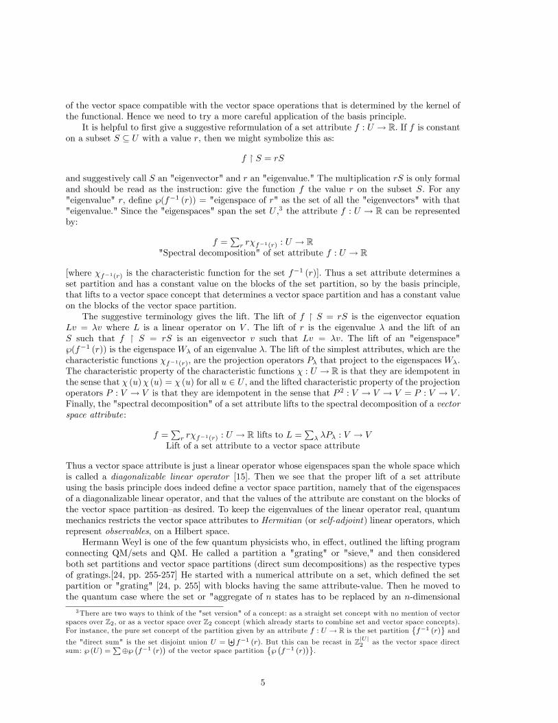
Figure 1: Set numerical attributes lift to linear operators

2.5 Lifting compatible attributes to commuting operators

Since two set attributes f : U → R and g : U ′ → R define two inverse image partitions{f−1 (r)

}and{

g−1 (s)}on their domains, we need to extend the concept of compatible partitions to the attributes

that define the partitions. That is, two attributes f : U → R and g : U ′ → R are compatible if theyhave the same domain U = U ′. We have previously lifted the notion of compatible set partitions tocompatible vector space partitions. Since real-valued set attributes lift to Hermitian linear operators,the notion of compatible set attributes just defined would lift to two linear operators being compatibleif their eigenspace partitions are compatible. It is a standard fact of QM math (e.g., [16, pp. 102-3] or[15, p. 177]) that two (Hermitian) linear operators L,M : V → V are compatible if and only if theycommute, LM = ML. Hence the commutativity of linear operators is the lift of the compatibility(i.e., defined on the same set) of set attributes. Thus the join of two eigenspace partitions is definediff the operators commute. Weyl already pointed this out: "Thus combination [join] of two gratings[vector space partitions] presupposes commutability...". [24, p. 257]

Given two compatible set attributes f : U → R and g : U → R, the join of their "eigenspace"partitions has as blocks the non-empty intersections f−1 (r) ∩ g−1 (s). Each block in the join ofthe "eigenspace" partitions could be characterized by the ordered pair of "eigenvalues" (r, s). An"eigenvector" of f , S ⊆ f−1 (r), and of g, S ⊆ g−1 (s), would be a "simultaneous eigenvector":S ⊆ f−1 (r) ∩ g−1 (s).

In the lifted case, two commuting Hermitian linear operator L andM have compatible eigenspacepartitions WL = {Wλ} (for the eigenvalues λ of L) and WM = {Wµ} (for the eigenvalues µ of M).The blocks in the join WL ∨ WM of the two compatible eigenspace partitions are the non-zerosubspaces {Wλ ∩Wµ} which can be characterized by the ordered pairs of eigenvalues (λ, µ). Thenonzero vectors v ∈ Wλ ∩Wµ are simultaneous eigenvectors for the two commuting operators, and

6

there is a basis for the space consisting of simultaneous eigenvectors.4

A set of compatible set attributes is said to be complete if the join of their partitions is discretein the sense that the blocks have cardinality 1. Each element of U is then characterized by theordered n-tuple (r, ..., s) of attribute values.

In the lifted case, a set of commuting linear operators is said to be complete if the join oftheir eigenspace partitions is nondegenerate, i.e., the blocks have dimension 1. The eigenvectors thatgenerate those one-dimensional blocks of the join are characterized by the ordered n-tuples (λ, ..., µ)of eigenvalues so the eigenvectors are usually denoted as the eigenkets |λ, ..., µ〉 in the Dirac notation.These Complete Sets of Commuting Operators are Dirac’s CSCOs [7].

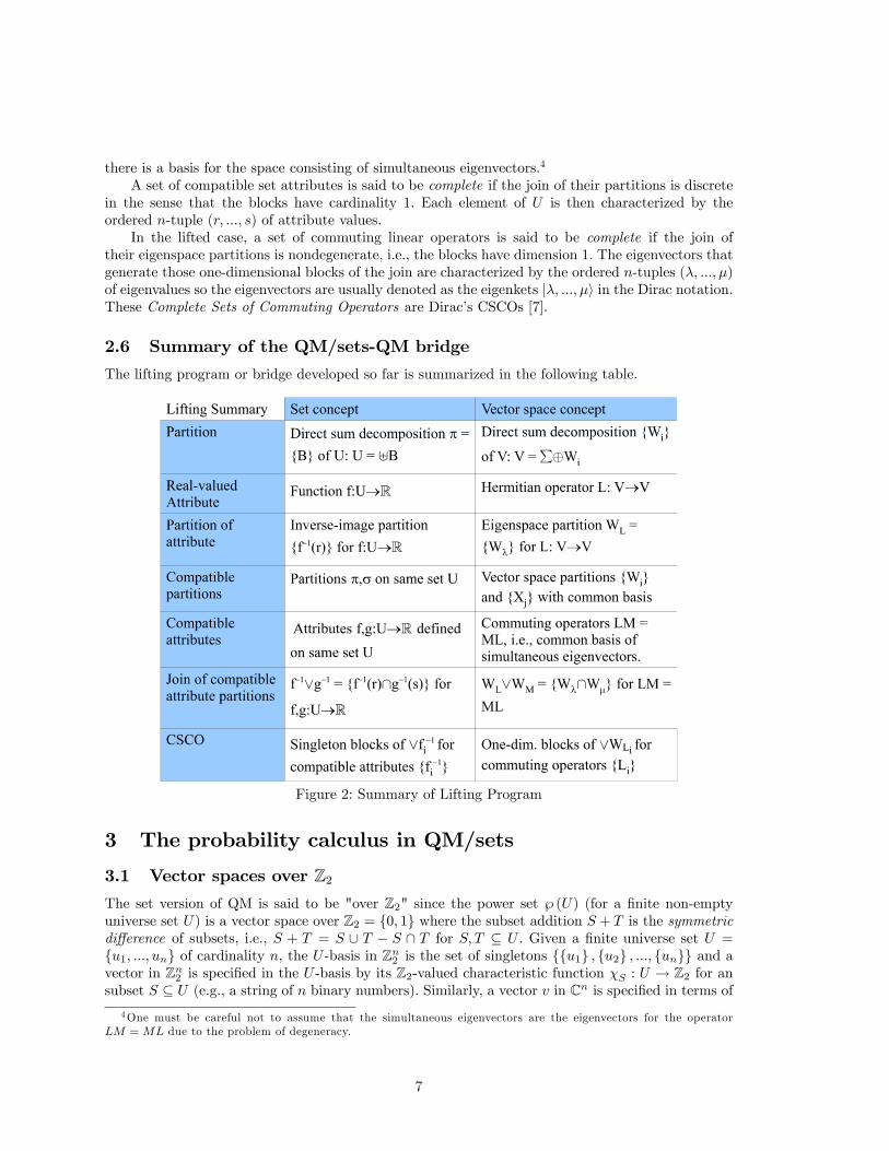
2.6 Summary of the QM/sets-QM bridge

The lifting program or bridge developed so far is summarized in the following table.

Figure 2: Summary of Lifting Program

3 The probability calculus in QM/sets

3.1 Vector spaces over Z2The set version of QM is said to be "over Z2" since the power set ℘ (U) (for a finite non-emptyuniverse set U) is a vector space over Z2 = {0, 1} where the subset addition S + T is the symmetricdifference of subsets, i.e., S + T = S ∪ T − S ∩ T for S, T ⊆ U . Given a finite universe set U ={u1, ..., un} of cardinality n, the U -basis in Zn2 is the set of singletons {{u1} , {u2} , ..., {un}} and avector in Zn2 is specified in the U -basis by its Z2-valued characteristic function χS : U → Z2 for ansubset S ⊆ U (e.g., a string of n binary numbers). Similarly, a vector v in Cn is specified in terms of

4One must be careful not to assume that the simultaneous eigenvectors are the eigenvectors for the operatorLM =ML due to the problem of degeneracy.

7

an orthonormal basis {|vi〉} by a C-valued function 〈_|v〉 : {vi} → C assigning a complex amplitude〈vi|v〉 to each basis vector. One of the key pieces of mathematical machinery in QM, namely theinner product, does not exist in vector spaces over finite fields but basis-dependent "brackets" canbe defined and a norm or absolute value can be defined to play a similar role in the probabilityalgorithm of QM/sets.5

Seeing ℘ (U) as the vector space Z|U |2 allows different bases in which the vectors can be expressed(as well as the basis-free notion of a vector as a ket, since only the bra is basis-dependent). Considerthe simple case of U = {a, b, c} where the U -basis is {a}, {b}, and {c}. But the three subsets{a, b}, {b, c}, and {a, b, c} also form a basis since: {a, b} + {a, b, c} = {c}; {b, c} + {c} = {b}; and{a, b} + {b} = {a}. These new basis vectors could be considered as the basis-singletons in anotherequicardinal universe U ′ = {a′, b′, c′} where a′ = {a, b}, b′ = {b, c}, and c′ = {a, b, c}. In the followingket table, each row is a ket of V = Z32 expressed in the U -basis, the U ′-basis, and a U ′′-basis.

U = {a, b, c} U ′ = {a′, b′, c′} U ′′ = {a′′, b′′, c′′}{a, b, c} {c′} {a′′, b′′, c′′}{a, b} {a′} {b′′}{b, c} {b′} {b′′, c′′}{a, c} {a′, b′} {c′′}{a} {b′, c′} {a′′}{b} {a′, b′, c′} {a′′, b′′}{c} {a′, c′} {a′′, c′′}∅ ∅ ∅

Vector space isomorphism: Z32 ∼= ℘ (U) ∼= ℘ (U ′) ∼= ℘ (U ′′) where row = ket.

3.2 The brackets

In a Hilbert space, the inner product is used to define the amplitudes 〈vi|v〉 and the norm |v| =√〈v|v〉, and the probability algorithm can be formulated using this norm. In a vector space over

Z2, the Dirac notation can still be used but in a basis-dependent form (like matrices as opposedto operators) that defines a real-valued norm even though there is no inner product. The kets |S〉for S ⊆ U are basis-free but the corresponding bras are basis-dependent. For u ∈ U , the "bra"〈{u}|U : ℘ (U)→ R is defined by the "bracket" :

〈{u} |US〉 =

{1 if u ∈ S0 if u /∈ S = χS (u)

Then 〈{ui} |U {uj}〉 = χ{uj} (ui) = χ{ui} (uj) = δij is the set-version of 〈vi|vj〉 = δij (for anorthonormal basis {|vi〉}). Assuming a finite U , the "bracket" linearly extends to the more generalbasis-dependent form (where |S| is the cardinality of S):

〈T |US〉 = |T ∩ S| for T, S ⊆ U .6

This basis principle can be run in reverse to "delift" a vector space concept to sets. Consider anorthonormal basis set {|vi〉} in a finite dimensional Hilbert space. Given two subsets T, S ⊆ {|vi〉}of the basis set, consider the unnormalized superpositions ψT =

∑|vi〉∈T |vi〉 and ψS =

∑|vi〉∈S |vi〉.

Then their inner product in the Hilbert space is 〈ψT |ψS〉 = |T ∩ S|, which "delifts" (crossing thebridge in the other direction) to 〈T |US〉 = |T ∩ S| for subsets T, S ⊆ U of the U -basis of Z|U |2 .

5Often scare quotes, as in "brackets," are used to indicate the named concept in QM/sets as opposed to fullQM—although this may also be clear from the context.

6Thus 〈T |US〉 = |T ∩ S| takes values outside the base field of Z2 just like the Hamming distance function |T + S|on vector spaces over Z2 in coding theory [18, p. 66] as applied to pairs of sets represented as binary strings.

8

3.3 Ket-bra resolution

The basis-dependent "ket-bra" |{u}〉 〈{u}|U is the "one-dimensional" projection operator:

|{u}〉 〈{u}|U = {u} ∩ () : ℘ (U)→ ℘ (U)

and the "ket-bra identity" holds as usual:∑u∈U |{u}〉 〈{u}|U =

∑u∈U ({u} ∩ ()) = I : ℘ (U)→ ℘ (U)

where the summation is the symmetric difference of sets in Zn2 . The overlap 〈T |US〉 can be resolvedusing the "ket-bra identity" in the same basis: 〈T |US〉 =

∑u 〈T |U {u}〉 〈{u} |US〉. Similarly a ket

|S〉 can be resolved in the U -basis;

|S〉 =∑u∈U |{u}〉 〈{u} |US〉 =

∑u∈U 〈{u} |US〉 |{u}〉 =

∑u∈U |{u} ∩ S| {u}

where a subset S ⊆ U is just expressed as the sum of the singletons {u} ⊆ S. That is ket-braresolution in sets. The ket |S〉 is the same as the ket |S′〉 for some subset S′ ⊆ U ′ in another U ′-basis, but when the basis-dependent bra 〈{u}|U is applied to the ket |S〉 = |S′〉, then it is the subsetS ⊆ U , not S′ ⊆ U ′, that comes outside the ket symbol | 〉 in 〈{u} |US〉 = |{u} ∩ S|.7

3.4 The norm

Then the (basis-dependent) U -norm ‖S‖U : ℘ (U) → R is defined, as usual, as the square root ofthe bracket:8

‖S‖U =√〈S|US〉 =

√|S|

for S ∈ ℘ (U) which is the set-version of the basis-free norm |ψ| =√〈ψ|ψ〉 (since the inner product

does not depend on the basis). Note that a ket has to be expressed in the U -basis to apply the basis-dependent definition so in the above example, ‖{a′}‖U =

√2 since {a′} = {a, b} in the U -basis.

3.5 The Born rule

For a specific basis {|vi〉} and for any nonzero vector v in a finite dimensional complex vectorspace, |v|2 =

∑i 〈vi|v〉 〈vi|v〉

∗ (∗ is complex conjugation) whose set version would be: ‖S‖2U =∑u∈U 〈{u} |US〉

2. Since

|v〉 =∑i 〈vi|v〉 |vi〉 and |S〉 =

∑u∈U 〈{u} |US〉 |{u}〉,

applying the Born rule by squaring the coeffi cients 〈vi|v〉 and 〈{u} |US〉 (and normalizing) gives theprobabilities of the eigen-elements vi or {u} given a state v or S in QM and QM/sets:∑

i〈vi|v〉〈vi|v〉∗|v|2 = 1 and

∑u〈{u}|US〉2‖S‖2U

=∑u|{u}∩S||S| = 1

where 〈vi|v〉〈vi|v〉∗

|v|2 is a ‘mysterious’quantum probability while 〈{u}|US〉2

‖S‖2U= |{u}∩S|

|S| is the unmysterious

Laplacian equal probability Pr ({u} |S) rule for getting u when sampling S.9

7The term "{u} ∩ S′" is not even defined since it is the intersection of subsets of two different universes. One ofthe luxuries of having a basis independent inner product in QM over C is being able to ignore bases in the bra-ketnotation.

8We use the double-line notation ‖S‖U for the norm of a set to distinguish it from the single-line notation |S| forthe cardinality of a set, whereas the customary absolute value notation for the norm of a vector in full QM is |v|.

9Note that there is no notion of a normalized vector in a vector space over Z2 (another consequence of the lack ofan inner product). The normalization is, as it were, postponed to the probability algorithm which is computed in therationals or reals.

9

3.6 Spectral decomposition on sets

An observable, i.e., a Hermitian operator, on a Hilbert space determines its home basis set of ortho-normal eigenvectors. In a similar manner, a real-valued attribute f : U → R defined on U has theU -basis as its "home basis set." As previously noted, the connection between the numerical attributesf : U → R of QM/sets and the Hermitian operators of QM is established by "seeing" the function fas a formal operator: f � () : ℘ (U)→ ℘ (U). Applied to the basis elements {u} ⊆ U , we may writef � {u} = f (u) {u} = r {u} as the set-version of an eigenvalue equation applied to an eigenvectorwhere the multiplication r {u} is only formal (read r {u} like the instructions: the function f takesthe value r on {u}). Then for any subset S ⊆ f−1 (r) where f is constant, we may also formally write:f � S = rS as an "eigenvalue equation" satisfied by all the "eigenvectors" S in the "eigenspace"℘(f−1 (r)

), a subspace of ℘ (U), for the "eigenvalue" r. Since f−1 (r) ∩ () : ℘ (U) → ℘ (U) is the

projection operator10 to the "eigenspace" ℘(f−1 (r)

)for the "eigenvalue" r, we have the spectral

decomposition for a Hermitian operator L =∑λ λPλ in QM and for a U -attribute f : U → R in

QM/sets:

L =∑λ λPλ : V → V and f � () =

∑r r(f−1 (r) ∩ ()

): ℘ (U)→ ℘ (U)

Spectral decomposition in QM and QM/sets.

When the base field increases from Z2 to R or C, then the formal multiplication r(f−1 (r) ∩ ()

)is internalized as an actual multiplication, and the projection operator f−1 (r)∩() on sets becomes aprojection operator on a vector space over R or C. Thus the operator representation L =

∑λ λPλ of

an observable numerical attribute is just the internalization of a numerical attribute made possibleby the enriched base field R or C. Similarly, the set brackets 〈T |US〉 taking values outside the basefield Z2 become internalized as an inner product with the same enrichment of the base field. It isthe comparative "poverty" of the base field Z2 that requires the QM/sets "brackets" to take "de-internalized" values outside the base field and for a formal multiplication to used in the operatorpresentation f � () =

∑r r(f−1 (r) ∩ ()

)of a numerical attribute f : U → R.11 Or put the other

way around, the only numerical attributes that can be internally represented in ℘ (U) ∼= Zn2 are thecharacteristic functions χS : U → Z2 that are internally represented in the U -basis as the projectionoperators S ∩ () : ℘ (U)→ ℘ (U).

3.7 Completeness and orthogonality of projection operators

The usual completeness and orthogonality conditions on eigenspaces also have set-versions in QMover Z2:

1. completeness:∑λ Pλ = I : V → V has the set-version:

∑r f−1 (r) ∩ () = I : ℘ (U) → ℘ (U),

and

2. orthogonality: for λ 6= λ′, PλPλ′ = 0 : V → V has the set-version: for r 6= r′,[f−1 (r) ∩ ()

] [f−1 (r′) ∩ ()

]=

∅ ∩ () : ℘ (U)→ ℘ (U).12

10Since ℘ (U) is now interpreted as a vector space, it should be noted that the projection operator T ∩ () : ℘ (U)→℘ (U) is not only idempotent but linear, i.e., (T ∩ S1) + (T ∩ S2) = T ∩ (S1 + S2). Indeed, this is the distributive lawwhen ℘ (U) is interpreted as a Boolean ring.11 In the engineering literature, eigenvalues are seen as "stretching or shrinking factors" but that is not their role in

QM. The whole machinery of eigenvectors [e.g., f � {u} = r {u}], eigenspaces [e.g., ℘(f−1 (r)

)], and eigenvalues [e.g.,

f(u) = r] is a way of representing a numerical attribute [e.g., f : U → R] inside a vector space that has a rich enoughbase field.12Note that in spite of the lack of an inner product, the orthogonality of projection operators S∩ () is perfectly well

defined in QM/sets where it boils down to the disjointness of subsets.

10

3.8 Measuring attributes on sets

The Pythagorean results (for the complete and orthogonal projection operators):

|v|2 =∑λ |Pλ (v)|2 and ‖S‖2U =

∑r

∥∥f−1 (r) ∩ S∥∥2U,

give the probabilities for measuring attributes. Since

|S| = ‖S‖2U =∑r

∥∥f−1 (r) ∩ S∥∥2U

=∑r

∣∣f−1 (r) ∩ S∣∣

we have in QM and in QM/sets:∑λ|Pλ(v)|2|v|2 = 1 and

∑r

‖f−1(r)∩S‖2U

‖S‖2U=∑r|f−1(r)∩S||S| = 1

where |Pλ(v)|2

|v|2 is the quantum probability of getting λ in an L-measurement of v while |f−1(r)∩S||S| has

the rather unmysterious interpretation of the probability Pr (r|S) of the random variable f : U → Rhaving the "eigen-value" r when sampling S ⊆ U . Thus the set-version of the Born rule is not someweird "quantum" notion of probability on sets but the perfectly ordinary Laplace-Boole rule for the

conditional probability |f−1(r)∩S||S| , given S ⊆ U , of a random variable f : U → R having the value r.

3.9 Contextuality

Given a ket |S〉, the probability of getting another ket |{a}〉 as an outcome of a measurement inQM/sets will depend on the context in terms of the measurement basis. In the previous ket table,comparing sets in the U -basis and U ′′-basis, we see that {a, b} = {b′′} (or in the ket notation:|{a, b}〉 = |{b′′}〉) and {a} = {a′′}. Taking S = {a, b}, the probability of getting {a} in a U -basismeasurement is: Pr ({a} |S) = | {a}∩{a, b} |/ |{a, b}| = 1/2. But taking the same ket |{a, b}〉 = |{b′′}〉as the given state and measuring in the U ′′-basis, the probability of getting the ket |{a}〉 = |{a′′}〉is: Pr ({a′′} | {b′′}) = |{a′′} ∩ {b′′}| / |{b′′}| = 0.

3.10 The objective indefiniteness interpretation

On top of the mathematics of QM/sets, there is an objective indefiniteness interpretation which isjust the set-version of the objective indefiniteness interpretation of QM developed elsewhere [10].The collecting-together of some elements u ∈ U into a subset S ⊆ U is interpreted as the super-position of the "eigen-elements" u ∈ S to form an "indefinite element" S (with the vector sumS =

∑u∈U 〈{u} |US〉 {u} in the vector space ℘ (U) over Z2 giving the superposition).13

The indefinite element S is being "measured" using the "observable" f where the probability

Pr (r|S) of getting the "eigenvalue" r is |f−1(r)∩S||S| and where the "damned quantum jump" goes

from S to the "projected resultant state" f−1 (r) ∩ S which is in the "eigenspace" ℘(f−1 (r)

)for

that "eigenvalue" r. That state represents a more-definite element f−1 (r) ∩ S that now has thedefinite f -value of r—so a second measurement would yield the same "eigenvalue" r and the samevector f−1 (r) ∩

[f−1 (r) ∩ S

]= f−1 (r) ∩ S using the idempotency of the set-version of projection

operators (all as in the standard Dirac-von-Neumann treatment of measurement). These questionsof interpretation will not be emphasized here where the focus is on the mathematical relationshipbetween QM/sets and full QM.

13 In logic, a choice function is a function ε() that applied to a non-empty subset S ⊆ U picks out an elementε (S) = u ∈ S (or equivalently a singleton ε (S) = {u} ⊆ S). The indeterminancy of a choice function is, as it were,where stochasticity enters QM. For finite sets, we might consider a probabilistic choice function that would pick outany element (or singleton) of S with the equal probability 1/ |S|. A (non-degenerate) "measurement" in QM/sets isa "physical" version of a probabilistic choice function; it goes from an indefinite element S to some definite element{u} ⊆ S with the probability 1/ |S|.

11

3.11 Summary of the probability calculus

These set-versions and more (the average value of an attribute is left to the reader) are summarizedin the following table for a finite U and a finite dimensional Hilbert space V with {|vi〉} as anyorthonormal basis.

Vector space over Z2: QM/sets Hilbert space case: QM over CProjections: S ∩ () : ℘ (U)→ ℘ (U) P : V → V

Spectral Decomp.: f � () =∑r r(f−1 (r) ∩ ()

)L =

∑λ λPλ

Compl.:∑r f−1 (r) ∩ () = I : ℘ (U)→ ℘ (U)

∑λ Pλ = I

Orthog.: r 6= r′,[f−1 (r) ∩ ()

] [f−1 (r′) ∩ ()

]= ∅ ∩ () λ 6= λ′, PλPλ′ = 0

Brackets: 〈S|UT 〉 = |S ∩ T | = overlap for S, T ⊆ U 〈ψ|ϕ〉 = "overlap" of ψ and ϕKet-bra:

∑u∈U |{u}〉 〈{u}|U =

∑u∈U ({u} ∩ ()) = I

∑i |vi〉 〈vi| = I

Resolution: 〈S|UT 〉 =∑u 〈S|U {u}〉 〈{u} |UT 〉 〈ψ|ϕ〉 =

∑i 〈ψ|vi〉 〈vi|ϕ〉

Norm: ‖S‖U =√〈S|US〉 =

√|S| where S ⊆ U |ψ| =

√〈ψ|ψ〉

Pythagoras: ‖S‖2U =∑u∈U 〈{u} |US〉

2= |S| |ψ|2 =

∑i 〈vi|ψ〉

∗ 〈vi|ψ〉Laplace: S 6= ∅,

∑u∈U

〈{u}|US〉2‖S‖2U

=∑u∈S

1|S| = 1 |ψ〉 6= 0,

∑i〈vi|ψ〉∗〈vi|ψ〉

|ψ|2 = |〈vi|ψ〉|2|ψ|2 = 1

Born: |S〉 =∑u∈U 〈{u} |US〉 |{u}〉, Pr (u|S) = 〈{u}|US〉2

‖S‖2U|ψ〉 =

∑i 〈vi|ψ〉 |vi〉, Pr (vi|ψ) = |〈vi|ψ〉|2

|ψ|2

‖S‖2U =∑r

∥∥f−1 (r) ∩ S∥∥2U

=∑r

∣∣f−1 (r) ∩ S∣∣ = |S| |ψ|2 =

∑λ |Pλ (ψ)|2

S 6= ∅,∑r

‖f−1(r)∩S‖2U

‖S‖2U=∑r|f−1(r)∩S||S| = 1 |ψ〉 6= 0,

∑λ|Pλ(ψ)|2|ψ|2 = 1

Measurement: Pr(r|S) =‖f−1(r)∩S‖2

U

‖S‖2U=|f−1(r)∩S||S| Pr (λ|ψ) = |Pλ(ψ)|2

|ψ|2

Average of attribute: 〈f〉S = 〈S|Uf�()|S〉〈S|US〉 〈L〉ψ = 〈ψ|L|ψ〉

〈ψ|ψ〉 .Probability mathematics for QM over Z2 and for QM over C

4 Measurement in QM/sets

4.1 Measurement as partition join operation

In QM/sets, numerical attributes f : U → R can be considered as equiprobable random variableson a set of outcomes U . The inverse images of attributes (or random variables) define set partitions{f−1 (r)

}on the set of outcomes U . Considered abstractly, the partitions on a set U are partially

ordered by refinement where a partition π = {B} refines a partition σ = {C}, written σ � π, if forany block B ∈ π, there is a block C ∈ σ such that B ⊆ C. The principal logical operation neededhere is the partition join: π ∨ σ is the partition whose blocks are the non-empty intersections B ∩Cfor B ∈ π and C ∈ σ.

Each partition π can be represented as a binary relation dit (π) ⊆ U×U on U where the orderedpairs (u, u′) in dit (π) are the distinctions or dits of π in the sense that u and u′ are in distinct blocksof π. These dit sets dit (π) as binary relations might be called "partition relations" but they are alsothe "apartness relations" in computer science. An ordered pair (u, u′) is an indistinction or indit ofπ if u and u′ are in the same block of π. The set of indits, indit (π), as a binary relation is just theequivalence relation associated with the partition π.

In the duality between the ordinary Boolean logic of subsets (usually mis-specified as "proposi-tional logic") and the logic of partitions ([9] or [11]), the elements of a subset and the distinctionsof a partition are dual concepts. The partial ordering of subsets in the powerset Boolean algebra℘ (U) is the inclusion of elements and the refinement ordering of partitions on U is just the inclusionof dit sets, i.e., σ � π iff dit (σ) ⊆ dit (π). The partial ordering in each case is a lattice wherethe top of the Boolean lattice is the subset U of all possible elements and the top of the lattice of

12

partitions is the discrete partition 1 = {{u}}u∈U of singletons which makes all possible distinctions:dit (1) = U ×U −∆ (where ∆ = {(u, u) : u ∈ U} is the diagonal). The bottom of the Boolean latticeis the empty set ∅ of no elements and the bottom of the lattice of partitions is the indiscrete partition(or blob) 0 = {U} which makes no distinctions.

The two lattices can be illustrated in the case of U = {a, b, c}.

Figure 3: Subset and partition lattices

In the correspondences between QM/sets and QM, a block in a partition on U [i.e., a vector in℘ (U)] corresponds to pure state in QM (a state vector in a quantum state space), and a partitionon U can be thought of as a mixture of orthogonal pure states with the probabilities given by theprobability calculus on QM/sets. Given a "pure state" S ⊆ U , the possible results of a non-degenerateU -measurement are the blocks of the discrete partition {{u}}u∈S on S with each singleton beingequiprobable. Each such measurement would have one of the potential "eigenstates" {u} ∈ S as theactual result.

In QM, measurements make distinctions that turn a pure state into a mixture. The abstractessentials of measurement are represented in QM/sets as a distinction-creating processes of turning a"pure state" S into a "mixed state" partition on S (with "distinctions" as defined above in partitionlogic). The distinction-creating process of "measurement" in QM/sets is the partition join of theindiscrete partition {S} (taking S as the universe) and the inverse-image partition

{f−1 (r)

}of the

numerical attribute f : U → R restricted to S. Again Weyl gets it right. Weyl refers to a partition asa "grating" or "sieve" and then notes that "Measurement means application of a sieve or grating"[24, p. 259], e.g., the application (i.e., join) of the set-grating

{f−1 (r)

}to the "pure state" {S} to

give the "mixed state"{S ∩ f−1 (r)

}.

4.2 Nondegenerate measurement

In the simple example illustrated below, we start at the one block or "state" of the indiscretepartition or blob which is the completely indistinct element {a, b, c}. A measurement always usessome attribute that defines an inverse-image partition on U = {a, b, c}. In the case at hand, there are"essentially" four possible attributes that could be used to "measure" the indefinite element {a, b, c}(since there are four partitions that refine the blob).

For an example of a "nondegenerate measurement," consider any attribute f : U → R which hasthe discrete partition as its inverse image, such as the ordinal number of a letter in the alphabet:f (a) = 1, f (b) = 2, and f (c) = 3. This attribute or "observable" has three "eigenvectors": f �{a} = 1 {a}, f � {b} = 2 {b}, and f � {c} = 3 {c} with the corresponding "eigenvalues." The"eigenvectors" are {a}, {b}, and {c}, the blocks in the discrete partition of U . Starting in the "purestate" S = {a, b, c}, a U -measurement using the observable f gives the "mixed state":

{U} ∨{f−1 (r)

}= 0 ∨ 1 = 1.

13

Each such measurement would return an "eigenvalue" r with the probability of Pr (r|S) =|f−1(r)∩S||S| =

13 .

A "projective measurement" makes distinctions in the measured "state" that are suffi cient toinduce the "quantum jump" or "projection" to the "eigenvector" associated with the observed "eigen-value." If the observed "eigenvalue" was 3, then the "state" {a, b, c} "projects" to f−1 (3)∩{a, b, c} ={c} ∩ {a, b, c} = {c} as pictured below.

Figure 4: "Nondegenerate measurement"

It might be emphasized that this is an objective state reduction (or "collapse of the wave packet")from the single indefinite element {a, b, c} to the single definite element {c}, not a subjective removalof ignorance as if the "state" had all along been {c}. For instance, Pascual Jordan in 1934 arguedthat:

the electron is forced to a decision. We compel it to assume a definite position; previously,in general, it was neither here nor there; it had not yet made its decision for a definiteposition... . ... [W]e ourselves produce the results of the measurement. (quoted in [17, p.161])

This might be illustrated using Weyl’s notion of a partition as a "sieve or grating" [24, p. 259]that is applied in a measurement. We might think of a grating as a series of regular polygonal shapesthat might be imposed on an indefinite blob of dough. In a measurement, the blob of dough fallsthrough one of the polygonal holes with equal probability and then takes on that shape.

Figure 5: Measurement as randomly giving an indefinite blob of dough a regular polygonal shape.

14

4.3 Degenerate measurements

For an example of a "degenerate measurement," we choose an attribute with a non-discrete inverse-image partition such as π = {{a} , {b, c}}. Hence the attribute could just be the characteristic func-tion χ{b,c} with the two "eigenspaces" ℘({a}) and ℘({b, c}) and the two "eigenvalues" 0 and 1 respec-tively. Since one of the two "eigenspaces" is not a singleton of an eigen-element, the "eigenvalue" of 1is a set version of a "degenerate eigenvalue." This attribute χ{b,c} has four (non-zero) "eigenvectors":χ{b,c} � {b, c} = 1 {b, c}, χ{b,c} � {b} = 1 {b}, χ{b,c} � {c} = 1 {c}, and χ{b,c} � {a} = 0 {a}.

The "measuring apparatus" makes distinctions by "joining" the "observable" partition

χ−1{b,c} ={χ−1{b,c} (1) , χ−1{b,c} (0)

}= {{b, c} , {a}}

with the "pure state" which is the single block representing the indefinite element S = U = {a, b, c}.A measurement apparatus of that "observable" returns one of "eigenvalues" with certain probabili-ties:

Pr(0|S) = |{a}∩{a,b,c}||{a,b,c}| = 1

3 and Pr (1|S) = |{b,c}∩{a,b,c}||{a,b,c}| = 2

3 .

Suppose it returns the "eigenvalue" 1. Then the indefinite element {a, b, c} "jumps" to the"projection" χ−1{b,c} (1) ∩ {a, b, c} = {b, c} of the "state" {a, b, c} to that "eigenvector" [5, p. 221].

Since this is a "degenerate" result (i.e., the "eigenspaces" don’t all have "dimension" one),another measurement is needed to make more distinctions. Measurements by attributes that giveeither of the other two partitions, {{a, b} , {c}} or {{b} , {a, c}}, suffi ce to distinguish {b, c} into {b}or {c}, so either attribute together with the attribute χ{b,c} would form a complete set of compatibleattributes (i.e., the set version of a CSCO). The join of the two attributes’ partitions gives thediscrete partition. Taking the other attribute as χ{a,b}, the join of the two attributes’partitions isdiscrete:

χ−1{b,c} ∨ χ−1{a,b} = {{a} , {b, c}} ∨ {{a, b} , {c}} = {{a} , {b} , {c}} = 1.

Hence all the "eigenstate" singletons can be characterized by the ordered pairs of the "eigenvalues"of these two "observables": {a} = |0, 1〉, {b} = |1, 1〉, and {c} = |1, 0〉 (using Dirac’s ket-notation togive the ordered pairs).

The second "projective measurement" of the indefinite "superposition" element {b, c} using theattribute χ{a,b} with the "eigenspace" partition χ

−1{a,b} = {{a, b} , {c}} would induce a jump to either

{b} or {c} with the probabilities:

Pr (1| {b, c}) = |{a,b}∩{b,c}||{b,c}| = 1

2 and Pr (0| {b, c}) = |{c}∩{b,c}||{b,c}| = 1

2 .

If the measured "eigenvalue" is 0, then the "state" {b, c} "projects" to χ−1{a,b} (0) ∩ {b, c} = {c} aspictured below.

Figure 6: "Degenerate measurement"

15

The two "projective measurements" of {a, b, c} using the complete set of compatible (both definedon U) attributes χ{b,c} and χ{a,b} produced the respective "eigenvalues" 1 and 0, and the resulting"eigenstate" was characterized by the "eigenket" |1, 0〉 = {c}.

5 "Time" evolution in QM/sets

The different "de-internalized" treatment of the "brackets" in QM/sets gives a probability calculus,unlike Schumacher and Westmoreland’s "modal quantum theory." [20] But both theories agree thatevolution of the quantum states over Z2 is given by non-singular linear transformations. Thesetransformations are, of course, reversible like the unitary transformations of full QM but "unitary" isnot defined in the absence of an inner product. QM/sets nevertheless has basis-dependent "brackets"and those "brackets" are preserved if we change the basis along with the non-singular transformation.Let A : Zn2 → Zn2 be a non-singular transformation where the images of the U -basis A |{u}〉 are takenas the basis vectors {u′} of a U ′-basis. Then for S, T ⊆ U , we have the following preservation of the"brackets":

〈T |US〉 = 〈AT |AUAS〉 = 〈T ′|U ′S′〉

where AT = T ′ ⊆ U ′ and AS = S′ ⊆ U ′.In the objective indefiniteness interpretation of QM based on partition logic [10], von Neu-

mann’s type 1 processes (measurements) and type 2 processes (unitary evolution) [23] are modeledrespectively as the processes that make distinctions or that preserve the degree of distinctness 〈ϕ|ψ〉between quantum states. That characterization of evolution carries over to QM/sets since it is pre-cisely the non-singular transformations that preserve distinctness of QM/sets quantum states, i.e.,distinctness of non-zero vectors in Zn2 .

6 Interference without waves in QM/sets

The role of the "waves" in ordinary quantum mechanics can be further clarified by viewing quantumdynamics in QM/sets. In QM over C, suppose the Hamiltonian H has an orthonormal basis ofenergy eigenstate {|Ej〉}. Then the application of the propagation operator U (t) from t = 0 to timet applied to |ψ0〉 =

∑j cj |Ej〉 has the action:

U (t) |ψ0〉 = |ψt〉 = eiHt |ψ0〉 =∑j cje

iHt |Ej〉 =∑j cje

iEjt |Ej〉.

Thus U (t) transforms the orthonormal basis {|Ej〉} into the orthonormal basis{∣∣E′j⟩} =

{eiEjt |Ej〉

}.

Even though this unitary transformation introduces different relative phases for the different en-ergy eigenstates in U (t) |ψ0〉, the probabilities for an energy measurement do not change since|cj |2 =

∣∣cjeiEjt∣∣2. The effects of time evolution show when the evolved state U (t) |ψ0〉 is measuredin another basis {|ak〉}. Suppose for each j, |Ej〉 =

∑k α

jk |ak〉 so that:

U (t) |ψ0〉 = |ψt〉 =∑j cje

iEjt |Ej〉 =∑j cje

iEjt∑k α

jk |ak〉 =

∑k

(∑j cje

iEjtαjk

)|ak〉.

Then under time evolution, there is interference in the coeffi cient∑j cje

iEjtαjk of each eigenstate|ak〉. Since the complex exponentials eiEjt can be mathematically interpreted as "waves," this is theinterference characteristic of wave-like behavior in the evolution of the quantum state |ψ0〉.

But there is interference without waves in QM/sets where many of the characteristic phenomenaof QM can nevertheless be reproduced (see later sections on the two-slit experiment and Bell’sTheorem). Suppose we start with a state S ⊆ U = {u1, ..., un} which is represented in the U -basis as |S〉 =

∑j 〈uj |US〉 |uj〉 =

∑j bj |uj〉 where 〈uj |US〉 = bj ∈ Z2. Then the "dynamics" of a

16

nonsingular transformation A : Zn2 → Zn2 takes the basis {|uj〉} to another basis{∣∣u′j⟩} which is

the set version of U (t) taking the orthonormal basis {|Ej〉} to the orthonormal basis{∣∣E′j⟩} where∣∣E′j⟩ = eiEjt |Ej〉. Thus |S〉 is transformed, by linearity, into |S′〉 =

∑j bj

∣∣u′j⟩ with the same bj’sso that Pr (uj |S) =

b2j|S| =

b2j|S′| = Pr

(u′j |S′

)and 〈S|UT 〉 = 〈S′|U ′T ′〉 (where for T ⊆ U , A |T 〉 = |T ′〉

for some T ′ ⊆ U ′). But the state |S′〉 =∑j bj

∣∣u′j⟩ could be measured in another U ′′-basis {∣∣u′′j ⟩}where

∣∣u′j⟩ =∑k α

jk |u′′k〉 so that:

A |S〉 = |S′〉 =∑j bj

∣∣u′j⟩ =∑j bj

∑k α

jk |u′′k〉 =

∑k

(∑j bjα

jk

) ∣∣u′′j ⟩.Then under time evolution, there is interference in the coeffi cient

∑j bjα

jk of each eigenstate

∣∣u′′j ⟩.This suffi ces to give the interference phenomena that are ordinarily seen as characteristic of wave-likebehavior but there is not even the mathematics of waves in QM/sets. The mathematics of waves(complex exponentials eiϕ) comes into the mathematics of quantum mechanics only over C; evenreal exponentials either grow or decay but don’t behave as waves.

The following table summarizes the results using the minimal superpositions: |S〉 = b1 |u1〉 +b2 |u2〉 and |ψ0〉 = c1 |E1〉+ c2 |E2〉.

QM/sets QM

|uj〉A→∣∣u′j⟩ |Ej〉

U→∣∣E′j⟩ = eigjt |Ej〉

|S〉 = b1 |u1〉+ b2 |u2〉 → b1 |u′1〉+ b2 |u′2〉 |ψ0〉 = c1 |E1〉+ c2 |E2〉 → c1 |E′1〉+ c2 |E′2〉∣∣u′j⟩ =∑k

⟨u′′k |U ′′u′j

⟩|u′′k〉 =

∑k α

jk |u′′k〉 |Ej〉 =

∑k α

jk |ak〉;

∣∣E′j⟩ = eigjt∑k α

jk |ak〉

b1 |u1〉+ b2 |u2〉 →∑k

(b1α

1k + b2α

2k

)|u′′k〉 c1 |E1〉+ c2 |E2〉 →

∑k

(c1e

ig1tα1k + c2eig2tα2k

)|ak〉

Table showing the role in interference in QM/sets and in QM

Thus QM/sets allows us to tease the QM behavior due to interference apart from the specificallywave-version of that interference in QM over C. The root of the interference is superposition, i.e.,the different j’s in the coeffi cients

∑j cje

iEjtαjk in QM or∑j bjα

jk in QM/sets, and superposition is

the mathematical representation of indefiniteness. It is indefiniteness that is the basic feature, and aparticle in a superposition state for a certain observable will have the evolution of that indefinitenessexpressed by coeffi cients

∑j cje

iEjtαjk using complex exponentials (i.e., the mathematics of waves)so the indefiniteness will then appear as "wave-like" behavior.

7 Double-slit experiment in QM/sets

QM/sets represents the logical essence of full QM without any of the physical assumptions. Henceto delift the double-slit experiment to QM/sets, we need to imagine the elements of some U -basisas say "positions" and an non-singular matrix A as giving the dynamic evolution for one "time"period.

Consider the dynamics given in terms of the U -basis where: {a} → {a, b}; {b} → {a, b, c}; and{c} → {b, c} in one time period. This is represented by the non-singular one-period change of statematrix:

A =

〈{a} |U {a, b}〉 〈{a} |U {a, b, c}〉 〈{a} |U {b, c}〉〈{b} |U {a, b}〉 〈{b} |U {a, b, c}〉 〈{b} |U {b, c}〉〈{c} |U {a, b}〉 〈{c} |U {a, b, c}〉 〈{c} |U {b, c}〉

=

1 1 01 1 10 1 1

.If we take the U -basis vectors as "vertical position" eigenstates, we can device a QM/sets version

of the double-slit experiment which models "all of the mystery of quantum mechanics" [12, p. 130].Taking {a}, {b}, and {c} as three vertical positions, we have a vertical diaphragm with slits at {a}and {c}. Then there is a screen or wall to the right of the slits so that a "particle" will travel fromthe diaphragm to the wall in one time period according to the A-dynamics.

17

Figure 7: Two-slit setup

We start with or prepare the state of a "particle" being at the slits in the indefinite positionstate {a, c}. Then there are two cases.

First case of distinctions at slits: The first case is where we measure the U -state at the slitsand then let the resultant position eigenstate evolve by the A-dynamics to hit the wall at the rightwhere the position is measured again. The probability that the particle is at slit 1 or at slit 2 is:

Pr ({a} at slits | {a, c} at slits) = 〈{a}|U{a,c}〉2‖{a,c}‖2U

= |{a}∩{a,c}||{a,c}| = 1

2 ;

Pr ({c} at slits | {a, c} at slits) = 〈{c}|U{a,c}〉2‖{a,c}‖2U

= |{c}∩{a,c}||{a,c}| = 1

2 .

If the particle was at slit 1, i.e., was in eigenstate {a}, then it evolves in one time period by theA-dynamics to {a, b} where the position measurements yield the probabilities of being at {a} or at{b} as:

Pr ({a} at wall | {a} at slits) = Pr ({a} at wall | {a, b} at wall) = 〈{a}|U{a,b}〉2‖{a,b}‖2U

= |{a}∩{a,b}||{a,b}| = 1

2 ,

Pr ({b} at wall | {a} at slits) = Pr ({b} at wall | {a, b} at wall) = 〈{b}|U{a,b}〉2‖{a,b}‖2U

= |{b}∩{a,b}||{a,b}| = 1

2 .

If on the other hand the particle was found in the first measurement to be at slit 2, i.e., was ineigenstate {c}, then it evolved in one time period by the A-dynamics to {b, c} where the positionmeasurements yield the probabilities of being at {b} or at {c} as:

Pr ({b} at wall | {c} at slits) = Pr ({b} at wall | {b, c} at wall) = |{b}∩{b,c}||{b,c}| = 1

2 ,

Pr ({c} at wall | {c} at slits) = Pr ({c} at wall | {b, c} at wall) = |{c}∩{b,c}||{b,c}| = 1

2 .

Hence we can use the laws of probability theory to compute the probabilities of the particle beingmeasured at the three positions on the wall at the right if it starts at the slits in the superpositionstate {a, c} and the measurements were made at the slits:

Pr({a} at wall | {a, c} at slits) = 1212 = 1

4 ;Pr({b} at wall | {a, c} at slits) = 1

212 + 1

212 = 1

2 ;Pr({c} at wall | {a, c} at slits) = 1

212 = 1

4 .

18

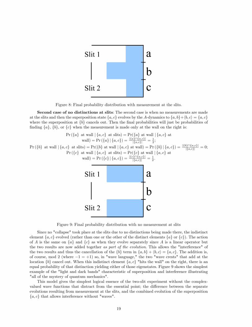
Figure 8: Final probability distribution with measurement at the slits.

Second case of no distinctions at slits: The second case is when no measurements are madeat the slits and then the superposition state {a, c} evolves by the A-dynamics to {a, b}+〈b, c〉 = {a, c}where the superposition at {b} cancels out. Then the final probabilities will just be probabilities offinding {a}, {b}, or {c} when the measurement is made only at the wall on the right is:

Pr ({a} at wall | {a, c} at slits) = Pr({a} at wall | {a, c} atwall) = Pr ({a} | {a, c}) = |{a}∩{a,c}|

|{a,c}| = 12 ;

Pr ({b} at wall | {a, c} at slits) = Pr({b} at wall | {a, c} at wall) = Pr ({b} | {a, c}) = |{b}∩{a,c}||{a,c}| = 0;

Pr ({c} at wall | {a, c} at slits) = Pr({c} at wall | {a, c} atwall) = Pr ({c} | {a, c}) = |{c}∩{a,c}|

|{a,c}| = 12 .

Figure 9: Final probability distribution with no measurement at slits

Since no "collapse" took place at the slits due to no distinctions being made there, the indistinctelement {a, c} evolved (rather than one or the other of the distinct elements {a} or {c}). The actionof A is the same on {a} and {c} as when they evolve separately since A is a linear operator butthe two results are now added together as part of the evolution. This allows the "interference" ofthe two results and thus the cancellation of the {b} term in {a, b}+ 〈b, c〉 = {a, c}. The addition is,of course, mod 2 (where −1 = +1) so, in "wave language," the two "wave crests" that add at thelocation {b} cancel out. When this indistinct element {a, c} "hits the wall" on the right, there is anequal probability of that distinction yielding either of those eigenstates. Figure 9 shows the simplestexample of the "light and dark bands" characteristic of superposition and interference illustrating"all of the mystery of quantum mechanics".

This model gives the simplest logical essence of the two-slit experiment without the complex-valued wave functions that distract from the essential point; the difference between the separateevolutions resulting from measurement at the slits, and the combined evolution of the superposition{a, c} that allows interference without "waves".

19

8 Entanglement in QM/sets

A QM concept that generates much interest is entanglement. Hence it might be useful to considerentanglement in QM/sets.

First we need to establish the connections across the set-vector-space bridge by lifting the setnotion of the direct (or Cartesian) product X × Y of two sets X and Y . Using the basis principle,we apply the set concept to the two basis sets {v1, ..., vm} and {w1, ..., wn} of two vector spacesV and W (over the same base field) and then we see what it generates. The set direct product ofthe two basis sets is the set of all ordered pairs (vi, wj), which we will write as vi ⊗ wj , and thenwe generate the vector space, denoted V ⊗W , over the same base field from those basis elementsvi ⊗ wj . That vector space is the tensor product, and it is not in general the direct product V ×Wof the vector spaces. The cardinality of X × Y is the product of the cardinalities of the two sets,and the dimension of the tensor product V ⊗W is the product of the dimensions of the two spaces(while the dimension of the direct product V ×W is the sum of the two dimensions).

A vector z ∈ V ⊗W is said to be separated if there are vectors v ∈ V and w ∈ W such thatz = v⊗w; otherwise, z is said to be entangled. Since vectors delift to subsets, a subset S ⊆ X×Y issaid to be separated or a product if there exists subsets SX ⊆ X and SY ⊆ Y such that S = SX×SY ;otherwise S ⊆ X × Y is said to be entangled. In general, let SX be the support or projection of Son X, i.e., SX = {x : ∃y ∈ Y, (x, y) ∈ S} and similarly for SY . Then S is separated iff S = SX ×SY .

For any subset S ⊆ X×Y , whereX and Y are finite sets, a natural measure of its "entanglement"can be constructed by first viewing S as the support of the equiprobable or Laplacian joint probabilitydistribution on S. If |S| = N , then define Pr (x, y) = 1

N if (x, y) ∈ S and Pr (x, y) = 0 otherwise.The marginal distributions14 are defined in the usual way:

Pr (x) =∑y Pr (x, y)

Pr (y) =∑x Pr (x, y).

A joint probability distribution Pr (x, y) on X × Y is independent if for all (x, y) ∈ X × Y ,

Pr (x, y) = Pr (x) Pr (y).Independent distribution

Otherwise Pr (x, y) is said to be correlated.

Proposition 1 A subset S ⊆ X×Y is "entangled" iff the equiprobable distribution on S is correlated(non-independent).

Proof: If S is "separated", i.e., S = SX × SY , then Pr (x) = |SY |/N for x ∈ SX and Pr (y) =|SX | /N for y ∈ SY where |SX | |SY | = N . Then for (x, y) ∈ S,

Pr (x, y) = 1N = N

N2 = |SX ||SY |N2 = Pr (x) Pr (y)

and Pr(x, y) = 0 = Pr (x) Pr (y) for (x, y) /∈ S so the equiprobable distribution is independent.If S is "entangled," i.e., S 6= SX × SY , then S $ SX × SY so let (x, y) ∈ SX × SY − S. ThenPr (x) ,Pr (y) > 0 but Pr (x, y) = 0 so it is not independent, i.e., is correlated. �

Consider the set version of one qubit space where U = {a, b}. The product set U × U has 15nonempty subsets. Each factor U of U × U has 3 nonempty subsets so 3 × 3 = 9 of the 15 subsetsare separated subsets leaving 6 entangled subsets.

14The marginal distributions are the set versions of the reduced density matrices of QM.

20

S ⊆ U × U{(a, a) , (b, b)}{(a, b) , (b, a)}

{(a, a) , (a, b), (b, a)}{(a, a) , (a, b), (b, b)}{(a, b), (b, a) , (b, b)}{(a, a), (b, a) , (b, b)}

The six entangled subsets

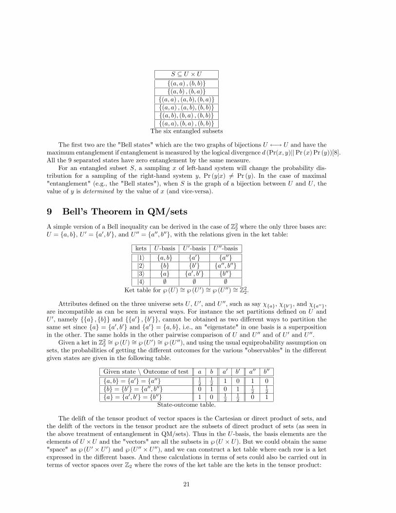
The first two are the "Bell states" which are the two graphs of bijections U ←→ U and have themaximum entanglement if entanglement is measured by the logical divergence d (Pr(x, y)||Pr (x) Pr (y))[8].All the 9 separated states have zero entanglement by the same measure.

For an entangled subset S, a sampling x of left-hand system will change the probability dis-tribution for a sampling of the right-hand system y, Pr (y|x) 6= Pr (y). In the case of maximal"entanglement" (e.g., the "Bell states"), when S is the graph of a bijection between U and U , thevalue of y is determined by the value of x (and vice-versa).

9 Bell’s Theorem in QM/sets

A simple version of a Bell inequality can be derived in the case of Z22 where the only three bases are:U = {a, b}, U ′ = {a′, b′}, and U ′′ = {a′′, b′′}, with the relations given in the ket table:

kets U -basis U ′-basis U ′′-basis

|1〉 {a, b} {a′} {a′′}|2〉 {b} {b′} {a′′, b′′}|3〉 {a} {a′, b′} {b′′}|4〉 ∅ ∅ ∅

Ket table for ℘ (U) ∼= ℘ (U ′) ∼= ℘ (U ′′) ∼= Z22.

Attributes defined on the three universe sets U , U ′, and U ′′, such as say χ{a}, χ{b′}, and χ{a′′},are incompatible as can be seen in several ways. For instance the set partitions defined on U andU ′, namely {{a} , {b}} and {{a′} , {b′}}, cannot be obtained as two different ways to partition thesame set since {a} = {a′, b′} and {a′} = {a, b}, i.e., an "eigenstate" in one basis is a superpositionin the other. The same holds in the other pairwise comparison of U and U ′′ and of U ′ and U ′′.

Given a ket in Z22 ∼= ℘ (U) ∼= ℘ (U ′) ∼= ℘ (U ′′), and using the usual equiprobability assumption onsets, the probabilities of getting the different outcomes for the various "observables" in the differentgiven states are given in the following table.

Given state \ Outcome of test a b a′ b′ a′′ b′′

{a, b} = {a′} = {a′′} 12

12 1 0 1 0

{b} = {b′} = {a′′, b′′} 0 1 0 1 12

12

{a} = {a′, b′} = {b′′} 1 0 12

12 0 1

State-outcome table.

The delift of the tensor product of vector spaces is the Cartesian or direct product of sets, andthe delift of the vectors in the tensor product are the subsets of direct product of sets (as seen inthe above treatment of entanglement in QM/sets). Thus in the U -basis, the basis elements are theelements of U ×U and the "vectors" are all the subsets in ℘ (U × U). But we could obtain the same"space" as ℘ (U ′ × U ′) and ℘ (U ′′ × U ′′), and we can construct a ket table where each row is a ketexpressed in the different bases. And these calculations in terms of sets could also be carried out interms of vector spaces over Z2 where the rows of the ket table are the kets in the tensor product:

21

Z22 ⊗ Z22 ∼= ℘ (U × U) ∼= ℘ (U ′ × U ′) ∼= ℘ (U ′′ × U ′′).

Since {a} = {a′, b′} = {b′′} and {b} = {b′} = {a′′, b′′}, the subset {a} × {b} = {(a, b)} ⊆ U × Uis expressed in the U ′ ×U ′-basis as {a′, b′} × {b′} = {(a′, b′) , (b′, b′)}, and in the U ′′ ×U ′′-basis it is{b′′} × {a′′, b′′} = {(b′′, a′′) , (b′′, b′′)}. Hence one row in the ket table has:

{(a, b)} = {(a′, b′) , (b′, b′)} = {(b′′, a′′) , (b′′, b′′)}.

Since the full ket table has 16 rows, we will just give a partial table that suffi ces for our calculations.

U × U U ′ × U ′ U ′′ × U ′′

{(a, a)} {(a′, a′) , (a′, b′) , (b′, a′) , (b′, b′)} {(b′′, b′′)}{(a, b)} {(a′, b′) , (b′, b′)} {(b′′, a′′) , (b′′, b′′)}{(b, a)} {(b′, a′) , (b′, b′)} {(a′′, b′′) , (b′′, b′′)}{b, b} {(b′, b′)} {(a′′, a′′) , (a′′, b′′) , (b′′, a′′) , (b′′, b′′)}

{(a, a) , (a, b)} {(a′, a′) , (b′, a′)} {(b′′, a′′)}{(a, a) , (b, a)} {(a′, a′) , (a′, b′)} {(a′′, b′′)}{(a, a) , (b, b)} {(a′, a′) , (a′, b′) , (b′, a′)} {(a′′, a′′) , (a′′, b′′) , (b′′, a′′)}{(a, b) , (b, a)} {(a′, b′) , (b′, a′)} {(a′′, b′′) , (b′′, a′′)}

Partial ket table for ℘ (U × U) ∼= ℘ (U ′ × U ′) ∼= ℘ (U ′′ × U ′′)

As before, we can classify each subset as separated or entangled and we can furthermore seehow that is independent of the basis. For instance {(a, a) , (a, b)} is separated since:

{(a, a) , (a, b)} = {a} × {a, b} = {(a′, a′) , (b′, a′)} = {a′, b′} × {a′} = {(b′′, a′′)} = {b′′} × {a′′}.

An example of an entangled state is:

{(a, a) , (b, b)} = {(a′, a′) , (a′, b′) , (b′, a′)} = {(a′′, a′′) , (a′′, b′′) , (b′′, a′′)}.

Taking this entangled state as the initial state, the probability of getting the state {a} by performinga U -basis measurement on the left-hand system is:

Pr ({(a,−)} | {(a, a) , (b, b)}) = |{(a,a)}||{(a,a),(b,b)}| = 1

2 .

The probability of getting the state {a′} by performing a U ′-basis measurement on the left-handsystem is:

Pr ({(a′,−)} | {(a′, a′) , (a′, b′) , (b′, a′)}) =|{(a′,a′),(a′,b′)}|

|{(a′,a′),(a′,b′),(b′,a′)}| = 23 .

The probability of getting the state {a′′} by performing a U ′′-basis measurement on the left-handsystem is:

Pr ({(a′′,−)} | {(a′′, a′′) , (a′′, b′′) , (b′′, a′′)}) =|{(a′′,a′′),(a′′,b′′)}|

|{(a′′,a′′),(a′′,b′′),(b′′,a′′)}| = 23 .

The probability of each of these outcomes occurring (if each is done instead of either of theothers) is the product of the probabilities. Then there is a probability distribution on U × U ′ × U ′′where:

Pr (a, a′, a′′)= Pr ({(a,−)} | {(a, a) , (b, b)})

×Pr ({(a′,−)} | {(a′, a′) , (a′, b′) , (b′, a′)})×Pr ({(a′′,−)} | {(a′′, a′′) , (a′′, b′′) , (b′′, a′′)})

= 122323 = 2

9 .

22

In this way, a probability distribution Pr (x, y, z) is defined on U × U ′ × U ′′.A Bell inequality can be obtained from this joint probability distribution over the outcomes

U ×U ′×U ′′ of measuring these three incompatible attributes [6]. Consider the following marginals:

Pr (a, a′) = Pr (a, a′, a′′) + Pr (a, a′, b′′)XPr (b′, b′′) = Pr (a, b′, b′′)X+ Pr (b, b′, b′′)

Pr (a, b′′) = Pr (a, a′, b′′)X+ Pr (a, b′, b′′)X.

The two terms in the last marginal are each contained in one of the two previous marginals (asindicated by the check marks) and all the probabilities are non-negative, so we have the followinginequality:

Pr (a, a′) + Pr (b′, b′′) ≥ Pr (a, b′′)Bell inequality.

All this has to do with measurements on the left-hand system. But the "Bell state" is left-right symmetrical so the same probabilities would be obtained if we used a right-hand systemmeasurement:

Pr ({(a,−)} | {(a, a) , (b, b)}) = Pr ({(−, a)} | {(a, a) , (b, b)}) = 12 ;

Pr ({(b,−)} | {(a, a) , (b, b)}) = Pr ({(−, b)} | {(a, a) , (b, b)}) = 12 ;

Pr ({(a′,−)} | {(a′, a′) , (a′, b′) , (b′, a′)}) = Pr ({(−, a′)} | {(a′, a′) , (a′, b′) , (b′, a′)}) = 23 ;

Pr ({(b′,−)} | {(a′, a′) , (a′, b′) , (b′, a′)}) = Pr ({(−, b′)} | {(a′, a′) , (a′, b′) , (b′, a′)}) = 13 ;

Pr ({(a′′,−)} | {(a′′, a′′) , (a′′, b′′) , (b′′, a′′)}) = Pr ({(−, a′′)} | {(a′′, a′′) , (a′′, b′′) , (b′′, a′′)}) = 23 ;

andPr ({(b′′,−)} | {(a′′, a′′) , (a′′, b′′) , (b′′, a′′)}) = Pr ({(−, b′′)} | {(a′′, a′′) , (a′′, b′′) , (b′′, a′′)}) = 1

3 .15

This is analogous to the assumption that each sock in a pair of socks will have the same properties.[1,Chap. 16] Hence the right-hand measurements give the same probability distribution and the sameinequality.

But there is an alternative interpretation to the probabilities Pr (x, y), Pr (y, z), and Pr (x, z)if we assume that the outcome of a measurement on the right-hand system is independent of theoutcome of the same measurement on the left-hand system. Then Pr (a, a′) is the probability ofa U -measurement on the left-hand system giving {a} and then in addition (not instead of) a U ′-measurement on the right-hand system giving {a′}, and so forth.

This is a crucial step in the argument so it worth being very clear using subscripts.

• Step 1: Pr (a, a′)1 is the probability of getting {a} in a left U -measurement and getting {a′} ifinstead a left U ′-measurement was made so:

Pr (a, a′)1 = Pr ({(a,−)} | {(a, a) , (b, b)})× Pr ({(a′,−)} | {(a′, a′) , (a′, b′) , (b′, a′)}) = 1223 = 1

3 .

• Step 2: Pr (a, a′)2 is the probability of getting {a} in a left U -measurement and getting {a′} ifinstead a right U ′-measurement was made so:

Pr (a, a′)2 = Pr ({(a,−)} | {(a, a) , (b, b)})× Pr ({(−, a′)} | {(a′, a′) , (a′, b′) , (b′, a′)}) = 1223 = 1

3 .

• Step 3: Pr (a, a′)3 is the probability of getting {a} in a left U -measurement and, under theassumption of independence of the left-right measurements, also (not instead of) getting {a′}in a right U ′-measurement:

Pr (a, a′)3 = Pr ({(a,−)} | {(a, a) , (b, b)})× Pr ({(−, a′)} | {(a′, a′) , (a′, b′) , (b′, a′)}) = 1223 = 1

3 .

15The same holds for the other "Bell state": {(a, b) , (b, a)}.

23

Hence the joint probability distribution would be the same and the above Bell inequality:

Pr (a, a′)3 + Pr (b′, b′′)3 ≥ Pr (a, b′′)3

would still hold under the independence assumption using the step 3 probabilities in all cases. But wecan use QM/sets to compute the probabilities for those different measurements on the two systemsto see if the independence assumption is compatible with QM/sets.

To compute Pr (a, a′)3, we first measure the left-hand component in the U -basis. Since {(a, a) , (b, b)}is the given state, and (a, a) and (b, b) are equiprobable, the probability of getting {a} (i.e., the"eigenvalue" 1 for the "observable χ{a}) is

12 . But the right-hand system is then in the state {a}

and the probability of getting {a′} (i.e., "eigenvalue" 0 for the "observable" χ{b′}) is12 (as seen in

the state-outcome table). Thus the probability is Pr (a, a′)3 = 1212 = 1

4 .To compute Pr (b′, b′′)3, we first perform a U ′-basis "measurement" on the left-hand component

of the given state {(a, a) , (b, b)} = {(a′, a′) , (a′, b′) , (b′, a′)}, and we see that the probability ofgetting {b′} is 1

3 . Then the right-hand system is in the state {a′} and the probability of getting{b′′} in a U ′′-basis "measurement" of the right-hand system in the state {a′} is 0 (as seen from thestate-outcome table). Hence the probability is Pr (b′, b′′)3 = 0.

Finally we compute Pr (a, b′′)3 by first making a U -measurement on the left-hand component ofthe given state {(a, a) , (b, b)} and get the result {a} with probability 1

2 . Then the state of the secondsystem is {a} so a U ′′-measurement will give the {b′′} result with probability 1 so the probability isPr (a, b′′)3 = 1

2 .Then we plug the probabilities into the Bell inequality:

Pr (a, a′)3 + Pr (b′, b′′)3 ≥ Pr (a, b′′)314 + 0 � 1

2Violation of Bell inequality.

The violation of the Bell inequality shows that the independence assumption about the measurementoutcomes on the left-hand and right-hand systems is incompatible with QM/sets. This result issomewhat less striking in QM/sets than in full QM since QM/sets just shows the bare logic of theBell argument in the simplest space Z22 without any dramatic physical assumption like a space-likeseparation between the left-hand and right-hand systems.

Part II

Quantum information and computationtheory in QM/sets10 Quantum information theory in QM/sets

10.1 Logical entropy

Obtaining quantum information theory for QM/sets is not a simple matter of delifting the ordinaryquantum information theory (QIT). This is because much of QIT is obtained by carrying over thenotion of Shannon entropy from classical information theory (which is then renamed "von Neumannentropy"). Shannon entropy is a higher-level concept adapted for questions of coding and communi-cation; it is not a basic logical concept. Classical information theory itself needs to be refounded ona logical basis using the logical notion of entropy that arises naturally out of partition logic (that is

24

dual to the usual Boolean subset logic). That logical information theory can then be simply refor-mulated using delifted machinery from QM, namely density matrices, and thus logical informationtheory is reformulated as quantum information theory for QM/sets.

The process is quite analogous to the way that classical logical finite probability was reformulatedas the probability calculus for QM/sets. Conceptually, the "next step" beyond subset logic was logicalfinite probability theory. Historically, Boole presented logical finite probability theory as the nextstep beyond subset logic in his book entitled: An Investigation of the Laws of Thought on which arefounded the Mathematical Theories of Logic and Probabilities. The universe U was the finite numberof possible outcomes and the subsets were events. Quoting Poisson, Boole defined "the measure ofthe probability of an event [as] the ratio of the number of cases favourable to that event, to the totalnumber of cases favourable and unfavourable, and all equally possible." [4, p. 253]

Hence one obvious next step beyond partition logic is to make the analogous conceptual movesand to see what theory emerges. The theory that emerges is a logical version of information theory.

For a finite U , the finite (Laplacian) probability Pr(S) of a subset ("event") is the normalizedcounting measure on the subset: Pr(S) = |S| / |U |. Analogously, the finite logical entropy h (π) ofa partition π is the normalized counting measure of its dit set: h (π) = |dit (π)| / |U × U |. If U isan urn with each "ball" in the urn being equiprobable, then Pr(S) is the probability of an elementrandomly drawn from the urn is an element in S, and, similarly, h (π) is the probability that a pairof elements randomly drawn from the urn (with replacement) is a distinction of π.

Let π = {B1, ..., Bm} with pi = |Bi| / |U | being the probability of drawing an element of theblock Bi. The number of indistinctions (non-distinctions) of π is |indit (π)| = Σi |Bi|2 so the numberof distinctions is |dit (π)| = |U |2 − Σi |Bi|2 and thus since Σipi = 1, the logical entropy of π is:

h (π) =[|U |2 − Σi |Bi|2

]/ |U |2 = 1− Σip

2i = (Σipi)− Σip

2i = Σipi (1− pi), so that:

Logical entropy: h (π) = Σipi (1− pi).

Shannon’s notion of entropy is a high-level notion adapted to communications theory [21]. TheShannon entropy H (π) of the partition π (with the same probabilities assigned to the blocks) is:

Shannon entropy: H (π) = Σipi log (1/pi)

where the log is base 2.Each entropy can be seen as the probabilistic average of the "block entropies" h (Bi) = 1 − pi

and H (Bi) = log (1/pi). To interpret the block entropies, consider a special case where pi = 1/2n

and every block is the same so there are 2n equal blocks like Bi in the partition. The logical entropyof that special equal-block partition, Σipi (1− pi) = (2n) pi (1− pi) = (2n) (1/2n) (1− pi) = 1− pi,is the:

Logical block entropy: h(Bi) = 1− pi.

Instead of directly counting the distinctions, we could take the number of binary equal-blockedpartitions it takes to distinguish all the 2n blocks in that same partition. As in the game of "twentyquestions," if there is a search for an unknown designated block, then each such binary questioncan reduce the number of blocks by a power of 2 so the minimum number of binary partitionsit takes to distinguish all the 2n blocks (and find the hidden block no matter where it was) isn = log (2n) = log (1/pi), which is the:

Shannon block entropy: H (Bi) = log (1/pi).

To precisely relate the block entropies, we solve each for pi which is then eliminated to obtain:

h (B) = 1−(1/2H(B)

).

Exact relation between Shannon and logical block entropies

25

The interpretation of the Shannon block entropy is then extended by analogy to the general casewhere 1/pi is not a power of 2 so that the Shannon entropy H (π) = ΣipiH (Bi) is then interpreted asthe average number of binary partitions needed to make all the distinctions between the blocks of π–whereas the logical entropy is still the exact normalized count h (π) = Σipih (Bi) = |dit (π)| / |U × U |of the distinctions of the partition π.

The two notions of entropy boil down to two different ways to count the distinctions of apartition. Thus the concept of a distinction from partition logic provides a logical basis for thenotion of entropy in information theory.16

10.2 Density matrices in QM/sets

The notion of logical entropy generalizes naturally to quantum information theory where it alsoprovides a new foundational notion of entropy based on the idea of information as distinctions thatare preserved in unitary transformations and made objectively in measurements.[10] Our purposehere is to formulate logical entropy using the delifted notion of density matrices which gives QIT/sets,and which then foreshadows how the "classical" logical information theory can be lifted to give anew foundation for the full QIT. The previous treatment of measurement in QM/sets can also bereformulated using density matrices and logical entropy.

Given a partition π = {B} on U = {u1, ..., un}, the blocks B ∈ π can be thought of as (nonover-lapping or "orthogonal") "pure states" where the "state" B occurs with the probability pB = |B|

|U | .Then we can mimic the usual procedure for forming the density matrix ρ (π) for the "orthogonalpure states" B with the probabilities pB . The (normalized) "pure state" B is represented by thecolumn vector |B〉 =

[√q1,√q2, ...,

√qn]twhere qj = 1/ |B| if uj ∈ B, and qj = 0 otherwise. Then

the density matrix ρ (B) for the pure state B ⊆ U is then (calculating in the reals):

ρ (B) = |B〉 (|B〉)t = |B〉 〈B| =

√q1√q2...√qn

[√q1,√q2, ...,√qn] =

q1

√q1q2 · · · √q1qn√

q2q1 q2 · · · √q2qn...

.... . .

...√qnq1

√qnq2 · · · qn

.For instance if U = {u1, u2, u3} = {a, b, c} then for the blocks in the partition π = {{a, b} , {c}}:

ρ ({a, b}) =

12 12 0

12

12 0

0 0 0

and ρ ({c}) =

0 0 00 0 00 0 1

.Then the "mixed state" density matrix ρ (π) of the partition π is the weighted sum:

ρ (π) =∑B∈π pBρ (B).

In the example, this is:

ρ (π) = 23

12 12 0

12

12 0

0 0 0

+ 13

0 0 00 0 00 0 1

=

13 13 0

13

13 0

0 0 13

.While this construction mimics the usual construction of the density matrix for orthogonal purestates, the remarkable thing is that the entries have a direct interpretation in terms of the dits andindits of the partition π:

16For further development of logical information theory, see Ellerman [8].

26

ρjk (π) =

{ 1|U | if (j, k) ∈ indit (π)

0 if (j, k) ∈ dit (π) .

All the entries are real "amplitudes" whose squares are the two-draw probabilities of drawing a pairof elements from U (with replacement) that is an indistinction of π. To foreshadow the quantum

case, the non-zero entries ρjk (π) =√

1|U |

1|U | = 1

|U | indicate that uj and uk "cohere" together in

a block or "pure state" of the partition, i.e., are an indit of the partition. Since the ordered pairs(uj , uj) in the diagonal ∆ ⊆ U×U are always indits of any partition, the diagonal entries in ρ (π) arealways 1

|U | . After interchanging some rows and the corresponding columns, the density matrix ρ (π)

would be a block-diagonal matrix with the blocks corresponding to the blocks B of the partition π.The quantum logical entropy of a density matrix ρ in full QM is: h (ρ) = 1 − tr

[ρ2], and the

logical entropy of a set partition π with equiprobable points is h (π) = 1−∑B∈π p

2B . The following

proposition shows that the above defined density matrix ρ (π) in QM/sets was the right definition.

Proposition 2 h (π) = 1− tr[ρ (π)

2].

Proof: The proof is simplified if we assume that rows and columns have been interchanged so thatρ (π) is a block-diagonal matrix with the submatrix-blocks corresponding to the blocks of partitionπ. If ui ∈ B ∈ π,then the ith diagonal element of the squared matrix ρ (π)

2 is 1|U |

1|U | + ... + 1

|U |1|U |

(|B| times) or|B|(

1|U |

)2and that diagonal element will occur |B| times. Hence the trace (sum of

diagonal elements) is:

tr[ρ (π)

2]

=∑B∈π |B| × |B| 1

|U |2 =∑B∈π

(|B||U |

)2=∑B∈π p

2B

so h (π) = 1−∑B p

2B equals the delifted quantum version: h (ρ (π)) = 1− tr

[ρ (π)

2]. �

The logical entropy h (π) of a partition is interpreted as the total two-draw probability of

drawing a distinction of the partition π. Hence by the above proposition, tr[ρ (π)

2]is the to-

tal probability of drawing an indistinction of π. For a pure state, we have the logical entropy

h (ρ (B)) = 1 − tr[ρ (B)

2]

= 0 since the sum of the indistinction probabilities tr[ρ (B)

2]is 1

(all pairs are indistinctions in a pure state) while in the general "mixed state" of a partition π (with

"orthogonal pure state" blocks B ∈ π), tr[ρ (π)

2]is the sum of the indistinction probabilities.

All this carries over from QM/sets to full QM where it provides an interpretation of the entriesin a density matrix. Let ρ =

∑mi=1 λi |ψi〉 〈ψi| be an n × n density matrix in its orthogonal decom-

position so the non-negative eigenvalues λi sum to one and the eigenvectors ψi are orthonormal. Let{|j〉 : j = 1, ..., n} be an orthonormal eigenvector basis for the whole space so that ψi =

∑j αij |j〉

and∑j αijα

∗ij = 1 where both sums can be taken as only over the j such that |j〉 has the eigenvalue

λi (since αij = 0 elsewhere). Previously the square ρjk (π)2 was the two-draw probability for the

ordered pair of indices (j, k) if they are in the same block, i.e., are indits of π, otherwise ρjk (π) = 0.Similarly, the absolute square ρjkρ

∗jk of that j, k entry of ρ is nonzero only if |j〉 and |k〉 are in

the same pure state ψi so those probabilities can be interpreted as the coherence probabilities for(|j〉 , |k〉) cohering together in the same pure state ψi. That is,

ρjkρ∗jk = λiαijα

∗ikλiα

∗ijαik = ρjjρkk

which is the probability of getting the ordered pair of eigenvectors (|j〉 , |k〉) in a pair of indepen-dent nondegenerate measurements in the {|j〉} basis—if |j〉 and |k〉 cohere together in the samepure state ψi. Thus in full QM, tr

[ρ2]is the total coherence probability while the logical entropy

h (ρ) = 1 − tr[ρ2]is the total decoherence probability. For a pure state, there are no distinctions

27

or decoherence, so the logical entropy is 0 in both cases. The following table then summarizes thelifting-delifting relationship between the density matrix ρ (π) of a partition in QM/sets and (theorthogonal decomposition presentation of) a density matrix ρ in QM.

Density matrix: ρ (π) in QM over sets ρ =∑i λi |ψi〉 〈ψi| in QM over C

Disjoint blocks: B ∈ π Orthogonal eigenvectors: |ψi〉Block probabilities: pB = |B|

|U | Eigenvalues of ρ: λiPoint probabilities: 1

|U | λiαijα∗ij = ρjj

Pure state matrix: ρ (B) = |B〉 〈B| ρ (ψi) = |ψi〉 〈ψi|Density matrix: ρ (π) =

∑B∈π pBρ (B) ρ =

∑i λiρ (ψi)

Prob. (j, k) if indit of π: ρjk (π)2

= 1/ |U |2 Coherence prob.: ρjkρ∗jk = ρjjρkk

Logical entropy: h (ρ (π)) = 1− tr[ρ (π)

2]

h (ρ) = 1− tr[ρ2]

h (ρ (π)) = total distinction probability h (ρ) = total decoherence prob.Pure state: h (ρ (Bi)) = 0 (no dits) h (ρ (ψi)) = 0 (no decoherence)

Density matrices QM/sets and in QM

Previously we formulated a probability calculus for QM/sets and then noted that it was justthe usual logical finite probability theory (in a "non-commutative" version) so that reflects back togive a better understanding of the usual probability calculus in full QM. Now we have formulatedthe notion of density matrices in QM/sets, and then we noted that it was just a reformulation oflogical information theory using the density matrix formalism. Then that reflects back to full QMso that we can now provide an interpretation of the off-diagonal entries in a density matrix ρ ascoherence probabilities (like the indistinction probabilities in the set case). And then the quantumlogical entropy is the total decoherence probability.

10.3 Density matrices and expectations

Given an attribute f : U = {u1, ..., un} → R, the matrix representing this attribute in QM/sets is:

f =

f(1) 0 · · · 0

0 f (2) · · · 0...

.... . .

...0 0 · · · f (n)

.Given a subset S ⊆ U , the "density matrix" for that state has, with some column and row

interchanges, a constant |S| × |S| block with the values 1/ |S| and zeros elsewhere:

ρ (S) =

1|S| · · ·

1|S| 0 · · · 0

.... . .

......

. . ....

1|S| · · ·

1|S| 0 · · · 0

0 · · · 0 0 · · · 0...

. . ....

.... . .

...0 · · · 0 0 · · · 0

.

Then, as in full QM, we have the result that the average value of an operator f in a state given bya density matrix ρ (S) is the trace of the product fρ (S):

tr [fρ (S)] = 1|S|∑u∈S f (u) = 1

|S|∑u∈U f (u) 〈S|U {u}〉 〈{u} |US〉

= 1|S| 〈S|Uf � ()

∑u |{u}〉 〈{u}|U |S〉 = 〈S|Uf�()|S〉

〈S|US〉 = 〈f〉Swhere f � |{u}〉 = f (u) |{u}〉 and

∑u |{u}〉 〈{u}|U = I.

28

10.4 Measuring measurement in QM/sets

A real-valued "observable" is a set attribute f : U → R which defines an inverse-image partition{f−1 (r)

}. Recall from the logic of partitions that the blocks of the join π ∨ σ of two partitions

π = {B} and σ = {C} are the non-empty intersections B ∩ C. This action of the join operationcould be considered as a set of projection operators {B ∩ ()}B∈π acting on the blocks C ∈ σ—or on asingle subset S ⊆ U . The partition f−1 =

{f−1 (r)

}acts as a set of projection operators f−1 ∨ () ={

f−1 (r) ∩ ()}on the "pure-state" S to partition it into the parts f−1 ∨ (S) =

{f−1 (r) ∩ S

}.

What is the "law of motion" to describe the change in the density matrix resulting from ameasurement? Given the density matrix ρ (S) of the "pure state" S, the density matrix ρ̂ (S) resultingfrom the measurement of the observable f is the "mixed state" density matrix ρ (π) for the partitiongiven by the join operation π = f−1 ∨ (S). Thus the "law of motion" is the join operation onpartitions. That is the canonical way that distinctions are made to move to a more refined partition.

Let’s put the previous measurement of the state S = U using the non-degenerate attributef(a) = 1, f(b) = 2, and f(c) = 3 in this form using density matrices. The pre-measurement densitymatrix is the previous ρ (U), the constant matrix with all entries 1/3. The three projection operatorsto the eigenspaces of the f -attribute in the U -basis are now:

P1 =

1 0 00 0 00 0 0

, P2 =

0 0 00 1 00 0 0

, and P3 =

0 0 00 0 00 0 1

instead of

{f−1 (r) ∩ ()

}r=1,2,3

in the non-matrix version. Hence the "density matrix" for the projec-

tion to the eigenspace for λ = 1 is obtained by first projecting the state P1 |U〉 (like f−1 (1)∩ (U) ={a} in the non-matrix version) and then forming the "density matrix"

(P1 |U〉) (P1 |U〉)t = P1 |U〉 〈U |P1 = P1ρ (U)P1 = P1

1√31√31√3

[ 1√3

1√3

1√3

]P1

= P1

13 13

13

13

13

13

13

13

13

P1 =

13 13

13

0 0 00 0 0

P1 =

13 0 00 0 00 0 0

so doing the same for the other eigenvalues and summing gives the mixed state density matrix ρ̂ (U)that results from the measurement:

ρ̂ (U) =∑3i=1 Pi |U〉 〈U |Pi =

13 0 00 1

3 00 0 1

3

.The main result is that this standard diagonal density matrix representing the result of a non-degenerate measurement is the density matrix ρ (π) of the partition formed by the join-action:

π = f−1 ∨ (U) = {{a} , {b} , {c}} ∨ {a, b, c} = {{a} , {b} , {c}} = 1.

Since it was a non-degenerate measurement, all the distinctions were made so all the off-diagonalterms are 0. Each of the off-diagonal terms was "decohered" by the nondegenerate measurement sothe post-measurement "amplitude" of (i, j) still "cohering" is 0. The density matrix version of the

ρ (U)measurement−→ ρ̂ (U) = ρ

(f−1 ∨ (U)

)Measurement as join-action

29

allows us, as usual, to state the general result of a measurement without assuming a particularoutcome.17

The general result is that the logical entropy increase resulting from a measurement is the sumof the new distinction probabilities created by the join, which is the sum of the squared amplitudesof the off-diagonal indistinction amplitudes in the density matrix that were zeroed or "decohered"by the measurement.

In the example, the six off-diagonal amplitudes of 13 were all zeroed so the change in logical

entropy is: 6×(13

)2= 6

9 = 23 .

ρ (U) =

13 13

13

13

13

13

13

13

13

measurement−→ ρ̂ (U) =

13 0 00 1

3 00 0 1

3

.In terms of sets, there are no distinctions in the indiscrete partition 0 = {U} so h (0) = |dit(0)|

|U×U | = 0.

Measurement by a non-degenerate attribute f gives the discrete partition 1 = f−1 ∨ (U) where thedistinctions are the ordered pairs (a, b), (a, c), and (b, c) together with the three opposite orderedpairs (b, a), (c, a), and (c, b) so the logical entropy is h (1) = |dit(1)|

|U×U | = 69 = 2

3 . Those ordered pairs

correspond exactly to off-diagonal terms zeroed in the transition ρ (U)→ ρ̂ and h (1) = 1− tr[ρ̂2]

=

1−(19 + 1

9 + 19

)= 2

3 .In this manner, the density matrices of QM/sets capture the set-based operations of logical

information theory, and that, in turn, shows how to interpret the density matrices of full QM interms of coherence and decoherence probabilities. The usual notion of von Neumann entropy inquantum information theory provides no such information-theoretic term-by-term interpretation ofdensity matrices, not to mention of the process of measurement. In this manner, QM/sets shows,from the information-theoretic viewpoint, the essence at the logical level of what is going on inthe full QM, i.e., QM/sets shows the "logic" of QM. The further development of the "classical" orquantum information theory using logical entropy is beyond the scope of this introductory paper [8].

11 Quantum computation theory in QM/sets

11.1 Qubits over 2 and non-singular gates

In QM over C, a quantum bit or qubit is a non-zero (normalized) vector in C2. A standard ortho-normal basis is denoted |0〉 and |1〉 so a qubit can be any (normalized) superposition α |0〉+β |1〉 forα, β ∈ C. In QM/sets, i.e., QM over Z2, a qubit over 2 or qubit/ 2 is any non-zero vector in Z22 whichfor a given basis |0〉 and |1〉 would have the form α |0〉 + β |1〉 for α, β ∈ Z2. As previously noted,Schumacher and Westmoreland (S&W) [20] restrict their treatment of Dirac’s brackets to take valuesin the base field of Z2 which precludes a probability calculus so they develop a modal interpretation(0 = impossible and 1 = possible). Hence they call a non-zero vector in Z22 a "mobit" and call theresulting theory "modal quantum theory." Since our different treatment of the brackets yields a fullprobability calculus in QM/sets, we will not use the "modal" terminology but, nevertheless, their"mobit" is the same as our "qubit/2."

In C2, there is a continuum of qubits α |0〉+β |1〉 for α, β ∈ C but in Z22, there are only 3 qubits/2,namely |0〉, |1〉, and |0〉+ |1〉. Hence a qubit/2 can be seen as the simplest possible extension beyondthe classical bit with the two possibilities |0〉 and |1〉 by adding the superposition |0〉 + |1〉.18 As17Note that this set-version of "decoherence" means actual reduction of state, not a "for all practical purposes" or

FAPP [2] reduction.18Here we are following the mild conceptual sloppiness common in the field of referring to any binary option as

a "classical bit" when the bit as defined in Shannon’s information theory is an equiprobable binary option. Thecomparable notion in logical information theory is a distinction or dit of a partition π on U which is defined as anordered pair (u, u′) elements distinguished by π in the sense of the elements being in distinct blocks of π.

30

already noted in our treatment of Bell’s Theorem in QM/sets, there are only three basis sets for Z22;any two of non-zero vectors are a basis with the third as their superposition.

In QM/sets (as in S&W’s modal quantum theory), the dynamics are given by non-singulartransformations which may be represented as non-singular zero-one matrices (which have non-zerodeterminants mod 2). A qubit over 2, α |0〉 + β |1〉, is represented in the standard basis |0〉 and |1〉by the column vector [α, β]t.

The non-singular transformations are the gates that may be used in an algorithm for quantumcomputing over 2 (QC/2). The two one-qubit gates that carry over from quantum computing overC are the:

identity I =

[1 00 1

]and negation X =

[0 11 0

].

The four other one-qubit/2 gates in QC/2 are non-singular but when interpreted as matrices in C2are not unitary. In particular, there is no requirement that a gate preserves the norm of a vector.One one-qubit/2 gate puts |0〉 into the superposition |0〉+ |1〉 and leaves |1〉 the same:

H0 =

[1 01 1

].

Similarly another one-qubit/2 gate puts |1〉 into the superposition and leaves |0〉 the same:

H1 =

[1 10 1

].

And finally the other two one-qubit/2 gates are their negations:

XH0 =

[0 11 0

] [1 01 1

]=

[1 11 0

]and XH1 =

[0 11 0

] [1 10 1

]=

[0 11 1

].

These six one-qubit/2 gates are the only non-singular transformations Z22 → Z22.As we will see below, some problems like the simplest Deutsch problem of determining if a single-

variable Boolean function is balanced or constant can be solved in QC/2 solely with one-qubit/2gates, whereas the usual solution to that problem in quantum computing over C uses two-qubit gates(four dimensional matrices). This is not as paradoxical as it may seem if we recall that quantumcomputing over 2 allows non-singular gates whereas the gates over C have to be unitary.

In representing these gates in the standard basis, we will use the standard Alice-Bob conventionthat the first or top one-qubit/2 (on the left) belongs to Alice and the second or bottom one-qubit/2(on the right) belongs to Bob so the four basis vectors are: |0A〉⊗|0B〉 = |0A0B〉, |0A〉⊗|1B〉 = |0A1B〉,|1A〉 ⊗ |0B〉 = |1A0B〉, and |1A〉 ⊗ |1B〉 = |1A1B〉 (they are arranged in that order in the columnvectors).

One two-qubit gate that carries over from quantum computing over C is the controlled negationgate:

CnotA =

1 0 0 00 1 0 00 0 0 10 0 1 0

which may be represented as acting on Alice’s top line and Bob’s bottom line:

→ • →|

→ ⊕ →.

31

The action of a gate is specified by how it acts on the basis vectors. For either case |0A0B〉 and|0A1B〉 where Alice’s qubit/2 is |0A〉, the gate acts like the identity. But in the cases |1A0B〉 and|1A1B〉 where Alice’s qubit/2 is |1A〉, then Bob’s qubit/2 is negated so that |1A0B〉 → |1A1B〉 and|1A1B〉 → |1A0B〉. In this case, Alice’s qubit/2 is said to be the controlling qubit/2 (indicated bythe subscript on CnotA) and Bob’s the target qubit/2.

The controlling and target roles are reversed in the gate:

CnotB =

1 0 0 00 0 0 10 0 1 00 1 0 0

represented as → ⊕→|→ • →

where if Bob’s qubit/2 is |0B〉, then it acts like the identity, but if Bob’s qubit/2 is |1B〉, then Alice’squbit/2 is negated.

In a two-qubit/2 system, if a one-qubit/2 gate is to be applied to only one line, then tensorproduct of matrices is used. For instance to apply H0 only to Bob’s line, the two-qubit/2 gate is:

I ⊗H0 =

1 0 0 01 1 0 00 0 1 00 0 1 1

represented as −→→ H0 →

.

11.2 Teleportation of a qubit/2 with 1 classical bit

S&W’s treatment [20] of the no-cloning theorem and superdense coding would work the same inQC/2 so we will not repeat it here. But after their treatment of superdense coding (of two classicalbits), they remark: "The same set of entangled mobit states and single-mobit transformations canalso be used to accomplish the MQT analogue of quantum teleportation." [20, p. 924] But thatMQT (modal quantum theory) analogue of the usual quantum teleportation in full QM is somewhatodd since there are only three possible non-zero qubits/2 or mobits, and two classical bits suffi ceto transmit the identity of four different states—without entanglement having anything to do withit—if Alice knew which of the three mobits she had. It would be more in the spirit of quantumteleportation to transmit a qubit/2 (or mobit) using only one classical bit so that the entanglementhas a real role. That is what we do.

In contrast with the usual teleportation scheme ([3], [19, pp. 26-28]), Alice only has one lineinstead of two, and she starts off with the qubit/2 |ψ〉 = α |0A〉 + β |1A〉 to be teleported to Bob,while Bob starts with the usual |0B〉, so the initial state in the two-qubit/2 system is |ϕ0〉 =(α |0A〉+ β |1A〉) ⊗ |0B〉 = α |0A0B〉 + β |1A0B〉. The circuit diagram for the teleportation protocolis:

Figure 10: Teleportation scheme for a qubit/2 using 1 classical bit

32

where M refers to Alice measuring her qubit/2. Alice and Bob start off together. First Bob appliesthe H0 gate to his line (i.e., I ⊗H0 is applied to both lines) to put Bob’s state in the superposition|0B〉+ |1B〉:

|ϕ1〉 = (I ⊗H0)

α0β0

=

1 0 0 01 1 0 00 0 1 00 0 1 1

α0β0

=

ααββ

= α (|0A0B〉+ |0A1B〉) + β (|1A0B〉+ |1A1B〉)

= (α |0A〉+ β |1A〉)⊗ (|0B〉+ |1B〉).

That non-entangled mutual state is then entangled by applying the CnotB gate:

|ϕ2〉 =

1 0 0 00 0 0 10 0 1 00 1 0 0

ααββ

=

αββα

= α (|0A0B〉+ |1A1B〉) + β (|0A1B〉+ |1A0B〉)

= |0A〉 ⊗ (α |0B〉+ β |1B〉) + |1A〉 ⊗ (β |0B〉+ α |1B〉).

Then Bob and Alice "separate" (like a pair of particles in the EPR experiment) so their onlyconnection is the entangled state—and a classical communication channel for one classical bit. Alicethen measures her line and gets either a |0A〉 or |1A〉. If she gets |0A〉, then the state on Bob’s lineis α |0B〉 + β |1B〉 so that |ψ〉 = α |0A〉 + β |1A〉 has been teleported to Bob. If Alice gets |1A〉 thenBob’s state is β |0B〉 + α |1B〉 so he only need apply the negation gate X to get α |0B〉 + β |1B〉.Hence Alice only has to send one classical bit with 0 = "do nothing" and 1 = "apply X" in orderto tell Bob how to get the teleported state on his line. Taking M as the classical bit sent by Aliceand X0 = I, then the instruction to Bob is to apply XM to his state to get the teleported state.

Replace the non-unitary H0 by the unitary Hadamard matrix

H = 1√2

[1 11 −1

]and the protocol will teleport a full qubit |ψ〉 = α |0A〉 + β |1A〉 ∈ C2 with one classical bit. That(little known) protocol is called X-teleportation, was developed by Charles Bennett, and analyzed,along with some other single-bit teleportation schemes, by Zhou, Leung, and Chuang [25].

11.3 Deutsch’s simplest problem in QC/2

Deutsch’s simplest problem is that of determining if a given Boolean function y = f (x) is balanced inthe sense of being one-one or is constant (two-to-one). An equivalent classification of the four unaryBoolean functions is whether their parity in the sense of the mod 2 sum of their values f (0) + f (1)is odd (balanced) or even (constant)—which is called the parity satisfiability problem or Parity SAT[22]. In the usual treatment of Deutsch’s problem in quantum computation over C, the gates Ufthat evaluate the function are 4× 4 gates which are unitary. But in quantum computing over 2, thegates need only be non-singular. A scheme to encode the four functions in non-singular evaluation2× 2 gates is:

Ef = Xf(1)Hf(0)

so the four function evaluation gates are:

33

f = X so f (0) = 1 and f(1) = 0: Ef = X0H1 =

[1 10 1

]=

[f (0) f(1) + 1f(1) f (0)

];

f = I so f (0) = 0 and f (1) = 1: Ef = X1H0 =

[1 11 0

]=

[f(1) f (0) + 1

f (0) + 1 f(1) + 1

];

f = 0 so f (0) = 0 and f (1) = 0: Ef = X0H0 =

[1 01 1

]=

[f (0) + 1 f(1)f(1) + 1 f (0) + 1

];

f = 1 so f (0) = 1 and f (1) = 1: Ef = X1H1 =

[0 11 1

]=

[f(1) + 1 f (0)f (0) f(1)

].

Then it is evident that the mod 2 sum across the rows is the same for all four cases:

Ef

[11

]=

[f (0) + f (1) + 1f (0) + f (1)

]so we only need measure that one-qubit/2 line to determine the function’s parity. If the result is |0〉,then f (0) + f (1) + 1 = 1 (and f (0) + f (1) = 0) so the parity is even (or function is constant) andif the result is |1〉, then f (0) + f (1) = 1 so the parity is odd (or function is balanced). Hence thecircuit diagram for the QC/2 algorithm is:

|0〉 −→ H0 −→ Ef −→ M

QC/2 algorithm for the Deutsch problem or Parity SAT problem for unary Boolean functions

and the matrix operation giving the one-qubit/2 to be measured is:

Xf(1)Hf(0)H0

[10

]= Xf(1)Hf(0)

[1 01 1

] [10

]= Xf(1)Hf(0)

[11

]=

[f (0) + f (1) + 1f (0) + f (1)

].

This is the same Deutsch problem usually solved by a two-qubit circuit in full quantum com-puting over C. In either case, two classical function evaluations are needed to determine the parityof the sum of the functions values so the "quantum speedup" is seen in the quantum algorithm inQC/2 or full QC only requiring one function evaluation.

11.4 The general Parity SAT problem solved in QC/2

The generalization to n-ary Boolean functions f : Zn2 → Z2 is simple for the problem of determiningthe parity of the function where the parity is determined by the mod 2 sum of the function’s 2n

values. To keep the notation manageable, we will consider the case of n = 2 which will make thepattern clear.

The function evaluation matrices Ef for binary Boolean functions y = f (x1, x2) may be takenas:

Ef = Xf(0,1)Hf(0,0) ⊗Xf(1,1)Hf(1,0).

Consider the binary Boolean function of the truth-functional conditional or implication x1 ⇒ x2where (simplifying f (0, 0) to f00 etc.) f00 = f01 = f11 = 1 but f10 = 0, the function evaluationmatrix is:

Xf(0,1)Hf(0,0) ⊗Xf(1,1)Hf(1,0) = X1H1 ⊗X1H0

=

[0 11 1

]⊗[1 11 0

]=

[f01 + 1 f00f00 f01

]⊗[

f11 f10 + 1f10 + 1 f11 + 1

]

=

(f01 + 1)

[f11 f10 + 1

f10 + 1 f11 + 1

]f00

[f11 f10 + 1

f10 + 1 f11 + 1

]f00

[f11 f10 + 1

f10 + 1 f11 + 1

]f01

[f11 f10 + 1

f10 + 1 f11 + 1

]

34

=

(f01 + 1) f11 (f01 + 1) (f10 + 1) f00f11 f00 (f10 + 1)

(f01 + 1) (f10 + 1) (f01 + 1) (f11 + 1) f00 (f10 + 1) f00 (f11 + 1)f00f11 f00 (f10 + 1) f01f11 f01 (f10 + 1)

f00 (f10 + 1) f00 (f11 + 1) f01 (f10 + 1) f01 (f11 + 1)

.The key to any quantum algorithm is the clever use of superposition to extract the needed

information. In this case, the superposition just adds up each row, which after some simplification,yields the two-qubit/2 column vector:

(f00 + f01 + 1) (f10 + f11 + 1)(f00 + f01 + 1) (f10 + f11)(f00 + f01) (f10 + f11 + 1)

(f00 + f01) (f10 + f11)

.And regardless of the binary function (calculated above for the implication), the above column vectorof the row sums in terms of the function values is always the same!19 Note further that regardless ofthe values of the function, only one row has sum of 1 and the others sum to 0. Hence we only needto measure that two-qubit/2 to determine the parity of the function. Moreover the sum of values ofthe function occur in pairs with the first variable fixed, e.g., f00 + f01 and f10 + f11, so each rowsum also contains the information about the parity of those unary functions f (0, x2) and f (1, x2).Hence the significance of the row sums being 1 is:

(f00 + f01 + 1) (f10 + f11 + 1)(f00 + f01 + 1) (f10 + f11)(f00 + f01) (f10 + f11 + 1)

(f00 + f01) (f10 + f11)

=

1 = EE1 = EO1 = OE1 = OO

.For instance, if the measurement gives |10〉, then the entry in the third row (f00 + f01) (f10 + f11 + 1)

is 1 which can only happen if each factor is 1 so the unary function f (0, x2) is odd and the unaryfunction f (1, x2) is even.20 Hence the 1 in the third row signifies 1 = OE. The parity of the wholebinary function is immediately determined by the parity of those two unary functions since the sumof all the values is only even in the EE and OO cases (since the rule for adding even and oddnumbers is: E + E = E = O +O), and is otherwise odd (since E +O = O = O + E).

Starting with the initial state |00〉, the gate H0 ⊗H0 gives the superposition [1, 1, 1, 1]t and the

evaluation of the function gate Ef at that superposition takes the row sums of the evaluation matrixto yield the column vector to be measured. Hence the circuit diagram of two-qubit/2 gates is:

|00〉 −→ H0 ⊗H0 −→ Ef −→ M

QC/2 algorithm for parity problem for binary Boolean functions.

This n = 2 example indicates the pattern for the general case which uses n-qubit/2 gates inZ22 ⊗ ...⊗ Z22 (n times) = Z2n2 :

|00〉 −→ H⊗n0 −→ Ef −→ M

QC/2 algorithm for Parity SAT problem for n-ary Boolean functions.

The Unambiguous SAT problem is—when one is given or "promised" that a Boolean functionhas at most one case where it is satisfied—to find if it is satisfied or not. The solution to the Parity

19The proof is just an elaboration on the fact that the row sums of the tensor product of two matrices is the productof the row sums of the two matrices.20 It could also be arranged for the pairs to represent the other two unary functions f (x1, 0) and f (x1, 1) by changing

the functional evaluation matrix to: Xf(1,0)Hf(0,0) ⊗Xf(1,1)Hf(0,1).

35

SAT problem also solves the Unambiguous SAT problem since "even" means no satisfying cases and"odd" means one satisfying case.21

The quantum speedup is particularly clear since classically each of the 2n values of an n-ary Booleanfunction needs to be evaluated to determine the parity of the sum of the values, but the QC/2algorithm only makes one functional evaluation for any n.

12 Concluding overview

QM/sets is the set version of the mathematics of quantum mechanics—without any specifically phys-ical concepts (e.g., the Hamiltonian or DeBroglie relations). The connection between the two math-ematical theories is the sets-to-vector-spaces bridge (or ladder) provided by the basis principle andused particularly by Weyl, but also by von Neumann and many others as it is essentially part of themathematical folklore.

In the context of toy models of QM on vector spaces over finite fields (i.e., "modal quantumtheory" of Schumacher and Westmoreland [20] or the better-named "discrete quantum theory" ofHanson et al. [13]), the special case of the base field Z2 stands out since vectors can then beinterpreted as a natural mathematical objects, i.e., sets. It is only this special case of base field Z2that engages the sets-to-vector-spaces bridge of the lifting program. Thus the notion of a partitionof a set lifts to a direct sum decomposition of a vector space, a numerical attribute on a set lifts toa linear operator on the space, the inverse-image set partition given by the numerical attribute liftsto the direct sum decomposition given by the eigenspaces of a (diagonalizable) linear operator, andso forth.

The set version of some QM concept, result, or model represents the simplest (Z2 is base field)essentials or "logic" of the matter, and in that old-fashioned sense, QM/sets is proposed as the"logic" of QM. Thus QM/sets is not only of pedagogical importance by showing the essential logicof the subject; it provides a treatment of many aspects of "quantum weirdness" using simple setconcepts and thus it adds to the conceptual understanding (and demystification) of QM. For in-stance, the probability calculus of QM distills down in QM/sets to the usual Laplace-Boole calculusof logical finite probability theory (reformulated in a "non-commutative" fashion over the vectorspace Z|U |2 which allows different bases instead of just one set U of outcomes). And quantum en-tanglement distills down in QM/sets to joint probability distributions on the direct product of twosets being correlated rather than independent, and Bell’s Theorem carries over to sets by showingthat the probabilities involved in QM/sets measurements could not come from an independent jointdistribution.

Quantum information theory based on QM/sets is essentially the logical information theorydefined by the normalized counting measure on partitions (represented as partition relations orapartness relations) just as logical probability theory is defined by the normalized counting measureon subsets (events) of a universe set of outcomes. The normalized counting measure on partitionsis the notion of logical entropy [8] that provides a new logical foundation for information theory.Shannon’s notion of entropy is a higher-level concept adapted to the theory of communication (asShannon always named the theory [21]). The notion of logical entropy of a partition can be formulatedin terms of "delifted" density matrices and it provides an exact interpretation of the entries in adensity matrix in terms of indistinction probabilities (and in terms of "coherence probabilities" inthe relifted version). The Shannon notion of entropy lifted to quantum information theory as vonNeumann entropy provides no such logical analysis of a state (pure or mixed) represented in adensity matrix; it is suited for analyzing the quantum communications protocols lifted to QM fromShannon’s theory of communication through classical channels.

21Hanson et al. [13] give a somewhat more complicated algorithm that solves the Unambiguous SAT problem inQC/2.

36

In quantum computing in QM/sets or QC/2, the coeffi cients in the gates are only from Z2but the gates need only be non-singular (unitarity is only defined on inner product spaces andvector spaces over finite fields have no inner products). In addition to the no-cloning theorem andsuperdense coding, there is a simple protocol for teleporting a qubit/2 using only one classical bit(that foreshadows a little-known single-bit protocol in full QM [25]). As an example of a quantumcomputing algorithm over 2 (or Z2), the simplest Deutsch problem is reformulated as the ParitySAT problem for unary Boolean functions, and is solved by a simple algorithm using only one-qubit/2 gates. This then generalizes immediately to a QC/2 algorithm solving the general ParitySAT problem (to determine the parity of sum of values of an n-ary Boolean function). As expected,the algorithm is so simple that the key role of superposition is obvious, and that superposition givesthe quantum speedup of a single function evaluation in contrast with the 2n evaluations neededclassically.22

Finally, quantum mechanics over sets or QM/sets is not just a stand-alone mathematical theory;it is part of a research program that arose out of the recent development of the logic of partitions ([9]and [11]) that is mathematically dual to the ordinary Boolean logic of subsets (using mis-specifiedas "propositional logic"). This research program ultimately aims to interpret quantum mechanicsusing the notion of objective indefiniteness [10]. Quantum mechanics over sets is a key part of thatprogram since the fundamental QM notions such as eigenstates, superpositions of eigenstates, andmeasurement in vector spaces are distilled down into the "definite" (i.e., singleton) subsets, the"indefinite" subsets that "superpose" (i.e., collect together) a number of definite elements, and thejoin-action of a set partition (inverse-image of a numerical attribute) on a "pure" indefinite subsetto create a "mixed state" of more definite subsets.

References

[1] Bell, John S. 1987. Speakable and unspeakable in quantum mechanics. Cambridge: CambridgeUniversity Press.

[2] Bell, John S. 1990. Against "Measurement". In Sixty-Two Years of Uncertainty. Arthur I. Millered., New York: Plenum Press: 17-31.

[3] Bennett, C.H., G. Brassard, C. Crepeau, R. Jozsa, A. Peres and W. Wootters 1993. Teleportingan unknown quantum state via dual classical and EPR channels. Phys. Rev. Lett., 70: 1895-1899.

[4] Boole, George 1854. An Investigation of the Laws of Thought on which are founded the Mathe-matical Theories of Logic and Probabilities. Cambridge: Macmillan and Co.

[5] Cohen-Tannoudji, Claude, Bernard Diu and Franck Laloë 2005. Quantum Mechanics Vol. 1.New York: John Wiley & Sons.

[6] D’Espagnat, Bernard 1979. The quantum theory and reality. Scientific American. 241 (5): 158-181.

[7] Dirac, P. A. M. 1958. The Principles of Quantum Mechanics (4th ed.). Oxford: Clarendon Press.

[8] Ellerman, David 2009. Counting Distinctions: On the Conceptual Foundations of Shannon’sInformation Theory. Synthese. 168 (1 May): 119-149. Downloadable at: www.ellerman.org.

[9] Ellerman, David 2010. The Logic of Partitions: Introduction to the Dual of the Logic of Subsets.Review of Symbolic Logic. 3 (2 June): 287-350. Downloadable at: www.ellerman.org.

22This shows that the quantum speedup has nothing to do with the greater power of calculations in the complexnumbers C as opposed to classical computing using Z2, since QC/2 is also restricted to Z2.

37

[10] Ellerman, David 2013. The Objective Indefiniteness Interpretation of Quantum Mechanics,arXiv:1210.7659.

[11] Ellerman, David (forthcoming). An Introduction to Partition Logic. Logic Journal of the IGPL.

[12] Feynman, Richard P. 1967. The Character of Physical Law. Cambridge: MIT Press.

[13] Hanson, Andrew J., Gerardo Ortiz, Amr Sabry and Yu-Tsung Tai 2013. Discrete QuantumTheories. arXiv:1305.3292v1: 13 pages.

[14] Hardy, L. 1993. Non-locality for two particles without inequalities for almost all entangledstates. Phys. Rev. Lett., 71, 1665.

[15] Hoffman, Kenneth and Ray Kunze 1961. Linear Algebra. Englewood Cliffs NJ: Prentice-Hall.

[16] Hughes, R.I.G. 1989. The structure and interpretation of quantum mechanics. Cambridge: Har-vard University Press.

[17] Jammer, Max 1974. The Philosophy of Quantum Mechanics: The Interpretations of QuantumMechanics in Historical Perspective. New York: John Wiley.

[18] McEliece, Robert J. 1977. The Theory of Information and Coding: A Mathematical Frameworkfor Communication (Encyclopedia of Mathematics and its Applications, Vol. 3). Reading MA:Addison-Wesley.

[19] Nielsen, Michael and Isaac Chuang 2000. Quantum Computation and Quantum Information.Cambridge: Cambridge University Press.

[20] Schumacher, B. and M. Westmoreland 2012. Modal Quantum Theory. Foundations of Physics,42, 918-925.

[21] Shannon, Claude E. 1948. A Mathematical Theory of Communication. Bell System TechnicalJournal. 27: 379-423; 623-56.

[22] Valiant, L. G. and V. V. Vazirani 1986. NP is as easy as detecting unique solutions. TheoreticalComputer Science. 47: 85-93.

[23] von Neumann, John 1955. Mathematical Foundations of Quantum Mechanics. Robert T. Beyertrans., Princeton: Princeton University Press.

[24] Weyl, Hermann 1949. Philosophy of Mathematics and Natural Science. Princeton: PrincetonUniversity Press.

[25] Zhou, Xinlan, Debbie W. Leung and Isaac L. Chuang 2000. Methodology for quantum logic gateconstruction. arXiv:quant-ph:0002039v2. 17 pages.

38