What econometrics cannot teach quantum mechanics
38
1355-2198(95)00012-7 What Econometrics Cannot Teach Quantum Mechanics Joseph Berkovitz* Cartwright (1989) and Humphreys (1989) have suggested theories of probabilistic causation for singular events, which are based on modifications of traditional causal linear modelling. On the basis of her theory, Cartwright offered an allegedly local, and non-factorizable, common-cause model for the EPR exper- iment. In this paper I consider Cartwright’s and Humphreys’ theories. I argue that, provided plausible assumptions obtain, local models for EPR in the framework of these theories are committed to Bell inequalities, which are violated by experiment. 1. Introduction Cartwright (1989) and Humphreys (1989) have suggested using linear causal modelling for representing indeterministic causation among singular events. Traditionally these models were supposed to represent deterministic causal structures, in which the (‘individually’ partial) causes, taken together, com- pletely determine the effect. In Sections 2-5 and 7-9, I discuss Humphreys’ and Cartwright’s modifications of the traditional models. In Section 2, I introduce the metaphysical framework of Humphreys’ theory of random-variable causation, and in Section 3 I suggest a natural extension of this framework. In Section 4, I discuss Humphreys’ theory of event causation, and in Section 5 I argue that, in the context of this theory, my suggested extension is well motivated. In Section 7, I discuss Cartwright’s theory of random-variable causation, and in Section 8 I concentrate on her theory of event causation. In these sections I also compare Cartwright’s and Humphreys’ theories, and I show the deep metaphysical difference between them. In Section 6 and Sections 9-l 1, I consider Humphreys’ and Cartwright’s theories in the context of the EPR experiment. I will now give the background for my discussion in these sections. *Faculty of Philosophy, Cambridge University, Cambridge CB3 9DA, U.K. Received 9 November 1995. Pergamon Stud. Hist. Phil. Mod. Phys., Vol. 26, No. 2, pp. 163-200, 1995 Copyright 0 1996 Elsevier Science Ltd Printed in Great Britain. All rights reserved 1355-2198/95 $9.50+00.00 163
-
Upload
independent -
Category
Documents
-
view
4 -
download
0
Transcript of What econometrics cannot teach quantum mechanics

1355-2198(95)00012-7
What Econometrics Cannot Teach Quantum Mechanics
Joseph Berkovitz*
Cartwright (1989) and Humphreys (1989) have suggested theories of probabilistic causation for singular events, which are based on modifications of traditional causal linear modelling. On the basis of her theory, Cartwright offered an allegedly local, and non-factorizable, common-cause model for the EPR exper- iment. In this paper I consider Cartwright’s and Humphreys’ theories. I argue that, provided plausible assumptions obtain, local models for EPR in the framework of these theories are committed to Bell inequalities, which are violated by experiment.
1. Introduction
Cartwright (1989) and Humphreys (1989) have suggested using linear causal
modelling for representing indeterministic causation among singular events.
Traditionally these models were supposed to represent deterministic causal
structures, in which the (‘individually’ partial) causes, taken together, com-
pletely determine the effect. In Sections 2-5 and 7-9, I discuss Humphreys’ and
Cartwright’s modifications of the traditional models.
In Section 2, I introduce the metaphysical framework of Humphreys’ theory
of random-variable causation, and in Section 3 I suggest a natural extension of
this framework. In Section 4, I discuss Humphreys’ theory of event causation,
and in Section 5 I argue that, in the context of this theory, my suggested
extension is well motivated.
In Section 7, I discuss Cartwright’s theory of random-variable causation, and
in Section 8 I concentrate on her theory of event causation. In these sections I
also compare Cartwright’s and Humphreys’ theories, and I show the deep
metaphysical difference between them.
In Section 6 and Sections 9-l 1, I consider Humphreys’ and Cartwright’s
theories in the context of the EPR experiment. I will now give the background
for my discussion in these sections.
*Faculty of Philosophy, Cambridge University, Cambridge CB3 9DA, U.K. Received 9 November 1995.
Pergamon Stud. Hist. Phil. Mod. Phys., Vol. 26, No. 2, pp. 163-200, 1995 Copyright 0 1996 Elsevier Science Ltd
Printed in Great Britain. All rights reserved 1355-2198/95 $9.50+00.00
163

164 Studies in History and Philosophy of Modern Physics
Recall the Einstein-Podolsky-Rosen experiment (henceforth, EPR). Pairs of particles are emitted from a source and rush off in opposite directions-L (left) and R (right). When they are widely separated in space, i.e. when they are spacelike separated, they each encounter a measuring apparatus which can be set to measure either one of two quantities: 1 or I’ in the L-wing, and Y and r’ in the R-wing. The choice of the quantities may be determined either in advance, or randomly just before the particle arrives at the apparatus. We suppose that for each quantity, there are just two possible outcomes, + 1 and - 1. I shall denote the measurement outcome + 1 on each of the quantities 1, Z’, r and r’ by X, x’, y and y’, respectively.
Clauser and Horne (1974) have shown that any factorizable stochastic local model for EPR is committed to BelYClauser and Horne (henceforth, Bell/CH) inequalities [see (1.4) below]. To explain this, we first need the more general idea of a stochastic model for EPR. Such a model makes three assumptions:
(14
(lb)
(14
It supposes that for each particle pair there is some physical state (some value of the ‘hidden variable’) A, which together with the choice of quantities 1 and r to be measured in the two wings, prescribes probabilities both for single-wing outcomes, and for double outcomes. So for each state A, and for any choice 1 and r, there are single probabilities P(xlUU,) and P(y/A.&r), and joint probabilities P(x&y/R&l&r).l One can think of A as the state of the particle pair either at the time of emission, or just before the measurements. It is usual to think of Iz in the first way.
It assumes a probability measure over the set A of all A. We get the predicted probabilities for the experiment by averaging over all the 1 in A: for every 1 and r
(Predict) P(x&y/Z&r) = J 1E A P(x&ylU?&r)~p(illl&r)d~, (1.1)
where p(tikr) denotes the distribution of 1 given that I and r are chosen; and similarly for single probabilities. It assumes that the distribution of R is independent of the choice I vs I’ and r vs r’, or the choice not to measure on L or on R, or both. That is, for all A., 1 and r:
(Indep) p(lll&r) = p(M) = &A/r) = p(l), (1.2)
‘Notice that here we are assuming that there is one big probability space for x, x’, y, y’. I, I, r, r’ and all the Is in A, rather than many probability spaces, each labelled by a triple <I, I, r>, where I ranges over the different Is in A, I ranges over I and I’ and r ranges over r and r’. With this big space, one is committed to apparatus settings having a probability. [For a detailed discussion of the differences between these approaches, see Butterfield (1989, pp. 117-I 18) and Butterfield (1992, Sections 2 and 6)] Nevertheless, for the sake of simplicity and uniformity with Cartwright’s discussion of EPR, I will use the big-space approach. Nothing in my argument hinges on this choice: my argument can be reformulated in terms of the many-spaces approach.

What Econometrics Cannot Teach Quantum Mechanics 165
where p(l) is the distribution of 1, given that no measurement is made in
both wings.
It is usual to think of P and p in (1.1) and (1.2) as objective, in the sense that they reflect irreducible indeterminism, with weights attached to the various possibilities. I will follow this assumption. (Indeed, granted certain plausible assumptions, my argument can go through even if P and p do not reflect irreducible indeterminism. I will return to this issue in footnotes 8 and 12.)
A stochastic model is called factorizable iff for all A,1 and r, not only (1.1) and (1.2) but also (1.3) obtains:
(Factor) P(x&ylA!?zl&r) = P(xlUd)~P(y/A&r). (1.3)
(Predict), (Indep) and (Factor) are sufficient for the derivation of BelYCH inequalities:
for every 1, I’, r, r’, x, x’, y and y’
(BelVCH) - I I P(x&ylZ&r) + P(x’&ylZ’&r) + P(x&y’/Z&r’)
- P(x’&y’ll’&r’) - P(xIc) - P(y/r) 10.
(1.4)
(Factor) is frequently motivated by the requirement that a causal account of the EPR experiment should be given by a local model, in which spacelike separated events have no causal connections. (Thus, in particular, there is no causal influence between events in the L-wing and events in the R-wing.) That is, one assumes that the measurement outcomes, x and y, neither of which is a partial cause of the other, should factorize on their common cause, 1, and the choice of the measured quantities, 1 and r. (Here and henceforth, whenever I write 1, I mean any of the Is in the set /1; and whenever I write 1 and r, I mean any one of possible quantities to be measured in the L- and the R-wing respectively.)
It is usual to derive (Factor) from the following two conditions. [The fullest analysis is due to Jarrett (1984); Suppes and Zanotti (1976, p. 449) and van Fraassen (1982, p. 104) are precursors.]
(i) ‘Jarrett Locality’ [henceforth, (JLoc)] which says that the probability of a single outcome is the same whichever quantity is measured in the other spacelike separated wing. That is, for any 2, 1 and r
(JLoc) P(x/A&l&r) = P(x/A&l) and PCyll&l&r) = P(y/A&r). (1.5)
(ii) ‘Completeness’ [henceforth, (Comp)] which says that the hidden variable A together with the quantities to be measured render the outcomes statistically independent. That is, for any 2, I and r

166 Studies in History and Philosophy of Modern Physics
(Comp) P(x&ylMzl&r) = P(xl~&Z&r).PCv/~&l&r). (1.6)
Cartwright (1989, Chap. 6) and Chang and Cartwright (1993, Section II) argue that the proofs against factorizable stochastic models do not rule out local, common-cause, models for EPR, since neither (Factor) nor even (Comp) is a necessary condition for two events having a common cause.2 Here by a ‘common cause of events x and y’, Cartwright and Chang mean all the causes shared in common by x and y.
Though (Factor) is not, in general, a necessary condition for a common cause, Chang and Cartwright (ibid.) argue that if certain conditions about causal propagation hold [see Section 11, conditions (1 la)-(1 Id)], (Comp), and maybe also (Factor), becomes a necessary condition for a local, common-cause model for EPR.3
Although these conditions are natural, Chang and Cartwright argue that they are not reasonable for the EPR experiment. In particular, they think that, in that context, it is hard to maintain the assumption of ‘Contiguity’, condition (1 la) below, which says that causal processes propagate continuously in space and time. So according to them, the argument that the violation of (Factor) in EPR rules out local models for that experiment is, at best, based on the desire to retain a classical description of nature that consists of processes that are continuous in space and time (ibid., pp. 169 and 181). Accordingly, the failure of (Factor) in EPR does not rule out the possibility of a local, but non- factorizable and non-contiguous, common-cause model, in which the (quan- tum) state prepared in the source serves as a common cause of the outcomes in the two opposite wings; so it is not even necessary to look for a hidden variable theory for EPR (Cartwright, 1989, p. 248). By a non-contiguous common cause, Cartwright (ibid.) and Chang and Cartwright (1993, p. 181) mean that there is no causal process connecting the common cause with its effects: the common cause here acts across gaps in space and time.
I will argue below that although local models for EPR in the framework of Humphreys’ and Cartwright’s theories of event causation are not committed to Contiguity, they are committed to Bell/CH inequalities. To explain how I will do this in the following sections, I need to introduce a generalization of
*For earlier arguments against statistical independence as a necessary condition for a common cause see, for instance, Van Fraassen (1980, pp. 25-31) and Salmon (1984, pp. 168-169).
‘It is not clear from Chang and Cartwright’s (1993, Section 11.3) discussion whether by ‘factorizability’ they really mean (Factor) or rather statistical independence, in the sense of (Comp). Cartwright’s (1989, Chap. 3) terminology and Healey’s (1992, Section III) reconstruction of Chang and Cartwright’s argument seem to support the second interpretation. That is, Chang and Cartwright’s (ibid.) argument seems to be that, granted conditions (llat(lld), (Comp) is a necessary condition for a local, common-cause model for EPR. In my latest work (Berkovitz, 1995, Subsection 6.7), I argue that, in their argument, Chang and Cartwright must have implicitly made another assumption, which I call the cause-probability link. But, then, I show that, granted this extra assumption and Chang and Cartwright’s other suggested assumptions, local (common-cause) models for EPR are committed to (Factor). I return to this issue in Note 12 below.

What Econometrics Cannot Teach Quantum Mechanics 161
factorizability, (1.7) below, and to summarize how (1.7) will be used in
discussing Humphreys’ and Cartwright’s theories. Let us define the direct causaZpast of an event variable x as the value of all
the event variables that stand for its direct causes. (The exact meaning of these terms will be clarified below and in Sections 3, 5, 6 and 9.) Let us denote the direct causal past of events x and y by CP(x) and CP@) respectively, and the conjunction of their direct causal pasts by CCP(x,y). We say that events x and y factorize on CCP(x,y) if
(FactorCCP) P[x&ylCCP(.x,y)] = P[xlCP(x)]~P~ICP(_v)]. (1.7)
I will argue in Section 5 that, given my suggested extension for Humphreys’ theory of event-causation, any two events, that are not connected to each other by any cuusal chain must factorize on the conjunction of the direct causal past of each; that is, (FactorCCP) holds. [I will define the notion of a causal chain in Section 3; see (3a) below.] Thus, as I show in Subsection 6.2, any local model for EPR will be committed to (Factor). Moreover, granted plausible assump- tions, local models for EPR in the framework of Humphreys’ theory are also committed to (Indep). Thus, since (Predict) is trivially obtained by the assumption that the predicted probabilities in the EPR experiment are recov-
ered by averaging over the set A of all A [(lb) above], local models for EPR in the extension of Humphreys’ theory are committed to Bell/CH inequalities.
In my argument in Subsection 6.2, I follow the literature and ignore the influence of measurement interactions on the probabilities of outcomes. But this is hardly justified. On the other hand, if these interactions are taken into account, it is in fact much more difficult to justify both (Factor) and (Indep); see my (1995, Subsection 2.5.4). However, building upon my discussion in Subsection 6.2, I show in Subsection 6.3 that this problem has a natural solution in the framework of Humphreys’ theory.
I now turn to summarize how (FactorCCP) will play a role in my argument that local models for EPR in the framework of Cartwright’s theory are committed to Bell/CH inequalities. In Cartwright’s theory, the relation between causes and their effects is a relation of operation: causes (sometimes) operate to produce their effects. In Section 9, I will show that if we define the direct cuusul past of an event, say x, to be the disjunction of the conjunction of each of x’s actual causes and the (event of the) operation (or lack of operation) of this cause to produce X, then any two events factorize upon the conjunction of their direct causal pasts; see (9.2) below. Thus, in particular. local, common-cause models for EPR in Cartwright’s theory of event causation are committed to (FactorCCP). Furthermore, using another condi- tion of locality that Cartwright seems to endorse, I will show in Subsection 10.1 that Cartwright’s model for EPR is also committed to (Indep). Thus.

168 Studies in History and Philosophy of Modern Physics
Cartwright’s model is committed to Bell/CH inequalities; accordingly, it cannot reproduce the EPR correlations.
In informal correspondence, Cartwright seems to propose a new model, which is not committed to BelYCH inequalities. I consider this model in Subsection 10.2, and I argue that either it explains the EPR correlations by introducing further mysterious correlations, or it is committed to some kind of non-locality.
As we shall see below, nothing in my arguments turns on Contiguity. Thus, I conclude in Section 11 that, in Cartwright’s and Humphreys’ theories, local and explanatory models for EPR are committed to BelKH inequalities, independently of whether they presuppose the continuity of causal processes in
space and time. Finally, I should note that Humphreys, in contrast with Cartwright, neither
claims to provide a local model for EPR, nor even considers his theory of probabilistic causation in the context of quantum mechanics. So the material to follow is, adpersonam, more an argument against Cartwright’s reasoning, than
against Humphreys’.
2. Humphreys’ Theory of Random-variable Causation
The traditional framework of linear causal modelling is usually designed to represent deterministic causation, where independent variables (the exogenous variables), taken together, completely determine a dependent variable (the endogenous variable). Humphreys (1989) modifies this framework to accom- modate indeterministic causation, where the independent variables do not completely determine a dependent variable. He bases his model on four assumptions which are supposed to provide a minimal basis from which much of the apparatus of linear causal models can be derived and justified. In this section I will discuss these four assumptions. In the next section, I will suggest that the model can be naturally extended by two more assumptions.
Humphreys’ first assumption postulates the basic relation between the dependent and the independent variables. This provides us with part of Humphreys’ conception of probabilistic random-variable causation.
Assumption 1
The value of the real-valued random variable X, (the dependent variable), is the sum of a traditional deterministic functional of the real-valued random variables X ,,,..,Xm (the independent variables), and a stochastic disturbance U,,. That is,

What Econometrics Cannot Teach Quantum Mechanics 169
Each of the Xi, 1 I i I m I n, is supposed to have a time index less or equal to
that for Xi+[, and only variables with earlier indices are causal factors: i.e. only such variables occur on the right-hand side of any equation.
According to the most usual interpretations of U,, in traditional linear causal modelling, this variable represents: either the sum of the contributions from all the causal factors that have not been explicitly mentioned, i.e. factors other than those represented by X1,...,Xm; or measurement errors of the causal factors that have been explicitly mentioned. On either interpreta- tion, X, is completely determined by the exact values of all its causal factors (known and unknown). On Humphrey? model of probabilistic causation, in contrast with traditional linear modelling, U,, is supposed to represent a separable purely chancelike component, which is uncontrollable, unobservable and unpredictable (ibid. Sections 13 and 14 and Appendix B). Thus, X, is not completely determined by the exact value of all its causal factors (known and unknown).
Assumptions 24 characterize the nature of the functional f,.
Assumption 2 (invariance)
‘The contribution of an individual variable Xi must be the same at whatever level the other variables are held constant’ (ibid, p. 28).
Humphreys interprets Assumption 2 as requiring that Vi, i = 1 ,...,m:
ZIf,(X, I..., X,)/W, = h; (X,). (2.1)
Thus, he says that f, is restricted to an additive form:
f,(X,...,X,J = C;hi (Xi) + ho. (2.2)
Humphrey? argument for this invariance condition, borrowed from J. S. Mill, is the following. Suppose that a unit change in the exogenous variable X, caused a change of (L,,~ units in X,, when all the other exogenous variables were constant at a particular level. Then that change must occur irrespective of the particular level at which the other exogenous variables happen to be. For if not, it was not the change in Xi that caused the change of (xni units in X,,, but rather the change in Xi together with the prevailing level of the other exogenous variables (ibid., pp. 28-29)”
41t is noteworthy that (2.2), is less restrictive than (2.1) in the sense that it is applicable to cases for that (2.1) is not. That is, whenever a change in the value of one exogenous variable changes a value of another, (2.1), in contrast to (2.2) is not applicable. (I will return to this issue in Section 5, Note 6.) As Humphreys remarks, the restricted scope of (2.1) is a consequence of the fact that the linear causal models are intended to provide a theoretical apparatus that replicates for non-experimental phenomena a methodology based on experimental controls (ihid., p. 30).

170 Studies in History and Philosophy of Modern Physics
Assumption 3 (linearity)
For each Xi, the contribution of a unit change in Xi to f, is the same at whatever level Xi itself is. That is, V’i (1 I i 5 m in): hi(&) = a,; Xi. And we add, by convention, h, = a,e.
Unlike the invariance condition, the linearity condition is not motivated by purely general causal arguments. Humphreys assumes this condition in ‘order to simplify the discussion’, and ‘in order to recover the linear models’, while recognizing that the resulting model represents only a ‘special case of causal relations’. Hence, ‘violations of linearity do not in themselves preclude quan- titative causal attributions’, and Assumption 3 ‘does have a conventional role’ in Humphreys’ theory (ibid., p. 30). Thus, in my discussion below I will not assume the linearity condition. In any event, I will argue in Section 4 that, in the context of binary-event causation, Assumption 1 and (2.2) together entail Assumption 3.
From Assumptions l-3 we have:
X, =_fXx~,...,x~J + U, = Xc,Uni.Xi + ano + U,,
where each of the a,, represents the strength of the influence of the variable Xi on the variable X,.
The third assumption imposed on the functionalf, is the following:
Assumption 4 The functional f, should be that which minimizes the contribution of the
stochastic element U,, to changes in X, (ibid., p. 31). Humphreys says that this assumption should not be viewed as an attempt at
legislative metaphysics, for he knows of no convincing argument which establishes that the world must be such as to be minimally indeterministic. Assumption 4 is methodological. It attempts to conform to the widely held precept that our scientific theories should be as predictively accurate and as explanatorily complete as possible. Thus, this assumption should be viewed as a part of a selection procedure for choosing a theory among all those consistent with the data (ibid.). In Subsection 5.1, I will argue that, in the context of event causation, a similar assumption can be justified by general causal arguments- i.e. arguments that are similar to those by which Humphreys motivates Assumption 2.
Humphreys makes Assumption 4 more precise in the following way:
Assumption 4’
Let x ,,..., x,, denoted by the vector x, be the value of the variables Xi ,..., X,, denoted by the vector X. For every value x of X, E(Un2/x) is to be minimized, where E denotes the expectation.

What Econometrics Cannot Teach Quantum Mechanics 171
Humphreys (ibid., p. 32) demonstrates that, under this specification, the
functional f, is such that
(2.3)
and therefore
E( UJx) = 0 (2.4)
This means that, for every value x of X, the spread of values of X, for that fixed value has a mean which is equal to the systematic contribution of x to X,. In his demonstration Humphreys uses only Assumption 1, so the scope of Assumption 4’ is not restricted to linear (or even additive) models.
Finally, from Assumptions 1-4, we have:
f,(x) = E(XJx) = Cpni.xi + a,(),
for all values x of X
3. A Suggested Extension for Humphreys’ Model
In his discussion of random-variable causation, Humphreys focuses on the specific case where one dependent random-variable is causally related to m
independent random-variables. But in the general case the independent vari- ables may themselves be embedded in a network of (non-reciprocal) causal relationships. And in this context it is natural to extend the scope of Assumption 4. In this section I will suggest such an extension. Then I will show that it commits Humphreys’ theory to a strong result: any two events, which are not connected to each other by any causal chain, are committed to factoriz- ability on the conjunction of their direct causal pasts in terms of expectation values; see (3.3) below. Here, by the direct causal past of a variable, Xi, I mean the value of all its exogenous variables. Thus, the conjunction of the direct causal pasts of two variables, Xi and Xi, CCP(X,,Xj), is represented by the values of the exogenous variables of both Xi and Xi.
My suggested extension is that, in addition to Assumptions 14. the functionals J; should obey the following assumptions:
Assumption 5
The functionals J;- should be those which minimize the contribution of the stochastic element Ui to changes in Xi.

172 Studies in History and Philosophy of Modern Physics
Assumption 6 For any Xi and Xi, the functionalsJ;: andfj should minimize the systematic
contribution of the correlations between the stochastic elements Vi and Uj to correlations between the Xi and Xi
Assumptions 5 and 6 may be motivated by explanatory grounds, i.e. grounds similar to those by which Humphreys motivates Assumption 4. Like Assump- tion 4, Assumptions 5 and 6 need to be made precise. I suggest we make them precise by Assumptions 5’ and 6’, below. To present Assumptions 5’ and 6’ and their consequences, [see (3.1) (3.2) and (3.4) below], I need to introduce the following definition:
Causal Chain (3a) There is a causal chain from Xi to Xj iff there is a sequence of variables
X, = Xi, Xi , x,, . . . ) 1, = Xi, where each member of the sequence is an exogenous
variable of its successor, or at least a conjunct of a conjunctive exogenous variable of its successor.
I will also need to extend the notation x, X, introduced in Assumption 4’, as follows: for any i, let the vector Xi represent the set of (exogenous) variables [XJ, 1 I k<i, that influence the (endogenous) variable Xi and let the vector xi represent a set of values, [xJ, for [X,].
Then, Assumptions 5’ and 6’ are the following:
Assumption 5’
For any Xi and Xi, which are not connected to each other by any causal chain, and for all values xi and xi of Xi and Xi, respectively, the functionals& and fi should be those that minimize E( Vi*/X,Xj) and E(Uj2/xi,xj).
Assumption 6’
For any Xi and Xj, which are not connected to each other by any causal chain, and for all values xi and xi of Xi and Xi, respectively, f. and& should be those that minimize ) E(U;U/xi,xj) 1.
We can characterize the functionalsA and& that obey Assumptions 5’ and 6’ by Theorems 1 and 2; (proved in Appendix A). Theorem 1 characterizes thef;: and fi that obey Assumption 5’, and Theorem 2 characterizes the h and fi that obey Assumptions 4’, 5’ and 6’.
Theorem I Granted Assumption 5’, for any Xi and X,, which are not connected to each
other by any causal chain, and for all values xi and xi of Xi and Xi, respectively, the functionalsh andJ that minimize E( UF/xi,xj) and E( Uj21xi,xj) are those that obey

What Econometrics Cannot Teach Quantum Mechanics
_&(xJ = E(XilX,Xj) and J{;(xi> = E(XJX,,X~),
173
(3.1)
and (therefore, by Assumption 1)
E(Uilxexj) = 0 and E(Ujxi,xj) = 0. (3.2)
Theorem 2
Granted Assumptions 4’, 5’ and 6’, for any Xi and Xi, which are not connected to each other by any causal chain, the functionals f;. and ji that minimize IE(Ui.U/xi,xj)j are those that, for all values xi and xj of Xi and X, respectively, obey
E(X,Xj/X;,Xj) = E(XiIXj)'E(XiIxi), (3.3)
which is the analogue of (FactorCCP), (1.7), in terms of expectation values. As we shall see in the proof of Theorem 2, this means that, granted Assumptions 4’ and 5’, the functionalsf; andfi that obey Assumption 6’ are those which, for any Xi and Xi that satisfy the conditions specified in Theorem 2,
E(U, Ujlxi,xj) = 0, (3.4)
for all values xi and xi of Xi and Xi, respectively. So far we have seen that Assumption 1, and the consequences of Assump-
tions 4’, 5’ and 6’ [(2.3), (3.1) and (3.4), respectively], entail that any two exogenous variables, which are not connected to each other by any causal chain, factorize on the conjunction of their direct causal pasts, i.e. (FactorCCP) in terms of expectation values, (3.3) holds. But one may challenge Assumption 4’. Recall (p. 170) that Humphreys himself says that he knows of no convincing argument for Assumption 4’; Assumption 4’ is methodological. Thus, he says (in informal correspondence) that he was always uneasy about this assumption. Obviously (recalling that the motivation for Assumptions 5’ and 6’ is similar to that of Assumption 4’), a similar worry can be raised against Assumptions 5’ and 6’. And if one of these assumptions fails to hold, (3.3) need not hold in Humphreys’ theory of random-variable causation. So if the same worries carry over to the case of event causation, which is supposed to be just a special case of random-variable causation (see ibid., p. 33) my main claim, that local models of EPR in Humphreys’ theory of event causation are committed to BelKH inequalities, will not go through.
However, I will argue in Section 5 that, in the context of Humphreys’ theory of binary-event causation, (2.3), (3.1) and (3.4) can be motivated by general causal arguments. Thus, (FactorCCP) in terms of expectation values (3.3), and
174 Studies in History and Philosophy of Modern Physics
its analogue in terms of probabilities (1.7) will be motivated by general causal arguments and so my claim that local models for EPR in the framework of Humphreys’ theory of binary-event causation are committed to Bell/CH will go through.
Before turning to these arguments, let us first consider Humphrey& theory of singular event causation.
4. Humphreys’ Theory of Event Causation
For Humphreys, a singular event is a change in, or possession of, a specific value of a property on a given trial by an individual system, where events and event types in his theory are what might be called in other theories aspects of spatiotemporal events (ibid., pp. 24-25). An event variable is a specific system and a trial, but with an undesignated value of the property. (Hereafter, I will denote singular events by A, B, etc. and I will denote event variables by A, B, etc.)
Humphreys defines singular event causation in the following way (ibid., p.74).
B is an actual direct contributing cause of A just in case
(4a) A occurs; (4b) B occurs; (4~) B increases the chance of A in all circumstances Z that are physically
compatible with A and B, and with A and B, where B, is the neutral state of the event variable B; i.e. P(A/B,,&Z)<P(AIB&Z) for all such Z; and
(4d) B&Z and A are logically independent.
Similarly, B is an actual direct counteracting cause of A just in case (4a), (4b), (4~) and (4d) hold, but with the appropriate substitutions in (4~): i.e. with ‘increases’ replaced by ‘decreases’ and with the inequality reversed.
Four comments about Humphreys’ definition and my application of it in the argument below: the first is about the distinction between actual and potential causes; and the last three comments clarify condition (4~).
(4i) Humphreys himself uses the term ‘a direct contributing (counteracting) cause’ rather than ‘an actual direct contributing (counteracting) cause’. Nevertheless, I use this terminology to emphasize the distinction between actual causes and what I shall call potential causes. Similarly to actual direct causation, we may say that B is a potential direct contributing cause
of A just in case both (4~) and (4d) hold; and B is a potential direct
counteracting cause of A just in case both (4~) and (4d) hold, but with the appropriate substitutions in (4~); see above.
(4ii) By a neutral state of an event variable, i.e. the neutral level of the event variable, Humphreys means ‘the level of the variable at which the

What Econometrics Cannot Teach Quuntum Mechanics 175
property corresponding to that variable is completely absent’ (ibid.,
p. 38). The neutral state will ordinarily be factor or system dependent.
Thus, for instance, if we wish to assess the causal influence of the
contributing factor, speed, on a car skid, the neutral state will be a speed
of 0 mph (ibid., p. 39).
(4iii) The neutral state of a compound cause is defined to be the conjunction of
the neutral states of its components. The reason for that is that the
comparison in (4~) must be made with a state that is completely neutral
(ibid., p. 45). As we shall see, this will be important to our argument in
Subsection 5.2.
(4iv) ‘in all circumstances Z’ in (4~) is an invariance condition. As Humphreys
(ibid., p. 29) notes, (4~) is stronger than (2.2) of Section 2. According to
(2.2), an actual contributing (counteracting) cause might increase
(decrease) the chance of its effect when other factors are not held
constant. In (4c), in contrast, it is required that a direct contributing
(counteracting) cause raises (decreases) the chance of its effect not just
when other factors are held constant but under all circumstances
specified by the compatibility condition. Thus, condition (4~) commits
Humphreys’ theory to very complex causes. Subject to the compatibility
conditions, a direct contributing (counteracting) cause must include the
absence of every possible condition that, in concert with what we
intuitively consider as a ‘simple’ cause, would have decreased (increased)
the chance of the effect. The cause must also include any other factors
that are necessary for the effect, and the negation of any other factors
which are sufficient for the effect (but are neither necessary nor sufficient
for the cause). Otherwise, the absence of these factors will be included in
some circumstances Z, violating the inequality in (4~) (ibid., pp. 80 and
93). As we shall see in Subsection 6.1, all these conditions will complicate
our argument that local models in Humphreys’ theory are committed to
Bell’s inequalities.
For the sake of simplicity, I will focus in this paper on Humphreys’ theory of
binary event causation, in which event variables take only two values, 1 and 0.
which stand for the occurrence and the non-occurrence of that event. Nothing
in my argument hinges on this simplification, since much of what is said about
the binary case can be extended to the (general) case of non-dichotomous
discrete variables by use of a technique described in Hanushek and Jackson
(1977, Section 4.7).
The above definition does not yet constitute a quantitative model for event
causation. To get such a model, Humphreys goes on to say that the key measure
for probabilistic binary-event causation is the difference that the presence of
the putative cause, say B, makes to the chance of the effect, say A, compared

176 Studies in History and Philosophy of Modern Physics
with that chance in the absence of that putative cause. So the measure is: P(AIB) - P(AI~B), where 1B denotes the negation of Bi, P(AIlB) is the chance of A just before the occurrence of B, and P(AIB) is the chance of A just after B
occurred. Humphreys calls this measure the relevance dzfirence and denotes it
by ZWW). Assuming that the relevance difference is the key measure of binary-event
causation, and granted Assumptions 14, Humphreys proposes the following quantitative model for binary-event causation. Let us consider the indicator variables IA and Z, for the event variables A and B respectively, so that Z,, = 1 if A occurs, and Z, = 0 if A does not occur; and similarly for Is and B. Then a simple case where B is the only potential direct cause of A can be quantified by
IA = P(AIlB) + R(A, B).Z, + U. 5 (4.1)
Assuming that the change in ZB from 0 to 1 is the only change which occurs prior to the consequent change in Z,, Humphreys claims that we can assert that the increase in the chance of A just after the change in Is is caused by this change. ‘At this point, however, after the contribution of B has been taken into account through its effect on the propensity, it is a matter of sheer chance whether or not A occurs, i.e. whether IA takes on the value 1 or 0. U then represents the de facto contribution of chance to the eventual outcome’, and the ‘chance must top up the propensity value to unity, or drain it to zero’ (ibid.,
p. 35).
5. Factorizability in Humphreys’ Theory of Event Causation
As we have seen in Section 3, in the context of random-variable causation, (FactorCCP) (factorizability on the conjunction of the direct causal pasts) in terms of expectation values, (3.3), follows from (2.3),(3.1) and (3.4). Obviously, the same reasoning holds for the case of binary-event causation, where the random variables take only two values, 1 and 0. The direct causal past of an endogenous indicator variable is now the values of all its exogenous indicator variables. Similarly, the conjunction of the direct causal pasts of two indicator variables, say IA and ZB, is represented by the values of both the exogenous indicator variables that stand for the indicator variable IA and the exogenous indicator variables that stand for the indicator variable ZB. And in the case of binary-event causation, (3.3), (FactorCCP) in terms of expectation values implies (1.7) (FactorCCP) in terms of probabilities. [For recall that in binary
‘In fact, the ‘linearity’ condition, Assumption 3, is redundant in the case of binary-event causation. Formally, (4.1) seems to obey the ‘linearity’ condition: IA =fA(ZB) + U = q, + a,.Zs + U, where a, = P(A/-B) and a, = R(A,B). However, since the indicator variables take only two values, 0 and 1, it is not difficult to show that, given (2.2) (additivity), any I, =f~ZB,...,lM) + U can be represented as ‘linear’; so Assumption 3 follows from Assumption I and (2.2). This shows that, in the context of binary-event causation, ‘linearity condition’ is a misnomer for Assumption 3.

What Econometrics Cannot Teach Quantum Mechanics 177
event-causation, the value of the conditional expectation of the occurrence of an event (given its direct causal past) equals the conditional probability of its occurrence (given this direct causal past).]
In this section, I will argue that, in the context of Humphrey? theory of binary-event causation, the conditions (2.3), (3.1) and (3.4), i.e. the conse- quences of Assumptions 4’, 5’ and 6’, respectively, are motivated by general causal arguments. The argument will have three parts. In the first part, Subsection 5.1, I will motivate (2.3) and in the second part, Subsection 5.2, I will motivate (3.1). Finally, building on the second part, I will motivate (3.4) in Subsection 5.3.
5.1. Motivating (2.3) (2.3), the consequence of Assumption 4’, is motivated by the view (which
Humphreys himself endorses) that the relevance dzfirence (see Section 4) is the key measure for binary event causation. For granted that view, it is always possible to substitute a model that obeys (2.3) for one that violates it. The reasoning is as follows. Consider a simple case where event B is the only potential direct cause of event A. Granted Assumption 1 and (2.2) of Section 2, we may represent this case by
z, = a, + qz, + u,. (5.1)
The conditional expectations of Z, are the following
E(zA/zB = 1) = P(AIZ3) = a0 + al + E( U,lZ, = 1) (5.2)
E(ZAIZB = 0) = P(AI~B) = a0 + E( U,/Z, = 0),
and so
a, = P(AIB) - P(AI~B) + E(U,lZ, = 1) - E(U,IZ, = 0) (5.3) = Z?(A, B) + E( U,lZ, = 1) - E( U,lZ, = 0).
[As before, in Section 4, P(.) denotes a chance function.] Thus, if the relevance
difference is to be the key measure for binary-event causation, i.e. if aI is to be equal to R(A,Z?), E( U,/Z, = 1) must equal E( U,lZ, = 0). But, if the conditional expectations of U, in (5.1) are different from zero, (2.4) fails; and so (2.3) fails.
However, there always exists a trivial reformulation of (5.1) which obeys (2.3):
Z, = alo + afl.ZB + VA, (5.4)
;hy;)u’o = a0 + E(U,lZ, = 0) = P(AIyB), CZ’~ = Q, = R(A,B) and U’, = E( Cl,/
A *

178 Studies in History and Philosophy of Modern Physics
But since this argument can be trivially generalized to more complicated cases, where A has more than one potential cause, (2.3) is established.
I now turn to (3.1), the consequence of Assumption 5’ (see Section 3).
5.2. Motivating (3.1) I will argue that (3.1) is motivated by Humphreys’ theory of event
causation (see Section 4). The argument will comprise two stages. First, I will construct an apparent counter-example for (3.1). Then I will argue that, according to Humphreys’ theory of event causation, there always exists a different model of the same situation that obeys (3.1); and this model will provide a more detailed description of the causal connections between the relevant events.
Consider the following case where B is supposed to be the only potential direct contributing cause of A, and C is supposed to be the only potential direct contributing cause of D. As before, let us consider the indicator variables IA, ZB, I, and Z. for the event variables A, B, C and D respectively, so that IA = 1 if A occurs, and Z, = 0 if A does not occur; and similarly for Z,, I, and IO. Thus, we have
IA = a, + a,.Z, + U, = fA(Z,) + U, (5.5)
1, = PO + Bl .z, + UC = fc(ZD) + u, (5.6)
where a, = P(AIlB), a, = P(AIB) - P(AbB), & = P(CIlD) and PI = P(CI~D).
Let us suppose that D influences the chance of A, i.e. P(AIB&D) # P(AIB)
and P(AbB&D) # P(AbB), although D is not a potential direct cause of A.
[That is, D violates condition (4~): it does not invariantly change A’s chance.]
Thus,
E(ZA/ZB = l&Z, = 1) # E(Z,lZ, = 1) and E(Z,/Z, = O&Z, = 1) # E(Z,lZ, = 0).
(5.7)
Let us also suppose that A is not connected to D by any causal chain, i.e. A
is neither a direct cause of D, nor even an indirect potential cause of it, in the sense that there exists no chain of potential direct causal links from A to D.
Then, it follows from (5.7) that the model in (5.5) and (5.6) violates (3.1). I now turn to the second stage of my argument, in which I show that there
exists a different model of the same situation above that obeys (3.1). Let us consider the situation described in (5.5) in more detail, i.e. let us make more assumptions about the influence of B and D on the chance of A. First, for the sake of simplicity, let us assume that:
(5a) B and D are the only events which are relevant for the chance of A.
Let us also assume without any loss of generality that

What Econometrics Cannot Teach Quantum Mechanics 179
(5b) when B occurs, D increases the chance of A, i.e. P(AIB&lD) <
P(AIB&D); and
(5~) when B does not occur, D decreases the chance of A, i.e. P(Ah B&D) <
P(AbBc+D).
Then, applying Humphreys’ definition of binary-event causation, and assum-
ing that the relevunce difSerence is the key measure for binary-event causation.
it follows from (5a)-(5c) and the assumption that B is a potential direct
contributing cause of A that:
(5d) B&D is a potential direct contributing cause of A;
(5e) B&lD is a potential direct contributing cause of A; and
(5f) lB&D is a potential direct counteracting cause of A.
[The proof of (5d))(5f) is given in Appendix B.]
Thus, granted that the relevance dtjjkrence is the key measure for binary-
event causation, the causal situation between A, B and D can be represented
by
I, = (10 + a,.z,,, + $.I,&,, + “i.l,,, + C’, =,fA(I,,,J,,&,)* (5.8)
where a0 = P(AI~B&~D), a, = P(A/B&D) - P(AIlB&D), a2 = P(AIB&lD) -
P(AI~B&~D) and a3 = P(AbB&D) - P(AI~B~L-D).~ And it is not difficult to
show that (5.8) obeys (2.3) and (3.1). [Obviously, the same argument applies
to (5.6).]
A similar argument can be trivially generalized to more complicated cases.
where: (i) B is supposed to be the only potential direct counteracting cause of
A; (ii) B is not the only potential direct cause of A; and (iii) there are many
events which are not potential causes of A, but nevertheless influence its chance.
Thus, (3.1) is established.
In fact, it is not difficult to show that our argument above entails a stronger
result: for any two events, A and D, of which A is not connected to D by any
causal chain, the direct causal past of A screens it off from D, i.e.
P[AICP(A)&D] = P[AICP(A)], (5.9)
where CP(A) denotes the direct causal past of A, and P( ) denotes a chance
function.
5.3. Motivating (3.4)
I will now turn to (3.4), the consequence of Assumption 6’. Similarly to (3.1),
(3.4) is motivated by Humphrey’s definition of event causation. The argument
is as follows: (3.4) will hold if for any two events, say A and B, which are not
‘Recall our remark (in Note 4) about the distinction between (2.1) and (2.2). (2.1), as opposed to (2.2). is not applicable to (5.8).

180 Studies in History and Philosophy of Modern Physics
connected to each other by any causal chain, the conditional expectation of U, and U, given the conjunction of the direct causal pasts of A and B (i.e. given the value of the corresponding exogenous indicator variables) equals zero. I will argue below that if this conditional expectation is not zero, either A or B is probabilistically relevant to the other. But then, it follows from our argument for (3.1) in Subsection 5.2 that there exists a more detailed model of the causal situation for which B (or A) is a partial (potential) cause of A (or B). And on that model, (3.4) holds.
Consider the following case in which C is a potential direct common cause of A and B, and neither A nor B has other potential causes. Granted Assumptions 1 and 2 of Section 2, we may represent it by
IA = a, + a,.zc + u, (5.10)
The conditional expectation of U,&U, given I, = 1 is the following
E( U,&UJZ, = 1) = P(A&B/C) + (a0 + a,)&, + PI) (5.11) - (a,, + u,).P(B/C) - co, + &).P(AIC).
Granted Assumption 4’, we have a, + a, = &4/C) and & + PI = P(B/c);
see our reasoning for (2.3) in Subsection 5.1. Thus,
E( U,&UJZc = 1) = P(A&B/C) - P(AIC)~P(B/C). (5.12)
Similarly, the conditional expectation of U,&U, given I, = 0 is the following
E(U,&UJZc = 0) = P(A&BI%‘) - P(A/-1C)~P(BIf). (5.13)
Accordingly, assuming non-zero P(BIc) and P(BbQ E(U,8zUJZc = 1) =t= P(AIC) and E(U,&UJZc = 0) =k 0 iff P(AIB&X’) 9 P(AIlC). So the model in (5.10) will violate (3.4) if (given either C or TC,) B is probabilistically relevant to A, but A and B are not connected to each other by any causal chain.
But then, it follows from our reasoning in Subsection 5.2 that the causal connections between A, B and C can be described in more detail than in (5.10). And on the more detailed description, either B&C or B&C, or both, will be potential direct causes of A. Thus, since the qualification ‘which are not connected to each other by any causal chain’ does not hold for A and B in the more detailed model, non-zero E( U,& UJZ, = 0) and E( U,& UJZ, = 1) will not entail a failure of (3.4) in that model.

What Econometrics Cannot Teach Quantum Mechanics 181
Generalizing our reasoning above, it is not difficult to show that for any model that violates (3.4), there exists a model that: (i) describes the causal connections between the relevant events in more detail; and (ii) obeys (3.4).
To sum up: I have argued in Subsections 5.1-5.3 and Appendix B that Humphreys’ definition of binary-event causation (see Section 4) together with his definition of the neutral state of a compound cause [see remark (4iv) of the the same section], and the assumption that the relevance dzfirence is the key measure for binary-event causation (see Section 4) entail a strong result: any two events, which are not connected to each other by any causal chain, factorize on the conjunction of their direct causal pasts, i.e. (FactorCCP) in terms of probabilities, (1.7) holds.
6. Superluminal Causation in Humphreys’ Theory of Event Causation
Following up our discussion in Section 5, it is not difficult to show that in local models for EPR in the framework of Humphreys’ theory (where spacelike causation is prohibited), the spacelike separated outcomes (which cannot be connected to each other by any causal chain) factorize on the conjunction of their direct causal pasts. In this section, I will argue that from this result, and some other plausible assumptions, it follows that local models of EPR in Humphreys’ theory are committed to Bell/CH inequalities.
The argument will comprise three parts. First, I will show in Subsection 6.1 that the derivation of Bell/CH inequalities in local models for EPR in the framework of Humphreys’ theory cannot be straightforward because of complications coming from the invariance condition, condition (4~) above. Then, assuming instantaneous measurements, i.e. assuming that the measure- ment interaction and the outcome in each wing are one and the same event, I will show in Subsection 6.2 how to surmount these difficulties. Agreed, this assumption is hardly justified. But, building on my discussion in Subsection 6.2, I will argue in Subsection 6.3 that local models in the framework of Humphreys’ theory of event causation are committed to Bell/CH inequalities also when the measurement interactions are taken into account.
6.1. Complications Coming From the Invariance Condition
Recall (our discussion of stochastic models in Section 1) that (Predict), (Indep) and (Factor), (1.1) (1.2) and (1.3) of Section 1, are sufficient conditions for Bell/CH inequalities, (1.4). (Predict) is trivially obtained by the assumption [( 1 b) of Section 1] that the predicted probabilities in the EPR experiment should be recovered by averaging over the set A of all 1. So the question arises: Are local models in the framework of Humphreys’ theory committed to (Factor) and (Indep)? The answer to this question is not straightforward because of complications coming from the invariance condition.

182 Studies in History and Philosophy of Modern Physics
In more detail: On the usual understanding of A, 1 and r, where 2 represents the (‘hidden’) state of a particle pair at the source and I and r represent the choice of the quantities to be measured, A&f cannot be the direct (invariant) contributing cause of x and A!kr cannot be the direct (invariant) contributing cause of y. (As before, whenever I write 2, I mean any one of the /zs in the set ,4; and whenever I write I and Y, I mean any of the possible quantities to be measured in the L- and the R-wing, respectively.) For recall [comment (4iv) of Section 41 that according to the invariance condition, a direct cause must include: the absence of every possible condition that, in concert with the intuitive ‘simple’ cause, say 1&Z (A&r), would have lowered the chance of the effect, say x (J); and the presence of all the conditions nomologically necessary for the effect.7 Therefore, if causation is taken to be invariant, &Z&r, as usually understood, cannot be the conjunction of the direct causal pasts of x and y, CCP(s,y). So since (FactorCCP) implies only that spacelike separated x and y factorize on CCP(x,y), we cannot conclude from (FactorCCP) that x and y must factorize on /W&r. Thus, (Factor) need not hold for local models of EPR in Humphreys’ theory.
The solution to this problem is clear. For (Factor) to obtain in such models, we have to redefine A, I and r so that they will constitute CCP(x,y). In Bell’s theorem the A, 1 and r are schematic. In a sense, this is a strength. It provides the theorem with a great generality; for different concepts of causation, we try to make appropriate choices of 2, 1 and r that render (Indep) and (Factor) plausible. I follow this tradition and consider choices of 1, I and r that make (Indep) and (Factor) plausible in Humphreys’ theory of event causation. For related exercises, of choosing 2, 1 and r as total states of space-time regions in the causal past histories of the measurement out- comes, see Bell (1976, 1977, 1987), Shimony et al. (1976) Shimony (1993, pp. 168-170) and Butterfield (1989, pp. 135-144); the last gives the fullest analysis of how to derive Bell inequalities in a space-time approach. However, there is an important difference between these exercises and mine. These exercises assume various versions of the principle of contact action, while mine does not. For recall that my intention is to show that local models for EPR in Humphreys’ and Cartwright’s theory are committed to BelVCH inequalities, independently of whether they presuppose Contiguity [condition (1 la) below]. Thus, for instance, my exercise will be also applica- ble to models that allow for retarded action-at-a-distance; see Earman (1986, pp. 455457).
7Recall that the cause must also include the negation of any factor which is sufficient for the effect, but neither necessary, nor sufficient for the cause. This requirement is important when the same quantities are being measured in the opposite wings (because of the strict correlations between the outcomes). But since my argument is also applicable to all the other cases of the EPR experiment, where different quantities are being measured in the opposite wings, I will ignore this requirement.

What Econometrics Cannot Teach Quantum Mechanics 183
Before considering how to redefine A, I and r so that l&l&r will constitute
CCP(x, y), we also need to consider the constraints coming from (Indep); i.e. we
need to collect all the constraints coming from both (Factor) and (Indep), then
satisfy all of them. As it turns out, satisfying (Indep) is even more difficult
than satisfying (Factor). Again the complication comes from the invariance
condition.
In more detail: It is usual to assume that:
(6a) the preparation of the particle pair at the source and the choice of the
measured quantities could be made so as to avoid a causal link between
them; and
(6b) the (hidden) state of the particle pair at the time of emission is
indeterministically caused by an initial state in the history of the
(indeterministic) process of preparing the pair.
Thus, given the usual understanding of i, 1 and Y, and granted that causation
is not invariant, it is natural to assume that (Indep) holds. [It is noteworthy that
(Indep) does not follow from assumptions (6a) and (6b) alone. Some other
assumptions are required. A natural additional assumption is that the cause of
the (‘hidden’) state of the pair at the source (some initial state in the history of
the preparation), fixes the probability of this state.] However, this reasoning is
not applicable to local models in Humphreys’ theory, where A, 1 and r must be
logically stronger [as required for satisfying (Factor)], and causation is under-
stood as invariant. Thus, I propose to derive (Indep) from the following
conditions the choice of ?., I and r should be made so as to avoid:
(6~) any causal chain from 1 to I and from 2 to r: and
(6d) any direct causal link from either 1, or r, to 2.
The derivation of (Indep) from (6~) and (6d) is as follows. Recall (the end of
Subsection 5.2) that, in Humphreys’ theory of event causation, the direct causal
past of any event screens it off from any other event which is not connected to
it by any causal chain; see (5.9) above. Accordingly, it follows from condition
(6~) that
P[i.ll&r&CP(I)] = P[UI&CP(1)] = P[M&CP(1.)] = P[KP(;1)]. (6.1)
where CP(L) is the direct causal past of 2. But, assuming (6d), and defining p(i)
as P[UCP(/1,)], (Indep) follows immediately from (6.1).
6.2. The Simple Case: Instantaneous Measurement Interactions
Assuming that measurement interactions are instantaneous, I will now
propose a redefinition of 2, I and r that meets the conditions coming from
(Indep) and (Factor). For any 2, I and r, let 3. be the conjunction of the state of

184 Studies in History and Philosophy of Modern Physics
the particle pair at the time of the emission and the totality of the necessary conditions for a proper emission. Let 1 be the conjunction of: the preparation of the L-apparatus, the choice of the quantity 1 to be measured in the L-wing, all the nomologically necessary conditions for a proper flight and a proper measurement, and the negation of all the conditions that, in concert with 1, would have lowered the chance of x; and similarly for 2, r and y.
It is not difficult to see that the redefined 2, 1 and r meet the constraints coming from (Factor). For on this redefinition, Xl is the direct (invariant) cause of x, and I&r is the direct (invariant) cause of y; and so &l&r constitutes the conjunction of the direct (invariant) causal pasts of x and y. Thus, assuming no spacelike causation between x and y, (FactorCCP) holds; and so (Factor) holds.
I now turn to argue that the redefinition above also meets the constraints coming from (Indep), i.e. to show that this redefinition meets (6~) and (6d). I will consider first (6c), then (6d). (6~) says that 1 is neither a direct cause of 1,
nor even an indirect cause of it, in the sense that there exists no chain of direct causal links from I to I; and similarly for ;1 and r. Granted instantaneous measurements, it is plausible to assume that 1 is neither a potential direct cause of 1, nor even a part (conjunct) of a potential direct (conjunctive) cause of it. A is not a potential direct contributing (or counteracting) cause of 1 since it does not invariantly increase (or decrease) the chance of 1 in all circumstances 2 which are physically compatible with A., 1 and 1, (no preparation of pairs at the source). A does not seem to be a part of a potential direct cause of 1, since if the conjunction of J. and another factor, call it B, were a potential direct contributing (or counteracting) cause of 1, P(l/A&B&Z) would have to be greater (or lower) than P(l/&&B,,&Z) for all Z which are physically compatible with l,McB and @kB,. But this does not seem very plausible, since it would have meant that proper measurements of some quantities cannot be made (or at least are unlikely to occur) unless a certain A is obtained. For, assuming that A includes no nomologically necessary conditions for a specific choice of quantity 1, such a correlation between A and 1 would seem like a conspiracy: Surely, the choice of the measured quantities can be made by either a (real) ‘chance machine’, or at the experimenter’s will, just before the measurement interactions; and all the other conditions included in 1 seem to be the same for any such choice.*
So, granted plausible assumptions, there is no direct causation between A and 1. Obviously, the same argument applies also to A and r. Can il be an indirect
*The above reasoning may seem less compelling in some deterministic models in which the predicted probabilities are due to variations in the initial conditions. For then the correlation between 1 and I, and between A and r, might be due to specific initial conditions and the laws of nature rather than due to direct causation. Still, many authors would find this possibility incredible; cf. Bell (1987, p. 103). Thus, they would probably find the above reasoning compelling even in deterministic models.

What Econometrics Cannot Teach Quantum Mechanics 185
cause of 1 (r)? The answer seems to be: no; for there seem to be no other factors
that could establish the required chain of direct (invariant) causal links from 1 to I (r). Thus, (6~) is established.
I now turn to argue that (6d) holds for our redefined 1, I and r. (6d) would fail if either I or r were a part of a potential direct (conjunctive) cause of 1. But the choice of the measured quantities in both wings can be made after the emission, so as to prevent any non-backward causation from either I or r to 2. (Again, here I make the very plausible assumption, at least with respect to our current background knowledge, that the nomologically necessary conditions for all the 2s are compatible with any choice of I and r.) Thus, (6d) is established.
We can thus conclude that, provided measurements are instantaneous and given some other very plausible assumptions, our redefined A,1 and r also obey (Indep).
Before I turn to the more general case where measurements are not taken to be instantaneous, two remarks:
(6i) Each of I, 1’, r and r’ as redefined above is logically strong. Thus, the probabilities in BellKH inequalities, (1.4), are less testable than they would have been if these parameters were logically weak (in the sense that they included only information intrinsic to the apparatus). So it is more difficult to conclude from actual experiments that BellKH inequalities are indeed violated. However, it is also possible to derive BelVCH inequalities with a logically stronger A and weaker I, I’, r and r’, so that the resulted inequalities will be more testable. The idea is that 1 and r will code only the choice of the quantities to be measured in the L-wing and the R-wing, respectively, while 1 will code the information about the conjunction of the state of the particle pair at the time of the emission; the totality of the necessary conditions for a proper emission, the preparation of the measurement apparatus except for the choice of the quantities to be measured, all the nomologically necessary conditions for a proper flight and a proper measurement, the negation of all the conditions that, in concert with 1 would have lowered the chance of x, and the negation of all the conditions that, in concert with r, would have lowered the chance of y.
(6ii) Following up remark (6i), it is not difficult to see that not only local models for EPR are committed to Bell/CH inequalities, but also some non-local models for that experiment; for notice that in our suggested derivation in remark (6i), the information encoded in I is not restricted to events in the intersection of the backward light cones of x and y.
6.3. The General Case: Non-Instantaneous Measurement Interactions
In my argument above, I have shown that, given instantaneous measurements (and some other very plausible assumptions), local models in

186 Studies in History and Philosophy of Modern Physics
Humphreys’ theory of event causation are committed to BelYCH inequalities. However, real measurements take time. And, in general, some aspects of the measurement interactions will be relevant for the probabilities of outcomes, so that A&Z and 1&r, as defined in Subsection 6.2, will not constitute the direct causal pasts of x and y, respectively. The direct causal past of x will include some aspects of the measurement interaction in the L-wing; and similarly for y in the R-wing. Accordingly, U&cr, as defined in Subsection 6.2, will not be the conjunction of the direct causal pasts of x and y. Thus, Subsection 6.2’s argument for BelYCH inequalities in local models for EPR in the framework of Humphreys’ theory will not go through.
Indeed, we can include information about the relevant aspects of the measurement interactions either in i, or in I and r (respectively); and so I&Z and Mzr will constitute the direct causal pasts of x and of y, respectively, and M&r will constitute the conjunction of the direct causal pasts of x and y. But, then, (Indep) will fail, since either assumption (6~) or assumption (6d) (see Subsection 6.1) will not be justifiable: if the information about the relevant aspects of the measurement interactions is to be included in A, 1 and r is a part of the direct cause of 1; alternatively, if this information is to be included in I and r,
respectively, ,J would probably be a part of the direct cause of both I and r.
Either way, it would not be justifiable to suppose that J and l&r are not connected to each other by any causal chain.
These difficulties are not peculiar to local models in the framework of Humphreys’ theory; they will appear in any derivation of Bell/CH inequalities that takes into account the influence of the measurement interactions upon the probabilities of the outcomes. And it is noteworthy that these difficulties are different from those induced by the so-called ‘apparatus hidden variables’ or ‘apparatus microstates’, although the solutions for both challenges might be similar; see Berkovitz (1995, Subsections 2.5.2 and 2.5.4).
For lack of space, I will not take up this issue in general. I will only show how to resolve these difficulties raised by the measurement interactions in the framework of Humphreys’ theory. The argument is as follows. Let y and 6 be the events of the measurement interactions in the L-wing and in the R-wing, respectively; and let r be the set of all the y, and A be the set of all the 6. (Here, the sets r and A range over all the possible ways the measurement interactions, 1’ and 6 respectively, might develop in the EPR experiment.) Let us define /2, 1 and r as in remark (6i) of Subsection 6.2. Then, for any y, that is physically compatible with i and I, I&l&y will constitute the direct causal past of x; and for any 6, which is physically compatible with ,J and r, ;1&r&6 will constitute the direct causal past of y; and for any y and 6, that are physically compatible with each other and with 1,1 and r, I&l&r&y&S will constitute the conjunction of the direct causal pasts of x and y. Thus, applying (FactorCCP), we have: for 3,, 1, r, y and 6 (that are compatible with each other):

What Econometrics Cannot Teach Quantum Mechanics 187
P(x&ylA&l&r&y&6) = P(xl~&l&y).P(yl~&r&6). (6.2)
But, 2 and Z, and 1 and r, [as defined in remark (6i) of Subsection 6.21,
constitute also the direct causal pasts of y and 6, respectively. Thus, a further
application of (FactorCCP) yields: for any A, I, r, y and 6 (that are compatible
with each other),
P(y&cSlA!kl&r) = P(ylA&@ P(6//1&r). (6.3)
Assuming a probability distributionp, over the sets rand A, we have: for any
A, I and y (that are compatible with each other),
P(xl&Z) = iYE ,-P(xlA&l&y)~d,u( y/i&); (6.4)
for any A, r and 6 (that are compatible with each other),
P(ylkkr) = j& ,P(yll&r&6)~d,u(GlA&r);
and for any II, 1, r, y and 6 (that are compatible with each other),
(6.5)
P(xW~&l&r) = Jre r,:6E d P(x&yll&l&r&y&6).d~(y&6/~&1&r). (6.6)
Finally, (Factor) [(1.3) above] follows from (6.2)-(6.6) and the assumption
that y and 6 are independent variables, in the sense that all possible combina-
tions of their values are physically possible. (It is not difficult to show that, in
local models for EPR in Humphreys’ theory, the same argument can also be
applied to meet the challenge of the ‘apparatus microstates’.)
Now, since (6~) and (6d) hold for our choice of A, I and r [see remark (6i)].
(Indep) holds. So local models for EPR in the framework of Humphreys’ theory
are committed to Bell/CH inequalities even when the measurement interactions
are taken into account.
7. Cartwright’s Theory of Random-Variable Causation
In this section, I review Cartwright’s theory of random-variable causation,
and in the next section I focus on her theory of event causation. In Section 9, I
discuss the question of factorizability in Cartwright’s theory of event causation;
and in Section 10, I consider her suggested model for the EPR experiment.
Cartwright’s (1989) theory of random-variable causation is also based on
traditional linear causal modelling. However, Cartwright’s theory is essen-
tially different from Humphreys’. Recall that on Humphreys’ theory of
random variables, the independent variables always contribute their custom-
ary influence to the expectation of the dependent variable. Then, in any
individual case, it is due to pure chance which specific value the dependent
variable takes.

188 Studies in History and Philosophy of Modern Physics
On Cartwright’s theory of random-variable causation, by contrast, the independent variables sometimes do not contribute their customary influence on the dependent variable. That is, in any individual case, each of the independent variables either operates to produce its customary influence on the dependent variable, or it does not. When causes are purely probabilistic, no physical state determines whether or not the independent variable will operate in any specific case. Cartwright calls an independent variable a probabilistic
cause of a dependent variable, if its probability of operation to produce its customary influence on the dependent variable is strictly between 0 and 1. Thus, her main modification of the traditional deterministic model is to introduce a new random variable, bji, which represents whether or not an independent variable, Xi, operates to produce a dependent variable, Xj (icj). This variable, which is an indicator function, takes on two values: ‘it has the value 1 if Xi operates to produce its customary influence [on Xj]...; and it takes value 0 when Xi fails to operate. The new variable [djJ is meant to represent a genuine physical
occurrence’ (ibid., p. 109).9 In other words, dji represents the physical event of Xi operating to produce Xi (ibid., p. 236).
Using the djis to represent the fundamentally probabilistic nature of the causes leaves the Us free to represent spontaneous uncaused occurrences. Like the hjis, the Us represent genuine physical happenings-the spontaneous occurrence of the corresponding Xi (ibid., pp. 109-l 10). Thus, it is natural to assume that the Us are mutually uncorrelated with each other.
Cartwright’s resulting model is the following
x, = u,
x, = “i,,Y,z,,~X, + u,
X3 = ci,, - a,,.X, + d,,.a,,.X, + U, . . . )
where each of the uji represents the strength of the influence of the independent variable Xi on the dependent variable Xj when Xi operates to produce its normal influence on Xi (i.e. when bji = 1). As before, each of the X,s is supposed to have a time index less or equal to that for Xi+I, and only variables (causal factors) with earlier indices occur on the right-hand side of any of the linear equations.
8. Cartwright’s Theory of Probabilistic Event-Causation
Cartwright’s preferred strategy to accommodate her theory of random- variable causation to the case of event-causation is as follows. As before, we let
9My emphasis.
What Econometrics Cannot Teach Quantum Mechanics 189
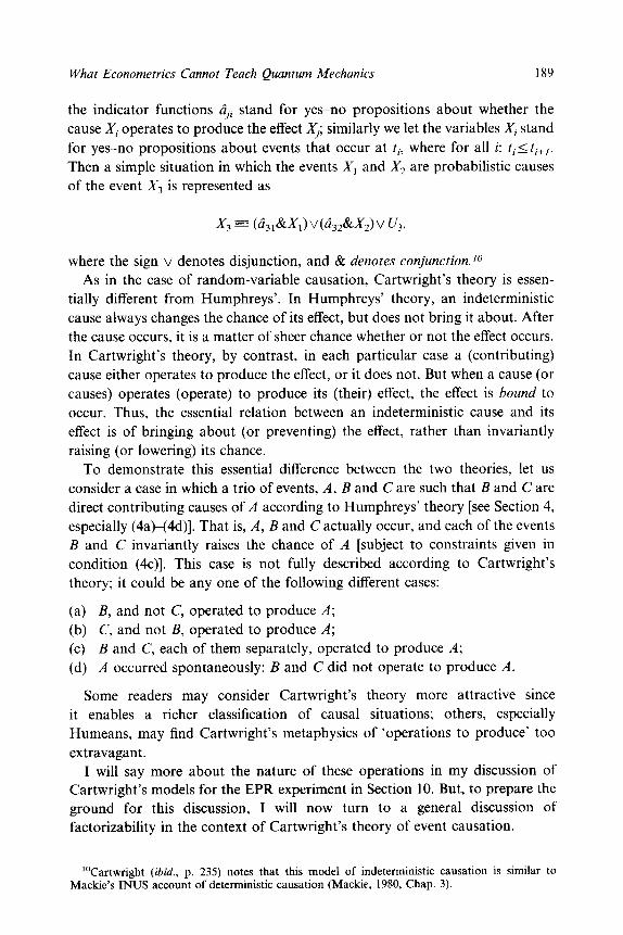
the indicator functions Li;l stand for yes-no propositions about whether the cause Xi operates to produce the effect Xj; similarly we let the variables Xi stand for yes-no propositions about events that occur at ti, where for all i: ti< ti+,.
Then a simple situation in which the events X, and X2 are probabilistic causes of the event X3 is represented as
where the sign v denotes disjunction, and & denotes conjunction.fO
As in the case of random-variable causation, Cartwright’s theory is essen- tially different from Humphreys’. In Humphreys’ theory, an indeterministic
cause always changes the chance of its effect, but does not bring it about. After the cause occurs, it is a matter of sheer chance whether or not the effect occurs. In Cartwright’s theory, by contrast, in each particular case a (contributing) cause either operates to produce the effect, or it does not. But when a cause (or causes) operates (operate) to produce its (their) effect, the effect is hound to occur. Thus, the essential relation between an indeterministic cause and its effect is of bringing about (or preventing) the effect, rather than invariantly raising (or lowering) its chance.
To demonstrate this essential difference between the two theories, let us consider a case in which a trio of events, A, B and C are such that B and C are direct contributing causes of A according to Humphreys’ theory [see Section 4, especially (4at(4d)]. That is, A, B and C actually occur, and each of the events B and C invariantly raises the chance of A [subject to constraints given in condition (4c)]. This case is not fully described according to Cartwright’s theory; it could be any one of the following different cases:
(a) B, and not C, operated to produce A;
(b) C, and not B, operated to produce A;
(c) B and C, each of them separately, operated to produce A;
(d) A occurred spontaneously: B and C did not operate to produce A.
Some readers may consider Cartwright’s theory more attractive since it enables a richer classification of causal situations; others, especially Humeans, may find Cartwright’s metaphysics of ‘operations to produce’ too
extravagant. I will say more about the nature of these operations in my discussion of
Cartwright’s models for the EPR experiment in Section 10. But, to prepare the ground for this discussion, I will now turn to a general discussion of
factorizability in the context of Cartwright’s theory of event causation.
“‘Cartwright (ibid., p. 235) notes that this model of indeterministic causation is similar to Mackie’s INUS account of deterministic causation (Mackie, 1980, Chap. 3).

190 Studies in History and Philosophy of Modern Physics
9. Factorizability is a Necessary Condition for a Common Cause in
Cartwright’s Theory
Cartwright (1989, Chaps 3 and 6) argues that factorizability of two events, say x and y, upon an (earlier) third event, say z, is not a necessary condition for z being the common cause of x and y. [Here by ‘factorizability of x and y upon z’, Cartwright means that P(x&y/z) = P(xlz).P(y/z).] In her view, unless the operation of a common cause to produce one of its effects is independent of its operation to produce the other one, (joint) effects do not factorize upon their common cause. But, argues Cartwright, in the EPR experiment the operations of the common cause, viz the quantum state of the particle pair just at the time of the emission, to produce its effects, viz the measurement outcomes, are indeed correlated with each other. So the outcomes do not factorize upon the quantum state at the source and the choice of the measured quantities. (I discuss this model in more detail in Section 10.)
I agree with Cartwright that in local models for EPR the outcomes need not factorize upon their common cause and the choice of the measured quantities. However, in the context of Cartwright’s theory, there is an alternative set of real physical events which induces factorization in the probabilities of these out- comes. That is, the outcomes factorize upon the conjunction of their common cause, its operations to produce them, and the choice of the measured quantities. In fact, I will now prove a more general result: I will show that if we define the direct causal past of an event, say X, to be the disjunction of the conjunction of each of x’s actual causes and the (event of the) operation (or lack of operation) of this cause to produce x, then any two events factorize upon the conjunction of their direct causal pasts [see (9.1) below], independently of whether the common cause and the effects are connected by continuous causal processes, i.e. independently of whether Contiguity [condition (lla) below] holds.
Consider the following general model:
x = V,ci,;~X, v u, (9.1)
where: each of the variables Xi (Xi> stands for a yes-no proposition about whether the corresponding cause of x b) occurs; each of the indicator functions LiXi (Q stand for yes-no propositions about whether the cause Xi (Xi> operates to produce the effect x (y); vi &.Xj (vi iYj.Xj) is the disjunction of the conjunction of each of the xs (ys) actual causes and the (event of the) operation (or lack of operation) of this cause to produce x (y); and U, and U, are the spontaneous occurrences of x and y, respectively. Let us assume, for the sake of simplicity, that there are no spontaneous occurrences of x and y. Nothing in my
What Econometrics Cannot Teach Quantum Mechanics 191
‘\ 1’
to - A
al s r ci
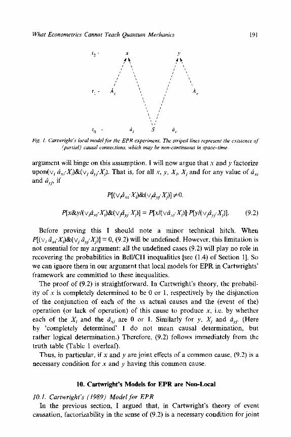
Fig. 1. Cartwright’s local model for the EPR experiment. The striped lines represent the existence oj
(partial) causal connections, which may he non-continuous in space-time.
argument will hinge on this assumption. I will now argue that x and y factorize upon(v, &.X,)&(v, &.Xi>. That is, for all x, y, Xi, Xj and for any value of d,; and Liyj, if
P[X&yl(Va,,‘Xi)&(V,Li,i.Xj)] = p[Xl(Vci_~,.X;)]‘plvl(V,ci,~.Xj)]. (9.2)
Before proving this I should note a minor technical hitch. When P[(v, ci,i*Xi)&(vj dYiXj)] = 0, (9.2) will be undefined. However, this limitation is not essential for my argument: all the undefined cases (9.2) will play no role in recovering the probabilities in BelYCH inequalities [see (1.4) of Section 11. So we can ignore them in our argument that local models for EPR in Cartwrights’ framework are committed to these inequalities.
The proof of (9.2) is straightforward. In Cartwright’s theory, the probabil- ity of x is completely determined to be 0 or 1, respectively by the disjunction of the conjunction of each of the xs actual causes and the (event of the) operation (or lack of operation) of this cause to produce x, i.e. by whether each of the Xi and the & are 0 or 1. Similarly for y, Xi and ci,i. (Here by ‘completely determined’ I do not mean causal determination, but rather logical determination.) Therefore, (9.2) follows immediately from the truth table (Table 1 overleaf).
Thus, in particular, if x and y are joint effects of a common cause, (9.2) is a necessary condition for x and y having this common cause.
10. Cartwright’s Models for EPR are Non-Local
10.1. Cartwright’s (1989) Model for EPR
In the previous section, I argued that, in Cartwright’s theory of event causation, facto&ability in the sense of (9.2) is a necessary condition for joint

192 Studies in History and Philosophy of Modern Physics
Table 1
vi ax/xi v; dyj.Xj E Y X&Y 0 0 0 0 0 1 0 1 0 1 0 1 0 0 1 1 1 1 1
effects to have a common cause. Since nothing in the proof of (9.2) turned on Contiguity, local, non-continuous common-cause models for EPR in the framework of Cartwright’s theory are committed to (9.2). Thus, using the framework of Bell-type models (see Section l), I will argue in this section that in Cartwright’s model of EPR (9.2) entails (1.3), i.e. (Factor), independently of
whether they presuppose Contiguity. However, as we have already seen in Sections 1 and 6, this condition is not
sufficient for BelYCH inequalities. Another condition is required, viz (Indep)- that the distribution of the hidden variable 1 is independent of the choice of the measured quantities, I and r; see (1.2) above. Thus, the question of non-locality in Cartwright’s model turns on the question of whether or not (Indep) holds. [Agreed, Cartwright does not intend to introduce a hidden variable model for EPR (ibid., p. 248). But, as we shall see below, this model can be formally understood as a deterministic hidden variable model of that experiment.] I will argue below that Cartwright’s model is committed to (Indep), and thus to BelKH inequalities. In my argument, I will review the model as it appears in her 1989 (pp. 241-242) without any philosophical interpretation. That is, I will consider its formal structure without assigning any particular meaning to the term ‘operation to produce’. Then I will argue that, on any reasonable
interpretation of this term, the model faces a serious difficulty. Cartwright’s model for EPR is as follows (see Fig. 1). Let x represent the
proposition, ‘the outcome, at t,, of a measurement of the quantity 1 in the L-wing, begun at t, (<t-J, is + 1’; and similarly for y and r in the R-wing. Let the indicator variable a,, represent the state of the L-wing apparatus, at t,, that is positively relevant for x; and similarly for a, and y in the R-wing. That is: a, (A,) equals 1 when the L-wing (R-wing) apparatus is ready, at t, (the time the measurement starts), to measure 1 (Y). Let S be the proposition, ‘the particle pair is in the singlet state at the time of the emission, say t, (to < t,)‘. Finally, let ci, be ‘the operation, at t, of S to produce x, at t2’; and similarly for ri, in the R-wing.
The resulting model is then the following. For any 1 and r,
x = (ci,&S&&v U, (10.1)
y = (S,&S&&v uy,

What Econometrics Cannot Teach Quantum Mechanics 193
where U, and U, denote the spontaneous occurrences of x and y, respectively, and 6, and 6, are supposed to be correlated as dictated by quantum mechanics. As before, I will assume, for the sake of simplicity, that there are no spontaneous occurrences of x and y. Nothing in my argument will hinge on this assumption.
Cartwright’s model is local in the following senses:
No Spacelike Causation (IOa)
There is no direct causal connection between spacelike separated events, i.e. S&a, is the complete cause of x, and S&a,, is the complete cause of y.
Localization of Partial Causes (lob)
The partial causes of x and y, respectively, namely S and a,, and S and a,., respectively, are well localized in space and time.
Locality of Operations at the Source (10~)
The operations of S, ‘which occur at the source’, say at t,, ‘are independent of the states the apparatuses take on somewhere else at a later time’, say just before t,. Thus, the probability that S operates, at t, to produce both x and J is independent of the state the apparatuses take on at t, (ibid., p. 242). So the probabilities of ci,, 6,. are completely determined by S. That is, for every I, r, x.
y, ci, and ci,,
P(Li&&s~S&&c&a,) = P(B/&&BJS&A^,) = P(ci@~S&k,) = P(ci/&&B,lS). (10.2)
Two remarks: (i) The ‘locality-of-operations-at-the-source’ condition, (10.2) is a special case of a more general condition of locality of operations which I discuss in Subsection 10.2 [see (1Od) below]; (ii) in her 1989 (ibid.) Cartwright does not use (10.2) but rather an equivalent condition:
P(x&ylS&A/&A,) = P(ci&qS). (10.3)
Having presented the formal structure of Cartwright’s model, I will now argue that it is committed both to (Factor) and (Indep). Following up our discussion in Section 9, it is not difficult to show that, in the model above, S&Z&&a, (logically) determines the value of x to be 0 or 1, and S&L&&~, (logically) determines the value of y to be 0 or 1. Accordingly, we have
P(xlS&&&&Li,&AJ = P(xlS&Li/&A,)
P(ylS&ci&&ci,&A,) = P(ylS&ri,&A,)
P(x&ylS&ci&&ci,&A/&A^,) = P(XlS&ci~&a,)~P~lS&ri,&~,). (10.4)

194 Studies in History and Philosophy of Modern Physics
Thus, defining 1, I and r in the following way: for any 1, r, 6, and B,
(10.5)
(Factor) follows from (10.4).” Cartwright’s model is also committed to (Indep). The argument is straight-
forward. It follows from (lO.l), (10.3) and probability theory that
P(a&&a,&sls&a/&&a,) = P(B&&ri,&SIs). (10.6)
Thus, defining the probability distribution p(.) as P(.Is), (Indep) follows from (10.5) and (10.6).
So far I have presented Cartwright’s model without any philosophical interpretation. However, on philosophical reflection, this model seems to face a serious difficulty. In this model, S is a common partial cause which acts in conjunction with the relevant states of each of the apparatuses, a, and a,, to produce x and y. However, as we have seen above, Cartwright assumes that the operations of S to produce x and y occur at the source before the choice of the quantities to be measured has been made. This assumption raises an immediate problem for Cartwright’s metaphysics. If the common partial cause operates to produce its outcomes, they are bound to happen. But how can a partial cause operate to produce its effects even before the other partial causes occur?
Provided that correlations between measurement outcomes are to be ex- plained neither in terms of backward causation from the apparatus, at t,, to the source, at t,, nor by mysterious correlations between the operations of the quantum state at the source, at t,, and the state the apparatuses take on (randomly) at t,, this problem seems insoluble.12
10.2. Cartwright’s New Model is Non-Local
If the operations do not occur before the act of measurement, i.e. they do not occur at the source at t, but rather at t, (just after the measurements start), at the apparatus’ locations, the above problem will not exist. That is what Cartwright seems to propose in informal correspondence. On this new model, the quantum state at the source, at to, operates at t,, together with the state the apparatus take on at that time to produce the outcomes at t,. Thus, using the
“There is an important difference between Section 9’s model and Cartwright’s model. In Section 9, we have assumed that complete causes operate to produce their effects, while in Cartwright’s model it is the common partial cause of the joint outcomes which operates to produce them. However, this distinction is insignificant to my formal proof of BelllCH inequalities in Cartwright’s (1989) model. I return to discuss this issue in the last two paragraphs of Subsection 10.1.
“Two remarks: (i) Maudlin (1993, p. 603) suggests that Cartwright’s model involves backward causation. However, Cartwright (1989, p. 248) says explicitly that it is crucial for causation that causes precede their effects; (ii) recall our remark (in Note 8) about deterministic models that many authors would find incredible. The correlation between ci&&ci, and a,&, might be considered less mysterious in this kind of model. Nevertheless, the essential philosophical problem still remains.

What Econometrics Cannot Teach Quantum Mechanics 195
same notation as before, S&A, operates at t, to produce x at t,, and S&a,
operates at t, to produce y at t,. Finally, the operations are supposed to be correlated as dictated by quantum mechanics.
Before arguing that Cartwright’s new model is non-local, let me point out some of its peculiar features. (In fact, these features are not particular only to EPR situations.) First, the complete cause, S&A, (S&a,.) is supposed to operate, at t,, to produce x (v) when some of the partial components (some conjuncts) of that complete cause, S no longer exist (Cartwright ibid.). And it is not clear at all how a no longer existing partial cause S could join the presently existing partial cause a, (A,), in operating to produce the outcome x Cy). Secondly, the operation of S&a, (S&a,), to produce x (v), which starts at t,, continues until x (y) comes into existence. Thus, S will be out of existence before S&its (S&a,‘s) operation ceases. The situation might be even worse in cases where all the complete cause’s partial components will be out of existence before its
operation to produce its effect ceases. I now turn to consider Cartwright’s new model. As before, this model is
factorizable in the sense of (9.2). Thus, (Factor) follows from (10.4) and (10.5).’ i However, in this new model, the operations are not independent of the choice of the measured quantities. That is, (10.2) and (10.3) (with 8, and 6, as the operations, at t,, of %A^, and S&a, respectively, to produce x and y) do not hold. Thus, (Indep) fails; and accordingly Bell/CH inequalities (1.4), cannot be derived.
So we have a local model in the sense of (lOa), i.e. there is no spacelike causation. But there is no paradise on the cheap: the model violates the following locality condition that Cartwright herself seems to endorse (1989, pp. 245-246).
Locality of Operations (1Od)
Let Li,, represent the operation of the cause c, at F, t to produce an effect e,, and ci, the operation of the cause c2 at 7,t’ to produce e2. Then P(ri,&&) = P(B,).P(B,) unless ? = 7 and t = t’.
For, in Cartwright’s new model, the operations of S&a, (or a)) to produce .Y and the operation of S&A, (or a,.) to produce y are correlated though they occur at spacelike separated locations.
Cartwright says that the locality-of-operation condition ‘is an assumption about how causes operate: distant causes cannot act in coincidence; once two causes are separated, their operations must be independent of each other’ (ibid.,
p. 245). And she motivates this condition by the idea that distant correlations
“Indeed, since the operations do not complete their actions until the effects come into existence, factorizability in the sense of (9.2) is trivially true: the event of the operation to produce the effect includes the occurrence of that effect. But notice that this does not influence the conclusion that Cartwright’s (1989) model is committed to BelVCH inequalities. Moreover, (9.2) and “so (Factor), will hold even if we take 6, and 6, to represent the beginning of the operations of S&A, and S&A,, respectively, to produce x and y, respectively.

196 Studies in History and Philosophy of Modern Physics
must have a causal explanation. But this reasoning discredits the model above: for this model explains the EPR correlations by introducing other mysterious correlations.
11. Factorizability and Contiguity
Cartwright (1989, Chaps 3 and 6) and Chang and Cartwright (1993, Section II) argue that (Factor), (1.3), is not, in general, a necessary condition for a common cause. Nevertheless, Chang and Cartwright claim, (Factor) is a necessary condition for a common cause if the following conditions about causal propagation hold.
The Contiguity Condition (lla)
Every cause and effect must be connected by a causal process that is continuous in space-time.
The Relativistic Finite-Speed Condition (Ilb)
Causal processes do not exceed the speed of light.
The Markov Condition (11~)
The stages of the causal processes have no memory.
The Cause-Correlation Link (Ild)
All correlations between spatially separated events must be completely explainable by either a direct (spatio-temporally continuous) causal connection between them, or by common events in the causal past of each.
Although the above assumptions are fairly reasonable, Chang and Cartwright (ibid.) think that they are not reasonable for the EPR experiment. In particular, they argue that Contiguity does not hold in that experiment. Thus, they conclude, the violation of (Factor) in the EPR experiment does not constitute a compelling reason to rule out local, but nevertheless non- contiguous, models, in which the event of pair-creation at the source acts in conjunction with each of the apparatus settings to produce the outcomes in the two wings.
But nothing in my argument against local models for the EPR experiment in Cartwright’s and Humphreys’ theories turned on Contiguity. Assuming that correlations should have a causal explanation, local models for the EPR experiment in Cartwright’s and Humphreys’ theories, though they may violate the Contiguity and the Markov conditions, are committed to BelYCH inequalities, which are violated by experiment.14
i4Recall from Note 3 that Chang and Cartwright must have made in their argument another assumption: what I call the cause-probability link. Subsection 6.7.2.1 of my 1995 shows that, granted this assumption, (Factor) follows from (Chang and Cartwright’s intended interpretation for) the relativistic finite-speed condition, condition (11 b). Thus, my argument in this paper that contiguity plays no essential role in deriving (Factor) is vindicated.

What Econometrics Cannot Teach Quantum Mechanics 197
Acknowledgements-For discussions and correspondence about various parts of this paper, I thank Meir Hemmo, Jay Kennedy, Peter Lipton, Michael Redhead and in particular Nancy Cartwright, Paul Humphreys and two anonymous referees. I am especially grateful to Jeremy Butterfield for important discussions and for the many invaluable remarks he made on earlier versions. I thank the Cambridge ORS Trust and the Arnold Gerstenberg Fund for supporting my research on this paper.
References
Bell, J. (1976), ‘The Theory of Local Beables’, in Bell (1987), pp. 52-62. Bell, J. (1977) ‘Free Variables and Local Causality’, in Bell (1987), pp. 100-104. Bell, J. (1987), Speakable and Unspeakable in Quantum Mechanics (Cambridge:
Cambridge University Press). Berkovitz, J. (1995), ‘Quantum Nonlocality: An Analysis of the Implications of Bell’s
Theorem and Quantum Correlations for Nonlocality’, Ph.D. Thesis, Cambridge University.
Butterfield, J. (1989), ‘A Space-Time Approach to the Bell Inequality’, in Cushing and McMullin (1989), pp. 114-144.
Butterfield, J. (1992), ‘Bell’s Theorem: What it Takes’, British Journalfor the Philosophy of Science 43, 41-83.
Cartwright, N. (1989) Nature’s Capacities and Their Measurement (Oxford: Clarendon Press).
Chang, H. and Cartwright, N. (1993) ‘Causality and Realism in the EPR Experiment’, Erkenntnis 38, pp. 169-190.
Clauser, J. F. and Horne, M. A. (1974) ‘Experimental Consequences of Objective Local Theories’, Physical Review DlO, pp. 526-535.
Cushing, J. and McMullin, E. (eds) (1989), Philosophical Consequences of Quantum Theory (South Bend: Notre Dame Press).
Earman, J. (1986), ‘Locality, Nonlocality, and Action at a Distance: A Skeptical Review of Some Philosophical Dogmas’, in P. Achinstein and R. Kargon (eds) Theoretical Physics in 100 Years since Kelvin’s Baltimore Lectures (Cambridge Mass.: MIT Press), pp. 449490.
Hanushek, E. and Jackson, J. (1977), Statistical Methods for Social Scientists (Orlando, Fla.: Academic Press).
Humphreys, P. (1989), The Chances of Explanation (Princeton: Princeton University Press).
Mackie, J. L. (1980) The Cement of the Universe (Oxford: Clarendon Press). Maudlin, T. (1993), ‘Book Review of Nature’s Capacities and Their Measurement’,
Journal of Philosophy 90, 599-603. Salmon, W. (1984), Scientljic Explanation and the Causal Structure of the World
(Princeton: Princeton University Press). Shimony, A., Horne, M. A. and Clauser, J. F. (1976) ‘An Exchange on Local Beables’.
in Shimony (1993), pp. 163-168. Shimony, A. (1976), ‘Reply to Bell’ in Shimony (1993) pp. 168-170. Shimony, A. (1993), Search for a Naturalistic World View, Vols 2 (Cambridge:
Cambridge University Press). Suppes, P. and Zanotti M. (1976), ‘On the Determinism of Hidden Variable Theories
with Strict Correlation and Conditional Stochastic Independence of Observables’, in P. Suppes (ed.), Logic and Probability in Quantum Mechanics. Dordecht: Reidel.
van Fraassen, B. (1980), The Scientzfic Image (Oxford: Clarendon Press). van Fraassen, B. (1982), ‘The Charybdis of Realism’, Synthese 52, 25-38. Page
references refer to reprint in Cushing and McMullin (1989) pp. 97-l 13.

198 Studies in History and Philosophy of Modern Physics
Appendix A
Proofs of Theorems 1 and 2 of Section 3
In this appendix, I will prove Theorems 1 and 2.
Proof 1
Theorem 1 is composed of two claims: the two equations in (3.1). I will only prove the first claim; the proof of the second claim is trivially obtained by substituting j for i and i for j.
E(X2,/Xi,Xj) = E{[X, -~(xi)]2/xi,xif
= E(x2i/xi,xj) - 2f(Xi).E(X,lXi,Xj) +yi(xi)
= If;:(Xj) - E(X,IX,Xj)12 + E(X2ilXi,Xj) - E2(X,lXj7Xj)
= [fi(xi) - E(X~X~,XJ]~ + Var(_Y,/x,xi>,
where Var(Xjxi,xi) is the conditional variance of Xi given the value of the exogenous variables of Xi and Xi, xi and xi, respectively. Since only the first term on the right-hand side is dependent upon L, we have that E( U~/xi,xj) is minimized when h(xi) = E(XJxi,xj). QED.
Two remarks: (i) In this proof, I followed the reasoning Humphreys (1989, p. 32) uses in his proof of Assumption 4’ of Section 2; (ii) The qualification ‘Xi and Xi which are not connected to each other by any causal chain’ in Theorem 1 is important. Without this qualification, the consequences of Assumptions 4’ and 5’, (2.3) and (3.1) respectively, can lead to a contradiction. For if Xi is connected to Xj by a causal chain, i.e. if there is a chain of direct causal links from Xi to Xi, Xi might indicate the value of Xi. In such a case, E(XJxi,xj). will be equal to this value, which will generally be different from E(X,Ix,).
Having proved Theorem 1, we can now prove Theorem 2.
Proof 2
E(Ui.vjlXi,Xj) = E{[Xi -&(XJ][q -J(Xj)]/xi,xj}
From Theorem 1, we have J(xi) = E(Xjxi,xj) and jJxj) = E(X/xi,xj) for all values xi and xj of Xi and Xi, respectively. Thus, E( U; Ujxi,xj) = E(X;XJxi,xj) - J;.(xi).$(xj). Now, by Assumption 6’, J;. and 6 should be those which minimize
lE( ui* q/x,xi>l. Thus, .f<XJ$<Xi>, and equivalently, by (2.3) E(XjxJ*E(XjIxj), should equal E(X:X/xi,xj); [and so E(U;Ujxexj) = 01. QED
Three remarks: (i) notice that I do not use the linearity condition, Assump- tion 3, in the proofs above. (I thank Paul Humphreys for calling my attention
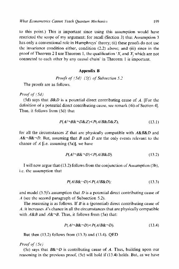
What Econometrics Cannot Teach Quantum Mechanics 199
to this point.) This is important since using this assumption would have restricted the scope of my argument; for recall (Section 3) that Assumption 3
has only a conventional role in Humphreys’ theory; (ii) these proofs do not use the invariance condition either, condition (2.2) above; and (iii) since in the proof of Theorem 2 I use Theorem 1, the qualification ‘Xi and X, which are not connected to each other by any causal chain’ in Theorem 1 is important.
Appendix B
Proofs of (5d)-(5fj of Subsection 5.2
The proofs are as follows.
Proof of (5d)
(5d) says that B&D is a potential direct contributing cause of A. [For the definition of a potential direct contributing cause, see remark (4i) of Section 41. Thus, it follows from (5d) that
P(AhB&~D&Z)<P(AlB&D&Z), (13.1)
for all the circumstances Z that are physically compatible with A&B&D and A&~B&~D. But, assuming that B and D are the only events relevant to the chance of A [i.e. assuming (5a)], we have
P(AbB&-D)<P(AIB&D). (13.2)
I will now argue that (13.2) follows from the conjunction of Assumption (5b), i.e. the assumption that
P(A/B&lD) < P(AIB&D); (13.3)
and model (5.5)‘s assumption that D is a potential direct contributing cause of A (see the second paragraph of Subsection 5.2).
The reasoning is as follows. If B is a (potential) direct contributing cause of A, it increases A’s chance in all the circumstances that are physically compatible with A&B and A&-B. Thus, it follows from (5a) that:
P(AbB&~D)<P(A/B&~D). (13.4)
But then (13.2) follows from (13.3) and (13.4). QED
Proof of (5e)
(5e) says that B8zlD is contributing cause of A. Thus, building upon our reasoning in the previous proof, (5e) will hold if (13.4) holds. But, as we have

200 Studies in History and Philosophy of Modern Physics
seen above, (13.4) follows from Assumption (5a) and the assumption that B is a potential direct contributing cause of A. QED
Proof of f5fl (5f) says that lB8zD is a potential direct counteracting cause of A. Thus,
granted assumption (5a), it implies that
P(AI-B&D)<P(AI~B&~D). (13.5)
But, (13.5) is equivalent to our assumption (5~). QED