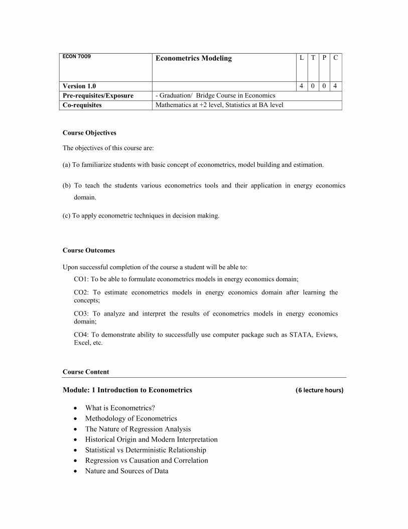
Course Objectives

The objectives of this course are:

(a) To familiarize students with basic concept of econometrics, model building and estimation.

(b) To teach the students various econometrics tools and their application in energy economics

domain.

(c) To apply econometric techniques in decision making.

Course Outcomes Upon successful completion of the course a student will be able to:

CO1: To be able to formulate econometrics models in energy economics domain;

CO2: To estimate econometrics models in energy economics domain after learning the concepts;

CO3: To analyze and interpret the results of econometrics models in energy economics domain;

CO4: To demonstrate ability to successfully use computer package such as STATA, Eviews, Excel, etc.

Course Content

Module: 1 Introduction to Econometrics (6 lecture hours)

What is Econometrics?

Methodology of Econometrics

The Nature of Regression Analysis

Historical Origin and Modern Interpretation

Statistical vs Deterministic Relationship

Regression vs Causation and Correlation

Nature and Sources of Data

ECON 7009 Econometrics Modeling L T P C

Version 1.0 4 0 0 4

Pre-requisites/Exposure - Graduation/ Bridge Course in Economics

Co-requisites Mathematics at +2 level, Statistics at BA level

Module: 2 Simple Linear Regression Model: Two Variable Case (10 lecture

hours)

Estimation of model by the method of Ordinary Least Square Method

Properties of estimators, goodness of fit

Assumption of CNLRM, Gauss-Markov Theorem

Test of hypothesis, scaling and unit of measurement, confidence intervals

Normality Assumption, The Method of Maximum Likelihood Module 3: The Multiple Regression Model (10 lecture hours)

Estimation of parameters; Interpretation of partial regression coefficients; Properties of OLS estimators

2R and adjusted2R

Hypothesis testing -individual and joint

Functional Forms of regression models;

Module: 4 Violation of Classical Assumption: Consequences, Detection, and Remedies (7 lecture hours)

Multicollinearity

Heteroscedasticity

Autocorrelation

Module: 5 Dummy Variable Regression Models (8 lecture hours)

The Nature of Dummy Variables

Regression models with all dummy explanatory variables, with mixture of quantitative and qualitative regressors, interaction effect

Dummy variable in seasonal analysis; piecewise linear regression Qualitative response regression models-LPM, Logit, Probit, Multinomial logit

Module: 6 Time Series Analysis (7 lecture hours)

Stochastic Process; Unit Root Stochastic Process; Trend stationary and Difference Stationary Stochastic Process; Integrated Stochastic Process

Tests of Stationarity-Graphical Analysis, Autocorrelation Function and Correlogram; The Unit Root Test

Transforming Non-stationary time series; Cointegration; D-W Test, ECM

Unit Root and Cointrgration

AR, MA, ARMA, ARIMA

BJ Methodology and Forecasting energy demand and supply

Modeling Energy consumption using VAR and VECM

Text Books

Gujarati, D. N. (2004). Basic Econometrics. Tata McGraw-Hill.

Gujarati, D. N. (2006). Essentials of Econometrics. Tata McGraw-Hill Salvatore, D. and Reagle, B. (2002). Statistics and Econometrics. Schaum Outline

Series Modes of Evaluation: Quiz/Assignment/ presentation/ extempore/ Written Examination Examination Scheme:

Components Class Test

Assignment Project Report

Presentation ESE

Weightage (%)

10 10 15 15 50

Relationship between the Course Outcomes (COs) and Program Outcomes (POs)

Program Outcome / Course Outcome mapping

CO CO 1 CO 2 CO 3 CO 4

PO 1 3 3 3

PO 2 3 3 3

PO 3 3 3 3

PO 4 3 3

PO 5 3

PO 6 2

PO 7 3 3

PO 8 3 3 3 3

PSO 9 3 3 3

Mapping between COs and POs

Course Outcomes (COs) Mapped

Programme Outcomes

CO1 To be able to formulate econometrics models in energy economics domain;

PO 1,2, 3,4,7,8,9,10, 11,13, 14

CO2 To estimate econometrics models in energy economics domain after learning the concepts;

PO 1,2, 3, 7,8,9,10, 11,14

CO3

To analyze and interpret the results of econometrics models in energy economics domain;

PO 1,2, 3,6 8,9,10, 11, 13,14

CO4 To demonstrate ability to successfully use computer package such as STATA, Eviews, Excel, etc.

PO 4,5, 8,12,13, 14

PSO 10 3 3 3

PSO 11 3 3 3

PSO 12 3

PSO 13 3 3 3

PSO 14 3 3 3 3

Stud

ents

will

be

able

to d

evel

op a

nd e

valu

ate

alte

rnat

e m

anag

eria

l ch

oice

s and

iden

tify

optim

al s

olut

ions

. St

uden

ts w

ill d

emon

stra

te e

ffec

tive

appl

icat

ion

capa

bilit

ies o

f the

ir th

eore

tical

und

erst

andi

ng o

f eco

nom

ics

theo

ries

– M

icro

econ

omic

s,

Mac

roec

onom

ics a

nd tr

ade

theo

ries t

o th

e re

new

able

and

non

-re

new

able

ene

rgy

sect

ors.

St

uden

ts w

ill e

xhib

it ef

fect

ive

deci

sion-

mak

ing

skill

s, e

mpl

oyin

g an

alyt

ical

and

crit

ical

thin

king

abi

lity.

St

uden

ts w

ill d

emon

stra

te e

ffect

ive

oral

and

writ

ten

com

mun

icat

ion

skill

s in

pres

entin

g fr

amew

orks

, mod

els a

nd re

gula

tions

of t

he e

nerg

y se

ctor

. St

uden

ts w

ill b

e ab

le to

wor

k ef

fect

ivel

y in

team

s an

d de

mon

stra

te

team

-wor

king

cap

abili

ties.

Stud

ents

will

exh

ibit

lead

ersh

ip a

nd n

etw

orki

ng sk

ills.

Stud

ents

will

dem

onst

rate

sens

itivi

ty to

war

ds e

thic

al a

nd m

oral

issu

es

and

have

abi

lity

to a

ddre

ss th

em in

ene

rgy

econ

omic

s.

Stud

ents

will

dem

onst

rate

em

ploy

abili

ty tr

aits

in li

ne w

ith th

e ne

eds o

f ch

angi

ng d

ynam

ics o

f ren

ewab

le a

nd n

on-r

enew

able

ene

rgy

sect

ors.

Stud

ents

will

dem

onst

rate

str

ong

conc

eptu

al k

now

ledg

e of

eco

nom

ic

theo

ry in

the

cont

ext o

f ren

ewab

le a

nd n

on-r

enew

able

ene

rgy

sect

ors.

Stud

ents

will

dem

onst

rate

eff

ectiv

e un

ders

tand

ing

of e

cono

mic

s as

it is

ap

plic

able

to

ener

gy m

arke

ts,

ener

gy p

ricin

g, e

nerg

y tr

adin

g an

d ris

k m

anag

emen

t. St

uden

ts w

ill d

emon

stra

te a

naly

tical

ski

lls i

n de

signi

ng s

olut

ions

for

en

ergy

effi

cien

cy.

Stud

ents

will

exh

ibit

the

abili

ty to

eva

luat

e w

orki

ng o

f ene

rgy

polic

ies.

Stud

ents

w

ill

have

do

mes

tic

and

glob

al

pers

pect

ive

tow

ards

le

gal

fram

ewor

ks a

nd e

nviro

nmen

tal

regu

latio

ns w

ith r

espe

ct t

o en

ergy

se

ctor

s.

Stud

ents

will

exh

ibit

depl

oyab

le s

kills

per

tinen

t to

the

ren

ewab

le a

nd

non-

rene

wab

le e

nerg

y se

ctor

s.

PO

1

PO

2

PO

3

PO

4

PO

5

PO

6

PO

7

PO

8

PSO

9

PSO

10

PSO

11

PSO

12

PSO

13

PSO

14

3 3 3 2 1 1 2 3 3 3 3 1 2 3

Course Code

ECON 7009

Course Title

Econometrics Modeling

1 – Weakly mapped 2 – Moderately mapped 3 – Strongly mapped

Model Question Paper

Name:

Enrolment No:

End Semester Examination-May 2017 Program/course : MA Economics (EE) Semester : II Subject : Econometric Modeling Max. Marks : 100 Code : ECON 7009 Duration : 3 Hrs

Section A ( attempt all) Q1. Fill in the blanks

i. Under the least square procedure, RSS need to be________. [2] CO1

ii. When choosing between regression models it is preferable to choose the one with____. [2] CO1

iii. For coefficient of determination r2 for a regression model is _______________.

[2] CO1

iv. E(Y | Xi) = f (Xi) is known as _______. [2] CO1

v. ui = Yi − E(Y | Xi) is known as ________. [2] CO1

vi. The in a confidence interval given by

1Pr 2

^

22

^

is known as ___. [2] CO1

vii. Systematic component of the equation, Yi = E(Y | Xi) + ui is _______. [2] CO1

viii. The in a confidence interval given by

1Pr 2

^

22

^

should be ___. [2] CO1

ix. In confidence interval estimation, %5 , this means that this interval includes the true with probability of _____.

[2] CO1

x. ^

iY is the estimator of _____________. [2] CO1

SECTION B Answer any four questions 5 X4= 20

Q2. The VIF of regression considering oil consumption (OC) as dependent variable is

given below. Analysis both VIF and TOL and discuss about presence of

multicollinearity in the model.

[5]

CO3, CO4

Q3. State positive or negative relationship between OC and independent variables.

Sl.No. OC β Coeff. Calculated t-Value

Critical t-Value (at 5%)

State positive or negative relationship between OC and independent variables

1 OE 0.018 -2.30 1.697

2 RT -0.030 4.70 1.697

3 P -0.070 2.56 1.697

4 OP -0.862 6.65 1.697

5 PR 0.073 -1.33 1.697

6 Const. 55.40 -4.44 1.697

[5] CO3, CO4

Q4. Formulate one energy consumption function, write down its functional form and

econometric specification for the following variables:

C : amount of energy consumed per annum

Y : GDP of a given country

FDI : FDI inflow for a given country

[5] CO3, CO4

Q5. Consider the following regression output: [5] CO3, CO4

t

^

4563X.03133.0 iY

se= (0.0976) (0.1961)

P= (0.005) (0.003)

RSS = 0.0544 ESS = 0.0358 r2 = 0.397

Where, Y = Household Electricity Consumption in rural area (in KW)

X = Electricity tariff (in Rupees)

The regression results were obtained from a sample of 19 households.

a) How do you interpret this regression?

b) Test the hypothesis that H0: β2 = 0 against H1: β2 ≠ 0. Which test do you use?

And why?

Q6. The ANOVA table of one regression result is given below.

The critical value of F( 1, 16) = 2.4904 and α = 5%.

Source SS Df MSS Model 326765512 1 Residual 167697811 16 Total 494463323 17

Compute (i) Mean sum of squares, (ii) F and (iii) state the overall significance of the

model.

[5] CO3, CO4

SECTION C Answer any two questions 2 X 15 = 30

Q7. In the following multiple regression result, Carbon Emission (co2) is estimated using

factors such as oil consumption (oc), per capita GDP (pgdp), import of goods and

services (om), and export of goods and services (ox).

[15]

CO1, CO4

Using individual and joint hypothesis testing find out relationship between co2 and its

determinants.

Q8. Detect problems of heteroscedasticity for a regression model, where oil consumption

(oc) is estimated. The post estimation results are given below. Critically analyze and

interpret the results.

i. Graphical Method

ii. Breusch-Pagan/ Cook-Weisberg test

iii. Park Test: Park suggests that σ2i is some function of the explanatory variable

[15]

CO3, CO4

-400

-200

020

040

0R

esi

dua

ls

14000 16000 18000 20000 22000Fitted values

Xi. The functional form he suggested was

σ2i = σ2Xβ

i evi

Using this functional form suggest how to detect heteroscedasticity.

Q9. The multiple regression and its post estimation results are given below. Interpret the

post estimation results and justify whether multicollinearity is present in the model

or not.

Multiple Regression Results

Post Estimation Tests

(i) Scatter Plot Matrix

(ii) Correlation Matrix

[15] CO3, CO4

P

IM

EX

PGDP

CO2

0

50

100

0 50 100

4000

5000

6000

4000 5000 6000

2000

4000

6000

2000 4000 6000

0

50000

0 50000

1000

1200

1400

1000 1200 1400

(iii) Variance Inflation Factor (VIF) and Tolerance(TOL)

Section D

Answer any one question 1 X 30 = 30

Q10. Results of summery statistics and stationarity of oil consumption (oc) are given below along with some result of crude oil production (cop). Write the name of model specification in each case, analyze critically and test the stationarity of the series.

i. Summery statistics

ii. Graphical Method

[30] CO1, CO3, CO4

050

100

150

200

1960 1980 2000 2020Year

Oil Consumption_Million Tones Crude oil price (US dollars per barrel)

ii. The Unit Root Test

Yt = ρYt−1 + ut − 1 ≤ ρ ≤ 1

∆Yt = δYt−1 + ut

iii. DF Test

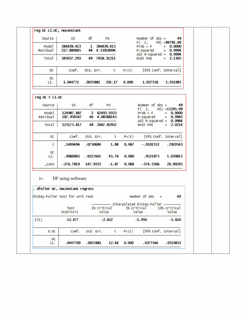
iv. DF using software

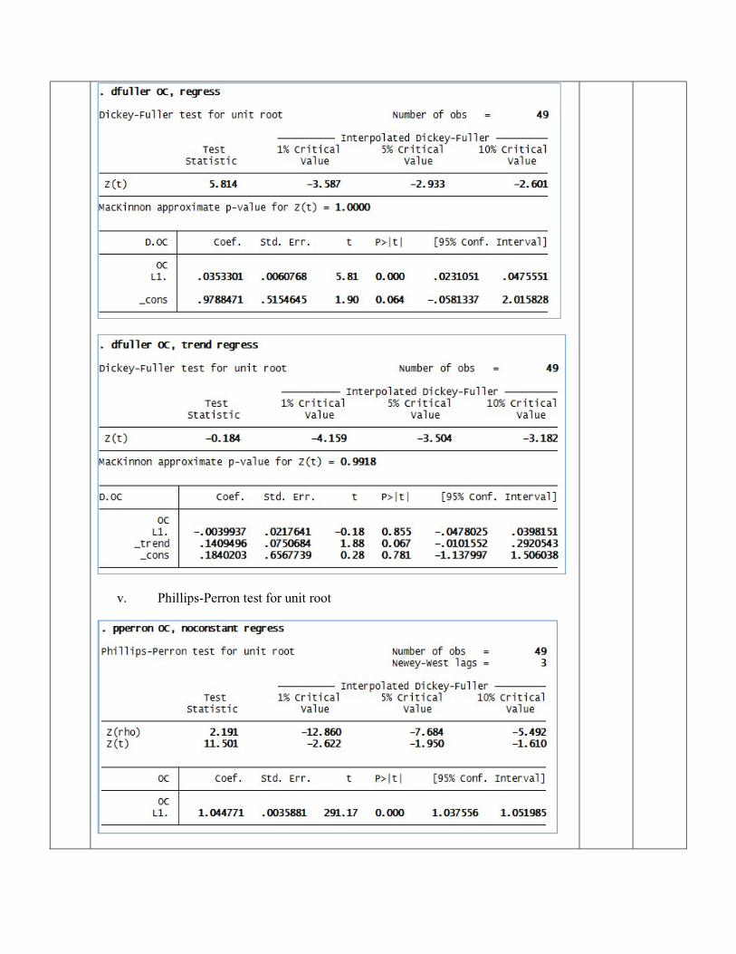
v. Phillips-Perron test for unit root

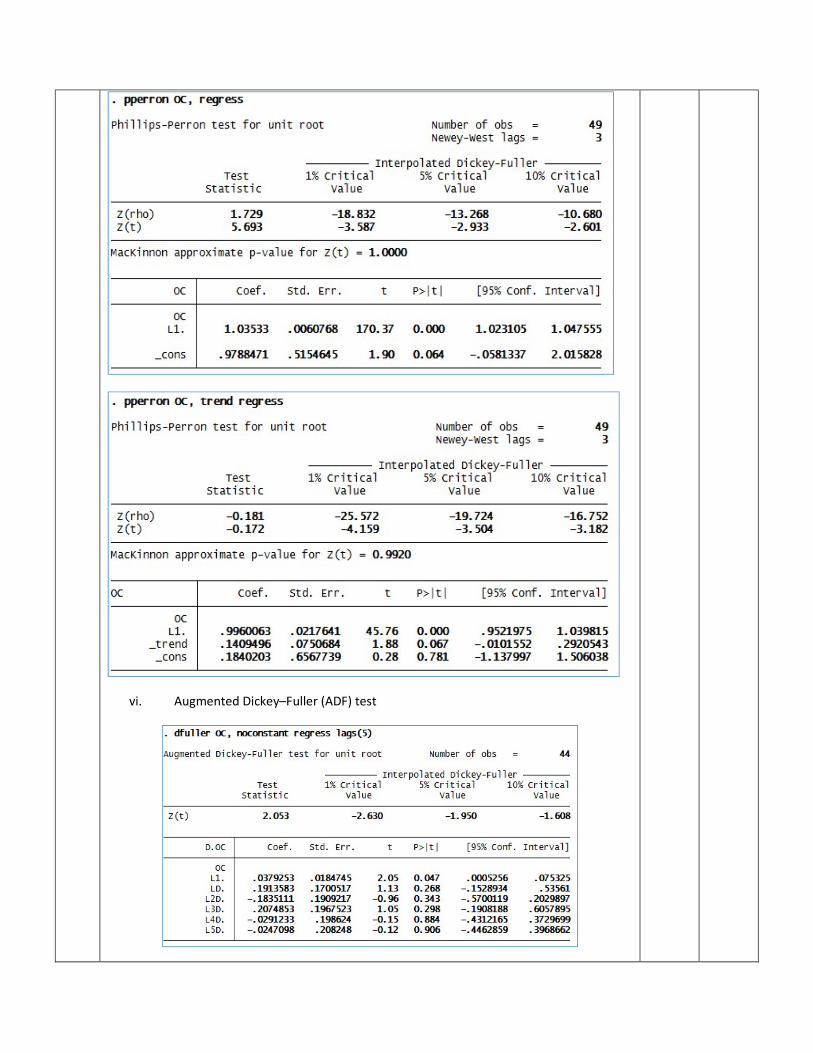
vi. Augmented Dickey–Fuller (ADF) test