Introduction to Python forEconometrics, Statistics and Data Analysis

4th Edition

Kevin SheppardUniversity of Oxford

Thursday 31st December, 2020

2

-

©2020 Kevin Sheppard

Solutions and Other Material

Solutions

Solutions for exercises and some extended examples are available on GitHub.https://github.com/bashtage/python-for-econometrics-statistics-data-analysis

Introductory Course

A self-paced introductory course is available on GitHub in the course/introduction folder. Solutions are avail-able in the solutions/introduction folder.https://github.com/bashtage/python-introduction/

Video Demonstrations

The introductory course is accompanied by video demonstrations of each lesson on YouTube.https://www.youtube.com/playlist?list=PLVR_rJLcetzkqoeuhpIXmG9uQCtSoGBz1

Using Python for Financial Econometrics

A self-paced course that shows how Python can be used in econometric analysis, with an emphasis on financialeconometrics, is also available on GitHub in the course/autumn and course/winter folders.https://github.com/bashtage/python-introduction/

ii

Changes

Changes since the Fourth Edition

• Added a discussion of context managers using the with statement.

• Switched examples to prefer the context manager syntax to reflect best practices.

iv

Notes to the Fourth Edition

Changes in the Fourth Edition

• Python 3.8 is the recommended version. The notes require Python 3.6 or later, and all references toPython 2.7 have been removed.

• Removed references to NumPy’s matrix class and clarified that it should not be used.

• Verified that all code and examples work correctly against 2020 versions of modules. The notable pack-ages and their versions are:

– Python 3.8 (Preferred version), 3.6 (Minimum version)

– NumPy: 1.19.1

– SciPy: 1.5.3

– pandas: 1.1

– matplotlib: 3.3

• Expanded description of model classes and statistical tests in statsmodels that are most relevant for econo-metrics. TODO

• Expanded the list of packages of interest to researchers working in statistics, econometrics and machinelearning. TODO

• Introduced f-Strings in Section 21.3.3 as the preferred way to format strings using modern Python.

• Added minimize as the preferred interface for non-linear function optimization in Chapter 20. TODO

Changes since the Third Edition

• Verified that all code and examples work correctly against 2019 versions of modules. The notable pack-ages and their versions are:

– Python 3.7 (Preferred version)

– NumPy: 1.16

– SciPy: 1.3

– pandas: 0.25

– matplotlib: 3.1

• Python 2.7 support has been officially dropped, although most examples continue to work with 2.7. Donot Python 2.7 in 2019 for numerical code.

vi

• Small typo fixes, thanks to Marton Huebler.

• Fixed direct download of FRED data due to API changes, thanks to Jesper Termansen.

• Thanks for Bill Tubbs for a detailed read and multiple typo reports.

• Updated to changes in line profiler (see Ch. 23)

• Updated deprecations in pandas.

• Removed hold from plotting chapter since this is no longer required.

• Thanks for Gen Li for multiple typo reports.

• Tested all code on Pyton 3.6. Code has been tested against the current set of modules installed by condaas of February 2018. The notable packages and their versions are:

– NumPy: 1.13

– Pandas: 0.22

Notes to the Third Edition

This edition includes the following changes from the second edition (August 2014).

Changes in the Third Edition

• Rewritten installation section focused exclusively on using Continuum’s Anaconda.

• Python 3.5 is the default version of Python instead of 2.7. Python 3.5 (or newer) is well supported bythe Python packages required to analyze data and perform statistical analysis, and bring some new usefulfeatures, such as a new operator for matrix multiplication (@).

• Removed distinction between integers and longs in built-in data types chapter. This distinction is onlyrelevant for Python 2.7.

• dot has been removed from most examples and replaced with @ to produce more readable code.

• Split Cython and Numba into separate chapters to highlight the improved capabilities of Numba.

• Verified all code working on current versions of core libraries using Python 3.5.

• pandas

– Updated syntax of pandas functions such as resample.

– Added pandas Categorical.

– Expanded coverage of pandas groupby.

– Expanded coverage of date and time data types and functions.

• New chapter introducing statsmodels, a package that facilitates statistical analysis of data. statsmodelsincludes regression analysis, Generalized Linear Models (GLM) and time-series analysis using ARIMAmodels.

Changes since the Second Edition

• Fixed typos reported by a reader – thanks to Ilya Sorvachev

• Code verified against Anaconda 2.0.1.

• Added diagnostic tools and a simple method to use external code in the Cython section.

• Updated the Numba section to reflect recent changes.

• Fixed some typos in the chapter on Performance and Optimization.

viii

• Added examples of joblib and IPython’s cluster to the chapter on running code in parallel.

• New chapter introducing object-oriented programming as a method to provide structure and organizationto related code.

• Added seaborn to the recommended package list, and have included it be default in the graphics chapter.

• Based on experience teaching Python to economics students, the recommended installation has beensimplified by removing the suggestion to use virtual environment. The discussion of virtual environmentsas been moved to the appendix.

• Rewrote parts of the pandas chapter.

• Changed the Anaconda install to use both create and install, which shows how to install additional pack-ages.

• Fixed some missing packages in the direct install.

• Changed the configuration of IPython to reflect best practices.

• Added subsection covering IPython profiles.

• Small section about Spyder as a good starting IDE.

Notes to the Second Edition

This edition includes the following changes from the first edition (March 2012).

Changes in the Second Edition

• The preferred installation method is now Continuum Analytics’ Anaconda. Anaconda is a completescientific stack and is available for all major platforms.

• New chapter on pandas. pandas provides a simple but powerful tool to manage data and perform prelim-inary analysis. It also greatly simplifies importing and exporting data.

• New chapter on advanced selection of elements from an array.

• Numba provides just-in-time compilation for numeric Python code which often produces large perfor-mance gains when pure NumPy solutions are not available (e.g. looping code).

• Dictionary, set and tuple comprehensions

• Numerous typos

• All code has been verified working against Anaconda 1.7.0.

x

Contents

1 Introduction 11.1 Background . . . . . . . . . . . . . . . . . . . . . . . . . . . . . . . . . . . . . . . . . . . . 11.2 Conventions . . . . . . . . . . . . . . . . . . . . . . . . . . . . . . . . . . . . . . . . . . . 21.3 Important Components of the Python Scientific Stack . . . . . . . . . . . . . . . . . . . . . 31.4 Setup . . . . . . . . . . . . . . . . . . . . . . . . . . . . . . . . . . . . . . . . . . . . . . . 41.5 Using Python . . . . . . . . . . . . . . . . . . . . . . . . . . . . . . . . . . . . . . . . . . . 51.6 Exercises . . . . . . . . . . . . . . . . . . . . . . . . . . . . . . . . . . . . . . . . . . . . . 121.A Additional Installation Issues . . . . . . . . . . . . . . . . . . . . . . . . . . . . . . . . . . 12

2 Built-in Data Types 152.1 Variable Names . . . . . . . . . . . . . . . . . . . . . . . . . . . . . . . . . . . . . . . . . . 152.2 Core Native Data Types . . . . . . . . . . . . . . . . . . . . . . . . . . . . . . . . . . . . . 162.3 Additional Container Data Types in the Standard Library . . . . . . . . . . . . . . . . . . . 242.4 Python and Memory Management . . . . . . . . . . . . . . . . . . . . . . . . . . . . . . . 262.5 Exercises . . . . . . . . . . . . . . . . . . . . . . . . . . . . . . . . . . . . . . . . . . . . . 27

3 Arrays 293.1 Array . . . . . . . . . . . . . . . . . . . . . . . . . . . . . . . . . . . . . . . . . . . . . . . 293.2 1-dimensional Arrays . . . . . . . . . . . . . . . . . . . . . . . . . . . . . . . . . . . . . . . 303.3 2-dimensional Arrays . . . . . . . . . . . . . . . . . . . . . . . . . . . . . . . . . . . . . . . 313.4 Multidimensional Arrays . . . . . . . . . . . . . . . . . . . . . . . . . . . . . . . . . . . . . 313.5 Concatenation . . . . . . . . . . . . . . . . . . . . . . . . . . . . . . . . . . . . . . . . . . 323.6 Accessing Elements of an Array . . . . . . . . . . . . . . . . . . . . . . . . . . . . . . . . . 333.7 Slicing and Memory Management . . . . . . . . . . . . . . . . . . . . . . . . . . . . . . . . 373.8 import and Modules . . . . . . . . . . . . . . . . . . . . . . . . . . . . . . . . . . . . . . 393.9 Calling Functions . . . . . . . . . . . . . . . . . . . . . . . . . . . . . . . . . . . . . . . . . 403.10 Exercises . . . . . . . . . . . . . . . . . . . . . . . . . . . . . . . . . . . . . . . . . . . . . 41

4 Basic Math 434.1 Operators . . . . . . . . . . . . . . . . . . . . . . . . . . . . . . . . . . . . . . . . . . . . . 434.2 Broadcasting . . . . . . . . . . . . . . . . . . . . . . . . . . . . . . . . . . . . . . . . . . . 434.3 Addition (+) and Subtraction (-) . . . . . . . . . . . . . . . . . . . . . . . . . . . . . . . . . 454.4 Multiplication (⁎) . . . . . . . . . . . . . . . . . . . . . . . . . . . . . . . . . . . . . . . . . 454.5 Matrix Multiplication (@) . . . . . . . . . . . . . . . . . . . . . . . . . . . . . . . . . . . . . 454.6 Array and Matrix Division (/) . . . . . . . . . . . . . . . . . . . . . . . . . . . . . . . . . . . 46

xii CONTENTS

4.7 Exponentiation (**) . . . . . . . . . . . . . . . . . . . . . . . . . . . . . . . . . . . . . . . . 464.8 Parentheses . . . . . . . . . . . . . . . . . . . . . . . . . . . . . . . . . . . . . . . . . . . 464.9 Transpose . . . . . . . . . . . . . . . . . . . . . . . . . . . . . . . . . . . . . . . . . . . . . 464.10 Operator Precedence . . . . . . . . . . . . . . . . . . . . . . . . . . . . . . . . . . . . . . 464.11 Exercises . . . . . . . . . . . . . . . . . . . . . . . . . . . . . . . . . . . . . . . . . . . . . 47

5 Basic Functions and Numerical Indexing 495.1 Generating Arrays . . . . . . . . . . . . . . . . . . . . . . . . . . . . . . . . . . . . . . . . 495.2 Rounding . . . . . . . . . . . . . . . . . . . . . . . . . . . . . . . . . . . . . . . . . . . . . 525.3 Mathematics . . . . . . . . . . . . . . . . . . . . . . . . . . . . . . . . . . . . . . . . . . . 525.4 Complex Values . . . . . . . . . . . . . . . . . . . . . . . . . . . . . . . . . . . . . . . . . 545.5 Set Functions . . . . . . . . . . . . . . . . . . . . . . . . . . . . . . . . . . . . . . . . . . . 545.6 Sorting and Extreme Values . . . . . . . . . . . . . . . . . . . . . . . . . . . . . . . . . . . 565.7 Nan Functions . . . . . . . . . . . . . . . . . . . . . . . . . . . . . . . . . . . . . . . . . . 575.8 Functions and Methods/Properties . . . . . . . . . . . . . . . . . . . . . . . . . . . . . . . 585.9 Exercises . . . . . . . . . . . . . . . . . . . . . . . . . . . . . . . . . . . . . . . . . . . . . 58

6 Special Arrays 616.1 Exercises . . . . . . . . . . . . . . . . . . . . . . . . . . . . . . . . . . . . . . . . . . . . . 62

7 Array Functions 637.1 Shape Information and Transformation . . . . . . . . . . . . . . . . . . . . . . . . . . . . . 637.2 Linear Algebra Functions . . . . . . . . . . . . . . . . . . . . . . . . . . . . . . . . . . . . 697.3 Views . . . . . . . . . . . . . . . . . . . . . . . . . . . . . . . . . . . . . . . . . . . . . . . 717.4 Exercises . . . . . . . . . . . . . . . . . . . . . . . . . . . . . . . . . . . . . . . . . . . . . 72

8 Importing and Exporting Data 758.1 Importing Data using pandas . . . . . . . . . . . . . . . . . . . . . . . . . . . . . . . . . . 758.2 Importing Data without pandas . . . . . . . . . . . . . . . . . . . . . . . . . . . . . . . . . 768.3 Saving or Exporting Data using pandas . . . . . . . . . . . . . . . . . . . . . . . . . . . . 818.4 Saving or Exporting Data without pandas . . . . . . . . . . . . . . . . . . . . . . . . . . . 818.5 Exercises . . . . . . . . . . . . . . . . . . . . . . . . . . . . . . . . . . . . . . . . . . . . . 82

9 Inf, NaN and Numeric Limits 839.1 inf and NaN . . . . . . . . . . . . . . . . . . . . . . . . . . . . . . . . . . . . . . . . . . . 839.2 Floating point precision . . . . . . . . . . . . . . . . . . . . . . . . . . . . . . . . . . . . . 839.3 Exercises . . . . . . . . . . . . . . . . . . . . . . . . . . . . . . . . . . . . . . . . . . . . . 84

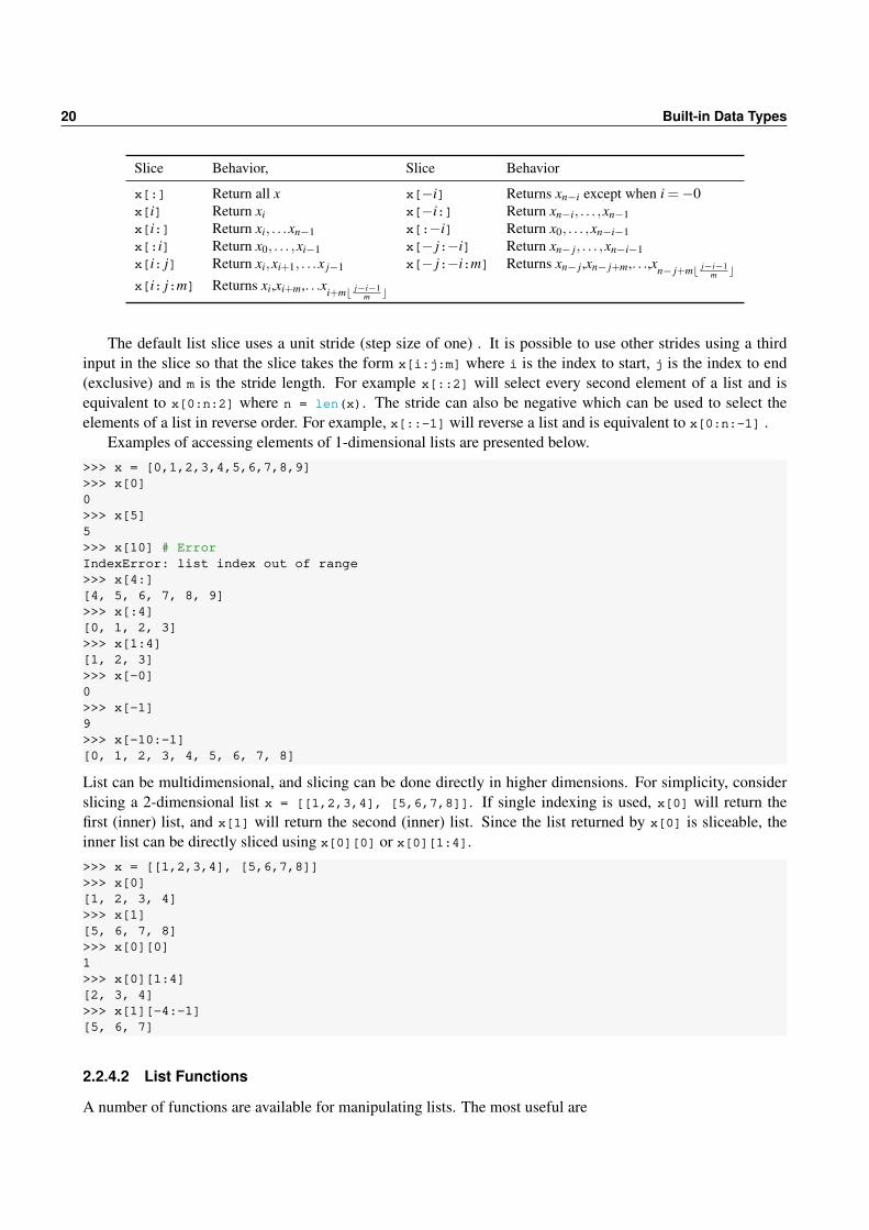
10 Logical Operators and Find 8510.1 >, >=, <, <=, ==, != . . . . . . . . . . . . . . . . . . . . . . . . . . . . . . . . . . . . . . . 8510.2 and, or, not and xor . . . . . . . . . . . . . . . . . . . . . . . . . . . . . . . . . . . . . . . . 8610.3 Multiple tests . . . . . . . . . . . . . . . . . . . . . . . . . . . . . . . . . . . . . . . . . . . 8710.4 is⁎ . . . . . . . . . . . . . . . . . . . . . . . . . . . . . . . . . . . . . . . . . . . . . . . . 8810.5 Exercises . . . . . . . . . . . . . . . . . . . . . . . . . . . . . . . . . . . . . . . . . . . . . 88

CONTENTS xiii

11 Advanced Selection and Assignment 9111.1 Numerical Indexing . . . . . . . . . . . . . . . . . . . . . . . . . . . . . . . . . . . . . . . . 9111.2 Logical Indexing . . . . . . . . . . . . . . . . . . . . . . . . . . . . . . . . . . . . . . . . . 9511.3 Performance Considerations and Memory Management . . . . . . . . . . . . . . . . . . . 9911.4 Assignment with Broadcasting . . . . . . . . . . . . . . . . . . . . . . . . . . . . . . . . . 9911.5 Exercises . . . . . . . . . . . . . . . . . . . . . . . . . . . . . . . . . . . . . . . . . . . . . 101

12 Flow Control, Loops and Exception Handling 10312.1 Whitespace and Flow Control . . . . . . . . . . . . . . . . . . . . . . . . . . . . . . . . . . 10312.2 if . . . elif . . . else . . . . . . . . . . . . . . . . . . . . . . . . . . . . . . . . . . . . . . 10312.3 for . . . . . . . . . . . . . . . . . . . . . . . . . . . . . . . . . . . . . . . . . . . . . . . . 10412.4 while . . . . . . . . . . . . . . . . . . . . . . . . . . . . . . . . . . . . . . . . . . . . . . 10712.5 try . . . except . . . . . . . . . . . . . . . . . . . . . . . . . . . . . . . . . . . . . . . . . 10812.6 List Comprehensions . . . . . . . . . . . . . . . . . . . . . . . . . . . . . . . . . . . . . . . 10912.7 Tuple, Dictionary and Set Comprehensions . . . . . . . . . . . . . . . . . . . . . . . . . . 11012.8 Exercises . . . . . . . . . . . . . . . . . . . . . . . . . . . . . . . . . . . . . . . . . . . . . 110

13 Dates and Times 11313.1 Creating Dates and Times . . . . . . . . . . . . . . . . . . . . . . . . . . . . . . . . . . . . 11313.2 Dates Mathematics . . . . . . . . . . . . . . . . . . . . . . . . . . . . . . . . . . . . . . . . 11313.3 Numpy . . . . . . . . . . . . . . . . . . . . . . . . . . . . . . . . . . . . . . . . . . . . . . 114

14 Graphics 11714.1 seaborn . . . . . . . . . . . . . . . . . . . . . . . . . . . . . . . . . . . . . . . . . . . . . . 11714.2 2D Plotting . . . . . . . . . . . . . . . . . . . . . . . . . . . . . . . . . . . . . . . . . . . . 11714.3 Advanced 2D Plotting . . . . . . . . . . . . . . . . . . . . . . . . . . . . . . . . . . . . . . 12414.4 3D Plotting . . . . . . . . . . . . . . . . . . . . . . . . . . . . . . . . . . . . . . . . . . . . 13114.5 General Plotting Functions . . . . . . . . . . . . . . . . . . . . . . . . . . . . . . . . . . . . 13514.6 Exporting Plots . . . . . . . . . . . . . . . . . . . . . . . . . . . . . . . . . . . . . . . . . . 13514.7 Exercises . . . . . . . . . . . . . . . . . . . . . . . . . . . . . . . . . . . . . . . . . . . . . 135

15 pandas 13715.1 Data Structures . . . . . . . . . . . . . . . . . . . . . . . . . . . . . . . . . . . . . . . . . . 13715.2 Statistical Functions . . . . . . . . . . . . . . . . . . . . . . . . . . . . . . . . . . . . . . . 15815.3 Time-series Data . . . . . . . . . . . . . . . . . . . . . . . . . . . . . . . . . . . . . . . . 15915.4 Importing and Exporting Data . . . . . . . . . . . . . . . . . . . . . . . . . . . . . . . . . . 16315.5 Graphics . . . . . . . . . . . . . . . . . . . . . . . . . . . . . . . . . . . . . . . . . . . . . 16715.6 Examples . . . . . . . . . . . . . . . . . . . . . . . . . . . . . . . . . . . . . . . . . . . . . 168

16 Structured Arrays 17516.1 Mixed Arrays with Column Names . . . . . . . . . . . . . . . . . . . . . . . . . . . . . . . 17516.2 Record Arrays . . . . . . . . . . . . . . . . . . . . . . . . . . . . . . . . . . . . . . . . . . 178

17 Custom Function and Modules 17917.1 Functions . . . . . . . . . . . . . . . . . . . . . . . . . . . . . . . . . . . . . . . . . . . . . 179

xiv CONTENTS

17.2 Variable Scope . . . . . . . . . . . . . . . . . . . . . . . . . . . . . . . . . . . . . . . . . . 18417.3 Example: Least Squares with Newey-West Covariance . . . . . . . . . . . . . . . . . . . . 18617.4 Anonymous Functions . . . . . . . . . . . . . . . . . . . . . . . . . . . . . . . . . . . . . . 18617.5 Modules . . . . . . . . . . . . . . . . . . . . . . . . . . . . . . . . . . . . . . . . . . . . . . 18717.6 Packages . . . . . . . . . . . . . . . . . . . . . . . . . . . . . . . . . . . . . . . . . . . . . 18817.7 PYTHONPATH . . . . . . . . . . . . . . . . . . . . . . . . . . . . . . . . . . . . . . . . . . 18917.8 Python Coding Conventions . . . . . . . . . . . . . . . . . . . . . . . . . . . . . . . . . . . 18917.9 Exercises . . . . . . . . . . . . . . . . . . . . . . . . . . . . . . . . . . . . . . . . . . . . . 19017.A Listing of econometrics.py . . . . . . . . . . . . . . . . . . . . . . . . . . . . . . . . . . . . 191

18 Probability and Statistics Functions 19518.1 Simulating Random Variables . . . . . . . . . . . . . . . . . . . . . . . . . . . . . . . . . . 19518.2 Simulation and Random Number Generation . . . . . . . . . . . . . . . . . . . . . . . . . 19818.3 Statistics Functions . . . . . . . . . . . . . . . . . . . . . . . . . . . . . . . . . . . . . . . . 20118.4 Continuous Random Variables . . . . . . . . . . . . . . . . . . . . . . . . . . . . . . . . . 20318.5 Select Statistics Functions . . . . . . . . . . . . . . . . . . . . . . . . . . . . . . . . . . . . 20618.6 Select Statistical Tests . . . . . . . . . . . . . . . . . . . . . . . . . . . . . . . . . . . . . . 20818.7 Exercises . . . . . . . . . . . . . . . . . . . . . . . . . . . . . . . . . . . . . . . . . . . . . 209

19 Statistical Analysis with statsmodels 21119.1 Regression . . . . . . . . . . . . . . . . . . . . . . . . . . . . . . . . . . . . . . . . . . . . 21119.2 Generalized Linear Models . . . . . . . . . . . . . . . . . . . . . . . . . . . . . . . . . . . 21419.3 Other Notable Models . . . . . . . . . . . . . . . . . . . . . . . . . . . . . . . . . . . . . . 21419.4 Time-series Analysis . . . . . . . . . . . . . . . . . . . . . . . . . . . . . . . . . . . . . . . 21419.5 Generalized Linear Models . . . . . . . . . . . . . . . . . . . . . . . . . . . . . . . . . . . 214

20 Non-linear Function Optimization 21520.1 Unconstrained Optimization . . . . . . . . . . . . . . . . . . . . . . . . . . . . . . . . . . . 21520.2 Derivative-free Optimization . . . . . . . . . . . . . . . . . . . . . . . . . . . . . . . . . . . 21820.3 Constrained Optimization . . . . . . . . . . . . . . . . . . . . . . . . . . . . . . . . . . . . 21920.4 Scalar Function Minimization . . . . . . . . . . . . . . . . . . . . . . . . . . . . . . . . . . 22320.5 Nonlinear Least Squares . . . . . . . . . . . . . . . . . . . . . . . . . . . . . . . . . . . . . 22420.6 Exercises . . . . . . . . . . . . . . . . . . . . . . . . . . . . . . . . . . . . . . . . . . . . . 225

21 String Manipulation 22721.1 String Building . . . . . . . . . . . . . . . . . . . . . . . . . . . . . . . . . . . . . . . . . . 22721.2 String Functions . . . . . . . . . . . . . . . . . . . . . . . . . . . . . . . . . . . . . . . . . 22821.3 Formatting Numbers . . . . . . . . . . . . . . . . . . . . . . . . . . . . . . . . . . . . . . . 23121.4 Regular Expressions . . . . . . . . . . . . . . . . . . . . . . . . . . . . . . . . . . . . . . . 23621.5 Safe Conversion of Strings . . . . . . . . . . . . . . . . . . . . . . . . . . . . . . . . . . . 237

22 File System Operations 23922.1 Changing the Working Directory . . . . . . . . . . . . . . . . . . . . . . . . . . . . . . . . 23922.2 Creating and Deleting Directories . . . . . . . . . . . . . . . . . . . . . . . . . . . . . . . . 23922.3 Listing the Contents of a Directory . . . . . . . . . . . . . . . . . . . . . . . . . . . . . . . 240

CONTENTS xv

22.4 Copying, Moving and Deleting Files . . . . . . . . . . . . . . . . . . . . . . . . . . . . . . . 24022.5 Executing Other Programs . . . . . . . . . . . . . . . . . . . . . . . . . . . . . . . . . . . . 24122.6 Creating and Opening Archives . . . . . . . . . . . . . . . . . . . . . . . . . . . . . . . . . 24222.7 Reading and Writing Files . . . . . . . . . . . . . . . . . . . . . . . . . . . . . . . . . . . . 24222.8 Exercises . . . . . . . . . . . . . . . . . . . . . . . . . . . . . . . . . . . . . . . . . . . . . 244

23 Performance and Code Optimization 24523.1 Getting Started . . . . . . . . . . . . . . . . . . . . . . . . . . . . . . . . . . . . . . . . . . 24523.2 Timing Code . . . . . . . . . . . . . . . . . . . . . . . . . . . . . . . . . . . . . . . . . . . 24523.3 Vectorize to Avoid Unnecessary Loops . . . . . . . . . . . . . . . . . . . . . . . . . . . . . 24623.4 Alter the loop dimensions . . . . . . . . . . . . . . . . . . . . . . . . . . . . . . . . . . . . 24723.5 Utilize Broadcasting . . . . . . . . . . . . . . . . . . . . . . . . . . . . . . . . . . . . . . . 24723.6 Use In-place Assignment . . . . . . . . . . . . . . . . . . . . . . . . . . . . . . . . . . . . 24823.7 Avoid Allocating Memory . . . . . . . . . . . . . . . . . . . . . . . . . . . . . . . . . . . . . 24823.8 Inline Frequent Function Calls . . . . . . . . . . . . . . . . . . . . . . . . . . . . . . . . . . 24823.9 Consider Data Locality in Arrays . . . . . . . . . . . . . . . . . . . . . . . . . . . . . . . . 24823.10Profile Long Running Functions . . . . . . . . . . . . . . . . . . . . . . . . . . . . . . . . . 24823.11Exercises . . . . . . . . . . . . . . . . . . . . . . . . . . . . . . . . . . . . . . . . . . . . . 252

24 Improving Performance using Numba 25324.1 Quick Start . . . . . . . . . . . . . . . . . . . . . . . . . . . . . . . . . . . . . . . . . . . . 25324.2 Supported Python Features . . . . . . . . . . . . . . . . . . . . . . . . . . . . . . . . . . . 25624.3 Supported NumPy Features . . . . . . . . . . . . . . . . . . . . . . . . . . . . . . . . . . 25624.4 Diagnosing Performance Issues . . . . . . . . . . . . . . . . . . . . . . . . . . . . . . . . . 26124.5 Replacing Python function with C functions . . . . . . . . . . . . . . . . . . . . . . . . . . 26324.6 Other Features of Numba . . . . . . . . . . . . . . . . . . . . . . . . . . . . . . . . . . . . 26524.7 Exercises . . . . . . . . . . . . . . . . . . . . . . . . . . . . . . . . . . . . . . . . . . . . . 265

25 Improving Performance using Cython 26725.1 Diagnosing Performance Issues . . . . . . . . . . . . . . . . . . . . . . . . . . . . . . . . . 27125.2 Interfacing with External Code . . . . . . . . . . . . . . . . . . . . . . . . . . . . . . . . . . 27525.3 Exercises . . . . . . . . . . . . . . . . . . . . . . . . . . . . . . . . . . . . . . . . . . . . . 279

26 Executing Code in Parallel 28126.1 map and related functions . . . . . . . . . . . . . . . . . . . . . . . . . . . . . . . . . . . . 28126.2 multiprocessing . . . . . . . . . . . . . . . . . . . . . . . . . . . . . . . . . . . . . . 28226.3 joblib . . . . . . . . . . . . . . . . . . . . . . . . . . . . . . . . . . . . . . . . . . . . . . 28426.4 IPython’s Parallel Cluster . . . . . . . . . . . . . . . . . . . . . . . . . . . . . . . . . . . . 28526.5 Converting a Serial Program to Parallel . . . . . . . . . . . . . . . . . . . . . . . . . . . . . 29126.6 Other Concerns when executing in Parallel . . . . . . . . . . . . . . . . . . . . . . . . . . . 293

27 Object-Oriented Programming (OOP) 29527.1 Introduction . . . . . . . . . . . . . . . . . . . . . . . . . . . . . . . . . . . . . . . . . . . . 29527.2 Class basics . . . . . . . . . . . . . . . . . . . . . . . . . . . . . . . . . . . . . . . . . . . 29627.3 Building a class for Autoregressions . . . . . . . . . . . . . . . . . . . . . . . . . . . . . . 298

xvi CONTENTS

27.4 Exercises . . . . . . . . . . . . . . . . . . . . . . . . . . . . . . . . . . . . . . . . . . . . . 304

28 Other Interesting Python Packages 30528.1 Statistics and Statistical Modeling . . . . . . . . . . . . . . . . . . . . . . . . . . . . . . . . 30528.2 Machine Learning . . . . . . . . . . . . . . . . . . . . . . . . . . . . . . . . . . . . . . . . 30528.3 Deep Learning . . . . . . . . . . . . . . . . . . . . . . . . . . . . . . . . . . . . . . . . . . 30628.4 Other Packages . . . . . . . . . . . . . . . . . . . . . . . . . . . . . . . . . . . . . . . . . 306

29 Examples 30729.1 Estimating the Parameters of a GARCH Model . . . . . . . . . . . . . . . . . . . . . . . . 30729.2 Estimating the Risk Premia using Fama-MacBeth Regressions . . . . . . . . . . . . . . . . 31129.3 Estimating the Risk Premia using GMM . . . . . . . . . . . . . . . . . . . . . . . . . . . . 31429.4 Outputting LATEX . . . . . . . . . . . . . . . . . . . . . . . . . . . . . . . . . . . . . . . . . 317

30 Quick Reference 32130.1 Built-ins . . . . . . . . . . . . . . . . . . . . . . . . . . . . . . . . . . . . . . . . . . . . . . 32130.2 NumPy (numpy) . . . . . . . . . . . . . . . . . . . . . . . . . . . . . . . . . . . . . . . . . 32730.3 SciPy . . . . . . . . . . . . . . . . . . . . . . . . . . . . . . . . . . . . . . . . . . . . . . . 34030.4 Matplotlib . . . . . . . . . . . . . . . . . . . . . . . . . . . . . . . . . . . . . . . . . . . . . 34430.5 pandas . . . . . . . . . . . . . . . . . . . . . . . . . . . . . . . . . . . . . . . . . . . . . . 34530.6 IPython . . . . . . . . . . . . . . . . . . . . . . . . . . . . . . . . . . . . . . . . . . . . . . 350

Chapter 1

Introduction

Solutions

Solutions for exercises and some extended examples are available on GitHub at https://github.com/bashtage/python-for-econometrics-statistics-data-analysis.

1.1 Background

These notes are designed for someone new to statistical computing wishing to develop a set of skills necessaryto perform original research using Python. They should also be useful for students, researchers or practition-ers who require a versatile platform for econometrics, statistics or general numerical analysis (e.g. numericsolutions to economic models or model simulation).

Python is a popular general–purpose programming language that is well suited to a wide range of problems.1

Recent developments have extended Python’s range of applicability to econometrics, statistics, and generalnumerical analysis. Python – with the right set of add-ons – is comparable to domain-specific languages suchas R, MATLAB or Julia. If you are wondering whether you should bother with Python (or another language),an incomplete list of considerations includes:

You might want to consider R if:

• You want to apply statistical methods. The statistics library of R is second to none, and R is clearly at theforefront of new statistical algorithm development – meaning you are most likely to find that new(ish)procedure in R.

• Performance is of secondary importance.

• Free is important.

You might want to consider MATLAB if:

• Commercial support and a clear channel to report issues is important.

• Documentation and organization of modules are more important than the breadth of algorithms available.

• Performance is an important concern. MATLAB has optimizations, such as Just-in-Time (JIT) compila-tion of loops, which is not automatically available in most other packages.

1According to the ranking on http://www.tiobe.com/tiobe-index/, Python is the 5th most popular language. http://langpop.corger.nl/ ranks Python as 4th or 5th.

2 Introduction

You might want to consider Julia if:

• Performance in an interactive based language is your most important concern.

• You don’t mind learning enough Python to interface with Python packages. The Julia ecosystem is lesscomplete than Python and a bridge to Python is used to provide missing features.

• You like to do most things yourself or you are on the bleeding edge and so existing libraries do not existwith the features you require.

Having read the reasons to choose another package, you may wonder why you should consider Python.

• You need a language which can act as an end-to-end solution that allows access to web-based services,database servers, data management and processing and statistical computation. Python can even be usedto write server-side apps such as a dynamic website (see e.g. http://stackoverflow.com), appsfor desktop-class operating systems with graphical user interfaces, or apps for tablets and phones apps(iOS and Android).

• Data handling and manipulation – especially cleaning and reformatting – is an important concern. Pythonis substantially more capable at data set construction than either R or MATLAB.

• Performance is a concern, but not at the top of the list.2

• Free is an important consideration – Python can be freely deployed, even to 100s of servers in on acloud-based cluster (e.g. Amazon Web Services, Google Compute or Azure).

• Knowledge of Python, as a general purpose language, is complementary to R/MATLAB/Julia/Ox/-GAUSS/Stata.

1.2 Conventions

These notes will follow two conventions.

1. Code blocks will be used throughout."""A docstring"""

# Comments appear in a different color

# Reserved keywords are highlightedand as assert break class continue def del elif elseexcept exec finally for from global if import in islambda not or pass print raise return try while with yield

# Common functions and classes are highlighted in a# different color. Note that these are not reserved,# and can be used although best practice would be# to avoid them if possiblearray range list True False None

# Long lines are indentedsome_text = 'This is a very, very, very, very, very, very, very, very, very, very,

very, very long line.'

2Python performance can be made arbitrarily close to C using a variety of methods, including numba (pure python), Cython(C/Python creole language) or directly calling C code. Moreover, recent advances have substantially closed the gap with respect toother Just-in-Time compiled languages such as MATLAB.

1.3 Important Components of the Python Scientific Stack 3

2. When a code block contains >>>, this indicates that the command is running an interactive IPythonsession. Output will often appear after the console command, and will not be preceded by a commandindicator.

>>> x = 1.0>>> x + 23.0

If the code block does not contain the console session indicator, the code contained in the block isintended to be executed in a standalone Python file.

import numpy as np

x = np.array([1,2,3,4])y = np.sum(x)print(x)print(y)

1.3 Important Components of the Python Scientific Stack

1.3.1 Python

Python 3.6 (or later) is required, and Python 3.8 (the latest release) is recommended. This provides the corePython interpreter.

1.3.2 NumPy

NumPy provides a set of array data types which are essential for statistics, econometrics and data analysis.

1.3.3 SciPy

SciPy contains a large number of routines needed for analysis of data. The most important include a wide rangeof random number generators, linear algebra routines, and optimizers. SciPy depends on NumPy.

1.3.4 Jupyter and IPython

IPython provides an interactive Python environment which enhances productivity when developing code orperforming interactive data analysis. Jupyter provides a generic set of infrastructure that enables IPython to berun in a variety of settings including an improved console (QtConsole) or in an interactive web-browser basednotebook.

1.3.5 matplotlib and seaborn

matplotlib provides a plotting environment for 2D plots, with limited support for 3D plotting. seaborn is aPython package that improves the default appearance of matplotlib plots without any additional code.

1.3.6 pandas

pandas provides high-performance data structures and is essential when working with data.

4 Introduction

1.3.7 statsmodels

statsmodels is pandas-aware and provides models used in the statistical analysis of data including linear regres-sion, Generalized Linear Models (GLMs), and time-series models (e.g., ARIMA).

1.3.8 Performance Modules

A number of modules are available to help with performance. These include Cython and Numba. Cython is aPython module which facilitates using a Python-like language to write functions that can be compiled to native(C code) Python extensions. Numba uses a method of just-in-time compilation to translate a subset of Pythonto native code using Low-Level Virtual Machine (LLVM).

1.4 Setup

The recommended method to install the Python scientific stack is to use Continuum Analytics’ Anaconda.Appendix ?? describes a more complex installation procedure with instructions for directly installing Pythonand the required modules when it is not possible to install Anaconda.

Continuum Analytics’ Anaconda

Anaconda, a free product of Continuum Analytics (www.continuum.io), is a virtually complete scientificstack for Python. It includes both the core Python interpreter and standard libraries as well as most modulesrequired for data analysis. Anaconda is free to use and modules for accelerating the performance of linear alge-bra on Intel processors using the Math Kernel Library (MKL) are provided. Continuum Analytics also providesother high-performance modules for reading large data files or using the GPU to further accelerate performancefor an additional, modest charge. Most importantly, installation is extraordinarily easy on Windows, Linux, andOS X. Anaconda is also simple to update to the latest version using

conda update condaconda update anaconda

Windows

Installation on Windows requires downloading the installer and running. Anaconda comes in both Python2.7 and 3.x flavors, and the latest Python 3.x is required. These instructions use ANACONDA to indicatethe Anaconda installation directory (e.g., the default is C:\Anaconda). Once the setup has completed, open aPowerShell command prompt and run

cd ANACONDA\Scriptsconda init powershellconda update condaconda update anacondaconda install html5lib seaborn jupyterlab

which will first ensure that Anaconda is up-to-date. conda install can be used later to install other packagesthat may be of interest. Note that if Anaconda is installed into a directory other than the default, the full pathshould not contain Unicode characters or spaces.

1.5 Using Python 5

Notes

The recommended settings for installing Anaconda on Windows are:

• Install for all users, which requires admin privileges. If these are not available, then choose the “Justfor me” option, but be aware of installing on a path that contains non-ASCII characters which can causeissues.

• Run conda init powershell to ensure that Anaconda commands can be run from the PowerShellprompt.

• Register Anaconda as the system Python unless you have a specific reason not to (unlikely).

Linux and OS X

Installation on Linux requires executing

bash Anaconda3-x.y.z-Linux-ISA.sh

where x.y.z will depend on the version being installed and ISA will be either x86 or more likely x86_64.Anaconda comes in both Python 2.7 and 3.x flavors, and the latest Python 3.x is required. The OS X installer isavailable either in a GUI installed (pkg format) or as a bash installer which is installed in an identical manner tothe Linux installation. It is strongly recommended that the anaconda/bin is prepended to the path. This can beperformed in a session-by-session basis by entering conda init bash and then restarting your terminal. Notethat other shells such as zsh are also supported, and can be initialized by replacing bash with the name of yourpreferred shell.

After installation completes, execute

conda update condaconda update anacondaconda install html5lib seaborn jupyterlab

which will first ensure that Anaconda is up-to-date and then install some optional modules. conda installcan be used later to install other packages that may be of interest.

Notes

All instructions for OS X and Linux assume that conda init bash has been run. If this is not the case, it isnecessary to run

cd ANACONDAcd bin

and then all commands must be prepended by a . as in

./conda update conda

1.5 Using Python

Python can be programmed using an interactive session using IPython or by directly executing Python scripts– text files that end with the extension .py – using the Python interpreter.

6 Introduction

1.5.1 Python and IPython

Most of this introduction focuses on interactive programming, which has some distinct advantages when learn-ing a language. The standard Python interactive console is very basic and does not support useful features suchas tab completion. IPython, and especially the QtConsole version of IPython, transforms the console into ahighly productive environment which supports a number of useful features:

• Tab completion - After entering 1 or more characters, pressing the tab button will bring up a list offunctions, packages, and variables which match the typed text. If the list of matches is large, pressing tabagain allows the arrow keys can be used to browse and select a completion.

• “Magic” function which make tasks such as navigating the local file system (using %cd ~/directory/or just cd ~/directory/ assuming that %automagic is on) or running other Python programs (usingrun program.py) simple. Entering %magic inside and IPython session will produce a detaileddescription of the available functions. Alternatively, %lsmagic produces a succinct list of availablemagic commands. The most useful magic functions are

– cd - change directory

– edit filename - launch an editor to edit filename

– ls or ls pattern - list the contents of a directory

– run filename - run the Python file filename

– timeit - time the execution of a piece of code or function

– history - view commands recently run. When used with the -l switch, the history of previous ses-sions can be viewed (e.g., history -l 100 will show the most recent 100 commands irrespectiveof whether they were entered in the current IPython session of a previous one).

• Integrated help - When using the QtConsole, calling a function provides a view of the top of the helpfunction. For example, entering mean( will produce a view of the top 20 lines of its help text.

• Inline figures - Both the QtConsole and the notebook can also display figure inline which produces atidy, self-contained environment. This can be enabled by entering %matplotlib inline in an IPythonsession.

• The special variable _ contains the last result in the console, and so the most recent result can be savedto a new variable using the syntax x = _.

• Support for profiles, which provide further customization of sessions.

1.5.2 Launching IPython

OS X and Linux

IPython can be started by running

ipython

in the terminal. IPython using the QtConsole can be started using

jupyter qtconsole

A single line launcher on OS X or Linux can be constructed using

bash -c "jupyter qtconsole"

1.5 Using Python 7

Figure 1.1: IPython running in the Windows Terminal app.

This single line launcher can be saved as filename.command where filename is a meaningful name (e.g. IPython-Terminal) to create a launcher on OS X by entering the command

chmod 755 /FULL/PATH/TO/filename.command

The same command can to create a Desktop launcher on Ubuntu by running

sudo apt-get install --no-install-recommends gnome-panelgnome-desktop-item-edit ~/Desktop/ --create-new

and then using the command as the Command in the dialog that appears.

Windows (Anaconda)

To run IPython open PowerShell and enter IPython in the start menu. Starting IPython using the QtConsoleis similar and is simply called QtConsole in the start menu. Launching IPython from the start menu shouldcreate a window similar to that in figure 1.1.

Next, run

jupyter qtconsole --generate-config

in the terminal or command prompt to generate a file named jupyter_qtconsole_config.py. This file containssettings that are useful for customizing the QtConsole window. A few recommended modifications are

c.ConsoleWidget.font_size = 12c.ConsoleWidget.font_family = "Bitstream Vera Sans Mono"c.JupyterWidget.syntax_style = "monokai"

These commands assume that the Bitstream Vera fonts have been locally installed, which are available fromhttp://ftp.gnome.org/pub/GNOME/sources/ttf-bitstream-vera/1.10/. Opening Qt-Console should create a window similar to that in figure 1.2 (although the appearance might differ) if youdid not use the recommendation configuration.

8 Introduction

Figure 1.2: IPython running in a QtConsole session.

1.5.3 Getting Help

Help is available in IPython sessions using help(function). Some functions (and modules) have very long helpfiles. When using IPython, these can be paged using the command ?function or function? so that the text can bescrolled using page up and down and q to quit. ??function or function?? can be used to type the entire functionincluding both the docstring and the code.

1.5.4 Running Python programs

While interactive programming is useful for learning a language or quickly developing some simple code,complex projects require the use of complete programs. Programs can be run either using the IPython magicwork %run program.py or by directly launching the Python program using the standard interpreter usingpython program.py. The advantage of using the IPython environment is that the variables used in theprogram can be inspected after the program run has completed. Directly calling Python will run the programand then terminate, and so it is necessary to output any important results to a file so that they can be viewedlater.3

To test that you can successfully execute a Python program, input the code in the block below into a textfile and save it as firstprogram.py.

# First Python programimport time

print("Welcome to your first Python program.")input("Press enter to exit the program.")print("Bye!")time.sleep(2)

Once you have saved this file, open the console, navigate to the directory you saved the file and enter pythonfirstprogram.py. Finally, run the program in IPython by first launching IPython, and the using %cd to

3Programs can also be run in the standard Python interpreter using the command:exec(compile(open(’filename.py’).read(),’filename.py’,’exec’))

1.5 Using Python 9

change to the location of the program, and finally executing the program using %run firstprogram.py.

1.5.5 %pylab and %matplotlib

When writing Python code, only a small set of core functions and variable types are available in the interpreter.The standard method to access additional variable types or functions is to use imports, which explicitly al-low access to specific packages or functions. While it is best practice to only import required functions orpackages, there are many functions in multiple packages that are commonly encountered in these notes. Pylabis a collection of common NumPy, SciPy and Matplotlib functions that can be easily imported using a singlecommand in an IPython session, %pylab. This is nearly equivalent to calling from pylab import ⁎, since italso sets the backend that is used to draw plots. The backend can be manually set using %pylab backend wherebackend is one of the available backends (e.g., qt5 or inline). Similarly %matplotlib backend can be used toset just the backend without importing all of the modules and functions come with %pylab .

Most chapters assume that %pylab has been called so that functions provided by NumPy can be calledwithout explicitly importing them.

1.5.6 Testing the Environment

To make sure that you have successfully installed the required components, run IPython using shortcut or byrunning ipython or jupyter qtconsole run in a terminal window. Enter the following commands,one at a time (the meaning of the commands will be covered later in these notes).

>>> %pylab qt5>>> x = randn(100,100)>>> y = mean(x,0)>>> import seaborn>>> plot(y)>>> import scipy as sp

If everything was successfully installed, you should see something similar to figure 1.3.

1.5.7 jupyterlab notebooks

A jupyter notebook is a simple and useful method to share code with others. Notebooks allow for a fluidsynthesis of formatted text, typeset mathematics (using LATEX via MathJax) and Python. The primary methodfor using notebooks is through a web interface, which allows creation, deletion, export and interactive editingof notebooks.

To launch the jupyterlab server, open a command prompt or terminal and enter

jupyter lab

This command will start the server and open the default browser which should be a modern version of Chrome(preferable), Chromium, Firefox or Edge. If the default browser is Safari or Internet Explorer, the URL canbe copied and pasted into Chrome. The first screen that appears will look similar to figure 1.4, except that thelist of notebooks will be empty. Clicking on New Notebook will create a new notebook, which, after a bit oftyping, can be transformed to resemble figure 1.5. Notebooks can be imported by dragging and dropping andexported from the menu inside a notebook.

1.5.8 Integrated Development Environments

As you progress in Python and begin writing more sophisticated programs, you will find that using an IntegratedDevelopment Environment (IDE) will increase your productivity. Most contain productivity enhancements

10 Introduction

Figure 1.3: A successful test that matplotlib, IPython, NumPy and SciPy were all correctly installed.

Figure 1.4: The default IPython Notebook screen showing two notebooks.

1.5 Using Python 11

Figure 1.5: A jupyterlab notebook showing formatted markdown, LATEX math and cells containing code.

such as built-in consoles, code completion (or IntelliSense, for completing function names) and integrateddebugging. Discussion of IDEs is beyond the scope of these notes, although Spyder is a reasonable choice(free, cross-platform). Visual Studio Code is an excellent alternative. My preferred IDE is PyCharm, which hasa community edition that is free for use (the professional edition is low cost for academics).

spyder

spyder is an IDE specialized for use in scientific applications of Python rather than for general purpose applica-tion development. This is both an advantage and a disadvantage when compared to a full featured IDE such asPyCharm or VS Code. The main advantage is that many powerful but complex features are not integrated intoSpyder, and so the learning curve is much shallower. The disadvantage is similar - in more complex projects,or if developing something that is not straight scientific Python, Spyder is less capable. However, netting thesetwo, Spyder is almost certainly the IDE to use when starting Python, and it is always relatively simple to migrateto a sophisticated IDE if needed.

Spyder is started by entering spyder in the terminal or command prompt. A window similar to that infigure 1.6 should appear. The main components are the editor (1), the object inspector (2), which dynamicallywill show help for functions that are used in the editor, and the console (3). By default, Spyder opens a standardPython console, although it also supports using the more powerful IPython console. The object inspectorwindow, by default, is grouped with a variable explorer, which shows the variables that are in memory and thefile explorer, which can be used to navigate the file system. The console is grouped with an IPython consolewindow (needs to be activated first using the Interpreters menu along the top edge), and the history log whichcontains a list of commands executed. The buttons along the top edge facilitate saving code, running code anddebugging.

12 Introduction

Figure 1.6: The default Spyder IDE on Windows.

1.6 Exercises

1. Install Python.

2. Test the installation using the code in section 1.5.6.

3. Customize IPython QtConsole using a font or color scheme. More customization options can be foundby running ipython -h.

4. Explore tab completion in IPython by entering a<TAB> to see the list of functions which start with a andare loaded by pylab. Next try i<TAB>, which will produce a list longer than the screen – press ESC toexit the pager.

5. Launch IPython Notebook and run code in the testing section.

6. Open Spyder and explore its features.

1.A Additional Installation Issues

1.A.1 Frequently Encountered Problems

All

Whitespace sensitivity

Python is whitespace sensitive and so indentation, either spaces or tabs, affects how Python interprets files. Theconfiguration files, e.g. ipython_config.py, are plain Python files and so are sensitive to whitespace. Introducingwhite space before the start of a configuration option will produce an error, so ensure there is no whitespacebefore active lines of a configuration.

1.A Additional Installation Issues 13

Windows

Spaces in path

Python may work when directories have spaces.

Unicode in path

Python does not always work well when a path contains Unicode characters, which might occur in a username. While this isn’t an issue for installing Python or Anaconda, it is an issue for IPython which looksin c:\user\username\.ipython for configuration files. The solution is to define the HOME variable beforelaunching IPython to a path that has only ASCII characters.

mkdir c:\anaconda\ipython_configset HOME=c:\anaconda\ipython_configc:\Anaconda\Scripts\activate econometricsipython profile create econometricsipython --profile=econometrics

The set HOME=c:\anaconda\ipython_config can point to any path with directories containing only ASCIIcharacters, and can also be added to any batch file to achieve the same effect.

OS X

Installing Anaconda to the root of the partition

If the user account used is running as root, then Anaconda may install to /anaconda and not ~/anaconda bydefault. Best practice is not to run as root, although in principle this is not a problem, and /anaconda can beused in place of ~/anaconda in any of the instructions.

1.A.2 Setup using Virtual Environments

The simplest method to install the Python scientific stack is to use directly Continuum Analytics’ Anaconda.These instructions describe alternative installation options using virtual environments, which allow alternativeconfigurations to simultaneously co-exist on a single system. The primary advantage of a virtual environmentis that it allows package versions to be frozen so that code that upgrading a module or all of Anaconda does notupgrade the packages in a particular virtual environment.

Windows

Installation on Windows requires downloading the installer and running. These instructions use ANACONDAto indicate the Anaconda installation directory (e.g. the default is C:\Anaconda). Once the setup has completed,open a PowerShell prompt and run

cd ANACONDA\Scriptsconda init powershellconda update condaconda update anacondaconda create -n econometrics qtconsole notebook matplotlib numpy pandas scipy spyder

statsmodelsconda install -n econometrics cython lxml nose numba numexpr pytables sphinx xlrd xlwt

html5lib seaborn

14 Introduction

which will first ensure that Anaconda is up-to-date and then create a virtual environment named economet-rics. Using a virtual environment is a best practice and is important since component updates can lead toerrors in otherwise working programs due to backward incompatible changes in a module. The long list ofmodules in the conda create command includes the core modules. conda install contains the remain-ing packages and is shown as an example of how to add packages to an existing virtual environment af-ter it has been created. It is also possible to install all available Anaconda packages using the commandconda create -n econometrics anaconda.

The econometrics environment must be activated before use. This is accomplished by running

conda activate econometrics

from the command prompt, which prepends [econometrics] to the prompt as an indication that virtual environ-ment is active. Activate the econometrics environment and then run

cd c:\ipython

which will open an IPython session using the newly created virtual environment.Virtual environments can also be created using specific versions of packages using pinning. For example,

to create a virtual environment names old using Python 3.6 and NumPy 1.16,

conda create -n old python=3.6 numpy=1.16 scipy pandas

which will install the requested versions of Python and NumPy as well as the latest version of SciPy and pandasthat are compatible with the pinned versions.

Linux and OS X

Installation on Linux requires executing

bash Anaconda3-x.y.z-Linux-ISA.sh

where x.y.zwill depend on the version being installed and ISAwill be either x86 or more likely x86_64. TheOS X installer is available either in a GUI installed (pkg format) or as a bash installer which is installed in anidentical manner to the Linux installation. After installation completes, change to the folder where Anacondainstalled (written here as ANACONDA, default ~/anaconda) and execute

cd ANACONDAcd bin./conda init bash./conda update conda./conda update anaconda./conda create -n econometrics qtconsole notebook matplotlib numpy pandas scipy spyder

statsmodels./conda install -n econometrics cython lxml nose numba numexpr pytables sphinx xlrd xlwt

html5lib seaborn

which will first ensure that Anaconda is up-to-date and then create a virtual environment named econometricswith the required packages. conda create creates the environment and conda install installs additionalpackages to the existing environment. conda install can be used later to install other packages that may beof interest. To activate the newly created environment, run

conda activate econometrics

and then run the command

ipython

to launch IPython using the newly created virtual environment.

Chapter 2

Built-in Data Types

Before diving into Python for analyzing data or running Monte Carlos, it is necessary to understand some basicconcepts about the core Python data types. Unlike domain-specific languages such as MATLAB or R, wherethe default data type has been chosen for numerical work, Python is a general purpose programming languagewhich is also well suited to data analysis, econometrics, and statistics. For example, the basic numeric type inMATLAB is an array (using double precision, which is useful for floating point mathematics), while the basicnumeric data type in Python is a 1-dimensional scalar which may be either an integer or a double-precisionfloating point, depending on the formatting of the number when input.

2.1 Variable Names

Variable names can take many forms, although they can only contain numbers, letters (both upper and lower),and underscores (_). They must begin with a letter or an underscore and are CaSe SeNsItIve. Additionally,some words are reserved in Python and so cannot be used for variable names (e.g. import or for). For example,

x = 1.0X = 1.0X1 = 1.0X1 = 1.0x1 = 1.0dell = 1.0dellreturns = 1.0dellReturns = 1.0_x = 1.0x_ = 1.0

are all legal and distinct variable names. Note that names which begin or end with an underscore, while legal,are not normally used since by convention these convey special meaning.1 Illegal names do not follow theserules.

# Not allowedx: = 1.01X = 1X-1 = 1for = 1

1Variable names with a single leading underscore, for example _some_internal_value, indicate that the variable is for internaluse by a module or class. While indicated to be private, this variable will generally be accessible by calling code. Double leadingunderscores, for example __some_private_value, indicate that a value is actually private and is not accessible. Variable nameswith trailing underscores are used to avoid conflicts with reserved Python words such as class_ or lambda_. Double leading andtrailing underscores are reserved for “magic” variable (e.g. __init__) , and so should be avoided except when specifically accessinga feature.

16 Built-in Data Types

Multiple variables can be assigned on the same line using commas,

x, y, z = 1, 3.1415, 'a'

2.2 Core Native Data Types

2.2.1 Numeric

Simple numbers in Python can be either integers, floats or complex. This chapter does not cover all Python datatypes and instead focuses on those which are most relevant for numerical analysis, econometrics, and statistics.The byte, bytearray and memoryview data types are not described.

2.2.1.1 Floating Point (float)

The most important (scalar) data type for numerical analysis is the float. Unfortunately, not all non-complexnumeric data types are floats. To input a floating data type, it is necessary to include a . (period, dot) in theexpression. This example uses the function type() to determine the data type of a variable.

>>> x = 1>>> type(x)int

>>> x = 1.0>>> type(x)float

>>> x = float(1)>>> type(x)float

This example shows that using the expression that x = 1 produces an integer-valued variable while x = 1.0produces a float-valued variable. Using integers can produce unexpected results and so it is important to include“.0” when expecting a float.

2.2.1.2 Complex (complex)

Complex numbers are also important for numerical analysis. Complex numbers are created in Python using jor the function complex().

>>> x = 1.0>>> type(x)float

>>> x = 1j>>> type(x)complex

>>> x = 2 + 3j>>> x(2+3j)

>>> x = complex(1)>>> x(1+0j)

Note that a+bj is the same as complex(a,b), while complex(a) is the same as a+0j.

2.2 Core Native Data Types 17

2.2.1.3 Integers (int)

Floats use an approximation to represent numbers which may contain a decimal portion. The integer datatype stores numbers using an exact representation, so that no approximation is needed. The cost of the exactrepresentation is that the integer data type cannot express anything that isn’t an integer, rendering integers oflimited use in most numerical work.

Basic integers can be entered either by excluding the decimal (see float), or explicitly using the int()function. The int() function can also be used to convert a float to an integer by round towards 0.

>>> x = 1>>> type(x)int

>>> x = 1.0>>> type(x)float

>>> x = int(x)>>> type(x)int

Python integers support have unlimited range since the amount of bits used to store an integer is dynamic.

>>> x = 1>>> x1

>>> type(x)int

>>> x = 2 ⁎⁎ 127 + 2 ⁎⁎ 65 # ⁎⁎ is denotes exponentiation, y^64 in TeX>>> x170141183460469231768580791863303208960

2.2.2 Boolean (bool)

The Boolean data type is used to represent true and false, using the reserved keywords True and False. Booleanvariables are important for program flow control (see Chapter 12) and are typically created as a result of logicaloperations (see Chapter 10), although they can be entered directly.

>>> x = True>>> type(x)bool

>>> x = bool(1)>>> xTrue

>>> x = bool(0)>>> xFalse

Non-zero, non-empty values generally evaluate to true when evaluated by bool(). Zero or empty values suchas bool(0), bool(0.0), bool(0.0j), bool(None), bool('') and bool([]) are all false.

18 Built-in Data Types

2.2.3 Strings (str)

Strings are not usually important for numerical analysis, although they are frequently encountered when dealingwith data files, especially when importing or when formatting output for human consumption. Strings aredelimited using single quotes ('') or double quotes ("") but not using combination of the two delimiters (i.e.,do not use '") in a single string, except when used to express a quotation.

>>> x = 'abc'>>> type(x)str

>>> y = '"A quotation!"'>>> print(y)"A quotation!"

String manipulation is further discussed in Chapter 21.

2.2.3.1 Slicing Strings

Substrings within a string can be accessed using slicing. Slicing uses [] to contain the indices of the charactersin a string, where the first index is 0, and the last is n− 1 (assuming the string has n letters). The followingtable describes the types of slices which are available. The most useful are s[i], which will return the characterin position i, s[:i], which return the leading characters from positions 0 to i−1, and s[i:] which returns thetrailing characters from positions i to n− 1. The table below provides a list of the types of slices which canbe used. The second column shows that slicing can use negative indices which essentially index the stringbackward.

Slice Behavior

s[:] Entire strings[i] Charactersis[i:] Charactersi, . . . ,n−1s[:i] Characters0, . . . , i−1s[i: j] Charactersi, . . . , j−1s[i: j:m] Charactersi,i+m,. . .i+mb j−i−1

m cs[−i] Characters n− is[−i:] Charactersn− i, . . . ,n−1s[:−i] Characters0, . . . ,n− i−1s[− j:−i] Characters n− j, . . . ,n− i−1, − j <−is[− j:−i:m] Characters n− j,n− j+m,. . .,n− j+mb j−i−1

m c

>>> text = 'Python strings are sliceable.'>>> text[0]'P'

>>> text[10]'i'

>>> L = len(text)>>> text[L] # ErrorIndexError: string index out of range

>>> text[L-1]

2.2 Core Native Data Types 19

'.'

>>> text[:10]'Python str'

>>> text[10:]'ings are sliceable.'

2.2.4 Lists (list)

Lists are a built-in container data type which hold other data. A list is a collection of other objects – floats,integers, complex numbers, strings or even other lists. Lists are essential to Python programming and are usedto store collections of other values. For example, a list of floats can be used to express a vector (although theNumPy data type array is better suited to working with collections of numeric values). Lists also supportslicing to retrieve one or more elements. Basic lists are constructed using square braces, [], and values areseparated using commas.

>>> x = []>>> type(x)builtins.list

>>> x=[1,2,3,4]>>> x[1,2,3,4]

# 2-dimensional list (list of lists)>>> x = [[1,2,3,4], [5,6,7,8]]>>> x[[1, 2, 3, 4], [5, 6, 7, 8]]

# Jagged list, not rectangular>>> x = [[1,2,3,4] , [5,6,7]]>>> x[[1, 2, 3, 4], [5, 6, 7]]

# Mixed data types>>> x = [1,1.0,1+0j,'one',None,True]>>> x[1, 1.0, (1+0j), 'one', None, True]

These examples show that lists can be regular, nested and can contain any mix of data types including otherlists.

2.2.4.1 Slicing Lists

Lists, like strings, can be sliced. Slicing is similar, although lists can be sliced in more ways than strings. Thedifference arises since lists can be multi-dimensional while strings are always 1×n. Basic list slicing is identicalto slicing strings, and operations such as x[:], x[1:], x[:1] and x[-3:] can all be used. To understand slicing,assume x is a 1-dimensional list with n elements and i≥ 0, j > 0, i < j,m≥ 1. Python uses 0-based indices, andso the n elements of x can be thought of as x0,x1, . . . ,xn−1.

20 Built-in Data Types

Slice Behavior, Slice Behavior

x[:] Return all x x[−i] Returns xn−i except when i =−0x[i] Return xi x[−i:] Return xn−i, . . . ,xn−1x[i:] Return xi, . . .xn−1 x[:−i] Return x0, . . . ,xn−i−1x[:i] Return x0, . . . ,xi−1 x[− j:−i] Return xn− j, . . . ,xn−i−1x[i: j] Return xi,xi+1, . . .x j−1 x[− j:−i:m] Returns xn− j,xn− j+m,. . .,xn− j+mb j−i−1

m cx[i: j:m] Returns xi,xi+m,. . .xi+mb j−i−1

m c

The default list slice uses a unit stride (step size of one) . It is possible to use other strides using a thirdinput in the slice so that the slice takes the form x[i:j:m] where i is the index to start, j is the index to end(exclusive) and m is the stride length. For example x[::2] will select every second element of a list and isequivalent to x[0:n:2] where n = len(x). The stride can also be negative which can be used to select theelements of a list in reverse order. For example, x[::-1] will reverse a list and is equivalent to x[0:n:-1] .

Examples of accessing elements of 1-dimensional lists are presented below.>>> x = [0,1,2,3,4,5,6,7,8,9]>>> x[0]0>>> x[5]5>>> x[10] # ErrorIndexError: list index out of range>>> x[4:][4, 5, 6, 7, 8, 9]>>> x[:4][0, 1, 2, 3]>>> x[1:4][1, 2, 3]>>> x[-0]0>>> x[-1]9>>> x[-10:-1][0, 1, 2, 3, 4, 5, 6, 7, 8]

List can be multidimensional, and slicing can be done directly in higher dimensions. For simplicity, considerslicing a 2-dimensional list x = [[1,2,3,4], [5,6,7,8]]. If single indexing is used, x[0] will return thefirst (inner) list, and x[1] will return the second (inner) list. Since the list returned by x[0] is sliceable, theinner list can be directly sliced using x[0][0] or x[0][1:4].>>> x = [[1,2,3,4], [5,6,7,8]]>>> x[0][1, 2, 3, 4]>>> x[1][5, 6, 7, 8]>>> x[0][0]1>>> x[0][1:4][2, 3, 4]>>> x[1][-4:-1][5, 6, 7]

2.2.4.2 List Functions

A number of functions are available for manipulating lists. The most useful are

2.2 Core Native Data Types 21

Function Method Description

list.append(x,value) x.append(value) Appends value to the end of the list.len(x) – Returns the number of elements in the list.list.extend(x,list) x.extend(list) Appends the values in list to the existing list.2

list.pop(x,index) x.pop(index) Removes the value in position index and returns the value.list.remove(x,value) x.remove(value) Removes the first occurrence of value from the list.list.count(x,value) x.count(value) Counts the number of occurrences of value in the list.del x[slice] Deletes the elements in slice.

>>> x = [0,1,2,3,4,5,6,7,8,9]>>> x.append(0)>>> x[0, 1, 2, 3, 4, 5, 6, 7, 8, 9, 0]

>>> len(x)11

>>> x.extend([11,12,13])>>> x[0, 1, 2, 3, 4, 5, 6, 7, 8, 9, 0, 11, 12, 13]

>>> x.pop(1)1

>>> x[0, 2, 3, 4, 5, 6, 7, 8, 9, 0, 11, 12, 13]

>>> x.remove(0)>>> x[2, 3, 4, 5, 6, 7, 8, 9, 0, 11, 12, 13]

Elements can also be deleted from lists using the keyword del in combination with a slice.>>> x = [0,1,2,3,4,5,6,7,8,9]>>> del x[0]>>> x[1, 2, 3, 4, 5, 6, 7, 8, 9]

>>> x[:3][1, 2, 3]

>>> del x[:3]>>> x[4, 5, 6, 7, 8, 9]

>>> del x[1:3]>>> x[4, 7, 8, 9]

>>> del x[:]>>> x[]

2.2.5 Tuples (tuple)

A tuple is virtually identical to a list with one important difference – tuples are immutable. Immutability meansthat a tuple cannot be changed once created. It is not possible to add, remove, or replace elements in a tuple.

22 Built-in Data Types

However, if a tuple contains a mutable data type, for example a tuple that contains a list, the contents mutabledata type can be altered.

Tuples are constructed using parentheses (()) in place of the square brackets ([]) used to create lists. Tuplescan be sliced in an identical manner as lists. A list can be converted into a tuple using tuple() (Similarly, atuple can be converted to list using list()).

>>> x =(0,1,2,3,4,5,6,7,8,9)>>> type(x)tuple

>>> x[0]0

>>> x[-10:-5](0, 1, 2, 3, 4)

>>> x = list(x)>>> type(x)list

>>> x = tuple(x)>>> type(x)tuple

>>> x= ([1,2],[3,4])>>> x[0][1] = -10>>> x # Contents can change, elements cannot([1, -10], [3, 4])

Note that tuples containing a single element must contain a comma when created, so that x = (2,) is assigna tuple to x, while x=(2) will assign 2 to x. The latter interprets the parentheses as if they are part of amathematical formula rather than being used to construct a tuple. x = tuple([2]) can also be used to create asingle element tuple. Lists do not have this issue since square brackets do not have this ambiguity.

>>> x =(2)>>> type(x)int

>>> x = (2,)>>> type(x)tuple

>>> x = tuple([2])>>> type(x)tuple

2.2.5.1 Tuple Functions

Tuples are immutable, and so only have the methods index and count, which behave in an identical manner totheir list counterparts.

2.2.6 Dictionary (dict)

Dictionaries are encountered far less frequently than then any of the previously described data types in numer-ical Python. They are, however, commonly used to pass options into other functions such as optimizers, andso familiarity with dictionaries is important. Dictionaries in Python are composed of keys (words) and values

2.2 Core Native Data Types 23

(definitions). Dictionaries keys must be unique immutable data types (e.g. strings, the most common key, in-tegers, or tuples containing immutable types), and values can contain any valid Python data type.3 Values areaccessed using keys.

>>> data = 'age': 34, 'children' : [1,2], 1: 'apple'>>> type(data)dict

>>> data['age']34

Values associated with an existing key can be updated by making an assignment to the key in the dictionary.

>>> data['age'] = 'xyz'>>> data['age']'xyz'

New key-value pairs can be added by defining a new key and assigning a value to it.

>>> data['name'] = 'abc'>>> data1: 'apple', 'age': 'xyz', 'children': [1, 2], 'name': 'abc'

Key-value pairs can be deleted using the reserved keyword del.

>>> del data['age']>>> data1: 'apple', 'children': [1, 2], 'name': 'abc'

2.2.7 Sets (set, frozenset)

Sets are collections which contain all unique elements of a collection. set and frozenset only differ in that thelatter is immutable (and so has higher performance), and so set is similar to a unique list while frozensetis similar to a unique tuple . While sets are generally not important in numerical analysis, they can be veryuseful when working with messy data – for example, finding the set of unique tickers in a long list of tickers.

2.2.7.1 Set Functions

A number of methods are available for manipulating sets. The most useful areFunction Method Description

set.add(x,element) x.add(element) Appends element to a set.len(x) – Returns the number of elements in the set.set.difference(x,set) x.difference(set) Returns the elements in x which are not in set.set.intersection(x,set) x.intersection(set) Returns the elements of x which are also in set.set.remove(x,element) x.remove(element) Removes element from the set.set.union(x,set) x.union(set) Returns the set containing all elements of x and set.

The code below demonstrates the use of set. Note that 'MSFT' is repeated in the list used to initialize theset, but only appears once in the set since all elements must be unique.

>>> x = set(['MSFT','GOOG','AAPL','HPQ','MSFT'])>>> x'AAPL', 'GOOG', 'HPQ', 'MSFT'

3Formally dictionary keys must support the __hash__ function, equality comparison and it must be the case that different keyshave different hashes.

24 Built-in Data Types

>>> x.add('CSCO')>>> x'AAPL', 'CSCO', 'GOOG', 'HPQ', 'MSFT'

>>> y = set(['XOM', 'GOOG'])>>> x.intersection(y)'GOOG'

>>> x = x.union(y)>>> x'AAPL', 'CSCO', 'GOOG', 'HPQ', 'MSFT', 'XOM'

>>> x.remove('XOM')'AAPL', 'CSCO', 'GOOG', 'HPQ', 'MSFT'

A frozenset supports the same methods except add and remove.

2.2.8 range

A range is most commonly encountered in a for loop. range(a,b,i) creates the sequences that followsthe pattern a,a+ i,a+2i, . . . ,a+(m−1)i where m = d b−a

i e. In other words, it find all integers x starting witha such a ≤ x < b and where two consecutive values are separated by i. range can be called with 1 or twoparameters – range(a,b) is the same as range(a,b,1) and range(b) is the same as range(0,b,1).>>> x = range(10)>>> type(x)range

>>> print(x)range(0, 10)

>>> list(x)[0, 1, 2, 3, 4, 5, 6, 7, 8, 9]

>>> x = range(3,10)>>> list(x)[3, 4, 5, 6, 7, 8, 9]

>>> x = range(3,10,3)>>> list(x)[3, 6, 9]

range is not technically a list, which is why the statement print(x) returns range(0,10). Explicitlyconverting with list produces a list which allows the values to be printed. range is technically an iteratorwhich does not actually require the storage space of a list.

2.3 Additional Container Data Types in the Standard Library

Python includes an extensive standard library that provides many features that extend the core Python language.Data types in the standard library are always installed alongside the Python interpreter. However, they are not“built-in” since using one requires an explicit import statement to make a particular data type available. Thestandard library is vast and some examples of the included functionality are support for working with dates(provided by the datetime module, see Chapter 13), functional programming tools (itertools , functoolsand operator), tools for accessing the file system (os.path and glob inter alia., see Chapter 22), and supportfor interacting with resources on the the internet (urllib and ftplib inter alia.). One of the more usefulmodules included in the standard library is the collections module. This module provides a set of specialized

2.3 Additional Container Data Types in the Standard Library 25

container data types that extend the built-in data container data types. Two are particularly useful when workingwith data: OrderedDict and defaultdict. Both of these extend the built-in dictionary dict with usefulfeatures.

2.3.1 OrderedDict

When using a standard Python dict, items order is not guaranteed. OrderedDict addresses this frequent short-coming by retaining a list of the keys inserted into the dictionary in the order in which they have been inserted.The order is also preserved when deleting keys from an OrderedDict.

>>> from collections import OrderedDict>>> od = OrderedDict()>>> od['key1'] = 1>>> od['key2'] = 'a'>>> od['key3'] = 'alpha'>>> plain = dict(od)>>> print(list(od.keys()))['key1', 'key2', 'key3']

>>> print(list(plain.keys()))['key2', 'key1', 'key3']

>>> del od['key1']>>> print(list(od.keys()))['key2', 'key3']

>>> od['key1'] = 'some other value'print(list(od.keys()))['key2', 'key3', 'key1']

This functionality is particularly useful when iterating over the keys in a dictionary since it guarantees a pre-dictable order when accessing the keys (see Chapter 12). Recent versions of pandas also respect the order in anOrderedDict when adding columns to a DataFrame (see Chapter 15).

2.3.2 defaultdict

By default attempting to access a key in a dictionary that does not exist will produce an error. There arecircumstances where this is undesirable, and when a key is encountered that doesn’t exist, a default valueshould be added to the dictionary and returns. One particularly useful example of this behavior is when makingkeyed lists – that is, grouping like elements according to a key in a list. If the key exists, the elements shouldbe appended to the existing list. If the key doesn’t exist, the key should be added and a new list containing thenew element should be inserted into the disctionary. defaultdict enables this exact scenario by accepting acallable function as an argument. When a key is found, it behaved just like a standard dictionary. When a keyisn’t found, the output of the callable function is assigned to the key. This example uses list to add a new listwhenever a key is not found.

>>> d = >>> d['one'].append('an item') # ErrorKeyError: 'one'

>>> from collections import defaultdict>>> dd = defaultdict(list)>>> dd['one'].append('first')>>> dd['one'].append('second')>>> dd['two'].append('third')>>> print(dd)

26 Built-in Data Types

defaultdict(<class 'list'>, 'one': ['first', 'second'], 'two': ['third'])

The callable argument provided to defaultdict can be anything that is useful including other containers,objects that will be initialized the first time called, or an anonymous function (i.e. a function defined usinglambda, see Section 17.4).

2.4 Python and Memory Management

Python uses a highly optimized memory allocation system which attempts to avoid allocating unnecessarymemory. As a result, when one variable is assigned to another (e.g. to y = x), these will actually point to thesame data in the computer’s memory. To verify this, id() can be used to determine the unique identificationnumber of a piece of data.4

>>> x = 1>>> y = x>>> id(x)82970264

>>> id(y)82970264

>>> x = 2.0>>> id(x)93850568

>>> id(y)82970264

In the above example, the initial assignment of y = x produced two variables with the same ID. However, oncex was changed, its ID changed while the ID of y did not, indicating that the data in each variable was storedin different locations. This behavior is both safe and efficient and is common to the basic Python immutabletypes: int, float, complex, string, tuple, frozenset and range.

2.4.1 Example: Lists

Lists are mutable and so assignment does not create a copy , and so changes to either variable affect both.

>>> x = [1, 2, 3]>>> y = x>>> y[0] = -10>>> y[-10, 2, 3]

>>> x[-10, 2, 3]

Slicing a list creates a copy of the list and any immutable types in the list – but not mutable elements in the list.

>>> x = [1, 2, 3]>>> y = x[:]>>> id(x)86245960

>>> id(y)86240776

4The ID numbers on your system will likely differ from those in the code listing.

2.5 Exercises 27

To see that the inner lists are not copied, consider the behavior of changing one element in a nested list.

>>> x=[[0,1],[2,3]]>>> y = x[:]>>> y[[0, 1], [2, 3]]

>>> id(x[0])117011656

>>> id(y[0])117011656

>>> x[0][0]0.0

>>> id(x[0][0])30390080

>>> id(y[0][0])30390080

>>> y[0][0] = -10.0>>> y[[-10.0, 1], [2, 3]]

>>> x[[-10.0, 1], [2, 3]]

When lists are nested or contain other mutable objects (which do not copy), slicing copies the outermost list toa new ID, but the inner lists (or other objects) are still linked. In order to copy nested lists, it is necessary toexplicitly call deepcopy(), which is in the module copy.

>>> import copy as cp>>> x=[[0,1],[2,3]]>>> y = cp.deepcopy(x)>>> y[0][0] = -10.0>>> y[[-10.0, 1], [2, 3]]

>>> x[[0, 1], [2, 3]]

2.5 Exercises

1. Enter the following into Python, assigning each to a unique variable name:

(a) 4

(b) 3.1415

(c) 1.0

(d) 2+4j

(e) 'Hello'

(f) 'World'

2. What is the type of each variable? Use type if you aren’t sure.

28 Built-in Data Types

3. Which of the 6 types can be:

(a) Added +

(b) Subtracted -

(c) Multiplied ⁎

(d) Divided /

4. What are the types of the output (when an error is not produced) in the above operations?

5. Input the variableex = 'Python is an interesting and useful language for numerical computing!'

Using slicing, extract the text strings below. Note: There are multiple answers for all of the problems.

(a) Python

(b) !

(c) computing

(d) in(e) !gnitupmoc laciremun rof egaugnal lufesu dna gnitseretni na si nohtyP' (Reversed)

(f) nohtyP

(g) Pto sa neetn n sfllnug o ueia optn!

6. What are the direct 2 methods to construct a tuple that has only a single item? How many ways are thereto construct a list with a single item?

7. Construct a nested list to hold the array [1 .5.5 1

]so that item [i][j] corresponds to the position in the array (Remember that Python uses 0 indexing).

8. Assign the array you just created first to x, and then assign y=x. Change y[0][0] to 1.61. What happensto x?

9. Next assign z=x[:] using a simple slice. Repeat the same exercise using y[0][0] = 1j. What happensto x and z ? What are the ids of x, y and z? What about x[0], y[0] and z[0]?

10. How could you create w from x so that w can be changed without affecting x?

11. Initialize a list containing 4, 3.1415, 1.0, 2+4j, 'Hello', 'World'. How could you:

(a) Delete 1.0 if you knew its position? What if you didn’t know its position?

(b) How can the list [1.0, 2+4j, 'Hello'] be added to the existing list?

(c) How can the list be reversed?

(d) In the extended list, how can you count the occurrence of 'Hello'?

12. Construct a dictionary with the keyword-value pairs: 'alpha' and 1.0, 'beta' and 3.1415, 'gamma'and -99. How can the value of alpha be retrieved?

13. Convert the final list at the end of problem 11 to a set. How is the set different from the list?

Chapter 3

Arrays

NumPy provides the core data type for numerical analysis – arrays. NumPy arrays are widely used throughthe Python econsystem and are extended by other key libraries including pandas, an essential library for dataanalysis.

3.1 Array

Arrays are the base data type in NumPy, are in similar to lists or tuples since they both contain collections of el-ements. The focus of this section is on homogeneous arrays containing numeric data – that is, an array where allelements have the same numeric type (heterogeneous arrays are covered in Chapters 16 and 15). Additionally,arrays, unlike lists, are always rectangular so that all dimensions have the same number of elements.

Arrays are initialized from lists (or tuples) using array. Two-dimensional arrays are initialized using listsof lists (or tuples of tuples, or lists of tuples, etc.), and higher dimensional arrays can be initialized by furthernesting lists or tuples.

>>> from numpy import array>>> x = [0.0, 1, 2, 3, 4]>>> y = array(x)>>> yarray([ 0., 1., 2., 3., 4.])

>>> type(y)numpy.ndarray

Two (or higher) -dimensional arrays are initialized using nested lists.

>>> y = array([[0.0, 1, 2, 3, 4], [5, 6, 7, 8, 9]])>>> yarray([[ 0., 1., 2., 3., 4.],

[ 5., 6., 7., 8., 9.]])

>>> shape(y)(2, 5)

>>> y = array([[[1,2],[3,4]],[[5,6],[7,8]]])>>> yarray([[[1, 2],

[3, 4]],

[[5, 6],[7, 8]]])

30 Arrays

>>> shape(y)(2, 2, 2)

3.1.1 Array dtypes

Homogeneous arrays can contain a variety of numeric data types. The most common data type is float64 (ordouble), which corresponds to the python built-in data type of float (and C/C++ double). By default, calls toarray will preserve the type of the input, if possible. If an input contains all integers, it will have a dtype ofint32 (similar to the built-in data type int). If an input contains integers, floats, or a mix of the two, the array’sdata type will be float64. If the input contains a mix of integers, floats and complex types, the array will beinitialized to hold complex data.

>>> x = [0, 1, 2, 3, 4] # Integers>>> y = array(x)>>> y.dtypedtype('int32')

>>> x = [0.0, 1, 2, 3, 4] # 0.0 is a float>>> y = array(x)>>> y.dtypedtype('float64')

>>> x = [0.0 + 1j, 1, 2, 3, 4] # (0.0 + 1j) is a complex>>> y = array(x)>>> yarray([ 0.+1.j, 1.+0.j, 2.+0.j, 3.+0.j, 4.+0.j])

>>> y.dtypedtype('complex128')

NumPy attempts to find the smallest data type which can represent the data when constructing an array. Itis possible to force NumPy to select a particular dtype by using the keyword argument dtype=datatype wheninitializing the array.

>>> x = [0, 1, 2, 3, 4] # Integers>>> y = array(x)>>> y.dtypedtype('int32')

>>> y = array(x, dtype='float64') # String dtype>>> y.dtypedtype('float64')

>>> y = array(x, dtype=float32) # NumPy type dtype>>> y.dtypedtype('float32')

3.2 1-dimensional Arrays

A vector

x = [1 2 3 4 5]

is entered as a 1-dimensional array using

3.3 2-dimensional Arrays 31

>>> x=array([1.0, 2.0, 3.0, 4.0, 5.0])array([ 1., 2., 3., 4., 5.])

>>> ndim(x)1

If an array with 2-dimensions is required, it is necessary to use a trivial nested list.

>>> x=array([[1.0,2.0,3.0,4.0,5.0]])array([[ 1., 2., 3., 4., 5.]])

>>> ndim(x)2

Notice that the output representation uses nested lists ([[ ]]) to emphasize the 2-dimensional structure of thearray. The column vector,

x =

12345

is entered as a 2-dimensional array using a set of nested lists

>>> x = array([[1.0],[2.0],[3.0],[4.0],[5.0]])>>> xarray([[ 1.],

[ 2.],[ 3.],[ 4.],[ 5.]])

3.3 2-dimensional Arrays

Two-dimensional arrays are rows of columns, and so

x =

1 2 34 5 67 8 9

,is input by enter the array one row at a time, each in a list, and then encapsulate the row lists in another list.

>>> x = array([[1.0,2.0,3.0],[4.0,5.0,6.0],[7.0,8.0,9.0]])>>> xarray([[ 1., 2., 3.],

[ 4., 5., 6.],[ 7., 8., 9.]])

3.4 Multidimensional Arrays

Higher dimensional arrays have a number of uses, for example when modeling a time-varying covariance.Multidimensional (N-dimensional) arrays are available for N up to about 30, depending on the size of eachdimension. Manually initializing higher dimension arrays is tedious and error prone, and so it is better to usefunctions such as zeros((2, 2, 2)) or empty((2, 2, 2)).

32 Arrays

Matrix

Matrices are essentially a subset of arrays and behave in a virtually identical manner. The matrix class isdeprecated and so should not be used. While NumPy is likely to support the matrix class for the forseeablefuture, its use is discouraged. In practice, there is no good reason to not use 2-dimensional arrays.The two important differences are:

• Matrices always have 2 dimensions

• Matrices follow the rules of linear algebra for ⁎

1- and 2-dimensional arrays can be copied to a matrix by calling matrix on an array. Alternatively, mat orasmatrix provides a faster method to coerce an array to behave like a matrix without copying any data.

>>> x = [0.0, 1, 2, 3, 4] # Any float makes all float>>> y = array(x)>>> type(y)numpy.ndarray

>>> y ⁎ y # Element-by-elementarray([ 0., 1., 4., 9., 16.])

>>> z = asmatrix(x)>>> type(z)numpy.matrixlib.defmatrix.matrix

>>> z ⁎ z # ErrorValueError: matrices are not aligned

3.5 Concatenation

Concatenation is the process by which one array is appended to another. Arrays can be concatenation horizon-tally or vertically. For example, suppose

x =[

1 23 4

]and y =

[5 67 8

]and z =

[xy

]needs to be constructed. This can be accomplished by treating x and y as elements of a new array and usingthe function concatenate to join them. The inputs to concatenate must be grouped in a tuple and the key-word argument axis specifies whether the arrays are to be vertically (axis = 0) or horizontally (axis = 1)concatenated.

>>> x = array([[1.0,2.0],[3.0,4.0]])>>> y = array([[5.0,6.0],[7.0,8.0]])>>> z = concatenate((x,y),axis = 0)>>> zarray([[ 1., 2.],

[ 3., 4.],[ 5., 6.],[ 7., 8.]])

>>> z = concatenate((x,y),axis = 1)>>> zarray([[ 1., 2., 5., 6.],

3.6 Accessing Elements of an Array 33

[ 3., 4., 7., 8.]])

Concatenating is the code equivalent of block forms in linear algebra. Alternatively, the functions vstack andhstack can be used to vertically or horizontally stack arrays, respectively.>>> z = vstack((x,y)) # Same as z = concatenate((x,y),axis = 0)>>> z = hstack((x,y)) # Same as z = concatenate((x,y),axis = 1)

3.6 Accessing Elements of an Array

Four methods are available for accessing elements contained within an array: scalar selection, slicing, numericalindexing and logical (or Boolean) indexing. Scalar selection and slicing are the simplest and so are presentedfirst. Numerical indexing and logical indexing both depends on specialized functions and so these methods arediscussed in Chapter 11.

3.6.1 Scalar Selection

Pure scalar selection is the simplest method to select elements from an array, and is implemented using [i] for1-dimensional arrays, [i, j] for 2-dimensional arrays and [i1,i2,. . .,in] for general n-dimensional arrays. Likeall indexing in Python, selection is 0-based so that [0] is the first element in a 1-d array, [0,0] is the upper leftelement in a 2-d array, and so on.>>> x = array([1.0,2.0,3.0,4.0,5.0])>>> x[0]1.0

>>> x = array([[1.0,2,3],[4,5,6]])>>> xarray([[ 1., 2., 3.],

[ 4., 5., 6.]])

>>> x[1, 2]6.0

>>> type(x[1,2])numpy.float64

Pure scalar selection always returns a single element which is not an array. The data type of the selected elementmatches the data type of the array used in the selection. Scalar selection can also be used to assign values in anarray.>>> x = array([1.0,2.0,3.0,4.0,5.0])>>> x[0] = -5>>> xarray([-5., 2., 3., 4., 5.])

3.6.2 Array Slicing

Arrays, like lists and tuples, can be sliced. Arrays slicing is virtually identical list slicing except that a simplerslicing syntax is available when using multiple dimensions. Arrays are sliced using the syntax [:,:,. . .,:](where the number of dimensions of the arrays determines the size of the slice).1 Recall that the slice notation

1It is not necessary to include all trailing slice dimensions, and any omitted trailing slices are set to select all elements (the slice :).For example, if x is a 3-dimensional array, x[0:2] is the same as x[0:2,:,:] and x[0:2,0:2] is the same as x[0:2,0:2,:].

34 Arrays

a:b:s will select every sth element where the indices i satisfy a ≤ i < b so that the starting value a is alwaysincluded in the list and the ending value b is always excluded. Additionally, a number of shorthand notationsare commonly encountered

• : and :: are the same as 0:n:1 where n is the length of the array (or list).

• a: and a:n are the same as a:n:1 where n is the length of the array (or list).

• :b is the same as 0:b:1.

• ::s is the same as 0:n:s where n is the length of the array (or list).

Basic slicing of 1-dimensional arrays is identical to slicing a simple list, and the returned type of all slicingoperations matches the array being sliced.

>>> x = array([1.0,2.0,3.0,4.0,5.0])>>> y = x[:]array([ 1., 2., 3., 4., 5.])

>>> y = x[:2]array([ 1., 2.])

>>> y = x[1::2]array([ 2., 4.])

In 2-dimensional arrays, the first dimension specifies the row or rows of the slice and the second dimen-sion specifies the column or columns. Note that the 2-dimensional slice syntax y[a:b,c:d] is the same asy[a:b,:][:,c:d] or y[a:b][:,c:d], although the shorter form is preferred. In the case where only rowslicing in needed y[a:b], the equivalent of y[a:b,:], is the shortest syntax.

>>> y = array([[0.0, 1, 2, 3, 4],[5, 6, 7, 8, 9]])>>> yarray([[ 0., 1., 2., 3., 4.],

[ 5., 6., 7., 8., 9.]])

>>> y[:1,:] # Row 0, all columnsarray([[ 0., 1., 2., 3., 4.]])

>> y[:1] # Same as y[:1,:]array([[ 0., 1., 2., 3., 4.]])

>>> y[:,:1] # all rows, column 0array([[ 0.],

[ 5.]])

>>> y[:1,0:3] # Row 0, columns 0 to 2array([[ 0., 1., 2.]])

>>> y[:1][:,0:3] # Same as previousarray([[ 0., 1., 2.]])

>>> y[:,3:] # All rows, columns 3 and 4array([[ 3., 4.],

[ 8., 9.]])

>>> y = array([[[1.0,2],[3,4]],[[5,6],[7,8]]])>>> y[:1,:,:] # Panel 0 of 3D yarray([[[ 1., 2.],

[ 3., 4.]]])

3.6 Accessing Elements of an Array 35

In the previous examples, slice notation was always used even when only selecting 1 row or column. This wasdone to emphasize the difference between using slice notation, which always returns an array with the samedimension and using a scalar selector which will perform dimension reduction.

3.6.3 Mixed Selection using Scalar and Slice Selectors

When arrays have more than 1-dimension, it is often useful to mix scalar and slice selectors to select an entirerow, column or panel of a 3-dimensional array. This is similar to pure slicing with one important caveat –dimensions selected using scalar selectors are eliminated. For example, if x is a 2-dimensional array, thenx[0,:] will select the first row. However, unlike the 2-dimensional array constructed using the slice x[:1,:],x[0,:] will be a 1-dimensional array.

>>> x = array([[1.0,2],[3,4]])>>> x[:1,:] # Row 1, all columns, 2-dimensionalarray([[ 1., 2.]])

>>> x[0,:] # Row 1, all columns, dimension reducedarray([ 1., 2.])

While these two selections appear similar, the first produces a 2-dimensional array (note the [[ ]] syntax)while the second is a 1-dimensional array. In most cases where a single row or column is required, using scalarselectors such as y[0,:] is the best practice. It is important to be aware of the dimension reduction since scalarselections from 2-dimensional arrays will not have 2-dimensions. This type of dimension reduction may matterwhen evaluating linear algebra expression.

The principle adopted by NumPy is that slicing should always preserve the dimension of the underlyingarray, while scalar indexing should always collapse the dimension(s). This is consistent with x[0,0] returninga scalar (or 0-dimensional array) since both selections are scalar. This is demonstrated in the next examplewhich highlights the differences between pure slicing, mixed slicing, and pure scalar selection. Note that thefunction ndim returns the number of dimensions of an array.

>>> x = array([[0.0, 1, 2, 3, 4],[5, 6, 7, 8, 9]])>>> x[:1,:] # Row 0, all columns, 2-dimensionalarray([[ 0., 1., 2., 3., 4.]])

>>> ndim(x[:1,:])2

>>> x[0,:] # Row 0, all column, dim reduction to 1-d arrayarray([ 0., 1., 2., 3., 4.])

>>> ndim(x[0,:])1

>>> x[0,0] # Top left element, dim reduction to scalar (0-d array)0.0

>>> ndim(x[0,0])0

>>> x[:,0] # All rows, 1 column, dim reduction to 1-d arrayarray([ 0., 5.])

36 Arrays

3.6.4 Assignment using Slicing

Slicing and scalar selection can be used to assign arrays that have the same dimension as the slice.2

>>> x = array([[0.0]⁎3]⁎3) # ⁎3 repeats the list 3 times>>> xarray([[0, 0, 0],

[0, 0, 0],[0, 0, 0]])

>>> x[0,:] = array([1.0, 2.0, 3.0])>>> xarray([[ 1., 2., 3.],

[ 0., 0., 0.],[ 0., 0., 0.]])

>>> x[::2,::2]array([[ 1., 3.],

[ 0., 0.]])

>>> x[::2,::2] = array([[-99.0,-99],[-99,-99]]) # 2 by 2>>> xarray([[-99., 2., -99.],

[ 0., 0., 0.],[-99., 0., -99.]])

>>> x[1,1] = pi>>> xarray([[-99. , 2. , -99. ],

[ 0. , 3.14159265, 0. ],[-99. , 0. , -99. ]])

NumPy attempts to automatic (silent) data type conversion if an element with one data type is inserted intoan array with a different type. For example, if an array has an integer data type, placing a float into the arrayresults in the float being truncated and stored as an integer. This is dangerous, and so in most cases, arraysshould be initialized to contain floats unless a considered decision is taken to use a different data type.

>>> x = [0, 1, 2, 3, 4] # Integers>>> y = array(x)>>> y.dtypedtype('int32')

>>> y[0] = 3.141592>>> yarray([3, 1, 2, 3, 4])

>>> x = [0.0, 1, 2, 3, 4] # 1 Float makes all float>>> y = array(x)>>> y.dtypedtype('float64')

>>> y[0] = 3.141592>>> yarray([ 3.141592, 1. , 2. , 3. , 4. ])

2Formally, the array to be assigned must be broadcastable to the size of the slice. Broadcasting is described in Chapter 4, andassignment using broadcasting is discussed in Chapter 11.

3.7 Slicing and Memory Management 37

3.6.5 Linear Slicing using flat

Data in arrays is stored in row-major order – elements are indexed by first counting across rows and then downcolumns. For example, in the 2-dimensional array

x =

1 2 34 5 67 8 9

the first element of x is 1, the second element is 2, the third is 3, the fourth is 4, and so on.

In addition to slicing using the [:,:,. . .,:] syntax, k-dimensional arrays can be linear sliced. Linear slicingassigns an index to each element of the array, starting with the first (0), the second (1), and so on until the finalelement (n− 1). In 2-dimensions, linear slicing works by first counting across rows, and then down columns.To use linear slicing, the method or function flat must first be used.

>>> y = reshape(arange(25.0),(5,5))>>> yarray([[ 0., 1., 2., 3., 4.],

[ 5., 6., 7., 8., 9.],[ 10., 11., 12., 13., 14.],[ 15., 16., 17., 18., 19.],[ 20., 21., 22., 23., 24.]])

>>> y[0] # Same as y[0,:], first rowarray([ 0., 1., 2., 3., 4.])

>>> y.flat[0] # Scalar slice, flat is 1-dimensional0

>>> y[6] # ErrorIndexError: index out of bounds

>>> y.flat[6] # Element 66.0

>>> y.flat[12:15]array([ 12., 13., 14.])

>>> y.flat[:] # All element slicearray([[ 0., 1., 2., 3., 4., 5., 6., 7., 8., 9., 10.,

11., 12., 13., 14., 15., 16., 17., 18., 19., 20., 21.,22., 23., 24.]])

Note that arange and reshape are useful functions are described in later chapters.

3.7 Slicing and Memory Management

Unlike lists, slices of arrays do not copy the underlying data. Instead, a slice of an array returns a view of thearray which shares the data in the sliced array. This is important since changes in slices will propagate to theoriginal array as well as to any other slices which share the same element.

>>> x = reshape(arange(4.0),(2,2))>>> xarray([[ 0., 1.],

[ 2., 3.]])

>>> s1 = x[0,:] # First row

38 Arrays

>>> s2 = x[:,0] # First column>>> s1[0] = -3.14 # Assign first element>>> s1array([-3.14, 1. ])

>>> s2array([-3.14, 2. ])

>>> xarray([[-3.14, 1. ],

[ 2. , 3. ]])

If changes should not propagate to parent and sibling arrays, it is necessary to call copy on the slice. Alterna-tively, they can also be copied by calling array on an existing array.

>>> x = reshape(arange(4.0),(2,2))>>> s1 = copy(x[0,:]) # Function copy>>> s2 = x[:,0].copy() # Method copy, more common>>> s3 = array(x[0,:]) # Create a new array>>> s1[0] = -3.14>>> s1array([-3.14, 1.])

>>> s2array([ 0., 2.])

>>> s3array([0., 1.])

>>> x[0,0]array([[ 0., 1.],

[ 2., 3.]])

There is one notable exception to this rule – when using pure scalar selection the (scalar) value returned isalways a copy.

>>> x = arange(5.0)>>> y = x[0] # Pure scalar selection>>> z = x[:1] # A pure slice>>> y = -3.14>>> y # y Changes-3.14

>>> x # No propagationarray([ 0., 1., 2., 3., 4.])

>>> z # No changes to z eitherarray([ 0.])

>>> z[0] = -2.79>>> y # No propagation since y used pure scalar selection-3.14

>>> x # z is a view of x, so changes propagatearray([-2.79, 1. , 2. , 3. , 4. ])

Finally, assignments from functions which change values will automatically create a copy of the underlyingarray.

>>> x = array([[0.0, 1.0],[2.0,3.0]])>>> y = x

3.8 import and Modules 39

>>> print(id(x),id(y)) # Same id, same object129186368 129186368

>>> y = x + 1.0>>> yarray([[ 1., 2.],

[ 3., 4.]])

>>> print(id(x),id(y)) # Different129186368 129183104

>>> x # Unchangedarray([[ 0., 1.],

[ 2., 3.]])

>>> y = exp(x)>>> print(id(x),id(y)) # Also Different129186368 129185120

Even trivial function such as y = x + 0.0 create a copy of x, and so the only scenario where explicit copyingis required is when y is directly assigned using a slice of x, and changes to y should not propagate to x.

3.8 import and Modules

Python, by default, only has access to a small number of built-in types and functions. The vast majorityof functions are located in modules, and before a function can be accessed, the module which contains thefunction must be imported. For example, when using %pylab in an IPython session a large number of modulesare automatically imported, including NumPy, SciPy, and matplotlib. While this style of importing useful forlearning and interactive use, care is needed to make sure that the correct module is imported when designingmore complex programs. For example, both NumPy and SciPy have functions called sqrt and so it is not clearwhich will be used by Pylab.

import can be used in a variety of ways. The simplest is to use from module import ⁎ which importsall functions in module. This method of using import can dangerous since it is possible for functions in onemodule to be hidden by later imports from other modeuls. A better method is to only import the requiredfunctions. This still places functions at the top level of the namespace while preventing conflicts.

from pylab import log2 # Will import log2 onlyfrom scipy import log10 # Will not import the log2 from SciPy

The functions log2 and log10 can both be called in subsequent code. An alternative and more common methodis to use import in the form

import pylabimport scipyimport numpy

which allows functions to be accessed using dot-notation and the module name, for example scipy.log2. It isalso possible to rename modules when imported using as

import pylab as plimport scipy as spimport numpy as np

The only difference between the two types is that import scipy is implicitly calling import scipy as scipy.When this form of import is used, functions are used with the “as” name. For example, the square root providedby SciPy is accessed using sp.sqrt, while the pylab square root is pl.sqrt. Using this form of import allowsboth to be used where appropriate.

40 Arrays

3.9 Calling Functions

Functions calls have different conventions than most other expressions. The most important difference is thatfunctions can take more than one input and return more than one output. The generic structure of a functioncall is out1, out2, out3, . . . = functionname(in1, in2, in3, . . .). The important aspects of this structure are

• If multiple outputs are returned, but only one output variable is provided, the output will (generally) be atuple.

• If more than one output variable is given in a function call, the number of output must match the numberof output provided by the function. It is not possible to ask for two output if a function returns three –using an incorrect number of outputs results in ValueError: too many values to unpack.

• Both inputs and outputs must be separated by commas (,)

• Inputs can be the result of other functions. For example, the following are equivalent,

>>> y = var(x)>>> mean(y)

and

>>> mean(var(x))

Required Arguments

Most functions have required arguments. For example, consider the definition of array from help(array),

array(object, dtype=None, copy=True, order=None, subok=False, ndmin=0)

Array has 1 required input, object, which is the list or tuple which contains values to use when creating thearray. Required arguments can be determined by inspecting the function signature since all of the input followthe pattern keyword=default except object – required arguments will not have a default value provided. Theother arguments can be called in order (array accepts at most 2 non-keyword arguments).

>>> array([[1.0,2.0],[3.0,4.0]])array([[ 1., 2.],

[ 3., 4.]])

>>> array([[1.0,2.0],[3.0,4.0]], 'int32')array([[1, 2],

[3, 4]])

Keyword Arguments

All of the arguments to array can be called by the keyword that appears in the help file definition.

array(object=[[1.0,2.0],[3.0,4.0]])array([[1.0,2.0],[3.0,4.0]], dtype=None, copy=True, order=None, subok=False)

Keyword arguments have two important advantages. First, they do not have to appear in any order (Note:randomly ordering arguments is not good practice, and this is only an example), and second, keyword argumentscan be used only when needed since a default value is always given.

>>> array(dtype='complex64', object = [[1.0,2.0],[3.0,4.0]], copy=True)array([[ 1.+0.j, 2.+0.j],

[ 3.+0.j, 4.+0.j]], dtype=complex64)

3.10 Exercises 41

Default Arguments

Functions have defaults for optional arguments. These are listed in the function definition and appear in thehelp in the form keyword=default. Returning to array, all inputs have default arguments except object – theonly required input.

Multiple Outputs

Some functions can have more than 1 output. These functions can be used in a single output mode or in multipleoutput mode. For example, shape can be used on an array to determine the size of each dimension.

>>> x = array([[1.0,2.0],[3.0,4.0]])>>> s = shape(x)>>> s(2, 2)

Since shape will return as many outputs as there are dimensions, it can be called with 2 outputs when the inputis a 2-dimensional array.

>>> x = array([[1.0,2.0],[3.0,4.0]])>>> M, N = shape(x)>>> M2

>>> N2

Requesting more outputs than are required will produce an error.

>>> M, N, P = shape(x) # ErrorValueError: need more than 2 values to unpack

Similarly, providing two few output can also produce an error. Consider the case where the argument used withshape is a 3-dimensional array.

>>> x = randn(10,10,10)>>> shape(x)(10, 10, 10)>>> M, N = shape(x) # ErrorValueError: too many values to unpack

3.10 Exercises

1. Input the following mathematical expressions into Python as arrays.

u = [1 1 2 3 5 8]

v =

112358

x =

[1 00 1

]

42 Arrays

y =[

1 23 4

]

z =

1 2 1 23 4 3 41 2 1 2

w =

[x xy y

]Note: A column vector must be entered as a 2-dimensional array.

2. What command would select x from w? (Hint: w[?,?] is the same as x.)

3. What command would select [x′ y′]′ from w? Is there more than one? If there are, list all alternatives.

4. What command would select y from z? List all alternatives.

5. Explore the options for creating an array using keyword arguments. Create an array containing

y =[

1 −2−3 4

]

with combination of keyword arguments in:

(a) dtype in float, float64, int32 (32-bit integers), uint32 (32-bit unsigned integers) andcomplex128 (double precision complex numbers).

(b) copy either True or False.

(c) ndim either 3 or 4. Use shape(y) to see the effect of this argument.

6. Enter y = [1.6180 2.7182 3.1415] as an array. Define x = mat(y). How is x different from y?

Chapter 4

Basic Math

Note: Python contains a math module providing functions which operate on built-in scalar data types (e.g.float and complex). This and subsequent chapters assume mathematical functions must operate on arrays,and so are imported from NumPy.

4.1 Operators

These standard operators are available:

Operator Meaning Example Algebraic+ Addition x + y x+ y- Subtraction x - y x− y* Multiplication x ⁎ y xy/ Division (Left divide) x/y x

y// Integer Division x//y b x

yc** Exponentiation x⁎⁎y xy

When x and y are scalars, the behavior of these operators is obvious. When x and y are arrays, the behaviorof mathematical operations is more complex.

4.2 Broadcasting

Under the normal rules of array mathematics, addition and subtraction are only defined for arrays with thesame shape or between an array and a scalar. For example, there is no obvious method to add a 5-elementvector and a 5 by 4 2-dimensional array. NumPy uses a technique called broadcasting to allow element-by-element mathematical operations on arrays which would not be compatible under the standard rules of arraymathematics.

Arrays can be used in element-by-element mathematics if x is broadcastable to y. Suppose x is an m-dimensional array with dimensions d = [d1,d2. . . dm], and y is an n-dimensional array with dimensions f =[ f1, f2. . . fn] where m≥ n. Formally, two arrays are broadcastable if the following two conditions hold.

1. If m > n, then treat y as a m-dimensional array with size g = [1,1, . . . ,1, f1, f2. . . fn] where the numberof 1s prepended is m−n. The dimensions are gi = 1 for i = 1, . . .m−n and gi = fi−m+n for i > m−n.

2. For i = 1, . . . ,m, max(di,gi)/min(di,gi) ∈ 1,max(di,gi).

44 Basic Math

The first rule specified that if one array has fewer dimensions, it is treated as having the same number ofdimensions as the larger array by prepending 1s. The second rule specifies that arrays will only be broadcastableif either (a) they have the same dimension along axis i or (b) one has dimension 1 along axis i. When 2 arraysare broadcastable, the dimension of the output array is max(di,gi) for i = 1, . . .n.

Consider the following examples where m, n, and p are assumed to have different values.

x y Broadcastable Output Size x Operation y Operation

Any Scalar X Same as x x tile(y,shape(x))m,1 1,n or n X m,n tile(x,(1,n)) tile(y,(m,1))m,1 n,1 ×m,n 1,n or n X m,n x tile(y,(m,1))

m,n,1 1,1, p or 1, p or p X m,n, p tile(x,(1,1,p)) tile(y,(m,n,1))m,n, p 1,1, p or 1, p or p X m,n, p x tile(y,(m,n,1))m,n,1 p,1 ×m,1, p 1,n,1, 1,n, p or n,1 X m,n, p tile(x,(1,n,1)) tile(y,(m,1,p))

One simple method to visualize broadcasting is to use an add and subtract operation where the addition causesthe smaller array to be broadcast, and then the subtract removes the values in the larger array. This will producea replicated version of the smaller array which shows the nature of the broadcasting.

>>> x = array([[1,2,3.0]])>>> xarray([[ 1., 2., 3.]])

>>> y = array([[0],[0],[0.0]])>>> yarray([[ 0.],

[ 0.],[ 0.]])

>>> x + y # Adding 0 produces broadcastarray([[ 1., 2., 3.],

[ 1., 2., 3.],[ 1., 2., 3.]])

In the next example, x is 3 by 5, so y must be either scalar or a 5-element array or a 1× 5 array to bebroadcastable. When y is a 3-element array (and so matches the leading dimension), an error occurs.

>>> x = reshape(arange(15),(3,5))>>> xarray([[ 0, 1, 2, 3, 4],

[ 5, 6, 7, 8, 9],[10, 11, 12, 13, 14]])

>>> y = 5>>> x + y - xarray([[5, 5, 5, 5, 5],

[5, 5, 5, 5, 5],[5, 5, 5, 5, 5]])

>>> y = arange(5)>>> yarray([0, 1, 2, 3, 4])

>>> x + y - x

4.3 Addition (+) and Subtraction (-) 45

array([[0, 1, 2, 3, 4],[0, 1, 2, 3, 4],[0, 1, 2, 3, 4]])

>>> y = arange(3)>>> yarray([0, 1, 2])

>>> x + y - x # ErrorValueError: operands could not be broadcast together with shapes (3,5) (3)

4.3 Addition (+) and Subtraction (-)

Subject to broadcasting restrictions, addition and subtraction operate element-by-element.

4.4 Multiplication (⁎)

The standard multiplication operator, ⁎, performs element-by-element multiplication and so inputs must bebroadcastable.

4.5 Matrix Multiplication (@)

The matrix multiplication operator @ was introduced in Python 3.5. It can only be used to two arrays and cannotbe used to multiply an array and a scalar. If x is N by M and y is K by L and both are non-scalar matrices,x @ y requires M = K. Similarly, y @ x requires L = N. When x and y are both arrays, z = x @ y producesan array with zi j =

∑Mk=1 xikyk j . Notes: The rules for @ conform to the standard rules of matrix multiplication

except that scalar multiplication is not allowed. Multiplying an array by a scalar requires using ⁎ or dot. x @ yis identical to x.dot(y) or np.dot(x, y).

>>> x = array([[1.0, 2],[ 3, 2], [3, 4]])>>> y = array([[9.0, 8],[7, 6]])>>> x @ yarray([[ 23., 20.],

[ 41., 36.],[ 55., 48.]])

>>> x.dot(y)array([[ 23., 20.],

[ 41., 36.],[ 55., 48.]])

>>> 2 @ x # ErrorValueError: Scalar operands are not allowed, use '⁎' instead

>>> 2 ⁎ xarray([[ 2., 4.],

[ 6., 4.],[ 6., 8.]])

@ supports broadcasting in the sense that multiplying a 1-d array and a 2-d array will promote the 1-d array tobe a 2-d array using the rules of broadcasting so that the m element array is created as a 1 by m element array.

46 Basic Math

4.6 Array and Matrix Division (/)

Division is always element-by-element, and the rules of broadcasting are used.

4.7 Exponentiation (**)

Array exponentiation operates element-by-element.

4.8 Parentheses

Parentheses can be used in the usual way to control the order in which mathematical expressions are evaluated,and can be nested to create complex expressions. See section 4.10 on Operator Precedence for more informationon the order mathematical expressions are evaluated.

4.9 Transpose

Matrix transpose is expressed using either .T or the transpose function. For instance, if x is an M by N array,transpose(x), x.transpose() and x.T are all its transpose with dimensions N by M. In practice, using the.T is the preferred method and will improve readability of code. Consider

>>> x = randn(2,2)>>> xpx1 = x.T @ x>>> xpx2 = x.transpose() @ x>>> xpx3 = transpose(x) @ x

Transpose has no effect on 1-dimensaional arrays. In 2-dimensions, transpose switches indices so that ifz=x.T, z[j,i] is that same as x[i,j]. In higher dimensions, transpose reverses the order or the indices. Forexample, if x has 3 dimensions and z=x.T, then x[i,j,k] is the same as z[k,j,i]. Transpose takes an optionalsecond argument to specify the axis to use when permuting the array.

4.10 Operator Precedence

Computer math, like standard math, has operator precedence which determined how mathematical expressionssuch as

2⁎⁎3+3⁎⁎2/7⁎13

are evaluated. Best practice is to always use parentheses to avoid ambiguity in the order or operations. Theorder of evaluation is:

4.11 Exercises 47

Operator Name Rank( ), [ ] , ( ,) Parentheses, Lists, Tuples 1

⁎⁎ Exponentiation 2~ Bitwise NOT 3

+,- Unary Plus, Unary Minus 3⁎, /, //, % Multiply, Divide, Modulo 4

+,- Addition and Subtraction 5& Bitwise AND 6^ Bitwise XOR 7

Bitwise OR 8<, <=, >, >= Comparison operators 9

==, != Equality operators 9in, not in Identity Operators 9is, is not Membership Operators 9

not Boolean NOT 10and Boolean AND 11or Boolean OR 12

=,+=,-=,/=,⁎=,⁎⁎= Assignment Operators 13

Note that some rows of the table have the same precedence, and are only separated since they are conceptu-ally different. In the case of a tie, operations are executed left-to-right. For example, x⁎⁎y⁎⁎z is interpretedas (x⁎⁎y)⁎⁎z. This table has omitted some operators available in Python which are not generally useful innumerical analysis (e.g. shift operators).Note: Unary operators are + or - operations that apply to a single element. For example, consider the expression(-4). This is an instance of a unary negation since there is only a single operation and so (-4)⁎⁎2 produces16. On the other hand, -4⁎⁎2 produces -16 since ∗∗ has higher precedence than unary negation and so isinterpreted as -(4⁎⁎2). -4 ⁎ -4 produces 16 since it is interpreted as (-4) ⁎ (-4) since unary negation hashigher precedence than multiplication.

4.11 Exercises

1. Using the arrays entered in exercise 1 of chapter 3, compute the values of u+ v′, v+ u′, vu, uv and xy(where the multiplication is as defined as linear algebra).

2. Which of the arrays in exercise 1 are broadcastable with:

a = [3 2],

b =

[32

],

c = [3 2 1 0] ,

d =

3210

.3. Is x/1 legal? If not, why not. What about 1/x?

4. Compute the values (x+y)⁎⁎2 and x⁎⁎2+x⁎y+y⁎x+y⁎⁎2. Are they the same when x and y are arrays?

48 Basic Math

5. Is x⁎⁎2+2⁎x⁎y+y⁎⁎2 the same as any of the above?

6. For conformable arrays, is a⁎b+a⁎c the same as a⁎b+c? If so, show with an example. If not, how can thesecond be changed so they are equal?

7. Suppose a command x⁎⁎y⁎w+z was entered. What restrictions on the dimensions of w, x, y and z mustbe true for this to be a valid statement?

8. What is the value of -2⁎⁎4? What about (-2)⁎⁎4? What about -2⁎-2⁎-2⁎-2?

Chapter 5

Basic Functions and Numerical Indexing

5.1 Generating Arrays

linspace

linspace(l,u,n) generates a set of n points uniformly spaced between l, a lower bound (inclusive) and u, anupper bound (inclusive).

>>> x = linspace(0, 10, 11)>>> xarray([ 0., 1., 2., 3., 4., 5., 6., 7., 8., 9., 10.])

logspace

logspace(l,u,n) produces a set of logarithmically spaced points between 10l and 10u. It is identical to10⁎⁎linspace(l,u,n).

arange

arange(l,u,s) produces a set of points spaced by s between l, a lower bound (inclusive) and u, an upper bound(exclusive). arange can be used with a single parameter, so that arange(n) is equivalent to arange(0,n,1).Note that arange will return integer data type if all inputs are integer.

>>> x = arange(11)array([ 0, 1, 2, 3, 4, 5, 6, 7, 8, 9, 10])

>>> x = arange(11.0)array([ 0., 1., 2., 3., 4., 5., 6., 7., 8., 9., 10.])

>>> x = arange(4, 10, 1.25)array([ 4. , 5.25, 6.5 , 7.75, 9. ])

meshgrid

meshgrid broadcasts two vectors to produce two 2-dimensional arrays, and is a useful function when plotting3-dimensional functions.

>>> x = arange(5)>>> y = arange(3)>>> X,Y = meshgrid(x,y)>>> X

50 Basic Functions and Numerical Indexing

array([[0, 1, 2, 3, 4],[0, 1, 2, 3, 4],[0, 1, 2, 3, 4]])

>>> Yarray([[0, 0, 0, 0, 0],

[1, 1, 1, 1, 1],[2, 2, 2, 2, 2]])

r_

r_ is a convenience function which generates 1-dimensional arrays from slice notation. While r_ is highlyflexible, the most common use it r_[ start : end : stepOrCount ] where start and end are the start and endpoints, and stepOrCount can be either a step size, if a real value, or a count, if complex.

>>> r_[0:10:1] # arange equivarray([0, 1, 2, 3, 4, 5, 6, 7, 8, 9])

>>> r_[0:10:.5] # arange equivarray([ 0. , 0.5, 1. , 1.5, 2. , 2.5, 3. , 3.5, 4. , 4.5, 5. ,

5.5, 6. , 6.5, 7. , 7.5, 8. , 8.5, 9. , 9.5])

>>> r_[0:10:5j] # linspace equiv, includes end pointarray([ 0. , 2.5, 5. , 7.5, 10. ])

r_ can also be used to concatenate slices using commas to separate slice notation blocks.

>>> r_[0:2, 7:11, 1:4]array([ 0, 1, 7, 8, 9, 10, 1, 2, 3])

Note that r_ is not a function and that is used with [].

c_

c_ is virtually identical to r_ except that column arrays are generates, which are 2-dimensional (second dimen-sion has size 1)

>>> c_[0:5:2]array([[0],

[2],[4]])

>>> c_[1:5:4j]array([[ 1. ],

[ 2.33333333],[ 3.66666667],[ 5. ]])

c_, like r_, is not a function and is used with [].

ix_

ix_(a,b) constructs an n-dimensional open mesh from n 1-dimensional lists or arrays. The output of ix_ is ann-element tuple containing 1-dimensional arrays. The primary use of ix_ is to simplify selecting slabs insidean array. Slicing can also be used to select elements from an array as long as the slice pattern is regular. ix_ isparticularly useful for selecting elements from an array using indices which are not regularly spaced, as in thefinal example.

5.1 Generating Arrays 51

>>> x = reshape(arange(25.0),(5,5))>>> xarray([[ 0., 1., 2., 3., 4.],

[ 5., 6., 7., 8., 9.],[ 10., 11., 12., 13., 14.],[ 15., 16., 17., 18., 19.],[ 20., 21., 22., 23., 24.]])

>>> x[ix_([2,3],[0,1,2])] # Rows 2 & 3, cols 0, 1 and 2array([[ 10., 11., 12.],

[ 15., 16., 17.]])

>>> x[2:4,:3] # Same, standard slicearray([[ 10., 11., 12.],

[ 15., 16., 17.]])

>>> x[ix_([0,3],[0,1,4])] # No slice equiv

mgrid

mgrid is very similar to meshgrid but behaves like r_ and c_ in that it takes slices as input, and uses a realvalued variable to denote step size and complex to denote number of values. The output is an n+1 dimensionalvector where the first index of the output indexes the meshes.>>> mgrid[0:3,0:2:.5]array([[[ 0. , 0. , 0. , 0. ],

[ 1. , 1. , 1. , 1. ],[ 2. , 2. , 2. , 2. ]],

[[ 0. , 0.5, 1. , 1.5],[ 0. , 0.5, 1. , 1.5],[ 0. , 0.5, 1. , 1.5]]])

>>> mgrid[0:3:3j,0:2:5j]array([[[ 0. , 0. , 0. , 0. , 0. ],

[ 1.5, 1.5, 1.5, 1.5, 1.5],[ 3. , 3. , 3. , 3. , 3. ]],

[[ 0. , 0.5, 1. , 1.5, 2. ],[ 0. , 0.5, 1. , 1.5, 2. ],[ 0. , 0.5, 1. , 1.5, 2. ]]])

ogrid

ogrid is identical to mgrid except that the arrays returned are always 1-dimensional. ogrid output is generallymore appropriate for looping code, while mgrid is usually more appropriate for vectorized code. When the sizeof the arrays is large, then ogrid uses much less memory.>>> ogrid[0:3,0:2:.5][array([[ 0.],

[ 1.],[ 2.]]), array([[ 0. , 0.5, 1. , 1.5]])]

>>> ogrid[0:3:3j,0:2:5j][array([[ 0. ],

[ 1.5],[ 3. ]]),

array([[ 0. , 0.5, 1. , 1.5, 2. ]])]

52 Basic Functions and Numerical Indexing

5.2 Rounding

around, round

around rounds to the nearest integer, or to a particular decimal place when called with two arguments.

>>> x = randn(3)array([ 0.60675173, -0.3361189 , -0.56688485])

>>> around(x)array([ 1., 0., -1.])

>>> around(x, 2)array([ 0.61, -0.34, -0.57])

around can also be used as a method on an ndarray – except that the method is named round. For example,x.round(2) is identical to around(x, 2). The change of names is needed to avoid conflicting with the Pythonbuilt-in function round.

floor

floor rounds to the next smallest integer.

>>> x = randn(3)array([ 0.60675173, -0.3361189 , -0.56688485])

>>> floor(x)array([ 0., -1., -1.])

ceil

ceil rounds to the next largest integer.

>>> x = randn(3)array([ 0.60675173, -0.3361189 , -0.56688485])

>>> ceil(x)array([ 1., -0., -0.])

Note that the values returned are still floating points and so -0. is the same as 0..

5.3 Mathematics

sum, cumsum

sum sums elements in an array. By default, it will sum all elements in the array, and so the second argumentis normally used to provide the axis to use – 0 to sum down columns, 1 to sum across rows. cumsum producesthe cumulative sum of the values in the array, and is also usually used with the second argument to indicate theaxis to use.

>>> x = randn(3,4)>>> xarray([[-0.08542071, -2.05598312, 2.1114733 , 0.7986635 ],

[-0.17576066, 0.83327885, -0.64064119, -0.25631728],[-0.38226593, -1.09519101, 0.29416551, 0.03059909]])

>>> sum(x) # all elements

5.3 Mathematics 53

-0.62339964288008698

>>> sum(x, 0) # Down rows, 4 elementsarray([-0.6434473 , -2.31789529, 1.76499762, 0.57294532])

>>> sum(x, 1) # Across columns, 3 elementsarray([ 0.76873297, -0.23944028, -1.15269233])

>>> cumsum(x,0) # Down rowsarray([[-0.08542071, -2.05598312, 2.1114733 , 0.7986635 ],

[-0.26118137, -1.22270427, 1.47083211, 0.54234622],[-0.6434473 , -2.31789529, 1.76499762, 0.57294532]])

sum and cumsum can both be used as function or as methods. When used as methods, the first input is the axisso that sum(x,0) is the same as x.sum(0).

prod, cumprod

prod and cumprod behave similarly to sum and cumsum except that the product and cumulative product arereturned. prod and cumprod can be called as function or methods.

diff

diff computes the finite difference of a vector (also array) and returns n-1 an element vector when used onan n element vector. diff operates on the last axis by default, and so diff(x) operates across columns andreturns x[:,1:size(x,1)]-x[:,:size(x,1)-1] for a 2-dimensional array. diff takes an optional keywordargument axis so that diff(x, axis=0) will operate across rows. diff can also be used to produce higherorder differences (e.g. double difference).>>> x= randn(3,4)>>> xarray([[-0.08542071, -2.05598312, 2.1114733 , 0.7986635 ],

[-0.17576066, 0.83327885, -0.64064119, -0.25631728],[-0.38226593, -1.09519101, 0.29416551, 0.03059909]])

>>> diff(x) # Same as diff(x,1)-0.62339964288008698

>>> diff(x, axis=0)array([[-0.09033996, 2.88926197, -2.75211449, -1.05498078],

[-0.20650526, -1.92846986, 0.9348067 , 0.28691637]])

>>> diff(x, 2, axis=0) # Double difference, column-by-columnarray([[-0.11616531, -4.81773183, 3.68692119, 1.34189715]])

exp

exp returns the element-by-element exponential (ex) for an array.

log

log returns the element-by-element natural logarithm (ln(x)) for an array.

log10

log10 returns the element-by-element base-10 logarithm (log10 (x)) for an array.

54 Basic Functions and Numerical Indexing

sqrt

sqrt returns the element-by-element square root (√

x) for an array.

square

square returns the element-by-element square (x2) for an array, and is equivalent to calling x⁎⁎2.0 when x isan array.

absolute, abs

abs and absolute returns the element-by-element absolute value for an array. Complex modulus is returnedwhen the input is complex valued (|a+bi| =

√a2 +b2).

sign

sign returns the element-by-element sign function, defined as 0 if x = 0, and x/|x| otherwise.

5.4 Complex Values

real

real returns the real elements of a complex array. real can be called either as a function real(x) or as anattribute x.real.

imag

imag returns the complex elements of a complex array. imag can be called either as a function imag(x) or asan attribute x.imag.

conj, conjugate

conj returns the element-by-element complex conjugate for a complex array. conj can be called either as afunction conj(x) or as a method x.conj(). conjugate is identical to conj.

5.5 Set Functions

unique

unique returns the unique elements in an array. It only operates on the entire array. An optional secondargument can be returned which contains the original indices of the unique elements.

>>> x = repeat(randn(3),(2))array([ 0.11335982, 0.11335982, 0.26617443, 0.26617443, 1.34424621,

1.34424621])

>>> unique(x)array([ 0.11335982, 0.26617443, 1.34424621])

>>> y,ind = unique(x, True)>>> indarray([0, 2, 4], dtype=int64)

5.5 Set Functions 55

>>> x.flat[ind]array([ 0.11335982, 0.26617443, 1.34424621])

in1d

in1d returns a Boolean array with the same size as the first input array indicating the elements which are alsoin a second array.

>>> x = arange(10.0)>>> y = arange(5.0,15.0)>>> in1d(x,y)array([False, False, False, False, False, True, True, True, True, True])

intersect1d

intersect1d is similar to in1d, except that it returns the elements rather than a Boolean array, and only uniqueelements are returned. It is equivalent to unique(x.flat[in1d(x,y)]).

>>> x = arange(10.0)>>> y = arange(5.0,15.0)>>> intersect1d(x,y)array([ 5., 6., 7., 8., 9.])

union1d

union1d returns the unique set of elements in 2 arrays.

>>> x = arange(10.0)>>> y = arange(5.0,15.0)>>> union1d(x,y)array([ 0., 1., 2., 3., 4., 5., 6., 7., 8., 9., 10.,

11., 12., 13., 14.])

setdiff1d

setdiff1d returns the set of the elements which are only in the first array but not in the second array.

>>> x = arange(10.0)>>> y = arange(5.0,15.0)>>> setdiff1d(x,y)array([ 0., 1., 2., 3., 4.])

setxor1d

setxor1d returns the set of elements which are in one (and only one) of two arrays.

>>> x = arange(10.0)>>> y = arange(5.0,15.0)>>> setxor1d(x,y)array([ 0., 1., 2., 3., 4., 10., 11., 12., 13., 14.])

56 Basic Functions and Numerical Indexing

5.6 Sorting and Extreme Values

sort

sort sorts the elements of an array. By default, it sorts using the last axis of x. It uses an optional secondargument to indicate the axis to use for sorting (i.e. 0 for column-by-column, None for sorting all elements).sort does not alter the input when called as function, unlike the method version of sort.>>> x = randn(4,2)>>> xarray([[ 1.29185667, 0.28150618],

[ 0.15985346, -0.93551769],[ 0.12670061, 0.6705467 ],[ 2.77186969, -0.85239722]])

>>> sort(x)array([[ 0.28150618, 1.29185667],

[-0.93551769, 0.15985346],[ 0.12670061, 0.6705467 ],[-0.85239722, 2.77186969]])

>>> sort(x, 0)array([[ 0.12670061, -0.93551769],

[ 0.15985346, -0.85239722],[ 1.29185667, 0.28150618],[ 2.77186969, 0.6705467 ]])

>>> sort(x, axis=None)array([-0.93551769, -0.85239722, 0.12670061, 0.15985346, 0.28150618,

0.6705467 , 1.29185667, 2.77186969])

ndarray.sort, argsort

ndarray.sort is a method for ndarrays which performs an in-place sort. It economizes on memory use,although x.sort() is different from x after the function, unlike a call to sort(x). x.sort() sorts along thelast axis by default, and takes the same optional arguments as sort(x). argsort returns the indices necessaryto produce a sorted array, but does not actually sort the data. It is otherwise identical to sort, and can be usedeither as a function or a method.>>> x = randn(3)>>> xarray([ 2.70362768, -0.80380223, -0.10376901])

>>> sort(x)array([-0.80380223, -0.10376901, 2.70362768])

>>> xarray([ 2.70362768, -0.80380223, -0.10376901])

>>> x.sort() # In-place, changes x>>> xarray([-0.80380223, -0.10376901, 2.70362768])

max, amax, argmax, min, amin, argmin

max and min return the maximum and minimum values from an array. They take an optional second argumentwhich indicates the axis to use.

5.7 Nan Functions 57

>>> x = randn(3,4)>>> xarray([[-0.71604847, 0.35276614, -0.95762144, 0.48490885],

[-0.47737217, 1.57781686, -0.36853876, 2.42351936],[ 0.44921571, -0.03030771, 1.28081091, -0.97422539]])

>>> amax(x)2.4235193583347918

>>> x.max()2.4235193583347918

>>> x.max(0)array([ 0.44921571, 1.57781686, 1.28081091, 2.42351936])

>>> x.max(1)array([ 0.48490885, 2.42351936, 1.28081091])

max and min can only be used on arrays as methods. When used as a function, amax and amin must be used toavoid conflicts with the built-in functions max and min. This behavior is also seen in around and round. argmaxand argmin return the index or indices of the maximum or minimum element(s). They are used in an identicalmanner to max and min, and can be used either as a function or method.

minimum, maximum

maximum and minimum can be used to compute the maximum and minimum of two arrays which are broad-castable.

>>> x = randn(4)>>> xarray([-0.00672734, 0.16735647, 0.00154181, -0.98676201])

>>> y = randn(4)array([-0.69137963, -2.03640622, 0.71255975, -0.60003157])

>>> maximum(x,y)array([-0.00672734, 0.16735647, 0.71255975, -0.60003157])

5.7 Nan Functions

NaN function are convenience function which act similarly to their non-NaN versions, only ignoring NaNvalues (rather than propagating) when computing the function.

nansum

nansum is identical sum, except that NaNs are ignored. nansum can be used to easily generate other NaN-functions, such as nanstd (standard deviation, ignoring nans) since variance can be implemented using 2 sums.

>>> x = randn(4)>>> x[1] = nan>>> xarray([-0.00672734, nan, 0.00154181, -0.98676201])

>>> sum(x)nan

58 Basic Functions and Numerical Indexing

>>> nansum(x)-0.99194753275859726

>>> nansum(x) / sum(x[logical_not(isnan(x))])1.0

>>> nansum(x) / sum(1-isnan(x)) # nanmean-0.33064917999999999

nanmax, nanargmax, nanmin, nanargmin

nanmax, nanmin, nanargmax and nanargmin are identical to their non-NaN counterparts, except that NaNs areignored.

5.8 Functions and Methods/Properties

Many operations on NumPy arrays can be performed using a function or as a method of the array. For example,consider reshape.

>>> x = arange(25.0)>>> y = x.reshape((5,5))>>> yarray([[ 0., 1., 2., 3., 4.],

[ 5., 6., 7., 8., 9.],[ 10., 11., 12., 13., 14.],[ 15., 16., 17., 18., 19.],[ 20., 21., 22., 23., 24.]])

>>> z = reshape(x,(5,5))>>> zarray([[ 0., 1., 2., 3., 4.],

[ 5., 6., 7., 8., 9.],[ 10., 11., 12., 13., 14.],[ 15., 16., 17., 18., 19.],[ 20., 21., 22., 23., 24.]])

Both the function and method produce the same output and the choice of which to use is ultimately a personaldecision. I use both and the choice primarily depends on the context. For example, to get the shape of an array,my preference is for x.shape over shape(x) since shape appears to be integral to x.1 On the other hand, Iprefer shape(y+z) over (y+z).shape due to the presence of the mathematical operation.

5.9 Exercises

1. Construct each of the following sequences using linspace, arange and r_:

0,1, . . . ,10

4,5,6, . . . ,13

0, .25, .5, .75,1

0,−1,−2, . . . ,−51Formally shape is a property of an array, not a method since it does not require a function call.

5.9 Exercises 59

2. Show that logspace(0,2,21) can be constructed using linspace and 10 (and ⁎⁎). Similarly, show howlinsapce(2,10,51) can be constructed with logspace and log10.

3. Determine the differences between the rounding by applying round (or around), ceil and floor to

y = [0,0.5,1.5,2.5,1.0,1.0001,−0.5,−1,−1.5,−2.5]

4. Prove the relationship that∑n

j=1 j = n(n+1)/2 for 0≤ n≤ 10 using cumsum and directly using math onan array.

5. randn(20) will generate an array containing draws from a standard normal random variable. If x=randn(20),which element of y=cumsum(x) is the same as sum(x)?

6. cumsum computes the cumulative sum while diff computes the difference. Is diff(cumsum(x)) thesame as x? If not, how can a small modification be made to the this statement to recover x?

7. Compute the exp ofy = [ln0.5 ln1 lne]

Note: You should use log and the constant numpy.e to construct y.

8. What is absolute of 0.0, -3.14, and 3+4j?

9. Suppose x = [−4 2 −9 −8 10]. What is the difference between y = sort(x) and x.sort()?

10. Using the same x as in the previous problem, find the max. Also, using argmax and a slice, retrieve thesame value.

11. Show that setdiff1d could be replaced with in1d and intersect1d using x= [1 2 345] and y= [1 246]?How could setxor1d be replaced with union1d, intersect1d and in1d?

12. Suppose y = [nan 2.2 3.9 4.6 nan 2.4 6.1 1.8] . How can nansum be used to compute the variance or thedata? Note: sum(1-isnan(y)) will return the count of non-NaN values.

60 Basic Functions and Numerical Indexing

Chapter 6

Special Arrays

Functions are available to construct a number of useful, frequently encountered arrays.

ones

ones generates an array of 1s and is generally called with one argument, a tuple, containing the size of eachdimension. ones takes an optional second argument (dtype) to specify the data type. If omitted, the data typeis float.

>>> M, N = 5, 5>>> x = ones((M,N)) # M by N array of 1s>>> x = ones((M,M,N)) # 3D array>>> x = ones((M,N), dtype='int32') # 32-bit integers

ones_like creates an array with the same shape and data type as the input. Calling ones_like(x) is equivalentto calling ones(x.shape,x.dtype).

zeros

zeros produces an array of 0s in the same way ones produces an array of 1s, and commonly used to initializean array to hold values generated by another procedure. zeros takes an optional second argument (dtype) tospecify the data type. If omitted, the data type is float.

>>> x = zeros((M,N)) # M by N array of 0s>>> x = zeros((M,M,N)) # 3D array of 0s>>> x = zeros((M,N),dtype='int64') # 64 bit integers

zeros_like creates an array with the same size and shape as the input. Calling zeros_like(x) is equivalentto calling zeros(x.shape,x.dtype).

empty

empty produces an empty (uninitialized) array to hold values generated by another procedure. empty takes anoptional second argument (dtype) which specifies the data type. If omitted, the data type is float.

>>> x = empty((M,N)) # M by N empty array>>> x = empty((N,N,N,N)) # 4D empty array>>> x = empty((M,N),dtype='float32') # 32-bit floats (single precision)

62 Special Arrays

Using empty is slightly faster than calling zeros since it does not assign 0 to all elements of the array – the“empty” array created will be populated with (essential random) non-zero values. empty_like creates an arraywith the same size and shape as the input. Calling empty_like(x) is equivalent to calling empty(x.shape,x.dtype).

eye, identity

eye generates an identity array – an array with ones on the diagonal, zeros everywhere else. Normally, anidentity array is square and so usually only 1 input is required. More complex zero-padded arrays containingan identity matrix can be produced using optional inputs.

>>> In = eye(N)

identity is a virtually identical function with similar use, In = identity(N).

6.1 Exercises

1. Produce two arrays, one containing all zeros and one containing only ones, of size 10×5.

2. Multiply (linear algebra) these two arrays in both possible ways.

3. Produce an identity matrix of size 5. Take the exponential of this matrix, element-by-element.

4. How could ones and zeros be replaced with tile?

5. How could eye be replaced with diag and ones?

6. What is the value of y=empty((1,))? Is it the same as any element in y=empty((10,))?

Chapter 7

Array Functions

Many functions operate exclusively on array inputs, including functions which are mathematical in nature, forexample computing the eigenvalues and eigenvectors and functions for manipulating the elements of an array.

7.1 Shape Information and Transformation

shape

shape returns the size of all dimensions or an array as a tuple. shape can be called as a function or an attribute.shape can also be used to reshape an array by entering a tuple of sizes. Additionally, the new shape can contain-1 which indicates to expand along this dimension to satisfy the constraint that the number of elements cannotchange.

>>> x = randn(4,3)>>> x.shape(4, 3)

>>> shape(x)(4, 3)

>>> M,N = shape(x)>>> x.shape = 3,4>>> x.shape(3, 4)

>>> x.shape = 6,-1>>> x.shape(6, 2)

reshape

reshape transforms an array with one set of dimensions and to one with a different set, preserving the numberof elements. Arrays with dimensions M by N can be reshaped into an array with dimensions K by L as long asMN = KL. The most useful call to reshape switches an array into a vector or vice versa.

>>> x = array([[1,2],[3,4]])>>> y = reshape(x,(4,1))>>> yarray([[1],

[2],[3],

64 Array Functions

[4]])

>>> z=reshape(y,(1,4))>>> zarray([[1, 2, 3, 4]])

>>> w = reshape(z,(2,2))array([[1, 2],

[3, 4]])

The crucial implementation detail of reshape is that arrays are stored using row-major notation. Elements inarrays are counted first across rows and then then down columns. reshape will place elements of the old arrayinto the same position in the new array and so after calling reshape, x(1) = y(1), x(2) = y(2), and so on.

size

size returns the total number of elements in an array. size can be used as a function or an attribute.

>>> x = randn(4,3)>>> size(x)12

>>> x.size12

ndim

ndim returns the number of dimensions of an array. ndim can be used as a function or an attribute .

>>> x = randn(4, 3)>>> ndim(x)2

>>> x.ndim2

tile

tile, along with reshape, are two of the most useful non-mathematical functions. tile replicates an arrayaccording to a specified size vector. To understand how tile functions, imagine forming an array composed ofblocks. The generic form of tile is tile(X , (M, N) ) where X is the array to be replicated, M is the numberof rows in the new block array, and N is the number of columns in the new block array. For example, supposeX was an array

X =

[1 23 4

]and the block array

Y =

[X X XX X X

]was required. This could be accomplished by manually constructing y using hstack and vstack.

>>> x = array([[1,2],[3,4]])>>> z = hstack((x,x,x))>>> y = vstack((z,z))

7.1 Shape Information and Transformation 65

However, tile provides a much easier method to construct y

>>> w = tile(x,(2,3))>>> y - warray([[0, 0, 0, 0, 0, 0],

[0, 0, 0, 0, 0, 0],[0, 0, 0, 0, 0, 0],[0, 0, 0, 0, 0, 0]])

tile has two clear advantages over manual allocation: First, tile can be executed using parameters determinedat run-time, such as the number of explanatory variables in a model and second tile can be used for arbitrarydimensions. Manual array construction becomes tedious and error prone with as few as 3 rows and columns.repeat is a related function which copies data in a less useful manner.

ravel

ravel returns a flattened view (1-dimensional) of an array. ravel does not copy the underlying data (whenpossible), and so it is very fast.

>>> x = array([[1,2],[3,4]])>>> xarray([[ 1, 2],

[ 3, 4]])

>>> x.ravel()array([1, 2, 3, 4])

>>> x.T.ravel()array([1, 3, 2, 4])

flatten

flatten works like ravel except that it copies the array when producing the flattened version. In most cases,ravel should be used.

flat

flat produces a numpy.flatiter object (flat iterator) which is an iterator over a flattened view of an array.Because it is an iterator, it is especially fast and memory friendly. flat can be used as an iterator in a for loopor with slicing notation.

>>> x = array([[1,2],[3,4]])>>> x.flat<numpy.flatiter at 0x6f569d0>

>>> x.flat[2]3

>>> x.flat[1:4] = -1>>> xarray([[ 1, -1],

[-1, -1]])

66 Array Functions

broadcast, broadcast_arrays

broadcast can be used to broadcast two broadcastable arrays without actually copying any data. It returns abroadcast object, which works like an iterator.

>>> x = array([[1,2,3,4]])>>> y = reshape(x,(4,1))>>> b = broadcast(x,y)>>> b.shape(4, 4)

>>> for u,v in b:... print('x: ', u, ' y: ',v)x: 1 y: 1x: 2 y: 1x: 3 y: 1x: 4 y: 1x: 1 y: 2... ... ...

broadcast_arrays works similarly to broadcast, except that it copies the broadcast arrays into new arrays.broadcast_arrays is generally slower than broadcast, and should be avoided if possible.

>>> x = array([[1,2,3,4]])>>> y = reshape(x,(4,1))>>> b = broadcast_arrays(x,y)>>> b[0]array([[1, 2, 3, 4],

[1, 2, 3, 4],[1, 2, 3, 4],[1, 2, 3, 4]])

>>> b[1]array([[1, 1, 1, 1],

[2, 2, 2, 2],[3, 3, 3, 3],[4, 4, 4, 4]])

vstack, hstack

vstack, and hstack stack compatible arrays vertically and horizontally, respectively. Arrays are vstack com-patible if they have the same number of columns, and are hstack compatible if they have the same number ofrows. Any number of arrays can be stacked by placing the input arrays in a list or tuple, e.g. (x,y,z).

>>> x = reshape(arange(6),(2,3))>>> y = x>>> vstack((x,y))array([[0, 1, 2],

[3, 4, 5],[0, 1, 2],[3, 4, 5]])

>>> hstack((x,y))array([[0, 1, 2, 0, 1, 2],

[3, 4, 5, 3, 4, 5]])

7.1 Shape Information and Transformation 67

concatenate

concatenate generalizes vstack and hsplit to allow concatenation along any axis using the keyword argu-ment axis.

split, vsplit, hsplit

vsplit and hsplit split arrays vertically and horizontally, respectively. Both can be used to split an array inton equal parts or into arbitrary segments, depending on the second argument. If scalar, the array is split into nequal sized parts. If a 1 dimensional array, the array is split using the elements of the array as break points. Forexample, if the array was [2,5,8], the array would be split into 4 pieces using [:2] , [2:5], [5:8] and [8:].Both vsplit and hsplit are special cases of split, which can split along an arbitrary axis.

>>> x = reshape(arange(20),(4,5))>>> y = vsplit(x,2)>>> len(y)2

>>> y[0]array([[0, 1, 2, 3, 4],

[5, 6, 7, 8, 9]])

>>> y = hsplit(x,[1,3])>>> len(y)3

>>> y[0]array([[ 0],

[ 5],[10],[15]])

>>> y[1]array([[ 1, 2],

[ 6, 7],[11, 12],[16, 17]])

delete

delete removes values from an array, and is similar to splitting an array, and then concatenating the valueswhich are not deleted. The form of delete is delete(x,rc, axis) where rc are the row or column indices todelete, and axis is the axis to use (0 or 1 for a 2-dimensional array). If axis is omitted, delete operated on theflattened array.

>>> x = reshape(arange(20),(4,5))>>> delete(x,1,0) # Same as x[[0,2,3]]array([[ 0, 1, 2, 3, 4],

[10, 11, 12, 13, 14],[15, 16, 17, 18, 19]])

>>> delete(x,[2,3],1) # Same as x[:,[0,1,4]]array([[ 0, 1, 4],

[ 5, 6, 9],[10, 11, 14],[15, 16, 19]])

68 Array Functions

>>> delete(x,[2,3]) # Same as hstack((x.flat[:2],x.flat[4:]))array([ 0, 1, 4, 5, 6, 7, 8, 9, 10, 11, 12, 13, 14, 15, 16, 17, 18,

19])

squeeze

squeeze removes singleton dimensions from an array, and can be called as a function or a method.

>>> x = ones((5,1,5,1))>>> shape(x)(5, 1, 5, 1)

>>> y = x.squeeze()>>> shape(y)(5, 5)

>>> y = squeeze(x)

fliplr, flipud

fliplr and flipud flip arrays in a left-to-right and up-to-down directions, respectively. flipud reverses theelements in a 1-dimensional array, and flipud(x) is identical to x[::-1]. fliplr cannot be used with 1-dimensional arrays.

>>> x = reshape(arange(4),(2,2))>>> xarray([[0, 1],

[2, 3]])

>>> fliplr(x)array([[1, 0],

[3, 2]])

>>> flipud(x)array([[2, 3],

[0, 1]])

diag

The behavior of diag differs depending on the shape of the input. If the input is a square array, it will return acolumn vector containing the elements of the diagonal. If the input is an vector, it will return an array containingthe elements of the vector along its diagonal. Consider the following example:

>>> x = array([[1,2],[3,4]])>>> xarray([[1, 2],

[3, 4]])

>>> y = diag(x)>>> yarray([1, 4])

>>> z = diag(y)>>> zarray([[1, 0],

[0, 4]])

7.2 Linear Algebra Functions 69

triu, tril

triu and tril produce upper and lower triangular arrays, respectively.

>>> x = array([[1,2],[3,4]])>>> triu(x)array([[1, 2],

[0, 4]])

>>> tril(x)array([[1, 0],

[3, 4]])

7.2 Linear Algebra Functions

matrix_power

matrix_power raises a 2-dimensional square array to an integer power, and matrix_power(x,n) is identical tox⁎⁎n.

svd

svd computes the singular value decomposition of an 2-dimensional arrayX , defined as

X =UΣV

where Σ is diagonal, and U and V are unitary arrays (orthonormal if real valued). SVDs are closely related toeigenvalue decompositions when X is a real, positive definite array. The returned value is a tuple containing(U,s,V) where Σ = diag(s).

cond

cond computes the condition number of a 2-dimensional array, which measures how close to singular a matrixis. Lower numbers indicate that the input is better conditioned (further from singular).

>>> x = array([[1.0,0.5],[.5,1]])>>> cond(x)3>>> x = array([[1.0,2.0],[1.0,2.0]]) # Singular>>> cond(x)inf

slogdet

slogdet computes the sign and log of the absolute value of the determinant. slogdet is useful for computingdeterminants which may be very large or small to avoid numerical problems.

solve

solve solves the system Xβ = y when X is square and invertible so that the solution is exact.

70 Array Functions

>>> X = array([[1.0,2.0,3.0],[3.0,3.0,4.0],[1.0,1.0,4.0]])>>> y = array([[1.0],[2.0],[3.0]])>>> solve(X,y)array([[ 0.625],

[-1.125],[ 0.875]])

lstsq

lstsq solves the system Xβ = y when X is n by k, n > k by finding the least squares solution. lstsq returns a4-element tuple where the first element is β and the second element is the sum of squared residuals. The finaltwo outputs are diagnostic – the third is the rank of X and the fourth contains the singular values of X .

>>> X = randn(100, 2)>>> y = randn(100)>>> lstsq(X, y, rcond=None)(array([ 0.03414346, 0.02881763]),array([ 3.59331858]),2,array([ 3.045516 , 1.99327863]))array([[ 0.625],

[-1.125],[ 0.875]])

Note: The rcond=None line is used to suppress a NumPy warning. Calling lstsq(X, y) produces awarning about future changes to how singular regressor arrays X are checked.

cholesky

cholesky computes the Cholesky factor of a 2-dimensional positive definite array. The Cholesky factor is alower triangular matrix and is defined as C in

CC′ = Σ

where Σ is a positive definite matrix.

>>> x = array([[1,.5],[.5,1]])>>> c = cholesky(x)>>> c@c.T - xarray([[ 0.00000000e+00, 0.00000000e+00],

[ 0.00000000e+00, -1.11022302e-16]])

det

det computes the determinant of a square array.

>>> x = array([[1,.5],[.5,1]])>>> det(x)0.75

eig

eig computes the eigenvalues and eigenvectors of a square array. When used with one output, the eigenvaluesand eigenvectors are returned as a tuple.

7.3 Views 71

>>> x = array([[1,.5],[.5,1]])>>> val,vec = eig(x)>>> vec@diag(val)@vec.Tarray([[ 1. , 0.5],

[ 0.5, 1. ]])

eigvals can be used if only eigenvalues are needed.

eigh

eigh computes the eigenvalues and eigenvectors of a symmetric array. When used with one output, the eigen-values and eigenvectors are returned as a tuple. eigh is faster than eig for symmetrix inputs since it exploitsthe symmetry of the input. eigvalsh can be used if only eigenvalues are needed from a symmetric array.

inv

inv computes the inverse of an array.

>>> x = array([[1,.5],[.5,1]])>>> xInv = inv(x)>>> dot(x,xInv)array([[ 1., 0.],

[ 0., 1.]])

kron

kron computes the Kronecker product of two arrays,

z = x⊗ y

and is written as z = kron(x,y).

trace

trace computes the trace of a square array (sum of diagonal elements). trace(x) equals sum(diag(x)).

matrix_rank

matrix_rank computes the rank of an array using a SVD.

>>> x = array([[1,.5],[1,.5]])>>> xarray([[ 1. , 0.5],

[ 1. , 0.5]])>>> matrix_rank(x)1

7.3 Views

Views are computationally efficient methods to produce objects of one type which behave as other objects ofanother type without copying data.

72 Array Functions

view

view can be used to produce a representation of an array as another type without copying the data. Using viewis faster than copying data into a new class.

>>> x = arange(5)>>> type(x)numpy.ndarray

>>> x.view(recarray)rec.array([0, 1, 2, 3, 4])

asarray

asarray is commonly used to ensure that a value is a NumPy array. It will create a new array if its input isnot an array. If its input is an array, it defaults to returning the array without copying.

>>> from pandas import DataFrame>>> x = DataFrame([[1,2],[3,4]])>>> type(x) # not an arraypandas.core.frame.DataFrame

>>> asarray(x)array([[1, 2],

[3, 4]], dtype=int64)

7.4 Exercises

1. Let x = arange(12.0). Use both shape and reshape to produce 1× 12, 2× 6, 3× 4,4× 3, 6× 2 and2×2×3 versions or the array. Finally, return x to its original size.

2. Let x = reshape(arange(12.0),(4,3)). Use ravel, flatten and flat to extract elements 1, 3, . . .,11 from the array (using a 0 index).

3. Let x be 2 by 2 array, y be a 1 by 1 array, and z be a 3 by 2 array. Construct

w =

xy y yy y y

zz′

y y y

using hstack, vstack, and tile.

4. Let x = reshape(arange(12.0),(2,2,3)). What does squeeze do to x?

5. How can a diagonal array containing the diagonal elements of

y =[

2 .5.5 4

]be constructed using only diag?

6. Using the y array from the previous problem, verify that cholesky work by computing the Choleskyfactor, and then multiplying to get y again.

7.4 Exercises 73

7. Using the y array from the previous problem, verify that the sum of the eigenvalues is the same as thetrace, and the product of the eigenvalues is the determinant.

8. Using the y array from the previous problem, verify that the inverse of y is equal to V D−1V ′ where V isthe array containing the eigenvectors, and D is a diagonal array containing the eigenvalues.

9. Simulate some data where x = randn(100,2), e = randn(100,1), B = array([[1],[0.5]]) and y =xβ + ε . Use lstsq to estimate β from x and y.

10. Suppose

y =

5 −1.5 −3.5−1.5 2 −0.5−3.5 −0.5 4

use matrix_rank to determine the rank of this array. Verify the results by inspecting the eigenvaluesusing eig and check that the determinant is 0 using det.

11. Let x = randn(100,2). Use kron to compute

I2⊗ΣX

where ΣX is the 2 by 2 covariance matrix of x.

74 Array Functions

Chapter 8

Importing and Exporting Data

8.1 Importing Data using pandas

pandas is an increasingly important component of the Python scientific stack, and a complete discussion of itsmain features is included in Chapter 15. All of the data readers in pandas load data into a pandas DataFrame(see Section 15.1.2), and so these examples all make use of the values property to extract a NumPy array. Inpractice, the DataFrame is much more useful since it includes useful information such as column names readfrom the data source. In addition to the three formats presented here, pandas can also read json, SQL, htmltables or from the clipboard, which is particularly useful for interactive work since virtually any source that canbe copied to the clipboard can be imported.

8.1.1 CSV and other formatted text files

Comma-separated value (CSV) files can be read using read_csv. When the CSV file contains mixed data, thedefault behavior will read the file into an array with an object data type, and so further processing is usuallyrequired to extract the individual series.

>>> from pandas import read_csv>>> csv_data = read_csv('FTSE_1984_2012.csv')>>> csv_data = csv_data.to_numpy() # As a NumPy array>>> csv_data[:4]array([['2012-02-15', 5899.9, 5923.8, 5880.6, 5892.2, 801550000, 5892.2],

['2012-02-14', 5905.7, 5920.6, 5877.2, 5899.9, 832567200, 5899.9],['2012-02-13', 5852.4, 5920.1, 5852.4, 5905.7, 643543000, 5905.7],['2012-02-10', 5895.5, 5895.5, 5839.9, 5852.4, 948790200, 5852.4]],dtype=object)

>>> open_price = csv_data[:,1]

When the entire file is numeric, the data will be stored as a homogeneous array using one of the numericdata types, typically float64. In this example, the first column contains Excel dates as numbers, which are thenumber of days past January 1, 1900.

>>> csv_data = read_csv('FTSE_1984_2012_numeric.csv')>>> csv_data = csv_data.to_numpy()>>> csv_data[:4,:2]array([[ 40954. , 5899.9],

[ 40953. , 5905.7],[ 40952. , 5852.4],[ 40949. , 5895.5]])

76 Importing and Exporting Data

8.1.2 Excel files

Excel files, both 97/2003 (xls) and 2007/10/13 (xlsx), can be imported using read_excel. Two inputs arerequired to use read_excel, the filename and the sheet name containing the data. In this example, pandasmakes use of the information in the Excel workbook that the first column contains dates and converts these todatetimes. Like the mixed CSV data, the array returned has object data type.>>> from pandas import read_excel>>> excel_data = read_excel('FTSE_1984_2012.xls','FTSE_1984_2012')>>> excel_data = excel_data.values>>> excel_data[:4,:2]array([[datetime.datetime(2012, 2, 15, 0, 0), 5899.9],

[datetime.datetime(2012, 2, 14, 0, 0), 5905.7],[datetime.datetime(2012, 2, 13, 0, 0), 5852.4],[datetime.datetime(2012, 2, 10, 0, 0), 5895.5]], dtype=object)

>>> open_price = excel_data[:,1]

8.1.3 STATA files

pandas also contains a method to read STATA files.>>> from pandas import read_stata>>> stata_data = read_stata('FTSE_1984_2012.dta')>>> stata_data = stata_data.values>>> stata_data[:4,:2]array([[ 0.00000000e+00, 4.09540000e+04],

[ 1.00000000e+00, 4.09530000e+04],[ 2.00000000e+00, 4.09520000e+04],[ 3.00000000e+00, 4.09490000e+04]])

8.2 Importing Data without pandas

Importing data without pandas ranges from easy to difficult depending on whether the files contain only num-bers, the data size and the regularity of the format of the data. A few principles can simplify this task:

• The file imported should contain numbers only, with the exception of the first row which may contain thevariable names.

• Use another program, such as Microsoft Excel, to manipulate data before importing.

• Each column of the spreadsheet should contain a single variable.

• Dates should be converted to YYYYMMDD, a numeric format, before importing. This can be done inExcel using the formula:=10000⁎YEAR(A1)+100⁎MONTH(A1)+DAY(A1)+(A1-FLOOR(A1,1))

• Store times separately from dates using a numeric format such as seconds past midnight or HHmmSS.sss.

8.2.1 CSV and other formatted text files

A number of importers are available for regular (e.g. all rows have the same number of columns) comma-separated value (CSV) data. The choice of which importer to use depends on the complexity and size of thefile. Purely numeric files are the simplest to import, although most files which have a repeated structure can bedirectly imported (unless they are very large).

8.2 Importing Data without pandas 77

loadtxt

loadtxt is a simple, fast text importer. The basic use is loadtxt(filename), which will attempt to load thedata in file name as floats. Other useful named arguments include delim, which allow the file delimiter to bespecified, and skiprows which allows one or more rows to be skipped.loadtxt requires the data to be numeric and so is only useful for the simplest files.

>>> data = loadtxt('FTSE_1984_2012.csv',delimiter=',') # ErrorValueError: could not convert string to float: Date

# Fails since CSV has a header>>> data = loadtxt('FTSE_1984_2012_numeric.csv',delimiter=',') # ErrorValueError: could not convert string to float: Date

>>> data = loadtxt('FTSE_1984_2012_numeric.csv',delimiter=',',skiprows=1)>>> data[0]array([ 4.09540000e+04, 5.89990000e+03, 5.92380000e+03, 5.88060000e+03,5.89220000e+03, 8.01550000e+08, 5.89220000e+03])

genfromtxt

genfromtxt is a slightly slower, more robust importer. genfromtxt is called using the same syntax as loadtxt,but will not fail if a non-numeric type is encountered. Instead, genfromtxt will return a NaN (not-a-number)for fields in the file it cannot read.

>>> data = genfromtxt('FTSE_1984_2012.csv',delimiter=',')>>> data[0]array([ nan, nan, nan, nan, nan, nan, nan])>>> data[1]array([ nan, 5.89990000e+03, 5.92380000e+03, 5.88060000e+03, 5.89220000e+03, 8.01550000e+08,5.89220000e+03])

Tab delimited data can be read in a similar manner using delimiter='\t'.

>>> data = genfromtxt('FTSE_1984_2012_numeric_tab.txt',delimiter='\t')

csv2rec

csv2rec has been removed from matplotlib. pandas is the preferred method to import csv data.

8.2.2 Excel Files

xlrd

Reading Excel files in Python is more involved, and it is simpler to convert the xls to CSV. Excel files can beread using xlrd (which is part of xlutils).

import xlrd

wb = xlrd.open_workbook('FTSE_1984_2012.xls')# To read xlsx change the filename# wb = xlrd.open_workbook('FTSE_1984_2012.xlsx')sheetNames = wb.sheet_names()# Assumes 1 sheet namesheet = wb.sheet_by_name(sheetNames[0])excelData = [] # List to hold datafor i in range(sheet.nrows):

78 Importing and Exporting Data

excelData.append(sheet.row_values(i))

# Subtract 1 since excelData has the header rowopen_price = empty(len(excelData) - 1)for i in range(len(excelData) - 1):

open_price[i] = excelData[i+1][1]

The listing does a few things. First, it opens the workbook for reading (open_workbook), then it gets thesheet names (wb.sheet_names()) and opens a sheet (wb.sheet_by_name using the first sheet name in the file,sheetNames[0]). From the sheet, it gets the number of rows (sheet.nrows), and fills a list with the values,row-by-row. Once the data has been read-in, the final block fills an array with the opening prices. This issubstantially more complicated than importing from a CSV file, although reading Excel files is useful forautomated work (e.g. you have no choice but to import from an Excel file since it is produced by some othersoftware).

openpyxl

openpyxl reads and writes the modern Excel file format (.xlsx) that is the default in Office 2007 or later.openpyxl also supports a reader and writer which is optimized for large files, a feature not available in xlrd.Unfortunately, openpyxl uses a different syntax from xlrd, and so some modifications are required when usingopenpyxl.

import openpyxl

wb = openpyxl.load_workbook('FTSE_1984_2012.xlsx')sheetNames = wb.sheetnames# Assumes 1 sheet namesheet = wb[sheetNames[0]]rows = sheet.rows

# rows is a generator, so it is directly iterableopen_price = [row[1].value for row in rows]

The strategy with 2007/10/13 xlsx files is essentially the same as with 97/2003 files. The main difference isthat the command sheet.rows() returns a tuple containing the all of the rows in the selected sheet. Each rowis itself a tuple which contains Cells (which are a type created by openpyxl), and each cell has a value (Cellsalso have other useful attributes such as data_type and methods such as is_date()) .

Using the optimized reader is similar. The primary differences are:

• The rows are sequentially accessible using iter_rows().

• value is not available, and so internal_value must be used.

• The number of rows is not known, and so it isn’t possible to pre-allocate the storage variable with thecorrect number of rows.

import openpyxl

wb = openpyxl.load_workbook('FTSE_1984_2012.xlsx')sheetNames = wb.sheetnames# Assumes 1 sheet namesheet = wb[sheetNames[0]]

# Use list to store dataopen_price = []

8.2 Importing Data without pandas 79

# Changes since access is via memory efficient iterator# Note () on iter_rowsfor row in sheet.iter_rows():

# Must use internal_valueopen_price.append(row[1].internal_value)

# Burn first row and convert to arrayopen_price = array(open_price[1:])

8.2.3 MATLAB Data Files (.mat)

Modern mat files

MATLAB stores data in a standard format known as Hierarchical Data Format, of HDF. HDF is a generic stor-age technology that provides fast access to stored data as well as on-the-fly compression. Starting in MATLAB7.3, mat files are stored using HDF version 5, and so can be read in using the PyTables package.

>>> import tables>>> matfile = tables.open_file('FTSE_1984_2012_v73.mat')>>> matfile.root/ (RootGroup) ''

children := ['volume' (CArray), 'high' (CArray), 'adjclose' (CArray), 'low' (CArray), 'close' (CArray), 'open' (CArray)]

>>> matfile.root.open/open (CArray(1, 7042), zlib(3)) ''

atom := Float64Atom(shape=(), dflt=0.0)maindim := 0flavor := 'numpy'byteorder := 'little'chunkshape := (1, 7042)

>>> open_price = matfile.root.open.read()>>> open_pricearray([[5899.9, 5905.7, 5852.4, ..., 1095.4, 1095.4, 1108.1]])

>>> matfile.close() # Close the file

Legacy mat files

SciPy enables legacy MATLAB data files (mat files) to be read. The most recent file format, V7.3, is notsupported but can be read using PyTables or h5py. Data from compatible mat files can be loaded using loadmat.The data is loaded into a dictionary, and individual variables are accessed using the keys of the dictionary.

>>> import scipy.io as sio>>> mat_data = sio.loadmat('FTSE_1984_2012.mat')>>> type(mat_data)dict

>>> mat_data.keys()['volume','__header__','__globals__','high','adjclose','low','close',

80 Importing and Exporting Data

'__version__','open']

>>> open_price = mat_data['open']

8.2.4 Reading Complex Files

Python can be programmed to read any text file format since it contains functions for directly accessing filesand parsing strings. Reading poorly formatted data files is an advanced technique and should be avoided ifpossible. However, some data is only available in formats where reading in data line-by-line is the only option.For example, the standard import methods fail if the raw data is very large (too large for Excel) and is poorlyformatted. In this case, the only possibility may be to write a program to read the file line-by-line (or in blocks)and to directly process the raw text.

The file IBM_TAQ.txt contains a simple example of data that is difficult to import. This file was downloadedfrom Wharton Research Data Services and contains all prices for IBM from the TAQ database between January1, 2001, and January 31, 2001. It is too large to use in Excel and has both numbers, dates, and text on each line.The following code block shows one method for importing this data set.

from numpy import array

f = open('IBM_TAQ.txt', 'r')line = f.readline()# Burn the first list as a headerline = f.readline()

date = []time = []price = []volume = []while line:

data = line.split(',')date.append(int(data[1]))price.append(float(data[3]))volume.append(int(data[4]))t = data[2]time.append(int(t.replace(':','')))line = f.readline()

# Convert to arrays, which are more useful than lists# for numeric datadate = array(date)price = array(price)volume = array(volume)time = array(time)

all_data = array([date, price, volume, time])

f.close()

This block of code does a few things:

• Open the file directly using open1

• Reads the file line by line using readline

1See Section 22.4 for information on context managers, the preferred way to use open.

8.3 Saving or Exporting Data using pandas 81

• Initializes lists for all of the data

• Rereads the file parsing each line by the location of the commas using split(',') to split the line ateach comma into a list

• Uses replace(':','') to remove colons from the times

• Uses int() and float() to convert strings to numbers

• Closes the file directly using close()

8.3 Saving or Exporting Data using pandas

pandas supports writing to CSV, other delimited text formats, Excel files, json, html tables, HDF5 and STATA.An understanding of the pandas’ DataFrame is required prior to using pandas file writing facilities, and Chapter15 provides further information.

8.4 Saving or Exporting Data without pandas

Native NumPy Format

A number of options are available for saving data. These include using native npz data files, MATLAB datafiles, CSV or plain text. Multiple NumPy arrays can be saved using NumPy’s savez_compressed.

x = arange(10)y = zeros((100,100))savez_compressed('test',x,y)data = load('test.npz')# If no name is given, arrays are generic names arr_1, arr_2, etcx = data['arr_1']

savez_compressed('test',x=x,otherData=y)data = load('test.npz')# x=x provides the name x for the data in xx = data['x']# otherDate = y saves the data in y as otherDatay = data['otherData']

A version which does not compress data but is otherwise identical is savez. Compression is usually a goodidea and is very helpful for storing arrays which have repeated values and are large.

8.4.1 Writing MATLAB Data Files (.mat)

SciPy enables MATLAB data files to be written. Data can be written using savemat, which takes two inputs, afile name and a dictionary containing data, in its simplest form.

import scipy.io as sio

x = array([1.0,2.0,3.0])y = zeros((10,10))# Set up the dictionarysaveData = 'x':x, 'y':ysio.savemat('test',saveData,do_compression=True)# Read the data back inmat_data = sio.loadmat('test.mat')

82 Importing and Exporting Data

savemat uses the optional argument do_compression = True, which compresses the data, and is generally agood idea on modern computers and/or for large datasets.

8.4.2 Exporting Data to Text Files

Data can be exported to a tab-delimited text files using savetxt. By default, savetxt produces tab delimitedfiles, although then can be changed using the names argument delimiter.

x = randn(10,10)# Save using tabssavetxt('tabs.txt',x)# Save to CSVsavetxt('commas.csv',x,delimiter=',')# Reread the datax_data = loadtxt('commas.csv',delimiter=',')

8.5 Exercises

Note: There are no exercises using pandas in this chapter. For exercises using pandas to read or write data,see Chapter 15.

1. The file exercise3.xls contains three columns of data, the date, the return on the S&P 500, and the returnon XOM (ExxonMobil). Using Excel, convert the date to YYYYMMDD format and save the file.

2. Save the file as both CSV and tab delimited. Use the three text readers to read the file, and compare thearrays returned.

3. Parse loaded data into three variables, dates, SP500 and XOM.

4. Save NumPy, compressed NumPy and MATLAB data files with all three variables. Which files is thesmallest?

5. Construct a new variable, sumreturns as the sum of SP500 and XOM. Create another new variable,outputdata as a horizontal concatenation of dates and sumreturns.

6. Export the variable outputdata to a new CSV file using savetxt.

7. (Difficult) Read in exercise3.xls directly using xlrd.

8. (Difficult) Save exercise3.xls as exercise3.xlsx and read in directly using openpyxl.

Chapter 9

Inf, NaN and Numeric Limits

9.1 inf and NaN

inf represents infinity and inf is distinct from -inf. inf can be constructed in a number for ways, for exampleor exp(710). nan stands for Not a Number, and nans are created whenever a function produces a result thatcannot be clearly evaluated to produce a number or infinity. For example, inf/inf results in nan. nans oftencause problems since most mathematical operations involving a nan produce a nan.

>>> x = nan>>> 1.0 + xnan

>>> 1.0 ⁎ xnan

>>> 0.0 ⁎ xnan

>>> mean(x)nan

9.2 Floating point precision

All numeric software has limited precision; Python is no different. The easiest to understand the upper andlower limits, which are 1.7976× 10308 (see finfo(float).max) and −1.7976× 10308 (finfo(float).min).Numbers larger (in absolute value) than these are inf. The smallest positive number that can be expressedis 2.2250× 10−308 (see finfo(float).tiny). Numbers between −2.2251× 10−308 and 2.2251× 10−308 arenumerically 0.

However, the hardest concept to understand about numerical accuracy is the limited relative precision whichis 2.2204×10−16 on most x86 and x86_64 systems. This value is returned from the command finfo(float).epsand may vary based on the type of CPU and/or the operating system used. Numbers which differ by less than2.2204×10−16 are numerically the same. To explore the role of precision, examine the results of the following:

>>> x = 1.0>>> eps = finfo(float).eps>>> x = x+eps/2>>> x == 1True

>>> x-1

84 Inf, NaN and Numeric Limits

0.0

>>> x = 1 + 2⁎eps>>> x == 1False

>>> x-1ans = 4.4408920985006262e-16

Moreover, any number y where y <(x×2.2204×10−16

)is treated as 0 when added or subtracted. This is

referred to as the relative range.

>>> x=10>>> x+2⁎eps>>> x-100

>>> (x-10) == 0True

>>> (1e120 - 1e103) == 1e120True

>>> 1e103 / 1e1201e-17

In the first example, eps/2<eps when compared to 1 so it has no effect while 2⁎eps>eps and so this valueis different from 1. In the second example, 2⁎eps/10<eps, it has no effect when added. The final examplesubtracts 10103 from 10120 and shows that this is numerically the same as 10120 – again, this occurs since10103/10120 = 10−17 <eps. While numeric limits is a tricky concept to understand, failure to understand theselimits can produce unexpected results in code that appears to be otherwise correct. The practical usefulnessof limited precision is to consider data scaling since many variables have natural scales which differ by manyorders of magnitude.

9.3 Exercises

Let eps = finfo(float).eps in the following exercises.

1. What is the value of log(exp(1000)) both analytically and in Python? Why do these differ?

2. Is eps/10 different from 0? If x = 1 + eps/10 - 1, is x different from 0?

3. Is 1-eps/10-1 difference from 0? What about 1-1-eps/10?

4. Is .1 different from .1+eps/10?

5. Is x = 10.0⁎⁎120 (1×10120) different from y = 10.0⁎⁎120 + 10.0⁎⁎102? (Hint: Test with x == y)

6. Why is x = 10⁎⁎120 (1×10120) different from y = 10⁎⁎120 + 10⁎⁎102?

7. Suppose x = 2.0. How many times (n) can x = 1.0 + (x-1.0)/2.0 be run before x==1 shows True?What is the value of 2.0⁎⁎(-n). Is this value surprising?

Chapter 10

Logical Operators and Find

Logical operators are useful when writing batch files or custom functions. Logical operators, when combinedwith flow control, allow for complex choices to be compactly expressed.

10.1 >, >=, <, <=, ==, !=

The core logical operators are

Symbol Function Definition> greater Greater than

>= greater_equal Greater than or equal to< less Less than

<= less_equal Less than or equal to== equal Equal to!= not_equal Not equal to

Logical operators can be used on scalars, arrays or matrices. All comparisons are done element-by-elementand return either True or False. For example, suppose x and y are arrays which are broadcastable. z= x < ywill be an array of the same size as broadcast(x,y).shape composed of True and False. Alternatively, ifone is scalar, say y, then the elements of z are z[i,j] = x[i,j] < y. For instance, suppose z = xLy where Lis one of the logical operators above such as < or ==. The following table examines the behavior when x and/ory are scalars or arrays. Suppose z = x < y:

yScalar Array

Scalar Any Anyx z = x < y zi j = x < yi j

Array Any Broadcastablezi j = xi j < y zi j = xi j < yi j

where x and y are the post-broadcasting versions of x and y. Logical operators are frequently used in portionsof programs known as flow control (e.g. if ... else ... blocks) which are be discussed in Chapter 12. Itis important to remember that array logical operations return arrays and that flow control blocks require scalarlogical expressions.

>>> x = array([[1,2],[-3,-4]])>>> x > 0array([[ True, True],

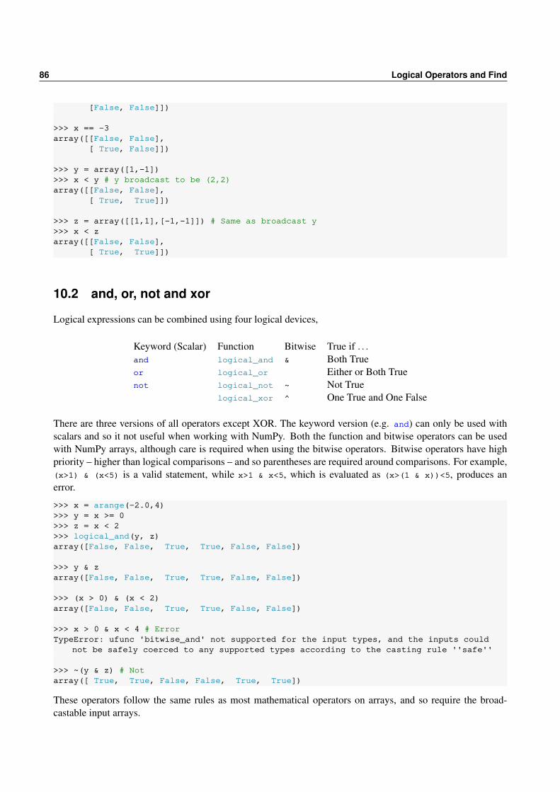
86 Logical Operators and Find

[False, False]])

>>> x == -3array([[False, False],

[ True, False]])

>>> y = array([1,-1])>>> x < y # y broadcast to be (2,2)array([[False, False],

[ True, True]])

>>> z = array([[1,1],[-1,-1]]) # Same as broadcast y>>> x < zarray([[False, False],

[ True, True]])

10.2 and, or, not and xor

Logical expressions can be combined using four logical devices,

Keyword (Scalar) Function Bitwise True if . . .and logical_and & Both Trueor logical_or Either or Both Truenot logical_not ~ Not True

logical_xor ^ One True and One False

There are three versions of all operators except XOR. The keyword version (e.g. and) can only be used withscalars and so it not useful when working with NumPy. Both the function and bitwise operators can be usedwith NumPy arrays, although care is required when using the bitwise operators. Bitwise operators have highpriority – higher than logical comparisons – and so parentheses are required around comparisons. For example,(x>1) & (x<5) is a valid statement, while x>1 & x<5, which is evaluated as (x>(1 & x))<5, produces anerror.

>>> x = arange(-2.0,4)>>> y = x >= 0>>> z = x < 2>>> logical_and(y, z)array([False, False, True, True, False, False])

>>> y & zarray([False, False, True, True, False, False])

>>> (x > 0) & (x < 2)array([False, False, True, True, False, False])

>>> x > 0 & x < 4 # ErrorTypeError: ufunc 'bitwise_and' not supported for the input types, and the inputs could

not be safely coerced to any supported types according to the casting rule ''safe''

>>> ~(y & z) # Notarray([ True, True, False, False, True, True])

These operators follow the same rules as most mathematical operators on arrays, and so require the broad-castable input arrays.

10.3 Multiple tests 87

10.3 Multiple tests

all and any

The commands all and any take logical input and are self-descriptive. all returns True if all logical elementsin an array are 1. If all is called without any additional arguments on an array, it returns True if all elements ofthe array are logical true and 0 otherwise. any returns logical(True) if any element of an array is True. Bothall and any can be also be used along a specific dimension using a second argument or the keyword argumentaxis to indicate the axis of operation (0 is column-wise and 1 is row-wise). When used column- or row-wise,the output is an array with one less dimension than the input, where each element of the output contains thetruth value of the operation on a column or row.

>>> x = array([[1, 2], [3, 4]])>>> y = x <= 2>>> yarray([[ True, True],

[False, False]])

>>> any(y)True

>>> any(y,0)array([[ True, True]])

>>> any(y,1)array([[ True],

[False]])

allclose

allclose can be used to compare two arrays for near equality. This type of function is important when com-paring floating point values which may be effectively the same although not identical.

>>> eps = np.finfo(np.float64).eps>>> eps2.2204460492503131e-16

>>> x = randn(2)>>> y = x + eps>>> x == yarray([False, False])

>>> allclose(x,y)True

The tolerance for being close can be set using keyword arguments either relatively (rtol) or absolutely (atol).

array_equal

array_equal tests if two arrays have the same shape and elements. It is safer than comparing arrays directlysince comparing arrays which are not broadcastable produces an error.

array_equiv

array_equiv tests if two arrays are equivalent, even if they do not have the exact same shape. Equivalence isdefined as one array being broadcastable to produce the other.

88 Logical Operators and Find

>>> x = randn(10,1)>>> y = tile(x,2)>>> array_equal(x,y)False

>>> array_equiv(x,y)True

10.4 is⁎

A number of special purpose logical tests are provided to determine if an array has special characteristics. Someoperate element-by-element and produce an array of the same dimension as the input while other produce onlyscalars. These functions all begin with is.

Operator True if . . . Method of operationisnan 1 if nan element-by-elementisinf 1 if inf element-by-element

isfinite 1 if not inf and not nan element-by-elementisposfin,isnegfin 1 for positive or negative inf element-by-element

isreal 1 if not complex valued element-by-elementiscomplex 1 if complex valued element-by-element

isreal 1 if real valued element-by-elementis_string_like 1 if argument is a string scalar

is_numlike 1 if is a numeric type scalarisscalar 1 if scalar scalarisvector 1 if input is a vector scalar

>>> x=array([4,pi,inf,inf/inf])>>> xarray([4. , 3.14159265, inf, nan])

>>> isnan(x)array([False, False, False, True])

>>> isinf(x)array([False, False, True, False])

>>> isfinite(x)array([ True, True, False, False])

>>> isnan(x) isinf(x) isfinite(x)array([ True, True, True, True])

isnan(x) isinf(x) isfinite(x) always equals True for elements of a numeric array, implying any elementfalls into one (and only one) of these categories.

10.5 Exercises

1. Using the data file created in Chapter 8, count the number of negative returns in both the S&P 500 andExxonMobil.

10.5 Exercises 89

2. For both series, create an indicator variable that takes the value 1 if the return is larger than 2 standarddeviations or smaller than -2 standard deviations. What is the average return conditional on falling eachrange for both returns.

3. Construct an indicator variable that takes the value of 1 when both returns are negative. Compute thecorrelation of the returns conditional on this indicator variable. How does this compare to the correlationof all returns?

4. What is the correlation when at least 1 of the returns is negative?

5. What is the relationship between all and any. Write down a logical expression that allows one or theother to be avoided (i.e. write def myany(x) and def myall(y)).

90 Logical Operators and Find

Chapter 11

Advanced Selection and Assignment

Elements from NumPy arrays can be selected using four methods: scalar selection, slicing, numerical (or list-of-locations) indexing and logical (or Boolean) indexing. Chapter 3 described scalar selection and slicing,which are the basic methods to access elements in an array. Numerical indexing and logical indexing areclosely related and allow for more flexible selection. Numerical indexing uses lists or arrays of locations toselect elements while logical indexing uses arrays containing Boolean values to select elements.

11.1 Numerical Indexing

Numerical indexing, also called list-of-location indexing, is an alternative to slice notation. The fundamentalidea underlying numerical indexing is to use coordinates to select elements, which is similar to the underlyingidea behind slicing. Numerical indexing differs from standard slicing in three important ways:

• Arrays created using numerical indexing are copies of the underlying data, while slices are views (and sodo not copy the data). This means that while changing elements in a slice also changes elements in theslice’s parent, changing elements in an array constructed using numerical indexing does not. This alsocan create performance concerns and slicing should generally be used whenever it is capable of selectingthe required elements.

• Numerical indices can contain repeated values and are not required to be monotonic, allowing for moreflexible selection. The sequences produced using slice notation are always monotonic with unique values.

• The shape of the array selected is determined by the shape of the numerical indices. Slices are similar to1-dimensional arrays but the shape of the slice is determined by the slice inputs.

Numerical indexing in 1-dimensional arrays uses the numerical index values as locations in the array (0-basedindexing) and returns an array with the same dimensions as the numerical index. To understand the core conceptbehind numerical indexing, consider the case of selecting 4 elements form a 1-dimensional array with locationsi1, . . ., i4. Numerical indexing uses the four indices and arranges them to determine the shape (and order) of theoutput. For example, if the order was [

i3 i2i4 i1

]then the array selected would be 2 by 2 with elements[

xi3 xi2xi4 xi1

].

Numerical indexing allows for arbitrary shapes and repetition, and so the selection matrix

92 Advanced Selection and Assignment

i3 i2 i3 i2i4 i1 i3 i2i4 i1 i4 i1

could be used to produce a 4 by 2 array containing the corresponding elements of x. In these examples theindices are not used in any particular order and are repeated to highlight the flexibility of numerical indexing.

Note that the numerical index can be either a list or a NumPy array and must contain integer data.

>>> x = 10 ⁎ arange(5.0)>>> x[[0]] # List with 1 elementarray([ 0.])

>>> x[[0,2,1]] # Listarray([ 0., 20., 10.])

>>> sel = array([4,2,3,1,4,4]) # Array with repetition>>> x[sel]array([ 40., 20., 30., 10., 40., 40.])

>>> sel = array([[4,2],[3,1]]) # 2 by 2 array>>> x[sel] # Selection has same size as selarray([[ 40., 20.],

[ 30., 10.]])

>>> sel = array([0.0,1]) # Floating point data>>> x[sel] # ErrorIndexError: arrays used as indices must be of integer (or boolean) type

>>> x[sel.astype(int)] # No errorarray([ 10., 20.])

>>> x[0] # Scalar selection, not numerical indexing1.0

These examples show that the numerical indices determine the element location and the shape of the array usedto index determines the output shape. The final three examples show slightly different behavior. The first twoof these demonstrate that only integer arrays can be used in numerical indexing, while the final example showsthat there is a subtle difference between x[[0]] (or x[array([0])]), which is using numerical indexing andx[0] which is using a scalar selector. x[[0]] returns a 1-dimensional array since the list has 1 dimension whilex[0] returns a non-array (or scalar or 0-dimensional array) since the input is not a list or array.

Numerical indexing in 2- or higher-dimensional arrays uses numerical index arrays for each dimension.The fundamental idea behind numerical indexing in 2-dimensional arrays is to format coordinate pairs of theform (ik, jk) into separate arrays. The size of the arrays will determine the shape of the array selected. Forexample, if the two selection arrays were

[i1, i3, i2, i4] and [ j1, j3, j2, j4]

then a 1-dimensional array would be selected containing the elements

[x(ii, ji) ,x(i3, j3) ,x(i2, j2) ,x(i4, j4)] .

In practice multidimensional indexing is more flexible that this simple example since the arrays used as selectorscan have either the same shape or can be broadcastable (see Section 4.2).

Consider the following four examples.

11.1 Numerical Indexing 93

>>> x = reshape(arange(10.0), (2,5))>>> xarray([[ 0., 1., 2., 3., 4.],

[ 5., 6., 7., 8., 9.]])

>>> sel = array([0,1])>>> x[sel,sel] # 1-dim arrays, no broadcastingarray([ 0., 6.])

>>> x[sel, sel+1]array([ 1., 7.])

>>> sel_row = array([[0,0],[1,1]])>>> sel_col = array([[0,1],[0,1]])>>> x[sel_row,sel_col] # 2 by 2, no broadcastingarray([[ 0., 1.],

[ 5., 6.]])

>>> sel_row = array([[0],[1]])>>> sel_col = array([[0,1]])>>> x[sel_row,sel_col] # 2 by 1 and 1 by 2 - difference shapes, broadcasted as 2 by 2array([[ 0., 1.],

[ 5., 6.]])

In the first example, sel is a 1-dimensional array containing [0,1], and so the returned value is also a 1-dimensional array containing the (0,0) and (1,1) elements of x. Numerical indexing uses the array in the firstposition to determine row locations and the array in the second position to determine column locations. Thefirst element of the row selection is paired with the first element of column selection (as is the second element).This is why x[sel,sel+1] selects the elements in the (0,1) and (1,2) positions (1 and 7, respectively). Thethird example uses 2-dimensional arrays and selects the elements (0,0), (0,1), (1,0) and (1,1). The finalexample also uses 2-dimensional arrays but with different sizes – 2 by 1 and 1 by 2 – which are broadcastableto a common shape of 2 by 2 arrays.

Next, consider what happens when non-broadcastable arrays are used in as numerical indexing.

>>> sel_row = array([0,1]) # 1-dimensional with shape (2,)>>> sel_col = array([1,2,3]) # 1-dimensional with shape (3,)>>> x[sel_row,sel_col] # ErrorValueError: shape mismatch: objects cannot be broadcast to a single shape

An error occurs since these two 1-dimensional arrays are not broadcastable. ix_ can be used to easily selectrows and columns using numerical indexing by translating the 1-dimesnional arrays to be the correct size forbroadcasting.

>>> x[ix_([0,1],[1,2,3])]array([[ 2., 3., 4.],

[ 7., 8., 9.]])

11.1.1 Mixing Numerical Indexing with Scalar Selection

NumPy permits using difference types of indexing in the same expression. Mixing numerical indexing withscalar selection is trivial since any scalar can be broadcast to any array shape.

>>> sel=array([[1],[2]]) # 2 by 1>>> x[0,sel] # Row 0, elements selarray([[ 1.],

[ 2.]])

>>> sel_row = array([[0],[0]])

94 Advanced Selection and Assignment

>>> x[sel_row,sel] # Identicalarray([[ 1.],

[ 2.]])

11.1.2 Mixing Numerical Indexing with Slicing

Mixing numerical indexing and slicing allow for entire rows or columns to be selected.>>> x[:,[1]]array([[ 2.],

[ 7.]])

>>> x[[1],:]array([[ 6., 7., 8., 9., 10.]])

Note that the mixed numerical indexing and slicing uses a list ([1]) so that it is not a scalar. This is importantsince using a scalar will result in dimension reduction.>>> x[:,1] # 1-dimensionalarray([ 2., 7.])

Numerical indexing and slicing can be mixed in more than 2-dimensions, although some care is required. In thesimplest case where only one numerical index is used which is 1-dimensional, then the selection is equivalentto calling ix_ where the slice a:b:s is replaced with arange(a,b,s).>>> x = reshape(arange(3⁎⁎3), (3,3,3)) # 3-d array>>> sel1 = x[::2,[1,0],:1]>>> sel2 = x[ix_(arange(0,3,2),[1,0],arange(0,1))]>>> sel1.shape(2, 2, 1)

>>> sel2.shape(2, 2, 1)

>>> amax(abs(sel1-sel2))0

When more than 1 numerical index is used, the selection can be viewed as a 2-step process.

1. Select using only slice notation where the dimensions using numerical indexing use the slice :.

2. Apply the numerical indexing to the array produced in step 1.

>>> sel1 = x[[0,0],[1,0],:1]>>> step1 = x[:,:,:1]>>> step2 = x[[0,0],[1,0],:]>>> step2.shape(2, 1)

>>> amax(abs(sel1-step2))0

In the previous example, the shape of the output was (2, 1) which may seem surprising since the numericalindices where both 1-dimensional arrays with 2 elements. The “extra” dimension comes from the slice notationwhich always preserves its dimension. In the next example, the output is 3-dimensional since the numericalindices are 1-dimensional and the 2 slices preserve their dimension.>>> x = reshape(arange(4⁎⁎4), (4,4,4,4))>>> sel = x[[0,1],[0,1],:2,:2] # 1-dimensional numerical and 2 slices>>> sel.shape(2, 2, 2)

11.2 Logical Indexing 95

It is possible to mix multidimensional numerical indexing with slicing and multidimensional arrays. This typeof selection is not explicitly covered since describing the output is complicated and this type of selection israrely encountered.

11.1.3 Linear Numerical Indexing using flat

Like slicing, numerical indexing can be combined with flat to select elements from an array using the row-major ordering of the array. The behavior of numerical indexing with flat is identical to that of using numericalindexing on a flattened version of the underlying array.

>>> x.flat[[3,4,9]]array([ 4., 5., 10.])

>>> x.flat[[[3,4,9],[1,5,3]]]array([[ 4., 5., 10.],

[ 2., 6., 4.]])

11.1.4 Mixing Numerical Indexing with Slicing and Scalar Selection

Mixing the three is identical to using numerical indexing and slicing since the scalar selection is always broad-cast to be compatible with the numerical indices.

11.2 Logical Indexing

Logical indexing differs from slicing and numeric indexing by using logical indices to select elements, rowsor columns. Logical indices act as light switches and are either “on” (True) or “off” (False). Pure logicalindexing uses a logical indexing array with the same size as the array being used for selection and alwaysreturns a 1-dimensional array.

>>> x = arange(-3,3)>>> x < 0array([ True, True, True, False, False, False])

>>> x[x < 0]array([-3, -2, -1])

>>> x[abs(x) >= 2]array([-3, -2, 2])

>>> x = reshape(arange(-8, 8), (4,4))>>> x[x < 0]array([-8, -7, -6, -5, -4, -3, -2, -1])

It is tempting to use two 1-dimensional logical arrays to act as row and column masks on a 2-dimensional array.This does not work, and it is necessary to use ix_ if interested in this type of indexing.

>>> x = reshape(arange(-8,8),(4,4))>>> cols = any(x < -6, 0)>>> rows = any(x < 0, 1)>>> colsarray([ True, True, False, False])

>>> rowsarray([ True, True, False, False])

>>> x[cols,rows] # Not upper 2 by 2

96 Advanced Selection and Assignment

array([-8, -3])

>>> x[ix_(cols,rows)] # Upper 2 by 2array([[-8, -7],

[-4, -3]])

The difference between the final 2 commands is due to the implementation of logical indexing when more thanone logical index is used. When using 2 or more logical indices, they are first transformed to numerical indicesusing nonzero which returns the locations of the non-zero elements (which correspond to the True elements ofa Boolean array).

>>> cols.nonzero()(array([0, 1], dtype=int64),)

>>> rows.nonzero()(array([0, 1], dtype=int64),)

The corresponding numerical index arrays have compatible sizes – both are 2-element, 1-dimensional arrays –and so numeric selection is possible. Attempting to use two logical index arrays which have non-broadcastabledimensions produces the same error as using two numerical index arrays with non-broadcastable sizes.

>>> cols = any(x < -6, 0)>>> rows = any(x < 4, 1)>>> rowsarray([ True, True, True, False])

>>> x[cols,rows] # ErrorValueError: shape mismatch: objects cannot be broadcast to a single shape

11.2.1 Mixing Logical Indexing with Scalar Selection

Logical indexing can be combined with scalar selection to select elements from a specific row or column ina 2-dimensional array. Combining these two types of indexing is no different from first applying the scalarselection to the array and then applying the logical indexing.

>>> x = reshape(arange(-8,8), (4,4))>>> xarray([[-8, -7, -6, -5],

[-4, -3, -2, -1],[ 0, 1, 2, 3],[ 4, 5, 6, 7]])

>>> sum(x, 0)array([-8, -4, 0, 4])

>>> sum(x, 0) >= 0array([False, False, True, True])

>>> x[0,sum(x, 0) >= 0]array([-6, -5])

11.2.2 Mixing Logical Indexing with Slicing

Logical indexing can be freely mixed with slices by using 1-dimensional logical index arrays which act asselectors for columns or rows.

>>> sel = sum(x < -1, 0) >= 2>>> sel

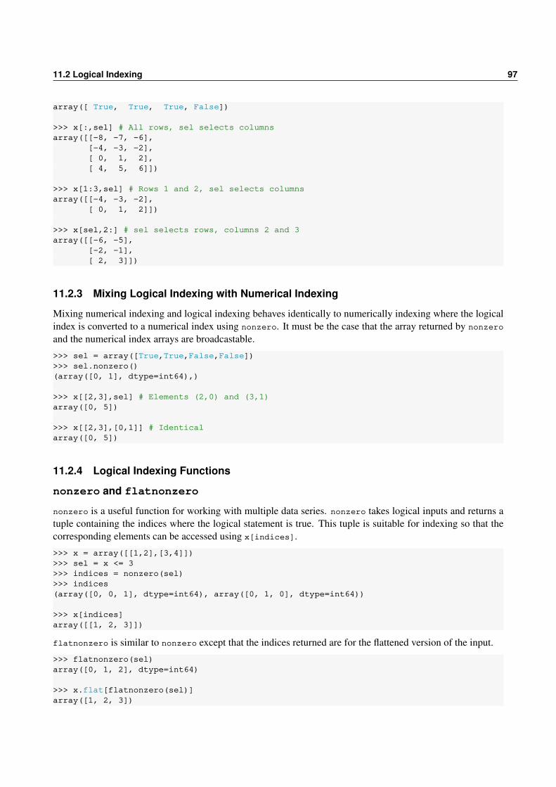
11.2 Logical Indexing 97

array([ True, True, True, False])

>>> x[:,sel] # All rows, sel selects columnsarray([[-8, -7, -6],

[-4, -3, -2],[ 0, 1, 2],[ 4, 5, 6]])

>>> x[1:3,sel] # Rows 1 and 2, sel selects columnsarray([[-4, -3, -2],

[ 0, 1, 2]])

>>> x[sel,2:] # sel selects rows, columns 2 and 3array([[-6, -5],

[-2, -1],[ 2, 3]])

11.2.3 Mixing Logical Indexing with Numerical Indexing

Mixing numerical indexing and logical indexing behaves identically to numerically indexing where the logicalindex is converted to a numerical index using nonzero. It must be the case that the array returned by nonzeroand the numerical index arrays are broadcastable.

>>> sel = array([True,True,False,False])>>> sel.nonzero()(array([0, 1], dtype=int64),)

>>> x[[2,3],sel] # Elements (2,0) and (3,1)array([0, 5])

>>> x[[2,3],[0,1]] # Identicalarray([0, 5])

11.2.4 Logical Indexing Functions

nonzero and flatnonzero

nonzero is a useful function for working with multiple data series. nonzero takes logical inputs and returns atuple containing the indices where the logical statement is true. This tuple is suitable for indexing so that thecorresponding elements can be accessed using x[indices].

>>> x = array([[1,2],[3,4]])>>> sel = x <= 3>>> indices = nonzero(sel)>>> indices(array([0, 0, 1], dtype=int64), array([0, 1, 0], dtype=int64))

>>> x[indices]array([[1, 2, 3]])

flatnonzero is similar to nonzero except that the indices returned are for the flattened version of the input.

>>> flatnonzero(sel)array([0, 1, 2], dtype=int64)

>>> x.flat[flatnonzero(sel)]array([1, 2, 3])

98 Advanced Selection and Assignment

argwhere

argwhere returns an array containing the locations of elements where a logical condition is True. It is the sameas transpose(nonzero(x))

>>> x = randn(3)>>> xarray([-0.5910316 , 0.51475905, 0.68231135])

>>> argwhere(x<0.6)array([[0],

[1]], dtype=int64)

>>> argwhere(x<-10.0) # Empty arrayarray([], shape=(0, 1), dtype=int64)

>>> x = randn(3,2)>>> xarray([[ 0.72945913, 1.2135989 ],

[ 0.74005449, -1.60231553],[ 0.16862077, 1.0589899 ]])

>>> argwhere(x<0)array([[1, 1]], dtype=int64)

>>> argwhere(x<1)array([[0, 0],

[1, 0],[1, 1],[2, 0]], dtype=int64)

extract

extract is similar to argwhere except that it returns the values where the condition is true rather than theindices.

>>> x = randn(3)>>> xarray([-0.5910316 , 0.51475905, 0.68231135])

>>> extract(x<0, x)array([-0.5910316])

>>> extract(x<-10.0, x) # Empty arrayarray([], dtype=float64)

>>> x = randn(3,2)>>> xarray([[ 0.72945913, 1.2135989 ],

[ 0.74005449, -1.60231553],[ 0.16862077, 1.0589899 ]])

>>> extract(x>0,x)array([ 0.72945913, 1.2135989 , 0.74005449, 0.16862077, 1.0589899 ])

11.3 Performance Considerations and Memory Management 99

11.3 Performance Considerations and Memory Management

Arrays constructed using any numerical indexing and/or logical indexing are always copies of the underlyingarray. This is different from the behavior of slicing and scalar selection which returns a view, not a copy, of anarray. This is easily verified by selecting the same elements using different types of selectors.

>>> x = reshape(arange(9), (3,3))>>> s_slice = x[:1,:] # Pure slice>>> s_scalar = x[0] # Scalar selection>>> s_numeric = x[[0],:] # Numeric indexing>>> s_logical = x[array([True,False,False]),:] # Logical indexing>>> s_logical[0,0] = -40>>> s_numeric[0,0] = -30>>> s_numeric # -30array([[-10, 1, 2]])

>>> s_logical # -40, not -30array([[-40, 1, 2]])

>>> s_scalar[0] = -10>>> s_scalararray([-10, 1, 2])

>>> x # Has a -10array([[-10, 1, 2],

[ 3, 4, 5],[ 6, 7, 8]])

>>> s_slice # Has a -10array([[-10, 1, 2]])

Since both numerical and logical indexing produce copies, some care is needed when using these selectors onlarge arrays.

11.4 Assignment with Broadcasting

Any of the selection methods can be used for assignment. When the shape of the array to be assigned is thesame as the selection, the assignment simply replaces elements using an element-by-element correspondence.

>>> x = arange(-2,2.0)>>> xarray([-2., -1., 0., 1.])

>>> x[0] = 999 # Scalar>>> xarray([999., -1., 0., 1.])>>> x[:2] = array([99.0,99]) # Slice>>> xarray([ 99., 99., 0., 1.])

>>> x[[0,1,2]] = array([-3.14,-3.14,-3.14]) # Numerical indexing>>> xarray([-3.14, -3.14, -3.14, 1. ])

>>> x[x<0] = zeros(3) # Logical indexingarray([ 0., 0., 0., 1.])

100 Advanced Selection and Assignment

Assignment is not limited to arrays with exact shape matches, and any assignment where two conditions aremet is allowed:

• Each dimension of the array to be assigned is either 1 or matches the selection.

• The array to be assigned and the selection are broadcastable.

These two conditions ensure that the array to be assigned can be broadcast up to the shape of the selection –it is not sufficient that the selection and the array to be assigned are simply broadcastable. The simplest formof broadcasting assigns a scalar to a selection, and since a scalar can always be broadcast to any shape this isalways possible.

>>> x = array([99.0, 99.0, nan, nan])>>> xarray([ 99., 99., nan, nan])

>>> x[isnan(x)] = 0 # Logical indexing>>> xarray([ 99., 99., 0., 0.])

>>> x.shape = (2,2)>>> x[:,:] = 3.14 # Could also use x[:]>>> xarray([[ 3.14, 3.14],

[ 3.14, 3.14]])

While broadcasting a scalar is the most frequently encountered case, there are useful applications of vector (or1-dimensional array) to 2-dimensional array assignment. For example, it may be necessary to replace all rowsin an array where some criteria are satisfied in the row.

>>> x = reshape(arange(-10,10.0),(4,5))array([[-10., -9., -8., -7., -6.],

[ -5., -4., -3., -2., -1.],[ 0., 1., 2., 3., 4.],[ 5., 6., 7., 8., 9.]])

>>> x[sum(x,1)<0,:] = arange(5.0) # Replace rows w/ negative sum>>> x = reshape(arange(-10,10.0),(4,5))>>> # Replace columns with negative sum>>> x[:, sum(x,0)<0] = arange(4.0) # ErrorValueError: shape mismatch: value array of shape (4,) could not be broadcast to

indexing result of shape (3,4)

>>> x[:, sum(x,0)<0] = reshape(arange(4.0),(4,1)) # Broadcastable col replacement>>> xarray([[ 0., 0., 0., -7., -6.],

[ 1., 1., 1., -2., -1.],[ 2., 2., 2., 3., 4.],[ 3., 3., 3., 8., 9.]])

The error in the previous example occurs because the slice selects a 4 by 2 array, but the array to be assignedis 1-dimensional with 4 elements. The rules of broadcasting always prepend 1s when determining whethertwo arrays are broadcastable, and so the 1-dimensional array is considered to be a 1 by 4 array, which isnot broadcastable to a 4 by 2 array. Using an explicitly 2-dimensional array with shape 4 by 1 allows forbroadcasting.

11.5 Exercises 101

11.5 Exercises

Let x=arange(10.0), y=reshape(arange(25.0),(5,5)) and z=reshape(arange(64.0),(4,4,4)) in all ex-ercises.

1. List all methods to select 4.0 from x.

2. List all methods to select the first 5 elements of x.

3. List all methods to select every second element of x.

4. List all methods to select the row 2 from y.

5. List all methods to select the rows 2 and 4 from y.

6. List all methods to select the rows 2 and 4 and columns 2, 3 and 4 from y.

7. Select all rows of y which have at least one number divisible by 5 and at least one divisible by 7.

8. List all the methods to select panel 1 from z.

9. List all the methods to select rows 2 and 3 from all panels of z.

10. Assign 0 to every second element of z. List the alternative methods.

11. Assign [−1,−1,−1,−1] to all rows of z which have at least one number divisible by 4 and one divisibleby 6. For example, the row containing [16,17,18,19] satisfies this criteria.

12. (Difficult) Define sel = array([[0,1],[1,0]]), What shape does y[sel,:] have? Can this be ex-plained?

102 Advanced Selection and Assignment

Chapter 12

Flow Control, Loops and ExceptionHandling

The previous chapter explored one use of logical variables, selecting elements from an array. Flow control alsoutilizes logical variables to allow different code to be executed depending on whether certain conditions aremet. Flow control in Python comes in two forms - conditional statement and loops.

12.1 Whitespace and Flow Control

Python uses white space changes to indicate the start and end of flow control blocks, and so indention matters.For example, when using if . . . elif . . . else blocks, all of the control blocks must have the same indentationlevel and all of the statements inside the control blocks should have the same level of indentation. Returningto the previous indentation level instructs Python that the block is complete. Best practice is to only use spaces(and not tabs) and to use 4 spaces when starting a new level of indentation which represents a reasonablebalance between readability and wasted space.

12.2 if . . . elif . . . else

if . . . elif . . . else blocks always begin with an if statement immediately followed by a scalar logicalexpression. elif and else are optional and can always be replicated using nested if statements at the expenseof more complex logic and deeper nesting. The generic form of an if . . . elif . . . else block is

if logical_1:Code to run if logical_1

elif logical_2:Code to run if logical_2 and not logical_1

elif logical_3:Code to run if logical_3 and not logical_1 or logical_2

...

...else:

Code to run if all previous logicals are false

However, simpler forms are more common,

if logical:Code to run if logical true

or

104 Flow Control, Loops and Exception Handling

if logical:Code to run if logical true

else:Code to run if logical false

Important: Remember that all logicals must be scalar logical values. While it is possible to use arrays con-taining a single element, attempting to use an array with more than 1 element results in an error.

A few simple examples

>>> x = 5>>> if x<5:... x += 1... else:... x -= 1

>>> x4

and

>>> x = 5;>>> if x<5:... x = x + 1... elif x>5:... x = x - 1... else:... x = x ⁎ 2

>>> x10

These examples have all used simple logical expressions. However, any scalar logical expressions, such as(y<0 or y>1), (x<0 or x>1) and (y<0 or y>1) or isinf(x) or isnan(x), can be used in if . . . elif . . .else blocks.

12.3 for

for loops begin with for item in iterable:, and the generic structure of a for loop is

for item in iterable:Code to run

item is an element from iterable, and iterable can be anything that is iterable in Python. The most commonexamples are range, lists, tuples, arrays or matrices. The for loop will iterate across all items in iterable,beginning with item 0 and continuing until the final item. When using multidimensional arrays, only theoutside dimension is directly iterable. For example, if x is a 2-dimensional array, then the iterable elements arex[0], x[1] and so on.

count = 0for i in range(100):

count += i

count = 0x = linspace(0,500,50)for i in x:

count += i

count = 0x = list(arange(-20,21))

12.3 for 105

for i in x:count += i

The first loop will iterate over i = 0,1,2,. . . ,99. The second loops over the values produced by the functionlinspace, which returns an array with 50 uniformly spaced points between 0 and 500, inclusive. The finalloops over x, a vector constructed from a call to list(arange(-20,21)), which produces a list containing theseries −20,−19,. . . ,0, . . .19,20. All three – range, arrays, and lists – are iterable. The key to understanding forloop behavior is that for always iterates over the elements of the iterable in the order they are presented (i.e.iterable[0], iterable[1], . . .).

Loops can also be nestedcount = 0for i in range(10):

for j in range(10):count += j

or can contain flow control variablesreturns = randn(100)count = 0for ret in returns:

if ret<0:count += 1

This for expression can be equivalently expressed using range as the iterator and len to get the number ofitems in the iterable.returns = randn(100)count = 0for i in range(len(returns)):

if returns[i]<0:count += 1

Finally, these ideas can be combined to produce nested loops with flow control.x = zeros((10,10))for i in range(size(x,0)):

for j in range(size(x,1)):if i<j:

x[i,j]=i+j;else:

x[i,j]=i-j

or loops containing nested loops that are executed based on a flow control statement.x = zeros((10,10))for i in range(size(x,0)):

if (i % 2) == 1:for j in range(size(x,1)):

x[i,j] = i+jelse:

for j in range(int(i/2)):x[i,j] = i-j

Important: The iterable variable should not be reassigned once inside the loop. Consider, for example,x = range(10)for i in x:

print(i)print('Length of x:', len(x))x = range(5)

106 Flow Control, Loops and Exception Handling

This produces the output

# Output0Length of x: 101Length of x: 52Length of x: 53...8Length of x: 59Length of x: 5

It is not safe to modify the sequence of the iterable when looping over it. The means that the iterable should notchange size, which can occur when using a list and the functions pop(), insert() or append() or the keyworddel. The loop below would never terminate (except for the if statement that breaks the loop) since L is beingextended each iteration.

L = [1, 2]for i in L:

print(i)L.append(i+2)if i>5:

break

Finally, for loops can be used with 2 items when the iterable is wrapped in enumerate, which allows theelements of the iterable to be directly accessed, as well as their index in the iterable.

x = linspace(0,100,11)for i,y in enumerate(x):

print('i is :', i)print('y is :', y)

12.3.1 Whitespace

Like if . . . elif . . . else flow control blocks, for loops are whitespace sensitive. The indentation of the lineimmediately below the for statement determines the indentation that all statements in the block must have.

12.3.2 break

A loop can be terminated early using break. break is usually used after an if statement to terminate the loopprematurely if some condition has been met.

x = randn(1000)for i in x:

print(i)if i > 2:

break

Since for loops iterate over an iterable with a fixed size, break is generally more useful in while loops.

12.3.3 continue

continue can be used to skip an iteration of a loop, immediately returning to the top of the loop using the nextitem in iterable. continue is commonly used to avoid a level of nesting, such as in the following two examples.

12.4 while 107

x = randn(10)for i in x:

if i < 0:print(i)

for i in x:if i >= 0:

continueprint(i)

Avoiding excessive levels of indentation is essential in Python programming – 4 is usually considered themaximum reasonable level. continue is particularly useful since it can be used to in a for loop to avoid onelevel of indentation.

12.4 while

while loops are useful when the number of iterations needed depends on the outcome of the loop contents.while loops are commonly used when a loop should only stop if a certain condition is met, such as when thechange in some parameter is small. The generic structure of a while loop iswhile logical:

Code to runUpdate logical

Two things are crucial when using a while loop: first, the logical expression should evaluate to true whenthe loop begins (or the loop will be ignored) and second, the inputs to the logical expression must be updatedinside the loop. If they are not, the loop will continue indefinitely (hit CTRL+C to break an interminable loopin IPython). The simplest while loops are (wordy) drop-in alternatives to for loops:count = 0i = 1while i<10:

count += ii += 1

which produces the same results ascount=0;for i in range(0,10):

count += i

while loops should generally be avoided when for loops are sufficient. However, there are situations where nofor loop equivalent exists.# randn generates a standard normal random numbermu = abs(100⁎randn(1))index = 1while abs(mu) > .0001:

mu = (mu+randn(1))/indexindex=index+1

In the block above, the number of iterations required is not known in advance and since randn is a standardnormal pseudo-random number, it may take many iterations until this criterion is met. Any finite for loopcannot be guaranteed to meet the criteria.

12.4.1 break

break can be used in a while loop to immediately terminate execution. Normally, break should not be used ina while loop – instead the logical condition should be set to False to terminate the loop. However, break can

108 Flow Control, Loops and Exception Handling

be used to avoid running code below the break statement even if the logical condition is False.

condition = Truei = 0x = randn(1000000)while condition:

if x[i] > 3.0:break # No printing if x[i] > 3

print(x[i])i += 1

It is better to update the logical statement which determines whether the while loop should execute.

i = 0while x[i] <= 3:

print(x[i])i += 1

12.4.2 continue

continue can be used in a while loop to skip any remaining code in the loop, immediately returning to the topof the loop, which then checks the while condition, and executes the loop if it still true. Using continue whenthe logical condition in the while loop is False is the same as using break.

12.5 try . . . except

Exception handling is an advanced programming technique which can be used to produce more resilient code(often at the cost of speed). try . . . except blocks are useful for running code which may fail for reasonsoutside of the programmer’s control. In most numerical applications, code should be deterministic and sodangerous code can usually be avoided. When it can’t, for example, if reading data from a data source whichisn’t always available (e.g. a website), then try . . . except can be used to attempt to execute the code, and thento do something if the code fails to execute. The generic structure of a try . . . except block is

try:Dangerous Code

except ExceptionType1:Code to run if ExceptionType1 is raised

except ExceptionType2:Code to run if ExceptionType1 is raised

...

...except:

Code to run if an unlisted exception type is raised

A simple example of exception handling occurs when attempting to convert text to numbers.

text = ('a','1','54.1','43.a')for t in text:

try:temp = float(t)print(temp)

except ValueError:print('Not convertable to a float')

12.6 List Comprehensions 109

12.6 List Comprehensions

List comprehensions are an optimized method of building a list which may simplify code when an iterableobject is looped across and the results are saved to a list, possibly conditional on some logical test. A simplelist can be used to convert a for loop which includes an append into a single line statement.

>>> x = arange(5.0)>>> y = []>>> for i in range(len(x)):... y.append(exp(x[i]))>>> y[1.0,2.7182818284590451,7.3890560989306504,20.085536923187668,54.598150033144236]

>>> z = [exp(x[i]) for i in range(len(x))]>>> z[1.0,2.7182818284590451,7.3890560989306504,20.085536923187668,54.598150033144236]

This simple list comprehension saves 2 lines of typing. List comprehensions can also be extended to include alogical test.

>>> x = arange(5.0)>>> y = []>>> for i in range(len(x)):... if floor(i/2)==i/2:... y.append(x[i]⁎⁎2)>>> y[0.0, 4.0, 16.0]

>>> z = [x[i]⁎⁎2 for i in range(len(x)) if floor(i/2)==i/2]>>> z[0.0, 4.0, 16.0]

List comprehensions can also be used to loop over multiple iterable inputs.

>>> x1 = arange(5.0)>>> x2 = arange(3.0)>>> y = []>>> for i in range(len(x1)):... for j in range(len(x2)):... y.append(x1[i]⁎x2[j])>>> y[0.0, 0.0, 0.0, 0.0, 1.0, 2.0, 0.0, 2.0, 4.0, 0.0, 3.0, 6.0, 0.0, 4.0, 8.0]

>>> z = [x1[i]⁎x2[j] for i in range(len(x1)) for j in range(len(x2))][0.0, 0.0, 0.0, 0.0, 1.0, 2.0, 0.0, 2.0, 4.0, 0.0, 3.0, 6.0, 0.0, 4.0, 8.0]

>>> # Only when i==j>>> z = [x1[i]⁎x2[j] for i in range(len(x1)) for j in range(len(x2)) if i==j][0.0, 1.0, 4.0]

While list comprehensions are powerful methods to compactly express complex operations, they are neveressential to Python programming.

110 Flow Control, Loops and Exception Handling

12.7 Tuple, Dictionary and Set Comprehensions

The other mutable Python structures, the dictionary and the set, support construction using comprehension, asdoes the immutable type tuple. Set and dictionary comprehensions use while tuple comprehensions requirean explicit call to tuple since () has another meaning.

>>> x = arange(-5.0,5.0)>>> z_set = x[i]⁎⁎2.0 for i in range(len(x))>>> z_set0.0, 1.0, 4.0, 9.0, 16.0, 25.0

>>> z_dict = i:exp(i) for i in x-5.0: 0.006737946999085467,-4.0: 0.018315638888734179,-3.0: 0.049787068367863944,-2.0: 0.1353352832366127,-1.0: 0.36787944117144233,...

>>> z_tuple = tuple(i⁎⁎3 for i in x)(-125.0, -64.0, -27.0, -8.0, -1.0, 0.0, 1.0, 8.0, 27.0, 64.0)

12.8 Exercises

1. Write a code block that would take a different path depending on whether the returns on two series aresimultaneously positive, both are negative, or they have different signs using an if . . . elif . . . elseblock.

2. Simulate 1000 observations from an ARMA(2,2) where εt are independent standard normal innovations.The process of an ARMA(2,2) is given by

yt = φ1yt−1 +φ2yt−2 +θ1εt−1 +θ2εt−2 + εt

Use the values φ1 = 1.4, φ2 = −.8, θ1 = .4 and θ2 = .8. Note: A T vector containing standard normalrandom variables can be simulated using e = randn(T). When simulating a process, always simulatemore data than needed and throw away the first block of observations to avoid start-up biases. Thisprocess is fairly persistent, at least 100 extra observations should be computed.

3. Simulate a GARCH(1,1) process where εt are independent standard normal innovations. A GARCH(1,1)process is given by

yt = σtεt

σ2t = ω +αy2

t−1 +βσ2t−1

Use the values ω = 0.05, α = 0.05 and β = 0.9, and set h0 = ω/(1−α−β ).

4. Simulate a GJR-GARCH(1,1,1) process where εt are independent standard normal innovations. A GJR-GARCH(1,1) process is given by

yt = σtεt

σ2t = ω +αy2

t−1 + γy2t−1I[yt−1<0]+βσ

2t−1

12.8 Exercises 111

Use the values ω = 0.05, α = 0.02 γ = 0.07 and β = 0.9 and set h0 = ω/(1−α− 1

2 γ−β). Note that

some form of logical expression is needed in the loop. I[•] is an indicator variable that takes the value 1if the expression inside the [ ] is true.

5. Simulate a ARMA(1,1)-GJR-GARCH(1,1)-in-mean process,

yt = φ1yt−1 +θ1σt−1εt−1 +λσ2t +σtεt

σ2t = ω +ασ

2t−1ε

2t−1 + γσ

2t−1ε

2t−1I[εt−1<0]+βσ

2t−1

Use the values from Exercise 4 for the GJR-GARCH model and use the φ1 =−0.1, θ1 = 0.4 and λ = 0.03.

6. Find two different methods to use a for loop to fill a 5×5 array with i× j where i is the row index, and jis the column index. One will use range as the iterable, and the other should directly iterate on the rows,and then the columns of the matrix.

7. Using a while loop, write a bit of code that will do a bisection search to invert a normal CDF. A bisectionsearch cuts the interval in half repeatedly, only keeping the sub-interval with the target in it. Hint: keeptrack of the upper and lower bounds of the random variable value and use flow control. This problemrequires stats.norm.cdf.

8. Test out the loop using by finding the inverse CDF of 0.01, 0.5 and 0.975. Verify it is working by takingthe absolute value of the difference between the final value and the value produced by stats.norm.ppf.

9. Write a list comprehension that will iterate over a 1-dimensional array and extract the negative elements toa list. How can this be done using only logical functions (no explicit loop), without the list comprehension(and returning an array)?

112 Flow Control, Loops and Exception Handling

Chapter 13

Dates and Times

pandas provides sophisticated tools for creating and manipulating dates such as the Timestamp object, and isthe preferred method for working with dates. Section 15.3.1 builds on the content of this chapter and showshow pandas is used with dates.

Date and time manipulation is provided by a built-in Python module datetime. This chapter assumes thatdatetime has been imported using import datetime as dt.

13.1 Creating Dates and Times

Dates are created using date by providing integer values for year, month and day and times are created usingtime using hours, minutes, seconds and microseconds.

>>> import datetime as dt>>> yr, mo, dd = 2012, 12, 21>>> dt.date(yr, mo, dd)datetime.date(2012, 12, 21)

>>> hr, mm, ss, ms= 12, 21, 12, 21>>> dt.time(hr, mm, ss, ms)dt.time(12,21,12,21)

Dates created using date do not allow times, and dates which require a time stamp can be created usingdatetime, which combine the inputs from date and time, in the same order.

>>> dt.datetime(yr, mo, dd, hr, mm, ss, ms)datetime.datetime(2012, 12, 21, 12, 21, 12, 21)

13.2 Dates Mathematics

Date-times and dates (but not times, and only within the same type) can be subtracted to produce a timedelta,which consists of three values, days, seconds and microseconds. Time deltas can also be added to dates andtimes compute different dates – although date types will ignore all information in the time delta hour, minute,second and millisecond fields.

>>> d1 = dt.datetime(yr, mo, dd, hr, mm, ss, ms)>>> d2 = dt.datetime(yr + 1, mo, dd, hr, mm, ss, ms)>>> d2-d1datetime.timedelta(365)

114 Dates and Times

Date Unit Common Name Range Time Unit Common Name Range

Y Year ±9.2×1018 years h Hour ±1.0×1015 yearsM Month ±7.6×1017 years m Minute ±1.7×1013 yearsW Week ±2.5×1016 years s Second ±2.9×1011 yearsD Day ±2.5×1016 years ms Millisecond ±2.9×108 years

us Microsecond ±2.9×105 yearsns Nanosecond ±292 yearsps Picosecond ±106 daysfs Femtosecond ±2.3 hoursas Attosecond ±9.2 seconds

Table 13.1: NumPy datetime64 range. The absolute range is January 1, 1970 plus the range.

>>> d2 + dt.timedelta(30,0,0)datetime.datetime(2014, 1, 20, 12, 21, 12, 20)

>>> dt.date(2012,12,21) + dt.timedelta(30,12,0)datetime.date(2013, 1, 20)

If times stamps are important, date types can be promoted to datetime using combine and a time.

>>> d3 = dt.date(2012,12,21)>>> dt.datetime.combine(d3, dt.time(0))datetime.datetime(2012, 12, 21, 0, 0)

Values in dates, times and datetimes can be modified using replace through keyword arguments.

>>> d3 = dt.datetime(2012,12,21,12,21,12,21)>>> d3.replace(month=11,day=10,hour=9,minute=8,second=7,microsecond=6)datetime.datetime(2012, 11, 10, 9, 8, 7, 6)

13.3 Numpy

pandas provides a closely related format for dates and times known as a Timestamp, which should be preferredin most cases to direct use of NumPy’s datetime64. See Section 15.3.1 for more information.

Version 1.7.0 of NumPy introduces a NumPy native date and time type known as datetime64 (to distin-guish it from the Python-provided datetime type). The NumPy date and time type is still maturing and isalways fully supported in the scientific python stack at the time of writing these notes. This said, it is alreadywidely used and should see complete support in the near future. Additionally, the native NumPy data typeis generally better suited to data storage and analysis and extends the Python date and time with additionalfeatures such as business day functionality.

NumPy contains both date and time (datetime64) and time-difference (timedelta64) objects. These differfrom the standard Python datetime since they always store the date and time or time difference using a 64-bitinteger plus a date or time unit. The choice of the date/time unit affects both the resolution of the datetime64as well as the permissible range. The unit directly determines the resolution - using a date unit of a day ('D')limits the resolution to days. Using a date unit of a week ('W') will allow a minimum of 1 week difference.Similarly, using a time unit of a second ('s') will allow resolution up to the second (but not millisecond). Theset of date and time units, and their range are presented in Table 13.1.

13.3 Numpy 115

NumPy datetime64s can be initialized using either human readable strings or using numeric values. Thestring initialization is simple and datetime64s can be initialized using year only, year and month, the completedate or the complete date including a time. The default time resolution is nanoseconds (10−9) and T is used toseparate the time from the date.

>>> datetime64('2013')numpy.datetime64('2013')

>>> datetime64('2013-09')numpy.datetime64('2013-09')

>>> datetime64('2013-09-01')numpy.datetime64('2013-09-01')

>>> datetime64('2013-09-01T12:00') # Timenumpy.datetime64('2013-09-01T12:00+0100')

>>> datetime64('2013-09-01T12:00:01') # Secondsnumpy.datetime64('2013-09-01T12:00:01+0100')

>>> datetime64('2013-09-01T12:00:01.123456789') # Nanosecondsnumpy.datetime64('2013-09-01T12:00:01.123456789+0100')

Date or time units can be explicitly included as the second input. The final example shows that rounding canoccur if the date input is not exactly representable using the date unit chosen.

>>> datetime64('2013-01-01T00','h')numpy.datetime64('2013-01-01T00:00+0000','h')

>>> datetime64('2013-01-01T00','s')numpy.datetime64('2013-01-01T00:00:00+0000')

>>> datetime64('2013-01-01T00','ms')numpy.datetime64('2013-01-01T00:00:00.000+0000')

>>> datetime64('2013-01-01','W')numpy.datetime64('2012-12-27')

NumPy datetime64s can also be initialized from arrays.

>>> dates = array(['2013-09-01','2013-09-02'],dtype='datetime64')>>> datesarray(['2013-09-01', '2013-09-02'], dtype='datetime64[D]')

>>> dates[0]numpy.datetime64('2013-09-01')

Note that datetime64 is not timezone aware. For timezone support use pandas Timestamp.Dates which are initialized using one of the shorter forms are initialized at the earliest date (and time) in

the period.

>>> datetime64('2013')==datetime64('2013-01-01')True

>>> datetime64('2013-09')==datetime64('2013-09-01')True

A corresponding time difference class, similarly named timedelta64, is created when dates are differenced.

>>> datetime64('2013-09-02') - datetime64('2013-09-01')numpy.timedelta64(1,'D')

116 Dates and Times

>>> datetime64('2013-09-01') - datetime64('2013-09-01T00:00:00')numpy.timedelta64(3600,'s')

timedelta64 types contain two pieces of information, a number indicating the number of steps between thetwo dates and the size of the step.

Chapter 14

Graphics

Matplotlib is a complete plotting library capable of high-quality graphics. Matplotlib contains both high levelfunctions which produce specific types of figures, for example a simple line plot or a bar chart, as well as alow level API for creating highly customized charts. This chapter covers the basics of producing plots and onlyscratches the surface of the capabilities of matplotlib. Further information is available on the matplotlib websiteor in books dedicated to producing print quality graphics using matplotlib.

Throughout this chapter, the following modules have been imported.

>>> import matplotlib.pyplot as plt>>> import scipy.stats as stats

Other modules will be included only when needed for a specific plot.A datatime converter is requried when using pandas to plot time series. The converter is installed using

>>> from pandas.plotting import register_matplotlib_converters>>> register_matplotlib_converters()

14.1 seaborn

seaborn is a Python package which provides a number of advanced data visualized plots. It also provides ageneral improvement in the default appearance of matplotlib-produced plots, and so I recommend using it bydefault.

>>> import seaborn as sns

All figure in this chapter were produced with seaborn loaded, using the default options. The dark grid back-ground can be swapped to a light grid or no grid using sns.set(style='whitegrid') (light grid) or sns.set(style='white')(no grid, most similar to matplotlib).

14.2 2D Plotting

14.2.1 autoscale and tight_layout

Two funciton, plt.autoscale and plt.tight_layout will generally improve the appearance of figures. autoscalecan be used to set tight limits within a figure’s axes and tight_layout will remove wasted space around a fig-ure. These were used in figures that appear in this chapter, although they have been omitted the code listings(aside from the first)

118 Graphics

14.2.2 Line Plots

The most basic, and often most useful 2D graphic is a line plot. Basic line plots are produced using plot usinga single input containing a 1-dimensional array.

>>> y = randn(100)>>> plot(y)>>> autoscale(tight='x')>>> tight_layout()

The output of this command is presented in panel (a) of figure 14.1. A more flexible form adds a format stringwhich has 1 to 3 elements: a color, represented using a letter (e.g. g for green), a marker symbol which is eithera letter of a symbol (e.g. s for square, ^ for triangle up), and a line style, which is always a symbol or series ofsymbols. In the next example, 'g--' indicates green (g) and dashed line (–).

>>> plot(y,'g--')

Format strings may contain any of the elements in the next table.

Color Marker Line Style

Blue b Point . Solid -Green g Pixel , Dashed --Red r Circle o Dash-dot -.Cyan c Square s Dotted :

Magenta m Diamond DYellow y Thin diamond dBlack k Cross xWhite w Plus +

Star ⁎Hexagon H

Alt. Hexagon hPentagon pTriangles ^, v, <, >

Vertical LineHorizontal Line _

The default behavior is to use a blue solid line with no marker (unless there is more than one line, in whichcase the colors will alter, in order, through those in the Colors column, skipping white). The format stringcontains 1 or more or the three categories of formatting information. For example, kx-- would produce a blackdashed line with crosses marking the points, ⁎: would produce a dotted line with the default color using starsto mark points and yH would produce a solid yellow line with a hexagon marker.

When plot is called with one array, the default x-axis values 1,2, . . . are used. plot(x,y) can be used toplot specific x values against y values. Panel (c) shows the results of running the following code.

>>> x = cumsum(rand(100))>>> plot(x,y,'r-')

While format strings are useful for quickly adding meaningful colors or line styles to a plot, they only exposea limited range of the available customizations. The next example shows how keyword arguments are used toadd customizations to a plot. Panel (d) contains the plot produced by the following code.

>>> plot(x,y,alpha = 0.5, color = '#FF7F00', \... label = 'Line Label', linestyle = '-.', \

14.2 2D Plotting 119

... linewidth = 3, marker = 'o', markeredgecolor = '#000000', \

... markeredgewidth = 2, markerfacecolor = '#FF7F00', \

... markersize=30)

Note that in the previous example, \ is used to indicate to the Python interpreter that a statement is spanningmultiple lines. Some of the more useful keyword arguments are listed in the table below.

Keyword Description

alpha Alpha (transparency) of the plot – default is 1 (no transparency)color Color description for the line.1

label Label for the line – used when creating legendslinestyle A line style symbollinewidth A positive integer indicating the width of the linemarker A marker shape symbol or charactermarkeredgecolor Color of the edge (a line) around the markermarkeredgewidth Width of the edge (a line) around the markermarkerfacecolor Face color of the markermarkersize A positive integer indicating the size of the marker

Many more keyword arguments are available for a plot. The full list can be found in the docstring or byrunning the following code. The functions getp and setp can be used to get the list of properties for a line (orany matplotlib object), and setp can also be used to set a particular property.

>>> h = plot(randn(10))>>> getp(h)

agg_filter = Nonealpha = Noneanimated = False...

>>> setp(h, 'alpha')alpha: float (0.0 transparent through 1.0 opaque)

>>> setp(h, 'color')color: any matplotlib color

>>> setp(h, 'linestyle')linestyle: [ ``'-'`` | ``'--'`` | ``'-.'`` | ``':'`` | ``'None'`` | ``' '`` | ``''`` ]and any drawstyle in combination with a linestyle, e.g. ``'steps--'``.

>>> setp(h, 'linestyle', '--') # Change the line style

Note that setp(h,prop) returns a description of the property and setp(h,prop,value) sets prop to value.

14.2.3 Scatter Plots

scatter produces a scatter plot between 2 1-dimensional arrays. All examples use a set of simulated normaldata with unit variance and correlation of 50%. The output of the basic scatter command is presented in figure14.2, panel (a).

>>> z = randn(100,2)>>> z[:,1] = 0.5⁎z[:,0] + sqrt(0.5)⁎z[:,1]>>> x=z[:,0]>>> y=z[:,1]>>> scatter(x,y)

120 Graphics

(a) (b)

0 20 40 60 80 1003

2

1

0

1

2

3

0 20 40 60 80 1003

2

1

0

1

2

3

(c) (d)

0 10 20 30 40 50 603

2

1

0

1

2

3

0 10 20 30 40 50 603

2

1

0

1

2

3

Figure 14.1: Line plots produced using plot.

14.2 2D Plotting 121

(a) (b) (c)

3 2 1 0 1 2 3 42.5

2.0

1.5

1.0

0.5

0.0

0.5

1.0

1.5

2.0

3 2 1 0 1 2 3 42.5

2.0

1.5

1.0

0.5

0.0

0.5

1.0

1.5

2.0

3 2 1 0 1 2 3 42.5

2.0

1.5

1.0

0.5

0.0

0.5

1.0

1.5

2.0

Figure 14.2: Scatter plots produced using scatter.

Scatter plots can also be modified using keyword arguments. The most important are included in the nextexample, and have identical meaning to those used in the line plot examples. The effect of these keywordarguments is shown in panel (b).

>>> scatter(x,y, s = 60, c = '#FF7F00', marker='s', \... alpha = .5, label = 'Scatter Data')

One interesting use of scatter is to add a 3rd dimension to the plot by including an array of size data whichuses the shapes to convey an extra dimension of data. The use of variable size data is illustrated in the codebelow, which produced the scatter plot in panel (c).

>>> size_data = exp(exp(exp(rand(100))))>>> size_data = 200 ⁎ size_data/amax(size_data)>>> size_data[size_data<1]=1.0>>> scatter(x,y, s = size_data, c = '#FF7F00', marker='s', \... label = 'Scatter Data')

14.2.4 Bar Charts

bar produces bar charts using two 1-dimensional arrays . The first specifies the left ledge of the bars and thesecond the bar heights. The next code segment produced the bar chart in panel (a) of figure 14.3.

>>> y = rand(5)>>> x = arange(5)>>> bar(x,y)

Bar charts take keyword arguments to alter colors and bar width. Panel (b) contains the output of the followingcode.

>>> bar(x,y, width = 0.5, color = '#FF7F00', \... edgecolor = '#000000', linewidth = 5)

Finally, barh can be used instead of bar to produce a horizontal bar chart. The next code snippet produces thehorizontal bar chart in panel (c), and demonstrates the use of a list of colors to alter the appearance of the chart.

>>> colors = sns.color_palette('colorblind')>>> barh(x, y, height = 0.5, color = colors, \... edgecolor = '#000000', linewidth = 5)

122 Graphics

(a) (b) (c)

0 1 2 3 4 50.0

0.1

0.2

0.3

0.4

0.5

0.6

0.7

0.8

0.0 0.5 1.0 1.5 2.0 2.5 3.0 3.5 4.0 4.50.0

0.1

0.2

0.3

0.4

0.5

0.6

0.7

0.8

0.0 0.1 0.2 0.3 0.4 0.5 0.6 0.7 0.80.0

0.5

1.0

1.5

2.0

2.5

3.0

3.5

4.0

4.5

Figure 14.3: Bar charts produced using bar and barh.

14.2.5 Pie Charts

pie produces pie charts using a 1-dimensional array of data (the data can have any values, and does not need tosum to 1). The basic use of pie is illustrated below, and the figure produced appears in panel (a) of figure 14.4.

>>> y = rand(5)>>> y = y/sum(y)>>> y[y<.05] = .05>>> pie(y)

Pie charts can be modified using a large number of keyword arguments, including labels and custom colors. Inthis example, the colors re generated using seaborn’s pallate generator with 8 colors – although only the first 5are used so that the darkest color is not too dark so that the text can be read. Exploded views of a pie chart can beproduced by providing a vector of distances to the keyword argument explode. Note that autopct = '%2.0f'is using an old style format string to format the numeric labels. The results of running this code is shown inpanel (b).

>>> explode = array([.2,0,0,0,0])>>> colors = sns.dark_palette("skyblue", 8, reverse=True)>>> labels = ['One', 'Two', 'Three', 'Four', 'Five']>>> pie(y, explode = explode, colors = colors, \... labels = labels, autopct = '%2.0f', shadow = True)

14.2.6 Histograms

Histograms can be produced using hist. A basic histogram produced using the code below is presented inFigure 14.5, panel (a). This example sets the number of bins used in producing the histogram using the keywordargument bins.

>>> x = randn(1000)>>> hist(x, bins = 30)

Histograms can be further modified using keyword arguments. In the next example, cumulative=True pro-duces the cumulative histogram. The output of this code is presented in figure (b).

>>> hist(x, bins = 30, cumulative=True, color='#FF7F00')

14.2 2D Plotting 123

(a) (b)

One

30

Two

7

Three 26

Four

25

Five

12

Figure 14.4: Pie charts produced using pie.

(a) (b)

4 3 2 1 0 1 2 3 40

20

40

60

80

100

4 3 2 1 0 1 2 3 40

200

400

600

800

1000

Figure 14.5: Histograms produced using hist.

124 Graphics

14.3 Advanced 2D Plotting

14.3.1 Multiple Plots

In some scenarios it is advantageous to have multiple plots or charts in a single figure. Implementing this issimple using figure to initialize the figure window and then using add_subplot. Subplots are added to thefigure using a grid notation with m rows and n columns where 1 is the upper left, 2 is the right of 1, and soon until the end of a row, where the next element is below 1. For example, the plots in a 3 by 2 subplot haveindices 1 2

3 45 6

.add_subplot is called using the notation add_subplot(mni) or add_subplot(m,n,i) where m is the numberof rows, n is the number of columns and i is the index of the subplot.

Note that add_subplot must be called as a method from figure. Note that the next code block is sufficientlong that it isn’t practical to run interactively, and so draw() is used to force an update to the window to ensurethat all plots and charts are visible. Figure 14.6 contains the result running the code below.from matplotlib.pyplot import figure, plot, bar, pie, draw, scatterfrom numpy.random import randn, randfrom numpy import sqrt, arange

fig = figure()# Add the subplot to the figure# Panel 1ax = fig.add_subplot(2, 2, 1)y = randn(100)plot(y)ax.set_title('1')

# Panel 2y = rand(5)x = arange(5)ax = fig.add_subplot(2, 2, 2)bar(x, y)ax.set_title('2')

# Panel 3y = rand(5)y = y / sum(y)y[y < .05] = .05ax = fig.add_subplot(2, 2, 3)pie(y, colors=colors)ax.set_title('3')

# Panel 4z = randn(100, 2)z[:, 1] = 0.5 ⁎ z[:, 0] + sqrt(0.5) ⁎ z[:, 1]x = z[:, 0]y = z[:, 1]ax = fig.add_subplot(2, 2, 4)scatter(x, y)ax.set_title('4')draw()

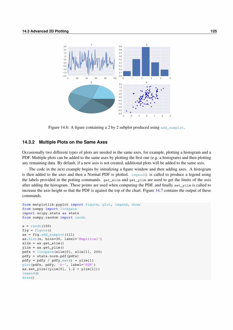
14.3 Advanced 2D Plotting 125

0 20 40 60 80 1002.01.51.00.50.00.51.01.52.02.5

1

0 1 2 3 4 50.00.10.20.30.40.50.60.70.80.9

2

3

3 2 1 0 1 2 32.52.01.51.00.50.00.51.01.52.0

4

Figure 14.6: A figure containing a 2 by 2 subplot produced using add_subplot.

14.3.2 Multiple Plots on the Same Axes

Occasionally two different types of plots are needed in the same axes, for example, plotting a histogram and aPDF. Multiple plots can be added to the same axes by plotting the first one (e.g. a histogram) and then plottingany remaining data. By default, if a new axis is not created, additional plots will be added to the same axis.

The code in the next example begins by initializing a figure window and then adding axes. A histogramis then added to the axes and then a Normal PDF is plotted. legend() is called to produce a legend usingthe labels provided in the potting commands. get_xlim and get_ylim are used to get the limits of the axisafter adding the histogram. These points are used when computing the PDF, and finally set_ylim is called toincrease the axis height so that the PDF is against the top of the chart. Figure 14.7 contains the output of thesecommands.

from matplotlib.pyplot import figure, plot, legend, drawfrom numpy import linspaceimport scipy.stats as statsfrom numpy.random import randn

x = randn(100)fig = figure()ax = fig.add_subplot(111)ax.hist(x, bins=30, label='Empirical')xlim = ax.get_xlim()ylim = ax.get_ylim()pdfx = linspace(xlim[0], xlim[1], 200)pdfy = stats.norm.pdf(pdfx)pdfy = pdfy / pdfy.max() ⁎ ylim[1]plot(pdfx, pdfy, 'r-', label='PDF')ax.set_ylim((ylim[0], 1.2 ⁎ ylim[1]))legend()draw()

126 Graphics

4 3 2 1 0 1 2 30

20

40

60

80

100

120PDFEmpirical

Figure 14.7: A figure containing a histogram and a line plot on the same axes.

14.3.3 Adding a Title and Legend

Titles are added with title and legends are added with legend. legend requires that lines have labels, whichis why 3 calls are made to plot – each series has its own label. Executing the next code block produces a theimage in figure 14.8, panel (a).

>>> x = cumsum(randn(100,3), axis = 0)>>> plot(x[:,0],'b-',label = 'Series 1')>>> plot(x[:,1],'g-.',label = 'Series 2')>>> plot(x[:,2],'r:',label = 'Series 3')>>> legend()>>> title('Basic Legend')

legend takes keyword arguments which can be used to change its location (loc and an integer, see the doc-string), remove the frame (frameon) and add a title to the legend box (title). The output of a simple exampleusing these options is presented in panel (b).

>>> plot(x[:,0],'b-',label = 'Series 1')>>> plot(x[:,1],'g-.',label = 'Series 2')>>> plot(x[:,2],'r:',label = 'Series 3')>>> legend(loc = 0, frameon = False, title = 'The Legend')>>> title('Improved Legend')

14.3.4 Dates on Plots

Plots with date x-values on the x-axis are important when using time series data. Producing basic plots withdates is as simple as plot(x,y) where x is a list or array of dates. This first block of code simulates a randomwalk and constructs 2000 datetime values beginning with March 1, 2012 in a list.

from numpy import cumsumfrom numpy.random import randnfrom matplotlib.pyplot import figure, drawimport matplotlib.dates as mdatesimport datetime as dt

14.3 Advanced 2D Plotting 127

(a) (b)

0 20 40 60 80 10020

15

10

5

0

5

10

15Basic Legend

Series 1Series 2Series 3

0 20 40 60 80 10020

15

10

5

0

5

10

15Improved Legend

The LegendSeries 1Series 2Series 3

Figure 14.8: Figures with titles and legend produced using title and legend.

# Simulate dataT = 2000x = []for i in range(T):

x.append(dt.datetime(2012,3,1)+dt.timedelta(i,0,0))y = cumsum(randn(T))

A basic plot with dates only requires calling plot(x,y) on the x and y data. The output of this code is in panel(a) of figure 14.9.

fig = figure()ax = fig.add_subplot(111)ax.plot(x,y)draw()

Once the plot has been produced autofmt_xdate() is usually called to rotate and format the labels on thex-axis. The figure produced by running this command on the existing figure is in panel (b).

fig.autofmt_xdate()draw()

Sometime, depending on the length of the sample plotted, automatic labels will not be adequate. To showa case where this issue arises, a shorted sample with only 100 values is simulated.

T = 100x = []for i in range(1,T+1):

x.append(dt.datetime(2012,3,1)+dt.timedelta(i,0,0))y = cumsum(randn(T))

A basic plot is produced in the same manner, and is depicted in panel (c). Note the labels overlap and so thisfigure is not acceptable.

fig = figure()ax = fig.add_subplot(111)ax.plot(x,y)draw()

A call to autofmt_xdate() can be used to address the issue of overlapping labels. This is shown in panel (d).

fig.autofmt_xdate()draw()

128 Graphics

While the formatted x-axis dates are an improvement, they are still unsatisfactory in that the date labels havetoo much information (month, day and year) and are not at the start of the month. The next piece of code showshow markers can be placed at the start of the month using MonthLocator which is in the matplotlib.datesmodule. This idea is to construct a MonthLocator instance (which is a class), and then to pass this axesusing xaxis.set_major_locator which determines the location of major tick marks (minor tick marks can beset using xaxis.set_mijor_locator). This will automatically place ticks on the 1st of every month. Otherlocators are available, including YearLocator and WeekdayLocator, which place ticks on the first day of theyear and on week days, respectively. The second change is to format the labels on the x-axis to have the shortmonth name and year. This is done using DateFormatter which takes a custom format string containing thedesired format. Options for formatting include:

• %Y - 4 digit numeric year

• %m - Numeric month

• %d - Numeric day

• %b - Short month name

• %H - Hour

• %M - Minute

• %D - Named day

These can be combined along with other characters to produce format strings. For example, %b %d, %Y wouldproduce a string with the format Mar 1, 2012. Finally autofmt_xdate is used to rotate the labels. The result ofrunning this code is in panel (e).

months = mdates.MonthLocator()ax.xaxis.set_major_locator(months)fmt = mdates.DateFormatter('%b %Y')ax.xaxis.set_major_formatter(fmt)fig.autofmt_xdate()draw()

Note that March 1 is not present in the figure in panel (e). This is because the plot doesn’t actually includethe date March 1 12:00:00 AM, but starts slightly later. To address this, simply change the axis limits using firstcalling get_xlim to get the 2-element tuple containing the limits, change the it to include March 1 12:00:00 AMusing set_xlim. The line between these call is actually constructing the correctly formatted date. Internally,matplotlib uses serial dates which are simply the number of days past some initial date. For example March 1,2012 12:00:00 AM is 734563.0, March 2, 2012 12:00:00 AM is 734564.0 and March 2, 2012 12:00:00 PM is734563.5. The function date2num can be used to convert datetimes to serial dates. The output of running thisfinal price of code on the existing figure is presented in panel (f)

xlim = list(ax.get_xlim())xlim[0] = mdates.date2num(dt.datetime(2012,3,1))ax.set_xlim(xlim)draw()

14.3.5 Shading Areas

For a simple demonstration of the range of matplotlib, consider the problem of producing a plot of Macroeco-nomic time series with shaded regions to indicate business conditions. Capacity utilization data from FRED

14.3 Advanced 2D Plotting 129

(a) (b)

2013 2014 2015 2016 201770

60

50

40

30

20

10

0

10

20132014

20152016

201770

60

50

40

30

20

10

0

10

(c) (d)

Mar 02 2012 Mar 16 2012 Mar 30 2012 Apr 13 2012 Apr 27 2012 May 11 2012 May 25 2012 Jun 08 20128

6

4

2

0

2

4

6

8

Mar 02 2012

Mar 16 2012

Mar 30 2012

Apr 13 2012

Apr 27 2012

May 11 2012

May 25 2012

Jun 08 20128

6

4

2

0

2

4

6

8

(e) (f)

Apr 2012

May 2012

Jun 20128

6

4

2

0

2

4

6

8

Mar 2012

Apr 2012

May 2012

Jun 20128

6

4

2

0

2

4

6

8

Figure 14.9: Figures with dates and additional formatting.

130 Graphics

has been used to illustrate the steps needed to produce a plot with the time series, dates and shaded regionsindicate periods classified as recessions by the National Bureau of Economic Research.

The code has been split into two parts. The first is the code needed to read the data, find the common dates,and finally format the data so that only the common sample is retained.

# Reading the datafrom matplotlib.pyplot import figure, plot_date, axis, drawimport matplotlib.mlab as mlabimport pandas as pd

# pd.read_csv is the best method to read csv datarecessionDates = pd.read_csv('USREC.csv', index_col='DATE', parse_dates=True)capacityUtilization = pd.read_csv('TCU.csv', index_col='DATE', parse_dates=True)# Merge the two data sets and keep the common rowscombined = pd.concat([recessionDates, capacityUtilization], 1).dropna()

# Find the data after the first dateplotData = capacityUtilization.loc[combined.index]shadeData = recessionDates.loc[combined.index]

The second part of the code produces the plot. Most of the code is very simple. It begins by constructinga figure, then add_subplot to the figure, and the plotting the data using plot. fill_between is only oneof many useful functions in matplotlib – it fills an area whenever a variable is 1, which is the structure of therecession indicator. The final part of the code adds a title with a custom font (set using a dictionary), and thenchanges the font and rotation of the axis labels. The output of this code is figure 14.10.

# The shaded plotx = plotData.indexy = plotData.values

# z is the shading values, 1 or 0, need to be 1-dz = (shadeData != 0).squeeze()

# Figurefig = figure()ax = fig.add_subplot(111)plot_date(x,y,'r-')limits = axis()font = 'fontname':'Times New Roman', 'fontsize':14 ax.fill_between(x, limits[2], limits[3], where=z, edgecolor='#BBBBBB', \

facecolor='#222222', alpha=0.3)axis(ymin=limits[2])ax.set_title('Capacity Utilization',font)xl = ax.get_xticklabels()for label in xl:

label.set_fontname('Times New Roman')label.set_fontsize(14)label.set_rotation(45)

yl = ax.get_yticklabels()for label in yl:

label.set_fontname('Times New Roman')label.set_fontsize(14)

draw()

14.4 3D Plotting 131

1972

1977

1982

1987

1992

1997

2002

2007

2012

65

70

75

80

85

90 Capacity Utilization

Figure 14.10: A plot of capacity utilization (US data) with shaded regions indicating NBER recession dates.

14.3.6 TEX in plots

Matplotlib supports using TEX in plots. The only steps needed are the first three lines in the code below, whichconfigure some settings. the labels use raw mode (r'...') to avoid needing to escape the \ in the TEX string.The final plot with TEX in the labels is presented in figure 14.11.

>>> from matplotlib import rc>>> rc('text', usetex=True)>>> rc('font', family='serif')>>> y = 50⁎exp(.0004 + cumsum(.01⁎randn(100)))>>> plot(y)>>> xlabel(r'time ($\tau$)')>>> ylabel(r'Price',fontsize=16)>>> title(r'Geometric Random Walk: $d\ln p_t = \mu dt + \sigma dW_t$',fontsize=16)>>> rc('text', usetex=False)

14.4 3D Plotting

The 3D plotting capabilities of matplotlib are decidedly weaker than the 2D plotting facilities, and yet the 3Dcapabilities are typically adequate for most application (especially since 3D graphics are rarely necessary, andoften distracting).

14.4.1 Line Plots

Line plot in 3D are virtually identical to plotting in 2D, except that 3 1-dimensional vectors are needed: x, y andz (height). This simple example demonstrates how plot can be used with the keyword argument zs to constructa 3D line plot. The line that sets up the axis using Axed3D(fig) is essential when producing 3D graphics. Theother new command, view_init, is used to rotate the view using code (the view can be interactive rotated inthe figure window). The result of running the code below is presented in figure 14.12.

>>> from mpl_toolkits.mplot3d import Axes3D

132 Graphics

0 20 40 60 80 100

time (τ)

47

48

49

50

51

52

53

Pri

ce

Geometric Random Walk: dlnpt =µdt+ σdWt

Figure 14.11: A plot that uses TEX in the labels.

>>> x = linspace(0,6⁎pi,600)>>> z = x.copy()>>> y = sin(x)>>> x= cos(x)>>> fig = plt.figure()>>> ax = Axes3D(fig) # Different usage>>> ax.plot(x, y, zs=z, label='Spiral')>>> ax.view_init(15,45)>>> plt.draw()

14.4.2 Surface and Mesh (Wireframe) Plots

Surface and mesh or wireframe plots are occasionally useful for visualizing functions with 2 inputs, such as abivariate probability density. This example produces both types of plots for a bivariate normal PDF with mean0, unit variances and correlation of 50%. The first block of code generates the points to use in the plot withmeshgrid and evaluates the PDF for all combinations of x and y.

from numpy import linspace, meshgrid, mat, zeros, shape, sqrtimport numpy.linalg as linalg

x = linspace(-3,3,100)y = linspace(-3,3,100)x,y = meshgrid(x,y)z = zeros((1,2))p = zeros(shape(x))R = array([[1,.5],[.5,1]])Rinv = linalg.inv(R)for i in range(len(x)):

for j in range(len(y)):z[0,0] = x[i,j]z[0,1] = y[i,j]p[i,j] = 1.0/(2⁎pi)⁎sqrt(linalg.det(R))⁎exp(-(z@Rinv@z.T)/2)

14.4 3D Plotting 133

1.00.5

0.00.5

1.0

1.00.5

0.00.5

1.0

0

5

10

15

20

Figure 14.12: A 3D line plot constructed using plot.

The next code segment produces a mesh (wireframe) plot using plot_wireframe. The setup of the case isidentical to that of the 3D line, and the call ax = Axes3D(fig) is again essential. The figure is drawn using the2-dimensional arrays x, y and p. The output of this code is presented in panel (a) of 14.13.

>>> from mpl_toolkits.mplot3d import Axes3D>>> fig = plt.figure()>>> ax = Axes3D(fig)>>> ax.plot_wireframe(x, y, p, rstride=5, cstride=5, color='#AD5300')>>> ax.view_init(29,80)>>> plt.draw()

Producing a surface plot is identical, only that a color map is needed from the module matplotlib.cm toprovide different colors across the range of values. The output of this code is presented in panel (b).

>>> import matplotlib.cm as cm>>> fig = plt.figure()>>> ax = Axes3D(fig)>>> ax.plot_surface(x, y, p, rstride=2, cstride=2, cmap=cm.coolwarm, shade='interp')>>> ax.view_init(29,80)>>> plt.draw()

14.4.3 Contour Plots

Contour plots are not technically 3D, although they are used as a 2D representation of 3D data. Since they areultimately 2D, little setup is needed, aside from a call to contour using the same inputs as plot_surface andplot_wireframe. The output of the code below is in figure 14.14.

>>> fig = plt.figure()>>> ax = fig.gca()>>> ax.contour(x,y,p)>>> plt.draw()

134 Graphics

(a) (b)

3210123

3

2

1

0

1

2

3

0.00

0.02

0.04

0.06

0.08

0.10

0.12

0.14

3210123

3

2

1

0

1

2

3

0.00

0.02

0.04

0.06

0.08

0.10

0.12

0.14

Figure 14.13: 3D figures produced using plot_wireframe and plot_surface.

3 2 1 0 1 2 33

2

1

0

1

2

3

Figure 14.14: Contour plot produced using contour.

14.5 General Plotting Functions 135

14.5 General Plotting Functions

figure

figure is used to open a figure window, and can be used to generate axes. fig = figure(n) produces a figureobject with id n, and assigns the object to fig.

add_subplot

add_subplot is used to add axes to a figure. ax = fig.add_subplot(111) can be used to add a basic axes toa figure. ax = fig.add_subplot(m,n,i) can be used to add an axes to a non-trivial figure with a m by n gridof plots.

close

close closes figures. close(n) closes the figure with id n, and close('all') closes all figure windows.

show

show is used to force an update to a figure, and pauses execution if not used in an interactive console (close thefigure window to resume execution). show should not be used in standalone Python programs – draw should beused instead.

draw

draw forces an update to a figure.

14.6 Exporting Plots

Exporting plots is simple using savefig('filename.ext') where ext determines the type of exported file toproduce. ext can be one of png, pdf, ps, eps or svg.

>>> plot(randn(10,2))>>> savefig('figure.pdf') # PDF export>>> savefig('figure.png') # PNG export>>> savefig('figure.svg') # Scalable Vector Graphics export

savefig has a number of useful keyword arguments. In particular, dpi is useful when exporting png files. Thedefault dpi is 100.

>>> plot(randn(10,2))>>> savefig('figure.png', dpi = 600) # High resolution PNG export

14.7 Exercises

1. Download data for the past 20 years for the S&P 500 from Yahoo!. Plot the price against dates, andensure the date display is reasonable.

2. Compute Friday-to-Friday returns using the log difference of closing prices and produce a histogram.Experiment with the number of bins.

136 Graphics

3. Compute the percentage of weekly returns and produce a pie chart containing the percentage of weeklyreturns in each of:

(a) r ≤−2%

(b) −2% < r ≤ 0%

(c) 0 < r ≤ 2%

(d) r > 2%

4. Download 20 years of FTSE data, and compute Friday-to-Friday returns. Produce a scatter plot of theFTSE returns against the S&P 500 returns. Be sure to label the axes and provide a title.

5. Repeat exercise 4, but add in the fit line showing is the OLS fit of regressing FTSE on the S&P plus aconstant.

6. Compute EWMA variance for both the S&P 500 and FTSE and plot against dates. An EWMA variancehas σ2

t‘ = (1−λ )r2t−1 +λσ2

t−1 where r20 = σ2

0 is the full sample variance and λ = 0.97.

7. Explore the chart gallery on the matplotlib website.

Chapter 15

pandas

pandas is a high-performance package that provides a comprehensive set of structures for working with data.pandas excels at handling structured data, such as data sets containing many variables, working with miss-ing values and merging across multiple data sets. pandas is an essential component of the Python scientificstack when operating on data. pandas also provides high-performance, robust methods for importing from andexporting to a wide range of formats.

15.1 Data Structures

pandas provides a set of data structures which include Series, DataFrames and Panels. Series are the equivalentof 1-dimensional arrays. DataFrames are collections of Series and so are 2-dimensional. Panels are collectionsof DataFrames, and have 3 dimensions. Note that the Panel type is scheduled for deprecation and so is notcovered in this chapter.

15.1.1 Series

Series are the primary building block of the data structures in pandas, and in many ways a Series behavessimilarly to a NumPy array. A Series is initialized using a list, tuple, directly from a NumPy array or using adictionary.

>>> a = array([0.1, 1.2, 2.3, 3.4, 4.5])>>> aarray([ 0.1, 1.2, 2.3, 3.4, 4.5])

>>> from pandas import Series>>> s = Series([0.1, 1.2, 2.3, 3.4, 4.5])>>> s0 0.11 1.22 2.33 3.44 4.5dtype: float64

>>> s = Series(a) # NumPy array to Series

Series, like arrays, are sliceable. However, unlike a 1-dimensional array, a Series has an additional column– an index – which is a set of values which are associated with the rows of the Series. In this example, pandashas automatically generated an index using the sequence 0,1, . . . since no index was provided. It is also possibleto use other values as the index when initializing the Series using a keyword argument.

138 pandas

>>> s = Series([0.1, 1.2, 2.3, 3.4, 4.5], index = ['a','b','c','d','e'])>>> sa 0.1b 1.2c 2.3d 3.4e 4.5dtype: float64

The index is an important part of the utility of the pandas’s data structures (Series and DataFrame) andallows for dictionary-like access using values in the index (in addition to both numeric slicing and logicalindices).1

>>> s['a']0.10000000000000001

>>> s[0]0.10000000000000001

>>> s.iloc[0]0.10000000000000001

>>> s[['a','c']]a 0.1c 2.3dtype: float64

>>> s[[0,2]]a 0.1c 2.3dtype: float64

>>> s[:2]a 0.1b 1.2dtype: float64

>>> s[s>2]c 2.3d 3.4e 4.5dtype: float64

In this examples, ’a’ and ’c’ behave in the same manner as 0 and 2 would in a standard NumPy array.The elements of an index do not have to be unique which another way in which a Series generalizes a NumPyarray.

>>> s = Series([0.1, 1.2, 2.3, 3.4, 4.5], index = ['a','b','c','a','b'])>>> sa 0.1b 1.2c 2.3a 3.4b 4.5dtype: float64

>>> s['a']

1Using numeric index values other than the default sequence will break scalar selection since there is ambiguity between numericalslicing and index access. For this reason, access using numerical indices should .iloc[slice].

15.1 Data Structures 139

a 0.1a 3.4dtype: float64

Series can also be initialized directly from dictionaries.

>>> s = Series('a':0.1 ,'b': 1.2, 'c': 2.3, 'd':3.4, 'e': 4.5)>>> sa 0.1b 1.2c 2.3d 3.4e 4.5dtype: float64

Series are like NumPy arrays in that they support most numerical operations.

>>> s = Series('a': 0.1, 'b': 1.2, 'c': 2.3)>>> s ⁎ 2.0a 0.2b 2.4c 4.6dtype: float64

>>> s - 1.0a -0.9b 0.2c 1.3dtype: float64

However, Series are different from arrays when math operations are performed across two Series. In particu-lar, math operations involving two series operate by aligning indices. The mathematical operation is performedin two steps. First, the union of all indices is created, and then the mathematical operation is performed onmatching indices. Indices that do not match are given the value NaN (not a number), and values are computedfor all unique pairs of repeated indices.

>>> s1 = Series('a': 0.1, 'b': 1.2, 'c': 2.3)>>> s2 = Series('a': 1.0, 'b': 2.0, 'c': 3.0)>>> s3 = Series('c': 0.1, 'd': 1.2, 'e': 2.3)>>> s1 + s2a 1.1b 3.2c 5.3dtype: float64

>>> s1 ⁎ s2a 0.1b 2.4c 6.9dtype: float64

>>> s1 + s3a NaNb NaNc 2.4d NaNe NaNdtype: float64

Mathematical operations performed on series which have non-unique indices will broadcast the operationto all indices which are common. For example, when one array has 2 elements with the same index, and another

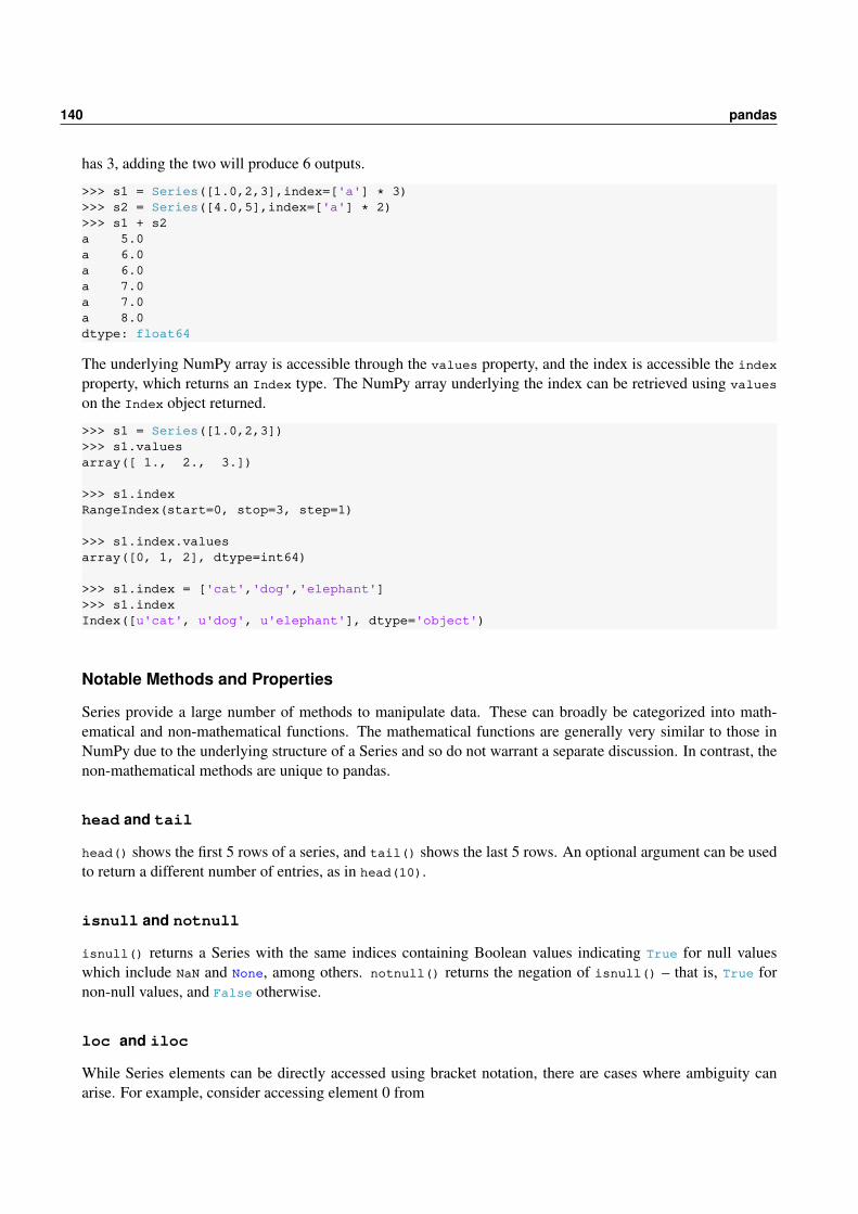
140 pandas

has 3, adding the two will produce 6 outputs.

>>> s1 = Series([1.0,2,3],index=['a'] ⁎ 3)>>> s2 = Series([4.0,5],index=['a'] ⁎ 2)>>> s1 + s2a 5.0a 6.0a 6.0a 7.0a 7.0a 8.0dtype: float64

The underlying NumPy array is accessible through the values property, and the index is accessible the indexproperty, which returns an Index type. The NumPy array underlying the index can be retrieved using valueson the Index object returned.

>>> s1 = Series([1.0,2,3])>>> s1.valuesarray([ 1., 2., 3.])

>>> s1.indexRangeIndex(start=0, stop=3, step=1)

>>> s1.index.valuesarray([0, 1, 2], dtype=int64)

>>> s1.index = ['cat','dog','elephant']>>> s1.indexIndex([u'cat', u'dog', u'elephant'], dtype='object')

Notable Methods and Properties

Series provide a large number of methods to manipulate data. These can broadly be categorized into math-ematical and non-mathematical functions. The mathematical functions are generally very similar to those inNumPy due to the underlying structure of a Series and so do not warrant a separate discussion. In contrast, thenon-mathematical methods are unique to pandas.

head and tail

head() shows the first 5 rows of a series, and tail() shows the last 5 rows. An optional argument can be usedto return a different number of entries, as in head(10).

isnull and notnull

isnull() returns a Series with the same indices containing Boolean values indicating True for null valueswhich include NaN and None, among others. notnull() returns the negation of isnull() – that is, True fornon-null values, and False otherwise.

loc and iloc

While Series elements can be directly accessed using bracket notation, there are cases where ambiguity canarise. For example, consider accessing element 0 from

15.1 Data Structures 141

>>> s = Series([1.0,2,3], index=[7,2,8])>>> s[0] # ErrorKeyError: 0>>> s[2]2.0

This error occurs since 0 is not in the index. To access element by their position using iloc only provides thisaccess.

>>> s.iloc[0]1.0>>> s.iloc[::2]7 1.08 3.0dtype: float64

loc, on the other hand, only allow access using index value or logical arrays.

>>> s.loc[0] # ErrorKeyError: 'the label [0] is not in the [index]'>>> s.loc[[7,8]]7 1.08 3.0dtype: float64>>> s.loc[s.index<8]7 1.02 2.0dtype: float64

describe

describe() returns a simple set of summary statistics. The values returned is a series where the index containsthe names of the statistics computed.

>>> s1 = Series(arange(10.0,20.0))>>> s1.describe()count 10.00000mean 14.50000std 3.02765min 10.0000025% 12.2500050% 14.5000075% 16.75000max 19.00000dtype: float64

>>> summ = s1.describe()>>> summ['mean']14.5

unique and nunique

unique() returns the unique elements of a series and nunique() returns the number of unique values in aSeries.

drop and dropna

drop(labels) drop elements with the selected labels from a Series.

142 pandas

>>> s1 = Series(arange(1.0,6),index=['a','a','b','c','d'])>>> s1a 1.0a 2.0b 3.0c 4.0d 5.0dtype: float64

>>> s1.drop('a')b 3.0c 4.0d 5.0dtype: float64

dropna() is similar to drop() except that it only drops null values – NaN or similar.

>>> s1 = Series(arange(1.0,4.0),index=['a','b','c'])>>> s2 = Series(arange(1.0,4.0),index=['c','d','e'])>>> s3 = s1 + s2>>> s3a NaNb NaNc 4d NaNe NaNdtype: float64

>>> s3.dropna()c 4dtype: float64

Both return Series and so it is necessary to assign the values to have a series with the selected elements dropped.

fillna

fillna(value) fills all null values in a series with a specific value.

>>> s1 = Series(arange(1.0,4.0),index=['a','b','c'])>>> s2 = Series(arange(1.0,4.0),index=['c','d','e'])>>> s3 = s1 + s2>>> s3.fillna(-1.0)a -1.0b -1.0c 4.0d -1.0e -1.0dtype: float64

append

append(series) appends one series to another, and is similar to list.append.

replace

replace(list,values) replaces a set of values in a Series with a new value. replace is similar to fillna exceptthat replace also replaces non-null values.

15.1 Data Structures 143

update

update(series) replaces values in a series with those in another series, matching on the index, and is similar toan update operation in SQL.

>>> s1 = Series(arange(1.0,4.0),index=['a','b','c'])>>> s1a 1.0b 2.0c 3.0dtype: float64

>>> s2 = Series(-1.0 ⁎ arange(1.0,4.0),index=['c','d','e'])>>> s1.update(s2)>>> s1a 1.0b 2.0c -1.0dtype: float64

15.1.2 DataFrame

While the Series class is the building block of data structures in pandas, the DataFrame is the work-horse.DataFrames collect multiple series in the same way that a spreadsheet collects multiple columns of data. Ina simple sense, a DataFrame is like a 2-dimensional NumPy array – and when all data is numeric and of thesame type (e.g. float64), it is virtually indistinguishable. However, a DataFrame is composed of Series andeach Series has its own data type, and so not all DataFrames are representable as homogeneous NumPy arrays.

A number of methods are available to initialize a DataFrame. The simplest method uses a homogeneousNumPy array.

>>> from pandas import DataFrame>>> a = array([[1.0,2],[3,4]])>>> df = DataFrame(a)>>> df

0 10 1 21 3 4

Like a Series, a DataFrame contains the input data as well as row labels. However, since a DataFrame is acollection of columns, it also contains column labels (located along the top edge). When none are provided, thenumeric sequence 0,1, . . . is used.

Column names are entered using a keyword argument or later by assigning to columns.

>>> df = DataFrame(array([[1,2],[3,4]]),columns=['a','b'])>>> df

a b0 1 21 3 4

>>> df = DataFrame(array([[1,2],[3,4]]))>>> df.columns = ['dogs','cats']>>> df

dogs cats

144 pandas

0 1 21 3 4

Index values are similarly assigned using either the keyword argument index or by setting the index property.>>> df = DataFrame(array([[1,2],[3,4]]), columns=['dogs','cats'],... index=['Alice','Bob'])>>> df

dogs catsAlice 1 2Bob 3 4

DataFrames can also be created from NumPy arrays with structured data.>>> import datetime as dt>>> t = dtype([('datetime', 'O8'), ('value', 'f4')])>>> x = zeros(1,dtype=t)>>> x[0][0] = dt.datetime(2013,1,1)>>> x[0][1] = -99.99>>> xarray([(dt.datetime(2013, 1, 1, 0, 0), -99.98999786376953)],

dtype=[('datetime', 'O'), ('value', '<f4')])

>>> df = DataFrame(x)>>> df

datetime value0 2013-01-01 -99.989998

In the previous example, the DataFrame has automatically pulled the column names and column types from theNumPy structured data.

The final method to create a DataFrame uses a dictionary containing Series, where the keys contain thecolumn names. The DataFrame will automatically align the data using the common indices.>>> s1 = Series(arange(0.0,5))>>> s2 = Series(arange(1.0,3))>>> DataFrame('one': s1, 'two': s2)

one two0 0.0 1.01 1.0 2.02 2.0 NaN3 3.0 NaN4 4.0 NaN

>>> s3 = Series(arange(0.0,3))>>> DataFrame('one': s1, 'two': s2, 'three': s3)

one three two0 0.0 0.0 1.01 1.0 1.0 2.02 2.0 2.0 NaN3 3.0 NaN NaN4 4.0 NaN NaN

In the final example, the third series (s3) has fewer values and the DataFrame automatically fills missing valuesas NaN. Note that is possible to create DataFrames from Series which do not have unique index values, althoughin these cases the index values of the two series must match exactly – that is, have the same index values in thesame order.

Manipulating DataFrames

The use of DataFrames will be demonstrated using a data set containing a mix of data types using state-levelGDP data from the US. The data set contains both the GDP level between 2009 and 2012 (constant 2005 US$)

15.1 Data Structures 145

and the growth rates for the same years as well as a variable containing the region of the state. The data isloaded directly into a DataFrame using read_excel, which is described in Section 15.4.

>>> from pandas import read_excel>>> state_gdp = read_excel('US_state_GDP.xls','Sheet1')>>> state_gdp.head()

state_code state gdp_2009 gdp_2010 gdp_2011 gdp_2012 \0 AK Alaska 44215 43472 44232 447321 AL Alabama 149843 153839 155390 1572722 AR Arkansas 89776 92075 92684 938923 AZ Arizona 221405 221016 224787 2306414 CA California 1667152 1672473 1692301 1751002

gdp_growth_2009 gdp_growth_2010 gdp_growth_2011 gdp_growth_2012 region0 7.7 -1.7 1.7 1.1 FW1 -3.9 2.7 1.0 1.2 SE2 -2.0 2.6 0.7 1.3 SE3 -8.2 -0.2 1.7 2.6 SW4 -5.1 0.3 1.2 3.5 FW

Selecting Columns

Single columns are selectable using the column name, as in state_gdp['state'], and the value returned in aSeries. Multiple columns are similarly selected using a list of column names as in

state_gdp[['state_code', 'state']]

or equivalently using an Index object. Note that these two methods are slightly different – selecting a singlecolumn returns a Series while selecting multiple columns returns a DataFrame. This is similar to how NumPy’sscalar selection returns an array with a lower dimension. Use a list of column names containing a single nameto return a DataFrame with a single column.

>>> state_gdp['state_code'].head() # Series0 AK1 AL2 AR3 AZ4 CAName: state_code, dtype: object

>>> state_gdp[['state_code']].head() # DataFramestate_code

0 AK1 AL2 AR3 AZ4 CA

>>> state_gdp[['state_code','state']].head()state_code state

0 AL Alabama1 AK Alaska2 AZ Arizona3 AR Arkansas4 CA California

>>> cols = state_gdp.columns>>> state_gdp[cols[1:3]].head() # Elements 1 and 2 (0-based counting)

state gdp_2009

146 pandas

0 Alabama 1498431 Alaska 442152 Arizona 2214053 Arkansas 897764 California 1667152

Finally, single columns can also be selected using dot-notation and the column name.2 This is identical to usingdf['column'] and so the value returned is a Series.>>> state_gdp.state_code.head()0 AL1 AK2 AZ3 AR4 CAName: state_code, dtype: object

>>> type(state_gdp.state_code)pandas.core.series.Series

Selecting Rows

Rows can be selected using standard numerical slices.>>> state_gdp[1:3]

state_code state gdp_2009 gdp_2010 gdp_2011 gdp_2012 \1 AL Alabama 149843 153839 155390 1572722 AR Arkansas 89776 92075 92684 93892

gdp_growth_2009 gdp_growth_2010 gdp_growth_2011 gdp_growth_2012 region1 -3.9 2.7 1.0 1.2 SE2 -2.0 2.6 0.7 1.3 SE

A function version is also available using iloc[rows] which is identical to the standard slicing syntax. Labeledrows can also be selected using the method loc[label] or loc[list of labels] to elect multiple rows using theirlabel .

Finally, rows can also be selected using logical selection using a Boolean array with the same number ofelements as the number of rows as the DataFrame.>>> state_long_recession = state_gdp['gdp_growth_2010']<0>>> state_gdp[state_long_recession].head()

state_code state gdp_2009 gdp_2010 gdp_2011 gdp_2012 \0 AK Alaska 44215 43472 44232 447323 AZ Arizona 221405 221016 224787 23064133 NV Nevada 110001 109610 111574 11319750 WY Wyoming 32439 32004 31231 31302

gdp_growth_2009 gdp_growth_2010 gdp_growth_2011 gdp_growth_2012 region0 7.7 -1.7 1.7 1.1 FW3 -8.2 -0.2 1.7 2.6 SW33 -8.2 -0.4 1.8 1.5 FW50 3.4 -1.3 -2.4 0.2 RM

Selecting Rows and Columns

Since the behavior of slicing depends on whether the input is text (selects columns) or numeric/Boolean (selectsrows), it isn’t possible to use standard slicing to select both rows and columns. Instead, the selector method

2The column name must be a legal Python variable name, and so cannot contain spaces or reserved notation.

15.1 Data Structures 147

ix[rowselector,colselector] allows joint selection where rowselector is either a scalar selector, a slice selector,a Boolean array, a numeric selector or a row label or list of row labels and colselector is a scalar selector, a sliceselector, a Boolean array, a numeric selector or a column name or list of column names.

>>> state_gdp.loc[state_long_recession,'state']1 Alaska2 Arizona28 Nevada50 WyomingName: state, dtype: object

>>> state_gdp.loc[state_long_recession,... ['state','gdp_growth_2009','gdp_growth_2010']]

state gdp_growth_2009 gdp_growth_20101 Alaska 7.7 -1.72 Arizona -8.2 -0.228 Nevada -8.2 -0.450 Wyoming 3.4 -1.3

>>> state_gdp.iloc[10:15,0] # Slice and scalar10 GA11 HI12 IA13 ID14 IL15 IN

>>> state_gdp.iloc[10:15,:2] # Slice and slicestate_code state

10 GA Georgia11 HI Hawaii12 IA Iowa13 ID Idaho14 IL Illinois15 IN Indiana

Adding Columns

Columns are added using one of three methods. The most natural method adds a Series using a dictionary-likesyntax. Here .copy() is used to ensure state_gdp_2012 contains its own copy of the original data and is notsharing with state_gdp

>>> state_gdp_2012 = state_gdp[['state','gdp_2012']].copy()>>> state_gdp_2012.head()

state gdp_20120 Alabama 1572721 Alaska 447322 Arizona 2306413 Arkansas 938924 California 1751002

>>> state_gdp_2012['gdp_growth_2012'] = state_gdp['gdp_growth_2012']>>> state_gdp_2012.head()

state gdp_2012 gdp_growth_20120 Alabama 157272 1.21 Alaska 44732 1.12 Arizona 230641 2.63 Arkansas 93892 1.3

148 pandas

This syntax always adds the column at the end. insert(location,column_name,series) inserts a Series at aspecific location, where location uses 0-based indexing (i.e. 0 places the column first, 1 places it second, etc.),column_name is the name of the column to be added and series is the series data. series is either a Series oranother object that is readily convertible into a Series such as a NumPy array.

>>> state_gdp_2012 = state_gdp[['state','gdp_2012']].copy()>>> state_gdp_2012.insert(1,'gdp_growth_2012',state_gdp['gdp_growth_2012'])>>> state_gdp_2012.head()

state gdp_growth_2012 gdp_20120 Alabama 1.2 1572721 Alaska 1.1 447322 Arizona 2.6 2306413 Arkansas 1.3 938924 California 3.5 1751002

Formally this type of join performs a left join which means that only index values in the base DataFrame willappear in the combined DataFrame, and so inserting columns with different indices or fewer items than theDataFrame results in a DataFrame with the original indices with NaN-filled missing values in the new Series.

>>> state_gdp_2012 = state_gdp[['state','gdp_2012']].head(3)>>> state_gdp_2012

state gdp_20120 Alabama 1572721 Alaska 447322 Arizona 230641

>>> gdp_2011 = state_gdp['gdp_2011']>>> state_gdp_2012['gdp_2011'] = gdp_2011>>> state_gdp_2012.head(3)

state gdp_2012 gdp_20110 Alabama 157272 NaN1 Alaska 44732 442322 Arizona 230641 224787

Deleting Columns

Columns are deleted using the del keyword, using pop(column) on the DataFrame or by calling drop(listof columns,axis=1) . The behavior of these differs slightly: del will simply delete the Series from theDataFrame. pop() will both delete the Series and return the Series as an output, and drop() will return aDataFrame with the Series dropped without modify the original DataFrame.

>>> state_gdp_copy = state_gdp.copy()>>> columns = ['state_code','gdp_growth_2011','gdp_growth_2012']>>> state_gdp_copy = state_gdp_copy[columns]>>> state_gdp_copy.index = state_gdp['state_code']>>> state_gdp_copy.head()

gdp_growth_2011 gdp_growth_2012state_codeAK 1.7 1.1AL 1.0 1.2AR 0.7 1.3AZ 1.7 2.6CA 1.2 3.5

>>> gdp_growth_2012 = state_gdp_copy.pop('gdp_growth_2012')>>> gdp_growth_2012.head()state_codeAK 1.1

15.1 Data Structures 149

AL 1.2AR 1.3AZ 2.6CA 3.5Name: gdp_growth_2012, dtype: float64

>>> state_gdp_copy.head()gdp_growth_2011

state_codeAK 1.7AL 1.0AR 0.7AZ 1.7CA 1.2

>>> del state_gdp_copy['gdp_growth_2011']>>> state_gdp_copy.head()Empty DataFrameColumns: []Index: [AK, AL, AR, AZ, CA]

>>> state_gdp_copy = state_gdp.copy()>>> state_gdp_copy = state_gdp_copy[columns]>>> state_gdp_dropped = state_gdp_copy.drop(['state_code','gdp_growth_2011'],... axis=1)>>> state_gdp_dropped.head()

gdp_growth_20120 1.11 1.22 1.33 2.64 3.5

Notable Properties and Methods

drop, dropna and drop_duplicates

drop(), dropna() and drop_duplicates() can all be used to drop rows or columns from a DataFrame.drop(labels) drops rows based on the row labels in a label or list labels. drop(column_name,axis=1) dropscolumns based on a column name or list column names.

dropna() drops rows with any NaN (or null) values. It can be used with the keyword argument dropna(how='all' ) to only drop rows which have missing values for all variables. It can also be used with the keywordargument dropna(axis=1) to drop columns with missing values. Finally, drop_duplicates() removes rowswhich are duplicates or other rows, and is used with the keyword argument drop_duplicates(cols=col_list)to only consider a subset of all columns when checking for duplicates.

values and index

values retrieves a the NumPy array (structured if the data columns are heterogeneous) underlying the DataFrame,and index returns the index of the DataFrame or can be assigned to set the index.

fillna

fillna() fills NaN or other null values with other values. The simplest use fill all NaNs with a single valueand is called fillna(value=value ). Using a dictionary allows for more sophisticated na-filling with column

150 pandas

names as the keys and the replacements as the values.

>>> df = DataFrame(array([[1, nan],[nan, 2]]))>>> df.columns = ['one','two']>>> replacements = 'one':-1, 'two':-2>>> df.fillna(value=replacements)

one two0 1 -21 -1 2

T and transpose

T and transpose are identical – both swap rows and columns of a DataFrame. T operates like a property, whiletranspose is used as a method.

sort and sort_index

sort_values and sort_index provide methods to sort a DataFrame. sort_values sorts the contents of theDataFrame along either axis using the contents of a single column or row. Passing a list of coumns names orindex values implements lexicographic search. sort_index will sort a DataFrame by the values in the index.Both support the keyword argument ascending to determine the direction of the sort (ascending by default).ascending can be used with a list to allow sorting in different directions for different sort variables.

>>> df = DataFrame(array([[1, 3],[1, 2],[3, 2],[2,1]]), columns=['one','two'])>>> df.sort_values(by='one')

one two0 1 31 1 23 2 12 3 2

>>> df.sort_values(by=['one','two'])one two

1 1 20 1 33 2 12 3 2

>>> df.sort_values(by=['one','two'], ascending=[0,1])one two

2 3 23 2 11 1 20 1 3

The default behavior is to not sort in-place and so it is necessary to assign the output of a sort. Using thekeyword argument inplace=True will change the default behavior.

pivot

pivot reshapes a table using column values when reshaping. pivot takes three inputs. The first, index,defines the column to use as the index of the pivoted table. The second, columns, defines the column to useto form the column names, and values defines the columns to for the data in the constructed DataFrame. Thefollowing example shows how a flat DataFrame with repeated values is transformed into a more meaningfulrepresentation.

15.1 Data Structures 151

>>> prices = [101.0,102.0,103.0]>>> tickers = ['GOOG','AAPL']>>> import itertools>>> data = [v for v in itertools.product(tickers,prices)]>>> import pandas as pd>>> dates = pd.date_range('2013-01-03',periods=3)>>> df = DataFrame(data, columns=['ticker','price'])>>> df['dates'] = dates.append(dates)>>> df

ticker price dates0 GOOG 101.0 2013-01-031 GOOG 102.0 2013-01-042 GOOG 103.0 2013-01-053 AAPL 101.0 2013-01-034 AAPL 102.0 2013-01-045 AAPL 103.0 2013-01-05

>>> df.pivot(index='dates',columns='ticker',values='price')ticker AAPL GOOGdates2013-01-03 101.0 101.02013-01-04 102.0 102.02013-01-05 103.0 103.0

stack and unstack

stack and unstack transform a DataFrame to a Series (stack) and back to a DataFrame (unstack). Thestacked DataFrame (a Series) uses an index containing both the original row and column labels.

concat and append

append appends rows of another DataFrame to the end of an existing DataFrame. If the data appended has adifferent set of columns, missing values are NaN-filled. The keyword argument ignore_index=True instructsappend to ignore the existing index in the appended DataFrame. This is useful when index values are notmeaningful, such as when they are simple numeric values.

pd.concat is a core function which concatenates two or more DataFrames using an outer join by default.An outer join is a method of joining DataFrames which will return a DataFrame using the union of the indicesof input DataFrames. This differs from the left join that is used when adding a Series to an existing DataFrameusing dictionary syntax. The keyword argument join='inner' can be used to perform an inner join, whichwill return a DataFrame using the intersection of the indices in the input DataFrames. Be default pd.concatwill concatenate using column names, and the keyword argument axis=1 can be used to join using index labels.

>>> df1 = DataFrame([1,2,3],index=['a','b','c'],columns=['one'])>>> df2 = DataFrame([4,5,6],index=['c','d','e'],columns=['two'])>>> pd.concat((df1,df2), axis=1)

one twoa 1.0 NaNb 2.0 NaNc 3.0 4.0d NaN 5.0e NaN 6.0

>>> pd.concat((df1,df2), axis=1, join='inner')one two

c 3 4

152 pandas

reindex and reindex_like

reindex changes the labels while null-filling any missing values, which is useful for selecting subsets of aDataFrame or re-ordering rows. reindex_like behaves similarly but instead uses the index from anotherDataFrame. The keyword argument axis directs reindex to alter either rows or columns.

>>> original = DataFrame([[1,1],[2,2],[3.0,3]],... index=['a','b','c'],... columns=['one','two'])>>> original.reindex(index=['b','c','d'])

one twob 2.0 2.0c 3.0 3.0d NaN NaN

>>> different = DataFrame([[1,1],[2,2],[3.0,3]],... index=['c','d','e'],... columns=['one','two'])>>> original.reindex_like(different)

one twoc 3.0 3.0d NaN NaNe NaN NaN

>>> original.reindex(['two','one'], axis = 1)two one

a 1 1.0b 2 2.0c 3 3.0

merge and join

merge and join provide SQL-like operations for merging the DataFrames using row labels or the contents ofcolumns. The primary difference between the two is that merge defaults to using column contents while joindefaults to using index labels. Both commands take a large number of optional inputs. The important keywordarguments are:

• how, which must be one of 'left', 'right', 'outer', 'inner' describes which set of indices to usewhen performing the join. 'left' uses the indices of the DataFrame that is used to call the method and'right' uses the DataFrame input into merge or join. 'outer' uses a union of all indices from bothDataFrames and 'inner' uses an intersection from the two DataFrames.

• on is a single column name or list of column names to use in the merge. on assumes the names arecommon. If no value is given for on or left_on/right_on, then the common column names are used.

• left_on and right_on allow for a merge using columns with different names. When left_on andright_on contains the same column names, the behavior is the same as on.

• left_index and right_index indicate that the index labels are the join key for the left and rightDataFrames.

>>> left = DataFrame([[1,2],[3,4],[5,6]],columns=['one','two'])>>> right = DataFrame([[1,2],[3,4],[7,8]],columns=['one','three'])>>> left.merge(right,on='one') # Same as how='inner'

one two three0 1 2 2

15.1 Data Structures 153

1 3 4 4

>>> left.merge(right,on='one', how='left')one two three

0 1 2 2.01 3 4 4.02 5 6 NaN

>>> left.merge(right,on='one', how='right')one two three

0 1 2.0 21 3 4.0 42 7 NaN 8

>>> left.merge(right,on='one', how='outer')one two three

0 1 2.0 2.01 3 4.0 4.02 5 6.0 NaN3 7 NaN 8.0

update

update updates the values in one DataFrame using the non-null values from another DataFrame, using theindex labels to determine which records to update.

>>> left = DataFrame([[1,2],[3,4],[5,6]],columns=['one','two'])>>> left

one two0 1 21 3 42 5 6

>>> right = DataFrame([[nan,12],[13,nan],[nan,8]],... columns=['one','two'],... index=[1,2,3])>>> right

one two1 NaN 122 13 NaN3 NaN 8

>>> left.update(right) # Updates values in left>>> left

one two0 1.0 2.01 3.0 12.02 13.0 6.0

apply

apply executes a function along the columns or rows of a DataFrame. The following example applies the meanfunction both down columns and across rows, which is trivial example since mean could be executed on theDataFrame directly. apply is more general since it allows custom functions to be applied to a DataFrame.

>>> cols = ['gdp_growth_2009', 'gdp_growth_2010', 'gdp_growth_2011']>>> subset = state_gdp[cols]

154 pandas

>>> subset.index = state_gdp['state_code'].to_numpy()>>> subset.head()

gdp_growth_2009 gdp_growth_2010 gdp_growth_2011AK 7.7 -1.7 1.7AL -3.9 2.7 1.0AR -2.0 2.6 0.7AZ -8.2 -0.2 1.7CA -5.1 0.3 1.2

>>> subset.apply(mean) # Same as subset.mean()gdp_growth_2009 -2.313725gdp_growth_2010 2.462745gdp_growth_2011 1.590196dtype: float64

>>> subset.apply(mean, axis=1).head() # Same as subset.mean(axis=1)AK 2.200AL 0.250AR 0.650AZ -1.025CA -0.025dtype: float64

applymap

applymap is similar to apply, only that it applies element-by-element rather than column- or row-wise.

pivot_table

pivot_table provides a method to summarize data by groups. A pivot table first forms groups based using thekeyword argument index and then returns an aggregate of all values within the group (using mean by default).The keyword argument aggfun allows for other aggregation function.

>>> subset = state_gdp[['gdp_growth_2009','gdp_growth_2010','region']]>>> subset.head()

gdp_growth_2009 gdp_growth_2010 region0 7.7 -1.7 FW1 -3.9 2.7 SE2 -2.0 2.6 SE3 -8.2 -0.2 SW4 -5.1 0.3 FW

>>> subset.pivot_table(index='region')gdp_growth_2009 gdp_growth_2010

regionFW -2.483333 1.550000GL -5.400000 3.660000MW -1.250000 2.433333NE -2.350000 2.783333PL -1.357143 2.900000RM -0.940000 1.380000SE -2.633333 2.850000SW -2.175000 1.325000

pivot_table differs from pivot since an aggregation function is used when transforming the data.

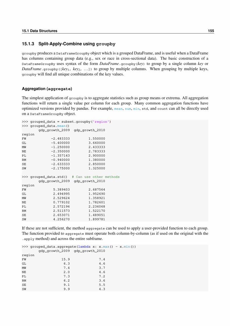
15.1 Data Structures 155

15.1.3 Split-Apply-Combine using groupby

groupby produces a DataFrameGroupBy object which is a grouped DataFrame, and is useful when a DataFramehas columns containing group data (e.g., sex or race in cross-sectional data). The basic construction of aDataFrameGroupBy uses syntax of the form DataFrame.groupby(key) to group by a single column key orDataFrame.groupby([key1, key2, . . .]) to group by multiple columns. When grouping by multiple keys,groupby will find all unique combinations of the key values.

Aggregation (aggregate)

The simplest application of groupby is to aggregate statistics such as group means or extrema. All aggregationfunctions will return a single value per column for each group. Many common aggregation functions haveoptimized versions provided by pandas. For example, mean, sum, min, std, and count can all be directly usedon a DataFrameGroupBy object.

>>> grouped_data = subset.groupby('region')>>> grouped_data.mean()

gdp_growth_2009 gdp_growth_2010regionFW -2.483333 1.550000GL -5.400000 3.660000MW -1.250000 2.433333NE -2.350000 2.783333PL -1.357143 2.900000RM -0.940000 1.380000SE -2.633333 2.850000SW -2.175000 1.325000

>>> grouped_data.std() # Can use other methodsgdp_growth_2009 gdp_growth_2010

regionFW 5.389403 2.687564GL 2.494995 1.952690MW 2.529624 1.358921NE 0.779102 1.782601PL 2.572196 2.236068RM 2.511573 1.522170SE 2.653071 1.489051SW 4.256270 1.899781

If these are not sufficient, the method aggregate can be used to apply a user-provided function to each group.The function provided to aggregate must operate both column-by-column (as if used on the original with the.apply method) and across the entire subframe.

>>> grouped_data.aggregate(lambda x: x.max() - x.min())gdp_growth_2009 gdp_growth_2010

regionFW 15.9 7.4GL 6.3 4.6MW 7.4 3.7NE 2.0 4.6PL 7.3 7.2RM 6.2 3.6SE 9.1 5.5SW 9.9 4.3

156 pandas

Transformation (transform)

Unlike aggregate which returns a single value for each column using some forms of aggregation function,transform returns a DataFrame where each subframe has transformed using a user provided function. Forexample, transform can be used to fill values in the subframe of a particular group based on other values inthe group.

>>> subset_copy = subset.copy()>>> subset_copy.iloc[::3,:2] = np.nan>>> subset_copy.head()

gdp_growth_2009 gdp_growth_2010 region0 NaN NaN FW1 -3.9 2.7 SE2 -2.0 2.6 SE3 NaN NaN SW4 -5.1 0.3 FW

>>> filled_data = grouped_data.transform(lambda x:x.fillna(x.mean()))>>> filled_data.head()

gdp_growth_2009 gdp_growth_20100 -3.6 2.851 -3.9 2.702 -2.0 2.603 0.6 2.454 -5.1 0.30

Filtration (filter)

filter allows groups to be selected based on some function. The function input is the group subframe and itmust return either True or False. This example selects any regions with a single growth rate over 3.3%.

>>> grouped_data = subset.groupby(by='region')>>> grouped_data.filter(lambda x: x.gdp_growth_2009.max() > 3.3)

gdp_growth_2009 gdp_growth_2010 region0 7.7 -1.7 FW4 -5.1 0.3 FW5 -2.2 2.2 RM11 -3.7 3.1 FW13 -2.8 1.6 RM26 -2.1 2.1 RM33 -8.2 -0.4 FW37 -3.2 5.7 FW44 -1.0 2.3 RM47 -2.4 2.3 FW50 3.4 -1.3 RM

Iteration and Selection of a Group

groupby supports iteration across groups if the desired result cannot be computed using one of the directmethods – aggregation, transformation or filtration. Iteration returns two values, the group key and the subsetof data in the group. This example makes use of the state GDP data and groups the data by the region.

>>> subset = state_gdp[['gdp_growth_2009','gdp_growth_2010','region']]>>> subset.head()

gdp_growth_2009 gdp_growth_2010 region0 7.7 -1.7 FW1 -3.9 2.7 SE

15.1 Data Structures 157

2 -2.0 2.6 SE3 -8.2 -0.2 SW4 -5.1 0.3 FW

>>> grouped_data = subset.groupby(by='region')>>> for group_name, group_data in grouped_data:... if group_name == 'SW':... print(group_data)

gdp_growth_2009 gdp_growth_2010 region103 -8.2 -0.2 SW132 1.7 0.8 SW136 -1.7 0.6 SW143 -0.5 4.1 SW

groupby also exposes a property, groups, which will return a dictionary containing the group name and theindex values of the group members.

>>> grouped_data.groups # Lists group names and index labels'FW': Int64Index([0, 4, 11, 33, 37, 47], dtype='int64'),'GL': Int64Index([14, 15, 22, 35, 48], dtype='int64'),'MW': Int64Index([7, 8, 20, 31, 34, 38], dtype='int64'),'NE': Int64Index([6, 19, 21, 30, 39, 46], dtype='int64'),'PL': Int64Index([12, 16, 23, 24, 28, 29, 41], dtype='int64'),'RM': Int64Index([5, 13, 26, 44, 50], dtype='int64'),'SE': Int64Index([1, 2, 9, 10, 17, 18, 25, 27, 40, 42, 45, 49], dtype='int64'),'SW': Int64Index([3, 32, 36, 43], dtype='int64')

15.1.4 Categorical

Categoricals are a special type of Series optimized to efficiently store repeated values. In most relevant casesthe underlying data will be a string, although this is not a requirement. For example, genders or state codes canbe efficiently stored as a Categorical. Categoricals map the inputs onto integer values and use a lookup tableto map the original values to the integer values used to represent the categorical data. In practice, Categoricalsshould only be used when values are repeated – using a Categorical on a string Series containing onlyunique values will require more storage than the original string Series. This example shows the gain to used aCategorical to represent 1,000,000 gender values coded as strings. A DataFrame containing the string versionrequires about 7.6 MiB, which a DataFrame containing the Categorical requires less than 1 MiB. Savings canbe substantially larger when the original string values are larger.

>>> from numpy.random import choice>>> from pandas import Categorical>>> gender = Series(choice(['M','F'], 1000000))>>> df = DataFrame(gender)>>> df.info(memory_usage=True)<class 'pandas.core.frame.DataFrame'>RangeIndex: 1000000 entries, 0 to 999999Data columns (total 1 columns):0 1000000 non-null objectdtypes: object(1)memory usage: 7.6+ MB

>>> gender_cat = Categorical(gender)>>> df = DataFrame([gender_cat])

158 pandas

>>> df.info(memory_usage=True)<class 'pandas.core.frame.DataFrame'>RangeIndex: 1000000 entries, 0 to 999999Data columns (total 1 columns):0 1000000 non-null categorydtypes: category(1)memory usage: 976.7 KB

15.2 Statistical Functions

pandas Series and DataFrame are derived from NumPy arrays and so the vast majority of simple statisticalfunctions are available. This list includes sum, mean, std, var, skew, kurt, prod, median, quantile, abs,cumsum, and cumprod. DataFrame also supports cov and corr – the keyword argument axis determines thedirection of the operation (0 for down columns, 1 for across rows). Novel statistical routines are describedbelow.

count

count returns number of non-null values – that is, those which are not NaN or another null value such as Noneor NaT (not a time, for datetimes).

describe

describe provides a summary of the Series or DataFrame.

>>> state_gdp.describe()gdp_2009 gdp_2010 gdp_2011 gdp_2012 \

count 5.100000e+01 5.100000e+01 5.100000e+01 5.100000e+01mean 2.468670e+05 2.528407e+05 2.569956e+05 2.633273e+05std 2.991342e+05 3.044468e+05 3.096895e+05 3.198425e+05min 2.210800e+04 2.334100e+04 2.363900e+04 2.391200e+0425% 6.407050e+04 6.522900e+04 6.571400e+04 6.628800e+0450% 1.498430e+05 1.538390e+05 1.553900e+05 1.572720e+0575% 3.075225e+05 3.187485e+05 3.274885e+05 3.370160e+05max 1.667152e+06 1.672473e+06 1.692301e+06 1.751002e+06

gdp_growth_2009 gdp_growth_2010 gdp_growth_2011 gdp_growth_2012count 51.000000 51.000000 51.000000 51.000000mean -2.313725 2.462745 1.590196 2.103922std 3.077663 1.886474 1.610497 1.948944min -9.100000 -1.700000 -2.600000 -0.10000025% -3.900000 1.450000 0.900000 1.25000050% -2.400000 2.300000 1.700000 1.90000075% -1.050000 3.300000 2.200000 2.500000max 7.700000 7.200000 7.800000 13.400000

value_counts

value_counts performs histogramming of a Series or DataFrame.

>>> state_gdp.region.value_counts()SE 12PL 7NE 6FW 6

15.3 Time-series Data 159

MW 6GL 5RM 5SW 4dtype: int64

15.3 Time-series Data

The pandas TimeSeries object is currently limited to a span of about 585 years centered at 1970. While this isunlikely to create problems, it may not be appropriate for some applications.

pandas includes a substantial number of routines which are primarily designed to work with time-seriesdata. A TimeSeries is basically a series where the index contains datetimes index values (more formally theclass TimeSeries inherits from Series), and Series constructor will automatically promote a Series with datetimeindex values to a TimeSeries. The TimeSeries examples all make use of US real GDP data from the FederalReserve Economic Database (FRED).

>>> GDP_data = read_excel('GDP.xls','GDP',skiprows=19)>>> GDP_data.head()

DATE VALUE0 1947-01-01 243.11 1947-04-01 246.32 1947-07-01 250.13 1947-10-01 260.34 1948-01-01 266.2

>>> type(GDP_data.VALUE)pandas.core.series.Series

>>> gdp = GDP_data.VALUE>>> gdp.index = GDP_data.DATE>>> gdp.head()DATE1947-01-01 243.11947-04-01 246.31947-07-01 250.11947-10-01 260.31948-01-01 266.2Name: VALUE, dtype: float64

>>> type(gdp.index)pandas.tseries.index.DatetimeIndex

TimeSeries have some useful indexing tricks. For example, all of the data for a particular year can retrievedusing gdp['yyyy'] syntax where yyyy is a year.

>>> gdp['2009']DATE2009-01-01 14381.22009-04-01 14342.12009-07-01 14384.42009-10-01 14564.1Name: VALUE, dtype: float64

>>> gdp['2009-04'] # All for a particular monthDATE2009-04-01 14342.1Name: VALUE, dtype: float64

160 pandas

Dates can also be used for slicing using the notation gdp['d1:d2:'] where d1 and d2 are both valid dateformats (e.g '2009' or '2009-01-01')

>>> gdp['2009':'2010']DATE2009-01-01 14381.22009-04-01 14342.12009-07-01 14384.42009-10-01 14564.12010-01-01 14672.52010-04-01 14879.22010-07-01 15049.82010-10-01 15231.7Name: VALUE, dtype: float64

>>> gdp['2009-06-01':'2010-06-01']DATE2009-07-01 14384.42009-10-01 14564.12010-01-01 14672.52010-04-01 14879.2Name: VALUE, dtype: float64

Slicing indexing can also be accomplished using datetime, for example gdp[datetime( 2009,01, 01): datetime(2011,12,31)] where datetime has been imported using from pandas import datetime.

pct_change

Growth rates are computed using pct_change. The keyword argument periods constructs overlapping growthrates which are useful when using seasonal data.

>>> gdp.pct_change().tail()DATE2012-04-01 0.0074062012-07-01 0.0121042012-10-01 0.0039312013-01-01 0.0070042013-04-01 0.008019Name: VALUE, dtype: float64

>>> gdp.pct_change(periods=4).tail() # Quarterly data, annual differenceDATE2012-04-01 0.0451762012-07-01 0.0476692012-10-01 0.0380312013-01-01 0.0307762013-04-01 0.031404Name: VALUE, dtype: float64

15.3.1 Dates and Times

pandas provides its own date and time functionality that extends NumPy’s datetime64. There are two maintypes to represent dates and times. The first, pandas Timestamps are directly based on NumPy’s datetime64and add time zone support. Timestamps always use datetime64 with nano-second resolution, indicated by[ns], and so only support dates and times in the between 1677 and 2262 (1970 ± 292 years). The second,Periods, is a custom pandas data type that can be used to express dates and times over a wider interval. Theconceptual difference between the two is that a Timestamp represents a point in time which a Period represents

15.3 Time-series Data 161

a range. For example, January 2010 when represented as a Timestamp has to be some specific point in time inJanuary 2010, while represented as a Period is it just January 2010 (with no day, hour, etc.).

Timestamp and Timedelta

Timestamps and Timedeltas are the pandas analogs of NumPy’s datetime64s and timedelta64s. The primarydifference is that pandas continues to support time zone information using the timezone information providedby either the pytz or dateutil packages (pytz is preferred and dateutil will only be used if pytz is not installed).

Timestamps can be created from strings, NumPy datetime64s or Python native datetimes.>>> from pandas import Timestamp, Timedelta>>> from numpy import datetime64>>> import datetime as dt>>> Timestamp('1960-1-1')Timestamp('1960-01-01 00:00:00')

>>> Timestamp(datetime64('1960-01-01'))Timestamp('1960-01-01 00:00:00')

>>> Timestamp(dt.datetime(1960, 1, 1))Timestamp('1960-01-01 00:00:00')

to_datetime

The simplest method to create arrays of Timestamps is to use to_datetime which accepts iterable inputs con-taining dates in any of the convertible formats: strings, datetime or datetime64. to_datetime also providesadditional options for parsing string dates include a format string which allow non-standard date formats to beparsed.>>> from pandas import to_datetime>>> to_datetime(['1960-1-1', '1970-1-1', '1980-1-1'])DatetimeIndex(['1960-01-01', '1970-01-01', '1980-01-01'],

dtype='datetime64[ns]', freq=None)

Period

Periods are an alternative format to Timestamps that represent an interval of time rather than a point in time.Periods are only specified up to the required resolution. For example, when using quarterly data, a Period willonly have a year and quarter while a Timestamp will always be specified up to the nanosecond. Using a Periodavoids choices such as using quarter start or end dates, as well as choosing an arbitrary time of day. Periods canbe specified using a string or through inputs that accept numeric values representing the year, month, day, hour,minute and second. When using a string the frequency is inferred. When using numeric inputs, the frequencymust also be specified.>>> from pandas import Period>>> Period('1980')Period('1980', 'A-DEC')

>>> Period(year=1980, freq='A')Period('1980', 'A-DEC')

>>> Period(year=1980, month=1, freq='Q')Period('1980Q1', 'Q-DEC')

>>> Period(year=1980, month=5, freq='Q')Period('1980Q2', 'Q-DEC')

162 pandas

Periods can be used to represent dates outside the range supported by Timestampss. The supported range isyears between 1 and 9999.

date_range and bdate_range

date_range is a very useful function provided by pandas to generate ranges of dates. The basic use is ei-ther date_range(beginning_date,ending_date) which will produce a daily series between the two dates (in-clusive) or date_range(beginning_date, periods=numperiods) which will produce a daily series starting atbeginning_date with numperiods periods.

>>> from pandas import date_range, bdate_range>>> date_range('2013-01-03','2013-01-05')DatetimeIndex(['2013-01-03', '2013-01-04', '2013-01-05'],

dtype='datetime64[ns]', freq='D')

>>> date_range('2013-01-03', periods = 3)DatetimeIndex(['2013-01-03', '2013-01-04', '2013-01-05'],

dtype='datetime64[ns]', freq='D')

The keyword argument freq changes the frequency, and common choices include

'S' seconds 'U' micro-second'T' minutes 'L' millisecond'H' hourly 'B' daily (business)'D' daily 'W' weekly'M' monthly (end) 'Q' quarterly (end)'A' annual (end)

Many of the frequency choices can be modified to produce only business dates (e.g., Monday to Friday) orstart of period dates. For example, 'MS' will produce the first day in the month, 'BQ' will produce the lastbusiness day in a quarter, and 'BMS' will produce the first business day in the month.

>>> date_range('2013-01-03',periods=2, freq='Q')DatetimeIndex(['2013-03-31', '2013-06-30'],dtype='datetime64[ns]',freq='Q-DEC')

>>> date_range('2013-01-03',periods=2, freq='BQ')DatetimeIndex(['2013-03-29', '2013-06-28'],dtype='datetime64[ns]',freq='BQ-DEC')

Scaling the frequency produces skips that are a multiple of the default, such as in 2D which uses every otherday. Combining multiple frequencies produces less regular skips, e.g. 2H10T.

>>> date_range('2013-01-03',periods=4, freq='Q')DatetimeIndex(['2013-03-31', '2013-06-30', '2013-09-30', '2013-12-31'],

dtype='datetime64[ns]', freq='Q-DEC')

>>> date_range('2013-01-03',periods=4, freq='7D4H')DatetimeIndex(['2013-01-03 00:00:00', '2013-01-10 04:00:00',

'2013-01-17 08:00:00', '2013-01-24 12:00:00'],dtype='datetime64[ns]', freq='172H')

bdate_range is identical to date_range except the defult frequency is business days.

15.4 Importing and Exporting Data 163

>>> date_range('2013-01-03', periods=4)DatetimeIndex(['2013-01-03', '2013-01-04', '2013-01-05', '2013-01-06'],

dtype='datetime64[ns]', freq='D')

>>> bdate_range('2013-01-03', periods=4)DatetimeIndex(['2013-01-03', '2013-01-04', '2013-01-07', '2013-01-08'],

dtype='datetime64[ns]', freq='B')

period_range

period_range is the analogue function to date_range for generating Periods. It is normally called with threearguments, either start, end, and frequency or start, periods, and frequency.

>>> from pandas import period_range>>> period_range('2013-01-03', periods=4, freq='M')PeriodIndex(['2013-01', '2013-02', '2013-03', '2013-04'],

dtype='period[M]', freq='M')

>>> period_range('2013-01-03', periods=4, freq='A')PeriodIndex(['2013', '2014', '2015', '2016'],

dtype='period[A-DEC]', freq='A-DEC')

>>> period_range('2013-01-03', '2019-01-01', freq='A')PeriodIndex(['2013', '2014', '2015', '2016', '2017', '2018', '2019'],

dtype='period[A-DEC]', freq='A-DEC')

15.3.2 resample

pandas supports sophisticated resampling which is useful for aggregating from a higher frequency to a lowerone using resample. resample is similar to groupby and so requires calling an aggregation function on theoutput of the resample call. This example resamples from quarterly to annual ('A') and shows alternativeaggregation functions.

>>> gdp.resample('A').mean().tail() # Annual averageDATE2009-12-31 14417.9502010-12-31 14958.3002011-12-31 15533.8252012-12-31 16244.5752013-12-31 16601.600Freq: A-DEC, Name: VALUE, dtype: float64

>>> gdp.resample('A').max().tail() # MaximumDATE2009-12-31 14564.12010-12-31 15231.72011-12-31 15818.72012-12-31 16420.32013-12-31 16667.9gdp.resample('A').max().tail() # Maximum

15.4 Importing and Exporting Data

In addition to providing data management tools, pandas also excels at importing and exporting data. pandassupports reading and Excel, csv and other delimited files, Stata files, fixed-width text, html, json, HDF5 and

164 pandas

from SQL databases. The functions to read follow the common naming convention read_type where type isthe file type, e.g. excel or csv. The writers are all methods of Series or DataFrame and follow the namingconvention to_type.

Reading Data

read_excel

read_excel supports reading data from both xls (Excel 2003) and xlsx (Excel 2007/10/13) formats. Readingthese formats depends on the Python package xlrd. The basic usage required two inputs, the file name and thesheet name. Other notable keyword arguments include:

• header, an integer indicating which row to use for the column labels. The default is 0 (top) row, and ifskiprows is used, this value is relative.

• skiprows, typically an integer indicating the number of rows at the top of the sheet to skip before readingthe file. The default is 0.

• skip_footer, typically an integer indicating the number of rows at the bottom of the sheet to skip whenreading the file. The default is 0.

• index_col, an integer or column name indicating the column to use as the index. If not provided, a basicnumeric index is generated.

• parse_cols, None, an integer, a list of integers or strings, tells pandas whether to attempt to parse acolumn. The default is None which will parse all columns. Alternatively, if an integer is provided thenthe value is interpreted as the last column to parse. Finally, if a list of integers is provided, the values areinterpreted as the columns to parse (0-based, e.g. [0,2,5]). The string version takes one of the forms'A', 'A,C,D', 'A:D' or a mix of the latter two ('A,C:D,G,W:Z').

read_csv

read_csv reads comma separated value files. The basic use only requires one input, a file name. read_csv alsoaccepts valid URLs (HTTP, FTP, or S3 (Amazon) if the boto package is available) or any object that providesa read method in places of the file name. A huge range of options are available, and so only the most relevantare presented in the list below.

• delimiter, the delimiter used to separate values. The default is ','. Complicated delimiters are matchedusing a regular expression.

• delim_whitespace, Boolean indicating that the delimiter is white space (space or tab). This is preferredto using a regular expression to detect white space.

• header, an integer indicating the row number to use for the column names. The default is 0.

• skiprows, similar to skiprows in read_excel.

• skip_footer, similar to skip_footer in read_excel.

• index_col, similar to index_col in read_excel.

• names, a list of column names to use in-place of any found in the file Must use header=0 (the defaultvalue).

15.4 Importing and Exporting Data 165

• parse_dates, either a Boolean indicating whether to parse dates encountered or a list of integers orstrings indicating which columns to parse. Supports more complicated options to combine columns (seeread_csv).

• date_parser, a function to use when parsing dates. The default parser is dateutil.parser.

• dayfirst, a Boolean indicating whether to use European date format (DD/MM, True) or American dateformat (MM/DD False) when encountering dates. The default is False.

• error_bad_lines, when True stops processing on a bad line. If False, continues skipping any bad linesencountered.

• encoding, a string containing the file encoding (e.g. 'utf-8' or 'latin-1').

• converters, a dictionary of functions for converting values in certain columns, where keys can eitherintegers (column-number) or column labels.

• nrows, an integer, indicates the maximum number of rows to read. This is useful for reading a subset ofa file.

• usecols, a list of integers or column names indicating which column to retain.

• dtype A data type to use for the read data or a dictionary of data types using the column names as keys.If not provided, the type is inferred.

read_table

read_table is similar to read_csv and both are wrappers around a private read function provided by pandas.

read_hdf

read_hdf is primarily for reading pandas DataTables which were written using DataTable.to_hdf

read_stata

read_stata can be used to import Stata DTA files into Python.

Writing Data

Writing data from a Series or DataFrame is much simpler since the starting point (the Series or the DataFrame)is well understood by pandas. While the file writing methods all have a number of options, most can safely beignored.>>> state_gdp.to_excel('state_gdp_from_dataframe.xls')>>> state_gdp.to_excel('state_gdp_from_dataframe_sheetname.xls', sheet_name='State GDP')>>> state_gdp.to_excel('state_gdp_from_dataframe.xlsx')>>> state_gdp.to_csv('state_gdp_from_dataframe.csv')>>> from io import StringIO>>> sio = StringIO()>>> state_gdp.to_json(sio)>>> sio.seek(0)>>> sio.read(50)'"state_code":"0":"AK","1":"AL","2":"AR","3":"AZ"'

>>> state_gdp.to_string()[:50]u' state_code state gdp_2009 gdp'

166 pandas

Stata DTA files can be exported using to_stata. One writer, to_hdf is worth special mention. to_hdfwrites pandas DataFrames to HDF5 files which are binary files which support compression. HDF5 files canachieve fantastic compression ratios when data are regular, and so are often much more useful than CSV or xlsx(which is also compressed). The usage of to_hdf is not meaningfully different from the other writers exceptthat:

• In addition to the filename, an argument is required containing the key, which is usually the variablename.

• Two additional arguments must be passed to compressed the output file. These two keyword argumentsare complib and complevel, which I recommend to setting to ’zlib’ and 6, respectively.

>>> df = DataFrame(zeros((1000,1000)))>>> df.to_csv('size_test.csv')>>> df.to_hdf('size_test.h5','df') # h5 is the usual extension for HDF5# h5 is the usual extension for HDF5>>> df.to_hdf('size_test_compressed.h5','df',complib='zlib',complevel=6)>>> ls size_⁎ # Ignore09/19/2013 04:16 PM 4,008,782 size_test.csv09/19/2013 04:16 PM 8,029,160 size_test.h509/19/2013 04:16 PM 33,812 size_test_compressed.h5

>>> df.to_csv('size_test.csvz', compression='gzip')>>> ls size_test.csvz # Ignore09/19/2013 04:18 PM 10,544 size_test.csvz>>> from pandas import read_csv>>> df_from_csvz = read_csv('size_test.csvz',compression='gzip')

The final block of lines shows how a CSV with gzip compression is written and directly read using pandas.This method also achieves a very high level of compression.

Any NumPy array is easily written to a file using a single, simple line using pandas.

>>> x = randn(100,100)>>> DataFrame(x).to_csv('numpy_array.csv',header=False,index=False)

15.4.1 HDFStore

HDFStore is the Class that underlies to_hdf, and is useful for storing multiple Series or DataFrames to a singleHDF file. Its use is similar to that of any generic file writing function in Python – it must be opened, data canbe read or written, and then it must be closed. Storing data is as simple as inserting objects into a dictionary.

The basic use of a HDFStore for saving data is

>>> from pandas import HDFStore>>> store = HDFStore('store.h5',mode='w',complib='zlib',complevel=6)

which opens the HDFStore named store for writing (mode='w') with compression. Stores can also be openedfor reading (mode='r') or appending (mode='a'). When opened for reading, the compression options are notneeded. Data can then be stored in the HDFStore using dictionary syntax.

>>> store['a'] = DataFrame([[1,2],[3,4]])>>> store['b'] = DataFrame(np.ones((10,10)))

and finally, the store must be closed.

>>> store.close()

The data can then be read using similar commands,

15.5 Graphics 167

>>> store = HDFStore('store.h5',mode='r')>>> a = store['a']>>> b = store['b']>>> store.close()

which will read the data with key 'a' in a variable named a, and similarly for b.A slightly better method for using a store is to use the Python keyword with and HDFStore. When HDFStore

is used in the manner, it is called a context manager. Context managers automatically call close() when thewith block exists, and so ensures that files are always closed.3

with HDFStore('store.h5') as store:a = store['a']b = store['b']

is equivalent to the previous code block, only the close() is called implicitly after the variables are read.The context manager usage of HDFStore can also be used to write HDF files and accepts the usual keywordarguments to, e.g., enable compression or set the mode for opening the file.

15.5 Graphics

pandas provides a set of useful plotting routines based on matplotlib which makes use of the structure of aDataFrame. Everything in pandas plot library is reproducible using matplotlib, although often at the cost ofadditional typing and code complexity (for example, axis labeling).

plot

plot is the main plotting method, and by default will produce a line graph of the data in a DataFrame. Callingplot on a DataFrame will plot all series using different colors and generate a legend. A number of keywordargument are available to affect the contents and appearance of the plot.

• style, a list of matplotlib styles, one for each series plotted. A dictionary using column names as keysand the line styles as values allows for further customization.

• title, a string containing the figure title.

• subplots, a Boolean indicating whether to plot using one subplot per series (True). The default it False.

• legend, a Boolean indicating whether to show a legend

• secondary_y, a Boolean indicating whether to plot a series on a secondary set of axis values. See theexample below.

• ax, a matplotlib axis object to use for the plot. If no axis is provided, then a new axis is created.

• kind, a string, one of:

– 'line', the default

– 'bar' to produce a bar chart. Can also use the keyword argument stacked=True to produce astacked bar chart.

– 'barh' to produce a horizontal bar chart. Also support stacked=True.

– 'kde' or 'density' to produce a kernel density plot.3See Section 22.4 for further details on context managers.

168 pandas

hist

hist produces a histogram plot, and is similar to producing a bar plot using the output of value_count.

boxplot

boxplot produces box plots of the series in a DataFrame.

scatter_plot

scatter_plot produce a scatter plot from two series in a DataFrame. Three inputs are required: the DataFrame,the column name for the x-axis data and the column name for the y-axis data. scatter_plot is located inpandas.tools.plotting.

scatter_matrix

scatter_matrix produces a n by n set of subplots where each subplot contains the bivariate scatter of twoseries. One input is required, the DataFrame. scatter_matrix is located in pandas.tools.plotting. Bydefault, the diagonal elements are histograms, and the keyword argument diagonal='kde' produces a kerneldensity plot.

lag_plot

lag_plot produces a scatter plot of a series against its lagged value. The keyword argument lag chooses thelag used in the plot (default is 1).

15.6 Examples

15.6.1 FRED Data

The Federal Reserve Economics Database is a comprehensive database of US, and increasingly global, macroe-conomics data. This example will directly download a small macroeconomics data set from FRED and mergeit into a single DataFrame. The data in FRED is available in CSV using the url pattern https://fred.stlouisfed.org/graph/fredgraph.csv?id=CODE where CODE is the series code. This examplewill make use of Real GDP, Industrial Production, Core CPI the Unemployment Rate, the Treasury yield slope(10-year yield minus 1-year yield) and the default premium, based on the difference between BAA and AAArated bonds. The list of series is in table 15.1.

The initial block of code imports the future functions, read_csv, DataFrame and scatter_matrix, theonly pandas functions directly used in this example. It also sets up lists containing the codes and nice namesfor the series and contains the URL root for fetching the data

from pandas import read_csvfrom pandas.plotting import scatter_matrix

codes = ['GDPC1','INDPRO','CPILFESL','UNRATE','GS10','GS1','BAA','AAA']names = ['Real GDP','Industrial Production','Core CPI','Unemployment Rate',\

'10 Year Yield','1 Year Yield','Baa Yield','Aaa Yield']

# r to disable escapebase_url = r'https://fred.stlouisfed.org/graph/fredgraph.csv?id=code'

The next piece of code starts with an empty list to hold the DataFrames produced by read_csv. The codes arethen looped over and directly used in the CSV reader.

15.6 Examples 169

Series Code Frequency

Real GDP GDPC1 QuarterlyIndustrial Production INDPRO QuarterlyCore CPI CPILFESL MonthlyUnemployment Rate UNRATE Monthly10 Year Yield GS10 Monthly1 Year Yield GS1 MonthlyBaa Yield BAA MonthlyAaa Yield AAA Monthly

Table 15.1: The series, codes and their frequencies used in the FRED example.

data = []for code in codes:

print(code)url = base_url.format(code=code)data.append(read_csv(url))

Next, the data is merged into a single DataFrame by building a dictionary where the keys are the codes and thevalues are the Series from each downloaded DataFrame. This block makes use of zip to quickly concatenatetwo lists into a single iterable.

time_series = for code, d in zip(codes,data):

d.index = d.DATEtime_series[code] = d[code]

merged_data = DataFrame(time_series)# Unequal length seriesprint(merged_data)

The next step is to construct the Term and Default premia series using basic math on the series. The resultingSeries are given a name, which is required for the join operation. Finally, the non-required columns are dropped.

term_premium = merged_data['GS10'] - merged_data['GS1']term_premium.name = 'Term'merged_data = merged_data.join(term_premium,how='outer')default_premium = merged_data['BAA'] - merged_data['AAA']default_premium.name = 'Default'merged_data = merged_data.join(default_premium,how='outer')merged_data = merged_data.drop(['AAA','BAA','GS10','GS1'],axis=1)print(merged_data.tail())

The next block forms a quarterly data set by dropping the rows with any null values.

quarterly = merged_data.dropna()print(quarterly.tail())

Finally, it is necessary to transform some of the series to be growth rates since the data contains both I(0) andI(1) series. This is done using pct_change on a subset of the quarterly data.

growth_rates_selector = ['GDPC1','INDPRO','CPILFESL']growth_rates = 100 ⁎ quarterly[growth_rates_selector].pct_change()final = quarterly.drop(growth_rates_selector, axis=1).join(growth_rates)

170 pandas

Series Description

Treated Dummy indicating whether the candidate received the treatmentAge Age in yearsEducation (years) Years of EducationBlack Dummy indicating African-AmericanHispanic Dummy indicating HispanicMarried Dummy indicating marriedReal income Before ($) Income before programReal income After ($) Income after program

Table 15.2: The series, codes and their frequencies used in the FRED example.

The last step is to rename some of the columns using rename with the keyword argument columns. The namesare changed using a dictionary where the key is the old name and the value is the new name. The last two linessave the final version of the data to HDF5 and to an excel file.

new_names = 'GDPC1':'GDP_growth', \'INDPRO':'IP_growth', \'CPILFESL':'Inflation', \'UNRATE':'Unemp_rate'

final = final.rename(columns = new_names ).dropna()final.to_hdf('FRED_data.h5','FRED',complevel=6,complib='zlib')final.to_excel('FRED_data.xlsx')

The plots provide a simple method to begin exploring the data. Both plots are shown in Figure 15.1.

ax = final[['GDP_growth','IP_growth','Unemp_rate']].plot(subplots=True)fig = ax[0].get_figure()fig.savefig('FRED_data_line_plot.pdf')

columns = ['GDP_growth','IP_growth','Unemp_rate']ax = scatter_matrix(final[columns], diagonal='kde')fig = ax[0,0].get_figure()fig.savefig('FRED_data_scatter_matrix.pdf')

15.6.2 NSW Data

The National Supported Work Demonstration was a program to determine whether giving disadvantaged work-ers useful job skills would translate into increased earnings. The data set used here is a subset of the completedata set and contains the variables in table 15.2.

The first block contains the standard imports as well as the functions which are used in this example. Bothsqrt and stats are used to perform a t-test.

from pandas import read_excelfrom numpy import sqrtimport scipy.stats as statsimport seaborn

The data is contained in a well-formatted Excel file, and so importing the data using read_excel is straightfor-ward. The second line in this block prints the standard descriptive statistics.

NSW = read_excel('NSW.xls','NSW')print(NSW.describe())

15.6 Examples 171

32101234

GDP_growth

864202468

10IP_growth

1957-04-01

1969-10-01

1982-04-01

1994-10-01

2007-04-013456789

1011

Unemp_rate

-2

-1

0

1

2

3

4

GD

P_gr

owth

5

0

5

10

IP_g

row

th

2 1 0 1 2 3 4

GDP_growth

4

5

6

7

8

9

10

Une

mp_

rate

5 0 5 10

IP_growth

4 5 6 7 8 9 10

Unemp_rate

Figure 15.1: The top panel contains line plots of the FRED data. The bottom panel shows the output ofscatter_matrix using kernel density plots along the diagonal.

172 pandas

rename is then used to give the columns some more useful names – names with spaces cannot be directlyaccessed using dot notation (i.e. NSW.Income_after works, but there is no method to do the same usingNSW.'Real income After ($)'.

NSW = NSW.rename(columns='Real income After ($)':'Income_after','Real income Before ($)':'Income_before','Education (years)':'Education')

NSW['Minority'] = NSW['Black']+NSW['Hispanic']

Next, pivot_table is used to look at the variable means using some of the groups. The third call uses twoindices and a double sort.

print(NSW.pivot_table(index='Treated'))

print(NSW.pivot_table(index='Minority'))

print(NSW.pivot_table(index=['Minority','Married']))

Next, density plots of the income before and after are plotted. Figure 15.2 shows the plots.

ax = NSW[['Income_before','Income_after']].plot(kind='kde',subplots=True)fig = ax[0].get_figure()fig.savefig('NSW_density.pdf')

Finally a t-test of equal incomes using the before and after earnings for the treated and non-treated is computed.The t-stat has a one-sided p-val of .9%, indicating rejection of the null of no impact at most significance levels.

income_diff = NSW['Income_after']-NSW['Income_before']t = income_diff[NSW['Treated']==1]nt = income_diff[NSW['Treated']==0]tstat = (t.mean() - nt.mean())/sqrt(t.var()/t.count() - nt.var()/nt.count())pval = 1 - stats.norm.cdf(tstat)print(f'T-stat: tstat:.2f, P-val: pval:.3f')

15.6 Examples 173

0.000000.000020.000040.000060.000080.000100.000120.000140.000160.00018

Den

sity

Income_before

40000 20000 0 20000 40000 60000 80000 1000000.00000

0.00002

0.00004

0.00006

0.00008

0.00010

Den

sity

Income_after

Figure 15.2: Density plot of the before and after income.

174 pandas

Chapter 16

Structured Arrays

pandas, the topic of Chapter 15, has substantially augmented the structured arrays provided by NumPy. Thepandas Series and DataFrame types are the preferred method to handle heterogeneous data and/or data setswhich have useful metadata. This chapter has been retained since the NumPy data structures may be encoun-tered when using some functions, or in legacy code produced by others.

The standard, homogeneous NumPy array is a highly optimized data structure where all elements have thesame data type (e.g. float) and can be accessed using slicing in many dimensions. These data structures areessential for high-performance numerical computing – especially for linear algebra. Unfortunately, actual datais often heterogeneous (e.g. mixtures of dates, strings and numbers) and it is useful to track series by meaningfulnames, not just “column 0”. These features are not available in a homogeneous NumPy array. However, NumPyalso supports mixed arrays which solve both of these issues and so are a useful data structures for managingdata prior to statistical analysis. Conceptually, a mixed array with named columns is similar to a spreadsheetwhere each column can have its own name and data type.

16.1 Mixed Arrays with Column Names

A mixed NumPy array can be initialized using array, zeros or other functions which create arrays and allowthe data type to be directly specified. Mixed arrays are in many ways similar to standard NumPy arrays,except that the dtype input to the function is specified either using tuples of the form (name,type), or usinga dictionary of the form 'names':names,'formats':formats) where names is a tuple of column names andformats is a tuple of NumPy data types.

>>> x = zeros(4,[('date','int'),('ret','float')])>>> x = zeros(4,'names': ('date','ret'), 'formats': ('int', 'float'))>>> xarray([(0, 0.0), (0, 0.0), (0, 0.0), (0, 0.0)],

dtype=[('date', '<i4'), ('ret', '<f8')])

These two commands are identical, and illustrate the two methods to create arrays that contain a named col-umn “date”, for integer data, and a named column “ret” for floats. Named columns allows for access usingdictionary-type syntax.

>>> x['date']array([0, 0, 0, 0])

>>> x['ret']array([0.0, 0.0, 0.0, 0.0])

Standard multidimensional slice notation is not available since heterogeneous arrays behave like nested listsand not homogeneous NumPy arrays.

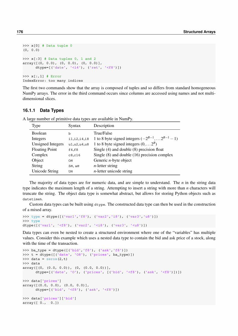
176 Structured Arrays

>>> x[0] # Data tuple 0(0, 0.0)

>>> x[:3] # Data tuples 0, 1 and 2array([(0, 0.0), (0, 0.0), (0, 0.0)],

dtype=[('date', '<i4'), ('ret', '<f8')])

>>> x[:,1] # ErrorIndexError: too many indices

The first two commands show that the array is composed of tuples and so differs from standard homogeneousNumPy arrays. The error in the third command occurs since columns are accessed using names and not multi-dimensional slices.

16.1.1 Data Types

A large number of primitive data types are available in NumPy.

Type Syntax Description

Boolean b True/FalseIntegers i1,i2,i4,i8 1 to 8 byte signed integers (−2B−1, . . .2B−1−1)Unsigned Integers u1,u2,u4,u8 1 to 8 byte signed integers (0, . . .2B)Floating Point f4,f8 Single (4) and double (8) precision floatComplex c8,c16 Single (8) and double (16) precision complexObject On Generic n-byte objectString Sn, an n-letter stringUnicode String Un n-letter unicode string

The majority of data types are for numeric data, and are simple to understand. The n in the string datatype indicates the maximum length of a string. Attempting to insert a string with more than n characters willtruncate the string. The object data type is somewhat abstract, but allows for storing Python objects such asdatetimes.

Custom data types can be built using dtype. The constructed data type can then be used in the constructionof a mixed array.>>> type = dtype([('var1','f8'), ('var2','i8'), ('var3','u8')])>>> typedtype([('var1', '<f8'), ('var2', '<i8'), ('var3', '<u8')])

Data types can even be nested to create a structured environment where one of the “variables” has multiplevalues. Consider this example which uses a nested data type to contain the bid and ask price of a stock, alongwith the time of the transaction.>>> ba_type = dtype([('bid','f8'), ('ask','f8')])>>> t = dtype([('date', 'O8'), ('prices', ba_type)])>>> data = zeros(2,t)>>> dataarray([(0, (0.0, 0.0)), (0, (0.0, 0.0))],

dtype=[('date', 'O'), ('prices', [('bid', '<f8'), ('ask', '<f8')])])

>>> data['prices']array([(0.0, 0.0), (0.0, 0.0)],

dtype=[('bid', '<f8'), ('ask', '<f8')])

>>> data['prices']['bid']array([ 0., 0.])

16.1 Mixed Arrays with Column Names 177

In this example, data is an array where each item has 2 elements, the date and the price. Price is also an arraywith 2 elements. Names can also be used to access values in nested arrays (e.g. data['prices']['bid']returns an array containing all bid prices). In practice nested arrays can almost always be expressed as a non-nested array without loss of fidelity.

Determining the size of object NumPy arrays can store objects which are anything which fall outside ofthe usual data types. One example of a useful, but abstract, data type is datetime. One method to determinethe size of an object is to create a plain array containing the object – which will automatically determine thedata type – and then to query the size from the array.

>>> import datetime as dt>>> x = array([dt.datetime.now()])>>> x.dtype.itemsize # The size in bytes>>> x.dtype.descr # The name and description

16.1.2 Example: TAQ Data

TAQ is the NYSE Trade and Quote database which contains all trades and quotes of US listed equities whichtrade on major US markets (not just the NYSE). A record from a trade contains a number of fields:

• Date - The Date in YYYYMMDD format stored as a 4-byte unsigned integer

• Time - Time in HHMMSS format, stored as a 4-byte unsigned integer

• Size - Number of shares trades, stores as a 4 byte unsigned integer

• G127 rule indicator - Numeric value, stored as a 2 byte unsigned integer

• Correction - Numeric indicator of a correction, stored as a 2 byte unsigned integer

• Condition - Market condition, a 2 character string

• Exchange - The exchange where the trade occurred, a 1-character string

First consider a data type which stores the data in an identical format.

>>> t = dtype([('date', 'u4'), ('time', 'u4'),... ('size', 'u4'), ('price', 'f8'),... ('g127', 'u2'), ('corr', 'u2'),... ('cond', 'S2'), ('ex', 'S2')])>>> taqData = zeros(10, dtype=t)>>> taqData[0] = (20120201,120139,1,53.21,0,0,'','N')

An alternative is to store the date and time as a datetime, which is an 8-byte object.

>>> import datetime as dt>>> t = dtype([('datetime', 'O8'), ('size', 'u4'), ('price', 'f8'), \... ('g127', 'u2'), ('corr', 'u2'), ('cond', 'S2'), ('ex', 'S2')])>>> taqData = zeros(10, dtype=t)>>> taqData[0] = (dt.datetime(2012,2,1,12,1,39),1,53.21,0,0,'','N')

178 Structured Arrays

16.2 Record Arrays

The main feature of record arrays, that the series can be accessed by series name as a property of a variable,is also available in a pandas’ DataFrame.

Record arrays are closely related to mixed arrays with names. The primary difference is that elementsrecord arrays can be accessed using variable.name format.

>>> x = zeros((4,1),[('date','int'),('ret','float')])>>> y = rec.array(x)>>> y.datearray([[0],

[0],[0],[0]])

>>> y.date[0]array([0])

In practice record arrays may be slower than standard arrays, and unless the variable.name is really important,record arrays are not compelling.

Chapter 17

Custom Function and Modules

This chapter uses @ to multiply arrays. If using Python 3.4 or earlier, or if using a version of NumPy that doesnot support @, these commands should be replaced with dot. For example, X @ X.T would be X.dot(X.T) ornp.dot(X,X.T).

Python supports a wide range of programming styles including procedural (imperative), object orientedand functional. While object oriented programming and functional programming are powerful programmingparadigms, especially in large, complex software, procedural is often both easier to understand and a directrepresentation of a mathematical formula. The basic idea of procedural programming is to produce a functionor set of function (generically) of the form

y = f (x).

That is, the functions take one or more inputs and produce one or more outputs.

17.1 Functions

Python functions are very simple to declare and can occur in the same file as the main program or a standalonefile. Functions are declared using the def keyword, and the value produced is returned using the returnkeyword. Consider a simple function which returns the square of the input, y = x2.

def square(x):return x⁎⁎2

# Call the functionx = 2y = square(x)print(x,y)

In this example, the same Python file contains the main program – the final 3 lines – as well as the function.More complex function can be crafted with multiple inputs.

def l2distance(x,y):return (x-y)⁎⁎2

# Call the functionx = 3y = 10z = l2distance(x,y)print(x,y,z)

Function can also be defined using NumPy arrays and matrices.

180 Custom Function and Modules

import numpy as np

def l2_norm(x,y):d = x - yreturn np.sqrt(d @ d)

# Call the functionx = np.random.randn(10)y = np.random.randn(10)z = l2_norm(x,y)print(x-y)print("The L2 distance is ",z)

When multiple outputs are returned but only a single variable is available for assignment, all outputs are returnedin a tuple. Alternatively, the outputs can be directly assigned when the function is called with the same numberof variables as outputs.

import numpy as np

def l1_l2_norm(x,y):d = x - yreturn sum(np.abs(d)),np.sqrt(d @ d)

# Call the functionx = np.random.randn(10)y = np.random.randn(10)# Using 1 output returns a tuplez = l1_l2_norm(x,y)print(x-y)print("The L1 distance is ",z[0])print("The L2 distance is ",z[1])

# Using 2 output returns the valuesl1,l2 = l1_l2_norm(x,y)print("The L1 distance is ",l1)print("The L2 distance is ",l2)

All of these functions have been placed in the same file as the main program. Placing functions in modulesallows for reuse in multiple programs, and will be discussed later in this chapter.

17.1.1 Keyword Arguments

All input variables in functions are automatically keyword arguments, so that the function can be accessedeither by placing the inputs in the order they appear in the function (positional arguments), or by calling theinput by their name using keyword=value.

import numpy as np

def lp_norm(x,y,p):d = x - yreturn sum(abs(d)⁎⁎p)⁎⁎(1/p)

# Call the functionx = np.random.randn(10)y = np.random.randn(10)z1 = lp_norm(x,y,2)z2 = lp_norm(p=2,x=x,y=y)print("The Lp distances are ",z1,z2)

17.1 Functions 181

Because variable names are automatically keywords, it is important to use meaningful variable names whenpossible, rather than generic variables such as a, b, c or x, y and z. In some cases, x may be a reasonabledefault, but in the previous example which computed the Lp norm, calling the third input z would be bad idea.

17.1.2 Default Values

Default values are set in the function declaration using the syntax input=default.

import numpy as np

def lp_norm(x,y,p = 2):d = x - yreturn sum(abs(d)⁎⁎p)⁎⁎(1/p)

# Call the functionx = np.random.randn(10)y = np.random.randn(10)# Inputs with default values can be ignoredl2 = lp_norm(x,y)l1 = lp_norm(x,y,1)print("The l1 and l2 distances are ",l1,l2)print("Is the default value overridden?", sum(abs(x-y))==l1)

Default values should not normally be mutable (e.g. lists or arrays) since they are only initialized the firsttime the function is called. Subsequent calls will use the same value, which means that the default value couldchange every time the function is called.

import numpy as np

def bad_function(x = zeros(1)):print(x)x[0] = np.random.randn(1)

# Call the functionbad_function()bad_function()bad_function()

Each call to bad_function shows that x has a different value – despite the default being 0. The solution to thisproblem is to initialize mutable objects to None, and then the use an if to check and initialize only if the valueis None. Note that tests for None use the is keyword rather the testing for equality using ==.

import numpy as np

def good_function(x = None):if x is None:

x = zeros(1)print(x)x[0] = np.random.randn(1)

# Call the functiongood_function()good_function()

Repeated calls to good_function() all show x as 0.

182 Custom Function and Modules

17.1.3 Variable Number of Inputs

Most function written as an “end user” have an known (ex ante) number of inputs. However, functions whichevaluate other functions often must accept variable numbers of input. Variable inputs can be handled usingthe ⁎args (arguments) or ⁎⁎kwargs (keyword arguments) syntax. The ⁎args syntax will generate tuple acontaining all inputs past the required input list. For example, consider extending the Lp function so that it canaccept a set of p values as extra inputs (Note: in practice it would make more sense to accept an array for p).

import numpy as np

def lp_norm(x,y,p = 2, ⁎args):d = x - yprint('The L' + str(p) + ' distance is :', sum(abs(d)⁎⁎p)⁎⁎(1/p))out = [sum(abs(d)⁎⁎p)⁎⁎(1/p)]

print('Number of ⁎args:', len(args))for p in args:

print('The L' + str(p) + ' distance is :', sum(abs(d)⁎⁎p)⁎⁎(1/p))out.append(sum(abs(d)⁎⁎p)⁎⁎(1/p))

return tuple(out)

# Call the functionx = np.random.randn(10)y = np.random.randn(10)# x & y are required inputs and so are not in ⁎argslp = lp_norm(x,y)# Function takes 3 inputs, so no ⁎argslp = lp_norm(x,y,1)# Inputs with default values can be ignoredlp = lp_norm(x,y,1,2,3,4,1.5,2.5,0.5)

The alternative syntax, ⁎⁎kwargs, generates a dictionary with all keyword inputs which are not in the functionsignature. One reason for using ⁎⁎kwargs is to allow a long list of optional inputs without having to have anexcessively long function definition. This is how this input mechanism operates in many matplotlib functionssuch as plot.

import numpy as np

def lp_norm(x,y,p = 2, ⁎⁎kwargs):d = x - yprint('Number of ⁎kwargs:', len(kwargs))for key in kwargs:

print('Key :', key, ' Value:', kwargs[key])

return sum(abs(d)⁎⁎p)

# Call the functionx = np.random.randn(10)y = np.random.randn(10)# Inputs with default values can be ignoredlp = lp_norm(x,y,kword1=1,kword2=3.2)# The p keyword is in the function def, so not in ⁎⁎kwargslp = lp_norm(x,y,kword1=1,kword2=3.2,p=0)

It is possible to use both ⁎args and ⁎⁎kwargs in a function definition and their role does not change – ⁎argsappears in the function as a tuple that contains all extraneous non-keyword inputs, and ⁎⁎kwargs appearsinside the function as a dictionary that contains all keyword arguments not appearing in the function definition.

17.1 Functions 183

Functions with both often have the simple signature y = f(⁎args, ⁎⁎kwargs) which allows for any set ofinputs.

17.1.4 The Docstring

The docstring is one of the most important elements of any function – especially a function written for useby others. The docstring is a special string, enclosed with triple-quotation marks, either ''' or """, which isavailable using help(). When help(fun) is called (or fun?/?fun in IPython), Python looks for the docstringwhich is placed immediately below the function definition.

import numpy as np

def lp_norm(x,y,p = 2):""" The docstring contains any available help for

the function. A good docstring should explain theinputs and the outputs, provide an example and a listof any other related function.

"""d = x - yreturn sum(abs(d)⁎⁎p)

Calling help(lp_norm) produces

>>> help(lp_norm)Help on function lp_norm in module __main__:

lp_norm(x, y, p=2)The docstring contains any available help forthe function. A good docstring should explain theinputs and the outputs, provide an example and a listof any other related function.

This docstring is not a good example. I suggest following the NumPy guidelines, currently available at theNumPy source repository (or search for numpy docstring). Also see NumPy example.py These differ from andare more specialized than the standard Python docstring guidelines, and are more appropriate for numericalcode. A better docstring for lp_norm would be

import numpy as np

def lp_norm(x,y,p = 2):r""" Compute the distance between vectors.

The Lp normed distance is sum(abs(x-y)⁎⁎p)⁎⁎(1/p)

Parameters----------x : ndarray

First argumenty : ndarray

Second argumentp : float, optional

Power used in distance calculation, >=0

Returns-------output : scalar

Returns the Lp normed distance between x and y

Notes

184 Custom Function and Modules

-----

For p>=1, returns the Lp norm described above. For 0<=p<1,returns sum(abs(x-y)⁎⁎p). If p<0, p is set to 0.

Examples-------->>> x=[0,1,2]>>> y=[1,2,3]

L2 norm is the default

>>> lp_norm(x,y)

Lp can be computed using the optional third input

>>> lp_norm(x,y,1)

"""

if p<0: p=0d = x - y

if p == 0:return sum(d != 0)

elif p < 1:return sum(abs(d)⁎⁎p)

else:return sum(abs(d)⁎⁎p)⁎⁎(1/p)

Convention is to use triple double-quotes in docstrings, with r""" used to indicate “raw” strings, which willignore backslashes rather than treating them like an escape character (use u""" if the docstring contains Unicodetext, which is not usually necessary). A complete docstring may contain, in order:

• Parameters - a description of key inputs

• Returns - a description of outputs

• Other Parameters - a description of seldom used inputs

• Raises - an explanation of any exceptions raised. See Section 12.5.

• See also - a list of related functions

• Notes - details of the algorithms or assumptions used

• References - any bibliographic information

• Examples - demonstrates use form console

17.2 Variable Scope

Variable scope determines which functions can access, and possibly modify a variable. Python determinesvariable scope using two principles: where the variable appears in the file, and whether the variable is inside afunction or in the main program. Variables declared inside a function are local variables and are only availableto that function. Variables declared outside a function are global variables, and can be accessed but not modified(unless using global) . Consider the example which shows that variables at the root of the program that havebeen declared before a function definition can be printed by that function.

17.2 Variable Scope 185

import numpy as np

a, b, c = 1, 3.1415, 'Python'

def scope():print(a)print(b)print(c)# print(d) #Error, d has not be declared yet

scope()d = np.array(1)

def scope2():print(a)print(b)print(c)print(d) # Ok now

scope2()

def scope3():a = 'Not a number' # Local variableprint('Inside scope3, a is ', a)

print('a is ',a)scope3()print('a is now ',a)

Using the name of a global variable inside a function does produce any changes outside of the function. Inscope3, a is given a different value. That value is specific to the function scope3 and outside of the function, awill have its global value. Generally, global variables can be accessed, but not modified inside a function. Theonly exception is when a variable is declared inside the function using the keyword global.

import numpy as np

a = 1

def scope_local():a = -1print('Inside scope_local, a is ',a)

def scope_global():global aa = -10print('Inside scope_global, a is ',a)

print('a is ',a)scope_local()print('a is now ',a)scope_global()print('a is now ',a)

One word of caution: a variable name cannot be used as a local and global variable in the same function.Attempting to access the variable as a global (e.g. for printing) and then locally assign the variable produces anerror.

186 Custom Function and Modules

17.3 Example: Least Squares with Newey-West Covariance

Estimating cross-section regressions using time-series data is common practice. When regressors are persistent,and errors are not white noise, standard inference, including White standard errors, is no longer consistent. Themost common solution is to use a long-run covariance estimator, and the most common long-run covarianceestimator is known as the Newey-West covariance estimator which uses a Bartlett kernel applied to the auto-covariances of the scores. This example produces a function which returns parameter estimates, the estimatedasymptotic covariance matrix of the parameters, the variance of the regression error, the R2, and adjusted R2

and the fit values (or errors, since actual is equal to fit plus errors). These are computed using a T -vector forthe regressand (dependent variable), a T by k matrix for the regressors, an indicator for whether to includea constant in the model (default True), and the number of lags to include in the long-run covariance (defaultbehavior is to automatically determine based on sample size). The steps required to produce the function are:

1. Determine the size of the variables

2. Append a constant, if needed

3. Compute the regression coefficients

4. Compute the errors

5. Compute the covariance or the errors

6. Compute the covariance of the parameters

7. Compute the R2 and R2

The function definition is simple and allows for up to 4 inputs, where 2 have default values: def olsnw(y,X, constant=True, lags=None):. The size of the variables is then determined using size and the constant isprepended to the regressors, if needed, using hstack. The regression coefficients are computed using lstsq,and then the Newey-West covariance is computed for both the errors and scores. The covariance of the parame-ters is then computed using the NW covariance of the scores. Finally the R2 and R2 are computed. A completecode listing is presented in the appendix to this chapter.

17.4 Anonymous Functions

Python supports anonymous functions using the keyword lambda. Anonymous functions are usually encoun-tered when another function expects a function as an input and a simple function will suffice. Anonymousfunction take the generic form lambda a,b,c,. . .:code using a,b,c. The key elements are the keyword lambda,a list of comma separated inputs, a colon between the inputs and the actual function code. For examplelambda x,y:x+y would return the sum of the variables x and y.

Anonymous functions are simple but useful. For example, when lists contain other lists it isn’t directlypossible to sort on an arbitrary element of the nested list. Anonymous functions allow sorting through thekeyword argument key by returning the element Python should use to sort. In this example, a direct call tosort() will sort on the first element (first name). Using the anonymous function lambda x:x[1] to return thesecond element of the tuple allows for sorting on the last name. lambda x:x[2] would allow for sorting on theUniversity.

>>> nested = [('John','Doe','Oxford'),\... ('Jane','Dearing','Cambridge'),\... ('Jerry','Dawn','Harvard')]

17.5 Modules 187

>>> nested.sort()>>> nested[('Jane', 'Dearing', 'Cambridge'),('Jerry', 'Dawn', 'Harvard'),('John', 'Doe', 'Oxford')]

>>> nested.sort(key=lambda x:x[1])>>> nested[('Jerry', 'Dawn', 'Harvard'),('Jane', 'Dearing', 'Cambridge'),('John', 'Doe', 'Oxford')]

17.5 Modules

The previous examples all included the function in the same Python as the main program. While this is conve-nient, especially when coding the function, it hinders use in other code. Modules allow multiple functions to becombined in a single Python file and accessed using import module and then module.function syntax. Supposea file named core.py contains the following code:

r"""Demonstration module.This is the module docstring."""

def square(x):r"""Returns the square of a scalar input"""return x⁎x

def cube(x):r"""Returns the cube of a scalar input"""return x⁎x⁎x

The functions square and cube can be accessed by other files in the same directory using

import core

y = -3print(core.square(y))print(core.cube(y))

The functions in core.py can be imported using any of the standard import methods: import core as c,from core import square or from core import ⁎ in which case both functions could be directly accessed.

17.5.1 __main__

Normally modules should only have code required for the module to run, and other code should reside in adifferent function. However, it is possible that a module could be both directly importable and also directlyrunnable. If this is the case, it is important that the directly runnable code should not be executed when themodule is imported by other code. This can be accomplished using a special construct, if __name__ =="__main__":before any code that should execute when the module is run as a standalone program. Considerthe following simple example in a module named test.py.

def square(x):return x⁎⁎2

if __name__ == "__main__":

188 Custom Function and Modules

print('Program called directly.')else:

print('Program called indirectly using name: ', __name__)

Running and importing test cause the different paths to be executed.>>> %run test.pyProgram called directly.

>>> import testProgram called indirectly using name: test

17.6 Packages

As a modules grows, organizing large amounts of code a single file – especially code that serve very differentpurposes – becomes difficult. Packages solve this problem by allowing multiple files to exist in the samenamespace, as well as sub-namespaces. Python packages are constructed using directory structures using aspecial file name: __init__.py. A Python package begins with a file folder using the name of the package. Forexample, consider developing a package called metrics which will contain common econometrics routines. Theminimal package structure would havemetrics/

__init__.py

The __init__.py file instructs Python to treat this directory as part of a package. __init__.py is a standard Pythonfile, although it is not necessary to include any code in this file. However, code included in __init__.py willappear in the root of the package namespace. Suppose __init__.py contained a function with the name reg.Assuming import core was used to import the module, this function would be accessible as core.reg. Next,suppose other Python files are included in the directory under core, so that the directory structure looks likecore/

__init__.pycrosssection.pytimeseries.py

This would allow functions to be directly included the core namespace by including the function in __init__.py.Functions that resided in crosssection.py would be accessible using import core.crosssection as cs andthen cs.reg.

Finally, suppose that crosssection.py was replaced with a directory where the directory contained otherPython files, including __init__.py.core/

__init__.pycrosssection/

__init__.pyregression.pylimdep.py

timeseries/__init__.pyarma.pyvar.py

This structure allows functions to be accessible directly from core using the __init__.py file, accessible fromcore.crosssection using the __init__.py located in the directory crosssection or accessible using core.crosssection.regressionfor functions inside the file regression.py.

__init__.py is useful in Python packages beyond simply instructing Python that a directory is part of a pack-age. It can be used to initialize any common information required by functions in the module or to “fake” the

17.7 PYTHONPATH 189

location of a deeply nested functions. __init__.py is executed whenever a package is imported, and since it cancontain standard Python code, it is possible define variables in the package namespace or execute code whichwill be commonly used by functions in the module (e.g. reading a config file). Suppose that the __init__.pylocated in the directory core contains

from core.crosssection.regression import ⁎

This single import will make all functions in the file regression.py available directly after running import core.For example, suppose regression.py contains the function leastsquares. Without the import statement in__init__.py, leastsquares would only be available through core.crosssection.regression. However, af-ter including the import statement in __init__.py, leastsquares is directly accessible from core. Using__init__.py allows for a flexible file and directory structure that reflects the code’s function while avoidingcomplex import statements.

17.7 PYTHONPATH

While it is simple to reference files in the same current working directory, this behavior is undesirable forcode shared between multiple projects. The PYTHONPATH allows directories to be added so that they areautomatically searched if a matching module cannot be found in the current directory. The current path can bechecked by running

>>> import sys>>> sys.path

Additional directories can be added at runtime using

import sys

# New directory is first to be searchedsys.path.insert(0, 'c:\\path\\to\add')# New directory is last to be searchedsys.path.append('c:\\path\\to\add')

Directories can also be added permanently by adding or modifying the environment variable PYTHONPATH.On Windows, the System environment variables can be found in My Computer > Properties > Advanced SystemSettings > Environment Variables. PYTHONPATH should be a System Variable. If it is present, it can be edited,and if not, added. The format of PYTHONPATH is

c:\dir1;c:\dir2;c:\dir2\dir3;

which will add 3 directories to the path. On Linux, PYTHONPATH is stored in either ~/.bash_rc or ~/.bash_profile,and it should resemble

PYTHONPATH="$PYTHONPATH:/dir1/:/dir2/:/dir2/dir3/"export PYTHONPATH

after three directories have been added, using : as a separator between directories. On OSX the PYTHONPATHis stored in ~/.profile.

17.8 Python Coding Conventions

There are a number of common practices which can be adopted to produce Python code which looks more likecode found in other modules:

1. Use 4 spaces to indent blocks – avoid using tab, except when an editor automatically converts tabs to 4spaces

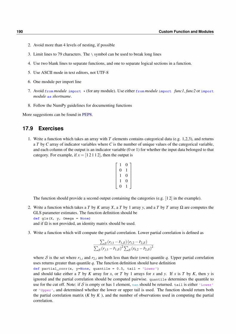
190 Custom Function and Modules

2. Avoid more than 4 levels of nesting, if possible

3. Limit lines to 79 characters. The \ symbol can be used to break long lines

4. Use two blank lines to separate functions, and one to separate logical sections in a function.

5. Use ASCII mode in text editors, not UTF-8

6. One module per import line

7. Avoid from module import ⁎ (for any module). Use either from module import func1, func2 or importmodule as shortname.

8. Follow the NumPy guidelines for documenting functions

More suggestions can be found in PEP8.

17.9 Exercises

1. Write a function which takes an array with T elements contains categorical data (e.g. 1,2,3), and returnsa T by C array of indicator variables where C is the number of unique values of the categorical variable,and each column of the output is an indicator variable (0 or 1) for whether the input data belonged to thatcategory. For example, if x = [1 2 1 1 2], then the output is

1 00 11 01 00 1

The function should provide a second output containing the categories (e.g. [1 2] in the example).

2. Write a function which takes a T by K array X , a T by 1 array y, and a T by T array Ω are computes theGLS parameter estimates. The function definition should bedef gls(X, y, Omega = None)and if Ω is not provided, an identity matrix should be used.

3. Write a function which will compute the partial correlation. Lower partial correlation is defined as∑S (ri,1− r1,S)(ri,2− r2,S)∑

S (r j,1− r1,S)2∑

S (rk,2− r2,S)2

where S is the set where r1,i and r2,i are both less than their (own) quantile q. Upper partial correlationuses returns greater than quantile q. The function definition should have definitiondef partial_corr(x, y=None, quantile = 0.5, tail = 'Lower')and should take either a T by K array for x, or T by 1 arrays for x and y. If x is T by K, then y isignored and the partial correlation should be computed pairwise. quantile determines the quantile touse for the cut off. Note: if S is empty or has 1 element, nan should be returned. tail is either 'Lower'or 'Upper', and determined whether the lower or upper tail is used. The function should return boththe partial correlation matrix (K by K ), and the number of observations used in computing the partialcorrelation.

17.A Listing of econometrics.py 191

17.A Listing of econometrics.py

The complete code listing of econometrics, which contains the function olsnw, is presented below.from numpy import mat, asarray, mean, size, shape, hstack, ones, ceil, \

zeros, arangefrom numpy.linalg import inv, lstsq

def olsnw(y, X, constant=True, lags=None):r""" Estimation of a linear regression with Newey-West covariance

Parameters----------y : array_like

The dependent variable (regressand). 1-dimensional with T elements.X : array_like

The independent variables (regressors). 2-dimensional with sizes Tand K. Should not include a constant.

constant: bool, optionalIf true (default) includes model includes a constant.

lags: int or None, optionalIf None, the number of lags is set to 1.2⁎T⁎⁎(1/3), otherwise thenumber of lags used in the covariance estimation is set to the valueprovided.

Returns-------b : ndarray, shape (K,) or (K+1,)

Parameter estimates. If constant=True, the first value is theintercept.

vcv : ndarray, shape (K,K) or (K+1,K+1)Asymptotic covariance matrix of estimated parameters

s2 : floatAsymptotic variance of residuals, computed using Newey-West varianceestimator.

R2 : floatModel R-square

R2bar : floatAdjusted R-square

e : ndarray, shape (T,)Array containing the model errors

Notes-----The Newey-West covariance estimator applies a Bartlett kernel to estimatethe long-run covariance of the scores. Setting lags=0 produces White'sHeteroskedasticity Robust covariance matrix.

See also--------np.linalg.lstsq

Example------->>> X = randn(1000,3)>>> y = randn(1000)>>> b,vcv,s2,R2,R2bar = olsnw(y, X)

Exclude constant:

192 Custom Function and Modules

>>> b,vcv,s2,R2,R2bar = olsnw(y, X, False)

Specify number of lags to use:

>>> b,vcv,s2,R2,R2bar = olsnw(y, X, lags = 4)

"""

T = y.sizeif size(X, 0) != T:

X = X.T

T,K = shape(X)if constant:

X = copy(X)X = hstack((ones((T,1)),X))K = size(X,1)

if lags is None:lags = int(ceil(1.2 ⁎ float(T)⁎⁎(1.0/3)))

# Parameter estimates and errors

out = lstsq(X,y)b = out[0]e = y - X @ b

# Covariance of errorsgamma = zeros((lags+1))for lag in range(lags+1):

gamma[lag] = (e[:T-lag] @ e[lag:]) / T

w = 1 - arange(0,lags+1)/(lags+1)w[0] = 0.5s2 = gamma @ (2⁎w)

# Covariance of parametersXe = mat(zeros(shape(X)))for i in range(T):

Xe[i] = X[i] ⁎ float(e[i])

Gamma = zeros((lags+1,K,K))for lag in range(lags+1):

Gamma[lag] = Xe[lag:].T⁎Xe[:T-lag]

Gamma = Gamma/T

S = Gamma[0].copy()for i in range(1,lags+1):

S = S + w[i]⁎(Gamma[i]+Gamma[i].T)

XpX = (X.T @ X)/TXpXi = inv(XpX)vcv = mat(XpXi)⁎S⁎mat(XpXi)/Tvcv = asarray(vcv)

# R2, centered or uncenteredif constant:

17.A Listing of econometrics.py 193

R2 = (e @ e) / (y-mean(y) @ y-mean(y))else:

R2 = (e @ e) / (y @ y)

R2bar = 1-R2⁎(T-1)/(T-K)R2 = 1 - R2

return b,vcv,s2,R2,R2bar,e

194 Custom Function and Modules

Chapter 18

Probability and Statistics Functions

This chapter is divided into two main parts, one for NumPy and one for SciPy. Both packages contain importantfunctions for simulation, probability distributions and statistics.

NumPy

18.1 Simulating Random Variables

18.1.1 Core Random Number Generators

NumPy random number generators are all stored in the module numpy.random. These can be imported with us-ing import numpy as np and then calling np.random.rand, for example, or by importing import numpy.randomas rnd and using rnd.rand.1

rand, random_sample

rand and random_sample are uniform random number generators which are identical except that rand takes avariable number of integer inputs – one for each dimension – while random_sample takes a n-element tuple.random_sample is the preferred NumPy function, and rand is a convenience function primarily for MATLABusers.

>>> x = rand(3,4,5)>>> y = random_sample((3,4,5))

randn, standard_normal

randn and standard_normal are standard normal random number generators. randn, like rand, takes a variablenumber of integer inputs, and standard_normal takes an n-element tuple. Both can be called with no argumentsto generate a single standard normal (e.g. randn()). standard_normal is the preferred NumPy function, andrandn is a convenience function primarily for MATLAB users .

>>> x = randn(3,4,5)>>> y = standard_normal((3,4,5))

1Other import methods can also be used, such as from numpy.random import rand and then calling rand.

196 Probability and Statistics Functions

randint

randint is a uniform integer random number generators which take 3 inputs, low, high and size. Low is thelower bound of the integers generated, high is the upper and size is a n-element tuple. randint and differ inthat randint generates integers exclusive of the value in high (as do most Python functions, e.g., range andnp.arange).

>>> x = randint(0,10,(100))>>> x.max() # Is 9 since range is [0,10)9

random_integers is a similar function that treats the upper end point differently. It has been deprecated and soshould not be used as an alternative to randint.

18.1.2 Random Array Functions

shuffle

shuffle randomly reorders the elements of an array in place.

>>> x = arange(10)>>> shuffle(x)>>> xarray([4, 6, 3, 7, 9, 0, 2, 1, 8, 5])

permutation

permutation returns randomly reordered elements of an array as a copy while not directly changing the input.

>>> x = arange(10)>>> permutation(x)array([2, 5, 3, 0, 6, 1, 9, 8, 4, 7])

>>> xarray([0, 1, 2, 3, 4, 5, 6, 7, 8, 9])

18.1.3 Select Random Number Generators

NumPy provides a large selection of random number generators for specific distribution. All take between 0and 2 required inputs which are parameters of the distribution, plus a tuple containing the size of the output.All random number generators are in the module numpy.random.

Bernoulli

There is no Bernoulli generator. Instead use binomial(1,p) to generate a single draw or binomial(1,p,(10,10))to generate an array where p is the probability of success.

beta

beta(a,b) generates a draw from the Beta(a,b) distribution. beta(a,b,(10,10)) generates a 10 by 10 arrayof draws from a Beta(a,b) distribution.

18.1 Simulating Random Variables 197

binomial

binomial(n,p) generates a draw from the Binomial(n, p) distribution. binomial(n,p,(10,10)) generates a10 by 10 array of draws from the Binomial(n, p) distribution.

chisquare

chisquare(nu) generates a draw from the χ2ν distribution, where ν is the degree of freedom. chisquare(nu,

(10,10)) generates a 10 by 10 array of draws from the χ2ν distribution.

exponential

exponential() generates a draw from the Exponential distribution with scale parameter λ = 1. exponential(lambda, (10,10)) generates a 10 by 10 array of draws from the Exponential distribution with scale parameterλ .

f

f(v1,v2) generates a draw from the distribution Fν1,ν2distribution where ν1 is the numerator degree of freedomand ν2 is the denominator degree of freedom. f(v1,v2,(10,10)) generates a 10 by 10 array of draws from theFν1,ν2distribution.

gamma

gamma(a) generates a draw from the Gamma(α,1) distribution, where α is the shape parameter. gamma(a,theta, (10,10)) generates a 10 by 10 array of draws from the Gamma(α,θ) distribution where θ is the scaleparameter.

laplace

laplace() generates a draw from the Laplace (Double Exponential) distribution with centered at 0 and unitscale. laplace(loc, scale, (10,10)) generates a 10 by 10 array of Laplace distributed data with locationloc and scale scale. Using laplace(loc, scale) is equivalent to calling loc + scale⁎laplace().

lognormal

lognormal() generates a draw from a Log-Normal distribution with µ = 0 and σ = 1. lognormal(mu,sigma, (10,10)) generates a 10 by 10 array or Log-Normally distributed data where the underlying Normaldistribution has mean parameter µ and scale parameter σ .

multinomial

multinomial(n, p) generates a draw from a multinomial distribution using n trials and where each outcomehas probability p, a k-element array where Σk

i=1 p = 1. Note that p must be an array or other iterable value. Theoutput is a k-element array containing the number of successes in each category. multinomial(n, p, (10,10))generates a 10 by 10 by k array of multinomially distributed data with n trials and probabilities p.

198 Probability and Statistics Functions

multivariate_normal

multivariate_normal(mu, Sigma) generates a draw from a multivariate Normal distribution with mean µ

(k-element array) and covariance Σ (k by k array). multivariate_normal(mu, Sigma, (10,10)) generates a10 by 10 by k array of draws from a multivariate Normal distribution with mean µ and covariance Σ.

negative_binomial

negative_binomial(n, p) generates a draw from the Negative Binomial distribution where n is the numberof failures before stopping and p is the success rate. negative_binomial(n, p, (10, 10)) generates a 10by 10 array of draws from the Negative Binomial distribution where n is the number of failures before stoppingand p is the success rate.

normal

normal() generates draws from a standard Normal (Gaussian). normal(mu, sigma) generates draws froma Normal with mean µ and standard deviation σ . normal(mu, sigma, (10,10)) generates a 10 by 10 ar-ray of draws from a Normal with mean µ and standard deviation σ . normal(mu, sigma) is equivalent tomu + sigma ⁎ standard_normal().

poisson

poisson() generates a draw from a Poisson distribution with λ = 1. poisson(lambda) generates a draw froma Poisson distribution with expectation λ . poisson(lambda, (10,10)) generates a 10 by 10 array of drawsfrom a Poisson distribution with expectation λ .

standard_t

standard_t(nu) generates a draw from a Student’s t with shape parameter ν . standard_t(nu, (10,10))generates a 10 by 10 array of draws from a Student’s t with shape parameter ν .

uniform

uniform() generates a uniform random variable on (0,1). uniform(low, high) generates a uniform on (l,h).uniform(low, high, (10,10)) generates a 10 by 10 array of uniforms on (l,h).

18.2 Simulation and Random Number Generation

Computer simulated random numbers are usually constructed from very complex but ultimately deterministicfunctions. Because they are not actually random, simulated random numbers are generally described to aspseudo-random. All pseudo-random numbers in NumPy use one core random number generator based on theMersenne Twister, a generator which can produce a very long series of pseudo-random data before repeating(up to 219937−1 non-repeating values).

RandomState

RandomState is the class used to control the random number generators. Multiple generators can be initializedby RandomState.

18.2 Simulation and Random Number Generation 199

>>> gen1 = np.random.RandomState()>>> gen2 = np.random.RandomState()>>> gen1.uniform() # Generate a uniform0.6767614077579269

>>> state1 = gen1.get_state()>>> gen1.uniform()0.6046087317893271

>>> gen2.uniform() # Different, since gen2 has different seed0.04519705909244154

>>> gen2.set_state(state1)>>> gen2.uniform() # Same uniform as gen1 after assigning state0.6046087317893271

18.2.1 State

Pseudo-random number generators track a set of values known as the state. The state is usually a vector whichhas the property that if two instances of the same pseudo-random number generator have the same state, thesequence of pseudo-random numbers generated will be identical. The state of the default random numbergenerator can be read using numpy.random.get_state and can be restored using numpy.random.set_state.

>>> st = get_state()>>> randn(4)array([ 0.37283499, 0.63661908, -1.51588209, -1.36540624])

>>> set_state(st)>>> randn(4)array([ 0.37283499, 0.63661908, -1.51588209, -1.36540624])

The two sequences are identical since they the state is the same when randn is called. The state is a 5-elementtuple where the second element is a 625 by 1 vector of unsigned 32-bit integers. In practice the state shouldonly be stored using get_state and restored using set_state.

get_state

get_state() gets the current state of the random number generator, which is a 5-element tuple. It can becalled as a function, in which case it gets the state of the default random number generator, or as a method on aparticular instance of RandomState.

set_state

set_state(state) sets the state of the random number generator. It can be called as a function, in which caseit sets the state of the default random number generator, or as a method on a particular instance of RandomState.set_state should generally only be called using a state tuple returned by get_state.

18.2.2 Seed

numpy.random.seed is a more useful function for initializing the random number generator, and can be usedin one of two ways. seed() will initialize (or reinitialize) the random number generator using some actualrandom data provided by the operating system.2 seed( s) takes a vector of values (can be scalar) to initialize

2All modern operating systems collect data that is effectively random by collecting noise from device drivers and other systemmonitors.

200 Probability and Statistics Functions

the random number generator at particular state. seed( s) is particularly useful for producing simulation studieswhich are reproducible. In the following example, calls to seed() produce different random numbers, sincethese reinitialize using random data from the computer, while calls to seed(0) produce the same (sequence) ofrandom numbers.

>>> seed()>>> randn()array([ 0.62968838])

>>> seed()>>> randn()array([ 2.230155])

>>> seed(0)>>> randn()array([ 1.76405235])

>>> seed(0)>>> randn()array([ 1.76405235])

NumPy always calls seed() when the first random number is generated. As a result. calling standard_normal()across two “fresh” sessions will not produce the same random number.

seed

seed(value) uses value to seed the random number generator. seed() takes actual random data from theoperating system when initializing the random number generator (e.g. /dev/random on Linux, or CryptGen-Random in Windows).

18.2.3 Replicating Simulation Data

It is important to have reproducible results when conducting a simulation study. There are two methods toaccomplish this:

1. Call seed() and then state = get_state(), and save state to a file which can then be loaded in thefuture when running the simulation study.

2. Call seed(s) at the start of the program (where s is a constant).

Either of these will allow the same sequence of random numbers to be used.Warning: Do not over-initialize the pseudo-random number generators. The generators should be initializedonce per session and then allowed to produce the pseudo-random sequence. Repeatedly re-initializing thepseudo-random number generators will produce a sequence that is decidedly less random than the generatorwas designed to provide.

Considerations when Running Simulations on Multiple Computers

Simulation studies are ideally suited to parallelization, although parallel code makes reproducibility more dif-ficult. There are 2 methods which can ensure that a parallel study is reproducible.

1. Have a single process produce all of the random numbers, where this process has been initialized us-ing one of the two methods discussed in the previous section. Formally this can be accomplished bypre-generating all random numbers, and then passing these into the simulation code as a parameter, orequivalently by pre-generating the data and passing the state into the function. Inside the simulation

18.3 Statistics Functions 201

function, the random number generator will be set to the state which was passed as a parameter. Thelatter is a better option if the amount of data per simulation is large.

2. Seed each parallel worker independently, and then return the state from the simulation function alongwith the simulation results. Since the state is saved for each simulation, it is possible to use the samestate if repeating the simulation using, for example, a different estimator.

18.3 Statistics Functions

mean

mean computes the average of an array. An optional second argument provides the axis to use (default is to useentire array). mean can be used either as a function or as a method on an array.

>>> x = arange(10.0)>>> x.mean()4.5

>>> mean(x)4.5

>>> x= reshape(arange(20.0),(4,5))>>> mean(x,0)array([ 7.5, 8.5, 9.5, 10.5, 11.5])

>>> x.mean(1)array([ 2., 7., 12., 17.])

median

median computed the median value in an array. An optional second argument provides the axis to use (defaultis to use entire array).

>>> x= randn(4,5)>>> xarray([[-0.74448693, -0.63673031, -0.40608815, 0.40529852, -0.93803737],

[ 0.77746525, 0.33487689, 0.78147524, -0.5050722 , 0.58048329],[-0.51451403, -0.79600763, 0.92590814, -0.53996231, -0.24834136],[-0.83610656, 0.29678017, -0.66112691, 0.10792584, -1.23180865]])

>>> median(x)-0.45558017286810903

>>> median(x, 0)array([-0.62950048, -0.16997507, 0.18769355, -0.19857318, -0.59318936])

Note that when an array or axis dimension contains an even number of elements (n), median returns the averageof the 2 inner elements.

std

std computes the standard deviation of an array. An optional second argument provides the axis to use (defaultis to use entire array). std can be used either as a function or as a method on an array.

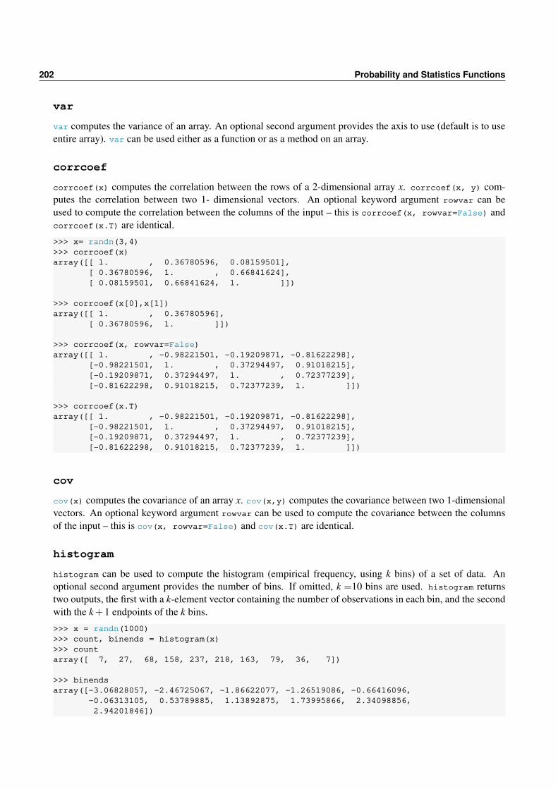
202 Probability and Statistics Functions

var

var computes the variance of an array. An optional second argument provides the axis to use (default is to useentire array). var can be used either as a function or as a method on an array.

corrcoef

corrcoef(x) computes the correlation between the rows of a 2-dimensional array x. corrcoef(x, y) com-putes the correlation between two 1- dimensional vectors. An optional keyword argument rowvar can beused to compute the correlation between the columns of the input – this is corrcoef(x, rowvar=False) andcorrcoef(x.T) are identical.

>>> x= randn(3,4)>>> corrcoef(x)array([[ 1. , 0.36780596, 0.08159501],

[ 0.36780596, 1. , 0.66841624],[ 0.08159501, 0.66841624, 1. ]])

>>> corrcoef(x[0],x[1])array([[ 1. , 0.36780596],

[ 0.36780596, 1. ]])

>>> corrcoef(x, rowvar=False)array([[ 1. , -0.98221501, -0.19209871, -0.81622298],

[-0.98221501, 1. , 0.37294497, 0.91018215],[-0.19209871, 0.37294497, 1. , 0.72377239],[-0.81622298, 0.91018215, 0.72377239, 1. ]])

>>> corrcoef(x.T)array([[ 1. , -0.98221501, -0.19209871, -0.81622298],

[-0.98221501, 1. , 0.37294497, 0.91018215],[-0.19209871, 0.37294497, 1. , 0.72377239],[-0.81622298, 0.91018215, 0.72377239, 1. ]])

cov

cov(x) computes the covariance of an array x. cov(x,y) computes the covariance between two 1-dimensionalvectors. An optional keyword argument rowvar can be used to compute the covariance between the columnsof the input – this is cov(x, rowvar=False) and cov(x.T) are identical.

histogram

histogram can be used to compute the histogram (empirical frequency, using k bins) of a set of data. Anoptional second argument provides the number of bins. If omitted, k =10 bins are used. histogram returnstwo outputs, the first with a k-element vector containing the number of observations in each bin, and the secondwith the k+1 endpoints of the k bins.

>>> x = randn(1000)>>> count, binends = histogram(x)>>> countarray([ 7, 27, 68, 158, 237, 218, 163, 79, 36, 7])

>>> binendsarray([-3.06828057, -2.46725067, -1.86622077, -1.26519086, -0.66416096,

-0.06313105, 0.53789885, 1.13892875, 1.73995866, 2.34098856,2.94201846])

18.4 Continuous Random Variables 203

>>> count, binends = histogram(x, 25)

histogram2d

histogram2d(x,y) computes a 2-dimensional histogram for 1-dimensional vectors. An optional keywordargument bins provides the number of bins to use. bins can contain either a single scalar integer or a 2-element list or array containing the number of bins to use in each dimension.

SciPy

SciPy provides an extended range of random number generators, probability distributions and statistical tests.

import scipyimport scipy.stats as stats

18.4 Continuous Random Variables

SciPy contains a large number of functions for working with continuous random variables. Each functionresides in its own class (e.g. norm for Normal or gamma for Gamma), and classes expose methods for randomnumber generation, computing the PDF, CDF and inverse CDF, fitting parameters using MLE, and computingvarious moments. The methods are listed below, where dist is a generic placeholder for the distribution namein SciPy. While the functions available for continuous random variables vary in their inputs, all take 3 genericarguments:

1. ⁎args a set of distribution specific non-keyword arguments. These must be entered in the order listedin the class docstring. For example, when using a F-distribution, two arguments are needed, one for thenumerator degree of freedom, and one for the denominator degree of freedom.

2. loc a location parameter, which determines the center of the distribution.

3. scale a scale parameter, which determine the scaling of the distribution. For example, if z is a standardnormal, then s× z is a scaled standard normal.

dist.rvs

Pseudo-random number generation. Generically, rvs is called using dist.rvs(⁎args, loc=0, scale=1, size=size)where size is an n-element tuple containing the size of the array to be generated.

dist.pdf

Probability density function evaluation for an array of data (element-by-element). Generically, pdf is called us-ing dist.pdf(x, ⁎args, loc=0, scale=1) where x is an array that contains the values to use when evaluatingPDF.

dist.logpdf

Log probability density function evaluation for an array of data (element-by-element). Generically, logpdfis called using dist.logpdf(x, ⁎args, loc=0, scale=1) where x is an array that contains the values to usewhen evaluating log PDF.

204 Probability and Statistics Functions

dist.cdf

Cumulative distribution function evaluation for an array of data (element-by-element). Generically, cdf iscalled using dist.cdf(x, ⁎args, loc=0, scale=1) where x is an array that contains the values to use whenevaluating CDF.

dist.ppf

Inverse CDF evaluation (also known as percent point function) for an array of values between 0 and 1. Generi-cally, ppf is called using dist.ppf(p, ⁎args, loc=0, scale=1) where p is an array with all elements between0 and 1 that contains the values to use when evaluating inverse CDF.

dist.fit

Estimate shape, location, and scale parameters from data by maximum likelihood using an array of data. Gener-ically, fit is called using dist.fit(data, ⁎args, floc=0, fscale=1) where data is a data array used toestimate the parameters. floc forces the location to a particular value (e.g. floc=0). fscale similarly forcesthe scale to a particular value (e.g. fscale=1) . It is necessary to use floc and/or fscale when computingMLEs if the distribution does not have a location and/or scale. For example, the gamma distribution is definedusing 2 parameters, often referred to as shape and scale. In order to use ML to estimate parameters from agamma, floc=0 must be used.

dist.median

Returns the median of the distribution. Generically, median is called using dist.median(⁎args, loc=0,scale=1).

dist.mean

Returns the mean of the distribution. Generically, mean is called using dist.mean(⁎args, loc=0, scale=1).

dist.moment

nth non-central moment evaluation of the distribution. Generically, moment is called using dist.moment(r, ⁎args,loc=0, scale=1) where r is the order of the moment to compute.

dist.varr

Returns the variance of the distribution. Generically, var is called using dist.var(⁎args, loc=0, scale=1).

dist.std

Returns the standard deviation of the distribution. Generically, std is called using dist.std(⁎args, loc=0,scale=1).

18.4.1 Example: gamma

The gamma distribution is used as an example. The gamma distribution takes 1 shape parameter a (a is the onlyelement of ⁎args), which is set to 2 in all examples.

18.4 Continuous Random Variables 205

>>> import scipy.stats as stats>>> gamma = stats.gamma>>> gamma.mean(2), gamma.median(2), gamma.std(2), gamma.var(2)(2.0, 1.6783469900166608, 1.4142135623730951, 2.0)

>>> gamma.moment(2,2) - gamma.moment(1,2)⁎⁎2 # Variance2

>>> gamma.cdf(5, 2), gamma.pdf(5, 2)(0.95957231800548726, 0.033689734995427337)

>>> gamma.ppf(.95957231800548726, 2)5.0000000000000018

>>> log(gamma.pdf(5, 2)) - gamma.logpdf(5, 2)0.0

>>> gamma.rvs(2, size=(2,2))array([[ 1.83072394, 2.61422551],

[ 1.31966169, 2.34600179]])

>>> gamma.fit(gamma.rvs(2, size=(1000)), floc = 0) # a, 0, shape(2.209958533078413, 0, 0.89187262845460313)

18.4.2 Important Distributions

SciPy provides classes for a large number of distribution. The most important are listed in the table below,along with any required arguments (shape parameters). All classes can be used with the keyword argumentsloc and scale to set the location and scale, respectively. The default location is 0 and the default scale is 1.Setting loc to something other than 0 is equivalent to adding loc to the random variable. Similarly settingscale to something other than 0 is equivalent to multiplying the variable by scale.

Distribution Name SciPy Name Required Arguments Notes

Normal norm Use loc to set mean (µ), scale to set std. dev. (σ )Beta(a,b) beta a: a, b: bCauchy cauchyχ2

ν chi2 ν : dfExponential(λ ) expon Use scale to set shape parameter (λ )Exponential Power exponpow shape: b Nests normal when b=2, Laplace when b=1F(ν1,ν2) f ν1: dfn, ν2: dfdGamma(a,b) gamma a: a Use scale to set scale parameter (b)Laplace, Double Exponential laplace Use loc to set mean (µ), scale to set std. dev. (σ )Log Normal(µ,σ2) lognorm σ : s Use scale to set µ where scale=exp(mu)Student’s-tν t ν : df

18.4.3 Frozen Random Variable Object

Random variable objects can be used in one of two ways:

1. Calling the class along with any shape, location and scale parameters, simultaneously with the method.For example gamma(1, scale=2).cdf(1).

2. Initializing the class with any shape, location and scale arguments and assigning a variable name. Usingthe assigned variable name with the method. For example:

206 Probability and Statistics Functions

>>> g = scipy.stats.gamma(1, scale=2)>>> g.cdf(1)0.39346934028736652

The second method is known as using a frozen random variable object. If the same distribution (with fixedparameters) is repeatedly used, frozen objects can be used to save typing potentially improve performancesince frozen objects avoid re-initializing the class.

18.5 Select Statistics Functions

mode

mode computes the mode of an array. An optional second argument provides the axis to use (default is to useentire array). Returns two outputs: the first contains the values of the mode, the second contains the number ofoccurrences.

>>> x=randint(1,11,1000)>>> stats.mode(x)(array([ 4.]), array([ 112.]))

moment

moment computed the rth central moment for an array. An optional second argument provides the axis to use(default is to use entire array).

>>> x = randn(1000)>>> moment = stats.moment>>> moment(x,2) - moment(x,1)⁎⁎20.94668836546169166

>>> var(x)0.94668836546169166

>>> x = randn(1000,2)>>> moment(x,2,0) # axis 0array([ 0.97029259, 1.03384203])

skew

skew computes the skewness of an array. An optional second argument provides the axis to use (default is touse entire array).

>>> x = randn(1000)>>> skew = stats.skew>>> skew(x)0.027187705042705772

>>> x = randn(1000,2)>>> skew(x,0)array([ 0.05790773, -0.00482564])

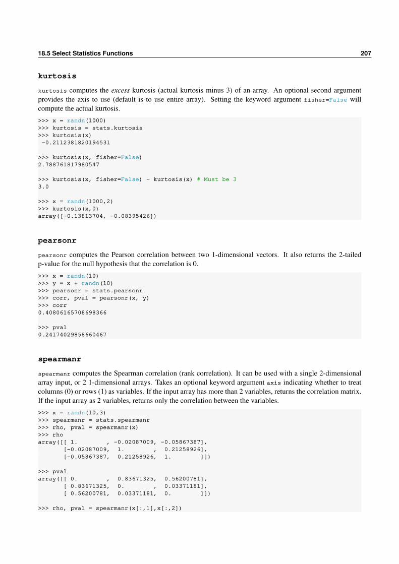
18.5 Select Statistics Functions 207

kurtosis

kurtosis computes the excess kurtosis (actual kurtosis minus 3) of an array. An optional second argumentprovides the axis to use (default is to use entire array). Setting the keyword argument fisher=False willcompute the actual kurtosis.

>>> x = randn(1000)>>> kurtosis = stats.kurtosis>>> kurtosis(x)-0.2112381820194531

>>> kurtosis(x, fisher=False)2.788761817980547

>>> kurtosis(x, fisher=False) - kurtosis(x) # Must be 33.0

>>> x = randn(1000,2)>>> kurtosis(x,0)array([-0.13813704, -0.08395426])

pearsonr

pearsonr computes the Pearson correlation between two 1-dimensional vectors. It also returns the 2-tailedp-value for the null hypothesis that the correlation is 0.

>>> x = randn(10)>>> y = x + randn(10)>>> pearsonr = stats.pearsonr>>> corr, pval = pearsonr(x, y)>>> corr0.40806165708698366

>>> pval0.24174029858660467

spearmanr

spearmanr computes the Spearman correlation (rank correlation). It can be used with a single 2-dimensionalarray input, or 2 1-dimensional arrays. Takes an optional keyword argument axis indicating whether to treatcolumns (0) or rows (1) as variables. If the input array has more than 2 variables, returns the correlation matrix.If the input array as 2 variables, returns only the correlation between the variables.

>>> x = randn(10,3)>>> spearmanr = stats.spearmanr>>> rho, pval = spearmanr(x)>>> rhoarray([[ 1. , -0.02087009, -0.05867387],

[-0.02087009, 1. , 0.21258926],[-0.05867387, 0.21258926, 1. ]])

>>> pvalarray([[ 0. , 0.83671325, 0.56200781],

[ 0.83671325, 0. , 0.03371181],[ 0.56200781, 0.03371181, 0. ]])

>>> rho, pval = spearmanr(x[:,1],x[:,2])

208 Probability and Statistics Functions

>>> corr-0.020870087008700869

>>> pval0.83671325461864643

kendalltau

kendalltau computed Kendall’s τ between 2 1-dimensonal arrays.

>>> x = randn(10)>>> y = x + randn(10)>>> kendalltau = stats.kendalltau>>> tau, pval = kendalltau(x,y)>>> tau0.46666666666666673

>>> pval0.06034053974834707

linregress

linregress estimates a linear regression between 2 1-dimensional arrays. It takes two inputs, the independentvariables (regressors) and the dependent variable (regressand). Models always include a constant.

>>> x = randn(10)>>> y = x + randn(10)>>> linregress = stats.linregress>>> slope, intercept, rvalue, pvalue, stderr = linregress(x,y)>>> slope1.6976690163576993

>>> rsquare = rvalue⁎⁎2>>> rsquare0.59144988449163494

>>> x.shape = 10,1>>> y.shape = 10,1>>> z = hstack((x,y))>>> linregress(z) # Alternative form, [x y](1.6976690163576993,-0.79983724584931648,0.76905779008578734,0.0093169560056056751,0.4988520051409559)

18.6 Select Statistical Tests

normaltest

normaltest tests for normality in an array of data. An optional second argument provides the axis to use(default is to use entire array). Returns the test statistic and the p-value of the test. This test is a small samplemodified version of the Jarque-Bera test statistic.

18.7 Exercises 209

kstest

kstest implements the Kolmogorov-Smirnov test. Requires two inputs, the data to use in the test and thedistribution, which can be a string or a frozen random variable object. If the distribution is provided as a string,then any required shape parameters are passed in the third argument using a tuple containing these parameters,in order.

>>> x = randn(100)>>> kstest = stats.kstest>>> stat, pval = kstest(x, 'norm')>>> stat0.11526423481470172

>>> pval0.12963296757465059

>>> ncdf = stats.norm().cdf # No () on cdf to get the function>>> kstest(x, ncdf)(0.11526423481470172, 0.12963296757465059)

>>> x = gamma.rvs(2, size = 100)>>> kstest(x, 'gamma', (2,)) # (2,) contains the shape parameter(0.079237623453142447, 0.54096739528138205)

>>> gcdf = gamma(2).cdf>>> kstest(x, gcdf)(0.079237623453142447, 0.54096739528138205)

ks_2samp

ks_2samp implements a 2-sample version of the Kolmogorov-Smirnov test. It is called ks_2samp(x,y) whereboth inputs are 1-dimensonal arrays, and returns the test statistic and p-value for the null that the distribution ofx is the same as that of y.

shapiro

shapiro implements the Shapiro-Wilk test for normality on a 1-dimensional array of data. It returns the teststatistic and p-value for the null of normality.

18.7 Exercises

1. For each of the following distributions, simulate 1000 pseudo-random numbers:

(a) N(0,12)

(b) N(3,32

)(c) Uni f (0,1)

(d) Uni f (−1,1)

(e) Gamma(1,2)

(f) LogN(.08, .22

)2. Use kstest to compute the p-value for each set of simulated data.

210 Probability and Statistics Functions

3. Use seed to re-initialize the random number generator.

4. Use get_state and set_state to produce the same set of pseudo-random numbers.

5. Write a custom function that will take a T vector of data and returns the mean, standard deviation,skewness and kurtosis (not excess) as a 4-element array.

6. Generate a 100 by 2 array of normal data with covariance matrix[1 −.5−.5 1

]

and compute the Pearson and Spearman correlation and Kendall’s τ .

7. Compare the analytical median of a Gamma(1,2) with that of 10,000 simulated data points. (You willneed a hist , which is discussed in the graphics chapter to finish this problem.)

8. For each of the sets of simulated data in exercise 1, plot the sorted CDF values to verify that these lie ona 45o line. (You will need plot , which is discussed in the graphics chapter to finish this problem.)

Chapter 19

Statistical Analysis with statsmodels

Note: This chapter provides an short introduction to statsmodels. There are many models, statistical pro-ceedures and diagnostics that are not covered. See statsmodel’s documentation for more information on theavailable models and statistics.

statsmodels provides a large range of cross-sectional models as well as some time-series models. statsmod-els uses a model descriptive language (provided via the Python package patsy) to formulate the model whenworking with pandas DataFrames. Models supported include linear regression, generalized linear models, lim-ited dependent variable models, ARMA and VAR models.

19.1 Regression

Basic linear regression is provided by OLS. Estimating a model requires specifying the model and then calling amethod to estimate the parameters (named fit in most models). This example will make use of one of the datasets provided with statsmodels named statecrime which contains data from the American National ElectionsStudy of 1996.

>>> import statsmodels.api as sm>>> data = sm.datasets.statecrime.load_pandas()

The dataset contains a number of variables, including

• state – State name (51 including Washington, DC)

• violent – Rate of violent crimes / 100,000 population. Includes murder, forcible rape, robbery, andaggravated assault.

• murder – Rate of murders / 100,000 population.

• hs_grad – Percent of the population having graduated from high school or higher.

• poverty – Percent of individuals below the poverty line.

• white – Percent of population that is one race - white only.

• single – Percent of family households that have a single parent.

• urban - Percent of population in urbanized areas.

212 Statistical Analysis with statsmodels

The dataset includes attributes that list the exogeneous and endogenous variables, endog_name and exog_name,respectively. The variables can be directly accessed as pandas structures using the attributes endog and exog.

>>> data.endog_name'murder'>>> data.exog_name['urban', 'poverty', 'hs_grad', 'single']

The model measures the murder rate using four explanatory variables. Models can be expressed using one oftwo equivalent formats. The first simply inputs the endogenous variable (y-variable, left-hand-side variable)as a 1-dimensional vector and the exogenous variables (x-variables, right-hand-side variables) as a 2-d array.When using this form it is necessary to explicitly include a column containing 1s as the constant in the model.Here this is column is added using the convenience function add_constant.

The standard pattern in statsmodels is to specify the model and then to call fit to estimate parameters.The allows the same specification to be estimated using different options when calling fit. Here the modelis specified using OLS and then the parameters and other quantities are estimated by a parameter-less call tofit which return a class containing results. While the various quantities computed can be directly accessedby attribute from the result class (res in this example), summary is a useful method for printing a formattedsummary of the estimation results.

>>> mod = sm.OLS(data.endog, sm.add_constant(data.exog))>>> res = mod.fit()>>> print(res.summary())

OLS Regression Results==============================================================================Dep. Variable: murder R-squared: 0.813Model: OLS Adj. R-squared: 0.797Method: Least Squares F-statistic: 50.08Date: Fri, 04 Nov 2016 Prob (F-statistic): 3.42e-16Time: 22:32:08 Log-Likelihood: -95.050No. Observations: 51 AIC: 200.1Df Residuals: 46 BIC: 209.8Df Model: 4Covariance Type: nonrobust==============================================================================

coef std err t P>t [0.025 0.975]------------------------------------------------------------------------------const -44.1024 12.086 -3.649 0.001 -68.430 -19.774urban 0.0109 0.015 0.707 0.483 -0.020 0.042poverty 0.4121 0.140 2.939 0.005 0.130 0.694hs_grad 0.3059 0.117 2.611 0.012 0.070 0.542single 0.6374 0.070 9.065 0.000 0.496 0.779==============================================================================Omnibus: 1.618 Durbin-Watson: 2.507Prob(Omnibus): 0.445 Jarque-Bera (JB): 0.831Skew: -0.220 Prob(JB): 0.660Kurtosis: 3.445 Cond. No. 5.80e+03==============================================================================

The result class has a large number of attributes which can be listed using dir.

# All attributed directly available>>> print(sorted([v for v in dir(res) if not v.startswith('_')]))['HC0_se', 'HC1_se', 'HC2_se', 'HC3_se', 'aic', 'bic', 'bse', 'centered_tss','compare_f_test', 'compare_lm_test', 'compare_lr_test', 'condition_number','conf_int', 'conf_int_el', 'cov_HC0', 'cov_HC1', 'cov_HC2', 'cov_HC3','cov_kwds', 'cov_params', 'cov_type', 'df_model', 'df_resid', 'eigenvals','el_test', 'ess', 'f_pvalue', 'f_test', 'fittedvalues', 'fvalue','get_influence', 'get_prediction', 'get_robustcov_results', 'initialize',

19.1 Regression 213

'k_constant', 'llf', 'load', 'model', 'mse_model', 'mse_resid', 'mse_total','nobs', 'normalized_cov_params', 'outlier_test', 'params', 'predict','pvalues', 'remove_data', 'resid', 'resid_pearson', 'rsquared', 'rsquared_adj','save', 'scale', 'ssr', 'summary', 'summary2', 't_test', 'tvalues','uncentered_tss', 'use_t', 'wald_test', 'wald_test_terms', 'wresid']

A detailed description of the regression result outputs is available using the help forsm.regression.linear_model.RegressionResults.

The fit method allows estimation options to be specified. The most useful option in OLS is the specificationof the parameter covariance. The default uses the classical covariance which assumes that the model errorsare homoskedastic. Using the option cov_type='HC0' will instead use White’s heteroskedasticity-consistentcovariance estimator.

>>> res_white = mod.fit(cov_type='HC0')>>> import pandas as pd>>> se = pd.concat([res.bse, res_white.bse],1)>>> se.columns = ['No option', 'HC0']>>> print(se)

No option HC0const 12.086045 11.873042urban 0.015397 0.013380poverty 0.140220 0.114653hs_grad 0.117179 0.110730single 0.070314 0.082418

The previous results were constructed be specifying the model by explicitly inputting arrays containing theendogenous and exogenous data. Models can alternatively be specified using formulas similar to R through themethod from_formula. Two inputs are required. The first is the formula to fit where the exogenous (left-hand-side) variable is listed first, a tilde (~) is used to separate this variable from the exogenous variables which arespecified using a list. The formula is a string. The second input is a DataFrame which should have columnnames that match the formula. Here the 1 in the formula indicates that a constant should be included in themodel. Here the murder rate is modeled using a constant, the percent urban and the percent single.

>>> df = pd.concat([data.endog, data.exog],1)>>> mod = sm.OLS.from_formula('murder ~ 1 + urban + single', data=df)>>> res = mod.fit()

The primary advantage of formulas is that extending the model is simple and direct. This next example extendsthe previous to include the percent that graduated high school.

>>> new_mod = sm.OLS.from_formula('murder ~ 1 + urban + single + hs_grad', data=df)>>> new_res = new_mod.fit()

Related estimators for weighted least squares (WLS), generalized least squares (GLS) and generalized leastsquares with autoregressive errors (GLSAR). These are virtually identical to OLS except that they allow weights(WLS) or error variances (GLS) to be specified to improve the model estimation.

214 Statistical Analysis with statsmodels

19.1.1 Weighted Least Squares (WLS)

19.1.2 Generalized Least Squares (WLS)

19.1.3 Diagnostics and Graphics

19.2 Generalized Linear Models

19.3 Other Notable Models

19.4 Time-series Analysis

19.4.1 Models

19.4.2 Statistics

19.4.3 Graphics

19.5 Generalized Linear Models

Chapter 20

Non-linear Function Optimization

SciPy contains a number of routines to the find extremum of a user-supplied objective function located inscipy.optimize. Most of these implement a version of the Newton-Raphson algorithm which uses the gradientto find the minimum of a function. However, this is not a limitation since if f is a function to be maximized,−1× f is a function with the minimum located at the same point as the maximum of f .

A custom function that returns the function value at a set of parameters – for example a log-likelihood or aGMM quadratic form – is required to use one an optimizer. All optimization targets must have the parametersas the first argument. For example, consider finding the minimum of x2. A function which allows the optimizerto work correctly has the form

def optim_target1(x):return x⁎⁎2

When multiple parameters (a parameter vector) are used, the objective function must take the form

def optim_target2(params):x, y = params

return x⁎⁎2-3⁎x+3+y⁎x-3⁎y+y⁎⁎2

Optimization targets can also have additional inputs that are not parameters of interest such as data or hyper-parameters.

def optim_target3(params,hyperparams):x, y = paramsc1, c2, c3=hyperparams

return x⁎⁎2+c1⁎x+c2+y⁎x+c3⁎y+y⁎⁎2

This form is especially useful when optimization targets require both parameters and data. Once an optimizationtarget has been specified, the next step is to use one of the optimizers find the minimum. The remainder of thischapter assumes that the following import is used to import the SciPy optimizers.

import scipy.optimize as opt

20.1 Unconstrained Optimization

A number of functions are available for unconstrained optimization using derivative information. Each uses adifferent algorithm to determine the best direction to move and the best step size to take in the direction. Thebasic structure of all of the unconstrained optimizers is

optimizer(f, x0)

216 Non-linear Function Optimization

where optimizer is one of fmin_bfgs, fmin_cg, fmin_ncg or fmin_powell, f is a callable function and x0 isan initial value used to start the algorithm. All of the unconstrained optimizers take the following keywordarguments, except where noted:

Keyword Description Note

fprime Function returning derivative of f. Must take same inputs as f (1)args Tuple containing extra parameters to pass to fgtol Gradient norm for terminating optimization (1)norm Order of norm (e.g. inf or 2) (1)epsilon Step size to use when approximating f ′ (1)maxiter Integer containing the maximum number of iterationsdisp Boolean indicating whether to print convergence messagefull_output Boolean indicating whether to return additional outputretall Boolean indicating whether to return results for each iteration.callback User supplied function to call after each iteration.

(1) Except fmin, fmin_powell.

fmin_bfgs

fmin_bfgs is a classic optimizer which uses information in the 1st derivative to estimate the second derivative,an algorithm known as BFGS (after the initials of the creators). This should usually be the first option exploredwhen optimizing a function without constraints. A function which returns the first derivative of the problemcan also be provided, and if not provided, the first derivative is numerically approximated. The basic use offmin_bfgs for finding the minimum of optim_target1 is shown below.

>>> opt.fmin_bfgs(optim_target1, 2)Optimization terminated successfully.

Current function value: 0.000000Iterations: 2Function evaluations: 12Gradient evaluations: 4

array([ -7.45132576e-09])

This is a very simple function to minimize and the solution is accurate to 8 decimal places. fmin_bfgs can alsouse first derivative information, which is provided using a function which must have the same inputs are theoptimization target. In this simple example, f ′ (x) = 2x.

def optim_target1_grad(x):return 2⁎x

The derivative information is used through the keyword argument fprime. Using analytic derivatives typicallyimproves both the accuracy of the solution and the time required to find the optimum.

>>> opt.fmin_bfgs(optim_target1, 2, fprime = optim_target1_grad)Optimization terminated successfully.

Current function value: 0.000000Iterations: 2Function evaluations: 4Gradient evaluations: 4

array([ 2.71050543e-20])

Multivariate optimization problems are defined using an array for the starting values, but are otherwise identical.

>>> opt.fmin_bfgs(optim_target2, array([1.0,2.0]))Optimization terminated successfully.

20.1 Unconstrained Optimization 217

Current function value: 0.000000Iterations: 3Function evaluations: 20Gradient evaluations: 5

array([ 1. , 0.99999999])

Additional inputs are can be passed to the optimization target using the keyword argument args and a tuplecontaining the input arguments in the correct order. Note that since there is a single additional input, the commais necessary in (hyperp,) to let Python know that this is a tuple.

>>> hyperp = array([1.0,2.0,3.0])>>> opt.fmin_bfgs(optim_target3, array([1.0,2.0]), args=(hyperp,))Optimization terminated successfully.

Current function value: -0.333333Iterations: 3Function evaluations: 20Gradient evaluations: 5

array([ 0.33333332, -1.66666667])

Derivative functions can be produced in a similar manner, although the derivative of a scalar function withrespect to an n-element vector is an n-element vector. It is important that the derivative (or gradient) returnedhas the same order as the input parameters. Note that the inputs must both be present, even when not needed,and in the same order.

def optim_target3_grad(params,hyperparams):x, y = paramsc1, c2, c3=hyperparams

return array([2⁎x+c1+y, x+c3+2⁎y])

Using the analytical derivative reduces the number of function evaluations and produces the same solution.

>>> optimum = opt.fmin_bfgs(optim_target3, array([1.0,2.0]),... fprime=optim_target3_grad,... args=(hyperp ,))Optimization terminated successfully.

Current function value: -0.333333Iterations: 3Function evaluations: 5Gradient evaluations: 5

>>> optimumarray([ 0.33333333, -1.66666667])>>> optim_target3_grad(optimum, hyperp) # Numerical zeroarray([ -2.22044605e-16, 0.00000000e+00])

fmin_cg

fmin_cg uses a nonlinear conjugate gradient method to minimize a function. A function which returns the firstderivative of the problem can be provided, and when not provided, the gradient is numerically approximated.

>>> opt.fmin_cg(optim_target3, array([1.0,2.0]),... args=(hyperp ,))Optimization terminated successfully.

Current function value: -0.333333Iterations: 7Function evaluations: 59Gradient evaluations: 12

array([ 0.33333334, -1.66666666])

218 Non-linear Function Optimization

fmin_ncg

fmin_ncg use a Newton conjugate gradient method. fmin_ncg requires a function which can compute the firstderivative of the optimization target, and can also take a function which returns the second derivative (Hessian)of the optimization target. It not provided, the Hessian will be numerically approximated.

>>> opt.fmin_ncg(optim_target3,... array([1.0,2.0]),... optim_target3_grad, args=(hyperp,))Optimization terminated successfully.

Current function value: -0.333333Iterations: 5Function evaluations: 6Gradient evaluations: 21Hessian evaluations: 0

array([ 0.33333333, -1.66666666])

The hessian can optionally be provided to fmin_ncg using the keyword argument fhess. The hessian returns∂ 2 f/∂x∂x′, which is an n by n array of derivatives. In this simple problem, the hessian does not depend on thehyper-parameters, although the Hessian function must take the same inputs are the optimization target.

def optim_target3_hess(params,hyperparams):x, y = paramsc1, c2, c3=hyperparams

return(array([[2, 1],[1, 2]]))

Using an analytical Hessian can reduce the number of function evaluations. While in theory an analyticalHessian should produce better results, it may not improve convergence, especially if the Hessian is nearlysingular for some parameter values (for example, near a saddle point which is not a minimum).

>>> opt.fmin_ncg(optim_target3, array([1.0,2.0]), optim_target3_grad, \... fhess = optim_target3_hess, args=(hyperp ,))Optimization terminated successfully.

Current function value: -0.333333Iterations: 5Function evaluations: 6Gradient evaluations: 5Hessian evaluations: 5

array([ 0.33333333, -1.66666667])

In addition to the keyword argument outlined in the main table, fmin_ncg can take the following additionalarguments.

Keyword Description Note

fhess_p Function returning second derivative of f times Only fmin_ncga vector p. Must take same inputs as f

fhess Function returning second derivative of f. Only fmin_ncgMust take same inputs as f

avestol Average relative error to terminate optimizer. Only fmin_ncg

20.2 Derivative-free Optimization

Derivative free optimizers do not use gradients and so can be used in a wider variety of problems such asfunctions which are not continuously differentiable. They can also be used for functions which are continuously

20.3 Constrained Optimization 219

differentiable, although they are likely to be slower than derivative-based optimizers. Derivative free optimizerstake some alternative keyword arguments.

Keyword Description Note

xtol Change in x to terminate optimizationftol Change in function to terminate optimizationmaxfun Maximum number of function evaluationsdirec Initial direction set, same size as x0 by m Only fmin_powell

fmin

fmin uses a simplex algorithm to minimize a function. The optimization in a simplex algorithm is often de-scribed as an amoeba which crawls around on the function surface expanding and contracting while lookingfor lower points. The method is derivative free, and so optimization target need not be continuously differen-tiable(e.g. the “tick” loss function used in estimation of quantile regression).

def tick_loss(quantile, data, alpha):e = data - quantile

return (alpha - (e<0)) @ e

The tick loss function is used to estimate the median by using α = 0.5. This loss function is not continuouslydifferential and so standard derivative-based optimizers cannot be used.

>>> data = randn(1000)>>> opt.fmin(tick_loss, 0, args=(data, 0.5))Optimization terminated successfully.

Current function value: -0.333333Iterations: 48Function evaluations: 91

array([-0.00475])>>> median(data)-0.0047118168472319406

The estimate is close to the sample median, as expected.

fmin_powell

fmin_powell used Powell’s method, which is derivative free, to minimize a function. It is an alternative tofmin which uses a different algorithm.

>>> opt.fmin_powell(tick_loss, 0, args=(data, 0.5))Optimization terminated successfully.

Current function value: 396.760642Iterations: 1Function evaluations: 17

array(-0.004673123552046776)

fmin_powell converged quickly and requires far fewer function calls.

20.3 Constrained Optimization

Constrained optimization is frequently encountered in economic problems where parameters are only mean-ingful in some particular range – for example, a variance which must be weakly positive. The relevant class

220 Non-linear Function Optimization

constrained optimization problems can be formulated

minθ f (θ) subject to

g(θ) = 0 (equality)

h(θ)≥ 0 (inequality)

θL ≤ θ ≤ θH (bounds)

where the bounds constraints are redundant if the optimizer allows for general inequality constraints since whena scalar x satisfies xL ≤ x ≤ xH , then x− xL ≥ 0 and xH − x ≥ 0. The optimizers in SciPy allow for differentsubsets of these constraints.

fmin_slsqp

fmin_slsqp is the most general constrained optimizer and allows for equality, inequality and bounds con-straints. While bound constraints are redundant, constraints which take the form of bounds should be imple-mented using bounds since this provides more information directly to the optimizer. Constraints are providedeither as list of callable functions or as a single function which returns an array. The latter is simpler if there aremultiple constraints, especially if the constraints can be easily calculated using linear algebra. Functions whichcompute the derivative of the optimization target, the derivative of the equality constraints, and the derivativeof the inequality constraints can be optionally provided. If not provided, these are numerically approximated.

As an example, consider the problem of optimizing a CRS Cobb-Douglas utility function of the formU(x1,x2) = xλ

1 x1−λ

2 subject to a budget constraint p1x1 + p2x2 ≤ 1. This is a nonlinear function subject to alinear constraint (note that is must also be that case that x1 ≥ 0 and x2 ≥ 0). First, specify the optimizationtarget

def utility(x, p, alpha):# Minimization, not maximization so -1 neededreturn -1.0 ⁎ (x[0]⁎⁎alpha)⁎(x[1]⁎⁎(1-alpha))

There are three constraints, x1 ≥ 0, x2 ≥ 0 and the budget line.1 All constraints must take the form of ≥ 0constraint, so that the budget line can be reformulated as 1− p1x1− p2x2 ≥ 0 . Note that the arguments in theconstraint must be identical to those of the optimization target, which is why the utility function takes prices asan input, even though the prices are not required to compute the utility. Similarly the constraint function takesα as an unnecessary input.

def utility_constraints(x, p, alpha):return array([x[0] - 1e-8, x[1] - 1e-8, 1 - p[0]⁎x[0] - p[1]⁎x[1]])

The optimal combination of goods can be computed using fmin_slsqp once the starting values and other inputsfor the utility function and budget constraint are constructed.

>>> p = array([1.0,1.0])>>> alpha = 1.0/3>>> x0 = array([.4,.4])>>> opt.fmin_slsqp(utility, x0, f_ieqcons=utility_constraints, args=(p, alpha))Optimization terminated successfully. (Exit mode 0)

Current function value: -0.529133683989Iterations: 2Function evaluations: 8Gradient evaluations: 2

array([ 0.33333333, 0.66666667])

1The code imposes the constraints that x j ≥ 10−8 to ensure that the the values are always slightly positive.

20.3 Constrained Optimization 221

fmin_slsqp can also take functions which compute the gradient of the optimization target, as well as thegradients of the constraint functions (both inequality and equality). The gradient of the optimization functionshould return a n-element vector, one for each parameter of the problem.def utility_grad(x, p, alpha):

grad = zeros(2)grad[0] = -1.0 ⁎ alpha ⁎ (x[0]⁎⁎(alpha-1))⁎(x[1]⁎⁎(1-alpha))grad[1] = -1.0 ⁎ (1-alpha) ⁎ (x[0]⁎⁎(alpha))⁎(x[1]⁎⁎(-alpha))return grad

The gradient of the constraint function returns a m by n array where m is the number of constraints. When bothequality and inequality constraints are used, the number of constraints will be meq and min which will generallynot be the same.def utility_constraint_grad(x, p, alpha):

grad = zeros((3,2)) # 3 constraints, 2 variablesgrad[0,0] = 1.0grad[0,1] = 0.0grad[1,0] = 0.0grad[1,1] = 1.0grad[2,0] = -p[0]grad[2,1] = -p[1]return grad

The two gradient functions can be passed using keyword arguments.>>> opt.fmin_slsqp(utility, x0, f_ieqcons=utility_constraints, args=(p, alpha), \... fprime = utility_grad, fprime_ieqcons = utility_constraint_grad)Optimization terminated successfully. (Exit mode 0)

Current function value: -0.529133683989Iterations: 2Function evaluations: 2Gradient evaluations: 2

array([ 0.33333333, 0.66666667])

Like in other problems, gradient information reduces the number of iterations and/or function evaluationsneeded to find the optimum.

fmin_slsqp also accepts bounds constraints. Since two of the three constraints are x1 ≥ 0 and x2 ≥ 0, thesecan be easily specified as a bound. Bounds are given as a list of tuples, where there is a tuple for each variablewith an upper and lower bound. It is not always possible to use np.inf as the upper bound, even if there isno implicit upper bound since this may produce a nan. In this example, 2 was used as the upper bound sinceit was outside of the possible range given the constraint. Using bounds also requires reformulating the budgetconstraint to only include the budget line.def utility_constraints_alt(x, p, alpha):

return array([1 - p[0]⁎x[0] - p[1]⁎x[1]])

Bounds are used with the keyword argument bounds.>>> opt.fmin_slsqp(utility, x0, f_ieqcons=utility_constraints_alt, args=(p, alpha), \... bounds = [(0.0,2.0),(0.0,2.0)])Optimization terminated successfully. (Exit mode 0)

Current function value: -0.529133683989Iterations: 2Function evaluations: 8Gradient evaluations: 2

array([ 0.33333333, 0.66666667])

The use of non-linear constraints can be demonstrated by formulating the dual problem of cost minimizationsubject to achieving a minimal amount of utility. In this alternative formulation, the optimization problemsbecomes

222 Non-linear Function Optimization

minx1,x2

p1x1 + p2x2 subject to U(x1,x2)≥ U

def total_expenditure(x,p,alpha,Ubar):return x @ p

def min_utility_constraint(x,p,alpha,Ubar):x1,x2 = xu=x1⁎⁎(alpha)⁎x2⁎⁎(1-alpha)return array([u - Ubar]) # >= constraint, must be array, even if scalar

The objective and the constraint are used along with a bounds constraint to solve the constrained optimiza-tion problem.

>>> x0 = array([1.0,1.0])>>> p = array([1.0,1.0])>>> alpha = 1.0/3>>> Ubar = 0.529133683989>>> opt.fmin_slsqp(total_expenditure, x0, f_ieqcons=min_utility_constraint, \... args=(p, alpha, Ubar), bounds =[(0.0,2.0),(0.0,2.0)])Optimization terminated successfully. (Exit mode 0)

Current function value: 0.999999999981Iterations: 6Function evaluations: 26Gradient evaluations: 6

Out[84]: array([ 0.33333333, 0.66666667])

As expected, the solution is the same.

fmin_tnc

fmin_tnc supports only bounds constraints.

fmin_l_bfgs_b

fmin_l_bfgs_b supports only bounds constraints.

fmin_cobyla

fmin_cobyla supports only inequality constraints, which must be provided as a list of functions. Since itsupports general inequality constraints, bounds constraints are included as a special case, although these mustbe included in the list of constraint functions.

def utility_constraints1(x, p, alpha):return x[0] - 1e-8

def utility_constraints2(x, p, alpha):return x[1] - 1e-8

def utility_constraints3(x, p, alpha):return (1 - p[0]⁎x[0] - p[1]⁎x[1])

Note that fmin_cobyla takes a list rather than an array for the starting values. Using an array produces awarning, but otherwise works.

20.4 Scalar Function Minimization 223

>>> p = array([1.0,1.0])>>> alpha = 1.0/3>>> x0 = array([.4,.4])>>> cons = [utility_constraints1, utility_constraints2, utility_constraints3]>>> opt.fmin_cobyla(utility, x0, cons, args=(p, alpha), rhoend=1e-7)array([ 0.33333326, 0.66666674])

20.3.1 Reparameterization

Many constrained optimization problems can be converted into an unconstrained program by reparameterizingfrom the space of unconstrained variables into the space where the parameters must reside. For example, theconstraints in the utility function optimization problem require 0≤ x1 ≤ 1/p1 and 0≤ x2 ≤ 1/p2. Additionallythe budget constraint must be satisfied so that if x1 ∈ [0,1/p1], x2 ∈ [0,(1− p1x1)/p2]. These constraints canbe implemented using a “squasher” function which maps x1 into its domain, and x2 into its domain and isone-to-one and onto (i.e. a bijective relationship). For example,

x1 =1p1

ez1

1+ ez1, x2 =

1− p1x1

p2

ez2

1+ ez2

will always satisfy the constraints, and so the constrained utility function can be mapped to an unconstrainedproblem, which can then be optimized using an unconstrained optimizer.

def reparam_utility(z,p,alpha,printX = False):x = exp(z)/(1+exp(z))x[0] = (1.0/p[0]) ⁎ x[0]x[1] = (1-p[0]⁎x[0])/p[1] ⁎ x[1]if printX:

print(x)return -1.0 ⁎ (x[0]⁎⁎alpha)⁎(x[1]⁎⁎(1-alpha))

The unconstrained utility function can be minimized using fmin_bfgs. Note that the solution returned is inthe transformed space, and so a special call to reparam_utility is used to print the actual values of x at thesolution (which are virtually identical to those found using the constrained optimizer).

>>> x0 = array([.4,.4])>>> optX = opt.fmin_bfgs(reparam_utility, x0, args=(p,alpha))Optimization terminated successfully.

Current function value: -0.529134Iterations: 24Function evaluations: 104Gradient evaluations: 26

>>> reparam_utility(optX, p, alpha, printX=True)[ 0.33334741 0.66665244]

20.4 Scalar Function Minimization

SciPy provides a number of scalar function minimizers. These are very fast since additional techniques areavailable for solving scalar problems which are not applicable when the parameter vector has more than 1element. A simple quadratic function will be used to illustrate the scalar solvers. Scalar function minimizersdo not require starting values, but may require bounds for the search.

def optim_target5(x, hyperparams):c1,c2,c3 = hyperparams

return c1⁎x⁎⁎2 + c2⁎x + c3

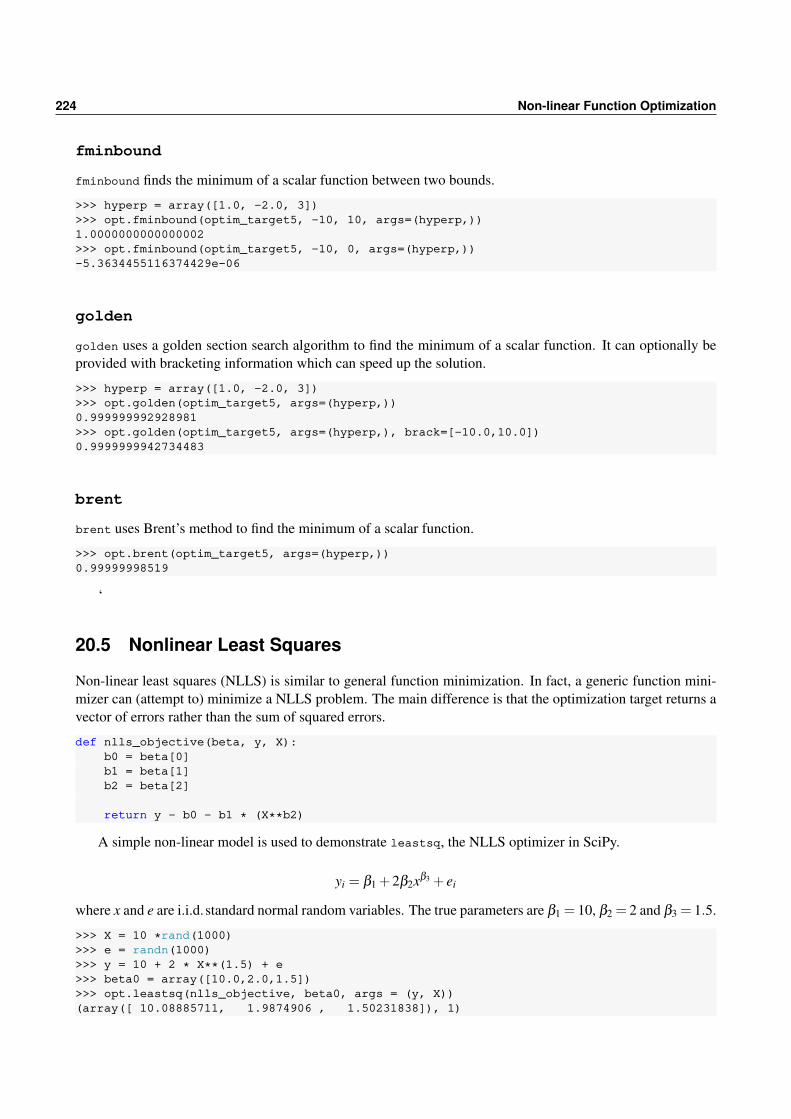
224 Non-linear Function Optimization

fminbound

fminbound finds the minimum of a scalar function between two bounds.

>>> hyperp = array([1.0, -2.0, 3])>>> opt.fminbound(optim_target5, -10, 10, args=(hyperp,))1.0000000000000002>>> opt.fminbound(optim_target5, -10, 0, args=(hyperp,))-5.3634455116374429e-06

golden

golden uses a golden section search algorithm to find the minimum of a scalar function. It can optionally beprovided with bracketing information which can speed up the solution.

>>> hyperp = array([1.0, -2.0, 3])>>> opt.golden(optim_target5, args=(hyperp,))0.999999992928981>>> opt.golden(optim_target5, args=(hyperp,), brack=[-10.0,10.0])0.9999999942734483

brent

brent uses Brent’s method to find the minimum of a scalar function.

>>> opt.brent(optim_target5, args=(hyperp,))0.99999998519

‘

20.5 Nonlinear Least Squares

Non-linear least squares (NLLS) is similar to general function minimization. In fact, a generic function mini-mizer can (attempt to) minimize a NLLS problem. The main difference is that the optimization target returns avector of errors rather than the sum of squared errors.

def nlls_objective(beta, y, X):b0 = beta[0]b1 = beta[1]b2 = beta[2]

return y - b0 - b1 ⁎ (X⁎⁎b2)

A simple non-linear model is used to demonstrate leastsq, the NLLS optimizer in SciPy.

yi = β1 +2β2xβ3 + ei

where x and e are i.i.d. standard normal random variables. The true parameters are β1 = 10, β2 = 2 and β3 = 1.5.

>>> X = 10 ⁎rand(1000)>>> e = randn(1000)>>> y = 10 + 2 ⁎ X⁎⁎(1.5) + e>>> beta0 = array([10.0,2.0,1.5])>>> opt.leastsq(nlls_objective, beta0, args = (y, X))(array([ 10.08885711, 1.9874906 , 1.50231838]), 1)

20.6 Exercises 225

leastsq returns a tuple containing the solution, which is very close to the true values, as well as a flag indi-cating that convergence was achieved. leastsq takes many of the same additional keyword arguments as otheroptimizers, including full_output, ftol, xtol, gtol, maxfev (same as maxfun). It has the additional keywordargument:

Keyword Description Note

Ddun Function to compute the Jacobian of the problem.Element i, j should be ∂ei/∂β j

col_deriv Direction to use when computing Jacobian numericallyepsfcn Step to use in numerical Jacobian calculation.diag Scalar factors for the parameters.

Used to rescale if scale is very different.factor used to determine the initial step size. Only fmin_powell

20.6 Exercises

1. The MLE for µ in a normal random variable is the sample mean. Write a function which takes a scalarparameter µ (1st argument) and a T vector of data and computes the negative of the log-likelihood,assuming the data is random and the variance is 1. Minimize the function (starting from something otherthan the same mean) using fmin_bfgs and fmin.

2. Extend to previous example where the first input is a 2-element vector containing µ and σ2, and computethe negative log-likelihood. Use fmin_slsqp along with a lower bound of 0 for σ2.

3. Repeat the exercise in problem 2, except using reparameterization so that σ is input (and then squared).

4. Verify that the OLS β is the MLE by writing a function which takes 3 inputs: K vector β ,T by K arrayX and T by 1 array y, and computes the negative log-likelihood for these values. Minimize the functionusing fmin_bfgs starting at the OLS estimates of β .

226 Non-linear Function Optimization

Chapter 21

String Manipulation

Strings are usually less interesting than numerical values in econometrics and statistics. There are, however,some important uses for strings:

• Reading complex data formats

• Outputting formatted results to screen or file

Recall that strings are sliceable, but unlike arrays, are immutable, and so it is not possible to replace part of astring.

21.1 String Building

21.1.1 Adding Strings (+)

Strings are concatenated using +.

>>> a = 'Python is'>>> b = 'a rewarding language.'>>> a + ' ' + b'Python is a rewarding language.'

While + is a simple method to join strings, the modern method is to use join. join is a string methodwhich joins a list of strings (the input) using the object calling the string as the separator.

>>> a = 'Python is'>>> b = 'a rewarding language.'>>> ' '.join([a,b])'Python is a rewarding language.'

Alternatively, the same output may be constructed using an empty string ''.

>>> a = 'Python is'>>> b = 'a rewarding language.'>>> ''.join([a,' ',b])'Python is a rewarding language.'

join is also useful for producing comma separated lists.

>>> words = ['Python','is','a','rewarding','language']>>> ','.join(words)'Python,is,a,rewarding,language'

228 String Manipulation

21.1.2 Multiplying Strings (⁎)

Strings, like lists, can be repeated using ⁎.

>>> a = 'Python is '>>> 2⁎a'Python is Python is '

21.1.3 Using StringIO

While adding strings using + or join is extremely simple, concatenation is slow for large strings. The moduleio provides an optimized class, StringIO, for performing string operations, including buffering strings for faststring building. This example shows how write(string) fills a StringIO buffer. Before reading the contentsseek(0) is called to return to cursor to the beginning of the buffer, and then read() returns the entire stringfrom the buffer.

>>> from io import StringIO>>> sio = StringIO()>>> for i in range(10000):... sio.write('cStringIO is faster than +! ')

>>> sio.seek(0)>>> sio.read()

Note that this example is trivial since ⁎ could have been used instead.

21.2 String Functions

21.2.1 split and rsplit

split splits a string into a list based on a character, for example a comma. An optional third argument maxsplitcan be used to limit the number of outputs in the list. rsplit works identically to split, only scanning from theend of the string – split and rsplit only differ when maxsplit is used.

>>> s = 'Python is a rewarding language.'>>> s.split(' ')['Python', 'is', 'a', 'rewarding', 'language.']

>>> s.split(' ',3)['Python', 'is', 'a', 'rewarding language.']

>>> s.rsplit(' ',3)['Python is', 'a', 'rewarding', 'language.']

21.2.2 join

join concatenates a list or tuple of strings using the first argument sep to specify a separator. The more commonform directly calls join on the string to use as the separator.

>>> import string>>> a = 'Python is'>>> b = 'a rewarding language.'>>> str.join(' ', (a,b))'Python is a rewarding language.'

>>> str.join(':', (a,b))

21.2 String Functions 229

'Python is:a rewarding language.'

>>> ' '.join((a,b)) # Preferred version'Python is a rewarding language.'

21.2.3 strip, lstrip, and rstrip

strip removes leading and trailing whitespace from a string. An optional input char removes leading andtrailing occurrences of the input value (instead of space). lstrip and rstrip work identically, only strippingfrom the left and right, respectively.

>>> s = ' Python is a rewarding language. '>>> s=s.strip()'Python is a rewarding language.'

>>> s.strip('P')'ython is a rewarding language.'

21.2.4 find and rfind

find locates the lowest index of a substring in a string and returns -1 if not found. Optional arguments limit therange of the search, and s.find('i',10,20) is identical to s[10:20].find('i'). rfind works identically,only returning the highest index of the substring.

>>> s = 'Python is a rewarding language.'>>> s.find('i')7

>>> s.find('i',10,20)18

>>> s.rfind('i')18

find and rfind are commonly used in flow control.

>>> words = ['apple','banana','cherry','date']>>> words_with_a = []>>> for word in words:... if word.find('a')>=0:... words_with_a.append(word)

>>> words_with_a['apple', 'banana', 'date']

21.2.5 index and rindex

index returns the lowest index of a substring, and is identical to find except that an error is raised if thesubstring does not exist. As a result, index is only safe to use in a try . . . except block.

>>> s = 'Python is a rewarding language.'>>> s.index('i')7

>>> s.index('q') # ErrorValueError: substring not found

230 String Manipulation

21.2.6 count

count counts the number of occurrences of a substring, and takes optional arguments to limit the search range.

>>> s = 'Python is a rewarding language.'>>> s.count('i')2

>>> s.count('i', 10, 20)1

21.2.7 lower and upper

lower and upper convert strings to lower and upper case, respectively. They are useful to remove case whencomparing strings.

>>> s = 'Python is a rewarding language.'>>> s.upper()'PYTHON IS A REWARDING LANGUAGE.'

>>> s.lower()'python is a rewarding language.'

21.2.8 ljust, rjust and center

ljust, rjust and center left justify, right justify and center, respectively, a string while expanding its size toa given length. If the desired length is smaller than the string, the unchanged string is returned.

>>> s = 'Python is a rewarding language.'>>> s.ljust(40)'Python is a rewarding language. '

>>> s.rjust(40)' Python is a rewarding language.'

>>> s.center(40)' Python is a rewarding language. '

21.2.9 replace

replace replaces a substring with an alternative string, which can have different size. An optional argumentlimits the number of replacement.

>>> s = 'Python is a rewarding language.'>>> s.replace('g','Q')'Python is a rewardinQ lanQuaQe.'

>>> s.replace('is','Q')'Python Q a rewarding language.'

>>> s.replace('g','Q',2)'Python is a rewardinQ lanQuage.'

21.3 Formatting Numbers 231

21.2.10 textwrap.wrap

The module textwrap contains a function wrap which reformats a long string into a fixed width paragraphstored line-by-line in a list. An optional argument changes the width of the output paragraph form the defaultof 70 characters.

>>> import textwrap>>> s = 'Python is a rewarding language. '>>> s = 10⁎s>>> textwrap.wrap(s)['Python is a rewarding language. Python is a rewarding language. Python','is a rewarding language. Python is a rewarding language. Python is a','rewarding language. Python is a rewarding language. Python is a','rewarding language. Python is a rewarding language. Python is a','rewarding language. Python is a rewarding language.']

>>> textwrap.wrap(s,50)['Python is a rewarding language. Python is a','rewarding language. Python is a rewarding','language. Python is a rewarding language. Python','is a rewarding language. Python is a rewarding','language. Python is a rewarding language. Python','is a rewarding language. Python is a rewarding','language. Python is a rewarding language.']

21.3 Formatting Numbers

Formatting numbers when converting to a string allows for automatic generation of tables and well formattedscreen output. Numbers are formatted using the format function, which is used in conjunction with a formatspecifier. For example, consider these examples which format π .

>>> pi3.141592653589793

>>> ':12.5f'.format(pi)' 3.14159'

>>> ':12.5g'.format(pi)' 3.1416'

>>> ':12.5e'.format(pi)' 3.14159e+00'

These all provide alternative formats and the difference is determined by the letter in the format string. Thegeneric form of a format string is n: f aswc.pt or n: f aswcmt. To understand the alternative choices,consider the output produced by the basic output string '0:'

>>> '0:'.format(pi)'3.14159265359'

• n is a number 0,1,. . . indicating which value to take from the format function

>>> '0:, 1: and 2: are all related to pi'.format(pi,pi+1,2⁎pi)'3.14159265359, 4.14159265359 and 6.28318530718 are all related to pi'

>>> '2:, 0: and 1: reorder the output.'.format(pi,pi+1,2⁎pi)'6.28318530718, 3.14159265359 and 4.14159265359 reorder the output.

232 String Manipulation

• f a are fill and alignment characters, typically a 2 character string. Fill may be any character except ,although space is the most common choice. Alignment can < (left) ,> (right), ^ (center) or = (pad to theright of the sign). Simple left 0-fills can omit the alignment character so that f a = 0.>>> '0:0<20'.format(pi) # Left, 0 padding, precion 20'3.141592653590000000'

>>> '0:0>20'.format(pi) # Right, 0 padding, precion 20'00000003.14159265359'

>>> '0:0^20'.format(pi) # Center, 0 padding, precion 20'0003.141592653590000'

>>> '0: >20'.format(pi) # Right, space padding, precion 20' 3.14159265359'

>>> '0:$^20'.format(pi) # Center, dollar sign padding, precion 20'$$$3.14159265359$$$$'

• s indicates whether a sign should be included. + indicates always include sign, - indicates only include ifneeded, and a blank space indicates to use a blank space for positive numbers, and a − sign for negativenumbers – this format is useful for producing aligned tables.

>>> '0:+'.format(pi)'+3.14159265359'

>>> '0:+'.format(-1.0 ⁎ pi)'-3.14159265359'

>>> '0:-'.format(pi)'3.14159265359'

>>> '0: '.format(pi)' 3.14159265359'

>>> '0: '.format(-1.0 ⁎ pi)'-3.14159265359'

• m is the minimum total size of the formatted string

>>> '0:10'.format(pi)'3.14159265359'

>>> '0:20'.format(pi)' 3.14159265359'

>>> '0:30'.format(pi)' 3.14159265359'

• c may be , or omitted. , produces numbers with 1000s separated using a ,. In order to use c it isnecessary to include the . before the precision.>>> '0:.10'.format(1000000 ⁎ pi)'3141592.654'

>>> '0:,.10'.format(1000000 ⁎ pi)'3,141,592.654'

21.3 Formatting Numbers 233

• p is the precision. The interpretation of precision depends on t. In order to use p, it is necessary toinclude a . (dot). If not included, p will be interpreted as m.

>>> '0:.1'.format(pi)'3e+00'

>>> '0:.2'.format(pi)'3.1'

>>> '0:.5'.format(pi)'3.1416'

• t is the type. Options include:

Type Description

e, E Exponent notation, e produces e+ and E produces E+ notationf, F Display number using a fixed number of digitsg, G General format, which uses f for smaller numbers, and e for larger. G is equivalent to

switching between F and E. g is the default format if no presentation format is givenn Similar to g, except that it uses locale specific information.% Multiplies numbers by 100, and inserts a % sign

>>> '0:.5e'.format(pi)'3.14159e+00'

>>> '0:.5g'.format(pi)'3.1416'

>>> '0:.5f'.format(pi)'3.14159'

>>> '0:.5%'.format(pi)'314.15927%'

>>> '0:.5e'.format(100000 ⁎ pi)'3.14159e+05'

>>> '0:.5g'.format(100000 ⁎ pi)'3.1416e+05'

>>> '0:.5f'.format(100000 ⁎ pi)'314159.26536'

Combining all of these features in a single format string produces complexly presented data.

>>> '0: > 20.4f, 1: > 20.4f'.format(pi,-pi)' 3.1416, -3.1416'

>>> '0: >+20,.2f, 1: >+20,.2f'.format(100000 ⁎ pi,-100000 ⁎ pi)' +314,159.27, -314,159.27'

In the first example, reading from left to right after the colon, the format string consists of:

1. Space fill (the blank space after the colon)

2. Right align (>)

234 String Manipulation

3. Use no sign for positive numbers, − sign for negative numbers (the blank space after >)

4. Minimum 20 digits

5. Precision of 4 fixed digits

The second is virtually identical to the first, except that it includes a , to show the 1000s separator and a + toforce the sign to be shown.

21.3.1 Formatting Strings

format outputs formatted strings using a similar syntax to number formatting, although some options such asprecision, sign, comma and type are not relevant.

>>> s = 'Python'>>> '0:'.format(s)'Python'

>>> '0: >20'.format(s)' Python'

>>> '0:!>20'.format(s)'!!!!!!!!!!!!!!Python'

>>> 'The formatted string is: 0:!<20'.format(s)'The formatted string is: Python!!!!!!!!!!!!!!'

21.3.2 Formatting Multiple Objects

format also formats multiple objects in the same string output. There are three methods to do this:

• No position arguments, in which case the objects are matched to format strings in order

• Numeric positional arguments, in which case the first object is mapped to '0:', the second to '1:',and so on.

• Named arguments such as 'price:' and volume 'volume:', which match keyword argumentsinside format.

>>> price = 100.32>>> volume = 132000>>> 'The price yesterday was : with volume :'.format(price,volume)'The price yesterday was 100.32 with volume 132000'

>>> 'The price yesterday was 0: and the volume was 1:'.format(price,volume)'The price yesterday was 100.32 with volume 132000'

>>> 'The price yesterday was 1: and the volume was 0:'.format(volume,price)'The price yesterday was 100.32 with volume 132000'

>>> 'The price yesterday was price: and the volume was volume:'.format(price=price,volume=volume)'The price yesterday was 100.32 with volume 132000'

21.3 Formatting Numbers 235

21.3.3 f-Strings

f-Strings were introduced in Python 3.6 and provide a compact method to produce formatted strings using aspecial syntax. f-Strings allow variables to be directly included in the string which save appending formatmathod to the string. the All f-Strings being with the character f followed by one of the quotation marks.Variables in f-Strings are included by enclosing them in braces, e.g., some_variable. To appreciate theelegance of f-Strings, consider the previous example:

>>> price = 100.32>>> volume = 132000>>> 'The price yesterday was price: and the volume was volume:'.format(price=price,volume=volume)'The price yesterday was 100.32 with volume 132000'

When written using an f-String, the simpler version is:

>>> f'The price yesterday was price and the volume was volume''The price yesterday was 100.32 with volume 132000'

This allows the variable to be directly included in the string. The default behavior is equivalent to calling stron each variable and then replacing the variable expressions with their str version. Formatting information canbe provided using a :. For example, to format both price and volume volume using exponent notation:

>>> f'The price yesterday was price:4.4e and the volume was volume:10.1e''The price yesterday was 1.0032e+02 and the volume was 1.3e+05'

f-Strings are increasingly common and are the preferred way to format text in most cases. The main limitationof f-Strings is that the variable must be defined when the f-String is created. If the variable is not known, thenit is still necessary to use the format method. For example

>>> f'The new price of new_price is not known' # ErrorNameError: name 'new_price' is not defined

>>> txt = 'The new price of new_price is now known'>>> new_price = price + 1>>> txt.format(new_price=new_price)'The new price of 101.32 is now known'

21.3.4 Old style format strings

Some Python code still uses an older style format string. Old style format strings have %(map) f lm.pt, where:

• (map) is a mapping string containing a name, for example (price)

• f l is a flag which may be one or more of:

– 0: Zero pad

– (blank space)

– - Left adjust output

– + Include sign character

• m, p and t are identical to those of the new format strings.

In general, the old format strings should only be used when required by other code (e.g. matplotlib). Below aresome examples of their use in strings.

236 String Manipulation

>>> price = 100.32>>> volume = 132000>>> 'The price yesterday was %0.2f with volume %d' % (price, volume)'The price yesterday was 100.32 with volume 132000'

>>> 'The price yesterday was %(price)0.2f with volume %(volume)d' \... % 'price': price, 'volume': volume'The price yesterday was 100.32 with volume 132000'

>>> 'The price yesterday was %+0.3f and the volume was %010d' % (price, volume)'The price yesterday was +100.320 and the volume was 0000132000'

21.4 Regular Expressions

Regular expressions are powerful tools for matching patterns in strings. While reasonable coverage of regularexpressions is beyond the scope of these notes – there are 500 page books dedicated to constructing regularexpressions – they are sufficiently useful to warrant an introduction. There are many online regular expressiongenerators which can assist in finding the pattern to use, and so they are accessible to even casual users workingwith unformatted text.

Using regular expression requires the re module. The most useful functions for regular expression matchingare findall, finditer and sub. findall and finditer work in similar manners, except that findall returnsa list while finditer returns an iterable. finditer is preferred if a large number of matches is possible. Bothsearch through a string and find all non-overlapping matches of a regular expression.

>>> import re>>> s = 'Find all numbers in this string: 32.43, 1234.98, and 123.8.'>>> re.findall('[\s][0-9]+\.\d⁎',s)[' 32.43', ' 1234.98', ' 123.8']

>>> matches = re.finditer('[\s][0-9]+\.\d⁎',s)>>> for m in matches:... print(s[m.span()[0]:m.span()[1]])32.431234.98123.8

finditer returns MatchObjects which contain the method span. span returns a 2 element tuple which containsthe start and end position of the match.

sub replaces all matched text with another text string (or a function which takes a MatchObject).

>>> s = 'Find all numbers in this string: 32.43, 1234.98, and 123.8.'>>> re.sub('[\s][0-9]+\.\d⁎',' NUMBER',s)'Find all numbers in this string: NUMBER, NUMBER, and NUMBER.'

>>> def reverse(m):... """Reverse the string in the MatchObject group"""... s = m.group()... s = s.rstrip()... return ' ' + s[::-1]

>>> re.sub('[\s][0-9]+\.\d⁎',reverse,s)'Find all numbers in this string: 34.23, 89.4321, and 8.321.'

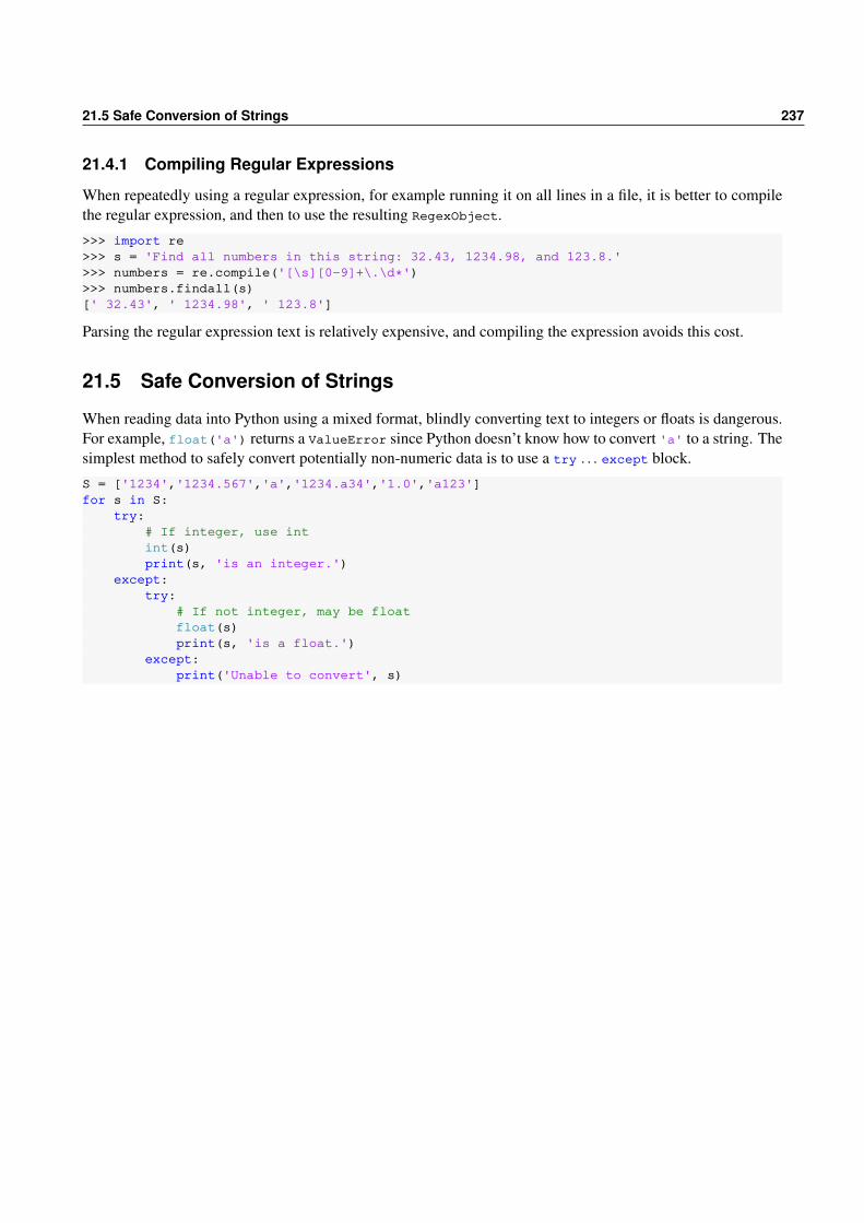
21.5 Safe Conversion of Strings 237

21.4.1 Compiling Regular Expressions

When repeatedly using a regular expression, for example running it on all lines in a file, it is better to compilethe regular expression, and then to use the resulting RegexObject.

>>> import re>>> s = 'Find all numbers in this string: 32.43, 1234.98, and 123.8.'>>> numbers = re.compile('[\s][0-9]+\.\d⁎')>>> numbers.findall(s)[' 32.43', ' 1234.98', ' 123.8']

Parsing the regular expression text is relatively expensive, and compiling the expression avoids this cost.

21.5 Safe Conversion of Strings

When reading data into Python using a mixed format, blindly converting text to integers or floats is dangerous.For example, float('a') returns a ValueError since Python doesn’t know how to convert 'a' to a string. Thesimplest method to safely convert potentially non-numeric data is to use a try . . . except block.

S = ['1234','1234.567','a','1234.a34','1.0','a123']for s in S:

try:# If integer, use intint(s)print(s, 'is an integer.')

except:try:

# If not integer, may be floatfloat(s)print(s, 'is a float.')

except:print('Unable to convert', s)

238 String Manipulation

Chapter 22

File System Operations

Manipulating files and directories is surprising useful when undertaking complex projects. The most importantfile system commands are located in the modules os and shutil. This chapter assumes that

import osimport shutil

have been included.

22.1 Changing the Working Directory

The working directory is where files can be created and accessed without any path information. os.getcwd()can be used to determine the current working directory, and os.chdir(path) can be used to change the workingdirectory, where path is a directory, such as /temp or c:\\temp.1 Alternatively, path can can be .. to more up thedirectory tree.

pwd = os.getcwd()os.chdir('c:\\temp')os.chdir(r'c:\temp') # Raw string, no need to escape \os.chdir('c:/temp') # Identicalos.chdir('..') # Walk up the directory treeos.getcwd() # Now in 'c:\\'

22.2 Creating and Deleting Directories

Directories can be created using os.mkdir(dirname), although it must be the case that the higher level direc-tories exist (e.g. to create /temp/Python/new , it /temp/Python already exists). os.makedirs(dirname) workssimilar to os.mkdir(dirname), except that is will create any higher level directories needed to create the targetdirectory.

Empty directories can be deleted using os.rmdir(dirname) – if the directory is not empty, an error occurs.shutil.rmtree(dirname) works similarly to os.rmdir(dirname), except that it will delete the directory, andany files or other directories contained in the directory.

os.mkdir('c:\\temp\\test')os.makedirs('c:/temp/test/level2/level3') # mkdir will failos.rmdir('c:\\temp\\test\\level2\\level3')shutil.rmtree('c:\\temp\\test') # rmdir fails, since not empty

1On Windows, directories use the backslash, which is used to escape characters in Python, and so an escaped backslash – \\ – isneeded when writing Windows’ paths. Alternatively, the forward slash can be substituted, so that c:\\temp and c:/temp are equivalent.

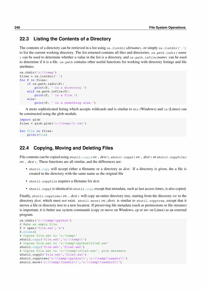
240 File System Operations

22.3 Listing the Contents of a Directory

The contents of a directory can be retrieved in a list using os.listdir(dirname), or simply os.listdir('.')to list the current working directory. The list returned contains all files and directories. os.path.isdir( name) can be used to determine whether a value in the list is a directory, and os.path.isfile(name) can be usedto determine if it is a file. os.path contains other useful functions for working with directory listings and fileattributes.os.chdir('c:\\temp')files = os.listdir('.')for f in files:

if os.path.isdir(f):print(f, ' is a directory.')

elif os.path.isfile(f):print(f, ' is a file.')

else:print(f, ' is a something else.')

A more sophisticated listing which accepts wildcards and is similar to dir (Windows) and ls (Linux) canbe constructed using the glob module.import globfiles = glob.glob('c:\\temp\\⁎.txt')

for file in files:print(file)

22.4 Copying, Moving and Deleting Files

File contents can be copied using shutil.copy( src , dest ), shutil.copy2( src , dest ) or shutil.copyfile(src , dest ). These functions are all similar, and the differences are:

• shutil.copy will accept either a filename or a directory as dest. If a directory is given, the a file iscreated in the directory with the same name as the original file

• shutil.copyfile requires a filename for dest.

• shutil.copy2 is identical to shutil.copy except that metadata, such as last access times, is also copied.

Finally, shutil.copytree( src , dest ) will copy an entire directory tree, starting from the directory src to thedirectory dest, which must not exist. shutil.move( src,dest) is similar to shutil.copytree, except that itmoves a file or directory tree to a new location. If preserving file metadata (such as permissions or file streams)is important, it is better use system commands (copy or move on Windows, cp or mv on Linux) as an externalprogram.os.chdir('c:\\temp\\python')# Make an empty filef = open('file.ext','w')f.close()# Copies file.ext to 'c:\temp\'shutil.copy('file.ext','c:\\temp\\')# Copies file.ext to 'c:\temp\\python\file2.ext'shutil.copy('file.ext','file2.ext')# Copies file.ext to 'c:\\temp\\file3.ext', plus metadatashutil.copy2('file.ext','file3.ext')shutil.copytree('c:\\temp\\python\\','c:\\temp\\newdir\\')shutil.move('c:\\temp\\newdir\\','c:\\temp\\newdir2\\')

22.5 Executing Other Programs 241

Context Managers

Context managers are the preferred method to use when opening and closing files. A context manager alwaysbegins with the keyword with and uses the syntax with command as variable. command is the command youare using (e.g., open) and variable is the name of the variable you with to assign the output of the commandto. A context manager will keep the file open while the code in the with block is executed. It will thenautomatically close the file when the block finishes. The following two blocks of commands are equivalent:

f = open('file.txt','w')f.write("Some text in the file")f.close()

and

with open('file.txt','w') as f:f.write("Some text in the file")

The second block is shorter and less error-prone since there is no need to call close() directly.

Beyond File Operations

While context managers are most commonly encountered in file I/O operations, they are more flexible. When-ever you initialize a context manager, Python calls the method __enter__(). This function performs anyinitialization such as opening a file handle and returns the object that is assigned using the as statement. Whenthe context manager completes, the companion method __exit__() is automatically called. This method per-forms any clean-up operations such as closing open file handles. The previous examples could be equivalentlywritten as:

f = open('file.txt','w').__enter__()f.write("Some text in the file")f.__exit__()

Note that __enter__() and __exit__() should not usually be directly called and so should only be (silently)used in conjunction with a with statement.

22.5 Executing Other Programs

Occasionally it is necessary to call other programs, for example to decompress a file compressed in an un-usual format or to call system copy commands to preserve metadata and file ownership. Both os.system andsubprocess.call (which requires import subprocess) can be used to execute commands as if they wereexecuted directly in the shell.

import subprocess

# Copy using xcopyos.system('xcopy /S /I c:\\temp c:\\temp4')subprocess.call('xcopy /S /I c:\\temp c:\\temp5',shell=True)# Extract using 7-zipsubprocess.call('"C:\\Program Files\\7-Zip\\7z.exe" e -y c:\\temp\\zip.7z')

242 File System Operations

22.6 Creating and Opening Archives

Creating and extracting files from archives often allows for further automation in data processing. Python hasnative support for zip, tar, gzip and bz2 file formats using shutil.make_archive( archivename , format, root)where archivename is the name of the archive to create, without the extension, format is one of the supportedformats (e..g 'zip' for a zip archive or 'gztar', for a gzipped tar file) and root is the root directory which canbe '.' for the current working directory.

# Creates files.zipshutil.make_archive('files','zip','c:\\temp\\folder_to_archive')# Creates files.tar.gzshutil.make_archive('files','gztar','c:\\temp\\folder_to_archive')

Creating a standard gzip from an existing file is slightly more complicated, and requires using the gzip module.2

This example makes use of context managers to open and close both the CSV and the gzip files.

import gzip

# Create file.csv.gz from file.csvwith open('file.csv','rb') as csvin:

with gzip.GzipFile('file.csv.gz','wb') as gz:gz.writelines(csvin.read())

Zip files can be extracted using the module zipfile, gzip files can be extracted using gzip, and gzippedtar files can be extracted using tarfile.

import zipfileimport gzipimport tarfile

# Extract zipwith zipfile.ZipFile('files.zip') as zip:

zip.extractall('c:\\temp\\zip\\')

# Extract gzip tar 'r:gz' indicates read gzippedwith tarfile.open('file.tar.gz', 'r:gz') as gztar:

gztar.extractall('c:\\temp\\gztar\\')

# Extract csv from gzipped csvwith gzip.GzipFile('file.csv.gz','rb') as gz:

with open('file.csv','wb') as csvout:csvout.writelines(gz.read())

22.7 Reading and Writing Files

Occasionally it may be necessary to directly read or write a file, for example to output a formatted LATEX table.Python contains low level file access tools which can be used to generate files with any structure. Writingtext files begins by using file to create a new file or to open an existing file. Files can be opened in differentmodes: ’r’ for reading, ’w’ for writing, and ’a’ for appending (’w’ will overwrite an existing file). An additionalmodifier ’b’ can be be used if the file is binary (not text), so that ’rb’, ’wb’ and ’ab’ allow reading, writing andappending binary files.

Reading text files is usually implemented using readline() to read a single line, readlines( n) to readsapproximately n bytes or readlines() to read all lines in a file. readline and readlines( n) are usually used

2A gzip can only contain 1 file, and is usually used with a tar file to compress a directory or set of files.

22.7 Reading and Writing Files 243

inside a while loop which terminates if the value returned is an empty string ('', readline ) or an empty list([], readlines) . Note that both '' and [] are false, and so can be directly used in a while statement.

# Read all lines using readlines()with open('file.csv','r') as f:

lines = f.readlines()for line in lines:

print(line)

# Using blocking via readline()with open('file.csv','r') as f:

line = f.readline()while line:

print(line)line = f.readline()

# Using larger blocks via readlines(n)with open('file.csv','r') as f

lines = f.readlines(2)while lines:

for line in lines:print(line)

lines = f.readline(2)

Writing text files is similar, and begins by using file to create a file and then fwrite to output information.fwrite is conceptually similar to using print, except that the output will be written to a file rather than printedon screen. The next example show how to create a LATEX table from an array.

import numpy as npimport scipy.stats as stats

x = np.random.randn(100,4)mu = np.mean(x,0)sig = np.std(x,0)sk = stats.skew(x,0)ku = stats.kurtosis(x,0)

summaryStats = np.vstack((mu,sig,sk,ku))rowHeadings = ['Var 1','Var 2','Var 3','Var 4']colHeadings = ['Mean','Std Dev','Skewness','Kurtosis']

# Build table, then printlatex = []latex.append('\\begintabularr|rrrr')line = ' 'for i in range(len(colHeadings)):

line += ' & ' + rowHeadings[i]

line += ' \\ \hline'latex.append(line)

for i in range(size(summaryStats,0)):line = rowHeadings[i]for j in range(size(summaryStats,1)):

line += ' & ' + str(summaryStats[i,j])

latex.append(line)

latex.append('\\endtabular')

244 File System Operations

# Output using write()with open('latex_table.tex','w') as f:

for line in latex:f.write(line + '\n')

22.8 Exercises

1. Create a new directory, chapter22.

2. Change into this directory.

3. Create a new file names tobedeleted.py a text editor in this new directory (It can be empty).

4. Create a zip file tobedeleted.zip containing tobedeleted.py.

5. Get and print the directory listing.

6. Delete the newly created file, and then delete this directory.

Chapter 23

Performance and Code Optimization

We should forget about small efficiencies, say about 97% of the time: premature optimizationis the root of all evil.

Donald Knuth

23.1 Getting Started

Occasionally the performance of a direct implementation of a statistical algorithm will not execute quicklyenough be applied to interesting data sets. When this occurs, there are a number of alternatives ranging fromimprovements possible using only NumPy and Python to using native code through a Python module.

Note that before any code optimization, it is essential that a clean, working implementation is available.This allows for both measuring performance improvements and to ensure that optimizations have not introducedany bugs. The famous quote of Donald Knuth should also be heeded, and in practice code optimization is onlyneeded for a very small amount of code – code that is frequently executed.

23.2 Timing Code

Timing code is an important step in measuring performance. IPython contains the magic keywords %timeitand %time which can be used to measure the execution time of a block of code. %time simply runs the code andreports the time needed. %timeit is smarter in that it will vary the number of iterations to increase the accuracyof the timing. Both are used with the same syntax, %timeit code to time.1

>>> x = randn(1000,1000)>>> %timeit inv(x.T @ x)1 loops, best of 3: 387 ms per loop

>>> %time inv(x.T @ x)Wall time: 0.52 s

>>> x = randn(100,100)>>> %timeit inv(x.T @ x)1000 loops, best of 3: 797 us per loop

1All timings were performed using Anaconda version 2.0.1.

246 Performance and Code Optimization

23.3 Vectorize to Avoid Unnecessary Loops

Vectorization is the key to writing high performance code in Python. Code that is vectorized run insidesNumPy and so executes as quickly as possible (with some small technical caveats, see NumExpr). Considerthe difference between manually multiplying two matrices and using @.

def pydot(a, b):M,N = shape(a)P,Q = shape(b)c = zeros((M,Q))for i in range(M):

for j in range(Q):for k in range(N):

c[i,j] += a[i,k] ⁎ b[k,j]return c

Timing the difference shows that NumPy is about 10000x faster than looping Python.

>>> a = randn(100,100)>>> b = randn(100,100)>>> %timeit pydot(a,b)1 loops, best of 3: 830 ms per loop

>>> %timeit a @ b10000 loops, best of 3: 53.4 us per loop

>>> f'The speed-up is 0.83/0.0000534 - 1.0:.1f times''The speed-up is 15542.1 times'

A less absurd example is to consider computing a weighted moving average across m consecutive values of avector.

def naive_weighted_avg(x, w):T = x.shape[0]m = len(w)m12 = int(ceil(m/2))y = zeros(T)for i in range(len(x)-m+1):

y[i+m12] = x[i:i+m].T @ w

return y

>>> w = array(r_[1:11,9:0:-1],dtype=float64)>>> w = w/sum(w)>>> x = randn(10000)>>> %timeit naive_weighted_avg(x,w)100 loops, best of 3: 13.3 ms per loop

An alternative method which completely avoids loops can be constructed by carefully constructing an arraycontaining the data. This array allows @ to be used with the weights.

def clever_weighted_avg(x,w):T = x.shape[0]m = len(w)wc = copy(w)wc.shape = m,1T = x.sizexc = copy(x)xc.shape=T,1y = vstack((xc,zeros((m,1))))y = tile(y,(m,1))

23.4 Alter the loop dimensions 247

y = reshape(y[:len(y)-m],(m,T+m-1))y = y.Ty = y[m-1:T,:]

return y @ flipud(wc)

>>> %timeit clever_weighted_avg(x,w)1000 loops, best of 3: 1.03 ms per loop

The loop-free method which uses copying and slicing is about 12 times faster than the simple loopingspecification.

23.4 Alter the loop dimensions

In many applications, it may be natural to loop over the long dimension in a time series. This is especiallycommon if the mathematical formula underlying the program has a sum from t = 1 to T . In some cases, itis possible to replace a loop over time, which is assumed to be the larger dimension, with an alternative loopacross another iterable. For example, in the moving average, it is possible to loop over the weights rather thanthe data, and if the moving windows length is much smaller than the length of the data, the code should runmuch faster.

def sideways_weighted_avg(x, w):T = x.shape[0]m = len(w)y = zeros(T)m12 = int(ceil(m/2))for i in range(m):

y[m12:T-m+m12] = x[i:T+i-m] ⁎ w[i]

return y

>>> %timeit sideways_weighted_avg(x,w)1000 loops, best of 3: 262 us per loop

In this example, the “sideways” loop is much faster than fully vectorized version since it avoids allocating alarge amount of memory.

23.5 Utilize Broadcasting

NumPy uses broadcasting for virtually all primitive mathematical operations (and for some more complicatedfunctions). Broadcasting avoids unnecessary data replication and memory allocation, and so improves perfor-mance.

>>> x = randn(1000,1)>>> y = randn(1,1000)>>> %timeit x⁎y100 loops, best of 3: 2.66 ms per loop

>>> %timeit (x @ ones((1,1000))) ⁎ (ones((1000,1)) @ y)100 loops, best of 3: 13.1 ms per loop

In this example, broadcasting is about 4 times faster than manually expanding the arrays.

248 Performance and Code Optimization

23.6 Use In-place Assignment

In-place assignment uses the save variable and avoids unnecessary memory allocation. The in-place operatorsuse a syntax similar to x += 0.0 or x ⁎= 1.0 instead of x = x + 0.0.

>>> x = zeros(1000000)>>> %timeit global x; x += 0.01000 loops, best of 3: 613 us per loop

>>> %timeit global x; x = x + 0.0100 loops, best of 3: 2.74 ms per loop

The gains to in-place allocation are larger as the dimension of x increases.

23.7 Avoid Allocating Memory

Memory allocation is relatively expensive, especially if it occurs inside a for loop. It is often better to pre-allocate storage space for computed values, and also to reuse existing space. Similarly, prefer slices and viewsto operations which create copies of arrays.

23.8 Inline Frequent Function Calls

Function calls are fast but not completely free. Simple functions, especially inside loops, should be in-lined toavoid the cost of calling functions.

23.9 Consider Data Locality in Arrays

Arrays are stored using row major format, and so data is stored across a row first, and then down columnssecond. This means that in an m by n array, element i, j is stored next to elements i, j+ 1 and i, j− 1 (exceptwhen j is the first (previous is i− 1,n) or last element in a row (next is i+ 1,1)). Spatial location mattersfor performance, and it is faster to access data which is stored physically adjacent. The simplest method tounderstand array storage is to use:

>>> x = arange(16.0)>>> x.shape = 4,4>>> xarray([[ 0., 1., 2., 3.],

[ 4., 5., 6., 7.],[ 8., 9., 10., 11.],[ 12., 13., 14., 15.]])

23.10 Profile Long Running Functions

Profiling provides detailed information about the number of times a line is executed as well as the execution timespent on each line. The default Python profiling tools are not adequate to address all performance measurementissues in NumPy code, and so a third party library known as line_profiler is needed. line_profiler is not currentlyavailable in Anaconda and so it must be installed before use. line_profiler is available through conda and socan be installed using

conda install line_profiler

23.10 Profile Long Running Functions 249

IPython Magic Keyword for Line Profiling

The simplest method to profile function is to use IPython. This requires a small amount of setup to define anew magic word, %lprun.

>>> import IPython>>> ip = IPython.get_ipython()>>> import line_profiler>>> ip.register_magics(line_profiler.LineProfilerMagics)

Note that the final two of these fours lines can also be incorporated into startup.py (see Chapter 1) so that themagic word %lprun is available in all IPython sessions.

To demonstrate the use of line_profiler, the three moving average functions where combined into a singlepython file moving_avgs.py. line_profiler is used with the syntax %lprun -f function command where functionis the function to profile and command is a command which will cause the function to run. command can beeither a simple call to the function or a call to some other code that will run the function.

>>> from moving_avgs import naive_weighted_avg>>> w = array(r_[1:11,9:0:-1],dtype=float64)>>> w = w/sum(w)>>> x = randn(100000)>>> %lprun -f naive_weighted_avg naive_weighted_avg(x,w)Timer unit: 3.94742e-07 s

File: moving_avgs.pyFunction: naive_weighted_avg at line 16Total time: 1.04589 s

Line # Hits Time Per Hit % Time Line Contents==============================================================

16 def naive_weighted_avg(x, w):17 1 27 27.0 0.0 T = x.shape[0]18 1 13 13.0 0.0 m = len(w)19 1 120 120.0 0.0 m12 = int(ceil(m/2))20 1 755 755.0 0.0 y = zeros(T)21 99983 505649 5.1 19.1 for i in range(len(x)-m+1):22 99982 2142994 21.4 80.9 y[i+m12] = x[i:i+m].T @ w2324 1 6 6.0 0.0 return y

The first attempt at a weighted average, naive_weighted_average, spent all of the time in the loop and mostof this on the matrix multiplication.

>>> from moving_avgs import clever_weighted_avg>>> %lprun -f clever_weighted_avg clever_weighted_avg(x,w)Timer unit: 3.94742e-07 s

File: moving_avgs.pyFunction: clever_weighted_avg at line 27Total time: 0.0302076 s

Line # Hits Time Per Hit % Time Line Contents==============================================================

27 def clever_weighted_avg(x,w):28 1 33 33.0 0.0 T = x.shape[0]29 1 11 11.0 0.0 m = len(w)30 1 98 98.0 0.1 wc = copy(w)31 1 33 33.0 0.0 wc.shape = m,132 1 9 9.0 0.0 T = x.size33 1 738 738.0 1.0 xc = copy(x)

250 Performance and Code Optimization

34 1 42 42.0 0.1 xc.shape=T,135 1 1605 1605.0 2.1 y = vstack((xc,zeros((m,1))))36 1 25286 25286.0 33.0 y = tile(y,(m,1))3738 1 98 98.0 0.1 y = reshape(y[:len(y)-m],(m,T+m-1))39 1 12 12.0 0.0 y = y.T40 1 38 38.0 0.0 y = y[m-1:T,:]4142 1 48522 48522.0 63.4 return y @ flipud(wc)

The second attempt, clever_weighted_avg, spends 1/3 of the time in the tile tile command and the remainderin the @.

>>> from moving_avgs import sideways_weighted_avg>>> %lprun -f sideways_weighted_avg sideways_weighted_avg(x,w)Timer unit: 3.94742e-07 s

File: moving_avgs.pyFunction: sideways_weighted_avg at line 45Total time: 0.00962302 s

Line # Hits Time Per Hit % Time Line Contents==============================================================

45 def sideways_weighted_avg(x, w):46 1 25 25.0 0.1 T = x.shape[0]47 1 10 10.0 0.0 m = len(w)48 1 417 417.0 1.7 y = zeros(T)49 1 182 182.0 0.7 m12 = int(ceil(m/2))50 20 230 11.5 0.9 for i in range(m):51 19 23508 1237.3 96.4 y[m12:T-m+m12] = x[i:T+i-m] ⁎ w[i]5253 1 6 6.0 0.0 return y

The final version spends most of its time in the matrix multiplication and the only other line with meaningfultime is the call to zeros. Note the actual time was .0096 vs 1.06 for the naive version and .030 for the loop-freeversion. Comparing the naive and the sideways version really highlights the cost of repeated calls to simplefunctions inside loops @ as well as the loop overhead.

Directly Using the Line Profiler

Directly using line_profiler requires adding the decorator @profile to a function. Consider profiling the threeweighted average functions.

from numpy import ceil, zeros, copy, vstack, flipud, reshape, tile, array, float64, r_from numpy.random import randn

# Useful block but not necessaryimport builtins

try:builtins.profileprint("Running with kernprof")

except AttributeError:# No line profiler, provide a pass-through versiondef profile(func): return funcbuiltins.profile = profileprint("Running without kernprof")

@profile

23.10 Profile Long Running Functions 251

def naive_weighted_avg(x, w):T = x.shape[0]m = len(w)m12 = int(ceil(m/2))y = zeros(T)for i in range(len(x)-m+1):

y[i+m12] = x[i:i+m].T @ w

return y

@profiledef clever_weighted_avg(x,w):

T = x.shape[0]m = len(w)wc = copy(w)wc.shape = m,1T = x.sizexc = copy(x)xc.shape=T,1y = vstack((xc,zeros((m,1))))y = tile(y,(m,1))

y = reshape(y[:len(y)-m],(m,T+m-1))y = y.Ty = y[m-1:T,:]

return y @ flipud(wc)

@profiledef sideways_weighted_avg(x, w):

T = x.shape[0]m = len(w)y = zeros(T)m12 = int(ceil(m/2))y = zeros(x.shape)for i in range(m):

y[m12:T-m+m12] = x[i:T+i-m] ⁎ w[i]

return y

w = array(r_[1:11,9:0:-1],dtype=float64)w = w/sum(w)x = randn(100000)

naive_weighted_avg(x,w)clever_weighted_avg(x,w)sideways_weighted_avg(x,w)

The decorator @profile specifies which functions should be profiled by line_profiler, and should only be usedon functions where profiling is needed. The final lines in this file call the functions, which is necessary for theprofiling.

To profile the on Windows code (saved in moving_avgs_direct.py), run the following commands from acommand prompt (not inside IPython)

cd PATHTOFILEANACONDA\Scripts\kernprof.exe -l moving_avgs_direct.pypython -m line_profiler moving_avgs_direct.py.lprof > moving_avgs_direct.prof.txt

where PATHTOFILE is the location of moving_avgs_direct.py. The first command changes to the directory

252 Performance and Code Optimization

where moving_avgs_direct.py is located. The second actually executes the file with profiling, and the finalproduces a report in moving_avgs_direct.prof.txt, which can then be viewed in any text editor.2

On Linux or OSX, run

cd PATHTOFILEkernprof -l moving_avgs_direct.pypython -m line_profiler moving_avgs_direct.py.lprof > moving_avgs_direct.prof.txt

The file moving_avg.prof.txt will contain a line-by-line listing of the three function which includes the numberto times the line was hit as well as the time spent on each line.

Modification of Code

In the direct method, the file moving_avgs_direct.py has a strange block reproduced below.

# Useful block but not necessaryimport builtins

try:builtins.profileprint("Running with kernprof")

except AttributeError:# No line profiler, provide a pass-through versiondef profile(func): return funcbuiltins.profile = profileprint("Running without kernprof")

I like to use this block since the decorator @profile is only defined when running in a profile session. At-tempting to run a file without this block in a standard python session will produce an AttributeError sinceprofile is not defined. This block allows the code to be run both with and without profiling by first checkingif profile is defined, and if not, providing a trivial definition that does nothing.

23.11 Exercises

1. Write a Python function which will accept a p+q+1 vector of parameters, a T vector of data, and p andq (integers, AR and MA order, respectively) and recursively computes the ARMA error beginning withobservation p+1. If an MA index is negative it should be backcast to 0.

2. Use line_profiler to measure the performance of the ARMA written in exercise 1.

3. Use jit to accelerate the ARMA function written in the exercise 1. Compare the speed to the purePython implementation.

4. [Only for the brave] Convert the ARMA function to Cython, compile it, and compare the performanceagainst both the pure Python and the Numba versions.

2The Windows command is more complex than the Linux command to ensure that the correct Python interpreter and environmentis used to execute kernprof.py.

Chapter 24

Improving Performance using Numba

Numba is a rapidly evolving project that releases new versions monthly. This chapter was written againstNumba 0.50.1 and so it is recommended to check for important changes in the the Numba documentation(http://numba.pydata.org).

24.1 Quick Start

If pure Python/NumPy is slow due to the presence of loops, Numba may be useful for compiling Python to op-timized machine code using LLVM. Numba is particularly attractive since in many cases the only modificationrequired to improve code execution speed is the addition of a decorator immediately before the def function():line. Consider a generic recursion from a GARCH(P,Q) model that computes the conditional variance givenparameters, data, and a backcast value. A pure Python/NumPy implementation is provided below.

def garch_recursion(parameters, data, sigma2, p, q, backcast):T = data.shape[0]for i in range(T):

sigma2[i] = parameters[0]for j in range(1, p + 1):

if (i - j) < 0:sigma2[i] += parameters[j] ⁎ backcast

else:sigma2[i] += parameters[j] ⁎ (data[i - j] ⁎ data[i - j])

for j in range(1, q + 1):if (i - j) < 0:

sigma2[i] += parameters[p + j] ⁎ backcastelse:

sigma2[i] += parameters[p + j] ⁎ sigma2[i - j]

return sigma2

This example is simple and only involves the (slow) recursive calculation of the conditional variance, not theother portions of the log-likelihood (which can be vectorized using NumPy). The pure Python version can betested using %timeit.

>>> parameters = array([.1,.1,.8])>>> data = randn(10000)>>> sigma2 = zeros(shape(data))>>> p, q = 1,1>>> backcast = 1.0>>> %timeit -r20 garch_recursion(parameters, data, sigma2, p, q, backcast)

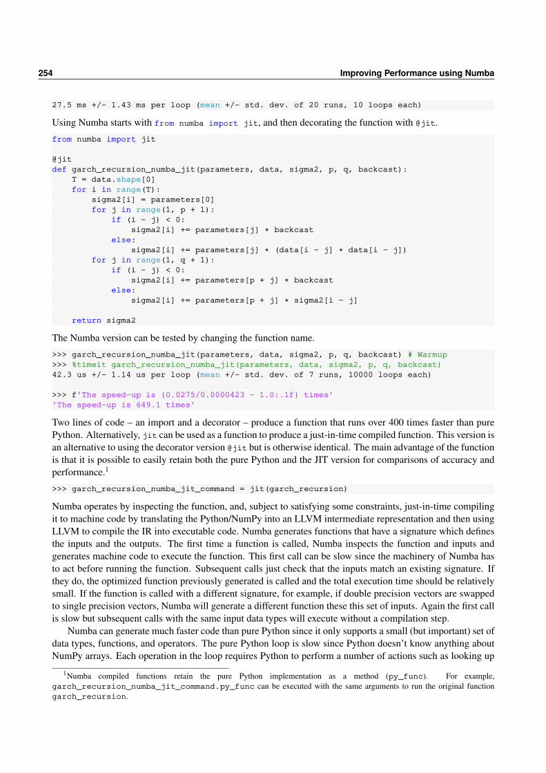
254 Improving Performance using Numba

27.5 ms +/- 1.43 ms per loop (mean +/- std. dev. of 20 runs, 10 loops each)

Using Numba starts with from numba import jit, and then decorating the function with @jit.

from numba import jit

@jitdef garch_recursion_numba_jit(parameters, data, sigma2, p, q, backcast):

T = data.shape[0]for i in range(T):

sigma2[i] = parameters[0]for j in range(1, p + 1):

if (i - j) < 0:sigma2[i] += parameters[j] ⁎ backcast

else:sigma2[i] += parameters[j] ⁎ (data[i - j] ⁎ data[i - j])

for j in range(1, q + 1):if (i - j) < 0:

sigma2[i] += parameters[p + j] ⁎ backcastelse:

sigma2[i] += parameters[p + j] ⁎ sigma2[i - j]

return sigma2

The Numba version can be tested by changing the function name.

>>> garch_recursion_numba_jit(parameters, data, sigma2, p, q, backcast) # Warmup>>> %timeit garch_recursion_numba_jit(parameters, data, sigma2, p, q, backcast)42.3 us +/- 1.14 us per loop (mean +/- std. dev. of 7 runs, 10000 loops each)

>>> f'The speed-up is 0.0275/0.0000423 - 1.0:.1f times''The speed-up is 649.1 times'

Two lines of code – an import and a decorator – produce a function that runs over 400 times faster than purePython. Alternatively, jit can be used as a function to produce a just-in-time compiled function. This version isan alternative to using the decorator version @jit but is otherwise identical. The main advantage of the functionis that it is possible to easily retain both the pure Python and the JIT version for comparisons of accuracy andperformance.1

>>> garch_recursion_numba_jit_command = jit(garch_recursion)

Numba operates by inspecting the function, and, subject to satisfying some constraints, just-in-time compilingit to machine code by translating the Python/NumPy into an LLVM intermediate representation and then usingLLVM to compile the IR into executable code. Numba generates functions that have a signature which definesthe inputs and the outputs. The first time a function is called, Numba inspects the function and inputs andgenerates machine code to execute the function. This first call can be slow since the machinery of Numba hasto act before running the function. Subsequent calls just check that the inputs match an existing signature. Ifthey do, the optimized function previously generated is called and the total execution time should be relativelysmall. If the function is called with a different signature, for example, if double precision vectors are swappedto single precision vectors, Numba will generate a different function these this set of inputs. Again the first callis slow but subsequent calls with the same input data types will execute without a compilation step.

Numba can generate much faster code than pure Python since it only supports a small (but important) set ofdata types, functions, and operators. The pure Python loop is slow since Python doesn’t know anything aboutNumPy arrays. Each operation in the loop requires Python to perform a number of actions such as looking up

1Numba compiled functions retain the pure Python implementation as a method (py_func). For example,garch_recursion_numba_jit_command.py_func can be executed with the same arguments to run the original functiongarch_recursion.

24.1 Quick Start 255

an element in memory (without knowing anything that happened before, such as the location of the previouselement), checking whether this element supports addition or multiplication, looking up the element’s additionor multiplication function, and then calling this function with the arguments. This is a very general approachwhich is why Python can multiply virtually anything that supports multiplication including numbers, strings,and lists. The post-JIT code produced by Numba knows substantially more about the structure of the problem.For example, through inspection, it knows that sigma2, parameters, and data are all double precision NumPyarrays that are contiguous in memory. This means that the ith element of the array is exactly 8× i bytes awayfrom the first and that consecutive elements are 8 bytes apart. This means that looping up elements in thesearrays is much faster than in Python. There are also gains since Numba knows these are all double precisionarrays and so the elements are plain double precision numbers which have native operations for addition andmultiplication. When Numba adds or multiplies these numbers it doesn’t waste time looking up the function toadd these – it can just issue the CPU instruction to add or multiply these numbers.

In some cases, it may be desirable to give more information to Numba. This can be done by describingthe inputs and outputs to jit. In the code below, double[::1] means 1-dimensional float64 array that iscontiguous in memory (float in Python, which corresponds to double precision in C), double indicates ascalar double precision number and int64 indicates a 64-bit integer. The string tells Numba to return a 1-dimensional double precision array, and that the inputs are 3 1-dimensional arrays containing doubles followedby 2 64-bit integers and finally a scalar double.

>>> garch_recursion_numba_descr = jit('double[::1](double[::1], double[::1], double[::1],int64, int64, double)')(garch_recursion)

Running the timing code, there is a no gain over the automatic version. In most cases the difference betweenthe two versions is negligible and the additional effort is usually only helpful if Numba cannot infer types onits own.

>>> %timeit garch_recursion_numba_descr(parameters, data, sigma2, p, q, backcast)41.5 us +/- 693 ns per loop (mean +/- std. dev. of 7 runs, 10000 loops each)

>>> f'The speed-up is 0.0275/0.0000415 - 1.0:.1f times''The speed-up is 661.7 times'

The pure Python dot product can also be easily converted to Numba using only the @jit decorator.

def pydot(a, b):M,N = shape(a)P,Q = shape(b)c = zeros((M,Q))for i in range(M):

for j in range(Q):for k in range(N):

c[i,j] += a[i,k] ⁎ b[k,j]return c

@jitdef pydot_jit(a, b):

M,N = shape(a)P,Q = shape(b)c = zeros((M,Q))for i in range(M):

for j in range(Q):for k in range(N):

c[i,j] += a[i,k] ⁎ b[k,j]return c

Timing both the simple jit version and the jit with input descriptions produce large gains, although theperformance of the two versions is similar. The input declaration in jit uses the notation double[:,::1]

256 Improving Performance using Numba

which tells Numba to expect a 2-dimensional array using row-major ordering, which is the default in NumPy.

>>> a = randn(100, 100)>>> b = randn(100, 100)>>> %timeit pydot(a,b)873 ms +/- 25.1 ms per loop (mean +/- std. dev. of 7 runs, 1 loop each)

>>> %timeit -r 10 pydot_jit(a,b) # -r 10 uses 10 instead of 31.01 ms +/- 18.8 us per loop (mean +/- std. dev. of 10 runs, 1000 loops each)

>>> f'The speed-up is 0.873/.00101 - 1.0:.1f times''The speed-up is 863.4 times'

>>> pydot_jit_descr = jit('double[:,::1](double[:,::1],double[:,::1])')(pydot)>>> %timeit -r 10 pydot_jit_descr(a,b)%timeit -r 10 pydot_jit_descr(a,b)

24.2 Supported Python Features

Numba is continually evolving and generally releases a new version monthly. This section focuses on a subsetof available features and the full, up-to-date list of available features is available in the Numba documentation(http://numba.pydata.org).

Numba has support for a small set of core Python features that are useful for numerical work. Numbasupports two modes of operation: object mode and nopython mode. Object mode is slow and would normallynot be any faster than Python. Nopython mode requires that every command in a function can be translated toLLVM IR so that a fast version can be compiled to machine code without interfacing with the Python runtime.The list of supported features only includes those which can be used in nopython mode.

Basic data types such as bool, int, float, and complex are all supported. tuples are fairly well supportedincluding construction, unpacking and iteration across the elements of a tuple. lists are supported but onlyif they contain a homogeneous data type. In general, it is better to use a NumPy array than a list since thegenerality of lists imposes additional overheads. sets are also supported but only if homogeneous.

Many of the built-in functions are supported including bool, int, float, complex, len, enumerate, andrange. Many functions in the cmath and math modules are supported such as abs, exp, log and trigonometricfunctions. Many of the same functions are supported if imported from NumPy, and so it isn’t strictly necessaryto use these modules unless intentionally avoiding NumPy. Many functions from the standard library randomare also available. However, since the same functions are also supported when imported from NumPy, there islittle reason to use the standard library’s random module.

24.3 Supported NumPy Features

Numba is continually evolving and generally releases a new version monthly. This section focuses on a subsetof available features and the full, up-to-date list of available features is available in the Numba documentation(http://numba.pydata.org).

Numba has added support for a large swath of NumPy features including array creation, array concatena-tion, core mathematical functions, nearly all NumPy ufuncs2, the NumPy random number generator (numpy.random)

2A NumPy ufunc is a function that operated element by element and supports broadcasting when called with more than one input.

24.3 Supported NumPy Features 257

and a core subset of the linear algebra module (numpy.linalg). While the support for NumPy is fairly per-vasive, there are many caveats and it isn’t reasonable to expect a complex function, even if NumPy only, tobe supported. For example, many of the supported functions only support the most common inputs, linearalgebra support is only available for 1- and 2-dimensional arrays containing single-precision, double-precision,or complex arrays, and in many cases automatic type promotion is not implemented (e.g. functions that acceptdouble-prevision but return complex in certain cases).

Array Creation and Concatenation

Direct creation of arrays using array is supported. Creating multidimensional arrays is supported althoughthese must be constructed using nested tuples rather than nested lists. Standard methods of special arraysincluding empty, zeros, ones, and fill are all supported. The *_like methods are also supported (e.g.,empty_like). These all support only 2 input – the required input (either object or shape) and the dtype(fill also accepts the fill values). Other array creation methods supported include arange, linspace, eye, andidentity. These also have limitations The common array concatenation function, concatenate, column_stack,dstack, hstack, and vstack are all supported.

Array Properties and Functions

Most array properties such as ndim, size, shape, dtype, and T (transpose) are supported, as are most arraymethods are supported, including

all, any, argmax, argmin, cumprod, cumsum, max, meanmin, nonzero, prod, std, sum, var

Common array functions including sorting (argsort, sort), copy, diag, reshaping (ravel, flatten, diag),and location lookup (where) are all supported.

Array Indexing

Arrays can be accessed using many of the common index methods. The most useful method to access elementsin an array is scalar selection, although more complex access including slicing is permitted. One importantdifference to standard NumPy indexing is that list indexing is not supported. This prevents certain types ofdimension-preserving selection. For example,

>>> def list_sel(x, i):... return x[[i]]

>>> nb_list_sel = jit(list_sel, nopython=True) # ErrorInternalError: unsupported array index type list(int64) in [list(int64)]

>>> x = randn(4,4)>>> list_sel(x,2)array([[-0.46901103, -0.0850643 , -0.89310329, 0.66715405]])

The solution is to use slice indexing to preserve dimension.

>>> def slice_sel(x, i):... return x[i:i+1]

>>> nb_slice_sel = jit(slice_sel, nopython=True)>>> slice_sel(x,2)array([[-0.46901103, -0.0850643 , -0.89310329, 0.66715405]])

Leading examples of ufuncs include exp, log, sqrt, isnan, trigonometric functions the logical functions (e.g., sin, cos, etc.) andthe logical functions (e.g., logical_and, logical_or, etc.).

258 Improving Performance using Numba

>>> nb_slice_sel(x,2)array([[-0.46901103, -0.0850643 , -0.89310329, 0.66715405]])

ufunc Support

Universal functions, or ufuncs, are NumPy functions that operate element-by-element. Since these are fun-damentally scalar functions, NumPy automatically provides support for broadcasting when there are multipleinputs. There are dozens of ufuncs including basic math (e.g., add, multiply), exp and log, powers (e.g.,sqrt and recipricol), trigonometric functions, bit-twiddling functions (e.g., bitwise_and), logical functions(e.g., greater, less_than and logical_and), and rounding (e.g., ceil and trunc). Numba also supports thecreation of user-defined ufuncs using the @vectorize decorator (see Section 24.3.2).

Linear Algebra

A core set of the linear algebra library is supported including matrix multiplication (@ in Python 3.5+, dot).There are important limitations to many of the supported linear algebra functions. In particular, most onlyoperate on 1- or 2-dimensional arrays of the same type and do not support returning a type that is different fromthe input type (e.g. returning complex if the input is real).

Class Supported Functions

Multiplication @ (Python 3.5+), dot, vdotEigenvalues and vectors eig, eigh, eigvals, eigvalshMatrix powers cholesky, inv, matrix_power, pinvRank cond, matrix_rank, det, slogdetFactorization qr, svdEstimation and solving lstsq, solve

Random Number Generation

Numba supported a vendorized version of NumPy’s random number generator. Numba maintains has a separatecopy of the code underlying NumPy’s random modules and these two may differ in subtle ways. The mostimportant difference is that when using functions from numpy.random inside a just-in-time compiled function,the state of the RNG is completely independent of the state of the NumPy random number generator. The onlyway to get or set the state or to seed the RNG used by Numba is to wrap the corresponding function fromNumPy in a @jit decorated function and to call this function. Direct calls to numpy.seed or numpy.set_statewill not affect the Numba RNG. The next two blocks of code demonstrate this issue. The first calls show thatthe Numba and NumPy RNGs will generate the same sequences when both set with the same seed. The nextset of calls shows that the two do not share the same underlying RNG state. In particular, after setting the seedin Numba but not NumPy, the random numbers generated differ since the state is no longer identical.

from numpy.random import randn

@jitdef set_nb_seed(seed):

np.random.seed(seed)

@jitdef nb_randn(n):

return randn(n)

24.3 Supported NumPy Features 259

>>> import numpy.random>>> numpy.random.seed(0)>>> set_nb_seed(0)>>> randn(2)array([ 1.76405235, 0.40015721])

>>> nb_randn(2)array([ 1.76405235, 0.40015721])

>>> set_nb_seed(0)>>> nb_randn(2)array([ 1.76405235, 0.40015721])

>>> randn(2)array([ 0.97873798, 2.2408932 ])

Other Functions

The support for NumPy is extensive and support extends to most nan-aware functions (e.g. nanmean, nanstd),median calculation, and differencing (diff). The NumPy type functions (e.g., int32, uint8, float32, doubleand complex) which can be used to cast a value are also supported using either scalar or array inputs.

24.3.1 Example: Multivariate Time-series Simulation

A simple example showing the support for NumPy function in Numba is the generation of a process drivenfrom a hidden state. This is the type of process that the Kalman filter is frequently applied to. The mainfunctionsimulates a process that can be described by two equations

αt = T αt−1 +ηt

yt = Zαt + εt

where ηt and εt are i.i.d. Gaussian random variables with ηt ∼ N (0,R) and εt ∼ N (0,H) and ηt and εt areindependent from each other.

from numpy import zeros, emptyfrom numpy.linalg import choleskyfrom numpy.random import randn

def kalman_simulate(tau,T,R,Z,H):H12 = cholesky(H)R12 = cholesky(R)k = H.shape[0]m = R.shape[0]eps = randn(tau,k) @ H12eta = randn(tau,m) @ R12alpha = empty((tau,m))y = empty((tau,k))alpha[0] = eta[0] @ (eye(m) - T@T)y[0] = alpha[0] @ Z + eps[0]for t in range(1, tau):

alpha[t] = alpha[t-1] @ T + eta[t]y[t] = alpha[t] @ Z + eps[t]

return alpha, y

kalman_simulate_jit = jit(kalman_simulate, nopython=True)

260 Improving Performance using Numba

This first run simulates a trivariate system with a bivariate hidden state. The gains from using Numba arereasonable – a factor of 5 – although much smaller than in really simple scalar code.

>>> tau = 1000>>> k = 3>>> m = 2>>> H = 0.7 ⁎ np.eye(k) + 0.3 ⁎ np.ones((k,k))>>> R = (eye(m) - (ones((m,m)) - eye(m)) / m)>>> T = 0.9 ⁎ eye(m)>>> Z = 2 ⁎ (rand(m,k) - 1)>>> kalman_simulate_jit(tau, T, R, Z, H)>>> %timeit kalman_simulate(tau, T, R, Z, H)5.51 ms +/- 48.4 us per loop (mean +/- std. dev. of 7 runs, 100 loops each)

>>> %timeit kalman_simulate_jit(tau, T, R, Z, H)826 us +/- 9.45 us per loop (mean +/- std. dev. of 7 runs, 1000 loops each)

This second example shows that when the dimension of the problem is increased, the gains from JIT compilationare smaller. This process has a 100-dimensional observable driven by a 10-dimensional hidden process. Thegains seem smaller and the performance only differs by a factor or 2. However, the actual wall time differenceis virtually identical, about 4.5 seconds. This occurs since the computational effort inside the functions thatmultiply matrices or generate random numbers has increased when the loop overhead is constant.

>>> tau = 1000>>> k = 100>>> m = 10>>> H = 0.7 ⁎ np.eye(k) + 0.3 ⁎ np.ones((k,k))>>> R = (eye(m) - (ones((m,m)) - eye(m)) / m)>>> T = 0.9 ⁎ eye(m)>>> Z = 2 ⁎ (rand(m,k) - 1)>>> %timeit kalman_simulate(tau, T, R, Z, H)9.21 ms +/- 320 us per loop (mean +/- std. dev. of 7 runs, 100 loops each)

>>> %timeit kalman_simulate_jit(tau, T, R, Z, H)4.29 ms +/- 226 us per loop (mean +/- std. dev. of 7 runs, 100 loops each)

24.3.2 Custom universal functions

Numba includes a decorator @vectorize that can turn any function that uses supported features of Python andNumPy, accepts scalar inputs, and has a scalar output into a NumPy universal function. Decorated functionswill automatically broadcast inputs if broadcasting is required. Consider a simple function that computes thelargest root of a 3-lag auto regression,

yt = φ1yt−1 +φ2yt−2 +φ3yt−3 + εt .

A scalar function that implements this is simple to write using abs, max, array and roots, which are allsupported by Numba. The input types have been specified as complex128 even though they are not complexto ensure that Numba uses a version of roots that supports complex-valued roots. Failure to provide forcedtyping results in an error.

from numpy import abs, reciprocal, rootsfrom numba import vectorize, float64, complex128

@vectorize([float64(complex128,complex128,complex128)])def largest_root(p1,p2,p3):

return reciprocal(abs(roots(array([-p3,-p2,-p1,1])))).max()

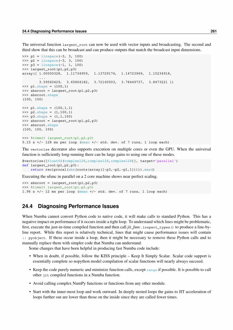
24.4 Diagnosing Performance Issues 261

The universal function largest_root can now be used with vector inputs and broadcasting. The second andthird show that this can be broadcast and can produce outputs that match the broadcast input dimensions.>>> p1 = linspace(-3, 3, 100)>>> p2 = linspace(-3, 3, 100)>>> p3 = linspace(-1, 1, 100)>>> largest_root(p1,p2,p3)array([ 1.00000328, 1.11734959, 1.13729174, 1.14723969, 1.15234918,

...3.59560429, 3.65864182, 3.72160503, 3.78449737, 3.8473221 ])

>>> p1.shape = (100,1)>>> absroot = largest_root(p1,p2,p3)>>> absroot.shape(100, 100)

>>> p1.shape = (100,1,1)>>> p2.shape = (1,100,1)>>> p3.shape = (1,1,100)>>> absroot = largest_root(p1,p2,p3)>>> absroot.shape(100, 100, 100)

>>> %timeit largest_root(p1,p2,p3)5.15 s +/- 128 ms per loop (mean +/- std. dev. of 7 runs, 1 loop each)

The vectorize decorator also supports execution on multiple cores or even the GPU. When the universalfunction is sufficiently long-running there can be large gains to using one of these modes.@vectorize([float64(complex128,complex128,complex128)], target='parallel')def largest_root(p1,p2,p3):

return reciprocal(abs(roots(array([-p3,-p2,-p1,1])))).max()

Executing the ufunc in parallel on a 2 core machine shows near perfect scaling.>>> absroot = largest_root(p1,p2,p3)>>> %timeit largest_root(p1,p2,p3)1.96 s +/- 12 ms per loop (mean +/- std. dev. of 7 runs, 1 loop each)

24.4 Diagnosing Performance Issues

When Numba cannot convert Python code to native code, it will make calls to standard Python. This has anegative impact on performance if it occurs inside a tight loop. To understand which lines might be problematic,first, execute the just-in-time compiled function and then call jit_func.inspect_types() to produce a line-by-line report. While this report is relatively technical, lines that might cause performance issues will contain:: pyobject. If these occur inside a loop, then it might be necessary to remove these Python calls and tomanually replace them with simpler code that Numba can understand.

Some changes that have been helpful in producing fast Numba code include:

• When in doubt, if possible, follow the KISS principle – Keep It Simply Scalar. Scalar code support isessentially complete so nopython model compilation of scalar functions will nearly always succeed.

• Keep the code purely numeric and minimize function calls, except range if possible. It is possible to callother jit compiled functions in a Numba function.

• Avoid calling complex NumPy functions or functions from any other module.

• Start with the inner-most loop and work outward. In deeply nested loops the gains to JIT acceleration ofloops further out are lower than those on the inside since they are called fewer times.

262 Improving Performance using Numba

• Numpy functions that are not currently supported in Numba can often by implemented in pure Pythonand JIT compiled so that they are not required.

• If loops are not accelerated, add type information, as in @jit(float64(float64[:,::1])).

• If, after adding type information for inputs, loops are still not accelerated, add type information aboutlocal variables. This information can be added using a dictionary where the keys are local variable namesand the values are Numba types. For example,

from numba import jit, double, int32locals = 'var1': double[:], 'var2': int32@jit(float64(float64[:,::1]), locals = locals)

A continuous time stochastic volatility model will be used to illustrate some of the issues in converting amoderately complex piece of code for use with Numba. The model is described by the two equations

d pt = µdt + exp(β0 +β1vt)dwt

dvt = αvtdt +dvt

where T = 1 indicates 1 day. The model parameters are µ = 0.03, α = −0.100, β0 = 0, β1 = 0.125, ρ =Corr [dwt ,dvt ] =−0.62. Pure Python code to implement the model is presented below.

import numpy as np

# SetupT = 10000# 1 yearnstep = 23400 # 1 secondp0, v0 = 0.0, 0.0

# Model Parametersmu = 0.03b0 = 0.000b1 = 0.125alpha = -0.100rho = -0.62# Initialize daily vectorslog_closing_price = np.zeros(T, dtype=np.float64)integrated_variance = np.zeros(T, dtype=np.float64)# Initialize intradaily vectorsv = np.zeros(nstep + 1, dtype=np.float64)spot_vol = np.zeros(nstep + 1, dtype=np.float64)p = np.zeros(nstep + 1, dtype=np.float64)p[0] = p0v[0] = v0

R_root = np.linalg.cholesky(np.array([[1, rho], [rho, 1]])).T

dt = 1.0 / nstep #/ 252root_dt = np.sqrt(dt)

for t in range(T):e = np.random.standard_normal((nstep, 2)).dot(R_root) ⁎ root_dtdwp = e[:, 0]dwv = e[:, 1]# Replacement function# innerloop_jit(mu, alpha, b0, b1, nstep, p, v, spot_vol, dt, dwv, dwp)

24.5 Replacing Python function with C functions 263

# Key loop#for i in range(1, nstep + 1):# dv = alpha ⁎ v[i - 1] ⁎ dt + dwv[i - 1]# v[i] = v[i - 1] + dv# spot_vol[i] = np.exp(b0 + b1 ⁎ v[i - 1])# dp = mu ⁎ dt + spot_vol[i] ⁎ dwp[i - 1]# p[i] = p[i - 1] + dp

# Save dataintegrated_variance[t] = np.mean(spot_vol ⁎⁎ 2.0)log_closing_price[t] = p[-1]

# Reset the first price for the next dayp[0] = p[-1]v[0] = v[-1]

The first step in converting code is to extract the core loop so that it can be converted into a function.

for i in range(1, nstep):dv = alpha ⁎ v[i - 1] ⁎ dt + dwv[i]v[i] = v[i - 1] + dvspot_vol[i] = np.exp(b0 + b1 ⁎ v[i - 1])dp = mu ⁎ dt + spot_vol[i] ⁎ dwp[i]p[i] = p[i - 1] + dp

In this example the code in the function was already basic scalar code and so there was no need to further alterit, aside from adding the def line and adding the decorator @jit. The final step is to comment out the loop inthe original code and to uncomment the function call to innerloop_jit.

from numba import jit

@jitdef innerloop(mu, alpha, b0, b1, nstep, p, v, spot_vol, dt, dwv, dwp):

for i in range(1, nstep):dv = alpha ⁎ v[i - 1] ⁎ dt + dwv[i]v[i] = v[i - 1] + dvspot_vol[i] = np.exp(b0 + b1 ⁎ v[i - 1])dp = mu ⁎ dt + spot_vol[i] ⁎ dwp[i]p[i] = p[i - 1] + dp

It might be tempting to wrap both the inner loop and the other loop. At the time of writing, Numba cannotcompile this function – however line profiling shows that 99.5% of the time is spent in the inner loop, and theother 0.5% of the time on the random number generator. Once the JIT function is included, 86.2% of the timeis still spent in the inner loop and 12.9% is in generating the random numbers. Most importantly, the total runtime of the program drops from 158 to 3.23 seconds when simulating 10,000 days of data, a speed up by afactor of 50. JIT compiling the entire function would be unlikely to bring further gains.

24.5 Replacing Python function with C functions

Some Python functions are not natively available in Numba, and so including these in a loop can deteriorateperformance. This code uses the ctypes modules to import the standard C library which contains commonmathematical functions, and then provides a simple interface to the exponential function. argtypes is a list ofinput argument types and restype contains the type of the value returned.

import numpy as npfrom ctypes import ⁎from math import pifrom numba import jit, double

264 Improving Performance using Numba

proc = cdll.msvcrt# Linux/OSX# proc = CDLL(None)

c_exp = proc.expc_exp.argtypes = [c_double]c_exp.restype = c_double

@jitdef use_numpy_exp(x):

return np.exp(x)

@jitdef use_c_exp(x):

return c_exp(x)

After calling both compiled functions with a double (e.g., 1.0), .inspect_types() shows that neither versionrequires a Python call (object mode). The C version is slightly simpler since it can directly call the C function.The output of use_numpy_exp.inspect_types() is

use_numpy_exp (float64,)@jit

def use_numpy_exp(x):

# --- LINE 16 ---# label 0# x = arg(0, name=x) :: float64# $4load_method.1 = getattr(value=$2load_global.0, attr=exp) :: Function(<ufunc '

exp'>)# del $2load_global.0# del x# del $4load_method.1# $10return_value.4 = cast(value=$8call_method.3) :: float64# del $8call_method.3# return $10return_value.4

return np.exp(x)

The output of use_c_exp.inspect_types() is

use_c_exp (float64,)

@jit

def use_c_exp(x):

# --- LINE 20 ---# label 0# x = arg(0, name=x) :: float64# $2load_global.0 = global(c_exp: <_FuncPtr>) :: ExternalFunctionPointer((float64

,) -> float64)# del x# del $2load_global.0# $8return_value.3 = cast(value=$6call_function.2) :: float64# del $6call_function.2# return $8return_value.3

return c_exp(x)

24.6 Other Features of Numba 265

24.6 Other Features of Numba

Numba is too large to fully describe in a single chapter. In particular, there are a number of features that havenot been described. The most important of these features is the ability to write code that executed on either theon Nvidia GPUs that is compiled using LLVM and CUDA or on Heterogeneous System Architectures (HSAs)such as some AMD CPUs. Targeting these platforms can produce huge performance gains in some applications.Another useful feature is the ability to compile function Ahead of Time (AOT) which allows both the feature tobe used without the warm-up compilation as well as the possibility of distributing the function for use in Pythonwithout requiring Numba to be installed. Numba has also been extended to all JIT compilation of classes (withmany restrictions) and so it is possible to use the features of OOP in conjunction with Numba.

24.7 Exercises

1. Write a Python function which will accept a p+q+1 vector of parameters, a T vector of data, and p andq (integers, AR and MA order, respectively) and recursively compute the ARMA error beginning withobservation p+1. If an MA index is negative it should be backcast to 0.

2. Use jit to accelerate the ARMA function written in the exercise 1. Compare the speed to the purePython implementation.

266 Improving Performance using Numba

Chapter 25

Improving Performance using Cython

Cython is a powerful, but somewhat complex, solution for situations where pure NumPy or Numba cannotachieve performance targets. Cython is a creole of Python and C, and so some familiarity, mostly with Cdatatypes, is helpful. Cython translates its hybrid Python code into C code, which can then be compiled into aPython extension. Cython code has a number of distinct advantages over Numba’s just-in-time compilation ofPython code:

• Cython modules are statically compiled and so using a Cython module does not incur a “warm-up”penalty due to just-in-time compilation.

• A Python extension produced by Cython can be distributed to other users and does not require Cythonto be installed. In contrast, Numba must be installed and performance gains may vary across Numba orLLVM versions.

• Numba is a relatively new, rapidly evolving project , and so code that works in one version might breakin a future version.

• Cython can be used interface to existing C/C++ code.

Using Cython on Linux is relatively painless and only requires that the system compiler is installed in additionto Cython. Using Cython on OSX requires that XCode or at least the command line tools for Xcode have beeninstalled. To use Cython in Python x64 Windows, it is necessary to have the x64 version of Cython installedalong with Visual Studio 2014 or later. All editions including the free Community edition provide the requiredC compiler.

Using Cython can be broken down into a two-step process. The first is to write standard Python. Thesecond is to add some special syntax and hints about the type of data used. This first example will use thesame GARCH(P,Q) code as in the Numba example. Applying Cython to an existing Python function requiresa number of steps (for standard numeric code):

• Save the file with the extension pyx – for Python Extension.

• Use cimport, which is a special version of import for Cython, to import both cython and numpy as np.

• Declare types for every variable:

– Scalars have standard C-types, and in almost all cases should be double (same as float64 inNumPy, and float in Python), int (signed integer), uint (unsigned integer), or size_t (systemunsigned integer type). size_t would typically only be used to counter variables in loops.

268 Improving Performance using Cython

– NumPy arrays should have a memory view type. These resemble C types, but also indicate thenumber of dimensions, the order of data in the array, and whether that data in the array is contiguousin memory. For example, a 1-dimensional array containing double (float64 in NumPy, float inPython) is indicated by double[:], a 2-dimensional array is indicated double[:, ::1] where the::1 indicates that the array is contiguous and in C order. Arrays containing other data types canbe similarly typed, e.g. int[:,:,::1] for a 3-dimensional array of integers or float[::1, :] fora 2-d single-precision array in Fortran order (note the position of ::1 in the declaration). Whileeither C or Fortran ordered arrays can be used, C ordering is the default in NumPy. It is importantto specify as much as possibly about the array – using double[:] and double[::1] will producecode that runs at different speed since double[::1] instructs Cython that you are passing an arraythat is contiguous so that the elements are contiguous in memory. Iterating across arrays that arecontiguous requires fewer calculations to determine the position of the next element.

• Declare all arrays as not None.

• Ensure that all array access uses only single item access and not more complex slicing. For example is xis a 2-dimensional array, x[i,j] must be used and not x[i,:] or x[:,j].

• Add decorators to disable Python safety checks. Naturally, it is important to verify that these checks arenot needed, and if they are, problems like memory corruption or crashes of Python may occur. The mostimportant of these are

– @cython.boundscheck(False) - Do not check for access beyond the end of an array

– @cython.wraparound(False) - Do not allow negative indexing

– @cython.cdivision(True) - Do not check for division by zero

The Cythonized version of the GARCH(P,Q) recursion is presented below. All arrays are declared usingdouble[:] and so the inputs must all have 1 dimension (and 1 dimension only). The inputs p and q aredeclared to be integers, and backcast is declared to be a double. The three local variables T, i and j are alldeclared to be ints. Note that is crucial that the variables used as iterators are declared as int (or other integertype, such as uint or size_t). The remainder of the function is unchanged.

# garch_ext.pyximport numpy as npcimport numpy as npcimport cython

@cython.boundscheck(False)@cython.wraparound(False)def garch_recursion(double[::1] parameters not None,

double[::1] data not None,double[::1] sigma2 not None,int p,int q,double backcast):

cdef int T = np.size(data, 0)cdef int i, j

for i in range(T):sigma2[i] = parameters[0]for j in range(1, p + 1):

if (i - j) < 0:

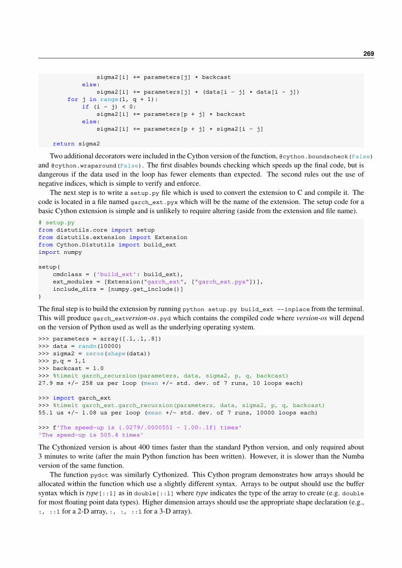
269

sigma2[i] += parameters[j] ⁎ backcastelse:

sigma2[i] += parameters[j] ⁎ (data[i - j] ⁎ data[i - j])for j in range(1, q + 1):

if (i - j) < 0:sigma2[i] += parameters[p + j] ⁎ backcast

else:sigma2[i] += parameters[p + j] ⁎ sigma2[i - j]

return sigma2

Two additional decorators were included in the Cython version of the function, @cython.boundscheck(False)and @cython.wraparound(False). The first disables bounds checking which speeds up the final code, but isdangerous if the data used in the loop has fewer elements than expected. The second rules out the use ofnegative indices, which is simple to verify and enforce.

The next step is to write a setup.py file which is used to convert the extension to C and compile it. Thecode is located in a file named garch_ext.pyx which will be the name of the extension. The setup code for abasic Cython extension is simple and is unlikely to require altering (aside from the extension and file name).# setup.pyfrom distutils.core import setupfrom distutils.extension import Extensionfrom Cython.Distutils import build_extimport numpy

setup(cmdclass = 'build_ext': build_ext,ext_modules = [Extension("garch_ext", ["garch_ext.pyx"])],include_dirs = [numpy.get_include()]

)

The final step is to build the extension by running python setup.py build_ext --inplace from the terminal.This will produce garch_extversion-os.pyd which contains the compiled code where version-os will dependon the version of Python used as well as the underlying operating system.>>> parameters = array([.1,.1,.8])>>> data = randn(10000)>>> sigma2 = zeros(shape(data))>>> p,q = 1,1>>> backcast = 1.0>>> %timeit garch_recursion(parameters, data, sigma2, p, q, backcast)27.9 ms +/- 258 us per loop (mean +/- std. dev. of 7 runs, 10 loops each)

>>> import garch_ext>>> %timeit garch_ext.garch_recursion(parameters, data, sigma2, p, q, backcast)55.1 us +/- 1.08 us per loop (mean +/- std. dev. of 7 runs, 10000 loops each)

>>> f'The speed-up is .0279/.0000551 - 1.00:.1f times''The speed-up is 505.4 times'

The Cythonized version is about 400 times faster than the standard Python version, and only required about3 minutes to write (after the main Python function has been written). However, it is slower than the Numbaversion of the same function.

The function pydot was similarly Cythonized. This Cython program demonstrates how arrays should beallocated within the function which use a slightly different syntax. Arrays to be output should use the buffersyntax which is type[::1] as in double[::1] where type indicates the type of the array to create (e.g. doublefor most floating point data types). Higher dimension arrays should use the appropriate shape declaration (e.g.,:, ::1 for a 2-D array, :, :, ::1 for a 3-D array).

270 Improving Performance using Cython

import numpy as npcimport numpy as npcimport cython

@cython.boundscheck(False)@cython.wraparound(False)def pydot(double[:, ::1] a not None,

double[:, ::1] b not None):cdef int M, N, P, QM,N = np.shape(a)P,Q = np.shape(b)assert N==Pcdef double[:, ::1] c = np.zeros((M,N), dtype=np.float64)for i in range(M):

for j in range(Q):for k in range(N):

c[i,j] = c[i,j] + a[i,k] ⁎ b[k,j]return c

The Cythonized function is about 350 times faster than straight Python, although it is still much slower than thenative NumPy routine underlying @.

>>> a = randn(100,100)>>> b = randn(100,100)>>> %timeit pydot(a,b)907 ms +/- 29.4 ms per loop (mean +/- std. dev. of 7 runs, 1 loop each)

>>> import pydot as p>>> %timeit p.pydot(a,b)2.72 ms +/- 40.4 us per loop (mean std. dev. of 7 runs, 100 loops each)

>>> f'The speed-up is 0.907/0.00272- 1.0:.1f times''The speed-up is 332.5 times'

>>> %timeit a @ b24.8 us +/- 3.55 us per loop (mean +/- std. dev. of 7 runs, 100000 loops each)

>>> f'The speed-up is 0.00272/0.0000248 - 1.0:.1f times''The speed-up is 108.7 times'

The final example will produce a Cython version of the weighted average. Since the original Python codeused slicing, this is removed and replaced with a second loop.

def naive_weighted_avg(x, w):T = x.shape[0]m = len(w)m12 = int(ceil(m/2))y = zeros(T)for i in range(len(x)-m+1):

for j in range(m):y[i+m12] += x[i+j] ⁎ w[j]

return y

This makes writing the Cython version simple.

import numpy as npcimport numpy as npcimport cython

@cython.boundscheck(False)

25.1 Diagnosing Performance Issues 271

@cython.wraparound(False)def cython_weighted_avg(double[::1] x,

double[::1] w):cdef int T, m, m12, i, jT = x.shape[0]m = len(w)m12 = int(np.ceil(float(m)/2))cdef double[::1] y = np.zeros(T, dtype=np.float64)for i in range(T-m+1):

for j in range(m):y[i+m12] += x[i+j] ⁎ w[j]

return y

The Cython version can be compiled using a setup function in the same way that the GARCH recursion wascompiled.

>>> w = array(r_[1:11,9:0:-1],dtype=float64)>>> w = w/sum(w)>>> x = randn(10000)>>> %timeit naive_weighted_avg(x,w)160 ms +/- 4.01 ms per loop (mean +/- std. dev. of 7 runs, 10 loops each)

>>> import cython_weighted_avg as c>>> %timeit c.cython_weighted_avg(x,w)251 us +/- 5.69 us per loop (mean +/- std. dev. of 7 runs, 1000 loops each)

>>> from numba import jit>>> weighted_avg_jit = jit(naive_weighted_avg)>>> %timeit weighted_avg_jit(x,w)130 us +/- 4.75 us per loop (mean +/- std. dev. of 7 runs, 10000 loops each)

The gains are unsurprisingly large (around 500×) – however, the Cython code is no faster than the pure NumPysideways version. This demonstrates that Cython is not a magic bullet and that good vectorized code, even witha small amount of looping, can be very fast. The final lines produce a Numba version of the same function,which is also much faster than the pure Python version. It is also faster than the Cython version.

25.1 Diagnosing Performance Issues

If a function contains calls to Python code which cannot be optimized by Cython, the performance of thecompiled code may be similar to that in the original code. Fortunately, Cython provides a diagnostic facility toexamine the Cython code for performance issues. This tool is run using the command cython -a my_ext.pyxwhich will produce a HTML report containing Cython code as well as the translated C (the C is hidden bydefault, double click on a line to see the translation). Highlighted lines indicate locations where the Cythoninterfaces with Python, which can be slow. An idealized function in Cython will have only three interfacepoints. The first is at the top of the file, the second is the function definition line, which is required to get thedata from Python and the final is in the return statement, which moves data back to Python.

Figure 25.1 shows the diagnostic output from running cython -a garch_ext.pyx. There are 5 highlightedlines. Three are those discussed above and are unavoidable. The remaining two are the import numpy as npand the call to np.ones, both of which require interfacing with Python. In general, the more highlighting thesmaller the gains will be for converting a function to Cython. However, the most important consideration is toensure that the core loop contains no Python calls. This important consideration is satisfied here, which is whythe performance gains are large.

272 Improving Performance using Cython

Figure 25.1: Diagnostic report produced by running cython -a garch_ext.pyx. Highlighted lines indicateperformance concerns due to interfacing with Python.

25.1 Diagnosing Performance Issues 273

25.1.1 Replacing Python function with C functions

Some algorithms require calling functions in the innermost loop. If left untreated, the Cython code will be nofaster than standard Python code. To illustrate this issue, consider a simple recursion from an EGARCH model

lnσ2t = ω +α |rt−1/σt−1|+β lnσt−1

which can be expressed as a Python function

import numpy as np

def egarch_recursion(parameters, data, backcast):

T = np.size(data,0)lnsigma2 = np.zeros(T)sigma2 = np.zeros(T)lnsigma2[0] = backcast

for t in range(1, T):sigma2[t-1] = np.exp(lnsigma2[t-1])lnsigma2[t] = parameters[0]

+ parameters[1] ⁎ data[t-1] / sigma2[t]+ parameters[2] ⁎ lnsigma2[t-1]

sigma2[T - 1] = np.exp(lnsigma2[t])

return sigma2

A standard Cython version can be constructed using the same steps as above. This version declares an array inthe function, and so it is important to declare the types of the array. This version also includes the decorator@cython.cdivision(True) which disables division by 0 warnings.

import numpy as npcimport numpy as npcimport cython

@cython.boundscheck(False)@cython.wraparound(False)@cython.cdivision(True)def egarch_recursion(double[::1] parameters not None,

double[::1] data not None,double backcast):

cdef int T = np.size(data, 0)cdef int tcdef double lnsigma2cdef double[::1] sigma2 = np.zeros(T, dtype=np.float64)

lnsigma2 = backcast

for t in range(1, T):sigma2[t - 1] = np.exp(lnsigma2)lnsigma2 = parameters[0] \

+ parameters[1] ⁎ data[t - 1] / sigma2[t] \+ parameters[2] ⁎ lnsigma2

sigma2[T - 1] = np.exp(lnsigma2[t])

return sigma2

Running cython -a egarch_ext.pyx produces the report in top panel of Figure 25.2, which shows thatthe call to np.exp is a performance concern since it requires interfacing with Python (dark highlighting).

274 Improving Performance using Cython

Using NumPy’s exp

Using the C library’s exp

Figure 25.2: Diagnostic report produced by running cython -a garch_ext.pyx. The top panel shows high-lighted lines indicate performance concerns due to interfacing with Python. The bottom panel uses the Clibrary’s exponential and the loop will now execute quickly.

25.2 Interfacing with External Code 275

The solution to this problem is to replace the NumPy exponential with the standard math libraries expo-nential function which will not incur a penalty. This change is implemented using the cdef extern commandwhich declares an external function that takes a float and returns a float.

import numpy as npcimport numpy as npcimport cython

cdef extern from "math.h":double exp(double x)

@cython.boundscheck(False)@cython.wraparound(False)@cython.cdivision(True)def egarch_recursion(double[::1] parameters not None,

double[::1] data not None,double backcast):

cdef int T = np.size(data, 0)cdef int tcdef double lnsigma2cdef double[::1] sigma2 = np.zeros(T, dtype=np.float64)

lnsigma2 = backcast

for t in range(1, T):sigma2[t - 1] = exp(lnsigma2)lnsigma2 = parameters[0] \

+ parameters[1] ⁎ data[t - 1] / sigma2[t] \+ parameters[2] ⁎ lnsigma2

sigma2[T - 1] = exp(lnsigma2[t])

return sigma2

The diagnostic report from this change is shown in the bottom panel of Figure 25.2.

25.2 Interfacing with External Code

The final, and most extreme, method to maximize performance is to interface with native code, usually in theform of some hand-written C/C++/Fortran or an existing DLL. There are a number of method to interface withexisting code, including directly interfacing with Python using the API, wrapping code in Cython or SWIG,using ctypes to call compiled libraries (.dll on Windows, .so on Linux) and f2Py, which only works with Fortran.This section only discusses two methods – ctypes for interfacing with an existing DLL using a C interface andwraping a C file using Cython. Both examples will build on the GARCH recursion.

25.2.1 ctypes and Shared Libraries (DLL/so)

ctypes provides a simple method to call existing code in libraries that present a C interface. There are two mainreasons why using a shared library might be better than directly interfacing with the code:

• The DLL/so is available but the source is not – as long as API documentation is available, the sharedlibrary can be directly used.

• The code in the DLL/so has complex dependencies – directly using the DLL, if it has been compiled towork stand-alone, does not require managing its dependencies.

276 Improving Performance using Cython

• A different, higher performance compiler is required. DLLs can be compiled with any standard compliantcompiler including the Intel C compiler, which allows advanced options such as autovectorization to beused. Code that is directly interfaced is usually compiled with the same compiled used to compile Python.

ctypes was previously used in the Numba example to import an external C function (exp). This example willshow how to interface with both scalars and NumPy arrays. Two code files are required - the first is the headerand the second contains the GARCH recursion that will be called from Python. First, the header,// garch_recursion.h

__declspec(dllexport) void garch_recursion(int T, double ⁎parameters, double ⁎data,double ⁎sigma2, int p, int q, double backcast);

and then the main code. This function does not return anything and instead modifies the elements of sigma2directly.// garch_recursion.c#include "garch_recursion.h"

#ifdef WIN32#define WINAPI __declspec(dllexport)#else#define WINAPI#endif

WINAPI void garch_recursion(int T, double ⁎parameters, double ⁎data, double ⁎sigma2, intp, int q, double backcast)

int i, j;for(i = 0; i<T; i++)

sigma2[i] = parameters[0];for (j=1; j<=p; j++)

if((i-j)<0)

sigma2[i] += parameters[j] ⁎ backcast;else

sigma2[i] += parameters[j] ⁎ (data[i-j]⁎data[i-j]);

for (j=1; j<=q; j++)

if((i-j)<0)

sigma2[i] += parameters[p+j] ⁎ backcast;else

sigma2[i] += parameters[p+j] ⁎ sigma2[i-j];

On Windows, the DLL can be built by running the commandscl.exe -nologo -EHsc -GS -W3 -D_WIN32 -D_USRDLL -MD -Ox -c garch_recursion.clink.exe /nologo /DLL garch_recursion.obj /OUT:garch_recursion.dll

25.2 Interfacing with External Code 277

On Linux, a shared library can be produced by runninggcc -O3 -Wall -ansi -pedantic -c -fPIC garch_recursion.c -o garch_recursion.ogcc garch_recursion.o -shared -o garch_recursion.so

Once the DLL/so has been built, only the DLL/so is needed. First, the DLL/so is imported using the NumPyversion of the ctypes’ load_library. This is important when interfacing with NumPy arrays but is not re-quired if only using scalar data. The second step is to use ctypes to import the library and declare both theargument and return types. Scalar types are obvious – they have the same name as in C. NumPy arrays usePOINTER(c_double) (or another C type if not double precision). The final step is to write a wrapper aroundthe imported code which simply calls the C routine, with the caveat that NumPy arrays must be called usingarray.ctypes.data_as(ct.POINTER(ct.c_double)) (or another C type if the array contains something otherthan double precision floating point data) which calls the function with a pointer to the array’s data rather thanwith the actual NumPy array.# garch_recursion_dll_wrapper.pyimport ctypes as ct

import numpy as np

# Open the librarygarchlib = np.ctypeslib.load_library("garch_recursion.dll", '.')# Linux/OSX# garchlib = np.ctypeslib.load_library("garch_recursion.so", '.')

# Define output and input typesgarchlib.garch_recursion.restype = ct.c_void_pgarchlib.garch_recursion.argtypes = [ct.c_int,

ct.POINTER(ct.c_double),ct.POINTER(ct.c_double),ct.POINTER(ct.c_double),ct.c_int,ct.c_int,ct.c_double]

# Wrapper functiondef garch_recursion(parameters, data, sigma2, p, q, backcast):

# Optional, but can be important if data is not contiguous# Will copy to temporary value, only if neededparameters = np.ascontiguousarray(parameters)data = np.ascontiguousarray(data)sigma2 = np.ascontiguousarray(sigma2)T = data.shape[0]return garchlib.garch_recursion(T,

parameters.ctypes.data_as(ct.POINTER(ct.c_double)),data.ctypes.data_as(ct.POINTER(ct.c_double)),sigma2.ctypes.data_as(ct.POINTER(ct.c_double)),p,q,backcast)

Finally, it is useful to verify that the code works and to assess the performance gains, which are similar to theother compiled versions.>>> import garch_recursion_dll_wrapper as dll>>> %timeit dll.garch_recursion(parameters, data, sigma2, p, q, backcast)60.3 us +/- 549 ns per loop (mean +/- std. dev. of 7 runs, 10000 loops each)

More information on using ctypes with NumPy is available in the SciPy cookbook, http://wiki.scipy.org/Cookbook/Ctypes.

278 Improving Performance using Cython

25.2.2 Wrapping code with Cython

An alternative to using an existing a DLL is to directly interface the C code with Python using Cython togenerate the interface. This example uses the same C and header files as in the DLL example, and so the onlysteps are to write the Cython file (pyx) and the setup. The Cython file has the usual header and the C function isreferenced using cdef extern from header file . The function definition is identical to the previous Cythonexample that made use of a C function. The final step is to call the external code using a wrapper function.Best practice is to call np.ascontiguousarray on arrays to ensure that are contiguous – in other words, thatthe second element is adjacent to the first in the computer’s memory. These can be omitted if the functionwill always be used on contiguous arrays, although the cost of using them on already contiguous arrays isvery small while incorrect results will be produced if the arrays are non-contiguous. The final step is to callthe C function passing NumPy arrays using a pointer to the first element &array[0]. Note that if passingmultidimensional arrays, the pointer should be to the first element (e.g. &array[0, 0] for a 2-dimensionalarray or &array[0, 0, 0] for a 3-dimensional array).

# garch_recursion_wrapper.pyximport numpy as npcimport numpy as npcimport cython

cdef extern from "garch_recursion_standalone.h":void garch_recursion(int T, double ⁎ parameters, double ⁎ data, double ⁎ sigma2, int p,

int q, double backcast)

@cython.boundscheck(False)def garch_recursion_wrapped(double[:] parameters not None,

double[:] data not None,double[:] sigma2 not None,int p,int q,double backcast):

cdef int T = np.size(data, 0)# Best practice is to ensure arrays are contiguousparameters = np.ascontiguousarray(parameters)data = np.ascontiguousarray(data)sigma2 = np.ascontiguousarray(sigma2)

# No return, sigma2 modified in placegarch_recursion(T, &parameters[0] , &data[0], &sigma2[0], p, q, backcast)

return sigma2

The setup file is similar to the previous setup, only sources must be modified to include both the Cython fileand the C source.

# setup_garch_recursion_wrapper.pyimport numpyfrom distutils.core import setupfrom distutils.extension import Extensionfrom Cython.Distutils import build_ext

ext_modules = [Extension(name="garch_recursion_wrapper",sources=["garch_recursion_wrapper.pyx", "garch_recursion.c"],include_dirs = [numpy.get_include()])]

setup(name = 'garch_recursion_wrapper',

25.3 Exercises 279

cmdclass = 'build_ext': build_ext,ext_modules = ext_modules)

The hand-written module performs no better than any of the other methods, while it takes more time to imple-ment the C function and wrap it. However, this example is somewhat misleading since most applications ofthese methods interface with existing C or C++ code.

>>> import garch_recursion_wrapper as wrapper>>> %timeit wrapper.garch_recursion_wrapped(parameters, data, sigma2, p, q, backcast)67.5 us +/- 2.21 us per loop (mean +/- std. dev. of 7 runs, 10000 loops each)

25.3 Exercises

1. Write a Python function which will accept a p+q+1 vector of parameters, a T vector of data, and p andq (integers, AR and MA order, respectively) and recursively computes the ARMA error beginning withobservation p+1. If an MA index is negative it should be backcast to 0.

2. [Only for the brave] Convert the ARMA function to Cython, compile it, and compare the performanceagainst both the pure Python and the Numba versions.

280 Improving Performance using Cython

Chapter 26

Executing Code in Parallel

26.1 map and related functions

map is a built-in method to apply a function to a generic iterable. It is used as map( function , iterable ), andreturns a list containing the results of applying function to each item of iterable. The list returned can be eithera simple list if the function returns a single item, or a list of tuples if the function returns more than 1 value.def powers(x):

return x⁎⁎2, x⁎⁎3, x⁎⁎4

This function can be called on any iterable, for example, a list.>>> y = [1.0, 2.0, 3.0, 4.0]>>> list(map(powers, y))[(1.0, 1.0, 1.0), (4.0, 8.0, 16.0), (9.0, 27.0, 81.0), (16.0, 64.0, 256.0)]

map is a generator which defers generating results until required, and so list is used to force it to execute. Theoutput is a list of tuples where each tuple contains the result of calling the function on a single input. In thiscase, the same result could be achieved using a list comprehension, which is the preferred syntax.>>> [powers(i) for i in y][(1.0, 1.0, 1.0), (4.0, 8.0, 16.0), (9.0, 27.0, 81.0), (16.0, 64.0, 256.0)]

map can be used with more than 1 iterable, in which case it iterates using the length of the longest iterable. Ifone of the iterable is shorter than the other(s), then it is extended with None. It is usually best practice to ensurethat all iterables have the same length before using map.def powers(x,y):

if x is None or y is None:return None

else:return x⁎⁎2, x⁎y, y⁎⁎2

>>> x = [10.0, 20.0, 30.0]>>> y = [1.0, 2.0, 3.0, 4.0]>>> list(map(powers, x, y))[(100.0, 10.0, 1.0), (400.0, 40.0, 4.0), (900.0, 90.0, 9.0), None]

A related function is zip which combines two or more lists into a single list of tuples. It is similar to callingmap except that it will stop at the end of the shortest iterable, rather than extending using None.>>> x = [10.0, 20.0, 30.0]>>> c>>> list(zip(x, y))[(10.0, 1.0), (20.0, 2.0), (30.0, 3.0)]

282 Executing Code in Parallel

26.2 multiprocessing

The real advantage of map over list comprehensions is that it can be combined with the multiprocessingmodule to run code on more than 1 (local) processor. Note that on Windows, the multiprocessing module doesnot work correctly in IPython, and so it is necessary to use stand-alone Python programs. multiprocessingincludes a map function which is similar to that in the standard Python distribution except that it executes usinga Pool rather than on a single processor. The performance gains to using a Pool may be large and should beclose to the number of pool processes if code execution is completely independent (which should be less thanor equal to the number of physical processors on a system).

This example uses multiprocessing to compute critical values for a non-standard distribution and is illus-trative of a Monte Carlo-like setup. The program has the standard set of imports including the multiprocessingmodule.

import multiprocessing as mpimport numpy as npimport matplotlib.pyplot as plt

Next, a simple function is defined to compute a simulated supF test statistic which arises when testing fora structural break in a regression model when the break date is unknown. The underlying mathematical model,under the null of no structural break, is

yt = β0 +β′1xt + εt

and the alternative model is

yt = β0 +β′1xt + γ

′xtI[t>τ]+ εt

where I[t>τ] is an indicator variable that takes the value 1 when true. If τ is known, the test statistic,

F =

(R2

r −R2u)/k

(1−R2u)/(T −2k−1)

is a standard Chow test and follows an F distribution. When τ ∈ [bpLTc,bpHTc] where 0< pL < pH < 1 and p•is suitable far from 0 or 1, then a sup version of this test can be implemented. The test is no longer distributed asan Fk,T−2k−1 where k is the number of variables in x but is based on the expected maximum value of many suchtests. One method to get critical values is to simulate these, and the function supf can be used to produce onesuch test statistic from simulated x and y data. The code runs a full sample regression to compute the restrictedR2 and then run regressions with breaks across a range of possibly break dates, computing unrestricted R2 foreach break and the associated F-stat. Finally, the maximum of these is returned. map requires both a functionand an iterable, the function can be any function located in any module and so does not need to reside inthe same file as the main code. In this example, this function is stored in supf.py. An additional functionsupf_wrapper that takes a tuple input is also used for convenience.

# supf.py

import numpy as npfrom numpy.linalg import pinv

def supf(y, x, p):T = y.shape[0]range = np.floor(np.array([T ⁎ p, T ⁎ (1 - p)]))range = np.arange(range[0], range[1] + 1, dtype=np.int32)# Demean since intercept doesn't breakx = x - np.mean(x)y = y - np.mean(y)b = pinv(x) @ y

26.2 multiprocessing 283

e = y - x @ b# Compute full sample R2R2_r = 1 - (e @ e) / (y @ y)

k = x.shape[1]F_stat = np.zeros(T)for t in range:

X1 = x[:t]X2 = x[t:]# Parameters and errors before the breakb = pinv(X1) @ y[:t]e[:t] = y[:t] - X1 @ b# Parameters and errors after the breakb = pinv(X2) @ y[t:]e[t:] = y[t:] - X2 @ b# R2 from model with breakR2_u = 1 - (e @ e) / (y @ y)# F stat for break at tF_stat[t] = ((R2_u - R2_r) / k) / ((1 - R2_u) / (T - 2⁎ k - 1))

# Only return maximum F statreturn F_stat.max()

def supf_wrapper(args):# Convenience wrapper for use with mapreturn supf(args[0], args[1], args[2])

Using multiprocessing requires a __name__=='main' block in the function. The main block does threethings:

1. Compute the setup for the simulation. This is done so that the variables can be passed to the functionexecuted in parallel.

2. Initialize the pool using mp.Pool(processes=2) (normally should use the same number as the numberof physical cores on the system)

3. Call map from the multiprocessing module

4. Plot the results.

# multiprocessing_example.pyimport multiprocessing as mp

import matplotlib.pyplot as pltimport numpy as np

from supf import supf_wrapper

if __name__ == '__main__':reps = 1000T = 200

setup = []for i in range(reps):

y = np.random.standard_normal(T)x = np.random.standard_normal((T, 1))p = 0.2setup.append((y, x, p))

284 Executing Code in Parallel

# Non parallel map# res = map(surf_wrapper, setup)

# Parallel mappo = mp.Pool(processes=2)res = po.map(supf_wrapper, setup)print(len(res))po.close()

ax = plt.hist(res)ax = ax[2]fig = ax[0].get_figure()fig.savefig('multiprocessing.pdf')

26.3 joblib

joblib is a Python package that provides a simple interface to the multiprocessing module with an easier touse syntax, especially for functions taking multiple arguments. This improved syntax allow for some argumentsto vary according to an index but others to stay fixed, which is not simple to handle in map, which requires settingup a tuple with the both the dynamic and fixed parameters. joblib can be easily installed using conda fromthe console,

conda install joblib

Using joblib is a two step process:

1. Produce a delayed version of the function to be called using delayed(func)

2. Call Parallel with a simple loop across iterations

Parallel takes two sets of inputs. The first are options for use by Parallel, while the second is the functionand loop statement. The most important options are n_jobs which sets the number of jobs (omit to use allcores) and verbose which takes a non-negative integer and instructs joblib to produce some output aboutprogress and expected completion time. Reasonable values for verbose are typically between 5 and 10 – using50 will produce an update on every job completion, while used 0 produces no output.

# joblib_example.pyfrom joblib import Parallel, delayedimport numpy as np

from supf import supf_wrapper, supf

if __name__ == '__main__':reps = 1000T = 200

setup = []for i in range(reps):

y = np.random.standard_normal(T)x = np.random.standard_normal((T, 1))p = 0.2setup.append((y, x, p))

# Non parallel map# res = map(surf_wrapper, setup)

26.4 IPython’s Parallel Cluster 285

# joblibfunc = delayed(supf_wrapper)res = Parallel(n_jobs=2)(func(s) for s in setup)

# joblib, no wrapperfunc = delayed(supf)res = Parallel(n_jobs=2)(func(s[0], s[1], s[2]) for s in setup)

# joblib, no wrapper, fixed parameterfunc = delayed(supf)res = Parallel(n_jobs=2)(func(s[0], s[1], 0.15) for s in setup)

# joblib, status outputfunc = delayed(supf)res = Parallel(n_jobs=2, verbose=10)(func(s[0], s[1], s[2]) for s in setup)

26.4 IPython’s Parallel Cluster

IPython contains a sophisticated cluster framework which allows for interactive parallel execution both locallyand across a network (e.g. a supercomputer or using a cloud provider such as Amazon Web Services). IPython’sparallelization framework provides both mechanisms similar to map in the previous example as well as moresophisticated schedulers that perform load balancing, which is useful if processing time per work unit is notdeterministic. IPython parallel can be installed by runningconda install ipyparalleljupyter nbextension install --sys-prefix --py ipyparalleljupyter nbextension enable --sys-prefix --py ipyparalleljupyter serverextension enable --sys-prefix --py ipyparallel

The first command installs the core module. The next threeprovide a GUI interface for starting IPythonparallel sessions in the notebook interface. Using IPython parallel on a local machine is relatively simple, anda standard (local) cluster server can be initialized by runningipcluster start

which will start a cluster with as many workers as the number of hardware threads supported on the localsystem. Alternatively, the formatipcluster start -n=2

can be used to a cluster with a specific number of workers. The cluster can also be started using the Cluster tabin an IPython notebook. The cluster can be stopped by either pressing CTRL+C in the terminal or by runningipcluster stop

in another terminal.

26.4.1 Interfaces

There are two methods to use the cluster. The first is the DirectView which will break up a list of tasks andrun it across the cluster. The DirectView interface will break up jobs at the time of submission and so is wellsuited to jobs which are deterministic in nature. The other interface is the LoadBalancedView which distributestasks when workers are ready. Since it waits for workers to be available, it is better suited to tasks that differingin their execution times, such as non-linear optimization problems. The cost of using the LoadBalancedViewis that the scheduling takes more effort and so it is a little slower than the DirectView. When using theLoadBalancedView, it is common to use the DirectView to perform setup tasks prior to executing the paralleljob.

286 Executing Code in Parallel

26.4.1.1 DirectView

The DirectView is the natural and simplest method to execute in parallel. Using IPython parallel requirescalling Client to connect to the cluster. When the cluster is local, a simple call to Client() is sufficient.Additional arguments can be used to select a remote cluster or provide information about how to connect to thecluster. client.ids can be used to see the number of workers available

>>> from ipyparallel import Client>>> client = Client()>>> client.ids # Running on a 2 worker cluster[0, 1]

The DirectView interface is created by slicing client. Normally the trivial slice is used, more complex sliceswill return a subset of the workers available.

>>> dview = client[:]

To begin, consider a trivial example which will square numbers using the workers in the cluster. This is doneby writing a function and then calling map. Note that there are three versions of map available: map, map_syncand map_async. map and map_async are identical and will submit the job but then return immediately, beforethe result is ready. This means that it necessary to wait for the result to be ready by calling .ready() beforeattempting to access the function’s output. map_sync is simpler and will wait for all jobs to be completed. Forsimplicity, map_sync is used below.

>>> dview = client[:]>>> def square(x):... return x ⁎⁎ 2.0

>>> res = dview.map_sync(square, arange(10000.0))>>> res[-5:][99900025.0,99920016.0,99940009.0,99960004.0,99980001.0]

In more complex situations, there are some important issues to be aware of when using a cluster. These allarise since cluster workers are freshly initialized Python instances which have no variables declared or modulesimported, even those that are available in the local IPython session (or main program). Important issues include:

• Importing modules on the workers

• Pushing global variables to the workers

• Setting the Python path on the workers so they can find custom (user written) modules

Importing Modules

Workers start with no modules loaded. There are two methods to import modules on workers. The first usesdview.execute(statement) which can be used to execute any Python code on workers. The second, moresophisticated method is to use a with block,

>>> with dview.sync_imports():... import sys... import numpy

The with block method is more elegant, but has one important caveat – it isn’t possible to rename modules,so import numpy as np will not work as expected and NumPy will only be available using it’s full module

26.4 IPython’s Parallel Cluster 287

name (numpy). The following code shows two equivalent methods to import the modules on the workers withcommon names.

# Execute statement>>> dview.execute('import numpy as np')

# With plus fix>>> with dview.sync_imports():... import numpyimporting numpy on engine(s)

>>> dview.execute('np = numpy') # Equiv to as

# Show np can be used on worker>>> dview.map_sync(lambda x: np.ones(1), range(2))[array([ 1.]), array([ 1.])]

Pushing global variables

Since workers are just plain Python instances, they will not have access to global variables in the current IPythonsession or in the function. These can be passed using a dictionary syntax.

# Execute statement>>> x = 'hello'>>> dview['x'] = x>>> def print_hello(i):... return x

>>> res = dview.map_sync(print_hello, range(2))>>> res['hello', 'hello']

Anything that can be pickled can pushed as a global variable.

Setting the Python path

Workers are just plain Python instances and so have only the standard Python path. This will not, for example,include the current directory or other user directories. The path is simply a list containing strings, and soextend, append or insert can be used to modify the Python path.

>>> additional_path = ['c:\\temp\\one','c:\\temp\\two']>>> dview['additional_path'] = additional_path>>> with dview.sync_imports():... import sysimporting sys on engine(s)

>>> dview.execute('sys.path.extend(additional_path)')>>> def view_path(i):... return sys.path>>> res = dview.map_sync(view_path, range(2))>>> res[0][-2:]['c:\\temp\\one', 'c:\\temp\\two']

>>> import os>>> cwd = os.getcwd() # Current working directory>>> dview['cwd'] = cwd>>> dview.execute('sys.path.insert(0,cwd)')

288 Executing Code in Parallel

Complete Example

All of these ideas can be used to create sophisticated parallel programs. This example continues with the sim-ulation exercise only using IPython’s cluster in place joblib or multiprocessing. The program is structuredin a small number of blocks:

• General imports

• Helper functions

• IPython cluster setup

• Actual code

This example executes the simulation both in serial and in parallel on a machine with 2 cores (and workers).# ipython_parallel_example.py# General importsimport datetime as dtimport multiprocessing as mpfrom ipyparallel import Clientimport numpy as npfrom supf import supf_wrapperimport os

# Helper functionsdef print_elapsed(start):

time_diff = dt.datetime.now() - startprint(str(time_diff.seconds + time_diff.microseconds / 1000000.0) + ' secs')

# IPython cluster setupclient = Client()dview = client[:]

cwd = os.getcwd()dview['cwd'] = cwdwith dview.sync_imports():

import sysdview.execute('sys.path.insert(0, cwd)')

dview.execute('import numpy as np')dview.execute('from supf import supf, supf_wrapper')

# Actual codereps = 1000T = 200

setup = []for i in range(reps):

y = np.random.standard_normal(T)x = np.random.standard_normal((T, 1))p = 0.2setup.append((y, x, p))

now = dt.datetime.now()sup_F_stats = np.zeros(reps)for b in range(reps):

sup_F_stats[b] = supf_wrapper(setup[b])print('Serial execution time')

26.4 IPython’s Parallel Cluster 289

print_elapsed(now)

now = dt.datetime.now()res = dview.map_sync(supf_wrapper, setup)print('Parallel execution time')print_elapsed(now)

The program produces the following output, showing that there is a substantial gain to using the parallelinterface.importing sys on engine(s)Serial execution time17.606 secsParallel execution time11.933 secs

26.4.1.2 LoadBalancedView

The LoadBalancedView use dynamic scheduling and is better suited to executing non-deterministic code suchas non-linear optimization or various Monte Carlo algorithms that use dynamic stopping rules. This ex-ample runs the supF simulation (which is deterministic) and compares the performance of DirectView toLoadBalancedView. Unsurprisingly, the DirectView is (somewhat) faster.# lbv_example.py# General importsimport datetime as dtimport os

from ipyparallel import Clientimport numpy as np

from supf import supf_wrapper

# Helper functionsdef print_elapsed(start):

time_diff = dt.datetime.now() - startprint(str(time_diff.seconds + time_diff.microseconds / 1000000.0) + ' secs')

# IPython cluster setupclient = Client()dview = client[:]

cwd = os.getcwd()dview['cwd'] = cwdwith dview.sync_imports():

dview.execute('sys.path.insert(0, cwd)')

dview.execute('import numpy as np')dview.execute('from supf import supf, supf_wrapper')

# Actual codereps = 1000T = 200

setup = []for i in range(reps):

290 Executing Code in Parallel

y = np.random.standard_normal(T)x = np.random.standard_normal((T, 1))p = 0.2setup.append((y, x, p))

now = dt.datetime.now()res = dview.map_sync(supf_wrapper, setup)print('DirectView execution time')print_elapsed(now)

lbv = client.load_balanced_view()now = dt.datetime.now()res = lbv.map_sync(supf_wrapper, setup)print('LoadBalancedView execution time')print_elapsed(now)

The output from running this program shows that the LoadBalancedView is slower than serial executionhere. This is due to relatively short nature of the individual simulations (around 17 ms each) and the overheadof load balancing.

importing os on engine(s)DirectView execution time11.67 secsLoadBalancedView execution time17.371 secs

Long Running Jobs

IPython’s cluster controller cleverly caches results so that other workers can access them. When using thecluster on a long running job, this can lead to out-of-memory errors and so it is necessary to manually clean outthe caches. This can be implemented by calling the function

def clear_cache(client, view):"""Cache-clearing function from mailing list"""assert not rc.outstanding, "don't clear history when tasks are outstanding"client.purge_results('all') # clears controllerclient.results.clear()client.metadata.clear()view.results.clear()client.history = []view.history = []client.session.digest_history.clear()

using the client and either lbv or dview, depending on how code is executed.1

26.4.2 Advanced Configuration

Many of the issues identified here such as setting the path or importing common modules can be addressed bycreating a custom IPython parallel configuration. A blank profile can be created by running

ipython profile create --parallel --profile=parallel_profile

which will create a blank profile in the default profile location. There are three files relevant to the cluster: ip-controller_config.py, ipengine_config.py and ipcluster_config.py. The most important is ipengine_config.pywhich is used to import standard modules and set the path to a specific location each time the cluster is started.

1See https://github.com/robertnishihara/gess.

26.5 Converting a Serial Program to Parallel 291

26.5 Converting a Serial Program to Parallel

The framework used to execute code in parallel makes little difference to the steps required to convert a serialprogram to run in parallel. This section provides some guidance on converting a serial program to run in parallel(joblib). The first step is to produce a correct serial version of the program. Naturally, simulation parameterssuch as the number of replications should be kept small so that the serial program completed in reasonable time.Below is a serial version of a program that would compute the critical values for a supF test statistic.

import numpy as npfrom numpy.linalg import pinv

reps = 1000T = 200k = 1p = 0.2

sup_F_stat = np.zeros(reps)

for j in range(reps):y = np.random.standard_normal(T)x = np.random.standard_normal((T,k))range = np.floor(np.array([T ⁎ p, T ⁎ (1 - p)]))range = np.arange(range[0], range[1] + 1, dtype=np.int32)x = x - np.mean(x)y = y - np.mean(y)b = pinv(x) @ ye = y - x @ bR2_r = 1 - (e @ e) / (y @ y)

k = x.shape[1]F_stat = np.zeros(T)for t in range:

X1 = x[:t]X2 = x[t:]b = pinv(X1) @ y[:t]e[:t] = y[:t] - X1 @ bb = pinv(X2) @ y[t:]e[t:] = y[t:] - X2 @ bR2_u = 1 - (e @ e) / (y @ y)

F_stat[t] = ((R2_u - R2_r) / k) / ((1 - R2_u) / (T - k))

sup_F_stat[j] = F_stat.max()

The next step is to separate the key code into a function. The program should be identical at this point – it isstill serial – and if given the same inputs (including the RandomState), it should produce identical results. Onlysetup code should remain in the loop.

import numpy as npfrom numpy.linalg import pinv

def supf(y, x, p):T = y.shape[0]range = np.floor(np.array([T ⁎ p, T ⁎ (1 - p)]))range = np.arange(range[0], range[1] + 1, dtype=np.int32)x = x - np.mean(x)y = y - np.mean(y)b = pinv(x) @ ye = y - x @ b

292 Executing Code in Parallel

R2_r = 1 - (e @ e) / (y @ y)

k = x.shape[1]F_stat = np.zeros(T)for t in range:

X1 = x[:t]X2 = x[t:]b = pinv(X1) @ y[:t]e[:t] = y[:t] - X1 @ bb = pinv(X2) @ y[t:]e[t:] = y[t:] - X2 @ bR2_u = 1 - (e @ e) / (y @ y)

F_stat[t] = ((R2_u - R2_r) / k) / ((1 - R2_u) / (T - k))

return F_stat.max()

reps = 1000T = 200k = 1p = 0.2

sup_F_stat = np.zeros(reps)

for j in range(reps):y = np.random.standard_normal(T)x = np.random.standard_normal((T,k))sup_F_stat[j] = supf(y, x, p)

The final step is to replace the loop by the setup block and then finally to call the main function from the parallelframework.

import numpy as npfrom numpy.linalg import pinvfrom joblib import Parallel, delayed

# Omitted code...

if __name__ == '__main__':reps = 1000T = 200k = 1p = 0.2

# Setup BlockX = []Y = []for j in range(reps):

Y.append(np.random.standard_normal(T))X.append(np.random.standard_normal((T,k)))

# Parallel blockdelayed_func = delayed(supf)sup_F_stat = Parallel(n_jobs=2)(delayed_func(Y[i], X[i], 0.2) for i in range(len(Y)))

26.6 Other Concerns when executing in Parallel 293

26.6 Other Concerns when executing in Parallel

There are two important concerns that arise when executing code in parallel. The first is memory usage. Whilea single-threaded program can be easily monitored for excess memory use, this problem becomes acuter whenexecuting in parallel since the amount of memory is typically greater than n times the memory of a singleinstance. Moreover, typical Desktop or Laptops have 8 – 32 GB of memory which can become small, on aper job basis, when running 4 – 8 parallel jobs. The second concern arises when using random numbers ifreplication is important. There are three options to address this:

• Generate all random numbers and save them locally and have workers read the file containing the randomnumbers.

• Generate all random numbers but only save the state. The state can then be passed to workers which canthen set it in a new RandomState instance. This requires less storage and so is generally preferable to thefirst option.

• Ignore the issue and use a fresh random number generator in each worker using a different seed on eachworker. Save the state from each worker and pass it back as part of the results. This can then be restoredif results need to be exactly reproduced. Random numbers produced with method may be less randomthan draws produced using a single seed.

294 Executing Code in Parallel

Chapter 27

Object-Oriented Programming (OOP)

27.1 Introduction

Objected-oriented programming (OOP) is an advanced programming paradigm that makes use of objects whichcontain both data (attributes or properties in Python) and methods (functions). The data in the object belongs tothe object and the methods operate on the object’s data, often changing some if it when called (but not neces-sarily). In Python, OOP allows for more structure than the procedural paradigm that has been used throughoutthese notes. OOP also allows code re-use through inheritance – where one class inherits the attributes, proper-ties, and methods of a parent class – which can lead to improved long-term maintainability and shallower bugsin large code bases.

The main advantage of using OOP for most end-users is the ability to tightly couple related data andcode. The example in this chapter will describe building a class for fitting, simulating and forecasting anautoregressive process. Note that the class based approach is not necessary – everything in this chapter can beimplemented using procedural code – but can be much cleaner. For example, commands similar to those belowwould be used to estimate, forecast and simulate an autoregressive process in a purely procedural approach.

T = 500ar_order = 2in_sample = 250

parameters = ar_estimate(data, ar_order)forecasts = ar_forecast(data, parameters, ar_order, in_sample)simulated_data = ar_simulate(data, parameters, T)

The class-based (object-oriented) approach will use the following code to accomplish the same with some-what cleaner code.

T = 500ar_order = 2in_sample = 250

# Initialize the objectar = AR(data, ar_order)ar.estimate()forecasts = ar.forecast(in_sample)simulated_data = ar.simulate(T)

The simplicity in the code above is possible since ar is an object which has properties data, ar_order andparameters and methods estimate, forecast and simulate.

296 Object-Oriented Programming (OOP)

27.2 Class basics

27.2.1 Class declaration

Classes are declared using the reserved keyword class and must inherit from another class. In many cases, ifthere is no further structure, the class should inherit from the generic class object.class AR(object):

pass

27.2.2 __init__

__init__ is a key function of a class and is implicitly called whenever the class is initialized. The __init__must have self as its first argument, and can also have positional and/or keyword arguments. self allowsaccess to the object (itself ) and is used to store attributes in the object, access properties of the object and callmethods from the object.class AR(object):

def __init__(self):# Do things herepass

This trivial __init__ does nothing, but is still called whenever an object is initialized from the AR class,as inar = AR()

27.2.3 Attributes

Attributes are the usual method for storing data in an object. Attributes should usually be declared in the__init__, although they can be added to the object at any time. The __init__ in the next listing takes twooptional (keyword) arguments. add_an_attribute is a method which adds an attribute not declared in the__init__, which is usually a bad idea.class AR(object):

def __init__(self, data=None, ar_order=0):# Attributesself.data = dataself._ar_order = ar_order

def add_an_attribute(self):self.new_attribute = 'New attribute added'

This class can be initialized in a variety of ways, including treating keyword arguments as positional or bydirectly using the keyword.>>> data = np.random.standard_normal((100,1))>>> ar = AR()>>> ar = AR(data)>>> ar = AR(data, 2)>>> ar = AR(ar_order = 1)>>> ar.__dict__ # Shows all attributed (and more usually)'ar_order': 1, 'data': None

>>> ar.add_an_attribute()>>> ar.new_attribute'New attribute added'>>> ar.__dict__'ar_order': 1, 'data': None, 'new_attribute': 'New attribute added'

27.2 Class basics 297

Attributes are easy to both get and set using their name. They are, however, completely unprotected fromincorrect types or formats, and so if some protection is required (or if further processing is required) then aproperty is needed.

27.2.4 Properties

Properties, while superficially similar to attributes, differ since their value is set or retrieved using a functionthat can perform other functions. For example, it may be that a property requires a non-trivial calculation, andso it should not be computed until required. In this case, using a property allows a private value to be checked,and to perform the calculation before returning a value if needed. Similarly, the setter allows for arguments tobe checked or other internal parameters to be changed whenever the variable’s value is changed.

This example has two properties, data, and ar_order. The properties are initialized using the decorator@property which defaults to being read-only. When the additional .setter is defined, the property can alsobe used to set a value. In the code below, ar_order is read-only (it has no setter), and data can be both readand set. The data.setter checks the length of data to ensure there are sufficient observations for estimation.Note that the function immediately below the @property decorator is the “getter” method.

class AR(object):def __init__(self, data=None, ar_order=0):

# Attributesself._ar_order = ar_orderself._data = data

@propertydef data(self):

return self._data

@data.setterdef data(self, value):

if len(value)/2.0 < self.ar_order:raise ValueError('Data does not have enough elements ' /

'to estimate parameters.')self._data = value

@propertydef ar_order(self):

return self._ar_order

Properties can also have an optional .deleter this is called to remove the property, as in del ar.data. Adeleter is useful when removing a property requires some internal clean-up in the object.

27.2.5 Methods

Methods are simply functions that operate on the objects attributes and properties plus possibly other variables.In this example, estimate should estimate unknown parameters (although it only raises an exception for now)

class AR(object):def __init__(self, data=None, ar_order=0):

# Attributesself._ar_order = ar_orderself._data = data

def estimate(self):raise NotImplementedError('This has not been implemented')

298 Object-Oriented Programming (OOP)

27.2.6 self

self is an important keyword inside a class and is used to refer to the object from within the object. Forexample, attributes can be set

self.var = 'Some value'

and methods that require data from the object must reference self as their first argument

class ExampleClass(object):def __init__(self):

self.var = 'Hello'

def a_method(self, var1, var2, var3='default'):print(self.var + var1 + var2 + var3)return False

Methods that do not include self as an argument cannot access data stored in an object, and are called static.Static methods should be decorated with the @staticmethod decorator.

class ExampleClass(object):

@staticmethoddef a_static_method(var1, var2):

print(var1 + var2)

27.2.7 Private Attributed and Methods

It is common for classes to have both private attributes and methods which use a leading _ to indicate that theyare private. While the leading underscore is an indication to users not to directly set the value of an attribute orto call a method, private variables are fully available to read or assign from Python. The example below usesprivate variables to back properties, and private methods to perform calculations that are not directly usually ofinterest for someone using the AR class.

27.3 Building a class for Autoregressions

The code below builds a basic class for fitting, forecasting and simulating autoregressive processes. Seestatsmodels.tsa.AR for a complete, production-ready version of a class for estimation of Autoregressivemodels.

27.3.1 Imports and __init__

The imports include the usual packages, including seaborn (treating it as optional). The __init__ takes 2 op-tional arguments, and initializes a large number of private variables, which will either act as backing for proper-ties or hold intermediate values. The __init__ also calls the private function _generate_regressor_array()if data is non-empty.

import numpy as npimport numpy.random as rndfrom numpy import hstack, nan, tile, vstack, zerosimport matplotlib.pyplot as plt

try:import seaborn

except ImportError:pass

27.3 Building a class for Autoregressions 299

class AR(object):def __init__(self, data=None, ar_order=1):

self._data = dataself._ar_order = ar_orderself._sigma2 = 1self._T = Noneself._X = Noneself._y = Noneself._roots = Noneself._abs_roots = Noneself._fit_values = Noneself._parameters = Noneself._errors = Noneif data is not None:

self._generate_regressor_array()

27.3.2 Properties

The class has a many properties, and most simply return the value of a private variable with the same name.The exceptions are parameters which estimates the model if needed and fit_values which computes the fitvalues if needed.

@propertydef data(self):

return self._data

@propertydef ar_order(self):

return self._ar_order

@propertydef parameters(self):

return self._parameters

@propertydef sigma2(self):

return self._sigma2

@propertydef roots(self):

return self._roots

@propertydef abs_roots(self):

return self._abs_roots

@propertydef fit_values(self):

if self._fit_values is None:self.estimate()

return self._fit_values

27.3.3 Property Setters

Most of the properties are read-only. data, parameters, and sigma2 can be directly set. Whenever data isset, the regressors are updated, and, when the object has parameters, other quantities, such as the fitted values,

300 Object-Oriented Programming (OOP)

are computed. Setting parameters checks that the correct number of elements is present and then updates thecharacteristic equation roots. Setting sigma2 checks that the value is positive.

@data.setterdef data(self, value):

self._data = valueself._generate_regressor_array()if self._parameters is not None:

self._update_values()

@parameters.setterdef parameters(self, value):

if value.ndim not in (1, 2):raise ValueError("parameters must be a vector")

value = value.ravel()[:, None]if value.shape[0] != (self._ar_order + 1):

raise ValueError(f"parameters must have self._ar_order + 1 elements.")

self._parameters = valueself._update_roots()

@sigma2.setterdef sigma2(self, value):

if value <= 0.0:raise ValueError("sigma2 must be positive")

self._sigma2 = value

27.3.4 Private methods

There are three private methods which:

• Generate the regressor and regressand arrays. This is called whenever data is changed.

• Update the roots and absolute roots. This is called whenever parameters are set.

• Compute fitted values, errors and estimate the variance. This is called whenever the model is estimatedor the data is changed.

def _generate_regressor_array(self):p = self._ar_orderT = self._T = len(self._data)x = np.ones((T - p, p + 1))y = self._data[:, None]for i in range(p):

x[:, [i + 1]] = y[p - i - 1:T - i - 1, :]self._y = self.data[p:, None]self._X = x

def _update_roots(self):if self._ar_order > 0:

coeffs = self._parameters[1:].ravel()char_equation = np.concatenate(([1], -1.0 ⁎ coeffs))self._roots = np.roots(char_equation)self._abs_roots = np.absolute(self._roots)

else:self._roots = Noneself._abs_roots = None

27.3 Building a class for Autoregressions 301

def _update_values(self):fv = self._X.dot(self._parameters)e = self._y - fvself._sigma2 = np.dot(e.T, e) / len(e)self._errors = vstack((tile(nan, (self._ar_order, 1)), e))self._fit_values = vstack((tile(nan, (self._ar_order, 1)), fv))

27.3.5 Methods

There are 5 methods:

• estimate – Estimate the model parameters. Accepts an optional input insample to limit the amount ofdata that is used in the estimation.

• forecast – Generate h-step ahead forecast errors. The matrix returned is T by h with the h forecastsoriginating at time t in location t.

• forecast_plot – Plot the data and aligned forecasts, or the forecast errors.

• hedgehog_plot – A plot the original series along with multi-step forecasts originating from the series.

• simulate – Simulate a time series with the same parameters are the model using Gaussian shocks.

estimate

Estimation uses the already generated regressors and regressand along with pinv to compute OLS parameterestimates. If insample is specified, the size of the in-sample data is adjusted so that only the first insampledata points are used in estimation.

def estimate(self, insample=None):x = self._Xy = self._yy = y[:, None]p = self._ar_orderif insample is not None:

x = x[:(insample - p),:]y = y[:(insample - p)]

xpxi = np.linalg.pinv(x)self.parameters = xpxi.dot(y)

forecast

The forecasts are generated by reversing (self._X[:, :0:-1]) and augmenting (hstack) the regressors withh columns of zeros (zeros((tau, h))), to produce a row which look like

[yt−p+1 yt−p+2 . . . yt 0 . . . 0]

so that after the first forecast is generated, the row will look like[yt−p+1 yt−p+2 . . . yt yt+1|t . . . 0

]and after h forecasts have been produced, the row will look like[

yt−p+1 yt−p+2 . . . yt yt+1|t . . . yt+h|t]

so that the final h columns are the forecasts. Once the forecasts are generated, the final steps are to augment theforecast array to have the correct size and then to set values in the in-sample period to nan.

302 Object-Oriented Programming (OOP)

def forecast(self, h=1, insample=None):tau = self._X[:, 1:].shape[0]fcasts = hstack((self._X[:, :0:-1], zeros((tau, h))))p = self._ar_orderparams = self._parametersfor i in range(h):

fcasts[:, p + i] = params[0]for j in range(p):

fcasts[:, p + i] += params[j + 1] ⁎ fcasts[:, p + i - (j + 1)]

fcasts = vstack((tile(nan, (p, p + h)), fcasts))if insample is not None:

fcasts[:insample, :] = nan

return fcasts[:, p:]

forecast_plot

The only non-trivial component of the forecast plot is the data alignment, which aligns the realization with theforecast, and is essentially staggering the two T -element vector by h. The plot is simple to produce using theaugmented data. The output of this method is shown in panel (a) of figure 27.1 for h = 5.

def forecast_plot(self, h=1, show=True, show_errors=False):fcasts = self.forecast(h=h)T = self._Tp = self._ar_orderaligned = zeros((T + h, 2))aligned[:T, 0] = self._dataaligned[-T:, 1] = fcasts[:, -1]

aligned = aligned[p:T, :]fig = plt.figure()ax = fig.add_subplot(1, 1, 1)if show_errors:

ax.plot(aligned[:, 0] - aligned[:, 1])else:

ax.plot(aligned)if show:

plt.show(fig)

return fig

hedgehog_plot

The hedgehog plot has two components, the original data and the “hairs”, which are multi-step forecasts. Theplot is produced by first plotting the data, then holding the plot, and iterating across all multi-step forecasts,where the data plotted are the forecasts augmented by the last value when the forecast was made. These areplotted against the index. The output of this method is shown in panel (a) of figure 27.1 for h = 10 with skipset to 5.

def hedgehog_plot(self, h=1, show=True, skip=0):fcasts = self.forecast(h=h)fig = plt.figure()ax = fig.add_subplot(1, 1, 1)ax.plot(self._data)data = self._datafor i in range(0, self._T, skip + 1):

27.3 Building a class for Autoregressions 303

(a) (b)

0 50 100 150 200 2500

2

4

6

8

10

12

14

16

18

0 50 100 150 200 250

6

8

10

12

14

16

Figure 27.1: The left panel shows the forecast plot for h = 5 and the right panel shows a hedgehog plot withh = 10 where the skip parameter is set to 5.

x = i + np.arange(h + 1)y = hstack((data[[i]], fcasts[i]))ax.plot(x, y, 'r')

ax.autoscale(tight='x')fig.tight_layout()if show:

plt.show(fig)

return fig

simulate

Simulation of AR(p) models with Gaussian errors is straightforward and involves recursively computing values.This function generates T plus the burn-in size vectors of errors and allocates the output vector with the samesize, and then loops across time to simulate the process.

def simulate(self, T=500, burnin=500):tau = T + burnin + self._ar_ordere = rnd.standard_normal((tau,))y = zeros((tau,))p = self._ar_orderfor t in range(p, tau):

y[t] = self._parameters[0]for i in range(p):

y[t] += self._parameters[i + 1] ⁎ y[t - i - 1]y[t] += e[t]

return y[-T:]

27.3.6 Improvements

There are a number of ways the AR class could be improved, including:

• Returning the log-likelihood and information criteria for a model (AIC/BIC)

304 Object-Oriented Programming (OOP)

• Handling “hold out” observations – those which are in the data but are not used in estimation. These areuseful to ensure that models are estimated using the same number of data points when comparing modelswith different AR orders.

• Adding high-quality doc strings, which are essential even for your own code.

• Adding confidence intervals to the forecast plot and the forecast error plot.

• Improving the simulation code to allow errors to be directly input or other error distributions to be used.

• Compute theoretical ACF and PACF values for the model parameters.

• Initialize the simulation using the long-run variance. Note that computing the long-run variance requiresthe first p autocorrelations.

• The code should be tested for defects. nose or py.test are the recommended packages for writing formaltests of code.

• Make the code compatible with a pandas DataFrame or Series so that plots will show time, not justnumerical indices.

These are left as an exercise.

27.4 Exercises

1. Add the log-likelihood, AIC, BIC and HQIC.

2. Allow “hold-out” observations to be specified when calling estimate.

3. Test the code with a Series or DataFrame containing a single column. Make any modifications requiredto seamlessly handle 1-d and 2-d NumPy arrays, Series and DataFrames.

4. Improve the simulation code to allow for either a T + b by 1 vector of errors to be input directly or sothat a function that can generate random numbers can be used.

5. Add high-quality, NumPy-style doc strings to the properties and methods. See NumPy’s documentationon writing doc strings.

Chapter 28

Other Interesting Python Packages

To be completed

28.1 Statistics and Statistical Modeling

SciPy

linearmodels

pysal

pingouin

pymc

PyMC provides the tools required to fit models using Bayesian techniques, as well as to perform standarddiagnostics.

pystan

pystan provides a Python interface to Stan which provides Bayesian inference using the No-U-Turn sampler.

28.2 Machine Learning

scikit-learn

scikit-learn is one of the premier in-core machine learning libraries on any platform. It contains optimizedstate-of-the-art algorithms suitable for many problems.

306 Other Interesting Python Packages

PyCaret

XGBoost

LightGBM

pdarima

28.3 Deep Learning

TensorFlow

Theano

Theano is a lower-level library that allows numerical expressions to be defined and evaluated. It support execu-tion on the GPU as well as symbolic differentiation of expressions.

Keras

PyTorch

mlpy

mlpy is an alternative machine learning module that makes use of the GNU scientific library.

NLTK

NLTK is a complete natural language processing module for working with human langauge data.

28.4 Other Packages

pytz and babel

ptyz and babel provide extended support for time zones and formatting information.

rpy2

rpy2 provides an interface for calling R 3.0.x in Python, as well as facilities for easily moving data between thetwo platforms.

PyTables and h5py

PyTables and h5py both provide direct access to HDF5 files, a flexible data storage format optimized fornumeric data.

Chapter 29

Examples

These examples are all actual econometric problems chosen to demonstrate the use of Python in an end-to-endmanner, from importing data to presenting estimates. A reasonable familiarity with the underlying econometricmodels and methods is assumed and this chapter focuses on translating the mathematics to Python.

These examples all use @ to multiply arrays. If using Python 3.4 or earlier, or if using a version of NumPy thatdoes not support @, these commands should be replaced with dot. For example, X @ X.T would be X.dot(X.T)or np.dot(X,X.T).

29.1 Estimating the Parameters of a GARCH Model

This example will highlight the steps needed to estimate the parameters of a GJR-GARCH(1,1,1) model with aconstant mean. The volatility dynamics in a GJR-GARCH model are given by

σ2t = ω +

p∑i=1

αiε2t−i +

o∑j=1

γ jε2t− jI[εt− j<0]+

q∑k=1

βkσ2t−k.

Returns are assumed to be conditionally normal, rt |Ft−1 ∼ N(µ,σ2

t), εt = rt−µ and parameters are estimated

by maximum likelihood. To estimate the parameters, it is necessary to:

1. Produce some starting values

2. Estimate the parameters using (quasi-) maximum likelihood

3. Compute standard errors using a “sandwich” covariance estimator (also known as the Bollerslev andWooldridge (1992) covariance estimator)

The first task is to write the log-likelihood which can be used in an optimizer. The log-likelihood functionwill compute the volatility recursion and the log-likelihood. It will also, optionally, return the T by 1 vector ofindividual log-likelihoods which are useful when approximating the scores.

The first step is to import the required modules. I prefer to use the import form from module import func1,func2 for commonly used functions. This both saves typing and increases code readability. I use import moduleas shortname for functions which are used less. This is a personal choice, and any combination is acceptable,although from module import ⁎ should be avoided.

import matplotlib.pyplot as pltimport numpy as npimport pandas as pd

308 Examples

from numpy import size, log, pi, sum, array, zeros, diag, mat, asarray, sqrt, copyfrom numpy.linalg import invfrom scipy.optimize import minimize

The conditional log-likelihood of a normal random variable is

ln f(rt |µ,σ2

t)=−1

2

(ln2π + lnσ

2t +

(rt −µ)2

σ2t

),

which is negated in the code since the optimizers all minimize.

def gjr_garch_likelihood(parameters, data, sigma2, out=None):"""Negative log-likelihood for GJR-GARCH(1,1,1) model"""mu = parameters[0]omega = parameters[1]alpha = parameters[2]gamma = parameters[3]beta = parameters[4]

T = size(data,0)eps = data - mu# Data and sigma2 are T by 1 vectorsfor t in range(1,T):

sigma2[t] = (omega + alpha ⁎ eps[t-1]⁎⁎2+ gamma ⁎ eps[t-1]⁎⁎2 ⁎ (eps[t-1]<0) + beta ⁎ sigma2[t-1])

logliks = 0.5⁎(log(2⁎pi) + log(sigma2) + eps⁎⁎2/sigma2)loglik = sum(logliks)

if out is None:return loglik

else:return loglik, logliks, copy(sigma2)

The keyword argument out has a default value of None, and is used to determine whether to return 1 output or3. This is common practice since the optimizer requires a single output – the log-likelihood function value, butit is also useful to be able to output other useful quantities, such as

σ2

t

.The optimization is constrained so that α + γ/2+β ≤ 1, and the constraint is provided in a separate func-

tion.

def gjr_constraint(parameters):""" Constraint that alpha+gamma/2+beta<=1"""

alpha = parameters[2]gamma = parameters[3]beta = parameters[4]

return array([1-alpha-gamma/2-beta])

constraint = "type": "ineq", "fun": gjr_constraint

Note that the constraint function takes the same inputs as the negative of the log-likelihood function, eventhough only parameters is required to compute the constraint.

It is necessary to discuss one other function before proceeding with the main block of code. The asymptoticvariance is estimated using the “sandwich” form which is commonly expressed as

J −1IJ −1

29.1 Estimating the Parameters of a GARCH Model 309

where J is the expected Hessian and I is the covariance of the scores. Both are numerically approximated,and the strategy for computing the Hessian is to use the definition that

Ji j ≈f (θ + eihi + e jh j)− f (θ + eihi)− f (θ + e jh j)+ f (θ)

hih j

where hi is a scalar “step size” and ei is a vector of 0s except for element i, which is 1. A 2-sided version ofthis approximation, which takes both forward and backward steps and then averages, is below. For more onnumerical derivatives, see FlanneryPressTeukolskyTeukolsky::1992.

def hessian_2sided(fun, theta, args):f = fun(theta, ⁎args)h = 1e-5⁎np.abs(theta)thetah = theta + hh = thetah - thetaK = size(theta,0)h = np.diag(h)

fp = zeros(K)fm = zeros(K)for i in range(K):

fp[i] = fun(theta+h[i], ⁎args)fm[i] = fun(theta-h[i], ⁎args)

fpp = zeros((K,K))fmm = zeros((K,K))for i in range(K):

for j in range(i,K):fpp[i,j] = fun(theta + h[i] + h[j], ⁎args)fpp[j,i] = fpp[i,j]fmm[i,j] = fun(theta - h[i] - h[j], ⁎args)fmm[j,i] = fmm[i,j]

hh = (diag(h))hh = hh.reshape((K,1))hh = hh @ hh.T

H = zeros((K,K))for i in range(K):

for j in range(i,K):H[i,j] = (fpp[i,j] - fp[i] - fp[j] + f

+ f - fm[i] - fm[j] + fmm[i,j])/hh[i,j]/2H[j,i] = H[i,j]

return H

Finally, the code that does the actual work can be written. The first block imports the data, flips it using aslicing operator, and computes 100 times returns. Scaling data can be useful to improve optimizer performance,and ideally estimated parameters should have similar magnitudes (i.e. ω ≈ .01 and α ≈ .05).

# Import dataftse = pd.read_csv('FTSE_1984_2012.csv', parse_dates=[0])# Set indexftse.index = ftse.pop('Date')# Flip upside downftse = ftse.iloc[::-1]# Compute returnsftse_price = ftse['Adj Close']ftse_return = 100 ⁎ ftse_price.pct_change().dropna()

310 Examples

Good starting values are important. These are my guesses based on experience fitting these types of modelsmodels. An alternative is to attempt a crude grid search and use the best (smallest) log-likelihood value fromthe grid search.

# Starting valuesstarting_vals = array([ftse_return.mean(),

ftse_return.var() ⁎ .01,.03, .09, .90])

Bounds are used in estimation to ensure that all parameters in the conditional variance are ≥ 0 and to setsensible upper bounds on the mean and ω . The vector sigma2 is then initialized, and the arguments are placedin a tuple.

# Estimate parametersfinfo = np.finfo(np.float64)bounds = [(-10⁎ftse_return.mean(), 10⁎ftse_return.mean()),

(finfo.eps, 2⁎ftse_return.var() ),(0.0,1.0), (0.0,1.0), (0.0,1.0)]

T = ftse_return.shape[0]sigma2 = np.ones(T) ⁎ ftse_return.var()# Pass a NumPy array, not a pandas Seriesargs = (np.asarray(ftse_return), sigma2)opt = minimize(gjr_garch_likelihood,

starting_vals,constraints=constraint,bounds = bounds,args = args)

estimates = opt.x

The optimized log-likelihood and the time series of variances are computed by calling the objective using thekeyword argument out=True.

loglik, logliks, sigma2final = gjr_garch_likelihood(estimates, ftse_return,sigma2, out=True)

Next, the numerical scores and the covariance of the scores are computed. These exploit the definition of aderivative, so that for a scalar function,

∂ f (θ)∂θi

≈ f (θ + eihi)− f (θ)hi

.

The covariance is computed as the outer product of the scores since the scores should have mean 0 whenevaluated at the solution to the optimization problem.

step = 1e-5 ⁎ estimatesscores = zeros((T,5))for i in range(5):

h = step[i]delta = np.zeros(5)delta[i] = h

loglik, logliksplus, sigma2 = gjr_garch_likelihood(estimates + delta, \np.asarray(ftse_return), sigma2, out=True)

loglik, logliksminus, sigma2 = gjr_garch_likelihood(estimates - delta, \np.asarray(ftse_return), sigma2, out=True)

scores[:,i] = (logliksplus - logliksminus)/(2⁎h)

I = (scores.T @ scores)/T

29.2 Estimating the Risk Premia using Fama-MacBeth Regressions 311

The next block calls hessian_2sided to estimate the Hessian, and then computes the asymptotic covariance.

J = hessian_2sided(gjr_garch_likelihood, estimates, args)J = J/TJinv = mat(inv(J))vcv = Jinv⁎mat(I)⁎Jinv/Tvcv = asarray(vcv)

The penultimate step is to pretty print the results and to produce a plot of the conditional variances.

output = np.vstack((estimates,sqrt(diag(vcv)),estimates/sqrt(diag(vcv)))).Tprint('Parameter Estimate Std. Err. T-stat')param = ['mu','omega','alpha','gamma','beta']for i in range(len(param)):

print(f'param[i]:<11 output[i,0]:>0.6f output[i,1]:0.6f output[i,2]: 0.5f')

This final block produces a plot of the annualized conditional standard deviations.

# Register date convertersfrom pandas.plotting import register_matplotlib_convertersregister_matplotlib_converters()

# Produce a plotdates = ftse.index[1:]fig = plt.figure()ax = fig.add_subplot(111)volatility = pd.DataFrame(np.sqrt(252 ⁎ sigma2), index=dates)ax.plot(volatility)ax.autoscale(tight='x')fig.autofmt_xdate()fig.tight_layout(pad=1.5)ax.set_ylabel('Volatility')ax.set_title('FTSE Annualized Volatility (GJR GARCH(1,1,1))')plt.show()

29.2 Estimating the Risk Premia using Fama-MacBeth Regressions

This example highlights how to implement a Fama-MacBeth 2-stage regression to estimate factor risk premia,make inference on the risk premia, and test whether a linear factor model can explain a cross-section of portfolioreturns. This example closely follows Cochrane (2001) (See also Jagannathan, Skoulakis, and Wang (2010)).As in the previous example, the first segment contains the imports.

from numpy import mat, cov, mean, hstack, multiply, sqrt, diag, squeeze, ones, array, vstack, kron, zeros, eye, savez_compressedfrom numpy.linalg import invfrom scipy.stats import chi2from pandas import read_csvimport statsmodels.api as sm

Next, the data are imported. I formatted the data downloaded from Ken French’s website into an easy-to-import CSV which can be read by pandas.read_csv. The data is split using named columns for the small setsof variables and ix for the portfolios. The code uses pure NumPy arrays, and so values is used to retrieve thearray from the DataFrame. The dimensions are determined using shape. Finally the risk free rate is forced tohave 2 dimensions so that it will be broadcastable with the portfolio returns in the construction of the excessreturns to the Size and Value-weighted portfolios. mat is used to return matrix views of all of the arrays. Thiscode is linear algebra-heavy and so matrices are easier to use than arrays.

data = read_csv('FamaFrench.csv')

312 Examples

# Split using both named colums and ix for larger blocksdates = data['date'].valuesfactors = data[['VWMe', 'SMB', 'HML']].valuesriskfree = data['RF'].valuesportfolios = data.iloc[:, 5:].values

# Use mat for easier linear algebrafactors = mat(factors)riskfree = mat(riskfree)portfolios = mat(portfolios)

# Shape informationt,k = factors.shapet,n = portfolios.shape# Reshape rf and compute excess returnsriskfree.shape = t,1excess_returns = portfolios - riskfree

The next block does 2 things:

1. Compute the time-series β s. This is done be regressing the full array of excess returns on the factors(augmented with a constant) using OLS.

2. Compute the risk premia using a cross-sectional regression of average excess returns on the estimatesβ s. This is a standard regression where the step 1 β estimates are used as regressors, and the dependentvariable is the average excess return.

# Time series regressionsx = sm.add_constant(factors)ts_res = sm.OLS(excess_returns, x).fit()alpha = ts_res.params[0]beta = ts_res.params[1:]avgexcess_returns = mean(excess_returns, 0)# Cross-section regressioncs_res = sm.OLS(avgexcess_returns.T, beta.T).fit()risk_premia = cs_res.params

The asymptotic variance requires computing the covariance of the demeaned returns and the weightedpricing errors. The problem is formulated using 2-step GMM where the moment conditions are

gt (θ) =

ε1t

ε1t ftε2t

ε2t ft...

εNt

εNt ftβut

where εit = re

it−αi−β ′i ft , βi is a K by 1 vector of factor loadings, ft is a K by 1 set of factors, β = [β1 β2 . . .βN ]is a K by N matrix of all factor loadings, ut = re

t −β ′λ are the N by 1 vector of pricing errors and λ is a K by 1vector of risk premia. The collection of parameters is then θ =[α1 β ′1 α2 β ′2 . . . αN β ′N λ ′]′. To make inference inthis problem, the derivative of the moments with respect to the parameters, ∂gt (θ)/∂θ ′ is needed. With somework, the estimator of this matrix can be seen to be

G = E[

∂gt (θ)

∂θ ′

]=

[−In⊗ΣX 0

G21 −ββ ′

].

29.2 Estimating the Risk Premia using Fama-MacBeth Regressions 313

where Xt = [1 f ′t ]′ and ΣX = E [XtX ′t ]. G21 is a matrix with the structure

G21 = [G21,1 G21,2 . . .G21,N ]

whereG21,i =

[0K,1 diag(E [ui]−βiλ )

]and where E [ui] is the expected pricing error. In estimation, all expectations are replaced with their sampleanalogues.

# Moment conditionsX = sm.add_constant(factors)p = vstack((alpha, beta))epsilon = excess_returns - x @ pmoments1 = kron(epsilon, ones((1, k + 1)))moments1 = multiply(moments1, kron(ones((1, n)), x))u = excess_returns - risk_premia[None,:] @ betamoments2 = u ⁎ beta.T# Score covarianceS = mat(cov(hstack((moments1, moments2)).T))# JacobianG = mat(zeros((n ⁎ k + n + k, n ⁎ k + n + k)))sigma_x = (x.T @ x) / tG[:n ⁎ k + n, :n ⁎ k + n] = kron(eye(n), sigma_x)G[n ⁎ k + n:, n ⁎ k + n:] = -beta @ beta.Tfor i in range(n):

temp = zeros((k, k + 1))values = mean(u[:, i]) - multiply(beta[:, i], risk_premia)temp[:, 1:] = diag(values)G[n ⁎ k + n:, i ⁎ (k + 1):(i + 1) ⁎ (k + 1)] = temp

vcv = inv(G.T) ⁎ S ⁎ inv(G) / t

The J-test examines whether the average pricing errors, α , are zero. The J statistic has an asymptotic χ2N

distribution, and the model is badly rejected.

vcv_alpha = vcv[0:n ⁎ k + n:4, 0:n ⁎ k + n:4]J = alpha @ inv(vcv_alpha) @ alpha.TJ = J[0, 0]Jpval = 1 - chi2(25).cdf(J)

The final block using formatted output to present all of the results in a readable manner.

vcvrisk_premia = vcv[n ⁎ k + n:, n ⁎ k + n:]annualized_rp = 12 ⁎ risk_premiaarp = list(squeeze(annualized_rp))arp_se = list(sqrt(12 ⁎ diag(vcvrisk_premia)))print(' Annualized Risk Premia')print(' Market SMB HML')print('--------------------------------------')print(f'Premia arp[0]:0.4f arp[1]:0.4f arp[2]:0.4f')print(f'Std. Err. arp_se[0]:0.4f arp_se[1]:0.4f arp_se[2]:0.4f')print('\n\n')

print(f'J-test: J:0.4f')print(f'P-value: Jpval:0.4f')

i = 0beta_se = []for j in range(5):

for m in range(5):

314 Examples

a = alpha[i]b = beta[:, i]variances = diag(vcv[(k + 1) ⁎ i:(k + 1) ⁎ (i + 1), (k + 1) ⁎ i:(k + 1) ⁎ (i + 1)])beta_se.append(sqrt(variances))s = sqrt(variances)c = hstack((a, b))t = c / sprint(f'Size: j+1, Value:m+1 Alpha Beta(VWM) Beta(SMB) Beta(HML)')print(f'Coefficients: a:>10,.4f b[0]:>10,.4f b[1]:>10,.4f b[2]:>10,.4f')print(f'Std Err. s[0]:>10,.4f s[1]:>10,.4f s[2]:>10,.4f s[3]:>10,.4f')print(f'T-stat t[0]:>10,.4f t[1]:>10,.4f t[2]:>10,.4f t[3]:>10,.4f')print('')i += 1

The final block converts the standard errors of β to be an array and saves the results.beta_se = array(beta_se)savez_compressed('fama-macbeth-results', alpha=alpha, beta=beta,

beta_se=beta_se, arp_se=arp_se, arp=arp, J=J, Jpval=Jpval)

29.3 Estimating the Risk Premia using GMM

The final numeric example estimates examines the same problem, only using GMM rather than 2-stage re-gression. The first block imports relevant modules and functions. GMM requires non-linear optimization, andfmin_bfgs will be used.from numpy import hstack, ones, array, mat, tile, reshape, squeeze, eye, asmatrixfrom numpy.linalg import invfrom pandas import read_csv, Seriesfrom scipy.linalg import kronfrom scipy.optimize import minimizeimport numpy as npimport statsmodels.api as sm

Before defining the problem, the next code block defines a callback function that can be called after eachiteration of the minimizer. This function will be used to display information about the progress of the optimizer:the current function value, the iteration and the number of function calls. Because the callback only gets1 input, the current value of the parameters used by the optimizer, it is necessary to use global variablesto pass information between functions. Three variables have been declared: iteration, last_value andfunction_count. iteration is updated only by the callback function since it should report the number ofcompleted iterations of the optimizer, and the callback is called once per iteration. last_value is updated eachtime the main GMM objective function is called, and function_count is incremented by 1 each time the mainGMM objective is called. The variables are all initialized using global inside the callback so that their valuescan be updated.iteration = 0last_value = 0function_count = 0

def iter_print(params):global iteration, last_value, function_countiteration += 1print(f'Func value: last_value:6.6g, Iteration: iteration, Function Count: function_count')

The GMM objective takes the parameters, portfolio returns, factor returns and the weighting matrix andcomputes the moments, average moments and the objective value. The moments used can be described as(

r2it −βi ft

)ft ∀i = 1, . . .N

29.3 Estimating the Risk Premia using GMM 315

andrit −βiλ ∀i = 1, . . .N.

def gmm_objective(params, p_rets, f_rets, Winv, out=False):global last_value, function_countt,n = p_rets.shapet,k = f_rets.shapebeta = squeeze(array(params[:(n⁎k)]))lam = squeeze(array(params[(n⁎k):]))beta = reshape(beta,(n,k))lam = reshape(lam,(k,1))betalam = beta @ lamexpected_ret = f_rets @ beta.Te = p_rets - expected_retinstr = tile(f_rets,n)moments1 = kron(e,ones((1,k)))moments1 = moments1 ⁎ instrmoments2 = p_rets - betalam.Tmoments = hstack((moments1,moments2))

avg_moment = moments.mean(axis=0)

J = t ⁎ mat(avg_moment) ⁎ mat(Winv) ⁎ mat(avg_moment).TJ = J[0,0]last_value = Jfunction_count += 1if not out:

return Jelse:

return J, moments

The final function needed is the Jacobian of the moment conditions. Mathematically it is simply to expressthe Jacobian using ⊗(Kronecker product). This code is so literal that it is simple to reverse engineer themathematical formulas used to implement this estimator.

G =

[IN⊗ΣF 0IN⊗−λ −β

]def gmm_G(params, p_rets, f_rets):

t,n = p_rets.shapet,k = f_rets.shapebeta = squeeze(array(params[:(n⁎k)]))lam = squeeze(array(params[(n⁎k):]))beta = reshape(beta,(n,k))lam = reshape(lam,(k,1))G = np.zeros((n⁎k+k,n⁎k+n))ffp = (f_rets.T @ f_rets) / tG[:(n⁎k),:(n⁎k)]=kron(eye(n),ffp)G[:(n⁎k),(n⁎k):] = kron(eye(n),-lam)G[(n⁎k):,(n⁎k):] = -beta.T

return G

The data import step is virtually identical to that in the previous example. Note that only every otherportfolio is used to speed up the GMM optimization.

data = read_csv('FamaFrench.csv')

# Split using both named colums and ix for larger blocks

316 Examples

dates = data['date'].valuesfactors = data[['VWMe','SMB','HML']].valuesriskfree = data['RF'].valuesportfolios = data.iloc[:,5:].values

t,n = portfolios.shapeportfolios = portfolios[:,np.arange(0,n,2)]t,n = portfolios.shapeexcess_ret = portfolios - np.reshape(riskfree,(t,1))k = np.size(factors,1)

Starting values are important in any optimization problem. The GMM problem is closely related to Fama-MacBeth regression, and so it is sensible to use the output from a FMB regression.betas = []for i in range(n):

res = sm.OLS(excess_ret[:,i],sm.add_constant(factors)).fit()betas.append(res.params[1:])

avg_return = excess_ret.mean(axis=0)avg_return.shape = n,1betas = array(betas)res = sm.OLS(avg_return, betas).fit()risk_premia = res.params

The GMM objective can be minimized using an identity matrix as covariance of the moment conditionsalong with the starting values computed using a Fama-MacBeth regression. The keyword argument callbackis used to pass the callback function to the optimizer.risk_premia.shape = 3starting_vals = np.concatenate((betas.flatten(),risk_premia))

Winv = np.eye(n⁎(k+1))args = (excess_ret, factors, Winv)iteration = 0function_count = 0opt = minimize(gmm_objective, starting_vals, args=args, callback=iter_print)step1opt = opt.x

premia = step1opt[-3:]premia = Series(premia,index=['VWMe', 'SMB', 'HML'])print('Annualized Risk Premia (First step)')print(12 ⁎ premia)

Once the initial estimates have been computed, these can be used to estimate the covariance of the momentconditions, which is then used to estimate the optimal weighting matrix. The keyword argument out is usedto return the moments in addition to the objective function value. Note that the variables iteration andlast_value which are used in the callback are both reset to 0 so that the count will be accurate.out = gmm_objective(step1opt, excess_ret, factors, Winv, out=True)S = np.cov(out[1].T)Winv2 = inv(S)args = (excess_ret, factors, Winv2)

iteration = 0function_count = 0opt = minimize(gmm_objective, step1opt, args=args, callback=iter_print)step2opt = opt.x

The final block computes estimates the asymptotic covariance of the parameters using the usual efficientGMM covariance estimator, assuming that the moments are a martingale.

29.4 Outputting LATEX 317

out = gmm_objective(step2opt, excess_ret, factors, Winv2, out=True)G = gmm_G(step2opt, excess_ret, factors)S = np.cov(out[1].T)vcv = inv(G @ inv(S) @ G.T)/t

premia = step2opt[-3:]premia = Series(premia,index=['VWMe', 'SMB', 'HML'])premia_vcv = vcv[-3:,-3:]print('Annualized Risk Premia')print(12 ⁎ premia)

premia_stderr = np.diag(premia_vcv)premia_stderr = Series(premia_stderr,index=['VWMe', 'SMB', 'HML'])print('T-stats')print(premia / premia_stderr)

29.4 Outputting LATEX

Automatically outputting results to LATEX or another format can eliminate export errors and avoid tedious work.This example show how two of the tables in the previous Fama-MacBeth example can be exported to a completeLATEX document, and how, if desired, the document can be compiled to a PDF. The first code block contains theimports needed and defines a flag which determines whether the output LATEX should be compiled.

# importsimport numpy as npimport subprocess

# Flag to compile output tablescompile_latex = True

The next code block loads the npz file created using the output from the Fama-MacBeth example. Thesecond part shows a generic method to restore all variables. The loaded data is in a dictionary, and so iteratingover the keys and using globals() (a dictionary) in the main program.

# Load variablesf = np.load('fama-macBeth-results.npz')data = f.items()# Manually load parameters and std errorsarp = f['arp']arpSE = f['arpSE']beta = f['beta']betaSE = f['betaSE']J = f['J']Jpval = f['Jpval']

# Generic restore of all data in a npz filefor key in f.keys():

globals()[key] = f[key]f.close()

The document is stored in a list. The first few lines contain the required header for a LATEX document, includingsome packages used to improve table display and to select a custom font. All strings are raw r'' so that \ doesnot have to be escaped (i.e. r'\' rather than '\\' in normal strings).

# List to hold tablelatex = []# Initializd LaTeX documentlatex.append(r'\documentclass[a4paper]article')

318 Examples

latex.append(r'\usepackageamsmath')latex.append(r'\usepackagebooktabs')latex.append(r'\usepackage[adobe-utopia]mathdesign')latex.append(r'\usepackage[T1]fontenc')latex.append(r'\begindocument')

Table 1 will be stored in its own list, and then extend will be used to add it to the main list. Building thistable is simple string manipulation and use of format.# Table 1table1 = []table1.append(r'\begincenter')table1.append(r'\begintabularlrrr \toprule')# HeadercolNames = [r'VWM$^e$','SMB','HML']header = ''for cName in colNames:

header += ' & ' + cName

header += r'\\ \cmidrule2-4'table1.append(header)# Main rowrow = ''for a,se in zip(arp,arpSE):

row += rf' & $\underset(se:0.3f)a:0.3f$'table1.append(row)# Blank rowrow = r'\\'table1.append(row)# J-stat rowrow = rf'J-stat: $\underset(float(Jpval):0.3f)float(J):0.1f$ \\'table1.append(row)table1.append(r'\bottomrule \endtabular')table1.append(r'\endcenter')# Extend latex with table 1latex.extend(table1)latex.append(r'\newpage')

Table 2 is a bit more complex, and uses loops to iterate over the rows of the arrays containing the β s and theirstandard errors.# Format information for table 2sizes = ['S','2','3','4','B']values = ['L','2','3','4','H']# Table 2 has the same header as table 1, copy with a slicetable2 = table1[:3]m = 0for i in range(len(sizes)):

for j in range(len(values)):row = f'Size: sizes[i], Value: values[j] 'b = beta[:,m]s = betaSE[m,1:]for k in range(len(b)):

row += r' & $\underset(s[k]:0.3f)b[k]: .3f$'row += r'\\ 'table2.append(row)m += 1

if i<(len(sizes)-1):table2.append(r'\cmidrule2-4')

table2.append(r'\bottomrule \endtabular')

29.4 Outputting LATEX 319

table2.append(r'\endcenter')# Extend with table 2latex.extend(table2)

The penultimate block finished the document, and uses write to write the lines to the LATEX file. write doesnot automatically insert the newline character, and so \n is added to each line.

# Finish documentlatex.append(r'\enddocument')# Write to tablewith open('latex.tex','w') as fid:

for line in latex:fid.write(line + '\n')

Finally, if the flag is set, subprocess is used to compile the LATEX. This assumes that pdflatex is on the systempath.

# Compile if neededif compile_latex:

exit_status = subprocess.call(r'pdflatex latex.tex', shell=True)else:

print("\n".join(latex))

320 Examples

Chapter 30

Quick Reference

30.1 Built-ins

import

import is used to import modules for use in a program.

from

from is used to import selected functions from a module in a program.

def

def is used to denote the beginning of a function.

return

return is used return a value from a function.

range

range is an iterator commonly used in for loops.

tuple

A tuple is an immutable collection of other types, and is initialized using parentheses, e.g. (a,) for a singleelement tuple or (a,b) for a 2-element tuple.

list

A list is a mutable collection of other types, and is initialized using square brackets, e.g. [a] or [a,b].

dict

dict initialized a dictionary, which is a list of named values where the names are unique.

set, frozenset

set initializes a set which is a unique, mutable collection. frozenset is an immutable counterpart.

322 Quick Reference

for

for being a for loop, and should have the structure for var in iterable: .

while

while begins a while loop, and should have the structure while logical :

break

break terminates a loop prematurely.

continue

continue continues a loop without processing any code below the continue statement.

try

try begin a block which can handle code which may not succeed. It must be followed by an except statement.

except

except catches errors generated in a try statement.

if

if begins an if . . . elif . . . else, and should have the structure if logical :

elif

elif stands for else if, and can be used after an if statement to refine the expression. It should have thestructure elif logical :

else

else finalizes an if block and executes if no previous path was taken.

print

print outputs information to the console.

file

file opens a file for low-level file reading and writing.

30.1.1 file Methods

File methods operate on a file object, which is initialized using file. For example, f = file('text.txt','r')opens the file text.txt for reading, and close is used as f.close().

30.1 Built-ins 323

close

close closes an open file handle, and flushes any unwritten data to disk.

flush

flush flushes any unwritten data to disk without closing the file.

read

read reads data from an open file.

readline

readline reads a single line from an open file.

readlines

readlines reads one or more lines from an open file.

write

write writes a single line to a file without appending the new line character.

writelines

writelines writes the contents of an iterable (e.g. a list) to a file without appending the new line character toeach line.

30.1.2 String (str) Methods

String methods operate on strings. For example, strip can be used on a string x = 'abc ' as x.strip(), orcan be directly used as ' abc '.strip().

split

split splits a string at every occurrence of another string, left to right.

rsplit

rsplit splits a string at every occurrence of another string, right to left.

join

join combines an iterable of strings using a given string to combine.

strip

strip removes leading and trailing whitespace from a string.

324 Quick Reference

lstrip

lstrip removes leading whitespace from a string.

rstrip

rstrip removes trailing whitespace from a string.

find

find returns the index of the first occurrence of a substring. -1 is returned if not found.

rfind

rfind returns the index of the first occurrence of a substring, scanning from the right. -1 is returned if notfound.

index

index behaves like find, but raises an error when not found.

count

count counts the number of occurrences of a substring.

upper

upper converts a string to upper case.

lower

lower coverts a string to lower case.

ljust

ljust right pads a string with whitespace or a specified character up to a given width.

rjust

rjust left pads a string with whitespace or a specified character up to a given width.

center

center left and right pads a string with whitespace or a specified character up to a given width.

replace

replace returns a copy of a string with all occurrences of a substring replaced with an alternative substring.

format

format formats and inserts formattable objects (e.g. numbers) into a string.

30.1 Built-ins 325

30.1.3 Operating System (os)

os.system

system executes (external) system commands.

os.getcwd

getcwd returns the current working directory.

os.chdir

chdir changes the current working directory.

os.mkdir

mkdir creates a new directory, but requires all higher level directories to exist.

os.makedirs

makedirs creates a directory at any level, and creates higher level directories if needed.

os.rmdir

rmdir removes an empty directory.

os.listdir

listdir returns the contents of a directory. See glob.glob for a more useful form.

os.path.isfile

path.isfile determines whether a string corresponds to a file.

os.path.isdir

path.isdir determines whether a string corresponds to a directory.

30.1.4 Shell Utilities (shutil)

shutil.copy

copy copies a files using either a file name to use for the copy or a directory to use as a destination, in whichcase the current file name is used.

shutil.copyfile

copyfile copies a file using a file name.

shutil.copy2

copy2 is identical to copy only that (some) file meta-data is also copied.

326 Quick Reference

shutil.copytree

copytree copies an entire directory tree to a destination that must not exist.

shutil.move

move moves a directory tree to a destination which must not exist.

shutil.make_archive

make_archive creates zip, gztar and bztar archives.

shutil.rmtree

rmtree recursively removes a directory tree.

30.1.5 Regular Expressions (re)

re.findall

findall returns all occurrences of a regular expression in a string as a list.

re.split

split splits a string on occurrences of a regular expression.

re.sub

sub substitutes a string of each occurrence of a regular expression.

re.finditer

finditer works similarly to findall, only returning an iterable object rather than a list.

re.compile

compile compiles a regular expression for repeated use.

30.1.6 Dates and Times (datetime)

datetime.datetime

datetime initializes a date-time object.

datetime.date

date initializes a date object.

datetime.time

time initializes a time object.

30.2 NumPy (numpy) 327

datetime.timedelta

timedelta represents the difference between two datetimes.

datetime.datetime.replace

replace replaces fields in a date-time object. replace is a method of a date-time, date or time object.

datetime.datetime.combine

combine combines a date object and a time object and returns a date-time object. combine is a method of adate-time, date or time object.

30.1.7 Other

These function all are contained in other modules, as listed to the left of the dot.

glob.glob

glob.glob returns a directory listing allowing for wildcards.

subprocess.call

subprocess.call can be used to run external commands.

textwrap.wrap

textwrap.wrap wraps a long block of text at a fixed width.

30.2 NumPy (numpy)

The functions listed in this section are all provided by NumPy. When a function is listed using only the functionname, this function appears in the NumPy module, and so can be accessed as numpy.function, assuming thatNumPy was imported using import numpy. When a function name contains a dot, for example linalg.eig,then the function eig is in the linalg module of numpy, and so the function is accessed as numpy.linalg.eig.

30.2.1 Core NumPy Types

dtype

dtype is used for constructing data types for use in arrays.

array

array is the primary method for constructing arrays from iterables (e.g., a list). Variables created using arrayhave type numpy.ndarray.

30.2.2 ndarray

ndarray is the core array data type provided by NumPy. Attributes are accessed directly from an array, e.g.x.dtype, and methods are calls to functions which operate on an array, e.g. x.sum().

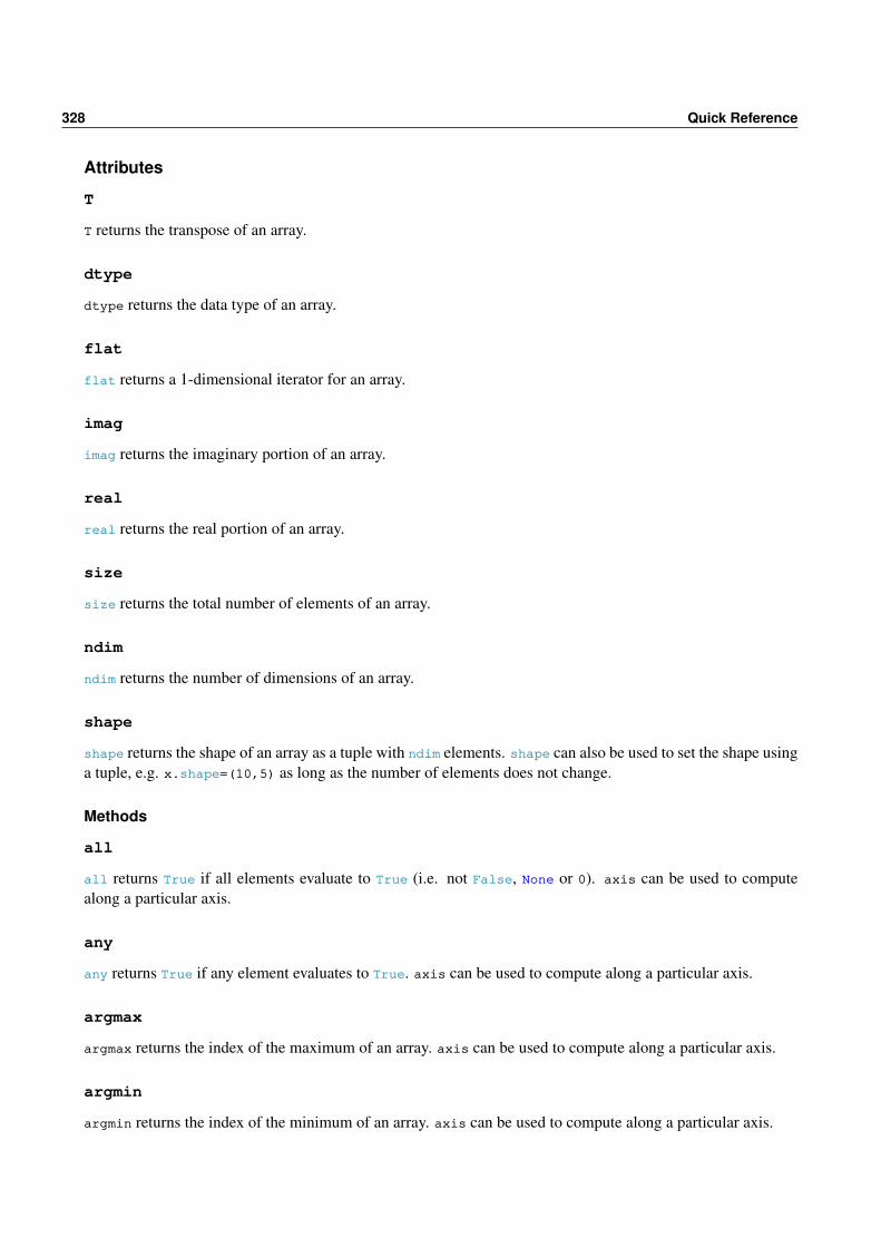
328 Quick Reference

Attributes

T

T returns the transpose of an array.

dtype

dtype returns the data type of an array.

flat

flat returns a 1-dimensional iterator for an array.

imag

imag returns the imaginary portion of an array.

real

real returns the real portion of an array.

size

size returns the total number of elements of an array.

ndim

ndim returns the number of dimensions of an array.

shape

shape returns the shape of an array as a tuple with ndim elements. shape can also be used to set the shape usinga tuple, e.g. x.shape=(10,5) as long as the number of elements does not change.

Methods

all

all returns True if all elements evaluate to True (i.e. not False, None or 0). axis can be used to computealong a particular axis.

any

any returns True if any element evaluates to True. axis can be used to compute along a particular axis.

argmax

argmax returns the index of the maximum of an array. axis can be used to compute along a particular axis.

argmin

argmin returns the index of the minimum of an array. axis can be used to compute along a particular axis.

30.2 NumPy (numpy) 329

argsort

argsort returns the indices needed to sort an array. axis can be used to compute along a particular axis.

astype

astype allows an array to be viewed as another type (e.g., recarray) and copies the underlying.

conj, conjugate

conj and conjugate both return the complex-conjugate element-by-element.

copy

copy returns a copy of an array.

cumprod

cumprod returns the cumulative product of an array. axis can be used to compute along a particular axis.

cumsum

cumsum return the cumulative sum of an array. axis can be used to compute along a particular axis.

dot

dot computes the dot-product (standard matrix multiplication) or an array with another array.

flatten

flatten returns a copy of an array flattened into a 1-dimensional array.

max

max returns the maximum value of an array. axis can be used to compute along a particular axis.

mean

mean returns the average of an array. axis can be used to compute along a particular axis.

min

min returns the minimum of an array. axis can be used to compute along a particular axis.

nonzero

nonzero returns the indices of the non-zero elements of an array.

prod

prod computes the produce of all elements of an array. axis can be used to compute along a particular axis.

330 Quick Reference

ravel

ravel returns a flattened view of an array without copying data.

repeat

repeat returns an array repeated, element-by-element.

reshape

reshape returns returns an array with a different shape. The number of elements must not change.

resize

resize changes the size shape of an array in-place. If the new size is larger then new entries are 0 filled. If thenew size is smaller, then the elements selected are ordered according by their order in ravel.

round

round returns an array with each element rounded to a provided number of decimals.

sort

sort sorts an array (in-place). axis can be used to compute along a particular axis.

squeeze

squeeze returns an array with any singleton dimensions removed.

std

std returns the standard deviation of an array. axis can be used to compute along a particular axis.

sum

sum returns the sum of an array. axis can be used to compute along a particular axis.

tolist

tolist returns a list of an array. If the array has more than 1 dimension, the list will be nested.

trace

trace returns the sum of the diagonal elements.

transpose

transpose returns a view of the array transposed. x.transpose() is the same as x.T.

var

var returns the variance of an array. axis can be used to compute along a particular axis.

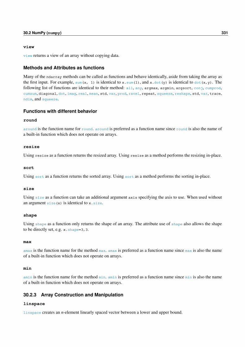
30.2 NumPy (numpy) 331

view

view returns a view of an array without copying data.

Methods and Attributes as functions

Many of the ndarray methods can be called as functions and behave identically, aside from taking the array asthe first input. For example, sum(x, 1) is identical to x.sum(1), and x.dot(y) is identical to dot(x,y). Thefollowing list of functions are identical to their method: all, any, argmax, argmin, argsort, conj, cumprod,cumsum, diagonal, dot, imag, real, mean, std, var, prod, ravel, repeat, squeeze, reshape, std, var, trace,ndim, and squeeze.

Functions with different behavior

round

around is the function name for round. around is preferred as a function name since round is also the name ofa built-in function which does not operate on arrays.

resize

Using resize as a function returns the resized array. Using resize as a method performs the resizing in-place.

sort

Using sort as a function returns the sorted array. Using sort as a method performs the sorting in-place.

size

Using size as a function can take an additional argument axis specifying the axis to use. When used withoutan argument size(x) is identical to x.size.

shape

Using shape as a function only returns the shape of an array. The attribute use of shape also allows the shapeto be directly set, e.g. x.shape=3,3.

max

amax is the function name for the method max. amax is preferred as a function name since max is also the nameof a built-in function which does not operate on arrays.

min

amin is the function name for the method min. amin is preferred as a function name since min is also the nameof a built-in function which does not operate on arrays.

30.2.3 Array Construction and Manipulation

linspace

linspace creates an n-element linearly spaced vector between a lower and upper bound.

332 Quick Reference

logspace

logspace creates a logarithmically spaced (base-10) vector between a lower and upper (log-10) bound.

arange

arange creates an equally spaced vector between a lower and upper bound using a fixed step size.

ones

ones creates an array of 1s.

zeros

zeros creates an array of 0s.

empty

empty creates an array without initializing the values.

eye

eye creates an identity array.

identity

identify creates an identity array.

meshgrid

meshgrid creates 2-dimensional arrays from 2 1-dimensional arrays which contain all combinations of theoriginal arrays.

tile

tile block repeats an array.

broadcast_arrays

broadcast_arrays produces the broadcasted version of 2 broadcastable arrays.

vstack

vstack vertically stacks 2 or more size compatible arrays.

hstack

hstack horizontally stacks 2 or more size compatible arrays.

vsplit

vsplit splits an array into 2 or more arrays vertically.

30.2 NumPy (numpy) 333

hsplit

hsplit splits an array into 2 or more arrays horizontally.

split

split splits an array into 2 or more arrays along an arbitrary axis.

concatenate

concetenate combines 2 or more arrays along an arbitrary axis.

delete

delete deletes elements from an array. axis can be used to delete along a particular axis.

flipud

flipud flips an array top-to-bottom.

fliplr

fliplrud flips an array left-to-right.

diag

diag returns the diagonal from a 2-dimensional array, or returns a diagonal 2-dimensional array when usedwith a 1-dimensional input.

triu

triu returns the upper triangular array from an array.

tril

tril returns the lower triangular array from an array.

30.2.4 Array Functions

kron

kron returns the Kronecker product of 2 arrays.

trace

trace returns the sum of the diagonal elements of an array.

diff

diff returns the 1st difference of an array. An optional second input allows for higher order differencing. axiscan be used to compute the difference along a particular axis.

334 Quick Reference

30.2.5 Input/Output

loadtxt

loadtxt loads a rectangular array from a text file. No missing values are allowed. Automatically decompressesgzipped or bzipped text files.

genfromtxt

genfromtxt loads text from a data file and can accept missing values.

load

load loads a npy or npz file.

save

save saves a single array a NumPy data file (npy).

savez

savez saves an array or set of arrays to a NumPy data file (npz).

savez_compressed

savez_compressed saves an array or set of arrays to a NumPy data file (npz) using compression.

savetxt

savetxt saves a single array to a text file.

30.2.6 nan Functions

nansum

nansum returns the sum of an array, ignoring NaN values. axis can be used to compute along a particular axis.

nanmax

nanmax returns the maximum of an array, ignoring NaN values. axis can be used to compute along a particularaxis.

nanargmax

nanargmax returns the index of the maximum of an array, ignoring NaN values. axis can be used to computealong a particular axis.

nanmin

nanmin returns the minimum of an array, ignoring NaN values. axis can be used to compute along a particularaxis.

30.2 NumPy (numpy) 335

nanargmin

nanargmin returns the index of the minimum of an array, ignoring NaN values. axis can be used to computealong a particular axis.

30.2.7 Set Functions

unique

unique returns the set of unique elements of an array.

in1d

in1d returns a Boolean array indicating which elements of one array are in another.

intersect1d

intersect1d returns the set of elements of one array which are in another.

union1d

union1d returns the set of elements which are in either of 2 arrays, or both.

setdiff1d

setdiff1d returns the set of elements on one array which are not in another.

setxor1d

setxor1d returns the set of elements which are in either or 2 arrays, but not both.

30.2.8 Logical and Indexing Functions

logical_and

logical_and compute the value of applying and to the elements of two broadcastable arrays.

logical_or

logical_or compute the value of applying or to the elements of two broadcastable arrays.

logical_xor

logical_xor compute the value of applying xor to the elements of two broadcastable arrays.

logical_not

logical_not compute the value of applying not to the elements of an array.

allclose

allclose returns True if all elements of two arrays differ by less than some tolerance.

336 Quick Reference

array_equal

array_equal returns True if two arrays have the same shape and elements.

array_equiv

array_equiv returns True if two arrays are equivalent int eh sense that one array can be broadcast to becomethe other.

find

find returns the indices of an array where a logical statement is true. The indices returned correspond to theflattened array.

argwhere

argwhere returns the indices from an array where a logical condition is True.

extract

extract returns the elements from an array where a logical condition is True.

isnan

isnan returns a Boolean array indicating whether the elements of the input are nan .

isinf

isinf returns a Boolean array indicating whether the elements of the input are inf .

isfinite

isfinite returns a Boolean array indicating whether the elements of the input are not inf and not nan.

isposinf

isposinf returns a Boolean array indicating whether the elements of the input are inf.

isneginf

isneginf returns a Boolean array indicating whether the elements of the input are -inf

isreal

isreal returns a Boolean array indicating whether the elements of the input are either real or have 0j complexcomponent.

iscomplex

iscomplex returns a Boolean array indicating whether the elements of the input are either have non-zero com-plex component.

30.2 NumPy (numpy) 337

is_string_like

is_string_like returns True if the input is a string or similar to a string.

isscalar

isscalar returns True if the input is not an array.

is_numlike

is_numlike returns True if the input is numeric.

isvector

isvector returns True if the input has at most 1 dimension which is not unity.

30.2.9 Numerics

nan

nan represents Not a Number.

inf

inf represents infinity.

finfo

finfo can be used along with a data type to return machine specific information about numerical limits andprecision.

30.2.10 Mathematics

log

log returns the natural logarithm of the elements of an array.

log10

log10 returns the bast-10 logarithm of the elements of an array.

sqrt

sqrt returns the square root of the elements of an array.

exp

exp returns the exponential of the elements of an array.

absolute

absolute returns the absolute value of the elements of an array.

338 Quick Reference

sign

sign returns the sign of the elements of an array.

30.2.11 Rounding

floor

floor rounds to next smallest integer.

ceil

ceil round to next largest integer

30.2.12 Views

asarray

asarray converts its input to an ndarray if it is not, and avoids copies if its input is already an ndarray.

30.2.13 rec

rec.array

rec.array construct record arrays.

30.2.14 linalg

linalg.matrix_power

matrix_power raises a square array to an integer power.

linalg.cholesky

cholesky computes the Cholesky factor of a positive definite array.

linalg.qr

qr computes the QR factorization of an array.

linalg.svd

svd computes the singular value decomposition of an array.

linalg.eig

eig computes the eigenvalues and eigenvectors of an array.

linalg.eigh

eigh computes the eigenvalues and eigenvectors of a Hermitian (symmetric) array.

30.2 NumPy (numpy) 339

linalg.cond

cond computes the conditioning number of an array.

linalg.det

det computes the determinant of an array.

linalg.slogdet

slogdet computes the log determinant and the sign of the determinant of an array.

linalg.solve

solve solves a just-identified set of linear equations.

linalg.lstsq

lstsq finds the least squares solutions of an over-identified set of equations.

linalg.inv

inv computes the inverse of a square array.

30.2.15 random

random.rand

rand returns standard uniform pseudo-random numbers. Uses n inputs to produce an n-dimensional array.

random.randn

randn returns standard normal pseudo-random numbers. Uses n inputs to produce an n-dimensional array.

random.randint

randing returns uniform integers on a specified range, exclusive of end point. Uses an n-element tuple toproduce an n-dimensional array.

random.random_integers

random_integers returns uniform integers on a specified range, inclusive of end point. Uses an n-elementtuple to produce an n-dimensional array.

random.random_sample

random_sample returns standard Uniform pseudo-random numbers. Uses an n-element tuple to produce ann-dimensional array.

random.random

random returns standard Uniform pseudo-random numbers. Uses an n-element tuple to produce an n-dimensionalarray.

340 Quick Reference

random.standard_normal

standard_normal returns standard normal pseudo-random numbers. Uses an n-element tuple to produce ann-dimensional array.

random.sample

sample returns standard Uniform pseudo-random numbers. Uses an n-element tuple to produce an n-dimensionalarray.

random.shuffle

shuffle shuffles the elements of an array in-place.

random.permutation

permutation returns a random permutation of an array.

random.RandomState

RandomState is a container for the core random generator. RandomState is used to initialize and controladditional random number generators.

random.seed

seed seeds the core random number generator.

random.get_state

get_state gets the state of the core random number generator.

random.set_state

set_state sets the state of the core random number generator.

Random Number Generators

Random number generators are available for distribution in the following list: beta , binomial, chisquare,exponential, f, gamma, geometric, laplace, logistic, lognormal, multinomial, multivariate_normal,negative_binomial, normal, poisson, uniform.

30.3 SciPy

30.3.1 Statistics (stats)

30.3.1.1 Continuous Random Variables

Normal (norm), Beta (beta), Cauchy (cauchy), χ2 (chi2), Exponential (expon), Exponential Power (exponpow),F (f), Gamma (gamma), Laplace/Double Exponential (laplace), Log-Normal (lognorm), Student’s t (t)

30.3 SciPy 341

stats.dist.rvs

rvs generates pseudo-random variables.

stats.dist.pdf

pdf returns the value of the PDF at a point in the support.

stats.dist.logpdf

logpdf returns the log of the PDF value at a point in the support.

stats.dist.cdf

cdf returns the value of the CDF at a point in the support.

stats.dist.ppf

ppf returns the value of the random variable from a point in (0,1). PPF is the same as the inverse CDF.

stats.dist.fit

fit estimates parameters by MLE.

stats.dist.median

median returns the median of random variables which follow the distribution.

stats.dist.mean

mean returns the mean of random variables which follow the distribution.

stats.dist.moment

moment returns non-central moments of random variables which follow the distribution.

stats.dist.var

var returns the variance of random variables which follow the distribution.

stats.dist.std

std returns the standard deviation of random variables which follow the distribution.

30.3.1.2 Statistical Functions

stats.mode

mode returns the empirical mode of an array.

stats.moment

moment computes non-central moments of an array.

342 Quick Reference

stats.skew

skew computes the skewness of an array.

stats.kurtosis

kurtosis computes the excess kurtosis of an array.

stats.pearsonr

pearsonr computes the correlation of an array.

stats.spearmanr

spearmanr computes the rank correlation of an array.

stats.kendalltau

kendalltau computed Kendall’s τ , which is similar to a correlation, from an array.

stats.normaltest

normaltest computes a Jarque-Bera like test for normality.

stats.kstest

kstest computes a Kolmogorov-Smirnov test for a specific distribution.

stats.ks_2samp

ks_2samp computes a Kolmogorov-Smirnov test from directly from two samples.

stats.shapiro

shapire computes the Shapiro-Wilks test of normality.

30.3.2 Optimization (optimize)

30.3.2.1 Unconstrained Function Minimization

optimize.fmin_bfgs

fmin_bfgs minimizes functions using the BFGS algorithm.

optimize.fmin_cg

fmin_cg minimizes functions using a Conjugate Gradient algorithm.

optimize.fmin_ncg

fmin_ncg minimizes functions using a Newton-Conjugate Gradient algorithm.

30.3 SciPy 343

30.3.2.2 Derivative Free Unconstrained Function Minimization

optimize.fmin

fmin minimizes a function using a simplex algorithm.

optimize.fmin_powell

fmin_powell minimizes a function using Powell’s algorithm.

30.3.2.3 Constrained Function Minimization

optimize.fmin_slsqp

fmin_slsqp minimizes a function subject to inequality, equality and bounds constraints.

optimize.fmin_tnc

fmin_tnc minimizes a function subject to bounds constraints.

optimize.fmin_l_bfgs_s

fmin_l_bfgs_s minimizes a function subject to bounds constraints.

optimize.fmin_colyba

fmin_colyba minimizes a function subject to inequality and equality constraints.

30.3.2.4 Scalar Function Minimization

optimize.fmin_bound

fmin_bound minimizes a function in a bounded region.

optimize.golden

golden uses a golden section search to minimize a scalar function.

optimize.brent

brent uses Brent’s method to minimize a scalar function.

30.3.2.5 Nonlinear Least Squares

optimize.lstsq

lstsq performs non-linear least squares minimization of a function which returns a 1-dimensional array oferrors.

30.3.3 Input/Output (io)

io.loadmat

loadmat loads a MATLAB data file.

344 Quick Reference

io.savemat

savemat saves an array or set of arrays to a MATLAB data file.

30.4 Matplotlib

30.4.1 2D plotting

plot

plot plots a 2-dimensional line or set of lines.

pie

pie produces a pie chart.

hist

hist computes and plots a histogram.

scatter

scatter produces a scatter plot.

bar

bar produces a vertical bar chart.

barh

barh produces a horizontal bar chart.

contour

contour produces a 2-dimensional contour representation of 3-dimensional data.

30.4.2 3D plotting

plot

plot using the optional keyword argument zs produces 3-dimensional plots.

plot_wireframe

plot_wireframe plots a 3-dimensional wire-frame surface.

plot_surface

plot_surface plots a 3-dimensional solid surface.

30.5 pandas 345

30.4.3 Utility Commands

figure

figure opens a new figure or changes the current figure to an existing figure.

add_axes

add_axes adds a single axes to a figure.

add_subplot

add_subplot adds a subplot to a figure.

show

show updates a figure and pauses the running of a non-interactive program until the figure is closed.

draw

draw updates a figure.

close

close closes figures. close('all') closes all figures.

legend

legend adds a legend to a plot or chart using the information in label keyword arguments.

title

title adds a title to a plot or chart.

savefig

savefig exports figures to common file formats including PDF, EPS, PNG and SVG.

30.4.4 Input/Output

csv2rec

csv2rec reads data in a CSV file and returns a NumPy record array. Columns are automatically types based onthe first few rows of the input array, and importing dates is supported.

30.5 pandas

The format DataFrame.method is used to indicate that method is called directly on a DataFrame (e.g.x.method()).

346 Quick Reference

30.5.1 Data Structures

Series

Series constructs the 1-dimensional array-like (or column-like) structure underlying a DataFrame.

TimeSeries

TimeSeries is a sub-class of Series where the index is a set of datetimes.

DataFrame

DataFrame constructs the primary 2-dimensional array-like (or table-like) structure in pandas.

30.5.2 Series/DataFrame Methods

drop

drop drops rows or columns using a list of labels.

dropna

dropna drops rows containing null-values.

drop_duplicates

drop_duplicates drops rows that contain duplicate values.

values

values returns the NumPy array underlying the DataFrame.

index

values returns an Index object containing the index labels.

fillna

fillna allows null-values to be filled with another value.

T, transpose

T transposes a DataFrame and is used as a property (i.e. df.T). transpose is identical except that it is used asa method (i.e. df.transpose())

sort

sort sorts a DataFrame using either index or column labels or values in one or more columns.

sort_index

sort_index is identical to sort except for the keyword argument names.

30.5 pandas 347

pivot

pivot reshapes a DataFrame

stack

stack creates a single Series representation of a DataFrame.

unstack

unstack converts a single Series representation to a Series.

concat

concat concatenates two DataFrames into a single DataFrame. concat is a function which operated onDataFrames and is not a method.

append

append concatenates a DataFrame to the existing DataFrame.

reindex

reindex changes the index and/or column labels.

reindex_like

reindex_like reindexes a DataFrame using the index of another DataFrame.

reindex_axis

reindex_axis reindexes one axis of a DataFrame.

merge

merge performs a SQL-like join of two DataFrames using index values to construct the union.

join

join performs a SQL-like join of two DataFrames using values in columns to construct the union.

update

update updates the values of cells in one DataFrame using index labels.

groupby

groupby produces a DataFrameGroupBy object that can be used to compute grouped statistics or plots.

apply

apply applies a function column- or row-wise to a DataFrame.

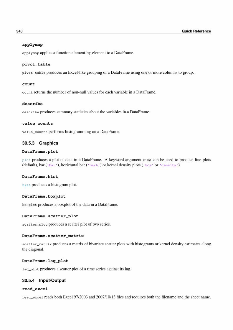
348 Quick Reference

applymap

applymap applies a function element-by-element to a DataFrame.

pivot_table

pivot_table produces an Excel-like grouping of a DataFrame using one or more columns to group.

count

count returns the number of non-null values for each variable in a DataFrame.

describe

describe produces summary statistics about the variables in a DataFrame.

value_counts

value_counts performs histogramming on a DataFrame.

30.5.3 Graphics

DataFrame.plot

plot produces a plot of data in a DataFrame. A keyword argument kind can be used to produce line plots(default), bar ('bar'), horizontal bar ('barh') or kernel density plots ('kde' or 'density').

DataFrame.hist

hist produces a histogram plot.

DataFrame.boxplot

boxplot produces a boxplot of the data in a DataFrame.

DataFrame.scatter_plot

scatter_plot produces a scatter plot of two series.

DataFrame.scatter_matrix

scatter_matrix produces a matrix of bivariate scatter plots with histograms or kernel density estimates alongthe diagonal.

DataFrame.lag_plot

lag_plot produces a scatter plot of a time series against its lag.

30.5.4 Input/Output

read_excel

read_excel reads both Excel 97/2003 and 2007/10/13 files and requires both the filename and the sheet name.

30.5 pandas 349

read_csv

read_csv reads csv and other delimited files.

read_stata

read_stata reads STATA data files.

read_table

read_table reads general delimited files.

read_hdf

read_hdf reads data from HDF5 files (usually created using DataFrame.to_hdf)

read_html

read_html reads html tables.

read_json

read_html reads data from JavaScript Object Notation.

DataFrame.to_excel

to_excel writes data to an Excel file.

DataFrame.to_csv

to_csv writes data to a CSV file.

DataFrame.to_string

to_string writes data to a string variable or buffer (file or StringIO).

DataFrame.to_latex

to_latex writes data to a LATEX file.

DataFrame.to_stata

to_stata writes data to a STATA data file.

DataFrame.to_hdf

to_hdf writes data to a HDF5 data file.

DataFrame.to_html

to_hdf writes data to a HTML data table.

350 Quick Reference

DataFrame.to_json

to_hdf writes data to a JSON string.

30.6 IPython

?⁎partial⁎, ?module.⁎partial⁎

?⁎partial⁎ list any known objects – variables, functions or modules – which match the wild card expression⁎partial⁎ where partial can be any string.

function?, magic?

?function, ?magic, ?module, function?, magic? and module? all pretty print the docstring for a function, magicword or module.

function??, magic??

??function, ??magic, ??module, function??, magic?? and module?? all pretty print the entire function, magicword or module, including both the docstring and the code inside the function.

!command

!command is used to run a system command as if executed in the terminal. For example, !copy file.py backup.pywill copy file.by to backup.py. An output can be used to capture the command window text printed by thecommand to a local variable. For example, dirListing = !dir ⁎.py will capture the contents to running adirectory listing for all py files. This can then be parsed or used for error checking.

%bookmark

%bookmark allows bookmarks to be created to directories. Manage IPython’s bookmark system. For exam-ple, the current directory can be bookmarked using %bookmark currentDir, and can be returned to using%cd currentDir (assuming the current directory doesn’t contain a directory named currentDir).

%cd

%cd changes the current working directory. In Windows, \, \\ or / can be used as directory separators. In Linux,/ should be used to separate directories. %cd support tab completion, so that only a few letters are needed beforehitting the tab key to complete the directory name.

%clear, %cls

%clear and %cls both clear the terminal window (but do not remove any variables, functions or modules).

%edit

%edit opens the editor for py files, and is usually used %edit filename.py.

30.6 IPython 351

%hist

%hist lists command history. %hist -g searchterm can be used to search for a specific term or wildcardexpression.

%lsmagic

%lsmagic lists all defined magic functions.

%magic

%magic prints detailed information about all magic functions.

%pdb

%pdb controls the use of the Python debugger.

%pdef

%pdef prints only the definition header (the line beginning with def) for functions.

%precision

%precision sets the display precision. For example %precision 3 will show 3 decimal places.

%prun

%prun runs a statement in the profiler, and returns timing and function call information. Use %run -p file-name.py to profile a standalone file.

%psearch

%psearch searches for variables, functions and loaded modules using wildcards.

%pwd

%pwd shows the current working directory.

%pycat, %more, %less

%pycat, %more and %less all show the contents of a file in the IPython window.

%pylab

%pylab initializes pylab if not initialized from the command line.

%quickref

%quickref shows a reference sheet for magic commands.

352 Quick Reference

%reset

%reset resets the session by removing all variables, functions and imports defined by the user.

%reset_selective

%reset_selective re resets all names which match the regular expression re.

%run

%run filename.py executes a file containing Python code in the IPython environment.

%time

%time code provides the time needed to run the code once. %timeit is often more useful.

%timeit

%timeit code times a segment of code, and is useful for finding bottlenecks and improving algorithms. If codeis very fast, multiple runs are used to improve timing accuracy.

>>> %timeit x=randn(100,100);dot(x.T,x)1000 loops, best of 3: 758 us per loop

%who

%who lists all variables in memory.

%who_ls

%who_ls returns a sorted list containing the names of all variables in memory.

%whos

%whos provides a detailed list of all variables in memory.

%xdel

%xdel variable deletes the variable from memory.

Bibliography

Bollerslev, Tim and Jeffrey M. Wooldridge (1992). “Quasi-Maximum Likelihood Estimation and Inference inDynamic Models with Time-Varying Covariances”. In: Econometric Reviews 11.2, pp. 143–172.

Cochrane, John H (2001). Asset Pricing. Princeton, N. J.: Princeton University Press.Jagannathan, R, G Skoulakis, and Z Wang (2010). “The analysis of the cross section of security returns”. In:

Handbook of financial econometrics. Ed. by Yacine Aït-Sahalia and Lars Peter Hansen. Vol. 2. ElsevierB.V., pp. 73–134.

Index

(, 46), 46+, 227+, 43-, 43/, 43<, 85<=, 85==, 85>, 85>=, 85%time, 245%timeit, 245⁎, 43⁎, 228⁎⁎, 43

abs, 54absolute, 54all, 87allclose, 87and, 86any, 87arange, 49argmax, 56argmin, 56argsort, 56around, 52array

Inputting, 31array, 29array_equal, 87array_equiv, 87Arrays, 29–30

Broadcasting, 43–45Complex Values, 54conj, 54conjugate, 54imag, 54real, 54

Extreme Values, 56–57

argmax, 56argmin, 56max, 56maximum, 57min, 56minimum, 57

Inputting, 30–33Manipulation, 63–69broadcast, 66concatenate, 67delete, 67diag, 68dsplit, 67flat, 65flatten, 65fliplr, 68flipud, 68hsplit, 67hstack, 66ndim, 64ravel, 65reshape, 63shape, 63size, 64squeeze, 68tile, 64tril, 69triu, 69vsplit, 67vstack, 66

Mathematics, 45–46, 52–54absolute, 54abs, 54cumprod, 53cumsum, 52diff, 53exp, 53log, 53log10, 53prod, 53

INDEX 355

sign, 54sqrt, 54square, 54sum, 52

NaN Functions, 57–58nanargmax, 58nanargmin, 58nanmax, 58nanmin, 58nansum, 57

Set Functions, 54–55in1d, 55intersect1d, 55setdiff1d, 55setxor1d, 55union1d, 55unique, 54

Slicing, 33–38Sorting, 56argsort, 56sort, 56

Specialempty, 61eye, 62identity, 62ones, 61zeros, 61

Viewsasarray, 72view, 72

as, 39asarray, 72

beta, 196binomial, 197break, 106, 107brent, 224broadcast, 66broadcast_arrays, 66Broadcasting, 247

c_, 50ceil, 52center, 230chisquare, 197cholesky, 70close, 81concatenate, 67cond, 69

conj, 54conjugate, 54Context Managers, 241continue, 106, 108corrcoef, 202count, 230cov, 202ctypes, 275–277cumprod, 53cumsum, 52Cython, 267–275, 278–279

DataFramegroupbyfilter, 156transform, 156

date, 113Dates and Times, 113–116

date, 113datetime, 113datetime64, 114Mathematics, 113time, 113timedelta, 113timedelta64, 114

datetime, 113datetime64, 114def, 179del, 21delete, 67det, 70diag, 68Dictionary comprehensions, 110diff, 53docstring, 183dsplit, 67dtype, 30

eig, 70eigh, 71elif, 103else, 103empty, 61empty_like, 62enumerate, 106equal, 85except, 108exp, 53exponential, 197

356 INDEX

Exporting DataCSV, 82Delimited, 82MATLAB, 81savez, 81savez_compressed, 81

extract, 98eye, 62

f, 197find, 229finfo, 83flat, 65flatnonzero, 97flatten, 65fliplr, 68flipud, 68float, 81float, 237floor, 52Flow Control

elif, 103else, 103except, 108if, 103try, 108

fmin, 219fmin_1_bfgs_b, 222fmin_bfgs, 216fmin_cg, 217fmin_cobyla, 222fmin_ncg, 218fmin_powell, 219fmin_slsqp, 220fmin_tnc, 222fminbound, 224for, 104from, 39Functions, 58

Custom, 179–190Default Values, 181docstring, 183Keyword Arguments, 180Variable Inputs, 182Variable Scope, 184

Custom Modules, 187def, 179PYTHONPATH, 189

gamma, 197Generating Arrays, 49–51

arange, 49c_, 50ix_, 50linspace, 49logspace, 49meshgrid, 49mgrid, 51ogrid, 51r_, 50

get_state, 199golden, 224greater, 85greater_equal, 85

histogram, 202histogram2d, 203hsplit, 67hstack, 66

identity, 62if, 103imag, 54import, 39Importing Data, 75–81

CSV, 75Excel, 76–78loadtxt, 77MATLAB, 79pandas, 75STATA, 76

in1d, 55index, 229inf, 83int, 81int, 237intersect1d, 55inv, 71is_string_like, 88iscomplex, 88isfinite, 88isinf, 88isnan, 88isneginf, 88isnumlike, 88isposinf, 88isreal, 88isscalar, 88

INDEX 357

isvector, 88ix_, 50

join, 227, 228

kendalltau, 208kron, 71ks_2samp, 209kstest, 209kurtosis, 207

laplace, 197leastsq, 224less, 85less_equal, 85Linear Algebra

cholesky, 70cond, 69det, 70eig, 70eigh, 71eigvals, 70inv, 71kron, 71lstsq, 70matrix_power, 69matrix_rank, 71slogdet, 69solve, 69svd, 69trace, 71

linregress, 208linspace, 49List comprehensions, 109ljust, 230loadtxt, 77log, 53log10, 53Logical

<, 85<=, 85==, 85>, 85>=, 85all, 87allclose, 87and, 86any, 87argwhere, 98

array_equal, 87array_equiv, 87equal, 85extract, 98flatnonzero, 97greater, 85greater_equal, 85is_string_like, 88iscomplex, 88isfinite, 88isinf, 88isnan, 88isneginf, 88isnumlike, 88isposinf, 88isreal, 88isscalar, 88isvector, 88less, 85less_equal, 85logical_and, 86logical_not, 86logical_or, 86logical_xor, 86nonzero, 97not, 86not_equal, 85or, 86

logical_and, 86logical_not, 86logical_or, 86logical_xor, 86lognormal, 197logspace, 49Looping, 104–108

break, 106, 107continue, 106, 108for, 104while, 107

LoopingWhitespace, 103

lower, 230lstrip, 229lstsq, 70

Mathematics+, 43-, 43/, 43

358 INDEX

⁎, 43⁎⁎, 43Array, 45Arrays

), 46Operator Precedence, 46

Matrix, 32matrix, 32matrix_power, 69matrix_rank, 71max, 56maximum, 57mean, 201median, 201meshgrid, 49Methods, 58mgrid, 51min, 56minimum, 57mode, 206moment, 206multinomial, 197multivariate_normal, 198

nan, 83nanargmax, 58nanargmin, 58nanmax, 58nanmin, 58nansum, 57ndaray

mean, 201std, 201var, 202

ndarrayargmax, 56argmin, 56argsort, 56conj, 54cumprod, 53cumsum, 52flat, 65flatten, 65imag, 54max, 56min, 56ndim, 64prod, 53

ravel, 65real, 54reshape, 63round, 52shape, 63size, 64sort, 56squeeze, 68sum, 52T, 46transpose, 46view, 72

ndim, 64negative_binomial, 198nonzero, 97normal, 198normaltest, 208not, 86not_equal, 85Numba, 253–264

jit, 253Numerics

eps, 83Limits, 83Precision, 83

NumPydatetime64, 114timedelta64, 114

numpyarray, 29dtype, 30matrix, 32ndarray, 29

ogrid, 51ones, 61ones_like, 61open, 80Optimization

Constrained, 219–223fmin_1_bfgs_b, 222fmin_cobyla, 222fmin_slsqp, 220fmin_tnc, 222

Least Squares, 224–225leastsq, 224

Scalar, 223–224brent, 224

INDEX 359

fminbound, 224golden, 224

Unconstrained, 215–219fmin, 219fmin_bfgs, 216fmin_cg, 217fmin_ncg, 218fmin_powell, 219

or, 86

pandas, 137–172Data

Exporting, 163Importing, 163Reading, 163Writing, 163

Data Exporting, 163to_csv, 165to_excel, 165to_hdf, 165to_json, 165to_stata, 165

Data Importing, 163DataFrame, 143–157append, 151apply, 153applymap, 154boxplot, 168columns, 145–148concat, 151count, 158describe, 158drop, 149drop_duplicates, 149dropna, 149fillna, 149groupby, 155head, 144hist, 168index, 149Initialization, 143join, 152lag_plot, 168merge, 152pivot, 150pivot_table, 154plot, 167reindex, 152

reindex_like, 152rows, 146scatter_matrix, 168scatter_plot, 168sort_index, 150sort_values, 150stack, 151T, 150transpose, 150unstack, 151update, 153value_counts, 158values, 149

DataFrame, 143describe, 158Examples, 168Graphics, 167boxplot, 168hist, 168lag_plot, 168plot, 167scatter_matrix, 168scatter_plot, 168

groupbyfilter, 156transform, 156

iloc, 140loc, 140Plotting, 167read_csv, 75read_excel, 76read_stata, 76Series, 137–143append, 142Categorical, 157Categorical Variables, 157describe, 141drop, 141dropna, 141fillna, 142head, 140iloc, 140Initialization, 137isnull, 140loc, 140Math, 139notnull, 140nunique, 141

360 INDEX

replace, 142tail, 140unique, 141update, 143

Series, 137TimeSeries, 159–163bdate_range, 162date_range, 162Initialization, 159pct_change, 160Period, 161period_range, 163read_csv, 164read_excel, 164read_hdf, 165read_stata, 165read_table, 165resample, 163rows, 159Timedelta, 161Timestamp, 161to_datetime, 161

pearsonr, 207Performance and Optimization, 245–252

Broadcasting, 247ctypes, 275–277Cython, 252, 267–275, 278Loop Order, 247Memory Management, 248Numba, 253Numba)(, 264Timing, 245Vectorization, 246

permutation, 196poisson, 198prod, 53Python

as, 39Built-in Data Types, 16–27bool, 17Boolean Values, 17complex, 16Complex Numbers, 16dict, 22Dictionaries, 22float, 16Floating Point Numbers, 16frozenset, 23

int, 17Integers, 17list, 19Lists, 19range, 24Range Iteration, 24Real Numbers, 16set, 23Sets, 23str, 18Strings, 18tuple, 21Tuples, 21

Coding Conventions, 189from, 39Functions

Calling, 40–41import, 39Importing Modules, 39Memory Management, 26, 37–39, 99, 248Setup, 3–5, 14

Anaconda, 4Continuum Analytics, 4Linux, 5, 14OS X, 5, 14Windows, 4, 13

Slicing, 18, 19, 33–38Variable Names, 15–16Variable Scope, 184

r_, 50rand, 195randint, 196randn, 195Random Numbers, 195–200

beta, 196binomial, 197chisquare, 197exponential, 197f, 197gamma, 197get_state, 199laplace, 197lognormal, 197multinomial, 197multivariate_normal, 198negative_binomial, 198normal, 198

INDEX 361

permutation, 196poisson, 198rand, 195randint, 196randn, 195random_integers, 196random_sample, 195RandomState, 198seed, 200set_state, 199shuffle, 196Simulation, 198–201standard_normal, 195standard_t, 198uniform, 198

random_integers, 196random_sample, 195RandomState, 198ravel, 65readline, 80real, 54Regular Expressions, 236

compile, 237findall, 236finditer, 236sub, 236

replace, 81replace, 230reshape, 63rfind, 229rindex, 229rjust, 230round, 52Rounding, 52

around, 52ceil, 52floor, 52round, 52

rsplit, 228rstrip, 229

savetxt, 82SciPy, 203–209

statsbeta, 205cauchy, 205cdf, 204chi2, 205

Continuous Random Variables, 203expon, 205f, 205fit, 204gamma, 205kendalltau, 208ks_2samp, 209kstest, 209kurtosis, 207laplace, 205linregress, 208lognorm, 205logpdf, 203mean, 204median, 204mode, 206moment, 204, 206norm, 205normaltest, 208pdf, 203pearsonr, 207ppf, 204rvs, 203shapiro, 209skew, 206spearmanr, 207std, 204t, 205var, 204

seed, 199, 200Set comprehensions, 110set_state, 199setdiff1d, 55setxor1d, 55shape, 63shapiro, 209shuffle, 196sign, 54Simulation, 198–201

get_state, 199seed, 199set_state, 199

size, 64skew, 206slogdet, 69solve, 69sort, 56spearmanr, 207

362 INDEX

split, 81split, 228sqrt, 54square, 54squeeze, 68standard_normal, 195standard_t, 198Statistics, 201–203

corrcoef, 202cov, 202histogram, 202histogram2d, 203mean, 201median, 201std, 201var, 202

std, 201Strings, 227–237

+, 227⁎, 228Building, 227center, 230Conversion, 237count, 230f-Strings, 235find, 229format, 231–234Formatting, 231–236Formatting (Legacy), 235Functions, 228–231index, 229join, 227, 228ljust, 230lower, 230lstrip, 229Regular Expressions, 236–237replace, 230rfind, 229rindex, 229rjust, 230rsplit, 228rstrip, 229split, 228strip, 229upper, 230wrap, 231

strip, 229Structured Data, 175–178

Mixed Arrays, 175Named Arrays, 175Record Arrays, 178

sum, 52svd, 69

T, 46tile, 64time, 113timedelta64, 114Timing Code, 245trace, 71transpose, 46tril, 69triu, 69try, 108Tuple comprehensions, 110

uniform, 198union1d, 55unique, 54upper, 230

var, 202Vectorization, 246view, 72vsplit, 67vstack, 66

while, 107wrap, 231

zeros, 61zeros_like, 61