
Guida all'uso di gretl Gnu Regression, Econometrics and Time-series library
Upload
khangminh22Category
view
3download
0
Econometrics with gretlProceedings of the
gretl Conference 2009
Bilbao, Spain, May 28-29
I. Dıaz-Emparanza, P. Mariel, M.V. Esteban(Editors)


Econometrics with gretl
Proceedings of the gretl Conference 2009
Bilbao, Spain, May 28-29, 2009

Econometrics with gretl
Proceedings of the
gretl Conference 2009
Bilbao, Spain, May 28-29, 2009
I. Dıaz-Emparanza, P. Mariel, M.V. Esteban(Editors)

Editors:
Ignacio Dıaz-EmparanzaDepartamento de Economıa Aplicada III (Econometrıa y Estadıstica)Facultad de Ciencias Economicas y EmpresarialesUniversidad del Paıs VascoAvenida Lehendakari Aguirre, 8348015 BilbaoSpain
Petr MarielDepartamento de Economıa Aplicada III (Econometrıa y Estadıstica)Facultad de Ciencias Economicas y EmpresarialesUniversidad del Paıs VascoAvenida Lehendakari Aguirre, 8348015 BilbaoSpain
Marıa Victoria EstebanDepartamento de Economıa Aplicada III (Econometrıa y Estadıstica)Facultad de Ciencias Economicas y EmpresarialesUniversidad del Paıs VascoAvenida Lehendakari Aguirre, 8348015 BilbaoSpain
c© UPV/EHUISBN: 978-84-692-2600-1Deposito Legal: BI-1428-09

Preface
This proceedings volume contains the papers presented at the GRETL CONFER-ENCE held in Bilbao, Spain, May 28-29, 2009.
The gretl project (GNU Regression, Econometrics and Time Series Library)was initially promoted at the beginning of 2000 by Allin Cottrell, who took,as the basis for it, the econometric program “ESL”, originally developed byRamu Ramanathan and published under an open source license. It was aroundAugust 2000 when the Free Software Foundation decided to accept gretl as aGNU program. It was at that point when the community of gretl users startedto grow. In 2004 Riccardo (Jack) Lucchetti started his collaboration with theproject, acting as a second programmer.
The use of the gettext program has really been the turning point for gretlto become a more international software. In fact, gretl is currently translated toBasque (Susan Orbe and Marian Zubia), Czech (the CERGE-EI team lead by J.Hanousek), German (Markus Hahn and Sven Schreiber), French (Florent Bres-son and Michel Robitaille), Italian (Cristian Rigamonti), Polish (Pawel Kufel,Tadeusz Kufel and Marcin Blazejowski), Portuguese (Hélio Guilherme), Brazil-ian Portuguese (Hélio Guilherme and Henrique Andrade), Russian (AlexanderB. Gedranovich), Spanish (Ignacio Díaz-Emparanza), Turkish (A. Talha Yalta),and, pretty soon, Chinese (Y. N. Yang).
The 2009 gretl Conference has been the first gretl program users and devel-opers meeting. The conference has been organized as a small scientific meet-ing, having three invited conferences given by Allin Cottrell, Stephen Pollockand Jack Lucchetti, to whom conference organizers wish to give their specialthanks for their collaboration and willingness to participate in the conference.Papers presented in the different sessions scheduled at the conference have con-tributed to develop and extend our knowledge about gretl and some other freesoftware programs for econometric computations and teaching. Allin Cottrelltalked about the evolution and development of gretl from its beginnings and, inaddition, he also described which ones would be, in his view, the future chal-lenges and paths this interesting project could follow. Stephen Pollock intro-duced IDEOLOG, a program that allows the filtering of economic time seriesand that also includes several novel specific filtering procedures that mainly op-erate in the frequency domain. Jack Lucchetti presented an econometric analysisof the data from the gretl downloads from SourceForge. His findings suggestedthat, even though gretl has become a fundamental tool for teaching Economet-

II
rics, it has not yet been widely accepted as a computation program for researchin Economics.
Organizers wish to thank specially authors who sent their papers for evalu-ation. Their active collaboration has allowed organizers to be able to have fourvery interesting and differently focused sessions in the scientific programmefor this conference. The first one dealt with Econometric Theory, the secondone centered on Econometric Applications , the third one on the use of Free-software programs for teaching Econometrics, and the last one concentrated onContributions to the development of gretl.
The editors of this volume wish to show their most sincere appreciationand thanks to Josu Arteche, Giorgio Calzolari, Michael Creel, Josef Jablonsky,and Tadeusz Kufel, for their effort and dedication to the conference success asmembers of the Scientific Committee. We also wish to thank specially thoseauthors presenting papers appearing in this proceedings volume, for their care-ful manuscript preparation so that our editing work was a lot easier to handle.Finally, we wish to thank Vicente Núñez-Antón for his valuable help in thepreparation and organization of this conference.
Ignacio, Petr and Maria Victoria
Bilbao, April 2009

Organization
The gretl Conference 2009 is organized by the Department of Applied Eco-nomics III (Econometrics and Statistics), the University of the Basque Countryand the School of Economics and Business Administration in cooperation withthe gretl Development Team.
Organizing Commitee
Conference Chair: Ignacio Díaz-Emparanza (University of theBasque Country, Spain)
Co-Chair: Petr Mariel (University of the Basque Country,Spain)
Members: Maria Victoria Esteban (University of theBasque Country, Spain)Allin Cottrell (Wake Forest University, USA)Ricardo (Jack) Lucchetti (Università Politec-nica delle Marche, Italy)A. Talha Yalta (TOBB University of Eco-nomics and Technology, Turkey)
Scientific Committee
Josu Arteche (University of the Basque Country, Spain)Giorgio Calzolari (University of Firenze, Italy)Michael Creel (Universitat Autònoma de Barcelona, Spain)Josef Jablonsky (University of Economics, Prague, Czech Republic)Tadeusz Kufel (Nicolaus Copernicus University, Poland)
Sponsoring Institutions
Department of Education of the Basque Government through grant IT-334-07(UPV/EHU Econometrics Research Group)EUSTAT (Basque Institute of Statistics)Bilbao Turismo and Convention Bureau

IV

Table of Contents
gretl Conference 2009
Invited Lectures
Gretl: Retrospect, Design and Prospect . . . . . . . . . . . . . . . . . . . . . . . . . . . 3Allin Cottrell
IDEOLOG: A Program for Filtering Econometric Data—A Synopsisof Alternative Methods . . . . . . . . . . . . . . . . . . . . . . . . . . . . . . . . . . . . . . . . 15
D.S.G. Pollock
Who Uses gretl? An Analysis of the SourceForge Download Data . . . . . . 45Riccardo (Jack) Lucchetti
Econometric Theory
An Instrumental Variables Probit Estimator using gretl . . . . . . . . . . . . . . . 59Lee C. Adkins
Automatic Procedure of Building Congruent Dynamic Model . . . . . . . . . 75Marcin Błazejowski, Paweł Kufel, and Tadeusz Kufel
Instrumental Variable Interval Regression . . . . . . . . . . . . . . . . . . . . . . . . . 91Giulia Bettin, Riccardo (Jack) Lucchetti
Applied Econometrics
A Model for Pricing the Italian Contemporary Art Paintings . . . . . . . . . . . 111Nicoletta Marinelli, Giulio Palomba
Analysis of the Tourist Sector Investment Appeal Using the PCA in gretl 135Tetyana Kokodey
Has the European Structural Fisheries Policy Influenced on the SecondHand Market of Fishing Vessels? . . . . . . . . . . . . . . . . . . . . . . . . . . . . . . . . 143
Ikerne del Valle, Kepa Astorkiza, Inmaculada Astorkiza
Vertical Integration in the Fishing Sector of the Basque Country:Applications to the Market of Mackerel . . . . . . . . . . . . . . . . . . . . . . . . . . . 171
Javier García Enríquez

VI
Teaching Econometrics with Free Software
Useful Software for Econometric Beginners . . . . . . . . . . . . . . . . . . . . . . . 179Šárka Lejnarová, Adéla Rácková
Teaching and Learning Econometrics with Gretl . . . . . . . . . . . . . . . . . . . . 191Rigoberto Pérez, Ana Jesús López
The Roster-in-a-Box Course Management System . . . . . . . . . . . . . . . . . . 203Tavis Barr
Contributions to gretl Development
On Embedding Gretl in a Python Module . . . . . . . . . . . . . . . . . . . . . . . . . 219Christine Choirat, Raffaello Seri
An Alternative to Represent Time Series: “the Time Scatter Plot” . . . . . . 229Alberto Calderero, Hanna Kuittinen, Javier Fernández-Macho
Wilkinson Tests and gretl . . . . . . . . . . . . . . . . . . . . . . . . . . . . . . . . . . . . . . 243A. Talha Yalta, A. Yasemin Yalta
Subject Index . . . . . . . . . . . . . . . . . . . . . . . . . . . . . . . . . . . . . . . . . . . . . . 252
Author Index . . . . . . . . . . . . . . . . . . . . . . . . . . . . . . . . . . . . . . . . . . . . . . 253

Invited Lectures

2
Gretl: Retrospect, Design and Prospect
Allin Cottrell
Department of Economics, Wake Forest [email protected]
Abstract. In this paper I will give a brief overview of the history of gretl’s de-velopment, comment on some issues relating to gretl’s overall design, and set outsome thoughts on gretl’s future.
1 Retrospect
Gretl’s “modern history” began in September, 2001, when the gretl code wasfirst imported to CVS at sourceforge.net. The program’s “pre-history”goes back to the mid-1990s. I will briefly describe this background.
1.1 Econometrics software on DOS and Windows 3.0
I began teaching econometrics at Wake Forest University in 1989. I had taughta related course, Business Statistics, at Elon College in North Carolina overthe previous few years, and had tried using various statistical packages—RATSand PcGive in particular. Both of these were powerful programs but neither wasparticularly user-friendly for undergraduates with little computing background.“EZ-RATS” was a brave attempt at user-friendliness but not a great success: itregular crashed and lost my students’ work. When I started at Wake Forest I trieda different approach, using Ramanathan’s (1989) textbook, which came with itsown DOS software, Ecslib (later known as ESL). Ecslib offered a limited rangeof estimators—OLS, TSLS, and a few FGLS variants—but it was stable, free(as in beer, to users of the textbook) and easy to learn.
Over the first half of the 1990s Microsoft Windows 3.0 (released in May,1990) became increasingly popular and DOS software came to look dated andunfriendly. I decided to learn to program in Microsoft’s Visual Basic. This wasnot a pretty language, but it did make for easy construction of a Graphical UserInterface (GUI). Also in the early ’90s I was introduced to TEX and LATEX by acomputer-scientist friend, and I used Visual Basic to write GUI “front-ends” forboth Ramanathan’s ESL and what was at the time the best free implementationof TEX for the PC, Eberhard Mattes’ emTEX.1
1 Archive item: the web page for my emTEX front-end is still viewable at http://www.wfu.edu/economics/ftp/emtexgi.html.

4 Allin Cottrell
Since it will be of some relevance in the sequel, let me define a “front-end”.I mean a GUI program whose raison d’être is to make it easier for a user tointeract with a command-driven (or CLI, “Command line interface”) program,that is, a program that is driven either by commands typed at an interactiveprompt or by a “script” of commands previously written to file. A front-endsupplies an apparatus of dialog boxes, buttons, drop-down lists and so on, bymeans of which it enables the user to formulate a request to the CLI program.The front end then
1. translates the user’s request into commands intelligible to the CLI program;2. feeds these commands to the CLI program;3. retrieves the output from the CLI program; and4. displays the output to the user in a “window” of some sort.
From the user’s point of view the attraction of such a front-end is that itobviates the need to master the command-line vocabulary and syntax of theunderlying CLI program. From the programmer’s point of view, it can be aninteresting intellectual challenge to take one’s knowledge of the CLI programand parlay it into an easy-to-use interface. This offers the same sort of rewardas teaching: the satisfaction of taking something difficult and making it as clearand simple as possible.
Anyway, gretl’s first precursor was ESLWIN, a Windows front-end for Ra-manathan’s DOS program ESL.
1.2 Linux comes on the scene
In the mid-1990s Wake Forest University set out an ambitious Plan for the Classof 2000 which would put it among the most “wired” universities in the US. Thisinvolved distributing IBM ThinkPads to all students and faculty,2 and a team ofIBM people came to campus to discuss the plan. Windows 3.11 had reached theend of the road and Windows 95 was about to appear, but IBM’s OS/2 couldstill (just about) be presented as a credible alternative, and the IBM guys gaveout copies of OS/2 to faculty members who were willing to give it a try. I triedit but didn’t like it much. But in carrying out the experiment with OS/2 I foundthat it wasn’t really all that hard to install a parallel operating system, and thatmade me think of installing Linux, about which I had been hearing good things.
Linux was very much to my liking from the start, and I have used it almostexclusively since 1995. Since I didn’t want to “waste time” using any OS otherthan Linux, but was still using Ramanathan’s ESL with my students, I askedRamu if he’d be willing to give me a copy of the source code for ESL so that
2 This was long before IBM sold its ThinkPad business to Lenovo.
Gretl: Retrospect, Design and Prospect 5
I could build a Linux version. He kindly said Yes. Around this time I had asabbatical semester and spent much of the time learning the C programminglanguage. ESL was written in C, and it didn’t take much effort to get it runningon Linux.
My first attempt at a GUI econometrics program on Linux was a re-writeof ESLWIN using the GUI scripting language Tcl/Tk, namely TkESL: again,a “front-end” for a command-line program. This was workable but I soon feltthe need for something better. Front-ends are inherently limited. The externalrelation between the GUI apparatus and the underlying command-processor is aproblem—there’s always the possibility of a disconnect when translating fromGUI objects to commands, then translating back from text output to GUI display.The smallest change in the CLI program can wreak havoc. Besides, the mecha-nism is inherently inefficient: too much parsing and re-parsing is required,3 andfor each command, or batch of commands, passed to the CLI program, that pro-gram must be run from scratch, which always involves costs of initialization.All of the burden of “remembering the state” is placed on the GUI wrapper.
1.3 Enter GTK
The graphical image manipulation program GIMP—initially written by SpencerKimball and Peter Mattis when they were graduate students at Berkeley—wasone of the first “modern” open-source GUI programs to emerge, and it quicklybecame a flagship product for the Free Software movement.4 Mattis had origi-nally used Motif—a proprietary graphical interface toolkit for unix-type systems—for GIMP, but by the time of the 0.6x series he was “really fed up with Motif”and decided to write his own toolkits, which he called gtk and gdk for the GimpTool Kit and the Gimp Drawing Kit. By version 0.99 of GIMP (1997) this hadevolved into GTK+, and as the historian on www.gimp.org relates, “Somedevelopers got the crazy idea that it was a great toolkit and should be used ineverything.” GTK+ became the basis for the Gnome desktop, and (in a smallerway) it also became the basis for the gretl GUI.
Previously available GUI toolkits for unix/Linux were proprietary and/orvery “low-level” and difficult to program. GTK+ introduced a new paradigm
3 I have no expertise in biology, but I enjoy reading popular science. Over the years I’ve of-ten been somewhat puzzled by accounts of various sorts of “transcription” of information atsub-cellular level: isn’t there more transcription going on than is strictly required? But hav-ing programmed GUI front-ends I think I now understand what’s happening. Evolution is ahack—a brilliant hack, but a hack nonetheless—and as such it partakes of the same sort ofhackery as a GUI front-end, where information that is “well understood” at point A cannot becommunicated directly to point B, but must be coded up for re-parsing at B!
4 The first public release of GIMP was version 0.54 (January 1996). See http://www.gimp.org/about/ancient_history.html.
6 Allin Cottrell
and it was quickly apparent that this was the wave of the future. In the late ’90sI first experimented by coding gstar, a GTK+ front end for the “starchart” pro-gram (written by Alan Paeth and Craig Counterman),5 and then began makinga proper econometrics GUI using GTK+.
2 Design
Ramanathan’s ESL was an all-in-one command-line program.6 If gretl was tobe more than a front-end for that program, the first task was to take the basiceconometric code and put it into the form of a library, preferably a “shared” oneof the modern sort. The next step was to reconstitute a working command-lineprogram linked against the library, and check that it produced the same results asthe original ESL. And the step after that would be to write a GUI client programfor the same library—not just an external “front end” but an integrated program.
I’ll spare you the details of this process, and just note that it was a greatlearning experience. I remember my excitement when gretlcli plus libgretl firstchurned out a set of OLS estimates that checked out correctly against ESL.
The GUI took longer, of course, but eventually it fell into place too. When Istarted with GTK+ it was clearly a good way to go for the Linux platform, butI began to wonder if I’d have to learn Windows programming if I ever wantedto produce a similar GUI for Microsoft Windows (e.g. for my students). For-tunately this was not so. Thanks to Tor Lillqvist’s efforts in porting GTK+ toWindows (originally because he wanted to port the GIMP), programmers work-ing on Linux can now create Windows versions of their GTK+ programs withease.
2.1 Design schema
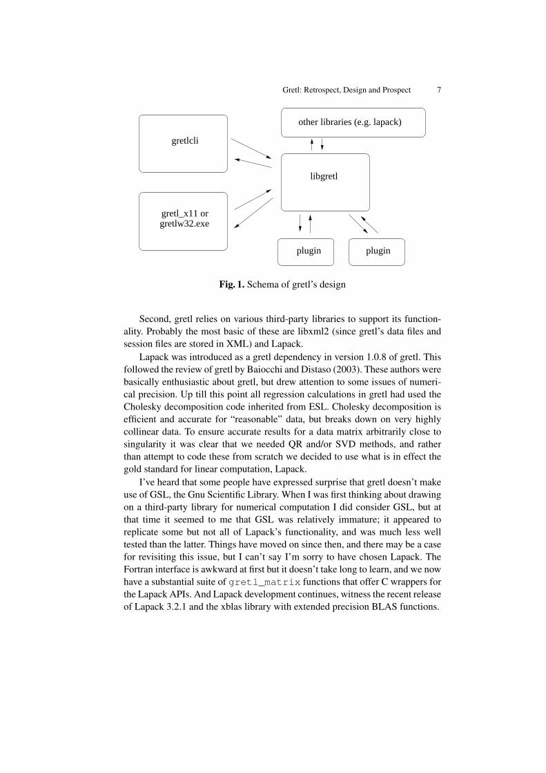
Gretl’s design schema is shown in Figure 1. The command-line and GUI clientsare in a sense at par as clients of libgretl (although of course the GUI programis a great deal more complicated). There are two other elements in the picture.
First, we have implemented several of the less commonly used features ingretl as dynamically loadable modules (“plugins”). The basic idea here was toavoid “bloat” in libgretl itself and hold down the memory footprint of the mainlibrary. This may now seem over-scrupulous given the amount of RAM to befound in today’s PCs. You may blame my thrifty Scottish upbringing if youwish.
5 See http://ricardo.ecn.wfu.edu/~cottrell/gstar/.6 Although the ‘L’ in ESL stood for “Library”, ESL did not provide a library in the technical
sense.
Gretl: Retrospect, Design and Prospect 7
gretlcli
gretlw32.exegretl_x11 or
libgretl
plugin plugin
other libraries (e.g. lapack)
Fig. 1. Schema of gretl’s design
Second, gretl relies on various third-party libraries to support its function-ality. Probably the most basic of these are libxml2 (since gretl’s data files andsession files are stored in XML) and Lapack.
Lapack was introduced as a gretl dependency in version 1.0.8 of gretl. Thisfollowed the review of gretl by Baiocchi and Distaso (2003). These authors werebasically enthusiastic about gretl, but drew attention to some issues of numeri-cal precision. Up till this point all regression calculations in gretl had used theCholesky decomposition code inherited from ESL. Cholesky decomposition isefficient and accurate for “reasonable” data, but breaks down on very highlycollinear data. To ensure accurate results for a data matrix arbitrarily close tosingularity it was clear that we needed QR and/or SVD methods, and ratherthan attempt to code these from scratch we decided to use what is in effect thegold standard for linear computation, Lapack.
I’ve heard that some people have expressed surprise that gretl doesn’t makeuse of GSL, the Gnu Scientific Library. When I was first thinking about drawingon a third-party library for numerical computation I did consider GSL, but atthat time it seemed to me that GSL was relatively immature; it appeared toreplicate some but not all of Lapack’s functionality, and was much less welltested than the latter. Things have moved on since then, and there may be a casefor revisiting this issue, but I can’t say I’m sorry to have chosen Lapack. TheFortran interface is awkward at first but it doesn’t take long to learn, and we nowhave a substantial suite of gretl_matrix functions that offer C wrappers forthe Lapack APIs. And Lapack development continues, witness the recent releaseof Lapack 3.2.1 and the xblas library with extended precision BLAS functions.

8 Allin Cottrell
2.2 Other third-party libraries
It’s not necessary to enumerate all the additional libraries that gretl either re-quires or uses optionally (from libfftw to gtksourceview), but a few issues maybe worth mentioning.
One issue is Internet connectivity. For several years we’ve had a “databaseserver” at Wake Forest University from which gretl users can download databasefiles. More recently we’ve extended this to traffic in “function package” files,and this month (May 2009) I’ve added the ability to download from within gretlthe packages of data files associated with the textbooks by Wooldridge, Stockand Watson, Verbeek and so on. The code we use to enable such traffic wasoriginally “borrowed” from GNU wget and modified for gretl. It seems to workOK for the most part, but I wonder if we could do better, in terms of robustnessand extensibility, by linking against libcurl (see http://curl.haxx.se/).One nice thing about linking to a third-party library that is under active devel-opment is that one gets bug-fixes and new features “for free”—just sit back andenjoy.
Another issue relates to the reading and writing of files in the PKZIP format.Gretl sessions files are zipped in this format, following the pattern of ODF files;and we now read ODS spreadsheets. Similarly to the borrowing from wget,the gretl code for handling zip archives is adapted from code by Mark Adleret al from Info-ZIP (zip version 2.31). Since I made that adaptation, libgsf—the Gnome Structured File library, coded in conjunction with Gnumeric—hasbecome reasonably mature. It still (as of version 1.14.12) does not offer all thefunctionality of Info-ZIP for handling zipfiles, but while our chunk of zip codeis effectively frozen it’s likely that libgsf will continue to develop apace, so theremay be a case for switching to libgsf at some point.
The third and last point that I’ll raise in this context does not concern alibrary, but a third-party program of which we make extensive use, namely gnu-plot. In this case gretl plays the role of a “front-end”, and I spoke earlier of theinherent limitations of that role. There has been talk in the gnuplot communityat various times of making a “libgnuplot” library, which would be very helpfulfrom our point of view, but there doesn’t seem to be much momentum behindthat move, so far as I can see. Over the years I have from time to time checkedout some seemingly promising options for graphing libraries, but have not foundanything that offers all the functionality of gnuplot. Meanwhile, although there’sno gnuplot library yet, gnuplot—which has been very full-featured for a longtime—continues to improve. And we’ve established good relations with thegnuplot developers, and have gained acceptance for some patches which makegnuplot more “gretl-friendly”.
Gretl: Retrospect, Design and Prospect 9
This is one area where things are easier in relation to the gretl packagesfor Windows and OS X than for gretl on Linux. With the Windows and OS Xpackages we can ship a build of CVS gnuplot that we know will “do the rightthing”—specifically, that it can handle UTF-8 encoding, and will produce high-quality PNG and PDF output using the Pango and Cairo libraries. On Linux,gnuplot is probably already installed, but we can’t be sure what version andhow well it’s configured, so we have to implement a lot of workarounds. Theremay be a case for making a comprehensive gretl package for Linux that bundlesgnuplot, though this rather goes against the grain.
3 Prospect
Gretl began life as a teaching tool—specifically, a tool for teaching econometricsat the undergraduate level—but it has grown far beyond that.
As an index of this growth, let me refer back to 2005, when I visited gretlcontributors in Ancona, Torun and Bilbao. I recall a discussion in Bilbao wherepeople were putting forward their wish lists for future developments: these in-cluded general purpose MLE functionality, GMM, and a general facility formanipulating matrices. I’ll admit that these tasks seemed quite daunting at thetime, but there followed a flurry of gretl activity in which all of these thingswere added and more. After spending time together in person, Jack Lucchettiand I were able to collaborate very effectively in coding some of the more chal-lenging additions. The mle command was introduced in gretl 1.5.0 (December2005) and general matrix functionality in 1.5.1 (March 2006). Version 1.6.0(September 2006) introduced “native” exact ML estimation of ARMA modelsusing the Kalman filter. GMM followed in 1.6.1 (February 2007), along withthe Arellano–Bond dynamic panel estimator.
Over the same period the internationalization of gretl accelerated. The firsttranslations were into French and Spanish (2002), then Italian and Polish (2004).Since then we have added Basque, German, Turkish, Russian, Portuguese, Tra-ditional Chinese and most recently Czech. And these are challenging transla-tions, requiring a firm grasp of technical econometric terminology.
The question arises, what should be gretl’s role? What should we be aimingfor? Reverting to the discussions of 2005 for a moment, there was some de-bate at the time on the gretl mailing list as to whether it really made sense forgretl to aim for a substantially higher level of econometric sophistication—thealternative being to concentrate on polishing gretl as a robust and user-friendlyteaching tool. De facto, this debate has been resolved in favour of the pursuit ofsophistication. I think there’s at least one good rationale for this.

10 Allin Cottrell
It has occasionally been put to me that maybe I’m not doing my students aservice by teaching econometrics using gretl. The argument is that students arebetter served if they use from the start a software package that they can continueto use as researchers and professionals; by doing so they would be learning mar-ketable skills and avoiding the need to re-learn how to do things with “standard”software. This sort of comment rankled greatly, but I recognize it has some va-lidity. If gretl were a “dead end” it would be relatively difficult to justify its usein teaching, even if it is more user-friendly than the alternatives. Why not useStata, Eviews or SAS? Just because we’re Free Software ideologues, or happento enjoy messing about with coding?
3.1 Promoting the adoption of gretl
For several reasons, those of us involved in gretl’s development would like to seegretl used more widely, both in teaching and in research. We believe that free,open-source software is desirable in its own right, and is particularly desirablein the scientific domain where it ought to be clear precisely how results areobtained (which is not the case with closed-source proprietary software). [Addreference to Talha Yalta’s paper?] We also believe that we have an excellentpiece of software in gretl and that students would benefit from using it.7 Andwe’d like to see the gretl developer community expand, so that we are less relianton just a few coders and the project can become self-sustaining.8
Jack Lucchetti’s analysis of downloads of gretl from the SourceForge site(Lucchetti, 2009) shows a rising trend. That’s good, but there are factors makingit difficult for gretl to achieve a “break through” to a substantially higher levelof adoption. Jack mentions some of these; I’ll elaborate a little.
One obvious point is that gretl is competing in a tough market. I don’t havesolid data to back up this claim, but it seems that Stata and Eviews are currentlythe leading products in the teaching of econometrics. These programs are alsowidely used in research, and seem to have edged previously popular softwaresuch as RATS and Limdep into niche roles. If gretl were a commercial prod-uct aiming to break into this market in a big way (and not just to find a niche)we’d be spending a great deal on advertising, would have a booth at the an-nual meetings of the Allied Social Science Association, and so on. In fact, ofcourse, from the start we had to rely on “osmosis”, achieved through, for ex-ample, personal contacts and web searches (e.g. people looking specifically foropen-source statistical software). However, we now have a factor working in
7 This opinion is not confined to gretl developers. I have received many, many emails over theyears from professors and students around the world, to just this effect.
8 And, of course, at a personal level, a bit more recognition would not go amiss: those of usewho work on gretl make no money out of it—that was not the plan—but we’re only human.

Gretl: Retrospect, Design and Prospect 11
our favour, namely the gretl-aware textbooks that have been published in Pol-ish (Kufel, 2007, also available in a Russian edition) and Spanish (Gallastegui,2005). In addition we have Lee Adkins’ gretl-based ebook (2009) and the forth-coming fourth edition of Christopher Dougherty’s Introduction to Econometrics(Oxford). In this context I wonder if it would be worth exploring the possibil-ity of writing collaboratively an English-language econometrics text that makesuse of gretl? Lee Adkins has done a great deal in this direction already, but I’mthinking of something that would not be tied to a specific existing text (Ad-kins’ ebook is designed to accompany Hill, Griffiths and Lim (2008)), and that,hopefully, could be placed with a major publisher.
3.2 Gretl and R
Still under the general topic of the difficulty of breaking into the highly compet-itive market in econometric software, one special issue arises for gretl. Besidesits specific design features, gretl’s most notable attribute is obviously that it isopen source and free. But gretl is not entering an empty space in that respect: inresidence is the highly respected and full-featured GNU R.
It’s noteworthy that R achieved a very positive write-up in the New YorkTimes earlier this year (Vance, 2009). Hal Varian (now chief economist at Google)is quoted as saying, “The great beauty of R is that you can modify it to do allsorts of things. And you have a lot of prepackaged stuff that’s already available,so you’re standing on the shoulders of giants.” The article notes the increasingadoption of R for data analysis in both academic and commercial contexts andcites Max Kuhn, associate director of nonclinical statistics at Pfizer: “R has re-ally become the second language for people coming out of grad school now,and there’s an amazing amount of code being written for it. You can look on theSAS message boards and see there is a proportional downturn in traffic.” Therejoinder by a SAS spokesperson, “We have customers who build engines foraircraft. I am happy they are not using freeware when I get on a jet,” soundsdefensive and out of touch.
What does R’s success mean for gretl? On the one hand it demonstrates thatthere is scope for free software to make substantial inroads on the turf of the ven-dors of proprietary statistical software, which is very encouraging. On the otherhand it may be seen as raising the question of whether gretl is really needed. Isthere room for gretl alongside R in this domain? The gretl developers are wellaware of R’s strengths but consider that gretl still has a role to play. Gretl hasan intuitive GUI; R does not. While gretl is in general much less comprehen-sive than R it nonetheless adds some specialized econometric functionality inrelation to R. And we have taken pains to make gretl as interoperable with R aspossible, so that users can take advantage of the complementarity between the

12 Allin Cottrell
two programs. Nonetheless, this is an area where more thought and more workare required: what exactly should be the relationship between gretl and R?
3.3 Extending gretl
I mentioned earlier the goal that gretl should become self-sustaining, and notoverly dependent on the work of a few individuals. In that regard, the wayin which the range of packages for R has mushroomed (see Varian’s com-ment above) is very pertinent. In 2006 we introduced a facility to create (anddownload) “function packages” containing user-contributed code for gretl—code written in the gretl scripting language rather than C. I think this is theright way to go, but although some excellent packages have been contributedit’s fair to say that this has not “taken off” to date. This is something we shouldrevisit. There are some awkward aspects of the gretl function packager and weshould resolve these. We also need to think about the issue more generally: isthere anything we can do specifically to promote the contribution of packages?What can we learn from R?
In closing I’ll mention one other aspect of extending gretl and getting itto be better known. In section 2 I spoke about gretl’s shared library, libgretl,which was originally created by adapting Ramanathan’s ESL code base. Thething is that libgretl in some ways still bears the marks of its origins. Basically,it contains all the common code that is needed by both the command-line andthe GUI client programs. Some of this code (in particular sections that havebeen added relatively recently) is quite general and offers a reasonably cleanand consistent API—for example the gretl_matrix code, the probabilitydistribution code based on Stephen Moshier’s cephes, the BFGS maximizer,the Kalman filter—while some of it is highly gretl-specific and presents APIsthat are unlikely to be comprehensible to anyone who hasn’t worked on gretl foryears.
One idea for the future then, is to factor out the “private” and “public” com-ponents of the current libgretl and to spruce up the APIs of the latter. We’dhave, say, libgretl_priv and (public) libgretl. It would become easier fornew contributors to find their way around the code base, and at the same timethird-party developers would have access to a cleaner and more manageableeconometrics library for use in their own projects, hence promoting the use ofgretl code and gretl’s visibility.

Bibliography
[1] ADKINS, L. (2009): Using gretl for Principles of Econometrics, 3rdedition. online., Version 1.211, http://www.learneconometrics.com/gretl/ebook.pdf
[2] BAIOCCHI, G. AND DISTASO, W. (2003): “GRETL: Econometric softwarefor the GNU generation”, Journal of Applied Econometrics, 18, pp. 105–10.
[3] GALLASTEGUI, A. F. (2005): Econometrìa, Madrid: Pearson Educación.[4] HILL, R. C., GRIFFITHS, W. E. AND G. C. LIM (2008) Principles of
Econometrics, 3e, New York: Wiley.[5] KUFEL, TADEUSZ (2007) Ekonometria, 2e, Warsaw: Wydawnictwo
Naukowe PWN.[6] LUCCHETTI, RICCARDO (JACK) (2009), “Who uses gretl? An analysis of
the SourceForge download data”, this volume.[7] RAMANATHAN, RAMU (1989), Introductory Econometrics with Applica-
tions, San Diego: Harcourt Brace Jovanovich.[8] VANCE, ASHLEE (2009) “Data Analysts Captivated by R’s Power”, The
New York Times, January 6 http://www.nytimes.com/2009/01/07/technology/business-computing/07program.html Vis-ited 2009-04-04.

IDEOLOG: A Program for FilteringEconometric Data—A Synopsis
of Alternative Methods
D.S.G. Pollock
University of Leicesteremail: [email protected]
Abstract. An account is given of various filtering procedures that have beenimplemented in a computer program, which can be used in analysing economet-ric time series. The program provides some new filtering procedures that oper-ate primarily in the frequency domain. Their advantage is that they are able toachieve clear separations of components of the data that reside in adjacent fre-quency bands in a way that the conventional time-domain methods cannot.Several procedures that operate exclusively within the time domain have alsobeen implemented in the program. Amongst these are the bandpass filters of Bax-ter and King and of Christiano and Fitzgerald, which have been used in estimat-ing business cycles. The Henderson filter, the Butterworth filter and the Leseror Hodrick–Prescott filter are also implemented. These are also described in thispaperEconometric filtering procedures must be able to cope with the trends that aretypical of economic time series. If a trended data sequence has been reduced tostationarity by differencing prior to its filtering, then the filtered sequence willneed to be re-inflated. This can be achieved within the time domain via the sum-mation operator, which is the inverse of the difference operator. The effects of thedifferencing can also be reversed within the frequency domain by recourse to thefrequency-response function of the summation operator.
1 Introduction
This paper gives an account of some of the facilities that are available in a newcomputer program, which implements various filters that can be used for extract-ing the components of an economic data sequence and for producing smoothedand seasonally-adjusted data from monthly and quarterly sequences.
The program can be downloaded from the following web address:
http://www.le.ac.uk/users/dsgp1/
It is accompanied by a collection of data and by three log files, which recordsteps that can be taken in processing some typical economic data. Here, we givean account of the theory that lies behind some of the procedures of the program.
16 D.S.G. Pollock
The program originated in a desire to compare some new methods withexisting procedures that are common in econometric analyses. The outcomehas been a comprehensive facility, which will enable a detailed investigation ofunivariate econometric time series. The program will also serve to reveal theextent to which the results of an economic analysis might be the consequenceof the choice of a particular filtering procedure.
The new procedures are based on the Fourier analysis of the data, and theyperform their essential operations in the frequency domain as opposed to thetime domain. They depend upon a Fourier transform for carrying the data intothe frequency domain and upon an inverse transform for carrying the filtered ele-ments back to the time domain. Filtering procedures usually operate exclusivelyin the time domain. This is notwithstanding fact that, for a proper understandingof the effects of a filter, one must know its frequency-response function.
The sections of this paper give accounts of the various classes of filters thathave been implemented in the program. In the first category, to which section2 is devoted, are the simple finite impulse response (FIR) or linear moving-average filters that endeavour to provide approximations to the so-called idealfrequency-selective filters. Also in this category of FIR filters is the time-honouredfilter of Henderson (1916), which is part of a seasonal-adjustment program thatis widely used in central statistical agencies.
The second category concerns filters of the infinite impulse response (IIR)variety, which involve an element of feedback. The filters of this category thatare implemented in the program are all derived according to the Wiener–Kolmogorovprinciple. The principle has been enunciated in connection with the filtering ofstationary and doubly-infinite data sequences—see Whittle (1983), for exam-ple. However, the purpose of the program is to apply these filters to short nonstationary sequences. In section 3, the problem of non stationarity is broached,whereas, in section 4, the adaptations that are appropriate to short sequences areexplained.
Section 5 deals with the new frequency-domain filtering procedures. Thedetails of their implementation are described and some of their uses are high-lighted. In particular, it is shown how these filters can achieve an ideal frequencyselection, whereby all of the elements of the data that fall below a given cut-offfrequency are preserved and all those that fall above it are eliminated.
2 The FIR filters
One of the purposes in filtering economic data sequences is to obtain a rep-resentation of the business cycle that is free from the distractions of seasonalfluctuations and of high-frequency noise. According to Baxter and King (1999),
IDEOLOG—A Filtering Program 17
0
0.25
0.5
0.75
1
1.25
0
0 π/4 π/2 3π/4 π
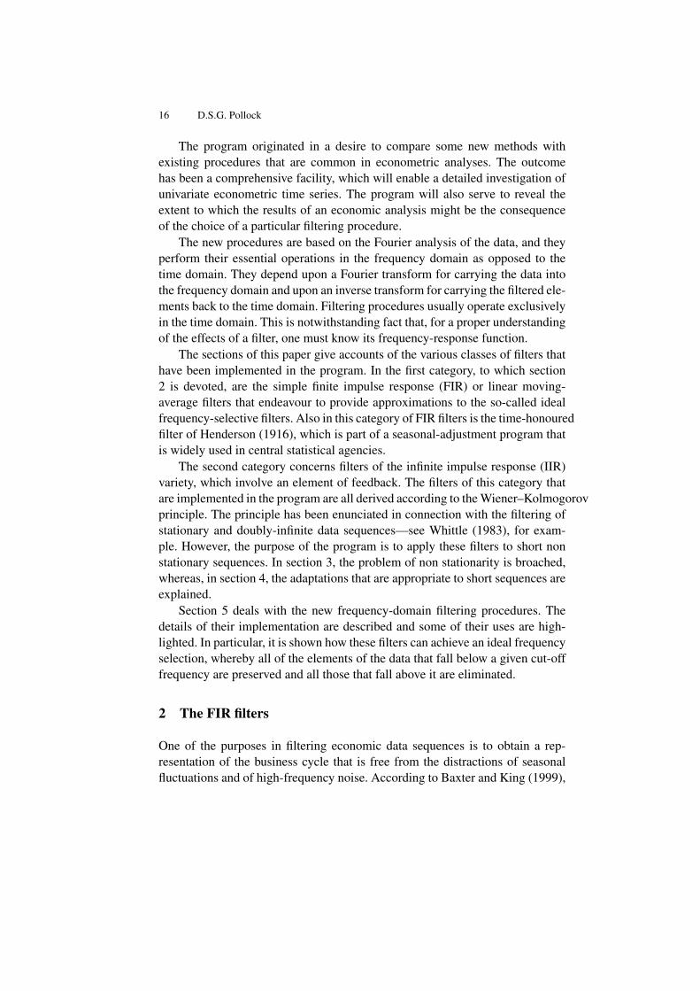
Fig. 1. The frequency response of the truncated bandpass filter of 25 coefficientssuperimposed upon the ideal frequency response. The lower cut-off point is atπ/16 radians (11.25), corresponding to a period of 32 quarters, and the uppercut-off point is at π/3 radians (60), corresponding to a period of the 6 quarters.
the business cycle should comprise all elements of the data that have cyclicaldurations of no less than of one and a half years and not exceeding eight years.For this purpose, they have proposed to use a moving-average bandpass filter toapproximate the ideal frequency-selective filter. An alternative approximation,which has the same purpose, has been proposed by Christiano and Fitzgerald(2003). Both of these filters have been implemented in the program.
A stationary data sequence can be resolved into a sum of sinusoidal ele-ments whose frequencies range from zero up to the Nyquist frequency of πradians per sample interval, which represents the highest frequency that is ob-servable in sampled data. A data sequence yt, t = 0, 1, . . . , T − 1 comprisingT observations has the following Fourier decomposition:
yt =[T/2]∑t−0
αj cos(ωjt) + βj sin(ωjt). (1)
Here, [T/2] denotes the integer quotient of the division of T by 2. The harmon-ically related Fourier frequencies ωj = 2πj/T ; j = 0, . . . , [T/2], which areequally spaced in the interval [0, π], are integer multiples of the fundamentalfrequency ω1 = 2π/T , whereas αj , βj are the associated Fourier coefficients,which indicate the amplitudes of the sinusoidal elements of the data sequence.An ideal filter is one that transmits the elements that fall within a specified fre-quency band, described as the pass band, and which blocks elements at all otherfrequencies, which constitute the stop band.
18 D.S.G. Pollock
In representing the properties of a linear filter, it is common to imaginethat it is operating on a doubly-infinite data sequence of a statistically station-ary nature. Then, the Fourier decomposition comprises an infinity of sinusoidalelements of negligible amplitudes whose frequencies form a continuum in theinterval [0, π]. The frequency-response function of the filter displays the factorsby which the amplitudes of the elements are altered in their passage through thefilter.
For an ideal filter, the frequency response is unity within the pass band andzero within the stop band. Such a response is depicted in Figure 1, where thepass band, which runs from π/16 to π/3 radians per sample interval, is intendedto transmit the elements of a quarterly econometric data sequence that constitutethe business cycle.
To achieve an ideal frequency selection with a linear moving-average filterwould require an infinite number of filter coefficients. This is clearly impracti-cal; and so the sequence of coefficients must be truncated, wherafter it may bemodified in certain ways to diminish the adverse effects of the truncation.
2.1 Approximation to the Ideal Filter
Figure 1 also shows the frequency response of a filter that has been derivedby taking twenty-five of the central coefficients of the ideal filter and adjustingtheir values by equal amounts so that they sum to zero. This is the filter thathas been proposed by Baxter and King (1999) for the purpose of extractingthe business cycle from economic data. The filter is affected by a considerableleakage, whereby elements that fall within the stop band are transmitted in partby the filter.
The z-transform of a sequence ψj of filter coefficients is the polynomialψ(z) =
∑j ψjz. Constraining the coefficients to sum to zero ensures that the
polynomial has a root of unity, which is to say that ψ(1) =∑
j ψj = 0. Thisimplies that∇(z) = 1−z is a factor of the polynomial, which indicates that thefilter incorporates a differencing operator.
If the filter is symmetric, such that ψ(z) = ψ0+ψ1(z+z−1)+· · ·+ψq(zq+z−q) and, therefore, ψ(z) = ψ(z−1), then 1 − z−1 is also a factor. Then, ψ(z)has the combined factor (1 − z)(1 − z−1) = −z∇(z)2, which indicates thatthe filter incorporates a twofold differencing operator. Such a filter is effectivein reducing a linear trend to zero; and, therefore, it is applicable to econometricdata sequences that have an underlying log-linear trend.
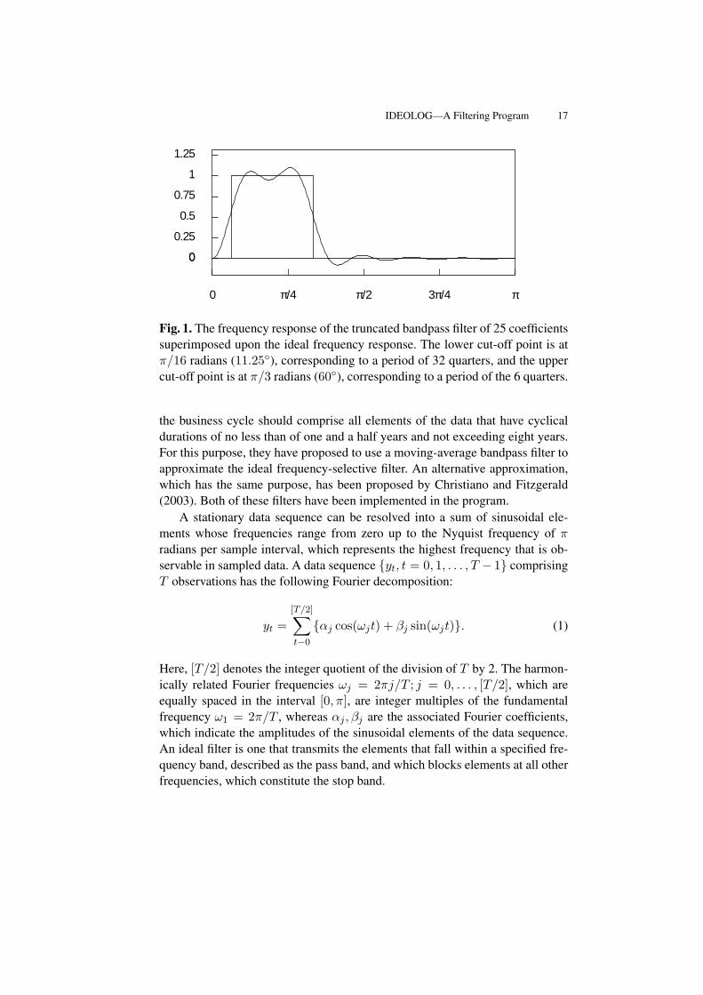
The filter of Baxter and King (1999), which fulfils this condition, is appro-priate for the purpose of extracting the business cycle from a trended data se-quence. Figure 2 shows the logarithms of data of U.K. real domestic consump-
IDEOLOG—A Filtering Program 19
10
10.5
11
11.5
1960 1970 1980 1990
Fig. 2. The quarterly sequence of the logarithms of consumption in the U.K., forthe years 1955 to 1994, together with a linear trend interpolated by least-squaresregression.
00.010.020.030.040.05
0−0.01−0.02−0.03−0.04
0 50 100 150
Fig. 3. The sequence derived by applying the truncated bandpass filter of 25coefficients to the quarterly logarithmic data on U.K. consumption.
0
0.05
0.1
0.15
0
−0.05
−0.1
0 50 100 150
Fig. 4. The sequence derived by applying the bandpass filter of Christiano andFitzgerald to the quarterly logarithmic data on U.K. consumption.
20 D.S.G. Pollock
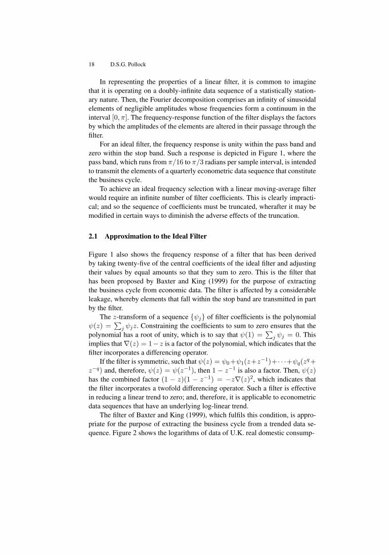
tion for the years 1955–1994 through which a linear trend has been interpolated.Figure 3 shows the results of subjecting these data to the Baxter–King filter. Adisadvantage of the filter, which is apparent in Figure 3, is that it is incapable ofreaching the ends of the sample. The first q sample values and the last q remainunprocessed.
To overcome this difficulty, Christiano and Fitzgerald (2003) have proposeda filter with a variable set of coefficients. To generate the filtered value at timet, they associate the central coefficient ψ0 with yt. If yt−p falls within the sam-ple, then they associate it with the coefficient ψp. Otherwise, if it falls outsidethe sample, it is disregarded. Likewise, if yt+p falls within the sample, then itis associated with ψp, otherwise it is disregarded. If the data follow a first-orderrandom walk, then the first and the last sample elements y0 and yT−1 receiveextra weights A and B, which correspond to the sums of the coefficients dis-carded from the filter at either end. The resulting filtered value at time t may bedenoted by
xt = Ay0 + ψty0 + · · ·+ ψ1yt−1 + ψ0yt (2)
+ ψ1yt+1 + · · ·+ ψT−1−tyT−1 +ByT−1.
This equation comprises the entire data sequence y0, . . . , yT−1; and thevalue of t determines which of the coefficients of the infinite-sample filter areinvolved in producing the current output. The value of x0 is generated by look-ing forwards to the end of the sample, whereas the value of xT−1 is generatedby looking backwards to the beginning of the sample.
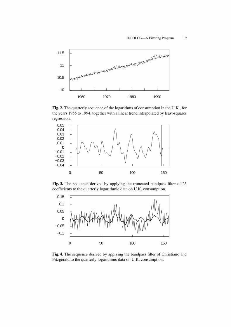
For data that appear to have been generated by a first-order random walkwith a constant drift, it is appropriate to extract a linear trend before filtering theresidual sequence. Figure 4 provides an example of the practice. In fact, this hasproved to be the usual practice in most circumstances.
Within the category of FIR filters, the program also implements the timehonoured smoothing filter of Henderson (1916), which forms an essential part ofthe detrending procedure of the X-11 program of the Bureau of the Census. Thisprogram provides the method of seasonal adjustment that is used predominantlyby central statistical agencies.
Here, the end-of-sample problem is overcome by supplementing the Hen-derson filter with a set of asymmetric filters that can be applied to the elementsof the first and the final segments. These are the Musgrave (1964) filters. (SeeQuenneville, Ladiray and Lefranc, 2003 for a recent account of these filters.)In the X-11 ARIMA variant, which is used by Statistics Canada, the alternativerecourse is adopted of extrapolating the data beyond the ends of the sample sothat it can support a time-invariant filter that does run to the ends.
IDEOLOG—A Filtering Program 21
3 The Wiener–Kolmogorov Filters
The program also provides several filters of the feedback variety that are com-monly described as infinite-impulse response (IIR) filters. The filters in questionare derived according to the finite-sample Wiener–Kolmogorov principle thathas been expounded by Pollock (2000, 2007).
The ordinary theory of Wiener–Kolmogorov filtering assumes a doubly-infinite data sequence y(t) = ξ(t) + η(t) = yt; t = 0,±1,±2, . . . generatedby a stationary stochastic process. The process is compounded from a signalprocess ξ(t) and a noise process η(t) that are assumed to be statistically inde-pendent and to have zero-valued means. Then, the autocovariance generatingfunction of y(t) is given by
γy(z) = γξ(z) + γη(z), (3)
which is sum of the autocovariance functions of ξ(t) and η(t).The object is to extract estimates of the signal sequence ξ(t) and the noise
sequence η(t) from the data sequence. The z-transforms of the relevant filtersare
βξ(z) =γξ(z)
γξ(z) + γη(z)=ψξ(z−1)ψξ(z)φ(z−1)φ(z)
, (4)
and
βη(z) =γη(z)
γξ(z) + γη(z)=ψη(z−1)ψη(z)φ(z−1)φ(z)
. (5)
It can been that βξ(z)+βη(z) = 1, in view of which the filters can be describedas complementary.
The factorisations of the filters that are given on the RHS enable them to beapplied via a bi-directional feedback process. In the case of the signal extractionfilter βξ(z), the process in question can be represented by the equations
φ(z)q(z) = ψξ(z)y(z) and φ(z−1)x(z) = ψξ(z−1)q(z−1), (6)
wherein q(z), y(z) and x(z) stand for the z-transforms of the correspondingsequences q(t), y(t) and x(t).
To elucidate these equations, we may note that, in the first of them, theexpression associated with zt is
m∑j=0
φjqt−j =n∑j=0
ψξ,jyt−j . (7)
Given that φ0 = 1, this serves to determine the value of qt. Moreover, given thatthe recursion is assumed to be stable, there need be no restriction on the range
22 D.S.G. Pollock
of t. The first equation, which runs forward in time, generates an intermediateoutput q(t). The second equation, which runs backwards in time, generates thefinal filtered output x(t).
3.1 Filters for Trended Data
The classical Wiener–Kolmogorov theory can be extended in a straightforwardway to cater for non stationary data generated by integrated autoregressive moving-average (ARIMA) processes in which the autoregressive polynomial containsroots of unit value. Such data processes can be described by the equation
y(z) =δ(z)∇p(z)
+ η(z) or, equivalently, ∇p(z)y(z) = δ(z) +∇p(z)η(z),
(8)where δ(z) and η(z) are, respectively, the z-transforms of the mutually indepen-dent stationary stochastic sequences δ(t) and η(t), and where∇p(z) = (1−z)pis the p-th power of the difference operator.
Here, there has to be some restriction on the range of t together with thecondition that the elements δt and ηt are finite within this range. Also, the z-transforms must comprise the appropriate initial conditions, which are effec-tively concealed by the notation. (See Pollock 2008 on this point.)
Within the program, two such filters have been implemented. The first isthe filter of Leser (1961) and of Hodrick and Prescott (1980, 1997), which isdesigned to extract the non stationary signal or trend component when the dataare generated according to the equation
∇2(z)y(z) = g(z) = δ(z) +∇2(z)η(z), (9)
where δ(t) are η(t) are mutually independent sequences of independently andidentically distributed random variables, generated by so-called white-noise pro-cesses. With γδ(z) = σ2
δ and γξ(z) = σ2δ∇(z−1)∇(z) and with γη(z) = σ2
η ,the z-transforms of the relevant filters become
βξ(z) =1
1 + λ∇2(z−1)∇2(z), (10)
and
βη(z) =∇2(z−1)∇2(z)
λ−1 +∇2(z−1)∇2(z), (11)
where λ = σ2η/σ
2δ , which is described as the smoothing parameter.
The frequency-response functions of the filters for various values of λ areshown in Figure 5. These are obtained by setting z = e−iω = cos(ω)− i sin(ω)
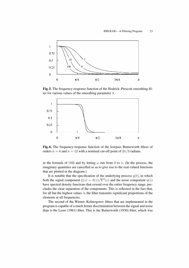
IDEOLOG—A Filtering Program 23
Fig. 5. The frequency-response function of the Hodrick–Prescott smoothing fil-ter for various values of the smoothing parameter λ.
Fig. 6. The frequency-response function of the lowpass Butterworth filters oforders n = 6 and n = 12 with a nominal cut-off point of 2π/3 radians.
in the formula of (10) and by letting ω run from 0 to π. (In the process, theimaginary quantities are cancelled so as to give rise to the real-valued functionsthat are plotted in the diagram.)
It is notable that the specification of the underlying process y(t), in whichboth the signal component ξ(z) = δ(z)/∇2(z) and the noise component η(z)have spectral density functions that extend over the entire frequency range, pre-cludes the clear separation of the components. This is reflected in the fact that,for all but the highest values λ, the filter transmits significant proportions of theelements at all frequencies.
The second of the Wiener–Kolmogorov filters that are implemented in theprogram is capable of a much firmer discrimination between the signal and noisethan is the Leser (1961) filter. This is the Butterworth (1930) filter, which was
24 D.S.G. Pollock
−i
i
−1 1Re
Im
−i
i
−1 1Re
Im
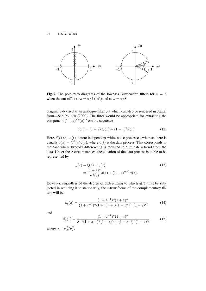
Fig. 7. The pole–zero diagrams of the lowpass Butterworth filters for n = 6when the cut-off is at ω = π/2 (left) and at ω = π/8.
originally devised as an analogue filter but which can also be rendered in digitalform—See Pollock (2000). The filter would be appropriate for extracting thecomponent (1 + z)nδ(z) from the sequence
g(z) = (1 + z)nδ(z) + (1− z)nκ(z). (12)
Here, δ(t) and κ(t) denote independent white-noise processes, whereas there isusually g(z) = ∇2(z)y(z), where y(t) is the data process. This corresponds tothe case where twofold differencing is required to eliminate a trend from thedata. Under these circumstances, the equation of the data process is liable to berepresented by
y(z) = ξ(z) + η(z) (13)
=(1 + z)n
∇2(z)δ(z) + (1− z)n−2κ(z).
However, regardless of the degree of differencing to which y(t) must be sub-jected in reducing it to stationarity, the z-transforms of the complementary fil-ters will be
βξ(z) =(1 + z−1)n(1 + z)n
(1 + z−1)n(1 + z)n + λ(1− z−1)n(1− z)n, (14)
and
βη(z) =(1− z−1)n(1− z)n
λ−1(1 + z−1)n(1 + z)n + (1− z−1)n(1− z)n, (15)
where λ = σ2κ/σ
2δ .
IDEOLOG—A Filtering Program 25
It is straightforward to determine the value of λ that will place the cut-off ofthe filter at a chosen point ωc ∈ (0, π). Consider setting z = exp−iω in theformula of (14) of the lowpass filter. This gives the following expression for thegain:
βξ(e−iω) =1
1 + λ
(i1− e−iω
1 + e−iω
)2n (16)
=1
1 + λ
tan(ω/2)2n .
At the cut-off point, the gain must equal 1/2, whence solving the equationβξ(exp−iωc) = 1/2 gives λ = 1/ tan(ωc/2)2n.
Figure 6 shows how the rate of the transition of the Butterworth frequencyresponse between the pass band and the stop band is affected by the order ofthe filter. Figure 7 shows the pole–zero diagrams of filters with different cut-off points. As the cut-off frequency is reduced, the transition between the twobands becomes more rapid. Also, some of the poles of the filter move towardsthe perimeter of the unit circle.
3.2 A Filter for Seasonal Adjustment
The Wiener–Kolmogorov principle is also used in deriving a filter for the sea-sonal adjustment of monthly and quarterly econometric data. The filter is de-rived from a model that combines a white-noise component η(t) with a sea-sonal component obtained by passing an independent white noise ν(t) througha rational filter with poles located on the unit circle at angles corresponding tothe seasonal frequencies and with corresponding zeros at the same angles butlocated inside the circle. The z-transform of the output sequence gives
y(z) = η(z) +R(z)S(z)
ν(z) or (17)
S(z)y(z) = S(z)η(z) +R(z)ν(z),
whereR(z) = 1 + ρz + ρ2z2 + · · ·+ ρs−1zs−1 (18)
with ρ < 1, andS(z) = 1 + z + z2 + · · ·+ zs−1. (19)
The z-transform of the seasonal-adjustment filter is
β(z) =σ2ηS(z)S(z−1)
S(z)S(z−1)σ2η + σ2
νR(z)R(z−1). (20)
26 D.S.G. Pollock
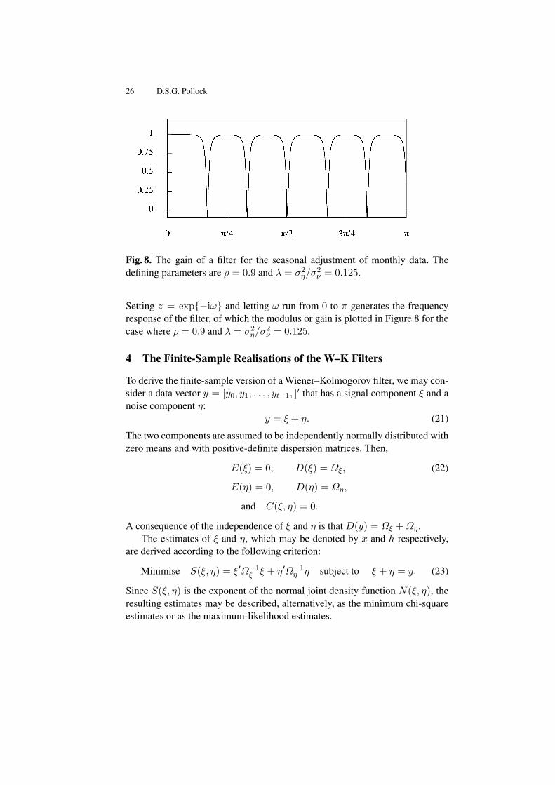
Fig. 8. The gain of a filter for the seasonal adjustment of monthly data. Thedefining parameters are ρ = 0.9 and λ = σ2
η/σ2ν = 0.125.
Setting z = exp−iω and letting ω run from 0 to π generates the frequencyresponse of the filter, of which the modulus or gain is plotted in Figure 8 for thecase where ρ = 0.9 and λ = σ2
η/σ2ν = 0.125.
4 The Finite-Sample Realisations of the W–K Filters
To derive the finite-sample version of a Wiener–Kolmogorov filter, we may con-sider a data vector y = [y0, y1, . . . , yt−1, ]′ that has a signal component ξ and anoise component η:
y = ξ + η. (21)
The two components are assumed to be independently normally distributed withzero means and with positive-definite dispersion matrices. Then,
E(ξ) = 0, D(ξ) = Ωξ, (22)
E(η) = 0, D(η) = Ωη,
and C(ξ, η) = 0.
A consequence of the independence of ξ and η is that D(y) = Ωξ +Ωη.The estimates of ξ and η, which may be denoted by x and h respectively,
are derived according to the following criterion:
Minimise S(ξ, η) = ξ′Ω−1ξ ξ + η′Ω−1
η η subject to ξ + η = y. (23)
Since S(ξ, η) is the exponent of the normal joint density function N(ξ, η), theresulting estimates may be described, alternatively, as the minimum chi-squareestimates or as the maximum-likelihood estimates.
IDEOLOG—A Filtering Program 27
Substituting for η = y − ξ gives the concentrated criterion function S(ξ) =ξ′Ω−1
ξ ξ + (y − ξ)′Ω−1(y − ξ). Differentiating this function in respect of ξ andsetting the result to zero gives a condition for a minimum, which specifies theestimate x. This is Ω−1
η (y − x) = Ω−1ξ x, which, on pre multiplication by Ωη,
can be written as y = x−ΩηΩ−1ξ x = (Ωξ +Ωη)Ω−1
ξ x. Therefore, the solutionfor x is
x = Ωξ(Ωξ +Ωη)−1y. (24)
Moreover, since the roles of ξ and η are interchangeable in this exercise, and,since h+ x = y, there are also
h = Ωη(Ωξ +Ωη)−1y and x = y −Ωη(Ωξ +Ωη)−1y. (25)
The filter matrices Bξ = Ωξ(Ωξ + Ωη)−1 and Bη = Ωη(Ωξ + Ωη)−1 of (24)and (25) are the matrix analogues of the z-transforms displayed in equations (4)and (5).
A simple procedure for calculating the estimates x and h begins by solvingthe equation
(Ωξ +Ωη)b = y (26)
for the value of b. Thereafter, one can generate
x = Ωξb and h = Ωηb. (27)
IfΩξ andΩη correspond to the narrow-band dispersion matrices of moving-average processes, then the solution to equation (26) may be found via a Choleskyfactorisation that sets Ωξ + Ωη = GG′, where G is a lower-triangular matrixwith a limited number of nonzero bands. The system GG′b = y may be cast inthe form of Gp = y and solved for p. Then, G′b = p can be solved for b. Theprocedure has been described by Pollock (2000).
4.1 Filters for Short Trended Sequences
To adapt these estimates to the case of trended data sequences may require theprovision of carefully determined initial conditions with which to start the re-cursive processes. A variety of procedures are available that are similar, if notidentical, in their outcomes. The procedures that are followed in the programdepend upon reducing the data sequences to stationarity, in one way or another,before subjecting them to the filters. After the data have been filtered, the trendis liable to be restored.
The first method, which is the simplest in concept, requires the trend to berepresented by a polynomial function. In some circumstances, when the econ-omy has been experiencing steady growth, the polynomial will serve as a reason-able characterisation of its underlying trajectory. Thus, in the period 1955–1994
28 D.S.G. Pollock
a log-linear trend function provides a firm benchmark against which to measurethe cyclical fluctuations of the U.K. economy. The residual deviations from thistrend may be subjected to a lowpass filter; and the filtered output can be addedto the trend to produce a representation of what is commonly described as thetrend-cycle component.
It is desirable that the polynomial trend should interpolate the scatter ofpoints at either end of the data sequence. For this purpose, the program providesa method of weighted least-squares polynomial regression with a wide choiceof weighting schemes, which allow extra weight to be placed upon the initialand the final runs of observations.
An alternative way of eliminating the trend is to take differences of the data.Usually, twofold differencing is appropriate. The matrix analogue of the second-order backwards difference operator in the case of T = 5 is given by
∇25 =
[Q′∗Q′
]=
1 0 0 0 0−2 1 0 0 0
1 −2 1 0 00 1 −2 1 00 0 1 −2 1
. (28)
The first two rows, which do not produce true differences, are liable to be dis-carded. In general, the p-fold differences of a data vector of T elements will beobtained by pre multiplying it by a matrix Q′ of order (T − p) × T . ApplyingQ′ to equation (21) gives
Q′y = Q′ξ +Q′η (29)
= δ + κ = g.
The dispersion matrices of the differenced vectors are
D(δ) = Ωδ = Q′D(Ωξ)Q and D(κ) = Ωκ = Q′D(Ωη)Q. (30)
The estimates d and k of the differenced components are given by
d = Ωδ(Ωδ +Q′ΩηQ)−1Q′y (31)
andk = Q′ΩηQ(Ωδ +Q′ΩηQ)−1Q′y. (32)
To obtain estimates of ξ and η, the estimates of their difference versions mustbe re-inflated via an anti-differencing or summation operator. We begin by ob-
IDEOLOG—A Filtering Program 29
serving that the inverse of∇25 is a twofold summation operator given by
∇−25 =
[S∗ S
]=
1 0 | 0 0 02 1 | 0 0 03 2 | 1 0 04 3 | 2 1 05 4 | 3 2 1
. (33)
The first two columns, which constitute the matrix S∗, provide a basis for alllinear functions defined on t = 0, 1, . . . , T − 1 = 5. The example can begeneralised to the case of a p-fold differencing matrix∇−pT of order T . However,in the program, the maximum degree of differencing is p = 2.
We observe that, if g∗ = Q′∗y and g = Q′y are available, then y can berecovered via the equation
y = S∗g∗ + Sg. (34)
In effect, the elements of g∗, which may be regarded as polynomial parameters,provide the initial conditions for the process of summation or integration, whichwe have been describing as a process of re-inflation.
The equations by which the estimates of ξ and η may be recovered fromthose of δ and κ are analogous to equation (34). They are
x = S∗d∗ + Sd and h = S∗k∗ + Sk. (35)
In this case, the initial conditions d∗ and k∗ require to be estimated. The appro-priate estimates are the values that minimise the function
(y − x)′Ω−1η (y − x) = (y − S∗d∗ − Sd)′Ω−1
η (y − S∗d∗ − Sd) (36)
= (S∗k∗ + Sk)′Ω−1η (S∗k∗ + Sk).
These values arek∗ = −(S′∗Ω
−1η S∗)−1S′∗Ω
−1η Sk (37)
andd∗ = (S′∗Ω
−1η S∗)−1S′∗Ω
−1η (y − Sd). (38)
Equations (37) and (38) together with (31) and (32) provide a completesolution to the problem of estimating the components of the data. However,it is possible to eliminate the initial conditions from the system of estimatingequations. This can be achieved with the help of the following identity:
P∗ = S∗(S′∗Ω−1η S∗)−1S′∗Ω
−1η (39)
= I −ΩηQ(Q′ΩηQ)−1Q′ = I − PQ.
30 D.S.G. Pollock
In these terms, the equation of (35) for h becomes h = (I − P∗)Sk = PQSk.Using the expression for k from (32) together with the identity Q′S = IT−2
givesh = ΩηQ(Ωδ +Q′ΩηQ)−1Q′y. (40)
This can also be obtained from the equation (32) for k by the removal of theleading differencing matrix Q′. It follows immediately that
x = y − h (41)
= y −ΩηQ(Ωδ +Q′ΩηQ)−1Q′y.
The elimination of the initial conditions is due to the fact that η is a sta-tionary component. Therefore, it requires no initial conditions other than thezeros that are the appropriate estimates of the pre-sample elements. The directestimate x of ξ does require initial conditions, but, in view of the adding-upconditions of (21), x can be obtained more readily by subtracting from y theestimate h of η, in the manner of equation (41).
Fig. 9. The periodogram of the first differences of the U.K. logarithmic con-sumption data.
Observe that, sincef = S∗(S′∗S∗)
−1S′∗y (42)
is an expression for the vector of the ordinates of a polynomial function fitted tothe data by an ordinary least-squares regression, the identity of (39) informs usthat
f = y −Q(Q′Q)−1Q′y (43)
is an alternative expression.
IDEOLOG—A Filtering Program 31
Fig. 10. The periodogram of the residual sequence obtained from the linear de-trending of the logarithmic consumption data. A band, with a lower bound ofπ/16 radians and an upper bound of π/3 radians, is masking the periodogram.
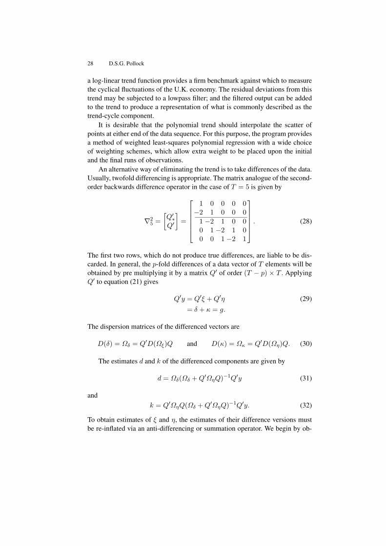
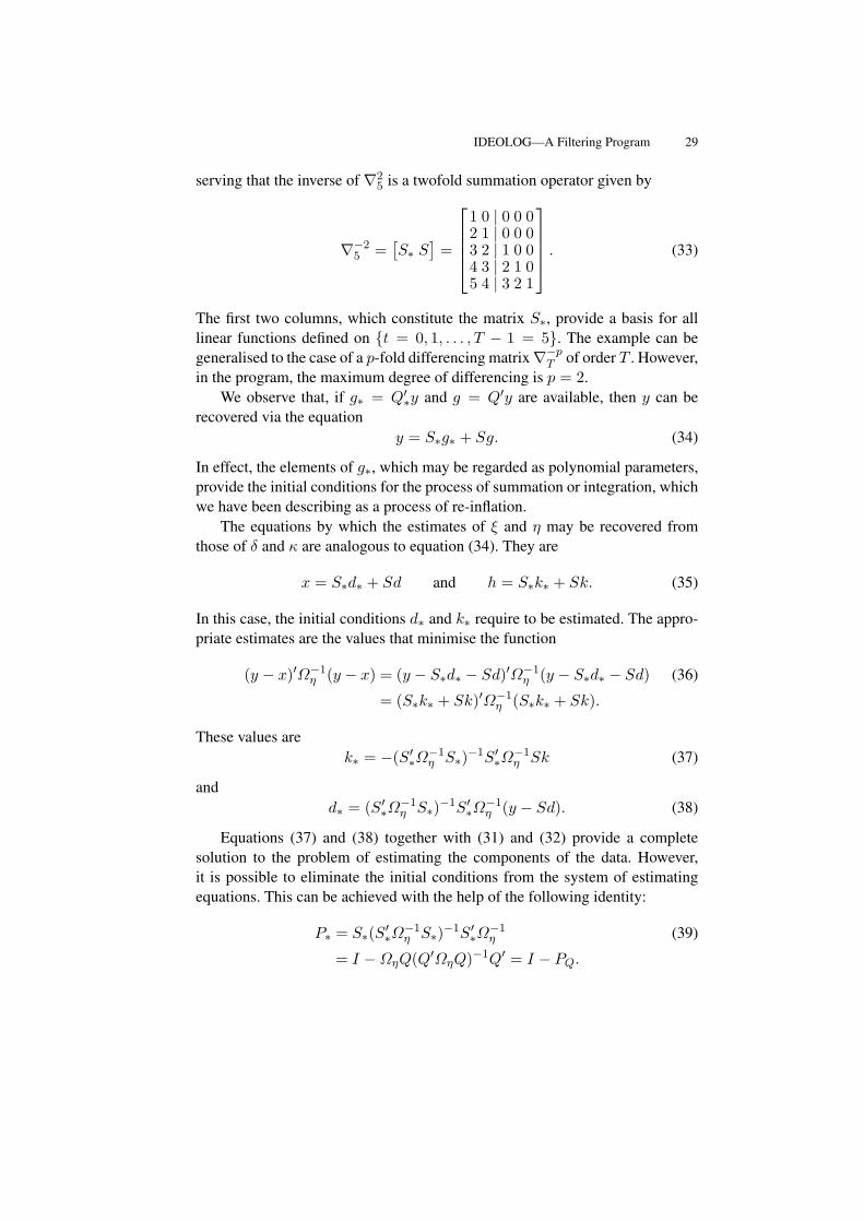
The residuals of an OLS polynomial regression of degree p, which are givenby y−f = Q(Q′Q)−1Q′y, contain same the information as the vector g = Q′yof the p-th differences of the data. The difference operator has the effect of nul-lifying the element of zero frequency and of attenuating radically the adjacentlow-frequency elements. Therefore, the low-frequency spectral structures of thedata are not perceptible in the periodogram of the differenced sequence. Figure9 provides evidence of this.
On the other hand, the periodogram of a trended sequence is liable to bedominated by its low-frequency components, which will mask the other spec-tral structures. However, the periodogram of the residuals of the polynomialregression can be relied upon to reveal the spectral structures at all frequencies.Moreover, by varying the degree p of the polynomial, one is able to alter therelative emphasis that is given to high-frequency and low-frequency structures.Figure 10 shows that the low-frequency structure of the U.K. consumption datais fully evident in the periodogram of the residuals from fitting a linear trend tothe logarithmic data.
4.2 A Flexible Smoothing Filter
A derivation of the estimator of ξ is available that completely circumvents theproblem of the initial conditions. This can be illustrated with the case of a gen-eralised version of the Leser (1961) filter in which the smoothing parameter ispermitted to vary over the course of the sample. The values of the smoothingparameter are contained in the diagonal matrix Λ = diagλ0, λ1, . . . , λT−1.
32 D.S.G. Pollock
Then, the criterion for finding the vector is to minimise
L = (y − ξ)′(y − ξ) + ξ′QΛQ′ξ. (44)
The first term in this expression penalises departures of the resulting curvefrom the data, whereas the second term imposes a penalty for a lack of smooth-ness in the curve. The second term comprises d = Q′ξ, which is the vector ofthe p-fold differences of ξ. The matrix Λ serves to generalise the overall mea-sure of the curvature of the function that has the elements of ξ as its sampledordinates, and it serves to regulate the penalty for roughness, which may varyover the sample.
10
11
12
13
1875 1900 1925 1950 1975 2000
Fig. 11. The logarithms of annual U.K. real GDP from 1873 to 2001 with aninterpolated trend. The trend is estimated via a filter with a variable smoothingparameter.
Differentiating L with respect to ξ and setting the result to zero, in accor-dance with the first-order conditions for a minimum, gives
y − x = QΛQ′x = QΛd. (45)
Multiplying the equation by Q′ gives Q′(y − x) = Q′y − d = Q′QΛd, whenceΛd = (Λ−1 +Q′Q)−1Q′y. Putting this into the equation x = y −QΛd gives
x = y −Q(Λ−1 +Q′Q)−1Q′y (46)
= y − ΛQ(I + ΛQ′Q)−1Q′y.
This filter has been implemented in the program under the guise of a variablesmoothing procedure. By giving a high value to the smoothing parameter, a
IDEOLOG—A Filtering Program 33
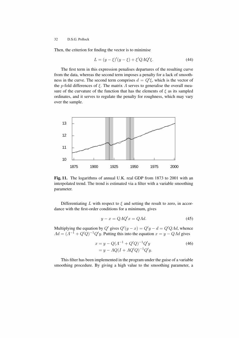
stiff curve can be generated, which approaches a straight line as λ → ∞. Onthe other hand, structural breaks can be accommodated by greatly reducing thevalue of the smoothing parameter in their neighbourhood. When λ → 0, thefilter tends to transmit the unaltered data values.
Figure 11 shown an example of the use of this filter. There were brief dis-ruptions to the steady upwards progress of GDP in the U.K. after the two worldwars. These breaks have been absorbed into the trend by reducing the value ofthe smoothing parameter in their localities. By contrast, the break that is evidentin the data following the year 1929 has not been accommodated in the trend.
4.3 A Seasonal-Adjustment Filter
The need for initial conditions cannot be circumvented in cases where the sea-sonal adjustment filter is applied to trended sequences. Consider the filter thatis applied to the differenced data g = Q′y to produce a seasonally-adjustedsequence q. Then, there is
q = QS(Q′SQS + λ−1Q′RQR)−1Q′Sg, (47)
whereQ′R andQ′S are the matrix counterparts of the polynomial operatorsR(z)and S(z) of (18) and (19) respectively. The seasonally adjusted version of theoriginal trended data will be obtained by re-inflating the filtered sequence q viathe equation
j = S∗q∗ + Sq, (48)
whereq∗ = (S′∗S∗)
−1S′∗(y − Sq) (49)
is the value that minimises the function
(y − j)′(y − j) = (y − S∗q∗ + Sq)′(S∗q∗ + Sq). (50)
5 The Frequency-Domain Filters
Often, in the analysis economic data, we would profit from the availability ofa sharp filter, with a rapid transition between the stop band and the pass bandthat is capable of separating components of the data that lie in closely adjacentfrequency bands.
An example of the need for such a filter is provided by a monthly data se-quence with an annual seasonal pattern superimposed on a trend–cycle trajec-tory. The fundamental seasonal frequency is of π/6 radians or 30 degrees permonth, whereas the highest frequency of the trend–cycle component is liable to
34 D.S.G. Pollock
exceed π/9 radians or 20 degrees. This leaves a narrow frequency interval inwhich a filter that is intended to separate the trend–cycle component from theremaining elements must make the transition from its pass band to its stop band.
To achieve such a sharp transition, an FIR or moving-average filter requiresnumerous coefficients covering a wide temporal span. Such filters are inappro-priate to the short data sequences that are typical of econometric analyses. Ra-tional filters or feedback filters, as we have described them, are capable of some-what sharper transitions, but they also have their limitations.
When a sharp transition is achieved by virtue of a rational filter with rela-tively many coefficients, the filter tends to be unstable on account of the prox-imity of some its poles to the circumference of the unit circle. (See Figure 7 foran example.) Such filters can be excessively influenced by noise contaminationin the data and by the enduring effects of ill-chosen initial conditions.
A more effective way of achieving a sharp cut-off is to conduct the filteringoperations in the frequency domain. Reference to equation (1) shows that anideal filter can be obtained by replacing with zeros the Fourier coefficients thatare associated with frequencies that fall within the stop band.
5.1 Complex Exponentials and the Fourier Transform
The Fourier coefficients are determined by regressing the data on the trigono-metrical functions of the Fourier frequencies according to the following formu-lae:
αj =2T
∑t
yt cosωjt, and βj =2T
∑t
yt sinωjt. (51)
Also, there is α0 = T−1∑
t yt = y, and, in the case where T = 2n is an evennumber, there is αn = T−1
∑t(−1)tyt.
It is more convenient to work with complex Fourier coefficients and withcomplex exponential functions in place sines and cosines. Therefore, we define
ζj =αj − iβj
2. (52)
Since cos(ωjt) − sin(ωjt) = e−iωjt, it follows that the complex Fourier trans-form and its inverse are given by
ζj =1T
T−1∑t=0
yte−iωjt ←→ yt =
T−1∑j=0
ζjeiωjt, (53)
IDEOLOG—A Filtering Program 35
where ζT−j = ζ∗j = (αj + βj)/2. For a matrix representation of these trans-forms, one may define
U = T−1/2[exp−i2πtj/T; t, j = 0, . . . , T − 1], (54)
U = T−1/2[expi2πtj/T; t, j = 0, . . . , T − 1],
which are unitary complex matrices such that UU = UU = IT . Then,
ζ = T−1/2Uy ←→ y = T 1/2Uζ, (55)
where y = [y0, y1, . . . yT−1]′ and ζ = [ζ0, ζ1, . . . ζT−1]′ are the vectors of thedata and of their spectral ordinates, respectively.
This notation can be used to advantage for representing the process of ap-plying an ideal frequency-selective filter. Let J be a diagonal selection matrixof order T of zeros and units, wherein the units correspond to the frequenciesof the pass band and the zeros to those of the stop band. Then, the selectedFourier ordinates are the nonzero elements of the vector Jζ. By an applicationof the inverse Fourier transform, the selected elements are carried back to thetime domain to form the filtered sequence. Thus, there is
x = UJUy = Ψy. (56)
Here, UJU = Ψ = [ψ|i−j|; i, j = 0, . . . , T − 1] is a circulant matrix of thefilter coefficients that would result from wrapping the infinite sequence of theideal bandpass coefficients around a circle of circumference T and adding theoverlying elements. Thus
ψk =∞∑
q=−∞ψqT+k. (57)
Applying the wrapped filter to the finite data sequence via a circular convo-lution is equivalent to applying the original filter to an infinite periodic extensionof the data sequence. In practice, the wrapped coefficients of the time-domainfilter matrix Ψ would be obtained from the Fourier transform of the vector ofthe diagonal elements of the matrix J . However, it is more efficient to performthe filtering by operating upon the Fourier ordinates in the frequency domain,which is how the program operates.
The method of frequency-domain filtering can be used to mimic the effectsof any linear time-invariant filter, operating in the time domain, that has a well-defined frequency-response function. All that is required is to replace the selec-tion matrix J of equation (56) by a diagonal matrix containing the ordinates of
36 D.S.G. Pollock
0
0.05
0.1
0.15
0
−0.05
−0.1
0 50 100 150
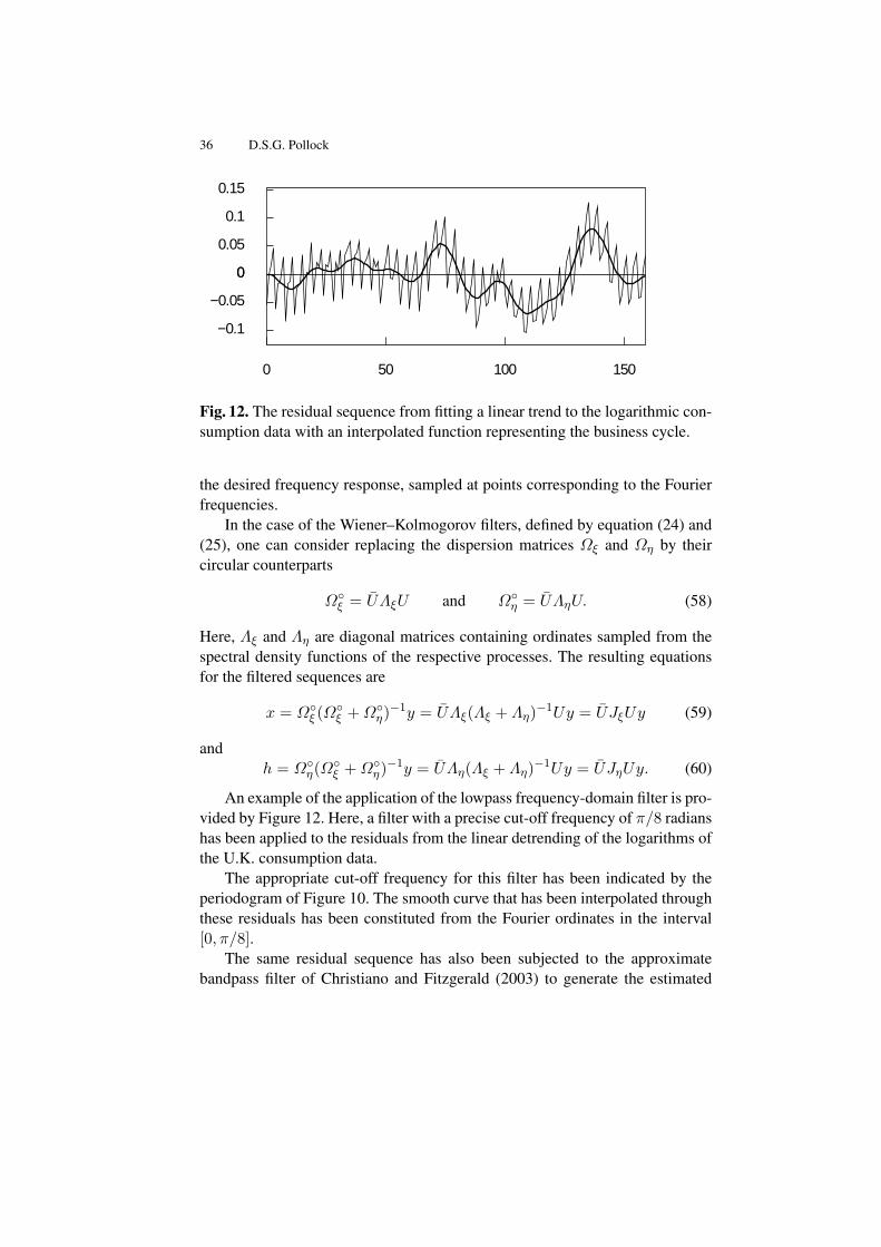
Fig. 12. The residual sequence from fitting a linear trend to the logarithmic con-sumption data with an interpolated function representing the business cycle.
the desired frequency response, sampled at points corresponding to the Fourierfrequencies.
In the case of the Wiener–Kolmogorov filters, defined by equation (24) and(25), one can consider replacing the dispersion matrices Ωξ and Ωη by theircircular counterparts
Ωξ = UΛξU and Ωη = UΛηU. (58)
Here, Λξ and Λη are diagonal matrices containing ordinates sampled from thespectral density functions of the respective processes. The resulting equationsfor the filtered sequences are
x = Ωξ (Ωξ +Ωη)−1y = UΛξ(Λξ + Λη)−1Uy = UJξUy (59)
andh = Ωη(Ωξ +Ωη)−1y = UΛη(Λξ + Λη)−1Uy = UJηUy. (60)
An example of the application of the lowpass frequency-domain filter is pro-vided by Figure 12. Here, a filter with a precise cut-off frequency of π/8 radianshas been applied to the residuals from the linear detrending of the logarithms ofthe U.K. consumption data.
The appropriate cut-off frequency for this filter has been indicated by theperiodogram of Figure 10. The smooth curve that has been interpolated throughthese residuals has been constituted from the Fourier ordinates in the interval[0, π/8].
The same residual sequence has also been subjected to the approximatebandpass filter of Christiano and Fitzgerald (2003) to generate the estimated

IDEOLOG—A Filtering Program 37
business cycle of Figure 4. This estimate fails to capture some of the salientlow-frequency fluctuations of the data.
The highlighted region Figure 10 also show the extent of the pass band ofthe bandpass filter; and it appears that the low-frequency structure of the datafalls mainly below this band. The fact that, nevertheless, the filter of Christianoand Fitzgerald does reflect a small proportion of the low-frequency fluctuationsis due to its substantial leakage over the interval [0, π/16], which falls within itsnominal stop band.
5.2 Extrapolations and Detrending
To apply the frequency-domain filtering methods, the data must be free of trend.The detrending can be achieved either by differencing the data or by applyingthe filter to data that are residuals from fitting a polynomial trend. The programhas a facility for fitting a polynomial time trend of a degree not exceeding 15.To avoid the problems of collinearity that arise in fitting ordinary polynomialsspecified in terms of the powers of the temporal index t, a flexible generalisedleast-squares procedure is provided that depends upon a system of orthogonalpolynomials.
In applying the methods, it is also important to ensure that there are nosignificant disjunctions in the periodic extension of the data at the points wherethe end of one replication of the sample sequence joins the beginning of thenext replication. Equivalently, there must be a smooth transition between thestart and finish points when the sequence of T data points is wrapped around acircle of circumference T .
The conventional means of avoiding such disjunctions is to taper the mean-adjusted, detrended data sequence so that both ends decay to zero. (See Bloom-field 1976, for example.) The disadvantage of this recourse is that it falsifies thedata at the ends of the sequence, which is particularly inconvenient if, as is oftenthe case in economics, attention is focussed on the most recent data. To avoidthis difficulty, the tapering can be applied to some extrapolations, which can beadded to the data, either before or after it has been detrended.
In the first case, a polynomial is fitted to the data; and tapered versionsof the residual sequence that have been reflected around the endpoints of thesample are added to the extrapolated branches of the polynomial. Alternatively,if the data show strong seasonal fluctuations, then a tapered sequence basedon successive repetitions of the ultimate seasonal cycle is added to the upperbranch, and a similar sequence based on the first cycle is added to the lowerbranch.
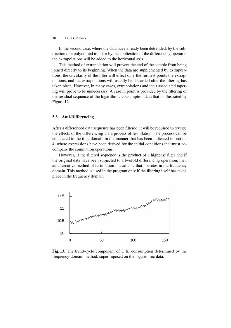
38 D.S.G. Pollock
In the second case, where the data have already been detrended, by the sub-traction of a polynomial trend or by the application of the differencing operator,the extrapolations will be added to the horizontal axis.
This method of extrapolation will prevent the end of the sample from beingjoined directly to its beginning. When the data are supplemented by extrapola-tions, the circularity of the filter will effect only the furthest points the extrap-olations, and the extrapolations will usually be discarded after the filtering hastaken place. However, in many cases, extrapolations and their associated taper-ing will prove to be unnecessary. A case in point is provided by the filtering ofthe residual sequence of the logarithmic consumption data that is illustrated byFigure 12.
5.3 Anti-Differencing
After a differenced data sequence has been filtered, it will be required to reversethe effects of the differencing via a process of re-inflation. The process can beconducted in the time domain in the manner that has been indicated in section4, where expressions have been derived for the initial conditions that must ac-company the summation operations.
However, if the filtered sequence is the product of a highpass filter and ifthe original data have been subjected to a twofold differencing operation, thenan alternative method of re-inflation is available that operates in the frequencydomain. This method is used in the program only if the filtering itself has takenplace in the frequency domain.
10
10.5
11
11.5
0 50 100 150
Fig. 13. The trend-cycle component of U.K. consumption determined by thefrequency-domain method, superimposed on the logarithmic data.
IDEOLOG—A Filtering Program 39
In that case, the reduction to stationarity will be by virtue of a centralisedtwofold differencing operator of the form
(1− z−1)(1− z) = −z∇2(z) (61)
The frequency-response function of the operator, which is obtained by settingz = exp−iω in this equation, is
f(ω) = 2− 2 cos(ω). (62)
The frequency response of the anti-differencing operator is v(ω) = 1/f(ω).The matrix version of the centralised operator can be illustrated by the case
where T = 5:
N5 =
n′0
−Q′
n′4
= −
−2 1 0 0 0
1 −2 1 0 00 1 −2 1 00 0 1 −2 10 0 0 1 −2
. (63)
In applying this operator to the data, the first and the last elements of NT y,which are denoted by n′0y and n′T−1y, respectively, are not true differences.Therefore, they are discarded to leave −Q′y = [q1, . . . , qT−2]′. To compensatefor this loss, appropriate values are attributed to q0 and qT−1, which are formedfrom combinations of the adjacent values, to create a vector of order T denotedby q = [q0, q1, . . . , qT−2, qT−1]′.
The highpass filtering of the data comprises the following steps. First, thevector q is translated to the frequency domain to give γ = Uq. Then, thefrequency-response matrix Jη is applied to the resulting Fourier ordinates. Next,in order to compensate for the effects of differencing, the vector of Fourierordinates is premultiplied by a diagonal matrix V = diagv0, v1, . . . , vT−1,wherein vj = 1/f(ωj); j = 0, . . . , T − 1, with ωj = 2πj/T . Finally, the resultis translated back to the time domain to create the vector h.
The vector of the complementary component is x = y − h. Thus there are
h = UHηUq and x = y − UHηUq, (64)
where Hη = V Jη. It should be noted that the technique of re-inflating thedata within the frequency domain cannot be applied in the case of a lowpasscomponent for the reason that f(0) = 0 and, therefore, the function v(ω) =1/f(ω) is unbounded at the zero frequency ω = 0. However, as the aboveequations indicate, this is no impediment to the estimation of the correspondingcomponent x.
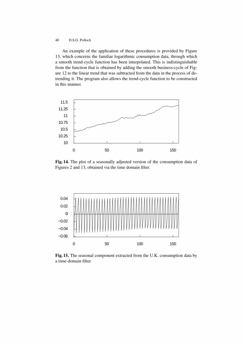
40 D.S.G. Pollock
An example of the application of these procedures is provided by Figure13, which concerns the familiar logarithmic consumption data, through whicha smooth trend-cycle function has been interpolated. This is indistinguishablefrom the function that is obtained by adding the smooth business-cycle of Fig-ure 12 to the linear trend that was subtracted from the data in the process of de-trending it. The program also allows the trend-cycle function to be constructedin this manner.
10
10.25
10.5
10.75
11
11.25
11.5
0 50 100 150
Fig. 14. The plot of a seasonally adjusted version of the consumption data ofFigures 2 and 13, obtained via the time domain filter.
0
0.02
0.04
0
−0.02
−0.04
−0.06
0 50 100 150
Fig. 15. The seasonal component extracted from the U.K. consumption data bya time-domain filter.
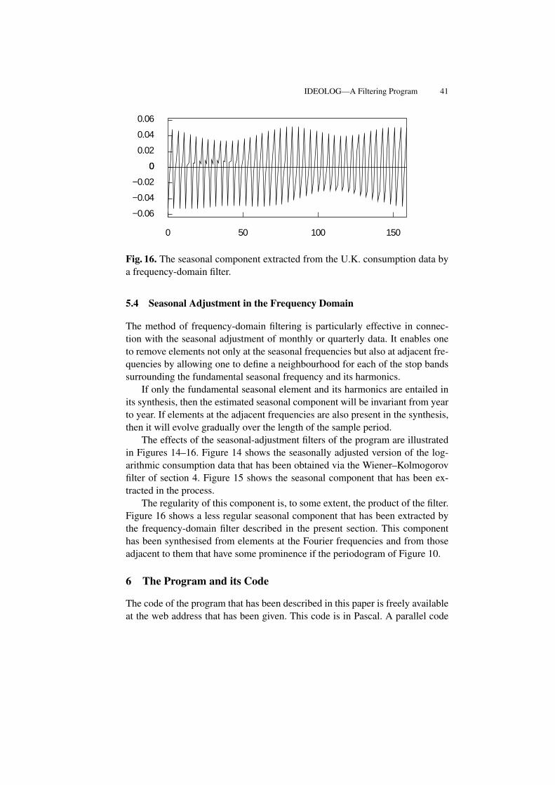
IDEOLOG—A Filtering Program 41
0
0.02
0.04
0.06
0
−0.02
−0.04
−0.06
0 50 100 150
Fig. 16. The seasonal component extracted from the U.K. consumption data bya frequency-domain filter.
5.4 Seasonal Adjustment in the Frequency Domain
The method of frequency-domain filtering is particularly effective in connec-tion with the seasonal adjustment of monthly or quarterly data. It enables oneto remove elements not only at the seasonal frequencies but also at adjacent fre-quencies by allowing one to define a neighbourhood for each of the stop bandssurrounding the fundamental seasonal frequency and its harmonics.
If only the fundamental seasonal element and its harmonics are entailed inits synthesis, then the estimated seasonal component will be invariant from yearto year. If elements at the adjacent frequencies are also present in the synthesis,then it will evolve gradually over the length of the sample period.
The effects of the seasonal-adjustment filters of the program are illustratedin Figures 14–16. Figure 14 shows the seasonally adjusted version of the log-arithmic consumption data that has been obtained via the Wiener–Kolmogorovfilter of section 4. Figure 15 shows the seasonal component that has been ex-tracted in the process.
The regularity of this component is, to some extent, the product of the filter.Figure 16 shows a less regular seasonal component that has been extracted bythe frequency-domain filter described in the present section. This componenthas been synthesised from elements at the Fourier frequencies and from thoseadjacent to them that have some prominence if the periodogram of Figure 10.
6 The Program and its Code
The code of the program that has been described in this paper is freely availableat the web address that has been given. This code is in Pascal. A parallel code

42 D.S.G. Pollock
in C has been generated with the help of a Pascal-to-C translator, which hasbeen written by the author. The aim has been to make the program platform-independent and to enable parts of it to be realised in other environments.
This objective has dictated some of the features of the user interface of theprogram, which, in its present form, eschews such devices as pull-down menusand dialogue boxes etc. Subsequent versions of the program will make limiteduse of such enhancements.
However, the nostrum that a modern computer program should have a mod-eless interface will be resisted. Whereas such an interface is necessary for pro-grams such as word processors, where all of the functions should be accessibleat all times, it is less appropriate to statistical programs where, in most circum-stances, the user will face a restricted set of options. Indeed, the present programis designed to restrict the options, at each stage of the operations, to those thatare relevant.
A consequence of this design is that there is no need of a manual of instruc-tions to accompany the program. Instead, the three log files that record the stepstaken in filtering some typical data sequences should provide enough help to getthe user underway. What is more important is that the user should understandthe nature of the statistical procedures that have been implemented; and this hasbeen the purpose of the present paper.

Bibliography
[1] Baxter, M., and R.G. King, (1999). Measuring Business Cycles: Approxi-mate Band-Pass Filters for Economic Time Series. Review of Economics andStatistics, 81, 575–593.
[2] Bloomfield, P., (1976). Fourier Analysis of Time Series: An Introduction.John Wiley and Sons, New York.
[3] Butterworth, S., (1930). On the Theory of Filter Amplifiers. The WirelessEngineer (From 1923 to 1930, the journal was called Experimental Wirelessand the Radio Engineer), 7, 536–541.
[4] Christiano, L.J. and T.J. Fitzgerald, (2003). The Band-pass Filter. Interna-tional Economic Review, 44, 435–465.
[5] Henderson, R., (1916). Note on Graduation by Adjusted Average. Transac-tions of the Actuarial Society of America, 17, 43–48.
[6] Henderson, R., (1924). A New Method of Graduation. Transactions of theActuarial Society of America, 25, 29–40.
[7] Hodrick, R.J., and E.C. Prescott, (1980). Postwar U.S. Business Cycles: AnEmpirical Investigation, Working Paper, Carnegie–Mellon University, Pitts-burgh, Pennsylvania.
[8] Hodrick, R.J., and E.C. Prescott, (1997). Postwar U.S. Business Cycles: AnEmpirical Investigation. Journal of Money, Credit and Banking, 29, 1–16.
[9] Ladiray, D., and B. Quenneville, (2001). Seasonal Adjustment with the X-11Method, Springer Lecture Notes in Statistics 158, Springer Verlag, Berlin.
[10] Leser, C.E.V. (1961). A Simple Method of Trend Construction. Journal ofthe Royal Statistical Society, Series B, 23, 91–107.
[11] Musgrave, J. (1964). A Set of End Weights to End all End Weights, WorkingPaper, US Bureau of the Census, Washington
[12] Pollock, D.S.G., (2000). Trend Estimation and De-Trending via RationalSquare Wave Filters. Journal of Econometrics, 99, 317–334.
[13] Pollock, D.S.G., (2007). Wiener–Kolmogorov Filtering, Frequency-Selective Filtering and Polynomial Regression. Econometric Theory, 23, 71–83.
[14] Pollock, D.S.G., (2008). Investigating Economic Trends and Cycles, inPalgrave Handbook of Econometrics: Vol. 2 Applied Econometrics, T.C.Mills and K. Patterson (editors). Palgrave Macmillan Ltd, Houndmills, Bas-ingstoke.
[15] Quenneville, B., D. Ladiray and B. Lefranc, (2003). A Note on MusgraveAsymmetrical Trend-cycle Filters. International Journal of Forecasting, 19,727–734.

44 D.S.G. Pollock
[16] Whittle, P., (1983). Prediction and Regulation by Linear Least-SquareMethods, Second Edition, Basil Blackwell, Oxford.
Who Uses gretl? An Analysis of the SourceForgeDownload Data
Riccardo (Jack) Lucchetti
Dipartimento di Economia - Università Politecnica delle Marche - Ancona, [email protected]
Abstract. This paper analyses the SourceForge download data to infer somecharacteristics of the population of gretl users. The rising number of downloadsindicates Gretl’s strong popularity as a teaching tool; however, despite the vastimprovements in its features and performance, gretl’s perceived status as a com-putational platform for research does not seem to be firmly established as yet,although this may change in the medium-long run.
1 Introduction
In the past few years, gretl has undoubtably come a long way in terms of fea-tures: thanks to constant feedback by a loyal user base and, most importantly,to Allin Cottrell’s incredible committment and outstanding productivity, whatused to be considered little more than a toy package now comprises a rangeof features which equal, and in some cases surpass, those found in commercialstatistical programs. For example, the scope and efficiency of the routines forestimating GARCH-like models written for gretl by Balietti [2] are unrivalledby any other free software package.
The question I ask myself in this paper is: how has the gretl userbase evolvedin response to the new features and the overall increase in usability of the pack-age? In order to provide an answer, I will analyse the download data fromSourceForge.
2 The SourceForge data
SourceForge is arguably the largest and most important hosting site for FreeSoftware projects. It currently hosts tens of thousands of projects, among whichhugely successful ones such as eMule and 7-zip.
Gretl ranks, at present, about 930th for number of total downloads, whichamounts to about 300,000. However, it must be stressed that the number ofdownloads may not match the number of users for several reasons:
– The total number of downloads refers to all versions; a user who installed10 versions of gretl on a computer counts as 10 downloads;
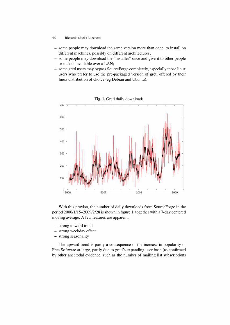
46 Riccardo (Jack) Lucchetti
– some people may download the same version more than once, to install ondifferent machines, possibly on different architectures;
– some people may download the “installer” once and give it to other peopleor make it available over a LAN;
– some gretl users may bypass SourceForge completely, especially those linuxusers who prefer to use the pre-packaged version of gretl offered by theirlinux distribution of choice (eg Debian and Ubuntu).
Fig. 1. Gretl daily downloads
With this proviso, the number of daily downloads from SourceForge in theperiod 2006/1/15–2009/2/28 is shown in figure 1, together with a 7-day centeredmoving average. A few features are apparent:
– strong upward trend– strong weekday effect– strong seasonality
The upward trend is partly a consequence of the increase in popularity ofFree Software at large, partly due to gretl’s expanding user base (as confirmedby other anectodal evidence, such as the number of mailing list subscriptions
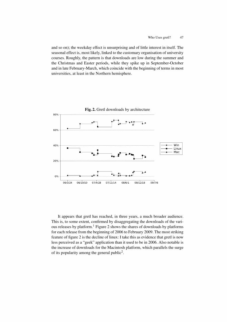
Who Uses gretl? 47
and so on); the weekday effect is unsurprising and of little interest in itself. Theseasonal effect is, most likely, linked to the customary organisation of universitycourses. Roughly, the pattern is that downloads are low during the summer andthe Christmas and Easter periods, while they spike up in September-Octoberand in late February-March, which coincide with the beginning of terms in mostuniversities, at least in the Northern hemisphere.
Fig. 2. Gretl downloads by architecture
It appears that gretl has reached, in three years, a much broader audience.This is, to some extent, confirmed by disaggregating the downloads of the vari-ous releases by platform.1 Figure 2 shows the shares of downloads by platformsfor each release from the beginning of 2006 to February 2009. The most strikingfeature of figure 2 is the decline of linux: I take this as evidence that gretl is nowless perceived as a “geek” application than it used to be in 2006. Also notable isthe increase of downloads for the Macintosh platform, which parallels the surgeof its popularity among the general public2.
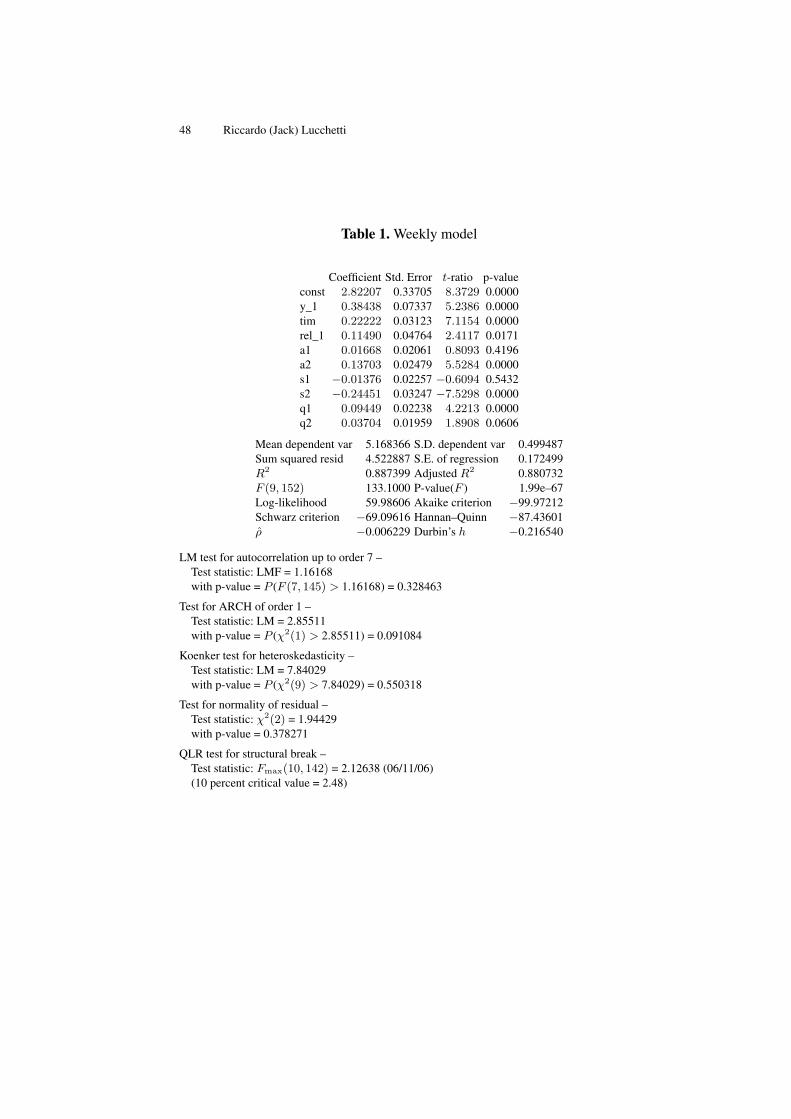
48 Riccardo (Jack) Lucchetti
Table 1. Weekly model
Coefficient Std. Error t-ratio p-valueconst 2.82207 0.33705 8.3729 0.0000y_1 0.38438 0.07337 5.2386 0.0000tim 0.22222 0.03123 7.1154 0.0000rel_1 0.11490 0.04764 2.4117 0.0171a1 0.01668 0.02061 0.8093 0.4196a2 0.13703 0.02479 5.5284 0.0000s1 −0.01376 0.02257 −0.6094 0.5432s2 −0.24451 0.03247 −7.5298 0.0000q1 0.09449 0.02238 4.2213 0.0000q2 0.03704 0.01959 1.8908 0.0606
Mean dependent var 5.168366 S.D. dependent var 0.499487Sum squared resid 4.522887 S.E. of regression 0.172499R2 0.887399 Adjusted R2 0.880732F (9, 152) 133.1000 P-value(F ) 1.99e–67Log-likelihood 59.98606 Akaike criterion −99.97212Schwarz criterion −69.09616 Hannan–Quinn −87.43601ρ −0.006229 Durbin’s h −0.216540
LM test for autocorrelation up to order 7 –Test statistic: LMF = 1.16168with p-value = P (F (7, 145) > 1.16168) = 0.328463
Test for ARCH of order 1 –Test statistic: LM = 2.85511with p-value = P (χ2(1) > 2.85511) = 0.091084
Koenker test for heteroskedasticity –Test statistic: LM = 7.84029with p-value = P (χ2(9) > 7.84029) = 0.550318
Test for normality of residual –Test statistic: χ2(2) = 1.94429with p-value = 0.378271
QLR test for structural break –Test statistic: Fmax(10, 142) = 2.12638 (06/11/06)(10 percent critical value = 2.48)
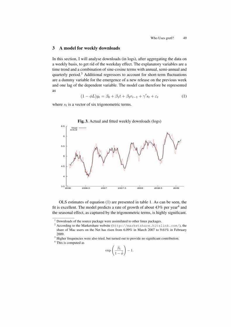
Who Uses gretl? 49
3 A model for weekly downloads
In this section, I will analyse downloads (in logs), after aggregating the data ona weekly basis, to get rid of the weekday effect. The explanatory variables are atime trend and a combination of sine-cosine terms with annual, semi-annual andquarterly period.3 Additional regressors to account for short-term fluctuationsare a dummy variable for the emergence of a new release on the previous weekand one lag of the dependent variable. The model can therefore be representedas
(1− φL)yt = β0 + β1t+ β2rt−1 + γ′st + εt (1)
where st is a vector of six trigonometric terms.
Fig. 3. Actual and fitted weekly downloads (logs)
OLS estimates of equation (1) are presented in table 1. As can be seen, thefit is excellent. The model predicts a rate of growth of about 43% per year4 andthe seasonal effect, as captured by the trigonometric terms, is highly significant.
1 Downloads of the source package were assimilated to other linux packages.2 According to the Marketshare website (http://marketshare.hitslink.com/), the
share of Mac users on the Net has risen from 6.09% in March 2007 to 9.61% in February2009.
3 Higher frequencies were also tried, but turned out to provide no significant contribution.4 This is computed as
exp
β1
1− φ
!− 1.
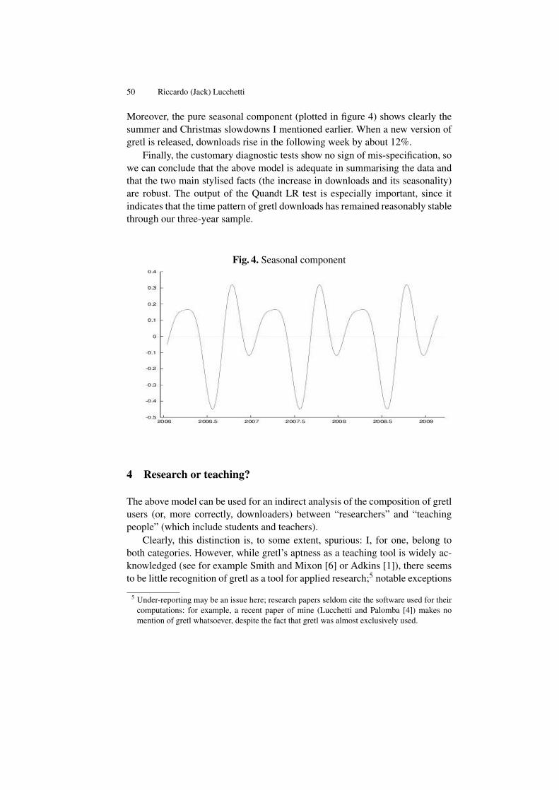
50 Riccardo (Jack) Lucchetti
Moreover, the pure seasonal component (plotted in figure 4) shows clearly thesummer and Christmas slowdowns I mentioned earlier. When a new version ofgretl is released, downloads rise in the following week by about 12%.
Finally, the customary diagnostic tests show no sign of mis-specification, sowe can conclude that the above model is adequate in summarising the data andthat the two main stylised facts (the increase in downloads and its seasonality)are robust. The output of the Quandt LR test is especially important, since itindicates that the time pattern of gretl downloads has remained reasonably stablethrough our three-year sample.
Fig. 4. Seasonal component
4 Research or teaching?
The above model can be used for an indirect analysis of the composition of gretlusers (or, more correctly, downloaders) between “researchers” and “teachingpeople” (which include students and teachers).
Clearly, this distinction is, to some extent, spurious: I, for one, belong toboth categories. However, while gretl’s aptness as a teaching tool is widely ac-knowledged (see for example Smith and Mixon [6] or Adkins [1]), there seemsto be little recognition of gretl as a tool for applied research;5 notable exceptions
5 Under-reporting may be an issue here; research papers seldom cite the software used for theircomputations: for example, a recent paper of mine (Lucchetti and Palomba [4]) makes nomention of gretl whatsoever, despite the fact that gretl was almost exclusively used.

Who Uses gretl? 51
are Yalta and Yalta [7] (now slightly dated) and Rosenblad [5], who discussesgretl as a teaching tool but also highlights its potential for research use.
In my opinion, the composition of gretl’s user base is of crucial importancefor shaping gretl’s future: people from the “teaching” community provide in-valuable feedback and motivation to keep improving gretl’s already excellentuser interface. On the other hand, gretl’s computing accuracy, scope and effi-ciency are put to the test (and pushed forward accordingly) primarily by thosewho use it for “real” applied statistical tasks. Moreover, if a true community ofcoders is to emerge, it is more likely that new coders come from the ranks ofyoung, computer-literate researchers.6 Therefore, it is important to ascertain thecomposition of gretl’s user base if one wants to forecast, and possibly steer, theevolution of gretl as a computing platform.
Of course, a few assumptions are necessary here: I assume (a) that researchactivity is not seasonal and (b) that the share of “researchers” is a linear functionof time. Needless to say, both hypotheses are a bit strong; we all have holidaysin the summer and even atheists take a Christmas break. On the other hand, mostof us do take advantage of periods when classes stop, to work on our researchpapers.
However, assumption (b) should be also only viewed as an approximation,meant to capture the overall trend, rather than a hard-edged fact and is in itselfrather innocuous. As an indirect confirmation of assumption (a), I ran a simpleseasonality extraction procedure on monthly download data for four popularscientific applications7: apart from gretl, I used gnuplot (the data visualistiontool that gretl also uses), maxima (a computer algebra system) and the GNUOctave software repository (a collection of additional modules for GNU octave,a free Matlab replacement). All these are mature projects, which are certainlyused in teaching but also have a well-established reputation as research tools.
For each of these packages, the seasonality extraction routine is based on anOLS regression of the log of monthly downloads on a constant, one lag, a lineartrend and the six trigonometric variables used above. The seasonality componentis then reconstructed as the sum of each trigonometric variable weighted by itsown estimated coefficient. Results are plotted in figure 5: it should be obviousthat gretl’s seasonal component is much larger than the other packages’.
In the light of assumptions (a) and (b), equation (1) can be generalised viaa logistic smooth-transition regression model, similar in spirit to a STAR model
6 It is true, however, that having been exposed to gretl as a student may encourage a researcherto study the source code and contribute original ideas and code.
7 The source in all cases is, again, SourceForge. Unfortunately, I was unable to find downloaddata for the R statistical project, which is not hosted by SourceForge and would have beenextremely interesting to analyse.
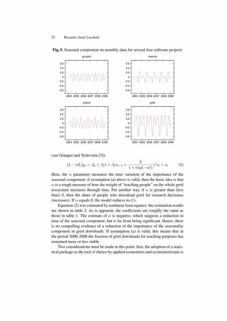
52 Riccardo (Jack) Lucchetti
Fig. 5. Seasonal component on monthly data for several free software projects
(see Granger and Teräsvirta [3]):
(1− φL)yt = β0 + β1t+ β2rt−1 +2
1 + exp(−αt)γ′st + εt (2)
Here, the α parameter measures the time variation of the importance of theseasonal component: if assumption (a) above is valid, then the basic idea is thatα is a rough measure of how the weight of “teaching people” on the whole gretlecosystem increases through time. Put another way, if α is greater than (lessthan) 0, then the share of people who download gretl for research decreases(increases). If α equals 0, the model reduces to (1).
Equation (2) was estimated by nonlinear least squares: the estimation resultsare shown in table 2. As is apparent, the coefficients are roughly the same asthose in table 1. The estimate of α is negative, which suggests a reduction intime of the seasonal component, but is far from being significant. Hence, thereis no compelling evidence of a reduction of the importance of the seasonalitycomponent in gretl downloads. If assumption (a) is valid, this means that inthe period 2006-2008 the fraction of gretl downloads for teaching purposes hasremained more or less stable.
Two considerations must be made at this point: first, the adoption of a statis-tical package as the tool of choice by applied economists and econometricians is

Who Uses gretl? 53
Table 2. Weekly nonlinear model
Estimate Std. Error t-ratio p-value
const 2.82425 0.33827 8.349 0.0000y_1 0.38382 0.07364 5.212 0.0000tim 0.11411 0.04787 2.384 0.0184rel_1 -0.22265 0.03134 -7.104 0.0000a1 0.01663 0.02139 0.778 0.4380a2 0.14188 0.02995 4.738 0.0000s1 -0.01456 0.02357 -0.618 0.5377s2 -0.25353 0.04499 -5.635 0.0000q1 0.09868 0.02715 3.634 0.0004q2 0.03803 0.02071 1.836 0.0683α -0.04465 0.14856 -0.301 0.7642
Mean dependent var 5.168366 S.D. dependent var 0.499487Sum squared resid 4.520373 S.E. of regression 0.173021R2 0.887462 Adjusted R2 0.880009Log-likelihood 60.03124 Akaike criterion −98.06221Schwarz criterion −64.09892 Hannan–Quinn −84.27276ρ −0.005810 Durbin–Watson 2.001861
a long process: path-dependence and acquired habits may cause people to stickto obsolete tools for years, so, even if assumptions (a) and (b) are valid, it mayjust be the case that the sample I am using here is simply too short to capturethis aspect adequately.
Moreover, the emergence of a community of gretl code contributors, well-versed in econometrics and programming at the same time, is unlikely to de-pend on the relative share of researchers on gretl’s total user base, but ratheron its absolute value. What counts is the number of “hackers” we have, not thepercentage of users who are. In this sense, the stability of the share of “researchpeople” on an increasing number of users allows us to be mildly optimistic.
5 Conclusions
Gretl has been so far a spectacular success story in terms of expansion of its userbase. Obviously, the characteristic of free software that most people perceiveas paramount (being “free as in beer”) played its role, but this factor does notexplain the whole story by itself: the Internet is full of gratis software whichfew people, if any, use. A large part of the merit goes to its intuitive and friendlyinterface, which makes it an ideal tool for teaching econometrics.

54 Riccardo (Jack) Lucchetti
On the other hand, gretl’s capabilities as a computing platform, which havealso evolved dramatically, seem to have been overlooked by most practitioners,although lack of evidence may simply be a consequence of the limited time spanof the data used here. Only time will tell gretl’s future reputation as a solid andreliable computing nad there are reasons for moderate optimism. In any case, itis vitally important for the gretl community to work to advertise gretl’s presentcapabilities to the widest possible audience and to work as hard as possible toextend and perfect them.

Bibliography
[1] ADKINS, L. (2009): Using gretl for Principles of Econometrics, 3rd edition.online.
[2] BALIETTI, S. (2008): “gig: a GARCH-like Implementation in Gretl,”Master’s thesis, Università Politecnica delle Marche.
[3] GRANGER, C. W., AND T. TERÄSVIRTA (1993): Modelling Nonlinear Eco-nomic Relationships. Oxford University Press.
[4] LUCCHETTI, R., AND G. PALOMBA (2009): “Nonlinear adjustment in USbond yields: An empirical model with conditional heteroskedasticity,” Eco-nomic Modelling, forthcoming.
[5] ROSENBLAD, A. (2008): “gret1 1.7.3,” Journal of Statistical Software, Soft-ware Reviews, 25(1), 1–14.
[6] SMITH, R. J., AND J. W. MIXON (2006): “Teaching undergraduate econo-metrics with GRETL,” Journal of Applied Econometrics, 21(7), 1103–1107.
[7] YALTA, A. T., AND A. Y. YALTA (2007): “GRETL 1.6.0 and its numericalaccuracy,” Journal of Applied Econometrics, 22(4), 849–854.


Econometric Theory

An Instrumental Variables Probit Estimator using gretl
Lee C. Adkins
Professor of Economics, Oklahoma State University, Stillwater, OK [email protected]
Abstract. The most widely used commercial software to estimate endogenousprobit models offers two choices: a computationally simple generalized leastsquares estimator and a maximum likelihood estimator. Adkins [1, 2] comparesthese estimators to several others in a Monte Carlo study and finds that the GLSestimator performs reasonably well in some circumstances. In this paper the smallsample properties of the various estimators are reviewed and a simple routine us-ing the gretl software is given that yields identical results to those produced byStata 10.1. The paper includes an example estimated using data on bank holdingcompanies.
1 Introduction
Yatchew and Griliches [19] analyze the effects of various kinds of misspecifi-cation on the probit model. Among the problems explored was that of errors-in-variables. In linear regression, a regressor measured with error causes leastsquares to be inconsistent and Yatchew and Griliches find similar results forprobit. Rivers and Vuong [14] and Smith and Blundell [16] suggest two-stageestimators for probit and tobit, respectively. The strategy is to model a con-tinuous endogenous regressor as a linear function of the exogenous regressorsand some instruments. Predicted values from this regression are then used inthe second stage probit or tobit. These two-step methods are not efficient, butare consistent. Consistent estimation of the standard errors is not specificallyconsidered and these estimators are used mainly to test for endogeneity of theregressors–not to establish their statistical significance.
Newey [12] looked at the more generic problem of endogeneity in limiteddependent variable models (which include probit and tobit). He proposed whatis sometimes called Amemiya’s Generalized Least Squares (AGLS) estimator asa way to efficiently estimate the parameters of probit or tobit when they includea continuous endogenous regressor. This has become one of the standard waysto estimate these models and is an option (twostep) in Stata 10.0 when the MLEis difficult to obtain. The main benefit of using this estimator is that it yieldsa consistent estimator of the variance-covariance matrix that and can easily beused for subsequent hypothesis tests about the parameters.

60 Lee C. Adkins
Adkins [1] compares the AGLS estimator to several alternatives, which in-clude a maximum likelihood estimator. The AGLS estimator is simple to com-pute and yields significance tests that are close in size to the nominal level whensamples are not very large (e.g., n=200). The other plug-in estimators are con-sistent for the parameters but not the standard errors, making it unlikely that theywill perform satisfactorily in hypothesis testing. The latter problem is taken upby Adkins [3] who uses a Murphy and Topel [11] correction to obtain consistentstandard errors with some success.
Others have explored limited dependent variable models that have discreteendogenous regressors. Nicoletti and Peracchi [13] look at binary response mod-els with sample selection, Kan and Kao [10] consider a simulation approach tomodeling discrete endogenous regressors, and Arendt and Holm [5] extendsNicoletti and Peracchi [13] to include multiple endogenous discrete variables.
Iwata [9] uses a very simple approach to dealing with errors-in-variables forprobit and tobit. He shows that simple recentering and rescaling of the observeddependent variable may restore consistency of the standard IV estimator if thetrue dependent variable and the IV’s are jointly normally distributed. His MonteCarlo simulation shows evidence that the joint normality may not be necessaryto obtain improved results. However, the results for tobit were quite a bit betterthan those for probit. He compares this estimator to a linear instrumental vari-able estimator that uses a consistent estimator of standard errors. This estimatoris considered by Adkins [1] in his comparison.
Blundell and Powell [6] develop and implement semiparametric methodsfor estimating binary dependent variable models that contain continuous en-dogenous regressors. Their paper “extends existing results on semiparametricestimation in single-index binary response models to the case of endogenousregressors. It develops an approach to account for endogeneity in triangular andfully simultaneous binary response models." Blundell and Powell [6], p. 655
In the following sections a linear model with continuous endogenous re-gressors and its estimators are considered. With respect to models having adichotomous dependent variable, a relatively simple generalized least squaresestimator discussed in Newey [12] is presented and an algorithm for its compu-tation in gretl is given. To give the reader an idea of how this estimator comparesto alternatives, including a maximum likelihood estimator (mle), some resultsfrom a simulation study conducted by Adkins [1, 2] are summarized. The re-sults from the gretl routine and from Stata 10 are compared using an examplefrom the banking literature.
An Instrumental Variables Probit Estimator using gretl 61
2 Linear Model and Estimators
Following the notation in Newey [12], consider a linear statistical model inwhich the continuous dependent variable will be called y∗t but it is not directlyobserved. Instead, we observe yt in only one of two possible states. So,
y∗t = Ytβ +X1tγ + ut = Ztδ + ut, t = 1, . . . , N (1)
where Zt = [Yt, X1t], δ′ = [β′, γ′], Yt is the tth observation on an endogenousexplanatory variable, X1t is a 1xs vector of exogenous explanatory variables,and δ is the qx1 vector of regression parameters.
The endogenous variable is related to a 1Xk vector of instrumental variablesXt by the equation
Yt = X1tΠ1 +X2tΠ2 + Vt = XtΠ + Vt (2)
where Vt is a disturbance. The k − s variables in X2t are additional exogenousexplanatory variables. Equation (2) is the reduced form equation for the endoge-nous explanatory variable. Without loss of generality only one endogenous ex-planatory variable is considered below. See Newey [12] for notation extendingthis to additional endogenous variables.
When the continuous variable y∗t is observed, then one could use either leastsquares or instrumental variable estimator to estimate δ. Collecting the n ob-servations into matrices y∗, X , and Z of which the tth row is y∗t , Xt, and Zt,respectively we have the least squares estimator of δ, δols = (ZTZ)−1ZT y∗,which is biased and inconsistent.
The instrumental variable estimator uses the orthogonal projection ofZ ontothe column space of X , i.e., PXZ where PX = X(XTX)−1XT . The IV esti-mator is
δliv = (ZTPXZ)−1ZTPXy∗. (3)
The (linear) instrumental variable estimator is biased in finite samples, but con-sistent. The heteroskedasticity robust estimator of covariance Davidson and MacK-innon [7], p. 335 is
ΣHCCME = (ZTPXZ)−1ZTPX ΦPXZ(ZTPXZ)−1 (4)
where Φ is an nxn diagonal matrix with the tth diagonal element equal to u2t ,
the squared IV residual.
62 Lee C. Adkins
3 Binary Choice Model and Estimators
In some cases, y∗t is not directly observed. Instead, we observe
yt =
1 y∗t > 00 otherwise
(5)
Assuming the errors of the model (1) are normally distributed leads to the probitmodel.
3.1 Linear, MLE, and Plug-in
There are several estimators of this model, some consistent for δ and others not.The first is least squares. The least squares estimator δols = (ZTZ)−1ZT y∗ isconsistent if Z is exogenous. If any of the elements of Z are endogenous then itis not. Still, it is easy to compute and the degree of inconsistency may be smallin certain circumstances.
The linear instrumental variable estimator (3) is also inconsistent and het-eroscedastic. Iwata [9] suggests a means of rescaling and recentering (RR) thedata that can bring about consistency in this case. However, in his Monte Carlothe RR versions of OLS and IV estimation don’t perform particularly well forprobit (although much better for tobit).
The usual probit mle can be used to estimate the parameters. However, whenany of the regressors are endogenous, then this estimator is also inconsistent(Yatchew and Griliches [19]). To develop the notation, let the probability that ytis equal one be denoted
pr(yt = 1) = Φ(yt, Ytβ +X1tγ) = Φ(yt, Ztδ) (6)
where Φ is the normal cumulative density, yt is the observed binary dependentvariable, and Ytβ + X1tγ is the (unnormalized) index function. As usual, themodel is normalized assuming σ2 = 1. Basically, this equation implies that Yt,and X1t be included as regressors in the probit model and the log likelihoodfunction is maximized with respect to δT = [βT , γT ]. Since the endogeneity ofYt is ignored, the mle is inconsistent.
Another estimator uses predicted values of Yt from a first stage least squaresestimation of equation (2). Denote the first stage as Yt = X1tΠ1 + X2tΠ2 =
XtΠ where Xt = [X1t...X2t] and ΠT = [ΠT
1
...ΠT2 ]. Then the conditional proba-
bilitypr(yt = 1) = Φ(yt, Ztδ) (7)
An Instrumental Variables Probit Estimator using gretl 63
with Zt = [Yt...X1t]. The parameters are found by maximizing the conditional
likelihood. This is referred to here as IV probit (IVP). Although IVP is consis-tent for δ the standard errors estimated as the outer product of the gradient arenot. This can be easily remedied using a Murphy and Topel [11] type correction.
Another estimator adds the least squares residuals from equation (2), Vt =Yt −XtΠ to (7). This brings
pr(yt = 1) = Φ(yt, Ytβ +X1tγ + Vtλ) = Φ(yt, Ztδ + Vtλ) (8)
which is estimated by maximum likelihood, again conditional on Π . This issimilar to an estimator used by Rivers and Vuong [14] which takes the form
pr(yt = 1) = Φ(yt, Ztδ + Vtρ) (9)
The parameter ρ is related to λ in (8) by λ = ρ + β. This follows becauseZtδ = Ztδ + Vtβ. This estimator is useful for testing endogeneity, but seldomused to estimate δ.
3.2 AGLS
An efficient alternative to (8), proposed by Newey [12], and credited to Amemiya,is a generalized least squares estimator (AGLS). The AGLS estimator of theendogenous probit model is fairly easy to compute, though there are severalsteps–more than the two suggested by the name of its option in Stata. The basicalgorithm proceeds as follows:
1. Estimate the reduced form (2), saving the estimated residuals, Vt and pre-dicted values Yt.
2. Estimate the parameters of a reduced form equation for the probit modelusing the mle. In this case,
pr(yt = 1) = Φ(yt, Xtα+ Vtλ) (10)
Note that all exogenous variables, X1t and instruments X2t are used in theprobit reduced form and the parameters on these variables is labeled α. Letthe mle be denoted α. Also, save the portion of the estimated covariancematrix that corresponds to α, calling it J−1
αα .3. Another probit model is estimated by maximum likelihood. In this case it is
the 2SIV estimator of equation (8). Save ρ = λ− β which is the coefficientof Vt minus that of Yt.
4. Multiply ρYt and regress this on Xt using least squares. Save the estimatedcovariance matrix from this, calling it Σ.

64 Lee C. Adkins
5. Combine the last two steps into a matrix, Ω = J−1αα + Σ.
6. Then, the AGLS estimator is
δA = [D(Π)TΩ−1D(Π)]−1D(Π)TΩ−1α (11)
The estimated variance covariance is [D(Π)TΩ−1D(Π)]−1 and D(Π) =
[Π...I1] where I1 is a kxs selection matrix such that X1t = XtI1.
The AGLS estimator is one of the options available in Stata 10 (the other isan mle). Adkins [2, 1] conducts a Monte Carlo simulation to compare the biasof each of these estimators as well as the size of nominal 10% significance testof model parameter. He finds that in some circumstances the AGLS estimatorperforms reasonably well and can be used successfully to test for significance,especially if the sample is small and the instruments not very strong. The mainfindings of Adkins [1] are reproduced in the next section.
4 Summary of Simulation Results from Adkins (2008)
The main results of Adkins [1] can be summarized as follows:
1. When there is no endogeneity, OLS and Probit work well (as expected). Biasis very small and tests have the desired size.
2. It is clear that OLS and Probit should be avoided when you have an endoge-nous regressor. Both estimators are significantly biased and significancetests do not have the desired size.
3. Weak instruments increases the bias of AGLS. The bias worsens as thecorrelation between the endogenous regressor and the equation’s error in-creases.
4. The actual size of a parameter significance test based on the instrumentalvariable probit is reasonably close to the nominal level in nearly every in-stance. This is surprising for at least two reasons. 1) The bias of IVP issubstantial when instruments are weak. 2) The test statistic is based on aninconsistent estimator of the standard error. No attempt was made to esti-mate the covariance of this estimator consistently, as is done in Limdep 9Greene [8]. This is explored further in Adkins [3] who uses a Murphy andTopel [11] correction to obtain consistent standard errors.
5. The size of the significance tests based on the AGLS estimator is also rea-sonable, but the actual size is larger than the nominal size–a situation thatgets worse as severity of the endogeneity problem increases. When instru-ments are very weak, the actual test rejects a true null hypothesis twice asoften as it should.

An Instrumental Variables Probit Estimator using gretl 65
6. Linear instrumental variables estimators that use consistent estimators ofstandard errors can be used for this purpose (significance testing) thoughtheir performance is not quite up to that of the AGLS estimator. The LinearIV estimator performs better when the model is just identified.
7. There is an improvement in bias and the size of the significance test whensamples are larger (n=1000). Mainly, smaller samples (n=200) require strongerinstruments in order for bias to be small and tests to work properly (otherthan IVP, which as mentioned above, works fairly well all the time).
8. There is little to be gained by pretesting for endogeneity. When instrumentsare extremely weak it is outperformed by the other estimators considered,except when the no endogeneity hypothesis is true (and probit should beused). Bias is reduced by small amounts, but it is uncertain what one woulduse as an estimator of standard errors for a subsequent t-test.
9. When instruments are weak, t-tests based on ML are no better than onesbased on AGLS (in fact, one could argue that they are worse). Significancetesting based on the ML estimator is much more reliable in large samples.
The picture that emerges from this is that the AGLS estimator may be usefulwhen the sample is relatively small and the instruments not very strong. It isalso useful when the mle cannot be computed–a situation which limited thesimulations conducted by Adkins [1, 2]. Given the usefulness of the AGLSestimator, a gretl script is provided to compute is and its standard errors. Thescript is provided below in section 6. In the next section, a brief example isgiven the results from Stata 10 and the gretl script are compared.
5 Example
In this section a brief example based on Adkins et al. [4] is presented and theresults from Stata and gretl compared.
The main goal of Adkins et al. [4] was to determine whether managerialincentives affect the use of foreign exchange derivatives by bank holding com-panies (BHC). There was some speculation that several of the variables in themodel were endogenous. The dependent variable of interest is an indicator vari-able that takes the value 1 if the BHC uses foreign exchange derivative. Theindependent variables are as follows:
Ownership by Insiders When managers have a higher ownership position inthe bank, their incentives are more closely aligned with shareholders so theyhave an incentive to take risk to increase the value of the call option associ-ated with equity ownership. This suggests that a higher ownership position by

66 Lee C. Adkins
insiders (officers and directors) results in less hedging. The natural logarithmof the percentage of the total shares outstanding that are owned by officers anddirectors is used as the independent variable.
Ownership by Institutional Blockholders Institutional blockholders have in-centive to monitor the firm’s management due to the large ownership stake theyhave in the firm (Shleifer and Vishny [15]). Whidbee and Wohar [18] argue thatthese investors will have imperfect information and will most likely be con-cerned about the bottom line performance of the firm. The natural logarithm ofthe percentage of the total shares outstanding that are owned by all institutionalinvestors is included as an independent variable and predict that the sign will bepositive, with respect to the likelihood of hedging.
CEO Compensation CEO compensation also provides its own incentives withrespect to risk management. In particular, compensation with more option-likefeatures induces management to take on more risk to increase the value of theoption (Smith and Blundell [16]; Tufano [17]). Thus, higher options compensa-tion for managers results in less hedging. Two measures of CEO compensationare used: 1) annual cash bonus and 2) value of option awards.
There is a possibility that CEO compensation is endogenous in that success-ful hedging activity could in turn lead to higher executive compensation. Theinstruments used for the compensation variables are based on the executive’shuman capital (age and experience), and the size and scope of the firm (num-ber of employees, number of offices and subsidiaries). These are expected to becorrelated with the CEOs compensation and be predetermined with respect tothe BHCs foreign exchange hedging activities.
BHC Size The natural logarithm of total assets is used to control for the size ofthe BHC.
Capital The ratio of equity capital to total assets is included as a control vari-able. The variable for dividends paid measures the amount of earnings that arepaid out to shareholders. The higher the variable, the lower the capital positionof the BHC. The dividends paid variable is expected to have a sign opposite thatof the leverage ratio.
Like the compensation variables, leverage should be endogenously deter-mined. Firms that hedge can take on more debt and thus have higher leverage,other things equal.

An Instrumental Variables Probit Estimator using gretl 67
Foreign Exchange Risk A bank’s use of currency derivatives should be relatedto its exposure to foreign exchange rate fluctuations. The ratio of interest incomefrom foreign sources to total interest income measures foreign exchange expo-sure. Greater exposure, as represented by a larger proportion of income beingderived from foreign sources, should be positively related to both the likelihoodand extent of currency derivative use.
Profitability The return on equity is included to represent the profitability ofthe BHCs. It is used as a control.
5.1 Results
In this section the results of estimation are reported. Table 1 contains some im-portant results from the reduced form equations. Due to the endogeneity ofleverage and the CEO compensation variables, instrumental variables estima-tion is used to estimate the probability equations. Table 2 reports the coefficientestimates for the instrumental variable estimation of the probability that a BHCwill use foreign exchange derivatives for hedging. The first column of resultscorrespond to the Stata two-step estimator and the second column, gretl.
In Table 1 summary results from the reduced form are presented. The columnscontain p-values associated with the null hypothesis that the indicated instru-ment’s coefficient is zero in each of the four reduced form equations. The instru-ments include number of employees, number of subsidiaries, number of offices,CEO’s age–which proxies for his or her experience, the 12 month maturity mis-match, and the ratio of cash flows to total assets (CFA). The p-values associatedwith the other variables have been suppressed to conserve space.
Each of the instruments appears to be relevant in that each is significantlydifferent from zero at the 10% (p-value< 0.1) in at least one equation; the num-ber of employees, number of subsidiaries, and CEO age and CFA are significantin one equation; the number of offices, employees, subsidiaries are significantin two equations.
The overall strength of the instruments can be roughly gauged by looking atthe overall fit of the equations. The R2 in the leverage equation is the smallest(0.29), but is still high relative to the results of the Monte Carlo simulation. Theinstruments, other than the 12 month maturity mismatch, appear to be strongand we have no reason to expect poor performance from either the AGLS or themle in terms of bias.
The simulations from Adkins [1] suggest discarding extra instruments, andthis would be recommended here. Which to drop, other than the mismatch vari-able is unclear. CFA, Age, and subsidiaries are all strongly correlated with lever-
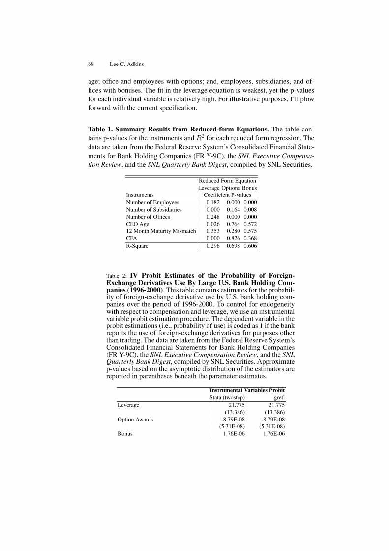
68 Lee C. Adkins
age; office and employees with options; and, employees, subsidiaries, and of-fices with bonuses. The fit in the leverage equation is weakest, yet the p-valuesfor each individual variable is relatively high. For illustrative purposes, I’ll plowforward with the current specification.
Table 1. Summary Results from Reduced-form Equations. The table con-tains p-values for the instruments and R2 for each reduced form regression. Thedata are taken from the Federal Reserve System’s Consolidated Financial State-ments for Bank Holding Companies (FR Y-9C), the SNL Executive Compensa-tion Review, and the SNL Quarterly Bank Digest, compiled by SNL Securities.
Reduced Form EquationLeverage Options Bonus
Instruments Coefficient P-valuesNumber of Employees 0.182 0.000 0.000Number of Subsidiaries 0.000 0.164 0.008Number of Offices 0.248 0.000 0.000CEO Age 0.026 0.764 0.57212 Month Maturity Mismatch 0.353 0.280 0.575CFA 0.000 0.826 0.368R-Square 0.296 0.698 0.606
Table 2: IV Probit Estimates of the Probability of Foreign-Exchange Derivatives Use By Large U.S. Bank Holding Com-panies (1996-2000). This table contains estimates for the probabil-ity of foreign-exchange derivative use by U.S. bank holding com-panies over the period of 1996-2000. To control for endogeneitywith respect to compensation and leverage, we use an instrumentalvariable probit estimation procedure. The dependent variable in theprobit estimations (i.e., probability of use) is coded as 1 if the bankreports the use of foreign-exchange derivatives for purposes otherthan trading. The data are taken from the Federal Reserve System’sConsolidated Financial Statements for Bank Holding Companies(FR Y-9C), the SNL Executive Compensation Review, and the SNLQuarterly Bank Digest, compiled by SNL Securities. Approximatep-values based on the asymptotic distribution of the estimators arereported in parentheses beneath the parameter estimates.
Instrumental Variables ProbitStata (twostep) gretl
Leverage 21.775 21.775(13.386) (13.386)
Option Awards -8.79E-08 -8.79E-08(5.31E-08) (5.31E-08)
Bonus 1.76E-06 1.76E-06
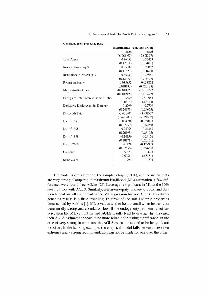
An Instrumental Variables Probit Estimator using gretl 69
Continued from preceding pageInstrumental Variables Probit
Stata gretl(8.88E-07) (8.88E-07)
Total Assets 0.36453 0.36453(0.17011) (0.17011)
Insider Ownership % 0.25882 0.25882(0.11623) (0.11623)
Institutional Ownership % 0.36981 0.36981(0.13477) (0.13477)
Return on Equity -0.033852 -0.033852(0.028188) (0.028188)
Market-to-Book ratio -0.0018722 -0.0018722(0.0012422 (0.0012422)
Foreign to Total Interest Income Ratio -3.5469 -3.546958(3.8414) (3.8414)
Derivative Dealer Activity Dummy -0.2799 -0.2799(0.24675) (0.24675)
Dividends Paid -8.43E-07 -8.43E-07(5.62E-07) (5.62E-07)
D=1 if 1997 -0.024098 -0.024098(0.27259) (0.27259)
D=1 if 1998 -0.24365 -0.24365(0.26195) (0.26195)
D=1 if 1999 -0.24156 -0.24156(0.28171) (0.28171)
D=1 if 2000 -0.128 -0.127999(0.27656) (0.27656)
Constant -9.673 -9.673(2.5351) (2.5351)
Sample size 794 794
The model is overidentified, the sample is large (700+), and the instrumentsare very strong. Compared to maximum likelihood (ML) estimation, a few dif-ferences were found (see Adkins [2]). Leverage is significant in ML at the 10%level, but not with AGLS. Similarly, return-on-equity, market-to-book, and div-idends paid are all significant in the ML regression but not AGLS. This diver-gence of results is a little troubling. In terms of the small sample propertiesdocumented by Adkins [1], ML p-values tend to be too small when instrumentswere mildly strong and correlation low. If the endogeneity problem is not se-vere, then the ML estimation and AGLS results tend to diverge. In this case,then AGLS estimator appears to be more reliable for testing significance. In thecase of very strong instruments, the AGLS estimator tended to be insignificanttoo often. In the banking example, the empirical model falls between these twoextremes and a strong recommendation can not be made for one over the other.
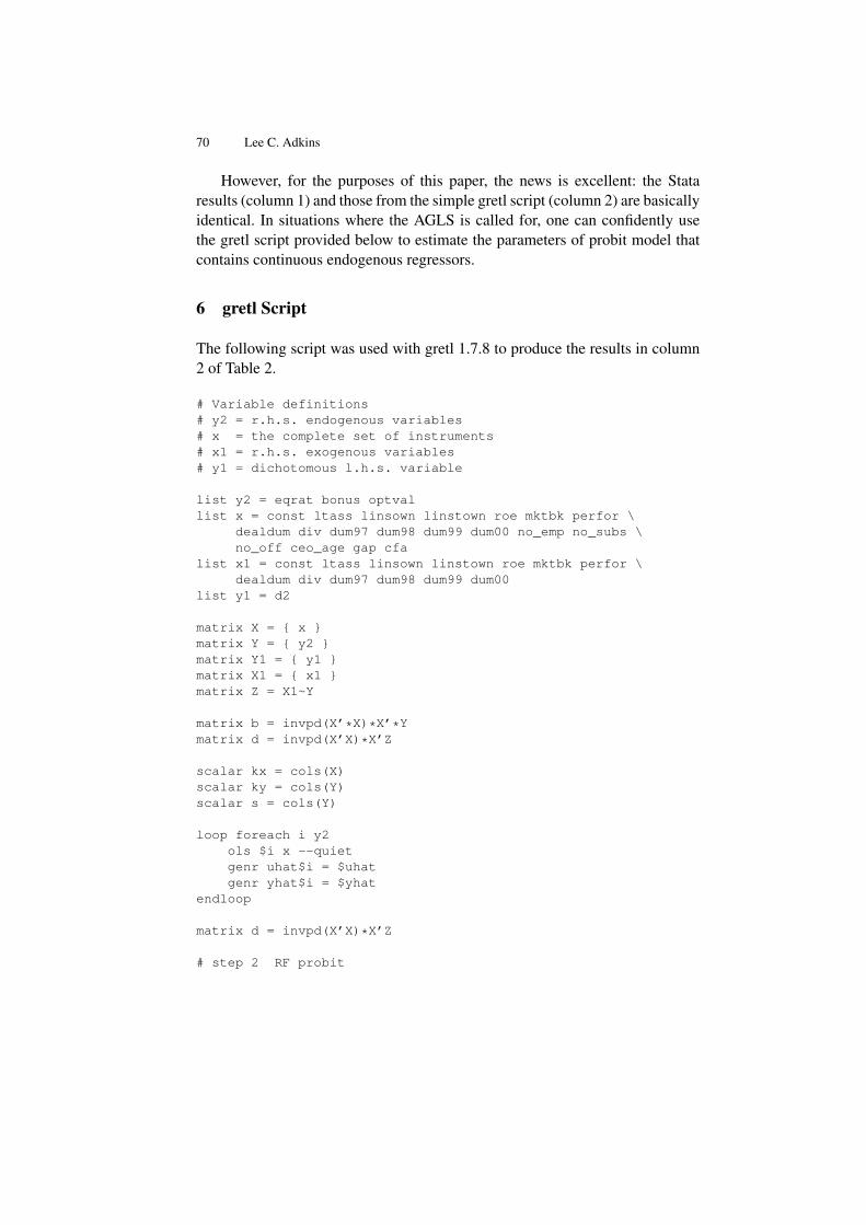
70 Lee C. Adkins
However, for the purposes of this paper, the news is excellent: the Stataresults (column 1) and those from the simple gretl script (column 2) are basicallyidentical. In situations where the AGLS is called for, one can confidently usethe gretl script provided below to estimate the parameters of probit model thatcontains continuous endogenous regressors.
6 gretl Script
The following script was used with gretl 1.7.8 to produce the results in column2 of Table 2.
# Variable definitions# y2 = r.h.s. endogenous variables# x = the complete set of instruments# x1 = r.h.s. exogenous variables# y1 = dichotomous l.h.s. variable
list y2 = eqrat bonus optvallist x = const ltass linsown linstown roe mktbk perfor \
dealdum div dum97 dum98 dum99 dum00 no_emp no_subs \no_off ceo_age gap cfa
list x1 = const ltass linsown linstown roe mktbk perfor \dealdum div dum97 dum98 dum99 dum00
list y1 = d2
matrix X = x matrix Y = y2 matrix Y1 = y1 matrix X1 = x1 matrix Z = X1~Y
matrix b = invpd(X’*X)*X’*Ymatrix d = invpd(X’X)*X’Z
scalar kx = cols(X)scalar ky = cols(Y)scalar s = cols(Y)
loop foreach i y2ols $i x --quietgenr uhat$i = $uhatgenr yhat$i = $yhat
endloop
matrix d = invpd(X’X)*X’Z
# step 2 RF probit

An Instrumental Variables Probit Estimator using gretl 71
probit y1 x uhat* --quietgenr J = $vcvmatrix alph = $coeffmatrix alpha = alph[1:kx]matrix lam = alph[kx+1:kx+ky]matrix Jinv=J[1:kx,1:kx]
# Step 3 2sivprobit y1 x1 uhat* yhat* --quietmatrix beta = $coeffmatrix beta = beta[rows(beta)-ky+1:rows(beta)]matrix rho = lam - beta
# step 4 v2*inv(x’x)matrix rhoY=Y*rhoseries ry = rhoYols ry x --quietmatrix v2 = $vcv
matrix omega = (v2+Jinv)
# Step 5matrix cov = invpd(d’*invpd(omega)*d)matrix se = sqrt(diag(cov))matrix delt = cov*d’*invpd(omega)*alphaprint delt se
This code could be used as the basis for a more elegant gretl function that couldbe used to estimate this model. Basically, one just needs to load the data andreplace the variable names to be used in the list statements. This version of thecode illustrates just how easy it is to perform matrix computations in gretl inthat the code mimics the steps listed in section 3.2.
One of the very useful properties of gretl is the way in which matrix compu-tations and native gretl results can be intermixed. In this case, the usual probitmle can be estimated using native gretl routines and the resulting variance co-variance matrix can be saved, converted to a matrix and used in subsequentcomputations. The –quiet option reduces the amount of output to a manageablelevel.
7 Conclusion
In this paper a simple gretl script is used to estimate the parameters of an di-chotomous choice model that contains endogenous regressors. The routine issimple and yields the same results as the two-step option in the commerciallyavailable Stata 10 software.

72 Lee C. Adkins
The next step is to duplicate the maximum likelihood estimator, a consider-ably more challenging undertaking given the multitude of ways the mle can becomputed. It should be noted that the only other commericial software that esti-mates this model via mle is Limdep; Limdep and Stata use different algorithmsand yield different results.
Another possibility is to use the plug-in IVP estimator with Murphy-Topelstandard errors. In very preliminary research Adkins [3] finds that this estimatorcompares favorably to AGLS and ML estimation in approximating the nomi-nal size of 10% tests of parameter significance. Like the AGLS estimator, thisshould also be a relatively simple computation in gretl.

Bibliography
[1] Adkins, Lee C. [2008a], Small sample performance of instrumental vari-ables probit estimators: A monte carlo investigation.
[2] Adkins, Lee C. [2008b], ‘Small sample performance of instrumental vari-ables probit estimators: A monte carlo investigation’, Department of Eco-nomics, Oklahoma State University, Stillwater OK 74078. available athttp://www.learneconometrics.com/pdf/JSM2008.pdf.
[3] Adkins, Lee C. [2009], A comparison of two-step and ml estimators of theinstrumental variables probit estimators: A monte carlo investigation.
[4] Adkins, Lee C., David A. Carter and W. Gary Simpson [2007], ‘Man-agerial incentives and the use of foreign-exchange derivatives by banks’,Journal of Financial Research 15, 399–413.
[5] Arendt, Jacob Nielsen and Anders Holm [2006], Probit models with binaryendogenous regressors, Discussion Papers on Business and Economics4/2006, Department of Business and Economics Faculty of Social Sci-ences University of Southern Denmark.
[6] Blundell, Richard W. and James L. Powell [2004], ‘Endogeneity in semi-parametric binary response models’, Review of Economic Studies 71, 655–679. available at http://ideas.repec.org/a/bla/restud/v71y2004ip655-679.html.
[7] Davidson, Russell and James G. MacKinnon [2004], Econometric Theoryand Methods, Oxford University Press, Inc., New York.
[8] Greene, William H. [2007], LIMDEP Version 9.0 Econometric ModelingGuide, Volume 1, Econometrics Software, Inc., 15 Gloria Place, Plainview,NY.
[9] Iwata, Shigeru [2001], ‘Recentered and rescaled instrumental variable es-timation of tobit and probit models with errors in variables’, EconometricReviews 24(3), 319–335.
[10] Kan, Kamhon and Chihwa Kao [2005], Simulation-based two-step esti-mation with endogenous regressors, Center for Policy Research WorkingPapers 76, Center for Policy Research, Maxwell School, Syracuse Univer-sity. available at http://ideas.repec.org/p/max/cprwps/76.html.
[11] Murphy, Kevin M. and Robert H. Topel [1985], ‘Estimation and infer-ence in two-step econometric models’, Journal of Business and EconomicStatistics 3(4), 370–379.
[12] Newey, Whitney [1987], ‘Efficient estimation of limited dependent vari-able models with endogenous explanatory variables’, Journal of Econo-metrics 36, 231–250.

74 Lee C. Adkins
[13] Nicoletti, Cheti and Franco Peracchi [2001], Two-step estimation of bi-nary response models with sample selection, Technical report, Faculty ofEconomics, Tor Vergata University, I-00133 Rome, Italy. Please do notquote.
[14] Rivers, D. and Q. H. Vuong [1988], ‘Limited information estimators andexogeneity tests for simultaneous probit models’, Journal of Econometrics39(3), 347–366.
[15] Shleifer, A. and R. W. Vishny [1986], ‘Large shareholders and corporatecontrol’, Journal of Political Economy 94, 461–488.
[16] Smith, Richard J. and Richard W. Blundell [1985], ‘An exogeneity test fora simultaneous equation tobit model with an application to labor supply’,Econometrica 54(3), 679–685.
[17] Tufano, P. [1996], ‘Who manages risk? an empirical examination of riskmanagement practices in the gold mining industry’, Journal of Finance51, 1097–1137.
[18] Whidbee, D. A. and M. Wohar [1999], ‘Derivative activities and man-agerial incentives in the banking industry’, Journal of Corporate Finance5, 251–276.
[19] Yatchew, Adonis and Zvi Griliches [1985], ‘Specification error in probitmodels’, The Review of Economics and Statistics 67(1), 134–139.
Automatic Procedure of BuildingCongruent Dynamic Model in Gretl
Marcin Błazejowski, Paweł Kufel, and Tadeusz Kufel
Torun School of Banking,Młodziezowa 31a, 87-100 Torun, Poland
[email protected] Copernicus University,
Department of Econometrics and Statistics,Gagarina 13a, 87-100 Torun, [email protected],
Abstract. In the last years we can observe intensive development of automaticmodel selection procedures. Best known are PcGets and RETINA. Such intensivework encourage to work on a new procedures. The concept of Congruent Mod-elling, formulated by Prof. Zygmunt Zielinski, is a very good framework for suchdevelopment, including programming work, as well as many theoretical consider-ations. In the paper we present our concept of algorithm for automatic congruentmodelling procedure and propose it’s implementation in Gretl.
Key words: congruent dynamic modelling, automatic model selection, forecast-ing, PcGets, RETINA
1 Introduction
In article [3] there is a very interesting dialog between Prof. Granger and Prof.Hendry about PcGets – automatic model selection procedure described in [5].Prof. Granger had formulated 20 questions concerning specification of GUM,simplification the GUM, testing economic theories, policy applications, nonsta-tionarity, nonlinearity, multiple equation models and forecasting and asked Prof.Hendry how PcGets – automatic model selection procedure – handles with it.
That dialog shows how automatic model selection tools are important incontemporary econometrics, but also shows how difficult this area is. There aretwo major automatic model selection procedures – PcGets1 and RETINA, de-scribed in [9]. The aim of this paper is formulation of algorithm for automatic
1 Since PcGive 12 and OxMetrics 5, PcGets is no longer available and current automatic modelselection procedure is called Autometrics (see [2]). In this article we still use the former name,but all our considerations on PcGets refer to Autometrics as well.
76 M. Błazejowski, P. Kufel, and T. Kufel
model selection procedure based on congruent modelling approach and – as thenext step – implementation that algorithm in Gretl2.
1.1 Idea of congruent modeling
The congruent modeling refers to building dynamic econometric models andwas presented by Prof. Zygmunt Zielinski from Nicolaus Copernicus Universityfrom Torun in 1984.
Many assumptions underlay the formulating of initial model specification.Some approaches refere to causal relationships, the other ones – to the internalstructure of processes of interest with omission of causality, and others take bothinto account. The concept of congruent modeling, in Zielinski sense, refers toboth approaches – casual relationship and internal structure of given processes3.
A model is congruent, according to Zielinski, if the harmonic structure ofdependent process Yt is the same as the joint harmonic structure of explanatoryprocesses Xit (i = 1, 2, . . . , k) and the residual process, which is independentof explanatory processes. This means that the variability of left side of model– (Yt) must be explained by the variability of right side of model – (Xit). Itis obvious that the model built for processes having white noise properties isalways congruent:
εyt =k∑i=1
ρiεxit + εt, (1)
where εyt, εxit and εt are white noises. Model (1) is congruent because har-monic structure of both sides of equation are equal or, in other words, the pro-cesses spectra are parallel to the frequency axis.
Let Yt and Xit (i = 1, 2, . . . , k) denote the endogenous process and ex-planatory processes respectively with the internal structure of:
– models describing non-stationary components:
Yt = Pyt + Syt + ηyt, (2)
Xit = Pxit + Sxit + ηxit,
where Pyt, Pxit are polynomial functions of variable t, Syt, Sxit denote sea-sonal component with constant or changing in time amplitude of fluctuationsand ηyt, ηxit are stationary autoregressive processes for respective variables,and
2 Any information about Gretl (Gnu Regression, Econometrics and Time-series), can be foundin [1].
3 More on congruent dynamic modelling one can find in: [13], [16], [14], [7], [11], [12].

Automatic Procedure of Building Congruent Dynamic Model in Gretl 77
– autoregressive processes:
B(u)ηyt = εyt, (3)
Ai(u)ηxit = εxit, (4)
where B(u), Ai(u) denote stationary autoregressive back shift operators forwhich all roots of equations |B(u)| = 0 and |Ai(u)| = 0 lie outside the unitroot circle and εyt, εxit are white noises for respective processes.
Information about internal structure of Yt and Xit processes enable to build thecongruent dynamic econometric model by substituting εyt and εxit in model (1)from models (3) and next for autoregressive processes in models (2). After trans-formations the congruent general dynamic econometric model is as follows:
B(u)Yt =k∑i=1
A∗i (u)Xit + Pt + St + εt, (5)
where B(u), A∗i (u) are autoregressive back shift operators, Pt is polynomialfunction of variable t, St denotes seasonal component with constant or chang-ing in time amplitude of fluctuations and εt is white noise. The white noise εtin model (5) has the same properties as white noise εt in model (1). Whole in-formation of internal structure of all processes is taken into consideration. Thevariability of endogenous process Yt is explained by variability of exogenousprocesses Xit, (i = 1, . . . , k).
Described concept of building dynamic econometric model shows the ne-cessity of including information about internal structure of given processes atthe model specification stage.
1.2 Linear congruent model for intergrated processes
Let4 assume that endogenous Yt and exogenous Xit are intergrated processeswith zero mean of order, respectively, dy ≥ 1 and dxi ≥ 1. It means, that:
Y ∗t = (1− u)dyYt = ∆dyYt ,
X∗it = (1− u)dxiXit = ∆dxiXit , (6)
are covariance stationary processes with zero mean, where u is such back shiftoperator, that usZt = Zt−s. Processes Y ∗t and X∗it can be expressed in ARnotation:
B(u)Y ∗t = εyt ,
Ai(u)X∗it = εxit , (7)4 This paragraph is based on [15] and [14].
78 M. Błazejowski, P. Kufel, and T. Kufel
where εyt and εxit are white noises with zero mean, B(u) and Ai(u) are sta-tionary autoregressive operators of order, respectively, py and qxi .
Operators:
B∗(u) = B(u)(1− u)dy = 1−py+dy∑s=1
α∗sus = 1−B∗1(u) ,
A∗i (u) = Ai(u)(1− u)dxi = 1−pxi+dxi∑s=1
γ∗sus = 1−A∗i1(u) , (8)
are nonstationary autoregressive operators which satisfy condition, that dy ordxi roots of B∗(z) = 0 or A∗i (z) = 0 lie on a unit circle. Taking (8) intoaccount, nonstationary processes Yt and Xit can be expressed as:
Yt = B∗1(u)Yt + εyt ,
Xit = A∗i1(u)Xit + εxit . (9)
Linear congruent model (1), describing relationship between Yt andXit, canbe write down in the following form:
Yt =k∑i=1
ρiXit −k∑i=1
ρiA∗i1(u)Xit +B∗1Yt + εt , (10)
Coefficient ρ in (10) is the same as in (1). Orders of autoregressions in model (10)are extended of orders of integration, which means, that lags of Yt are equal topy + dy and lags of Xit are equal to pxi + dxi .
2 General algorithm for automatic building congruent dynamicmodel
This is a very general algorithm for building congruent dynamic model, whereonly main stages are described without talking over any specific solutions, in-ternal variables, used external functions and so on. This algorithm shows onlya general idea of our procedure and it’s compatibility with congruent dynamiceconometric modelling procedure in Zielinski sense.
1. Getting outgoing data, setting following internal variables:(a) Getting model variables: endogenous Y, list of explanatory X, list of
deterministic (dummy) variables.(b) Getting range of the sample and setting minimal degrees of freedom
dfmin for starting general congruent model:

Automatic Procedure of Building Congruent Dynamic Model in Gretl 79
i. if n < 200, then dfmin = round(0.1× n),ii. if n ≥ 200, then dfmin = 20.
(c) Checking the frequency of time-series and setting:i. deterministic cycle for consideration in pt. 2,
ii. maximum order pmax for autoregressive models in pt. 2c,2. Analysis the internal structure of given processes:
(a) Checking, whether given processes have deterministic components.(b) Checking, whether error terms after subtraction of deterministic compo-
nents are integrated.(c) Setting orders of autoregression for given processes, starting from a
maximum order of pmax, after subtraction of deterministic componentsand differentiation if there was an integration.
3. Building starting specification of general unrestricted congruent model:(a) Checking the degrees of freedom of starting general congruent model
dfstart, taking into account all possible variables (lagged Y, current andlagged X, trend and/or cycle, deterministic variables):
i. if dfstart < dfmin, then maximum order of autoregressive model(s),specified in pt. 2c, is decreased by 1,
ii. if dfstart ≥ dfmin, then the starting general model is stored inGretl session.
4. Building congruent empirical model (specific):(a) Specified in pt. 3 starting congruent general model is reduced according
to a posterior procedure of variable selection with use of t statistics.(b) Congruent empirical model is stored in Gretl session.
At stage 1, we just import dataset for model: endogenous Y, list of “normal”explanatory X and some deterministic (dummy) variables, which indicate somespecial moments, i.e. free days. For next stages, we check dataset structure.
At stage 2 we perform the analysis of internal structure of explained pro-cess Yt and explanatory processes Xit. We are looking for deterministic com-ponents: time trend and periodicity. We assume, that we only check presence oflinear trend and ”typical” periodicity for given data: seasonality for monthly orquarterly time-series, 1 year (52 weeks) cycle for weekly time-series and 1 weekcycle for daily data. After that we subtract deterministic components from ana-lyzed processes and perform ADF test. If there is an integration, we differenceseries and examine order of autoregression of all time-series.
At stage 3 we formulate starting congruent general model and check, if wehave sufficient degrees of freedom for running OLS estimation. This is crucial,that we want at least 0.1 × n degrees of freedom or, if series have more then200 observations, at least 20. If we can’t meet this condition, maximum order

80 M. Błazejowski, P. Kufel, and T. Kufel
of autoregressive models is decreased by 1, so we earn at least 2 degrees offreedom at each reduction.
At stage 4 we perform OLS estimation of coefficients of starting generalcongruent model with strategy of model reduction based on a posterior elimi-nation with t statistics as a criterion. Empirical congruent model build on abovealgorithm always has white noise error terms.
3 Comparison of Congruent Modelling algorithm vs. PcGets vs.RETINA
In this section there are shown some similarities and differences beetwen algo-rithm based on congruent dynamic modelling theory and approaches in PcGetsand RETINA. PcGets and RETINA comparison one can find in [10] and ta-bles (1)-(9) are based on it. There are just delivered suitable information aboutour approach, so comparison of that three automatic model selection proceduresis now possible and easy. Comparison of General-to-Specific vs. CongruentModelling one can find in [8].
Table 1. Goals
PcGets RETINA Congruent Modelling1. Select a parsimonious
undominated representa-tion of an overly generalinitial model, the gen-eral unrestricted model(GUM).
2. Best model fit within sam-ple.
3. Congruent with theory.
1. Identify a parsimonious setof transformed attributeslikely to be relevant forpredicting out-of-sample.
1. Congruent general modelis reduced parsimoniouscongruent model inZielinski sense, whichmeans error term of whitenoise properties.
2. Very good behavior in pre-diction out of the sample.
3. Congruent with theory.
In congruent modelling we believe, that DGP is nested in the starting gen-eral model and reduction irrelevant variables can discover it. This is very similarto general-to-specific approach, but the starting general model is formulated indifferent ways. Starting specification is based on theory and extended of in-formation about internal structure of given processes, including deterministiccomponents, integration and autoregression. Autoregressive models can havedifferent starting order, which is the biggest difference with general-to-specificapproach.
In congruent modelling we start with congruent general model and step bystep this model is reduced to congruent empirical model with white noise error

Automatic Procedure of Building Congruent Dynamic Model in Gretl 81
Table 2. Strategy
PcGets RETINA Congruent Modelling1. General to specific.2. Formulate a GUM and re-
duce it to a parsimoniousmodel using residual testsand hypothesis testing oncoefficients.
1. Specific to general: Startfrom a model with a sin-gle transform. Add addi-tional transforms only ifthey contribute to out-of-sample forecast ability.
2. Flexible and parsimoniousmodel.
3. Selective search of trans-forms.
4. Control for collinearity.
1. Congruent general modelis reduced to congruentempirical model.
2. Elimination insignificantvariables using a posteriorprocedure based on tstatistics.
3. Empirical model is parsi-monious.
term. As a strategy we use t statistics which has sufficient power to discoverDGP (see numerical experiment).
Table 3. Base Model
PcGets RETINA Congruent Modelling1. GUM: specified by the re-
searcher, usually based ontheory. May use transformsof the original variables.
1. Based on original inputsand transforms, automat-ically selected from thefirst subsample by cross-validation in the second,controlling for collinearity.
1. Specification of startinggeneral congruent is basedon a theory and extendedof information of internalstructure of all includedprocesses.
2. Congruent model may usetransformed processes.
Base model is formulated on two basis: theory, which gives us causal rela-tionships between variables and on the internal structure of all processes. Thisguarantee, that hole variability of Yt and all Xit processes is included, so modelis congruent (error term has white noise properties).
Congruent modelling assumes linear in parameters model, but variables canbe log-transformed. Model can be nonlinear in variables, so congruent mod-elling gives maximum flexibility.
Starting congruent general model is unrestricted and, because of specifica-tion, based on the internal structure of all processes, overparametrizied, but stepby step model is being reduced with use of t statistics and a posterior procedure.Final (empirical) congruent model is parsimonious.

82 M. Błazejowski, P. Kufel, and T. Kufel
Table 4. Flexibility
PcGets RETINA Congruent Modelling1. The GUM determines
maximum flexibility. Mayinclude transforms of theoriginal variables.
1. The permitted transforma-tions of the inputs deter-mine maximum flexibility.
2. The actual flexibility of thecandidate model is chosenby the procedure.
1. Congruent general modelis unrestricted, so it givesmaximum flexibility.
Table 5. Selective/Systematic Search
PcGets RETINA Congruent Modelling1. Starting from the GUM,
performs a systematicsearch using multiplereduction paths.
2. Using diagnostics, checksthe validity of each reduc-tion until terminal selec-tion.
3. When all paths are ex-plored, repeatedly testsmodels against their unionuntil a unique final modelis obtained.
1. Uses a selective search toavoid the heavy task ofevaluating all 2m possi-ble models and of applyingsome form of model selec-tion.
2. A saliency feature of thetransforms, such as the cor-relation with the dependentvariable, is used to con-struct a natural order of thetransforms in which theyare considered.
3. Only a number of candi-date models of order pro-portional to m is consid-ered.
1. Starting from congruentgeneral model and reduceit by eliminating irrelevantvariables with t statistics.
Table 6. Colinearity
PcGets RETINA Congruent Modelling1. Seeks to formulate the
GUM, in search for a rela-tively orthogonal specifica-tion.
2. A quick modeler optionis available in PcGets fornonexpert users.
1. Controls for collinearity byadding an additional trans-form to the candidate listonly if the collinearity isbelow a certain (user de-fined) threshold.
1. Colinearity is controlled byGRETL.
Table 7. Explanatory Variables
PcGets RETINA Congruent Modelling1. Original variables and
transformations specifiedin the GUM.
1. Original variables and non-linear transformations al-lowed for by the procedure.
1. Original variables andhandmade transformationsspecified at the beginningof procedure.
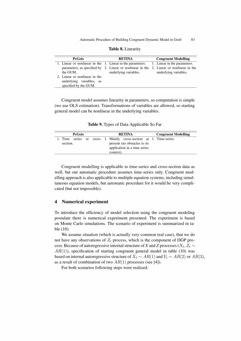
Automatic Procedure of Building Congruent Dynamic Model in Gretl 83
Table 8. Linearity
PcGets RETINA Congruent Modelling1. Linear or nonlinear in the
parameters, as specified bythe GUM.
2. Linear or nonlinear in theunderlying variables, asspecified by the GUM.
1. Linear in the parameters.2. Linear or nonlinear in the
underlying variables.
1. Linear in the parameters.2. Linear or nonlinear in the
underlying variables.
Congruent model assumes linearity in parameters, so computation is simple(we use OLS estimation). Transformations of variables are allowed, so startinggeneral model can be nonlinear in the underlying variables.
Table 9. Types of Data Applicable So Far
PcGets RETINA Congruent Modelling1. Time series or cross-
section.1. Mainly cross-section at
present (no obstacles to itsapplication in a time seriescontext).
1. Time-series.
Congruent modelling is applicable to time-series and cross-section data aswell, but our automatic procedure assumes time-series only. Congruent mod-elling approach is also applicable to multiple equation systems, including simul-taneous equation models, but automatic procedure for it would be very compli-cated (but not impossible).
4 Numerical experiment
To introduce the efficiency of model selection using the congruent modelingpostulate there is numerical experiment presented. The experiment is basedon Monte Carlo simulations. The scenario of experiment is summarized in ta-ble (10).
We assume situation (which is actually very common real case), that we donot have any observations of Zt process, which is the component of DGP pro-cess. Because of autoregressive internal structure of X and Z processes (Xt, Zt ∼AR(1)), specification of starting congruent general model in table (10) wasbased on internal autoregressive structure ofXt ∼ AR(1) and Yt ∼ AR(2) or AR(3),as a result of combination of two AR(1) processes (see [4]).
For both scenarios following steps were realized:
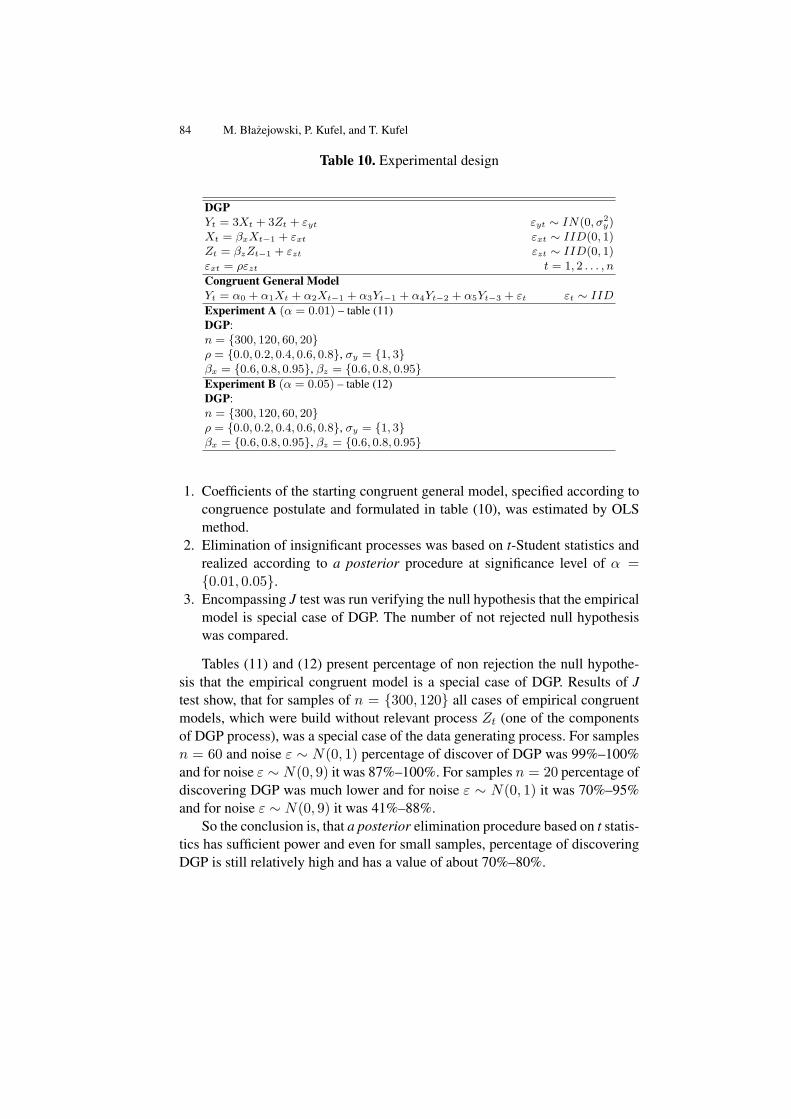
84 M. Błazejowski, P. Kufel, and T. Kufel
Table 10. Experimental design
DGPYt = 3Xt + 3Zt + εyt εyt ∼ IN(0, σ2
y)Xt = βxXt−1 + εxt εxt ∼ IID(0, 1)Zt = βzZt−1 + εzt εzt ∼ IID(0, 1)εxt = ρεzt t = 1, 2 . . . , n
Congruent General ModelYt = α0 + α1Xt + α2Xt−1 + α3Yt−1 + α4Yt−2 + α5Yt−3 + εt εt ∼ IIDExperiment A (α = 0.01) – table (11)DGP:n = 300, 120, 60, 20ρ = 0.0, 0.2, 0.4, 0.6, 0.8, σy = 1, 3βx = 0.6, 0.8, 0.95, βz = 0.6, 0.8, 0.95Experiment B (α = 0.05) – table (12)DGP:n = 300, 120, 60, 20ρ = 0.0, 0.2, 0.4, 0.6, 0.8, σy = 1, 3βx = 0.6, 0.8, 0.95, βz = 0.6, 0.8, 0.95
1. Coefficients of the starting congruent general model, specified according tocongruence postulate and formulated in table (10), was estimated by OLSmethod.
2. Elimination of insignificant processes was based on t-Student statistics andrealized according to a posterior procedure at significance level of α =0.01, 0.05.
3. Encompassing J test was run verifying the null hypothesis that the empiricalmodel is special case of DGP. The number of not rejected null hypothesiswas compared.
Tables (11) and (12) present percentage of non rejection the null hypothe-sis that the empirical congruent model is a special case of DGP. Results of Jtest show, that for samples of n = 300, 120 all cases of empirical congruentmodels, which were build without relevant process Zt (one of the componentsof DGP process), was a special case of the data generating process. For samplesn = 60 and noise ε ∼ N(0, 1) percentage of discover of DGP was 99%–100%and for noise ε ∼ N(0, 9) it was 87%–100%. For samples n = 20 percentage ofdiscovering DGP was much lower and for noise ε ∼ N(0, 1) it was 70%–95%and for noise ε ∼ N(0, 9) it was 41%–88%.
So the conclusion is, that a posterior elimination procedure based on t statis-tics has sufficient power and even for small samples, percentage of discoveringDGP is still relatively high and has a value of about 70%–80%.
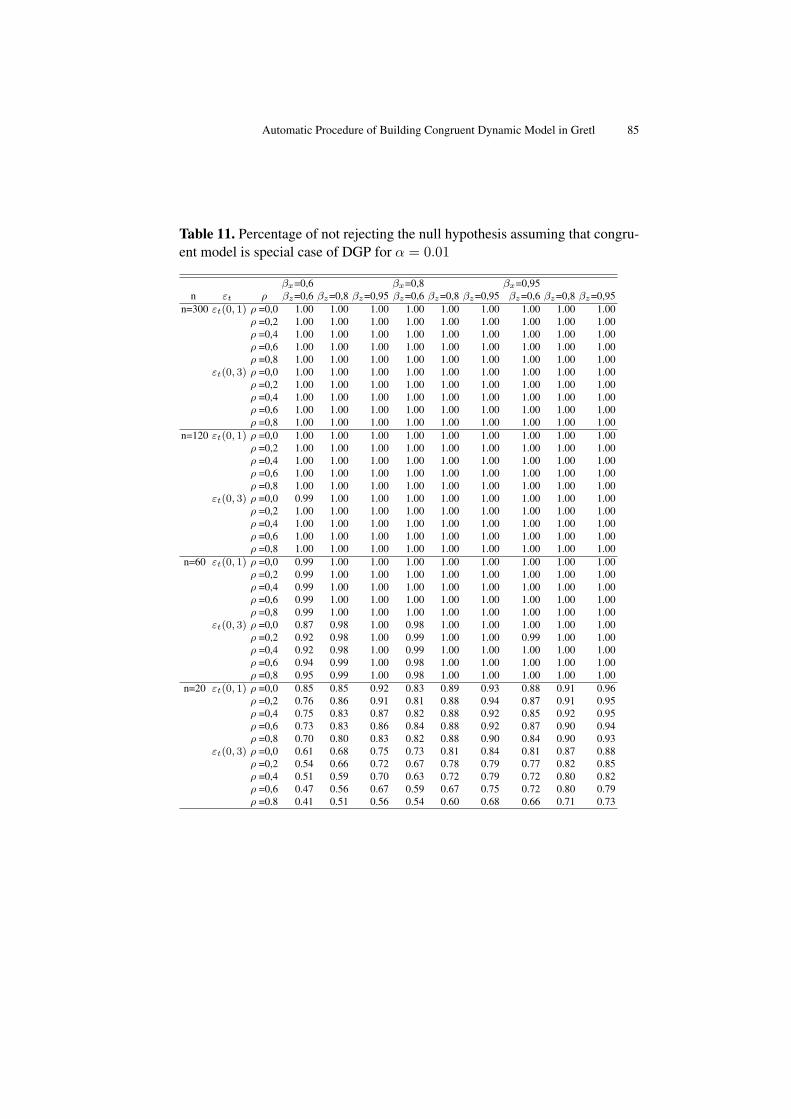
Automatic Procedure of Building Congruent Dynamic Model in Gretl 85
Table 11. Percentage of not rejecting the null hypothesis assuming that congru-ent model is special case of DGP for α = 0.01
βx=0,6 βx=0,8 βx=0,95n εt ρ βz=0,6 βz=0,8 βz=0,95 βz=0,6 βz=0,8 βz=0,95 βz=0,6 βz=0,8 βz=0,95
n=300 εt(0, 1) ρ =0,0 1.00 1.00 1.00 1.00 1.00 1.00 1.00 1.00 1.00ρ =0,2 1.00 1.00 1.00 1.00 1.00 1.00 1.00 1.00 1.00ρ =0,4 1.00 1.00 1.00 1.00 1.00 1.00 1.00 1.00 1.00ρ =0,6 1.00 1.00 1.00 1.00 1.00 1.00 1.00 1.00 1.00ρ =0,8 1.00 1.00 1.00 1.00 1.00 1.00 1.00 1.00 1.00
εt(0, 3) ρ =0,0 1.00 1.00 1.00 1.00 1.00 1.00 1.00 1.00 1.00ρ =0,2 1.00 1.00 1.00 1.00 1.00 1.00 1.00 1.00 1.00ρ =0,4 1.00 1.00 1.00 1.00 1.00 1.00 1.00 1.00 1.00ρ =0,6 1.00 1.00 1.00 1.00 1.00 1.00 1.00 1.00 1.00ρ =0,8 1.00 1.00 1.00 1.00 1.00 1.00 1.00 1.00 1.00
n=120 εt(0, 1) ρ =0,0 1.00 1.00 1.00 1.00 1.00 1.00 1.00 1.00 1.00ρ =0,2 1.00 1.00 1.00 1.00 1.00 1.00 1.00 1.00 1.00ρ =0,4 1.00 1.00 1.00 1.00 1.00 1.00 1.00 1.00 1.00ρ =0,6 1.00 1.00 1.00 1.00 1.00 1.00 1.00 1.00 1.00ρ =0,8 1.00 1.00 1.00 1.00 1.00 1.00 1.00 1.00 1.00
εt(0, 3) ρ =0,0 0.99 1.00 1.00 1.00 1.00 1.00 1.00 1.00 1.00ρ =0,2 1.00 1.00 1.00 1.00 1.00 1.00 1.00 1.00 1.00ρ =0,4 1.00 1.00 1.00 1.00 1.00 1.00 1.00 1.00 1.00ρ =0,6 1.00 1.00 1.00 1.00 1.00 1.00 1.00 1.00 1.00ρ =0,8 1.00 1.00 1.00 1.00 1.00 1.00 1.00 1.00 1.00
n=60 εt(0, 1) ρ =0,0 0.99 1.00 1.00 1.00 1.00 1.00 1.00 1.00 1.00ρ =0,2 0.99 1.00 1.00 1.00 1.00 1.00 1.00 1.00 1.00ρ =0,4 0.99 1.00 1.00 1.00 1.00 1.00 1.00 1.00 1.00ρ =0,6 0.99 1.00 1.00 1.00 1.00 1.00 1.00 1.00 1.00ρ =0,8 0.99 1.00 1.00 1.00 1.00 1.00 1.00 1.00 1.00
εt(0, 3) ρ =0,0 0.87 0.98 1.00 0.98 1.00 1.00 1.00 1.00 1.00ρ =0,2 0.92 0.98 1.00 0.99 1.00 1.00 0.99 1.00 1.00ρ =0,4 0.92 0.98 1.00 0.99 1.00 1.00 1.00 1.00 1.00ρ =0,6 0.94 0.99 1.00 0.98 1.00 1.00 1.00 1.00 1.00ρ =0,8 0.95 0.99 1.00 0.98 1.00 1.00 1.00 1.00 1.00
n=20 εt(0, 1) ρ =0,0 0.85 0.85 0.92 0.83 0.89 0.93 0.88 0.91 0.96ρ =0,2 0.76 0.86 0.91 0.81 0.88 0.94 0.87 0.91 0.95ρ =0,4 0.75 0.83 0.87 0.82 0.88 0.92 0.85 0.92 0.95ρ =0,6 0.73 0.83 0.86 0.84 0.88 0.92 0.87 0.90 0.94ρ =0,8 0.70 0.80 0.83 0.82 0.88 0.90 0.84 0.90 0.93
εt(0, 3) ρ =0,0 0.61 0.68 0.75 0.73 0.81 0.84 0.81 0.87 0.88ρ =0,2 0.54 0.66 0.72 0.67 0.78 0.79 0.77 0.82 0.85ρ =0,4 0.51 0.59 0.70 0.63 0.72 0.79 0.72 0.80 0.82ρ =0,6 0.47 0.56 0.67 0.59 0.67 0.75 0.72 0.80 0.79ρ =0.8 0.41 0.51 0.56 0.54 0.60 0.68 0.66 0.71 0.73
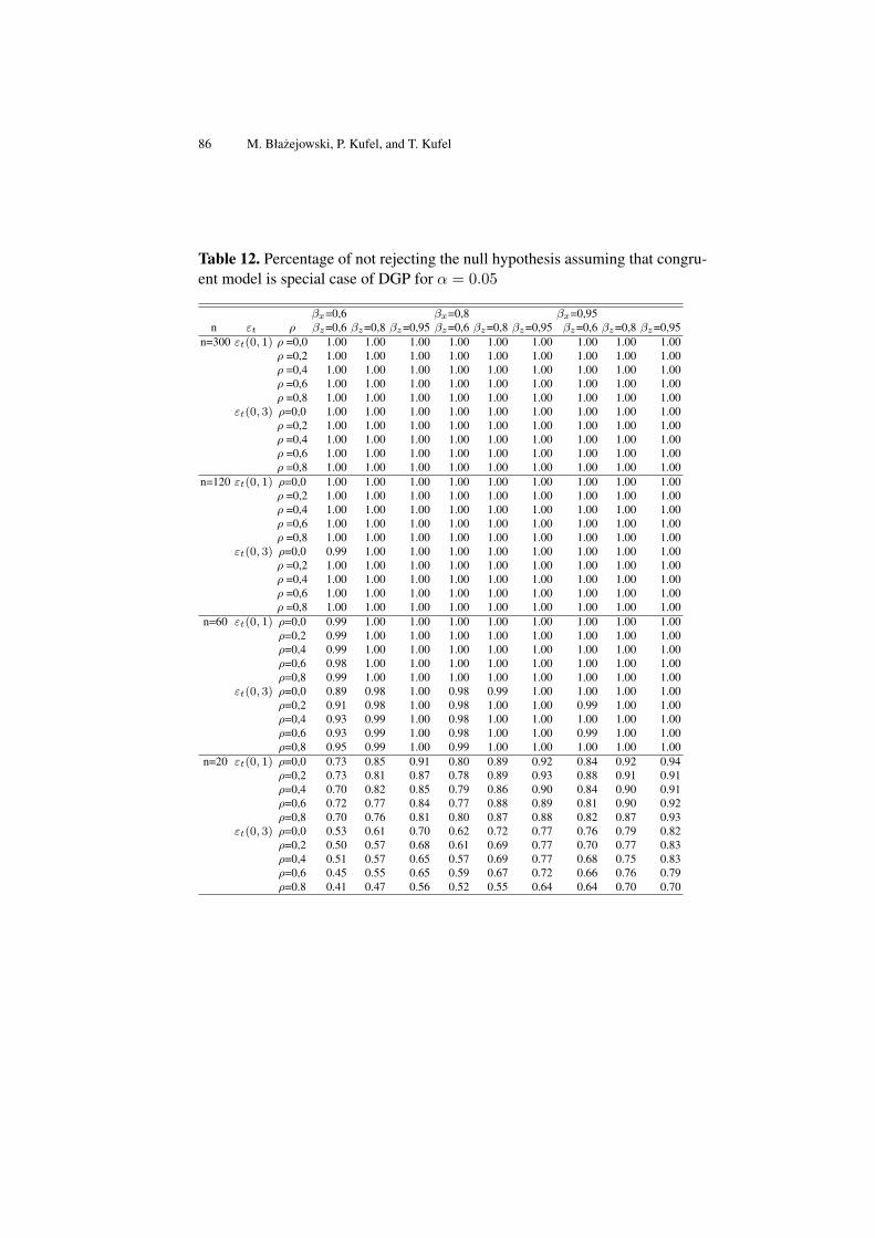
86 M. Błazejowski, P. Kufel, and T. Kufel
Table 12. Percentage of not rejecting the null hypothesis assuming that congru-ent model is special case of DGP for α = 0.05
βx=0,6 βx=0,8 βx=0,95n εt ρ βz=0,6 βz=0,8 βz=0,95 βz=0,6 βz=0,8 βz=0,95 βz=0,6 βz=0,8 βz=0,95
n=300 εt(0, 1) ρ =0,0 1.00 1.00 1.00 1.00 1.00 1.00 1.00 1.00 1.00ρ =0,2 1.00 1.00 1.00 1.00 1.00 1.00 1.00 1.00 1.00ρ =0,4 1.00 1.00 1.00 1.00 1.00 1.00 1.00 1.00 1.00ρ =0,6 1.00 1.00 1.00 1.00 1.00 1.00 1.00 1.00 1.00ρ =0,8 1.00 1.00 1.00 1.00 1.00 1.00 1.00 1.00 1.00
εt(0, 3) ρ=0,0 1.00 1.00 1.00 1.00 1.00 1.00 1.00 1.00 1.00ρ =0,2 1.00 1.00 1.00 1.00 1.00 1.00 1.00 1.00 1.00ρ =0,4 1.00 1.00 1.00 1.00 1.00 1.00 1.00 1.00 1.00ρ =0,6 1.00 1.00 1.00 1.00 1.00 1.00 1.00 1.00 1.00ρ =0,8 1.00 1.00 1.00 1.00 1.00 1.00 1.00 1.00 1.00
n=120 εt(0, 1) ρ=0,0 1.00 1.00 1.00 1.00 1.00 1.00 1.00 1.00 1.00ρ =0,2 1.00 1.00 1.00 1.00 1.00 1.00 1.00 1.00 1.00ρ =0,4 1.00 1.00 1.00 1.00 1.00 1.00 1.00 1.00 1.00ρ =0,6 1.00 1.00 1.00 1.00 1.00 1.00 1.00 1.00 1.00ρ =0,8 1.00 1.00 1.00 1.00 1.00 1.00 1.00 1.00 1.00
εt(0, 3) ρ=0,0 0.99 1.00 1.00 1.00 1.00 1.00 1.00 1.00 1.00ρ =0,2 1.00 1.00 1.00 1.00 1.00 1.00 1.00 1.00 1.00ρ =0,4 1.00 1.00 1.00 1.00 1.00 1.00 1.00 1.00 1.00ρ =0,6 1.00 1.00 1.00 1.00 1.00 1.00 1.00 1.00 1.00ρ =0,8 1.00 1.00 1.00 1.00 1.00 1.00 1.00 1.00 1.00
n=60 εt(0, 1) ρ=0,0 0.99 1.00 1.00 1.00 1.00 1.00 1.00 1.00 1.00ρ=0,2 0.99 1.00 1.00 1.00 1.00 1.00 1.00 1.00 1.00ρ=0,4 0.99 1.00 1.00 1.00 1.00 1.00 1.00 1.00 1.00ρ=0,6 0.98 1.00 1.00 1.00 1.00 1.00 1.00 1.00 1.00ρ=0,8 0.99 1.00 1.00 1.00 1.00 1.00 1.00 1.00 1.00
εt(0, 3) ρ=0,0 0.89 0.98 1.00 0.98 0.99 1.00 1.00 1.00 1.00ρ=0,2 0.91 0.98 1.00 0.98 1.00 1.00 0.99 1.00 1.00ρ=0,4 0.93 0.99 1.00 0.98 1.00 1.00 1.00 1.00 1.00ρ=0,6 0.93 0.99 1.00 0.98 1.00 1.00 0.99 1.00 1.00ρ=0,8 0.95 0.99 1.00 0.99 1.00 1.00 1.00 1.00 1.00
n=20 εt(0, 1) ρ=0,0 0.73 0.85 0.91 0.80 0.89 0.92 0.84 0.92 0.94ρ=0,2 0.73 0.81 0.87 0.78 0.89 0.93 0.88 0.91 0.91ρ=0,4 0.70 0.82 0.85 0.79 0.86 0.90 0.84 0.90 0.91ρ=0,6 0.72 0.77 0.84 0.77 0.88 0.89 0.81 0.90 0.92ρ=0,8 0.70 0.76 0.81 0.80 0.87 0.88 0.82 0.87 0.93
εt(0, 3) ρ=0,0 0.53 0.61 0.70 0.62 0.72 0.77 0.76 0.79 0.82ρ=0,2 0.50 0.57 0.68 0.61 0.69 0.77 0.70 0.77 0.83ρ=0,4 0.51 0.57 0.65 0.57 0.69 0.77 0.68 0.75 0.83ρ=0,6 0.45 0.55 0.65 0.59 0.67 0.72 0.66 0.76 0.79ρ=0.8 0.41 0.47 0.56 0.52 0.55 0.64 0.64 0.70 0.70

Automatic Procedure of Building Congruent Dynamic Model in Gretl 87
5 Summary
In the paper we discussed power of the congruent modelling concept and it isintrinsic features for being the base for automatic model selection procedure.Although we formulated full algorithm for such procedure, our considerationswas theoretical. So the next stage of our work will be implementation this algo-rithm in Gretl. Our automatic procedure will:
1. Investigate internal trend-seasonal-autoregressive structure for all processes.2. Formulate congruent general model on the basis of initial list of explanatory
extended of it’s internal components.3. Run OLS estimation and eliminate insignificant variables according to a
posterior procedure based on t statistics.4. Store empirical congruent model in Gretl session.

Bibliography
[1] Cottrell, A., Lucchetti, R.: Gnu Regression, Econometrics and Time-series,http://gretl.sourceforge.net
[2] Doornik, J. A., Hendry, D. F.: Empirical Econometric Modelling – PcGive12. Timberlake Consultants Press, London (2007)
[3] Granger, C. W. J., Hendry, D. F.: A dialogue concerning a new instrumentfor econometric modeling. Econometric Theory, vol. 21, pp. 278–297, (2005)
[4] Granger, C. W. J., Morris, M. J.: Time Series Modelling and Interpretation.Journal of the Royal Statistical Society. Series A (General). 139(2), 246–257(1976)
[5] Hendry, D. F., Krolzig, H.-M.: Automatic Econometric Model Selection.Timberlake Consultants Press, London (2001)
[6] Krolzig, H.-M., Hendry, D. F.: Computer automation of general-to-specificmodel selection procedures. Journal of Economic Dynamics and Control. 25,831–866 (2001)
[7] Kufel, T, Piłatowska, M.: The White Noise Properties in the Dynamic Con-gruent Modelling. In: MACROMODELS ’90, pp. 163–178. Łódz UniversityPress, Łódz (1997)
[8] Kufel, T.: General-to-Specific Modelling vs. Congruent Modelling inPcGets. In: Zielinski, Z. (ed.) Dynamic Econometric Models, vol. 6, pp. 83–92. Nicolaus Copernicus University Press, Torun (2004)
[9] Perez-Amaral, T., Gallo, G. M., White, H.: Flexible Tool for ModelBuilding: the Relevant Transformation of the Inputs Network Approach(RETINA). Technical report, Universidad Complutense de Madrid, Facultadde Ciencias Económicas y Empresariales (2003)
[10] Perez-Amaral, T., Gallo, G. M., White, H.: A Comparison of Comple-mentary Automatic Modeling Methods: RETINA and PcGets. EconometricTheory, Vol. 21, No. 1, pp. 262–277, (2005)
[11] Piłatowska, M.: Realization of the Congruence Postulate as a Method ofAvoiding the Effect of a Spurious Relationship. In: Zielinski, Z. (ed.) Dy-namic Econometric Models, vol. 6, pp. 117–126. Nicolaus Copernicus Uni-versity Press, Torun (2004)
[12] Piłatowska, M.: The Econometric Models Satisfying the Congruence Pos-tulate – an Overview. In: Zielinski, Z. (ed.) Dynamic Econometric Models,vol. 8, pp. 53–60. Nicolaus Copernicus University Press, Torun (2008)
[13] Zielinski, Z.: Dynamic Econometric Linear Models as a Tool of Descrip-tion and Analysis of Causal Relationships in Economics. In: Zielinski, Z.

Automatic Procedure of Building Congruent Dynamic Model in Gretl 89
(ed.) Some Aspects of the Dynamic Eeconometric Modelling, pp. 7–58.Nicolaus Copernicus University Press, Torun (1993)
[14] Zielinski, Z.: Linear Congruent Models Describing Relationships for In-tegrated Economic Processes. In: Zielinski, Z. (ed.) Dynamic Economet-ric Models, vol. 1, pp. 7–20. Nicolaus Copernicus University Press, Torun(1994)
[15] Zielinski, Z.: Liniowe modele zgodne opisujace zaleznosci suma-cyjnych (zintegrowanych) procesów ekonomicznych. In: Zelias, A. (ed.)Przestrzenno-czasowe modelowanie i prognozowanie zjawisk gospodar-czych, pp. 77–87. AE Kraków, Kraków (1995)
[16] Zielinski, Z., Kufel, T.: Specification of Dynamic Properties of the Econo-metric Models in the Light of Congruent Models Concept. In: MACRO-MODELS ’86, pp. 25–52. Łódz University Press, Łódz (1995)

Instrumental Variable Interval Regression
Giulia Bettin1 and Riccardo (Jack) Lucchetti2
1 HWWI - Hamburg Institute for International Economics - Hamburg, [email protected]
2 Dipartimento di Economia - Universita Politecnica delle Marche - Ancona, [email protected]
Abstract. In this paper, we introduce a maximum-likelihood estimator for groupeddata with endogenous regressors and briefly analyse its properties. An exampleapplication to migrants’ remittances is included, which shows that endogeneityeffects, so far neglected by the applied literature, are substantial.
1 Introduction
The estimation of interval models by maximum likelihood, introduced by [16],is nowadays relatively straightforward and has been applied in a number of con-texts, most notably in willingness-to-pay double bound models (for a recentexample, see [15]). The data generating process is assumed to be
y∗i = x′iβ + εi (1)
where y∗i is unobservable per se; what is observed are the limits of an intervalthat contains it, that is
mi ≤ y∗i ≤Mi
where the interval may be left- or right-unbounded. Once a distributional hy-pothesis for εi is made, estimation becomes a simple application of maximumlikelihood techniques. Under normality, the log-likelihood for one observationis
`i(β, σ) = lnP (mi < y∗i ≤Mi) = ln[Φ
(Mi − x′iβ
σ
)− Φ
(mi − x′iβ
σ
)](2)
and the total log-likelihood can be maximised by standard numerical methods,which are, in most cases, very effective. The above procedure is implementednatively in several econometric packages, among which Gretl, Limdep, Stataand TSP.
However, the extension of this model to the case of endogenous regressorsseems to be absent from the literature. To consider this case, equation (1) can be
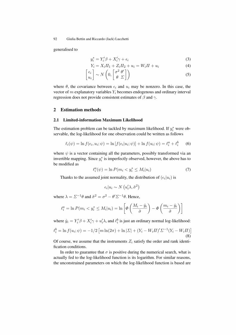
92 Giulia Bettin and Riccardo (Jack) Lucchetti
generalised to
y∗i = Y ′i β +X ′iγ + εi (3)
Yi = XiΠ1 + ZiΠ2 + ui = WiΠ + ui (4)[εiui
]∼ N
(0,[σ2 θ′
θ Σ
])(5)
where θ, the covariance between εi and ui may be nonzero. In this case, thevector ofm explanatory variables Yi becomes endogenous and ordinary intervalregression does not provide consistent estimates of β and γ.
2 Estimation methods
2.1 Limited-information Maximum Likelihood
The estimation problem can be tackled by maximum likelihood. If y∗i were ob-servable, the log-likelihood for one observation could be written as follows
`i(ψ) = ln f(εi, ui;ψ) = ln [f(εi|ui;ψ)] + ln f(ui;ψ) = `ai + `bi (6)
where ψ is a vector containing all the parameters, possibly transformed via aninvertible mapping. Since y∗i is imperfectly observed, however, the above has tobe modified as
`ai (ψ) = lnP (mi < y∗i ≤Mi|ui) (7)
Thanks to the assumed joint normality, the distribution of (εi|ui) is
εi|ui ∼ N(u′iλ, σ
2)
where λ = Σ−1θ and σ2 = σ2 − θ′Σ−1θ. Hence,
`ai = lnP (mi < y∗i ≤Mi|ui) = ln[Φ
(Mi − yi
σ
)− Φ
(mi − yiσ
)]where yi = Y ′i β +X ′iγ + u′iλ, and `bi is just an ordinary normal log-likelihood:
`bi = ln f(ui;ψ) = −1/2[m ln(2π) + ln |Σ|+ (Yi −WiΠ)′Σ−1(Yi −WiΠ)
](8)
Of course, we assume that the instruments Zi satisfy the order and rank identi-fication conditions.
In order to guarantee that σ is positive during the numerical search, what isactually fed to the log-likelihood function is its logarithm. For similar reasons,the unconstrained parameters on which the log-likelihood function is based are
IV Interval Regression 93
not the elements of Σ itself, but rather those of the Cholesky factorisation of itsinverse. In practice, `bi , the second component of the log-likelihood, is computedas
`bi = const + ln |C| − ω′iωi2
where C is the Cholesky factorisation of Σ−1 and ωi = C ′(Yi −Π ′Wi). Thisproduces faster and more accurate computation than evaluating (8) directly fortwo reasons: first, a matrix inversion is avoided; moreover, the determinant ofC (which is by construction |Σ|−1/2) is trivial to compute since C is triangular,via
−0.5 ln |Σ| =m∑i=1
lnCii.
The computational gain is negligible (arguably null) when m = 1, but may be-come substantial for m > 1; in fact, casual experimenting show non-negligibleimprovements even for m = 2.
A recent paper by [8] advocates the usage of the EM algorithm for dealingwith numerical problems in a closely related case (the ordered probit model),but we found it unnecessary in our case.
The ML setup also enables us to build two hypothesis tests which are likelyto be of interest: the first one is an exogeneity test, which is constructed bytesting for λ = 0 by means of a Wald test. In addition, a LR test for overi-dentifying restrictions may be computed via the difference `a and that for aninterval regression of (mi,Mi) on Wi and ui, which would be the unrestrictedlog-likelihood.
2.2 Alternative estimators
In certain cases, it may be worthwhile to consider alternative estimators thanML. Two are briefly considered here, although no serious effort is made toanalyse them in detail; both belong to the two-step category of estimators. Assuch, they may suffer from the typical shortcoming of two-step estimators: in-efficiency and a cumbersome-to-compute covariance matrix3. Hence, we onlysketch briefly the possibility for alternative estimators; proper analysis of theirproperties is left as a future project.
Both estimators depend on the availability of an ordinary interval regressionroutine. One possibility is:
1. perform first-stage OLS of Yi on Wi and collect the residuals ui2. perform an interval regression on Yi, Xi and ui3 The obligatory reference here is [12], but see also [17], chapter 12.
94 Giulia Bettin and Riccardo (Jack) Lucchetti
This estimator ought to be consistent4. This estimator is very easy to computeif an interval regression routine is available: as a consequence, it was a naturalchoice for initialising our ML algorithm.
Another two-step estimator may be obtained by considering that, given aninterval regression of the form (1), it is easy to form an unbiased estimator of y∗ifrom
E(y∗i |xi,mi,Mi) = x′iβ+E(εi|xi,mi,Mi) = x′iβ+σϕ(mi−x′iβ
σ
)− ϕ
(Mi−x′iβ
σ
)Φ(Mi−x′iβ
σ
)− Φ
(mi−x′iβ
σ
)and substituting unknown parameters with their estimates to get the estimate yi.The procedure is the following:
1. do an interval regression of (mi,Mi) onWi; that is, estimate the unrestrictedreduced form of equation (3).
2. compute yi, an unbiased estimate if y∗i ; By construction,
vi ≡ y∗i − yi
will have the property E(vi|Wi) = 0.3. do TSLS using yi as the dependent variable; this should be valid since (from
equation (3)yi = Y ′i β +X ′iγ + (εi − vi)
and the composite error term (εi − vi) is incorrelated with the instrumentsWi (although it will be heteroskedastic by construction).
Again, we conjecture that this estimator should also be consistent, but like theother one, it would be inefficient and the estimation of the parameters’ covari-ance matrix would need a two-step adjustment.
3 Why bother?
From the viewpoint of an applied economist, the ML method outlined abovemay seem overkill. After all, how much inaccuracy do we introduce in the databy choosing the interval midpoint? In fact, a procedure that is commonly usedis to approximate y∗i by
yi =Mi +mi
24 We do not have a formal proof, but it should follow from consistency of Π and the clear
fulfillment of the identification condition stated in Wooldridge [17], p. 354.
IV Interval Regression 95
and assume that yi can be used as a proxy for y∗i more or less painlessly: anadditional source of error in the model (most likely heteroskedastic), that couldbe accommodated via robust estimation of the parameters covariance matrix.Hence, running TSLS on yi may look as a simple and inexpensive procedure.
Trivially, a first problem that arises with this method is that it does not pro-vide an obvious indication on how to treat unbounded observations (that is,whenmi = −∞ orMi =∞). A more serious problem, however, is that that theabove procedure leads to substantial inference errors. The analytical explanationis obvious after rearranging equation (3) as
yi = Y ′i β +X ′iγ + (εi + ηi), (9)
where ηi is defined as yi − y∗i . The intuition behind this reasoning is that if theinterval (mi,Mi) is “small”, then σ2
η should be negligible compared to σ2ε . (It
should be noted that, by construction, the support of ηi is a finite interval, whoselength goes to 0 as Mi −mi → 0.)
However, even if the basic instrument validity condition E(εi|Wi) = 0holds, there is no reason why the midpoint rule should guaranteeE(ηi|Wi) = 0.This can be proven by a simple extension to the IV case of the line of reason-ing in [16]. As a consequence, the TSLS estimator converges in probability toa vector that differs from the true values of β and γ. It is worth noting thatinconsistency is not a small sample issue, but a much more fundamental flaw.
Clearly, how serious the problem is depends on the relative magnitudes ofσ2η and σ2
ε . To explore the consequences of the above, in a seemingly harmlesscase, we run a small Monte Carlo experiment. The Monte Carlo setup is:
y∗i = γ0 + Yiβ +Xiγ1 + εi
γ0 = β = γ1 = 1Yi = 1 +Xi + Zi + ui[εiui
]∼ N
(0,[
1 0.250.25 1
])and the cutpoints are represented by the vector [−2, 0, 1, 2, 5], so that, for ex-ample, if y∗i = 3, then mi = 2 and Mi = 5. The variables Xi and Zi areindependent N(0, 1). A “naive” proxy for y∗i was constructed via the midpointrule, as
yi =
−4 for y∗i < −2Mi+mi
2 for −2 < y∗i < 510 for y∗i > 5
The above DGP was simulated with sample sizes of 100, 500 and 2500 obser-vations. For each case, 4096 simulations were run.
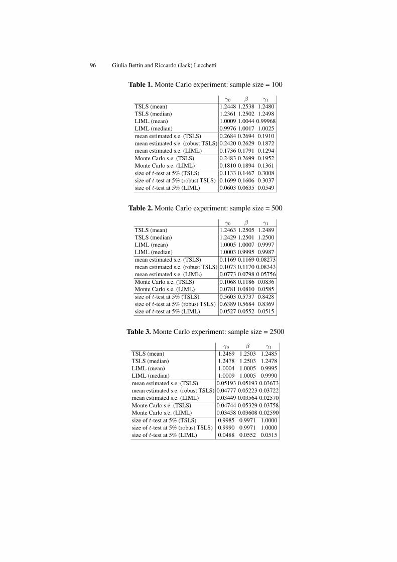
96 Giulia Bettin and Riccardo (Jack) Lucchetti
Table 1. Monte Carlo experiment: sample size = 100
γ0 β γ1
TSLS (mean) 1.2448 1.2538 1.2480TSLS (median) 1.2361 1.2502 1.2498LIML (mean) 1.0009 1.0044 0.99968LIML (median) 0.9976 1.0017 1.0025mean estimated s.e. (TSLS) 0.2684 0.2694 0.1910mean estimated s.e. (robust TSLS) 0.2420 0.2629 0.1872mean estimated s.e. (LIML) 0.1736 0.1791 0.1294Monte Carlo s.e. (TSLS) 0.2483 0.2699 0.1952Monte Carlo s.e. (LIML) 0.1810 0.1894 0.1361size of t-test at 5% (TSLS) 0.1133 0.1467 0.3008size of t-test at 5% (robust TSLS) 0.1699 0.1606 0.3037size of t-test at 5% (LIML) 0.0603 0.0635 0.0549
Table 2. Monte Carlo experiment: sample size = 500
γ0 β γ1
TSLS (mean) 1.2463 1.2505 1.2489TSLS (median) 1.2429 1.2501 1.2500LIML (mean) 1.0005 1.0007 0.9997LIML (median) 1.0003 0.9995 0.9987mean estimated s.e. (TSLS) 0.1169 0.1169 0.08273mean estimated s.e. (robust TSLS) 0.1073 0.1170 0.08343mean estimated s.e. (LIML) 0.0773 0.0798 0.05756Monte Carlo s.e. (TSLS) 0.1068 0.1186 0.0836Monte Carlo s.e. (LIML) 0.0781 0.0810 0.0585size of t-test at 5% (TSLS) 0.5603 0.5737 0.8428size of t-test at 5% (robust TSLS) 0.6389 0.5684 0.8369size of t-test at 5% (LIML) 0.0527 0.0552 0.0515
Table 3. Monte Carlo experiment: sample size = 2500
γ0 β γ1
TSLS (mean) 1.2469 1.2503 1.2485TSLS (median) 1.2478 1.2503 1.2478LIML (mean) 1.0004 1.0005 0.9995LIML (median) 1.0009 1.0005 0.9990mean estimated s.e. (TSLS) 0.05193 0.05193 0.03673mean estimated s.e. (robust TSLS) 0.04777 0.05223 0.03722mean estimated s.e. (LIML) 0.03449 0.03564 0.02570Monte Carlo s.e. (TSLS) 0.04744 0.05329 0.03758Monte Carlo s.e. (LIML) 0.03458 0.03608 0.02590size of t-test at 5% (TSLS) 0.9985 0.9971 1.0000size of t-test at 5% (robust TSLS) 0.9990 0.9971 1.0000size of t-test at 5% (LIML) 0.0488 0.0552 0.0515
IV Interval Regression 97
The results are summarised in tables 1–3, which are organised as follows:the first four lines report the Monte Carlo mean and median for the two estima-tors. The next three lines report the mean of the estimated standard errors: forTSLS both robust and non-robust versions are reported, while the robust “sand-wich” estimator5 is used for ML. The next two lines report the ex-post disper-sion of the parameters, namely the standard error of the estimates across the4096 replications. Note that estimated and Monte Carlo standard errors shouldroughly match, if inference is to be at all credible. The last group of three rowsshows the frequency of rejection of the hypothesis that the corresponding pa-rameter equals its true value at 95%.
The message should be rather clear: while the LIML estimator is consistentand remarkably reliable even at a moderate sample size, the application of TSLSto the naïve “midpoint” dependent variable proxy leads to seriously inconsistentestimates and substantial inference errors.
4 An Empirical Application: the Analysis of Immigrants’Remittance Behaviour
Remittance flows are certainly one of the most interesting aspects connected tointernational migration, drawing in the last decades the attention of economicliterature.
Macroeconomic analyses of this phenomenon are usually built on aggregatedata from countries’ Balance of Payments and need to take care of the factthat these measure only official flows of remittances, while the huge amountsof money transferred through unofficial channels are not taken into account.This shortcoming is less affecting survey data, where generally information onremittances are collected regardless the channel used to send them in the countryof origin.
At the microeconomic level, remittance behaviour of immigrants is usuallyanalysed as a function of migrants’ characteristics and of the household’s wel-fare in the country of origin.
Since the pioneering work of [9] on Botswana, many attemps have beenmade to identify the motivations to remit: altruism, inheritance, self-insuranceand so forth; for an exhaustive survey of the contributions on the topic, see[13]. Remittance behaviour, anyway, could hardly be expected to depend on asingle driving force, since different motivations can coexist in the same indi-vidual. Moreover, discriminative tests are empirically difficult to build for thefact that surveys seldom account for characteristics of migrants together with
5 See for instance Davidson and MacKinnon [4], chap. 10.

98 Giulia Bettin and Riccardo (Jack) Lucchetti
information on recipient households6, that are both essential elements to inferexplanations on the motivation to remit.
The most interesting and crucial aspect in our opinion is that the empiricalliterature dealing with the topic usually treats migrant’s income as an exogenousdeterminant of remittance behaviour. Yet, the need of sending money back homecan affect working, consumption and possibly also investment decisions. In or-der to remit more an immigrant could, for example, either decide to increase thenumber of hours worked per week, or invest a share of his savings and makeprofits out of it. The amount of money to remit (if any) is therefore determinedjointly in the broader context of household’s strategies. Hence, in our opinion thebest way to address the problem would be estimating a remittance equation thatdetects the main determinants of remittance behaviour addressing endogeneityand reverse causality relationships between remittances, income, consumptionand saving7.
Another central point to be noted is that, as mentioned before, data for mi-croeconomic analyses on remittance behaviour often are taken from householdsurveys and it is commonly the case that in surveys’ questionnaires the amountof remittances is designed as a discrete ordered variable, with different intervalsmutually exclusive. If the problem is then to analyse remittance behaviour deal-ing with a discrete ordered dipendent variable, and addressing reverse causalitybetween remittances, income and consumption using IV techniques, the Gretlroutine just illustrated is the instrument needed to carried out our estimations.
4.1 Data and estimation issues
The dataset used in this empirical application is the Longitudinal Survey of Im-migrants to Australia (LSIA), a longitudinal study of recently arrived visaedimmigrants undertaken by the Research Section of the Commonwealth Depart-ment of Immigration and Multicultural and Indigenous Affairs.
We consider the first cohort of the LSIA (LSIA1), that was selected fromvisaed immigrants aged 15 years and over, who arrived in Australia in the twoyear period between September 1993 and August 1995. The sampling unit is thePrimary Applicant (PA), the person upon whom the approval to immigrate was
6 An exception is represented by the paper by [11], where migrants are considered togetherwith their respective origin-families. Such a complete information, on the other hand, cometogether with a very limited number of observation, 61 pairs.
7 [5] propose a simple theoretical model where the optimal level of remittances and savingsare jointly determined. However, being mainly interested in how temporary migration affectremittance behaviour, in the empirical part they only address the possible endogeneity of thedecision to come back permanently to the home country.
IV Interval Regression 99
based. The population for the survey consisted of around 75000 PAs and wasstratified by the major visa groups and by individual countries of birth.
Individuals were interviewed three times: the first time five or six monthsafter arrival, the second time one year later and the third a further two yearslater8. Questionnaires were divided into sections and each of them is related toa different topic: migrant’s family in Australia and relatives left in the countryof origin, the immigration process, the initial settlement in Australia, financialassets and transfers (remittances), working status, income, consumption expen-ditures, education and English knowledge, health, citizenship and return visits tothe former country. All these information together give an incomparable socio-economic picture of immigrants, that is essential to understand their remittancebehaviour.
The sample includes 5192 individuals, but only 3752 were interviewed inall the three waves. What is relevant here is that data do not concern only aspecific ethnic group, but people from more than 130 different countries9 (bothdeveloped and developing countries). As we will highlight later, the exploitationof this cross-country dimension is an important element of the present analysis.The remittance equation that we estimate can be written as:
ri = α∗1yi + α∗2ci + α∗3Xi + ui
where ri represents the amount of money sent home every year, yi the yearlyincome of the migrants’ household and ci the total yearly consumption expen-ditures. ri, yi and ci are all expressed in natural logarithms.
Both income yi and consumption ci, our endogenous variables10, are re-gressed on Xi together with another set of exogenous variable, Zi, defined asinstruments:
yi = β∗1Xi + β∗2Zi + εici = γ∗1Xi + γ∗2Zi + υi
When immigrants were asked about the amount of money sent home, theyhad to choose between six different intervals: 1-1000 AUS $, 1001-5000, 5001-10000, 10001-20000, 20001-50000, more than 50000 AUS $.11 Since observa-
8 Unfortunately, the time between interviews may vary substantially between households; thisproblem, together with considerable sample attrition, led us to ignore the “panel” aspect of ourdataset and use all data as pooled data.
9 As a matter of fact, the vast majority of the contributes investigate remittance behaviour ofa specific nationality of migrants. Exceptions are the studies carried on using data from theGerman Socio-Economic Panel [10, 5, 14, 7] and the work by [3].
10 Strictly speaking, yi and ci are not observed continuously either, but expressed in intervalsjust like the remittance variable. Not to introduce further difficulties, we take the midpoints ofthe intervals.
11 There is an explicit question - section T in wave 1, section F in wave 2 and 3 - where immi-grants have to answer about the amount of money sent overseas. Moreover, immigrants were
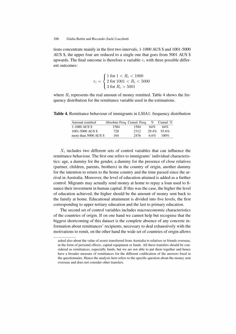
100 Giulia Bettin and Riccardo (Jack) Lucchetti
tions concentrate mainly in the first two intervals, 1-1000 AUS $ and 1001-5000AUS $, the upper four are reduced to a single one that goes from 5001 AUS $upwards. The final outcome is therefore a variable ri with three possible differ-ent outcomes:
ri =
1 for 1 < Ri < 10002 for 1001 < Ri < 50003 for Ri > 5001
where Ri represents the real amount of money remitted. Table 4 shows the fre-quency distribution for the remittance variable used in the estimations.
Table 4. Remittance behaviour of immigrants in LSIA1: frequency distribution
Amount remitted Absolute Freq. Cumul. Freq. % Cumul. %1-1000 AUS $ 1584 1584 64% 64%1001-5000 AUS $ 728 2312 29.4% 93.6%more than 5000 AUS $ 164 2476 6.6% 100%
Xi includes two different sets of control variables that can influence theremittance behaviour. The first one refers to immigrants’ individual characteris-tics: age, a dummy for the gender, a dummy for the presence of close relatives(partner, children, parents, brothers) in the country of origin, another dummyfor the intention to return to the home country and the time passed since the ar-rival in Australia. Moreover, the level of education attained is added as a furthercontrol. Migrants may actually send money at home to repay a loan used to fi-nance their investment in human capital. If this was the case, the higher the levelof education achieved, the higher should be the amount of money sent back tothe family at home. Educational attainment is divided into five levels, the firstcorresponding to upper tertiary education and the last to primary education.
The second set of control variables includes macroeconomic characteristicsof the countries of origin. If on one hand we cannot help but recognise that thebiggest shortcoming of this dataset is the complete absence of any concrete in-formation about remittances’ recipients, necessary to deal exhaustively with themotivations to remit, on the other hand the wide set of countries of origin allows
asked also about the value of assets transferred from Australia to relatives or friends overseas,in the form of personal effects, capital equipment or funds. All these transfers should be con-sidered as remittances, especially funds, but we are not able to put them together and hencehave a broader measure of remittances for the different codification of the answers fixed inthe questionnaire. Hence the analysis here refers to the specific question about the money sentoverseas and does not consider other transfers.
IV Interval Regression 101
us to consider if and how remittance behaviour is influenced by macroenonomicaggregates. What we use here is first of all the level of per capita GDP, as a gen-eral measure of the level of development and wealth12. Secondly, the level of fi-nancial development proxied by a measure of demand, time and saving depositsin deposit money banks as a share of GDP, taken from the widely employeddataset on financial structure built by [1] for the World Bank. The rationalebehind this choice is that the decision to send money back home could be influ-enced by the trust in the domestic financial system, especially in case of returnmigration when immigrants could be inclined to invest or simply save moneyin their home country. Finally, the distance between Australia and the countryof origin is considered to proxy somehow for the costs connected to moneytransfers that are likely to increase the farther the homecountry is13.
As explained before, to address problems of endogeneity both income andconsumption are instrumented using a set Zi of five instruments. The first twoinstrument refer to the migrant’s knowledge of the English language: we use twodummy variables, one for English being the language the immigrant speaks bestand another one which equals 1 if the immigrant declared a good knowledge ofEnglish; we assume that language skills should influence income prospects butnot remittance behaviour. The third instrument is a dummy variable stating if theimmigrant lives in a urban or a rural environment. The idea behind this choice isthat the level of consumption may different between urban and rural population,but this should not affect the amount of money sent home. A dummy for childpresence in migrant’s household is also employed, supposing that its incidenceon remittances is limited to the effects of having children on consumtpion levels.Finally, the last instrument is represented by the number of migrant’s householdmembers, expressed in natural logarithm.
4.2 Dealing with the selection problem
While estimating the remittance equation just illustrated above, we do not con-sider selection problems that arise when the sample is made up of people whoremit and people who do not, and the variable is therefore truncated below azero threshold. Remittances actually could be equal to zero either because im-migrants are not interested in remitting to anybody, or simply because they donot earn enough to send a share of their income overseas.
12 Data are from the World Development Indicators database.13 Even if we are not entering the debate on motivations to remit, geographical distance could
represent in a sense also a measure of the strength of family relationship with those leftbehind. The source of the data employed here is CEPII (Centre d’Etudes Prospectives etd’Informations Internationales) dataset on bilateral distances.

102 Giulia Bettin and Riccardo (Jack) Lucchetti
A solution widely used in the empirical literature on the topic is the estima-tion approach outlined by [6], following which the decision to remit is modeledas a two-stage sequential process. In our case, an extension of sample selectionmodels à la Heckman that involves interval estimation as a second step insteadof OLS does not exist in the literature, to the best of our knowledge, and is cer-tainly not straightforward to conceive and implement. All the more so, wheninstrumental variable interval estimations are needed.
We have made a rough attempt to redesign the remittance variable addingone initial class that includes people who send zero AUS$ in the country of ori-gin. These observations are singled out looking if at the yes/no question whetherthey remit, immigrants gave a negative answers. If this is the case, the observa-tion is considered as zero.
The main idea behind this strategy is that, if the population were homoge-neous, the problem coul be dealt with simply by considering the non-senders ashaving −∞ < y∗i ≤ 0 (in the language of equation (3)). In this scenario, theonly possible reason for not sending money abroad is the budget contraint. If, onthe other hand, there are people who would not send remittances whatever theirincome, then the two-stage decision process should be modelled separately.
Running again estimations with the zero-augmented dependent variable weget results that are quite different from the original ones, both in terms of signif-icance and in terms of magnitude. This has to be read as a clear sign that sampleselection is a problem we absolutely have to deal with, but at the same time italso shows that a suitable tool is needed. Considering a class of zeros de factodoes not address correctly the selection mechanism, because we use a commonmodel for the two different group of individuals and the estimation of a remit-tance equation actually does not make much sense for an immigrant who is notinterested in sending money back home.
We prefer therefore not to introduce a strong source of heterogeneity byjoining two samples (remitters and non remitters) that are most likely to bestructurally different; we are aware that our results should be considered as con-ditional on the fact that the individual is a remitter.
The next step in our research then will be to include in the model a selectionequation to control properly for the selection mechanism, but meanwhile themain focus of the work is on endogeneity treatment and the adoption of IVtechnique in interval estimations.
4.3 Results
Results are reported in Table 5. The first three columns show results obtainedwith simple interval estimations, while from column 4 onward we introduce IVtechniques.
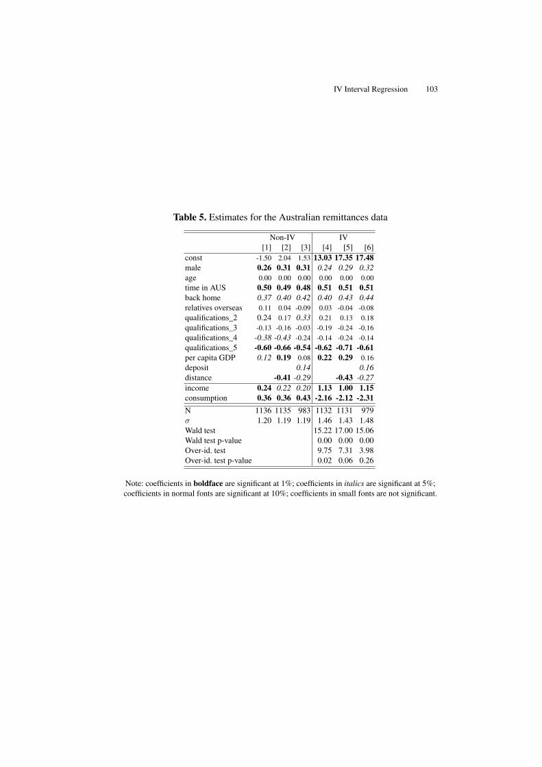
IV Interval Regression 103
Table 5. Estimates for the Australian remittances data
Non-IV IV[1] [2] [3] [4] [5] [6]
const -1.50 2.04 1.53 13.03 17.35 17.48male 0.26 0.31 0.31 0.24 0.29 0.32age 0.00 0.00 0.00 0.00 0.00 0.00time in AUS 0.50 0.49 0.48 0.51 0.51 0.51back home 0.37 0.40 0.42 0.40 0.43 0.44relatives overseas 0.11 0.04 -0.09 0.03 -0.04 -0.08qualifications_2 0.24 0.17 0.33 0.21 0.13 0.18qualifications_3 -0.13 -0.16 -0.03 -0.19 -0.24 -0.16qualifications_4 -0.38 -0.43 -0.24 -0.14 -0.24 -0.14qualifications_5 -0.60 -0.66 -0.54 -0.62 -0.71 -0.61per capita GDP 0.12 0.19 0.08 0.22 0.29 0.16deposit 0.14 0.16distance -0.41 -0.29 -0.43 -0.27income 0.24 0.22 0.20 1.13 1.00 1.15consumption 0.36 0.36 0.43 -2.16 -2.12 -2.31N 1136 1135 983 1132 1131 979σ 1.20 1.19 1.19 1.46 1.43 1.48Wald test 15.22 17.00 15.06Wald test p-value 0.00 0.00 0.00Over-id. test 9.75 7.31 3.98Over-id. test p-value 0.02 0.06 0.26
Note: coefficients in boldface are significant at 1%; coefficients in italics are significant at 5%;coefficients in normal fonts are significant at 10%; coefficients in small fonts are not significant.

104 Giulia Bettin and Riccardo (Jack) Lucchetti
When not instrumented, both income and consumption are statistically sig-nificant with a positive sign. The result is expected for income, and in line withthe previous findings of the empirical literature14, but quite puzzling for con-sumption. If we consider remittances as a sort of savings, the natural predictionwould be that they diminish as the level of consumption expenditure of the im-migrants’ household increases. This clearly shows how results are biased whenwe do not take reverse causality into account.
Moving to IV interval estimations (column 4-6), income and consumptionare statistically significant at 1%, the former with a positive sign and the latternegatively. Elasticity of remittances to income is around 1-1.15, while elasticityto consumption is slightly bigger than 2. Remittances seem therefore much moreresponsive to change in consumption expenditure compared to change in thelevel of income.
Among individual characteristics, the age of immigrants seems not to in-fluence their remittance behaviour, while gender differences result statisticallysignificant: other things being equal, male migrants remit on average 30% morethan female. The desire to return living in the country of origin predictably af-fects the amount remitted in a significant way, with potential returnees remittingaround 40% more. Time elapsed from the arrival in Australia has also a positiveand significant effect.
The presence of a close relative still living overseas does not play such asignificant role in determining remittances. This somehow surprisingly resultcould be due to the fact that in the sample considered here almost everybodywho sends money overseas has at least one close relative (spouse, children, par-ents, brothers/sisters) still living in the country of origin.
As far as the immigrants’ education is concerned, just one out of four dum-mies is significant across all the specifications, with a negative sign, and is theone associated to the lowest level of education (primary school). What emergesis hence that, even after controlling for the level of income, more educated mi-grants are likely to remit higher amounts than the less educated.
The Wald test rejects firmly the exogeneity hypothesis for income and con-sumption. Endogeneity effects are therefore highly significant, so specification1-3, which do not take this into account, must be regarded as incorrect. If co-variances between residuals from the first steps and residuals from the remit-tance equation are considered, it is clear that the result of the Wald test is drivenmainly by consumption that is strongly endogenous, while income is under-standably less affected from problems of reverse causality. Moreover, the resultfrom the LR test of over-identifying restrictions confirms the validity of the set
14 Among others, see [2] and [3].

IV Interval Regression 105
of instruments we have chosen to address endogeneity of income and consump-tion, especially in the complete specification.
As explained before, the cross-country dimension is taken into account addingto individual characteristics macroeconomic variables concerning the home coun-tries. Surprisingly, per capita GDP of immigrants’ country of origin turns out tobe significant with a positive sign. Immigrants coming from richer countriesseem to remit more. This result is confirmed when we consider also the distancebetween Australia and immigrants’ home country (column 5).
The most interesting aspect is that per capita GDP loses all its explanatorypower when the level of financial development is added as a further explanatoryvariable (column 6), while financial development is significant at 5% and playsan important role in immigrants’ household decision. Per capita GDP henceseems to act, when significant, as a sort of proxy for the level of financial devel-opment of immigrants’ country of origin, but this is indeed the macroeconomicfeature that matters when immigrants consider how much money to remit.
5 Conclusions
We argue that estimation of models in which the dependent variable is observedby intervals and explanatory variables may be endogenous ought to be con-ducted via maximum likelihood, all the alternative possibilities being inefficientat best and plain wrong at worst.
An example with Australian remittances data shows that our procedure iseffective. Endogeneity of income and consumption in the context of immigrants’remittance behaviour does matter. Consumption is strongly endogenous, whileincome is less affected from problems of reverse causality; anyway, endogeneityeffects are altogether highly significant and need to be addressed in empiricalmodels. Failing to account for them will lead to incorrect estimates.

Bibliography
[1] BECK, T., A. DEMIRGUÇ-KÜNT, AND R. LEVINE (2000): “A NewDatabase on Financial Development and Structure,” World Bank EconomicReview, 14, 597–605.
[2] BROWN, R. P. (1997): “Estimating Remittance Functions for Pacific IslandMigrants,” World Development, 25(4), 613–626.
[3] CLARK, K., AND S. DRINKWATER (2007): “An Investigation of HouseholdRemittance Behaviour; Evidence from the United Kingdom,” The Manch-ester School, 75(6), 717–741.
[4] DAVIDSON, R., AND J. G. MACKINNON (1999): Econometric Theory andMethods. Oxford University Press, Oxford.
[5] DUSTMANN, C., AND J. MESTRES (2008): “Remittances and TemporaryMigration,” mimeo.
[6] HECKMAN, J. J. (1979): “Sample Selection Bias As a Specification Error,”Econometrica, 47(1), 153–161.
[7] HOLST, E., A. SCHAEFER, AND M. SCHROOTEN (2008): “Gender, Migra-tion, Remittances : Evidence from Germany,” SOEPpapers 111, DIW Berlin,The German Socio-Economic Panel (SOEP).
[8] KAWAKATSU, H., AND A. G. LARGEY (2009): “EM Algorithms for Or-dered Probit Models with Endogenous Regressors,” Econometrics Journal,forthcoming.
[9] LUCAS, R. E., AND O. STARK (1985): “Motivations to remit: evidence fromBotswana,” Journal of Political Economy, 93, 901–918.
[10] MERKLE, L., AND K. F. ZIMMERMANN (1992): “Savings, Remittancesand Return Migration,” Economics Letters, 38, 77–81.
[11] OSILI, U. O. (2007): “Remittances and Savings from International Mi-gration: Theory and Evidence using a Matched Sample,” Journal of Devel-opment Economics, 83, 446–465.
[12] PAGAN, A. (1986): “Two Stage and Related Estimators and Their Appli-cations,” Review of Economic Studies, 53(4), 517–538.
[13] RAPOPORT, H., AND F. DOCQUIER (2005): “The Economics of Migrants’Remittances,” IZA Discussion Papers 1531, Institute for the Study of Labor(IZA).
[14] SINNING, M. (2007): “Determinants of Savings and Remittances: Empir-ical Evidence from Immigrants to Germany,” IZA Discussion Papers 2966,Institute for the Study of Labor (IZA).

IV Interval Regression 107
[15] SOLIÑO, M., M. X. VÁZQUEZ, AND A. PRADA (2009): “Social demandfor electricity from forest biomass in Spain: Does payment periodicity affectthe willingness to pay?,” Energy Policy, 37(2), 531–540.
[16] STEWART, M. B. (1983): “On least squares estimation when the depen-dent variable is grouped,” Review of Economic Studies, 50(3), 737–753.
[17] WOOLDRIDGE, J. M. (2002): Econometric Analysis of Cross Section andPanel Data. MIT Press, Cambridge, Mass.


Applied Econometrics


A Model for Pricing the Italian Contemporary ArtPaintings at Auction
Nicoletta Marinelli1 and Giulio Palomba2
1 Dipartimento di Economia, Università Politecnica delle Marche, Italy. [email protected] Dipartimento di Economia, Università Politecnica delle Marche, Italy. [email protected]
Abstract. This paper aims to model the auction prices of Italian contemporaryart paintings. The contribution to the existing literature is twofold concerning boththe methodological and the conceptual aspects. From the former point of view, weuse the two-stages Heckit model which allows us to take into account the sampleselection bias deriving from the “buying” risk, that affects transactions at auction.From the latter point of view, we have found that some sale characteristics suchas auction house prestige and year of sale, are more important than the physicalaspects of the paintings. Moreover, some artistic characteristics, the artist’s nameand their living status are also relevant.The whole analysis is carried out after creating a new dataset of 2817 transactionswhich took place at the most important auction houses between 1990 and 2006.
1 Introduction
The prices of paintings depend upon a set of variables, concerning the charac-teristics of the paintings themselves, but also other aspects more difficult to bemeasured, such as the artist’s popularity or the auction house’s prestige. Severalquestions about the level of art prices are still open and literature has not clearlydefined what are the main drivers of their dynamics and what are the conditionsfor a more liquid and riskless investment in artworks.
From the theoretical point of view, there are two main theories regarding theprice determination: on one hand, [3] claims that there may exist no equilibriumlevel for art prices, so they can float more or less aimlessly with unpredictableoscillations emphasized by the activities of investors/speculators; on the otherhand, [17] assume that a “natural price” does not exist for paintings, neverthlessmarket forces related to demand and supply determine prices for artworks, asfor any other economic good.
From the empirical point of view, the pricing of paintings is generally dis-cussed within the framework of market price indexes, with the aim of evaluatingthe rate of return of an investment upon such assets. In this context, the hedonicregression (from [2] onwards) seems to be a good methodology to select thevariables which can be useful to model the evolution of artwork prices.
112 N. Marinelli and G. Palomba
The key-objective of this paper is to carry out an empirical analysis about theprice determinants of Italian contemporary art paintings at auction. The analysisis two-fold because it allows us to jointly model how some explanatory variablescontribute to the probability of having an unsold item and to the price levels ofsold works.
In doing so, a preliminary sample selection is obviously required. We con-sider a sample of 2817 painting transactions from the 21 Italian contemporaryartists who showed the biggest turnover at auction during the period 1998-2002,according to [35]. Starting from the available information about this sample oftransactions, we made a new dataset in which all the variables are grouped intofour categories, being the usual painting-specific attributes: they are the physi-cal qualities of the work, the characteristics of the artist, the artistic and the salecharacteristics of the paintings.
The reminder of this paper is organized as follows: in section 2 we intro-duce the problems related to the sample selection and the choice of the relevantvariables. The whole empirical analysis is carried out in section 3 and section4 concludes. Finally, the Appendix includes the complete list of all availablevariables.
2 The sample selection
The analysis of the price dynamics of paintings sold at auction has to be basedupon the choice of an appropriate sample. In this article, all the available infor-mation is taken from “Artindex Plus”, a detailed database which contains thecatalogue’s information about several artworks3: more precisely, it provides thepicture of the painting plus different pieces of information about the artist andthe artwork itself (see section 2.1 for details).
Our sample choice substantially depends upon the reaching of a sort of ho-mogeneity between variables: given that the market of paintings is composed ofunique goods, we focus the attention upon Italian contemporary art because weneed to deal with goods as comparable as possible4.
Since Italian contemporary art itself is not completely homogeneous5, welimited our analysis to the 21 Italian contemporary artists who showed the biggestturnover at the most important international auctions during the period 1998-
3 Artindex Plus is provided by Gabrius S.p.A. operating in Milan and belonging to the MunusCulture Holding (AMB network); for more details see http://www.munusartinvest.com.
4 The market of paintings is usually divided in four branches which have their own dynamicsand characteristics: Old Master, XIX Century, Modern Art and Contemporary Art.
5 In practice, there are differences among “emerging” and “historical” contemporary artpainters.
A Model for Pricing the Italian Contemporary Art. . . 113
2002, according to [35]6. The reason for this selection is that the paintings areconsidered as investment goods for which the main characteristics depend uponthe market dynamics; the aestethic component is not supposed to be relevanthere. The homogeneity in our sample is also preserved by the exclusion of printsand drawnings because these items have their own specific price dynamics, asclaimed by [26], and are often traded in separate sessions at auction.
Finally, we restrict the period of observation to the years which go from1990 to 2006, since the Artindex Plus data regarding auction sales before 1990are very poor and incomplete. Following this sample selection, we work witha dataset of 2817 painting transactions placed at the most important auctionhouses.
A problem encountered in studying art prices stems from the fact that theauction data samples could suffer from some problems of selection bias, as al-ready underlined by [38]. It is well known that the art market is divided into“primary”, “secondary” and “auction” market: in the former the artist person-ally sells her works to buyers, while in the second the galleries and the art deal-ers trade paintings with private or institutional collectors. Auction represents theremaining solution, therefore it can not take into account all types of paintings.Neverthless, in this case public information exists and this overcomes most ofthe typical problems due to the incomplete and asymmetric information avail-ability of the art market. Moreover, we suppose that auction prices affect the artmarket because collectors and professional art dealers take these price as guide-lines, following the approach of [16]. Finally, we also consider auction prices asadequate approximations of true equilibrium prices, as pointed out by [6].
With this sample selection, we try to give an empirical contribution for asector that literature has often neglected7.
2.1 The data
For each item Artindex Plus provides the following information: a picture of thepainting, personal details about the artist, physical characteristics of the painting(date of execution, width and height, support, medium), artistic characteristics
6 [35] define the “turnover” as the number of sold works multiplied by their mean price.Moreover, they conventionally define as the Italian contemporary artists those Italian
painters who carried out their activity after 60’s. This selection criterium is not strictly ap-plied, since some Italian painters, still working after 1960’s, but historically placed with thebest artists of Futurism or other artistic currents preceding the 1960’s, are not included intheir sample (for example, Carlo Carrà). So, in the analysis of [35], the Italian contemporaryart conventionally starts with the contributions of Fontana (1899-1968), Burri (1915-1995),Marini (1901-1980) and Manzoni (1933-1963).
7 For previous contribution see for example [5], [1], [30], [34] or [25]. Only [6] uses data aboutthe Italian market of Modern and Contemporary oil paintings.

114 N. Marinelli and G. Palomba
of the painting (list of previous owners, signature, date, title, expertise, litera-ture citations, list of exibitions), sale characteristics of the painting (lot number,auction house, city, month and year of transaction), economic characteristicsof the paintings (hammer prices, hammer prices plus transaction fees, pre-saleevaluation by experts who provide the estimation of a range of prices).
Tables in the Appendix report the descriptions of the variables used in ourwork.
2.2 Dependent variables
Given that we aim to model the auction price levels taking into account theproblem of unsold paintings, our dependent variable is given by the auctionprice of each painting. In our dataset we have both the hammer price and thetotal purchase price: the latter differs from the former because it includes theauction house’s transaction fees. All the prices related to unsold paintings atauction are not observable, hence they are set as zero.
Both types of prices are all converted to US Dollars to make them compara-ble, obtaining series pi and Pi respectively. Finally, we consider their logarith-mic transformation, indicated with yi and Yi.
2.3 Explanatory variables
The main evidence related to the variables identification concerns the qualita-tive nature of most of the available data; for this reason several variables aredummies. The explanatory variables for the price of Italian contemporary artpaintings are organized into four categories; the list of potential price determi-nants and their codes are reported in the Appendix.
A. Characteristics of the artist: personal characteristics of the artist who paintedthe work.1) Name of the artist: 21 different dummy variables, one for each artist in
the sample.2) Living status: dummy variable8 (1 if the painter is deceased at the time
of the sale and 0 otherwise).3) Year of birth.
B. Physical characteristics: related to the execution of the artwork.4) Medium: this variable allows us to control the assumption of a superior
market value as a consequence of the media durability and particulars9.8 All other things being equal, the price of artworks are often supposed to increase once an artist
has died, as pointed out by [24].9 Generally, oil paintings are supposed to be more expensive than other media. See, among
others, [11], [34], [25], [24].

A Model for Pricing the Italian Contemporary Art. . . 115
5) Support: 10 different types of support upon which the artwork is paintedare available. The related dummy variables have the value of one whenthe specified support is used, alone or jointly with another, and zerootherwise.
6) Size: the surface (expressed in m2) and the squared surface as in [34],[24] and [40]. In particular, [11] describes the price of painting as aconcave function of dimensions.
C. Artistic characteristics: these variables are supposed to be as proxies ofthe prestige and the popularity of the artwork in the art world. They are alldummy variables taking into account for the following characteristics:7) Authentication by the artist8) Publication in catalogues or monographies9) Date
10) Recognition by experts11) Literature: citations in the artistic literature (see [14])12) Signature13) Title14) Exhibitions15) Number of previous owners: according to auction houses, the price reached
for a painting is influenced by its provenance. The number of previousowners can be useful in order to test whether a painting rarely traded inthe auction market reaches a greater price than a painting that has oftenbeen put on sale (see [15]). Obviously, this is not a dummy variable10.
D. Sale characteristics: with this set of explanatory variables we test the hy-pothesis that sale conditions have an effect upon the marketability and uponthe final price reached by the painting at auction.
16) Auction house: [32], [13], [34], [25], [24], among others, show thatChristie’s and Sotheby’s systematically obtain higher hammer prices;this evidence is generally attributed to the leading role played by bothinstitutions in this business.
17) Marketplace: dummy variables for the 18 different marketplaces in database.18) Sale date: dummy variable for each year (from 1990 to 2006) and for
each month of sale.19) Pre-sale estimates: before an auction sale takes place, experts usually
provide an estimate of the potential market value of the painting. Pre-sale estimates are usually provided as a range.
10 The dataset does not allow us to classify all previous owners according to their institutionalnature (for example, museum, gallery or private collector), because it provides only the namesof previous owners.
116 N. Marinelli and G. Palomba
3 The model
The aim of our proposed methodology is to model the auction prices of the Ital-ian Contemporary Art paintings. Examining the determinants of auction pricesfrom a speculative perspective, we have to consider the possibility of unob-served final prices; in other words, as well as the price reached by sold works,we have to take into account the “buying risk” affecting each transaction. Sincein our sample various artworks go unsold, the analysis must be divided into twostages: in the first stage, a distinction between sold and unsold paintings is made,while in the second stage, prices of sold paintings are modelled.
3.1 The Heckit model
From the statistical point of view the possibility of unsold items at auction implya problem of selection bias which can arise from censoring data. In particular,the properties of painting prices can vary taking unsold works into account, thusdata can suffer from nonrandomness.
To address this problem the Heckit model [23] is used; this model allowsus to carry out the analysis when the dependent variable is continous but cen-sored for values under a defined threshold. This methodology was introduced tocorrect the selection bias occurred for nonrandomly selected samples and pro-vides consistent estimates which eliminate the specification error for the case ofcensored data. Recently, [40] used this methodology upon a sample of Picassoprints censored for repeat-sales, as well as [8] upon a sample of Symbolist paint-ings.
Analitically, the Heckit model consists ofs∗i = z′iγ + ui i = 1, 2, ....., Nwi = x′iβ + εi ⇔ s∗i > 0,
(1)
whereN is the sample size. The first equation is the “selection equation”, wheres∗i is a latent variable which is positive if the auction price is greater than thereservation price. Moreover, the 1×K vector z′i contains the individual charac-teristics that determine if the painting is sold or not, γ is aK-dimensional vectorof unknown parameters and ui is a random disturbance. The latent variable s∗iis not observed, therefore we define a dichotomic variable si as
si =
1 if s∗i > 00 otherwise.
(2)
In practice, for sold paintings si = 1, while it is zero otherwise.The second equation of the system (1) is the linear model of interest in which
wi is the dependent variable; xi is the 1 ×M vector of exogenous variables, β
A Model for Pricing the Italian Contemporary Art. . . 117
is a M -dimensional vector of unknown parameters and εi is a random errorterm. The explanatory variables in xi could be also included in zi and viceversa.Moreover, we assume that the random disturbances are jointly distributed as[
uiεi
]∼ i.i.d.
([00
],
[σ2u σuε
σuε σ2ε
]). (3)
In our model the selection bias arises because the price wi is observed onlywhen the i-th painting is sold (therefore si = 1) and when σuε is differentfrom zero; in such a situation, [23] shows that OLS estimation yields biased andinconsistent estimates of β.
Generally, the estimator for the Heckit model is the Maximum Likelihood(ML) under the assumption of joint normal distribution in equation (3); thismethod guarantees consistent and asymptotically normal and efficient estimates(see for example [22]). Unfortunately, in our analysis ML estimation of themodel (1) does not achieve convergence, hence we use the Heckman’s (1979)two-step procedure which yields a less efficient estimator.
The whole procedure can be briefly outlined as follows: given that φ(·) andΦ(·) respectively are the density and the cumulative density functions of thestandardised Gaussian distribution, the first step consists of the ML estimationof the probit model Pr(si = 1) = Φ(z′iγ). This equation predicts whether anitem goes sold/unsold and it is useful to obtain the inverse of the Mills Ratiogiven by λi = φ(z′iγ)/Φ(z′iγ), which will be used as an additional regressorduring the second step to correct the potential sample selection bias.
Once λi is inserted in xi vector, its coefficient is βλ = σuεσ2ε and the second
equation in (1) can be estimated via the OLS method. The covariance betweenui and εi can also be estimated and the standard t-statistic on βλ is used to testif any problem of selection bias occurrs in our analysis.
Moreover, as shown by [31], the assumption of normality of the probit resid-uals ui is required to have consistency and plays a key role because it representsthe sufficient condition to define λi as in equation given above. Following [12]we carried out the following conditional moment (CM) test based on the OPGRegression11
ι = γZ + bG+ residuals, (4)
where ι is a vector of ones, Z is the matrix whose each row is z′i and γ, b areML estimates from the probit Pr(si = 1) = Φ(z′iγ +G′ib). To take into accountfor asymmetry and kurtosis, the i-th row of the matrix G is
G′i =[[(z′iγ)2 + 2]ui z′iγ[(z′iγ)2 + 3]ui
], (5)
11 Outer Product Gradients Regression; see for example [12] for details.

118 N. Marinelli and G. Palomba
where ui are the model generalised residuals [see for example 31]. It can beshown that, for each observation, G′i contains the sample counterparts of the or-thogonality conditions about the conditional moments E(uki |ui < −z′iγ), whenk is 3 and 4 respectively [see 36].
The basic idea is that, if G′i is not statistically relevant in the selection equa-tion, the probit model is correctly specified. Hence, the null hypothesis of theCM test is H0 : b = 0 and the test statistic is given by N times the R2 of theregression (4). Given that G has two columns, the asymptotic distribution is thestandard χ2
2.
3.2 Empirical results
The starting point of our analysis consists of the Heckit estimation where thesecond equation in (1) can be thought as a sort of an hedonic regression inwhich the selection bias has been taken into account. All results for wi = yi, Yiare provided in Tables 1 and 2, while Table 3 contains some regression statistics;some explanatory variables among those presented in section 2.3 are droppedto avoid collinearity and, after some preliminary estimates, other variables areexcluded to reach the possible maximum reduction of parameters, without anyloss of relevant information.
The first emerging aspect is that the estimates of the auction prices of theItalian Contemporary Art paintings are quite similar for the logarithms of thehammer price (yi) and of the total purchase price (Yi): the presence of trans-action fees does not seem to have any relevant impact upon our analysis, alsoconsidering that there are 4 missing values for Pi in our original sample (see thetotal observations in Table 3). The sample size reduction is due to three missingvalues in surface and squares.
The null hypothesis of the CM test is strongly accepted in both cases andthis supports the consistency of our estimates in which λi is not statisticallydifferent from the inverse of the Mills Ratio.
The t-statistic evaluated for λi indicates that some correction for the sampleselection bias is needed and, for this reason, the Heckit model is superior toOLS.
The negative estimated value of the coefficient related to λi depends uponσuε < 0: this suggests that paintings that go sold are more likely to be thosewith a lower price, since cheaper paintings are likely to be bought by a widergroup of potential buyers.
Moreover, the [4] normality test highlights that the model disturbances arenot jointly normally distributed and this is probably the reason why the MLestimation process does not converge.

A Model for Pricing the Italian Contemporary Art. . . 119
The contributions given by the explanatory variables in the two steps of theestimation are discussed below.
First step Only the dummies related to painters Boetti, Campigli, Fontana andMagnelli positively contribute to the outcome of artwork transactions. This sug-gests that the paintings made by this group of artists are, on average, less likelyto go unsold at auction, showing a strong tendence to be easily traded. If theartist is dead at the moment of sale the painting has a higher probability togo unsold, as highlighted by the negative and significant coefficient related todead. The variable birth has been dropped according to the results of prelimi-nary analysis in which it was found to be not statistically relevant in both stepsof estimation.
Media and support do not play any relevant role upon the probabiliy thatpaintings go unsold; only items painted with enamel are less likely to be sold.Even if in our sample most of the paintings are made on canvas and paper (seeTable 5), they do not affect the estimation.
All the variables used to capture the prestige and the popularity of the paint-ings do not seem to be relevant at this stage of the estimation, with the onlyexception being literature which has a very feeble effect (the p-value is about0.11).
The outcome of the sale, in terms of sold/unsold work, is highly determinedby the auction house where the sale is arranged. For the need of parsimony, weconsider only Christie’s, Sotheby’s and Finarte where more than 90% of trans-actions are placed. All their coefficients are positive and highly significant. Thefindings about Christie’s and Sotheby’s are coherent with those of [13] who ar-gued that some auction houses are able to systematically influence the successfuloutcome of the sale since they often attract more high valued artistic works12.The result of Finarte could be intepreted as a consequence of the “home biaseffect”, that is a general preference of buyers for domestic art production, aspointed out by [7].
It has also been previously proved that the other auction houses, the cityand month of sale do not seem to have an additional effect on the probability ofgoing unsold.
Some years affect the outcome of the sale more than others: in particular1993, 1997 and 2002 show negative and statistically significance relationships,while 1992 and 2004 instead have a positive and significant parameter.
12 ...the quality of a painting , not captured by our characteristics, is partly picked up by thesaleroom coefficients: a “good” Picasso would go to Christie’s or Sotheby’s New York, a lessgood one would be sold at Drouot’s [...] it is impossibile to disentangle the two effects.

120 N. Marinelli and G. Palomba
Second step It is straightforward evident from Table 2 that almost all variablesplay a key role in determining auction prices and the impact given by the ma-jority of painters seems to be decisive. The number of the exceptions is verysmall and the statistical significance attributed to Pomodoro is scarse probablybecause only two works belong to our sample (see Table 4).
The estimation highlights that Campigli and Fontana, who have a positiveand significant impact upon the selection equation, also show an analogous ef-fect upon the second step; on the contrary, the coefficient related to Boetti hasthe opposite sign of that in the selection equation. The paintings made by Burri,Cattelan, Manzoni and Marini also seem to reach market values higher, on aver-age, than other artists, while the negative parameters related to different painterssuggest that their works generally achieve lower prices.
The variable dead do not have any effect, while the variable birth is droppedbecause of its statistical irrelevance. From our model one can argue that thedeath of the artist before the moment of sale only increases the probability thatpaintings go unsold, but does not affect auction prices. This result is in contrastwith both contributions of [1] and [39]: the former paper showed an increase by154% of the auction prices of American art when the artist was still alive, whilethe latter work found that paintings made by deceased artists are associated witha price increase of 100.58%.
Our estimation suggests that painting media do not have a relevant effectupon the total purchase price of a painting; the only exceptions are oil and theresidual variable other for which the coefficients produce an increasing effectupon artwork prices. It is difficult to compare these findings with previous anal-yses especially because these contributions are sometimes limited to historicalperiods when only few media were known [see for instance 14] or restricted tosingle medium samples [6].
The contributions of the supports are heterogeneous because canvas seemsto have a significant and positive influence upon painting prices, while paperhas the opposite effect.
The coefficient signs of the variables regarding the size of paintings are thoseexpected and coherent with the findings of [11]: in particular, the artwork pricescan be described as a concave function in which the surface and the squaredsurface have a positive and negative relationship respectively. This suggests that,if the size is augmented, the Italian Contemporary Art prices tend to increase atfirst, but then decrease when the painting becomes too large and difficult tohang.
Among the artistic characteristics of the paintings, the publication in cat-alogues, the number of exhibitions, the literature and the number of previousowners have a positive effect, while the variable expertise surprisingly shows
A Model for Pricing the Italian Contemporary Art. . . 121
negative contributions, contrary to our expectation. Variables authentic andsignature do not have any effect upon the estimation, maybe because the pres-tige of some auction houses serves as a guarantee of authenticity.
The sale year substantially affects the final purchase price of Italian contem-porary art paintings: each year from 1991 to 2004 shows statistically significantand negative coefficients, while years 2005 and 2006 do not seem to be rele-vant. From the economic perspective the series of these coefficients can be usedto built the yearly price index It, with all other characteristics being equal. Thisindex shows the contribution to auction prices dynamics given by years of saleand its equation is It = 100 · expβt, where t = 1991, 1992, . . . , 2006. Justthe hammer price index is plotted in Figure 1 since the curve related to the totalpurchase price (Yi) is very similar. The base year is 1990 in which It = 100.For both series this index substantially shows an increase from 1994, while onlyin 2006 it has a value greater than those of the base year. This is consistent withthe evidence of the art market downturn experienced in the early ninetees [see,among others, 29] and the upturn of the market in recent years.
Finally, even if Table 1 highlights that principal auction houses stronglydetermine the outcome of sale, their contribution to price levels is not relevantand, for this reason, they have been dropped from the second the step of theestimation.
4 Concluding remarks
This paper aims to model the prices of paintings given a set of explanatory vari-ables regarding different characteristics. The whole analysis is carried out aftercreating a sample of 2817 transactions of paintings made by 21 Italian contem-porary painters and sold at auction during the period 1990-2006. To take theproblem of sample selection bias arising from the inclusion of unsold paintingsinto account, the Heckit model [23] is used to obtain consistent estimates.
Our estimation highlights that some mechanism of selection bias occurrshence this methodology is superior to OLS. The main finding is that auctionprices for the Italian Contemporary Art market depend upon several variablessuch as auction house prestige, year of sale, artist’s popularity and differentartistic characteristics of paintings (publication in catalogues, number of ex-hibitions, citations in the artistic literature, number of previous owners). Thisfinding is consistent with the main existing literature.
Contrary to previous studies [see for example, 11 or 39], we found thattraditional media, supports and conventional proxies of artistic qualities are lessable to explain the marketability of paintings, while they have a strong effect onprice levels. Other variables playing a leading role upon the outcome of sale are

122 N. Marinelli and G. Palomba
those related to sale characteristics (for example, auction house prestige) and tothe years in which the transactions take place; the years of sale also affect theauction price determination.
A price index that fits the cyclical nature of the Italian Contemporary Artmarket has been derived from the coefficients related to the years of sale: afteran initial decline it tends to increase from 1994 and finally have a strong riseafter 2003. This evidence reflects the downturn of the art market in the earlyninetees and it is coherent with previous literature. This is also consistent withthe upturn in contemporary painting prices experienced in recent years. Somesuggested reasons for this cycle could be macroeconomic factors such as thedependence of the art market upon per capita income [17], financial coursessuch as the correlation between art market cycles and bullish/bearish financialmarkets [9] or simply art fads such as collectors’ changing attitudes towardscontemporary art [5].

Bibliography
[1] Agnello, R. and Pierce, R.: Financial returns, price determinants and genreeffects in American art investment. Journal of Cultural Economics 20(1996) 359–383
[2] Anderson, R.C.: Paintings as an investment. Economic Inquiry 12 (1974)13–26
[3] , Baumol, W.J.: Unnatural value: or art investment as floating crap game.American Economic Review 76 (1986) 10–14
[4] Box, G.E.P. and Pierce, D.A.: Distribution of residual autocorrelations inautoregressive-integrated moving average time series models. Journal ofthe American Statistical Association 65 (1970) 1509–1526
[5] Buelens, N. and Ginsburg, V.: Revisiting Baumol’s “art as a floating crapgame”. European Economic Review 37 (1993) 1351–1371
[6] Candela, G. and Scorcu, A.E.: A price index for art market auctions. Anapplication to the Italian market for modern and contemporary oil paint-ings. Journal of Cultural Economics 21 (1997) 175–196
[7] Candela, G. and Scorcu, A.E.: Economia delle arti. Zanichelli, Bologna(2004)
[8] Collins, A., Scorcu, A.E. and Zanola, R.: Sample selection bias and timeinstability of hedonic Art Price Indexes. Working Paper DSE 610 (2007)
[9] Chanel, O.: Is art market behaviour predictable?. European Economic Re-view 39 (1995) 519–527
[10] Chanel, O., Gérard-Varet, L.-A. and Ginsburgh, V.: The relevance of he-donic price indices. The case of paintings. Journal of Cultural Economics20 (1996) 1–24
[11] Czujack, C.: Picasso paintings at auction, 1963-1994. Journal of CulturalEconomics 21 (1997) 229–247
[12] Davidson, R. and MacKinnon, J.D.: Estimation and inference in econo-metrics. Oxford University Press, New York (1993)
[13] De la Barre, M., Docclo, S. and Ginsburgh, V.: Returns of Impression-ist, Modern and Contemporary European Painters, 1962-1991. Annalesd’Economie et Statistique 35 (1994) 143–181
[14] Figini, P. and Onofri, L.: Old master paintings: price formation and publicpolicy implication. in Marciano, A. & Josselin, J. M. (eds.), The law andeconomics of the Welfare State: a political economics approach, EdwarElgar Publisher (2005)
[15] Fiz, A.: Investire in arte contemporanea. Franco Angeli, Milano (1995)

124 N. Marinelli and G. Palomba
[16] Frey, B.S. and Pommerehne, W.W.: Art investment: an empirical inquiry.Southern Economic Journal 56 (1989) 396–409
[17] Frey, B.S. and Pommerehne, W. W.: Muse e Mercati. Indaginesull’economia dell’arte. Il Mulino, Bologna (1991)
[18] Ginsburgh, V. and Jeanfils, P.: Long-term comovements in internationalmarkets for paintings. European Economic Review 39 (1995) 538–548
[19] Goetzmann, W.N.: Accounting for taste: art and financial markets overthree centuries. The American Economic Review 83 (1993) 1370–1376
[20] Goetzmann, W. and Spiegel, M.: Private value components and the win-ner’s curse in Art Index. European Economic Review 39 (1995) 549–555
[21] Grampp, W.D.: Pricing the priceless. Art, Artists and Economics. BasicBooks, Inc., New York (1989)
[22] Greene, W.H.: Sample selection bias as a specification error: comment.Econometrica 49 (1981) 795–798
[23] Heckman, J.J.: Sample selection bias as a specification error. Economet-rica 47 (1979) 153–161
[24] Higgs, H. and Worthington, A.: Financial return and price determinantsin the australian art market, 1973-2003. The Economic Record 81 (2005)113–123
[25] Hodgson, D. and Vorkink, K.P.: Asset pricing theory and the valuation ofcanadian paintings. Canadian Journal of Economics 37 (2004) 629–655
[26] Holub, H. W., Hutter, M. and Tappeiner, G.: Light and shadow in art pricecomputation. Journal of Cultural Economics 17 (1993) 49–69
[27] Locatelli-Biey, M. and Zanola, R.: The market for Picasso prints: an hybridapproach. Journal of Cultural Economics 29 (2005) 127-136
[28] Locatelli-Biey, M. and Zanola, R.: Investment in paintings: a short runprice index. Journal of Cultural Economics 23 (1999) 211–222
[29] Mei, J. and Moses, M.: Art as an investment and the underperformance ofmasterpieces. American Economic Review 92 (2002) 1656–1668
[30] Mok, H.M., Ko, V.W., Woo, S.S. and Kwok, K.Y.: Modern Chinese paint-ings: an investment alternative? Southern Economic Journal 59 (1993)808–816
[31] Pagan, A. and Vella, F.: Diagnostic tests for models based on individualdata: a survey. Journal of Applied Econometrics 4 (1989) 29–59
[32] Pesando, J.E.: Art as an investment: the market for modern prints. TheAmerican Economic Review 83 (1993) 1075–1089
[33] Pesando, J.E. and Shum, P.M.: The return to Picasso’s prints and to tra-ditional financial assets, 1977 to 1996. Journal of Cultural Economics 23(1999) 183–192

A Model for Pricing the Italian Contemporary Art. . . 125
[34] Renneboog, L. and Van Houtte, T.: The monetary appreciation of paint-ings: from Realism to Magritte. Cambridge Political Economy Society 26(2002) 331–358
[35] Sacco, P., Santagata, W. and Trimarchi, M.: L’arte contemporanea ital-iana nel mondo. Analisi e strumenti, Collana Opera DARC, Skira, Milano(2005)
[36] Skeels, C.L. and Vella, F.: A Monte Carlo investigation of the samplingbehavior of conditional moment tests in Tobit and Probit models. Journalof Econometrics 92 (1999) 275–294
[37] Stein, J.P.: The monetary appreciation of paintings. Journal of PoliticalEconomy 85 (1977) 1021–1035
[38] Wieand, K., Donaldson, J. and Quintero, S.: Are real asset prices interna-tionally? Evidence from the art market. Multinational Finance Journal 2(1998) 167–187
[39] Worthington, A.C. and Higgs, H.: A note on financial risk, return and assetpricing in Australian modern and contemporary art. Journal of CulturalEconomics 30 (2006) 73–84
[40] Zanola, R.: The dynamics of art prices: The selection corrected repeat-sales index. Working Paper 85, Dipartimento di Politiche Pubbliche eScelte Collettive (POLIS), Università del Piemonte Orientale (2007)
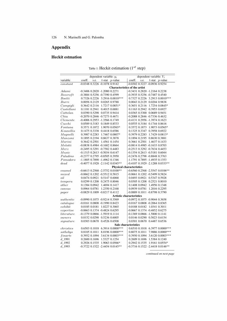
126 N. Marinelli and G. Palomba
Appendix
Heckit estmation
Table 1: Heckit estimation (1st step)
dependent variable: yi dependent variable: Yi
variable coeff. s.e. t-stat p-value coeff. s.e. t-stat p-valueconstant -0.0348 0.3226 -0.1078 0.9142 -0.0302 0.3227 -0.0936 0.9254
Characteristics of the artistAdami -0.3406 0.2820 -1.2080 0.2271 -0.3431 0.2820 -1.2164 0.2238Beecroft -0.3884 0.5256 -0.7390 0.4599 -0.3935 0.5256 -0.7487 0.4540Boetti 0.7326 0.2226 3.2916 0.0010*** 0.7327 0.2226 3.2913 0.0010***Burri 0.0056 0.2129 0.0265 0.9788 0.0043 0.2129 0.0204 0.9838Campigli 0.3642 0.2116 1.7217 0.0851* 0.3651 0.2116 1.7254 0.0845*Castellani 0.1181 0.2941 0.4015 0.6881 0.1163 0.2942 0.3953 0.6927Cattelan 0.0390 0.5298 0.0735 0.9414 0.0365 0.5300 0.0689 0.9451Chia -0.2070 0.2846 -0.7273 0.4671 -0.2088 0.2846 -0.7336 0.4632Clemente -0.4006 0.2953 -1.3566 0.1749 -0.4131 0.2956 -1.3974 0.1623Cucchi 0.0589 0.3183 0.1849 0.8533 0.0555 0.3184 0.1744 0.8616Fontana 0.3571 0.1872 1.9070 0.0565* 0.3572 0.1873 1.9073 0.0565*Kounellis 0.1475 0.3338 0.4418 0.6586 0.1325 0.3347 0.3958 0.6922Magnelli 0.3987 0.2283 1.7467 0.0807* 0.3979 0.2283 1.7429 0.0813*Manzoni 0.1895 0.2194 0.8637 0.3878 0.1894 0.2195 0.8630 0.3881Marini 0.3642 0.2501 1.4561 0.1454 0.3661 0.2501 1.4637 0.1433Melotti -0.0838 0.4984 -0.1682 0.8664 -0.0814 0.4985 -0.1633 0.8703Merz -0.2495 0.3291 -0.7582 0.4483 -0.2513 0.3292 -0.7634 0.4453Music -0.1315 0.2613 -0.5034 0.6147 -0.1354 0.2613 -0.5181 0.6044Paladino -0.2377 0.2795 -0.8505 0.3950 -0.2476 0.2798 -0.8848 0.3763Pomodoro -1.1805 0.7890 -1.4962 0.1346 -1.1791 0.7895 -1.4935 0.1353dead -0.4077 0.1928 -2.1142 0.0345** -0.4107 0.1929 -2.1288 0.0333**
Physical characteristicsenamel -0.6613 0.2568 -2.5752 0.0100** -0.6560 0.2568 -2.5547 0.0106**mixed -0.0662 0.1202 -0.5512 0.5815 -0.0661 0.1202 -0.5499 0.5824oil 0.0474 0.0921 0.5147 0.6068 0.0493 0.0921 0.5347 0.5928tempera 0.0299 0.1208 0.2475 0.8046 0.0305 0.1208 0.2521 0.8010other 0.1384 0.0942 1.4694 0.1417 0.1408 0.0942 1.4956 0.1348canvas 0.0964 0.0781 1.2350 0.2168 0.0939 0.0781 1.2016 0.2295paper -0.0829 0.1009 -0.8217 0.4112 -0.0889 0.1011 -0.8798 0.3790
Artistic characteristicsauthentic -0.0990 0.1075 -0.9214 0.3569 -0.0972 0.1075 -0.9044 0.3658catalogue -0.0161 0.0808 -0.1990 0.8423 -0.0167 0.0808 -0.2064 0.8365exhibit 0.0185 0.0181 1.0227 0.3065 0.0188 0.0182 1.0341 0.3011expertise -0.0663 0.1374 -0.4824 0.6295 -0.0667 0.1374 -0.4852 0.6275literature -0.1379 0.0866 -1.5919 0.1114 -0.1369 0.0866 -1.5800 0.1141owners 0.0152 0.0290 0.5236 0.6005 0.0146 0.0290 0.5023 0.6154signature 0.0303 0.0670 0.4526 0.6508 0.0301 0.0670 0.4487 0.6536
Sale characteristicschristies 0.6503 0.1018 6.3914 0.0000*** 0.6510 0.1018 6.3977 0.0000***sothebys 0.8105 0.1011 8.0196 0.0000*** 0.8075 0.1011 7.9886 0.0000***finarte 0.3952 0.1094 3.6134 0.0003*** 0.3950 0.1094 3.6120 0.0003***d_1991 0.2600 0.1696 1.5327 0.1254 0.2609 0.1696 1.5384 0.1240d_1992 0.2926 0.1535 1.9063 0.0566* 0.2942 0.1535 1.9161 0.0554*d_1993 -0.3722 0.1522 -2.4454 0.0145** -0.3716 0.1522 -2.4418 0.0146**
————————continued on next page
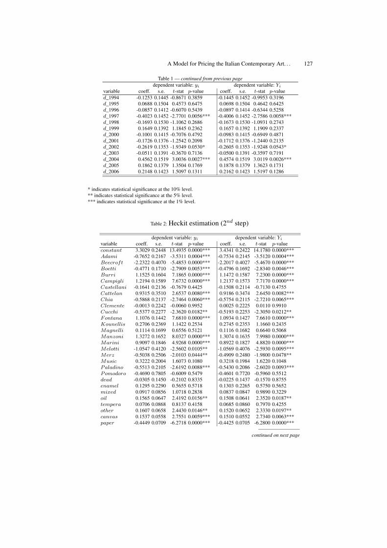
A Model for Pricing the Italian Contemporary Art. . . 127
Table 1 — continued from previous pagedependent variable: yi dependent variable: Yi
variable coeff. s.e. t-stat p-value coeff. s.e. t-stat p-valued_1994 -0.1253 0.1445 -0.8671 0.3859 -0.1445 0.1452 -0.9953 0.3196d_1995 0.0688 0.1504 0.4573 0.6475 0.0698 0.1504 0.4642 0.6425d_1996 -0.0857 0.1412 -0.6070 0.5439 -0.0897 0.1414 -0.6344 0.5258d_1997 -0.4023 0.1452 -2.7701 0.0056*** -0.4006 0.1452 -2.7586 0.0058***d_1998 -0.1693 0.1530 -1.1062 0.2686 -0.1673 0.1530 -1.0931 0.2743d_1999 0.1649 0.1392 1.1845 0.2362 0.1657 0.1392 1.1909 0.2337d_2000 -0.1001 0.1415 -0.7076 0.4792 -0.0983 0.1415 -0.6949 0.4871d_2001 -0.1726 0.1376 -1.2542 0.2098 -0.1712 0.1376 -1.2440 0.2135d_2002 -0.2619 0.1353 -1.9349 0.0530* -0.2605 0.1353 -1.9248 0.0543*d_2003 -0.0511 0.1391 -0.3670 0.7136 -0.0500 0.1391 -0.3597 0.7191d_2004 0.4562 0.1519 3.0036 0.0027*** 0.4574 0.1519 3.0119 0.0026***d_2005 0.1862 0.1379 1.3504 0.1769 0.1878 0.1379 1.3623 0.1731d_2006 0.2148 0.1423 1.5097 0.1311 0.2162 0.1423 1.5197 0.1286
* indicates statistical significance at the 10% level.** indicates statistical significance at the 5% level.*** indicates statistical significance at the 1% level.
Table 2: Heckit estimation (2nd step)
dependent variable: yi dependent variable: Yi
variable coeff. s.e. t-stat p-value coeff. s.e. t-stat p-valueconstant 3.3029 0.2448 13.4935 0.0000*** 3.4341 0.2422 14.1780 0.0000***Adami -0.7652 0.2167 -3.5311 0.0004*** -0.7534 0.2145 -3.5120 0.0004***Beecroft -2.2322 0.4070 -5.4853 0.0000*** -2.2017 0.4027 -5.4670 0.0000***Boetti -0.4771 0.1710 -2.7909 0.0053*** -0.4796 0.1692 -2.8340 0.0046***Burri 1.1525 0.1604 7.1865 0.0000*** 1.1472 0.1587 7.2300 0.0000***Campigli 1.2194 0.1589 7.6732 0.0000*** 1.2137 0.1573 7.7170 0.0000***Castellani -0.1641 0.2136 -0.7679 0.4425 -0.1508 0.2114 -0.7130 0.4755Cattelan 0.9315 0.3510 2.6537 0.0080*** 0.9186 0.3474 2.6450 0.0082***Chia -0.5868 0.2137 -2.7464 0.0060*** -0.5754 0.2115 -2.7210 0.0065***Clemente -0.0013 0.2242 -0.0060 0.9952 0.0025 0.2225 0.0110 0.9910Cucchi -0.5377 0.2277 -2.3620 0.0182** -0.5193 0.2253 -2.3050 0.0212**Fontana 1.1076 0.1442 7.6810 0.0000*** 1.0934 0.1427 7.6610 0.0000***Kounellis 0.2706 0.2369 1.1422 0.2534 0.2745 0.2353 1.1660 0.2435Magnelli 0.1114 0.1699 0.6556 0.5121 0.1116 0.1682 0.6640 0.5068Manzoni 1.3272 0.1652 8.0327 0.0000*** 1.3074 0.1635 7.9980 0.0000***Marini 0.9097 0.1846 4.9268 0.0000*** 0.8922 0.1827 4.8820 0.0000***Melotti -1.0547 0.4120 -2.5602 0.0105** -1.0569 0.4076 -2.5930 0.0095***Merz -0.5038 0.2506 -2.0103 0.0444** -0.4909 0.2480 -1.9800 0.0478**Music 0.3222 0.2004 1.6073 0.1080 0.3218 0.1984 1.6220 0.1048Paladino -0.5513 0.2105 -2.6192 0.0088*** -0.5430 0.2086 -2.6020 0.0093***Pomodoro -0.4690 0.7805 -0.6009 0.5479 -0.4601 0.7720 -0.5960 0.5512dead -0.0305 0.1450 -0.2102 0.8335 -0.0225 0.1437 -0.1570 0.8755enamel 0.1295 0.2290 0.5655 0.5718 0.1303 0.2265 0.5750 0.5652mixed 0.0917 0.0856 1.0718 0.2838 0.0837 0.0847 0.9890 0.3229oil 0.1565 0.0647 2.4192 0.0156** 0.1508 0.0641 2.3520 0.0187**tempera 0.0706 0.0868 0.8137 0.4158 0.0685 0.0860 0.7970 0.4255other 0.1607 0.0658 2.4430 0.0146** 0.1520 0.0652 2.3330 0.0197**canvas 0.1537 0.0558 2.7551 0.0059*** 0.1510 0.0552 2.7340 0.0063***paper -0.4449 0.0709 -6.2718 0.0000*** -0.4425 0.0705 -6.2800 0.0000***
————————continued on next page
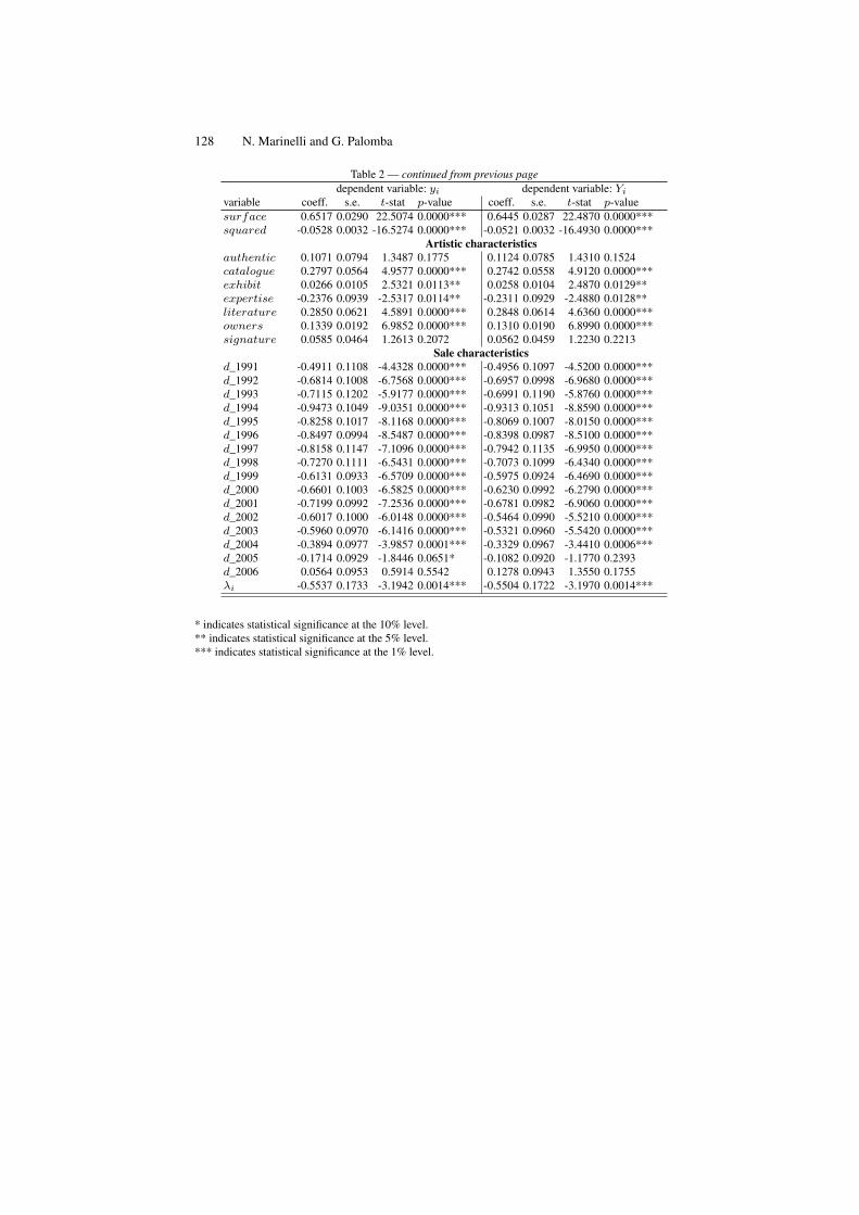
128 N. Marinelli and G. Palomba
Table 2 — continued from previous pagedependent variable: yi dependent variable: Yi
variable coeff. s.e. t-stat p-value coeff. s.e. t-stat p-valuesurface 0.6517 0.0290 22.5074 0.0000*** 0.6445 0.0287 22.4870 0.0000***squared -0.0528 0.0032 -16.5274 0.0000*** -0.0521 0.0032 -16.4930 0.0000***
Artistic characteristicsauthentic 0.1071 0.0794 1.3487 0.1775 0.1124 0.0785 1.4310 0.1524catalogue 0.2797 0.0564 4.9577 0.0000*** 0.2742 0.0558 4.9120 0.0000***exhibit 0.0266 0.0105 2.5321 0.0113** 0.0258 0.0104 2.4870 0.0129**expertise -0.2376 0.0939 -2.5317 0.0114** -0.2311 0.0929 -2.4880 0.0128**literature 0.2850 0.0621 4.5891 0.0000*** 0.2848 0.0614 4.6360 0.0000***owners 0.1339 0.0192 6.9852 0.0000*** 0.1310 0.0190 6.8990 0.0000***signature 0.0585 0.0464 1.2613 0.2072 0.0562 0.0459 1.2230 0.2213
Sale characteristicsd_1991 -0.4911 0.1108 -4.4328 0.0000*** -0.4956 0.1097 -4.5200 0.0000***d_1992 -0.6814 0.1008 -6.7568 0.0000*** -0.6957 0.0998 -6.9680 0.0000***d_1993 -0.7115 0.1202 -5.9177 0.0000*** -0.6991 0.1190 -5.8760 0.0000***d_1994 -0.9473 0.1049 -9.0351 0.0000*** -0.9313 0.1051 -8.8590 0.0000***d_1995 -0.8258 0.1017 -8.1168 0.0000*** -0.8069 0.1007 -8.0150 0.0000***d_1996 -0.8497 0.0994 -8.5487 0.0000*** -0.8398 0.0987 -8.5100 0.0000***d_1997 -0.8158 0.1147 -7.1096 0.0000*** -0.7942 0.1135 -6.9950 0.0000***d_1998 -0.7270 0.1111 -6.5431 0.0000*** -0.7073 0.1099 -6.4340 0.0000***d_1999 -0.6131 0.0933 -6.5709 0.0000*** -0.5975 0.0924 -6.4690 0.0000***d_2000 -0.6601 0.1003 -6.5825 0.0000*** -0.6230 0.0992 -6.2790 0.0000***d_2001 -0.7199 0.0992 -7.2536 0.0000*** -0.6781 0.0982 -6.9060 0.0000***d_2002 -0.6017 0.1000 -6.0148 0.0000*** -0.5464 0.0990 -5.5210 0.0000***d_2003 -0.5960 0.0970 -6.1416 0.0000*** -0.5321 0.0960 -5.5420 0.0000***d_2004 -0.3894 0.0977 -3.9857 0.0001*** -0.3329 0.0967 -3.4410 0.0006***d_2005 -0.1714 0.0929 -1.8446 0.0651* -0.1082 0.0920 -1.1770 0.2393d_2006 0.0564 0.0953 0.5914 0.5542 0.1278 0.0943 1.3550 0.1755λi -0.5537 0.1733 -3.1942 0.0014*** -0.5504 0.1722 -3.1970 0.0014***
* indicates statistical significance at the 10% level.** indicates statistical significance at the 5% level.*** indicates statistical significance at the 1% level.
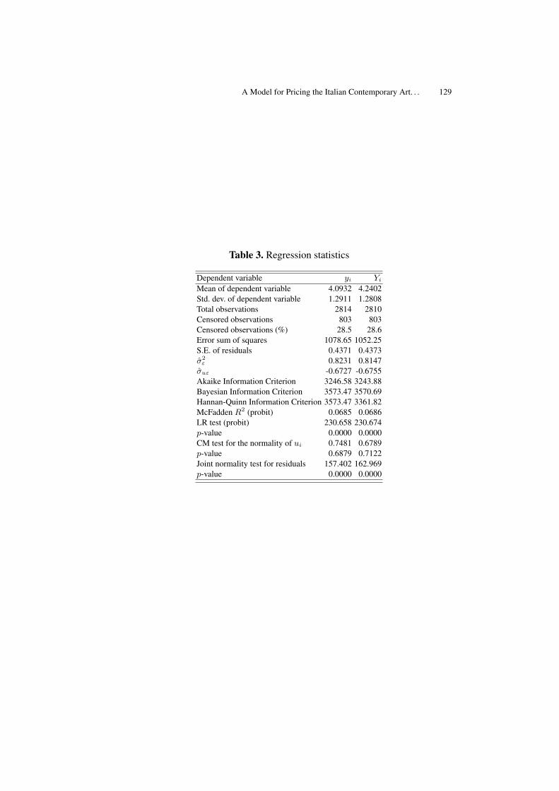
A Model for Pricing the Italian Contemporary Art. . . 129
Table 3. Regression statistics
Dependent variable yi Yi
Mean of dependent variable 4.0932 4.2402Std. dev. of dependent variable 1.2911 1.2808Total observations 2814 2810Censored observations 803 803Censored observations (%) 28.5 28.6Error sum of squares 1078.65 1052.25S.E. of residuals 0.4371 0.4373σ2
ε 0.8231 0.8147σuε -0.6727 -0.6755Akaike Information Criterion 3246.58 3243.88Bayesian Information Criterion 3573.47 3570.69Hannan-Quinn Information Criterion 3573.47 3361.82McFadden R2 (probit) 0.0685 0.0686LR test (probit) 230.658 230.674p-value 0.0000 0.0000CM test for the normality of ui 0.7481 0.6789p-value 0.6879 0.7122Joint normality test for residuals 157.402 162.969p-value 0.0000 0.0000

130 N. Marinelli and G. Palomba
List of variables
Table 4. Characteristics of the artist (N=2817)
variable description birth dead obs.Name of the artistAdami 1 if the author is Valerio Adami, 0 otherwise 1935 - 170Beecroft 1 if the author is Vanessa Beecroft, 0 otherwise 1966 - 9Boetti 1 if the author is Alighiero Boetti, 0 otherwise 1940 1994 212Burri 1 if the author is Alberto Burri, 0 otherwise 1915 1995 126Campigli 1 if the author is Massimo Campigli, 0 otherwise 1895 1971 268Castellani 1 if the author is Enrico Castellani, 0 otherwise 1930 - 114Cattelan 1 if the author is Maurizio Cattelan, 0 otherwise 1960 - 10Chia 1 if the author is Sandro Chia, 0 otherwise 1946 - 155Clemente 1 if the author is Francesco Clemente, 0 otherwise 1952 - 101Cucchi 1 if the author is Enzo Cucchi, 0 otherwise 1950 - 65Fontana 1 if the author is Lucio Fontana, 0 otherwise 1899 1968 720Gnoli 1 if the author is Domenico Gnoli, 0 otherwise 1933 1970 64Kounellis 1 if the author is Jannis Kounellis, 0 otherwise 1936 - 51Magnelli 1 if the author is Alberto Magnelli, 0 otherwise 1888 1971 105Manzoni 1 if the author is Piero Manzoni, 0 otherwise 1934 1963 137Marini 1 if the author is Marino Marini, 0 otherwise 1901 1980 68Melotti 1 if the author is Fausto Melotti, 0 otherwise 1901 1986 8Merz 1 if the author is Mario Merz, 0 otherwise 1925 - 41Music 1 if the author is Zoran Music, 0 otherwise 1909 2005 241Paladino 1 if the author is Mimmo Paladino, 0 otherwise 1948 - 150Pomodoro 1 if the author is Arnaldo Pomodoro, 0 otherwise 1926 - 2Living statusDead 1 if the painter is dead at the moment of selling, 0 otherwise 1705Year of birthBirth Year of birth
Source: Artindex Plus - Gabrius S.p.A.
A Model for Pricing the Italian Contemporary Art. . . 131
Table 5. Physical characteristics (N=2817)
variable description obs.Mediumcollage 1 if the medium is collage, 0 otherwise 5enamel 1 if the medium is enamel, 0 otherwise 29gouache 1 if the medium is gouache, 0 otherwise 1mixed 1 if the medium is mixed, 0 otherwise 385pencil 1 if the medium is pencil, 0 otherwise 2oil 1 if the medium is oil, 0 otherwise 1429tempera 1 if the medium is tempera, 0 otherwise 320other 1 if the medium is other, 0 otherwise 1037Supportboard 1 if the support is board, 0 otherwise 185canvas 1 if the support is canvas, 0 otherwise 2254cartoon 1 if the support is cartoon, 0 otherwise 173fabric 1 if the support is fabric, 0 otherwise 75marble 1 if the support is marble, 0 otherwise 5masonite 1 if the support is masonite, 0 otherwise 26panel 1 if the support is panel, 0 otherwise 166paper 1 if the support is paper, 0 otherwise 275wood 1 if the support is wooden base, 0 otherwise 7support 1 if the support is other, 0 otherwise 146Sizesurface Painting area (in m2)squared Painting squared area
Source: Artindex Plus - Gabrius S.p.A.
Note: for some paintings different media or different supports are jointly used.
Table 6. Artistic characteristics (N=2817)
variable description obs.authentic 1 if the painter has confirmed the authenticity, 0 otherwise 187catalogue 1 if the painting is published on catalogs/monographies, 0 otherwise 680date 1 if the painting is dated, 0 otherwise 1700expertise 1 if the painting is recognised by experts, 0 otherwise 132literature 1 if the painting is cited in literature, 0 otherwise 1049signature 1 if the painting is signed, 0 otherwise 2071title 1 if the painting is titled, 0 otherwise 1722exhibit Number of exhibitionsowners Number of previous owners
Source: Artindex Plus - Gabrius S.p.A.
132 N. Marinelli and G. Palomba
Table 7: Sale characteristics (N=2817)
variable description obs.Auction housesCurial 1 if the painting was sold at Art Curial, 0 otherwise 36Bonhams 1 if the painting was sold at Bonhams, 0 otherwise 4Bruun 1 if the painting was sold at Bruun Rasmussen, 0 otherwise 2Bukowskis 1 if the painting was sold at Bukowskis, 0 otherwise 2Camels 1 if the painting was sold at Camels Cohen, 0 otherwise 2Christies 1 if the painting was sold at Christie’s, 0 otherwise 914Dorotheum 1 if the painting was sold at Dorotheum, 0 otherwise 9Doyle 1 if the painting was sold at Doyle, 0 otherwise 2Finarte 1 if the painting was sold at Finarte Semenzato, 0 otherwise 536Grisebach 1 if the painting was sold at Grisebach, 0 otherwise 8Koller 1 if the painting was sold at Koller, 0 otherwise 5Lempertz 1 if the painting was sold at Lempertz, 0 otherwise 39Neumeister 1 if the painting was sold at Nuemeister, 0 otherwise 3Pandolfini 1 if the painting was sold at Pandolfini, 0 otherwise 1Phillips 1 if the painting was sold at Phillips, 0 otherwise 37Piasa 1 if the painting was sold at Piasa, 0 otherwise 1Porro 1 if the painting was sold at Porro & C., 0 otherwise 27Sothebys 1 if the painting was sold at Sotheby’s, 0 otherwise 1137Tajan 1 if the painting was sold at Tajan, 0 otherwise 43MarketplaceAmsterdam 1 if the painting was sold in Amsterdam, 0 otherwise 4NY 1 if the painting was sold in New York, 0 otherwise 363Berlin 1 if the painting was sold in Berlin, 0 otherwise 8Paris 1 if the painting was sold in Paris, 0 otherwise 88Cologne 1 if the painting was sold in Cologne, 0 otherwise 39Copenhagen 1 if the painting was sold in Copenhagen, 0 otherwise 2London 1 if the painting was sold in London, 0 otherwise 1109LA 1 if the painting was sold in Los Angeles, 0 otherwise 4Lugano 1 if the painting was sold in Lugano, 0 otherwise 17Milan 1 if the painting was sold in Milan, 0 otherwise 994Montecarlo 1 if the painting was sold in Montecarlo, 0 otherwise 3Munich 1 if the painting was sold in Munich, 0 otherwise 3Rome 1 if the painting was sold in Rome, 0 otherwise 140Stockholm 1 if the painting was sold in Stokholm, 0 otherwise 11Sidney 1 if the painting was sold in Sidney, 0 otherwise 1V enice 1 if the painting was sold in Venice, 0 otherwise 17V ienna 1 if the painting was sold in Vienna, 0 otherwise 9Zurich 1 if the painting was sold in Zurich, 0 otherwise 5Sale dated_1990 1 if the painting was sold in 1990, 0 otherwise 242d_1991 1 if the painting was sold in 1991, 0 otherwise 100d_1992 1 if the painting was sold in 1992, 0 otherwise 140d_1993 1 if the painting was sold in 1993, 0 otherwise 109d_1994 1 if the painting was sold in 1994, 0 otherwise 133d_1995 1 if the painting was sold in 1995, 0 otherwise 135d_1996 1 if the painting was sold in 1996, 0 otherwise 148d_1997 1 if the painting was sold in 1997, 0 otherwise 127d_1998 1 if the painting was sold in 1998, 0 otherwise 116d_1999 1 if the painting was sold in 1999, 0 otherwise 190d_2000 1 if the painting was sold in 2000, 0 otherwise 158d_2001 1 if the painting was sold in 2001, 0 otherwise 182
————————continued on next page
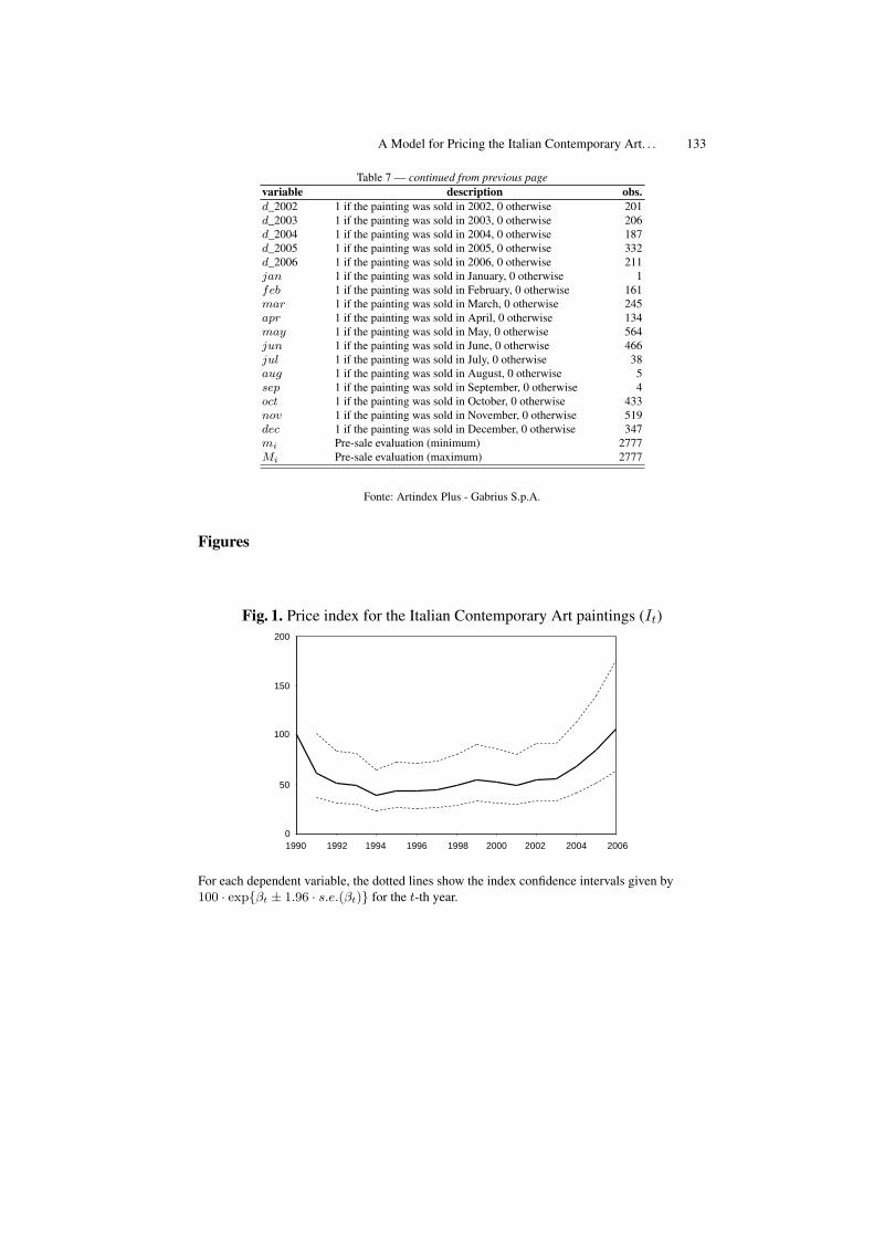
A Model for Pricing the Italian Contemporary Art. . . 133
Table 7 — continued from previous pagevariable description obs.d_2002 1 if the painting was sold in 2002, 0 otherwise 201d_2003 1 if the painting was sold in 2003, 0 otherwise 206d_2004 1 if the painting was sold in 2004, 0 otherwise 187d_2005 1 if the painting was sold in 2005, 0 otherwise 332d_2006 1 if the painting was sold in 2006, 0 otherwise 211jan 1 if the painting was sold in January, 0 otherwise 1feb 1 if the painting was sold in February, 0 otherwise 161mar 1 if the painting was sold in March, 0 otherwise 245apr 1 if the painting was sold in April, 0 otherwise 134may 1 if the painting was sold in May, 0 otherwise 564jun 1 if the painting was sold in June, 0 otherwise 466jul 1 if the painting was sold in July, 0 otherwise 38aug 1 if the painting was sold in August, 0 otherwise 5sep 1 if the painting was sold in September, 0 otherwise 4oct 1 if the painting was sold in October, 0 otherwise 433nov 1 if the painting was sold in November, 0 otherwise 519dec 1 if the painting was sold in December, 0 otherwise 347mi Pre-sale evaluation (minimum) 2777Mi Pre-sale evaluation (maximum) 2777
Fonte: Artindex Plus - Gabrius S.p.A.
Figures
Fig. 1. Price index for the Italian Contemporary Art paintings (It)
1990 1992 1994 1996 1998 2000 2002 2004 2006
100
150
200
50
0
For each dependent variable, the dotted lines show the index confidence intervals given by100 · expβt ± 1.96 · s.e.(βt) for the t-th year.

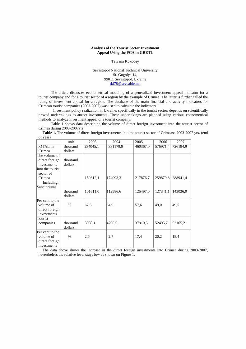
Analysis of the Tourist Sector Investment Appeal Using the PCA in GRETL
Tetyana Kokodey
Sevastopol National Technical University
St. Gogolya 14, 99011 Sevastopol, Ukraine
The article discusses econometrical modeling of a generalized investment appeal indicator for a tourist company and for a tourist sector of a region by the example of Crimea. The latter is further called the rating of investment appeal for a region. The database of the main financial and activity indicators for Crimean tourist companies (2003-2007) was used to calculate the indicators.
Investment policy realization in Ukraine, specifically in the tourist sector, depends on scientifically proved undertakings to attract investments. These undertakings are planned using various econometrical methods to analyze investment appeal of a tourist company.
Table 1 shows data describing the volume of direct foreign investment into the tourist sector of Crimea during 2003-2007yrs.
Table 1. The volume of direct foreign investments into the tourist sector of Crimeaза 2003-2007 yrs. (end of year)
unit 2003 2004 2005 2006 2007 TOTAL in Crimea
thousand dollars
234045,1 331179,9 460367,0 576971,4 726194,9
The volume of direct foreign investments
into the tourist sector of Crimea
thousand dollars.
150312,1
174093,3
217876,7
259879,8
288941,4
Including: Sanatoriums
thousand dollars.
101611,0
112986,6
125497,0
127341,1
143026,0
Per cent to the volume of direct foreign investments
%
67,6
64,9
57,6
49,0
49,5
Tourist companies
thousand dollars.
3908,1
4700,5
37910,5
52495,7
53165,2
Per cent to the volume of direct foreign investments
%
2,6
2,7
17,4
20,2
18,4
The data above shows the increase in the direct foreign investments into Crimea during 2003-2007, nevertheless the relative level stays low as shown on Figure 1.
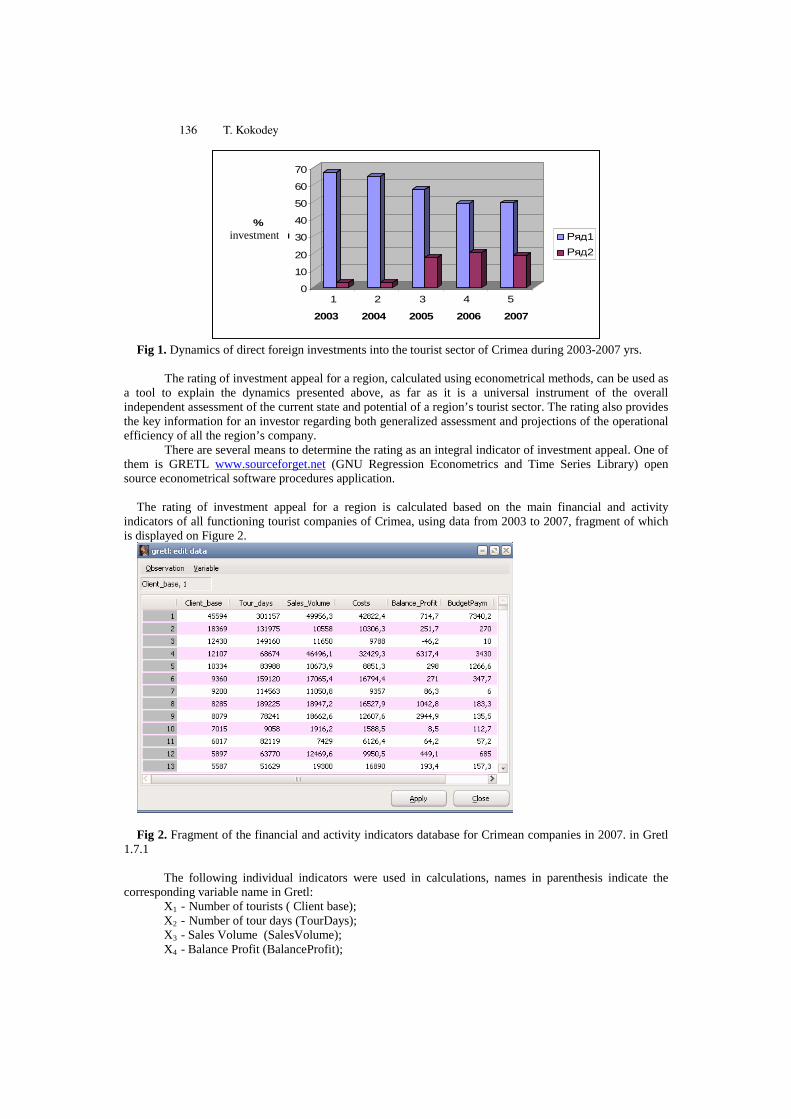
0
10
20
30
40
50
60
70
% инвестиций
1 2 3 4 5
2003 2004 2005 2006 2007
Ряд1
Ряд2
Fig 1. Dynamics of direct foreign investments into the tourist sector of Crimea during 2003-2007 yrs.
The rating of investment appeal for a region, calculated using econometrical methods, can be used as
a tool to explain the dynamics presented above, as far as it is a universal instrument of the overall independent assessment of the current state and potential of a region’s tourist sector. The rating also provides the key information for an investor regarding both generalized assessment and projections of the operational efficiency of all the region’s company.
There are several means to determine the rating as an integral indicator of investment appeal. One of them is GRETL www.sourceforget.net (GNU Regression Econometrics and Time Series Library) open source econometrical software procedures application.
The rating of investment appeal for a region is calculated based on the main financial and activity
indicators of all functioning tourist companies of Crimea, using data from 2003 to 2007, fragment of which is displayed on Figure 2.
Fig 2. Fragment of the financial and activity indicators database for Crimean companies in 2007. in Gretl
1.7.1 The following individual indicators were used in calculations, names in parenthesis indicate the
corresponding variable name in Gretl: X1 - Number of tourists ( Client base); X2 - Number of tour days (TourDays); X3 - Sales Volume (SalesVolume); X4 - Balance Profit (BalanceProfit);
investment
136 T. Kokodey
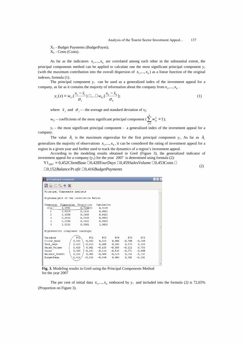
X5 - Budget Payments (BudgetPaym); X6 - Costs (Costs). As far as the indicators 61,...,xx are correlated among each other in the substantial extent, the
principal components method can be applied to calculate one the most significant principal component у1 (with the maximum contribution into the overall dispersion of 61,...,xx ) as a linear function of the original
indexes, formula (1). The principal component у1 can be used as a generalized index of the investment appeal for a
company, as far as it contains the majority of information about the company from 61,...,xx .
);(...)()(6
6661
1
11111 σσ
xxw
xxwxy
−++
−= (1)
where jx and jσ — the average and standard deviation of xj;
wj1 – coefficients of the most significant principal component (∑=
=6
1
21j 1
j
w );
у1 – the most significant principal component - a generalized index of the investment appeal for a company.
The value 1λ is the maximum eigenvalue for the first principal component у1. As far as 1λ
generalizes the majority of observations 61,...,xx , it can be considered the rating of investment appeal for a
region in a given year and further used to track the dynamics of a region’s investment appeal. According to the modeling results obtained in Gretl (Figure 3), the generalized indicator of
investment appeal for a company (у1) for the year 2007 is determined using formula (2):
entsBudgetPaymofitBalance
eSalesVolumTourDays
416,0Pr0,152
Costs453,0459,0428,0tBase0,452ClienY12007
++++++=
(2)
Fig. 3. Modeling results in Gretl using the Principal Components Method for the year 2007
The per cent of initial data 61,...,xx embraced by у1 and included into the formula (2) is 72,65%
(Proportion on Figure 3).
Analysis of the Tourist Sector Investment Appeal... 137

Thus, eigenvalue 3593,42007 =λ can be considered the rating of investment appeal for a region in
2007. Similar calculations were conducted using 2006 data (Figure 4), formula (3) was obtained:
entsBudgetPaymofitBalance
eSalesVolumTourDays
436,0Pr0,06
Costs453,0451,0434,0tBase0,457ClienY12006
++++++=
(3)
Fig. 4. Modeling results in Gretl using the Principal Components Method for the year 2006
The per cent of initial data 61,...,xx embraced by у1 and included into the formula (3) is 74,49%
(Proportion on Figure 4). Thus, eigenvalue 4692,42006 =λ can be considered the rating of investment appeal for a region in
2006. Similar calculations were conducted using 2005 data (Figure 5), formula (4) was obtained:
entsBudgetPaymofitBalance
eSalesVolumTourDays
399,0Pr0,004
-Costs469,0472,0446,0tBase0,447ClienY12005
+−+++= (4)
138 T. Kokodey
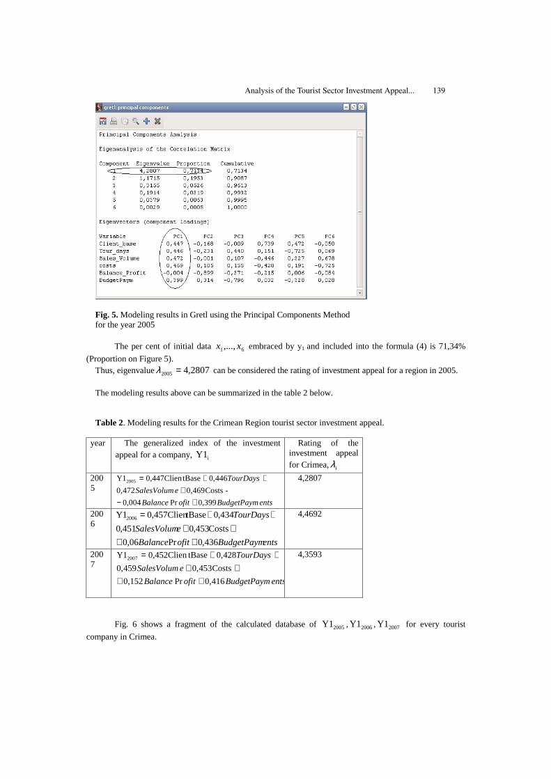
Fig. 5. Modeling results in Gretl using the Principal Components Method for the year 2005
The per cent of initial data 61,...,xx embraced by у1 and included into the formula (4) is 71,34%
(Proportion on Figure 5). Thus, eigenvalue 2807,42005 =λ can be considered the rating of investment appeal for a region in 2005.
The modeling results above can be summarized in the table 2 below. Table 2. Modeling results for the Crimean Region tourist sector investment appeal.
year The generalized index of the investment appeal for a company, iY1
Rating of the investment appeal for Crimea, iλ
2005
entsBudgetPaymofitBalance
eSalesVolum
TourDays
399,0Pr0,004
-Costs469,0472,0
446,0tBase0,447ClienY12005
+−+
++=
4,2807
2006
entsBudgetPaymofitBalance
eSalesVolum
TourDays
436,0Pr0,06
Costs453,0451,0
434,0tBase0,457ClienY12006
++++
++=
4,4692
2007
entsBudgetPaymofitBalance
eSalesVolum
TourDays
416,0Pr0,152
Costs453,0459,0
428,0tBase0,452ClienY12007
++++
++=
4,3593
Fig. 6 shows a fragment of the calculated database of 2005Y1 , 2006Y1 , 2007Y1 for every tourist
company in Crimea.
Analysis of the Tourist Sector Investment Appeal... 139
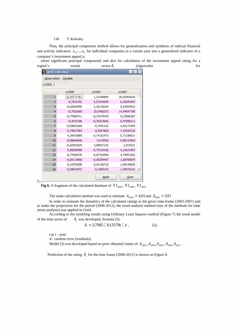
Thus, the principal component method allows for generalization and synthesis of indicial financial and activity indicators 61,...,xx for individual companies in a certain year into a generalized indicator of a
company’s investment appeal y1 (most significant principal component) and also for calculation of the investment appeal rating for a
region’s tourist sector1λ (eigenvalue for
y1.) Fig 6. A fragment of the calculated database of 2005Y1 , 2006Y1 , 2007Y1
The same calculation method was used to estimate 01,42004 =λ and 91,32003 =λ
In order to estimate the dynamics of the calculated ratings in the given time-frame (2003-2007) and to make the projections for the period (2008-2012), the trend analysis method (one of the methods for time series analysis) was applied in Gretl.
According to the modeling results using Ordinary Least Squares method (Figure 7) the trend model of the time series of iλ was developed, formula (5):
ελ ++= t13578,07985,3i , (5), где t - year; ε - random error (residuals).
Model (5) was developed based on prior obtained values of 2007,20062005,20042003 ,, λλλλλ .
Prediction of the rating iλ for the time frame (2008-2012) is shown on Figure 8.
140 T. Kokodey
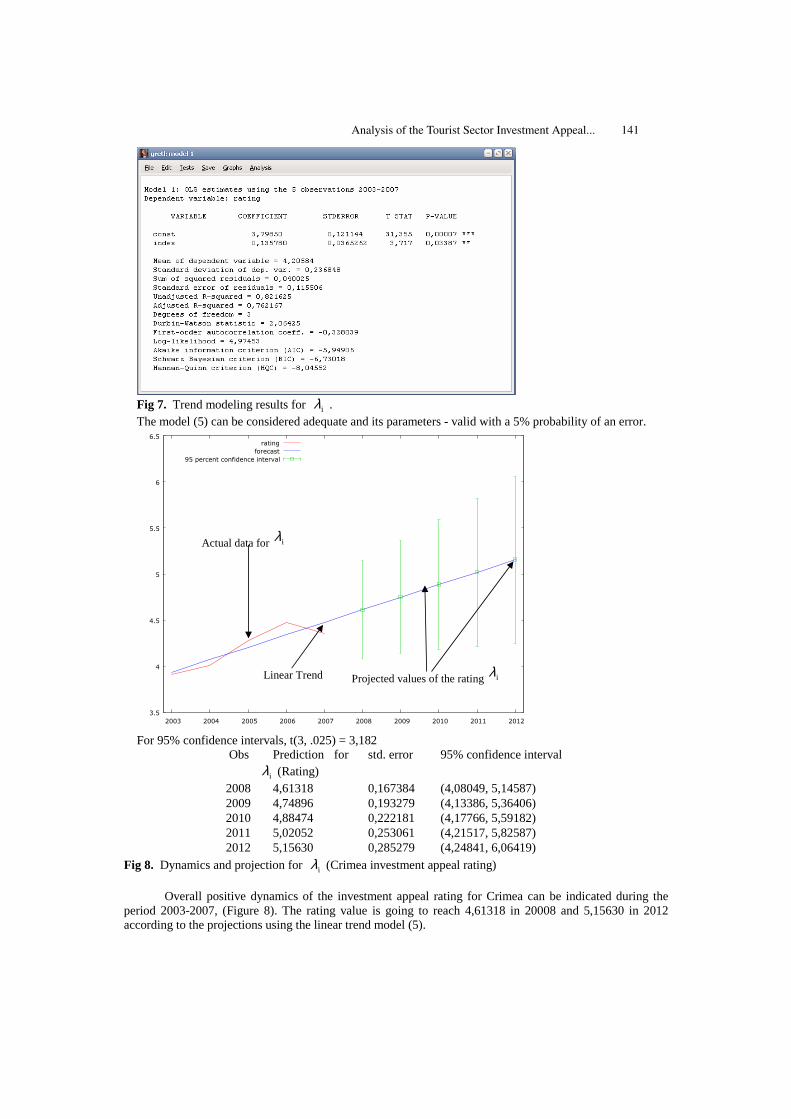
Fig 7. Trend modeling results for iλ . The model (5) can be considered adequate and its parameters - valid with a 5% probability of an error.
3.5
4
4.5
5
5.5
6
6.5
2003 2004 2005 2006 2007 2008 2009 2010 2011 2012
rating
forecast
95 percent confidence interval
For 95% confidence intervals, t(3, .025) = 3,182
Obs Prediction for
iλ (Rating) std. error 95% confidence interval
2008 4,61318 0,167384 (4,08049, 5,14587) 2009 4,74896 0,193279 (4,13386, 5,36406) 2010 4,88474 0,222181 (4,17766, 5,59182) 2011 5,02052 0,253061 (4,21517, 5,82587) 2012 5,15630 0,285279 (4,24841, 6,06419)
Fig 8. Dynamics and projection for iλ (Crimea investment appeal rating) Overall positive dynamics of the investment appeal rating for Crimea can be indicated during the
period 2003-2007, (Figure 8). The rating value is going to reach 4,61318 in 20008 and 5,15630 in 2012 according to the projections using the linear trend model (5).
Linear Trend Projected values of the rating iλ
Actual data for iλ
Analysis of the Tourist Sector Investment Appeal... 141

Modeling results obtained in the research allow to make a conclusion that investment appeal of Crimea is going to increase 5,82% in 2008 and 18,28% in 2012 due to the positive dynamics of individual financial and activity indicators of tourist companies in the region.
142 T. Kokodey
Has the European Structural Fisheries Policy Influenced on the Second Hand Market
of Fishing Vessels1?
Ikerne del Valle*, Kepa Astorkiza,* and Inmaculada Astorkiza*2 * Department of Applied Economics V. University of The Basque Country
(UPV-EHU) Avda. Lehendakari Agirre No. 83, 48015 Bilbao, Spain
Abstract. The main objective of this paper is to analyze the potential effects that the principal instrument of European structural fisheries policy, that is the Multi-Annual Guidance Plans (MAGP), may have exercised in the second hand market of fishing vessels. In order to test the starting hypothesis that the shortage generated in the periods with the most significant and radical capacity adjustment may have influenced increases on prices of vessels, the main determinants of the second hand market of fishing vessels are analyzed by estimating and discriminating among alternative hedonic price models, such as the linear, log-linear, semi-log, mixed semi-log, TRANSLOG or Box-Cox. Especial attention is paid not only to the correct specification of the numerical variables by carrying out a battery of tests to discriminate among alternative non-nested models, but also to checking for structural change and the convenience of using alternative estimation methods including OLS, weighted least squares (WLS) and trimmed least squares (TLS), based on heteroskedasticity and OLS regression diagnostic. Pooled data is available for 228 transactions taking place during the period 1985-2005 for the Basque artisan and trawling fleets. The principal results achieved indicate that the higher increase of prices precisely happens under the MAGP with major capacity adjustment.
Keywords: European Fisheries Policy, Second Hand Market of Fishing Vessels, Hedonic Model.
1 This study has received financial from the EFIMAS project (No SSP8-CT-2003
502516) and ETORTEK2003/IMPRES (Basque Government). 2 The authors are grateful to conference participants at 4th Conference Developments
in Economic Theory and Policy (10-11 July 2008, Bilbao) and 35th Annual Conference of the Eastern Economic Association (Feb27-March1 2009, New York). All errors and opinions are the author’s responsibility.

1 Background and Problem Definition
Since the mid eighties the European Fisheries Structural Policy has been leaning on the figure of Multi Annual Guidance Plans (MAGP) as the principal vehicle to adapt fleet’s fishing capacity to the abundance of the fishing stocks. Basically the design of MAGP has been oriented to the reduction of fishing effort by the limitation of capacity in order to adjust fleets to the real biological situation of fish stocks and also to incentive the modernisation and competitiveness of fishing fleets. In practice the principal materialisation of the measure has been the elimination of vessels by giving incentives in the form of decommissioning grants, the exportation of the vessel to third countries outside the European Union, and even, although is less degree, the reallocation of vessels to another activities. Each MAGP establishes the specific fleet reduction target by member States for a period of 5 years starting from 1982.
Our initial hypothesis is that the shortage generated in the periods with the most significant and radical capacity adjustment, may have influenced increases on prices of the second hand market of vessels. Notice that since entry to the fisheries is limited to those having an authorised vessel, the only way for a firm to add another vessel to the business is by accessing to the second hand market. Moreover, since the effective adjustment patterns differ by State and fishing sub-sector, one may expect disparities on the influence on prices depending not only on MAGP but also on the State and fishing sub-sector. Therefore, some of the related questions we intend to answer are: Have MAGP influenced on the prices of second hand market of fishing vessels? Have they affected homogeneously to the different fishing sub-sectors? Is this potential effect on prices especially significant during some of the MAGP? Is there any interaction effect between the previous the fishing sub-sector and MAGP? We focus on the Basque artisan and trawling fleets to address the researching questions set out.
Vessels constitute a heterogeneous asset. Even when the specifications and their technical characteristics are the same, if the age differs, the degree of deterioration differs accordingly, so that one might say that there are no two identical vessels, or to put in another words, vessels have the particularity of few equivalents. Moreover, the quality of vessels may change with time owing to technological progress. Heterogeneity and potential quality improvements justify the need of methods able to compare heterogeneous vessels prices at different times. These methods should distinguish between movements in prices and changes in the composition of vessels sold from one period to the next. Moreover the objectives of the paper demand a modelling approach open to accommodating for structural changes. The structure of the market changes in accordance with the changes in the preferences of vessels owners, which are influenced in turn by the situation of the fisheries, and
144 I. del Valle, K. Astorkiza, I. Astorkiza

specifically by the fisheries policy. This implies that in more or less degree but the model should be open to structural flexibility.
There are two price modelling approaches that specifically focus on the issues resulting from heterogeneity and changes in quality: the hedonic approach ([1], [2], [3]) and the repeat sales technique [4]. The former controls for quality by using regression models with the attributes of the good as independent variables, while in the second quality control is directly achieved by only including the transactions involving the same assets. The hedonic approach as three principal advantages. First, it uses all of the information on sales in each sample period and not just the data that can be matched, which mitigates the sample selection bias issue. Second, it can adjust for the effects of depreciation if the age of the structure is known at the time of sale. Third, it can adjust for the effects of renovations and repairs if expenditures on renovation and extensions are known at the time of sale.
Different basis explain our methodological choice in favour of the hedonic approach. For one side, since the fluidity of the second hand fishing vessel market is rather low, the sample selection bias would be an extremely la rge problem if the repeated sales method was adopted. Moreover, we could not get a usable database containing repeated sales transactions of the same vessels because there were an insufficient number of matched observations. Last but not least, since the Boskin report [5], hedonic analysis is gaining academic acceptance as a tool for quality adjustment. Proof of this is it has been applied in a great variety of goods and services, such as automobiles ([2], [6], [7]), Internet services ([8], [9]) and very especially computers ([10], [11]) and houses ([12], [13], [14], [15], [16]), by far the two most popular products for which much of the hedonic research has been concentrated on. To our knowledge this is the first application following the hedonic approach that concerns fishing vessels.
Two alternative approaches have been followed in the literature when dealing to incorporate structural change in the hedonic regression framework ([16], [14], [17]): the characteristic price index approach (CPI) ([2], [6]) and the time dummy variable method (TDV). In the CPI a separate regression is performed for each time period included in the sample, which allows both the coefficients of the good’s characteristics and the intercept to change across different periods. The TDV approach consists of performing a pooled regression including time dummy variables to discriminate among different time periods, and thus estimating a common set of coefficients for the attributes, often under the assumption of time independent implicit prices. Compared to the TDV, the CPI has the advantage of being completely structurally unrestricted. Notice however that additional flexibility might be gained in the TDV approach by estimating implicit prices with a time trend, including a series of time dummies for each hedonic characteristic or by including cross terms between the hedonic characteristics and time dummies.
Has the European Structural Fisheries... 145

Although the CPI is clearly preferable due to its less demanding assumptions and its structural flexibility, not only the own objectives of the paper but also the data structure and availability (in some individual years we have not enough data to undertake the regression analysis) entails the adoption of the TDV. Thus in the framework of the time dummy variable method, we follow the approach developed by [18]), [19], [20]) and [15] in order to face the structural change and separate the data in different sub-periods using exogenously determined breaking points based on the different MAGP periods. The breaking points of structural change may also be endogenously identified using a switching regression model [15]. However, for the purposes of our study it is reasonable to divide the entire sample into 5 sub-samples, namely “MAGP1”, “MAGP2”, “MAGP3”, “MAGP4” and SUB, attending to the MAGP under which the transaction was materialized. In order to gain the additional structural flexibility needed to test whether each plan has affect in different way to vessels belonging to different sub-sectors, artisan or inshore vessels (B) and offshore or trawler vessels (A) the interaction term “MAGPi * SECTORi” will be also included in the model.
2 Data and Fleet Performance
Sample data is available for N=228 transactions of the second hand market of fishing vessels taking place in the Basque Country during the period 1985-2005. NB=159 transactions correspond to artisan vessels (B), and the remaining NA=69 are trawlers (A). The information includes the transaction price (P) (in € 2006), gross tonnes of the vessel (GT), horse power of the engine when the sale took place (HP), length (ESL), the AGE of the vessel, the sector the vessel belongs to (i.e. artisan (B) or offshore vessels (trawlers) (A) and the date of the transaction. Following the time dummy variable method we are dividing the data using the breaking points determined by each MAGP. Thus, the category MAGP1 groups all the transactions taking place during the period (1982-86), MAGP2 the ones during the validity of the second plan (1987-1991), MAGP3 includes the ones during the years (1992-1996), MAGP4 the transactions happening during (1997-2001) and finally SUB the ones in the period (2002-2005). Data sample statistics are summarised in Table 1.
146 I. del Valle, K. Astorkiza, I. Astorkiza
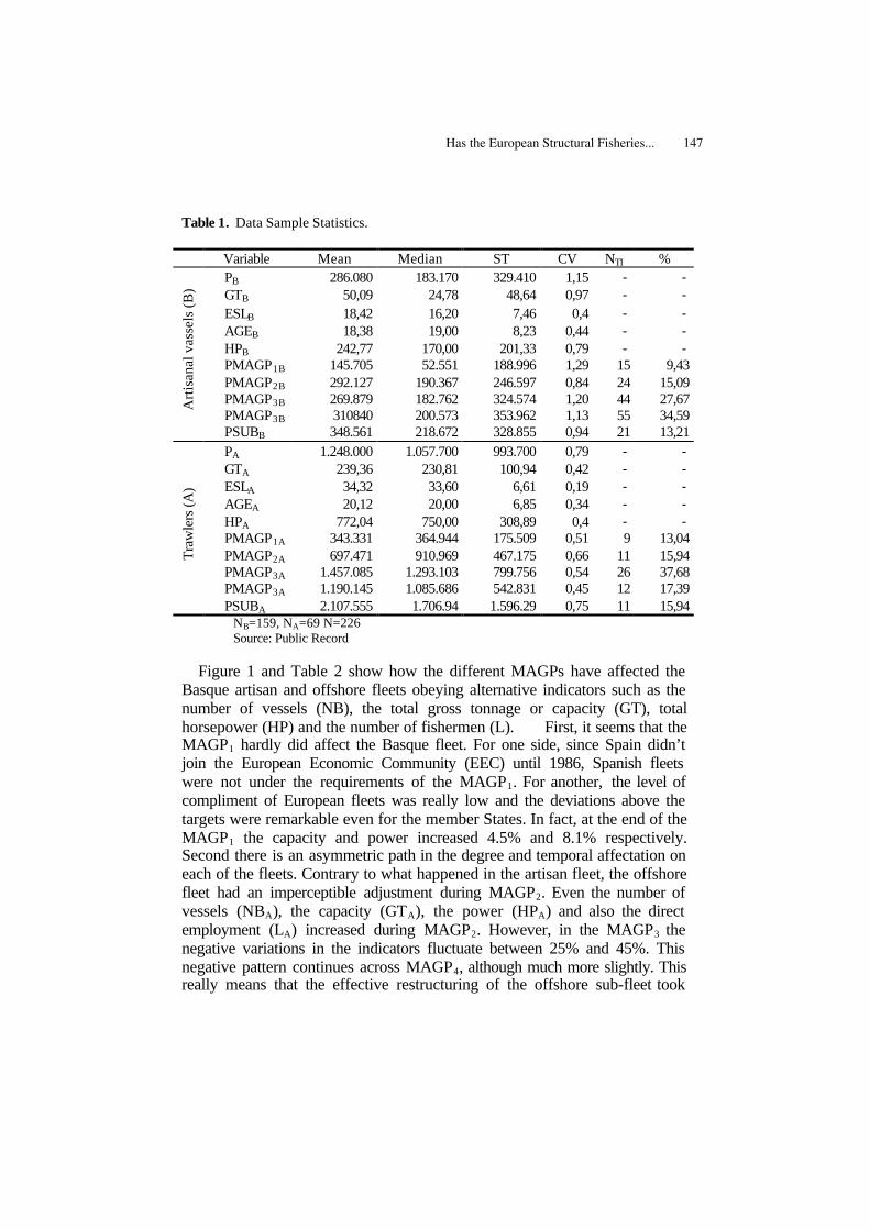
Table 1. Data Sample Statistics.
Variable Mean Median ST CV NTI % PB 286.080 183.170 329.410 1,15 - - GTB 50,09 24,78 48,64 0,97 - - ESLB 18,42 16,20 7,46 0,4 - - AGEB 18,38 19,00 8,23 0,44 - - HPB 242,77 170,00 201,33 0,79 - - PMAGP1B 145.705 52.551 188.996 1,29 15 9,43 PMAGP2B 292.127 190.367 246.597 0,84 24 15,09 PMAGP3B 269.879 182.762 324.574 1,20 44 27,67 PMAGP3B 310840 200.573 353.962 1,13 55 34,59
Art
isan
al v
asse
ls (B
)
PSUBB 348.561 218.672 328.855 0,94 21 13,21 PA 1.248.000 1.057.700 993.700 0,79 - - GTA 239,36 230,81 100,94 0,42 - - ESLA 34,32 33,60 6,61 0,19 - - AGEA 20,12 20,00 6,85 0,34 - - HPA 772,04 750,00 308,89 0,4 - - PMAGP1A 343.331 364.944 175.509 0,51 9 13,04 PMAGP2A 697.471 910.969 467.175 0,66 11 15,94 PMAGP3A 1.457.085 1.293.103 799.756 0,54 26 37,68 PMAGP3A 1.190.145 1.085.686 542.831 0,45 12 17,39
Traw
lers
(A)
PSUBA 2.107.555 1.706.94 1.596.29 0,75 11 15,94 NB=159, NA=69 N=226 Source: Public Record
Figure 1 and Table 2 show how the different MAGPs have affected the
Basque artisan and offshore fleets obeying alternative indicators such as the number of vessels (NB), the total gross tonnage or capacity (GT), total horsepower (HP) and the number of fishermen (L). First, it seems that the MAGP1 hardly did affect the Basque fleet. For one side, since Spain didn’t join the European Economic Community (EEC) until 1986, Spanish fleets were not under the requirements of the MAGP1. For another, the level of compliment of European fleets was really low and the deviations above the targets were remarkable even for the member States. In fact, at the end of the MAGP1 the capacity and power increased 4.5% and 8.1% respectively. Second there is an asymmetric path in the degree and temporal affectation on each of the fleets. Contrary to what happened in the artisan fleet, the offshore fleet had an imperceptible adjustment during MAGP2. Even the number of vessels (NBA), the capacity (GTA), the power (HPA) and also the direct employment (LA) increased during MAGP2. However, in the MAGP3 the negative variations in the indicators fluctuate between 25% and 45%. This negative pattern continues across MAGP4, although much more slightly. This really means that the effective restructuring of the offshore sub-fleet took
Has the European Structural Fisheries... 147
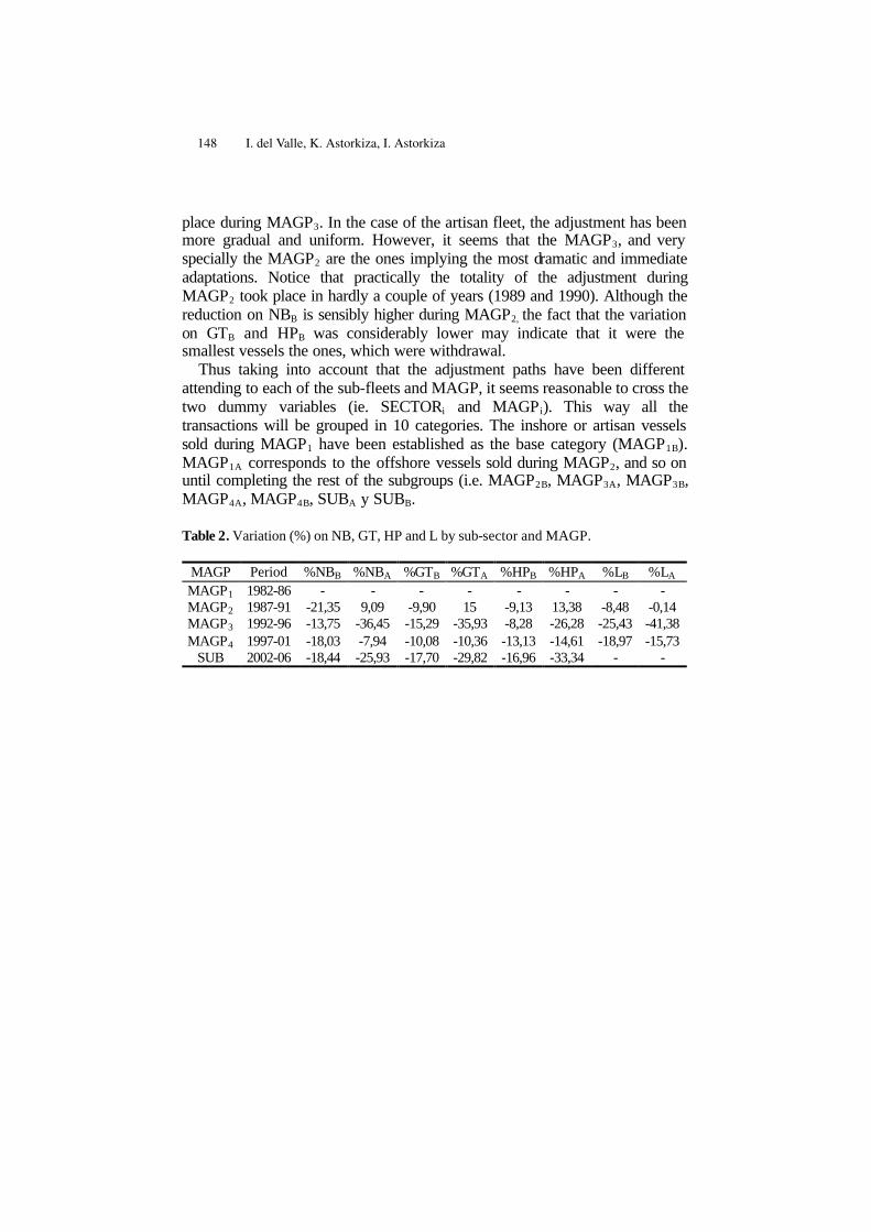
place during MAGP3. In the case of the artisan fleet, the adjustment has been more gradual and uniform. However, it seems that the MAGP3, and very specially the MAGP2 are the ones implying the most dramatic and immediate adaptations. Notice that practically the totality of the adjustment during MAGP2 took place in hardly a couple of years (1989 and 1990). Although the reduction on NBB is sensibly higher during MAGP2, the fact that the variation on GTB and HPB was considerably lower may indicate that it were the smallest vessels the ones, which were withdrawal.
Thus taking into account that the adjustment paths have been different attending to each of the sub-fleets and MAGP, it seems reasonable to cross the two dummy variables (ie. SECTORi and MAGPi). This way all the transactions will be grouped in 10 categories. The inshore or artisan vessels sold during MAGP1 have been established as the base category (MAGP1B). MAGP1A corresponds to the offshore vessels sold during MAGP2, and so on until completing the rest of the subgroups (i.e. MAGP2B, MAGP3A, MAGP3B, MAGP4A, MAGP4B, SUBA y SUBB.
Table 2. Variation (%) on NB, GT, HP and L by sub-sector and MAGP.
MAGP Period %NBB %NBA %GTB %GTA %HPB %HPA %LB %LA MAGP1 1982-86 - - - - - - - - MAGP2 1987-91 -21,35 9,09 -9,90 15 -9,13 13,38 -8,48 -0,14 MAGP3 1992-96 -13,75 -36,45 -15,29 -35,93 -8,28 -26,28 -25,43 -41,38 MAGP4 1997-01 -18,03 -7,94 -10,08 -10,36 -13,13 -14,61 -18,97 -15,73
SUB 2002-06 -18,44 -25,93 -17,70 -29,82 -16,96 -33,34 - -
148 I. del Valle, K. Astorkiza, I. Astorkiza
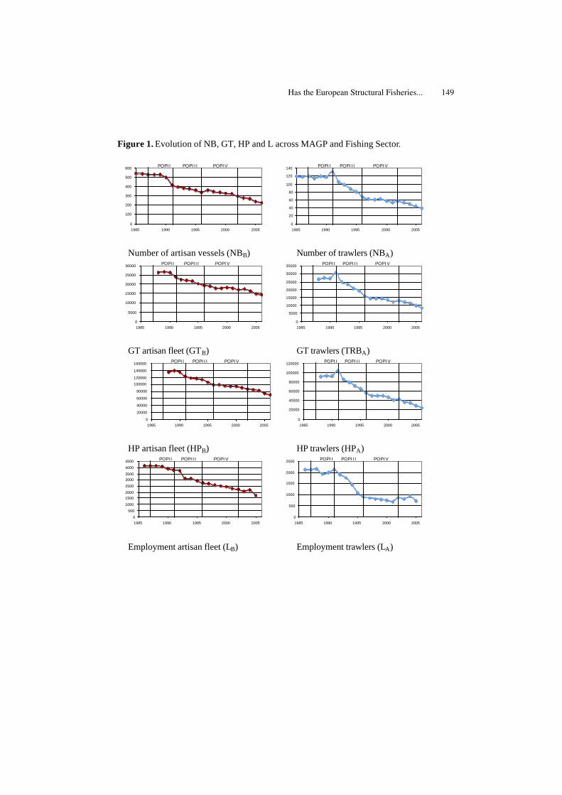
Figure 1. Evolution of NB, GT, HP and L across MAGP and Fishing Sector.
Number of artisan vessels (NBB) Number of trawlers (NBA)
GT artisan fleet (GTB) GT trawlers (TRBA)
HP artisan fleet (HPB) HP trawlers (HPA)
Employment artisan fleet (LB) Employment trawlers (LA)
0
100
200
300
400
500
600
1985 1990 1995 2000 2005
POPII POPIII POPIV
0
20
40
60
80
100
120
140
1985 1990 1995 2000 2005
POPII POPIII POPIV
0
5000
10000
15000
20000
25000
30000
1985 1990 1995 2000 2005
POPII POPIII POPIV
0
5000
10000
15000
20000
25000
30000
35000
1985 1990 1995 2000 2005
POPII POPIII POPIV
0
20000
40000
60000
80000
100000
120000
140000
160000
1985 1990 1995 2000 2005
POPII POPIII POPIV
0
20000
40000
60000
80000
100000
120000
1985 1990 1995 2000 2005
POPII POPIII POPIV
0
500
1000
15002000
2500
30003500
4000
4500
1985 1990 1995 2000 2005
POPII POPIII POPIV
0
500
1000
1500
2000
2500
1985 1990 1995 2000 2005
POPII POPIII POPIV
Has the European Structural Fisheries... 149

3 An Empirical Model for the 2nd Hand of Fishing Vessels
Following the hedonic approach, vessels are considered to be composite products formed by a heterogeneous set of attributes, whose market price at time t (Pit) is determined by a set of characteristics X=(X1, X2,…, Xn) (i.e. GT, AGE, the fishing SECTOR the vessel belongs to) and by the potential effects that the European Fisheries Structural Policy, via MAGP, may have exercised on the second hand market (MAGP t). Therefore, when acquiring a vessel, we can consider the price to be the sum of the price paid for each one of its attributes [(Xi=GT, AGE, SECTOR), MAGPt)], so that an implicit price, or hedonic price exists for each one of the attributes defining the vessel.
Hence, assuming an optimal behaviour by buyers and sellers the second hand market fishing vessels price hedonic function may be estimated under market equilibrium and using transactions data Pit=f((Xi=GT, AGE, SECTOR), MAGP t). The essence of the approach consists of finding what portion of the price is determined by each of the atributtes (Xi, MAGPt). This information is obtained by calculating the partial derivative of the price with respect to each of the attributes (∂Pit ∂X i ,∂Pit ∂MAGPt ). Besides the marginal willingness to pay for an additional unit of each of the vessels’ characteristics, this method also gives us the structural policy asset, allowing us to obtain an estimate of its monetary value. To put in another words, we focus on vessels of the same quality (i.e. vessels sharing identical characteristics (Xit), and then compare the hedonic price at different time periods grouped in each of the MAGP. This way, the part of overall price change from one MAGP to another, which is not accounted by the changes in characteristics may be then interpreted as pure price change related to changes in economic policy. If this price change is significantly great under the most radical fleet adjustment one may derive that the structural policy is affecting the market.
The modelling requirements implicit in the applied hedonic regression literature focuses the attention on three major points: a) the specification of the functional form; b) the configuration of models suitable to test for structural break; and c) the discussion of the appropriate estimation method, mainly discriminating among OLS and weighted least squares (WLS). All of these topics are covered in the next three subsections. Since this is the first application of the hedonic framework to fishing vessels, special attention will be plaid to the functional form selection procedure. This procedure is based on two steps. First the performance of a priori established functional forms in undertaken attending to the usual goodness of fit measures and the signs of the estimated parameters. Second a battery of non-nested test is completed in
150 I. del Valle, K. Astorkiza, I. Astorkiza

order to check the performance of alternative transformations of the numerical variables included in the model chosen in the first step. Afterwards the issue of the structural time stability is addressed in the framework of the previously selected function by estimating an augmented model incorporating time varying slopes for the numerical independent variables; and carrying on a related F test. Finally the convenience of using other estimation methods instead of OLS is considered based on heteroskedasticity tests and also the regression diagnostic. The estimated coefficients derived by OLS, WLS and trimmed least squares (TLS) are compared in other to see if the results do not radically change depending on the estimation method.
3.1 The Functional Form
Although the specification of the functional form of hedonic regression models has been the subject of considerable debate, the hedonic theory does not give an explicit answer to this central issue and there is no a priori structural restriction on the choice of functional forms. The general view is that the functional form of a hedonic model is purely an empirical issue (Rosen, 1974) and that therefore decisions should be made on a case-by-case basis, taking into account several interrelated issues such as, the purpose for which the hedonic regression is undertaken, the kind of data used, the estimation method, the appropriateness of the derived empirical results and also the results of homoskedasticity tests.
In most empirical studies carried on durable goods using the hedonic framework the model selection procedure is limited to choosing among three popular functional forms (the linear (1), the semi-log (2) and the log linear (or double log) (3)) based on the usual goodness of fit measures (R2, the standard error of the regression, AIC, etc.). Notice that strictly speaking when dummy variables are included, since these are not transformed, equation (2) is in fact a mixed functional form. Besides, all of the variables of the right side of the equation need not have the same form. For example Barzyk [21] employed a mixed functional form in which some of the variables appear linearly and some logarithmically depending on the data fit and the empirical standards summarized in (Wooldridge [22])3. Following the terminology in Triplett (2004) we will refer to these forms as mixed–semilog functions. The semilog and log-linear forms are usually preferred, mainly because they generate a better goodness of fit and because heteroskedasticity is mitigated [23]. However, a simple log model may not be the correct specification due to the
3 When a priori choosing which of the variables are transformed it is usual to take logs when
working with monetary variables taking high values. However, the variables measured in years normally appear in their original form.
Has the European Structural Fisheries... 151
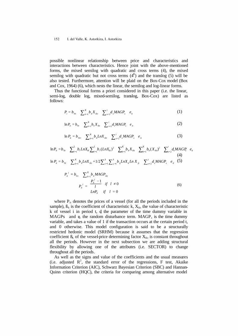
possible nonlinear relationship between price and characteristics and interactions between characteristics. Hence joint with the above-mentioned forms, the mixed semilog with quadratic and cross terms (4), the mixed semilog with quadratic but not cross terms (4R) and the translog (5) will be also tested. Furthermore, attention will be plaid on the Box-Cox model (Box and Cox, 1964) (6), which nests the linear, the semilog and log-linear forms.
Thus the functional forms a priori considered in this paper (i.e. the linear, semi-log, double log, mixed-semilog, translog, Box-Cox) are listed as follows:
Pi = β0t + βkk =1
K∑ X ikt + δ ss=2
t∑ MAGPs + εit (1) ln Pit = β0t + βkk=1
K∑ X ikt + δss=2
t∑ MAGPs + ε it (2)
ln Pit = β0t i + βkk=1
K∑ LnX ikt + δ ss=2
t∑ MAGPs + ε it (3)
lnPit =β0t + βll=1
L∑ LnXilt βll=1
L∑ (LnXilt )2 + βkk=1
K∑ X ikt + βkk=1
K∑ (X ikt)2 + δss=2
t∑ MAGPs +εit
(4) ln Pit = β0t + βkk=1
K∑ LnX ikt +1/2 β ijLnX itj =1
k∑i=1
k∑ Ln X jt + δss=2
t∑ MAGPs + ε it (5)
Pit
λ = β0 t + βkk=1
K∑ MAGPikt
Pitλ =
Pitλ − 1λ
if λ ≠ 0
LnPit if λ = 0
(6)
where Pit denotes the prices of a vessel (for all the periods included in the
sample), ßk is the coefficient of characteristic k, Xikt the value of characteristic k of vessel i in period t, ds the parameter of the time dummy variable in MAGPs and eit the random disturbance term. MAGPs is the time dummy variable, and takes a value of 1 if the transaction occurs at the certain period t, and 0 otherwise. This model configuration is said to be a structurally restricted hedonic model (SRHM) because it assumes that the regression coefficient ßk of the vessel-price determining factor Xikt is constant throughout all the periods. However in the next subsection we are adding structural flexibility by allowing one of the attributes (i.e. SECTOR) to change throughout all the periods.
As well as the signs and value of the coefficients and the usual measures (i.e. adjusted R2, the standard error of the regressions, F test, Akaike Information Criterion (AIC), Schwarz Bayesian Criterion (SBC) and Hannan-Quinn criterion (HQC), the criteria for comparing among alternative model
152 I. del Valle, K. Astorkiza, I. Astorkiza

specification includes a full battery of nested on non-nested tests: Ramsey’s RESET test, Davidson-MacKinnon (1981) (DM) test, Minzon y Richard (1986) (MR) test, Wooldridge (1994) and Box Cox test (1964). Notice that while RESET is limited to nested models, DM F and MR t tests are useful to discriminate between non-nested models of the independent variables, provided that the model includes the same dependent. However DM and MR are not valid in order to contrast among alternative non-nested models when they have different dependent variables, such as log(Pi) against Pi. Since in these cases you cannot make direct comparisons of R2 or the sums of the squares of the residuals (SSR), additional test, such the Box-Cox test (1964) (BC) and Wooldridge (1994) tests (W) are required. The OLS results for the lineal (1), semi-log (2), log-linear (3), mixed semilog with quadratic and cross term between TRB and AGE (4), mixed-semilog with quadratic but no interaction term (4R), and the translog (5) are summarised in Table 3. For one side, attending both to adjusted R2, the AIC, SBC and HQC the linear model performs worse than the others, although at least it passes the RESET test for model configuration. The models including quadratic and or cross terms perform better attending to the R2, the AIC, SBC and HQC. Besides, all of them pass the RESET. Moreover apart from the translog the signs for the estimated parameters are the expected ones. Both the AIC and the rest of the models selection criteria and F test for the omission of the cross term between AGE and TRB constitute complement arguments in favour of model (4R) [F(1, 213)=0.05, p-value=0.8147].
Has the European Structural Fisheries... 153

Table 3. Regression results for alternative functional forms
Variable
Linear(1)
SemiLog(2) Loglinear(3) MSemilog†(4)
MSemilog(b)†(4)R
T raslog(5)
constant 165,017 (145,761) [93,286]*
7.6785 (0.2829)*** [0.2903]***
8.3568 (0.3563)*** [0.3537]***
6.7097 (0.4768)*** [0.4282]***
6.7621 (0.4204)*** [0.3604]***
6.0342 (0.8550)*** [0.8950]***
GT 3034.09 (481.10)*** [577.78]***
1.0865 (0.0525)*** [0,0530]***
1.0824 (0.0528)*** (0.0520)***
2.0662 (0.2250)*** [0.1960]***
2.0560 (0.2203)*** [0.1845]***
2.00235 (0.2628)*** [0.2515]***
AGE -12810.9 (4169.69)*** [4047.49]***
-0.0334 (0.0069)*** [0.0069]***
-0.4509 (0.1016)*** [0.1038]***
(-0.0777) (0.0309)** [0.0299]***
-0.0813 (0.0268)*** [0.0251]***
0.555934 (0.5687) [0.5739]
GT 2 - - - -0.1494
(0.0339) *** [0.0291]***
-0.1507 (0.0268)*** [0.0299]***
-0.145207 (0.0337)*** [0.0294]***
AGE2 - - - 0.0011
(0.0006)* [0.00062]*
0.0011 (0.00067)* [0.00062]*
-0.223959 (0.1161)* [0.1137]*
GT*AGE - - - -0.0011
(0.0047) [0.0046]
_ 0.00620675 (0.0627) [0.0612]
MAGP 1A -266,610 (219,151) [116,470]**
-0.3497 (0.3507) [0.3163]
-0.3084 (0.3526) [0.3155]
0.0960 (0.3532) [0.3041]
0.1058 (0.3500) [0.3075]
0.0725587 (0.3523) [0.3091]
MAGP 2B 169,240 (162,127) [79,416]**
0.5414 (0.2642)** [0.3163]
0.5069 (0.2656)* [0.3418]
0.6315 (0.2548)** [0.3415]*
0.6272 (0.2536)** [0.3359]*
0.633033 (0.2561)** [0.3429]*
MAGP 2A 117,610 (207,621) [161,793]
0.1497 (0.3303) [0.4046]
0.1410 (0.3327) [0.4104]
0.6029 (0.3333)* [0.4408]
0.6094 (0.3314)* [0.4394]
0.600905 (0.3337)* [0.4423]
MAGP 3B 200,915 (147,531) [63,774]***
1.1809 (0.2412)*** [0.2683]***
1.1385 (0.2422)*** [0.2683]***
1.1671 (0.2316)*** [0.2644]***
1.1668 0.2311*** [0.2647]***
1.1912 (0.2329)*** [0.2676]***
MAGP 3A 725,644 (190,004)*** [182,417]***
0.9941 (0.2783)*** [0.2888]***
0.9771 (0.2804)*** [0.2864]***
1.6162 (0.3006)*** [0.3082]***
1.6182 (0.2998)*** [0.3086]***
1.59677 (0.3005)*** [0.3106]***
MAGP 4B 261,139 (144,648)* [64,041]***
1.3240 (0.2362)*** [0.2502]***
1.2924 (0.2371)*** [0.2470]***
1.3060 (0.2267)*** [0.2436]***
1.3071 (0.2261)*** [0.2431]***
1.32225 (0.2279)*** [0.2517]***
MAGP 4A 606,392 (213,315)*** [199,991]***
1.1692 (0.3272)*** [0.3052]***
1.1160 (0.3225)*** [0.2470]***
1.7333 (0.3393)*** [0.3011]***
1.7253 (0.3368)*** [0.2948]***
1.72128 (0.3397)*** [0.3025]***
SUBB 231,166 (166,266) [69,828]***
1.3979 (0.2709)*** [0.2709]***
1.3468 (0.2725)*** [0.2732]***
1.3036 (0.2633)*** [0.2675]***
1.3046 (0.2627)*** [0.2675]***
1.3598 (0.2615)*** [0.2743]***
SUBA 1,553,830 (210,933)*** [541,888]***
1.4950 (0.3313)*** [0.3770]***
1.4742 (0.3334)*** [0.3814]***
1.987 (0.3363)*** [0.3810]
1.9834 (0.3352)*** [0.3795]***
1.97449 (0.3370)*** [0.3822]***
adj. R2 0.57 0.78 0.76 0,78 0,78 0.78 F test 28.8391*** 70.2724*** 69.069*** 61.53*** 66.56*** 61.1951*** SER 491,500 0.8007 0.8061 0.7682 0.7699 AIC 6634.69 557.385 560.473 541.3 539.358 542.32 SBC 6675.84 598.537 601.625 592.74 587.37 593.76 HQC 6651.29 573.989 577.076 562.054 558.73 563.075 RESET 0.5836 7.2237*** 8.6588*** 0.5302 0.1525 0.3196 RESETR 9.3072*** 10.1092*** 0.6017 0.1059 0.2724
Standard error in () and standard error robust to het. in []. † LP and LTRB (transformed) and AGE not transformed
154 I. del Valle, K. Astorkiza, I. Astorkiza

Accordingly, the mixed semilog with quadratic but no iteration term between the numerical independent variables is the candidate for a more exhaustive analysis. Notice that the price elasticity for TRB and semielasticity for AGE are not constant and that there is no interaction among them.
Once the mixed-semilog (4R) has been selected, we wonder if the transformation we have a priori chosen for the dependent numerical variables (i.e the price and GT in logs and AGE untransformed) has any statistical support, or in other words, if there exist and alternative transformation pattern with a superior fit to the data. Our decisions will be based on the results of the t test of Davidson-MacKinnon (DM) [24] and F test of Mizon y Richard (MR) [25] and the, test that are appropriate to discriminate among any two non-nested models provided that they have the same dependent variable (in our case log(P) and/or P). In order to show the complete picture and compare alternative model configurations following the structure (4R) with alternative transformation of the dependent variable, we are also including the results of the Box-Cox (1964) (BC) [26] and Wooldridge tests (W) [22]. Tables 4(a) and 4(b) summarise the results.
For one side, both MR4 and DK5 are coincident when discriminating among alternative models derived from the inclusion of numerical independent variables in log or in level. Thus, based on the test carried on in order to discriminate among the alternative non-nested models included in Table 4(a), a priori accepting the log(P) transformation for the dependent variable, (4R2) is the one that fits the data best. For another side, BC6 and W7
4 The M&R test works as follows. For example, in order to discriminate between Model 2 and Model 4 M&R test is based on the joint significance tests for the coefficients (AGE), (AGE)2, log(AGE) and log(AGE)2 derived from the estimation of the joint model including both, [AGE, AGE2] and [log(AGE) y log(AGE)2]. The joint test for AGE y AGE2 is significant [F(2, 212) = 3.34649 p-value 0.0370773], which implies that MODEL 2 is preferred. However, when discriminating between Model 4 and Model 2, the joint significance test of the coefficients for log(AGE) y log(AGE)2 [F(2, 212) = 2.88147, (p-value = 0.0582)], although significant, it’s not as conclusive as the previous (5,8%). 5 The D&M test works as follows. For example in order to discriminate between Model 2 and Model 4 MR test is based on the individual t statistics derived from regressing Models 2 including also the fitted values coming from MODEL 4 as an additional independent variable. Since t is not significant for this added variable [t=1.6418 , p=0.1012], Model 2 offers a best fit. When following the same procedure, one discriminates between Model 4 and Model 2, the resulting t statistics is significant [t=2.4591, p=0.0147], which constitutes a clear evidence against Model 4. 6 We are using the version of the Box-Cox test (1964) developed by Zarembka (1968) to compare the linear and log transformations of the dependent variable. The underlying idea behind the procedure is to scale the observations on dependent variable (Pi) so that the residual sum of squares in the linear and logarithmic models are rendered directly comparable. The next steps are followed in order to calculate the test statistics reported in Table 4(b): 1) Scale the observations on Pi by dividing them by the sample geometric mean of Pi (Pi*=Pi/GMPi). 2) Regress the lineal model using Pi* instead of Pi (Model 7) and the logarithmic model using
Has the European Structural Fisheries... 155
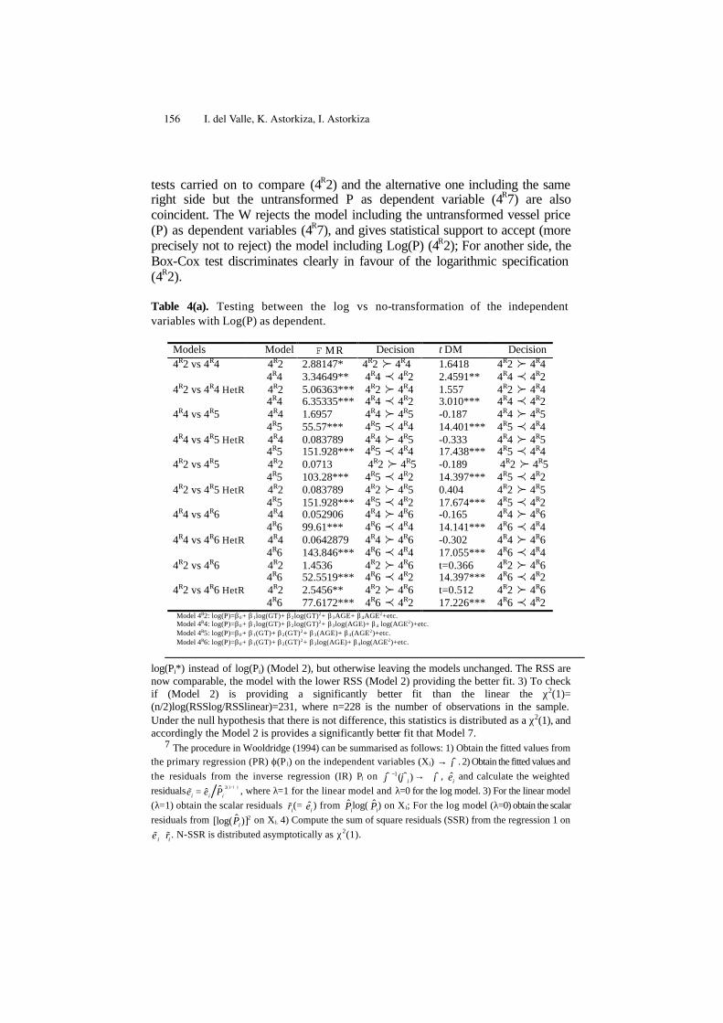
tests carried on to compare (4R2) and the alternative one including the same right side but the untransformed P as dependent variable (4R7) are also coincident. The W rejects the model including the untransformed vessel price (P) as dependent variables (4R7), and gives statistical support to accept (more precisely not to reject) the model including Log(P) (4R2); For another side, the Box-Cox test discriminates clearly in favour of the logarithmic specification (4R2).
Table 4(a). Testing between the log vs no-transformation of the independent variables with Log(P) as dependent.
Models Model F MR Decision t DM Decision 4R2 vs 4R4 4R2 2.88147* 4R2 f 4R4 1.6418 4R2 f 4R4 4R4 3.34649** 4R4 p 4R2 2.4591** 4R4 p 4R2 4R2 vs 4R4 HetR 4R2 5.06363*** 4R2 f 4R4 1.557 4R2 f 4R4 4R4 6.35335*** 4R4 p 4R2 3.010*** 4R4 p 4R2 4R4 vs 4R5 4R4 1.6957 4R4 f 4R5 -0.187 4R4 f 4R5 4R5 55.57*** 4R5 p 4R4 14.401*** 4R5 p 4R4 4R4 vs 4R5 HetR 4R4 0.083789 4R4 f 4R5 -0.333 4R4 f 4R5 4R5 151.928*** 4R5 p 4R4 17.438*** 4R5 p 4R4 4R2 vs 4R5 4R2 0.0713 4R2 f 4R5 -0.189 4R2 f 4R5 4R5 103.28*** 4R5 p 4R2 14.397*** 4R5 p 4R2 4R2 vs 4R5 HetR 4R2 0.083789 4R2 f 4R5 0.404 4R2 f 4R5 4R5 151.928*** 4R5 p 4R2 17.674*** 4R5 p 4R2 4R4 vs 4R6 4R4 0.052906 4R4 f 4R6 -0.165 4R4 f 4R6 4R6 99.61*** 4R6 p 4R4 14.141*** 4R6 p 4R4 4R4 vs 4R6 HetR 4R4 0.0642879 4R4 f 4R6 -0.302 4R4 f 4R6 4R6 143.846*** 4R6 p 4R4 17.055*** 4R6 p 4R4 4R2 vs 4R6 4R2 1.4536 4R2 f 4R6 t=0.366 4R2 f 4R6 4R6 52.5519*** 4R6 p 4R2 14.397*** 4R6 p 4R2 4R2 vs 4R6 HetR 4R2 2.5456** 4R2 f 4R6 t=0.512 4R2 f 4R6 4R6 77.6172*** 4R6 p 4R2 17.226*** 4R6 p 4R2 Model 4R2: log(P)=β0+ β1log(GT)+ β2log(GT)2+ β3AGE+ β4AGE2+etc. Model 4R4: log(P)=β0+ β1log(GT)+ β2log(GT)2+ β3log(AGE)+ β4 log(AGE2)+etc. Model 4R5: log(P)=β0+ β1(GT)+ β2(GT)2+ β3(AGE)+ β4(AGE2)+etc. Model 4R6: log(P)=β0+ β1(GT)+ β2(GT)2+ β3log(AGE)+ β4log(AGE2)+etc.
log(Pi*) instead of log(Pi) (Model 2), but otherwise leaving the models unchanged. The RSS are now comparable, the model with the lower RSS (Model 2) providing the better fit. 3) To check if (Model 2) is providing a significantly better fit than the linear the χ2(1)= (n/2)log(RSSlog/RSSlinear)=231, where n=228 is the number of observations in the sample. Under the null hypothesis that there is not difference, this statistics is distributed as a χ2(1), and accordingly the Model 2 is provides a significantly better fit that Model 7.
7 The procedure in Wooldridge (1994) can be summarised as follows: 1) Obtain the fitted values from the primary regression (PR) ϕ(P i) on the independent variables (Xi) → ˆ ϕ . 2) Obtain the fitted values and the residuals from the inverse regression (IR) Pi on ˆ ϕ −1( ˆ ϕ i )→ ˆ ϕ , ˆ e i and calculate the weighted residuals ˜ e i = ˆ e i ˆ P i
2(1− λ ) , where λ=1 for the linear model and λ=0 for the log model. 3) For the linear model (λ=1) obtain the scalar residuals ˜ r i(= ˆ e i ) from ˆ P ilog( ˆ P i) on Xi; For the log model (λ=0) obtain the scalar residuals from [log( ˆ P i )]
2 on Xi. 4) Compute the sum of square residuals (SSR) from the regression 1 on
˜ e i ⋅ ˜ r i . N-SSR is distributed asymptotically as χ2(1).
156 I. del Valle, K. Astorkiza, I. Astorkiza
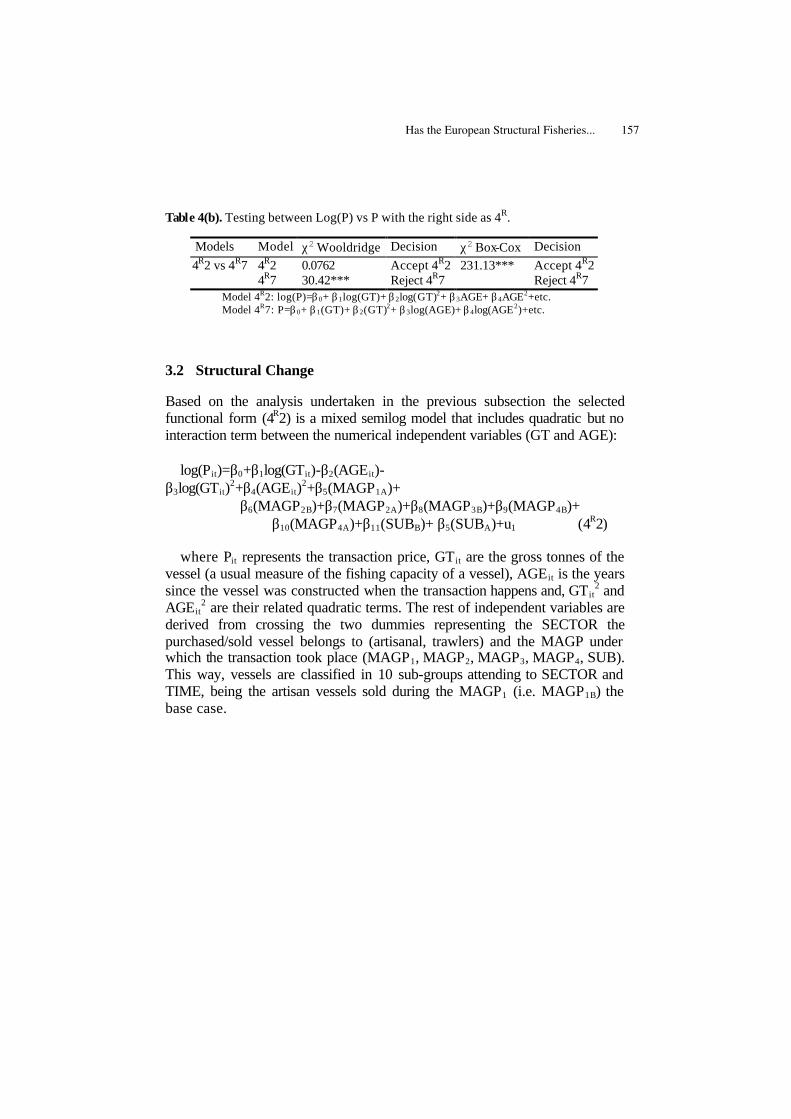
Table 4(b). Testing between Log(P) vs P with the right side as 4R.
Models Model χ2 Wooldridge Decision χ2 Box-Cox Decision 4R2 vs 4R7 4R2 0.0762 Accept 4R2 231.13*** Accept 4R2
4R7 30.42*** Reject 4R7 Reject 4R7 Model 4R2: log(P)=β0+ β1log(GT)+ β2log(GT)2+ β3AGE+ β4AGE2+etc. Model 4R7: P=β0+ β1(GT)+ β2(GT)2+ β3log(AGE)+ β4log(AGE2)+etc.
3.2 Structural Change
Based on the analysis undertaken in the previous subsection the selected functional form (4R2) is a mixed semilog model that includes quadratic but no interaction term between the numerical independent variables (GT and AGE):
log(Pit)=β0+β1log(GTit)-β2(AGEit)-
β3log(GTit)2+β4(AGEit)2+β5(MAGP1A)+ β6(MAGP2B)+β7(MAGP2A)+β8(MAGP3B)+β9(MAGP4B)+ β10(MAGP4A)+β11(SUBB)+ β5(SUBA)+u1 (4R2)
where Pit represents the transaction price, GT it are the gross tonnes of the vessel (a usual measure of the fishing capacity of a vessel), AGE it is the years since the vessel was constructed when the transaction happens and, GTit
2 and AGEit
2 are their related quadratic terms. The rest of independent variables are derived from crossing the two dummies representing the SECTOR the purchased/sold vessel belongs to (artisanal, trawlers) and the MAGP under which the transaction took place (MAGP1, MAGP2, MAGP3, MAGP4, SUB). This way, vessels are classified in 10 sub-groups attending to SECTOR and TIME, being the artisan vessels sold during the MAGP1 (i.e. MAGP1B) the base case.
Has the European Structural Fisheries... 157
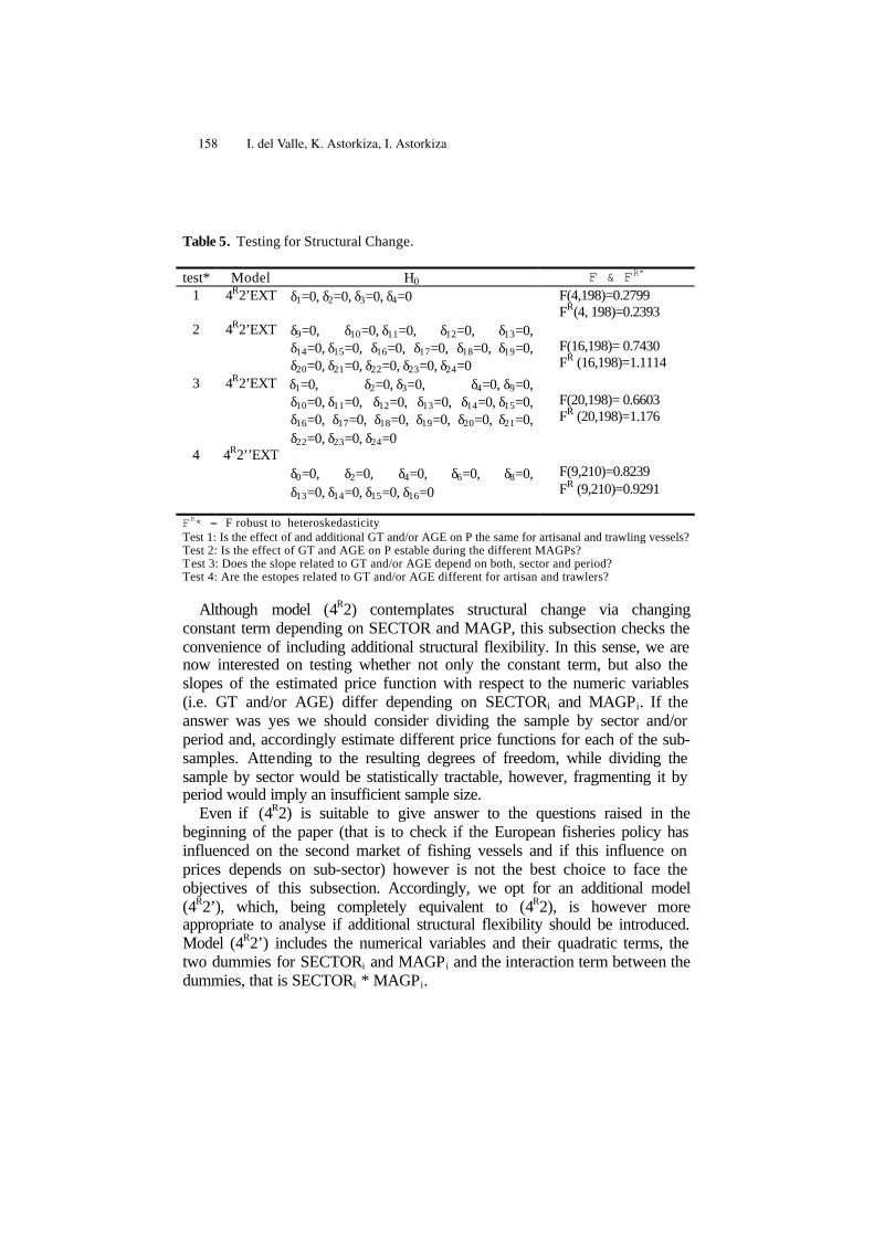
Table 5. Testing for Structural Change.
test* Model H0 F & FR* 1 4R2’EXT δ1=0, δ2=0, δ3=0, δ4=0 F(4,198)=0.2799
FR(4, 198)=0.2393 2 4R2’EXT δ9=0, δ10=0, δ11=0, δ12=0, δ13=0,
δ14=0, δ15=0, δ16=0, δ17=0, δ18=0, δ19=0, δ20=0, δ21=0, δ22=0, δ23=0, δ24=0
F(16,198)= 0.7430 FR (16,198)=1.1114
3 4R2’EXT δ1=0, δ2=0, δ3=0, δ4=0, δ9=0, δ10=0, δ11=0, δ12=0, δ13=0, δ14=0, δ15=0, δ16=0, δ17=0, δ18=0, δ19=0, δ20=0, δ21=0, δ22=0, δ23=0, δ24=0
F(20,198)= 0.6603 FR (20,198)=1.176
4 4R2’’EXT δ0=0, δ2=0, δ4=0, δ6=0, δ8=0, δ13=0, δ14=0, δ15=0, δ16=0
F(9,210)=0.8239 FR (9,210)=0.9291
FR* = F robust to heteroskedasticity Test 1: Is the effect of and additional GT and/or AGE on P the same for artisanal and trawling vessels? Test 2: Is the effect of GT and AGE on P estable during the different MAGPs? Test 3: Does the slope related to GT and/or AGE depend on both, sector and period? Test 4: Are the estopes related to GT and/or AGE different for artisan and trawlers?
Although model (4R2) contemplates structural change via changing constant term depending on SECTOR and MAGP, this subsection checks the convenience of including additional structural flexibility. In this sense, we are now interested on testing whether not only the constant term, but also the slopes of the estimated price function with respect to the numeric variables (i.e. GT and/or AGE) differ depending on SECTORi and MAGPi. If the answer was yes we should consider dividing the sample by sector and/or period and, accordingly estimate different price functions for each of the sub-samples. Attending to the resulting degrees of freedom, while dividing the sample by sector would be statistically tractable, however, fragmenting it by period would imply an insufficient sample size.
Even if (4R2) is suitable to give answer to the questions raised in the beginning of the paper (that is to check if the European fisheries policy has influenced on the second market of fishing vessels and if this influence on prices depends on sub-sector) however is not the best choice to face the objectives of this subsection. Accordingly, we opt for an additional model (4R2’), which, being completely equivalent to (4R2), is however more appropriate to analyse if additional structural flexibility should be introduced.
Model (4R2’) includes the numerical variables and their quadratic terms, the two dummies for SECTORi and MAGPi and the interaction term between the dummies, that is SECTORi * MAGPi.
158 I. del Valle, K. Astorkiza, I. Astorkiza

log(P)= β0+β1log(GT)+β2log(GT)2+β3AGE+β4AGE2+β5MAGP2+ β6MAGP3+β7MAGP4+β8SUB+β9SECTOR+
β10MAGP2*SECTOR+ β11MAGP3*SECTOR+ β12MAGP4*SECTOR+β13SUB*SECTOR+u
(4R2’)
log(P)=β0+δ0SECTOR+β1log(GT)+δ1log(GT)*SECTOR+β2log(GT)2+ δ2log(GT)*SECTOR+β3AGE+δ3AGE*SECTOR+β4AGE2+
δ4AGE2*SECTOR+δ5MAGP2+δ6MAGP3 +δ7MAGP4+δ8SUB+ δ9MAGP2*LGT+ δ10MAGP2*LGT2+ δ11MAGP2*AGE+
δ12MAGP2*AGE2+δ13MAGP3*LGT+δ14MAGP3*LGT2+ δ15
MAGP3*AGE+δ16MAGP3*AGE2+δ17MAGP4*LTRB+ δ18MAGP4*LTRB2+δ19MAGP4*AGE+δ20MAGP4*AGE2+
δ21SUB*LGT+ δ22SUB*LGT2+ δ23SUB*AGE + δ24SUB*AGE2+u (4R2’EXT)
In order to achieve the objective above mentioned we first estimate an
extended version of model 4R2’, that is model (4R2’EXT). In this extended model not only the constant terms (such as in 4R2 and 4R2’) but also all the slopes are allowed to change depending on subgroups. In other words, model 4R2’EXT permits testing whether the price elasticity for GT (εGT) or the price semi-elasticity of AGE (εAGE) are equal for artisan and trawling vessels (Test 1) or whether εGT or εAGE are stable (i.e. if the slope of the price function changes with time (Test 2), as wells as if the slope of the price function depend both on SECTOR and MAGP (Test 3). The F statistics for each of the tests (Table 5) are non significant. This means that the interaction terms between the numerical and dummies are irrelevant to explain prices, or to put in another words, that the slope of price respect GT and AGE are the same for inshore and offshore vessels and that they remain constant during the different MAGPs periods.
Once we have rejected the extended version of the models 4R2 and 4R2’, for completeness, we are also checking if there are structural differences between artisan and trawling vessels, that is, if the slopes for the independent variables (ie. GT and AGE) are different by sector (test 4). Based on an additional model (4R2’’EXT) the F test is performed. Since the resulting F statistics is not significant there is not evidence against working with the pooled sample. This allows working with more degrees of freedom.
Has the European Structural Fisheries... 159
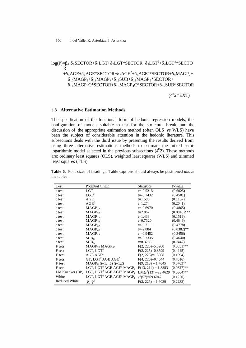
log(P)=β0+δ0SECTOR+δ1LGT+δ2LGT*SECTOR+δ3LGT2+δ4LGT2*SECTOR +δ5AGE+δ6AGE*SECTOR+δ7AGE2+δ8AGE2*SECTOR+δ9MAGP2+
δ10MAGP3+δ11MAGP4+δ12SUB+δ13MAGP2*SECTOR+ δ14MAGP3C*SECTOR+δ15MAGP4C*SECTOR+δ16SUB*SECTOR
(4R2’’EXT)
3.3 Alternative Estimation Methods
The specification of the functional form of hedonic regression models, the configuration of models suitable to test for the structural break, and the discussion of the appropriate estimation method (often OLS vs WLS) have been the subject of considerable attention in the hedonic literature. This subsections deals with the third issue by presenting the results derived from using three alternative estimations methods to estimate the mixed semi-logarithmic model selected in the previous subsections (4R2). These methods are: ordinary least squares (OLS), weighted least squares (WLS) and trimmed least squares (TLS).
Table 6. Font sizes of headings. Table captions should always be positioned above the tables .
Test Potential Origin Statistics P-value t test LGT t=-0.5215 (0.6025) t test LGT2 t=-0.7432 (0.4581) t test AGE t=1.590 (0.1132) t test AGE2 t=1.274 (0.2041) t test MAGP1A t=-0.6970 (0.4865) t test MAGP2B t=2.867 (0.0045)*** t test MAGP2A t=1.438 (0.1519) t test MAGP3B t=0.7320 (0.4649) t test MAGP3A t=-0.7111 (0.4778) t test MAGP4B t=-2.084 (0.0382)** t test MAGP4A t=-0.9452 (0.3456) t test SUBB t=-0.7335 (0.4640) t test SUBA t=0.3266 (0.7442) F tets MAGP2B MAGP4B F(2, 225)=5.3900 (0.0051)** F test LGT, LGT2 F(2, 225)=0.8599 (0.4245) F test AGE AGE2 F(2, 225)=1.8508 (0.1594) F tets GT, LGT2 AGE AGE2 F(4, 223)=0.4644 (0.7616) F test MAGPij (i=1…5) (j=1,2) F(9, 218) = 1.7645 (0.0763)* F tets LGT, LGT2 AGE AGE2 MAGPij F(13, 214) = 1.8883 (0.0327)** LM Koenker (BP) LGT, LGT2 AGE AGE2 MAGPij LM(χ2(13))=23.4629 (0.0364)** White LGT, LGT2 AGE AGE2 MAGPij χ2(57)=69.6047 (0.1220) Reduced White
) y , ) y 2 F(2, 225) = 1.6039 (0.2233)
160 I. del Valle, K. Astorkiza, I. Astorkiza

In order to judge the convenience of using WLS instead of OLS to remove heteroskedasticity of variances, alternative test have been carried on to detect it. Table 6 summarises the results including also the respective potential origin. For one side, both the F and Breusch-Pagan test are significant, which implies that het might bias the inference based on OLS standard errors. However, for another, White and reduced White tests do not detect it. Thus, since the results of the tests are inconclusive, we are also reporting the WLS estimates. The approach summarised in Woldridge (2003, pag. 306) has been followed to calculate the weighted factors.
Last but not least, the regression diagnostic has been carried out in order to see if there are atypical or/and influential observations in the data set with a powerful influence on the estimated parameters and/or predictions of the model. Once selected these will be candidates to be omitted to deal with robust regression techniques. Usual measures in regression diagnostic (i.e. the leverage (ht), Cook’s distance (CD), the standardised residual (e*), DFBETAs and DFFITS are reported in Table 7. All the data points exceeding any of the rule-of-thumb cut-offs of the above-mentioned measures have been market with an asterisk. Six data points (market with double asterisk (0bs coded: 12, 112, 145, 244, 246 and 294)) either with a moderate leverage and/or outliers or a significant contribution on the values of the estimated parameters and/or the model’s predictions have been detected, which represents the 2.63% of the sample data8. The trimming proportion that guaranties the elimination of all
8 While not necessarily undesirable, influential observations are those observations that make a
relatively large contribution to the values of the estimates, that is, observations whose inclusion or exclusion may result in substantial changes in the fitted model. The most common measures for the degree of influence are the leverage (ht) and to some degree Cook’s distance (CD). As a general rule, data points satisfying [0.2>ht>0.5] are considered moderately influent, while those in which ht>0,5 should be especially kept watch. The sample size corrected rule of thumb suggested by Belsey et al. (1980) is h>2p/N, where p is the number of estimated parameters and N the sample size. Similarly, the general criterion stands to watch out for observations where CD>1, although in large samples some authors suggest a sample corrected rule of CD>4/N. Applying these rules to our case study, hardly 2.19% of the observations are moderately influent attending to ht, while the 8.3% does go beyond the sample corrected rule relative to CD. Thus, it may be concluded that none of the observations are riskily influent according nor to the leverage, nor the CD. Together with influential observations, it is also convenient to include measures designed to detect large errors. In a model which fits in every cell formed by the independent variables, no absolute standardized residual will be e*>2 (0,05 level) (or e*> 1.96(0.01 level)). Cells not meeting this criterion indicate combinations of independent variables for which the model is not working well. In our model about 94 % of the observations fit the specified rule of thumb, and consequently regarded as acceptable in term of the model specification. Thus, about 6 % of the observations may be considered outliers. Outliers and high leverage points can be an indication of exceptional data points that are worthy of further study. What is likely to be of more importance however is whether these points significantly contribute to the values of the
Has the European Structural Fisheries... 161
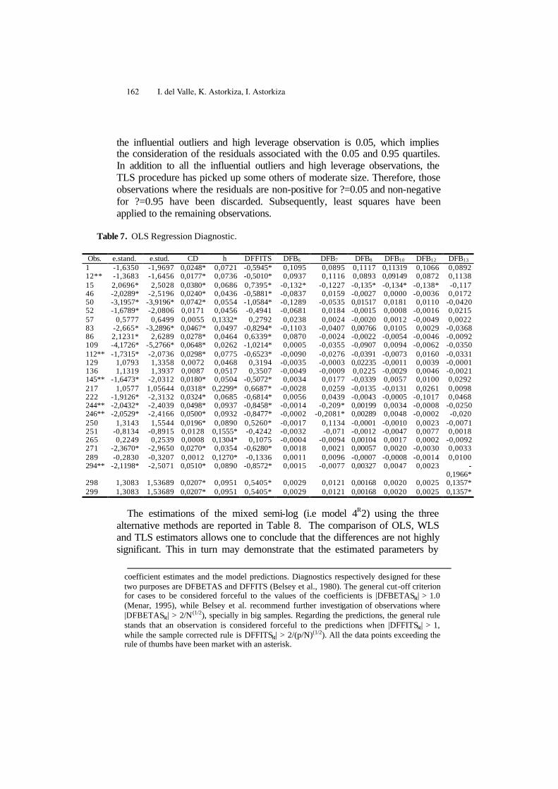
the influential outliers and high leverage observation is 0.05, which implies the consideration of the residuals associated with the 0.05 and 0.95 quartiles. In addition to all the influential outliers and high leverage observations, the TLS procedure has picked up some others of moderate size. Therefore, those observations where the residuals are non-positive for ?=0.05 and non-negative for ?=0.95 have been discarded. Subsequently, least squares have been applied to the remaining observations.
Table 7. OLS Regression Diagnostic.
Obs. e.stand. e.stud. CD h DFFITS DFB6 DFB7 DFB8 DFB10 DFB12 DFB13 1 -1,6350 -1,9697 0,0248* 0,0721 -0,5945* 0,1095 0,0895 0,1117 0,11319 0,1066 0,0892 12** -1,3683 -1,6456 0,0177* 0,0736 -0,5010* 0,0937 0,1116 0,0893 0,09149 0,0872 0,1138 15 2,0696* 2,5028 0,0380* 0,0686 0,7395* -0,132* -0,1227 -0,135* -0,134* -0,138* -0,117 46 -2,0289* -2,5196 0,0240* 0,0436 -0,5881* -0,0837 0,0159 -0,0027 0,0000 -0,0036 0,0172 50 -3,1957* -3,9196* 0,0742* 0,0554 -1,0584* -0,1289 -0,0535 0,01517 0,0181 0,0110 -0,0420 52 -1,6789* -2,0806 0,0171 0,0456 -0,4941 -0,0681 0,0184 -0,0015 0,0008 -0,0016 0,0215 57 0,5777 0,6499 0,0055 0,1332* 0,2792 0,0238 0,0024 -0,0020 0,0012 -0,0049 0,0022 83 -2,665* -3,2896* 0,0467* 0,0497 -0,8294* -0,1103 -0,0407 0,00766 0,0105 0,0029 -0,0368 86 2,1231* 2,6289 0,0278* 0,0464 0,6339* 0,0870 -0,0024 -0,0022 -0,0054 -0,0046 -0,0092 109 -4,1726* -5,2766* 0,0648* 0,0262 -1,0214* 0,0005 -0,0355 -0,0907 0,0094 -0,0062 -0,0350 112** -1,7315* -2,0736 0,0298* 0,0775 -0,6523* -0,0090 -0,0276 -0,0391 -0,0073 0,0160 -0,0331 129 1,0793 1,3358 0,0072 0,0468 0,3194 -0,0035 -0,0003 0,02235 -0,0011 0,0039 -0,0001 136 1,1319 1,3937 0,0087 0,0517 0,3507 -0,0049 -0,0009 0,0225 -0,0029 0,0046 -0,0021 145** -1,6473* -2,0312 0,0180* 0,0504 -0,5072* 0,0034 0,0177 -0,0339 0,0057 0,0100 0,0292 217 1,0577 1,05644 0,0318* 0,2299* 0,6687* -0,0028 0,0259 -0,0135 -0,0131 0,0261 0,0098 222 -1,9126* -2,3132 0,0324* 0,0685 -0,6814* 0,0056 0,0439 -0,0043 -0,0005 -0,1017 0,0468 244** -2,0432* -2,4039 0,0498* 0,0937 -0,8458* -0,0014 -0,209* 0,00199 0,0034 -0,0008 -0,0250 246** -2,0529* -2,4166 0,0500* 0,0932 -0,8477* -0,0002 -0,2081* 0,00289 0,0048 -0,0002 -0,020 250 1,3143 1,5544 0,0196* 0,0890 0,5260* -0,0017 0,1134 -0,0001 -0,0010 0,0023 -0,0071 251 -0,8134 -0,8915 0,0128 0,1555* -0,4242 -0,0032 -0,071 -0,0012 -0,0047 0,0077 0,0018 265 0,2249 0,2539 0,0008 0,1304* 0,1075 -0,0004 -0,0094 0,00104 0,0017 0,0002 -0,0092 271 -2,3670* -2,9650 0,0270* 0,0354 -0,6280* 0,0018 0,0021 0,00057 0,0020 -0,0030 0,0033 289 -0,2830 -0,3207 0,0012 0,1270* -0,1336 0,0011 0,0096 -0,0007 -0,0008 -0,0014 0,0100 294** -2,1198* -2,5071 0,0510* 0,0890 -0,8572* 0,0015 -0,0077 0,00327 0,0047 0,0023 -
0,1966* 298 1,3083 1,53689 0,0207* 0,0951 0,5405* 0,0029 0,0121 0,00168 0,0020 0,0025 0,1357* 299 1,3083 1,53689 0,0207* 0,0951 0,5405* 0,0029 0,0121 0,00168 0,0020 0,0025 0,1357*
The estimations of the mixed semi-log (i.e model 4R2) using the three
alternative methods are reported in Table 8. The comparison of OLS, WLS and TLS estimators allows one to conclude that the differences are not highly significant. This in turn may demonstrate that the estimated parameters by
coefficient estimates and the model predictions. Diagnostics respectively designed for these two purposes are DFBETAS and DFFITS (Belsey et al., 1980). The general cut-off criterion for cases to be considered forceful to the values of the coefficients is |DFBETASkt| > 1.0 (Menar, 1995), while Belsey et al. recommend further investigation of observations where |DFBETASkt| > 2/N(1/2), specially in big samples. Regarding the predictions, the general rule stands that an observation is considered forceful to the predictions when |DFFITSkt| > 1, while the sample corrected rule is DFFITSkt| > 2/(p/N)(1/2). All the data points exceeding the rule of thumbs have been market with an asterisk.
162 I. del Valle, K. Astorkiza, I. Astorkiza

OLS are robust to using additional procedures. Nevertheless the elasticity estimation and price patterns using the alternative estimated functions will be also compared.
Table 8. Regression Results Using OLS, WLS and TLS.
Variable OLS WLS TLS*
constant 6.7621 (0.4204)***
6.63155 (0.3713)***
6.3885 (0.3265)***
LGT 2.0560 (0.2203)***
2.13523 (0.1634)***
2.2181 (0.1714)***
AGE -0.0813 (0.0268)***
-0.0790 (0.0166)***
-0.046780 (0.0049)**
LGT2 -0.1507 (0.0268)***
-0.1621 (0.0233)***
-.18333 (0.0208)***
AGE2 0.0011 (0.00067)*
0.0012132 (0.0004)****
0.0049039 (0.0052)
MAGP1A 0.1058 (0.3500)
0.116813 (0.3425)
.22671 (0.2715)
MAGP2B 0.6272 (0.2536)**
0.796769 (0.3290)**
.66758 (0.1964)***
MAGP2A 0.6094 (0.3314)*
0.364523 (0.5856)
1.10247 (0.2571)***
MAGP3B 1.1668 0.2311***
1.04569 (0.2550)***
1.1595 (0.1793)***
MAGP3A 1.6182 (0.2998)***
1.65537 80.2795)***
1.8134 (0.2326)***
MAGP4B 1.3071 (0.2261)***
1.2601 (80.2410)***
1.1481 (0.1754)***
MAGP4A 1.7253 (0.3368)***
1.6832 (0.2820)***
1.7903 (0.2612)***
SUBB 1.3046 (0.2627)***
1.14844 (0.2522)***
1.3037 (0.2038)***
SUBA 1.9834 (0.3352)***
1.98734 (0.3631)***
1.9934 (0.2600)***
adj. R2 0.78 0.85 0.79 *Number of observations after trimming= 189
4 Interpreting the Results
Based on the analysis carried out in section 3, the OLS estimations for the mixed semilog function (4R2) will be used to answer the researching questions raised in the beginning. Mainly, if the European Fisheries Structural Policy
Has the European Structural Fisheries... 163
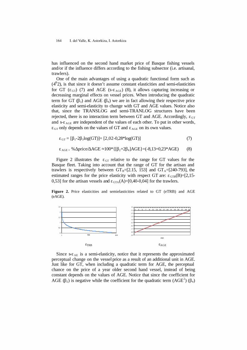
has influenced on the second hand market price of Basque fishing vessels and/or if the influence differs according to the fishing subsector (i.e. artisanal, trawlers).
One of the main advantages of using a quadratic functional form such as (4R2), is that since it doesn’t assume constant elasticities and semi-elasticities for GT (εGT) (7) and AGE (s-εAGE) (8), it allows capturing increasing or decreasing marginal effects on vessel prices. When introducing the quadratic term for GT (β3) and AGE (β4) we are in fact allowing their respective price elasticity and semi-elasticity to change with GT and AGE values. Notice also that, since the TRANSLOG and semi-TRANLOG structures have been rejected, there is no interaction term between GT and AGE. Accordingly, εGT and s-εAGE are independent of the values of each other. To put in other words, εGT only depends on the values of GT and εAGE on its own values.
εGT = [β1-2β3log(GT)]= [2,02-0,28*log(GT)] (7)
εAGE = %∆price/∆AGE ≈100*[β2+2β4]AGE=(-8,13+0,23*AGE) (8)
Figure 2 illustrates the εGT relative to the range for GT values for the
Basque fleet. Taking into account that the range of GT for the artisan and trawlers is respectively between GTB=[2.15, 153] and GTA=[240-793], the estimated ranges for the price elasticity with respect GT are: εGTB(B)=[2,15-0,53] for the artisan vessels and εGTA(A)=[0,40-0,04] for the trawlers.
Figure 2. Price elasticities and semielasticities related to GT (eTRB) and AGE (eAGE).
0
0,5
1
1,5
2
2,5
1 800TRB
-9
-8
-7
-6
-5
-4
-3
-2
-1
01 3 5 7 9 11 13 15 17 19 21 23 25 27 29 31
AGE
εTRB εAGE
Since s-εAE is a semi-elasticity, notice that it represents the approximated
perceptual change on the vessel price as a result of an additional unit in AGE. Just like for GT, when including a quadratic term for AGE, the perceptual chance on the price of a year older second hand vessel, instead of being constant depends on the values of AGE. Notice that since the coefficient for AGE (β2) is negative while the coefficient for the quadratic term (AGE2) (β4)
164 I. del Valle, K. Astorkiza, I. Astorkiza

is positive, it may indicate that for small AGE values (almost new vessels) the fact that the vessel has an additional year has a negative effect on log(price). For AGE exceeding a critical value (β2/2β4 = 0,00004), this effect turns into positive. The shape of the quadratic form related to AGE means that the semielasticity of price with respect to AGE is increasing as AGE does. Thus, for example an increase of AGE from 5 to 6 years would decrease the price of a second hand market vessel in 6.73%. Taking into account that the sample average AGE is AGE=18, a one year older vessel would reach a price 3.69 % lower. Accordingly, it seems that the perceptual chance on prices as a result of a perceptual chance in AGE is sensibly higher for the newer vessels.
As well as analyzing the performance of the numerical variables (GT and AGE), the estimated model allows capturing the differences on prices related to the ten categories resulting from crossing the two dummy variables (i.e. SECTORi and MAGPi). This modeling approach, not only possibilities searching the price differences among the resulting ten categories, but also allows making significance test about the estimated differences in order to see if they are statistically significant or not.
For dealing with this, the subgroup of artisan vessels sold during MAGP1 has been set up as the base category (i.e. MAGP1B). Hence, the estimated coefficients for the rest of the MAGP ij measure the proportional difference on transaction price of a vessel sold during the MAGP ij (i?1, j?B) with respect to an artisan vessel sold during MAGP1, keeping the same levels for GT and AGE. Table 9 includes all the estimated proportional differences among the categories and the results of the significance test carried on to determine if the differences are statistically significant.
The artisan vessels sold during MAGP2 reached 62% higher prices than the ones sold during MAGP1. The trawlers sold during the validity of MAGP2 were approximately 10.5% more expensive than the artisan vessels during the same period. Likewise, the prices of the artisan vessels sold during the MAGP2 were %53 higher than the ones sold during the previous period. At a first glance, the raising on price for the artisan vessels happened during MAGP2 stands out, a period in which the trawlers were sold at 100% higher prices.
Has the European Structural Fisheries... 165

Table 9. Estimated Proportional Price Differences among Sub-groups.
Difference Variation Std. Error t-statistic p-value ∆log(p)[MAGP2B-MAGP1B] 0,6272 0,2536 2,4733 0.0141** ∆log(p)[MAGP3B-MAGP2B] 0,5395 0,1964 2,7468 0,0065*** ∆log(p)[MAGP4B-MAGP3B] 0,1403 0,1559 0,9003 0,369 ∆log(p)[SUBB-MAGP4B] -0,0025 0,2020 0,0125 0,9900 ∆log(p)[MAGP2A-MAGP1A] 0,5036 0,3449 1,4602 0,1457 ∆log(p)[MAGP3A-MAGP2A] 1,0087 0,2794 3,6096 0,00038*** ∆log(p)[MAGP4A-MAGP3A] 0,1071 0,2701 0.3965 0,6921 ∆log(p)[SUBA-MAGP4A] 0,2581 0,3211 0,8037 0,4224 ∆log(p)[MAGP1A-MAGP1B] 0,1058 0,3500 0,3024 0,7626 ∆log(p)[MAGP2A-MAGP2B] -0,0177 0,3055 -0,0580 0,9536 ∆log(p)[MAGP3A-MAGP3B] 0,4514 0,2614 1,7260 0,0857* ∆log(p)[MAGP4A-MAGP1B] 0,4181 0,2935 1,4240 0,1557 ∆log(p)[SUBA-SUBB] 0,6788 0,3249 2,0890 0,0378**
The calculation of the standard errors for the difference on prices between
groups (ij) needs further explanation. Notice that the estimated equation (4R2) cannot be used to test for the statistical significance of such differences. The easiest way to execute this issue is by re-estimating the equation changing the base category in favour of one of the two categories whose differences one aims to check. Substantially nothing relevant changes, and this way, the required estimated values for the differences and the standard errors are directly obtained to conduct the related t tests. For example, focusing on the transactions of the artisan vessels taking place during MAGP2, the t statistics to test the nil hypothesis H0 that there is not difference on prices between the artisan vessels sold during MAGP2B and MAGP1B is t=0,6272/0,2536=2,47 (0,01417**), implying evidence against H0.
It is worth pointing out that the differences on the second hand market of fishing vessels prices found to be statistically significant are MAGP2 and MAGP3 for the case of artisan vessels, and MAGP3 for the trawlers. So there seems to be a link between the effective adjustment pattern happening in each sub-sector and the market prices of the second hand market vessels, because precisely, in the periods when the adjustments for each fleets have been most radical (i.e. MAGP2 and MAGP3 for the artisan fleet and MAGP3 for the trawlers) the price variations has been also higher, not only in magnitude but also in statistical significance. What all of this may be indicating? Since the fishing rights are concentrated in the hands of a lower number of hands, or to put in another words, since the remaining vessels increase their share in potential access rights, the resulting transaction prices my be force to increase.
166 I. del Valle, K. Astorkiza, I. Astorkiza

For one side the shortage may induce price to move up. For another the gains in market power of the vessel owners may have also plaid a roll.
5 Conclusion and Economic Policy Recommendations
The result of this study suggests that there is a link between the evolution of the second hand market of fishing vessels and the European Fisheries Structural Policy. Effective capacity adjustments joint with a progressive tighten up of the requirements to access to European fishing grounds seems to have increased the hedonic price of a GT unit. Since building a new vessel requires the withdrawal of another with al least the same capacity, the second hand market of vessels stops being a mere market to buy-sell an asset and it in fact becomes in a market were fishing rights are exchanged. Evidence of this is that based on the applied hedonic model developed for the second hand Basque fishing vessels, the higher and statistically significant increases of prices precisely happens under the MAGP with major capacity adjustment: MAGP2 and MAGP3 in the case of inshore or artisan vessels and MAGP3 in the case of offshore vessels (trawlers). This gives support to accept our hypothesis. Concretely our model deduces that: a) The inshore vessels sold during MAGP2 reached 62%*** higher prices than the ones sold during MAGP1. b) The inshore vessels sold during MAGP3 reached a 53%*** higher price than the ones sold during MAGP2. F) The offshore vessels sold during MAGP3 reached a 100%*** higher price than the ones sold during MAGP2. K) The offshore vessels sold during MAGP3 reached a 45%* higher price than the inshore ones sold during MAGP3. M) The offshore vessels sold during SUB reached a 67%** higher price than the ones sold during MAGP1. Thus taking into account that there is a narrow link between fisheries policy and the second hand market of vessels, policy makers should take into account the extra surplus that is being transferred to the vessels owners via second hand market when calculating the amount of decommissioning grant per gross tonnage. This way they may succeed in considerable budget savings.
References
1. Lancaster, K. (1966): Change and innovation in the technology of consumption. American Economic Review (1966).
2. Griliches, Z.: Hedonic price indexes for automobiles: an econometric analysis of quality change, Cambridge (MA). Harvard University Press (1971).
3. Rosen, S. (1974): Hedonic prices and implicit markets: production differentiation in pure competition. Journal of Political Economy . 82, 34-5 (1974).
Has the European Structural Fisheries... 167

4. Bayley, M.J., Muth, R.F. and Nourse, H.O.: A regression method for real estate price index construction. Journal of the American Statistical Association. 58(304), 933-942 (1963).
5. Boskin, M.J., Dulberger, E.R., Gordon, R.J., Griliches, Z. and Jorgenson, D.W.. Towards a more accurate measure of the cost of living. Final report to the Senate finance committee from the advisory Commission to study. The consumer price index, December 4). Senate Finance Committee. Washinton, DC (1996).
6. Van Dalen, J. and Bode, B.: Quality corrected price indexes: the case of Dutch new passenger car market, 1990-1999. Applied Economics. 36, 1169-1197 (2004).
7. Reis, H.J. and Silva, S.: Hedonic price indexes for new passenger cars in Portugal (1999-2001). Economic Modelling 23, 890-908 (2006).
8. Yu, K. and Prud’homme, M.: Econometric issues in hedonic price indixes: The case of Internet service providers. Paper presented at the Brookings Workshop on communications output and productivity (2007).
9. Williams, B. (2008): A hedonic model for Internet access service in the Consumer Price Index. Monthly Labour Review, July 2008, 33- 48 (2008).
10. Chow, G.: Technological Change and the Demand for Computers. American Economic Review. 57: 1117–30 (1967).
11. Berndt, E. R. and Neal J. R.: Hedonics for Personal Computers: A Reexamination of Selected Econometric Issues, presented at "R&D, Education and Productivity", an international conference in memory of Zvi Griliches. Paris, France (2003).
12. Leishman, 2001: House building and product differentiation: an hedonic price approach. Journal of Housing and the Built Environment. 16:131-152 (2001).
13. McCluskey, J.J. and Rausser, G.C.: Hazardous waste sites and housing appreciation rates. Journal of Environmental Economics and Management. 45, 166-176 (2003).
14. Bourassa, S.C., Hoesli, M. and Sun, J.: A simple alternative house price index method. Journal of Housing Economics. 15, 80-87 (2006).
15. Shimizu, C. and Nishimura, K.G.: Pricing structure in Tokyo metropolitan land markets and its structural changes: pre-bubble, bubble, and post-bubble periods. Journal of Real Estate Financial Economics. 36, 475-496 (2007).
16. Li, W., Prud’homme, M. and Yu, K.: Studies in hedonic resale housing price indexes. Paper presented to the Canadian Economic Association 40th Annual Meetings. Concordia University, Montréal (2006).
17. Triplet, J.: Handbook on hedonic indexes and quality adjustments in price indexes. OECD Publishing (2006).
18. Smith, B.A. and Tesarek, W.: House Prices and Regional Real Estate Cycles: Market Adjustments in Houston. Real State Economics. Volume 19 Issue 3, Pages 396 – 416, (2001).
19. Hidano, N.: The economic valuation of the environment and public policy: a hedonic approach. Northampton, MA: Edward Elgar (2003).
20. Kiel, K.A., McClain, K.T.: House prices during siting decision stages: the case of an incinerator from rumor through operation. Journal of Environmental Economics and Management. 28, 241-255 (1995).
21. Barzyk, F.: Updating the hedonic equations for the price of computers. Working paper of Statistics Canada. Prices Division. November.
22. Wooldridge, J.M. (1994): A simple specification test for the predictive ability of
168 I. del Valle, K. Astorkiza, I. Astorkiza

transformations models. Review of Economics and Statistics. 76, 59-65. 23. Malpezzi, S.: Hedonic pricing models: a selective and applied review. In:
O’Sullivan, T., Gibb, L. (Eds.). Housing Economy and Public Policy. Blackwell, Malder, MA (2003).
24. Davidson, R. and MacKinnon, J.G.: Several tests of model specification in the presence of alternative hypothesis. Econometrica. 49, 781-793 (1981).
25. Minzon, G.E. and Richard, J.F.: The encompassing principle and its application to testing non-nested hypotheses. Econometrica. 54, 657-678 (1986).
26. Box, E.P. and Cox, D.R.: An analysis of transformations. Journal of the Statistics Society Series. 26(2): 211-243 (1964).
Has the European Structural Fisheries... 169


Vertical integration in the fishing sector of the Basque Country: applications to the market of mackerel
Javier García Enríquez
Department of Applied Economics III (Econometrics and Statistics)
University of the Basque Country Avda Lehendakari Aguirre, 83
48015 Bilbao (Spain) e-mail: [email protected]
tel: (34) 94 601 3773
Abstract. This paper analyses the internal market of fresh fish at the Basque Country, in particular the prices of mackerel coming from the inshore sector. The existence of vertical equilibrium relationships between the prices of mackerel sold at auction (at ports) and sold at central market is examined. For that purpose, different econometric techniques for the analysis of market integration are applied, paying especial attention to the long-term equilibrium relationships by means of both integer and fractional cointegration. The results show that it is a non-integrated market, and each price series, at port and at central market, has an independent evolution.
Keywords: Integrated markets, structural change, cointegration, mackerel.
This paper examines the possibility of vertical equilibrium relationships in an internal market of fresh fish at the Basque Country. In particular we analyse the monthly prices of mackerel, coming from the inshore sector, sold at auction (at ports) and at the central market, from January 1997 to December 2006. Different econometric techniques for the analysis of market integration are applied, examining the long-term equilibrium relationships by means of both integer and fractional cointegration.
A necessary condition for cointegration is that the potentially cointegrated series be balanced, i.e. they should have the same integration order. Also, as a previous step to that verification, it is convenient to make sure that the series does not have any structural change, which can mislead the conclusions in favour of the I(1) hypothesis. The series of prices in Fig 1 show an apparent change in the structure of prices at the central market, which goes from being quite steady before 2002 to have an increasing tendency from 2002 onwards.
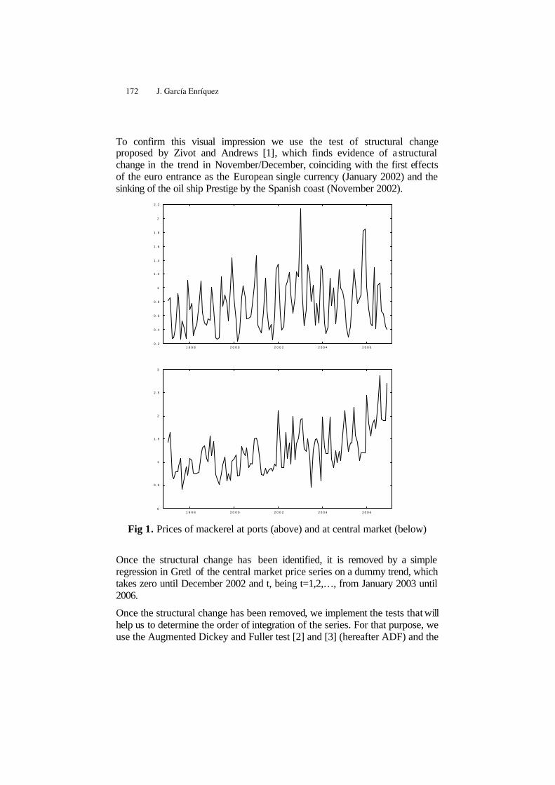
To confirm this visual impression we use the test of structural change proposed by Zivot and Andrews [1], which finds evidence of a structural change in the trend in November/December, coinciding with the first effects of the euro entrance as the European single currency (January 2002) and the sinking of the oil ship Prestige by the Spanish coast (November 2002).
Fig 1. Prices of mackerel at ports (above) and at central market (below)
Once the structural change has been identified, it is removed by a simple regression in Gretl of the central market price series on a dummy trend, which takes zero until December 2002 and t, being t=1,2,…, from January 2003 until 2006.
Once the structural change has been removed, we implement the tests that will help us to determine the order of integration of the series. For that purpose, we use the Augmented Dickey and Fuller test [2] and [3] (hereafter ADF) and the
0.2
0.4
0.6
0.8
1
1.2
1.4
1.6
1.8
2
2.2
1 9 9 8 2 0 0 0 2 0 0 2 2004 2006
0
0.5
1
1.5
2
2.5
3
1 9 9 8 2 0 0 0 2 0 0 2 2004 2006
172 J. García Enríquez

Kwiatkowski, Phillips, Schmidt and Shin stationarity test [4] (hereafter KPSS), both implemented in Gretl. Whereas the ADF test is not affected by the strong seasonality of the data, the results obtained with the KPSS test can be seriously distorted. For that reason, we first remove the seasonality in order to focus on the cointegration at frequency zero, which is the frequency related with a long run equilibrium.
Due to the limited number of observations, the estimation of the memory parameter at different cycles and the tests to detect the presence of seasonal unit roots are not very reliable . For that reason, we naively consider unit roots at all seasonal frequencies, and apply the summation filter over the corresponding series: 2 3 4 5 6 7 8 9 10 111 L L L L L L L L L L L+ + + + + + + + + + + , where L is the lag operator. Notice that this filter is easily applicable in Gretl, cause it is only a sum of lagged series.
After the series have been seasonally adjusted, the ADF and KPSS tests are carried out. Both tests agree in not rejecting the I(1) hypothesis in the price series at ports at 5% significance level. However, the results for the price series at central market are more ambiguous. Whereas the ADF does not reject the unit root null hypothesis at 5% level, the KPSS test identifies the series as I(0) at 5% and I(1) at 10%. It is not possible, thus, to assure the existence of unit root on the basis of these tests. Therefore, in order to shed more light on the situation, we estimate the memory parameter of the differenced price series (to avoid nonstationarities) at central market by means of the semiparametric estimator of Geweke and Porter-Hudak [5] (hereafter GPH). A bandwdith 0.6m T = is chosen, for T the sample size, because this is the value predetermined by Gretl. We obtain that 0d = falls in the 95% confidence interval, giving further evidence of unit root also in the price series at central market. In consequence, a cointegration analysis between these two series can be proposed.
In order to analyse the cointegration relationships, the two most usual tests in econometrics are used, that is, the Engle-Granger [6] and the Johansen [7] tests, both implemented in Gretl.
Taking into account that the direction of causality in the Engle-Granger test is unknown, we prefer to consider the two possible situations: the one in which the central market prices have an influence in the ports ones and vice versa. After applying the ADF test on the residuals of both cointegration relationships, evidence in favour of the I(1) hypothesis is confirmed.
Again, the results with the KPSS are more ambiguous. Whereas the stationarity of the cointegrating residuals is rejected at 5% significance level in the first causality specification, the results are less conclusive in the case of causality ports-central market, with a null hypothesis which is rejected at 10%
Vertical integration in the fishing sector ... 173

but not at 5%. Again we estimate the memory parameter of the first differences of the cointegrating residuals by means of the GPH method, and the value 0d = falls inside the corresponding confidence interval, supporting the unit root hypothesis.
Thus, according to the Engle-Granger method, it does not exist neither fractional nor integer cointegration, since the residuals in both cointegration relationships can be considered integrated of the same order as the series, that is, I(1).
Finally, the Johansen’s trace and maximum eigen value tests are applied. The hypothesis of zero cointegrating relationships is not rejected in any case, giving further evidence that the mackerel prices series at ports and at the central market are not cointegrated.
The methods to detect cointegration show that, even in the absence of structural change in the central market, the two studied links of the mackerel value chain in the Basque Country are not integrated, taking each one an independent evolution. The regulation systems of this fishery have an influence in the configuration of both markets (ports and central market), contributing to very different process in the fixing of prices. The fish prices at ports depend on aspects such as the Total Allowed Captures (hereafter TAC), the bilateral agreements with other countries, the fishing zones or areas, the fishing techniques used, etc. In the particular case of the mackerel, the auctioned amounts at ports do not depend as much on the demand as on the fixed TAC, and on the consecutive agreements, becoming a rigid supply. However, the prices at central market seem to answer a traditional demand and supply model. Thus, the result here described is not surprising. Whereas the central market has managed to transmit to the prices the shocks that have affected negatively to this fishery (environmental disaster derivate from the Prestige sinking), fishermen have not transferred these effects to prices at port, highlighting its limited market power.
This situation has unleashed an important rentability problem of the inshore subsector. Both the Administration and the sector itself have become aware of this problem. Thus, regarding the demand incentives, the local authorities have been financing advertising campaigns trying to increase the mackerel consumption. As far as the supply is concerned, a pilot experience has been introduced during 2008, consisting on a daily coupon system, per ship and sailor, that limits the fished units in order to induce a rise of the mackerel prices.
Acknowledgments. This work has been financially supported by the assistance programme for training researchers (2007/2010) of the University
174 J. García Enríquez

of the Basque Country, and the predoctoral fellowship “Ciencias económicas aplicadas al sector medioambiental con especial incidencia en el sector pesquero” of the Basque Government Department of Agriculture, Fishing and Feeding, developed in the Marine Research Unit in the technological centre AZTI-Tecnalia (2006/2007). The author thanks the supervision and direction of Josu Arteche (Department of Applied Economics III, University of the Basque Country) and Arantza Murillas (Marine Research Unit, AZTI-Tecnalia)
References
1. Zivot, E., Andrews, D.W.K.: Further evidence on the great crash, the oil-price shock and the unit-root hypothesis. Journal of Business and Economic Statistics. 10, 251--270 (1992)
2. Dickey, D., Fuller, W.: Distribution of the estimators for autoregressive time series with a unit root. Journal of the American Statistical Association. 74, 427--431 (1979)
3. Dickey, D., Fuller, W.: Likelihood ratio statistics for autoregressive time series with a unit root. Econometrica. 56, 1057--1071(1981)
4. Kwiatkowski, D., Phillips, P., Schmidt, P., Shin, Y.: Testing the null hypothesis of stationary against the alternative of a unit root: How sure are we that economic time series have a unit root? Journal of Econometrics. 54, 159--78 (1992)
5. Geweke, J., Porter-Hudak, S.: Estimation and applications of long memory time series models. Journal of Time Series Analysis. 14, 221--238 (1983)
6. Engle, R.F., Granger, C.W.J.: Cointegration and error correction representation, estimation and testing. Econometrica. 55, 251--276 (1987)
7. Johansen, S.: Statistical analysis of cointegration vectors. Journal of Economic Dynamics and Control. 12, 231--254 (1988)
Vertical integration in the fishing sector ... 175


Teaching Econometrics withFree Software

Useful software for econometric beginners
Šárka Lejnarová, Adéla Rácková,
University of Economics, Prague, Department of econometrics, Nám. W. Churchilla 4, Praha 3, 130 67, Czech Republic
[email protected], [email protected]
Abstract. In this paper we analyzed econometric software suitable for basic econometric lessons. We were limited by software availability at the University of Economics in Prague and that is why the following econometric software was selected for our analysis. We discussed advantages and disadvantages of GiveWin, Gretl and SAS Enterprise Guide and we evaluated them according to their convenience for econometric beginners. Using multiple criteria decision methods, Gretl was chosen as the most suitable econometric software for basic econometric lessons.
Keywords: Gretl, SAS, GiveWin, teaching, basic econometrics
1 Introduction
The importance of the science we all know as econometrics has risen during last years. Econometric lectures were involved in many majors and nowadays not only students with econometric majors but even students with major of economics, finance, national economy, accounting, marketing and management have to deal with this science. Such an expansion of lectures among students who are highly educated in economics but have very basic knowledge of statistics, math and relevant software programs causes many troubles during econometric lessons. The main goal of basic econometric lessons is to introduce students into the ideas of econometric and statistical analysis on real economic dates. This is crucial for the possibility to use a simple econometric analysis in students’ final thesis to support their research.
After few lessons we recognized that usage of relevant software during lectures is one of the foundation-stones in the successful education of econometrics. It is not a problem to choose one program and present it to our students but the question is which software is the most appropriate. Majority of students is worried about the software and they concentrate on how to be familiar with the program and the fundamental of the lecture – in the meaning of studying econometrics – is hidden behind this program. That is why we would like to compare used and accessible programs at our university and decide which one is the best or the most acceptable.
At the University of Economics in Prague, we have the possibility to teach econometrics in three programs – in GiveWin, SAS and Gretl. That is the reason why

we chose these three programs for our comparison in this thesis. It is not our goal to make a comparison at the whole market of accessible econometric programs because this market is very wide and the fact is that not all programs are appropriate for students starting with the study of econometrics.
The confrontation of these programs was accomplished on the basis of several different criteria. One of them was the financial availability of the program. We explored if there is any freeware or limited free of charge version of program because we expect that students are not willing to buy the necessary program which they usually need only a half-year of their five years studies. And then we tried to take into account the spread of these programs in the use or in the other lectures.
The other criterion was how the work with the program is intuitive - based on the knowledge of commonly used software like MS Office, and how easy it is to familiarize students with the program in eleven lessons we have during the term. If the program is not complicated, students are more focused on econometrics and then they gain required knowledge of this science.
We compared the heftiness of model creation, the graphic interface of the program and other functions like the graphic or statistic analysis. The important criteria were the ability of the programs to run different data files, their collaboration with MS Office (in the meaning of data export and import) or if the data samples are included in the program or on the program’s web pages. We confronted the results provided with the programs and if they are intelligible and well-arranged even for econometric beginners. We focused on whether software displays all statistical tests important for the basic statistical and econometric verification of the model.
In this paper we discussed advantages and disadvantages of mentioned programs and tried to decide which one of these three programs is the most suitable for lessons of econometrics especially from the point of view of econometric students.
2 The illustrative example
A model of dependency of inflation rate on unemployment rate was selected as an illustrative example. This dependency was modeled on data sets from the Czech Republic during time period 1993 – 2007.
The basic Phillips curve describes the inverse relationship between the rate of wage inflation and unemployment rate. We estimated the modified Phillips curve which was published by P. A. Samuelson and R. M. Solow and it represents the inverse relationship between the unemployment rate and inflation rate. Friedman and Phelps criticized the long-term Phillips curve and they proved that the negative slope of the Phillips curve represents the money illusion of the workers and that this illusion is only short-term and there is no tradeoff between the inflation and unemployment and the long-term Phillips curve is vertical (Mach, 2001).
Students have to prove the inverse relationship between inflation and unemployment known as the Phillips curve. Furthermore they have to figure out the goodness of fitted model, test classical linear regression model assumption and then discuss the economic interpretation of the model and model’s compliance with the known economic theory.
180 Š. Lejnarová, A. Rácková
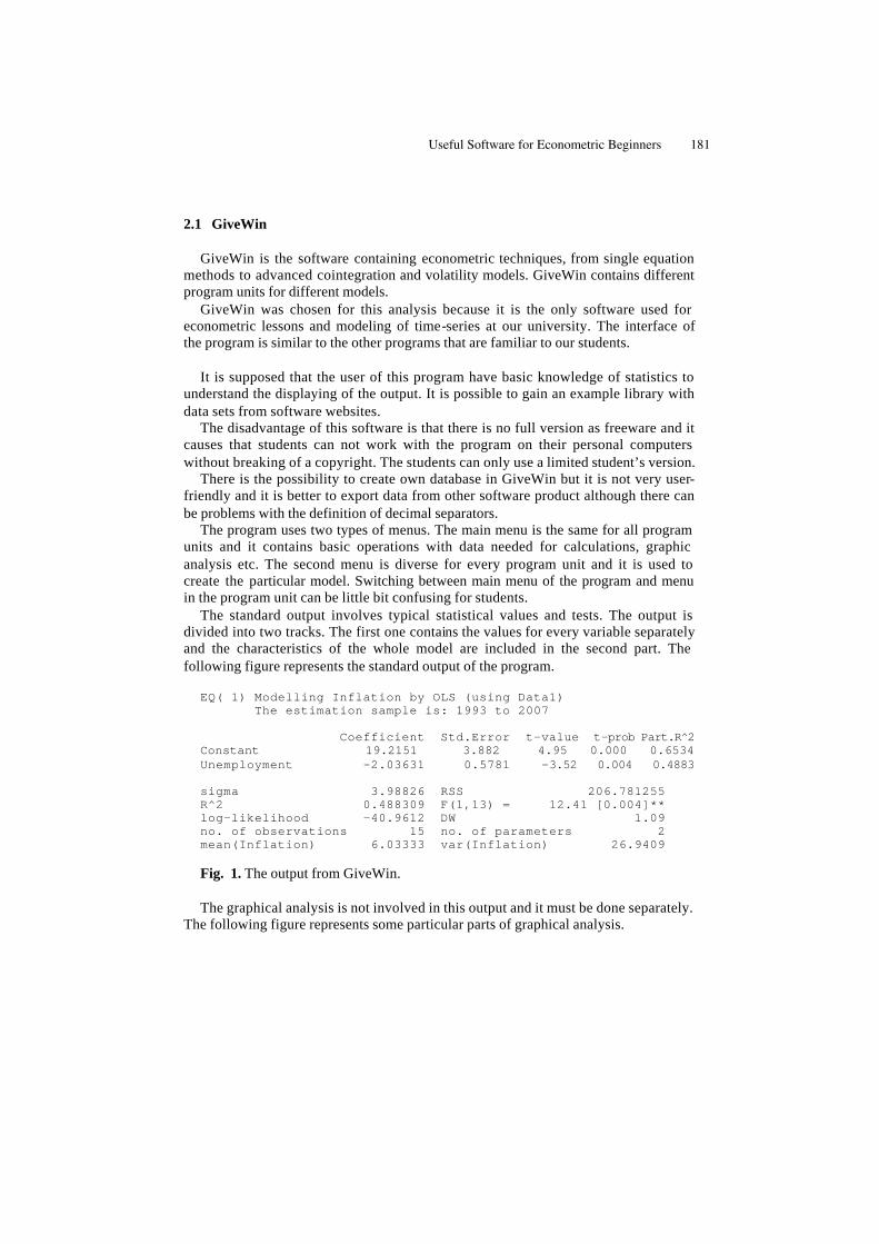
2.1 GiveWin
GiveWin is the software containing econometric techniques, from single equation methods to advanced cointegration and volatility models. GiveWin contains different program units for different models.
GiveWin was chosen for this analysis because it is the only software used for econometric lessons and modeling of time-series at our university. The interface of the program is similar to the other programs that are familiar to our students.
It is supposed that the user of this program have basic knowledge of statistics to
understand the displaying of the output. It is possible to gain an example library with data sets from software websites.
The disadvantage of this software is that there is no full version as freeware and it causes that students can not work with the program on their personal computers without breaking of a copyright. The students can only use a limited student’s version.
There is the possibility to create own database in GiveWin but it is not very user-friendly and it is better to export data from other software product although there can be problems with the definition of decimal separators.
The program uses two types of menus. The main menu is the same for all program units and it contains basic operations with data needed for calculations, graphic analysis etc. The second menu is diverse for every program unit and it is used to create the particular model. Switching between main menu of the program and menu in the program unit can be little bit confusing for students.
The standard output involves typical statistical values and tests. The output is divided into two tracks. The first one contains the values for every variable separately and the characteristics of the whole model are included in the second part. The following figure represents the standard output of the program.
EQ( 1) Modelling Inflation by OLS (using Data1) The estimation sample is: 1993 to 2007 Coefficient Std.Error t-value t-prob Part.R^2 Constant 19.2151 3.882 4.95 0.000 0.6534 Unemployment -2.03631 0.5781 -3.52 0.004 0.4883 sigma 3.98826 RSS 206.781255 R^2 0.488309 F(1,13) = 12.41 [0.004]** log-likelihood -40.9612 DW 1.09 no. of observations 15 no. of parameters 2 mean(Inflation) 6.03333 var(Inflation) 26.9409 Fig. 1. The output from GiveWin. The graphical analysis is not involved in this output and it must be done separately.
The following figure represents some particular parts of graphical analysis.
Useful Software for Econometric Beginners 181
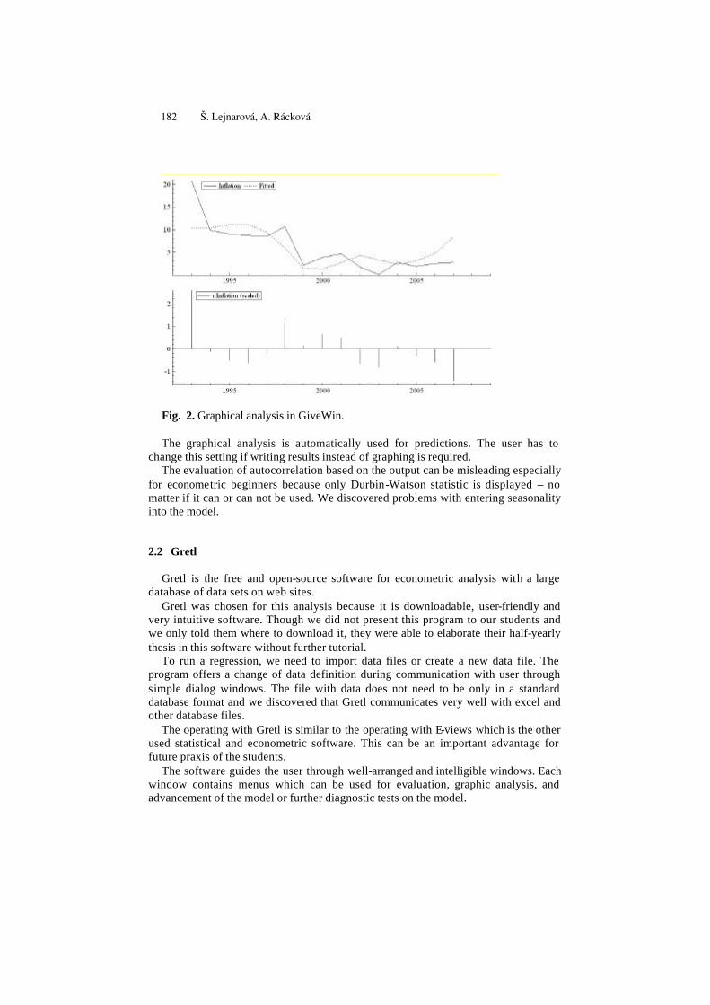
Fig. 2. Graphical analysis in GiveWin. The graphical analysis is automatically used for predictions. The user has to
change this setting if writing results instead of graphing is required. The evaluation of autocorrelation based on the output can be misleading especially
for econometric beginners because only Durbin-Watson statistic is displayed – no matter if it can or can not be used. We discovered problems with entering seasonality into the model.
2.2 Gretl
Gretl is the free and open-source software for econometric analysis with a large database of data sets on web sites.
Gretl was chosen for this analysis because it is downloadable, user-friendly and very intuitive software. Though we did not present this program to our students and we only told them where to download it, they were able to elaborate their half-yearly thesis in this software without further tutorial.
To run a regression, we need to import data files or create a new data file. The program offers a change of data definition during communication with user through simple dialog windows. The file with data does not need to be only in a standard database format and we discovered that Gretl communicates very well with excel and other database files.
The operating with Gretl is similar to the operating with E-views which is the other used statistical and econometric software. This can be an important advantage for future praxis of the students.
The software guides the user through well-arranged and intelligible windows. Each window contains menus which can be used for evaluation, graphic analysis, and advancement of the model or further diagnostic tests on the model.
182 Š. Lejnarová, A. Rácková
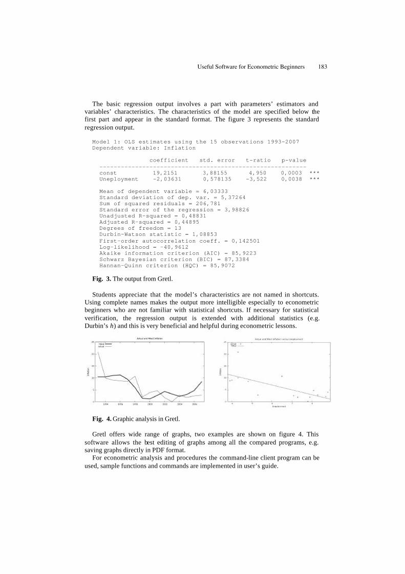
The basic regression output involves a part with parameters’ estimators and variables’ characteristics. The characteristics of the model are specified below the first part and appear in the standard format. The figure 3 represents the standard regression output.
Model 1: OLS estimates using the 15 observations 1993-2007 Dependent variable: Inflation coefficient std. error t-ratio p-value ---------------------------------------------------------- const 19,2151 3,88155 4,950 0,0003 *** Uneployment -2,03631 0,578135 -3,522 0,0038 *** Mean of dependent variable = 6,03333 Standard deviation of dep. var. = 5,37264 Sum of squared residuals = 206,781 Standard error of the regression = 3,98826 Unadjusted R-squared = 0,48831 Adjusted R-squared = 0,44895 Degrees of freedom = 13 Durbin-Watson statistic = 1,08853 First-order autocorrelation coeff. = 0,142501 Log-likelihood = -40,9612 Akaike information criterion (AIC) = 85,9223 Schwarz Bayesian criterion (BIC) = 87,3384 Hannan-Quinn criterion (HQC) = 85,9072 Fig. 3. The output from Gretl. Students appreciate that the model’s characteristics are not named in shortcuts.
Using complete names makes the output more intelligible especially to econometric beginners who are not familiar with statistical shortcuts. If necessary for statistical verification, the regression output is extended with additional statistics (e.g. Durbin’s h) and this is very beneficial and helpful during econometric lessons.
Fig. 4. Graphic analysis in Gretl. Gretl offers wide range of graphs, two examples are shown on figure 4. This
software allows the best editing of graphs among all the compared programs, e.g. saving graphs directly in PDF format.
For econometric analysis and procedures the command-line client program can be used, sample functions and commands are implemented in user’s guide.
Useful Software for Econometric Beginners 183
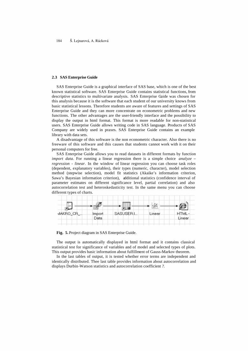
2.3 SAS Enterprise Guide
SAS Enterprise Guide is a graphical interface of SAS base, which is one of the best known statistical software. SAS Enterprise Guide contains statistical functions, from descriptive statistics to multivariate analysis. SAS Enterprise Guide was chosen for this analysis because it is the software that each student of our university knows from basic statistical lessons. Therefore students are aware of features and settings of SAS Enterprise Guide and they can more concentrate on econometric problems and new functions. The other advantages are the user-friendly interface and the possibility to display the output in html format. This format is more readable for non-statistical users. SAS Enterprise Guide allows writing code in SAS language. Products of SAS Company are widely used in praxes. SAS Enterprise Guide contains an example library with data sets.
A disadvantage of this software is the non econometric character. Also there is no freeware of this software and this causes that students cannot work with it on their personal computers for free.
SAS Enterprise Guide allows you to read datasets in different formats by function import data. For running a linear regression there is a simple choice analyze – regression - linear. In the window of linear regression you can choose task roles (dependent, explanatory variables), their types (numeric, character), model selection method (stepwise selection), model fit statistics (Akaike’s information criterion, Sawa’s Bayesian information criterion), additional statistics (confidence interval of parameter estimates on different significance level, partial correlation) and also autocorrelation test and heteroskedasticity test. In the same menu you can choose different types of charts.
Fig. 5. Project diagram in SAS Enterprise Guide. The output is automatically displayed in html format and it contains classical
statistical test for significance of variables and of model and selected types of plots. This output provides basic information about fulfillment of Gauss-Markov theorem.
In the last tables of output, it is tested whether error terms are independent and identically distributed. Thee last table provides information about autocorrelation and displays Durbin-Watson statistics and autocorrelation coefficient ?.
184 Š. Lejnarová, A. Rácková
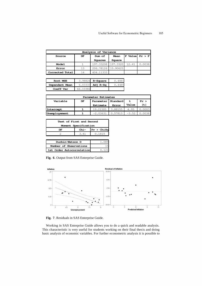
Sum of MeanSquares Square
Model 1 197.33208 197.33208
12.41 0.0038Error 13 206.78126 15.90625
Corrected Total 14 404.11333
Root MSE 3.98826 R-Square 0.4883Dependent Mean 6.03333 Adj R-Sq 0.4489
Coeff Var 66.10382
Parameter StandardEstimate Error
Intercept 1 19.21505 3.88155 4.95 0.0003Unemployement 1 -2.03631 0.57813 -3.52 0.0038
DF Chi-Square
Pr > ChiSq2 3.41 0.1815
1.08915
0.121
Parameter Estimates
Analysis of VarianceSource DF F Value Pr > F
t Value
Pr > |t|
Number of Observations1st Order Autocorrelation
Durbin-Watson D
Variable DF
Test of First and SecondMoment Specification
Fig. 6. Output from SAS Enterprise Guide.
Fig. 7. Residuals in SAS Enterprise Guide. Working in SAS Enterprise Guide allows you to do a quick and readable analysis.
This characteristic is very useful for students working on their final thesis and doing basic analysis of economic variables. For further econometric analysis it is possible to
Useful Software for Econometric Beginners 185

use other tests by “writing code”, samples codes are implemented in SAS Enterprise Guide help.
3 Decision analysis
We applied methods of multiple criteria decision making to choose one of three programs. Each program was evaluated according to seven criteria: Financial availability, Intuitiveness of program, Heftiness of model creation, Graphic interface, Using in praxes, Import of data files, Econometrics function. Methods of multiple criteria decision making are searching a compromise solution by trying “maximize” or “minimize” different criteria. The list of the criteria and the values used in our analysis are in the Table 1.
Table 1. Criteria. Criteria Label GRETLGiveWin SAS Scale
DAT Run different data files MAX 4 3 5 5 - runs different kinds of data files, 0 - just one type of data files
ECO Econometrics function MAX 5 5 3 5 - large scale, 0 - restricted
FIN Financial availability MAX 2 1 0 2 - freeware, 1 - restricted student version, 0 - no freeware
GRA Graphic interface MAX 4 2 5 5 - advanced graphic interface, 0 - restricted graphic interface
HEF Heftiness of model creation MAX 5 2 4 5 - easy fitting, 0 - complecated fitting
INT Intuitiveness of program MAX 5 2 5 5 - user friedly, 0 - user unfriendly
PRA Using in praxes MAX 1 2 5 5 - widly use, 0 - no use
The criteria have a different importance in this analysis. We used Fuller method to
define weights of criteria. Fuller method uses the couple comparison of criteria. There is the graphical scheme of comparison called Fuller’s triangle.
186 Š. Lejnarová, A. Rácková
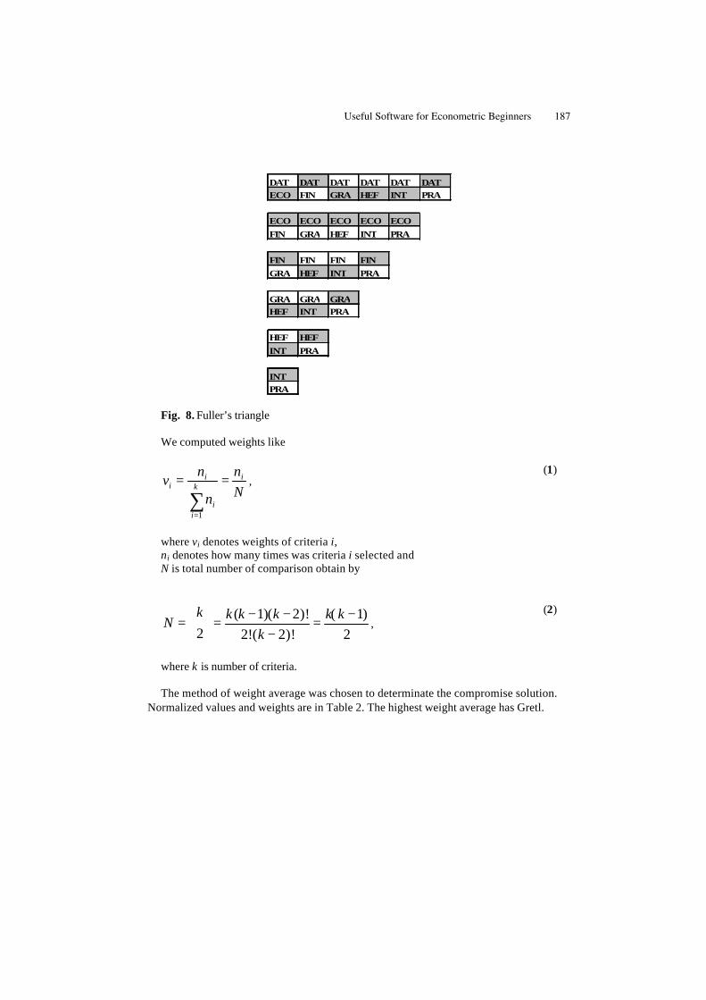
DAT DAT DAT DAT DAT DATECO FIN GRA HEF INT PRA
ECO ECO ECO ECO ECOFIN GRA HEF INT PRA
FIN FIN FIN FINGRA HEF INT PRA
GRA GRA GRAHEF INT PRA
HEF HEFINT PRA
INTPRA
Fig. 8. Fuller’s triangle We computed weights like
1
i ii k
ii
n nv
Nn=
= =
∑,
(1)
where vi denotes weights of criteria i, ni denotes how many times was criteria i selected and N is total number of comparison obtain by
( 1)( 2)! ( 1)2 2!( 2)! 2
k k k k k kN
k − − −
= = = − ,
(2)
where k is number of criteria. The method of weight average was chosen to determinate the compromise solution.
Normalized values and weights are in Table 2. The highest weight average has Gretl.
Useful Software for Econometric Beginners 187
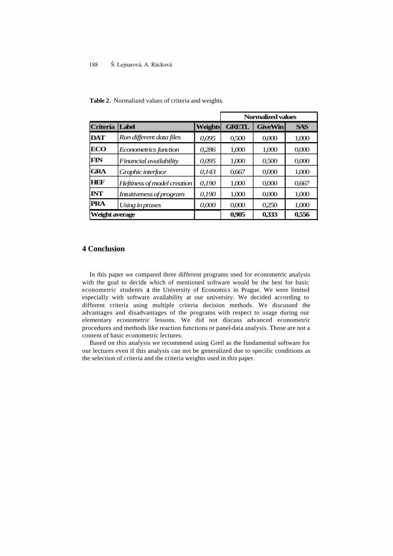
Table 2. Normalized values of criteria and weights.
Criteria Label Weights GRETL GiveWin SAS
DAT Run different data files 0,095 0,500 0,000 1,000
ECO Econometrics function 0,286 1,000 1,000 0,000
FIN Financial availability 0,095 1,000 0,500 0,000
GRA Graphic interface 0,143 0,667 0,000 1,000
HEF Heftiness of model creation 0,190 1,000 0,000 0,667
INT Intuitiveness of program 0,190 1,000 0,000 1,000PRA Using in praxes 0,000 0,000 0,250 1,000
0,905 0,333 0,556
Normalized values
Weight average
4 Conclusion
In this paper we compared three different programs used for econometric analysis
with the goal to decide which of mentioned software would be the best for basic econometric students at the University of Economics in Prague. We were limited especially with software availability at our university. We decided according to different criteria using multiple criteria decision methods. We discussed the advantages and disadvantages of the programs with respect to usage during our elementary econometric lessons. We did not discuss advanced econometric procedures and methods like reaction functions or panel-data analysis. Those are not a content of basic econometric lectures.
Based on this analysis we recommend using Gretl as the fundamental software for our lectures even if this analysis can not be generalized due to specific conditions as the selection of criteria and the criteria weights used in this paper.
188 Š. Lejnarová, A. Rácková

References
1. GRETL webpage: http://gretl.sourceforge.net/ 2. Guaranti D.N,: Basic econometrics. McGraw-Hill, Inc.,USA (1988) 3. Hušek, R.: Ekonometrická Analýza. Ekopress, Praha (1999) 4. Jablonský, J.: Operacní výzkum: kvantitativní modely pro ekonomické
rozhodování. 5. Professional Publishing, Praha (2007). 6. Mach M.: Makroekonomie II pro magisterské (inženýrské) studium 1. a 2. cást,
p. 268-269. Melandrium, Slaný (2001) 7. OxMetrix webpage: http://www.oxmetrics.net/ 8. SAS webpage: http://www.sas.com/technologies/bi/query_reporting/guide/
Useful Software for Econometric Beginners 189


Teaching and Learning Econometrics with GretlSummarizing Some Experiences
Rigoberto Pérez, Ana Jesús López?
University of Oviedo, Department of Applied Economics,Campus del Cristo, s/n, 33006, Oviedo, Spain
[email protected], [email protected]
Abstract. The European Higher Education Area (EHEA) provides the oppor-tunity of exploring new ways of teaching and learning, emphasizing the role ofstudents in the learning process. In the case of Econometrics (which will play anoutstanding role in Economics and Business degrees), our experience has shownthat doing Econometrics is a suitable way of learning Econometrics and also thatGretl is a powerful teaching tool, providing our students a wide variety of com-petences and skills.This paper summarizes our experiences with Gretl during the last years, includingboth presential and online learning and combining teachers and students pointsof view.Keywords: Econometrics, Competences, Skills, Gretl, AulaNet, Virtual Campus,European Higher Education Area (EHEA)
1 Econometrics in the European Higher Education Area
More than seventy years ago Joseph Schumpeter published his famous work“The common sense in Econometrics”, where he claimed that every economist isan econometrician since data should be used as a complement of economic the-ories. Since then, the role of Econometrics in Economics and Business degreeshas gradually increased, including not only the study of the main techniquesfor the estimation and testing of econometric models but also a more realisticapproach, which is often based on the use of econometric software.
This more practically-oriented study has become especially important in thepresent context, since European Universities are currently facing the challengesof the so called “Bologna process”1 which aims to increase the mobility and
? Corresponding author1 The Bologna declaration was signed in 1999 by the ministers of education from 29 European
countries, with the aim to develop the European higher education area (EHEA) by makingacademic degree standards and quality assurance standards more comparable and compatiblethroughout Europe. Since then and after several governmental meetings [Prague (2001), Berlin(2003), Bergen (2005), London (2007)] this process has further developed into a major reformencompassing 45 countries.

192 Rigoberto Pérez, Ana Jesús López
employability of European higher education graduates thus ensuring competi-tiveness of European higher education on the world scale. In the case of Span-ish universities, the Bologna process has to face several difficulties since thestructure of university degrees in Spain is quite different from the Anglo-Saxonmodel adopted as a reference2
The European dimension of education and the contribution of education insetting the European Information and Knowledge Society have been stressed inthe Lisbon Summit (2000) with the strategic goal of “making out of the Euro-pean Union the world´s most competitive and dynamic knowledge-based econ-omy, capable of sustainable economic growth and with more and better jobs andgreater social cohesion”. Since Economic and Business degrees are narrowly re-lated to these objectives, in this paper we focus on Econometrics as a strategictool in these fields, also showing the potential of Gretl in the teaching-learningprocess and summarizing some recent experiences.
1.1 Competences and skills
A concrete approach to implement the Bologna Process is offered by the project“Tuning Educational Structures in Europe”, which provides a methodology tore-design, develop, implement and evaluate studies. Furthermore Tuning servesas a platform for developing reference points at subject area level, which arerelevant for making programmes of study comparable and compatible.
According to this approach, reference points are expressed in terms of learn-ing outcomes and competences. Learning outcomes are statements of what alearner is expected to know, understand and be able to demonstrate after a learn-ing experience, while competences represent a dynamic combination of cog-nitive and meta-cognitive skills, knowledge and understanding, interpersonal,intellectual and practical skills, and ethical values.
Competences can be distinguished in subject specific and generic ones, whichcan be classified into three types: instrumental competences (cognitive abilities,methodological abilities, technological abilities and linguistic abilities), inter-personal competences (individual abilities like social skills) and systemic com-petences (combination of understanding, sensibility and knowledge).
In order to identify the most important generic competences, a large scaleconsultation was organized among graduates, employers and academics. Thequestionnaire included 30 competences and a total of 101 university depart-
2 The Spanish system has two kinds of degrees, respectively leading to a medium-level technicalprofession (three year Diplomatura) and to higher-level professions or academic disciplines(four or five year Licenciatura or Ingeniería). Nevertheless, the Diplomatura has never beenthe exact equivalent of a BA/BSc, nor the Licenciatura that of a MA/MSC.
Teaching and Learning Econometrics with Gretl 193
ments took place in the consultation, leading to the results3 summarized in table1.
Referring to the generic competences, it is necessary to adapt the students´knowledge and capacities to the labour market requirements, trying to attenuatethe traditional existing distance between the perceptions of academics, employ-ers and graduates.
If we focus on the Economics and Business degrees, which is one of theseven areas considered in the Tuning project, the consultation involved 921graduates, 153 employers and 153 academics, representing a 17% of the totalsample.
Although the available information is quite scarce, according to the provi-sional guidelines these studies should train individuals capable of analyzing andinterpreting the functioning of the economy, with the intention of improvingthe well-being of the society with the achievement of equity and efficiency andin general to approach the analysis of the most relevant economic and socialproblems.
More specifically, these degrees should provide competences as “to use ana-lytical instruments in the decision-making processes" or "to handle informationtechnologies”, aspects in which Econometrics is expected to play an outstand-ing role. In fact, the competences related to Econometrics represent a significantproportion of the total list, including some of the items heading the previouslydescribed rankings.
In this context, and following the main guidelines of the Bologna process,during the last academic years we have adopted a “learning by doing” approachleading to a more realistic methodology, characterized by an intensive use ofe-learning and Gretl.
1.2 The role of Gretl in the teaching-learning process
The e-learning, understood as “the use of new multimedia technologies and theInternet to improve the quality of learning” has become increasingly popularduring the last years. In the University of Oviedo the virtual campus AulaNetwas created in 1999, providing a wide variety of online learning facilities forour students and also joining the Shared Virtual Campus of the G9 Group ofUniversities4.
3 The academics were asked to rank seventeen items previously selected from the thirty item listgiven to graduates and employers. Therefore thirteen items are not present in the academicsranking.
4 The G9 Group includes nine Spanish public universities: Cantabria, Castilla-La Mancha, Ex-tremadura, Illes Balears, La Rioja, Pública de Navarra, Oviedo, País Vasco and Zaragoza.
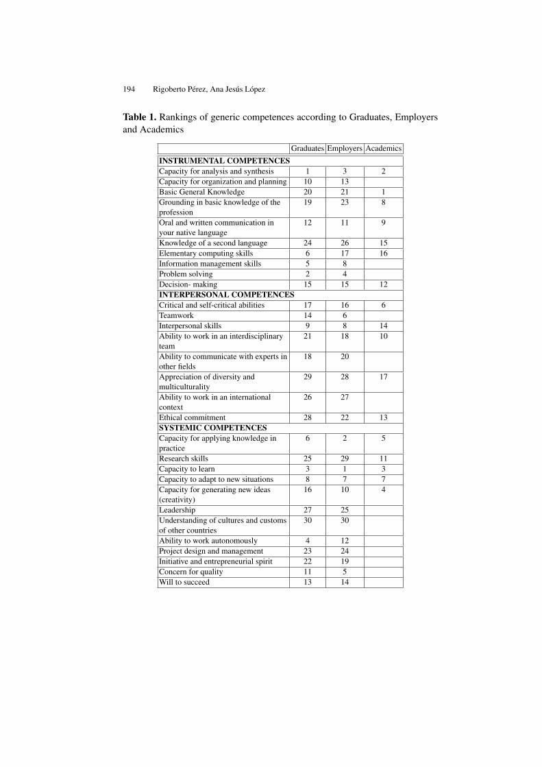
194 Rigoberto Pérez, Ana Jesús López
Table 1. Rankings of generic competences according to Graduates, Employersand Academics
Graduates Employers Academics
INSTRUMENTAL COMPETENCESCapacity for analysis and synthesis 1 3 2Capacity for organization and planning 10 13Basic General Knowledge 20 21 1Grounding in basic knowledge of theprofession
19 23 8
Oral and written communication inyour native language
12 11 9
Knowledge of a second language 24 26 15Elementary computing skills 6 17 16Information management skills 5 8Problem solving 2 4Decision- making 15 15 12INTERPERSONAL COMPETENCESCritical and self-critical abilities 17 16 6Teamwork 14 6Interpersonal skills 9 8 14Ability to work in an interdisciplinaryteam
21 18 10
Ability to communicate with experts inother fields
18 20
Appreciation of diversity andmulticulturality
29 28 17
Ability to work in an internationalcontext
26 27
Ethical commitment 28 22 13SYSTEMIC COMPETENCESCapacity for applying knowledge inpractice
6 2 5
Research skills 25 29 11Capacity to learn 3 1 3Capacity to adapt to new situations 8 7 7Capacity for generating new ideas(creativity)
16 10 4
Leadership 27 25Understanding of cultures and customsof other countries
30 30
Ability to work autonomously 4 12Project design and management 23 24Initiative and entrepreneurial spirit 22 19Concern for quality 11 5Will to succeed 13 14

Teaching and Learning Econometrics with Gretl 195
Since then, the virtual campus AulaNet has experienced some changes,moving from the initial self-developed platform to WebCT and then to Moo-dle, and providing an increasing number of learning resources, which have beenproved to be very useful for communication, teamwork and evaluation.
Furthermore, in the case of Econometrics, our experience shows that theelection of suitable software is a main point in order to provide students the re-quired competences and skills. The need of a user-friendly, flexible, open-sourceand accurate software lead us to Gretl, whose main advantages for teachers andstudents are described in the next sections.
The outstanding role played by Gretl in the Econometrics teaching-learningprocess is shown in table 2, which summarizes the main competences related todifferent learning resources.
Table 2. Teaching-Learning methods in Econometrics and related competences
Teaching-Learning Methods CompetencesTheoretical Sessions Basic General Knowledge, Capacity for
analysis and synthesis, Capacity to learnPractical Sessions with Gretl Capacity for applying knowledge in practice, Elementary
computing skills, Knowledge of a second languageTeam Work with Gretl
Database building, ModelSpecification, Estimation,
Testing Analysis, Forecasting ,Oral exposition, Final Report
Teamwork, Information management skills, Creativity(capacity for generating new ideas), Problem solving,Decision-making, Capacity to adapt to new situations,Oral and written communication, Concern for quality,
Research skillsSelf-assessment, Online
surveyAbility to work autonomously, Critical andself-critical abilities, Ethical commitment
2 Teaching Econometrics with Gretl
From the teachers´ perspective the use of Gretl offers several advantages, sincethis open source software provides an easy intuitive interface, allowing differentways of working from interactive point-and-click to batch processing.
This flexibility is one of the most outstanding characteristics of Gretl, of-fering teachers a good opportunity to re-think contents, methods and evaluationprocedures. Therefore, during the last years we have carried out some interest-ing experiences with Gretl both in presential and online learning.
As it is summarized in table 3 these experiences refer to three different sub-jects whose characteristics are quite different, but nevertheless we can confirm

196 Rigoberto Pérez, Ana Jesús López
that in all the cases the implementation of practical sessions with Gretl has beena successful experience for students and teachers.
Table 3. Description of teaching-learning experiences with Gretl
Econometrics Time Series ForecastingSubject Description Compulsory subject
Third year, Degree inEconomics, Univ.
Oviedo
Optional subject,Third-fourth year,
Degree in Economics,Univ. Oviedo
Free-election subject,all years and degrees,
G9 Shared VirtualCampus
Teaching-LearningMethod
Presential, Blendedlearning [Theoretical
and practical sessions,oral expositions,
teamwork]
Presential, Blendedlearning [Theoretical
and practical sessions,oral expositions,personal project]
Number of students 120 14 Online learning[multimedia facilities,
online practicalsessions, forum, chat,mail, self-assessment]
Gretl sessions 1 hour/week 2 hours/week Online sessionsEvaluation 50% Final Exam 30%
Teamwork with Gretl20% Continuous
assessment
40% Project with Gretl20% Oral exposition
20% Continuousassessment 20% Final
test
40% Gretl Practices40% Tests 20% Online
participation
It is interesting to stress the role played by Gretl in the whole teaching-learning process, including contents, methods and evaluation. Furthermore, withthe aim of achieving coherence, Gretl use has been designed according to thespecific syllabus, teaching conditions and student profiles for each of the con-sidered subjects.
Thus, in the case of Econometrics Gretl provides a wide variety of menuoptions including least squares estimators, maximum likelihood, generalizedmethod of moments, single-equation and system methods, also offering a “con-sole” option where users can type commands which are recorded as a batch file.
Our teaching strategy has been designed taking advantage of the flexiblecharacter of Gretl. Therefore we combine the quick point-and-click menu op-tions with the use of some commands and console facilities in order to re-buildspecific results, improving the autonomous work and the comprehension of themain econometric concepts and techniques.

Teaching and Learning Econometrics with Gretl 197
For instance, after obtaining a least squares estimation, students are sug-gested to obtain the results through matrix computing; some residual tests canbe re-build through auxiliar regressions, two stages least squares can be recov-ered by running the instrumental variables regression and then substituting theestimated results, . . .
Nevertheless, the most powerful teaching tool of this subject is the team-work which provides the students the opportunity to work with real informationallowing them to get familiar with the main problems of the econometric mod-eling. This work is developed with Gretl in 3-4 student groups, also includingthe presentation of an oral exposition and a final report.
According to our experience, one of the most useful characteristics of Gretlis the session concept, which provides an iconic space containing several objectsas data sets, model tables, scalars, graphs, . . . thus allowing users to save acomplete dossier of the whole developed work.
Regarding Time Series, Gretl facilities include ARIMA and VARMA, VEC,GARCH, unit-root and cointegration tests,. . . Since this is an optional subjectwith quite few students, they are required to develop along the semester a per-sonal project consisting in the estimation of time series models for real monthlyor quarterly economic data.
Finally, the case of Forecasting shows some differential characteristics re-ferred both to the teaching method and the university context. With regard tothe first aspect, while Econometrics and Time Series are based on “BlendedLearning”, understood as “the combination of different learning styles that canbe accomplished through the use of ’blended’ virtual and physical resources”,Forecasting is an online free-election matter included in the Shared Virtual Cam-pus of the G9 Group of Universities.
This second aspect must also be stressed due to the diversity of students,belonging to nine Spanish universities and also to different degrees and courses.
Once again, the flexibility of Gretl has been very helpful in the design ofthis online subject, whose second year will start next February.
In all the described cases, from the teachers perspective we must stress someadditional advantages related to Gretl educational and research resources: theaccess to datasets associated with Econometrics texts as those of Ramanathan,Greene, Stock and Watson, Greene or Gujarati, and the existence of an openscientific community.
3 Learning Econometrics with Gretl
The Bologna process leads to a student-oriented approach, which focuses onthe usefulness of study programmes for a future position of the graduate in the

198 Rigoberto Pérez, Ana Jesús López
society. Therefore, a sensible definition of learning outcomes and the allocationof credits (according to the European Credit Transfer System, ECTS, based onstudents´ workload) play a decisive role.
The experiences we are summarizing in this work include students´ partici-pation in these new aspects: the competence-based learning and computation onECTS credits for different subjects.
Since the virtual campus AulaNet allows an easy implementation of on-line questionnaires, during the last academic years students have been asked toprovide information about their personal effort, the perceived difficulty of theeducational contents and the acquired competences and skills. A scheme of theEconometrics survey is shown in table 4.
Table 4. Online survey for Econometrics Students
Sections Quantitative aspects Qualitative aspectsPersonal Work Hours of study Perceived difficulty for each
itemTeam Work Hours for different stages:
database building, modelestimation, hypotheses testing,forecasting, exposition, final
report
Perceived difficulty for theteam work Satisfaction with
Gretl facilities Comparison ofpersonal and team effort
Quality of the work comparedwith others
Quality of the workcompared with others
AssessmenPerceived difficulty ofassessment questionsSatisfaction with theassessment system
General vision Level of satisfaction with thesubject Opinion about
professional skills Commentsand suggestions
Although the rate of response was quite low (50%), the obtained informationshows some interesting facts. A first consideration is the heterogeneity of stu-dents (which should be considered when designing and implementing the learn-ing methodology), reflected in the high dispersion of times of personal work,leading to non-representative means.
On the other side a considerable homogeneity is found in the perceived lev-els of difficulty (approached by the percentages of students whose answers tothe proposed questions are “difficult” or “very difficult”) and also in the level

Teaching and Learning Econometrics with Gretl 199
of agreement with the achieved competences and skills (approached by the per-centage of students answering “Total agree” or “Agree”). Besides, since thesesurveys have been carried out along four academic courses we have also con-firmed the stability of the obtained results.
Table 5. Results of the Econometrics online survey
Course Contents Level ofdifficulty
Level ofagreement
Econometric Models 0.5% 90,0%Single Regression Model 17,4% 70,6%
Multiple Regression Model 65,2% 76,9%Qualitative Variables 43,5% 61,5%Testing Hypotheses 73,9% 80,0%
Simultaneous Equation Models 50,0% 72,7%Practical Sessions with Gretl 10,5% 70,0%
Teamwork with Gretl 73,3% 94,1%Continuous Assessment 17,9% 70,8%
Final Exam 8,3% 100%
Regarding students´ opinions about learning outcomes, they mainly empha-size competences as problem solving, capacity for applying knowledge in prac-tice, computing skills and information management skills. Teamwork is alsoappreciated as a valuable although rather hard competence.
The application of the described methodology and evaluation system hasimproved the academic indicators of Econometrics as shown in table 6.
Table 6. Econometrics Academic Indicators
Academic Year Proportion ofpresented students
(%)
Rate of Success(Proportion of passed
students, %)2004-05 77% 77%2005-06 68% 80%2006-07 73% 80%2007-08 79% 88%

200 Rigoberto Pérez, Ana Jesús López
4 Concluding remarks
In the framework of the Bologna process the new Economics and Business De-grees must face the challenge of training individuals capable of analyzing andinterpreting the functioning of the economy improving the well-being of thesociety with the achievement of equity and efficiency. With this aim, Economet-rics should be considered as a strategic tool whose teaching-learning methodshould be designed paying special attention to competences as problem solving,decision-making or information management.
Since the election of a suitable software is a key point in the teaching-learning process, during the last years we have experienced the potential ofGretl in three different subjects, leading to satisfactory results for both teach-ers and learners. More specifically, students surveys show the contribution ofthese learning methods in the achievement of competences as problem solving,capacity for applying knowledge in practice, computing and information man-agement and teamwork.
To end, we would like to thank the colleagues of the G9 Virtual Campusfor sharing valuable experiences during nine years, our students for their col-laboration in the online surveys and the Gretl Community for developing andspreading the use of open source econometric software.

Bibliography
[1] Commission of the European Communities: Challenges for the EuropeanInformation Society beyond 2005, Communication from the Commissionto the Council, the European Parliament, the European Economic and So-cial Committee and the Committee of the Regions, 757 (2004)
[2] Commission of the European Communities.: Progress towards the Lisbonobjectives in Education and Training, Commission Staff Working Paper,419 (2005)
[3] Cottrell, A.; Lucchetti, R.J.: Gretl User´s Guide, Gnu Rregression, Econo-metrics and Time Series (2008)
[4] Esteban, M.V. et al: Análisis de regresión con Gretl, Departamento deeconomía Aplicada III, Universidad del País Vasco.
[5] González, J.; Wagenaar, R.: Tuning Educational Structuresin Europe. Universities´ contribution to the Bologna Process,http://tuning.unideusto.org/tuningeu (2005)
[6] González, J.; Wagenaar, R.: Universities´contribution to the Bologna Pro-cess, http://tinyurl.com/anylvc (2008)
[7] López, A.J.: El papel del E-Learning en el Espacio Europeo de EducaciónSuperior, Congreso Online Educa, Madrid (2004)
[8] López, A.J.; Pérez, R.: An experience on virtual teaching: AulaNet, inComputers and Education: Towards an Interconnected Society, M. Ortegaand J. Bravo Ed., Kluwer Academic Publishers, pp. 207—214 (2001)
[9] López, A.J.; Pérez, R.: Networking Universities to bridge the DigitalDivide, International Journal of Instructional Technology and DistanceLearning, vol.3, n.5, pp. 73–82. (2006)
[10] López, A.J.; Pérez, R.; Mayor, M.: Learning Econometrics by DoingEconometrics. Some pilot experiences, ISI Lisboa (2007)
[11] Pagani, R.; González, J.: El crédito europeo y el sistema educativo español,Informe Técnico ECTS Counsellors and Diploma Supplement Promoters(2002)
[12] Reichert, S.; Tauch, C.: Bologna four years after: Steps toward sustainablereform of higher education in Europe”, Trends 2003: Progress towardsthe European Higher Education Area, European University Association(2003)
[13] Schumpeter, J.: The common sense in Econometrics, Econometrica, Vol.1, n.1, p. 5–12 (1933)


The Roster-in-a-BoxCourse Management System
Tavis Barr
Long Island Unversity/Makerere University
Abstract. Roster-in-a-Box is an open source course management system writtenin PHP, with a MySQL back end. It is designed to handle only the homework partof course management, leaving the instructor to design other parts of the courseweb page. It includes a complete semester of auto-graded assignment modulesfor introductory and intermediate microeconomics, and for introductory statis-tics, which I have quality-tested by using multiple times in my courses. I haveevaluated the effectiveness of the system by comparing student test scores in myintroductory statistics course before and after I began using the system (the mate-rial in the other courses changed to much before and after for exam performanceto be comparable); there is weak evidence of improvement, and no evidence ofworse student performance. I briefly discuss ways in which the software might beimproved.
1 Introduction
Roster-in-a-Box is a course management system designed to facilitate the useof autograded homework assignments, while also allowing for text-based ques-tions to be submitted online and graded online by the instructor. I developedand currently use the system for my introductory statistics and undergraduatemicroeconomics courses at Long Island University, and I have had it in produc-tion since 2005. While any instructor who tries hard enough could break theprogram, it is stable and very much ready for use.
I wrote the program because I wanted something simpler than Moodle (andalso because my school was not supporting Moodle at the time that I startedthe project). I have no complaints about Moodle, but it was not right for me,because I did not want the course management system to take over my courseweb site. Roster-in-a-Box handles the homework and grading functions with acouple of web pages that can be inserted into any course web site. It requires theweb server to run PHP and MySQL, but otherwise can be used quite flexibly.
The program consists of two web pages, namely a homework page and anadministration module, as well as several utilities. Each page is its own PHPprogram. The homework page can be linked to from the main course web page,and is responsible for displaying, correcting, and recording all homework as-signments. The administrative module, though password protected, should not

204 Tavis Barr
be made viewable to the rest of the world; the instructor can use this module toset up and modify the list of homework assigments, as well as to grade the man-ually graded assignments and track student performance. Additionally, smallutilities display web pages through which students can request an account andview their grades.
The package comes with a set of modules for three different courses: Intro-ductory microeconomics, intermediate microeconomics, and introductory statis-tics. I have used all of these modules in my teaching, so they are tested in thatway. Each set consists of around thirty to fifty autograded questions based onmaterial from the respective course; the instructor merely needs to use the ad-ministrative page to create an assignment, insert a module or modules into thatassignment, and set the number of points for each question. The software takescare of the rest, although manually graded text questions can also be given.When a student enters an incorrect answer, the homework module explains howto solve the problem correctly. The student has as many chance as she wishesto try the assignment again with a different set of problems. Instructors can seta minimum score requirement below which the system will not accept an as-signment. It is also possible to provide a late penalty for every day beyond thedue date that the assignment is submitted, as well as a final cutoff date beyondwhich the system will not accept assignments.
The statistic modules cover summary statistics, probability, random vari-ables, the Central Limit Theorem, confidence intervals, one- and two-samplehypothesis tests, and univariate regression. Nearly all of the sample problemsare based on real-world data, and contain a sufficient number of exercises thatit is very unlikely for a student to see the same problem twice. The intro-ductory microeconomics modules cover topics such as supply and demand,consumer choice and demand, market demand, production, monopoly power,perfect competition, oligopoly, public goods, and externalities at the US in-troductory level. The intermediate microeconomics modules cover the samematerial at the US intermediate level, and are meant to accompany my open-source textbook, Intermediate Microeconomics, available from my web site athttp://myweb.liu.edu/~tbarr. To some degree, the exercises reflect my idiosyn-cratic way of presenting the material for these courses, but I am confident thatevery instructor will find useful questions from the modules, and I welcomecontributions from others.
There are also two administrative modules that I found a need for: One e-mails students when they have overdue assignments, leaving them without theexcuse to complain that they did not know an assignment was due. It is also pos-sible to e-mail announcements to the class using the main administrative page.The other module e-mails a backup of the roster to the administrator and can be
The Roster-in-a-Box Course Management System 205
set to run on a daily or weekly basis; aside from protecting against catastrophicsystem failure, I find this useful when I need to respond to students who claimthat the system “lost” their assignment.
2 Teaching Experience
Although I have used Roster-in-a-Box in three courses, I can only conduct aplausible before-and-after comparison in my introductory statistics course, be-cause the material in the other two courses (introductory and intermediate mi-croeconomics) changed as I implemented the system – chiefly because the timesaved in class by not going over homework assignments freed me up to covermore material. Therefore I have examined the quantitative determinants of stu-dent performance in the statistics class, and their changes over time, to gaugeeffectiveness of the course management software.
Since the Summer of 2004, I have used the same computer program to gen-erate my midterms and final exams. The program allows each student to get anexam with identically-worded questions but different answers, thereby making itfar more difficult for students to cheat by copying answers from their neighbors.I change the wordings of the questions every year, but not the statistical calcula-tions involved; this makes exam scores comparable year after year. In Summer2004, the midterm covered measures of central tendency and dispersion, prob-ability theory, and discrete random variables, while the final exam covered theNormal distribution, the Central Limit Theorem, confidence intervals, and one-and two-sample hypothesis tests.
The only major change came in 2005, when I switched to an online home-work assignment system. Because I no longer had to go over homework assign-ments in class, my lecture time was freed up to cover more material. I thereforeadded one more topic (the Normal distribution) to the midterm, and added uni-variate linear regression to the final exam in its place. Therefore, the midtermbecame a bit harder (since it covered one more topic), while it is difficult to saywhether the final exam became harder or easier (my inclination is to think that itbecame harder because regression is more difficult than the Normal distribution,but this is certainly a matter of perspective).
Other factors may have made exam performance incomparable betweensemesters. It is possible that my ability to explain material has improved, forexample. I have also replaced contrived examples during my lectures with ex-amples from actual data sources, which may keep students more interested. Ido more in-class problem solving than I used to. And, I devote a little bit moreattention to following up with under-performing students than I used to. Nev-ertheless, aside from the increase in material, the course content and the level
206 Tavis Barr
of difficulty has pretty much remained constant. It is with all of these caveatsthat I am comparing midterm and final exam scores between semesters over thelast three and a half years. The homework scores are certainly not comparablebefore and after I introduced the online homework system, if nothing else be-cause I used a different marking system. Nevertheless, within each of the twohomework regimes, the assignments are quite similar.
Figures 1 and 2 show the mean, 25th, and 75th percentiles of exam per-formance between Summer 2004 and mid-Fall 2007 (Spring and Fall 2006 aremissing because I was on leave). The online grading system was introduced insemester 4 (Summer 2005). The means suggest a slight upward trend, thoughwith as much random variation between semesters as over time. The 75th per-centile shows relatively little movement, while the 25th percentile is quite er-ratic; I can only hope that the apparent upward movement of that percentileover the last two to three semesters will continue.
Table 1 shows t-tests of whether the exam performance was better before orafter the online grading system was introduced. The point estimates suggest amean improvement of about four percentage points in both the midterm and thefinal exam, however neither result is statistically significant as a two-tailed test(both are borderline significant when considered as a one-tailed test). It is worthbearing in mind that the exams in the “after” case cover slightly more material.
Table 2 shows a regression of midterm performance on homework perfor-mance before and after online grading was implemented. The explanatory powerof the homework exercises drops slightly after the implementation of onlinegrading. I ascribe this mainly to the fact that the first homework assignment be-came easier (which allows the students a chance to adjust to the online gradingsystem), and therefore a poorer predictor of midterm performance; the less sig-nificant coefficient on this assignment bears out that hypothesis. However, it isalso possible that before I implemented the online system, I gave harsh marks tostudents whose homework pages suggested a poor understanding, holding con-stant the number of questions the student got correct, which would have mademanual grading a more effective way to predict performance based on subjec-tive indications. Table 3 repeats the same exercise for final exam performance.Here, the level of explanatory power is not too different between the online andmanual grading regimes.
Table 4 performs regressions of final exam performance on both the relevanthomework assignments, as well as on the first four homework assignments andmidterm performance. The latter items should not contain any relevant material,but may predict overall student performance. In fact, these indicators taken to-gether can predict about two thirds in the variation of final exam performanceboth before and after the online grading system was implemented. Table 5 shows
The Roster-in-a-Box Course Management System 207
that the midterm score is a less successful predictor of the final exam scorein more recent semesters; I hope that this is because I have been increasinglyvigilant about intervening in the cases of students who perform poorly on themidterm.
Finally, Table 6 compares performance across different types of semesters.As my intuition would tell me, students in the Summer semester perform sig-nificantly higher than academic-year students (the point estimate is ten pointshigher, and the result is significant at the one percent level), but there is no sig-nificant difference between Spring and Fall semesters.
Overall, these numbers suggest that the online grading system had beenmodestly successful at improving student performance. Exam scores appear tohave improved slightly and certainly did not worsen, and moreover, those examscover more material than before the online system was implemented. The bot-tom quartile of student performance has not improved as much as I would like,and I should work on developing better mechanisms to assist the performanceof this particular group of students.
3 Future Directions
Although I have a professional background in programming and systems ad-ministration, I wrote Roster-in-a-Box as a teacher trying to get a particular jobdone for myself, rather than as a developer generating a product for a partic-ular audience. Nevertheless, I put a certain amount of effort into ensuring thatthe code is modular, generic, and reusable, and I hope that others may find thatRoster-in-a-Box fits their needs.
At this point, the software does what I need it to do, so any further devel-opment would be to improve its usefulness to others. I have two ideas in mind.First, although the software does not take over an entire course web site, someinstructors would prefer a product that does – that is, they should merely needto enter in topics on a syllabus template, links to course readings, etc., and thecourse web site is ready to go without them ever having to touch any HTML. Imay try to add a module that allows users to do this.
The project that I would find most personally useful is to improve and ex-pand the existing homework modules. I would like to add more questions for allof the courses; I would also like to add modules for other standard economicscourses, such as macroeconomics, finance, industrial organization, health eco-nomics, etc. Finally, I would like to add features to the modules: First, by usingAJAX routines so that students can draw graphs online; and second, allowingstudents to submit arbitrary files (such as spreadsheets, word processing docu-ments, etc.) to be graded and returned.

208 Tavis Barr
Because modules can be written one-by-one, I hope that I can interest otherswho use the software to write a module or two on their own, and then send itback to me to include in the software. First, however, this requires getting othersto actually use the software. I would urge readers and participants to ask them-selves: What is the main reason you would not wish to use Roster-in-a-Box?What improvements in the software, if any, would get you to want to use it? Iwelcome any frank and honest feedback and suggestions.
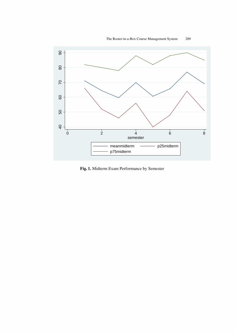
The Roster-in-a-Box Course Management System 209
4050
6070
8090
0 2 4 6 8semester
meanmidterm p25midtermp75midterm
Fig. 1. Midterm Exam Performance by Semester
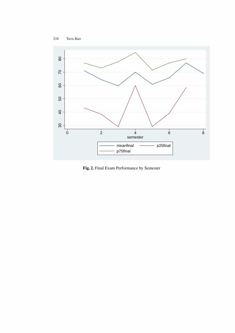
210 Tavis Barr
3040
5060
7080
0 2 4 6 8semester
meanfinal p25finalp75final
Fig. 2. Final Exam Performance by Semester

The Roster-in-a-Box Course Management System 211
Exam No. Obs Mean Std. Dev. 95% Confidence IntervalMidterm, Before Online Grading 89 x1 =63.67 21.03 (59.24,68.10)Midterm, After Online Grading 204 x2 =67.02 22.64 (63.89.70.14)Final, Before Online Grading 87 x3 =54.05 23.47 (49.05,59.05)Final, After Online Grading 140 x4 =58.22 24.65 (54.10,62.34)
t test, equal variances assumed t Statistic p-valueµ1 = µ2 vs.µ1 6= µ2 -1.1881 0.2358µ1 = µ2 vs.µ1 < µ2 -1.1881 0.1179µ3 = µ4 vs.µ3 6= µ4 -1.2616 0.2084µ3 = µ4 vs.µ3 < µ4 -1.2616 0.1042
Table 1. Means of midterms and finals, before vs after online grading
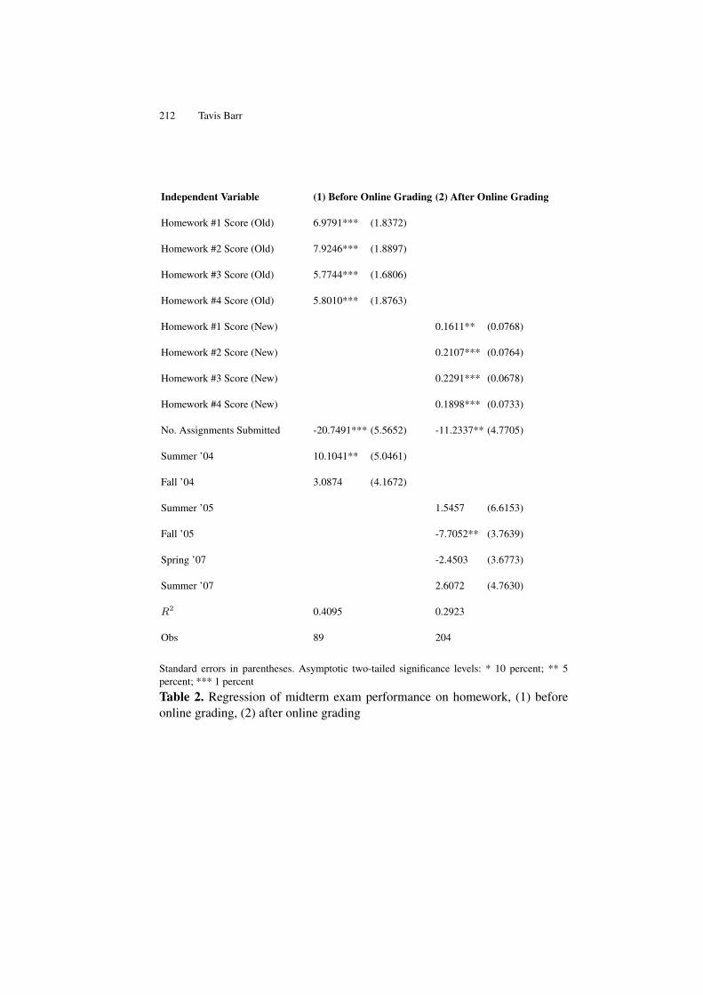
212 Tavis Barr
Independent Variable (1) Before Online Grading (2) After Online Grading
Homework #1 Score (Old) 6.9791*** (1.8372)
Homework #2 Score (Old) 7.9246*** (1.8897)
Homework #3 Score (Old) 5.7744*** (1.6806)
Homework #4 Score (Old) 5.8010*** (1.8763)
Homework #1 Score (New) 0.1611** (0.0768)
Homework #2 Score (New) 0.2107*** (0.0764)
Homework #3 Score (New) 0.2291*** (0.0678)
Homework #4 Score (New) 0.1898*** (0.0733)
No. Assignments Submitted -20.7491*** (5.5652) -11.2337** (4.7705)
Summer ’04 10.1041** (5.0461)
Fall ’04 3.0874 (4.1672)
Summer ’05 1.5457 (6.6153)
Fall ’05 -7.7052** (3.7639)
Spring ’07 -2.4503 (3.6773)
Summer ’07 2.6072 (4.7630)
R2 0.4095 0.2923
Obs 89 204
Standard errors in parentheses. Asymptotic two-tailed significance levels: * 10 percent; ** 5percent; *** 1 percent
Table 2. Regression of midterm exam performance on homework, (1) beforeonline grading, (2) after online grading
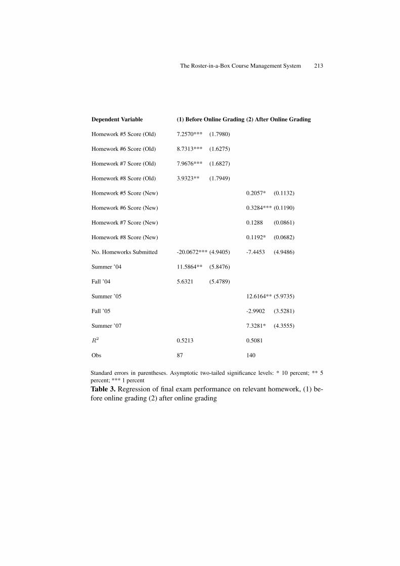
The Roster-in-a-Box Course Management System 213
Dependent Variable (1) Before Online Grading (2) After Online Grading
Homework #5 Score (Old) 7.2570*** (1.7980)
Homework #6 Score (Old) 8.7313*** (1.6275)
Homework #7 Score (Old) 7.9676*** (1.6827)
Homework #8 Score (Old) 3.9323** (1.7949)
Homework #5 Score (New) 0.2057* (0.1132)
Homework #6 Score (New) 0.3284*** (0.1190)
Homework #7 Score (New) 0.1288 (0.0861)
Homework #8 Score (New) 0.1192* (0.0682)
No. Homeworks Submitted -20.0672*** (4.9405) -7.4453 (4.9486)
Summer ’04 11.5864** (5.8476)
Fall ’04 5.6321 (5.4789)
Summer ’05 12.6164** (5.9735)
Fall ’05 -2.9902 (3.5281)
Summer ’07 7.3281* (4.3555)
R2 0.5213 0.5081
Obs 87 140
Standard errors in parentheses. Asymptotic two-tailed significance levels: * 10 percent; ** 5percent; *** 1 percent
Table 3. Regression of final exam performance on relevant homework, (1) be-fore online grading (2) after online grading
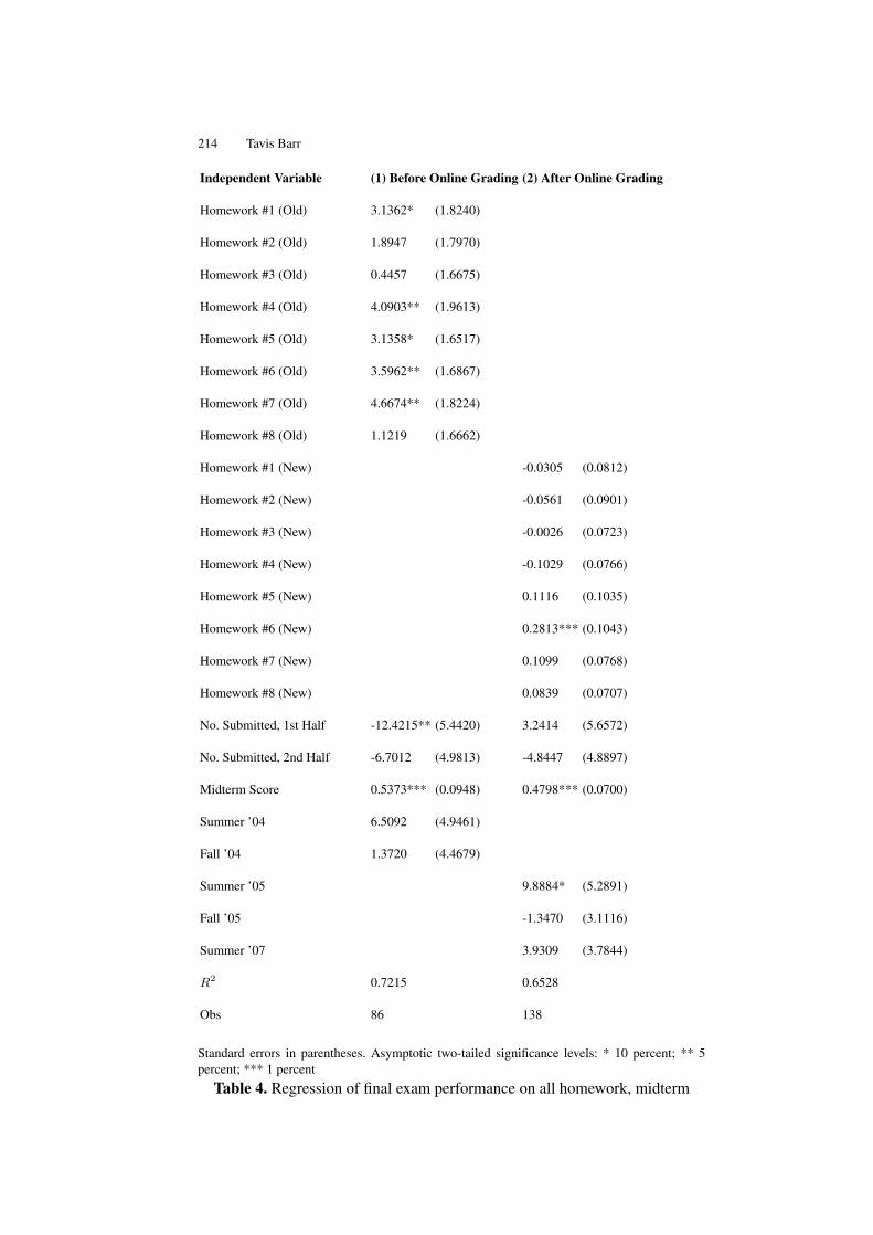
214 Tavis Barr
Independent Variable (1) Before Online Grading (2) After Online Grading
Homework #1 (Old) 3.1362* (1.8240)
Homework #2 (Old) 1.8947 (1.7970)
Homework #3 (Old) 0.4457 (1.6675)
Homework #4 (Old) 4.0903** (1.9613)
Homework #5 (Old) 3.1358* (1.6517)
Homework #6 (Old) 3.5962** (1.6867)
Homework #7 (Old) 4.6674** (1.8224)
Homework #8 (Old) 1.1219 (1.6662)
Homework #1 (New) -0.0305 (0.0812)
Homework #2 (New) -0.0561 (0.0901)
Homework #3 (New) -0.0026 (0.0723)
Homework #4 (New) -0.1029 (0.0766)
Homework #5 (New) 0.1116 (0.1035)
Homework #6 (New) 0.2813*** (0.1043)
Homework #7 (New) 0.1099 (0.0768)
Homework #8 (New) 0.0839 (0.0707)
No. Submitted, 1st Half -12.4215** (5.4420) 3.2414 (5.6572)
No. Submitted, 2nd Half -6.7012 (4.9813) -4.8447 (4.8897)
Midterm Score 0.5373*** (0.0948) 0.4798*** (0.0700)
Summer ’04 6.5092 (4.9461)
Fall ’04 1.3720 (4.4679)
Summer ’05 9.8884* (5.2891)
Fall ’05 -1.3470 (3.1116)
Summer ’07 3.9309 (3.7844)
R2 0.7215 0.6528
Obs 86 138
Standard errors in parentheses. Asymptotic two-tailed significance levels: * 10 percent; ** 5percent; *** 1 percent
Table 4. Regression of final exam performance on all homework, midterm
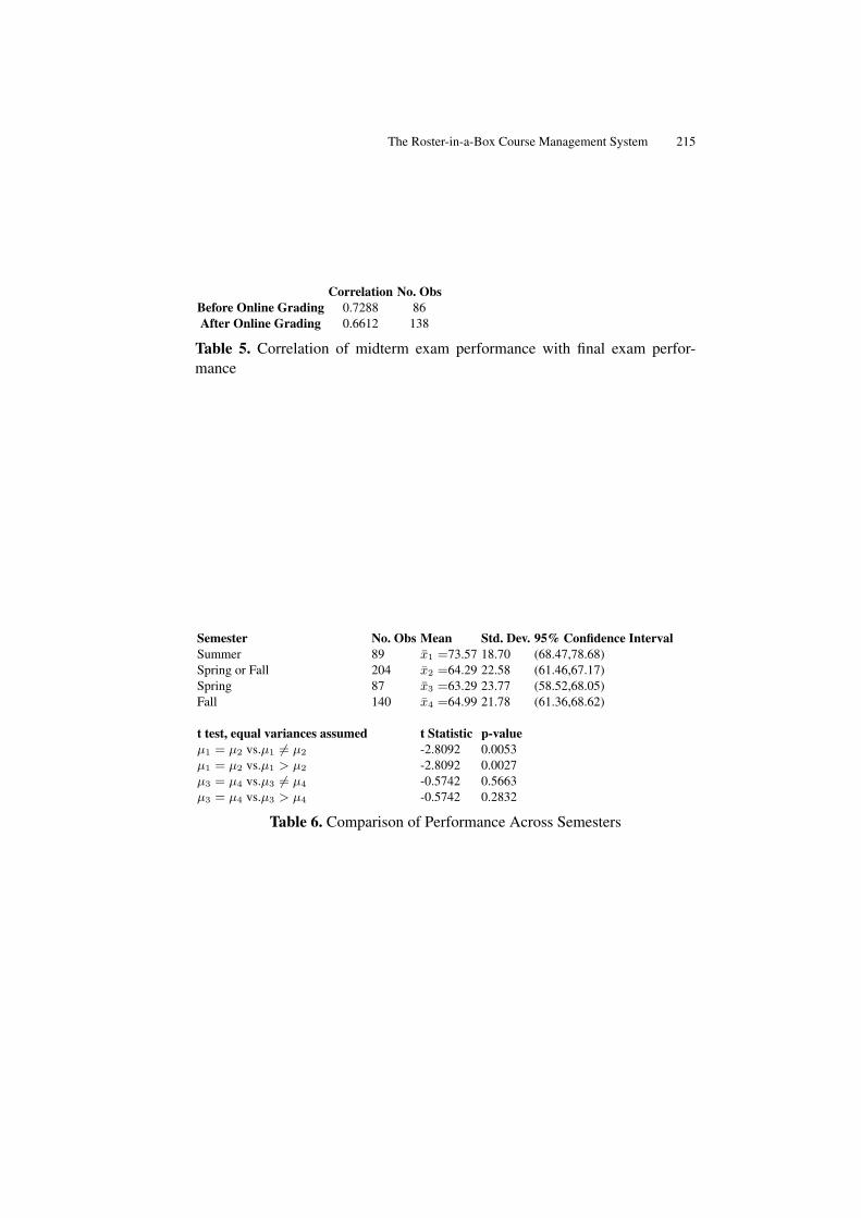
The Roster-in-a-Box Course Management System 215
Correlation No. ObsBefore Online Grading 0.7288 86After Online Grading 0.6612 138
Table 5. Correlation of midterm exam performance with final exam perfor-mance
Semester No. Obs Mean Std. Dev. 95% Confidence IntervalSummer 89 x1 =73.57 18.70 (68.47,78.68)Spring or Fall 204 x2 =64.29 22.58 (61.46,67.17)Spring 87 x3 =63.29 23.77 (58.52,68.05)Fall 140 x4 =64.99 21.78 (61.36,68.62)
t test, equal variances assumed t Statistic p-valueµ1 = µ2 vs.µ1 6= µ2 -2.8092 0.0053µ1 = µ2 vs.µ1 > µ2 -2.8092 0.0027µ3 = µ4 vs.µ3 6= µ4 -0.5742 0.5663µ3 = µ4 vs.µ3 > µ4 -0.5742 0.2832
Table 6. Comparison of Performance Across Semesters


Contributions to gretlDevelopment

On Embedding Gretl in a Python Module
Christine Choirat and Raffaello Seri
1 Department of Quantitative Methods,School of Economics and Business Management,
Universidad de Navarra, Pamplona (Spain)[email protected]
2 Dipartimento di Economia,Università degli Studi dell’Insubria , Varese (Italy)
Abstract. Additional functionalities can be developed for Gretl either directlyin the main C code or with the Gretl scripting language. We illustrate through anexample how it would be possible to wrap the C source of Gretl with SWIG tocreate an interface to Python that makes use of the matrix library NumPy. Suchan interface would make it easier for users to extend Gretl since it would allowfor developing and distributing Gretl extensions as Python modules.
Key words: Python, C, SWIG, Libgretl API
1 Introduction and motivation
To extend the functionalities of Gretl,3 it is either possible to add them in the Csource or to use the Gretl scripting language. The former option is only possiblefor users who have a very sound knowledge of C and who understand how thesource of Gretl is structured. Besides, it makes it hard to share these addedfunctionalities with the rest of the user base unless they are accepted for a nextrelease. The latter option requires learning yet another field-specific language.Even if the speed benchmarks are good and the syntax easy, a program-specificmacro language can never be as powerful as a full-featured scripting language(either domain-specific such as R, see [1, 2], or general such as Python, see [3]).
The scripting language that we have chosen to embed Gretl in is Python,which is free, open-source and available on many platforms. Python is indeeda very powerful, easy-to-learn and well-documented language with a very clearsyntax. Writing and distributing documented Python modules is simple as well.Matrices are not a native Python data type. However, the very mature projectNumPy4 provides an efficient implementation of N−dimensional arrays (and
3 See http://gretl.sourceforge.net/.4 See http://www.scipy.org/.
220 Christine Choirat, Raffaello Seri
therefore matrices) accessible via its C API. Moreover, many other Python mod-ules are of interest, such as the NumPy-based scientific library SciPy5 or theplotting module matplotlib.6 So, the objective is to get the Gretl embeddingmake use of NumPy.
In Section 2, we review the tools that can be used to embed C code in aPython module. We show that SWIG is the most powerful one (though not theeasiest). Then in Section 3, we see how Gretl could be embedded. Section 4concludes.
2 Possible implementation choices
Let us consider the following code (which is a simplified version of the f2pyexample found on the SciPy wiki).7
/* example1.c */void func(int n, double *x)
int i;for (i=0; i<n; i++)
x[i] = x[i] + i;
Python cannot be extended as trivially as R (in particular as can be done throughthe .C function, see Section 5.2 of the R manual [4]) and some nontrivial knowl-edge of the NumPy C API8 is required even in the case of such a simple function(see e.g. Chapter 14 of [5]). Fortunately, two popular tools, namely f2py andSWIG, make extension development much easier.
2.1 f2py
f2py9 is a utility that is primarily meant to wrap Fortran code as Python/NumPymodules. However, it seems to be the easiest way to wrap C code as well. Itgenerates a documented Python module that works very smoothly with NumPy.The only required step is to write a signature file, which states that the functionto be wrapped is a C function and provides the necessary information about itsarguments:
5 SciPy provides among others routines for statistics, optimization, numerical integration, linearalgebra, Fourier transforms, signal processing, image processing, genetic algorithms, ODEsolvers and special functions.
6 See http://matplotlib.sourceforge.net/.7 See http://www.scipy.org/Cookbook/f2py_and_NumPy.8 See http://docs.scipy.org/doc/numpy/reference/c-api.html.9 See http://www.scipy.org/F2py.
On Embedding Gretl in a Python Module 221
! m1.pyfpython module m1interface
subroutine func(n,x)intent(c) funcintent(c)integer intent(hide), depend(x) :: n=len(x)double precision intent(inplace) :: x(n)
end subroutine funcend interfaceend python module m1
Compilation is straightforward: f2py m1.pyf example1.c -c generatesa Python extension module m1.so (on Linux, since the extension is platform-dependent). On the Python side, we get (the »> symbol indicates the Pythonprompt):
»> import numpy, m1»> a = numpy.array([1., 3., 5.])»> aarray([1., 3., 5.])»> m1.func(a)»> aarray([ 1., 4., 7.])»> print m1.func.__doc__func - Function signature:
func(x)Required arguments:
x : rank-1 array(’d’) with bounds (n)
However, as far as we know, no large-scale project as ever been wrapped withf2py, since a lot of manual work is required: an interface has to be written forevery C function.
2.2 SWIG
On the other hand, SWIG10 allows for an almost automatic wrapper generation(including such things as documentation generation and exception handling),the price to pay however is that integration with NumPy is not as easy as withf2py by default. SWIG stands for “Simplified Wrapper and Interface Generator”10 See http://www.swig.org/.
222 Christine Choirat, Raffaello Seri
and allows for interfacing C (and C++) code with several target languages (C#,Java, Ocaml, Octave, Python, R, to name a few). It is successfully used in verylarge scale projects, one of the most famous being wxPython,11 which providesPython bindings to the C++ cross-platform GUI library wxWidgets.12
For standard data types (int, double, . . . ), SWIG works very smoothly.Let us consider the following case, where we have a C file and its associatedheader file.
/* example2.c */#include "example2.h"int add1(int n)
return n + 1;double add2(double x, double y)
return x + y;
and
/* example2.h */int add1(int n);double add2(double x, double y);
The only required step is to write an interface file example2.i (made of twomain parts, the headers to be directly included and the functions to be parsed).
// example2.i%module m2%#define SWIG_FILE_WITH_INIT// Includes the header in the wrapper code#include "example2.h"%// Parses the header file to generate wrappers%include "example2.h"
and use SWIG to generate wrappers for the target language Python:
swig -python example2.i
11 See http://www.wxpython.org/.12 See http://wxwidgets.org/.
On Embedding Gretl in a Python Module 223
A simple Python script
# setup_example2.pyfrom distutils.core import setup, Extensionsetup(name="m2",
ext_modules=[Extension("_m2",["example2.i", "example2.c"])])
takes care of building the extension module m2:
python setup_example2.py build_ext --inplace
From the Python interpreter, we get:
»> import m2»> m2.add1(3)4»> m2.add2(3, 4.0)7.0
2.3 SWIG and NumPy
Applying directly the method of Section 2.2 to example1.c (and the associ-ated header example1.h) leads to a Python function that does not behave theexpected way. If we build a module m3 as above, we get:
»> import numpy, m3»> a = numpy.array([1., 3., 5.])»> m3.func(a)Traceback (most recent call last):
File "<stdin>", line 1, in <module>TypeError: func() takes exactly 2 arguments (1 given)»> m3.func(3, a)Traceback (most recent call last):
File "<stdin>", line 1, in <module>TypeError: in method ’func’, argument 2 of type ’double *’
The problem comes from the fact that SWIG does not know how to trans-form pointers into NumPy arrays. However, it is possible to define typemaps,which are SWIG procedures written in a C-like syntax, in order to make thetransformation easier. Many of these typemaps are already available in the filenumpy.i (which is part of the NumPy distribution). We can use it in the in-terface file example1.i to specify (with %apply) that the arguments of thefunction call are the length of the array and the array itself:
224 Christine Choirat, Raffaello Seri
// example1.i%module m4%#define SWIG_FILE_WITH_INIT#include "example1.h"%%include "numpy.i"%init %import_array();%%apply (int DIM1, double* INPLACE_ARRAY1) (int n, double *x);%feature("autodoc", "func(array x) -> x") func;void func(int n, double *x);
We now get the expected behavior, together with a customized documentation(that could also be generated automatically):
»> import numpy, m4»> a = numpy.array([1., 3., 5.])»> m4.func(a)»> aarray([ 1., 4., 7.])»> print m4.func.__doc__func(array x) -> x
3 SWIG and Gretl
As we have seen in Section 2, SWIG can be used to wrap a program as largeas Gretl in an almost automatic way. Let us consider the minimalistic (and ob-viously very incomplete) case of three interface files (assuming the source codeof Gretl is in src/), namely libgretl.i, version.i and gretl.i
// libgretl.i%module gretl%#include "src/libgretl.h"%%include "src/libgretl.h"
// version.i%module gretl
On Embedding Gretl in a Python Module 225
%#include "src/version.h"%%include "src/version.h"
// gretl.i%module gretl%include "version.i"%include "libgretl.i"%#define SWIG_FILE_WITH_INIT%
The following setup script (hard-coding the directory of the XML library) gen-erates a Python module gretl:
# setup_gretl.pyfrom distutils.core import setup, Extensionsetup(name="gretl",
ext_modules=[Extension("_gretl", ["gretl.i"],include_dirs=["/usr/include/libxml2/"])])
The module can then be called from Python:
»> import gretl»> gretl.GRETL_VERSION’1.8.0’
C structures are automatically transformed into Python classes. For example,the following structure (in src/libgretl.h)
typedef struct _cmplx cmplx;struct _cmplx
double r;double i;
;
can be accessed from Python as
»> gretl._cmplx<class ’gretl._cmplx’>»> z = gretl._cmplx()
226 Christine Choirat, Raffaello Seri
»> z.r0.0»> z.i0.0
4 Conclusion and further developments
We have provided an illustration of the fact that it is possible to embed Gretl’sfunctionalities into a high-level scripting language such as Python. At this point,it would be very fruitful to get some comments from the Gretl community.
– Which target language should be focused upon? Python is the easiest interms of SWIG integration, but R has more built-in econometric functionsand is of more widespread use. (Remark however that the Python packageRPy13 allows for using R from within Python. Moreover, the R communitytends now to favor the use of the Rcpp14 package to create bindings to largeC/C++ libraries such as RQuantLib15).
– How far should we go in the use of SWIG? The source code of Gretl islarge and complex. Gretl defines its own matrix library and matrix oper-ations (in src/gretl_matrix.c), its own optimization functions (insrc/gretl_bfgs.c), etc. All these tools (and many more) are avail-able through NumPy (not to mention Python’s XML standard library andthe graphical library matplotlib). So, some help from the Gretl developerswould allow for selecting the crucial parts to be wrapped.
Writing the proper SWIG typemaps (along the lines of the C++ machine learn-ing library Shogun,16 see [6]), it would be possible to build a Gretl module forR, Python, Octave and Matlab (and any other language supported by SWIG)with only a minimal effort.
13 See http://rpy.sourceforge.net/.14 See http://cran.r-project.org/web/packages/Rcpp/index.html.15 See http://cran.r-project.org/web/packages/RQuantLib/index.html.16 See http://www.shogun-toolbox.org/.

Bibliography
[1] Cribari-Neto, F., Zarkos, S.: R: yet another econometric programming en-vironment. Journal of Applied Econometrics 14(3) (June 1999) 319–329
[2] Racine, J., Hyndman, R.: Using R to teach econometrics. Journal of App-plied Econometrics 17(2) (April 2002) 175 – 189
[3] Choirat, C., Seri, R.: Econometrics with Python. Journal of Applied Econo-metrics (forthcoming)
[4] R Development Core Team: Writing R extensions.http://cran.r-project.org/doc/manuals/R-exts.html
[5] Oliphant, T.: Guide to NumPy.http://numpy.scipy.org/numpybook.pdf
[6] Sonnenburg, S., Raetsch, G., Schaefer, C., Schoelkopf, B.: Large scalemultiple kernel learning. Journal of Machine Learning Research 7 (July2006) 1531–1565

An Alternative to Represent Time Series:“the Time Scatter Plot”
Alberto Calderero1, Hanna Kuittinen1, and Javier Fernández-Macho2
1 Innovation Systems Unit, [email protected]
2 Department of Applied Economics III, University of the Basque Country
Abstract. This paper presents a substantial improvement for the representationof panel data. The time scatter plot is an alternative type of graph using Cartesiancoordinates to display values across the time for two variables of a set of data. Thedata is displayed as a collection of points, linked by lines and ending by an arrow,each having the value of one variable determining the position on the horizontalaxis and the value of another variable determining the position on the verticalaxis. The purpose of the lines and the final arrow is to link the consecutive pointsin time for each case, resulting in a chain of lines in the shape of an irregulararrow which starts in the first period of time and ends in the last. This paperillustrates the usability of time scatter plot with two case studies 1) Research anddevelopment as a driver of innovation and growth and 2) The goal of social andeconomy convergence in Europe.
Key words: time scatter plot, convergence plot, graphing time series, plottingtools.
1 Introduction
Graphical demonstration is a very powerful means to present statistical data.For presenting a long-term development in time or relationship between twovariables a graph can compress the data in a very interpretable manner for theuse of decision support (e.g. policy makers, managers of companies). As theend-users of statistics are not necessarily very familiar with statistical models, awell design and structured graph can give the requested information in a formthat is very easy to understand.
This paper presents a substantial improvement from the deficient presentgraphical representation of panel data (in Gretl and probably in other statisti-cal packages). Gretl’s graphical representation of panel data simply shows eachof the “groups”=cases sequentially (with the option of individual graphs if thenumber of cases is small), which is not satisfactory when the number of casesis relatively high. Besides, this is only useful to present the time evolution ofsome cases, whilst there is nothing to visualize the evolution of the relation-ship between two characteristics of the whole set of cases in the panel, which isprecisely what the present instrument does.
230 Alberto Calderero et al.
Our graphical proposal shows an alternative way to represent time seriesin a scatter plot. When compared to classical scatter plot, the advantage of socalled time scatter plot is in its representation capacity. It can show two variablesand their evolvement in time for several cases (or individuals) using a simplevariation of a traditional scatter plot.
The idea of time scatter plot came up from the practical need to comparethe evolution and the relationship of gross domestic product per capita and re-search and development expenditures of European countries in the same graph.Therefore, our efforts were focused on finding a graphical way to represent si-multaneously these two variables and their evolution in time for a subset ofEuropean countries.
Traditional scatter plots allow us to represent only two variables (or dimen-sions) in the same moment, whereas a graph of time series shows the evolutionin time for different variables of the same case or only for one variable of differ-ent cases. The classical graphing tools are not able to combine in a unique graphthe statistical information that we wanted to show. This was the main reason todevelop a variant of the traditional scatter plot.
The time scatter plot is an alternative type of graph using Cartesian coordi-nates to display values across the time for two variables of a set of data. The datais displayed as a collection of points, linked by lines and ending by an arrow,each having the value of one variable determining the position on the horizontalaxis and the value of another variable determining the position on the verticalaxis. The purpose of the lines and the final arrow is to link the consecutive pointsin time for each case, resulting in a chain of lines in the shape of an irregulararrow which starts in the first period of time and ends in the last.
The time scatter plot enables a researcher to obtain a visual comparison oftwo variables in time and helps to determine what kind of relationship thereis between the two variables. This approach also allows to integrate in a twoaxis plot a third additional dimension, the time, providing more information andinterpretability to the figure. We present two empirical application of the timescatter plot to demonstrate its usability in practise. The first example demon-strates the already mentioned relationship of R&D expenditures and GDP inEurope for 10 years period of 1995-2005. The second case shows the GDP con-vergence process of certain European regions.
2 Methodology
The objective of a chart must be to convey the major story being revealed by thedata in an unambiguous and illuminating form, transmitting to the researcher or
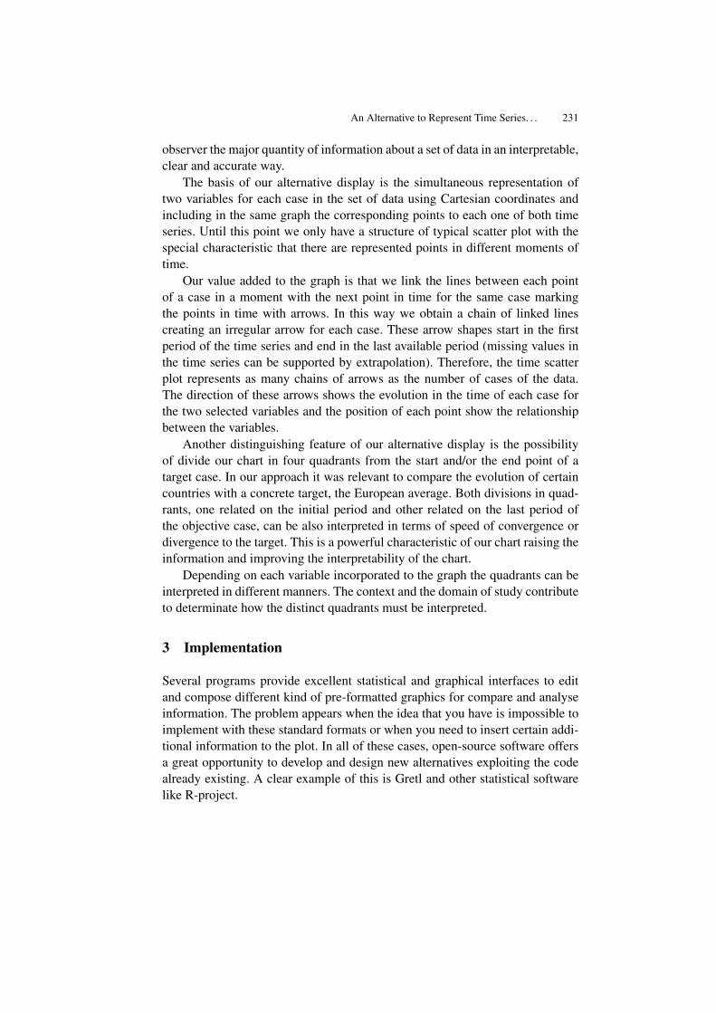
An Alternative to Represent Time Series. . . 231
observer the major quantity of information about a set of data in an interpretable,clear and accurate way.
The basis of our alternative display is the simultaneous representation oftwo variables for each case in the set of data using Cartesian coordinates andincluding in the same graph the corresponding points to each one of both timeseries. Until this point we only have a structure of typical scatter plot with thespecial characteristic that there are represented points in different moments oftime.
Our value added to the graph is that we link the lines between each pointof a case in a moment with the next point in time for the same case markingthe points in time with arrows. In this way we obtain a chain of linked linescreating an irregular arrow for each case. These arrow shapes start in the firstperiod of the time series and end in the last available period (missing values inthe time series can be supported by extrapolation). Therefore, the time scatterplot represents as many chains of arrows as the number of cases of the data.The direction of these arrows shows the evolution in the time of each case forthe two selected variables and the position of each point show the relationshipbetween the variables.
Another distinguishing feature of our alternative display is the possibilityof divide our chart in four quadrants from the start and/or the end point of atarget case. In our approach it was relevant to compare the evolution of certaincountries with a concrete target, the European average. Both divisions in quad-rants, one related on the initial period and other related on the last period ofthe objective case, can be also interpreted in terms of speed of convergence ordivergence to the target. This is a powerful characteristic of our chart raising theinformation and improving the interpretability of the chart.
Depending on each variable incorporated to the graph the quadrants can beinterpreted in different manners. The context and the domain of study contributeto determinate how the distinct quadrants must be interpreted.
3 Implementation
Several programs provide excellent statistical and graphical interfaces to editand compose different kind of pre-formatted graphics for compare and analyseinformation. The problem appears when the idea that you have is impossible toimplement with these standard formats or when you need to insert certain addi-tional information to the plot. In all of these cases, open-source software offersa great opportunity to develop and design new alternatives exploiting the codealready existing. A clear example of this is Gretl and other statistical softwarelike R-project.

232 Alberto Calderero et al.
Gretl [1] has implemented several models of graphs to represent the mostimportant kinds of statistical output, in particular, those related to cross section,time series and panel data analysis. Also, with the command line window, theuser can add and modify the standard graphs by including additional parame-ters to the call of the gnuplot function. This function controls the transferenceof information between Gretl and a plotting utility, Gnuplot, which is used togenerate graphs.
Gnuplot [2] is a portable command-line driven interactive data and functionplotting utility for different operative systems. The software is copyrighted butfreely distributed and support many uses, including web scripting and integra-tion as a plotting engine for third-party applications like Octave, Gretl, etc. Thismeans that any display or graphical model built in Gnuplot could be supportedby Gretl. This is a great opportunity to generate new models and graphical de-signs to explain statistical information, which could be provided by Gretl.
For the implementation of the time scatter plot we have different options.One of them is to download the source code of Gretl and implement the newmodel of graph by the modification of those functions involved in the plottingprocess (mainly, in graphing file). An easier option is however to control the flowof information by scripting or launching the command line console of Gretl.Gnuplot function in Gretl accepts literal commands to control the appearanceof the plot. In this way it is possible to build the proposed time scatter plot byediting the script with the appropriate commands. These scripts need a lot ofnumerical information and commands which make them preferable to write bycode. Finally, for control in a more detailed way the output, as in this case, it ispossible to operate directly, and with the same commands, in Gnuplot applica-tion. An easy R-script can generate, as in this case, the literal code for Gnuplot(also the graphical tool of R can support this kind of representation, as in theoriginal version).
4 Practical application
Next two different practical applications of the alternative display are shown, thefirst of them relative to the R&D effort and its influence in the GDP per capita ofthe European states and the second relative to one of the traditional objectivesof the European Union, the social and economic convergence, analyzing thecurrent situation and the speed of convergence of certain regions of the EU.
4.1 Research and development as driver of innovation and growth
In the context of a global economy and from the Lisbon Strategy point of view,research is a component of a knowledge triangle (the other two being education
An Alternative to Represent Time Series. . . 233
and innovation) meant to boost growth and employment in the European Union[3], [4].
Relevance of the case Knowledge has been increasingly acknowledged to bea main driver of economical growth [5], [6]. Consequently, the member statesof European Union agreed in 2002 to increase the research and developmentinvestments following the Lisbon Strategy. Specifically they set the goal of R&Dexpenditure to reach 3% of GDP by 2010 [7].
The European Commission intends to play a central role in driving and coor-dinating European research across the Framework Programmes to have a lever-age effect on national research spending, in order to achieve the objective of 3%R&D expenditure of GDP on research in Europe [8].
Analyse the current position and speed of convergence with regard to thistarget is a relevant purpose for the Commission, comparing the effort of theEuropean nations in R&D expenditures (percentage of GDP) and its impact onthe income expressed by GDP per capita.
From a theoretical point of view, it is expected that high level of investmentsin research and development are resulting in higher level of GDP in future. Onthe other hand, also the countries with higher initial level of GDP are proneto have relatively higher level of investments in R&D because of more capitalavailable for investing and vice versa the countries with low initial level of GDPare not expected to have very high level of R&D investments.
Showing the results The following time scatter plot shows the R&D expen-ditures (% of GDP) and GDP per capita (euros) of European Union membercountries in years 1995-2005. Each country is having a line with arrows mark-ing each year. The starting point for each arrow is the level of R&D expendituresand GDP per capita in year 1995 (expect for certain countries with missing val-ues in the first periods) and accordingly, the ending point of the arrow remarksthe levels of year 2005 (for all the countries).
For a better representation of the points and arrow, we use in this case asquare scale in both axes. The black lines crossing the axes are representing theEU-27 averages and the red line crossing the y-axis shows the R&D expendituretarget for 2010.
Generally the graph demonstrates rather linear relationship between R&Dexpenditures and GDP of EU-27 countries -the higher the level of R&D expen-ditures, the higher the GDP per capita.
Quadrant A shows the observations with higher than EU average spendingon R&D but lower than average GDP per capita. As expected, there are veryfew points in this quadrant. Similarly, there are only view countries with high
234 Alberto Calderero et al.
Fig. 1. Time scatter plot: R&D expenditures vs. GDP per capita (1995-2005)
An Alternative to Represent Time Series. . . 235
GDP per capita but lower than average spending on R&D as it can be seen fromquadrant D.
Most of the EU-15 countries are in quadrant B implying that they have highlevel of investment on R&D and rather high level of GDP. Only two countries,Sweden and Finland, have reached the EU R&D spending target of 3% but alsoothers like Denmark, Austria and Germany are showing a rather fast growth inR&D expenditures.
The quadrant C represents the countries with below the average R&D spend-ing and GDP per capita lower than EU-27. Relative increases in both R&D ex-penditure and GDP per capita are the highest in this quadrant.
4.2 The goal of social and economy convergence in Europe
Gross Domestic Product per capita is an excellent indicator for measuring thelevel and speed of economic and social convergence in Europe. One of the ob-jectives of EU is to increase the welfare of its citizens, reducing the incomedisparities between different countries and regions.
Relevance of the case Economical convergence has been in interest of eco-nomic research for long -first by neo-classical growth theory and later by newgrowth theory-. Neo-classical growth theory [9] rationalized convergence bydiminishing returns on investments of physical capital, thus implying fastergrowth rates for countries with lower initial level of capital.
The theory expected the economical growth in long-run to be dependentonly on exogenous production factors (availability of labour, technological de-velopment) and economical convergence between countries occurred when thelevels of these factors were equal between economies. However, the majority ofempirical evidence was not consistent with this theory as it seemed that richercountries were growing faster than poorer ones.
So called new growth theory on the other hand believed that the growthof economy is endogenous and depends on new knowledge created by the ac-cumulated capital [10], [11]. Instead of diminishing returns, new growth theorysuggests that the returns remains steady thus benefiting the countries with higherinitial level of capital. The theory also points out how public policies can effecton growth by governmental investments on R&D [12].
European Union’s 27 member states form an internal market for 493 mil-lion citizens. The economical and social inequalities are still however very largeamongst the 268 regions of Europe. Monitoring the convergence or divergenceof EU regions is very important as union’s ultimate goal is to promote econom-ical, social and territorial cohesion [13].

236 Alberto Calderero et al.
The recent enlargements of European Union have significantly increased theeconomical disparities between member states and its regions. The richest mem-ber state (measured by per-capita income) Luxembourg, has seven times largerincome per capita than Romania. The differences are even larger at regionallevel where Inner London reaches 290% of EU-27 income per capita averageand at the same time the poorest region Nord-Est Romania has only the level of23% of EU-27 average [14].
To respond this economical disparity of the EU regions, the European Coun-cil agreed on the budget of $347 billion on Structural and Cohesion Funds forthe period of 2007-2013 [15]. In total, the structural and cohesion funds yieldabout 30% share of the budget of EU. Majority of these funds (81.5%) are allo-cated to convergence regions and targeted on investments on infrastructure andhuman capital. These investments are expected to result on faster growth rateof economy and better employment performance. Consequently, there is a needfor monitoring the regional development policies and especially the economicalcatch up speed of the convergence regions.
Showing the results The Table 1 presents the list of selected regions, all fromNUTS 2 level, which we included in the second exercise for showing the appli-cability of the time scatter plot. In all case, the researcher is the one who mustselect the number and adequacy of the cases to be represented in the plot.
The criteria for selecting one or other case should answer to the interest orrelevance of the study. In our case it was very important to analyze the trend ofBasque Country during the last years because of the great effort executed by theBasque governance institutions for reaching the EU15 average. The other re-gions are shown as reference to our case of interest, facilitating the developmentof benchmarking activities to identify best practices in other leader regions.
The second time scatter plot (Fig. 2) represents the convergence of GDP percapita for selected EU-15 regions. In this graph, the axes are GDP per capita(euro) and its annual variation rate (%). This figure helps to analyse the con-vergence (or divergence) of different regions in comparison with the Europeanaverage.
The European averages of GDP and its growth rates for both the beginning(1996) and ending periods (2005) are marked with black lines crossing the axes.Each line with arrows marks the development of a selected European region,start point of the line showing the level and growth rate of GDP at beginningperiod (1996) and the arrow ending the line pointing the situation at endingperiod (2005).

An Alternative to Represent Time Series. . . 237
Table 1. Set of regions in the analysis by code (NUTS)
Code Region Name Country
DE11 Stuttgart GermanyDE21 Oberbayern GermanyDE24 Oberfranken GermanyDED2 Dresden GermanyES21 Basque Country SpainFI18 Etelä-Suomi FinlandGR43 Kriti GreeceNL11 Groningen NetherlandsNL31 Utrecht NetherlandsPT11 Norte PortugalPT15 Algarve Portugal
To explain the second plot we must characterize the different quadrants inthe graph, especially, those determinate in the last period of time by Europeanaverage.
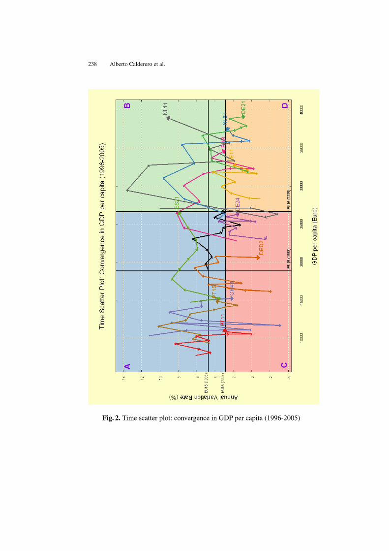
238 Alberto Calderero et al.
Fig. 2. Time scatter plot: convergence in GDP per capita (1996-2005)

An Alternative to Represent Time Series. . . 239
• Quadrant A (blue colour): Regions with disadvantage but convergingThis area is relevant to identify regions in a disadvantaged position in termsof GDP per capita, which means these regions have low level of GDP percapita in comparison with the absolute convergence value (the Europeanaverage). Nevertheless, the regions in this quadrant reached higher annualvariation rates. Therefore the relative speed of growth in terms of GDP percapita is higher for all of these regions, generating a very positive process ofconvergence.
• Quadrant B (green colour): Regions with advantage and diverging (highrelative growth)This quadrant corresponds to regions with a high GDP per capita, higherthan the European average. Also these regions have an annual variation rategreater than the mean. Regions in this quadrant are in advanced position,since they have a relatively higher level of GDP and a better variation rate.However, from European point of view, this situation increases the diver-gence between European regions: rich regions are having a higher growthspeed.
• Quadrant C (red colour): Regions with disadvantage and diverging (lowrelative growth)In the red area there are placed those regions with disadvantaged positionfrom both point of views. They have low speed of growth and lower levelof GDP. In other words, they are regions in disadvantaged economical leveland they are diverging instead of converging due lower speed of growth.Consequently, these regions are worsening the European convergence.
• Quadrant D (orange colour): Regions with advantage but convergingFinally, quadrant D covers another converging area. It includes those regionswith a good relative level in terms of GDP per capita but with low growth.From convergence view this is a positive situation (Europe progress towardsthe global convergence), nevertheless these regions must remain alert be-cause of their lower growth rate.
From the point of view of strict convergence in European frame, the opti-mum position for the regions is in the quadrants A and D. Placing all Europeanregions in both quadrants Europe would reach the perfect convergence in termsof GDP per capita. On the contrary, regions in quadrants B and C contribute toincrease the economic divergence in Europe, promoting income inequalities.
Generally, Figure 2 helps us to evaluate, in an analytical way, the conditionand the convergence (or divergence) level of different regions in comparisonwith the European average (EU15) that is considered as reference level.
240 Alberto Calderero et al.
Analysing the regions by quadrants, Algarve (PT15) and Norte (PT11) re-gions in Portugal (quadrant A) were initially in unfavourable positions and weregrowing above the European average during last years. This has reduced the ex-isting gap of these regions with the European reference. Though their positionis not favourable yet, the current trend is encouraging.
Similarly, the Basque Country (ES21) starting in the same quadrant with anunfavourable position, has grown well above the European average during lastyears, reaching in the last analysed year (2005) the European convergence point,maintaining a high speed of growth.
During the observation period the Basque economy presented high ratesof GDP growth, which can be explained through some competitive advantagesgained from the past -such as appropriate public policies, human capital withhigh educative level and greater efforts in R&D. In order to maintain the dif-ferential growth achieved, the Basque Country may base its future on a clearincrement of the productivity level, accelerating the transition towards the econ-omy based on knowledge and technology.
The regions in quadrant B, Etelä-Suomi (FI18) and Groningen (NL11), arein a very favoured position. Their GDP per head was higher than the Europeanaverage (advantage) and the growth rate was over European Union’s averageduring the whole observation period (divergence trend). Consequently though,they did not contribute towards the aim of converging Europe.
On the other hand, regions like Oberfranken (DE24) and Dresden (DED2)from Germany are placed in the quadrant C. Also Kriti (GR43) in Greece endsup in this quadrant, although the growth rate was more erratic than the average(high variance). The situation for these regions is not so good because they didnot reach an acceptable speed of growth and their levels of GDP per capita werenot able to reduce the gap with the European average.
Finally, in the last quadrant, the regions of Stuttgart (DE11), Oberbayern(DE21) and, also in the last periods, Utrecht (NL31), began from a very favouredposition, but presented a GDP growth below the European Union during theobservation period and therefore were converging with the European average.Notwithstanding, the excellent starting positions of these regions have permit-ted them to keep rather favourable positions also at the end of the observationperiod.
5 Conclusions
This paper presented a new graphical application to represent time series datacalled time scatter plot and two empirical cases to illustrate its usability. The ad-vantage of the time scatter plot is that it is able to show the possible correlation

An Alternative to Represent Time Series. . . 241
of two variables and in addition their evolvement in time. This is a very illustra-tive manner to present statistical data, especially with relatively small numberof cases.
Flexibility offered by open-source programs like Gretl is essential when ap-plying new modified manners to represent statistical data in graphical forms.
Gretl provides us with an excellent environment to develop and implementnew graphical designs and statistical algorithms, due to its flexibility and theaccessibility of the source code.
The two empirical cases that we presented as illustrative examples of us-ability of time scatter plot showed its advantages in presenting time series dataof two variables for multiple cases. Although combining the relationship of twovariables and dimension of time in same plot may sound complex, the illus-tration of time scatter plot is very clear and easy to interpret. This is a clearadvantage of time scatter plot in the face of end-users of statistical data whomay not be experts in statistical models.
In future other type of graphical models applied in different knowledge ar-eas could be adopted to measure and analyze this kind of economic aspects.For example, a violin plot (a combination of a box plot and a kernel densityplot) could be applied to show simultaneously the rank and the dispersion of asynthetic index.

Bibliography
[1] Cottrell, A., Lucchetti, R.: Gretl User’s Guide - Gnu Regression, Economet-rics and Time-series (September, 2008)
[2] Williams, T., Kelley, C.: Gnuplot - An Interactive Plotting Program (March,2007)
[3] European Council: Presidency Conclusions - Lisbon European Council 23and 24 (March 2000), http://tinyurl.com/bks2bq
[4] Commission of the European Communities: Facing the challenge - The Lis-bon strategy for growth and employment (2004), http://europa.eu.int/comm/lisbon_strategy/index_en.html
[5] Schumpeter, J.: The Theory of Economic Development. Harvard UniversityPress, Cambridge, MA (1934)
[6] Grossman, G. M., Helpman, E.: Innovation and Growth in the Global Econ-omy - Cambridge, MA: MIT Press (1991)
[7] European Council: Presidency Conclusions: Barcelona European Council15 and 16 (March 2002), http://tinyurl.com/bks2bq
[8] Commission of the European Communities: Implementing the Commu-nity Lisbon Programme: A policy framework to strengthen EU manufac-turing - towards a more integrated approach for industrial policy. Brussels5.10.2005. Communication from the Commission, COM (2005)474final
[9] Solow, R.: “A Contribution to the Theory of Economic Growth”. QuarterlyJournal of Economics 70 (1): 65-94. (1956)
[10] Romer, P. M.: “Increasing Returns and Long Run Growth” Journal of Po-litical Economy, 94, 1002-38 (1986)
[11] Romer, P. M.: “Endogenous Technological Change”, Journal of PoliticalEconomy 98, 71-102 (1990)
[12] Aghion, P., Howitt, P.: “A Model of Growth Through Creative Destruc-tion”, Econometrica 60: 322-351 (1992)
[13] EUR-Lex: Treaty on European Union, Official Journal C 191, (29 July1992)
[14] European Union: Working for the Regions - EU Regional Policy 2007-2013. (2008) http://tinyurl.com/bqn6q6
[15] Commission of the European Communities: Investing in our future - TheEuropean Union’s Financial Framework 2007-2013. Second revised edition(March 2008)
Wilkinson Tests and gretl
A. Talha Yalta1 and A. Yasemin Yalta2
1 TOBB University of Economics and TechnologySogutozu Caddesi No:43; Sogutozu, 06560, Ankara, Turkey
[email protected] Hacettepe University, Turkey
Abstract. Applied econometrics has become fully dependent on computers andsoftware tools. It is therefore important that the reliability of various programsproviding econometric functionality is vetted within the profession. Here, wereport on the results of our verifying the accuracy of Gretl (GNU Regression,Econometrics and Time-series Library) using the Wilkinson tests. Our study wasimportant in the implementation of a number of modifications improving the gen-eral accuracy and reliability of this open source econometric package.
Key words: Gretl, econometric software, accuracy testing, open source
1 Introduction
Like science itself, scientific software is a work in progress and it is possiblethat any such program at any given time contains errors and imperfections. Inthe case of econometrics, this is well documented by various authors such asSawitzki [1], McCullough [2, 3] and Yalta [4], who find important flaws andinconsistencies in the programs widely used within the profession. Because it isnearly impossible to test all of the functionality offered by a typical econometricprogram, such studies generally employ an introductory or an intermediary testsuite such as Wilkinson’s 1985 “Statistics Quiz” [5], the Statistical ReferenceDatasets (StRD) by the U.S. National Institute of Standards and Technology(NIST) or McCullough’s set of tests [6]. These procedures are based on compar-ing the output from a sample of econometric functions against the correspondingcorrect answers or benchmarked values.
Gretl (GNU Regression, Econometrics and Time-series Library) is a sophis-ticated and cross-platform program for econometric analysis.3 It is open sourceand can be freely used, modified and redistributed under the terms of the GNUGeneral Public License (GPLv3). The program has been gaining in popularity
3 We first became familiar with Gretl several years ago. Although we never got involved in thecoding process of the program, we made contributions in the form of testing the numericalaccuracy of its various functions, submitting bug reports, and helping its internationalizationefforts.
244 A. T. Yalta, A. Y. Yalta
in the recent years and according to the project’s web host SourceForge.net, itwas downloaded more than 100,000 times in 2008.4 See Baiocchi and Distaso[8], Mixon and Smith [9], Yalta and Yalta [10], and Rosenblad [11] for reviewsof Gretl versions 0.997, 1.51, 1.6.0, and 1.7.3 respectively.
An important tool offered by Gretl but unavailable in most other statisti-cal packages is the StRD linear regression test suite, which automatically as-sesses the regression results through a series of 11 tests using the reference datasets compiled by the NIST. This function, which is readily available from the“Tools” menu, helps make sure that a given installation of Gretl produces thecertified results, thereby increasing reliability. The so called “Wilkinson Tests”is an alternative entry-level testing procedure also useful for assessing econo-metric software. Just like the StRD, Wilkinson’s method has been widely usedfor testing different software packages. As a result, the objective of this paper isto describe in detail and report on our experience while applying this procedure,which is currently not available in Gretl.
In the next section, we discuss the Wilkinson tests and their effectiveness inexposing flaws in statistical and econometric programs. In section 3, we reporton the various accuracy errors, existence of which we discovered in Gretl ver-sions 1.7.9 and earlier. We also discuss how these errors were fixed followingour reporting them to the developers as well as the openness of the whole pro-cess, which made it possible to understand the nature of the error and verify itscorrection directly from the source code. Section 4 concludes.
2 The Wilkinson Tests
The Wilkinson procedure is an entry-level test suite for computational accu-racy, which was originally released as a booklet by Wilkinson [5] and describedin detail by Sawitzki [12]. The tests are deliberately designed to reveal flaws instatistical software using a small but effective data set NASTY shown in Table 1.As discussed by Wilkinson [13], each column in the table is designed to exposea different type of flaw. For example, ZERO is used for testing the conditionslikely to cause various zero divide or singularity errors in computational algo-rithms. MISS contains all missing values, which are important in some areasof economics. BIG and LITTLE have a significant variation in the eighth digit,making them problematic to analyze using a badly designed program. Togetherwith HUGE and TINY, they are also used for revealing the formatting problems
4 For the popularity of Gretl, also see the econometric study by Lucchetti [7] (available in thisvolume) finding that the users of Gretl have been steadily increasing at a yearly rate of 43percent since 2006.
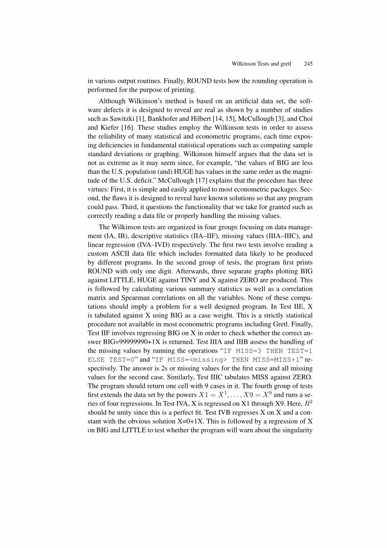
Wilkinson Tests and gretl 245
in various output routines. Finally, ROUND tests how the rounding operation isperformed for the purpose of printing.
Although Wilkinson’s method is based on an artificial data set, the soft-ware defects it is designed to reveal are real as shown by a number of studiessuch as Sawitzki [1], Bankhofer and Hilbert [14, 15], McCullough [3], and Choiand Kiefer [16]. These studies employ the Wilkinson tests in order to assessthe reliability of many statistical and econometric programs, each time expos-ing deficiencies in fundamental statistical operations such as computing samplestandard deviations or graphing. Wilkinson himself argues that the data set isnot as extreme as it may seem since, for example, “the values of BIG are lessthan the U.S. population (and) HUGE has values in the same order as the magni-tude of the U.S. deficit.” McCullough [17] explains that the procedure has threevirtues: First, it is simple and easily applied to most econometric packages. Sec-ond, the flaws it is designed to reveal have known solutions so that any programcould pass. Third, it questions the functionality that we take for granted such ascorrectly reading a data file or properly handling the missing values.
The Wilkinson tests are organized in four groups focusing on data manage-ment (IA, IB), descriptive statistics (IIA–IIF), missing values (IIIA–IIIC), andlinear regression (IVA–IVD) respectively. The first two tests involve reading acustom ASCII data file which includes formatted data likely to be producedby different programs. In the second group of tests, the program first printsROUND with only one digit. Afterwards, three separate graphs plotting BIGagainst LITTLE, HUGE against TINY and X against ZERO are produced. Thisis followed by calculating various summary statistics as well as a correlationmatrix and Spearman correlations on all the variables. None of these compu-tations should imply a problem for a well designed program. In Test IIE, Xis tabulated against X using BIG as a case weight. This is a strictly statisticalprocedure not available in most econometric programs including Gretl. Finally,Test IIF involves regressing BIG on X in order to check whether the correct an-swer BIG=99999990+1X is returned. Test IIIA and IIIB assess the handling ofthe missing values by running the operations “IF MISS=3 THEN TEST=1ELSE TEST=0” and “IF MISS=<missing> THEN MISS=MISS+1” re-spectively. The answer is 2s or missing values for the first case and all missingvalues for the second case. Similarly, Test IIIC tabulates MISS against ZERO.The program should return one cell with 9 cases in it. The fourth group of testsfirst extends the data set by the powers X1 = X1, . . . , X9 = X9 and runs a se-ries of four regressions. In Test IVA, X is regressed on X1 through X9. Here,R2
should be unity since this is a perfect fit. Test IVB regresses X on X and a con-stant with the obvious solution X=0+1X. This is followed by a regression of Xon BIG and LITTLE to test whether the program will warn about the singularity
246 A. T. Yalta, A. Y. Yalta
Table 1. The Data Set NASTY
X ZERO MISS BIG LITTLE HUGE TINY ROUND
1 0 NA 99999991 0.99999991 1e+012 1e-012 0.52 0 NA 99999992 0.99999992 2e+012 2e-012 1.53 0 NA 99999993 0.99999993 3e+012 3e-012 2.54 0 NA 99999994 0.99999994 4e+012 4e-012 3.55 0 NA 99999995 0.99999995 5e+012 5e-012 4.56 0 NA 99999996 0.99999996 6e+012 6e-012 5.57 0 NA 99999997 0.99999997 7e+012 7e-012 6.58 0 NA 99999998 0.99999998 8e+012 8e-012 7.59 0 NA 99999999 0.99999999 9e+012 9e-012 8.5
problem. Finally, ZERO is regressed on a constant and X, with the expectationof a warning about ZERO having no variance or a regression output where boththe correlation and total sum of squares are given as 0.
3 The Performance of Gretl
During our testing of Gretl, we found a number of errors, which mainly affectthe display of the data and the presentation of various computation results.5 Thefirst problem that we found was in Test IB and was regarding the lack of a for-matting function for a “display data” window showing more than one variables.The lack of this functionality has the potential to mislead the users. For example,the default format Gretl uses is printing such values with 6 significant digits. Inthe case of the Wilkinson data set, this leads to an output wrongly implying thatLITTLE is constant for observations 1 to 5, while BIG is constant through 5 to9. We reported this problem to Gretl developers and within three days there wasan update adding the “reformat” function to all data display windows.
The second issue that we encountered was in Test IIA and was due to the factthat the Gretl commands print, printf, and sprintf rounded numericalvalues using “unbiased rounding” or the “round-to-even” method. As a result,attempting to print ROUND with only one digit returned 0, 2, 2, 4, 4, 6, 6, 8, 8instead of the correct answer of printing the numbers from 1 to 9. This problemwas because of not following the principle that rounding for the purpose ofprinting is not about calculation but about the presentation of the results. Gretldevelopers acknowledged this issue and corrected it within just four days.
Thirdly, in Test IIB, Gretl failed to plot BIG against LITTLE accurately andalso refused to plot X against ZERO returning an error message. These were
5 This report is abbreviated. See Yalta [18] for a more detailed discussion.
Wilkinson Tests and gretl 247
due to a number of communication problems with the Gnuplot program, whichhandle the plotting functionality of Gretl. Within six days of our reporting ofthe errors, the Gretl source files handling the graphing behavior were revised.As can be seen in Figure 1 below, Gretl now correctly shows a 45 degree lineand a vertical line for the two plots.
99999990
99999991
99999992
99999993
99999994
99999995
99999996
99999997
99999998
99999999
1e+08
0.99999992 0.99999994 0.99999996 0.99999998
BIG
LITTLE
BIG versus LITTLE (with least squares fit)
Y = -0.326 + 1.00e+08X
1
2
3
4
5
6
7
8
9
X
ZERO
X versus ZERO
Fig. 1. Gretl’s “BIG versus LITTLE” and “X versus ZERO” Plots After Correc-tions
A fourth error that we came across was while attempting to compute thevarious descriptive statistics for the eight series in Test IIC. Gretl performedthese calculations accurately, however, printed out after rounding the standarddeviation of TINY as effectively 0 instead of the correct value 2.7386e+012.This error was also fixed within 24 hours of our reporting it.
Finally, we discovered in Test IID that Gretl produced an erratic output forthe calculation of Spearman’s rank correlations between ZERO and the othervariables. This problem, which was due to numerically printing the special “NotAvailable DouBLe” (NADBL) value was corrected by the Gretl developers in amatter of 24 hours as well. Gretl passed the remaining 10 tests successfully bycomputing the results accurately and showing the correct behavior as requiredby these tests.
In addition to a number of worthwhile improvements, an important benefitof our testing Gretl using the Wilkinson tests was being able to observe how theaccess to the programming code made it possible to see the cause, facilitated arapid fix and enabled the verification of the various corrections. Table 2 showssome revision details on the various Gretl source files updated within just afew days after our exposing of the various software defects. It is possible toexamine all these changes using SourceForge’s “viewvc” interface available athttp://gretl.cvs.sourceforge.net/viewvc/gretl/.
248 A. T. Yalta, A. Y. Yalta
Table 2. Some Revision Details on the Updated Gretl Source Files
TEST SOURCE FILE REV. DATE TEST SOURCE FILE REV. DATE
IB lib/src/printout.c 1.375 Dec 20 IIA lib/src/printscan.c 1.24 Dec 21IB gui2/series view.c 1.44 Dec 18 IIA lib/src/printscan.c 1.25 Dec 22IB gui2/series view.c 1.45 Dec 19 IIB lib/src/graphing.c 1.409 Dec 19IB gui2/series view.c 1.46 Dec 19 IIB lib/src/graphing.c 1.410 Dec 23IB gui2/series view.c 1.47 Dec 20 IIB lib/src/graphing.c 1.412 Dec 23IB gui2/series view.c 1.48 Dec 21 IIB lib/src/graphing.c 1.413 Dec 23IB gui2/series view.c 1.49 Dec 22 IIB lib/src/graphing.c 1.414 Dec 24IIA lib/src/printout.c 1.372 Dec 19 IIB lib/src/graphing.c 1.415 Dec 24IIA lib/src/printout.c 1.373 Dec 19 IIB lib/src/graphing.c 1.416 Dec 24IIA lib/src/printout.c 1.375 Dec 20 IIB lib/src/plotspec.c 1.42 Dec 24IIA lib/src/printout.c 1.376 Dec 22 IIB lib/src/plotspec.c 1.43 Dec 24IIA lib/src/printout.c 1.377 Dec 22 IIB lib/src/gretl_matrix.c 1.393 Dec 23IIA lib/src/printout.c 1.378 Dec 22 IIC lib/src/gretl_matrix.c 1.388 Dec 19IIA lib/src/printscan.c 1.21 Dec 19 IID lib/src/gretl_matrix.c 1.392 Dec 23IIA lib/src/printscan.c 1.22 Dec 19 IID lib/src/graphing.c 1.411 Dec 23IIA lib/src/printscan.c 1.23 Dec 20
4 Final Thoughts
It is not extraordinary or uncommon that a complex econometric program suchas Gretl contains errors and imperfections. The important issue is the mech-anism through which such problems are addressed by the developers. Earlierstudies on the reliability of econometric packages show that software vendorsare unequal in their attention to computational accuracy. Sawitzki [1] ran theWilkinson tests on nine different commercial packages, found a number of er-rors in all them and reported that the reaction he received from different ven-dors varied ranging between “cooperative concern and rude comments.” Yalta[4] found that the various numerical issues in the GAUSS software package re-ported by Knusel [19, 20] and later by Vinod [21] were not fully fixed in sevenyears and after several major revisions. Yalta and Jenal [22] report that Addin-soft did not fix the grossly erroneous least squares estimator for ARIMA in theXLSTAT statistical program and let the users obtain invalid results by using adefective function. Microsoft Excel is widely used in the field of economics andMcCullough and Heiser [23] discuss that errors found in Excel97 were still ei-ther not fixed or wrongly fixed in Excel2007. On the other hand, there also existstudies such as Zeileis and Kleiber [24], Keeling and Pavur [25] and McKenzieand Takaoka [26] which report correction of errors or more accurate results incomparison to earlier versions of various econometric packages.

Wilkinson Tests and gretl 249
A question worth investigating is whether the transparent and collaborativenature of the open source development model provides some advantages in theprocess of error correction, resulting in better and more reliable software in ascientific setting. Indeed, McCullough [27] finds that the open source Gnumericspreadsheet program fixed within a few weeks all the reported flaws surpris-ingly similar to those found in Excel. Similarly, Kuan [28] examines three pairsof commercial and open source programs and reports generally faster fixing ofbugs in the latter. Our experience applying the Wilkinson tests on Gretl was con-current with these cursory studies. We observed the correction of all the reportedflaws after just six days. This is a remarkable performance considering the factthat the developers do not receive any monetary compensation for their contri-butions to the program. In addition, here it was also possible for us to accessthe source code and see the exact cause of the problem each time we discoveredan error. Furthermore, the open source nature of Gretl also enabled an instantdissemination of the various fixes and enabled our verifying the correction ofthe errors.
In conclusion, our assessment of Gretl using the Wilkinson tests allowed thedetection of several important flaws and resulted in a number of worthwhile revi-sions. Also, it is our understanding that the availability of the programming codeand the absence of commercial concerns can provide an open source economet-rics package such as Gretl an advantage in the reliability department.
Acknowledgments
We wish to thank Allin Cottrell for providing prompt and useful answers for ourreports and inquiries regarding Gretl and its inner workings.

Bibliography
[1] Sawitzki, G.: Report on the numerical reliability of data analysis systems.Computational Statistics and Data Analysis 18 (1994) 289–301
[2] McCullough, B.D.: Assessing the reliability of statistical software: Part II.American Statistician 53 (1999) 149–159
[3] McCullough, B.D.: Wilkinson’s tests and econometric software. Journalof Economic and Social Measurement 29 (2004) 261–270
[4] Yalta, A.T.: The numerical reliability of gauss 8.0. The American Statisti-cian 61 (2007) 262–268
[5] Wilkinson, L.: Statistics Quiz. 1 edn. SYSTAT, Evanston, IL (1985)[6] McCullough, B.D.: Assessing the reliability of statistical software: Part I.
American Statistician 52 (1998) 358–366[7] Lucchetti, R.: Who uses gretl? an analysis of the SourceForge download
data. In: Proceedings of the 1st Gretl Conference, Bilbao, Spain (Forth-coming)
[8] Baiocchi, G., Distaso, W.: GRETL: Econometric software for the GNUgeneration. Journal of Applied Econometrics 18 (2003) 105–110
[9] Mixon, J.W., Smith, R.J.: Teaching undergraduate econometrics withGRETL. Journal of Applied Econometrics 21 (2006) 1103–1107
[10] Yalta, A.T., Yalta, A.Y.: GRETL 1.6.0 and its numerical accuracy. Journalof Applied Econometrics 22 (2007) 849–854
[11] Rosenblad, A.: Gretl 1.7.3. Journal of Statistical Software 25 (2008) 19[12] Sawitzki, G.: Testing numerical reliability of data analysis systems. Com-
putational Statistics and Data Analysis 18 (1994) 269–286[13] Wilkinson, L.: Practical guidelines for testing statistical software. In
Dirschedl, P., Ostermann, R., eds.: Computational Statistics, 25th Con-ference on Statistical Computing at Schloss Reisenburg, Physica, Verlag(1994)
[14] Bankhofer, U., Hilbert, A.: Statistical software packages for windows - amarket survey. Statistical Papers 38 (1997) 377–471
[15] Bankhofer, U., Hilbert, A.: An Application of Two-Mode Classificationto Analyze the Statistical Software Market. In: Klar, R., Opitz, O., eds.:Classification and Knowledge Organisation. Springer, Heidelberg (1997)567–572
[16] Choi, H.S., Kiefer, N.M.: Software evaluation: EasyReg international. In-ternational Journal of Forecasting 21 (2005) 609–616

Wilkinson Tests and gretl 251
[17] McCullough, B.D.: The Accuracy of Econometric Software. In: Belsley,Kontoghiorghes eds.: Handbook of Computational Econometrics. Wiley(to appear)
[18] Yalta, A.T.: Should economists use open source software for doing re-search? (2009) [Unpublished Manuscript].
[19] Knüsel, L.: On the accuracy of the statistical distributions in GAUSS.Computational Statistics and Data Analysis 20 (1995) 699–702
[20] Knüsel, L.: Telegrams. Computational Statistics and Data Analysis 21(1996) 116
[21] Vinod, H.D.: Review of GAUSS for Windows, including its numericalaccuracy. Journal of Applied Econometrics 15 (2000) 211–220
[22] Yalta, A.T., Jenal, O.: On the importance of verifying forecasting results.International Journal of Forecasting 25 (2009) forthcoming
[23] McCullough, B.D., Heiser, D.A.: On the accuracy of statistical proceduresin Microsoft Excel 2007. Computational Statistics and Data Analysis 52(2008) forthcoming
[24] Zeileis, A., Kleiber, C.: Validating multiple structural change models – acase study. Journal of Applied Econometrics 20 (2005) 685–690
[25] Keeling, K.B., Pavur, R.J.: A comparative study of the reliability of ninestatistical software packages. Computational Statistics and Data Analysis51 (2007) 3811 – 3831
[26] McKenzie, C.R., Takaoka, S.: Eviews 5.1. Journal of Applied Economet-rics 22 (2007) 1145–1152
[27] McCullough, B.D.: Fixing statistical errors in spreadsheet software: Thecases of Gnumeric and Excel (2004) [CSDA Statistical Software Newslet-ter; retrieved December 10, 2008].
[28] Kuan, J.: Open source software as consumer integration into production(2001) [Unpublished Working Paper, Stanford University].

252 Subject Index
Subject index
Art paintings, 94
Basic Econometrics, 162Baxter and King, 5
C, 198Cointegration, 156Congruent dynamic model, 60Course management system, 184
EHEA, 173Embedding Gretl, 198Endogenous explanatory variable, 46European Fisheries Policy, 129
Filtering, 2Finite Impulse Response filters, 3
GiveWin, 162Gretl, 162
Heckit model, 99Hedonic Model, 129Hodrick–Prescott, 2
Instrumental variable interval regres-sion, 76
Instrumental variables, 44Integrated markets, 156Interval regression, 78
Libgretl API, 198
Mackerel, 156
PcGet, 61Principal components, 117Python, 198
Rating of investment appeal, 117RETINA, 61
Roster-in-a-Box, 184
SAS, 162Second Hand Market of Fishing Ves-
sels, 129Smooth-transition regression model,
38SourceForge download data, 32Structural change, 156SWIG, 198
Teaching, 162Teaching Econometrics with Gretl,
177Teaching–Learning process, 175Time scatter plot, 207Tourist sector investment, 117
Wiener–Kolmogorov Filters, 8Wilkinson tests, 221

AUTHOR INDEX 253
Author index
Adkins, L. C., 44Astorkiza, I., 129Astorkiza, K., 129
Błazejowski, M., 60Barr, T., 184Bettin, G., 76
Calderero, A., 207Choirat, C., 198
Fernández-Macho, J., 207
García Enríquez, J, 156
Kokodey, T, 117Kufel, P., 60Kufel, T., 60Kuittinen, H., 207
López, A. J., 173Lejnarová, Š., 162Lucchetti, R., 32, 76
Marinelli, N., 94
Pérez, R., 173Palomba, G., 94Pollock, D.S.G., 2
Rácková, A., 162
Seri, R., 198
del Valle, I., 129
Yalta, A. T., 221Yalta, A. Y., 221
Copyright © 2022 FDOKUMEN