Assessing Urban Flood Risk with Probabilistic ... - CORE

Assessing Urban Flood Risk with Probabilistic Approaches

Pelin Sertyesilisik

Submitted in accordance with the requirements for the degree of Doctor of

Philosophy

The University of Leeds

Institute of Resilient Infrastructure

School of Civil Engineering

November 2017

-i-

The candidate confirms that the work submitted is her own and that

appropriate credit has been given where reference has been made to the

work of others.

This copy has been supplied on the understanding that it is copyright

material and that no quotation from the thesis may be published without

proper acknowledgement.

The right of Pelin Sertyesilisik to be identified as Author of this work has

been asserted by her in accordance with the Copyright, Designs, and

Patents Act 1988.

© 2017 The University of Leeds and Pelin Sertyesilisik

- ii -

Acknowledgements

I would like to express my gratitude to my supervisors; Professor Nigel

Wright, Dr. P. Andrew Sleigh and Dr. Sangaralingam Ahilan for their

supervision, guidance, and support on my PhD project.

I would like to thank to Republic of Turkey Ministry of National Education for

funding my PhD.

I would like to thank to Simon Jepps and John Jepps, and TUFLOW support

group.

I would like to thank to the friends and colleagues at the School of Civil

Engineering Yuhan Zhao, Mark Brotherton, Claudia, Thomas, Andrea, Sura

Faleh, Carolina and Water@Leeds group.

I sincerely would like to thank to my mother Oya Sertyesilisik.

- iii -

Abstract

Flooding is a serious natural disaster in urban areas. Moreover, the

consequences of land use change and rainfall can affect the flood process in

urbanised catchments. Fluvial flooding can be seen at downstream locations

due to the high and fast discharge from sub-catchments. In addition, pluvial

flooding can be seen at settlements are situated on the floodplains by river

channel at downstream locations, due to the impermeable surfaces and

insufficient drainage capacity. Therefore, the combined pluvial and fluvial

flooding can be observed on the floodplains of urban stream basins.

Although, flood risk can be severe for these places, research on combined

fluvial and pluvial flooding is very rare.

One of these places is Wortley Beck catchment, Leeds, UK. To observe the

interaction between fluvial and pluvial flooding, the floods were modelled for

different land-use scenarios and rainfall events for an urbanised and

ungauged catchment. The inflow hydrographs and rainfall hyetograph were

designed by using the ReFH rainfall-runoff method. 1D and 2D

hydrodynamic models were used to simulate fluvial and pluvial flooding.

The outcomes were peak flow values and probabilistic inundation maps with

maximum water depth values. The peak flow values were used to

investigate the relationship of return period between rainfall and flow by

using the FEH statistical model. The effects of the land use change and

rainfall on the flood risk were observed from the maps. In addition, the flood

extent of combined pluvial and fluvial flooding was observed from these

maps. Water depth values in the inundation area by combined flooding were

computed. Hence, fluvial flooding in combination with pluvial flooding was

observed to have a higher flood risk in the urban stream basins. These

outcomes can be used to manage flood risk due to land use change in the

future for ungauged catchments by National and Local Governments.

- iv -

Table of Contents

Abstract ................................................................................................. iii

Table of Contents .................................................................................. iv

List of Figures ....................................................................................... vii

List of Tables ......................................................................................... xi

List of Equations ................................................................................... xii

Chapter 1 Introduction ................................................................................ 1

1.1 Research framework ..................................................................... 8

1.1.1 Aim.. ...................................................................................... 8

1.1.2 Objectives ............................................................................. 8

1.1.3 Research methodology ......................................................... 8

1.1.4 Research steps ................................................................... 11

1.2 Wortley Beck catchment.............................................................. 15

1.2.1 Flood risk in Wortley Beck catchment ................................. 15

1.2.2 Farnley flood storage reservoir............................................ 17

1.2.3 Culvert and backwater effect ............................................... 19

1.2.4 Flood risk assessment in the Wortley Beck catchment ....... 19

1.2.5 The suitability of Wortley Beck catchment with the research purpose ................................................................ 20

Chapter 2 Literature review ...................................................................... 21

2.1 Existing combination methods of fluvial and pluvial flooding ....... 21

2.2 Review of the methodology ......................................................... 27

2.2.1 Hydrological cycle in a watershed ....................................... 27

2.2.2 Rainfall-runoff process in a watershed ................................ 27

2.2.3 Flooding in a watershed ...................................................... 29

2.2.4 Flood risk............................................................................. 29

2.2.5 Land use change and flooding ............................................ 29

2.2.6 Flood risk management ....................................................... 30

2.2.7 Flood frequency analysis .................................................... 31

2.2.8 Flood estimation .................................................................. 31

2.2.9 Flood modelling ................................................................... 34

2.2.10 Flood estimation methods in ungauged catchments .......................................................................... 36

2.2.11 Loss model .................................................................. 39

2.2.12 Flood frequency analysis for ungauged catchments .......................................................................... 40

- v -

Chapter 3 Fluvial flood event modelling ................................................. 43

3.1 Introduction ................................................................................. 43

3.2 Methodology ................................................................................ 46

3.2.1 Setting-up the 1D/2D fluvial hydraulic model ...................... 47

3.2.2 Flood movement equations in the 1D/2D Fluvial Model ...... 50

3.2.3 2D Free Surface Shallow Water Flow Equations ................ 55

3.2.4 Estimation of the inflow hydrographs .................................. 57

3.2.5 Assessment of the land use change and fluvial flood risk… ................................................................................... 60

3.3 Calibration of the fluvial flood model ........................................... 64

3.4 Results and Discussions ............................................................. 67

3.4.1 Fluvial Flood Risk at the Lower Wortley Beck ..................... 68

3.4.2 The impact of land-use change of sub-catchment on the fluvial flood risk .................................................................... 73

3.4.3 The impact of land use change on the fluvial flood risk ....... 77

3.4.4 The impact of rainfall duration on the fluvial flood risk ......... 82

3.5 Conclusion .................................................................................. 88

Chapter 4 Single Event Simulation .......................................................... 90

4.1 Introduction ................................................................................. 90

4.1.1 Research Area .................................................................... 90

4.2 Research Methodology ............................................................... 92

4.2.1 The Rational Method ........................................................... 92

4.2.2 Modified Rational Method ................................................... 93

4.2.3 The parameters of the calculation peak flow ....................... 94

4.3 Single Event Simulation Results ................................................. 98

4.3.1 Results of fluvial flood inundation area and water depth ... 102

4.4 Conclusion ................................................................................ 111

Chapter 5 Pluvial Flood Modelling ......................................................... 114

5.1 Introduction ............................................................................... 114

5.1.1 The suitability of Wortley Beck catchment ......................... 115

5.2 Methodology of the pluvial flooding ........................................... 116

5.2.1 Direct rainfall method ........................................................ 117

5.2.2 TUFLOW 2D hydrodynamic surface flooding model ......... 117

5.2.3 Build-up process of the direct rainfall model ..................... 118

5.2.4 Estimation of the rainfall events for the pluvial flood risk assessment ....................................................................... 121

- vi -

5.2.5 Roughness ........................................................................ 128

5.2.6 Calibration process of the pluvial flood model ................... 130

5.2.7 Estimation of the flood frequency for Farnley Beck sub-catchment.......................................................................... 136

5.3 Pluvial flood modelling results ................................................... 141

5.3.3 Water depth results ........................................................... 154

5.3.4 Flood frequency analysis of the Farnley Beck (FB) catchment.......................................................................... 156

5.4 Conclusion ................................................................................ 158

Chapter 6 Combined fluvial and pluvial flooding ................................. 160

6.1 Introduction ............................................................................... 160

6.2 Methodology of the combined fluvial and pluvial flooding ......... 162

6.2.1 Modelling approach of the combined fluvial and pluvial flooding on the floodplain .................................................. 163

6.3 Results of the combined fluvial and pluvial flooding .................. 165

6.3.1 Assessment of the fluvial flood model and single event flood models ...................................................................... 167

6.3.2 Assessment of discrete pluvial and fluvial flooding ........... 170

6.3.3 Assessment of the combined pluvial and fluvial flood events ............................................................................... 177

6.3.4 Discussion of the combination fluvial and pluvial flooding at the Lower Wortley Beck area ........................... 184

6.4 Conclusion ................................................................................ 195

Chapter 7 Conclusion ............................................................................. 196

7.1 Introduction ............................................................................... 196

Chapter 8 References ............................................................................. 201

- vii -

List of Figures

Figure 1.1 Wortley Beck catchment............................................................. 15

Figure 1.2 Flood alert areas of the Wortley Beck catchment ....................... 16

Figure 1.3 The historic flood map ................................................................ 17

Figure 1.4 Farnley flood storage reservoir picture 1 .................................... 18

Figure 1.5 Farnley flood storage reservoir picture 2 .................................... 18

Figure 3.1 Flood zone 3 area of the Lower Wortley Beck catchment at Flood Map for Planning (Rivers and Sea) (Environment Agency, 2017) ................................................................................................... 44

Figure 3.2 The fluvial flood model region .................................................. 48

Figure 3.3 Geometry of fluvial flood modelling ............................................ 49

Figure 3.4 Weir Spill (Atkins, 2004) ............................................................. 51

Figure 3.5 Road bridge (Atkins, 2004)......................................................... 53

Figure 3.6 The location of Pudsey gauge station ........................................ 64

Figure 3.7 06/07/2012 Date input data ........................................................ 65

Figure 3.8 Water depth (m) from 06/07/2012 event day .............................. 66

Figure 3.9 Figure 3.9 24/09/2012 Event Date input data ............................. 66

Figure 3.10 Water depth (m) from 24/09/2012 event day ............................ 67

Figure 3.11 Inflow hydrographs ................................................................... 68

Figure 3.12 Flood inundation map ............................................................... 69

Figure 3.13 ReFH URBEXT1990 1% AEP (flood movements) ...................... 70

Figure 3.14 Fluvial flooding 1 % AEP (water depth / stages) ...................... 71

Figure 3.15 Fluvial flooding 1 % AEP (velocity / stages) ............................. 71

Figure 3.16 Flood risk area ......................................................................... 72

Figure 3.17 Inflows for a 2 % AEP for each URBEXT ................................. 74

Figure 3.18 Flood extent of no inflow from FWB ......................................... 75

Figure 3.19 Flood extent of inflow from URBEXT2016 of FWB ..................... 75

Figure 3.20 Water depth percentage (%) .................................................... 76

Figure 3.21 Flood inundation area (km2) ..................................................... 77

Figure 3.22 Inflow hydrographs of FWB and FB ......................................... 78

Figure 3.23 Flood extent of inflow from URBEXT2016 of FWB and FB sub-catchments ................................................................................... 79

Figure 3.24 Flood extent of inflow from URBEXT value 0.15 FWB and URBEXT value 0.17 FB ...................................................................... 80

Figure 3.25 Water depth percentage (%) .................................................... 81

Figure 3.26 Flood Inundation area (km2) ..................................................... 81

- viii -

Figure 3.27 Inflow hydrographs for 0.5-hour rainfall duration ...................... 82

Figure 3.28 Flood extent from 0.5-hour rainfall duration.............................. 83

Figure 3.29 Inflow hydrographs for 1-hour rainfall duration ......................... 83

Figure 3.30 Flood extent from 1-hour rainfall duration................................. 84

Figure 3.31 Inflow hydrographs for 6-hour rainfall duration ......................... 85

Figure 3.32 Flood extent of 6-hour rainfall duration ..................................... 86

Figure 3.33 Fluvial flood inundation Area (km2) for each rainfall duration (h) for a 1% AEP ................................................................... 86

Figure 3.34 Water depth percentage (%) for each rainfall duration (hr.) ..... 87

Figure 4.1 Location of New Farnley Beck catchment .................................. 91

Figure 4.2 Urbanisation and flood inundation area .................................... 103

Figure 4.3 Return period and flood inundation area .................................. 104

Figure 4.4 Rainfall duration and flood inundation Area.............................. 105

Figure 4.5 Water depth percentages (%) and urbanisation ....................... 106

Figure 4.6 Water depth percentages (%) and rainfall return period (yr.) ... 106

Figure 4.7 Water depth percentages (%) and rainfall duration (hr.) .......... 107

Figure 4.8 URBEXT 1990 1 % AEP ............................................................. 108

Figure 4.9 URBEXT 2016 1 % AEP ............................................................. 108

Figure 4.10 URBEXT 1990 1 % AEP for 0.5 hour rainfall duration .............. 109

Figure 4.11 URBEXT 1990 1 % AEP for 1 hour rainfall duration .................. 109

Figure 4.12 URBEXT1990 1 % AEP for 6 hour rainfall duration .................. 110

Figure 5.1Lower Wortley surface flood risk (Environment Agency, 2013 RFI no: 29864) .................................................................................. 115

Figure 5.2 The Wortley Beck Catchment (WBC) ....................................... 116

Figure 5.3 2D Hydrodynamic direct rainfall-urban surface flood-modelling approach ........................................................................... 119

Figure 5.4 Framework of direct rainfall- runoff model for TUFLOW ........... 119

Figure 5.5 The DEM of the Wortley Beck Catchment (WBC) .................... 120

Figure 5.6 Impermeable surfaces in the Wortley Beck Catchment ............ 125

Figure 5.7 06/07/2012 event day ............................................................... 131

Figure 5.8 24/09/2012 event day ............................................................... 132

Figure 5.9 Thiessen method ...................................................................... 133

Figure 5.10 Gross rainfall of the 06/07/2012 event ................................... 133

Figure 5.11 Gross rainfall of the 24/09/2012 event ................................... 134

Figure 5.12 Water level from rainfall data of 06/07/2012 ........................... 135

Figure 5.13 Water level from rainfall data of 24/09/2012 ........................... 135

- ix -

Figure 5.14 Peak flow discharge point ...................................................... 137

Figure 5.15 Estimated hyetographs for the 1 in 5-year event .................... 142

Figure 5.16 Estimated hyetographs for the 1 in 15-year event .................. 142



Figure 5.19 Estimated hyetographs for the 1 in 100-year event ................ 144

Figure 5.20 Cumulative gross rainfall events for the1 in 100-year event for 0.5/1/6 hr., rainfall durations ............................................... 145

Figure 5.21 Rainfall event for the 1 in 5-year event .................................. 146

Figure 5.22 Rainfall event for the 1 in 15-year event ................................ 147

Figure 5.23 Rainfall event for the 1 in 30-year event ................................. 148

Figure 5.24 Rainfall event for the 1 in 50-year event ................................. 149

Figure 5.25 Rainfall event for the 1 in 100-year event ............................... 150

Figure 5.26 Rainfall event for the 0.5 hour duration of the 1 in 100-year event ................................................................................................. 151

Figure 5.27 Rainfall event for the 1 hour duration of the 1 in 100-year event ................................................................................................. 152

Figure 5.28 Rainfall event for the 6hour duration of the 1 in 100-year event ................................................................................................. 153

Figure 5.29 The percentages of the water depth values for rainfall return periods (30 yr., 50 yr., and 100 yr.) ......................................... 154

Figure 5.30 The percentages of the water depths (m) for rainfall durations ........................................................................................... 155

Figure 6.1 The combined fluvial and pluvial flood modelling at the Lower Wortley Beck area .................................................................. 163

Figure 6.2 2D Rainfall boundary condition control area............................. 164

Figure 6.3 Observation points on the Lower Wortley Beck ........................ 166

Figure 6.4 The water level at Point 3 ......................................................... 167



Figure 6.7 Fluvial flood inundation map..................................................... 169

Figure 6.8 Single flood inundation map ..................................................... 169

Figure 6.9 The water levels at Point 2 ....................................................... 171

Figure 6.10 The water levels at Point 4 ..................................................... 171




Figure 6.14 Fluvial flood inundation map ................................................... 174

- x -

Figure 6.15 Pluvial flood inundation map .................................................. 175

Figure 6.16 Fluvial flooding 2 % AEP on the Lower Wortley Beck area .... 176

Figure 6.17 Pluvial flooding 2 % AEP on the Lower Wortley Beck area .... 176

Figure 6.18 Combined fluvial and pluvial flooding ..................................... 178

Figure 6.19 Combined fluvial and pluvial flooding water depth/ stages (1%AEP) ........................................................................................... 179

Figure 6.20 Combined fluvial and pluvial 1 %AEP flooding velocity map .. 180

Figure 6.21 Combined fluvial and pluvial flooding 1% AEP (velocity /stages) ............................................................................................. 181

Figure 6.22 Pluvial flooding with the fluvial flood (no inflow from upstream) .......................................................................................... 182

Figure 6.23 Combined fluvial and pluvial 2 %AEP flooding on the flood plain .................................................................................................. 183






Figure 6.29 Fl1 and FI2 water level points ................................................ 187

Figure 6.30 Comparison of the water levels for each simulation at point FI1 ..................................................................................................... 187

Figure 6.31 Comparison of the water levels for each simulation at point FI2 ..................................................................................................... 188

Figure 6.32 The water depth at Point 1 ..................................................... 189





Figure 6.37 The water level at Point 3 ....................................................... 192

Figure 6.38 The water level at Point 4 ....................................................... 192



- xi -

List of Tables

Table 3.1 Manning's roughness (n) values of the materials ........................ 50

Table 3.2 Catchment descriptors of FB and FWB basins ............................ 59

Table 3.3 Urbanisation of Farnley Beck (FB) basin ..................................... 63

Table 3.4 Urbanisation of Farnley Wood Beck (FWB) basin ....................... 63

Table 4.1New Farnley (Lateral Inflow Sub-Catchment) Properties ............. 91

Table 4.2 Catchment design rainfall parameters ......................................... 92

Table 4.3 URBEXT values of the New Farnley ........................................... 94

Table 4.4 Time to peak (TP), rainfall duration (D) ........................................ 99

Table 4.5 Return period (T) and Rainfall intensity (i) ................................... 99

Table 4.6 Rainfall duration and Intensity ................................................... 100

Table 4.7 Peak flows (Q) from different rational methods ......................... 101

Table 4.8 Peak Flow (Q) from Rational Method for different return periods and URBEXT values ............................................................ 101

Table 4.9 Peak Flow (Q) (m3/s) from Rational Method for different rainfall duration (h) and return periods (yr) ........................................ 102

Table 5.1 Catchment descriptors of WBC ................................................. 122

Table 5.2The αT correction factor for each return periods ......................... 128

Table 5.3 Land use materials .................................................................... 128

Table 5.4 The relationship between the return periods ............................. 156

- xii -

List of Equations

Equation 2.1: The Muskingum Routing the continuity equation ................... 33

Equation 2.2 Dynamic Model ...................................................................... 33

Equation 2.3 Diffusion Model ...................................................................... 33

Equation 2.4 Kinematic Model ..................................................................... 33

Equation 3.1The weir equation for free flow used in the Spill ...................... 51

Equation 3.2 The spill coefficient equation .................................................. 52

Equation 3.3 Drowned Weir Flow equation ................................................. 52

Equation 3.4 The expression for computation of backwater upstream from a bridge constricting flow ............................................................ 53

Equation 3.5 The conservation of mass equation ....................................... 54

Equation 3.6 Continuity Equation ................................................................ 54

Equation 3.7 The momentum conservation or dynamic equation ................ 54

Equation 3.8 Channel conveyance (k)......................................................... 55

Equation 3.9 The 2D Continuity .................................................................. 55

Equation 3.10 X Momentum ........................................................................ 56

Equation 3.11 Y Momentum ........................................................................ 56

Equation 3.12 The Critical Storm Duration .................................................. 58

Equation 3.13 Time to Peak ........................................................................ 58

Equation 3.14 Baseflow Lag ........................................................................ 59

Equation 3.15 Baseflow Recharge .............................................................. 59

Equation 3.16 Baseflow Recharge .............................................................. 59

Equation 3.17 Urbanisation expansion factor (UEF) ................................... 61

Equation 3.18 An empirical relationship between Urban and URBEXT....... 62

Equation 3.19 Total percentage imperviousness ........................................ 62

Equation 3.20 Undeveloped (Rural Area) .................................................... 63

Equation 3.21 Paved (Urban Area) ............................................................. 63

Equation 4.1Rational method (Houghton-Carr, 1999) ................................. 93

Equation 4.2 Urbanisation Expansion Factor (UEF) .................................... 94

Equation 4.3Runoff coefficient of the modified rational method .................. 95

Equation 4.4 Urban percentage runoff ........................................................ 95

Equation 4.5 Storm Duration (D) ................................................................. 97

Equation 4.6 Time to peak equation ............................................................ 97

Equation 5.1 The Critical Storm Duration (h) ............................................. 123

Equation 5.2 Time to Peak ........................................................................ 123

- xiii -

Equation 5.3 The percentage runoff .......................................................... 126

Equation 5.4 Cmax .................................................................................... 126

Equation 5.5 The initial soil moisture content (Cini) .................................. 127

Equation 5.6 Initial soil moisture correction factor ..................................... 127

Equation 5.7 QMEDrural catchment descriptor ........................................... 137

Equation 5.8 Urban Extension Factor (UEF) ............................................. 138

Equation 5.9 The urban adjustment .......................................................... 139

Equation 5.10 The Urban Adjustment Factor (UAF) .................................. 139

Equation 5.11 the percentage runoff urban adjustment factor ................... 139

Equation 5.12 The transfer equation ......................................................... 139

Equation 5.13 Estimation of the peak flow for return interval .................... 140

-1-

Chapter 1 Introduction

Changes in watershed hydrology may affect the catchment water balance

thus causing, as a result, adverse hydrological events such as a flooding

and droughts (Weng, 2001). Flood events can be observed when a normally

dry land is inundated. Magnitude, frequency, and duration are fundamental

parameters for consideration of the effect of a flood event. The parameters

that govern a flood event are varied, uncertain, and very difficult to estimate.

For instance, a flood event can re-occur at irregular intervals and with

varying magnitude and duration. It means that to predict with accuracy the

timing and magnitude of any particular flood event in a given location is a

significant challenge. Furthermore, the consequences of flood events may

depend heavily on floodwater depth, return period, the location of the

inundated area and the length of the event itself. These add that the

designing of appropriate (i.e. offering sufficient protection for acceptable

cost) flood defences is difficult (Jha et al., 2012). Moreover, there are

several reasons why flooding occurs, for example, flooding may be the result

of natural circumstances, human actions or, very often, a combination of

both (Calder and Aylward, 2006). In addition, within a particular catchment,

one or more of several types of flooding processes and their combinations

can often be observed namely: fluvial flooding, coastal flooding, pluvial

flooding, and groundwater flooding (Thorne, 2014). Any or all of these flood

events can have negative effects on residences, sewerage systems,

agriculture and the economy and these may be anywhere on the planet

(Marsh et al., 2016). Consequently, to manage the flood events, flood

frequency and consequences are the primary parameters to examine. Both

the frequency and the consequences of flooding are affected by future

changes in land use and climate (Ashley et al., 2005).

- 2 -

Flooding is possible in anywhere in the world, where it rains, and it is a

significant risk worldwide (Guha-Sapir et al., 2016). Flooding is often

described as being the most dangerous natural disaster (MunichRe, 2015).

Guha-Sapir et al. (2014) reported that nearly 10000 people were killed from

flooding in 2013 in the world. Furthermore, the most frequent natural disaster

has been flooding specifically, between in 1994 and 2013 years (UNISDR,

2015). Flooding is the most frequent disasters in Asia also (Budiyono et al.,

2015). In addition, the flooding happened in 2014/2015, 2013/2014, 2009,

2007, 2006, 2000/2001, 1998, 1995, 1990, 1986, 1982, 1974, and 1968

years at the regional scale in the UK (Marsh et al., 2016).

In all of these cases, there is a significant impact on the economy in all over

the world. Floods are one of the biggest reasons for the economic losses

from the natural disasters (UNISDR, 2009). Annual economic losses from

natural disasters decreased between 2003 and 2012 years in all areas,

except flooding. Estimates of the cost of flood damage have been put at US$

53.2 billion in 2013 in the world (Guha-Sapir et al., 2014). Similarly, the cost

of property damage is high. More than 5 million properties can be at flood

risk in the UK (Thorne, 2014). It is clear that expense has increased sharply

due to the effects of flood damage. The budget can be expected to rise

because annual damage of flooding could increase in the future (CCRA,

2012). Besides the economic cost of flooding, consequences of flooding can

also cause of disruption of daily life, industrial and agricultural production

(Pitt, 2008). During and after flooding, life routine can be disrupted in both

urban and rural areas. For instance, flooding can cause disruptions in

transportation or water supply system (Rafiq et al., 2016), e.g. the water

supply and electrical system were not functional for a while following the July

2007 floods in the UK (Pitt, 2008). Similarly, some residences were left

without power because of the flood event on the Christmas 2013 in the UK

(Thorne, 2014). A further potentially more widespread effect could occur in

the form of diseases and discomfort trauma (Ahern et al., 2005). For

instance, Malaria and leptospirosis diseases can spread because of

contamination after flooding (Hammond et al., 2013). Lastly, cultural heritage

can also be damaged by the flooding (Nedvedová and Pergl, 2013).

- 3 -

The rainfall-runoff process in urban areas is that during or immediately after

the precipitation event, rainfall can enter the subsurface by infiltration

through permeable surfaces in parks and gardens, storm runoff can be

conveyed by sewer system and discharged into river channel. The rainfall-

runoff process in urbanised catchment may depend heavily on the

magnitude of a rainfall event, the capacity, quantity of the permeable

surfaces, and the effectiveness of the sewer system in the city (Dawson et

al., 2008; Rafiq et al., 2016).

When climate change and urbanisation are incorporated into this process,

the consequences of flooding can be much serious in the future. The

magnitude of the rainfall event can be a major contributory factor of flood risk

in the UK (Marsh et al., 2016) while climate change is expected to increase

the rainfall intensity and frequency and thus the magnitude (Waters et al.,

2003). Therefore, climate change can affect the magnitude of flood risk. For

instance, 1 % AEP river flood can increase 20% from 2025 year to 2115

year in England due to the climate change (DCLG, 2010).

In addition, urbanisation is constantly expanding in terms of space and

population density throughout the world. Population is expected to rise to 6.3

billion in 2050 in urban areas (Nations, 2014), due to the economic growth,

employment opportunities, better living standards, and education in cities

(Turok and McGranahan, 2013). Therefore, land use in cities is changing

from green fields and permeable areas to the impervious areas by building

residential areas, roads, highways, roofs, pavements, car parks, industrial

places and asphalt surfaces (Cheng and Wang, 2002; Evans et al., 2008;

Abdullah, 2012) by Governments, city councils and businessmen. The

increased ratio of impervious surfaces on previously rural land, (due to the

urbanisation process of a watershed), increase the volume of water runoff,

and flood peak, or reduce the infiltration, and the time of catchment

response (Weng, 2001; Cheng and Wang, 2002; Abdullah, 2012). In fact, it

is common to see ephemeral ponds on the low-level surface during high

rainfall.

- 4 -

This urban surface water becomes a flood, when it is too deep, extensive or

it stays too long i.e. does not drain or is not managed (Shi et al., 2007;

Wheater and Evans, 2009; Du et al., 2015).

Capacity and performance of the infrastructure systems rarely can manage

heavy runoff in streets effectively. The performance of a sewer system can

have a significant impact on the flood management in the cities. When the

surface runoff cannot be managed by the sewer system due to being

overwhelmed with water, the runoff process can become a flooding situation

(Dawson et al., 2008). For example, debris, rubbish inside of the pipe

system can affect the capacity of the sewer system. Furthermore, some

infrastructure systems are designed as combined storm water and sewerage

system. These can be resulting in that the infrastructure system struggle to

manage and to collect surface runoff in the streets along with the sewage, so

that pluvial flooding can occur as local flooding or backup events in urban

areas (WMO and GWP, 2008; Abdullah, 2012; Rafiq et al., 2016). According

to OFWAT (2002), in the UK, 16,000 settlements have been identified as at

risk of being affected by the 10-year return period of a sewer flooding, which

means that pluvial flood is a high risk for these places. Whatever the

capacity issue is with existing infrastructure systems, maintenance and

upgrading of the systems to increase their performance are never cheap or

easy. Impermeable surfaces, the lack of sewer system and growth of

population in the flood-prone areas have the significant influence on flood

incidents in urban watershed. These have resulted in flooding becoming a

serious problem in cities all over the world (Jha et al., 2012). Some of the

cities that have been particularly affected are Bangkok, Dhaka, Jakarta, and

Kuala Lumpur (Abdullah, 2012). In the cities, the management of the factors

of urban flood risk is becoming an emergency mission. Climate change and

urbanisation can increase the risk to assets and population that are the

exposure to floods in urban areas. Therefore, climate change and

urbanisation can be considered the primary factors of concern for the future

for predicting flood events in urban areas (Merz et al., 2010; Yin et al.,

2015).

- 5 -

Besides the climate change and land use change factors, the combination of

flood events can be added into the strategies of flood risk management to be

addressed in urban areas (Cheng and Wang, 2002; Re, 2005; Dawson et

al., 2008; Evans et al., 2008; WMO and GWP, 2008; Ten Veldhuis, 2010;

Singh and Singh, 2011).

Various flood events such as coastal flooding, fluvial flooding, pluvial

flooding, and their combinations can be observed in urban areas due to the

location (Ten Veldhuis, 2010). Coastal flooding can happen, where the cities

are settled by a coastline, at high sea water levels. Fluvial flooding can

happen, where the cities are settled by a tributary, by overflowing of

riverbanks (Burton et al., 2010). Furthermore, the processes of these flood

events can have a relationship. Therefore, a combined flood event can incur

from the combination of these various floods in urban areas. More than one

simultaneous flood events can be observed such as, overwhelmed urban

stream channel and coastal with high sea levels, or tidal and surface runoff

(Ten Veldhuis, 2010; Lian et al., 2013; Thorne, 2014; House of Commons,

2015). Flood events such as those in the UK in winter 2013/14 were results

of a variety of combinations of tidal, rainfall, river, and groundwater source

(Thorne, 2014). Asian mega-cities are prone to the combination of flood

events due to their extraordinary urban growth by river channels and their

monsoonal rainfall events (Chan et al., 2012), these resulting in both pluvial

flooding and fluvial flooding, and are being observed either consecutively or

coincidentally in these locations. Similarly, in tropical regions in smaller

towns and cities the annual monsoon, local intensive precipitation events are

observed (and predictable) and often result in both fluvial and pluvial

flooding occurring at the same time (Apel et al., 2015). Chen et al. (2010)

and Apel et al. (2015) pointed out that the reason of a fluvial flooding is

heavy rainfall in upstream locations while the reason for pluvial flooding is

intense precipitation in the local area.

The process of the combined pluvial and fluvial flooding in urban areas can

be explained as that. Historically, people have settled near the rivers.

Settlements have been built on the floodplains thus impermeable surfaces

have rapidly grown up along the rivers (Evans et al., 2008).

- 6 -

Urbanisation on the floodplains such as farmland, forested land can reduce

the land’s ability to retain rainfall thus the generation of surface runoff and of

discharge from the sub-catchments may increase (WMO and GWP, 2008;

Du et al., 2015).

These lowland locations also have a potential to have riverine flooding

(WMO and GWP, 2008; Hammond et al., 2015). These locations are usually

low cost, so become subject to being impacted by the spatial distribution of

population. This situation is likely to encourage more settlements on the

floodplains (WMO and GWP, 2008). Therefore, the urban drainage system

cannot manage runoff after an intense rainfall event and pluvial flood events

can occur in these locations. Consequently, intensive precipitation on

saturated soil and impervious surfaces, an excessive flow load within a

sewer/storm water system, also an overwhelmed river channel with

inadequate flood defence structures on the floodplains in urban stream

basins can cause combined pluvial and fluvial flooding.

In general, the impact of the fluvial and pluvial flood events are analysed

separately. Studies considering the combined effects of fluvial and pluvial

flooding in detail are very few (Apel et al., 2015; Breinl et al., 2015).

Furthermore, Chen et al. (2010) and Ashley et al. (2005) implied that the

effects of the combination of fluvial and pluvial flood events can be severe

than their individual potential effects. Burton et al. (2010) added that if

simultaneous flood events are analysed separately, the hazard could be

underestimated.

Briefly, as land use change, population and climate change parameters are

considered for urbanised catchments, flood frequency and magnitude of

flood damage can be expected at significant level in the future (Ten

Veldhuis, 2010). All these aspects make flood resilience approaches to be

insufficient in the future. Therefore, the urban flood risk might have

assessment priority alongside other natural disasters (Winsemius et al.,

2013). The primary challenges can be to predict the process of the urban

flood event, to construct resilient infrastructure, and to update these

approaches (Hammond et al., 2015).

- 7 -

Probabilistic approaches can be applied to adapt flood inundation analysis

with future growth taken into account in the urbanised catchments (Yanyan

et al., nd.; Thompson and Frazier, 2014).

These strategies are not likely to be low cost and can require long-term

adaptation plans, and various vulnerability assessments (Budiyono et al.,

2015) by local and national planning boards. To apply flood defence

strategies with the long-term adaptation plans estimation of the future flood

risk is always required. Adaptation scenarios can be created to define these

risk factors by setting up the hydrology models, hydraulic models, and flood

damage assessment models (Yanyan et al., nd.).

In conclusion, changes in water balance in a watershed can cause flood

events. Magnitude, frequency, and duration of flood events have many

uncertainties. These facts make difficult the estimation of flooding. Flooding

is one of the most dangerous natural disasters. Urban areas are most prone

to flooding. These locations have many more frequent flood events, severe

damage, destruction of the properties and the human life than rural areas. In

addition, the effects of the land use change and climate change on the flood

processes can have multiple and changing aspects. Due to urbanisation and

climate change, the ratio of saturated surfaces decreases and with high

rainfall magnitude, surface runoff cannot be managed by the sewer system

in the cities. These can result in various flood events and their combinations

in urban areas. Old-style and single-line wall flood defences of a single flood

event can be recognised as ineffective for these events. Moreover, it is clear

that the definition and understanding of the interdependencies of the flood

processes are essential to developing the flood defence systems. In

addition, the analysis of the frequency, magnitude, and interaction of any

flooding are required for the advanced and predictive assessment of the

urban flood risk. As a consideration of this, Sustainable Urban Drainage

Systems (SUDS) as a toolbox of solutions might be useful to attenuate

runoff.

All of the above contribute to the easily drawn conclusion that urban flood

risk assessment deserves priority amongst the other natural disasters.

National and local governments have an imperative to achieve the balance

- 8 -

between urbanisation and vulnerability to flooding due to the economic

growth and population in cities. To manage the land use change and to

adapt to the climate change are essential approaches to analyse and

mitigate the consequences of flood risk. It is important to note that the

influence of climate change and urbanisation on the relationship between

direct runoff generation and flood risk are not straightforward. Therefore,

significant research is needed and ongoing in this area. To update and

modify strategies of the flood risk management for the future and the variety

of flood events will always be necessary.

1.1 Research framework

1.1.1 Aim

The aim of this research is to assess the urban flood risk to enrich the

mitigation approaches of the adverse flood consequences in urban areas of

local government agencies.

1.1.2 Objectives

To reach the aim the below objectives have been set,

1. To analyse the impact of land use changes on flood risk in urban basins.

2. To analyse the impact of rainfall events on flood risk in urban basins.

3. To develop a method to assess the interactions between the fluvial and

pluvial flood events in urban basins.

All research was undertaken at the representative urban catchment, Wortley

Beck catchment, Leeds, UK.

1.1.3 Research methodology

This section gives a brief explanation of the methodology of this research.

The case study was developed for Wortley Beck catchment. Wortley Beck

catchment has three sub-catchments. These are Farnley, Farnley Wood,

and New Farnley basins. Wortley Beck catchment is an ungauged and

urbanised catchment. The flood risk of the Wortley Beck catchment was

analysed by simulating three flood processes. These were fluvial flooding,

single event, and pluvial flooding.

- 9 -

The probabilistic flood events were simulated by using hydrodynamic

models. One- dimensional (1D) hydraulic model was used to simulate river

system of the Lower Wortley Beck. Flood Modeller Suite (v 3.7.0) software

was used for this simulation. Flood Modeller Suite software was developed

by CH2MHILL and was benchmarked by the Environment Agency. Flood-

prone areas of the Wortley Beck catchment were simulated by using a two-

dimensional (2D) hydrodynamic model. Two-dimensional Unsteady FLOW

(TUFLOW, 2013-12-AD-w64) software was used for this simulation.

TUFLOW was developed by BMT.

The urban flood risk can be assessed based on the results of the

simulations. The outcomes from this research can be used to improve urban

flood resilience tools in Wortley Beck catchment. In this study, the sewer

system is neglected neither pluvial nor fluvial, due to its limited capacity in

the hydraulic flood simulations.

A.) Modelling of fluvial flooding

To assess the impact of the discharge at the outfall of the sub-catchment on

the downstream fluvial flood risk, fluvial flood event simulation was

undertaken.

The following methodology steps were used to simulate the probabilistic

fluvial flood events at the Lower Wortley Beck, Leeds, UK,

1. The inflows from Farnley Beck and Farnley Wood Beck basins were

estimated for different return periods, by using the Revitalised Flood

Hydrograph (ReFH) model.

2. A coupled 1D-2D hydrodynamic model was set up.

B.) Modelling of single event simulation

To assess the impact of the peak flow at the outfall of a sub-catchment on

the downstream fluvial flood risk, single event simulation was undertaken.

The maximum discharge was used to display the surface runoff at the

upstream basin. The peak flow at the outfall of a sub-catchment was

modelled as a lateral flow in the river system. New Farnley sub-catchment

was assessed and utilised for this approach.

- 10 -


single event at the Lower Wortley Beck, Leeds, UK,

1. The Rational model was used to calculate peak flows for various return

periods.

2- A coupled 1D-2D hydrodynamic model was set up. In addition to the

inflows, lateral flow was integrated within the fluvial system of the Lower

Wortley Beck.

C.) Modelling of pluvial flooding

To assess the surface flood risk in the Wortley Beck catchment, a direct

rainfall-runoff model was set up.


pluvial flood events at the Wortley Beck catchment, Leeds, UK,

1. A net event hyetograph was estimated by using the Revitalised FSR/FEH

loss model. Rainfall events were produced by using the Flood Modeller Suite

ReFH boundary framework.

2. Rainfall-runoff process was simulated by using a 2D hydrodynamic model.

3. Surface runoff was modelled for permeable and impermeable surfaces.

4. Peak flows were computed from various rainfall events.

D.) Calibration

Calibration process was carried out by using measured rainfall and water

level data. Measured rainfall data set was taken from Headingley,

Knostrop, and Heckmondwike rain gauges stations. The water level data

was taken from Pudsey stage gauge station. The data sets were supplied by

the UK Environment Agency and Met office in 2016 for this research.

E.) Probabilistic flood inundation maps

It was essential to produce flood inundation maps for a range of annual

exceedance probability (AEP) to identify vulnerability of regions within this

urban area, which could then be translated to reach generalizable

conclusions on the effect of other urban areas. Probabilistic flood inundation

maps with water depth were produced by using the outcomes of the

- 11 -

hydrological and hydraulic models simulations. These maps were used to

identify the flood vulnerable areas in the research areas. Hydrodynamic

model was linked geographic information system (GIS) tool to produce these

maps by using LiDAR data and the master map of the catchment.

Catchment surface was investigated by using the LiDAR data, and Master

Map. The data sets and surface roughness parameters were supplied by the

UK Environment Agency and Leeds City Council for this research.

Background of the probabilistic flood inundation map was created by using

the ordnance survey 1:25 000-scale colour raster in this research.

1.1.4 Research steps

The below research steps were taking to reach the objectives.

Fluvial and pluvial flood processes in urbanised catchments were simulated

in this research. The flood events were designed by using the following

parameters: different ranges of land use scenario, rainfall duration, and

annual exceedance probability.

1. The impact of land use change (urban developments, SUDS) on the flood

risk were analysed in this research.

2. The impact of rainfall events on the flood risk were analysed in this

research.

3. The interaction between fluvial and pluvial flood drivers on the floodplains

of urban stream basins was assessed in this research.

Step 1. Analysis of the impact of the land use change on flood risk in

urban basins

The impact of the land use change (urban developments, SUDS) on flood

risk was analysed by adjusting the ratio of impermeable surfaces. Thus, the

effects of the impermeable surfaces on surface runoff and on outflow

discharge of the sub-basin could be examined. This also means that the

impacts of the land use on the downstream flood risk could be observed.

The ratio of the impermeable surface was adjusted by using URBEXT

parameter. The URBEXT is a catchment descriptor parameter, which refers

to the extent of urban and suburban land cover for a specific year.

- 12 -

The URBEXT was used to calculate different urban growth ratios of various

years in this research.

Step 2. Analysis of the impact of rainfall events on flood risk in urban

basins

Climate change is expected to affect rainfall events. The effects of rainfall

events on pluvial flooding and downstream fluvial flooding were investigated

in this research. The rainfall event analysis was performed by using various

rainfall durations and return periods in this research.

The Wortley Beck catchment is an ungauged catchment. Therefore, the

flood events were designed from the rainfall-based hydrological model.

Catchment response time is used to estimate rainfall duration in this

research. The link between rainfall event and flood risk can be determined

by using assessments of the catchment response time.

Step 3. Assessment of the interactions between the fluvial and pluvial

flood events in urban basins

To assess the interaction between the fluvial and pluvial flooding in urban

basins, various fluvial and pluvial flood events were simulated. In addition,

the combined fluvial and pluvial flooding on the floodplains of urban stream

basin was analysed.

Firstly, the fluvial flood events at the Lower Wortley Beck area were

designed. Secondly, the single event simulations were modelled to

understand the impact of the lateral flow on the downstream fluvial flood risk.

Thirdly, the pluvial flooding was designed on the Wortley Beck catchment.

Lastly, the combined fluvial and pluvial flood events on the floodplains of the

Lower Wortley Beck were modelled.

The interaction between fluvial and pluvial flooding in the urban areas was

investigated by using the below approaches.

1. Assess the fluvial flood model and single event simulations,

2. Assess independent fluvial flood events and pluvial flood events,

3. Determine the relationship between the return period of the rainfall and

the return period of the flow,

- 13 -

4. Assess the combinations of the pluvial and fluvial flood events on the

floodplains of the Lower Wortley Beck.

The interaction between the fluvial and pluvial flood events on the

floodplains was determined by using flood frequency, flood extent, flow

values, and water depth parameters. The probabilistic flood inundation maps

and water level results were used to present the independent and dependent

relationship between fluvial and pluvial flooding.

3.1) Assessment of the fluvial flood model and single event simulations

The probabilistic fluvial flood events were simulated to observe the Lower

Wortley Beck fluvial flood extent. Inflow event hydrographs of the Lower

Wortley Beck were estimated for Farnley Beck and Farnley Wood Beck sub-

catchments of the Wortley Beck catchment. Probabilistic single flood events

were simulated to observe the impact of the peak discharge at the outlet of

New Farnley Beck basin on the Lower Wortley Beck fluvial flood extent. In

addition to the inflow hydrographs, the lateral flow was integrated within the

simulations. These simulations were designed for various return periods and

urbanisation scenarios. The advantage of this method is to analyse the

interaction between surface runoff in the upper catchment and river flow at

the downstream.

Limitation of this method can be that lateral flow was applied as constant

during the simulation. However, the lateral flow and inflow of the fluvial flood

event could have different time durations and peak time.

3.2) Assessment of independent fluvial flood events and pluvial flood

events,

1. Fluvial flooding and pluvial flooding were modelled by using various return

periods.

2. The probabilistic flood inundation maps with water depth scale were

produced by using the results of the simulations.

3. The common flood-prone areas were observed for a specific return

period.

- 14 -

The advantage of this method is to design various pluvial and fluvial flood

events in Wortley Beck catchment. A limitation of this method is that the

interaction between pluvial and fluvial flood risk cannot be captured in detail.

3.3) Determination of the relationship between the return period of

rainfall events and the return period of flows

The Regional (Pooled) approach of the statistical flood estimation method

was applied to determine the return period of flows from the specified return

period of rainfall events.

A rainfall-runoff model was set up to analyse flood frequency for an

ungauged catchment, by using 2D TUFLOW hydrodynamic model. The

advantage of the usage of 2D TUFLOW for a rainfall-runoff model is that it is

capable of computing the flow over the whole period at selected locations in

the research area for each rainfall events. This application was very suitable

to compute peak flow in the ungauged catchment.

3.4) Assessment of the combinations of the pluvial and fluvial flood

events on floodplain

The interdependency of pluvial and fluvial flooding has been discussed for

the Lower Wortley Beck area in this research. The combined fluvial and

pluvial flooding was simulated by using the 2D direct rainfall model link with

the river channel in Lower Wortley Beck area. Inflow hydrographs of the sub-

catchments of Wortley Beck and net rainfall hyetograph of the Lower Wortley

Beck area were integrated within the simulations. Thus, the flood extent with

water depth of the combined fluvial and pluvial flooding on the floodplains of

the Lower Wortley Beck can be simulated and observed.

Probabilistic flood inundation maps with water depth scales were used to

display the flood-prone locations from combined fluvial and pluvial flood

events on the floodplains of the Lower Wortley Beck area.

According to this approach, various combined fluvial and pluvial flood events

can be simulated. In addition, the consequences of the combined flood

events can be observed.

- 15 -

1.2 Wortley Beck catchment

The research area is Wortley Beck catchment. This catchment is located in

the south-west of Leeds, UK. The basin is approximately 63 km2 and drains

into the River Aire. The catchment consists in Farnley Beck, New Farnley,

and Farnley Wood Beck sub-catchments (Figure 1.1).This catchment is

ungauged and urbanised.

Figure 1.1 Wortley Beck catchment

1.2.1 Flood risk in Wortley Beck catchment

Flood alert areas of the Wortley Beck catchment can be found in Figure 1.2.

This area has been flooded since 1886 (Atkins, 2004). Historically, Wortley

Beck catchment was flooded in 1946, 2005, 2007 (Hope, 2011). Moreover,

Atkins (2004) informed that flooding occurred at the Farnley Wood Beck and

Farnley Beck basins in 1946, on September 1993, December 2000, and

August 2002.

In addition, in the Christmas period, in 2015/2016, approximately 1,000

homes were flooded in Leeds as the Aire River overtopped its banks (Marsh

et al., 2016).

- 16 -

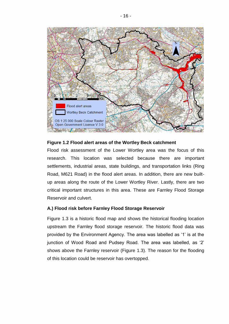
Figure 1.2 Flood alert areas of the Wortley Beck catchment

Flood risk assessment of the Lower Wortley area was the focus of this

research. This location was selected because there are important

settlements, industrial areas, state buildings, and transportation links (Ring

Road, M621 Road) in the flood alert areas. In addition, there are new built-

up areas along the route of the Lower Wortley River. Lastly, there are two

critical important structures in this area. These are Farnley Flood Storage

Reservoir and culvert.

A.) Flood risk before Farnley Flood Storage Reservoir

Figure 1.3 is a historic flood map and shows the historical flooding location

upstream the Farnley flood storage reservoir. The historic flood data was

provided by the Environment Agency. The area was labelled as ‘1’ is at the

junction of Wood Road and Pudsey Road. The area was labelled, as ‘2’

shows above the Farnley reservoir (Figure 1.3). The reason for the flooding

of this location could be reservoir has overtopped.

- 17 -

Figure 1.3 The historic flood map

1.2.2 Farnley flood storage reservoir

Farnley flood storage reservoir was built to manage the flood risk in the

Lower Wortley Beck area by attenuating flows for a 15-year return period.

However, this reservoir is not efficient in its present state because it filled

with silt, rubbish, and sediments (Figure 1.4 and 1.5). In order to use it with

original capacity, it should regularly be cleaned and maintained, which is

very expensive and difficult.

- 18 -

Figure 1.4 Farnley flood storage reservoir picture 1

Figure 1.5 Farnley flood storage reservoir picture 2

- 19 -

1.2.3 Culvert and backwater effect

A culvert is located at the junction of the Ring Road and M621, in the Lower

Wortley Beck area. The capacity of the culvert is generally not sufficient for

the flow. Culvert can be blocked so the backwater effect can be observed.

1.2.4 Flood risk assessment in the Wortley Beck catchment

The first flood risk assessment of Wortley Beck catchment report was

produced by Atkins, in 2004. This report analysed the 18.0 km length area

by using unsteady one-dimensional hydrodynamic model. Atkins- Transport

Solutions Warrington - Survey Department completed a topographic survey

in October 2003 for this report. Outcomes of this survey were used to

determine the hydraulic characteristics of the channels such as roughness

values, the physical properties of cross section and hydraulic structures. The

hydraulic model was version 2.2 of the Flood Modeller Suite (ISIS) one-

dimensional model. Farnley Flood Storage Reservoir and culvert were built

to manage the flood risk. However, the reservoir and culvert could have

limited capacity for the flow. There could be backwater risk in the area.

Potential flood risk was found at the Ring Road in Lower Wortley. The model

could not be calibrated. Some recommendations of this study were to have a

measured data to calibrate the model, to update the topographic survey

data, to maintain regularly the hydraulic structures and to update the

URBEXT values to analyse the impact of urban growth on the flood risk

(Atkins, 2004).

Another report was prepared by the Thomas Mackay Ltd as required by

PPS25. The flood level and extent were examined in this report because

flood risk was severe at the Farnley Beck basin. Hydrological data,

topographical data, roughness values of the cross sections, and 1D model

schematisation were the same as Atkins (2004)`s research. The 1m

resolution LiDAR data of Environment Agency was used in this research.

The research area was visited on 22 July 2010 for this research. The Flood

Modeller Suite (1D ISIS version 3.4) model was linked to the TUFLOW 2D

model to simulation. Ordnance Survey Master Map with scale 1:10000 was

- 20 -

used to model 2D domain of the research area. The 2D domain 6.7 km2 area

was modelled with a cell size of 5 metre.

The downstream of the model was at the River Aire. Flood extents maps

were produced for a fixed time step of 1 second in the 1D domain and 2

second in the TUFLOW 2D domain. Lastly, the model could not be

calibrated (Jepps, 2011). This report recommended that hydrological

assessment should be updated (Jepps, 2011).

Consequently, the reports recommended a further research for the Wortley

Beck catchment to update the fluvial flood risk assessment. The updates

could contain in calibration the model, in a new survey data, or in a high

resolution updated topographical data.

1.2.5 The suitability of Wortley Beck catchment with the research

purpose

Wortley Beck catchment is an urban stream basin. There are some

settlements and population along the route of the river. In addition, this

location has built-up areas. Moreover, the ratio of impermeable surfaces has

increased on the floodplains. Therefore, the catchment has several levels of

both fluvial and pluvial flood risk. In addition, the combination of fluvial and

pluvial flood event can be observed more often than the present in the

future. The consequences of flood events will be much serious. Lastly,

updated information is necessary to manage the future flood risk for Wortley

Beck catchment.

- 21 -

Chapter 2 Literature review

2.1 Existing combination methods of fluvial and pluvial

flooding

In this section, the evaluation of methodologies for assessing combined

fluvial and pluvial flooding is presented.

Flooding can be observed from multiple causes and sources, which may

affect individually or in some combined way. To disregard the combined

flood events can cause failures of flood defences (Burton et al., 2010). In

publications, fluvial flooding is mostly investigated (Moncoulon et al., 2014)

with more recently pluvial flooding is incoming of interest, but the combined

fluvial and pluvial flooding is a very new approach in literature (Breinl et al.,

2015). Furthermore, the papers have discussed the different combinations of

coastal, tidal, fluvial, pluvial, and groundwater flooding; and by using

procedures mostly based on Monte-Carlo analysis, the joint probability of

tidal and fluvial flooding (Apel et al. 2006; Chen et al., 2010; Lian et al.,

2013).

The approaches of previous papers that investigated the combined fluvial

and pluvial flooding can be listed as that.

Burton et al. investigated the combined hazard of fluvial and pluvial flooding

for the South East London Resilience Zone (SELRZ) in 2010. The nested

modelling approach provided datasets for simultaneous analysis of pluvial

and fluvial flooding. Both disaggregated rainfall data and upstream discharge

were applied into the urban inundation hydraulic model to assess both

pluvial and fluvial flooding. This simulation and analysis were performed by

using two-dimensional non-inertial overland flow model (Burton et al., 2010).

Rainfall data was estimated by using climate projections. The methodology

of the climate projections based on the UKCP09 future climate scenarios for

the 2050s. The discharge was estimated by using hourly rainfall data and

then, was entered into the fluvial flood model. The disaggregated rainfall

data at 15-minute on a 2 km resolution, (and finer spatial-temporal

resolution), was entered into the hydraulic model of pluvial flooding.

- 22 -

Horton Soil infiltration was applied to calculate the runoff on rural areas.

Sewer drainage loss was applied to the runoff in urban areas (Burton et al.,

2010).

In summary, Burton et al. (2010) investigated the combined hazard of fluvial

and pluvial flooding in an urbanised catchment. Rainfall dataset was

produced with consideration climate change. Combined hydraulic and

hydrological modelling approach was used for simulations of flooding. The

nested modelling approach was recommended to provide input datasets for

both pluvial and fluvial flooding analysis.

Chen et al. (2010) investigated both pluvial and fluvial flood events in

Stockbridge area in Keighley (Bradford, UK), and stated that heavy rainfall

could cause both pluvial and fluvial flooding in this area because it is both an

urban and settled along the route of the River Aire. They simulated

combined fluvial and pluvial flood events and compared the consequences.

The combined peak river water level and rainfall were assessed in this

research.

Fluvial flood events with a return period of 200 years were set-up for

hypothetical overtopping and breaching situations. The pluvial rainfall

durations ranged from 15 minutes to 360 minutes with return periods from 1

in 2 to 100 years. The SIPSON software was used to design 1D flow in the

drainage system. While UIM software was used to model 2D overland flow

for the surface flow simulation. The results of the composite flood events

were used to identify the dominant factor that caused flood inundations in

different parts of the research area. The results showed that the combined

flood extents displayed greater flood inundation areas and depths than the

results of a single type of flood event.

In summary, Chen et al. (2010) studied the determination of the risk of the

combined pluvial and fluvial flooding for settlements along the route of the

river. Intense rainfall can cause both pluvial flood events because of the

overwhelmed sewer system and can cause fluvial flooding because of the

limited capacity of the river channels in urban areas. This situation is very

similar to the combined flooding process in the Wortley Beck catchment as

well. They recommended that the timing and the duration of the rainfall

- 23 -

events should be considered, in addition to the peak water level in flood

inundation areas of composite flood events. This approach can make the

parameter of the catchment response time very significant to evaluate the

rainfall and discharge in a catchment.

They recommended that the joint probability approach based on Monte

Carlo could be used to analyse the combination flood risk in more detail. The

main outcome of this research seems to be that the consequences of the

combined flood events can be much serious than the consequences of a

single type of flood event. This knowledge could be used to develop flood

damage mitigation approaches much efficiently in the future.

Horritt et al. (2010) suggested two different approaches to combine flood

events. These are the fully integrated approach and the map combination

approach. The different flood event sources were combined, and then routed

along pathways to the risk receptors in the fully integrated approach. The

different sources of flooding probability can be assessed at the same time by

this approach (Horritt et al., 2010). In the map combination approach,

common boundary conditions of the flood events of different sources were

generated and were routed separately then probabilistic flood maps were

combined.

Horritt et al. (2010) aimed to combine different sources of a flood event, such

as, river, coastal, surface water etc. into the single map with both the

individual and combined probability of each of these events. Therefore, the

outcomes, such as likelihood, extent, depth, velocities of flood events from

different sources could be used by flood risk professionals, decision makers

and the public to improve the flood risk assessment.

The approach of the overlapped map can have a limitation for the evaluation

of the independent sources and probability. Therefore, the fully integrated

approach could be very useful to evaluate risk of combination flooding.

Lian et al. (2013) investigated the effects of the combined rainfall and the

tidal level in Fuzhou City, which is a coastal city. Lian et al. (2013) examined

the joint impact of rainfall and downstream tidal level on flood risk in a

coastal city with a complex river network. The effects of the combined rainfall

and tidal levels with and without pumped flood relief systems on flood

- 24 -

probability were assessed. Rainfall events were derived based on the 10,

20, 50 and 100-year return period and the hydrographs were estimated by

using design rainfall events. A precipitation event and a typical tide event

were selected and used as boundary condition for the simulation by using

HEC-RAS software.

In the analysis of the results, they introduced the joint probability method to

examine the relationship between tidal floods and extreme precipitation. The

results showed that a high tidal level is usually accompanied by heavy rains

and this causes the greatest threat in Fuzhou to be from heavy rainfall

events. However, the risk of both rainfall and tidal level exceeded their

threshold is very low. In this methodology, the decision for the threshold

could be very critical to assess the combination of the flooding. Lian et al.

(2013) recommended investigating the joint of flood probability and

consequence into a single risk function in the future in detail.

Moncoulon et al. (2014) combined two independent probabilistic events

involving overflowing rivers and surface water runoff due to heavy rainfall on

the slopes of the watershed. They used a stochastic distribution of river

discharges on the large catchments and a stochastic distribution of

spatialized rainfall on the small catchments. Moncoulon et al. (2014)

produced a distributed hazard model from the combined stochastic runoff–

rainfall and river routing models. River overflow and surface runoff were

combined with a homogeneous approach.

In this approach, to produce data for rainfall-runoff model and river routing

model could be the hardest part. In addition, the length and the quality of the

measured input data can be the most important part.

Breinl et al. (2015) focused on finding the days of combined of fluvial and

pluvial flooding so they developed a joint probabilistic modelling framework

to simulate daily peak discharge and maximum hourly precipitation in the city

of Salzburg (over 30 km2 area). Daily peak discharge was used to identify of

the days of fluvial flooding, and maximum hourly precipitation was used to

identify of the days of pluvial flooding. A stochastic Weather generator was

used to produce daily precipitation, which was passed through a hydrological

model to produce daily mean discharge, and subsequently daily peak

- 25 -

discharge. Daily precipitation was also converted into maximum hourly

precipitation data. Occurrence critical thresholds of river discharge for fluvial

flooding and extreme precipitation for pluvial flooding were studied to define

and to examine combined fluvial and pluvial flood in this research (Breinl et

al., 2015).

The joint occurrence of fluvial and pluvial flooding was investigated by using

long-term data. Breinl et al. (2015) estimated the probabilities of joint

occurrence of fluvial and pluvial floods. In addition, they asked whether or

not the days when fluvial or pluvial flooding occurred could be simultaneous

and whether this could be analysed by using observational data. In this

approach, the quality of the observed data of the flood days can be very

important.

They presented a joint probabilistic modelling framework to identify the

combined fluvial and pluvial flood events days. The results showed that the

days of the combined floods are rare. They pointed out that to define exact

catchment response times is not easy, and to determine a certain threshold

for flood days can be very complicated. In addition, the land use properties

in the catchments have changed since urbanisation. They recommended

that future research could focus on the definition of critical thresholds to

define it better.

Lastly, they mentioned that this method could be coupled with a hydraulic

model to produce inundation maps and these maps could be used to assess

the hazard from fluvial and pluvial flood events. This kind of approaches can

be linked with the GIS tool as well to produce flood inundation maps.

Apel et al. (2015) examined the combined fluvial and pluvial flood hazard in

a set of joint flood events. The events were simulated by using the combined

fluvial and pluvial flood events with the same individual probability of

occurrence. The research area was the Mekong River basin that is in a

tropical environment. Fluvial and pluvial flooding can be seen at the same

time due to heavy local convective rainfall events during the annual

monsoon season. However, the fluvial and pluvial flood events were

assumed independent from each other even they were observed in the

- 26 -

same season. The probabilistic hazard maps were produced for both

individual and combined hazard.

A synthetic rainfall event was added at the time of the maximum water level

of the fluvial boundary for per probability level of fluvial flood scenarios, to

produce combined fluvial and pluvial flood hazard maps. Maximum

inundation maps were produced to display the median maximum inundation

depth for different probability levels from the 5% to 95%.

In conclusion, based on the observations from the previous papers that

investigated the combined fluvial and pluvial flooding, these can be said that;

some research approaches consisted in rainfall data set as the input into the

combined hydraulic and hydrological modelling approach. Furthermore, the

combined flood events were investigated mostly to assess the hazard.

Moreover, the studies mostly focused on the fluvial and pluvial events

independently, also, fluvial and pluvial events were modelled separately. To

model pluvial and fluvial flood events separately can cause to underestimate

the hazard. Lastly, some flood extents of the different sources were

observed by only overlapping the inundation maps. The assessment of the

combined events by only overlapping the maps may not give realistic

outcomes.

The interdependency of pluvial and fluvial flooding has been discussed for

urbanised catchments to identify the relationship between fluvial and pluvial

flooding in this research. The combination of the fluvial flooding from urban

streams and pluvial flooding on the settlements that lie on the floodplains of

these streams are the main aspects of this research.

If a dependency is determined and a relationship is assessed by fluvial and

pluvial flood events in an urban stream basin, the inflow hydrograph and

hyetograph must be considered with the land use change. It is crucial to

examine the impact of rainfall duration, discharge from upstream basins and

land use change of the floodplain on the flood processes to assess the

combined flood risk.

- 27 -

2.2 Review of the methodology

This section presents a review of the fundamental methodology that is used

to estimate and simulate the flooding in ungauged catchments.

2.2.1 Hydrological cycle in a watershed

Water evaporates by heat, followed by vapor, which transpires from plants,

and then condenses, after which precipitation can occur. During this cycle,

some parts of precipitation may be intercepted by vegetation and be

returned back into the atmosphere by evaporation. Some parts can be

infiltrated by soil and be stored in the subsurface as groundwater. Later, the

excess level in the water table can be discharged to fill rivers. Some

precipitation can become runoff on saturated or impermeable surfaces

(Buttle, 1998).

Water balance in a watershed can be analyzed from precipitation, storage

and discharge functions (Black, 1997). Analyzing the water balance is crucial

for water management. The Parameters for consideration when analyzing

the water balance can be agriculture, population growth, urbanization, and

industrialization (Kumar et al., 2017). Climate change and change of land

use can influence water quantity and the quality of the watershed hydrology,

due to the relationship between water and heat transfer, in addition to the

relationship between the land surface and atmosphere (Singh and

Woolhiser, 2002).

2.2.2 Rainfall-runoff process in a watershed

Investigation of the amount of water in a catchment can be one of the

primary scopes of the water management. This can be done by analysing

rainfall (input) and discharge (output) in the water cycle (Davie, 2008).

2.2.2.1 Rainfall

Rainfall estimation is essential for rainfall-runoff modelling, watershed

management, discharge estimation, and flood estimation (Keller et al.,

2015). The frequency of rainfall distribution can be estimated from measured

data (Guo and Adams, 1998).

- 28 -

Rainfall data sets can be obtained from sources such as rain gauges,

weather radar, or satellites. However, each of them has own errors and

uncertainty (Brauer et al., 2016).

The quality of measured rainfall data can be affected by the number of

available rainfall gauge stations, its location, the elevation differences

between the rain gauge and catchment, wind direction, and spatial

distribution of the rainfall. It is important to consider these factors because

errors in the rainfall data can cause errors when estimating the runoff (Smith,

2006; Taesombat and Sriwongsitanon, 2009; Romanowicz and Kiczko,

2016).

2.2.2.2 Areal rainfall estimation procedure

When rainfall data is measured from the rain falling at a point in a space, this

is point rainfall estimation. However, mean rainfall estimation for the whole

catchment is required for hydrological modelling (Lebel et al., 1987; Keller et

al., 2015).

Areal rainfall can be estimated by calculating the average rainfall depths of

several point rain gauges by using arithmetic mean (Thiessen method, and

Isohyetal method) (Tabios and Salas, 1985). Taesombat and

Sriwongsitanon (2009) found that areal rainfall depths from isohyetal

techniques are smaller than those are from the Thiessen polygon technique.

However, the effects of topographical variation on the rainfall data cannot be

analysed using the hypsometric method, isohyetal or Thiessen polygon

techniques (Davie, 2008; Taesombat and Sriwongsitanon, 2009). Keller et

al. (2015) recommended using 1 km grids of daily and monthly rainfall data

sets to estimate mean areal rainfall. This dataset can be used to calibrate

the rainfall-runoff model.

2.2.2.3 Runoff in a watershed

Horton (1933) determined that surface runoff could be seen when rainfall

events exceed the soil infiltration capacity. Green and Ampt (1911) stated

that runoff could be calculated by subtracted infiltration from total rainfall.

Storm runoff mechanisms can be different in each catchment (Davie, 2008).

- 29 -

Runoff is affected by rainfall duration, intensity, season, and catchment

characteristics, such as catchment area, soil porosity, soil moisture, and land

use material (Tarboton, 2003; Davie, 2008). Effective runoff can be

calculated by subtracting hydrological loses from total rainfall. These losses

could be caused by evaporation, depression storage loss, and infiltration

losses (Guo and Adams, 1998; El-Kafagee and Rahman, 2011). Total

infiltration loses consists of initial soil wetting and throughout the duration of

the runoff event (Guo and Adams, 1998). Soil infiltration capacity can be

affected by humid air conditions as well (Beven and Kirby, 1979).

2.2.3 Flooding in a watershed

Changes in water balance can cause flooding in a watershed. The reasons

could be prolonged and intense rain, snowmelt, insufficient saturated

surface, flood defence failure, or a combination of these reasons (Pilgrim

and Cordery, 1993).

2.2.4 Flood risk

The flood risk must somehow be identified to improve the protection of land

and communities in a catchment against flooding. Helm (1996) pointed that

risk can be determined by analysing probabilities and consequences. Jones

et al. (2004) determined the risk by analysing probabilities and

consequences. Further, Pitt (2008) defined the flood risk as combining the

probability with the potential negative consequences of the flood event.

Lastly, Chen et al. (2013) added that these two primary components must

both be assessed properly in order to enable a full analysis of the risk of

flooding. In summary, likelihood and the potential effects of flooding should

be clearly understood to manage the flood risk and reduce the adverse

impacts of flood events (Pitt, 2008).

2.2.5 Land use change and flooding

Land use change due to the human activity such as agricultural techniques

(deforestation) and urbanization (population, industrial, residential buildings)

in a watershed can have a significant impact on streams, rivers, and wetland

(Guo and Adams, 1998). Urbanization could increase the direct runoff. The

increase of the overland flow can increase the discharge. In addition,

impervious areas of the watershed cause both a quick response to storms

- 30 -

and rapid fluctuations in the flow (Weng, 2001; Shi et al., 2007; Marshall et

al., 2009). This kind of water movement with high rainfall intensity in a

watershed can cause increased flooding events (Cheng and Feng, 1994).

Land use change has an impact on downstream flood risk. Pattison et al.

(2009) pointed out the timing and magnitude of the discharge from sub-

catchment can have a significant impact on downstream flood risk. When

outfall from a highly developed sub-catchment enters into the stream, the

river water level can increase. In addition, populations tend to live closer the

rivers, so urbanization can cause a reduction of floodplains and can change

the balance of the river ecosystem and floodplains. As results of these

processes, pluvial flooding in a catchment, and fluvial flood risk on the

downstream of the catchment can be observed (Hayes and Young, 2006;

Chen et al., 2010; Kummu et al., 2011; Jha et al., 2012). Therefore, both

pluvial and fluvial flooding can be observed in the urban areas due to

impervious surfaces and rainfall event (Breinl et al., 2015). Lastly, the

surface runoff can be managed by using some land-use management

practices and supportive infrastructure such as SUDS in urbanised

catchments.

2.2.6 Flood risk management

Flood risk management approaches can be applied to decrease adverse

effects of flooding. Some flood risk management approaches can be used

to assess flood hazards, and to prepare effective flood resilience tools (Apel

et al., 2015).

The water balance can be protected by using some land-use management

practices and supporting infrastructure such as SUDS in urban areas. The

estimation of flood discharges of a given return period and extent of a flood

event are required to design flood defences, to improve flood resilience and

to update a flood elevation scheme (Fernández and Salas, 1999; Smithers,

2012). For instance, urbanisation can make the surface runoff faster or to

use of SUDS can make the surface runoff slower in the catchment.

- 31 -

2.2.7 Flood frequency analysis

Flood frequency analyzes the relationship between flood magnitude and

annual exceedance probability so flood defense structures can be designed

(Abdo et al., 2005). Return period determines the magnitude of a flood and

can be used to define flood frequency for a certain probability (Smithers,

2012). Bedient et al. (1948) defined the return period as an annual maximum

event that has a recurrence interval as years (T). The return period is

calculated as T return = 1/ (exceedance probability) (Urías et al., 2007). An

annual maximum event has a return period (or “recurrence interval”) of T

years if its magnitude is exceeded, on average, every T years (Fernández

and Salas, 1999).

Flood frequency can be analysed and its distribution produced for a

catchment when there are a sufficient record of flood flows, and rainfall data

(Romanowicz and Kiczko, 2016). When there is not sufficient flow data of

the study site, regional method can be used to produce the flood frequency

from a number of gauged basins (pooled method), or rainfall data can be

used as intensity/ duration/ frequency curve or storm events can be

designed (Blazkov and Beven, 1997; Abdo et al., 2005).

2.2.8 Flood estimation

Flood risk estimation may be required to design and improve flood

management tools (Krupka et al., 2007). There is wide range of approaches

to estimate flood in the literature but selecting methods may depend heavily

on the purpose, availability of sufficient measured rainfall and flow data of

the research area. The quality and quantity of these data sets can also have

a very significant impact on the methodology. If high quality and sufficient

length streamflow records are available, the frequency, location, magnitude,

and extent of the flood event can be estimated directly from the data.

However, sufficient records of flow data are rarely available. In these cases,

flood estimation can require input data for initial and boundary conditions of

the watershed (Krupka et al., 2007). Therefore, rainfall data, catchment

characteristics, and flow routing models can be the primary parameters for

flood estimation. Flood estimation can be used to present the watershed

response to rainfall input.

- 32 -

Thus, a relationship between input, rainfall dataset (hyetograph, rainfall

depth, intensity) and output (runoff volume, peak discharge rate) can be

established (Falter et al., 2015; Romanowicz and Kiczko, 2016).

Simulation of the water movement on the surface and in an open channel

can be required for flood estimation in a watershed, and hydrological models

can be used for the simulation (Yu, 2002). Flood processes in rivers and

urban areas can be simulated and described in time and space by

conceptual and mathematical models. Thus, catchment hydrological

responses can be predicted (Guo and Adams, 1998: Yu, 2002). For

example, the upstream flow data can be put in a mathematical model to

estimate downstream hydrograph. Routing model procedure is used to

determine the flow hydrograph at a point on a watershed from a known

hydrograph upstream. This procedure could be applied as a lumped

approach to model the entire catchment, as a semi-distributed model by

modelling sub-catchments of the basin or as a distributed model by diving

the catchment into the grids (Moore, et al., 2007; WMO, 2009). Lumped

models can be used in hydrological assessments and fluvial flood

forecasting of the whole drainage basin. Lumped (hydrologic) model is used

to calculate flow at time duration for a particular location in the catchment.

Parameters of the lumped models do not change in space. Distributed

(hydraulic) model is used to calculate flow movement at space and time

duration of sub-catchments of the basin. The advantage of applying a

distribution approach is that the rainfall model can assume the events are

independent and realistic (Moore, et al., 2007; WMO, 2009).

Moreover, rainfall-runoff models with a dynamic model can be used to

investigate the relationship between river flow in a cross-section of interest

and earlier rainfall events over this cross-section in the basin (WMO, 2009).

Instead of using sole large-scale hydrological models, rainfall-runoff models

with a hydrodynamic model can be used for better flood estimations. Large-

scale hydrological models usually use simple flow routing models that focus

only on the flood wave delay and attenuation. They cannot deal with some of

the hydrodynamic processes such as backwater effects, floodplain storage

effects and 2D flood extent (Paiva et al., 2011). However, hydrodynamic

models can require much detailed information about boundary and initial

- 33 -

conditions, such as; land use material, soil type, and hydraulic properties

(Yu, 2002; Paiva et al., 2011).

Continuity and momentum equations can be used calculations of the flood

estimations in a watershed (Yu, 2002).

The relationship between storage and flow is determined empirically by

Muskingum method (McCarthy, 1938; Moore et al., 2007).

Equation 2.1: The Muskingum Routing the continuity equation

I − Q = dS/dt

Where in Equation 2.1 (McCarthy, 1938); I is input, Q is output, S is storage.

Complete dynamic routing determines flows and water-surface elevations

accurately by using unsteady flow situations known as the Saint Venant

equations (Patowary and Sarma, 2017).

The momentum conservation equation of the Saint Venant contains

Dynamic model, Diffusion model and Kinematic model (WMO, 2009).

Equation 2.2 Dynamic Model

1

g

∂h

∂t+

v

g

∂v

∂x+

∂h

∂x− SO + Sf = 0

Where in Equation 2.2: t is Time; x is distance through the channel (m); g is

Acceleration due to gravity (m/s2); So is the bottom slope of the channel; Sf is

Friction Slope of the energy line.

Equation 2.3 Diffusion Model

∂h

∂x− SO + Sf = 0

When the time variation of inflow and the spatial variation in velocity are

neglected, this approximation is known as the diffusion model. The diffusion

model can be used on rivers with smaller slopes (WMO, 2009).

Equation 2.4 Kinematic Model

−SO + Sf = 0

When the momentum equation has a balance between the forces of gravity

and friction, this approximation is known as the kinematic model.

- 34 -

The kinematic and diffusion models can be used to describe overland flows

and flows in streams. However, the kinematic model cannot simulate

backwater effects from lateral inflows (WMO, 2009).

On the other hand, fully distributed models are often computationally

expensive and data demanding. In addition, partial differential equations

(PDEs) are used to represent hydrological processes by the physical

distributed models (WMO, 2009). The partial differential equations can be

solved by using the numerical scheme and a finite difference scheme (Yu,

2002). A linear and implicit finite difference numerical scheme was

developed by Chen (1973), and the Preissman scheme was developed by

Cunge et al. (1980) (Paiva et al., 2011).

2.2.9 Flood modelling

Flood modelling software packages are required to design appropriate

mitigation measures, for flood risk assessment in urban areas at local,

street, and catchment-scale. Flood risk can be assessed by defining the flow

paths, ponding areas, and water depth values in the research area. These

modelling tools can be used to convert the overflow to water level (m AOD)

and flow (m3/s) values along the flooding pathway. Thus, high-risk

inundation areas could be identified, water depths (m) and peak flows (m3/s)

can be computed (Evans et al., 2004; Paiva et al., 2011). The 1D simulation

can be performed using software packages such as Info works-RS, Flood

Modeller Suite, Mike-11, and HEC-RAS. Two-dimensional shallow water

equation models can be used for inundation prediction in flood risk

management, through the application of commercial packages such as

TUFLOW, MIKE FLOOD, Flood modeller Suite (ISIS) 2D, Info works 2D and

SoBEK.

One-dimensional (1D) hydrodynamic river models have been used to solve

the full Saint Venant equations since 1980 (Cunge et al., 1980). The

advantages of one-dimensional models can be fast in the calculation and

they require fewer bathymetry data (Villanueva and Wright, 2006). However,

this approach could result in a very simple model to represent floodplain

(Paiva et al., 2011).

- 35 -

To simulate fluvial flood extents in detailed, the one-dimensional and two-

dimensional models can be linked to combine the river channel and

floodplain. Hence, the river channel is displayed with nodes and floodplain

are determined by light detection and ranging (LiDAR) data (Villanueva and

Wright, 2006). The movement of the fluvial floodwater is expected towards

the floodplain areas (Néelz, 2009). A rainfall–runoff model with a dynamic

link can be used to observe the interactions between flows in the main

channel and floodplain. In this approach, the hydrological model is linked to

both the 1D flood routing model along and 2-D flood inundation model. This

approach can be applied to combine 1D river channels with 2D overland flow

hydrodynamic models (Evans et al., 2007; Chen et al., 2010). WBM Oceanic

Australia and The University of Queensland developed a 2D/1D dynamically

linked modelling system in 1990 (Syme, 1992). 2D solutions can solve the

two-dimensional depth-averaged shallow water wave equations, so that

interaction between river and floodplain can be simulated accurately (Syme

et al., 1999). The value of water depth at each cross-section is taken from

the 1D model and is overlaid onto a DEM by 2D model with using GIS

software to simulate flood inundation extent (BMT WMB, 2016). Thus, the

size of the 2D domain is smaller than the research basin therefore; model

run times can be shorter (Engineers Australia, 2012).

The flow in the streets is mostly one-dimensional, such as overland flows

and pipe flow whereas, in reality, flows by junctions can be three-

dimensional. However, simulation of urban runoff can be done by using a 2D

modelling method on a catchment scale analysis (Mignot et al., 2006). In

addition, a two-dimensional model can combine topographical data such as;

DEM, and hydraulic principles to determine flow movement in the channel

and on the floodplain surface (Bates and De Roo, 2000; Engineers Australia,

2012). Thereby, the two-dimensional model can be used to simulate

complex flow pathways, flood depth, velocity, and direction of urban surface

flow (Morris et al., 2009). Additionally, the impact of different land-use

scenarios on these results can be analysed to investigate flood risks (Evans

et al., 2007). Outcomes of these simulations, such as the water depth,

velocity, flood levels, and peak flow can be computed at each computational

node for each time step (Bates and De Roo, 2000).

- 36 -

2D free surface models can represent water flow in a horizontal and can be

used for many flood events, such as; fluvial, direct rainfall and urban flood

modelling. However, the use of full 2D hydrodynamic models in simulations

and predictions is still relatively expensive due to requiring long computer

run time and detailed, high-resolution topographic data (Syme et al., 1999;

Zhang, 2015).

However, Floods Directive requires using flood risk mapping to analyse flood

hazard in detail, to identify flood risk areas and to develop flood risk

management plans (Martinkova, 2013). Therefore, to manage flood risk

efficiently, flood risk assessment should be done strategically by producing

and analysing flood risk maps, flood hazard maps, and flood inundation

maps.

Flood risk maps can be derived starting from the design rainfall based on

observed rainfall events followed by a rainfall–runoff and flow routing

models. Flood risk maps are estimated using 1-D or 2-D hydrodynamic

models with flood wave input data (Martinkova, 2013: Romanowicz and

Kiczko, 2016). In addition, the GIS-based algorithms have been developed

to extract the parameters from DEM for hydrodynamic models (Paiva et al.,

2011).

2.2.10 Flood estimation methods in ungauged catchments

Measured flow data is required to model flood events, and to estimate flood

risk. However, sufficient observed flow records may not available for the site

of interest (Smithers, 2012). Therefore, rainfall-based flood estimation

methods have to be used. These are continuous simulation or event–based

approaches (Romanowicz and Kiczko, 2016). To select a suitable method of

estimating stream flow; catchment characteristics, quality, and quantity of

the measured rainfall data are the primary concerns. If there are sufficient

quality and quantity rainfall historical or stochastic rainfall data sets, flood

estimation can be performed by using continuous simulation. The continuous

simulation can be used to observe water balance and to estimate discharge

in a watershed (Boughton and Droop, 2003). For instance, catchment

behavior at the evaporation, transpiration, infiltration, interception, and

storage stages of the water cycle can be observed in the catchment.

- 37 -

Whereas, this simulation requires rainfall data sets and computation time for

a long period.

On the other hand, the event-based method can be applied to estimate flood

(Faulkner and Wass, 2005). Guo and Adams (1998) proposed the event-

based probabilistic models as an alternative to continuous simulation

models. They are user-friendly and preferred for real-time operational

applications in Southern Europe (Tramblay et al., 2012).

Moreover, event-based uses probabilistic approaches to estimate runoff

volumes and peak discharge for specified return periods. Probabilistic

approaches can produce results for reinsurance brokers and modelling

companies.

Moreover, to design urban drainage facilities, flood defenses, and to improve

flood resilience, event-based probabilistic models can be used as an

alternative to the Numerical hydrologic model (Guo and Adams, 1998).

Flood events can be estimated from a design rainfall event, which can be

designed for a given return period in ungauged catchments (Faulkner and

Wass, 2005). The limitations of this approach are, firstly, return period is

assumed the same as the flood event. Whereas, the rainfall return period

could be bigger than flood return period. Secondly, this method could

overestimate design flows in some catchments. Even after similar rainfall

events, different magnitude of flood events can be observed due to the soil

moisture capacity before and during the rainfall event (Romanowicz and

Kiczko, 2016). In addition, by using this method, only single peak flow can

be estimated and flood estimation is performed for a fixed duration (Faulkner

and Wass, 2005).

To simulate flood inundation scenarios in ungauged catchment, rainfall data

set is entered into a rainfall–runoff model with a flow routing model. Faulkner

and Wass (2005) generated rainfall series and used the rainfall–runoff model

to compute inflows. These inflows were used as an input to a 1-D hydraulic

model. Moreover, Falter et al. (2015) added a flood loss model in this

approach (Romanowicz and Kiczko, 2016). However, these studies showed

that model simplifications are necessary to run the simulations in an

acceptable computational time (Romanowicz and Kiczko, 2016).

- 38 -

Hence, simple flow routing methods can be used with hydrological models,

these methods can still provide reasonable outputs with reasonable input

data (Paiva et al., 2011). A similar integrated approach to flood risk

assessment was presented by McMillan and Brasington (2008). Falter et al.

(2015) extend the approach by presenting the complete flood risk chain,

apart from rainfall generator, rainfall–runoff, and flow routing models.

Additionally, a flood loss model was included (Romanowicz and Kiczko,

2016).

A rainfall based flood estimation approach consists of rainfall estimation and

flow routing models. Rainfall data is used as an input to a rainfall–runoff

model.

Rainfall intensity can be produced from the intensity/duration/frequency

analysis (IDF) to produce peak flow. Alternatively, rainfall depth values and

durations can be used to produce a hydrograph from a long-time series

rainfall data set.

Using flood frequency analysis on this rainfall data in a flow routing

hydrological model allows runoff as peak flow or a discharge hydrograph to

be calculated for a required return period. Finally, this can be used in a

hydrodynamic model so that flood risk maps can be produced (Blazkov and

Beven, 1997; Romanowicz and Kiczko, 2016).

2.2.10.1 Rainfall estimation methods

When streamflow data is not available at the subject site, flood events can

be designed from storm events in ungauged catchments. Rainfall event is

designed from rainfall depth, intensity and return period of the storm

(Romanowicz and Kiczko, 2016). Rainfall frequency estimation can be done

by using depth/duration/frequency (DDF) curves (Svensson and Jones,

2010). Rainfall depth parameter can be used as a function of duration for

given return periods or probabilities of exceedance (Overeem et al., 2008)

Firstly, annual maximum precipitation depth can be calculated for a given

duration for each year. Next, frequency analysis can be performed to derive

design precipitation depth for different return periods by using the Extreme

Value Type I (EV1 distribution), or Gumbel distribution (Chow et al., 1988).

- 39 -

The frequency is determined as return period (T); this parameter represents

the average length of time (year) between rainfall events that equal or

exceed the design period. The return period is fundamental for depth-

duration-frequency curves, to calculate the depth of the rainfall event

(Fitzgerald, 2007). The frequency of occurrence of total rainfall may depend

heavily on the length of rainfall duration, and season (Shaw et al., 2011).

Finally, after plotting depth versus duration for different frequencies, the

rainfall depths (D) are converted to intensities (Chow et al., 1988). To

estimate the flood frequency distribution from rainfall records may require

the estimation of an effective runoff coefficient or percentage runoff for each

storm and this is a particularly difficult problem for ungauged catchments

(Blazkov and Beven, 1997).

2.2.11 Loss model

The magnitude of loss is dependent on a number of catchment parameters

such as topography, vegetation, soil moisture conditions, and storage (El-

Kafagee and Rahman, 2011). In design flood estimation, the initial loss and

continuing loss model are calculated to obtain surface runoff (El-Kafagee

and Rahman, 2011). Initial and continuous loss parameters are developed

with some assumptions in rainfall-runoff models of event-based approaches.

Initial loss is the amount of rainfall that occurs before the start of surface

runoff, while continuous loss is assumed the average loss rate throughout

the remainder of the rainfall event. Infiltration starts after surface

depressions are filled. Runoff starts after initial soil wetting is satisfied by

infiltration. Initial soil wetting is accepted as the same during the rainfall

event (Guo and Adams, 1998). Initial soil moisture conditions can depend on

the antecedent soil moisture (Tramblay et al., 2012).

Loss models in the design of flood estimation might not represent the spatial

and temporal distribution of the actual loss in a catchment. Rainfall could not

be uniform during the event over the entire catchment in space and time.

Similarly, Antecedent moisture conditions should not be assumed as fixed

values for the whole catchment (Blazkov and Beven, 1997; El-Kafagee and

Rahman, 2011).

- 40 -

2.2.12 Flood frequency analysis for ungauged catchments

The analysis of flood frequency of an event is an important concept. If the

measured rainfall and flood data (annual maximum series) are sufficient, the

magnitude of flood events can be estimated from the measured data for a

catchment. However, in ungauged catchments, the magnitude of flood

events can be estimated from measured data of a similar catchment as the

subject ungauged catchment. If the characteristics of two catchments are

similar and have similar rainfall events, flood events could have similarities.

If the subject catchment in the UK does not have sufficient measured flow

data, by using pooling approach of FEH statistical flood estimation method,

flood frequency analysis can be performed for this catchment. In this

method, measured flood data of the catchment with similar characteristics

are used. Thus, flood frequency curve of the ungauged subject site can be

plotted and peak flow values for different return periods can be estimated

(Cunderlik and Burn, 2002; WHS, 2009; Kjeldsen, 2010).

Calculation of flood frequency can be used to gain a better understanding of

the relationship between flood magnitude and rainfall intensity in ungauged

catchments. This knowledge can contribute to design flood resilience tools

and assessing the magnitude of the flood events in detail at ungauged sites

(Viglione and Blöschl, 2009).

To investigate the probability of peak flow values in the ungauged Wortley

Beck catchment, the pooled method of statistical procedures for flood

frequency estimation in ungauged catchments was used. Statistical Flood

estimation procedure can be one of the primary techniques to calculate the

frequency of peak flow.

2.2.12.1 Statistical flood estimation method

Index flood method can be used to create flood frequency curves in this

research like the Flood Estimation Handbook guideline. In addition,

improved statistical procedures and the index flood methods have been

selected from hydrologists and engineers for design flood estimation in the

- 41 -

UK as well (Institute of Hydrology, 1999; Kjeldsen and Jones, 2007; Kjeldsen

and Jones, 2010).

Briefly, the steps of producing flood frequency curve are:

1. Estimation of the QMED (the index flood),

2. Definition of a pooling group for the catchment of interest,

3. Application of the urban adjustment equation to the QMED rural,

4. Estimation of an appropriate flood growth curve (zT),

5. Production of the flood frequency curve,

2.2.12.2 Estimation QMED (the index flood)

The index flood can be defined as the median annual maximum flood

(Kjeldsen and Jones, 2007). QMED (m3/s) has a two-year return period

(Robson and Reed, 1999).

QMED is used to produce the flood growth curve. QMED can be estimated

from either AM data, and POT data if there are sufficient measured flood

data, or QMED can be estimated by using the catchment descriptors

equation (Kjeldsen and Jones, 2007; WHS, 2009).

Measured flood data of gauged catchments in the pooled group is used for

the subject-ungauged catchment. The gauged catchments in the pooled

group are selected according to their similarity to the ungauged subject

catchment descriptors (WHS, 2009). The catchment descriptors parameters

are the catchment area (AREA), standard average annual rainfall (SAAR),

flood attenuation by reservoirs and lakes (FARL), and floodplain extent

(FPEXT) (WHS, 2009). Gauged sites in the pooled group are recommended

to have at least 5 years (preferably 8 years) of AM data, to be larger than 0.5

km2 and the URBEXT2000 value of the Gauged sites in the pooled group

should be lower than 0.030. In addition to these, similar flood history, and

flood seasonality factors can be assessed (Robson and Reed, 1999;

Kjeldsen et al., 2008; WHS, 2009). Catchments in the pooled group can be

selected by using WINFAP-FEH 3™ software.

After calculation QMED rural from catchment descriptors equation, it is

recommended to adjust QMED rural value by using a donor site.

- 42 -

This adjustment can be accomplished by using the data transfer method

(Kjeldsen et al., 2007; WHS, 2009). The donor catchment is recommended

to be nearby the subject catchment, such as by the same river, upstream or

downstream of the subject site and have good quality flood data (Robson

and Reed, 1999; Kjeldsen et al., 2008; WHS, 2009; Kjeldsen and Jones,

2010).

Lastly, a flood growth curve (zT) was constructed by using the pooling-group

data to derive a flood frequency curve because the flood frequency curve

can be obtained by multiplying with the zT by QMED (Kjeldsen et al., 2008;

WHS, 2009). A flood growth curve is created by fitting a distribution to the

observed AM data (WHS, 2009). This distribution is selected by using the

goodness-of-fit measure (Z).

The Generalised Logistic distribution and the Generalised Extreme Value

distribution could give the best fit for the UK data (Robson and Reed, 1999;

Kjeldsen et al., 2008). Finally, a flood frequency curve is plotted. A flood

frequency curve can be used to define the relationship between peak flow

(Q, m3/s) and the return period (T, year) (WHS, 2009).

- 43 -

Chapter 3 Fluvial flood event modelling

3.1 Introduction

River flooding (Fluvial flooding) is the most frequent, a harmful and an

effective natural threat in the worldwide (Field et al., 2012; Jongman et al.,

2012; Tanoue et al., 2016). A river flooding can be seen, when the riverbank

is overwhelmed, and the flood defence systems are insufficient, so the water

overflows onto the floodplain.

The initial reason for the river flooding can be intense discharge at the outfall

of sub-catchment because of the high and fast runoff volumes in the sub-

catchment. The reason for the great magnitude of runoff volumes in a sub-

catchment can be an intense rainfall event, ice melting, impermeable

surfaces, and the failure of drainage systems (Chen et al., 2010; Jha et al.,

2012). As consequences of climate change, and urbanisation in the sub-

catchments, high discharge can be observed. Thus, fluvial flooding can be

observed frequently and can have a great magnitude at the downstream

area (Putro, 2013). Therefore, the downstream area can have a potential to

be inundated with fluvial floodwaters. Furthermore, under natural conditions,

wetlands are located on the floodplains (riverine wetlands) therefore the

adverse effects of flooding can be mitigated (Nghia and Chau, 2000; Old et

al., 2008). However, population increases and settlements can be found on

the floodplains (Uyen, 2002; Hung et al., 2010; Kummu et al., 2011).

Consequently, fluvial flood frequency, flood event duration, and magnitude of

flooding can be affected by land use change in the sub-basins (Old et al.,

2008). Land use assessment could have a priority to mitigate discharge and

to decrease the flood risk at the downstream location (Pattison et al., 2010;

Putro, 2013).

The aim of this chapter is to assess the fluvial flood risk for the Lower

Wortley Beck. The effects of the inflows from sub-catchments of the Wortley

Beck catchment on fluvial flood risk of the Lower Wortley Beck were

assessed in this research.

- 44 -

The suitability of the Lower Wortley Beck with this research

The sub-catchments of Wortley Beck catchments are Farnley Wood Beck

and Farnley Beck basins. The locations of these sub-catchments can be

found in Figure 3.3. Farnley Wood Beck and Farnley Beck are Critical

Ordinary Watercourses. Critical Ordinary Watercourses (COWs) represent

that this area has a risk of flooding (Atkins, 2004). In addition, Flood Map for

Planning (Rivers and Sea) (Environment Agency, 2017) displays that the

Lower Wortley Beck is in the Flood Zone 3 (Figure 3.1). Flood Zone 3

means that the area could have the 1 in 100-year or greater chance of the

fluvial flood event for each year (Environment Agency, 2017).

Figure 3.1 Flood zone 3 area of the Lower Wortley Beck catchment at

Flood Map for Planning (Rivers and Sea) (Environment Agency, 2017)

In addition, valuable properties have been building in the flood-vulnerable

locations in the research area.

- 45 -

Research Steps

The fluvial flood risk was assessed by investigating the impact of inflows

from sub-catchments on the Lower Wortley Beck area. The inflows were

predicted for various ratios of the impermeable surfaces of the sub-

catchments and rainfall durations on the sub-catchments. These inflow

hydrographs were integrated with the 1D/2D hydrodynamic fluvial flood

model to assess the downstream flood risk.

1. Fluvial flood extent maps of the Lower Wortley Beck area were produced.

Fluvial flood extent was predicted for 1% AEP flood event and 1990 year of

URBEXT values of the sub-catchments.

2. The effects of the land-use change in the sub-catchments on the fluvial

flood risk were assessed.

The impacts of the ratio of impermeable surfaces of the sub-catchments on

the discharge at outfalls of the sub-catchments and flood extents at the

Lower Wortley Beck area were investigated in this section. This assessment

was performed by changing the value of the URBEXT parameter of the sub-

catchments.

3. The effects of rainfall duration on the fluvial flood risk were assessed.

The impacts of the rainfall duration on the discharge at outfalls of the sub-

catchments and flood extents at the Lower Wortley Beck area were

investigated in this section. The length of the rainfall events was changed

from 0.5 hr. to 1 hr., and then to 6 hr.

- 46 -

3.2 Methodology

Fluvial flood model of the Lower Wortley Beck is explained in this section.

In the UK, as a part of the fluvial flood risk management, river channel,

hydraulic structures can be modelled using the 1D hydrodynamic software

such as Flood Modeller Suite software (Evans et al., 2007). Flood Modeller

Suite 1D model is one of the preferred simulators to investigate the hydraulic

effect, flows and water levels in open channels and estuaries such as

bridges, culverts and other hydraulic structures (Wangpimool and Pongput,

2011).

Flood Modeller Suite 1D hydrodynamic model was produced by CH2M HILL

/Halcrow (UK). Flood Modeller Suite software can be used for both

unsteady and steady flow with options that include simple backwaters and

flow routing (Wangpimool and Pongput, 2011). Flood Modeller Suite

software uses an implicit finite difference method called the Preissmann

implicit scheme to solve the De Saint Venant Equation in unsteady flow.

Flood Modeller Suite software uses adaptive time-stepping methods to

manage run-time and model stability (Wangpimool and Pongput, 2011).

To simulate fluvial flooding, the Environment Agency investigated a tool to

link 1D to 2D between Flood Modeller Suite and 2D solvers. For instance,

embankments and structures including culverts can be displayed in one

dimension, and the flood extents can be represented in 2D domains. In

addition, computational run time can be reduced (Evans et al., 2007).

Hydraulic structures such as the drain, creek, and rivers are not

recommended to represent by the 2D cells. They are better represented by

1D cross-section. The 2D cells can be shown as wet and dry at any point

during a simulation (Syme, 2001). Moreover, the 2D solution is used to

manage momentum for downstream controlled regimes by switching with

upstream controlled regimes (weir or supercritical flow) (BMT WMB, 2010).

Lastly, 2D models are used for flow and inundation patterns in floodplains,

coastal waters, estuaries, rivers, and urban areas. Among of these 2D

solvers, TUFLOW and DIVAST were recommended to present reasonable

predictions of flood extents (Evans et al., 2007).

- 47 -

Advantages of this dynamically link with TUFLOW or DIVAST are that river

and floodplain can be schematisation easily. The TUFLOW is specifically

adjusted for these flood simulations (BMT WMB, 2016). TUFLOW is

selected due to its strengths over finite element schemes in rapid wetting

and drying, and its unique and flexible dynamic links with a 1D scheme

(Syme, 2001).

The Flood Modeller Suite (CH2M) and the TUFLOW (BMT WMB) software

can be classified as suitable to simulate flood events in literature such as

Liang et al, 2008; Delis and Kampanis, 2009 (BMT WMB, 2010); Zhang,

2015. For instance, 1D channel model and two-dimensional (2D) floodplain

hydrodynamic model (Flood Modeller Suite linked TUFLOW) was

constructed by Jacobs for the flood modelling and mapping of the Thames

River.

Flood Modeller Suite link to TUFLOW produces depth, velocity, and water

level outputs and that can be imported into GIS software to produce flood

inundation maps (BMT WMB, 2010). This approach is suitable to identify

flood zones, flood hazard and water depth so that the results can be used for

strategic level decision-making and development planning.

In conclusion, in this research, a 1D / 2D finite difference numerical model

(Flood Modeller Suite/TUFLOW hydrodynamic model) was preferred to

investigate the flood flow routing across the floodplain. This approach was

considered suitable given the perceived mechanisms of flooding to the site

and in the study area.

3.2.1 Setting-up the 1D/2D fluvial hydraulic model

The ReFH FSR/FEH rainfall-runoff method and a one-dimensional (1D) link

two-dimensional (2D) hydrodynamic model were used. Flood Modeller Suite

1D (CH2M HILL) 3.7.0 version was linked to the TUFLOW 2D (BMT WBM)

Build 2013-12-AD-ISP-w64 version software.

Hydraulic structures and initial conditions of the river channel were

constructed by Environment Agency. However, the model was updated and

calibrated during this research.

- 48 -

The river channel of Lower Wortley Beck was linked to the domain of the

Lower Wortley Beck. Wortley Beck sub-catchments were integrated with the

model by using inflow hydrographs.

1. The estimation of the inflow hydrographs

The inflow hydrographs were entered into the model. These were produced

by using the ReFH rainfall-runoff method. The inflow hydrographs presented

the discharge from Farnley Beck and Farnley Wood Beck basins into the

Lower Wortley Beck.

2. 1D Flood Modeller Suite Model

One-dimensional river flow was run unsteady. 1D Domain time step was 1

second.

3. 1D link 2D

One-dimensional Flood Modeller Suite software was linked to two-

dimensional TUFLOW software by control file (.tcf). 2D Time step was 2 sec.

2D TUFLOW model controlled geometry, boundary condition, and land-use

categories (materials) in the 2D Domain. Geometry was used to define river

channel and flood extent area. 2D domain elevation information was

obtained from topographical data.

Figure 3.2 The fluvial flood model region

- 49 -

Figure 3.2 displays that the inflow points of the Lower Wortley Beck, and the

2D domain area of the Lower Wortley Beck. The inflow points are the outfalls

of the Farnley Wood Beck and Farnley Beck sub-catchments. The length of

the river channel was measured nearly 3.5 km in the research area.

Topographic and bathymetric data were used in the construction of the

hydraulic model and in the production of flood maps. 2D domain elevation

information was obtained from topographic data. Light Detection and

Ranging (LiDAR) data was used to generate digital elevation map (DEM) by

using GIS software (Figure 3.3). Grid resolution of the data is 2m and it was

taken from Environment Agency data. Figure 3.3 displays the surface

elevation of the Lower Wortley Beck area. Cell size of the model was 8

metre for this simulation.

Figure 3.3 Geometry of fluvial flood modelling

The material file was used to define roughness. Manning`s n values were

applied for each surface material in the research area. Material values were

defined for both river channel and along the right and left floodplains of the

Lower Wortley Beck (Table 3.1). The values were determined by the

Environment Agency in the 2003 (summer) topographic survey (Atkins,

2004). The values were selected according to Table 4.8 in French (1985)

(Atkins, 2004). Values were selected between 0.030 and 0.045 for the

channel (Atkins, 2004). Values of Manning’s n (Table 3.1) for the 2D

TUFLOW domain of the floodplain have been schematised based upon OS

- 50 -

1:10000 mapping of the model area, aerial photography and Google Street

view and site walkover (Atkins, 2004). The upstream area of the Wortley

Beck catchment was observed mainly rural in nature and some grassed

fields were found on the floodplains. The downstream area of the Wortley

Beck catchment was observed mainly urbanised. A mixture of grassed

banks and impermeable surfaces were seen on the floodplains in this area

(Atkins, 2004; Jepps, 2011).

Table 3.1 Manning's roughness (n) values of the materials

n Materials

0.04 Grass

0.06 Dense trees

0.05 Fence shrubs

0.035 Gravel road

0.025 Footpaths and paved areas (roads)

0.05 Hard surface, standing areas, work

yards

0.04 Open Carparks

0.20 Multi-storey carparks

2.00 Buildings

3.2.2 Flood movement equations in the 1D/2D Fluvial Model

Flood Modeller Suite hydraulic model was used to model along the river

channel. In order to represent the river channel, nodes were used. The types

of the nodes displayed the hydraulic units such as river section, spill, bridge,

and conduit. Watercourses, bridges, culverts, weirs, and rail embankments

etc. were investigated from field survey and were inserted into the model.

Hydraulic structures of Lower Wortley Beck were constructed by

Environment Agency in this research.

- 51 -

1. Spill

The Spill unit was used to calculate the flow over an irregular weir in this

model (Figure 3.4). Fundamental knowledge can be read from “A

mathematical model of overbank spilling and urban flooding” by EP Evans

and PH von Lany (1983).

Figure 3.4 Weir Spill (Atkins, 2004)

Equation 3.1The weir equation for free flow used in the Spill

Q = C𝑑 bh1.5

Where in Equation 3.1; b is the width of spill section; h is inverted elevation

as a function of time t (above datum); Cd value can be 1.85 for sharp crested

weirs and 1.7 for round nosed horizontal-crested weirs (Flood modeller,

2017).

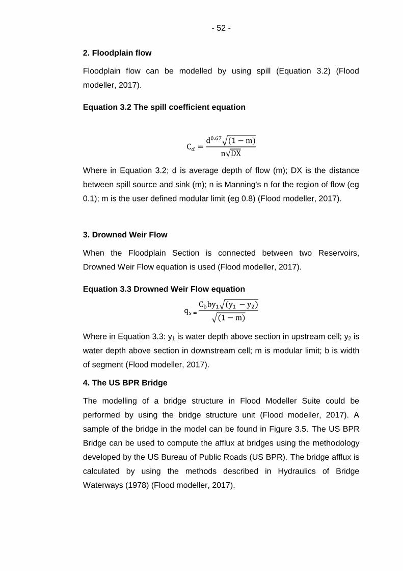
- 52 -

2. Floodplain flow

Floodplain flow can be modelled by using spill (Equation 3.2) (Flood

modeller, 2017).

Equation 3.2 The spill coefficient equation

C𝑑 =d0.67√(1 − m)

n√DX

Where in Equation 3.2; d is average depth of flow (m); DX is the distance

between spill source and sink (m); n is Manning's n for the region of flow (eg

0.1); m is the user defined modular limit (eg 0.8) (Flood modeller, 2017).

3. Drowned Weir Flow

When the Floodplain Section is connected between two Reservoirs,

Drowned Weir Flow equation is used (Flood modeller, 2017).

Equation 3.3 Drowned Weir Flow equation

qs =

Cbby1√(y1 − y2)

√(1 − m)

Where in Equation 3.3: y1 is water depth above section in upstream cell; y2 is

water depth above section in downstream cell; m is modular limit; b is width

of segment (Flood modeller, 2017).

4. The US BPR Bridge

The modelling of a bridge structure in Flood Modeller Suite could be

performed by using the bridge structure unit (Flood modeller, 2017). A

sample of the bridge in the model can be found in Figure 3.5. The US BPR

Bridge can be used to compute the afflux at bridges using the methodology

developed by the US Bureau of Public Roads (US BPR). The bridge afflux is

calculated by using the methods described in Hydraulics of Bridge

Waterways (1978) (Flood modeller, 2017).

- 53 -

Figure 3.5 Road bridge (Atkins, 2004)

To set up the bridge section into the model, a River section can be required

at the upstream of the US BPR Bridge and this point is the maximum

backwater. In addition, a River section can be required at the downstream

of the US BPR Bridge and this point has the normal water level (Flood

modeller, 2017).

Equation 3.4 The expression for computation of backwater upstream from a bridge constricting flow

h1∗ = K∗ α 2

VB2

2g+ α 1 [((

AB

A4)

2

− (AB

A1)

2

)]VB

2

2g

Where in Equation 3.4: h1* is total backwater (or afflux); K*is total backwater

coefficient; a1 is kinetic energy coefficient at the upstream section; a2 is

kinetic energy coefficient in the constriction; VB is average velocity in

constriction; AB is gross water area in constriction; A4 is water area in

downstream section; A1 is total water area in upstream section including that

produced by the backwater (Flood modeller, 2017).

- 54 -

5. Reservoir

There is Farnley flood storage reservoir in the model.

Equation 3.5 The conservation of mass equation

qnet − A(h) ∗∂h

∂t= 0

qnet = ∑ qi

N

1

Where in Equation 3.5: h is water surface elevation, 𝜕t is time step; N is

number of inflows; qi is flow at node; A is surface area of the reservoir (Flood

modeller, 2017)

6. The Rectangular Conduit

A 4-kilometre culvert was modelled on the Lower Wortley Beck area as the

Rectangular Conduit. The Rectangular Conduit is based on the Saint-Venant

equations, which express the conservation of mass and momentum of the

water body. The equations used for the Rectangular Conduit are the mass

conservation or continuity equation (Flood modeller, 2017).

The continuity and momentum equation can be expressed as Equations

(3.6) and (3.7) (Flood modeller, 2017).

Equation 3.6 Continuity Equation

∂Q

∂x+

∂A

∂t= q

Where in Equation 3.6: q is lateral inflow (m3 /s/m); Q is the flow (m3 /s); A is

cross section area of flow (m2); X is longitudinal channel distance (m); t is

time (s)

Equation 3.7 The momentum conservation or dynamic equation

∂Q

∂t+

∂

∂X(

βQ2

A) + gA

∂h

∂x− g

AQ/Q/

𝑘2= 0

Where in Equation 3.7: t is the time (s); β is the momentum correction

coefficient; g is the gravitational acceleration (m/s2); h is the water surface

elevation above datum (m) and k is channel conveyance (Flood modeller,

2017).

- 55 -

Equation 3.8 Channel conveyance (k)

k2 = A2R4/3

n2

Where in Equation 3.8: n is Manning's roughness coefficient; R is hydraulic

radius = (A/P) (Flood modeller, 2017)

The relationship between stage (water level) and discharge is normally

estimated by using Manning’s equation.

The representation of some of the hydraulic structures was simplified in

order to improve the stability of model runs.

3.2.3 2D Free Surface Shallow Water Flow Equations

TUFLOW “Classic” (Two-dimensional Unsteady FLOW) is a two-dimensional

depth-averaged hydrodynamic model. It can model free surface flow pattern

of the catchment. TUFLOW software uses the Finite Difference Alternating

Direction Implicit (ADI) solution scheme to solve the full Two-dimensional

(2D) free surface Shallow Water flow Equation (SWE). This 2D SWE

solution scheme was proposed in Stelling (1984). The Stelling`s (1984)

scheme is an alternating direction implicit finite difference based on the well-

established Leendertse`s (1967, 1970) schemes (Syme, 1992). The 2D

SWE consist of continuity and conservation of momentum equations in the

horizontal x and y directions in Cartesian coordinates (Syme 1992; Krupka,

et al., 2007; BMT WMB, 2010; Abdullah 2012).

The 2D Continuity equation

Equation 3.9 The 2D Continuity

0 = y

(Hv) +

x

(Hu) +

t

ζ

- 56 -

Equation 3.10 X Momentum

F = x

p

ρ

1

y

u +

x

u μ - v + u

2gΔg

f

H

n u g

+ x

ζ g + v c -

y

u v +

x

u u +

t

u

x2

2

2

222l

34

2

f

Equation 3.11 Y Momentum

F = y

p

ρ

1

y

v +

x

v μ - v + u

2gΔg

f

H

n v g

+ y

ζ g + u c

y

v v +

x

v u +

t

v

y2

2

2

222l

34

2

f

Where in Equation 3.9, 3.10 and 3.11: ζ is water surface elevation; u and v

are depth averaged velocity components in X and Y directions; H is depth of

water; t is Time; x and y is distance in X and Y directions; Δx and Δy are cell

Dimensions in X and Y directions; Cf is Coriolis force coefficient; n is

Manning`s n; ƒi is Form (Energy) Loss coefficient; p is Atmospheric

pressure; ρ is density of water; Fx and Fy is sum of components of external

forces (eg.the wind) in X and Y directions (BMT WMB, 2010).

In TUFLOW, the solutions of these equations proceed in stages: Stage 1

has two steps; Step 1 involves solving the momentum equation in the y-

direction for the v-velocities. The equation is solved using a

predictor/corrector method, which involves two sweeps. For the first sweep,

the calculation proceeds column by column in the y-direction. If the signs of

all velocities in the x-direction are the same the second sweep is not

necessary, otherwise the calculation is repeated sweeping in the opposite

direction (BMT WMB, 2010).

The second step of Stage 1 solves for the water levels and x-direction

velocities by solving the equations of mass continuity and of momentum in

the x-direction. A tridiagonal equation is obtained by substituting the

momentum equation into the mass equation and eliminating the x-velocity.

- 57 -

The water levels are calculated and back substituted into the momentum

equation to calculate the x-velocities. Stage 2 proceeds in a similar manner

to Stage 1 with the first step using the X-direction momentum equation and

the second step using the mass equation and the Y-direction momentum

equation (BMT WMB, 2010).

3.2.4 Estimation of the inflow hydrographs

After set–up the 1D/2D hydrodynamic model, inflow hydrographs were

computed and entered into the model. Inflow hydrograph displayed the

discharge from the outflow points of the Farnley Beck (FB) and Farnley

Wood Beck (FWB) basins into the Lower Wortley Beck. Inflow hydrograph

was estimated by using event-based approach because the catchment did

not have sufficient measured flow data. The hydrographs can be computed

by using the rainfall-runoff model in the ungauged catchments. Therefore,

inflow hydrographs were estimated by using the ReFH rainfall-runoff

method. This model was applied by using revitalised boundary unit of the

Flood Modeller Suite tool in this research.

The Revitalised Flood Hydrograph (ReFH) FSR/FEH method was generated

by the Centre for Ecology and Hydrology. This method has been used since

2006 for the UK catchments. This flood estimation method can be applied to

catchments that are bigger than 0.5 km2. This method consists of three main

processes. These are Loss model (Cmax), Routing model (Tp) and Baseflow

model (Kjeldsen et al., 2005).

The loss model is used to estimate the net rainfall from total rainfall. Then,

the direct runoff is entered into the routing model. Lastly, the Baseflow is

added and total discharge into the river channel can be obtained (Kjeldsen

et al., 2005).

1. The Critical Storm Duration

To design the fluvial flood events, storm durations (D) for FB and FWB

basins were calculated from the response time of the catchment (time to

peak, Tp) and the general wetness of the catchment (the standard average

annual rainfall, SAAR) from Equation 3.12

- 58 -

Equation 3.12 The Critical Storm Duration

D = TP(1 + SAAR

1000)

Where in Equation 3.12 (Houghton-Carr, 1999): D is the Critical Storm

Duration (h)

Secondly, the response time of the catchment (time to peak, Tp) was

calculated to calculate the critical storm duration (h).

TP = Time to Peak (h)

Equation 3.13 Time to Peak

Tp = 1.563 ∗ PROPWET−1.09 ∗ DPLBAR0.60 ∗ (1 + URBEXT)−3.34 ∗ DPSBAR−0.28

Where in Equation 3.13 (Kjeldsen, 2007): DPLBAR is mean drainage path

length (km); DPSBAR is mean of all the inter-nodal slopes for the catchment

(m/km); PROPWET is index of proportion of time that soils are wet; SAAR is

Standard Period Average Annual Rainfall (mm); SPRHOST is Standard

Percentage Runoff (%) derived using HOST classification; URBEXT1990 is a

FEH index of urban and suburban land cover in 1990 (Houghton-Carr, 1999;

Kjeldsen, 2007).

Storm duration for critical flood peak was produced by using catchment

descriptors.

1.1 Catchment descriptors

The catchment descriptors were obtained from the FEH CD-ROM 3.0 (CEH,

2009) by using Easting-Northing coordinates (Table 3.2).

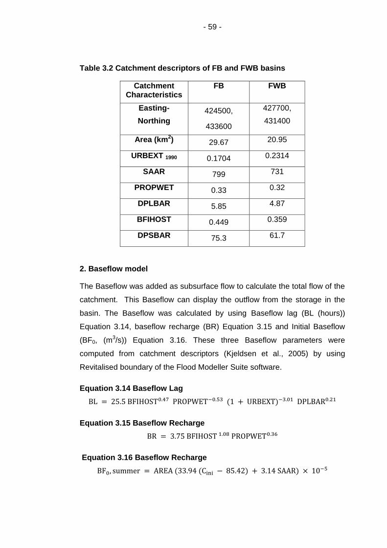
- 59 -

Table 3.2 Catchment descriptors of FB and FWB basins

Catchment Characteristics

FB FWB

Easting-

Northing

424500,

433600

427700,

431400

Area (km2) 29.67 20.95

URBEXT 1990 0.1704 0.2314

SAAR 799 731

PROPWET 0.33 0.32

DPLBAR 5.85 4.87

BFIHOST 0.449 0.359

DPSBAR 75.3 61.7

2. Baseflow model

The Baseflow was added as subsurface flow to calculate the total flow of the

catchment. This Baseflow can display the outflow from the storage in the

basin. The Baseflow was calculated by using Baseflow lag (BL (hours))

Equation 3.14, baseflow recharge (BR) Equation 3.15 and Initial Baseflow

(BF0, (m3/s)) Equation 3.16. These three Baseflow parameters were

computed from catchment descriptors (Kjeldsen et al., 2005) by using

Revitalised boundary of the Flood Modeller Suite software.

Equation 3.14 Baseflow Lag

BL = 25.5 BFIHOST0.47 PROPWET−0.53 (1 + URBEXT)−3.01 DPLBAR0.21

Equation 3.15 Baseflow Recharge

BR = 3.75 BFIHOST 1.08 PROPWET0.36

Equation 3.16 Baseflow Recharge

BF0, summer = AREA (33.94 (Cini − 85.42) + 3.14 SAAR) × 10−5

- 60 -

Where in Equation 3.14, 3.15, and 3.16 (Kjeldsen, 2007): BFIHOST is

Baseflow Index derived by using the UK Hydrology of Soil Types (HOST)

classification; Cini is initial loss; AREA is Catchment Area (km2)

3.2.5 Assessment of the land use change and fluvial flood risk

The components of the water balance can be influenced by land-use change

(Piao et al., 2007; Kumar et al., 2017). The urbanisation of the sub-

catchments could have a significant impact on the fluvial flood risk. Kumar

(2017) found that annual surface runoff rose evidently due to the expansion

in urbanisation over the years. This situation can be observed at sub-

catchment level as well. The impact on the water balance of the sub-

catchment can be determined like that infiltration decreases and surface

runoff increases (Kumar et al., 2017). This could result in increased river

discharge worldwide (Piao et al. 2007). Kumar et al. (2017) stated that the

variety and concentration of vegetation land cover could be one of the

important parameters to affect the surface runoff and evapotranspiration.

WMO and GWP (2008) added that soil, vegetation cover, and land use have

a direct impact on the amount of runoff generated. The water balance can be

managed by using some land-use management practices and sustainable

drainage systems (Kumar et al., 2017). Putro (2013) investigated the impact

of urbanisation on the river system and water quality by analysing the rainfall

and Urban Extent (URBEXT) values with the changes in the river flow, river

temperature, and dissolved oxygen.

As considered the above knowledge, the impact of surface runoff of a sub-

catchment on the discharge hydrograph at the outfall of the sub-catchment

could be observed. In addition, the relationship between the land use

change of a sub-catchment and fluvial flood risk of the downstream location

can be investigated.

A part of this research focused to investigate the effects of land use change

on the fluvial flood risk. The impact of the land use change was assessed by

changing the ratio of the impermeable surfaces thus, surface runoff can be

observed. This link was obtained by using urban extent (URBEXT)

catchment parameter and 1D/2D hydrodynamic fluvial model in this

- 61 -

research. The URBEXT parameter was used to manage the ratio of the

impermeable surface in a catchment.

Inflow hydrographs were estimated for different URBEXT values. Firstly, the

URBEXT value was increased to assess the impact of the urbanisation. The

1990-year and the 2016-year of URBEXT values were used. Secondly, the

URBEXT value was decreased to assess the impact of the Sustainable

Urban Drainage Systems (SUDS). Thus, the change of the impermeable

surface of the sub-catchment on the discharge hydrograph at the outfall of

the sub-catchment could be examined in this research.

Consequently, the impact of the ratio of the impervious surface of sub-

catchments (Farnley Beck and Farnley Wood Beck basins) on the flood risk

of the downstream area (between The Ring Road and the Gelderd Road,

and M621 in Figure 3.16) was assessed.

A. Urbanisation of the sub-catchment and fluvial flood risk

Urban extent is calculated for the 2016 year for two sub-catchments so the

impact of future urbanisation on the fluvial flood risk could be assessed by

using the Equation 6.8 on Page 53 in FEH VOL 5 (Bayliss, 1999).

Equation 3.17 Urbanisation expansion factor (UEF)

UEF= 0.8165+ 0.2254 TAN-1 {(YEAR-1967.5) /21.25}

URBEXT1990 values (obtained from the FEH CD-ROM) were adjusted, by

using the Urbanisation Expansion Factor (UEF) according to the year of

2016.

The urban extent of the Farnley Beck (FB) sub-catchment was calculated by

using the Equation 3.17, as 0.275 and urban extent of the Farnley Wood

Beck (FWB) sub-catchment was calculated as 0.375 for the year of 2016.

B. Reducing the ratio of impermeable surface of the sub-catchment

In this section of the research, the relationship between the ratio of the

impermeable surface and discharge at the outfall of the sub-catchment was

assessed by decreasing the ratio of the impermeable surface in the sub-

catchment. This part can be used to analyse the impact of the sustainable

urban drainage systems on the fluvial flood risk.

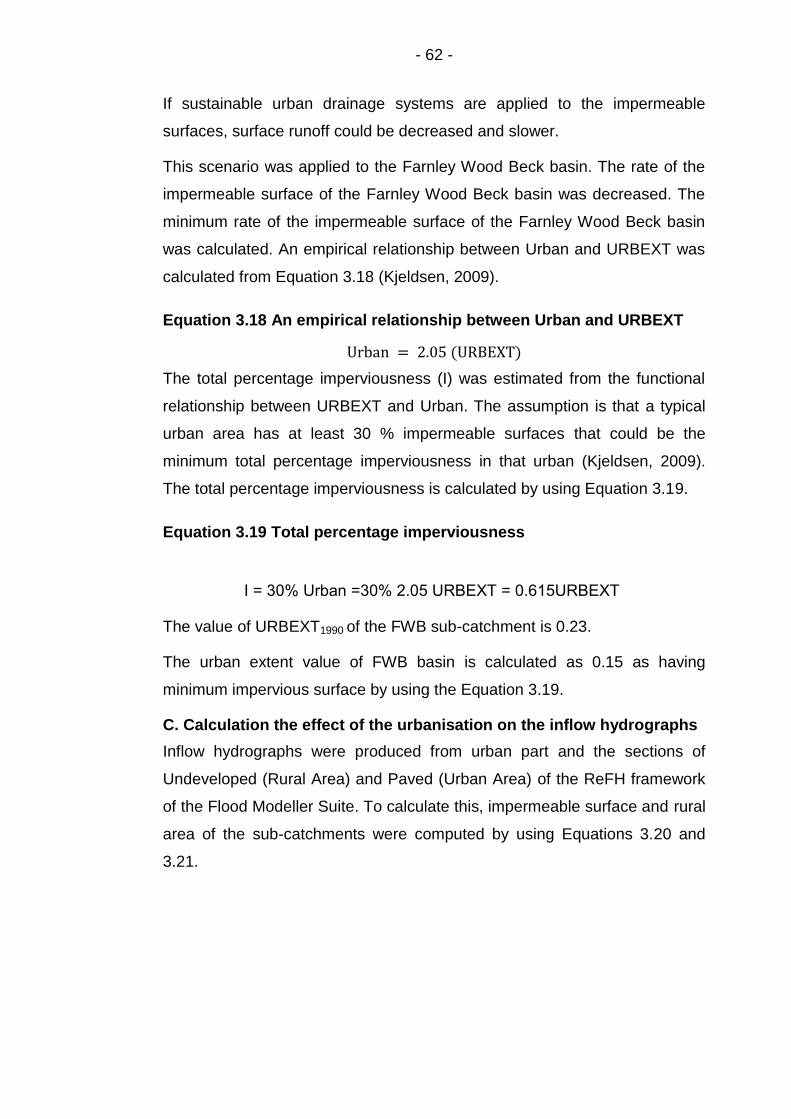
- 62 -

If sustainable urban drainage systems are applied to the impermeable

surfaces, surface runoff could be decreased and slower.

This scenario was applied to the Farnley Wood Beck basin. The rate of the

impermeable surface of the Farnley Wood Beck basin was decreased. The

minimum rate of the impermeable surface of the Farnley Wood Beck basin

was calculated. An empirical relationship between Urban and URBEXT was

calculated from Equation 3.18 (Kjeldsen, 2009).

Equation 3.18 An empirical relationship between Urban and URBEXT

Urban = 2.05 (URBEXT)

The total percentage imperviousness (I) was estimated from the functional

relationship between URBEXT and Urban. The assumption is that a typical

urban area has at least 30 % impermeable surfaces that could be the

minimum total percentage imperviousness in that urban (Kjeldsen, 2009).

The total percentage imperviousness is calculated by using Equation 3.19.

Equation 3.19 Total percentage imperviousness

I = 30% Urban =30% 2.05 URBEXT = 0.615URBEXT

The value of URBEXT1990 of the FWB sub-catchment is 0.23.

The urban extent value of FWB basin is calculated as 0.15 as having

minimum impervious surface by using the Equation 3.19.

C. Calculation the effect of the urbanisation on the inflow hydrographs

Inflow hydrographs were produced from urban part and the sections of

Undeveloped (Rural Area) and Paved (Urban Area) of the ReFH framework

of the Flood Modeller Suite. To calculate this, impermeable surface and rural

area of the sub-catchments were computed by using Equations 3.20 and

3.21.

- 63 -

Equation 3.20 Undeveloped (Rural Area)

Undeveloped area = (AREA - (AREA*URBEXT))

Equation 3.21 Paved (Urban Area)

Paved area = (AREA*URBEXT)

In this study, the developed area was accepted as paved, drawing towards

watercourse. Runoff was accepted 70 percent for impermeable surfaces

(Flood modeller, 2017).

Table 3.3 Urbanisation of Farnley Beck (FB) basin

URBEXT

value

(1990yr)

0.17

(2016yr)

0.275

Undeveloped

(km2)

24.6 21.5

Urban( km2 ) 5.0 8.13

Table 3.4 Urbanisation of Farnley Wood Beck (FWB) basin

URBEXT

value

(SUDs)

0.15

(1990yr)

0.23

(2016yr)

0.375

Undeveloped (km2)

17.81 16.10 13.09

Urban (km2) 3.14 4.85 7.86

According to the above assumptions, Urban (impermeable surface) and

Undeveloped (permeable surface) of Farnley Beck (FB) basin (Table 3.3),

and Farnley Wood Beck (FWB) basin (Table 3.4) were computed.

- 64 -

3.3 Calibration of the fluvial flood model

The fluvial model of the Lower Wortley Beck was tested for the credibility of

the results in this section. The calibration process was the comparison of the

measured data of the Pudsey gauge station to the predicted results from the

fluvial model of the Lower Wortley Beck.

Measured water level data was taken from Pudsey gauge station and

measured rainfall data was taken from Headingley, Knostrop and

Heckmondwike gauge stations. These datasets were provided by

Environment Agency during this research.

The predicted results from the fluvial model of the Lower Wortley Beck were

computed for the same location as the Pudsey gauge station (Figure 3.6).

Figure 3.6 The location of Pudsey gauge station

Figure 3.6 displays the location of the Pudsey stage gauge station. This

location presents both observation point and computed point.

- 65 -

According to the data quality and historical flood events, the data of

06/07/2012 date and 24/09/2012 date were selected. Measured rainfall data

from Headingley, Knostrop and Heckmondwike gauge stations were

assessed for these dates and were adjusted by using mean precipitation

theory (Thiessen method) for the catchment area. To calibrate the model,

firstly, measured rainfall data was entered into the ReFH rainfall-runoff

framework tool of the Flood Modeller Suite. Hydrograph was produced for

each Farnley Beck and Farnley Wood Beck basins. Inflows from these sub-

catchments into the Lower Wortley Beck were computed by using this

rainfall data. Next step was to enter these inflow hydrographs into the fluvial

model of the Lower Wortley Beck and to compute water depth for the

Pudsey Location.

1. 06/07/2012 Event day for calibration

Figure 3.7 06/07/2012 Date input data

Calibration input data of the 06/07/2012 date can be seen in Figure 3.7

0

2

4

6

8

100

5

10

15

20

25

30

35

40

02

.5 57

.5 10

12.5 15

17.5 20

22.5 25

Flo

w (

m3/s

)

Time (h)

06/07/12 Date input data 06/07/12MeasuredRainfall(mm)

FB Inflow

FWB Inflow

Rain

fall

dep

th (

mm

)

- 66 -

Figure 3.8 Water depth (m) from 06/07/2012 event day

The measured water depth (m) data from observed Pudsey gauge station

and the computed water depth (m) data from the Lower Wortley Beck fluvial

model were compared for 06/07/2012 event day. Maximum measured water

depth is 0.9 m, and maximum computed water depth is 0.7 m (Figure 3.8).

2. 24/09/2012 event day for calibration

Figure 3.9 Figure 3.9 24/09/2012 Event Date input data

Calibration input data of the 24/09/2012 date can be seen in Figure3.9.

00.10.20.30.40.50.60.70.80.9

1

03

.25

6.5

9.7

51

31

6.2

51

9.5

22.7

52

62

9.2

53

2.5

35.7

53

94

2.2

54

5.5

Wa

ter

dep

th(m

)

Time (h)

06-07/07/2012 Data 06-07/07/2012MeasuredWaterDepth (m)

ComputedWaterDepth (m)

0.0

0.5

1.0

1.5

2.0

2.5

3.00

5

10

15

20

25

30

0

2.2

5

4.5

6.7

5 9

11.3

13.5

15.8 18

20.3

22.5

24.8 27

29.3

infl

ow

(m

3/s

)

Time(h)

MeasuredRainfall(mm)

inflow FB

inflow FWB

Rain

fall

dep

th

(mm

)

24/09/2012 Data

- 67 -

Figure 3.10 Water depth (m) from 24/09/2012 event day

The measured water depth (m) data from observed Pudsey gauge station

and the computed water depth (m) data from the Lower Wortley Beck fluvial

model were compared for 24/09/2012 event day. Maximum measured water

depth is 1.1 m, and maximum computed water depth is 0.7 m (Figure 3.10).

The differences could be because the geomorphology of the river channel

could not be displayed exactly in the model.

3.4 Results and Discussions

Catchment response time (time to peak (TP)) and storm duration (D) of

Farnley Beck (FB) and Farnley Wood Beck (FWB) basins were calculated to

estimate inflow hydrographs of the Lower Wortley Beck. Ungauged

catchment equations of the ReFH rainfall-runoff method (Kjeldsen, 2007)

were used.

URBEXT1990 values of the FB and FWB basins are 0.17 and 0.23

respectively. Catchment response time of the FB and FWB basins are 2.7 h

and 2.2 h respectively. The estimated rainfall duration values of the FB and

FWB basins are 4.8 h and 3.8 h respectively. The urban area of FB basin is

5.06 km2, and FWB basin is 4.8 km2 in 1990 yr.

0

0.2

0.4

0.6

0.8

1

1.2

04

.25

8.5

12.7

51

72

1.2

52

5.5

29.7

53

43

8.2

54

2.5

46.7

55

15

5.2

5

Wa

ter

dep

th (

m)

Time (h)

24-25/09/2012 Date

Measured 24-25/09/2012Water Depth(m)

ComputedWaterDepth(m)

- 68 -


respectively. Catchment response time of the FB and FWB basins are 2.0 h

and 1.5 h respectively. The estimated rainfall duration values of the FB and

FWB basins are 3.6 h and 2.64 h respectively

While the ratio of impervious surface increases (URBEXT values), both time

to peak and rainfall duration decrease so that catchment response becomes

faster.

The above rainfall duration (h) and time to peak values (h), and the URBEXT

values were used to obtain the inflow hydrographs. Inflows from FB and

FWB basins into the Lower Wortley Beck were computed. Inflow

hydrographs were produced to display the discharge from FB and FWB sub-

catchments into the Lower Worley Beck. The results were displayed by

producing probabilistic flood inundation maps. The background of Figure

3.12, 3.18, 3.19, 3.23, 3.24, 3.28, 3.30 and 3.32 were produced by using OS

1:25 000 Scale Colour Raster and contain OS data © Crown copyright and

database right (2015) (Ordnance Survey, 2015). Arc MAP 10.2.2 tool was

used to produce these maps.

3.4.1 Fluvial Flood Risk at the Lower Wortley Beck

The hydrographs were estimated for a 1% annual exceedance probability

(AEP) event by using the ReFH rainfall-runoff method. In addition to this,

URBEXT1990 value was used for FB and FWB basins. Inflow hydrographs

were displayed in Figure 3.11.

Figure 3.11 Inflow hydrographs

25.9 23.1

0

5

10

15

20

25

30

0 5 10 15 20

Flo

w (

m3/s

)

Time(h)

FB Inflow FWB Inflow

- 69 -

The peak flow of FB basin hydrograph is 26 m3/s at the 4th hour of simulation

(Figure 3.11). Peak flow of FWB basin hydrograph is 23 m3/s at the 3.4th

hour of simulation (Figure 3.11).

Figure 3.12 Flood inundation map

This above probabilistic flood inundation map was created to display flood

extent for the 1 in 100-year event by using the URBEXT1990 value of the sub-

catchments (Figure 3.12).

This event was analysed in detail in Figure 3.13, Figure 3.14 and Figure 3.15

maps.

- 70 -

Figure 3.13 ReFH URBEXT1990 1% AEP (flood movements)

Background of Figure 3.13 that is street view contains OS data © Crown

copyright and database right (2013) (Ordnance Survey, 2013).

- 71 -

Figure 3.14 Fluvial flooding 1 % AEP (water depth / stages)

Figure 3.15 Fluvial flooding 1 % AEP (velocity / stages)

- 72 -

Figure 3.13, Figure 3.14, and Figure 3.15 display fluvial flooding at different

times (hour) of the simulation. According to fluvial flood inundation maps in

Figure 3.15, Lower Wortley Beck area, specifically, the Gelderd Road, Ring

road, and A62 road were observed as primary flood risk areas.

Flood event began at between the Ring road and the A58 Road. Later water

cumulated at the Lower Wortley Beck area between the A6110 and the

M621 on the Gelderd Road. The reason of this flood could be the limitation

of the culvert and reservoir capacity, and so backwater effect was observed.

Figure 3.16 Flood risk area

Figure 3.16 presents the map of the Lower Wortley Beck, Leeds, and West

Yorkshire (Google Map, 2015). It shows the areas that would be inundated

by the flooding of the 1 in 100-year event. The map can be used to identify

the built-up locations in the fluvial flood risk. According to the baseline

results, primary risk places were determined. It was seen that there are

developing places in the fluvial risk location such as industrial and residential

settlements. In addition, there is an important transportation link.

Consequently, fluvial flood risk should be managed for this area.

- 73 -

3.4.2 The impact of land-use change of sub-catchment on the

fluvial flood risk

The impact of Farnley Wood Beck (FWB) basin on fluvial flood risk of the

Lower Wortley Beck area was observed.

Below scenarios were created

1. There is no inflow from FWB sub-catchment into the system

2. The impervious surface ratio of FWB basin is 0.375

The impervious surface ratio of FWB basin was changed from 0.23 that is

the URBEXT value of the 1990 year, to 0.375 URBEXT value of the 2016

year to assess the future land-use change.

3. The impervious surface ratio of FWB basin is 0.15

The impervious surface ratio of FWB basin is 0.23. It was decreased to the

0.15. The ratio of the impermeable surface was decreased to assess the

discharge from FWB.

This assumption can be accepted like that if sustainable urban drainage

systems (SUDS) were applied in the Farnley Wood Beck basin, the ratio of

the impermeable surface would decrease, and the discharge would be

affected.

The limitation of this method that it is an approximate value, also specific

flood resilience methods and their locations could not be observed and

assessed.

Farnley Beck basin was kept the same as the value of the URBEXT of the

1990 year and the 1 in 50-year event of the inflow hydrograph was used

(Figure 3.17).

The inflow hydrographs were estimated for the 1 in 15-year, 1 in 50-year,

and 1 in 100-year fluvial flood event for both the baseline and proposed

scenarios. To observe this risk, 15-year return period created low flood risk,

whereas the 1 in 100-year event created a big flood event and it was an

obvious flood risk. Therefore, to observe the influence of Farnley Wood Beck

basin on downstream location a 2% AEP flood event was analysed.

- 74 -

The impermeable surfaces of the Farnley Wood Beck basin were computed

for each scenario. The ratios of the impermeable surface are 0.15, 0.23, and

0.375 respectively and the area of impermeable surfaces of the FWB basin

is 3 km2, 4.8 km2, and 7.86 km2 at each urban percent scenarios.

Figure 3.17 Inflows for a 2 % AEP for each URBEXT

Figure 3.17 indicates the inflow values (m3/s) from the Farnley Wood Beck

(FWB) sub-catchment for each URBEXT values. Peak flows of inflow

hydrograph from the FWB are 14 m3/s, 19 m3/s and 29 m3/s respectively for

a 2 % AEP flood event.

29.4

13.6

18.9 21.8

0

5

10

15

20

25

30

350

1.2

2.4

3.6

4.8 6

7.2

8.4

9.6

10.8 12

13.2

14.4

15.6

16.8 18

19.2

20.4

Flo

w (

m3/s

)

Time (h)

FWB 50yr. URBEXT0.375

FWB 50yr. URBEXT0.23

FWB 50yr. URBEXT 0.15

FB 50yr. URBEXT 0.17

- 75 -

Figure 3.18 Flood extent of no inflow from FWB

Scenario 1 was applied and the flood inundation map in Figure 3.18 was

produced.

Figure 3.19 Flood extent of inflow from URBEXT2016 of FWB

- 76 -

Scenario 2 was applied and the flood inundation map in Figure 3.19 was

produced.

It can be observed that there is a significant impact from Farnley Wood sub-

catchment on the Lower Wortley Beck fluvial flood risk. In addition,

backwater flow movement might be observed at the Lower Wortley Beck

area due to the inflow from Farnley Wood Beck, and in consequence of

limited culvert capacity. Lastly, Farnley Wood Beck basin has been

developing, and urbanisation is expected to be much more in the future.

Figure 3.20 Water depth percentage (%)

Figure 3.20 indicates the water depth percentage (%) in the flood inundation

area for each scenario of FWB sub-catchment. When the URBEXT value

increases, water depth at the flood inundation area can become higher.

0%

10%

20%

30%

40%

50%

60%

70%

80%

90%

100%

FWB0.15 FWB0.23 FWB0.375

Wa

ter

dep

th p

erc

en

tag

e(%

)

FWB URBEXT values

1- <

0.8-1 m

0.6-0.8 m

0.4-0.6 m

0.2-0.4 m

0-0.2 m

Water depth (m)

2% AEP

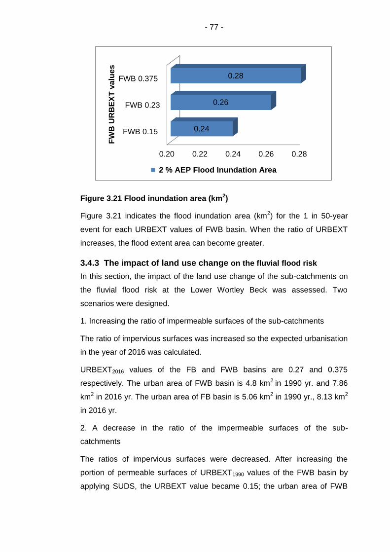
- 77 -

Figure 3.21 Flood inundation area (km2)

Figure 3.21 indicates the flood inundation area (km2) for the 1 in 50-year

event for each URBEXT values of FWB basin. When the ratio of URBEXT

increases, the flood extent area can become greater.

3.4.3 The impact of land use change on the fluvial flood risk

In this section, the impact of the land use change of the sub-catchments on

the fluvial flood risk at the Lower Wortley Beck was assessed. Two

scenarios were designed.

1. Increasing the ratio of impermeable surfaces of the sub-catchments

The ratio of impervious surfaces was increased so the expected urbanisation

in the year of 2016 was calculated.


respectively. The urban area of FWB basin is 4.8 km2 in 1990 yr. and 7.86

km2 in 2016 yr. The urban area of FB basin is 5.06 km2 in 1990 yr., 8.13 km2

in 2016 yr.

2. A decrease in the ratio of the impermeable surfaces of the sub-

catchments

The ratios of impervious surfaces were decreased. After increasing the

portion of permeable surfaces of URBEXT1990 values of the FWB basin by

applying SUDS, the URBEXT value became 0.15; the urban area of FWB

0.20 0.22 0.24 0.26 0.28

FWB 0.15

FWB 0.23

FWB 0.375

0.24

0.26

0.28

FW

B U

RB

EX

T v

alu

es

2 % AEP Flood Inundation Area

- 78 -

basin became 3.14 km2. Whereas, the SUDS was not applied into the FB

basin because its URBEXT1990 value is already very small that is 0.17.

These scenarios were applied for the 1 in 100-year event.

Figure 3.22 Inflow hydrographs of FWB and FB

Figure 3.22 displays the inflows from FWB and FB sub-catchments for the 1

in 100-year event for each URBEXT values. The peak flow of the inflow

hydrograph from FB sub-catchment is 39 m3/s and URBEXT value is 0.27

for the year of 2016 (Figure 3.22). The peak flow of the inflow hydrograph

from FWB sub-catchment is 35 m3/s and URBEXT value is 0.375 for the

year of 2016 (Figure 3.22). The peak flow of the inflow hydrograph from

FWB sub-catchment is 16 m3/s and URBEXT value is 0.15 with SUDS

(Figure 3.22).

0

10

20

30

400

1.4

2.8

4.2

5.6 7

8.4

9.8

11.2

12.6 14

15.4

16.8

18.2

19.6

Flo

w (

m3/s

)

Time (h)

URBEXT values

FB URBEXT0.27

FWB URBEXT0.375

FWB URBEXT0.15

- 79 -

Figure 3.23 Flood extent of inflow from URBEXT2016 of FWB and FB

sub-catchments

Figure 3.23 indicates the flood extent for the 1 in 100-year event. Inflows

hydrographs were estimated for the URBEXT value of FWB basin was

0.375, and URBEXT value of FB basin was 0.27.

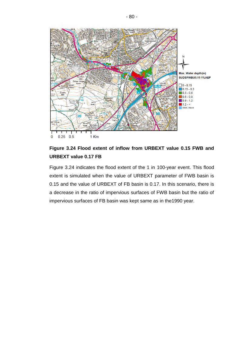
- 80 -

Figure 3.24 Flood extent of inflow from URBEXT value 0.15 FWB and

URBEXT value 0.17 FB

Figure 3.24 indicates the flood extent of the 1 in 100-year event. This flood

extent is simulated when the value of URBEXT parameter of FWB basin is

0.15 and the value of URBEXT of FB basin is 0.17. In this scenario, there is

a decrease in the ratio of impervious surfaces of FWB basin but the ratio of

impervious surfaces of FB basin was kept same as in the1990 year.

- 81 -

Figure 3.25 Water depth percentage (%)

According to the impact of the land use change of the sub-catchments,

maximum water depth (m) was computed. Figure 3.25 indicates maximum

water depth percentages of these scenarios. It seems that SuDS did not

have a significant impact on the water depth values in the flood extent. It is

similar to the scenario of URBEXT 1990 values. Whereas, urbanisation has a

significant impact on the water depth values (m). Water depth became

higher in the flood extent.

Figure 3.26 Flood Inundation area (km2)

79% 78%

68%

21% 22%

32%

1%

60%

65%

70%

75%

80%

85%

90%

95%

100%

(URBEXTSuDS) URBEXT1990 URBEXT2016Wa

ter

dep

th p

erc

en

tag

e(%

)

URBEXT values

2- <

1 - 2

0 - 1

Water depth (m) 1% AEP

0.53

0.39

0.38

0.00 0.20 0.40 0.60

Flood Inundation Area (km2)

URBEXT

(SuDS)

1990 yr.

2016 yr.

- 82 -

Flood extent area reached to 0.53 km2 when urbanisation increased in the

catchment (Figure 3.26). However, flood extent area can be decreased to

the 0.38 km2 by applying SUDS.

3.4.4 The impact of rainfall duration on the fluvial flood risk

The impact of the rainfall duration on the inflow hydrograph and downstream

fluvial flood risk was investigated in this section. Inflow hydrographs were

produced to display the discharge from FB and FWB sub-catchments into

the Lower Worley Beck. The hydrographs were estimated for a 1% annual

exceedance probability (AEP) event by using the ReFH rainfall-runoff

method. In addition to this, URBEXT of the 1990 year was used for FB and

FWB basins. The length of the rainfall events in the FB and FWB basins

were changed from 0.5 hr. to 1 hr., and then to 6 hr.

1.) Rainfall duration is 0.5 hour in the Wortley Beck catchment

Figure 3.27 Inflow hydrographs for 0.5-hour rainfall duration

Figure 3.27 indicates the inflow hydrographs of the sub-catchments and for

0.5 h rainfall duration for the 1 in 100-year event. The peak flow of inflow

hydrograph of FB sub-catchment is 17.9 (m3/h) and FWB sub-catchment is

17.05 (m3/h).

0

5

10

15

20

0.0

1.2

2.4

3.6

4.8

6.0

7.2

8.4

9.6

10.8

12.0

13.2

14.4

15.6

Flo

w (

m3/s

)

Time (h)

inflow FB100yr0.5h

inflow FWB100yr0.5h

- 83 -

Figure 3.28 Flood extent from 0.5-hour rainfall duration

Fluvial flood inundation area of the 0.5-hour rainfall duration at the Lower

Wortley Beck area can be seen in Figure 3.28. Inflow hydrographs were

computed for URBEXT1990 and for a 1 % AEP. This event does not have a

significant flood risk at the Gelderd Road.

2.) Rainfall duration is 1 hour in the Wortley Beck catchment

Figure 3.29 Inflow hydrographs for 1-hour rainfall duration

Figure 3.29 indicates the inflow hydrographs of the sub-catchments and for

one-hour rainfall duration for the 1 in 100-year event.

0

5

10

15

20

25

0.0

1.6

3.2

4.8

6.4

8.0

9.6

11.2

12.8

14.4

16.0

Flo

w (

m3/s

)

Time (h)

inflow FB 100yr1h

inflow FWB100yr 1h

- 84 -

Peak flow of inflow hydrograph of FB sub-catchment is 21.6 (m3/h), and

FWB sub-catchment is 20.08 (m3/h). Fluvial flood inundation area at the

Lower Wortley Beck can be seen in Figure 3.30.

Figure 3.30 Flood extent from 1-hour rainfall duration

Figure 3.30 displays the flood extent from 1-hour rainfall duration and inflow

hydrographs were produced from URBEXT1990 and for a 1 % AEP flood

event.

- 85 -

3.) Rainfall duration is 6hour in the Wortley Beck catchment

Figure 3.31 Inflow hydrographs for 6-hour rainfall duration

Figure 3.31 indicates the inflows from the sub-catchments, for 6-hour rainfall

duration and for the 1 in 100-year event. Peak Inflow value of FB sub-

catchment is 25.74 (m3/h), and Peak inflow value of FWB sub-catchment is

22.59 (m3/h). Fluvial flood extend at the Lower Wortley Beck area can be

seen in Figure 3.32.

0

5

10

15

20

25

30

0.0

1.6

3.2

4.8

6.4

8.0

9.6

11.2

12.8

14.4

16.0

17.6

19.2

20.8

Flo

w(m

3/s

)

Time (h)

inflow FB 100yr 6h

inflow FWB 100yr6h

- 86 -

Figure 3.32 Flood extent of 6-hour rainfall duration

Flood inundation area of the rainfall event of the rainfall duration (6-hour) is

the biggest one when the rainfall event duration becomes smaller; flood

inundation area is also smaller (Figure 3.33). When rainfall duration event is

0.5-hour flood inundation area is 0.07 km2. When rainfall duration event is 6-

hour, flood inundation area is 0.4 km2.

Figure 3.33 Fluvial flood inundation Area (km2) for each rainfall

duration (h) for a 1% AEP

0.07

0.17

0.43

0.00 0.10 0.20 0.30 0.40 0.50

0.5h

1h

6h

Fluvial Flood inundation Area (km2)

Sto

rm D

ura

tio

n

(h)

- 87 -

Figure 3.34 Water depth percentage (%) for each rainfall duration (hr.)

Figure 3.34 displays that water depth percentage (%) in the flood inundation

area at the Lower Wortley Beck area. The flood inundation area was

simulated by using the 1 in 100-year event. Flood event was created by

using 0.5 hr., 1 hr., and 6hr., rainfall duration. 6-hour rainfall duration

created higher floodwater depth than 1-hour and 0.5-hour rainfall duration.

Water depth levels become greater when the rainfall duration become longer

in the catchment.

89%

77%

35%

8%

22%

36%

2.47% 1.45%

29.07%

30%

40%

50%

60%

70%

80%

90%

100%

0.5hr. 1hr. 6hr.

Wa

ter

dep

th p

erc

en

tag

e (

%)

1% AEP Water

Depth (m)

Rainfall Duration (hr.)

1.0 m- <

0.5 - 1.0 m

0 - 0.5 m

- 88 -

3.5 Conclusion

The fluvial flood event of the Lower Wortley Beck is a sample fluvial flooding

from an urban stream. The Lower Wortley Beck area has a severe level of

fluvial flood risk and new developments can be found on the floodplains in

the area. Therefore, fluvial flood risk can be more series in the future.

The impact of the inflows from sub-catchments of the Wortley Beck

catchment on the downstream fluvial flood risk was assessed in this

research. The assessment of the Lower Wortley Beck fluvial flood risk

insisted in two main sections. These were that the impact of the land-use

change of sub-catchments and the impact of rainfall event duration in the

sub-catchments.

The land-use change scenarios were used to display the impact of the

urbanisation and sustainable urban drainage systems of the sub-catchment

on the discharge at the outfall of the sub-catchment. This approach can be

useful to have an assumption between the ratio of the impermeable surfaces

and its impact on the discharge from the basin.

The impact of the rainfall duration on the downstream fluvial flood risk was

assessed as well in this chapter. This approach can be useful to have an

assumption between the rainfall event and runoff. Thus, interdependency

can be established between surface runoff and discharge in urbanised and

ungauged catchments.

The assessment of fluvial flood risk was performed with the probabilistic

fluvial flood inundation maps and the maximum water depth (m).

The contributions of this chapter are that

1. The hydrological modelling part of the 1D/2D hydraulic model of Lower

Wortley Beck catchment was updated.

Inflow hydrographs were estimated by using the ReFH rainfall-runoff

method. Inflows from sub-catchments were produced for different scenarios

such as return periods and the critical rainfall duration (h) in this research

section.

- 89 -

2. The 1D/2D hydraulic model of Lower Wortley Beck was calibrated.

3. The impact of the ratio of the impermeable surface and the rainfall

duration on the fluvial flooding risk were analysed in the Lower Wortley Beck

location.

The urbanisation level (URBEXT) of the sub-catchments has a significant

impact on the fluvial flood extent and magnitude. When the urbanisation is

increased on the sub-catchment, the peak flow can be seen earlier and

greater in the hydrograph.

The rainfall event duration becomes shorter, flood inundation area and flood

water levels are smaller. Longer rainfall duration can make longer surface

runoff thus inflows can become greater.

- 90 -

Chapter 4 Single Event Simulation

4.1 Introduction

This chapter presents an assessment of the impact of the peak discharge on

the downstream fluvial flood risk. The peak discharge was used to display

the surface runoff of the upstream basin. The assessment was carried by

simulating a range of peak flows. The peak discharges were estimated by

using the rational method for different rainfall and land-use scenarios. Then,

the peak flow was entered into the Flood Modeller Suite-TUFLOW

hydrodynamic model to estimate the fluvial flood risk of the Lower Wortley

Beck (Figure 4.1).

4.1.1 Research Area

The hydrological analysis of the peak discharge was carried for New

Farnley. New Farnley is a small-ungauged urbanised catchment. The

catchment boundary of the New Farnley (SE 26150 31850) is shown in

Figure 4.1 with the corresponding drainage area of 2.18 km2. The catchment

characteristics were obtained from FEH CD-ROM version 3.0 (CEH, 2009)

as shown in Table 4.1 and Table 4.2. Catchment Properties of the New

Farnley can be found in Table 4.1.

- 91 -

Figure 4.1 Location of New Farnley Beck catchment

Table 4.1New Farnley (Lateral Inflow Sub-Catchment) Properties

DPLBAR 1.41km

DPSBAR 56.5 m/km

PROPWET 0.32

SAAR 742 mm

SPRHOST 38.58

URBEXT1990 0.13

Where in Table 4.1: DPLBAR is mean drainage path length (km); DPSBAR

is mean of all the inter-nodal slopes for the catchment (m/km); PROPWET is

index of proportion of time that soils are wet; SAAR (mm) is Standard Period

Average Annual Rainfall (mm); SPRHOST is Standard Percentage Runoff

(%) derived by using HOST classification; URBEXT1990 is FEH index of

fractional urban extent for 1990 (Houghton-Carr, 1999).

- 92 -

Table 4.2 Catchment design rainfall parameters

The design rainfall parameters of the New Farnley, which were extracted

from FEH data CD-ROM version 3.0 (CEH, 2009), are indicated in Table 4.2.

4.2 Research Methodology

The peak flow rates were estimated by incorporating the urban extent

(URBEXT) scenarios and the rainfall durations, to analyse the impact of the

maximum discharge on the downstream fluvial flood risk. URBEXT value

displays the ratio of the impermeable surface in the catchment. In addition,

rainfall durations were used to assess the rainfall intensity. Thus, the impact

of land-use change and rainfall events on the flood risk could be assessed.

The rational method was selected based on the New Farnley catchment

properties. After calculation peak flow by using the rational method, the peak

flow was added as lateral flow into the coupled 1D/2D (Flood Modeller Suite

link TUFLOW) hydrodynamic model. This modelling approach was the same

as Chapter 3 fluvial flood modelling. Fluvial flood modelling consisted of two

inflows from Farnley Beck and Farnley Wood Beck basins in the model. In

addition to these, the peak discharge at the outfall of New Farnley Beck

basin was incorporated as a lateral flow in this methodology. The outcomes

of this approach were examined and observed by using the flood inundation

maps and water depth values thus the flood risk of the Lower Wortley Beck

area was analysed.

4.2.1 The Rational Method

Mulvaney established the principles of the rational method in 1851

(Alsuwaidi et al., 2015). Kuichling (1889) mentioned firstly rational method in

the United States (Hayes and Young, 2006). Chow (1964) mentioned that

the rational method referred to the Lloyd-Davies approach in England, and

was published in 1906. The Rational formula can be used to calculate peak

flow in the drainage system in the UK (Chadwick et al., 2004).

c d1 d2 d3 e f

-0.026 0.377 0.35 0.318 0.301 2.38

- 93 -

Rational method can be used to assess a simplified relationship between

rainfall and runoff, and to estimate floods in small and urbanised catchments

(Faulkner et al., 2012). In addition, Fleig and Wilson (2013) recommended

the rational method in the absence of flood data as an empirical method for

small catchments. Watts and Hawke (2003) added that this method has

been used for the urban and small rural ungauged catchments (Gebre and

Nicholson, 2012). In the UK, the rational method is applied to basins that are

between 2 to 4 km2 size (Gebre and Nicholson, 2012). Whereas, Virginia

Department of Transportation recommended the use of the rational method

for basins are less than 0.8km2 in the USA (Hayes and Young, 2006).

The rational method consists of the catchment surface characteristics,

average rainfall intensity, and drainage area to calculate the peak flow

(Hayes and Young, 2006). Land use change, the ratio of imperviousness,

watershed slope, surface roughness, duration and intensity of rainfall,

recurrence interval of the precipitation can also have an impact on peak flow

(Gebre and Nicholson, 2012; Fleig and Wilson, 2013). For example, if a

catchment has low land-surface slopes, or high infiltration rates, and surface

storage, it could cause low runoff (Hayes and Young, 2006).

Rational method (Equation 4.1) was used to calculate the peak flow rate for

the drainage area.

Equation 4.1Rational method (Houghton-Carr, 1999)

Q = 0.278 × C × i × A

Where in Equation 4.1: Q is the peak flow rate (m3/s); i is the rainfall intensity

(mm/hr); A is catchment area (km2); C is the runoff coefficient.

4.2.2 Modified Rational Method

On the other hand, the Institute of Hydrology, Meteorological Office, and HR-

Wallingford assessed the rational method and obtained the modified rational

method (Gebre and Nicholson, 2012). The modified rational method could

be used to design drainage systems (Faulker et al., 2012).

- 94 -

4.2.3 The parameters of the calculation peak flow

The parameters of the equation to calculate peak flow are the runoff

coefficient, catchment area (km2), and the rainfall intensity (mm/hr). These

parameters were explained for both the rational method and the modified

rational method.

1. The runoff coefficient

Runoff coefficient (C) was used to calculate the peak flow. The runoff

coefficient is a dimensionless empirical coefficient (Hayes and Young, 2006).

The runoff coefficient can be between 0.1 and 0.5 in the rational method

(Houghton-Carr, 1999). In the rational method (Houghton-Carr, 1999), the

runoff coefficient value was computed by using the ratio of the impervious

surface of the New Farney. It is URBEXT parameter of the catchment

descriptors (Table 4.1). It can assist to analyse the impact of urbanisation on

the runoff.

Urban extent was calculated for the 2016 year for New Farnley by using the

Equation 6.8 on Page 53 in FEH VOL 5 (Bayliss, 1999).

Equation 4.2 Urbanisation Expansion Factor (UEF)

UEF = 0.8165 + 0.2254ATAN {(YEAR − 1967.5)/21.25}

Equation 4.2 was used to calculate the rate of impermeable surface in the

New Farnley and the results were displayed in Table 4.3.

Table 4.3 URBEXT values of the New Farnley

URBEXT1990 0.13

URBEXT2000 0.19

URBEXT2016 0.22

On the other hand, in the modified rational method, the runoff coefficient (C)

value was calculated from Wallingford Procedure volume 1(National Water

Council, 1981) as given in Equation 4.3 (Chadwick et al., 2013). Runoff

coefficient values are higher in the equation of the modified rational method.

- 95 -

Equation 4.3Runoff coefficient of the modified rational method

C = CV × CR

Where in Equation 4.3: CR is 1.3 and CV is PR/100 (Chadwick et al., 2004).

PR is urban the percentage runoff of an urban catchment calculated from

Equation 4.4.

Equation 4.4 Urban percentage runoff

PR = 0.829 × PIMP + 25 × SOIL + 0.078 × UCWI − 20.7

Where in Equation 4.4: Percentage runoff represents the proportion of

rainfall, which flows directly contribute to in the river; PIMP is percentage

impermeable area to total area (URBEXT value); SOIL is a number

depending on soil type (BFIHOST value); UCWI is the urban catchment

wetness index (mm) (SAAR value) (Chadwick et al., 2004).

PIMP value is the URBEXT values per each year (Table 4.3), SOIL value is

used as BFIHOST value is 0.329, UCWI parameter was used as SAAR.

SAAR value is 742 from catchment descriptors data (Table 4.1). In the

modified rational method, the runoff coefficient (C) value was 0.6.

Nevertheless, the runoff coefficient should be modified due to the change in

soil permeability as precipitation occurs (Gebre and Nicholson, 2012;

Faulkner et al., 2012). The runoff coefficient can be affected by soil moisture

condition, rainfall event, and land use (El-Hames, 2012). Hayes and Young

(2006) mentioned that the runoff coefficient could be between 0 and 1.0.

While the value of the runoff coefficient is 0, no surface runoff and is 1, a

100% surface runoff can be observed in the basin. The runoff coefficient in a

catchment is associated with the infiltration, storage, and evapotranspiration

(Hayes and Young, 2006).

2. Catchment Area

Catchment area (A) was accepted as the whole basin area to calculate the

peak flow in the rational method (Houghton-Carr, 1999). Whereas, the

catchment area was accepted as equal to the area of the impermeable

surface of the basin in the modified rational method, that was 0.3 km2 for

URBEXT1990 and 0.5km2 for URBEXT2016 (Chadwick et al., 2004).

- 96 -

Calculation of rainfall intensity for the rational method in an ungauged

catchment was explained in this section.

4.2.3.1 Rainfall intensity to calculate peak flow

Peak flow (m3/s) can be calculated by using the rational method from the

use of point precipitation (Chow et al., 1988). One of the links between point

precipitation and peak flow is rainfall intensity (i). The rainfall intensity

represents total precipitation for each unit of time (Nyman et al., 2002). The

rainfall intensity can be calculated by dividing the rainfall depth (mm) to the

rainfall duration (hr) for any frequency of the catchment of interest. This

calculation can be done by producing rainfall Depth (D)/ Duration (D)/

Frequency (F) curve (Nyman et al., 2002, Chadwick et al., 2004).

The DDF curves can be used to estimate total depth (mm) from the rainfall

duration and frequency at any point in the catchment when there is not

sufficient measured rainfall data in the catchment (Faulkner, 1999;

Fitzgerald, 2007). New Farnley is an ungauged catchment so that a DDF

curve was plotted by using FEH data CD-ROM v3.0 software by NERC

(CEH, 2009). The curve was plotted by entering defined rainfall duration.

The time of concentration of the catchment can be accepted as equal to the

storm duration (D) (Hayes and Young, 2006). Time to peak (TP) formula of

the ReFH method was applied to calculate the rainfall duration in this work.

Rational method and Depth-Duration-Frequency curve can allow the

estimation of the peak flow only for the same defined return period of a

rainfall event (Fleig and Wilson, 2013). This assumption causes the return

period of the peak flow is the same as the return period of the rainfall

intensity (Hayes and Young, 2006).

The rainfall-runoff models need a rainfall depth value to design flood events

(Faulkner, 1999). Thus, these flood events can be used to design flood

defence in ungauged catchments (Faulkner, 1999).

Rainfall duration of the design rainfall event should be computed to calculate

rainfall intensity for a rainfall frequency.

- 97 -

1. Calculation of the Storm Duration

Rainfall duration was supplied to compute rainfall depth from FEH data CD

for each return period. Storm duration (D) was calculated (Equation 4.5) by

using the time to peak. Time to peak was calculated for various URBEXT

values by using the ReFH rainfall-runoff method (Equation 4.6). Finally,

rainfall intensity was calculated for each frequency by using depth-duration-

frequency model. This calculation method of rainfall depth is used in

ungauged catchments.

Equation 4.5 Storm Duration (D)

D = TP(1 + SAAR

1000)

Where in Equation 4.5: D is Critical Storm Duration (h); TP is Time to Peak;

SAAR is Standard Average Annual Rainfall.

SAAR is 742 mm from FEH data CD-ROM v3.0 (CEH, 2009). It can be seen

from Equation 4.5 that time to peak should be known to calculate rainfall

duration.

TP was calculated by using the Revitalised Flood Hydrograph (ReFH)

method (Kjeldsen, 2007 page 19. Equation 3.19) as follows:

Tp can be calculated by using Equation 4.6 below

Equation 4.6 Time to peak equation


Parameters of the TP Equation 4.6 can be found in Table 4.1: New Farnley

(Lateral Inflow Sub-Catchment) Properties.

2. Plotting rainfall Depth-Duration-Frequency (DDF) Curve

The rainfall duration (hour) and return period (year) are entered into the FEH

CD-ROM software to calculate the rainfall depth (mm). The FEH CD-ROM

software was generated by NERC (CEH, 2009) for any catchment in the UK

(Faulkner, 1999). Joint Environment Agency/Defra funded the project,

researchers from the Met Office, CEH, and the Universities of Salford and

Sheffield developed the model of rainfall Depth-Duration-Frequency (DDF)

for the UK.

- 98 -

The DDF model can estimate rainfall return periods from 2 years. The model

is based on the analysis of annual maxima. Data from 1 hour to 8 days can

be derived from rain gauges throughout the UK. The Met Office, the

Environment Agency, and SEPA supplied the rain gauge data. The model

can fit across the UK on a 1-km grid (CEH, 2009; Stewart et al., 2010).

3. Calculation of the rainfall depth (mm)

After the catchment was defined by the outlet coordinates, the rainfall return

period and duration were entered into the FEH CD-ROM software. Rainfall

duration was used the same as the time of concentration and the return

period of rainfall intensity was accepted the same as the return period of the

peak flow. Rainfall has been estimated for a return period on the POT scale,

by using the approach of FEH Volume 2, Section 2.4 and by using sliding

duration. The biggest total rainfall could be captured during the rainfall event,

by using sliding duration. Catchment design rainfall parameters (c, d1, d2,

d3, e, and f) can be found in Table 4.2.

An areal reduction factor has been applied to a point rainfall to yield a

catchment rainfall (Faulkner, 1999; Fitzgerald, 2007). Areal reduction factor

values were obtained from FEH CD-ROM v3.0 (CEH, 2009) for the rainfall

DDF curves of the New Farnley area (Table 4.3).

4.3 Single Event Simulation Results

These results present the impact of peak discharge at the outlet of a New

Farnley basin on the fluvial flood risk of the Lower Wortley Beck.

A.) Rainfall duration and Time to peak

The impact of rainfall duration on the rainfall-runoff process was analysed.

Rainfall duration (hr) was calculated from time to peak value to design the

rainfall event in ungauged catchments. Time to peak and rainfall durations

were calculated by using ReFH rainfall-runoff model (Equation 4.5 and 4.6).

- 99 -

Table 4.4 Time to peak (TP), rainfall duration (D)

URBEXT

values

Tp D Areal

reduction

factor

URBEXT(1990) 0.13 1.4(hr) 2.45(hr) 0.963

URBEXT(2016) 0.22 1.1(hr) 1.94(hr) 0.959

While URBEXT value changes from 0.13 to 0.22, time to peak changes from

1.4 hr., to 1.1 hr., and rainfall duration changes from 2.45 hr., to 1.94 hr., for

New Farnley area (Table 4.4). The impact of urbanisation on the estimation

of the rainfall duration could be observed in Table 4.4. Time to peak shows

the catchment response time to the rainfall event. The increase in the ratio of

the impermeable surface can cause a decrease in the catchment respond

time.

B.) Rainfall return period and rainfall intensity

The rainfall duration (hr) was used to calculate rainfall intensity (mm/h) for

various return periods. After calculating rainfall duration as 2.45 hour for

urbanisation value of the 1990 year, rainfall intensity (mm/hr) was computed

for each rainfall return periods (T) by using FEH CD-ROM v3.0 (Table 4.5).

Table 4.5 Return period (T) and Rainfall intensity (i)

Return

period

Intensity

(mm/hr)

15 yr. 12.65

50 yr. 17.67

100 yr. 21.42

Rainfall intensity is getting higher with the increase of the rainfall return

period.

- 100 -

C.) The relationship between rainfall duration, and rainfall intensity

Rainfall intensity was assessed for various rainfall durations for the New

Farnley area in this section. Rainfall return period was used as the 1 in 100-

year event to calculate rainfall intensity for this assessment.

Table 4.6 Rainfall duration and Intensity

Rainfall

Duration

Rainfall

Intensity

0.5 hr 67.58 (mm/h)

1hr 41.1 (mm/h)

2hr 24.84 (mm/h)

3hr 18.49 (mm/h)

6hr 11.14 (mm/h)

12hr 6.70 (mm/h)

Table 4.6 indicates the relationship between rainfall duration and intensity.

Rainfall duration is changing from 0.5 hr., to 12 hr., rainfall intensity

decreases from 67.6 to 6.7 mm/h. Rainfall duration increases when rainfall

intensity decreases for a design rainfall event.

D.) Calculation of peak discharge

Peak discharge was calculated by using rainfall intensity, surface runoff

coefficient, and catchment area parameters. After calculation rainfall

intensity by using the ReFH rainfall–runoff model and FEH CD-ROM v 3.0

(CEH, 2009) software, peak flow (Q) was computed for both Modified

Rational method (Chadwick et al., 2004) and Rational method (Houghton-

Carr, 1999) approaches.

- 101 -

Table 4.7 Peak flows (Q) from different rational methods

Method Modified

Rational

Method

Rational

Method

(URBEXT1990) 1.04(m3/s) 1.7(m3/s)

(URBEXT2016) 2.0(m3/s) 3.4(m3/s)

Peak flows (m3/s) were compared between Modified Rational Method

(Chadwick et al., 2004) and Rational Method (Houghton-Carr, 1999) of the 1

in 100-year event (Table 4.7). It is observed that peak flow values of the

rational method (Houghton-Carr, 1999) are higher than the values of the

modified rational method (Chadwick et al., 2004). The impact of peak flow on

the discharge and on the fluvial flood risk of the Lower Wortley Beck can be

observed better in the rational method (Table 4.7). Therefore, the rational

method (Houghton-Carr, 1999) was chosen to assess the fluvial flood risk for

various situations such as frequency, land use change, and rainfall duration

in this research.

Table 4.8 Peak Flow (Q) from Rational Method for different return periods and URBEXT values

Return period 15 yr. 50 yr. 100 yr.

Peak flow (Q)

URBEXT1990

(0.13)

1(m3/s) 1.4(m3/s) 1.7(m3/s)

Peak flow (Q)

(URBEXT2016)

(0.22)

1.97(m3/s) 2.8(m3/s) 3.4(m3/s)

Peak flow values (Q) (m3/s) for each URBEXT values and return periods can

be found in Table 4.8. When the ratio of the impermeable surfaces

increases, the response time of the catchment (time to peak, Tp) can be

smaller, so that runoff can be faster.

- 102 -

In addition, when the ratio of the impermeable surfaces increases, the

design rainfall duration decreases, and peak flow increases. It is obvious

that when the rainfall return period increases, peak flow values increase.

The crucial outcome from this table is that the peak discharge from high-

urbanised catchments with long return periods can cause serious flood risk.

Table 4.9 Peak Flow (Q) (m3/s) from Rational Method for different rainfall duration (h) and return periods (yr)

Rainfall

Duration

Q

15 yr.

Q

50 yr.

Q

100 yr.

0.5 hr 2.9(m3/s) 4.3(m3/s) 5.4(m3/s)

1hr 1.8(m3/s) 2.6(m3/s) 3.3(m3/s)

2hr 1.15(m3/s) 1.6(m3/s) 1.97(m3/s)

6hr 0.55(m3/s) 0.74(m3/s) 0.88(m3/s)

Peak flow values (Q) (m3/s) were assessed for various rainfall durations (hr)

and return periods (yr) (Table 4.9). Table 4.9 displays that rainfall duration

increases, peak flow decreases, when the return period (yr.) is constant.

Return period increases from 15 yr. to 100 yr., peak flow increases, when

the rainfall duration (hr) is constant. The primary outcome from this table is

that peak discharge from longer rainfall duration events can be lower, but a

short rainfall event can cause high rainfall intensity for design rainfall events

and so high peak flow can be observed. Therefore, short but high-intensity

rainfall event may cause flash flooding, backwater effect and pluvial flooding

in the sub-catchment area.

4.3.1 Results of fluvial flood inundation area and water depth

The results of this chapter were used to assess fluvial flood risk of the Lower

Wortley Beck. The fluvial flood risk was assessed by using the flood

inundation area, the percentage of water depth values and flood inundation

maps. The fluvial flooding at the Lower Wortley Beck area was simulated by

integrated the lateral inflow from New Farnley basin with the inflows from the

Farnley Beck and Farnley Wood Beck basins, in this chapter.

- 103 -

Inflow hydrographs from Farnley Beck and Farnley Wood Beck sub-

catchments were plotted by using ReFH rainfall-runoff model. The lateral

inflows were calculated by using the rational method of the Houghton-Carr

(1999). The 1D/2D fluvial hydrodynamic model was used for the simulations.

During these simulations, the input data of sub-catchments were designed

for the constant rainfall return period, rainfall duration, and the URBEXT

values in the whole catchment. Inflow hydrographs, sub-catchments, and the

hydrodynamic model were explained in detail in fluvial flood event chapter.

The outcomes were produced for various design events. These model

simulations were performed for the URBEXT value of the 1990-year, and the

URBEXT value of the 2016-year for the 15, 50 and 100-year return periods.

In addition, these model simulations were performed for the rainfall durations

were 0.5-hr., 1-hr., and 6-hr. The impact of the ratio of the impermeable

surface (URBEXT) was used to assess the urbanisation. The impact of the

rainfall frequency and rainfall duration were applied to assess the rainfall-

runoff process of the sub-catchment.

A.) Flood inundation area

The effects of impermeable surfaces (URBEXT values), the return periods,

and the rainfall durations were assessed on the flood inundation areas in this

section (Figure 4.2, Figure 4.3, and Figure 4.4). Flood inundation area is at

the Lower Wortley Beck area.

Figure 4.2 Urbanisation and flood inundation area

0.59

0.42

2016 (0.22)

1990(0.13)

0.00 0.20 0.40 0.60

UR

BE

XT

va

lue

s (

%)

Area (km2)

FloodInundationArea 1% AEP

- 104 -

The interaction between the URBEXT value of sub-catchment and flood

inundation area was assessed in Figure 4.2 for the 1 in 100-year event of

peak flow.

The impact of the ratio of the impermeable surface (URBEXT) of the New

Farnley was assessed to analyse fluvial flood risk of the Lower Wortley

Beck. The values of URBEXT1990 and URBEXT2016 were 0.13 and 0.22

respectively for this assessment. Flood inundation area is 0.42 km2 for the

URBEXT1990 and 0.6 km2 for the URBEXT2016 for 1 % AEP flood event.

Figure 4.2 displays that when the ratio of impermeable surface increases by

urbanisation or decreases by the sustainable urban drainage system, these

situations can have an impact on maximum discharge and the downstream

fluvial flood risk.

Figure 4.3 Return period and flood inundation area

The interaction between the return period (yr.) of peak flow and flood

inundation area was assessed in Figure 4.3. The ratio of the impermeable

surface (URBEXT 1990) of the New Farnley was used. The return period of

the peak flow was changed from 100 yr. to 50 yr., fluvial flood inundation

area of the Lower Wortley Beck changed from 0.4 km2 to 0.3 km2.

Figure 4.3 displays that the magnitude of the rainfall event can have an

impact on the maximum discharge value and the downstream fluvial flood

risk.

0.42

0.30

100 yr.

50 yr.

0.00 0.10 0.20 0.30 0.40

Re

turn

pe

rio

d (

yr.

)

Flood inundation area (km2)

FloodInundationArea U1990(0.13)

- 105 -

Figure 4.4 Rainfall duration and flood inundation Area

The interaction between the rainfall duration (hr.) and flood inundation area

(km2) was assessed in Figure 4.4. The ratio of the impermeable surface

(URBEXT1990) of the New Farnley and the 1 in 100-year event were used for

simulation. The rainfall duration was changed from 0.5 hr. to 1 hr. and to 6

hr., so that the fluvial flood inundation area of the Lower Wortley Beck

changed from 0.18 km2 to 0.23 km2 and to 0.45 km2 respectively.

Figure 4.4 displays that the rainfall duration can have an impact on the

maximum discharge and the downstream fluvial flood risk.

B.) The percentage of water depth values

The effects of the URBEXT values, the return periods and the rainfall

durations on the ratio of water depth values in flood extent of the Lower

Wortley Beck area were assessed in this section (Figure 4.5, Figure 4.6, and

Figure 4.7).

0.18

0.23

0.45

0.5 hr.

1 hr.

6 hr.

0 0.2 0.4 0.6

Rain

fall

Du

rati

on

(h

r.)

Flood inundation area (km2)

Flood InundationArea 1 % AEP U1990

- 106 -

Figure 4.5 Water depth percentages (%) and urbanisation

Figure 4.5 displays the percentages of water depth (m) in a flood inundation

area for URBEXT1990 and URBEXT2016 values. The water depth becomes

higher when the ratio of the impermeable surface of the sub-catchment

becomes larger.

Figure 4.6 Water depth percentages (%) and rainfall return period (yr.)

Figure 4.6 displays the percentages of water depth (m) values for return

period of the catchment of the 1 in 100-year and 1 in 50-year event. The

water depth becomes higher when the return period of the peak flow

becomes longer.

10.81% 15.12%

10.97% 10.76%

22.86% 13.96%

23.14%

13.82%

13.94%

14.34%

18.28% 31.99%

0%

10%

20%

30%

40%

50%

60%

70%

80%

90%

100%

U1990 100yr U2016 100yr

Wa

terd

ep

th p

erc

en

tag

es

(%

)

URBEXT value (%)

1.2- <

0.9-1.2

0.6-0.9

0.3-0.6

0.15-0.3

0-0.15

Max. Water Depth (m) 1%AEP

10.81% 18.64%

10.97%

18.60% 22.86%

24.34% 23.14%

20.92% 13.94%

14.62% 18.28%

2.89%

0%

10%

20%

30%

40%

50%

60%

70%

80%

90%

100%

U1990 100yr U1990 50yr

Wa

ter

dep

th p

erc

en

tag

es

(%

)

Return period (yr.)

1.2- <

0.9-1.2

0.6-0.9

0.3-0.6

0.15-0.3

0-0.15

Max. Water Depth (m) U1990

- 107 -

Figure 4.7 Water depth percentages (%) and rainfall duration (hr.)

Figure 4.7 displays the percentages of water depth (m) values for rainfall

duration of 0.5 hr., 1 hr., and 6 hr. The water depth becomes higher when

the rainfall duration of the rainfall event in the catchment becomes longer.

C.) Probabilistic flood Inundation Maps

Probabilistic flood inundation maps were examined in this section. Figures

(4.8, 4.9, 4.10, 4.11, and 4.12) display the flood inundation area at the Lower

Wortley Beck location for the probability of occurrence of the flood event is

the 1 in 100-year event. These flood inundation maps display the flood

events for the URBEXT value of the 1990 year, and the URBEXT value of

the 2016 year in the catchment. In addition, flood inundation maps were

produced for various rainfall durations (0.5 hr., 1hr., and 6 hr.) of rainfall

event in the catchment. Rational method (Houghton-Carr, 1999) was used to

estimate the peak discharge from New Farnley sub-catchment. The ReFH

rainfall-runoff method was used to estimate the inflows from FB and FWB

sub-catchments. The background of Figures (4.8, 4.9, 4.10, 4.11 and 4.12)

were produced by using OS 1:25 000 Scale Colour Raster and contain OS

24.52% 18.96%

10.5%

25.23%

16.72%

9.4%

35.43%

34.24%

20.1%

10.77%

22.88%

22.6%

2.48% 5.90%

14.3%

1.57% 1.29%

23.1%

0%

10%

20%

30%

40%

50%

60%

70%

80%

90%

100%

0.5hr. 1hr. 6hr.

Wa

ter

dep

th p

erc

en

tag

es

(%)

Rainfall duration (hr.)

1.2- <

0.9-1.2

0.6-0.9

0.3-0.6

0.15-0.3

0-0.15

Max. Water Depth (m) 1% AEP U 1990

- 108 -

data © Crown copyright and database right (2015) (Ordnance Survey, 2015).

Arc MAP 10.2.2 tool was used to produce these maps.

1. ) URBEXT 1990 1 % AEP

Figure 4.8 URBEXT 1990 1 % AEP

Flood inundation area in Figure 4.8 displays the flood event for URBEXT

value year of 1990.

2.) URBEXT 2016 1 % AEP

Figure 4.9 URBEXT 2016 1 % AEP

- 109 -

Flood inundation area in Figure 4.9 displays the flood event for URBEXT

value year of 2016.

The urbanisation parameter can affect both catchment response time in the

sub-catchments and flood extent at the downstream

3. URBEXT 1990 1 % AEP for 0.5 hour rainfall duration

Figure 4.10 URBEXT 1990 1 % AEP for 0.5 hour rainfall duration

Figure 4.10 displays the flood event of the rainfall duration 0.5 hr., for all the

catchment with the urbanisation of the 1990-year. Flood extent area is 0.18

km2.

4. URBEXT 1990 1 % AEP for 1 hour rainfall duration

Figure 4.11 URBEXT 1990 1 % AEP for 1 hour rainfall duration

- 110 -

Figure 4.11 displays the flood event of the rainfall duration 1 hr., for all the

catchment with urbanisation of the 1990-year. Flood extent area is 0.23 km2.

5. URBEXT1990 1 % AEP for 6 hour rainfall duration

Figure 4.12 URBEXT1990 1 % AEP for 6 hour rainfall duration

Figure 4.12 displays the flood event of the rainfall duration 6 hr., for all the

catchment with urbanisation of the 1990-year. Flood extent area is 0.45 km2.

Results of the design flood events were produced for the same return period

and URBEXT value in the Wortley Beck catchment. In addition, the rainfall

durations were changed from 0.5 hr., to 1 hr., and to 6 hr.

Results indicate that when the rainfall durations are changed from 0.5 hr., to

6 hr., inflow hydrograph becomes greater, and peak flow becomes smaller.

In addition, when the rainfall durations are changed from 0.5 hr., to 6 hr., the

flood extent area becomes greater, and the water depth becomes higher.

- 111 -

The outcomes show that the area of the flood extent becomes larger. Flood

inundation areas are 0.18 km2, 0.23 km2, and 0.45 km2 respectively. The

reason of this can be that longer rainfall duration is significant for fluvial flood

risk whereas short with high-intensity rainfall event can be more significant

for pluvial flooding in urbanised catchments.

Lastly, the main flood risk areas in the Lower Wortley Beck area could be

Gelderd road and A6110 transportation link, and Leeds train station. Flood

risk mitigation approaches such as sustainable urban drainage systems in

the upstream catchment can be used to retard the surface runoff and to

attenuate the downstream flood risk for large river basins (de Kok and

Grossmann, 2010; Du et al., 2015).

4.4 Conclusion

The relationship between maximum discharge and downstream fluvial flood

events was assessed in this chapter. The maximum discharge that drains

into the river channel from a sub-catchment was observed for this

assessment. It was integrated as a lateral flow with the Lower Wortley Beck

fluvial system. This lateral flow represents the peak flow at the outlet of the

New Farnley Beck basin. The flooding at the downstream area can be

affected by the properties of the surface and the rainfall intensity in the New

Farnley Beck basin. The interaction between surface overflow and fluvial

flood risk at the downstream was analysed by using the ratio of impermeable

surfaces and rainfall event duration in this research.

The lateral flow was computed by using the rational method in this research.

However, in literature, this method has been mostly used to estimate peak

flow in the design of urban drainage systems. The rational method

calculation has three main parameters. These are surface runoff coefficient,

rainfall intensity, and basin area. To calculate peak flow, rainfall intensity

was computed from a Depth (mm) /Duration (hr.)/ Frequency (T, return

period year) curve by using FEH software version 3.0 by NERC (CEH,

2009). However, the D/D/F curve can only allow estimation of the peak flow

for the same defined return period of a rainfall event.

- 112 -

To investigate the fluvial flood risk at the downstream of Wortley Beck

catchment and to produce probabilistic flood inundation maps, the coupled

1D (Flood Modeller Suite) / 2D (TUFLOW) hydrodynamic model was linked

with GIS software. Both rainfall event and the impermeable surfaces in the

sub-catchments influence the flood peak magnitude and arrival time.

1. The impact of the ratio of impermeable surfaces on the peak flow was

investigated to assess the urbanisation.

The URBEXT value was used to observe the impact of the impermeable

surfaces of the New Farnley on the peak flow. When the ratio of the

impermeable surface increases, the catchment response time decreases,

because the surface runoff becomes faster. This can cause high peak flow;

as a result, a higher discharge value can be seen, causing a large flood

extent downstream.

2. The impact of rainfall duration on the peak flow was investigated to

observe the discharge.

Inflows from Farnley Beck and Farnley Wood Beck sub-catchments and

peak discharge from New Farnley sub-catchment were estimated for the

same rainfall durations, the same return periods, and the same urban

extents in the whole basin. Rainfall duration has a significant impact on peak

flow. Short rainfall duration causes high rainfall intensity.

When the URBEXT and return period are constant, and rainfall duration is

increased to estimate peak flow and inflow hydrographs, rainfall intensity

becomes lower, peak flow becomes lower, but inflow hydrograph becomes

greater. Inflow hydrograph becomes longer with longer rainfall durations.

The flow of the inflow hydrograph becomes higher, so that even when peak

flow is low at the outlet of the New Farnley Beck basin, the flood extent area

becomes larger, water depth becomes higher, and downstream flood risk

increases.

Longer rainfall duration is significant for fluvial flood risk whereas short with

high-intensity rainfall event can be more significant for pluvial flooding in

urbanised catchments.

- 113 -

3. The impact of return period on peak flow, when the URBEXT value and

the rainfall duration are constant, shows that as the return period increases,

rainfall intensity increases, peak flow increases, and flood extent increases

with higher water depth values.

In summary, increasing in rainfall intensity and impermeable surfaces can

cause great overflows.

Rainfall duration is effective on water depth and flood extent, but the impact

of urbanisation on flood events is the most significant one. Moreover, short

duration but high-intensity rainfall on an urbanised basin can cause a serious

of high-level peak flow. Therefore, this event can be the source of a pluvial

flooding in the basin. When the rainfall duration increases, this can cause a

low level of rainfall intensity and so a small magnitude of peak flow, but

fluvial flood risk is higher at downstream location.

Due to the methodology, the application of this method has a number of

inherent assumptions. The assumptions could cause some limitations in the

calculation. Rainfall intensity cannot be uniform during the event but peak

flow was applied as constant in the basin. The runoff coefficient or

antecedent soil moisture was accepted as constant over the basin during the

rainfall event. Drainage loss and the influence of basin storage were not

considered. The basin surface was assumed homogeneous. These could

cause the estimation of the maximum discharge becomes greater in this

research.

Consequently, this project assesses the impact of urbanisation and rainfall

duration on the rainfall-runoff process of the upstream. Peak flow calculation

was used to assess surface overflow in the New Farnley area. The surface

overflow in the sub-catchment can be the source of the urban drainage

outfall as maximum discharge into the river channel. The discharge

efficiency of the urban drainage system, the ratio of impermeable surfaces,

and rainfall intensity could create an interaction between the pluvial flooding

and fluvial flooding. Sustainable urban drainage systems (SUDS) can be

used in the urbanised catchment to decrease and retard runoff. Flood risk

mitigation approaches in the upstream catchment can be applied to

decrease the downstream flood risk.

- 114 -

Chapter 5 Pluvial Flood Modelling

5.1 Introduction

This chapter introduces an assessment of the pluvial flooding in the Wortley

Beck catchment, Leeds. The pluvial flooding can be observed in a

combination of high-intensity rainfall events, limited urban drainage systems

capacity, and limited permeable surfaces in urban areas. Surface runoff and

ponds could occur, when rainfall could not be infiltrated by the saturated

ground and could not be managed by the drainage system in urban areas

(Falconer et al., 2008; Pitt, 2008; Falconer et al., 2009; Morris et al., 2009;

Kellagher et al., 2010; Houston et al., 2011; Falconer and Smyth, 2012; Jha

et al., 2012). Pluvial flood events can occur in a short time; therefore, it is

difficult to warn, and to detect the vulnerable places with in a sufficient lead-

time (Pitt, 2008; Houston et al., 2011).

Pluvial flood events were observed in many locations including in

Newtownards, Comber, Omagh, Magherafelt, and Belfast in Northern

Ireland, Newcastle West, in England, and Dublin in Ireland. Some pluvial

flood events were observed in Glasgow, Scotland in 2002. Similarly, pluvial

flood events were observed in Hull and other parts of the UK in summer

2007 (Falconer et al., 2008; Morris et al., 2009). One-third of flood risk in the

UK is a result of pluvial flooding (Houston et al., 2011).

The consequences of pluvial flooding can be severe, due to the physical

damage to property and due to the disruption to daily life in heavily built

urban areas. Moreover, when rainfall exceeds the capacity of the drainage

system, the effects of pluvial flooding can be the health hazard to the public

due to the contaminated surface water with foul sewage (Falconer et al.,

2009). Vulnerable places can be residences, industrial locations, rail

stations, infrastructure systems, and transportation links in the urban areas

(Houston et al., 2011; Falconer and Smyth, 2012).

These consequences can be much more adverse in the future due to

urbanisation and climate change. These factors can result in faster and

larger magnitude runoff in urban areas so it is difficult to manage runoff with

urban drainage systems.

- 115 -

According to the annual growth projections, population growth can anticipate

as between 1% and 1.5% (Falconer and Smyth, 2012). Around three times

more population can be at surface flood risk due to the population growth in

the urban areas than due to climate change, by 2050, in the UK (Houston et

al., 2011).

5.1.1 The suitability of Wortley Beck catchment

Wortley Beck catchment is an ungauged and urbanised catchment. The

population growth and valuable investment in the flood risk locations can

make the Wortley Beck catchment vulnerable. Moreover, The Environment

Agency confirmed that this area (Figure 5.1) Lower Wortley has a severe

level surface flood risk (Environment Agency, 2013). Therefore, flood risk

should be managed as soon as possible, and flooding is a research priority

for the Wortley Beck catchment.

Figure 5.1Lower Wortley surface flood risk (Environment Agency, 2013 RFI no: 29864)

- 116 -

5.2 Methodology of the pluvial flooding

The simulation methodology of the pluvial flood modelling for the Wortley

Beck catchment is explained in this section. The Wortley Beck catchment

can be seen in Figure 5.2. Pluvial flooding was assessed by using a 2D

direct rainfall method.

Figure 5.2 The Wortley Beck Catchment (WBC)

- 117 -

5.2.1 Direct rainfall method

The Direct Rainfall Model (DRM) is a relatively new approach and can

replace traditional rainfall-runoff processes (Engineers Australia, 2012;

Boyte, 2014; Hall, 2015). The traditional flood modelling approach consists

of hydrological and hydraulic analysis. Hydrological models can generate

peak flows significantly faster than direct rainfall models but to build a

traditional hydrologic model can take longer time (Engineers Australia,

2012). This approach uses only one model, the rainfall event is applied over

the 2D domain for the entire catchment without using any hydrological

routing model and runoff can be observed on the 2D flow pathways of the

research area (Engineers Australia, 2012). Therefore, this modelling

approach does not require the estimation of flow at discrete locations

because the flow is automatically generated from the rainfall event, so that

the hydrological routing process can be partially or completely removed from

the modelling in the direct rainfall approach (Davin et al., 2011; Engineers

Australia, 2012; Johnson, 2015). Rehman et al. (2003) discovered that the

DRM has longer runoff times than Lumped conceptual models. Caddis et al.

(2008) and Clark et al. (2008) supported this (Johnson, 2015). The 2D model

uses the entire catchment area so model run times could be longer, high-

quality terrain data and aerial survey data are necessary as well (Engineers

Australia, 2012; Hall, 2015). Nevertheless, it could be said that a direct

rainfall model with good quality topographic basin data and drainage system

data could indicate more realistic outcomes than the traditional rainfall-runoff

models (Engineers Australia, 2012).

5.2.2 TUFLOW 2D hydrodynamic surface flooding model

The direct rainfall method was applied by using Two-Dimensional Unsteady

Flow (TUFLOW) hydrodynamic modelling package software. The version of

software was TUFLOW (2013-12-AD-w64) “Classic”. It uses a CPU based

second order semi-implicit solution (BMT WMB, 2016). The reason for the

selection of the TUFLOW 2D hydrodynamic model for direct rainfall

modelling was that the software could simulate the overland flow pattern of

the catchment from direct rainfall data input. In addition, the TUFLOW

software can be used to assess the impact of urbanisation, to compute water

- 118 -

level and peak flow in the research area. This is very useful for ungauged

catchments.

The software solves the full two-dimensional depth averaged shallow water

equations to produce flow and water depth values for each rainfall events

and probabilistic flood inundation maps. The theory was implemented within

the program by BMT WBM Pty Ltd and The University of Queensland in

1990 (Syme, 2001; BMT WMB, 2016). Later, a 2D/1D dynamically linked, an

advanced 2D/1D, 2D/2D linked modelling system, and Geographic

Information System (GIS) link application system were developed and

integrated into this (Syme, 1992; Syme, 2001; BMT WMB, 2016). TUFLOW

has been tested and validated in many published research studies, for

example, Barton, 2001; Huxley, 2004; Néelz and Pender, 2013 (BMT WMB,

2016).

5.2.3 Build-up process of the direct rainfall model

To simulate pluvial flooding in the Wortley Beck catchment, main input data

was the rainfall hyetograph. However, TUFLOW does not have a UK rainfall

generator built in, so the rainfall has to be generated separately and put into

the model manually. Net rainfall data was the first input of the modelling

process. The format was rainfall depth (mm) for per time step (hour). The net

rainfall hyetograph was estimated by using loss model section of the

Revitalised boundary unit of the Flood Modeller Suite tool. Interception,

evaporation, depression storage, and infiltration are excessed from gross

rainfall data to define the net rainfall. The net rainfall hyetograph was applied

on the permeable and impermeable surfaces of the Wortley Beck Catchment

(WBC). Two kinds of rainfall input data were used for this modelling. These

were the measured rainfall data and design rainfall event data. The

measured rainfall data was taken from the Environment Agency.

A LiDAR data and master map data of WBC were the second input data,

and used to simulate the surface runoff. The LiDAR data with 2 m resolution

was used to assess elevation of the catchment (Figure 5.5), the master map

was used to assess feature of the land surfaces in Figure 5.6 Impermeable

surfaces in the Wortley Beck catchment. In addition, the roughness values of

the land surface materials can be found in Table 5.3 Land use materials.

- 119 -

These data sets for the Wortley Beck catchment were obtained from the

Environment Agency. A 2D (TUFLOW) hydrodynamic modelling tool was

used for the interaction between rainfall data and topographical data.

Lastly, model run time was the final input. Figure 5.3 displays the steps of

the build-up the pluvial flood model. Figure 5.4 displays the framework of

direct rainfall- runoff model for TUFLOW.

Figure 5.3 2D Hydrodynamic direct rainfall-urban surface flood-modelling approach

Figure 5.4 Framework of direct rainfall- runoff model for TUFLOW

- 120 -

Figure 5.5 The DEM of the Wortley Beck Catchment (WBC)

The model was run for 10 m and 5 m cell resolutions. As cell size becomes

smaller, the model-run time significantly increases (Hall, 2015). However,

model cell size should be smaller than 10m (Clark et al., 2008). Model cell

size 5 m resolution was found to be suitable for the evaluation of the results

in this research.

The function of sewer drainage was neglected in this methodology. The

outcomes of this model were analysed by using probabilistic flood inundation

maps with maximum water depth (m), water level (m AOD), and peak flows

(m3/s) so that vulnerable areas were determined. These outcomes were

produced by using the (1 in 5 yr., 15 yr., 30 yr., 50 yr., and 100 yr., also 0.5

hr., 1hr., and 6hr., of a 100-year return period) rainfall events for the Wortley

Beck catchment (WBC).

- 121 -

5.2.4 Estimation of the rainfall events for the pluvial flood risk

assessment

In this section, the calculation of a hyetograph for the pluvial flood modelling

is explained. The Wortley Beck catchment did not have sufficient recorded

rainfall data to estimate rainfall events. As a result, the net rainfall

hyetograph was produced by using the ReFH boundary (ReFHBDY) unit of

the Flood modeller suite. The net rainfall hyetograph was calculated for

impermeable and permeable surfaces of the Wortley Beck catchment, by

using ReFH loss model. The FEH techniques accounting for infiltration

losses could be applied either implicitly (in the case of the statistical method)

or explicitly (using ReFH) (Davin et al., 2011). In this research, the loss

model was based on the assumptions and parameters of the Revitalised

FSR/FEH rainfall-runoff method (Kjeldsen et al., 2005; Kjeldsen, 2007). The

scope of usage of the ReFH model was to compute the infiltration loss and

to produce the net rainfall hyetograph.

ReFHBDY unit of the Flood modeller suite interface consists of Catchment

descriptor tab, Rainfall tab, and Models tab. Wortley Beck catchment

descriptors, rainfall duration and loss model parameters were the essential

inputs for this calculation.

1. Catchment descriptor tab

The catchment descriptors tab was filled with catchment descriptors data.

The data was extracted from the Flood Estimation Handbook (FEH) CD-

ROM Version 3 database (CEH, 2009) by using the easting and northing

coordinates of Wortley Beck catchment.

- 122 -

Table 5.1 Catchment descriptors of WBC

Catchment Characteristics

WBC

Easting-

Northing

X is 429750

and Y is

433000

Area (km2) 63

URBEXT 2016 0.375

SAAR 761 mm

PROPWET 0.32 mm

DPLBAR 9.72 km

BFIHOST 0.394

DPSBAR 68.0 (m/km)

SPRHOST 34.42

Physical Characteristics of the catchment can be found at Table 5.1, where

DPLBAR is mean drainage path length (km); DPSBAR is mean of all the

inter-nodal slopes for the catchment (m/km); PROPWET is index of

proportion of time that soils are wet; SAAR is Standard Period Average

Annual Rainfall (mm); SPRHOST is Standard Percentage Runoff (%)

derived using HOST classification; BFIHOST is Base flow index catchment

descriptor URBEXT2016 is a FEH index of urban and suburban land cover in

2016 (Houghton-Carr, 1999; Kjeldsen, 2007).

Depth-duration-frequency model catchment descriptor parameters are that c

is -0.025, d1is 0.369, d2 is 0.365, d3 is 0.310, e is 0.300, and f is 2.380. The

parameters of the Depth/Duration/Frequency (DDF) model were exported

from FEH CD-ROM 3 (CEH, 2009), at 21:13:58 GMT on Tue 18-Aug-2015

for this research.

- 123 -

2. Rainfall tab

The rainfall duration of a rainfall event can be estimated from catchment

descriptors and rainfall data. The rainfall duration of the Wortley Beck

catchment was calculated by using ReFH rainfall-runoff model equation in

this tab. One of the fundamental sections of a rainfall profile is the

calculation of rainfall duration. Time to peak (Tp) and rainfall duration (D)

were calculated (Equation 5.2 and 5.1) for Wortley Beck catchment by using

the ungauged catchment equations of the ReFH rainfall-runoff method,

which can be found in Equation 3.19 (Kjeldsen, 2007 document at page 19)

and the value of the URBEXT2016. Tp value was calculated as 2.24 hr., and

D was calculated as 3.95 hr.

Equation 5.1 The Critical Storm Duration (h)

D = TP(1 + SAAR

1000)

Where in Equation 5.1: D is the Critical Storm Duration (h)

The storm duration (D) is calculated by using the response time of the

catchment (time to peak, Tp) and the general wetness of the catchment

(SAAR).

Equation 5.2 Time to Peak


Where in Equation 5.2: TP is Time to Peak; SAAR is Standard Average

Annual Rainfall (mm).

Storm Duration (hr.) was found as 3.9h for the Wortley Beck catchment.

Return period was selected for each design event. Storm area is the Wortley

Beck catchment size. The estimation of the rainfall duration can be affected

by the catchment topography, land use, size, and steepness. These

parameters and values can be found in the Catchment descriptor tab.

- 124 -

3. Flood modeller suite REFHBDY Loss model

Loss model is applied to the total rainfall hyetograph to derive the net rainfall

hyetograph by using a soil moisture accounting approach (Kjeldsen, 2007).

A net rainfall hyetograph can display the direct runoff when simulating a

flood event. In the Revitalised FSR/FEH rainfall-runoff method, the loss is

calculated for each individual time step. In addition, this option is

recommended for the design events. As the soil becomes increasingly wet

during the rainfall, the loss decreases, and the runoff rate increases so the

loss could change during this time. The loss model that is based on the

uniform Probability Distributed Model (PDM) of Moore (1985) (Kjeldsen,

2007) and was used to remove the evaporation and infiltration rate of soil

moisture storage, groundwater recharge and interception losses from gross

rainfall. This allowed the net rainfall could be computed (Kjeldsen and Fry,

2006; Kjeldsen, 2007; Martinkova, 2013).

Loss model parameters are Cmax, Cini and α factor method. Cmax means

maximum soil moisture capacity (mm). Cmax (Equation 5.4) can be

estimated from Baseflow index BFIHOST and PROPWET of catchment

descriptors, for ungauged catchments (Kjeldsen, 2007).

Cini means initial soil moisture content (mm) (Equation 5.5). Lastly, α factor

method relies on the selected return period. It was estimated from ReFH

Design Standard in the Flood modeller suite REFHBDY interface in this

research.

A) Loss model for impermeable surfaces

Urbanised areas consist of the permeable and impermeable surfaces. The

Wortley Beck catchment was divided into urban and rural areas according to

the master map data. Urbanised areas were accepted as impermeable

surfaces that could resist the infiltration of water. Whereas, in rural areas

water could be more able to infiltrate into the soil and these permeable

surfaces could have a tendency to be converted to direct runoff.

Calculating the loss model for impermeable surfaces is straightforward.

ReFH boundary framework of the Flood modeller suite could define a fixed

value of percentage runoff for impermeable areas. (Design rainfall event X

loss factor of developed areas) formula gave net rainfall of the impermeable

- 125 -

areas for each time step. Figure 5.6 displays the impermeable surfaces in

the Wortley Beck catchment.

Figure 5.6 Impermeable surfaces in the Wortley Beck Catchment

In this research, direct surface runoff value was applied as 70% to the

impermeable surfaces. The 70% is a good average value for built-up areas,

and a mix of the city centre and more suburban land uses (Kjeldsen, 2007).

The area of impermeable surfaces can be calculated from this formula (WBC

AREA*URBEXT value).

B) Loss model for permeable surfaces

Permeable surfaces are undeveloped areas in the catchment. Undeveloped

area was calculated from this formula (WBC AREA - (WBC

AREA*URBEXT)). Hyetograph of the permeable surfaces was computed

from the undeveloped tool in the flood modeller suite.

The loss model was applied to the permeable surfaces to generate net

rainfall hyetograph. The formula (Design rainfall event X loss factor of

undeveloped areas) gave net rainfall of the permeable areas for each time

step. Loss factor of undeveloped areas can be applied by using percentage

runoff value.

- 126 -

This value can be calculated from the maximum soil moisture capacity

(Cmax), initial soil moisture content (Cini), and soil moisture correction factor

(αT) parameters.

B1.) The percentage runoff

During a rainfall event, the depth of water in each storage element is

increased by rainfall and when rainfall exceeds the storage capacity, direct

runoff (qt) generates. The depth of water in each storage element increases

by rainfall volume (Pt) at time (t). It is depleted by evaporation. The ratio qt/Pt

of rainfall transformed into the direct runoff is a measure of the percentage

runoff. Equation 5.3 can be used to derive the percentage runoff (Kjeldsen,

2007).

Equation 5.3 The percentage runoff

qt

Pt=

Ct−1

Cmax+

Pt

2Cmax

Where in Equation 5.3: C is soil moisture capacity at any time. It is constant

for elements of the capacity greater than soil moisture storage (Ct) and it is

at full capacity, for elements of the capacity smaller than Ct. Once Ct

exceeds Cmax, the model assumes that 100% of the rainfall is converted

into the runoff. Cmax is the maximum soil moisture capacity within the

selected catchment (Stewart et al., 2003; Kjeldsen, et al., 2005; Kjeldsen

and Fry, 2006).

B2.) The maximum soil moisture capacity (Cmax)

The model also requires an estimate for Cmax, which can also be obtained

from catchment descriptors or defined by the user.

Equation 5.4 Cmax

Cmax = 596.7x BFIHOST 0.95 x PROPWET−0.24

Where in Equation 5.4 (Kjeldsen, 2007): Cmax is the maximum soil moisture

capacity within the selected catchment (mm). Cmax of Wortley Beck

catchment value was found as 323.774 mm (Equation 5.4).

- 127 -

B3.) The initial soil moisture content (Cini)

Cini is estimated from the soil moisture content at the start of an event. Initial

loss is applied to the rainfall amount before surface runoff occurs. It can

include interception, surface wetting, and infiltration. Infiltration loss can

change due to the surface properties. It is an estimation of the initial soil

moisture content (Cini) at time zero. Cini is estimated on a seasonal basis

(summer or winter) by using catchment descriptors (equations), or the user

can define a value in millimetres. Cini was calculated from the catchment

descriptor values in the ReFH rainfall-runoff model in this research

(Kjeldsen, 2007).

Equation 5.5 The initial soil moisture content (Cini)

Cini, summer = 0.5 x CMAX x( 0.9 − 0.82xBFIHOST − 0.43 xPROPWET )

Where in Equation 5.5 (Kjeldsen, 2007): Cmax / 2 is the catchment average

soil moisture capacity; BFIHOST is the base flow index derived from HOST

classes and PROPWET is the proportion of time catchment soils are wet as

described by Bayliss (1999). Cini value was found as 71.120 mm for the

Wortley Beck catchment in this research (Equation5.5).

The season of storm profile was selected as summer, because the

URBEXT1990 value of Wortley Beck catchment is greater than 0.125.

Therefore, the 50% summer profile was used in the calculation (Kjeldsen,

2007).

B4.) Soil moisture correction factor (αT)

The soil moisture correction factor (αT) was necessary to calculate the loss

factor of undeveloped areas. The correction factor (αT) was set for the

summer season in this calculation. The αT correction factor from return

period can be calculated by using Equation 5.6 (Kjeldsen, 2007) below,

Equation 5.6 Initial soil moisture correction factor

𝛼𝑇,𝑠𝑢𝑚𝑚𝑒𝑟 = 1.444 𝑥 T−0.182

Where in Equation 5.6: T is return period.

- 128 -

For return periods less than 5 years, initial soil moisture correction equals to

1 in both seasons. If return period (T) is bigger than 5 yr., this factor is

applied to the calculation (Kjeldsen, 2007). Table 5.2 displays the correction

factor (αT) values for each design event for this research.

Table 5.2The αT correction factor for each return periods

Design storm

events (T)

correction

factor (αT)

1 in 5-year 1.0

1 in 15-year 0.886

1 in 30-year 0.776

1 in 50-year 0.710

1 in 100-year 0.630

5.2.5 Roughness

The surfaces of the catchment such as buildings, roads, car parks, and

green areas were identified by using Master Map classification data.

Manning`s n roughness values were taken from the Environment agency

data and were applied for the feature of surfaces in the Wortley Beck

catchment (Table 5.3).

Table 5.3 Land use materials

Manning’s

n values

Feature of the surface

0.1 Buildings, Building , Manmade

0.050 Land, General Surface, Multi

Surface, Multiple,

0.050 Land, General Surface, Step,

Manmade,

0.050 Land, General Surface, Natural,

Manmade

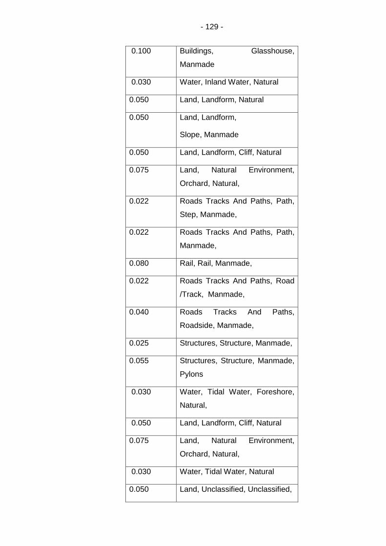
- 129 -

0.100 Buildings, Glasshouse,

Manmade

0.030 Water, Inland Water, Natural

0.050 Land, Landform, Natural

0.050 Land, Landform,

Slope, Manmade

0.050 Land, Landform, Cliff, Natural

0.075 Land, Natural Environment,

Orchard, Natural,

0.022 Roads Tracks And Paths, Path,

Step, Manmade,

0.022 Roads Tracks And Paths, Path,

Manmade,

0.080 Rail, Rail, Manmade,

0.022 Roads Tracks And Paths, Road

/Track, Manmade,

0.040 Roads Tracks And Paths,

Roadside, Manmade,

0.025 Structures, Structure, Manmade,

0.055 Structures, Structure, Manmade,

Pylons

0.030 Water, Tidal Water, Foreshore,

Natural,

0.050 Land, Landform, Cliff, Natural

0.075 Land, Natural Environment,

Orchard, Natural,

0.030 Water, Tidal Water, Natural

0.050 Land, Unclassified, Unclassified,

- 130 -

5.2.6 Calibration process of the pluvial flood model

The aim of the calibration process was to assess the credibility of the

computed results. The computed water level values were compared with the

observed water level of the Pudsey stage gauge station. The measured

water level at the Pudsey station was taken from the Environment Agency

data. The predicted water level results were obtained by using TUFLOW 2D

direct rainfall model for the same coordinate as the Pudsey stage gauge

station.

A.) To compute water level

1. Measured stage water level data

Dates of the historical flood events were checked for the Wortley Beck

catchment, then, water level values of the Pudsey station were analysed.

There were water level data sets between 05/08/2011 and 21/01/2016.

The dates to use from the Pudsey stage gauge station were obtained by

selecting high water values dates. The dates were listed below that,

06/07/2012, 24/09/2012, 25/11/2012, 15/11/2015, 12/12/2015, and

26/12/2015

After selection of the dates of the water level data from Pudsey stage

station, rainfall data was analysed for these dates.

2. Measured gross rainfall data

The predicted water level results were produced by using measured rainfall

data. Measured rainfall data was taken from Headingley, Knostrop and

Heckmondwike rain gauge logger stations (Figure 5.9). Initially, historical

flood events at the Wortley Beck catchment were investigated. Two criteria

were used to select measured rainfall data. These were return period and

the quality of the rainfall data. Firstly, return period of measured rainfall data

was analysed, it should be enough to create flood flow for the model.

Secondly, the continuity and consistency of the rainfall data were analysed.

- 131 -

These records have missing data due to natural damage or a fault with the

rain gauge during the measurements. The data from these dates might not

be enough for calibration. Therefore, the measured rainfall data of the

06/07/2012 and 24/09/2012 dates were found suitable for the validation

process.

Figure 5.7 06/07/2012 event day

0

5

10

15

20

25

30

35

40

45

0

0.1

0.2

0.3

0.4

0.5

0.6

0.7

0.8

0.9

1

0

1.7

5

3.5

5.2

5 7

8.7

5

10.5

12.2

5

14

15.7

5

17.5

19.2

5

21

22.7

5

Wa

ter

de

pth

(m

)

Time (hr.)

06/07/2012 06072012Pudsey [m]

Headingleycumulative

Heckmondwikecumulative

Knostropcumulative C

um

ula

tive

R

ain

fall

(m

m)

- 132 -

Figure 5.8 24/09/2012 event day

Figure 5.7 and 5.8 were created to observe the cumulative rainfall (mm) and

water depth (m) values for event days.

5.2.6.1 Thiessen polygon method

Measured rainfall data was applied by using the mean precipitation

approach in the model. Mean precipitation can be calculated from Thiessen

polygon method (Tilford et al., 2003). Mean precipitation was computed by

using gross rainfall data of the Headingley, Knostrop and Heckmondwike

rain gauge logger stations.

The spatially averaged rainfall calculation was performed by using the below

approach (Thiessen, 1911),

((Rainfall value of Headingley x area of Headingley rain gauge station) +

(Rainfall value of Knostrop x area of Knostrop rain gauge station) + (Rainfall

value of Heckmondwike x area of Heckmondwike rain gauge station)) / (The

area of Wortley Beck catchment)

The areas of the rain gauge stations were calculated by using GIS tool and

the results are displayed below (Figure 5.9). The areas for the rain gauge

stations are 26 km2 for Headingley, 18 km2 for Knostrop and 17 km2 for

Heckmondwike in Figure 5.9.

0

5

10

15

20

25

30

35

40

45

50

0

0.2

0.4

0.6

0.8

1

1.2

01

.5 34

.5 67

.5 91

0.5 12

13.5 15

16.5 18

19.5 21

22.5

Cu

mu

lati

ve

Rain

fall

(m

m)

24/09/2012

24/09/2012Pudsey [m]

cumulativeHeadingley

Heckmondwikecumulative

Knostropcumulative

Wa

ter

dep

th (

m)

Time (hr.)

- 133 -

Figure 5.9 Thiessen method

Figure 5.9 indicates locations of rain gauges and denotes the area of each

polygon.

Figure 5.10 Gross rainfall of the 06/07/2012 event

Figure 5.10 displays the gross rainfall data of the 06/07/2012 date from

Thiessen polygon method. Rainfall duration is 11 hours of the 06/07/2012

event.

00.5

11.5

22.5

33.5

44.5

0.0

0

0.7

5

1.5

0

2.2

5

3.0

0

3.7

5

4.5

0

5.2

5

6.0

0

6.7

5

7.5

0

8.2

5

9.0

0

9.7

5

10.5

0

Me

an

pre

cip

ita

tio

n (

mm

)

Time (h)

06/07/12Thiessen

- 134 -

Figure 5.11 Gross rainfall of the 24/09/2012 event

Figure 5.11 displays the gross rainfall data of the 24/09/2012 date from

Thiessen polygon method. Rainfall duration is 14.25 hours of 24/09/2012

event.

3. Net rainfall data was calculated from the gross rainfall data

After mean precipitation was calculated by using Thiessen polygon method,

net rainfall hyetograph was computed for impermeable and permeable

surfaces by using the ReFH boundary unit of the Flood modeller suite.

4. Net rainfall data was entered to the 2D Hydrodynamic model to

compute water level

The net rainfall hyetograph was entered into the TUFLOW 2D direct rainfall

model to produce water level. The computed water level data was used to

compare with the measured water level data of the Pudsey gauge station.

TUFLOW 2D surface flood was simulated by using 5 m cell resolution.

Urban permeable and impermeable surfaces data based on the year of 2016

were used.

- 135 -

5. The computed water level

Figure 5.12 Water level from rainfall data of 06/07/2012

Figure 5.12 displays the computed water level of the 06/07/2012 date from

Thiessen polygon method and measured water level values from Pudsey

stage gauge station of 06/07/2012 date.

Figure 5.13 Water level from rainfall data of 24/09/2012

Figure 5.13 displays the computed water level of the 24/09/2012 date from

Thiessen polygon method and measured water level values from Pudsey

stage gauge station of 24/09/2012 date.

55.7

55.9

56.1

56.3

56.5

56.7

56.9

57.1

0

2.2

5

4.5

6.7

5 9

11.2

5

13.5

15.7

5

18

20.2

5

22.5W

ate

r L

eve

l (

m A

OD

)

Time(hr.)

06/07/2012 Data

Computed waterlevel (TUFLOW2D)

Measured waterlevel( Pudseystage)

55.5

55.7

55.9

56.1

56.3

56.5

56.7

56.9

57.1

57.3

0 2 4 6 8

10

12

14

16

18

20

22

24

Wa

ter

Leve

l (m

AO

D)

Time (hr.)

24/09/2012 Data

Computedwater level(Tuflow 2D)

Measuredwater level(Pudsey stage)

- 136 -

It can be said that the predicted water levels are higher than the water levels

of the Pudsey stage station. The reasons for the differences between

measured and computed results could be due to the quality of rainfall data.

Rainfall data for some days was either missing or suspected. In addition to

this, rainfall cannot be uniform over the entire catchment. The lack of adding

the continuous loss in the model could cause this result. Thiessen polygon

method and simplified surface features from the master map data cannot

capture the influence of topography on the rainfall event. Lastly, the

behaviour of computed and measured water level is similar, only computed

water level value is higher than measured water level. The reason for this

difference could be the model resolution. Using smaller than 5 m cell size of

model resolution can make the computed water level values lower so they

can be closer.

5.2.7 Estimation of the flood frequency for Farnley Beck sub-

catchment

To determine the relationship of return period between the rainfall events

and flood events, flood frequency analysis was performed in this research.

The peak flow value of the discharge at the outfall point of the Farnley Beck

sub-catchment was computed by using 2D TUFLOW direct rainfall modelling

approach (Figure 5.14).

The statistical flood estimation (pooled group) method was used to estimate

the return periods of peak flow values. The pooled group was obtained from

WINFAB FEH CD version 3.0 according to the catchment descriptor

parameters of the Farnley Beck sub-catchment.

- 137 -

Figure 5.14 Peak flow discharge point

The location of the peak flow discharge at the Lower Wortley Beck can be

found in the Figure 5.14.

The FEH statistical procedure for flood frequency estimation was applied by

using WINFAP-FEH 3™ software. WINFAP-FEH 3™ software package was

released on 9 September 2009 by Wallingford HydroSolutions Ltd (WHS,

2009). The WINFAP-FEH 3™ software could create flood frequency curves

for flood estimation so that a relationship between the peak flow and the

expected frequency of occurrence could be defined (WHS, 2009).

1. Estimating QMEDrural from catchment descriptors

QMEDrural can be estimated by using the catchment descriptor method when

the subject catchment is ungauged or had a length of the AM or POT flood

data is lower than two years (WHS, 2009). Therefore, Kjeldsen et al. (2008)

`s QMEDrural catchment descriptor was used (Equation 5.7) in this research.

Equation 5.7 QMEDrural catchment descriptor

QMEDrural = 8.3062AREA0.8510 0.1536(1000SAAR

)FARL3.4451 0.0460BFIHOST2

- 138 -

Where in Equation 5.7: AREA is catchment area (km2); SAAR is standard

average annual rainfall (mm); BFIHOST is hydrological soil properties and

FARL is index of flood attenuation based on upstream reservoirs and lakes

(Kjeldsen et al., 2008; WHS, 2009; Kjeldsen and Jones, 2010). These

catchment descriptors can be found at FEH CD-ROM 3 software.

Farnley Beck catchment descriptors for the calculation Qmedrural were that

AREA was 29.67 km2, SAAR value was 799 (mm), FARL value was 1.0, and

the BFIHOST value was 0.449. Qmedrural value was calculated as a 7.66

m3/s by using catchment descriptor (Equation 5.7).

2. Defining a pooling group

While gauged catchments of pooled group were selected, the pooled group

was generated by using WINFAP-FEH_v4.1 data at the Centre of Ecology

and Hydrology (CEH) web page (http://nrfa.ceh.ac.uk/winfap-feh-files).

3. Urbanisation calculation

URBEXT2000 value can be updated for the year of the present. Equation 5.8

by Bayliss et al. (2006) was used to apply the urbanisation adjustment to the

URBEXT2000.

Equation 5.8 Urban Extension Factor (UEF)

UEF = 0.7851 + (0.2124 ∗ ATAN ((YEAR − 1967.5)/20.32))

To estimate flood frequency of Farnley Beck sub-catchment, a statistical

procedure was applied by using URBEXT2000. According to the URBEXT 2000

value, that is 0.219, the urban extent of the Farnley Beck sub-catchment in

the 2016 year was assumed by using urban extent factor equation (Equation

5.8).

During this research, urbanisation of Wortley Beck catchment was assumed

as a 2016 year so the urban adjustment was applied to the Qmedrural. So, it

was calculated as a 0.226 m3/s.

4. The urban adjustment methods

If the URBEXT 2000 value of the subject site is bigger than 0.03, additional

procedures are recommended to apply to produce a growth curve because

urbanisation has a significant impact on flooding.

http://nrfa.ceh.ac.uk/winfap-feh-files

- 139 -

Urban adjustment Equation 5.9 was applied to the QMEDrural to assess the

impact of urbanisation on the flood frequency curve (WHS, 2009).

Equation 5.9 The urban adjustment

QMED = UAF QMEDrural

Where in Equation 5.9: QMEDrural is multiplied by the Urban Adjustment

Factor (UAF) (WHS, 2009).

UAF is calculated by using Equation 5.10:

Next, by using this value in urban adjustment factor, Equation 5.10 (Robson

and Reed, 1999) Qmed was calculated as 9.894 m3/s value.

Equation 5.10 The Urban Adjustment Factor (UAF)

UAF = (1 + URBEXT2000)0.37PRUAF2.16

Where in Equation 5.10: URBEXT 2000 is Urban extent value of the 2000

year; PRUAF is the percentage runoff urban adjustment factor and was

defined by Kjeldsen (2010) (Equation 5.11).

Equation 5.11 the percentage runoff urban adjustment factor

PRUAF = 1 + 0.47URBEXT2000 (BFIHOST

1 − BFIHOST)

5. Estimating QMED by data transfer

In addition to this, because of Qmed was calculated from catchment

descriptor equation, it was adjusted by using donor catchment. The closest

gauged catchment was used for this aim, and it was selected by using

WINFAB FEH CD version 3. The basic transfer process for adjustment was

applied by using Kjeldsen et al., (2008) `s data transfer equation (Equation

5.12).

Equation 5.12 The transfer equation

QMEDs,adj = QMEDs,cds (QMEDg,obs

QMEDg,cds)

asg

asg = 0.4598 exp(−0.02dsg) + (1 − 0.4598)exp(−0.4785dsg)

- 140 -

The steps of the procedure of the data transfer

1. A donor site is selected

2. QMED (QMEDg,obs) of the donor site is derived.

QMEDobs is the observed QMED value and calculated from the AM data.

3. QMED value is calculated from catchment descriptors for both the subject

site and donor site, QMEDs,cds and QMEDg,cds, respectively.

QMED s,adj is the adjusted value of QMED for the subject site

4. dsg is the geographical distance (km) between the centroid of the subject

site and the centroid of the donor site (Kjeldsen et al., 2008; WHS, 2009).

The QMEDs,adj value was calculated as a 10.18 m3/s.

6. Estimating an appropriate flood growth curve

A flood growth curve (zT) was constructed by using the pooling-group data to

derive a flood frequency curve. The flood frequency curve can be obtained

by multiplying with the zT by QMED (Kjeldsen et al., 2008; WHS, 2009).

Equation 5.13 Estimation of the peak flow for return interval

QT = QMEDzT

Where in Equation 5.13: QT is the peak flow for a return interval (T)

Estimation of peak flow for the return interval was calculated by using

Equation 5.13. A flood growth curve was created by fitting the Generalised

Logistic (GL) distribution. Finally, flood frequency was computed by using

this value.

A given return period of a rainfall event is used as an input to a rainfall-runoff

model. The return period of the rainfall event is accepted as the same as the

return period of computed peak discharge in the ungauged catchment

(Packman and Kidd, 1980; Bradley and Potter, 1992). However, return

period of the rainfall event could be different from the return period of the

flood event in nature (Linsley et al., 1988). The correlation between rainfall

return period (TR) and flood return period (TQ) is an important parameter to

assess flood frequency and to manage flood risk. Nevertheless, this

relationship could not be completely identified (Viglione and Blöschl, 2009).

- 141 -

It is not a straightforward process. Rainfall intensity, rainfall duration,

temporal and spatial storm patterns, and antecedent soil moisture are

required in detail to assess this relationship (Viglione and Blöschl, 2009).

5.3 Pluvial flood modelling results

In this section, the results of the TUFLOW 2D direct rainfall model were

displayed. These outcomes can be used for the assessment of the pluvial

flood risk in Wortley Beck Catchment.

The estimated hyetograph was the main input data of the direct rainfall

model and each hyetograph can be seen in between Figure 5.15 and 5.20.

The storm duration of Wortley Beck catchment was calculated as 3.95 hr.,

by the Revitalised Flood Hydrograph (ReFH) model. Net rainfall hyetograph

of the impermeable areas, permeable areas, and total rainfall (mm) were

obtained for each design event.

5.3.1 The estimated hyetographs

Storm hyetograph was generated for the following events

1. Pluvial flood events were designed by estimating hyetographs for various

return periods, covering the 1 in 5-year, 1 in 15-year, 1 in 30-year, 1 in 50-

year, and 1 in 100-year event (from Figure 5.15 to Figure 5.19).

2. Pluvial flood events were designed for different rainfall durations (hr.) as

well, covering the 0.5hr., 1hr., and 6hr. rainfall durations of the 1 in 100-year

event (Figure 5.20).

Figures display the rainfall depth (mm) for time durations (hr.). The rainfall

depth values display total rainfall (gross), impermeable surfaces (Imp) and

permeable surfaces (Perm), lastly, cumulative gross rainfall depth values.

These figures can be used to assess the input values for the modelling

approach.

- 142 -

Figure 5.15 Estimated hyetographs for the 1 in 5-year event


0

5

10

15

20

25

30

35

40

45

500

1

2

3

4

5

6

7

8

9

10

0.0

0

0.3

0

0.6

0

0.9

0

1.2

0

1.5

0

1.8

0

2.1

0

2.4

0

2.7

0

3.0

0

3.3

0

3.6

0

Rain

fall

dep

th (

mm

)

5yr. Gross

5yr. Imp

5yr. Perm

Cumulative5yr rainfall

Time(hr.)

Cu

mu

lati

ve

g

ros

s

ra

infa

ll (

mm

)

0

5

10

15

20

25

30

35

40

45

500

1

2

3

4

5

6

7

8

9

10

0 0.30.60.91.21.51.82.12.42.7 3 3.33.6

Rain

fall

dep

th (

mm

)

15yr. Gross

15yr. Imp

15yr. Perm


Cu

mu

lati

ve

gro

ss

ra

infa

ll (

mm

)

Time(hr.)

- 143 -



0

10

20

30

40

50

600

1

2

3

4

5

6

7

8

9

10

0 0.3

0.6

0.9

1.2

1.5

1.8

2.1

2.4

2.7

3 3.3

3.6

Rain

fall

dep

th (

mm

)

30 yr. Gross

30yr. Imp

30yr. Perm


Time(hr.)

Cu

mu

lati

ve

gro

ss

r

ain

fall

(m

m)

0

10

20

30

40

50

60

700

1

2

3

4

5

6

7

8

9

10

0 0.30.60.91.21.51.82.12.42.7 3 3.33.6

Rain

fall

dep

th (

mm

)

50 yr. Gross

50yr. Imp

50yr. Perm


Time (hr.)

Cu

mu

lati

ve

gro

ss

ra

infa

ll (

mm

)

- 144 -


While the frequency of the rainfall event is greater, rainfall depth values of

the rainfall events become greater.

0

10

20

30

40

50

60

70

80

90

1000

1

2

3

4

5

6

7

8

9

10

0 0.3

0.6

0.9

1.2

1.5

1.8

2.1

2.4

2.7

3 3.3

3.6

Rain

fall

dep

th (

mm

)

100yr. Gross

100yr. Imp

100yr. Perm


Time (hr.)

Cu

mu

lati

ve

g

ros

s r

ain

fall

(m

m)

- 145 -

Figure 5.20 Cumulative gross rainfall events for the1 in 100-year event for 0.5/1/6 hr., rainfall durations

Longer rainfall duration (6 hr.) can have lower peak rainfall depth (mm) but

have greater cumulative gross rainfall depth (mm) in comparison to short

duration of rainfall events (0.5/1hr.) within the same return period (1 in 100-

year event) (Figure 5.20).

After estimating the rainfall events, the rainfall data of impermeable and

permeable surfaces was entered into the 2D hydrodynamic model directly,

and probabilistic flood inundation maps were obtained.

5.3.2 Pluvial flood inundation maps

The pluvial flood inundation maps of the Wortley Beck catchment (WBC)

were produced from each estimated rainfall data. This was to assess the

impact of return period of rainfall event and the impact of rainfall duration on

the pluvial flooding. Pluvial flood extent maps were produced by using

TUFLOW 2D hydrodynamic software link GIS tool.

0

10

20

30

40

50

60

70

80

90

1000

5

10

15

20

25

0 0.4

0.8

1.2

1.6

2 2.4

2.8

3.2

3.6

4 4.4

4.8

5.2

5.6

0.5h Grossrainfall

1h Grossrainfall

6h Grossrainfall

Cumulativegross 0.5hr.

Cumulativegross 1 hr.

Cumulativegross 6hr.

Cu

mu

lati

ve

gro

ss

ra

infa

ll (

mm

)

Rain

fall

d

ep

th (

mm

)

Time (hr.)

- 146 -

Figure 5.21 Rainfall event for the 1 in 5-year event

Figure 5.21 displays surface flood inundation areas in the Wortley Beck

catchment for the 1 in 5-year rainfall event.

- 147 -




- 148 -




- 149 -




- 150 -




- 151 -

Figure 5.26 Rainfall event for the 0.5 hour duration of the 1 in 100-year event


catchment for the 30 minutes of 1 in 100-year rainfall event.

- 152 -

Figure 5.27 Rainfall event for the 1 hour duration of the 1 in 100-year event


catchment for the 1-hour of 1 in 100-year rainfall event.

- 153 -

Figure 5.28 Rainfall event for the 6hour duration of the 1 in 100-year event


catchment for the 6-hour of 1 in 100-year rainfall event.

- 154 -

5.3.3 Water depth results

From design rainfall events, the figures and probabilistic flood inundation

maps were produced

1. To assess the impact of return period of rainfall event on the surface flood

water depth.

2. To assess the impact of rainfall duration of rainfall event on the surface

flood water depth.

A.) Water depth percentages and Rainfall return periods

Figure 5.29 The percentages of the water depth values for rainfall return periods (30 yr., 50 yr., and 100 yr.)

Figure 5.29 displays the percentages of water depth values in the flood

inundation areas of rainfall events for the 1 in 30-year, 1 in 50-year, and 1 in

100-year event of 4hr. rainfall duration. Water depth values were scaled

between 0.15 m and 0.6 m above.

92.59% 92.30% 91.90%

5.05% 5.15% 5.32%

1.57% 1.67% 1.85%

0.79% 0.87% 0.93%

90%91%92%93%94%95%96%97%98%99%

100%

30 yr. 50 yr. 100 yr.Wa

ter

dep

th p

erc

en

tag

es

(%

)

Rainfall return period (yr.)

Pluvial Flood Modelling

0.6-<

0.3-0.6

0.15-0.3

0-0.15

Max. Water Depth (m)

- 155 -

B.) Water depth percentages and Rainfall duration

Figure 5.30 The percentages of the water depths (m) for rainfall durations

Figure 5.30 displays the percentages of the water depths (m) for various

rainfall durations (0.5 hr., 1 hr., and 6 hr.).

It is apparent in Figure 5.29 that water depths become deeper when design

rainfall events from for the 1 in 5-year to for the 1 in 100-year event. The

locations of vulnerable places can be identified on the maps. In addition,

when the rainfall duration becomes longer water depth can become higher

for the same return period events (Figure 5.30).

93.19% 92.72% 91.74%

4.86% 5.07% 5.35%

1.45% 1.53% 1.87%

0.49% 0.68% 1.04%

90%91%92%93%94%95%96%97%98%99%

100%

05hr. 1hr. 6hr.Wa

ter

dep

th p

erc

en

tag

es

(%

)

Rainfall Duration(hr.)

Pluvial Flood Modelling

0.6-<

0.3-0.6

0.15-0.3

0-0.15

Max. Water Depth (m) 1 % AEP

- 156 -

5.3.4 Flood frequency analysis of the Farnley Beck (FB)

catchment

This section aimed to determine the return period of the maximum discharge

of the Farnley Beck (FB) sub-catchment. Initially, the rainfall events were

designed for the 1 in 5 year, 1 in 10-year, 1 in 15-year, 1 in 25-year, 1 in 50-

year and 1 in 100-year event and rainfall durations (D) were applied 0.5/1/6

hour for the 1 in 100-year event. Then, peak flow values were computed

from these rainfall events. Meanwhile, return periods of the peak flow were

determined by using the pooled method of statistical flood estimation

procedure for the Farnley Beck (FB) sub-catchment. Next, the return periods

of the statistical approach were used to determine the return periods of the

computed peak flows from TUFLOW 2D direct rainfall model. Lastly, the

return periods of the computed peak flow were compared to the return

periods of the rainfall event. Table 5.4 indicates the relationship of the return

periods between rainfall event and flood frequency for Farnley Beck (FB)

sub-catchment.

Table 5.4 The relationship between the return periods

Rainfall

Event

T(year)

D (h)

FB

Computed

Peak flow

(m3/s)

Return period of

the Peak Flow

(year)

(Pooled method)

Peak flow

value

(Pooled

method)

5 yr (4h) 3.97 2 10.18

15 yr (4h) 9.38 5 13.4

30 yr (4h) 12.84 10 15.65

50 yr (4h) 16.69 15 16.99

100 yr (4h) 23.99 25 18.76

100 yr

0.5h

3.117 30 19.42

100 yr

1 h

8.918 50 21.35

- 157 -

100 yr

6 h

24.77 75 22.985

100 24.20

200 27.36

Table 5.4 displays the flood frequency and the relationship of return period

between the rainfall and peak flow.

The first column shows the rainfall return period and duration of the design

rainfall events. The second column displays the peak flow values of the

discharge at the outfall point Farnley Beck basin from each design rainfall

events. The return period of the peak flow from the pooled method of the

statistical flood frequency approach is shown in the third column. The fourth

column displays the peak flow values from the pooled method of the

statistical flood frequency approach.

This could be said that from Table 5.4

The 1in 5-year rainfall event cannot create a flood event.

The 1in 15-year rainfall event can create the 1 in 2-year flood even,

The 1 in 30-year rainfall event can create the 1 in 5-year flood event,

The 1 in 50-year rainfall event can create the 1 in 15-year flood event,

The 1 in 100-year rainfall event can create the 1 in 100-year flood event.

When the impact of rainfall duration is assessed for the 1 in 100-year rainfall

event, it is observed that short rainfall durations could not cause flood event

such as 0.5-hr. 1-hour rainfall duration of the 1 in 100-year event could

cause nearly for the 1 in 2-year flood event. The 6-hour rainfall duration of

the 1 in 100-year rainfall event could nearly cause the 1 in 100-year flood

event.

- 158 -

However, the FEH recommends using observed annual maximum flood data

where are available (Kjeldsen and Jones, 2007). The FEH noted that the

uncertainty of QMED estimation is generally larger than the uncertainty of

QMED estimation from directly flood data (Kjeldsen et al., 2008).

To assess the relationship of return period between the rainfall and flood

events, catchment soil characteristics can need to be investigated in detail.

The season can influence the runoff as well. Usually, flow return period can

be smaller than the return period of the rainfall event (Viglione and Blöschl,

2009). In addition, rainfall duration can influence flood magnitudes as well. If

catchment size is small, short rainfall durations can create strong flood

events (Viglione and Blöschl, 2009). Consequently, rainfall return period is

not always the same as return period of the flood.

5.4 Conclusion

Pluvial flooding in Wortley Beck catchment was assessed by using a direct

rainfall approach in this research. It can be used as an alternative to

traditional rainfall-runoff models. The approach of the direct rainfall model

consisted of two main sections. These were net rainfall estimation by using

ReFH loss model and flood inundation simulation by using the 2D TUFLOW

hydrodynamic model. The advantage of the TUFLOW 2D hydrodynamic

model for this research was that peak flow values could be computed

anywhere inside the research area. Hence, flow values can be computed for

different rainfall events and flood frequency analysis can be applied in an

ungauged catchment by using this method.

The model was used to analyse the effects of various rainfall events on the

Wortley Beck catchment. The results display that

1. When the rainfall return period is changed from 1 in 50-year to 1 in 100-

year, the rainfall depth of the rainfall event becomes higher.

2. Long duration rainfall events have lower peak rainfall depth (mm) in

comparison to short duration rainfall events (0.5/1hr.) for the same return

period, but the total rainfall depth value become larger for longer rainfall

durations.

- 159 -

3. The probabilistic flood inundation maps display the drain area of the

Wortley Beck River. When return period changed from the 1 in 5-year to a 1

in 100-year event in this research, the water becomes higher both on the

surface and inside river channel. In addition, similar behaviour was observed

when the rainfall duration became longer (from 0.5 hour to 6 hours for the 1

in 100-year rainfall event). However, the ratios of the water depth values

display that majority of the water depth is lower than 0.6 m.

4. The peak flow of the Farnley Beck sub-catchment was also computed.

The results shows that rainfall return period can be different from return

period of the flood event.

In conclusion, it can be said that if the return period of a rainfall event is

longer than the 1 in 30-year event, the surface flood event can become

serious, but if the rainfall duration becomes longer, any event can have

serious consequences.

Some limitations points of the research methodology to reach the aims were

that there was not sufficient measured rainfall data. Therefore, design rainfall

events were created as input for the direct rainfall model. Furthermore,

drainage system data could not be provided for this research so that the loss

for the drainage system could not be added to the model. Moreover,

improvements and updates necessary to verify the methodology because

the direct rainfall model is a new approach. Lastly, to capture the peak flow

anywhere in the catchment requires the model running with a cell size

smaller than 5 m. However, computation can take weeks or longer.

In summary, the outcomes of this chapter can be used to improve the flood

resilience approaches, as well as assist to understand the relationship

between rainfall and flow in ungauged catchments. In addition, the results

can be used to better identify Wortley Beck catchment vulnerability to the

pluvial flood risk.

- 160 -

Chapter 6 Combined fluvial and pluvial flooding

6.1 Introduction

The main motivation of this research is that the risk of combined flood events

should be estimated by simulating the combined sources and pathways of

the flood events in models. Floodwater depth and flood extent are estimated

by simulating the combined fluvial and pluvial flood models in this research.

In this section of Chapter 6, firstly, the differences between pluvial and fluvial

flood events in a catchment are explained. Secondly, the relationship

between pluvial and fluvial flood events in an urbanised catchment is

determined. Thirdly, the importance of the investigation of the combined

fluvial and pluvial flooding is discussed.

Pluvial and fluvial flood events can have different flood pathways, and

different event durations so that pluvial and fluvial flood events have been

mostly seen as independent. The fluvial flood event can affect the

floodplains by streams while a pluvial flood event can affect the lower local

locations in urbanised basins (Chen et al., 2010; Bhattarai et al., 2015).

Pluvial flooding can be on smaller spatial and temporal scales than fluvial

flooding can (Rözer et al., 2016). Pluvial flood events can be seen sooner

than fluvial flood event. Fluvial flood event can take time, and the

consequences of the fluvial flooding can be observed after days or weeks

because the river water level rises slowly (Chen et al., 2010).

Intense rainfall event and land use change might affect the fluvial and pluvial

flood process in an urbanised catchment. Firstly, heavy precipitation can be

a source of an intense surface runoff. The overflow on saturated soil or

impermeable surfaces can result in a pluvial flooding. In addition, the surface

runoff in the upstream location can be the source of discharge into the river

channel and this could result in a fluvial flooding. Secondly, the land use

change in a catchment can increase the ratio of the impermeable surfaces.

Urbanisation can cause fast runoff, overwhelmed drainage systems, and the

settlements on the floodplains so that pluvial flooding can be seen on the

floodplains. In addition, the settlements on the floodplains by urban streams

- 161 -

can face to the fluvial flooding (Evans, 2004; Pitt, 2008; Chen et al., 2010;

Apel, et al., 2015).

In summary, this could be said that the consequences of the rainfall events

and impermeable surfaces on the floodplains by urban streams could create

combined fluvial and pluvial flood events. Therefore, pluvial and fluvial flood

events could be considered consecutively and dependently in these

locations.

Fluvial flooding and local heavy rainfall events can be observed during the

annual monsoon therefore both fluvial and pluvial flooding can occur at the

same time in the tropical environments (Apel et al., 2015). Historically, there

are some samples of combined fluvial and pluvial flood events in England.

Surface water and Local River flooding were observed between 23 and 27

December 2013 from Dorset through Hampshire also Surrey to Kent

(Thorne, 2014). In addition, pluvial flooding occurred in conjunction with the

fluvial flood event in January 2005 at Carlisle (Falconer et al., 2009). A

pluvial flood event was observed due to the limited capacity of the drainage

system in the River Eden catchment, after a while a fluvial flood event was

observed due to the limited capacity of the banks of the River Eden and its

tributaries in the Carlisle in January 2005 (Shaw et al., 2011).

Naturally, the combined fluvial and pluvial flood events can occur. If flood

events are considered separately, the hazard can be underestimated

(Ashley et al., 2005; Burton et al., 2010; Chen et al., 2010). This can result

that the flood defence systems cannot be used efficiently and to manage the

flooding can be very difficult. Consequently, the approaches of simulation of

the combined events should be generated. The outcomes of the simulations

can be used to improve and update the flood risk management approaches

and flood resilience tools (Houston et al., 2011).

- 162 -

6.2 Methodology of the combined fluvial and pluvial

flooding

The most of the research in the literature has assessed fluvial and pluvial

flood events independently and the flood extents maps have been

overlapped to observe the combined floods. However, this method can have

some limitations. For instance, firstly, if pluvial and fluvial flood events are

simulated separately, the interactions of the sources and the interactions

along on the pathway cannot be obtained and observed. Secondly, if the

flood inundation maps of the pluvial and fluvial flood events are only

overlapped, the water depth in the inundation area of the combined events

could not be computed and the flood extents from combined events cannot

be observed.

Alternatively, a method to assess the combined fluvial and pluvial flooding

should be generated. Horritt et al. (2010) recommended two approaches;

these were to compare independent flood inundation maps of the different

flood events and to assess the dependency of the flood events at the

sources. Lian et al. (2013) recommended researching the combination of the

effect of flood probability and consequences as a single risk function. Breinl

et al. (2015) recommended adding a hydrodynamic model to simulate the

flood inundation maps to improve the combined flood risk assessment.

The aim of this methodology is to assess the interactions between the fluvial

pluvial flood events on the floodplains in urban stream basins. Thus, flood

risk from the combined fluvial and pluvial flooding on the urbanised

floodplains by urban streams can be observed. This methodology was

applied to the Lower Wortley Beck area. The Lower Wortley Beck area is

suitable for this research because there is a fluvial flood risk by the Lower

Wortley Beck, and urbanised areas are located by the stream. Pluvial flood

risk can also be observed on the impermeable and lower locations by the

stream.

- 163 -

6.2.1 Modelling approach of the combined fluvial and pluvial

flooding on the floodplain

The methodology of the combined fluvial and pluvial flood simulations is

explained in this section. The modelling approach is to produce and examine

the combined fluvial flooding and pluvial flooding on the floodplain in urban

stream basins. In order to simulate the combined fluvial and pluvial flood

events, both inflow hydrograph and net rainfall hyetograph were included in

the same model.

Figure 6.1 The combined fluvial and pluvial flood modelling at the Lower Wortley Beck area

The 2D domain of the Lower Wortley was activated for both fluvial and

pluvial flooding (Figure 6.1). Inflows from the Farnley Beck and Farnley

Wood Beck basins entered into the Lower Wortley Beck, and net rainfall

hyetograph of the Lower Wortley Beck area were applied on the 2D domain

of the Lower Wortley area. Inflows enter the river channel at the same time

with the rainfall event starts. Inflow points of the sub-catchments, active area

of the rainfall event, and 1D river channel can be seen in Figure 6.1 for this

modelling approach.

- 164 -

The Flood Modeller Suite 1D River model was set up with initial conditions

and inflow events. River nodes of the Lower Wortley Beck channel were

used. The model was run with the hydrograph time that was 20 hours. The

1D model time step was 1 second. Roughness values of the 1D river

channel were selected between 0.030 and 0.045 (Atkins, 2004). The Flood

modeller Suite 1D Model was linked with the 2D scheme of the TUFLOW

software. 2D model time step was 2 second. 2D control file was used to

manage the 2D domain geometry for the active area, to manage the

boundary condition commands of 2D net rainfall events, and to manage the

2D domain topography from the material file of roughness values.

Roughness values of the 2D surface can be found at Table 5.3 Master Map

land use assessment. Elevation data was used for both river channel and

Lower Wortley surface area. Model topographical area (DEM) can be found

in Figure 6.1.

Net rainfall hyetograph was applied on the impermeable and permeable

surfaces of Lower Wortley Beck area (Figure 6.2). The net rainfall profiles

were designed for the 1 in 100-year event and for 4-hour rainfall duration.

Net rainfall event was added into the 2D domain boundary condition

database in the model.

Figure 6.2 2D Rainfall boundary condition control area

- 165 -

This modelling approach was applied by using tools are 1D Flood Modeller

Suite version 3.7 linked to TUFLOW 2D software (version 2013-12-AD-IDP-

w64). The model was run for 1D unsteady flow and 2D double precision.

Model Grid cell size was 8 metre.

The results display the combination of river overflow and surface runoff on

the floodplain, along with the Lower Wortley Beck.

6.3 Results of the combined fluvial and pluvial flooding

In this section, fluvial and pluvial flooding and their interaction on the

floodplain by the Lower Wortley Beck are assessed.

The assessment considers three comparison steps:

1. Fluvial flooding and single event simulation,

2. Independent fluvial and pluvial flood events,

3. Combined pluvial and fluvial flood events,

The assessment parameters were taken to be water level data and flood

inundation extents (as assessed via comparison of inundation maps that

also serve to indicate flood risk at the Lower Wortley Beck catchment) from

the simulation results. The models of fluvial flooding, single event simulation,

pluvial flooding, and combined fluvial and pluvial flooding were set-up for the

1 in 100-year event, with the ratio of impermeable surface was for the year

of 2016 being consistently used. Arc MAP 10.2.2 tool was used to produce

the maps.

Water level graphs were produced for specific observation points for all

simulation for comparison, these locations points are shown in Figure 6.3.

Flood inundation maps were produced to assess the flood risk at the Lower

Wortley Beck area.

- 166 -

Figure 6.3 Observation points on the Lower Wortley Beck

Figure 6.3 displays the observation points used to compare the water levels

of different flood events. They are at specific locations that are each useful

points to indicate flood behaviours in the sub-regions of the catchment.

Point 1 located downstream of the Farnley Beck basin thus the impact of the

inflow from the Farnley sub-catchment can be observed.

Point 2 lies just before the river enters into the reservoir. Data from this point

allows flood events to be identified between point 1 and point 2.

Point 3 is located just below the reservoir so the impact of the reservoir can

be determined.

Point 4 is the upstream extent of where fluvial flooding occurs.

Point 5, 6, and 7 are within the flood inundation area. This area is between

Gelderd Road and A6110 transportation link M621 highway. The points of

these locations are important because these areas have settlements and

transportation links. The inflow from Farnley Wood Beck enters in this

location. The backwater effect observed here might be the reason for the

flood event due to overcapacity of the culvert at this location. Both pluvial

and fluvial flooding can be seen in these locations while a combination of

events can increase the risk here as well. Point 8 is toward the end of the

catchment after longer culvert and gives as an indication of the water that is

able to flow through the catchment.

- 167 -

6.3.1 Assessment of the fluvial flood model and single event

flood models

Fluvial and single event model simulations were set-up for the 1 in 100-year

event, with the urbanisation scenario was for the 2016 year. The same 1D

/2D linked fluvial flood model was used for each simulation.

Inflows were added from Farnley Beck and Farnley Wood Beck sub-

catchments for the fluvial flood simulation. In addition, the lateral flow was

included in the fluvial system for the single event simulation. The lateral flow

was computed by using the rational method to estimate the peak discharge

at the outlet of the New Farnley Beck basin. The peak flow was used to

display the impact of the drainage system outfall on the downstream fluvial

flood risk. The impact of the outfall indicates the resulting difference between

the fluvial flooding and the single event simulation in the catchment.

A.) Comparison of the computed water levels between fluvial and

single event simulations

The impact of the peak discharge at the outfall of New Farnley area on the

water level can be observed from the examination of Figures 6.4, 6.5 and

6.6 for the Point 3, 4 and 5. The points can be seen in Figure 6.3. Point 3 is

the location where the entrance of lateral flow. The impact of the outfall

shows the difference between the fluvial flooding and the single event

simulation in the catchment.

Figure 6.4 The water level at Point 3

50.60

50.80

51.00

51.20

51.40

51.60

51.80

52.00

0 2 4 6 8 10 12 14 16 18 20

Wa

ter

Leve

l (m

AO

D)

Time (h)

Point 3

Single eventflooding

Fluvial flooding

- 168 -



Single event simulation displays higher water levels than fluvial flooding

because of the impact of the peak discharge from the outlet of New Farnley

Beck basin.

45.2045.4045.6045.8046.0046.2046.4046.6046.8047.0047.20

1 3 5 7 9 11 13 15 17 19 21

Wa

ter

Leve

l (m

AO

D)

Time (h)

Point 4


Fluvial flooding

38.5038.8039.1039.4039.7040.0040.3040.6040.9041.2041.50

1 3 5 7 9 11 13 15 17 19 21

Wa

ter

leve

l (m

AO

D)

Time (h)

Point 5


Fluvial flooding

- 169 -

B.) Comparison of the flood inundation maps between fluvial and

single event simulations

The impact of the lateral flow from the New Farnley on the Lower Wortley

Beck area can be observed in Figure 6.8. OS 1:25 000 Scale Colour Raster

was used for background map.

Figure 6.7 Fluvial flood inundation map

The fluvial flood inundation area can be seen in Figure 6.7 for the 1 in 100-

year event.

Figure 6.8 Single flood inundation map

- 170 -

The flood inundation area of the single event simulation can be seen in

Figure 6.8 for the 1 in 100-year event.

In summary, the outfall from New Farnley caused higher water level, water

depth, and larger flood extent area on the Lower Wortley Beck area.

6.3.2 Assessment of discrete pluvial and fluvial flooding

The discrete fluvial and pluvial flooding was designed for the 1 in 100-year

event and for the impermeable surface of the 2016 year in the catchment.

Inflows from the Farnley Beck and Farnley Wood Beck sub-catchments were

estimated for the fluvial flooding. Hyetograph of the Wortley Beck catchment

was estimated for the pluvial flooding. The 1D link 2D river model (Flood

Modeller Suite/TUFLOW) was used for fluvial flooding and the rainfall-runoff

model (2D TUFLOW) was used for the pluvial flooding.

The aim at using these arrangements was to observe the independent fluvial

and pluvial flood processes in the catchment. Thus allowing flood risk from

fluvial and pluvial to be identified in the catchment.

The fluvial flood event consists of both baseflow (initial conditions) in the

river channel and inflow from the upstream sub-catchment. The pluvial flood

event uses the rainfall-runoff process from the Wortley Beck catchment. In

order to assess these events and detailed inspections, the focus of this

research was on the Lower Wortley Beck area.

A.) Comparison of the computed water levels between fluvial and

pluvial flood events

The results of this section display that the comparison of the computed water

levels between fluvial and pluvial flooding. The water level data were

computed from the river model for fluvial flooding, and from the rainfall-runoff

model for pluvial flooding. The results are shown in Figure 6.9 to 6.13 for the

observation points (described in Figure 6.3).

- 171 -

Figure 6.9 The water levels at Point 2


52.5052.7052.9053.1053.3053.5053.7053.9054.1054.30

0 1 2 3 4 5 6 7 8 9 10 11

Wa

ter

Le

ve

l (m

AO

D)

Time (h)

Point 2

River Model

Rainfall-RunoffModel

46.00

46.20

46.40

46.60

46.80

47.00

47.20

1 2 3 4 5 6 7 8 9 10 11 12

Wa

ter

Leve

l (m

AO

D)

Time (h)

Point 4

RiverModel


- 172 -



39.50

39.70

39.90

40.10

40.30

40.50

40.70

40.90

41.10

41.30

1 2 3 4 5 6 7 8 9 10 11 12

Wa

ter

leve

l (m

AO

D)

Time (h)

Point 5

River Model


36.00

37.00

38.00

39.00

40.00

41.00

42.00

0 2 4 6 8 10 12 14 16 18 20

Wa

ter

leve

l (m

AO

D)

Time (h)

Point 6

RiverModel


- 173 -


The water levels from the fluvial flooding are higher than from those for the

pluvial flooding (see Figures 6.9 to 6.13). However, the values of the pluvial

flooding virtually reach to the water levels of the fluvial flooding. This could

mean that fluvial flooding is fast when inside the river channel while pluvial

flooding takes more time due to the runoff being slower and longer.

B.) Comparison of the flood inundation maps between fluvial and

pluvial event simulations

The probabilistic flood inundation maps with maximum depth (m) scales

were created to assess of fluvial flood risk and pluvial flood risk at Lower

Wortley Beck area.

37.00

37.50

38.00

38.50

39.00

39.50

40.00

40.50

41.00

41.50

1 3 5 7 9 11 13 15 17 19

Wa

ter

leve

l (m

AO

D)

Time (h)

Point 7

RiverModel


- 174 -

Figure 6.14 Fluvial flood inundation map

Fluvial flooding of the 1 in 100-year event on the Lower Wortley Beck area

can be seen in Figure 6.14.

- 175 -

Figure 6.15 Pluvial flood inundation map

Pluvial flooding on the Lower Wortley Beck area is shown in Figure 6.15.

This map displays the rainfall-runoff event from the rainfall event of the 1 in

100-year event on the Wortley Beck catchment. Pluvial flooding was

simulated for the Wortley Beck catchment. This approach did not have river

channel and urban drainage system within the 2D model.

Figure 6.14 and Figure 6.15 were produced to enable comparison of the

independent fluvial and pluvial flooding.

Figure 6.14 and Figure 6.15 display similar locations by Lower Wortley Beck

where there is a higher risk of flooding.

- 176 -

Figure 6.16 Fluvial flooding 2 % AEP on the Lower Wortley Beck area

Fluvial flooding of the 1 in 50-year event on the Lower Wortley Beck area is

shown in Figure 6.16.

Figure 6.17 Pluvial flooding 2 % AEP on the Lower Wortley Beck area

- 177 -

Pluvial flooding on the Lower Wortley Beck area displayed in Figure 6.17.

This shows the result of the rainfall-runoff event from rainfall event of 1 in 50-

year event on the Wortley Beck catchment. Again, this approach did not

have river channel embedded within the model.

The limitation of the analysis of the discrete fluvial and pluvial flooding maps

is that water levels of the same points inside the flood inundation area of

fluvial flooding and pluvial flooding cannot be merged so flood extent cannot

be quantified directly from this figure.

6.3.3 Assessment of the combined pluvial and fluvial flood

events

The effects of the combined fluvial and pluvial flooding on the flood risk are

assessed in this section. The fluvial flood model was simulated by using the

1 in 100-year event of 20-hour inflow hydrograph, and pluvial flood event

was simulated by using the 1 in 100-year event of 4-hour duration net rainfall

hyetograph. The ratio of the impermeable surface was the year of 2016. This

map was produced by combining inflow hydrographs and rainfall

hyetographs and to observe flood risk on the floodplains at the Lower

Wortley Beck area from combined flood events.

A.) Probabilistic flood inundation maps of the combined pluvial and

fluvial flooding

Probabilistic flood inundation maps are used to display the combination

between rainfall and river flow on the floodplain. From these, it is possible to

observe the combined fluvial and pluvial flood events in the Lower Wortley

Beck area.

- 178 -

Figure 6.18 Combined fluvial and pluvial flooding

Combined fluvial and pluvial flooding of the 1 in 100-year event is displayed

in Figure 6.18

- 179 -

Figure 6.19 Combined fluvial and pluvial flooding water depth/ stages (1%AEP)

The processes of the combined fluvial and pluvial flooding can be seen in

Figure 6.19. Stages display the flood inundation area at different times from

the modelling at the Lower Wortley Beck area.

- 180 -

Figure 6.20 Combined fluvial and pluvial 1 %AEP flooding velocity map

The velocity (m/s) of the combined fluvial and pluvial flooding can be seen in

Figure 6.20. The Gelderd Road location at the Lower Wortley Beck area is

shown to be within the flood risk area.

- 181 -

Figure 6.21 Combined fluvial and pluvial flooding 1% AEP (velocity /stages)

The velocity (m/s) of the combined fluvial and pluvial flooding can be seen in

Figure 6.21. Stages display the velocity movement for different times of the

modelling at the Lower Wortley Beck.

- 182 -

Figure 6.22 Pluvial flooding with the fluvial flood (no inflow from upstream)

The pluvial flooding simulation was designed for the 1 in 100-year rainfall

event with the sole baseflow of the Lower Wortley Beck and no inflow from

sub-catchments. The flood inundation area of this event can be seen in

Figure 6.22. In addition, the effects of inflows on the fluvial flooding at the

lower Wortley Beck area can be observed from the pluvial flooding map of

the Lower Wortley Beck area (Figure 6.22) by comparing with Figure 6.18.

- 183 -

Figure 6.23 Combined fluvial and pluvial 2 %AEP flooding on the flood plain

The flood inundation area of the combined fluvial and pluvial flooding on the

floodplain for the 1 in 50-year event can be seen in Figure 6.23.

In conclusion, the combined fluvial and pluvial flooding maps show the

merged water depth and flood extent along the river channel from both river

flow and rainfall.

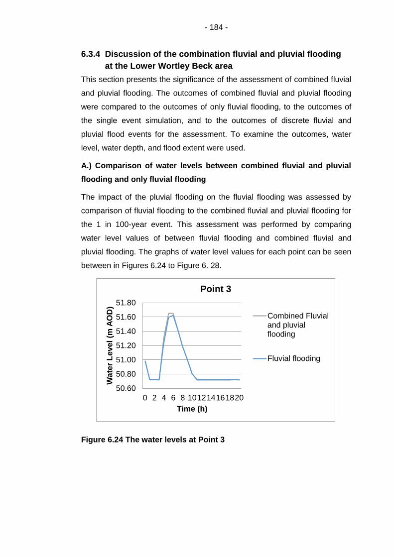
- 184 -

6.3.4 Discussion of the combination fluvial and pluvial flooding

at the Lower Wortley Beck area

This section presents the significance of the assessment of combined fluvial

and pluvial flooding. The outcomes of combined fluvial and pluvial flooding

were compared to the outcomes of only fluvial flooding, to the outcomes of

the single event simulation, and to the outcomes of discrete fluvial and

pluvial flood events for the assessment. To examine the outcomes, water

level, water depth, and flood extent were used.

A.) Comparison of water levels between combined fluvial and pluvial

flooding and only fluvial flooding

The impact of the pluvial flooding on the fluvial flooding was assessed by

comparison of fluvial flooding to the combined fluvial and pluvial flooding for

the 1 in 100-year event. This assessment was performed by comparing

water level values of between fluvial flooding and combined fluvial and

pluvial flooding. The graphs of water level values for each point can be seen

between in Figures 6.24 to Figure 6. 28.


50.60

50.80

51.00

51.20

51.40

51.60

51.80

0 2 4 6 8 101214161820

Wa

ter

Leve

l (m

AO

D)

Time (h)

Point 3

Combined Fluvialand pluvialflooding

Fluvial flooding

- 185 -



45.0045.2045.4045.6045.8046.0046.2046.4046.6046.8047.0047.2047.40

1 3 5 7 9 11 13 15 17 19 21

Wa

ter

Leve

l (m

AO

D)

Time (h)

Point 4

Combined fluvialand pluvialflooding

Fluvial flooding

38.5038.7038.9039.1039.3039.5039.7039.9040.1040.3040.5040.7040.9041.1041.3041.50

1 3 5 7 9 11 13 15 17 19 21

Wa

ter

leve

l (m

AO

D)

Time (h)

Point 5

Combinedfluvial andpluvialflooding

Fluvialflooding

- 186 -



The figures (Figure 6.24 to Figure 6.28) show that the combined fluvial and

pluvial flooding has higher water level value than only fluvial flooding.

Results from Figure 6.24 and Figure 6.28 show that the combined fluvial and

pluvial flooding can be dangerous than sole fluvial flood event.

40.00

40.20

40.40

40.60

40.80

41.00

41.20

41.40

41.60

1 3 5 7 9 111315171921

Wa

ter

leve

l (m

AO

D)

Time (h)

Point 7


Fluvial flooding

28.60

28.80

0 2 4 6 8 10 12 14 16 18 20

Wa

ter

dep

th (

m A

OD

)

Time (h)

Point 8


Fluvial flooding

- 187 -

B.) The impact of the combined fluvial and pluvial flooding on the water

level in the flood extent

Fl1 and FI2 water level points were positioned inside the severe flood risk

area (as shown in Figure 6.29). Both fluvial and pluvial flood events and

backwater effects can be seen at the Fl1 and FI2 locations. Thus, the impact

of the combined fluvial and pluvial flooding on the flood extent can be

obtained for these points.

Figure 6.29 Fl1 and FI2 water level points

Figure 6.30 Comparison of the water levels for each simulation at point FI1

40.2

40.4

40.6

40.8

41

41.2

41.4

1 3 5 7 9 111315171921

Wa

ter

leve

l (m

AO

D)

Time (h)

Point FI1


Fluvial flooding

- 188 -

Figure 6.31 Comparison of the water levels for each simulation at point FI2

It can be seen in Figure 6.30 and in Figure 6.31 that the combined fluvial

and pluvial flooding can cause higher water levels than only fluvial flooding

can for the same point, and the same return period. The combined fluvial

and pluvial flooding has a significant impact on the flood inundation area.

C.) Comparison of water depths (m) between combined and discrete

flood events

The combined flood events with discrete flood events were compared in this

section. Firstly, water depth was calculated from the summation of the water

depth values of the same point from discrete pluvial and fluvial flooding

(Figure 6.3). These discrete fluvial and pluvial flooding events were designed

for the 1 in 100-year event. The methodology of the fluvial flooding can be

found at the methodology section of Chapter 3. The methodology of the

pluvial flooding can be found at the methodology section of Chapter 5. The

water depth value of discrete events was named as Sum in the figures.

Secondly, water depth was calculated directly from the combined fluvial and

pluvial flooding event simulation for the 1 in 100-year event. The

methodology of the combined fluvial and pluvial flooding can be found in the

methodology section of Chapter 6. This was named as Combination in the

figures.

41.05

41.25

41.45

1 3 5 7 9 111315171921

Wa

ter

Leve

l (

m A

OD

)

Time (h)

Point FI2


Fluvial flooding

- 189 -

Figure 6.32 The water depth at Point 1


0.00

0.50

1.00

1.50

2.00

2.50

3.00

3.50

4.00

4.50

0

1.2

5

2.5

3.7

5 5

6.2

5

7.5

8.7

5

10

11.2

12.5

13.7 15

Wa

ter

dep

th(m

)

Time(h)

Point 1

Point 1 SUM

Point 1 Combination

0.00

1.00

2.00

3.00

4.00

5.00

6.00

7.00

0

1.2

5

2.5

3.7

5 5

6.2

5

7.5

8.7

5

10

11.2

12.5

13.7 15

Wa

ter

de

pth

(m

)

Time(h)

Point 2

POINT 2SUM

POINT 2Combination

- 190 -



1.00

1.50

2.00

2.50

3.00

3.50

0 1 2 3 4 5 6 7 8 9

10

11

12

13

14

15

Wa

ter

dep

th (

m)

Time(h)

Point 4

POINT 4 SUM

POINT 4Combination

1.00

2.00

3.00

4.00

5.00

6.00

7.00

0

1.2

5

2.5

3.7

5 5

6.2

5

7.5

8.7

5

10

11.2

12.5

13.7 15

Wa

ter

dep

th (

m)

Time(h)

Point 5

POINT 5SUM

POINT 5Combination

- 191 -


The discrete fluvial and pluvial flooding (Figure 6.14 and 6.15) was

compared to the combined fluvial and pluvial flooding. The combined fluvial

and pluvial flooding map (Figure 6.18) displays the flood extent and the

water level of both river flow and rainfall.

Figures (from Figure 6.32 to Figure 6.36) display that water depth (m) from

sum-up of independent fluvial and pluvial flooding is bigger than combined

fluvial and pluvial flooding. The limit can be that the results from discrete

flood events cannot indicate the sum of outcomes from the different flooding

source directly. For instance, the water level of the fluvial and pluvial flooding

at the same point in the flood extent cannot be summed directly. Therefore,

to overlap the maps of discrete flood events is not realistic approach to

observe the water depth of combined events. However, the combined pluvial

and fluvial flooding can be displayed in the flood inundation area directly

because this approach has both rainfall and river flow inside the model.

1.00

1.50

2.00

2.50

3.00

3.50

4.00

0 1 2 3 4 5 6 7 8 9

10

11

12

13

14

15

Wa

ter

dep

th (

m)

Time(h)

Point 8

POINT 8SUM

POINT 8Combination

- 192 -

D.) Discussion of single event simulation and combined fluvial and pluvial events

The levels of the water level in the single event simulation and combined

fluvial and pluvial flooding model can be seen in Figures 6.37 to 6.40 for the

observation points (see Figure 6.3).



50.60

50.80

51.00

51.20

51.40

51.60

51.80

52.00

0 2 4 6 8 101214161820

Wa

ter

Leve

l (m

AO

D)

Time (h)

Point 3


Combined Fluvialand pluvialflooding

45.00

45.50

46.00

46.50

47.00

47.50

1 3 5 7 9 111315171921

Wa

ter

Leve

l (m

AO

D)

Time (h)

Point 4



- 193 -



The water levels of the single event simulation are almost similar with the

combined of fluvial and pluvial flooding for the points, except point 3 in

Figure 6.37. The reasons are likely to be that lateral flow is effective at this

particular point, the peak flow could have been calculated high, and it was

applied as constant value during the single event simulation. In addition,

rainfall event was applied only on the Lower Wortley Beck area in the

combined simulation.

40.50

40.70

40.90

41.10

41.30

41.50

1 3 5 7 9 11 13 15 17 19 21

Wa

ter

leve

l (m

AO

D)

Time (h)

Point 5


Combinedfluvial andpluvialflooding

28.60

28.80

0 2 4 6 8 101214161820

Wa

ter

dep

th (

m A

OD

)

Time (h)

Point 8



- 194 -

This assessment presented comparisons of combined fluvial and pluvial

flooding with the only fluvial flood, with the single event simulations and with

discrete flood events.

The important outcomes of the assessments are that

1. Single event simulation displays higher water levels than fluvial flooding

because of the impact of the peak flow at the outfall of the New Farnley sub-

catchment to the river channel.

2. The water levels from the fluvial flooding are higher than from those for

the pluvial flooding. However, the values of the pluvial flooding virtually

became closer to the water levels of the fluvial flooding. This could mean

that rainfall-runoff process of the pluvial flooding takes more time due to the

runoff being slower and longer.

3. There are some limitations of only overlapping discrete fluvial and pluvial

flooding maps. Firstly, water levels of the same points in the flood extent

area of fluvial flooding and pluvial flooding cannot be aggregated directly.

Secondly, flood extent of the combined sources cannot be presented

accurately. Lastly, the impact of combined water depth on the flood extent

cannot be observed.

The dependence of the fluvial and pluvial flood events can be investigated

by assessing sufficient long time series of river flow and rainfall data or by

utilizing a large-scale weather generator and a hydrological model (Apel et

al., 2015; Breinl et al., 2015). The peak water level in river channels, also the

timing and the duration of local rainfall events are critical to examine the

fluvial and pluvial flood inundation. To assess the dependency of the fluvial

and pluvial flood events, the rainfall duration, catchment respond time, and

land use materials can be the primary concerns. However, the analysis of

combined fluvial and pluvial events would increase the computational time

(Apel et al., 2015).

In summary, to evaluate the flood risk of the combined fluvial and pluvial

flooding, flood level and extent of the combined events, rainfall-runoff and

river flow should be combined in the model, and during the simulation. Thus,

the combined fluvial and pluvial flooding can be observed on the floodplains

directly.

- 195 -

6.4 Conclusion

Pluvial and fluvial flood events are usually investigated discretely. The

interdependency of pluvial and fluvial flooding in an urbanised stream basin

was discussed in this chapter. The interaction point between pluvial and

fluvial flooding was determined as the floodplains of urban streams in this

research. The fluvial flooding can be seen because of the overflow urban

streams, and pluvial flooding can be seen because of the impermeable

surfaces on the floodplains by these streams. Lower Wortley Beck area is an

example of this link between the fluvial and pluvial events on the floodplain.

The aim of this research was to observe combined pluvial and fluvial

flooding on the floodplains, to aggregate floodwater from both river overflow

along the river channel and surface runoff on the floodplains by the river.

The combined fluvial and pluvial flooding was simulated by using the 1D

river channel link with the 2D direct rainfall model for the Lower Wortley

Beck area. This approach enables both rainfall and river flow within the

model as such demonstrates the simulation of pluvial and fluvial flooding on

the floodplains. Thus, the flood extent with the water depth of the combined

fluvial and pluvial flooding on the floodplains of the Lower Wortley Beck can

be simulated and observed. Maximum water depth, water levels, and

common flood inundation areas from combined fluvial and pluvial flood

events were produced and examined. The Lower Wortley Beck area is

suitable for this research because there is both fluvial flood risk and pluvial

flood risk by the Lower Wortley Beck due to the area by the stream is

urbanised. This approach was used for the Lower Wortley Beck area, but

this approach can be applied to other urban stream basins. Lastly, the

outcomes confirmed that the combined flooding could be more dangerous

than single flood event, to analyse flood events separately can cause to

underestimate the flood risk and only overlapping the flood inundation maps

cannot display the realistic flood extents and depth values.

- 196 -

Chapter 7 Conclusion

7.1 Introduction

Urban flooding is a significant risk all over the world because the adverse

effects of flood events on society and economy. In addition, process,

magnitude, and length of the flood events have many uncertainties. When all

of these factors are considered, to enrich the approaches of the urban flood

risk assessment and management used by National and Local Governments

are necessary.

In this research, to enrich the approaches of the urban flood risk

assessment, the effects of rainfall events (rainfall duration), land use

changes (urban developments, SUDS), and return periods (AEP) were

analysed on flood risk in urbanised catchments. In addition, combined pluvial

and fluvial flooding on the floodplains of urban stream basins was

investigated. The interdependencies of flood processes were defined, and

their interactions were viewed on the floodplains. The consequences of the

combined flooding can be severe because the magnitude of their combined

effects can be larger. However, the studies of combined fluvial and pluvial

flooding are very rare.

The area for this research is the Wortley Beck catchment, in the South West

of the City of Leeds, UK. Wortley Beck catchment is an ungauged and

urbanised catchment. Fluvial and pluvial flood events were modelled by

using hydrological and hydrodynamic models. The simulation results

confirmed that the site has a severe level flood risk from both pluvial and

fluvial, specifically, between Gelderd Road and the Ring Road area. The

reasons for food risk of this area could be both the lack of culvert capacity

and Farnley Reservoir. This research area is important because new

settlements are expected to be built in the flood zone.

- 197 -

Chapter 3 presents the fluvial flood model of the Lower Wortley Beck in this

research. The Revitalised Flood Hydrograph (ReFH) model was used to

estimate the inflows from Farnley Beck and Farnley Wood Beck sub-

catchments. 1D (Flood Modeller Suite) linked with the 2D (TUFLOW) fluvial

hydrodynamic model. The effects of the sub-catchments were assessed on

fluvial flood risk of the Lower Wortley Beck, Leeds, UK.

Chapter 4 presents single event simulation. In this chapter, in addition to the

inflow, lateral flow from New Farnley was integrated within the fluvial system

of the Lower Wortley Beck. Lateral flow represents the peak discharge at the

outlet of the New Farnley basin. Peak flow was estimated by using rational

method. Therefore, surface overflow at the New Farnley was observed as

discharge at the outfall of the basin. The peak flow was estimated by using

different rainfall event and land-use scenarios. Single event simulation was

performed to assess the effects of the peak discharge of the upstream sub-

catchment on the fluvial flood risk at Lower Wortley Beck.

In Chapter 5 a pluvial urban flooding, caused by extreme rainfall intensities

combined with impermeable surfaces, was modelled. As there is not

sufficient recorded data in the Wortley Beck catchment, net rainfall

hyetograph was estimated by using Revitalised loss model in the Flood

Modeller Suite tool. 2D TUFLOW hydrodynamic model with direct rainfall

approach was used to model pluvial flooding so that the relationship

between rainfall event and flood risk can be determined. The primary

advantage of this method for an ungauged catchment was that flow values

were computed from different design rainfall events.

Chapter 6 combined fluvial and pluvial flooding presents a methodology to

assess the interaction between the pluvial and fluvial flooding on the

floodplains of urban stream basins. Combined fluvial and pluvial flooding

was examined on the floodplains in the Lower Wortley Beck area.

Settlements in urban areas have increased specifically, on the floodplains.

These settlements create impermeable surfaces so that an intense rainfall

event can cause pluvial flooding in the Lower Wortley Beck area.

- 198 -

In addition, due to urbanisation and high-intensity rainfall events, fast

discharge can be observed from the sub-catchments of Wortley Beck. Thus,

fluvial flooding can be observed at the Lower Wortley Beck area.

The methodology was used to combine inflow hydrographs of the sub-

catchments of Wortley Beck catchments and net rainfall hyetograph of the

Lower Wortley Beck area. This approach was developed specifically, for this

part of Leeds but this method can be applied to other cities in the world.

Overall, the results were produced for various return periods, land use and

rainfall event scenarios to display the flood depth and flood extents. The

flood extents were displayed by using the probabilistic flood inundation

maps.

Key contributions of the project are that,

1. This research reviewed and updated the hydrological and hydraulic

assessments of the Wortley Beck catchment. Hydrological assessment of

the fluvial floods system was updated by using the ReFH rainfall-runoff

model. The fluvial model was calibrated by using measured rainfall and

water level data in this research.

2. The rational method has been used to design the urban drainage system.

However, the rational method was used to calculate the maximum discharge

to display the surface runoff of the upstream basin in this research. Thus, the

impact of peak flow on the fluvial food risk at the downstream locations could

be assessed.

3. Urban pluvial flooding was modelled by using the direct rainfall modelling

approach rather than the traditional rainfall-runoff models.

4. Flood frequency was investigated for the ungauged catchments by

computed discharge for any location in the catchment by using direct rainfall-

runoff model and pooled method.

5. This research provided an approach that can be used to assess combined

fluvial and pluvial flooding in urbanised catchments and displayed their

interaction on the floodplains.

- 199 -

Key findings of the project are that,

1. The rainfall intensity, duration, and ratio, location of the impermeable

surface area in sub-catchments can influence the flood magnitude and

arrival time.

2. The overflow of the upstream basin has a significant impact on the flood

risk of the downstream location. Therefore, land use change, the capacity of

drainage system and rainfall duration of the upstream area should be

considered to manage flood risk at the downstream area.

3. The results indicated that rainfall return period is not always the same as

the flood return period.

4. Combined flood events can have larger flood extents and depths than a

single type of flood event. This information could be used to develop further

flood damage mitigation approaches.

However, there are some limitations of this research. For instance, urban

drainage system data of the Wortley Beck catchment could not be provided

in this research. A continuous loss can be integrated into the pluvial flood

modelling. There were not sufficient measured flow data to estimate flood

events from the measured data directly. In addition, there were not sufficient

historical flood records of Wortley Beck catchment.

Further work is required to improve the methodology of combined fluvial and

pluvial flood events. The peak time and duration of the rainfall event and

flooding should be considered. This approach can be enriched by analysing

the catchment response time. To improve the results of the simulations of

fluvial and pluvial flooding, small grid resolution can be used.

New settlements should be avoided building in the flood-prone areas. In

addition, some flood resilience approaches can be used to manage the

surface runoff. In these places, sustainable urban drainage systems should

be used, such as, permeable surfaces in car parks or green roofs. Flood risk

assessment should regularly be conducted and updated. Innovative

research approaches can be adapted to the urbanised and ungauged

catchments.

- 200 -

The outcomes of this research can be used to enhance the flood resilience

approaches to mitigate the adverse flood consequences of flooding in urban

areas by the insurance agencies, stakeholders, urban planners, and local

government agencies.

- 201 -

Chapter 8 References

Abdo, G., Sonbol, M. and Willems, P., 2005. Flood Frequency Analysis of

the Eastern Nile Rivers.

Abdullah, A.F.B., 2012. A Methodology for Processing Raw LIDAR Data to

Support Urban Flood Modelling Framework (Doctoral dissertation, TU Delft,

Delft University of Technology).

Ahern, M., Kovats, R.S., Wilkinson, P., Few, R. and Matthies, F., 2005.

Global health impacts of floods: epidemiologic evidence. Epidemiologic

reviews, 27(1), pp.36-46.

Alsuwaidi, O., Haque, M., Rahman, A. and Haddad, K., 2015. A new

probabilistic rational method for design flood estimation in ungauged

catchments for the state of New South Wales in Australia. In Partnering with

Industry and the Community for Innovation and Impact through Modelling:

Proceedings of the 21st International Congress on Modelling and Simulation

(MODSIM2015), 29 November-4 December 2015, Gold Coast,

Queensland (p. 2158).

Apel, H., Thieken, A.H., Merz, B. and Blöschl, G., 2006. A probabilistic

modelling system for assessing flood risks. Natural hazards, 38(1-2), pp.79-

100.

Apel, H., Trepat, O.M., Hung, N.N., Chinh, D.T., Merz, B. and Dung, N.V.,

2015. Combined fluvial and pluvial urban flood hazard analysis: method

development and application to Can Tho City, Mekong Delta, Vietnam.

Natural Hazards and Earth System Sciences Discussions, 3, pp.4967-5013.

Ashley, R.M., Balmforth, D.J., Saul, A.J. and Blanskby, J.D., 2005. Flooding

in the future–predicting climate change, risks, and responses in urban

areas. Water Science and Technology, 52(5), pp.265-273.

Atkins., 2004. Wortley Beck Flood Risk Mapping - Phase 2 Investigations.

UK: ATKINS.

Bates, P.D. and De Roo, A.P.J., 2000. A simple raster-based model for flood

inundation simulation. Journal of hydrology, 236(1), pp.54-77.

- 202 -

Barton, C.L., 2001. Flow Through an Abrupt Constriction: 2D Hydrodynamic

Model Performance and Influence of Spatial Resolution. Griffith University.

Bayliss, A.C., 1999. Catchment descriptors. Flood Estimation Handbook,

Vol. 5, Institute of Hydrology, Wallingford, UK.

Bayliss, A.C., Black, K.B., Fava-Verde, A. and Kjeldsen, T.R., 2006.

URBEXT2000-A new FEH catchment descriptor. Calculation, dissemination

and application.

Beven, K.J. and Kirkby, M.J., 1979. A physically based, variable contributing

area model of basin hydrology/Un modèle à base physique de zone d'appel

variable de l'hydrologie du bassin versant. Hydrological Sciences

Journal, 24(1), pp.43-69.

Bhattarai, R., Yoshimura, K., Seto, S., Nakamura, S. and Oki, T., 2015.

Statistical model for economic damage from pluvial flood in Japan using

rainfall data and socio-economic parameters. Nat. Hazards Earth Syst. Sci.

Discuss, 3, pp.6075-6116.

Black, P., 1997. Watershed Functions. JAWRA Journal of the American

Water Resources Association, 33(1), pp.1-11.

Blazkov, S. and Beven, K., 1997. Flood frequency prediction for data limited

catchments in the Czech Republic using a stochastic rainfall model and

TOPMODEL. Journal of Hydrology, 195(1-4), pp.256-278.

BMT WMB., 2010.TUFLOW USER Manual – Build 2010-10-AA

BMT WMB., 2016.TUFLOW USER Manual – Build 2016-03-AA

Boyte, C., 2014. The Application of Direct Rainfall Models as Hydrologic

Models Incorporating Hydraulic Resistance at Shallow Depths. [Accessed 31

October 2017]. Available from:

https://www.tuflow.com/Download/Publications/2012Boyte_DirectRainfallVali

dation.pdf

Boughton, W. and Droop, O., 2003. Continuous simulation for design flood

estimation—a review. Environmental Modelling & Software, 18(4), pp.309-

318

https://www.tuflow.com/Download/Publications/2012Boyte_DirectRainfallValidation.pdf




- 203 -

Bradley, A.A. and Potter, K.W., 1992. Flood frequency analysis of simulated

flows. Water Resources Research, 28(9), pp.2375-2385. in Viglione, A. and

Blöschl, G., 2009. On the role of storm duration in the mapping of rainfall to

flood return periods. Hydrology and Earth System Sciences, 13(2), pp.205-

216.

Brauer, C.C., Overeem, A., Leijnse, H. and Uijlenhoet, R., 2016.

The effect of differences between rainfall measurement techniques on

groundwater and discharge simulations in a lowland catchment. Hydrological

Processes, 30(21), pp.3885-3900.

Breinl, K., Strasser, U., Bates, P. and Kienberger, S., 2015. A joint modelling

framework for daily extremes of river discharge and precipitation in urban

areas. Journal of Flood Risk Management.

Budiyono, Y., Aerts, J., Brinkman, J., Marfai, M.A. and Ward, P., 2015. Flood

risk assessment for delta mega-cities: a case study of Jakarta. Natural

hazards, 75(1), pp.389-413.

Burton, A., Glenis, V., Bovolo, C.I., Blenkinsop, S., Fowler, H.J., Chen, A.S.,

Djordjevic, S. and Kilsby, C.G., 2010, July. Stochastic rainfall modelling for

the assessment of urban flood hazard in a changing climate. In British

Hydrological Society Third International Symposium (pp. 19-23).

Buttle, J.M., 1998. Fundamentals of small catchment hydrology (Vol. 839).

Elsevier: Amsterdam. In McDonnell, J.J., 1998. Isotope Tracers in

Catchment Hydrology. Elsevier.

Caddis, B. M., Jempson, M. A., Ball, J. E. and Syme, W. J., 2008.

“Incorporating hydrology into 2D hydraulic models – the direct rainfall

approach”, Proceedings of the Engineers Australia 9th National Conference

on Hydraulics in Water Engineering, Darwin Convention Centre, Australia,

23-36 September.

Calder, I.R. and Aylward, B., 2006. Forest and Floods: Moving to an

Evidence-based Approach to Watershed and. Water International, 31(1),

pp.87-99.

- 204 -

CCRA, 2012. Summary of the key findings from the UK Climate Change

Risk Assessment.

CEH, 2009. The Flood Estimation Handbook CD-ROM Version 3. Centre for

Ecology & Hydrology, Wallingford, Oxon, UK. (17:51:42 GMT on Tue 09-

Dec-2014).

Chadwick, A., Morfett, J. and Borthwick, M., 2004. Hydraulics in civil and

environmental engineering.

Chadwick, A., Morfett, J. and Borthwick, M., 2013. Hydraulics in civil and

environmental engineering. Crc Press.

Chan, F.K.S., Mitchell, G., Adekola, O. and McDonald, A., 2012. Flood risk

in Asia’s urban mega-deltas: drivers, impacts, and response. Environment

and Urbanization ASIA, 3(1), pp.41-61.

Chen, Y.H., 1973. Mathematical Modelling of Water and Sediment Routing

in Natural Channels. PhD Dissertation, Colorado State University, USA. In

Paiva, R.C., Collischonn, W. and Tucci, C.E., 2011. Large scale hydrologic

and hydrodynamic modelling using limited data and a GIS based

approach. Journal of Hydrology, 406(3), pp.170-181.

Chen, A.S., Djordjević, S., Leandro, J. and Savić, D.A., 2010. An analysis of

the combined consequences of pluvial and fluvial flooding. Water Science

and Technology, 62(7), pp.1491-1498.

Chen, A.S., Hammond, M.J., Djordjević, S. and Butler, D., 2013, September.

Flood damage assessment for urban growth scenarios. In International

Conference on Flood Resilience: Experiences in Asia and Europe (pp. 5-7).

Cheng, X.T. and Feng, Z.Y., 1994. Flood disaster evolution in urbanization

and modern society (in Chinese): prospect of Shenzhen from the

experiences of Japan. Journal of Natural Disasters 3 (2), 41– 48.

Cheng, S.J. and Wang, R.Y., 2002. An approach for evaluating the

hydrological effects of urbanization and its application. Hydrological

Processes, 16(7), pp.1403-1418.

Chow, V.T., 1964. Handbook of applied hydrology.

Chow, V.T., Maidment, D.R. and Mays, L.W., 1988. Applied hydrology.

- 205 -

Clark, K.M., Ball, J.E. and Babister, M.K., 2008. Can fixed grid 2D hydraulic

models be used as hydrologic models?. Proceedings of Water Down Under

2008, p.2496.

Cunderlik, J.M. and Burn, D.H., 2002. Analysis of the linkage between rain

and flood regime and its application to regional flood frequency

estimation. Journal of Hydrology, 261(1), pp.115-131.

Cunge, J.A., Holly, and F.M., Verwey, A., 1980. Practical Aspects of

Computational River Hydraulics. Pitman Advanced Publishing Program. In




Davie, T., 2008. Fundamentals of hydrology. Taylor &Francis.

Davin, M., Hann. C., and Lester T., 2011. Cambridge and Milton Surface

Water Management Plan—Detailed Assessment and Options Appraisal

Report Hyder Consulting (UK) Limited-2212959 – Edenvale Young

Associates Ltd Page 49 k:\ua002163 - cambridgeshire swmp\f-reports\5014

cam milton detailed assessment report\5014-ua002163-bmr-10

cambridge_and_milton_swmp_report.docx

Dawson, R.J., Speight, L., Hall, J.W., Djordjevic, S., Savic, D. and Leandro,

J., 2008. Attribution of flood risk in urban areas. Journal of

Hydroinformatics, 10(4), pp.275-288.

DCLG (Department for Communities and Local Government), 2010.

Planning Policy Statement 25: Development and Flood Risk. DCLG, London,

UK.

de Kok, J.L. and Grossmann, M., 2010. Large-scale assessment of flood risk

and the effects of mitigation measures along the Elbe River. Natural

hazards, 52(1), pp.143-166.

Delis, A.I. and Kampanis, N.A., 2009. Numerical flood simulation by depth

averaged free surface flow models. Environmental Systems- Encyclopedia

of Life Support Systems (EOLSS).

- 206 -

Du, S., Van Rompaey, A., Shi, P., and Wang, J., 2015. A dual effect of urban

expansion on flood risk in the Pearl River Delta (China) revealed by land-use

scenarios and direct runoff simulation. Natural Hazards, 77(1), pp.111-128.

El-Hames, A.S., 2012. An empirical method for peak discharge prediction in

ungauged arid and semi-arid region catchments based on morphological

parameters and SCS curve number. Journal of Hydrology, 456, pp.94-100.

El-Kafagee, M. and Rahman, A., 2011. A study on initial and continuing

losses for design flood estimation in New South Wales. In Proceedings of

the 19th International Congress on Modelling and Simulation

(MODSIM2011): Sustaining our Future: Understanding and Living with

Uncertainty: Perth Convention and Exhibition Centre, Perth, Western

Australia, 12-16 December 2011 (pp. 3782-3787).

Engineers Australia, 2012. “Two dimensional modelling in urban and rural

floodplains”, Stage 1 & 2 Report, Australian Rainfall and Runoff Revision

Projects, Project 15, P15/S1/009, November.

Evans, E., 2004. Foresight: future flooding: scientific summary: volume I:

future risks and their drivers.

Evans, E., Ashely, R., Hall, J., Penning- Rowsell, E., Sayers, P., Thorne, C.

and Watkinson, A., 2004. Foresight Future Flooding, Volume I and Volume

II. Office of Science and Technology, London.

Evans, E.P., Wicks, J.M., Whitlow, C.D. and Ramsbottom, D.M., 2007,

March. The evolution of a river modelling system. In Proceedings of the

Institution of Civil Engineers-Water Management (Vol. 160, No. 1, pp. 3-13).

Thomas Telford Ltd.

Evans, E.P., Simm, J.D., Thorne, C.R., Arnell, N.W., Ashley, R.M., Hess,

T.M., Lane, S.N., Morris, J., Nicholls, R.J., Penning-Rowsell, E.C. and

Reynard, N.S., 2008. An updated of the foresight future flooding 2004

qualitative risk analysis.

Environment Agency, 2013. Risk of flooding from Surface Water – Wortley

Beck & Farnley Reservoir- RFI no: 29864 – Date 14/07/14 © Crown

Copyright and database right 2013. Ordnance Survey licence number

100024198.

- 207 -

Environment Agency, 2017. Wortley Flood Map for Planning (Rivers and

Sea) [Accessed 9 February 2017]. Available from:

http://maps.environment-

agency.gov.uk/wiyby/wiybyController?value=Wortley%2C+Leeds&submit.x=

19&submit.y=3&submit=Search%09&lang=_e&ep=map&topic=floodmap&lay

erGroups=default&scale=9&textonly=off

Falconer, R., Smyth, P. and Maani, L., 2008. Pluvial extreme event risk

appraisal techniques with recent applications in Ireland and the UK. In Irish

National Hydrology Conference (pp. 43-52).

Falconer, R.H., Cobby, D., Smyth, P., Astle, G., Dent, J. and Golding, B.,

2009. Pluvial flooding: new approaches in flood warning, mapping, and risk

management. Journal of Flood Risk Management, 2(3), pp.198-208.

Falconer, R. and Smyth, P., 2012. The Dublin Pluvial Flooding Study.

In World Congr. on Water, Climate and Energy. IWA Dublin, Ireland May

2012. [Accessed 02/11/2017]. Available from:

https://keynote.conference-

services.net/resources/444/2653/pdf/IWAWCE2012_0779.pdf

Falter, D., Schröter, K., Dung, N.V., Vorogushyn, S., Kreibich, H., Hundecha,

Y., Apel, H. and Merz, B., 2015. Spatially coherent flood risk assessment

based on long-term continuous simulation with a coupled model chain.

Journal of Hydrology, 524, p. 182-193. In Romanowicz, R.J. and Kiczko, A.,

2016. An event simulation approach to the assessment of flood level

frequencies: risk maps for the Warsaw reach of the River

Vistula. Hydrological Processes, 30(14), pp.2451-2462.

Faulkner, D.S., 1999. Rainfall Frequency Estimation. Flood Estimation

Handbook Vol. 2, Institute of Hydrology, Wallingford, UK

Faulkner, D., Kjeldsen, T., Packman, J. and Stewart, L., 2012. Estimating

flood peaks and hydrographs for small catchments: Phase 1. Report

SC090031/R, Joint Defra/EA FCERM R&D Programme.[Accessed

02/11/2017]. Available from:

http://maps.environment-agency.gov.uk/wiyby/wiybyController?value=Wortley%2C+Leeds&submit.x=19&submit.y=3&submit=Search%09&lang=_e&ep=map&topic=floodmap&layerGroups=default&scale=9&textonly=off




- 208 -

http://evidence.environment-

agency.gov.uk/FCERM/Libraries/FCERM_Project_Documents/SC090031_-

_Phase_1_Technical_Report.sflb.ashx

Faulkner, D. and Wass, P., 2005. Flood estimation by continuous simulation

in the Don catchment, South Yorkshire, UK. Water and Environment

Journal, 19(2), pp.78-84.

Fernández, B. and Salas, J.D., 1999. Return period and risk of hydrologic

events. I: mathematical formulation. Journal of Hydrologic Engineering, 4(4),

pp.297-307.

Field, C. B., Barros, V., Stocker, T. F., Qin, D., Dokken, D. J., Ebi, K. L.,

Mastrandrea, M. D., Mach, K. J., Plattner, G.-K., Allen, S. K., Tignor, M., and

Midgley, P. M., 2012. IPCC: Managing the Risks of Extreme Events and

Disasters to Advance Climate Change Adaptation: A Special Report of

Working Groups I and II of the Intergovernmental Panel on Climate Change,

Cambridge University Press.

Fitzgerald, D.L., 2007. Estimation of point rainfall frequencies. Met Éireann.

Irish Meteorological Service, Technical Note 61 ISSN 1393-905X. [Available

online at: http://www.met.ie/climate/dataproducts/Estimation-of-Point-

Rainfall-Frequencies_TN61.pdf

Fleig, A. K. and Wilson D., 2013. NIFS - Flood estimation in small

catchments. Oslo: Norwegian Water Resources and Energy Directorate.

Report, 60. ISBN 978-82-410-0929-7.

Flood modeller, 2017. CH2M. [Accessed 02/07/2017]. Available from:

http://help.floodmodeller.com/isis/ISIS.htm

Gebre, F.A., and Nicholson, O., 2012. Flood Estimation in Small and

Urbanised Catchments in Ireland. Irish National Hydrology Conference 2012,

pp 88-100. [Available on line: http://www.opw.ie/hydrology/].

Google Map, 2015. Wortley Beck Leeds, West Yorkshire -53.7797871,

-1.5836043,952 m. Map satellite Data. [Accessed 30 May 2015]. Available

from: https://www.google.co.uk/maps/@ 53.7797871,-1.5836043, 952 m

http://www.met.ie/climate/dataproducts/Estimation-of-Point-Rainfall-Frequencies_TN61.pdf

http://www.met.ie/climate/dataproducts/Estimation-of-Point-Rainfall-Frequencies_TN61.pdf

http://help.floodmodeller.com/isis/ISIS.htm

http://www.opw.ie/hydrology/

- 209 -

Green, W.H. and Ampt, G.A., 1911. Studies on Soil Phyics. The Journal of

Agricultural Science, 4(1), pp.1-24.

Guha-Sapir, D., Hoyois, P.H. and Below, R., 2014. Annual disaster statistical

review 2013: the numbers and trends. Brussels: Centre for Research on the

Epidemiology of Disasters (CRED).

Guha-Sapir, D., Hoyois, P.H. and Below, R., 2016. Annual disaster statistical

review 2015: the numbers and trends. Brussels: Centre for Research on the

Epidemiology of Disasters (CRED).

Guo, Y. and Adams, B.J., 1998. Hydrologic analysis of urban catchments

with event‐based probabilistic models: 1. Runoff volume. Water Resources

Research, 34(12), pp.3421-3431.

Hall, J., 2015. “Direct rainfall flood modelling: The good, the bad and

the ugly”, Australian Journal of Water Resources, Vol. 19, No. 1, pp. 74-85,

http://dx.doi. org/10.7158/W14-016.2015.19.1.

Hammond, M. J., Chen, A. S., Butler, D., Djordjevic, S., and Manojlovic N.,

2013. A framework for flood impact assessment in urban areas. In:Floods:

From Risk to Opportunity, 27/29 September, Tokyo. IAHS, pp. 41-47.

Hammond, M.J., Chen, A.S., Djordjević, S., Butler, D. and Mark, O., 2015.

Urban flood impact assessment: A state-of-the-art review. Urban Water

Journal, 12(1), pp.14-29.

Hayes, D.C. and Young, R.L., 2006. Comparison of peak discharge and

runoff characteristic estimates from the rational method to field observations

for small basins in central Virginia (No. 2005-5254).

Helm, P., 1996. Integrated risk management for natural and technological

disasters. Tephra, 15(1), pp.4-13.

Hope, I., 2011. Preliminary Flood Risk Assessment (PFRA), Leeds City

Council, September .

Horritt, M., Lovell, L., Wicks J., and Buss, S., 2010. Developing a prototype

tool for mapping flooding from all sources. Phase 1, Scoping and conceptual

method development. [Online]. [Accessed 13/07/2017]. Available from:

http://www.envia.bl.uk/handle/123456789/2953.

http://dx.doi/

http://www.envia.bl.uk/handle/123456789/2953

- 210 -

Horton, R.E., 1933. The Rôle of infiltration in the hydrologic

cycle. Transactions, American Geophysical Union, 14, pp.446-460.

Houghton-Carr, H.A., 1999. Restatement and application of the Flood

Studies Report rainfall-runoff method. Flood Estimation Handbook, Vol. 4,

Institute of Hydrology, Wallingford, UK.

House of Common, March 2015. Living with water, page 11-12.

Houston, D., Werritty, A., Bassett, D., Geddes, A., Hoolachan, A. and

McMillan, M., 2011. Pluvial (rain-related) flooding in urban areas: the

invisible hazard. Joseph Rowntree Foundation.

Hung, H.V., Shaw, R. and Kobayashi, M., 2010. “Flood risk management for

the RUA of Hanoi: importance of community perception of catastrophic flood

risk”, Disaster Prevention and Management, Vol. 19 No. 1, pp. 102-17.

Huxley, C. D., 2004.TUFLOW Testing and Validation. Griffith University.

[Accessed 31 October 2017]. Available from:

https://www.tuflow.com/Download/Publications/TUFLOW%20Validation%20

and%20Testing,%20Huxley,%202004.pdf

Institute of Hydrology, 1999. Flood Estimation Handbook. 5 volumes.

Institute of Hydrology, Wallingford, UK.

Jepps, S., 2011. Flood Modelling Study – Wortley Beck, Leeds. [ Accessed

07Jan 2014]. Available from:

http://plandocs.leeds.gov.uk/WAM/doc/BackGround%20Papers-

420149.pdf?extension=.pdf&id=420149&location=VOLUME3&contentType=

application/octet-stream&pageCount=1

Jha, A. K., Bloch, R. and Lamond, J., 2012. Cities and Flooding A Guide to

Integrated Urban Flood Risk Management for the 21st Century. Washington,

DC: The World Bank

Jones, R., Boer, R., Magezi, S. and Mearns, L., 2004. Assessing current

climate risks. Adaptation policy frameworks for climate change: developing

strategies, policies and measures, pp.91-117.

Johnson, P., 2015. Comparison of Direct Rainfall And Lumped-Conceptual

Rainfall Runoff Routing Methods in Tropical North Queensland–A Case


http://plandocs.leeds.gov.uk/WAM/doc/BackGround%20Papers-420149.pdf?extension=.pdf&id=420149&location=VOLUME3&contentType=application/octet-stream&pageCount=1



- 211 -

Study of Low Drain, Mount Low, Townsville. Floodplain Management

Association National Conference

Jongman, B., Kreibich, H., Apel, H., Barredo, J.I., Bates, P.D., Feyen, L.,

Gericke, A., Neal, J., Aerts, J.C.J.H. and Ward, P.J., 2012. Comparative

flood damage model assessment: towards a European approach. Nat.

Hazards Earth Syst. Sci, 12, pp.3733-3752.

Kellagher, R., Panzeri, M., L’Homme J., Cesses, Y., Gouldby,B., Martin, J.,

Nicholson, O. and Adamson. M., 2010. National pluvial flood mapping for all

Ireland – the modelling approach. Irish National Hydrology Conference 2010.

Athlone 16th November

Keller, V.D.J., Tanguy, M., Prosdocimi, I., Terry, J.A., Hitt, O., Cole, S.J.,

Fry, M., Morris, D.G. and Dixon, H., 2015. CEH-GEAR: 1 km resolution daily

and monthly areal rainfall estimates for the UK for hydrological and other

applications.

Kjeldsen, T. R., 2007. The revitalised FSR/FEH rainfall-runoff method. FEH

Supplementary Report No. 1, Centre for Ecology & Hydrology, Wallingford,

UK.

Kjeldsen, T.R., 2009, October. Modelling the impact of urbanisation on flood

runoff volume. In Proceedings of the Institution of Civil Engineers-Water

Management (Vol. 162, No. 5, pp. 329-336). Thomas Telford Ltd.

Kjeldsen, T.R., 2010. Modelling the impact of urbanization on flood

frequency relationships in the UK. Hydrology Research, 41(5), pp.391-405.

Kjeldsen, T.R. and Fry, M., 2006. Dissemination of the revitalised FSR/FEH

rainfall-runoff method. Environment Agency.

Kjeldsen, T.R. and Jones, D., 2007. Estimation of an index flood using data

transfer in the UK. Hydrological sciences journal, 52(1), pp.86-98.

Kjeldsen, T.R. and Jones, D.A., 2009. A formal statistical model for pooled

analysis of extreme floods. Hydrology Research, 40(5), pp.465-480.

Kjeldsen, T.R. and Jones, D.A., 2010. Predicting the index flood in

ungauged UK catchments: on the link between data-transfer and spatial

model error structure. Journal of Hydrology, 387(1), pp.1-9.

- 212 -

Kjeldsen, T.R., Jones, D.A. and Bayliss, A.C., 2007. Statistical modelling of

flood risk at ungauged sites

Kjeldsen, T.R., Jones, D.A. and Bayliss, A.C., 2008. Improving the FEH

statistical procedures for flood frequency estimation: Science Report:

SC050050.

Kjeldsen, T.R., Stewart, E.J., Packman, J.C., Folwell, S.S. and Bayliss, A.C.,

2005. Revitalisation of the FSR/FEH rainfall-runoff method. Final Report to

DEFRA/EA, CEH, Wallingford.

Krupka, M., Pender, G., Wallis, S., Sayers, P.B. and Mulet-Marti, J., 2007,

July. A rapid flood inundation model. In Proceedings of the congress-

international association for hydraulic research (Vol. 32, No. 1, p. 28).

Kuichling, E., 1889. The relation between the rainfall and the discharge of

sewers in populous districts. Transactions of the American Society of Civil

Engineers, 20(1), pp.1-56.

Kumar, N., Tischbein, B., Kusche, J., Beg, M.K. and Bogardi, J.J., 2017.

Impact of land-use change on the water resources of the Upper Kharun

Catchment, Chhattisgarh, India. Regional Environmental Change, pp.1-13.

Kummu M., de Moel, H., Ward, P.J. and Varis, O., 2011. How close do we

live to water? A global analysis of population distance to freshwater

bodies. PLoS ONE 6(6): e20578. doi:10.1371/journal.pone.0020578 [pdf]

Lebel, T., Bastin, G., Obled, C. and Creutin, J.D., 1987. On the accuracy of

areal rainfall estimation: a case study. Water Resources Research, 23(11),

pp.2123-2134.

Lian, J.J., Xu, K. and Ma, C., 2013. Joint impact of rainfall and tidal level on

flood risk in a coastal city with a complex river network: a case study of

Fuzhou City, China. Hydrology and Earth System Sciences, 17(2), pp.679-

689.

Liang, Q., Du, G., Hall, J.W. and Borthwick, A.G., 2008. Flood inundation

modeling with an adaptive quadtree grid shallow water equation

solver.Journal of Hydraulic Engineering, 134(11), pp.1603-1610.

http://dx.plos.org/10.1371/journal.pone.0020578

http://www.plosone.org/article/fetchObjectAttachment.action?uri=info%3Adoi%2F10.1371%2Fjournal.pone.0020578&representation=PDF

- 213 -

Linsley, R.K., Kohler, M.A. and Paulhus, J.L., 1988. Hydrology for

Engineers, McGraw-Hill Book Company, London, Si Metric Edn., 492 pp.. In

Viglione, A. and Blöschl, G., 2009. On the role of storm duration in the

mapping of rainfall to flood return periods. Hydrology and Earth System

Sciences, 13(2), pp.205-216.

Marsh, T., Kirby,C., Muchan, K., Barker, L., Henderson, E., Hannaford, J.,

2016. The winter floods of 2015/2016 in the UK - a review. Wallingford,

NERC/Centre for Ecology & Hydrology, 37pp. (UNSPECIFIED)

Marshall, M.R., Francis, O.J., Frogbrook, Z.L., Jackson, B.M., McIntyre, N.,

Reynolds, B., Solloway, I., Wheater, H.S. and Chell, J., 2009. The impact of

upland land management on flooding: results from an improved pasture

hillslope. Hydrological Processes, 23(3), pp.464-475.

Martinkova, M., 2013. A review of applied methods in Europe for flood-

frequency analysis in a changing environment: Floodfreq COST action

ES0901: European procedures for flood frequency estimation.

McMillan, H.K. and Brasington, J., 2008. End‐to‐end flood risk assessment:

A coupled model cascade with uncertainty estimation. Water Resources

Research, 44(3). In Romanowicz, R.J. and Kiczko, A., 2016. An event

simulation approach to the assessment of flood level frequencies: risk maps

for the Warsaw reach of the River Vistula. Hydrological Processes, 30(14),

pp.2451-2462.

Merz, B., Hall, J., Disse, M. and Schumann, A., 2010. Fluvial flood risk

management in a changing world. Natural Hazards and Earth System

Sciences, 10(3), p.509.

Mignot, E., Paquier, A. and Haider, S., 2006. Modelling floods in a dense

urban area using 2D shallow water equations. Journal of Hydrology, 327(1),

pp.186-199.

Moncoulon, D., Labat, D., Ardon, J., Leblois, E., Onfroy, T., Poulard, C., Aji,

S., Rémy, A. and Quantin, A., 2014. Analysis of the French insurance

market exposure to floods: a stochastic model combining river overflow and

surface runoff. Natural Hazards and Earth System Sciences, 14, pp.p-2469.

- 214 -

Moore, R.J., Bell, V.A., Cole, S.J. and Jones, D.A., 2007. Rainfall-runoff and

other modelling for ungauged/low-benefit locations

Morris, M., Bryant, R., Waller, S., Hunter, N., Lamb, R., Crossley, A. and

Balmbra, V., 2009. An innovative approach to pluvial flood risk assessment.

In Irish National Hydrology Seminar, Tullamore, Ireland (Vol. 68, p. 78).

Mulvaney, T.J., 1851. On the use of self-registering rain and flood gauges in

making observations of the relations of rainfall and flood discharges in a

given catchment. Proceedings of the institution of Civil Engineers of

Ireland, 4(2), pp.18-33.

MunichRe, 2015.Natural Disasters 2014.[online]. [Accessed25 February

2015]. Available from:

https://www.munichre.com/touch/naturalhazards/en/

25 natcatservice/annual-statistics/index.html. In Apel, H., Trepat, O.M., Hung,

N.N., Chinh, D.T., Merz, B. and Dung, N.V., 2015. Combined fluvial and

pluvial urban flood hazard analysis: method development and application to

Can Tho City, Mekong Delta, Vietnam. Natural Hazards and Earth System

Sciences Discussions, 3, pp.4967-5013.

National Water Council, 1981. Design and Analysis of Urban Storm

Drainage. The Wallingford Procedure. Vol. 1

Principles, Methods and Practice. Vol. 2 Program User`s Guide Vol. 3 Maps.

Vol. 4 Modified Rational Method. Vol. 5 Programmers Manual, Hydraulics

Research Ltd. Wallingford, UK. In Chadwick, A., Morfett, J. and Borthwick,

M., 2013. Hydraulics in civil and environmental engineering. Crc Press.

Nations, U., 2014. World Urbanization Prospects: The 2014 Revision,

Highlights. Department of Economic and Social Affairs. Population Division,

United Nations.

Nedvedová, K. and Pergl, R., 2013. Cultural Heritage and Floods Risk

Preparedness. ISPRS-International Archives of the Photogrammetry,

Remote Sensing and Spatial Information Sciences, (2), pp.449-451.

Néelz, S., 2009. Desktop review of 2D hydraulic modelling packages. Bristol:

Environment Agency. Environment Agency Science Report-SC080035/SR

- 215 -

Nghia, T.T. and Chau, V.H., 2000. Flood control planning for Red River

basin. In Proceedings of International European-Asian Workshop Ecosystem

& Flood, Hanoi, Vietnam (pp. 246-256).

Nyman, D., Chiang, E., Eggleston, E., Eisenberg, B., Kennedy, M. and

Maguire, T., 2002. Hydrology Handbook for Conservation Commissioners: A

Guide to Understanding Hydrologic and Hydraulic Data and Calculations

under the Massachusetts Wetlands Protection Act. Commonwealth of

Massachusetts, Department of Environmental Protection, Division of

Watershed Management, Wetlands and Waterways Program.

OFWAT, 2002. Flooding from Sewers—A Way Forward. OFWAT,

Birmingham. In Dawson, R.J., Speight, L., Hall, J.W., Djordjevic, S., Savic,

D. and Leandro, J., 2008. Attribution of flood risk in urban areas. Journal of

Hydroinformatics, 10(4), pp.275-288.

Old, G., Thompson, J., Ramsbottom, D., Nottage, A., Packman, J., Thorne,

C., Booker, D., Fisher, J., Durell, S. and Acreman, M., 2008. Methods to

Assess, Model and Map the Environmental Consequences of Flooding.

Literature review. The Environment Agency

Open Government Licence v3.0. 2016. Flood Alert Areas.

[Accessed 03 MAY 2016]. Available from:

http://environment.data.gov.uk/ds/catalogue/index.jsp#/catalogue

Open Government Licence v 3.0. 2016. The Historic Flood Map.

[Accessed 03 MAY 2016]. Available from:

http://environment.data.gov.uk/ds/catalogue/index.jsp#/catalogue

Ordnance Survey, 2013. Wortley Beck, Leeds UK. (OS Street View),

1:125,000 [online]. [Accessed15 January 2014]. Available from:

http://edina.ac.uk/digimap.

Ordnance Survey, 2015. 1:25 000 Scale Colour Raster [TIFF geospatial

data], Scale 1:25000, Tile :se23, Updated: 15 May 2015, Ordnance Survey

(GB), Using: EDINA Digimap Ordnance Survey Service,

<http://digimap.edina.ac.uk>, Downloaded: 2015-10-07 13:37:18.22

- 216 -

Overeem, A., Buishand, A. and Holleman, I., 2008. Rainfall depth-duration-

frequency curves and their uncertainties. Journal of Hydrology, 348(1),

pp.124-134.

Packman, J.C. and Kidd, C.H.R., 1980. A logical approach to the design

storm concept. Water Resources Research, 16(6), pp.994-1000. In Viglione,

A. and Blöschl, G., 2009. On the role of storm duration in the mapping of

rainfall to flood return periods. Hydrology and Earth System Sciences, 13(2),

pp.205-216.




Patowary, S. and Sarma, A.K., 2017. A modified hydrodynamic model for

routing unsteady flow in a river having piedmont zone. Journal of Hydrology

and Hydromechanics, 65(1), pp.60-67.

Pattison, I., Lane, S.N., Hardy, R.J. and Reaney, S., 2009, April. Importance

of sub-catchments peak flow relative timing on downstream flood risk.

In EGU General Assembly Conference Abstracts (Vol. 11, p. 9517).

Pattison, I., Lane, S., Hardy, R. and Reaney, S., 2010, May. Downscaling

catchment scale flood risk to contributing sub-catchments to determine the

optimum location for flood management. In EGU General Assembly

Conference Abstracts (Vol. 12, p. 807).

Piao, S., Friedlingstein, P., Ciais, P., de Noblet-Ducoudré, N., Labat, D. and

Zaehle, S., 2007. Changes in climate and land use have a larger direct

impact than rising CO2 on global river runoff trends. Proceedings of the

National academy of Sciences, 104(39), pp.15242-15247.

Pilgrim, DH. and Cordery I., 1993. Flood runoff. In Handbook of hydrology,

Maidment DR. (Ed). McGraw-Hill Companies, International Edn., Chap. 9,

42. In Romanowicz, R.J. and Kiczko, A., 2016. An event simulation

approach to the assessment of flood level frequencies: risk maps for the

Warsaw reach of the River Vistula. Hydrological Processes, 30(14),

pp.2451-2462.

Pitt, M., 2008. The Pitt review: learning lessons from the 2007 floods

Cabinet Office, London. [online]. [Accessed 02 December 2015]. Available

- 217 -

from:

http://archive.cabinetoffice.gov.uk/pittreview/thepittreview/final_report.html .

Putro, B., 2013. Links between environmental change and its impacts on

river flow regime and quality in urbanising catchments (Doctoral dissertation,

Royal Holloway, University of London).

Rafiq, F., Ahmed, S., Ahmad, S. and Khan, A.A., 2016. Urban Floods in

India.

Re, M., 2005. Topics Geo Annual review: natural catastrophes 2005. Munich

Re, Munich, 15.

Rehman, H.U., Zollinger, M.W. and Collings, G.B., 2003. Hydrological vs

Hydraulic Routing Possibilities with Two-dimensional Hydraulic Modelling.

In 28th International Hydrology and Water Resources Symposium: About

Water; Symposium Proceedings (p. 3). Institution of Engineers, Australia.

Robson, A. J. and Reed, D. W., 1999. Statistical procedures for flood

frequency estimation. Flood Estimation Handbook, Vol. 3, Institute of

Hydrology, Wallingford, UK.

Romanowicz, R.J. and Kiczko, A., 2016. An event simulation approach to

the assessment of flood level frequencies: risk maps for the Warsaw reach

of the River Vistula. Hydrological Processes, 30(14), pp.2451-2462.

Rözer, V., Müller, M., Bubeck, P., Kienzler, S., Thieken, A., Pech, I.,

Schröter, K., Buchholz, O. and Kreibich, H., 2016. Coping with pluvial floods

by private households. Water, 8(7), p.304.

Shaw, E.M., Beven, K.J., Chappell, N.A. and Lamb, R., 2011. Hydrology in

practice. CRC Press.

Shi, P.J., Yuan, Y., Zheng, J., Wang, J.A., Ge, Y. and Qiu, G.Y., 2007. The

effect of land use/cover change on surface runoff in Shenzhen region,

China. Catena, 69(1), pp.31-35.

Singh, R.B. and Singh, S., 2011. Rapid urbanization and induced flood risk

in Noida, India. Asian Geographer, 28(2), pp.147-169.

Singh, V.P. and Woolhiser, D.A., 2002. Mathematical modelling of

watershed hydrology. Journal of hydrologic engineering, 7(4), pp.270-292.

http://archive.cabinetoffice.gov.uk/pittreview/thepittreview/final_report.html

- 218 -

Smith, R.B., 2006. Progress on the theory of orographic precipitation. In

Tectonics, climate, and landscape evolution: GSA special paper 398, Willett

SD, Hovius N, Brandon M, Fisher DM (eds). Geological Society of America:

Boulder, CO; 1–16.

Smithers, J.C., 2012. Methods for design flood estimation in South

Africa. Water SA, 38(4), pp.633-646.

Stewart, E. J., Packman, J. C. and Bayliss, A. C., 2003. Revitalising the

FSR/FEH rainfall-runoff method. In: Proceedings of the 38th Defra Flood and

Coastal Management Conference 2003, 16-18 July, Keele University, Keele,

UK, pp. 09.3.1-09.3.8.

Stewart, L., Jones, D., Morris, D., Svensson, C. and Surendran, S., 2010,

June. Developing FEH methods-a new model of rainfall frequency. In Flood

& Coastal Risk Management Conference 2010. Environment Agency.

Svensson, C. and Jones, D.A., 2010. Review of rainfall frequency estimation

methods. Journal of Flood Risk Management, 3(4), pp.296-313.

Syme, W.J., 1992. Dynamically linked two-dimensional/one-dimensional

hydrodynamic modelling program for rivers, estuaries & coastal waters.

Syme, W.J., 2001, February. TUFLOW-Two & Onedimensional unsteady

flow Software for rivers, estuaries, and coastal waters. In IEAust Water

Panel Seminar and Workshop on 2d Flood Modelling, Sydney.

Syme, W.J., Rogencamp, G.J. and Nielsen, C.F., 1999. Two-Dimensional

Modelling of Floodplains û A Powerful Floodplain Management Tool NSW

Flood Mitigation Conference, Tamworth. NSW.

Tabios, G.Q. and Salas, J.D., 1985. A comparative analysis of techniques

for spatial interpolation of precipitation. JAWRA Journal of the American

Water Resources Association, 21(3), pp.365-380.

Taesombat, W. and Sriwongsitanon, N., 2009. Areal rainfall estimation using

spatial interpolation techniques. Science Asia, 35(3), pp.268-275.

Tanoue, M., Hirabayashi, Y. and Ikeuchi, H., 2016. Global-scale river flood

vulnerability in the last 50 years. Scientific reports, 6.

Tarboton, D.G., 2003. Rainfall-runoff processes. Utah State University.

- 219 -

Ten Veldhuis, J.A.E., 2010. Quantitative risk analysis of urban flooding in

lowland areas (Doctoral dissertation, TU Delft, Delft University of

Technology).

Thiessen, A.H., 1911. Precipitation averages for large areas. Monthly

weather review, 39(7), pp.1082-1089.

Thompson, C.M. and Frazier, T.G., 2014. Deterministic and probabilistic

flood modeling for contemporary and future coastal and inland precipitation

inundation. Applied Geography, 50, pp.1-14.

Thorne, C., 2014. Geographies of UK flooding in 2013/4. The Geographical

Journal, 180(4), pp.297-309.

Tilford, K.A., Sene, K., and Collier, C.G., 2003. Flood Forecasting - Rainfall

Measurement and Forecasting. Environment Agency R&D Technical Report

W5C-013/4/TR.

Tramblay, Y., Bouaicha, R., Brocca, L., Dorigo, W., Bouvier, C., Camici, S.

and Servat, E., 2012. Estimation of antecedent wetness conditions for flood

modelling in northern Morocco. Hydrology and Earth System

Sciences, 16(11), p.4375.

Turok, I. and McGranahan, G., 2013. Urbanization and economic growth: the

arguments and evidence for Africa and Asia. Environment and

Urbanization, 25(2), pp.465-482.

UNISDR, M., 2009. UNISDR Terminology for Disaster Risk

Reduction. United Nations International Strategy for Disaster Reduction

(UNISDR) Geneva, Switzerland.

UNISDR, C., 2015. The human cost of natural disasters: A global

perspective.

Urías, H.Q., Garcia, H. and Plata Mendoza, J.S., 2007. Determination of the

relationship between precipitation and return periods to assess flood risks in

the city of Juarez, Mexico.

Uyen, V.T., 2002. Planning of Drainage System in the Red River of

Hanoi. Report, Institute of Scientific Irrigation, Hanoi (Vietnamese).

- 220 -

Viglione, A. and Blöschl, G., 2009. On the role of storm duration in the

mapping of rainfall to flood return periods. Hydrology and Earth System

Sciences, 13(2), pp.205-216.

Villanueva, I. and Wright, N.G., 2006, March. Linking Riemann and storage

cell models for flood prediction. In Proceedings of the Institution of Civil

Engineers-Water Management (Vol. 159, No. 1, pp. 27-33). Thomas Telford

Ltd.

Wangpimool, W. and Pongput, K., 2011. Integrated hydrologic and

hydrodynamic model for flood risk assessment in Nam Loei basin, Thailand.

In Proceedings of the 1stEIT International conference on water resources

engineering (pp. 18-19).

Waters, D., Watt, W.E., Marsalek , J. and Anderson, B.C., 2003. Adaptation

of a storm drainage system to accommodate increased rainfall resulting from

climate change. J. Environ. Plan. Manage., 46, 755-770.

Watts, L.F. and Hawke, R.M., 2003. The effects of urbanisation on

hydrologic response: a study. Journal of Hydrology (NZ), 42(2), pp.125-

1113.

Weng, Q., 2001. Modelling urban growth effects on surface runoff with the

integration of remote sensing and GIS. Environmental management, 28(6),

pp.737-748.

Wheater, H. and Evans, E., 2009. Land use, water management and future

flood risk. Land Use Policy, 26, pp.S251-S264.

WHS, 2009. WINFAP-FEH 3 Design Flood Modelling Software, User Guide;

Wallingford HydroSolutions Ltd.: Oxfordshire, UK.

Winsemius, H.C., Van Beek, L.P.H., Jongman, B., Ward, P.J. and

Bouwman, A., 2013. A framework for global river flood risk

assessments. Hydrology and Earth System Sciences, 17(5), pp.1871-1892.

WMO, 2009. Guide to Hydrological Practices, Volume II: Management of

Water Resources and Application of Hydrological Practices, WMO-No.168,

6th edition, Geneva.

- 221 -

WMO and GWP, 2008. Urban Flood Risk Management – A Tool for

Integrated Flood Management Version 1.0. APFM Technical Document

No.11, Flood Management Tools Series, World Meteorological Organisation,

Geneva.

Yanyan, W., Jingwei, Z., Jinhe, J. and Xiaotao, C., nd. The assessment of

flood alleviation benefit of land use management.

Yin, J., Ye, M., Yin, Z. and Xu, S., 2015. A review of advances in urban flood

risk analysis over China. Stochastic environmental research and risk

assessment, 29(3), pp.1063-1070.

Yu, Z., 2002. Modelling and prediction. Hydrology.

Zhang, H., 2015. Urban food simulation by coupling a hydrodynamic model

with a hydrological model.

Assessing Urban Flood Risk with Probabilistic ... - CORE

Documents

Transcript of Assessing Urban Flood Risk with Probabilistic ... - CORE