Probabilistic Analysis of Carlitz Compositions

Discrete Mathematics and Theoretical Computer Science5, 2002, 71–96

Probabilistic Analysis of Carlitz Compositions

Guy Louchard1 and Helmut Prodinger2

1 Universite Libre de Bruxelles, Departement d’Informatique, CP 212, Boulevard du Triomphe, B-1050 Bruxelles,Belgium,e-mail: [email protected] University of the Witwatersrand, School of Mathematics, P.O. Wits, 2050 Johannesburg, South Africa,e-mail: [email protected]

received Dec 31, 1999, accepted Apr 23, 2002.

Using generating functions and limit theorems, we obtain a stochastic description of Carlitz compositions of largeintegern (i.e. compositions two successive parts of which are different). We analyze: the numberM of parts,the number of compositionsT(m,n) with m parts, the distribution of the last part size, the correlation between twosuccessive parts, leading to a Markov chain. We describe also the associated processes and the limiting trajectories, thewidth and thickness of a composition. We finally present a typical simulation. The limiting processes are characterizedby Brownian Motion and some discrete distributions.

Keywords: Carlitz compositions, Smirnov words, polyominoes, central limit theorems, local limit theorems, largedeviation theorems, Markov chains, Brownian motion

1 IntroductionA Carlitz composition ofn is a composition two successive parts of which are different (see Carlitz [6]).T(m,n) will denote the number of Carlitz compositions ofn with mparts. AllT(·,n) compositions will beconsidered as equiprobable. We callM the random variable (R.V.): number of parts. In [18], Knopfmacherand Prodinger found asymptotic values for:T(·,n), the mean number of partsE[M], the number of generalcompositions with exactlym equal adjacent parts, the mean of equal adjacent parts number, the mean ofthe largest part. They also analyze Carlitz composition with zeros and with some restrictions. Carlitzcompositions can also be studied usingSmirnov words; see [10] and [18].

In [19], [20], and [21], Louchard analyzes some polyominoes (or animals) such as: directed column-convex animals, column-convex animals and directed diagonally convex animals. He obtained asymptoticdistributions forM and for the size of columns. He also derived limiting processes for typical trajectoriesand shapes. Related material can be found in [3].

In the present paper, we consider Carlitz compositions as particular polyominoes and obtain a stochasticdescription of their behaviour for largen. We analyze the numberM of parts, the number of compositionT(m,n) with m parts, the distribution of the last part size, the correlation between two successive parts,leading to a Markov chain. We consider also the associated processes and the limiting trajectories and

1365–8050c© 2002 Discrete Mathematics and Theoretical Computer Science (DMTCS), Nancy, France

72 Guy Louchard and Helmut Prodinger

shapes (which show a “filament silhouette”), the width and the thickness (part size) of a composition. Wepresent an algorithm for efficient large Carlitz composition simulation.

We use such tools as asymptotic analysis of generating functions (based on their singularities) leadingto central limit, local limit and large deviation theorems. The limiting processes are characterized byBrownian Motion, the extreme value-distribution and some discrete distributions.

Our results can be summarized as follows: the numberM of parts andT(m,n) are analyzed in Theorems2.1, 2.2, 2.3. The distribution of the last part size is given in Theorem 2.4. The distribution of intermediatepart size and the correlation between two successive parts are considered in Theorems 2.5, 2.6 (includingthe Markov chain description). The associated processes are discussed in Theorems 2.7, 2.8, 2.9. Thesimulation algorithm is given in Sec. 3.1 and the thickness is considered in Theorem 3.1, 3.2, and 3.3.

The paper is organized as follows: Section 2 gives the probabilistic analysis of Carlitz compositions,Section 3 analyzes the simulation algorithm and the composition thickness, Section 4 concludes the paper.An Appendix provides some identities we need in the paper. Several notations will appear in the sequel.Let us summarize some of them:

• “D∼” means “convergence in distribution.”

• N (µ,V) is the Normal (or Gaussian) random variable with meanµ and varianceV.

• “∼” means “asymptotic to” (n or m→ ∞).

• T(m,n) is the number of Carlitz compositions ofn with m parts.

• “Vertical distribution” means “Expression forT(m,n) for given number of partsm.”

• “Horizontal distribution” means “distribution of the number of partsM for givenn.”

• ⇒n→∞: weak convergence of random functions in the space of all right continuous functions havingleft limits with values inR2 and endowed with the Skorohod metricd0 (see Billingsley [4] Chap.III).

• VAR(T ) := Variance(T ).

• B(t) := the classical Brownian Motion.

2 Probabilistic analysis of Carlitz CompositionsIn this section, we first analyze the numberM of parts. Then we obtain the distribution of the last part size(LP). Next we compute the correlation between two successive intermediate parts, leading to a Markovchain. Finally, we consider the associated processes and limiting trajectories.

2.1 Number of partsLet T(m,n) be the number of Carlitz Compositions (CC) ofn with m parts and letfm(i,n) be the numberof CC with the same characteristics and last part of sizei. We shall markn by z, m by w and i byθ. The corresponding generating functions (GF) satisfyf j(θ,z) = f j−1(1,z) zθ

1−zθ − f j−1(zθ,z), j ≥ 2 and

f1 = zθ1−zθ . (The first part can be of any size.) Henceφ(w,θ,z) := ∑∞

1 w j f j(θ,z) satisfies

φ(w,θ,z) =wzθ

1−zθ+

wzθ1−zθ

φ(w,1,z)−wφ(w,zθ,z).

Probabilistic Analysis of Carlitz Compositions 73

-0.8

-0.6

-0.4

-0.2

0

0.2

0.4

0.6

0.8

0.5 1 1.5 2 2.5

Fig. 1: Winding number ofh

Iterating, this leads toφ = A1(w,θ,z)[1+D1], (1)

where

D1 := φ(w,1,z) = A1(w,1,z)/[1−A1(w,1,z)],

A1(w,θ,z) =∞

∑j=1

(−1) j+1 zjθw j

1−zjθ. (2)

Notice that1+D1 = 1/h, (3)

whereh(w,z) := 1−A1(w,1,z). This generating function was already known to Carlitz [6].First setθ = 1. Whenw = 1 we get the GF of the total numberT(·,n) of CC(n) (CC ofn): this is given

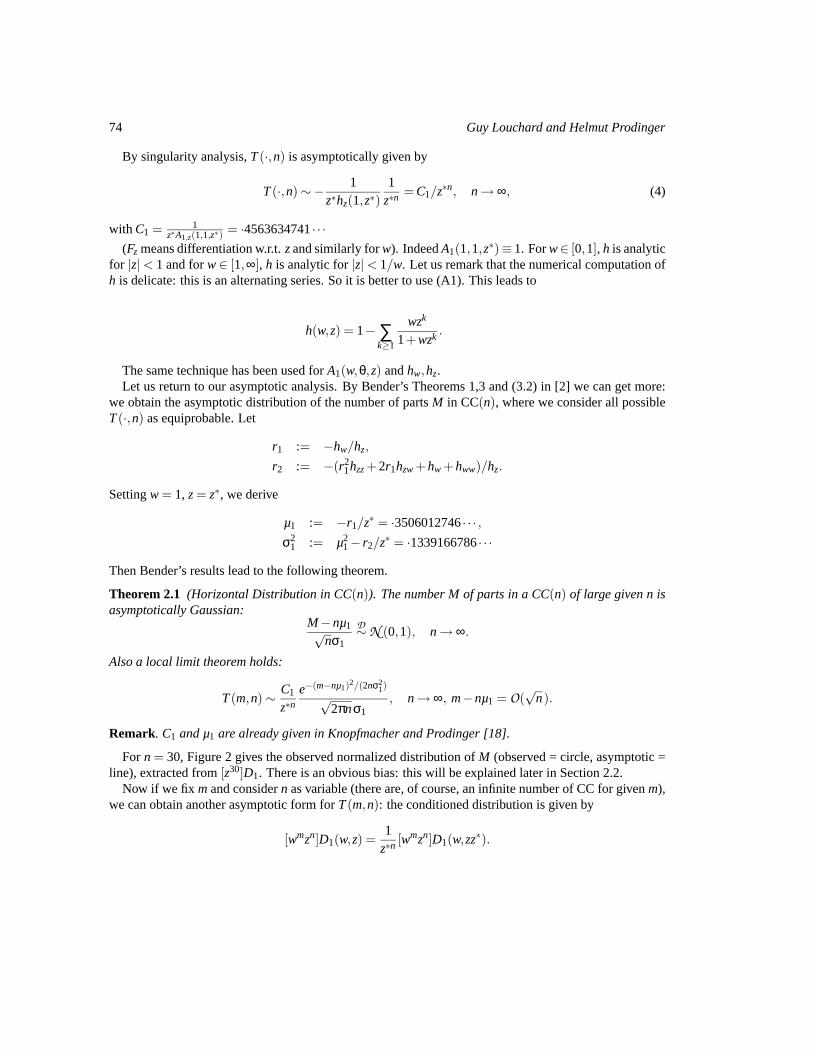
by D1(1,z). The dominant singularity ofD1 is given by the rootz∗ (with smallest module) ofh(1,z), i.e.z∗ = ·571349793158088. . . h(1,z) is analytic for|z| < 1. To be sure thatz∗ is the dominant singularity,we use the principle of the argument of Henrici [11]: the number of solutions of the equationf (z) = 0that lie inside a simple closed curveΓ, with f (z) analytic inside and onΓ, is equal to the variation of theargument off (z) alongΓ, a quantity also equal to the winding number of the transformed curvef (Γ)around the origin. The argument was used in Flajolet and Prodinger [8] in a similar situation. Figure 1represents[ℜ(h),ℑ(h)] for z= .60exp(it ), t = 0..2π, whereh is converted into a series up toO(z60). Thewinding number is 1, so thath has only one rootz∗ for |z|< .60.


By singularity analysis,T(·,n) is asymptotically given by

T(·,n)∼− 1z∗hz(1,z∗)

1z∗n

= C1/z∗n, n→ ∞, (4)

with C1 = 1z∗A1,z(1,1,z∗)

= ·4563634741· · ·(Fz means differentiation w.r.t.zand similarly forw). IndeedA1(1,1,z∗)≡ 1. Forw∈ [0,1], h is analytic

for |z|< 1 and forw∈ [1,∞], h is analytic for|z|< 1/w. Let us remark that the numerical computation ofh is delicate: this is an alternating series. So it is better to use (A1). This leads to

h(w,z) = 1−∑k≥1

wzk

1+wzk .

The same technique has been used forA1(w,θ,z) andhw,hz.Let us return to our asymptotic analysis. By Bender’s Theorems 1,3 and (3.2) in [2] we can get more:

we obtain the asymptotic distribution of the number of partsM in CC(n), where we consider all possibleT(·,n) as equiprobable. Let

r1 := −hw/hz,

r2 := −(r21hzz+2r1hzw+hw +hww)/hz.

Settingw = 1, z= z∗, we derive

µ1 := −r1/z∗ = ·3506012746· · · ,

σ21 := µ2

1− r2/z∗ = ·1339166786· · ·

Then Bender’s results lead to the following theorem.

Theorem 2.1 (Horizontal Distribution in CC(n)). The number M of parts in a CC(n) of large given n isasymptotically Gaussian:

M−nµ1√nσ1

D∼N (0,1), n→ ∞.

Also a local limit theorem holds:

T(m,n)∼ C1

z∗ne−(m−nµ1)2/(2nσ2

1)√

2πnσ1, n→ ∞, m−nµ1 = O(

√n).

Remark. C1 and µ1 are already given in Knopfmacher and Prodinger [18].

For n = 30, Figure 2 gives the observed normalized distribution ofM (observed = circle, asymptotic =line), extracted from[z30]D1. There is an obvious bias: this will be explained later in Section 2.2.

Now if we fix mand considern as variable (there are, of course, an infinite number of CC for givenm),we can obtain another asymptotic form forT(m,n): the conditioned distribution is given by

[wmzn]D1(w,z) =1

z∗n[wmzn]D1(w,zz∗).


0

0.05

0.1

0.15

0.2

6 8 10 12 14 16 18 20 22x

Fig. 2: Observed normalized distribution ofM(n = 30)

But, for z= 1, the dominant singularity ofD1(w,zz∗) is w∗ = 1. So with

C2 =−1

hw(1,z∗)= 1·3016594836· · · ,

µ2 := 1/µ1 = 2·852242911· · · , (5)

σ22 = σ2

1/µ31 = 3·1073787943· · · ,

we obtain the following theorem.

Theorem 2.2 (Vertical Distribution in CC(n)). For large given number of parts m, T(m,n) is asymptoti-cally given by

T(m,n)∼ C2

z∗ne−(n−mµ2)2/(2mσ2

2)√

2πmσ2, m→ ∞, n−mµ2 = O(

√m).

Note thatC1/C2 = µ1.For further use, we have also computedC2( j) based on a first part of fixed sizej. We first derive

(conditioning onj):φ(w,θ,z| j) = A2(w,θ,z| j)+A1(w,θ,z)D2, (6)

where

D2 := φ(w,1,z| j) = A2(w,1,z| j)/h,A2(w,θ,z| j) = θ jwzj/(1+wzj),


andA1 is given by (2).This leads to

C2( j) =−A2(1,1,z∗| j)hw(1,z∗)

=−z∗ j

1+z∗ j

1hw(1,z∗)

. (7)

Note that, by (A1),∑ j C2( j) = C2, as it should. Theorem 2.3 is still valid.

Bender’s theorems are based on the analysis ofϕ(w) = [ r(1)r(w) ]n where r(w) is the root of (3), seen

as az-equation, andr(1) = z∗. But r(1)/r(w) is usually not a Probability GF (PGF). Indeed, we obtain1

r(w) = 1+w− 12w2+ 7

12w3+ · · ·which of course doesn’t correspond to a PGF. Similarly, we could consider

t(z), the root of (3) (seen as aw-equation), witht(z∗) = 1, and analyze 1t(z∗z) . But we can’t even construct

a series inz.It is possible to derive a large deviation result for the number of parts, usingr(w).Following Bender [2] Theorem 3, we first setw = es. We have

r ′(s) = −hwes/hz,

r ′′(s) = −(r ′2hzz+2r ′eshzw+eshw +e2shww)/hz.

where, here,hw = hw(w, r(w)), etc.Bender leads to the following large deviation result:

Theorem 2.3 For m outside the range[nµ1−O(√

n),nµ1 + O(√

n)], choose s∗ such that µ= m/n =−r ′(s∗)/r(s∗). The following asymptotic relation holds:

T(m,n)∼ e−ms∗A1[es∗ ,1, r(s∗)][r(s∗)]nσ(s∗)

√2πn[−hz(es∗ , r(s∗))]r(s∗)

, n→ ∞,

with σ2(s∗) = (m/n)2− r ′′(s∗)/r(s∗).

The range of validity of Theorem 2.3 can be established as follows. First, we must consider the contourof h(w,z) = 0. After detailed analysis, it appears that this contourh(w,z) = 0 is made of 2 parts: seeFigure 3.

Part I, forw∈ (0,1], z∈ [z∗,1), with r(w) −→w→0

1.

Part II, forw∈ [1,w1),z∈ (1/w1,z∗] andw1 is the limit of the solution ofh[w, 1w− ε] = 0,ε→ 0.

The computation ofw1 offers no special numerical problem and leads to

w1 = 2·584243690· · · ,z1 = 1/w1 = ·3869604109· · ·

(we must only be careful with the precision: 20 digits are enough in the range we use).µ(w1) andσ2(w1)are given by

µ(w1) = ·4657044011· · · ,σ2(w1) = ·1056119001· · · .The functionµ(w) is increasing from 0 toµ(w1),σ2(w) goes from 0 (forw = 0) to some maximum and

then decreases toσ2(w1). So finally, the range forµ is given by(0,µ(w1)), z= r(w) following the contourdefined above.

The verification of condition (V) of Bender’s Theorem 3 (which allows to go from a central limittheorem to a local limit theorem) amounts to prove thath(es,z) is analytic and bounded for

|z| ≤ |r(ℜ(s))|(1+ δ) and ε≤ |ℑ(s)| ≤ π,


0

0.5

1

1.5

2

2.5

ww

0.4 0.5 0.6 0.7 0.8 0.9 1zz

Fig. 3: Contour ofh = 0 and domain of convergence

for someε > 0, δ > 0, wherer(s) is the suitable solution ofh(es, r(s)) = 0 (i.e. with r(0) = z∗): thisfollows from the analyticity analysis ofh in the beginning of this section.

2.2 Distribution of the last part size in CC

We want to analyze the asymptotic distribution of the size LP of the last part of a CC(n). Settingw = 1 in(1), we derive

[zn]φ(1,θ,z)∼ A1(1,θ,z∗)−z∗nz∗hz(1,z∗)

, n→ ∞,

uniformly for θ in some complex neighbourhood of the origin. This may be checked by the method ofsingularity analysis of Flajolet and Odlyzko, as used in Flajolet and Soria [9] or Hwang [13]. Normalizingby the total number of CC(n) (4) this leads to the following asymptotic(n→∞) PGF for the last part sizeLP:

G(θ) = A1(1,θ,z∗).

Expanding, this leads to

π1(i) := [θi ]G(θ) =z∗i

1+z∗i,

with typical geometric behaviour. Of courseG(1) = 1 by (A1) andE(LP) = ∑ iπ(i) = 2·5833049669· · ·.Forn = 12, we have computed the observed normalized distribution ofLP corresponding to

[z12]φ(θ,1,z).


0

0.05

0.1

0.15

0.2

0.25

0.3

0.35

1 2 3 4 5 6 7 8 9

Fig. 4: Observed normalized distribution of the last part size LP(n = 12).

This gives the following Figure 4 (observed = circle, asymptotic = line). The agreement is quite good.We can now obtain more information from (1). The asymptotic distribution of the last part size in

CC(n) of m parts is related to[wmzn]φ(w,θ,z) and Bender’s Theorems 1 and 3 lead to the GF:

T(θ,m,n)∼ C1

z∗ne−(m−nµ1)2/(2nσ2

1)√

2πnσ1G(θ),

for m− nµ1 = O(√

n), uniformly for θ in some complex neighbourhood of the origin. Again the uni-formity can be checked by following Bender’s analysis. Normalizing byT(m,n) (see Theorem 2.1), thisgives againG(θ). So we have proved the following result:

Theorem 2.4 For m−nµ1 = O(√

n), the asymptotic distribution of the size LP of the last part in CC(n)with m parts is given byπ1( j) = z∗ j/(1+z∗ j) for n→ ∞ uniformly for all j.

For instance, forn = 30,m = 9,11,13,(bnµ1c = 10,b√

nσ1c = 2) we have computed the observednormalized distribution of LP.

Figure 5 shows that the fit is quite good near the mean, but there is a bias for the two other values ofm:n is not yet large enough to yield a distribution of LP that is nearly independent ofm

Returning to the proof of Bender’s theorem, we must compute from (1)[θkwm]ϕ1ϕ2[ z∗

r(w) ]n with

ϕ1(θ,w) = A1(w,θ, r(w)),

ϕ2(w) = − 1r(w)hz(w, r(w))

,


0

0.1

0.2

0.3

0.4

1 2 3 4 5 6 7 8 9

Fig. 5: Observed normalized LP distribution (cross:m= 9, circle:m= 11, box:m= 13,n = 30)

andr(w) is again the root of (3) withr(1) = z∗. But according to Hwang [13], [14, Theorem 2], we knowthat the mean value ofM for largen is given byE(M)∼ nµ1 +v′(0), where

v(s) := log[ϕ1(1,es)ϕ2(es)/(ϕ1(1,1)ϕ2(1))],

i.e.

v′(0) =ϕ1,w(1,1)ϕ1(1,1)

+ϕ2,w(1)ϕ2(1)

= β say.

But it is easy to check thatϕ1,w(1,1) = 0 and

ϕ2,w(1) = [rwhz+z∗hz,zrw +z∗hz,w]/[z∗hz]2,ϕ2(1) = −1/(z∗hz),

rw = −hw/hz.

From now on, we sethz = hz(1,z∗), etc.Numerical computation givesβ = ·5365417012· · · This biasβ is now reintroduced in Figure 1 (n= 30).

This gives Figure 6, where the fit is now nearly perfect.

2.3 Correlation between two successive intermediate parts

Let us now turn to two successive partsm1,m1 +1, of sizek, j, such that their distances from the first andthe last part are of orderO(n). Let T(m,n, j) be the total number of CC(n) with m parts and last part size


0

0.05

0.1

0.15

0.2

6 8 10 12 14 16 18 20 22x

Fig. 6: Observed normalized distribution ofM with bias (observed = circle, asymptotic = line,n = 30)

j, let #(m,n,m1,k) be the total number of CC(n) with m parts, partm1 of sizek, and setm2 := m−m1.We have, conditioning onj,

#(m,n,m1,k) = ∑n1

∑j 6=k

T(m1,n1,k)T(m2,n−n1, ·)| j.

With Theorem 2.4 (vertical form) and Theorem 2.2 [Eq. 7], this leads, after normalization byT(m,n), tothe following distribution:

#(m,n,m1,k)T(m,n)

∼ ∑n1

∑j 6=k

e−(n1−m1µ2)2/2m1σ22

√2πm1σ2

π1(k)×

×C2( j)e−(n−n1−m2µ2)2/2m2σ2

2√

2πm2σ2

/e−(n−mµ2)/2mσ2

2√

2πmσ2, (8)

and with (A1) we readily obtain the following distributionπ2(k) for k:

π2(k) = ∑j 6=k

π1(k)C2( j) =−z∗k

(1+z∗k)2hw.

For further use, we compute, for`≥ k

π2(`) = π(1)2 (`)z∗k + π(2)

2 (`)z∗2k + O(z∗3k), k→ ∞,


with

π(1)2 (`) =−z∗(l−k)

hw, π(2)

2 (`) =2z∗2(l−k)

hw. (9)

By (A2), we obtain∑∞1 π2(k) = 1 and by (A3),∑kπ2(k) = µ2 as it should. So we obtain the following

theorem.

Theorem 2.5 The asymptotic(n→∞) distribution of intermediate part size is given byπ2(k), with meanµ2.

But we can get more from (8), which shows that the asymptotic joint distribution (in stationary distribu-tion) of two successive intermediate part sizesk and j is given by

π1(k)C2( j), j 6= k.

Normalizing byπ2(k), this leads to the following Markov chain related to two successive intermediateparts:

Π(k, j) =z∗ j(1+z∗k)

1+z∗ j , j 6= k. (10)

The chain is irreducible, recurrent positive and reversible. Of course the stationary distribution ofΠ isgiven byπ2(k). Therefore, we obtain the following theorem.

Theorem 2.6 The asymptotic, n→ ∞, distribution of two successive intermediate parts in a CC (n) isgiven by a Markov chainΠ(i, j), with stationary distributionπ2(k), and with mean µ2.

Let us now analyze the asymptotic behaviour ofΠ(i, j). This will be used in Sec. 3.2. For fixed, weobtain

Π+(`,k) :=∞

∑j=k

Π(`, j) = (1+z∗`)z∗k

1−z∗(1+ O(z∗k)), k→ ∞.

For further use, we set

ϕ3(`) :=1+z∗`

1−z∗. (11)

2.4 Associated processes and limiting trajectories

Let us now turn to trajectories. Letxi be the size of parti and setX( j) := ∑ j1xi . We haveE[X(m)]∼mµ2

and we must check that VAR[X(m)]∼mσ22 as given by (5). We first derivemσ2

X := VAR[X(m)]∼m[S2−µ2

2]+2m∑∞1 Cx

k where

S2 := ∑π2( j) j2 = 12·208296194· · · ,Cx

k := ∑i

∑j

(i−µ2)π2(i)Πk(i, j)( j−µ2).

But it is easily checked thatS3 := ∑∞1 Cx

k can be written as

S3 = limw→1

[− 1

hw

{∑i

∑j

i1+z∗i

[θ j ]φ(w,θ,z∗|i) j1+z∗ j −w∑

i

z∗i i2

(1+z∗i)2

}−µ2

2w2

1−w

].


With (6), this can be simplified as

S3 = limw→1

[∑i

∑j− 1

hw

i1+z∗i

j1+z∗ j [θ

j ]{

A2(w,θ,z∗|i)−wz∗iθi

w

+A1(w,θ,z∗)A2(w,1,z∗|i)

wh(w,z∗)

}− µ2

2w1−w

].

This leads to (we setw = 1− ε)

S3 = limε→0

[−µ2

2

ε+µ2

2 + ϕ6−1hw

[− ϕ5(1)

hwε+

ϕ5,w(1)hw

− ϕ5(1)hww

2h2w

]], (12)

where

ϕ6 :=1hw

∑i

i2

(1+z∗i)2

z∗2i

(1+z∗i)=−·95938032262· · · ,

ϕ5(w,θ, i) = A1(w,θ,z∗)A2(w,1,z∗|i)/w.

But A1(1,θ,z∗)≡G(θ), so we derive

− 1hw· −ϕ5(1)

hw=− 1

hw∑i

∑j

[i

1+z∗i· −z∗i

(1+z∗i)hw. · z∗ j

1+z∗ j ·j

1+z∗ j

]≡ µ2

2.

So the singularity in (12) is removed.Similarly, we obtain

ϕ5,w(1) = ∑i

∑j

[i

1+z∗i· j1+z∗ j [θ

j ]ϕ5,w(1,θ, i)],

and finally

mσ2X ∼m

[S2 +µ2

2 +2

{ϕ6−

ϕ5,w(1)h2

w+

µ22hww

2hw

}]= mσ2

2, (13)

by (A4) as expected.We can now apply the Functional Central Limit Theorem (for dependent R.V.) (see for instance Billings-

ley [4, p. 168 ff.]) and we obtain the following result, whereB(t) is the standard Brownian Motion (BM).

Theorem 2.7X([Nt])−µ2Nt

σ2√

N⇒ B(t), N→ ∞, t ∈ [0,1],

where N:= number of parts ofCC(n).

Let us now condition onX(m) = n. A realization ofX for fixed n is given by Theorem 2.7, where westop at a random timemsuch thatX(m) = n. Proceeding as in [19] it is easy to check that this amounts tofix N = n/µ2 in Theorem 2.7 (denominator) and we obtain the following result.


Theorem 2.8 Conditioned on X(m) = n,

X([mt])−µ2mt

σ2√

n/µ2⇒ B(t).

Let us now consider the oscillations ofX(·) around its mean. Let us define the lower oscillation boundW−n and the rangeWn:

W−n := − infi ∈ [0,m]

[X(i)−µ2i],

Wn :={

sup − inf[0,m] [0,m]

}[X(i)−µ2i],

wherem is the number of parts in CC(n).

But now the lower boundW−n , normalized by√

n/µ2 σ2, is asymptotically given by inf B(t)[0,1]

and

the rangeWn corresponds to the range

{sup − inf[0,1] [0,1]

}B(t). The densities of these R.V. are well

known: the first one is given by

f1(x) =2e−x2/2√

2π,

the second one is given by

f2(x) =8√2π

∞

∑k=1

k2(−1)k−1exp[−k2x2/2],

or

f2(x) = (2π

)1/2 1x

L′(x2

),

where

L(z) = 1−2∞

∑k=1

(−1)k−1exp[−2k2z2]

= (2π)1/2 1z

∞

∑k=1

exp[−2(k−1)2π2/8z2],

by Jacobiθ–relations (see e.g. Whittaker and Watson [22].This immediately leads to the following result

Theorem 2.9 For large n, and with N= n/µ2,W−n /(σ2

√N) has the asymptotic density f1,

Wn/(σ2√

N) has the asymptotic density f2.

In summary, we can see the CC as a B.M. with some thickness (part size). The distribution of the thicknessis characterized by Theorem 2.6.


0

2000

4000

6000

8000

10000

0 500 1000 1500 2000 2500 3000 3500

Fig. 7: UnnormalizedX(·).

3 Simulations and thicknessIn this section, we present an algorithm for CC(n) simulation, then we analyze the CC thickness maxi-mum.

3.1 RealizationsA simulated realization of a CC(n) proceeds as follows.2 Start with a part of sizej at timei = 1 givenby π1( j). Proceed from a part of sizek at timei−1 to a part of sizej at timei by using a Markov chaindefined by the probability matrixΠ(k, j) given by (10). Stop the chain as soon asS:= ∑m

i=1 j i > n.For n = 10.000, a typical unnormalized trajectory forX(i) is given in Figure 7, which shows a “fila-

ment silhouette.” A typical normalized trajectory forX(i)−µ2iσ2√

Nand X(i−1)−µ2i

σ2√

N, showing the thickness (here

the thickness is defined by the size of the parts) is given in Figure 8. Of course, both trajectories areasymptotically equivalent forn→ ∞. A zoom oni = [1030..1050] is given in Figure 9.

3.2 Hitting times and maximum for CC thicknessLet us call thickness the part size. In this section, we derive the thickness hitting times (to high level)asymptotic distribution. This leads to a maximum asymptotic density. We consider the setxi of R.V.describing the thickness of CC. Let us define the setD := [k..∞), k >> 1. By (11), we see that theprobability transition toD is O(ε),ε = z∗k and by standard properties (see Keilson [16], Aldous [1]) weknow that the hitting time toD is such that (we dropk for ease of notation):

• E`[TD] = C3ε + ψ(`)+ O(ε) (Actually a Laurent series exists forε sufficiently small),


-1

-0.5

0

0.5

1

0 500 1000 1500 2000 2500 3000 3500

Fig. 8: NormalizedX(·), with thickness.

3010

3020

3030

3040

3050

3060

3070

3080

1030 1035 1040 1045 1050

Fig. 9: UnnormalizedX(·) with thickness (zoom).


• Pr [TD ≥ x]∼ e−x/E`[TD], x→ ∞.

We should writeC3(`) but we will soon check thatC3 is independent of. To computeC3 andψ(`), weuse the classical relation:

E`[TD] = 1+ ∑j∈DC

Π[`, j]E j [TD] (14)

i.e.

C3 + ψ(`)ε = ε + ∑j∈DC

Π[`, j][C3 + ψ( j)ε]+ O(ε2)

= ε + ΠC3− εϕ3(`)C3 +∑j

Π(`, j)ψ( j)ε + O(ε2), (15)

andϕ3 is given by (11).Eq. (14) leads to

1 = ∑D

π2(`)E`(TD).

(This is equivalent to a formula of Kac, see [15]).Therefore, we obtain

1 = C3∑D

π(1)2 (`), (16)

0 = ∑D

π(1)2 (`)ψ(`)+C3∑

Dπ(2)

2 (`) (17)

(π(1)2 andπ(2)

2 are given by (9)).Comparison of powers ofε in (15) leads to[I −Π]C3 = 0, which confirms thatC3 is independent of.

We deriveψ(`) = 1−ϕ3(`)C3 +∑

jΠ(`, j)ψ( j),

or[I −Π]ψ = δ, with δ(`) := 1−ϕ3(`)C3. (18)

We must haveπ2δ = 0, therefore

1 = ∑π2(`)ϕ3(`)C3, C3 = 1/∑π2(`)ϕ3(`),

which fixesC3 =−hw(1−z∗). (This is of course equivalent to (16).)We denote byM1 the Drazin inverse ofI −Π. We refer to Campbell and Meyer [5] for a detailed

definition and analysis of the Drazin inverse. We have

M1 = ∑n≥0

(Πn−1×π2) = M2−1×π2, (19)

whereM2 := [I −Π + 1×π2]−1 = ∑n≥0[Π−1×π2]n is the potential used in Kemeny, Snell and Knapp[17]. The solution of (18) is given byψ = M1δ + π2ψ.


To fix C6 := π2ψ, we first derive

∑D

π(1)2 ψ = ∑

Dπ(1)

2 M1δ +C6∑D

π(1)2 ,

and with (17),

C6 = [hw(1−z∗)2

hw(1−z∗2)−∑

Dπ(1)

2 M1δ][−hw(1−z∗)].

We can summarize our results in the following form.

Theorem 3.1 The thickness hitting time E`[TD] to D := [k..∞], k>> 1 is given by

E`[TD]∼ C3

z∗k+ ψ(`)+ O(z∗k),

with C3 =−hw(1−z∗), ψ(`) = M1[1−C3ϕ3(`)]+C6 (M1 is the potential kernel given in (19)).

Pr`[TD ≥ x]∼ e−xz∗k/C3,x→ ∞.

Now let M (t) := supi∈[1..t] xi (maximum thickness witht parts). We know that

Pr[M (t)< k] = Pr[TD ≥ t +1].

So, by standard asymptotic analysis,

Pr[M (t)< k]∼ exp[−exp[logt−k log(z∗−1)− logC3]], t→ ∞.

Set nowk := j +1 andC4 = z∗/C3.By Theorem 2.1, we know thatt = nµ1 + O(

√n) andµ1 = hw/(hzz∗).

Hence, we derive the following theorem (we use now the notationM (n)).

Theorem 3.2 Letη := j− [logn+ logC4 + logµ1]/ log(z∗−1).

Then, with integer j andη = O(1),

Pr[M (n)≤ j]∼G1(η), n→ ∞,

where G1(η) := exp[−exp[−η log(z∗−1)]]. Let

ψ1(n) := log(C4nµ1)/ log(z∗−1) = [logn− log(−hz)− log(1−z∗)]/ log(z∗−1),

and η = j −bψ1(n)c− {ψ1(n)}. Asymptotically, the distribution is a periodic function ofψ1(n) (withperiod 1), which can be written as

logPr[M (n)≤ (bψ1(n)c+k)e−{ψ1(n)} log(z∗−1) −→n→∞−e−k log(z∗−1).

We also havePr[M (n) = j]∼ f1(η),

where f1(η) := G1(η)−G1(η−1).


0

0.05

0.1

0.15

0.2

10 15 20 25 30 35

Fig. 10: Distribution of maximum thickness.

The asymptotic moments ofM (n) are also periodic functions ofψ1(n). They can be written as Har-monic sums which are usually analyzed with Mellin transforms: see Flajolet et al [7]. The asymptoticnon-periodic term in the moments ofM (n) is given by the following result.

Theorem 3.3 The constant termE in the Fourier expansion (inψ1(n)) of the moments ofM (n) is asymp-totically given by

E[M (n)−ψ1(n)]i ∼∫ +∞

−∞ηi [G1(η)−G1(η−1)]dη.

It is well known that the extreme-value distribution functione−e−xhas meanγ and varianceπ2/6. From

this, we can for instance derive

E[M (n)]∼ ψ1(n)+12

+γ

log(z∗−1). (20)

The other periodic terms have very small amplitude (see Flajolet et al [7]).Forn= 10.000, we have simulated 2.000 trajectories. The observed distribution for maximum thickness

is given in Figure 10.The observed and limiting distribution function (DF) are given in Figure 11 (observed = circle, asymp-

totic = line). The limiting DF is given byG1[ j−ψ1(n)] and, due to the sensitivity ofG1 to the mean, wehave takenψ1(n) = M0(n)− 1

2 −γ

log(z∗−1) whereM0(n) is the observed mean = 17·17. . . The limiting

meanE(M (n)) is given by (20) and leads to 17·09739171. . .


0

0.2

0.4

0.6

0.8

1

10 15 20 25 30 35x

Fig. 11: Observed and limiting DF.

4 ConclusionUsing some generating functions and limit convergence theorems, we have obtained a complete stochasticdescription of Carlitz compositions. The same techniques could be used for some generalizations such asCarlitz compositions with zeros and with some restrictions. In a recent paper by Hitczenko and Louchard[12], the distinctness of classical and Carlitz compositions has been fully analyzed.

Acknowledgements

The pertinent comments of the referee led to improvements in the presentation.

References[1] D. Aldous. Probability Approximations via the Poisson Clumping Heuristic. Springer-Verlag, 1989.

[2] E.A. Bender. Central and local limit theorems applied to asymptotics enumeration.Journal ofCombinatorial Theory,Series A, 15:91–111, 1973.

[3] Edward A. Bender. Convexn-ominoes.Discrete Math., 8:219–226, 1974.

[4] P. Billingsley. Convergence of Probability Measures. Wiley, 1968.

[5] S. L. Campbell and C. D. Meyer.Generalized Inverse of Linear Transformations. Pitman, 1979.


[6] L. Carlitz. Restricted compositions.Fibonacci Quarterly, 14:254–264, 1976.

[7] P. Flajolet, X. Gourdon, and P. Dumas. Mellin transforms and asymptotics: Harmonic sums.Theo-retical Computer Science, 144:3–58, 1995.

[8] P. Flajolet and H. Prodinger. Level number sequences for trees.Discrete Mathematics, 65:149–156,1987.

[9] P. Flajolet and M. Soria. General combinatorial schemes: Gaussian limit distribution and exponentialtails. Discrete Mathematics, 114:159–180, 1993.

[10] I. P. Goulden and D. M. Jackson.Combinatorial enumeration. John Wiley & Sons Inc., New York,1983. With a foreword by Gian-Carlo Rota, Wiley-Interscience Series in Discrete Mathematics.

[11] P. Henrici.Applied and Computational Complex Analysis. Wiley, 1988.

[12] P. Hitczenko and G. Louchard. Distinctness of compositions of an integer: a probabilistic analysis.Random Structures and Algorithms, 19(3,4):407–437, 2001.

[13] H.K. Hwang. Theoremes limites pour les structures aleatoires et les fonctions arithmetiques. 1994.These, Ecole Polytechnique de Palaiseau.

[14] H.K. Hwang. On convergence rates in the central limit theorems for combinatorial structures.Euro-pean Journal of Combinatorics, 19:329–343, 1998.

[15] M. Kac. On the notion of recurrence in discrete stochastic processes.Bulletin of the AmericanMathematical Society, 53:1002–1019.

[16] J. Keilson.Markov Chain Models-Rarity and Exponentiality. Springer-Verlag, 1979.

[17] J. G. Kemeny, J. L. Snell, and A. W. Knapp.Denumerable Markov Chains. Van Nostrand, 1966.

[18] A. Knopfmacher and H. Prodinger. On Carlitz compositions.European Journal of Combinatorics,19:579–589, 1998.

[19] G. Louchard. Probabilistic analysis of some (un)directed animals.Theoretical Computer Science,159(1):65–79, 1996.

[20] G. Louchard. Probabilistic analysis of column-convex and directed diagonally-convex animals.Ran-dom Structures and Algorithms, 11:151–178, 1997.

[21] G. Louchard. Probabilistic analysis of column-convex and directed diagonally-convex animals. II:Trajectories and shapes.Random Structures and Algorithms, 15:1–23, 1999.

[22] E.T. Whittaker and G.N. Watson.A Course of Modern Analysis. Cambridge University press(reprinted 1973), 1927.


A Appendix : Some combinatorial identitiesLet us first setT(a,b,c) := ∑k≥1ka zbk

(1+zk)c .

∞

∑1

z∗ j

1+z∗ j = 1. (A1)

Proof

∑j≥1

(−1) j+1 zj

1−zj = ∑j≥1

(−1) j+1 ∑k≥1

zk j

=− ∑k, j≥1

(−zk) j = T(0,1,1)

Since for the special choicez∗ of z the left side equals 1, the right side also does. Note that this is theonly identity where we need the valuez∗. All next identities are on arbitraryz. 2

∞

∑1

z∗ j

(1+z∗ j)2 =−hw. (A2)

Proof

h(w,z) = 1+ ∑j≥1

(−1) j zjw j

1−zj .

Hence

−hw = ∑j≥1

(−1) j+1 jz j

1−zj

= ∑j,k≥1

(−1) j+1 jz jk

= − ∑j,k≥1

j(−zk) j

= T(0,1,2).

2

∞

∑1

jz∗ j

(1+z∗ j)2 =−z∗hz. (A3)

Proof

−zhz = ∑j≥1

(−1) j+1 jz j

(1−zj)2


= ∑j,k≥1

(−1) j+1 jkzjk

= − ∑j,k≥1

k j(−zk) j

= T(1,1,2).

2

σ22≡ σ2

X. (A4)

Proof

S2 =T(2,1,2)T(0,1,2)

,

µ22 =

(zhz

hw

)2

=(

T(1,1,2)T(0,1,2)

)2

,

ϕ6 =−T(2,2,3)T(0,1,2)

,

σ2X = S2−µ2

2 +2Σ,

or, by (13),

T(2,1,2)T(0,1,2)

+(

T(1,1,2)T(0,1,2)

)2

−2T(2,2,3)T(0,1,2)

−2ϕ5,w

T(0,1,2)2 −ϕ5hww

(T(0,1,2))3 .

hww = ∑j≥1

(−1) j+1 j( j−1)zj

1−zj

= ∑j,k≥1

(−1) j+1 j( j−1)zjk

= − ∑j,k≥1

j( j−1)(−zk) j

= 2T(0,2,3).

ϕ5 = h2wµ2

2 = (zhz)2 = T(1,1,2)2.

ϕ5(w,θ, i) = ∑k≥1

(−1)k+1 zkθwk

1−θzk ·zi

1+wzi .


[θ j ]ϕ5(w,θ, i) = ∑k≥1

(−1)k+1zkwkzk( j−1) zi

1+wzi

= ∑k≥1

(−1)k+1zk jwkzi ∑≥0

(−1)`(wzi)`.

[θ j ]ϕ5,w(1,θ, i) = ∑≥0

∑k≥1

(−1)k+1zk jzizi`(k+ `)(−1)`.

ϕ5,w(1) = ∑i≥1

∑j≥1

∑≥0

∑k≥1

i1+zi

j1+zj (−1)k+1zk jzizi`(k+ `)(−1)`

= −∑i≥1

iz2i

(1+zi)3 ∑j≥1

jz j

(1+zj)2 + ∑i≥1

izi

(1+zi)2 ∑j≥1

jz j

(1+zj)3 .

This gives

ϕ5,w(1) = T(1,1,2)[T(1,1,3)−T(1,2,3)].

Soσ2X becomes

σ2X =

T(2,1,2)T(0,1,2)

+T(1,1,2)2

T(0,1,2)2 −2T(2,2,3)T(0,1,2)

− 2T(1,1,2)[T(1,1,3)−T(1,2,3)]

T(0,1,2)2 −2T(1,1,2)2T(0,2,3)

T(0,1,2)3 .

This should equalσ22 = σ2

1/µ31 = 1/µ1− r2

3µ31.

But, after a boring but simple computation we find

hzz=1z2

[T(2,2,3)+T(1,2,3)−T(2,1,3)+T(1,1,3)

],

µ1 =hw

zhz=

T(0,1,2)T(1,1,2)

,

hww = 2T(0,2,3),

hzw =1z

[T(1,2,3)−T(1,1,3)

].

Therefore


σ22 =

σ21

µ31

=1µ1− r2

zµ31

=T(1,1,2)T(0,1,2)

− r2

zT(1,1,2)3

T(0,1,2)3

=T(1,1,2)T(0,1,2)

+r21hzz+2r1hzw+hw +hww

zhz

T(1,1,2)3

T(0,1,2)3

=T(1,1,2)T(0,1,2)

− r21hzz+2r1hzw+hw +hww

T(1,1,2)T(1,1,2)3

T(0,1,2)3

=T(1,1,2)T(0,1,2)

−[r21hzz+2r1hzw+hw +hww

]T(1,1,2)2

T(0,1,2)3

=T(1,1,2)T(0,1,2)

− T(0,1,2)2

T(1,1,2)2

[T(2,2,3)+T(1,2,3)−T(2,1,3)+T(1,1,3)

]T(1,1,2)2

T(0,1,2)3

−[2r1hzw+hw +hww

]T(1,1,2)2

T(0,1,2)3

=T(1,1,2)T(0,1,2)

−[T(2,2,3)+T(1,2,3)−T(2,1,3)+T(1,1,3)

] 1T(0,1,2)

−[2r1hzw+hw +hww

]T(1,1,2)2

T(0,1,2)3

=T(1,1,2)T(0,1,2)

− T(2,2,3)T(0,1,2)

− T(1,2,3)T(0,1,2)

+T(2,1,3)T(0,1,2)

− T(1,1,3)T(0,1,2)

−[2r1hzw+hw +hww

]T(1,1,2)2

T(0,1,2)3

=T(1,1,2)T(0,1,2)

− T(2,2,3)T(0,1,2)

− T(1,2,3)T(0,1,2)

+T(2,1,3)T(0,1,2)

− T(1,1,3)T(0,1,2)

+ 2T(0,1,2)T(1,1,2)

[T(1,2,3)−T(1,1,3)

]T(1,1,2)2

T(0,1,2)3

−[hw +hww

]T(1,1,2)2

T(0,1,2)3

=T(1,1,2)T(0,1,2)

− T(2,2,3)T(0,1,2)

− T(1,2,3)T(0,1,2)

+T(2,1,3)T(0,1,2)

− T(1,1,3)T(0,1,2)

+ 2[T(1,2,3)−T(1,1,3)

] T(1,1,2)T(0,1,2)2

−[−T(0,1,2)+2T(0,2,3)

]T(1,1,2)2

T(0,1,2)3

=T(1,1,2)T(0,1,2)

− T(2,2,3)T(0,1,2)

− T(1,2,3)T(0,1,2)

+T(2,1,3)T(0,1,2)

− T(1,1,3)T(0,1,2)


+ 2[T(1,2,3)−T(1,1,3)

] T(1,1,2)T(0,1,2)2

+T(1,1,2)2

T(0,1,2)2 −2T(0,2,3)T(1,1,2)2

T(0,1,2)3 .

But now, we easily check that

T(2,1,3)−T(2,2,3)≡−2T(2,2,3)+T(2,1,2),

andT(1,1,3)+T(1,2,3) = T(1,1,2).

Identification ofσ22 andσ2

X is now immediate.2

Probabilistic Analysis of Carlitz Compositions

Documents

Transcript of Probabilistic Analysis of Carlitz Compositions