5 Probabilistic Analysis and Randomized Algorithms

5 Probabilistic Analysis and RandomizedAlgorithms

This chapter introduces probabilistic analysis and randomized algorithms. If youare unfamiliar with the basics of probability theory, you should read Appendix C,which reviews this material. We shall revisit probabilistic analysis and randomizedalgorithms several times throughout this book.

5.1 The hiring problem

Suppose that you need to hire a new office assistant. Your previous attempts athiring have been unsuccessful, and you decide to use an employment agency. Theemployment agency sends you one candidate each day. You interview that personand then decide either to hire that person or not. You must pay the employmentagency a small fee to interview an applicant. To actually hire an applicant is morecostly, however, since you must fire your current office assistant and pay a substan-tial hiring fee to the employment agency. You are committed to having, at all times,the best possible person for the job. Therefore, you decide that, after interviewingeach applicant, if that applicant is better qualified than the current office assistant,you will fire the current office assistant and hire the new applicant. You are willingto pay the resulting price of this strategy, but you wish to estimate what that pricewill be.

The procedure HIRE-ASSISTANT, given below, expresses this strategy for hiringin pseudocode. It assumes that the candidates for the office assistant job are num-bered 1 through n. The procedure assumes that you are able to, after interviewingcandidate i , determine whether candidate i is the best candidate you have seen sofar. To initialize, the procedure creates a dummy candidate, numbered 0, who isless qualified than each of the other candidates.

5.1 The hiring problem 115

HIRE-ASSISTANT.n/

1 best D 0 // candidate 0 is a least-qualified dummy candidate2 for i D 1 to n

3 interview candidate i

4 if candidate i is better than candidate best5 best D i

6 hire candidate i

The cost model for this problem differs from the model described in Chapter 2.We focus not on the running time of HIRE-ASSISTANT, but instead on the costsincurred by interviewing and hiring. On the surface, analyzing the cost of this algo-rithm may seem very different from analyzing the running time of, say, merge sort.The analytical techniques used, however, are identical whether we are analyzingcost or running time. In either case, we are counting the number of times certainbasic operations are executed.

Interviewing has a low cost, say ci , whereas hiring is expensive, costing ch. Let-ting m be the number of people hired, the total cost associated with this algorithmis O.cin C chm/. No matter how many people we hire, we always interview n

candidates and thus always incur the cost cin associated with interviewing. Wetherefore concentrate on analyzing chm, the hiring cost. This quantity varies witheach run of the algorithm.

This scenario serves as a model for a common computational paradigm. We of-ten need to find the maximum or minimum value in a sequence by examining eachelement of the sequence and maintaining a current “winner.” The hiring problemmodels how often we update our notion of which element is currently winning.

Worst-case analysis

In the worst case, we actually hire every candidate that we interview. This situationoccurs if the candidates come in strictly increasing order of quality, in which casewe hire n times, for a total hiring cost of O.chn/.

Of course, the candidates do not always come in increasing order of quality. Infact, we have no idea about the order in which they arrive, nor do we have anycontrol over this order. Therefore, it is natural to ask what we expect to happen ina typical or average case.

Probabilistic analysis

Probabilistic analysis is the use of probability in the analysis of problems. Mostcommonly, we use probabilistic analysis to analyze the running time of an algo-rithm. Sometimes we use it to analyze other quantities, such as the hiring cost

116 Chapter 5 Probabilistic Analysis and Randomized Algorithms

in procedure HIRE-ASSISTANT. In order to perform a probabilistic analysis, wemust use knowledge of, or make assumptions about, the distribution of the inputs.Then we analyze our algorithm, computing an average-case running time, wherewe take the average over the distribution of the possible inputs. Thus we are, ineffect, averaging the running time over all possible inputs. When reporting such arunning time, we will refer to it as the average-case running time.

We must be very careful in deciding on the distribution of inputs. For someproblems, we may reasonably assume something about the set of all possible in-puts, and then we can use probabilistic analysis as a technique for designing anefficient algorithm and as a means for gaining insight into a problem. For otherproblems, we cannot describe a reasonable input distribution, and in these caseswe cannot use probabilistic analysis.

For the hiring problem, we can assume that the applicants come in a randomorder. What does that mean for this problem? We assume that we can compareany two candidates and decide which one is better qualified; that is, there is atotal order on the candidates. (See Appendix B for the definition of a total or-der.) Thus, we can rank each candidate with a unique number from 1 through n,using rank.i/ to denote the rank of applicant i , and adopt the convention that ahigher rank corresponds to a better qualified applicant. The ordered list hrank.1/;

rank.2/; : : : ; rank.n/i is a permutation of the list h1; 2; : : : ; ni. Saying that theapplicants come in a random order is equivalent to saying that this list of ranks isequally likely to be any one of the nŠ permutations of the numbers 1 through n.Alternatively, we say that the ranks form a uniform random permutation; that is,each of the possible nŠ permutations appears with equal probability.

Section 5.2 contains a probabilistic analysis of the hiring problem.

Randomized algorithms

In order to use probabilistic analysis, we need to know something about the distri-bution of the inputs. In many cases, we know very little about the input distribution.Even if we do know something about the distribution, we may not be able to modelthis knowledge computationally. Yet we often can use probability and randomnessas a tool for algorithm design and analysis, by making the behavior of part of thealgorithm random.

In the hiring problem, it may seem as if the candidates are being presented to usin a random order, but we have no way of knowing whether or not they really are.Thus, in order to develop a randomized algorithm for the hiring problem, we musthave greater control over the order in which we interview the candidates. We will,therefore, change the model slightly. We say that the employment agency has n

candidates, and they send us a list of the candidates in advance. On each day, wechoose, randomly, which candidate to interview. Although we know nothing about

5.1 The hiring problem 117

the candidates (besides their names), we have made a significant change. Insteadof relying on a guess that the candidates come to us in a random order, we haveinstead gained control of the process and enforced a random order.

More generally, we call an algorithm randomized if its behavior is determinednot only by its input but also by values produced by a random-number gener-ator. We shall assume that we have at our disposal a random-number generatorRANDOM. A call to RANDOM.a; b/ returns an integer between a and b, inclu-sive, with each such integer being equally likely. For example, RANDOM.0; 1/

produces 0 with probability 1=2, and it produces 1 with probability 1=2. A call toRANDOM.3; 7/ returns either 3, 4, 5, 6, or 7, each with probability 1=5. Each inte-ger returned by RANDOM is independent of the integers returned on previous calls.You may imagine RANDOM as rolling a .b � a C 1/-sided die to obtain its out-put. (In practice, most programming environments offer a pseudorandom-numbergenerator: a deterministic algorithm returning numbers that “look” statisticallyrandom.)

When analyzing the running time of a randomized algorithm, we take the expec-tation of the running time over the distribution of values returned by the randomnumber generator. We distinguish these algorithms from those in which the inputis random by referring to the running time of a randomized algorithm as an ex-pected running time. In general, we discuss the average-case running time whenthe probability distribution is over the inputs to the algorithm, and we discuss theexpected running time when the algorithm itself makes random choices.

Exercises

5.1-1Show that the assumption that we are always able to determine which candidate isbest, in line 4 of procedure HIRE-ASSISTANT, implies that we know a total orderon the ranks of the candidates.

5.1-2 ?

Describe an implementation of the procedure RANDOM.a; b/ that only makes callsto RANDOM.0; 1/. What is the expected running time of your procedure, as afunction of a and b?

5.1-3 ?

Suppose that you want to output 0 with probability 1=2 and 1 with probability 1=2.At your disposal is a procedure BIASED-RANDOM, that outputs either 0 or 1. Itoutputs 1 with some probability p and 0 with probability 1� p, where 0 < p < 1,but you do not know what p is. Give an algorithm that uses BIASED-RANDOM

as a subroutine, and returns an unbiased answer, returning 0 with probability 1=2


and 1 with probability 1=2. What is the expected running time of your algorithmas a function of p?

5.2 Indicator random variables

In order to analyze many algorithms, including the hiring problem, we use indicatorrandom variables. Indicator random variables provide a convenient method forconverting between probabilities and expectations. Suppose we are given a samplespace S and an event A. Then the indicator random variable I fAg associated withevent A is defined as

I fAg D(

1 if A occurs ;

0 if A does not occur :(5.1)

As a simple example, let us determine the expected number of heads that weobtain when flipping a fair coin. Our sample space is S D fH; T g, with Pr fH g DPr fT g D 1=2. We can then define an indicator random variable XH , associatedwith the coin coming up heads, which is the event H . This variable counts thenumber of heads obtained in this flip, and it is 1 if the coin comes up heads and 0

otherwise. We write

XH D I fH g

D(

1 if H occurs ;

0 if T occurs :

The expected number of heads obtained in one flip of the coin is simply the ex-pected value of our indicator variable XH :

E ŒXH � D E ŒI fH g�D 1 � Pr fH g C 0 � Pr fT gD 1 � .1=2/C 0 � .1=2/

D 1=2 :

Thus the expected number of heads obtained by one flip of a fair coin is 1=2. Asthe following lemma shows, the expected value of an indicator random variableassociated with an event A is equal to the probability that A occurs.

Lemma 5.1Given a sample space S and an event A in the sample space S , let XA D I fAg.Then E ŒXA� D Pr fAg.

5.2 Indicator random variables 119

Proof By the definition of an indicator random variable from equation (5.1) andthe definition of expected value, we have

E ŒXA� D E ŒI fAg�D 1 � Pr fAg C 0 � Pr

˚A

D Pr fAg ;

where A denotes S � A, the complement of A.

Although indicator random variables may seem cumbersome for an applicationsuch as counting the expected number of heads on a flip of a single coin, they areuseful for analyzing situations in which we perform repeated random trials. Forexample, indicator random variables give us a simple way to arrive at the resultof equation (C.37). In this equation, we compute the number of heads in n coinflips by considering separately the probability of obtaining 0 heads, 1 head, 2 heads,etc. The simpler method proposed in equation (C.38) instead uses indicator randomvariables implicitly. Making this argument more explicit, we let Xi be the indicatorrandom variable associated with the event in which the i th flip comes up heads:Xi D I fthe i th flip results in the event H g. Let X be the random variable denotingthe total number of heads in the n coin flips, so that

X DnX

iD1

Xi :

We wish to compute the expected number of heads, and so we take the expectationof both sides of the above equation to obtain

E ŒX� D E

"nX

iD1

Xi

#:

The above equation gives the expectation of the sum of n indicator random vari-ables. By Lemma 5.1, we can easily compute the expectation of each of the randomvariables. By equation (C.21)—linearity of expectation—it is easy to compute theexpectation of the sum: it equals the sum of the expectations of the n randomvariables. Linearity of expectation makes the use of indicator random variables apowerful analytical technique; it applies even when there is dependence among therandom variables. We now can easily compute the expected number of heads:


E ŒX� D E

"nX

iD1

Xi

#

DnX

iD1

E ŒXi �

DnX

iD1

1=2

D n=2 :

Thus, compared to the method used in equation (C.37), indicator random variablesgreatly simplify the calculation. We shall use indicator random variables through-out this book.

Analysis of the hiring problem using indicator random variables

Returning to the hiring problem, we now wish to compute the expected number oftimes that we hire a new office assistant. In order to use a probabilistic analysis, weassume that the candidates arrive in a random order, as discussed in the previoussection. (We shall see in Section 5.3 how to remove this assumption.) Let X be therandom variable whose value equals the number of times we hire a new office as-sistant. We could then apply the definition of expected value from equation (C.20)to obtain

E ŒX� DnX

xD1

x Pr fX D xg ;

but this calculation would be cumbersome. We shall instead use indicator randomvariables to greatly simplify the calculation.

To use indicator random variables, instead of computing E ŒX� by defining onevariable associated with the number of times we hire a new office assistant, wedefine n variables related to whether or not each particular candidate is hired. Inparticular, we let Xi be the indicator random variable associated with the event inwhich the i th candidate is hired. Thus,

Xi D I fcandidate i is hiredg

D(

1 if candidate i is hired ;

0 if candidate i is not hired ;

and

X D X1 C X2 C � � � C Xn : (5.2)

5.2 Indicator random variables 121

By Lemma 5.1, we have that

E ŒXi � D Pr fcandidate i is hiredg ;

and we must therefore compute the probability that lines 5–6 of HIRE-ASSISTANT

are executed.Candidate i is hired, in line 6, exactly when candidate i is better than each of

candidates 1 through i � 1. Because we have assumed that the candidates arrive ina random order, the first i candidates have appeared in a random order. Any one ofthese first i candidates is equally likely to be the best-qualified so far. Candidate i

has a probability of 1=i of being better qualified than candidates 1 through i � 1

and thus a probability of 1=i of being hired. By Lemma 5.1, we conclude that

E ŒXi � D 1=i : (5.3)

Now we can compute E ŒX�:

E ŒX� D E

"nX

iD1

Xi

#(by equation (5.2)) (5.4)

DnX

iD1

E ŒXi � (by linearity of expectation)

DnX

iD1

1=i (by equation (5.3))

D ln nCO.1/ (by equation (A.7)) . (5.5)

Even though we interview n people, we actually hire only approximately ln n ofthem, on average. We summarize this result in the following lemma.

Lemma 5.2Assuming that the candidates are presented in a random order, algorithm HIRE-ASSISTANT has an average-case total hiring cost of O.ch ln n/.

Proof The bound follows immediately from our definition of the hiring costand equation (5.5), which shows that the expected number of hires is approxi-mately ln n.

The average-case hiring cost is a significant improvement over the worst-casehiring cost of O.chn/.


Exercises

5.2-1In HIRE-ASSISTANT, assuming that the candidates are presented in a random or-der, what is the probability that you hire exactly one time? What is the probabilitythat you hire exactly n times?

5.2-2In HIRE-ASSISTANT, assuming that the candidates are presented in a random or-der, what is the probability that you hire exactly twice?

5.2-3Use indicator random variables to compute the expected value of the sum of n dice.

5.2-4Use indicator random variables to solve the following problem, which is known asthe hat-check problem. Each of n customers gives a hat to a hat-check person at arestaurant. The hat-check person gives the hats back to the customers in a randomorder. What is the expected number of customers who get back their own hat?

5.2-5Let AŒ1 : : n� be an array of n distinct numbers. If i < j and AŒi� > AŒj �, thenthe pair .i; j / is called an inversion of A. (See Problem 2-4 for more on inver-sions.) Suppose that the elements of A form a uniform random permutation ofh1; 2; : : : ; ni. Use indicator random variables to compute the expected number ofinversions.

5.3 Randomized algorithms

In the previous section, we showed how knowing a distribution on the inputs canhelp us to analyze the average-case behavior of an algorithm. Many times, we donot have such knowledge, thus precluding an average-case analysis. As mentionedin Section 5.1, we may be able to use a randomized algorithm.

For a problem such as the hiring problem, in which it is helpful to assume thatall permutations of the input are equally likely, a probabilistic analysis can guidethe development of a randomized algorithm. Instead of assuming a distributionof inputs, we impose a distribution. In particular, before running the algorithm,we randomly permute the candidates in order to enforce the property that everypermutation is equally likely. Although we have modified the algorithm, we stillexpect to hire a new office assistant approximately ln n times. But now we expect

5.3 Randomized algorithms 123

this to be the case for any input, rather than for inputs drawn from a particulardistribution.

Let us further explore the distinction between probabilistic analysis and random-ized algorithms. In Section 5.2, we claimed that, assuming that the candidates ar-rive in a random order, the expected number of times we hire a new office assistantis about ln n. Note that the algorithm here is deterministic; for any particular input,the number of times a new office assistant is hired is always the same. Furthermore,the number of times we hire a new office assistant differs for different inputs, and itdepends on the ranks of the various candidates. Since this number depends only onthe ranks of the candidates, we can represent a particular input by listing, in order,the ranks of the candidates, i.e., hrank.1/; rank.2/; : : : ; rank.n/i. Given the ranklist A1 D h1;2;3;4;5;6; 7; 8; 9; 10i, a new office assistant is always hired 10 times,since each successive candidate is better than the previous one, and lines 5–6 areexecuted in each iteration. Given the list of ranks A2 D h10; 9; 8; 7; 6; 5; 4; 3; 2; 1i,a new office assistant is hired only once, in the first iteration. Given a list of ranksA3 D h5; 2; 1; 8; 4; 7; 10; 9; 3; 6i, a new office assistant is hired three times,upon interviewing the candidates with ranks 5, 8, and 10. Recalling that the costof our algorithm depends on how many times we hire a new office assistant, wesee that there are expensive inputs such as A1, inexpensive inputs such as A2, andmoderately expensive inputs such as A3.

Consider, on the other hand, the randomized algorithm that first permutes thecandidates and then determines the best candidate. In this case, we randomize inthe algorithm, not in the input distribution. Given a particular input, say A3 above,we cannot say how many times the maximum is updated, because this quantitydiffers with each run of the algorithm. The first time we run the algorithm on A3,it may produce the permutation A1 and perform 10 updates; but the second timewe run the algorithm, we may produce the permutation A2 and perform only oneupdate. The third time we run it, we may perform some other number of updates.Each time we run the algorithm, the execution depends on the random choicesmade and is likely to differ from the previous execution of the algorithm. For thisalgorithm and many other randomized algorithms, no particular input elicits itsworst-case behavior. Even your worst enemy cannot produce a bad input array,since the random permutation makes the input order irrelevant. The randomizedalgorithm performs badly only if the random-number generator produces an “un-lucky” permutation.

For the hiring problem, the only change needed in the code is to randomly per-mute the array.


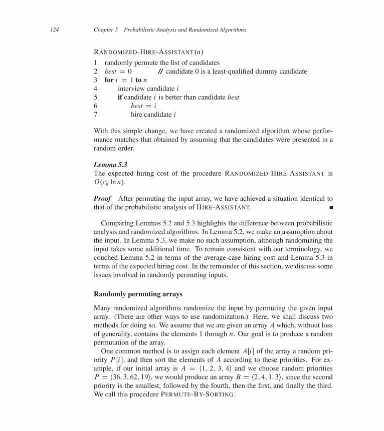
RANDOMIZED-HIRE-ASSISTANT.n/

1 randomly permute the list of candidates2 best D 0 // candidate 0 is a least-qualified dummy candidate3 for i D 1 to n

4 interview candidate i

5 if candidate i is better than candidate best6 best D i

7 hire candidate i

With this simple change, we have created a randomized algorithm whose perfor-mance matches that obtained by assuming that the candidates were presented in arandom order.

Lemma 5.3The expected hiring cost of the procedure RANDOMIZED-HIRE-ASSISTANT isO.ch ln n/.

Proof After permuting the input array, we have achieved a situation identical tothat of the probabilistic analysis of HIRE-ASSISTANT.

Comparing Lemmas 5.2 and 5.3 highlights the difference between probabilisticanalysis and randomized algorithms. In Lemma 5.2, we make an assumption aboutthe input. In Lemma 5.3, we make no such assumption, although randomizing theinput takes some additional time. To remain consistent with our terminology, wecouched Lemma 5.2 in terms of the average-case hiring cost and Lemma 5.3 interms of the expected hiring cost. In the remainder of this section, we discuss someissues involved in randomly permuting inputs.

Randomly permuting arrays

Many randomized algorithms randomize the input by permuting the given inputarray. (There are other ways to use randomization.) Here, we shall discuss twomethods for doing so. We assume that we are given an array A which, without lossof generality, contains the elements 1 through n. Our goal is to produce a randompermutation of the array.

One common method is to assign each element AŒi� of the array a random pri-ority P Œi�, and then sort the elements of A according to these priorities. For ex-ample, if our initial array is A D h1; 2; 3; 4i and we choose random prioritiesP D h36; 3; 62; 19i, we would produce an array B D h2; 4; 1; 3i, since the secondpriority is the smallest, followed by the fourth, then the first, and finally the third.We call this procedure PERMUTE-BY-SORTING:


PERMUTE-BY-SORTING.A/

1 n D A: length2 let P Œ1 : : n� be a new array3 for i D 1 to n

4 P Œi� D RANDOM.1; n3/

5 sort A, using P as sort keys

Line 4 chooses a random number between 1 and n3. We use a range of 1 to n3

to make it likely that all the priorities in P are unique. (Exercise 5.3-5 asks youto prove that the probability that all entries are unique is at least 1 � 1=n, andExercise 5.3-6 asks how to implement the algorithm even if two or more prioritiesare identical.) Let us assume that all the priorities are unique.

The time-consuming step in this procedure is the sorting in line 5. As we shallsee in Chapter 8, if we use a comparison sort, sorting takes �.n lg n/ time. Wecan achieve this lower bound, since we have seen that merge sort takes ‚.n lg n/

time. (We shall see other comparison sorts that take ‚.n lg n/ time in Part II.Exercise 8.3-4 asks you to solve the very similar problem of sorting numbers in therange 0 to n3 � 1 in O.n/ time.) After sorting, if P Œi� is the j th smallest priority,then AŒi� lies in position j of the output. In this manner we obtain a permutation. Itremains to prove that the procedure produces a uniform random permutation, thatis, that the procedure is equally likely to produce every permutation of the numbers1 through n.

Lemma 5.4Procedure PERMUTE-BY-SORTING produces a uniform random permutation of theinput, assuming that all priorities are distinct.

Proof We start by considering the particular permutation in which each ele-ment AŒi� receives the i th smallest priority. We shall show that this permutationoccurs with probability exactly 1=nŠ. For i D 1; 2; : : : ; n, let Ei be the eventthat element AŒi� receives the i th smallest priority. Then we wish to compute theprobability that for all i , event Ei occurs, which is

Pr fE1 \E2 \E3 \ � � � \En�1 \Eng :

Using Exercise C.2-5, this probability is equal to

Pr fE1g � Pr fE2 j E1g � Pr fE3 j E2 \E1g � Pr fE4 j E3 \E2 \E1g� � � Pr fEi j Ei�1 \Ei�2 \ � � � \E1g � � � Pr fEn j En�1 \ � � � \E1g :

We have that Pr fE1g D 1=n because it is the probability that one prioritychosen randomly out of a set of n is the smallest priority. Next, we observe


that Pr fE2 j E1g D 1=.n � 1/ because given that element AŒ1� has the small-est priority, each of the remaining n � 1 elements has an equal chance of hav-ing the second smallest priority. In general, for i D 2; 3; : : : ; n, we have thatPr fEi j Ei�1 \Ei�2 \ � � � \E1g D 1=.n� i C1/, since, given that elements AŒ1�

through AŒi � 1� have the i � 1 smallest priorities (in order), each of the remainingn� .i � 1/ elements has an equal chance of having the i th smallest priority. Thus,we have

Pr fE1 \E2 \E3 \ � � � \En�1 \Eng D�

1

n

��1

n � 1

��

1

2

��1

1

�D 1

nŠ;

and we have shown that the probability of obtaining the identity permutationis 1=nŠ.

We can extend this proof to work for any permutation of priorities. Considerany fixed permutation D h.1/; .2/; : : : ; .n/i of the set f1; 2; : : : ; ng. Let usdenote by ri the rank of the priority assigned to element AŒi�, where the elementwith the j th smallest priority has rank j . If we define Ei as the event in whichelement AŒi� receives the .i/th smallest priority, or ri D .i/, the same proofstill applies. Therefore, if we calculate the probability of obtaining any particularpermutation, the calculation is identical to the one above, so that the probability ofobtaining this permutation is also 1=nŠ.

You might think that to prove that a permutation is a uniform random permuta-tion, it suffices to show that, for each element AŒi�, the probability that the elementwinds up in position j is 1=n. Exercise 5.3-4 shows that this weaker condition is,in fact, insufficient.

A better method for generating a random permutation is to permute the givenarray in place. The procedure RANDOMIZE-IN-PLACE does so in O.n/ time. Inits i th iteration, it chooses the element AŒi� randomly from among elements AŒi�

through AŒn�. Subsequent to the i th iteration, AŒi� is never altered.

RANDOMIZE-IN-PLACE.A/

1 n D A: length2 for i D 1 to n

3 swap AŒi� with AŒRANDOM.i; n/�

We shall use a loop invariant to show that procedure RANDOMIZE-IN-PLACE

produces a uniform random permutation. A k-permutation on a set of n ele-ments is a sequence containing k of the n elements, with no repetitions. (SeeAppendix C.) There are nŠ=.n � k/Š such possible k-permutations.


Lemma 5.5Procedure RANDOMIZE-IN-PLACE computes a uniform random permutation.

Proof We use the following loop invariant:

Just prior to the i th iteration of the for loop of lines 2–3, for each possible.i � 1/-permutation of the n elements, the subarray AŒ1 : : i � 1� containsthis .i � 1/-permutation with probability .n � i C 1/Š=nŠ.

We need to show that this invariant is true prior to the first loop iteration, that eachiteration of the loop maintains the invariant, and that the invariant provides a usefulproperty to show correctness when the loop terminates.

Initialization: Consider the situation just before the first loop iteration, so thati D 1. The loop invariant says that for each possible 0-permutation, the sub-array AŒ1 : : 0� contains this 0-permutation with probability .n � i C 1/Š=nŠ DnŠ=nŠ D 1. The subarray AŒ1 : : 0� is an empty subarray, and a 0-permutationhas no elements. Thus, AŒ1 : : 0� contains any 0-permutation with probability 1,and the loop invariant holds prior to the first iteration.

Maintenance: We assume that just before the i th iteration, each possible.i � 1/-permutation appears in the subarray AŒ1 : : i � 1� with probability.n � i C 1/Š=nŠ, and we shall show that after the i th iteration, each possiblei-permutation appears in the subarray AŒ1 : : i � with probability .n � i/Š=nŠ.Incrementing i for the next iteration then maintains the loop invariant.

Let us examine the i th iteration. Consider a particular i-permutation, and de-note the elements in it by hx1; x2; : : : ; xii. This permutation consists of an.i � 1/-permutation hx1; : : : ; xi�1i followed by the value xi that the algorithmplaces in AŒi�. Let E1 denote the event in which the first i � 1 iterations havecreated the particular .i �1/-permutation hx1; : : : ; xi�1i in AŒ1 : : i �1�. By theloop invariant, Pr fE1g D .n� i C 1/Š=nŠ. Let E2 be the event that i th iterationputs xi in position AŒi�. The i-permutation hx1; : : : ; xi i appears in AŒ1 : : i � pre-cisely when both E1 and E2 occur, and so we wish to compute Pr fE2 \E1g.Using equation (C.14), we have

Pr fE2 \E1g D Pr fE2 j E1g Pr fE1g :

The probability Pr fE2 j E1g equals 1=.n�iC1/ because in line 3 the algorithmchooses xi randomly from the n� i C 1 values in positions AŒi : : n�. Thus, wehave


Pr fE2 \E1g D Pr fE2 j E1g Pr fE1gD 1

n � i C 1� .n � i C 1/Š

nŠ

D .n � i/Š

nŠ:

Termination: At termination, i D nC 1, and we have that the subarray AŒ1 : : n�

is a given n-permutation with probability .n�.nC1/C1/=nŠ D 0Š=nŠ D 1=nŠ.

Thus, RANDOMIZE-IN-PLACE produces a uniform random permutation.

A randomized algorithm is often the simplest and most efficient way to solve aproblem. We shall use randomized algorithms occasionally throughout this book.

Exercises

5.3-1Professor Marceau objects to the loop invariant used in the proof of Lemma 5.5. Hequestions whether it is true prior to the first iteration. He reasons that we could justas easily declare that an empty subarray contains no 0-permutations. Therefore,the probability that an empty subarray contains a 0-permutation should be 0, thusinvalidating the loop invariant prior to the first iteration. Rewrite the procedureRANDOMIZE-IN-PLACE so that its associated loop invariant applies to a nonemptysubarray prior to the first iteration, and modify the proof of Lemma 5.5 for yourprocedure.

5.3-2Professor Kelp decides to write a procedure that produces at random any permuta-tion besides the identity permutation. He proposes the following procedure:

PERMUTE-WITHOUT-IDENTITY.A/

1 n D A: length2 for i D 1 to n � 1

3 swap AŒi� with AŒRANDOM.i C 1; n/�

Does this code do what Professor Kelp intends?

5.3-3Suppose that instead of swapping element AŒi� with a random element from thesubarray AŒi : : n�, we swapped it with a random element from anywhere in thearray:


PERMUTE-WITH-ALL.A/

1 n D A: length2 for i D 1 to n

3 swap AŒi� with AŒRANDOM.1; n/�

Does this code produce a uniform random permutation? Why or why not?

5.3-4Professor Armstrong suggests the following procedure for generating a uniformrandom permutation:

PERMUTE-BY-CYCLIC.A/

1 n D A: length2 let BŒ1 : : n� be a new array3 offset D RANDOM.1; n/

4 for i D 1 to n

5 dest D i C offset6 if dest > n

7 dest D dest � n

8 BŒdest� D AŒi�

9 return B

Show that each element AŒi� has a 1=n probability of winding up in any particularposition in B . Then show that Professor Armstrong is mistaken by showing thatthe resulting permutation is not uniformly random.

5.3-5 ?

Prove that in the array P in procedure PERMUTE-BY-SORTING, the probabilitythat all elements are unique is at least 1 � 1=n.

5.3-6Explain how to implement the algorithm PERMUTE-BY-SORTING to handle thecase in which two or more priorities are identical. That is, your algorithm shouldproduce a uniform random permutation, even if two or more priorities are identical.

5.3-7Suppose we want to create a random sample of the set f1; 2; 3; : : : ; ng, that is,an m-element subset S , where 0 � m � n, such that each m-subset is equallylikely to be created. One way would be to set AŒi� D i for i D 1; 2; 3; : : : ; n,call RANDOMIZE-IN-PLACE.A/, and then take just the first m array elements.This method would make n calls to the RANDOM procedure. If n is much largerthan m, we can create a random sample with fewer calls to RANDOM. Show that


the following recursive procedure returns a random m-subset S of f1; 2; 3; : : : ; ng,in which each m-subset is equally likely, while making only m calls to RANDOM:

RANDOM-SAMPLE.m; n/

1 if m == 0

2 return ;3 else S D RANDOM-SAMPLE.m � 1; n � 1/

4 i D RANDOM.1; n/

5 if i 2 S

6 S D S [ fng7 else S D S [ fig8 return S

? 5.4 Probabilistic analysis and further uses of indicator random variables

This advanced section further illustrates probabilistic analysis by way of four ex-amples. The first determines the probability that in a room of k people, two ofthem share the same birthday. The second example examines what happens whenwe randomly toss balls into bins. The third investigates “streaks” of consecutiveheads when we flip coins. The final example analyzes a variant of the hiring prob-lem in which you have to make decisions without actually interviewing all thecandidates.

5.4.1 The birthday paradox

Our first example is the birthday paradox. How many people must there be in aroom before there is a 50% chance that two of them were born on the same day ofthe year? The answer is surprisingly few. The paradox is that it is in fact far fewerthan the number of days in a year, or even half the number of days in a year, as weshall see.

To answer this question, we index the people in the room with the integers1; 2; : : : ; k, where k is the number of people in the room. We ignore the issueof leap years and assume that all years have n D 365 days. For i D 1; 2; : : : ; k,let bi be the day of the year on which person i’s birthday falls, where 1 � bi � n.We also assume that birthdays are uniformly distributed across the n days of theyear, so that Pr fbi D rg D 1=n for i D 1; 2; : : : ; k and r D 1; 2; : : : ; n.

The probability that two given people, say i and j , have matching birthdaysdepends on whether the random selection of birthdays is independent. We assumefrom now on that birthdays are independent, so that the probability that i’s birthday

5.4 Probabilistic analysis and further uses of indicator random variables 131

and j ’s birthday both fall on day r is

Pr fbi D r and bj D rg D Pr fbi D rg Pr fbj D rgD 1=n2 :

Thus, the probability that they both fall on the same day is

Pr fbi D bj g DnX

rD1

Pr fbi D r and bj D rg

DnX

rD1

.1=n2/

D 1=n : (5.6)

More intuitively, once bi is chosen, the probability that bj is chosen to be the sameday is 1=n. Thus, the probability that i and j have the same birthday is the sameas the probability that the birthday of one of them falls on a given day. Notice,however, that this coincidence depends on the assumption that the birthdays areindependent.

We can analyze the probability of at least 2 out of k people having matchingbirthdays by looking at the complementary event. The probability that at least twoof the birthdays match is 1 minus the probability that all the birthdays are different.The event that k people have distinct birthdays is

Bk Dk\

iD1

Ai ;

where Ai is the event that person i’s birthday is different from person j ’s forall j < i . Since we can write Bk D Ak \ Bk�1, we obtain from equation (C.16)the recurrence

Pr fBkg D Pr fBk�1g Pr fAk j Bk�1g ; (5.7)

where we take Pr fB1g D Pr fA1g D 1 as an initial condition. In other words,the probability that b1; b2; : : : ; bk are distinct birthdays is the probability thatb1; b2; : : : ; bk�1 are distinct birthdays times the probability that bk ¤ bi fori D 1; 2; : : : ; k � 1, given that b1; b2; : : : ; bk�1 are distinct.

If b1; b2; : : : ; bk�1 are distinct, the conditional probability that bk ¤ bi fori D 1; 2; : : : ; k � 1 is Pr fAk j Bk�1g D .n � k C 1/=n, since out of the n days,n� .k � 1/ days are not taken. We iteratively apply the recurrence (5.7) to obtain


Pr fBkg D Pr fBk�1g Pr fAk j Bk�1gD Pr fBk�2g Pr fAk�1 j Bk�2g Pr fAk j Bk�1g:::

D Pr fB1g Pr fA2 j B1g Pr fA3 j B2g � � � Pr fAk j Bk�1gD 1 �

�n � 1

n

��n � 2

n

��

n � k C 1

n

�D 1 �

�1� 1

n

��1 � 2

n

��

1 � k � 1

n

�:

Inequality (3.12), 1C x � ex , gives us

Pr fBkg � e�1=ne�2=n � � � e�.k�1/=n

D e�Pk�1iD1 i=n

D e�k.k�1/=2n

� 1=2

when �k.k � 1/=2n � ln.1=2/. The probability that all k birthdays are distinctis at most 1=2 when k.k � 1/ � 2n ln 2 or, solving the quadratic equation, whenk � .1 C

p1C .8 ln 2/n/=2. For n D 365, we must have k � 23. Thus, if at

least 23 people are in a room, the probability is at least 1=2 that at least two peoplehave the same birthday. On Mars, a year is 669 Martian days long; it thereforetakes 31 Martians to get the same effect.

An analysis using indicator random variables

We can use indicator random variables to provide a simpler but approximate anal-ysis of the birthday paradox. For each pair .i; j / of the k people in the room, wedefine the indicator random variable Xij , for 1 � i < j � k, by

Xij D I fperson i and person j have the same birthdayg

D(

1 if person i and person j have the same birthday ;

0 otherwise :

By equation (5.6), the probability that two people have matching birthdays is 1=n,and thus by Lemma 5.1, we have

E ŒXij � D Pr fperson i and person j have the same birthdaygD 1=n :

Letting X be the random variable that counts the number of pairs of individualshaving the same birthday, we have


X DkX

iD1

kXj DiC1

Xij :

Taking expectations of both sides and applying linearity of expectation, we obtain

E ŒX� D E

"kX

iD1

kXj DiC1

Xij

#

DkX

iD1

kXj DiC1

E ŒXij �

D

k

2

!1

n

D k.k � 1/

2n:

When k.k � 1/ � 2n, therefore, the expected number of pairs of people with thesame birthday is at least 1. Thus, if we have at least

p2nC1 individuals in a room,

we can expect at least two to have the same birthday. For n D 365, if k D 28, theexpected number of pairs with the same birthday is .28 � 27/=.2 � 365/ � 1:0356.Thus, with at least 28 people, we expect to find at least one matching pair of birth-days. On Mars, where a year is 669 Martian days long, we need at least 38 Mar-tians.

The first analysis, which used only probabilities, determined the number of peo-ple required for the probability to exceed 1=2 that a matching pair of birthdaysexists, and the second analysis, which used indicator random variables, determinedthe number such that the expected number of matching birthdays is 1. Althoughthe exact numbers of people differ for the two situations, they are the same asymp-totically: ‚.

pn/.

5.4.2 Balls and bins

Consider a process in which we randomly toss identical balls into b bins, numbered1; 2; : : : ; b. The tosses are independent, and on each toss the ball is equally likelyto end up in any bin. The probability that a tossed ball lands in any given bin is 1=b.Thus, the ball-tossing process is a sequence of Bernoulli trials (see Appendix C.4)with a probability 1=b of success, where success means that the ball falls in thegiven bin. This model is particularly useful for analyzing hashing (see Chapter 11),and we can answer a variety of interesting questions about the ball-tossing process.(Problem C-1 asks additional questions about balls and bins.)


How many balls fall in a given bin? The number of balls that fall in a given binfollows the binomial distribution b.kIn; 1=b/. If we toss n balls, equation (C.37)tells us that the expected number of balls that fall in the given bin is n=b.

How many balls must we toss, on the average, until a given bin contains a ball?The number of tosses until the given bin receives a ball follows the geometricdistribution with probability 1=b and, by equation (C.32), the expected number oftosses until success is 1=.1=b/ D b.

How many balls must we toss until every bin contains at least one ball? Let uscall a toss in which a ball falls into an empty bin a “hit.” We want to know theexpected number n of tosses required to get b hits.

Using the hits, we can partition the n tosses into stages. The i th stage consists ofthe tosses after the .i � 1/st hit until the i th hit. The first stage consists of the firsttoss, since we are guaranteed to have a hit when all bins are empty. For each tossduring the i th stage, i � 1 bins contain balls and b � i C 1 bins are empty. Thus,for each toss in the i th stage, the probability of obtaining a hit is .b � i C 1/=b.

Let ni denote the number of tosses in the i th stage. Thus, the number of tossesrequired to get b hits is n D Pb

iD1 ni . Each random variable ni has a geometricdistribution with probability of success .b� iC1/=b and thus, by equation (C.32),we have

E Œni � Db

b � i C 1:

By linearity of expectation, we have

E Œn� D E

"bX

iD1

ni

#

DbX

iD1

E Œni �

DbX

iD1

b

b � i C 1

D b

bXiD1

1

i

D b.ln b CO.1// (by equation (A.7)) .

It therefore takes approximately b ln b tosses before we can expect that every binhas a ball. This problem is also known as the coupon collector’s problem, whichsays that a person trying to collect each of b different coupons expects to acquireapproximately b ln b randomly obtained coupons in order to succeed.


5.4.3 Streaks

Suppose you flip a fair coin n times. What is the longest streak of consecutiveheads that you expect to see? The answer is ‚.lg n/, as the following analysisshows.

We first prove that the expected length of the longest streak of heads is O.lg n/.The probability that each coin flip is a head is 1=2. Let Aik be the event that astreak of heads of length at least k begins with the i th coin flip or, more precisely,the event that the k consecutive coin flips i; i C 1; : : : ; i C k � 1 yield only heads,where 1 � k � n and 1 � i � n�kC1. Since coin flips are mutually independent,for any given event Aik, the probability that all k flips are heads is

Pr fAikg D 1=2k : (5.8)

For k D 2 dlg ne,Pr fAi;2dlg neg D 1=22dlg ne

� 1=22 lg n

D 1=n2 ;

and thus the probability that a streak of heads of length at least 2 dlg ne begins inposition i is quite small. There are at most n � 2 dlg ne C 1 positions where sucha streak can begin. The probability that a streak of heads of length at least 2 dlg nebegins anywhere is therefore

Pr

(n�2dlg neC1[

iD1

Ai;2dlg ne

)�

n�2dlg neC1XiD1

1=n2

<

nXiD1

1=n2

D 1=n ; (5.9)

since by Boole’s inequality (C.19), the probability of a union of events is at mostthe sum of the probabilities of the individual events. (Note that Boole’s inequalityholds even for events such as these that are not independent.)

We now use inequality (5.9) to bound the length of the longest streak. Forj D 0; 1; 2; : : : ; n, let Lj be the event that the longest streak of heads has length ex-actly j , and let L be the length of the longest streak. By the definition of expectedvalue, we have

E ŒL� DnX

j D0

j Pr fLj g : (5.10)


We could try to evaluate this sum using upper bounds on each Pr fLj g similar tothose computed in inequality (5.9). Unfortunately, this method would yield weakbounds. We can use some intuition gained by the above analysis to obtain a goodbound, however. Informally, we observe that for no individual term in the sum-mation in equation (5.10) are both the factors j and Pr fLj g large. Why? Whenj � 2 dlg ne, then Pr fLj g is very small, and when j < 2 dlg ne, then j is fairlysmall. More formally, we note that the events Lj for j D 0; 1; : : : ; n are disjoint,and so the probability that a streak of heads of length at least 2 dlg ne begins any-where is

Pn

j D2dlg ne Pr fLj g. By inequality (5.9), we havePn

j D2dlg ne Pr fLj g < 1=n.

Also, noting thatPn

j D0 Pr fLj g D 1, we have thatP2dlg ne�1

j D0 Pr fLj g � 1. Thus,we obtain

E ŒL� DnX

j D0

j Pr fLj g

D2dlg ne�1X

j D0

j Pr fLj g CnX

j D2dlg nej Pr fLj g

<

2dlg ne�1Xj D0

.2 dlg ne/ Pr fLj g CnX

j D2dlg nen Pr fLj g

D 2 dlg ne2dlg ne�1X

j D0

Pr fLj g C n

nXj D2dlg ne

Pr fLj g

< 2 dlg ne � 1C n � .1=n/

D O.lg n/ :

The probability that a streak of heads exceeds r dlg ne flips diminishes quicklywith r . For r � 1, the probability that a streak of at least r dlg ne heads starts inposition i is

Pr fAi;rdlg neg D 1=2rdlg ne

� 1=nr :

Thus, the probability is at most n=nr D 1=nr�1 that the longest streak is atleast r dlg ne, or equivalently, the probability is at least 1� 1=nr�1 that the longeststreak has length less than r dlg ne.

As an example, for n D 1000 coin flips, the probability of having a streak of atleast 2 dlg ne D 20 heads is at most 1=n D 1=1000. The chance of having a streaklonger than 3 dlg ne D 30 heads is at most 1=n2 D 1=1,000,000.

We now prove a complementary lower bound: the expected length of the longeststreak of heads in n coin flips is �.lg n/. To prove this bound, we look for streaks


of length s by partitioning the n flips into approximately n=s groups of s flipseach. If we choose s D b.lg n/=2c, we can show that it is likely that at least oneof these groups comes up all heads, and hence it is likely that the longest streakhas length at least s D �.lg n/. We then show that the longest streak has expectedlength �.lg n/.

We partition the n coin flips into at least bn= b.lg n/=2cc groups of b.lg n/=2cconsecutive flips, and we bound the probability that no group comes up all heads.By equation (5.8), the probability that the group starting in position i comes up allheads is

Pr fAi;b.lg n/=2cg D 1=2b.lg n/=2c

� 1=p

n :

The probability that a streak of heads of length at least b.lg n/=2c does not beginin position i is therefore at most 1 � 1=

pn. Since the bn= b.lg n/=2cc groups are

formed from mutually exclusive, independent coin flips, the probability that everyone of these groups fails to be a streak of length b.lg n/=2c is at most�1 � 1=

pn�bn=b.lg n/=2cc � �

1 � 1=p

n�n=b.lg n/=2c�1

� �1 � 1=

pn�2n= lg n�1

� e�.2n= lg n�1/=p

n

D O.e� lg n/

D O.1=n/ :

For this argument, we used inequality (3.12), 1C x � ex , and the fact, which youmight want to verify, that .2n= lg n � 1/=

pn � lg n for sufficiently large n.

Thus, the probability that the longest streak exceeds b.lg n/=2c is

nXj Db.lg n/=2cC1

Pr fLj g � 1 �O.1=n/ : (5.11)

We can now calculate a lower bound on the expected length of the longest streak,beginning with equation (5.10) and proceeding in a manner similar to our analysisof the upper bound:


E ŒL� DnX

j D0

j Pr fLj g

Db.lg n/=2cX

j D0

j Pr fLj g CnX

j Db.lg n/=2cC1

j Pr fLj g

�b.lg n/=2cX

j D0

0 � Pr fLj g CnX

j Db.lg n/=2cC1

b.lg n/=2c Pr fLj g

D 0 �b.lg n/=2cX

j D0

Pr fLj g C b.lg n/=2cnX

j Db.lg n/=2cC1

Pr fLj g

� 0C b.lg n/=2c .1�O.1=n// (by inequality (5.11))

D �.lg n/ :

As with the birthday paradox, we can obtain a simpler but approximate analysisusing indicator random variables. We let Xik D I fAikg be the indicator randomvariable associated with a streak of heads of length at least k beginning with thei th coin flip. To count the total number of such streaks, we define

X Dn�kC1X

iD1

Xik :

Taking expectations and using linearity of expectation, we have

E ŒX� D E

"n�kC1X

iD1

Xik

#

Dn�kC1X

iD1

E ŒXik�

Dn�kC1X

iD1

Pr fAikg

Dn�kC1X

iD1

1=2k

D n � k C 1

2k:

By plugging in various values for k, we can calculate the expected number ofstreaks of length k. If this number is large (much greater than 1), then we expectmany streaks of length k to occur and the probability that one occurs is high. If


this number is small (much less than 1), then we expect few streaks of length k tooccur and the probability that one occurs is low. If k D c lg n, for some positiveconstant c, we obtain

E ŒX� D n � c lg nC 1

2c lg n

D n � c lg nC 1

nc

D 1

nc�1� .c lg n � 1/=n

nc�1

D ‚.1=nc�1/ :

If c is large, the expected number of streaks of length c lg n is small, and we con-clude that they are unlikely to occur. On the other hand, if c D 1=2, then we obtainE ŒX� D ‚.1=n1=2�1/ D ‚.n1=2/, and we expect that there are a large numberof streaks of length .1=2/ lg n. Therefore, one streak of such a length is likely tooccur. From these rough estimates alone, we can conclude that the expected lengthof the longest streak is ‚.lg n/.

5.4.4 The on-line hiring problem

As a final example, we consider a variant of the hiring problem. Suppose now thatwe do not wish to interview all the candidates in order to find the best one. Wealso do not wish to hire and fire as we find better and better applicants. Instead, weare willing to settle for a candidate who is close to the best, in exchange for hiringexactly once. We must obey one company requirement: after each interview wemust either immediately offer the position to the applicant or immediately reject theapplicant. What is the trade-off between minimizing the amount of interviewingand maximizing the quality of the candidate hired?

We can model this problem in the following way. After meeting an applicant,we are able to give each one a score; let score.i/ denote the score we give to the i thapplicant, and assume that no two applicants receive the same score. After we haveseen j applicants, we know which of the j has the highest score, but we do notknow whether any of the remaining n�j applicants will receive a higher score. Wedecide to adopt the strategy of selecting a positive integer k < n, interviewing andthen rejecting the first k applicants, and hiring the first applicant thereafter who hasa higher score than all preceding applicants. If it turns out that the best-qualifiedapplicant was among the first k interviewed, then we hire the nth applicant. Weformalize this strategy in the procedure ON-LINE-MAXIMUM.k; n/, which returnsthe index of the candidate we wish to hire.


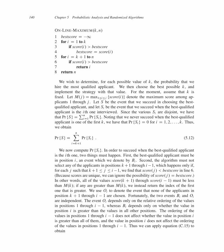
ON-LINE-MAXIMUM.k; n/

1 bestscore D �12 for i D 1 to k

3 if score.i/ > bestscore4 bestscore D score.i/

5 for i D k C 1 to n

6 if score.i/ > bestscore7 return i

8 return n

We wish to determine, for each possible value of k, the probability that wehire the most qualified applicant. We then choose the best possible k, andimplement the strategy with that value. For the moment, assume that k isfixed. Let M.j / D max1�i�j fscore.i/g denote the maximum score among ap-plicants 1 through j . Let S be the event that we succeed in choosing the best-qualified applicant, and let Si be the event that we succeed when the best-qualifiedapplicant is the i th one interviewed. Since the various Si are disjoint, we havethat Pr fSg DPn

iD1 Pr fSig. Noting that we never succeed when the best-qualifiedapplicant is one of the first k, we have that Pr fSig D 0 for i D 1; 2; : : : ; k. Thus,we obtain

Pr fSg DnX

iDkC1

Pr fSig : (5.12)

We now compute Pr fSig. In order to succeed when the best-qualified applicantis the i th one, two things must happen. First, the best-qualified applicant must bein position i , an event which we denote by Bi . Second, the algorithm must notselect any of the applicants in positions kC1 through i �1, which happens only if,for each j such that kC1 � j � i�1, we find that score.j / < bestscore in line 6.(Because scores are unique, we can ignore the possibility of score.j / D bestscore.)In other words, all of the values score.k C 1/ through score.i � 1/ must be lessthan M.k/; if any are greater than M.k/, we instead return the index of the firstone that is greater. We use Oi to denote the event that none of the applicants inposition k C 1 through i � 1 are chosen. Fortunately, the two events Bi and Oi

are independent. The event Oi depends only on the relative ordering of the valuesin positions 1 through i � 1, whereas Bi depends only on whether the value inposition i is greater than the values in all other positions. The ordering of thevalues in positions 1 through i � 1 does not affect whether the value in position i

is greater than all of them, and the value in position i does not affect the orderingof the values in positions 1 through i � 1. Thus we can apply equation (C.15) toobtain


Pr fSig D Pr fBi \Oig D Pr fBig Pr fOig :

The probability Pr fBig is clearly 1=n, since the maximum is equally likely tobe in any one of the n positions. For event Oi to occur, the maximum value inpositions 1 through i�1, which is equally likely to be in any of these i�1 positions,must be in one of the first k positions. Consequently, Pr fOig D k=.i � 1/ andPr fSig D k=.n.i � 1//. Using equation (5.12), we have

Pr fSg DnX

iDkC1

Pr fSig

DnX

iDkC1

k

n.i � 1/

D k

n

nXiDkC1

1

i � 1

D k

n

n�1XiDk

1

i:

We approximate by integrals to bound this summation from above and below. Bythe inequalities (A.12), we haveZ n

k

1

xdx �

n�1XiDk

1

i�Z n�1

k�1

1

xdx :

Evaluating these definite integrals gives us the bounds

k

n.ln n � ln k/ � Pr fSg � k

n.ln.n � 1/ � ln.k � 1// ;

which provide a rather tight bound for Pr fSg. Because we wish to maximize ourprobability of success, let us focus on choosing the value of k that maximizes thelower bound on Pr fSg. (Besides, the lower-bound expression is easier to maximizethan the upper-bound expression.) Differentiating the expression .k=n/.ln n�ln k/

with respect to k, we obtain

1

n.ln n � ln k � 1/ :

Setting this derivative equal to 0, we see that we maximize the lower bound on theprobability when ln k D ln n�1 D ln.n=e/ or, equivalently, when k D n=e. Thus,if we implement our strategy with k D n=e, we succeed in hiring our best-qualifiedapplicant with probability at least 1=e.


Exercises

5.4-1How many people must there be in a room before the probability that someonehas the same birthday as you do is at least 1=2? How many people must there bebefore the probability that at least two people have a birthday on July 4 is greaterthan 1=2?

5.4-2Suppose that we toss balls into b bins until some bin contains two balls. Each tossis independent, and each ball is equally likely to end up in any bin. What is theexpected number of ball tosses?

5.4-3 ?

For the analysis of the birthday paradox, is it important that the birthdays be mutu-ally independent, or is pairwise independence sufficient? Justify your answer.

5.4-4 ?

How many people should be invited to a party in order to make it likely that thereare three people with the same birthday?

5.4-5 ?

What is the probability that a k-string over a set of size n forms a k-permutation?How does this question relate to the birthday paradox?

5.4-6 ?

Suppose that n balls are tossed into n bins, where each toss is independent and theball is equally likely to end up in any bin. What is the expected number of emptybins? What is the expected number of bins with exactly one ball?

5.4-7 ?

Sharpen the lower bound on streak length by showing that in n flips of a fair coin,the probability is less than 1=n that no streak longer than lg n�2 lg lg n consecutiveheads occurs.

Problems for Chapter 5 143

Problems

5-1 Probabilistic countingWith a b-bit counter, we can ordinarily only count up to 2b � 1. With R. Morris’sprobabilistic counting, we can count up to a much larger value at the expense ofsome loss of precision.

We let a counter value of i represent a count of ni for i D 0; 1; : : : ; 2b�1, wherethe ni form an increasing sequence of nonnegative values. We assume that the ini-tial value of the counter is 0, representing a count of n0 D 0. The INCREMENT

operation works on a counter containing the value i in a probabilistic manner. Ifi D 2b � 1, then the operation reports an overflow error. Otherwise, the INCRE-MENT operation increases the counter by 1 with probability 1=.niC1 � ni/, and itleaves the counter unchanged with probability 1 � 1=.niC1 � ni /.

If we select ni D i for all i � 0, then the counter is an ordinary one. Moreinteresting situations arise if we select, say, ni D 2i�1 for i > 0 or ni D Fi (thei th Fibonacci number—see Section 3.2).

For this problem, assume that n2b�1 is large enough that the probability of anoverflow error is negligible.

a. Show that the expected value represented by the counter after n INCREMENT

operations have been performed is exactly n.

b. The analysis of the variance of the count represented by the counter dependson the sequence of the ni . Let us consider a simple case: ni D 100i forall i � 0. Estimate the variance in the value represented by the register after n

INCREMENT operations have been performed.

5-2 Searching an unsorted arrayThis problem examines three algorithms for searching for a value x in an unsortedarray A consisting of n elements.

Consider the following randomized strategy: pick a random index i into A. IfAŒi� D x, then we terminate; otherwise, we continue the search by picking a newrandom index into A. We continue picking random indices into A until we find anindex j such that AŒj � D x or until we have checked every element of A. Notethat we pick from the whole set of indices each time, so that we may examine agiven element more than once.

a. Write pseudocode for a procedure RANDOM-SEARCH to implement the strat-egy above. Be sure that your algorithm terminates when all indices into A havebeen picked.


b. Suppose that there is exactly one index i such that AŒi� D x. What is theexpected number of indices into A that we must pick before we find x andRANDOM-SEARCH terminates?

c. Generalizing your solution to part (b), suppose that there are k � 1 indices i

such that AŒi� D x. What is the expected number of indices into A that wemust pick before we find x and RANDOM-SEARCH terminates? Your answershould be a function of n and k.

d. Suppose that there are no indices i such that AŒi� D x. What is the expectednumber of indices into A that we must pick before we have checked all elementsof A and RANDOM-SEARCH terminates?

Now consider a deterministic linear search algorithm, which we refer to asDETERMINISTIC-SEARCH. Specifically, the algorithm searches A for x in order,considering AŒ1�; AŒ2�; AŒ3�; : : : ; AŒn� until either it finds AŒi� D x or it reachesthe end of the array. Assume that all possible permutations of the input array areequally likely.

e. Suppose that there is exactly one index i such that AŒi� D x. What is theaverage-case running time of DETERMINISTIC-SEARCH? What is the worst-case running time of DETERMINISTIC-SEARCH?

f. Generalizing your solution to part (e), suppose that there are k � 1 indices i

such that AŒi� D x. What is the average-case running time of DETERMINISTIC-SEARCH? What is the worst-case running time of DETERMINISTIC-SEARCH?Your answer should be a function of n and k.

g. Suppose that there are no indices i such that AŒi� D x. What is the average-caserunning time of DETERMINISTIC-SEARCH? What is the worst-case runningtime of DETERMINISTIC-SEARCH?

Finally, consider a randomized algorithm SCRAMBLE-SEARCH that works byfirst randomly permuting the input array and then running the deterministic lin-ear search given above on the resulting permuted array.

h. Letting k be the number of indices i such that AŒi� D x, give the worst-case andexpected running times of SCRAMBLE-SEARCH for the cases in which k D 0

and k D 1. Generalize your solution to handle the case in which k � 1.

i. Which of the three searching algorithms would you use? Explain your answer.

Notes for Chapter 5 145

Chapter notes

Bollobas [53], Hofri [174], and Spencer [321] contain a wealth of advanced prob-abilistic techniques. The advantages of randomized algorithms are discussed andsurveyed by Karp [200] and Rabin [288]. The textbook by Motwani and Raghavan[262] gives an extensive treatment of randomized algorithms.

Several variants of the hiring problem have been widely studied. These problemsare more commonly referred to as “secretary problems.” An example of work inthis area is the paper by Ajtai, Meggido, and Waarts [11].

5 Probabilistic Analysis and Randomized Algorithms

Documents

Transcript of 5 Probabilistic Analysis and Randomized Algorithms