1

Towards Combining Probabilistic and Interval

Uncertainty in Engineering Calculations

S. A. Starks, V. Kreinovich, L. Longpre, M. Ceberio, G. Xiang,R. Araiza, J. Beck, R. Kandathi, A. Nayak and R. TorresNASA Pan-American Center for Earth and Environmental Studies (PACES),University of Texas, El Paso, TX 79968, USA (vladik@cs.utep.edu)

Abstract. In many engineering applications, we have to combine probabilistic andinterval errors. For example, in environmental analysis, we observe a pollution levelx(t) in a lake at different moments of time t, and we would like to estimate stan-dard statistical characteristics such as mean, variance, autocorrelation, correlationwith other measurements. In environmental measurements, we often only know thevalues with interval uncertainty. We must therefore modify the existing statisticalalgorithms to process such interval data. Such modification are described in thispaper.

Keywords: probabilistic uncertainty, interval uncertainty, engineering calculations

1. Formulation of the Problem

Computing statistics is important. In many engineering applications,we are interested in computing statistics. For example, in environmen-tal analysis, we observe a pollution level x(t) in a lake at differentmoments of time t, and we would like to estimate standard statisticalcharacteristics such as mean, variance, autocorrelation, correlation withother measurements. For each of these characteristics C, there is anexpression C(x1, . . . , xn) that enables us to provide an estimate forC based on the observed values x1, . . . , xn. For example, a reasonablestatistic for estimating the mean value of a probability distribution is

the population average E(x1, . . . , xn) =1n

(x1 + . . . + xn); a reason-able statistic for estimating the variance V is the population variance

V (x1, . . . , xn) =1n·n∑i=1

(xi − x)2, where x def=1n·n∑i=1

xi.

Interval uncertainty. In environmental measurements, we often onlyknow the values with interval uncertainty. For example, if we did notdetect any pollution, the pollution value v can be anywhere between 0and the sensor’s detection limit DL. In other words, the only informa-tion that we have about v is that v belongs to the interval [0, DL]; we

2

have no information about the probability of different values from thisinterval.

Another example: to study the effect of a pollutant on the fish, wecheck on the fish daily; if a fish was alive on Day 5 but dead on Day6, then the only information about the lifetime of this fish is that it issomewhere within the interval [5, 6]; we have no information about theprobability of different values within this interval.

In non-destructive testing, we look for outliers as indications of pos-sible faults. To detect an outlier, we must know the mean and standarddeviation of the normal values – and these values can often only be mea-sured with interval uncertainty (see, e.g., (Rabinovich, 1993; Oseguedaet al., 2002)). In other words, often, we know the result x of measuringthe desired characteristic x, and we know the upper bound ∆ on theabsolute value |∆x| of the measurement error ∆x def= x− x (this upperbound is provided by the manufacturer of the measuring instrument),but we have no information about the probability of different values∆x ∈ [−∆,∆]. In such situations, after the measurement, the onlyinformation that we have about the actual value x of the measuredquantity is that this value belongs to interval [x−∆, x+ ∆].

In geophysics, outliers should be identified as possible locations ofminerals; the importance of interval uncertainty for such applicationswas emphasized in (Nivlet et al., 2001; Nivlet et al., 2001a). Detectingoutliers is also important in bioinformatics (Shmulevich and Zhang,2002).

In bioinformatics and bioengineering applications, we must solvesystems of linear equations in which coefficients come from experts andare only known with interval uncertainty; see, e.g., (Zhang et al., 2004).

In biomedical systems, statistical analysis of the data often leadsto improvements in medical recommendations; however, to maintainprivacy, we do not want to use the exact values of the patient’s param-eters. Instead, for each parameter, we select fixed values, and for eachpatient, we only keep the corresponding range. For example, insteadof keeping the exact age, we only record whether the age is between 0and 10, 10 and 20, 20 and 30, etc. We must then perform statisticalanalysis based on such interval data; see, e.g., (Kreinovich and Longpre,2003; Xiang et al., 2004).

Estimating statistics under interval uncertainty: a problem. In all suchcases, instead of the actual values x1, . . . , xn, we only know the intervalsx1 = [x1, x1], . . . ,xn = [xn, xn] that contain the (unknown) actualvalues of the measured quantities. For different values xi ∈ xi, we get,in general, different values of the corresponding statistical characteristicC(x1, . . . , xn). Since all values xi ∈ xi are possible, we conclude that

3

all the values C(x1, . . . , xn) corresponding to xi ∈ xi are possible esti-mates for the corresponding statistical characteristic. Therefore, for theinterval data x1, . . . ,xn, a reasonable estimate for the correspondingstatistical characteristic is the range

C(x1, . . . ,xn)def= {C(x1, . . . , xn) |x1 ∈ x1, . . . , xn ∈ xn}.

We must therefore modify the existing statistical algorithms so thatthey would be able to estimate such ranges. This is a problem that wesolve in this paper.

This problem is a part of a general problem. The above range es-timation problem is a specific problem related to a combination ofinterval and probabilistic uncertainty. Such problems – and their po-tential applications – have been described, in a general context, in themonographs (Kuznetsov, 1991; Walley, 1991); for further developments,see, e.g., (Rowe, 1988; Williamson, 1990; Berleant, 1993; Berleant,1996; Berleant and Goodman-Strauss, 1998; Ferson et al., 2001; Ferson,2002; Berleant et al., 2003; Lodwick and Jamison, 2003; Moore andLodwick, 2003; Regan et al., (in press)) and references therein.

2. Analysis of the Problem

Mean. Let us start our discussion with the simplest possible character-istic: the mean. The arithmetic average E is a monotonically increasingfunction of each of its n variables x1, . . . , xn, so its smallest possiblevalue E is attained when each value xi is the smallest possible (xi = xi)and its largest possible value is attained when xi = xi for all i. In otherwords, the range E of E is equal to [E(x1, . . . , xn), E(x1, . . . , xn)]. In

other words, E =1n

(x1 + . . .+ xn) and E =1n

(x1 + . . .+ xn).

Variance: computing the exact range is difficult. Another widely usedstatistic is the variance. In contrast to the mean, the dependence of thevariance V on xi is not monotonic, so the above simple idea does notwork. Rather surprisingly, it turns out that the problem of computingthe exact range for the variance over interval data is, in general, NP-hard (Ferson et al., 2002; Kreinovich, (in press)) which means, crudelyspeaking, that the worst-case computation time grows exponentiallywith n. Moreover, if we want to compute the variance range with agiven accuracy ε, the problem is still NP-hard. (For a more detailed

4

description of NP-hardness in relation to interval uncertainty, see, e.g.,(Kreinovich et al., 1997).)

Linearization. From the practical viewpoint, often, we may not needthe exact range, we can often use approximate linearization techniques.For example, when the uncertainty comes from measurement errors∆xi, and these errors are small, we can ignore terms that are quadratic(and of higher order) in ∆xi and get reasonable estimates for thecorresponding statistical characteristics. In general, in order to esti-mate the range of the statistic C(x1, . . . , xn) on the intervals [x1, x1],. . . , [xn, xn], we expand the function C in Taylor series at the mid-point xi

def= (xi + xi)/2 and keep only linear terms in this expansion.As a result, we replace the original statistic with its linearized ver-

sion Clin(x1, . . . , xn) = C0 −n∑i=1

Ci · ∆xi, where C0def= C(x1, . . . , xn),

Cidef=

∂C

∂xi(x1, . . . , xn), and ∆xi

def= xi−xi. For each i, when xi ∈ [xi, xi],

the difference ∆xi can take all possible values from −∆i to ∆i, where∆i

def= (xi − xi)/2. Thus, in the linear approximation, we can esti-mate the range of the characteristic C as [C0 − ∆, C0 + ∆], where

∆ def=n∑i=1

|ci| ·∆i.

In particular, for variance, Ci =∂V

∂xi=

2n

(xi − ¯x), where ¯x is the

average of the midpoints xi. So, here, V0 =1n

n∑i=1

(xi− ¯x)2 is the variance

of the midpoint values x1, . . . , xn, and ∆ =2n

n∑i=1

|xi − ¯x| ·∆i.

It is worth mentioning that for the variance, the ignored quadratic

term is equal to1n

n∑i=1

(∆xi)2 − (∆x)2, where ∆x def=1n

n∑i=1

∆xi, and

therefore, can be bounded by 0 from below and by ∆(2) def=1n

n∑i=1

∆2i

from above. Thus, the interval [V0 −∆, V0 + ∆ + ∆(2)] is a guaranteedenclosure for V.

Linearization is not always acceptable. In some cases, linearized esti-mates are not sufficient: the intervals may be wide so that quadraticterms can no longer be ignored, and/or we may be in a situation wherewe want to guarantee that, e.g., the variance does not exceed a certainrequired threshold. In such situations, we need to get the exact range– or at least an enclosure for the exact range.

5

Since, even for as simple a characteristic as variance, the problem ofcomputing its exact range is NP-hard, we cannot have a feasible-timealgorithm that always computes the exact range of these characteristics.Therefore, we must look for the reasonable classes of problems for whichsuch algorithms are possible. Let us analyze what such classes can be.

First class: narrow intervals. As we have just mentioned, the compu-tational problems become more complex when we have wider intervals.In other words, when intervals are narrower, the problems are easier.How can we formalize “narrow intervals”? One way to do it is as follows:the actual values x1, . . . , xn of the measured quantity are real numbers,so they are usually different. The data intervals xi contain these values.When the intervals xi surrounding the corresponding points xi arenarrow, these intervals do not intersect. When their widths becomeslarger than the distance between the original values, the intervals startintersecting.

Definition. Thus, the ideal case of “narrow intervals” can be describedas the case when no two intervals xi intersect.

Second class: slightly wider intervals. Slightly wider intervals corre-spond to the situation when few intervals intersect, i.e., when for someinteger K, no set of K intervals has a common intersection.

Third class: single measuring instrument. Since we want to find theexact range C of a statistic C, it is important not only that intervalsare relatively narrow, it is also important that they are approximatelyof the same size: otherwise, if, say, ∆x2

i is of the same order as ∆xj ,we cannot meaningfully ignore ∆x2

i and retain ∆xj . In other words,the interval data set should not combine high-accurate measurementresults (with narrow intervals) and low-accurate results (with wide in-tervals): all measurements should have been done by a single measuringinstrument (or at least by several measuring instruments of the sametype).

How can we describe this mathematically? A clear indication thatwe have two measuring instruments (MI) of different quality is that oneinterval is a proper subset of the other one: [xi, xi] ⊆ (xj , xj).

Definition. So, if all pairs of non-degenerate intervals satisfy the fol-lowing subset property [xi, xi] 6⊆ (xj , xj), we say that the measurementswere done by a single MI.

Comment. This restriction only refers to inexact measurement re-sults, i.e., to non-degenerate intervals. In additional to such interval

6

values, we may have exact values (degenerate intervals). For example,in geodetic measurements, we may select some point (“benchmark”) asa reference point, and describe, e.g., elevation of each point relative tothis benchmark. For the benchmark point itself, the relative elevationwill be therefore exactly equal to 0. When we want to compute thevariance of elevations, we want to include the benchmark point too.From this viewpoint, when we talk about measurements made by asingle measuring instrument, we may allow degenerate intervals (i.e.,exact numbers) as well.

A reader should be warned that in the published algorithms de-scribing a single MI case (Xiang et al., 2004), we only considerednon-degenerate intervals. However, as one can easily see from the pub-lished proofs (and from the idea of these proofs, as described below),these algorithms can be easily modified to incorporate possible exactvalues xi.

Fourth class: same accuracy measurement. In some situations, it isalso reasonable to consider a specific case of the single MI case whenall measurements are performed with exactly the same accuracy, i.e.,in mathematical terms, when all non-degenerate intervals [xi, xi] have

exactly the same half-width ∆i =12· (xi − xi).

Fifth class: several MI. After the single MI case, the natural nextcase is when we have several MI, i.e., when our intervals are dividedinto several subgroups each of which has the above-described subsetproperty.

Sixth class: privacy case. Although these definitions are in terms ofmeasurements, they make sense for other sources of interval data aswell. For example, for privacy data, intervals either coincide (if thevalue corresponding to the two patients belongs to the same range)or are different, in which case they can only intersect in one point.Similarly to the above situation, we also allow exact values in additionto ranges; these values correspond, e.g., to the exact records made inthe past, records that are already in the public domain.

Definition. We will call interval data with this property – that ev-ery two non-degenerate intervals either coincide or do nor intersect –privacy case.

Comment. For the privacy case, the subset property is satisfied, soalgorithms that work for a single MI case work for the privacy case aswell.

7

Seventh class: non-detects. Similarly, if the only source of intervaluncertainty is detection limits, i.e., if every measurement result is ei-ther an exact value or a non-detect, i.e., an interval [0, DLi] for somereal number DLi (with possibly different detection limits for differentsensors), then the resulting non-degenerate intervals also satisfy thesubset property. Thus, algorithms that work for a single MI case workfor this “non-detects” case as well.

Also, an algorithm that works for the general privacy case also worksfor the non-detects case when all sensors have the same detection limitDL.

3. Results

Variance: known results. The lower bound V can be always computedin time O(n · log(n)) (Granvilliers et al., 2004).

Computing V is, in general, an NP-hard problem; V can be com-puted in time 2n. If intervals do not intersect (and even if “narrowed”intervals [xi − ∆i/n, xi + ∆i/n] do not intersect), we can compute Vin time O(n · log(n)) (Granvilliers et al., 2004). If for some K, no morethan K interval intersect, we can compute V in time O(n2) (Ferson etal., 2002; Kreinovich, (in press)).

For the case of a single MI, V can be computed in time O(n · log(n));for m MIs, we need time O(nm+1) (Xiang et al., 2004).

Variance: main ideas behind the known results. The algorithm forcomputing V is based on the fact that when a function V attains a

minimum on an interval [xi, xi], then either∂V

∂xi= 0, or the minimum

is attained at the left endpoint xi = xi – then∂V

∂xi> 0, or xi = xi

and∂V

∂xi< 0. Since the partial derivative is equal to (2/n) · (xi − x),

we conclude that either xi = x, or xi = xi > x, or xi = xi < x. Thus,if we know where x is located in relation to all the endpoints, we canuniquely determine the corresponding minimizing value xi for every i:if xi ≤ x then xi = xi; if xi ≤ xi, then xi = xi; otherwise, xi = x. Thecorresponding value x can be found from the condition that x is theaverage of all the selected values xi.

So, to find the smallest value of V , we can sort all 2n bounds xi, xiinto a sequence x(1) ≤ x(2) ≤ . . .; then, for each zone [x(k), x(k+1)], wecompute the corresponding values xi, find their variance Vk, and thencompute the smallest of these variances Vk.

8

For each of 2n zones, we need O(n) steps, so this algorithm requiresO(n2) steps. It turns out that the function Vk decreases until the desiredk then increases, so we can use binary search – that requires that weonly analyze O(log(n)) zones – find the appropriate zone k. As a result,we get an O(n · log(n)) algorithm.

For V , to the similar analysis of the derivatives, we can add thefact that the second derivative of V is ≥ 0, so there cannot be amaximum inside the interval [xi, xi]. So, in principle, to compute V ,it is sufficient to consider all 2n combinations of endpoints. When fewintervals intersect, then, when xi ≤ x, we take xi = xi; when x ≤ xi,we take xi = xi; otherwise, we must consider both possibilities xi = xiand xi = xi.

For the case of a single MI, we can sort the intervals in lexicographicorder: xi ≤ xj if and only if xi < xj or (xi = xj and xi ≤ xj). It canbe proven that the maximum of V is always attained if for some k,the first k values xi are equal to xi and the next n − k values xi areequal to xi. This result is proven by reduction to a contradiction: ifin the maximizing vector x = (x1, . . . , xn), some xi is preceding somexj , i < j, then we can increase V while keeping E intact – which is incontradiction with the assumption that the vector x was maximizing.Specifically, to increase V , we can do the following: if ∆i ≤ ∆j , wereplace xi with xi = xi − 2∆i and xj with xj + 2∆i; otherwise, wereplace xj with xj = xj + 2∆j and xi with xi − 2∆j .

As a result, to find the maximum of V , it is sufficient to sort theintervals (this takes O(n · log(n)) time), and then, for different valuesk, check vectors (x1, . . . , xk, xk+1, . . . , xn). The dependence of V on kis concave, so we can use binary search to find k; binary search takesO(log(n)) steps, and for each k, we need linear time, so overall, we needtime O(n · log(n)).

In case of several MI, we sort intervals corresponding to each of mMI. Then, to find the maximum of V , we must find the values k1, . . . , kmcorresponding to m MIs. There are ≤ nm combinations of kis, andchecking each combination requires O(n) time, so overall, we need timeO(nm+1).

Variance: new results. Sometimes, most of the data is accurate, soamong n intervals, only d � n are non-degenerate intervals. For ex-ample, we can have many accurate values and m non-detects. In thissituation, to find the extrema of V , we only need to find xi for d non-degenerate intervals; thus, we only need to consider 2d zones formedby their endpoints. Within each zone, we still need O(n) computationsto compute the corresponding variance.

9

So, in this case, to compute V , we need time O(n · log(d)), andto compute V , we need O(n · 2d) steps. If narrowed intervals do notintersect, we need time O(n · log(d)) to compute V ; if for some K, nomore than K interval intersect, we can compute V in time O(n · d).

For the case of a single MI, V can be computed in time O(n · log(d));for m MIs, we need time O(n · dm).

In addition to new algorithms, we also have a new NP-hardnessresult. In the original proof of NP-hardness, we have x1 = . . . = xn = 0,i.e., all measurement results are the same, only accuracies ∆i are dif-ferent. What if all the measurement results are different? We can showthat in this case, computing V is still an NP-hard problem: namely, forevery n-tuple of real numbers x1, . . . , xn, the problem of computing Vfor intervals xi = [xi −∆i, xi + ∆i] is still NP-hard.

To prove this result, it is sufficient to consider ∆i = N ·∆(0)i , where

∆(0)i are the values used in the original proof. In this case, we can

describe ∆xi = xi − xi as N · ∆x(0)i , where ∆(0)

i ∈ [−∆(0)i ,∆(0)

i ]. ForlargeN , the difference between the variance corresponding to the valuesxi = xi + N · ∆x(0)

i and N2 times the variance of the values ∆x(0)i is

bounded by a term proportional to N (and the coefficient at N canbe easily bounded). Thus, the difference between V and N2 · V (0) isbounded by C · N for some known constant C. Hence, by computingV for sufficiently large N , we can compute V (0) with a given accuracyε > 0, and we already know that computing V (0) with given accuracy isNP-hard. This reduction proves that our new problem is also NP-hard.

Covariance: known results. In general, computing the range of covari-

ance Cxy =1n

n∑i=1

(xi− x) · (yi− y) based on given intervals xi and yi is

NP-hard (Osegueda et al., 2002). When boxes xi × yi do not intersect– or if ≥ K boxes cannot have a common point – we can compute therange in time O(n3) (Beck et al., 2004).

The main idea behind this algorithm is to consider the derivativesof C relative to xi and yi. Then, once we know where the point (x, y)is in relation to xi and yi, we can uniquely determine the optimizingvalues xi and yi – except for the boxes xi × yi that contain (x, y).The bounds xi and xi divide the x axis into 2n+ 2 intervals; similarly,the y-bounds divide the y-axis into 2n + 2 intervals. Combining theseintervals, we get O(n2) zones. Due to the limited intersection property,for each of these zones, we have finitely many (≤ K) indices i for whichthe corresponding box intersects with the zone. For each such box, wemay have two different combinations: (xi, yi) and (xi, yi) for C and

10

(xi, yi) and (xi, yi) for C. Thus, we have finitely many (≤ 2K) possiblecombinations of (xi, yi) corresponding to each zone. Hence, for each ofO(n2) zones, it takes O(n) time to find the corresponding values xi andyi and to compute the covariance; thus, overall, we need O(n3) time.

Covariance: new results. If n−dmeasurement results (xi, yi) are exactnumbers and only d are non-point boxes, then we only need O(d2)zones, so we can compute the range in time O(n · d2).

In the privacy case, all boxes xi × yi are either identical or non-intersecting, so the only case when a box intersects with a zone is whenthe box coincides with this zone. For each zone k, there may be many(nk) such boxes, but since they are all identical, what matters for ourestimates is how many of them are assigned one of the possible (xi, yi)combinations and how many the other one. There are only nk + 1 suchassignments: 0 to first combination and nk to second, 1 to first andnk − 1 to second, etc. Thus, the overall number of all combinations forall the zones k is

∑knk +

∑k

1, where∑nk = n and

∑k

1 is the overall

number of zones, i.e., O(n2). For each combination of xi and yi, weneed O(n) steps. Thus, in the privacy case, we can compute both Cand C in time O(n2) · O(n) = O(n3) (or O(n · d2) if only d boxes arenon-degenerate).

Another polynomial-time case is when all the measurements areexactly of the same accuracy, i.e., when all non-degenerate x-intervalshave the same half-width ∆x, and all non-degenerate y-intervals havethe same half-width ∆y. In this case, e.g., for C, if we have at leasttwo boxes i and j intersecting with the same zone, and we have(xi, yi) = (xi, yi) and (xj , yj) = (xj , yj), then we can swap i and j

assignments – i.e., make (x′i, y′i) = (xi, yi) and (x′j , y

′j) = (xj , yj) –

without changing x and y. In this case, the only change in Cxy comesfrom replacing xi · yi + xj · yj . It is easy to see that the new value C is

larger than the old value if and only if zi > zj , where zidef= xi·∆y+yi·∆x.

Thus, in the true maximum, whenever we assign (xi, yi) to some i and(xi, yj) to some j, we must have zi ≤ zj . So, to get the largest valueof C, we must sort the indices by zi, select a threshold t, and assign(xi, yi) to all the boxes with zi ≤ t and (xj , yj) to all the boxes jwith zj > t. If nk ≤ n denotes the overall number of all the boxesthat intersect with k-th zone, then we have nk + 1 possible choices ofthresholds, hence nk+1 such assignments. For each of O(n2) zones, wetest ≤ n assignments; testing each assignment requires O(n) steps, sooverall, we need time O(n4).

If only d boxes are non-degenerate, we only need time O(n · d3).

11

Detecting outliers: known results. Traditionally, in statistics, we fix avalue k0 (e.g., 2 or 3) and claim that every value x outside the k0-sigmainterval [L,U ], where L def= E − k0 · σ, U def= E + k0 · σ (and σ def=

√V ),

is an outlier; thus, to detect outliers based on interval data, we mustknow the ranges of L and U . It turns out that we can always computeU and L in O(n2) time (Kreinovich et al., 2003a; Kreinovich et al.,2004). In contrast, computing U and L is NP-hard; in general, it canbe done in 2n time, and in quadratic time if ≤ K intervals intersect(even if ≤ K appropriately narrowed intervals intersect) (Kreinovich etal., 2003a; Kreinovich et al., 2004).

For every x, we can also determine the “degree of outlier-ness” R asthe smallest k0 for which x 6∈ [E − k0 · σ,E + k0 · σ], i.e., as |x−E|/σ.It turns out that R can be always computed in time O(n2); the lowerbound R can be also computed in quadratic time if ≤ K narrowedintervals intersect (Kreinovich et al., 2003a).

Detecting outliers: new results. Similar to the case of variance, if weonly have d� n non-degenerate intervals, then instead of O(n2) steps,we only need O(n · d) steps (and instead of 2n steps, we only needO(n · 2d) steps).

For the case of a single MI, similarly to variance, we can provethat the maximum of U and the minimum of L are attained at oneof the vectors (x1, . . . , xk, xk+1, . . . , xn); actually, practically the sameproof works, because increasing V without changing E increases U =E + k0 ·

√V as well. Thus, to find U and L, it is sufficient to check n

such sequences; checking each sequence requires O(n) steps, so overall,we need O(n2) time. For m MI, we need O(nm+1) time.

If only d � n intervals are non-degenerate, then we need, corre-spondingly, time O(n · d) and O(n · dm).

Moments. For population moments1n·n∑i=1

xqi , known interval bounds

on xq leads to exact range. For central moments Mq =1n·n∑i=1

(xi− x)q,

we have the following results (Kreinovich et al., 2004a). For even q, thelower endpoint M q can be computed in O(n2) time; the upper endpointM q can always be computed in time O(2n), and in O(n2) time if ≤ Kintersect. For odd q, if ≤ K intervals do not intersect, we can computeboth M q and M q in O(n3) time.

If only d out of n intervals are non-degenerate, then we need O(n·2d)time instead of O(2n), O(n · d) instead of O(n2), and O(n · d2) insteadof O(n3).

12

For even q, we can also consider the case of a single MI. The argu-ments work not only for Mq, but also for a generalized central moment

Mψdef=

1n

n∑i=1

ψ(xi − E) for an arbitrary convex function ψ(x) ≥ 0 for

which ψ(0) = 0 and ψ′′(x) > 0 for all x 6= 0. Let us first show that themaximum cannot be attained inside an interval [xi, xi]. Indeed, in thiscase, at the maximizing point, the first derivative

∂Mψ

∂xi=

1n· ψ′(xi − E)− 1

n2·n∑j=1

ψ′(xj − E)

should be equal to 0, and the second derivative

∂2Mψ

∂x2i

=1n· ψ′′(xi − E) ·

(1− 2

n

)+

1n3

·n∑j=1

ψ′′(xj − E)

is non-positive. Since the function ψ(x) is convex, we have ψ′′(x) ≥ 0, sothis second derivative is a sum of non-negative terms, and the only casewhen it is non-negative is when all these terms are 0s, i.e., when xj = Efor all j. In this case, Mψ = 0 which, for non-degenerate intervals, isclearly not the largest possible value of Mψ.

So, for every i, the maximum of Mψ is attained either when xi =xi or when xi = xi. Similarly to the proof for the variance, we willnow prove that the maximum is always attained for one of the vectors(x1, . . . , xk, xk+1, . . . , xn). To prove this, we need to show that if xi = xiand xj = xj for some i < j (and xi ≤ xj), then the change described inthat proof, while keeping the average E intact, increases the value ofMψ. Without losing generality, we can consider the case ∆i ≤ ∆j . Inthis case, the fact that Mψ increase after the above-described change isequivalent to: ψ(xi+2∆i−E)+ψ(xj−E) ≤ ψ(xi−E)+ψ(xj+2∆i−E),i.e., that ψ(xi + 2∆i−E)−ψ(xi−E) ≤ ψ(xj + 2∆j −E)−ψ(xj −E).Since xi ≤ xj and xi − E ≤ xj − E, this can be proven if we showthat for every ∆ > 0 (and, in particular, for ∆ = 2∆i), the functionψ(x+ ∆)−ψ(x) is increasing. Indeed, the derivative of this function isequal to ψ′(x+∆)−ψ′(x), and since ψ′′(x) ≥ 0, we do have ψ′(x+∆) ≥ψ′(x).

Therefore, to find Mψ, it is sufficient to check all n vectors of thetype (x1, . . . , xk, xk+1, . . . , xn), which requires O(n2) steps. For m MIs,we similarly need O(nm+1) steps.

Summary. These results are summarized in the following table. In thistable, the first row corresponds to a general case, other rows correspondto different classes of problems described in Section 2:

13

class number class description

0 general case

1 narrow intervals: no intersection

2 slightly wider intervals≤ K intervals intersect

3 single measuring instrument (MI):subset property –

no interval is a “proper” subset of the other

4 same accuracy measurements:all intervals have the same half-width

5 several (m) measuring instruments:intervals form m groups,

with subset property in each group

6 privacy case:intervals same or non-intersecting

7 non-detects case:only non-degenerate intervals are [0, DLi]

# E V Cxy L,U,R M2p M2p+1

0 O(n) NP-hard NP-hard NP-hard NP-hard ?

1 O(n) O(n · log(n)) O(n3) O(n2) O(n2) O(n3)

2 O(n) O(n2) O(n3) O(n2) O(n2) O(n3)

3 O(n) O(n · log(n)) ? O(n2) O(n2) ?

4 O(n) O(n · log(n)) O(n4) O(n2) O(n2) ?

5 O(n) O(nm+1) ? O(nm+1) O(nm+1) ?

6 O(n) O(n · log(n)) O(n3) O(n2) O(n2) ?

7 O(n) O(n · log(n)) ? O(n2) O(n2) ?

14

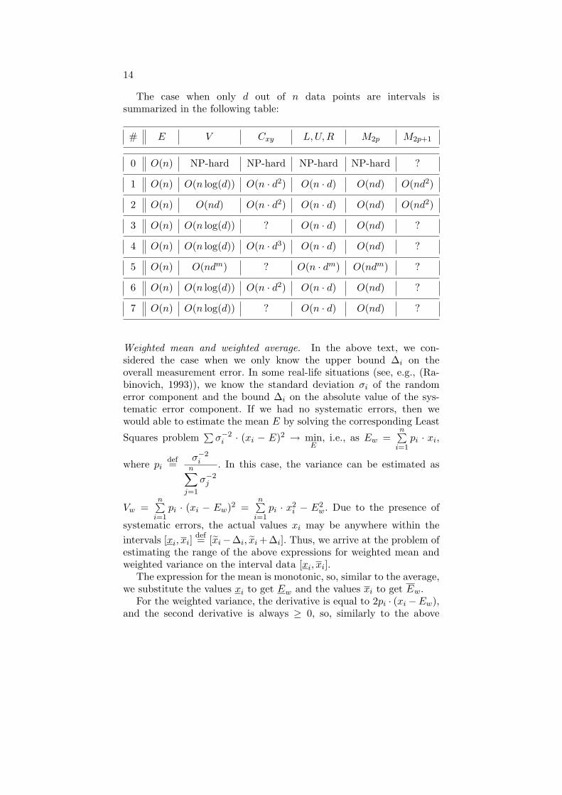
The case when only d out of n data points are intervals issummarized in the following table:

# E V Cxy L,U,R M2p M2p+1

0 O(n) NP-hard NP-hard NP-hard NP-hard ?

1 O(n) O(n log(d)) O(n · d2) O(n · d) O(nd) O(nd2)

2 O(n) O(nd) O(n · d2) O(n · d) O(nd) O(nd2)

3 O(n) O(n log(d)) ? O(n · d) O(nd) ?

4 O(n) O(n log(d)) O(n · d3) O(n · d) O(nd) ?

5 O(n) O(ndm) ? O(n · dm) O(ndm) ?

6 O(n) O(n log(d)) O(n · d2) O(n · d) O(nd) ?

7 O(n) O(n log(d)) ? O(n · d) O(nd) ?

Weighted mean and weighted average. In the above text, we con-sidered the case when we only know the upper bound ∆i on theoverall measurement error. In some real-life situations (see, e.g., (Ra-binovich, 1993)), we know the standard deviation σi of the randomerror component and the bound ∆i on the absolute value of the sys-tematic error component. If we had no systematic errors, then wewould able to estimate the mean E by solving the corresponding Least

Squares problem∑σ−2i · (xi − E)2 → min

E, i.e., as Ew =

n∑i=1

pi · xi,

where pidef=

σ−2i

n∑j=1

σ−2j

. In this case, the variance can be estimated as

Vw =n∑i=1

pi · (xi − Ew)2 =n∑i=1

pi · x2i − E2

w. Due to the presence of

systematic errors, the actual values xi may be anywhere within theintervals [xi, xi]

def= [xi−∆i, xi+∆i]. Thus, we arrive at the problem ofestimating the range of the above expressions for weighted mean andweighted variance on the interval data [xi, xi].

The expression for the mean is monotonic, so, similar to the average,we substitute the values xi to get Ew and the values xi to get Ew.

For the weighted variance, the derivative is equal to 2pi · (xi −Ew),and the second derivative is always ≥ 0, so, similarly to the above

15

proof for the non-weighted variance, we conclude that the minimum isalways attained at a vector (x1, . . . , xk, Ew, . . . , Ew, xk+l, . . . , xn). So,by considering 2n+ 2 zones, we can find V w in time O(n2).

For V w, we can prove that the maximum is always attained at valuesxi = xi or xi = xi, so we can always find it in time O(2n). If no morethanK intervals intersect, then, similarly to the non-weighted variance,we can compute V w in time O(n2).

Robust estimates for the mean. Arithmetic average is vulnerable tooutliers: if one of the values is accidentally mis-read as 106 times largerthan the others, the average is ruined. Several techniques have beenproposed to make estimates robust; see, e.g., (Huber, 2004). The bestknown estimate of this type is the median; there are also more general

L-estimates of the typen∑i=1

wi ·x(i), where w1 ≥ 0, . . . , wn ≥ 0 are given

constants, and x(i) is the i-th value in the ordering of x1, . . . , xn inincreasing order. Other techniques include M-estimates, i.e., estimates

a for whichn∑i=1

ψ(|xi − a|) → maxa

for some non-decreasing function

ψ(x).Each of these statistics C is a (non-strictly) increasing function

of each of the variables xi. Thus, similarly to the average, C =[C(x1, . . . , xn), C(x1, . . . , xn)].

Robust estimates for the generalized central moments. When we dis-cussed central moments, we considered generalized central moments

Mψ =1n·n∑i=1

ψ(xi − E) for an appropriate convex function ψ(x). In

that description, we assumed that E is the usual average.It is also possible to consider the case when E is not the average,

but the value for whichn∑i=1

ψ(xi − E) → minE

. In this case, the robust

estimate for the generalized central moment takes the form

M robψ = min

E

(1n·n∑i=1

ψ(xi − E)

).

Since the function ψ(x) is convex, the expressionn∑i=1

ψ(xi − E) is also

convex, so it only attains its maximum at the vertices of the convexbox x1 × . . .× xb, i.e., when for every i, either xi = xi or xi = xi. Forthe case of a single MI, the same proof as for the average E enables usto conclude that the maximum of the new generalized central momentis also always attained at one of n vectors (x1, . . . , xk, xk+1, . . . , xn),

16

and thus, that this maximum can be computed in time O(n2). For mMIs, we need time O(nm+1).

Correlation. For correlation, we only know that in general, theproblem of computing the exact range is NP-hard (Ferson et al., 2002d).

4. Additional Issues

On-line data processing. In the above text, we implicitly assumed thatbefore we start computing the statistics, we have all the measurementresults. In real life, we often continue measurements after we startedthe computations. Traditional estimates for mean and variance can beeasily modified with the arrival of the new measurement result xn+1:E′ = (n ·E+xn+1)/(n+1) and V ′ = M ′− (E′)2, where M ′ = (n ·M +x2n+1)/(n+ 1) and M = V +E2. For the interval mean, we can have a

similar adjustment. However, for other statistics, the above algorithmsfor processing interval data require that we start computation fromscratch. Is it possible to modify these algorithms to adjust them to on-line data processing? The only statistic for which such an adjustmentis known is the variance, for which an algorithm proposed in (Wu etal., 2003; Kreinovich et al., (in press)) requires only O(n) steps toincorporate a new interval data point.

In this algorithm, we store the sorting corresponding to the zonesand we store auxiliary results corresponding to each zone (finitely manyresults for each zone). So, if only d out of n intervals are non-degenerate,we only need O(d) steps to incorporate a new data point.

Fuzzy data. Often, in addition to (or instead of) the guaranteedbounds, an expert can provide bounds that contain xi with a certaindegree of confidence. Often, we know several such bounding intervalscorresponding to different degrees of confidence. Such a nested family ofintervals is also called a fuzzy set, because it turns out to be equivalentto a more traditional definition of fuzzy set (Nguyen and Kreinovich,1996; Nguyen and Walker, 1999) (if a traditional fuzzy set is given,then different intervals from the nested family can be viewed as α-cutscorresponding to different levels of uncertainty α).

To provide statistical analysis of fuzzy-valued data, we can there-fore, for each level α, apply the above interval-valued techniques to thecorresponding α-cuts (Martinez, 2003; Nguyen et al., 2003).

Can we detect the case of several MI? For the several MI case, weassumed that measurement are labeled, so that we can check which

17

measurements were done by each MI; this labeling is used in the algo-rithms. What if we do not keep records on which interval was measuredby which MI; can we then reconstruct the labels and thus apply thealgorithms?

For two MI, we can: we pick an interval and call it MI1. If any otherinterval is in subset relation with this one, then this new interval isMI2. At any given stage, if one of the un-classified intervals is in subsetrelation with one of the already classified ones, we classify it to theopposite class. If none of the un-classified intervals is in subset relationwith classified ones, we pick one of the un-classified ones and assign toMI1. After ≤ n iterations, we get the desired labeling.

In general, for m MI, the labeling may not be easy. Indeed, wecan construct a graph in which vertices are intervals, and vertices areconnected if they are in a subset relation. Our objective is to assign aclass to each vertex so that connected vertices cannot be of the sameclass. This is exactly the coloring problem that is known to be NP-hard(Garey and Johnson, 1979).

Parallelization. In the general case, the problem of computing therange C of a statistic C on interval data xi requires too much com-putation time. One way to speed up computations is to use parallelcomputations.

If we have a potentially unlimited number of parallel processors,then, for the mean, the addition can be done in time O(log(n)) (Jaja,1992). In O(n·log(n)) and O(n2) algorithms for computing V and V , wecan perform sorting in time O(log(n)), then compute Vk for each zonein parallel, and find the largest of the n resulting values Vk in parallel(in time O(log(n))). The sum that constitutes the variance can also becomputed in parallel in time O(log(n)), so overall, we need O(log(n))time.

Similarly, we can transform polynomial algorithms for computingthe bounds for covariance, outlier statistics (L, U , andR), and momentsinto O(log(n)) parallel algorithms.

In the general case, to find V and other difficult-to-compute bounds,we must compute the largest of the N def= 2n values corresponding to 2n

possible combinations of xi and xi. This maximum can be computedin time O(log(N)) = O(n). This does not mean, of course, that we canalways physically compute V in linear time: communication time growsexponentially with n; see, e.g., (Morgenstein and Kreinovich, 1995).

It is desirable to also analyze the case when we have a limited numberof processors p� n.

18

Quantum algorithms. Another way to speed up computations is touse quantum computing. In (Martinez, 2003; Kreinovich and Longpre,2004), we describe how quantum algorithms can speed up the compu-tation of C.

What if we have partial information about the probabilities? Enter p-boxes. In the above text, we assumed that the only information thatwe have about the measurement error ∆x is that this error is somewherein the interval [−∆,∆], and that we have no information about theprobabilities of different values from this interval. In many real-life sit-uations, we do not know the exact probability distribution for ∆x, butwe have a partial information about the corresponding probabilities.How can we describe this partial information?

To answer this question, let us recall how the complete informationabout the probability distribution is usually described. A natural wayto describe a probability distribution is by describing its cumulativedensity function (cdf) F (t) def= Prob(∆x ≤ t). In practice, a reasonableway to store the information about F (t) is to store quantiles, i.e., to fixa natural number n and to store, for every i from 0 to n, the values tifor which F (ti) = i/n. Here, t0 is the largest value for which F (t0) = 0and tn is the smallest value for which F (tn) = 1, i.e., [t0, tn] is thesmallest interval on which the probability distribution is located withprobability 1.

If we only have partial information about the probabilities, thismeans that – at least for some values t – we do not know the exact valueof F (t). At best, we know an interval F(t) = [F (t), F (t)] of possiblevalues of F (t). So, a natural way to describe partial information aboutthe probability distribution is to describe the two functions F (t) andF (t). This pair of cdfs is called a p-box; see, e.g., a book (Ferson, 2002).In addition to the theoretical concepts, this book describes the softwaretool for processing different types of uncertainty, a tool based on thenotion of a p-box.

Similarly to the case of full information, it is reasonable to store thecorresponding quantiles, i.e., the values ti for which F (ti) = i/n andthe values ti for which F (ti) = i/n. (The reason why we switched thenotations is because F (t) ≤ F (t) implies ti ≤ ti.) This is exactly therepresentation used in (Ferson, 2002).

What if we have partial information about the probabilities? Processingp-boxes and how the above alorithms can help. Once we have a prob-ability distribution F (t), natural questions are: what is the mean andthe variance of this distribution? A p-box means that several differentdistributions are possible, and for different distributions, we may have

19

different values of means and variance. So, when we have a p-box,natural questions are: what is the range of possible values of the mean?what is the range of possible values of the variance?

The mean E is a monotonic function of F (t); so, for the mean E,the answer is simple: the mean of F (t) is the desired upper bound Efor E, and the mean of F (t) is the desired lower bound E for E. Thevariance V is not monotonic, so the problem of estimating the varianceis more difficult.

For the case of the exact distribution, if we have the quantiles t(α)corresponding to all possible probability values α ∈ [0, 1], then we candescribe the mean of the corresponding probability distribution as E =∫t(α) dα, and the variance as V =

∫(t(α)−E)2 dα. If we only know the

quantiles t1 = t(1/n), . . . , tn = t(n/n), then it is reasonable to replacethe integral by the corresponding integral sum; as a result, we get the

estimates E =1n

n∑i=1

ti and V =1n

n∑i=1

(ti − E)2.

In these terms, a p-box means that instead of the exact value ti ofeach quantile, we have an interval of possible values [ti, ti]. So, to findthe range of V , we must consider the range of possible values of V whenti ∈ [ti, ti]. There is an additional restriction that the values ti shouldbe (non-strictly) increasing: ti ≤ ti+1.

The resulting problem is very similar to the problems of estimatingmean and variance of the interval data. In this case, intervals satisfy thesubset property, i.e., we are in the case that we called the case of singleMI. The only difference between the current problem of analyzing p-boxes and the above problem is that in the above problem, we lookedfor minimum and maximum of the variance over all possible vectorsxi for which xi ∈ xi for all i, while in our new problem, we have anadditional monotonicity restriction ti ≤ ti+1. However, the solutions toour previous problems of computing V and V for the case of a singleMI are actually attained at vectors that are monotonic. Thus, to findthe desired value V , we can use the same algorithm as we describedabove.

Specifically, to find V , we find k for which the variance of the vec-tor t = (t1, . . . , tk, t, . . . , t, tk+l, . . . , tn) for which the variance is thesmallest. To find V , we find k for which the variance of the vectort = (t1, . . . , tk, tk+1, . . . , tn) for which the variance is the largest. Intu-itively, this makes perfect sense: to get the smallest V , we select thevalues ti as close to the average t as possible; to get the largest V , weselect the values ti as far away from the average t as possible. In bothcase, we can compute V and V in time O(n · log(n)).

The above algorithm describes a heuristic estimate based on approx-imating an integral with an integral sum. To get reliable bounds, we can

20

take into consideration that both bounds F (t) and F (t) are monotonic;thus, we can always replace the p-box by a larger p-box in which thevalues t(α) are piecewise-constant: namely, we take t′i = [ti−1, ti] foreach i. For this new p-box, the integral sum coincides with the integral,so the range [V , V ] produced by the above algorithm is exactly therange of the variance over all possible distributions from the enlargedp-box. It is therefore guaranteed to contain the range of possible valuesof the variance V for the original p-box.

What if we have partial information about probabilities? Multi-dimensional case. How can we describe partial information aboutprobabilities in multi-dimensional case? A traditional analogue of acdf is a multi-dimensional cdf

F (t1, . . . , tp) = Prob(x1 ≤ t1 & . . . &xp ≤ tp);

see, e.g., (Wadsworth, 1990). The problem with this definition is thatoften multi-D data represent, e.g., vectors with components x1, . . . , xp.The components depend on the choice of coordinates. As a result,even if a distribution is symmetric – e.g., a rotation-invariant Gaus-sian distribution – the description in terms of a multi-D cdf is notrotation-invariant.

It is desirable to come up with a representation that preserves sucha symmetry. A natural way to do it is to store, for each half-space, theprobability that the vector ~x = (x1, . . . , xp) is within this half-space. Inother words, for every unit vector ~e and for every value t, we store theprobability F (~e, t) def= Prob(~x ·~e ≤ t), where ~x ·~e = x1 · e1 + . . .+xn · enis a scalar (dot) product of the two vectors. This representation isclearly rotation-invariant: if we change the coordinates, we keep thesame values F (~e, t); the only difference is that we store each valueunder different (rotated) ~e. Moreover, this representation is invariantunder arbitrary linear transformations.

Based on this information, we can uniquely determine the prob-ability distribution. For example, if the probability distribution hasa probability density function (pdf) ρ(~x), then this pdf can be re-constructed as follows. First, we determine the characteristic functionχ(~ω) def= E[exp(i · (~x · ~ω))], where E[·] stands for the expected value.To get the value of χ(~ω), we apply the 1-D Fourier transform, to thevalues F (~e, t) for different t, where ~e def= ~ω/‖~ω‖ is a unit vector in thedirection of ~ω. Then, we can find ρ(~x) by applying the p-dimensionalInverse Fourier Transform to χ(~ω).

21

It is therefore reasonable to represent a partial information aboutthe probability distribution by storing, for each ~e and t, the boundsF (~e, t) and F (~e, t) that describe the range of possible values for F (~e, t).

It is worth mentioning that since for continuous distributions,F (~e, t) = 1 − F (−~e,−t), we have F (~e, t) = 1 − F (−~e,−t). So, it issufficient to only describe F (~e, t), the lower bounds F (~e, t) can then beuniquely determined (or, vice versa, we can only describe the valuesF (~e, t); then the values F (~e, t) will be uniquely determined).

In order to transform this idea into an efficient software tool, weneed to solve two types of problems. First, we must solve algorithmicproblems: develop algorithms for estimating the ranges of statisticalcharacteristics (such as moments) for the corresponding multi-D p-boxes.

Second, we must solve implementation problems. Theoretically, touniquely describe a probability distribution, we need to know infinitelymany values F (~e, t) corresponding to infinitely many different vectors ~eand infinitely many different numbers t. In practice, we can only storefinitely many values F (~e, t) corresponding to finitely many vectors ~e.

In principle, we can simply select a rectangular grid and store thevalues for the vectors ~e from this grid. However, the selection of thegrid violates rotation-invariance and thus, eliminates the advantage ofselecting this particular multi-D analogue of a cdf. It turns out thatthere is a better way: instead of using a grid, we can use rational pointson a unit sphere. There exists efficient algorithms for generating suchpoints, and the set of all such points is almost rotation-invariant: it isinvariant with respect to all rotations for which all the entries in thecorresponding rotation matrix are rational numbers (Oliverio, 1996;Trautman, 1998).

Beyond p-boxes? A p-box does not fully describe all kinds of possiblepartial information about the probability distribution. For example, thesame p-box corresponds to the class of all distributions located on aninterval [0, 1] and to the class of all distributions located at two points0 and 1.

Similarly, in the multi-D case, if we only use the above-defined multi-D cdfs, we will not be able to distinguish between a set S (= the classof all probability distributions localized on the set S with probability1) and its convex hull. To provide such a distinction, we may want, inaddition to the bounds on the probabilities Prob(f(x) ≤ t) for all linearfunctions f(x), to also keep the bounds on the similar probabilitiescorresponding to all quadratic functions f(x).

Let us show that this addition indeed enables us to distinguishbetween different sets S. Indeed, for every point x, to check whether

22

x ∈ S, we ask, for different values ε > 0, for the upper bound for theprobability Prob(d2(x, x0) ≤ ε2), where d(x, x0) denotes the distancebetween the two points. If x 6∈ S, then for sufficiently small ε, thisprobability will be 0; on the other hand, if x ∈ S, then it is possiblethat we have a distribution located at this point x with probability 1,so the upper bound is 1 for all ε (Nguyen et al., 2000).

In 1-D case, the condition f(x) ≤ t for a non-linear quadratic func-tion f(x) is satisfied either inside an interval, or outside an interval.Thus, in 1-D case, our idea means that in addition to cdf, we alsostore the bounds on the probabilities of x being within different in-tervals. Such bounds are analyzed, e.g., in (Berleant, 1993; Berleant,1996; Berleant and Goodman-Strauss, 1998; Berleant et al., 2003).

Acknowledgements

This work was supported in part by NASA under cooperative agree-ment NCC5-209, by the Future Aerospace Science and TechnologyProgram (FAST) Center for Structural Integrity of Aerospace Systems,effort sponsored by the Air Force Office of Scientific Research, Air ForceMateriel Command, USAF, under grant F49620-00-1-0365, by NSFgrants EAR-0112968, EAR-0225670, and EIA-0321328, by the ArmyResearch Laboratories grant DATM-05-02-C-0046, and by a researchgrant from Sandia National Laboratories as part of the Department ofEnergy Accelerated Strategic Computing Initiative (ASCI).

The authors are greatly thankful to the anonymous referees forhelpful suggestions.

References

Beck, B., V. Kreinovich, and B. Wu, Interval-Valued and Fuzzy-Valued Ran-dom Variables: From Computing Sample Variances to Computing SampleCovariances, In: M. Lopez, M. A. Gil, P. Grzegorzewski, O. Hrynewicz, andJ. Lawry, editor, Soft Methodology and Random Information Systems, pages85–92, Springer-Verlag, Berlin Heidelberg New York Tokyo, 2004.

Berleant, D., Automatically verified arithmetic with both intervals and probabilitydensity functions, Interval Computations, 1993, (2):48–70.

Berleant, D., Automatically verified arithmetic on probability distributions and in-tervals, In: R. B. Kearfott and V. Kreinovich, editors, Applications of IntervalComputations, Kluwer, Dordrecht, 1996.

Berleant, D., and C. Goodman-Strauss, Bounding the results of arithmetic oper-ations on random variables of unknown dependency using intervals, ReliableComputing, 1998, 4(2):147–165.

23

Berleant, D., L. Xie, and J. Zhang, Statool: A Tool for Distribution Envelope De-termination (DEnv), an Interval-Based Algorithm for Arithmetic on RandomVariables, Reliable Computing, 2003, 9(2):91–108.

Ferson, S. RAMAS Risk Calc 4.0: Risk Assessment with Uncertain Numbers, CRCPress, Boca Raton, Florida, 2002.

Ferson, S., L. Ginzburg, V. Kreinovich, and M. Aviles, Exact Bounds on SampleVariance of Interval Data. Extended Abstracts of the 2002 SIAM Workshop onValidated Computing, Toronto, Canada, 2002, pp. 67–69

Ferson, S., L. Ginzburg, V. Kreinovich, and M. Aviles, Exact Bounds on Fi-nite Populations of Interval Data, University of Texas at El Paso, De-partment of Computer Science, Technical Report UTEP-CS-02-13d, 2002,http://www.cs.utep.edu/vladik/2002/tr02-13d.pdf

Ferson, S., L. Ginzburg, V. Kreinovich, L. Longpre, and M. Aviles, ComputingVariance for Interval Data is NP-Hard, ACM SIGACT News, 33(2):108–118,2002.

Ferson, S., D. Myers, and D. Berleant, Distribution-free risk analysis: I. Range,mean, and variance, Applied Biomathematics, Technical Report, 2001.

Garey, M. E., and D. S. Johnson, Computers and intractability: a guide to the theoryof NP-completeness, Freeman, San Francisco, 1979.

Granvilliers, L., V. Kreinovich, and N. Muller, Novel Approaches to NumericalSoftware with Result Verification”, In: R. Alt, A. Frommer, R. B. Kearfott, andW. Luther, editors, Numerical Software with Result Verification, InternationalDagstuhl Seminar, Dagstuhl Castle, Germany, January 19–24, 2003, RevisedPapers, Springer Lectures Notes in Computer Science, 2004, Vol. 2991, pp.274–305.

Huber, P. J., Robust statistics, Wiley, New York, 2004.Jaja, J. An Introduction to Parallel Algorithms, Addison-Wesley, Reading, MA, 1992.Kreinovich, V. Probabilities, Intervals, What Next? Optimization Problems Related

to Extension of Interval Computations to Situations with Partial Informationabout Probabilities, Journal of Global Optimization (in press).

Kreinovich, V., A. Lakeyev, J. Rohn, and P. Kahl, Computational complexity andfeasibility of data processing and interval computations, Kluwer, Dordrecht, 1997.

Kreinovich, V., and L. Longpre, Computational complexity and feasibility of dataprocessing and interval computations, with extension to cases when we have par-tial information about probabilities, In: V. Brattka, M. Schroeder, K. Weihrauch,and N. Zhong, editors, Proc. Conf. on Computability and Complexity in AnalysisCCA’2003, Cincinnati, Ohio, USA, August 28–30, 2003, pp. 19–54.

Kreinovich, V., and L. Longpre, Fast Quantum Algorithms for Handling Probabilis-tic and Interval Uncertainty, Mathematical Logic Quarterly, 2004, 50(4/5):507–518.

Kreinovich, V., L. Longpre, S. Ferson, and L. Ginzburg, Computing HigherCentral Moments for Interval Data, University of Texas at El Paso, De-partment of Computer Science, Technical Report UTEP-CS-03-14b, 2004,http://www.cs.utep.edu/vladik/2003/tr03-14b.pdf

Kreinovich, V., L. Longpre, P. Patangay, S. Ferson, and L. Ginzburg, Outlier De-tection Under Interval Uncertainty: Algorithmic Solvability and ComputationalComplexity, In: I. Lirkov, S. Margenov, J. Wasniewski, and P. Yalamov, editors,Large-Scale Scientific Computing, Proceedings of the 4-th International Confer-ence LSSC’2003, Sozopol, Bulgaria, June 4–8, 2003, Springer Lecture Notes inComputer Science, 2004, Vol. 2907, pp. 238–245

24

Kreinovich, V., H. T. Nguyen, and B. Wu, On-Line Algorithms for Computing Meanand Variance of Interval Data, and Their Use in Intelligent Systems, InformationSciences (in press).

Kreinovich, V., P. Patangay, L. Longpre, S. A. Starks, C. Campos, S. Ferson, and L.Ginzburg, Outlier Detection Under Interval and Fuzzy Uncertainty: AlgorithmicSolvability and Computational Complexity, Proceedings of the 22nd Interna-tional Conference of the North American Fuzzy Information Processing SocietyNAFIPS’2003, Chicago, Illinois, July 24–26, 2003, pp. 401–406.

Kuznetsov, V. P., Interval Statistical Models, Radio i Svyaz, Moscow, 1991 (inRussian).

Lodwick, W. A., and K. D. Jamison, Estimating and Validating the CumulativeDistribution of a Function of Random Variables: Toward the Development ofDistribution Arithmetic, Reliable Computing, 2003, 9(2):127–141.

Martinez, M., L. Longpre, V. Kreinovich, S. A. Starks, and H. T. Nguyen, Fast Quan-tum Algorithms for Handling Probabilistic, Interval, and Fuzzy Uncertainty,Proceedings of the 22nd International Conference of the North American FuzzyInformation Processing Society NAFIPS’2003, Chicago, Illinois, July 24–26,2003, pp. 395–400.

Moore, R. E., and W. A. Lodwick, Interval Analysis and Fuzzy Set Theory, FuzzySets and Systems, 2003, 135(1):5–9.

Morgenstein, D., and V. Kreinovich, Which algorithms are feasible and which arenot depends on the geometry of space-time, Geombinatorics, 1995, 4(3):80–97.

Nguyen, H. T., and V. Kreinovich, Nested Intervals and Sets: Concepts, Relationsto Fuzzy Sets, and Applications, In: R. B. Kearfott and V. Kreinovich, editors,Applications of Interval Computations, Kluwer, Dordrecht, 1996, pp. 245–290

Nguyen, H. T., and E. A. Walker, First Course in Fuzzy Logic, CRC Press, BocaRaton, Florida, 1999.

Nguyen, H. T., T. Wang, and V. Kreinovich, Towards Foundations of ProcessingImprecise Data: From Traditional Statistical Techniques of Processing CrispData to Statistical Processing of Fuzzy Data, In: Y. Liu, G. Chen, M. Ying,and K.-Y. Cai, editors, Proceedings of the International Conference on FuzzyInformation Processing: Theories and Applications FIP’2003, Beijing, China,March 1–4, 2003, Vol. II, pp. 895–900.

Nguyen, H. T., B. Wu, and V. Kreinovich, Shadows of Fuzzy Sets – A NaturalApproach Towards Describing 2-D and Multi-D Fuzzy Uncertainty in LinguisticTerms, Proc. 9th IEEE Int’l Conference on Fuzzy Systems FUZZ-IEEE’2000,San Antonio, Texas, May 7–10, 2000, Vol. 1, pp. 340–345.

Nivlet, P., F. Fournier, and J. Royer, A new methodology to account for uncer-tainties in 4-D seismic interpretation, Proc. 71st Annual Int’l Meeting of Soc.of Exploratory Geophysics SEG’2001, San Antonio, TX, September 9–14, 2001,1644–1647.

Nivlet, P., F. Fournier, and J. Royer, Propagating interval uncertainties in su-pervised pattern recognition for reservoir characterization, Proc. 2001 Societyof Petroleum Engineers Annual Conf. SPE’2001, New Orleans, LA, September30–October 3, 2001, paper SPE-71327.

Oliverio, P., Self-generating Pythagorean quadruples and n-tuples, Fibonacci Quar-terly, May 1996, pp. 98–101.

Osegueda, R., V. Kreinovich, L. Potluri, R. Alo, Non-Destructive Testing ofAerospace Structures: Granularity and Data Mining Approach, Proc. FUZZ-IEEE’2002, Honolulu, HI, May 12–17, 2002, Vol. 1, pp. 685–689

25

Rabinovich, S., Measurement Errors: Theory and Practice, American Institute ofPhysics, New York, 1993.

Regan, H., S. Ferson, and D. Berleant, Equivalence of five methods for boundinguncertainty, Journal of Approximate Reasoning (in press).

Rowe, N. C., Absolute bounds on the mean and standard deviation of transformeddata for constant-sign-derivative transformations, SIAM Journal of ScientificStatistical Computing, 1988, 9:1098–1113.

Shmulevich, I., and W. Zhang, Binary analysis and optimization-based normaliza-tion of gene expression data, Bioinformatics, 2002, 18(4):555–565.

Trautman, A., Pythagorean Spinors and Penrose Twistors, In: S. A. Hugget et al.,editors, The Geometric Universe; Science, Geometry, and the Work of RogerPenrose, Oxford Univ. Press, Oxford, 1998.

Wadsworth, H. M. Jr., editor, Handbook of statistical methods for engineers andscientists, McGraw-Hill Publishing Co., N.Y., 1990.

Wu, B., H. T. Nguyen, and V. Kreinovich, Real-Time Algorithms for StatisticalAnalysis of Interval Data, Proceedings of the International Conference on In-formation Technology InTech’03, Chiang Mai, Thailand, December 17–19, 2003,pp. 483–490.

Walley, P., Statistical Reasoning with Imprecise Probabilities, Chapman & Hall, N.Y.,1991.

Williamson, R., and T. Downs, Probabilistic arithmetic I: numerical methodsfor calculating convolutions and dependency bounds, International Journal ofApproximate Reasoning, 1990, 4:89–158.

Xiang, G., S. A. Starks, V. Kreinovich, and L. Longpre, New Algorithms for Statis-tical Analysis of Interval Data, Proceedings of the Workshop on State-of-the-Artin Scientific Computing PARA’04, Lyngby, Denmark, June 20–23, 2004, Vol. 1,pp. 123–129.

Zhang, W., I. Shmulevich, and J. Astola, Microarray Quality Control, Wiley,Hoboken, New Jersey, 2004.