Estimating Measurement Uncertainty

Oscar ChinellatoErwin Achermann

Institute of Scientific ComputingETH Zurich

28th June 2000

Abstract

Most analytical methods are relative and hence require calibration. Calibration measurementsare normally performed with reference materials or calibration standards. Typically least squaresmethods have been employed in such a manner as to ignore uncertainties associated with the cal-ibration standards. However different authors [3, 4, 11] have shown that by taking into accountthe uncertainties associated with the calibration standards, better approximations to the model arepossible.

We show a complete, numerically stable and fast way to compute the Maximum Likelihood (fittingof a) Functional Relationship (MLFR), and we show how the model described in [11] is a unnecessarilyrestricted case of our fully general model.

1 Calibration and Measurement

Since measurement instruments obey physical laws, they can be modelled by mathematical functions.These functions describe only the qualitative behaviour unless all free parameters p are quantified. Cal-ibration is the process of quantifying these parameters. For example, consider the measurement of aweight using a spring balance.

Here we denote weights with x ∈ R and stretches of the spring with y ∈ R. Let xcs be a known weightof a calibration standard and ycs be the stretch of the spring balance for this calibration standard. Fora given calibrated balance p the following holds true: ycs = f(xcs,p). This f is called the calibrationfunction. The art of calibrating consists of adjusting the parameters p (e.g. spring constant) using severalcalibrating pairs xi and yi such that yi ≈ f(xi,p) holds for all i as well as possible.

For an unknown mass x, weighing with a calibrated spring balance requires the measurement of a springstretch y and subsequent application of the measurement function g(y,p). In other words, x ≈ g(y,p).Note that g is the inverse function of f .

In the case that the pairs (xi, yi) were exact this would be a standard problem. But in practice everymeasurement is subject to uncertainties. Therefore, not only the calibrating pairs (xi, yi) but also theirrespective uncertainties (αi, βi) must be known and taken into consideration. Throughout this paper theerror random variables e

(x)i respectively e

(y)i are treated as e

(x)i ∼ N (0, αi) respectively e

(y)i ∼ N (0, βi).

This fully conforms with the “Guide to the Expression of Uncertainty in Measurement” (GUM) [10].

With respect to our spring balance example, this implies that the real calibration weights are not xi

but xi + e(x)i . Analogously the correct values for the stretch are no longer yi but yi + e

(y)i .

Note that the uncertainties of x and y are uncorrelated. That is, the error of the calibration standard isindependent of the error of the reading.

1

Estimating Measurement Uncertainty, O. Chinellato and E. Achermann 2

2 Calibration Models

Before we start considering calibration models, it is necessary to agree on a number of the assumptions.

The measurement tool is expected to work according to the function f(·, ·) in use. This means that thereexists a set of parameters which describes the apparatus correctly. In other words, the model is assumedto be exact.

Every error random vector (rv) u is assumed to be normally distributed and is denoted by u ∼ N (µ,C)where µ ∈ Rn is the mean vector and C ∈ Rn×n is the covariance matrix of the rv u ∈ Rn. The wellknown probability density function (pdf) is

pdf(u) = err (u− µ,C) = (2π)−n2

1√det (C)

e−12 (u−µ)TC−1(u−µ).

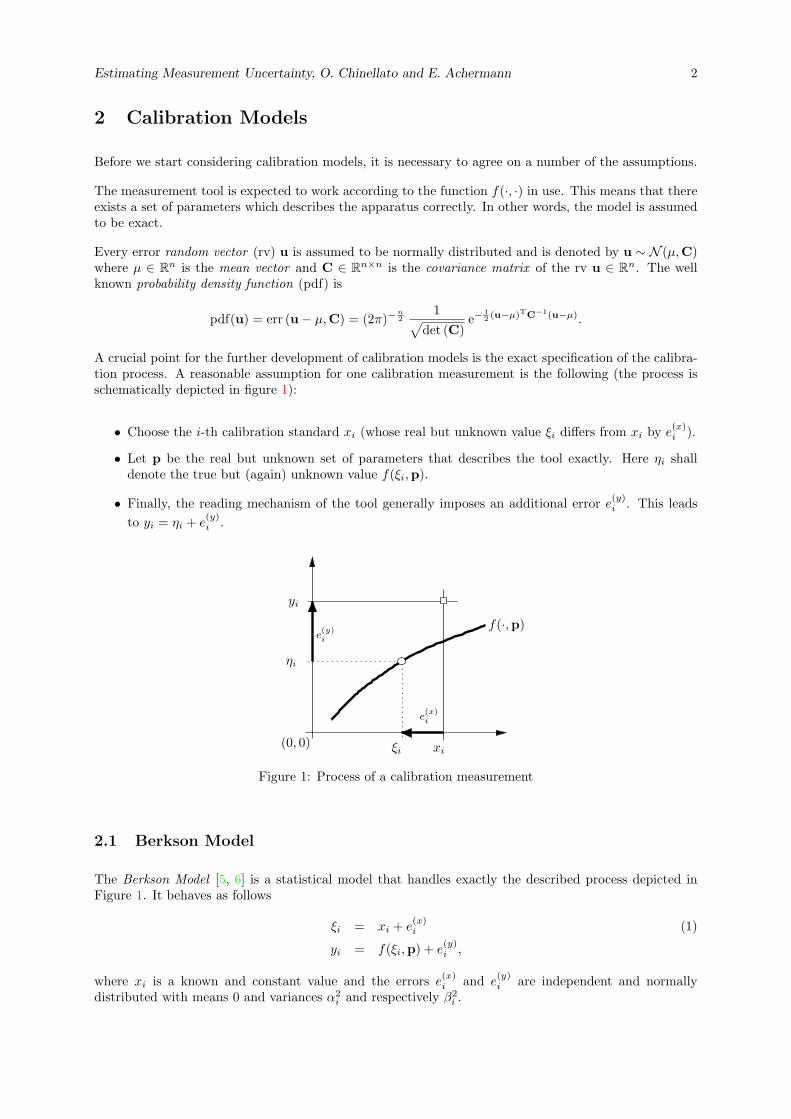
A crucial point for the further development of calibration models is the exact specification of the calibra-tion process. A reasonable assumption for one calibration measurement is the following (the process isschematically depicted in figure 1):

• Choose the i-th calibration standard xi (whose real but unknown value ξi differs from xi by e(x)i ).

• Let p be the real but unknown set of parameters that describes the tool exactly. Here ηi shalldenote the true but (again) unknown value f(ξi,p).

• Finally, the reading mechanism of the tool generally imposes an additional error e(y)i . This leads

to yi = ηi + e(y)i .

ξi

e(y)i

(0, 0)

e(x)i

f(·,p)

xi

yi

ηi

Figure 1: Process of a calibration measurement

2.1 Berkson Model

The Berkson Model [5, 6] is a statistical model that handles exactly the described process depicted inFigure 1. It behaves as follows

ξi = xi + e(x)i (1)

yi = f(ξi,p) + e(y)i ,

where xi is a known and constant value and the errors e(x)i and e

(y)i are independent and normally

distributed with means 0 and variances α2i and respectively β2

i .

Estimating Measurement Uncertainty, O. Chinellato and E. Achermann 3

A Taylor series expansion of f(ξi,p) around xi yields an expression that reveals the connection between ξi

and yi

yi ≈ f(xi,p) +∂

∂xf(xi,p) · e(x)

i + e(y)i = f

(i) + f(i)x e

(x)i + e

(y)i , (2)

where f(i) = f(xi,p) and f

(i)x = ∂

∂xf(xi,p). Equations (1) and (2) make the following relations obvious:

Var (ξi) = Var(xi + e

(x)i

)= α2

i

Var (yi) ≈ Var(f

(i) + f(i)x e

(x)i + e

(y)i

)= f

(i)x

2α2

i + β2i

Cov (ξi, yi) ≈ E[e(x)i

(f

(i)x e

(x)i + e

(y)i

)]= f

(i)x α2

i .

2.1.1 Fitting of ξ and p (XiP-fit)

As can be seen in Section 2.1, the pdf of (ξi, yi) can be written as bivariate normal distribution

pdf(zi) = err (zi,Ci) =12π

1√det (Ci)

e−12zi

TC−1i zi ,

where zi and Ci are defined as follows:

zi =(

ξi − xi

yi − f(i)

)and Ci =

(α2

i f(i)x α2

i

f(i)x α2

i f(i)x

2α2

i + β2i

).

We generalize to all n measurements, and allow additional correlations amongst the errors e(x)i respec-

tively e(y)i denoted by Cx respectively Cy. This leads to the

pdf(ξ,y) = err (z,C) = (2π)−n 1√det (C)

e−12zTC−1z,

where z and C now are defined as

z =(

ξ − xy − f

)and C =

(Cx CxFx

FxCx FxCxFx + Cy

).

Now, analogously,

f =(f

(1), . . . , f

(n))T

and Fx = diag(f

(1)x , . . . , f

(n)x

).

Thus we know the value of the pdf at (ξ,p) given x and y. The maximum likelihood principle aims atmaximizing this value. Hence

maxξ,p

((2π)−n 1√

det (C)e−

12zTC−1z

)(3)

must be solved for p and ξ. See Section 3 for computational details.

2.1.2 Fitting of p (P-fit)

In the previous section we fitted for both parameters p and ξ. Hence we found the most probable pairingof p and ξ, i.e. an estimation for the true shape of f and simultaneously the true values of the calibrationstandards x. However, it is often the case that one is not interested in an estimation of the calibrationstandard values, but rather one is interested in the most probable shape of the calibration function fregardless of any estimation for x.

Estimating Measurement Uncertainty, O. Chinellato and E. Achermann 4

Consequently, we are looking for the pdf of y only. This is computed by the law of total probability [13].We show the derivation of it for one calibration pair (x, y). We use f = f(x,p) and fx = ∂

∂xf(x,p) asshort forms.

pdf(y) =∫ ∞−∞

pdf(y∣∣ ξ) pdf (ξ) dξ

=∫ ∞−∞

err (y − f(ξ,p), β) err (ξ − x, α) dξ

≈∫ ∞−∞

err (y − f − fx(ξ − x), β) err (ξ − x, α) dξ

=12π

1αβ

∫ ∞−∞

e−12

(y−f−fx(ξ−x))2

β2 e−12

(ξ−x)2

α2 dξ

=1√2π

1√α2f2

x + β2e− 1

2(y−f)2

α2f2x+β2

=⇒ pdf(y) ≈ err(y − f,

√α2f2

x + β2)

The generalization to the n-dimensional case is now straight forward:

pdf(y) ≈ err (z,C) = (2π)−n2

1√det (C)

e−12zTC−1z

withz = y − f and C = FxCxFx + Cy.

Hence we know the value of the pdf at p given x and y. Again using the principle of maximum likelihood,we are left with the maximization problem

maxp

((2π)−

n2

1√det (C)

e−12zTC−1z

). (4)

Superficially, this looks equivalent to equation (3), but recall that C and z are defined differently. SeeSection 3 for the computation of p.

2.2 Model proposed in ISO 6143

The method proposed by ISO 6143 [11] is again a maximum likelihood fit:

maxξ,p

(K e−

12 (ξ−x)TC−1

x (ξ−x)− 12 (f(ξ,p)−y)TC−1

y (f(ξ,p)−y))

(5)

with K = (2π)−n(det (Cx)det (Cy))−1/2 constant. Comparing this formula with equation (3), one cansee that it is transformed to (5) by assuming that Cx and Cy are both diagonal matrices. This is notalways the case [11, p. 22].

However, using this assumption (5), leads to the minimization problem

minξ,p

(n∑

i=1

((ξi − xi)2

α2i

+(f(ξi,p)− yi)2

β2i

)).

This is the minimization problem described in [11, p. 19]. It belongs to the class of weighted orthogonaldistance regression (Weighted ODR) problems that are thoroughly studied in [2] and [9].

Estimating Measurement Uncertainty, O. Chinellato and E. Achermann 5

3 Computations

In this section we show how to solve the maximization problems (3) and (4). For quantifying the mea-surement uncertainty later, when using the calibrated tool, we need the covariances of the parameters p,i.e. the covariance matrix Cp. Its use will be demonstrated in Section 4. We explain the computation ofthe covariance matrix Cp at the end of each subsection.

Notation We use the following symbols, notations and abbreviations for readability. For matrices, M(i)

denotes the i-th column vector. Additionally, ∂k abbreviates the element-wise derivative with respectto pk.

JTp =

(∂

∂p f(1)

, . . . , ∂∂p f

(n))

JTxp =

(∂

∂p f(1)x , . . . , ∂

∂p f(n)x

)Jppk

= ∂kJp

Jxppk= ∂kJxp

Fxpk= ∂kFx

3.1 Computing ξ and p

Consider the maximization problem (3). This is equivalent (after taking the logarithm) to the followingminimization problem:

minξ,p

(n log(2π) +

12

log(det (C)) +12zTC−1z

).

Now we can drop constant terms. Note that det (C) is also constant. This can be seen by applying aCholesky factorization1 on C.

C = RTR =(

RTx 0

FxRTx RT

y

)(Rx RxFx

0 Ry

),

where Cx = RTx Rx and Cy = RT

y Ry. Note, that det (C) = det(RT

x

)det (Rx)det

(RT

y

)det (Ry) =

det(RT

x Rx

)det(RT

y Ry

)= det (Cx)det (Cy) and since it is independent from ξ and p, it is constant.

Lucky us! We are left with the following minimization problem

minξ,p

(zTC−1z

).

Solving this is equivalent to solving a nonlinear least squares problem:

minξ,p

(zTC−1z

)= min

ξ,p

(zTR−1R−Tz

)= min

ξ,p

(rTr)

= minξ,p

r 2 = minξ,p

S (ξ,p) .

There are different standard solvers for such problems, e.g. the Gauss-Newton (or the further developedLevenberg-Marquardt method), the Newton method, the spectral decomposition method, etc. [14, 1, 12,8, 7]. The following condition holds for the computed minimum

JTr = 0, (6)

where J denotes the jacobian of r with respect to ξ and p. Its structure is shown in equation (8). Thestatement above can be verified as follows: we define w = (ξ,p)T. Linearizing the function r(w+∆w) ≈r(w) + J∆w we get S (w + ∆w) ≈ S (w) + 2∆wTJTr +O( ∆w 2). Thus equation (6) is obviously truein a minimum.

1There exists a Cholesky factorization for any symmetric positive definite matrix. This is the case for all covariancematrices by definition.

Estimating Measurement Uncertainty, O. Chinellato and E. Achermann 6

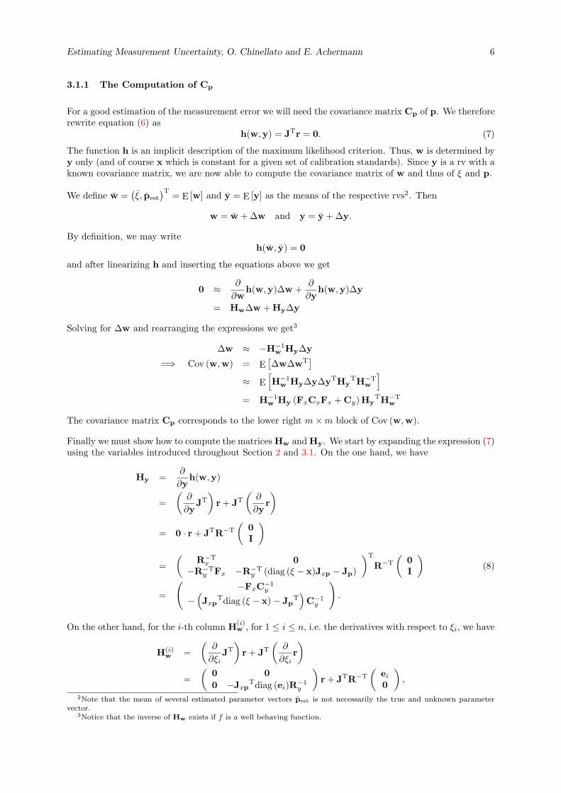
3.1.1 The Computation of Cp

For a good estimation of the measurement error we will need the covariance matrix Cp of p. We thereforerewrite equation (6) as

h(w,y) = JTr = 0. (7)

The function h is an implicit description of the maximum likelihood criterion. Thus, w is determined byy only (and of course x which is constant for a given set of calibration standards). Since y is a rv with aknown covariance matrix, we are now able to compute the covariance matrix of w and thus of ξ and p.

We define w =(ξ, pest

)T = E [w] and y = E [y] as the means of the respective rvs2. Then

w = w + ∆w and y = y + ∆y.

By definition, we may writeh(w, y) = 0

and after linearizing h and inserting the equations above we get

0 ≈ ∂

∂wh(w,y)∆w +

∂

∂yh(w,y)∆y

= Hw∆w + Hy∆y

Solving for ∆w and rearranging the expressions we get3

∆w ≈ −H−1w Hy∆y

=⇒ Cov (w,w) = E[∆w∆wT

]≈ E

[H−1

w Hy∆y∆yTHyTH−T

w

]= H−1

w Hy (FxCxFx + Cy)HyTH−T

w

The covariance matrix Cp corresponds to the lower right m×m block of Cov (w,w).

Finally we must show how to compute the matrices Hw and Hy. We start by expanding the expression (7)using the variables introduced throughout Section 2 and 3.1. On the one hand, we have

Hy =∂

∂yh(w,y)

=(

∂

∂yJT

)r + JT

(∂

∂yr)

= 0 · r + JTR−T

(0I

)

=(

R−Tx 0

−R−Ty Fx −R−T

y (diag (ξ − x)Jxp − Jp)

)T

R−T

(0I

)(8)

=

(−FxC−1

y

−(Jxp

Tdiag (ξ − x)− JpT)C−1

y

).

On the other hand, for the i-th column H(i)w , for 1 ≤ i ≤ n, i.e. the derivatives with respect to ξi, we have

H(i)w =

(∂

∂ξiJT

)r + JT

(∂

∂ξir)

=(

0 00 −Jxp

Tdiag (ei)R−1y

)r + JTR−T

(ei

0

),

2Note that the mean of several estimated parameter vectors pest is not necessarily the true and unknown parametervector.

3Notice that the inverse of Hw exists if f is a well behaving function.

Estimating Measurement Uncertainty, O. Chinellato and E. Achermann 7

and for 1 ≤ k ≤ m, i.e. the derivatives with respect to pk, we have

H(n+k)w =

(∂kJT

)r + JT (∂kr)

=(

0 −FxpiR−1

y

0 −(JT

xppidiag (ξ − x)− JT

ppi

)R−1

y

)r

+JT

((0 0

−R−Ty Fxpi

0

)z + R−T

(0

−J(i)p

)),

where ei is the i-th unity vector.

3.2 Computing p only

Consider the maximization problem (4). This is equivalent to the following minimization problem (aftertaking logarithms again):

minp

(12n log(2π) +

12

log(det (C)) +12zTC−1z

).

Note that the matrix C used here is different from the one in Section 3.1. R is again the upper triangularmatrix resulting from the Cholesky factorization of the new C. It is readily seen that det (C) is no longerconstant in p and cannot be neglected. The only constant term we can drop is 1

2n log(2π). Thus, we arenot so lucky anymore! We are now left with the following general minimization problem

minp

(log(det (C)) + zTC−1z

). (9)

Solving (9) is no longer equivalent to solving a nonlinear least squares problem, as can be seen by thefollowing derivation

minp

(log(det (C)) + zTC−1z

)= min

p

(log(det

(RTR

)) + zTR−1R−Tz

)= min

p

(2 log(det (R)) + rTr

)= min

pS (p) (10)

Nonetheless the standard techniques mentioned in section 3.1 can be applied to this problem. But theeffort to solve problem (10) is larger. The construction of the jacobian is more difficult (see Section 3.2.1).In the minimum the following condition holds:

q + JTr = 0 (11)

Here q = ∂∂p2 log(det (R)) and J denotes the jacobian of r with respect to p. Again, as in equation (6),

this means that the first derivative with respect to p is zero. The computation of these entities is shownin the following section.

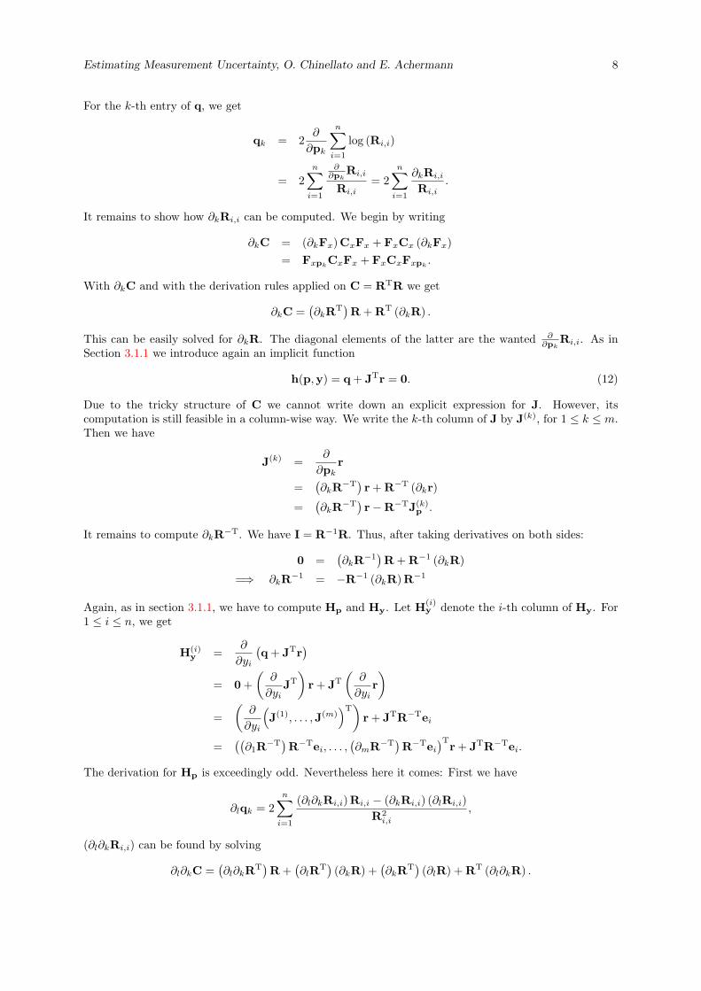
3.2.1 Computing of Cp

In the first step we derive an expression for

q =∂

∂p2 log(det (R))

=∂

∂p2 log

(n∏

i=1

Ri,i

)

= 2∂

∂p

n∑i=1

log (Ri,i).

Estimating Measurement Uncertainty, O. Chinellato and E. Achermann 8

For the k-th entry of q, we get

qk = 2∂

∂pk

n∑i=1

log (Ri,i)

= 2n∑

i=1

∂∂pk

Ri,i

Ri,i= 2

n∑i=1

∂kRi,i

Ri,i.

It remains to show how ∂kRi,i can be computed. We begin by writing

∂kC = (∂kFx)CxFx + FxCx (∂kFx)= Fxpk

CxFx + FxCxFxpk.

With ∂kC and with the derivation rules applied on C = RTR we get

∂kC =(∂kRT

)R + RT (∂kR) .

This can be easily solved for ∂kR. The diagonal elements of the latter are the wanted ∂∂pk

Ri,i. As inSection 3.1.1 we introduce again an implicit function

h(p,y) = q + JTr = 0. (12)

Due to the tricky structure of C we cannot write down an explicit expression for J. However, itscomputation is still feasible in a column-wise way. We write the k-th column of J by J(k), for 1 ≤ k ≤ m.Then we have

J(k) =∂

∂pkr

=(∂kR−T

)r + R−T (∂kr)

=(∂kR−T

)r−R−TJ(k)

p .

It remains to compute ∂kR−T. We have I = R−1R. Thus, after taking derivatives on both sides:

0 =(∂kR−1

)R + R−1 (∂kR)

=⇒ ∂kR−1 = −R−1 (∂kR)R−1

Again, as in section 3.1.1, we have to compute Hp and Hy. Let H(i)y denote the i-th column of Hy. For

1 ≤ i ≤ n, we get

H(i)y =

∂

∂yi

(q + JTr

)= 0 +

(∂

∂yiJT

)r + JT

(∂

∂yir)

=(

∂

∂yi

(J(1), . . . ,J(m)

)T)

r + JTR−Tei

=((

∂1R−T)R−Tei, . . . ,

(∂mR−T

)R−Tei

)Tr + JTR−Tei.

The derivation for Hp is exceedingly odd. Nevertheless here it comes: First we have

∂lqk = 2n∑

i=1

(∂l∂kRi,i)Ri,i − (∂kRi,i) (∂lRi,i)R2

i,i

,

(∂l∂kRi,i) can be found by solving

∂l∂kC =(∂l∂kRT

)R +

(∂lRT

)(∂kR) +

(∂kRT

)(∂lR) + RT (∂l∂kR) .

Estimating Measurement Uncertainty, O. Chinellato and E. Achermann 9

Further we need

∂lJTr = (∂lJ)Tr + JT (∂lr)

=(∂lJ(1), . . . , ∂lJ(m)

)T

r + JT (∂lr)

∂lr =(∂lR−T

)z−R−TJ(l)

p

∂lJ(k) =(∂l∂kR−T

)r +

(∂kR−T

)(∂lr)−

(∂lR−T

)J(k)p −R−T

(∂lJ(k)

p

).

Putting things together yieldsH(l)

p = ∂lq + ∂lJTr,

where ∂lq is of course the vector with elements ∂lqk, for k = 1, . . . ,m.

4 Measurement

The first goal of calibration is to compute a good set of parameters to quantify the measurement tool.An equally important goal is to estimate the measurement uncertainty when using the calibrated device.

Assume that the measuring tool is calibrated. Thus we have a set of estimated parameters p togetherwith an estimated covariance matrix Cp = Cov (p, p).

Let y ∈ Rs be a measurement vector whose elements are readings taken from the measurement tool. Thereadings are subject to errors, of the form y− y = N (0,E), where y is the correct but unknown readingvector.

For 1 ≤ i ≤ s compute xi by applying xi = g(yi, p) or by solving yi = f(xi, p). For arbitrary (but stillwell behaved) functions f(x, p) we propose the use of a standard solver such as bisection, regula falsi,Newton method etc.

The computation of the measurement uncertainty is performed as follows. We represent the exact physicswith yi = f(xi,pex), where these are the exact and never known values. The given values are xi +∆xi =xi, yi + ∆yi = yi and pex + ∆p = p. Substituting and linearizing these equations leads to

∆yi ≈ f(i)x ∆xi +∇pf

(i)T∆p,

where f(i) = f(xi, p) and f

(i)x = fx(xi, p). Extending this approximation to s readings y and solving

for ∆x, we get∆x ≈ F−1

x ∆y − F−1x Jp∆p

and furthermore

Cx = E[∆x∆xT

]≈ F−1

x Cov (y,y)F−1x

+ F−1x Jp Cov (p, p)Jp

TF−1x

− 2F−1x Cov (y, p)Jp

TF−1x .

There are two thing to note. First, Cov (y, p) can safely be assumed to be 0, since the uncertainties ofthe reading for the s measurements are independent of p found during calibration. Second, it is obviousthat no f

(i)x is not allowed to be 0. In practice this does not present a problem, since nobody would use

a measurement device in a range where the slope of the measurement function is too large.

So we end up with the calculation for

Cx ≈ F−1x

(Cov (y,y) + Jp Cov (p, p)Jp

T)F−1

x .

Estimating Measurement Uncertainty, O. Chinellato and E. Achermann 10

5 Numerical Comparisons and Simulations

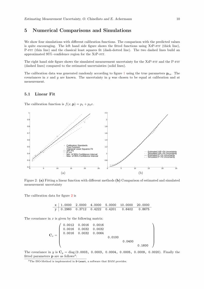
We show four simulations with different calibration functions. The comparison with the predicted valuesis quite encouraging. The left hand side figure shows the fitted functions using XiP-fit (thick line),P-fit (thin line) and the classical least squares fit (dash-dotted line). The two dashed lines build anapproximated 95%–confidence region for the XiP-fit.

The right hand side figure shows the simulated measurement uncertainty for the XiP-fit and the P-fit(dashed lines) compared to the estimated uncertainties (solid lines).

The calibration data was generated randomly according to figure 1 using the true parameters pex. Thecovariances in x and y are known. The uncertainty in y was chosen to be equal at calibration and atmeasurement.

5.1 Linear Fit

The calibration function is f(x,p) = p1 + p2x.

0 5 10 15 20 250.2

0.3

0.4

0.5

0.6

0.7

0.8

0.9

1

Calibration Standards True Function Classical Least Squares Fit XiP−Fit P−Fit Min. of 95% Confidence IntervalMax. of 95% Confidence Interval

0 5 10 15 20 25

0.8

1

1.2

1.4

1.6

1.8

2

2.2

Estimated XiP−Fit UncertaintySimulated XiP−Fit UncertaintyEstimated P−Fit Uncertainty Simulated P−Fit Uncertainty

(a) (b)

Figure 2: (a) Fitting a linear function with different methods (b) Comparison of estimated and simulatedmeasurement uncertainty

The calibration data for figure 2 is

x 1.0000 2.0000 4.0000 5.0000 10.0000 20.0000y 0.2960 0.3712 0.4222 0.4201 0.6402 0.8675

The covariance in x is given by the following matrix:

Cx =

0.0012 0.0016 0.00160.0016 0.0032 0.00320.0016 0.0032 0.0064

0.01000.0400

0.1600

The covariance in y is Cy = diag (0.0003, 0.0003, 0.0004, 0.0005, 0.0009, 0.0020). Finally thefitted parameters p are as follows4:

4The ISO-Method is implemented in B-Least, a software that BAM provides.

Estimating Measurement Uncertainty, O. Chinellato and E. Achermann 11

p1 p2

Exact 0.3 0.03Classic LS 0.2956 0.029XiP-fit 0.28567 0.031282P-fit 0.28577 0.031256ISO-Method 0.28577 0.031272

Remarks The match of estimated and simulated measurement uncertainty is quite nice. Note that themeasurement uncertainty5 is chosen to be 2%.

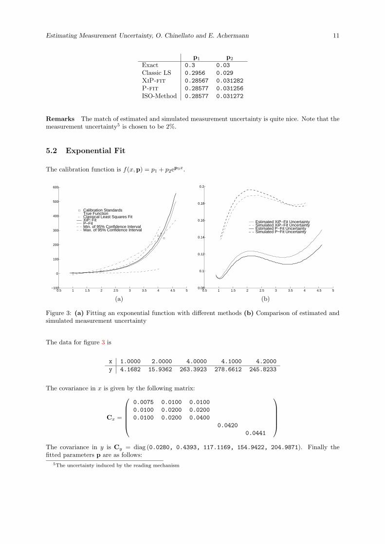
5.2 Exponential Fit

The calibration function is f(x,p) = p1 + p2ep3x.

0.5 1 1.5 2 2.5 3 3.5 4 4.5 5−100

0

100

200

300

400

500

600

Calibration Standards True Function Classical Least Squares Fit XiP−Fit P−Fit Min. of 95% Confidence IntervalMax. of 95% Confidence Interval

0.5 1 1.5 2 2.5 3 3.5 4 4.5 50.08

0.1

0.12

0.14

0.16

0.18

0.2

Estimated XiP−Fit UncertaintySimulated XiP−Fit UncertaintyEstimated P−Fit Uncertainty Simulated P−Fit Uncertainty

(a) (b)

Figure 3: (a) Fitting an exponential function with different methods (b) Comparison of estimated andsimulated measurement uncertainty

The data for figure 3 is

x 1.0000 2.0000 4.0000 4.1000 4.2000y 4.1682 15.9362 263.3923 278.6612 245.8233

The covariance in x is given by the following matrix:

Cx =

0.0075 0.0100 0.01000.0100 0.0200 0.02000.0100 0.0200 0.0400

0.04200.0441

The covariance in y is Cy = diag (0.0280, 0.4393, 117.1169, 154.9422, 204.9871). Finally thefitted parameters p are as follows:

5The uncertainty induced by the reading mechanism

Estimating Measurement Uncertainty, O. Chinellato and E. Achermann 12

p1 p2 p3

Exact 0.1 0.8 1.4Classic LS -62.9821 31.2164 0.5699XiP-fit 0.39654 0.91511 1.3883P-fit 0.47711 0.88251 1.3724ISO-Method -0.060929 1.1143 1.3338

Remarks The uncertainties in the calibration and the measurement data are 5%. This is quite consid-erable. The errors induced by linearization become now obvious. The simulated uncertainties are thusbigger but qualitatively still acceptable. Note also that the classical least squares fit is way out of bounds.The ISO-Method, despite the different numbers, would be just crowding the picture between the XiP-fitand the P-fit. There was a warning of the B-Least software about a division by zero, but the outputseems still reasonable.

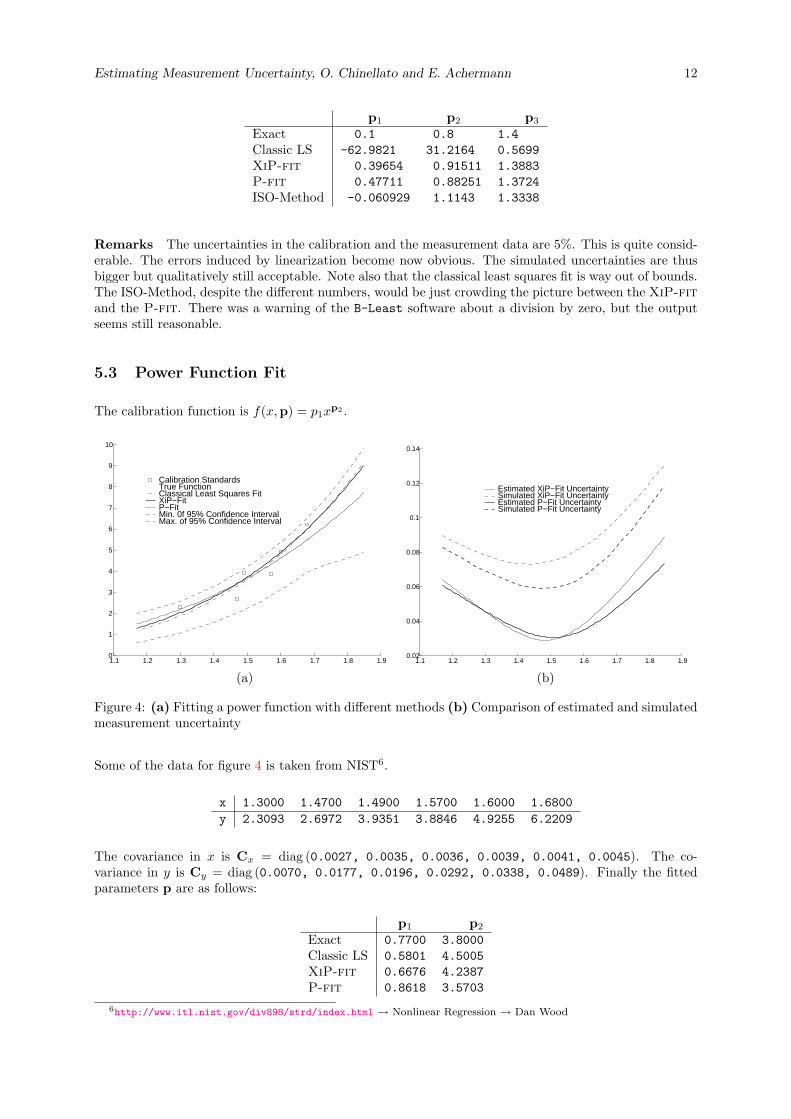
5.3 Power Function Fit

The calibration function is f(x,p) = p1xp2 .

1.1 1.2 1.3 1.4 1.5 1.6 1.7 1.8 1.90

1

2

3

4

5

6

7

8

9

10

Calibration Standards True Function Classical Least Squares Fit XiP−Fit P−Fit Min. 0f 95% Confidence IntervalMax. of 95% Confidence Interval

1.1 1.2 1.3 1.4 1.5 1.6 1.7 1.8 1.90.02

0.04

0.06

0.08

0.1

0.12

0.14

Estimated XiP−Fit UncertaintySimulated XiP−Fit UncertaintyEstimated P−Fit Uncertainty Simulated P−Fit Uncertainty

(a) (b)

Figure 4: (a) Fitting a power function with different methods (b) Comparison of estimated and simulatedmeasurement uncertainty

Some of the data for figure 4 is taken from NIST6.

x 1.3000 1.4700 1.4900 1.5700 1.6000 1.6800y 2.3093 2.6972 3.9351 3.8846 4.9255 6.2209

The covariance in x is Cx = diag (0.0027, 0.0035, 0.0036, 0.0039, 0.0041, 0.0045). The co-variance in y is Cy = diag (0.0070, 0.0177, 0.0196, 0.0292, 0.0338, 0.0489). Finally the fittedparameters p are as follows:

p1 p2

Exact 0.7700 3.8000Classic LS 0.5801 4.5005XiP-fit 0.6676 4.2387P-fit 0.8618 3.5703

6http://www.itl.nist.gov/div898/strd/index.html → Nonlinear Regression → Dan Wood

Estimating Measurement Uncertainty, O. Chinellato and E. Achermann 13

Remarks The uncertainties in the calibration and the measurement data are 4%. Again the lineariza-tion induces a shift between the estimated and the simulated measurement uncertainty. Note that theP-fit is visually better in the sense that it is closer to the exact function. This is the case for most ofthe experiments we have studied.

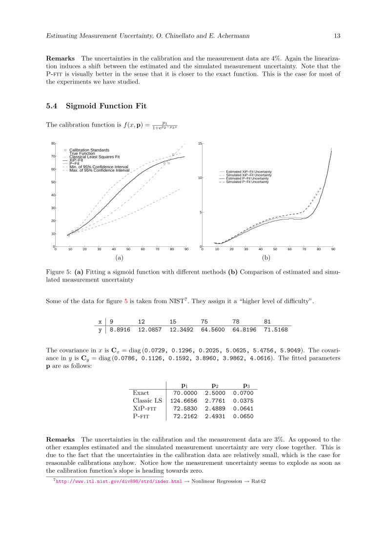
5.4 Sigmoid Function Fit

The calibration function is f(x,p) = p11+ep2−p3x

0 10 20 30 40 50 60 70 80 900

10

20

30

40

50

60

70

80

Calibration Standards True Function Classical Least Squares Fit XiP−Fit P−Fit Min. of 95% Confidence IntervalMax. of 95% Confidence Interval

0 10 20 30 40 50 60 70 80 900

5

10

15

Estimated XiP−Fit UncertaintySimulated XiP−Fit UncertaintyEstimated P−Fit Uncertainty Simulated P−Fit Uncertainty

(a) (b)

Figure 5: (a) Fitting a sigmoid function with different methods (b) Comparison of estimated and simu-lated measurement uncertainty

Some of the data for figure 5 is taken from NIST7. They assign it a “higher level of difficulty”.

x 9 12 15 75 78 81y 8.8916 12.0857 12.3492 64.5600 64.8196 71.5168

The covariance in x is Cx = diag (0.0729, 0.1296, 0.2025, 5.0625, 5.4756, 5.9049). The covari-ance in y is Cy = diag (0.0786, 0.1126, 0.1592, 3.8960, 3.9862, 4.0616). The fitted parametersp are as follows:

p1 p2 p3

Exact 70.0000 2.5000 0.0700Classic LS 124.6656 2.7761 0.0375XiP-fit 72.5830 2.4889 0.0641P-fit 72.2162 2.4931 0.0650

Remarks The uncertainties in the calibration and the measurement data are 3%. As opposed to theother examples estimated and the simulated measurement uncertainty are very close together. This isdue to the fact that the uncertainties in the calibration data are relatively small, which is the case forreasonable calibrations anyhow. Notice how the measurement uncertainty seems to explode as soon asthe calibration function’s slope is heading towards zero.

7http://www.itl.nist.gov/div898/strd/index.html → Nonlinear Regression → Rat42

Estimating Measurement Uncertainty, O. Chinellato and E. Achermann 14

6 Conclusion

Taking the of calibration data into account is important for cases with very strong correlation or withrelatively large uncertainties. However, there is no sound reason to ignore it, since it does not seriouslyaffect the runtime behaviour.

The P-fit leads to slightly higher measurement uncertainties, but it recovers the “exact” parametersgenerally better (in our experiments). This is explainable with it’s property of “integrating over allpossible true x–values”.

Classical least squares fitting is not suitable for calibration tasks.

References

[1] Ake Bjorck. Numerical Methods for Least Squares Problems. SIAM, Philadelphia, 1996. ISBN 0-89871-360-9. 5

[2] Paul T. Boggs, Richard H. Byrd, and Robert B. Schnabel. A stable and efficient algorithm fornonlinear orthogonal distance regression. SIAM Journal Sci. and Stat. Computing, 8(6):1052–1078,November 1987. 4

[3] Paul T. Boggs and Janet E. Rogers. The computation and use of the asymptotic covariance matrixfor measurement error models. Technical Report IR 89-4102, NIST, 1990. U.S. Government PrintingOffice. 1

[4] Wolfram Bremser and Werner Hasselbarth. Controlling uncertainty in calibration. Analytica ChimicaActa, pages 61–69, 1997. 1

[5] R.J. Carroll, D. Ruppert, and L.A. Stefanski. Measurement Error in Nonlinear Models. Number 63in Monographs on Statistics and Applied Probability. Chapman and Hall, London, 1995. ISBN 0-412-04721-7. 2

[6] Wayne A. Fuller. Measurement Error Models. Wiley Series in Probability and Mathematical Statis-tics. John Wiley & Sons, Inc., 1987. ISBN 0-471-86187-1. 2

[7] Philip E. Gill, Walter Murray, and Margaret H. Wright. Practical Optimization. Academic PressInc., London, 1981. 5

[8] Philip E. Gill, Walter Murray, and Margaret H. Wright. Numerical Linear Algebra and Optimization,volume 1. Addison-Wesley, 1991. 5

[9] Sabine Van Huffel, editor. Recent Advances in Total Least Squares Techniques and Errors-In-Variables Modelling, Proceedings of the 2nd International Workshop. Society for Industrial andApplied Mathematics, SIAM, 1997. ISBN 0-89871-393-5. 4

[10] ISO, IEC, BIPM, IFCC, IUPAC, IUPAP, and OIML. Guide to the Expression of Uncertainty inMeasurement. ISO Central Secretariat, 1st edition, 1995. 1

[11] ISO, IEC, BIPM, IFCC, IUPAC, IUPAP, and OIML. ISO 6143, chapter B.2, pages 18–31. ISOCentral Secretariat, 2000. 1, 4

[12] William H. Press, Saul A. Teukolsky, William T. Vetterling, and Brian P. Flannery. NumericalRecipes in C. Cambridge University Press, 2 edition, 1996. 5

[13] John A. Rice. Mathematical Statistics and Data Analysis. Duxbury Press, 2nd edition, 1995. 4

[14] H. R. Schwarz. Numerische Mathematik. B.G. Teubner, Stuttgart, 4th edition, 1997. ISBN 3-519-32960-3. 5