JOURNAL OF APPLIED ECONOMETRICSJ. Appl. Econ. 24: 1117–1135 (2009)Published online 22 June 2009 in Wiley InterScience(www.interscience.wiley.com) DOI: 10.1002/jae.1094

ESTIMATING CLASS-SPECIFIC PARAMETRIC MODELSUNDER CLASS UNCERTAINTY: LOCAL POLYNOMIAL

REGRESSION CLUSTERING IN AN HEDONICANALYSIS OF WINE MARKETS

MARCO COSTANIGRO,a RON C. MITTELHAMMERb AND JILL J. McCLUSKEYc*a Colorado State University, Fort Collins, CO, USA

b School of Economic Sciences and Department of Statistics, Washington State University, Pullman, WA, USAc School of Economic Sciences, Washington State University, Pullman, WA, USA

SUMMARYWe introduce a method for estimating multiple class regression models when class membership is uncertain.The procedure— local polynomial regression clustering —first estimates a nonparametric model via localpolynomial regression, and then identifies the underlying classes by aggregating sample observations intodata clusters with similar estimates of the (local) functional relationships between dependent and independentvariables. Finally, parametric functions specific to each class are estimated. The technique is applied to theestimation of a multiple-class hedonic model for wine, resulting in the identification of four distinct wineclasses based on differences in implicit prices of the attributes. Copyright 2009 John Wiley & Sons, Ltd.

1. INTRODUCTION

As Heckman (2001, p. 674) stated in his Nobel lecture, ‘The most important discovery was theevidence and pervasiveness of heterogeneity and diversity in economic life.’ According to Heck-man, these findings weakened the foundations of the long-standing edifice of the representativeconsumer. In this article, we propose an econometric technique that contributes to the growingliterature seeking to incorporate unexplained heterogeneity in the estimation of micro-econometricmodels of economic phenomena. The procedure, which we call local polynomial regression clus-tering (LPRC), identifies cohorts of sample observations exhibiting similar economic structuralbehavior. In brief, this is accomplished by first estimating the functional relationships betweendependent and independent variables locally, via local polynomial regression. This first nonpara-metric step allows the representation of a wide range of possible functional relationships betweenregressand and regressors. Then data are aggregated into data clusters sharing functionally similarestimates of the local nonparametric estimates. Finally, class-specific parametric functions are esti-mated. While the statistical approach is quite general and need not be confined to the estimationof hedonic models, we apply LPRC to estimate a multi-class hedonic model for wine, resulting inthe identification of four distinct wine classes based on implicit prices of product attributes.

Ł Correspondence to: Jill J. McCluskey, School of Economic Sciences, Washington State University, Pullman, WA99164-6210, USA. E-mail: mccluskey@wsu.edu

Copyright 2009 John Wiley & Sons, Ltd.

1118 M. COSTANIGRO, R. C. MITTELHAMMER AND J. J. McCLUSKEY

To introduce the estimation problem context, let the true data-generating process correspondingto n observations on the set of m class-specific relationships be represented by

yi Dm∑

jD1

gj�xi; bj�IDj �xi, zi� C εi, i D 1, . . . , n �1�

where I�Dj��xi, zi� is an indicator function that equals 1 when �xi, zi� 2 Dj and 0 otherwise, andnj D ∑n

iD1 IDj �xi, zi� denotes the number of sample observations associated with the jth classrelationship. The value of the dependent variable yi is thus represented by the value of a residualplus the value of one of m possible functions of the explanatory variables, xi. The specific functionis identified by the associated subset of the observation partition to which the value of �xi, zi�resides, zi denoting any variables, besides xi, relevant to the identification of the different classesof observations. For simplicity, we assume that the number of classes, m, is known a priori,1 butthat the class membership of each observation in the dataset (y,x,z) and the correct functional formfor each class-specific model gj�xi; bj� are not known.

Owing to class membership uncertainty, estimating equation (1) is problematic, and severalalternative approaches have been proposed in the literature. While methods differ widely intechnical aspects, they can be categorized into two alternative but related general ideas. Oneapproach consists of first partitioning the data into classes according to some data similaritycriterion and then estimating class-specific regression models within each data partition. Thesecond method is based on specifying more complex models that simultaneously estimate classmembership of the observations and associated class-specific vectors of parameters.

Examples of the data-partitioning approach can be drawn from the real estate hedonic literature.Straszeim (1974), in order to identify sub-markets in the San Francisco Bay Area real estatemarket, divided the dataset a priori into geographical areas and estimates group-specific hedonicmodels. In this context, equation (1) represents a hedonic model whose parameters change acrosssub-markets. Straszeim’s results show that the within-sample predictive ability of the segmentedmodel is superior to a model ignoring geographical segmentation.

The study generated a subsequent stream of research using multivariate analysis to identifydata partitions that are homogeneous under some distance criterion measuring data similarity.Data-clustering algorithms (Ward and K-means are frequent choices) are often applied either tothe original data or to factor and principal component scores relating to the data. Dale-Johnson(1982) and Watkins (1999) provide examples of the application of factor analysis, and Bourassaet al. (1999, 2003) apply clustering algorithms to principal component factor scores. Wilhelmsson(2004) adopts a slightly different method, clustering on the residuals from a regression performedusing the entire dataset, ignoring submarkets.

An alternative to these two-step procedures consists in specifying a likelihood function thatembeds an explicit model for determining class membership, thereby accounting for the existenceof product classes. In this context, uncertainty regarding product class is represented by adensity function (most commonly logistic) describing how observations are randomly assigned todifferent classes. Maximization of the likelihood function involves simultaneous estimation of class

1 This simplifying assumption is not strictly necessary for the implementation of LPRC and it is possible to search forthe appropriate number of classes. Alternatively, one can also apply the methodology under the objective of finding thebest possible partition of the data given a pre-specified number of classes. The concept of ‘best’ will be defined later inthe paper.

Copyright 2009 John Wiley & Sons, Ltd. J. Appl. Econ. 24: 1117–1135 (2009)DOI: 10.1002/jae

ESTIMATING CLASS-SPECIFIC PARAMETRIC MODELS 1119

membership of the sample observations and the parameter estimates of the associated class-specificregression functions, which must usually be done numerically using iterative computer-intensivefunction maximization algorithms. The resulting models are often complicated to interpret, andthe estimated coefficients are often not straightforwardly usable, per se, for deriving modelimplications such as marginal effects. General examples are random parameter models (see Allenbyand Rossi, 1999), latent class models (see Greene, 2001, for a survey of literature) and mixtureapproaches that are used to model unexplained heterogeneity (for example, Arcidiacono and Jones,2003).

Both of the preceding approaches have strengths and weaknesses. Data-clustering proceduresare relatively simple to implement and yield models that are both generally tractable to estimateand readily interpretable. The main concern with data-clustering procedures is their effectivenessin identifying data partitions whose observations correspond to the appropriate class. Bourassaet al(2003), his application being a real estate hedonic model, finds that the performance inout-of-sample prediction of models identifying market segments by multivariate data-clusteringtechniques is poor when compared to models that partition data a priori based only on location.The reasons underlying such poor performance are perhaps multiple, but at least one appearsprominent: a direct, constant proportionality between changes in the values of covariates andchanges in parameters is needed for the data-clustering approaches to yield data partitions withstable parameters or negligible aggregation bias. We suggest that, in most cases, such an assumptionhas no real theoretical basis.

The likelihood-based approaches have the attractive feature of embedding the existence of sep-arate product classes within a general nested model framework. On the other hand, the processdetermining class membership must be an explicit part of the overall model specification, accen-tuating the risk of model misspecification. In certain econometric applications, the representationof class uncertainty via a random process parameterized via a probability density function thatassigns sample observations to classes, which is a fundamental tenet underlying the specificationof such models, can itself be questionable.2 On the empirical side, even though statistical softwareis available to estimate random parameters and latent class models, the implementation is stilloften subject to technical difficulties: the presence of multiple classes and the need to calculateparameter vectors for each of the classes can lead to convergence issues, exacerbate the risk oflocal minima, and prompts researchers to find good starting values for numerical algorithms inways that are often, of necessity, rather ad hoc.

A remaining issue common to both of the preceding general approaches, in addition tohow class membership is modeled and estimated, is specification of a particular functionalform for the class-specific relationships between dependent and explanatory variables. Motivatedby the challenges and problems of existing approaches, we propose and implement localpolynomial regression clustering (LPRC). The approach is designed to identify and estimateclass-specific functions that are stable in their parametric representations when class membershipis uncertain and complement the existing methodologies by mitigating some of their principalchallenges.

2 In this article we estimate a hedonic model for wine with product-class dependent parameter heterogeneity. While classmembership of each wine in a product class (i.e., commercial, semi-premium, premium, and ultra-premium) is uncertain,the use of a random process to allocate observations to wine classes is not a fundamental characteristic of the hedonicdata-generating process of valuators unless membership, itself, is considered uncertain by the valuators.

Copyright 2009 John Wiley & Sons, Ltd. J. Appl. Econ. 24: 1117–1135 (2009)DOI: 10.1002/jae

1120 M. COSTANIGRO, R. C. MITTELHAMMER AND J. J. McCLUSKEY

2. GENERAL LPRC METHODOLOGY

In order to motivate the general methodology, consider the model described in (1). Let

brj �x0� �

[∂gj �x0; bj�

∂x0[�1]8�1;

∂2gj�x0; bj�

∂x0[�1]∂x0[�2]8�1, �2; . . .

∂rgj�x0; bj�

∂x0[�1]∂x0[�2] Ð Ð Ð ∂x0[�r]8�1, �2, . . . , �r

]0

�2�

be the∑r

iD1 ki ð 1 vector of derivatives of the function gj�x0; bj�, up to order r, at an evaluationpoint x0, where x0[�] denotes the �th element of the vector x0.

The overall objective of LPRC is to identify a partition⋃m

jD1ODj D OD of the observed sample

data such that the estimated model

yi Dm∑

jD1

Ogj�xi; Obj�I� ODj��xi, zi� C vi, i D 1, . . . , n �3�

approximates well the relationship between yi and each of the associated elements of xi in terms ofderivative relationships up to the rth order. This goal is pursued by using local polynomial regres-sion of order r to generate local nonparametric observation-specific estimates of the derivatives

Obr �x0� �[

∂ Og�x0�

∂x0[�1]8�1;

∂2 Og�x0�

∂x0[�1]∂x0[�2]8�1, �2; . . .

∂r Og�x0�

∂x0[�1]∂x0[�2] Ð Ð Ð ∂x0[�r]8�1, �2, . . . , �r

]0

�4�8�x0, z0� in the dataset, where y D Og�x� C Oe, denotes the underlying nonparametric regression thatis estimated locally at each data point, and then clustering into m classes on the basis of similarityin the values of Obr �x0�. The clustering step is intended to identify data partitions for which thefunctional relationship between y and x is relatively stable up to a specified order of derivativerelationship, enabling equation (1) to be approximated and estimated via simpler class-specificparametric models to that order. To further clarify the methodology and its rationale, we nowpresent the sequence of calculations implied by LPRC in more detail.

2.1. Step One: Local Polynomial Regression

The first step of LPRC is the estimation of a nonparametric regression relationship y D Og�x� C Oefor each of the n evaluation points �x0, z0� by local polynomial regression (a nonparametrictechnique motivated by the Weierstrass polynomial approximation theorem See Fan and Gijbels,1996). To simplify the presentation, assume that a first-order approximation to g(x) is chosen,3 sothat a local linear regressor (LLR) is defined with r D 1 in (4). The LLR estimator then solvesthe minimization problem

arg min

Oa�x0�, Ob�x0�

{n∑

iD1

[yi � Oa�x0� � �xi. � x 00� Ob�x0�]2K��xi. � x0

0�/h�

}�5�

3 If the bandwidth h is optimally chosen using a data-driven technique, the degree of expansion of the polynomial doesnot represent a crucial decision: in the presence of significant curvature, a low-degree polynomial will induce the choiceof a narrower bandwidth. On the other hand, using a low-degree polynomial reduces computational cost and simplifiescalculating the marginal effects.

Copyright 2009 John Wiley & Sons, Ltd. J. Appl. Econ. 24: 1117–1135 (2009)DOI: 10.1002/jae

ESTIMATING CLASS-SPECIFIC PARAMETRIC MODELS 1121

where K�� represents a kernel weighting function, h is the bandwidth in the kernel weightingfunction, x refers to the data used in defining the kernel domain in the local weighted regressions,x0 is the vector representing the point of evaluation, and xi. represents the ith row in x. In theclassical application of nonparametric regression, it is customary to set x D x , so that the setof regressor variables is used to identify the neighborhood in which the nonparametric functionis estimated as well as the weights that are applied to observations within the neighborhood.In the context of LPRC, such a specification for the Kernel domain is appropriate when theresearcher knows little about the causes of parameter heterogeneity across classes. In some cases,it may be possible to identify an augmented set of variables (x,z) with the variables z providingadditional information on the identification of data neighborhoods having similarly valued entriesin Ob. The specification in (5) provides flexibility for utilizing such additional information. Tomitigate scale effects in the estimated local derivatives, standardization of the regressors isapplied.

In the minimization of the weighted sum of squares function in (5), we choose theLOESS algorithm (Cleveland et al., 1988), based on the tricube weight function, so that theexplicit definition of the Kernel is K��xi. � x0

0�/h� D W�[�xi. � x00��xi. � x0

0�0]1/2/h�, where W�u� D�1 � juj3�3 for juj 2 [0, 1], and W�u� D 0 otherwise. The LOESS approach is based on the useof a nearest-neighbor type of bandwidth in which h not only affects the relative weights appliedto sample observations used in the local regression estimates, but also determines the propor-tion of the sample that is included in the estimation procedure (i.e., observations that receivea nonzero weight). Regarding bandwidth choice, we suggest an approach in the spirit of leastsquares cross-validation (Stone, 1974) and perform a search on h, selecting the bandwidth thatyields the best-fitting final estimated system of class-specific models using various fit criteria,which is discussed in greater detail below.

2.2. Step Two: Ward Clustering

The matrix of estimated partial derivatives, OB D [ Ob�x0�0, x0 2 D], is the object of the second-stageanalysis in the LPRC procedure. In this clustering step, we use the Ward algorithm to groupestimates on the basis of similarity of the Ob�x0� values, thereby identifying domains of data withsimilar estimated (first order in the current application) derivatives. The Ward algorithm seeks tominimize, through the choice of the data clusters ODj, j D 1, . . . , m and the associated data partition⋃m

jD1ODj D OD, the sum of squared deviations (SSD) from the cluster centroids Obj, j D 1, . . . , m,

the objective function then being

minODj,jD1,..,m

m∑jD1

∑x02 ODj

� Ob�x0� � Obj�0� Ob�x0� � Obj� �6�

The algorithm begins by treating each observation in OB as a cluster. At each iteration of thealgorithm, the number of clusters is reduced as unions of the existing clusters are considered. Theunion that minimizes the SSD upon iterative agglomeration of the data into the target number ofm clusters is the stopping point of the algorithm.

Copyright 2009 John Wiley & Sons, Ltd. J. Appl. Econ. 24: 1117–1135 (2009)DOI: 10.1002/jae

1122 M. COSTANIGRO, R. C. MITTELHAMMER AND J. J. McCLUSKEY

2.3. Step Three: Class-Specific Regression

Once the data partition solving (6) is identified, a classification of the dataset into m classesexists, and the final step of LPRC is implemented, consisting of the estimation of m class-specificregression models. The unknown functional forms of gj�xi; bj�, j D 1, . . . , m are approximatedempirically at this stage using linear or higher-order polynomial specifications consistent with theorder of derivatives in (4). The resulting regression functions represent the empirical counterpartto the model in equation (1) and by virtue of having been fit to subsets of data for which rth-order derivatives of the regression model are similar via the clustering step, specification error isexpected to be mitigated to that order of derivative.

2.4. LPRC General Characteristics

We emphasize that LPRC shares a number of general characteristics with the more traditionalmodeling approaches discussed earlier. As in the multivariate data clustering approaches, LPRCimplements a distance metric (i.e., via the clustering algorithm) to determine an appropriatepartition of the data into m classes. However, rather than clustering on similarities in valuesof covariates, LPRC clusters on similarities in estimated local derivatives of the underlying class-specific functions.

The connection with the likelihood-based approaches is perhaps not as obvious, but we pointout that Ward clustering received attention in the model-based Gaussian hierarchical clusteringliterature. As Fraley (1998) shows, if the process generating the multiple class dataset can bemodeled using a multivariate normal distribution with class-specific means and common variances,then using the Ward algorithm to identify classes is equivalent to maximizing the classificationlikelihood function.4 Therefore, under certain distributional assumptions on the observation-specificlocal polynomial regression coefficients, LPRC can be considered as a likelihood-based method.

Because LPRC allows estimating class-specific models without requiring the researcher tocommit a priori to a detailed parametric specification of the process determining classes andparameter heterogeneity, we suggest that it is most appropriate when a clear choice of specificationis not obvious. On the other hand, the advantage of avoiding possible misspecification is obtainedat the cost of some loss in efficiency (relative to a correctly specified likelihood-based model),as the determination of class membership is based on local nonparametric estimates. Regardingcomputational advantages, a unique solution always exists when implementing LPRC, and thereis no need to devise parameter starting values in order to implement optimization algorithms.

An approach that is similar in spirit but notably different in implementation and estimationobjective is that of so-called ‘Partition Regression’ introduced by Guthrey (1974). The methodseeks to minimize the sum of squared errors over the choice of a fixed number of partitions, andimplementation is effectively relegated to data that is intrinsically ordered in some fashion, as in atime series. Another recent approach by Christopeit and Hoderlein (2006), called ‘Local PartitionedRegression’, is a method that significantly extends the reach of nonparametric regression models

4 More formally, modifying Fraley’s (1998) model, we denote by J the total number of classes and the density ofa p-dimensional observation xi from the jth class by fj�xijqj�, for some vector of parameters qj. Given observationsx D �x1, . . . , xn�, let g D ��1, . . . , �n� denote identifying labels for the classification, where �i D j if xi comes form the jthsubpopulation. It can then be shown that the Ward algorithm maximizes the classification likelihood:L��1, . . . , �J; gjx� D∏n

iD1 f�i �xijq�i �, under the assumption that fj�xijqj� is the multivariate normal distribution with mean m D ��1, . . . , �J�and variance 6j D 2I .

Copyright 2009 John Wiley & Sons, Ltd. J. Appl. Econ. 24: 1117–1135 (2009)DOI: 10.1002/jae

ESTIMATING CLASS-SPECIFIC PARAMETRIC MODELS 1123

beyond additive models and can incorporate local polynomial approximations in the process.However, it remains a local observation-specific method that does not lead to the identification ofmodels differentiated by and associated with different classes.

3. ESTIMATING A MULTI-CLASS HEDONIC REGRESSION FOR WINE

In this section, we present an application of LPRC to the estimation of a class-specific hedonicmodel for wine. We first introduce the relevance of estimating a multi-class hedonic model for wineand the rationale for applying LPRC. The data are then presented, and LPRC is implemented. Wethen compare the forecasting performance of LPRC to some alternative estimation techniques.Lastly, we discuss the major estimated differences across wine classes and their economicimplications and draw conclusions.

3.1. Latent Classes and Market Segmentation in Hedonic Models

Economists have long been interested in markets for differentiated products. Examples includewine, automobiles, and real estate. When differentiated products are located farther apart in productspace, they no longer compete against each other (Hotelling, 1929). Based on these examples, onecan hypothesize that product space is likely multidimensional and the boundaries of product classesare uncertain. The hedonic approach (Rosen, 1974) was developed to estimate implicit prices ofproduct attributes within a given product class.5 It is assumed that the goods in question aresomewhat differentiated but similar enough that consumers consider them as variations of thesame product. However, as two products diverge, the market valuation of the attributes includedin them will diverge as well.

A use-based classification of products is helpful in better formalizing how composite productclasses originate in the hedonic context. Intuitively, as the vectors of attribute levels characterizingtwo goods increasingly diverge, it is more likely that consumers purchase the goods for differentpurposes. That is, the more two products are differentiated, the less they are fungible in the sameor similar use. Further, the costs associated with assembling a given bundle of attributes in thesame product will change as the vector of attributes changes. This transition process can be eithergradual, perhaps generating hybrid products that can be employed for multiple purposes, or thepresence of an attribute might unambiguously determine the membership of a good to a givenproduct class.6

Acknowledging this process in modeling is challenging when a clear-cut classification ruledoes not exist, but the cost of ignoring the problem is potentially faulty estimates of implicitattribute prices derived from the hedonic price function. Conversely, deriving accurate informationon the marginal contribution of each attribute can help firms in their pricing and productiondecisions. Hedonic techniques have also been proposed for calculating consumer price indexes asan alternative to the conventional matched models.7 These considerations make hedonic modeling

5 In the remainder of the article we use the terms ‘product class’, ‘class’, ‘market’, and ‘market segment’ equivalently tosignify collections of goods sharing similar implicit prices of the attributes.6 Note that this argues against the application cluster-on-covariates techniques to identify market segments.7 See Triplett (2006) for an extensive review of the methods and Pakes (2003) on the necessity to estimate multiplehedonic functions.

Copyright 2009 John Wiley & Sons, Ltd. J. Appl. Econ. 24: 1117–1135 (2009)DOI: 10.1002/jae

1124 M. COSTANIGRO, R. C. MITTELHAMMER AND J. J. McCLUSKEY

an appropriate problem context for applying LPRC, our application being a multi-class hedonicmodel for wine.

The characteristics that differentiate one wine from another and how the market values suchdifferences are intriguing research questions and have been the object of a significant body ofresearch. Several authors utilized the hedonic approach to investigate the determinants of wineprices, with substantial agreement on the important characteristics. Relevant examples includeCombris et al. (1997, 2000), Landon and Smith (1997), Oczkowski (1994), and Schamel andAnderson (2003). While we draw from the existing wine hedonic literature in specifying thedeterminants of wine prices, we note several studies estimated a single hedonic price function,implicitly assuming that there is limited variation over product characteristics, or, if the variationis substantial, consumers’ reactions to it are either limited and/or they are somewhat unable toappreciate it.

A strong argument can be made against the assumption of limited variation (real or perceived)in wine. The general product category of wine is a composite product class, which includes anumber of product classes. ‘Two-Buck Chuck’ and a bottle of Penfolds Grange have little incommon and will be consumed on radically different occasions. Between these two extremes, acontinuum of product differentiation exists. Wines sharing similar characteristics compete witheach other as substitute goods. However, beyond a certain level of differentiation, two wines areno longer substitutes and might be considered as different products. Hall et al. (2001) support thisidea with their empirical finding that consumers value the same attributes differently, dependingon the occasion in which the wine is meant to be consumed.

The identification of wine classes and the estimation of wine class-specific hedonic functions aimat providing the wine industry with more informative and accurate estimates of the implicit pricesof wine attributes, which can be used to develop successful production and marketing strategies. Asa matter of fact, the importance of correctly identifying product classes when developing marketingstrategies has already been recognized by the wine industry: a study commissioned by Australianwine producers and conducted by Ernst & Young Consulting (1999) concluded that multiple winemarkets exist. The analysts, on the basis of discussions with industry stakeholders and qualitativeanalysis, classified wines into four market segments by retail price ranges: commercial wines,semi-premium, premium, and ultra-premium. In this article, we proceed under the assumption thatfour wine classes (i.e., m D 4) exist, and use LPRC to empirically determine the class membershipof each data point, thereby providing an alternative analysis of the price ranges associated withthe different wine classes as well as providing information on the different valuations of productattributes that exist across wine classes.

3.2. LPRC and Hedonic Regression

In the current hedonic modeling context, equation (1) with m D 4 represents the underlyinghedonic price functions corresponding to the four wine product classes. The vector xi thenrepresents attributes associated with the wine and bj is a vector of coefficients related to theestimation of implicit prices. As usual in the hedonic model, the first-order derivative of the priceof the commodity with respect to the kth attribute represents the implicit price of that attribute. If yi

in (1) were specified to be the price itself, then the first-order derivatives represented in (2) wouldrefer to the implicit prices of the attributes. In the application ahead, we apply a normalizing andvariance-stabilizing transformation to prices that has been used previously in the literature on wine

Copyright 2009 John Wiley & Sons, Ltd. J. Appl. Econ. 24: 1117–1135 (2009)DOI: 10.1002/jae

ESTIMATING CLASS-SPECIFIC PARAMETRIC MODELS 1125

hedonic analysis, so that implicit prices will be a function of the derivatives in (2), the details ofwhich are presented ahead.

The objective of the subsequent clustering step is the achievement of similarity in implicit pricefunctions up to a given order of derivative relationship. The nonparametric regression step of LPRCproduces local, observation-specific estimates of the hedonic price functions. In this application,we set r D 1, and thus we utilize local linear nonparametric regression in representing the hedonicprice functions. In the hedonic framework, differences in the estimated local hedonic surfacesreflect changes in the underlying supply and demand functions and represent an objective criterionfor determining product classes in the clustering step. Since the focus of this clustering exercise arethe implicit prices, which embed supply and demand, cost and willingness to pay factors (Nerlove,1995); LPRC effectively ‘lets the market be the guide’ in determining class membership.

3.3. Data

The dataset is composed of 9600 observations derived from 10 years (1991–2000) of tasting ratingsreported in the Wine Spectator Magazine (online version) for California (8667 observations) andWashington (933 observations) red wines. Table I presents the variable names and short datadescriptions. Four of the variables in the dataset are non-binary: the real price of wine, tastingscore provided by the Wine Spectator, the number of cases produced, and the years of aging beforecommercialization. Descriptive statistics for these variables are reported in the second columnof Table II. Note that wine prices have a positively skewed distribution, but most observationsfall in the $10–50 range. Indicator variables were used to denote region of production, winevariety, and the presence of other label information. The regions of production for Californiawines include Napa Valley, Bay Area, Sonoma, South Coast, Carneros, Sierra Foothills, andMendocino. Washington wines were not separated by regions.8 Varieties include Zinfandel, PinotNoir, Cabernet, Merlot and Syrah grapes, as well as wines made from blending different varieties(non-varietals). Additional variables refer to information appearing on the label of certain bottles:some wines are produced from the vineyards adjacent to the wineries (‘estate’ wines), while someothers are classified as ‘reserve’ by the wine maker.

3.4. Empirical Model Specification and Estimation

A local linear regressor (LLR) was chosen to implement the first step of LPRC and theminimization of equation (5) was carried out by setting y D Price�0.5, x D [ScoreŁ, AgeŁ,CasesŁ, Variety1,...,6, Region1,..7, Label1,..,3, Vintage1991,...,2000], and x D [ScoreŁ,AgeŁ,CasesŁ];where asterisks indicate that a standardization has been applied. The reciprocal square root power ofprices is a normalizing and variance-stabilizing transformation used in the hedonic wine literature.9

In accordance with our previous use-based, attribute-dependent justification for the genesis ofmultiple wine classes, we choose the continuous wine attributes (i.e., Score, Age, Cases) for the

8 These geographical partitions are the ones adopted by the Wine Spectator to categorize the wines, often pooling severalAmerican Viticultural Areas (AVAs) in the same region.9 Cleveland et al. (1988) derived their results on the sample variability of the loess estimator based on an assumptionof normality. Estimating a hedonic model for wine, Landon and Smith (1997) find that the reciprocal square roottransformation outperforms the classical semi-log specification. Also note the inclusion of original quantity produced(cases) in the right-hand side of the hedonic function. While (8) is not an inverse demand function, we estimateˇ3 toestimate the effect that ‘rarity’ has on certain cult wines.

Copyright 2009 John Wiley & Sons, Ltd. J. Appl. Econ. 24: 1117–1135 (2009)DOI: 10.1002/jae

1126 M. COSTANIGRO, R. C. MITTELHAMMER AND J. J. McCLUSKEY

Table I. Short descriptions and abbreviations of variables

Variable Description Binary/Non-binary

Price Retail prices suggested by the winery Non-binaryScore Rating score from Wine Spectator Non-binaryAge Years of aging before commercialization Non-binaryCases Thousands of cases produced Non-binaryGeneric Californiaa Regions of production BinaryNapa ValleyBay AreaSonomaSouth CoastCarnerosSierra FoothillsMendocinoWashingtonZinfandela Grape variety BinaryNon-varietalPinot NoirCabernetMerlotSyrahReserve Label information: ‘Reserve’ BinaryVineyard Label information: specific name of vineyardEstate Label information: ‘Estate’-produced wine91, . . ., 99, 00a Vintage Binary

a Benchmark variable (omitted) in the set of dummies variables in regression context.

Table II. Descriptive statistics of the non-binary variables (whole sample and by wine class)

Variable Descriptive statistic Whole sample Wine class

Commercial Semi-premium Premium Ultra-premium

N 9600 4748 3345 1022 485% 100.00% 49.46% 34.84% 10.65% 5.05%

Pricea Mean $30.10 $17.23 $32.18 $53.25 $92.9525th percentile $17.60 $13.80 $27.50 $47.46 $76.50Median $24.80 $17.55 $31.03 $52.00 $88.3375th percentile $35.70 $20.80 $36.30 $57.50 $104.00

Cases Mean 4.87 8.10 1.70 1.62 1.9025th percentile 0.500 0.850 0.400 0.295 0.310Median 1.200 2.100 0.862 0.661 0.70075th percentile 3.600 7.000 1.690 1.436 1.950

Score Mean 86.14 84.39 87.29 88.60 90.2425th percentile 84 82 86 87 88Median 87 85 87 88 9175th percentile 88 87 89 91 93

Age Mean 2.77 2.64 2.82 3.01 3.1725th percentile 2 2 2 3 3Median 3 3 3 3 375th percentile 3 3 3 3 3

a CPI adjusted to base year 2000

Copyright 2009 John Wiley & Sons, Ltd. J. Appl. Econ. 24: 1117–1135 (2009)DOI: 10.1002/jae

ESTIMATING CLASS-SPECIFIC PARAMETRIC MODELS 1127

domain of the Kernel weighting function. The optimal bandwidth was empirically determined bythe performance of the final model relative to a number of goodness-of-fit criteria.10

Following the nonparametric estimation step denoted in (5), an n ð k matrix of estimated implicitprices of attributes, OP , was calculated which, owing to the transformation of the dependent variable,

are in the form OPi D ∂ Og�xi�∂xi

D �2(Pricei)1.5 Ob�xi�0 for xi 2 ODj in this application. While a completeset of estimated implicit prices is technically available, we focus the clustering search on similarityof the elements of OP that refer to the derivatives of non-binary attribute variables (i.e., Score, Ageand Cases), and thus focus on attributes for which derivatives are naturally defined. The Ward algo-rithm was iterated until four data partitions, corresponding to the four wine classes, were identified.

The estimation of a parametric hedonic function for each of the four wine classes completes theLPRC procedure. Equation (7) depicts the general form of the resulting model, which representsthe empirical counterpart to (1) and is interpretable as a conditional-on-class form of the hedonicrelationships between wine prices and attributes.

Price�0.5j D ˛j0 C ˇj1�Score� C ˇj2�Age� C ˇj3�Cases� C

5∑iD1

ˇj4Ci�Variety�

C9∑

iD1ˇj9Ci�Vintage� C

3∑iD1

ˇj18Ci�Label� C7∑

iD1ˇj21Ci�Region� C ε

j D 1, . . . , 4

�7�

3.5. Forecasting Performance

Before proceeding to an interpretation of the results, we evaluate the use of LPRC in the currentapplication by analyzing its forecasting performance. We compare the out-of-sample predictiveability of LPRC to an unconditional-on-class model, which we refer to as ‘pooled’, and in whichonly one common version of the relationship in (7) was estimated (i.e., j D 1). In addition toLPRC, three cluster-on-covariate approaches drawn from the real estate hedonic literature wereexamined. A comparable latent class, maximum likelihood-based model was unstable and failedto converge to a unique solution, and a fuller comparison between these methods and LPRC is leftfor future simulation experiments.11 For all of the multi-class methods examined, the parameters

10 A grid search for h yielded an optimal bandwidth of hŁ D 0.8, this optimality being robust across multiple fit statistics,including the Akaike and Shwartz information criteria and the adjusted R2. The direct application of an LSCV criterionto the first nonparametric step of LPRC suggested a smaller value of hŁ, and also yielded an inferior fit in the final stepof LPRC. In this application, smaller bandwidths induced highly collinear data neighborhoods, causing instability in theestimated local derivatives and poor fit in the final parametric estimation. This general tendency is common wheneverKernel domains and regressors coincide.11 Among the latent class, maximum likelihood-based methods, a finite mixture linear regression model best adheres tothe current estimation context. To provide for specification symmetry with the LPRC model, a finite mixture of fournormal densities was assumed for the dependent variable, while a logistic random process was used to govern classmembership. In particular, f(price�0.5

i jj) D N[b0jxi, j

2], where xi represents the full vector of regressors for observation

i, and Pr�Class D j� D Fj D exp��1j C �2jScore C �3jAge C �4jCases�4∑

jD1

exp��1j C �2jScore C �3jAge C �4jCases�

, j D 1, . . . , 4. This model, which entails the

ML estimation of �29 ð 4� C �4 ð 3� D 128 free parameters, failed to converge to a unique solution. A more parsimoniousspecification, which allowed the coefficients of the non-binary variables to vary but constrained all indicator variablescoefficients to be the same across classes, did achieve convergence, yielding a within-sample median percent error rateof 18.82%. Additional comparisons of the two estimators are being pursued in the context of simulation experiments.

Copyright 2009 John Wiley & Sons, Ltd. J. Appl. Econ. 24: 1117–1135 (2009)DOI: 10.1002/jae

1128 M. COSTANIGRO, R. C. MITTELHAMMER AND J. J. McCLUSKEY

of the specification in equation (7) were estimated using the data described in Section 3.3 andused to predict out-of-sample based on an additional data set of 3265 observations collected forthis purpose.12

As discussed earlier, multivariate analysis methods identify wine classes based on data similaritycriteria. Following the real estate literature, in a first application we clustered on the standardizednon-binary variables (i.e., Price, Score, Age and Cases); a second application consists in clusteringon predicted values and residuals obtained from the pooled model (in the spirit of Wilhemsson,2004). In a third application, we extracted two principal components (which accounts for more than80% of the variance) from the correlation matrix of the non-binary variables and then identifiedwine classes by clustering on the principal components scores (similar to Bourassa et al, 1999, andWatkins, 1999). For each method, two popular clustering algorithms were utilized: one hierarchical(i.e., Ward) and one non-hierarchical (i.e., K-means). Once a data partition was revealed throughclustering, the model in equation (7) was estimated and used to forecast out-of-sample.

For all tested methods, we evaluate forecasting performance by calculating a median percentageerror rate, MPER D median [abs�y � Oy�/y]. Results are reported in Table III, showing the MPERwithin each wine class and across the whole dataset (‘overall’). We find that LPRC outperformsthe pooled model by more than 60%. Moreover, the cluster-on-covariates methods improved overthe pooled model only marginally, or not at all. It is interesting to note that, while LPRC yieldsa rather stable forecasting performance across all classes, the forecasts of other methods areespecially imprecise in the ultra-premium class.

3.6. Results and Discussion

Based on LPRC, 50% of the observations can be classified as commercial, 34% are semi-premium,10% are premium, and 5% are ultra-premium (Table II). Within-class descriptive statistics of thenon-binary (Table II) and binary variables (Table IV) can be used to identify and characterize wineclasses. Utilizing the estimated categorizations based on local estimates of implicit prices, it is clearthat wine attributes differ across classes. Commercial wines are inexpensive, produced in largequantities, aged an average of 2.5 years, and have the lowest quality scores among all wine classes.

Table III. Forecasting performance: median percent error rate

Method Algorithm CommercialMPER

Semi-premiumMPER

PremiumMPER

Ultra-premiumMPER

OverallMPER

Pooled model — — — — 19.71%Clustering methods Original data K-means ŁŁŁ 18.80% 18.14% 83.00% 18.50%

Ward 18.07% 17.69% 16.31% 21.30% 18.07%Fitted/residuals K-means 18.80% 23.60% ŁŁŁ ŁŁŁ 18.80%

Ward 17.70% 16.10% 16.10% 39.40% 17.70%Principal component K-means 18.30% 17.20% 17.43% 23.10% 18.30%

Ward 22.01% 17.03% 22.50% 37.82% 22.01%

LPRC 13.70% 11.12% 10.54% 12.60% 12.24%

ŁŁŁ too few observations in cluster to estimate model

12 This forecasting sample is also drawn from the years 1991–2000 of Washington and California wine ratings from theWine Spectator.

Copyright 2009 John Wiley & Sons, Ltd. J. Appl. Econ. 24: 1117–1135 (2009)DOI: 10.1002/jae

ESTIMATING CLASS-SPECIFIC PARAMETRIC MODELS 1129

On the other extreme, ultra-premium wines are expensive, high-quality wines, which are producedin smaller quantities, and aged more than 3 years.13 It can be observed that all viticultural regionshave a significant share of the commercial market segment (even though 88% of all ‘genericCalifornia’ wines in the dataset are found in this class), while 86% of the ultra-premium marketis captured by the two viticultural areas of Napa Valley and Sonoma. In terms of grape variety,most of the wines produced with Merlot and Zinfandel grapes belong to the commercial class,while premium and ultra-premium wines are mostly Cabernet, Pinot, or a melange of varieties.

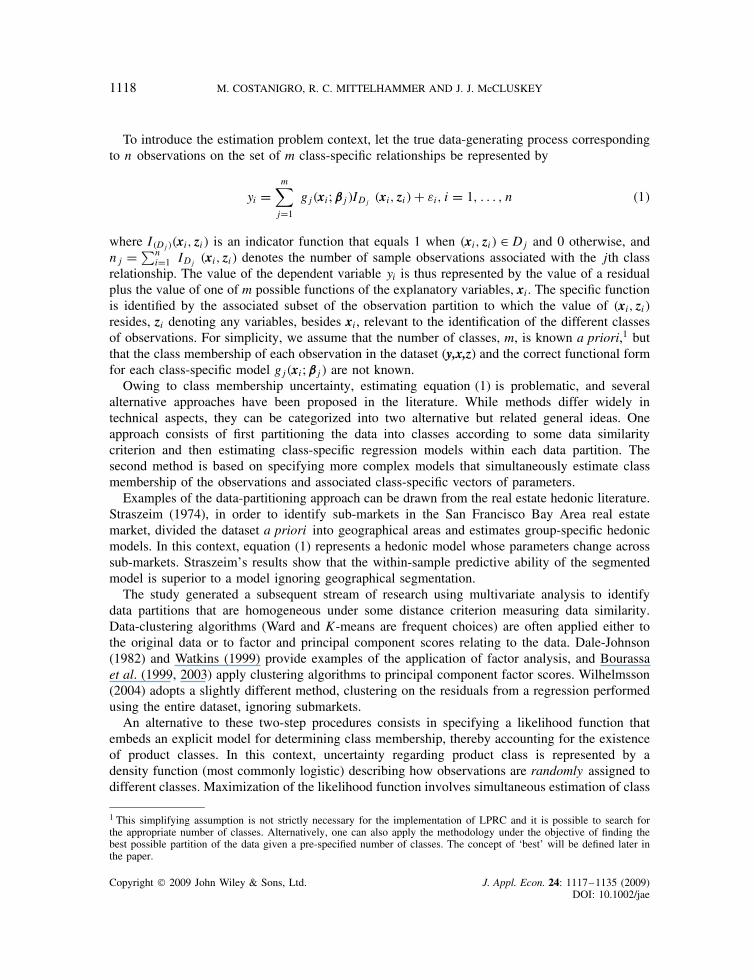
Parameter estimates for the hedonic model are reported in Tables V and VI. To ease comparisonand interpretation, we also include estimates relative to the pooled model and estimated implicitprices of the attributes (the coefficients are not particularly interesting in themselves because ofthe nonlinear transformation of the dependent variable). The first and most important result is thatparameter estimates and implicit prices of the attributes differ significantly across wine classes.14

This result and the superior forecasting performance of LPRC support the estimation of class-specific hedonic models and provide evidence that estimating a single hedonic regression resultsin misleading estimates of the implicit prices.

While all parameter estimates for the commercial wine class are statistically significant,significance becomes progressively sparser for the remaining classes. A partial explanation for thisresult may be purely empirical. The data are increasingly collinear moving from the commercialto the ultra-premium wine class.15 Moreover, the smaller number of observations in the premiumand ultra-premium classes diminishes the power of significance tests.

However, this result may also be signifying a more substantive result with regard to how winesare valued. In particular, once the ultra-premium wine class is reached, it is effectively only scoreand age, whether the wine originates in Washington, and a few vintage years that have a significanteffect on wine price. This suggests that in the upper-class wine segment only a few key attributessignal quality differences in wines in the class, as opposed to lower-class wines whose quality isdifferentiated on the basis of a large number of product attributes. One could make the argumentthat attributes that signal quality in lower- and mid-tier wines are less useful for the upper-tiersegment. There is supporting evidence for this in other food products. Using a hedonic approach,Loureiro and McCluskey (2000) analyzed the effect of the Protected Geographical Indication (PGI)label, ‘Galician Veal’, in Spain. They found that the PGI label was an effective signal of qualityonly in combination with other indicators or signals of quality, but it had diminishing marginalreturns with respect to quality. The PGI label was not significant for the high-quality extreme.At the highest end of the wine market buyers are typically extremely knowledgeable or rely onexpert advice to make their purchases. Some of the quality signals relevant to other wine marketsegments should not be significant for the elite wines.

For the sake of both brevity and clarity, we focus the discussion of implicit prices on theidentification of recognizable patterns in implicit price changes across classes, and their economicinterpretation. In the commercial class, unitary increases in tasting scores and years of aging

13 The aging datum refers to the number of years in the winery premises before commercialization. It is likely that,on average, consumers drink commercial wines shortly after purchase, while storing ultra-premium wines for additionalaging.14 A Wald test for equality of parameters across classes strongly rejected the null hypothesis (W D 11, 638; p D 0.000).15 The average variance inflation factor is 1.9 for the commercial wines model, 2.59 for semi-premium, 3.72 for premium,and 6.25 for ultra-premium.

Copyright 2009 John Wiley & Sons, Ltd. J. Appl. Econ. 24: 1117–1135 (2009)DOI: 10.1002/jae

1130 M. COSTANIGRO, R. C. MITTELHAMMER AND J. J. McCLUSKEY

Tabl

eIV

.Pe

rcen

tdi

stri

butio

nof

bina

ryva

riab

les

with

inan

dac

ross

win

ecl

asse

s

Dis

trib

utio

nby

win

ecl

ass

Dis

trib

utio

nac

ross

win

ecl

asse

sTo

tal

Com

mer

cial

Sem

i-pr

emiu

mPr

emiu

mU

ltra-

prem

ium

Com

mer

cial

Sem

i-pr

emiu

mPr

emiu

mU

ltra-

prem

ium

Reg

ion

ofpr

oduc

tion

Gen

eric

Cal

ifor

nia

17.7

5%2.

72%

1.86

%1.

03%

88.0

0%9.

50%

1.98

%0.

52%

100%

Nap

aV

alle

y16

.74%

33.9

6%48

.34%

71.1

3%28

.70%

41.0

1%17

.83%

12.4

5%10

0%B

ayA

rea

5.10

%5.

89%

6.95

%5.

15%

45.2

3%36

.82%

13.2

7%4.

67%

100%

Sono

ma

25.6

7%24

.78%

23.1

9%15

.05%

51.7

0%35

.16%

10.0

5%3.

10%

100%

Sout

hC

oast

10.0

5%10

.97%

6.95

%1.

24%

51.7

9%39

.85%

7.71

%0.

65%

100%

Car

nero

s4.

06%

5.47

%4.

70%

3.30

%43

.86%

41.5

9%10

.91%

3.64

%10

0%Si

erra

Foot

hills

4.25

%1.

67%

0.10

%0.

41%

77.3

9%21

.46%

0.38

%0.

77%

100%

Men

doci

no5.

64%

3.50

%2.

45%

0.41

%65

.05%

28.4

0%6.

07%

0.49

%10

0%W

ashi

ngto

n10

.72%

11.0

3%5.

48%

2.27

%53

.86%

39.0

5%5.

93%

1.16

%10

0%To

tal

100%

100%

100%

100%

Gra

peva

riet

yN

on-v

arie

tal

4.23

%7.

74%

11.1

5%22

.89%

29.3

%16

.6%

37.8

%16

.2%

100%

Pino

tN

oir

14.9

3%20

.78%

28.3

8%13

.20%

40.3

%39

.5%

16.5

%3.

6%10

0%C

aber

net

26.2

0%28

.76%

42.7

6%56

.08%

42.7

%33

.0%

15.0

%9.

3%10

0%M

erlo

t21

.15%

18.1

2%10

.08%

5.77

%57

.7%

34.8

%5.

9%1.

6%10

0%Sh

yrah

6.57

%8.

40%

4.70

%1.

24%

48.2

%43

.4%

7.4%

0.9%

100%

Zin

fand

el26

.92%

16.2

0%2.

94%

0.82

%68

.9%

29.2

%1.

6%0.

2%10

0%To

tal

100%

100%

100%

100%

Copyright 2009 John Wiley & Sons, Ltd. J. Appl. Econ. 24: 1117–1135 (2009)DOI: 10.1002/jae

ESTIMATING CLASS-SPECIFIC PARAMETRIC MODELS 1131

Tabl

eV

.H

edon

icre

gres

sion

estim

ated

coef

ficie

nts

and

impl

icit

pric

esa

byw

ine

clas

s

Var

iabl

eW

hole

sam

ple

Com

mer

cial

Sem

i-pr

emiu

mPr

emiu

mU

ltra-

prem

ium

Coe

ff.

tIm

p.C

oeff

.t

Imp.

Coe

ff.

tIm

p.C

oeff

.t

Imp.

Coe

ff.

tIm

p.

Cas

es0.

0010

32.2

3ŁŁŁ

�$0.

160.

0005

17.1

3ŁŁŁ

�$0.

07�0

.000

1�1

.15

$0.0

3�0

.000

2�3

.62ŁŁ

Ł$0

.15

�0.0

002

�1.3

7$0

.24

Scor

e�0

.005

4�5

4.43

ŁŁŁ

$0.8

9�0

.002

9�2

3.21

ŁŁŁ

$0.3

7�0

.001

3�1

5.56

ŁŁŁ

$0.4

1�0

.001

5�1

6.61

ŁŁŁ

$0.9

4�0

.001

5�9

.46ŁŁ

Ł$1

.97

Age

�0.0

117

�21.

92ŁŁ

Ł$1

.91

�0.0

107

�16.

14ŁŁ

Ł$1

.35

�0.0

044

�11.

02ŁŁ

Ł$1

.38

�0.0

051

�13.

23ŁŁ

Ł$3

.12

�0.0

020

�2.9

1ŁŁŁ

$2.6

2N

apa

Val

ley

�0.0

546

�38.

39ŁŁ

Ł$8

.93

�0.0

475

�29.

41ŁŁ

Ł$5

.98

�0.0

064

�4.1

7ŁŁŁ

$1.9

80.

0029

1.61

�$1.

800.

0014

0.31

�$1.

82B

ayA

rea

�0.0

366

�19.

35ŁŁ

Ł$5

.99

�0.0

295

�13.

15ŁŁ

Ł$3

.72

�0.0

019

�1.1

0$0

.60

0.00

251.

25�$

1.54

�0.0

002

�0.0

5$0

.31

Sono

ma

�0.0

393

�28.

37ŁŁ

Ł$6

.43

�0.0

422

�29.

06ŁŁ

Ł$5

.31

�0.0

021

�1.3

8$0

.66

0.00

392.

10ŁŁ

�$2.

370.

0020

0.43

�$2.

60So

uth

Coa

st�0

.034

4�2

0.96

ŁŁŁ

$5.6

3�0

.039

2�2

1.77

ŁŁŁ

$4.9

3�0

.001

0�0

.63

$0.3

20.

0052

2.54

ŁŁŁ

�$3.

160.

0007

0.11

�$0.

90C

arne

ros

�0.0

391

�18.

88ŁŁ

Ł$6

.39

�0.0

443

�17.

05ŁŁ

Ł$5

.58

�0.0

013

�0.7

1$0

.40

0.00

361.

71Ł

�$2.

230.

0028

0.54

�$3.

65Si

erra

Foot

�0.0

271

�11.

26ŁŁ

Ł$4

.43

�0.0

277

�11.

47ŁŁ

Ł$3

.49

�0.0

008

�0.3

2$0

.24

0.01

151.

47�$

7.02

�0.0

022

�0.2

3$2

.89

Men

doci

no�0

.022

9�1

1.18

ŁŁŁ

$3.7

5�0

.027

1�1

2.42

ŁŁŁ

$3.4

10.

0020

1.01

�$0.

610.

0061

2.56

ŁŁŁ

�$3.

700.

0040

0.47

�$5.

22W

ashi

ngto

n�0

.017

4�1

0.48

ŁŁŁ

$2.8

4�0

.021

3�1

1.65

ŁŁŁ

$2.6

80.

0017

1.01

�$0.

510.

0042

2.04

ŁŁ�$

2.59

0.00

911.

69Ł

�$11

.77

Non

-var

ieta

l�0

.034

6�2

1.69

ŁŁŁ

$5.6

7�0

.007

3�3

.14ŁŁ

$0.9

2�0

.013

1�1

1.47

ŁŁŁ

$4.0

7�0

.004

9�2

.86ŁŁ

Ł$3

.01

�0.0

073

�1.4

0$9

.48

Pino

tN

oir

�0.0

325

�26.

96ŁŁ

Ł$5

.32

�0.0

141

�9.1

0ŁŁŁ

$1.7

7�0

.010

3�1

1.78

ŁŁŁ

$3.2

0�0

.005

2�3

.37ŁŁ

Ł$3

.18

�0.0

001

�0.0

1$0

.09

Cab

erne

t�0

.023

4�2

0.71

ŁŁŁ

$3.8

3�0

.006

2�4

.72ŁŁ

Ł$0

.79

�0.0

101

�11.

39ŁŁ

Ł$3

.14

�0.0

053

�3.3

5ŁŁŁ

$3.2

6�0

.005

7�1

.11

$7.4

4M

erlo

t�0

.021

6�1

8.08

ŁŁŁ

$3.5

3�0

.014

9�1

0.96

ŁŁŁ

$1.8

8�0

.006

5�7

.21ŁŁ

Ł$2

.01

�0.0

038

�2.2

8ŁŁ$2

.32

0.00

010.

03�$

0.18

Shyr

ah�0

.009

8�6

.15ŁŁ

Ł$1

.60

�0.0

067

�3.3

9ŁŁŁ

$0.8

4�0

.004

2�3

.98ŁŁ

Ł$1

.30

�0.0

051

�2.7

5ŁŁŁ

$3.1

10.

0010

0.14

�$1.

26

Ast

eris

ksin

dica

tesi

gnifi

canc

eat

Ł ˛D

0.1;

ŁŁ˛

D0.

05;

ŁŁŁ ˛

D0.

01.

aC

alcu

late

dus

ing

clas

s-sp

ecifi

cm

ean

pric

es.

Copyright 2009 John Wiley & Sons, Ltd. J. Appl. Econ. 24: 1117–1135 (2009)DOI: 10.1002/jae

1132 M. COSTANIGRO, R. C. MITTELHAMMER AND J. J. McCLUSKEY

Tabl

eV

I.H

edon

icre

gres

sion

estim

ated

coef

ficie

nts

and

impl

icit

pric

esby

win

ecl

ass

(con

tinue

d)

Var

iabl

eW

hole

sam

ple

Com

mer

cial

Sem

i-pr

emiu

mPr

emiu

mU

ltra-

prem

ium

Coe

ff.

tIm

p.C

oeff

.t

Imp.

Coe

ff.

tIm

p.C

oeff

.t

Imp.

Coe

ff.

tIm

p.

Res

erve

�0.0

127

�11.

96ŁŁ

Ł$2

.08

�0.0

040

�2.5

0ŁŁ$0

.50

�0.0

055

�8.0

2ŁŁŁ

$1.7

10.

0003

0.44

�$0.

180.

0010

0.77

�$1.

27V

iney

ard

�0.0

138

�15.

38ŁŁ

Ł$2

.26

�0.0

094

�6.8

8ŁŁŁ

$1.1

8�0

.003

1�5

.47ŁŁ

Ł$0

.97

�0.0

004

�0.7

5$0

.27

�0.0

003

�0.2

6$0

.40

Est

ate

�0.0

076

�3.3

0ŁŁŁ

$1.2

5�0

.004

4�1

.21ŁŁ

Ł$0

.55

�0.0

024

�1.6

4Ł$0

.75

0.00

141.

06�$

0.88

�0.0

003

�0.1

6$0

.43

910.

0435

23.3

8ŁŁŁ

�$7.

120.

0256

10.6

1ŁŁŁ

�$3.

220.

0106

7.47

ŁŁŁ

�$3.

290.

0011

0.58

�$0.

69�0

.004

3�1

.30

$5.6

192

0.04

4924

.56ŁŁ

Ł�$

7.35

0.02

6010

.91ŁŁ

Ł�$

3.28

0.00

976.

88ŁŁ

Ł�$

3.01

0.00

321.

93ŁŁ

�$1.

95�0

.007

8�2

.39ŁŁ

$10.

1093

0.03

8421

.45ŁŁ

Ł�$

6.29

0.02

289.

56ŁŁ

Ł�$

2.88

0.01

028.

14ŁŁ

Ł�$

3.17

0.00

151.

00�$

0.91

�0.0

074

�2.1

6ŁŁ$9

.66

940.

0316

18.3

7ŁŁŁ

�$5.

170.

0157

6.66

ŁŁŁ

�$1.

970.

0091

7.82

ŁŁŁ

�$2.

830.

0004

0.36

�$0.

27�0

.007

4�2

.42ŁŁ

$9.5

495

0.02

1612

.68ŁŁ

Ł�$

3.53

0.00

763.

20ŁŁ

Ł�$

0.96

0.00

696.

21ŁŁ

Ł�$

2.13

0.00

040.

35�$

0.25

�0.0

024

�0.8

8$3

.15

960.

0153

9.12

ŁŁŁ

�$2.

500.

0040

1.71

�$0.

510.

0057

5.26

ŁŁŁ

�$1.

770.

0004

0.40

�$0.

27�0

.004

0�1

.52

$5.2

297

0.01

086.

56ŁŁ

Ł�$

1.76

0.00

251.

04�$

0.31

0.00

312.

98ŁŁ

Ł�$

0.98

�0.0

007

�0.7

0$0

.44

�0.0

033

�1.3

1$4

.25

980.

0019

1.12

�$0.

310.

0008

0.32

�$0.

100.

0018

1.65

Ł�$

0.55

�0.0

016

�1.5

5$0

.97

�0.0

056

�2.2

6ŁŁ$7

.25

990.

0035

2.11

�$0.

570.

0028

1.13

�$0.

360.

0018

1.74

Ł�$

0.56

�0.0

013

�1.3

4$0

.79

�0.0

036

�1.4

9$4

.67

Con

stan

t0.

7404

86.7

4ŁŁŁ

0.54

8650

.86ŁŁ

Ł0.

3126

41.2

1ŁŁŁ

0.29

2234

.95ŁŁ

Ł0.

2572

16.5

4ŁŁŁ

Ast

eris

ksin

dica

tesi

gnifi

canc

eat

Ł ˛D

0.1;

ŁŁ˛

D0.

05;

ŁŁŁ ˛

D0.

01.

aC

alcu

late

dus

ing

clas

s-sp

ecifi

cm

ean

pric

es.

Copyright 2009 John Wiley & Sons, Ltd. J. Appl. Econ. 24: 1117–1135 (2009)DOI: 10.1002/jae

ESTIMATING CLASS-SPECIFIC PARAMETRIC MODELS 1133

have, ceteris paribus, price premia of $0.37 and $1.35, respectively. These price premia rise aswe consider the premium and ultra-premium wines, increasing to $1.97 and $3.12, respectively.Interpreting how the number of cases made affects prices, a 1000-case increase lowers the priceof a commercial wine, while the effect is not statistically significant for any of the other classesof wine.16

All viticultural areas (including Washington) command significant and positive price premia withrespect to generic California wines in the commercial class, the highest values being attributableto Sonoma and Napa Valley wines. These estimates approach zero in the semi-premium class andbecome negative for a few regions in the premium and ultra-premium classes. An explanation forthis phenomenon is that macro-regions of production are relevant in the lower class wines, whilehigh-end wine shoppers value micro-regions. More specifically, we notice that the macro-regionNapa Valley contains 14 smaller recognized American Viticultural Areas (AVAs). It is possiblethat ultra-premium wine shoppers are knowledgeable enough to consider trade-offs between thesemicro-AVAs. Price differentials attributable to grape variety are of the order of $1 for commercialwines, increasing to more than $3 dollars for premium and ultra-premium wines. Merlot andPinot Noir varietals are the most expensive commercial wines, while Cabernet Sauvignon grapesproduce the most expensive varietal wines in the premium and ultra-premium classes. Finally,label information such as ‘Reserve’ or ‘Estate’ receives a positive price premium only in thecommercial and semi-premium classes.

4. SUMMARY AND CONCLUSIONS

This study makes two main contributions. First, we present and implement a new approach forestimating product class-specific parametric models with class membership uncertainty called localpolynomial regression clustering (LPRC). Second, we present empirical evidence that wine isdecomposable into distinct product classes. Following the industry’s findings of four wine classes,we are able to objectively characterize and differentiate these classes. Realizing the compositenature of wine, estimation by product classes allows the estimation of a set of differentiatedand class-informative hedonic models. In particular, results show that implicit prices of attributesdiffer structurally across wine classes, supporting the notion that separate hedonic price functionequilibria exist for these product classes.

This empirical application of LPRC yields implications for the wine industry in the form of class-specific implicit prices of wine attributes, and also provides a method of identifying wines, andwineries, that compete in the same market segment. The approach could be applied with a greaterlevel of generality in other empirical econometric settings. The advantages of LPRC over existingmethods for identifying and analyzing differentiated product classes under class membershipuncertainty are multiple: first, it allows researchers to introduce, relatively straightforwardly andgenerally, sample information relating to the process generating class-specific parameters valuesvia the specification of kernel function arguments without requiring a detailed structural model

16 In addition to statistical insignificance of the effect of cases in the non-commercial classes of wine, the practicalsignificance of the estimated effect is also nil. While commercial wines are low-priced and have a wide range ofvariability in the number of cases produced, premium and ultra-premium wines are expensive and uniformly produced insmall quantities. For example, according to our estimates, the price differential between a premium wine with 310 (25thpercentile) cases made and one with 1400 (75th percentile) is about 15 cents, which is economically insignificant giventhe price distribution of premium wines.

Copyright 2009 John Wiley & Sons, Ltd. J. Appl. Econ. 24: 1117–1135 (2009)DOI: 10.1002/jae

1134 M. COSTANIGRO, R. C. MITTELHAMMER AND J. J. McCLUSKEY

specification of the process by which market observations are categorized into product classes.Second, no specific assumptions regarding the parametric family of distributions underlying thesample of data are necessary to justify the use of the approach. Finally, a unique solution, consistingof an optimal data partition and class-specific parameter estimates, always exists. The risk of localsolutions and the need to find starting values for parameters in more complicated nested models ofdifferentiated product classes is also mitigated. Future research is ongoing that is related to findingways to increase computational efficiency and to make the number of classes endogenous to theLPRC approach in order to accommodate applications in cases where less or no prior informationis available relating to the number of existent product classes.

ACKNOWLEDGEMENTS

The authors wish to thank without implicating Kym Anderson, Orley Ashenfelter, Wade Brorsen,Jayson Lusk, Dan McFadden, and Jon Yoder for helpful comments and/or discussions.

REFERENCES

Allenby G, Rossi P. 1999. Marketing models of consumer heterogeneity. Journal of Econometrics 89: 57–78.Arcidiacono P, Jones JB. 2003. Finite mixture distributions, sequential likelihood and the EM algorithm.

Econometrica 71: 933–946.Bourassa SC, Hamelink F, Hoesli M, MacGregor BD. 1999. Defining housing submarkets. Journal of

Housing Economics 8: 160–183.Bourassa SC, Hoesli M, Peng VS. 2003. Do housing submarkets really matter? Journal of Housing Eco-

nomics 12: 12–28.Christopeit N, Hoderlein SGN. 2006. Local partitioned regression. Econometrica 74: 787–817.Cleveland WS, Devlin SJ, Grosse E. 1988. Regression by local fitting Journal of Econometrics 37: 87–114.Combris P, Lecocq S, Visser M. 1997. Estimation of a Hedonic price equation for Bordeaux wine: does

quality matter? Economic Journal 107: 390–403.Combris P, Lecocq S, Visser M. 2000. Estimation of a Hedonic price equation for Burgundy wine. Applied

Economics 32: 961–967.Dale-Johnson D. 1982. An alternative approach to housing market segmentation using hedonic price data.

Journal of Urban Economics 11: 311–332.Ernst & Young Entrepreneurs. 1999. Etude des filieres et des strategies de developpement des pays

producteurs de vins dans le monde: analyse de la filiere viticole Australienne. ONIVINS (Office NationalInterprofessionnel des Vins).

Fan J, Gijbels I. 1996. Local Polynomial Modeling and its Applications. Chapman & Hall: New York.Fraley C. 1998. Algorithms for model-based Gaussian hierarchical clustering. SIAM Journal on Scientific

Computing 20: 270–281.Greene W. 2001. Fixed and random effects in nonlinear models. Working Paper EC-01-01, Stern School of

Business, Department of Economics, New York.Guthrey SB. 1974. Partition regression. Journal of the American Statistical Association 69: 945–947.Hall J, Lockshin L, O’Mahony GB. 2001. Exploring the links between the choice and dining occasion: factors

of influence. International Journal of Wine Marketing 13: 36–54.Heckman JJ. 2001. Micro data, heterogeneity, and the evaluation of public policy: Nobel lecture. Journal

of Political Economy 109: 673–748.Hotelling H. 1929. Stability in competition. Economic Journal 39: 41–57.Landon S, Smith CE. 1997. The use of quality and reputation indicators by the consumers: the case of

Bordeaux wine. Journal of Consumer Policy 20: 289–323.Loureiro ML, McCluskey JJ. 2000. Assessing consumers’ response to protected geographical indication

labeling. Agribusiness 16: 309–320.

Copyright 2009 John Wiley & Sons, Ltd. J. Appl. Econ. 24: 1117–1135 (2009)DOI: 10.1002/jae

ESTIMATING CLASS-SPECIFIC PARAMETRIC MODELS 1135

Nerlove M. 1995. Hedonic price functions and the measurement of preferences: the case of Swedish wineconsumers. European Economic Review 39: 1967–1716.

Oczkowski E. 1994. Hedonic wine price function for Australian premium table wine. Australian Journal ofAgricultural Economics 38: 93–110.

Pakes A. 2003. A Reconsideration of hedonic price indexes with an application to PCs. American EconomicReview 93: 1578–1596.

Rosen S. 1974. Hedonic prices and implicit markets: product differentiation in pure competition. Journal ofPolitical Economy 82: 34–55.

Schamel G, Anderson K. 2003. Wine quality and varietal, regional and winery reputations: hedonic pricesfor Australia and New Zealand. Economic Record 79: 357–369.

Stone M. 1974. Cross-validatory choices and assessment of statistical prediction (with discussion). Journalof the Royal Statistical Society 36: 111–147.

Straszheim M. 1974. Hedonic estimation of housing market prices: a further comment. Review of Economicsand Statistics 56: 404–406.

Triplett J. 2006. Handbook on Hedonic Indexes and Quality Adjustments in Price Indexes: Special Applicationto Information Technology Products. OECD General Economics & Future Studies 3. OECD: Paris, France.

Watkins K. 1999. Property valuation and the structure of urban housing markets. Journal of PropertyInvestment and Finance 17: 157–175.

Wilhemsson M. 2004. A method to derive housing sub-markets and reduce spatial dependency. PropertyManagement 22: 276–288.

Copyright 2009 John Wiley & Sons, Ltd. J. Appl. Econ. 24: 1117–1135 (2009)DOI: 10.1002/jae