The Application of Hedonic Grid Regression to Commercial Real Estate

1

A Commercial Real Estate Matching

Method for Return Estimations

Spenser Robinson1*

Alan Reichert2

*Corrensponding Author 1 Spenser Robinson, Department of Finance and Law, Central Michigan University,

Mt Pleasant, MI 48859. [email protected] 989-774-1243 2 Alan Reichert, Department of Finance, Emeritus, Cleveland State University,

Cleveland OH 44015

2

The Application of Hedonic Grid Regression to Commercial Real Estate

Abstract

This paper applies hedonic regression to estimate the grid adjustment factors for a

national sample of commercial office properties. The paper demonstrates the viability of

hedonic grid regression in commercial real estate. Several robustness tests are employed

to test the reliability of the empirical results. The study finds that the hedonic approach

yields slightly more accurate and stable prediction result than a basic matching model

without hedonic adjustments.

3

1 Introduction

In standard commercial real estate (CRE) appraisal real estate professionals generally

employ a carefully selected sample of comparable commercial properties to determine the

market value or likely rental rate for a subject property. The heterogeneity of commercial

property has not generally made it suitable for automated mass rent or value estimation

techniques.

By contrast, in the residential appraisal field statistical models are often used by tax

assessors and federal mortgage insurers in the mass appraisals of a large number of

properties within their taxing jurisdiction. Mass assessment does not lend itself to the

hand selection of comparables, hence the use of multiple regression techniques to adjust

for differences in property characteristics.

The objective of this research is to determine the effectiveness of estimating

commercial property rents using an automated matching procedure derived from grid

analysis and further augmented by hedonic regression techniques. Due to the increased

heterogeneity of commercial real estate relative to residential real estate, numerous

adjustments are made to create a viable model. In addition to customizing regression

coefficients for each market, stepwise models are implemented to determine ideal

comparable selection and additional techniques to determine the best comparables.

Furthermore, the majority of the literature uses sales to estimate value while this research

is among the few to use automated techniques to estimate fair market rent on a building

level. The models employ a large national cross-sectional sample of commercial office

transactions supplied by CoStar.i While the general principles would remain consistent,

some adaptions would be required to implement the model in industrial, retail or other

4

commercial property types. Additionally, the model tests whether the inclusion of green

variables materially impact the results, which they do not.

In addition to filling a gap in the literature by examining CRE rental estimations with

hedonic grid regression, a number of potential academic and practical applications

motivate this research. On the academic side, much of the academic real estate literature

relies on various forms of hedonic regression modeling which estimate values for

individual characteristics bundled together to form a good or service, and are well-suited

for real estate applications. For example, the U.S. Consumer Price Index (CPI) uses

hedonic models to estimate the housing price component. At the same time, serious flaws

can be introduced when using hedonic regression in large scale studies at the national

level.

Hedonic grid regression may offer alternative methods for analyzing data in CRE

focused valuation studies, attribute level analysis, and rental estimations. Potential

practical applications include use in commercial backed mortgage security rental

estimates, reports for office owners or investors of their buildings’ performance relative to

expected rates, or for use in comparing expected rental rates across metropolitan areas.

This method may be measured against hedonics, hand appraisal, and simple averaging,

along with prior efforts at hedonic grid method in the residential sector.

This study represents an initial effort to apply hedonic regression and grid estimate to

CRE. The results indicate that their application is possible at both the national and local

levels and that this quantitative approach yields slightly superior results in terms of both

accuracy and reliability.

The remainder of the study is organized as follows. The second section discusses

previous work in grid and hedonic regression analyses. The third section outlines the

5

model customized for CRE, followed by an outline of the testing procedures in the fourth

section. A discussion of results comprises the fifth section, followed by robustness tests in

the sixth. The final section concludes.

2 Literature Review

Previous authors have examined alternatives to hedonic regression for real estate

estimation. Error! Reference source not found. (1993) offered a systematic overview of

the grid method for residential real estate. Error! Reference source not found. (1991)

empirically tested the grid method combined with hedonic regression to estimate attribute

adjustments in the housing sector. This paper introduces the hedonic grid-regression into

the CRE arena

Using an automated matching method this study estimate commercial rental rates

using a set of localized market parameters, eliminating the issue of imposing a single set

of coefficients on a national data set. When valuing a single property single property

appraisers traditionally utilize the comparable grid approach. The Appraisal Institute

refers to the grid method as a set of procedures in which an indicated or predicted value is

derived by comparing the property being appraised to similar properties that have recently

sold, making appropriate adjustments to reflect differences in the physical structure and

value of the selected comparables. (Error! Reference source not found. (2001): 63).

They utilize standard comparison metrics like location, submarket, square feet, building

class, etc.

The precise selection of CRE comps is somewhat subjective and will vary from

appraiser to appraiser and how they determine the underlying value of the individual

property characteristics will also vary. As the number and complexity of leases increase,

6

the degree of difficulty in accurately assessing value increases (Firstenberg, Ross and

Zisler, 1998). The lack of a uniform pricing mechanism creates information asymmetry,

and inconsistent pricing in the market (Garmais and Moskowitz, 2004).

Most quantitative approaches to mass appraisal employ hedonic regression which is a

specific form of ordinary least squares regression (OLS) where a products own unique

attributes determine its overall value. Assuming that the statistical assumptions implied in

the OLS regression are met, the technique yields consistent, unbiased and efficient

coefficients. These coefficients are employed to adjust for different characteristics

between the subject and comparable properties and thus could potentially play an

important role in estimating CRE rental rates. However, in a large national sample not all

the required OLS assumptions may hold, particularly the assumption of independence.

Although hedonic regression captures the concept that buyers exhibit different

preferences for the same product, those buyer preferences may vary across geographic

markets (Sirmans, Macpherson and Zietz, 2005). When a large number of submarket

dummy variables are included in the model to address this issue hedonic regressions may

suffer from the incidental parameter problem (Baltagi and Kao, 2001). When this occurs,

the estimation process may no longer yield consistent results. Yet, we know that local

knowledge is key to effective market pricing.

The original hedonic model proposed by Error! Reference source not found. (1974)

involved a two stage least squares (2SLS) approach where both demand and supply were

simultaneously estimated. Two stage regression involves the inclusion of an instrumental

variable to complete the model. Several authors expressed concern that a one-stage

hedonic regression may be under-identified (Ekeland, Heckman, and Nesheim, 2002).

7

Despite these concerns researchers often estimate a one step hedonic regression, e.g., the

effect of a vector of attributes on CRE sales prices (Fuerst and McAllister, 2011).

Many criticisms of hedonic estimations exist in the literature. Error! Reference

source not found. (1982) expand on Rosen’s original work suggesting that second stage

estimation may not always yield new information. Specifically, they suggest that in real

estate related hedonic models, researchers may have to... “impose the condition that the

structural demand and supply parameters be identical across markets, even though the

hedonic price loci are not.”

In fact, current CRE literature demonstrates that demand and supply parameters are

not consistent from city to city in the form of fundamental supply/demand parameters and

especially with regard to cap ratesii (Chichernea, Miller, Fisher, Sklarz, and White, 2008;

Binkley-Ciochetti, 2010). Simons, Robinson, and Lee (2014) show regional differences

in building value metrics. Thus, in the context of a national CRE hedonic regression, it is

inappropriate to impose homogeneous structural demand and supply conditions across all

markets. Yet, this is frequently done, using only linear adjustments to the intercept in the

form of (sub)market dummy variables.

To further illustrate the usefulness of adopting an alternative estimation method,

Error! Reference source not found. argue that hedonic models in a single market are

under-identified and that the empirical results are inherently biased. Error! Reference

source not found. (1992) outlined similar concerns that hedonic models are not fully

identified in a sector like real estate because price is a function of both buyer

characteristics and building characteristics. Error! Reference source not found. (2002)

concurs with potential specification problems in single equation hedonic regressions, and

further argues that two-stage hedonic regression must be of a different form to be

8

estimable. In other words, models that involve a logarithmic first stage and a linear

second stage may be estimable, but there may be problems when both stages are in

logarithmic form. Error! Reference source not found. (1987) suggests that the majority

of hedonic models include endogenous terms as explanatory variables, and hence may not

produce consistent parameter estimates.

The literature has clearly demonstrated cap rate diversity across metropolitan

statistical areas (Hayunga,2010; Chichernea-etal, 2008). Error! Reference source not

found. (2002) suggests that more studies are needed that disaggregate location and

delineate specific submarkets. Whether dummy variables or market clusters adequately

control for locational heterogeneity remains an open question.

As argued previously, limitations on the availability and reliability of property level

Commercial Real Estate (CRE) data have constrained broad empirical testing of existing

theories, and the development of new empirical methods Fisher (2002). Several authors

have addressed weakness in the various real estate indices like NAREIT, NCREIF, and

ACLI (Fisher, Gatzlaff, Geltner, and Haurin, 2003). While many are excellent, some use

Real Estate Investment trust data which is not direct investment, and the correlation

between returns on direct and indirect real estate investments has been typically found to

be weak (Oikarinen, Hoesli, and Serrano, 2011). Issues such as price smoothing and

information asymmetry also exist in these indices (Cheng, Lin, and Liu, 2011).

The hedonic grid regression’s core characteristics originate from the Grid Comparable

method. In individual real estate valuation, investors and appraisers hand select a set of

comparable properties for valuation purposes (Colwell et al, 1983; Pace and Gilley.1998).

Subjectivity enters the process when determining how much to adjust per square foot

9

(PSF) (Pagourtzi et al., 2003). In this example, the valuer chooses class and location

based on their subjective expert knowledge of the market.

Incorporating local market knowledge, property specific knowledge, and potentially

transaction level knowledge represent the primary advantages of subjective grid

comparable method (Knight, Carter Hill, and Sirmans, 1993). However, the lack of

consistent valuation metrics from expert to expert and the wide range of potential

adjustments make it ill suited for academic studies on its own.

Previous Attempts at Systematizing the Grid Method

Previous authors have attempted to systematize the comparison process. Error!

Reference source not found. (1986) uses a “nearest neighbors” approach based on the

Mahalanobis distance of the various attributes.iii The advantage of this method is that it

relies on the weighted average of prices, and circumvents the need to model differences in

property characteristics. The downside, according to Error! Reference source not

found. (1991) is that it lacks the ability to gauge the relative import of these property

characteristics, or the degree of confidence in the magnitude of each adjustment factor. To

address this issue, Error! Reference source not found. created a minimum variance

method for grid weighting. These models primarily relied on residential properties for

subsequent empirical testing.

Error! Reference source not found. (1988) applies the nearest neighbor approach to

a sample of commercial properties in Dallas, Texas with mixed results. He found

consistency in valuing retail properties, but not in office or industrial properties. Error!

Reference source not found. (2011) employ spacial interpolation methods, comparing

inverse distance weighting, 2-D shape functions for triangles, kriging, and cokriging.

10

Artificial intelligence appraisal methods are compared by Error! Reference source not

found. (2011) using a residential data set.

It appears that no research has been reported using a grid method with hedonic

adjustments in the commercial real estate field. However, one prior article, using

residential data, tested the grid method combined with hedonic regression to provide

necessary adjustment coefficients Kang and Reichert (1991).

Hedonic regression involves estimating the unique value for key property

characteristics such as property age. Once the comparable set is selected and the

adjustment coefficients estimated, the research still must decide the optimal weighting

scheme for the comparable set. Equally weighting each comparable may not be optimal

because different properties may be more representative of the subject property Error!

Reference source not found. (1983).

3 Model Specification

The hedonic grid model described below closely follows the work Error! Reference

source not found. (1991), however the model is customized for commercial real estate

applications, rather than residential.

As a first step, a basic systematic matching approach is employed which focuses on

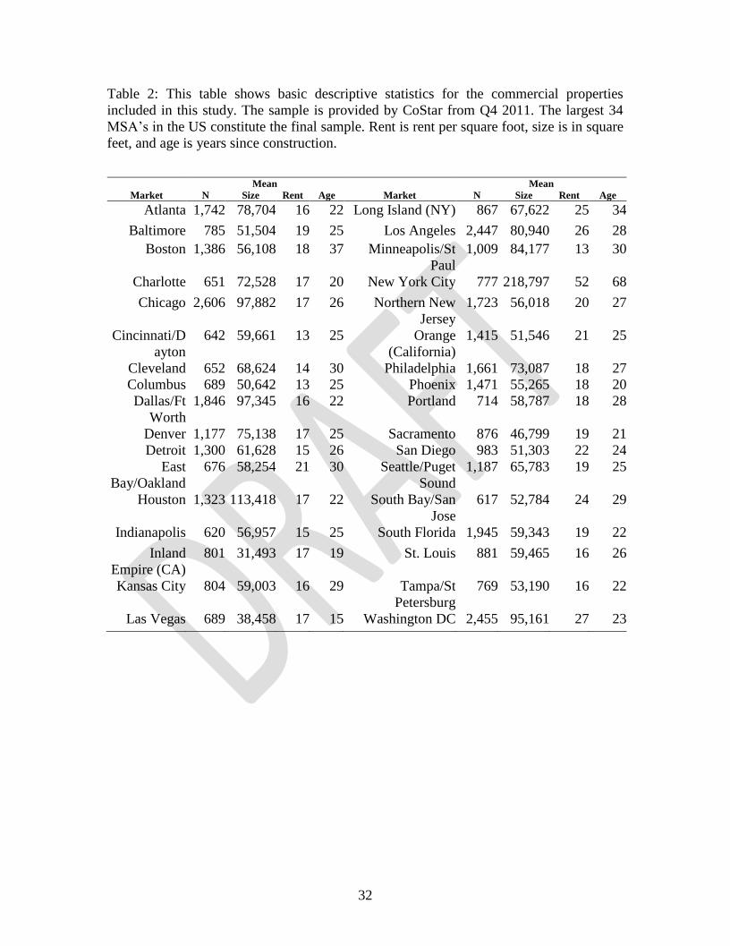
the most important property characteristics in the selection process. Table 2 provides

descriptive statistics on some key variables in the research sample such as building size,

age, and rent for 34 major US markets.

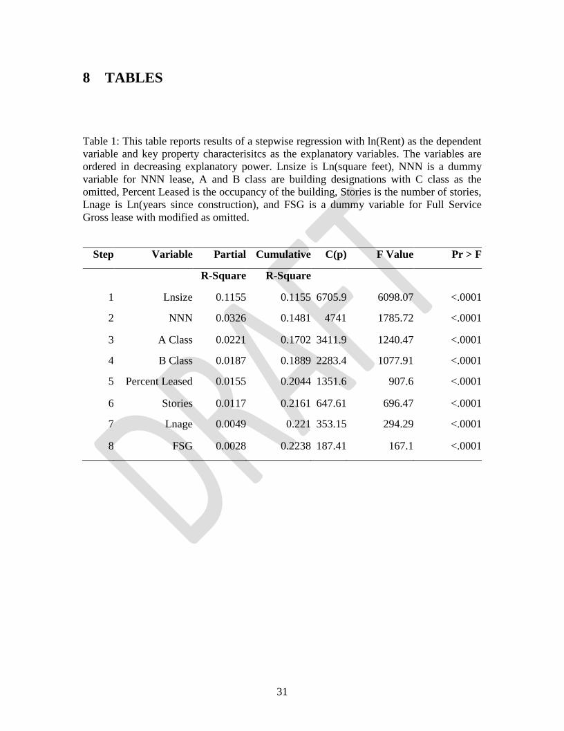
The characteristics used for matching are selected through a combination of stepwise

regression, professional judgment, and informal practitioner interviews. The results of

stepwise regression on lnrent (natural log of rent) for the entire database are shown in

11

Table 1.iv Based on these regression results and practitioner judgment the final matching

criteria includes the following variables: 1) distinct geographic submarkets, 2) property

size (square footage), and 3) property class (A, B and C class buildings)

INSERT TABLE 1

The triple net variable (NNN)v was not included as a matching parameter because it

might unnecessarily limit the matching process. Furthermore, the hedonic-grid adjustment

technique itself accounts for a portion of the rent differentials between NNN and full

service gross (FSG) properties, and submarkets tend to have some degree of homogeneity

regarding lease structure.

While there may be some small variations the following procedure is commonly

employed by many practitioners in selecting comps. They begin with either an explicit or

perhaps implicit set of screening criteria to narrow the field of all possible comps.

Depending upon the number of comps this initial screening procedure identified the

appraiser may then reduce the number of comps by further analysis and ,where possible,

by quantifying key differences in property characteristics between the subject property

and each perspective comp. To arrive at an estimated or appraised value or rent the values

and/or rents associated with the final set of comps are then averaged to obtain the

appraised value or rent of the subject property.

To approximate this comp selection approach an hedonic regression model is

estimated using the variables found to be statistically significant in the stepwise

regression model (Table 1). Thus, these explanatory variables are regressed with the

natural log of property rent as the dependent variable. The regression coefficients for a

given property characteristic, say building size, is then multiplied by the difference

between the subject property size and the size of each potential comp in the market.

12

Differences are then calculated in a similar fashion for all of the property

characteristics in the hedonic model. These differences are then squared and summed to

yield a comparability index, using a sum of squares method from Error! Reference

source not found. (1983). Following this procedure, all the comps in the relevant market

have an assigned comparability index. (Note: Later in this paper this index is referred to

as ANET and is more formally depicted in Equation 3). This index is then arrayed from

smallest to highest with a smaller value indicating greater comparability.

The number of comparables (N) associated with each subject property varies but the

minimum number is three. If less than three comparables exist the subject property is

excluded from the sample. The maximum number of comparables is set at ten. When

more than ten comparables are identified in the matching process the number is narrowed

to ten based upon the ten smallest comparability indices

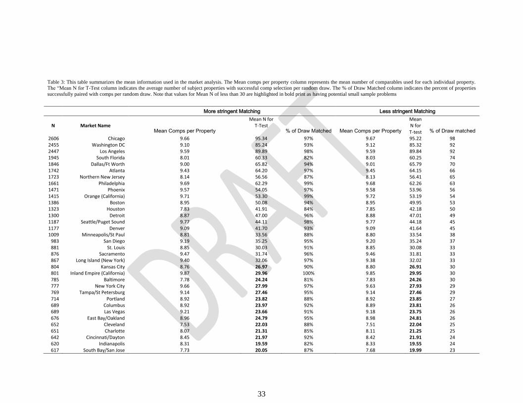
Table 8 summarizes several important sample characteristics. For example it shows

the average number of comps selected for each major sub-market (Mean Comps). The

Mean N for T-Test column represents the average number of subject properties which

experienced a successful comparable selection per random draw. The Mean N% of draw

column represents the Mean N for T-Test as a percentage of the total properties drawn.

For example, a 90% value indicates that only 10% of the properties selected failed to

draw three or more comps. All Mean N less than 30 were highlighted in bold print to

indicate potential small sample bias.

Insert Table 8

13

3.1 Basic Matching Model

The basic matching model simply compares properties but does not adjust for property

level differences. In the basic model, RS

j is defined as the rent for the subject property j.

First, a set of comparables, RCj for R

S

j based on the vector of control variables, Xi, is

determined. There are three to ten (N) comps for each each jth

observation, such that RCj

= [Rc1j, R

c2j, ..., R

cNtj].

Second, the model estimates �̂�𝑗𝑠 based on the simple average rent for the selected

comps:

�̂�𝑗𝑠 =

∑ 𝑅𝑛𝑗𝑐𝑁

1

𝑁 (1)

Finally, to test whether the expected rent, �̂�𝑗𝑠, is different from the observed rent, a

paired t-test for dependent populations is performed.

𝑡 = �̂�

𝜎𝐷√𝑁

(2)

Where: �̂� represents the mean of the differenced data (RSj −�̂�𝑗

𝑠), σD

represents the

standard deviation of the differenced data (RSj −�̂�𝑗

𝑠) and N is the number of random draws

being tested.

The paired t-test is employed to test whether a statistically significant difference exists

between the observed Rj for a random sample of buildings and the estimated 𝑅�̂� from its

comparable set of buildings.

14

A failure to reject the null hypothesis of no difference indicates model success. That

is, if the model’s expected rent fails to show a sizable prediction error then the expected

rent is not statistically different from the observed rent; hence the model is effective in

generating accurate rental estimations.

3.2 Matching Model with Hedonic Coefficient Adjustment /

Grid Method

As previously mentioned, the hedonic grid regression method closely follows Error!

Reference source not found. (1991).

First, individual submarket hedonic regressions are used to estimate the appropriate

adjustment coefficients for each property attribute. The values by attribute are used for

creating the net adjustments in equation 3.vi

Second, a net adjustment factor (ANETi), is calculated based on the closeness of fit

between the subject property and each comparable as follows:

𝐴𝑁𝐸𝑇𝑖 = ∑|𝛽𝑖(𝑋𝑖𝑠 − 𝑋𝑖

𝑐)| (3)

Where Xi represents the ith

explanatory variable in the model, βi represents the

regression-derived market value (hedonic price) for each property characteristic, s and c

stand for subject and comparable properties, respectively, and j indicates a specific

comparable property. ANETi is used to rank the quality of each comp with properties

having the smallest value representing the best match. In the third step, each comp set’s

rent is adjusted based on the estimated weight of the attribute, using the positive or

negative adjustment as opposed to the absolute value above. In mathematical terms:

�̂�𝑗𝑠 = 𝑅𝑗

𝑐 + 𝑁𝐸𝑇𝑗 = 𝑅𝑗𝑐 + ∑ 𝛽𝑖 (𝑋𝑖

𝑠 − 𝑋𝑖𝑐) (4)

15

Where �̂�𝑗𝑠 represents the estimated rent or indicated value of the subject property

based upon comparable j, RCj indicates the actual rent of the comparable property, NET

j

represents the net adjustment from the property including both positive and negative

adjustments.

The fourth step estimates a single value for the subject property by taking a weighted

average of the indicated value as defined in equation 4. This weighting procedure is

described in the next section.

3.3 Comparable Weighting

Error! Reference source not found. (1983) discuss the five possible weighting

schemes.vii They reached no conclusion regarding the optimal weighting scheme, but

rather suggested that selection of weights is... “a matter of judgment tempered by

experience.” Error! Reference source not found. (1991) found the quadratic sum of

squares method to be statistically reliable and is the technique employed in this paper.viii

Using quadratic sum of squares weighting, equation 1 is modified to incorporate

weighting factor w*

j :

�̂�𝑗𝑠 = ∑ 𝑤𝑗

∗𝑁1 𝑅𝑛𝑗

𝑐 (6)

Following the weighting process, DRj

is computed as follows:

𝑅𝑗𝑠 − �̂�𝑗

𝑠 = 𝐷𝑅𝑗 (7)

Finally, as in the prior analysis a paired t-test is conducted on DRj

. As before, note

that a failure to reject the null signifies strength in the modeling approach.

16

3.4 Comparable Selection

Comps are first selected by matching its geographic submarket clusterix to the submarket

cluster of the subject property. In order to effectively compare different size ranges each

market is arrayed into twenty categorical sections of equal number. In order to be selected

as a comp, size is required to be within plus or minus two categories. Thus, a building

ranked in the 14th size category, would draw comps from size categories 12-16. In

addition, the comp is required to be of the same building class.

The model selection is thus:

1. Comparable submarket = Subject submarket,

2. Comparable Size - 2 <= Subject Size <= Comparable Size +2,

3. Comparable Building Class = Subject Building Class.

A building comparable has to meet all the criteria to be selected in the pool. In the the

results shown, a subject property is excluded if it fails to generate at least 3 comps.

Separate robustness tests were performed with lesser exclusion criteria, and yielded

similar results.

In the event there are more than ten comps selected, the sum of squares weighting

method is used on the entire comparable set. Of the initial set, the top ten properties in

terms of closeness of fit are kept, and the rest discarded. The sum of squares method is

re-calculated for hedonic weighting based on the final ten comps.

17

4 Testing the Models

4.1 Data

The primary data source for this analysis came from CoStar. CoStar contains sales and/or

leasing information on over 2.8 Million US Commercial properties including location,

physical buildings characteristics, tenants, and lease details and other information.

4.2 Descriptive Statistics

The data consisted of 48,733 rent observations across the top 50 Metropolitan Statistical

Areas (MSA) (56 CoStar defined markets) in the United States; all data are from Q4

2011. From the total data set two separate sub- samples are created: an estimation sample

consisting of a random draw of 80% of the full sample and a 20% percent holdout sample

used for model validation. While the entire data set consist of the top 50 US MSAs, a

number of the MSAs were deemed to small for analytical purposes. Thus only 34 of the

top 50 MSAa are included in the actual analysis. Descriptive statistics are shown in Table

2.

INSERT TABLE 2

Model estimation consists of the following seven steps:

1. Randomly select five percent of subject properties from each market.

2. For each subject property selected, determine its matched set of three to ten comps.

• The comps are drawn from the entire MSA, excluding only the subject.

3. Estimate expected Rent for subject each property based on its comps, using either

the Basic or Hedonic method.

4. Perform a paired T-test on the differences between the estimated and actual rents

for the full random draw.

18

• If a property does not successfully generate a minimum of three comps, it is

excluded from the data set. For example in a market of 1,000 buildings, 50

properties are selected. If 90%, or 45 properties have three or more comps,

then paired T-Test examines the 45 properties collectively.

5. Repeat steps 1-4 a total of 500 times.x

• In given draw, each building can only be selected once but no constraints on

future draws are placed.

6. Examine the distribution of paired T-Tests from the 500 draws to determine if the

model functions as expected.

7. Repeat steps 1-6 for the following different test scenarios:

(a) Use only regression coefficients with statistical significance of 10% or better.

(b) Use only regression coefficients with statistical significance of 10% or better,

but exclude all “green” building designation coefficients (ESTAR, LEED,

Dual).xi

(c) Use all regression coefficients regardless of statistical significance.

(d) Use all regression coefficients, but exclude the “green” building designation

coefficients (ESTAR, LEED, Dual).

4.3 Distribution of T-Tests

Generally following the procedure outlined in Error! Reference source not found.

(1997), overall model efficacy would be indicated by an observed null hypothesis

rejection rate of less than 500α, where α represents the two tail level of statistical

19

significance. For example, using a 5% significance level, if the model rejects the null less

than 25 times (500*0.05), then the model effectively estimates rent.

To test forecasting bias, both the lower and upper portions of the distribution should

reject no more than 500α/2. Results for the 500 random samples are shown at the 1% ,5%

and 10% significance levels.

A graphical representation of the T-test distribution is shown below:

The graph shows that both the upper and lower tails of the distribution fail to reject

the null of no difference at conventional levels. Thus the model effectively determines

expected rent. As shown in Table Error! Reference source not found., only 0.6% and

1.2% of the random results reject the null at a 5% significance level at the lower and

upper tails respectively.

20

5 Results

The Basic and Hedonic models both appear to effectively estimate expected rent. The

empirical results for the Basic Model are presented in Table Error! Reference source

not found. (All Coefficients) and Table Error! Reference source not found.

(Significant Coefficients only), while the comparable results for the Hedonic Model are

presented in Table Error! Reference source not found. (All coefficients) and Table

Error! Reference source not found. (Significant Coefficients only). These tables shows

the distribution of paired T-test results from the 500 random draws for the entire national

sample. For ease of exposition results are summarized in Table Error! Reference source

not found..

The results show various significance levels for the lower and upper bounds of a

two-tailed T-test. An effective model would have less than 500*(α/2) of the draws

rejected at the α significance level. For example, less than 2.5% of the random tests

should reject the null hypothesis at the upper or lower bounds for a 5% two-tail

significance level. Results are bolded where a market rejects the null at a higher than

expected level.

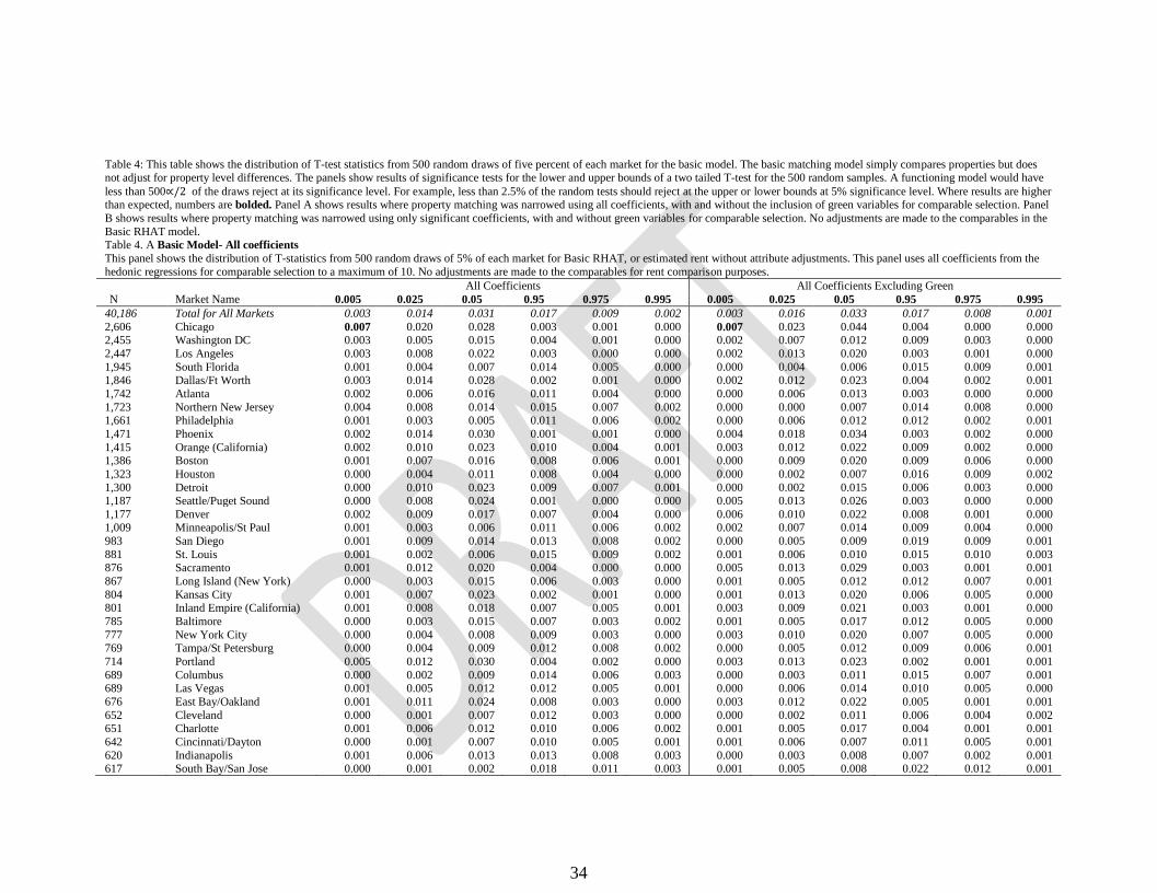
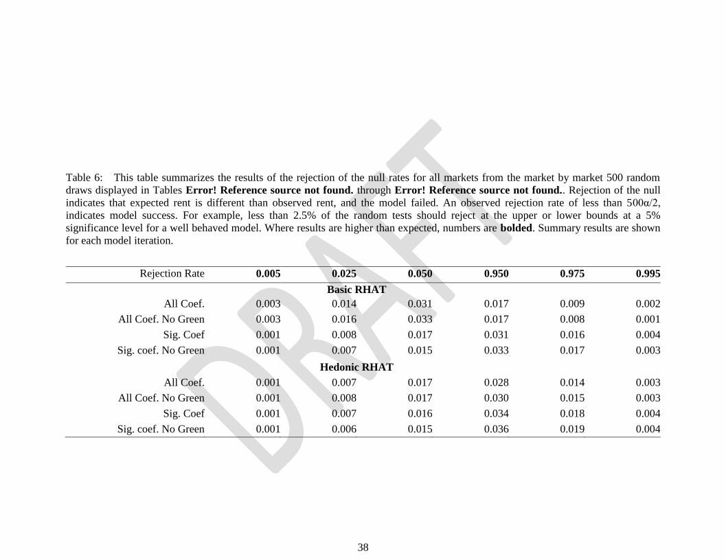
Examining the Basic model results for the entire sample as shown in the first row of

Table Error! Reference source not found., only 1.4% of the results reject the null at the

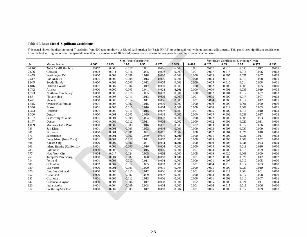
lower tail at a 5% significance level (0.025 one-tail probability column). The comparable

results using only the significant coefficients (Table Error! Reference source not

found.) indicate an even smaller rejection rate of 0.8%. Looking at the same 5%

significance level for the Hedonic Model the comparable rejection rates are quite similar.

For the All Coefficients model (Table Error! Reference source not found.) the rejection

rate is 1.4% and 0.07% for the significant only coefficients (Table Error! Reference

21

source not found.). For both models excluding the green building designation variables

increases these rejection rates a very small amount.

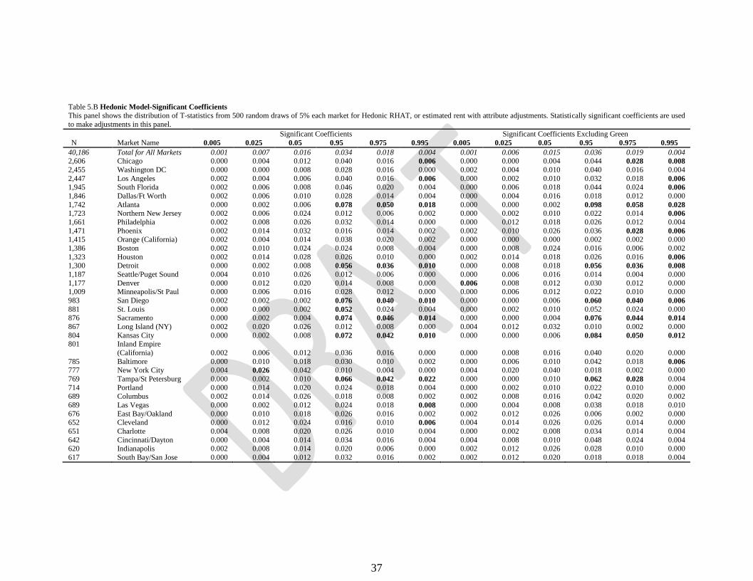
At the upper end of the distribution of T-test results the rejection rates for the Basic

Model are even lower for the All Coefficient model (0.009 vs. 0.014) but noticeably

higher for the Significant Only model (0.016 vs. 0.008). Thus, the upper portion of the

rental T-test distribution does not perform quite as well as the lower tail. This may

indicate increased heterogeneity in those markets at the upper end of the rent and size

distribution. It could also suggest that the regression coefficients are a bit inconsistent in

the upper tails.

When examining the rejection rates for the individual markets, virtually every market

detects no statistical difference between the estimated and observed rent generated by

either model. The model which most consistently rejected the null hypothesis is the

Hedonic Model using all the regression coefficients. Furthermore, the Basic Model

performs almost as well as the more complex Hedonic Model. The area where the Basic

Model slightly outperforms the Hedonic Model was in the upper portion of the rent

distribution (0.016 vs. 0.018) at the 5% level of significance when including only the

statistically significant coefficients. This once again suggests that the regression

coefficients from the hedonic coefficients may be slightly less reliable at the upper

portions of the rent distribution.

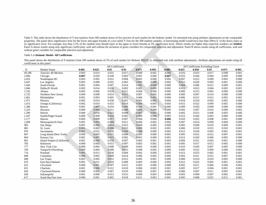
The summary data (Table Error! Reference source not found.) suggests that the

Hedonic Model provides somewhat more stable results across all the various model

specifications. Furthermore, the Hedonic Model was substantially more accurate in the

lower portion of the T-test distribution. Finally, the inclusion of the green building

designation variables has a relatively minor effect on either of the two models. In

22

summary the results provide strong support for using some form of matching models to

estimate commercial property rent.

The Mean N for T-Test represents the average number of subjects with successful

comparable selection per random draw. As noted, 5% of each market is drawn, but those

properties with less than 3 comparables are disregarded. The Mean N column shows the

average N used in the paired T-test for each market. Mean N % of draw represents the

Mean N for T-Test as a percentage of the total properties drawn. An 80% number means

that 20% of the properties selected do not successfully draw three or more comparables.

All Mean N less than 30 were highlighted as potential small sample issues.

Following the summary tables, the detailed results are reported. Tables Error!

Reference source not found. and Error! Reference source not found. show results for

Basic RHAT, or the unadjusted estimation of expected rent using strict matching criteria.

Tables Error! Reference source not found. and Error! Reference source not found.

show the results for Hedonic RHAT, or the hedonic adjusted models.

INSERT TABLE Error! Reference source not found. INSERT TABLE Error!

Reference source not found. INSERT TABLE Error! Reference source not found.

INSERT TABLE Error! Reference source not found. INSERT TABLE Error!

Reference source not found.

6 Robustness Tests

6.1 Holdback Results

To test their robustness, the models are validated using the 20% holdout sample reserved

at the beginning of the analysis. Due to the smaller number of available properties, the

number of iterations for each model is reduced to 200. While the subject properties are

23

drawn exclusively from the holdback sample, comparable properties are drawn from the

whole market. The regression coefficients for hedonic adjustments are those generated

from the 80% estimation sample. Detailed results are omitted due to space constraints.

In general the results are remarkably similar to the results obtained using the full

estimation sample. The larger markets consistently fail to reject the null at the five percent

on-tail T-test level. The stability of the holdout results indicate that the model design is

not sample specific and the model should continue to perform well when applied to

comparable data sets.

6.2 Less Stringent Matching Parameters

In the results presented, if a comp fails to meet all the matching criteria, it is not selected;

if the subject property fails to generate at least three comps it is excluded from the

analysis. As a robustness test a more liberal matching process is employed as follows. If

the matching process does not generate at least 3 comps for a given subject property, the

building class matching requirement is dropped. This allows the matching process to

draws from a wider pool of comps although the quality of the selected comps would

likely be lower. Thus, there is a potential trade-off when a greater number of comps leads

to less representative comps being selected. However, in the case of the hedonic model

the expected rent would still be adjusted for building class. The robustness test is

performed in the same manner as before for each of the four model scenarios, with 500

random draws of a five percent sample for each market. The results are omitted due to

space constraints but they are qualitatively very similar to the previous results.

24

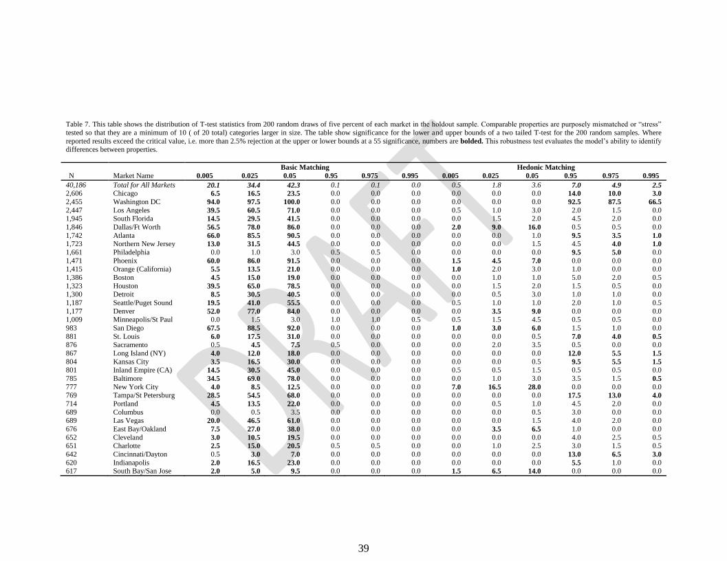
6.3 Control Tests

To further test the robustness of the model the matching process is intentionally

“stressed” to see how reliable the results are when estimating rent for clearly dissimilar

properties. To create this dissimilar sample, properties are considered comparable when

the building is at least 10 size categories larger (out of 20 total). In general, larger

buildings tend to command higher rents. The results are shown in Table Error!

Reference source not found..

The stress test results show that the basic model consistently rejects the null of no

difference in rent. The hedonic model does adjust for the differences in the buildings, but

performs more poorly than the original model. The stress results indicate that hedonic

adjustments significantly compensate for poorly matched properties, but the most

efficient model is includes well matched properties. This finding also shows that the basic

model can be used to identify potential market discounts or premiums.

INSERT TABLE Error! Reference source not found.

6.4 Whole Market Testing

The primary purposes of testing random selections of a market is to ensure results are not

sample specific, to permit a holdback sample and to mirror real life applications with

small portfolio evaluation. However, further insight as to the robustness of the overall

model is gained through evaluating an entire market. Table 9 shows results from

Equation 2, with N as the entire market. They show that the model performs even better

than in random swatches and that the hedonic model clearly outperforms the basic model.

INSERT TABLE 9

25

7 Conclusion

This paper explores alternatives approaches to basic regression models for predicting

commercial real estate rents. The first model is a basic matching model based on the grid

method commonly used by appraisers. An automated algorithm selects three to ten

comparable properties and uses a simple average of the selected comps rent to estimate

the expected rent for the subject property. A second more sophisticated model uses

hedonic regression to determine the appropriate property adjustment coefficients to

estimate rent based upon a matched set of comps.

The various models consistently failed to reject the null hypothesis of no difference

between expected and observed rents which indicates success in the modeling effort. That

is, the paired differences between the expected and observed rents proved to be small and

statistically insignificant. Not surprisingly, the strongest performance is observed in larger

markets with more comps from which to select. The Hedonic model which adjusts the

expected rent using the hedonic coefficients as the adjustment parameters proved to be

somewhat more reliable overall. On the other hand, the Basic model also performed quite

well. As a secondary finding, the results indicate limited appraisal enhancements with the

inclusion of green variables.

The models were estimated using the CoStar commercial real estate database. Tests

using separate estimation and holdout samples performed equally well, suggesting that the

models are sufficiently flexible and adaptable for analyzing other data sets. Furthermore,

the matching models were “stressed” to see if observable differences could be captured

and potentially normalized. The Basic model clearly showed the difference in rent

between purposefully mismatched buildings, demonstrating the potential of the model to

26

identify statistically significant attribute differences. The Hedonic model effectively

adjusted for many of those differences.

Multiple research opportunities could stem from this paper. In addition to the further

refinement of the model, confirmation or rejection of a wide range of prior findings can

be tested using this method. Differences in size, stories, view premiums, or other building

attributes could be purposefully mismatched to identify market premiums. Another

potential research avenue is a detailed comparison of stand-alone hedonic regression to

matching in a constructed data set. In addition, models indicating whether a building

captures its “fair share” of market rent could be created. This foundation could potentially

be adapted to commercial real estate bond analysis.

Increased data availability for real estate researchers may represent the beginning of

new analysis techniques in real estate research. No longer confined to private, one-off

data sets, researchers can now begin to investigate the best ways to research. Alternative

research methods may open the door to a host of fresh findings, and new ideas in the

field.

While the hedonic/grid approach will not necessarily replace the more traditional

approach to appraisal, this paper suggest the feasibility for practitioners and researchers to

at least consider it a possible option if they have sufficient data and expertise

27

References

Appraisal Institute (U.S.), 2001. The appraisal of real estate. Appraisal Institute.

Baltagi, B.H., and C. Kao, 2001. Nonstationary panels, cointegration in panels and

dynamic panels: A survey.

Barber, Brad M., and John D. Lyon, 1997. Detecting long-run abnormal stock returns:

The empirical power and specification of test statistics. Journal of Financial Economics

43 (3), 341 – 372.

Binkley, A.G., and B.A. Ciochetti, 2010. Carbon markets: A hidden value source for

commercial real estate. Journal of Sustainable Real Estate 2 (1), 67–90.

Bowden, R.J., 1992. Competitive selection and market data: the mixed-index problem.

The Review of Economic Studies 59 (3), 625.

Brown, James N., and Harvey S. Rosen, 1982. On the estimation of structural hedonic

price models.

Cheng, Ping, Zhenguo Lin, and Yingchun Liu, Oct 2011. Heterogeneous information and

appraisal smoothing. Journal of Real Estate Research 33 (4), 443–469.

Chichernea, Doina, Norm Miller, Jeff Fisher, Michael Sklarz, and Bob White, 2008. A

cross-sectional analysis of cap rates by msa. Journal of Real Estate Research 30 (3), 249 –

292.

Colwell, P.F., R.E. Cannaday, and C. Wu, 1983. The analytical foundations of adjustment

grid methods. Real Estate Economics 11 (1), 11–29.

28

Ekeland, I., J.J. Heckman, and L. Nesheim, 2002. Identifying hedonic models. American

Economic Review, 304–309.

Epple, Dennis, 1987. Hedonic prices and implicit markets: Estimating supply and demand

functions for differentiated products. Journal of Political Economy 95 (1), 59.

Firstenberg, P.M., S.A. Ross, and R.C. Zisler, 1998. Real estate: the whole story.

Streetwise: the best of the Journal of portfolio management, 189.

Fisher, J.D., 2002. Real time valuation. Journal of Property Investment & Finance 20 (3),

213–221.

Fisher, J., D. Gatzlaff, D. Geltner, and D. Haurin, 2003. Controlling for the impact of

variable liquidity in commercial real estate price indices. Real Estate Economics 31 (2),

269–303.

Fuerst, Franz, and Patrick McAllister, 2011. Green noise or green value? measuring the

effects of environmental certification on office values. Real Estate Economics 39 (1), 45–

69.

Garmaise, Mark J., and Tobias J. Moskowitz, 2004. Confronting information

asymmetries: Evidence from real estate markets. Review of Financial Studies 17 (2), 405–

437.

Hayunga, D.K., and R.K. Pace, 2010. Spatial statistics applied to commercial real estate.

The Journal of Real Estate Finance and Economics, 1–23.

29

Isakson, H.R., 1986. The nearest neighbors appraisal technique: An alternative to the

adjustment grid methods. Real Estate Economics 14 (2), 274–286.

Isakson, H.R., 1988. Valuation analysis of commercial real estate using the nearest

neighbors appraisal technique. Growth and Change 19 (2), 11–24.

Kang, Han-Bin, and Alan K. Reichert, 1991. An empirical analysis of hedonic regression

and grid-adjustment techniques in real estate appraisal. Real Estate Economics 19 (1), 70–

91.

Knight, J.R., R. Carter Hill, and CF Sirmans, 1993. Stein rule estimation in real estate

appraisal. Appraisal Journal 61, 539–539.

Malpezzi, S., 2002. Hedonic pricing models: a selective and applied review. Housing

Economics and Public Policy, 67–89.

McDonald, J.F., 2002. A survey of econometric models of office markets. Journal of Real

Estate Literature 10 (2), 223–242.

Montero, Jose M., and Beatriz Larraz, Apr 2011. Interpolation methods for geographical

data: Housing and commercial establishment markets. Journal of Real Estate Research

33 (2), 233–244.

Oikarinen, E., M. Hoesli, and C. Serrano, 2011. The long-run dynamics between direct

and securitized real estate. Journal of Real Estate Research 33 (1), 73–103.

Pace, R.K., and O.W. Gilley, 1998. Generalizing the ols and grid estimators. Real Estate

Economics 26 (2), 331–347.

30

Pagourtzi, E., V. Assimakopoulos, T. Hatzichristos, and N. French, 2003. Real estate

appraisal: a review of valuation methods. Journal of Property Investment & Finance

21 (4), 383–401.

Robinson, S. Sanderford, A. 2015 Green Buildings: Similar to Other Premium Buildings?

Journal of Real Estate Finance and Economics, Forthcoming.

Rosen, Sherwin, 1974. Hedonic prices and implicit markets: Product differentiation in

pure competition. Journal of Political Economy 82 (1), 34–55.

Simons, R. A., Robinson, S., & Lee, E. (2014). Green Office Buildings: A Qualitative

Exploration of Green Office Building Attributes. The Journal of Sustainable Real Estate,

6(2), 211-232.

Sirmans, G. Stacy, David A. Macpherson, and Emily N. Zietz, 2005. The composition of

hedonic pricing models. Journal of Real Estate Literature 13 (1), 3 – 43.

Vandell, Kerry D., 1991. Optimal comparable selection and weighting in real property

valuation. Real Estate Economics 19 (2), 213–239.

Zurada, Jozef, Alan S. Levitan, and Jian Guan, 2011. A comparison of regression and

artificial intelligence methods in a mass appraisal context. Journal of Real Estate

Research 33 (3), 349–387.

31

8 TABLES

Table 1: This table reports results of a stepwise regression with ln(Rent) as the dependent

variable and key property characterisitcs as the explanatory variables. The variables are

ordered in decreasing explanatory power. Lnsize is Ln(square feet), NNN is a dummy

variable for NNN lease, A and B class are building designations with C class as the

omitted, Percent Leased is the occupancy of the building, Stories is the number of stories,

Lnage is Ln(years since construction), and FSG is a dummy variable for Full Service

Gross lease with modified as omitted.

Step Variable Partial Cumulative C(p) F Value Pr > F

R-Square R-Square

1 Lnsize 0.1155 0.1155 6705.9 6098.07 <.0001

2 NNN 0.0326 0.1481 4741 1785.72 <.0001

3 A Class 0.0221 0.1702 3411.9 1240.47 <.0001

4 B Class 0.0187 0.1889 2283.4 1077.91 <.0001

5 Percent Leased 0.0155 0.2044 1351.6 907.6 <.0001

6 Stories 0.0117 0.2161 647.61 696.47 <.0001

7 Lnage 0.0049 0.221 353.15 294.29 <.0001

8 FSG 0.0028 0.2238 187.41 167.1 <.0001

32

Table 2: This table shows basic descriptive statistics for the commercial properties

included in this study. The sample is provided by CoStar from Q4 2011. The largest 34

MSA’s in the US constitute the final sample. Rent is rent per square foot, size is in square

feet, and age is years since construction.

Mean Mean

Market N Size Rent Age Market N Size Rent Age

Atlanta 1,742 78,704 16 22 Long Island (NY) 867 67,622 25 34

Baltimore 785 51,504 19 25 Los Angeles 2,447 80,940 26 28

Boston 1,386 56,108 18 37 Minneapolis/St

Paul

1,009 84,177 13 30

Charlotte 651 72,528 17 20 New York City 777 218,797 52 68

Chicago 2,606 97,882 17 26 Northern New

Jersey

1,723 56,018 20 27

Cincinnati/D

ayton

642 59,661 13 25 Orange

(California)

1,415 51,546 21 25

Cleveland 652 68,624 14 30 Philadelphia 1,661 73,087 18 27

Columbus 689 50,642 13 25 Phoenix 1,471 55,265 18 20

Dallas/Ft

Worth

1,846 97,345 16 22 Portland 714 58,787 18 28

Denver 1,177 75,138 17 25 Sacramento 876 46,799 19 21

Detroit 1,300 61,628 15 26 San Diego 983 51,303 22 24

East

Bay/Oakland

676 58,254 21 30 Seattle/Puget

Sound

1,187 65,783 19 25

Houston 1,323 113,418 17 22 South Bay/San

Jose

617 52,784 24 29

Indianapolis 620 56,957 15 25 South Florida 1,945 59,343 19 22

Inland

Empire (CA)

801 31,493 17 19 St. Louis 881 59,465 16 26

Kansas City 804 59,003 16 29 Tampa/St

Petersburg

769 53,190 16 22

Las Vegas 689 38,458 17 15 Washington DC 2,455 95,161 27 23

33

Table 3: This table summarizes the mean information used in the market analysis. The Mean comps per property column represents the mean number of comparables used for each individual property. The “Mean N for T-Test column indicates the average number of subject properties with successful comp selection per random draw. The % of Draw Matched column indicates the percent of properties

successfully paired with comps per random draw. Note that values for Mean N of less than 30 are highlighted in bold print as having potential small sample problems

More stringent Matching Less stringent Matching

N

Market Name

Mean Comps per Property

Mean N for T-Test

% of Draw Matched Mean Comps per Property

Mean N for T-test % of Draw matched

2606 Chicago 9.66 95.34 97% 9.67 95.22 98 2455 Washington DC 9.10 85.24 93% 9.12 85.32 92 2447 Los Angeles 9.59 89.89 98% 9.59 89.84 92 1945 South Florida 8.01 60.33 82% 8.03 60.25 74 1846 Dallas/Ft Worth 9.00 65.82 94% 9.01 65.79 70 1742 Atlanta 9.43 64.20 97% 9.45 64.15 66 1723 Northern New Jersey 8.14 56.56 87% 8.13 56.41 65 1661 Philadelphia 9.69 62.29 99% 9.68 62.26 63 1471 Phoenix 9.57 54.05 97% 9.58 53.96 56 1415 Orange (California) 9.71 53.30 99% 9.72 53.19 54 1386 Boston 8.95 50.08 94% 8.95 49.95 53 1323 Houston 7.83 41.91 84% 7.85 42.18 50 1300 Detroit 8.87 47.00 96% 8.88 47.01 49 1187 Seattle/Puget Sound 9.77 44.11 98% 9.77 44.18 45 1177 Denver 9.09 41.70 93% 9.09 41.64 45 1009 Minneapolis/St Paul 8.81 33.56 88% 8.80 33.54 38

983 San Diego 9.19 35.25 95% 9.20 35.24 37 881 St. Louis 8.85 30.03 91% 8.85 30.08 33 876 Sacramento 9.47 31.74 96% 9.46 31.81 33 867 Long Island (New York) 9.40 32.06 97% 9.38 32.02 33 804 Kansas City 8.76 26.97 90% 8.80 26.91 30 801 Inland Empire (California) 9.87 29.96 100% 9.85 29.95 30 785 Baltimore 7.78 24.24 81% 7.83 24.26 30 777 New York City 9.66 27.99 97% 9.63 27.93 29 769 Tampa/St Petersburg 9.14 27.46 95% 9.14 27.46 29 714 Portland 8.92 23.82 88% 8.92 23.85 27 689 Columbus 8.92 23.97 92% 8.89 23.81 26 689 Las Vegas 9.21 23.66 91% 9.18 23.75 26 676 East Bay/Oakland 8.96 24.79 95% 8.98 24.81 26 652 Cleveland 7.53 22.03 88% 7.51 22.04 25 651 Charlotte 8.07 21.31 85% 8.11 21.25 25 642 Cincinnati/Dayton 8.45 21.97 92% 8.42 21.91 24 620 Indianapolis 8.31 19.59 82% 8.33 19.55 24 617 South Bay/San Jose 7.73 20.05 87% 7.68 19.99 23

34

Table 4: This table shows the distribution of T-test statistics from 500 random draws of five percent of each market for the basic model. The basic matching model simply compares properties but does not adjust for property level differences. The panels show results of significance tests for the lower and upper bounds of a two tailed T-test for the 500 random samples. A functioning model would have

less than 500∝/2 of the draws reject at its significance level. For example, less than 2.5% of the random tests should reject at the upper or lower bounds at 5% significance level. Where results are higher than expected, numbers are bolded. Panel A shows results where property matching was narrowed using all coefficients, with and without the inclusion of green variables for comparable selection. Panel

B shows results where property matching was narrowed using only significant coefficients, with and without green variables for comparable selection. No adjustments are made to the comparables in the

Basic RHAT model. Table 4. A Basic Model- All coefficients

This panel shows the distribution of T-statistics from 500 random draws of 5% of each market for Basic RHAT, or estimated rent without attribute adjustments. This panel uses all coefficients from the

hedonic regressions for comparable selection to a maximum of 10. No adjustments are made to the comparables for rent comparison purposes.

All Coefficients All Coefficients Excluding Green

N Market Name 0.005 0.025 0.05 0.95 0.975 0.995 0.005 0.025 0.05 0.95 0.975 0.995

40,186 Total for All Markets 0.003 0.014 0.031 0.017 0.009 0.002 0.003 0.016 0.033 0.017 0.008 0.001

2,606 Chicago 0.007 0.020 0.028 0.003 0.001 0.000 0.007 0.023 0.044 0.004 0.000 0.000 2,455 Washington DC 0.003 0.005 0.015 0.004 0.001 0.000 0.002 0.007 0.012 0.009 0.003 0.000

2,447 Los Angeles 0.003 0.008 0.022 0.003 0.000 0.000 0.002 0.013 0.020 0.003 0.001 0.000

1,945 South Florida 0.001 0.004 0.007 0.014 0.005 0.000 0.000 0.004 0.006 0.015 0.009 0.001 1,846 Dallas/Ft Worth 0.003 0.014 0.028 0.002 0.001 0.000 0.002 0.012 0.023 0.004 0.002 0.001

1,742 Atlanta 0.002 0.006 0.016 0.011 0.004 0.000 0.000 0.006 0.013 0.003 0.000 0.000

1,723 Northern New Jersey 0.004 0.008 0.014 0.015 0.007 0.002 0.000 0.000 0.007 0.014 0.008 0.000 1,661 Philadelphia 0.001 0.003 0.005 0.011 0.006 0.002 0.000 0.006 0.012 0.012 0.002 0.001

1,471 Phoenix 0.002 0.014 0.030 0.001 0.001 0.000 0.004 0.018 0.034 0.003 0.002 0.000

1,415 Orange (California) 0.002 0.010 0.023 0.010 0.004 0.001 0.003 0.012 0.022 0.009 0.002 0.000 1,386 Boston 0.001 0.007 0.016 0.008 0.006 0.001 0.000 0.009 0.020 0.009 0.006 0.000

1,323 Houston 0.000 0.004 0.011 0.008 0.004 0.000 0.000 0.002 0.007 0.016 0.009 0.002

1,300 Detroit 0.000 0.010 0.023 0.009 0.007 0.001 0.000 0.002 0.015 0.006 0.003 0.000 1,187 Seattle/Puget Sound 0.000 0.008 0.024 0.001 0.000 0.000 0.005 0.013 0.026 0.003 0.000 0.000

1,177 Denver 0.002 0.009 0.017 0.007 0.004 0.000 0.006 0.010 0.022 0.008 0.001 0.000 1,009 Minneapolis/St Paul 0.001 0.003 0.006 0.011 0.006 0.002 0.002 0.007 0.014 0.009 0.004 0.000

983 San Diego 0.001 0.009 0.014 0.013 0.008 0.002 0.000 0.005 0.009 0.019 0.009 0.001

881 St. Louis 0.001 0.002 0.006 0.015 0.009 0.002 0.001 0.006 0.010 0.015 0.010 0.003 876 Sacramento 0.001 0.012 0.020 0.004 0.000 0.000 0.005 0.013 0.029 0.003 0.001 0.001

867 Long Island (New York) 0.000 0.003 0.015 0.006 0.003 0.000 0.001 0.005 0.012 0.012 0.007 0.001

804 Kansas City 0.001 0.007 0.023 0.002 0.001 0.000 0.001 0.013 0.020 0.006 0.005 0.000 801 Inland Empire (California) 0.001 0.008 0.018 0.007 0.005 0.001 0.003 0.009 0.021 0.003 0.001 0.000

785 Baltimore 0.000 0.003 0.015 0.007 0.003 0.002 0.001 0.005 0.017 0.012 0.005 0.000

777 New York City 0.000 0.004 0.008 0.009 0.003 0.000 0.003 0.010 0.020 0.007 0.005 0.000 769 Tampa/St Petersburg 0.000 0.004 0.009 0.012 0.008 0.002 0.000 0.005 0.012 0.009 0.006 0.001

714 Portland 0.005 0.012 0.030 0.004 0.002 0.000 0.003 0.013 0.023 0.002 0.001 0.001

689 Columbus 0.000 0.002 0.009 0.014 0.006 0.003 0.000 0.003 0.011 0.015 0.007 0.001 689 Las Vegas 0.001 0.005 0.012 0.012 0.005 0.001 0.000 0.006 0.014 0.010 0.005 0.000

676 East Bay/Oakland 0.001 0.011 0.024 0.008 0.003 0.000 0.003 0.012 0.022 0.005 0.001 0.001

652 Cleveland 0.000 0.001 0.007 0.012 0.003 0.000 0.000 0.002 0.011 0.006 0.004 0.002 651 Charlotte 0.001 0.006 0.012 0.010 0.006 0.002 0.001 0.005 0.017 0.004 0.001 0.001

642 Cincinnati/Dayton 0.000 0.001 0.007 0.010 0.005 0.001 0.001 0.006 0.007 0.011 0.005 0.001

620 Indianapolis 0.001 0.006 0.013 0.013 0.008 0.003 0.000 0.003 0.008 0.007 0.002 0.001 617 South Bay/San Jose 0.000 0.001 0.002 0.018 0.011 0.003 0.001 0.005 0.008 0.022 0.012 0.001

35

Table 4.B Basic Model- Significant Coefficients

This panel shows the distribution of T-statistics from 500 random draws of 5% of each market for Basic RHAT, or estimated rent without attribute adjustments. This panel uses significant coefficients

from the hedonic regressions for comparable selection to a maximum of 10. No adjustments are made to the comparables for rent comparison purposes.

Significant Coefficients Significant Coefficients Excluding Green

N Market Name 0.005 0.025 0.05 0.95 0.975 0.995 0.005 0.025 0.05 0.95 0.975 0.995


2,606 Chicago 0.002 0.011 0.016 0.005 0.002 0.000 0.001 0.007 0.015 0.016 0.006 0.002

2,455 Washington DC 0.000 0.002 0.009 0.018 0.010 0.002 0.000 0.003 0.005 0.021 0.007 0.003 2,447 Los Angeles 0.001 0.003 0.008 0.014 0.006 0.001 0.000 0.003 0.010 0.013 0.008 0.001

1,945 South Florida 0.000 0.003 0.006 0.012 0.005 0.001 0.000 0.005 0.010 0.014 0.008 0.001

1,846 Dallas/Ft Worth 0.001 0.002 0.004 0.017 0.010 0.003 0.000 0.002 0.006 0.009 0.005 0.000 1,742 Atlanta 0.000 0.000 0.003 0.041 0.024 0.006 0.000 0.000 0.001 0.038 0.019 0.005

1,723 Northern New Jersey 0.000 0.005 0.010 0.005 0.003 0.001 0.000 0.002 0.004 0.012 0.007 0.003

1,661 Philadelphia 0.002 0.003 0.011 0.013 0.005 0.000 0.001 0.005 0.009 0.013 0.007 0.003 1,471 Phoenix 0.000 0.005 0.014 0.011 0.006 0.003 0.001 0.004 0.006 0.019 0.012 0.001

1,415 Orange (California) 0.001 0.005 0.007 0.015 0.010 0.002 0.000 0.000 0.000 0.001 0.000 0.000

1,386 Boston 0.001 0.006 0.010 0.010 0.004 0.001 0.000 0.006 0.014 0.008 0.003 0.001 1,323 Houston 0.001 0.005 0.011 0.015 0.007 0.000 0.001 0.005 0.009 0.018 0.010 0.003

1,300 Detroit 0.000 0.001 0.002 0.029 0.018 0.005 0.000 0.004 0.008 0.031 0.017 0.003 1,187 Seattle/Puget Sound 0.001 0.004 0.008 0.004 0.002 0.000 0.000 0.002 0.008 0.005 0.003 0.000

1,177 Denver 0.001 0.009 0.012 0.011 0.005 0.002 0.000 0.002 0.006 0.020 0.011 0.000

1,009 Minneapolis/St Paul 0.000 0.002 0.009 0.016 0.007 0.000 0.002 0.003 0.005 0.012 0.006 0.000 983 San Diego 0.001 0.001 0.003 0.022 0.016 0.001 0.000 0.002 0.006 0.020 0.009 0.001

881 St. Louis 0.000 0.001 0.001 0.021 0.011 0.002 0.000 0.002 0.004 0.025 0.010 0.000

876 Sacramento 0.000 0.001 0.002 0.030 0.016 0.006 0.000 0.001 0.002 0.031 0.017 0.003 867 Long Island (New York) 0.001 0.007 0.012 0.011 0.007 0.000 0.000 0.005 0.009 0.008 0.002 0.000

804 Kansas City 0.000 0.002 0.006 0.031 0.014 0.006 0.000 0.000 0.003 0.044 0.023 0.004

801 Inland Empire (California) 0.001 0.003 0.006 0.016 0.004 0.000 0.000 0.004 0.008 0.019 0.010 0.000 785 Baltimore 0.000 0.003 0.012 0.015 0.005 0.001 0.001 0.003 0.006 0.015 0.009 0.001

777 New York City 0.004 0.017 0.024 0.005 0.002 0.000 0.005 0.009 0.020 0.008 0.000 0.000

769 Tampa/St Petersburg 0.000 0.004 0.007 0.028 0.018 0.008 0.001 0.002 0.005 0.020 0.012 0.002 714 Portland 0.001 0.006 0.012 0.011 0.004 0.002 0.000 0.001 0.007 0.010 0.005 0.000

689 Columbus 0.002 0.007 0.012 0.005 0.003 0.000 0.001 0.004 0.010 0.014 0.003 0.000

689 Las Vegas 0.000 0.001 0.005 0.020 0.011 0.004 0.000 0.001 0.006 0.020 0.010 0.005 676 East Bay/Oakland 0.000 0.005 0.010 0.012 0.006 0.001 0.001 0.006 0.014 0.004 0.001 0.000

652 Cleveland 0.000 0.003 0.007 0.009 0.007 0.003 0.000 0.003 0.009 0.017 0.008 0.000

651 Charlotte 0.001 0.005 0.012 0.013 0.006 0.002 0.000 0.001 0.003 0.010 0.007 0.001 642 Cincinnati/Dayton 0.000 0.004 0.006 0.017 0.008 0.001 0.002 0.005 0.006 0.021 0.011 0.004

620 Indianapolis 0.001 0.004 0.009 0.008 0.004 0.000 0.001 0.006 0.015 0.013 0.006 0.000

617 South Bay/San Jose 0.000 0.002 0.005 0.017 0.010 0.004 0.001 0.006 0.009 0.012 0.009 0.001

36

Table 5: This table shows the distribution of T-test statistics from 500 random draws of five percent of each market for the hedonic model. Or estimated rent using attribute adjustments on the comparable

properties. The panel show significance tests for the lower and upper bounds of a two tailed T-Test for the 500 random samples. A functioning model would have less than 500∝/2 of the draws reject at

its significance level. For example, less than 2.5% of the random tests should reject at the upper or lower bounds at 5% significance level. Where results are higher than expected, numbers are bolded.

Panel A shows results using only significant coefficients, with and without the inclusion of green variables for comparable selection and adjustment. Panel B shows results using all coefficients, with and

without green variables for comparable selection and adjustment.

Table 5.A Hedonic Model- All Coefficients

This panel shows the distribution of T-statistics from 500 random draws of 5% of each market for Hedonic RHAT, or estimated rent with attribute adjustments. Attribute adjustments are made using all

coefficients in this panel.

All Coefficients All Coefficients Excluding Green

N Market Name 0.005 0.025 0.05 0.95 0.975 0.995 0.005 0.025 0.050 0.95 0.975 0.995


2,606 Chicago 0.007 0.020 0.028 0.003 0.001 0.000 0.007 0.023 0.044 0.004 0.000 0.000

2,455 Washington DC 0.003 0.005 0.015 0.004 0.001 0.000 0.002 0.007 0.012 0.009 0.003 0.000 2,447 Los Angeles 0.003 0.008 0.022 0.003 0.000 0.000 0.002 0.013 0.020 0.003 0.001 0.000

1,945 South Florida 0.001 0.004 0.007 0.014 0.005 0.000 0.000 0.004 0.006 0.015 0.009 0.001

1,846 Dallas/Ft Worth 0.003 0.014 0.028 0.002 0.001 0.000 0.002 0.012 0.023 0.004 0.002 0.001 1,742 Atlanta 0.002 0.006 0.016 0.011 0.004 0.000 0.000 0.006 0.013 0.003 0.000 0.000


1,661 Philadelphia 0.001 0.003 0.005 0.011 0.006 0.002 0.000 0.006 0.012 0.012 0.002 0.001 1,471 Phoenix 0.002 0.014 0.030 0.001 0.001 0.000 0.004 0.018 0.034 0.003 0.002 0.000


1,386 Boston 0.001 0.007 0.016 0.008 0.006 0.001 0.000 0.009 0.020 0.009 0.006 0.000

1,323 Houston 0.000 0.004 0.011 0.008 0.004 0.000 0.000 0.002 0.007 0.016 0.009 0.002

1,300 Detroit 0.000 0.010 0.023 0.009 0.007 0.001 0.000 0.002 0.015 0.006 0.003 0.000

1,187 Seattle/Puget Sound 0.000 0.008 0.024 0.001 0.000 0.000 0.005 0.013 0.026 0.003 0.000 0.000 1,177 Denver 0.002 0.009 0.017 0.007 0.004 0.000 0.006 0.010 0.022 0.008 0.001 0.000

1,009 Minneapolis/St Paul 0.001 0.003 0.006 0.011 0.006 0.002 0.002 0.007 0.014 0.009 0.004 0.000 983 San Diego 0.001 0.009 0.014 0.013 0.008 0.002 0.000 0.005 0.009 0.019 0.009 0.001

881 St. Louis 0.001 0.002 0.006 0.015 0.009 0.002 0.001 0.006 0.010 0.015 0.010 0.003

876 Sacramento 0.001 0.012 0.020 0.004 0.000 0.000 0.005 0.013 0.029 0.003 0.001 0.001 867 Long Island (New York) 0.000 0.003 0.015 0.006 0.003 0.000 0.001 0.005 0.012 0.012 0.007 0.001

804 Kansas City 0.001 0.007 0.023 0.002 0.001 0.000 0.001 0.013 0.020 0.006 0.005 0.000

801 Inland Empire (California) 0.001 0.008 0.018 0.007 0.005 0.001 0.003 0.009 0.021 0.003 0.001 0.000 785 Baltimore 0.000 0.003 0.015 0.007 0.003 0.002 0.001 0.005 0.017 0.012 0.005 0.000

777 New York City 0.000 0.004 0.008 0.009 0.003 0.000 0.003 0.010 0.020 0.007 0.005 0.000

769 Tampa/St Petersburg 0.000 0.004 0.009 0.012 0.008 0.002 0.000 0.005 0.012 0.009 0.006 0.001

714 Portland 0.005 0.012 0.030 0.004 0.002 0.000 0.003 0.013 0.023 0.002 0.001 0.001

689 Columbus 0.000 0.002 0.009 0.014 0.006 0.003 0.000 0.003 0.011 0.015 0.007 0.001

689 Las Vegas 0.001 0.005 0.012 0.012 0.005 0.001 0.000 0.006 0.014 0.010 0.005 0.000 676 East Bay/Oakland 0.001 0.011 0.024 0.008 0.003 0.000 0.003 0.012 0.022 0.005 0.001 0.001

652 Cleveland 0.000 0.001 0.007 0.012 0.003 0.000 0.000 0.002 0.011 0.006 0.004 0.002

651 Charlotte 0.001 0.006 0.012 0.010 0.006 0.002 0.001 0.005 0.017 0.004 0.001 0.001 642 Cincinnati/Dayton 0.000 0.001 0.007 0.010 0.005 0.001 0.001 0.006 0.007 0.011 0.005 0.001

620 Indianapolis 0.001 0.006 0.013 0.013 0.008 0.003 0.000 0.003 0.008 0.007 0.002 0.001


37

Table 5.B Hedonic Model-Significant Coefficients

This panel shows the distribution of T-statistics from 500 random draws of 5% each market for Hedonic RHAT, or estimated rent with attribute adjustments. Statistically significant coefficients are used

to make adjustments in this panel.

Significant Coefficients Significant Coefficients Excluding Green

N Market Name 0.005 0.025 0.05 0.95 0.975 0.995 0.005 0.025 0.05 0.95 0.975 0.995

40,186 Total for All Markets 0.001 0.007 0.016 0.034 0.018 0.004 0.001 0.006 0.015 0.036 0.019 0.004 2,606 Chicago 0.000 0.004 0.012 0.040 0.016 0.006 0.000 0.000 0.004 0.044 0.028 0.008

2,455 Washington DC 0.000 0.000 0.008 0.028 0.016 0.000 0.002 0.004 0.010 0.040 0.016 0.004

2,447 Los Angeles 0.002 0.004 0.006 0.040 0.016 0.006 0.000 0.002 0.010 0.032 0.018 0.006

1,945 South Florida 0.002 0.006 0.008 0.046 0.020 0.004 0.000 0.006 0.018 0.044 0.024 0.006

1,846 Dallas/Ft Worth 0.002 0.006 0.010 0.028 0.014 0.004 0.000 0.004 0.016 0.018 0.012 0.000

1,742 Atlanta 0.000 0.002 0.006 0.078 0.050 0.018 0.000 0.000 0.002 0.098 0.058 0.028


1,661 Philadelphia 0.002 0.008 0.026 0.032 0.014 0.000 0.000 0.012 0.018 0.026 0.012 0.004

1,471 Phoenix 0.002 0.014 0.032 0.016 0.014 0.002 0.002 0.010 0.026 0.036 0.028 0.006


1,386 Boston 0.002 0.010 0.024 0.024 0.008 0.004 0.000 0.008 0.024 0.016 0.006 0.002

1,323 Houston 0.002 0.014 0.028 0.026 0.010 0.000 0.002 0.014 0.018 0.026 0.016 0.006

1,300 Detroit 0.000 0.002 0.008 0.056 0.036 0.010 0.000 0.008 0.018 0.056 0.036 0.008

1,187 Seattle/Puget Sound 0.004 0.010 0.026 0.012 0.006 0.000 0.000 0.006 0.016 0.014 0.004 0.000


983 San Diego 0.002 0.002 0.002 0.076 0.040 0.010 0.000 0.000 0.006 0.060 0.040 0.006

881 St. Louis 0.000 0.000 0.002 0.052 0.024 0.004 0.000 0.002 0.010 0.052 0.024 0.000 876 Sacramento 0.000 0.002 0.004 0.074 0.046 0.014 0.000 0.000 0.004 0.076 0.044 0.014

867 Long Island (NY) 0.002 0.020 0.026 0.012 0.008 0.000 0.004 0.012 0.032 0.010 0.002 0.000

804 Kansas City 0.000 0.002 0.008 0.072 0.042 0.010 0.000 0.000 0.006 0.084 0.050 0.012

801 Inland Empire

(California) 0.002 0.006 0.012 0.036 0.016 0.000 0.000 0.008 0.016 0.040 0.020 0.000

785 Baltimore 0.000 0.010 0.018 0.030 0.010 0.002 0.000 0.006 0.010 0.042 0.018 0.006

777 New York City 0.004 0.026 0.042 0.010 0.004 0.000 0.004 0.020 0.040 0.018 0.002 0.000

769 Tampa/St Petersburg 0.000 0.002 0.010 0.066 0.042 0.022 0.000 0.000 0.010 0.062 0.028 0.004

714 Portland 0.000 0.014 0.020 0.024 0.018 0.004 0.000 0.002 0.010 0.022 0.010 0.000 689 Columbus 0.002 0.014 0.026 0.018 0.008 0.002 0.002 0.008 0.016 0.042 0.020 0.002

689 Las Vegas 0.000 0.002 0.012 0.024 0.018 0.008 0.000 0.004 0.008 0.038 0.018 0.010

676 East Bay/Oakland 0.000 0.010 0.018 0.026 0.016 0.002 0.002 0.012 0.026 0.006 0.002 0.000 652 Cleveland 0.000 0.012 0.024 0.016 0.010 0.006 0.004 0.014 0.026 0.026 0.014 0.000

651 Charlotte 0.004 0.008 0.020 0.026 0.010 0.004 0.000 0.002 0.008 0.034 0.014 0.004

642 Cincinnati/Dayton 0.000 0.004 0.014 0.034 0.016 0.004 0.004 0.008 0.010 0.048 0.024 0.004 620 Indianapolis 0.002 0.008 0.014 0.020 0.006 0.000 0.002 0.012 0.026 0.028 0.010 0.000


38

Table 6: This table summarizes the results of the rejection of the null rates for all markets from the market by market 500 random

draws displayed in Tables Error! Reference source not found. through Error! Reference source not found.. Rejection of the null

indicates that expected rent is different than observed rent, and the model failed. An observed rejection rate of less than 500α/2,

indicates model success. For example, less than 2.5% of the random tests should reject at the upper or lower bounds at a 5%

significance level for a well behaved model. Where results are higher than expected, numbers are bolded. Summary results are shown

for each model iteration.

Rejection Rate 0.005 0.025 0.050 0.950 0.975 0.995

Basic RHAT

All Coef. 0.003 0.014 0.031 0.017 0.009 0.002

All Coef. No Green 0.003 0.016 0.033 0.017 0.008 0.001

Sig. Coef 0.001 0.008 0.017 0.031 0.016 0.004

Sig. coef. No Green 0.001 0.007 0.015 0.033 0.017 0.003

Hedonic RHAT

All Coef. 0.001 0.007 0.017 0.028 0.014 0.003

All Coef. No Green 0.001 0.008 0.017 0.030 0.015 0.003

Sig. Coef 0.001 0.007 0.016 0.034 0.018 0.004

Sig. coef. No Green 0.001 0.006 0.015 0.036 0.019 0.004

39

Table 7. This table shows the distribution of T-test statistics from 200 random draws of five percent of each market in the holdout sample. Comparable properties are purposely mismatched or “stress”

tested so that they are a minimum of 10 ( of 20 total) categories larger in size. The table show significance for the lower and upper bounds of a two tailed T-test for the 200 random samples. Where

reported results exceed the critical value, i.e. more than 2.5% rejection at the upper or lower bounds at a 55 significance, numbers are bolded. This robustness test evaluates the model’s ability to identify differences between properties.

Basic Matching Hedonic Matching

N Market Name 0.005 0.025 0.05 0.95 0.975 0.995 0.005 0.025 0.05 0.95 0.975 0.995

40,186 Total for All Markets 20.1 34.4 42.3 0.1 0.1 0.0 0.5 1.8 3.6 7.0 4.9 2.5 2,606 Chicago 6.5 16.5 23.5 0.0 0.0 0.0 0.0 0.0 0.0 14.0 10.0 3.0

2,455 Washington DC 94.0 97.5 100.0 0.0 0.0 0.0 0.0 0.0 0.0 92.5 87.5 66.5

2,447 Los Angeles 39.5 60.5 71.0 0.0 0.0 0.0 0.5 1.0 3.0 2.0 1.5 0.0 1,945 South Florida 14.5 29.5 41.5 0.0 0.0 0.0 0.0 1.5 2.0 4.5 2.0 0.0

1,846 Dallas/Ft Worth 56.5 78.0 86.0 0.0 0.0 0.0 2.0 9.0 16.0 0.5 0.5 0.0

1,742 Atlanta 66.0 85.5 90.5 0.0 0.0 0.0 0.0 0.0 1.0 9.5 3.5 1.0


1,661 Philadelphia 0.0 1.0 3.0 0.5 0.5 0.0 0.0 0.0 0.0 9.5 5.0 0.0

1,471 Phoenix 60.0 86.0 91.5 0.0 0.0 0.0 1.5 4.5 7.0 0.0 0.0 0.0 1,415 Orange (California) 5.5 13.5 21.0 0.0 0.0 0.0 1.0 2.0 3.0 1.0 0.0 0.0

1,386 Boston 4.5 15.0 19.0 0.0 0.0 0.0 0.0 1.0 1.0 5.0 2.0 0.5

1,323 Houston 39.5 65.0 78.5 0.0 0.0 0.0 0.0 1.5 2.0 1.5 0.5 0.0 1,300 Detroit 8.5 30.5 40.5 0.0 0.0 0.0 0.0 0.5 3.0 1.0 1.0 0.0

1,187 Seattle/Puget Sound 19.5 41.0 55.5 0.0 0.0 0.0 0.5 1.0 1.0 2.0 1.0 0.5


983 San Diego 67.5 88.5 92.0 0.0 0.0 0.0 1.0 3.0 6.0 1.5 1.0 0.0

881 St. Louis 6.0 17.5 31.0 0.0 0.0 0.0 0.0 0.0 0.5 7.0 4.0 0.5

876 Sacramento 0.5 4.5 7.5 0.5 0.0 0.0 0.0 2.0 3.5 0.5 0.0 0.0

867 Long Island (NY) 4.0 12.0 18.0 0.0 0.0 0.0 0.0 0.0 0.0 12.0 5.5 1.5

804 Kansas City 3.5 16.5 30.0 0.0 0.0 0.0 0.0 0.0 0.5 9.5 5.5 1.5

801 Inland Empire (CA) 14.5 30.5 45.0 0.0 0.0 0.0 0.5 0.5 1.5 0.5 0.5 0.0

785 Baltimore 34.5 69.0 78.0 0.0 0.0 0.0 0.0 1.0 3.0 3.5 1.5 0.5

777 New York City 4.0 8.5 12.5 0.0 0.0 0.0 7.0 16.5 28.0 0.0 0.0 0.0 769 Tampa/St Petersburg 28.5 54.5 68.0 0.0 0.0 0.0 0.0 0.0 0.0 17.5 13.0 4.0

714 Portland 4.5 13.5 22.0 0.0 0.0 0.0 0.0 0.5 1.0 4.5 2.0 0.0

689 Columbus 0.0 0.5 3.5 0.0 0.0 0.0 0.0 0.0 0.5 3.0 0.0 0.0

689 Las Vegas 20.0 46.5 61.0 0.0 0.0 0.0 0.0 0.0 1.5 4.0 2.0 0.0

676 East Bay/Oakland 7.5 27.0 38.0 0.0 0.0 0.0 0.0 3.5 6.5 1.0 0.0 0.0

652 Cleveland 3.0 10.5 19.5 0.0 0.0 0.0 0.0 0.0 0.0 4.0 2.5 0.5 651 Charlotte 2.5 15.0 20.5 0.5 0.5 0.0 0.0 1.0 2.5 3.0 1.5 0.5

642 Cincinnati/Dayton 0.5 3.0 7.0 0.0 0.0 0.0 0.0 0.0 0.0 13.0 6.5 3.0

620 Indianapolis 2.0 16.5 23.0 0.0 0.0 0.0 0.0 0.0 0.0 5.5 1.0 0.0 617 South Bay/San Jose 2.0 5.0 9.5 0.0 0.0 0.0 1.5 6.5 14.0 0.0 0.0 0.0

40

Table8 . This table shows results from a single t-tests of each marke in its entiretyt for all the of the different methods analyzed in the paper—both the Basic and Hedonic models in each iteration. Bolded numbers demonstrate where the model failed to reject the null of no difference. Virtually every hedonic model rejected the null of no difference between observed and estimated rent.

Basic Hedonic

All Coef All Coef No Green Sig Coef Sig Coef No Green All Coef All Coef No Green Sig Coef Sig Coef No Green

N Difference t

Value

Pr >

|t|

t Value Pr > |t| t

Value

Pr >

|t|

t Value Pr > |t| t

Value

Pr >

|t|

t Value Pr > |t| t

Value

Pr >

|t|

t Value Pr > |t|

2606 Chicago -2.11 0.0347 -2.34 0.0194 1.57 0.1173 1.53 0.1255 0.76 0.4473 0.48 0.6321 1.08 0.28 1.13 0.2607

2455 Washington DC -0.91 0.3638 -0.81 0.4161 0.85 0.3928 1 0.3179 -0.75 0.4507 -0.54 0.5873 0.87 0.3865 1.04 0.2965

2447 Los Angeles -1.23 0.2184 -1.29 0.197 0.3 0.7631 0.11 0.9138 0.38 0.7022 0.42 0.671 1.12 0.2609 0.88 0.3784

1945 South Florida -0.09 0.9247 0.55 0.5821 0.9 0.3667 0.41 0.6798 -0.58 0.5602 0.08 0.9399 1.62 0.1051 1.27 0.2053

1846 Dallas/Ft Worth -2.29 0.0223 -2.41 0.0159 0.67 0.5009 0.22 0.825 -0.18 0.8586 0.1 0.9212 0.28 0.7834 -0.14 0.8859

1742 Atlanta -1.31 0.1911 -1.46 0.1438 1.19 0.2336 0.96 0.336 -0.24 0.8085 -0.16 0.8749 1.6 0.1097 1.56 0.119

1723 Northern New Jersey

0.39 0.6951 0.14 0.8898 -0.54 0.5917 0.06 0.9543 0.88 0.3777 0.71 0.4755 -0.58 0.5588 -0.06 0.9541

1661 Philadelphia -0.5 0.6174 -0.48 0.6328 -0.02 0.9802 0.02 0.9877 0.34 0.7325 0.5 0.6198 0.05 0.9595 0.09 0.9248

1471 Phoenix -2.6 0.0094 -3.14 0.0017 -0.92 0.3558 -0.44 0.6624 -0.16 0.869 -0.17 0.8638 -1.18 0.2383 -0.69 0.4911

1415 Orange (California) -0.66 0.5119 -0.64 0.5196 0.81 0.4198 0.64 0.5203 0.49 0.6217 0.53 0.5966 1.36 0.1749 1.23 0.219

1386 Boston -0.85 0.3945 -0.87 0.3834 -0.23 0.8212 -0.12 0.9042 -0.55 0.5824 -0.54 0.59 -0.04 0.9692 0.16 0.8707

1323 Houston -0.12 0.9019 -0.4 0.6914 -0.39 0.6977 -0.53 0.5953 0.25 0.8019 0.38 0.7065 -0.56 0.5758 -0.86 0.3908

1300 Detroit -1.69 0.0919 -1.58 0.1138 0.96 0.3351 0.64 0.5205 0.13 0.8965 0.33 0.7452 0.88 0.3791 0.69 0.4932

1187 Seattle/Puget Sound -2.17 0.0299 -2.19 0.029 -0.07 0.9448 0.05 0.9578 -0.54 0.592 -0.55 0.5792 -0.48 0.6331 -0.43 0.6705

1177 Denver -1.56 0.1186 -1.93 0.0543 0.28 0.7805 0.39 0.6948 -0.27 0.7852 -0.24 0.8116 -0.23 0.8194 -0.1 0.9202

1009 Minneapolis/St Paul -0.34 0.7321 -0.58 0.5644 0.42 0.6775 0.23 0.8165 0.27 0.7878 -0.05 0.9617 0.4 0.6875 0.3 0.7649

983 San Diego 0.2 0.8428 0.23 0.8198 0.87 0.3854 1.12 0.2648 0.8 0.4247 0.9 0.366 1.77 0.0777 2.14 0.0331

876 Sacramento -2.01 0.0448 -2.24 0.0255 0.61 0.5449 0.83 0.4089 -0.1 0.9227 -0.36 0.7169 1.31 0.1907 1.49 0.137

867 Long Island (New York)

-0.65 0.5149 -0.21 0.83 0.01 0.9884 -0.14 0.8873 -0.9 0.3698 -0.56 0.5757 -0.54 0.5881 -0.79 0.4308

804 Kansas City -1.94 0.0524 -2.5 0.0127 0.15 0.8845 0.81 0.4193 0.25 0.8016 0.2 0.8438 0.84 0.4035 1.19 0.2356

801 Inland Empire (California)

-1.64 0.1011 -1.66 0.0977 0.31 0.7597 0.23 0.8218 -0.16 0.869 -0.17 0.8662 0.44 0.6574 0.29 0.769

785 Baltimore -0.09 0.9251 -0.86 0.3918 -0.92 0.3572 0.15 0.8808 0.42 0.675 0.54 0.5906 -0.7 0.4818 0.46 0.6477

777 New York City 0.06 0.9486 0.42 0.6757 0.72 0.4719 0.44 0.6625 0.35 0.7283 0.56 0.5743 0.94 0.3478 0.71 0.4752

769 Tampa/St Petersburg

-1.03 0.304 -1.16 0.2462 0.91 0.3656 0.6 0.5483 -0.7 0.4851 -0.6 0.5457 1.6 0.1107 1.39 0.1642

714 Portland -1.21 0.2287 -2.09 0.037 -0.85 0.3934 0.12 0.9015 0.09 0.9319 -0.21 0.836 -0.57 0.5658 0.23 0.8145

689 Columbus -0.35 0.7299 -0.83 0.4089 -0.81 0.4163 -0.68 0.4955 0.14 0.8852 -0.51 0.6077 -0.25 0.8059 -0.09 0.9257

689 Las Vegas -1.27 0.2039 -1.01 0.313 1.02 0.3091 0.55 0.583 0.31 0.7591 0.45 0.6559 0.55 0.5852 0.47 0.6375

676 East Bay/Oakland -1.29 0.1975 -1.2 0.2325 -0.53 0.5965 -0.83 0.4081 0.01 0.995 0.11 0.9133 -0.55 0.5821 -0.72 0.4742

652 Cleveland -0.02 0.9847 -0.44 0.6614 -0.79 0.4318 -0.04 0.9677 0.07 0.9425 0.14 0.8867 -1.22 0.2238 -0.37 0.7108

651 Charlotte -1.1 0.2736 -1.29 0.1976 -0.54 0.5869 -0.12 0.9078 -0.28 0.7784 -0.43 0.6668 -0.57 0.5676 -0.02 0.9815

642 Cincinnati/Dayton -0.87 0.3836 -1.29 0.1972 -0.25 0.8064 0.03 0.9759 -0.45 0.6542 -0.68 0.4956 0.02 0.9837 0.23 0.8146

620 Indianapolis -0.8 0.4228 -0.45 0.6538 -0.35 0.7289 -0.39 0.6934 0.06 0.9485 0.84 0.4029 0.08 0.9327 0.12 0.9073

617 South Bay/San Jose -0.08 0.9354 -0.32 0.7477 -0.03 0.9738 -0.14 0.8877 0.29 0.771 0.38 0.7013 -0.16 0.8752 -0.02 0.9802

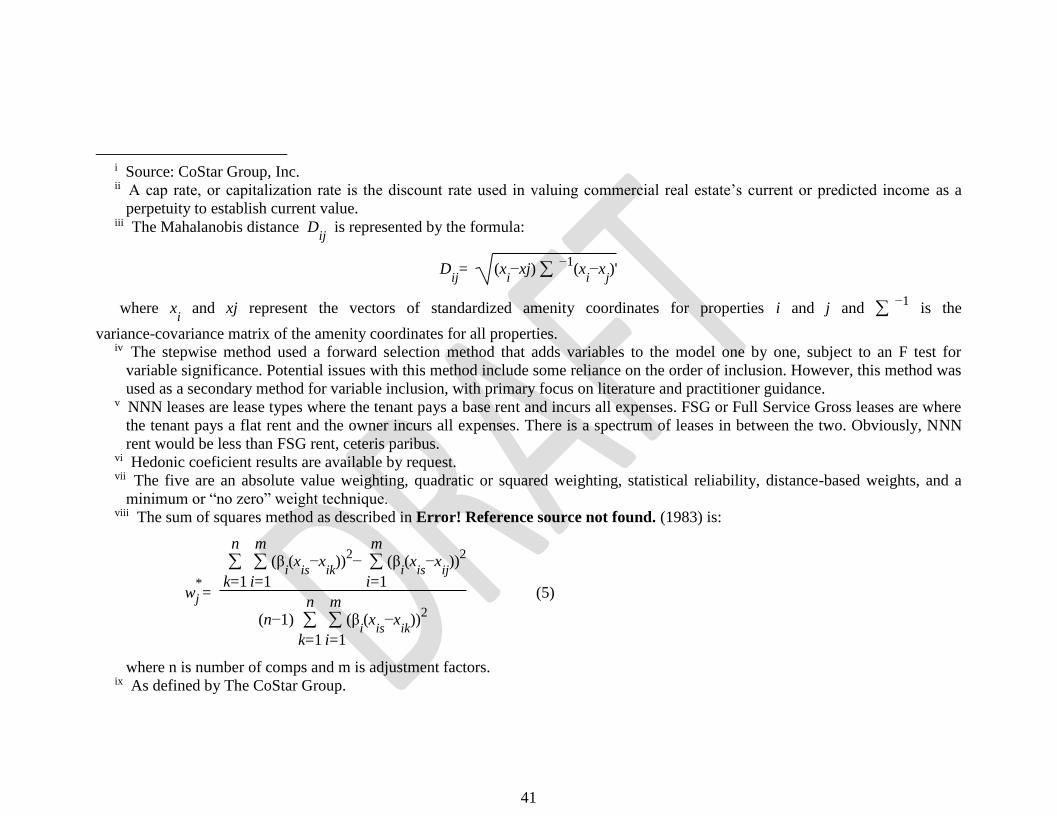
41

i Source: CoStar Group, Inc. ii A cap rate, or capitalization rate is the discount rate used in valuing commercial real estate’s current or predicted income as a

perpetuity to establish current value. iii The Mahalanobis distance D

ij is represented by the formula:

Dij= (x

i−xj)

−1(x

i−x

j)'

where xi and xj represent the vectors of standardized amenity coordinates for properties i and j and

−1 is the

variance-covariance matrix of the amenity coordinates for all properties. iv The stepwise method used a forward selection method that adds variables to the model one by one, subject to an F test for

variable significance. Potential issues with this method include some reliance on the order of inclusion. However, this method was

used as a secondary method for variable inclusion, with primary focus on literature and practitioner guidance. v NNN leases are lease types where the tenant pays a base rent and incurs all expenses. FSG or Full Service Gross leases are where

the tenant pays a flat rent and the owner incurs all expenses. There is a spectrum of leases in between the two. Obviously, NNN

rent would be less than FSG rent, ceteris paribus. vi Hedonic coeficient results are available by request. vii The five are an absolute value weighting, quadratic or squared weighting, statistical reliability, distance-based weights, and a

minimum or “no zero” weight technique. viii The sum of squares method as described in Error! Reference source not found. (1983) is:

w*

j =

k=1

n

i=1

m (β

i(x

is−x

ik))

2−

i=1

m (β

i(x

is−x

ij))

2

(n−1) k=1

n

i=1

m (β

i(x

is−x

ik))

2

(5)

where n is number of comps and m is adjustment factors. ix As defined by The CoStar Group.

42

x Each full set of data took 5-7 days to complete. Each full market sample is comprised of roughly 2,000 randomly drawn

properties, tested 500 times, for a total of 1 million tests. Each property averages over 8 comparables, using roughly 8 million

observations for each full set of 500 random draws. In addition, each full market samples is executed in four ways, for an

approximate total of 4 Million subject properties compared to 32 Million comps. xi Recent research by Robinson and Sanderford (2015) shows green variables may not be reliable indicators.

The Application of Hedonic Grid Regression to Commercial Real Estate

Documents

Transcript of The Application of Hedonic Grid Regression to Commercial Real Estate