PERGAMON

An International Joumal

computers & mathematics with applications

Computers and Mathematics with Applications 41 (2001) 269-280 www.elsevier.nl/locate/camwa

Frobenius-Chebyshev Polynomial Approximations with A Priori Error Bounds for Nonlinear Initial Value

Differential Problems

B . C H E N Department of Mathematics, University of Wyoming

Laramie, WY 82071-3036, U.S.A. bchenOuwyo, edu

R. GARCIA BOLdS AND L. JODAR Departamento de MatemAtica Aplicada

Universidad Polit6cniea de Valencia Valencia 46071, Spain

l j odar©mat, upv. es

(Received and accepted July 2000)

A b s t r a c t - - I n this paper, we present a method for approximating the solution of initial value ordinary differential equations with a priori error bounds. The method is based on a Chebyshev perturbation of the original differential equation together with the Frobenius method for solving the equation. Chebyshev polynomials in two variables are developed. Numerical results are presented. @ 2001 Elsevier Science Ltd. All rights reserved.

K e y w o r d s - - A priori error bound, Initial value problem, Differential equation, Chevyshev poly- nomials.

1. I N T R O D U C T I O N

In the recent paper [1], a new method has been proposed for constructing polynomial approxi- mations with a pr ior i error bounds of initial value problems of the type

y' = f ( x , y), y(0) = Y0. (1.1)

T h e m e t h o d presen ted in [1] is first based on the cons idera t ion of a p e r t u r b e d in i t ia l value p rob l e m

y' = B~( f ; x, y), y(O) = Yo, (1.2)

where B n ( f ; x, y) is an a p p r o p r i a t e Berns te in po lynomia l in two var iables . Then , the F roben ius

m e t h o d is app l i ed to (1.2) and fur ther t r un c a t i on of the infini te series solu~ion of (1.2) provides

the po lynomia l app rox ima t ion . The m e t h o d of [1] has many adwmtages and is one of the very

0898-1221/01/$ - see front matter @ 2001 Elsevier Science Ltd. All rights reserved. Typeset by Aj~g-~zX PII: S0898-1221 (00)00271-6

270 B. CHEN et al.

few methods which provide explicit a priori error bounds without assuming smoothness of the function f ( x , y) (see [2]). However, numerical experiments show an important drawback of the method of [1] from a computational point of view. The drawback comes from the fact that the approximating Bernstein polynomials converg6 very slowly, and even more, when the function is smooth, its Bernstein polynomials do not take advantage of this property to improve the rate of convergence, see [3]. In [2], Corliss describes another method with a priori error bounds for ordinary differential equations. He finds a rough estimate using Picard-Lindelbf iterations and then using truncated Taylor series for the solution, he can enclose the remainder. However, this method works only for equations with analytic right-hand sides, and furthermore, evaluating the derivatives for the Taylor series expansion is usually a very difficult and expensive task.

The aim of this paper is to preserve the advantages of the method proposed in [1] and to eliminate its deficiencies by replacing Bernstein polynomials with Chebyshev polynomials which not only converge much faster than the corresponding Bernstein polynomials, but have the added advantage that the convergence is greatly accelerated with the increasing smoothness properties. This paper is organized as follows. In Section 2, the Chebyshev polynomials in two variables are introduced. Chebyshev series of two-variable functions are defined and some important proper- ties of the coefficients of the Chebyshev series, obtained by [4] for the one-variable Chebyshev series are extended to the bidimensional framework. Section 3 deals with the error bounds of the two-variable truncated Chebyshev series. Section 4 adapts the results of [1] and the information of Chebyshev series obtained in Sections 2 and 3, in order to construct new polynomial approx- imations to the solution of (1.1). Numerical experiments showing the advantages of Chebyshev versus Bernstein approach are included.

2. C H E B Y S H E V POLYNOMIALS IN TWO VARIABLES

This section deals with the introduction of Chebyshev polynomials in two variables and it may be regarded as an extension of results given in Section 1.2 of [4] for the case of Chebyshev polynomials in one variable.

Let us denote by J the rectangle J = [-1, 1] × [-1, 1] and let E ( J ) be the set of all continuous real valued functions endowed with the inner product (,)q for f , g in E(J) , by

( f (x , y), g(x, y) )q = (f(cos O, cos 99), g(cos O, cos ~))q

~r 2 f(cos 0, cos ~)g(cos 0, cos ~) dO d~, (2.1)

which induces the norm

Ilfllq = ~ [f(cosO, cos~)[ 2 dOd~ , f C E(J) . (2.2)

We also consider the supremum norm defined by

Jlfll~ = max {If(x,Y)] , - 1 <_ x , y <_ 1}, f c E(J) . (2.3)

Let {Tn(x)}n> o be the one-variable Chebyshev polynomials defined by

To(x) = 1, TI(Z) = X , Tn+l(X ) = 2xTn(x) - Tn-l(X), n > 1. (2.4)

Considering the change of variable t = cos~, one gets Tn(t) = cos(~u), and normalizing, we obtain the Chebyshev basis in the set E ([-1, 1]) of all continuous real valued functions defined on the interval [-1, 1] defined by

¢0(cos~') = 1, ¢,,(cos~) = v~cos(n~), n > 1. (2.5)

Frobenius-Chebyshev Polynomial Approx imat ions 271

In accordance with [5], an orthogonal basis of E(J) is given by

r~m(x, y) = r,~(x)T,~(y), (2.6)

where {Tr,(X)}n> o is the Chebyshev basis of E ([-1, 1]). Note that by (2.4) one gets an explicit expression of Tn,m(x,y) in terms of Tn(x) and Tin(y). So, for instance,

T n + l , m T l ( x , y ) = ( 2 x T n ( x ) - T n - l ( X ) ) ( 2 y T r n ( Y ) - T m - l ( y ) ) , n >_ 1, m > 1.

Considering the substitution x -- cos 0, y = cos ~ with 0 _< 0, ~ <_ 7r, one gets

T~,~ (z, y) = T~,m (cos 0, cos ~) = Tn(cOs O)Tm(cos ~) = cos(n0) cos(m~). (2.7)

Since

if we define

{11 1 Itr.,.~(cos 0, cos ~)11~ =

17,---- m = 0,

r~ = 0 , ?i't > 0,

n > 0, m > 0,

or m = O , n > O ,

e~ = { v~, i=O, 1, i > 0 ,

we obtain the two-dimensional orthonormal Chebyshev basis {¢~m(x, y)}, where

2 • nm(cosO, cos~) = Yn,,(COSO, COS~). (2.S)

e n e m

The Chebyshev series for a function f (x , y) of the space E(J) takes the form

cos(n0) cos(nqo) (2.9) / (cos0, cos~) = 2 E E anm enem '

n>0 m>0

where

fo fo 2 f (cos O, cos ~)Tn (cos O)Tm (cos ~) dO d~ a n m - - 7r2ene m

(2.10) _ 2 f(cos O, cos p) cos(nO) cos(m~) dO d~.

7r2enem

Let us suppose that a function f in L2([0, 7r] x [0, 7r]) is orthogonal, with respect to the inner product defined by (2.1), to all Tnm defined by (2.7) with n > 0, m _> 0. Then

0 = ( f ( c o s O, cos ~), Thin(cos O, cos ~ ) ) q

= -~ fo~ fo" f ( cos O, cos ~ ) cos( nO ) cos( m(p ) dO d~, n ~ 0 , m ~ 0 .

Hence, the function gn (cos y)) = fo f(cos 0, cos ~) cos(n0) dO satisfies

g , d c o s , ) c o s ( m , ) d , = 0, m > 0.

Since, by [6, pp. 196-197], the one-variable Chebyshev polynomials are complete in L 2 ([0, 7r]), from the last expression it follows that gn = 0 for all n > 0. Hence,

- f (cos 0, cos q~) cos(n0) dO = O, 7r

n>_0.

272 B. CHEN et al.

By the completeness of {T,~}n_>0 and the last expression, it follows that f ( * , c o s : ) = 0. In an analogous way, from the orthogonality hypothesis 0 = (f(cos 0, cos : ) , Tn,m(COS 0, cos :))q, it follows that

/: hm(cos0) = f(cosO, cos:)cos(m:)d: = O, m > O.

From the completeness of {Tm}m_>0, one gets f (cos 0,*) = 0. This proves the completeness of {T~,m}~>_0,m~0 in L2([0, 7r] x [0, ~r]). Hence, the orthonormal system {~)n,m}n>_O,m>O is complete in E(J) and, for all f in E(J), one gets the Parseval equality

IlSll~ = E E la,-,~l 2 ( 2 . 1 1 ) n_>0 m>_0

Assume that f(x,y) and ~ ( x , y ) both lie in E(J), and consider the Chebyshev series of

°2/ (x,y) given by OxOy

02f(cos0, c o s : ) = 2 E E axy cos(n0)cos(m:) (2.12) 0(COS 0)0(cos : ) n>0 m>0 nm enem '

_ 2 r = r = : s ( cos 0, cos :) anm enem r:2 Jo Jo 0(cos 0)0(cos : )

cos(nO) cos(n:) dO d:. (2.13)

Integrating by parts for n _> 1, it follows that

/] L ~ cos c o s : ) sin(nO f(cos 0, cos : ) cos(nO) dO = 0=0

1 L ~ 0f(cos 0, cos : ) sin(n0) sin 0 dO + - n 0(cos 0)

1 /0 ~ Of(cos 0, cos : ) = n 0(cos 0) sin(n0) sip. 0 dO.

By (2.10) and (2.14) and taking into account the formula

we get

1 [cos((n - 1)0) - cos((n + 1)0)], sin 0 sin(n0) =

(11 - - I2) - - , n > l , m > 0 , anm en em,ff 2n _ _

L ~ L ~r Of(coSO, COS:) I1 = O(cosO) cos ((n - 1)O) cos(m:) dO d:,

L~ L ~ Of(cosO, cos:) I2 = 0(cos 0) cos ((m + 1)0) cos(m:) dO d:.

Integrating by parts (2.16) with respect to the variable : for m > 0, it follows that

1 f " f " Of(cosO, cos:) s i n : s i n ( m : ) c o s ((n - 1)0) d:dO. 11 = m J0 J0 0(cos0)0(cos : )

Taking into account the formula

1 [cos ((m - 1) : ) - cos ((m + 1) : ) ] , sin : s in(m:) =

(2.14)

(2.15)

(2.16)

(2.17)

(2.18)

Frobenius-Chebyshev Polynomial Approximat ions 273

equat ion (2.18) can be wri t ten as

1 fo '~ fo ~ O2f (cos0, cos~0) e o s ( ( m - 1 ) ~ ) c o s ( ( n - 1)0) d~dO I1 = ~ 0 (cos 0) 0 (cos ~) (2.19)

1 /o ~r fo ~r 02f (cos0, cosqo )cos ( (m + 1 )>~)cos ( (n - 1)~9)d~dO. 2m. 0 (cos 0) 0 (cos ~)

By the definition of the Chebyshev coefficients and (2.19), for n > 0, m > 0, it follows tha t

I , 1 [en- iem-1 xy e,~_l ,~y 1 7c2n 2nm ~ - - an_l ,m_l _~ a , _ t , m + l ] . (2.20)

Working with I2 in a similar way for n > O, m > O, one gets

I2 I [e.-1 ~, i xy ] -- [---~--an+l,m-1 -- ~%+1,,~+1] , n > 0, ',n > 0. (2.21)

7r2n 2rim

Subst i tu t ing (2.20) and (2.21) into (2.15), it follows tha t

era- 1 en- l ax~ 1,m- 1 xy xy my - - en- la n_ 1.m+l - - C n - lan+l,m-1 + an+l,m+l

aura = 4nm ' (2.22)

n > 0 , .nz > 0 .

Formula (2.22) provides for odd values of n in the following equations•

x y cry x y x y n = 1, 4 • 1 • rn • aim = e m - l e o a o , m - 1 - e o a o , m + l - e m - l a 2 , m - 1 -}- a2,m+l,

x y - - e x y x y x y n = 3, 4 • 3 • 7n • a3m = e m - l e 2 a 2 , m _ 1 -232,m+1 -- e m - l a 4 , m - t + a 4 , m + l ,

x y - - e x y x y x y ?~ --= 5 , 4 • 5 • ?Tt • a b m = C m - l e 4 a 4 , m - 1 434,m+1 -- e m - l a 6 , m - 1 + a 6 , m + l

Adding the above equations for n _> i + 1, with i odd, and using lirn~-~oc,,~-~ --~m°xY = 0 from

Parseval 's equality, one gets the following.

4m [(i + 1)ai+1,,~ + (i + 3)ai+3,m + (i + 5)ai+5,,, + ] = xy xy e (2.23) • " • e i e m - l a i , r n _ l - - a i , m + 1 i.

Considering odd values of m in (2.23), one gets the following•

r e = l , 4[(i + l)ai+l l + (i + 3)at+s,l + (i + 5)ai+5,1+ . . .] = x y .xy c i e o a i , 0 - - e, i~i ,2~

m = 3, 4 • 3 [(i + 1)ai+1,3 + (i + 3)ai+3,3 @ (i @ 5)ai+5, 3 -}-... ] ~- Gie2ai,2xY _ Cict:[~,~,

x y m = 5, 4 . 5 [(i + 1)ai+1,5 + (i + 3)a~+35 + (i + 5)ai+5,5 + . . . ] = e.ie4ai~y4 - eiai,6

Adding the above equat ions for m > j + 1, with j and i even, and taking into account tha t

• zy = O, it follows tha t [ l I n t t ~ o o , m , - + o o a n m

e.iej aZYij = 4 [(i + 1)(j + 1)ai+l , j+l + (i + 3)(j + 1)ai+:~ j+t, + (i + 5)(j + 1)a.i+5,j+~ (2.24)

+ . . . + (i + 1)(j + 3)a/+1,j+3 + (i + 3)(j + 3)a~+3,j+3 + (i + 5)(j + 3)ai+5d+3 + ' " ] .

Considering even values of n in (2.22), we can write the following.

:r y X y 'ra = 2, 4 . 2 [(i + 1)ai+L2 + (i + 3)a /+3 ,2 + (i + 5)a i+5 ,2 + . . . ] = eielail - ai3 el,

xy x~ 'm = 4, 4 . 4 [(i + 1)ai+1,4 + (i + 3)ai+3,4 + (i + 5)ai+5,4 + " " ] = eieaai3 - ai5 el,

x y x y m = 6, 4• 6 [(i + 1)ai+l,6 + (i + 3)a i+3 ,6 q- ( i q- 5 ) a i + 5 , 6 + . . . ] = eiebai5 - a i 7 e i

Adding the above equat ions for values of m > j + 1, with j odd and i even, it follows tha t

eieja,~j~v = 4 [(i + 1)(j + 1)ai+l,j+l + (i + 3)( j + 1)ai+,%y+l + (i + 5)( j + 1)a/+.~4+1 (2.25) + - . . + (i + 1)(j + 3)ai+1,j+3 + (i + 3)(j + 3)ai+3,j+3(i + 5)(j + 3)ai+5,j+3 + . . - ] .

Note tha t (2.25) coincides with (2.24) obta ined for the case where j was even•

274 B. CHEN et al.

Starting again from (2.22) for even values of n and adding the resulting equations for n _> i + 1 for odd values of i, one gets (2.23) for odd values of i. Summarizing, expression (2.23) holds true for all i _> 0, j _> 0, and it can be written in the following compact form:

xy _ 4 E j>~l (n + 2i -- 1)(m + 2j - 1)an+2i-l,m+2j-1, a n m e n e m i>l "

n > O , m_>0. (2.26)

Expression (2.26) relates the Chebyshev coefficients of ~ in terms of those of f(x, y), and it OxOy is a two-variable analog of expression (1.9) of [4].

3. THE T R U N C A T I O N OF T W O - V A R I A B L E S C H E B Y S H E V SERIES

°2f(c°s°'c°s ~') also in E(J). Consider the Chebyshev series Let f (cos 0, cos ~) be in E(J) with O(cos0)O(cos ~) of f (cos 0, cos ~)

f (cos 0, cos ~) = 2 E E aij cos(i0) cos( j~) , (3.1) i>_O j>O eieJ

and for n > 0, m > 0, let us consider the finite partial sum of (3.1) defined by

P n , m f (COS0, COS~) : 2 ~ ~ Cos(i0) Cos(j~) i=0 j=0 e i e j

(3.2)

and the residual series

(I -- Pn,m) f (COS 0 , COS(fl) = 2 E E aijC°s(iO) c°s(ri°) (3.3) i>n+l j > m + l e i e j

In this section, we are interested in finding bounds for the norm ]] (I - Pn,m)f][~, assuming certain differentiability hypothesis for f E E. By (2.22) and (3.3) for n > 0, m > 0, one gets

2

= 4 E E ei-lej-lai-l 'j-1 - ei-lai-l'j+l - e j - l a i + l ' j - 1 + a i + l ' j + l

i>n+l >m+l 4ij

= 4 1 e i - l e j - l a i _ l , j _ l -- e i - l a i _ l , j + l - e j - l a i + l , j _ l + a i+ l , j+ 1

E i>n+l j > m + l

By the Cauchy-Schwartz inequality the east equation is bounded by

4 xy xy xy xy

1 e i - l e j - l a i _ l , j _ 1 - e i - l a i _ l , j + 1 - e j - l a i + l , j _ 1 -~ a i + l , j + 1 j •

\ i>_n+l / i 1 j 1

Moreover, by applying the Cauchy-Schwartz inequality to the series

xy xy xy _ _ q- a i + l , i + 1 E e i - l e j - l a i - l ' j - 1 e i - l a x Y l e j - l a i + l ' j - 1

j>_rn+ l J '

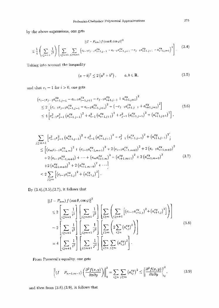
Probenius-Chebyshev Polynomial Approximat ions 275

by the above expressions, one gets

1 < - - 4

[(I - P,~m) f (cos0, cos ~)]2

1 ( e i_ l e j_ la iXY l , j _ l_e i_ ta i_ l . j+ l_e j_ la i+ l , j _ l +ai+l , j+l) ] . i 1 ~ i 1 1

Taking into account the inequality

(a ± b) 2 < 2 (a 2 + b2), a,b ~ R,

(3.4)

(3.5)

and that e z = 1 for i > 0, one gets

xy xy xy xy 2 ( e i _ l e j _ l a i _ l , j _ 1 - e i _ l a i _ l , j + 1 - e j _ l a i + l , j _ 1 + ai+l , j+l)

< 2 e i _ l e j _ l a i _ l , j _ 1-4-ci_l t~i_Lj+l } + ( - e j - l a i + l , j _ l + a i + l d + l

2 2 xy 2 e2 / xy ~2 e2 {aXY ~2 [ xy ~21 <_ 4 e i _ l e j _ l (ai_l , j_l) + i -1 [ai-~,j+l) + ~-1 ~ i+~,j-~) + [ai+l,j+l} J '

(3.6)

xy (aZy ~2] E 2 2 e xy ,2 2 / xy ,2 2 ( a i + l , j - 1 ) 2 + \ i+l,j+l] j e~- le j - l [a i - l , j - l ) + e i - l kai-l,j+l) +e j -1

j > m + l [I xy "~2 [ xy .~2 [ xy "~2 [ xy "~2

< L[eme.i_la.i_kmj + [ei_lai_l,m+ D + 2 [ei_lai_l.m+2] + 2 (ei_la~_l,m+3)

zy {aXY ~2 + 2 lazy ~2 + 2 (ei_lai_l,m+5) + " " q- (emaXYl,m) 2 + \ i+l,m+l] \ i+l,m+2/

+2{aXY ~2+2[aZy ~ 2 + . . . ] k i+1 ,m+3] \ i + l , m + 4 ]

[[ xy .~2 I xy .~2~ <_ 2 E [~e i - la i - l , J ) + ~ai+l,J) J

j>_m

By (3.4),(3.5),(3.7), it follows that

[(1 - Prim) f (c°s O, c°s ~)] 2

j_>m+l

1 Ey j>_m+l [1 j>_m+l

1 [~-la~_l,j) +lai+l,j) J

From Pavseval's equality, one gets

(i - 2 ; E E (aX?) 2 < 02 (x,y) i \ ÜxOy ][Iq ,>nj>m - OxOy '

(3.7)

(3.8)

(3.9)

and then from (3.8),(3.9), it follows that

276 B. CHEN et al.

I1( I - Pnm)fl{~ _ < a2(n)a2(m) ( I - Pnm) ~{02f(x'-Y)hoxOy filial2 _< a2(n)~r2(m) 02f(x,y i , (3.10)

where 2

(i + 1) 2 i > 0. (3.11)

By (3.10),(3.11), one gets

i f~ 2 --<:(0=2 ~ ~ <2 d~=-, kki+l

2 102f(x,y) q 11(/- P,,,~) fl]~ > - ~ ~ •

Summarizing, the following result has been proved.

THEOREM 3.1.

it:/(3.12) holds.

THEOREM 3.2.

(3.12)

PROOF. gets

II(±- P~)fll~-- ~ ~ laol 2 i>n+l j>m+l

xy xy xy 2 _ _ e j_ la i+l , j_ 1 : E E ( e i - l e j - l a i - l ' j - 1 ei- laXYl ' j+l q-ai+l ' j+l)

i>n+l j>m+l (4ij)2

-< 16(n + 1)2(m + 1) 2 E E [ei-lej-1 lai_l,j_ll + el-1 lai_l , j+ll i>_n+l j>_rn+l

+ej-1 [a,~l,j-l[ + [a,~l,j+,[] 2 1 [ zy aXY ~ 2

-< 8 (n+l )2 (m+1) 2 ~ ~ (ei-lej-1 lai_l,j_l[ +e,-1 i-1,i+1: i>_n+l j>_m+l

xy xy -{-(ej-1 lai+l,j_ll q-]a,+l,j+l]) 2]

1 [j xy < 4(n + 1)2(m + 1) 2 E E e2 e2 xy q_ ei-1 - , - 1 . 1 f a , - m . - x ? la,- .+il

i>_n+l >m+l

xy xy ] +4 la,+l,J-ll 2 -1 + la,+l,j+112

[ < 2(n + ]~)ff(m +1)2 E E e/2-1 a~y 2 , i+1,jl J -- i-- 1,j ~- axy [ 2] i>_n+l [j>_m

1 j~>m \ i kn+ l xy 2 a i + l ' J ) = ai-l ,J .q_ xy 2~ 2(n + 1)2(m + 1) 2

1 1

--< (~'z -'1- 1)2(m q- 1)2 j>~m" [ai'Jl) = (n + 1)2(m + 1)2 Eien ~>mY'~la~'[2

= 1 ( I - Pn-l,m-1) 02:(x'Y) < 1 02f(x,y) [ 2 (n + 1)2(m + 1) 2 OxOy - (n+l)2(m+l) ~ OxOy q"

Hence, (3.13) is established.

Let f be in E( J) with ~ lying in E( J). Then for n > O, m > O, inequal- axOy

With the hypothesis and notation of Theorem 3.1, it follows that

( 1 ) 1 02f(x,y) q (3.13) [[(I-Pnm)fllq -< ~ ~ OxOy "

By applying Parseval's equality to (3.3) and taking into account (2.22) and (3.5), one

Frobenius-Chebyshev Polynomial Approximations 277

COROLLARY 3.3.

Then 2 04f(z ,y) q

I[(I- Pn,m) f[[o~ < (ran)a~-----'- ~ Ox20y2 •

PROOF. By application of Theorem 3.2 to ~ it follows that O x O y '

( I - Ram) ( 02f ~ q < 1 04f kOxOy] -(~+1)(~+1) ~ ~

Then, from (3.12) and (3.15), one gets (3.14).

lies in E( J) Then COROLLARY 3.4. Let f be in E(J) such that for 1 < k < p oz~oy~

2 0 2p II(X- Pnm)fl[oo < (mn)(2p_l)/2 0xPOyP q"

~4 Let f be in E(J) with °--~J--rx .~ and ~ both in E(J) and let n > O, m > O.

O z O y ~, ' "~J

(3.14)

(3.15)

(3.16)

02(p--l) PROOF. By applying Theorem 3.2 to go = ox,,-~oy,,-~, it follows that

1 0290 1 O2Pf II(I-Pnm)g01[q<_ ( m + l ) ( n + l ) ~ q = ( m + l ) ( n + l ) OxOy q"

020,--2) By application of Theorem 3.1 to gl = o~.-~Oy,,-~, one gets

2 02gl 2 0 2(p-l) q

]l(Z- Pnm)g, llo~ < ~ ~ q = ~ OxP_~OyP_, •

Also, from (3.17) and (3.18), it follows that

2 02p

(ran) a/2 ~ q"

02(p--3) f Considering g2 = oz,,-~oy,,-3 . . . . , gp-1 = f , by induction one gets (3.16).

(3.17)

(3.1s)

(3.19)

4. C O N S T R U C T I V E A P P R O X I M A T I O N S

Consider the initial value problem (1.1) where f : [a, b] x [c,d] ~ N satisfies the Lipschitz condition

[f(x, y l ) - f ( x , y 2 ) l ~ L [ y l - y 2 1 , a < x < b , c ~ _ y l , y 2 ~ d , (4.1)

where a _< 0 < b. Consider the substitution

(b - a)u + (b + a) (d - c)v + (d + e) x - - - - - , y = ,

2 2

where 2z - (b + a) 2y - (d + c)

U-- V = ( b - a) ' d - c

and

-1 <_ u, v < 1~

2 x - ( b + a ) 2 y - ( d + c ) ) 9(u,v) = g ~ - a ' -d----i = f (x ,~) .

Then the Chebyshev series of f (x , y) is given by

Tn(u)Tm(v) f ( x , y ) = g(u,v) = 2 Z ~ a n m ~ "

,~>_o m>o IITn,m(U, V)ll

(4.2)

(4.3)

(4.4)

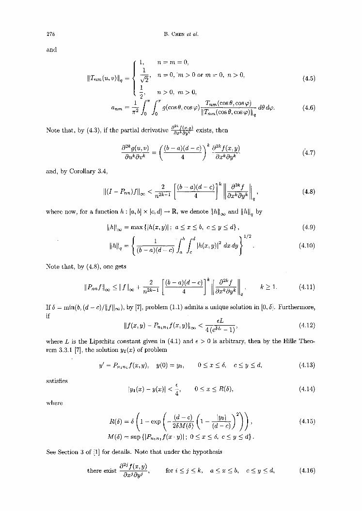
278 B. CHEN et al.

and

1 , n : m = O , 1

[ITnm(U,v)llq= , n = O , ' m > O o r m = O , n > 0 ,

1 -~, n > O, re>O,

1 [rr [~r Tnm(COSO, COSCfl) a,~m = 7"~ j ° Jo g ( c ° s O ' c ° s q ° ) ) [ ~ ~°s~-~]lq dOd~.

(4.5)

(4.6)

Note that, by (4.3), if the partial derivative ~ exists, then

02kg(u' v) = ( (b - a)(d - c) ) k O2k k 4 OxkOy k (a.7)

and, by Corollary 3.4,

2 [ ( b - a ) ( d - c ) ] k c92kf II(I-Pnn)fl]oo < ~ 4 ~ q' (4.8)

where now, for a function h : [a,b] x [c,d] -~ IR, we denote Ilhlloo and Ilhllq by

Ilhlloo = m a x { I h ( x , y ) l ; a < x < b, c < y < d},

1 - b d

IIhNq = ( b - a)-(d- c) Ih(x,y)l 2 dxdy

(4.9)

(4.10)

Note that, by (4.8), one gets

2 [ ( b - a ) ( d - c ) ] k 02kf IlPnnfIIoo < II/lloo + ~ [ J 4 ~ q ' k _> 1. (4.11)

If 5 = min(b, (d - c)/llfll~), by [r], problem (1.1) admits a unique solution in [0, 5]. Furthermore, if

EL Ilf(x'Y) - Pn'n ' f (x 'Y)l lm < 4(e aL - 1)' (4.12)

where L is the Lipschitz constant given in (4.1) and e > 0 is arbitrary, then by the Hille Theo- rem 3.3.1 [7], the solution yl(x) of problem

y ' = P n l n l f ( x , Y ) , y(0)=y0, 0 < x < 5 , c < y < _ d , (4.13)

satisfies

where

[ y l ( X ) -- y(X)I < ~, 0 < x < R(5) , ( 4 . 1 4 )

R ( 6 ) = 5 1 - e x p ~37r('~ 1 ( d - c ) ]

M(5) = sup{Ign,nl f (x" Y)I; 0 < z < 5, c _< y < d}.

(4.15)

See Section 3 of [1] for details. Note that under the hypothesis

o 2j y (z, y) there exist OxJOyJ ' f o r i < j < k , a < x < b , c < _ y < d , (4.16)

Frobenius-Chebyshev Polynomial Approximations 279

by (4.8), condition (4.12) holds if nl satisfies

2 [ ( b - a ) ( d - c ) ] k 02kf eL n~ k-1 4 ~ q < 4(e 6L-1)

or

n l >

cq2k 8 (e ~L - 1)[(b - a)(d - c)/4] k ~ q

Le

1/(2k-l)

REMARK 1. By (4.8), the quantity M(5) appearing in (4.15) can be computed as

(4.17)

2 [ ( b - a ) ( d - c ) ] k { 0 2 k f } / ~ f ( 5 ) = l l f [ I o c - ~ 4 sup ~ ; O < x < 5 , c < y < d . (4.18)

Following the ideas developed in [1], if

y = E a n x n , 0 < x <R, (4.19) n>0

is the series solution of problem (4.13) obtained by the Frobenius method, see [8], taking 0 < Ro(5) < R(5) and the first natural number no satisfying

In [(3e5 (R(5)-Ro(5))3)/(d(Ro(5)+ R(5))3 [ (R(5)-Ro(5)) 2 +45 (Ro(5)+ 3K(5))] ) ]

no > In (4Ro(5)/(Ro(5)+R(5))) , (4.20)

then the truncation of degree no of y(x), denoted by y(x, no), then

3e l y ( z ) - y ( x , no)L < 0 < x <

The explicit construction of the approximation is as follows. Let

Pnlntf(x,Y) = E E bjkxjyk j=O k=0

(4.21)

(4.22)

be the explicit expansion of the Chebyshev polynomial Pnl,~lf(x,y), then from expressions (4.13)-(4.17) of [1], y(x, uo)is given by

y(x, no)= ao + nix +.. . + anox n°, (4.23)

where

a0 = yo, (4.24)

Ah(k) = E amlam: "" "hmk, (4.25) ml +m2.-}-...mk=h

min(i,nl)

Cik= E bpkAi-p(h), (4.26) p=O

1 ~nl

a~+l -- i + 1 ~ c i k ' 0 < i < no - 1. (4.27) k=O

Summarizing, the following result has been established.

280 B. CHEN et al.

THEOREM 4.1. Consider problem (1.1) where f (x, y) is continuous and satisfies (4.1) and (4.16). Let ~ > 0 and 5 = min(b, (d - c)/llfllo~), where Ilfll~ is defined by (4.9). Let nl be the first positive integer satisfying (4.17) and let M(5) and R(5) be defined by (4.18) and (4.15), respec-

tively. Take R0(~) with 0 < Ro(~) < R(5) and let no be the first positive integer satisfying (4.20) and for 0 < i < no - 1, 0 < j , k < nl, define ao = yo, Ah(k) by (4.25), bjk by (4.22), and c~k by (4.26). Then the polynomial

y(x, no) = ao + alx ~- . . . ~- ano xn°,

where ai is defined by (4.27), is an approximation of the exact solution y of (1.1) satisfying

ly(x) - y(x, n0)l < e, 0 < x < R0(5).

In the following example, we compare the computational advantages of using Chebyshev poly- nomials versus Bernstein polynomials used in [1].

EXAMPLE. Consider problem (1.1) with Y0 = 0.5 and

y 2 + y - 1 f ( x , y ) - , O < x , y < 1.

x + l

Note that the above function f is twice continuously differentiable. So we can apply the results of Theorem 4.1 with k = 1. The following tables show the truncation degrees no and nl for the same values of the admissible error ~ using Bernstein treated in [1] and Chebyshev polynomials using the results of Theorem 4.1, for the values 5 = 1, R(5) = 0.117503, and Ro(5) = 0.1174.

Table 1. (Bernstein). Table 2. (Chebyshev).

10-1

10-2

10-3

10-4

n l no

6.47569.104 6.28184.104

6.47569.106 6.80636.104

6.47569. l0 s 7.33089.104

6.47569.101° 7.85542.104

£ n l nO

10 -1 27 61690

10 -2 87 66921

10 -3 276 72150

10 -4 873 77380

The results could be even better taking into account that function f admits higher-order partial derivatives that correspond to k > 1. This is one of the main advantages of the Chebyshev approach: the smoothness of f can be used to reduce the computational cost.

R E F E R E N C E S

1. L. J6dar, A.E. Posso and H. Castej6n, Constructive polynomial approximation with a priori error bounds for nonlinear initial value differential problems, Computers Math. Applic. 38 (7/8), 9-19, (1999).

2. G.F. Corliss, Guaranteed error bounds for ordinary differential equations, In In Theory and Numeric of Ordi- nary and Partial Differential Equations, (Edited by M. Ainsworth, J. Levesley, W.A. Light and M. Marietta), pp. 1-75, Oxford University Press, (1995).

3. I.P. Natanson, Constructive Function Theory, Ungar, New York, (1964). 4. M. Urabe, Numerical solution of multi-point boundary value problems in Chebyshev series. Theory of the

method, Numer. Math. 9, 341-366, (1967). 5. H.L. Krall and I.M. ShelTer, Orthogonal polynomials in two variables, Annal. Mate. Pura Appl. 76, 325-376,

(1967). 6. G.B. Folland, Fourier Analysis and its Applications, Wadsworth and Brooks, Pacific Grove, CA, (1992). 7. E. Hille, Lectures on Ordinary Differential Equations, Addison Wesley, Reading, MA, (1969). 8. G. Birkhoff and G.C. Rota, Ordinary Differential Equations, 3 rd Edition, Wiley, New York, (1978).