Closed-Form Waiting Time Approximations for PollingSystems∗

M.A.A. Boon†

marko@win.tue.nlE.M.M. Winands ‡

emm.winands@few.vu.nlI.J.B.F. Adan†

iadan@win.tue.nl

A.C.C. van Wijk§

a.c.c.v.wijk@tue.nl

October 21, 2009

Abstract

A typical polling system consists of a number of queues, attended by a single server in afixed order. The present study derives closed-form approximations for the mean waiting timesand mean marginal queue lengths of polling systems with renewal arrival processes, which canbe computed by simple calculations. The results of the present research may be very suitablefor the design and optimisation phase in many application areas, such as telecommunication,maintenance, manufacturing and transportation.

Keywords: Polling, waiting times, queue lengths, approximation

1 Introduction

Polling systems are queueing systems consisting of multiple queues, visited by a single server - typ-ically in a fixed, cyclic order. They find their origin in many real-life applications, e.g. (computer)communication, production and manufacturing environments, traffic and transportation. For a goodliterature overview of polling systems and their applications, we refer to surveys of, e.g., Takagi [15],Levy and Sidi [9], and Vishnevskii and Semenova [18]. When studying literature on polling systems,it rapidly becomes apparent that the computation of the distributions and moments of the waiting timesand marginal queue lengths is very cumbersome. Closed form expressions do not exist, and even whenone specifies the number of queues and solves the set of equations that leads to the mean waiting times,the obtained expressions are still too lengthy and complicated to interpret directly. Numerical proce-dures, both approximate and exact, have been developed in the past to compute these performance∗The research was done in the framework of the BSIK/BRICKS project, and of the European Network of Excellence

Euro-NF.†EURANDOM and Department of Mathematics and Computer Science, Eindhoven University of Technology, P.O. Box

513, 5600MB Eindhoven, The Netherlands‡Department of Mathematics, Section Stochastics, VU University, De Boelelaan 1081a, 1081HV Amsterdam, The

Netherlands§Department of Industrial Engineering & Innovation Sciences and Department of Mathematics and Computer Science,

Eindhoven University of Technology, P.O. Box 513, 5600MB Eindhoven, The Netherlands

1

measures. However, these methods have several drawbacks. Firstly, they are not transparent and actas a kind of black box. It is, for instance, rather difficult to study the impact of parameters like theoccupation rate and the service level. Secondly, these procedures are computationally complex andhard, if not impossible, to implement in a standard spreadsheet program commonly used on the workfloor. Finally, the vast majority of standard methods focusses on Poisson arrival processes, whichmay not be very realistic in many application areas. In the present paper we study polling systemsin which the arrival streams are not (necessarily) Poisson, i.e., the interarrival times follow a generaldistribution. The goal is to derive closed-form approximate solutions for the mean waiting times andmean marginal queue lengths, which can be computed by simple spreadsheet calculations.

Our approach in developing an approximation for the mean waiting times uses novel developments inpolling literature. Recently, a heavy traffic (HT) limit has been developed for the mean waiting timesas the system becomes saturated [17]. In the present paper we derive an approximation for the lighttraffic (LT) limit, i.e. as the load goes down to zero, which is exact for Poisson arrivals. The mainidea is to create an interpolation between the LT limit and the HT limit. This interpolation yields goodresults, and has several nice properties, like satisfying the Pseudo Conservation Law (PCL), and beingexact for symmetric systems with Poisson arrivals and in many limiting cases. These properties aredescribed in more detail in the present paper. In polling literature, several alternative approximationshave been developed before, most of which assume Poisson arrivals. For polling systems with Poissonarrivals and gated or exhaustive service, the best results, by far, are obtained by an approximationbased on the PCL (see, e.g., [2, 4, 7]). Fischer et al. [5] study an approximation for the mean waitingtimes in polling systems, which is also based on an interpolation between (approximate) LT and HTlimits. Their approach, however, is applied to a system with Poisson arrivals and time-limited service.Hardly any closed-form approximations exist for non-Poisson arrivals. The few that exist, performwell in specific limiting cases, e.g., under HT conditions [10, 17], or if switch-over times become verylarge [21, 22], but performance deteriorates rapidly if these limiting conditions are abandoned. Weshow in an extensive numerical study that the quality of our approximation can be compared to thePCL approximation for systems with Poisson arrivals, but provides good results as well for systemswith renewal arrivals.

Because of its simple form, the approximation function is very suitable for optimisation purposes.Although only the mean waiting times of systems with exhaustive or gated service are studied, theresults can be extended to higher moments and general branching-type service disciplines. Pollingsystems with polling tables and/or batch service can also be analysed in a similar manner.

The structure of the present paper is as follows: the next section introduces the model and the requirednotation, and states the main result. Section 3 illustrates how this main result is obtained, whileSection 4 provides results on the accuracy of the approximation for a large set of combinations ofinput parameter values. The last section discusses further research topics and possible extensions ofthe model.

2 Model description and main result

The model under consideration is a polling system consisting of N queues, Q1, . . . , QN , with renewalarrival processes. Indices throughout the present paper are understood to be modulo N : QN+1 actuallyrefers to Q1. Whenever a server switches from Qi to Qi+1, a random switch-over time Si is incurred.The generic service requirement of a customer arriving in Qi , also referred to as a type i customer, isdenoted by the random variable Bi . We make the usual independence assumptions for polling systems;

2

the interarrival times, service times and switch-over times are all independent. The moment at whichthe server switches from one queue to the next queue, is determined by the service discipline of thequeue that is being served. In the present paper we focus on polling systems in which each queue iseither served according to the gated service discipline, which states that during the course of a visitof the server to Qi , only those type i customers are served that were present at the beginning of thatvisit, or according to the exhaustive service discipline, which means that the server keeps on servingtype i customers until Qi is empty, before switching to Qi+1.

We regard several variables as a function of the load ρ in the system. Scaling is done by keepingthe service time distributions fixed, and varying the interarrival times. For each variable x that is afunction of the load in the system, ρ, its value evaluated at ρ = 1 is denoted by x . For ρ = 1, thegeneric interarrival time of the stream in Qi is denoted by Ai . Reducing the load ρ is done by scalingthe interarrival times, i.e., taking the random variable Ai := Ai/ρ as generic interarrival time at Qi .After scaling, the load at Qi becomes ρi = ρ E[Bi ]

E[ Ai ]. The (scaled) rate of the arrival stream at Qi is

defined as λi = 1/E[Ai ]. Similarly, we define arrival rates λi = 1/E[ Ai ], and proportional load atQi , ρi =

ρiρ

(“proportional” because∑N

i=1 ρi = 1). The system is assumed to be stable, so ρ is variedbetween 0 and 1.

We use B to denote the generic service requirement of an arbitrary customer entering the system, with

E[Bk] =

∑Ni=1 λiE[Bk

i ]∑Nj=1 λ j

for any integer k > 0, and S =∑N

i=1 Si denotes the total switch-over time in

a cycle. Finally, the (equilibrium) residual length of a random variable X is denoted by X res, withE[X res

] =12E[X

2]/E[X ].

We now present the main result of this paper, which is a closed-form approximation formula for themean waiting time E[Wi ] of a type i customer as a function of ρ:

E[Wi,app] =K0,i + K1,iρ + K2,iρ

2

1− ρ, i = 1, . . . , N . (2.1)

The constants K0,i , K1,i , and K2,i depend on the input parameters and the service discipline. If allqueues receive exhaustive service, the constants become:

K0,i =E[Sres], (2.2)

K1,i =ρi(E[ Ai ]gi (0)− 1

)E[Bres

i ] + E[Bres] + ρi

(E[Sres

] − E[S])−

1E[S]

N−1∑j=0

j∑k=0

ρi+kVar[Si+ j ],

(2.3)

K2,i =1− ρi

2

∑Nj=1 λ j

(Var[B j ] + ρ

2jVar[ A j ]

)∑N

j=1 ρ j (1− ρ j )+ E[S]

− K0,i − K1,i . (2.4)

3

If all queues receive gated service, we get:

K0,i =E[Sres], (2.5)

K1,i =ρi(E[ Ai ]gi (0)− 1

)E[Bres

i ] + E[Bres] + ρiE[Sres

] −1

E[S]

N−1∑j=0

j∑k=0

ρi+kVar[Si+ j ],

(2.6)

K2,i =1+ ρi

2

∑Nj=1 λ j

(Var[B j ] + ρ

2jVar[ A j ]

)∑N

j=1 ρ j (1+ ρ j )+ E[S]

− K0,i − K1,i . (2.7)

The term gi (t) is the density of Ai , the interarrival times at ρ = 1. This term is discussed in moredetail in the next section, but for practical purposes it is useful to know that E[ Ai ]gi (0) can be verywell approximated by

E[ Ai ]gi (0) ≈

2cv2

Aicv2

Ai+1

if cv2Ai> 1,(

cv2Ai

)4 if cv2Ai≤ 1,

where cv2Ai

is the squared coefficient of variation (SCV) of Ai (and, hence, also of Ai ). Note thatthis simplification results in an approximation that requires only the first two moments of each inputvariable (i.e., service times, switch-over times, and interarrival times).

Remark 2.1 In case of Poisson arrivals, the constants K1,i and K2,i simplify considerably. E.g., forexhaustive service they simplify to:

K Poisson1,i =E[Bres

] + ρi(E[Sres

] − E[S])−

1E[S]

N−1∑j=0

j∑k=0

ρi+kVar[Si+ j ],

K Poisson2,i =(1− ρi )

(E[Bres

]∑Nj=1 ρ j (1− ρ j )

+E[S]

2

)− K0,i − K Poisson

1,i .

The derivation of this approximative formula for the mean waiting time is the topic of the next section.An approximation for the mean queue length at Qi , E[L i ] is obtained by application of Little’s Lawto the sojourn time of type i customers, i.e. the waiting time plus the service time. As a function of ρ,we have

E[L i,app] = ρE[Wi,app] + E[Bi ]

E[ Ai ].

3 Idea behind the approximation

In the present section, we explain the idea behind approximation (2.1) for E[Wi ]. The restrictionsthat we impose on our approximation, are firstly that the formula should be closed-form, and easy toimplement, since these are necessities for optimisation purposes and implementation in a spreadsheet.Secondly, we want the approximation to capture the light traffic limit, i.e. ρ ↓ 0, and high traffic limit,i.e. ρ ↑ 1, behaviour in an exact way. Based on these restrictions, we have chosen the form

E[Wi,app] =K0,i + K1,iρ + K2,iρ

2

1− ρ, i = 1, . . . , N .

4

It is proved in [17] that capturing the HT behaviour in an exact way, requires the (1 − ρ) term inthe denominator. This term is not surprising at all, because the mean waiting times of practically allqueueing systems show this behaviour (the best known exception is an M/G/1 queue with shortestremaining processing time policy [13]). The motivation for taking a polynomial in the numeratorof (2.1) can be found in several other approximations based on interpolation between LT and HTlimits. E.g., Reiman and Simon [11] (see also [14]), and Whitt [19] use this approach to developapproximations for the mean waiting time in, respectively, queueing systems with Poisson input andG I/G/1 queues. A second-order polynomial fulfills the need for simplicity, and is sufficient to obtainan approximation which is exact for the two limiting situations (and, as is shown in Subsection 3.4, inmany other limiting cases).

The remainder of this section is devoted to finding the constants K0,i , K1,i , and K2,i . The requirementfor the interpolation is an approximation for E[Wi ] in light traffic. No such approximation exists inexisting literature, so the next subsection is devoted to finding one. We can use this LT expression tofind constants K0,i and K1,i in (2.1). The last unknown in the interpolation, K2,i , is obtained using theHT limit of the mean waiting time, which has been found quite recently [17].

3.1 Light traffic

The mean waiting times in the polling model under consideration in light-traffic, have been studiedin Blanc and Van der Mei [1], under the assumption of Poisson arrivals. They obtain expressionsfor the mean waiting times in light traffic that are exact up to (and including) first-order terms inρ. These expressions have been found by carefully inspecting numerical results obtained with thePower-Series Algorithm, but no proof is provided. In the present section we shall not only prove thecorrectness of the light-traffic results in a system with Poisson arrivals, but also use them as base for anapproximation for the mean waiting times in polling systems with renewal interarrival times. The keyingredient to the LT analysis of a polling system, is the well-known Fuhrmann-Cooper decomposition[6]. It states that in a vacation system with Poisson arrivals the queue length of a customer is the sumof two independent random variables: the number of customers in an isolated M/G/1 queue, and thenumber of customers during an arbitrary moment in the vacation period. The distributional form ofLittle’s Law [8] can be used to translate this result to waiting times. Since no independence is requiredbetween the length of a vacation and the length of the preceding visit period, this decomposition alsoholds for polling systems with Poisson arrivals. We introduce Vi to denote the length of a visit periodto Qi , and Ii to denote the length of the intervisit period, i.e. the time that the server is away betweentwo successive visits to Qi . Using Ci to denote the cycle time, starting at a visit beginning to Qi , wehave E[Vi ] = ρiE[Ci ] and E[Ii ] = (1−ρi )E[Ci ]. It is well-known that the mean cycle time in pollingsystems, unlike higher moments, does not depend on the starting point: E[Ci ] = E[C] = E[S]

1−ρ .

The Fuhrmann-Cooper decomposition, applied to the mean waiting time, results in:

exhaustive: E[Wi ] = E[Wi,M/G/1] + E[I resi ], (3.1)

gated: E[Wi ] = E[Wi,M/G/1] + E[I resi ] +

E[Vi Ii ]

E[Ii ]. (3.2)

For our approximation, we assume that this decomposition also holds for renewal arrival processesin light traffic. Determining the LT limit of the mean waiting time, E[W LT

i ], in a polling system withexhaustive or gated service is based on the following two-step approach. The first step is to find theLT limit of E[Wi,G I/G/1], the mean waiting time of a G I/G/1 queue with only type i customers in

5

isolation, i = 1, . . . , N . The second step is determining E[I resi ], the mean residual intervisit time of

Qi , and E[Vi Ii ]E[Ii ]

, the mean visit time of Qi given that it is being observed at a random epoch during thefollowing intervisit time.

For the LT limit of the mean waiting time in a G I/G/1 queue, we use Whitt’s result (Equation (16)in [19]), which gives:

limρi↓0

E[Wi,G I/G/1]

ρi=

1+ cv2Bi

2E[ Ai ]gi (0)E[Bi ], (3.3)

where cv2Bi

is the SCV of the service times, and gi (t) is the density of the interarrival times Ai . Forpractical purposes, it may be more convenient to express gi (0) in terms of the density of Ai , the genericinterarrival time of Qi in the scaled situation.The relation between the density of the scaled interarrivaltimes Ai (= Ai/ρ), denoted by gi (t), and the density of Ai , gi (t), is simply: gi (t) = ρ gi (ρt). Thismeans that the term E[ Ai ]gi (0) can be rewritten as

E[ Ai ]gi (0) = E[Ai ]gi (0).

Because of this equality, in the remainder of the paper we might use either notation. Since determin-ing E[ Ai ]gi (0) is a required step in the computation of our approximation for E[Wi ], we give somepractical examples.

Example 1 If the scaled interarrival times Ai are exponentially distributed with parameter λi :=

1/E[Ai ], we have gi (t) = λi e−λi t . This implies that E[Ai ]gi (0) = 1.

Example 2 In this example we assume that Ai follows a H2 distribution with balanced means. TheSCV of Ai is denoted by cv2

Ai. The density of this hyper-exponential distribution is (see, e.g., [16])

gi (t) = pµ1e−µ1t+ (1− p)µ2e−µ2t ,

with

p =12

1+

√√√√cv2Ai− 1

cv2Ai+ 1

,µ1 =

1E [Ai ]

1+

√√√√cv2Ai− 1

cv2Ai+ 1

,µ2 =

1E [Ai ]

1−

√√√√cv2Ai− 1

cv2Ai+ 1

.This leads to E[Ai ]gi (0) = 1+ cv2

A−1cv2

A+1= 2 cv2

Acv2

A+1.

Example 3 Now we assume that the interarrival times follow a mixed Erlang distribution. The densityof the scaled interarrival times is:

gi (t) = pµk−1tk−2

(k − 2)!e−µt+ (1− p)

µk tk−1

(k − 1)!e−µt ,

6

i.e., a mixture of an Erlang(k − 1) and an Erlang(k) distribution with

k =

⌈1

cv2Ai

⌉,

p =

k cv2Ai−

√k(1+ cv2

Ai)− k2 cv2

Ai

1+ cv2Ai

,

µ =k − pE[Ai ]

.

If k > 2, this leads to E[Ai ] gi (0) = 0.

The distributions in Examples 1 − 3 are typical distributions to be used in a two-moment fit if theSCV of the interarrival times is respectively 1, greater than 1, and less than 1 (cf. [16]). The examplesillustrate how E[Ai ]gi (0) can be computed if the density of the (scaled) interarrival times is known.If no information is available about the complete density, but the first two moments of Ai are known,Whitt suggests to use the following approximation for E[Ai ]gi (0):

E[Ai ]gi (0) =

2cv2

Aicv2

Ai+1

if cv2Ai> 1,(

cv2Ai

)4 if cv2Ai≤ 1,

where cv2Ai

is the squared coefficient of variation of the interarrival times of Qi . This approximationis exact for cv2

Ai> 1, if the interarrival time distribution is a hyper-exponential distribution as dis-

cussed in Example 2. For cv2Ai≤ 1, the approximation is rather arbitrary, but Example 3 shows that

E[Ai ]gi (0) becomes small (or even zero) very rapidly as cv2Ai

gets smaller.

Summarising, the LT limit of a G I/G/1 queue (ignoring O(ρ2i ) terms and higher) is:

E[W LTi,G I/G/1] = ρi E[Ai ]gi (0)E[Bres

i ]. (3.4)

For Poisson arrivals (E[Ai ]gi (0) = 1), it is known that E[Wi,M/G/1] =ρi

1−ρiE[Bres

i ] = ρiE[Bresi ] +

O(ρ2i ), which is consistent with our approximation.

The second step in determining the LT limit of the mean waiting time of a type i customer in a pollingsystem, is finding the LT limits of E[I res

i ], the mean residual intervisit time of Qi , and (for gatedservice only) E[Vi Ii ]

E[Ii ], the mean visit time Vi given that it is observed from the following intervisit

time Ii . In this LT analysis we need to focus on first order terms only. Noting the fact that Ii =

Si + Vi+1 + Si+1 + · · · + Vi+N−1 + Si+N−1, we condition on the moment at which Ii is observed. Wedistinguish between two cases. The moment of observation either takes place during a visit time, orduring a switch-over time:

E[I LT,resi ] =

N−1∑j=1

E[Vi+ j ]

E[Ii ]E[I LT,res

i |observed during Vi+ j ]

+

N−1∑j=0

E[Si+ j ]

E[Ii ]E[I LT,res

i |observed during Si+ j ]. (3.5)

7

Observation during visit time. The probability that a random observation epoch takes place duringa visit time, say V j , is E[V j ]

E[Ii ], for any j 6= i . However, we are only interested in order ρ terms, so this

probability simplifies toE[V j ]

E[Ii ]=

ρ jE[C](1− ρi )E[C]

= ρ j +O(ρ2).

The fact that this probability is O(ρ), implies that all further O(ρ) terms in E[I LT,resi |observed during V j ]

can be ignored, because in LT we focus on first order terms only.

The length of the residual intervisit time is the length of the residual visit period of type j customers,V res

j , plus all switch-over times S j + · · · + Si−1, plus all visit times V j+1 + · · · + Vi−1. The first termsimplifies to E[V res

j ] = E[Bresj ] +O(ρ). The terms E[Vk |observed from V j ], k = j + 1, . . . , i − 1, in

light traffic, are all O(ρ). Summarising, the mean residual intervisit period when observed during V j

is simply a mean residual service time E[Bresj ], plus all mean switch-over times E[S j + · · · + Si−1],

plus O(ρ) terms:

E[I LT,resi |observed during V j ] = E[Bres

j ] +

i−1∑k= j

E[Sk] +O(ρ). (3.6)

Observation during switch-over time. We continue by determining the mean residual intervisitperiod, conditioned on a random observation epoch during a switch-over time, say S j , j = 1, . . . , N .The probability that such an epoch takes place during S j , is

E[S j ]

E[Ii ]=

E[S j ]

(1− ρi )E[C]=

E[S j ]

E[S]1− ρ1− ρi

=E[S j ]

E[S](1− ρ + ρi )+O(ρ2).

It becomes apparent from this expression that things get slightly more complicated now, because orderρ terms in the conditional residual intervisit time may no longer be neglected. The residual intervisittime now consists of the residual switch-over time Sres

j , plus the switch-over times S j + · · · + Si−1,plus all visit periods V j+1 + · · · + Vi−1. The length of a visit period Vk , for k > j , is the sumof the busy periods of all type k customers that have arrived during Si , . . . , S j−1, Spast

j , Sresj , and

S j+1, . . . , Sk−1. By Spastj we denote the elapsed switch-over time during which the intervisit period

is observed, which has the same distribution as the residual switch-over time Sresj . Compared to an

observation during a visit time, it is more difficult to determine the conditional mean length of a busyperiod E[Vk |observed during S j ] under LT. We use a heuristic approach, which is exact if the arrivalprocess of type k customers is Poisson, and approximate it by:

E[Vk |observed during S j ] ≈ ρk

∑l 6= j

E[Sl] + E[Spastj ] + E[Sres

j ]

+O(ρ2), k = j+1, . . . , i−1.

If Ak is exponentially distributed, the above expression is exact. Nevertheless, numerical experimentshave shown that this approximative assumption has no or at least negligible impact on the accuracy ofthe approximated mean waiting times. Summarising:

E[I LT,resi |observed during S j ] ≈

j−1∑k=i

E[Sk]( i+N−1∑

l= j+1

ρl)+ E

(Spast

j

) ( i+N−1∑k= j+1

ρk)+ E

(Sres

j

) (1+

i+N−1∑k= j+1

ρk)

+

i+N−1∑k= j+1

E[Sk](1+

i+N−1∑l= j+1

ρl)+O(ρ2). (3.7)

8

The expression for I resi under light traffic conditions now follows from substituting (3.6) and (3.7) in

(3.5). The result can be rewritten to:

E[I LT,resi ] ≈

i+N−1∑j=i+1

ρ jE[Bresj ] +

i+N−1∑j=i+1

ρ j

i+N−1∑k= j

E[Sk]

+

i+N−1∑j=i

12E[S]

E (S2j

) (1− ρ + ρi + 2

i+N−1∑k= j+1

ρk)

+1

E[S]

j−1∑k=i

E[S j ]E[Sk]( i+N−1∑

l= j+1

ρl)+

i+N−1∑k= j+1

E[S j ]E[Sk](1− ρ + ρi +

i+N−1∑l= j+1

ρl)

+O(ρ2)

=

i+N−1∑j=i+1

ρ jE[Bresj ] +

i+N−1∑j=i+1

ρ j

i+N−1∑k= j

E[Sk]

+ (1− ρ + ρi )E[Sres] +

1E[S]

i+N−1∑j=i

i+N−1∑k=i

E[S j Sk]( i+N−1∑

l= j+1

ρl)+O(ρ2)

=E[Sres] + ρE[Bres

] − ρiE[Bresi ] + ρi

(E[Sres

] − E[S])−

1E[S]

N−1∑j=0

j∑k=0

ρi+kVar[Si+ j ]

+O(ρ2), (3.8)

for i = 1, . . . , N . The last step in (3.8) follows after some straightforward (but tedious) rewriting.

The Fuhrmann-Cooper decomposition of the mean waiting time for customers in a polling systemwith gated service (3.2), also requires computing E[Vi Ii ]

E[Ii ]under LT conditions. Here, again, we have

to resort to using a heuristic and use E[Vi Ii ]E[Ii ]

= ρiE[S] + O(ρ2), because this value is exact in thecase of Poisson arrivals. Intuitively this term can be explained by observing that the only thing thatchanges for gated service, compared to exhaustive service, is that type i customers arriving during Vi

are not served until the next cycle. As we have seen before, the probability of a type i arrival takingplace during Vi is ρi + O(ρ2). The mean residual cycle, observed from a random epoch in Vi , isE[C res

i |observed during Vi ] = E[S] + O(ρ). Combined, this gives E[Vi Ii ]E[Ii ]

= ρiE[S] + O(ρ2), in thecase of Poisson arrivals. If the arrival process is not Poisson, this is not exact, but we use it as anapproximation.

Having made all required preparations, we are ready to formulate the main result of the present sub-section. Under light traffic, an approximation for the mean waiting time of a type i customer in apolling model with general arrivals and respectively exhaustive and gated service in Qi , is:

E[W LT,exhi ] ≈E[Sres

] + ρi (E[ Ai ]gi (0)− 1)E[Bresi ] + ρE[B

res] + (ρ − ρi ) (E[S] − E[Sres

])

+1

E[S]

i+N−1∑k=i+1

ρk

k−1∑j=i

Var[S j ] +O(ρ2), i = 1, . . . , N , (3.9)

E[W LT,gatedi ] ≈E[W LT,exh

i ] + ρiE[S], (3.10)

where gi (t) is the density of the interarrival times of type i customers at ρ = 1. Equation (3.9) follows

9

from substitution of (3.4) and (3.8) in

E[Wi ] ≈ E[Wi,G I/G/1] + E[I resi ], i = 1, . . . , N . (3.11)

For Poisson arrivals, (3.9) en (3.10) are exact. The LT limit for polling systems with Bernoulli service(and Poisson arrivals) has been experimentally found in [1] and, indeed, it can be shown that theirresult for exhaustive service, which is a special case of Bernoulli service, agrees with our result aftersubstituting E[ Ai ]gi (0) = 1 in (3.9).

3.2 Heavy traffic

The mean delay in a polling system with renewal arrivals in HT, i.e. as ρ tends to 1, has been analysedin [17], where the following result has been obtained:

E[W HTi ] =

ωi

1− ρ+ o((1− ρ)−1), ρ ↑ 1. (3.12)

Obviously, in HT, all queues become unstable and, thus, E[Wi ] tends to infinity for all i . The rate atwhich E[Wi ] tends to infinity as ρ ↑ 1 is indicated by ωi , which is referred to as the mean asymptoticscaled delay at queue i , and depends on the service discipline. For exhaustive service,

ωi =1− ρi

2

(σ 2∑N

j=1 ρ j (1− ρ j )+ E[S]

), i = 1, . . . , N ,

with

σ 2:=

N∑i=1

λi

(Var[Bi ] + ρ

2i Var[ Ai ]

).

Here, the limits are taken such that the arrival rates are increased, while keeping the service-timedistributions fixed, and keeping the distributions of the interarrival times Ai (i = 1, . . . , N ) fixed upto a common scaling constant ρ. Notice that in the case of Poisson arrivals we have σ 2

= E[B2]/E[B].

For gated service, we have

ωi =1+ ρi

2

(σ 2∑N

j=1 ρ j (1+ ρ j )+ E[S]

).

3.3 Interpolation

Now that we have the expressions for the mean delay in both LT and HT, we can determine theconstants K0,i , K1,i , and K2,i in approximation formula (2.1). We simply impose the requirementsthat approximation (2.1) results in the same mean waiting time for ρ = 0 as the LT limit, and forρ ↑ 1 as the HT limit. Since (3.9) (and (3.10) for gated service) has been determined up to the firstorder of ρ terms, we also add the requirement that the derivative with respect to ρ, taken at ρ = 0,of our approximation is equal to the derivative of the LT limit. A more formal definition of theserequirements is presented below:

E[Wi,app]∣∣ρ=0 = E[Wi ]

∣∣ρ=0,

ddρ

E[Wi,app]∣∣ρ=0 =

ddρ

E[Wi ]∣∣ρ=0,

(1− ρ)E[Wi,app]∣∣ρ=1 = (1− ρ)E[Wi ]

∣∣ρ=1.

10

This leads to (2.1) as approximation for E[Wi ] in a polling system with general arrivals. ConstantsK0,i , K1,i , and K2,i are defined in (2.2)–(2.4) for systems with exhaustive service, or (2.5)–(2.7) forgated service.

3.4 Special cases

The approximation for the mean waiting time of a type i customer, E[Wi,app], has several nice proper-ties discussed in the remainder of this subsection.

Pseudo-conservation law. A well-known result in polling literature, is the pseudo-conservationlaw, derived by Boxma and Groenendijk [3] using the concept of work decomposition. This law givesthe following exact expression for the weighted sum of the mean waiting times in a polling systemwith Poisson arrivals:

N∑i=1

ρiE[Wi ] =ρ2

1− ρE[Bres

] + ρE[Sres] +

E[S]2

ρ2−∑N

j=1 ρ2j

1− ρ+

N∑j=1

E[Z j j ], (3.13)

where E[Z j j ] denotes the mean amount of work left behind in Q j at the completion of a visitof the server to Q j . It is shown in [3] that E[Z j j ] is the only term that depends on the servicediscipline. For exhaustive service E[Z j j ] = 0, for gated service E[Z j j ] = ρ2

jE[S]1−ρ . It can be

shown that our approximation satisfies the pseudo-conservation law in the case of Poisson arrivals: ifE[ Ai ]gi (0) = 1 for i = 1, . . . , N , then

∑Ni=1 ρiE[Wi,app] also equals the right-hand side of (3.13).

The derivation consists of basic, but cumbersome, algebraic manipulations only, and is therefore omit-ted. We only mention a helpful intermediate result:

∑Ni=1∑i+N

k=i+1∑k−1

j=i ρiρk = N∑N

i=1∑N

k=i ρiρk ,

so∑N

i=1∑i+N

k=i+1∑k−1

j=i ρiρkVar[S j ] =12

(ρ2+∑N

i=1 ρ2i

)Var[S]. Using this result, it follows that∑N

i=1 ρi K2,i = 0.

Light and heavy traffic. The light traffic limit of E[Wi ], given by (3.9) for exhaustive service andby (3.10) for gated service, is exact for Poisson arrivals. The heavy traffic limit (3.12) of E[Wi ] is evenexact for renewal arrivals. An appropriate choice of constants K0,i , K1,i and K2,i can reduce (2.1) toeither (3.9), (3.10), or (3.12). Since the LT and HT limits have been used in the set of equations thatdetermine the coefficients of the approximation, it goes without saying that E[Wi,app] is equal to (3.9)(or (3.10) for gated service) and (3.12), for ρ ↓ 0 and ρ ↑ 1 respectively. This implies that the LTlimit of our approximation is exact for Poisson arrivals, and the HT limit is exact for general arrivals.

Symmetric system. If ρi =1N for all i = 1, . . . , N , all Bi have the same distribution, and the

variances Var[Si ] of all switch-over times are equal, then our approximation is exact if all interarrival

11

distributions are exponential. For exhaustive service, we obtain

K1,i =E[Bres] +

N − 1N

E[S] −(

2−1N

)E[Sres

] +1

E[S]

i+N−1∑k=i+1

ρk

k−1∑j=i

Var[S j ]

=E[Bres] +

N − 1N

E[S] −(

2−1N

)E[Sres

] +N − 1

NVar[S]2E[S]

=E[Bres] +

(1−

1N

)E[S]

2− E[Sres

],

which means that E[Wi,app] = E[Wi,symm] (because K2,i = 0 in a symmetric system), with

E[Wi,symm] =ρ

1− ρE[Bres

] + E[Sres] +

ρ(1− 1N )

1− ρE[S]

2.

Note that we do not require that the mean switch-over times E[Si ] are equal. One can verify that thesame holds for gated service.

Single queue (vacation model). An immediate consequence of the fact that our approximation isexact in symmetric polling systems with Poisson arrivals, is that it also gives exact results for the meanwaiting time of customers in a single-queue polling system with Poisson arrivals. A polling systemconsisting of only one queue, but with a switch-over time between successive visits to this queue, isgenerally referred to as a queueing system with multiple server vacations.

Large switch-over times. For S deterministic, S→∞, and, again, under the assumption of Poissonarrivals, it is proven in [20, 21] that E[Wi ]

S →1−ρi

2(1−ρ) for exhaustive service. It can easily be verifiedthat our approximation has the same limiting behaviour:

limS→∞

E[Wi,app]

S=

1− ρi

2(1− ρ).

For gated service, E[Wi,app]

S →1+ρi

2(1−ρ) , which is also the exact limit (see, e.g., [20]).

Miscellaneous other exact results. The approximation is also exact in several other cases, all withPoisson arrivals, when the parameter values are carefully chosen. The relations between the inputparameters that yield exact approximation results become very complicated, especially in polling sys-tems with more than two queues. We only mention one interesting example here: our approximationgives exact results for a two-queue polling system with exhaustive service and

E[B1] = E[B2],E[S1] = E[S2], cv2A1= cv2

A2, cv2

B1= cv2

B2, cv2

S1= cv2

S2, (3.14)

if the following constraint is satisfied:

ρ =1+ I 2

Ai

2IAi

−cv2

Si

1+ cv2Bi

·E[Si ]

E[Bi ], (3.15)

where IAi =ρ1ρ2

is the ratio of the loads of the two queues. Obviously, if IAi = 1, the system issymmetric and our approximation gives exact results regardless of the other parameter settings.

12

4 Numerical study

4.1 Initial glance at the approximation

Before we study the accuracy of the approximation to a huge test bed of polling systems, we justpick a rather arbitrary, simple system to compare the approximation with exact results in order to getsome initial insights. Consider a three-queue polling system with loads of Q1, Q2, and Q3 divided asfollows: ρ1 = 0.1, ρ2 = 0.3, and ρ3 = 0.6. All service times and switch-over times are exponentiallydistributed, with mean 1. The interarrival times have SCV cv2

Ai= 3 for i = 1, 2, 3. In Figure 1 we

plot the approximated mean waiting time of Q2, E[W2,app], versus the load of the system ρ. Since thissystem cannot be analysed analytically, we compare the approximated values with simulated values.Both in the approximation and in the simulation we fit a H2 distribution as described in Example 2.

The errors are largest for Q2, which is the reason why we chose this queue in particular in Figure1. The most important information that this figure reveals, is that even though the accuracy of theapproximation is worst for this queue (a relative error of −4.47% for ρ = 0.7), the shape of the ap-proximation function is very close to the shape of the exact function, which makes it very suitable foroptimisation purposes. The maximum relative errors of Q1 and Q3 are 3.10% and 2.90% respectively.

In order to get more insight in the numerical accuracy of the approximation for a huge variety ofdifferent parameter settings, we create a large test bed in the next subsection and compare the approx-imation with exact or simulated results. It turns out that the maximum relative errors for most of thepolling systems are smaller than the one selected in the above example.

0.0 0.2 0.4 0.6 0.8 1.0Ρ

10

20

30

40EHW2L

Simulation

Approximation

Figure 1: Approximated and simulated mean waiting time E[W2] of Q2 of the example in subsection4.1.

4.2 Accuracy of the approximation

In the present section we study the accuracy of our approximation. We compare the approximatedmean waiting times of customers in various polling systems to the exact values. The complete testbed of polling systems that are analysed, contains 2304 different combinations of parameter values,all listed in Table 1. We show detailed results for exhaustive service first, and discuss polling systems

13

with gated service at the end of this section. We have varied the load between 0.1 and 0.9 with steps of

Parameter Notation ValuesNumber of queues N 2, 3, 4, 5Load ρ 0.1, 0.3, 0.5, 0.7, 0.9, 0.99SCV interarrival times cv2

Ai0.25, 1, 2

SCV service times cv2Bi

0.25, 1SCV switch-over times cv2

Si0.25, 1

Imbalance interarrival times IAi 1, 5Imbalance service times IBi 1, 5Ratio service and switch-over times ISi /Bi 1, 5

Table 1: Test bed used to compare the approximation to exact results.

0.2, and included ρ = 0.99 to analyse the limiting behaviour of our approximation when the load tendsto 1. The SCV of the interarrival times, cv2

Ai, is varied between 0.25 and 2. In case of non-Poisson

arrivals, i.e. cv2Ai6= 1, the exact values have been established through extensive simulation because

they cannot be obtained in an analytic way. In these simulations we fit a phase-type distribution to thefirst two moments of the interarrival times, as described in Examples 2 and 3. For service times andswitch-over times, only SCVs of 0.25 and 1 are considered. SCVs greater than 1 are less commonin practice and are discussed separately from the test bed later in this section. The imbalance ininterarrival times and service times, IAi and IBi , is the ratio between the largest and the smallest meaninterarrival/service time. The interarrival times are determined in such a way, that the overall mean isalways 1, λ1 is the largest and λN the smallest, and the steps between the λi are linear. E.g., for N = 5and IAi = 5 we get λi = 2 − i/3, i = 1, . . . , 5. The mean service times E[Bi ] increase linearly ini = 1, . . . , N , with E[BN ] = IBiE[B1] (so E[B1] is the smallest mean service time). They followfrom the relation

∑Ni=1 λiE[Bi ] = ρ. E.g., for N = 5, and IAi = IBi = 5 we get E[Bi ]/ρ = 3i/35.

The last parameter that is varied in the test bed, is the ratio between the mean switch-over times andthe mean service times, ISi /Bi =

E[Si ]E[Bi ]

. The total number of systems analysed is 4×6×3×25= 2304.

A system consisting of N queues results N mean waiting times, E[W1], . . . ,E[WN ], so in total these2304 systems yield 8064 mean waiting times. The absolute relative errors, defined as |o− e|/e, whereo stands for observed (approximated) value, and e stands for expected (exact) value, are computed forall these 8064 queues. Table 2 shows these relative errors (times 100%) categorised in bins of 5%. Inthis table, and in all other tables, results for systems with a different number of queues are displayed inseparate rows. The reader should keep in mind that the statistics in each row are based on 1

4×2304×Nabsolute relative errors, where N is the number of queues used in the specified row. Table 2 showsthat, e.g., 98.84% of the approximated mean waiting times in polling systems consisting of 3 queuesdeviate less than 5% from their true values. From Table 2 it can be concluded that the approximationaccuracy increases with the number of queues in a polling system. More specifically, for systems withmore than 2 queues, no approximation errors are greater than 10%, and the vast majority is less than5%. The mean relative errors for N = 2, . . . , 5 are respectively 2.18%, 0.93%, 0.70% and 0.57%. Itis also noteworthy, that 193 out of the 2304 systems yield exact results. All of these 193 systems havePoisson input, and all of them – except for one – are symmetric. The only asymmetric case for whichour approximation yields an exact result, happens to satisfy constraints (3.14) and (3.15).

In Table 3 the mean relative error percentages are shown for a combination of input parameter set-tings. The number of queues is always varied per row, while per column another input parameter is

14

varied. This way we can find in more detail which (combinations of) parameter settings result in largeapproximation errors. In Table 3(a) the load ρ is varied, and it can be seen that for a load of ρ = 0.7the approximation is least accurate. E.g., the mean relative error of all approximated waiting times inpolling systems consisting of 3 queues with a load of ρ = 0.7 is 1.69%. Table 3(b) shows the impactof the SCV of the interarrival times on the accuracy. Especially for systems with more than 2 queuesthe accuracy is very satisfactory, in particular for the case cv2

Ai= 1. In Table 3(c) the impact of imbal-

ance in a polling system on the accuracy is depicted, and, as could be expected, it can be concludedthat a high imbalance in either service or interarrival times has a considerable, negative, impact onthe approximation accuracy. Polling systems with more than 2 queues are much less bothered by thisimbalance than polling systems with only 2 queues.

N 0− 5% 5− 10% 10− 15% 15− 20%2 86.46 10.24 2.78 0.523 98.84 1.16 0.00 0.004 99.78 0.22 0.00 0.005 99.93 0.07 0.00 0.00

Table 2: Errors of the approximation applied to the 2304 test cases with exhaustive service, as de-scribed in Section 4, categorised in bins of 5%.

N Load (ρ)0.10 0.30 0.50 0.70 0.90 0.99

2 0.31 1.81 3.41 4.17 2.70 0.673 0.16 0.84 1.44 1.69 1.07 0.394 0.13 0.68 1.14 1.28 0.73 0.255 0.11 0.57 0.94 1.03 0.57 0.22

(a)

N SCV interarrival times (cv2Ai

)0.25 1 2

2 2.27 1.76 2.503 1.36 0.52 0.924 1.13 0.29 0.695 0.97 0.19 0.56

(b)

N Imbalance interarrival and service timesIAi = 1, IBi = 1 IAi = 1, IBi = 5 IAi = 5, IBi = 1 IAi = 5, IBi = 5

2 0.69 2.92 2.80 2.303 0.65 1.27 0.75 1.064 0.56 0.89 0.62 0.735 0.49 0.69 0.53 0.59

(c)

Table 3: Mean relative approximation error, categorised by number of queues (N ) and total load ofthe system (a), SCV interarrival times (b), and imbalance of the interarrival and service times (c).

15

4.3 Miscellaneous other cases

More queues. In this subsection we discuss several cases that are left out of the test bed becausethey might not give any new insights, or because the combination of parameter values might be rarelyfound in practice. Firstly, we discuss polling systems with more than 5 queues briefly. Without listingthe actual results, we mention here that the approximations become more and more accurate whenletting N grow larger, and still varying the other parameters in the same way as is described in Table1. For N = 10 already, all relative errors are less than 5%, with an average of less than 0.5% and itonly gets smaller as N grows further.

More variation in service times and switch-over times. In the test bed we only use SCVs 0.25 and1 for the service times and switch-over times, because these seem more relevant from a practical pointof view. As the coefficient of variation grows larger, our approximation will become less accurate.E.g., for Poisson arrivals we took cv2

Bi∈ {2, 5}, cv2

Si∈ {2, 5}, and varied the other parameters as in our

test bed (see Table 1). This way we reproduced Table 2. The result is shown in Table 4 and indicatesthat the quality of our approximation deteriorates in these extreme cases. The mean relative errorsfor N = 2, . . . , 5 are respectively 3.58%, 1.78%, 1.07%, and 0.77%, which is still very good forsystems with such high variation in service times and switch-over times. For non-Poisson input, noinvestigations were carried out because the results are expected to show the same kind of behaviour.

N 0− 5% 5− 10% 10− 15% 15− 20%2 74.22 14.84 6.51 2.083 89.76 7.29 2.08 0.694 94.53 4.56 0.91 0.005 97.71 2.19 0.10 0.00

Table 4: Errors of the approximation applied to the 768 test cases with Poisson arrival processes andhigh SCVs of the service times and switch-over times, categorised in bins of 5%.

Small switch-over times. Systems with small switch-over times, in particular smaller than the meanservice times, also show a deterioration of approximation accuracy - especially in systems with 2queues. In Figure 2 we show an extreme case with N = 2, service times and switch-over times areexponentially distributed with E[Bi ] =

940 and E[Si ] =

9200 for i = 1, 2, which makes the mean

switch-over times 5 times smaller than the mean service times. Furthermore, the interarrival timesare exponentially distributed with λ1 = 5λ2. In Figure 2 the mean waiting times of customers in bothqueues are plotted versus the load of the system. Both the approximation and the exact values areplotted. For customers in Q1 the mean waiting time approximations underestimate the true values,which leads to a maximum relative error of−11.2% for ρ = 0.7 (E[W1,app] = 0.43, whereas E[W1] =

0.49). The approximated mean waiting time for customers in Q2 is systematically overestimating thetrue value. The maximum relative error is attained at ρ = 0.5 and is 28.8% (E[W1,app] = 0.41,whereas E[W1] = 0.52). Although the relative errors are high in this situation, the absolute errors arestill rather small compared to the mean service time of an individual customer. This implies that themean sojourn time is already much better approximated. Nevertheless, this example illustrates one ofthe situations where our approximation gives unsatisfactory results.

16

0.0 0.2 0.4 0.6 0.8 1.0Ρ

2

4

6

8

10EHW1L

Exact

Approximation

0.0 0.2 0.4 0.6 0.8 1.0Ρ

2

4

6

8

10EHW2L

Figure 2: Approximated and exact mean waiting times for a two-queue polling system with smallswitch-over times.

4.4 Comparison with existing approximations

For non-exponential interarrival times hardly any good alternative approximations exist. In [10, 17]it is suggested to use the HT limit (3.12) as an approximation, but the accuracy is only found to beacceptable for ρ > 0.8. Another approximation for the mean waiting time in polling systems withnon-exponential interarrival times uses the limit for S → ∞ [21, 22]. This approximation is usableif either the total setup time in the system is large and the setup times have low variance, or the totalsetup time in the system is large and the system is in heavy traffic. The approximation discussedin the present paper is exact in all these limiting cases, but performs much better for systems underless extreme conditions. This makes our approximation the only one which can be applied under allcircumstances.

For polling systems with Poisson arrivals, several alternative approximations have been developed inexisting literature. The best one among them (see, e.g., [2, 4, 7]) uses the relation E[Wi ] = (1 ±ρi )E[C res

i ], where Ci is the cycle time, starting at a visit completion to Qi when service is exhaustive,and starting at a visit beginning for gated service. By ± we mean − for exhaustive service, and+ for gated service. The mean residual cycle time, E[C res

i ], is assumed to be equal for all queues,i.e. E[C res

i ] ≈ E[C res], and can be found by substituting E[Wi ] ≈ (1 ± ρi )E[C res

] in the pseudo-conservation law (3.13). We have used this PCL-based approximation to estimate the mean waitingtimes of all queues in the test bed described in Table 1, but taking only the 768 cases where C2

Ai= 1.

Table 5 shows the mean relative errors for our approximation (a) and the PCL approximation (b),categorised in bins of 5% as was done before in Table 2. From these tables (and from other performedexperiments that are not mentioned for the sake of brevity) it can be concluded that for N > 2both approximation have almost the same accuracy, our approximation being slightly better for smallvalues of ρ, and the PCL approximation being slightly better for high values of ρ (both methods areasymptotically exact as ρ ↑ 1). However, for N = 2 our method suffers greatly from imbalance inthe system, whereas the PCL approximation proves to be more robust.

4.5 Gated service

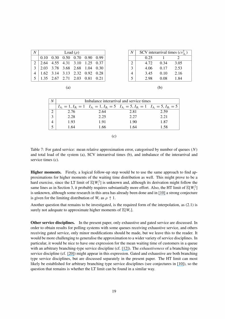
Until now we have only shown and discussed approximation results for polling systems with exhaus-tive service. The complete test bed described in Table 1 has also been analysed for polling systemswhere each queue receives gated service. As can be seen in Table 6, the overall quality of the ap-proximation is good, but worse than for polling systems with exhaustive service. More details on the

17

N 0− 5% 5− 10% 10− 15%2 89.32 9.11 1.563 100.00 0.00 0.004 100.00 0.00 0.005 100.00 0.00 0.00

(a)

N 0− 5% 5− 10% 10− 15%2 96.09 2.86 1.043 99.31 0.69 0.004 100.00 0.00 0.005 100.00 0.00 0.00

(b)

Table 5: Errors of the approximation applied to the 768 test cases with Poisson input, categorised inbins of 5%. In (a) the percentages of mean relative errors in each bin are shown for our approximation,in (b) results are shown for the PCL approximation.

reason for these inaccuracies can be found in Table 7, which is the equivalent of Table 3 for gated ser-vice. Table 7(b) illustrates that there is now a huge difference between systems with Poisson arrivals,and systems with non-Poisson arrivals. For the cases with cv2

Ai= 1, the approximation is extremely

accurate, even for two-queue polling systems. The accuracy in cases with cv2Ai6= 1 is worse, which

is caused by the assumptions that are made to approximate the LT limit (3.10). Firstly, the decompo-sition (3.2) does not hold for non-Poisson arrivals, and secondly, the terms E[I res

i ] and E[Vi Ii ]E[Ii ]

in thisdecomposition have only been approximated. For exhaustive service, these assumptions do not havemuch negative impact on the accuracy, but apparently, for gated service, they do. The mean relativeerrors for N = 2, . . . , 5 queues are respectively 2.70%, 2.25%, 1.90%, and 1.63%. The imbalance ofthe mean interarrival and service times hardly influences the accuracy of the approximation, as can beconcluded from Table 7(c).

If we consider the 768 cases with Poisson arrivals only, the mean relative errors of our approximationfor N = 2, . . . , 5 are respectively 0.34%, 0.17%, 0.10%, and 0.08%. This accuracy is even betterthan the one achieved by the PCL approximation.

N 0− 5% 5− 10% 10− 15% 15− 20%2 82.55 12.33 2.95 1.563 85.42 10.53 3.13 0.814 88.85 8.46 2.43 0.265 92.22 6.60 1.15 0.03

Table 6: Errors of the approximation applied to the 2304 test cases with gated service, as described inSubsection 4.5, categorised in bins of 5%.

5 Further research topics

The research that is done in the present paper can be extended in many different directions. In thissection we discuss some possibilities that we find most relevant.

18

N Load (ρ)0.10 0.30 0.50 0.70 0.90 0.99

2 2.64 4.55 4.31 3.10 1.25 0.373 2.03 3.78 3.68 2.68 1.04 0.304 1.62 3.14 3.13 2.32 0.92 0.285 1.35 2.67 2.71 2.03 0.81 0.21

(a)

N SCV interarrival times (cv2Ai

)0.25 1 2

2 4.72 0.34 3.053 4.06 0.17 2.534 3.45 0.10 2.165 2.98 0.08 1.84

(b)

N Imbalance interarrival and service timesIAi = 1, IBi = 1 IAi = 1, IBi = 5 IAi = 5, IBi = 1 IAi = 5, IBi = 5

2 2.76 2.64 2.81 2.593 2.28 2.25 2.27 2.214 1.93 1.91 1.90 1.875 1.64 1.66 1.64 1.58

(c)

Table 7: For gated service: mean relative approximation error, categorised by number of queues (N )and total load of the system (a), SCV interarrival times (b), and imbalance of the interarrival andservice times (c).

Higher moments. Firstly, a logical follow-up step would be to use the same approach to find ap-proximations for higher moments of the waiting time distribution as well. This might prove to be ahard exercise, since the LT limit of E[W 2

i ] is unknown and, although its derivation might follow thesame lines as in Section 3, it probably requires substantially more effort. Also, the HT limit of E[W 2

i ]

is unknown, although some research in this area has already been done and in [10] a strong conjectureis given for the limiting distribution of Wi as ρ ↑ 1.

Another question that remains to be investigated, is the required form of the interpolation, as (2.1) issurely not adequate to approximate higher moments of E[Wi ].

Other service disciplines. In the present paper, only exhaustive and gated service are discussed. Inorder to obtain results for polling systems with some queues receiving exhaustive service, and othersreceiving gated service, only minor modifications should be made, but we leave this to the reader. Itwould be more challenging to generalise the approximation to a wider variety of service disciplines. Inparticular, it would be nice to have one expression for the mean waiting time of customers in a queuewith an arbitrary branching-type service discipline (cf. [12]). The exhaustiveness of a branching-typeservice discipline (cf. [20]) might appear in this expression. Gated and exhaustive are both branchingtype service disciplines, but are discussed separately in the present paper. The HT limit can mostlikely be established for arbitrary branching type service disciplines (see conjectures in [10]), so thequestion that remains is whether the LT limit can be found in a similar way.

19

Optimisation. One of the main reasons to choose (2.1) as form of the interpolation, besides itsasymptotic correctness, is its simplicity. Having this exact and simple expression for the approximatemean waiting times, makes it very useful for optimisation purposes. In production environments,one can, for example, determine what the optimal strategy is to combine orders of different types(i.e., determine what queue customers should join). Because general arrivals are supported, one candetermine optimal sizes of batches in which items are grouped and sent to a specific machine. Thesimplicity of (2.1) makes it possible for a manager to create a handy Excel sheet that can be used byoperators to compute all kind of optimal parameter settings. No difficult computations are required atall, so a large variety of users can use the approximation.

In the present paper the accuracy of the approximation has been investigated and has been found tobe very good in most situations. Another advantage of our approximation regarding optimisationpurposes, is that the general shape of the approximated curve follows the exact curve very closely.Even in cases where the relative errors are rather large, like in Figure 1, the shape of the actual curvesis still very well approximated. This means that plugging our approximation, instead of an exactexpression if it had been available, in an optimisation function yields an optimum that should be closeto the true optimum.

Polling Table. The interpolation based approximation can also be extended to polling systems wherethe visiting order of the queues is not cyclic. Waiting times in polling systems with so-called pollingtables can be obtained in the same way as shown in the present paper. Both the LT and HT limits arenot difficult to determine in this situation, and the interpolation follows directly from these limits.

Model. The form of the interpolation might be changed to improve the accuracy of approximationsfor cases that give less satisfactory results in the present form. E.g., one could try other functions thana second-order polynomial as numerator of (2.1). Alternatively, one could try to find a correction termwhich could be added to (2.1) to obtain better results for, e.g., two-queue polling systems. But most ofall, if an exact LT limit of the mean waiting time in a polling system with non-Poisson arrivals couldbe found, the accuracy of the approximation in the case of gated service might be improved.

Acknowledgements

The authors wish to thank Onno Boxma for valuable discussions and for useful comments on earlierdrafts of the present paper.

References

[1] J. P. C. Blanc and R. D. van der Mei. Optimization of polling systems with Bernoulli schedules.Performance Evaluation, 22:139–158, 1995.

[2] O. J. Boxma. Workloads and waiting times in single-server systems with multiple customerclasses. Queueing Systems, 5:185–214, 1989.

[3] O. J. Boxma and W. P. Groenendijk. Pseudo-conservation laws in cyclic-service systems. Jour-nal of Applied Probability, 24(4):949–964, 1987.

20

[4] D. Everitt. Simple approximations for token rings. IEEE Transactions on Communications,COM-34(7):719–721, 1986.

[5] M. J. Fischer, C. M. Harris, and J. Xie. An interpolation approximation for expected wait in atime-limited polling system. Computers & Operations Research, 27:353–366, 2000.

[6] S. W. Fuhrmann and R. B. Cooper. Stochastic decompositions in the M/G/1 queue with gener-alized vacations. Operations Research, 33(5):1117–1129, 1985.

[7] W. P. Groenendijk. Waiting-time approximations for cyclic-service systems with mixed servicestrategies. In Proc. 12th ITC, pages 1434–1441. North-Holland Publ. Co., Amsterdam, 1989.

[8] J. Keilson and L. D. Servi. The distributional form of Little’s Law and the Fuhrmann-Cooperdecomposition. Operations Research Letters, 9(4):239–247, 1990.

[9] H. Levy and M. Sidi. Polling systems: applications, modeling, and optimization. IEEE Trans-actions on Communications, 38:1750–1760, 1990.

[10] T. L. Olsen and R. D. van der Mei. Polling systems with periodic server routing in heavy traffic:renewal arrivals. Operations Research Letters, 33:17–25, 2005.

[11] M. I. Reiman and B. Simon. An interpolation approximation for queueing systems with Poissoninput. Operations Research, 36(3):454–469, 1988.

[12] J. A. C. Resing. Polling systems and multitype branching processes. Queueing Systems, 13:409– 426, 1993.

[13] L. E. Schrage and L. W. Miller. The queue M/G/1 with the shortest remaining processing timediscipline. Operations Research, 14(4):670–684, 1966.

[14] B. Simon. A simple relationship between light and heavy traffic limits. Operations Research,40(Supplement 2):S342–S345, 1992.

[15] H. Takagi. Queuing analysis of polling models. ACM Computing Surveys (CSUR), 20:5–28,1988.

[16] H. C. Tijms. Stochastic models: an algorithmic approach. Wiley, Chichester, 1994.

[17] R. D. van der Mei and E. M. M. Winands. A note on polling models with renewal arrivals andnonzero switch-over times. Operations Research Letters, 36:500–505, 2008.

[18] V. M. Vishnevskii and O. V. Semenova. Mathematical methods to study the polling systems.Automation and Remote Control, 67(2):173–220, 2006.

[19] W. Whitt. An interpolation approximation for the mean workload in a G I/G/1 queue. Opera-tions Research, 37(6):936–952, 1989.

[20] E. M. M. Winands. Polling, Production & Priorities. PhD thesis, Eindhoven University ofTechnology, 2007.

[21] E. M. M. Winands. On polling systems with large setups. Operations Research Letters, 35:584–590, 2007.

[22] E. M. M. Winands. Branching-type polling systems with large setups. To appear in OR Spec-trum, 2009.

21