(Various Streets, Rhayader) (Prohibition of Waiting) Order 2016
Upload
khangminh22Category
view
3download
0
Operations MethodsManaging Waiting Line ApplicationsSecond Edition
Kenneth A. Shaw
Quantitative Approaches to Decision Making CollectionDonald N. Stengel, Editor
OPERATIO
NS M
ETHO
DS
SH
AW
Operations MethodsManaging Waiting Line Applications, Second EditionKenneth A. Shaw
Updated to integrate the management of associated infor
mation processes, expand some application discussions,
and provide additional reference material, the intent of this
monograph is to help business professionals use waiting
line (queuing) analysis methods to improve both service and
manufacturing business applications of queuing situations.
Emphasis is given to discussing the caveats in applying
waiting line theory and becoming aware of the assumptions
used in developing that theory. The importance of accounting
for variability in waiting line processes is discussed in some
detail because the basic queuing equations provide only
average performance data under steadystate conditions.
Understanding how much variability can exist for a given
waiting line scenario provides a manager with the insight
required to reduce these effects and develop innovative
solutions for improving service while reducing operating costs.
In general the mathematical tone of the book is focused
on applications, not the derivation of the formulas presented.
The few derivation exceptions illustrate some approaches not
commonly discussed in textbooks—for example, the use of
state diagrams and random number approximations of the
probability distributions for use in simple simulation models.
To aid in understanding the material presented, some
practical examples are given at appropriate points in the text
and some simulation approaches using common spreadsheet
software are described.
Kenneth (Ken) Shaw has a PhD and MS in electrical engineer
ing from Arizona State University and a BSEE from Purdue
University. His experience in industry was gained at a number
of hightechnology enterprises that include Naval Avionics
Facility, Royal Melbourne Institute of Technology, General
Electric, Motorola Semiconductor, Unisys, and four divisions
of HewlettPackard. He shared the lessons learned from that
experience as an adjunct professor teaching operations and
process management for the College of Business at Oregon
State University from 2003 to 2011.
Quantitative Approaches to Decision Making CollectionDonald N. Stengel, Editor
For further information, a free trial, or to order, contact:
[email protected] www.businessexpertpress.com/librarians
THE BUSINESS EXPERT PRESS DIGITAL LIBRARIES
EBOOKS FOR BUSINESS STUDENTSCurriculum-oriented, born-digital books for advanced business students, written by academic thought leaders who translate real-world business experience into course readings and reference materials for students expecting to tackle management and leadership challenges during their professional careers.
POLICIES BUILT BY LIBRARIANS• Unlimited simultaneous
usage• Unrestricted downloading
and printing• Perpetual access for a
one-time fee• No platform or
maintenance fees• Free MARC records• No license to execute
The Digital Libraries are a comprehensive, cost-effective way to deliver practical treatments of important business issues to every student and faculty member.
ISBN: 978-1-63157-085-8

Operations Methods

Operations Methods
Managing Waiting Line Applications
Second Edition
Kenneth A. Shaw, PhD
Operations Methods: Managing Waiting Line Applications, Second Edition
Copyright © Business Expert Press, LLC, 2016.
All rights reserved. No part of this publication may be reproduced, stored in a retrieval system, or transmitted in any form or by any means—electronic, mechanical, photocopy, recording, or any other except for brief quotations, not to exceed 400 words, without the prior permission of the publisher.
First published in 2011 byBusiness Expert Press, LLC222 East 46th Street, New York, NY 10017www.businessexpertpress.com
ISBN-13: 978-1-63157-085-8 (paperback)ISBN-13: 978-1-63157-086-5 (e-book)
Business Expert Press Quantitative Approaches to Decision Making Collection
Collection ISSN: 2163-9515 (print)Collection ISSN: 2163-9582 (electronic)
Cover and interior design by Exeter Premedia Services Private Ltd., Chennai, India
First edition: 2011Second edition: 2016
10 9 8 7 6 5 4 3 2 1
Printed in the United States of America.

Abstract
Updated to integrate the management of associated information pro-cesses, expand some application discussions, and provide additional reference material, the intent of this monograph is to help business professionals use waiting line (queuing) analysis methods to improve both service and manufacturing business applications of queuing situations. Emphasis is given to discussing the caveats in applying waiting line theory and becoming aware of the assumptions used in developing that theory. The importance of accounting for variability in waiting line processes is discussed in some detail because the basic queuing equations provide only average performance data under steady-state conditions. Understanding how much variability can exist for a given waiting line scenario provides a manager with the insight required to reduce these effects and develop innovative solutions for improving service while reducing operating costs.
In general the mathematical tone of the book is focused on applications, not the derivation of the formulas presented. The few derivation exceptions illustrate some approaches not commonly discussed in textbooks—for example, the use of state diagrams and random number approximations of the probability distributions for use in simple simulation models.
To aid in understanding the material presented, some practical exam-ples are given at appropriate points in the text and some simulation approaches using common spreadsheet software are described.
Keywords
arrival distributions, arrival rate, assembly line performance, cost trade-offs, deterministic process, Erlang distributions, Excel applications, exponential distribution, Kendall notation, limited population service, line capacity restrictions, Little’s law, Markovian, memoryless, multiple servers, normal distribution, poisson distribution, priority queues, queues, queuing theory, service classes, service distributions, service process design, service process improvement, service rate, simulation methods, state diagrams, stochastic process, triangular distribution, uniform distribution, utilization, variances, waiting lines, waiting time


Contents
Preface ��������������������������������������������������������������������������������������������������ixIntroduction ..........................................................................................xi
Chapter 1 Concepts, Probabilities, Models, and Costs .......................1Chapter 2 The Basics—Single-Channel, Single-Phase Model...........15Chapter 3 The Basics—Multiple-Channel, Single-Phase Model.......23Chapter 4 More Complex Single-Channel Models ..........................35Chapter 5 More Complex Multiple-Channel Models ......................55Chapter 6 Managerial Considerations .............................................71Chapter 7 Useful Tools and Simulation Methods ..........................109
Appendix A Glossary .......................................................................133Appendix B Symbol Definitions .......................................................141Appendix C Multiple-Channel Application Data ..............................145Appendix D Simulation Information ................................................155Appendix E Second Edition Supplements ..........................................163Notes��������������������������������������������������������������������������������������������������169References ...........................................................................................175Index .................................................................................................179


Preface
The initial impetus for writing this book was the product of several conversations with friends and colleagues, an accumulation of professional experiences, and interactions with business students and faculty regarding operations and process management improvements. This second edition augments the original content to include the important concept of integrating the management of information when improving waiting line processes. This concept is discussed separately in more detail in another Business Expert Press book by the author titled Integrated Management of Processes and Information (2013) for those readers who are interested. In addition, the content is revised in some of the chapters to answer some questions posed by astute readers and to provide some additional clarification and examples.
Nearly a decade ago, I retired from a long career that included individual and managerial responsibilities for a variety of engineering and business functions in several industries; many of these organizations were key players in the development of integrated circuit technology and computer applications. After a year or so working on restoring old cars, taking welding classes, and puttering around a small ranch property, the glow of retirement began to dim. When a former colleague approached me with the proposal of temporarily teaching an operations management course at the local university, I thought it would be an interesting challenge and agreed to do it. Little did I imagine then that this decision would lead to eight years of teaching, new professional relationships, developing new courses, and reviewing several textbooks for authors and publishers.
The increased focus on supply chain principles and business consid-erations in a global economy has often resulted in less classroom time in many business school curriculums for more in-depth coverage of specific operations methods, such as queuing analysis, linear programming, simulation methods, and the factors affecting the variability of the predicted results of such methods. As a result, these topics are often provided as chapter supplements on DVDs or the Internet for recent editions of

x PREFACE
operations management textbooks, and many analytical methods are only briefly discussed in undergraduate classes. The expectation is that if students are at least made aware of the existence of these methods and if their use is needed in a future career, our graduates should be capable of educating themselves regarding that use.
Discussions regarding this situation with my academic colleagues and some of the authors whose books I have reviewed indicate a need for small books focused on different operations methods to help senior-level students and business graduates in that self-education. This revised monograph on waiting lines will hopefully satisfy part of that need.
It is important that I acknowledge the valued discussions, advice, and inputs provided by colleagues, friends, and the professionals at Business Expert Press. These individuals include the following:
• John Sloan, Zhaohui Wu, Rene Reitsma, V. T. Raja, Michael Curry, James Moran, Bryon Marshall, and Erik Larson in the College of Business at Oregon State University. J. Sloan, J. Moran, and E. Larson have retired from the College of Business since the original publication of this book.
• James and Mona Fitzsimmons, who coauthored the textbook1 used in one of my courses and whose work provided me with a number of good ideas. They were the ones who inspired me to begin this book.
• Scott Eisenberg of Business Expert Press who provided encouragement, great feedback, and patience during the completion of the original text and this second edition.
Last, but far from least, I must express my thanks and appreciation to my wife, Judy, for her continued patience and support as I spent considerable retirement time on writing books to share my business knowledge with others.
Introduction
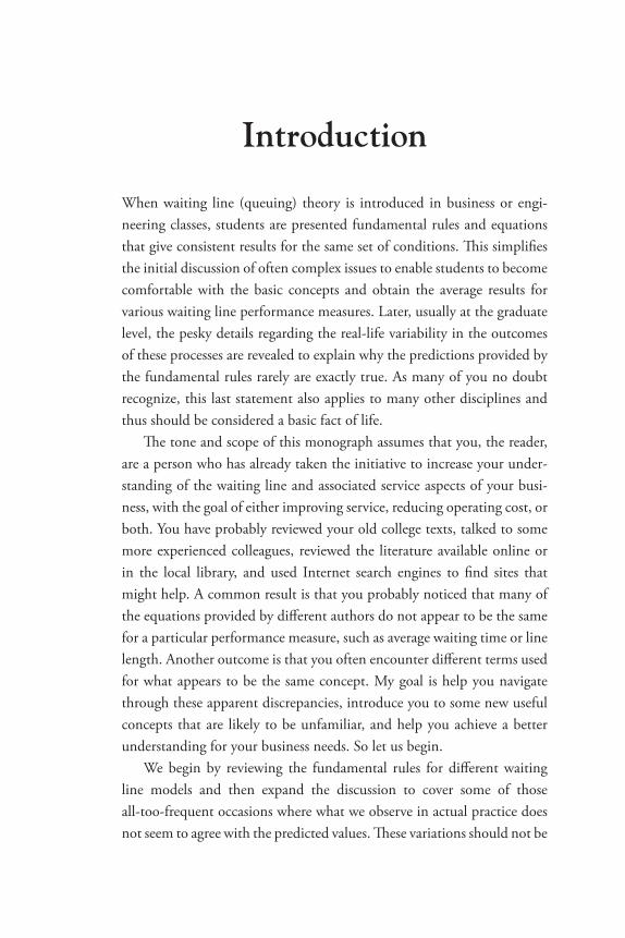
When waiting line (queuing) theory is introduced in business or engi-neering classes, students are presented fundamental rules and equations that give consistent results for the same set of conditions. This simplifies the initial discussion of often complex issues to enable students to become comfortable with the basic concepts and obtain the average results for various waiting line performance measures. Later, usually at the graduate level, the pesky details regarding the real-life variability in the outcomes of these processes are revealed to explain why the predictions provided by the fundamental rules rarely are exactly true. As many of you no doubt recognize, this last statement also applies to many other disciplines and thus should be considered a basic fact of life.
The tone and scope of this monograph assumes that you, the reader, are a person who has already taken the initiative to increase your under-standing of the waiting line and associated service aspects of your busi-ness, with the goal of either improving service, reducing operating cost, or both. You have probably reviewed your old college texts, talked to some more experienced colleagues, reviewed the literature available online or in the local library, and used Internet search engines to find sites that might help. A common result is that you probably noticed that many of the equations provided by different authors do not appear to be the same for a particular performance measure, such as average waiting time or line length. Another outcome is that you often encounter different terms used for what appears to be the same concept. My goal is help you navigate through these apparent discrepancies, introduce you to some new useful concepts that are likely to be unfamiliar, and help you achieve a better understanding for your business needs. So let us begin.
We begin by reviewing the fundamental rules for different waiting line models and then expand the discussion to cover some of those all-too-frequent occasions where what we observe in actual practice does not seem to agree with the predicted values. These variations should not be

xii INTRODUCTION
viewed with dismay, however, but rather as opportunities for innovating, developing a competitive advantage, and assessing possible business risks.
Some mention of the level of mathematic understanding expected of you is appropriate at this point. Several of the performance expres-sions will intuitively make sense. Others will require you to accept their validity on faith because the mathematics behind their derivation can be quite daunting to someone who is not a mathematician. For the most part, we will avoid the derivation of most formulas because this mono-graph is focused on application. However, we will occasionally need to delve more deeply into how a few formulas are derived so we can better understand their limitations in predicting actual business outcomes. In addition, we will develop some expressions that, while not exactly mathematically rigorous, will provide good enough approximations for pragmatic business decisions.
The following is likely to be the most useful and important piece of advice you can gain from reading this monograph: As people gain experience in business, they develop a gut feeling as to what the ballpark estimate of the results of a business analysis will be. Hence when the calculated result does not agree with their estimate, they double-check the calculations. Because of the probabilistic content in waiting line equations, it is more difficult to acquire an intuitive feeling as to what the result should be. Many of the waiting line equations can be quite complex, and the likelihood of typographical errors in equations presented in references and other mate-rial is increased. In fact, I discovered formula errors and other formula differences in many of the references consulted during my research for this monograph. Some of these are obvious to an astute reader, but others can take considerable effort to detect.
Therefore, I cannot stress enough how important it is to make sure that the units of measure for each parameter in a waiting line equation are accounted for and that their use balances out into the proper units for the answer� Consistent checking of the units in your answers will help indicate the presence of errors, whether they are caused by an error in the equation, an incorrect entry in the equation, or a calculation error on your part.
Chapter 1 reviews the basic concepts used for waiting line process analysis; discusses the most common probability distributions; and

INTRODUCTION xiii
introduces state diagrams that are used to derive many queuing formulas, descriptions and notation for different waiting line models, priority rules, and basic cost considerations.
Chapter 2 covers the characteristics and analysis of basic single- channel, single-phase models common to small businesses and sections of manufacturing lines. Chapter 3 covers the characteristics and analysis of basic multiple-channel, single-phase models like most of us have encountered in banks and post offices. You can skip these chapters if you feel that you are sufficiently familiar with the basics; but there are some useful clarifications not usually discussed in college textbooks that will be helpful when we address more complex situations.
Chapters 4 and 5 cover more complex concepts related to less com-mon arrival and service distributions, line capacity limitations, limited population applications commonly used for maintenance activities, multiple-server situations, and manufacturing applications. Chapter 5 also includes equations for direct computations of limited population models to allow you to use spreadsheet methods instead of finite queu-ing tables. Some new nomenclature is introduced to help avoid some confusion that can occur when using such equations.
Chapter 6 focuses on managerial considerations regarding waiting line decisions. The limitation that commonly used waiting line equations predict only average performance is discussed in some detail. Knowing more about performance variability is necessary to enable managerial consideration to reduce its effects on customer service and operating costs. Some possible strategies and methods for reducing variability in both the arrival and the service rates are reviewed, and some cost decisions, such as cost trade-offs between adding service capacity versus process improvements, are discussed. Chapter 6 also discusses some of the softer factors, such as waiting line psychology, priority management, and preferred customer treatment.
In Chapter 7, several tools are discussed. The first is Little’s Law, a useful mathematical expression relating waiting line length to waiting time using the arrival rate. The use of Little’s Law as a handy method to obtain some useful starting data about a waiting line situation with-out requiring extensive data gathering over extended periods of time is also described. To gain knowledge about performance variability for the

xiv INTRODUCTION
evaluation of best- and worst-case scenarios, simulation is required. Some examples show how simulation models can be constructed for several waiting line situations using functions commonly available in Excel 2007 or 2010.
A list of updated references and the chapter notes are provided at the end. Appendix A provides a revised glossary of terms; Appendix B lists symbols used with their definitions; Appendix C presents some use-ful tables and spreadsheet examples for multiple-channel applications; Appendix D provides some useful simulation design information and other helpful application data for Excel users; and a new Appendix E provides some new information regarding the use of Excel data tables for simulation applications for this second edition.

CHAPTER 1
Concepts, Probabilities, Models, and Costs
Standing in line for some service is a universal human experience. We all have had the experience of choosing one line that appears to be moving the fastest only to observe later that an adjacent line is now moving faster. The reality is that all customers do not have the same service require-ments, and even if they do, that service does not always take the same amount of time to complete.
Some of us are prepared to ask for what we need when we reach the server; others are still making up their minds as to exactly what they want. The process of paying for the service also adds to service time variabil-ity. How many of us have watched the person being served in front of us take a considerable amount of time collecting belongings and find-ing money or a credit card to pay the server while another customer is more organized, has exact change, and moves out of the line quickly when the service is completed. Such observations are important because they illustrate that one way to improve customer service is to help customers be better prepared when they reach the server. An illustration of this in practice is the security line process at many airports.
An important consideration for service businesses is being able to estimate how many customers might arrive during a given time period T. It is also important to know the nature of customer arrivals. Are they at regular intervals, random, one at a time, in groups, or in some other way? Given this information and the internal knowledge of how long service usually takes, businesses can use waiting line analysis to determine how many servers are needed to provide an acceptable level of performance at a reasonable cost. Some other performance measures of possible interest are as follows:
2 OPERATIONS METHODS
• How long is the average line?• What is the typical customer waiting time before being
served?• What is the probability that the line will exceed the available
waiting space?• What is the probability that a customer will not have to wait
in line?• Are customer arrivals relatively consistent during the hours
that the service is available or are they variable at predictable times during the hours of operation?
• If one server is not enough to satisfy demand in a timely manner, how many more servers are needed?
• How much do we have to reduce average service time to avoid adding another server?
• Which is more cost-effective—buying a new automated machine to handle part of the demand or hiring more servers?
• What effect would setting up separate lines for different classes of customers have on overall service performance and operating costs?
When applying queuing theory to factory applications, some waiting line parameters are more easily controlled; others become more complex, particularly when more than one process step (phase) is involved. Pro- duction scheduling can reduce variability in the arrival rate. The service rate variability is usually constrained when manufacturing standardized items but can vary much the same as when dealing with customers if the factory is providing repairs or custom items with varying work flows. Moving items between batch and one-at-a-time processes are also analytical challenges. Performance measures of possible interest in such applications include the following:
• What is the average throughput?• What is the typical processing time?• What is the line capacity and which step limits it?• What is the average amount of work in process (WIP)?

CONCEPTS, PROBABILITIES, MODELS, AND COSTS 3
• How much storage capacity is needed for the inventory (queue) before each step?
• How are mixed job flows handled?
In some cases, basic queuing equations can provide rough estimations for some of these manufacturing questions. For more accurate estimates, however, simulation methods are required. For those who do not want to develop their own applications, a variety of vendors have produced simulation programs for common situations. However, it is important if you take either path toward using simulation that you are aware of the assumptions and queuing models available. Selecting the wrong model for your application will not provide useful results no matter how sophisticated the simulation package is.
Managerial considerations regarding the previous performance ques-tions and others are discussed in Chapter 6. Many of them have different options depending on the waiting line model(s) used. Chapter 7 discusses some simple simulation applications and how a simple model can be used as a building block for more complex simulations. Appendix D provides information for using Excel for some basic simulations. Appendix B defines the symbols used throughout this monograph. Because three of these symbols are necessary to any discussion of waiting line situations, analysis, models, or concepts, they need to be defined here:
λ: the average arrival rate of customers or items seeking serviceµ: the average service rateρ: the ratio λ/µ, often referred to as the utilization factor
The fundamental assumption of waiting line analysis is that the behavior of customer arrivals and service times can be described by appropriate probability distributions given the average interarrival time 1/λ, the average service time 1/µ, and some knowledge of the pool of possible customers (the “calling population”) to be served.1 Many of the waiting line performance measure formulas discussed in this chapter are a result of this assumption combined with the insight and the contribu-tions of many talented individuals and organizations.

4 OPERATIONS METHODS
We will accept most of these formulas without derivation except when a partial or a complete derivation is necessary to gain a better understanding of what a particular formula does or does not address. For those interested in such derivations and some good application examples, the books by Laguna and Marklund2 on business process modeling and Hillier and Lieberman3 on operations research are useful references. Another reference is Nelson’s book4 on modeling stochastic processes.
The most commonly used probability distributions are the Poisson distribution for discrete values and the exponential distribution for continuous values with the assumption that the calling population is infinite. Other distributions are used when some control over the arrival rate or the service time is possible and when the population pool or the waiting line capacity is limited.
In selecting distributions that best represent a given queuing situation, it is important to select an appropriate time interval for data collection and the analysis on which the average values for arrival and service rates can be based. The average waiting line performance measures are independent of the time interval chosen, which will be shown later when using the formulas. However, you will lose sight of how much the arrival rate can vary during the day if you choose an interval that is too large.
Poisson Distribution
The Poisson distribution is a discrete distribution because there are no fractional arrivals. It is described by Equation 1.1, where P(n) is the probability that n arrivals will arrive during time interval T given an average arrival rate of λ:
P n
T en
nn T
( )( )
!, , ,...= =
−λ λ
for .0 1 2 (1.1)
The Poisson distribution for an average arrival rate of 4 is shown in Figure 1.1. It is important to note that there is a finite probability that no arrivals will occur during the time interval on which the average rate is based. Knowing this value—often designated as P0 rather than P(0)—is very useful in business decisions, as we will discuss in Chapter 6.

CONCEPTS, PROBABILITIES, MODELS, AND COSTS 5
Another useful property is that adding individual Poisson distribu-tions results in another Poisson distribution. Conversely, breaking down a Poisson distribution into two or more separate distributions results in a set of two or more Poisson distributions. This is advantageous when add-ing together the known arrival rates of individual classes of customers or determining the effect of diverting a part of an existing arrival distribution to a new branch office. We will discuss this in more detail in Chapter 6.
Exponential Distribution
An exponential distribution is a versatile probability distribution that is used to describe both service times and the times between arrivals in waiting line scenarios. It is most often expressed by Equation 1.2, where P(time > t) is the probability that the service time or the interarrival time will be greater than time t, setting α = µ for service time probabilities and α = λ for interarrival time probabilities:
P t e tt( ) .time for> = ≥−α 0 (1.2)
The exponential distributions for two average service rates of 3 and 6.5 are shown in Figure 1.2. Your intuition that the probability of a task requiring a given completion time should decrease as the service rate
Figure 1.1 Poisson distribution for an average arrival rate of 4
P(n
)l = 4
Arrivals
0.25
0.2
0.15
0.1
0.05
00 1 2 3 4 5 6 7 8 9 10 11 12 13 14 15 16 17 18 19 20

6 OPERATIONS METHODS
increases is now validated. You should also note that a probability of 36.79 percent5 corresponds to the average service time of 1/µ.
An exponential probability distribution has the property of being “memoryless.” That is, its predictions of what happens next are indepen-dent of what has happened before. For example, the probability at any given moment that the next customer will arrive in two minutes is the same whether the previous customer arrived a few seconds ago or an hour ago. Such a distribution is also referred to as being “Markovian” and is indicated by the symbol M in the waiting line model notation described later in this chapter. More common examples of this property are the probability of the next coin flip being heads or the next roll of two dice adding up to five. The odds of either occurring are unaffected by any knowledge of the results of previous coin flips or dice throws.
Other Probability Distributions
In many service scenarios, the performance data collected will indicate that either the arrival or the service characteristics are not well represented by Poisson and exponential distributions. For example, consider a coffee shop where there is a mix of customers, some who just want a standard cup of coffee and others who want more customized lattes and mochas. In addition, while the exponential distribution allows the probability of very short service times, in practice, the minimum time required to serve
Figure 1.2 Exponential distributions for service rates of 3 and 6.5
P (t
ime
> t)
(t)
1.2
1
0.8
0.6
0.4
0.2
00 0.5 1 1.5
m = 3
m = 6.5

CONCEPTS, PROBABILITIES, MODELS, AND COSTS 7
a customer is greater than those values. If we want to evaluate more than the average performance values, this mix of relatively constant and widely varying service times plus a minimum service time usually does not fit well with using a single exponential distribution.
Also, consider standardized service situations where the service times are more predictable (deterministic). In such cases, normal distributions or even constant values can be used. This situation is discussed in more detail in Chapter 4.
A variant of the Erlang6 distribution can be used to determine the number of customers turned away by insufficient capacity, and phase-type distributions can be used to characterize waiting lines with more than one phase (step) in sequence. When there is more than one phase in a channel, the mathematics for analytical expressions describing waiting line performance becomes much more challenging. In such cases, we can make some approximations or use computer simulation to provide more useful insight for business applications. One example is a production line with several assembly operations. This situation is discussed in more detail in Chapters 4 and 7.
State Diagrams and Balance Equations
The intent of this monograph is not to make you an expert on deriving waiting line expressions; however, it is useful to spend some time discussing how state diagrams are used to develop some of the simpler formulas. This then provides a better understanding of the relationships between arrival rates, service rates, and the probabilities of different line conditions, such as nobody in line (P0), two people in line (P2), and so forth.
Figure 1.3 shows a generic state diagram where each hexagon rep-resents a specific number of customers in a single-channel waiting line. In this case, we will keep it simple by limiting the maximum number of customers in the system to two. This is not a far-fetched simplification because it could represent an independent stockbroker’s telephone with a capacity for only one call on hold.
To obtain an intuitive feel for what this diagram represents, we first consider the first two states on the left (state 2 is ignored for now). One can see that the maximum flow from the state of no customers in the

8 OPERATIONS METHODS
system to the state of one customer in the system is the arrival rate λ. The maximum flow back to a state of no customers is the service rate µ. If both the arrival and the service rates are constant with no variability, then the proportion of time each state exists is determined by the difference between the arrival and the service rates. This then requires the service rate to be greater than the arrival rate to avoid the need for further states to account for inadequate capacity.
So, what is missing in this state diagram? While it may be obvious to the frequent state diagram user, it often is not obvious to many business students. The key factor here and the magic behind using state diagrams to develop queuing analysis formulas is that each state has a probability of existence that allows the rates into a state to equal the rates from that state. Such balance equations allow one to determine the probability for each state in terms of the given average arrival and service rates. This becomes particularly important when the distributions for the arrival and the service rates are taken into account. While their probabilities of occurring are low, there will be instances when the arrival rate is greater than the service rate. Then an overflow to higher states is necessary for situations when a momentary burst of customers overwhelms the service rate and results in more customers in the system.
For example, the balance equations (inputs equal outputs) for the three states in Figure 1.3 are as follows:
State 0: (P
1 × µ) = (P
0 × λ),
State 1: (P0 × λ) + (P
2 × µ) = (P
1 × λ) + (P
1 × µ),
State 2: (P1 × λ) = (P
2 × µ).
(1.3)
Figure 1.3 State diagram for a single-channel waiting line
0 1 2
λ λ
µ µµ

CONCEPTS, PROBABILITIES, MODELS, AND COSTS 9
Given the above set of balance equations for all the possible states, the individual probabilities for steady-state behavior can be derived. For example, we first use the equation for State 0 to solve for P0 in terms of P1. Then, using the requirement that the sum of all probabilities must be equal to 1, we solve for P2 in terms of P1 and P0. That is, P2 = 1 − P1 − P0 = 1 − P1 − [(µ/λ) × P1]. Remembering that µ/λ is 1/ρ and substituting these results for P0 and P2 in the equation for State 1, we can then determine the value for P1 in terms of ρ. Knowing P1, we can then obtain the values for P0 and P2 using the equations for States 0 and 2. The following results are produced:
P0 = 1/(1 + ρ + ρ2),
P 1 = ρ/(1 + ρ + ρ2),
P2 = ρ2/(1 + ρ + ρ2).
(1.4)
If our calculations are correct, the sum of P0, P1, and P2 should equal 1, which they do. What is also useful here is having answers requiring only the utilization factor ρ. This may not always be the case, but it simplifies the analysis when it is.
For a larger number of states, the mathematics involved can be quite daunting. However, for a queuing situation, where the number of states is limited by physical constraints such as a finite calling population, limited line length, or the number of phone lines, state diagrams can be quite useful in obtaining useful expressions without having to employ exten-sive mathematical methods. We will return to this state diagram when we discuss the more complex aspects of single-channel waiting lines in Chapter 4.
Waiting Line Models and Notation
Although there is some commonality across various waiting line mod-els, such as Little’s Law which is discussed in Chapter 7, many of the formulas predicting various performance measures are dependent on the type of model used. Most references use Kendall’s notation7 to identify which waiting line situation they are discussing. The original notation reportedly had just three characteristics, A/B/C, indicating, in order, the nature of the arrival distribution, the service distribution, and the number
10 OPERATIONS METHODS
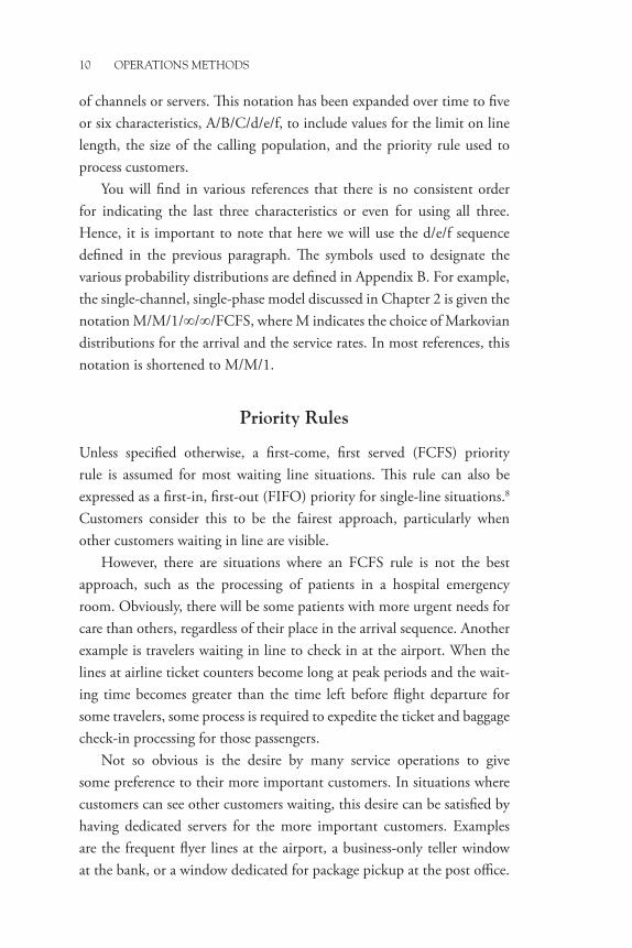
of channels or servers. This notation has been expanded over time to five or six characteristics, A/B/C/d/e/f, to include values for the limit on line length, the size of the calling population, and the priority rule used to process customers.
You will find in various references that there is no consistent order for indicating the last three characteristics or even for using all three. Hence, it is important to note that here we will use the d/e/f sequence defined in the previous paragraph. The symbols used to designate the various probability distributions are defined in Appendix B. For example, the single-channel, single-phase model discussed in Chapter 2 is given the notation M/M/1/∞/∞/FCFS, where M indicates the choice of Markovian distributions for the arrival and the service rates. In most references, this notation is shortened to M/M/1.
Priority Rules
Unless specified otherwise, a first-come, first served (FCFS) priority rule is assumed for most waiting line situations. This rule can also be expressed as a first-in, first-out (FIFO) priority for single-line situations.8 Customers consider this to be the fairest approach, particularly when other customers waiting in line are visible.
However, there are situations where an FCFS rule is not the best approach, such as the processing of patients in a hospital emergency room. Obviously, there will be some patients with more urgent needs for care than others, regardless of their place in the arrival sequence. Another example is travelers waiting in line to check in at the airport. When the lines at airline ticket counters become long at peak periods and the wait-ing time becomes greater than the time left before flight departure for some travelers, some process is required to expedite the ticket and baggage check-in processing for those passengers.
Not so obvious is the desire by many service operations to give some preference to their more important customers. In situations where customers can see other customers waiting, this desire can be satisfied by having dedicated servers for the more important customers. Examples are the frequent flyer lines at the airport, a business-only teller window at the bank, or a window dedicated for package pickup at the post office.
CONCEPTS, PROBABILITIES, MODELS, AND COSTS 11
Note that it is a good business practice to encourage the servers for the dedicated lines to take care of customers in other lines when there are no preferential customers waiting to be served.
More solutions for providing preferential treatment to selected cus-tomers are available when customers cannot view other customers wait-ing. One example is a call center for a financial institution. Such solutions are discussed in more detail in Chapter 5.
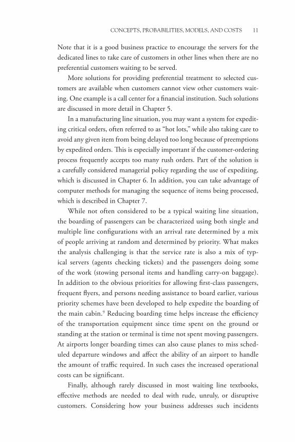
In a manufacturing line situation, you may want a system for expedit-ing critical orders, often referred to as “hot lots,” while also taking care to avoid any given item from being delayed too long because of preemptions by expedited orders. This is especially important if the customer-ordering process frequently accepts too many rush orders. Part of the solution is a carefully considered managerial policy regarding the use of expediting, which is discussed in Chapter 6. In addition, you can take advantage of computer methods for managing the sequence of items being processed, which is described in Chapter 7.
While not often considered to be a typical waiting line situation, the boarding of passengers can be characterized using both single and multiple line configurations with an arrival rate determined by a mix of people arriving at random and determined by priority. What makes the analysis challenging is that the service rate is also a mix of typ-ical servers (agents checking tickets) and the passengers doing some of the work (stowing personal items and handling carry-on baggage). In addition to the obvious priorities for allowing first-class passengers, frequent flyers, and persons needing assistance to board earlier, various priority schemes have been developed to help expedite the boarding of the main cabin.9 Reducing boarding time helps increase the efficiency of the transportation equipment since time spent on the ground or standing at the station or terminal is time not spent moving passengers. At airports longer boarding times can also cause planes to miss sched-uled departure windows and affect the ability of an airport to handle the amount of traffic required. In such cases the increased operational costs can be significant.
Finally, although rarely discussed in most waiting line textbooks, effective methods are needed to deal with rude, unruly, or disruptive customers. Considering how your business addresses such incidents

12 OPERATIONS METHODS
before they actually occur is especially important when such behavior is visible to other customers.
Cost Curves
The relationship between operation costs and the costs of waiting is illustrated in many references by similar versions of the simplified graph shown in Figure 1.4. As more servers are hired, customers have to wait less, but the costs of doing business increase. In addition to the obvious increase in salary and benefits costs additional equipment and facility increases are likely to be needed, particularly if the improved service performance attracts additional customers. This trade-off between customer service and operating costs is shown in Figure 1.4 to have a minimum value that intuitively would appear to be the desired business solution.
However, this simplified model does not depict actual conditions for many service businesses, particularly since the operating costs rarely increase in a linear fashion. So, you may ask, how does one obtain the actual waiting costs for a particular situation? The costs related to adding more servers or items being out of service while they wait for maintenance are more easily determined than the costs of unhappy customers. Some marketing firms have done surveys about how much a typical customer is willing to wait for service or what length of line will discourage a customer
Figure 1.4 Waiting and operating cost relationships
Staffing, Facilities, and Equipment Æ
Cos
ts Æ Queuing
Operating
Total

CONCEPTS, PROBABILITIES, MODELS, AND COSTS 13
from even entering it. But you need to be wary of this information unless such surveys have been done for your particular type of service in your locality. Even then, you should recognize that customer attitudes will vary from one day to the next, depending on whether or not customers are in a good mood, are in a hurry, or are with friends in line; the weather is sunny or miserable; and so forth. Did the marketing group survey people actually in line under different conditions or did they just interview a group of people about their service preferences?
Is your service one of choice—like buying a cup of coffee—or one of necessity—like obtaining a new driver’s license? Do you have several competitors or are you the only choice for the service? In the latter situ-ations, customers may not like the performance provided but must put up with it because there are no other alternatives available. This is often the case with government agencies, where the trade-off is better service or lower taxes.
In most business situations, operating costs are rarely linear, as implied in Figure 1.4. Increases in equipment and the number of servers create jumps in operating costs. Facility additions and other fixed costs required to support additional servers and equipment must be accounted for, and the effect on other behind-the-scenes (back office) support costs should be considered.
Waiting line costs are also not always linear. Waiting a few minutes longer may be inconvenient, but waiting long enough for a meal to get cold or to miss a deadline like a scheduled transportation departure can cause the cost for a customer to increase significantly.
In some situations the waiting line cost is also a significant part of the operating cost for a business and would be more accurately described as a queuing cost to make it clearer that the costs are just those caused by waiting. In the earlier section regarding priority rules we discussed pas-senger boarding processes and the potential increase in operational costs if they were not efficient. In essence, a transportation business is also a customer waiting in line for a service (boarding) to be completed. The range of cost components is broad and interactive between the passengers and the carrier. Boarding delays add to overall turnover time for equip-ment and reduce system capacity. Such delays can cause a passenger to miss a connecting flight or a critical business appointment or not be able

14 OPERATIONS METHODS
to attend an important family event. Complicating this situation is that normal approaches for reducing waiting time such as adding more servers or making existing servers more efficient are not an option. For example, adding another aisle on an aircraft could help speed up boarding, but would reduce passenger capacity. Since increasing server efficiency would involve making the passengers be more efficient in getting their items stowed and seated an airline could decide to prohibit carry-on luggage requiring an overhead bin and have it checked instead. However, this would increase baggage handling costs and could increase the time to load and unload the plane. The increased practice of charging for checked baggage to offset baggage handling costs has increased the use of carry- on luggage by passengers and as a consequence has made the boarding process less efficient and longer. This is not to say that there is no optimal solution for such cost trade-offs, but such a solution requires careful consideration of all system costs and their interactions.
These costs and some suggested methods for managing them are discussed in more detail in Chapter 6.

CHAPTER 2
The Basics— Single-Channel,
Single-Phase Model
A single line of people waiting for some service is arguably the most common business model on our planet (see Figure 2.1). The variations of this simple theme are nearly infinite when you consider the forms that the service can take and the nature of the customers desiring that service.
We will use a typical coffee shop where customers from different walks of life enter the shop; wait in line; and, when they reach the service window, order anything from a simple cup of coffee to a more complex mixture of coffee and other ingredients to larger orders of multiple combinations of these. To analyze the basic behavior of this model, we must make some assumptions where the full Kendall notation for the model is M/M/1/∞/∞/FCFS:
• The customer arrival rate is described by a Poisson distribution using an average rate λ, which means that the interarrival times can be characterized by an exponential distribution with an average interarrival time of 1/λ. Interarrival times are independent of the number of customers in the system.
• The variability in service time is defined by an exponential distribution with an average service time of 1/µ, where µ represents the average service rate. Service times are independent of the number of customers in the system. While one could argue that the server would be under more pressure to work faster when the customer line is longer, in practice this is not a good assumption for a service business to make.

16 OPERATIONS METHODS
Such actions increase the likelihood of mistakes that require additional time to correct and offset any potential reduction in average service time.
• The number of channels (servers) is one, and the number of phases in the service is one. We assume here that a single server does everything for the customer in the coffee shop: taking the order, preparing the coffee, and collecting the payment. Obviously, in many coffee shops with a higher volume of customers, more than one person likely performs these activities. We will discuss these complexities in Chapter 4.
• The arrival or calling population is infinite in size. This avoids complications introduced by the possibility of having served all available customers. Limited or fixed customer situations are discussed in Chapters 4 and 5.
• The length of the waiting line can be infinite. Although not really possible in real-world situations, this avoids analysis complications introduced by the rare possibility that some customers are blocked from entering the line. We will discuss the effects of limited line lengths in later chapters.
• The priority rule is first come, first served (FCFS).• Balking or reneging by customers is not considered in the
analysis.
Figure 2.1 M/M/1 configuration

THE BASICS—SINGLE-CHANNEL, SINGLE-PHASE MODEL 17
• The average arrival rate is less than the average service rate (λ < µ). That is, the utilization factor ρ = λ/µ is less than 1.
This last assumption should be intuitively obvious because the average line length will increase significantly when the arrival rate approaches the service rate, as shown in Figure 2.2.
One thing that is often confusing when reviewing the equations presented by different authors for a given waiting line model is that at first glance they do not always appear to be the same. However, with closer inspection, we can see that one version is equivalent to another version because some author(s) substituted ρ for some combinations of λ and µ or have applied Little’s Law (defined in a moment). The different versions are provided here for your reference with what is considered to be the most useful version listed first. The various per-formance measures for the basic M/M/1 model are listed in the same order in which they will be presented for other waiting line models later in the book.
• Utilization factor: ρ = λ/µ; for a basic M/M/1 model, ρ must be less than 1.
• Probability of 0 customers in the system (this is also the prob-ability that a customer will experience no waiting for service): P0 = 1 − ρ.
Figure 2.2 Increase in average line length as l Æ µ
120
100
80
60
Linr
leng
th in
sys
tem
40
20
00 0.2 0.4 0.6
λ/µ
0.8 1

18 OPERATIONS METHODS
• Probability of exactly n customers in the system: P = (1 − ρ)ρn = P0 ρ
n.• Probability that the number of customers in the system is
greater than k:P
n>k = ρk+1.
• Probability that the server is busy: Pn>0 = 1 − P0 = ρ.• Average number of customers in the system:
L = λ/(µ − λ) = ρ/(1 − ρ) = λW.
• Average total time customers spend in the system: W = 1/(µ − λ) = L/λ.
• Average number of customers waiting in the queue (not yet being served):
Lq = ρL = ρλ/(µ − λ) = λ2/[µ(µ − λ)] = ρ2/(1 − ρ) = L − ρ = λW
q.
• Average time customers wait in the queue before being served:
Wq = ρW = W − (1/µ) = ρ/(µ − λ) = λ/[µ(µ − λ)] = L
q/λ.
The term system applies to not only the number of customers waiting in line but also any customer(s) being served. Also useful to remember is that the sum of all possible probabilities for a parameter must equal 1. This allows you to determine a probability that may be difficult to calculate directly. In such a case, you add together all the other possible probabili-ties excluding the one you want to determine and subtract that sum from 1. An example of this is shown in the list of performance measures above for the probability that a server is busy.
If you study the formulas for line lengths and waiting time carefully, you can see that the ratio of the average number of people in the system to the average waiting time in that system is equal to the average arrival rate when the system is in a steady-state condition. Expressed in the form L = λW, this ratio is referred to as Little’s Law.1 This ratio also applies when considering just the number of people waiting in line and the time they spend waiting in that line before being served. As we will see in subsequent chapters, Little’s Law applies across a wide range of waiting line models regardless of the probability distributions chosen to represent the arrival and the service rates. Hence, Little’s Law is especially useful for

THE BASICS—SINGLE-CHANNEL, SINGLE-PHASE MODEL 19
manufacturing applications of queuing analysis where such probability distributions are often unknown.
Another significant observation can be drawn by looking at the formulas for L, Lq, and P0 that use only the utilization factor ρ = λ/µ. This means that these values vary only with ρ; that is, as long as the arrival and service rates increase in direct proportion to each other (ρ remains constant), the values for L, Lq, and P0 will remain unchanged. However, W and Wq will decrease with increasing values of λ and µ. Figure 2.2 shows the value for L versus ρ, and you can see that the line length is essentially flat for ρ < 0.4. In Chapter 3, you will see that this characteristic also holds true for multiple-channel lines.
You may observe what appears to be an inconsistency in the expres-sions for Lq, where it is shown as being equal to both ρL and L − ρ. Is this possible? Most textbooks avoid this question by presenting only one version for Lq; however, both versions were included in my class lectures as a check on whether students were reading the material. To answer the question: If both equations are true, then ρL must equal L − ρ. Moving all the L terms to one side of the equation gives the result that L(1 − ρ) = ρ. Dividing both sides by (1 − ρ) gives L = ρ/(1 − ρ), which is the equation for L.
Example 2.1 Coffee Shop with One Server
To gain a more comfortable understanding of how the preceding per-formance measures can be used, consider a small coffee shop we will call Ken’s Caffeine Fix. The shop is located in a downtown area and provides various forms of coffee to nearby office workers who stop in for a cup of their favorite brew at various times of the day. We will make two assumptions: (1) The average arrival rate does not vary during the day, and (2) the owner performs all parts of the service provided: takes the order, prepares the coffee, and collects the payment. The issues created by arrival rates varying during the day and having a helper do parts of the service will be discussed in later chapters. To assign some values to this operation, let us assume that it takes an average of two minutes to serve each customer, and the average number of customers per hour is 24.

20 OPERATIONS METHODS
This gives us an average arrival rate λ of 24 customers per hour and an average service rate µ of 1 customer per 2 minutes = 30 customers/hour. This illustrates a critical consideration when analyzing waiting line situations for small businesses—the arrival rate must be less than the service rate. Or put another way, the service rate must be greater than the expected arrival rate for the business.
Many businesses collect operating data in this way: the average number of customers per some time period and the typical service time. Thus some conversion of the data is necessary because the time references for the arrival and service rates must be the same. A real-life example of collecting data for coffee shops on a college campus will be given in Chapter 7.
The utilization factor ρ is 24/30 = 0.8 or 80 percent. This is the probability that the owner will be busy serving a customer when the next customer enters the shop. Hence the probability of no customers in the shop (P0) is 1 − ρ = 20 percent. This is a useful value to know because the owner needs some time during each hour for support activities such as replenishing the cream-and-sugar station, brewing more regular coffee, and general cleanup.
The average number of customers in the shop (L) is expected to be 24/(30 − 24) = 4 customers, and the average number waiting in line (Lq) is 0.8 × 4 = 3.2 customers. You should recognize that these values are independent of the time period chosen. If the owner had collected data on customer arrivals and service times over a sequence of 15- minute periods rather than hours, the results for L and Lq would be the same. In other words, because the utilization factor is unchanged, L and Lq are unchanged. That is, the average line length is independent of the time reference for the average arrival and service rates.
The average total time spent by customers getting their coffee is 60/(30 − 24) = 10 minutes, and the time spent waiting in line is 0.8 × 10 = 8 minutes. This obviously is too long for an office worker just wanting a quick cup of regular coffee. Ways to shorten the wait for this class of customer are discussed in Chapter 6. Of interest here is that Little’s Law indicates the waiting time decreases as the arrival rate increases, provided that the utilization factor remains constant (that is, the service rate increases proportionately with the arrival rate).

THE BASICS—SINGLE-CHANNEL, SINGLE-PHASE MODEL 21
Figure 2.3 shows typical individual waiting times and service (brew-ing) times along with the number of customers already in the shop when each customer arrives. These values were obtained using a simple Excel simulation program. This set of sample data does not show any values for L that are greater than 5, which could lead a person to assume that the line lengths for the business are not too long. However, subsequent simulation runs using the same interarrival and service time distributions and the
Figure 2.3 Some typical performance values for the first 100 customers entering a typical coffee shop
Line
Len
gth
LW
aiti
ng T
ime
(min
utes
)B
rew
ing
Tim
e (m
inut
es)
Customer #
Customer #
Customer #
6
5
4
3
2
1
0
16.00
14.00
12.00
10.00
8.00
6.00
4.00
2.00
0.00
9.00
8.00
7.006.00
5.00
4.00
3.002.00
1.00
0.00
1 5 9 13 17 21 25 29 33 37 41 45 49 53 57 61 65 69 73 77 81 85 89 93 97
1 5 9 13 17 21 25 29 33 37 41 45 49 53 57 61 65 69 73 77 81 85 89 93 97
1 4 7 10 13 16 19 22 25 28 31 34 37 40 43 46 49 52 55 58 61 64 67 70 73 76 79 82 85 88 91 94 97 100

22 OPERATIONS METHODS
same number of customers have demonstrated possible line lengths as great as 14, brewing times as long as 16 minutes, and waiting times up to 20 minutes. To obtain more information regarding the variability of the performance measures, multiple simulation runs are required. These will be explored in detail in Chapter 7. You should note in Figure 2.3 that the average for each performance measure depicted rarely occurs, if at all, for any customer. This leads to a very important observation that the average performance values derived from the queuing equations are primarily useful for the longer-term business perspective and are a very poor indicator of what a typical customer encounters.
As mentioned in Chapter 1, an exponential distribution is not the most accurate distribution to represent the service time for this type of business because the minimum service time required for even a simple cup of house coffee is likely to be greater than 30 seconds when the time for payment is included. Yet the simulated data in Figure 2.3 show several occasions when the brewing time is less than 30 seconds (0.5 minute). The longer brewing times shown can be expected when one considers a customer ordering several coffees for a group of people. Perhaps an Erlang distribution with an appropriate k factor would be a better representation for this type of service, as discussed in Chapter 4.
Finally, market surveys can provide estimates of how long a line can be before customers looking into the shop are likely to decide to not even enter (balking). For example, let us say that a line longer than five people, including the person being served, is a definite turnoff for a potential coffee shop customer.2 So, what is the probability of this occurring? Referring to the data in Example 2.1 and using the formula Pn>k = ρk+1, where k = 5, we obtain 0.86
= 0.2621 or 26.21 percent. Thus, Ken’s Caffeine Fix coffee shop is likely to lose at least one fourth of its possible customers. Conversely, the probability that the average number of customers in the shop is 5 or less is 1 − 0.2621 = 0.7379 or 73.79 percent.

CHAPTER 3
The Basics— Multiple-Channel, Single-Phase Model
When demand exceeds the output of a business, either that business must become more productive, increasing its output rate to cope with the increased demand, or adding more capacity to satisfy it. In a service situation, you either reduce your average service time per server or you add more servers. In this chapter, we expand the basic waiting line analysis to take into account the effects of adding more servers. In Chapter 6, we will explore the alternative of reducing service time.
Figure 3.1 shows a simple multiple-channel, single-phase model M/M/s with two servers. Two queue configurations are possible: a sepa-rate line for each server and one queue feeding both servers.
Grocery and retail store checkout lines, traffic lanes, and old-style ticket counters are common examples of the separate lines configuration, and most banks and post offices are common examples of the single line configuration that directs each customer to the next available server. Some authors refer to the single line arrangement as a “snake” configuration because it often requires a winding layout to accommodate its length. A common example is the arrangement at airports before the passenger security checkpoints.
You may think that analyzing this will be easy. Your intuition may lead you to believe that all you would have to do is either multiply the service rate by the number of servers for a single line feeding two servers or divide the arrival rate in half for two separate lines and then use the performance measures discussed in Chapter 2 for the single-channel, single-phase model M/M/1. However, this is incorrect for a single service location with more than one server because the number of customers for

24 OPERATIONS METHODS
one server is not independent of the number of customers for the other server. There are other nuances to be considered, such as the probability of no customers for one server when the other server is still busy, the probability that a newly arriving customer will pick a particular line in the separate line per server configuration, or the probability that a customer in a slowly moving line will change lines to a more quickly moving line (a process called jockeying).
Figure 3.1 Multiple-server waiting line configurations: (a) separate line per server and (b) one line feeding both servers
(a)
(b)
THE BASICS—MULTIPLE-CHANNEL, SINGLE-PHASE MODEL 25
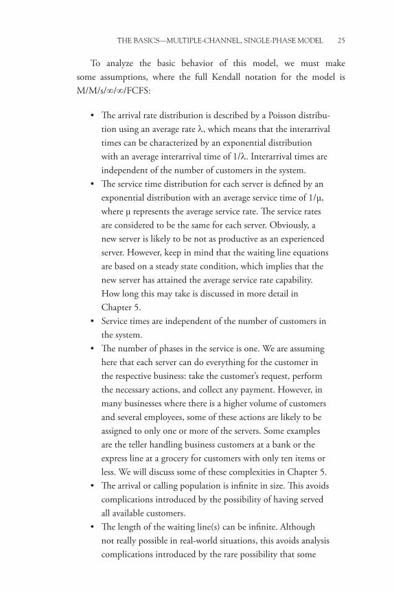
To analyze the basic behavior of this model, we must make some assumptions, where the full Kendall notation for the model is M/M/s/∞/∞/FCFS:
• The arrival rate distribution is described by a Poisson distribu-tion using an average rate λ, which means that the interarrival times can be characterized by an exponential distribution with an average interarrival time of 1/λ. Interarrival times are independent of the number of customers in the system.
• The service time distribution for each server is defined by an exponential distribution with an average service time of 1/µ, where µ represents the average service rate. The service rates are considered to be the same for each server. Obviously, a new server is likely to be not as productive as an experienced server. However, keep in mind that the waiting line equations are based on a steady state condition, which implies that the new server has attained the average service rate capability. How long this may take is discussed in more detail in Chapter 5.
• Service times are independent of the number of customers in the system.
• The number of phases in the service is one. We are assuming here that each server can do everything for the customer in the respective business: take the customer’s request, perform the necessary actions, and collect any payment. However, in many businesses where there is a higher volume of customers and several employees, some of these actions are likely to be assigned to only one or more of the servers. Some examples are the teller handling business customers at a bank or the express line at a grocery for customers with only ten items or less. We will discuss some of these complexities in Chapter 5.
• The arrival or calling population is infinite in size. This avoids complications introduced by the possibility of having served all available customers.
• The length of the waiting line(s) can be infinite. Although not really possible in real-world situations, this avoids analysis complications introduced by the rare possibility that some

26 OPERATIONS METHODS
customers are blocked from entering the line. We will discuss the effects of limited line lengths in later chapters.
• The priority rule is first come, first served (FCFS).• Balking or reneging by customers is not considered in the
analysis.• Jockeying is allowed in separate line configurations.• The average arrival rate is less than the average total service
rate (λ < sµ). That is, the multichannel utilization factor (ρs = λ/sµ) is less than 1.
This last requirement clarifies an error that occasionally occurs in the queuing literature. Some texts consistently use a value for ρ as defined for the M/M/1 model in their equations for the M/M/s model, while other texts use a ρ value equivalent to ρs but without the s subscript to indicate that their use of ρ has a different definition in the M/M/s equations. In this monograph, ρ always represents λ/µ, s represents the number of servers, and ρs is used to represent λ/sµ. Thus, ρs = ρ/s. For a given average arrival rate and an average service rate per server, the minimum number of servers must then be large enough so that ρs is less than one. The actual number of servers for many situations is likely to be greater than this minimum number to achieve desired performance values.
As for the M/M/1 model discussed in Chapter 2, there are different versions of some of the multiple-channel performance measure equations in the literature regarding queuing analysis. Some alternate versions are provided here for your reference, with what is considered to be the more common version listed first. The various performance measures are listed in the same order as they are presented for the M/M/1 model in Chapter 2. Additional measures special to the M/M/s model are discussed in Chapter 5. You are reminded that the term system includes not only the number of customers waiting in line but also the customer(s) being served.
• M/M/s utilization factor: ρs = λ/sµ: for an M/M/s model, this value must be less than one for the following equations to be valid.

THE BASICS—MULTIPLE-CHANNEL, SINGLE-PHASE MODEL 27
• Probability of zero customers in the system: The equation for P0 here is more complicated:1
P
n s s
n
n
ss0
0
1
1
1
=
+−=
−∑ ( )!
( )!( ( ))
λ µ λ µλ µ
/ //
(3.1)
• Probability of exactly n customers in the system: This equation has different forms dependent on n compared to the number of servers:
P nP n s
s sP n s
n
n
n
n s
=≤ ≤
≥
−
( )!
( )!
λ µ
λ µ
/for
/for
0
0
0
. (3.2)
• Probability that the number of customers in the system is equal to or greater than the number of servers (e.g., all the operators in a call center are busy):
P
s sPn s
s
≥ =−
( )!( ( ))
λ µλ µ
//
.1 0
(3.3)
• The average number of customers in the system:
Ls s
Ps
=− −
+λµ λ µµ λ
λµ
( )( )!( )
/,
1 2 0
or, alternatively,
L
s s sP
s
=−
++( )
! ( ( ))λ µ
λ µλµ
//
.1
2 01 (3.4)
• The average total time customers spend in the system:
W = L/λ = (Lq/λ) + (1/µ).
• The average number of customers waiting in the queue (not yet being served):
Lq
( – L = λ/µ),
or, alternatively,

28 OPERATIONS METHODS
L
s s sPq
s
=−
+( )! ( ( ))
λ µλ µ
//
.1
2 01 (3.5)
• The average time customers wait in the queue before being served:
Wq = L
q/λ.
Now, let us examine these expressions. First, we consider the case where s = 1. This is the M/M/1 model. Do the equations reduce down to the equations given in Chapter 2 for the M/M/1 model? Because they should, this is a good check for both typographical errors when using the multiple-channel equations from your favorite reference and for validating your understanding of what the more advanced mathematical notation signifies.
My classroom experiences indicate that it would be useful at this time to review some mathematical notation to save you the effort of looking it up for yourself.
The exclamation point indicates a factorial expression, where
n! = 1 × 2 × . . . × (n − 1) × n.
When n = 0, n! = 1.Any value raised to a power of zero is 1. For example, (x − 1)0 = 1.
The summation term i
nix
=∑
0 is shorthand notation for x0 + x1 + x2 +
. . . + xn+1 + xn, where i is a counter that represents the parameter range from 0 to n. Of course, x0 = 1.
Returning now to the equations at hand, the key parameter that must be derived first is P0 because its value is necessary to determine the other measures. Equation 3.1 can be a nasty piece of work with increasing chances of making a mathematical error when there are many servers to deal with. Likewise, determining L (Equation 3.4) also requires care. The equations for L and P0 can be expressed differently using only the value for s and the ratio of λ/µ. This allows an easier computation and enables the creation of reference tables for P0, Lq, and L for various combinations of λ/µ and s when using the M/M/s model. These tables are provided in Appendix C.

THE BASICS—MULTIPLE-CHANNEL, SINGLE-PHASE MODEL 29
The good news is that the expressions for queue length and waiting times are quite simple thanks to Little’s Law.
The probability of just n customers in the system (Equation 3.2) is useful for determining how likely it is that one or more servers are idle. This helps later when scheduling workloads in a place like a grocery store because it gives you an estimate of the slack time available for servers, who may then, for example, help restock shelves or do other work.
Another useful observation is that a service manager can obtain an estimate of the overall average waiting time per customer by merely tallying the number of customers who enter the business during some selected time interval and counting the number of customers in the business at the end of that time interval. By collecting this information for several selected sequential time periods, say every 15 minutes during a typical business day, you can average the results to obtain estimates of L and λ. Hence, using Little’s Law, W = L/λ. An example of this will be discussed in Chapter 7.
Example 3.1 Coffee Shop with Two Servers
Let’s return to the Ken’s Caffeine Fix example in Chapter 2. The coffee shop has an average arrival rate (λ) of 24 customers per hour and an average service rate (µ) of 1 customer every 2 minutes = 30 customers/ hour. Recall that the average time spent waiting to be served in that coffee shop was eight minutes, which is much too long for the typical office worker desiring a cup of coffee during his or her break. The average line length was 3.2 customers.
One solution to reduce the waiting time is for the owner to hire another server to increase the overall service rate for the coffee shop. So, plugging in the values for two servers in Equation 3.1 for P0, we should get
P0 2
1
1 24 3024 30
2 1 24 60
0 428571=+ +
−
=( )
( )( ( ))
. ./
//
You may ask, “Is this value correct? We only doubled the number of servers, but P0 has more than doubled compared to the M/M/1

30 OPERATIONS METHODS
model.” The answer is yes, and it indicates that simply doubling the service rate of a single server is not the same as adding another server. This observation has important implications when deciding whether to hire another person or invest in service improvements (discussed in Chapter 6). Table 3.1 compares the performance measure results for the M/M/1, M/M/2, M/M/1 with µ doubled, and M/M/1 with λ halved approaches. This will help illustrate why such simplified approaches, although they look like they would intuitively work, do not provide accurate answers.
Some readers may also ask, “Why are the answers expressed in so many significant digits?” In queuing analysis, particularly for the more complex models, it is important that you maintain as much precision as possible in the intermediate computations until you obtain the final result, which then can be rounded to a less detailed answer. Not doing this can have a noticeable effect on the final result. Not being aware of this creates considerable confusion for students who are doing homework together because when they compare their results, their answers often do not agree—leading them to assume that one of them has made a mistake.
Now that we have the value for P0, we can determine the probabil-ity that just one server will be idle. Using Equation 3.2 for one server idle (i.e., n = 1 customer in the system), this is simply
λP0/µ = ρP0 = 0.343.
Again, this is useful to know when considering how much of a new employee’s time can be used for work not directly related to serving customers.
Determining the probability of more than five customers in the shop is much more complicated than the simple formula used for the M/M/1 model. Now we need to determine the respective probabilities of just 0, 1, 2, 3, 4, and 5 customers in the shop using Equation 3.2, add those values together, and then, recalling that the total of all possi-ble probabilities must equal 1, subtract that sum from 1 to obtain the probability we seek. Without showing the intermediate calculations, the values in this example are P1 = 0.343, P2 = 0.137, P3 = 0.055,

THE BASICS—MULTIPLE-CHANNEL, SINGLE-PHASE MODEL 31
P4 = 0.022, and P5 = 0.009. We have already calculated P0 and sub-tracting the sum of probabilities from 1.0 gives a value for Pn>5 = 0.006 or 0.6 percent, which is a large improvement over the 26.2 percent value for the M/M/1 model.
Now we consider our major concern, “How much did we reduce the average waiting time?” First, we need to calculate the average line length using Equation 3.4. Plugging in the numbers using the P0 value determined earlier, we should get
L/
! /0.9
( )( ( ))
.=× −
× + =24 302 2 1 24 60
0 4285712430
3
2 552381 customer
Dividing L by λ gives us a total average customer time W in the shop of 0.039682 hour, or roughly 2.4 minutes, which is a much more reasonable time to get a cup of coffee. The corresponding average length of the queue is now 0.152381 customer, and the average wait in line before being served is less than a minute at 22.9 seconds.
Table 3.1 Comparison of the results using correct analysis methods with the results using incorrect methods (Shaded results)
M/M/1 M/M/2 M/M/1 (2µ) M/M/1 (l/2)P0 0.2 0.428 0.600 0.600
L 4 0.952 0.667 0.667
Lq 3.2 0.152 0.267 0.267
W 10 minutes 2.38 minutes 3.33 minutes 1.67 minutes
Wq 8 minutes 0.38 minute 1.33 minutes 0.67 minute
Finally, let’s return to the earlier comment about why one should not use the M/M/1 equations in Chapter 2 for determining the enhanced performance provided by adding another server. Referring to Table 3.1, if one simply doubles the service rate using a single line, the average line appears to be shorter than the M/M/2 solution, but the average total wait is longer. If one assumes that customers will evenly split between separate lines for each server (i.e., halving the arrival rate), the average line length and the average total waiting time are both smaller than for the M/M/2 solution. What are the reasons for not being able to use the results in the shaded cells of Table 3.1?

32 OPERATIONS METHODS
As will be explored further in subsequent chapters, there are several subtle things going on here. One server working at an average of 30 sec-onds per customer is not the same as the combination of two servers each working at an average of one minute per customer. The average throughput is the same, but the combined variance in the service rate for two servers is not the same as the variance for a single server. In addition, the average service rate of 2µ is valid only when both servers are busy. When only one server is busy, the service rate is µ.
Referring to our discussion of state diagrams in Chapter 1, let us change the situation from a single-channel system to a multiple-channel system with two servers. An example would be a call center with two operators and no ability to have callers on hold. The output from state 2 back to state 1 shown in Figure 1.3 would be 2µ for a two-server system. The output from state 1 back to state 0 would remain the same at µ because only one server would be required and the second server would be idle. The set of expressions for Equation 1.3 would change to
State 0: (P1 × µ) = (P
0 × λ),
State 1: (P0 × λ) + (P
2 × 2µ) = (P
1 × λ) + (P
1 × µ),
State 2: (P1 × λ) = (P
2 × 2µ).
Solving for P0, P1, and P2 in the same manner as described in Chapter 1, we obtain
P0 = 1/[1 + ρ + (ρ2/2)],
P1 = ρ/[1 + ρ + (ρ2/2)],
P2 = (ρ2/2)/[1 + ρ + (ρ2/2)].
The results show a relative increase in the probabilities of states 0 and 1 and a corresponding decrease in the probability of state 2, as we should expect. Again, adding P0, P1, and P2, we obtain a value of 1 as a check on our derivation.
When a customer enters a shop with two lines, the customer normally picks the shorter line, but he or she can pick the longer line if the customer perceives that the shorter line has a customer ahead in line that is likely to require a much longer service time (e.g., a person with a large number of packages at the post office).

THE BASICS—MULTIPLE-CHANNEL, SINGLE-PHASE MODEL 33
Customers may change lines if the line they are in is moving slower than the other line. (We all have done this in slow-moving traffic when given an opportunity to move into a lane that appears to be moving faster.) This behavior is called jockeying. The multiple-channel configuration of a single line feeding the next available server prevents jockeying and reduces the chances that a new customer will get stuck in a line behind a customer requiring a long service time.
You can divide the arrival rate if you establish a separate location for the second server because the possibility of customers choosing or jockeying between the lines is then eliminated. Then the two lines can be considered to be independent of each other, and each can be analyzed separately using the M/M/1 model equations. In such situations, the arrival rate for each location is determined by dividing the original total arrival rate according to what percentage of your customers you estimate will go to each location.
You can have an average total waiting time that is less than the average service time when the customer volume is low (ρ < 0.5) because the probability of a long service time for one customer delaying other customers is reduced. In effect, you are averaging the service time at the windows with a customer with zero service time at the windows with no customers. In addition, when you use an exponential distribution to describe the range of possible service times, there is a cumulative probability that at least 63 percent of the possible service times will be shorter than the average service time.
Correspondingly, the cumulative probability for possible service times greater than the average service time is therefore 37 percent. It should be noted that these service times can be much longer although they only account for 37 percent of the potential customers. If the service time can be more accurately represented with a normal distribution, such as businesses providing only standardized services, these cumulative proba-bilities would each be 50 percent.

CHAPTER 4
More Complex Single-Channel Models
In many service businesses and manufacturing line applications, the basic M/M/1 model does not provide useful results that appear to agree with reality. There are several possible reasons for this poor performance:
• Chief and foremost, the waiting line formulas are based on the waiting line achieving a steady-state condition. This takes time and should lead you to the observation that the formulas are likely to be a poor predictor of what occurs at the beginning of a business day.
• The service time distribution is not best described by an exponential distribution.
• The capacity for accommodating the waiting line is limited.• The calling population is not infinite.• The interarrival time distribution is not best described by an
exponential distribution.• The M/M/1 model is based on a single-service phase, where
the server performs all the service required. How do we handle situations where there is more than one phase or step? In some cases, we can combine the separate service steps to approximate a single phase. In others, we require either more complicated analysis approaches or simulations to obtain the performance data we want.
There are several adjustments we can make in the performance measures to cope with many of these situations. Some will work out well; others will give us only rough estimates of what is happening. In such cases, discrete simulation models may be the only way to gain more

36 OPERATIONS METHODS
accurate insight into what is occurring. Some examples of simple simu-lations that can be done in Excel to analyze these situations are discussed in Chapter 7.
Instead of the normal choice of an exponential distribution for the interarrival and service times, we have a variety of probability distribu-tions that can be used to more accurately represent a particular service business situation. Some of these distributions will make the performance measures more complicated to determine. Some will require the use of simulations because of the lack of suitable, closed-form (analytical) solu-tions. The good news is that because Little’s Law applies regardless of our choices for service and arrival distributions, all we have to be able to do is to calculate L, Lq, W, or Wq to determine the other values.
Alternate Service Time Distributions
The M/G/1 and M/D/1 models allow for other choices of service time distributions than the exponential distribution. Some common situations that require a different choice are when
• The minimum service time is significantly greater than the nearly zero times allowed by an exponential distribution;
• The service time may have a much smaller variance than allowed by the exponential distribution;
• The service time may even be consistent enough to be considered a constant value;
• The service time can have a discrete distribution, such as in the case of a business offering only a few standardized services;
• Or the service time can be a collection of exponentially distributed service times, such as in the case of different classes of customers being served by the same facility.
Fortunately, we can obtain the steady-state average performance measures for many of these situations by using the Pollaczek-Khintchine (P-K) formula.1 This formula uses the coefficient of variation (Cx) for a probability distribution of x to calculate the average waiting time in line (Wq). Because we are dealing only with the average steady-state value for

MORE COMPLEX SINGLE-CHANNEL MODELS 37
the waiting time, the shape of the probability distribution used for the service time is unimportant as long as we know the distribution’s mean value and standard deviation or variance (the standard deviation squared). Here we assume that for an M/G/1 model, x represents the mean service time, and the mean service time is the reciprocal of the average service rate (µ):
WC
where C(1/µ)
standamean
q = ×−( ) ×
+( )
=
1 1
21
2
µλ
µ λµ( / )
,
rrd deviation.
(4.1)
Examine this formula carefully. For a constant service time where the standard deviation is zero, the time spent waiting in line is exactly half of what is predicted for the M/M/1 model using the same average service time.
You may very well say, “No service time is exactly constant where people are involved, what then?” In that case, we can use a normal dis-tribution, where we collect samples of actual service times and calculate their average (1/µ) and corresponding standard deviation (σ). This would give a C(1/µ ) value of µσ, and Equation 4.1 for a M/G/1 model using a normal service time distribution becomes
W .q = ×
−×
+( )= +
−1 1
212
2 2 2
µλ
µ λ(µσ) ρ µ σ
µ λ( )( )
( ) (4.2)
Let us examine this expression more closely. It says that as the variance in the service time increases, the wait becomes longer even though the average service time does not change.
Here is an important corollary: Reducing variances in the service time reduces the average waiting time. This corollary is important because most textbook examples focus on shortening the average service time to reduce the average waiting time. Reducing variability in manufacturing or pro-duction step service times, particularly when there are many steps required can often be more beneficial than trying to shorten service time. This is one of the benefits of applying statistical process control (SPC) methods whose focus is on reducing variability in processes. Some other approaches for addressing service time variability are discussed in Chapter 6.

38 OPERATIONS METHODS
What about the problem with the probability of unrealistically short service times using the exponential distribution? Unfortunately, the steady-state performance measures do not illustrate this problem; one must use simulation to see its effect. However, the subtle effects on aver-age waiting time and line lengths can be taken into account by choosing general service time distributions that have a lower probability of shorter service times. In addition to the constant and normal distributions, we can use the Erlang probability density function, which is defined by the following formula:
f t
t ek
for tk t
k( )( )!
./
=−
≤ ≤ ∞− −1
10
α
α (4.3)
where α = the scale factor,2 k = the shape factor, αk = the mean, and the variance = α
2k. In a gamma distribution, k is a continuous value; in an Erlang distribution, k is restricted to integer values greater than zero and, in essence, represents the number of identical but still independent exponential distributions that are added together to form an Erlang distribution. When k = 1, this distribution defaults to the exponential distribution, where the average time is α (substitute 1/λ for the interarrival time or 1/µ for the service time). This leads to another version of Equation 4.3 that is easier to understand when using it for service time distribution in M/Ek/1 models because it is expressed in terms of the service rate instead of α:
f t
t ek
for tk k t
( )( )!
=−
≤ ≤ ∞− −µ µ1
10 . (4.4)
Therefore, the mean becomes k/µ, and the variance becomes k/µ2. Plots of Equation 4.4 for an average service rate of 5 and using values of k = 1, 2, and 4 are shown in Figure 4.1. This service rate corresponds to an average service time of 0.2; while you may observe that the peak of the probability distribution for k = 2 roughly occurs at that time, that fact does not mean that the best value for k is 2. However, the mean for that curve is k/µ = 2/5 = 0.4, indicating that there are a larger number of possible times greater than the most probable time compared to the number of possible times less than the most probable time.

MORE COMPLEX SINGLE-CHANNEL MODELS 39
This illustrates a common area of confusion when trying to under-stand the mathematics behind the waiting line performance equations. My students often confused the maximum value of a probability density function with the average they obtained from a collection of observa-tions. They also forgot that the Central Limit Theorem states that the distribution of sample averages is normally distributed regardless of the underlying distribution being sampled. I demonstrated to students that knowing the mean is not enough to determine which probability density function applies by giving them two sets of data that provided the same mean and standard deviation but showed significantly different frequency distributions when the raw sample results were plotted in histograms.
So, let us use the mean and variance for an Erlang distribution in the
P-K formula given in Equation 4.1. In this case, Ck
,/( )1
1µ = resulting in
W
/k kk
.q = ×−
×+( ) = +
−1 1 1
21
2µλ
µ λρ
µ λ( )
( ) ( )( )
(4.5)
As a check, you can see that when k = 1, we obtain the same equation for an exponential distribution in the M/M/1 model. What if we try k = 2 to reduce the possibility of really short service times? Then using Equation 4.5, Wq = 75 percent of the Wq for the M/M/1 model. If the choice for k is much larger, we converge on the same result as for a constant service time.
Figure 4.1 Probability density functions for an average service rate of 5 using an Erlang distribution with k = 1, 2, and 4
0
1
2
3
4
5
6
0 0.1 0.2 0.3 0.4 0.5 0.6 0.7 0.8 0.9
Time (t)
1 1.1 1.2 1.3 1.4 1.5
f (t)
k = 1k = 2k = 4

40 OPERATIONS METHODS
How can this be? We have reduced the probability of short service times, so should the wait not be longer? This illustrates how our intuition is sometimes misleading when it comes to analyzing waiting lines. First, keep in mind that the exponential distribution was not representing real-istic service times for Ken’s Caffeine Fix, so comparing the new Wq to an incorrect Wq is inappropriate. Second, the higher k factor could have also reduced the probability of really long service times. What really matters is which service time distribution is the best representation of reality for a business like Ken’s Caffeine Fix.
Example 4.1 Coffee Shop Using Different Service Distributions
Let us compare the differences in performance using different service distributions for Ken’s Caffeine Fix analyzed in Example 2.1. The val-ues for ρ and P0 remain the same, but Wq, Lq, W, and L will vary. The average service rate of 30 customers per hour will be the same for all distributions, and we will assume a standard deviation of service time of 15 seconds for the normal distribution. Table 4.1 shows the results.
Observe that the best performance is with a normal service time distribution. Why is the constant service time not providing the best performance? Once again we must consider that when there is some variance in service time, we can have better results because there is a reasonable probability that the shorter service times will occur at the same time as when there is a higher than average arrival rate, enabling the line to move faster in such cases. Similarly, there is also a probabil-ity of longer service times occurring when the arrival rate is lower than normal, which will reduce their usual effect in increasing line lengths.
Table 4.1 Ken’s caffeine fix coffee shop performance measures for different service distributions with an average service rate of 30 customers per hour
Performance Exponential Constant Normal Erlang (k = 2)Wq (minutes) 8 4 3.05 4.5
W (minutes) 10 5 3.18 5.63
Lq (customers) 3.2 1.6 1.22 1.8
L (customers) 4 2 1.52 2.25

MORE COMPLEX SINGLE-CHANNEL MODELS 41
The combination of these two possibilities results in slightly improved performance as long as the variance in service time is not too large. For example, if the standard deviation increases from 15 seconds to 30 seconds, Wq increases to 3.19 minutes, and Lq increases to 1.28 customers—as expected.
What about the beta distribution commonly used to represent com-pletion times in project management planning? This asymmetrical distri-bution could be used because it allows the selection of a minimum time and the probability for much longer times. However, its mean and variance terms are much more complex compared to the choice of an Erlang distribution with the proper value of k. In project management analy-sis, the beta distribution is often approximated by a normal distribution to simplify the mathematics. This approximation and its use for probabi-listic estimates of project completion time can be found in many project management texts.
Finally, sometimes there is not enough information to determine what might be the best distribution to use. In such cases, we can take what historical operational data we do have regarding service times to form a discrete distribution that can be used in a simulation program. An example of this will be discussed in Chapter 7.
Alternate Arrival Time Distributions
For most service business situations, the exponential distribution is a very good representation of customer arrival behavior. But, for some busi-nesses, a better representation is needed. The Kendall notation for this situation using a single-channel, single-phase system is G/M/1:
• The arrival distribution may not be best represented by a Poisson distribution.
• Arrival rates can vary during the day and often have regularly occurring peak and slack periods depending on the nature of the service(s) provided.
• The arrival population could be a combination of different types of customers.

42 OPERATIONS METHODS
When appointments or production schedules are used to control the arrival rate, the notation is D/M/1. You may ask why we would want to use waiting line analysis for such a predictable situation. If we want to select the best time between successive appointments, it is necessary to evaluate the effects of varying service times. If the appointment duration is too short, we end the day with a long line of disgruntled customers still waiting to be served. If the appointment time is too long, we reduce the number of customers we can accommodate per day and will have more idle time than we can profitably use to do other tasks, such as preparation, cleanup, record keeping, and so forth. In other words, we must ensure that the average arrival rate is sufficiently lower than the average service rate to prevent unnecessary backups but not so low that we unnecessarily limit our capacity and create excess idle time. Selecting the optimal value is a cost decision that we will discuss in Chapter 6.
Dealing with varying arrival rates is difficult because the waiting line equations assume steady-state conditions. For small businesses, there is likely to be insufficient volume to achieve a steady-state situation each day. For businesses such as government driver’s license bureaus or the post office, where the customer really does not have a choice of an alternate supplier, you can average the total number of arrivals during the day to determine the level of service required. For businesses such as Ken’s Caf-feine Fix, staffing has to better match the ebb and flow of customers to provide acceptable service for customers who are not as tolerant of long lines and waiting times.
In both cases, but more so for Ken’s and places like banks and gro-cery stores, it is important to have staff that can perform other business tasks when customer arrival volume is low. Knowing how much time is required for those tasks and the estimate of P0 from the queuing analysis can provide guidance as to the total staffing needed.
Many businesses have collected point-of-sale data regarding the nature of the services they provide and the types of customers. Such data can be used to improve waiting line performance in several ways, particularly when more than one server is available, as will be discussed in more detail in Chapter 5. For single server operations, this information can be used to ensure that adequate supplies are available for the different services

MORE COMPLEX SINGLE-CHANNEL MODELS 43
requested by customers and help identify those parts of the service that might be delegated to some of the customers. For example, a coffee shop, noting that about 30 percent of its customers want a cup of house coffee only, could set up a self-serve station for those customers so that customers wanting more complex coffee mixtures could be served more quickly.
In factory applications, manufacturing custom or semicustom prod-ucts creates different classes of arrival and service rates. Depending on the overall demand separate production lines or appropriate production scheduling could be used to provide such products efficiently. Another application where different classes of customers are likely is the machine repair model discussed later in this chapter when we cover the limited calling population model.
From an analysis viewpoint, it is relatively easy to combine separate classes of customers if the arrival behavior of each class can be described by a separate exponential distribution. In this case, the average arrival rate for the total distribution is just the sum of the individual average arrival rates. That is, λtotal = λ1 + λ2 + λ3 +. . . . Similarly, a total exponential distribution can be separated into individual exponential distributions according to their probability of occurrence.
Finally, there is one common arrival scenario that is difficult to classify, let alone analyze. Consider the restaurant situation where there is the usual exponential arrival of individual customers combined with regularly scheduled arrivals who have made reservations. So how does the restaurant handle an unscheduled tour bus unloading a large group of passengers for lunch or dinner? Does the restaurant mix them in with individual customers to determine the appropriate service level or do they treat the group separately? What if the tour bus stops are scheduled?
A closed-form solution does not exist for many of these arrival situations, and those that have been developed for very special situations are beyond the mathematical scope covered by this monograph. What we can do here is to attempt to break such a situation into separate parts that can be analyzed individually. For example, in the restaurant scenario, management could choose to require that groups above a certain size make a reservation to be served—in essence, creating two separate service operations that could be analyzed independently.

44 OPERATIONS METHODS
Limited Capacity
There can be physical limits on how many customers may be in line. This may take the form of how many customers can be accommodated on hold when a single operator at a call center is busy or when there is not enough room to accommodate a long line in a small shop. The Kendall notation for this situation is M/M/1/K/∞/FCFS, where K is the maxi-mum number of people in a queue, including the customers being served at the moment. A specific example of this model was analyzed by the state diagram discussed in Chapter 1 and shown in Figure 1.3. In that example, the value for K was two customers.
The performance measures for an M/M/1/K model are similar to those for the M/M/1 model but with slight modifications to account for a system capacity of K customers:
• Utilization factor: ρ = λ/µ; for a M/M/1/K model, ρ must be ≤ 1
• Probability of zero customers in the system: P0 = (1 − ρ)/(1 − ρ
K+1) for λ < µ and P0= 1/(1 + K) for λ = µ• Probability of exactly n customers in the system: Pn = P0 ρ
n for n ≤ K
• Probability that the server is busy: Pn>0 = 1 − P0 = ρ• Probability that a customer will be turned away: PK = P0 ρ
K
• Average number of customers in the system: L = K/2 for λ = µ and
L =
−− +
−( ) <+
+( )( ) ( )
( )
ρρ
ρρ
λ µ1
1
1
1
1
Kfor
K
K (4.6)
• Effective arrival rate: λ′ = λ(1 − PK)• Average total time customers spend in the system: W = L/λ′ =
L/(λ(1 − PK))• Average number of customers waiting in the queue (not yet
being served): • Average time customers wait in the queue before being served:

MORE COMPLEX SINGLE-CHANNEL MODELS 45
Recall that for Little’s Law, we need to use an effective arrival rate (λ′), which is the arrival rate multiplied by the probability of acceptance (one minus the probability that a customer will be turned away). There are three possible assumptions here: (1) We lose the customers who are turned away because they have alternate service choices with our competitors, (2) those customers return later to try again as would be the case for a call center where they have no other choice for the support they want, or (3) the blocked customers give up trying.
Because we lose some customers in the first assumption or can smooth out peak arrival rates for the second assumption by forcing customers to call back again later, we can allow the average arrival rate to be as high as the average service rate, which explains the conditional equations for P0 and L.
PK gives us a value for lost business that can be used to compare with the cost of adding additional line capacity. PK is sometimes called the blocking probability.
The astute reader may notice that the equation given for P0 when K = 2 is not the same as the state diagram equation derived for P0 in Chapter 1. Let us compare them:
Does 1/(1 + ρ + ρ2) = (1 − ρ)/(1 − ρ3)?
Multiplying both sides by the denominators to remove the fractions, we get
1 − ρ3 = (1 − ρ)(1 + ρ + ρ2) = 1 + ρ + ρ2 − ρ − ρ2 − ρ3 = 1 − ρ3.
Okay, they match! (Before I get too cocky, maybe we should also check the respective equations for L just to be sure.)
Once we have the probability for each state in Figure 1.3, we can determine the average number of persons in the system by multiplying the number of persons represented by each state by that state’s probability. That is, L = (P0 × 0) + (P1 × 1) + (P2 × 2) for the state diagram in Figure 1.3, which gives L = (ρ + 2ρ
2)/(1 + ρ + ρ2). Does that equate to the expression in Equation 4.6 when K = 2? That is, does (ρ + 2ρ
2)/(1 + ρ + ρ2) = [ρ/(1 − ρ)] − [3ρ
3/(1 − ρ3)]?
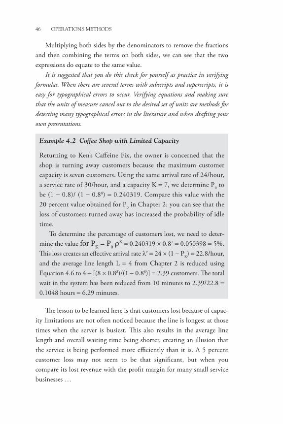
46 OPERATIONS METHODS
Multiplying both sides by the denominators to remove the fractions and then combining the terms on both sides, we can see that the two expressions do equate to the same value.
It is suggested that you do this check for yourself as practice in verifying formulas� When there are several terms with subscripts and superscripts, it is easy for typographical errors to occur� Verifying equations and making sure that the units of measure cancel out to the desired set of units are methods for detecting many typographical errors in the literature and when drafting your own presentations�
The lesson to be learned here is that customers lost because of capac-ity limitations are not often noticed because the line is longest at those times when the server is busiest. This also results in the average line length and overall waiting time being shorter, creating an illusion that the service is being performed more efficiently than it is. A 5 percent customer loss may not seem to be that significant, but when you compare its lost revenue with the profit margin for many small service businesses …
Example 4.2 Coffee Shop with Limited Capacity
Returning to Ken’s Caffeine Fix, the owner is concerned that the shop is turning away customers because the maximum customer capacity is seven customers. Using the same arrival rate of 24/hour, a service rate of 30/hour, and a capacity K = 7, we determine P0 to be (1 − 0.8)/ (1 − 0.88) = 0.240319. Compare this value with the 20 percent value obtained for P0 in Chapter 2; you can see that the loss of customers turned away has increased the probability of idle time.
To determine the percentage of customers lost, we need to deter-mine the value for PK = P0 ρ
K = 0.240319 × 0.87 = 0.050398 = 5%. This loss creates an effective arrival rate λ′ = 24 × (1 − PK) = 22.8/hour, and the average line length L = 4 from Chapter 2 is reduced using Equation 4.6 to 4 − [(8 × 0.88)/(1 − 0.88)] = 2.39 customers. The total wait in the system has been reduced from 10 minutes to 2.39/22.8 = 0.1048 hours = 6.29 minutes.

MORE COMPLEX SINGLE-CHANNEL MODELS 47
Limited Calling Population
The available customer population may be limited, as in the case for a service operation maintaining a fleet of airplanes for a major airline or a group servicing the copiers at a company. The Kendall notation for this situation when there is only one server is M/M/1/∞/N/FCFS, where N represents the number of customers or items to be served. In many textbooks and articles, this situation is often referred to as the machine repairman problem.
Because the costs of downtime can be quite high, there are often two or more servers to get equipment back in service quickly. This complicates the closed-form solutions considerably. This situation will be discussed in much more detail in Chapter 5. Here, we will discuss the single-server model because it provides some insight into the fundamental issues involved and is appropriate for many small service operations respon-sible for maintaining and repairing a small set of equipment. This also applies to those operations where one professional serves a select group of customers.
The arrival rate for a repair operation supporting N machines is usu-ally dictated by three things: the recommended preventive maintenance period, the expected failure rate, and the equipment usage rate (supplies replenishment). Equivalents of these rate components also apply to han-dling a select group of clients, such as at a financial advisor brokerage: regularly scheduled status appointments, typical percentage of emergency consultations, and volume-related requests.
We can attempt to analyze these classes as one combined calling population, or we can assign separate servers for each class. Consider that the preventive maintenance arrivals are essentially appointment based, and their respective service times are likely to be relatively constant or at least normally distributed with small standard deviations. The failure rate and subsequent repair times are more likely to be described by exponential distributions.
The base arrival rate for an M/M/1/∞/N model is defined by the needs of one customer, item, or machine for the situation under consideration. In the case of a machine, it can be the expected time between repairs

48 OPERATIONS METHODS
or scheduled maintenance. The effective arrival rate is the base arrival rate per unit λu multiplied by the number of units (N − L) in the finite population N that are not already in line for service in the system. The calculations for P0 with a finite population of N customers (machines) are considerably nastier because now we have to account for the reduced probability of future arrivals as current arrivals enter the system and are being taken care of. This requires using N summation terms, as shown in the following set of performance measures:
• Effective arrival rate: λ′ = λu(N − L)• Unit utilization factor ρu = λu/µ• Probability of zero customers in the system:
PN
N nn
N
un
0
0
1=
−×
=∑ !
( )!ρ (4.7)
• Probability of exactly n customers in the system:
P PN
N nfor n N P for n Nun
nn= ×
−×
≤ = >0 0!
( )!;ρ
• Average number of customers waiting in the queue (not yet being served):
L N Pqu
u
= −+
−
λ µλ
( )1 0
• Average number of customers in the system: L = Lq + (1 − P0)• Average time customers wait in the queue before being served:
Wq = L
q/(λ
u(N − L))
• Average total time customers spend in the system:
W = Wq + (1/µ) = L/( λ
u(N − L))
Looking at the equation for P0, it increases in value as N becomes smaller, which is what we would expect with a lighter workload. However,

MORE COMPLEX SINGLE-CHANNEL MODELS 49
as N becomes larger, there will be many terms in the denominator. This leads some business students to ask the question, “How large would N have to be where we could assume that an infinite calling population model could give us a ballpark estimate with only a small percentage of error? The calculations would certainly be easier to do.”
If we attempt to do this, students are reminded that they must recog-nize that we are not dealing with the same definition of arrival rate. In a repair service situation, the average arrival rate is based on some expected rate of failure per unit; as the number of possible items to be repaired increases, the effective arrival rate increases. The M/M/1/∞/N model takes these increases in N into account in its performance measures, but an M/M/1/∞/∞ model assumes an average arrival rate that is independent of population size. That is, some of that infinite population can choose to never arrive, or at least take a very long time before they choose to do so.
Example 4.3 Repair Service With One Server
Consider an in-house service activity staffed with a single person. Campus Reboot is responsible for maintaining a set of network print-ers located in several buildings clustered together as part of a liberal arts college. Campus Reboot is only responsible for repairs because routine reloading of paper, installing new toner cartridges, and clearing simple paper jams are done when needed by the respective department secretaries. At the moment, there are only 10 of these printers in use, but their popularity with the faculty for printing exams and quizzes is increasing, and the dean of the college wants to know what effect increasing the number of printers to 25 or even 50 units will have on the repair response. For now, we will ignore the associated costs but will return to this example in Chapter 6 to discuss the cost trade-offs. The failure rate for the current printer model used is 250 hours between repairs, and the typical repair takes an average of four hours, which includes any time spent to order parts or travel between build-ings. This information converts into an arrival rate λu per printer of 1/250 = 0.004 printer/hour and an average service rate of 0.25 printer/hour. This results in a value for ρu = 0.004/0.25 = 0.016.

50 OPERATIONS METHODS
There is an important consideration to note here. Some of you may be tempted to multiply the arrival rate per item by the total number of items to obtain the average arrival rate for λ. Do not do this because the derivation of the equations is based on the arrival rate per unit, which I designate by λu to avoid confusion with the more common understanding of what λ represents.
For example, consider the state diagram for a population of four items, as shown in Figure 4.2, where each state indicated by the hexagons represents the number of items L in the system. The arrival rate from state 0 to state 1 is 4λu because the entire population is available to move to that state. Similarly, the number of items available to move from state 3 to state 4 is only one because all the other items in the population are already in the system. The rate for moving the other direction, reducing the num-ber of items in the system, is the service rate, which can be applied to only one item at a time. If there are two servers instead of one server, then the reduction rate is 2µ from states 2, 3, and 4 and µ from state 1.
If you use Excel to determine P0, I recommend having separate col-umns as shown in Figure 4.3, for the terms in the summation portion of the denominator of Equation 4.7: n, (ρu)
n, (N − n)!, and the product within the brackets, rather than attempting to compose a single expression to calculate P0. Using N as an input value and summing the column for the products allows a simpler algorithm for computing the final result. This helps minimize computation errors, which is critically important for P0 because it is used for subsequent calculations. It also allows for easy expansion to larger N values by using Excel’s AutoFill capability to copy the respective formulas in each column further down the sheet. Appendix E shows the formulas used to determine the results in each of the cells depicted in Figure 4.3 for those interested.
0 1 2 3 4
4λu
3λu
2λu
1λu
µ µµ µ µ
Figure 4.2 State diagram for a single-server system with a limited population of four items with individual arrival rates of λu

MORE COMPLEX SINGLE-CHANNEL MODELS 51
Table 4.2 summarizes the results for repair populations of 10, 25, and 50 printers in response to the dean’s request regarding the effect of adding more printers to Campus Reboot’s repair response. With 10 printers, the average wait before repair work begins is about 39 minutes. This average waiting time increases to about 2.3 hours for 25 printers and nearly 10 hours for 50 printers. The number of printers
Table 4.2 Performance measures for M/M/∞/N model with N = 10, 25, and 50 units using the input data for campus reboot from Example 4.3
N 10 25 50P0 0.842919 0.609848 0.242301
Lq 0.025346 0.225374 1.886103
L 0.182427 0.615525 2.643802
λ′ 0.0392702 0.0975379 0.1894248
Wq (hours) 0.645432 2.310626 9.957002
W (hours) 4.645432 6.310626 13.957
Figure 4.3 Excel setup to determine P0 (shaded cell at upper right) and Pn for Example 4.3 with a population of 10 network printers. P0 is the inverse of the sum of the products in the fifth column, and the other Pns are the respective product for the value of n in the first column multiplied by the value for P0. As a check on the accuracy of the computations, the sum of the probabilities Pn in the sixth column is 1.0 (See the Excel formula view at the beginning of Appendix E for the calculations used in this table.)
n (N − n)! N!/(N − n)! (ρu)n Product Pn
0 3628800 1 1 1 0.842919
1 362880 10 0.016 0.16 0.134867
2 40320 90 0.000256 0.02304 0.019421
3 5040 720 4.1E-06 0.002949 0.002486
4 720 5040 6.55E-08 0.00033 0.000278
5 120 30240 1.05E-09 3.17E-05 2.67E-05
6 24 151200 1.68E-11 2.54E-06 2.14E-06
7 6 604800 2.68E-13 1.62E-07 1.37E-07
8 2 1814400 4.29E-15 7.79E-09 6.57E-09
9 1 3628800 6.87E-17 2.49E-10 2.1E-10
10 1 3628800 1.1E-18 3.99E-12 3.36E-12
Sum 1.186354 1

52 OPERATIONS METHODS
It should be noted here that many college textbooks still use lookup tables to solve this type of example for both single-channel and multiple- channel situations. As a result, the equations presented by those authors do not look anything like the equations used here. Instead, they use terms and expressions that work with these tables, often referred to in some textbooks as finite queuing tables (to be more correct some authors use the terms finite queuing for limited capacity models and finite sourcing for limited calling population models, which applies here). An example is the service factor X = average service (repair) time T divided by the sum of the average repair time T and the average time between repairs U. For Example 4.3, Campus Reboot’s service factor would be 4/(250 + 4) = 0.0157. The finite sourcing table for a given repair population level pro-vides two variables, D and F, for each combination of X and number of servers. Using these variables, one can then determine the usual perfor-mance measures.
Such methods are a product of an earlier time when personal com-puters and spreadsheet programs were not yet available. At that time, calculations like those shown in Figure 4.3 using pencil-and-paper methods were tedious, time-consuming, and more prone to errors. This led to the development of lookup tables for various values of N, service factors, and the number of servers (repair persons) to expedite such analysis. Often-quoted examples of finite sourcing tables in college
awaiting repair increases from the current value of 0.025 printer to nearly two printers for a 50-printer population.
Reviewing the results in Figure 4.3, the likelihood of more than one printer awaiting repair (two or more printers total in the repair shop) by Campus Reboot is less than (1 − P0 − P1) = 0.022214 = 2.22 percent for the current population of 10 printers.
If Campus Reboot works only a normal 8-hour day, it is likely that it will often take more than two days before some departments get back their broken printer if the number of printers increases to 50. This would be unacceptable given that a normal exam week is only five days long. We will return to this example in Chapter 5 to determine the effect of adding another repair person to Campus Reboot’s staff.

MORE COMPLEX SINGLE-CHANNEL MODELS 53
textbooks are sample tables for N = 5 or 10 used with permission from the 1958 reference published by Peck and Hazelwood.3
In this monograph readers are encouraged to use Excel-based methods because they allow a wider range of choices and conditions to best suit a given business situation. Instead of providing lookup tables, the equations for their creation are provided. Readers wishing more details regarding the derivation of these equations are encouraged to consult the excellent books by Hillier and Lieberman (2010) or Laguna and Marklund (2005).
Multiple Phases
In factory applications and some service businesses, there is more than one step (phase) in the process. How do we deal with those cases? Because each phase is likely to have a different service rate distribution, a closed-form generic solution would be unwieldy, even if the solution were possible. Some references are provided for those who are interested in pursuing closed-form solutions when they are available. A cautionary note is appropriate here. Many of the analytical solutions involve some in-depth mathematics and statistics understanding to determine whether they are appropriate for your business situation.
What if you do not want to become a math whiz to obtain some insight into how a multiple-phase process works? Not to fear, there are some characteristics we can work with to gain some understanding about such processes without the need for complex mathematics.
• The average arrival rate into each phase will be the same, assuming no losses or additions at each phase and that the average service rate for the phase is greater than the average arrival rate, because what went into the previous phase must come out of that phase.
• If losses or additions do occur during the process, they can be handled if we know their percentage related to the initial input arrival rate.
• In the case of factory applications, we usually have control over the arrival rate distribution by using production scheduling.

54 OPERATIONS METHODS
• Each phase can have a different service rate without affecting the average arrival rates into each phase. WARNING! This is still subject to the condition that the average service rate is greater than the average arrival rate. If the average service rate for a step is less than the average arrival rate, that step will become a bottleneck, causing work to pile up before that step and that step’s service rate will determine the capacity for the entire production sequence of steps.
Given these conditions, we can analyze or simulate a production process as a sequence of single-channel, single-phase waiting lines with the output of the preceding phase becoming the input to the following phase.
What do you need to look out for? A number of things can interfere with an otherwise successful simulation model. First, it is very, very difficult to include all of the disruptions that can occur in a multiple-phase process. Second, relatively predictable disruptions such as downtime for each phase for preventive maintenance, repair, operator training, late material deliveries, and tool setup time are often overlooked as to their effects on service and arrival rates. Third, while it is possible to include many disruptions in a simulation model many businesses do not collect sufficient operating data regarding their past frequency of occurrence or probability of happening. The need for such information and how to collect it is discussed in more detail in Chapter 6.
Because we can also accommodate a mixture of multiple-channel, single-phase process steps in manufacturing to deal with bottleneck capacity issues described above, there is a more detailed discussion of multiple-phase applications in Chapter 7.

CHAPTER 5
More Complex Multiple-Channel Models
In many service businesses and manufacturing line applications, the basic M/M/s model, like the M/M/1 model discussed in Chapter 4, does not always provide useful results that appear to agree with reality. In addition to the reasons listed at the beginning of Chapter 4, there are added factors as a result of using more than one server:
• More complex formulas to deal with, particularly for situations with limited queues or limited calling populations
• The opportunity to separate customers into different classes• The opportunity to treat customers with different priorities• The effects of using different line configurations• Server capability differences (varying service rates)
Equations 3.1 through 3.5 for the basic M/M/s model are restated here in a different form using ρ instead of λ/µ.1 This allows for easier computation of basic performance values and provides some insight into the minimum number of servers needed because ρ is now allowed to be greater than one.
P
n s /s
,
n
sn s0
0
1
1
1
=
+−=
−∑ ρ ρρ! !( )
(5.1)
Pn
P for
s sP
n
n
n
n s
=≤ ≤
≥
−
ρ
ρ!
!
0
0
0 n s
for n s
, (5.2)
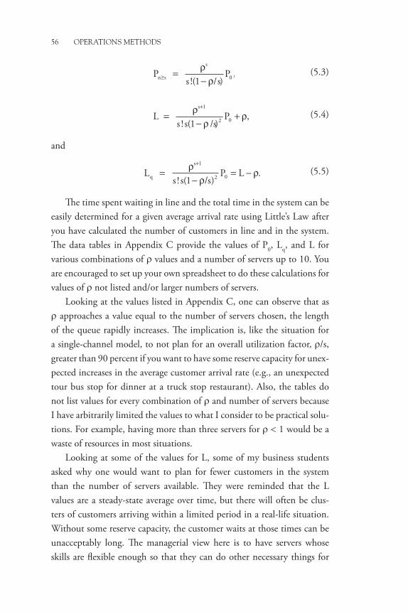
56 OPERATIONS METHODS
P
s /sP ,n s
s
≥ =−ρ
ρ!( )1 0 (5.3)
L
s s /sP ,
s
=−
++ρρ
1
2 01! ( )ρ (5.4)
and
L
s s /sP L .q
s
=−
= −+ρρ
ρ1
2 01! ( ) (5.5)
The time spent waiting in line and the total time in the system can be easily determined for a given average arrival rate using Little’s Law after you have calculated the number of customers in line and in the system. The data tables in Appendix C provide the values of P0, Lq, and L for various combinations of ρ values and a number of servers up to 10. You are encouraged to set up your own spreadsheet to do these calculations for values of ρ not listed and/or larger numbers of servers.
Looking at the values listed in Appendix C, one can observe that as ρ approaches a value equal to the number of servers chosen, the length of the queue rapidly increases. The implication is, like the situation for a single-channel model, to not plan for an overall utilization factor, ρ/s, greater than 90 percent if you want to have some reserve capacity for unex-pected increases in the average customer arrival rate (e.g., an unexpected tour bus stop for dinner at a truck stop restaurant). Also, the tables do not list values for every combination of ρ and number of servers because I have arbitrarily limited the values to what I consider to be practical solu-tions. For example, having more than three servers for ρ < 1 would be a waste of resources in most situations.
Looking at some of the values for L, some of my business students asked why one would want to plan for fewer customers in the system than the number of servers available. They were reminded that the L values are a steady-state average over time, but there will often be clus-ters of customers arriving within a limited period in a real-life situation. Without some reserve capacity, the customer waits at those times can be unacceptably long. The managerial view here is to have servers whose skills are flexible enough so that they can do other necessary things for

MORE COMPLEX MULTIPLE-CHANNEL MODELS 57
the business when the number of customers is sparse. Businesses that are good at this are grocery stores, banks, and the post office—either calling staff to the checkout lines when business is heavy or training employees to open another service window when a customer line exceeds a specified length.
Limited Capacity
This situation using multiple-channel models is often applied to call cen-ters where the number of people who can be put on hold awaiting the next available representative is limited. When that capacity is filled with waiting customers, new customers encounter a busy signal and in effect are blocked from entering the system. Estimating how many customers are being turned away is necessary to determine how many representatives (and phone lines) are needed to provide a desired level of service (the percentage of customers who do not encounter busy signals; that is, those not blocked from entering the system).
When the number of customers is equal to the number of servers, there are no customers waiting in line. This condition occurred in the early days of queuing theory when the most common application was telephone exchanges using operators to make connections for callers. The technology for allowing customers to wait in an electronic line was not yet developed, and callers got a busy signal if the operators were already engaged with helping previous callers. Such queuing models were called an Erlang loss system because potential customers were lost when all the servers were busy. When a waiting line application allowed customers waiting for service to form a line, it was then called an Erlang delay system because those customers were not lost when all the servers were busy; they were just delayed in receiving service.
The set of average performance equations for the M/M/s/K model with a system capacity of K customers is as follows (K must be ≥ s):
• Utilization factors (note that ρ can be greater than 1 if the number of servers is greater than 1):
ρs = λ/sµ
ρ = λ/µ

58 OPERATIONS METHODS
• Probability of zero customers in the system:
P
n sn
sn s
n s
K n s0
10
1=+
= = +−∑ ∑ρ ρ ρ
! !
(5.6)
• Probability of exactly n customers in the system:
Pn
P for
s sP for
n
n
n
n s
=
≤ ≤
≤ ≤−
ρ
ρ!
!
0
0
0 n s
s n K
n K0 for >
(5.7)
• Probability of customers in the system greater than the number of servers (probability that the servers are busy):
P Pnn
n
s n
>=
= − ∑s 1 00
ρ!
• Probability that a customer will be turned away: PK = P0ρ
K/s!sK − s
• Average number of customers waiting in the queue (not yet being served):
LP
s ss
K ssq
s
=−
− + − −
+0
1
2
1
1 1 1ρ
ρρ
!
( )
−ρs
K s
(5.8)
There is no solution in Equation 5.8 when ρs = ρ/s = 1. A solution can be found using L’Hospital’s Rule2 twice to obtain the limit for Lq when ρ/s approaches the value of 1. Although the resulting numerator terms can be complex, the denominator term reduces to 2s!s for ρ/s = 1.
• Average number of customers in the system:
L L nP s Pq
n
s
nn
s
n= + + −
=
−
=
−
∑ ∑0
1
0
1
1 (5.9)

MORE COMPLEX MULTIPLE-CHANNEL MODELS 59
• Effective arrival rate: λ′ = λ(1 − PK)• Average total time customers spend in the system: W = L/λ′ =
L/(λ(1 − PK))• Average time customers wait in the queue before being served:
Like the discussion in Chapter 4 for the M/M/1 model, we need to use an effective arrival rate (λ′) for Little’s Law. This is the arrival rate minus the customers or items turned away by the limit in line capacity. The assumption is that those customers are lost and do not return. Because we lose some customers, we can allow the average arrival rate to be as high as the average service rate, which explains the conditional equations for Pn expressed by Equation 5.7. PK gives us a value for lost business that can be used to compare with the cost of adding additional line capacity. PK is sometimes called the blocking probability.
Limited Calling Population
Example 4.3 described a repair service with one person responsible for maintaining 10 items. When the number of customers or items becomes significantly larger, as illustrated in that example, more than one person is usually needed to provide an adequate turnaround time for items need-ing repair or maintenance. There are two approaches for analyzing the performance of adding staff:
1. If an item requiring service is of the type where a service crew can be effectively used (such as maintenance on an airplane or a truck), then the repair crew is treated as a single server where adding a member to the crew hopefully reduces the average service time per item. In this case, the M/M/1/∞/N model discussed in Chapter 4 would still apply, but we would use a shorter repair time associated with the increased crew staff for our calculations.
2. However, in many repair and maintenance situations, the item requiring service can be effectively worked on by only one person.

60 OPERATIONS METHODS
In this situation we need to use the M/M/s/∞/N model to deter-mine the average performance expected if we decide to add one or more servers to improve performance. The disadvantage is that the equations become much more challenging to use, and additional care is required to avoid mathematical errors.
Recalling the use of an unit arrival rate and associated unit utilization factor as discussed for the single-channel limited population model in Chapter 4, the set of average performance equations for the M/M/s/∞/N model with a limited population of N customers or items to be served is as follows (N must be ≥ s):
• Arrival rate per unit in the population: λu
• Unit utilization factor: ρu = λu/µ• Probability of zero customers in the system:
PN
N n n
N
N nn
s un
n s
N un0
0
1
1=
−
+−=
−
=∑ ∑!
( )! !
!
( )
ρ ρ!!! s sn s−
(5.10)
• Probability of exactly n customers in the system:
P
N
N n nP for
N
N n sn
un
un=
−≤ ≤
−
!
( )! !
!
( )! !
ρ
ρ
0 0 n s
s sPn s− ≤ ≤
>
0
0
for s n N
for n N
• Probability of customers in the system equal to or greater than the number of servers (probability that the servers are busy):
P PN
N n nn sn
sun
>=
= −−∑1 0
0
!
( )! !
ρ
• Average number of customers waiting in the queue (not yet being served):
L n s Pq
n s
N
n= −−
∑( ) (5.12)

MORE COMPLEX MULTIPLE-CHANNEL MODELS 61
• Average number of customers in the system:
L L nP s Pqn
s
nn
s
n= + + −
=
−
=
−
∑ ∑0
1
0
1
1 (5.13)
• Effective arrival rate: λ′ = λu (N − L)• Average total time customers spend in the system: W = L/λ′ =
L/(λu (N − L))• Average time customers wait in the queue before being served:
• Probability of no waiting time for the next arrival:
Before returning to Example 4.3 to see what improvement is possible for a greater number of printers by adding staff, let us consider how we might develop our own finite queuing tables3 using Equations 5.10 through 5.13 in a spreadsheet program like Excel. Similar to the multiple-server tables in Appendix C, we can obtain some useful values of P0, Lq, and L for various combinations of N, ρ, and s. Like the finite queuing tables published by Peck and Hazelwood (1958), it will be best if we prepare separate tables for different calling population sizes. But unlike Peck and Hazelwood’s tables, we can set up our Excel solutions so that we can obtain P0, Lq, and L directly rather than going through the use of some intermediary variables in a lookup table.
Unlike the equations provided in Chapter 3 for the basic M/M/s model, the equations for P0, Lq, and L when the population is limited become too complicated to formulate in a single Excel cell because of the extensive summations required in the formulas. Therefore, if you want to set up your own set of tables, you will need to use some additional columns to compute the summation values for specific combinations of ρu and s for a specific population N. Recall that we did this in Chapter 4 when we analyzed a single-channel model with a limited line capacity K (see Figure 4.3).
An example spreadsheet solution is illustrated in Appendix C for Example 5.1, where we return to the Campus Reboot situation discussed in Chapter 4 and consider adding one or more servers to that repair service.

62 OPERATIONS METHODS
Example 5.1 Repair Service with Multiple Servers
Returning to the Campus Reboot service example in Chapter 4, we recall that the service response would become unacceptable if we added 25 or 50 printers. So the dean has asked us how much improvement we would obtain if we hired another repair person or two. Using the equations just given for the M/M/s/∞/N model, we obtain the values shown in Table 5.1. Appendix C shows a copy of the Excel spreadsheet for the N = 10, s = 3 situation. Like the Excel setup shown in Figure 4.3, it is useful to set up separate columns for the summation terms required. Once those columns are established, it is easy to add additional terms for larger values of N by just copying the formulas down the sheet for each value of 0 to N. The use of these columns also allows easier troubleshooting for mathematical errors.
As a check for mathematical errors, several conditions can be observed to indicate whether or not they are present. If these condi-tions are not present, then it is very likely that you have made either a mathematical error or incorrectly typed in a cell reference. Check the following:
• Is the waiting time in the system W at least equal to, or greater than the repair time for the item in question? For Example 5.1, the repair time is four hours per printer.
Table 5.1 Performance measures for M/M/s/∞/N Model with N = 10, 25, and 50 units using 1, 2, or 3 servers for example 5.1
N 10 Printers 25 Printers 50 PrintersServers s = 1 s = 2 s = 3 s = 1 s = 2 s = 3 s = 1 s = 2 s = 3
P0 0.842 0.853 0.853 0.609 0.669 0.672 0.242 0.434 0.450
Lq 0.025 0.001 0.000 0.225 0.014 0.001 1.886 0.131 0.016
L 0.182 0.158 0.158 0.616 0.407 0.395 2.644 0.917 0.803
λ′ 0.039 0.040 0.040 0.098 0.098 0.098 0.189 0.196 0.197
Wq (hours)
0.645 0.018 0.001 2.311 0.141 0.010 9.957 0.669 0.080
W (hours)
4.645 4.018 4.001 6.311 4.141 4.010 13.95 4.669 4.080

MORE COMPLEX MULTIPLE-CHANNEL MODELS 63
Different Classes of Customers
An important consideration in improving service performance when working with multiple-channel waiting lines is recognizing whether or not you have different classes of customers with different service distri-butions. When more than one server is required to provide acceptable service, a subsequent decision is whether you have each server handle any customer that arrives or designate servers to specific classes of customers. A common example is the use of express and regular checkout lines at a grocery store when the store is large enough to justify having more than one checkout clerk. Another example is providing a window at a bank for business customers in addition to windows for regular customers.
• Does P0 increase in diminishing increments as the number of servers increases for a given value of N?
• Do Lq and L decrease in diminishing increments as the number of servers increases for a given value of N?
• Does λ′ increase as the number of servers increases (minor change) and with increases in N (bigger change)?
• Is the sum of all the Pn’s calculated for a given value of N equal to 1.000? Given the numerical precision used in your calculations, the result could be off a significant digit or two, but it must be very close to 1.000.
Observing the results in Table 5.1, my initial conclusion would recommend staying with one server for the current population of 10 printers and using two servers for the populations of 25 printers and 50 printers. This recommendation would provide roughly equivalent turnaround performance for all populations. It should also be noted that with a population of 50 printers, it is more likely that a faculty member can find an alternate printer to use temporarily when his or her usual printer is being repaired. This possibility would support a business decision to not add a third server for the 50-printer situation.
To obtain a full analysis for a more informed recommendation, we need to consider the trade-offs in the costs of hiring another repair person versus having a faculty member wait longer for a repair to be completed.

64 OPERATIONS METHODS
More detailed aspects about taking advantage of customer classes for improving service performance is discussed in Chapter 6, where we also can take into account other managerial considerations.
Different Customer Priorities
Multiple-channel waiting lines provide additional options for handling customers with different service priorities. When there is only one server, priorities can be handled only by manipulating the order of customers in the queue. This is a frequent concern in a small hospital emergency room with only one doctor on duty, where the most gravely ill patient must be treated first. Obviously, when there is more than one of these patients at a time, then tough choices have to be made as to which one is treated first. That decision with its moral and ethical implications is clearly beyond the scope of the level of analysis discussed here.
When more than one server is available, several options are available for managing priority needs. In one aspect, priority defines a class of customers that are handled in a different way than we decide to handle other classes. This can be because some customers have more urgent needs, their service is more complicated or requires special skills, or their long-term relationship with a business merits some extra consideration. These approaches will be discussed in more detail in Chapter 6—where we will discuss class management.
Different Line Configurations
More servers also allow some creativity in how the line(s) of customers are arranged, particularly when some servers are dedicated to a particular customer class or priority. In addition to improving service performance, important considerations for line configuration design include the psy-chological effects on customers and opportunities to inform customers as to what they can do to help speed up the service process.
A common example of different line configuration approaches used in many banks, post offices, and airport security check-ins was shown in Figure 3.1. From a strict average performance business viewpoint, both

MORE COMPLEX MULTIPLE-CHANNEL MODELS 65
the separate line per server and one line feeding all servers (the “snake”) configurations have the same average values for service performance.
The differences between the two configurations are found in individual customer waiting time experiences and psychological impressions. Because of this, the configuration choice is often more dependent on managerial attitudes and prior experience rather than actual numbers. We will discuss this topic in more detail in Chapter 6 where we will focus on managerial concerns.
Service Capability Variations
In Chapter 3 and this chapter, our analysis has assumed a consistent service rate for each server. In reality, we all know that this assumption is often invalid based on our experiences in a line where a server gets tired at the end of their shift or, more noticeably, a new teller or checkout clerk is learning on the job. Most service activities are repetitive in nature, and repetition makes a person more proficient (faster and more accurate) as he or she gains experience doing that task. Such improvement is more dramatic at first and slowly diminishes in magnitude over time until the person’s performance essentially flattens out to a steady level; ignoring for the moment, any degradation caused by fatigue. Some good examples are learning how to ride a bicycle or memorizing commonly used reference values or coffee recipes instead of having to look them up each time you need them.
Learning curves can be used to estimate the time to reach a given proficiency if there is information available as to what percentage of improvement over time is typical for a given job content. In general, the more repetition and less variety of tasks involved, the faster the improvement rate. The learning curve equation is based on the concept that every time the total number of repetitions of a task is doubled, the amount of time per repetition is reduced by a constant percentage. The equation for a learning curve takes the following form:
T T n where b
ln(%)ln
.nb= × =1 2( )
(5.14)

66 OPERATIONS METHODS
Here Tn is the time required to do the nth repetition, T1 is the time required to do the first repetition, and the % sign is the learning percentage value in decimal form. A learning percentage value of 80 percent (0.8) corresponds to a 20 percent reduction in time per repetition every time the total number of repetitions doubles. So a higher learning percentage corresponds to a slower improvement in proficiency (100% = no improvement with repetitions).
If you have some data regarding how long each successive repetition takes for your situation, you can estimate your typical learning percentage in two different ways. The first method is more universal but a bit more complicated:
%ln T /T
ln(n)n
=
2
1( )
. (5.15)
The other method is to take the ratio of any pair of repetition times, where the number of repetitions for one time is double or half the num-ber of repetitions for the other time. Then the learning percentage is the shorter time divided by the longer time. That is, the % = Tx/Tx/2 or T2x/Tx.
Figure 5.1 shows several learning curves with different learning percentages. A table of the values used for the different learning curve percentages and numbers of repetitions in Figure 5.1 is in Appendix C.
Figure 5.1 Learning curves showing the decrease in time required per repetition as the number of repetitions increase experience for different learning rates. Contrary to intuition, the higher the learning curve percentage, the longer it takes to acquire proficiency
1.00
0.90
0.80
0.70
0.60
0.50
0.40
0.30
0.20
0.10
0.001 4 7 10 13 16 19 22 25 28 31 34 37
70%
75%
80%
85%
90%
40 43 46 49
Number of repetitions
Per
cent
age
of ti
me
for
firs
t rep
etit
ion
52 55 58 61 64 67 70 73 76 79 82 85 88 91 94 97 100

MORE COMPLEX MULTIPLE-CHANNEL MODELS 67
Example 5.2 Service Time Reduction Learning Rates
How long does it take for a server to become proficient in a given service activity? Searching the Internet can provide some estimates of what others think the time is if there is insufficient information for your business. For example, Grasing (2011) comments that many banking people estimate that it takes typically three months for a new teller to reach full proficiency, and a teller typically should be able to handle an average of 30 transactions per hour at that level. Like many pieces of information on the Internet, we must ask, “Are these realistic estimates by the banking crowd?” before proceeding to use them for our analysis. One verification is the article by Kotha et al. (1996), where they relate how the management at KeyCorp initiated a campaign that reduced average service time down from slightly more than four minutes to less than two minutes. This result is consistent with the value of 30 transactions per hour reported by Grasing.
Let us assume a relatively slow learning curve of 90 percent and use a Tn of two minutes from the 30 transactions per hour expectation. Further, let us assume that it takes about 10 minutes (T1) for a new teller to do a transaction for the first time. Manipulating Equation 5.14 to solve for n, the number of repetitions required to achieve a proficiency of 30 transactions per hour, we obtain
In(n) = (1/b) × In(Tn/T1) where b = −0.152 for a learning percentage of 90 percent.
Plugging in the other values, we get In(n) = 10.588191 → n = 39,664. Is this a realistic value? As a check, consider how many transac-tions could be done in three months by a proficient teller at an average of 30 transactions per hour. For thirteen 40-hour workweeks, the total would be 15,600 transactions. We are obviously off here either in the learning percentage, the first task time estimate, or both. Assuming that a typical business would more likely have an accurate estimate of the time required for the first repetition, we will stay with our 10- minute first-repetition time. Hence a faster learning rate estimate is needed to reduce the total number of repetitions required to reach an average two-minute transaction time. Because of the exponential nature of this

68 OPERATIONS METHODS
Is three months too long for a service employee to become proficient? Shortening the amount of time required would be to the advantage of any business. It obviously depends on the skills needed and the complexity of the tasks to be done. An earlier edition of a popular college operations management textbook4 used a bakery to illustrate the use of various manufacturing process strategies in a single business. In the video of the bakery operations that accompanied the text, the bakery manager com-mented on the typical training time for new employees for each process. The highly automated bread process required only a few weeks, work in a pastry shop required about three months, and a cake decorator required about six months to become proficient. Because effective train-ing approaches often are dependent on the right managerial support, we will reserve further discussion about such methods for Chapter 6.
When the server is a combination of a person and equipment or just primarily an equipment operation, other service variabilities come into play. Allowances must be made for maintaining the equipment and ensuring a steady supply of materials for it to use. One needs to be careful to not use the performance figures provided by the equipment makers without understanding how those performance figures were obtained. Did they include typical downtimes for service or repair, account for some degradation caused by wear, and so on?
Lacking such data, many businesses apply a fudge factor to such performance claims in the range of 75 to 90 percent with this rationale in
learning curve formula, only a small adjustment is required. Using a learning percentage of 88.5 percent, we obtain –0.176 for b and 9,242 transactions for n. This is a more reasonable result because we would expect that the total number of transactions for a new employee over three months would be less than 15,600. It also indicates that the esti-mate of three months by the banking crowd reported by Grasing is more likely a worst-case value.
Note: We could have solved this problem more accurately using Excel’s Goal Seek or Solver add-ins but doing so would have obscured the reasoning used to set up either of those tools. Readers might find determining a learning rate answer that best fits the values quoted in the literature using either of these add-ins to be a useful exercise.

MORE COMPLEX MULTIPLE-CHANNEL MODELS 69
mind. If they operate a piece of equipment at 80 percent of rated capacity and it unexpectedly goes down for an hour they can catch up on that lost hour’s production by running the equipment at 100 percent of rated capacity for four hours. In a similar manner, if the demand (arrival rate) unexpectedly increases for a short time they have some reserve capacity to satisfy it without adversely affecting their usual performance for the normal arrival rate. In the realistic situation where the equipment is no longer capable of running at rated capacity, they still have enough reserve capacity to catch up in less than six hours at 95 percent capacity or eight hours at 90 percent. As equipment wears out, this fudge factor should be reduced correspondingly.
Multiple Phases
In many multiple-phase applications the individual steps can be a sequence of single-channel configurations as discussed at the end of Chapter 4 or a mixture of single-channel and multiple-channel configurations to better handle situations where one of the single-channel steps does not have sufficient capacity. That is, its service rate is lower than that of the other steps and thus it limits the capacity of all of the steps following it and causes a pile up of partially completed work by the faster steps preceding it. Adding another server or piece of equipment at this step eliminates such a bottleneck by increasing the effective service rate for this step.
While this makes the simulation for such process more complex it can be done by treating the multiple-channel as a black box, if you will, with its input the arrival rate from the preceding step, its output as the arrival for the following step, and its internal workings described by mul-tiple-channel equations rather than single-channel equations. This is the approach discussed in more detail at the conclusion of Chapter 7.


CHAPTER 6
Managerial Considerations
This chapter covers topics where an astute managerial choice can minimize uncertainties and improve overall performance for businesses affected by some form of waiting line behavior. The areas of consideration include the following:
• Variances in waiting line performance, which includes looking at variances from both the customer and the business points of view plus estimating the risks of worst-case scenarios
• Waiting line cost factors from both the customer and the business perspectives. (As mentioned in Chapter 1 these factors can be strongly interrelated, particularly in transportation and delivery applications.)
• Cost trade-off analysis• Service improvement approaches• Use of customer participation to reduce waiting and service
times• Waiting line configuration considerations• Psychological factors (while difficult to quantify, these factors
are significant considerations that are interlinked with many other areas in this list.)
• Arrival rate management methods• Options for dealing with priorities, such as more urgent need,
rush orders, and preferred customers• The more effective use of information gathered by a business
and what additional information should be collected for managing and improving waiting line applications.
Some of you may have jumped ahead to this chapter because you feel that you already know all you have to know about waiting line theory.

72 OPERATIONS METHODS
That may be true for some; but for most, it would be wise to review at least some of the topics in Chapters 2 through 5 if parts of the following discussion are confusing.
Variance and Risk Considerations
When I asked business students to select the better business solution after giving them the average performance for each of the choices presented, most of them quickly chose the one with the highest average. When more than one choice had the same average performance, the same group of students often commented that any of those choices would do.
A few students will look beyond the average performance to consid-erations of risk or the accuracy of the average performance value before making their choice. To evaluate risk or accuracy, some knowledge of the variances in a process is necessary. Unfortunately waiting line equations provide only steady-state average performance. Start-up variances, such as whether there is a line of customers waiting when a business opens its doors or there is a set of items left over from the previous day of pro-duction that need to be completed before beginning new work, are not included in steady-state results. Larger variances, such as no customers for periods of time or a large group of customers that arrive all at once during the day, occur less often; but when they do, they can cause significant business disruptions.
Events such as the probability the line will be longer than the capac-ity of the business can be calculated, but when that condition can occur during a period of time cannot be predicted. Managers need to remember that waiting line arrivals and service times are memoryless. That is, what happens next is not influenced by what has just happened in the past. For example, when flipping a coin, the next coin toss result is unaffected by whether or not there were two heads, two tails, a head and a tail, or tail and a head for the previous two tosses.
One variance often not considered is the potential variance in normal service and arrival times when waiting lines are much longer or shorter than usual. This is often referred to as a state-dependent variance or rate.1
When waiting lines get long, some newly arriving customers may be discouraged from entering the line (balking), and some current custom-ers may choose to give up and leave (reneging). At the same time, many

MANAGERIAL CONSIDERATIONS 73
servers feel the pressure to speed up their work to help move the line faster. As a result, this creates three general managerial concerns:
1. Arrival rate variances caused by balking or reneging result in lost business opportunities, which were discussed in earlier chapters and can be assigned a cost value for trade-off decisions if sufficient infor-mation has been collected regarding various operating costs.
2. When the line is short, a server may unnecessarily chat with a cur-rent customer or otherwise work more slowly. This reduces the opportunity for the server to do other work useful for the business. (This can also happen when lines are long if the server is tired or a customer is someone they know well.)
3. When the line is long, servers may work faster by taking shortcuts and perhaps not being as careful to prevent mistakes, which, when they occur, often offset any time gained because of the additional time required to correct them. This affects the customer’s perception of the service quality received and can be quite serious if the mistake is preparing or assembling the wrong order, omitting something from the order, or making an error in recording the payment and/or giving the customer change.
Clear managerial communication and good server training can min-imize server variances by letting servers know they will not be penalized for remaining careful and not taking shortcuts when lines are long and making clear any requirements regarding what servers are expected to do during times when no customers are present or a customer wants to chat unnecessarily.
In manufacturing lines, some of the arrival rate variances can be minimized through careful production scheduling; but when dealing with customers, we have to work with arrival rate variances unless the business is conducive to using an appointment or reservation system. In customer service lines, reneging and balking can be reduced by opening up a temporary express window for customers with standard, easy-to-do needs. An advantage of this approach is that you can use a staff person who may not be trained in the full range of services offered. An example of this is opening up a window strictly for customers only picking up mail and/or packages at post offices when the line is long.

74 OPERATIONS METHODS
So, how do we assess potential variances and risks in waiting line performance? We can perform three basic actions:
1. Be aware that variances and their associated costs exist and often can be much larger than one would normally expect. In addition, we need to accept that average performance values predicted by queuing equations are the exception rather than the rule for indi-vidual customer experience or item behavior in a queue. Figure 2.3 illustrates this situation by showing some of the performance data for the first 100 customers entering a typical coffee shop.
2. Collect data about how the business operates (Shaw 2013, Chapter 4). Be particularly careful to be consistent across all business functions in acquiring data related to similar business operations. One exam-ple is using the same time references for arrival and service rates and for assessing costs. The value of an analysis is only as good as the data used to perform it, another statement of the principle of garbage-in, garbage-out (GIGO). Observing the number of arrivals per period and the number of customers or items in the system at the end of each period allows a determination of waiting times using Little’s Law and an estimation of service times. Processing point-of-sale (POS) data can provide estimates of the percentage of different customer classes and service time distributions. This data can be used to develop more accurate discrete distributions for arrival and service rates in simulation models. Some of these data collection and simulation methods are discussed in more detail in Chapter 7.
3. Simulation runs using an accurate model of the given business pro-cess can be used to provide more accurate average performance values than the standard queuing models can predict. This is particularly true when the arrival and service distributions for a business are not well described by the basic probability distributions. The simulation runs also can provide a picture over time as to how the performance values can vary and identify the possible worst-case and best-case scenarios. The caveat here is that the simulation results are useful only to the degree that the simulation model accurately represents how the particular business actually operates. Some of the Chapter 7

MANAGERIAL CONSIDERATIONS 75
simulation examples illustrate how to calculate data regarding possible variances.
Variances that are very difficult to quantify are differences in customer attitudes. Their tolerance of waiting times and long lines can vary greatly depending on the time of day, the weather, whether they are with a friend or not, whether their service need is urgent or not, any personal time limitations, and so forth. Although we cannot usually address the direct causes of these variations, we can reduce their intensity by considering the psychological factors associated with waiting. Some of these factors and methods for reducing their effects are discussed later in this chapter. The most important consideration to remember when accounting for variability in waiting line business decisions is that the variances experienced by the business are NOT directly related to the variances encountered by customers.
Waiting Line Costs
Many of us have been in the situation where the cost information is scanty, but our boss requires a quick decision. So, what do we do? We make the best decision we can with what data we have and fill in the gaps with our intuition and past experiences. This is a pretty good solution in many business situations, but when waiting line characteristics are involved, we need to recognize that there is a much higher level of uncertainty because we no longer can count heavily on our intuition and experience in processing limited data to guide us to a reasonable answer.
When evaluating cost trade-offs, you should also recognize that such analysis is only as good as the understanding you have regarding your business. Estimated values result in only ballpark guesses as to the best choice. Even worse is when you are unaware of a background activity that is necessary for you to be able to provide your service. Many of the textbook examples for waiting lines focus only on “front-office” activities when evaluating cost. However, some process changes when directly deal-ing with customers can have a significant effect on “back-office” processes. Therefore, it is strongly recommended that you and your staff develop a service blueprint2 of your business to help take into account all the costs and performance factors affecting its outcomes.

76 OPERATIONS METHODS
The simple graph in Figure 1.4 shows the basic idea that the total cost of a waiting line application has some minimal value per customer served or item produced when the proper balance of resources and customer satisfaction is achieved. The concept here is that adding more resources and/or improving service performance reduces the waiting time and the length of the queue.
• For manufacturing applications, this correlates to faster throughput time and reduced work-in-process (WIP) inventories.
• For repair and maintenance activities, this means that equipment is not out of service for as long, which reduces the size of the equipment fleet required for adequate operational capacity.
• For customer applications, this correlates to retaining more customers, reducing the possibility of balking, and increasing the business volume that can be accommodated.
However, these increases in resources and equipment to improve service performance also increase operational costs. The basic trade-off that must be considered, therefore, is as follows: “If I add more resources to improve service, is there enough reduction in waiting and other costs combined with a potential increase in the number of customers to more than pay for those resources?”
Table 6.1 lists several cost values that are needed to make useful waiting line business decisions. The list is not intended to be inclusive, but it provides enough items to help you identify the types of costs that you should consider for your business decisions. Table 6.1 also gives some symbols that we will use here to simplify the equations for analyzing cost trade-offs. Many textbook authors use C to represent cost, with a subscript or parenthetical notation to represent the particular type of cost. For example,
C(Total) = C(Waiting) + C(Resource)or
CTotal = CWaiting + CResource

MANAGERIAL CONSIDERATIONS 77
Here we will use a larger set of cost symbols, which are defined in greater detail in Appendix B. This helps us remember that there are several waiting-cost and service-cost components, as indicated in Tables 6.1 and 6.2.
It is rare that you can trade off one waiting cost factor against one resourcecost factor without having some effect on other cost factors� Therefore, do not be surprised if the result of your decision is not exactly what your analysis told you to expect�
Volume-related costs, such as utilities3 and the materials associated with what each customer or item requires for service, are usually ignored
Table 6.1 Some cost components to be considered when seeking a minimal cost balance between waiting costs and resource costs
Cost Symbols Components Data sourcesBalking CB Lost customers, bad PR Marketing
Blocking CB Limited capacity K M/M/s/K model
Reneging CB Line not moving fast enough Marketing
Waiting time CW Waiting time in line, total time in service process
All models and simulation
Throughput time CW Waiting time in line, total time in service process, capacity
Simulation
Financing C$ Credit interest, insurance Accounting
Spoilage C$ Production loss, step yields, perishable inventory, theft
Accounting and manufacturing
Warehouse space CH, CF Inventory holding costs, rent All models andAccounting
Lost business capacity
C$ Repair time, line length, population size N, late penalties
M/M/s/∞/N model
Appointment delays
C$ Appointment schedule, service time variation
All models and simulation
Staffing CS Salaries, benefits Accounting and human resources
Equipment CE Price, maintenance, spare parts, depreciation
Vendor and accounting
Facility CF Construction, permits, rent, maintenance, capacity, security, insurance, utilities, janitorial services
Vendors, accounting, service process

78 OPERATIONS METHODS
in cost trade-off analyses unless the supplies are perishable (such as food) and the cost decision has a direct effect on the amount of spoil-age. Where things get complicated is how we handle floor space costs. If these costs are solely due to business volume (more total customers → more space), then they are usually not a factor in determining the minimal total value. But if more floor space is required to not turn away potential customers, then the profits gained from the increased number of customers per period must exceed the increased facility cost per period.
Lost business capacity and lost profit costs are similar in that both lose a potential profit. Lost business capacity is when you lose some of your normal capacity for a short time, such as when a resource is delayed in the repair shop when you had planned to use that resource to satisfy an existing customer order. Lost profit is when your normal capacity is insufficient to accommodate a customer who would have entered your business to place an order if not discouraged by a long line or insufficient capacity for waiting customers. Lost business capacity often has addi-tional losses because you may have to pay a late-delivery penalty to the customer, or the customer may cancel the order after you have already put some work into its completion.
A tricky cost component is the percentage of server idle time. Most businesses include it as part of the service costs associated with a server. However, when P0 is more than 10 percent to 15 percent of an individual server’s time, there is an opportunity to reduce total costs by asking the server to do some routine maintenance or other support tasks instead of assigning them to back-office staff. In businesses with a staff of several servers, this practice could reduce the overall staffing needs by one or more people.
You may notice that I did not specifically list line length in the waiting costs column for Table 6.2. Line length plays a part when considering a limited capacity situation (M/M/1/K and M/M/s/K models), where the length of the line affects blocking costs. However, it is the time spent waiting in line that is the primary cost driver in many situations. The old adage “time is money” applies very well here. To help illustrate why line length is not as important as waiting time, consider Example 6.1. You may feel the background information is more than needed, but the intent

MANAGERIAL CONSIDERATIONS 79
is to illustrate the importance of considering factors that, at first glance, may not seem relevant to the goal of reducing total costs.
A special category included in Table 6.2 is when there is only one possible source for the service, such as a government agency (passport office, driver’s license bureau, business registration, the courts, airport security, etc.). In such situations, balking, lost customers, and customer satisfaction are not likely costs, and the only issue of primary interest is providing enough capacity in the form of facilities and staff to meet the average demand within some maximum time limit at the lowest cost possible. I have not included post offices in this category because many countries have alternatives to official government agencies for mail and package shipments.
Several examples follow to illustrate approaches for determining cost trade-offs for waiting line situations. Example 6.1 describes some basic cost calculations, and Examples 6.2 and 6.3 illustrate the nature of
Typical ApplicationWaiting Costs: CB,
CL, CW, and CH
Resource Costs: CS, CE, and CF
Coffee shop, bank Balking, blocking, waiting time, reneging
Staffing, equipment, facility
Single source: passport office, department of motor vehicles, licensing, other government agencies
Waiting time Staffing, equipment, facility
Manufacturing line Throughput time, financing, spoilage, warehouse space
Equipment, staffing, facility
Self-service Reneging, waiting time Equipment
Repair and maintenance Lost business (capacity reduction), spare equipment
Staffing, equipment, facility
Call centers Blocking, reneging, waiting time
Staffing, equipment, hold capacity
Parking lots Blocking, reneging, waiting time
Facility, maintenance
Health clinics, professional services
Appointment delays Staffing, facility
Table 6.2 Some waiting and resource costs to be considered when working with different categories of waiting line applications

80 OPERATIONS METHODS
things to consider for more complex cost trade-off analyses. For a good discussion regarding total cost analysis for queuing situations, readers are referred to the online Chapter 26 supplement by Hillier and Lieberman (2010).4
Example 6.1 Sandwich Stand Cost Trade-Offs
Samantha runs a small sandwich stand on the streets of Portland, Oregon, selling three types of ready-to-go sandwiches for $3.05 each. Because Oregon does not have a sales tax and her costs per sandwich are $2.80, she nets $0.25 per sandwich. We will also assume here that Samantha has learned her market very well and is careful to not make more sandwiches than she can sell in a day. When business is brisk, Samantha sells out more quickly and gets a longer afternoon off. For the few times she has any sandwiches left, Samantha cheerfully donates them to the local homeless shelter at the end of the day. Thus we will not consider monetary losses due to surplus sandwiches that must be discarded.
Samantha has been studying waiting line theory when she gets off early and has decided to collect some data about her business and see if it really works. She determines that it takes about one minute for a customer to choose which type of sandwich and pay for it. By check-ing the reduction in her inventory during her peak hours, she also has determined that the average number of customers between 11:30 a.m. and 1:30 p.m. is 54 per hour.
Using these values for λ and µ, Samantha determined that the uti-lization factor during the peak period is 0.9, the average line length (L) should be nine customers, and the average total time for a customer to get a sandwich is 10 minutes. Because the author of her waiting line book has stressed that average values are rarely actually experienced by customers, she concluded that if some customers get their sand-wiches in less than 10 minutes, then others have to wait longer than that. Thinking further, Samantha realized that because lunch-time customers do not want to spend any more time than necessary to get their lunches, she is likely losing some customers to other food vendors when her line gets longer.

MANAGERIAL CONSIDERATIONS 81
Wishing to reduce the average waiting time, Samantha worked on the only factor within her control—service time. Observing transac-tions for several days, Samantha noticed that the major part of the service time was making change for customers, particularly dealing with coins. In the interest of learning more about waiting line theory, Samantha decided to invest some of her profit in an experiment to shorten service time by reducing the price to $3.00, eliminating the need for handling coins. After a week, Samantha observed that this change reduced the average service time by 10 seconds, increasing her average service rate per hour from 60 to 72.
Plugging her new average service time into the M/M/1 equations, Samantha now determined that L should be three customers—a dramatic improvement from nine customers. But she was puzzled because such a change should have been evident, yet she had not noticed significant line differences during the lunchtime period. She was also selling out her stock of sandwiches earlier in the day, which agreed with the faster ser-vice time. What could be wrong with her analysis? Then she remembered to recheck her sales rate during the peak time and discovered that it had increased from 54 to 65 customers per hour. Plugging that value into the M/M/1 equations resulted in a revised average line length of nine cus-tomers and an average total time in line of 8.57 minutes per customer. The line length did not change, but the average time in the system did.
At this point, let us step back and look at what happened here. First, line lengths can stay the same while total waiting time changes as long as the utilization factor remains the same. That is, service rates keep up with increased arrival rates. Stated another way, arrival rates tend to increase when service times are reduced because customers can get faster service. The length of a line is not as important to customers if they perceive the line is moving faster (a psychological factor to consider). In this case, Samantha’s stand attracted more customers because they could observe the line moving more quickly (the price reduction and customers not having to deal with coinage could also be contributors). (Note: I fudged the amount of the service time reduc-tion to illustrate more clearly that the same line length could have different waiting times.)

82 OPERATIONS METHODS
To illustrate situations where reasonable service improvements could pay off in lower total cost, we will discuss three more examples. The first is a classic repair service problem, where long turnaround times could cost a company significant money. The second is a manufacturing system where WIP inventory is expensive. The third is evaluating the benefit of adding
Let us look at the profit margin during the peak period for the two scenarios: 108 × $0.25 versus 130 × $0.20 → $27 versus $26. From a profit viewpoint, the process improvement cost Samantha $1.00 of profit based on the lunchtime results, but we should take into account the effect of the improved service time on Samantha’s business the rest of the day and the possibility for her to sell more sandwiches per day before deciding whether or not to continue offering the sandwiches for $3.00.
Given the nature of Samantha’s service process, there are limited possibilities for her to reduce her service time. In such cases, the primary option is to add another server at the peak time. Referring to the table in Appendix C and using Samantha’s initial value of ρ = 0.9, adding one more server would reduce the average line length to 1.1285 customers, and the average total time to get a sandwich would decrease to 1.25 minutes. Now Samantha has an estimate of how many more customers she can expect to attract by reducing waiting time from her service time reduction experiment, so she estimated that with the even better performance provided by another server, she could keep the increased volume and also charge her original price of $3.05. Would this pay for the cost of another server? Running the numbers, the increased profit would be $5.50—not enough to pay minimum wage for even an hour.
The conclusion here is that sometimes the options available for improving a particular service process are not enough for the customer volume and profit model associated with that process. In Samantha’s case, she would have to have significantly higher volume to justify hiring another server. Just shortening the waiting time and the average line length are not likely to attract that many more customers; other things such as expanding her sandwich choices, adding beverages to the selection, and so forth, would be needed, which, in turn, would introduce a whole new set of cost factors.

MANAGERIAL CONSIDERATIONS 83
more space to accommodate longer lines. Working through the solutions is left to the reader as an exercise; each example discusses the situation, indicates what costs should be considered, and how one might go about determining the best solution.
Example 6.2 Helicopter Shuttle Business Costs
This business provides regular flights for residents of a small rural city to the nearest major airport located some distance away. The busi-ness goals are to not miss a regularly scheduled departure—because being late could cause greater hardship for their passengers—and accomplish that performance at a minimum total cost. Operational cost factors to consider include keeping the size of the helicopter as small as possible because helicopters are costly to own and maintain, determining the number of daily flights required to satisfy customer demand, the routine maintenance schedule required by the Federal Aviation Administration, how many reserve helicopters are required, the likelihood of unexpected breakdowns, and the possibility of unavailable staff due to illness or vacation. Some factors to compare are the costs of having or leasing spare helicopters versus reducing the average maintenance time by either adding staff to existing service crews to reduce the average service time, adding one or more service crews plus the facilities to support them to reduce maintenance and repair waiting time, or paying for some on-call staff. Performance and total costs for each business option can be evaluated using the M/M/s/∞/N model, where s, N, and µ and their unit costs are the variables.
For some specific examples discussed in detail, Hillier and Leiber-man (2010), Chapter 17, Section 17.10, is a good place to start.
Example 6.3 Factory Inventory Costs
A small business runs a factory line customizing an expensive large product with just one operation step. The demand for this product does not allow using a production schedule to help manage the average line length; thus its arrival rate is best described by an exponential distribution. The inventory costs associated with the average line

84 OPERATIONS METHODS
length can be quite high for this product. Some factors to compare, with the goal of achieving the lowest total cost, are inventory financing costs (price and interest) and warehouse costs (facility space, rent, handling, security, utilities, and insurance) versus hiring more staff to reduce waiting time or buying new or additional equipment to reduce service time. Performance and total costs for each business option can be evaluated using the M/M/s model, where s and µ and the unit costs for each option are the variables.
Example 6.4 Ice Cream Shop with Limited Customer Space
A small ice cream shop occasionally loses customers on hot summer days because it can only accommodate a small number of customers within the store. Is it worth adding more space for the line to accom-modate more customers? The factors to compare are the lost profit per customer not accommodated versus adding floor space, reducing the average line length (which reduces the probability that the line will exceed the current available space) by adding staff, or reducing the average service time by buying equipment or otherwise improving the service rate. Costs can be evaluated for all possible business options using the M/M/s/K model.
Improving Service Performance
There are several basic goals to consider when improving service performance. Some of these are strictly from the business perspective—reducing total cost, completing services faster, and accommodating higher customer volume. Others are from the customer perspective—not hav-ing to wait as long for service, a lower service charge, perceived fairness, and a more pleasant waiting experience. Because some of the possible approaches apply to both perspectives, they are listed first.
• Reducing the variation in service times reduces the average waiting time, even if the average service time remains the same (see Chapter 4).

MANAGERIAL CONSIDERATIONS 85
• Reduce the average service time.• Reduce the average waiting time.• Add capacity—more servers, more waiting space.
Variation reduction is normally the least expensive approach because you are working on using existing resources more effectively. Standardiz-ing all or part of the services provided reduces the variation in service time and reduces the average waiting time, even when the average service time remains the same. In Example 6.1, Samantha standardized part of her service by having sandwiches ready-to-go rather than assembling them to order. This reduced both variability and the duration of the average service time, allowing a single server, Samantha, to handle more custom-ers. She could provide more sandwich selections without adding to the service time by setting up a condiment station so that customers can add their own condiments rather than asking her to do it, a change that would help decrease her average service time and also reduce some of the vari-ability of that time.
Of course, Samantha will have to spend some time to maintain the condiment station, but this can be done during any idle time when there are no customers. For her utilization factor of 0.9, P0 = 10 percent, which gives her an average of six minutes per hour to maintain the station. The hidden cost factors to be considered are Samantha’s choice of method for obtaining ready-to-go sandwiches—typically a classic make-versus-buy decision.
Another approach for reducing service time variability is to replace the manual parts of a service with more automated methods. This in effect is another form of standardization most often applied to manufacturing situations, but it can also be used effectively in service situations. For example, consider the coffee machines at many gasoline station con-venience stores. The cost trade-off considered here is whether having a person keep a hot pot of coffee ready to pour a cup when a customer wants it or having a machine prepare the coffee for the customer on demand is the least expensive option. Doing the cost comparison involves not only the difference and variability in average service times between the two options but also the consideration of spoilage with the manual method,

86 OPERATIONS METHODS
variation in the coffee preparation time, equipment and maintenance costs for either option, and response times for a sudden jump in customer volume (probability the coffee pot is empty, the time to brew a full pot versus the fixed response time for a machine). Another factor, of course, to be considered is the average customer preference for pot-brewed coffee versus machine-brewed coffee. (Given the average age of most pot-brewed coffee in gas stations, I personally prefer the machine-brewed versions.)
Reducing the average service time reduces the average waiting time while increasing the capacity of the service system. Adding more servers is often the first strategy employed to reduce the average service time. But this also increases the probability of no customers in the system (idle time). Normally, the cost of adding servers is offset in the cost analysis by reductions in waiting time costs and expected increases in customer vol-ume. Hidden cost factors that are not often considered are the possibility of using idle server time to do other tasks required by the business that are not directly related to serving customers. Some examples are managing inventory and cleaning and restocking equipment or service areas, such as a convenience store coffee machine or Samantha’s condiment station. This, of course, requires servers who have more flexible job skills and thus may require a higher salary. The primary focus here should be that the added staff is hired primarily to be a server.
The opposite approach is when a staff member hired primarily for a back-office activity is asked to serve customers during periods of peak demand. The limitation of course is that back-office staff members are often not very skilled in performing the full range of service activities, but they can be used for providing simpler, more standardized services during peak demand periods. This often works well for situations such as banks, post offices, and grocery stores where the customer arrival rates are highly variable during the day.
Reducing the average service time by eliminating unnecessary (non–value-added) steps is a common approach discussed in process manage-ment texts, but it can be difficult to do when there is little possibility of standardization in the service process. What can be done is to eliminate the execution of some customized steps by the server and have the customer do them instead. Some examples are having customers fill out forms (health insurance, food orders, address labels, etc.) while they wait instead of the server asking questions and filling out the form for the

MANAGERIAL CONSIDERATIONS 87
customer. There is also a psychological benefit in doing this, which will be discussed in more detail later in this chapter.
Another way to reduce the average service time without adding serv-ers is to inform customers about what is expected from them when they reach the server. In fast-food restaurants and coffee shops, displaying the menu with prices in clear view of the line helps reduce the time customers spend at the server window deciding what they want to order. Promptly displaying the amount of payment due after receiving the order reduces more service time by allowing a customer to decide on the payment method or collect the appropriate change while the server either processes the order or forwards it on to the kitchen or the barista. This leads to one of my big rules regarding customer–server interactions: Uninformed customers require more service time� Use the time spent waiting in line to educate them.
The current best example of this is the airport security check-in process. Clear and properly located information signs5 can prepare the customer as to what the customer must do at each step instead of the secu-rity agents having to take time to explain individually what is expected of each customer at each stage of the check-in process. This saves the agent’s voice and lowers frustration for the agent as well as the customer.
Reducing the average waiting time is very difficult to do unilaterally for all customers because it is so strongly related to the arrival rate and service rates. But it can be reduced for some customers in the arrival population by either separating them into different service classes with different average service times or by assigning them a higher priority. Some common examples of this are as follows:
• Express lines at grocery stores for customers with only a few items
• Windows dedicated for mail pickup at the post office• Bank tellers dedicated to commercial business customers• Frequent-traveler express lines at airports, car rental agencies,
and hotel check-ins• Separate coffee shop line for customers just wanting a
standard cup of house coffee. They could even pour it themselves and self-pay with their cell phone.
• Self-service stations or checkout lines for standardized services

88 OPERATIONS METHODS
• Moving airline travelers who would otherwise miss their flight to the head of the airline counter check-in lines
• Taking care of more seriously ill patients in an emergency room first
• Prescreened air travelers at security check-in lines and customs checkpoints.
The disadvantage with methods that reduce the average service time and/or the average waiting time for some of your customers by serving them according to priority or class is that if you retain the same resource level for the same total average population, your average service rate will remain the same, but the overall variability in the waiting time experi-enced by your customers will increase: Some classes will have a shorter average waiting time, and others will have a longer average waiting time. The old adage “there is no such thing as a free lunch” holds true in waiting line operations.
The “classes” approach requires a multiple-server situation with at least two servers—more if there are several classes to be served separately. Thus, if you do not already have multiple servers, you are in effect adding resources to reduce waiting time. The “priority” approach can be used in both single-channel and multiple-channel waiting line models.
In the classes and priority approaches, the overall average throughput rate remains unchanged provided that in multiple-server applications a server who is normally assigned to higher priority or a specific class of customers is expected to take care of lower priority or other classes of customers when that server is idle (jockeying is allowed in that case). Therefore, from a business viewpoint, capacity and average throughput rate remain unchanged. From the customer viewpoint, some of them are served faster at the expense of other customers now having to wait longer.
At this point, some of you are likely thinking, “Why bother doing this? It sounds like a no-gain situation that rewards only some customers.” The answer is that sometimes there is little choice to not do it. For a hos-pital emergency room, it should be clear that having a priority approach is necessary. Rewarding customers who individually contribute a higher percentage of your profits with higher-priority service is a standard

MANAGERIAL CONSIDERATIONS 89
business practice to encourage them to continue being your customers when competing with other businesses that also provide such incentives.
What are not so obvious are the potential cost advantages. To keep the mathematics manageable, the basic closed-form, waiting line equa-tions assume that all servers are equally capable of providing the same service rate. In Chapter 5, we discussed the situation of how long it would take for a new bank teller to achieve that proficiency. Now consider the advantage of a classes approach that would allow new tellers to handle simple transactions, such as deposits and withdrawals, at first and move to more complicated banking transactions later. Their learning curve could then be broken into two or more learning curves with faster learning percentages.
This leads to an important conclusion: Classes allow the use of a range of server skills, which, in turn, allows the possibility of a range of server costs. For example, consider a three-server application where all the servers are expected to be able to handle the full range of expected customer transactions. But in many situations, part of the normal customer population needs only services that could be done using a self-service machine. Automatic teller machines (ATMs), online banking, Web check-in, flat-rate package mailing, and convenience store coffee machines are some examples that this is true.
This is one area where managers earn their salaries. We can do the cost comparisons using the three-server example versus two servers and a machine or even one server versus one or two machines. We can account for the differences in capabilities (flexibility of the server or server substi-tute) and relative costs, assuming we have a good estimate of how many customers in each class we plan to serve. This is the easier part. What is more difficult is considering the risks involved.
In this situation, if one server becomes ill, it is likely that the service can still be provided but with commensurate longer waiting times. This is also the case when we replace one server with a self-service machine: If the machine breaks down, the two remaining full-service servers can temporarily take up the slack. (In both cases, λ/µ must be less than two for this to be possible.) But if one of the two remaining servers becomes ill, the machine cannot take up the entire sick server’s load because of its more limited capability. That is, a server can take all the work of a broken

90 OPERATIONS METHODS
machine, but a machine can take over for only part of a server’s work. The risk imposed by this lack of interchangeability increases when cost comparisons indicate to a manager that the most economical situation is two machines and one server. (Note: Since this book was originally published the capability of the typical bank ATM has expanded consider-ably and even cell phones can be used to make check deposits and access account balance information.)
Considering that more complex transactions are usually more critical, I would want to be sure that they are covered. Therefore, without even looking at the cost comparisons beforehand, I would restrict my cost comparisons for this situation to the three-server or the two-server-plus-machine options.
If some of the possible classes turn out to be a very low percentage of the total population, it is usually better that they be included as part of a larger class. But, if a class is a significant percentage of a business’s clientele, it is usually worthwhile to consider how you can provide a separate service or priority for them.
One great example of how to serve one class of customer without add-ing either servers or machines was at a local coffee shop in Oregon where the owner set up a self-serve station for his customers who just wanted a cup of house coffee. He also eliminated the need for a server to handle payments for the house coffees by posting the price for each size of cup and trusting his customers to put the appropriate amount into a locked cashbox with a slit in it. I discretely observed that almost no customers skipped the payment, and some put in more than what was asked because they did not have adequate change. In this case, he reduced not only the average waiting time for his house coffee customers but also the need for server time to support that part of his business.
So how does a business owner identify different classes of customers? In sales operations, POS data can really help. Some examples are as follows:
• You can screen your POS receipts for the percentage of customers who buy less than a given number of items to determine whether or not an express checkout line would be useful.

MANAGERIAL CONSIDERATIONS 91
• You can screen the POS data for how many customers order products or services that require only a standard service time.
• You can analyze your sales data for your highest volume buyers or service requests.
• Adding a time stamp to the POS receipt allows an estimation of the number of customers served per time of day that can be used to develop discrete distributions for simulation models.
• Combined with the date stamp, seasonal variations in customer volume and demand for different services or items can be determined.
You can also ask your customers to help by allowing them to select the class of service they want. This is particularly useful for call center and repair service operations. When calling in for support, we all have encountered choice menus that let us identify what type of question we want answered. This not only directs us to the right person to answer that question but also provides data that the call center can use to adjust staffing levels, allows the looking up records by the computer for some requests like asking for your current account balance, or makes the records already available for an operator to reduce the average service time and required staffing levels.
A useful concept is to recognize that when arrival rates are described by exponential distributions with appropriate average values, one can easily combine or separate average arrival rate distributions for the classes. The results will also be exponential distributions with the same general characteristics.
For example, consider a typical banking call center operation where there are three choices (effectively classes where the customer tells you what class they are in) on the telephone menu, such as the following:
1. Account balance check2. Billing and payment questions3. All other questions
Assume that the bank knows the average arrival rate for each choice by analyzing its previous call history. We will designate these rates as λ1, λ2,

92 OPERATIONS METHODS
and λ3. Hence the total arrival rate λ to be handled by the call center if it is operated as a multiple-channel, single-phase system where any operator can answer the next call is merely the sum of λ1, λ2, and λ3. Of course, in a large call center with several operators with different skill levels, each individual arrival rate (menu choice) is likely to be assigned to a specific operator or even an automated response for some choice. It should be obvious that the third choice listed is the one that would require the most skilled operator because of the wide range of possible questions that choice allows.
Consider a similar situation with the same choices, where the business knows the overall average arrival rate λ for its customer base but has not yet collected enough data to break down that rate into the individual rates for each choice. Wanting to improve its service by possibly desig-nating specific operator(s) or automated responses to each choice, the business checks with a call center consulting firm for information about industry average percentages for each class of questions. The consulting firm provides the values of P1, P2, and P3, respectively, for the business’s choices. Because exponential distributions can also be easily separated into components that are also exponential distributions, the bank can then obtain λi by multiplying λ by the respective probability Pi.
You can get useful information even when a consulting firm does not have all the usual percentages. This is often the case because your customer base does not match up well with any of the databases that con-sulting firms might have. Software can monitor the frequency of choices selected in the telephone menu: Given that information, a manager can then decide whether or not in the future to address the choices separately or as a combined pool.
Finally, when improving service performance by adding more servers, the training time required for a new server to achieve an acceptable proficiency level becomes a business priority. Those businesses that can do it faster than their competitors have a competitive advantage when the demand for their type of services is increasing. The most important element is clear communication between the manager and the service employees about the training process and what is expected. This should include how to deal with long-line situations to avoid the state-dependent rate variances discussed earlier.
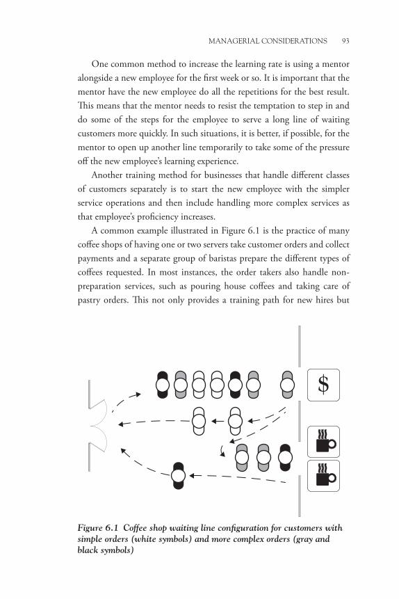
MANAGERIAL CONSIDERATIONS 93
One common method to increase the learning rate is using a mentor alongside a new employee for the first week or so. It is important that the mentor have the new employee do all the repetitions for the best result. This means that the mentor needs to resist the temptation to step in and do some of the steps for the employee to serve a long line of waiting customers more quickly. In such situations, it is better, if possible, for the mentor to open up another line temporarily to take some of the pressure off the new employee’s learning experience.
Another training method for businesses that handle different classes of customers separately is to start the new employee with the simpler service operations and then include handling more complex services as that employee’s proficiency increases.
A common example illustrated in Figure 6.1 is the practice of many coffee shops of having one or two servers take customer orders and collect payments and a separate group of baristas prepare the different types of coffees requested. In most instances, the order takers also handle non-preparation services, such as pouring house coffees and taking care of pastry orders. This not only provides a training path for new hires but
Figure 6.1 Coffee shop waiting line configuration for customers with simple orders (white symbols) and more complex orders (gray and black symbols)
$

94 OPERATIONS METHODS
also allows the more effective use of the more highly trained barista staff and the ability to use part-time workers for the order taking. In effect, two lines and two classes have been created here: one for all customers and a second line (phase) for customers with more complex orders.
Since the first edition of this book, advances in communication technology have resulted in new useful variations of the order taking process. For example, drive-through coffee shops can use smart phones or wireless tablet computers to allow taking orders from the cars waiting in line, shortening the service time at the pickup window. Taking this technology a step further, there are attachments for those devices that allow the use of credit cards for making payments to further reduce the service time at the window.
Waiting Line Configurations, Psychological Factors
Many times, it is not practical or even possible to do much to reduce the average waiting time for a service. First, it is important to not do things that would increase a customer’s perception of how long the wait is likely to be. Second, there are things we can do to reduce anxiety while waiting in line or even to allow a customer to make more effective use of that waiting time. Some suggestions paraphrased from the available online literature are given here; for more detailed information, con-sult the classic article by Maister (1985) and the discussion by Norman (2008).
Some general axioms regarding the waiting experience are as follows:
• If a customer has time limitations, anxiety increases, and the wait appears to be longer. This is especially appropriate for lunchtime customers and passengers at baggage check-in whose flight is scheduled to leave very soon.
• The more desirable the service, the longer people are willing to wait. Popular restaurants, popular movies and shows, and limited attendance venues are good examples. A corollary here is that excellent service can compensate for some poor waiting conditions. However, a business should avoid relying on this corollary if they want to remain competitive.

MANAGERIAL CONSIDERATIONS 95
• The more necessary the service, the more customers will tolerate a long wait.
• Waiting on hold seems longer than waiting in line because the customer cannot see how long the line really is and how fast it might be moving.
• When there is more than one line, your line always appears to be more slowly. You notice it when the other line moves with respect to you but not when your line moves with respect to the other line.
• Time moves more slowly when you have nothing to do but wait. The corollary is that the wait appears to end more quickly when you have something to do like reading a book or chatting with a companion.
Some negative psychological factors to be avoided are as follows:
• A clock on the wall that can be seen by those waiting in line reminds customers of the passage of time.
• Not informing customers about what is to be expected (priority rules, what preparation is required of the customer to obtain service, how long the current average wait is, etc.). One common failure in this regard is the practice of many restaurants to assign specific tables to each server on duty. Customers who are unaware of this can be quite upset when they have been waiting and a nearby server who is not assigned to their table seems to be ignoring them. Some customer dissatisfaction can be avoided by the host or hostess seating customers at their table and telling them who their assigned server will be and perhaps even taking their drink orders to get things started when the restaurant is busier than normal.
• An uncomfortable waiting environment: Expecting people to wait outside in a predominantly rainy climate like the Pacific Northwest or asking medical patients to stand instead of sit while waiting are just cruel practices. When people have other more comfortable waiting options at a competitor for the
96 OPERATIONS METHODS
service they want, such practices will cost a business many of its customers.
Some positive things a business can do are as follows:
• Give customers something to do while they wait. The best items are things that contribute to completing the service process, such as filling out forms, informing customers about what they will need to do when they reach the server, or letting them know about any personal data or items that may be required for service rather than finding out that need when they reach the server window after a long wait. In some cases, it is possible to allow a customer to leave the service facility to do other things during the waiting time and then return shortly before they are next in line for service.6,7
• Use a single-line configuration for multiple-server applications wherever possible. The single-line and parallel-line configu-rations in Figure 3.1 provide the same average waiting time from a business perspective, but the variability in individual customer experience and the perception of how fast the line moves are different. The single-line configuration moves every time a single customer is processed; parallel lines move only when a customer in that line is processed. The more servers, the faster the single line moves in respect to individual lines. In addition, the variability in individual customer waiting times is reduced because the effect of individual service times that are very long or very short are averaged out over the number of servers rather than affecting just the line in front of one server.
• Make the waiting area more comfortable and even produc-tive for customers while they wait. Seating, wireless access to the Internet, and self-serve coffee stations have become more common in many waiting areas as businesses become aware that customers who have something to do are more tolerant of uncertain or longer waits. The use of having customers take a numbered ticket when they enter allows much more flexibility

MANAGERIAL CONSIDERATIONS 97
in where they wait and how they use their waiting time. In an area where many customers are arriving and leaving, such as a governmental office, the progression of the numbers called up for service also provides a sense of how fast the line is being served.
Arrival Rate Management Methods
Another approach for reducing variability in service processes is to try to control the arrival rate to some degree. The most familiar method is using appointments or reservations. Appointments are used where there is more predictability in the nature of the services requested and the facility capacity and choice of servers are relatively constant. When the service time has a greater range of variability, such as serving meals in a popular restaurant, and a wider choice of servers can serve a given customer, res-ervations are more appropriate. Other significant factors here are the cost and availability of servers. The higher the skill requirements, the higher the cost per server and the lower the part-time availability is for such skilled individuals—hence the prevalent use of appointments for most professional services.
Consider a typical medical clinic appointment schedule. The facility has a fixed number of medical staff and examination rooms. The capacity of the facility is dependent on the effectiveness of the appointment schedule. Some medical services, such as vaccinations and routine tests, have a relatively constant service time, making their appointment schedule easy if the demand requires it (when some daily peaks are greater than the daily capacity). The appointment time then becomes whatever the service time is plus some easily calculated small addition to accommodate cleanup and preparation between patients.
But when we consider the appointment schedule for doctors on the staff, life just became more complicated. The factors to be considered are that not all doctors require the same average examination time, examination times can vary considerably from one patient to the next, patients sometimes arrive a bit late, some room must be left in the appointment schedule to accommodate unscheduled urgent care patients,8 and, most important of all, when a patient examination lasts

98 OPERATIONS METHODS
longer than the allotted appointment time, it affects the timing of some if not all the subsequent appointments that day. Taking all this into account, the goal of an appointment scheduling time analysis is to select an appointment duration that reduces the possibility of an appointment running late without trading off too much patient capacity. The trade-off is between the costs of having staff stay later to accommodate the patient who made the last appointment versus accommodating fewer patients during the day.
Having a probability distribution that accurately represents the distribution of examination times is essential. Unfortunately, the stan-dard use of an exponential service distribution to represent service time in general queuing analysis models does not work well here because it allows a high percentage of service times lower than the average time. A normal distribution is more representative of medical examinations, and Erlang or beta distributions are better, but the best is when the clinic has collected enough data to determine its own discrete distribution for use in simulation programs for scheduling. The process of moving med-ical records from paper form to online digital form makes it much easier to collect data for analyzing and improving service processes. Just the opportunity to readily and automatically record time-of-day data with medical observations recorded online makes it easier to determine discrete service time distributions for various medical activities.
Example 6.5 Appointment Schedule Analysis
A doctor and a nurse are reviewing their appointment schedule to see if they can revise the average appointment time. The goal is reduce the number of evenings working late to take care of the last patient when some appointments run over. Their data show that the average examination time for a patient takes 15 minutes. They also need an average of two minutes to prepare the examination room for the next patient and enter the current patient’s medical records into the computer. Their current appointment time is 20 minutes, which allows them to take care of 24 appointment or urgent-care patients in an 8-hour day. They had thought that amount of time would provide enough spare time to accommodate an occasional appointment

MANAGERIAL CONSIDERATIONS 99
overrun, but experience indicates that it is not enough. They have not yet accumulated enough data to have an accurate estimate of the variability of the examination times, but they do remember that a few examinations took as long as 30 minutes.9
Let’s use a normal service time distribution to see if we can get a rough estimate on what might be a better appointment time. We will use 15 minutes for the mean time and 30 minutes as a worst-case time; then we can estimate the standard deviation σ as being one-third of the difference between the maximum time and the mean time, which gives us a standard deviation of five minutes. We are assuming here that a ±3σ distribution around the average time will include almost all (99.74 percent) of the possible examination times. I have not included the two minutes for preparation and record-keeping because this is under the control of the doctor and nurse, does not vary much from patient to patient, and can be made up in different ways that do not affect patient times.
The current overrun margin is 20 − 15 = 5 minutes or 1σ. Con-sulting a normal distribution table, the percentage of the normal distribution less than or equal to 20 minutes is 84.13 percent, so there is a 15.87 percent chance that an examination will take longer than 20 minutes. Because there are currently 24 appointment periods per day, an average of 0.1587 × 24 = 3.8 appointments will run over each day. This, of course, does not tell us when those overrun appoint-ments will occur during the day. If they all occur early in the day, some following patients will have to wait longer for their appointments. (Keep in mind here that the normal distribution also has appointment times shorter than 15 minutes, providing an opportunity to make up some time during the day for longer appointments that occur early in the day. But the later in the day that those longer appointments occur, the less opportunity for making up time there is.) If they all occur late in the day, the doctor and nurse will really be working late. Thus, when the overruns occur is very important for this analysis.
If the doctor and nurse increase the appointment time to 25 minutes, the probability of an overrun drops to 2.28 percent, which is less than one appointment overrun per day. But we also have reduced

100 OPERATIONS METHODS
Example 6.5 illustrates how a normal service time probability distribution can be used to estimate the probability of an appointment running over. This simplified problem illustrates the need for using simulation methods, where the effect of various appointment times and different overrun times can be evaluated to determine the best result that provides the highest capacity without undue costs and customer waits. A normal distribution is rarely the best distribution for scheduling pur-poses, but it is often the choice because it is easier to use in queuing analysis models and more familiar to users.
Some other observations are that if the examination room preparation and patient record entry could be handled independently of the doctor and the nurse, it would free up another two minutes per appointment. For example, you could have a dedicated record clerk do the entries and a dedicated attendant prepare examination rooms. The problem of course is that you would lose the immediacy of the time-of-day data related to when the entry data were actually collected.
Staggering the appointment times so that each doctor in a practice does not start appointments at the same times would simplify the sched-uling of these back-office support activities. Staggering appointment times would also space out appointment check-ins for a smoother process flow at the check-in desk and provide a positive psychological effect in the waiting room because patients would be arriving and departing on a more regular basis, not intermittently in groups.
Actual operational data are necessary to provide the best representa-tions of the service time and arrival time distributions in simulations. It cannot be emphasized enough that the result of a simulation is only as good as the knowledge of the real-life process and the accuracy of the actual operational data available for it. For some good discussion about what operational data to collect for a variety of situations and ways to acquire it, refer to the book by Hubbard (2010).
the number of appointments per day from 24 to 19, a capacity loss of 20.8 percent. This would create a need to add facilities and doctors somewhere else to take care of the five patients who are being turned away each day.

MANAGERIAL CONSIDERATIONS 101
For this medical clinic problem, the following data are needed for an accurate simulation solution:
• A history of actual examination times is needed to build an accurate discrete probability distribution for those times.
• A history of appointment overruns, how long each was, and what time of day it occurred gives a picture of the typical overrun.
• Separate this information into values associated with regular patients and values associated with unscheduled urgent-care patients. (It is likely that longer examination times are more closely associated with urgent-care patients, but this assump-tion should be verified.)
• Identify the number of urgent-care patients per day per class of care. This helps in planning the number of open appointments needed per day and how they might be shared among the doctors who are most capable of handling the particular class of care required.10
• Identify the history of times that patients arrived for an appointment: how early or late were they and what time of day was the appointment. Such arrival timing variations can contribute to overruns and hinder the ability to catch up after an overrun or even get ahead of schedule.
Reservation policies have similar constraints and data collection needs, but they allow some simplifications because the number of reservations required per day is more limited. For many popular restaurants, the number of successive reservations (turns) for a given location is limited to how many groups they expect to seat at that location during a normal dining period (breakfast, lunch, or dinner). Obviously, the restaurant will require an estimate of how long customers will typically take to order and eat their meals and also must recognize that their service rate contributes to the length of this period. One rule of thumb to help judge the variability of dining time is that the larger the group, the longer one might expect customers will take for dinner because of the increased amount of socializing (and beverages) that are likely to occur.

102 OPERATIONS METHODS
In many European restaurants, a group has the table for the evening, so the likelihood of a late-night reservation is not considered. In that respect, such restaurants are no different from one-time events, such as airplane flights, hotel rooms, Broadway shows, and sporting events. The challenge here is to fill the available seats or rooms for maximum profit. There is always some risk that someone with a reservation will cancel at the last minute. Knowing the average number of no-shows based on their past experience, some businesses will accept that number of reservations over their available capacity to ensure full usage of that capacity. The risk they take on is possibly having to deal with a highly dissatisfied customer who has a reservation and no accommodation because the usual number of no-shows did not occur. This practice, called overbooking, is used by many airlines and hotels. While overbooking analysis also involves work-ing with arrival distributions and probabilities, it is not included in the scope of this monograph.11
Data and Information Management
Collecting the appropriate data and processing it to gain information for managing and improving waiting line applications is essential if a business using such applications wants to remain competitive. One obstacle to overcome is the exponentially increasing volume of data collected by most businesses today because the advances in information technology (IT) have made it easy to do. The challenge for management is winnow out the data potentially useful for queuing applications from this deluge of numbers, facts, customer feedback, and so on often referred to these days as Big Data. Sadly, despite the plethora of data, it is often lacking the one important set of data points required to process relevant data into useful information for waiting line problems. A common example is accurate time-of-occurrence data to help determine probability distributions, aver-age service and arrival rates, seasonality factors, customer losses because of inadequate service capability, and probabilities of downtime and other process disruptions.
A major contribution to this situation has been the growth of IT groups, departments, or functions, depending on the size of the business or enterprise, to manage the hardware and software technology required

MANAGERIAL CONSIDERATIONS 103
to collect and process the data a business requires to be successful. The catch is that many of these functions have also been given the respon-sibility for selecting what and how the data are collected and processed with an often unspoken understanding that those groups will, of course, consult with the other parts of the business dependent on that data and information regarding what is selected. This approach made a lot of sense in the beginning days of IT when there were few people that understood both how the technology worked and how it might be used. Today, how-ever, the average desktop system on a worker’s desk is more capable than a building full of mainframes, card readers, and tape/disk drives in the 1980s. In addition its operating system is much easier to use and minimal programming skills are required to take advantage of the computational features offered by programs such as Excel.
Okay, so what does this mean? It means that managers and employees need to be more involved in the selection of what data is collected, the conditions under which it is collected, and how it is processed to provide useful information. Otherwise, they may make a decision using information that is not exactly relevant to their situation or will obtain analytical results that are not representative of what actually is occurring in real life. That is, the management of information processes used in conjunction with other business processes such as waiting line applications needs to be done in an integrated manner as discussed in considerable depth by me in another Business Expert Press book (Shaw 2013). Some highlights from that book most appropriate for waiting line situations are:
• Information is the result of processing data and can be done internally using data collected directly by the business or can be purchased from others, such as a marketing firm, with the caution that in that case one often does not have any knowl-edge of what sets of data were chosen and how they were used to provide that information.
• For each step or process in a business, a manager or improve-ment professional should ask what data/information are required for its successful execution?, what data/information are created?, what data/information are stored?, and what data/information are transferred elsewhere in the business?

104 OPERATIONS METHODS
• Information and data security are not directly essential for managing and improving service and other queuing applications but they must be considered as critical to the overall success of a business and the trust of its customers. Thus, when answering the questions for the second bullet in this list, a manager should also determine which of those information and data components deserve some form of security appropriate to preventing the risk of them becoming available to undesired recipients. A concomitant question to be asked is which information or data are critical to ongo-ing business operations and what precautions are in place to prevent their loss?
• Regarding the question of what data/information are needed for managing and improving waiting line applications, the following are particularly important as illustrated in Chapter 7: frequency data (number of occurrences and times of occurrence) are required for determining which probabil-ity distributions to use in queuing models or in simulations, number of customers in line or in the system at the end of a defined time period and the number of arrivals during that time period to make use of Little’s Law, and accurate cost data for servers, lost customers, and service facilities and equipment.
Priority Management
To conclude this chapter, some discussion regarding suggested guidelines for using priorities in waiting line applications is in order. We will cover this in two parts: people and items. When dealing with people, one basic rule to remember is that when you selectively improve the wait-ing experience of one group in a queue, you have also chosen to make that experience worse for the other groups in the queue unless you add more resources for serving the queue. Another basic rule to also consider is that when dealing with systems where all servers are equally capable of handling all customers, priority management does not affect the overall average performance.

MANAGERIAL CONSIDERATIONS 105
Simply put, moving some people to the head of the line makes others wait longer. If you do this too often in a single line, you run the risk of delaying some customers long enough that they give up and leave the line without being served. If the reason you give some customers priority is not explained or appears to be unfair to the remaining customers, you risk losing even more customers who will take their business elsewhere.
Dealing with these issues is easy in some situations. Giving prefer-ence to more critically ill patients in an emergency room is generally understood by the other patients and even expected. Another commonly understood preference is when passengers who would otherwise miss their flights are called to the head of the line at the airline ticket counter. The announcement not only helps identify who needs preference but also tells the others why they are being given preference.
Giving preference to more valuable customers on hold in a call center is easy because the process is invisible to other customers on hold and the selection can even be automated.12 For face-to-face professional services, some businesses even use separate entrances for preferred customers to achieve a form of call center anonymity.
When the number of customers requiring some preference is rela-tively large, it is better to treat them as a class and set up either a separate line (frequent travelers at an airport) or a business process like an express line at a grocery store to handle them. This also helps communicate to other customers the reason for the different treatment to reduce their impressions of being treated unfairly.
Nonpreemptive and Preemptive Priorities
There are two ways to handle higher-priority customers: nonpreemptively and preemptively.
A nonpreemptive approach moves a higher-priority customer to the head of the waiting line, allowing a lower-priority customer currently being served to continue being served until that service is completed. A preemptive approach allows a higher-priority customer (A) to replace a lower-priority customer (B) currently being served, delaying the comple-tion of the service for B until later when there are no more higher-priority customers to preempt B. If there are a large number of higher-priority

106 OPERATIONS METHODS
customers, B is likely to wait a long time before his or her service can be completed. In general, the use of a preemptive approach should be limited to situations where there is a clear enough urgency for the current customer to have his or her service delayed such as in an emergency room situation.
The nonpreemptive approach is preferred for most call center priority applications because it best preserves the invisibility aspect of the priori-tization process. (Imagine being asked to be put back on hold while the operator takes care of another caller.) It is also preferred in most appli-cations where immediate service is not the sole reason for the priority and where the line behavior is observable by all customers because it is perceived as being fairer than the preemptive approach.
While this should be intuitively obvious, using priorities increases the variability of waiting times: the higher the percentage of customers get-ting preferential treatment, the higher the variability. Because variability adds uncertainty to business outcomes, using priority rules in processing waiting line customers should be carefully considered; if used, it should be limited to only a small percentage of the arrival population.
Some models13,14 have been developed to determine the increased variability in average waiting time when using both nonpreemptive and preemptive priorities. These models also aid in determining the degree of reduction in the average waiting time for higher-priority customers and the concomitant increase in waiting time for lower-priority customers. If you are interested in possibly applying these models to your situation, consult Hillier and Lieberman (2010), Chapter 17, and Haussmann (1970). Be sure to review the assumptions and conditions for using such models to make sure they are appropriate for your situation.
An effective use of intermittent nonpreemptive prioritization is when a customer being served needs to fill out a form or otherwise do something that only the customer can do to complete the service. Instead of asking the customers waiting in line to wait longer while this is done by the customer and the server waits, the server asks the customer to leave the line to fill out the form or do the other activity and then reenter at the head of the line when done, in effect giving that customer a higher priority. Such a line is occasionally referred to as a double-ended queue or dequeue. This has several benefits with no additional cost to the business

MANAGERIAL CONSIDERATIONS 107
to implement it; it reduces the average service and waiting times, improves customer satisfaction, and is generally viewed by customers as a fair use of prioritization.15
Manufacturing applications can use a wider range of priority rules when dealing with items or jobs with varying service times. These rules are normally applied as part of the production scheduling process. At the beginning of each day, the production scheduler reviews the list of jobs or items to be produced and then sequences them according to the priority rule used. Some of the more commonly used rules16,17 are as follows: shortest process time first (SPT), first-come, first-served (FCFS) or first-in, first-out (FIFO), earliest due date (EDD), slack per remaining operations (S/O or SRO), critical ratio (CR), and Johnson’s Rule (for the special case of items moving through two sequential steps with each item requiring varying service times at each step.).
Performance measures for such schedules include the average num-ber of jobs or work-in process (WIP inventory—same as L in queuing analysis), the average job lateness (missing any due dates), the job flow time (same as W in queuing analysis), and makespan (the total time to complete a group of jobs).18
It should be obvious that the scheduling goal is to minimize the value for each measure. Because priority rules do not all affect performance measures to the same degree or in the same manner, a manager should select a rule that best addresses the performance measure that is most important for that manager’s business. If all jobs must go through the same sequence of steps or operations, the queuing analysis models discussed in this monograph can be used to determine which scheduling priority rule provides the best performance measure values for a particular business.
However, when the job flow is not the same for all items, which occurs in many job shops, most queuing models are inadequate for the task and developing useful simulation models is very difficult. There is considerable work in progress to develop good mathematical models for job shop situations, but the mathematics involved is challenging, and the current results available are usually difficult to understand by someone who does not have strong mathematical or statistical skills.
One special priority rule used in manufacturing is the practice of using “hot lots” for preferentially moving selected items or jobs through a

108 OPERATIONS METHODS
process faster. While in practice it is best to avoid the need for expediting items through a manufacturing process, sometimes it is necessary to satisfy the need of a critical customer or cope with output constraints imposed by a manufacturing process. This need was prevalent in many early inte-grated circuit fab facilities because of the large variance in final product yields and long manufacturing times of several weeks or more. A problem frequently encountered then using hot lots was that there were often so many rush requests from different customer groups that the reduced pro-cessing time advantage for hot lots became so small that the prioritization was not worthwhile. This forced many fab managers to put restrictions on the number of hot lots they would accept at any one time. This limit was typically between 5 percent and 10 percent based on the experience of a given fab manager. Analysis using some of the priority, queuing, and simulation models available today would have allowed managers to set more appropriate hot-lot limits for a desired expedited throughput time.
In summary, my experience has indicated that using priority systems in single-channel queuing applications is less effective when dealing with people and should be generally avoided unless there is a clear justification for them (emergency rooms, 911 calls, etc.). Separating customers into different service classes with appropriate servers is a better way to offer improved services to customers.

CHAPTER 7
Useful Tools and Simulation Methods
This chapter discusses some tools that can simplify waiting line analyses and the basic simulation approaches for evaluating variances in waiting line behavior and analyzing situations for which no closed-form mathe-matical solution yet exists. Specific topics include the following:
• Little’s Law• Waiting line data collection• Probability distribution determination• Simulation models� Excel tools� Single-channel models
• M/M/1 model• M/G/1 model• G/M/1• G/G/1 model
� Multiple-channel models� Single-channel, multiple-phase manufacturing model
• Random number approximations of probability distributions
Little’s Law,1 L = λW or Lq = λWq, is arguably the most useful concept that waiting line analysts have in their toolboxes. It holds true regardless of the probability distributions used to describe the arrival and service rates for a waiting line; it is also independent of the number of servers used. Its primary value is that data for determining L, Lq, and λ can be collected easily in most businesses, which allows easy calculations of W and Wq. Knowing all these values allows an easy determination of the average service time for many of the waiting line models.

110 OPERATIONS METHODS
The following discussion on collecting waiting line data gives some examples of the versatility of Little’s Law.
Waiting Line Data Collection
Having actual operational data about your business is necessary for being able to use queuing analysis models effectively. In many situations, the classic exponential distributions for arrival and service rates do not rep-resent your business as well as the choice of another standard probability distribution or a discrete distribution tailored to fit your typical business conditions. To assess the need for choosing an alternate probability dis-tribution for either the arrival rate or the service rate, you need to collect enough data to guide you in that choice and provide some of the average performance values for the appropriate waiting line model. In many cases this data can be used to form a discrete distribution that can be used in simulation models to represent your particular business application.
One class exercise that I asked my process management students to do was to collect data while observing the waiting line behavior at various campus coffee shops. They were expected to analyze that data and use it in a subsequent waiting line simulation exercise. A sample data sheet from that exercise is shown in Figure 7.1. While these student exercises are specific to coffee shops, the general data collection and simulation approach is applicable to a wide variety of waiting line scenarios. We will discuss their work in more detail in the examples presented in this chapter.
We will collect data only about line lengths and arrival rates. Observ-ing actual waiting and service times is much more difficult and not needed because we can derive average waiting times from the line length and arrival data. Average service times are a bit trickier but can be estimated for most scenarios once we have the waiting time values. For good data, the following guidelines should be followed:
• Select a suitably short collection period for each pair of line length and arrival rate values. For low arrival rates, when there is typically enough time between arrivals to count the number of people in the facility being served and waiting for service, it is better to record the amount of time between each arrival to determine the arrival rate. If the arrival rate is too fast to

USEFUL TOOLS AND SIMULATION METHODS 111
count the number of customers in the facility between arriv-als, then select a fixed time segment that is at least three or four times as long as it typically takes to count the number of customers in line. Record the number of arrivals during each period and the number of customers in the facility at the end or the beginning of each period. For the student’s coffee shop exercise, the fixed time period was five minutes.
• Hint: It is useful to have one person note the arrivals and another person count the customers. Trying to do both at the same time can be challenging for a single person, particularly if the business is busy. Mechanical counters and stopwatches or kitchen timers are useful but unnecessary tools if you have a good watch and paper and pencil for making tally marks.
• If you want to determine average service times, note the number of servers on duty during each recording period.
Figure 7.1 A data collection form for a coffee shop waiting line process study. The length of the data collection period is five minutes

112 OPERATIONS METHODS
If not, you can ignore this information (more about this decision later).
• Unless you have good reason to believe that your arrival rate is relatively constant throughout the working day, record the starting time for each record period. This is not usually required for production lines, where the production schedule normally ensures a relatively steady arrival rate.
• If your business has different service classes (express lanes, commercial customers only, etc.), be sure to collect data separately for each class if you want to derive service time and arrival rates per class. In this case, for more accurate data, avoid having servers in one class serve customers from another class when those servers have an idle period. (The students were not asked to do this because the intent was to not have their collection actions interfere with any of the operations at the coffee shop they chose.)
• Pay close attention to the measurement units. In Figure 7.1, the average line length is independent of the length of the collection period. Not so for the average arrival rate shown; that average is dependent on the number of arrivals per period. The form also clearly states that the line values are for L, not Lq.
Example 7.1 Data Collection for an M/M/1 Model
This example demonstrates how we can use the information collected in Figure 7.1, where the duration of each data collection period is five minutes and two hours’ worth of data is collected. If we are comparing different businesses it is important that the two hours’ worth of data is collected at the same time of day for each business. For a business application, we would want more data, particularly if we wanted to also develop a more accurate discrete probability distribution that we could use to represent the arrival rate in a simulation model.
First, the students added the 24 line values they recorded for a total of 44 and divided that total by 24 to get an average line length of 1.833. However, they incorrectly added the line values because the total

USEFUL TOOLS AND SIMULATION METHODS 113
should be 50, not 44 (did you catch it?), so the correct average line length is 50/24 = 2.083 = L. This error indicates that their other results should also be checked. Sure enough, there is one more error where they translated five tally marks for the 50-minute period into the number 4 instead of the correct value of 5. Hence, the correct total number of arrivals is 131, not 130. This gives an average arrival rate per collection period of 131/24 = 5.458 arrivals every five minutes. Because we also know that the total time for the data collection took 120 minutes, we can also divide the total number of arrivals by that time to get the rate per minute = 1.0916/minute or 65.5 customers per hour.
Why did we spend time here dealing with mathematical errors? First, we are emphasizing that manual data collection methods are prone to mathematical errors because of the sheer volume of numbers involved. Second, even small errors, particularly when they occur in only one variable, can result in considerable analysis and simulation errors. It is always good to double-check your data before investing more analysis time in using it, another example of the GIGO principle.
Using Little’s Law, the average total time W spent in the coffee shop is therefore L/λ = 2.083 ÷ 1.0916/minute = 1.908 minutes or 114.5 seconds, a respectable time for students who want to just pop in for a quick coffee before going to class.
Now we did not collect waiting-in-line data for Lq, but we can still obtain that value, the average time spent waiting in line, and also the average service time with what we have because the coffee shop line can be described as an M/M/1 model. For that model, W = 1/(µ − λ) = L/λ and Wq = W − (1/µ). Because we now have L and λ from the data collection and W using Little’s Law, we can use the first equation to solve for µ and then use the second equation to solve for Wq, which in turn will give us Lq using Little’s Law again. Running the numbers, we obtain µ = λ + (1/W) = 1.0916/minute + 1/1.908 minutes = 1.6157 customers per minute. Therefore, Wq = 1.908 minutes − (1/1.6157) minutes = 1.289 minutes and Lq = λWq = 1.0916 × 1.289 = 1.407 customers.
In this example, there is not enough information (should have at least 50 values per set and at least 10 sets taken at different times during

114 OPERATIONS METHODS
the week) to determine whether a different probability distribution than the usual exponential distribution should be used for the arrival rate. Although we were able to determine the average service rate, there are no individual service time values to use for determining a service time distribution. We would need to collect actual individual service time values to do that; this could be done by having a staff member time each transaction for a long enough time to get at least 50 values, more when the variability of the values is high. Similarly, if we desire a more accurate estimate of the interarrival time distribution, we need to also collect at least 50 or more values for the length of time between each successive customer arrival. We will go into these data requirements in some more detail in Example 7.2. Note: Unlike line length values, arrival and service time values can be collected in any order and combined for the purpose of analyzing actual probability distributions because both values are memoryless.
Discrete Probability Distributions
A valuable characteristic of simulation models is that they can work with either continuous distributions, like the ones we have discussed for various queuing models, or discrete distributions based on collections of actual data. The difference in the approach is that we use random numbers to calculate the values for the simulation from the mathematical functions that describe the continuous distributions, or we use those random numbers in a lookup table to select a discrete value from the histogram of the data col-lection. Examples 7.2 and 7.3 illustrate these two approaches using some more data collected from my coffee shop data collection assignments.
Example 7.2 Continuous Distribution Determination
The data collection time for a different campus coffee shop from that used in Example 7.1 was increased to 500 minutes to enable the collection of 100 data values, keeping five-minute data periods for both arrival rate and the line length. Graphs of both values collected are shown in Figure 7.2. This length of time is consistent with an eight-hour day. Using the same types of calculations shown in

USEFUL TOOLS AND SIMULATION METHODS 115
Example 7.1 for this larger data set, we obtain λ = 1.470/minute or 7.35 arrivals every five minutes, L = 3.260, W = 2.218 minutes, and µ = 1.921/minute. Looking at the values versus time in Figure 7.2, we can observe that average values rarely occur and certainly not at the same time, line lengths are less than or equal to the arrival rates at any given time, line lengths sometimes decrease when arrival rates decrease (when a cluster of short service times occurs), and both values can be considerably larger or smaller than the average values. Like Figure 2.3, this reemphasizes the fact that the average values obtained from wait-ing line model equations are not good indicators of what a typical customer will observe.
Although you can obtain some useful information from this exer-cise, you must be careful in using the data. The values for L and λ were calculated using individual pieces of data, and a histogram of that data will represent the true distribution of that data. Calculating the average interarrival time for a period by dividing five minutes by the number of arrivals for that period gives an average interarrival time for a data sample that contains one or more pieces of individual data. Similarly, calculating the service rate for a period is an average of the service times that took place during that period and thus is also con-sidered a sample of data because it contains one or more pieces of
Figure 7.2 Arrival and line length data collected over a 500-minute interval for a coffee shop waiting line process study. The length of each data collection period is five minutes
0
5
10
15
20
25
0 50 100 150 200 250 300 350 400 450 500
Num
ber
or a
rriv
als
or li
ne le
ngth
Elapsed Time in Minutes
Arrivals
Line Length

116 OPERATIONS METHODS
individual data in its value. That is, each individual arrival has its own interarrival and service times that are being treated as being the same value during a data collection period when they actually differ for each arrival. Complicating the validity of the service time data is that some of the individual service times in one period are for some of the arrivals from the previous period.
Because the Central Limit Theorem states that the distribution of sample averages approaches that of a normal distribution as the num-ber of samples increases, this means that histograms of interarrival and service times obtained in the way discussed previously will not give us an idea of what their underlying probability distributions are. We have to have histograms of raw data to do that. This is the reason for also collecting individual service and interarrival times and is a key part of the discussion with students when they do this exercise.
So how do we proceed with the data we have? First, we must recognize that the line length values are results, not inputs or drivers to the situation. What we need to focus on are the drivers: arrivals and service times. We will begin with a histogram2 of the arrival data and see what it can tell us. We have some choices to make in setting up the histogram. The choice of bin size for sorting the arrival values is important. A large bin size reduces the number of bins required but requires counting the occurrences of a range of arrival values in each bin. A small bin size allows assigning a bin to record the number of occurrences for each distinctive arrival value but requires a large number of bins. In general, the number of bins should be roughly between 10 percent and 20 percent of the number of values to be plotted if you want to look at the shape of the distribution. Reviewing the arrival values plotted in Figure 7.2, I chose a bin range from 0 to 23 ( minimum to maximum arrival values) and a bin size of one. This bin size allows me to determine the number of occurrences ( frequency) for each distinctive arrival value. Because we have 100 values for this situation, the percentage of bins is 23 percent. I also asked the histogram function to plot the cumulative percentage of the arrival frequencies. The result is shown in Figure 7.3.
The frequency bars indicate that the arrival distribution approx-imates a Poisson distribution, and the cumulative percentage plot

USEFUL TOOLS AND SIMULATION METHODS 117
verifies this assumption by closely approximating the cumulative distribution function for an exponential distribution. To further verify this conclusion, we can check to see if our average arrival rate value corresponds to the 63.3 percent point3 on the curve. The histogram shows that value to be somewhere between seven and eight arrivals per period. Our value is 7.35 arrivals every five minutes, a close agreement. This allows us to use an exponential distribution with an average arrival rate of 1.47 arrivals per minute for this coffee shop.
This outcome is not unexpected because an exponential distribution is often a good representation of real-life arrival behavior. Thus we can use an exponential distribution formula with a random number as its input to simulate arrival rates and interarrival times in our simulation for this coffee shop business. Such formulas are discussed later in this chapter.
Figure 7.3 Arrival rate histogram for data shown in Figure 7.2. The bin size is one; the bin number represents the arrival rate value counted in that bin. For example, bin four shows the number of times only four arrivals occurred during a five-minute period
0.00%
20.00%
40.00%
60.00%
80.00%
100.00%
120.00%
0
2
4
6
8
10
12
14
0 1 2 3 4 5 6 7 8 9 10 11 12 13 14 15 16 17 18 19 20 21 22 23M
ore
Freq
uen
cy
Bin
Arrival Rate Distribution
Frequency
Cumulative %
Example 7.3 Discrete Distribution Determination
In an attempt to determine what service-time probability distribution we should use for a simulation of our coffee shop business, we will try a little experiment where we determine the average service rate for each five-minute data collection period by using the arrival rate and the line

118 OPERATIONS METHODS
length for that period to determine the waiting time for that period, which then should allow us to calculate an average service time for that period using the equation µ = (1/W) + λ from the M/M/1 model. Averaging those 100 average service rate values, we obtain an aver-age rate of 1.94/minute. Wait a minute! That does not agree with the 1.921/minute value derived at the beginning of Example 7.2. What did we do wrong?
Because the 1.921 value for µ was derived from the averages for λ and L using equations that account for probability distributions and the 1.94 value is based on only a global average of sample averages for µ, the methods are not exactly equivalent. Remembering that the average service rate for each period is partly based on service times for arrivals that occurred in previous periods but were not serviced in those periods, the 1.921 value is the more accurate estimate because averaging over the total time of 500 minutes minimizes those effects.
Because we do not have actual individual service times to deter-mine the most appropriate service distribution for our simulation, can we just use an exponential distribution with an average service rate of 1.921/minute as suggested by the waiting line models? Recogniz-ing that most service operations have a minimum service time, a pure exponential distribution is not appropriate for this simulation because it allows for a relatively high percentage of short service times. A nor-mal distribution could be used for fairly standard services, but for a typical coffee shop, there can be some fairly long service times associ-ated with large orders or complicated coffee requests.
Recalling Example 4.1, it would be better if we start with an Erlang distribution that can be adjusted to fit a variety of service distributions by varying its k value (the number of independent exponential distri-butions that are added together to form the overall distribution). Use k = 2 as a starting point for our simulation and compare its predictions with our actual values. If there is close agreement, we are good to go. If not, we can try different k values to achieve a better result. If that fails, we need to collect actual individual service time data to determine a more suitable distribution or use that data to describe a discrete proba-bility distribution that the simulation can use in a lookup table.

USEFUL TOOLS AND SIMULATION METHODS 119
Let’s look at the service rate values that we calculated for each five-minute period for the coffee shop in Figures 7.2 and 7.3. The histogram is shown in Figure 7.4. Keep in mind that decimal values will be counted in the bin preceding the next higher integer; that is, a value of 9.37 will be counted in bin nine.
As might be expected, given how the values were calculated, the distribution and the cumulative percentage curve are more ragged. Two values are not counted in the available bins, and there are two occurrences of zero service rates because there were zero arrivals for two periods. In actual practice, these are nonexistent values and must be ignored because service rate only has meaning when associated with a customer. The one occurrence for bin 13 indicates that the associ-ated service time (1/µ) is an unlikely service time for this coffee shop. Discrete distributions have an advantage over continuous distributions in that anomalies like this can be accounted for in simulations.
To convert this information into a discrete distribution for use in simulations, we need to do the following:
1. List the valid recorded values in order of value in one column. Ignore the zero service rate value for this example. List each distinct value only once.
2. List the associated number of occurrences for each value in an adjacent column to the right of the first column. Total the number of occurrences for all listed values at the bottom of that column.
3. In a third column adjacent and to the right of the second column, calculate the cumulative percentage for the occurrences, beginning at the top and ending with 100 percent at the bottom.
4. In a fourth column adjacent and to the left of the first column, assign ranges of random numbers to each value in the first column by specifying a random number equal to the cumulative percentage for the previous value. Although this may be con- fusing, it supports the format for lookup tables in Excel.
5. Use the columns created in steps 1 and 4 for creating a vertical lookup table in Excel, where random numbers can be used to select values according to their probability of occurring.

120 OPERATIONS METHODS
Figure 7.5 shows the result of this process using the service rate values shown in Figure 7.4. Unlike the histogram in Figure 7.4, this process allows us to use exact decimal values for our discrete distribu-tion rather than numbers rounded off according to bin size.
As an example of how the result in Figure 7.5 is used in a simu-lation, when a service time needs to be assigned to a new customer according to this discrete service rate distribution, the Excel expression in Equation 7.1 is used to obtain that service time. To help under-stand the cell assignments in the expression, the cell containing the title “Minimum Random Number Assigned” has a cell address of K4 in the spreadsheet.
The VLOOKUP function for a simulated service time for this coffee shop (remembering that service time = 1/µ and that µ here is based on data for a five-minute period) is as follows:
= 5/(VLOOKUP(RAND(),$K$6:$L$47,2,TRUE)) (7.1)
For a random number equal to 0.343681, this expression finds a service rate of 7.5 customers every five minutes and returns an average service time of 0.666667 minutes.
Figure 7.4 Service rate histogram for data shown in Figure 7.2. The bin size is one; the bin number represents the service rate value counted in that bin. For example, bin four shows the number of times only four customers were serviced during a five-minute period
0.00%
20.00%
40.00%
60.00%
80.00%
100.00%
120.00%
0
2
4
6
8
10
120 1 2 3 4 5 6 7 8 9 10 11 12 13 14 15 16 17 18 19 20 21 22 23
Mor
e
Freq
uenc
y
Bin
Service Rate Distribution
Frequency
Cumulative %

USEFUL TOOLS AND SIMULATION METHODS 121
Figure 7.5 Discrete distribution and lookup table
MinimumRandomNumberAssigned
Service Rateper Period
SortedCount per
ValueCumulativePercentage
Ignore0.000 1.50 1 1.02%
0.0102 2.00 2 3.06%0.0306 3.00 9 12.24%0.1224 4.00 8 20.41%0.2041 5.00 3 23.47%0.2347 6.00 5 28.57%0.2857 6.67 1 29.59%0.2959 7.00 3 32.65%0.3265 7.50 5 37.76%0.3776 8.00 5 42.86%0.4286 8.17 1 43.88%0.4388 8.40 1 44.90%0.4490 8.75 3 47.96%0.4796 9.00 3 51.02%0.5102 9.33 3 54.08%0.5408 10.00 5 59.18%0.5918 10.50 2 61.22%0.6122 10.67 2 63.27%0.6327 11.00 1 64.29%0.6429 11.25 2 66.33%0.6633 11.43 1 67.35%0.6735 12.00 5 72.45%0.7245 12.38 1 73.47%0.7347 13.50 1 74.49%0.7449 13.75 2 76.53%0.7653 14.00 5 81.63%0.8163 14.40 1 82.65%0.8265 15.00 1 83.67%0.8367 15.08 1 84.69%0.8469 15.60 1 85.71%0.8571 16.00 2 87.76%0.8776 16.15 1 88.78%0.8878 16.33 1 89.80%0.8980 16.80 1 90.82%0.9082 18.00 2 92.86%0.9286 18.29 1 93.88%0.9388 20.00 1 94.90%0.9490 20.57 1 95.92%0.9592 21.25 1 96.94%0.9694 22.00 1 97.96%0.9796 25.09 1 98.98%0.9898 30.00 1 100.00%
98

122 OPERATIONS METHODS
Simulation Models
Setting up simulation models for waiting lines is simpler than for some other types of simulations. Because waiting lines are time based with a defined sequence of steps or phases, all the simulation has to do is keep track of when each customer or item enters the queue and how much time a customer spends at each step in the waiting line sequence. The tricky part is that the movement of customers that enter the queue later can be affected by the movements of customers who entered the queue earlier. When the time between successive arrivals is short, the probability of this occurring obviously increases.
Figure 7.6 shows an example of the sequence of events for a simple M/M/1 model with one service operation. The vertical axis represents the number of customers who have entered the queue, and the horizontal axis represents the passage of time. A horizontal bar represents each customer; the length of the bar represents how long the customer spent in the service system, with the left end representing when he or she entered and the right end when he or she left. This bar is normally divided into two parts, one shaded gray to represent how long the customer waits in the queue for service and the other colored black to represent how long the service took. The entry times are determined by the arrival distribution associated with the type of queue being simulated, and their service times are determined by the service distribution appropriate for the service being simulated.
Figure 7.6 Time-lapse diagram of customer arrivals into an M/M/1 queuing system beginning at the top of the diagram for the first customer and showing the amount of time each customer spent waiting (gray rectangle) and being served (black rectangle)
Elapsed Time
A
B

USEFUL TOOLS AND SIMULATION METHODS 123
Of interest in Figure 7.6 are the conditions when there are no customers in the system, indicated by the arrow labeled A, and when there are five customers in the system, indicated by the arrow labeled B.
If Figure 7.6 is compared to the look of a typical computer spread-sheet, you should be able to recognize the similarities where the rows and columns of the spreadsheet could be used to represent the activities taking place and determine some of the performance values. Figure 7.7 shows an example of how this can be done and provides a template for a basic simulation module for waiting line analysis.
Like the diagram in Figure 7.6, the simulation model template in Figure 7.7 addresses each customer or unit in an order going down the sheet and determines the various performance times in an order moving toward the right. The Arrival Time column is where the entry time for the customer is entered in the template. This time is deter-mined by adding the interarrival time for customer n to the arrival time recorded for customer n – 1. The interarrival time is chosen at random from the arrival distribution chosen for the model using an appropriate method that determines an interarrival value based on a random num-ber input generated by the spreadsheet program. A similar method is done to select a service time for a customer using a separate random number. When using continuous probability distributions, the method uses the random number to calculate a corresponding value according to that distribution as described in Appendix D. When using discrete probability distributions, the method uses the random number to select a corresponding value using a lookup table similar to that shown in Figure 7.5.
The Service Starts column determines when the service begins for customer n by comparing customer n’s arrival time with the Service Ends time for customer n – 1. If that Service Ends time is greater than customer n’s arrival time, it becomes the start of service time for customer n; if not, the start of service time is the same as customer n’s arrival time. The Service Ends column is the randomly chosen service time for a customer added to that customer’s start of service time.
Hence the arrival times in the simulation are solely determined by the arrival distribution chosen for the simulation. But the service start and end times are affected by both the previous customer’s service end time and the nature of the service distribution chosen.

124 OPERATIONS METHODS
Fig
ure
7.7
Bas
ic s
prea
dshe
et s
imul
atio
n te
mpl
ate
for
an M
/M/1
que
uing
sys
tem
USEFUL TOOLS AND SIMULATION METHODS 125
Wq is merely the difference between a customer’s arrival time and when service starts for that customer. W is merely the difference between the service end time and the arrival time. Slack time is any positive difference between the service end time for customer n − 1 and the start of service for customer n (occurs only when customer n arrives after the service for customer n − 1 is completed). This time is idle time and can be used to determine P0 for the simulation.
Obtaining L is a bit tricky but not difficult. If you observe the situa-tion indicated by arrow B in Figure 7.6, you can see that the number of people in the system after customer n arrives is the number of customers, including customer n, whose start of service times are greater than customer n’s arrival time. So all you have to do is count the number of service start times for customers n, n − 1, n − 2, n − 3 . . . 3, 2, and 1 that are greater than the arrival time for customer n. If you desire an Lq result that indicates what a potential customer would see when entering your business, delete customer n in your Lq calculations. The Excel COUNTIF function is very useful for the L determination. Count the range of cells containing the service completion times for all the previous customers using the following criteria statement in the COUNTIF expression:
“>”&(cell address for customer n’s arrival time)
There is an example in Appendix D of using the COUNTIF function for the results shown in Figure 7.8.
You should see that this model works for all choices of arrival and service distributions. All you need to do is alter the algorithms for select-ing arrival times and service times to fit your chosen distributions. Hence, M/D/1, M/G/1, G/M/1, G/G/1, D/M/1, and D/G/1 models can be accommodated.
The last two models with deterministic (D) arrival distributions can be used to simulate appointment-based arrival distributions, such as the health-care situation discussed in Example 6.5. Using an exponential or Erlang distribution to describe service time, you can then evaluate different appointment durations by using constant interarrival times equal to those durations. You can even accommodate potential late or early arrivals by adding a small variation value to each interarrival time. That value could be normally distributed, or it could be based on a discrete distribution created from actual early or late arrival data.

126 OPERATIONS METHODS
Fig
ure
7.8
The
bas
ic s
imul
atio
n m
odul
e te
mpl
ate
from
Fig
ure
7.7
set
up fo
r an
M/M
/1
mod
el u
sing
the
dat
a fr
om E
xam
ples
7.2
and
7.3
USEFUL TOOLS AND SIMULATION METHODS 127
Random Number Approximations of Probability Distributions
Many arrival and service distributions are in a form that allows the use of random numbers to select a value from the distribution in accordance with its probability of occurring. Random numbers generated by many spreadsheet programs are in the form of a decimal value varying from one significant digit greater than 0 to one significant digit less than 1, for example, 0.00000001 to 0.99999999. These values have a uniform distribution; that is, the probability of any random number occurring is equally likely. This means that they can be used as probability values without introducing any bias to the selection.
Consider the probability density function for the exponential distri-bution as given by f(t) = αe− αt for t ≥ 0, where α can represent either λ or µ, and t is the time between arrivals or successive service starts (same as service times). The cumulative distribution function for this probabil-ity density function represents the cumulative area underneath the curve represented by the probability density function as a function of t. This function is described by the equation
P(t) = 1 − e− αt for t ≥ 0. (7.2)
For an exponential distribution, a plot of the cumulative distribution function is the vertical inverse of the plot for the probability density func-tion. That is, the first plot increases more rapidly at first from zero and then more slowly at the end as it approaches a maximum value of one. The other plot decreases rapidly at first from a maximum value of one and then more slowly at the end as it approaches a value of zero. Equation 7.2 gives us the probability that the time between intervals will be t or less. Now if we substitute a random number (RN) for P(t), in effect using the random number to represent a given probability value, we should be able to solve Equation 7.2 for the t value correlating to that probability value. The result is that we can use that equation to give us intervals of time using random numbers as the inputs:
P(t) = RN = 1 − e− αt for t ≥0. (7.3)
Rearranging Equation 7.3, we first obtain e− αt = 1 − RN. Then taking the natural logarithms of both sides gives us the result: −αt = ln(1 − RN).
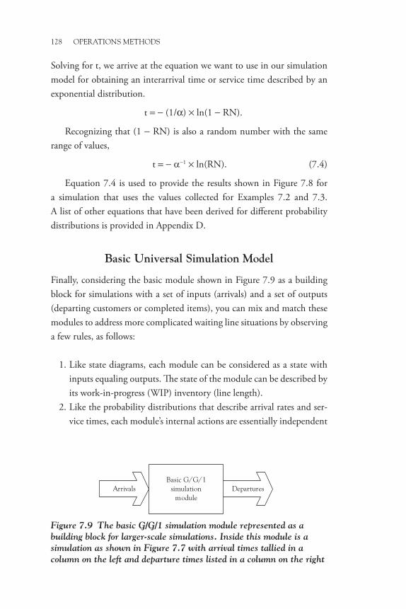
128 OPERATIONS METHODS
Solving for t, we arrive at the equation we want to use in our simulation model for obtaining an interarrival time or service time described by an exponential distribution.
t = − (1/α) × ln(1 − RN).
Recognizing that (1 − RN) is also a random number with the same range of values,
t = − α−1 × ln(RN). (7.4)
Equation 7.4 is used to provide the results shown in Figure 7.8 for a simulation that uses the values collected for Examples 7.2 and 7.3. A list of other equations that have been derived for different probability distributions is provided in Appendix D.
Basic Universal Simulation Model
Finally, considering the basic module shown in Figure 7.9 as a building block for simulations with a set of inputs (arrivals) and a set of outputs (departing customers or completed items), you can mix and match these modules to address more complicated waiting line situations by observing a few rules, as follows:
1. Like state diagrams, each module can be considered as a state with inputs equaling outputs. The state of the module can be described by its work-in-progress (WIP) inventory (line length).
2. Like the probability distributions that describe arrival rates and ser-vice times, each module’s internal actions are essentially independent
Figure 7.9 The basic G/G/1 simulation module represented as a building block for larger-scale simulations. Inside this module is a simulation as shown in Figure 7.7 with arrival times tallied in a column on the left and departure times listed in a column on the right
Basic G/G/1simulation
moduleArrivals Departures

USEFUL TOOLS AND SIMULATION METHODS 129
of each other, provided that there is no sharing of resources (servers, equipment) with other modules.
3. When the outputs of a module are divided among two or more subsequent modules or when the inputs to a module come from more than one source, separate types of simulation modules must be developed to manage this traffic, as illustrated in Figure 7.10. This is not difficult if the various input or output components can be defined by fixed percentages or known probability distributions.
4. Single-line configurations for multiple servers are easier to model than parallel-line configurations, but both require a traffic module, as shown in Figure 7.11a and Figure 7.11b. One module directs the next customer in a single line to the next available server; the other module distributes incoming customers to the available parallel lines accord-ing to whatever rule is desired. For example, in typical bank or gov-ernmental office applications the rule is likely to be to the parallel line with the least number of customers waiting in line. Another example is directing incoming customers according to their class or priority.
5. An advantage of simulation is that modules can have different service distributions, which are useful when simulating multiple-phase lines or customizing a multiple-server situation where not every server can be assumed to have the same service capability. For example, one can simulate the effect of dedicating one server to standardized services in a two- or three-server situation as compared to all servers handling the full range of services.
6. When one module’s output is the input to a following module, the arrival distribution for the following model is the same as the output distribution for the preceding model, as shown for the production
Figure 7.10 The basic traffic modules required as building blocks for more complex simulations. The services performed by these modules take essentially zero time and typically are combining or sorting algorithms
Input trafficmodule
Arrivals
Departures
Arrivals
Output trafficmodule
Departures
Departures
Departures

130 OPERATIONS METHODS
line simulation in Figure 7.12. Note that the output distribution of a previous module is not the same as that module’s service time distribution unless the server in that module is continually busy, as may be the case in a production line situation.
It can be seen that spreadsheet implementations of these modules for different simulations can be pretty straightforward. For example, a mul-tiple step production process can use the first few columns of the spread-sheet as shown in Figure 7.7 for the first step, the next set of columns for the second step set up in the same way as for the first step with the Service Ends column values for the first step also acting as the Arrival Time values for the second step and so forth. What is useful is that the line length val-ues for each module can be used to determine how much space is required for waiting material before each piece of equipment in a manufacturing or other production line with a number of phases or steps.
Finally, some useful references for further study about spreadsheet simulation methods are Laguna and Marklund (2005), Chapter 6; Winston (2004); and Weida et al. (2001).
Figure 7.11 Simulation module configurations for the two different multiple-server line configurations: (a) single-line multiple-server simulation and (b) parallel-line multiple-server simulation
Input trafficmodule
Departures
Arrivals
Arrivals
(a)
(b)
Arrivals Departures
Departures
Departures
Arrivals
Arrivals
Basic G/G/1simulation
module
Basic G/G/1simulation
module
Basic G/G/1simulation
module
Arrivals Departures
Departures
Departures
Arrivals
Arrivals
Basic G/G/1simulation
module
Basic G/G/1simulation
module
Basic G/G/1simulation
module
Input trafficmodule
Arrivals
Departures
Departures

USEFUL TOOLS AND SIMULATION METHODS 131
Fig
ure
7.12
Sim
ulat
ion
mod
ule
confi
gura
tion
for
a fo
ur-s
tep
prod
ucti
on li
ne.
Thi
s is
rel
ativ
ely
easy
to
set
up
in a
spr
eads
heet
and
allo
ws
diffe
rent
ser
vice
dis
trib
utio
ns a
t ea
ch s
tep.
If a
giv
en s
tep
has
inad
equa
te c
apac
ity,
one
or
mor
e m
odul
es c
an b
e us
ed in
par
alle
l for
tha
t st
ep,
wit
h th
e de
part
ures
fr
om t
he p
revi
ous
mod
ule
bein
g ea
sily
div
ided
am
ong
the
para
llel m
odul
es.
The
ir o
utpu
ts c
an t
hen
be
com
bine
d fo
r th
e in
put
to t
he fo
llow
ing
step
’s m
odul
e
Bas
ic G
/G/1
sim
ulat
ion
mod
ule
Arr
ival
sA
rriv
als
Bas
ic G
/G/1
sim
ulat
ion
mod
ule
Arr
ival
sB
asic
G/G
/1si
mul
atio
nm
odul
eA
rriv
als
Bas
ic G
/G/1
sim
ulat
ion
mod
ule
Dep
artu
res


APPENDIX A
Glossary
Arrival. A customer or item entering a line or queue for service or further processing.
Arrival distribution. The variability in the number of arrivals per some selected period of time. This variability can be represented by probability distributions selected to best describe the particular situation, with the Poisson distribution being most commonly used.
Arrival rate. The average number of arrivals per some selected period of time. This continuous value can have a decimal component for small arrival rates, but it is often rounded to whole numbers for larger rates. This value is represented by the Greek lambda (λ) in waiting line equations. Some typical values are 30 products per day, 18 customers per hour, or 1.6 cars every 15 minutes.
Back office. A term that denotes those activities in a service process where direct contact with the customer is not required for their completion.
Balance equation. A useful condition in waiting line analysis that can be used to derive several performance measures. Consider a state n where there are n customers in the system and the queue is in a steady state. At this time, the inputs to state n are equal to the outputs from state n. That is, Rate(→ n) = Rate(← n). This allows the creation of a set of equations, one per state, which then can be mathematically manipulated to determine the probability of existence for each state. Given those probabilities, average line lengths and, subsequently, the average waiting times can be determined.
Balking. Refusal of a customer to enter a line the customer considers to be too long. It is a variable component of waiting line cost, particularly larger if the customer decides to never return. Balking is also an example of a state-dependent rate in which the probability of its occurrence is related to the length of the waiting line observed by the next arrival.

134 GLOSSARY
Birth and death process. A continuous Markov chain that is occasion-ally abbreviated by some authors as BDP. In queuing analysis, its state diagram can be used to determine how long it will take for a queuing situation to reach a steady state of behavior. When that condition exists, it can be used to derive the various waiting line performance formulas.
Blocking. Not allowing a customer to enter a line because of limited capacity. One example is when all the lines to a call center are busy. It is a component of waiting line cost.
Calling population. The pool of possible arrivals. For most customer services, the calling population is assumed to be infinite; but for some situations, this population has a limited or fixed size that affects sub-sequent arrival rates over time. Some may wonder why the adjective calling is used; the likely reason is because early waiting line analysis was focused on the needs of telephone companies to provide their users (call-ers) acceptable service at the lowest cost.
Central Limit Theorem. A law that states that the distribution of sample averages approaches that of a normal distribution as the number of samples increases. This occurs regardless of the nature of the under-lying distribution of the individual data values from which the samples were taken.
Channel. A single server for a waiting line.
Coefficient of variation. The standard deviation/mean ratio for a distribution. This ratio is a key component of the Pollaczek-Khintchine formula used for general distributions in waiting line analysis equations. See also Pollaczek-Khintchine (P-K) formula.
Coxian distribution.1 A special case of a phase-type distribution where the requirement for entering the first phase in a sequence of phases is relaxed so that the sequence can be entered at any phase. A typical appli-cation would be sequencing analysis in a job shop to make the best use of each of its pieces of equipment.
CR. Critical ratio. A priority rule that processes arrivals per the smallest ratio of time remaining to a deadline divided by the amount of service time remaining to be done.

GLOSSARY 135
Dequeue (or sometimes deque). A concept usually reserved for com-puter applications, where a customer can be added or subtracted from either the head or the tail of the line.
Deterministic. Having a predictable value with a very narrow range of variance. As a result, deterministic variables do not require probability distributions to describe their behavior in analysis methods and can usually be represented by a constant value. In the context of this mono-graph, some examples are the service time for an automated process, arrival times created by a production schedule, the number of servers, finite population size, and finite capacity. See also stochastic.
EDD. Earliest due date. A priority rule giving preference to arrivals that have the least time left before they must be served or completed. An example is giving preference to travelers whose flight will be departing shortly.
Erlang distribution.2 A special case of the gamma distribution where the shape factor k is restricted to integer values. The shape factor represents the number of independent exponential distributions added together to form the distribution. When k = 1, the distribution defaults to a single exponential distribution.
Erlang loss function. Also referred to as the Erlang B expression, can be used to estimate how many customers are turned away (blocked) by limited capacity (no waiting positions, for example, all lines are busy at a call center). The Erlang C expression, which is more complicated, assumes that there are infinite waiting positions. It is used to estimate the probability that a customer will arrive, find that all servers are currently busy, and then get into line to wait until a server becomes available.
FCFS. First come, first serve. The most common priority rule for a waiting line.
FIFO. First in, first out. Same as FCFS in single-channel waiting lines.
Front office. A term used to denote those activities in a service process where direct contact with a customer is necessary for their completion.

136 GLOSSARY
GIGO. Garbage-in, garbage-out. An acronym for the principle that a result is only as good as the data, material, or effort required to produce it.
Interarrival distribution. The variability in the interarrival time, which can be represented by selected probability distributions that best describe the particular situation, with the exponential distribution being the most commonly used.
Interarrival time. The time between arrivals in a waiting line. The aver-age value is the inverse of the average arrival rate (i.e., 1/λ). The sequence of interarrival times is often characterized as a Markovian process.
Jockeying. Changing from a slowly moving line to another line that is perceived to be moving faster in a multiple-channel situation using separate lines for each server.
Johnson’s Rule. A priority rule for scheduling jobs through two work centers in a way that minimizes the makespan for completing all of the jobs and also minimizes the total idle time at each work center. See Stevenson (2012, pp. 718–720) for an example.
Kendall notation.3 A shorthand method for identifying different waiting line models using designated symbols for the arrival rate distribution, the service time distribution, the number of channels, the line length limitation, the calling population size, and the priority rule.
Line length. The number of customers or items in a queue. The average line length is characterized by two continuous values: the average number in line (Lq) awaiting service and the total number in the system (L), which includes those currently being served.
Little’s Law. An observation, valid for all waiting line models regardless of their arrival and service distributions, that the ratio between given average line length and waiting time values is equal to the average arrival rate value (λ = L/W).
Makespan. The total time required to complete a group of jobs in manufacturing. For waiting lines, this corresponds to the total amount of time required to process a group of waiting customers.

GLOSSARY 137
Markovian process.4 A process characterized by a sequence of random variables (x1, x2, x3, . . .) whose order is indicated by increasing values of a parameter, usually time in waiting line scenarios, and having the property that any prediction of the next value of the sequence (xn) can be based on knowing just the current state or previous value (xn−1). That is, the future value of such a variable is independent of the values of all of the previous values but the last one.
Memoryless. A condition where a value is independent of any previous value. That is, it can be said that the value has no memory of any preceding values.
PASTA. An abbreviation for the statement “Poisson arrivals see time averages.” In other words, for any line with exponentially distributed interarrival times, each customer has the same probability of seeing a given line condition. Therefore, the average of what a frequent customer observes each time he or she enters the same line at a business will be the same as the average determined by waiting line analysis.
Phase. A single step service with no internal waiting lines. Multiple-phase sequences can have lines between each phase, but also require a separate server for each phase.
Phase-type distribution. A distribution for one or more phases in sequence whose intervening arrival rates can be characterized by inter-related Poisson distributions. These complex expressions are beyond the scope of this monograph and are mentioned here only for readers wishing to delve further into analytical solutions.
Pollaczek-Khintchine (P-K) formula.5 An expression developed to determine the average delay in a single-channel waiting line for any general service time distribution. All that is needed to be known about the distribution is its mean and variance. The generalized formula in the context of the terms used in this monograph is as follows:
WC
q =
×−
×11 2
12
ρρ
ρρ/ .

138 GLOSSARY
POS. Point of sale. Useful information regarding the nature of services performed and the types of customers served can be gained by a business collecting and analyzing its POS data.
Priority queue. A waiting line where the order in which arrivals are served is different from first come, first served. Different preemptive and nonpreemptive rules can be applied within a single line, or separate lines can be established for different priorities.
Priority rule. A waiting line discipline for serving arrivals after they enter the queue. The most commonly used rule is first come, first served; but in other more urgent situations, the most important needs will prevail, such as in emergency room queues. See also priority queue.
Probability of zero customers. The percentage of time when a service business will have no customers in line and being served. This value is represented by the symbol P0 in most waiting line formulas and is important to managers because it allows an estimate of how much time servers can be available to work on other activities not directly related to customer service.
Queue. A line of people waiting for some service or a sequence of items waiting for the next process step. This term is more widely used outside the United States and is considered synonymous with the term waiting line.
Reneging. Leaving a line before being served after having spent some time in it. If a customer is dissatisfied enough to not come back, it is a significant component of waiting line cost.
Service blueprint. A process diagram for services where the activities are separated into two groups: customer involvement required (front office) and support behind the scenes (back office). Sometimes the service blueprint adds a third group of activities, where customer involvement may or may not be required depending on the particular circumstances.
Service distribution. The variability in a service time, which can be represented by probability distributions selected to best describe the particular situation, with the exponential distribution being most commonly used.

GLOSSARY 139
Service rate. The average number of arrivals serviced or processed per some selected period of time. This continuous value can have a decimal component for small service rates, but it is normally rounded to whole numbers for larger rates. This value is represented by the Greek mu (µ) in waiting line equations. Some typical values are 1.2 customers per minute, 6 cars per hour, or 120 products per week.
Service time. The time required to perform a service or process. The average value is the inverse of the service rate (i.e., 1/µ).
Sojourn time. The total time spent in a service system. See also waiting time.
SPC. Statistical process control. A method for evaluating and monitor-ing the variability in process outcomes.
SPT. Shortest processing time. A priority rule for giving preference to arrivals that require the least amount of service time. A common exam-ple is a grocery express line.
SRO. Shortest remaining time per operation. A priority rule giving preference to arrivals whose ratio of time left to a deadline divided by the number of steps or phases remaining is the smallest. A variation of the EDD priority rule.
State-dependent rate. A rate influenced by the current state of a waiting line. See also balking and reneging for examples of factors creating a state-dependent arrival rate. Some models that have a state-dependent arrival rate are those dealing with a limited population (K) or limited queuing capacity (N).
State diagram. A graphical method showing the conditions for each state of a waiting line. Each state represents a specific number of persons or items in the queue. When the queue reaches a steady-state condition, the movements from one state to another are governed by a balance equation based on the rule that the sum of the inputs to a state must equal the sum of the outputs from that state.
Stochastic. Having an unpredictable value because of the possibility of a wide range of possible results. As a result, stochastic variables must be
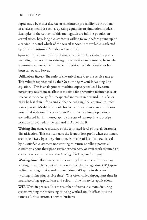
140 GLOSSARY
represented by either discrete or continuous probability distributions in analysis methods such as queuing equations or simulation models. Examples in the context of this monograph are infinite population arrival times, how long a customer is willing to wait before giving up on a service line, and which of the several service lines available is selected by the next customer. See also deterministic.
System. In the context of this book, a system includes what happens, including the conditions existing in the service environment, from when a customer enters a line or queue for service until that customer has been served and leaves.
Utilization factor. The ratio of the arrival rate λ to the service rate µ. This value is represented by the Greek rho (ρ = λ/u) in waiting line equations. This is analogous to machine capacity reduced by some percentage (cushion) to allow some time for preventive maintenance or reserve some capacity for unexpected increases in demand. This factor must be less than 1 for a single-channel waiting line situation to reach a steady state. Modifications of this factor to accommodate conditions associated with multiple servers and/or limited calling populations are indicated in this monograph by the use of appropriate subscript notation as defined in the text and in Appendix B.
Waiting line cost. A measure of the estimated level of overall customer dissatisfaction. This cost can take the form of lost profit when customers are turned away by a busy situation, estimates of lost business caused by dissatisfied customers not wanting to return or telling potential customers about their poor service experiences, or even work required to correct a service error. See also balking, blocking, and reneging.
Waiting time. The time spent in a waiting line or queue. The average waiting time is characterized by two values: the average time (Wq) spent in line awaiting service and the total time (W) spent in the system (waiting in line plus service time). W is often called throughput time in manufacturing applications and sojourn time in service applications.
WIP. Work in process. It is the number of items in a manufacturing system waiting for processing or being worked on. In effect, it is the same as L for a customer service business.
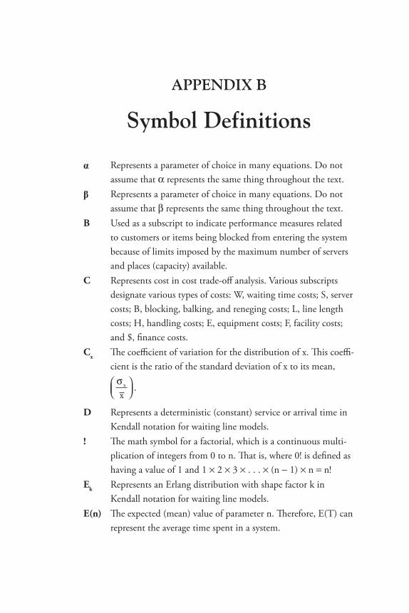
APPENDIX B
Symbol Definitions
a Represents a parameter of choice in many equations. Do not assume that α represents the same thing throughout the text.
b Represents a parameter of choice in many equations. Do not assume that β represents the same thing throughout the text.
B Used as a subscript to indicate performance measures related to customers or items being blocked from entering the system because of limits imposed by the maximum number of servers and places (capacity) available.
C Represents cost in cost trade-off analysis. Various subscripts designate various types of costs: W, waiting time costs; S, server costs; B, blocking, balking, and reneging costs; L, line length costs; H, handling costs; E, equipment costs; F, facility costs; and $, finance costs.
Cx The coefficient of variation for the distribution of x. This coeffi-cient is the ratio of the standard deviation of x to its mean,
σ x
x.
D Represents a deterministic (constant) service or arrival time in Kendall notation for waiting line models.
! The math symbol for a factorial, which is a continuous multi-plication of integers from 0 to n. That is, where 0! is defined as having a value of 1 and 1 × 2 × 3 × . . . × (n − 1) × n = n!
Ek Represents an Erlang distribution with shape factor k in Kendall notation for waiting line models.
E(n) The expected (mean) value of parameter n. Therefore, E(T) can represent the average time spent in a system.

142 SYMBOL DEFINITIONS
G Represents a general independent distribution in Kendall notation for waiting line models. One example is a normal distribution for service or arrival times that are relatively constant but can vary by a small percentage.
i Used as a counter for a sequence of values in equations.j Used as a counter for a sequence of values in equations.K Represents the buffer size in Kendall notation for waiting line
models (the number of places available for waiting and service when the line length is limited).
k Shape factor for Erlang distribution. It can also be used as a counter for a sequence of values in equations.
L The average length of a line in a service process, including the customers currently being served. That is, the total number of customers or items in the system.
Lb The average number of customers waiting to be served in a multiple-channel service process when all the servers are busy.
l The average arrival rate in number per unit of time.lu
The individual arrival rate per unit or customer in a limited population model.
l′ The effective average arrival rate. For limited capacity models, λ′ = λ(1 − PK); for limited population models, λ′ = λu(N − L).
Lq The average length of the line waiting to be served.M Represents a Markovian distribution in Kendall notation for
waiting line models. This is usually an exponential distribution for service rate and a Poisson distribution for arrival rate.
µ The average service rate in number per unit of time.N The maximum number of customers or items in a finite calling
population (also called a limited population).n The number of customers. It can also be a counter for a
sequence of values in equations.PH Represents a phase-type distribution in Kendall notation for
waiting line models with more than one phase in sequence. One example of this is a Coxian distribution for two or more phases, where the restriction on entering the first phase first is relaxed.

SYMBOL DEFINITIONS 143
PB The blocking probability. See also B and Pk.Pk The probability that the number of customers or items in the
system is equal to the maximum system capacity. It is often called the blocking probability with the alternate symbol PB.
Pn The probability of exactly n customers in a system during the given period of time on which the associated arrival and service rates are based. In many texts, this is expressed by P(n).
P0 The probability of no customers in the system during the given period of time on which the associated arrival and service rates are based. In other texts, this may be expressed as P(0) or even shortened to P0.
Π A math symbol for a continuous multiplication of a sequence of terms. A simplification of this function for a sequence of integers from 0 to n is called a factorial.
q Used as subscript to indicate values associated with the line awaiting service (not yet being served). Examples are line length and the time spent waiting in line.
r A utilization factor (λ/µ). Note: Some authors also use ρ as defined for ρs. This can be confusing when using multiple-channel queuing equations from other texts and references; be sure to check the author’s use of this symbol. In this monograph, ρ always represents only λ/µ.
rsThe utilization factor for a multiple-channel system (λ/sµ).
ruThe utilization factor for a single unit or customer in a limited population model.
s The number of servers or channels. In some textbooks, this value is represented by c or M. (These symbols are not used here to avoid confusion with the representation for a Markovian distribution in Kendall notation for waiting line models.)
 The math symbol for summation of a sequence of terms.s The standard deviation for a normal distribution.u A subscript used to designate a unit value. This is particularly
necessary in equations for limited population models.

144 SYMBOL DEFINITIONS
Vx The variance for the distribution of x. Equal to σ2 for a normal distribution of x.
W The average total waiting time in a service process, including the time when being served.
Wb The average time spent waiting in line before being served in a multiple-channel service process when all the servers are busy.
Wq The average time spent waiting in line before being served.

APPENDIX C
Multiple-Channel Application Data

146 MULTIPLE-CHANNEL APPLICATION DATA

MULTIPLE-CHANNEL APPLICATION DATA 147

148 MULTIPLE-CHANNEL APPLICATION DATA

MULTIPLE-CHANNEL APPLICATION DATA 149
The
follo
win
g pr
into
uts a
re fr
om E
xam
ple
5.1
for t
he N
= 1
0, s
= 3
calc
ulat
ions
. This
page
show
s the
out
put f
rom
Exc
el, a
nd th
e fo
llow
ing
page
s sho
w th
e in
term
edia
te c
alcu
latio
ns a
nd th
eir r
espe
ctiv
e Ex
cel f
orm
ulas
. Val
ues f
or P
0, L
q, a
nd L
for a
ll of
the
N a
nd
s set
s are
reco
rded
in th
e ta
ble
from
pre
viou
s run
s by
pasti
ng ju
st th
e re
sults
into
the
tabl
e.

150 MULTIPLE-CHANNEL APPLICATION DATA
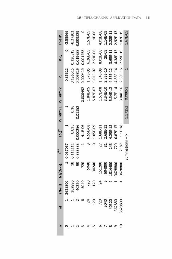
MULTIPLE-CHANNEL APPLICATION DATA 151

152 MULTIPLE-CHANNEL APPLICATION DATA

MULTIPLE-CHANNEL APPLICATION DATA 153
Learning Curve Tables (multiply all times by same constant to make repetition time 1 = actual value for first time)

154 MULTIPLE-CHANNEL APPLICATION DATA
Learning Curve Tables (multiply all times by same constant to make repetition time 1 = actual value for first time)

APPENDIX D
Simulation Information
This appendix serves as a reference for readers who are interested in developing their own simulation models using Excel� Figure D�1 shows the Excel expressions used for the M/M/1 simulation module described in Figures 7�6 and 7�7� Additional expressions for using random numbers to generate input values for simulation are provided along with some general tips for using Excel� A description of useful Excel functions and capabilities for simulation applications completes this appendix�
Basic simulation module set up for an M/M/1 model. See Figure D.1 on the following page. Note the necessary differences in the equations for the first three customers or items. To help identify what the cell addresses in the formulas are referring to, the cell address for the “Arrival Time” label is C11.
Inverse probability distributions expressions for simulating oper-ating values using random number (RN) inputs. Some of these distri-butions can be used in simulating failure probabilities for maintenance service applications or for distributing arrivals or outputs for the simula-tion modules described at the conclusion of Chapter 7.
Exponential distribution. t = − (1/(λ or µ) × ln(RN)
Uniform distribution. (min value = a, max value = b): t = a + RN(b − a); for an equivalent Excel function, use RANDBETWEEN(a,b)
Normal distribution.1 t t RNavgi
i= + −
=
∑σ1
12
6 ; for an equivalent Excel
function, use NORM.INV(RN,mean,sigma)
Beta distribution. Use Excel’s BETA.INV(RN,α,β,A,B) function.
Gamma distribution (often used instead of Erlang’s distribution). Use Excel’s GAMMA.INV(RN,α,β) function.
Log normal distribution. Use Excel’s LOGNORM.INV(RN,mean,stan-dard_dev) function.

156 SIMULATION INFORMATION
Fig
ure
D.1

SIMULATION INFORMATION 157
Excel Application Information and Tips
Data Analysis Package
The Analysis ToolPak option in Excel needs to be activated for simulations because many of the functions mentioned require it. It is loaded when the software is installed, but for reasons unknown, the user must activate it. Similarly, Excel’s Solver option must also be activated by the user. To activate both options, use the appropriate instructions given here.
Excel Version 2003: Select the Tools menu, scroll down to the Add-Ins choice, select, and you will see a list of add-ins. Click the box for Analysis ToolPak. If not already activated, clicking the boxes for the other choices that do not have VBA (Visual Basic for Applications) at the end would be a good idea for future use in business problems. (VBA is for advanced Excel users who wish to program their own special functions.) Click OK and return to Excel. The data analysis add-in is then found as a choice on the Tools menu.
Excel Version 2007: Click on the big button in the upper left corner, select Excel Options at the lower right of the menu, then select Add-Ins in the left column of choices. Then check to see if the Analysis ToolPak and the Solver Add-in applications are active. If not, click Go on the Manage Excel Add-ins menu at the bottom and then check the Analysis ToolPak and Solver Add-ins menu that appears and click OK. The Data Analysis and Solver Add-ins are then found on the far right of the Data tab menu.
Excel Version 2010: The instructions are similar to those for Excel 2007, but you select the File menu to access the Options menu instead of clicking on the big button.
Excel Version 2013: The instructions are similar to those for Excel 2010 to start, but you need to select the Manage box after selecting Add-ins. Then select Excel Add-ins and then click Go. In the Add-Ins available box, select the Analysis ToolPak check box, and then click OK. In the event that the Analysis ToolPak is not listed in the Add-Ins available box, click Browse to locate it. If you are informed that the Analysis ToolPak is not currently installed on your computer, click Yes to install it. After you activate the Analysis ToolPak, the Data Analysis command is displayed in the Analysis group on the Data tab.

158 SIMULATION INFORMATION
Useful Excel Functions for Simulation Model Creation
Excel has a fairly good help menu for learning new functions. The functions you may find particularly useful for simulations are presented here.
IF Function
Returns one result if the logical expression is true (e.g., X > 60), another if it is false. By cleverly concatenating IF functions, different sets of outcomes can be determined depending on the input conditions. A number of useful applications of this function are described by Held in Chapter 2 of his book.
VLOOKUP and HLOOKUP Functions
These functions are used to select one piece of data in a table based on a correlating piece of data in that table when there is no equation to relate the two values directly. An example would be selecting the arrival rate associated with a given probability of occurrence.
COUNTIF Function
This function, =COUNTIF(range,criteria), is very useful for determining the current line length for a waiting line simulation. Examples are given in the M/M/1 model shown in Figure D.1. The criteria statement in the function to tell it when to count an item is generally easy to set up as illustrated in the Help files, but the criteria here for counting when one cell value in a range of cells is greater than a reference cell value is tricky when that reference cell address keeps changing. That is, the critieria in Figure D.1 is “>” (cell address for customer n’s arrival time) and the range is all of the service end times for customers 1 through n − 1.
Descriptive Statistics, Histogram, Regression, Rank, and Percentile Functions
These functions are found in the Analysis ToolPak. The other functions provided are also useful from time to time, but the descriptive statistics,

SIMULATION INFORMATION 159
histogram, regression, rank, and percentile functions are more commonly needed. If you are unfamiliar with using any of these functions, the Excel Help button provided with each function provides a basic tutorial regarding its use:
• Descriptive statistics allows you to select a range of data values and obtain results, such as average, min, max, standard devia-tion, median, and kurtosis, with just one keystroke.
• Histogram sorts the selected data into bins and can also auto-matically create a histogram chart of the results. Bin sizes can be specified by you as described in Chapter 7, or the function will automatically choose an appropriate bin size if you wish. However, the automatic choice of bin size is likely to reduce the resolution of different arrival rates or service times in discrete probability lookup tables created from the histogram results. Hence, it is better if you learn how to specify the correct bin size for your situation as discussed in Chapter 7.
• Regression allows calculating the intercept and slope constants from a set of x and y data in a straight-line approximation of this information.
• Rank and Percentile sorts a set of integer data from highest occurrence to lowest and calculates the percentage for each occurrence value as a percentage of the whole. This function can be useful for determining probabilities for discrete distri-butions in simulations.
Data Tables
This obscure capability of Excel is useful for summarizing simulation results. For example, when you run a simulation for 100 customers that might represent one day’s work and summarize the result—for example, average line length, max and min values—it is laborious to press the F9 key to execute customer simulation run, copy and save the results in a table for the the summarization, and repeat this process 100 times or more for a simulation of perhaps a month’s worth of work. Data tables allow you to collect a number of such summaries with one press of the F9 key, a major savings in time for simulation analysis.
160 SIMULATION INFORMATION
The problem is that most Excel handbooks are quite vague about how to set data tables up for simulation runs and even finding the menu for more general use of data tables is difficult. In Excel 2010, the menu is part of the What If Analysis submenu under the Data tab on the tool-bar. Chapter 26 in the book by Jelen (2010) has a short discussion of What-If tables (data tables), which is a useful introduction. I attempted to use the Scenario Manager in the Excel 2010 What-IF Analysis menu for setting up a simulation data table, but had no success. The Scenario Manager may be able to help, but at this time I am unable to provide the proper inputs because its nomenclature does not seem to correlate with any familiar simulation terms.
The book by Weida et al. (2001) has a fair introduction to the use of data tables for queuing simulations if you are using an older version of Excel than the 2007 and 2010 versions. Chapter 15 of Winston (2004) provides several examples on how to set them up for one-way and two-way applications. The problem is that to apply them to summarizing simulation data, the handbooks rarely discuss how to use a variable that is not actually used in the calculations (such as the simulation run number) to trigger the number of repetitions desired. Normally, when you use a sequence of run numbers as the one input variable, but do not use it in the data table calculations, all you get is one result. The trick is recog-nizing that the use of the random number function in the simulation equations causes the results to change each time a run is done. When, and only when, random numbers are involved, you can designate the run numbers as the input variable to trigger the run calculations. Weida et al. (2001) does that in chapter 13.2.2, but it is often tricky to make it work right. The other difficulty is that help searches for data tables often assume that you meant pivot tables, so the search takes you there. But data tables and pivot tables are not the same!
I am working on a much clearer explanation on how to use data tables in later Excel versions for simulation applications, which I plan to include in a future revision of this monograph. In the meantime, it might take some effort to get a data table to work for you, but the effort is well worth it.

SIMULATION INFORMATION 161
Second Edition Update on Data Tables.
I have found two good online references on the subject that are worthwhile reading. The lengthy post (40 plus pages) by Hui (listed in the References) covers a wide range of data table applications including Monte Carlo simulations and includes a number of interesting exchanges between Hui and the readers.
The other by Susan Harkins (also listed in the References) on the Tech Republic website is a useful introduction with good examples, but sadly with the omission of how to use the input numbers for formulas that do not use them, but instead rely on the use of random numbers to generate the list of varying values in the table.
The trick is to use the first column to designate the run number, such as 1 through 10 for ten simulations, but not use those numbers in the calculations for arrival rate, service rate, line lengths, and waiting times. That is, you designate a column input cell that has a initial value in it but that value is not used in any of the formulas used for the column head-ers in the table. See the simple data table and the associated spreadsheet showing the formulas used for that table for the two-die throw example given in Appendix E.


APPENDIX E
Second Edition Supplements
Formulas for Figure 4.3. Figure E.1 shows the formulas used to determine the values shown in Figure 4.3 for Example 4.3 in Chapter 4.
Data Table Example. Here we want to calculate the results of 24 throws of a pair of dice and calculate some summary data such as the average value for each of the two dice and the average value of their sum. We use the RANDBETWEEN(Bottom value,Top value) function in Excel for the dice throw with the bottom and top values being, obviously, one and six.
We begin by setting up four column headings in a single row with the necessary formulas in the row just below. Using Excel’s Autofill feature we enter the throw numbers in the leftmost column for the desired number of throws. The results at this point are shown in Figure E.2.
The formulas used at this point are shown in Figure E.3 and the area that is shaded shows the area selected before we start to set up our Data Table. This step is important because the Data Table needs a defined range of cells to work with. Note that the shaded area does not include the column titles or the summary averages at the bottom.
Now we first select all of the cells in the shaded region and then choose the Data tab, then the What If analysis menu, and finally the Data Table choice. A small box appears offering the choice of either a row or column input cell. Since our changing variable is the throw number and the num-ber of throws is listed in the left column we first select the column input cell and then click on the cell showing throw number 1 and then click OK in the box. The results are shown in Figure E.4.

164 SECOND EDITION SUPPLEMENTS
Fig
ure
E.1
For
mul
as u
sed
for
valu
es s
how
n in
Fig
ure
4.3.
For
ref
eren
ce in
und
erst
andi
ng t
he fo
rmul
as t
he c
ell l
abel
ed w
ith
a lo
wer
-cas
e n
at t
he u
pper
left
has
a c
ell a
ddre
ss o
f G$
and
the
valu
e of
the
cel
l ref
eren
ced
as $
B$8
is 1
0, t
hat
is,
the
valu
e fo
r N
in a
ll ca
lcul
atio
ns h
ere
is 1
0
Com
puta
tion
of
fact
oria
l ter
ms:
nN
N–n
(N–n
)!N
!/(N
–n)!
(ρu)
nP
rodu
ctP
(n)
0=$
B$8
=H5–
G5
=FA
CT
(I5)
=(FA
CT
(H5)
)/J5
=($B
$4/$
B$5
)^G
5=K
5*L5
=1/M
16
1=$
B$8
=H6–
G6
=FA
CT
(I6)
=(FA
CT
(H6)
)/J6
=($B
$4/$
B$5
)^G
6=K
6*L6
=M6*
$N$5
2=$
B$8
=H7–
G7
=FA
CT
(I7)
=(FA
CT
(H7)
)/J7
=($B
$4/$
B$5
)^G
7=K
7*L7
=M7*
$N$5
3=$
B$8
=H8–
G8
=FA
CT
(I8)
=(FA
CT
(H8)
)/J8
=($B
$4/$
B$5
)^G
8=K
8*L8
=M8*
$N$5
4=$
B$8
=H9–
G9
=FA
CT
(I9)
=(FA
CT
(H9)
)/J9
=($B
$4/$
B$5
)^G
9=K
9*L9
=M9*
$N$5
5=$
B$8
=H10
–G10
=FA
CT
(I10
)=(
FAC
T(H
10))
/J10
=($B
$4/$
B$5
)^G
10=K
10*L
10=M
10*$
N$5
6=$
B$8
=H11
–G11
=FA
CT
(I11
)=(
FAC
T(H
11))
/J11
=($B
$4/$
B$5
)^G
11=K
11*L
11=M
11*$
N$5
7=$
B$8
=H12
–G12
=FA
CT
(I12
)=(
FAC
T(H
12))
/J12
=($B
$4/$
B$5
)^G
12=K
12*L
12=M
12*$
N$5
8=$
B$8
=H13
–G13
=FA
CT
(I13
)=(
FAC
T(H
13))
/J13
=($B
$4/$
B$5
)^G
13=K
13*L
13=M
13*$
N$5
9=$
B$8
=H14
–G14
=FA
CT
(I14
)=(
FAC
T(H
14))
/J14
=($B
$4/$
B$5
)^G
14=K
14*L
14=M
14*$
N$5
10=$
B$8
=H15
–G15
=FA
CT
(I15
)=(
FAC
T(H
15))
/J15
=($B
$4/$
B$5
)^G
15=K
15*L
15=M
15*$
N$5
Sum
:=S
UM
(M5:
M15
)=S
UM
(N5:
N15
)

SECOND EDITION SUPPLEMENTS 165
Throw Dice 1 Dice 2 Sum1 1 6 7
2
3
4
5
6
7
8
9
10
11
12
13
14
15
16
17
18
19
20
21
22
23
24
25
Averages 1 6 7
Figure E.2 Data table range for simulating the outcomes of two dice throws. See Figure E.3 for the formula view of this range
When random numbers are used for variations in the results of a set of formulas the data table variable is not used in those formulas but is still necessary as a counter for the iterations. This is important because if one would want a change to 40 iterations the entire process of setting up the data will need to be repeated from the beginning with a larger region to include the additional iterations. That is, the magnitude of a data table cannot be modified without starting over.

166 SECOND EDITION SUPPLEMENTS
Throw Dice 1 Dice 2 Sum1 =RANDBETWEEN(1,6) =RANDBETWEEN(1,6) =C5+D5
2
3
4
5
6
7
8
9
10
11
12
13
14
15
16
17
18
19
20
21
22
23
24
25
Averages =AVERAGE(C5:C29) =AVERAGE(D5:D29) =AVERAGE(E5:E29)
Figure E.3 Formulas and range (shaded region) selected for the data table. The reference for the cell titled “Throw” is B4.

SECOND EDITION SUPPLEMENTS 167
Throw Dice 1 Dice 2 Sum1 3 4 7
2 5 6 11
3 6 6 12
4 3 1 4
5 1 2 3
6 4 4 8
7 2 3 5
8 4 5 9
9 4 3 7
10 5 1 6
11 3 1 4
12 2 3 5
13 2 1 3
14 5 5 10
15 4 4 8
16 1 4 5
17 2 5 7
18 6 3 9
19 2 5 7
20 3 6 9
21 2 6 8
22 1 5 6
23 1 5 6
24 3 3 6
25 6 4 10
Averages 3 4 7
Figure E.4 Completed data table


Notes
Preface
1. Fitzsimmons and Fitzsimmons (2011).
Chapter 1
1. Refer to Appendices A and B for more detailed descriptions of the terms and symbols used in the text.
2. Laguna and Marklund (2005, ch. 6).3. Hillier and Lieberman (2010, ch. 17).4. Nelson (2010, ch. 8).5. Some of you are probably asking, “Shouldn’t this value be 50%?”
Many of my students ask this question because their familiarity in using normal distributions implies that the average should be at the 50% point. Although this is true for a normal distribution, it is not true for the majority of distributions. For an exponential distribution, the average value corresponds to the 36.78% point and to the 1 − 0.3678 = 63.21% point for the inverse exponential distribution.
6. Abner Krarup Erlang (1878–1929) is a Danish mathematician who developed a number of queuing theory concepts for telephone company applications in the early 1900s. Refer to Appendix A for further details.
7. Attributed to the British statistician D.G. Kendall (1918–2007) during the period from 1951 to 1953.
8. In multiple-line situations first-in-first-out does not always correctly specify what happens when a customer requires a long service time. Then it is possible for one or more successive customers to be served and leave before the service for the first customer is completed.
9. A few years ago when I took a regional flight in Japan I observed the boarding of about 140 passengers in less than six minutes using no defined boarding process. They lined up before the agent checking tickets, all had their tickets ready, and moved onto the aircraft quickly.
170 NOTES
Those with carry-on luggage promptly stowed it in the overhead bin taking care to not stand in the aisle impeding other passengers while doing so. In a similar manner the security check process at the airport was also very efficient and required little prompting by the officials about what was expected of the passengers. Both processes were an example of the increase in waiting line performance when the customers know what to do and focus on keeping the line moving.
Chapter 2
1. Named after J.D.C. Little, who published a proof of this formula in 1961. The formula had been observed and used by others shortly before Little published his proof.
2. How long a waiting line must be before it discourages potential customers is also a function of their perception of how fast the line is expected to move. If their prior experience is that the line moves swiftly they are more willing to enter a long line.
Chapter 3
1. Note the parentheses added around the summation term in the denominator to clarify that the second term is not to be included in the summation. This addresses a commonly observed mistake made by many of the students when we first added waiting line topics to our process and operations management courses.
Chapter 4
1. Pollaczek (1930) and Khintchine (1932). See glossary (Appendix A).2. This use of α should not be confused with its use in Equation (1.2)
for the exponential distribution.3. Peck and Hazelwood (1958).
Chapter 5
1. This is done to simplify the equations for calculating P0 and Lq because only ρ and the number of servers s is required in these

NOTES 171
equations. This also agrees with the P0 and Lq data tables provided for a range of ρ and s values in Appendix C. The reader is reminded that ρ here is not the same as ρs = λ/µs, the multiple-channel ρ used by some authors.
2. Named after a sixteenth-century French mathematician, L’Hospital or L’Hôpital. When confronted with an expression where it is not possible to define a limit as a variable approaches a certain value (1 in this case), successive derivatives of the numerator and the denominator with respect to that variable are taken until they converge to a definable limit.
3. The term “finite queuing table” is not exactly correct for this situation since we are discussing finite sources here, not finite queues. The term is more appropriate for our earlier discussion regarding limited line capacity. However, this term is used in many textbooks for both capacity and sourcing issues because it is consistent with its usage by Peck and Hazelwood (1958), a commonly used resource for solving finite sourcing problems.
4. Krajewski et al. (2010).
Chapter 6
1. Bekker (2005) is a good overall reference; Hillier and Lieberman (2010) discuss this in Chapter 17, Section 17.5.
2. If you are unfamiliar with service blueprints, the article by Shostack (1984) is a good introduction.
3. One utility cost often forgotten is waste management. A good waste management policy can help keep this cost low and reduce the number of staff required to support it.
4. This material was formerly Chapter 18 in the previous edition of this reference.
5. McCarran Airport in Las Vegas does this in an effective and enter-taining way by showing video clips on conveniently placed video monitors in the security check-in process area. The clips are of local Las Vegas Strip entertainers doing or being corrected for not doing the right thing at different security checkpoints.
6. Some Disney theme parks let customers buy tickets for popular rides, where the ticketing system calculates the average waiting time

172 NOTES
until the ticket holder can board the next available ride and prints that time on the ticket. This allows customers to visit other parts of the park, such as food and retail shops, instead of waiting in line. Longer waits are then not as significant, and park visitors can even go and buy other tickets for rides later in the day. The ticketing system’s job in forecasting the average waiting time is simplified because the service time (the duration of the ride) is essentially constant. The somewhat hidden advantage here is that park revenue from food and retail shops is less affected by lost customer visits while they wait in line at the rides.
7. Abilla (2007).8. This constrains us to a fixed appointment time during the day
because we cannot predict when these urgent-care situations will occur during the day. For doctors who are not expected to handle such drop-in patients, we have more flexibility regarding the length of the appointment times, allowing a mixture of short appointments and long appointments according to patient needs. Then we can even use short-term scheduling rules to schedule the order in which patients are offered appointment times.
9. These values used here should not be construed to represent all medical practices. When a full range of medical services is being provided and urgent care patients must be accommodated, these values are typically larger and have greater variance.
10. As a note of interest, the need to accommodate some urgent-care patients is often greater at the beginning and ending of the week. This is likely caused by the more limited availability of health care professionals on weekends.
11. For those interested in learning more about reservation systems and overbooking, Chapter 11 in Fitzsimmons and Fitzsimmons (2011) is a good introduction.
12. Asking a customer to key in their account number or other form of ID when they call for support allows the system to recognize more valued customers. Since many systems can also check the telephone number of the caller it can be compared against listed numbers for customers to not only identify more valued customers but also help verify their identity for account access or credit card activations.

NOTES 173
13. Hillier and Lieberman (2010, ch. 17).14. Haussmann (1970).15. It should be noted that the benefits of dequeuing can also be achieved
by educating the customers waiting in line as to what will be required when they reach the server window, allowing them to fill out such forms in advance while they are waiting. This gives them something to do while also improving line performance.
16. Stevenson (2012, ch. 16).17. Jacobs and Chase (2011, ch. 19).18. While we do not show a specific example of how makespan can be
used for waiting line management, one example would be estimating how long it would usually take to process customers remaining to be served after normal closing time.
Chapter 7
1. Little (1961).2. If you are unfamiliar with how to create histograms in Excel using
the function provided in Excel’s Analysis ToolPak, refer to the Excel tips section in Appendix D.
3. Where this value comes from was commented on earlier for the discussion regarding exponential distributions in Chapter 1.
Appendix A
1. Named for D.R. Cox (1995).2. Named for the Danish mathematician Agner Krarup Erlang (1878–
1929). His work with the Copenhagen Telephone Company in the early 1900s provided the foundation for several aspects of modern waiting line analysis.
3. Kendall (1951). This method is commonly indicated by the generic A/B/C/d/e/f notation. The last three characteristics are not shown in many textbooks; those that do use them often do not follow the order given in the definition above.
4. Named for the Russian mathematician Andrey Andreyevich Markov (1856–1922). Sometimes the term Markovian process is restricted to describing sequences of independent random variables with

174 NOTES
continuous values, such as those defined by exponential distribu-tions. When this is done, similar sequences of discrete variables are referred to as Markov chains.
5. Named for Felix Pollaczek and Aleksandr Khintchine. Each inde-pendently developed this formula, in 1930 and 1932, respectively. Many citations of their formula have a wide range of spelling variations for Khintchine.
Appendix D
1. See Fitzsimmons and Fitzsimmons (2011, 438), for the reasoning behind the derivation of this expression. For a more convenient method than using 12 random numbers for each value required, use Excel’s NORM.INV function.

References
You can find many useful queuing analysis references on the Internet, but many search listings containing the term queuing are likely to refer to communication network or software programming applications. Some useful references are listed here; using their titles in search engines as starting points are more likely to lead to the types of articles you are looking for.Abilla, P. 2007. Psychology of Queuing & Disneyland (Web log post). http://
www.shmula.com/psychology-of-queueing-disneyland/372 (accessed July 28, 2011).
Bekker, R. 2005. Queues with State-Dependent Rates. Eindhoven, The Netherlands: Technische Universiteit Eindhoven. http://alexandria.tue.nl/extra2/200513578.pdf (accessed July 30, 2011).
Bozarth, C.C., and R.B. Handfield. 2008. Introduction to Operations and Supply Chain Management. 2nd ed. Upper Saddle River, NJ: Prentice Hall.
Chander, H. 2006. “Contracts in Outsourcing.” http://www.math.vu.nl/en/Images/werkstuk-chander_tcm72-94371.doc (accessed March 10, 2011).
Easton, F.F. 2002. “Labor Requirements for Multi-Server Multi-Class Finite Queues.” http://myweb.whitman.syr.edu/ffeaston/Research/Mmck_2cl.PDF (accessed March 10, 2011).
Fitzsimmons, J.A., and M.J. Fitzsimmons. 2011. Service Management: Operations, Strategy, Information Technology. 7th ed. New York: McGraw-Hill.
Grasing, R.E. 2011. “Branch Performance by the New Numbers.” http://www.renolan.com/banking/article-branch_performance_by_the_new_numbers.htm (accessed July 24, 2011).
Harkins, S. August 10, 2015. “How to Use Excel’s Data Table Analysis Tool.” http://www.techrepublic.com/article/how-to-use-excels-data-table-analysis-tool/ (accessed August 18, 2015).
Haussmann, R.K.D. Summer 1970. “Waiting Time as an Index of Quality of Nursing Care.” Health Services Research 5, no. 2, pp. 92–105. http://www.ncbi.nlm.nih.gov/pmc/articles/PMC1067272/pdf/hsresearch00575-0014.pdf (accessed July 29, 2011).
Hawley, D., and R. Hawley. 2004. Excel Hacks. Sebastopol, CA: O’Reilly Media, Inc.
Heizer, J., and B. Render. 2008. Operations Management. 9th ed. Upper Saddle River, NJ: Prentice Hall.

176 REFERENCES
Held, B. 2007. Microsoft Excel Functions & Formulas� Plano, TX: Wordware Publishing, Inc.
Heyde, C.C., and E. Seneta, eds. 2001. Statisticians of the Centuries. New York: Springer-Verlag.
Hillier, F.S., and G.J. Lieberman. 2010. Introduction to Operations Research� 9th ed. New York: McGraw-Hill.
Hubbard, D.W. 2010. How to Measure Anything� 2nd ed� Hoboken, NJ: John Wiley & Sons, Inc.
Hui. 2013. “Data Tables & Monte Carlo Simulations in Excel—A Comprehensive Guide�” http://chandoo.org/wp/2010/05/06/data-tables-monte-carlo-simulations-in-excel-a-comprehensive-guide/ (accessed May 22, 2013).
Jacobs, F.R., and R.B. Chase. 2011. Operations and Supply Chain Management� 13th ed. New York: McGraw-Hill.
Jardine, A.K.S., and A.H.C. Tsang. 2005. Maintenance, Replacement, and Reliability: Theory and Applications. Boca Raton, FL: CRC Press.
Jelen, B. 2010. Microsoft 2010 Excel in Depth. Indianapolis, IN: Que.Khintchine, A.Y. 1932. “Mathematical Theory of a Stationary Queue.”
Matematicheskii Sbornik 39, no. 4 pp. 73–84.Koenigsberg, E. 1960. “Finite Queues and Cyclic Queues.” Operations Research
8, no. 2, pp. 246–53.Koerts, J. 1963. “On Mean Waiting Times and Their Reduction by Priority
Procedures: An Expository Survey and Some Tables.” Statistica Neerlandica 17, no. 3, pp. 267–83. http://onlinelibrary.wiley.com/doi/10.1111/j.1467- 9574.1963.tb01045.x/abstract
Kotha, S.K., M.P. Barnum, and D.A. Bowen. 1996. “KeyCorp Service Excellence Management System.” Interfaces 26, no. 1, pp. 54–74.
Krajewski, L.J., L.P. Ritzman, and M.K. Malhotra. 2010. Operations Management: Processes and Supply Chains� 9th ed. Upper Saddle River, NJ: Prentice Hall.
Laguna, M., and J. Marklund. 2005. Business Process Modeling, Simulation, and Design. Upper Saddle River, NJ: Prentice-Hall.
Little, J.D.C. 1961. “A Proof of the Queuing Formula: L = λW.” Operations Research 9, no. 3, pp. 383–87.
Maister, D.H. 1985. “The Psychology of Waiting Lines.” http://davidmaister.com/articles/5/52 (accessed July 28, 2011).
Nelson, B.L. 2010. Stochastic Modeling: Analysis & Simulation. Mineola, NY: Dover.
Norman, D.A. 2008. “The Psychology of Waiting Lines.” http://www.jnd.org/ms/Norman%20The%20Psychology%20of%20Waiting%20Lines.pdf (accessed July 28, 2011).
Oldrich, V. 1967. “On the Preemptive Priority Queues.” http://www.kybernetika.cz/content/1967/2/147/paper.pdf (accessed July 29, 2011).

REFERENCES 177
Peck, L.G., and R.N. Hazelwood. 1958. “Finite Queuing Tables.” In Publications in Operations Research� Vol. 2. New York: John Wiley & Sons.
Pollaczek, F. 1930. “Über eine Aufgabe der Wahrscheinlichkeitstheorie.” Mathematische Zeitschrift 32, no. 1, pp. 64–100.
Shaw, K.A. 2013. Integrated Management of Processes and Information� New York: Business Expert Press.
Shostack, G.L. 1984. “Designing Services that Deliver.” Harvard Business Review, no. 84115, pp. 133–39. http://www.semanticfoundry.com/docs/servicesThatDeliver.pdf (accessed July 27, 2011).
Stevenson, W.J. 2012. Operations Management. 11th ed. New York: McGraw-Hill.
Sztrik, J. 2001. “Finite-Source Queuing Systems and Their Applications: A Bibliography.” http://irh.inf.unideb.hu/user/jsztrik/research/fsqreview.pdf (accessed March 10, 2011).
Vignaux, G.A. 2007. “The Bank: An Example of a SimPy Simulation.” http://simpy.sourceforge.net/SimPyDocs/TheBank.html (accessed March 10, 2011).
Walkenbach, J. 2010. Excel 2010 Bible� Indianapolis, IN: Wiley Publishing, Inc.Walkenbach, J. 2010. John Walkenbach’s Favorite Excel 2010 Tips & Tricks�
Indianapolis, IN: Wiley Publishing, Inc.Weida, N.C., R. Richardson, and A. Vazsonyi. 2001. Operations Analysis Using
Microsoft Excel. Pacific Grove, CA: Duxbury–Thomson Learning.Winston, W.L. 2004. Microsoft Excel Data Analysis and Business Modeling.
Redmond, WA: Microsoft Press.


Index
alternate arrival time distributions, 41–43
alternate service time distributions, 36–41
appointment schedule analysis, 98–100
arrival, 133distribution, 4–5, 133
arrival rate, 3, 133effective, 44–46, 48, 59management methods, 97–102
back office, 13, 75, 86, 133balance equations, 7–9, 133balking, 16, 22, 72–73, 133birth and death process, 134blocking, 78, 134
costs, 77–79probability, 45, 59
calling population, 3, 134limited, 47–49, 59–61
Central Limit Theorem, 39, 116, 134channel, 134coefficient of variation, 134coffee shops
different service distributions, 40–41
with limited capacity, 46with one server, 19–20with two servers, 29–31
continuous distribution determination, 114–117
cost curves, 12–14coxian distribution, 134critical ratio, 107, 134customers
classes, 63–64priorities, 64
data analysis package, 157data tables, 159–161dequeue, 107, 135deterministic, 135discrete distribution determination,
117–121discrete probability distributions,
114–121
earliest due date (EDD), 107, 135Erlang delay system, 57Erlang distribution, 7, 135Erlang loss function, 135Erlang loss system, 57Excel applications, 50–51, 61–63,
157–161exponential distribution, 5–6, 155
factory inventory costs, 83–84first come, first served (FCFS) priority
rule, 10, 135first in, first out (FIFO) priority rule,
10, 107, 135front office, 75, 135
Grasing, R. E., 67, 68
Hazelwood, R. N., 53, 61helicopter shuttle business costs, 83Hillier, F. S., 4, 53, 80, 83, 106
ice cream shop with limited customer space, 84
improving service performance, 84–93
interarrival distribution, 136interarrival time, 3, 5, 15, 136inverse probability distributions,
155

180 INDEX
jockeying, 24, 136Johnson’s Rule, 107, 136
Kendall notation, 15, 25, 41, 44, 47, 136
Kotha, S. K., 67
Laguna, M., 4, 53, 130learning curves, 65, 153–154Lieberman, G. J., 4, 53, 80, 83, 106limited calling population, 47–53,
59–63limited capacity, 44–46, 57–59line configurations, 64–65line length, 136Little’s Law, 9, 17, 109, 136
makespan, 107, 136managerial considerations, 71–108Marklund, J., 4, 53, 130Markovian process, 6, 137memoryless, 6, 72, 137multiple-channel
application data, 145–154models, 55–69single-phase model, 23–33
multiple phases, 53–54, 69
Nelson, B. L., 4nonpreemptive priorities, 105–108notation, 9–10
overbooking, 102
PASTA, 137Peck, L. G., 53, 61performance measures, 1–4phase, 7, 35, 137phase-type distribution, 137point of sale (POS), 138Poisson distribution, 4–5Pollaczek-Khintchine (P-K) formula,
38, 137preemptive priorities, 105–108priority management, 104–108
priority queue, 138priority rules, 10–12, 107, 138probability of zero customers, 17,
20, 138psychological factors, waiting line
configurations, 93–97
queue, 138
random number approximations of probability distributions, 127–128
reneging, 72, 138repair service
with multiple servers, 62–63with one server, 49–52
sandwich stand cost trade-offs, 80–82service
blueprint, 72, 138capability variations, 65–69distribution, 138rate, 3, 139time, 3, 139time reduction learning rates, 67–68
shortest process time first (SPT), 107, 139
simulation information, 155–161simulation models, 122–126,
128–131, 158–161single-channel, single-phase model,
15–22sojourn time, 139state-dependent rate, 139state-dependent variance, 72state diagrams, 7–9, 45–46, 50, 139stochastic, 139–140symbols defined, 141–144system, 18, 140
utilization factor, 140
variance and risk considerations, 72–75
variation reduction, 85

INDEX 181
waiting lineconfigurations, psychological
factors, 93–97configurations, multiple servers,
23–24costs, 75–84, 140data collection, 110–121
models, 9–10theory, 1
waiting time, 140Weida, N. C., 130, 160Winston, W. L., 130, 160work in process (WIP), 76, 107,
140


OTHER TITLES IN QUANTITATIVE APPROACHES TO DECISION MAKING COLLECTION
Donald N. Stengel, California State University, Fresno, Editor
• Operations Methods: Waiting Line Applications by Ken Shaw• Regression Analysis: Understanding and Building Business and Economic Models
Using Excel by J. Holton Wilson, Barry P. Keating, and Mary Beal-Hodges• Service Mining: Framework and Application by Wei-Lun Chang• Regression Analysis: Unified Concepts, Practical Applications, and Computer
Implementation by Bruce L. Bowerman, Richard T. O’Connell, and Emily S. Murphree• Experimental Design: Unified Concepts, Practical Applications, and Computer
Implementation by Bruce L. Bowerman, Richard T. O’Connell, and Emily S. Murphree• An Introduction to Survey Research by Ernest L. Cowles and Edward Nelson• Business Applications of Multiple Regression, Second Edition by Ronny Richardson• Business Decision-Making: Streamlining the Process for More Effective Results
by Milan Frankl
Announcing the Business Expert Press Digital LibraryConcise e-books business students need for classroom and research
This book can also be purchased in an e-book collection by your library as
• a one-time purchase,• that is owned forever,• allows for simultaneous readers,• has no restrictions on printing, and• can be downloaded as PDFs from within the library community.
Our digital library collections are a great solution to beat the rising cost of textbooks. E-books can be loaded into their course management systems or onto students’ e-book readers.The Business Expert Press digital libraries are very affordable, with no obligation to buy in future years. For more information, please visit www.businessexpertpress.com/librarians. To set up a trial in the United States, please email [email protected].


Operations MethodsManaging Waiting Line ApplicationsSecond Edition
Kenneth A. Shaw
Quantitative Approaches to Decision Making CollectionDonald N. Stengel, Editor
OPERATIO
NS M
ETHO
DS
SH
AW
Operations MethodsManaging Waiting Line Applications, Second EditionKenneth A. Shaw
Updated to integrate the management of associated infor
mation processes, expand some application discussions,
and provide additional reference material, the intent of this
monograph is to help business professionals use waiting
line (queuing) analysis methods to improve both service and
manufacturing business applications of queuing situations.
Emphasis is given to discussing the caveats in applying
waiting line theory and becoming aware of the assumptions
used in developing that theory. The importance of accounting
for variability in waiting line processes is discussed in some
detail because the basic queuing equations provide only
average performance data under steadystate conditions.
Understanding how much variability can exist for a given
waiting line scenario provides a manager with the insight
required to reduce these effects and develop innovative
solutions for improving service while reducing operating costs.
In general the mathematical tone of the book is focused
on applications, not the derivation of the formulas presented.
The few derivation exceptions illustrate some approaches not
commonly discussed in textbooks—for example, the use of
state diagrams and random number approximations of the
probability distributions for use in simple simulation models.
To aid in understanding the material presented, some
practical examples are given at appropriate points in the text
and some simulation approaches using common spreadsheet
software are described.
Kenneth (Ken) Shaw has a PhD and MS in electrical engineer
ing from Arizona State University and a BSEE from Purdue
University. His experience in industry was gained at a number
of hightechnology enterprises that include Naval Avionics
Facility, Royal Melbourne Institute of Technology, General
Electric, Motorola Semiconductor, Unisys, and four divisions
of HewlettPackard. He shared the lessons learned from that
experience as an adjunct professor teaching operations and
process management for the College of Business at Oregon
State University from 2003 to 2011.
Quantitative Approaches to Decision Making CollectionDonald N. Stengel, Editor
For further information, a free trial, or to order, contact:
[email protected] www.businessexpertpress.com/librarians
THE BUSINESS EXPERT PRESS DIGITAL LIBRARIES
EBOOKS FOR BUSINESS STUDENTSCurriculum-oriented, born-digital books for advanced business students, written by academic thought leaders who translate real-world business experience into course readings and reference materials for students expecting to tackle management and leadership challenges during their professional careers.
POLICIES BUILT BY LIBRARIANS• Unlimited simultaneous
usage• Unrestricted downloading
and printing• Perpetual access for a
one-time fee• No platform or
maintenance fees• Free MARC records• No license to execute
The Digital Libraries are a comprehensive, cost-effective way to deliver practical treatments of important business issues to every student and faculty member.
ISBN: 978-1-63157-085-8
Copyright © 2022 FDOKUMEN