arX

iv:0

805.

2390

v3 [

gr-q

c] 3

0 M

ay 2

008

Ineffectiveness of Pade resummation techniques in post-Newtonian approximations

Abdul H. Mroue,1 Lawrence E. Kidder,1 and Saul A. Teukolsky1

1Center for Radiophysics and Space Research, Cornell University, Ithaca, New York, 14853

(Dated: June 14, 2013)

We test the resummation techniques used in developing Pade and Effective One Body (EOB)waveforms for gravitational wave detection. Convergence tests show that Pade approximants of thegravitational wave energy flux do not accelerate the convergence of the standard Taylor approxi-mants even in the test mass limit, and there is no reason why Pade transformations should help inestimating parameters better in data analysis. Moreover, adding a pole to the flux seems unnec-essary in the construction of these Pade-approximated flux formulas. Pade approximants may beuseful in suggesting the form of fitting formulas. We compare a 15-orbit numerical waveform of theCaltech-Cornell group to the suggested Pade waveforms of Damour et al. in the equal mass, non-spinning quasi-circular case. The comparison suggests that the Pade waveforms do not agree betterwith the numerical waveform than the standard Taylor based waveforms. Based on this result, wedesign a simple EOB model by modifiying the ET EOB model of Buonanno et al., using the Taylorseries of the flux with an unknown parameter at the fourth post-Newtonian order that we fit for.This simple EOB model generates a waveform having a phase difference of only 0.002 radians withthe numerical waveform, much smaller than 0.04 radians the phase uncertainty in the numericaldata itself. An EOB Hamiltonian can make use of a Pade transformation in its construction, butthis is the only place Pade transformations seem useful.

PACS numbers: 04.25.dg, 04.25.Nx, 04.30.Db

I. INTRODUCTION

Even though general relativity was developed at thebeginning of the twentieth century, no analytical solutionis known for the two-body problem. Until recently, at-tempts to find a numerical solution failed because of thecomplexity of the mathematical equations and the insta-bilities inherent in the analytical formulations being used.In the past few years, breakthroughs in numerical rela-tivity [1, 2, 3, 4] allowed a system of two inspiraling blackholes to be evolved through merger and the ringdown ofthe remnant black hole [5, 6, 7, 8, 9, 10, 11, 12, 13].

Studying the late dynamical evolution of these inspi-raling compact binaries is important because they areamong the most promising source of gravitational wavesfor the network of laser interferometric detectors suchas LIGO and VIRGO. The detection of these gravita-tional waveforms (GW) is important for testing generalrelativity in the strong field limit. Moreover, these de-tectors can extract from the waves physical data aboutthese sources such as the component masses and spinsand the orbital eccentricity. For an unbiased extractionof these parameters, a large bank of accurate waveformsneeds to be constructed. Numerical relativity alone can-not compute all the waveforms needed because of thecomputational cost. Instead, the waveforms are basedon post-Newtonian (PN) approximations [14, 15].

The post-Newtonian approximation is a slow-motion,weak-field approximation to general relativity. In orderto produce a post-Newtonian waveform, the PN equa-tions of motion of the binary are solved to yield explicitexpressions for the accelerations of each body in termsof the binary’s orbital frequency Ω [14, 16, 17, 18, 19,20, 21, 22, 23, 24, 25]. Then solving the post-Newtonian

wave generation problem yields expressions for the gravi-tational waveform h and the gravitational wave flux F interms of radiative multipole moments [26]. These radia-tive multipole moments are in turn related to the sourcemultipole moments, which can be given in terms of therelative position and relative velocity of the binary [27].Instead of comparing the post-Newtonian waveform witha numerical waveform along a certain direction with re-spect to the source, the comparison can be done in all di-rections by decomposing the waveform in terms of spher-ical harmonic modes. For an equal-mass non-spinningbinary, the (2, 2) mode h22 [28, 29, 30, 31] is often usedto compare numerical and post-Newtonian waveforms be-cause it is the dominant mode. Its time derivative h22 isused to compute the gravitational wave flux. The result-ing expressions for the orbital energy E, the gravitationalenergy flux F and the amplitude h22 are given as Taylorseries of the frequency-related parameter

x = (MΩ)2/3 , (1)

where M is the total mass of the binary and G = c = 1.The invariantly defined “velocity”

v = x1/2 , (2)

another dimensionless parameter, is often used in writingthese Taylor series.

Computing PN series to high order is difficult and timeconsuming. Since the various PN expressions are givenas slowly convergent Taylor series, the Pade transforma-tion [32, 33] was suggested in Ref. [34] to accelerate theconvergence of these series. The Pade transformation,Pm

n , consists of writing a Taylor series, Tk, of order k asthe ratio of two polynomials, one of order m in the nu-merator, and another of order n in the denominator, such

2

n Expn(v) P m+ǫ

m [Expn(v)]

0 1.0000000 1.0000000

1 3.0099999 3.0099999

2 5.0300499 -401.0000

3 6.3834834 9.1313636

4 7.0635838 7.0601492

5 7.3369841 7.4053299

6 7.4285732 7.4747817

7 7.4548724 7.4645660

8 7.4614801 7.4631404

9 7.4629558 7.4633014

10 7.4632524 7.4633191

11 7.4633066 7.4633174

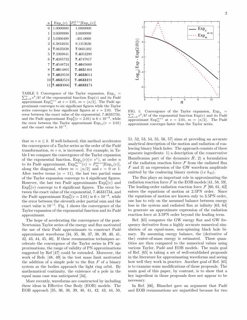
TABLE I: Convergence of the Taylor expansion, Expn

=P

n

k=0vk/k! of the exponential function Exp(v) and its Pade

approximant Expm+ǫ

mat v = 2.01, m = ⌊n/2⌋. The Pade ap-

proximant converges to six significant figures while the Taylorseries converges to four significant figures at v = 2.01. Theerror between the exact value of the exponential, 7.46331734,and the Pade approximant Exp6

5(v = 2.01) is 6 × 10−8, whilethe error between the Taylor approximant Exp11(v = 2.01)and the exact value is 10−5.

that m+n ≤ k. If well-behaved, this method acceleratesthe convergence of a Taylor series as the order of the Padetransformation, m + n, is increased. For example, in Ta-ble I we compare the convergence of the Taylor expansionof the exponential function, Expn(v)(≡ e

v), at order nto its Pade approximant, Expm+ǫ

m (v) = Pm+ǫm [Expn(v)],

along the diagonal, where m = ⌊n/2⌋ and ǫ = 0 or 1.After twelve terms (n = 11), the last two partial sumsof the Taylor expansion converge to 4 significant figures.However, the last two Pade approximants Exp5

5(v) andExp6

5(v) converge to 6 significant figures. The error be-tween the exact value of the exponential, 7.46331734, andthe Pade approximant Exp6

5(v = 2.01) is 6× 10−8, whilethe error between the eleventh order partial sum and theexact value is 10−5. Fig. 1 shows the convergence of theTaylor expansion of the exponential function and its Padeapproximant.

The hope of accelerating the convergence of the post-Newtonian Taylor series of the energy and flux motivatedthe use of their Pade approximants to construct Padeapproximant waveforms [34, 35, 36, 37, 38, 39, 40, 41,42, 43, 44, 45, 46]. If these resummation techniques ac-celerate the convergence of the Taylor series in PN ap-proximations, the range of validity of PN approximationssuggested by Ref [47] could be extended. Moreover, thework of Refs. [48, 49] in the test mass limit motivatedthe addition of a simple pole to the flux F of a binarysystem as the bodies approach the light ring orbit. Bymathematical continuity, the existence of a pole in theequal mass case was anticipated [34].

More recently, waveforms are constructed by includingthese ideas in Effective One Body (EOB) models. TheEOB approach [35, 36, 38, 39, 40, 41, 42, 43, 44, 50,

0 2 4 6 8 10n

-6

-4

-2

0

2

Log

10| E

xp -

Exp

(2.0

1) |

Expn

Expm

m+ε

FIG. 1: Convergence of the Taylor expansion, Expn

=P

n

k=0vk/k! of the exponential function Exp(v) and its Pade

approximant Expm+ǫ

mat v = 2.01, m = ⌊n/2⌋. The Pade

approximant converges faster than the Taylor series.

51, 52, 53, 54, 55, 56, 57] aims at providing an accurateanalytical description of the motion and radiation of coa-lescing binary black holes. The approach consists of threeseparate ingredients: 1) a description of the conservative

Hamiltonian part of the dynamics H , 2) a formulationof the radiation reaction force F from the radiated fluxF and 3) an expression of the GW waveform amplitudeemitted by the coalescing binary system (i.e h22).

The flux plays an important role in approximating theradiation reaction force F in the EOB models [41, 58, 59].The leading-order radiation reaction force F [60, 61, 62]enters the equations of motion at 2.5PN order. Sincethe equations of motion are known only to 3.5PN order,one has to rely on the assumed balance between energyloss in the system and radiated flux at infinity [63, 64]to generate an approximate expression of the radiationreaction force at 3.5PN order beyond the leading term.

Ref. [65] computes the GW energy flux and GW fre-quency derivative from a highly accurate numerical sim-ulation of an equal-mass, non-spinning black hole bi-nary. By assuming energy balance, the (derivative ofthe) center-of-mass energy is estimated. These quan-tities are then compared to the numerical values usingvarious Taylor, Pade and EOB models. The main goalof Ref. [65] is taking a set of well-established proposalsin the literature for approximating waveforms and seeinghow well they work in practice. Another goal of Ref. [65]is to examine some modifications of those proposals. Themain goal of this paper, by contrast, is to show that akey ingredient in those proposals does not appear to benecessary.

In Ref. [66], Blanchet gave an argument that Padeand EOB resummations are unjustified because for two

3

comparable-mass bodies there is no equivalent of theSchwarzschild light-ring orbit at the radius r = 3M . Hisargument is based on the PN coefficients of the binary’senergy and their relation to predicting the innermost cir-cular orbit. He finds that the radius of convergence of thePN series, which is related to the radius of the light-ringorbit, is around one (instead of 1/3 as for Schwarzschild).Blanchet concluded that Taylor series converge well forequal masses and that templates based on Pade/EOB arenot justified because the dynamics of two bodies in Gen-eral Relativity does not appear as a small ”deformation”of the motion of a test particle in Schwarzschild. Thispaper arrives at similar conclusions but not by consid-ering the innermost circular orbit, which is not preciselydefined in the full nonlinear case. Instead, we comparePade approximants of the flux and Pade/EOB waveformsto the numerical data of Refs. [67, 68].

In this paper, we focus on testing two main techniquesinvolved in building EOB models: the systematic use ofPade approximants, and the addition of a pole to theflux. The goal is to simplify these models by removingany unnecessary procedures in designing waveforms thatprovide good agreement with numerical waveforms.

Damour et al. [34, 35] first suggested techniques forresumming the Taylor expansions of the energy and fluxfunctions. Starting from the PN expansions of the en-ergy E and the flux F , they proposed a new class ofwaveforms called P -approximants, based on three essen-tial ingredients. The first step is the introduction ofnew energy-type (Eq. 4) and flux type (Eq. 16) func-tions, called e(v) and f(v) respectively. The second stepis to Pade-approximate the Taylor expansion of thesefunctions. The third step is to use these Pade trans-forms in the definition of the energy E (Eq. 6) and Pade-approximated flux (Eq. 20). The last step is to constructeither the Pade-approximated waveform as in Sec. IV orthe EOB waveform as in Sec. V. Schematically, the sug-gested procedure is summarized by the following map:

[

En, Fn

]

→[

en, fn

]

→[

emn , fm

n

]

→[

E(emn ), F (fm

n )

]

→ h . (3)

Our notation is to denote by T mn (x) the Pade approx-

imant of a k-th order Taylor series Tk(x) with an m-thorder polynomial in the numerator and an n-th orderpolynomial in the denominator such that m + n ≤ k, i.e.the Pade approximant of ek(x) is em

n (x).In Section II, we compare the 3PN Taylor series of the

energy function to its possible Pade approximants usingthe intermediate energy function e(x), as suggested byDamour et al. [34]. We compute the last stable orbitfrequency, defined as the frequency for which the energyreaches a minimum as a function of frequency, and alsothe poles of the energy in the complex plane correspond-ing to each possible Pade approximant. The large vari-ation of last stable orbit frequency and poles does not

PN order F n Fm+ǫ

m Fn F m+ǫ

m

0.0 1.000000 1.000000 1.530011 1.530011

0.5 1.000000 1.000000 1.000000 1.000000

1.0 0.851547 1.000000 0.772866 0.602534

1.5 0.952078 0.911487 1.005361 0.887757

2.0 0.944193 0.928720 0.940013 0.937227

2.5 0.931939 0.936461 0.925444 0.938929

3.0 0.941025 0.939366 0.945405 0.939502

3.5 0.939726 0.939399 0.938991 0.938082

4.0 0.939208 0.939363 0.939048 0.939471

4.5 0.939745 0.939719 0.939979 0.939516

5.0 0.939601 0.939653 0.939526 0.939684

5.5 0.939605 0.939623 0.939616 0.939621

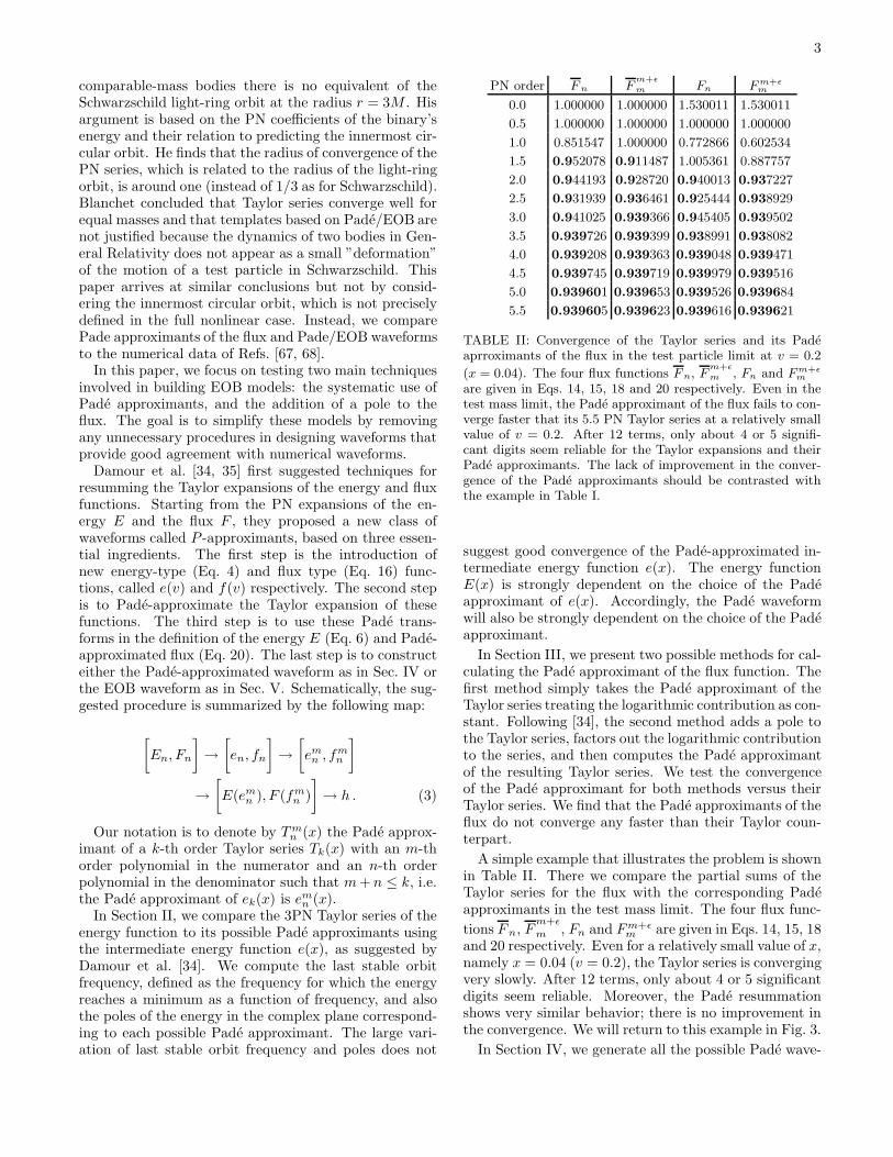
TABLE II: Convergence of the Taylor series and its Padeaprroximants of the flux in the test particle limit at v = 0.2

(x = 0.04). The four flux functions F n, Fm+ǫ

m , Fn and F m+ǫ

m

are given in Eqs. 14, 15, 18 and 20 respectively. Even in thetest mass limit, the Pade approximant of the flux fails to con-verge faster that its 5.5 PN Taylor series at a relatively smallvalue of v = 0.2. After 12 terms, only about 4 or 5 signifi-cant digits seem reliable for the Taylor expansions and theirPade approximants. The lack of improvement in the conver-gence of the Pade approximants should be contrasted withthe example in Table I.

suggest good convergence of the Pade-approximated in-termediate energy function e(x). The energy functionE(x) is strongly dependent on the choice of the Padeapproximant of e(x). Accordingly, the Pade waveformwill also be strongly dependent on the choice of the Padeapproximant.

In Section III, we present two possible methods for cal-culating the Pade approximant of the flux function. Thefirst method simply takes the Pade approximant of theTaylor series treating the logarithmic contribution as con-stant. Following [34], the second method adds a pole tothe Taylor series, factors out the logarithmic contributionto the series, and then computes the Pade approximantof the resulting Taylor series. We test the convergenceof the Pade approximant for both methods versus theirTaylor series. We find that the Pade approximants of theflux do not converge any faster than their Taylor coun-terpart.

A simple example that illustrates the problem is shownin Table II. There we compare the partial sums of theTaylor series for the flux with the corresponding Padeapproximants in the test mass limit. The four flux func-

tions Fn, Fm+ǫ

m , Fn and Fm+ǫm are given in Eqs. 14, 15, 18

and 20 respectively. Even for a relatively small value of x,namely x = 0.04 (v = 0.2), the Taylor series is convergingvery slowly. After 12 terms, only about 4 or 5 significantdigits seem reliable. Moreover, the Pade resummationshows very similar behavior; there is no improvement inthe convergence. We will return to this example in Fig. 3.

In Section IV, we generate all the possible Pade wave-

4

forms as suggested by Damour et al. [34] correspondingto 3 and 3.5 PN order. The waveform approximationrequires the choice of a pole. We use the only physi-cal pole, found from the 2PN Pade-approximated energyE1

1 . We also use the last stable orbit from the 3PN en-ergy Taylor series E3. The results are not very sensi-tive to this choice. We compare the Pade waveforms toa 15-orbit numerical waveform in the equal mass, non-spinning quasi-circular case [67]. The phase differencein these comparisons ranges between 0.05 and a few ra-dians for well-defined Pade approximants (not having apole in the frequency domain of interest) when the match-ing of the numerical and Pade waveforms is done at thegravitational wave frequency Mω = 0.1 [67]. None ofthe Pade waveforms agrees with the numerical waveformbetter than the Taylor series T4-3.5/3.0PN, which hasan error of 0.02 radians. (We identify post-Newtonianapproximants with three pieces of information: the labelintroduced by [35] for how the orbital phase is evolved;the PN order to which the orbital phase is computed;and the PN order at which the amplitude of the wave-form is computed. See Ref. [67] for more details.) Ourconclusion is that the Pade approximant might be help-ful in suggesting fitting formulas but it does not providea more rapidly convergent method. Note that the Padetransform also fails to accelerate the convergence of theT2, T3 and h22 Taylor series (see Refs. [35, 67] for thedefinition of these Taylor series).

In Section V, based on the results of the previous sec-tions, we design a simple EOB model (closely related tothe ET EOB model of Ref. [40]) using the Taylor series ofthe flux. We add one unknown 4PN term that we fit forby maximizing the agreement between the EOB modelwaveform and the numerical waveform. The model doesnot require adding a pole to the flux, nor an a prioriknowledge of the last stable orbit from the energy func-tion. This simple EOB model, with only one parameterto fit for, agrees with the numerical waveform to within0.002 radians (3×10−4 cycles). (This is six times smallerthan the claimed numerical accuracy of [39], smaller byan even larger factor than the claimed numerical accu-racy of [45], and 25 times smaller than the gravitationalwave phase uncertainty of the numerical waveform. SeeTable III in Ref [67] for more details.) This model agreeswith the numerical waveform better than any previouslysuggested Taylor, Pade or EOB waveform.

II. ENERGY FUNCTION

Damour et al. [34] introduced a new energy-type func-tion e(x), where x is the PN frequency related parameter.This assumed more “basic” energy function e(x) is con-structed out of the total relativistic energy Etot(x) of thebinary system. Explicitly

e(x) ≡(

E2tot − m2

1 − m22

2m1m2

)2

− 1 , (4)

where m1, m2 are the masses of the bodies. The totalrelativistic energy function Etot is related to the postNewtonian energy function E(x) through

Etot(x) = M [1 + E(x)] , (5)

where M is the total mass (M = m1 + m2). Solving forE(x) in terms of e(x) using Eqs. (4) and (5), we get[34]

E(x) =

1 + 2ν[

√

1 + e(x) − 1]1/2

− 1 , (6)

where the symmetric mass ratio is ν = m1m2/M2. The

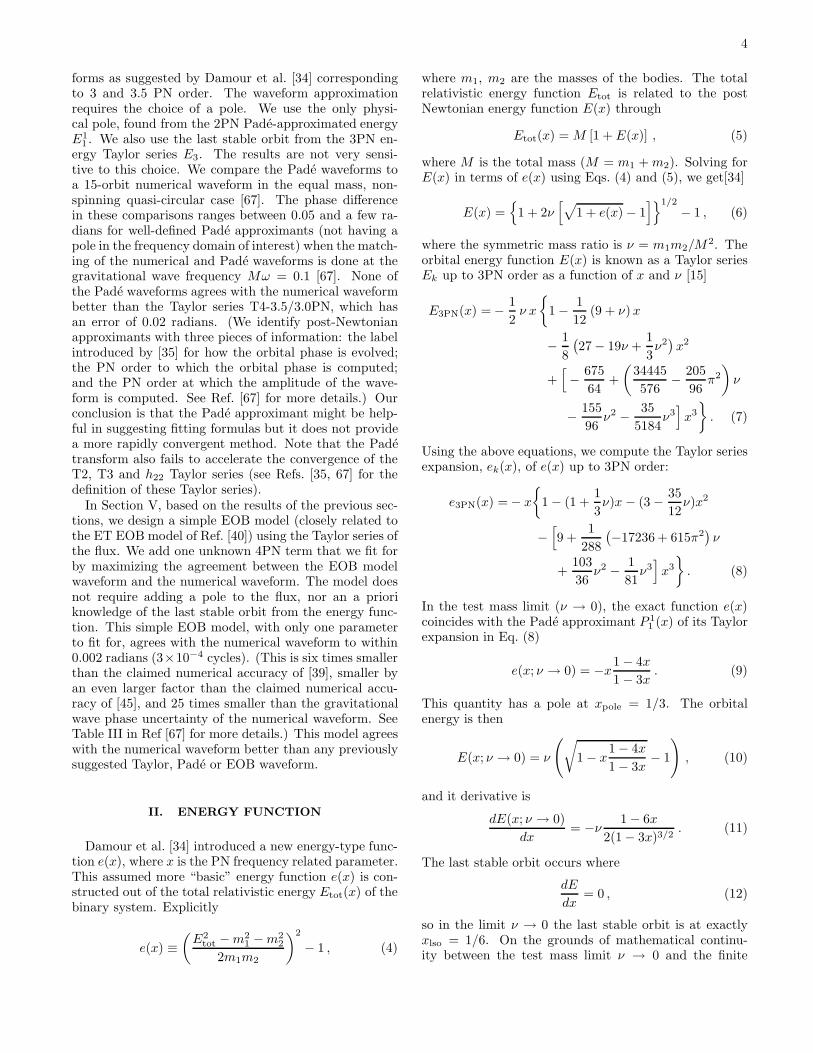
orbital energy function E(x) is known as a Taylor seriesEk up to 3PN order as a function of x and ν [15]

E3PN(x) = − 1

2ν x

1 − 1

12(9 + ν)x

− 1

8

(

27 − 19ν +1

3ν2)

x2

+[

− 675

64+

(

34445

576− 205

96π2

)

ν

− 155

96ν2 − 35

5184ν3]

x3

. (7)

Using the above equations, we compute the Taylor seriesexpansion, ek(x), of e(x) up to 3PN order:

e3PN(x) = − x

1 − (1 +1

3ν)x − (3 − 35

12ν)x2

−[

9 +1

288

(

−17236 + 615π2)

ν

+103

36ν2 − 1

81ν3]

x3

. (8)

In the test mass limit (ν → 0), the exact function e(x)coincides with the Pade approximant P 1

1 (x) of its Taylorexpansion in Eq. (8)

e(x; ν → 0) = −x1 − 4x

1 − 3x. (9)

This quantity has a pole at xpole = 1/3. The orbitalenergy is then

E(x; ν → 0) = ν

(

√

1 − x1 − 4x

1 − 3x− 1

)

, (10)

and it derivative is

dE(x; ν → 0)

dx= −ν

1 − 6x

2(1 − 3x)3/2. (11)

The last stable orbit occurs where

dE

dx= 0 , (12)

so in the limit ν → 0 the last stable orbit is at exactlyxlso = 1/6. On the grounds of mathematical continu-ity between the test mass limit ν → 0 and the finite

5

0.1 0.2 0.3 0.4

-0.02

-0.015

-0.01

-0.005

0

0.005

Ene

rgy

E0

3

E1

2

E2

1

E3

0

E1

1

E3PN

x

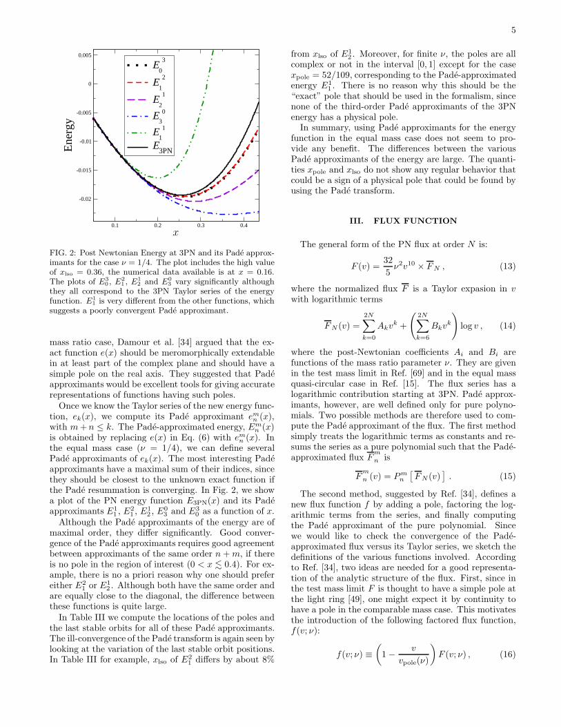
FIG. 2: Post Newtonian Energy at 3PN and its Pade approx-imants for the case ν = 1/4. The plot includes the high valueof xlso = 0.36, the numerical data available is at x = 0.16.The plots of E3

0 , E21 , E1

2 and E03 vary significantly although

they all correspond to the 3PN Taylor series of the energyfunction. E1

1 is very different from the other functions, whichsuggests a poorly convergent Pade approximant.

mass ratio case, Damour et al. [34] argued that the ex-act function e(x) should be meromorphically extendablein at least part of the complex plane and should have asimple pole on the real axis. They suggested that Padeapproximants would be excellent tools for giving accuraterepresentations of functions having such poles.

Once we know the Taylor series of the new energy func-tion, ek(x), we compute its Pade approximant em

n (x),with m + n ≤ k. The Pade-approximated energy, Em

n (x)is obtained by replacing e(x) in Eq. (6) with em

n (x). Inthe equal mass case (ν = 1/4), we can define severalPade approximants of ek(x). The most interesting Padeapproximants have a maximal sum of their indices, sincethey should be closest to the unknown exact function ifthe Pade resummation is converging. In Fig. 2, we showa plot of the PN energy function E3PN(x) and its Padeapproximants E1

1 , E21 , E1

2 , E03 and E3

0 as a function of x.Although the Pade approximants of the energy are of

maximal order, they differ significantly. Good conver-gence of the Pade approximants requires good agreementbetween approximants of the same order n + m, if thereis no pole in the region of interest (0 < x . 0.4). For ex-ample, there is no a priori reason why one should prefereither E2

1 or E12 . Although both have the same order and

are equally close to the diagonal, the difference betweenthese functions is quite large.

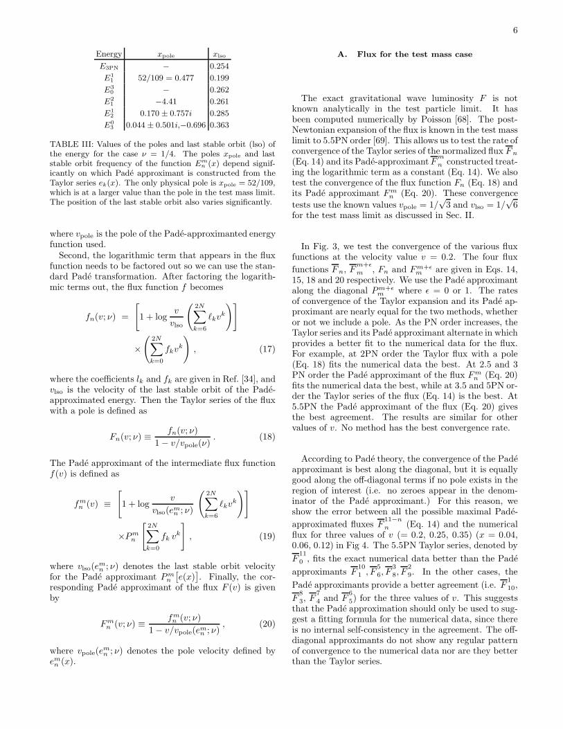
In Table III we compute the locations of the poles andthe last stable orbits for all of these Pade approximants.The ill-convergence of the Pade transform is again seen bylooking at the variation of the last stable orbit positions.In Table III for example, xlso of E2

1 differs by about 8%

from xlso of E12 . Moreover, for finite ν, the poles are all

complex or not in the interval [0, 1] except for the casexpole = 52/109, corresponding to the Pade-approximatedenergy E1

1 . There is no reason why this should be the“exact” pole that should be used in the formalism, sincenone of the third-order Pade approximants of the 3PNenergy has a physical pole.

In summary, using Pade approximants for the energyfunction in the equal mass case does not seem to pro-vide any benefit. The differences between the variousPade approximants of the energy are large. The quanti-ties xpole and xlso do not show any regular behavior thatcould be a sign of a physical pole that could be found byusing the Pade transform.

III. FLUX FUNCTION

The general form of the PN flux at order N is:

F (v) =32

5ν2v10 × FN , (13)

where the normalized flux F is a Taylor expasion in vwith logarithmic terms

FN (v) =

2N∑

k=0

Akvk +

(

2N∑

k=6

Bkvk

)

log v , (14)

where the post-Newtonian coefficients Ai and Bi arefunctions of the mass ratio parameter ν. They are givenin the test mass limit in Ref. [69] and in the equal massquasi-circular case in Ref. [15]. The flux series has alogarithmic contribution starting at 3PN. Pade approx-imants, however, are well defined only for pure polyno-mials. Two possible methods are therefore used to com-pute the Pade approximant of the flux. The first methodsimply treats the logarithmic terms as constants and re-sums the series as a pure polynomial such that the Pade-approximated flux F

m

n is

Fm

n (v) = Pmn

[

FN (v)]

. (15)

The second method, suggested by Ref. [34], defines anew flux function f by adding a pole, factoring the log-arithmic terms from the series, and finally computingthe Pade approximant of the pure polynomial. Sincewe would like to check the convergence of the Pade-approximated flux versus its Taylor series, we sketch thedefinitions of the various functions involved. Accordingto Ref. [34], two ideas are needed for a good representa-tion of the analytic structure of the flux. First, since inthe test mass limit F is thought to have a simple pole atthe light ring [49], one might expect it by continuity tohave a pole in the comparable mass case. This motivatesthe introduction of the following factored flux function,f(v; ν):

f(v; ν) ≡(

1 − v

vpole(ν)

)

F (v; ν) , (16)

6

Energy xpole xlso

E3PN − 0.254

E11 52/109 = 0.477 0.199

E30 − 0.262

E21 −4.41 0.261

E12 0.170 ± 0.757i 0.285

E03 0.044 ± 0.501i,−0.696 0.363

TABLE III: Values of the poles and last stable orbit (lso) ofthe energy for the case ν = 1/4. The poles xpole and laststable orbit frequency of the function Em

n (x) depend signif-icantly on which Pade approximant is constructed from theTaylor series ek(x). The only physical pole is xpole = 52/109,which is at a larger value than the pole in the test mass limit.The position of the last stable orbit also varies significantly.

where vpole is the pole of the Pade-approximanted energyfunction used.

Second, the logarithmic term that appears in the fluxfunction needs to be factored out so we can use the stan-dard Pade transformation. After factoring the logarith-mic terms out, the flux function f becomes

fn(v; ν) =

[

1 + logv

vlso

(

2N∑

k=6

ℓkvk

)]

×(

2N∑

k=0

fkvk

)

, (17)

where the coefficients lk and fk are given in Ref. [34], andvlso is the velocity of the last stable orbit of the Pade-approximated energy. Then the Taylor series of the fluxwith a pole is defined as

Fn(v; ν) ≡ fn(v; ν)

1 − v/vpole(ν). (18)

The Pade approximant of the intermediate flux functionf(v) is defined as

fmn (v) ≡

[

1 + logv

vlso(emn ; ν)

(

2N∑

k=6

ℓkvk

)]

×Pmn

[

2N∑

k=0

fk vk

]

, (19)

where vlso(emn ; ν) denotes the last stable orbit velocity

for the Pade approximant Pmn

[

e(x)]

. Finally, the cor-responding Pade approximant of the flux F (v) is givenby

Fmn (v; ν) ≡ fm

n (v; ν)

1 − v/vpole(emn ; ν)

, (20)

where vpole(emn ; ν) denotes the pole velocity defined by

emn (x).

A. Flux for the test mass case

The exact gravitational wave luminosity F is notknown analytically in the test particle limit. It hasbeen computed numerically by Poisson [68]. The post-Newtonian expansion of the flux is known in the test masslimit to 5.5PN order [69]. This allows us to test the rate ofconvergence of the Taylor series of the normalized flux Fn

(Eq. 14) and its Pade-approximant Fm

n constructed treat-ing the logarithmic term as a constant (Eq. 14). We alsotest the convergence of the flux function Fn (Eq. 18) andits Pade approximant Fm

n (Eq. 20). These convergence

tests use the known values vpole = 1/√

3 and vlso = 1/√

6for the test mass limit as discussed in Sec. II.

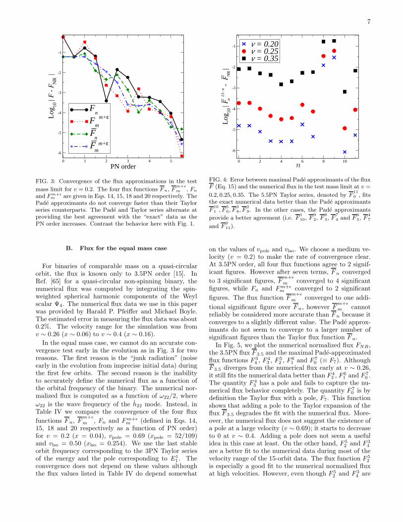
In Fig. 3, we test the convergence of the various fluxfunctions at the velocity value v = 0.2. The four flux

functions Fn, Fm+ǫ

m , Fn and Fm+ǫm are given in Eqs. 14,

15, 18 and 20 respectively. We use the Pade approximantalong the diagonal Pm+ǫ

m where ǫ = 0 or 1. The ratesof convergence of the Taylor expansion and its Pade ap-proximant are nearly equal for the two methods, whetheror not we include a pole. As the PN order increases, theTaylor series and its Pade approximant alternate in whichprovides a better fit to the numerical data for the flux.For example, at 2PN order the Taylor flux with a pole(Eq. 18) fits the numerical data the best. At 2.5 and 3PN order the Pade approximant of the flux Fm

n (Eq. 20)fits the numerical data the best, while at 3.5 and 5PN or-der the Taylor series of the flux (Eq. 14) is the best. At5.5PN the Pade approximant of the flux (Eq. 20) givesthe best agreement. The results are similar for othervalues of v. No method has the best convergence rate.

According to Pade theory, the convergence of the Padeapproximant is best along the diagonal, but it is equallygood along the off-diagonal terms if no pole exists in theregion of interest (i.e. no zeroes appear in the denom-inator of the Pade approximant.) For this reason, weshow the error between all the possible maximal Pade-

approximated fluxes F11−n

n (Eq. 14) and the numericalflux for three values of v (= 0.2, 0.25, 0.35) (x = 0.04,0.06, 0.12) in Fig 4. The 5.5PN Taylor series, denoted by

F11

0 , fits the exact numerical data better than the Pade

approximants F10

1 , F5

6, F3

8, F2

9. In the other cases, the

Pade approximants provide a better agreement (i.e. F1

10,

F8

3, F7

4 and F6

5) for the three values of v. This suggeststhat the Pade approximation should only be used to sug-gest a fitting formula for the numerical data, since thereis no internal self-consistency in the agreement. The off-diagonal approximants do not show any regular patternof convergence to the numerical data nor are they betterthan the Taylor series.

7

0 1 2 3 4 5

PN order

-6

-5

-4

-3

-2

-1L

og10

| F -

FN

R |

Fn

Fm

m+ε

Fn

Fm

m+ε

FIG. 3: Convergence of the flux approximations in the test

mass limit for v = 0.2. The four flux functions Fn, Fm+ǫ

m , Fn

and F m+ǫ

m are given in Eqs. 14, 15, 18 and 20 respectively. ThePade approximants do not converge faster than their Taylorseries counterparts. The Pade and Taylor series alternate atproviding the best agreement with the “exact” data as thePN order increases. Contrast the behavior here with Fig. 1.

B. Flux for the equal mass case

For binaries of comparable mass on a quasi-circularorbit, the flux is known only to 3.5PN order [15]. InRef. [65] for a quasi-circular non-spinning binary, thenumerical flux was computed by integrating the spin-weighted spherical harmonic components of the Weylscalar Ψ4. The numerical flux data we use in this paperwas provided by Harald P. Pfeiffer and Michael Boyle.The estimated error in measuring the flux data was about0.2%. The velocity range for the simulation was fromv ∼ 0.26 (x ∼ 0.06) to v ∼ 0.4 (x ∼ 0.16).

In the equal mass case, we cannot do an accurate con-vergence test early in the evolution as in Fig. 3 for tworeasons. The first reason is the “junk radiation” (noiseearly in the evolution from imprecise initial data) duringthe first few orbits. The second reason is the inabilityto accurately define the numerical flux as a function ofthe orbital frequency of the binary. The numerical nor-malized flux is computed as a function of ω22/2, where

ω22 is the wave frequency of the h22 mode. Instead, inTable IV we compare the convergence of the four flux

functions Fn, Fm+ǫ

m , Fn and Fm+ǫm (defined in Eqs. 14,

15, 18 and 20 respectively as a function of PN order)for v = 0.2 (x = 0.04), vpole = 0.69 (xpole = 52/109)and vlso = 0.50 (xlso = 0.254). We use the last stableorbit frequency corresponding to the 3PN Taylor seriesof the energy and the pole corresponding to E1

1 . Theconvergence does not depend on these values althoughthe flux values listed in Table IV do depend somewhat

0 2 4 6 8 10

-6

-5

-4

-3

-2

-1

Log

10| F

n11

-n

- F

NR

|

v = 0.20v = 0.25v = 0.35

n

FIG. 4: Error between maximal Pade approximants of the fluxF (Eq. 15) and the numerical flux in the test mass limit at v =

0.2, 0.25, 0.35. The 5.5PN Taylor series, denoted by F11

0 , fitsthe exact numerical data better than the Pade approximants

F10

1 , F5

6, F3

8, F2

9. In the other cases, the Pade approximants

provide a better agreement (i.e. F1

10, F9

2, F8

3, F7

4 and F6

5, F4

7

and F0

11).

on the values of vpole and vlso. We choose a medium ve-locity (v = 0.2) to make the rate of convergence clear.At 3.5PN order, all four flux functions agree to 2 signif-icant figures. However after seven terms, Fn converged

to 3 significant figures, Fm+ǫ

m converged to 4 significantfigures, while Fn and Fm+ǫ

m converged to 2 significant

figures. The flux function Fm+ǫ

m converged to one addi-

tional significant figure over Fn, however Fm+ǫ

m cannotreliably be considered more accurate than Fn because itconverges to a slightly different value. The Pade approx-imants do not seem to converge to a larger number ofsignificant figures than the Taylor flux function Fn.

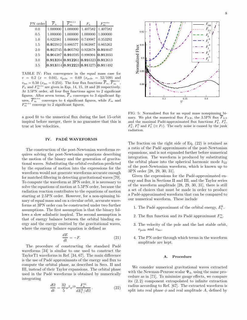
In Fig. 5, we plot the numerical normalized flux FNR,the 3.5PN flux F 3.5 and the maximal Pade-approximatedflux functions F 3

4 , F 43 , F 5

2 , F 61 and F 7

0 (≡ F7). AlthoughF 3.5 diverges from the numerical flux early at v ∼ 0.26,it still fits the numerical data better than F 4

3 , F 61 and F 7

0 .The quantity F 4

3 has a pole and fails to capture the nu-merical flux behavior completely. The quantity F 7

0 is bydefinition the Taylor flux with a pole, F7. This functionshows that adding a pole to the Taylor expansion of theflux F 3.5 degrades the fit with the numerical flux. More-over, the numerical flux does not suggest the existence ofa pole at a large velocity (v ∼ 0.69); it starts to decreaseto 0 at v ∼ 0.4. Adding a pole does not seem a usefulidea in this case at least. On the other hand, F 5

2 and F 34

are a better fit to the numerical data during most of thevelocity range of the 15-orbit data. The flux function F 5

2

is especially a good fit to the numerical normalized fluxat high velocities. However, even though F 5

2 and F 34 are

8

PN order F n Fm+ǫ

m Fn F m+ǫ

m

0.0 1.000000 1.000000 1.407582 1.407582

0.5 1.000000 1.000000 1.000000 1.000000

1.0 0.822381 1.000000 0.749987 0.353292

1.5 0.922912 0.886577 0.963887 0.865262

2.0 0.922745 0.905792 0.922678 0.910047

2.5 0.904387 0.910595 0.896904 0.912033

3.0 0.913204 0.912261 0.916323 0.912613

3.5 0.913314 0.912223 0.913275 0.911492

TABLE IV: Flux convergence in the equal mass case forv = 0.2 (x = 0.04), vpole = 0.69 (xpole = 52/109) and

vlso = 0.50 (xlso = 0.254). The four flux functions F n, Fm+ǫ

m ,Fn and F m+ǫ

m are given in Eqs. 14, 15, 18 and 20 respectively.At 3.5PN order, all four flux functions agree to 2 significantfigures. After seven terms, F n converges to 3 significant fig-

ures, Fm+ǫ

m converges to 4 significant figures, while Fm andF m+ǫ

m converge to 2 significant figures.

a good fit to the numerical flux during the last 15-orbitinspiral before merger, there is no guarantee that this istrue at low velocities.

IV. PADE WAVEFORMS

The construction of the post-Newtonian waveforms re-quires solving the post-Newtonian equations describingthe motion of the binary and the generation of gravita-tional waves. Substituting the orbital evolution predictedby the equations of motion into the expressions for thewaveform would not generate waveforms accurate enoughfor matched filtering in detecting gravitational waves [70].To compute the waveform at 3PN order, it is necessary tosolve the equations of motion at 5.5PN order, because theradiation reaction contributes to the equations of motionstarting at 2.5PN order. However, for a non-spinning bi-nary of equal mass and on a circular orbit, accurate wave-forms at 3PN order can be constructed under two furtherassumptions. The first assumption is that the binary fol-lows a slow adiabatic inspiral. The second assumption isthat of energy balance between the orbital binding en-ergy and the energy emitted by the gravitational waves,where the energy balance equation is defined as

dE

dt= −F. (21)

The procedure of constructing the standard Padewaveforms [34] is similar to one used to construct theTaylorT1 waveforms in Ref. [34, 67]. The main differenceis the use of Pade approximants of the energy and flux tocompute the orbital phase, as described in Secs. II andIII, instead of their Taylor expansions. The orbital phaseused in the Pade waveforms is obtained by numericallyintegrating

dΩ

dt=

32

5ν2v10 Fm

n

dEkl /dΩ

. (22)

0.3 0.35 0.4

0.88

0.89

0.9

0.91

0.92

Nor

mal

ized

Flu

x

FNR

F3.5

F0

7

F1

6

F3

4

F4

3

F2

5

v

FIG. 5: Normalized flux for an equal mass nonspinning bi-nary. We plot the numerical flux FNR, the 3.5PN flux F 3.5

and the maximal Pade-approximated flux functions F 34 , F 4

3 ,F 5

2 , F 61 and F 7

0 (≡ F7). The early noise is caused by the junkradiation.

The fraction on the right side of Eq. (22) is retained asa ratio of the Pade approximants of the post-Newtonianexpansions, and is not expanded further before numericalintegration. The waveform is produced by substitutingthe orbital phase into the spherical harmonic mode h22

of the post-Newtonian waveform, which is known up to3PN order [28, 29, 30, 31].

Given the expressions for the Pade-approximated en-ergy and flux in Sections II and III, and the Taylor seriesof the waveform amplitude [28, 29, 30, 31], there is stilla set of choices that must be made in order to producea Pade-approximated waveform that can be compared toour numerical waveform. These include

1. The Pade approximant of the orbital energy, Ekl .

2. The flux function and its Pade approximant Fnm.

3. The velocity of the pole and the last stable orbit,vpole and vlso.

4. The PN order through which terms in the waveformamplitude are kept.

A. Procedure

We consider numerical gravitational waves extractedwith the Newman-Penrose scalar Ψ4, using the same pro-cedure as in [71]. To minimize gauge effects, we compareits (2, 2) component extrapolated to infinite extractionradius according to Ref. [67]. The extracted waveform issplit into real phase φ and real amplitude A, defined by

9

0 2 4 6m

0

1

2

3

4| δ

φ |

F7-m

m :E11

F7-m

m:E1

2

F7-m

m:E2

1

F7-m

m:E0

3

F7-m

m:E3

0

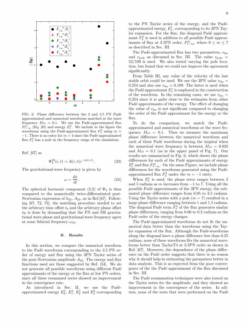
FIG. 6: Phase difference between the 3 and 3.5 PN Padeapproximated and numerical waveforms matched at the wavefrequency Mω = 0.1. We use the Pade-approximated fluxF m

7−m (Eq. 20) and energy Ek

l . We include in the figure thewaveforms using the Pade-approximated flux F 3

3 using m =−1. There is no entry for m = 4 since the Pade-approximatedflux F 4

3 has a pole in the frequency range of the simulation.

Ref. [67] as

Ψ224 (r, t) = A(r, t)e−iφ(r,t). (23)

The gravitational-wave frequency is given by

ω =dφ

dt. (24)

The spherical harmonic component (2,2) of Ψ4 is thencompared to the numerically twice-differentiated post-Newtonian expression of h22, A22, as in Ref.[67]. Follow-ing [67, 72, 73], the matching procedure needed to setthe arbitrary time offset t0 and the arbitrary phase offsetφ0 is done by demanding that the PN and NR gravita-tional wave phase and gravitational wave frequency agreeat some fiducial frequency ωM .

B. Results

In this section, we compare the numerical waveformto the Pade waveforms corresponding to the 3.5 PN or-der of energy and flux using the 3PN Taylor series ofthe post-Newtonian amplitude A22. The energy and fluxfunctions used are those suggested by Ref. [34]. We donot generate all possible waveforms using different Padeapproximants of the energy or the flux at low PN orders,since all these resummed series showed no improvementin the convergence rate.

As introduced in Sec. II, we use the Pade-approximated energy E3

0 , E21 , E1

2 and E03 corresponding

to the PN Taylor series of the energy, and the Pade-approximated energy, E1

1 , corresponding to its 2PN Tay-lor expansion. For the flux, the diagonal Pade approxi-mant F 3

3 is used in addition to all possible Pade approx-imants of flux at 3.5PN order, Fm

7−m, where 0 ≤ m ≤ 7as described in Sec. III.

The Pade-approximated flux has two parameters, vlso

and vpole as discussed in Sec. III. The value vpole =52/109 is used. We also tested varying the pole loca-tion, but found that we could not improve the agreementsignificantly.

From Table III, any value of the velocity of the laststable orbit could be used. We use the 3PN value vlso =0.254 and also use vlso = 0.199. The latter is used whenthe Pade approximant E1

1 is employed in the constructionof the waveform. In the remaining cases, we use vlso =0.254 since it is quite close to the estimates from otherPade approximants of the energy. The effect of changingthe value of vlso is not significant compared to changingthe order of the Pade approximant for the energy or theflux.

To do the comparison, we match the Pade-approximated and numerical waveforms at the wave fre-quency Mω = 0.1. Then we measure the maximumphase difference between the numerical waveform andeach of these Pade waveforms during the inspiral whenthe numerical wave frequency is between Mω = 0.035and Mω = 0.1 (as in the upper panel of Fig. 7). Ourresults are summarized in Fig. 6, which shows the phasedifferences for each of the Pade approximants of energyEk

l and flux Fm7−m. On the same Figure, we include phase

differences for the waveforms generated using the Pade-approximated flux F 3

3 under the m = −1 entry.

When E11 is used, the phase error ranges between 2

and 5 radians as m increases from −1 to 7. Using all thepossible Pade approximants of the 3PN energy, the esti-mated phase difference ranges from 0.05 to 2.5 radians.Using the Taylor series with a pole (m = 7) resulted in alarge phase difference ranging between 1 and 1.5 radians.The diagonal Pade term F 3

4 of the flux generates similarphase differences, ranging from 0.06 to 0.2 radians as thePade order of the energy changes.

The Pade-approximated waveforms do not fit the nu-merical data better than the waveforms using the Tay-lor expansion of the flux. Although the Pade-waveformsalong the diagonal have a phase difference less than 0.25radians, none of these waveforms fits the numerical wave-forms better than TaylorT4 at 3.5PN order as shown inRef. [67]. Moreover, the dependence of the phase differ-ence on the Pade order suggests that there is no reasonwhy it should help in estimating the parameters better indata analysis. This is as expected from the poor conver-gence of the the Pade approximant of the flux discussedin Sec. III.

The Pade resummation techniques were also tested onthe Taylor series for the amplitude, and they showed noimprovement in the convergence of the series. In adi-tion, none of the tests that were performed on the Pade

10

resummed Taylor series of the T2 and T3 waveformsshowed a faster convergence rate. In fact, there is noimprovement in convergence for any Taylor series in thePN approximation that we have investigated.

V. SIMPLE EOB MODEL

We have described the failure of the Pade resumma-tion techniques to accelerate the convergence of any PNTaylor series, the absence of any signature of a pole inthe flux in the equal mass case, and the erratic patternof agreement between the Pade waveforms and the nu-merical waveform. It seems one might as well simply usethe Taylor series at all steps of computing waveforms.Also it does not seem that the parameters vpole and vlso

are useful. In this section, we show how to get goodagreement with the numerical waveform by using a sim-ple EOB model. The only parameter we introduce andfit for is an unknown 4PN contribution to the flux.

A. EOB waveforms

The EOB formalism [53] is a non-perturbative ana-lytic approach that handles the relative dynamics of tworelativistic bodies. This approach of resumming the PNtheory is expected to extend the validity of the PN resultsinto the strong-field limit. The procedure for generatingan EOB waveform follows closely the steps in Sec. IV. In-stead of using the energy balance equation, we computethe orbital phase by numerically integrating Hamilton’sequations. The EOB waveform is generated by substitut-ing the orbital phase into the waveform amplitude A22 at3PN order. The two fundamental ingredients that allowcomputing the orbital phase are the real Hamiltonian Hand the the radiation reaction Fφ.

B. Hamilton’s equations

In terms of the canonical position variables r and φ andtheir conjugate canonical momenta pr and pφ, where r isthe relative separation and φ is the orbital phase, the realdynamical Hamiltonian is defined as [54]:

H =1

ν

√

1 + 2ν (HEOB − 1) , (25)

where

HEOB =

√

A(

1 +p2

φ

r2+

p2r

B+ 2ν(4 − 3ν)

p4r

r2

)

, (26)

and where the radial potential A function is defined asthe series

A = 1 − 2

r+

2ν

r3+(94

3− 41

32π2) ν

r4. (27)

The Taylor series of the A function is replaced by its Padeapproximant A1

3. Here the Pade approximant is not usedto accelerate the convergence of the Taylor expansion ofA. Instead, it leads to the existence of a last stable orbit(see Ref. [39] and references therein). Otherwise, theEOB Hamiltonian is non-physical for the last few orbits;the orbital frequency stays nearly constant for severalorbits before merger. For the B function, the Taylorexpansion suffices:

B =1

A

[

1 − 6ν

r2+ 2(3ν − 26)

ν

r3

]

. (28)

Then Hamilton’s equations of motion are given in thequasi-circular case by

∂tr = ∂prH , (29)

∂tφ = ∂pφH , (30)

∂tpr = −∂rH , (31)

∂tpφ = −Fφ , (32)

where Fφ is the radiation reaction in the φ direction rep-resenting the nonconservative part of the dynamics. InEq. 32, ∂φH = 0 since H is independent of φ. The radi-ation reaction is deduced from the post-Newtonian fluxas in Refs. [41, 58, 59]

Fφ =F + F8v

8

νv3. (33)

In this equation, we have introduced an unknown 4PNflux term, F8, the only parameter that we fit for in thisEOB model.

C. Initial conditions

To integrate Hamilton’s equations, we need appropri-ate initial conditions for a quasi-circular orbit. Refs. [41,42, 52] indicate how to define some “post-adiabatic” ini-tial conditions. However, these initial conditions do notgenerate an orbit with as low an eccentricity as the nu-merical simulation, roughly 5×10−5. At a given radius r,starting from the post-adiabatic initial conditions of pr

and pφ, we therefore reduce the eccentricity iterativelyin two steps. The first step includes evolving Hamilton’sequations in the conservative regime (F = 0) and it-eratively changing the value of pφ until the eccentricitymeasured from the evolution of the orbital separation isof the order 10−9. The second step is based on evolvingthe nonconservative Hamilton’s equations with the 4PNflux and iteratively changing the pr momentum until theeccentricity is again of the order 10−5. This circulariza-tion procedure is repeated as we iterate F8 to maximizethe agreement between the waveforms.

D. Best Fit of F8

To find the best fit for F8, we iteratively solve for theminimum in the phase difference between the numerical

11

1000 1500 2000 2500 3000 3500

(t-r*)/m

0.001

0.01

0.1

|AE

OB -

AN

R |

/AN

R

1000 2000 3000

-0.004

-0.002

0

0.002

0.004

δφ(r

adia

ns)

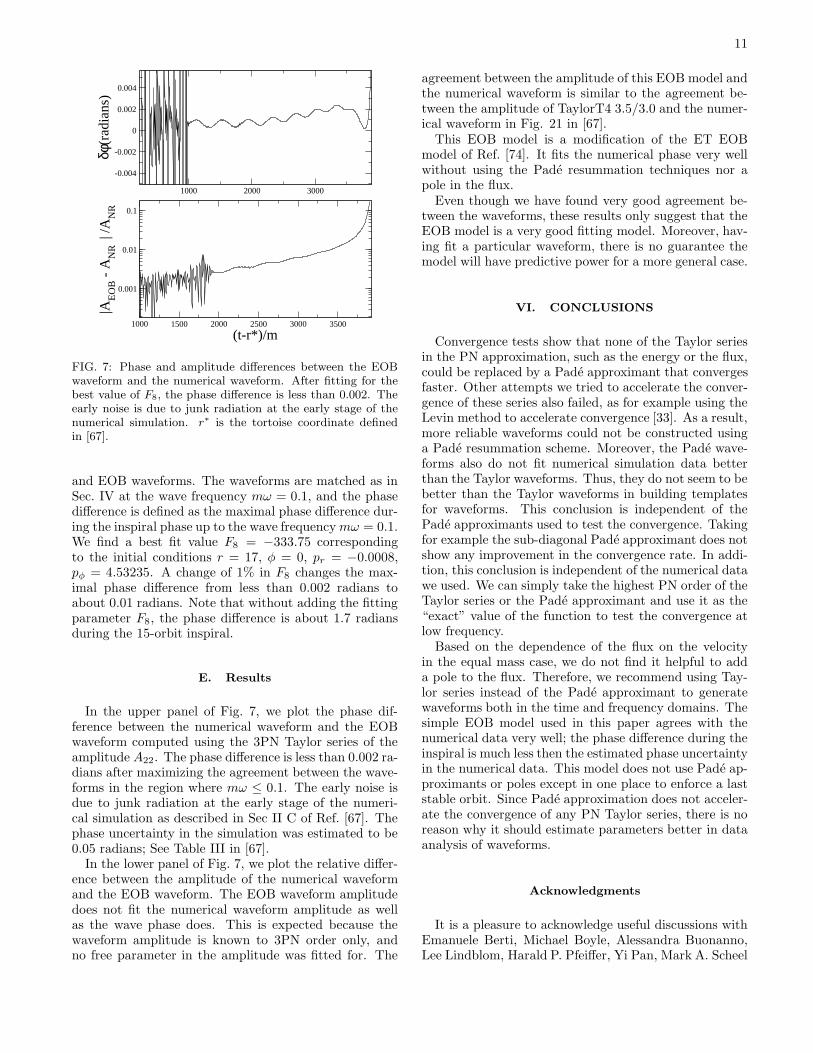
FIG. 7: Phase and amplitude differences between the EOBwaveform and the numerical waveform. After fitting for thebest value of F8, the phase difference is less than 0.002. Theearly noise is due to junk radiation at the early stage of thenumerical simulation. r∗ is the tortoise coordinate definedin [67].

and EOB waveforms. The waveforms are matched as inSec. IV at the wave frequency mω = 0.1, and the phasedifference is defined as the maximal phase difference dur-ing the inspiral phase up to the wave frequency mω = 0.1.We find a best fit value F8 = −333.75 correspondingto the initial conditions r = 17, φ = 0, pr = −0.0008,pφ = 4.53235. A change of 1% in F8 changes the max-imal phase difference from less than 0.002 radians toabout 0.01 radians. Note that without adding the fittingparameter F8, the phase difference is about 1.7 radiansduring the 15-orbit inspiral.

E. Results

In the upper panel of Fig. 7, we plot the phase dif-ference between the numerical waveform and the EOBwaveform computed using the 3PN Taylor series of theamplitude A22. The phase difference is less than 0.002 ra-dians after maximizing the agreement between the wave-forms in the region where mω ≤ 0.1. The early noise isdue to junk radiation at the early stage of the numeri-cal simulation as described in Sec II C of Ref. [67]. Thephase uncertainty in the simulation was estimated to be0.05 radians; See Table III in [67].

In the lower panel of Fig. 7, we plot the relative differ-ence between the amplitude of the numerical waveformand the EOB waveform. The EOB waveform amplitudedoes not fit the numerical waveform amplitude as wellas the wave phase does. This is expected because thewaveform amplitude is known to 3PN order only, andno free parameter in the amplitude was fitted for. The

agreement between the amplitude of this EOB model andthe numerical waveform is similar to the agreement be-tween the amplitude of TaylorT4 3.5/3.0 and the numer-ical waveform in Fig. 21 in [67].

This EOB model is a modification of the ET EOBmodel of Ref. [74]. It fits the numerical phase very wellwithout using the Pade resummation techniques nor apole in the flux.

Even though we have found very good agreement be-tween the waveforms, these results only suggest that theEOB model is a very good fitting model. Moreover, hav-ing fit a particular waveform, there is no guarantee themodel will have predictive power for a more general case.

VI. CONCLUSIONS

Convergence tests show that none of the Taylor seriesin the PN approximation, such as the energy or the flux,could be replaced by a Pade approximant that convergesfaster. Other attempts we tried to accelerate the conver-gence of these series also failed, as for example using theLevin method to accelerate convergence [33]. As a result,more reliable waveforms could not be constructed usinga Pade resummation scheme. Moreover, the Pade wave-forms also do not fit numerical simulation data betterthan the Taylor waveforms. Thus, they do not seem to bebetter than the Taylor waveforms in building templatesfor waveforms. This conclusion is independent of thePade approximants used to test the convergence. Takingfor example the sub-diagonal Pade approximant does notshow any improvement in the convergence rate. In addi-tion, this conclusion is independent of the numerical datawe used. We can simply take the highest PN order of theTaylor series or the Pade approximant and use it as the“exact” value of the function to test the convergence atlow frequency.

Based on the dependence of the flux on the velocityin the equal mass case, we do not find it helpful to adda pole to the flux. Therefore, we recommend using Tay-lor series instead of the Pade approximant to generatewaveforms both in the time and frequency domains. Thesimple EOB model used in this paper agrees with thenumerical data very well; the phase difference during theinspiral is much less then the estimated phase uncertaintyin the numerical data. This model does not use Pade ap-proximants or poles except in one place to enforce a laststable orbit. Since Pade approximation does not acceler-ate the convergence of any PN Taylor series, there is noreason why it should estimate parameters better in dataanalysis of waveforms.

Acknowledgments

It is a pleasure to acknowledge useful discussions withEmanuele Berti, Michael Boyle, Alessandra Buonanno,Lee Lindblom, Harald P. Pfeiffer, Yi Pan, Mark A. Scheel

12

and Nicolas Yunes. We thank Jihad Touma for helpfuldiscussions about Pade approximants, Harald P. Pfeifferand Michael Boyle for providing the numerical data ofthe flux in the equal mass case, and Eric Poisson forproviding the numerical data of the flux in the test mass

limit. This work was supported in part by grants fromthe Sherman Fairchild Foundation to Cornell; by NSFgrants PHY-0652952, DMS-0553677, PHY-0652929, andNASA grant NNG05GG51G at Cornell.

[1] F. Pretorius, Phys. Rev. Lett. 95, 121101 (2005).[2] F. Pretorius, Class. Quant. Grav. 23, S529 (2006).[3] M. Campanelli, C. O. Lousto, P. Marronetti, and Y. Zlo-

chower, Phys. Rev. Lett. 96, 111101 (2006).[4] J. G. Baker, J. Centrella, D. I. Choi, M. Koppitz, and

J. van Meter, Phys. Rev. Lett. 96, 111102 (2006).[5] M. Campanelli, C. O. Lousto, and Y. Zlochower, Phys.

Rev. D 73, 061501(R) (2006), gr-qc/0601091.[6] F. Herrmann, I. Hinder, D. Shoemaker, and P. Laguna,

Class. Quantum Grav. 24, S33 (2007), gr-qc/0601026.[7] P. Diener, F. Herrmann, D. Pollney, E. Schnetter, E. Sei-

del, R. Takahashi, J. Thornburg, and J. Ventrella, Phys.Rev. Lett. 96, 121101 (2006), gr-qc/0512108.

[8] M. A. Scheel, H. P. Pfeiffer, L. Lindblom, L. E. Kidder,O. Rinne, and S. A. Teukolsky, Phys. Rev. D 74, 104006(2006), gr-qc/0607056.

[9] U. Sperhake, Phys. Rev. D 76, 104015 (2007), gr-qc/0606079.

[10] B. Brugmann, J. A. Gonzalez, M. Hannam, S. Husa,U. Sperhake, and W. Tichy, Phys. Rev. D 77, 024027(2008), gr-qc/0610128.

[11] P. Marronetti, W. Tichy, B. Brugmann, J. Gonzalez,M. Hannam, S. Husa, and U. Sperhake, Class. QuantumGrav. 24, S43 (2007), gr-qc/0701123.

[12] Z. B. Etienne, J. A. Faber, Y. T. Liu, S. L. Shapiro, andT. W. Baumgarte, Phys. Rev. D 76, 101503(R) (2007),arXiv:0707.2083 [gr-qc].

[13] B. Szilagyi, D. Pollney, L. Rezzolla, J. Thornburg, andJ. Winicour, Class. Quantum Grav. 24, S275 (2007), gr-qc/0612150.

[14] L. Blanchet, T. Damour, and G. Esposito-Farese, Phys.Rev. D 69, 124007 (2004).

[15] L. Blanchet, Living Rev. Relativity 9, 4 (2006).[16] P. Jaranowski and G. Schafer, Phys. Rev. D 57, 7274

(1998).[17] P. Jaranowski and G. Schafer, Phys. Rev. D 60, 124003

(1999).[18] T. Damour, P. Jaranowski, and G. Schafer, Phys. Rev.

D 62, 021501(R) (2000), 63, 029903(E) (2000).[19] T. Damour, P. Jaranowski, and G. Schafer, Phys. Rev.

D 63, 044021 (2001), 66, 029901(E) (2002).[20] L. Blanchet and G. Faye, Phys. Lett. A 271, 58 (2000).[21] L. Blanchet and G. Faye, Phys. Rev. D 63, 062005 (2001).[22] T. Damour, P. Jaranowski, and G. Schafer, Phys. Lett.

B 513, 147 (2001).[23] Y. Itoh, T. Futamase, and H. Asada, Phys. Rev. D 63,

064038 (2001).[24] Y. Itoh and T. Futamase, Phys. Rev. D 68, 121501(R)

(2003).[25] Y. Itoh, Phys. Rev. D 69 (2004), 064018.[26] K. S. Thorne, Rev. Mod. Phys. 52, 299 (1980).[27] L. Blanchet, Class. Quantum Grav. 15, 1971 (1998).[28] L. E. Kidder, Phys. Rev. D 77, 044016 (2008),

arXiv:0710.0614.

[29] K.G. Arun, L. Blanchet, B.R. Iyer and M.S.S.Qusailah, Class. Quantum Grav. 21, 3771 (2004),arXiv:0404085[gr-qc].

[30] K.G. Arun, L. Blanchet, B.R. Iyer and M.S.S. Qusailah,Class. Quantum Grav. 22, 3115 (2005).

[31] L. Blanchet, G. Faye, B.R. Iyer and S. Sinha (2008),arXiv:0802.1249[gr-qc].

[32] C. M. Bender and S. A. Orszag, Advanced Mathematical

Methods for Scientists and Engineers: Asymptotic Meth-

ods and Perturbation Theory, 2nd ed. (Springer, NewYork, 1999).

[33] William H. Press, Saul A. Teukolsky, William T. Vetter-ling and Brian P. Flannery, Numerical Recipes: The Art

of Scientific Computing, 3rd ed. (Cambridge UniversityPress, New York, 2007).

[34] T. Damour, B. R. Iyer, and B. S. Sathyaprakash, Phys.Rev. D 57, 885 (1998).

[35] T. Damour, B. R. Iyer, and B. S. Sathyaprakash, Phys.Rev. D 63, 044023 (2001), 72, 029902(E) (2005).

[36] T. Damour, B. R. Iyer, and B. S. Sathyaprakash, Phys.Rev. D 66, 027502 (2002), 72, 029901(E) (2005).

[37] T. Damour, P. Jaranowski, and G. Schafer, Phys. Rev.D 62, 084011 (2000), arXiv:gr-qc/0005034.

[38] T. Damour and A. Nagar , Phys. Rev. D 76, 064028(2007).

[39] T. Damour and A. Nagar , Phys. Rev. D 77, 024043(2008), gr-qc/0803.0915.

[40] A. Buonanno, Y.-B. Chen, and M. Vallisneri, Phys.Rev. D 67, 024016 (2003), 74, 029903(E) (2006), gr-qc/0205122.

[41] A. Buonanno and T. Damour, Phys. Rev. D 62, 064015(2000).

[42] A. Buonanno, Y. Chen, and T. Damour, Phys. Rev. D74, 104005 (2006).

[43] A. Buonanno, Y. Pan, J. G. Baker, J. Centrella, B. J.Kelly, S. T. McWilliams, and J. R. van Meter, Phys.Rev. D 76, 104049 (2007), arXiv:0706.3732v2 [gr-qc].

[44] A. Buonanno and T. Damour, Phys. Rev. D 59, 084006(1999).

[45] T. Damour, A. Nagar, M. Hannam, S. Husa and B. Brug-mann (2008), arXiv:0803.3162[gr-qc].

[46] E.K. Porter and B.S. Sathyaprakash, Phys. Rev. D 71,024017 (2005).

[47] N. Yunes and E. Berti (2008), arXiv:0803.1853[gr-qc].[48] E. Poisson, Phys. Rev. D 47, 1497 (1993).[49] C. Cutler, L. S. Finn, E. Poisson, and G. J. Sussman,

Phys. Rev. D 47, 1511 (1993).[50] A. Buonanno, Y. Chen, Y. Pan, and M. Vallisneri, Phys.

Rev. D 70, 104003 (2004).[51] T. Damour, Phys. Rev. D 64, 124013 (2001).[52] T. Damour, B. R. Iyer, P. Jaranowski, and B. S.

Sathyaprakash, Phys. Rev. D 67, 064028 (2003).[53] T. Damour (2008), arXiv:gr-qc/0802.4047v1.[54] T. Damour and A. Nagar, Phys. Rev. D 76, 044003

13

(2007), arXiv:0704.3550 [gr-qc].[55] T. Damour, P. Jaranowski and G. Schafer (2008),

arXiv:0803.0915 [gr-qc].[56] T. Damour and A. Gopakumar, Phys. Rev. D 73, 124006

(2006).[57] T. Damour, A. Nagar, E. N. Dorband, D. Pollney, and

L. Rezzolla (2007), arXiv:0712.3003 [gr-qc].[58] B. R. Iyer and C. M. Will, Phys. Rev. Lett. 70, 113

(1993).[59] B. R. Iyer and C. M. Will, Phys. Rev. D 52, 6882 (1995).[60] T. Damour, N. Deruelle, Phys. Rev. Lett. 87A, 81

(1981).[61] T. Damour, in Gravitational Radiation, edited by

N. Deruelle and T. Piran (North-Holland, Amsterdam,1983), pp. 59–144.

[62] G. Schafer, Gen. Relativ. Gravit. 18, 255 (1986).[63] L. Blanchet, T. Damour, B.R. Iyer, C.M. Will and A.G.

Wiseman, Phys. Rev. Lett. 74, 3515 (1995).[64] L. Blanchet, Phys. Rev. D 55, 714 (1997).[65] M. Boyle, A. Buonanno, L.E. Kidder, A.H. Mroue,

Y. Pan, H.P. Pfeiffer and M.A. Scheel (2008),arXiv:0804.4184 [gr-qc].

[66] L. Blanchet (2002), arXiv:0207037[gr-qc].

[67] M. Boyle, D. A. Brown, L. E. Kidder, A. H. Mroue, H. P.Pfeiffer, M. A. Scheel, G. B. Cook, and S. A. Teukolsky,Phys. Rev. D 76, 124038 (2007), arXiv:0710.0158 [gr-qc].

[68] E. Poisson, Phys. Rev. D 52, 5719 (1995).[69] T. Tanaka, H. Tagoshi, and M. Sasaki, Prog. Theor.

Phys. 96, 1087 (1996).[70] C. Cutler, T. A. Apostolatos, L. Bildsten, L. S. Finn,

E. E. Flanagan, D. Kennefick, D. M. Markovic, A. Ori,E. Poisson, G. J. Sussman and K. S. Thorne, Phys. Rev.Lett. 70, 2984 (1993).

[71] H. P. Pfeiffer, D. A. Brown, L. E. Kidder, L. Lindblom,G. Lovelace, and M. A. Scheel, Class. Quantum Grav.24, S59 (2007).

[72] J. G. Baker, J. R. van Meter, S. T. McWilliams, J. Cen-trella, and B. J. Kelly, Phys. Rev. Lett. 99, 181101(2007).

[73] M. Hannam, S. Husa, U. Sperhake, B. Brugmann,and J. A. Gonzalez, Phys. Rev. D 77 (2008),arXiv:0706.1305v2 [gr-qc].

[74] A. Buonanno, Y. Chen, Y. Pan, and M. Vallisneri, Phys.Rev. D 70, 104003 (2004).