Journal of

Low Power Electronicsand Applications

Article

Low-Complexity Loeffler DCT Approximations forImage and Video Coding

Diego F. G. Coelho 1, Renato J. Cintra 2,3,*, Fábio M. Bayer 4, Sunera Kulasekera 5 ,Arjuna Madanayake 6, Paulo Martinez 3,7, Thiago L. T. Silveira 8 , Raíza S. Oliveira 9 andVassil S. Dimitrov 2

1 Independent Researcher, Calgary AB, T3A 2H6, Canada; diegofgcoelho@gmail.com2 Department of Electrical and Computer Engineering, University of Calgary, 2500 University Dr. NW

Calgary, AB T2N 1N4, Canada; vdvsd103@gmail.com3 Signal Processing Group, Departamento de Estatística, Universidade Federal de Pernambuco,

Recife 50670-901, PE, Brazil; pacm@protonmail.com4 Departamento de Estatística and LACESM, Universidade Federal de Santa Maria, Santa Maria 97105-900, RS,

Brazil; bayer@ufsm.br5 Department of Electrical and Computer Engineering, University of Akron, Akron, OH 44325, USA;

sunera87@gmail.com6 Department of Electrical and Computer Engineering, Florida International University, Miami, FL 33174,

USA; amadanay@fiu.edu7 Friedrich-Alexander-Universität Erlangen-Nürnberg, 91054 Erlangen, Germany8 Programa de Pós-Graduação em Computação, Universidade Federal do Rio Grande do Sul (UFRGS),

Porto Alegre 91501-970, RS, Brazil; thiago@inf.ufsm.br9 Programa de Pós-Graduação em Engenharia Elétrica, Universidade Federal de Pernambuco,

Recife 50670-901, PE, Brazil; raiza.s.oliveira@gmail.com* Correspondence: rjdsc@de.ufpe.br

Received: 9 October 2018; Accepted: 16 November 2018; Published: 22 November 2018�����������������

Abstract: This paper introduced a matrix parametrization method based on the Loeffler discretecosine transform (DCT) algorithm. As a result, a new class of 8-point DCT approximations wasproposed, capable of unifying the mathematical formalism of several 8-point DCT approximationsarchived in the literature. Pareto-efficient DCT approximations are obtained through multicriteriaoptimization, where computational complexity, proximity, and coding performance are considered.Efficient approximations and their scaled 16- and 32-point versions are embedded into image andvideo encoders, including a JPEG-like codec and H.264/AVC and H.265/HEVC standards. Results arecompared to the unmodified standard codecs. Efficient approximations are mapped and implementedon a Xilinx VLX240T FPGA and evaluated for area, speed, and power consumption.

Keywords: discrete cosine transform; approximation; multicriteria optimization; image/videocompression

1. Introduction

Discrete time transforms have a major role in signal-processing theory and application.In particular, tools such as the discrete Haar, Hadamard, and discrete Fourier transforms, and severaldiscrete trigonometrical transforms [1,2] have contributed to various image-processing techniques [3–6].Among such transformations, the discrete cosine transform (DCT) of type II is widely regarded asa pivotal tool for image compression, coding, and analysis [2,7,8]. This is because the DCT closelyapproximates the Karhunen–Loève transform (KLT) which can optimally decorrelate highly correlatedstationary Markov-I signals [2].

J. Low Power Electron. Appl. 2018, 8, 46; doi:10.3390/jlpea8040046 www.mdpi.com/journal/jlpea

J. Low Power Electron. Appl. 2018, 8, 46 2 of 26

Indeed, the recent literature reveals a significant number of works linked to DCT computation.Some noteworthy topics are: (i) cosine–sine decomposition to compute the 8-point DCT [9];(ii) low-complexity-pruned 8-point DCT approximations for image encoding [10]; (iii) improved8-point approximate DCT for image and video compression requiring only 14 additions [11];(iv) HEVC multisize DCT hardware with constant throughput, supporting heterogeneous codingunities [12]; (v) approximation of feature pyramids in the DCT domain and its application topedestrian detection [13]; (vi) performance analysis of DCT and discrete wavelet transform (DWT)audio watermarking based on singular value decomposition [14]; (vii) adaptive approximated DCTarchitectures for HEVC [15]; (viii) improved Canny edge detection algorithm based on DCT [16];and (ix) DCT-inspired feature transform for image retrieval and reconstruction [17]. In fact, severalcurrent image- and video-coding schemes are based on the DCT [18], such as JPEG [19], MPEG-1 [20],H.264 [21], and HEVC [22]. In particular, the H.264 and HEVC codecs employ low-complexitydiscrete transforms based on the 8-point DCT. The 8-point DCT has also been applied to dedicatedimage-compression systems implemented in large web servers with promising results [23]. As aconsequence, several algorithms for the 8-point DCT have been proposed, such as: Lee DCTfactorization [24], Arai DCT scheme [25], Feig–Winograd algorithm [26], and the Loeffler DCTalgorithm [27]. Among these methods, the Loeffler DCT algorithm [27] has the distinction of achievingthe theoretical lower bound for DCT multiplicative complexity [28,29].

Because the computational complexity lower bounds of the DCT have been achieved [28],the research community resorted to approximation techniques to further reduce the cost of DCTcalculation. Although not capable of providing exact computation, approximate transforms can furnishvery close computational results at significantly smaller computational cost. Early approximationsfor the DCT were introduced by Haweel [30]. Since then, several DCT approximations have beenproposed. In Reference [31], Lengwehasatit and Ortega introduced a scalable approximate DCT that canbe regarded as a benchmark approximation [5,31–40]. Aiming at image coding for data compression,a series of approximations have been proposed by Bouguezel-Ahmad-Swamy (BAS) [5,34–37,41]. Suchapproximations offer very low complexity and good coding performance [2,39].

The methods for deriving DCT approximation include: (i) application of simple functions,such as signum, rounding-off, truncation, ceil, and floor, to approximate the elements of the exactDCT matrix [30,39]; (ii) scaling and rounding-off [2,32,39,42–47]; (iii) brute-force computation overreduced search space [38,39]; (iv) inspection [33–35,41]; (v) single-variable matrix parametrizationof existing approximations [37]; (vi) pruning techniques [48]; and (vii) derivations based on otherlow-complexity matrices [5]. The above-mentioned methods are capable of supplying single orvery few approximations. In fact, a systematized approach for obtaining a large number of matrixapproximations and a unifying scheme is lacking.

The goal of this paper is two-fold. First we aim at unifying the matrix formalism of several 8-pointDCT approximations archived in the literature. For that, we consider the 8-point Loeffler algorithm asa general structure equipped with a parametrization of the multiplicands. This approach allows thedefinition of a matrix subspace where a large number of approximations could be derived. Second, wepropose an optimization problem over the introduced matrix subspace in order to discriminate the bestapproximations according to several well-known figures of merit. This discrimination is importantfrom the application point of view. It allows the user to select the transform that fits best to theirapplication in terms of balancing performance and complexity. The optimally found approximationsare subject to mathematical assessment and embedding into image- and video-encoding schemes,including the H.264/AVC and the H.265/HEVC standards. Third, we introduce hardware architecturebased on optimally found approximations realized in field programmable gate array (FPGA). Althoughthere are several subsystems in a video and image codec, this work is solely concentrated on the discretetransform subsystem.

The paper unfolds as follows. Section 2 introduces a novel DCT parametrization based on theLoeffler DCT algorithm. We provide the mathematical background and matrix properties, such as

J. Low Power Electron. Appl. 2018, 8, 46 3 of 26

invertibility, orthogonality, and orthonormalization, are examined. Section 3 reviews the criteriaemployed for identifying and assessing DCT approximations, such as proximity and coding measures,and computational complexity. In Section 4, we propose a multicriteria-optimization problem aimingat deriving optimal approximation subject to Pareto efficiency. Obtained transforms are sought tobe comprehensively assessed and compared with state-of-the-art competitors. Section 5 reports theresults of embedding the obtained transforms into a JPEG-like encoder, as well as in H.264/AVCand H.265/HEVC video standards. In Section 6, an FPGA hardware implementation of the optimaltransformations is detailed, and the usual FPGA implementation metrics are reported. Section 7presents our final remarks.

2. DCT Parametrization and Matrix Space

2.1. DCT Matrix Factorization

The type II DCT is defined according to the following linear transformation matrix [2,8]:

CDCT =12

c4 c4 c4 c4 c4 c4 c4 c4c1 c3 c5 c7 −c7 −c5 −c3 −c1c2 c6 −c6 −c2 −c2 −c6 c6 c2c3 −c7 −c1 −c5 c5 c1 c7 −c3c4 −c4 −c4 c4 c4 −c4 −c4 c4c5 −c1 c7 c3 −c3 −c7 c1 −c5c6 −c2 c2 −c6 −c6 c2 −c2 c6c7 −c5 c3 −c1 c1 −c3 c5 −c7

, (1)

where ck = cos(kπ/16), k = 1, 2, . . . , 7. Because several entries of CDCT are not rational, they are oftentruncated/rounded and represented in floating-point arithmetic [7,49], which requires demandingcomputational costs when compared with fixed-point schemes [5,7,33,50].

Fast algorithms can minimize the number of arithmetic operations required for the DCTcomputation [2,7]. A number of fast algorithms have been proposed for the 8-point DCT [24–26].The vast majority of DCT algorithms consist of the following factorization [2]:

CDCT = P ·M ·A, (2)

where A is the additive matrix that represents a set of butterfly operations, M is a multiplicativematrix, and P is a permutation matrix that simply rearranges the output components to natural order.Matrix A is often fixed [2] and given by:

A =

1 0 0 0 0 0 0 10 1 0 0 0 0 1 00 0 1 0 0 1 0 00 0 0 1 1 0 0 00 0 0 1 −1 0 0 00 0 1 0 0 −1 0 00 1 0 0 0 0 −1 01 0 0 0 0 0 0 −1

. (3)

Multiplicative matrix M can be further factorized. Since matrix factorization is not unique, each fastalgorithm is linked to a particular factorization of M. Finally, the permutation matrix is given below:

P =

1 0 0 0 0 0 0 00 0 0 0 0 0 0 10 0 1 0 0 0 0 00 0 0 0 0 1 0 00 1 0 0 0 0 0 00 0 0 0 0 0 1 00 0 0 1 0 0 0 00 0 0 0 1 0 0 0

. (4)

Among the DCT fast algorithms, the Loeffler DCT achieves the theoretical lower bound ofthe multiplicative complexity for 8-point DCT, which consists of 11 multiplications [27]. In thiswork, multiplications by irrational quantities are sought to be substituted with trivial multipliers,representable by simple bit-shifting operations ( Sections 2.2 and 3.2). Thus, we expect that

J. Low Power Electron. Appl. 2018, 8, 46 4 of 26

approximations based on Loeffler DCT could generate low-complexity approximations. Therefore, theLoeffler DCT algorithm was separated as the starting point to devise new DCT approximations.

The Loeffler DCT employs a scaled DCT with the following transformation matrix:

CLoeffler-DCT = 2√

2 · CDCT. (5)

Such scaling eliminates one multiplicand because 2√

2 · c4 = 1. Therefore, we can write thefollowing expression:

CLoeffler-DCT = P ·M′ ·A, (6)

where

M′ =2√

2 ·M

=

1 1 1 1 0 0 0 01 −1 −1 1 0 0 0 0√

2c2√

2c6 −√

2c6 −√

2c2 0 0 0 0√2c6 −

√2c2

√2c2 −

√2c6 0 0 0 0

0 0 0 0 −√

2c1√

2c3 −√

2c5√

2c70 0 0 0 −

√2c5 −

√2c1 −

√2c7√

2c30 0 0 0

√2c3

√2c7 −

√2c1√

2c50 0 0 0

√2c7

√2c5

√2c3√

2c1

. (7)

Matrix M′ carries all multiplications by irrational quantities required by Loeffler fast algorithm.It can be further decomposed as:

M′ =B · C ·D, (8)

where

B =

1 0 0 1 0 0 0 00 1 1 0 0 0 0 00 1 −1 0 0 0 0 01 0 0 −1 0 0 0 00 0 0 0 c3 0 0 c50 0 0 0 0 c1 c7 00 0 0 0 0 −c7 c1 00 0 0 0 −c5 0 0 c3

, (9)

C =

1 1 0 0 0 0 0 01 −1 0 0 0 0 0 00 0

√2c6√

2c2 0 0 0 00 0 −

√2c2√

2c6 0 0 0 00 0 0 0 1 0 1 00 0 0 0 0 −1 0 10 0 0 0 1 0 −1 00 0 0 0 0 1 0 1

, (10)

and

D =

1 0 0 0 0 0 0 00 1 0 0 0 0 0 00 0 1 0 0 0 0 00 0 0 1 0 0 0 00 0 0 0 −1 0 0 10 0 0 0 0

√2 0 0

0 0 0 0 1 0√

2 00 0 0 0 1 0 0 1

. (11)

In order to achieve the minimum multiplicative complexity, the Loeffler fast algorithm uses fastrotation for the rotation blocks in matrix B and C [2,50]. Since each of the three fast rotations requiresthree multiplications, and we have the two additional multiplications on matrix D, the Loeffler fastalgorithm requires a total of 11 multiplications.

J. Low Power Electron. Appl. 2018, 8, 46 5 of 26

2.2. Loeffler DCT Parametrization

DCT factorization suggests matrix parametrization. In fact, replacing multiplicands√

2 · ci,i ∈ {1, 2, 3, 5, 6, 7} in Matrix (8) by parameters αk, k = 1, 2, . . . , 6, respectively, yields the followingparametric matrix:

Mααα =

1 1 1 1 0 0 0 01 −1 −1 1 0 0 0 0

α2 α5 −α5 −α2 0 0 0 0α5 −α2 α2 −α5 0 0 0 0

0 0 0 0 −α1 α3 −α4 α60 0 0 0 −α4 −α1 −α6 α30 0 0 0 α3 α6 −α1 α40 0 0 0 α6 α4 α3 α1

, (12)

where subscript ααα =[α1 α2 · · · α6

]>denotes a real-valued parameter vector. Mathematically,

the following mapping is introduced:

f : R6 −→M(8)

ααα 7−→ Tααα = P ·Mααα ·A,(13)

whereM(8) represents the space of 8× 8 matrices over the real numbers [51]. Mapping f (·) results inimage set C(8) ⊂M(8) [51] that contains 8 × 8 matrices with the DCT matrix symmetry. In particular,

for ααα0 =√

2 ·[c1 c2 c3 c5 c6 c7

]>, we have that f (ααα0) = CLoeffler-DCT. Other examples

are ααα1 =[1 1 1 1 1 1 1

]>and ααα2 = 1/2 ·

[1 2 1 1 1 1 2

]>, which result in the

following matrices:

Tααα1 =

1 1 1 1 1 1 1 11 1 1 1 −1 −1 −1 −11 1 −1 −1 −1 −1 1 11 −1 −1 −1 1 1 1 −11 −1 −1 1 1 −1 −1 11 −1 1 1 −1 −1 1 −11 −1 1 −1 −1 1 −1 11 −1 1 −1 1 −1 1 −1

and Tααα2 =

12

2 2 2 2 2 2 2 21 1 1 2 −2 −1 −1 −12 1 −1 −2 −2 −1 1 21 −2 −1 −1 1 1 2 −12 −2 −2 2 2 −2 −2 21 −1 2 1 −1 −2 1 −11 −2 2 −1 −1 2 −2 12 −1 1 −1 1 −1 1 −2

, (14)

respectively. Although the above matrices have low complexity, they may not necessarily lead to agood transform matrix in terms of mathematical properties and coding capability.

Hereafter, we adopt the following notation:

Mααα =[

Eααα 0404 Oααα

], (15)

where 04 is the the 4× 4 null matrix, and

Eααα =

[1 1 1 11 −1 −1 1

α2 α5 −α5 −α2α5 −α2 α2 −α5

]and Oααα =

[ −α1 α3 −α4 α6−α4 −α1 −α6 α3

α3 α6 −α1 α4α6 α4 α3 α1

]. (16)

Submatrices Eααα and Oααα compute the even and odd index DCT components, respectively.

2.3. Matrix Inversion

The inverse of Tα is directly given by:

T−1α = A−1 ·M−1

ααα · P−1. (17)

J. Low Power Electron. Appl. 2018, 8, 46 6 of 26

Because A−1 = 12 A> = 1

2 A and P−1 = P> are well-defined, nonsingular matrices, we need only checkthe invertibility of Mααα [52]. By means of symbolic computation, we obtain:

M−1ααα =

14· (Mα′α′α′)

>, (18)

where ααα′ =[α′1 α′2 α′3 α′4 α′5 α′6

]>with coefficients equals to:

α′1 = −4(α31 + 2α1α3α4 + α1α2

6 + α23α6 − α2

4α6)/ det(Oααα),

α′2 = −16α2/ det(Eααα),

α′3 = 4(−α21α4 − 2α1α3α6 − α3

3 − α3α24 + α4α2

6)/ det(Oααα),

α′4 = −4(α21α3 − 2α1α4α6 + α2

3α4 − α3α26 + α3

4)/ det(Oααα),

α′5 = −16α5/ det(Eααα),

α′6 = 4(−α21α6 − α1α2

3 + α1α24 + 2α3α4α6 − α3

6)/ det(Oααα),

(19)

where det(·) returns the determinant.Note that the expression in Matrix (18) implies that the inverse of the matrix Mααα is a matrix

with the same structure, whose coefficients are a function of the parameter vector ααα. For the matrixinversion to be well-defined, we must have: det(Eααα) · det(Oααα) 6= 0. By explicitly computing det(Eααα)

and det(Oααα), we obtain the following condition for matrix inversion:

α22 + α2

5 6= 0,(α2

1+α26)

2−4α3α4(α26−α2

1)

(α23+α2

4)2−4α1α6(α

24−α2

3)6= −1.

(20)

2.4. Orthogonality

In this paper, we adopt the following definitions. A matrix T is orthonormal if T ·T> is an identitymatrix [53]. If product T · T> is a diagonal matrix, T is said to be orthogonal. For Tααα, we have thatsymbolic computation yields:

Tααα · T>ααα =

8 0 0 0 0 0 0 00 2s1 0 −2d 0 2d 0 00 0 2s0 0 0 0 0 00 −2d 0 2s1 0 0 0 2d0 0 0 0 8 0 0 00 2d 0 0 0 2s1 0 2d0 0 0 0 0 0 2s0 00 0 0 2d 0 2d 0 2s1

, (21)

where s0 = 2(α22 + α2

5), s1 = α21 + α2

3 + α24 + α2

6, and d = α1(α4 − α3) + α6(α4 + α3). Thus, if d = 0,then the transform Tααα is orthogonal.

2.5. Near Orthogonality

Some important and well-known DCT approximations are nonorthogonal [30,34]. Nevertheless,such transformations are nearly orthogonal [39,54]. Let A be a square matrix. Deviation fromorthogonality can be quantified according to the deviation from diagonality [39] of A ·A>, which isgiven by the following expression:

δ(A ·A>) = 1− ‖diag(A ·A>)‖2F

‖A ·A>‖2F

, (22)

J. Low Power Electron. Appl. 2018, 8, 46 7 of 26

where diag(·) returns a diagonal matrix with the diagonal elements of its argument and ‖ · ‖F denotesthe Frobenius norm [2]. Therefore, considering Tααα, we obtain:

δ(Tααα · T>ααα ) = 1− 1

1 + 32d2

128+8s20+16s2

1

. (23)

Nonorthogonal transforms have been recognized as useful tools. The signed DCT (SDCT) is aparticularly relevant DCT approximation [30] and its deviation from orthogonality is 0.20. We adoptsuch deviation as a reference value to discriminate nearly orthogonal matrices. Thus, for Tααα, we obtainthe following criterion for near orthogonality:

0 < d2 ≤ 1 +s2

016

+s2

18

. (24)

2.6. Orthonormalization

Discrete transform approximations are often sought to be orthonormal. Orthogonaltransformations can be orthonormalized as described in References [2,33,53]. Based on polardecomposition [55], orthonormal or nearly orthonormal matrix Cααα linked to Tααα is furnished by:

Cααα =

{Sααα · Tααα, if d = 0,

Sααα · Tααα, if (24) holds true,(25)

where Sααα =√(

Tααα · T>ααα)−1, Sααα =

√diag

(Tααα · T>ααα

)−1, and√· is the matrix square root [2].

3. Assessment Criteria

In this section, we describe the selected figures of merit for assessing the performance andcomplexity of a given DCT approximation. We separated the following performance metrics:(i) total error energy [32,54]; (ii) mean square error (MSE) [2,49]; (iii) unified coding gain [2,54],and (iv) transform efficiency [2]. For computational complexity assessment, we adopted arithmeticoperation counts as figures of merit.

3.1. Performance Metrics

3.1.1. Total Error Energy

Total error energy quantifies the error between matrices in a Euclidean distance way. This measureis given by References [32,54]:

ε(Cααα

)= π · ‖CLoeffler-DCT − Cααα‖2

F. (26)

3.1.2. Mean Square Error

The MSE of given matrix approximation Cααα is furnished by:

MSE(Cααα

)=

18· trace

((CLoeffler-DCT − Cααα) · Rxx

· (CLoeffler-DCT − Cααα)>)

,(27)

where Rxx represents the autocorrelation matrix of a Markov I stationary process with correlationcoefficient ρ, and trace(·) returns the sum of main diagonal elements of its matrix argument. The (i, j)-thentry of Rxx is given by ρ|i−j|, i, j = 0, 1, . . . , 7 [1,2]. The correlation coefficient is assumed as equal to0.95, which is representative for natural images [2].

J. Low Power Electron. Appl. 2018, 8, 46 8 of 26

3.1.3. Unified Transform Coding Gain

Unified transform coding gain provides a measure to quantify the compression capabilities ofa given matrix [54]. It is a generalization of usual transform coding gain as in Reference [2]. Let gkand hk be the kth row of C>ααα and Cααα, respectively. Then, the unified transform coding gain is given byReference [56]:

Cg(Cααα) = 10 · log10

[8

∏k=1

1

(Ak · Bk)18

](dB), (28)

where Ak = sum[(hk ·h>k ) ◦Rxx], sum(·) returns the sum of elements of its matrix argument, operator ◦denotes the element-wise matrix product, Bk = ‖gk‖2

2, and ‖ · ‖2 is the usual vector norm.

3.1.4. Transform Efficiency

Another measure for assessing coding performance is transform efficiency [2]. Let matrixRXX = Cααα · Rxx · C>ααα be the covariance matrix of transformed signal X. The transform efficiencyof Cααα is given by [2]:

η(Cααα

)=

trace (|RXX|)sum (|RXX|)

. (29)

3.2. Computational Cost

Based on Loeffler DCT factorization, a fast algorithm for Tααα is obtained and its signal flow graph(SFG) is shown in Figure 1. Stage 1, 2, and 3 correspond to matrices A, Mααα, and P, respectively.The computational cost of such an algorithm is closely linked to selected parameter values αk,k = 1, 2, . . . , 6. Because we aim at proposing multiplierless approximations, we restricted parametervalues αk to set P = {0,±1/2,±1,±2}, i.e., ααα ∈ P6. The elements in P correspond to trivialmultiplications that affect null multiplicative complexity. In fact, the elements in P represent onlyadditions and minimal bit-shifting operations.Version November 11, 2018 submitted to J. Low Power Electron. Appl. 8 of 26

x1

x2

x3

x4

x5

x6

x7

x0

Stage 1

α5

α5

α2 −α2

X0

X1

X2

X3

X4

X5

X6

X7

Stage 3Stage 2

Block A

(a)

−α1

α3

Block A

α3α6

α6

α4

α3−α1

−α4 −α6α3

α6

α4

α1

−α1

−α4

(b)

Figure 1. SFG of the Loeffler-based transformations. Dashed lines represents multiplication by −1. Thestages 1, 2, and 3 are represented by matrices A,M′, and P, respectively, as in (6).

3.1.4. Transform Efficiency117

Another measure for assessing the coding performance is the transform efficiency [2]. Let the matrixRXX = Cααα ·Rxx · C⊤

ααα be the covariance matrix of the transformed signal X. The transform efficiency of Cααα isgiven by [2]:

η(Cααα

)=

trace(|RXX|)sum (|RXX|)

. (29)

3.2. Computational Cost118

Based on the Loeffler DCT factorization, a fast algorithm for Tααα is obtained and its signal flow graph119

(SFG) is shown in Fig. 1. Stage 1, 2, and 3 correspond to matrices A, Mααα , and P, respectively. The120

computational cost of such algorithm is closely linked to the selected parameter values αk, k = 1,2, . . . ,6.121

Because we aim at proposing multiplierless approximations, we restricted the parameter values αk to the set122

P = {0,±1/2,±1,±2}, i.e., ααα ∈ P6. The elements in P correspond to trivial multiplications, which effect123

null multiplicative complexity. In fact, the elements in P represent only additions and minimal bit-shifting124

operations.125

The number of additions and bit-shifts can be evaluated by inspecting the discussed algorithm (Fig. 1).Thus, we obtain the following expressions for the addition and bit-shifting counts, respectively:

A(ααα) =8+ 2 ·max{

1,1P−{0}(α2)+ 1P−{0}(α5)}

+ 4 ·max

{1, ∑

k∈{1,3,4,6}1P−{0}(αk)

},

(30)

S(ααα) =2 · [1{± 12 ,±2}(α2)+ 1{± 1

2 ,±2}(α5)]

+ 4 · ∑k∈{1,3,4,6}

1{± 12 ,±2}(αk),

(31)

where 1A(x) = 1, if x ∈ A, and 0 otherwise.126

Figure 1. Signal flow graph (SFG) of the Loeffler-based transformations. Dashed lines representsmultiplication by −1. Stages 1, 2, and 3 are represented by matrices A, M′, and P, respectively,as in Matrix (6).

J. Low Power Electron. Appl. 2018, 8, 46 9 of 26

The number of additions and bit-shifts can be evaluated by inspecting the discussedalgorithm (Figure 1). Thus, we obtain the following expressions for the addition and bit-shiftingcounts, respectively:

A(ααα) =8 + 2 ·max{

1, 1P−{0}(α2) + 1P−{0}(α5)}

+ 4 ·max

1, ∑

k∈{1,3,4,6}1P−{0}(αk)

,

(30)

S(ααα) =2 · [1{± 12 ,±2}(α2) + 1{± 1

2 ,±2}(α5)]

+ 4 · ∑k∈{1,3,4,6}

1{± 12 ,±2}(αk),

(31)

where 1A(x) = 1, if x ∈ A, and 0 otherwise.

4. Multicriteria Optimization and New Transforms

In this section, we introduce an optimization problem that aims at identifying optimaltransformations derived from the proposed mapping (Matrix (13)). Considering the variousperformances and complexity metrics discussed in the previous section, we set up the followingmulticriteria optimization problem [57,58]:

minααα∈P6

(ε(Cααα), MSE(Cααα),−Cg(Cααα),−η(Cααα), A(ααα), S(ααα)

), (32)

subject to:

i the existence of inverse transformation, according to the condition established in Matrix (20);ii the entries of the inverse matrix must be in P ; to ensure both forwarded and inverse

low-complexity transformations;iii the property of orthogonality or near-orthogonality according to the criterion in Equation (24).

Quantities Cg(Cααα) and η(Cααα) are in negative form to comply to the minimization requirement.Being a multicriteria optimization problem, Problem (32) is based on objective function set

F = {ε(·), MSE(·),−Cg(·),−η(·), A(·), S(·)}. The problem in analysis is discrete and finite since thereis a countable number of values to the objective function. However, the nonlinear, discrete nature ofthe problem renders it unsuitable for analytical methods. Therefore, we employed exhaustive searchmethods to solve it. The discussed multicriteria problem requires the identification of the Paretoefficient solutions set [57], which is given by:

{α∗α∗α∗ ∈ P6 : there is no α ∈ P6, such that

f (ααα) ≤ f (α∗α∗α∗) for all f ∈ F and

f0(ααα) < f0(α∗α∗α∗) for some f0 ∈ F}.

(33)

4.1. Efficient Solutions

The exhaustive search [57] returned six efficient parameter vectors, which are listed in Table 1.For ease of notation, we denote the low-complexity matrices and their associated approximationslinked to efficient solutions according to: Ti , Tααα∗i

and Ci , Cααα∗i, respectively. Table 2 summarizes

the performance metrics, arithmetic complexity, and orthonormality property of obtained matrices Ci,i = 1, 2, . . . , 6. We included the DCT for reference as well. Note that all DCT approximations exceptthose by C3 are orthonormal.

J. Low Power Electron. Appl. 2018, 8, 46 10 of 26

Table 1. Efficient solutions.

i α∗i

1 [1 1 0 0 0 0]>

2 [1 1 0 0 12 0]>

3 [1 1 1 0 0 0]>

4 [1 1 1 1 12 0]>

5 [1 2 0 0 1 0]>

6 [1 2 1 1 1 0]>

Table 2. Efficient Loeffler-based discrete cosine transform (DCT) approximations and the DCT.

Transform ε MSE Cg η A(ααα) S(ααα) Orthonormal? Description

C1 8.66 0.059 7.33 80.90 14 0 Yes Proposed in Reference [33]C2 7.73 0.056 7.54 81.99 16 2 Yes Proposed as T10 in Reference [54]C3 1.44 0.007 8.30 89.77 18 0 No Proposed as T1 in Reference [39]C4 0.87 0.006 8.39 88.70 24 2 Yes Proposed as D1 in Reference [31]C5 7.73 0.056 7.54 81.99 16 2 Yes Equivalent to C2 and proposed as T4 in Reference [54]C6 0.87 0.006 8.39 88.70 24 2 Yes Equivalent to C4 and proposed as T9 in Reference [54]

DCT 0 0 8.85 93.99 – – Yes Exact DCT as described in Reference [2]

4.2. Comparison

Several DCT approximations are encompassed by the proposed matrix formalism. Suchtransformations include: the SDCT [30], the approximation based on round-off function proposed inReference [38], and all the DCT approximations introduced in Reference [39]. For instance, the SDCT [30]is another particular transformation fully described by the proposed matrix mapping. In fact, the SDCT

can be obtained by taking f (ααα1), where ααα1 =[1 1 1 1 1 1

]>. Nevertheless, none of these

approximations is part of the Pareto efficient solution set induced by the discussed multicriteriaoptimization problem [57]. Therefore, we compare the obtained efficient solutions with a variety ofstate-of-the-art 8-point DCT approximations that cannot be described by the proposed Loeffler-basedformalism. We separated the Walsh–Hadamard transform (WHT) and the Bouguezel–Ahmad–Swamy(BAS) series of approximations labeled BAS1 [34], BAS2 [35], BAS3 [41], BAS4 [36], BAS5 [37] (for a = 1),BAS6 [37] (for a = 0), BAS7 [37] (for a = 1/2), and BAS8 [5]. Table 3 shows the performance measuresfor these transforms. For completeness, we also show the unified coding gain and the transformefficiency measures for the exact DCT [2].

Some approximations, such as the SDCT, were not explicitly included in our comparisons.Although they are in the set of matrices generated by Loeffler parametrization, they are not in theefficient solution set. Thus, we removed them from further analyses for not being an optimal solution.

Table 3. Performance of the Bouguezel–Ahmad–Swamy (BAS) approximations, the Walsh–Hadamardtransform (WHT), and the DCT.

Transform Orthogonalizable ε MSE Cg η A(ααα) S(ααα)

BAS1 [34] No 4.19 0.019 6.27 83.17 21 0BAS2 [35] Yes 5.93 0.024 8.12 86.86 18 2BAS3 [41] Yes 6.85 0.028 7.91 85.38 18 0BAS4 [36] Yes 4.09 0.021 8.33 88.22 24 4BAS5 [37] Yes 26.86 0.071 7.91 85.38 18 0BAS6 [37] Yes 26.86 0.071 7.91 85.64 16 0BAS7 [37] Yes 26.40 0.068 8.12 86.86 18 2BAS8 [5] Yes 35.06 0.102 7.95 85.31 24 0WHT [2] Yes 5.05 0.025 7.95 85.31 24 0DCT [2] Yes 0 0 8.85 93.99 – –

J. Low Power Electron. Appl. 2018, 8, 46 11 of 26

In order to compare all the above-mentioned transformations, we aimed at identifying the Paretofrontiers [57] in two-dimensional plots considering the performance figures of the obtained efficientsolution as well as the WHT and BAS approximations. Thus, we devised scatter plots consideringthe arithmetic complexity and performance measures. The resulting plots are shown in Figure 2.Orthogonal transform approximations are marked with circles, and nonorthogonal approximationswith cross signs. The dashed curves represent the Pareto frontier [57] for each selected pair of themeasures. Transformations located on the Pareto frontier are considered optimal, where the pointsare dominated by the frontier correspond to nonoptimal transformations. The bivariate plots inFigure 2a,b reveal that the obtained Loeffler-based DCT approximations are often situated at theoptimality site prescribed by the Pareto frontier. The Loeffler approximations perform particularlywell in terms of total error energy and the MSE, which capture the matrix proximity to the exact DCTmatrix in a Euclidean sense. Such approximations are particularly suitable for problems that requirecomputational proximity to the the exact transformation as in the case of detection and estimationproblems [59,60]. Regarding coding performance, Figure 2c,d shows that transformations C1, C3, C6,and BAS6 are situated on the Pareto frontier, being optimal in this sense. These approximations areadequate for data compression and decorrelation [2].

Version November 11, 2018 submitted to J. Low Power Electron. Appl. 11 of 26

14 16 18 20 22 24

0

5

10

15

20

25

30

35

Additions

TotalErrorEnergy

BAS1

BAS2

BAS3

BAS4

BAS5BAS6BAS7

BAS8

WHT

C1C2

C3C4

(a) A(ααα)× ǫ (Cααα )

14 16 18 20 22 24

0

0.02

0.04

0.06

0.08

0.1

(b) A(ααα)×MSE(Cααα )

14 16 18 20 22 24

6

6.5

7

7.5

8

8.5

9

Additions

Unified

CodingGain

BAS1

BAS2BAS3

BAS4

BAS5BAS6

BAS7

BAS8

WHT

C1

C2

C3 C4

(c) A(ααα)×Cg(Cααα )

14 16 18 20 22 24

80

82

84

86

88

90

92

Additions

Transform

Efficiency

BAS1

BAS2

BAS3

BAS4

BAS5BAS6

BAS7

BAS8

WHT

C1

C2

C3

C4

(d) A(ααα)×η(Cααα )

Figure 2. Performance plots and Pareto frontiers for the discussed transformations. Orthogonal transforms aremarked with circles (◦) and non-orthogonal approximations with cross sign (×). The dashed curves representthe Pareto frontier.

Figure 2. Performance plots and Pareto frontiers for the discussed transformations. Orthogonaltransforms are marked with circles (◦) and nonorthogonal approximations with cross sign (×). Dashedcurves represent the Pareto frontier.

J. Low Power Electron. Appl. 2018, 8, 46 12 of 26

5. Image and Video Experiments

5.1. Image Compression

We implemented the JPEG-like compression experiment described in References [30,34,37,37,41]and submitted the standard Elaine image to processing at a high compression rate. For quantitativeassessment, we adopted the structural similarity (SSIM) index [61] and the peak signal-to-noise rate(PSNR) [8,18] measure. Figure 3 shows the reconstructed Elaine image according to the JPEG-likecompression considering the following transformations: DCT, C1, C2, C3, C4, and BAS6. We employedfixed-rate compression and retained only five coefficients, which led to 92.1875% compression rate.Despite very low computational complexity, the approximations could furnish images with qualitycomparable to the results obtained from the exact DCT. In particular, approximations C1 and C2 offeredgood trade-off, since they required only 14–16 additions and were capable of providing competitiveimage quality at smaller hardware and power requirements ( Section 6).

Version November 11, 2018 submitted to J. Low Power Electron. Appl. 12 of 26

(a) DCT (PSNR = 34.584,SSIM = 0.735)

(b) C1 (PSNR = 33.117,SSIM = 0.641)

(c) C2 (PSNR = 33.118,SSIM = 0.641)

(d) C3 (PSNR = 34.335,SSIM = 0.723)

(e) C4 (PSNR = 34.221,SSIM = 0.716)

(f) BAS6 (PSNR = 33.846,SSIM = 0.692)

Figure 3. Elaine image compressed for DCT and selected approximations: C1, C2, C3 C4, and BAS6. Onlyfive transform-domain coefficients are retained.

Figure 3. Elaine image compressed for DCT and selected approximations: C1, C2, C3 C4, and BAS6.Only five transform-domain coefficients were retained.

Figure 4 shows the PSNR and SSIM for different number of retained coefficients. ConsideringPSNR measurements, the difference between the measurements associated to the BAS6 and to theefficient approximation were less than≈1 dB. Similar behavior was reported when SSIM measurementswere considered.

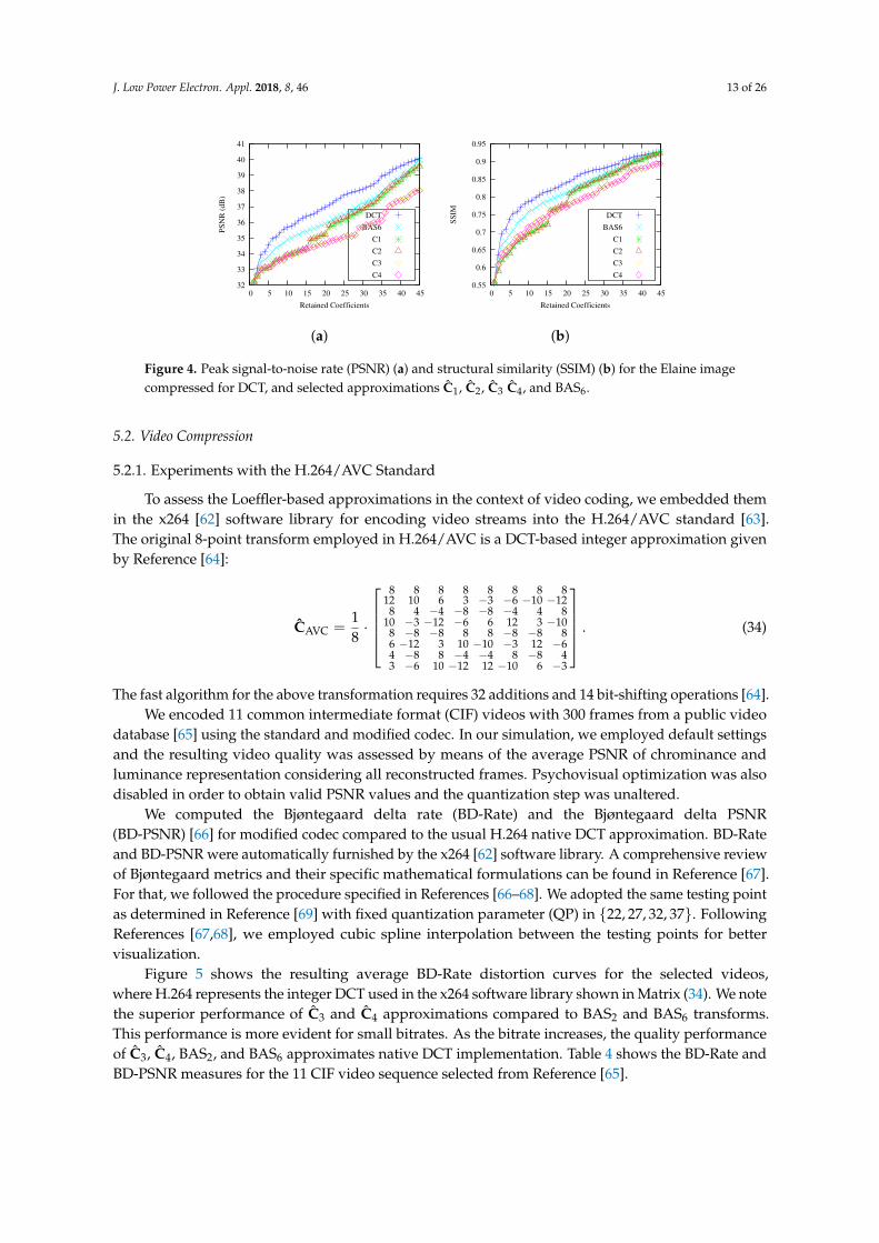
J. Low Power Electron. Appl. 2018, 8, 46 13 of 26

32

33

34

35

36

37

38

39

40

41

0 5 10 15 20 25 30 35 40 45

PS

NR

(d

B)

Retained Coefficients

DCT

BAS6

C1

C2

C3

C4

(a)

0.55

0.6

0.65

0.7

0.75

0.8

0.85

0.9

0.95

0 5 10 15 20 25 30 35 40 45

SS

IM

Retained Coefficients

DCT

BAS6

C1

C2

C3

C4

(b)

Figure 4. Peak signal-to-noise rate (PSNR) (a) and structural similarity (SSIM) (b) for the Elaine imagecompressed for DCT, and selected approximations C1, C2, C3 C4, and BAS6.

5.2. Video Compression

5.2.1. Experiments with the H.264/AVC Standard

To assess the Loeffler-based approximations in the context of video coding, we embedded themin the x264 [62] software library for encoding video streams into the H.264/AVC standard [63].The original 8-point transform employed in H.264/AVC is a DCT-based integer approximation givenby Reference [64]:

CAVC =18·

8 8 8 8 8 8 8 812 10 6 3 −3 −6 −10 −12

8 4 −4 −8 −8 −4 4 810 −3 −12 −6 6 12 3 −108 −8 −8 8 8 −8 −8 86 −12 3 10 −10 −3 12 −64 −8 8 −4 −4 8 −8 43 −6 10 −12 12 −10 6 −3

. (34)

The fast algorithm for the above transformation requires 32 additions and 14 bit-shifting operations [64].We encoded 11 common intermediate format (CIF) videos with 300 frames from a public video

database [65] using the standard and modified codec. In our simulation, we employed default settingsand the resulting video quality was assessed by means of the average PSNR of chrominance andluminance representation considering all reconstructed frames. Psychovisual optimization was alsodisabled in order to obtain valid PSNR values and the quantization step was unaltered.

We computed the Bjøntegaard delta rate (BD-Rate) and the Bjøntegaard delta PSNR(BD-PSNR) [66] for modified codec compared to the usual H.264 native DCT approximation. BD-Rateand BD-PSNR were automatically furnished by the x264 [62] software library. A comprehensive reviewof Bjøntegaard metrics and their specific mathematical formulations can be found in Reference [67].For that, we followed the procedure specified in References [66–68]. We adopted the same testing pointas determined in Reference [69] with fixed quantization parameter (QP) in {22, 27, 32, 37}. FollowingReferences [67,68], we employed cubic spline interpolation between the testing points for bettervisualization.

Figure 5 shows the resulting average BD-Rate distortion curves for the selected videos,where H.264 represents the integer DCT used in the x264 software library shown in Matrix (34). We notethe superior performance of C3 and C4 approximations compared to BAS2 and BAS6 transforms.This performance is more evident for small bitrates. As the bitrate increases, the quality performanceof C3, C4, BAS2, and BAS6 approximates native DCT implementation. Table 4 shows the BD-Rate andBD-PSNR measures for the 11 CIF video sequence selected from Reference [65].

J. Low Power Electron. Appl. 2018, 8, 46 14 of 26

Figure 6a–f displays the first encoded frame of the ‘Foreman’ video sequence at QP = 27 accordingto the modified coded based on the proposed efficient approximations and BAS approximations.For reference, Figure 6g shows the resulting frame obtained from the standard H.264.

Version November 11, 2018 submitted to J. Low Power Electron. Appl. 14 of 26

37

39

41

C1C2C3C4

BAS2BAS6

H.264

Bitrate (kbps)

PSN

R(d

B)

33

35

96.2 256.3 416.4 576.6 736.7

Figure 5. Average rate distortion curves of the modified H.264/AVC software for the selected 11 CIF videosfrom [65] for the PSNR (dB) in terms of bitrate.

Table 4. The average BD-Rate and BD-PSNR for the 11 CIF videos selected from [65]

Transform BD-Rate (%) BD-PSNR (dB)

C1 29.98 −1.08

C2 31.40 −1.13

C3 7.48 −0.29

C4 3.94 −0.15

BAS2 17.43 −0.68

BAS6 13.90 −0.54

and luminance representation considering all reconstructed frames. The psycho-visual optimization was also192

disabled in order to obtain valid PSNR values and the quantization step was unaltered.193

We computed the Bjøntegaard delta rate (BD-Rate) and the Bjøntegaard delta PSNR (BD-PSNR) [66]194

for modified codec compared to the usual H.264 native DCT approximation. The BD-Rate and BD-PSNR are195

automatically furnished by the x264 [62] software library. A comprehensive review of Bjøntegaard metrics196

and their specific mathematical formulations can be found in [67]. For that, we followed the procedure197

specified in [66–68]. We adopted the same testing point as determined in [69] with fixed quantization parameter198

(QP) in {22,27,32,37}. Following [67] and [68], we employed cubic spline interpolation between the testing199

points for better visualization.200

Fig. 5 shows the resulting average BD-Rate distortion curves for the selected videos, where H.264201

represents the integer DCT used in the x264 software library shown in (34). We note the superior performance202

of C3 and C4 approximations compared to BAS2 and BAS6 transforms. This performance is more evident203

for small bitrates. As the bitrate increases, the quality performance of C3, C4, BAS2 and BAS6 approximates204

the native DCT implementation. Table 4 shows the BD-Rate and BD-PSNR measures for the 11 CIF video205

sequence selected from [65]. Note that Loeffler approximations C1 and C2, again, show better performance in206

terms of BD-PSNR measures than the BAS transforms BAS2 and BAS6. We attribute the difference in quality207

between C3 and C4 in relation to C1 and C2 to the associated complexity discrepancy as depicted in Table 2.208

The reduction in the number of additions and bit-shifting operations come at the expense of performance.209

Figure 5. Average rate-distortion curves of the modified H.264/AVC software for the selected 11 CIFvideos from Reference [65] for the PSNR (dB) in terms of bitrate.Version November 11, 2018 submitted to J. Low Power Electron. Appl. 15 of 26

(a) C1 (b) C2 (c) C3

(d) C4 (e) BAS2 (f) BAS6

(g) H.264

Figure 6. First frame of the H.264/AVC compressed ‘Container’ sequence with QP = 27.

5.2.2. Experiments with the H.265/HEVC standard210

We have also embedded the Loeffler-based approximations into the HM-16.3 H.265/HEVC referencesoftware [70]. The H.265/HEVC employs the following integer transform:

CHEVC =164

·

64 64 64 64 64 64 64 6489 75 50 18 −18 −50 −75 −8983 36 −36 −83 −83 −36 36 8375 −18 −89 −50 50 89 18 −7564 −64 −64 64 64 −64 −64 6450 −89 18 75 −75 −18 89 −5036 −83 83 −36 −36 83 −83 3618 −50 75 −89 89 −75 50 −18

, (35)

which demands 72 additions and 62 bit-shifting operations, when considering the factorization method based211

on odd and even decomposition described in [2]. Besides a particular 8-point integer transformation, the HEVC212

standard also employs 4-, 16-, and 32-point transforms [22]. To obtain a modified version of the H.265/HEVC213

codec, we derived 16- and 32-point approximations based on the scalable recursive method proposed in [71].214

The 8-point Loeffler-based efficient solutions were employed as fundamental building blocks for scaling up.215

Since the 4-point DCT matrix possesses only integer coefficients, it was employed unaltered. The additive216

complexity of the scaled 16- and 32-point approximations is 2 ·A(ααα)+ 16 and 4 ·A(ααα)+ 64, respectively [71].217

For the bit-shifting count, we have 2 ·S(ααα) and 4 ·S(ααα), respectively.218

In order perform image quality assessment, we encoded the first 100 frames of one standard sequence of219

each A to F video classes defined in the Common Test Conditions and Software Reference Configurations220

(CTCSRC) document [72]. The selected videos and their attributes are made explicit in the first two221

columns of Table 6. Classes A and B present high-resolution content for broadcasting and video on demand222

services; Classes C and D are lower resolution contents for the same applications; Class E reflects typical223

examples of video conferencing data; and Class F provides computer generated image sequences [73]. All224

encoding parameters, including QP values, were set according to CTCSRC document for the Main profile225

Figure 6. First frame of the H.264/AVC compressed ‘Foreman’ sequence with QP = 27.

Table 4. Average Bjøntegaard delta (BD)-Rate and BD-PSNR for the 11 common intermediate format(CIF) videos selected from Reference [65].

Transform BD-Rate (%) BD-PSNR (dB)

C1 29.98 −1.08C2 31.40 −1.13C3 7.48 −0.29C4 3.94 −0.15

BAS2 17.43 −0.68BAS6 13.90 −0.54

J. Low Power Electron. Appl. 2018, 8, 46 15 of 26

Note that Loeffler approximations C1 and C2, again, show better performance in terms ofBD-PSNR measures than BAS transforms BAS2 and BAS6. We attribute the difference in qualitybetween C3 and C4 in relation to C1 and C2 to the associated complexity discrepancy as depicted inTable 2. The reduction in the number of additions and bit-shifting operations come at the expenseof performance.

5.2.2. Experiments with the H.265/HEVC Standard

We also embedded Loeffler-based approximations into the HM-16.3 H.265/HEVC referencesoftware [70]. The H.265/HEVC employs the following integer transform:

CHEVC =1

64·

64 64 64 64 64 64 64 6489 75 50 18 −18 −50 −75 −8983 36 −36 −83 −83 −36 36 8375 −18 −89 −50 50 89 18 −7564 −64 −64 64 64 −64 −64 6450 −89 18 75 −75 −18 89 −5036 −83 83 −36 −36 83 −83 3618 −50 75 −89 89 −75 50 −18

, (35)

which demands 72 additions and 62 bit-shifting operations, when considering the factorization methodbased on odd and even decomposition described in Reference [2]. Besides a particular 8-point integertransformation, the HEVC standard also employs 4-, 16-, and 32-point transforms [22]. To obtain amodified version of the H.265/HEVC codec, we derived 16- and 32-point approximations based on thescalable recursive method proposed in Reference [71]. The 8-point Loeffler-based efficient solutionswere employed as fundamental building blocks for scaling up. Since the 4-point DCT matrix onlypossesses integer coefficients, it was employed unaltered. The additive complexity of the scaled 16-and 32-point approximations is 2 · A(ααα) + 16 and 4 · A(ααα) + 64, respectively [71]. For the bit-shiftingcount, we have 2 · S(ααα) and 4 · S(ααα), respectively.

In order to perform image-quality assessment, we encoded the first 100 frames of one standardsequence of each A to F video classes defined in the Common Test Conditions and Software ReferenceConfigurations (CTCSRC) document [72]. The selected videos and their attributes are made explicit inthe first two columns of Table 5. Classes A and B present high-resolution content for broadcasting andvideo on demand services; Classes C and D are lower-resolution contents for the same applications;Class E reflects typical examples of video-conferencing data; and Class F provides computer-generatedimage sequences [73]. All encoding parameters, including QP values, were set according to theCTCSRC document for the Main profile and All-Intra (AI), Random Access (RA), Low Delay B (LD-B),and Low Delay P (LD-P) configurations. In the AI configuration, each frame from the input videosequence is independently coded. RA and LD (B and P) coding modes differ mainly by order ofcoding and outputting. In the former, the coding order and output order of the pictures (frames) maydiffer, whereas equal order is required for the latter (Reference [74], p. 94). RA configuration relates tobroadcasting and streaming use, whereas LD (B and P) represent conventional applications.

It is worth mentioning that Class A test sequences are not used for LDB and LDP coding tests,whereas Class E videos are not included in the RA test cases because of the nature of the content theyrepresent (Reference [74], p. 93).

As figures of merit, we computed the BD-Rate and BD-PSNR for the modified versions of thecodec. Figures 7–10 depict the rate-distortion curves and Table 5 presents the Bjøntegaard metricsfor the considered sets of 8- to 32-point approximations for modes AI, RA, LDB, and LDP. BD-Rateand BD-PSNR are also automatically furnished by HM-16.3 H.265/HEVC reference software [70].We employed the cubic spline interpolation based on four testing points on Figures 7–10, as specifiedin References [67,68]. The curves denoted by HEVC represents the native integer approximations forthe 8-, 16-, and 32-point DCT in the HM-16.3 H.265/HEVC software [70]. These four testing pointswere determined by the specification for HEVC as in Reference [69] with fixed QP ∈ {22, 27, 32, 37}.One can note that there is no significant image-quality degradation when considering approximate

J. Low Power Electron. Appl. 2018, 8, 46 16 of 26

transforms. Furthermore, in all the cases, it can be seen that C4 performs better with a degradation ofno more than 0.52 dB.

The Loeffler-based approximations could present competitive image quality while possessinglow computational complexity. Table 6 shows the arithmetic costs of both the original and modifiedextended versions, and the H.265/HEVC native transform. As a qualitative result, Figure 11 depicts thefirst frame of the ‘BasketballDrive’ video sequence resulting from the unmodified H.265/HEVC [70]and from the modified codec according to the discussed approximations and their scaled versions atQP = 32. We also display the related frames according to the BAS2 and BAS6 transforms.

Table 5. Bjøntegaard metrics of the modified HEVC reference software for tested video sequences.

Class NameResolution BD-PSNR (dB) and BD-Rate (%)

and Frame Rate C1 C2 C3 C4 BAS2 BAS6

A ’PeopleOnStreet’ 2560 × 1600 0.54 dB 0.53 dB 0.53 dB 0.34 dB 0.47 dB 0.50 dB30 fps −9.75% −9.61% −9.49% −6.30% −8.47% −8.99%

B ’BasketballDrive’ 1920 × 1080 0.33 dB 0.32 dB 0.45 dB 0.20 dB 0.25 dB 0.27 dB50 fps −11.56% −11.28% −15.52% −7.24% −8.90% −9.50%

C ’RaceHorses’ 832 × 480 0.67 dB 0.66 dB 0.83 0.52 dB 0.61 dB 0.61 dB30 fps −8.06% −7.98% −9.70% −6.36% −7.38% −7.38%

D ’BlowingBubbles’ 416 × 240 0.26 dB 0.25 dB 0.26 dB 0.15 dB 0.20 dB 0.22 dB50 fps −4.35% −4.25% −4.46% −2.59% −3.48% −3.74%

E ’KristenAndSara’ 1280 × 720 0.47 dB 0.46 dB 0.47 dB 0.30 dB 0.39 dB 0.41 dB60 fps −8.97% −8.78% −9.00% −5.93% −7.49% −7.90%

F ’BasketbalDrillText’ 832 × 480 0.20 dB 0.20 dB 0.19 dB 0.12 dB 0.16 dB 0.17 dB50 fps −3.82% −3.79% −3.63% −2.26% −3.06% −3.28%

Table 6. Computational complexity for N-point transforms employed in the H.265/ High EfficiencyVideo Coding (HEVC) experiments.

N Transform Add. Mult. Shifts

8

H.265/HEVC [75] 28 22 0T1 14 0 0T3 18 0 0T5 16 0 2T6 24 0 2

16

H.265/HEVC [75] 100 86 0T1 44 0 0T3 52 0 0T5 48 0 4T6 64 0 4

32

H.265/HEVC [75] 372 342 0T1 120 0 0T3 136 0 0T5 128 0 8T6 160 0 8

J. Low Power Electron. Appl. 2018, 8, 46 17 of 26

Version November 11, 2018 submitted to J. Low Power Electron. Appl. 17 of 26

C1C2C3C4

BAS2BAS6HEVC

Bitrate (Mbps)

PSN

R(d

B)

35

37

39

41

43

20.5 43.0 65.5 87.9 110.4

(a)

C1C2C3C4

BAS2BAS6HEVC

Bitrate (Mbps)

PSN

R(d

B)

37

38

39

40

41

42

7.7 21.9 36.2 50.5 64.7

(b)

C1C2C3C4

BAS2BAS6HEVC

Bitrate (Mbps)

PSN

R(d

B)

33

36

39

1.8 3.2 4.5 5.9 7.3

(c)

C1C2C3C4

BAS2BAS6HEVC

Bitrate (Mbps)

PSN

R(d

B)

34

37

40

1.6 3.6 5.6 7.6 9.6

(d)

C1C2C3C4

BAS2BAS6HEVC

Bitrate (Mbps)

PSN

R(d

B)

39

41

43

45

4.9 9.5 14.1 18.7 23.3

(e)

C1C2C3C4

BAS2BAS6HEVC

Bitrate (Mbps)

PSN

R(d

B)

34

36

38

40

42

3.7 8.0 12.4 16.7 21.0

(f)

Figure 7. Rate distortion curves of the modified HEVC software in mode AI for test sequences:(a) ‘PeopleOnStreet’, (b) ‘BasketballDrive’, (c) ‘RaceHorses’, (d) ‘BlowingBubbles’, (e) ‘KristenAndSara’, and(f) ’BasketbalDrillText’.

Figure 7. Rate-distortion curves of the modified HEVC software in AI mode for test sequences:(a) ‘PeopleOnStreet’, (b) ‘BasketballDrive’, (c) ‘RaceHorses’, (d) ‘BlowingBubbles’, (e) ‘KristenAndSara’,and (f) ‘BasketbalDrillText’.

J. Low Power Electron. Appl. 2018, 8, 46 18 of 26

Version November 11, 2018 submitted to J. Low Power Electron. Appl. 18 of 26

C1C2C3C4

BAS2BAS6HEVC

Bitrate (Mbps)

PSN

R(d

B)

33

35

37

39

41

4.7 11.9 19.2 26.4 33.6

(a)

C1C2C3C4

BAS2BAS6HEVC

Bitrate (Mbps)

PSN

R(d

B)

35

36

37

38

39

40

1.5 5.5 9.5 13.5 17.5

(b)

C1C2C3C4

BAS2BAS6HEVC

Bitrate (Mbps)

PSN

R(d

B)

26

29

32

35

0.8 3.0 4.0 5.11.9

(c)

C1C2C3C4

BAS2BAS6HEVC

Bitrate (Mbps)

PSN

R(d

B)

31

33

35

37

39

0.2 0.6 0.9 1.3 1.7

(d)

C1C2C3C4

BAS2BAS6HEVC

Bitrate (Mbps)

PSN

R(d

B)

33

35

37

39

41

0.4 1.1 1.9 2.6 3.4

(e)

Figure 8. Rate distortion curves of the modified HEVC software in mode RA for testsequences: (a) ‘PeopleOnStreet’, (b) ‘BasketballDrive’, (c) ‘RaceHorses’, (d) ‘BlowingBubbles’, and(e) ‘BasketbalDrillText’.

Figure 8. Rate-distortion curves of the modified HEVC software in RA mode for testsequences: (a) ‘PeopleOnStreet’, (b) ‘BasketballDrive’, (c) ‘RaceHorses’, (d) ‘BlowingBubbles’,and (e) ‘BasketbalDrillText’.

J. Low Power Electron. Appl. 2018, 8, 46 19 of 26

Version November 11, 2018 submitted to J. Low Power Electron. Appl. 19 of 26

C1C2C3C4

BAS2BAS6HEVC

Bitrate (Mbps)PS

NR

(dB

)

35

36

37

38

39

40

6.2 10.7 15.2 19.81.6

(a)

C1C2C3C4

BAS2BAS6HEVC

Bitrate (Mbps)

PSN

R(d

B)

27

30

33

36

39

1.0 2.1 3.3 4.4 5.6

(b)

C1C2C3C4

BAS2BAS6HEVC

Bitrate (Mbps)

PSN

R(d

B)

30

32

34

36

38

0.2 0.7 1.1 1.6 2.0

(c)

C1C2C3C4

BAS2BAS6HEVC

Bitrate (Mbps)

PSN

R(d

B)

37

39

41

43

0.2 0.7 1.1 1.6 2.0

(d)

C1C2C3C4

BAS2BAS6HEVC

Bitrate (Mbps)

PSN

R(d

B)

33

35

37

39

41

0.4 1.2 2.0 2.8 3.6

(e)

Figure 9. Rate distortion curves of the modified HEVC software in mode LDB for testsequences: (a) ‘BasketballDrive’, (b) ‘RaceHorses’, (c) ‘BlowingBubbles’, (d) ‘KristenAndSara’, and(e) ‘BasketbalDrillText’.

Figure 9. Rate-distortion curves of the modified HEVC software in LDB mode for testsequences: (a) ‘BasketballDrive’, (b) ‘RaceHorses’, (c) ‘BlowingBubbles’, (d) ‘KristenAndSara’,and (e) ‘BasketbalDrillText’.

J. Low Power Electron. Appl. 2018, 8, 46 20 of 26

Version November 11, 2018 submitted to J. Low Power Electron. Appl. 20 of 26

C1C2C3C4

BAS2BAS6HEVC

Bitrate (Mbps)PS

NR

(dB

)

35

36

37

38

39

40

6.6 11.4 16.3 21.11.7

(a)

C1C2C3C4

BAS2BAS6HEVC

Bitrate (Mbps)

PSN

R(d

B)

27

30

33

36

39

1.0 3.3 4.5 5.72.2

(b)

C1C2C3C4

BAS2BAS6HEVC

Bitrate (Mbps)

PSN

R(d

B)

30

32

34

36

38

0.2 0.7 1.61.2 2.1

(c)

C1C2C3C4

BAS2BAS6HEVC

Bitrate (Mbps)

PSN

R(d

B)

37

39

41

43

0.2 0.7 1.7 2.21.2

(d)

C1C2C3C4

BAS2BAS6HEVC

Bitrate (Mbps)

PSN

R(d

B)

33

35

37

39

41

0.4 1.2 2.1 3.0 3.8

(e)

Figure 10. Rate distortion curves of the modified HEVC software in mode LDP for testsequences: (a) ‘BasketballDrive’, (b) ‘RaceHorses’, (c) ‘BlowingBubbles’, (d) ‘KristenAndSara’, and(e) ‘BasketbalDrillText’.

Figure 10. Rate-distortion curves of the modified HEVC software in LDP mode for testsequences: (a) ‘BasketballDrive’, (b) ‘RaceHorses’, (c) ‘BlowingBubbles’, (d) ‘KristenAndSara’,and (e) ‘BasketbalDrillText’.

J. Low Power Electron. Appl. 2018, 8, 46 21 of 26

Version November 11, 2018 submitted to J. Low Power Electron. Appl. 21 of 26

(a) C1 (b) C2 (c) C3

(d) C4 (e) BAS2 (f) BAS6

(g) H.265

Figure 11. First frame of the H.265/HEVC compressed ‘BasketballDrive’ sequence with QP = 32.

Table 6. Bjøntegaard metrics of the modified HEVC reference software for tested video sequences

Class Name Resolution BD-PSNR (dB) and BD-Rate (%)

and frame rate C1 C2 C3 C4 BAS2 BAS6

A ’PeopleOnStreet’ 2560×1600 0.54 dB 0.53 dB 0.53 dB 0.34 dB 0.47 dB 0.50 dB30 fps -9.75 % -9.61 % -9.49 % -6.30 % -8.47 % -8.99 %

B ’BasketballDrive’1920×1080 0.33 dB 0.32 dB 0.45 dB 0.20 dB 0.25 dB 0.27 dB

50 fps -11.56 % -11.28 % -15.52 % -7.24 % -8.90 % -9.50 %

C ’RaceHorses’832×480 0.67 dB 0.66 dB 0.83 0.52 dB 0.61 dB 0.61 dB

30 fps -8.06 % -7.98 % -9.70 % -6.36 % -7.38 % -7.38 %

D ’BlowingBubbles’ 416×240 0.26 dB 0.25 dB 0.26 dB 0.15 dB 0.20 dB 0.22 dB50 fps -4.35 % -4.25 % -4.46 % -2.59 % -3.48 % -3.74 %

E ’KristenAndSara’1280×720 0.47 dB 0.46 dB 0.47 dB 0.30 dB 0.39 dB 0.41 dB

60 fps -8.97 % -8.78 % -9.00 % -5.93 % -7.49 % -7.90 %

F ’BasketbalDrillText’832×480 0.20 dB 0.20 dB 0.19 dB 0.12 dB 0.16 dB 0.17 dB

50 fps -3.82 % -3.79 % -3.63 % -2.26 % -3.06 % -3.28 %

Figure 11. First frame of the H.265/HEVC-compressed ‘BasketballDrive’ sequence with QP = 32.

6. FPGA Implementation

To compare the hardware-resource consumption of the discussed approximations, they wereinitially modeled and tested in Matlab Simulink and then physically realized on FPGA. The FPGA usedwas a Xilinx Virtex-6 XC6VLX240T installed on a Xilinx ML605 prototyping board. FPGA realizationwas tested with 100,000 random 8-point input test vectors using hardware cosimulation. Test vectorswere generated from within the Matlab environment and routed to the physical FPGA device using aJTAG-based hardware cosimulation. Then, measured data from the FPGA was routed back to Matlabmemory space.

We separated the BAS6 approximation for comparison with efficient approximations becauseits performance metrics lay on the Pareto frontier of the plots in Figure 2. The associated FPGAimplementations were evaluated for hardware complexity and real-time performance using metricssuch as configurable logic blocks (CLB) and flip-flop (FF) count, critical path delay (Tcpd) in ns, andmaximum operating frequency (Fmax) in MHz. Values were obtained from the Xilinx FPGA synthesisand place-route tools by accessing the xflow.results report file. In addition, static (Qp) and dynamicpower (Dp in mW/GHz) consumption were estimated using the Xilinx XPower Analyzer. We alsoreported area-time complexity (AT) and area-time-squared complexity (AT2). Circuit area (A) wasestimated using the CLB count as a metric, and time was derived from Tcpd. Table 7 lists the FPGAhardware resource and power consumption for each algorithm.

Considering the circuit complexity of the discussed approximations and BAS6 [5], as measuredfrom the CBL count for the FPGA synthesis report, it can be seen from Table 7 that T1 is the smallestoption in terms of circuit area. When considering maximum speed, matrix T5 showed the bestperformance on the Vertex-6 XC6VLX240T device. Alternatively, if we consider the normalizeddynamic power consumption, the best performance was again measured from T1.

J. Low Power Electron. Appl. 2018, 8, 46 22 of 26

Table 7. Hardware-resource consumption and power consumption using a Xilinx Virtex-6 XC6VLX240T1FFG1156 device.

Approximation CLB FF Tcpd (ns) Fmax (MHz) Dp (mW/GHz) Qp (W) AT AT2

T1 108 368 2.783 359 2.93 3.455 300.56 836.47T3 114 386 2.805 357 3.56 3.462 319.77 896.95T5 125 442 2.280 439 3.65 3.472 285 649.8T6 185 626 2.699 371 4.18 3.470 499.32 1347.65BAS6 [5] 116 316 2.740 365 4.05 3.468 317.84 870.88

7. Conclusions and Final Remarks

In this paper, we introduced a mathematical framework for the design of 8-point DCTapproximations. The Loeffler algorithm was parameterized and a class of matrices wasderived. Matrices with good properties, such as low-complexity, invertibility, orthogonality ornear-orthogonality, and closeness to the exact DCT, were separated according to a multicriteriaoptimization problem aiming at Pareto efficiency. The DCT approximations in this class were assessed,and the optimal transformations were separated.

The obtained transforms were assessed in terms of computational complexity, proximity,and coding measures. The derived efficient solutions constitute DCT approximations capable ofgood properties when compared to existing DCT approximations. At the same time, approximationrequires extremely low computation costs: only additions and bit-shifting operations are required fortheir evaluation.

We demonstrated that the proposed method is a unifying structure for several approximationsscattered in the literature, including the well-known approximation by Lengwehasatit–Ortega [31],and they share the same matrix factorization scheme. Additionally, because all discussedapproximations have a common matrix expansion, the SFG of their associated fast algorithmsare identical except for the parameter values. Thus, the resulting structure paves the way toperformance-selectable transforms according to the choice of parameters.

Moreover, approximations were assessed and compared in terms of image and video coding.For images, a JPEG-like encoding simulation was considered, and for videos, approximations wereembedded in the H.264/AVC and H.265/HEVC video-coding standards. Approximations exhibitedgood coding performance compared to exact DCT-based JPEG compression and the obtained framevideo quality was very close to the results shown by the H.264/AVC and H.265/HEVC standards.

Extensions for larger blocklengths can be achieved by considering scalable approaches such asthe one suggested in Reference [71]. Alternatively, one could employ direct parameterization of the16-point Loeffler DCT algorithm described in Reference [27].

Author Contributions: conceptualization, D.F.G.C. and R.J.C.; methodology, D.F.G.C. and R.J.C.; software,T.L.T.S., P. M. and R.S.O.; hardware, S.K., R.S.O., and A.M.; validation, D.F.G.C., R.J.C., T.L.T.S., P.M. and R.S.O.;writing—original draft preparation, D.F.G.C. and R.J.C.; writing, reviewing, and editing, D.F.G.C., R.J.C., T.L.T.S.,R.S.O., F.M.B. and S.K.; supervision, R.J.C.; funding acquisition, R.J.C. and V.S.D.

Funding: Partial support from CAPES, CNPq, FACEPE, and FAPERGS.

Conflicts of Interest: The authors declare no conflict of interest.

Abbreviations

The following abbreviations are used in this manuscript:

DCT Discrete cosine transformAVC Advanced video codingHEVC High-efficiency video codingFPGA Field-programmable gate arrayKLT Karhunen–Loève transform

J. Low Power Electron. Appl. 2018, 8, 46 23 of 26

DWT Discrete wavelet transformJPEG Joint photographic experts groupMPEG Moving-picture experts groupMSE Mean-squared errorSSIM Structural similarity index metricPSNR Peak signal-to-noise ratioWHT Walsh–Hadamard transformQP Quantization parameterBD Bjøntegaard deltaCIF Common intermediate formatCLB Configurable logic blockFF Flip-flop

References

1. Ahmed, N.; Rao, K.R. Orthogonal Transforms for Digital Signal Processing; Springer: New York, NY, USA, 1975.2. Britanak, V.; Yip, P.; Rao, K.R. Discrete Cossine and Sine Transforms; Academic Press: Orlando, FL, USA, 2007.3. Kolaczyk, E.D. Methods for analyzing certain signals and images in astronomy using Haar wavelets.

In Proceedings of the Asilomar Conference on Signals, Systems & Computers, Pacific Grove, CA, USA,2–5 November 1997; Volume 1, pp. 80–84.

4. Qiang, Y. Image denoising based on Haar wavelet transform. In Proceedings of the International Conferenceon Electronics and Optoelectronics, Dalian, China, 29–31 July 2011; Volume 3.

5. Bouguezel, S.; Ahmad, M.O.; Swamy, M.N.S. Binary Discrete Cosine and Hartley Transforms. IEEE Trans.Circuits Syst. I 2013, 60, 989–1002. [CrossRef]

6. Martucci, S.A.; Mersereau, R.M. New Approaches To Block Filtering of Images Using SymmetricConvolution and the DST or DCT. In Proceedings of the International Symposium on Circuits and Systems,Chicago, IL, USA, 3–6 May 1993; pp. 259–262.

7. Oppenheim, A.V.; Schafer, R.W.; Buck, J.R. Discrete-Time Signal Processing, 2nd ed.; Prentice-Hall, Inc.:Upper Saddle River, NJ, USA, 1999; Volume 1.

8. Gonzalez, R.C.; Woods, R.E. Digital Image Processing, 2nd ed.; Prentice-Hall, Inc.: Upper Saddle River,NJ, USA, 2001.

9. Parfieniuk, M. Using the CS decomposition to compute the 8-point DCT. In Proceedings of theIEEE International Symposium on Circuits and Systems (ISCAS), Lisbon, Portugal, 24–27 May 2015;pp. 2836–2839.

10. Coutinho, V.D.A; Cintra, R.J.; Bayer, F.M.; Kulasekera, S.; Madanayake, A. Low-complexity pruned 8-pointDCT approximations for image encoding. In Proceedings of the International Conference on Electronics,Communications and Computers (CONIELECOMP), Cholula, Mexico, 25–27 February 2015; pp. 1–7.

11. Potluri, U.S.; Madanayake, A.; Cintra, R.J.; Bayer, F.M.; Kulasekera, S.; Edirisuriya, A. Improved 8-pointApproximate DCT for Image and Video Compression Requiring Only 14 Additions. IEEE Trans. CircuitsSyst. I 2014, 61, 1727–1740. [CrossRef]

12. Goebel, J.; Paim, G.; Agostini, L.; Zatt, B.; Porto, M. An HEVC multi-size DCT hardware with constantthroughput and supporting heterogeneous CUs. In Proceedings of the IEEE International Symposium onCircuits and Systems (ISCAS), Montreal, QC, Canada, 22–25 May 2016; pp. 2202–2205.

13. Naiel, M.A.; Ahmad, M.O.; Swamy, M.N.S. Approximation of feature pyramids in the DCT domain and itsapplication to pedestrian detection. In Proceedings of the IEEE International Symposium on Circuits andSystems (ISCAS), Montreal, QC, Canada, 22–25 May 2016; pp. 2711–2714.

14. Lalitha, N.V.; Prasad, P.V.; Rao, S.U. Performance analysis of DCT and DWT audio watermarking basedon SVD. In Proceedings of the International Conference on Circuit, Power and Computing Technologies(ICCPCT), Nagercoil, India, 18–19 March 2016; pp. 1–5.

15. Masera, M.; Martina, M.; Masera, G. Adaptive Approximated DCT Architectures for HEVC. IEEE Trans.Circuits Syst. Video Technol. 2017, 27, 2714–2725. [CrossRef]

16. Zhao, M.; Liu, H.; Wan, Y. An improved Canny edge detection algorithm based on DCT. In Proceedingsof the IEEE International Conference on Progress in Informatics and Computing (PIC), Nanjing, China,18–20 December 2015; pp. 234–237.

J. Low Power Electron. Appl. 2018, 8, 46 24 of 26

17. Wang, Y.; Shi, M.; You, S.; Xu, C. DCT Inspired Feature Transform for Image Retrieval and Reconstruction.IEEE Trans. Image Process. 2016, 25, 4406–4420. [CrossRef] [PubMed]

18. Bhaskaran, V.; Konstantinides, K. Image and Video Compression Standards; Kluwer Academic Publishers:Norwell, MA, USA, 1997.

19. Wallace, G.K. The JPEG still picture compression standard. IEEE Trans. Consum. Electron. 1992, 38, xviii–xxxiv.[CrossRef]

20. Roma, N.; Sousa, L. Efficient hybrid DCT-domain algorithm for video spatial downscaling. EURASIP J. Adv.Signal Process. 2007, 2007, 057291. [CrossRef]

21. Wiegand, T.; Sullivan, G.J.; Bjøntegaard, G.; Luthra, A. Overview of the H.264/AVC video coding standard.IEEE Trans. Circuits Syst. Video Technol. 2003, 13, 560–576. [CrossRef]

22. Pourazad, M.T.; Doutre, C.; Azimi, M.; Nasiopoulos, P. HEVC: The New Gold Standard for VideoCompression: How Does HEVC Compare with H.264/AVC? IEEE Consum. Electron. Mag. 2012, 1, 36–46.[CrossRef]

23. Horn, D.R. Lepton Image Compression: Saving 22% Losslessly from Images at 15MB/s. 2016. Availableonline: https://blogs.dropbox.com/tech/2016/07/lepton-image-compression-saving-22-losslessly-from-images-at-15mbs/ (accessed on 10 November 2018).

24. Lee, B. A New Algorithm to Compute the Discrete Cosine Transform. IEEE Trans. Acoust. SpeechSignal Process. 1984, 32, 1243–1245.

25. Arai, Y.; Agui, T.; Nakajima, M. A fast DCT-SQ scheme for images. IEICE Trans. 1988, E71, 1095–1097.26. Feig, E.; Winograd, S. Fast Algorithms for the Discrete Cosine Transform. IEEE Trans. Signal Process. 1992,

40, 2174–2193. [CrossRef]27. Loeffler, C.; Ligtenberg, A.; Moschytz, G.S. Practical Fast 1-D DCT Algorithms with 11 Multiplications.

In Proceedings of the International Conference on Acoustics, Speech, and Signal Processing, Glasgow, UK,23–26 May 1989; Volume 2; pp. 988–991.

28. Duhamel, P.; H’Mida, H. New 2n DCT algorithms suitable for VLSI implementation. In Proceedings of theIEEE International Conference on Acoustics, Speech, and Signal Processing, Dallas, TX, USA, 6–9 April 1987;Volume 12, pp. 1805–1808.

29. Heideman, M.T.; Burrus, C.S. Multiplicative Complexity, Convolution, and the DFT; Springer: New York,NY, USA, 1988.

30. Haweel, T.I. A new square wave transform based on the DCT. Signal Process. 2001, 81, 2309–2319. [CrossRef]31. Lengwehasatit, K.; Ortega, A. Scalable Variable Complexity Approximate Forward DCT. IEEE Trans. Circuits

Syst. Syst. Video Technol. 2004, 14, 1236–1248. [CrossRef]32. Cintra, R.J.; Bayer, F.M. A DCT approximation for image compression. IEEE Signal Process. Lett. 2011,

18, 579–582. [CrossRef]33. Bayer, F.M.; Cintra, R.J. DCT-like transform for image compression requires 14 additions only. Electron. Lett.

2012, 48, 919–921. [CrossRef]34. Bouguezel, S.; Ahmad, M.O.; Swamy, M.N.S. A multiplication-free transform for image compression.

In Proceedings of the 2nd International Conference on Signals, Circuits and Systems, Monastir, Tunisia,7–9 November 2008; pp. 1–4.

35. Bouguezel, S.; Ahmad, M.O.; Swamy, M.N.S. Low-complexity 8x8 transform for image compression.Electron. Lett. 2008, 44, 1249–1250. [CrossRef]

36. Bouguezel, S.; Ahmad, M.O.; Swamy, M.N.S. A novel transform for image compression. In Proceedings of the53rd IEEE International Midwest Symposium on Circuits and Systems, Seattle, WA, USA, 1–4 August 2010;pp. 509–512.

37. Bouguezel, S.; Ahmad, M.O.; Swamy, M.N.S. A low-complexity parametric transform for image compression.In Proceedings of the IEEE International Symposium on Circuits and Systems, Rio de Janeiro, Brazil,15–18 May 2011; pp. 2145–2148.

38. Cintra, R.J. An Integer Approximation Method for Discrete Sinusoidal Transforms. Circuits Syst. Signal Process.2011, 30, 1481–1501. [CrossRef]

39. Cintra, R.J.; Bayer, F.M.; Tablada, C.J. Low-complexity 8-point DCT approximations based on integerfunctions. Signal Process. 2014, 99, 201–214. [CrossRef]

40. Zhang, D.; Lin, S.; Zhang, Y.; Yu, L. Complexity controllable {DCT} for real-time H.264 encoder. J. Vis.Commun. Image Represent. 2007, 18, 59–67. [CrossRef]

J. Low Power Electron. Appl. 2018, 8, 46 25 of 26

41. Bouguezel, S.; Ahmad, M.O.; Swamy, M.N.S. A fast 8× 8 transform for image compression. In Proceedingsof the International Conference on Microelectronics, Columbus, OH, USA, 4–7 August 2009; pp. 74–77.

42. Chen, Y.J.; Oraintara, S.; Tran, T.D.; Amaratunga, K.; Nguyen, T.Q. Multiplierless approximation oftransforms using lifting scheme and coordinate descent with adder constraint. In Proceedings ofthe IEEE International Conference on Acoustics, Speech, and Signal Processing, Orlando, FL, USA,13–17 May 2002, Volume 3.

43. Liang, M.J.; Tran, T.D. Approximating the DCT with the lifting scheme: Systematic design and applications.In Proceedings of the Asilomar Conference on Signals, Systems and Computers, Pacific Grove, CA, USA,29 October–1 November 2000; Volume 1; pp. 192–196.

44. Liang, M.J.; Tran, T.D. Fast multiplierless approximations of the DCT with the lifting scheme. IEEE Trans.Signal Process. 2001, 49, 3032–3044. [CrossRef]

45. Malvar, H. Fast computation of discrete cosine transform through fast Hartley transform. Electron. Lett.1986, 22, 352–353. [CrossRef]

46. Malvar, H.S. Fast computation of the discrete cosine transform and the discrete Hartley transform. IEEE Trans.Acoust. Speech Signal Process. 1987, 35, 1484–1485. [CrossRef]

47. Malvar, H. Erratum: Fast computation of discrete cosine transform through fast Hartley transform.Electron. Lett. 1987, 23, 608. [CrossRef]

48. Kouadria, N.; Doghmane, N.; Messadeg, D.; Harize, S. Low complexity DCT for image compression inwireless visual sensor networks. Electron. Lett. 2013, 49, 1531–1532. [CrossRef]

49. Manassah, J.T. Elementary Mathematical and Computational Tools for Electrical and Computer Engineers UsingMatlab R©; CRC Press: New York, NY, USA, 2001.

50. Blahut, R.E. Fast Algorithms for Digital Signal Processing; Cambridge University Press: Cambridge, UK, 2010.51. Halmos, P.R. Finite Dimensional Vector Spaces; Springer: New York, NY, USA, 2013.52. Graham, R.L.; Knuth, D.E.; Patashnik, O. Concrete Mathematics; Addison-Wesley Publishing Company:

Reading, MA, USA, 1989.53. Shores, T.S. Applied Linear Algebra and Matrix Analysis; Springer: Lincoln, NE, USA, 2007.54. Tablada, C.J.; Bayer, F.M.; Cintra, R.J. A Class of DCT Approximations Based on the Feig-Winograd

Algorithm. Signal Process. 2015, 113, 38–51. [CrossRef]55. Strang, G. Linear Algebra and Its Applications, 4th ed.; Thomson Learning; Massachusetts Institute of

Technology: Cambridge, MA, USA, 2005.56. Katto, J.; Yasuda, Y. Performance evaluation of subband coding and optimization of its filter coefficients.

J. Vis. Commun. Image Represent. 1991, 2, 303–313. [CrossRef]57. Ehrgott, M. Multicriteria Optimization, 2 ed.; Springer: Berlin, Germany, 2005.58. Barichard, V.; Ehrgott, M.; Gandibleux, X.; T’Kindt, V. Multiobjective Programming and Goal Programming:

Theoretical Results and Practical Applications, 1 ed.; Springer: Berlin, Germany, 2009.59. Kay, S.M. Fundamentals of Statistical Signal Processing: Estimation Theory; Prentice-Hall, Inc.: Upper Saddle River,

NJ, USA, 1993; Volume 1.60. Kay, S.M. Fundamentals of Statistical Signal Processing: Detection Theory; Prentice-Hall, Inc.: Upper Saddle River,

NJ, USA, 1998; Volume 2.61. Wang, Z.; Bovik, A.C.; Sheikh, H.R.; Simoncelli, E.P. Image Quality Assessment: From Error Visibility to

Structural Similarity. IEEE Trans. Image Process. 2004, 13, 600–612. [CrossRef] [PubMed]62. x264 Team. VideoLAN Organization. Available online: http://www.videolan.org/developers/x264.html

(accessed on 10 November 2018).63. Richardson, I. The H.264 Advanced Video Compression Standard, 2nd ed.; John Wiley and Sons: Hoboken, NJ,

USA, 2010.64. Gordon, S.; Marpe, D.; Wiegand, T. Simplified Use of 8× 8 Transform—Updated Proposal and Results; Technical

Report; Joint Video Team (JVT) of ISO/IEC MPEG and ITU-T VCEG: Munich, Germany, 2004.65. Xiph.Org Foundation. Xiph.org Video Test Media. 2014. Available online: https://media.xiph.org/video/derf/

(accessed on 10 November 2018).66. Bjøntegaard, G. Calculation of Average PSNR Differences between RD-curves. In Proceedings of the 13th

VCEG Meeting, Austin, TX, USA, 2–4 April 2001.67. Hanhart, P.; Ebrahimi, T. Calculation of average coding efficiency based on subjective quality scores. J. Vis.

Commun. Image Represent. 2014, 25, 555–564. [CrossRef]

J. Low Power Electron. Appl. 2018, 8, 46 26 of 26

68. Tan, T.K.; Weerakkody, R.; Mrak, M.; Ramzan, N.; Baroncini, V.; Ohm, J.R.; Sullivan, G.J. Video QualityEvaluation Methodology and Verification Testing of HEVC Compression Performance. IEEE Trans. CircuitsSyst. Video Technol. 2016, 26, 76–90. [CrossRef]

69. Bossen, F. 12th Meeting of Joint Collaborative Team on Video Coding (JCT-VC) of ITU-T SG16 WP3 andISO/IEC JTC1/SC29/WG11. Available online: http://phenix.it-sudparis.eu/jct/doc_end_user/current_document.php?id=7281 (accessed on 8 November 2018).

70. Joint Collaborative Team on Video Coding (JCT-VC). HEVC References Software Documentation; FraunhoferHeinrich Hertz Institute: Berlin, Germany, 2013.

71. Jridi, M.; Alfalou, A.; Meher, P.K. A Generalized Algorithm and Reconfigurable Architecture for Efficientand Scalable Orthogonal Approximation of DCT. IEEE Trans. Circuits Syst. I 2015, 62, 449–457. [CrossRef]

72. Bossen, F. Common Test Conditions and Software Reference Configurations; Document JCT-VC L1100;2013. Available online: http://phenix.it-sudparis.eu/jct/doc_end_user/current_document.php?id=7281(accessed on 8 November 2018).

73. Naccari, M.; Mrak, M. Chapter 5—Perceptually Optimized Video Compression. In Academic Press Library inSignal Processing Image and Video Compression and Multimedia; Theodoridis, S., Chellappa, R., Eds.; Elsevier:Amsterdam, Netherlands, 2014; Volume 5, pp. 155–196.

74. Wien, M. High Efficiency Video Coding; Signals and Communication Technology, Springer: Berlin/Heidelberg,Germany, 2015; p. 314.

75. Budagavi, M.; Fuldseth, A.; Bjøntegaard, G.; Sze, V.; Sadafale, M. Core Transform Design in the HighEfficiency Video Coding (HEVC) Standard. IEEE J. Sel. Top. Signal Process. 2013, 7, 1029–1041. [CrossRef]

c© 2018 by the authors. Licensee MDPI, Basel, Switzerland. This article is an open accessarticle distributed under the terms and conditions of the Creative Commons Attribution(CC BY) license (http://creativecommons.org/licenses/by/4.0/).