Integral Approximations in Ab Initio, Electron

Propagator Calculations

Roberto Flores–Moreno∗1,2 and J. V. Ortiz†1

1Department of Chemistry and Biochemistry,Auburn University, Auburn, AL 36849-5312

U.S.A.2Departamento de Quımica,

Centro de Investigacion y de Estudios Avanzadosdel Instituto Politecnico Nacional,

Avenida Instituto Politecnico Nacional 2508,A.P. 14-740, Mexico, D.F., C.P. 07000

Mexico

August 4, 2009

Abstract

Treatments of interelectronic repulsion that avoid four–center inte-grals have been incorporated in ab initio, electron–propagator calcula-tions with diagonal self–energy matrices. Whereas the formal scaling ofarithmetic operations in the propagator calculations is unaffected, thereduction of storage requirements is substantial. Moreover, the scal-ing of integral transformations to the molecular orbital base is loweredby one order. Four–index, electron–repulsion integrals are regeneratedfrom three–index intermediates. Test calculations with widely appliedself–energy approximations demonstrate the accuracy of this approach.Only small errors are introduced when this technique is used withquasiparticle virtual orbitals, provided that conventional techniques ofintegral evaluation are used in the construction of density–differencematrices, provided that conventional techniques of integral evaluationare used in the construction of density–difference matrices.

∗roberto.floresmoreno.qt@gmail.com†ortiz@auburn.edu

1

1 Introduction

Electron propagator theory [1, 2, 3, 4, 5] (EPT) provides a foundation for

the efficient, accurate evaluation of ionization energies and electron affini-

ties of large molecules. Diagonal self–energy, or quasiparticle, approxima-

tions to the electron propagator are frequently used to determine correla-

tion and relaxation corrections to Koopmans’s theorem [6] (KT) results for

the calculation of electron binding energies. Electrons assigned to canoni-

cal Hartree–Fock [7, 8] (HF) orbitals are thereby subjected to a correlated,

energy–dependent potential represented by the diagonal elements of the self–

energy matrix. Several approximations of this kind have been characterized

extensively in numerical tests and have been applied to many molecules and

ions [9, 10, 11, 12].

Most implementations of many–body methods such as EPT are ex-

pressed in terms of formulae that involve electron repulsion integrals (ERIs)

in the molecular orbital (MO) representation. For low–order, perturbative

approximations, one of the most computationally intensive tasks is the eval-

uation of these quantities. In conventional algorithms, ERIs in the MO base

are stored on external disks. This strategy is advantageous provided that

input/output operations are performed efficiently. At the cost of perform-

ing more arithmetic operations, direct or semidirect algorithms [13, 14] may

facilitate EPT calculations on larger species when disk storage of ERIs is

infeasible. (The term direct refers to embedding the recalculation of ERIs

2

in the formation of various intermediate matrices.) Transformation of ERIs

from atomic–orbital (AO) to MO bases scales formally as N5, where N is the

dimension of the former base. Therefore, for many low–order, perturbative

EPT methods, this transformation of four–index quantities constitutes the

computational bottleneck, especially in conventional algorithms that avoid

the recalculation of ERIs in the AO base.

Attempts to remove bottlenecks that arise from the rank of the ERI

matrix may be founded on improved representations of electron densities or

reductions in active orbital spaces. In the latter category, one finds a vari-

ety of improved virtual orbital techniques, such as a recent procedure that

is based on density difference matrices that accompany low–order electron

propagator methods [15, 16]. In the former category, systematic elimination

of redundant information in the base of electron densities generated by AOs

is represented by the Cholesky decomposition approach [17]. Alternatives

consider the expansion of AO–based densities in terms of auxiliary functions.

Density fitting (DF) methodology played a prominent role in the develop-

ment of programs that solve Kohn–Sham equations [18]. In correlated, ab

initio calculations where numerous electron densities require representation,

related strategies, dubbed resolution–of–the–identity (RI) methods, were

successfully implemented [19]. Many recent publications have considered

the numerical calibration and relative advantages of Cholesky decomposi-

tion and RI techniques in the execution of well–known self–consistent field

3

and perturbative methods [20, 21, 22, 23, 24, 25, 26, 27, 28].

DF–RI methods offer a way to overcome arithmetic or storage obsta-

cles to the execution of low–order, perturbative EPT calculations that arise,

respectively, from integral transformation or the quantity of ERIs. To pro-

vide clear criteria for assessing the reliability of this approach, comparisons

will be made with previous EPT calculations that employed HF reference

states. Because the resulting algorithms do not require the evaluation of

four–center ERIs in the AO base, they may be conveniently implemented

in codes (see, for example, Ref. [29]) that are designed chiefly for the so-

lution of Kohn–Sham (KS) equations and that possess optimal routines for

the evaluation of three–center integrals. This strategy also is advantageous

for AO–based, molecular electron propagator calculations that employ KS

reference determinants instead of their HF counterparts [30].

This manuscript is organized as follows. In Section 2, basic aspects of

density–fitting (DF) or resolution–of–the–identity (RI) techniques are dis-

cussed and their relevance to the execution of electron propagator calcula-

tions is established. The organization of the calculations is considered in

Section 3. In Section 4, the numerical performance of the method is ana-

lyzed for second–order and partial third–order quasiparticle approximations

of electron propagator theory. Final remarks are given in Section 5.

4

2 Methods

2.1 ERIs in EPT formulae

In the diagonal, or quasiparticle, approximation to the electron propagator,

the Dyson equation is reduced to

ωp = εp + Σpp(ωp). (1)

Here p labels a canonical, HF MO, εp is the corresponding energy, ωp is the

electron binding energy (ionization energy or electron affinity) and Σpp is a

diagonal element of the energy–dependent, self–energy matrix. Up to first

order in the fluctuation potential, the self–energy vanishes and the results

of Koopmans’s theorem are recovered for the ionization energy. For second

order, the diagonal elements of the self–energy matrix are

Σ[2]pp(ωp) =

∑

i,a<b

|〈pi||ab〉|2ωp + εi − εa − εb

+∑

a,i<j

|〈pa||ij〉|2ωp + εa − εi − εj

, (2)

where i and j label only occupied MOs and a and b are used only for virtual

orbitals. The brackets represent antisymmetrized ERIs in the MO represen-

tation. The three–fold summations of Eq. (2) imply that arithmetic opera-

tions for the evaluation of second–order, self–energy matrix elements scale

somewhat lower than N3. Therefore, second–order calculations are highly

efficient compared to self–consistent–field (SCF) iterations.

However, the evaluation of ERIs in the MO representation scales as N5.

MOs, ϕ, are built from linear combinations of atomic orbitals, µ, such that

ϕp(r) =∑µ

Cµpµ(r) (3)

5

and, therefore, evaluation of MO ERIs requires four transformation steps of

the following type,

〈pν||στ〉 =∑µ

Cµp〈µν||στ〉, (4)

in which a Latin MO index supplants a Greek AO index. This step consti-

tutes the bottleneck of many propagator calculations. If only one electron

binding energy is needed, second–order calculations can be executed more

efficiently by restricting the range of index p in Eq. (4) to a single value. The

first step of the transformation generates intermediates with three running

indices instead of four and therefore has N4 arithmetic scaling. Each of the

three subsequent steps has the same scaling factor.

For higher–order approximations such as partial third order [31] (P3) and

the outer valence Green’s function [3, 9], the pp self–energy matrix elements

include terms with five–fold summations such as

14

∑

abcij

〈pa||ij〉〈ij||bc〉〈bc||pa〉(ωp + εa − εi − εj)(εi + εj − εb − εc)

. (5)

ERIs with no common p index are needed and a more general integral trans-

formation must be executed. Even for the calculation of a single ionization

energy, the transformation of the required integrals scales as N5.

In conventional algorithms, MO ERIs are stored on disk and are recalled

as needed in the evaluation of self–energy matrix elements. The resulting

storage demands scale as N4. In competing semidirect schemes, intermedi-

ates defined in terms of MO ERIs with four or three virtual orbital indices

6

are generated through calculation of AO ERIs. For example, the intermedi-

ate X requires a subset of the MO ERIs with three virtual indices, where

Xpaij =∑

bc

〈ij||bc〉〈bc||pa〉(εi + εj − εb − εc)

. (6)

Such procedures may require repeated evaluations of AO ERIs.

2.2 Treatments of Interelectronic Repulsion

To reduce disk storage requirements and to avoid reevaluation of AO ERIs,

we consider alternatives based on DF or RI strategies. Antisymmetrized

ERIs may be denoted as follows:

Rpqst ≡ 〈pq||st〉 = 〈pq|st〉 − 〈pq|ts〉 (7)

with

〈pq|st〉 =∫ ∫ ϕ∗p(r)ϕ∗q(r′)ϕs(r)ϕt(r′)

|r− r′| drdr′. (8)

Here, p, q, s and t are labels of molecular spin–orbitals and {Rpq} is a set

of matrices that each contain a subset of ERIs with 〈pq| in the bra space.

The superscripts indicate only to which subset the matrix belongs. Spin is

already integrated. Mulliken notation [32] also will be employed to establish

relationships with DF–RI arguments, where

(ps|qt) ≡ 〈pq|st〉. (9)

Mulliken notation has the advantage of separating the coordinates of the

electrons. Such integrals are the ps matrix elements of the electrostatic po-

tential generated by a single orbital product, qt. In DF–RI techniques, [18,

7

19] orbital–products are expressed as linear combinations of auxiliary func-

tions, {gk(r)}, where

ϕq(r)ϕt(r) =∑

k

eqtk gk(r). (10)

Once again, superscripts identify a pair of MOs that generates the potential

that is being expanded in terms of auxiliary functions. The latter functions

will henceforth be assumed to be real. Left multiplication by a given function

of the auxiliary set multiplied by the Coulomb operator [19], gl(r′)/|r− r′|,

and integration over the full space of r and r′ yields

(l|qt) =∑

k

eqtk Glk (11)

with

(l|qt) ≡∫ ∫ gl(r)ϕ∗q(r′)ϕt(r′)

|r− r′| drdr′ (12)

Glk ≡∫ ∫

gl(r)gk(r′)|r− r′| drdr′. (13)

Expansion coefficients may be computed according to

eqtk =

∑

l

G−1kl (l|qt). (14)

Therefore, four–index integrals are given by:

(pr|qt) =∑

kl

(pr|k)G−1kl (l|qt). (15)

Because the matrix G−1 is needed only at this level of the calculation, its

absorption into three–index quantities can be exploited [33], such that

T qkt ≡

∑

l

G−1/2kl (l|qt). (16)

8

Here, only a single superscript labels the subset of three–center ERIs to

which a given matrix T belongs. The dimensions of the matrix Tq are

M ×N , where M is the number of auxiliary functions. M is, in general, a

small multiple of N . Representative M:N ratios for the GEN-A2* [34, 35,

36, 37] auxiliary basis set are: 4:1 for cc-pVDZ, 3:1 for cc-pVTZ and 2:1

for cc-pVQZ. This prefactor does not grow with the size of the system and,

therefore, is not part of the formal scaling. Thus, four–index integrals may

be obtained from simple matrix multiplications of three–index intermediates,

Rpq = (Tp)†Tq − (Tq)†Tp. (17)

Considerable economies of storage can be realized by saving T matrices on

disk instead of the R matrices that occur in previous electron propagator

algorithms. DF–RI techniques enable execution of conventional (as opposed

to semidirect) algorithms in which all intermediates are stored on disk and

AO ERIs need not be reevaluated. Moreover, the transformation from AO

to MO bases can be executed for three–index matrices, T, with a formal

scaling of M ×N3, thus gaining one order in the arithmetic scaling of this

task according to

T pkq =

∑µ

CµqTpkµ, ∀p. (18)

In DF–RI–EPT calculations beyond second order, the most intensive arith-

metic task is calculation of self–energy matrix elements and not the trans-

formation of integrals. Therefore, DF–RI–EPT calculations will not only

9

reduce storage requirements, but also can compete in speed with previous

algorithms despite the need for extra integral evaluation and handling.

Note that the method described here does not use DF–RI for the SCF

solution of the reference system. Such an approach would result in an ap-

proximate description of the self–energy’s pole structure, for MO energies

would be affected [38]. Preliminary calculations indicate that DF–RI ap-

proximations for the Coulomb contribution to the Fock matrix introduce

deviations in orbital energies that are less than 0.01 eV. Nevertheless, si-

multaneous application of DF–RI approximations to SCF and EPT methods

has not been attempted here, for procurement of HF wavefunctions does not

constitute a bottleneck in EPT calculations.

3 Computational details

All calculations were performed using the deMon2k program [29]. The two–

and three–center integrals of Eq.s (13) and (12) are evaluated efficiently

through employment of Hermite auxiliary functions [39, 40]. Extra func-

tionality was added to this program so that the modified version is able to

evaluate four–center integrals and, therefore, to perform HF calculations. It

also can execute EPT calculations of second order (EP2) and partial third

order (P3) in the quasiparticle approximation. An interface routine builds

four–index ERIs in the MO base by using deMon2k routines for evaluation of

two– and three–center ERIs. Auxiliary function sets are generated automat-

ically for each choice of basis set [34, 35, 36, 37]. Two basis sets commonly

10

employed in EPT calculations were used: cc-pVTZ [41] for small molecules

and 6-311G(d,p) [42, 43] for porphyrin.

4 Results and Discussion

4.1 Size dependence of errors

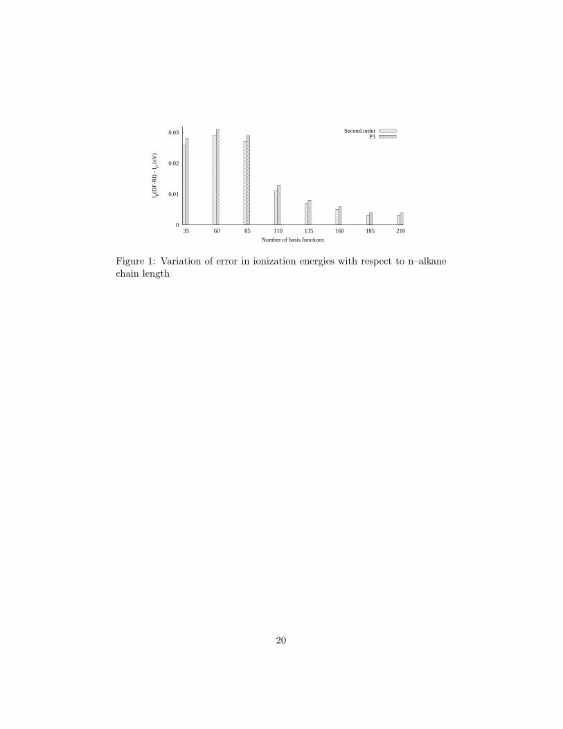
The present DR–RI techniques are intended for the study of large molecules

where ordinary EPT calculations are infeasible. Here, the behavior of errors

introduced by these techniques as a function of molecular size is examined.

A plot of such errors versus the number of carbons in alkane chains is shown

in Fig. 1. For these calculations, the cc–pVDZ and auxiliary GEN–A2*

basis sets were used. After an initial maximum for ethane, the error declines

through heptane and increases only slightly for octane. There is no evidence

that errors grow in proportion to chain length. Unlike the results of Ref. [44],

where DF–RI was applied in a different context, the approach presented here

is stable with respect to the size of the system, provided that auxiliary basis

sets of good quality are used.

4.2 Accuracy for small molecules

DF–RI methods also may be judged by their accuracy for valence ioniza-

tion energies of small molecules. Tables 1 and 2 compare conventional re-

sults [12] with their DF–RI counterparts in the second order (EP2) and P3

quasiparticle approximations. The same cc–pVTZ basis sets and molecular

structures were employed in both sets of calculations. Mean absolute devi-

11

ations (MADs) of the DF–RI results with respect to the conventional data

are below 0.1 eV for GEN-A2 and below 0.05 eV for GEN-A2* auxiliary

basis sets. MADs with respect to experimental values are no worse for the

use of the DF–RI methods.

4.3 Improved virtual orbitals

In a recent publication, we have described a novel method for the reduc-

tion of the virtual orbital space in quasiparticle electron propagator cal-

culations [15, 16]. Substantial computational efficiencies achieved through

the construction of quasiparticle virtual orbitals (QVOs) generally produced

only small deviations from electron binding energies obtained with the full

set of unoccupied orbitals. Here we consider DF–RI calculations performed

with QVOs. It is necessary to evaluate elements of the density–difference

matrix described in Ref. [15],

∆ρpab = δapδbp −

∑

j<k

〈pa||jk〉〈jk||pb〉(Ep + εa − εj − εk)(Ep + εb − εj − εk)

+∑

jc

〈pj||ac〉〈bc||pj〉(Ep + εj − εa − εc)(Ep + εj − εb − εc)

, (19)

with conventional techniques based on four–center ERIs. Preliminary tests

performed with DF–RI methods for the construction of the density difference

matrix indicate that extra errors appear in corresponding P3 calculations

with an active virtual space that is 50% as large as the original. Therefore, if

the QVOs procedure is employed, DF–RI methods should be activated only

after the reduction of the virtual orbital space is realized. Fortunately, exact,

12

four–center ERIs required for the determination of the density difference

matrix can be computed with N4 arithmetic scaling. Storage requirements

for intermediate matrices scale as N3. These scaling factors are the same

as those of the DF–RI procedure. Results from Ref. [15] with 100% (i.e.

no QVO reduction) or 50% retentions of virtual orbitals are compared with

analogous DF–RI calculations in Table 3. For the 100% case, the mean

absolute deviation of P3 results produced by the DF–RI method is 0.003

eV. When the dimension of the virtual orbital space is reduced by 50%, this

deviation is 0.008 eV. The mean effect of employing both approximations

(50% QVOs and DF–RI) is 0.086 eV for P3 calculations. Therefore, DF–

RI methods can be combined with QVOs for the treatment of even larger

molecules.

4.4 Porphyrin

Recent electron propagator studies of porphyrins and their derivatives [45,

46] provide a suitable standard of comparison for DF–RI techniques. P3/6-

311G** calculations generated a consistent and accurate assignment of the

lowest ionization energies of porphyrin. The results of Table 4 indicate the

DF–RI technique, executed with the GEN–A2 auxiliary basis set, introduces

deviations from ordinary P3 calculations that are less than 0.07 eV. The

DF–RI results are all slightly larger those of Ref. [45] by 0.05–0.07 eV and

provide a consistent account of the cationic final states.

13

5 Conclusions

Density fitting or resolution–of–the–identity techniques have been proposed

as a means to performing ab initio electron propagator calculations on large

systems. Test calculations on small molecules, alkanes, benzene, borazine

and porphyrin show that employment of standard auxiliary functions may

enable calculations of triple–ζ plus polarization quality to be executed with-

out unacceptable loss of accuracy. Significant reductions in external disk

storage and decreased arithmetic operations for the bottleneck of ordinary

calculations, the four–index integral transformation, have been achieved.

These techniques may be combined with methods for reducing the rank

of the virtual orbital space, provided that conventional electron repulsion

integral techniques are employed in the evaluation of density–difference ma-

trices. Applications to larger molecules on modestly constructed computa-

tional platforms lie in prospect.

6 Acknowledgments

Funding from Conacyt (Mexico) under grant 60117-F and from the Na-

tional Science Foundation (U.S.A.) under grant CHE-0809199 is gratefully

acknowledged.

14

References

[1] J. Linderberg and Y. Ohrn, Propagators in Quantum Chemistry, 2nd

ed., Wiley–Interscience, Hoboken, New Jersey, 2004.

[2] P. Jørgensen and J. Simons, Second–Quantization Based Methods in

Quantum Chemistry, Academic Press, New York, 1981.

[3] W. von Niessen, J. Schirmer and L. S. Cederbaum, Comput. Phys. Rep.

1, 57 (1984).

[4] M. F. Herman, K. F. Freed and D. L. Yeager, Adv. Chem. Phys. 48, 1

(1981).

[5] J. V. Ortiz, Adv. Quantum Chem. 35, 33 (1999).

[6] T. Koopmans, Physica 1, 104 (1933).

[7] D. R. Hartree, Proc. Camb. Phyl. Soc. 24, 328 (1928).

[8] V. A. Fock, Z. Phys. 15, 126 (1930).

[9] J. V. Ortiz, in Computational Chemistry: Reviews of Current Trends

2, 1, J. Leszczynski, ed., World Scientific, Singapore, 1997.

[10] J. V. Ortiz, V. G. Zakrzewski and O. Dolgounitcheva, in Conceptual

Perspectives in Quantum Chemistry 3, 465, J.-L. Calais and E. S. Kry-

achko, eds., Kluwer, Dordrecht, 1997.

15

[11] A. M. Ferreira, G. Seabra, O. Dolgounitcheva, V. G. Zakrzewski and J.

V. Ortiz, in Quantum–Mechanical Prediction of Thermochemical Data,

131, J. Cioslowski, ed., Kluwer, Dordrecht, 2001.

[12] R. Flores–Moreno, V. G. Zakrzewski and J. V. Ortiz, J. Chem. Phys.

127, 134106 (2007).

[13] V. G. Zakrzewski and J. V. Ortiz, Int. J. Quantum Chem. Symp. 28,

23 (1994).

[14] V. G. Zakrzewski and J. V. Ortiz, Int. J. Quantum Chem. 53, 583

(1995).

[15] R. Flores–Moreno and J. V. Ortiz, J. Chem. Phys. 128, 164105 (2008).

[16] O. Dolgounitcheva, R. Flores–Moreno, V. G. Zakrzewski and J. V. Or-

tiz, Int. J. Quantum Chem. 108, 2862 (2008).

[17] N. H. F. Beebe and J. Linderberg, Int. J. Quantum Chem. 12, 683

(1977).

[18] J. L. Whitten, J. Chem. Phys. 58, 4496 (1973); J. W. Mintmire, Int. J.

Quantum Chem. 13, 163 (1979); B. I. Dunlap, J. W. D. Connolly and

J. R. Sabin, J. Chem. Phys. 71, 3396, 4993 (1979); J. W. Mintmire and

B. I. Dunlap, Phys. Rev. A 25, 88 (1982).

16

[19] M. Feyereisen, G. Fitzgerald and A. Komornicki, Chem. Phys. Lett.

208, 359 (1993); O. Vahtras, J. Almlof, and M. W. Feyereisen, Chem.

Phys. Lett. 213, 514 (1993).

[20] F. Aquilante, T. B. Pedersen and R. Lindh, J. Chem. Phys., 126,

194106 (2007).

[21] F. Aquilante, R. Lindh and T. B. Pedersen, J. Chem. Phys., 127,

114107 (2007).

[22] F. Aquilante and T. B. Pedersen, Chem. Phys. Lett., 449, 354 (2007).

[23] I. Røeggen and T. Johansen, J. Chem. Phys., 128, 194107 (2008).

[24] F. Aquilante, T. B. Pedersen, R. Lindh, B. O. Roos, A. Sanchez de

Meras and H. Koch, J. Chem. Phys., 129, 024113 (2008).

[25] L. Boman, H. Koch, A. Sanchez de Meras, J. Chem. Phys., 129, 134107

(2008).

[26] F. Aquilante, L. Gagliardi, T. B. Pedesen and R. Lindh, J. Chem.

Phys., 130, 154107 (2009).

[27] J. Zienau, L. Clin, B. Doser and C. Ochsenfeld, J. Chem. Phys., 130,

204112 (2009).

[28] F. Weigend, M. Kattannek and R. Ahlrichs, J. Chem. Phys., 130,

164106 (2009).

17

[29] A. M. Koster, P. Calaminici, M. E. Casida, V. D. Domınguez, R. Flores–

Moreno, G. Geudtner, A. Goursot, T. Heine, A. Ipatov, F. Janetzko, J.

M. del Campo, S. Patchkovskii, J. U. Reveles, A. M. Vela, B. Zuniga and

D. R. Salahub, deMon2k, The International deMon Developers Com-

munity, Mexico, 2008.

[30] Y. Shigeta, A. M. Ferreira, V. G. Zakrzewski and J. V. Ortiz, Int. J.

Quantum Chem. 85, 411 (2001).

[31] J. V. Ortiz, J. Chem. Phys. 104, 7599 (1996).

[32] A. Szabo and N. S. Ortlund, Modern Quantum Chemistry, Dover Pubs.

Inc., Mineola, New York, 1996.

[33] A. P. Rendell and T. J. Lee, J. Chem. Phys. 101, 400 (1994).

[34] J. Andzelm, E. Radzio and D. R. Salahub, J. Comput. Chem. 6, 520

(1985).

[35] J. Andzelm, N. Russo and D. R. Salahub, J. Chem. Phys. 87, 6562

(1987).

[36] P. Calaminici, R. Flores–Moreno and A. M. Koster, Comput. Lett. 1,

164 (2005).

[37] P. Calaminici, F. Janetzko, A. M. Koster, R. Mejıa-Olvera and B.

Zuniga-Gutierrez, J. Chem. Phys. 126, 044108 (2007).

18

[38] S. Hamel, M. E. Casida and D. R. Salahub, J. Chem. Phys. 114, 7342

(2001).

[39] A. M. Koster, J. Chem. Phys. 104, 4114 (1996).

[40] A. M. Koster, J. Chem. Phys. 118, 9943 (2003).

[41] T. H. Dunning, J. Chem. Phys. 90, 1007 (1989).

[42] R. Krishnan, J. S. Binkley, R. Seeger and J. A. Pople, J. Chem. Phys.

72, 650 (1980).

[43] M. J. Frisch, J. A. Pople and J. S. Binkley, J. Chem. Phys. 80, 3265

(1984).

[44] C.-K. Skylaris, L. Gagliardi, N. C. Handy, A. G. Ioannou, S. Spencer

and A. Willetts, J. Mol. Struct. (THEOCHEM) 229, 501 (2000).

[45] O. Dolgounitcheva, V. G. Zakrzewski and J. V. Ortiz, J. Am. Chem.

Soc. 127, 8240 (2005).

[46] O. Dolgounitcheva, V. G. Zakrzewski and J. V. Ortiz, J. Phys. Chem.

A 109, 11596 (2005).

19

0

0.01

0.02

0.03

35 60 85 110 135 160 185 210

I p(D

F-R

I) -

Ip

(eV

)

Number of basis functions

Second orderP3

Figure 1: Variation of error in ionization energies with respect to n–alkanechain length

20

Table 1: Accuracy of RI-EP2 for small moleculesMolecule Orbital RI-EP2 EP21 Expt.1

GEN-A2 GEN-A2*B2H6 1b3g 12.066 12.208 12.21 11.9CH4 1t2 14.026 14.060 14.07 14.40C2H4 1b3u 10.455 10.328 10.33 10.51

1b3g 12.656 12.747 12.75 12.853ag 14.477 14.482 14.48 14.661b2u 15.847 15.882 15.89 15.872b1u 19.270 19.334 19.34 19.23

HCN 1π 13.778 13.678 13.68 13.61HNC 1π 13.856 13.746 13.74 12.55NH3 3a1 10.244 10.167 10.17 10.8N2 1πu 17.149 17.049 17.05 16.98

3σg 15.034 15.022 15.02 15.602σu 18.192 18.197 18.20 18.78

CO 5σ 14.045 14.056 14.06 14.011π 16.485 16.371 16.37 16.91

H2CO 2b2 9.936 9.938 9.94 10.9H2O 1b1 11.615 11.500 11.50 12.78

3a1 13.945 13.862 13.86 14.741b2 18.137 18.085 18.08 18.51

HF 1π 14.841 14.708 14.70 16.193σ 19.043 18.945 18.94 20.00

F2 1πg 14.301 14.205 14.20 15.833σg 20.643 20.470 20.46 21.11πu 17.451 17.358 17.35 18.8

MAD vs Expt. 0.574 0.613 0.615 0.000MAD vs EP2 0.081 0.042 0.000

1See Ref. [12]

21

Table 2: Accuracy of RI-P3 for small moleculesMolecule Orbital RI-P3 P31 Expt.1

GEN-A2 GEN-A2*B2H6 1b3g 11.984 12.137 12.14 11.9CH4 1t2 14.177 14.219 14.22 14.40C2H4 1b3u 10.676 10.554 10.55 10.51

1b3g 12.877 12.968 12.98 12.853ag 14.878 14.883 14.89 14.661b2u 16.067 16.102 16.11 15.872b1u 19.362 19.433 19.44 19.23

HCN 1π 14.061 13.957 13.96 13.61HNC 1π 14.220 14.112 14.11 12.55NH3 3a1 10.802 10.729 10.73 10.8N2 1πu 17.286 17.186 17.18 16.98

3σg 15.938 15.929 15.93 15.602σu 19.286 19.302 19.30 18.78

CO 5σ 14.255 14.270 14.27 14.011π 17.155 17.044 17.04 16.91

H2CO 2b2 10.901 10.899 10.90 10.9H2O 1b1 12.613 12.494 12.49 12.78

3a1 14.859 14.773 14.77 14.741b2 18.794 18.740 18.74 18.51

HF 1π 16.085 15.944 15.94 16.193σ 19.944 19.841 19.84 20.00

F2 1πg 15.734 15.625 15.62 15.833σg 21.223 21.047 21.04 21.11πu 18.999 18.892 18.89 18.8

MAD vs Expt. 0.248 0.249 0.250 0.000MAD vs P3 0.084 0.037 0.000

1See Ref. [12]

22

Table 3: Effects of RI methods on P3/cc–pVTZ ionization energies (eV)obtained with QVOs (50%) and full virtual orbital (100%) spaces

Molecule Orbital 50% 100%P3 [15] RI-P3 P3 [15] RI-P3

Benzene e1g 9.362 9.363 9.402 9.403e2g 12.166 12.167 12.302 12.298a2u 12.321 12.348 12.384 12.385e1u 14.362 14.359 14.466 14.462b2u 15.000 15.004 15.066 15.067b1u 15.636 15.628 15.757 15.750a1g 17.197 17.187 17.314 17.310

Borazine e′′ 10.290 10.295 10.318 10.320e′ 11.682 11.676 11.825 11.820a′′2 12.847 12.850 12.906 12.907a′1 13.926 13.908 14.037 14.030e′ 15.079 15.065 15.152 15.150a′2 14.872 14.869 14.929 14.930e′ 17.848 17.835 17.905 17.904

RI MAD 0.008 0.003

23

Table 4: Ionization energies (eV) of free porphyrin in RI calculations withGEN–A2 auxiliary functions

Orbital KT P31 RI-P3 Expt.1

au 6.14 7.02 7.078 7.1b1u 6.66 6.96 7.031 6.9b3g 9.13 8.30 8.368 8.4b1u 9.30 8.48 8.550 8.4

1 See Ref. [45]

24