Robust design considering optimization tools and reduced-basis approximations

This content has been downloaded from IOPscience. Please scroll down to see the full text.

Download details:

IP Address: 54.160.93.70

This content was downloaded on 12/06/2016 at 19:14

Please note that terms and conditions apply.

Robust design considering optimization tools and reduced-basis approximations

View the table of contents for this issue, or go to the journal homepage for more

2010 IOP Conf. Ser.: Mater. Sci. Eng. 10 012198

(http://iopscience.iop.org/1757-899X/10/1/012198)

Home Search Collections Journals About Contact us My IOPscience

iopscience.iop.org/page/terms

http://iopscience.iop.org/1757-899X/10/1

http://iopscience.iop.org/1757-899X

http://iopscience.iop.org/

http://iopscience.iop.org/search

http://iopscience.iop.org/collections

http://iopscience.iop.org/journals

http://iopscience.iop.org/page/aboutioppublishing

http://iopscience.iop.org/contact

http://iopscience.iop.org/myiopscience

Robust Design Considering Optimization Tools and Reduced-

Basis Approximations

S M B Afonso1, R S Motta

2, P R M Lyra

3 and R B Willmersdorf

4

Federal University of Pernambuco, Rua Acadêmico Hélio Ramos, s/n –

Cid. Universitária – Recife - Brasil. CEP: 50740-530 1,2

Civil Engineering Department, 3,4

Mechanical Engineering Department

E-mail: [email protected],

[email protected],

[email protected],

[email protected]

Abstract. This paper performs Robust Design Optimization (RDO) to obtain optimum solu-

tions since some degree of uncertainty in characterizing any real engineering system is inevita-

ble. The robustness measures considered here are the expected value and standard deviation of

the function involved in the optimization problem. To calculate such quantities, we employ two

nonintrusive uncertainty propagation analysis techniques that exploit deterministic computer

models: Monte Carlo (MC) method and Probabilistic Collocation Method (PCM). The uncer-

tainty propagation essentially involves computing the statistical moments of the output. When

using these robustness measures combined, the search for optimal design appears as a robust

multiobjetive optimization (RMO) problem. Several strategies are implemented to obtain the

Pareto front (multiobjective solutions). To overcome the time consuming problem inherent in

a RMO problem reduced basis (RB) approximation methodology is added to the optimization

system, in the whole optimization process. The integration of all the methodologies described

allows the computation of robust design, using a finite element model of 3.900 degrees of free-

dom, in a practical time (less than a minute).

1. Introduction

Optimization of most engineering applications traditionally considers deterministic models and pa-

rameters. However, the deterministic approach generally leads to a final design whose performance

may degrade significantly because of perturbations arising from uncertainties. In this scenario a better

target would consider an optima design with less outputs variability. The process to find such optimal

is referred to as robust design optimization (RDO).

Several robustness measures have been proposed in the literature [1]. In particular, the expected

value and standard deviation of the objective function are considered here, leading to a multicriteria

optimization (MO) problem to be solved [2]. In addition to that, the robustness in terms of feasible

conditions is also taken into account, considering the variability for some of the constraints.

The Pareto concept is adopted here to obtain the MO solutions. For that, efficient techniques such

as NBI (Normal-Boundary Intersection) [3], and NNC (Normalized Normal-Constraint) [4] are im-

plemented. Apart from these two strategies, two others approaches commonly considered in literature

weighted sum method and min-max method are also implemented.

Two nonintrusive methods are used for uncertainty propagation analysis: Monte Carlo (MC)

method [1] and Probabilistic Collocation Method (PCM) [5]. These approaches consider the computa-

WCCM/APCOM 2010 IOP PublishingIOP Conf. Series: Materials Science and Engineering 10 (2010) 012198 doi:10.1088/1757-899X/10/1/012198

c© 2010 Published under licence by IOP Publishing Ltd 1

tional system (code) as a black box, which returns function values and its gradients given an input vec-

tor.

As the generation of Pareto points and the uncertainty analysis could be very costly, approximation

techniques based on the use of reduced basis methodology [6] are also incorporated in our procedure.

The purpose of such scheme is to get high fidelity model information with acceptable computational

expense. Moreover, a parameter separation strategy together with the affine decomposition allows the

development of an efficient offline/online calculation strategy for the computational implementation

of the RB method. This is a very attractive tool for optimum design purposes as the offline calcula-

tions are computed only once and used subsequently in the online stage for each new desired parame-

ter. Therefore, in the optimization context for each new design, function evaluations, error estimators

and sensitivities are very efficiently obtained. Two dimensional continua problems under static loads

are the applications addressed in this work. The performance of the different strategies discussed is

compared.

2. Problem formulation

The deterministic approach for optimization problem can lead to a final design whose performance

may be very sensible to parameters variation. The Robust Optimisation (RO) takes into account the

problem uncertainties in order to obtain a design less susceptible to variability. In this work, two ob-

jective controls will be consider: the mean and the standard deviation of a selected output function [2].

This is a multiobjective problem, mathematically formulated as [2].

Minimize: F(x) = {E(F(x ,ξ )), σ(F(x ,ξ )) } (1)

subject to

( )

( )

, 0 1,...

, 0 1,...

1,...

i

j

u

k k k dv

g i m

h j

x x x k n

≤ =

= =

≤ ≤ =

x ξ

x ξ

l

l (2)

where x is the design variable vector, ξ is the random variable vector, F(x) is the set of objective

functions to be minimized, E(*) is the expected value, σ (*) is the standard deviation, F is the se-

lected output, ( , )ig x ξ and ( , )k

h x ξ are inequality and equality constraints, respectively, that could

(or not) be dependent on ξ and k

xl , u

kx are respectively the lower and upper bounds of a typical

design variable.

The MO problem presented above is solved using the techniques described in Section 3, consider-

ing the Pareto minima concept.

3. Pareto points distribution schemes There are several techniques to obtain the set of Pareto minima [7,8]. In this work we will discuss the

weighted sum (WS) method, min-max, the normal boundary intersection (NBI) method [3] and the

normalized normal-constrain (NNC) method [4]. Currently, in literature, the later two strategies are

said to have more success in obtaining the Pareto curves (bi-objective problems).

3.1. WS method

This is the most traditional and simple approach considered in the MO framework. In this procedure,

the original MO problem is converted into a single (or scalar) optimization problem.

The single objective function is obtained through the linear combination of the normalized objec-

tives functions, in which the weight coefficients ββββ satisfy the requirements 1iβ =∑ and 0i

β ≥ ,

1..i nobj= . Details of this technique can be found elsewhere [7].


2

3.2. Min-Max method

This is a variant of the weighted sum method. The normalization used here takes into account the

minimum and the maximum values of each objective function at all individual minima points (ob-

tained through scalar optimizations). This procedure try to transform each objective function into an-

other function f normalized in the interval [0, 1] [8].

The following optimization problem is carried out:

[ ]minx

γ (3)

where ( )max ( )f xk k

γ β= , 1,...,k nobj∈ , subject to the constraints of the original problem and an addi-

tional constraint, give by:

β γ≤k k

f , k = 1,..., n (4)

3.3. The NBI method

The NBI method [3] is based on the parameterization of the Pareto front and produces an even spread

points distribution.

The geometric representation of the NBI method is show in Figure 1, which illustrates the objective

function space and its feasible region. The Pareto points are obtained in the intersection of the quasi-

normal lines emanating from a Convex Hull of Individual Minima (CHIM) and the boundary of the

feasible objective function space (δF). The figure illustrates a set of quasi-normal lines, each line is

associate to a specific coefficient vector and, as can be seen, a different (intersection) solution is ob-

tained (in most cases, Pareto points). The whole concept can be extended for more than two objec-

tives.

Figure 1. The geometric representation of the NBI method for bi-objective problems.

3.4. The NNC method

The NNC method, introduced by Messac et al. [4], represents an improvement over the normal con-

straint method by removing numerical scaling problems through the normalization of the objectives.

NNC procedure works in a similar manner as the NBI method (discussed before) and its graphical rep-

resentation can be seen in figure 2, which illustrates the feasible space and the corresponding Pareto

frontier for a bi-objective case.

The utopia line indicated in Figure 2 (analogous to the CHIM in NBI method), is the line joining

the two individual minima points (or end points of the Pareto frontier). To obtain the Pareto points, in

bi-objective case, a set of points Xpj are created in the utopia line. Through an interactive process using

a pre-selected point Xpj, a normal line is employed to reduce the feasible space as indicated in Figure

2. Minimizing 2

f results in the Pareto point *f , consequently, after translating the normal line from

all points Xpj, the whole set of Pareto solutions will be found.

Feasible space

δF


3

Figure 2. Graphical representation of the NNC method for bi-objective problems.

4. Statistics calculations

The perturbations arising from uncertainties will be statistically analysed here as random variables.

For a random variable ξ there is an associated function named Probability Density Function (PDF)

( )P ξ , which defines the distribution of the occurrences of ξ ∈ ℜ related to a random phenomena [9].

Assuming ξ as a random variable, any function ( )f ξ will be random, with its specific PDF. The

PDFs are dependent on several parameters with practical interpretations such as its mean f

µ and vari-

ance υ, i.e. the expected value [ ]( )E f ξ and the square of the standard deviation 2

fσ . Such quantities

are calculated as

(5) [ ]

( ) [ ]2 22 2

( ) ( ) ( )

( ) ( ) ( ) ( )

f

f

E f f P d

f f P d E f E f

µ ξ ξ ξ ξ

σ ξ ξ ξ ξ ξ

∞

−∞

∞

−∞

= =

= − = −

∫

∫ (5)

In the present work two methodologies, Monte Carlo method and Probabilistic collocation method

[5] are employed for the statistics calculations. Both methodologies are described in the following

subsections.

4.1. Monte Carlo Method

The Monte Carlo method is the most popular non intrusive method and can be used for any uncer-

tainty propagation problem [1].

Given the joint probability distribution function of the involved random variables, the MC method

can be applied to compute approximated statistics of a particular quantity, including its distribution,

with an arbitrary error, as long a sufficient number of samplings points is adopted.

In the present work LHS technique from MATLAB 7.5 [10] will be used for samplings generation.

The LHS points are generated considering normal distributions for each random variable [11].

During the optimization process the same sampling will be used. A strategy for sampling selection

described in [12, 13] was adopted here.

4.2. Probabilistic collocation method

The basic idea of PCM is to approximate the ( )f ξ function by orthogonal polynomial functions and to

evaluate the integrals of equation (5) by Gaussian quadrature [14].

2f

1f

∗1f

∗2f

1

00 1

∗f

X pj

F easible

Region

Infeasible

Region

Utopia Line

line NU


4

4.2.1. Gaussian quadrature. In the numerical integration by Gaussian quadrature for integrals of the

form

(6) ( ) ( )F

f x P x dx∫ (6)

The function ( )f x is approximated by a polynomial of order (2n-1) from an orthonormal basis of the

polynomial space H [5, 12, 13], as follows

(7) 1 1

0 0

ˆ( ) ( ) ( ) ( ) ( )n n

i i n i i

i i

f x f x b h x h x c h x− −

= =

= + ∑ ∑� (7)

where ( )i

h x are the orthonormal polynomials with respect to a weighting function ( )P x and ci, bi are

the unknowns of the approximation. In equation (7), the subscript (i) of the polynomial indicates its

degree. Hence by orthogonality, equation (6) can be approximated as follows

(8) ( ) ( ) ( )0 0F F

f x P x dx b h P x dx∫ ∫� (8)

As the integral presented in equation (8) does not present the coefficients ci, it is required only the

calculations of function ( )f x at the n roots *x of ( )n

h x , cancelling in this way the second part of

equation (7) as *( ) 0, 1..n i

h x i n= = . For more details concerning coefficients evaluation see reference

[5].

4.2.2. Gaussian quadrature for statistics evaluations – PCM. The statistics evaluations considering

PCM consists on a direct application of Gaussian quadrature considering the random variables space

ξ and its PDF as weighting function. The ortonormal polynomials are defined for each PDF, therefore,

we have ( ) 1F

P d =∫ ξ ξ and 0

1h = .

It follows that the mean value and the standard deviation of an output of interest are approximated

by PCM as

*

( )

1

2 * 2 2

( )

1

( )

ˆ ( )

n

PC i i

i

n

PC i i PC

i

P f

P f f

µ

σ

=

=

=

= −

∑

∑

ξ

ξ

(9)

where *

( )iξ are the roots of the orthogonal polynomials.

The gradients of such quantities required by the optimizer are calculated through direct differen-

tiation of the above equations as presented in reference [13].

A drawback of Gaussian quadrature and consequently, PCM is the so called “dimensional curse”,

as the number of integration points increases exponentially with the problem dimensionality. This

means that in the PCM context the number of random variables must be small. To accomplish large

multidimensional problems, the use of numerical integration on sparse grids [15] might mitigate the

above-referred problem.

5. Governing equations Adopting a standard Galerkin spatial discretization, the static governing equation of a linear elastic

structural problem can be written in compact form as [16] =Ku F

(10)

where K is the stiffness matrix, u is the vector of unknown nodal displacements and F is the inde-

pendent vector, which takes into account loads and boundary conditions. The stiffness matrix K is giv-

en by

T

V

dV= ∫K B DB (11)


5

and the vector F has the form

n t

T T T

n t

V

dV d d

Γ Γ

= + Γ + Γ∫ ∫ ∫F N b N f N f . (12)

In above equations V is the domain, nΓ and tΓ are boundary parts, D is the elasticity matrix, B is a

matrix which relates the displacements to their derivatives, N is the matrix of shape functions, b, fn

and ft are associate to loads terms [16, 13].

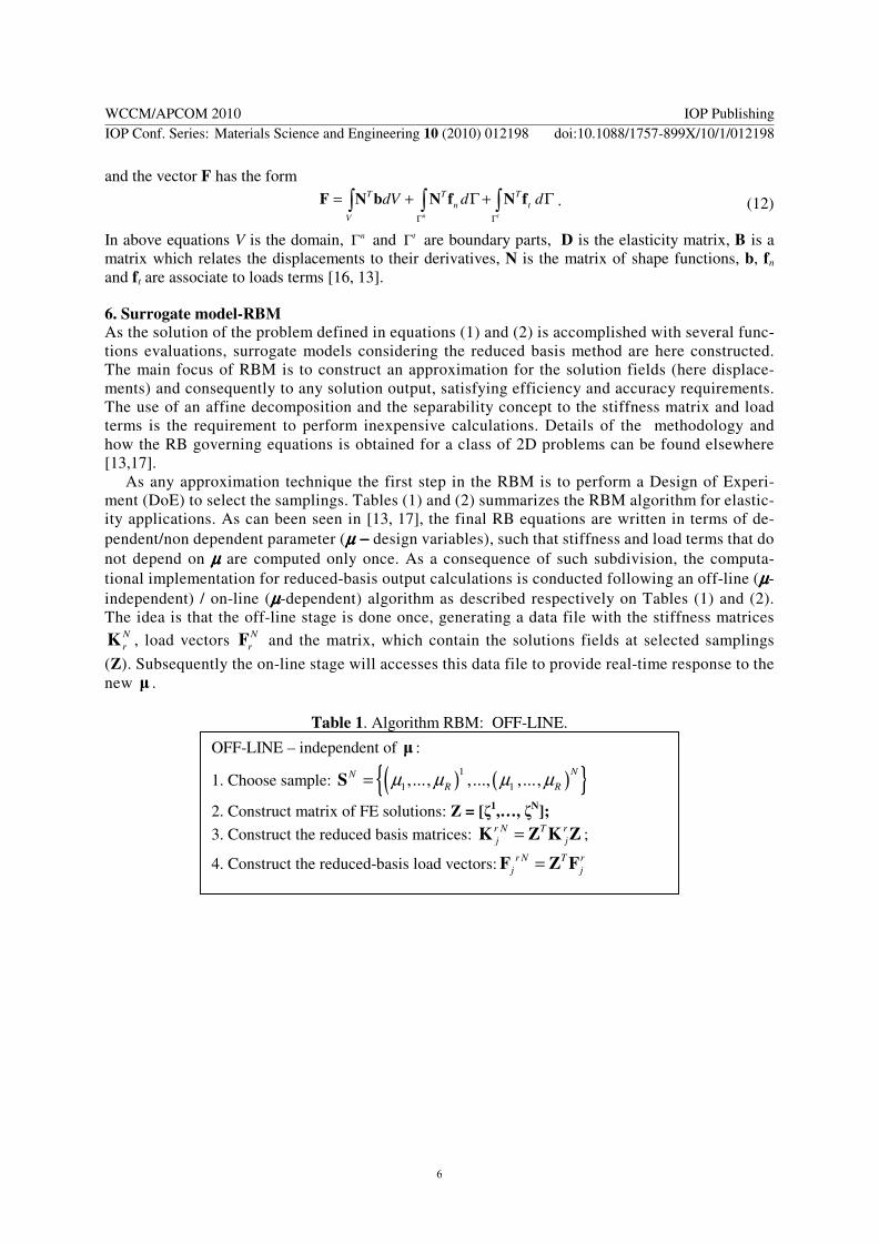
6. Surrogate model-RBM As the solution of the problem defined in equations (1) and (2) is accomplished with several func-

tions evaluations, surrogate models considering the reduced basis method are here constructed.

The main focus of RBM is to construct an approximation for the solution fields (here displace-

ments) and consequently to any solution output, satisfying efficiency and accuracy requirements.

The use of an affine decomposition and the separability concept to the stiffness matrix and load

terms is the requirement to perform inexpensive calculations. Details of the methodology and

how the RB governing equations is obtained for a class of 2D problems can be found elsewhere

[13,17].

As any approximation technique the first step in the RBM is to perform a Design of Experi-

ment (DoE) to select the samplings. Tables (1) and (2) summarizes the RBM algorithm for elastic-

ity applications. As can been seen in [13, 17], the final RB equations are written in terms of de-

pendent/non dependent parameter (µµµµ − − − − design variables), such that stiffness and load terms that do

not depend on µµµµ are computed only once. As a consequence of such subdivision, the computa-

tional implementation for reduced-basis output calculations is conducted following an off-line (µµµµ-

independent) / on-line (µµµµ-dependent) algorithm as described respectively on Tables (1) and (2).

The idea is that the off-line stage is done once, generating a data file with the stiffness matrices N

rK , load vectors N

rF and the matrix, which contain the solutions fields at selected samplings

(Z). Subsequently the on-line stage will accesses this data file to provide real-time response to the

new µ .

Table 1. Algorithm RBM: OFF-LINE.

OFF-LINE – independent of µ :

1. Choose sample: N

S ) (({ ) }1

1 1,..., ,..., ,...,N

R Rµ µ µ µ=

2. Construct matrix of FE solutions: Z = [ζ1,…, ζ

N];

3. Construct the reduced basis matrices: r N T r

j j=K Z K Z ;

4. Construct the reduced-basis load vectors:r N T r

j j=F Z F


6

Table 2. Algorithm RBM: ON-LINE.

7. Example

A square plate with central hole subject to plane stress condition is considered. Due to the double

symmetry only a quarter of the domain is modelled. The problem geometry, boundary conditions and

design variables are identified in Figure 3.

Figure 3. A quarter of a square plate with a central hole: Problem description.

The Young’s modulus of region 3 (see figure 3) is considered a random variable with Lognormal

distribution, with mean value 5x104 MPa and standard deviation 10

4 MPa. The others material proper-

ties and geometric dimensions are: Young’s modulus of regions 1 and 2 is E = 105 MPa, Poisson coef-

ficient υ = 0.3, plate thickness t = 1mm, lateral length 100mm and distributed load p = 1 N/mm. The

central hole dimensions are chosen as the optimization design variables. The initial value of them are

µ1 = µ2 = 50mm, and the lower and upper bounds are 25mm and 75mm, respectively.

Two stochastic objectives are considered: a) minimization of the mean and b) minimization of the

standard deviation of the total structural compliance. The total volume is constrained to be lower or

equal to its initial value. Apart from that constraint, the mean stress plus three times its standard devia-

tion is imposed to be lower or equal to 7.0 N/mm². The MO solutions will be obtained using 15 Pareto

points.

In this particular application, the RDO problem is formulated as:

µ 1

µ 2

2

1

3

ON-LINE – for a new vector µ :

1. Form the reduced basis matrix: 1 1

( ) ( )R nt

N r r N

j j

r j

β µ= =

=∑∑K µ K

2. Form the reduced-basis load vector: ( )1 1

R ntr N r N

j j

r j

ϕ= =

=∑∑F µ F

3. Solves: ( ) ( )( )N N=K µ α µ F µ ;

4. Evaluate: N

u ( ) T=µ α Z

5. Evaluate: N

s ( ) ( )T N=µ α F µ

8. Compute the sensitivities: ( ),

,kk

N T N

xxs α=µ F


7

Minimize:

( ) ( )3 3( , E ) , ( ,E )E C Cµ σ µ (13)

subjected to:

( )( ) ( )( )( )

( ) 3 ( ) 3

0

, E 3 ,E 7 MPa 1,...

25mm 75mm 1,...

eq i eq i

k

E i nel

V V

k ndv

τ µ σ τ µ

µ

µ

+ ≤ =

≤

≤ ≤ =

(14)

in which 3

( ,E )C µ is the total structural compliance, ( )( ) 3,E

eq iτ µ is the Von Misses stress at element i,

( )V µ is the total volume, 0

V is the initial total volume, nel is the total number of elements and ndv is

the number of design variables.

The RB approximation considers 3 regions (as shown in figure 3). The reduced basis is built at the

feasible space of the design variables and random variables, D = { [1, 9]x104,[25, 75]²}, and the num-

ber of samples analyzed was N=16. The finite element model adopted has 3900 degrees of freedom

with average element size of 2mm.

7.1. Samples Definition.

The described MC and PCM methods will be used to compute the problem statistics. In order to define

the number of sample points (sample size) to be used with each of the methods, a convergence test

was performed.

The sample size built by LHS ranges from 127 to 16.255 points. As a result of the performed study

the LHS sample size adopted for the optimization process when using MC is 5.000 points.

A similar convergence study was performed considering different number of collocation points for

the computation of the mean and standard deviation using PCM. A steep convergence is obtained even

with few points as the total structural compliance function varies smoothly with the Young’s module

of region 3 of the plate.

An error of the order of 10-4

is considered when MC is adopted with a selective LHS, using 5.000

points, for the optimization process. An error of the same order is achieved with only 2 points when

using PCM. However, as even smaller error can be achieved using few more points, with a small com-

putational time overhead, when using RBM, the optimization process using PCM was performed

adopting 5 collocation points and the error is of the order 10-11

.

7.2. The Robust Optimization Results.

Table 3 summarizes the computational performance of each of the analyzed methods. The solutions

computed using PCM are at approximately 3 orders faster than via MC and with an error 5 orders

smaller.

Table 3. Square plate with central hole – total computational time (s).

Methods WS (s) Min-Max (s) NBI (s) NNC (s)

MC 5000 points 38.623 26.486 19.480 18.633

PCM 5 points 60 43 31 28

Figure 4 presents the Pareto’s points distribution obtained using the different methodologies for the

multiobjective optimization.


8

(a)WS

(b)Min-Max

(c)NBI

(d)NNC

Figure 4. Square plate with central hole – Pareto’s points:

a) WS, b) Min-Max, c) NBI and d) NNC.

The Pareto frontiers using MC and PC are with good agreement, even using such a different num-

ber of sample points. As can be observed, the solutions using NBI and NNC present even distributed

points at the whole Pareto’s frontier.

These results show the tremendous advantage of using PCM for this class of problems, i.e. with

few random variables and smooth functions. The integration of all the methodologies described allows

the computation of a robust optimization problem, using a finite element model of 3.900 degrees of

freedom, in a practical time (less than a minute), in a simple single processor PC.

8. Conclusions

In this paper a design optimization tool to obtain optimum solutions under uncertainties was formu-

lated as a multiobjective optimization problem, which requires the implementation of specific tech-

niques to be solved. Both MC and PCM methodologies were implemented for the statistics calcula-

tion. As the whole procedure is very time consuming a surrogate model based on reduced basis ap-

proximations (RBM) was used. The main conclusions of the present study are:

• Among the implemented MO methodologies, NBI and NNC were the most effective schemes.

• The combination of all the approximate methodologies described in this work allows the com-

putations of robust multiobjetive optimization solutions, with very low computational time.

C

om

pli

ance

S.D

.

C

om

pli

ance

S.D

.

Co

mp

lian

ce S

.D.

C

om

pli

ance

S.D

.

Compliance MeanCompliance Mean

Compliance MeanStrain Energy Mean


9

• The results obtained show the advantage of using PCM for the problem considered, i.e. with

few random variables and smooth functions.

9. References

[1] Keane A J, Nair P B 2005 Computational Approaches for Aerospace Design: The Pursuit of

Excellence (New York: John-Wiley)

[2] Schuëller G I, Jensen H A 2008 Computational Methods in Optimization Considering Un-

Certainties – An Overview Computational Methods and Applications in Mechanical Engi-

neering

[3] Das I and Dennis J E 1996 Normal Boundary Intersection: A New Method for Generating

Pareto Surface in Nonlinear Multicriteria Optimization Problems SIAM J. Optimization 8

No 3 631-657

[4] Messac A, Ismail-Yahaya A and Mattson C A 2003 The Normalized Normal Constraint Method

for Generating the Pareto Frontier Structural Optimization 25 No 2 86-98

[5] Ramamurthy D 2005 Smart simulation techniques for the evaluation of parametric uncertainties

in black box systems Msc Thesis (Washington State University)

[6] Prud’homme C, Rovas D V, Veroy K, Machiels L, Maday Y, Patera A T, & Turicini G 2002

Reliable Real-time Solution of Parametrized Partial Differential Equations: Reduced-basis

Output Bound Method Journal of Fluids Eng. 124 70-79

[7] Steuer R E 1985 Multicriteria optimization – theory, computation and application (New York:

John-Wiley)

[8] Hwang C L, Paidy S R, Yoon K E Masud A S M 1980 Mathematical Programming with Multi-

ple Objectives: A Tutorial Comput. and Ops. Res. 7 5-31

[9] Meyer P L 1983 Probabilidade: Aplicações à Estatística, 2a edição, (Rio de Janeiro: LTC)

[10] Mathworks 2007 MATLAB User’s Guide, Mathworks Inc, Natacki

[11] Stein M, May 1987 Large Sample Properties of Simulations Using Latin Hypercube Sampling

Technometrics 29 no 2

[12] Motta R S, Afonso S M B, Lyra P R M 2009 Robust Optimization For 2d Problems Considering

Reduced-Basis Approximations XXX-CILAMCE - Iberian Latin American Congress on

Computational Methods in Engineering Búzios-RJ Brazil

[13] Motta R S 2009 Structural Robust Optimization Considering Reduced-Basis Method Msc The-

sis (Port.) Dep. de Eng. Civil UFPE Recife-PE Brazil

[14] Stoer J, Bulirsch R 1991 Introduction to Numerical Analysis - Second Edition (Berlin: Springer-

Verlag)

[15] Heiss F, Winschel V 2008 Likelihood Approximation by Numerical Integration on Sparse Grids

Jornal of Econometrics 144 62-80

[16] Zienkiewicz O C and Taylor R L 2000 The Finite Element Method (New York: McGraw-Hill)

[17] Afonso S M B, Lyra P R M, Albuquerque T M M, Motta R S 2009 Structural Analysis and Op-

timization in the Framework of Reduced-Basis Method Structural and Multidisciplinary Op-

timization 40 177-199

Acknowledgments

The authors acknowledge the financial support given by the Brazilian research councils CNPq,

CAPES and FACEPE.


10

Robust design considering optimization tools and reduced-basis approximations

Documents

Transcript of Robust design considering optimization tools and reduced-basis approximations