Noncommutative lattices as finite approximations

JOURNAL OF

GEOMETRY&D PHYSICS

ELSEVIER Journal of Geometry and Physics 18 (1996) 163-194

Noncommutative lattices as finite approximations

AX Balachandran a, G. Bimonte b,l, E. Ercolessi a, G. Landi arc, 1,2, F. Lizzi d,*,l, G. Sparano d91, I? Teotonio-Sobrinho a

a Department of Physics, Syracuse University, Syracuse, NY 13244.1130, USA b International Centre for Theoretical Physics, PO. Box 586, I-34100, Trieste, Italy

’ Dipartimento di Scienze Matematiche, Universitd di Trieste, P. le Europa I, I-34127, Trieste, Italy d Dipartimento di Scienze Fisiche, Vniversitci di Napoli, Mostra d’ Oltremare,

Pad. 19, l-80125, Napoli. Italy

Received 11 October 1994

Abstract

Lattice discretizations of continuous manifolds are common tools used in a variety of physical contexts. Conventional discrete approximations, however, cannot capture all aspects of the original manifold, notably its topology. In this paper we discuss an approximation scheme due to Sorkin (1991) which correctly reproduces important topological aspects of continuum physics. The approximating topological spaces are partially ordered sets (posets), the partial order encoding the topology. Now, the topology of a manifold M can be reconstructed from the commutative C*- algebra C(M) of continuous functions defined on it. In turn, this algebra is generated by continuous probability densities in ordinary quantum physics on M. The latter also serves to specify the domains of observables like the Hamiltonian. For a poset, the role of this algebra is assumed by a noncommutative Cc-algebra A. This fact makes any poset a genuine ‘noncommutative’ (‘quantum’) space, in the sense that the algebra of its ‘continuous functions’ is a noncommutative C*-algebra. We therefore also have a remarkable connection between finite approximations to quantum physics and noncommutative geometries. We use this connection to develop various approximation methods for doing quantum physics using d.

Keywords: Noncommutative differential geometry and field theory 1991 MSC: 06B35,58B30

* Corresponding author. ’ Also at: INFN, Sezione di Napoli, Napoli, Italy. 2 Fellow of the Italian National Council of Research (CNR) under Grant No. 203.01.60.

0393-0440/96/$15.00 @ 1996 Elsevier Science B.V. All rights reserved SSDI 0393-0440(95)00006-2

164 A.P Balachandran et al. /Journal of Geometry and Physics 18 (I 996) 163-l 94

1. Introduction

Realistic physical theories require approximations for the extraction of their predictions. A powerful approximation method is the discretization of continuum physics where manifolds are replaced by a lattice of points. This discretization is particularly effective for numerical work and has acquired a central role in the study of fundamental physical theories such as QCD [l] or Einstein gravity [2].

In these approximations, a manifold is typically substituted by a set of points with discrete topology. The latter is entirely incapable of describing any significant topological attribute of the continuum, this being equally the case for both local and global properties. As a consequence, all topological properties of continuum physical theories are lost. For example, there is no nontrivial concept of winding number on lattices with discrete topology and hence also no way to associate solitons with nonzero winding numbers in these approximations.

Some time ago, Sorkin [3] studied a very interesting method for finite approximations of manifolds by certain point sets in detail. These sets are partially ordered sets (posets) and have the ability to reproduce important topological features of the continuum with remarkable fidelity (see also Ref. [4]).

Subsequent researches [5] developed these methods and made them usable for approximate computations in quantum physics. They could thus become viable alternatives to computational schemes like those in lattice QCD [I]. This approximation scheme is briefly reviewed in Section 2.

In this paper, we develop the poset approximation scheme in a completely novel direction. In quantum physics on a manifold M, a fundamental role is played by the C*-algebra

C(M) of continuous functions on M. Indeed, it is possible to recover M, its topology and even its Coo -structure when this algebra and a distinguished subalgebra are given [6,7]. It is also possible to rewrite quantum theories on M by working exclusively with this algebra, the tools for doing calculations efficiently also being readily available [&lo]. All this material on C(M) is described in Section 3 with particular attention to its physical meaning.

In Section 4 we show that the algebra A replacing C(M), when M is approximated by a poset, is an infinite-dimensional noncommutative C*-algebra. The poset and its topology are recoverable from the knowledge of A. This striking result makes any poset a genuine ‘noncommutative’ (‘quantum’) space, in the sense that the algebra of its ‘continuous functions’ is a noncommutative C*-algebra. This explains also our use of the name ‘noncommutative lattices’ for these objects. 3

We thus have a remarkable connection between topologically meaningful finite approximations to quantum physics and noncommutative geometries. It bears emphasis that this conclusion emerges in a natural manner while approximating conventional quantum theory. Therefore the interest in noncommutative geometry for a physicist need not depend on unusual space-time topologies like the one used by Connes and Lott [lo] in building the standard model. Furthermore, these quantum models on posets are of independent interest

3 In the following we will use the phrases ‘poset’ and ‘noncommutative lattice’ in an interchangeable way.

AI! Balachandran et al./Joumal of Geometry and Physics 18 (1996) 163-194 165

and not just as approximations to continuum theories, as they provide us with a whole class of examples with novel geometries. 4

The C*-algebras for our posets are, as a rule, inductive limits of finite-dimensional matrix algebras, being examples of “approximately finite dimensional” algebras [6,12,13]. Therefore we can approximate A by finite-dimensional algebras and in particular by a commutative finite-dimensional algebra C(d). Their elements can be regarded as continuous “functions” to encode the topology of the latter. The algebra C(d) is also strikingly simple, so that it is relatively easy to build a quantum theory using C(d). We describe these approximations in Section 4.2.

In Section 5 we discuss many aspects of quantum physics based on A, drawing on known mathematical methods of the noncommutative geometer and the C*-algebraist.

Section 6 deals with a concrete example having nontrivial topological features, namely the poset approximation to a circle. We establish that global topological effects can be captured by poset approximations and algebras C(d) by showing that the “@-angle” for a particle on a circle can also be treated using C(d).

In Section 7 we show how the CL-algebra for a poset can be generated by a commutative subalgebra and a unitary group. We then argue that the algebra C(d) above can be recovered from this structural result and a gauge principle.

The article concludes with some final remarks in Section 8.

2. The finite topological approximation

Let M be a continuous topological space like, for example, the sphere SN or the Euclidean space RN. Experiments are never so accurate that they can detect events associated with points of M, rather they only detect events as occurring in certain sets Ok. It is therefore natural to identify any two points x, y of M if they can never be separated or distinguished by the sets Ok.

We assume that the sets 0~ cover M,

that each 0~ is open and that

u = lOA1 (2.2)

is a topology for M [ 141. This implies that both 0~. U 0, and 0,: n 0, are in U if Ok,, E U. This hypothesis is physically consistent because experiments can isolate events in 0,~ U 0, and 0~ rl 0, if they can do so in 0~ and 0, separately, the former by detecting an event in either 0~ or O,, and the latter by detecting it in both 0~ and 0,.

4 Dimakis and Miiller-Hoissen [I 11 have recently discussed a new approach to differential calculus and noncommutative geometry on discrete sets which has interesting connections with posets.

166 A.P. Balachandran et al./Journal of Geometry and Physics 18 (1996) 163-194

Fig. 1. (a) shows an open cover for the circle S’; and (b) the resultant discrete space P4(S1). 4~ is the map (2.4).

Given x and y in M, we write x - y if every set 0~ containing either point x or y contains the other too:

x - y means x E 0~ * y E 0~. for every 0~. (2.3)

Then - is an equivalence relation, and it is reasonable to replace M by Ml - E P(M) to reflect the coarseness of observations. It is this space, obtained by identifying equivalent points and equipped with the quotient topology explained later, that will be our approximation for M.

We assume that the number of sets 0,: is finite when M is compact so that P(M) is an approximation to M by a finite set in this case. When M is not compact, we assume instead that each point has a neighbourhood intersected by only finitely many 0~ so that P(M) is a “finitary” approximation to M [3]. In the notation we employ, if P(M) has N points, we sometimes denote it by PN(M).

The space P(M) inherits the quotient topology from M [14].This is defined as follows. Let @ be the map from M to P(M) obtained by identifying equivalent points. Then a set in P(M) is declared to be open if its inverse image for @ is open in M. The topology generated by these open sets is the finest one compatible with the continuity of @.

Let us illustrate these considerations for a cover of M = S’ by four open sets as in Fig. la. In this figure, 01.3 c 02 flO4. Fig. lb shows the corresponding discrete space P4(S’), the points xi being images of sets in St. The map @ : S’ -+ P4(S1) is given by

01 + Xl, 02 \ LO2 l-l 041 + x2. 03 + x3, 04 \ 102 n 041+ ~4. (2.4)

The quotient topology for P4(St) can be read off from Fig. 1, the open sets being

bl}, 1x31, {xl, x2, x31, (Xl, X4? x31, (2.5)

and their unions and intersections (an arbitrary number of the latter being allowed as P4(S1)

is finite). Notice that our assumptions allow us to isolate events in certain sets of the form 0~ \ [ 0~ n

O,] which may not be open. This means that there are in general points in P(M) coming from sets which are not open in M and therefore are not open in the quotient topology.

Now in a Hausdorff space [ 141, for any two distinct points x and y there exist open sets 0, and O,, containing x and y respectively, such that 0, n 0, = 0. A finite Hausdorff space necessarily has the discrete topology and hence each of its points is an open set. So

A.P. Balachandran et al./Journal of Geometry and Physics 18 (1996) 163-194 167

Fig. 2. The Hasse diagram for the circle poset Pd(S’).

P(M) is not Hausdorff. However, it can be shown [3] that it is a To space [14]. To spaces are defined as spaces in which, for any two distinct points, there is an open set containing at least one of these points and not the other. For example, given the points XI and x2 of P4(S1), the open set {xl) contains xt and not x2, but there is no open set containing x2 and not xi.

In P(M), we can introduce a partial order 5 [4,15,16] by declaring that:

X5Y if every open set containing y contains also x.

P(M) then becomes a partially ordered set or aposet. Later, we will write x -C y to indicate thatxiyandxfy.

Any poset can be represented by a Hasse diagram constructed by arranging its points at different levels and connecting them using the following rules: (1) if x -C y, then x is at a lower level than y; (2) if x -C y and there is no z such that x < z < y, then x is at the level immediately

below y and these two points are connected by a line called a link. For Pa(S’), the partial order reads

Xl ZS x2, Xl YS x4, x3 5 x2, x3 5 x4, (2.6)

where we have omitted writing the relations xj 5 xi. The corresponding Hasse diagram is shown in Fig. 2.

In the language of partially ordered sets, the smallest open set 0, containing a point x E P(M) consists of all y preceding x: 0, = {y E P(M): y 5 x). In the Hasse diagram, it consists of x and all points we encounter as we travel along links from x to the bottom. In Fig. 2, this rule gives (xl, x2, x3) as the smallest open set containing x2, just as in (2.5).

As another example, Fig. 3 shows a cover of S’ by 2N open sets Oj and the Hasse diagram of its poset &N(S’).

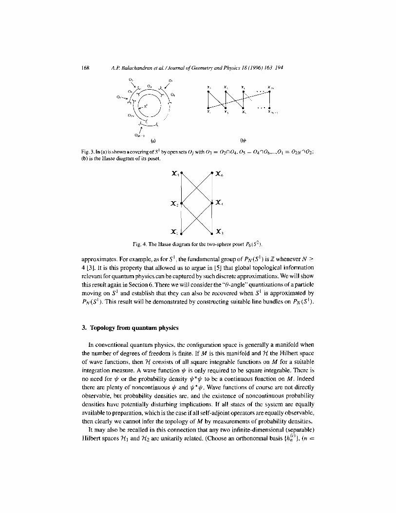
As one example of a three-level poset, consider the Hasse diagram of Fig. 4 for a finite approximation Ps(S2) of the two-dimensional sphere S2 derived in [3]. Its open sets are generated by

(xl). (x31, {X1.X2,X3). {X1,X4,X3),

{X~VX~,X~>X~,X~), (Xl, x2, -%T x4, x31

by taking unions and intersections.

(2.7)

We conclude this section by recalling that one of the most remarkable properties of a poset is its ability to accurately reproduce the fundamental group [17] of the manifold it

168 A.P Balachandran ef al. /Journal of Geometry and Physics 18 (1996) 163-194

Fig3,In(a)isshownacoveringofS’ byopensets 0; with03 = 02nO4,05 = 04n06,...,01 = 02NnO2; (b) is the Hasse diagram of its poset.

Fig. 4. The Hasse diagram for the two-sphere poset P6(S2)

approximates. For example, as for S’ , the fundamental group of PN (S’) is Z whenever N 2 4 [3]. It is this property that allowed us to argue in [5] that global topological information relevant for quantum physics can be captured by such discrete approximations. We will show this result again in Section 6. There we will consider the “O-angle” quantizations of a particle moving on S’ and establish that they can also be recovered when S’ is approximated by PN(S’). This result will be demonstrated by constructing suitable line bundles on PN(S~).

3. Topology from quantum physics

In conventional quantum physics, the configuration space is generally a manifold when the number of degrees of freedom is finite. If M is this manifold and X the Hilbert space of wave functions, then 7-L consists of all square integrable functions on M for a suitable integration measure. A wave function $ is only required to be square integrable. There is no need for $ or the probability density @*I$ to be a continuous function on M. Indeed there are plenty of noncontinuous I+? and r,k*$r. Wave functions of course are not directly observable, but probability densities are, and the existence of noncontinuous probability densities have potentially disturbing implications. If all states of the system are equally available to preparation, which is the case if all self-adjoint operators are equally observable, then clearly we cannot infer the topology of M by measurements of probability densities.

It may also be recalled in this connection that any two infinite-dimensional (separable) Hilbert spaces Xi and Hz are unitarily related. (Choose an orthonormal basis {hf)}, (n =

A.R Balachandran et al./Journal of Geomerry and Physics 18 (1996) 163-194 169

0, 1,2, . ..)for’Fli (i = 1, 2).ThenaunitarymapU : 711 + ‘Hzisdefinedby U/r:‘) = hL2).) They can therefore be identified, or thought of as the same. Hence the Hilbert space of states in itself contains no information whatsoever about the configuration space.

It seems however that not all self-adjoint operators have equal status in quantum theory. Instead, there seems to exist a certain class of privileged observables PC3 which carry information on the topology of M and also have a special role in quantum physics. This set PO contains operators like the Hamiltonian and angular momentum and particularly also the set of continuous functions C(M) on M, vanishing at infinity if M is noncompact.

In what way is the information on the topology of M encoded in PO? To understand this, recall that an unbounded operator such as a typical Hamiltonian H cannot be applied on all vectors in ‘H. Instead, it can be applied only on vectors in its domain D(H), the latter being dense in ‘H [ 181. In ordinary quantum mechanics, D(H) typically consists of twice-differentiable functions on M with suitable fall-off properties at cc in case M is noncompact. In any event, what is important to note is that if IJ?, x E D(H) in elementary quantum theory, then $*x E C(M). A similar property holds for the domain D of any unbounded operator in PO: if $, x E D, then $r*x E C(M). It is thus in the nature of these domains that we must seek the topology of M. 5

We have yet to remark on the special physical status of PO in quantum theory. Let & be the intersection of the domains of all operators in PO. Then it seems that the basic physical properties of the system, and even the nature of M, are all inferred from observations of the privileged observables on states associated with E. 6

This discussion shows that for a quantum theorist, it is quite important to understand clearly how M and its topology can be reconstructed from the algebra C(M). Such a reconstruction theorem already exists in the mathematical literature. It is due to Gel’fand and Naimark [6], and is a basic result in the theory of C*-algebras and their representations. Its existence is reassuring and indicates that we are on the right track in imagining that it is PO which contains information on M and its topology.

We should point out the following in this regard however: it is not clear that the specific mathematical steps one takes to reconstruct the manifold from the algebra have a counterpart in the physical operations done to reconstruct it from observations.

Let us start by recalling that a C*-algebra A, commutative or otherwise, is an algebra with a norm ]I I] and an antilinear involution * such that lbll = Ila*ll , lla*all = lla*ll llall and (ab)* = b*u* for a, b E A. The algebra A is also assumed to be complete in the given norm.

Examples of C*-algebras are: (1) The (noncommutative) algebra of n x n matrices T with T* given by the hermitian

conjugate of T and the squared norm ]]T]]2 being equal to the largest eigenvalue of T*T.

5 Our point of view about the manner in which topology is inferred from quantum physics was developed in collaboration with G. Marmo and A. Simoni.

6 Note in this connection that any observable of PO restricted to & must be essentially self-adjoint [IS]. This is because if significant observations are all confined to states given by &, they must be sufficiently numerous to determine the operators of PO uniquely.

170 A.P. Balachandran et al./Journd of Geometry and Physics 18 (1996) 163-194

(2) The (commutative) algebra C(M) of continuous functions on a Hausdorff topological space M (vanishing at infinity if M is not compact), with * denoting complex conjugation and the norm given by the supremum norm, ]I f I] = supXEM If(x)\.

It is the latter example, establishing that we can associate a commutative C*-algebra to a Hausdorff space, which is relevant for the Gel’fand-Naimark theorem. The Gel’fand- Naimark results then show how, given any commutative C*-algebra C, we can reconstruct a Hausdorff topological space M of which C is the algebra of continuous functions.

We now explain this theorem briefly. Given such a C, we let M denote the space of equivalence classes of irreducible representations (IRRs), 7 also called the structure space, of c.* The C*-algebra C being commutative, every IRR is one dimensional. Hence, if n E M and f E C!, the image x(f) of f in the IRR defined by x is a complex number. Writing x(f) as f(x). we can therefore regard f as a complex-valued function on M with the value f(x) at x E M. We thus get the interpretation of elements in C as @-valued functions on M.

We next topologise M by declaring a subset of M to be closed if it is the set of zeros of some f E C. (This is natural to do since the set of zeros of a continuous function is closed.) The topology of M is generated by these closed sets, by taking intersections and finite unions. It is called the hull kernel or Jacobson topology [6].

Gel’fand and Naimark then show that the algebra C(M) of continuous functions on M is isomorphic to the starting algebra C. It is therefore the case that the commutative C*- algebra C which reconstructs a given M in the above fashion is unique. Also the requirement C = C(N) uniquely fixes N up to homeomorphisms. In this way, we recover a topological space M, uniquely up to homeomorphisms, from the algebra C. 9

We next briefly indicate how we can do quantum theory starting from C(M) = C. Elements of C are observables, they are not quite wave functions. The set of all wave

functions forms a Hilbert space ti. Our first step in constructing 7& essential for quantum physics, is the construction of the space E which will serve as the common domain of all the privileged observables.

The simplest choice for & is C itself. lo With this choice, C acts on E, as C acts on itself by multiplication. The presence of this action is important as the privileged observables must act on E. Further, for +, x E E, $r*x E C, exactly as we want.

Now Gel’fand and Naimark have established that it is possible to define an integration measure dw over the structure space M of C, such that every f E C has a finite integral. A

7 The trivial IRR given by C + (0) is not included in M. It will therefore be ignored here and hereafter. 8 Some readers might be more familiar with a slightly different construction, where M is taken to be the space

of maximal two-sided ideals of C instead of the space of irreducible representations. These two constructions agree because for a commutative C*-algebra, not only are the kernels of irreducible representations maximal two-sided ideals, but also any maximal two-sided ideal is the kernel of an irreducible representation [6].

9 We remark that more refined attributes of M such as a P -structure, can also be recovered using only algebras if more data are given. For the Coo -structure, for example, we must also specify an appropriate subalgebra f?(M) of C(M). The CDs-structure on M is then the unique Coo -structure for which the elements of C?‘(M) are all the Coo-functions [7]. lo Differentiability requirements will in general further restrict &. As a mle we will ignore such details in

this article.

A.P: Balachandran et al./Journul of Geometry and Physics 18 (1996) 163-194 171

scalar product (. , .) for elements of E can therefore be defined by setting

($7 xl = s Wx)(1Cr*x)(x). M

(3.1)

The completion of the space E using this scalar product gives the Hilbert space 7-1. The final set-up for quantum theory here is conventional. What is novel is the shift in

emphasis to the algebra C. It is from this algebra that we now regard the configuration M and its topology as having been constructed.

There is of course no reason why I should always be C. Instead it can consist of sections of a vector bundle over M with a C-valued positive definite sesquilinear form (.;) . (The form (., .) is positive definite if (~,a) is a nonnegative function for any Q E E, which identically vanishes iff 01 = 0.) The scalar product is then written as

(@I, x) = J ddX)(1Cr, x)(x). M

(3.2)

The completion of E using this scalar product as before gives ‘If.

4. The noncommutative geometry of a noncommutative lattice

4.1. The noncommutative algebra of a noncommutative lattice

In the preceding sections we have seen how a commutative C*-algebra reconstructs a Hausdorff topological space. We have also seen that a poset is not Hausdorff. It cannot therefore be reconstructed from a commutative C*-algebra. It is however possible to reconstruct it, and its topology, from a noncommutative C*-algebra.

Let us first recall a few definitions and results from operator theory [ 181 before outlining this reconstruction theorem. An operator in a Hilbert space is said to be of finite rank if the orthogonal complement of its null space is finite dimensional. It is thus essentially like a finite-dimensional matrix as regards its properties even if the Hilbert space is infinite dimensional. An operator k in a Hilbert space is said to be compact if it can be approximated arbitrarily closely in norm by finite rank operators. Let hl ,12, . . . be the eigenvalues of k* k for such a k, with hi+t 5 & and an eigenvalue of multiplicity n occurring n times in this sequence. (Here and in what follows, * denotes the adjoint for an operator.) Then h, -+ 0 as n + co. It follows that the operator 1 in an infinite-dimensional Hilbert space is not compact.

The set K: of all compact operators k in a Hilbert space is a C*-algebra. It is a two-sided ideal in the C*-algebra B of all bounded operators [6,19].

Note that the sets of finite rank, compact and bounded operators are all the same in a finite-dimensional Hilbert space. All operators in fact belong to any of these sets in finite dimensions.

172 A.P Balachandran et al. /Journal of Geometry and Physics 18 (1996) 163-194

I

(An + k)(p) = x

1 (An + k)(q) = An + k

(a) (b) Fig. 5. (a) is the poset for the interval [r, s] when covered by the open sets [r, s[ and [r, s]; (b) shows the values of a generic element 11 + k of its algebra ,4 at its two points p and q.

The construction of A for a poset rests on the following result from the representation theory of K. The representation of K by itself is irreducible [6] and it is the only IRR of K up to equivalence.

The simplest nontrivial poset is PZ = (p, q} with q < p. It is shown in Fig. 5. It is the poset for the interval [r, s] (I < s) where the latter is covered by the open sets [r, s[ and [r, s]. The map from subsets of [r, s] to the points of P2 is

[r,s[+ 9. (4.1)

The algebra A for P2 is

A = Cl + K = {Al + k: h E @,k E K}, (4.2)

the Hilbert space on which the operators of A act being infinite dimensional. We can see this result from the fact that A has only two IRRs and they are given by

p:Ll+k+A, q:hl +k+Ll fk. (4.3)

This remark about IRRs becomes plausible if it is remembered that K has only one IRR. Thus the structure space of A has only two points p and q. An arbitrary element hl + k

of A can be regarded as a “function” on it if, in analogy to the commutative case, we set

(Al + k)(p) := h, (hl + k)(q) := Al + k. (4.4)

Notice that in this case the function Al + k is not valued in @ at all points. Indeed, at different points it is valued in different spaces, @ at p and a subset of bounded operators on an infinite Hilbert space at q. ’ ’

Now we can use the hull kernel topology for the set (p, q}. For this purpose, consider the function k. It vanishes at p and not at q, so p is closed. Its complement q is hence open. So of course is the whole space [p, q). The topology of {p, q} is thus given by Fig. 5a and is that of the P2 poset just as we want.

I1 Such an interpretation of A as functions on the poset can also be stated in a more rigorous way. In a paper under preparation, we will in fact show that A is isomorphic to the algebra of continuous sections of a suitable bundle over the poset, in the same way that the algebra of continuous functions on a manifold M is isomorphic to the algebra of continuous sections of the trivial one-dimensional complex vector bundle on M.

t

a(a) = x1 a(P) = x2

v

47) = XlP, + A,P, + k,z

6) b) Fig. 6. (a) shows the v poset and the association of an infinite dimensional Hilbert space ‘Hi to each of its arms; (b) shows the values of a typical element a = A,‘Pl + A2P2 + k12 of its algebra at its three points.

We remark here that for finite structure spaces one can equivalently define the Jacobson topology as follows. Let IX be the kernel for the IRR X. It is the (two-sided) ideal mapped to 0 by the IRR X. We set x -: y if IX c ZY thereby converting the space of IRRs into a poset. The topology in question is the topology of this poset. In our case, ZP = K, Z4 = {O] c ZP and hence q < p. This gives again Fig. 5a.

Hereafter in this paper, by ‘ideals’ we always mean two-sided ideals. We next consider the v poset. It can be obtained from the following open cover of the

interval [0, 11:

[O, 11 = u a, O1 = [0,2/3[, 02 =]1/3, 11, Cr3 =]1/3,2/3[. (4.5) A.

The map from subsets of [0, l] to the points of the v poset in Fig. 6a is given by

10, l/31 + 01, 11/3,2/3[-+ y, P/3, 11 + B. (4.6)

Let us now find the algebra A for the v poset. This poset has two arms 1 and 2. The first step in the construction is to attach an infinite-dimensional Hilbert space ‘Hi to each arm i as shown in Fig. 6a. Let Pi be the orthogonal projector on ‘Z& in Xl @ ?iz and lclz = (kl2) be the set of all compact operators in Xl CD ‘Z-Zz. Then [6]

A = @PI + CP2 + Kt2. (4.7)

The IRRs of A defined by the three points of the poset are given by Fig. 6b. It is easily seen that the hull kernel topology correctly gives the topology of the v poset.

The generalization of this construction to any (connected) two-level poset is as follows. Such a poset is composed of several vs. Number the arms and attach an infinite-dimensional Hilbert space tii to each arm i as in Fig. 7a and b. To a v with arms i, i + 1, attach the algebra di with elements hi Pi + Ai+t Pi+1 + ki,i+t . Here ki, )Li+t are any two complex numbers, Pi, Pi+1 are orthogonal projectors on Hi, ‘Z&+1 in the Hilbert space Hi @ ?t!i+l and ki,i+t is any compact operator in ‘Fli @ Xi+]. This is as before. But now, for glueing the various Vs together, we also impose the condition A.j = & if the lines j and k meet at a top point. The algebra A is then the direct sum of di’s with this condition:

174 A.P. Balachandran et al. /Journal of Geometry and Physics 18 (1996) 163-194

(a) (t.4 Fig. 7. These figures show how the Hilbert spaces Hi are attached to the arms of two two-level posets. They also show the values of a generic member a of their algebras A at their points.

d=@di, di =hiPi +Ai+lPi+l +ki,i+l (4.8)

with hj = hk if lines j, k meet at top. Fig. 7a and b also show the values of an element Q = @[J.iPi + ki+tPi+r + ki,i+t] at

the different points of two typical two-level posets. There is a systematic construction of A for any poset (that is, any “finite 7ii topological

space”) which generalizes the preceding constructions for two-level posets. It is explained in the book by Fell and Doran [6] and will not be described here.

It should be remarked that actually the poset does not uniquely fix its algebra as there are in general many nonisomorphic (noncommutative) C*-algebras with the same poset as structure space [20]. This is to be contrasted with the Gel’fand-Naimark result asserting that the (commutative) C*-algebra associated to a Hausdorff topological space (such as a manifold) is unique. The Fell-Doran choice of the algebra for the poset seems to be the simplest. We will call it A and adopt it in this paper.

4.2. Finite-dimensional and commutative approximations

In general, the algebra A is infinite dimensional. This makes it difficult to use it in explicit calculations, notably in numerical work.

We will show that there is a natural sequence of finite-dimensional approximations to the algebra A associated to a poset. For two-level posets, the leading nontrivial approximation here is commutative while the succeeding ones are not. In this case, the commutative approximation C(d) has a suggestive physical interpretation. Further these approximations correctly capture the topology of the poset and can thus provide us with excellent models to initiate practical calculations, and to gain experience and insight into noncommutative geometry in the quantum domain.

The existence of these finite-dimensional approximations relies on a remarkable property that characterizes the C*-algebra A associated to a poset, namely the fact that A is an approximately finite-dimensional (AF) algebra [12]. Technically this means that A is an inductive limit [6] of finite-dimensional C*-algebras (that is, direct sums of matrix algebras).

Incidentally, we remark here that there exists a construction to obtain such sequence of finite-dimensional algebras directly from the topology of the poset. It is explained in [ 121 and is based on the possibility of associating a diagram, the so-called Bratteli diagram, to

A.P. Balachmdran et al./Journal of Geometry and Physics 18 (1996) 163-194 17.5

any finite To space. This construction also gives a new way, different from the method of Fell and Doran discussed in the previous section, to obtain the algebra A of a poset. We will not describe it here. Instead, we limit ourselves to discussing only a few examples.

Let us start with the two-point poset of Fig. 5a. The algebra associated to it is A = Cl +K.

Consider the following sequence of C*-algebras of increasing dimensions, the *-operation being hermitian conjugation:

do = @, .A1 = ~(1, c) B c,

A2 = M(2,c) CBC,

A, = M(n,C> CB C,

(4.9)

where M(n, C) is the C*-algebra of n x n complex matrices. A typical element of d,, is

an=[ ““0”” a], (4.10)

where+,,, is an n x n complex matrix and h is a complex number. Note that the subalgebra M(n, C) consists of matrices of the form (4.10) with the last row and column zero.

The algebra d,, is seen to approach A as n becomes larger and larger. We can make this intuitive observation more precise. There is an inclusion

F n+l,n . ’ An * An+1 (4.1 I)

given by

(4.12)

It is a *-homomorphism [6] since

F n+l,n(an*) = [Fn+l,n(dl*. (4.13j

Thus the sequence

(4.14)

gives a directed system of C*-algebras. Its inductive limit is A as is readily proved using the definitions in [6].

We must now associate appropriate representations to A, which will be good approximations to the two-point poset.

176 A.P Balachandran et al./Journal of Geomerry and Physics 18 (1996) 163-194

(a) (b) Fig. 8. (a) is the poset for the algebra A, of (4.9): while (b) shows the values of a typical element a, of this algebra at its two points pn and qn.

The algebra A1 is trivial. Let us ignore it. All the remaining algebras d,, have the following two representations: (a) The one-dimensional representation pn with.

pn : a, + A. (4.15)

(b) The defining representation qn with

qn : a, -+ a,. (4.16)

It is clear that these representations approach the representations p and q of A, given in (4.3), as n + co.

The kernels ZPn and Zqn of pn and q,, are respectively

(4.17)

Since Zqn c Zpn. the hull kernel topology on the set (pn, qn) is given by q,, < pn.

Hence (pn , qn} is the two-point poset shown in Fig. 8a and is exactly the same as the one in Fig. 5a.

Thus the preceding two representations of A,, form a topological space identical to the poset of A.

All this suggests that it is possible to approximate A by A, and regard its representations p,, and qn as constituting the configuration space.

In our previous discussions, either involving the algebrac or the algebra A, we considered only their IRRs. But the representation qn of d,, is not IRR. It has the invariant subspace

0

0

c ; . !I 0

1

(4.18)

In this respect we differ from the previous sections in our treatment of d,, .

A.P. Balachandran et al. /Journal of Geometry and Physics 18 (1996) 163-194 117

The first nontrivial approximation is Al. It is a commutative algebra with elements

(4.19)

In this way, we can achieve a commutative simplification of A which will be denoted by

CW. Let us now consider the v poset and its algebra A = @PI + X12 + @Pz acting on the

Hilbert space ‘Ffl @ X2. Its finite-dimensional approximations are given by

do = @, A1 =C@C, A2 =C@M(2,@)@@,

A, =C@M(2n -2,@)@@,

where a typical element of a, E An is of the form

[

Al 0 0

an = 0 m2n-2x2n-2 0 . 0 0 A2 I

As before, there is a *-homomorphism

F n+l,n An --f dn+l,

given by

a, =

r

A.1 0

0 m2n-2x2n-2

0 1 0 +

0 0 A2

L

Al 0 0 0 0

0 Al 0 0 0

0 0 m2n-2x2n-2 0 0

0 0 0 A2 0

0 0 0 0 A.; 1. (4.23)

(4.20)

(4.21)

(4.22)

We thus have a directed system of C*-algebras whose inductive limit is A [6], showing that d,, approximates A.

The algebras dn have the following three representations:

64 01, : a, + )il ,

(b) Bn : an + 12 ,

Cc) yn : an + a, . (4.24)

Note that cr, and #?n are commutative IRRs while yn is not RR, just like q,, .

178 A.P: Balachandran et al./Journal of Geometry and Physics 18 (1996) 163-194

Fig. 9. (a) is the poset for the algebra A, defined in (4.9); while (b) shows the values of a typical eiement a, of this algebra at its three points cm, bn, yn

Now the kernels of these representations are

L, = 10) cl3 M(2n - 2, C) CB c,

I&¶” = @ cl3 Men - 2,C) a3 {O), (4.25)

zy” = WI.

Since

4% = zan a*d 1, c Ifin, (4.26)

we set

yn -c an. Yn -c Bn- (4.27)

The poset that results is shown in Fig. 9. It is again the v poset, suggesting that A, and its representations cr, , /l,, , yn are good approximations for our purposes.

Now the C*-algebra

(4.28)

is commutative and its representations at, ,!?I and yt also capture the poset topology correctly. It will be denoted again by C(d). It seems to be the algebra with the minimum number of degrees of freedom correctly reproducing the poset and its topology.

Is it possible to interpret Li? For this purpose, let us remember that the points of a manifold M are closed, and so correspond to the top or level one points of the poset. The latter somehow approximate the former. Since the values of ~1 at the level one points are ht and 12, we can regard ki as the values of a continuous function on M when restricted to this discrete set. The role of the bottom points in the poset and the value of at there is to somehow glue the top points together and generate a nontrivial approximation to the topology of M.

We can explain this interpretation further using simplicial decomposition. Thus the interval [0, l] has a simplicial decomposition with [0] and [l] as zero-simplices and [0, l] as the one-simplex. Assuming that experimenters cannot resolve two points if every simplex containing one contains also the other, they will regard [0, l] to consist of the three points

AX Balachandran et al./.lournul of Geometry and Physics 18 (1996) 163-194 179

~1 = [0], /It = [l] and yl =]0, l[. There is also a natural map from [0, l] to these points as in Section 2. Introducing the quotient topology on these points following that section, we get back the v poset. In this approach then, ht and L2 are the values of a continuous function at the two extreme points of [0, l] whereas the association of ht Pr +h2P2 with the open interval is necessary to cement the extreme points together in a topologically correct manner.

(We remark here that the simplicial decomposition of any manifold yields a poset in the manner just indicated. We will also suggest at the end of Section 5 that a probability density cannot be localized at level one points, unless they are isolated and hence both open and closed. This result appears eminently reasonable in the context of a simplicial decomposition where level one points are points of the manifold. Reasoning like this also suggests that localization must in general be possible only at the subsets of the poset representing the open sets of M. That seems in fact to be the case. For, as will be indicated in Section 5, localization seems possible only at the open sets of a poset and the latter correspond to open sets of M.)

5. Quantum theory using A

The noncommutative algebra A is an algebra of observables. It replaces the algebra C(M) when M is approximated by a poset. We must now find the space E on which A acts, convert I into a pre-Hilbert space and therefrom get the Hilbert space ‘H by completion.

Now as A is noncommutative, it turns out to be important to specify if A acts on E from the right or the left. We will take the action of A on E to be from the right, thereby making & a right d-module.

The simplest model for & is obtained from A itself. As for the scalar product, note that (t* n)(n) is an operator in a Hilbert space XX if 4, r] E A and x E poset. We can hence find a scalar product (., .) by first taking its operator trace Tr on l-t, and then summing it over ‘FIX with suitable weights pX :

As remarked in Section 3, there is no need for & to be A. It can be any space with the following properties: (1) It is a right d-module. So, if 6 E & and a E A, then ca E 1. (2) There is a positive definite “sesquilinear” form (., +) on & with values in A. That is, if

6, Q E 8, and a E A, then

(4 E,n)~d, E,rl)*=(~l,U, (~,6)>0 and E,U=O+c=O. (5.2)

Here “(c, c) > 0” means that it can be written as u*u for some a E A.

180 Ad? Balachandran et al. /Journal of Geometry and Physics 18 (1996) 163-194

The scalar product is then given by

(t+ t?) = c A Tr(t, v)(x) . x

(5.4)

As 6*17(x), (e, q}(x), (6, vu)(x) or (a.$, v)(x) may not be of trace class [19], there are questions of convergence associated with (5.1) and (5.4). We presume that these traces must be judiciously regularized and modified (using for example the Dixmier trace [8,9]> or suitable conditions put on E or both. But we will not address such questions in detail in this article.

When A is commutative and has structure space M, then an E with the properties described consists of sections of hermitian vector bundles over M. Thus, the above definition of 6 achieves a generalization of the familiar notion of sections of hermitian vector bundles to noncommutative geometry.

In the literature [8,9], a method is available for the algebraic construction of E. It works both when A is commutative and noncommutative. In the former case, Serre and Swan

[8,9] also prove that this construction gives (essentially) all E of physical interest, namely all E consisting of sections of vector bundles. It is as follows. Consider A @CN = AN for some integer N. This space consists of N-dimensional vectors with coefficients in A (that is, with elements of A as entries). We can act on it from the left with N x N matrices with coefficients in A. Let e = [et] be such a matrix which is idempotent, e* = e, and hermitian,

(et, r]) = (6, eq). Then, edN is an E, and according to the Serre-Swan theorem, every E [in the sense above] is given by this expression for some N and some e for commutative A. An I of the form edN is called a “projective module of finite type” or a “finite projective module”.

Note that such & are right d-modules. For, if t E edN, it can be written as a vector

(E’A2,- ,tN)withti ~dande$j=~‘.Theactionofa~donEis

-$ + ta = (e’a,t*a, . . . , tNa). (5.5)

With this formula for E, it is readily seen that there are many choices for (., .). Thus let g = [gij], gij E A, be an N x N matrix with the following properties: (a) gt = gji;

(b) t’*gijtj z 0 and 4’*gijt’ = 0 + < = 0. Then, if r] = (q’, q2,. . . , $‘) is another vector in E, we can set

(63 II) = ei*gijVi. (5.6)

In connection with (5.6), note that the algebras A we consider here generally have unity. In those cases, the choice gii E @ is a special case of the condition gij E d. But if A has no unity, we should also allow the choice gij E @.

The minimum we need for quantum theory is a Laplacian A and a potential function W, as a Hamiltonian can be constructed from these ingredients. We now outline how to write AandW.

Let us first look at A, and assume in the first instance that & = A.

Ad? Balachundran et al./Journal of Geometry ad Physics 18 (1996) 163-194 181

An element a E A defines the operator @,a(~) on the Hilbert space 7-l = eX3-IX, the map a -+ @,a(~) giving a faithful representation of A. So let us identify a with @,a(~) and A with this representation of A for the present.

In noncommutative geometry [8,9], A is constructed from an operator D with specific properties on ‘H. The operator D must be self-adjoint and the commutator [D, a] must be bounded for all a E A:

D*=D, [D,u]EB forall ucd. (5.7)

Given D, we construct the ‘exterior derivative’ of any a E A by setting

Sa = [D, a] := [D, &ax]. (5.8)

Note that du need not be in A, but it is in B. Next we introduce a scalar product on B by setting

(o, j3) = Tr[cz*/?] for all q B E B, (5.9)

the trace being in 3-1. (Restricted to A, it becomes (5.4) with pX = 1. This choice of ,D* is made for simplicity and can readily be dispensed with. See also the comment after (5.4).)

Let p be the orthogonal projection operator on A for this scalar product:

p2 = p* z p,

pa = a ifu E A, (5.10) per = 0 if(u,cr)=O and aed.

The Laplacian A on A is defined using p as follows. We first introduce the adjoint 6 of d. It is an operator from Z? to A:

6:B+d. (5.11)

It is defined as follows. Consider all b E Z? for which (b, da) can be written as (a’, a) for all a E A. Here a’ is an element of A linear in the elements b and independent of a. Thus

(b, da) = (a’, a), Vu and some a’ E A. (5.12)

Then we write

a’ = 6b. (5.13)

A computation shows that

6b = p[D, b]. (5.14)

The Laplacian can now be defined as usual as

Au = -6 da = -p[D, [D, a]]. (5.15)

Notice that the domain of A does not necessarily coincide with A.

182 A.P: Balachandran et al./Journal of Geometry and Physics 18 (1996) 163-194

As for W, it is essentially any element of A. (There may be restrictions on W from positivity requirements on the Hamiltonian.) It acts on a wave function a according to a --f aW, where (aW)(n) = u(x)W(x).

A possible Hamiltonian H now is -hA + W, k > 0, while a Schrodinger equation is

au iat = -kAu +uW. (5.16)

When E is a nontrivial projective module of finite type over A, it is necessary to introduce a connection and “lift” d from A to an operator V on E. Let us assume that I is obtained from the construction described before (5.5). In that case the definition of V proceeds as follows.

Because of our assumption, an element { E E is given by 4 = (c’, c2, . . . , tN) where 6’ E A and e$j = e’. Thus E is a subspace of A @ CN := AN:

IcAN, AN = {(a',...,~~):.~ E A}. (5.17)

Here we regard ui as operators on 7-1. Now AN is a subspace of Z? @I CN := BN where f3 consists of bounded operators on Ii. Thus

&GdNsBN, BN = {(a', . , *, aN) : oi = bounded operator on ‘7f). (5.18)

Let us extend the scalar product (., .) on E (given by (5.6) and (5.4)) to f?N by setting

(Cl, B) = &!'*gijBj, (a, p) = Tr(a, /I) for CX, B E BN. (5.19)

Next, having fixed d on A by a choice of D as in (5.7) we define d on E by

de = (dt’, d<‘, . . . , dcN). (5.20)

Note that dc may not be in &, but it is in BN:

d.$ E aN. (5.21)

A possible V for this d is

where (a) e is the matrix introduced earlier, (b) p is an N x N matrix with coefficients in L3:

(5.22)

(cl P = we, and

(5.23)

(5.24)

AI! Balachandran et al./.Journul of Geometry and Physics 18 (1996) 163-194 183

(d) p is hermitian:

bY, PB) - (PW B) = 0.

Note that if j?fulfills all conditions but (c), then p = eFe fulfills (c) as well. Condition (5.25) is equivalent to the compatibility of V with the hermitian structure

(5.19):

d(w B) = ((2, V/9 - Pa, B). (5.26)

Having chosen a V, we can try defining V*V using

(V6? Vrl) = (E, v*vrl), e, 17 E E, (5.27)

where (., .) is defined by (5.19). A calculation similar to the one done to define the Laplacian (5.15) on A then shows that we can define A on & by

Ar]= -qV*Vq, GEE, (5.28)

where q is the orthogonal projector on E for the scalar product (., .). A potential W is an element of A. It acts on E according to the rule (1) following (5.1). A Hamiltonian as before has the form -LA + W , J, > 0 . It gives the Schrodinger

equation

We will not try to find explicit examples for A here. That task will be taken up for a simple problem in Section 6.

We will conclude this section by pointing out an interesting property of states for posets. It does not seem possible to localize a state at the level one points (unless they happen to be isolated points, both open and closed). We can see this for example from Fig. 6b which shows that if a probability density vanishes at y. then hi (and k12) are zero and therefore they vanish also at cx and /l. It seems possible to show in a similar way that localization in an arbitrary poset is possible only at open sets.

6. Line bundles on circle poset and 8-quantization

A circle S’ = (e’@} is an infinitely connected space. It has the fundamental group H. Its universal covering space [21] is the real line Iw’ = [x: -cc < x < 00). The fundamental group Z acts on R’ according to

x-+x+N, N E Z.

The quotient of Iw’ by this action is S’, the projection map [w’ + S’ being

x + e’2nx.

(6.1)

(6.2)

184 A.P Balachandran et al./Joumal of Geometry and Physics 18 (1996) 163-194

a-2 a-1 a0 ai a2

. . . .,,~,~,r, . . .

b-z b-1 bo bl b2 Fig. 10. The figure shows the universal covering space of a circle poset

Now the domain of a typical Hamiltonian for a particle on 5’ need not consist of smooth functions on 5’. Rather it can be obtained from functions $0 on Iw’ transforming by an IRR

p0 : N + eiNe (6.3)

of Z according to

+e(x + N) = e’Ne+Cle(x). (6.4)

The domain De(H) for a typical Hamiltonian H then consists of these @Q restricted to a fundamental domain 0 5 x 5 1 for the action of Z and subjected to a differentiability requirement:

We(l) $0: @o(l) = e”@~(O); dx = e (6.5)

In addition, of course, if dx is the measure on S’ used to define the scalar product of wave functions, then HI& must be square integrable for this measure. It is also assumed that r+k is suitably smooth in IO, l[.

We obtain a distinct quantization, called &quantization, for each choice of eie. As has been shown earlier [5], there are similar quantization possibilities for a circle

poset as well. The fundamental group of a circle poset is Z. Its universal covering space is the poset of Fig. 10. Its quotient, for example by the action

N 1 Xj + xjj+3N, xj = aj Or bj of Fig. 10, N E B (6.6)

gives the circle poset of Fig. 7b. In [5], it has been argued that the poset analogue of f3-quantization can be obtained from

complex functions f on the poset of Fig. 10 transforming by an IRR of Z:

f(xj+3) = e"f(xj). (6.7)

While answers such as the spectrum of a typical Hamiltonian came out correctly, this approach was nevertheless affected by a serious defect: continuous complex functions on a connected poset are constants, so that our wave functions cannot be regarded as continuous.

This defect was subsequently repaired in [22] by using the algebra C(d) for a circle poset and the corresponding algebra c(d) for Fig. 10.

In this article we give an alternative description of the latter approach to quantization. We shall construct, much in the spirit of Section 5, the algebraic analogue of the trivial bundle on the poset PN(S’) with a ‘gauge connection’ such that the corresponding Laplacian gives the answer of Ref. [22].

A.P. Balachundran et al. /Journal of Geometry and Physics 18 (I 996) 163-I 94 185

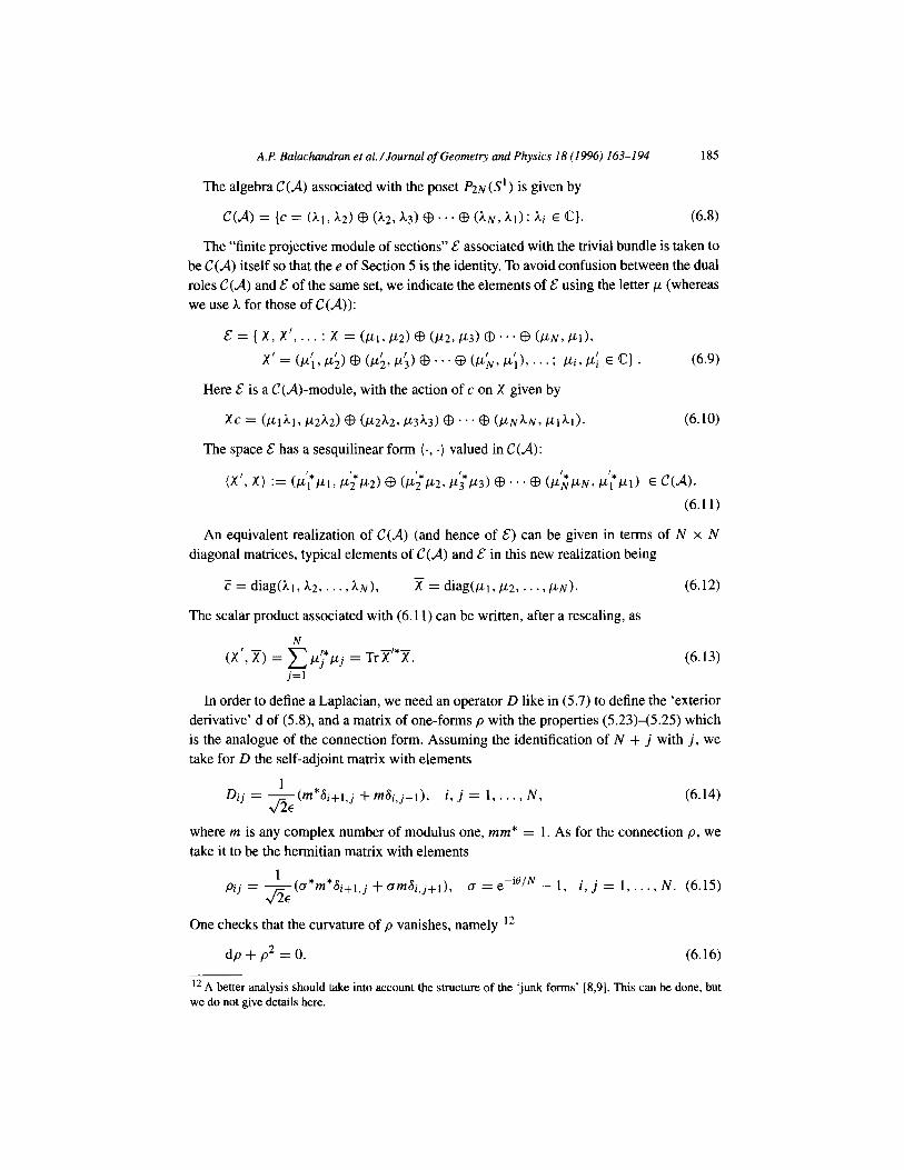
The algebra C(d) associated with the poset P2N(S1) is given by

C(d) = {c = (At, h2) @ (A27 h3) 63 ... @ (AN, Al): Ai E c). (6.8)

The “finite projective module of sections” & associated with the trivial bundle is taken to be C(d) itself so that the e of Section 5 is the identity. To avoid confusion between the dual roles C(d) and 8 of the same set, we indicate the elements of E using the letter /.L (whereas we use )r. for those of C(d)):

& = ( x, x', . . . : x =(~1,~2)~(LL2,CL3)$...~(~N,~l).

X’= (~;,cL;)~(cL;,cL;)$“‘~(LL~,~;),...; Pi,P: E cl. (6.9)

Here E is a C(d)-module, with the action of c on X given by

XC = (CLlkl, P2kd G3 (CL2h2, k3h3) Cl3 ... 63 (CLNAN, Flk1). (6.10)

The space E has a sesquilinear form (+, .) valued in C(d):

ix’, x) := d;*h L&2) CT3 (~4~2, &3) Q3.. . CB h-&N> &I) E C(d).

(6.11)

An equivalent realization of C(d) (and hence of E) can be given in terms of N x N diagonal matrices, typical elements of C(d) and & in this new realization being

-C = diag(hi, AZ, . . . ,h~), F= diagbl, P2, * *. 9 CLN). (6.12)

The scalar product associated with (6.11) can be written, after a resealing, as

(X’, 51) = 5 I.L(i*kj = Trx’*x. (6.13) j=l

In order to define a Laplacian, we need an operator D like in (5.7) to define the ‘exterior derivative’ d of (5.8), and a matrix of one-forms p with the properties (5.23)-(5.25) which is the analogue of the connection form. Assuming the identification of N + j with j, we take for D the self-adjoint matrix with elements

1 Dij = -(m*6i+l,j + mAi,j+l), i, j = 1, . . . , N,

4% (6.14)

where m is any complex number of modulus one, mm* = 1. As for the connection p, we take it to be the hermitian matrix with elements

Pij = 4, -(D*m*8i+l,j + am&,j+l), D = evieIN - 1, i, j = 1, . . . , N. (6.15)

One checks that the curvature of p vanishes, namely I2

dp + p2 = 0. (6.16)

I2 A better analysis should take into account the structure of the ‘junk forms’ [8,9]. This can be done, but we do not give details here.

186 A.P. Balachandran et al./.Journul of Geometry and Physics 18 (1996) 163-194

It is also possible to prove that p is a ‘pure gauge’, that is that there exists aT E C(d) such that p=F’d?,onlyfor0=2nk,k anyinteger.(If~=diag(hl,h~,...,h~),anysuch~will be given by A, = A , h2 = $nklN;1, . . . . hi = $~k(j-l)lN~, .._, kN = ei2nk(“‘-1)lNA, A

not equal to 0.) These properties are the analogues of the the well-known properties of the connection for a particle on S’ subjected to Gquantization, with single-valued wave functions on 5’ defining the domain of the Hamiltonian. If the Hamiltonian with the domain (6.5) is -d2/dx2, then the Hamiltonian with the domain Do(h) consisting of single-valued wave functions is -(d/dx + i0)2 while the connection one-form is i0 dn.

We next define V on & by

vx = [D, X] + p, (6.17)

in accordance with (5.22), e being the identity. The covariant Laplacian As can then be computed as follows.

We write

(VT, VX) = (Z’, v*vsT>, (6.18)

as in (5.27). Now the projection operator ~7 in the present case is readily seen to be defined

by

(qM)ij = Mii6ij, no summation on i, (6.19)

M being any N x N matrix. Hence

(AeST)ij = -(V*VF)iiSij,

-(V*Vjr)ii = [ - [D, [D, Xl] - 2PiD, xl - P2x]ii

_ zcLi + eiOIN A+1 ; 1 i = 1,2,..., N; /-‘,N+l = 111.

The solutions of the eigenvalue problem

(6.20)

(6.21)

are

A. = )ck = 9 cos(k + 8) - 1 , 1 x = jr(k) =diag(~~‘,$) ,..., PC)), k=rn$. m-l,2 ,..., N, (6.22)

where

LL(k) = A(kjeikj + B(k)e-W, J

A(k), B(k) E ,p. (6.23)

These are exactly the answers in Ref. [5] but for one significant difference. In Ref. 151, the operator A did not mix the values of the wave function at points of level one and level

AI! Balachandran et al./Journal of Geometry and Physics 18 (1996) 163-194 187

two, resulting in a double degeneracy of eigenvalues. That unphysical degeneracy has now been removed because of a better treatment of continuity properties. The latter prevents us from giving independent values to continuous probability densities at these two kinds of points. Note that the approach of Ref. [22] is equivalent to the present one and also give (6.23) without the spurious degeneracy.

7. Abelianization and gauge invariance

7.1. Commutative subalgebras and unitary groups

As remarked in Section 4.2, the C*-algebras for our posets are approximately finite dimensional (AF) [ 12,131. Besides the ones described there, they have additional nice structural properties which can be exploited to develop relatively transparent models for E. Further- more, these properties are of use in the analysis of the limit where the number of points of the poset approximation is allowed to go to infinity. This will be explored in a future publication.

Here we will describe very simple and physically suggestive presentations of such algebras in terms of their maximal commutative subalgebras. We will then use this presentation to derive the commutative algebra C(d) using a gauge principle.

We will start with some definitions [ 12,131. The commutant A’ of a subalgebra A of A consists of all elements of A commuting with all elements of A:

A’={x~d:xy=yx,Vy~A). (7.1)

A maximal commutative subalgebra C of A is a commutative C*-subalgebra of A which coincides with its cornmutant, C’ = C.

The C*-algebras A we consider have a unity 1. We therefore have the concepts of the inverse and unitary elements for A.

Let C be a maximal commutative subalgebra of A and let U be the normalizer of C among the unitary elements of A:

U = (u E A I u*u = 1; u*cu E C if c E C} . (7.2)

One can show [ 131 that if u E U, then u* E U, so that 24 is a unitary group. For an AF algebra A, a fundamental result in [ 131 states that the algebra generated by C

and U coincides with A. If Ml, MT, . . . , are subsets of the C*-algebra A, and we denote by

041, M2r . . . , ) the smallest C*-subalgebra of A containing U, Mn, then the above result can be written as

A = (C, U). (7.3)

Next note that C in general has unitary elements and hence U fl C # 0. Now U n C is a normal subgroup of U. We can in fact write U as the semidirect product tx of the group U n C with a group U isomorphic to U/[U r3 C]:

u = [uric] ku. (7.4)

188 A.R Balachandran et al. /Journal of Geometry and Physics 18 (1996) 163-194

Hence, by (7.3),

A= (C, U). (7.5)

This result is of great interest for us. The group U can be explicitly constructed in cases of interest to us. We will do so below

for the two-point and v posets. The general result for any two-level poset follows easily therefrom.

We will now see how A can be realized as operators on a suitable Hilbert space. Let t?be the space of IRRs or the structure space of C. Since the latter is a commutative

AF algebra, we can assert from known results [ 121 that the space c^ is a totally discon- nected Hausdorff space, that is, the connected component of each point consists of the point itself.

If, in the spirit of the Gel’fand-Naimark theorem, we regard elements of C as functions on c? each x E zdefines an ideal IX of C:

Ix = (f E c 1 f(x) = 0). (7.6)

Such ideals are called primitive ideals. They have the following properties for the commutative algebra C: (a) Every ideal is contained in a primitive ideal, and a primitive ideal is maximal, that is, it is contained in no other ideal; (b) A primitive ideal I uniquely fixes a point x of ?by the requirement Z X = I. Thus ?can be identified with the space Prim(?) of primitive ideals.

Now if I, E Prim(E) and c E C, then cu*ZXu = u*[ucu*]ZXu = u*Z,u since ucu* E Z,. Similarly u*ZXuc = u*ZXu. Hence u*ZXu is an ideal. That being so, there is a primitive ideal ZY containing u*ZXu, u*ZXu s ZY. Hence IX s uZ+*. Since uZYu* is an ideal too, we conclude that I, = uZYu* or u* ZXu = ZY. Calling

y := u*x = u-lx, (7.7)

we thus get an action of l4 on r!? With respect to the decomposition (7.4), only the elements in U act not trivially on C, whereas elements in 24 fl C act as the identity.

Let l’(c) be the Hilbert space of square summable functions on c^:

(g, h) = Cg(x)*h(x) < 00, vg, h E c'<c^>. x

(7.8)

It is a striking theorem of [ 131 that A can be realized as operators on e2 (z) using the formulae

(h . f)(x) = h(x)f(x), (h . u>(x) = h(u*x), Vf E c, u E u, h E l”(Z). (7.9)

We have shown the action as multiplication on the right in order to be consistent with the convention in Section 5. Also the dot has been introduced in writing this action for a reason which will immediately become apparent.

A.P: Balachandran et al./Joumal of Geometry and Physics 18 (1996) 163-194 189

This realization of A can give us simple models for E. To see this, first note that we had previously used A or ed” as models for E. But as elements of C are functions on zjust like h, we now discover that they are also d-modules in view of (7.9), the relation between the dot product of (7.9) and the algebra product (devoid of the dot) being

c f = cf, -1 c.u = ucu .

The verification of (7.10) is easy.

(7.10)

Thus C itself can serve as a simple model for 1. We may be able to go further along this line since certain finite-projective modules

over C may also serve as E. Recall for this purpose that such a module is ECN where E is an N x N matrix with coefficients in C, which is idempotent and hermitian (E* = E, E* = E, where (E*)j = (Ej)*). A vector in this module is c = (c’, c*, . . . , tN) with

e’ = Eiaj, uj E C. Now consider the action c + 6. u where (6 . u)’ = u(Ejaj)u-‘. The

vector 6 . u remains in ECN if

L&U-~ = Ej, that is, uEu-’ = E. (7.11)

Since C anyway acts on ECN, we get an action of A on ECN when (7.11) is fulfilled. Thus ECN is a model for & when E satisfies (7.11).

The scalar product for e*(F) written above may not be the most appropriate one and may require modifications or regularization as we shall see in Section 7.2. We only mention that the problem will arise with (7.8) because elements of E must belong to e*(C), a restriction which may be too strong to give an interesting E from C or an interesting finite-projective module thereon.

7.2. The two-point poset

We will illustrate the implementation of these ideas for the two-point, the v and finally for any two-level poset. That should be enough to see how to use them for a general poset.

We will treat the two-point poset first. Its algebra is (4.2). In its self-representation q, it acts on a Hilbert space 7f(= ‘FL,). Choose an orthonormal basis h, (n = 1,2, . . . , > for ‘7-L and let P,, be the orthogonal projector operator on Ch, . The maximal commutative subalgebra is then

(7.12)

The structure space of C is

cI={1,2,...;cm}, (7.13)

where

(4 n : 1 -+ 1 := 1 (n), pm + 6,, := Pm(n); (7.14)

(b) co:l+ l:=l(co), Pm-+o:=pm(co). (7.15)

190 A.l? Bakzchandran et al./Journal of Geometv and Physics 18 (1996) 163-194

The topology of c^is the one given by the one-point compactification of { 1,2, . . .) by adding co. A basis of open sets for this topology is

InI; n= 1,2,...; ok = (m 1 m 2 k] u {m}. (7.16)

A particular consequence of this topology is that the sequence 1,2, . . , converges to ~XJ. This topology is identical to the hull kernel topology [6]. Thus for instance, the zeros of

P,,andl -C~~~Piare(1,2 ,..., ;i,n+l,..., co]and{1,2 ,..., k-l),respectively, where the hatted entry is to be omitted. These being closed in the hull kernel topology, their complements, which are the same as (7.16), are open as asserted above.

The group U is generated by transpositions u(i, j) of hi and hj for i # j:

~(i, j)hi = hj, ~(i, j)hj = hi, ~(i, j)hk = hk if k # i, j. (7.17)

Since the ideals of n and 00 are

L = 11 - Pn, Pl, P2, . . . , E, Pn+l, . . .I, ko={P1,P2,...~, (7.18)

we find,

U(i, j)*Zju(i, j) = Zj, U(i, j)*ZjU(i, j) = Zi, u(i, j)*zku(i, j) = zk if k # i, j, (7.19)

u(i, j)*Z,u(i, j) = I,,

u(i, j)i = j, u(i, j)j = i,

u(i, j)k = k if k # i, j,

u(i, j)cc = 00.

(7.20)

It is worth noting that the representation (7.9) of A splits into a direct sum of the IRRs p, q for the two-point poset. The proof is as follows: 00 being a fixed point for U, the functions supported at co give an d-invariant one-dimensional subspace. It carries the IRR p by (4.3) and (7.15). And since the orbit of n under U is { 1,2 , . . .}, the functions vanishing at 03 give another invariant subspace. It carries the IRR q by (4.3) and (7.14).

There is a suggestive interpretation of the projection operators P,, . (See also the second paper of Ref. [ 121.) The IRR q of A corresponds to the open set [r, s[ which restricted to C splits into the direct sum of the IRR’s 1,2, . . . The IRR p of A corresponds to the point s which restricted to C remains IRR. We can think of 1,2, . . ., as a subdivision of [r, s[ into points. Then P,, can be regarded as the restriction to ?of a smooth function on [r, s] with the value 1 in a small neighbourhood of n and the value zero at all m # n and 00. In contrast, 1 is the function with value 1 on the whole interval. Hence it has value 1 at all n and 00 as in (7.14-7.15). This interpretation is illustrated in Fig. 11.

As mentioned previously, there is a certain difficulty in using the scalar product (7.8) for quantum physics. For the two-point poset, it reads

(gv h) = c g(n)*h(n) + g(m)*h(oo), n

(7.21)

A.P. Balachandran et al./Journal of Geometry and Physics 18 (1996) 163-194 191

@J* P

3 ;

7

4

2 .

1 .

Fig. Il. The figure shows the division of [r, s[ into an infinity of points 1,2, ., which get increasingly dense towards 00 or p. The point cm, being a limit point of 1,2, ., is distinguished by a star. According to the suggested interpretation, these points and 00 correspond to IRRs of C while q = { 1,2, .] and p = CCI correspond to IRRs of Sz.

where cc is the limiting point of { 1,2, . . .) . Hence, if h is a continuous function, and h(m) # 0, then limn+oo h(n) = h(m) # 0, and (h, h) = co. In other words, continuous functions in e’(F) must vanish at 00. This is in particular true for probability densities found from E. It is as though 00 has been deleted from the configuration space in so far as continuous wave functions are concerned.

There are two possible ways out of this difficulty. (a) We can try regularization and modification of (7.8) using some such tool as the Dixmier trace [8,9]; (b) we can try changing the scalar product for example to (. , .)L, E > 0, where

Wd: = F .,:, -g(n)*h(n) + g(oo)*h(wo), (7.22)

the choice of 6 being at our disposal. There are minor changes in the choice of u(i, j) if this scalar product is adopted.

7.3. The v poset and general two-level posets

In the case of the v poset, there are Hilbert spaces 1-11 and ‘Hz for each arm, A being the algebra (4.7) acting on 3-1 = tit @ ti2. After choosing orthonormal basis h?, i=

1,2,n= 1,2 ,...) where the superscript i indicates that the basis element corresponds to 7&, and orthogonal projectors P$’ on @hz’, the algebra C carrbe written as

c = (Pl, u,P;l); P*, u,P;“‘). (7.23)

Here Pi are projection operators on Xi. The group U as before is generated by transpositions of basis elements. The space cconsists of two sequences n(t), n(*) (n = 1,2, . . .) and two points co(l),

WC*), witi n(j) converging to 00~~):

z= (nG), ,(O; i=1,2;n=1,2 ,... }. (7.24)

Their meaning is explained by

pi(&)) = 6.. rJ ’

Pz)(n(j)) = SijSmn, (7.25)

pi (,(j)) = 6.. I I ’

p;)(,W) = 0 (7.26)

192 A.P: Balachandran et al/Journal of Geometry and Physics 18 (1996) 163-194

(b)

Fig. 12. The figures show the structure ofzfor three typical two-level posets.

The visual representation of c^is presented in Fig. 12a. The remaining discussion of Section 7.2 is readily carried out for the v poset as also for

a general two-level poset. So we content ourselves by showing the structure of t?for a v v

and a circle poset in Figs. 12b,c.

7.4. Abelianization from gauge invariance

The physical meaning of the algebra U c A is not very clear [22], even though it is essential to reproduce the poset as the structure space of A.

But if its role is just that and nothing more, is it possible to reduce A utilizing U or a suitable subgroup of U in some way and get the algebra C(d)? The answer seems to be yes in all interesting cases. We will now show this result and argue also that this subgroup can be interpreted as a gauge group.

Let us start with the two-point poset. It is an “uninteresting” example for us where our method will not work, but it is a convenient example to illustrate the ideas.

The condition we impose to reduce A here is that the observables must commute with U. The commutant U’ of U in A is just cl. The algebra A thus gets reduced to a commutative algebra, although it is not the algebra we want.

The next example is a “good” one, it is the example of the v poset. The group U here has two commuting subgroups U(l) and UC*). UC’) . is generated by the transpositions u(k, I; i)

which permute only the basis elements hf) and hl(‘):

A.P: Balachandran et al. /Journal of Geometry and Physics 18 (1996) 163-194

u(k, 1; i)hf) = hj’), u(k, 1; i)hy) = hf’;

u(k, E; i)hg) = hg) if 172 $ {k, I].

193

(7.27)

These are thus operators acting along each arm of v, but do not act across the arms of V.

The full group U is generated by U (l) and UC*) and the elements transposing hj’) and hy). Let us now require that the observables commute with U(l) and UC*). They are given by

the commutant of (U(‘), UC*)), the latter being

(UC’), U(2))’ = CP, + @P* (7.28)

in the notation of (4.7). This algebra being isomorphic to (4.28), we get the result we want. We can also find the correct representations to use in conjunction with (7.28). They are

isomorphic to the IRRs of A when restricted to (U (l), U(*))‘. This is an obvious result. The procedure for finding the algebra C(d) and its representations of interest for a general

poset now follows. Associated with each arm i of a poset, there is a subgroup U@) of U. It permutes the projections, or equivalently the IRRs (like the .ci) of (7.24) associated with this arm, while having the remaining projectors, or the IRRs, as fixed points. The algebra C(d) is then the commutant of (U. UC’))): I

C(d) = (U.U”))‘. I (7.29)

The representations of C(d) of interest are isomorphic to the restrictions of IRRs of A to

C(d). In gauge theories, observables are required to commute with gauge transformations. In

an analogous manner, we here require the observables to commute with the transformations generated by UN. The group generated by U (9 thus plays the role of the gauge group in the approach outlined here.

8. Final remarks

In this article, we have described a physically well-motivated approximation method to continuum physics based on partially ordered sets or posets. These sets have the power to reproduce important topological features of continuum physics with striking fidelity, and that too with just a few points.

In addition, there is also a remarkable connection of posets to noncommutative geometry. This connection comes about because a poset can be thought of as a ‘noncommutative lattice’, being the dual space (the space of representations) of a noncommutative algebra, and the latter is a basic algebraic ingredient in noncommutative geometry. The algebra of a poset also has a good intuitive meaning, being the analogue of the algebra of continuous functions on a topological space.

It is our impression that the above connection is quite deep, and can lead to powerful and novel schemes for numerical approximations which ate also topologically faithful. They seem in particular to be capable of describing solitons and the analogues of QCD O-angles.

Much work of course remains to be done, but there are already persuasive indications of the fruitfulness of the ideas presented in this article for finite quantum physics.

194 A.P Balachandran et al. /Journal of Geometry and Physics 18 (1996) 163-l 94

Acknowledgements

This work was supported by the Department of Energy, USA under contract number DE-FG02-ER40231. In addition, the work of G.L. was partially supported by the Italian ‘Minister0 dell’ Universim e della Ricerca Scientifica’.

A.P.B. wishes to thank Jose Mourao for very useful discussions and for drawing attention to Ref. [7]. He thanks Cassio Sigaud for pointing out an error in the preprint.

References

[1] J.M. Drouffe and C. Itzykson, Phys. Rep. 38 (1978) 134; M. Creutz, Quarks, Gluons and Lattices (Cambridge University Press, Cambridge, 1983); J.B. Kogut, Rev. Mod. Phys. 55 (1983) 785.

[2] F. David, Simplicial Quantum Gravity and Random Lartices, Lectures given at Les Houches Ecole d’ett de Physique Theorique, NATO Advanced Study Institute, July 5-August 1, 1993; Physique Theorique, Saclay preprint T93/028.

[3] R.D. So&in, Int. J. Theor. Phys. 30 (1991) 923. [4] P.S. Aleksandrov, Combinatorial Topology, Vols. l-3 (Greylock, 1960). [5] A.P. Balachandran, G. Bimonte, E. Ercolessi and P Teotonio-Sobrinho, Nucl. Phys. B 418 (1994) 477.

For another approach to discretization, see also A.V. Evako, Syracuse University preprint SU-GP-93/l- 1 ( 1993) and gr-qcI9402035.

[6] J.M.G. Fell and R.S. Doran, Representutions of *-Algebras, Locally Compact Groups and Banach *-Algebraic Bundles (Academic Press, New York, 1988).

[7] A. Mallios, Topological Algebras: Selected Topics, Mathematics Studies, Vol. 142 (North-Holland, Amsterdam, 1986).

[8] A. Connes, Non Commutative Geometry (Academic Press, New York, 1994). [9] J.C. Vsuilly and J.M. Gracia-Bondia, J. Geom. Phys. 12 (1993) 223.

[IO] A. Connes and J. Lott, Nucl. Phys. B (Proc. Suppl.) 18 (1990) 29. [ 111 A. Dimakis and F. Miiller-Hoissen, Discrete Differential Calculus, Graphs, Topologies and Gauge

Theories, hep-th 9404112 and references therein. [12] 0. Bratteli, Trans. Amer. Math. Sot. 171 (1972) 195; J. Functional Analysis 16 (1974) 192. [ 131 S. Stratila and D. Voiculescu, Representations ofAF-Algebras and the Group U(m), Lectures Notes in

Mathematics, Vol. 486 (Springer, Berlin, 1975). [ 141 ShSkichi Iyanaga and Yukiyosi Kawada, eds., Encyclopedic Dictionary of Mathematics, translation

reviewed by K.O. May (MIT Press, Cambridge, MA, 1977). [15] F!J. Hilton and S. Wylie, Homology T/u~ory (Cambridge University Press, Cambridge, 1966). [16] R.P. Stanley, Enumerative Combinatorics, Vol. 1 (Wordsworth and Brooks/Cole Advanced Books and

Software, 1986). [17] S.T. Hu, Homotopy Theory (Academic Press, New York, 1959). [ 181 M. Reed and B. Simon, Methods of Modern Mathematical Physics II: Fourier Analysis, Self-Aa’jointness

(Academic Press, New York, 1975). [ 191 B. Simon, Trace Ideals and their Applications, London Mathematical Society Lecture Notes, Vol. 35

(Cambridge University Press, Cambridge, 1979). [20] H. Behncke and H. Leptin, I. Funct. Anal. 14 (1973) 253; 16 (1974) 241. [21] A.P. Balachandmn, G. Marmo, B.S. Skagerstam and A. Stem, Classical Topology and Quantum States

(World Scientific, Singapore, 1991). [22] A.P Balachandran, G. Bimonte, E. Ercolessi, G. Landi, F. Lizzi, G. Sparano and P. Teotonio-Sobrinho,

Finite Quantum Physics and Noncommutative Geometry, ICl94138, DSF-T-U94 and SU-4240-567 (1994) (hep-th/9403067).

Noncommutative lattices as finite approximations

Documents

Transcript of Noncommutative lattices as finite approximations