Mining Optimal Decision Trees from

Itemset Lattices

Siegfried Nijssen

Elisa Fromont

Report CW476, March 2007

Katholieke Universiteit LeuvenDepartment of Computer Science

Celestijnenlaan 200A – B-3001 Heverlee (Belgium)

Mining Optimal Decision Trees from

Itemset Lattices

Siegfried Nijssen

Elisa Fromont

Report CW476, March 2007

Department of Computer Science, K.U.Leuven

We present an exact algorithm for finding a decision tree that optimizes a rank-

ing function under size, depth, accuracy and leaf constraints. Because the dis-

covery of optimal trees has high theoretical complexity, until now no efforts have

been made to compute such trees for real-world datasets. An exact algorithm

is of both scientific and practical interest. From the scientific point of view, it

can be used as a gold standard to evaluate the performance of heuristic deci-

sion tree learners, and it can be used to gain new insight in traditional decision

tree learners. From the application point of view, it can be used to discover

trees that cannot be found by heuristic decision tree learners. The key idea

behind our algorithm is the relation between constraints on decision trees and

constraints on itemsets. We propose to exploit lattices of itemsets, from which

we can extract optimal decision trees in linear time. We give several strategies

to efficiently build these lattices and show that the test set accuracies of C4.5compete with the test set accuracies of optimal trees.

Abstract

Keywords : Decision tree learning, Frequent itemset mining, Itemset lattice,

Constraint based mining

1. INTRODUCTIONDecision trees are among the most popular prediction

models in machine learning and data mining, because thereare efficient, relatively easily understandable learning algo-rithms and the models are easy to interpret. From this per-spective, it is surprising that mining decision trees underconstraints has not been given much attention. For the prob-lems listed below, currently no broadly applicable algorithmexists even though steps in this direction were made in [7]for the last problem:

• given a dataset D, find the most accurate tree on train-ing data in which each leaf covers at least n examples;

• given a dataset D, find the k most accurate trees ontraining data in which the majority class in each leafcovers at least n examples more than any of the mi-nority classes;

• given a dataset D, find the most accurate tree on train-ing data in which each leaf has a high statistical cor-relation with the target class according to a χ2 test;

• given a dataset D, find the smallest decision tree inwhich each leaf contains at least n examples, and theexpected accuracy is maximized on unseen examples;

• given a dataset D, find the shallowest decision treewhich has an accuracy higher than minacc;

• given a dataset D, find the smallest decision tree whichhas an accuracy higher than minacc.

Clearly, in the interactive process that knowledge discoveryin databases is, the ability to pose queries that answer thesequestions can be very valuable. In this paper we present analgorithm for answering these queries exactly.

Most known algorithms for building decision trees, for in-stance C4.5, rely on top-down induction and choose splitsheuristically. These heuristics impose an additional, implicitconstraint on the decision trees that can be learned. If tra-ditional heuristic algorithms do not find a tree that satisfiesa set of explicit constraints (for instance, on size or accu-racy), this does not mean that such a tree does not exist—itonly means that the chosen heuristic imposes an additionalconstraint that does not allow the algorithm to find it. Anexact algorithm could be desirable to answer queries with-out uncertainty about the influence of heuristics, and couldallow us to study the influence of constraints in a much morefundamental way than will ever be possible using heuristicdecision tree learners. For instance, we could determine fora sufficiently large number of datasets and constraints whatthe optimum under given constraints is —with and withoutheuristics— and learn from this in which cases heuristicshave a positive effect or a negative effect.

Until now, no attempt has been made to compute ex-act optimal trees for many datasets; most people have notseriously considered the problem as it is known to be NPcomplete [17], and therefore, an efficient algorithm can mostlikely not exist. The data mining community, however, hasan interesting track record of dealing with exponential prob-lems with reasonable computation times. In particular, formany years, the problem of frequent itemset mining, whichis exponential in its nature, has attracted a lot of research [1,28, 10] and although this problem is not always efficiently

solvable in theory, in practice many algorithms have beenapplied successfully.

In this paper, we propose DL8, an exact algorithm forbuilding decision trees that does not rely on the traditionalapproach of heuristic top-down induction, and addresses theproblem of finding exact optimal decision trees under con-straints. Its key feature is that it exploits a relation betweenconstraints on itemsets and decision trees. Even though ouralgorithm is not expected to work on all possible datasets,we will provide evidence that for a reasonable number ofdatasets, our approach is feasible and therefore a useful ad-dition to the data mining toolbox.

The paper is organized as follows. In Section 2, we in-troduce the concepts of decision trees and itemsets. In Sec-tion 3, we describe precisely which optimal trees we consider.In Section 4, we motivate the use of such optimal trees. InSections 5 and 6, we present our algorithm and its connec-tion to frequent itemset mining. In Section 7, we evaluatethe efficiency of our algorithm; we compare the accuracyand size of the trees computed by our system with the treeslearned by C4.5. Section 8 gives related work. We concludein Section 9.

2. ITEMSET LATTICES FOR DECISION TREEMINING

Let us first introduce some background information aboutfrequent itemsets and decision trees.

2.1 Itemset MiningLet I = {i1, i2, . . . , im} be a set of items and let D ={T1, T2, . . . , Tn} be a bag of transactions, where each trans-action Tk is an itemset such that Tk ⊆ I. A transactionTk contains a set of items I ⊆ I iff I ⊆ Tk. The transac-tion identifier set (TID-set) t(I) ⊆ {1, 2, . . . n} of an itemsetI ⊆ I is the set of all identifiers of transactions that containitemset I.

The frequency of an itemset I ⊆ I is defined to be thenumber of transactions that contain the itemset, i.e. freq(I) =|t(I)|; the support of an itemset is support(I) = freq/|D|. Anitemset I is said to be frequent if its support is higher thana given threshold minsup; this is written as support(I) ≥minsup (or, equivalently, freq(I) ≥ minfreq).

Definition 1. A complete lattice is a partially orderedset in which all elements have both a least upper bound anda greatest lower bound.

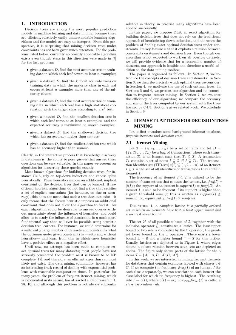
The set 2I of all possible subsets of I, together with theinclusion operator ⊆, constitutes a lattice. The least upperbound of two sets is computed by the ∩ operator, the great-est lower bound by the ∪ operator. There exists a lowerbound ⊥ = ∅ and a higher bound ⊤ = I for this lattice.Usually, lattices are depicted as in Figure 1, where edgesdenote a subset relation between sets; sets are depicted asnodes. The figure only shows parts of the lattice for the 6items I = {A,¬A, B,¬B, C,¬C}.

In this work, we are interested in finding frequent itemsetsfor databases that contain examples labeled with classes c ∈C. If we compute the frequency freqc(I) of an itemset I foreach class c separately, we can associate to each itemset theclass label for which its frequency is highest. The resultingrule I → c(I), where c(I) = argmaxc′∈C freqc′(I) is called aclass association rule.

A?

{}

B?

{A}

A

C?

{¬ A}

¬A

{B}

B

{¬ B}

¬B

{C}

C

{¬ C}

¬C

{AB}

B

C?

{A¬ B}

¬B

{AC}

C

{A¬ C}

¬C

{¬ AB}

B

{¬ A¬ B}

¬B

{¬ AC}

C

{¬ A¬ C}

¬CA ¬A

{BC}

C

{B¬ C}

¬C A ¬A

{¬ BC}

C

{¬ B¬ C}

¬CA ¬A B ¬B A ¬A B ¬B

{ABC}

C

{AB¬ C}

¬C

{A¬ BC}

C

{A¬ B¬ C}

¬CB ¬B B ¬B

{¬ ABC}

C

{¬ AB¬ C}

¬C

{¬ A¬ BC}

C

{¬ A¬ B¬ C}

¬CB ¬BB ¬BA ¬A A ¬AA ¬A A ¬A

Figure 1: An itemset lattice for items {A,¬A, B,¬B, C,¬C}; binary decision tree A(B(C(l,l),l),C(l,l)) is hiddenin this lattice

2.2 Decision treesA decision tree aims at classifying examples by sorting

them down a tree. The leaves of a tree provide the classi-fications of examples [15]. Each node of a tree specifies atest on one attribute of an example, and each branch of anode corresponds to one of the possible outcomes of the test.We assume that all tests are boolean; nominal attributes aretransformed into boolean attributes by mapping each pos-sible value to a separate attribute. The input of a decisiontree learner is then a binary matrix B, where Bij containsthe value of attribute i of example j.

Our results are based on the following observation.

Observation 1. Let us transform a binary table B intotransactional form D such that Tj = {i|Bij = 1}∪{¬i|Bij =0}. Then the examples that are sorted down every node of adecision tree for B are characterized by an itemset of itemsoccurring in D.

For example, consider the decision tree in Figure 2. We candetermine the leaf to which an example belongs by checkingwhich of the itemsets {B}, {¬B, C} and {¬B,¬C} it in-cludes. We denote the set of these itemsets with leaves(T ).Similarly, the itemsets that correspond to paths in the treeare denoted with paths(T ). In this case, paths(T ) = {∅, {B},{¬B}, {¬B, C}, {¬B,¬C}}.

B

C1

1 0

1 0

1 0

Figure 2: An example tree

The leaves of a decision tree correspond to class associa-tion rules, as leaves have associated classes. In decision treelearning, it is common to specify a minimum number of ex-amples that should be covered by each leaf. For associationrules, this would correspond to giving a support threshold.

The accuracy of a decision tree is derived from the num-ber of misclassified examples in the leaves: accuracy(T ) =|D|−e(T )

|D|, where

e(T ) =X

I∈leaves(T )

e(I) and e(I) = freq(I)−freqc(I)(I).

A further illustration of the relation between itemsets anddecision trees is given in Figure 1. In this figure, every noderepresents an itemset; an edge denotes a subset relation.Highlighted is one possible decision tree, which is nothingelse than a set of itemsets. The branches of the decisiontree correspond to subset relations.

In this paper we present DL8, an algorithm for miningDecision trees from Lattices.

3. QUERIES FOR DECISION TREESThe problems that we address in this paper, can be seen as

queries to a database. These queries consist of three parts.The first part specifies the constraints on the nodes of thedecision trees.

1. T := {T |T ∈ DecisionTrees, ∀I ∈ leaves(T ), p(I)}

The set T1 is called the set of locally constrained decisiontrees and DecisionTrees is the set of all possible decisiontrees. Predicate p(I) expresses a constraint on paths. In thesimplest setting, p(I) := (freq(I) ≥ minfreq). In general, pcan be a formula constructed from the following atoms.

• freqi(I) ≥ minfreqi, to express a constraint on the min-imum number of examples for a class;

• freq(I) ≥ minfreq, to express a constraint on the totalnumber of examples in each leaf;

• χ2(I) ≥ mincorr, to express that every leaf shouldhave a χ2 correlation of at least mincorr with the tar-get attribute of the prediction problem;

• diff(I) ≥ mindiff, where

diff(I) = freqm(I)−maxc6=m

freqc(I),

and m = argmaxcfreqc(I); this constraint expressesthat in every leaf there should be more examples forthe majority class than for any of the minority classes.

These atoms may be used in disjunctions and conjunctions,but may not be negated.

The first two predicates are well-known in data mining,as they are anti-monotonic. A predicate p(I) on itemsetsI ⊆ I is called anti-monotonic iff p(I) ∧ I ′ ⊆ I ⇒ p(I ′).Consequently, if p is an anti-monotonic predicate, the con-straint (∀I ∈ leaves(T ), p(I)) can equivalently be replacedwith the constraint (∀I ∈ paths(T ), p(I)).

The second two predicates are not anti-monotonic, butboundable. A predicate p(I) on itemsets I ⊆ I is boundableif there exists an anti-monotonic predicate q(I) such thatp(I) =⇒ q(I). Let us illustrate this for the atom diff(I) ≥mindiff. For a leaf to have diff(I) ≥ mindiff, it should atleast have one class c for which freqc(I) ≥ mindiff, or, inother words, a disjunction of minimum frequency constraintsmust be satisfied.

It is known that disjunctions and conjunctions of anti-monotonic predicates are also anti-monotonic [4]. We willdenote the local constraint p in which χ2 and diff have beenreplaced by their anti-monotonic bounds with pb.

The second (optional) part of the query expresses con-straints that refer to the tree as a whole.

2. T2 := {T |T ∈ T1, q(T )}

Set T2 is called the set of globally constrained decision trees.Formula q(T ) is a conjunction of constraints of the formf(T ) ≤ θ, where f(T ) can be

• e(T ), to constrain the error of a tree on a trainingdataset;

• ex(T ), to constrain the expected error on unseen exam-ples, according to some predefined estimate;

• size(T ), to constrain the number of nodes in a tree;

• depth(T ), to constrain the length of the longest root-leaf path in a tree.

In the mandatory third step, we express a preference fora tree in the set T2.

3. output argminT∈T2[r1(T ), r2(T ), . . . , rn(T )]

The tuples r(T ) = [r1(T ), r2(T ), . . . , rn(T )] are comparedlexicographically and define a ranked set of globally con-strained decision trees; ri ∈ {e, ex, size, depth}. Our currentalgorithm requires that at least e and size or ex and sizebe used in the ranking; If depth (respectively size) is usedin the ranking before e or ex, then q must contain an atomdepth(T ) ≤ maxdepth (respectively size(T ) ≤ maxsize).

We do not constrain the order of size(T ), e(T ) and depth(T )in r. We are minimizing the ranking function r(T ), thus, ouralgorithm is an optimization algorithm. The trees that wesearch for are optimal in terms of the problem setting thatis defined in the query.

To illustrate our querying mechanism we will now giveseveral examples.

Query 1. Small Accurate Trees with Frequent leaves.

T := {T | T ∈ DecisionTrees,∀I ∈ paths(T ), freq(I) ≥ minfreq}

output argminT∈T [e(T ), size(T )].

In other words, we have p(T ) := (freq(I) ≥ minfreq), q(T ) :=true and r(T ) := [e(T ), size(T )]. This query investigatesall decision trees in which each leaf covers at least minfreqexamples of the training data. Among these trees, we findthe smallest most accurate one.

In some cases, one is not interested in large trees, even ifthey are more accurate.

Query 2. Accurate Trees of Bounded Size.

T1 := {T | T ∈ DecisionTrees,∀I ∈ paths(T ), freq(I) ≥ minfreq}

T2 := {T | T ∈ T1, size(T ) ≤ maxsize}

output argminT∈T2[e(T ), size(T )].

One possible scenario in which DL8 can be used, is thefollowing. Assume that we have already applied a heuris-tic decision tree learner, such as C4.5, and we have someidea about decision tree error (maxerror) and size (maxsize).Then we can run the following query:

Query 3. Accurate Trees of Bounded Size and Accuracy.

T1 := {T | T ∈ DecisionTrees,∀I ∈ paths(T ), freq(I) ≥ minfreq}

T2 := {T | T ∈ T1, size(T ) ≤ maxsize,e(T ) ≤ maxerror}

output argminT∈T2[size(T ), e(T )].

This query finds the smallest tree that achieves at least thesame accuracy as the tree learned by C4.5.

The previous queries aim at finding compact models thatmaximize training set accuracy. Such trees might howeveroverfit training data. Another application of DL8 is to ob-tain trees with high expected accuracy. Several algorithmsfor estimating test set accuracy have been presented in theliterature. One such estimate is at the basis of the reducederror pruning algorithm of C4.5. Essentially, C4.5 com-putes an additional penalty term x(freq1(I), . . . freqn(I)) foreach leaf I of the decision tree, from which we can derive anew estimated number of errors

ex(T ) =X

I∈leaves(T )

e(I) + x(freq1(I), . . . freqn(I)).

We can now also be interested in answering the followingquery.

Query 4. Small Accurate Pruned Trees.

T := {T | T ∈ DecisionTrees,∀I ∈ paths(T ), freq(I) ≥ minfreq}

output argminT∈T [ex(T ), size(T )].

This query would find the most accurate tree after pruningsuch as done by C4.5. Effectively, the penalty terms makesure that trees with less leaves are sometimes preferable evenif they are less accurate.

Another query could be :

Query 5. Small Accurate Trees with Correlated leaves.

T := {T | T ∈ DecisionTrees,∀I ∈ leaves(T ), χ2(I) ≥ 10}

output argminT∈T [ex(T ), size(T )].

In this query, we restrict ourselves to trees that perform wellin terms of C4.5’s pruning measure. Each leaf in the treeshould have a significant correlation with the target class.

4. MOTIVATING EXAMPLESTo motivate our work, we will first provide some exam-

ples of situations in which traditional heuristic decision treelearners are not able to find trees that are both small andaccurate, but which can be solved by an optimal decisiontree learner.

A B Class Repeated1 1 0 5×0 1 0 5×1 0 1 40×0 0 2 50×

Figure 3: Example database 1

B

A0

1 2

1 0

1 0

Figure 4: The most accurate tree for exampledatabase 1

Given the database in Figure 3, in which we have 3 targetclasses, and instances are repeated several numbers of times,we are interested in finding the most accurate tree in whichevery leaf has at least 10 examples. A tree that predicts allexamples accurately exists and is given in Figure 4. How-ever, if information gain [23, 6] is used to find a split, wewill not be able to find this tree: the information gain of Ais 0.89, while the information gain of B is 0.47; a test onattribute A would be preferred in the root of the tree. Onlyby using a different heuristic —information gain ratio— weare able to find the optimal tree, as A’s information gainratio is 0.90, but B’s ratio is 1.0.

If we would use information gain without size constraint,we could find an accurate tree, but this tree would be largerthan necessary.

We can learn from this example that information gain con-centrates on the classes that have most examples, as splitsfor these classes will yield the largest entropy reductions.If smaller classes could easily be separated, this may re-main unnoticed. Contrary to traditional heuristic methods,an optimal decision tree learner would not need a differentheuristic to find a tree that satisfies the constraints.

A B C Class Repeated1 1 0 1 40×1 1 1 1 40×1 0 1 1 5×0 0 0 0 10×0 0 1 1 5×

Figure 5: Example database 2

B

C1

1 0

1 0

1 0

Figure 6: The most accurate tree for exampledatabase 2

A B C Class Repeated1 1 1 1 30×1 1 0 0 20×0 1 0 0 8×0 1 1 0 12×0 0 0 1 12×0 0 1 0 18×

Figure 7: Example database 3

As a second example consider the database in Figure 5, inwhich we have 2 target classes. Assume that we have reasonsto believe that only a difference of 10 examples between amajority and a minority class provides significant evidenceto prefer one class above the other in a leaf; therefore, weare interested in finding an optimal decision tree in whichthere is a difference of at least 10 examples between majorityand minority classes. A tree satisfying these constraintsexists, and is given in Figure 6. Clearly in this exampleA and B have approximately the same predictive power.However, C4.5 will prefer attribute A in the root, as it hasinformation gain 0.33 (resp. ratio 0.54), while B only hasinformation gain 0.26 (resp. ratio 0.37). C4.5, however, bymaking this choice, takes away examples that could havebeen used to find a significant next split; no further splitscan be performed. On the other hand, an optimal decisiontree learner can prefer initially sub-optimal splits, if this isuseful to build statistical support for tests deeper down thetree.

10 0 0 0 0 1 1 1 1 1 19 0 0 0 0 1 1 1 1 1 18 0 0 0 0 1 1 1 1 1 17 0 0 0 0 1 1 1 1 1 16 0 0 0 0 1 1 1 1 1 1 A

5 0 0 0 0 0 0 0 0 0 04 0 0 0 0 0 0 0 0 0 0 B

3 1 1 1 1 0 0 0 0 0 02 1 1 1 1 0 0 0 0 0 01 1 1 1 1 0 0 0 0 0 0

1 2 3 4 5 6 7 8 9 10C

Figure 8: Visualization of example database 3; everyelement of the matrix corresponds to one example,and contains its class label; A is true if y ≥ 6, B istrue if y ≥ 4, and C is true if x ≥ 5

C

BA

0 101

1 0

0101

A

CC

001 B

10

1 0

0101

1 0

(a) Smallest (b) Learned by C4.5

Figure 9: Two accurate trees for example database3

As a third example consider the database in Figure 7,which is a variation of the XOR problem, as depicted in Fig-ure 8. Assume that we are interested in finding the smallest(or shallowest) most accurate decision tree, and we do nothave a constraint on the number of examples in a leaf. Thenthe optimal tree is given in Figure 9(a), but C4.5 will findthe tree in Figure 9(b), as the information gain (cq. ratio) ofA is 0.098 (resp. 0.098), while the information gain of C is0.029 (resp. 0.030). What these examples illustrate, is thatheuristic decision tree learners can be ‘fooled’ into takingcertain decisions due to the proportions with which exam-ples are given. Optimal decision tree learners may exposesuch behavior less quickly.

Of course, these examples are all artificial. An interestingquestion is to what extent similar situations occur in realworld data. By using our algorithm, we are able to find thisout.

5. BUILDING OPTIMAL DECISION TREESFROM LATTICES

We will now present the DL8 algorithm for answeringdecision tree queries. Pseudo-code of the algorithm is givenin Algorithm 1.

Parameters of DL8 are the local constraint p and its anti-monotonic bound pb, the ranking function r, and the globalconstraints; each global constraint is passed in a separateparameter; global constraints that are not specified, are as-sumed to be set to ∞. The most important part of DL8is its recursive search procedure. Given an input itemset I,DL8-Recursive computes one or more decision trees for thetransactions t(I) that contain the itemset I. More than onedecision tree is returned only if a depth or size constraint isspecified. Let r(T ) = [r1(T ), . . . , rn(T )] be the ranking func-tion, and let k be the index of the obligatory error functionin this ranking. If r1, . . . , rk−1 ∈ {depth, size} then, for everyallowed value of depth d and size s, DL8-Recursive outputsthe best tree T that can be constructed for the transactionst(I) according to the ranking [rk(T ), . . . , rn(T )], such thatsize(T ) ≤ s and depth(T ) ≤ d.

In DL8-Recursive, we use several functions: l(c), whichreturns a tree consisting of a single leaf with class labelc; n(i, T1, T2), which returns a tree that contains test i inthe root, and has T1 and T2 as left-hand and right-handbranches; et(T ), which computes the error of tree T whenonly the transactions in TID-set t are considered; and fi-

Algorithm 1 DL8(p, pb, maxsize,maxdepth,maxerror, r)

1: if maxsize 6=∞ then2: S ← {1, 2, . . . ,maxsize}3: else4: S ← {∞}5: if maxdepth 6=∞ then6: D ← {1, 2, . . . ,maxdepth}7: else8: D ← {∞}9: T ←DL8-Recursive(∅)

10: if maxerror 6=∞ then11: T ← {T |T ∈ T , e(T ) ≤ maxerror}12: if T = ∅ then13: return undefined14: return argminT∈T r(T )15:16: procedure DL8-Recursive(I)17: if DL8-Recursive(I) was computed before then18: return stored result19: if p(I) = true then20: C ← {l(c(I))}21: else22: C ← ∅23: if pure(I) then24: store C as the result for I and return C25: for all i ∈ I do26: if pb(I ∪ {i}) = true and pb(I ∪ {¬i}) = true

then27: T1 ← DL8-Recursive(I ∪ {i})28: T2 ← DL8-Recursive(I ∪ {¬i})29: for all T1 ∈ T1, T2 ∈ T2 do30: C ← C ∪ {n(i, T1, T2)}31: end if32: T ← ∅33: for all d ∈ D, s ∈ S do34: L ← {T ∈ C|depth(T ) ≤ d ∧ size(T ) ≤ s}35: T ← T ∪ {argminT∈L[rk = et(I)(T ), . . . , rn(T )]}36: end for37: store T as the result for I and return T38: end procedure

nally, we use a predicate pure(I); predicate pure blocks therecursion if all examples t(I) belong to the same class.

The algorithm is most easily understood if maxdepth =∞,maxsize =∞, maxerror =∞ and r(T ) = [e(T )]; in this case,DL8-Recursive combines only two trees for each i ∈ I, andreturns the single most accurate tree in line 37.

The correctness of the DL8 algorithm is essentially basedon the fact that the left-hand branch and the right-handbranch of a node in a decision tree can be optimized inde-pendently. In more detail, the correctness follows from thefollowing observations.

(line 1-8) the valid ranges of sizes and depths are computedhere if a size or depth constraint was specified;

(line 11) for each depth and size, for so far necessary, DL8-Recursive finds the most accurate tree possible. Someof the accuracies might be too low for the given con-straint, and are removed from consideration.

(line 19) we check the leaf constraint here; only if the leafconstraint is satisfied, a candidate decision tree for

classifying the examples t(I) consists of a single leaf;this candidate is initialized in line 20.

(line 23) if all examples in a set of transactions belong to thesame class, continuing the recursion is not necessary;after all, any larger tree will not be more accurate thana leaf, and we require that size is used in the ranking.More sophisticated pruning is possible in some specialcases, for example the loose-pure predicate presentedin Section 6.3 can be sometimes be used instead of thepure predicate.

(line 26) in this line the anti-monotonic property of the pred-icate pb(I) is used: an itemset that does not satisfy thepredicate pb(I) cannot be part of a tree, nor can anyof its supersets; therefore the search is not continuedif pb(I ∪ {i}) = false or pb(I ∪ {¬i}) = false.

(line 25–36) these lines make sure that each tree that shouldbe part of the output T , is indeed returned. We canprove this by induction. Assume that for the set oftransactions t(I), tree T should be part of T as itis the most accurate tree that is smaller than s andshallower than d for some s ∈ S and d ∈ D; as-sume T is not a leaf, and contains test i in the root.Then T must have a left-hand branch T1 and a right-hand branch T2. Tree T1 must be the most accuratetree that can be constructed for t(I ∪ {i}) with sizeat most size(T1) and depth at most depth(T1); simi-larly, T2 must be the most accurate tree that can beconstructed for t(I ∪ {¬i}) under depth and size con-straints. We can inductively assume that trees withthese constraints are found by DL8-Recursive(I ∪{i}) and DL8-Recursive(I∪{¬i}) as size(T1), size(T2) ≤maxsize and depth(T1), depth(T2) ≤ maxdepth. Conse-quently T (or a tree with equal statistics) must beamong the trees found by combining results from thetwo recursive procedure calls in line 30.

A key feature of DL8-Recursive is that in line 37 it storesevery result that it computes. Consequently, DL8 avoidsthat optimal decision trees for any itemset are computedmore than once. We do not need to store entire decisiontrees with every itemset. It is sufficient to store their rootsand statistics (error, possibly size and depth), as left-handand right-hand subtrees can be recovered from the storedresults for the left-hand and right-hand itemsets if necessary.

Note that in our algorithm, we output the best tree ac-cording to the ranking. The k − best trees could also bestraightforwardly output.

To efficiently index the itemsets I that are considered byDL8, a trie data structure can be used. In the next sec-tion we will consider several strategies for building this datastructure.

6. MINING STRATEGIESAs with most data mining algorithms, the most time con-

suming operations are those that access the data. In the fol-lowing, we will provide four related strategies to obtain thefrequency counts that are necessary to check the constraintsand compute accuracies: the simple single-step approach,the frequent itemset mining (FIM) approach, the constraintfrequent itemset mining approach, and the closure basedsingle-step mining approach.

6.1 The Simple Single-Step ApproachThe most straightforward approach, referred to as DL8-

Simple, computes the itemset frequencies while DL8 is ex-ecuting. In this case, once DL8-Recursive is called for anitemset I, we obtain the frequencies of I in a scan over thedata, and store the result in a trie to avoid later recompu-tations.

6.2 The FIM ApproachAn alternative approach is based on the observation that

every itemset that occurs in a tree, must satisfy the localconstraint pb. If pb is a minimum frequency constraint, wecan use a frequent itemset miner to obtain the frequencies ina preprocessing step. DL8 then operates on the resulting setof itemsets, annotating every itemset with optimal decisiontrees.

Many frequent itemset miners have been studied in theliterature; all of these can be used with small modificationsto output the frequent itemsets in a convenient form anddetermine frequencies in multiple classes [1, 28, 10, 25].

We implemented an extension of Apriori that first com-putes and stores in a trie all frequent itemsets, and thenruns DL8 on the trie. This approach is abbreviated withApriori-Freq+DL8. Compared to other itemset miners,like Eclat or LCM, we expect that the additional runtimeto store all itemsets in Apriori is the lowest, as Apriorialready builds a trie of candidate itemsets itself.

If we assume that the output of the frequent itemset minerconsists of a graph structure such as Figure 1, then DL8operates in time linear in the number of edges of this graph.

6.3 The Constrained FIM ApproachUnfortunately, the frequent itemset mining approach may

compute frequencies of itemsets that can never be part of adecision tree. For instance, assume that {A} is a frequentitemset, but {¬A} is not; then no tree answering exampleQuery 1 will contain a test for attribute A; itemset {A}is redundant. In this section, we show that an additionallocal, anti-monotonic constraint can be used in the frequentitemset mining process to make sure that no such redundantitemsets are enumerated.

If we consider the DL8-Simple algorithm, an itemset I ={i1, . . . , in} is stored only if there is an order [ik1

, ik2, . . . , ikn

]of the items in I (which corresponds to an order of recursivecalls to DL8-Recursive) such that for none of the properprefixes I ′ = [ik1

, ik2, . . . , ikm

] (m < n) of this order

• the ¬pure(I ′) predicate is false in line (23);

• the conjunction pb(I′ ∪{ik

m+1})∧pb(I

′ ∪{¬ikm+1}) is

false in line (26).

It is helpful to negate the pure predicate, as one can easilysee that ¬pure is an anti-monotonic predicate (every super-set of a pure itemset, must also be pure). From now on,we will refer to ¬pure as a leaf constraint, as it defines aproperty that is only allowed to hold in the leaves of a tree.

We can now formalize the principle of itemset relevancy.

Definition 2. Let p1 be a local anti-monotonic tree con-straint and p2 be an anti-monotonic leaf constraint. Then

the relevancy of I, denoted by rel(I), is defined by

rel(I) =

8

>

>

>

<

>

>

>

:

p1(I) ∧ p2(I) if I = ∅ (Case 1)true if ∃i ∈ I s.t.

rel(I − i) ∧ p2(I − i)∧p1(I) ∧ p1(I − i ∪ ¬i) (Case 2)

false otherwise (Case 3)

Theorem 1. Let L1 be the set of itemsets stored by DL8-Simple, and let L2 be the set of itemsets {I ⊆ I|rel(I) =true}. Then L1 = L2.

Proof. We consider both directions.“⇒”: if an itemset is stored by DL8-Simple, there mustbe an order of the items in which each prefix satisfies theconstraints as defined in line (23) and line (26). Then wecan repeatedly pick the last item in this order to find theitems that satisfy the constraints in case 2 of the definitionof rel(I).“⇐”: if an itemset is relevant, we can construct an orderin which the items can be added in the recursion withoutviolating the constraints, as follows. For a relevant itemsetthere must be an item i ∈ I such that case 2 holds. Let thisbe the last item in the order; then recursively consider theitemset I − i. As this itemset is also relevant, we can againobtain an item i′ ∈ I − i, and put this on the second lastposition in the order, and so on.

Relevancy is a property that can be pushed in a frequentitemset mining process.

Theorem 2. Itemset relevancy is an anti-monotonic prop-erty.

Proof. By induction. The base case is trivial: if the ∅itemset is not relevant then none of its supersets is relevant.Assume that for all itemsets X ′, X upto size |X| = n wehave shown that if X ′ ⊂ X: ¬rel(X ′) ⇒ ¬rel(X). Assumethat Y = X ∪ i and that X is not relevant. To prove thatY is not relevant, we need to consider every j ∈ Y , andconsider whether case 2 of the definition is true for this j:

• i = j: certainly Y − i = X is not relevant;

• i 6= j: we know that j ∈ X, and given that X is notrelevant, either

– rel(X − j) = false: in this case rel(Y − j) =rel(X − j ∪ i) = false (inductive assumption);

– p1(X) = false: in this case p1(Y ) = false (anti-monotonicity of p1);

– p1(X − j ∪ ¬j) = false: in this case p1(Y − j ∪¬j) = p1(X−j∪¬j∪i) = false (anti-monotonicityof p1);

– p2(X−j) = false: in this case p2(Y −j) = p2(X−j ∪ i) = false (anti-monotonicity of p2).

Consequently, rel(Y ) can only be false.

It is relatively easy to integrate the computation of rele-vancy in frequent itemset mining algorithms, as long as theorder of itemset generation is such that all subsets of anitemset I are enumerated before I is enumerated itself. As-sume that we have already computed all relevant itemsets

that are a subset of an itemset I. Then we can determinefor each i ∈ I if the itemset I − i is part of this set, and ifso, we can derive the class frequencies of I− i∪¬i using theformula freqk(I− i∪¬i) = freqk(I− i)− freqk(I). If for eachi either I − i is not relevant, or the predicate p(I − i ∪ ¬i)fails, we can prune I.

Pruning of this kind can be integrated in both depth-firstand breadth-first frequent itemset miners.

Loose-PurenessUp until now, we have considered a pureness constraint thatstates that no internal node should be pure. If we are in-terested in finding a small accurate tree under a minimumsupport constraint, this definition of purity can be relaxed.

Definition 3. For a given itemset I, let us sort the fre-quencies in the classes in descending order, freq1, . . . , freqn.Let minfreq be the minimum frequency used to build the lat-tice. An itemset I is loose-pure if (minfreq−

Pn

i=2 freqi(I)) >freq2(I).

Let us illustrate this definition of loose-purity on an exam-ple. Given a prediction problem with 4 classes and minfreq =5, and assume that for an itemset (i.e. a node) we have :

Class 1: 10 examplesClass 2: 1 examplesClass 3: 1 examplesClass 4: 1 examples

It does not make sense to split this node to increase theglobal accuracy of the tree. Indeed, the best split wouldseparate all current errors (from class 2, 3 and 4) from themajority class, but since any leaf must contain at least 5examples, and since none of these classes (in particular notthe second most frequent class) have enough examples totake a majority in a leaf (5 − 3 = 2 > 1) compared to thefirst class, the error (3 in this example) in the tree cannotdecrease. As a further example, if class 2 would have 2 ex-amples, the node could still be split: we could create a splitsuch that 2 examples of class 2 become classified correctly, 2examples of class 3 and 4 remain classified incorrectly, and1 example of class 1 becomes classified incorrectly; in total,a decrease in error of 1 could be obtained in the example.

Obviously, loose-purity is monotonic, and is a strongerconstraint than purity. We prove now that splitting a loose-pure node will never improve accuracy; consequently, whenlooking for the smallest most accurate tree, loose-purity canbe used instead of purity.

Theorem 3. If freq(I) ≥ minfreq, loose-pure(I) = trueand class k is the majority class in I, then for all I ′ ⊃ Isuch that freq(I ′) ≥ minfreq, class k is the majority class ofI ′.

Proof. Let class 1 be the majority class in I. Thenfreq(I) ≥ minfreq ⇔

Pn

i=1 freqi(I) ≥ minfreq ⇔ freq1 ≥(minfreq −

Pn

i=2 freqi(I)). Since I is loose-pure we knowthat (minfreq−

Pn

i=2 freqi(I)) > freq2(I) ≥ 0 ⇔ ∀i, 2 ≤ i ≤n, freqi < minfreq.For class k (k 6= 1) to be the majority class in I ′ with I ′ ⊃ Iand freq(I ′) ≥ minfreq, the number of examples of class kin I ′ should be higher than the minimum number of exam-ples from class 1 that will still be in I ′. This number isat least (minfreq −

Pn

i=2 freqi(I)). So, for k (k 6= 1) to

be the new majority class in I ′, we must have freqk ≥(minfreq −

Pn

i=2 freqi(I)) which contradicts the definitionof loose-purity for I; therefore class 1 must be the majorityclass in I ′.

Integration in Frequent Itemset MinersIn case depth is the first ranking function, level-wise algo-rithms such as Apriori have an important benefit: aftereach level of itemsets is generated, we could run DL8 to ob-tain the most accurate tree up to that depth. Apriori canstop at the lowest level at which a tree is found that fulfilsthe constraints.

We implemented two versions of DL8 in which the rele-vancy constraints are pushed in the frequent itemset miningprocess: DL8-Apriori, which is based on Apriori [1], andDL8-Eclat, which is based on Eclat [28].

6.4 The Closure-Based Single-Step ApproachIn the simple direct approach, we computed an optimal

decision tree for every relevant itemset. However, if the localconstraint is only coverage based, it is easy to see that fortwo itemsets I1 and I2, if t(I1) = t(I2), the result of DL8-Recursive(I1) and DL8-Recursive(I2) must be the same.To reduce the number of results that we have to store, weshould avoid storing such duplicate sets of results.

The solution that we propose is to compute for every item-set its closure. Let i(t) be the function which computes

i(t) = ∩k∈tTk

for a TID-set t, then the closure of itemset I is the itemseti(t(I)). An itemset I is called closed iff I = i(t(I)). Ift(I1) = t(I2) it is easy to see that also i(t(I1)) = i(t(I2)).Thus, in the trie data-structure that is used in the directapproach, we can index the results on i(t(I)) instead of Iitself.

This means that we need to modify Algorithm 1 such thatit searches for the closure of I in line 17. Similarly, in line 37,we associate computed decision tree(s) to the closure of Iinstead of to I itself.

Our implementation of DL8-Simple which relies on closeditemsets is called DL8-Closed. Obviously, DL8-Closedwill never consider more itemsets then the naive direct im-plementation, DL8-Apriori or DL8-Eclat; itemsets storedby DL8-Closed may however be longer as they contain allitems in their closure.

Relevancy andDL8-Closed

We can characterize the closed itemsets that are consideredby DL8-Closed as follows.

Theorem 4. After running DL8-Closed the set of closeditemsets C contains exactly all itemsets C ⊆ I such that Cis closed, and there is at least one I ⊆ C with t(I) = t(C)and rel(I) = true.

Proof. This follows from the fact that DL8-Simple con-siders only relevant itemsets.

It follows from this theorem that DL8-Closed will nevercompute a larger set of itemsets than DL8-Simple. By com-bining closed itemset mining with relevancy, DL8-Closedsearches for δ-free-like itemsets within the concept latticeinstead of the original lattice [3].

Implementation DetailsAs we perform most experiments with DL8-Closed, andDL8-Closed is not based on a previously published fre-quent itemset mining algorithm, we provide some more de-tails about its implementation here.

The most time consuming operations in the algorithm arethe computation of closures of itemsets, and the computa-tion of frequencies. To speed up these operations, we com-bine these operations as follows. As parameters to DL8-Recursive we add the following:

• the item i that was last added to I;

• a set of active items, which includes item i;

• a set of active transaction identifiers storing t(I−{i});

• the set of all items C that are in the closure of I, butare not part of the set of active items.

In the first call to DL8-Recursive, all items and transac-tions are active. At the start of each recursive call (beforeline 17 of DL8-Recursive is executed) we scan each activetransaction, and test if it contains the item i; for each activetransaction that contains item i, we determine which otheractive items it contains. We use this scan to compute thefrequency of the active items, and build the new set of activetransaction identifiers t(I). Those active items of which thefrequency equals that of I, are added to the closure C. Afterthis scan of the data, we build a new set of active items. Forevery item we determine if pb(I ∪ {i}) and pb(I ∪ {¬i}) aretrue; if so, and if not i 6∈ C, we add the item to the new setof active items. In line 25 we only traverse the set of activeitems; the test of line 26 is then redundant. Finally, in line27 and 28 the updated sets of active transactions and activeitems are passed to the recursive calls.

This mechanism for maintaining sets of active transac-tions is akin to the idea of maintaining projected databasesthat is implemented in Eclat and FP-Growth. In con-trast to these algorithms, we know in our case that we haveto maintain projections that contain both an item i and itsnegation ¬i. As we know that |t(I)| = |t(I ∪ i)|+ |t(I ∪¬i)|,it is less beneficial to maintain TID-sets as in Eclat, andwe preferred this solution.

The main reason for calling DL8-Recursive with the setof active transactions t(I − {i}) instead of t(I), is that wecan optimize the memory use of the algorithm. Instead ofrepeatedly allocating new memory for storing sets of activeitems and transactions, we can now maintain a single arrayto store these sets across all recursive calls. A projectionis obtained by reordering the items in this array. Conse-quently, the memory use of our algorithm is entirely deter-mined by the amount of memory that is needed to storethe database and the closed itemsets; the memory use isθ(|D|+ |C|).

We store the closed itemsets in a trie data-structure, as iscommon in many other frequent itemset mining algorithms.Which information is stored for every itemsets, depends onthe query. If we are looking only for the smallest, mostaccurate decision tree, we associated to fields for storingerror, size and root (representing the test in the root of thetree for t(I)); in our implementation, we assume that eachof these elements can be stored in 32 bits. Thus the amountof memory used for each closed itemset is independent ofthe characteristics of the database.

Datasets #Ex #Test Datasets #Ex #Testanneal 812 36 tumor 336 18a-credit 653 56 segment 2310 55balance 625 13 soybean 630 45breast 683 28 splice 3190 3466chess 3196 41 thyroid 3247 36

diabetes 768 25 vehicle 846 55g-credit 1000 77 vote 435 49heart 296 35 vowel 990 48

ionosphere 351 99 yeast 1484 23mushroom 8124 116 zoo 101 15pendigits 7494 49

Figure 10: Datasets description

Algorithm Uses relevancy Closed Builds tree

DL8-Closed X X XDL8-Apriori X XDL8-Eclat X XApriori-FreqApriori-Freq+DL8 XEclat-FreqLCM-FreqLCM-Closed X

Figure 12: Properties of the algorithms used in theexperiments

7. EXPERIMENTSIn this section we compare the different versions of DL8 in

terms of efficiency; furthermore, we compare the quality ofthe constructed trees with those found by the J48 decisiontree learner implemented in Weka [26]. All experimentswere performed on Intel Pentium 4 machines with in be-tween 1GB and 2GB of main memory, running Linux. DL8and the frequent itemset miners were implemented in C++.

The experiments were performed on UCI datasets [19].Numerical data were discretized before applying the learn-ing algorithms using Weka’s unsupervised discretizationmethod with a number of bins equal to 4. We limited thenumber of bins in order to limit the number of created at-tributes. Figure 10 gives a brief description of the datasetsthat we used in terms of the number of examples and thenumber of attributes after binarization.

7.1 EfficiencyThe applicability of DL8 is limited by two factors: the

amount of itemsets that need to be stored, and the timethat it takes to compute these itemsets. We first evaluate ex-perimentally how these factors are influenced by constraintsand properties of the data. Furthermore, we determine howthe different approaches for computing the itemset latticescompare. A summary of the algorithms can be found inFigure 12. Besides DL8-Apriori, DL8-Eclat and DL8-Closed, we also include unmodified implementations of thefrequent itemset miners Apriori [1], Eclat [28] and LCM[25] in the comparison. These implementations were ob-tained from the FIMI website [2]. The inclusion of unmod-ified algorithms allows us to determine how well relevancypruning works, and allows us to determine the trade-off be-tween relevancy pruning and trie construction.

Results for twelve datasets are listed in Figure 11. Weaborted runs of algorithms that lasted for longer than 1800s.The results clearly show that in all cases the number of

closed relevant itemsets is the smallest. The difference be-tween the number of relevant itemsets and the number offrequent itemsets becomes smaller for lower minimum fre-quency values. The number of frequent itemsets is so largein most cases, that it is impossible to compute or storethem within a reasonable amount of time or space. In thosedatasets where we can use low minimum frequencies (15or smaller), the closed itemset miner LCM is usually thefastest; for low frequency values the number of closed item-sets is almost the same as the number of relevant closeditemsets. Bare in mind, however, that LCM does not out-put the itemsets in a form that can be used efficiently byDL8.

In most cases, DL8-Closed is faster than DL8-Apriorior DL8-Eclat, with the exception of the Mushroom, Chessand Splice datasets, which are the largest datasets used inthe experiments. The experiments reveil that for the highminimum support values that we had to use, the differencesbetween closed relevant itemsets and relevant itemsets aresmall; the overhead of DL8-Closed seems too large.

In those cases where we can store the entire output ofApriori in memory, we see that the additional runtime forstoring results is significant. On the other hand, if we per-form relevancy pruning, the resulting algorithm is usuallyfaster than the original itemset miner.

In the datasets shown here, the number of attributes isrelatively small. For the datasets with larger number ofattributes, such as ionosphere and splice, we found that onlyDL8-Closed managed to run for support thresholds lowerthan 25%, but still was unable to run for support thresholdslower than 10%.

7.2 AccuracyIn this section, we compare the accuracies of the deci-

sion trees learned by DL8 and J48 on the twenty differentUCI datasets. J48 is the Java implementation of C4.5 [23]in Weka. We used a stratified 10-fold cross-validation tocompute the training and test accuracies of both systems.The bottleneck of our algorithm is the in-memory construc-tion of the lattice, and, consequently, the application of ouralgorithm is limited by the amount of memory available forthe construction of this lattice. For the results of Figure 13,we used minimum frequency as local constraint. The fre-quency was lowered to the lowest value that still allowedthe computation to be performed within the memory of ourcomputers. We also give results for higher frequency valuesto evaluate the influence of frequency on the accuracy of thetrees.

For J48, results are provided for pruned trees and un-pruned trees; for DL8 results are provided in which the e(unpruned) and ex (pruned) error functions are optimized(cf. Queries 1 and 4 of Section 3). Both algorithms were ap-plied with the same minimum frequency setting. We used acorrected two-tailed t-test [18] with a significance thresholdof 5% to compare the test accuracies of both systems. A testset accuracy result is in bold when it is significantly betterthan its counterpart result on the other system. In the lastthree columns, we also give results for J48 with its defaultminfreq = 2 setting. The test accuracies of J48 are com-pared to the test accuracies given by DL8 using pruning.The results of the significance test are given in the “S” col-umn : “+” means that J48 is significantly better, “-” thatit is significantly worse and “0” not significantly different.

100

1000

10000

100000

1e+06

1e+07

0 20 40 60 80 100 120 140 160

#ite

mse

ts

minfreq

anneal

DL8-ClosedDL8-Simple

Closed

0.01

0.1

1

10

100

1000

0 20 40 60 80 100 120 140 160

runt

ime

(s)

minfreq

anneal

DL8-ClosedDL8-Eclat

DL8-AprioriLCM-Closed

10 100

1000 10000

100000 1e+06 1e+07 1e+08 1e+09 1e+10

50 100 150 200 250 300

#ite

mse

ts

minfreq

australian-credit

DL8-ClosedDL8-Simple

ClosedFreq

0.01

0.1

1

10

100

1000

10000

50 100 150 200 250 300

runt

ime

(s)

minfreq

australian-credit

DL8-ClosedDL8-Eclat

DL8-Apriori

LCM-ClosedLCM-FreqEclat-Freq

1000

10000

100000

1e+06

2 4 6 8 10 12 14 16 18 20

#ite

mse

ts

minfreq

balance-scale

DL8-ClosedDL8-Simple

ClosedFreq

0.01

0.1

1

10

2 4 6 8 10 12 14 16 18 20

runt

ime

(s)

minfreq

balance-scale

DL8-ClosedDL8-Eclat

DL8-AprioriLCM-Closed

LCM-FreqEclat-Freq

Apriori-FreqApriori-Freq+DL8

1000

10000

100000

1e+06

1e+07

1e+08

1e+09

1e+10

10 20 30 40 50 60

#ite

mse

ts

minfreq

breast-wisconsin

DL8-ClosedDL8-Simple

ClosedFreq

0.1

1

10

100

1000

10 20 30 40 50 60

runt

ime

(s)

minfreq

breast-wisconsin

DL8-ClosedDL8-Eclat

DL8-Apriori

LCM-ClosedLCM-FreqEclat-Freq

1000

10000

100000

1e+06

1e+07

1e+08

1e+09

200 250 300 350 400 450 500

#ite

mse

ts

minfreq

chess-kr-kp

DL8-ClosedDL8-Simple

Closed

0.1

1

10

100

1000

200 250 300 350 400 450 500

runt

ime

(s)

minfreq

chess-kr-kp

DL8-ClosedDL8-Eclat

DL8-AprioriLCM-Closed

10000

100000

1e+06

1e+07

1e+08

1e+09

0 10 20 30 40 50 60 70 80 90 100

#ite

mse

ts

minfreq

diabetes

DL8-ClosedDL8-Simple

ClosedFreq

0.1

1

10

100

1000

0 10 20 30 40 50 60 70 80 90 100

runt

ime

(s)

minfreq

diabetes

DL8-ClosedDL8-Eclat

DL8-AprioriLCM-Closed

LCM-FreqEclat-Freq

Apriori-FreqApriori-Freq+DL8

100

1000

10000

100000

1e+06

1e+07

1e+08

40 50 60 70 80 90 100

#ite

mse

ts

minfreq

ionosphere

DL8-Closed DL8-Simple

0.01

0.1

1

10

100

1000

40 50 60 70 80 90 100

runt

ime

(s)

minfreq

ionosphere

DL8-ClosedDL8-Eclat

DL8-Apriori

100

1000

10000

100000

1e+06

1e+07

800 1000 1200 1400 1600 1800 2000

#ite

mse

ts

minfreq

mushroom

DL8-Closed DL8-Simple

0.1

1

10

100

1000

800 1000 1200 1400 1600 1800 2000

runt

ime

(s)

minfreq

mushroom

DL8-ClosedDL8-Eclat

DL8-Apriori

100

1000

10000

100000

1e+06

1e+07

1e+08

1e+09

10 20 30 40 50 60 70 80 90 100

#ite

mse

ts

minfreq

vote

DL8-ClosedDL8-Simple

ClosedFreq

0.01

0.1

1

10

100

1000

10 20 30 40 50 60 70 80 90 100

runt

ime

(s)

minfreq

vote

DL8-ClosedDL8-Eclat

DL8-Apriori

LCM-ClosedLCM-Freq

1000

10000

100000

1e+06

1 2 3 4 5 6 7 8 9 10

#ite

mse

ts

minfreq

zoo

DL8-ClosedDL8-Simple

ClosedFreq

0.01

0.1

1

10

100

1 2 3 4 5 6 7 8 9 10ru

ntim

e (s

)

minfreq

zoo

DL8-ClosedDL8-Eclat

DL8-AprioriLCM-Closed

LCM-FreqEclat-Freq

Apriori-FreqApriori-Freq+DL8

10000

100000

1e+06

1e+07

1e+08

1e+09

0 10 20 30 40 50 60 70 80 90 100

#ite

mse

ts

minfreq

yeast

DL8-ClosedDL8-Simple

ClosedFreq

0.1

1

10

100

1000

10000

0 10 20 30 40 50 60 70 80 90 100

runt

ime

(s)

minfreq

yeast

DL8-ClosedDL8-Eclat

DL8-AprioriLCM-Closed

LCM-FreqEclat-Freq

Apriori-Freq

10

100

1000

10000

100000

1e+06

600 650 700 750 800 850 900 950 1000

#ite

mse

ts

minfreq

splice

DL8-Closed DL8-Simple

0.1

1

10

100

1000

600 650 700 750 800 850 900 950 1000

runt

ime

(s)

minfreq

splice

DL8-ClosedDL8-Eclat

DL8-Apriori

Figure 11: Comparison of the different miners on 12 UCI datasets

The experiments show that both with and without prun-ing the optimal trees computed by DL8 have a better train-ing accuracy than the trees computed by J48 with the samefrequency values. Furthermore, on the test data, in bothcases DL8 is significantly better than J48 on 9 of the 20datasets; only on two datasets is one result significantlyworse. The experiments also show that when pruned treesare compared to unpruned ones, the sizes of the trees are onaverage 1.75 times smaller for J48 and 1.5 time smaller forDL8. After pruning, DL8’s trees are still 1.5 times largerthan J48’s ones. In one case (vehicle), the test accuracy re-sult of DL8 is significantly better than the one given by J48

for a smaller tree. The trees computed by the pruned versionof J48 and DL8 on the vehicle dataset for minfreq = 80 aregiven in Figure 14. In the other cases where DL8’s accuracyis significantly better, the pruned trees of DL8 are 3 to 9nodes larger than those of J48. This confirms earlier find-ings which show that smaller trees are not always desirable[22].

If we decrease the frequency threshold down to a certainvalue, the training accuracy increases, but the experimentsin which we were able to reach a minfreq of 2 (yeast, p-tumor, balance and diabetes), indicate that for testing ac-curacy, low thresholds are not always the best option.

Unpruned Pruned Pruned Freq = 2Freq Train acc Test acc Size Train acc Test acc Size Test acc S size

Datasets # % J48 DL8 J48 DL8 J48 DL8 J48 DL8 J48 DL8 J48 DL8 J48 J48

anneal 50 6.1 0.78 0.78 0.77 0.75 4.0 12.0 0.78 0.78 0.77 0.78 3.4 4.2 0.82 + 44.4anneal 15 1.8 0.83 0.85 0.79 0.81 31.8 39.4 0.82 0.84 0.80 0.82 13.6 25.4 ” 0 ”anneal 10 1.2 0.85 0.87 0.82 0.81 43.2 56.6 0.83 0.85 0.81 0.82 22.2 31.4 ” 0 ”anneal 5 0.6 0.86 0.89 0.81 0.83 61.6 85.6 0.85 0.86 0.81 0.82 31.4 38.0 ” 0 ”anneal 2 0.2 0.89 0.89 0.82 0.82 106.6 87.8 0.86 0.87 0.82 0.82 44.4 45.6 ” 0 ”

a-credit 50 7.6 0.87 0.88 0.85 0.87 5.0 9.8 0.86 0.88 0.86 0.87 3.0 9.8 0.84 0 36.4a-credit 45 6.8 0.87 0.88 0.86 0.87 6.2 11 0.86 0.88 0.86 0.88 3.6 11 ” - ”

balance 20 3.2 0.80 0.84 0.76 0.78 19.6 34.8 0.81 0.84 0.78 0.79 14.8 24.6 0.80 0 72.4balance 15 2.4 0.81 0.85 0.76 0.79 23.8 40.8 0.81 0.85 0.79 0.80 17.2 31 ” 0 ”balance 10 1.6 0.83 0.87 0.79 0.80 23.8 52.6 0.83 0.86 0.79 0.79 28.2 38.4 ” 0 ”balance 5 0.8 0.86 0.89 0.82 0.82 84.8 86.2 0.85 0.87 0.81 0.80 42.2 48.6 ” 0 ”balance 2 0.3 0.90 0.90 0.82 0.81 99.0 114.4 0.89 0.89 0.80 0.80 72.4 65.4 ” 0 ”

breast-w 40 5.8 0.93 0.97 0.93 0.95 3.4 9.6 0.93 0.97 0.93 0.95 3.4 7.6 0.96 0 15.6breast-w 30 4.3 0.96 0.96 0.95 0.95 6.8 7.0 0.96 0.97 0.95 0.95 6.8 9.4 ” 0 ”

chess 200 6.2 0.91 0.91 0.91 0.90 9.0 13 0.91 0.95 0.90 0.95 8.6 13.0 0.99 + 54.4

diabetes 100 7.6 0.75 0.76 0.76 0.75 8.4 9.0 0.75 0.76 0.74 0.74 4.8 8.4 0.74 0 69diabetes 15 1.9 0.79 0.83 0.75 0.72 26.4 55.4 0.79 0.82 0.74 0.74 20.4 32.4 ” 0 ”diabetes 5 0.6 0.84 0.92 0.73 0.65 88 174.0 0.82 0.88 0.75 0.72 38.2 78.2 ” 0 ”diabetes 2 0.2 0.90 0.99 0.68 0.66 200.2 288.4 0.84 0.92 0.74 0.71 69 135.2 ” 0 ”

g-credit 150 15 0.72 0.74 0.71 0.73 6.4 7.0 0.72 0.74 0.71 0.73 5.8 6.8 0.71 0 163g-credit 100 10 0.73 0.75 0.70 0.70 6.4 11.6 0.73 0.75 0.70 0.71 6.2 9.6 ” 0 ”

heart-c 30 10.1 0.77 0.84 0.74 0.77 4.4 11.8 0.77 0.84 0.73 0.78 3.6 11.8 0.78 0 31.6heart-c 10 3.3 0.85 0.91 0.80 0.75 14 22.7 0.85 0.90 0.80 0.81 11.2 22.2 ” 0 ”heart-c 5 1.6 0.88 0.94 0.77 0.75 30.8 70 0.87 0.94 0.76 0.80 16.8 35.4 ” 0 ”

ionosph 50 14.2 0.83 0.86 0.79 0.84 4.0 7.4 0.83 0.86 0.79 0.84 4 6.8 0.86 0 34.6ionosph 40 11.3 0.89 0.89 0.88 0.88 5 6.8 0.89 0.89 0.88 0.88 5 5.6 ” 0 ”

mushro 800 9.8 0.92 0.97 0.92 0.97 5.0 11.0 0.92 0.97 0.92 0.97 5.0 11.0 1.0 + 16.8

pendigits 800 10.6 0.51 0.67 0.50 0.68 11.6 15 0.51 0.67 0.51 0.67 11.6 15.0 0.95 + 340

p-tumor 20 5.9 0.42 0.47 0.39 0.37 15.6 20.6 0.42 0.46 0.39 0.38 14.2 17.8 0.40 0 81.2p-tumor 15 4.4 0.44 0.49 0.38 0.37 22.6 26.8 0.44 0.49 0.39 0.37 19.2 22.2 ” 0 ”p-tumor 10 2.9 0.46 0.53 0.38 0.39 23.2 37.2 0.46 0.51 0.37 0.38 30.0 28.8 ” 0 ”p-tumor 5 1.4 0.53 0.60 0.40 0.37 56.6 74.2 0.52 0.58 0.39 0.39 42.6 55.4 ” 0 ”p-tumor 2 0.5 0.63 0.71 0.40 0.36 116.4 41.5 0.60 0.67 0.40 0.40 81.2 105.2 ” 0 ”

segment 300 12.9 0.55 0.72 0.55 0.72 7.0 11.0 0.55 0.72 0.55 0.72 7.0 11.0 0.95 0 112.6segment 200 8.6 0.72 0.83 0.73 0.83 12.6 15.0 0.73 0.83 0.73 0.83 12.6 15.0 ” 0 ”

soybean 70 11.1 0.51 0.51 0.49 0.49 12.0 12.0 0.51 0.51 0.49 0.49 11.8 11.8 0.82 + 88soybean 60 9.5 0.51 0.55 0.50 0.55 13.0 15.0 0.51 0.55 0.50 0.55 11.2 15.0 ” + ”soybean 50 7.9 0.55 0.59 0.52 0.59 14.6 16.8 0.55 0.59 0.51 0.58 14.2 16.8 ” + ”

splice 700 21.9 0.74 0.74 0.74 0.73 5.0 5.0 0.74 0.74 0.74 0.73 5.0 5.0 0.94 + 126.8

thyroid 80 2.4 0.91 0.92 0.91 0.91 1.0 13.4 0.91 0.91 0.91 0.91 1.0 3.0 0.91 + 34.2

vehicle 100 11.8 0.60 0.64 0.58 0.63 10.8 10.0 0.60 0.64 0.57 0.63 11.0 9.0 0.70 + 138vehicle 80 9.4 0.61 0.67 0.58 0.65 11.4 12.6 0.61 0.67 0.58 0.64 10.6 12.6 ” + ”vehicle 60 7.0 0.63 0.69 0.59 0.66 16 17 0.63 0.69 0.60 0.66 13.4 15.2 ” + ”vehicle 50 5.9 0.63 0.71 0.59 0.67 17 22.4 0.63 0.71 0.59 0.67 14.8 22.4 ” 0 ”

vote 20 4.5 0.96 0.97 0.96 0.94 3.0 15.0 0.96 0.96 0.96 0.94 3.0 7.6 0.96 0 12.6vote 15 3.4 0.96 0.97 0.95 0.94 3.4 18.0 0.96 0.97 0.96 0.95 3.0 9.2 ” 0 ”

vowel 100 10.1 0.36 0.39 0.34 0.33 11.0 14.4 0.36 0.39 0.34 0.33 11.0 14.4 0.78 + 290vowel 70 7.0 0.39 0.46 0.35 0.40 17.0 20.6 0.39 0.45 0.35 0.40 16.8 20.2 ” + ”

yeast 100 6.7 0.53 0.55 0.50 0.53 13.8 15.4 0.53 0.55 0.51 0.53 11.4 13.8 0.53 0 186.0yeast 20 1.3 0.58 0.62 0.54 0.52 49 84 0.57 0.61 0.54 0.53 32.2 59.0 ” 0 ”yeast 10 0.6 0.61 0.67 0.52 0.50 107.2 171.0 0.60 0.65 0.54 0.52 56.0 104.6 ” 0 ”yeast 2 0.1 0.74 0.82 0.49 0.48 501.2 724.2 0.68 0.75 0.53 0.50 186.0 307.2 ” + ”

Figure 13: Comparison of J48 and DL8, with and without pruning

If we compare the best results of DL8 with those givenby J48 with minimum frequency 2, we see that J48’s testaccuracy is significantly better on 9 of the 20 datasets used.However, for all datasets (even if there are no significantdifference), the sizes of the trees are a lot smaller for DL8.

There are many possible explanations for the worse re-sults of DL8. One possible explanation is that in many ofthe datasets with bad results, the number of classes is veryhigh. In some datasets, the lowest possible minimum fre-quency threshold is higher than the number of examples inthe smallest classes, which makes it impossible to classifyall examples correctly. To test this hypothesis, we decidedto change the minimum frequency constraint into a disjunc-tion of minimum support constraints; every class is giventhe same minimum support constraint. In this way, we al-low that a leaf covers a small number of examples if all

Datasets %sup Trainacc Testacc Size Depth

pendigits 50 0.770 0.770 19 7

segment 30 0.878 0.878 27 8

soybean 40 0.756 0.734 33.2 10.3

splice 40 0.740 0.731 5 3

vowel 20 0.610 0.584 52.8 7.8

yeast 10 0.600 0.530 74 11.2yeast 5 0.633 0.527 126.6 12.9

Figure 15: Results for a disjunction of class mini-mum support constraints (unpruned)

examples belong to the same class, but we do not allow thata leaf contains a small number of examples if they belong tomany different classes. The results of these experiments arelisted in Figure 15. As we can see, the accuracies increasein all cases, although not enough to beat J48.

BUS

n y

n

n

y

y

elongatedness <= 42.5

max_length_aspect_ratio <= 7.5

kurtosis_about_minor <= 188.5117/25

OPELSAAB

max_length_rectangularity <= 136.5

compactness <= 87.5

VAN

ny

SAAB

BUS

yn

166/37 119/25

152/102

116/50176/79

pr_axis_aspect_ratio <= 56.5

pr_axis_rectangularity >=19.5

distance_circularity <= 97

max_length_aspect_ratio >=6.5

pr_axis_rectangularity <=22.5

VAN

BUS

BUS

VAN

SAAB OPEL

(a) J48 Train acc = 0.62 (b) DL8 Train acc = 0.67

Figure 14: Trees computed by J48 and DL8 on the “vehicle” dataset for support = 80

Datasets Sup Max size Test acc SizeDL8 J48 DL8 J48 DL8

balance 2 100 0.82 0.81 99.0 96.6

diabetes 15 27 0.75 0.74 26.4 27.0

g-credit 100 7 0.70 0.72 6.7 7.0

heart-c 10 14 0.80 0.80 14.0 13.0

vote 15 4 0.95 0.96 3.4 3.0

yeast 10 108 0.52 0.52 107.2 107.0

Figure 16: Influence of the size constraint on thetest accuracy of DL8 (unpruned)

50

100

150

200

250

300

0 2 4 6 8 10 12 14 16 18 20

min

erro

r

decision tree size

australian-credit

minsup=55 minsup=60

10

100

1000

0 20 40 60 80 100 120 140 160 180 200

min

erro

r

decision tree size

balance-scale

minsup=1minsup=2

minsup=4

Figure 17: Sizes of decision trees

One of the strengths of DL8 is that it allows to explic-itly restrict the size or accuracy. We therefore studied therelation between decision tree accuracies and sizes in moredetail. In Figure 16, we show results in which the averagesize of trees constructed by J48, is taken as a constraint onthe size of trees mined by DL8. None of the results givenby DL8 are significantly better nor significantly worse thanthose given by J48.

DL8 can also compute, for every possible size of a decisiontree, the smallest error on training data that can possiblybe achieved. For two datasets, the results of such a queryare given in Figure 17. In general, if we increase the size ofa decision tree, its accuracy improves quickly at first. Onlysmall improvements can be obtained by further increasingthe size of the tree. If we lower the frequency threshold,we can obtain more accurate trees, but only if we allow asufficient amount of nodes in the tree.

Figures such as Figure 17 are of practical interest, as theyallow a user to trade-off the interpretability and the accuracyof a model.

The most surprising conclusion that may however be drawnfrom all our experiments, is that optimal trees perform re-markably well on most datasets. Our algorithm investigatesa vast search space, and its results are still competitive in all

cases. The experiments indicate that the constraints thatwe employed, either on size, or on minimum support, aresufficient to reduce model complexities and achieve goodpredictive accuracies.

8. RELATED WORKThe search for optimal decision trees dates back to the 70s,

when several algorithms for building such trees were pro-posed. Their applicability was however limited. Research inthis direction was therefore almost abandoned in the last twodecades. Heuristic tree learners were believed to be nearlyoptimal for prediction purposes. In this section, we will pro-vide a brief overview of the early work that has been doneon searching optimal decision trees. To clarify the relationof these old results with our work, we will summarize themin more modern terminology.

In 1972, Garey [8] proposed an algorithm for constructingan optimal binary identification procedure. In this setting, abinary database is given in which every example belongs to adifferent class. Furthermore, every example has a weight andevery attribute has a cost. The target is to build a decisiontree in which there is exactly one leaf for every example; theexpected cost for classifying examples should be minimal.First, a dynamic programming solution is proposed in whichbottom-up all subsets of the examples are considered; then,an optimization is introduced in which a distinction is madebetween two types of attributes: attributes that uniquelyidentify one example, and attributes that separate classes ofexamples.

Meisel et al. [14] studied a slightly different setting in1973, which we would call more common today: multipleexamples can have the same class labels, and even numericalattributes are allowed. The first step of this approach buildsan overfitting decision tree that classifies all examples cor-rectly; all possible boundaries in the discretization achievedby this tree partition the feature space. The probability ofan example is assumed to be the fraction of examples in itscorresponding partition in feature space. The task is to finda 100% accurate decision tree with lowest expected cost,where every test has unit cost and examples are distributedaccording to the previously determined probabilities. Theproblem is solved by dynamic programming over all possiblesubsets of tests.

In 1977, it was shown by Payne and Meisel [21] that

Meisel’s algorithm can also be applied for finding optimaldecision trees under many other types of optimization cri-teria, for instance, for finding trees of minimal height orminimal numbers of nodes. Furthermore, techniques werepresented to deal with the situation that some partitions donot contain any examples.

The dynamic programming algorithm of Payne and Meiselis very similar to our algorithm. The main difference is thatwe build a lattice of tests under a different set of constraints,and choose different datastructures to store the intermediateresults of the dynamic programming. The clear link betweenthe work of Payne and Meisel, and results obtained in thedata mining and formal concept analysis communities, hasnot been observed before.

Independently, Schumacher [24] studied the problem ofconverting decision tables into decision trees. A decision ta-ble is a table which contains (1) a row for every possibleexample in the feature space, and (2) a probability for ev-ery example. The problem is not to learn a predictor forunseen examples —there are no unseen examples—, but tocompress the decision table into a compact representationthat allows to retrieve the class of an example as quicklyas possible. Again, a dynamic programming solution wasproposed to compute an optimal tree.

Lew’s algorithm of 1978 [13] is a variation of the algo-rithm of Schumacher; the main difference is that in Lew’salgorithm it is possible to specify the input decision tablein a condensed form, for instance, by using wildcards as at-tributes. Other extensions allow entries in the decision tableto overlap, and to deal with data that is not binary.

More recently, pruning strategies of decision trees havebeen studied by Garafolakis et al. [9]. DL8, and its earlypredecessors, can be conceived as an application of Garafo-lakis’ pruning strategy to another type of datastructure.

Related is also the work of Moore and Lee on the ADtreedata structure [16]. Both ADtrees and itemset lattices aimat speeding up the lookup of itemset frequencies during theconstruction of decision trees, where ADtrees have the ben-efit that they are computed without frequency constraint.However, this is achieved by not storing specializations ofitemsets that are already relatively infrequent; for theseitemsets subsets of the data are stored instead. For ourbottom-up procedure to work it is necessary that all item-sets that fulfil the given constraints, are stored with associ-ated information. This is not straightforwardly achieved inADtrees.

The tree-relevancy constraint is closely related to the con-densed representation of δ-free itemsets [3]. Indeed, forδ = minsup × |D| and p(I) := (freq(I) ≥ minfreq), it canbe shown that if an itemset is δ-free, it is also tree-relevant.DL8-Closed employs ideas that have also been exploited inthe formal concept analysis (FCA) community and in closeditemset miners [25].

A popular topic in data mining is currently the selectionof itemsets from a large set of itemsets found by a frequentitemset mining algorithm [27, 12, 5]. DL8 can be seen asone such algorithm for selecting itemsets. It is however thefirst algorithm that outputs a well-known type of model, andprovides accuracy guarantees for this model.

9. CONCLUSIONSWe presented DL8, an algorithm for finding decision trees

that maximize an optimization criterion under constraints,

and successfully applied this algorithm on a large number ofdatasets.

We showed that there is a clear link between DL8 andfrequent itemset miners, which means that it is possible toapply many of the optimizations that have been proposedfor itemset miners also when mining decision trees underconstraints. The investigation that we presented here isonly a starting point in this direction; it is an open ques-tion how fast decision tree miners could become if they werethoroughly integrated with algorithms such as LCM or FP-Growth. Our investigations showed that high runtimes arehowever not as much a problem as the amount of memoryrequired for storing huge amounts of itemsets. A challengingquestion for future research is what kind of condensed repre-sentations could be developed to represent the informationthat is used by DL8 more compactly.

In experiments we compared the test set accuracies oftrees mined by DL8 and C4.5. Under the same frequencythresholds, we found that the trees learned by DL8 are of-ten significantly more accurate than trees learned by C4.5.When we compare the best settings of both algorithms, J48performs significantly better in 45% of the datasets. Effi-ciency considerations prevented us from applying DL8 onthe thresholds where C4.5 performs best, but preliminaryresults indicate that the best accuracies are not always ob-tained for the lowest possible frequency thresholds.

Still, our conclusion that trees mined under declarativeconstraints perform well both on training and test data,means that constraint-based tree miners deserve further study.Many open questions regarding the instability of decisiontrees, the influence of size constraints, heuristics, pruningstrategies, and so on, may be answered by further studiesof the results of DL8. Future challenges include extensionsof DL8 to other types of data, constraints and optimizationcriteria. DL8’s results could be compared to many othertypes of decision tree learners [20, 22].

Given that DL8 can be seen as a relatively cheap type ofpost-processing on a set of itemsets, DL8 suits itself per-fectly for interactive data mining on stored sets of patterns.This means that DL8 might be a key component of inductivedatabases [11] that contain both patterns and data.

AcknowledgmentsSiegfried Nijssen was supported by the EU FET IST project“Inductive Querying”, contract number FP6-516169. ElisaFromont was supported through the GOA project 2003/8,“Inductive Knowledge bases”, and the FWO project “Foun-dations for inductive databases”. The authors thank LucDe Raedt and Hendrik Blockeel for many interesting discus-sions; Ferenc Bodon and Bart Goethals for putting onlinetheir implementations of respectively Apriori and Eclat,which we used to implement DL8, and Takeaki Uno for pro-viding LCM. We also wish to thank Daan Fierens for pre-processing the data that we used in our experiments.

10. REFERENCES[1] R. Agrawal, H. Mannila, R. Srikant, H. Toivonen, and

A. I. Verkamo. Fast discovery of association rules. InAdvances in Knowledge Discovery and Data Mining,pages 307–328. AAAI/MIT Press, 1996.

[2] R. J. Bayardo, B. Goethals, and M. J. Zaki, editors.FIMI ’04, Proceedings of the IEEE ICDM Workshop

on Frequent Itemset Mining Implementations, volume126 of CEUR Workshop Proceedings. 2004.

[3] J.-F. Boulicaut, A. Bykowski, and C. Rigotti.Free-sets: A condensed representation of boolean datafor the approximation of frequency queries. Data Min.Knowl. Discov., 7(1):5–22, 2003.

[4] L. De Raedt. Towards Query Evaluation in InductiveDatabases Using Version Spaces. In KR 2004,438–446.

[5] L. De Raedt and A. Zimmermann. Constraint-BasedPattern Set Mining. In SIAM InternationalConference on Data Mining, to appear, 2007.

[6] Leo Breiman and J. H. Friedman and R. A. Olshenand C. J. Stone. Classification and Regression TreesStatistics/Probability Series, Wadsworth PublishingCompany, 1984.

[7] E. Fromont, H. Blockeel, and J. Struyf. Integratingdecision tree learning into inductive databases. InRevised selected papers of the workshop KDID’06,LNCS, to appear. Springer, 2007.

[8] M. R. Garey. Optimal binary identificationprocedures. SIAM Journal of Applied Mathematics,23(2):173–186, September 1972.

[9] M. N. Garofalakis, D. Hyun, R. Rastogi, and K. Shim.Building decision trees with constraints. Data Min.Knowl. Discov., 7(2):187–214, 2003.

[10] J. Han, J. Pei, and Y. Yin. Mining frequent patternswithout candidate generation. In 2000 ACM SIGMODIntl. Conference on Management of Data, pages 1–12.ACM Press, 2000.

[11] T. Imielinski and H. Mannila. A database perspectiveon knowledge discovery. Comm. Of The ACM,39:58–64, 1996.

[12] A. Knobbe and E. Ho. Maximally informativek−itemsets and their efficient discovery. In KDD,pages 237–244, 2006.

[13] A. Lew. Optimal conversion of extended-entrydecision tables with general cost criteria. Commun.ACM, 21(4):269–279, 1978.

[14] W. S. Meisel and D. Michalopoulos. A partitioningalgorithm with application in pattern classificationand the optimization of decision trees. IEEE Trans.Comput., 22:93–103, 1973.

[15] T. Mitchell. Machine Learning. McGraw-Hill, NewYork, 1997.

[16] A. Moore and M. S. Lee. Cached sufficient statisticsfor efficient machine learning with large datasets.Journal of AI Research, 8:67–91, March 1998.

[17] B. M. Moret, M. G.Thomason, and R. C. Gonzalez.Optimization criteria for decision trees. TechnicalReport CS81-6, Dep. of Computer Science, Univ. ofNew Mexico, Albuquerque, 1981.

[18] C. Nadeau and Y. Bengio. Inference for thegeneralization error. Mach. Learn., 52(3):239–281,2003.

[19] D. Newman, S. Hettich, C. Blake, and C. Merz. UCIrepository of machine learning databases, 1998.

[20] D. Page and S. Ray. Skewing: An Efficient Alternativeto Lookahead for Decision Tree Induction. In: IJCAI,pages 601–612, 2003.

[21] H. J. Payne and W. S. Meisel. An algorithm for

constructing optimal binary decision trees. IEEETrans. Computers, 26(9):905–916, 1977.

[22] F. Provost and P. Domingos. Tree Induction forProbability-based Ranking. Machine Learning,52(3):199–215, 2003.

[23] J. R. Quinlan. C4.5: Programs for Machine Learning.Morgan Kaufmann, 1993.

[24] H. Schumacher and K. C. Sevcik. The syntheticapproach to decision table conversion. Commun.ACM, 19(6):343–351, 1976.

[25] T. Uno, M. Kiyomi, and H. Arimura. LCM ver. 2:Efficient mining algorithms forfrequent/closed/maximal itemsets. In [2].

[26] I. H. Witten and E. Frank. Data Mining: Practicalmachine learning tools and techniques. MorganKaufmann, San Francisco, 2nd edition edition, 2005.

[27] X. Yan, H. Cheng, J. Han and D. Xin. Summarizingitemset patterns: a profile-based approach. In KDD,pages 314–323, 2005.

[28] M. J. Zaki, S. Parthasarathy, M. Ogihara, and W. Li.New algorithms for fast discovery of association rules.Technical Report TR651, 1997.