arX

iv:1

612.

0668

8v2

[m

ath.

QA

] 1

6 D

ec 2

017

The Ricci Curvature in Noncommutative Geometry

Remus Floricel†, Asghar Ghorbanpour† and Masoud Khalkhali ∗‡

†Department of Mathematics and Statistics, University of Regina‡Department of Mathematics, University of Western Ontario

Abstract

Motivated by the local formulae for asymptotic expansion of heat kernels in spectralgeometry, we propose a definition of Ricci curvature in noncommutative settings. TheRicci operator of an oriented closed Riemannian manifold can be realized as a spectralfunctional, namely the functional defined by the zeta function of the full Laplacian ofthe de Rham complex, localized by smooth endomorphisms of the cotangent bundle andtheir trace. We use this formulation to introduce the Ricci functional in a noncommu-tative setting and in particular for curved noncommutative tori. This Ricci functionaluniquely determines a density element, called the Ricci density, which plays the roleof the Ricci operator. The main result of this paper provides an explicit computationof the Ricci density when the conformally flat geometry of the noncommutative twotorus is encoded by the modular de Rham spectral triple.

Contents

1 Introduction 2

2 Ricci functional on Riemannian manifolds 4

2.1 Ricci curvature as a spectral functional of the de Rham complex . . . . 52.2 Spectral zeta function and the Ricci functional . . . . . . . . . . . . . . 62.3 Ricci functional and the de Rham spectral triple . . . . . . . . . . . . . 8

3 Ricci functional for the noncommutative two tori 8

3.1 The noncommutative two torus Aθ . . . . . . . . . . . . . . . . . . . . . 93.2 The de Rham spectral triple for the noncommutative two torus . . . . . 93.3 The modular de Rham spectral triple . . . . . . . . . . . . . . . . . . . 113.4 Laplacian of the modular de Rham spectral triple . . . . . . . . . . . . . 143.5 Ricci functional and Ricci density for the modular de Rham spectral triple 15

∗R. Floricel and M. Khalkhali are supported by NSERC Discovery grants. A. Ghorbanpour is partially

supported by a PIMS postdoctoral fellowship.

1

4 Computation of the Ricci density for the noncommutative two torus 17

4.1 Pseudodifferential calculus on Aθ . . . . . . . . . . . . . . . . . . . . . . 174.2 Heat kernel coefficients via pseudodifferential calculus . . . . . . . . . . 184.3 Computation of the Ricci density . . . . . . . . . . . . . . . . . . . . . . 20

References 25

1 Introduction

In Connes’ program of noncommutative geometry [4, 7], the role of geometrical ob-jects is played by spectral triples (A,H, D). Similar to the commutative case and thestandard spectral triple (C∞(M), L2(S), D), where (M, g, S) is a closed spin manifoldand D is the Dirac operator acting on the spinor bundle S, the spectrum of the Diracoperator D of a spectral triple (A,H, D) encodes the geometrical information of thespectral triple. However, to gain access to this information, one should first find aspectral formulation of the specific geometric notion, and then extend it to the level ofspectral triples. For instance, the dimension of the manifold is captured by the notionof p+ summability, and integration with respect to the Riemannian volume form iscaptured by the Dixmier trace [5].

The notion of scalar curvature for spectral triples has also been formulated in thismanner [7] as we recall now. Let (A,H, D) be a spectral triple of metric dimension mwhose (localized) trace of heat kernel has an asymptotic expansion of the form

Tr(ae−tD2

) ∼∞∑

n=0

an(a,D2)t

n−m2 , a ∈ A, (1)

as t → 0+. The scalar curvature is then represented by the scalar curvature functionalon A, given by

R(a) = a2(a,D2).

This functional can be written in terms of the (localized) spectral zeta function ofD2, ζD2(a, z) = Tr

(

aD−2z(I − Q))

, for ℜz > m/2. Here Q denotes the orthogonalprojection on the kernel of D2, and a ∈ A. Using the Mellin transform, we then have[7]:

R(a) =

ζD2(a, 0)− Tr(aQ), if m = 2

Ress=m2−1ζD2(a, s), if m > 2.

This definition is motivated by the classical case (C∞(M), L2(S), D) [7, Theorem1.148], where it was shown that

R(f) = Cm

∫

f(x)R(x)dx, f ∈ C∞(M).

Here R is the the scalar curvature of the metric g and Cm is a constant that dependsonly on the dimension m of the manifold.

Note that in the commutative case, the functional R determines uniquely the scalarcurvature R, as the density function of R. Although the scalar curvature functional

2

was defined in [7] in the general case of a spectral triple satisfying (1), an explicitcomputation of the scalar curvature R for the noncommutative torus Aθ is a formidabletask that required intriguing analytic ideas and computer assistance [9, 16]. The questto prove the Gauss-Bonnet theorem for curved noncommutative tori in the pioneeringwork of Connes and Tretkoff [2, 10] played a fundamental role here. As a rule, in allcalculations involving the noncommutative tori, Connes’ pseudodifferential calculus [3]plays a fundamental role.

Unlike the scalar curvature, the Ricci curvature does not appear in the coefficientsof the heat trace of the Dirac Laplacian, D2. Nevertheless, the Laplacian of the deRham complex, more precisely the Laplacian on one forms, captures the Ricci operatorin its second term. Exploiting this observation, we formulate the Ricci operator asa spectral functional on the algebra of sections of the endomorphism bundle of thecotangent bundle of M (Definition 2.1), and call it the Ricci functional:

Ric(F ) = a2(tr(F ),0)− a2(F,1), F ∈ C∞(End(T ∗M)).

An equivalent version of the Ricci functional in terms of the spectral zeta function isthen given in §2.2:

Ric(F ) =

ζ(0, tr(F ),0)− ζ(0, F,1) + Tr(tr(F )Q0)− Tr(FQ1), m = 2

Γ(m2 − 1)Ress=m

2−1

(

ζ(s, tr(F),0)− ζ(s,F,1))

, m > 2,

where Qj is the orthogonal projection on the kernel of j .In order to define the Ricci functional for the curved noncommutative two torus,

we first construct the analogue of the de Rham complex for the noncommutative twotorus. For this purpose, following [2, 10], we conformally change the metric by using anoncommutative Weyl factor e−h with h = h∗ ∈ A∞

θ . This procedure gives rise to themodular de Rham spectral triple with dilaton h (Definition 2.3), which is a modularspectral triple in the sense of [8]. We then define the Ricci functional for the modularde Rham spectral triple, and show that there exists an element Ric ∈ A∞

θ ⊗M2(C),called the Ricci density, such that (Lemma 3.2),

Ric(F ) =1

ℑ(τ)ϕ(tr(FRic)e−h), F ∈ A∞θ ⊗M2(C).

The main result of the paper, obtained in Theorem 3.1, provides a thorough descriptionof the Ricci density:

Ric =ℑ(τ)4π2

Rγ ⊗ I2 −1

4πS(∇1,∇2)

(

[δ1(log k), δ2(log k)])

eh ⊗(

iℑ(τ) ℑ(τ)2−1 iℑ(τ)

)

.

The term Rγ ∈ A∞θ turns out to be equal to the graded scalar curvature computed in

[9, 16], ∇(a) = −[h, a], and the function S is given by

S(s, t) =(s+ t− t cosh(s)− s cosh(t)− sinh(s)− sinh(t) + sinh(s+ t))

s t(

sinh(

s2

)

sinh(

t2

)

sinh(

s+t2

)) ,

3

which coincides with the function S found in [9, 16] for scalar curvature. The compu-tations and the proof of the theorem are placed in the last section §4.

It is an interesting feature of noncommutative geometry that, contrary to the com-mutative case, the Ricci curvature is not a multiple of the scalar curvature even indimension two. This manifests itself in the existence of off diagonal terms in the Riccioperator Ric above.

It is clear that one can define in a similar fashion a Ricci curvature operator forhigher dimensional noncommutative tori, as well as for noncommutative toric mani-folds. Its computation in these cases poses an interesting problem. It would also beinteresting to find the analogue of the Ricci flow based on our definition of Ricci cur-vature functional. It should be noted that for noncommutative two tori a definition ofRicci flow, without a notion of Ricci curvature, is proposed in [1].

The spectral geometry of a curved noncommutative two torus has been the subjectof intensive studies in recent years. Starting with the pioneering work [2], a Gauss-Bonnet theorem is proven in [10] and for general conformal structures in [15], while thescalar curvature for conformally flat metrics is computed in [9, 16]. This scalar curva-ture and its relation to higher order terms in the heat kernel expanion is further studiedin [6]. A version of the Riemann-Roch theorem is proven in [22] and in general in [23].The key idea in all of these works is that the conformal change of metric, first intro-duced in [2, 10], can be implemented in the noncommutative two torus by introducinga noncommutative Weyl factor. The complex geometry of the noncommutative twotorus, on the other hand, provides a Dirac operator which, in analogy with the classicalcase, originates from the Dolbeault complex. By perturbing this spectral triple, onecan construct a (modular) spectral triple that can be used to study the geometry ofthe conformally perturbed flat metric on the noncommutative two torus. Then, usingthe pseudodifferrential operator theory for C∗-dynamical systems developed in [3], thecomputation is performed and explicit formulas are obtained. The spectral geome-try and study of scalar curvature of noncommutative tori has been pursued further in[11, 12, 13, 17, 21, 14, 24].

2 Ricci functional on Riemannian manifolds

In this section, a spectral definition for the Ricci curvature is provided in the classicalcase. Let (M, g) be an oriented, closed Riemannian manifold of dimension m. We willfollow the convention used in [20] for the curvature tensor, however we will fix ourown notation. Let be the Levi-Civita connection of the metric g. The Riemannianoperator, Riem, and the curvature tensor, Riem, are define by

Riem(X,Y ) := X Y −Y X −[X,Y ],

Riem(X,Y, Z,W ) := g(Riem(X,Y )Z,W ).

With respect to the coordinate frame ∂µ = ∂∂xµ , the components of the curvature tensor

are denoted byRiemµνρǫ := Riem(∂µ, ∂ν , ∂ρ, ∂ǫ).

The components of the Ricci tensor Ric and scalar curvature R are given by

Ricµν := gρǫRiemµρǫν ,

4

R := gµνRicµν = gµνgρǫRiemµρǫν .

2.1 Ricci curvature as a spectral functional of the de Rham

complex

Let P : C∞(V ) → C∞(V ) be a positive elliptic differential operator of order twoacting on the sections of a smooth Hermitian vector bundle V over M . The heat traceTr(e−tP ) admits a complete asymptotic expansion of the form [19, Lemma 1.8.2]

Tr(e−tP ) ∼∞∑

n=0

an(P )tn−m

2 , t → 0+.

Each coefficient an(P ) can be realized as the integral of the trace of a locally computableEnd(V )-valued density an(x, P );

an(P ) =

∫

tr(an(x, P ))dx.

Here dx =√

det gµνdx1 · · · dxn is the Riemannian volume form and tr denotes the

matrix trace on the fibres of End(V ). The endomorphism an(x, P ) can be uniquelydetermined by localizing the heat trace by an auxiliary smooth endomorphism F of V ,called a smearing endomorphism. The localized heat trace Tr(Fe−tP ) has an asymp-totic expansion as t → 0+ of the form [20, Chapter 3]

Tr(Fe−tP ) ∼∞∑

n=0

an(F, P )tn−m

2 , (2)

with

an(F, P ) =

∫

M

tr(

F (x)an(x, P ))

dx. (3)

If P is a Laplace type operator i.e., its leading symbol is given by the metric tensor,then the densities an(x, P ) can be expressed in terms of the Riemannian curvature, anendomorphism E, and their derivatives. The endomorphism E measures how far theoperator P is from being the Laplacian ∗ of a connection on V ;

E = ∗ −P. (4)

Such a connection and endomorphism are unique for the given Laplace type operatorP [19, Lemma 4.1.1] The first two densities of the heat equation for such P are givenby [20, Theorem 3.3.1]

a0(x, P ) = (4π)−m/2I, (5)

a2(x, P ) = (4π)−m/2(1

6R(x) + E

)

. (6)

Here I denotes the identity bundle map on V . For the Laplacian on functions 0, theconnection is the de Rham exterior derivative d : C∞(M) → Ω1(M), and obviouslyE = 0. Hence the two first terms in the heat kernel of 0 are given by

a0(x,0) = (4π)−m/2, (7)

5

a2(x,0) = (4π)−m/2 1

6R(x). (8)

In the case of the Laplacian on one forms 1 : Ω1(M) → Ω1(M), also called theHodge-de Rham Laplacian, the connection in (4) is the Levi-Civita connection onthe cotangent bundle. The endomorphism E is the negative of the Ricci operator,E = −Ric, on the cotangent bundle,which is defined by raising the first index of theRicci tensor (denoted by Ric as well);

Ricx(α♯, X) = Ricx(α)(X), α ∈ T ∗

xM, X ∈ TxM.

Therefore, one has

a0(x,1) = (4π)−m/2I, (9)

a2(x,1) = (4π)−m/2(1

6R(x)− Ricx

)

. (10)

Furthermore, the function tr(F ) is smooth for every F ∈ C∞(End(T ∗M)), and can beused as a smearing function to localize the heat trace of 0. Then (8) and (10) leadto the identity

a2(tr(F ),0)− a2(F,1) = (4π)−m/2

∫

M

tr(

F (x)Ricx)

dx, (11)

for every F ∈ C∞(End(T ∗M)), which motivates the following definition.

Definition 2.1. The Ricci functional is the functional on C∞(End(T ∗M)) defined as

Ric(F ) = a2(tr(F ),0)− a2(F,1), F ∈ C∞(End(T ∗M)).

Proposition 2.1. For an oriented closed Riemannian manifold M of dimension m,

we have

Tr(

tr(F )e−t0

)

− Tr(

Fe−t1

)

∼ Ric(F ) t1−m2 as t → 0+.

Proof. By (5) and (3), we have tr(F )a0(x,0) = tr(F (x)a0(x,1)). This implies that

a0(tr(F ),0) = a0(F,1), F ∈ C∞(End(T ∗M)). (12)

The asymptotic expansion of the localized heat kernel (2) then shows that the firstterms will cancel each other. The difference of the second terms, which are multiplesof t1−

m2 , will become the first term in the asymptotic expansion of the differences of

localized heat kernels.

2.2 Spectral zeta function and the Ricci functional

The other spectral function assigned to a positive elliptic operator P is the spectralzeta function defined by

ζ(s, P ) = Tr(P−s(I−Q)), ℜ(s) ≫ 0,

6

where Q is the projection on the kernel of P , which is finite dimensional. The localizedversion of the spectral zeta function is ζ(s, F, P ) = Tr(FP−s(I − Q)). The spectralzeta function has a meromorphic extension to the complex plane C with isolated simplepoles [20, Lemma 1.3.7]. The residue at the poles, and also the values of the functionat some of the negative real numbers, are related to the coefficients of heat kernel (cf.[19, Lemma 1.12.2]). This enables us to write the Ricci functional in terms of zetafunctions.

Proposition 2.2. For an orientable closed Riemannian manifold M of dimension

m > 2, we have

Ric(F ) = Γ(m

2− 1)Ress=m

2−1

(

ζ(s, tr(F),0)− ζ(s,F,1))

, F ∈ C∞(End(T∗M)).

(13)Moreover, if M is two dimensional manifold of genus g, then we have

Ric(F ) = ζ(0, tr(F ),0)− ζ(0, F,1) + Tr(tr(F )Q0)− Tr(FQ1), (14)

where Qj is the projection on the kernel of Laplacian j, j = 0, 1.

Proof. The relation between the values and residues of the localized zeta function of asecond order positive elliptic operator P and its localized heat trace coefficients (3) isgiven by (cf. [20, Lemma 1.3.7])

a′n(F, P ) = Ress=m−n

2

(

Γ(s)ζ(s,F,P))

, (15)

where

a′n(F, P ) =

am(F, P ) − Tr(FQ) if n = m

an(F, P ) if n 6= m.

If m > 2, thena2(tr(F ),0) = Resm

2−1Γ(s)ζ(s, tr(F),0).

Since the gamma function is regular at s = m/2 − 1, the right hand side is equal toΓ(m/2− 1)Ress=(m/2)−1ζ(s, tr(F),0). Similar argument applies to 1

a2(F,1) = Γ(m/2− 1)Ress=m/2−1ζ(s,F,1).

Combining them, we obtain (13). In dimension two, on the other hand, we have

Ric(F )− Tr(

tr(F )Q0

)

+Tr(FQ1) = Ress=0(Γ(s)(ζ(s, tr(F),0)− ζ(s,F,1)).

The zeta function of j , j = 0, 1, is regular at zero hence the right hand side is equalto

(

ζ(0, tr(F ),0)− ζ(0, F,1))

Ress=0Γ(s) = ζ(0, tr(F),0)− ζ(0,F,1).

Putting it all together, (14) is proven.

Remark 2.1. By combining (15) and (12), it can be shown that the difference of zetafunctions ζ(s, tr(F ),0)− ζ(s, F,1) is regular at m/2, and its first pole is located ats = m/2− 1.

7

2.3 Ricci functional and the de Rham spectral triple

At first glance, it seems that the ingredients used to define the Ricci functional donot come from a spectral triple. In other words, 0 and 1 are not the Laplacian ofa Dirac type operator. Nevertheless, they are part of the Laplacian of the de Rhamcomplex, which as an elliptic complex gives rise to a Dirac type operator on forms. Byrestricting ourselves to smooth endomorphisms of the cotangent bundle, and producingthe right smearing endomorphism, we obtain the formalism given in Definition 2.1. Inthis section, we will investigate how the Ricci functional can be defined using the deRham complex spectral triple.

Let M be a closed orientable Riemannian manifold. Consider the de Rham spectraltriple,

(C∞(M), L2(Ωev(M))⊕ L2(Ωodd(M)), d+ δ, γ),

which is the even spectral triple constructed from the de Rham complex. Here, d andδ denote the exterior derivative and coderivative on the exterior algebra, and γ is theZ2-grading on the forms whose eigenspace for eigenvalues 1 and -1 are even and oddforms, respectively. The full Laplacian on forms = dδ + δd is the Laplacian of theDirac operator d+ δ, and is the direct sum of Laplacians on p-forms, = ⊕p. As aLaplace type operator, can be written as ∗ −E by Weitzenböck formula, where is the Levi-Civita connection extended to all forms and

E = −1

2c(dxµ)c(dxν )Ω(∂µ, ∂ν).

Here c denotes the Clifford multiplication and Ω is the curvature operator of the Levi-Civita connection acting on exterior algebra (cf. [19, Lemma 3.2.1]). The restrictionof E to one forms gives the Ricci operator.

To work with the Laplacian on one forms, we will use smooth endomorphisms F ofthe cotangent bundle. The smearing endomorphism F = tr(F )I0⊕F ∈ C∞(End(

∧•M)),

where I0 denotes the identity map on functions, can be used to localize the heat kernelof the full Laplacian and

Ric(F ) = a2(γF ,), F ∈ C∞(End(T ∗M)). (16)

With the above notation, we can also rewrite the formulae (13), (14) as

Ric(F ) =

Γ(m2 − 1)Ress=m

2−1ζ(s, Fγ,) m > 2,

ζ(0, γF ,) + Tr(tr(F )Q0)− Tr(FQ1) m = 2.

(17)

3 Ricci functional for the noncommutative two tori

We start this section by briefly reviewing several classical facts regarding the non-commutative two torus. Then we construct the modular de Rham spectral triple forthe noncommutative two torus for the conformally flat metrics. The Laplacian of thisspectral triple will be used to define the Ricci functional for the noncommutative twotorus, and then the Ricci density will explicitly be computed.

8

3.1 The noncommutative two torus Aθ

Let θ be a real number. The noncommutative two torus Aθ is the universal C∗-algebragenerated by two unitary elements U and V , U∗ = U−1 and V ∗ = V −1, which satisfythe commutation relation

V U = e2πiθUV.

The C∗-algebra Aθ is naturally acted upon by R2, the action being given by the two-parameter group αss∈R2 of *-automorphisms

αs(UnV m) = ei(s1n+s2m)UnV m, s = (s1, s2) ∈ R

2. (18)

The set of all elements a ∈ Aθ for which the map R2 ∋ s 7→ αs(a) is smooth is aninvolutive subalgebra of Aθ, which will henceforth be denoted as A∞

θ . The algebra A∞θ

admits the alternative description

A∞θ =

∑

(m.n)∈Z2

amnUmV n|amn(m,n)∈Z2 is rapidly decaying

.

The infinitesimal generators of the action α on Aθ in the direction of e1 = (1, 0) ande2 = (0, 1) respectively are the derivations δ1 and δ2 given by

δ1(U) = U, δ1(V ) = 0

δ2(U) = 0, δ2(V ) = V.

We note that δj(a)∗ = −δj(a

∗), for a ∈ A∞θ .

If θ is an irrational number, then it is well known that Aθ is simple and has a uniquetracial state ϕ, which acts on A∞

θ as

ϕ(∑

amnUmV n) = a00.

The trace ϕ is α-invariant. Consequently ϕ δj = 0 and ϕ(aδj(b)) = −ϕ(δj(a)b), forall a, b ∈ A∞

θ and j = 1, 2. The Hilbert space obtained by completing Aθ with respectto the norm associated to the following inner product, is denoted by H0;

〈a, b〉 = ϕ(b∗a), a, b ∈ Aθ.

For θ = 0, Aθ is the algebra C(T2) of continuous functions on the torus T2 and δ1 andδ2 turn to 1

i∂∂x and 1

i∂∂y and ϕ is nothing but integration with the volume form dxdy.

3.2 The de Rham spectral triple for the noncommutative two

torus

In this section, we describe the de Rham spectral triple of the noncommutative twotorus Aθ. For this purpose, consider the vector space W = R2, and let τ be a complexnumber in the upper half plane, i.e. ℑ(τ) > 0. Let gτ be the positive definite symmetricbilinear form on W given by

gτ =1

ℑ(τ)2(

|τ |2 −ℜ(τ)−ℜ(τ) 1

)

. (19)

9

The inverse g−1τ =

(

1 ℜ(τ)ℜ(τ) |τ |2

)

of gτ is a metric on the dual of W . The entries of

g−1τ will be denoted by gjk, 1 ≤ j, k ≤ 2.

Let now∧•

(W ∗C, g−1

τ ) be the exterior algebra of W ∗C= (W ⊗ C)∗. The algebra

A∞θ ⊗

∧•

(W ∗C , g

−1τ ),

will then play the role of the algebra of differential forms of the noncommutative twotorus Aθ. In this framework, the Hilbert space of functions, denoted H(0), is simply theHilbert space given by the GNS construction of A∞

θ with respect to 1ℑ(τ)ϕ. Additionally,

the Hilbert space of one forms, denoted H(1), is the space H0 ⊗ (C2, g−1τ ) with inner

product given by

〈a1 ⊕ a2, b1 ⊕ b2〉 =1

ℑ(τ)∑

j,k

gjkϕ(b∗kaj), ai, bi ∈ A∞θ , (20)

while the Hilbert space of two forms, denoted H(2), is given by the GNS constructionof A∞

θ with respect to ℑ(τ)ϕ.The exterior derivative on elements of A∞

θ is given by

a 7→ iδ1(a)⊕ iδ2(a), a ∈ A∞θ . (21)

It will be denoted by d0, when considered as a densely defined operator from H(0) toH(1). The operator d1 : H(1) → H(2) is defined on the elements of A∞

θ ⊕A∞θ as

a⊕ b 7→ iδ1(b)− iδ2(a), a, b ∈ A∞θ . (22)

The adjoints of the operators d0 : H(0) → H(1) and d1 : H(1) → H(2) are then given by

d∗0(a⊕ b) = −iδ1(a)− iℜ(τ)δ2(a)− iℜ(τ)δ1(b)− i|τ |2δ2(b),d∗1(a) = (i|τ |2δ2(a) + iℜ(τ)δ1(a))⊕ (−iℜ(τ)δ2(a)− iδ1(a)),

for all a, b ∈ A∞θ .

Definition 3.1. The (flat) de Rham spectral triple of Aθ is the even spectral triple

(Aθ,H, D), where H = H(0) ⊕H(2) ⊕H(1), D =

(

0 d∗

d 0

)

, and d = d0 + d∗1.

Note that the operator d and its adjoint d∗ = d1 + d∗0 act on A∞θ ⊕A∞

θ as

d =

(

iδ1 i|τ |2δ2 + iℜ(τ)δ1iδ2 −iℜ(τ)δ2 − iδ1

)

, d∗ =

(

−iδ1 − iℜ(τ)δ2 −iℜ(τ)δ1 − i|τ |2δ2−iδ2 iδ1

)

. (23)

Note also that the de Rham spectral triple introduced in Definition 3.1, is isospectralto the de Rham complex spectral triple of the flat torus T2 with the metric given by(19).

10

3.3 The modular de Rham spectral triple

In this section, we introduce the modular de Rham spectral triple for the noncommu-tative two torus Aθ, which resembles the de Rham complex on the torus when its flatmetric is conformally perturbed. We shall show that the modular de Rham spectraltriple is the transposed spectral triple, in the sense of [9], of a modular spectral tripleobtained by perturbing certain spectral triple by a Weyl factor k = eh/2.

The impact of a conformal change of the Riemannian metric on the de Rhamcomplex is prescribed by the change of pointwise inner products on forms and by thechange of the Riemannian volume form. Nonetheless, it can be represented by simplymultiplying the volume form by an appropriate function. For instance, on a manifoldof dimension m, if we denote e−hg by g, then the new volume form dx will be e−

m2hdx,

g−1 = ehg−1 on T ∗M , and ∧2g−1 = e2h ∧2 g−1 on ∧2T ∗M . As a result, the innerproducts on functions and on two forms will change as follows:

〈f1, f2〉g =

∫

M

f1f2e−m

2hdx f1, f2 ∈ Ω0(M),

〈α1, α2〉g =

∫

M

g−1(α1, α2)e2−m

2hdx α1, α2 ∈ Ω1(M),

〈ω1, ω2〉g =

∫

M

∧2g−1(ω1, ω2)e4−m

2hdx ω1, ω2 ∈ Ω2(M).

Note that in the two-dimension case, the inner product on one forms remains un-changed.

The above classical fact enables us to study the conformal change of metric for thenoncommutative two torus, by perturbing the tracial state ϕ by a noncommutativeWeyl factor. This strategy was considered in [2, 10] with the purpose of analyzing theconformal perturbation of metric for the Dolbeault complex on the noncommutativetwo torus. In this paper, we will employ the same strategy to find the de Rham complexand hence de Rham spectral triple for the noncommutative two torus when the metricis perturbed conformally.

The conformal perturbation of the metric on the noncommutative two torus isimplemented by changing the tracial state ϕ by a noncommutative Weyl factor e−h,where the dilaton h is a selfadjoint smooth element of the noncommutative two torus,h = h∗ ∈ A∞

θ . The conformal change of the metric by the Weyl factor e−h will changethe inner product on functions and on two forms as follows. On functions, the Hilbertspace given by GNS construction of Aθ with respect to the positive linear functional

ϕ0(a) =1

ℑ(τ)ϕ(ae−h) will be denoted by H(0)

h . Therefore the inner product of H(0)h is

given by

〈a, b〉0 =1

ℑ(τ)ϕ(b∗ae−h), a, b ∈ Aθ.

On one forms, the Hilbert space will stay the same as in (20), and will be denote by

H(1)h . On the other hand, the Hilbert space of two forms, denoted by H(2)

h , is the Hilbertspace given by the GNS construction of Aθ with respect to ϕ2(a) = ℑ(τ)ϕ(aeh). Henceits inner product is given by

〈a, b〉2 = ℑ(τ)ϕ(b∗aeh), a, b ∈ Aθ.

11

The positive functional a 7→ ϕ(ae−h), called the conformal weight, is a twisted traceof which modular operator is given by

∆(a) = e−haeh, a ∈ Aθ.

The logarithm log∆ of the modular operator will be denoted by ∇, and is given by∇(a) = −[h, a] (for more details, see [2, 10]).

The exterior derivatives are defined in the same way they were defined in the flatcase (21) and (22). However, to emphasize that they are acting on different Hilbert

spaces, we will denote them by dh,0 : H(0)h → H(1)

h and dh,1 : H(1)h → H(2)

h .

Lemma 3.1. Let k = eh/2 where h = h∗ ∈ A∞θ is the dilaton of the conformal weight.

Then the adjoint operators of dh,0 and dh,1 are given by

d∗h,0 = Rk2 d∗0,

d∗h,1 = d∗1 Rk2 ,

where Rk2 denotes the right multiplication by k2.

Proof. It is enough to show that the adjoint of δj : Hn → Hn′ , j = 1, 2, is equal to

Rk−2n′ δj Rk2n .

If for any n ∈ Z, the Hilbert space given by the GNS constructions of Aθ with respect tothe positive functional a 7→ ϕ(aenh) is denoted by Hn. For this purpose, let a, b ∈ A∞

θ .Then

〈δj(a), b〉n = ϕ(b∗δj(a)enh)

= ϕ((benh)∗δj(a))

= ϕ(δj(benh)∗a)

= 〈a, δj(benh)e−n′h〉n′ ,

which concludes the proof.

Next, we consider the Hilbert spaces H+h = H(0)

h ⊕ H(2)h and H−

h = H(1)h , and the

operator dh : H+h → H−

h , dh = dh,0 + d∗h,1. Therefore

dh =

(

iδ1(

i|τ |2δ2 + iℜ(τ)δ1)

Rk2

iδ2(

− iℜ(τ)δ2 − iδ1)

Rk2

)

,

and its adjoint is given by

d∗h =

(

Rk2 (

iδ1 − iℜ(τ)δ2)

Rk2 (

− iℜ(τ)δ1 − i|τ |2δ2)

−iδ2 iδ1

)

.

We also consider the operator

Dh =

(

0 d∗hdh 0

)

,

12

which acts on Hh = H+h ⊕H−

h . Define the Hilbert space H = H0 ⊕H0 ⊕H0 ⊕H0 andthe unitary operator W : H → Hh,

W = Rk ⊕Rk−1 ⊕ IH0⊕H0.

The operator Dh can be transferred to an operator Dh on H by the inner perturbation

Dh := W ∗DhW =

(

0 Rk d∗

d Rk 0

)

.

In order to define the modular de Rham spectral triple for the noncommutativetwo torus, we employ the following constructions from [9]. Let (A,H+ ⊕H−, D) be an

even spectral triple with grading operator γ, where D =

(

0 T ∗

T 0

)

and T : H+ → H−

is an unbounded operator with adjoint T ∗. If f ∈ A is positive and invertible, then(A,H, D(f,γ)) is a modular spectral triple with respect to the inner automorphismσ(a) = faf−1, a ∈ A ( [9, Lemma 1.1]), where the Dirac operator is given by

D(f,γ) =

(

0 fT ∗

Tf 0

)

.

On the other hand, any modular spectral triple (A,H, D) with an automorphism σadmits a transposed modular spectral triple (Aop, H, Dt) [9, Proposition 1.3], whereAop is the opposite algebra of A, H is the dual Hilbert space, the action of Aop on His the transpose of the the action of A on H, Dt is the transpose of D, and σ′ is theautomorphism of Aop given by σ′(aop) = (σ−1(a))op.

Proposition 3.1. Let k = eh/2, where h = h∗ ∈ A∞θ . The triple (Aop

θ ,H, Dh) is a

modular spectral triple, where the automorphism of Aopθ is given by

aop 7→ (k−1ak)op, a ∈ A∞θ ,

and the representation of Aopθ on H is given by the right multiplication of Aθ on H.

Moreover, the transposed of the modular spectral triple (Aopθ ,H, Dh) is isomorphic to

the perturbed spectral triple

(Aθ,H, Dh), Dh =

(

0 kdd∗k 0

)

, (24)

where the operators d and d∗ are as in (23).

Proof. First of all, we note that Dh = (Dt)(k,γ) where D is the Dirac operator of the

(flat) de Rham spectral triple (Definition 3.1) and Dt =

(

0 dd∗ 0

)

is the transposed of

D. Hence (Aθ,H, Dh) is a modular spectral triple with automorphism σ(a) = kak−1.We remark that the adjoint map a 7→ a∗ defines an anti-unitary operator J : H →

H, or equivalently a unitary map from H to its complex conjugate Hc. We transformthe spectral triple (24) using J . The action of Ad J on Aθ will transform an elementa ∈ Aθ into JaJ−1 = Ra∗ , and

JDhJ−1 =

(

0 Rk d∗

d Rk 0

)

.

13

Let JH : Hc → H be the unitary operator H ∋ ξ 7→ JH(ξ) = 〈·, ξ〉 ∈ H . One canreadily see that T t = JHT ∗J−1

H , for every T ∈ B(H). Then for any element a ∈ A∞θ ,

acting as an operator on H, we have,

JHJaJ−1J−1H = JHRa∗J−1

H = JHR∗aJ

−1H = Ra

t = a.

On the other hand,

JHJDhJ−1J−1

H = J−1H

(

0 Rk d∗

d Rk 0

)

J−1H = Dh

t.

Therefore the spectral triple (Aθ,H, Dh) is transformed, under the action of the unitarymap JHJ , into the transposed spectral triple (Aθ, H, Dt

h) of (Aopθ ,H, Dh). With respect

to this identification, the automorphism σ remains unchanged. Consequently the innerautomorphism for (Aθ, H, Dt

h) is given by σ′(aop) = (σ−1(a))op = (k−1ak)op.

Definition 3.2. The modular spectral triple (Aθ,H, Dh) in (24) will be called themodular de Rham spectral triple of the noncommutative two torus with dilaton h.

3.4 Laplacian of the modular de Rham spectral triple

The geometric information of the modular de Rham spectral triple can be extractedfrom the spectrum of its Laplacian D2

h. A straightforward computation shows thatthe Laplacian is the direct sum of three components, denoted by h,0,h,1 and h,2,which are the analogues of the Laplacian on functions, on one forms, and on two formsrespectively, i.e.,

Dh2 =

(

kdd∗k 00 d∗k2d

)

= h,0 ⊕h,2 ⊕h,1. (25)

If we denote the flat Laplacian on functions by

0 = d∗0d0 = δ21 + 2ℜ(τ)δ1δ2 + |τ |2δ22 ,

then

h,0 = h,2 = k0k.

Moreover, the operator h,1 : H(1) → H(1) is given on A∞θ ⊕A∞

θ by

h,1 =(

δ1k2δ1 + ℜ(τ)δ1k2δ2 + ℜ(τ)δ2k2δ1 + |τ |2δ2k2δ2

)

⊗ I2

+(

δ1k2δ2 − δ2k

2δ1)

(

0 ℑ(τ)2−1 0

)

.(26)

The Laplacian D2h is directly related to the Laplacian D2

ϕ of the modular spectral

triple (A∞θ ,H, Dϕ) of weight ϕ defined in [9, Definition 1.10], as follows. By [9, Lemma

1.11], the Laplacian D2ϕ is the direct sum of two parts

D2ϕ =

(ϕ 0

0 (0,1)ϕ

)

,

14

where ϕ is equal to our h,0 and

(0,1)ϕ = (δ1 + τδ2)k

2(δ1 + τ δ2) = δ1k2δ1 + τ δ1k

2δ2 + τδ2k2δ1 + |τ |2δ2k2δ2.

Furthermore, one can readily see that h,1 is a first order perturbation of (0,1)ϕ ,

namely

h,1 = (0,1)ϕ ⊗ I2 +

(

δ1(k2)δ2 − δ2(k

2)δ1

)

⊗ σ, (27)

where σ =

(

iℑ(τ) ℑ(τ)2−1 iℑ(τ)

)

.

3.5 Ricci functional and Ricci density for the modular de Rham

spectral triple

Using the pseudodifferential calculus with A∞θ ⊗ M4(C)-valued symbols (see Section

4), one can show that the localized heat trace of D2h has an asymptotic expansion of

the form (2), and its coefficients are of the following form (see the §4.2);

an(E, D2h) = ϕ

(

tr(

E cn(D2h))

), E ∈ A∞θ ⊗M4(C),

where cn(D2h) ∈ A∞

θ ⊗(

M2(C) ⊕ M2(C))

⊂ A∞θ ⊗ M4(C) and tr denotes the matrix

trace. Inspired by (17), now we can define the Ricci functional for the noncommutativetwo torus.

Definition 3.3. The Ricci functional of the modular de Rham spectral triple (Aθ,H, Dh)is the functional on Aθ ⊗M2(C) defined as

Ric(F ) = a2(γF , D2) = ζ(0, γF , D2h)+Tr(tr(F )Q0)−Tr(FQ1), F = tr(F )⊕0⊕F.

Here Qj denotes the orthogonal projection on the kernel of h,j, for j = 0, 1.

Lemma 3.2. There exists an element Ric ∈ A∞θ ⊗M2(C) such that

Ric(F ) =1

ℑ(τ)ϕ(tr(FRic)e−h), F ∈ A∞θ ⊗M2(C).

Proof. Because of the form of the Laplacian D2h (25), for any F ∈ A∞

θ ⊗ M2(C), wehave

a2(γF , D2) = a2(tr(F ),h,0)− a2(F,h,1).

On the other hand, tr(F )e−th,0 = tr(Fe−th,0⊗I2) for any t > 0, and thus

a2(tr(F ),h,0) = a2(F,h,0 ⊗ I2).

As a result, we have

Ric(F ) = a2(tr(F ),h,0)− a2(F,h,1)

= ϕ(

tr(

F(

c2(h,0)⊗ I2 − c2(h,1))

))

15

=1

ℑ(τ)ϕ(

ℑ(τ)tr(

F(

c2(h,0)⊗ I2 − c2(h,1))

)

ehe−h)

.

Hence,

Ric = ℑ(τ)(

c2(h,0)⊗ I2 − c2(h,1))

eh. (28)

Definition 3.4. The element Ric will be called the Ricci density of the modularspectral triple with dilaton h.

The terms c2(h,j) can be computed as integrals of the terms of the symbol ofparametrix of h,j (see §4.2). Since the operator h,1 is the first order perturbation

of (0,1)ϕ , we will only need to compute the difference c2(h,1)− c2((0,1)

ϕ ) ⊗ I2. The

terms c2(h,0) = c2(k0k) and c2((0,1)ϕ ) are computed in both [9, Theorem 3.2] and

[16, Theorem 5.3], and the difference is given by

Rγ =(

c2(kk)⊗ I2 − c2((0,1)ϕ )

)

eh (29)

= − π

ℑ(τ)(

Kγ(∇)(0(log k)) +Hγ

(

∇1,∇2

)

(ℜ(log k))

+S(∇1,∇2)(ℑ(log k)))

eh.

Here,

ℜ(ℓ) = (δ1(ℓ))2 + ℜ(τ) (δ1(ℓ)δ2(ℓ) + δ2(ℓ)δ1(ℓ)) + |τ |2(δ2(ℓ))2,

ℑ(ℓ) = iℑ(τ)(δ1(ℓ)δ2(ℓ)− δ2(ℓ)δ1(ℓ))

with ℓ = log k. Moreover,

Kγ(u) =12 + sinh(u/2)

u

cosh2(u/4),

Hγ(s, t) =(

1− cosh((s+ t)/2))

∗ t(s+ t) cosh(s)− s(s+ t) cosh(t) + (s− t)(s+ t+ sinh(s) + sinh(t)− sinh(s+ t))

st(s+ t) sinh(

s2

)

sinh(

t2

)

sinh(

s+t2

)2 ,

S(s, t) =(s+ t− t cosh(s)− s cosh(t)− sinh(s)− sinh(t) + sinh(s+ t))

s t(

sinh(

s2

)

sinh(

t2

)

sinh(

s+t2

)) . (30)

Now we can state the main result of this paper, which gives the Ricci density of themodular de Rham spectral triple. The computations can be found in the next section.

Theorem 3.1. Let k = eh/2 where h = h∗ ∈ A∞θ is the dilaton. Then the Ricci density

of the modular de Rham spectral triple with dilaton h is given by

Ric =ℑ(τ)4π2

Rγ ⊗ I2 −1

4πS(∇1,∇2)

(

[δ1(log k), δ2(log k)])

eh ⊗(

iℑ(τ) ℑ(τ)2−1 iℑ(τ)

)

.

16

Remark 3.1. In the commutative case, i.e. when θ = 0, the formula of the Ricci densityRic is given by lim(s,t)→(0,0) Ric. As noted in [16, Remark 5.4.],

lim(s,t)→(0,0)

Rγ = − π

ℑ(τ)0(log k),

and because [δ1(log k), δ2(log k)] = 0, we have

Ric|θ=0 =−1

4π0(log k)e

h ⊗ I2.

Considering the normalization of the classical case that comes from the heat kernelcoefficients (see for example (11)), this gives the formula for the Ricci operator in theclassical case.

Remark 3.2. For two dimensional manifolds, the Ricci tensor of the conformally per-turbed metric g = e−hg is given by

Ric = Ric +1

2(h)g,

where is the Laplacian on functions. In particular, if g is a flat metric then the Riccitensor is equal to 1

2(h)g. Hence the Ricci operator is a multiple of the identity mapof which coefficient is the half of the scalar curvature R = ehh.

Unlike the commutative case, the Ricci density Ric of the noncommutative twotorus is not a multiple of the identity matrix any more. It is not even a symmetricmatrix (with entries in A∞

θ ). Indeed, it has nonzero off diagonal terms, which aremultiples of S(∇1,∇2)([δ1(log k), δ2(log k)]). This phenomenon, observed here for thefirst time, is obviously a consequence of the noncommutative nature of the space underinvestigation.

4 Computation of the Ricci density for the noncom-

mutative two torus

Our main purpose in this section is to compute the Ricci density of the modular deRham spectral triple. To perform this task, we employ the strategy developed in [2, 10],which has also been used in [16, 9].

4.1 Pseudodifferential calculus on Aθ

In this section, we briefly review the notion of pseudodifferential calculus defined for aC∗-dynamical system (A,Rm, α) by Connes in [3]. Recently, a twisted version of thistheory was introduced in [23].

Let (A,R2, α) be a C∗-dynamical system. Let A∞ denote the algebra of smoothelements of A, i.e. these elements a ∈ A for which the A-values function R2 ∋ s → αs(a)is smooth. We denote by V : R2 → M(A⋊R2) the canonical unitary representation ofR2 on the multiplier algebra of the crossed product algebra. For a given non-negativeinteger multi index α = (α1, α2), we use the following notation:

∂α =∂α1

∂ξα1

1

∂α2

∂ξα2

2

, δα = δα1

1 δα2

2 ,

17

where δj is the infinitesimal generator of the α in the direction of ej .A smooth map ρ : R2 → A∞ is called a symbol of order d, if

(i) For every non-negative integers i1, i2, j1, j2, there exists a constant C such that

‖δ(i1,i2)∂(j1,j2)ρ(ξ)‖ ≤ C(1 + |ξ|)d−j1−j2 .

(ii) There exists a smooth map k : R2 → A∞ such that

limλ→∞

λ−dρ(λξ1, λξ2) = k(ξ1, ξ2).

The space of symbols of order d is denoted by Sd(A∞).To every symbol ρ ∈ Sd(A∞), one can assign the pseudodifferential multiplier

operator Pρ : S(R2, A∞) → S(R2, A∞) acting on the space S(R2, A∞) of all A∞-valued Schwartz functions, defined by

Pρ =

∫

Rn

ρ(ξ)Vξdξ. (31)

Here dξ = (2π)−2dLξ, where dLξ is the Lebesgue measure on R2, and ρ denotes theinverse Fourier transform of ρ. In [3, Proposition 8], it was shown that the product oftwo pseudodifferential multipliers Pρ1

and Pρ2, with ρj ∈ Sdj (A∞), j = 1, 2, is also a

pseudodifferential multiplier with symbol ρ ∈ Sd1+d2(A∞). The product symbol ρ isgiven asymptotically as follows:

ρ ∼∑

α=(α1,α2)≥0

1

α1!α2!∂α(ρ1)δ

α(ρ2). (32)

For a covariant representation (U, π) of the C∗-dynamical system (A,R2, α) on aHilbert space H, the pseudodifferential multiplier Pρ induces a densely-defined differ-ential operator on H, denoted by the same letter Pρ, by simply replacing Vξ with Uξ in(31). In particular, if ω is an α-invariant state of A, then the left regular representationof A on the GNS Hilbert space Hω gives rise to a covariant representation of (A,R2, α).Then the pseudodifferential operator Pρ on Hω is defined on the elements of A∞ as

Pρ(a) =

∫

R2

eisξρ(ξ)αξ(a)dξ.

The product of symbols of pseudodifferential operators with A∞-valued symbols on His also given by (32).

In this work, we shall use the symbol calculus of the pseudodifferential operators ofthe C∗-dynamical system (Aθ ⊗M2(C),R

2, α⊗ Id) on H0 ⊗C2, where α is the action(18).

4.2 Heat kernel coefficients via pseudodifferential calculus

The asymptotic expansion of the trace of the heat kernel can be computed using thesymbol calculus. In the classical case, this technique was effectively used in the heat

18

kernel proof of the index theorem (cf. [19, Section 1.8]). In the noncommutative case,it was used for local computations of spectral invariants for the noncommutative twotorus in [2, 10, 9, 15]. For the sake of completeness, we outline the main steps of thistechnique, and then we use it to compute the Ricci density for the noncommutativetwo torus.

Let P be a positive differential operator of order two with the symbol σ(P ), writtenas

σ(P ) = a2 + a1 + a0 ∈ S2(A∞θ ⊗M2(C)),

where each term aj is homogeneous of order j. Moreover we assume that P is elliptic,that is a2(ξ) is invertible for all non-zero ξ ∈ R

2. For every λ ∈ C\R≥0, the parametrix(P − λ)−1 of P is a pseudodifferential operator of order −2 and its symbol can beexpressed as

σ(

(P − λ)−1)

= b0(ξ, λ) + b1(ξ, λ) + b2(ξ, λ) + · · · , (33)

where bn(ξ, λ) is (−n− 2, 1)-homogeneous in (ξ, λ) (cf. [19]). The symbol product (32)resulted from the equation (P − λ)(P − λ)−1 = I, up to a pseudodifferential operatorof order −∞, provides a recursive formula that allows us to find bn(ξ, λ) [2, 10]. Forinstance,

b0(ξ, λ) = (a2(ξ) − λ)−1,

b1(ξ, λ) = −(

b0a1b0 + ∂1(b0)δ1(a2)b0 + ∂2(b0)δ2(a2)b0

)

,

b2(ξ, λ) = −(

b0a0b0 + b1a1b0 + ∂1(b0)δ1(a1)b0 + ∂2(b0)δ2(a1)b0 (34)

+∂1(b1)δ1(a2)b0 + ∂2(b1)δ2(a2)b0 + ∂1∂2(b0)δ1δ2(a2)b0

+1

2∂21(b0)δ

21(a2)b0 +

1

2∂22(b0)δ

22(a2)b0

)

.

The operator e−tP is a pseudodifferential operator of order −∞. It can also bedefined using the Cauchy formula in terms of the parametrix,

e−tP =1

2πi

∫

γ

e−tλ(P − λ)−1dλ,

where γ is a clockwise-oriented contour around the non-negative part of real axis. Theabove formula provides us with the asymptotic expansion formula of the symbol ast → 0+:

σ(e−tP ) ∼∞∑

n=0

tn−2

2 bn(ξ),

where

bn(ξ) =1

2πi

∫

γ

e−tλbn(ξ, λ)dλ.

Note that every F ∈ A∞θ ⊗ M2(C) is a differential operator of order zero. By fixing

such a F , one can readily see that

σ(Fe−tP ) ∼∞∑

n=0

tn−2

2 Fbn(ξ).

19

On the other hand, Fe−tP is a trace class operator and its trace is given by Tr(

Fe−tP)

=∫

R2 ϕ(

Fσ(e−tP ))

dξ. Therefore, the asymptotic expansion of the localized heat traceTr(Fe−tP ) is given by

Tr(Fe−tP ) ∼∞∑

n=0

tn−2

2

∫

R2

ϕ(

tr(

Fbn(ξ))

)

dξ.

The coefficient of the t−1+n/2, denoted by an(F, P ), is given by

an(F, P ) = ϕ(

tr(Fcn(P )))

, where cn(P ) =1

2πi

∫

R2

∫

γ

e−λbn(ξ, λ)dλdξ. (35)

For n = 2, it can be shown by using a homogeneity argument (cf. [9, Section 6]) that

c2(P ) =

∫

R2

b2(ξ,−1)dξ. (36)

In the next section, we will use these computations when the operator P is one of the

Laplacians h,j or (0,1)ϕ .

4.3 Computation of the Ricci density

The operators h,0 and h,1 are pseudodifferential operators associated with the dy-namical systems (Aθ,R

2, α) and (Aθ ⊗M2(C),R2, α⊗ Id) respectively, represented on

the covariant representation spaces H0 and H0 ⊕H0. In this section, we will performthe computation (36) for the Laplacians h,1, and then borrowing a computation donein [16, 9], we will find the Ricci density as it is given in Theorem 3.1. First of all, wedescribe the relation between the term b2(ξ, λ) for h,1 and the corresponding term

for (0,1)ϕ . Let us start with the symbol of h,1, which can easily be computed using

(26), as follows.

Lemma 4.1. The symbol σ(h,1) of the operator h,1 is the sum of homogeneous

terms aj(ξ), j = 0, 1, 2, given by

a2(ξ) = k2(

ξ21 + 2ℜ(τ)ξ1ξ2 + |τ |2ξ22)

⊗ I2, a0(ξ) = 0,

a1(ξ) =

(

δ1(k2)ξ1 + 2ℜ(τ )δ1(k

2)ξ2 + |τ |2δ2(k2)ξ2 |τ |2(δ1(k

2)ξ2 − δ1(k2)ξ1)

δ1(k2)ξ1 − δ1(k

2)ξ2 δ1(k2)ξ1 + 2ℜ(τ )δ2(k

2)ξ1 + |τ |2δ2(k2)ξ2

)

.

On the other hand, if σ((0,1)ϕ ) = a′2(ξ)+a′1(ξ)+a′0(ξ), where a′j is the homogeneous

term of order j, then we infer from (27) that

a2 = a′2 ⊗ I2

a1 = a′1 ⊗ I2 + a′′1 ⊗ σ

a0 = a′0 ⊗ I2 = 0.

Herea′′1(ξ) = δ1(k

2)ξ2 − δ2(k2)ξ1,

20

and using [9, Lemma 6.1], a′1(ξ) is given by

a′1(ξ) =(

(δ1(k2) + τδ2(k

2))

(ξ1 + τ ξ2).

Let us denote the terms of the symbol of the parametrix (h,1 − λ)−1 by bn(ξ, λ),as in (33), i.e.

σ(

(h,1 − λ)−1)

= b0(ξ, λ) + b1(ξ, λ) + b2(ξ, λ) + · · · .

Similarly, we denote the terms of the symbol of the parametrix of (0,1)ϕ by b′n(ξ, λ),

i.e.σ(

((0,1)ϕ − λ)−1

)

= b′0(ξ, λ) + b′1(ξ, λ) + b′2(ξ, λ) + · · · .

Note that both bn and b′n are given by (34), using the symbols of h,1 and (0,1)ϕ

respectively.In the following lines, we will show that each term bn(ξ, λ), n = 0, 1, 2, is the sum

of b′n(ξ, λ)⊗ I2 and another term, which will be computed explicitly. For the first term,we have

b0 = b′0 ⊗ I2 = (k2|ξ|2 − λ)−1 ⊗ I2.

Note that we have used the identity a′2 ⊗ I2 = a2. Furthermore,

b1 = − (b0a1b0 + ∂1(b0)δ1(a2)b0 + ∂2(b0)δ2(a2)b0)

= b′1 ⊗ I2 − b0a′′1b0σ.

Finally, the second term b2 is given by

b2 = −(

b0a0b0 + b1a1b0 + ∂1(b0)δ1(a1)b0 + ∂2(b0)δ2(a1)b0

+∂1(b1)δ1(a2)b0 + ∂2(b1)δ2(a2)b0 + ∂1∂2(b0)δ1δ2(a2)b0

+1

2∂1∂1(b0)δ

21(a2)b0 +

1

2∂2∂2(b0)δ

22(a2)b0

)

= b′2 ⊗ I2 −(

b′1a′′1b0 − 2iℑ(τ)b0a′′1b0a′′1b0 − b0a

′′1b0a

′1b0 + ∂1(b0)δ1(a

′′1)b0

+∂2(b0)δ2(a′′1)b0 − ∂1(b0a

′′1b0)δ1(a2)b0 − ∂2(b0a

′′1b0)δ2(a2)b0

)

σ.

By taking

b′′2 = b0a′1b0a

′′1b0 + ∂1(b0)δ1(a

′2)b0a

′′1b0 + ∂2(b0)δ2(a

′2)b0a

′′1b0

+ 2iℑ(τ)b0a′′1b0a′′1b0 + b0a′′1b0a

′1b0 − ∂1(b0)δ1(a

′′1 )b0 − ∂2(b0)δ2(a

′′1)b0

+ ∂1(b0a′′1b0)δ1(a2)b0 + ∂2(b0a

′′1b0)δ2(a2)b0,

(37)

and using the identity σ2 = 2iℑ(τ)σ, we then have

b2 = b′2 ⊗ I2 + b′′2σ.

Lemma 4.2. The Ricci density for the modular de Rham spectral triple with dilaton

h is given by

Ric = ℑ(τ)( 1

4π2Rγ ⊗ I2 −

∫

R2

b′′2(ξ,−1)dξ ⊗ σ)

eh.

21

Proof. We have already seen in (28) that the Ricci density can be described as

Ric = ℑ(τ)(

c2(h,0)⊗ I2 − c2(h,1))

eh.

By (35), we then have

c2(h,0)⊗ I2 − c2(h,1) =1

2πi

∫

R2

∫

γ

e−λbh,0

2 (ξ, λ)⊗ I2 − b2(ξ, λ) dλdξ

=1

2πi

∫

R2

∫

γ

e−λ(

bk0k2 (ξ, λ) − b′2(ξ, λ)

)

⊗ I2 − b′′2 ⊗ σ dλdξ

=

∫

R2

(

bk0k2 (ξ,−1)− b′2(ξ,−1)

)

⊗ I2 − b′′2(ξ,−1)⊗ σdξ.

The last identity was deduced from the same homogeneity argument used to prove(36). On the other hand, the term

∫

R2 bk0k2 (ξ,−1) − b′2(ξ,−1)dξ was computed in

[9, 16], where it was shown to be equal to 14π2R

γ . Therefore we have

c2(h,0)⊗ I2 − c2(h,1) =1

4π2Rγ ⊗ I2 −

∫

R2

b′′2(ξ,−1)⊗ σ dξ. (38)

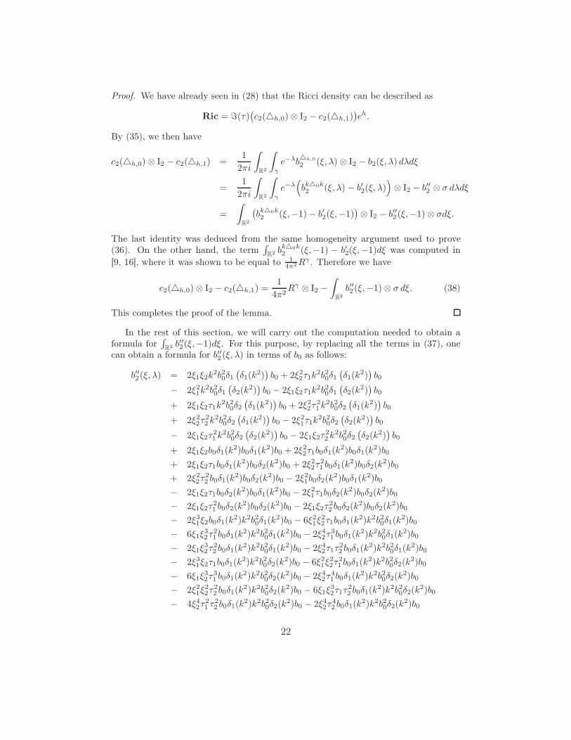
This completes the proof of the lemma.

In the rest of this section, we will carry out the computation needed to obtain aformula for

∫

R2 b′′2(ξ,−1)dξ. For this purpose, by replacing all the terms in (37), one

can obtain a formula for b′′2 (ξ, λ) in terms of b0 as follows:

b′′2(ξ, λ) = 2ξ1ξ2k2b20δ1

(

δ1(k2))

b0 + 2ξ22τ1k2b20δ1

(

δ1(k2))

b0

− 2ξ21k2b20δ1

(

δ2(k2))

b0 − 2ξ1ξ2τ1k2b20δ1

(

δ2(k2))

b0

+ 2ξ1ξ2τ1k2b20δ2

(

δ1(k2))

b0 + 2ξ22τ21 k

2b20δ2(

δ1(k2))

b0

+ 2ξ22τ22 k

2b20δ2(

δ1(k2))

b0 − 2ξ21τ1k2b20δ2

(

δ2(k2))

b0

− 2ξ1ξ2τ21 k

2b20δ2(

δ2(k2))

b0 − 2ξ1ξ2τ22 k

2b20δ2(

δ2(k2))

b0

+ 2ξ1ξ2b0δ1(k2)b0δ1(k

2)b0 + 2ξ22τ1b0δ1(k2)b0δ1(k

2)b0

+ 2ξ1ξ2τ1b0δ1(k2)b0δ2(k

2)b0 + 2ξ22τ21 b0δ1(k

2)b0δ2(k2)b0

+ 2ξ22τ22 b0δ1(k

2)b0δ2(k2)b0 − 2ξ21b0δ2(k

2)b0δ1(k2)b0

− 2ξ1ξ2τ1b0δ2(k2)b0δ1(k

2)b0 − 2ξ21τ1b0δ2(k2)b0δ2(k

2)b0

− 2ξ1ξ2τ21 b0δ2(k

2)b0δ2(k2)b0 − 2ξ1ξ2τ

22 b0δ2(k

2)b0δ2(k2)b0

− 2ξ31ξ2b0δ1(k2)k2b20δ1(k

2)b0 − 6ξ21ξ22τ1b0δ1(k

2)k2b20δ1(k2)b0

− 6ξ1ξ32τ

21 b0δ1(k

2)k2b20δ1(k2)b0 − 2ξ42τ

31 b0δ1(k

2)k2b20δ1(k2)b0

− 2ξ1ξ32τ

22 b0δ1(k

2)k2b20δ1(k2)b0 − 2ξ42τ1τ

22 b0δ1(k

2)k2b20δ1(k2)b0

− 2ξ31ξ2τ1b0δ1(k2)k2b20δ2(k

2)b0 − 6ξ21ξ22τ

21 b0δ1(k

2)k2b20δ2(k2)b0

− 6ξ1ξ32τ

31 b0δ1(k

2)k2b20δ2(k2)b0 − 2ξ42τ

41 b0δ1(k

2)k2b20δ2(k2)b0

− 2ξ21ξ22τ

22 b0δ1(k

2)k2b20δ2(k2)b0 − 6ξ1ξ

32τ1τ

22 b0δ1(k

2)k2b20δ2(k2)b0

− 4ξ42τ21 τ

22 b0δ1(k

2)k2b20δ2(k2)b0 − 2ξ42τ

42 b0δ1(k

2)k2b20δ2(k2)b0

22

+ 2ξ41b0δ2(k2)k2b20δ1(k

2)b0 + 6ξ31ξ2τ1b0δ2(k2)k2b20δ1(k

2)b0

+ 6ξ21ξ22τ

21 b0δ2(k

2)k2b20δ1(k2)b0 + 2ξ1ξ

32τ

31 b0δ2(k

2)k2b20δ1(k2)b0

+ 2ξ21ξ22τ

22 b0δ2(k

2)k2b20δ1(k2)b0 + 2ξ1ξ

32τ1τ

22 b0δ2(k

2)k2b20δ1(k2)b0

+ 2ξ41τ1b0δ2(k2)k2b20δ2(k

2)b0 + 6ξ31ξ2τ21 b0δ2(k

2)k2b20δ2(k2)b0

+ 6ξ21ξ22τ

31 b0δ2(k

2)k2b20δ2(k2)b0 + 2ξ1ξ

32τ

41 b0δ2(k

2)k2b20δ2(k2)b0

+ 2ξ31ξ2τ22 b0δ2(k

2)k2b20δ2(k2)b0 + 6ξ21ξ

22τ1τ

22 b0δ2(k

2)k2b20δ2(k2)b0

+ 4ξ1ξ32τ

21 τ

22 b0δ2(k

2)k2b20δ2(k2)b0 + 2ξ1ξ

32τ

42 b0δ2(k

2)k2b20δ2(k2)b0

− 4ξ31ξ2k2b20δ1(k

2)b0δ1(k2)b0 − 12ξ21ξ

22τ1k

2b20δ1(k2)b0δ1(k

2)b0

− 12ξ1ξ32τ

21 k

2b20δ1(k2)b0δ1(k

2)b0 − 4ξ42τ31 k

2b20δ1(k2)b0δ1(k

2)b0

− 4ξ1ξ32τ

22 k

2b20δ1(k2)b0δ1(k

2)b0 − 4ξ42τ1τ22 k

2b20δ1(k2)b0δ1(k

2)b0

+ 2ξ41k2b20δ1(k

2)b0δ2(k2)b0 + 4ξ31ξ2τ1k

2b20δ1(k2)b0δ2(k

2)b0

− 4ξ1ξ32τ

31 k

2b20δ1(k2)b0δ2(k

2)b0 − 2ξ42τ41 k

2b20δ1(k2)b0δ2(k

2)b0

− 4ξ1ξ32τ1τ

22 k

2b20δ1(k2)b0δ2(k

2)b0 − 4ξ42τ21 τ

22k

2b20δ1(k2)b0δ2(k

2)b0

+ 2ξ41k2b20δ2(k

2)b0δ1(k2)b0 − 2ξ42τ

42 k

2b20δ1(k2)b0δ2(k

2)b0

+ 4ξ31ξ2τ1k2b20δ2(k

2)b0δ1(k2)b0 − 4ξ1ξ

32τ

31 k

2b20δ2(k2)b0δ1(k

2)b0

− 4ξ1ξ32τ1τ

22 k

2b20δ2(k2)b0δ1(k

2)b0 − 2ξ42τ41 k

2b20δ2(k2)b0δ1(k

2)b0

− 4ξ42τ21 τ

22 k

2b20δ2(k2)b0δ1(k

2)b0 − 2ξ42τ42 k

2b20δ2(k2)b0δ1(k

2)b0

+ 4ξ41τ1k2b20δ2(k

2)b0δ2(k2)b0 + 12ξ31ξ2τ

21 k

2b20δ2(k2)b0δ2(k

2)b0

+ 12ξ21ξ22τ

31 k

2b20δ2(k2)b0δ2(k

2)b0 + 4ξ1ξ32τ

41 k

2b20δ2(k2)b0δ2(k

2)b0

+ 4ξ31ξ2τ22 k

2b20δ2(k2)b0δ2(k

2)b0 + 12ξ21ξ22τ1τ

22k

2b20δ2(k2)b0δ2(k

2)b0

+ 8ξ1ξ32τ

21 τ

22 k

2b20δ2(k2)b0δ2(k

2)b0 + 4ξ1ξ32τ

42 k

2b20δ2(k2)b0δ2(k

2)b0 .

In the above formula τ1 = ℜ(τ) and τ2 = ℑ(τ). We then change the variables (ξ1, ξ2)to the new variables (r, θ) via the transformation

ξ1 = r cos(θ)− rℜ(τ)ℑ(τ) sin(θ), ξ2 =

r

ℑ(τ) sin(θ).

This change of variable will change the volume form as follows:

dξ = (2π)−2dξ1dξ2 =1

(2π)2ℑ(τ) rdrdθ.

The integral b′′2(ξ,−1) with respect to θ ∈ [0, 2π] is equal to

r

(2π)2ℑ(τ)

∫ 2π

0

b′′2(ξ,−1)dθ =r

2πτ2

(

r2b0δ1(k2)b0δ2(k

2)b0 − r2b0δ2(k2)b0δ1(k

2)

−r4b0δ1(k2)k2b20δ2(k

2)b0 + r4b0δ2(k2)k2b20δ1(k

2)b0

)

.

We first write these expressions in terms of h/2 = log k. To do so, we will use thefollowing identities from [9]:

δj(k) = kf(∆)(δj(log(k))), f(u) =2(−1 +

√u)

log(u), (39)

23

and also ∆(ka) = k∆(a) and akn = kn∆n2 (a). Then we have,

δj(k2) = kδj(k) + δj(k)k

= kδj(k) + k∆1

2

(

δj(k))

= k(1 + ∆1

2 )(

δj(k))

= k(1 + ∆1

2 )(

kf(∆)(δj(log(k)))

= k2(1 + ∆1

2 )(

f(∆)(δj(log(k)))

= k2g(∆)(

δj(log(k))

.

where g(u) = 2(u−1)log(u) . We will also use the notation gj(u) = ujg(u).

There are only two different types of terms to be integrated with respect to the radialvariable r. To perform the integration, we will use the rearrangement lemma [9, Lemma6.2], which gives us

∫ ∞

0

r3b0δj(k2)b0δj′(k

2)b0dr

=

∫ ∞

0

r3b0δj(k2)b0k

2g(∆)(

δj′ (log(k)))

b0dr

=

∫ ∞

0

r3b0k2g(∆)

(

δj(log(k)))

k2b0g(∆)(

δj′ (log(k)))

b0dr

=

∫ ∞

0

r3b0k4g1(∆)

(

δj(log(k)))

b0g(∆)(

δj′(log(k)))

b0dr

=1

2F1,1,1(∆1,∆2)

(

g1(∆)(

δj(log(k)))

g(∆)(

δj′(log(k)))

)

.

Similarly,∫ ∞

0

r5b0δj(k2)k2b20δj′(k

2)b0dr

=

∫ ∞

0

r5b0k2g(∆)

(

δj(log(k)))

k2b20k2g(∆)

(

δj′(log(k)))

b0dr

=

∫ ∞

0

r5k6b0∆2g(∆)

(

δj(log(k)))

b20g(∆)(δj′ (log(k)))

b0dr

=1

2F1,2,1(∆1,∆2)

(

g2(∆)(

δj(log(k)))

g(∆)(

δj′(log(k)))

)

.

Note that

F111(es, et)g1(e

s)g(et)− F121(es, et)g2(e

s)g(et)

=(s+ t− t cosh(s)− s cosh(t)− sinh(s)− sinh(t) + sinh(s+ t))

s t(

sinh(

s2

)

sinh(

t2

)

sinh(

s+t2

)) ,

which is equal to the function S given in (30). Hence

∫ ∞

0

∫ 2π

0

b′′2(ξ,−1)1

(2π)2τ2rdrdθ =

1

4πτ2S(∇1,∇2)

(

[δ1(log k), δ2(log k)])

.

24

To compute the Ricci operator one could directly compute the second term a2 inthe asymptotic expansion of the heat kernel of the de Rham Laplacian using pseudod-ifferential calculus. This would involve substantial amount of computer aided symboliccalculations. Instead we have observed that our Laplcian is a first order perturbationof the Laplacian in [9, 16] (cf. formula (27)). With this observation, our calculationswere reduced to those carried in this section.

References

[1] Tanvir Ahamed Bhuyain and Matilde Marcolli, The Ricci flow on noncommutative

two-tori, Lett. Math. Phys. 101 (2012), no. 2, 173–194. MR 2947960

[2] Paula B. Cohen and Alain Connes, Conformal geomtry of the irrational roation

algebra, Priprint MPI/92-93.

[3] Alain Connes, C∗ algèbres et géométrie différentielle, C. R. Acad. Sci. Paris Sér.A-B 290 (1980), no. 13, A599–A604. MR 572645

[4] , Noncommutative geometry, Academic Press, Inc., San Diego, CA, 1994.MR 1303779

[5] , Noncommutative geometry and reality, J. Math. Phys. 36 (1995), no. 11,6194–6231. MR 1355905

[6] Alain Connes and Farzad Fathizadeh, The term a_4 in the heat kernel expansion

of noncommutative tori, arXiv:1611.09815 [math.QA] (2016).

[7] Alain Connes and Matilde Marcolli, Noncommutative geometry, quantum fields

and motives, American Mathematical Society Colloquium Publications, vol. 55,American Mathematical Society, Providence, RI; Hindustan Book Agency, NewDelhi, 2008. MR 2371808

[8] Alain Connes and Henri Moscovici, Type III and spectral triples, Traces in num-ber theory, geometry and quantum fields, Aspects Math., E38, Friedr. Vieweg,Wiesbaden, 2008, pp. 57–71. MR 2427588

[9] , Modular curvature for noncommutative two-tori, J. Amer. Math. Soc. 27

(2014), no. 3, 639–684. MR 3194491

[10] Alain Connes and Paula Tretkoff, The Gauss-Bonnet theorem for the noncommu-

tative two torus, Noncommutative geometry, arithmetic, and related topics, JohnsHopkins Univ. Press, Baltimore, MD, 2011, pp. 141–158. MR 2907006

[11] Ludwik Dabrowski and Andrzej Sitarz, An asymmetric noncommutative torus,SIGMA Symmetry Integrability Geom. Methods Appl. 11 (2015), Paper 075, 11.MR 3402793

[12] A. Fathi and M. Khalkhali, On Certain Spectral Invariants of Dirac Operators on

Noncommutative Tori, arXiv:1504.01174 [math.QA] (2015).

[13] Ali Fathi, Asghar Ghorbanpour, and Masoud Khalkhali, The Curvature of the De-

terminant Line Bundle on the Noncommutative Two Torus, To appear in Journalof Math. Phys. Anal. Geom., arXiv:1410.0475 [math.QA] (2014).

25

[14] Farzad Fathizadeh, On the scalar curvature for the noncommutative four torus, J.Math. Phys. 56 (2015), no. 6, 062303, 14. MR 3369894

[15] Farzad Fathizadeh and Masoud Khalkhali, The Gauss-Bonnet theorem for non-

commutative two tori with a general conformal structure, J. Noncommut. Geom.6 (2012), no. 3, 457–480. MR 2956317

[16] , Scalar curvature for the noncommutative two torus, J. Noncommut.Geom. 7 (2013), no. 4, 1145–1183. MR 3148618

[17] , Weyl’s law and Connes’ trace theorem for noncommutative two tori, Lett.Math. Phys. 103 (2013), no. 1, 1–18. MR 3004814

[18] , Scalar curvature for noncommutative four-tori, J. Noncommut. Geom. 9

(2015), no. 2, 473–503. MR 3359018

[19] Peter B. Gilkey, Invariance theory, the heat equation, and the Atiyah-Singer index

theorem, second ed., Studies in Advanced Mathematics, CRC Press, Boca Raton,FL, 1995. MR 1396308

[20] , Asymptotic formulae in spectral geometry, Studies in Advanced Mathe-matics, Chapman & Hall/CRC, Boca Raton, FL, 2004. MR 2040963

[21] M. Khalkhali, A. Moatadelro, and S. Sadeghi, A Scalar Curvature Formula For

the Noncommutative 3-Torus, arXiv:1610.04740 [math.OA] (2016).

[22] Masoud Khalkhali and Ali Moatadelro, A Riemann-Roch theorem for the non-

commutative two torus, J. Geom. Phys. 86 (2014), 19–30. MR 3282309

[23] Matthias Lesch and Henri Moscovici, Modular Curvature and Morita Equivalence,Geom. Funct. Anal. 26 (2016), no. 3, 818–873. MR 3540454

[24] Yang Liu, Modular curvature for toric noncommutative manifolds,arXiv:1510.04668 [math.QA] (2015).

Remus Floricel, Department of Mathematics and Statistics,University of Regina,

Regina, SK, Canada, S4S 0A2

E-mail address: Remus.Floricel@uregina.ca

Asghar Ghorbanpour,Department of Mathematics and Statistics,University of

Regina, Regina, SK, Canada, S4S 0A2

E-mail address:asghar.ghorbanpour@uregina.ca

Masoud Khalkhali, Department of Mathematics, University of Western On-

tario, London, Ontario, Canada, N6A 5B7

E-mail address: masoud@uwo.ca

26