Minimal surfaces and mean curvature flow - arXiv

Minimal surfaces and mean curvature

flow

Tobias H. Colding∗ and William P. Minicozzi II†

Abstract

We discuss recent results on minimal surfaces and mean curvature flow, focusingon the classification and structure of embedded minimal surfaces and the stablesingularities of mean curvature flow. This article is dedicated to Rick Schoen.

2000 Mathematics Subject Classification:

Keywords and Phrases:

c© Higher Education Pressand International PressBeijing-Boston

The title ofThis book*****ALM ?, pp. 1–?

1 Introduction

The main focus of this survey is on minimal surfaces and mean curvature flow,but to put these topics in perspective we begin with more elementary analysis ofthe energy of curves and functions. This leads us to first variation formulas forenergy and critical points for those. The critical points are of course geodesicsand harmonic functions, respectively. We continue by considering the gradient, orrather the negative gradient, flow for energy which leads us to the curve shorteningflow and the heat equation. Having touched upon these more elementary topics,we move on to one of our main topics which is minimal surfaces. We discuss firstand second variations for area and volume and the gradient (or rather negative)gradient flow for area and volume which is the mean curvature flow. Beginning aselementary as we do allows us later in the survey to draw parallels from the moreadvanced topics to the simpler ones.

The other topics that we cover are the Birkhoff min-max argument that pro-duces closed geodesics and its higher dimensional analog that gives existence ofclosed immersed minimal surfaces. We discuss stable and unstable critical pointsand index of critical points and eventually discuss the very recent classification ofall stable self-similar shrinkers for the mean curvature flow. For minimal surfaces,

∗MIT, Dept. of Math. 77 Massachusetts Avenue, Cambridge, MA 02139-4307.†Johns Hopkins University, Dept. of Math. 3400 N. Charles St. Baltimore, MD 21218

arX

iv:1

102.

1411

v1 [

mat

h.D

G]

7 F

eb 2

011

2 T. H. Colding and W. Minicozzi

stability and Liouville type theorems have played a major role in later devel-opments and we touch upon the Bernstein theorem that is the minimal surfaceanalog of the Liouville theorem for harmonic functions and the curvature estimatethat is the analog of the gradient estimate. We discuss various monotone quan-tities under curve shortening and mean curvature flow like Huisken’s volume, thewidth, and isoperimetric ratios of Gage and Hamilton. We explain why Huisken’smonotonicity leads to that blow ups of the flow at singular points in space timecan be modeled by self-similar flows and explain why the classification of stableself-similar flows is expected to play a key role in understanding of generic meancurvature flow where the flow begins at a hypersurface in generic position. One ofthe other main topics of this survey is that of embedded minimal surfaces wherewe discuss some of the classical examples going back to Euler and Monge’s studentMeusnier in the 18th century and the recent examples of Hoffman-Weber-Wolf andvarious examples that date in between. The final main results that we discuss arethe recent classification of embedded minimal surfaces and some of the uniquenessresults that are now known.

It is a great pleasure for us to dedicate this article to Rick Schoen.

2 Harmonic functions and the heat equation

We begin with a quick review of the energy functional on functions, where the criti-cal points are called harmonic functions and the gradient flow is the heat equation.This will give some context for the main topics of this survey, minimal surfacesand mean curvature flow, that are critical points and gradient flows, respectively,for the area functional.

2.1 Harmonic functions

Given a differentiable function u : Rn → R , the energy is defined to be

E(u) =1

2

∫|∇u|2 =

1

2

∫ (∣∣∣∣ ∂u∂x1

∣∣∣∣2 + · · ·+∣∣∣∣ ∂u∂xn

∣∣∣∣2). (1)

This gives a functional defined on the space of functions. We can construct a curvein the space of functions by taking a smooth function φ with compact support andconsidering the one-parameter family of functions u+ t φ . Restricting the energyfunctional to this curve gives

E(u+ tφ) =1

2

∫|∇(u+ t φ)|2 =

1

2

∫|∇u|2 + t

∫〈u,∇φ〉+

t2

2

∫|∇φ|2 . (2)

Differentiating at t = 0, we get that the directional derivative of the energy func-tional (in the direction φ) is

d

dt t=0E(u+ t φ) =

∫〈∇u,∇φ〉 = −

∫φ∆u , (3)

Minimal surfaces and MCF 3

where the last equality used the divergence theorem and the fact that φ has com-pact support. We conclude that:

Lemma 1. The directional derivative ddt t=0

E = 0 for all φ if and only if

∆u =∂2u

∂x21

+ · · ·+ ∂2u

∂x2n

= 0 . (4)

Thus, we see that the critical points for energy are the functions u with ∆u = 0;these are called harmonic functions. In fact, something stronger is true. Namely,harmonic functions are not just critical points for the energy functional, but areactually minimizers.

Lemma 2. If ∆u = 0 on a bounded domain Ω and φ vanishes on ∂Ω, then∫Ω

|∇(u+ φ)|2 =

∫Ω

|∇u|2 +

∫Ω

|∇φ|2 .

Proof. Since ∆u = 0 and φ vanishes on ∂Ω, the divergence theorem gives

0 =

∫Ω

div (φ∇u) =

∫Ω

〈∇φ,∇u〉 . (5)

So we conclude that∫Ω

|∇(u+ φ)|2 =

∫Ω

|∇u|2 + 2 〈∇φ,∇u〉+ |∇φ|2

=

∫Ω

|∇u|2 +

∫Ω

|∇φ|2 .

2.2 The heat equation

The heat equation is the (negative) gradient flow (or steepest descent) for theenergy functional. This means that we evolve a function u(x, t) over time in thedirection of its Laplacian ∆u, giving the linear parabolic heat equation

∂u

∂t= ∆u . (6)

Given any finite energy solution u of the heat equation that decays fast enoughto justify integrating by parts, the energy is non-increasing along the flow. In fact,we have

d

dtE(u) = −

∫∂u

∂t∆u = −

∫(∆u)2 .

Obviously, harmonic functions are fixed points, or static solutions, of the flow.


2.3 Negative gradient flows near a critical point

We are interested in the dynamical properties of the heat equation near a harmonicfunction. Before getting to this, it is useful to recall the simple finite dimensionalcase. Suppose therefore that f : R2 → R is a smooth function with a non-degenerate critical point at 0 (so ∇f(0) = 0 but the Hessian of f at 0 has rank 2).The behavior of the negative gradient flow

(x′, y′) = −∇f(x, y)

is determined by the Hessian of f at 0.The behavior depends on the index of the critical point, as is illustrated by the

following examples:

(Index 0): The function f(x, y) = x2 + y2 has a minimum at 0. The vector field is(−2x,−2y) and the flow lines are rays into the origin. Thus every flow linelimits to 0.

(Index 1): The function f(x, y) = x2−y2 has an index one critical point at 0. The vectorfield is (−2x, 2y) and the flow lines are level sets of the function h(x, y) = xy.Only points where y = 0 are on flow lines that limit to the origin.

(Index 2): The function f(x, y) = −x2 − y2 has a maximum at 0. The vector field is(2x, 2y) and the flow lines are rays out of the origin. Thus every flow linelimits to ∞ and it is impossible to reach 0.

Thus, we see that the critical point 0 is “generic”, or dynamically stable, if andonly if it has index 0. When the index is positive, the critical point is not genericand a “random” flow line will miss the critical point.

f(x, y) = x2 + y2 has a minimum at 0. Flow lines: Rays through the origin.


f(x, y) = x2− y2 has an index one critical point at 0. Flow lines: Level sets of xy.Only points where y = 0 limit to the origin.

2.4 Heat flow near a harmonic function

To analyze the dynamical properties of the heat flow, suppose first that u satisfiesthe heat equation on a bounded domain Ω with u = 0 on ∂Ω. By the maximumprinciple, a harmonic function that vanishes on ∂Ω is identically zero. Thus, weexpect that u limits towards 0. We show this next.

Since u = 0 on ∂Ω, applying the divergence theorem to u∇u gives∫Ω

|∇u|2 = −∫

Ω

u∆u .

Applying Cauchy-Schwarz and then the Dirichlet Poincare inequality gives(∫Ω

|∇u|2)2

≤∫

Ω

u2

∫Ω

(∆u)2 ≤ C

∫Ω

|∇u|2∫

Ω

(∆u)2.

Finally, dividing both sides by∫

Ω|∇u|2 gives

2E(t) ≡ 2 E(u(·, t)) =

∫Ω

|∇u|2 ≤ C∫

Ω

(∆u)2

= −C E′(t) ,

where C = C(Ω) is the constant from the Dirichlet Poincare inequality. Integratingthis gives that E(t) decays exponentially with

E(t) ≤ E(0) e−2C t .

Finally, another application of the Poincare inequality shows that∫u2(x, t) also

decays exponentially in t, as we expected.


If u does not vanish on ∂Ω, there is a unique harmonic function w with

u∣∣∂Ω

= w∣∣∂Ω.

It follows that (u − w) also solves the heat equation and is zero on ∂Ω. By theprevious argument, (u−w) decays exponentially and we conclude that all harmonicfunctions are attracting critical points of the flow. Since we have already shownthat harmonic functions are minimizers for the energy functional, and thus indexzero critical points, this is exactly what the finite dimensional toy model suggests.

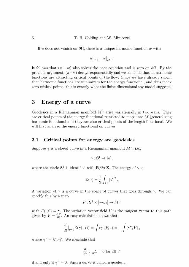
3 Energy of a curve

Geodesics in a Riemannian manifold Mn arise variationally in two ways. Theyare critical points of the energy functional restricted to maps into M (generalizingharmonic functions) and they are also critical points of the length functional. Wewill first analyze the energy functional on curves.

3.1 Critical points for energy are geodesics

Suppose γ is a closed curve in a Riemannian manifold Mn, i.e.,

γ : S1 →M ,

where the circle S1 is identified with R/2πZ. The energy of γ is

E(γ) =1

2

∫S1

|γ′|2 .

A variation of γ is a curve in the space of curves that goes through γ. We canspecify this by a map

F : S1 × [−ε, ε]→Mn

with F (·, 0) = γ. The variation vector field V is the tangent vector to this pathgiven by V = ∂F

∂t . An easy calculation shows that

d

dt

∣∣t=0

E(γ(·, t)) =

∫〈γ′, Fs,t〉 = −

∫〈γ′′, V 〉 ,

where γ′′ = ∇γ′γ′. We conclude that

d

dt

∣∣t=0

E = 0 for all V

if and only if γ′′ = 0. Such a curve is called a geodesic.


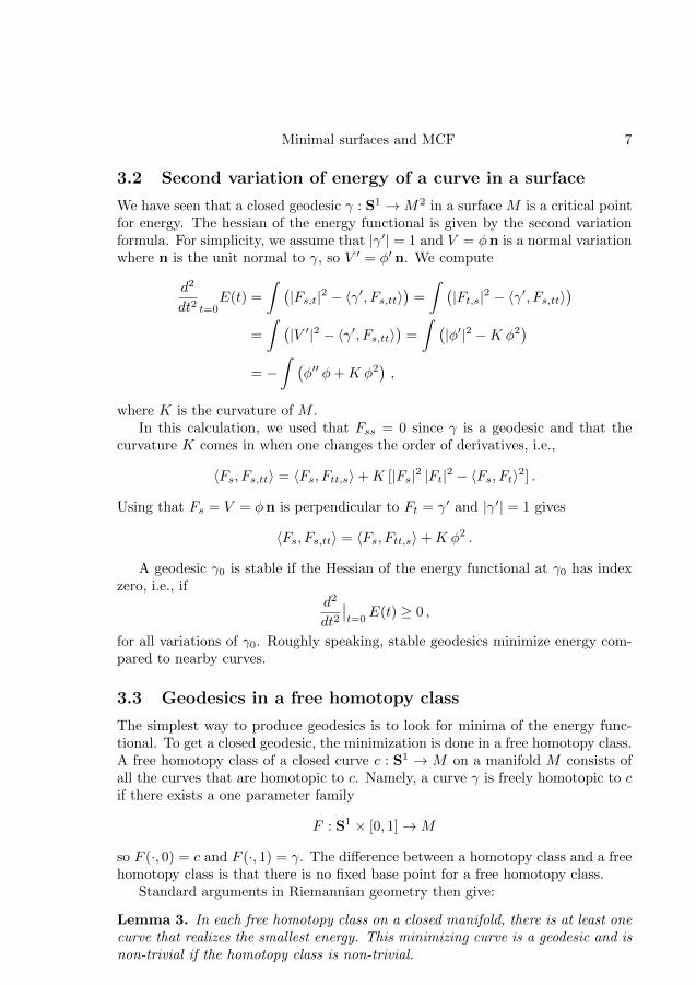
3.2 Second variation of energy of a curve in a surface

We have seen that a closed geodesic γ : S1 →M2 in a surface M is a critical pointfor energy. The hessian of the energy functional is given by the second variationformula. For simplicity, we assume that |γ′| = 1 and V = φn is a normal variationwhere n is the unit normal to γ, so V ′ = φ′ n. We compute

d2

dt2 t=0E(t) =

∫ (|Fs,t|2 − 〈γ′, Fs,tt〉

)=

∫ (|Ft,s|2 − 〈γ′, Fs,tt〉

)=

∫ (|V ′|2 − 〈γ′, Fs,tt〉

)=

∫ (|φ′|2 −K φ2

)= −

∫ (φ′′ φ+K φ2

),

where K is the curvature of M .In this calculation, we used that Fss = 0 since γ is a geodesic and that the

curvature K comes in when one changes the order of derivatives, i.e.,

〈Fs, Fs,tt〉 = 〈Fs, Ftt,s〉+K [|Fs|2 |Ft|2 − 〈Fs, Ft〉2] .

Using that Fs = V = φn is perpendicular to Ft = γ′ and |γ′| = 1 gives

〈Fs, Fs,tt〉 = 〈Fs, Ftt,s〉+K φ2 .

A geodesic γ0 is stable if the Hessian of the energy functional at γ0 has indexzero, i.e., if

d2

dt2∣∣t=0

E(t) ≥ 0 ,

for all variations of γ0. Roughly speaking, stable geodesics minimize energy com-pared to nearby curves.

3.3 Geodesics in a free homotopy class

The simplest way to produce geodesics is to look for minima of the energy func-tional. To get a closed geodesic, the minimization is done in a free homotopy class.A free homotopy class of a closed curve c : S1 → M on a manifold M consists ofall the curves that are homotopic to c. Namely, a curve γ is freely homotopic to cif there exists a one parameter family

F : S1 × [0, 1]→M

so F (·, 0) = c and F (·, 1) = γ. The difference between a homotopy class and a freehomotopy class is that there is no fixed base point for a free homotopy class.

Standard arguments in Riemannian geometry then give:

Lemma 3. In each free homotopy class on a closed manifold, there is at least onecurve that realizes the smallest energy. This minimizing curve is a geodesic and isnon-trivial if the homotopy class is non-trivial.


A torus (or donut) has genus 1.

Two curves in the same free homotopy class.

Figure 1: Freely homotopic curves.

4 Birkhoff: A closed geodesic on a two sphere

In the 1910s, Birkhoff came up with an ingenious method of constructing non-trivial closed geodesics on a topological 2-sphere. Since S2 is simply-connected,this cannot be done by minimizing in a free homotopy class. Birkhoff’s insteadused a min-max argument to find higher index critical points. We will describeBirkhoff’s idea and some related results in this section; see [B1], [B2] and section2 in [Cr] for more about Birkhoff’s ideas.

4.1 Sweepouts and the width

The starting point is a min-max construction that uses a non-trivial homotopyclass of maps from S2 to construct a geometric metric called the width. Later, wewill see that this invariant is realized as the length of a closed geodesic. Of course,one has to assume that such a non-trivial homotopy class exists (it does on S2,but not on higher genus surfaces; fortunately, it is easy to construct minimizerson higher genus surfaces).

Let Ω be the set of continuous maps

σ : S1 × [0, 1]→M

with the following three properties:

• For each t the map σ(·, t) is in W 1,2.

• The map t→ σ(·, t) is continuous from [0, 1] to W 1,2.

• σ maps S1 × 0 and S1 × 1 to points.


Figure 2: A sweepout.

Given a map σ ∈ Ω, the homotopy class Ωσ is defined to be the set of mapsσ ∈ Ω that are homotopic to σ through maps in Ω. The width W = W (σ)associated to the homotopy class Ωσ is defined by taking inf of max of the energyof each slice. That is, set

W = infσ∈Ωσ

maxt∈[0,1]

E (σ(·, t)) , (7)

where the energy is given by

E (σ(·, t)) =

∫S1

|∂xσ(x, t)|2 dx .

The width is always non-negative and is positive if σ is in a non-trivial homotopyclass.

A particularly interesting example is when M is a topological 2-sphere and theinduced map from S2 to M has degree one. In this case, the width is positiveand realized by a non-trivial closed geodesic. To see that the width is positiveon non-trivial homotopy classes, observe that if the maximal energy of a slice issufficiently small, then each curve σ(·, t) is contained in a convex geodesic ball inM . Hence, a geodesic homotopy connects σ to a path of point curves, so σ ishomotopically trivial.

4.2 Pulling the sweepout tight to obtain a closed geodesic

The key to finding the closed geodesic is to “pull the sweepout tight” using theBirkhoff curve shortening process (or BCSP). The BCPS is a kind of discrete


gradient flow on the space of curves. It is given by subdividing a curve and thenreplacing first the even segments by minimizing geodesics, then replacing the oddsegments by minimizing geodesics, and finally reparameterizing the curve so it hasconstant speed.

It is not hard to see that the BCSP has the following properties:

• It is continuous on the space of curves.

• Closed geodesics are fixed under the BCSP.

• If a curve is fixed under BCSP, then it is a geodesic.

It is possible to make each of these three properties quantitative.

6

5

2

4

3

1

1. Replace even segments by (red) geodesics.

1’

3’

5’

6

5

2

4

3

1

2. Replace odd segments by (blue) geodesics.

1’

3’

5’

Figure 3: Birkhoff’s curve shortening process.

Using this map and more refined versions of these properties, we showed theexistence of a sequence of tightened sweepouts:

Theorem 4. (Colding-Minicozzi, [CM2]) There exists a sequence of sweepouts γj

with the property that: Given ε > 0, there is δ > 0 so that if j > 1/δ and

2πE (γj(·, t0)) = Length2 (γj(·, t0)) > 2π (W − δ) , (8)

then for this j we have dist(γj(·, t0) , G

)< ε where G is the set of closed geodesics.

As an immediate consequence, we get the existence of non-trivial closed geodesicsfor any metric on S2; this is due to Birkhoff. See [LzWl] for an alternative proofusing the harmonic map heat flow.

4.3 Sweepouts by spheres

We will now define a two-dimensional version of the width, where we sweepout byspheres instead of curves. Let Ω be the set of continuous maps

σ : S2 × [0, 1]→M


Initial sweepout Tightened sweepout

Figure 4: Tightening the sweepout.

so that:

• For each t ∈ [0, 1] the map σ(·, t) is in C0 ∩W 1,2.

• The map t→ σ(·, t) is continuous from [0, 1] to C0 ∩W 1,2.

• σ maps S2 × 0 and S2 × 1 to points.

Given a map β ∈ Ω, the homotopy class Ωβ is defined to be the set of maps σ ∈ Ωthat are homotopic to β through maps in Ω. We will call any such β a sweepout .

The (energy) width WE = WE(β,M) associated to the homotopy class Ωβ isdefined by taking the infimum of the maximum of the energy of each slice. Thatis, set

WE = infσ∈Ωβ

maxt∈[0,1]

E (σ(·, t)) , (9)


E (σ(·, t)) =1

2

∫S2

|∇xσ(x, t)|2 dx . (10)

The next result gives the existence of a sequence of good sweepouts.

Theorem 5. (Colding-Minicozzi, [CM19]) Given a metric g on M and a map β ∈Ω representing a non-trivial class in π3(M), there exists a sequence of sweepoutsγj ∈ Ωβ with maxs∈[0,1] E(γjs)→W (g), and so that given ε > 0, there exist j andδ > 0 so that if j > j and

Area(γj(·, s)) > W (g)− δ , (11)

then there are finitely many harmonic maps ui : S2 →M with

dV (γj(·, s),∪iui) < ε . (12)


In (12), we have identified each map ui with the varifold associated to thepair (ui,S

2) and then taken the disjoint union of these S2’s to get ∪iui. Thedistance dV in (12) is a weak measure-theoretic distance called “varifold distance”;see [CM19] or Chapter 3 of [CM14] for the definition.

One immediate consequence of Theorem 5 is that if sj is any sequence withArea(γj(·, sj)) converging to the width W (g) as j → ∞, then a subsequence ofγj(·, sj) converges to a collection of harmonic maps from S2 to M . In particular,the sum of the areas of these maps is exactly W (g) and, since the maps areautomatically conformal, the sum of the energies is also W (g). The existence ofat least one non-trivial harmonic map from S2 to M was first proven in [SaUh],but they allowed for loss of energy in the limit; cf. also [St]. Ruling out thispossible energy loss in various settings is known as the “energy identity” and itcan be rather delicate. This energy loss was ruled out by Siu and Yau, using alsoarguments of Meeks and Yau (see Chapter VIII in [ScYa2]). This was also provenlater by Jost, [Jo].

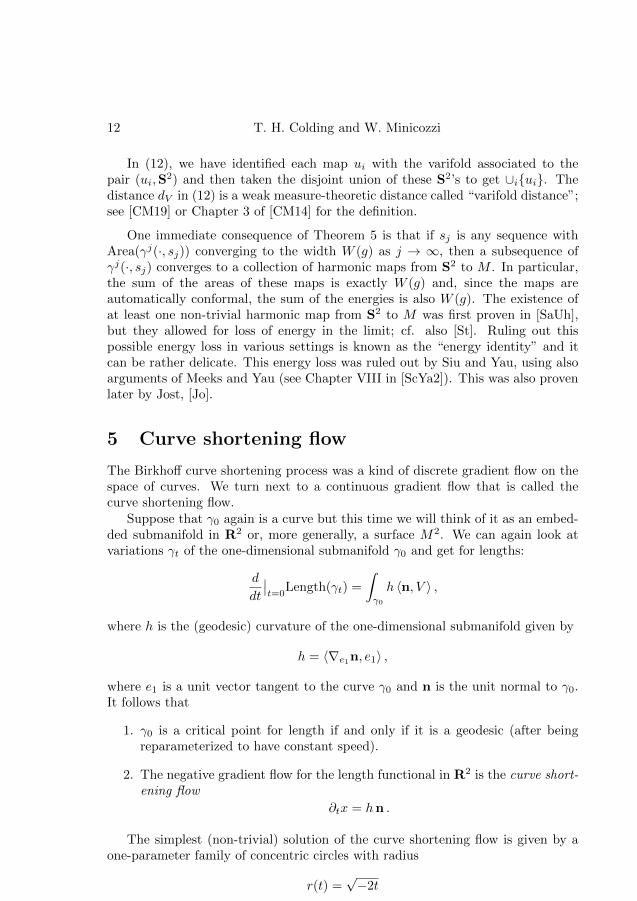
5 Curve shortening flow

The Birkhoff curve shortening process was a kind of discrete gradient flow on thespace of curves. We turn next to a continuous gradient flow that is called thecurve shortening flow.

Suppose that γ0 again is a curve but this time we will think of it as an embed-ded submanifold in R2 or, more generally, a surface M2. We can again look atvariations γt of the one-dimensional submanifold γ0 and get for lengths:

d

dt

∣∣t=0

Length(γt) =

∫γ0

h 〈n, V 〉 ,

where h is the (geodesic) curvature of the one-dimensional submanifold given by

h = 〈∇e1n, e1〉 ,

where e1 is a unit vector tangent to the curve γ0 and n is the unit normal to γ0.It follows that

1. γ0 is a critical point for length if and only if it is a geodesic (after beingreparameterized to have constant speed).

2. The negative gradient flow for the length functional in R2 is the curve short-ening flow

∂tx = hn .

The simplest (non-trivial) solution of the curve shortening flow is given by aone-parameter family of concentric circles with radius

r(t) =√−2t


Figure 5: Curve shortening flow: the curve evolves by its geodesic curvature. Thered arrows indicate direction of flow.

for t in (−∞, 0). This is an ancient solution since it is defined for all t < 0, it isself-similar since the shape is preserved (i.e., we can think of it as a fixed circlemoving under rigid motions of R2), and it becomes extinct at the origin in spaceand time.

5.1 Self-similar solutions

A solution of the curve shortening flow is self-similar if the shape does not changewith time. The simplest example is a static solution, like a straight line, that doesnot change at all. The next simplest is given by concentric shrinking circles, butthere are many other interesting possibilities. There are three types of self-similarsolutions that are most frequently considered:

• Self-similar shrinkers.

• Self-similar translators.

• Self-similar expanders.

We will explain shrinkers first. Suppose that ct is a one-parameter family ofcurves flowing by the curve shortening flow for t < 0. We say that ct is a self-similar shrinker if

ct =√−t c−1

for all t < 0. For example, circles of radius√−2t give such a solution. In 1986,

Abresch and Langer, [AbLa], classified such solutions and showed that the shrink-ing circles give the only embedded one (cf. Andrews, [An]). In 1987, Epstein-Weinstein, [EpW], showed a similar classification and analyzed the dynamics ofthe curve shortening flow near a shrinker.


Figure 6: Four snapshots in time of concentric circles shrinking under the curveshortening flow.

We say that ct is a self-similar translator if there is a constant vector V ∈ R2

so that

ct = c0 + t V

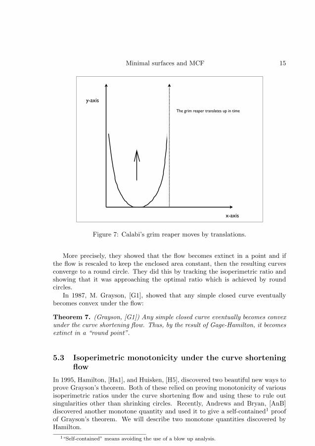
for all t ∈ R. These solutions are eternal in that they are defined for all time.It is easy to see that any translator must be non-compact. Calabi discovered aself-similar translator in the plane that he named the grim reaper . Calabi’s GrimReaper is given as the graph of the function

u(x, t) = t− log sinx .

Self-similar expanders are similar to shrinkers, except that they move by ex-panding dilations. In particular, the solutions are defined as t goes to +∞. It isnot hard to see that expanders must be non-compact.

There are other possible types of self-similar solutions, where the solutionsmove by one-parameter families of rigid motions over time. See Halldorsson, [Hh],for other self-similar solutions to the curve shortening flow.

5.2 Theorems of Gage-Hamilton and Grayson

In 1986, building on earlier work of Gage, [Ga1] and [Ga2], Gage and Hamiltonclassified closed convex solutions of the curve shortening flow:

Theorem 6. (Gage-Hamilton, [GaH]) Under the curve shortening flow every sim-ple closed convex curve remains smooth and convex and eventually becomes extinctin a “round point”.


y-axis

x-axis

The grim reaper translates up in time

2 TOBIAS H. COLDING AND WILLIAM P. MINICOZZI II

where x ! (0, !) and t ! [0,"). Note that #u(x, t) is a downward translating solution.More generally, a parabolic rescaling by " > 0 gives that the graph of

u!(x, t) =1

"u("x, "2t) = " t #

log sin("x)

", (0.6)

where x ! (0, !/"), is a translating solution flowing with speed "; see figure 1. Sincelimx!0

sinxx = 1, an easy calculation shows that for " > 0 su!ciently large

u!(e"!2

, 1) = " #log sin("e"!2

)

"$ 2" . (0.7)

x

#"!

y

#u!(x, 0)

"!

u!(x + "! , 0)

Figure 1. Two scaled grim reapers.

x

y

#3"

3"

w

u"

u+

Figure 2. Use u+ = u!(x + "! , t) # 3" and

u" = #u!(x, t) + 3" as barriers and let w bea graph between u+ and u".

Proposition 1. Given " > 1 su!ciently large, there is a solution w(x, t) on R % [0,") ofthe mean curvature flow with

3" < &w(·, 0)&# $ 4" , (0.8)

"e!2 $ max|x|$e!!2

|dw(x, 1)| . (0.9)

Proof. Define solutions u+(x, t) = u!(x + !/", t) # 3" for #!/" < x < 0 and u"(x, t) =#u!(x, t) + 3" for 0 < x < !/" of the mean curvature flow to be used as barriers. Sinceu+ ' #3" and u" $ 3", it is easy to choose (see figure 2) a smooth compactly supportedfunction w(·, 0) : R ( R satisfying (0.8) and so

w(x, 0) < u+(x, 0) for # !/" < x < 0 , (0.10)

u"(x, 0) < w(x, 0) for 0 < x < !/" . (0.11)

(We can choose w(·, 0) so that w(x, 0) = 0 for |x| > !/".) The existence results of [EH1]or [EH2] (see, e.g., theorem 1.7 in [E]) extend w(x, 0) to a solution w(x, t) of the meancurvature flow defined for x ! R and t ! [0,"); see figure 3. Moreover, the maximumprinciple extends (0.10) and (0.11) to all t ' 0. In particular, using this at x = ±e"!2

, t = 1

Figure 7: Calabi’s grim reaper moves by translations.

More precisely, they showed that the flow becomes extinct in a point and ifthe flow is rescaled to keep the enclosed area constant, then the resulting curvesconverge to a round circle. They did this by tracking the isoperimetric ratio andshowing that it was approaching the optimal ratio which is achieved by roundcircles.

In 1987, M. Grayson, [G1], showed that any simple closed curve eventuallybecomes convex under the flow:

Theorem 7. (Grayson, [G1]) Any simple closed curve eventually becomes convexunder the curve shortening flow. Thus, by the result of Gage-Hamilton, it becomesextinct in a “round point”.

5.3 Isoperimetric monotonicity under the curve shorteningflow

In 1995, Hamilton, [Ha1], and Huisken, [H5], discovered two beautiful new ways toprove Grayson’s theorem. Both of these relied on proving monotonicity of variousisoperimetric ratios under the curve shortening flow and using these to rule outsingularities other than shrinking circles. Recently, Andrews and Bryan, [AnB]discovered another monotone quantity and used it to give a self-contained1 proofof Grayson’s theorem. We will describe two monotone quantities discovered byHamilton.

1“Self-contained” means avoiding the use of a blow up analysis.


Figure 8: The snake manages to unwind quickly enough to become convex beforeextinction.

For both of Hamilton’s quantities, we start with a simple closed curve

c : S1 → R2 .

The image of c encloses a region in R2. Each simple curve γ inside this regionwith boundary in the image of c divides the region into two subdomains; let A1

and A2 be the areas of these subdomains and let L be the length of the dividingcurve γ.

Hamilton’s first quantity I is defined to be

I = infγ

L2

(1

A1+

1

A2

),

where the infimum is over all possible dividing curves γ.

Theorem 8. (Hamilton, [Ha1]) Under the curve shortening flow, I increases ifI ≤ π.

Hamilton’s second quantity J is defined to be

J = infγ

L

L0,

where the infimum is again taken over all possible dividing curves γ and the quan-tity L0 = L0(A1, A2) is the length of the shortest curve which divides a circle ofarea A1 +A2 into two pieces of area A1 and A2.

Theorem 9. (Hamilton, [Ha1]) Under the curve shortening flow, J always in-creases.


Figure 9: The minimizing curve γ inHamilton’s first isoperimetric quantity.

The curve c.

A circle enclosing the same area.

Figure 10: Defining the length L0 inHamilton’s second isoperimetric quan-tity.

We will give a rough idea why these theorems are related to Grayson’s theorem.Grayson had to rule out a singularity developing before the curve became convex.As you approach a singularity, the geodesic curvature h must be larger and larger.Since the curve is compact, one can magnify the curve just before this singular timeto get a new curve where the maximum of |h| is one. There is a blow up analysisthat shows that this dilated curve must look like a circle unless it is very longand skinny (like the grim reaper). Finally, a bound on any of these isoperimetricquantities rules out these long skinny curves.

6 Minimal surfaces

We turn next to higher dimensions and the variational properties of the areafunctional. Critical points of the area functional are called minimal surfaces. Inthis section, we will give a rapid overview of some of the basic properties of minimalsurfaces; see the book [CM14] for more details.

6.1 The first variation of area for surfaces

Let Σ0 be a hypersurface in Rn+1 and n its unit normal. Given a vector field

V : Σ→ Rn+1

with compact support, we get a one-parameter family of hypersurfaces

Σs = x+ s V (x) |x ∈ Σ0 .


The first variation of area (or volume) is

d

ds

∣∣s=0

Vol (Σs) =

∫Σ0

divΣ0V ,

where the divergence divΣ0is defined by

divΣ0V =

n∑i=1

〈∇eiV, ei〉 ,

where ei is an orthonormal frame for Σ. The vector field V can be decomposedinto the part V T tangent to Σ and the normal part V ⊥. The divergence of thenormal part V ⊥ = 〈V,n〉n is

divΣ0V ⊥ = 〈∇ei (〈V,n〉n) , ei〉 = 〈V,n〉〈∇ei n, ei〉 = H 〈V,n〉 ,

where the mean curvature scalar H is

H = divΣ0(n) =

n∑i=1

〈∇ein, ei〉 .

With this normalization, H is n/R on the n-sphere of radius R.

6.2 Minimal surfaces

By Stokes’ theorem, divΣ0V T integrates to zero. Hence, since divΣ0

V ⊥ = H 〈V,n〉,we can rewrite the first variation formula as

d

ds

∣∣s=0

Vol (Σs) =

∫Σ0

H 〈V,n〉 .

A hypersurface Σ0 is minimal when it is a critical point for the area functional,i.e., when the first variation is zero for every compactly supported vector field V .By the first variation formula, this is equivalent to H = 0.

6.3 Minimal graphs

If Σ is the graph of a function u : Rn → R, then the upward-pointing unit normalis given by

n =(−∇u, 1)√1 + |∇Rnu|2

, (13)

and the mean curvature of Σ is given by

H = −divRn

∇Rnu√1 + |∇Rnu|2

. (14)


MARCH 2003 NOTICES OF THE AMS 327

Disks That Are DoubleSpiral Staircases

Tobias H. Colding and William P. Minicozzi II*

What are the possible shapes of various thingsand why?

For instance, when a closed wire or a frame is dippedinto a soap solution and is raised up from the solu-tion, the surface spanning the wire is a soap film;see Figure I. What are the possible shapes of soapfilms and why? Or, for instance, why is DNA like a dou-ble spiral staircase? “What?” and “why?” are funda-mental questions and, when answered, help us un-derstand the world we live in.

The answer to any question about shape of natural objects is bound to involve mathematics, because as Galileo Galilei1 observed, the book ofNature is written in the characters of mathematics.

Soap films, soap bubbles, and surface tensionwere extensively studied by the Belgian physicistand inventor (of the stroboscope) Joseph Plateauin the first half of the nineteenth century. At leastsince his studies, it has been known that the rightmathematical models for soap films are minimalsurfaces: the soap film is in a state of minimum en-ergy when it is covering the least possible amountof area.

We will discuss here the answer to the question,What are the possible shapes of embedded mini-mal disks in R3 and why?

The field of minimal sur-faces dates back to the pub-lication in 1762 of La-grange’s famous memoir“Essai d’une nouvelle méth-ode pour déterminer lesmaxima et les minima desformules intégrales in-définies”. In a paper pub-lished in 1744 Euler had al-ready discussed minimizingproperties of the surfacenow known as the catenoid,but he considered only vari-ations within a certain classof surfaces. In the almostone quarter of a millenniumthat has passed since La-grange’s memoir, minimalsurfaces has remained a vibrant area of research andthere are many reasons why. The study of minimalsurfaces was the birthplace of regularity theory. Itlies on the intersection of nonlinear elliptic PDE,geometry, and low-dimensional topology, and overthe years the field has matured through the effortsof many people. However, some very fundamentalquestions remain. Moreover, many of the poten-tially spectacular applications of the field have yetto be achieved. For instance, it has long been thehope that several of the outstanding conjecturesabout the topology of 3-manifolds could be resolvedusing detailed knowledge of minimal surfaces.

Surfaces with uniform curvature (or area) boundshave been well understood, and the regularity the-ory is complete, yet essentially nothing was knownwithout such bounds. We discuss here the theory ofembedded minimal disks in R3 without a prioribounds. As we will see, the helicoid, which is a dou-ble spiral staircase, is the most important example

Tobias H. Colding is professor of mathematics at theCourant Institute of Mathematical Sciences. His email ad-dress is [email protected].

William P. Minicozzi II is professor of mathematics atJohns Hopkins University. His email address is [email protected].

*The article was written by Tobias H. Colding and is aboutjoint work of Colding and Minicozzi. Their research waspartially supported by NSF grants DMS 0104453 and DMS0104187.1Italian (from Pisa) Renaissance astronomer, mathemati-cian, and physicist (1564–1642).

Photo

grap

h c

ou

rtes

y of

Joh

n O

pre

a.

Figure I. The minimal surfacecalled the helicoid is a doublespiral staircase. The photo showsa spiral staircase—one half of ahelicoid—as a soap film.

Figure 11: The minimal surface called the helicoid is a double-spiral staircase.This photo shows half of a helicoid as a soap film.

Thus, minimal graphs are solutions of the nonlinear divergence-form PDE

divRn

∇Rnu√1 + |∇Rnu|2

= 0 . (15)

Every smooth hypersurface is locally graphical, so small pieces of a minimal surfacesatisfy this equation (over some plane).

In 1916, Bernstein proved that planes were the only entire solutions of theminimal surface equation:

Theorem 10. (Bernstein, [Be]) Any minimal graph over all of R2 must be flat(i.e., u is an affine function).

Remarkably, this theorem holds for n ≤ 7, but there are non-flat entire minimalgraphs in dimensions 8 and up.

The Bernstein theorem should be compared with the classical Liouville theoremfor harmonic functions:

Theorem 11. (Liouville) A positive harmonic function on Rn must be constant.


6.4 Consequences of the first variation formula

Suppose that Σ ⊂ Rn+1 is a hypersurface with normal n. Given f : Rn+1 → R,the Laplacian on Σ applied to f is

∆Σf ≡ divΣ(∇f)T =∑i=1

Hessf (ei, ei)− 〈∇f,n〉H , (16)

where ei is a frame for Σ and Hessf is the Rn+1 Hessian of f . We will use thisformula several times with different choices of f .

First, when f is the i-th coordinate function xi, (16) becomes

∆Σxi = −〈∂i,n〉H .

We see that:

Lemma 12. Σ is minimal ⇐⇒ all coordinate functions are harmonic.

Combining this with the maximum principle, we get Osserman’s convex hullproperty, [Os3]:

Proposition 13. If Σ is compact and minimal, then Σ is contained in the convexhull of ∂Σ.

Proof. If not, then we could choose translate and rotate Σ so that ∂Σ ⊂ x1 < 0but Σ contains a point p ∈ x1 > 0. However, the function x1 is harmonic on Σ,so the maximum principle implies that its maximum is on ∂Σ. This contradictionproved the proposition.

Applying (16) with f = |x|2 and noting that the Rn+1 Hessian of |x|2 is twicethe identity and the gradient is 2x, we see that

∆Σ|x|2 = 2n− 2 〈x,n〉H ,

when Σn ⊂ Rn+1 is a hypersurface. When Σ is minimal, this becomes

∆Σ|x|2 = 2n .

This identity is the key for the monotonicity formula:

Theorem 14. If Σ ⊂ Rn+1 is a minimal hypersurface, then

d

dr

Vol(Br ∩ Σ)

rn=

1

rn+1

∫∂Br∩Σ

∣∣x⊥∣∣2|xT |

≥ 0 .

Moreover, the density ratio is constant if and only if x⊥ ≡ 0; this is equivalentto Σ being a cone with its vertex at the origin (i.e., Σ is invariant with respect todilations about 0).


6.5 Examples of minimal surfaces

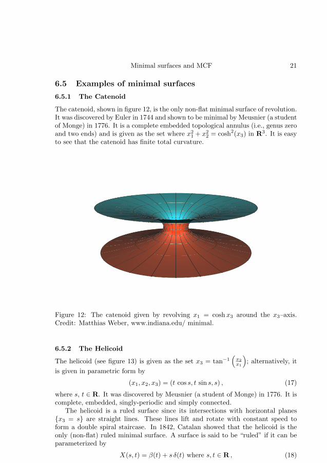
6.5.1 The Catenoid

The catenoid, shown in figure 12, is the only non-flat minimal surface of revolution.It was discovered by Euler in 1744 and shown to be minimal by Meusnier (a studentof Monge) in 1776. It is a complete embedded topological annulus (i.e., genus zeroand two ends) and is given as the set where x2

1 + x22 = cosh2(x3) in R3. It is easy

to see that the catenoid has finite total curvature.

Figure 12: The catenoid given by revolving x1 = coshx3 around the x3–axis.Credit: Matthias Weber, www.indiana.edu/ minimal.

6.5.2 The Helicoid

The helicoid (see figure 13) is given as the set x3 = tan−1(x2

x1

); alternatively, it

is given in parametric form by

(x1, x2, x3) = (t cos s, t sin s, s) , (17)

where s, t ∈ R. It was discovered by Meusnier (a student of Monge) in 1776. It iscomplete, embedded, singly-periodic and simply connected.

The helicoid is a ruled surface since its intersections with horizontal planesx3 = s are straight lines. These lines lift and rotate with constant speed toform a double spiral staircase. In 1842, Catalan showed that the helicoid is theonly (non-flat) ruled minimal surface. A surface is said to be “ruled” if it can beparameterized by

X(s, t) = β(t) + s δ(t) where s, t ∈ R , (18)


and β and δ are curves in R3. The curve β(t) is called the “directrix” of the surface,and a line having δ(t) as direction vector is called a “ruling”. For the standardhelicoid, the x3-axis is a directrix, and for each fixed t the line s→ (s cos t, s sin t, t)is a ruling.

Figure 13: The helicoid, with the ruling pictured. Credit: Matthias Weber,www.indiana.edu/ minimal.

6.5.3 The Riemann Examples

Around 1860, Riemann, [Ri], classified all minimal surfaces in R3 that are foliatedby circles and straight lines in horizontal planes. He showed that the only suchsurfaces are the plane, the catenoid, the helicoid, and a two-parameter family thatis now known as the Riemann examples. The surfaces that he discovered formeda family of complete embedded minimal surfaces that are singly-periodic and havegenus zero. Each of the surfaces has infinitely many parallel planar ends connectedby necks (“pairs of pants”).

Modulo rigid motions, this is a 2 parameter family of minimal surfaces. Theparameters are:


Figure 14: Two of the Riemann examples. The second one is starting to degenerateto helicoids. Credit: Matthias Weber, www.indiana.edu/ minimal.

• Neck size.

• Angle between period vector and the ends.

If we keep the neck size fixed and allow the angle to become vertical (i.e.,perpendicular to the planar ends), the family degenerates to a pair of oppositelyoriented helicoids. On the other hand, as the angle goes to zero, the family degen-erates to a catenoid.

6.5.4 The Genus One Helicoid

In 1993, Hoffman-Karcher-Wei gave numerical evidence for the existence of a com-plete embedded minimal surface with genus one that is asymptotic to a helicoid;they called it a “genus one helicoid”. In [HoWW], Hoffman, Weber and Wolfconstructed such a surface as the limit of “singly-periodic genus one helicoids”,where each singly-periodic genus one helicoid was constructed via the Weierstrassrepresentation. Later, Hoffman and White constructed a genus one helicoid vari-ationally in [HoWh1].

6.6 Second variation

Minimal surfaces are critical points for the area functional, so it is natural to lookat the second derivative of the area functional at a minimal surface. This is called


Figure 15: The genus one helicoid. Figure 16: A periodic minimal surfaceasymptotic to the helicoid, whose funda-mental domain has genus one.

Credit: Matthias Weber, www.indiana.edu/ minimal.

the second variation and it has played an important role in the subject since atleast the work of Simons, [Sim], in 1968.

To make this precise, let Σ0 be a 2-sided minimal hypersurface in Rn+1, n itsunit normal, f a function, and define the normal variation

Σs = x+ s f(x)n(x) |x ∈ Σ0 .

A calculation (see, e.g., [CM14]) shows that the second variation of area along thisone-parameter family of hypersurfaces is given by

d2

ds2

∣∣s=0

Vol (Σs) =

∫Σ0

|∇f |2 − |A|2 f2 = −∫

Σ0

f (∆ + |A|2) f , (19)

where A is the second fundamental form.When Σ0 is minimal in a Riemannian manifold M , the formula becomes

d2

ds2

∣∣s=0

Vol (Σs) =

∫Σ0

|∇f |2 − |A|2 f2 − RicM (n,n) f2 ,

where RicM is the Ricci curvature of M .A minimal surface Σ0 is stable when it passes the second derivative test, i.e.,

when

0 ≤ d2

ds2

∣∣s=0

Vol (Σs) = −∫

Σ0

f (∆ + |A|2) f ,

for every compactly supported variation Σs. Analytically, stability means that theJacobi operator ∆ + |A|2 is non-negative.

There is a useful analytic criterion to determine stability:


Proposition 15. (Fischer-Colbrie and Schoen, [FiSc]) A 2-sided minimal hy-persurface Σ ⊂ R3 is stable if and only if there is a positive function u with∆u = −|A|2 u.

Since the normal part of a constant vector field automatically satisfies theJacobi equation, we conclude that minimal graphs are stable. The same argumentimplies that minimal multi-valued graphs are stable.2

Stability is a natural condition given the variational nature of minimal surfaces,but one of the reasons that stability is useful is the following curvature estimateof R. Schoen, [Sc1]:

Theorem 16. (Schoen, [Sc1]) If Σ0 ⊂ R3 is stable and 2-sided and BR is ageodesic ball in Σ0, then

supBR

2

|A| ≤ C

R,

where C is a fixed constant.

When Σ0 is complete, we can let R go to infinity and conclude that Σ0 isa plane. This Bernstein theorem was proven independently by do Carmo-Peng,[dCP], and Fischer-Colbrie-Schoen, [FiSc].

See [CM15] for a different proof of Theorem 16 and a generalization to surfacesthat are stable for a parametric elliptic integrand. The key point for getting thecurvature estimate is to establish uniform area bounds just using stability:

Theorem 17. (Colding-Minicozzi, [CM15]) If Σ2 ⊂ R3 is stable and 2-sided andBr0 is simply-connected, then

Area (Br0) ≤ 4π

3r20 . (20)

The corresponding result is not known in higher dimensions, although Schoen,Simon and Yau proved curvature estimates assuming an area bound in low dimen-sions; see [ScSiY]. The counter-examples to the Bernstein problem in dimensionsseven and up show that such a bound can only hold in low dimensions. However,R. Schoen has conjectured that the Bernstein theorem and curvature estimateshould be true also for stable hypersurfaces in R4:

Conjecture 18. (Schoen) If Σ3 ⊂ R4 is a complete immersed 2-sided stableminimal hypersurface, then Σ is flat.

Conjecture 19. (Schoen) If Σ3 ⊂ Br0 = Br0(x) ⊂ M4 is an immersed 2-sidedstable minimal hypersurface where |KM | ≤ k2, r0 < ρ1(π/k, k), and ∂Σ ⊂ ∂Br0 ,then for some C = C(k) and all 0 < σ ≤ r0,

supBr0−σ

|A|2 ≤ C σ−2 . (21)

Any progress on these conjectures would be enormously important for thetheory of minimal hypersurfaces in R4.

2A multi-valued graph is a surface that is locally a graph over a subset of the plane, but theprojection down to the plane is not one to one.


7 Classification of embedded minimal surfaces

One of the most fundamental questions about minimal surfaces is to classify ordescribe the space of all complete embedded minimal surfaces in R3. We havealready seen three results of this type:

1. Bernstein showed that a complete minimal graph must be a plane.

2. Catalan showed that a ruled minimal surface is either a plane or a helicoid.

3. A minimal surface of revolution must be a plane or a catenoid.

Each of these theorems makes a rather strong hypothesis on the class of surfaces.It would be more useful to have classifications under weaker hypotheses, such asjust as the topological type of the surface.

The last decade has seen enormous progress on the classification of embeddedminimal surfaces in R3 by their topology. The surfaces are generally divided intothree cases, according to the topology:

• Disks.

• Planar domains - i.e., genus zero.

• Positive genus.

The classification of complete surfaces has relied heavily upon breakthroughson the local descriptions of pieces of embedded minimal surfaces with finite genus.

7.1 The topology of minimal surfaces

The topology of a compact connected oriented surface without boundary is de-scribed by a single non-negative number: the genus. The sphere has genus zero,the torus has genus one, and the connected sum of k-tori has genus k.

The genus of an oriented surface with boundary is defined to be the genusof the compact surface that you get by gluing in a disk along each boundarycomponent. Since an annulus with two disks glued in becomes a sphere, theannulus has genus zero. Thus, the topology of a connected oriented surface withboundary is described by two numbers: the genus and the number of boundarycomponents.

The last topological notion that we will need is properness. An immersedsubmanifold Σ ⊂M is proper when the intersection of Σ with any compact set inM is compact. Clearly, every compact submanifold is automatically proper.

There are two important monotonicity properties for the topology of minimalsurfaces in R3; one does not use minimality and one does.

Lemma 20. If Σ has genus k and Σ0 ⊂ Σ, then the genus of Σ0 is at most k.

Proof. This follows immediately from the definition of the genus and does not useminimality.


Lemma 21. If Σ ⊂ R3 is a properly embedded minimal surface and BR(0)∩∂Σ =∅, then the inclusion of BR(0)∩Σ into Σ is an injection on the first homology group.

Proof. If not, then BR(0)∩Σ contains a one-cycle γ that does not bound a surfacein BR(0) ∩ Σ but does bound a surface Γ ⊂ Σ. However, Γ is then a minimalsurface that must leave BR(0) but with ∂Γ ⊂ BR(0), contradicting the convexhull property (Proposition 13).

This has the following immediate corollary for disks:

Corollary 22. If Σ is a properly embedded minimal disk, then each component ofBR(0) ∩ Σ is a disk.

7.2 Multi-valued graphs

We will need the notion of a multi-valued graph from [CM6]–[CM9]. At a first ap-proximation, a multi-valued graph is locally a graph over a subset of the plane butthe projection down is not one to one. Thus, it shares many properties with min-imal graphs, including stability, but includes new possibilities such as the helicoidminus the vertical axis.

To be precise, let Dr be the disk in the plane centered at the origin and ofradius r and let P be the universal cover of the punctured plane C \ 0 withglobal polar coordinates (ρ, θ) so ρ > 0 and θ ∈ R. Given 0 ≤ r ≤ s and θ1 ≤ θ2,define the “rectangle” Sθ1,θ2r,s ⊂ P by

Sθ1,θ2r,s = (ρ, θ) | r ≤ ρ ≤ s , θ1 ≤ θ ≤ θ2 . (22)

An N -valued graph of a function u on the annulus Ds \Dr is a single valued graphover

S−Nπ,Nπr,s = (ρ, θ) | r ≤ ρ ≤ s , |θ| ≤ N π . (23)

(Σθ1,θ2r,s will denote the subgraph of Σ over the smaller rectangle Sθ1,θ2r,s ). Themulti-valued graphs that we will consider will never close up; in fact they willall be embedded. Note that embedded corresponds to that the separation nevervanishes. Here the separation w is the difference in height between consecutivesheets and is therefore given by

w(ρ, θ) = u(ρ, θ + 2π)− u(ρ, θ) . (24)

In the case where Σ is the helicoid [i.e., Σ can be parametrized by (s cos t, s sin t, t)where s, t ∈ R], then

Σ \ x3 − axis = Σ1 ∪ Σ2 , (25)

where Σ1, Σ2 are ∞-valued graphs. Σ1 is the graph of the function u1(ρ, θ) = θand Σ2 is the graph of the function u2(ρ, θ) = θ+ π. In either case the separationw = 2π.

Note that for an embedded multi–valued graph, the sign of w determineswhether the multi–valued graph spirals in a left–handed or right–handed manner,in other words, whether upwards motion corresponds to turning in a clockwisedirection or in a counterclockwise direction.


Figure 17: Multi–valued graphs. The helicoid is obtained by gluing together two∞–valued graphs along a line. Credit: Matthias Weber, www.indiana.edu/ mini-mal.


PLANAR DOMAINS 9

x3-axis

u(!, ")

u(!, " + 2#)

w

Figure 8. The separation w for amulti-valued graph in (II.1.1).

Interior boundary B1/4 ! $!.

z1

B1B! BR/!

! contains a large “flat region” betweenB! and BR/!. Since ! is embedded,this either (1) closes up to give a graphicalannulus or (2) spirals to give an N -valued graph.

Figure 9. Theorem II.1.2: Embed-ded stable annuli with small interiorboundary contain either (1) a graphi-cal annulus or (2) an N -valued graphaway from its boundary.

(1) Each component of BR/! ! ! \ B! is a graph with gradient " % .

(2) ! contains a graph !!N",N"!,R/! with gradient " % and dist!\!1(#)(z1, !0,0

!,!) < d0.

Note that if ! is as in Theorem II.1.2 and one component of BR/!!!\B! contains a graphover DR/(2!) \D2! with gradient " 1, then every component of BR/(C!) ! ! \BC! is a graphfor some C > 1. Namely, embeddedness and the gradient estimate (which applies because ofstability) would force any nongraphical component to spiral indefinitely, contradicting that! is compact. Thus it is enough to find one component that is a graph. This we be usedbelow.

We will eventually show in Section II.3 that (2) in Theorem II.1.2 does not happen; thusevery component is a (single-valued) graph. This will easily give Theorem 0.3.

&1

&2

'1

Geodesics.

"0n

&2(0)

$"0 \ ('1 # &1 # &2)

&1(0)

Figure 10. The subdomain "0 $ "in Lemma II.1.3 and below.

See fig. 10. Throughout this section (except in Corollary II.1.34), " $ R3 will be anembedded minimal planar domain (if the domain is stable, then we use ! instead of "),"0 $ " a subdomain and &1, &2, '1 $ $"0 curves (&1, &2 geodesics) so &1#&2#'1 is a simplecurve and &i(0) % '1. (By a geodesic we will mean a curve with zero geodesic curvature.

Figure 18: The separation w for a multi–valued minimal graph.


7.3 Disks are double spiral staircases or graphs

We will describe first the local classification of properly embedded minimal disksthat follows from [CM6]–[CM9]. This turns out to be the key step for under-standing embedded minimal surfaces with finite genus since any of these can bedecomposed into pieces that are either disks or pairs of pants.

There are two classical models for embedded minimal disks. The first is aminimal graph over a simply-connected domain in R2 (such as the plane itself),while the second is a double spiral staircase like the helicoid. A double spiralstaircase consists of two staircases that spiral around one another so that twopeople can pass each other without meeting.

In [CM6]–[CM9] we showed that these are the only possibilities and, in fact,every embedded minimal disk is either a minimal graph or can be approximatedby a piece of a rescaled helicoid. It is graph when the curvature is small and ispart of a helicoid when the curvature is above a certain threshold.

328 NOTICES OF THE AMS VOLUME 50, NUMBER 3

of such a disk. In fact, we will see that every em-bedded minimal disk is either a graph of a func-tion or is part of a double spiral staircase. Thehelicoid was discovered to be a minimal surfaceby Meusnier in 1776.

However, before discussing minimal disks wewill give some examples of where one can finddouble spiral staircases and structures.

Double Spiral StaircasesA double spiral staircase consists of two staircasesthat spiral around one another so that two peo-ple can pass each other without meeting. Figure

II shows Leonardo da Vinci’s double spiral stair-case in Château de Chambord in the Loire Valleyin France. The construction of the castle beganin 1519 (the same year that Leonardo da Vincidied) and was completed in 1539. In Figure IIIwe see a model of the staircase where we canclearly see the two staircases spiraling aroundone another. The double spiral staircase has,with its simple yet surprising design, fascinatedand inspired many people. We quote here fromMademoiselle de Montpensier’s2 memoirs.

“One of the most peculiar and remarkablethings about the house [the castle at Chambord]are the stairs, which are made so that one per-son can ascend and another descend withoutmeeting, yet they can see each other. Monsieur[Gaston of Orléans, the father of Mademoisellede Montpensier] amused himself by playingwith me. He would be at the top of the stairswhen I arrived; he would descend when I wasascending, and he would laugh when he saw merun in the hope of catching him. I was happywhen he was amused and even more when Icaught him.”

Leonardo da Vinci had many ideas for designsinvolving double spiral staircases. Two of hismain interests were water flow and military in-struments. For Leonardo everything was con-nected, from the braiding of a girl's hair (see forinstance the famous drawing of Leda and theswan) to the flow of water (which also exhibitsa double spiral behavior when it passes an ob-stacle like the branch of a tree). He designed wa-ter pumps that were formed as double spiralstaircases that supposedly would pump moreefficiently than the more standard Archimedeanpump then in use. He designed fire escapesformed as double (and greater multiples) spiralstaircases where each staircase was inap-proachable from another, thus preventing thefire from jumping from one staircase to an-

Figure II. Leonardo da Vinci’s double spiralstaircase in Château de Chambord.

Figure III. A modelof da Vinci’s

staircase.

Figure IV. Drawing by Leonardo da Vinci from around 1487–90.

2Duchess Montpensier (1627-1693), princess of theroyal house of France and author, who played a keyrole in the revolts known as the Fronde.


of such a disk. In fact, we will see that every em-bedded minimal disk is either a graph of a func-tion or is part of a double spiral staircase. Thehelicoid was discovered to be a minimal surfaceby Meusnier in 1776.

However, before discussing minimal disks wewill give some examples of where one can finddouble spiral staircases and structures.

Double Spiral StaircasesA double spiral staircase consists of two staircasesthat spiral around one another so that two peo-ple can pass each other without meeting. Figure

II shows Leonardo da Vinci’s double spiral stair-case in Château de Chambord in the Loire Valleyin France. The construction of the castle beganin 1519 (the same year that Leonardo da Vincidied) and was completed in 1539. In Figure IIIwe see a model of the staircase where we canclearly see the two staircases spiraling aroundone another. The double spiral staircase has,with its simple yet surprising design, fascinatedand inspired many people. We quote here fromMademoiselle de Montpensier’s2 memoirs.

“One of the most peculiar and remarkablethings about the house [the castle at Chambord]are the stairs, which are made so that one per-son can ascend and another descend withoutmeeting, yet they can see each other. Monsieur[Gaston of Orléans, the father of Mademoisellede Montpensier] amused himself by playingwith me. He would be at the top of the stairswhen I arrived; he would descend when I wasascending, and he would laugh when he saw merun in the hope of catching him. I was happywhen he was amused and even more when Icaught him.”

Leonardo da Vinci had many ideas for designsinvolving double spiral staircases. Two of hismain interests were water flow and military in-struments. For Leonardo everything was con-nected, from the braiding of a girl's hair (see forinstance the famous drawing of Leda and theswan) to the flow of water (which also exhibitsa double spiral behavior when it passes an ob-stacle like the branch of a tree). He designed wa-ter pumps that were formed as double spiralstaircases that supposedly would pump moreefficiently than the more standard Archimedeanpump then in use. He designed fire escapesformed as double (and greater multiples) spiralstaircases where each staircase was inap-proachable from another, thus preventing thefire from jumping from one staircase to an-

Figure II. Leonardo da Vinci’s double spiralstaircase in Château de Chambord.

Figure III. A modelof da Vinci’s

staircase.

Figure IV. Drawing by Leonardo da Vinci from around 1487–90.

2Duchess Montpensier (1627-1693), princess of theroyal house of France and author, who played a keyrole in the revolts known as the Fronde.

Figure 19: Left: Drawing by Leonardo Da Vinci of a double spiral staircase fromaround 1490. Right: Model of Da Vinci’s double spiral staircase in Chateau deChambord. Both figures reprinted from [CM20].


The main point in the proof is to show the double spiral staircase structurewhen the curvature is large. The proof of this is long, but can be split into threemain steps.

Three main steps.

A. Fix an integer N (the “large” of the curvature in what follows will dependon N). If an embedded minimal disk Σ is not a graph (or equivalently if thecurvature is large at some point), then it contains an N -valued minimal graphwhich initially is shown to exist on the scale of 1/max |A|. That is, the N -valuedgraph is initially shown to be defined on an annulus with both inner and outerradius inversely proportional to max |A|.B. Such a potentially small N -valued graph sitting inside Σ can then be seen toextend as an N -valued graph inside Σ almost all the way to the boundary. Thatis, the small N -valued graph can be extended to an N -valued graph defined on anannulus where the outer radius of the annulus is proportional to R. Here R is theradius of the ball in R3 that the boundary of Σ is contained in.

C. The N -valued graph not only extends horizontally (i.e., tangent to the initialsheets) but also vertically (i.e., transversally to the sheets). That is, once there areN sheets there are many more and, in fact, the disk Σ consists of two multi-valuedgraphs glued together along an axis.

The multivalued graphs that we will consider willall be embedded, which corresponds to a nonvan-ishing separation between the sheets (or the floors).Here the separation is the function (see Figure 2)

(8) w (!,") = u(!," + 2# )! u(!,").

If ! is the helicoid, then ! \ x3-axis = !1 " !2,where !1 and !2 are #-valued graphs on C \ 0.!1 is the graph of the function u1(!,") = " , and !2

is the graph of the function u2(!,") = " +#. (!1 isthe subset where s > 0 in (7), and !2 is the subsetwhere s < 0.) In either case the separation w = 2#.A multivalued minimal graph is a multivaluedgraph of a function u satisfying the minimal sur-face equation.

Note that for an embedded multivalued graph,the sign of w determines whether the multivaluedgraph spirals in a left-handed or a right-handedmanner, in other words, whether upwards motioncorresponds to turning in a clockwise direction orin a counterclockwise direction. For DNA, althoughboth spirals occur, the right-handed spiral is farmore common, because of certain details of thechemical structure; see [CaDr].

As we will see, a fundamental theorem about em-bedded minimal disks is that such a disk is eithera minimal graph or can be approximated by a pieceof a rescaled helicoid, depending on whether thecurvature is small or not; see Theorem 1 below. Toavoid tedious details about the dependence of var-ious quantities, we state this, our main result, notfor a single embedded minimal disk with suffi-ciently large curvature at a given point, but insteadfor a sequence of such disks where the curvaturesare blowing up. Theorem 1 says that a sequence ofembedded minimal disks mimics the following be-havior of a sequence of rescaled helicoids.

Consider a sequence !i = ai! ofrescaled helicoids, where ai $ 0. (Thatis, rescale R3 by ai, so points that usedto be distance d apart will in the rescaledR3 be distance ai d apart.) The curva-tures of this sequence of rescaled heli-coids are blowing up along the verticalaxis. The sequence converges (awayfrom the vertical axis) to a foliation byflat parallel planes. The singular set S(the axis) then consists of removablesingularities.

Throughout let x1, x2, x3 be the standard coor-dinates on R3 . For y % ! & R3 and s > 0 , theextrinsic and intrinsic balls are Bs (y) and Bs (y):namely, Bs (y) = x % R3 | |x! y| < s , and Bs (y) =x % ! | dist!(x, y) < s . The Gaussian curvatureof ! & R3 is K! = $1$2 , so if ! is minimal (i.e.,$1 = !$2), then |A|2 = !2K! .


See [CM1], [O], [S] (and the forthcoming book[CM3]) for background and basic properties of min-imal surfaces and [CM2] for a more detailed surveyof the results described here and for references. Seealso [C] for an abbreviated version of this paper in-tended for a general nonmathematical audience. Thearticle [A] discusses in a simple nontechnical waythe shape of various things that are of “minimal”type. These shapes include soap films and soap bubbles, metal alloys, radiolarian skeletons, and embryonic tissues and cells; see also D’ArcyThompson’s influential book, [Th], about form. The reader interested in some of the history of the field of minimal surfaces may consult [DHKW],[N], and [T].

The Limit Foliation and the Singular Curve In the next few sections we will discuss how to showthat every embedded minimal disk is either a graphof a function or part of a double spiral staircase;Theorem 1 below gives precise meaning to thisstatement. In particular, we will in the next few sections discuss the following (see Figure 3).

A. Fix an integer N (the meaning of “large” cur-vature in what follows will depend on N). If an embedded minimal disk ! is not a graph (or equivalently, if the curvature is large at some point),then it contains an N-valued minimal graph, whichinitially is shown to exist on the scale of 1/max |A|.That is, the N-valued graph is initially shown to bedefined on an annulus with both inner and outerradius inversely proportional to max |A| .

B. Such a potentially small N-valued graph sittinginside ! can then be seen to extend as an N-valuedgraph inside ! almost all the way to the boundary.That is, the small N-valued graph can be extended toan N-valued graph defined on an annulus whoseouter radius is proportional to the radius R of the ballin R3 whose boundary contains the boundary of ! .

C. The N-valued graph not only extends hori-zontally (i.e., tangent to the initial sheets) but alsovertically (i.e., transversally to the sheets). That is,once there are N sheets there are many more, andthe disk ! in fact consists of two multivaluedgraphs glued together along an axis.

A.

C.

B.

BR

Figure 3. Proving Theorem 1. A) Finding a smallN-valued graph in ! . B) Extending it in ! to a

large N-valued graph. C) Extending the numberof sheets.Figure 20: Three main steps: A. Finding a small N -valued graph in Σ. B. Ex-

tending it in Σ to a large N -valued graph. C. Extend the number of sheets.

This general structure result for embedded minimal disks, and the methodsused in its proof, give a compactness theorem for sequences of embedded minimaldisks. This theorem is modelled on rescalings of the helicoid and the precise


statement is as follows (we state the version for extrinsic balls; it was extended tointrinsic balls in [CM12]):

Theorem 23. (Theorem 0.1 in [CM9].) Let Σi ⊂ BRi = BRi(0) ⊂ R3 be asequence of embedded minimal disks with ∂Σi ⊂ ∂BRi where Ri →∞. If

supB1∩Σi

|A|2 →∞ , (26)

then there exists a subsequence, Σj, and a Lipschitz curve S : R → R3 such thatafter a rotation of R3:

1. x3(S(t)) = t. (That is, S is a graph over the x3-axis.)

2. Each Σj consists of exactly two multi-valued graphs away from S (whichspiral together).

3. For each 1 > α > 0, Σj \ S converges in the Cα-topology to the foliation,F = x3 = tt, of R3.

4. supBr(S(t))∩Σj |A|2 →∞ for all r > 0, t ∈ R. (The curvatures blow up along

S.)

This theorem is sometimes referred to as the lamination theorem. Meeksshowed in [Me2] that the Lipschitz curve S is in fact a straight line perpendic-ular to the foliation.

The assumption that the radii Ri go to infinity is used in several ways in theproof. This guarantees that the leaves are planes (this uses the Bernstein theorem),but it also is used to show that the singularities are removable. We will see in thenext subsection that this is not always the case in the “local case” where the Riremain bounded.

7.4 The local case

In contrast to the global case of the previous subsection, there are local examplesof sequence of minimal surfaces that do not converge to a foliation. The first suchexample was constructed in [CM17], where we constructed a sequence of embeddedminimal disks in a unit ball in R3 so that:

• Each contains the x3-axis.

• Each is given by two multi-valued graphs over x3 = 0 \ 0.

• The graphs spiral faster and faster near x3 = 0.

The precise statement is:

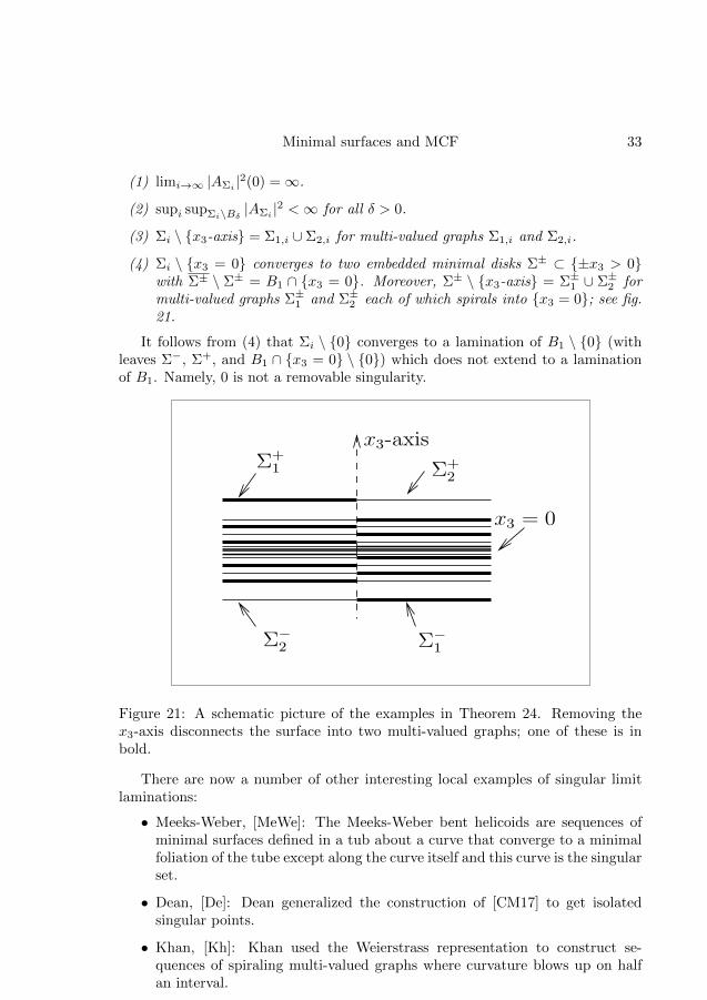
Theorem 24. (Colding-Minicozzi, [CM17]) There is a sequence of compact em-bedded minimal disks 0 ∈ Σi ⊂ B1 ⊂ R3 with ∂Σi ⊂ ∂B1 and containing thevertical segment (0, 0, t) | |t| < 1 ⊂ Σi so:


(1) limi→∞ |AΣi |2(0) =∞.

(2) supi supΣi\Bδ |AΣi |2 <∞ for all δ > 0.

(3) Σi \ x3-axis = Σ1,i ∪ Σ2,i for multi-valued graphs Σ1,i and Σ2,i.

(4) Σi \ x3 = 0 converges to two embedded minimal disks Σ± ⊂ ±x3 > 0with Σ± \ Σ± = B1 ∩ x3 = 0. Moreover, Σ± \ x3-axis = Σ±1 ∪ Σ±2 formulti-valued graphs Σ±1 and Σ±2 each of which spirals into x3 = 0; see fig.21.

It follows from (4) that Σi \ 0 converges to a lamination of B1 \ 0 (withleaves Σ−, Σ+, and B1 ∩ x3 = 0 \ 0) which does not extend to a laminationof B1. Namely, 0 is not a removable singularity.


Figure 1. The limit in a ball of a se-quence of degenerating helicoids is afoliation by parallel planes. This issmooth and proper.

!+1

!!2 !!

1

x3 = 0

x3-axis

!+2

Figure 2. A schematic picture of thelimit in Theorem 1 which is not smoothand not proper (the dotted x3-axis ispart of the limit). The limit containsfour multi-valued graphs joined at thex3-axis; !+

1 , !+2 above the plane x3 = 0

and !!1 , !!

2 below the plane. Each ofthe four spirals into the plane.

x3-axis

u(!, ")

u(!, " + 2#)

Figure 3. A multi-valued graph of afunction u.

Theorem 1. There is a sequence of compact embedded minimal disks 0 ! !i "B1 " R3 with !!i " !B1 and containing the vertical segment (0, 0, t) | |t| < 1 "!i, and such that the following conditions are satisfied:

(1) limi"# |A!i |2(0) = #.(2) supi sup!i\B!

|A!i |2 < # for all " > 0.(3) !i \ x3-axis = !1,i $ !2,i for multi-valued graphs !1,i and !2,i.(4) !i \ x3 = 0 converges to two embedded minimal disks !± " ±x3 > 0

with !± \ !± = B1 % x3 = 0. Moreover, !± \ x3-axis = !±1 $ !±

2 formulti-valued graphs !±

1 and !±2 each of which spirals into x3 = 0; see

Figure 2.

Figure 21: A schematic picture of the examples in Theorem 24. Removing thex3-axis disconnects the surface into two multi-valued graphs; one of these is inbold.

There are now a number of other interesting local examples of singular limitlaminations:

• Meeks-Weber, [MeWe]: The Meeks-Weber bent helicoids are sequences ofminimal surfaces defined in a tub about a curve that converge to a minimalfoliation of the tube except along the curve itself and this curve is the singularset.

• Dean, [De]: Dean generalized the construction of [CM17] to get isolatedsingular points.

• Khan, [Kh]: Khan used the Weierstrass representation to construct se-quences of spiraling multi-valued graphs where curvature blows up on halfan interval.


• Hoffman-White, [HoWh2]: They proved the definitive existence result forsubsets of an axis by getting an arbitrary closed subset as the singular set.Their proof is variational, seizing on the fact that half of the helicoid isarea-minimizing (and then using reflection to construct the other half).

• Kleene, [Kl]: Gave different proof of Hoffman-White using the Weierstrassrepresentation in the spirit of [CM17], [De] and [Kh].

• Calle-Lee, [CaL]: Constructed local helicoids in Riemannian manifolds.

One of the most interesting questions is when does a minimal lamination haveremovable singularities? This is most interesting when for minimal limit lamina-tions that arise from sequences of embedded minimal surfaces. It is clear fromthese examples that this is a global question. This question really has two sepa-rate cases depending on the topology of the leaves near the singularity. When theleaves are simply connected, the only possibility is the spiraling and multi-valuedgraph structure proven in [CM6]–[CM9]; see [CM18] for a flux argument to getremovability in the global case. A different type of singularity occurs when theinjectivity radius of the leaves goes to zero at a singularity; examples of this wereconstructed by Colding and De Lellis in [CD]. The paper [CM10] has a similarflux argument for the global case where the leaves are not simply-connected.

7.5 The one-sided curvature estimate

One of the key tools used to understand embedded minimal surfaces is the one-sided curvature estimate proven in [CM9] using the structure theory developed in[CM6]–[CM9].

The one-sided curvature estimate roughly states that an embedded minimaldisk that lies on one-side of a plane, but comes close to the plane, has boundedcurvature. Alternatively, it says that if the curvature is large at the center of aball, then the minimal disk propagates out in all directions so that it cannot becontained on one side of any plane that passes near the center of the ball.

Theorem 25. (Colding-Minicozzi, [CM9]) There exists ε0 > 0 so that the follow-ing holds. Let y ∈ R3, r0 > 0 and

Σ2 ⊂ B2r0(y) ∩ x3 > x3(y) ⊂ R3 (27)

be a compact embedded minimal disk with ∂Σ ⊂ ∂B2 r0(y). For any connectedcomponent Σ′ of Br0(y) ∩ Σ with Bε0 r0(y) ∩ Σ′ 6= ∅,

supΣ′|AΣ′ |2 ≤ r−2

0 . (28)

The example of a rescaled catenoid shows that simply-connected and embeddedare both essential hypotheses for the one-sided curvature estimate. More precisely,the height of the catenoid grows logarithmically in the distance to the axis ofrotation. In particular, the intersection of the catenoid with Br0 lies in a slab ofthickness ≈ log r0 and the ratio of

log r0

r0→ 0 as r0 →∞ . (29)


These three items, A, B, and C, will be used todemonstrate the following theorem, which is themain result.

Theorem 1. (See Figure 4). Let !i ! BRi =BRi (0) ! R3 be a sequence of embedded minimaldisks with !!i ! !BRi , where Ri "# . IfsupB1$!i |A|2 "# , then there exists a subsequence!j and a Lipschitz curve S : R " R3 such that aftera rotation of R3:

1. x3(S(t)) = t (that is, S is a graph over the x3-axis).

2. Each !j consists of exactly two multivaluedgraphs away from S (which spiral together).

3. For each " > 0, !j \ S converges in the C"-topol-ogy to the foliation F = x3 = tt of R3 by flatparallel planes.

4. supBr (S(t))$!j |A|2 "# for all r > 0 and t % R.(The curvature blows up along S.)

In 2 and 3 the statement that the !j \ S are mul-tivalued graphs and converge to F means that foreach compact subset K ! R3 \ S and j sufficientlylarge, K $ !j consists of multivalued graphs over(part of) x3 = 0 , and K $ !j " K $F.

As will be clear in the following sections, A, B,and C alone are not enough to prove Theorem 1.For instance, 1 does not follow from A, B, and Cbut needs a more precise statement than C ofwhere the new sheets form above and below agiven multivalued graph. This requires using the“one-sided curvature estimate”.

Here is a summary of the rest of the paper:First we discuss two key results that are used

in the proof of Theorem 1. These are the existenceof multivalued graphs, i.e., A and B, and the im-portant one-sided curvature estimate. Followingthat we discuss some bounds for the separation ofmultivalued minimal graphs. These bounds areused in both B and C above, and we discuss whatthey are used for in C. After that we explain howthe one-sided curvature estimate is used to showthat the singular set S is a Lipschitz curve. The lasttwo sections before our concluding remarks con-tain further discussion on the existence of multi-valued graphs and on the proof of the one-sidedcurvature estimate.

MARCH 2003 NOTICES OF THE AMS 333

Two Key Ingredients in the Proof ofTheorem 1: Existence of MultivaluedGraphs and the One-Sided CurvatureEstimateWe now come to the two key results about em-bedded minimal disks. The first says that if the curvature of such a disk ! is large at some pointx % !, then near x a multivalued graph forms (in! ) and this extends (in ! ) almost all the way to theboundary. Moreover, the inner radius rx of the annulus where the multivalued graph is defined isinversely proportional to |A|(x), and the initial sep-aration between the sheets is bounded by a con-stant times the inner radius, i.e., |w (rx,#)| & C rx .

An important ingredient in the proof of Theo-rem 1 is that, just like the helicoid, general em-bedded minimal disks with large curvature at someinterior point can be built out of N-valued graphs.In other words, any embedded minimal disk can bedivided into pieces, each of which is an N-valuedgraph. Thus the disk itself should be thought of asbeing obtained by stacking these pieces (graphs) ontop of each other.

The second key result (Theorem 2) is a curva-ture estimate for embedded minimal disks in ahalf-space. As a corollary of this theorem, we getthat the set of points in an embedded minimaldisk where the curvature is large lies within a cone,and thus the multivalued graphs, whose existencewas discussed above, will all start off within thiscone; see Figure 8 and Figure 9.

The curvature estimate for disks in a half-spaceis the following:

Theorem 2. (See Figure 5). There exists $ > 0 suchthat for all r0 > 0, if ! ! B2r0 $ x3 > 0 ! R3 is anembedded minimal disk with !! ! !B2r0, then forall components !' of Br0 $ ! which intersect B$r0

(9) supx%!'

|A!(x)|2 & r(20 .

Theorem 2 is an interior estimate where the cur-vature bound (9) is on the ball Br0 of one half ofthe radius of the ball B2r0 containing ! . This is just

!2r0

x3 0=

!r0

!"r0

!

Figure 5. The one-sided curvature estimate for an em-bedded minimal disk ! in a half-space with !! ! !B2r0: Thecomponents of Br0 $ ! intersecting B$r0 are graphs.

The other half.One half of !.S

Figure 4. Theorem 1: The singular set and thetwo multivalued graphs.

Figure 22: The one-sided curvature estimate.

Thus, after dilating the catenoid by 1j , we get a sequence of minimal surfaces in

the unit ball that converges as sets to x3 = 0 as j →∞. However, the catenoidis not flat, so these rescaled catenoids have |A| → ∞ and (28) does not apply forj large.

7.6 Genus zero have pair of pants decomposition

Thus far, we have concentrated on the case of embedded minimal disks. We turnnext to the general case of embedded minimal planar domains (i.e., where thesurfaces have genus zero but may not be simply connected). The new possibilitiesare illustrated by Riemann’s family of examples where small necks connect largegraphical regions that are asymptotic to planes. Cutting along these small necks,one can decompose the Riemann examples into “pairs of pants” that are topolog-ically disks with two sub-disks removed (think of the outer boundary as the waistand the two inner boundaries corresponding to the legs).

One of the main results from [CM10] is that a general embedded minimalplanar domain has a similar pair of pants decomposition:

Theorem 26. Any nonsimply connected embedded minimal planar domain witha small neck can be cut along a collection of short curves. After the cutting, weare left with graphical pieces that are defined over a disk with either one or twosubdisks removed (a topological disk with two subdisks removed is called a pair ofpants). Moreover, if for some point the curvature is large, then all of the necksare very small.

The following compactness result is a consequence:



like a gradient estimate for a harmonic functionwhere the gradient bound is on one half of the ballwhere the function is defined.

Using the minimal surface equation and the factthat !! has points close to a plane, it is not hardto see that, for ! > 0 sufficiently small, (9) is equiv-alent to the statement that !! is a graph over theplane x3 = 0 .

We will often refer to Theorem 2 as the one-sidedcurvature estimate (since ! is assumed to lie on oneside of a plane). Note that the assumption in Theo-rem 2 that ! is simply connected (i.e., that ! is a disk)is crucial, as can be seen from the example of arescaled catenoid. The catenoid (see Figure 6) is theminimal surface in R3 given by (cosh s cos t,cosh s sin t, s) , where s, t " R. Rescaled catenoidsconverge (with multiplicity two) to the flat plane; seeFigure 7. Likewise, by considering the universalcover of the catenoid, one sees that Theorem 2 requires the disk to be embedded and not just immersed.

Definition 1. (Cones; see Figure 8). If " > 0 andx " R3, then we denote by C"(x) the (convex) conewith vertex x, cone angle (#/2# arctan"), and axisparallel to the x3-axis. That is (see Figure 8),

(10) C"(x) = x " R3 | x23 $ "2 (x2

1 + x22) + x .

In the proof of Theorem 1, the following (direct)consequence of Theorem 2 (with !d playing the roleof the plane x3 = 0; see Figure 9) is needed. (Para-phrased, this corollary says that if an embeddedminimal disk contains a 2-valued graph, then thedisk consists of multivalued graphs away from acone with axis orthogonal to the 2-valued graph.

In Corollary 1 the “d” in !d stands for double-valued.)

Corollary 1. (See Figure 9.) There exists "0 > 0such that for all r0, R > 0 with r0 < R, if ! % B2Rwith $! % $B2R is an embedded minimal disk con-taining a 2-valued graph !d % R3 \ C"0 (0) over theannulus DR \Dr0 with gradient & "0 , then eachcomponent of BR/2 ' ! \ (C"0 (0)( B2r0 ) is a multi-valued graph.

Figure 9 illustrates how this corollary followsfrom Theorem 2. In this picture, Bs (y) is a ballaway from 0, and !! is a component of Bs (y)' !disjoint from !d. It follows easily from the maxi-mum principle that !! is topologically a disk. Since!! is assumed to contain points near !d, we can leta component of Bs (y)' !d play the role of theplane x3 = 0 in Theorem 2, and the corollary follows.

Using Theorems 1 and 2, W. Meeks and H. Rosen-berg proved in “The uniqueness of the helicoid andthe asymptotic geometry of properly embeddedminimal surfaces with finite topology” that the planeand the helicoid are the only complete properly

x3

x1

x2

Figure 6. The catenoid given by revolvingx1 = coshx3 around the x3-axis.

x3 0=

Rescaled Catenoid

Figure 7. Rescaling the catenoid shows that theproperty of being simply connected (andembedded) is needed in the one-sided curvatureestimate.

C (x)S

x

!

Figure 8. It follows from the one-sided curvatureestimate that the singular set has the coneproperty and hence is a Lipschitz curve.

Figure 9. Corollary 1: With !d playing the role ofthe plane x3 = 0 , by the one-sided estimate, !consists of multivalued graphs away from acone.

"2r0"s

!!

!d

C

(y)

(0)!0

A rescaled catenoid shows that simply-connected is essential.

Figure 23: Rescaled catenoids.

A genus zero minimal surface

Each end is asymptotic to a plane

Ends are connected by necks

Cut along necks to get a pair of pants

Figure 24: The pair of pants decomposition. Credit: Matthias Weber,www.indiana.edu/ minimal.


Corollary 27. (Colding-Minicozzi, [CM10]) A sequence of embedded minimal pla-nar domains that are not ULSC, but with curvatures blowing up, has a subsequencethat converges to a collection of flat parallel planes.

In the next section, we will turn to finer structure and compactness theoremsfor sequences of planar domains.

7.7 Compactness theorems for planar domains

In order to describe the results for sequence of planar domains, it will be useful todivide things into two cases depending on whether or not the topology is concen-trating a points. To distinguish between these cases, we will say that a sequenceof surfaces Σ2

i ⊂ R3 is uniformly locally simply connected (or ULSC) if for eachcompact subset K of R3, there exists a constant r0 > 0 (depending on K) so thatfor every x ∈ K, all r ≤ r0, and every surface Σi

each connected component of Br(x) ∩ Σi is a disk. (30)

For instance, a sequence of rescaled catenoids where the necks shrink to zero isnot ULSC, whereas a sequence of rescaled helicoids is.

Another way of locally distinguishing sequences where the topology does notconcentrate from sequences where it does comes from analyzing the singular set.The singular set S is defined to be the set of points where the curvature is blowingup. That is, a point y in R3 is in S for a sequence Σi if

supBr(y)∩Σi

|A|2 →∞ as i→∞ for all r > 0. (31)

We will show that for embedded minimal surfaces S consists of two types of points.The first type is roughly modelled on rescaled helicoids and the second on rescaledcatenoids:

• A point y in R3 is in Sulsc if the curvature for the sequence Σi blows up aty and the sequence is ULSC in a neighborhood of y.

• A point y in R3 is in Sneck if the sequence is not ULSC in any neighborhoodof y. In this case, a sequence of closed non-contractible curves γi ⊂ Σiconverges to y.

The sets Sneck and Sulsc are obviously disjoint and the curvature blows up at both,so Sneck ∪ Sulsc ⊂ S. An easy argument will later show that, after passing to asubsequence, we can assume that

S = Sneck ∪ Sulsc . (32)

Note that Sneck = ∅ is equivalent to that the sequence is ULSC as is the casefor sequences of rescaled helicoids. On the other hand, Sulsc = ∅ for sequences ofrescaled catenoids.

We will show that every sequence Σi has a subsequence that is either ULSC orfor which Sulsc is empty. This is the next “no mixing” theorem. We will see laterthat these two different cases give two very different structures.


Theorem 28. (Colding-Minicozzi, [CM10]) If Σi ⊂ BRi = BRi(0) ⊂ R3 is asequence of compact embedded minimal planar domains with ∂Σi ⊂ ∂BRi whereRi →∞, then there is a subsequence with either Sulsc = ∅ or Sneck = ∅.

In view of Theorem 28 and the earlier results for disks, it is natural to first an-alyze sequences that are ULSC, so where Sneck = ∅, and second analyze sequenceswhere Sulsc is empty. We will do this next.

Common for both the ULSC case and the case where Sulsc is empty is thatthe limits are always laminations by flat parallel planes and the singular sets arealways closed subsets contained in the union of the planes. This is the content ofthe next theorem:

Theorem 29. (Colding-Minicozzi, [CM10]) Let Σi ⊂ BRi = BRi(0) ⊂ R3 be asequence of compact embedded minimal planar domains with ∂Σi ⊂ ∂BRi whereRi →∞. If

supB1∩Σi

|A|2 →∞ , (33)

then there exists a subsequence Σj, a lamination L = x3 = tt∈I of R3 byparallel planes (where I ⊂ R is a closed set), and a closed nonempty set S in theunion of the leaves of L such that after a rotation of R3:

(A) For each 1 > α > 0, Σj \ S converges in the Cα-topology to the laminationL \ S.

(B) supBr(x)∩Σj |A|2 → ∞ as j → ∞ for all r > 0 and x ∈ S. (The curvatures

blow up along S.)

Loosely speaking, our next result shows that when the sequence is ULSC (butnot simply connected), a subsequence converges to a foliation by parallel planesaway from two lines S1 and S2. The lines S1 and S2 are disjoint and orthogonalto the leaves of the foliation and the two lines are precisely the points where thecurvature is blowing up. This is similar to the case of disks, except that we gettwo singular curves for non-disks as opposed to just one singular curve for disks.

Theorem 30. (Colding-Minicozzi, [CM10]) Let a sequence Σi, limit laminationL, and singular set S be as in Theorem 29. Suppose that each BR(0) ∩ Σi is notsimply-connected. If every Σi is ULSC and

supB1∩Σi

|A|2 →∞ , (34)

then the limit lamination L is the foliation F = x3 = tt and the singular set Sis the union of two disjoint lines S1 and S2 such that:

(Culsc) Away from S1 ∪ S2, each Σj consists of exactly two multi-valued graphs spi-raling together. Near S1 and S2, the pair of multi-valued graphs form doublespiral staircases with opposite orientations at S1 and S2. Thus, circling onlyS1 or only S2 results in going either up or down, while a path circling bothS1 and S2 closes up.


(Dulsc) S1 and S2 are orthogonal to the leaves of the foliation.

Theorem 31. (Colding-Minicozzi, [CM10]) Let a sequence Σi, limit laminationL, and singular set S be as in Theorem 29. If Sulsc = ∅ and

supB1∩Σi

|A|2 →∞ , (35)

then S = Sneck by (32) and

(Cneck) Each point y in S comes with a sequence of graphs in Σj that convergeto the plane x3 = x3(y). The convergence is in the C∞ topology awayfrom the point y and possibly also one other point in x3 = x3(y) ∩ S.If the convergence is away from one point, then these graphs are definedover annuli; if the convergence is away from two points, then the graphs aredefined over disks with two subdisks removed.

7.8 Uniqueness of complete examples: Catenoid

The catenoid is the only (non-flat) minimal surface of revolution, but there are anumber of other ways to uniquely characterize it. We will discuss this next. Inthis subsection, Σ will always be complete, minimal, and embedded in R3.

The first modern results assumed that Σ has finite total curvature3:

Theorem 32. (Schoen, [Sc2]) The catenoid is the unique Σ with finite total cur-vature and two ends.

It follows from Schoen’s result that an embedded finite total curvature minimalsurface with two ends cannot have positive genus.

Theorem 33. (Lopez and Ros, [LRo]) The catenoid is the unique (non-flat) Σwith finite total curvature and genus zero.

The main point of the Lopez-Ros theorem is to show that a (finite total curva-ture) genus zero minimal surface with more than two ends cannot be embedded.

A major breakthrough came in 1997 with Collin’s proof of the generalizedNittsche conjecture:

Theorem 34. (Collin, [Co]) If Σ is proper, has finite topology and at least twoends, then it has finite total curvature.

[CM11] gives an alternative proof of Collin’s theorem using the one-sided cur-vature estimate. The assumption that Σ has at least two ends rules out thepossibility of the helicoid (which has infinite total curvature)

Finally, in 2008, Colding-Minicozzi, [CM12], showed that embeddedness andfinite topology together imply properness, thus removing the assumption of proper-ness. The final result is:

3A minimal surface Σ has finite total curvature if∫Σ |A|

2 <∞.


Theorem 35. (Schoen, Lopez-Ros, Collin, Colding-Minicozzi) The catenoid isonly complete embedded minimal surface with finite topology and either:

• Exactly two ends, or

• Genus zero and more than one end.

There are local versions of these global uniqueness results for the catenoid. Thestarting point is a local version of Collin’s result that follows from the argument of[CM11], using the one-sided curvature estimate, although it is not recorded there.This was done in [CM16], where the following local version was proven:

Theorem 36. (Colding-Minicozzi, [CM16]) There exist ε > 0 and C1, C2, C3 > 1so that: If Σ ⊂ BR ⊂ R3 is an embedded minimal annulus with ∂Σ ⊂ ∂BR andπ1(BεR ∩ Σ) 6= 0, then there is a simple closed geodesic γ ⊂ Σ of length ` so that:

• The curve γ splits the connected component of BR/C1∩Σ containing it into

annuli Σ+ and Σ−, each with∫|A|2 ≤ 5π.

• Each of Σ± \ TC2`(γ) is a graph with gradient ≤ 1.

• ` log(R/`) ≤ C3 h where the separation h is given by

h ≡ min|x+ − x−|

∣∣x± ∈ ∂BR/C1∩ Σ±

.

Here Ts(S) denotes the (intrinsic in Σ) tubular neighborhood of radius s aboutthe set S ⊂ Σ.

7.9 Uniqueness of complete examples: Helicoid

In this subsection, Σ will always be complete, minimal, and embedded in R3.Using the lamination theorem and one-sided curvature estimate from [CM6]–

[CM9], Meeks-Rosenberg proved the uniqueness of the helicoid in 2005:

Theorem 37. (Meeks-Rosenberg, [MeR2]) The helicoid is the unique (non-flat)proper, simply-connected Σ.

By [CM12], the assumption of properness can be removed in Theorem 37.

Again using [CM6]–[CM9], Meeks-Rosenberg and Bernstein-Breiner studiedthe ends of finite genus embedded minimal surfaces, showing that these are asymp-totic to helicoids. The Bernstein-Breiner theorem gives:

Theorem 38. (Bernstein-Breiner, [BB2]) Any (non-flat) finite genus Σ with oneend is asymptotic to a helicoid.

In particular, any finite genus embedded minimal surface with one end must beconformal to a punctured Riemann surface and one gets rather good control on theWeierstrass data (it has an essential singularity at the puncture, but of the sametype that the helicoid does). It would be very interesting to get a finer descriptionof the moduli space of such examples. One natural result in this direction is arecent theorem of Bernstein and Breiner (that proves a conjecture of Bobenko,[Bo]):


Theorem 39. (Bernstein-Breiner, [BB3]) Let Σ be an embedded genus one heli-coid in R3. Then there is a line ` so that rotation by 180 degrees about ` is anorientation preserving isometry of Σ.

7.10 Uniqueness of complete examples: Riemann examples

Using [CM6]–[CM10] and Colding-De Lellis-Minicozzi, [CDM], Meeks-Perez-Rosrecently showed that the Riemann examples are the unique Σ’s with genus zeroand infinitely many ends.

Theorem 40. (Meeks-Perez-Ros, [MePRs4]) The Riemann examples are the uniquecomplete properly embedded minimal planar domains with infinitely many ends.

This theorem completes the classification of the genus zero properly embeddedminimal surfaces. Remarkably, it turned out that the classical examples discoveredin the 1700’s and 1800’s were the only ones. A number of central questions remain,including the structure of the moduli space of finite genus properly embeddedminimal surfaces and the systematic construction of examples.

7.11 Calabi-Yau conjectures

Recall that an immersed submanifold in Rn is proper if the pre-image of anycompact subset of Rn is compact in the surface. This property has played animportant role in the theory of minimal submanifolds and many of the classicaltheorems in the subject assume that the submanifold is proper. It is easy tosee that any compact submanifold is automatically proper. On the other hand,there is no reason to expect a general immersion to be proper. For example, thenon-compact curve parametrized in polar coordinates by

ρ(t) = π + arctan(t) ,

θ(t) = t

spirals infinitely between the circles of radius π/2 and 3π/2. However, it waslong thought that a minimal immersion (or embedding) should be better behaved.This principle was captured by the Calabi-Yau conjectures. Their original formwas given in 1965 in [Ce] where E. Calabi made the following two conjecturesabout minimal surfaces (see also S.S. Chern, page 212 of [Cs] and S.T. Yau’s 1982problem list, [Ya3]):

Conjecture 41. “Prove that a complete minimal hypersurface in Rn must beunbounded.”

Calabi continued: “It is known that there are no compact minimal subman-ifolds of Rn (or of any simply connected complete Riemannian manifold withsectional curvature ≤ 0). A more ambitious conjecture is”:

Conjecture 42. “A complete [non-flat] minimal hypersurface in Rn has an un-bounded projection in every (n− 2)–dimensional flat subspace.”


The immersed versions of these conjectures were shown to be false by examplesof Jorge and Xavier, [JXa2], and N. Nadirashvili, [Na]. The latter constructed acomplete immersion of a minimal disk into the unit ball in R3, showing that Con-jecture 41 also failed for immersed surfaces; cf. [MaMo1], [LMaMo1], [LMaMo2].

It is clear from the definition of proper that a proper minimal surface in R3

must be unbounded, so the examples of Nadirashvili are not proper.The strong halfspace theorem of D. Hoffman and W. Meeks shows that proper-

ness also prevented a minimal surface from being contained in a slab, or even ahalf-space:

Theorem 43. (Hoffman-Meeks, [HoMe]) A complete connected properly immersedminimal surface contained in x3 > 0 ⊂ R3 must be a horizontal plane x3 =Constant.

In [CM12], it was shown that the Calabi-Yau Conjectures were true for em-bedded surfaces. We will describe this more precisely below.

The main result of [CM12] is an effective version of properness for disks, giving achord-arc bound. Obviously, intrinsic distances are larger than extrinsic distances,so the significance of a chord-arc bound is the reverse inequality, i.e., a bound onintrinsic distances from above by extrinsic distances. This is accomplished in thenext theorem:

Theorem 44. (Colding-Minicozzi, [CM12]) There exists a constant C > 0 sothat if Σ ⊂ R3 is an embedded minimal disk, BΣ

2R = BΣ2R(0) is an intrinsic ball in

Σ \ ∂Σ of radius 2R, and if supBΣr0|A|2 > r−2

0 where R > r0, then for x ∈ BΣR

C distΣ(x, 0) < |x|+ r0 . (36)

The assumption of a lower curvature bound, supBΣr0|A|2 > r−2

0 , in the theorem

is a necessary normalization for a chord-arc bound. This can easily be seen byrescaling and translating the helicoid.

Properness of a complete embedded minimal disk is an immediate consequenceof Theorem 44. Namely, by (36), as intrinsic distances go to infinity, so do extrinsicdistances. Precisely, if Σ is flat, and hence a plane, then obviously Σ is proper andif it is non-flat, then supBΣ

r0|A|2 > r−2

0 for some r0 > 0 and hence Σ is proper by

(36).A consequence of Theorem 44 together with the one-sided curvature estimate

is the following version of that estimate for intrinsic balls:

Corollary 45. (Colding-Minicozzi, [CM12]) There exists ε > 0, so that if

Σ ⊂ x3 > 0 ⊂ R3 (37)

is an embedded minimal disk, BΣ2R(x) ⊂ Σ \ ∂Σ, and |x| < εR, then

supBΣR(x)

|AΣ|2 ≤ R−2 . (38)


As a corollary of this intrinsic one-sided curvature estimate we get that thesecond, and “more ambitious”, of Calabi’s conjectures is also true for embeddedminimal disks.

In fact, [CM12] proved both of Calabi’s conjectures and properness also forembedded surfaces with finite topology:

Theorem 46. (Colding-Minicozzi, [CM12]) The plane is the only complete em-bedded minimal surface with finite topology in R3 in a halfspace.

Theorem 47. (Colding-Minicozzi, [CM12]) A complete embedded minimal surfacewith finite topology in R3 must be proper.

There have been several properness results for Riemannian three-manifolds.W. Meeks and H. Rosenberg, [MeR3], generalized this to get a local version inRiemannian three-manifolds; they also extended it to embedded minimal surfaceswith finite genus and positive injectivity radius in R3. In [Cb], B. Coskunuzerproved properness for area minimizing disks in hyperbolic three-space, assumingthat there is at least one C1 point in the boundary at infinity. Finally, Daniel,Meeks and Rosenberg proved a version for Lie Groups in [DMR].

There has been extensive work on both properness and the halfspace prop-erty assuming various curvature bounds. Jorge and Xavier, [JXa1] and [JXa2],showed that there cannot exist a complete immersed minimal surface with boundedcurvature in ∩ixi > 0; later Xavier proved that the plane is the only such sur-face in a halfspace, [Xa]. Recently, G.P. Bessa, Jorge and G. Oliveira-Filho, [BJO],and H. Rosenberg, [Ro], have shown that if complete embedded minimal surfacehas bounded curvature, then it must be proper. This properness was extendedto embedded minimal surfaces with locally bounded curvature and finite topologyby Meeks and Rosenberg in [MeR2]; finite topology was subsequently replaced byfinite genus in [MePRs1] by Meeks, J. Perez and A. Ros.

Inspired by Nadirashvili’s examples, F. Martin and S. Morales constructed in[MaMo2] a complete bounded minimal immersion which is proper in the (open)unit ball. That is, the preimages of compact subsets of the (open) unit ball arecompact in the surface and the image of the surface accumulates on the boundaryof the unit ball. They extended this in [MaMo3] to show that any convex, pos-sibly noncompact or nonsmooth, region of R3 admits a proper complete minimalimmersion of the unit disk. There are a number of interesting related results,including [AFM], [MaMeNa], and [ANa].

8 Mean curvature flow

We will now turn to the gradient flow for volume, i.e., mean curvature flow (orMCF). This is the higher dimensional analog of the curve shortening flow. In thissection, we will give a rapid overview of the subject.

A one-parameter family of hypersurfaces Σt ⊂ Rn+1 flows by mean curvatureif

∂t x = −H n ,


where n is the unit normal and H is the mean curvature. Since the first variationformula gives that

d

dtVol (Σt) =

∫Σt

〈∂t x,H n〉 ,

we see that mean curvature flow is the (negative) gradient flow for volume and

d

dtVol(Σt) = −

∫Σt

H2 .

Minimal surfaces (where H = 0) are fixed points for this flow. The next simplestexample is given by concentric round n-dimensional spheres of radius

√−2nt for

t < 0.

Spheres

Cylinders

Planes

Figure 25: Cylinders, spheres and planes are self-similar solutions of the meancurvature flow. The shape is preserved, but the scale changes with time.

8.1 MCF of graphs

We saw earlier that the mean curvature of the graph of a function u : Rn → R isgiven by

H = −divRn

∇Rnu√1 + |∇Rnu|2

.


Thus, the graph of u(x, t) flows by MCF if

∂u

∂t=(

1 + |∇Rnu|2) 1

2

divRn

∇Rnu√1 + |∇Rnu|2

.

The factor(

1 + |∇Rnu|2) 1

2

on the right compensates for the fact that the xn+1

direction is not normal to the graph.We already saw that Calabi’s grim reaper u(x, t) = t−log sinx gives an example

of graphs flowing by mean curvature; see [AW] and [CSS] for similar examples andstability results.

8.2 Self-similar shrinkers

Let Σt ⊂ Rn+1 be a one-parameter family of hypersurfaces flowing by MCF fort < 0. Σt is said to be a self-similar shrinker if

Σt =√−tΣ−1

for all t < 0. We saw that spheres of radius√−2nt give such a solution. Unlike

the case of curves, numerical evidence suggests that a complete classification ofembedded self-shrinkers is impossible. In spite of all the numerical evidence, thereare very few rigorous examples of self-shrinkers.

In 1992, Angenent, [A], constructed a self-similar shrinking donut in R3. Theshrinking donut was given by rotating a simple closed curve around an axis. SeeKleene and Moller, [KlMo], for a classification of self-shrinkers of rotation (includ-ing ones with boundary).

8.3 The maximum principle

The parabolic maximum principle plays an important role in mean curvature flow.For instance, it is used to prove the following key facts:

1. If two closed hypersurfaces are disjoint, then they remain disjoint underMCF.

2. A closed embedded hypersurface remains embedded under MCF.

3. If a closed hypersurface is convex, then it remains convex under MCF.

4. Likewise, mean convexity (i.e, H > 0) is preserved under MCF.

In 1989, Grayson, [G2], showed that his result for curves does not extend tosurfaces. In particular, he showed that a dumbbell with a sufficiently long andnarrow bar will develop a pinching singularity before extinction. A later proofwas given by Angenent, [A], using the shrinking donut and the avoidance property(1). Figures 27 to 30 show 8 snapshots in time of the evolution of a dumbbell; thefigures were created by computer simulation by U. Mayer.


Figure 26: Angenent’s shrinking donut from numerical simulations of D. Chopp,[Ch]. The vertical z-axis is the axis of rotation and the horizontal r-axis is a lineof reflection symmetry.

Figure 27: Grayson’s dumbbell; initial surface and step 1.

Figure 28: The dumbbell; steps 2 and 3.




8.4 The self-shrinker equation

A MCF Mt is a self-similar shrinker if Mt =√−tM−1 for t < 0. This is equivalent

to that Σ = M−1 satisfies the equation4

H =〈x,n〉

2.

That is: Mt =√−tM−1 ⇐⇒ M−1 satisfies H = 〈x,n〉

2 .The self-shrinker equation arises variationally in two closely related ways: as

minimal surfaces for a conformally changed metric and as critical points for aweighted area functional. We return to the second later, but state the first now:

Lemma 48. Σ is a self-shrinker ⇐⇒ Σ is a minimal surface in the metric

gij = e−|x|22n δij .

The proof follows immediately from the first variation. Unfortunately, thismetric is not complete (the distance to infinity is finite) and the curvature blowsup exponentially.

8.5 Huisken’s theorem about MCF of convex hypersurfaces

In 1984, Huisken, [H1], showed that convexity is preserved under MCF and showedthat the surfaces become round:

Theorem 49. (Huisken, [H1]) Under MCF, every closed convex hypersurface inRn+1 remains convex and eventually becomes extinct in a “round point”.

4This equation differs by a factor of two from Huisken’s definition of a self-shrinker; this isbecause Huisken works with the time −1/2 slice.


The shrinking cube. Half of the shrinking cube.

A numerical example of Chopp, Exper. Math. 1994.

Figure 31: A numerical example of aclosed shrinker from Chopp, [Ch].

Chopp, 1994: A self-shrinker asymptotic to a cone.

Figure 32: A non-compact numerical ex-ample from Chopp, [Ch].

This is exactly analogous to the result of Gage-Hamilton for convex curves,but it’s interesting to note that Huisken’s proof works only for n > 1. Namely, heshows that the hypersurfaces become closer and closer to being umbilic and thatthe limiting shapes are umbilic. A hypersurface is umbilic if all of the eigenvaluesof the second fundamental form are the same; this characterizes the sphere whenthere are at least two eigenvalues, but is meaningless for curves.

We mention a few related results. First, Schulze showed a generalization ofthis for flows by other powers of mean curvature in [Sf1] and [Sf2]. Second, Sesumshowed that the rescaled mean curvature flow converges exponentially to a roundsphere in [Se].

Convexity means that every eigenvalue of A has the right sign. There areweaker conditions that are also preserved under mean curvature flow and wheresignificant results have been obtained. The first of these is mean convexity, wherethe hypersurfaces have positive mean curvature. Mean convex flows have beenanalyzed by Huisken-Sinestrari, [HS1] and [HS2], and White, [W2] and [W3]. Arelated class of hypersurfaces are the 2-convex ones, where the sum of any pairof principal curvatures is positive (it is not hard to see that this implies meanconvexity); this case has been studied by Huisken-Sinestrari, [HS3]. In addition,Smoczyk, [Sm1], showed that Star-shaped hypersurfaces remain star-shaped un-der MCF. Finally, Ecker-Huisken, [EH1] and [EH2], showed that being graphicalis also preserved under MCF and proved estimates for graphical mean curvatureflow. In each of these cases, the maximum principle is used to show that thecondition is preserved under MCF.


9 Width and mean curvature flow

We saw previously that every closed hypersurface must become extinct underMCF in a finite amount of time. It is interesting then to estimate this extinctiontime. On obvious estimate is in terms of the diameter since the hypersurface mustbecome extinct before a ball that encloses it. However, there are cases where thisestimate is far from sharp. In this section, we will prove another extinction timeestimate in terms of the geometric invariant called the width that was previouslyintroduced.

9.1 Sweepouts and one-dimensional width

Let M be a smooth closed convex surface in R3.5 Convexity implies that M isdiffeomorphic to S2 and, thus, we can fix a map σ : S1 × [0, 1] → M that mapsS1 × 0 and S1 × 1 to points and that is topologically a degree one map fromS2 to S2. Let Ωσ denote the homotopy class of such maps.

Figure 33: A sweepout.

5This works for convex hypersurfaces in Rn+1 too with the obvious modifications.


Given this homotopy class, the width W = W (σ) was defined in (7) to be

W = infσ∈Ωσ

maxs∈[0,1]

E (σ(·, s)) ,


E (σ(·, s)) =1

2

∫S1

|∂x σ(x, s)|2 dx .

It is not hard to see that the width is continuous in the metric, though thecurve realizing it may not be.


length at most 2!L. (The energy of a curve in ! is equal to its length squared divided by2!. In other words, energy and length are essentially equivalent.)

We will use the distance and topology on ! given by the W 1,2 norm (Sobolev norm) on thespace of maps from S1 to M . The simplest way to define the W 1,2 norm is to isometricallyembed the compact manifold M into some Euclidean space RN .1 It will be convenient toscale RN , and thus M , by a constant so that it satisfies the following: (M1) supM |A| ! 1/16,where |A|2 is the norm squared of the second fundamental form of M , i.e., the sum of thesquares of the principal curvatures (see, e.g., (1.24) on page 4 of [CM3]); (M2) the injectivityradius of M is at least 8! and the curvature is at most 1/64, so that every geodesic ball ofradius at most 4! in M is strictly geodesically convex; (M3) if x, y " M with |x # y| ! 1,then distM(x, y) ! 2|x # y|.

1.1. The width. Let " be the set of continuous maps " : S1 $ [#1, 1] % M so that foreach t the map "(·, t) is in W 1,2, the map t % "(·, t) is continuous from [#1, 1] to W 1,2, andfinally " maps S1 $ #1 and S1 $ 1 to points. Given a map " " ", the homotopy class"! is defined to be the set of maps " " " that are homotopic to " through maps in ". Thewidth W = W (") associated to the homotopy class "! is defined by taking inf of max ofthe energy of each slice. That is, set

(1.1) W = inf!!!!

maxt!["1,1]

Energy ("(·, t)) ,

where the energy is given by Energy ("(·, t)) =!

S1 |#x"(x, t)|2 dx. The width is alwaysnon-negative and is positive if " is in a non-trivial homotopy class.2

The main theorem, Theorem 1.9, that almost maximal slices in the tightened sweepoutare almost geodesics, is proven in subsection 1.4. The proof of this theorem as well as theconstruction of the sequence of tighter and tighter sweepouts uses a curve shortening mapthat is defined in the next subsection. We also state the key properties of the shorteningmap in the next subsection, but postpone their proofs to Section 4 and the appendices.

The width is continuous in the metric, butthe min-max curve that realizes it may notbe. In fact, elaborating on this example onecan easily see that the width is not in generalmore than continuous in the metric.The continuity of the width for a smooth one-

parameter family of metrics gtt![0,1] followsimmediately from the following: Given $ > 0,there exists a % > 0 such that if t " [0, 1] and|s # t| < %, then W (gs) < W (gt) + $.

1Recall that the square of the W 1,2 norm of a map f : S1 % RN is!

S1

"

|f |2 + |f !|2#

. Thus two curvesthat are W 1,2 close are also C0 close; cf. (1.8).

2A particularly interesting example is when M is a topological 2-sphere and the induced map from S2

to M has degree one. In this case, the width is positive and realized by a non-trivial closed geodesic. Tosee that the width is positive on non-trivial homotopy classes, observe that if the maximal energy of a sliceis su!ciently small, then each curve !(·, t) is contained in a convex geodesic ball in M . Hence, a geodesichomotopy connects ! to a path of point curves, so ! is homotopically trivial.

Figure 34: Three snapshots of a one-parameter family of “dumbbell” metrics. Thegeodesic realizing the width jumps from one bell to the other. The jump occursin the middle picture where the geodesic is not unique.

9.2 Estimates for rate of change of width under the meancurvature flow

In [CM2], we proved the following estimate for the rate of change of the widthunder MCF:

Theorem 50. (Colding-Minicozzi, [CM2]) If Mt is a MCF of closed convex hy-persurfaces and W (t) is the width of Mt, then

d

dtW ≤ −2π (39)

in the sense of limsup of forward difference quotients.


Note that W (t) is continuous but may not be differentiable in t, so (39) maynot hold in the classical sense. Still, the fact that it holds in the sense of limsupof forward difference quotients is enough to integrate and get that

W (t) ≤W (0)− 2π t . (40)

Since the width is obviously positive until Mt becomes extinct, we see that Mt

becomes extinct by time W (0)2π .

Finally, observe that capping off a long thin cylinder gives convex surfaceswith a fixed bound on the width (coming from the radius of the cylinder) but witharbitrarily large diameter. For these surfaces, the estimate on the extinction timecoming from the width is much better than what one would get from the diameter.

10 Singularities for MCF

We will now leave convex hypersurfaces and go to the general case. As Grayson’sdumbbell showed, there is no higher dimensional analog of Grayson’s theorem forcurves. The key for analyzing singularities is a blow up (or rescaling) analysissimilar to the tangent cone analysis for minimal surfaces. As for minimal surfaces,the starting point is a monotonicity formula that gives uniform control over therescalings.

10.1 Huisken’s monotonicity

We will need to recall Huisken’s monotonicity formula (see [H3], [E1], [E2]). Todo this, first define the non-negative function Φ on Rn+1 × (−∞, 0) by

Φ(x, t) = [−4πt]−n2 e|x|24t , (41)

and then set Φ(x0,t0)(x, t) = Φ(x − x0, t − t0). In 1990, G. Huisken proved thefollowing monotonicity formula for mean curvature flow, [H3]:

Theorem 51. (Huisken, [H3]) If Mt is a solution to the MCF and u is a C2

function, then

d

dt

∫Mt

uΦ(x0,t0) = −∫Mt

∣∣∣∣Hn− (x− x0)⊥

2 (t0 − t)

∣∣∣∣2 uΦ(x0,t0) +

∫Mt

[ut −∆u] Φ . (42)

When u is identically one, we get the monotonicity formula

d

dt

∫Mt

Φ(x0,t0) = −∫Mt

∣∣∣∣Hn− (x− x0)⊥

2 (t0 − t)

∣∣∣∣2 Φ(x0,t0) . (43)

Huisken’s density is the limit of∫Mt

Φx0,t0 as t→ t0. That is,

Θx0,t0 = limt→t0

∫Mt

Φx0,t0 ; (44)


this limit exists by the monotonicity (43) and the density is non-negative as theintegrand Φx0,t0 is non-negative.

It is also interesting to note that Huisken’s Gaussian volume is constant in timeif and only if Mt is a self-similar shrinker with

Mt =√−t (M−1) .

One drawback to Huisken’s formula is that it requires one to integrate overall of space. In 2001, K. Ecker discovered a local monotonicity formula where theintegral is over bounded sets. This formula is modeled on Watson’s mean-valueformula for the linear heat equation; see [E2] for details.

10.2 Tangent flows

If Mt is a MCF, then so is the parabolic scaling for any constant λ > 0

Mt = λMλ−2 t .

When λ is large, this magnifies a small neighborhood of the origin in space-time.

If we now take a sequence λi → ∞ and let M it = λiMλ−2

i t, then Huisken’s

monotonicity gives uniform Gaussian area bounds on the rescaled sequence. Com-bining this with Brakke’s weak compactness theorem for mean curvature flow, [B],it follows that a subsequence of the M i

t converges to a limiting flow M∞t (cf., forinstance, page 675–676 of [W2] and chapter 7 of [I2]). Moreover, Huisken’s mono-tonicity implies that the Gaussian area (centered at the origin) is now constantin time, so we conclude that M∞t is a self-similar shrinker. This M∞t is called atangent flow at the origin. The same construction can be done at any point ofspace-time.

We will return to this point of view later when we describe results from [CM1]classifying the generic tangent flows.

10.3 Gaussian integrals and the F functionals

For t0 > 0 and x0 ∈ Rn+1, define Fx0,t0 by

Fx0,t0(Σ) = (4πt0)−n/2∫

Σ

e−|x−x0|

2

4t0 dµ

=

∫Σ

Φx0,t0(·, 0) .

We will think of x0 as being the point in space that we focus on and t0 as beingthe scale. By convention, we set F = F0,1.

We will next compute the first variation of the F functionals, but we will allowvariations in all three parameters: the hypersurface Σ0, the center x0, and thescale t0. Namely, fix a hypersurface Σ0 ⊂ Rn+1 with unit normal n, a function f ,vectors x0, y ∈ Rn+1 and constants t0, h ∈ R with t0 > 0. Define variations (i.e.,


one-parameter families) by

Σs = x+ s f(x)n(x) |x ∈ Σ0 ,xs = x0 + s y ,

ts = t0 + s h .

The first variation is given by:

Lemma 52. (Colding-Minicozzi, [CM1]) If Σs, xs and ts are variations as above,then ∂

∂s (Fxs,ts(Σs)) is

(4π t0)−n2

∫Σ

[f

(H − 〈x− x0,n〉

2t0

)+ h

(|x− x0|2

4t20− n

2t0

)+〈x− x0, y〉

2t0

]e−|x−x0|

2

4t0 dµ .

Proof. From the first variation formula (for area), we know that

(dµ)′ = f H dµ . (45)

The s derivative of the weight e−|x−xs|2/(4ts) will have three separate terms coming

from the variation of the surface, the variation of xs, and the variation of ts. Using,respectively, that ∇|x− xs|2 = 2 (x− xs),

∂ts log

[(4πts)

−n/2 e−|x−xs|2

4ts

]=−n2ts

+|x− xs|2

4t2s(46)

and ∂xs |x− xs|2 = 2 (xs − x), we get that the derivative of

log[(4π ts)

−n2 e−|x−xs|2/(4ts)

]at s = 0 is given by

− f

2t0〈x− x0,n〉+ h

(|x− x0|2

4t20− n

2t0

)+

1

2t0〈x− x0, y〉 . (47)

Combining this with (45) gives the lemma.

We will say that Σ is a critical point for Fx0,t0 if it is simultaneously critical withrespect to variations in all three parameters, i.e., variations in Σ and all variationsin x0 and t0. Strictly speaking, it is the triplet (Σ, x0, t0) that is a critical pointof F , but we will refer to Σ as a critical point of Fx0,t0 . The next propositionshows that Σ is a critical point for Fx0,t0 if and only if it is the time −t0 slice ofa self-shrinking solution of the mean curvature flow that becomes extinct at thepoint x0 and time 0.

Proposition 53. (Colding-Minicozzi, [CM1]) Σ is a critical point for Fx0,t0 if

and only if H = 〈x−x0,n〉2t0

.


By Lemma 52, Σ is critical if and only if∫Σ0

[f

(H − 〈x− x0,n〉

2t0

)+ h

(|x− x0|2

4t20− n

2t0

)+〈x− x0, y〉

2t0

]e−|x−x0|

2

4t0 = 0

for any choice of f , y and h.

It is clear why this holds for f , but why h and y? The answer is that h andy correspond to scalings and translations, respectively, and these can equivalentlybe achieved by appropriate choices of f .

A self-shrinker Σ satisfies H = 〈x,n〉2 , so it is a critical point of the F = F0,1

functional. We will use these functionals to understand dynamical stability of self-shrinkers. The first step is to compute the Hessian, or second variation, of thisfunctional. Before doing this, it will be useful to introduce some of the operatorsthat will arise.

10.4 Weighted inner products and the drift Laplacian

Let f and g be functions. It is natural to look at the weighted L2 inner product∫Σ

fg e−|x|2

4 .

Similarly, we have the weighted inner product for gradients:∫Σ

〈∇T f,∇T g〉 e−|x|2

4 .

Since

divΣ

(e−|x|2

4 ∇T f)

=

(∆Σf −

1

2〈x,∇T f〉

)e−|x|2

4 ,

the divergence theorem applied to(g e−

|x|24 ∇T f

)gives

∫Σ

〈∇T f,∇T g〉 e−|x|2

4 = −∫

Σ

g

(∆Σf −

1

2〈x,∇T f〉

)e−|x|2

4 .

We call this operator the “drift Laplacian” L

L f = ∆Σf −1

2〈x,∇T f〉 .

It follows that L is symmetric in the weighted space.

The L operator plays a similar role for self-shrinkers that the Laplacian did forminimal surfaces. To see this, recall that given f : Rn+1 → R, the Laplacian onΣ applied to f is

∆Σf =∑i=1

Hessf (ei, ei)− 〈∇f,n〉H ,


where ei is a frame for Σ and Hessf is the Rn+1 Hessian of f . Therefore, when Σis a self-shrinker, it follows that

Lxi = −1

2xi , (48)

L|x|2 = 2n− |x|2 . (49)

The second formula is closely related to the fact that self-shrinkers are criticalpoints for variations in all three parameters of the F0,1 functional. Namely, wesaw earlier that on any self-shrinker Σ we must have∫

Σ

(|x|2

4− n

2

)e−|x|2

4 = 0

This can also be seen by using L operator. To do this, use the symmetry of L toget for any u and v (that do not grow too quickly)∫

Σ

(uLv) e−|x|2

4 = −∫

Σ

〈∇Tu,∇T v〉 e−|x|2

4 .

Applying this with u = 1 and v = |x|2 and using (49) gives∫Σ

(2n− |x|2

)e−|x|2

4 = 0 .

We will need another second order operator L which differs from L by a zero-thorder term:

L = L+ |A|2 +1

2,

where the drift Laplacian L is given by

L f = ∆Σf −1

2〈x,∇T f〉 .

Clearly, L is also symmetric with respect to the weighted inner product. Theoperator L plays the role of the second variation operator ∆ + |A|2 + Ric(n,n) forminimal surfaces.

10.5 Second variation

Let Σ0 ⊂ Rn+1 be a self-shrinker with unit normal n, a function f , a vectory ∈ Rn+1 and a constant h ∈ R. We will assume that Σ0 is complete, ∂Σ0 = ∅, andΣ0 has polynomial volume growth (so that all of our Gaussian integrals converge).As before, define variations

Σs = x+ s f(x)n(x) |x ∈ Σ0 ,xs = s y ,

ts = 1 + s h .


Theorem 54. (Colding-Minicozzi, [CM1]) If we set F ′′ = ∂ss∣∣s=0

(Fxs,ts(Σs)),then

F ′′ = (4π)−n/2∫

Σ

(−f Lf + 2f hH − h2H2 + f 〈y,n〉 − 〈y,n〉

2

2

)e−|x|2

4 dµ .

(50)

First observation: All (compact) critical points are unstable in the usualsense. Namely, if we set h = 0, y = 0 and f ≡ 1 so that

L 1 = L 1 + |A|2 +1

2= |A|2 +

1

2,

then we see that

∂2

∂s2

∣∣s=0

(F0,1(Σs)) = (4π)−n2

∫Σ0

(−|A|2 − 1

2

)< 0 .

This instability explains why there are very few examples of embedded self-shrinkersthat have been proven to exist. Namely, they are difficult to construct variationallysince they tend to be highly unstable critical points of F0,1.

In fact, we get the same instability for non-compact self-shrinkers, at leastwhen the volume growth is under control:

Theorem 55. (Colding-Minicozzi, [CM1]) If Σ ⊂ Rn+1 is a smooth complete self-shrinker without boundary and with polynomial volume growth, then there exists afunction u with compact support so that

−∫

(uLu) e−|x|2

4 < 0 . (51)

10.6 The L operator applied to H and translations

The link between the mean curvature H of a self-shrinker Σ and the second vari-ation is that H is an eigenfunction for L with eigenvalue −1; moreover, if y is aconstant vector, then 〈y,n〉 is also an eigenfunction for L.

Theorem 56. (Colding-Minicozzi, [CM1]) The mean curvature H and the normalpart 〈v,n〉 of a constant vector field v are eigenfunctions of L with

LH = H and L〈v,n〉 =1

2〈v,n〉 . (52)

This will be important later, but it is worth noting that this explains an oddfact in the second variation formula. Namely, since L is a symmetric operator(in the weighted L2 space) and H and 〈v,n〉 are eigenfunctions with differenteigenvalues, it follows that H and 〈v,n〉 are orthogonal. This explains why therewas no H 〈y,n〉 term in the second variation, Theorem 54.

Remark 57. Interestingly, there is an analogous situation for Ricci flow. In thiscase, Cao, Hamilton and Ilmanen, [CaHI], computed the second variation formulafor Perelman’s shrinker entropy and discovered an analog of the L operator. More-over, Cao and Zhu showed in [CaZ] that the Ricci tensor is an eigenvector for thisoperator.


11 Smooth compactness theorem for self-shrinkers

In [CM3], we proved the following smooth compactness theorem for self-shrinkersin R3:

Theorem 58. (Colding-Minicozzi, [CM3]) Given an integer g ≥ 0 and a constantV > 0, the space of smooth complete embedded self-shrinkers Σ ⊂ R3 with

• genus at most g,

• ∂Σ = ∅,

• Area (BR(x0) ∩ Σ) ≤ V R2 for all x0 ∈ R3 and all R > 0

is compact.Namely, any sequence of these has a subsequence that converges in the topology

of Cm convergence on compact subsets for any m ≥ 2.

The surfaces in this theorem are assumed to be homeomorphic to closed sur-faces with finitely many disjoint disks removed. The genus of the surface is definedto be the genus of the corresponding closed surface. For example, an annulus is asphere with two disks removed and, thus, has genus zero.

The main motivation for this result is that self-shrinkers model singularities inmean curvature flow. Thus, the above theorem can be thought of as a compactnessresult for the space of all singularities.

This should be compared with the Choi-Schoen compactness theorem for min-imal surfaces in a manifold with positive Ricci curvature, [CiSc]. However, theconformal metric is not complete and even the scalar curvature changes sign.

11.1 The proof of smooth compactness

There are five main points in the proof of Theorem 58:

1. The bound on the genus plus local area bounds imply local bounds on∫|A|2

(this follows from the local Gauss-Bonnet estimate in theorem 3 of [I1]).

2. Using (1) and the Choi-Schoen curvature estimate, [CiSc], we get a subse-quence that converges smoothly, possibly with multiplicity, away from iso-lated “singular points” where the curvature concentrates.

3. By Allard’s theorem, [Al], the existence of singular points implies that theconvergence is with multiplicity greater than one.

4. If the limit has multiplicity greater than one, then the limit is stable as aminimal surface in the conformally changed metric (by rescaling to get aJacobi field as in [CM13]).

5. Combining (4) and Theorem 55 shows that there cannot be any singularpoints.


We will say a bit more about step (4) and why multiplicity implies stability.The basic point is that as 2 sheets come together, they are both graphs over thelimit and the difference wi between these 2 graphs does not vanish (by embedded-ness). Thus, wi does not change sign and (almost) satisfies the linearized equationLwi = 0. The wi’s go to 0, but the Harnack inequality gives convergence for (asubsequence of)

ui =wiwi(p)

.

It is not hard to show that the limiting function u is a positive solution of Lu = 0with u(p) = 1. Of course, u is initially defined only away from the isolated singularpoints, but it is possible to show that it extends across these potential singularities.Finally, as we saw for minimal surfaces, this implies positivity of the operator L.

12 The entropy

The Fx0,t0 functional was defined for t0 > 0 and x0 ∈ Rn+1 by

Fx0,t0(Σ) = (4πt0)−n/2∫

Σ

e−|x−x0|

2

4t0 dµ .

If Mt flows by mean curvature and t > s, then Huisken’s monotonicity formulagives

Fx0,t0(Mt) ≤ Fx0,t0+(t−s)(Ms) . (53)

Thus, we see that a fixed Fx0,t0 functional is not monotone under the flow, butthe supremum over all of these functionals is monotone. We call this invariant theentropy and denote it by

λ(Σ) = supx0,t0

Fx0,t0(Σ) . (54)

The entropy has four key properties:

1. λ is invariant under dilations, rotations, and translations.

2. λ(Mt) is non-increasing under MCF.

3. If Σ is a self-shrinker, then λ(Σ) = F0,1(Σ) = Θ0,0.

4. Entropy is preserved under products with a line, i.e., λ(Σ×R) = λ(Σ).

12.1 A few entropies

Stone, [St], computed the densities Θ0,0, and thus also λ, for self-shrinking spheres,planes and cylinders:

• λ(R2) = 1.

• λ(S22) = 4

e ≈ 1.4715.

• λ(S1√2) =

√2πe ≈ 1.5203.

Moreover, he also showed that λ(Sn) is decreasing in n.


12.2 How entropy will be used

The main point about λ is that it can be used to rule out certain singularitiesbecause of the monotonicity of entropy under MCF and its invariance under dila-tions:

Corollary 59. If Σ is a self-shrinker given by a tangent flow for Mt with t > 0,then

F0,1(Σ) = λ(Σ) ≤ λ(M0) .

12.3 Classification of entropy stable singularities

To illustrate our results, we will first specialize to the case where n = 2, that is tomean curvature flow of surfaces in R3.

Theorem 60. (Colding-Minicozzi, [CM1]) Suppose that Σ ⊂ R3 is a smooth com-plete embedded self-shrinker without boundary and with polynomial volume growth.

• If Σ is not a sphere, a plane, or a cylinder, then there is a graph Σ over Σof a compactly supported function with arbitrarily small Cm norm (for anyfixed m) so that λ(Σ) < λ(Σ).

In particular, Σ cannot arise as a tangent flow to the MCF starting from Σ.

Thus, spheres, planes and cylinders are the only generic self-shrinkers. Thisshould be contrasted with Huisken’s result for convex flows, where we see thatany small perturbation remains convex and, thus, still becomes extinct at a roundpoint.

Essentially the same result holds in all dimensions, with one small difference:the perturbation does not have compact support if the shrinker is a product of alines with an unstable shrinker in one dimension less; see [CM1].

12.4 F-stability

We saw that every self-shrinker is unstable as a critical point of F0,1 and, infact, it is already unstable just from the variations corresponding to translationsand dilations. Roughly speaking, we will say that a self-shrinker is F -stable ifthese are the only sources of instability (this is essentially orbital stability for acorresponding dynamical system). Namely, a self-shrinker Σ is F -stable if for everyvariation Σs there exist variations xs and ts so that

d2

ds2

∣∣s=0

Fxs,ts(Σs) ≥ 0 .

It is not hard to see that Sn and Rn are F -stable:

Lemma 61. (Colding-Minicozzi, [CM1]) The n-sphere of radius√

2n in Rn+1 isF -stable.


Proof. Note that xT = 0, A is 1/√

2n times the metric, and L = ∆+1. Therefore,by Theorem 54, the lemma will follow from showing that given an arbitrary normalvariation fn, there exist h ∈ R and y ∈ Rn+1 so that∫

Sn

[−f (∆f + f) +

√2n f h− n

2h2 + f 〈y,n〉 − 〈y,n〉

2

2

]≥ 0 . (55)

Recall that the eigenvalues of the Laplacian6 on the n-sphere of radius one aregiven by k2 + (n − 1) k for k = 0, 1, . . . with 0 corresponding to the constantfunction and the first non-zero eigenvalue n corresponding to the restrictions ofthe linear functions in Rn+1. It follows that the eigenvalues of ∆ on the sphere ofradius

√2n are given by

µk =k2 + (n− 1) k

2n, (56)

with µ0 = 0 corresponding to the constant functions and µ1 = 12 corresponding to

the linear functions. Let E be the space of W 1,2 functions that are orthogonal toconstants and linear functions; equivalently, E is the span of all the eigenfunctionsfor µk for all k ≥ 2. Therefore, we can choose a ∈ R and z ∈ Rn+1 so that

f0 ≡ f − a− 〈z,n〉 ∈ E . (57)

Using the orthogonality of the different eigenspaces, we get that∫Sn−f (∆f + f) ≥ (µ2 − 1)

∫Snf2

0 + (µ1 − 1)

∫Sn〈z,n〉2 + (µ0 − 1)

∫Sna2

=1

n

∫Snf2

0 −1

2

∫Sn〈z,n〉2 −

∫Sna2 . (58)

Again using the orthogonality of different eigenspaces, we get∫Sn

[√2n f h+ f 〈y,n〉

]=

∫Sn

[√2nah+ 〈z,n〉〈y,n〉

]. (59)

Combining (58) and (59), we get that the left hand side of (55) is greater than orequal to∫

Sn

[f2

0

n− 1

2〈z,n〉2 − a2 +

√2nah− n

2h2 + 〈z,n〉〈y,n〉 − 〈y,n〉

2

2

]=

∫Sn

[f2

0

n− 1

2(〈z,n〉 − 〈y,n〉)2 −

(a−√nh√2

)2]. (60)

This can be made non-negative by choosing y = z and h =√

2 a√n

.

6See, e.g., (14) on page 35 of Chavel, [Ca].


12.5 The splitting theorem

The importance of F -stability comes from the following “splitting theorem” from[CM1]:

If Σ0 is a self-shrinker that does not split off a line and Σ0 is F -unstable, thenthere is a compactly supported variation Σs with

λ(Σs) < λ(Σ0) ∀ s 6= 0 .

The precise statement of the splitting theorem is :

Theorem 62. (Colding-Minicozzi, [CM1]) Suppose that Σ ⊂ Rn+1 is a smoothcomplete embedded self-shrinker with ∂Σ = ∅, with polynomial volume growth, andΣ does not split off a line isometrically.

If Σ is F -unstable, then there is a compactly supported variation Σs with Σ0 =Σ so that λ(Σs) < λ(Σ) for all s 6= 0.

The idea of the splitting theorem is roughly:

• Use that Σ does not split to show that F0,1 is a strict maximum for Fx0,t0 .

• Deform Σ0 in the F -unstable direction Σs.

• Consider the function G(s, x0, t0) given by

G(s, x0, t0) = Fx0,t0(Σs) .

and show that this has a strict maximum at x0 = 0, t0 = 1 and s = 0.

The precise statement of the first step is:

Lemma 63. (Colding-Minicozzi, [CM1]) Suppose that Σ is a smooth completeembedded self-shrinker with ∂Σ = ∅, polynomial volume growth, and Σ does notsplit off a line isometrically. Given ε > 0, there exists δ > 0 so

sup Fx0,t0(Σ) | |x0|+ | log t0| > ε < λ− δ . (61)

Proof. (sketch of Theorem 62). Assume that Σ is not F -stable and, thus, there isa one-parameter normal variation Σs for s ∈ [−2 ε, 2 ε] with Σ0 = Σ so that:

(V1) For each s, the variation vector field is given by a function fΣs times thenormal nΣs where every fΣs is supported in a fixed compact subset of Rn+1.

(V2) For any variations xs and ts with x0 = 0 and t0 = 1, we get that

∂ss∣∣s=0

Fxs,ts(Σs) < 0 . (62)

We will use this to prove that Σ is also entropy-unstable.

Setting up the proof: Define a function G : Rn+1 ×R+ × [−2 ε, 2 ε]→ R+ by

G(x0, t0, s) = Fx0,t0 (Σs) . (63)


We will show that there exists some ε1 > 0 so that if s 6= 0 and |s| ≤ ε1, then

λ(Σs) ≡ supx0,t0

G(x0, t0, s) < G(0, 1, 0) = λ(Σ) , (64)

and this will give the theorem with Σ equal to Σs for any s 6= 0 in (−ε1, ε1); bytaking s > 0 small enough, we can arrange that Σ is as close as we like to Σ0 = Σ.

The remainder of the proof is devoted to establishing (64). The key points willbe:

1. G has a strict local maximum at (0, 1, 0).

2. The restriction of G to Σ0, i.e., G(x0, t0, 0), has a strict global maximum at(0, 1).

3. |∂sG| is uniformly bounded on compact sets.

4. G(x0, t0, s) is strictly less than G(0, 1, 0) whenever |x0| is sufficiently large.

5. G(x0, t0, s) is strictly less than G(0, 1, 0) whenever |log t0| is sufficiently large.

The proof of (64) assuming (1)–(5): We will divide into three separate regionsdepending on the size of |x0|2 + (log t0)2.

First, it follows from steps (4) and (5) that there is some R > 0 so that (64)holds for every s whenever

x20 + (log t0)2 > R2 . (65)

Second, as long as s is small, step (1) implies that (64) holds when x20+(log t0)2

is sufficiently small.Finally, in the intermediate region where x2

0 + (log t0)2 is bounded from aboveand bounded uniformly away from zero, step (2) says that G is strictly less thanλ(Σ) at s = 0 and step (3) says that the s derivative of G is uniformly bounded.Hence, there exists some ε3 > 0 so that G(x0, t0, s) is strictly less than λ(Σ)whenever (x0, t0) is in the intermediate region as long as |s| ≤ ε3.

This completes the proof of (64) assuming (1)–(5). See [CM1] for the proofs of(1)–(5).

12.6 Classification of F-stable self-shrinkers

Theorem 64. (Colding-Minicozzi, [CM1]) If Σ is a smooth7 complete embeddedself-shrinker in Rn+1 without boundary and with polynomial volume growth that isF -stable with respect to compactly supported variations, then it is either the roundsphere or a hyperplane.

Combined with the splitting theorem, this gives the classification of genericself-shrinkers.

The main steps in the proof of Theorem 64 are:

7The theorem holds when n ≤ 6 and Σ is an oriented integral varifold that is smooth off of asingular set with locally finite (n− 2)-dimensional Hausdorff measure.


• Show that F -stability implies mean convexity (i.e., H ≥ 0).

• Classify the mean convex self-shrinkers (see Theorem 65 below).

The classification of mean convex self-shrinkers began with [H3], where Huiskenshowed that the only smooth closed self-shrinkers with non-negative mean curva-ture in Rn+1 (for n > 1) are round spheres (i.e., Sn). When n = 1, Abreschand Langer, [AbLa], had already shown that the circle is the only simple closedself-shrinking curve. In a second paper, [H4], Huisken dealt with the non-compactcase. He showed in [H4] that the only smooth open embedded self-shrinkers in

Rn+1 with H ≥ 0, polynomial volume growth, and |A| bounded are isometricproducts of a round sphere and a linear subspace (i.e. Sk ×Rn−k ⊂ Rn+1). Wewill show that Huisken’s classification holds even without the |A| bound which willbe crucial for our applications:

Theorem 65. ([H3], [H4] and [CM1]) Sk ×Rn−k are the only smooth completeembedded self-shrinkers without boundary, with polynomial volume growth, andH ≥ 0 in Rn+1.

The Sk factor in Theorem 65 is round and has radius√

2k; we allow thepossibilities of a hyperplane (i.e., k = 0) or a sphere (n− k = 0).

12.7 Proof in the compact case

Since L is symmetric in the weighted space, its spectral theory is similar to theLaplacian:

1. There are eigenvalues µ1 < µ2 ≤ . . . with µi → ∞ and eigenfunctions uiwith

Lui = −µi ui .

2. The lowest eigenfunction u1 does not change sign.

3. If µi 6= µj , then ui and uj are orthogonal, i.e.,∫Σ

ui uj e−|x|2

4 = 0 .

Let Σ be a closed self-shrinker and suppose that H changes sign. We will showthat Σ is F -unstable. We know that LH = H. Since H changes sign, it is NOTthe lowest eigenfunction. It follows that µ1 < −1. Let u1 be the corresponding(lowest) eigenfunction and define the variation

Σs = x+ s u1(x)n(x) |x ∈ Σ .

Given variations xs = sy and ts = 1 + sh, the second variation is (4π)−n2 times∫ [

µ1 u21 + 2u1hH − h2H2 + u1〈y,n〉 −

〈y,n〉2

2

]e−|x|2

4 .


But u1 is orthogonal to the other eigenfunctions H and 〈y,n〉, so

=

∫ [µ1 u

21 − h2H2 − 〈y,n〉

2

2

]e−|x|2

4 .

This is obviously negative no matter what h and y are.

13 An application

Fix D, V and g and let MD,V,g be all self-shrinkers in R3 with:

• Diameter at most D.

• Entropy at most V .

• Genus at most g.

Then: C-M compactness theorem implies that MD,V,g is smoothly compact.

Combined with our entropy stability: There exists ε > 0 so that if Σ ∈MD,V,g

is not S2, then there is a graph Σ over Σ with

λ(Σ) ≤ λ(Σ)− ε .

13.1 Piece-wise MCF

We next define an ad hoc notion of generic MCF that requires the least amountof technical set-up, yet should suffice for many applications.

A piece-wise MCF is a finite collection of MCF’s M it on time intervals [ti, ti+1]

so that each M i+1ti+1

is the graph over M iti+1

of a function ui+1,

Area(M i+1ti+1

)= Area

(M iti+1

),

λ(M i+1ti+1

)≤ λ

(M iti+1

).

With this definition, area is non-increasing in t even across the jumps.

13.2 Generic compact singularities

In this subsection, we will assume that the multiplicity one conjecture of Ilmanenholds. Under this assumption, we have the following generalization of the Grayson-Huisken theorems:


Theorem 66. (Colding-Minicozzi, [CM1]) For any closed embedded surface Σ ⊂R3, there exists a piece-wise MCF Mt starting at Σ and defined up to time t0where the surfaces become singular. Moreover, Mt can be chosen so that if

lim inft→t0

diamMt√t0 − t

<∞ ,

then Mt becomes extinct in a round point.

14 Non-compact self-shrinkers

14.1 The spectrum of L when Σ is non-compact

If Σ is non-compact, there may not be a lowest eigenvalue for L = L + |A|2 + 12 .

However, we can still define the bottom of the spectrum (which we still call µ1)by

µ1 = inff

−∫

Σ(f Lf) e−

|x|24∫

Σf2 e−

|x|24

,

where the infimum is taken over smooth functions f with compact support.Warning: Since Σ is non-compact, we must allow the possibility that µ1 = −∞.

We have the following characterization of µ1 generalizing the compact case (asusual Σ is a complete self-shrinker without boundary and with polynomial volumegrowth):

Proposition 67. (Colding-Minicozzi, [CM1]) If µ1 6= −∞, then:

• There is a positive function u on Σ with Lu = −µ1 u.

• If v is in the weighted W 1,2 space and Lv = −µ1 v, then v = C u for C ∈ R.

• |A| |x| is in the weighted L2 space.

(This proposition combines lemmas 9.15 and 9.25 in [CM1].)

14.2 µ1 when H changes sign

We have already seen that the mean curvature H is an eigenfunction of L witheigenvalue −1. The next theorem shows that if H changes, then the bottom ofthe spectrum µ1 is strictly less than −1.

Theorem 68. (Colding-Minicozzi, [CM1]) If the mean curvature H changes sign,then µ1 < −1.

The idea of the proof follows:

1. We can assume that µ1 6= −∞. Thus, Proposition 67 gives that |A| |x| is inthe weighted L2 space.


2. Differentiating the self-shrinker equation H = 12 〈x,n〉 gives

2∇e1H = −Aij〈x, ej〉 .

It follows from this and (1) that H, ∇H, and |A|H are in the weighted L2

space.

3. The bounds in (3) are enough to justify using H as a test function in thedefinition of µ1 and get that µ1 ≤ −1.

4. It remains to rule out that µ1 = −1. But this would imply that H does notchange sign by the uniqueness part of Proposition 67.

14.3 The F -unstable variation when µ1 < −1

We have shown that if H changes sign, then Σ has µ1 < −1. When Σ was closed,it followed immediately from this and the orthogonality of eigenfunctions withdifferent eigenvalues (for a symmetric operator) that Σ was F -unstable. However,this orthogonality uses an integration by parts which is not justified when Σ isopen. Instead, we show that the lowest eigenfunction on a sufficiently large ballis almost orthogonal to H and the translations. This turns out to be enough toprove F - instability:

Lemma 69. (Colding-Minicozzi, [CM1]) If µ1 < −1, then there exists R so thatif R ≥ R and u is a Dirichlet eigenfunction for µ1(BR), then for any h ∈ R andany y ∈ Rn+1 we have[

−uLu+ 2uhH + u 〈y,n〉 − h2H2 − 〈y,n〉2

2

]BR

< 0 . (66)

Here, in (66), we used [·]BR to denote the Gaussian weighted integral over theball BR.

To illustrate how the almost orthogonality comes in, we will explain a simplecase of Lemma 69 when µ1 < − 3

2 (this still leaves the possibility that µ1 is between− 3

2 and −1).

Sketch of (66) when µ1 < − 32 : Using the Cauchy-Schwartz inequality ab ≤

12 (a2 + b2) on the cross-term u 〈y,n〉, the left hand side of (66) is bounded fromabove by [(

1

2+ µ1(BR)

)u2 + 2uhH − h2H2

]BR

. (67)

We will show that this is negative when R is large. Since µ1 < − 32 , we can choose

R so that µ1(BR) < − 32 . Given any R ≥ R, then (67) is strictly less than[

−u2 + 2uhH − h2H2]BR

= −[(u− hH)

2]BR

, (68)

which gives (66) in this case.


14.4 Classification of mean convex self-shrinkers

Throughout this subsection, Σ is a complete, non-compact self-shrinker with poly-nomial volume growth, ∂Σ = ∅ and H > 0. We will sketch the proof of theclassification theorem, i.e., Theorem 65, which gives that Σ is a cylinder.

The classification relies heavily upon the following “Simons’ identity” for thesecond fundamental form A of a self-shrinker Σ:

LA = A ,

where we have extended L to act on tensors in the natural way. Taking the traceof this recovers that LH = H since traces and covariant derivatives commute (themetric is parallel).

Roughly speaking, the identity LA = A says that the whole matrix A is a lowesteigenfunction for L. Moreover, the matrix strong maximum principle shows thatthe kernel of A consists of parallel vector fields that split off a factor of Rk. Theremaining principle curvatures must then all be multiples of each other (by theuniqueness of the lowest eigenfunctions for L). We will show that the remainingnon-zero principle curvature are in fact the same, i.e., Σ is the product of an affinespace and a totally umbilic submanifold.

The main steps in the proof Theorem 65 are:

1. Using LA = A, it follows that

L |A| = |A|+ |∇A|2 − |∇|A||2

|A|≥ |A| .

2. Using LA = A and the “stability inequality” coming from H > 0, we showthat ∫ (

|A|2 + |A|4 + |∇|A||2 + |∇A|2)

e−|x|2

4 <∞ .

(This should remind you of the Schoen-Simon-Yau, [ScSiY], curvature esti-mates for stable minimal hypersurfaces.)

3. Using (2) to show that various integrals converge and justify various inte-grations by parts, (1) and LH = H imply that H = C |A| for C > 0.

4. The combination of |∇A|2 = |∇|A||2 and H = C |A| - and some work - givethe classification. This last step is essentially the same argument as in [H3].

References

[AbLa] U. Abresch and J. Langer, The normalized curve shortening flow and ho-mothetic solutions. J. Differential Geom. 23 (1986), no. 2, 175–196.

[AFM] A. Alarcon, L. Ferrer, and F. Martin, Density theorems for complete min-imal surfaces in R3, Geom. Funct. Anal. 18 (2008), no. 1, 1–49.


[ANa] A. Alarcon and N. Nadirashvili, Limit sets for complete minimal immer-sions, Math. Z. 258 (2008), no. 1, 107–113.

[Al] W.K Allard, On the first variation of a varifold. Ann. of Math. (2) 95 (1972),417–491.

[AAG] S. Altschuler, S. Angenent, and Y. Giga, Mean curvature flow throughsingularities for surfaces of rotation. J. Geom. Anal. 5 (1995), no. 3, 293–358.

[AW] S. Altschuler and L. Wu, Translating surfaces of the non-parametric meancurvature flow with prescribed contact angle, Calc. Var. Partial DifferentialEquations 2(1), 101–111 (1994)

[An] B. Andrews, Classification of limiting shapes for isotropic curve flows. J.Amer. Math. Soc. 16 (2003), no. 2, 443–459.

[AnB] B. Andrews and P. Bryan Curvature bound for curve shortening flow viadistance comparison and a direct proof of Grayson’s theorem, Crelle, to ap-pear.

[A] S. Angenent, Shrinking doughnuts, In: Nonlinear diffusion equations and theirequilibrium states, Birkhauser, Boston-Basel-Berlin, 3, 21-38, 1992.

[AChI] S. B. Angenent, D. L. Chopp, and T. Ilmanen. A computed exampleof nonuniqueness of mean curvature flow in R3. Comm. Partial DifferentialEquations, 20 (1995), no. 11-12, 1937–1958.

[BB1] J. Bernstein and C. Breiner, Distortions of the helicoid, Geom. Dedicata137 (2008), 143–147.

[BB2] J. Bernstein and C. Breiner, Conformal Structure of Minimal Surfaces withFinite Topology, Crelle, to appear.

[BB3] J. Bernstein and C. Breiner, Symmetry of Embedded Genus-One Helicoids,To appear, Duke Math. J.

[Be] S. Bernstein, Uber ein geometrisches Theorem und seine Anwendung auf diepartiellen Differentialgleichungen vom ellipschen Typos. Math. Zeit. 26 (1927)551–558 (translation of the original version in Comm. Soc. Math. Kharkov 2-eme ser. 15 (1915–17) 38–45).

[BJO] G.P. Bessa, L. Jorge and G. Oliveira-Filho, Half-space theorems for minimalsurfaces with bounded curvature, J. Diff. Geom. 57 (2001) 493–508.

[B1] G.D. Birkhoff, Dynamical systems with two degrees of freedom. TAMS 18(1917), no. 2, 199–300.

[B2] G.D. Birkhoff, Dynamical systems, AMS Colloq. Publ. vol 9, Providence, RI,1927.

[B] K. Brakke, The motion of a surface by its mean curvature. MathematicalNotes, 20. Princeton University Press, Princeton, N.J., 1978.


[Bo] A. Bobenko, Helicoids with handles and Baker-Akhiezer spinors. Math. Z.229 (1998), no. 1, 9–29.

[Ce] E. Calabi, Problems in differential geometry, Ed. S. Kobayashi and J. Eells,Jr., Proceedings of the United States-Japan Seminar in Differential Geometry,Kyoto, Japan, 1965. Nippon Hyoronsha Co., Ltd., Tokyo (1966) 170.

[CaKK] M. Calle, S. Kleene and J. Kramer, Width and flow of hypersurfaces bycurvature functions, Trans. Amer. Math. Soc. 363 (2011), 1125–1135.

[CaL] M. Calle and D. Lee, Non-proper helicoid-like limits of closed minimal sur-faces in 3-manifolds, Math. Z. 261 (2009), no. 4, 725–736.

[CaHI] H-D. Cao, R.S. Hamilton, and T. Ilmanen, Gaussian densities and stabilityfor some Ricci solitons, preprint 2004.

[CaZ] H-D. Cao and M. Zhu, On second variation of Perelman’s Ricci shrinkerentropy, preprint 2010.

[Ca] I. Chavel, Eigenvalues in Riemannian Geometry. Pure and Applied Mathe-matics, 115. Academic Press, Inc., Orlando, FL, 1984.

[CGG] Y. Chen, Y. Giga, and S. Goto, Uniqueness and existence of viscositysolutions of generalized mean curvature flow equations. J. Differential Geom.33 (1991), no. 3, 749–786.

[Cs] S.S. Chern, The geometry of G-structures, Bull. Amer. Math. Soc. 72 (1966)167–219.

[CiSc] H.I. Choi and R. Schoen, The space of minimal embeddings of a surfaceinto a three-dimensional manifold of positive Ricci curvature, Invent. Math.81 (1985) 387–394.

[Ch] D. Chopp, Computation of self-similar solutions for mean curvature flow.Experiment. Math. 3 (1994), no. 1, 1–15.

[CSS] J. Clutterbuck, O. Schnurer, and F. Schulze, Stability of translating so-lutions to mean curvature flow. Calc. Var. Partial Differential Equations 29(2007), no. 3, 281–293.

[CD] T.H. Colding and C. De Lellis, Singular limit laminations, Morse index, andpositive scalar curvature. Topology 44 (2005), no. 1, 2545.

[CDM] T.H. Colding, C. De Lellis, and W.P. Minicozzi II, Three circles theo-rems for Schrodinger operators on cylindrical ends and geometric applications,Comm. Pure Appl. Math. 61 (2008), no. 11, 1540–1602.

[CM1] T.H. Colding and W.P. Minicozzi II, Generic mean curvature flow I;generic singularities, preprint, http://lanl.arxiv.org/abs/0908.3788.

[CM2] T.H. Colding and W.P. Minicozzi II, Width and mean curvature flow,Geom. Topol. 12 (2008), no. 5, 2517–2535.

http://lanl.arxiv.org/abs/0908.3788


[CM3] T.H. Colding and W.P. Minicozzi II, Smooth compactness of self-shrinkers,Comm. Math. Helv., to appear, http://arxiv.org/pdf/0907.2594.

[CM4] T.H. Colding and W.P. Minicozzi II, Minimal surfaces. Courant LectureNotes in Mathematics, 4. NYU, Courant Institute of Math. Sciences, NY,1999.

[CM5] T. H. Colding and W.P. Minicozzi II, Shapes of embedded minimal surfaces.Proc. Natl. Acad. Sci. USA 103 (2006), no. 30, 11106–11111

[CM6] T. H. Colding and W.P. Minicozzi II, The space of embedded minimalsurfaces of fixed genus in a 3-manifold. I. Estimates off the axis for disks.Ann. of Math. (2) 160 (2004), no. 1, 27–68.

[CM7] T. H. Colding and W.P. Minicozzi II, The space of embedded minimalsurfaces of fixed genus in a 3-manifold. II. Multi-valued graphs in disks. Ann.of Math. (2) 160 (2004), no. 1, 69–92.

[CM8] T. H. Colding and W.P. Minicozzi II, The space of embedded minimalsurfaces of fixed genus in a 3-manifold. III. Planar domains. Ann. of Math.(2) 160 (2004), no. 2, 523–572.

[CM9] T. H. Colding and W.P. Minicozzi II, The space of embedded minimalsurfaces of fixed genus in a 3-manifold. IV. Locally simply connected. Ann. ofMath. (2) 160 (2004), no. 2, 573–615.

[CM10] T. H. Colding and W.P. Minicozzi II, The space of embedded minimalsurfaces of fixed genus in a 3-manifold. V. Fixed genus, preprint.

[CM11] T.H. Colding and W.P. Minicozzi II, Complete properly embedded mini-mal surfaces in R3, Duke Math. J. 107 (2001) 421–426.

[CM12] T.H. Colding and W.P. Minicozzi II, The Calabi-Yau conjectures for em-bedded surfaces, Ann. of Math. (2) 167 (2008), no. 1, 211–243.

[CM13] T.H. Colding and W.P. Minicozzi II, Embedded minimal surfaces withoutarea bounds in 3-manifolds. Geometry and topology: Aarhus (1998), 107–120,Contemp. Math., 258, Amer. Math. Soc., Providence, RI, 2000.

[CM14] T.H. Colding and W.P. Minicozzi II, A course in minimal surfaces, Grad-uate Studies in Math., Amer. Math. Soc., Providence, RI, 2011.

[CM15] T.H. Colding and W.P. Minicozzi II, Estimates for parametric ellipticintegrands, International Mathematics Research Notices, no. 6 (2002) 291-297.

[CM16] T.H. Colding and W.P. Minicozzi II, On the structure of embedded mini-mal annuli, International Mathematics Research Notices, no. 29 (2002) 1539–1552.

http://arxiv.org/pdf/0907.2594


[CM17] T.H. Colding and W.P. Minicozzi II, Embedded minimal disks: Properversus nonproper - global versus local, Transactions of the AMS, 356 (2004)283-289.

[CM18] T.H. Colding and W.P. Minicozzi II, Multi-valued minimal graphs andproperness of disks, International Mathematics Research Notices, no. 21(2002) 1111-1127.

[CM19] T.H. Colding and W.P. Minicozzi II, Width and finite extinction time ofRicci flow, Geom. Topol. 12 (2008), no. 5, 2537–2586.

[CM20] T.H. Colding and W.P. Minicozzi II, Disks that are double spiral stair-cases, Notices Amer. Math. Soc. 50 (2003), no. 3, 327–339.

[Co] P. Collin, Topologie et courbure des surfaces minimales proprement plongesde R3, Ann. of Math. (2) 145 (1997) 1–31.

[CoRo] P. Collin and H. Rosenberg, Notes sur la demonstration de N. Nadirashvilides conjectures de Hadamard et Calabi-Yau. Bull. Sci. Math. 123 (1999), no.7, 563–575.

[Cb] B. Coskunuzer, Least area planes in hyperbolic 3-space are properly embedded,Indiana Univ. Math. J. 58 (2009), no. 1, 381–392.

[Cc] C. Costa, Example of a complete minimal immersion in R3 of genus one andthree embedded ends, Bol. Soc. Brasil. Mat. 15 (1984), no. 1-2, 47–54.

[Cr] C.B. Croke, Area and the length of the shortest closed geodesic, J. Diff. Geom.,27 (1988), no. 1, 1–21.

[DMR] B. Daniel, W. Meeks and H. Rosenberg, Half-space theorems and theembedded Calabi-Yau problem in Lie groups, preprint, 2010.

[De] B. Dean, Embedded minimal disks with prescribed curvature blowup, Proc.Amer. Math. Soc. 134 (2006), no. 4, 1197–1204.

[dCP] M. do Carmo and C. K. Peng, Stable complete minimal surfaces in R3 areplanes, Bull. Amer. Math. Soc. (N.S.) 1 (1979), no. 6, 903–906.

[E1] K. Ecker, Local monotonicity formulas for some nonlinear diffusion equations.Calc. Var. Partial Differential Equations 23 (2005), no. 1, 67–81.

[E2] K. Ecker, Regularity theory for mean curvature flow. Progress in NonlinearDifferential Equations and their Applications, 57. Birkhuser Boston, Inc.,Boston, MA, 2004.

[E3] K. Ecker, A Formula Relating Entropy Monotonicity to Harnack Inequalities.Communications in Analysis and Geometry, Volume 15, Number 5, 1025 -1061, 2008.

[E4] K. Ecker, Heat equations in geometry and topology. Jahresber. Deutsch.Math.-Verein. 110 (2008), no. 3, 117–141.


[EH1] K. Ecker and G. Huisken, Mean curvature evolution of entire graphs, Ann.of Math. (2) 130 (1989), no. 3, 453–471.

[EH2] K. Ecker and G. Huisken, Interior estimates for hypersurfaces moving bymean curvature. Invent. Math. 105 (1991), no. 3, 547–569.

[EpG] C. Epstein and M. Gage, The curve shortening flow. Wave motion: theory,modelling, and computation (Berkeley, Calif., 1986), 15–59, Math. Sci. Res.Inst. Publ., 7, Springer, New York, 1987.

[EpW] C. Epstein and M. Weinstein, A stable manifold theorem for the curveshortening equation, Comm. Pure Appl. Math. 40 (1987), no. 1, 119–139.

[Ev] L. C. Evans, Partial differential equations. Graduate Studies in Mathematics,19. AMS, Providence, RI, 1998.

[EvSp] L. C. Evans and J. Spruck, Motion of level sets by mean curvature. I. J.Differential Geom. 33 (1991), no. 3, 635–681.

[FiSc] D. Fischer-Colbrie and R. Schoen, The structure of complete stable minimalsurfaces in 3-manifolds of nonnegative scalar curvature, Comm. Pure Appl.Math. 33 (1980) 199–211.

[Ga1] M. Gage, Curve shortening makes convex curves circular, Invent. Math. 76(1984), no. 2, 357–364.

[Ga2] M. Gage, An isoperimetric inequality with applications to curve shortening,Duke Math. J. 50 (1983), no. 4, 1225–1229.

[GaH] M. Gage and R. S. Hamilton, The heat equation shrinking convex planecurves. J. Differential Geom. 23 (1986) 69–96.

[G1] M. Grayson, The heat equation shrinks embedded plane curves to roundpoints. J. Differential Geom. 26 (1987), no. 2, 285–314.

[G2] M. Grayson, A short note on the evolution of a surface by its mean curvature.Duke Math. J. 58 (1989), no. 3, 555–558.

[G3] M. Grayson, Shortening embedded curves. Ann. of Math. (2) 129 (1989), no.1, 71–111.

[Hh] H. Halldorsson, Self-similar solutions to the curve shortening flow, preprint2010.

[Ha1] R. S. Hamilton, Isoperimetric estimates for the curve shrinking flow in theplane. Modern methods in complex analysis (Princeton, NJ, 1992), 201–222,Ann. of Math. Stud., 137, Princeton Univ. Press, Princeton, NJ, 1995.

[Ha2] R. S. Hamilton, Harnack estimate for the mean curvature flow. J. DifferentialGeom. 41 (1995), no. 1, 215–226.


[HP] L. Hauswirth and F. Pacard, Higher genus Riemann minimal surfaces. In-vent. Math. 169 (2007), no. 3, 569–620.

[HMR] L. Hauswirth, F. Morabito, and M. Rodrguez, An end-to-end constructionfor singly periodic minimal surfaces. Pacific J. Math. 241 (2009), no. 1, 1–61.

[HoK] D. Hoffman and H. Karcher, Complete embedded minimal surfaces withfinite total curvature, Geometry V (R. Osserman, ed.) Encyclopaedia Math.Sci. 90, Springer-Verlag, New York (1997) 5–93.

[HoMe] D. Hoffman and W. Meeks III, The strong halfspace theorem for minimalsurfaces, Invent. Math. 101 (1990) 373–377.

[HoWW] D. Hoffman, M. Weber, and M. Wolf, An embedded genus-one helicoid,Ann. of Math. (2) 169 (2009), no. 2, 347–448.

[HoWh1] D. Hoffman and B. White, Genus-one helicoids from a variational pointof view, Comment. Math. Helv. 83 (2008), no. 4, 767–813.

[HoWh2] D. Hoffman and B. White, Sequences of embedded minimal disks whosecurvatures blow up on a prescribed subset of a line, arXiv:0905.0851v2.

[HoWh3] D. Hoffman and B. White, The geometry of genus-one helicoids. Com-ment. Math. Helv. 84 (2009), no. 3, 547569.

[H1] G. Huisken, Flow by the mean curvature of convex surfaces into spheres.JDG 20 (1984) no. 1, 237–266.

[H2] G. Huisken, Local and global behaviour of hypersurfaces moving by meancurvature, Proc. CMA, ANU, vol. 26, 1991.

[H3] G. Huisken, Asymptotic behavior for singularities of the mean curvature flow.J. Differential Geom. 31 (1990), no. 1, 285–299.

[H4] G. Huisken, Local and global behaviour of hypersurfaces moving by meancurvature. Differential geometry: partial differential equations on manifolds(Los Angeles, CA, 1990), 175–191, Proc. Sympos. Pure Math., 54, Part 1,Amer. Math. Soc., Providence, RI, 1993.

[H5] G. Huisken, A distance comparison principle for evolving curves. Asian J.Math. 2 (1998), no. 1, 127–133.

[HS1] G. Huisken and C. Sinestrari, Convexity estimates for mean curvature flowand singularities of mean convex surfaces, Acta Math. 183 (1999) no. 1, 45–70.

[HS2] G. Huisken and C. Sinestrari, Mean curvature flow singularities for meanconvex surfaces. Calc. Var. Partial Differential Equations, 8 (1999), 1–14.

[HS3] G. Huisken and C. Sinestrari, Mean curvature flow with surgeries of two-convex hypersurfaces, Invent. Math. 175 (2009), no. 1, 137–221.

http://arxiv.org/abs/0905.0851


[I1] T. Ilmanen, Singularities of Mean Curvature Flow of Surfaces, preprint, 1995,http://www.math.ethz.ch/˜/papers/pub.html.

[I2] T. Ilmanen, Elliptic regularization and partial regularity for motion by meancurvature. Mem. Amer. Math. Soc. 108 (1994), no. 520.

[I3] T. Ilmanen, Lectures on Mean Curvature Flow and Related Equations (TriesteNotes), 1995.

[JXa1] L. Jorge and F. Xavier, On the existence of complete bounded minimalsurfaces in Rn, Bol. Soc. Brasil. Mat. 10 (1979), no. 2, 171–173.

[JXa2] L. Jorge and F. Xavier, A complete minimal surface in R3 between twoparallel planes, Annals of Math. (2) 112 (1980) 203–206.

[Jo] J. Jost, Two–dimensional geometric variational problems, J. Wiley and Sons,Chichester, N.Y. (1991).

[Ka] N. Kapouleas, Complete embedded minimal surfaces of finite total curvature,J. Diff. Geom., 47 (1997) 95–169.

[KWH] H. Karcher, F. Wei, and D. Hoffman, The genus one helicoid and the min-imal surfaces that led to its discovery. Global analysis in modern mathematics(Orono, ME, 1991; Waltham, MA, 1992), 119170, Publish or Perish, Houston,TX, 1993.

[Kh] S. Khan, A Minimal Lamination of the Unit Ball with Singularities along aLine Segment, Illinois J. Math., Volume 53, Number 3 (2009), 833-855.

[Kl] S. Kleene, A Minimal Lamination with Cantor Set-Like Singularities,arXiv:0910.0199.

[KlMo] S. Kleene and N. M. Moller, Self-shrinkers with a rotational symmetry,preprint 2010.

[L] H. B. Lawson, Jr., Local rigidity theorems for minimal hypersurfaces. Ann.of Math. (2) 89 1969 187–197.

[LzWl] L. Lin and L. Wang, Existence of good sweepouts on closed manifolds, Proc.Amer. Math. Soc. 138 (2010), 4081-4088.

[LMaMo1] F. Lopez, F. Martin, and S. Morales, Adding handles to Nadirashvili’ssurfaces, J. Diff. Geom. 60 (2002), no. 1, 155–175.

[LMaMo2] F. Lopez, F. Martin, and S. Morales, Complete nonorientable minimalsurfaces in a ball of R3, Trans. Amer. Math. Soc., 358 (2006), no. 9, 3807–3820.

[LRo] F. Lopez and A. Ros, On embedded complete minimal surfaces of genuszero. J. Differential Geom. 33 (1991), no. 1, 293–300.

http://www.math.ethz.ch/~/papers/pub.html

http://arxiv.org/abs/0910.0199


[MaMeNa] F. Martin, W. Meeks, and N. Nadirashvili, Bounded domains which areuniversal for minimal surfaces, Amer. J. Math. 129 (2007), no. 2, 455–461.

[MaMo1] F. Martin and S. Morales, A complete bounded minimal cylinder in R3,Michigan Math. J. 47 (2000), no. 3, 499–514.

[MaMo2] F. Martin and S. Morales, On the asymptotic behavior of a completebounded minimal surface in R3, Trans. AMS, 356 (2004), no. 10, 3985–3994.

[MaMo3] F. Martin and S. Morales, Complete proper minimal surfaces in convexbodies, Duke Math. J. 128 (2005), no. 3, 559–593.

[Mz] L. Mazet, Adding one handle to half-plane layers. J. Differential Geom. 84(2010), no. 2, 389407.

[Me1] W. Meeks III, The geometry, topology, and existence of periodic minimalsurfaces, Proc. Sympos. Pure Math., 54, Part 1, American MathematicalSociety, Providence, 1993.

[Me2] W. Meeks III, The regularity of the singular set in the Colding and Minicozzilamination theorem, Duke Math. J. 123 (2004), no. 2, 329–334.

[Me3] W. Meeks III, The limit lamination metric for the Colding-Minicozzi mini-mal lamination, Illinois J. Math. 49 (2005), no. 2, 645–658.

[MePRs1] W. Meeks III, J. Perez, and A. Ros, The geometry of minimal surfaces offinite genus I. Curvature estimates and quasiperiodicity, J. Differential Geom.66 (2004), no. 1, 1–45.

[MePRs2] W. Meeks III, J. Perez, and A. Ros, The geometry of minimal surfacesof finite genus II. Nonexistence of one limit end examples, Invent. Math. 158(2004), no. 2, 323–341.

[MePRs3] W. Meeks III, J. Perez, and A. Ros, The geometry of minimal surfacesof finite genus III; bounds on the topology and index of classical minimalsurfaces, preprint.

[MePRs4] W. Meeks III, J. Perez, and A. Ros, Properly embedded minimal planardomains, preprint.

[MeR1] W. Meeks III and H. Rosenberg, The geometry and conformal structureof properly embedded minimal surfaces of finite topology in R3, Invent. Math.114, no. 3 (1993) 625–639.

[MeR2] W. Meeks III and H. Rosenberg, The uniqueness of the helicoid, Ann. ofMath. (2) 161 (2005), no. 2, 727–758.

[MeR3] W. Meeks III and H. Rosenberg, The minimal lamination closure theorem,Duke Math. J. 133 (2006), no. 3, 467–497.

[MeWe] W.H. Meeks and M. Weber, Bending the helicoid, Math. Ann. 339 (2007),no. 4, 783–798.


[MiSi] J. H. Michael and L. M. Simon, Sobolev and mean-value inequalities ongeneralized submanifolds of Rn. Comm. Pure Appl. Math. 26 (1973), 361–379.

[Na] N. Nadirashvili, Hadamard’s and Calabi-Yau’s conjectures on negativelycurved and minimal surfaces, Invent. Math. 126 (1996) 457–465.

[N1] X. H. Nguyen, Construction of complete embedded self-similar surfaces undermean curvature flow. Part I, Trans. Amer. Math. Soc., 361 (2009), no. 4,1683–1701.

[N2] X. H. Nguyen, Construction of complete embedded self-similar surfaces undermean curvature flow. Part II, Adv. Differential Equations 15 (2010), no. 5-6,503530.

[N3] X. H. Nguyen, Translating Tridents, Comm. in PDE, Vol. 34 (2009), no. 3,257 - 280.

[OSe] S. Osher and J. Sethian, Fronts propagating with curvature-dependentspeed: algorithms based on Hamilton-Jacobi formulations. J. Comput. Phys.79 (1988), no. 1, 12–49.

[Os1] R. Osserman, A survey of minimal surfaces, Dover, 2nd. edition (1986).

[Os2] R. Osserman, Global properties of minimal surfaces in E3 and En, Ann. ofMath. (2) 80 1964 340–364.

[Os3] R. Osserman, The convex hull property of immersed manifolds, J. Diff.Geom., 6 (1971/72) 267–270.

[Pe1] G. Perelman, Finite extinction time for the solutions to the Ricci flow oncertain three–manifolds, math.DG/0307245.

[Ra1] T. Rado, On Plateau’s problem, Ann. of Math. 31 (1930) 457–469.

[Ra2] T. Rado, On the problem of Plateau, Ergebnisse der Mathematic und ihrerGrenzgebiete, vol. 2. Springer-Verlag, Berlin (1953).

[Ri] B. Riemann, Uber die Flache vom kleinsten Inhalt bei gegebener Begrenzung,Abh. Konigl. d. Wiss. Gottingen, Mathem. Cl., 13, 3–52 (1867).

[Ro] H. Rosenberg, Some recent developments in the theory of properly embeddedminimal surfaces in R3, Seminare Bourbaki 1991/92, Asterisque No. 206(1992) 463–535.

[RoTo] H. Rosenberg and E. Toubiana, A cylindrical type complete minimal sur-face in a slab of R3, Bull. Sci. Math. III (1987) 241–245.

[SaUh] J. Sacks and K. Uhlenbeck, The existence of minimal immersions of 2–spheres, Ann. of Math. (2) 113 (1981) no. 1, 1–24.

http://arxiv.org/abs/math/0307245


[Sc1] R. Schoen, Estimates for stable minimal surfaces in three–dimensional man-ifolds, In Seminar on Minimal Submanifolds, Ann. of Math. Studies, vol. 103,111–126, Princeton University Press, Princeton, N.J., 1983.

[Sc2] R. Schoen, Uniqueness, symmetry, and embeddedness of minimal surfaces,J. Diff. Geom. 18 (1983), no. 4, 791–809.

[ScSi1] R.M. Schoen and L.M. Simon, Regularity of stable minimal hypersurfaces.Comm. Pure Appl. Math. 34 (1981), no. 6, 741–797.

[ScSi2] R. Schoen and L. Simon, Regularity of simply connected surfaces withquasi-conformal Gauss map, In Seminar on Minimal Submanifolds, Annalsof Math. Studies, vol. 103, 127–145, Princeton University Press, Princeton,N.J., 1983.

[ScSiY] R.M. Schoen, L.M. Simon, and S.T. Yau, Curvature estimates for minimalhypersurfaces. Acta Math. 134 (1975), no. 3-4, 275–288.

[ScYa1] R. Schoen and S.T. Yau, On the proof of the positive mass conjecture ingeneral relativity, Comm. Math. Phys. 65 (1979), no. 1, 45–76.

[ScYa2] R. Schoen and S.T. Yau, Lectures on harmonic maps, Int. Press (1997).

[Sf1] F. Schulze, Evolution of convex hypersurfaces by powers of the mean curva-ture. Math. Z. 251 (2005), no. 4, 721–733.

[Sf2] F. Schulze, Convexity estimates for flows by powers of the mean curvature.Ann. Sc. Norm. Super. Pisa Cl. Sci. (5) 5 (2006), no. 2, 261–277.

[Se] N. Sesum, Rate of convergence of the mean curvature flow. Comm. Pure Appl.Math. 61 (2008), no. 4, 464–485.

[Si] L. M. Simon, Lectures on Geometric Measure Theory, Proceedings of theCMA, ANU No. 3, Canberra, 1983.

[Sim] J. Simons, Minimal varieties in Riemannian manifolds, Ann. of Math. 88(1968) 62–105.

[Sm1] K. Smoczyk, Starshaped hypersurfaces and the mean curvature flow,Manuscripta Math. 95 (1998), no. 2, 225–236.

[Sm2] K. Smoczyk, Self-shrinkers of the mean curvature flow in arbitrary codi-mension. Int. Math. Res. Not. 2005, no. 48, 2983–3004.

[St] A. Stone, A density function and the structure of singularities of the meancurvature flow, Calc. Var. 2 (1994), 443–480.

[Ti1] G. Tinaglia, Multi-valued graphs in embedded constant mean curvaturedisks, Trans. Amer. Math. Soc. 359 (2007), no. 1, 143–164.

[Ti2] G. Tinaglia, Structure theorems for embedded disks with mean curvaturebounded in Lp. Comm. Anal. Geom. 16 (2008), no. 4, 819836.


[V] J.J.L. Velazquez, Curvature blow-up in perturbations of minimal cones evolv-ing by mean curvature flow. Ann. Scuola Norm. Sup. Pisa Cl. Sci. (4) 21(1994), no. 4, 595–628.

[Tr1] M. Traizet, Construction de surfaces minimales en recollant des surfaces deScherk, Ann. Inst. Fourier (Grenoble) 46 (1996), no. 5, 1385–1442.

[Tr2] M. Traizet, Adding handles to Riemann’s minimal surfaces, J. Inst. Math.Jussieu 1 (2002) 145–174.

[Wa] L. Wang, A Bernstein Type Theorem For Self-similar Shrinkers, preprintDecember 2009, submitted.

[WeWo1] M. Weber and M. Wolf, Minimal surfaces of least total curvature andmoduli spaces of plane polygonal arcs, Geom. Funct. Anal. 8 (1998), no. 6,1129–1170.

[WeWo2] M. Weber and M. Wolf, Teichmuller theory and handle addition forminimal surfaces, Ann. of Math. (2), 156 (2002) 713–795.

[W1] B. White, Evolution of curves and surfaces by mean curvature. Proceedingsof the International Congress of Mathematicians, Vol. I (Beijing, 2002), 525–538, Higher Ed. Press, Beijing, 2002.

[W2] B. White, The size of the singular set in mean curvature flow of mean-convexsets. J. Amer. Math. Soc. 13 (2000), no. 3, 665–695

[W3] B. White, The nature of singularities in mean curvature flow of mean-convexsets. J. Amer. Math. Soc. 16 (2003), no. 1, 123–138.

[W4] B. White, Stratification of minimal surfaces, mean curvature flows, and har-monic maps. J. Reine Angew. Math. 488 (1997), 1–35.

[W5] B. White, A local regularity theorem for mean curvature flow. Ann. of Math.(2) 161 (2005), no. 3, 1487–1519.

[Wi] N. Wickramasekera, in preparation.

[Xa] F. Xavier, Convex hulls of complete minimal surfaces, Math. Ann. 269 (1984)179–182.

[Ya1] S.T. Yau, Nonlinear analysis in geometry, L’Eseignement Mathematique (2)33 (1987) 109–158.

[Ya2] S.T. Yau, Open problems in geometry, Proc. Sympos. Pure Math., 54, Part1, American Mathematical Society, Providence, 1993.

[Ya3] S.T. Yau, Problem section, Seminar on Differential Geometry, Ann. of Math.Studies, v. 102, Princeton University Press (1982) 669–706.

[Ya4] S.T. Yau, Review of geometry and analysis, Mathematics: frontiers andperspectives, Amer. Math. Soc., Providence, RI, (2000) 353–401.

Minimal surfaces and mean curvature flow - arXiv

Documents

Transcript of Minimal surfaces and mean curvature flow - arXiv