Facet{breaking for three{dimensionalcrystals evolving by mean curvatureG. BellettiniDipartimento di Matematica Applicata \U. Dini", Universit�a di Pisavia Bonanno 25 B, 56126 Pisa, Italy. email: belletti@mail.dm.unipi.itM. NovagaScuola Normale SuperiorePiazza dei Cavalieri 7, 56126 Pisa, Italy. email: novaga@cibs.sns.itM. PaoliniDipartimento di Matematica, Universit�a Cattolica del Sacro Cuorevia Trieste 17, 25121 Brescia, Italy. email: paolini@galileo.dmf.bs.unicatt.itAbstractWe show two examples of facet{breaking for three{dimensional poly-hedral surfaces evolving by crystalline mean curvature. The analysisshows that creation of new facets during the evolution is a commonphenomenon. The �rst example is completely rigorous, and the evolu-tion after the subdivision of one facet is explicitly computed for shorttimes. Moreover, the constructed evolution is unique among the crys-talline ows with the given initial datum. The second example suggeststhat curved portions of the boundary may appear even starting from apolyhedral set close to the Wul� shape.1 IntroductionMotion by crystalline curvature is an anisotropic evolution of sets when theambient space RN is endowed with a convex one-homogeneous function whoseunit ball (usually called the Wul� shape) is a polyhedron. It provides a geo-metric model for physical phenomena in phase transitions and crystal growthwhere the velocity of the evolving front depends on the orientation of the nor-mal vector and has a �nite number of preferred directions, corresponding tothe facets of the Wul� shape. We refer for instance to [7] for an overview of this1

kind of geometric evolutions, and to [3], [16], [25], [24] and references thereinfor some applications. From the mathematical point of view, the presence ofcorners and at regions in the Wul� shape is source of interesting problems,as pointed out in the pioneering papers of Taylor [20], [21], [23] who was alsoable to compute explicitly the velocity (i.e. the crystalline mean curvature) ofthe interface (see (7)).The variational nature of this evolution is of basic importance. There is indeedan associated natural free energy, which decreases as fast as possible undercrystalline motion by mean curvature, see [23], [2], [1] and Section 3 below.The simplest situation of motion by crystalline curvature in N = 2 dimensionshas been the object of several recent papers, see for instance [18], [19], [14],[1], [11], [12], [10]. In this case short time existence and uniqueness of theevolution has been established, as well as an inclusion principle between theevolving fronts. Moreover, if the initial set E is a polygon compatible with theWul� shape, its edges translate parallely to themselves during the evolution,so that no edge{breaking occurs. It is interesting to observe that the situationbecomes quite di�erent in presence of a space dependent forcing term [11].In the present paper we consider motion by crystalline curvature in N = 3dimensions: here the situation is much more complicated, and less is knownabout the qualitative behaviour of the evolving interfaces. In particular, tothe best knowledge of the authors, given an initial set, the prediction of in-stantaneous facet-breaking has not a de�nite answer, as well as the problemof understanding where subdivisions, if any, take place. In this direction, werefer to the papers [22], [17] for numerical simulations.Furthermore, the issue of short time existence of a \smooth" evolution is stillopen, as well as the construction of a unique weak solution [11] describing themotion after the onset of singularities.A comparison principle has been established in [13] for some particular evolu-tions in three dimensions, and generalized in any space dimension and for anyconvex Wul� shape in [4]. This result implies uniqueness of the evolution. Wenotice that in [13] the study of the crystalline evolution has been carried outunder the assumption that no facet-breaking occurs.Here we compute two examples of facet{breaking for three{dimensional poly-hedral surfaces evolving by crystalline mean curvature. Example 1 concerns acubic Wul� shape W� and a non convex �{regular initial set E. It turns outthat, for proper choices of the lengths of the edges of @E, a facet instantlysubdivides into two new facets. We explicitly compute the subsequent evolu-tion t ! E(t) for short times: this evolution is unique, i.e. is the crystallineevolution of E. Example 2 is more surprising, even if not completely rigorous:here the Wul� shape is a regular orthogonal prism with hexagonal basis, andthe initial set E is a convex polyhedron very close to W�. Depending on acertain parameter, there is evidence that a curved portion of the boundary2

instantly develops. Numerical simulations of all these phenomena will appearin [17]. Such an evolution is expected to be the crystalline evolution of E.These two examples show several facts. Firstly, subdivision of one facet intonew facets seems to be a common phenomenon in three dimensions, as alreadyremarked by Taylor in [22] by means of numerical simulations. Secondly, sinceit is natural to look for a short time existence theorem in a suitable class ofsurfaces, then (if our interpretation of Example 2 is correct) this class must besu�ciently large to include piecewise C1 surfaces. Notice also that the class of�{regular polyhedra is not stable under crystalline mean curvature ow, evenfor short times.We point out that Taylor expects the existence of initial data for which theamount of new subdivisions is not bounded, see [1], [21]. This could be relatedto our examples.The plan of the paper is the following. In Section 2 we give some notation. InSection 3 we recall, following [4], the general de�nitions of �-regular set and �-regular ow. These de�nitions concern basically Lipschitz surfaces; we do notrestrict ourselves to polyhedral surfaces, in view of Example 2. At the end ofSection 3 we partially compute the �rst variation of the crystalline perimeter.In Section 4 we give some preliminaries on crystalline evolutions of polyhedralsets. In particular, in De�nition 4.1 we introduce the class of �{calibrablesets. A �{calibrable set is, roughly speaking, a �{regular polyhedron with eachfacet of constant �-mean curvature, i.e. which admits a global Cahn-Ho�manvector �eld having constant divergence on each facet. Theorem 4.3 providesa necessary condition for a set to be �{calibrable, and this will be crucial toconstruct the examples, which are illustrated in Section 5. We conclude byobserving that �nding necessary and su�cient conditions on a set E to be�{calibrable would be very useful to understand the class of initial polyhedralsurfaces which do not develope new facets for short times.2 Some notationIn the following we denote by � the standard euclidean scalar product in R3and by j � j the euclidean norm of R3 . Given a subset A of R or R2 , wedenote by jAj the Lebesgue measure of A. Hk, for k = 1; 2; 3, will denotethe k-dimensional Hausdor� measure in R3 . If E � R3 , we denote by @E thetopological boundary of E. By a polyhedral set E we always mean a boundedclosed polyhedral set, and by a facet F (resp. an edge l) of @E (i.e. of E) wealways mean a closed facet (resp. a closed edge); we denote by int(F ) (resp.int(l)) the relative interior of F (resp. of l). We assume that all polyhedralsets have a �nite number of facets.Given a polyhedral set E, a facet F of E and an edge l of F , we denote by�F;l the euclidean unit normal to int(l) lying in the plane of F and pointing3

outside F .We indicate by � : R3 ! [0;+1[ a convex function satisfying the properties�(�) � �j�j; �(a�) = a�(�); � 2 R3 ; a � 0; (1)for a suitable constant � 2 ]0;+1[, and by �o : R3 ! [0;+1[, �o(��) :=sup f�� � � : �(�) � 1g the dual of �. We setF� := f�� 2 R3 : �o(��) � 1g; W� := f� 2 R3 : �(�) � 1g:F� and W� are convex sets whose interior parts contain the origin. In thispaper we shall assume that � is crystalline, i.e. W� (and hence F�) is a convexpolytope. F� is usually called the Frank diagram and W� the Wul� shape.Let T o : R3 ! P(R3) be the duality mapping de�ned byT o(��) := 12@(�o(��))2; �� 2 R3 ;where P(R3) is the class of all subsets of R3 and @ denotes the subdi�erentialin the sense of convex analysis. We observe that T o is a multivalued maximalmonotone operator; moreoverT o(a��) = aT o(��); a � 0;and T o takes @F� onto @W�.One can show that�� � � = �o(��)2 = �(�)2; �� 2 R3 ; � 2 T o(��):Given a nonempty set E � R3 and x 2 R3 , we setdist�(x; E) := infy2E �(x� y); dist�(E; x) := infy2E �(y � x);dE� (x) := dist�(x; E)� dist�(R3 n E; x):At each point x where dE� is di�erentiable, there holds rdE� (x) 2 @F�, i.e. thefollowing eikonal equation holds:�o(rdE� ) = 1:Let E be a polyhedral set and F a facet of @E. One can check that the functiondE� is di�erentiable on int(F ) and we set, for x 2 int(F ),fW F� := T o(rdE� (x)) � @W�:4

Notice that fW F� is a convex set independent of x 2 int(F ). Moreover fW F� is afacet of @W� if and only if F is a facet of @E parallel to a facet of @W� (i.e.fW F� ) and having the same exterior unit normal.Given a vector �eld n : @E ! R3 , the symbol div� n will denote the tangentialdivergence of n on @E in the sense of distributions.Finally, the crystalline perimeter is the integral functional de�ned byP�(E) := Z@E �o(�) dH2; (2)where E is a set of �nite perimeter and � denotes the euclidean unit normalto @E (both @E and � here must be intended in a geometric measure sense,see [15]). The crystalline perimeter is the natural free energy associated withcrystalline motion by mean curvature, see for instance [23], [13] and Section 3below.3 General de�nitions of �-regular set and �-regular owThe next de�nition generalizes to the three dimensional crystalline case thenotion of smooth compact surface, compare [4].De�nition 3.1. Let E � R3 and n� : @E ! R3 be Borel{measurable. Wesay that the pair (E; n�) is �-regular if the set @E is compact and Lipschitzcontinuous, and n�(x) 2 T o �rdE� (x)� H2 � a:e: x 2 @E;div� n� 2 L1(@E):As already remarked in the Introduction, such a generality (as in De�nition3.4 below) is needed in view of Example 2 of Section 5, and could be helpfulfor a short time existence theorem of �{regular ows.The vector �eld n� is called the Cahn-Ho�man �eld [8], [9]; in the case ofsmooth strictly convex anisotropies � and smooth sets E, n� is simply givenby T o(rdE� ).De�nition 3.1 slightly di�ers from De�nition 2.1 of [4], where the vector �eldn� is de�ned in a tubular neighbourhood A of @E, the Lebesgue measure onA takes the place of the measure H2 on @E, and div takes the place of div� .We anyway expect that for a large class of functions � and of �{regular setsthe two de�nitions are equivalent (see Remark 5.5 below). Notice that in thecase of smooth anisotropies � and smooth sets E, n� is extended in a naturalway out of the front, and one can check that div� n� = div n� on @E.5

Remark 3.2. Let E be a polyhedral set having the following property: givenany vertex v of @E, the intersection of fWQ� over all facets Q containing v isnon empty. Then it is not di�cult to prove that there exists a vector �eldn� 2 Lip(@E;R3) such that (E; n�) becomes �-regular.Concerning the next de�nition of intrinsic �-mean curvature we refer to [9],[23], [6].De�nition 3.3. Let (E; n�) be �-regular. We de�ne the �-mean curvature ��of @E at H2-almost every x 2 @E as�� := div� n�: (3)We now introduce the evolution by crystalline mean curvature.Let t 2 [0; T ]! E(t) � R3 be a parametrized family of subsets of R3 . De�nedE(t)� (x) := dist�(x; E(t))� dist�(R3 nE(t); x):Whenever no confusion is possible, we set d�(x; t) := dE(t)� (x). Let T > 0 begiven.De�nition 3.4. A �-regular ow on the interval [0; T ] is a family of pairs(E(t); n�(�; t))t2[0;T ], with n�(�; t) : @E(t) ! R3 , which satis�es the followingproperties:(1) (E(t); n�(�; t)) is �{regular for any t 2 [0; T ];(2) the function d� is Lipschitz continuous on R3 � [0; T ], di�erentiable for a.e.t 2 [0; T ] and for H2� a.e. x 2 @E(t), and such that@d�@t (x; t) = ��(x; t); a.e. t 2 [0; T ]; H2 � a.e. x 2 @E(t): (4)In [4] a �-regular ow is de�ned in a slightly di�erent manner. Precisely (1)and (2) are replaced by(1)' for any t 2 [0; T ] the pair (E(t); n�(�; t)) is �-regular with the set A(de�ned after De�nition 3.1) independent of t 2 [0; T ];(2)' d� 2 Lip(R3 � [0; T ]) and@d�@t (x; t) = div n�(x; t) +O�d�(x; t)� a.e. (x; t) 2 A� [0; T ]:As a consequence of Corollary 3.4 in [4], it follows that a �-regular ow in thesense of [4] depends only on E(0), i.e. it does not depend on the choice ofn�. We obviously expect that in most cases the two notions coincide, i.e. that6

given a �-regular ow it is always possible to extend the �eld n� in a suitableneighbourhood of the front. Reasoning as in [4], this would imply that two �-regular ows starting from the same set coincide, and also that a comparisonprinciple holds. In any case such an extension is easy to construct for theevolution of Example 1, and this shows that the evolution given in Figure 4 ofthe initial set E of Figure 1 is unique.Finally, in the polyhedral case and if no new facet creates, the evolution lawof De�nition 3.4 concides with the one considered in [23] and [13].We conclude this section by sketching the computation of the �rst variationof the crystalline perimeter (2), which motivates, from a variational point ofview, the geometric evolution law in De�nition 3.4. The computation of the�rst variation on all �-regular sets and for deformations with a generic initialvelocity is of course di�cult, because of the nondi�erentiability of both thesurface and the integrand, see [23], [13] for some discussion in this direction.We will therefore assume further regularity properties on (E; n�) and on thedeformation �.Let (E; n�) be �-regular and assume that there exists an open set A � @Esuch that n� 2 Lip(A;R3). Let � 2 Lip(A� R;R 3), with �(x; s) := x+ sg(x),for a given initial velocity �eld g 2 Lip(A;R3). We assume that g is H2{a.e. di�erentiable on @E. Set �s(x) := �(s; x), @Es := �s(@E). Notice that�s : A! R3 is bilipschitz for any s 2 [�s0; s0], for s0 su�ciently small. Denoteby P� the measure �o(�)H2 supported on @E and set�� := ��o(�) = rdE� ; a:e: in A;X := f� 2 Lip(A;R3); � 2 T o(��) a:e: in Ag:Notice that X is non empty, since n� 2 X, and every � 2 X admits divergenceon @E. Then the following holds:lim infs!0 P�(Es)� P�(E)s � Z@E g � �� div� dP�; � 2 X: (5)The above inequality can be interpreted as follows: the \subdi�erential" of thefunctional P� at E along the �eld g contains the convex setD(E) := fdiv� �� : � 2 Xg:Let us prove (5). Denote by �s the euclidean unit normal to @Es. We haveP�(Es)� P�(E) = Z@E �o (�s)� �o (�) dH2 + s Z@E �o (�) div�g dH2 + o(s):Using the regularity assumptions on @E and g, and the convexity of �o, onecan check that for H2{a.e. x 2 @E and for any � 2 X there holdslim infs!0 �o (�s(x))� �o (�(x)) � � � dds�sjs=0:7

Following [5], Theorem 5.1, we then getlim infs!0 P�(Es)� P�(E)s � Z@E � � (��rg + (�rg � �)�) dH2+ Z@E �o (�) div�g dH2:Observe that � � �� = 1 in A, thereforelim infs!0 P�(Es)� P�(E)s � Z@E divg � ��rg � dP�:Decomposing g as g = hg; ��i� + (g � hg; ��i�), (5) follows reasoning as in [5].Given now !� := div� �� 2 D(E), we want to �nd the �eld g� 2 X whichsolves min�Z@E g � !� dP� : g 2 X; Z@E �(g)2 dP� � 1� :A solution to this problem is given by g� = �c� div� �, where 1=(c�)2 =R@E �div��2 dP�, and this motivates De�nition 3.4.4 The polyhedral case. �{calibrable setsGiven a �{regular pair (E; n�), we say that F � @E is a planar facet of @E ifint(F ) = int(@E \ Tx@E) for some x 2 @E (where Tx@E denotes the tangentplane in x to @E de�ned H2{a.e. on @E), and F , if considered as a subset ofTx@E ' R2 , is the closure of an open set with Lipschitz boundary. For H1-a.e.s 2 @F , let �F (s) be the unit exterior normal to @F lying in Tx@E. By [13],Lemma 9.2, it is well de�ned a function c�;F 2 L1(@F ) which is the trace ofn� ��F on @F . For any planar facet F � @E, set fW F� := T o(rdE� ). We observethat, given a polyhedron E, F a facet of @E, l an edge of F and s 2 int(l), if�F (s) points outside E thenc�;F (s) = maxfn � �F (s) : n 2 fW F� g;and if �F (s) points inside E thenc�;F (s) = minfn � �F (s) : n 2 fW F� g:In particular, c�;F (s) does not depend on s 2 int(l) and, in the following, wewill sometimes denote it by c�;F;l.Let us de�ne a �{calibrable facet of a �{regular set (E; n�).8

De�nition 4.1. Let (E; n�) be �{regular and let F be a planar facet of @E.We say that F is �{calibrable if there exists a vector �eld n�;F 2 L1(F ;R3),with div� n�;F 2 L1(F ), solving the following problem:8<: n�;F 2 fW F� H2 � a.e. on F;div� n�;F = vF H2 � a.e. on F;n�;F � �F = c�;F ; H1 � a.e. on @F; (6)where the constant vF is uniquely determined by the Gauss-Green Theorem(see [20], [13]), i.e. vF := jF j�1 Z@F c�;F (s) dH1: (7)We say that E is �{calibrable if there exists a vector �eld n� 2 L1(@E;R3)with div� n� 2 L1(@E), such that the restriction of n� to each planar facet Fof @E solves problem (6).The constant vF de�ned in (7) coincides with the weighted mean curvatureintroducted by Taylor in the polyhedral case (compare [20], [23]), and �vF ��represents the velocity of the facet F .One can check that the following property holds.Lemma 4.2. Let E be a �{calibrable polyhedral set. Then there exists n� :@E ! R3 such that (E; n�) is �{regular and each facet of @E has constant�-mean curvature.Proof. See Theorem 9.2 of [13]. 2An interesting problem is to characterize those sets E � R3 which admit avector �eld n� : @E ! R3 such that (E; n�) is �{regular, with every facetof constant �-mean curvature. Theorem 4.3 below will provide a necessarycondition in order to guarantee the existence of such an n�, and will be usefulto construct the examples of Section 5.Theorem 4.3. Let (E; n�) be �{regular and let F be a �{calibrable planarfacet of @E. Then the following condition holds:vP := jP j�1 Z@P c�;P (s) dH1 � vF ; (8)for any P � F with Lipschitz boundary, wherec�;P (s) := (c�;F (s) if s 2 @P \ @F;sup fn � �P (s) : n 2 fW F� g otherwise:9

Wφ

F2

F1

l

l’

d

c

a

be

F

P

EFigure 1: example 1: the Wul� shape W� and the initial set EProof. From (6) we get div� n�;F = vF on F . If we integrate div� n�;F overP � F , using the Gauss-Green Theorem we getjP j div� n�;F = ZP div� n�;F dx = Z@P n�;F � �P dH1 � Z@P c�;P dH1;which implies (8). 2We expect that condition (8) is also su�cient for a facet F � @E to be �{calibrable, and this is subject of current research. This would imply that thesubdivision condition for a facet F reads as follows: F subdivides if and onlyif there exists P � F with vP < vF .Remark 4.4. The de�nitions and results of Sections 3 and 4 can be extendedwithout modi�cation in N space dimensions and for a generic convex one-homogeneous function �.5 The examplesExample 1.In this example we �x the Wul� shape to be W� := [�1; 1]3.Let E be the set of Figure 1. Observe that the set E sati�es the assumptionsof Remark 3.2. In Proposition 5.2 below we show that for suitable choices ofthe lengths of the edges of @E, there are facets of @E not satisfying condition(8). In addition, using Lemmas 5.3 and 5.4 we prove that in the crystallineevolution starting from E some facets instantly subdivide. In particular, we10

R

l

ll l

l

1

3

4 2l

ν

ν

νν

3

24

1Figure 2: �{calibrable rectangular facetobserve that the velocity �eld does not need to be continuous on a facet of theevolving front.The following lemma shows that a rectangular facet F is always �{calibrablewhen W� is a cube; using this fact we will show that �{calibrable facets F arenot necessarily rectangles.Lemma 5.1. Let R � R2 be a closed rectangle with edges l1; : : : ; l4 parallel tothe coordinate axes, and let �i := �R;li be the exterior unit normal to li (seeFigure 2). Let ai := ali 2 R, i = 1; : : : ; 4 be real numbers with jaij � 1. Thenthere exists a vector �eld n = (n1; n2) 2 C1(int(R);R2) \ C(R;R2) such that8<: max fjn1j; jn2jg � 1 in int(R);div n = vR := jRj�1P4i=1 aijlij in int(R);n � �i = ai; in int(li): (9)Proof. Fix for simplicity the origin at the intersection between l4 and l1. Given(x; y) 2 R we setn1(x; y) := a2xjl1j � a4�1� xjl1j� ; n2(x; y) := a3yjl4j � a1�1� yjl4j� :The vector �eld n := (n1; n2) satis�es (9). 2In the following we sometimes identify an edge of a polygon with its length.Proposition 5.2. Let F be the frontal facet of E with edges of length a; b; c; drespectively, see Figure 1. Then F is �{calibrable if and only ifb � cdc + d; c � aba+ b : (10)11

Proof. One directly checks that c�;F = 1 on each edge of @F , therefore, by theexpression of vF in (7) we getvF = 2(a+ d)cd+ b(a� c) :Assume now that F is �{calibrable. Let P be the rectangle in Figure 1, havingedges c and d. Recalling the de�nition of c�;P given in Theorem 4.3, we getc�;P = 1 on each edge of @P . Applying Theorem 4.3 to P and F we getvP = 2(c+ d)cd � 2(a+ d)cd+ b(a� c) = vF ;i.e. cdc+d � cd+b(a�c)a+d . Rearranging terms we haveb � � cdc+ d � cda+ d��a+ da� c� = cdc+ d;which is the �rst inequality of (10). The second inequality can be proved in asimilar way by applying Theorem 4.3 to F and the rectangle R with edges aand b. Indeed, the inequalityvR = 2(a+ b)ab � 2(a+ d)cd+ b(a� c) = vFyields aba+b � c(d�b)a+d + aba+d , i.e. � aba+b � aba+d� �a+dd�b � � c, which is the secondinequality in (10).Assume now that (10) holds. We have to prove that F is �{calibrable. Letus consider the rectangle F n P . In order to apply Lemma 5.1 to F n P , wehave to de�ne the constants a1; : : : ; a4. We set these constants equal to 1 on@(F n P ) n l0 and we de�ne al0 in such a way that there holdsvF = vFnP ;i.e. 1 + al02 = (a+ d)(a� c)cd+ b(a� c) � �ab � cb� = (a� c)(c+ d� cdb )cd+ b(a� c) :We need to check that jal0 j � 1. The condition al0 � �1 is equivalent tob � cd=(c + d), whereas the condition al0 � 1 is implied by c � ab=(a + b).Indeed, 1+al02 � 1 reads as(d� b)c2 � [(d� b)(a + b) + bd]c+ ab(d� b) � 0;and it is easy to check that the above quadratic polynomial is nonpositivewhen c satis�es the constraints ab=(a + b) � c � a. We conclude that (10)imply jal0j � 1. 12

The same argument applies to the edge l. Indeed, for the rectangle S � P ofedges c; e; d� b, the constant al is de�ned in such a way that vF = vS, i.e.1 + al2 = (d� b)(a + b� abc )cd+ b(a� c) ;and one checks that (1 + al)=2 2 [0; 1] when cd=(c + d) � b � d. Once al andal0 have been de�ned, we can apply three times Lemma 5.1 (separately to thethree rectangles partitioning F ) and we get a vector �eld F ! R2 satisfying(9). By adding a constant third component we get a vector �eld satisfying (6).2Notice that the vector �eld n�;F constructed in the last part of the proof ofProposition 5.2 is not continuous on F .Choosing for instance a := 2, b := 1=4, c := 1, d := 1, it turns out that F isnot �{calibrable, since vF = 245 > 4 = vP , and inequality (8) is violated.We want now to de�ne a �-regular evolution starting from E, when F is not�{calibrable; notice that during the evolution the facet F cannot translateparallely to itself.We begin with two preliminary lemmas, whose proof is similar to that ofProposition 5.2.Lemma 5.3. Let F2 be the polygon in Figure 3. The facet F2 is �{calibrablefor any � 2 ]0; e=2[ if and only if b � e � d.Proof. First we compute the constants c�;F2;l, where l is an edge of F2. Wehave c�;F2;� = c�;F2;d = c�;F2;e = 1; c�;F2;b = c�;F2;e�2� = �1;hence vF2 = 4� + 2(d� b)e(d� b) + 2�b:Assume that F2 is �{calibrable for � 2 ]0; e=2[. Let Q1 be the rectangle inFigure 3, having edges � and b. We have c�;Q1;� = c�;F2;� = 1, c�;Q1;b = c�;F2;b =�1, and c�;Q1;l0 = 1. Hence applying Theorem 4.3 to Q1 and F2 we get vQ1 =2=b � vF2 , which is equivalent to b � e. The inequality e � d can be obtainedby a similar argument applied to F2 and the rectangle Q2 of edges d� b ande� 2� in Figure 3. Indeed Theorem 4.3 yields vQ2 = (e�2�)+(2��e)+2(d�b)(e�2�)(d�b) � vF2 ,which is equivalent to e� d � 2�. Letting � # 0+ we get e � d.Assume now that b � e � d. We have to show that F2 is �{calibrable for� 2 ]0; e=2[. Let us consider the rectangle Q1. Choose al0 in such a way thatvF2 = vQ1. Since vQ1 = ��b+b+�al0�b = 1+al0b , we are imposing1 + al02 = b(2� + d� b)e(d� b) + 2�b:13

Clearly (1 + al0)=2 � 0, and one directly checks that b � e is equivalent to(1 + al0)=2 � 1.Similarly, let us consider the rectangle Q2. We havevQ2 = 2al00e� 2� :Imposing vF2 = vQ2 , the inequality e � d � 2� is equivalent to al00 � 1, whileal00 is always � �1. Applying Lemma 5.1 and reasoning as in Proposition 5.2,we conclude that F2 is �{cailbrable. 2Lemma 5.4. Let F1 be the polygon in Figure 3. The facet F1 is �{calibrablefor any � > 0 su�ciently small if and only if c � ae=(a+ e).Proof. We have c�;F1 = 1 on each edge of F1, hencevF1 = 2(a+ e)ae� 2�(a� c) :Assume that F1 is �{calibrable and � > 0 is su�ciently small. We have c�;Q3 =1 on each edge of Q3, hence vQ3 = 2(�+ c)�c :The inequality vQ3 � vF1 is always satis�ed for � su�ciently small. Reasoningin a similar way for the rectangle Q2, one can check that the inequality vQ2 =2(a�c)+2(e�2�)(a�c)(e�2�) � vF1 is always satis�ed for � su�ciently small.Assume now that c � aea+e . We have to prove that F1 is �{calibrable for any� > 0 su�ciently small. Choose al0 such that vF1 = vQ3; we have1 + al02 = �� (a+ e)ae� 2�(a� c) � 1c� :Hence (1 + al0)=2 � 1 for � small enough, and one checks that the inequality(1 + al0)=2 � 0 is equivalent to c � ae�2�(a�c)a+e .Similarly vQ2 = 2(a� c) + (e� 2�)(1 + al0)(a� c)(e� 2�) :Imposing vF1 = vQ2, we get1 + al002 = (a� c)� a+ eae� 2�(a� c) � 1e� 2�� :14

F2

F1

Q1

Q2

Q3

Q2

Q1

Q3

e-2 ε

e-2 ε

e

b

ε

c

e

ε

a-c

d

l’

l’’

l’’

l’

ε

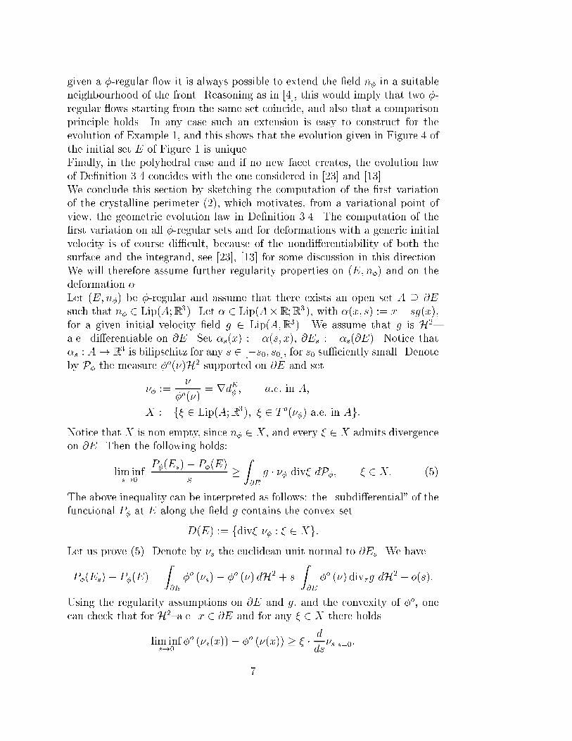
ε

Figure 3: �{calibrable facets. The side facet F2 and the lower facet F1 of E(t)E(t)Figure 4: example 1: qualitative shape of the evolving set E(t) starting fromE for short timesThen (1 + al00)=2 � 0 whenever e2 � 4�c, which is satis�ed for � small enough,and one checks that (1+al00)=2 � 1 is always satis�ed for � su�ciently small. 2Let now a = 2, b = 1=4, c = 1, d = 1, and choose e := 1=2. With this choiceof the lengths of the edges of @E, the facet F is not �{calibrable, whereas thefacets F1 and F2 are �{calibrable for � su�ciently small.We are in a position to construct an evolution of the set E of Figure 1, whichactually is the evolution of E by crystalline mean curvature, see Remark 5.5.The frontal facet F instantly subdivides into two disjoint facets (the fractureappears along l0) and then each facet translates parallely to itself with velocitygiven by (7). The same applies to the facet opposite to F . In this way weget an evolution t ! E(t) starting from E and de�ned on a suitable timeinterval [0; T ], with T > 0, having shape as in Figure 4. We need to provethat this evolution corresponds to a �-regular ow starting from E. In orderto prove this, we must construct a vector �eld n�(�; t) : @E(t)! R3 , t 2 [0; T ],as in De�nition 3.4. By Lemma 4.2, it is enough to prove that E(t) is �{15

Figure 5: example 1: numerical computation of E(t)calibrable for t 2 [0; T ], T > 0 su�ciently small. We observe that for anyt 2 [0; T ] the only facets of @E(t) which are not rectangular are like F1 andF2 of Figure 3. Applying Proposition 5.2 and Lemmas 5.4 and 5.3, it followsthat E(t) is �{calibrable. For t = 0 one can construct the �eld n� on @E, byconsidering the facet F (and similarly the facet opposite to F ) as the union ofP and F n P , and then solve (6) independently on the two rectangles, settingc�;P;l0 = 1 = �c�;FnP;l0. We observe that, with this de�nition, the �eld n� is notcontinuous on F : we do not know if there exists a continuous �eld equivalentto n� (i.e. with the same divergence and satisfying the same restrictions).Figure 5 is the result of a numerical computation.The following remark is crucial and concerns uniqueness of the �-regular ow.Remark 5.5. The vector �eld n� previously de�ned admits an extension (bylines) in a suitable space-time neighbourhood A � [0; T ] of the evolving front@E(t), where A is a suitable open set containing @E(t), t 2 [0; T ]. Moreprecisely, let y 2 A and let x 2 @E(t) be the unique point with the propertythat y belongs to the straight line �x + sn�(x; t)s2R (this property is ful�lledif A is su�ciently thin). Then we set n�(y; t) := n�(x; t). With this de�nition(E(t); n�(�; t)) becomes a �-regular evolution in the sense of Remark [4], andis unique in that class.Example 2.In this example we �x the Wul� shape to be the regular orthogonal prism withhexagonal basis centered at the origin; the apothem of the exagonal basis is setequal to 1. Let E be the convex set of Figure 6. Observe that also in this casethe set E satis�es the assumptions of Remark 3.2. We will prove that, for aproper choice of the parameter � > 0, the set E is not �{calibrable. Moreover,we expect that the evolution starting from such a set develops curve portionsof the boundary, i.e. the set does not seem to remain a polyhedral set.Assume for simplicity that r = 1 in Figure 6.16

Fε

qp

r

εε

l’

T Wφ

EFigure 6: example 2: the Wul� shape W� and the initial set ELemma 5.6. There exists � > 0 such that the frontal facet F� of @E is not�{calibrable for any � 2 ]0; �[.Proof. We have c�;F� = 1 on each edge of @F�, andvF� = 2(7� �)7� �2 � 2;for any � 2 [0; 1]. The function � ! vF� is strictly convex on [0; 1], withvF0 = vF1 = 2, and attains its minimum for � = 7 � p42, with value vF� =(7 +p42)=7 < 2. Hence F� is not �{calibrable for any � 2 ]0; �[. 2Let us �x � 2 ]0; �[. An interesting problem is to understand which is theevolution starting from this set. We expect that such an evolution E(t) doesnot remain a polyhedral set. This is motivated by the following heuristicargument.The facet F� strictly contains F�, and F� satis�es (8) with the choice c�;F� = 1 oneach edge of @F�. Hence we can expect that F� is �{calibrable (this correspondsto the opposite implication in Theorem 4.3, which has been proved in somevery special cases in Proposition 5.2 and Lemmas 5.3, 5.4). If this is true, thereexists a �eld n� : F� ! R3 satisfying (6). Let now p, q as in Figure 6, we letn(p) (resp. n(q)) be the unique vector obtained as intersection of fWQ� over allfacets Q of @E having p (resp. q) as vertex (see Remark 3.2). We de�ne the�eld n� on T := F� n F� by taking the linear combination of n(p) and n(q) onevery section of T parallel to l0. We can perform the same construction for thefacet of @E opposite to F�. Since the other facets of @E are all �{calibrable byProposition 5.2, we get a global �eld n� : @E ! R3 such that the pair (E; n�)is �-regular.We observe that, di�erently from the case of Example 1, the function div� n�is not constant (nor piecewise constant) on F�, but increases moving away17

Figure 7: example 2: numerical computation of the evolving set E(t) startingfrom E for short timesfrom l0 in T . Moreover, as can be shown by a direct computation, div� n�is continuous on F�, i.e. the two de�nitions of n� on F� and on T have thesame divergence on l0. This implies that, during an evolution starting fromE, the facet F� does not break in two di�erent facets as in Example 1, butrather bends inside E (with velocity given by div� n�) and becomes curve.Figure 7 (obtained by a numerical computation) shows the expected shape ofthe evolving set E(t) for small positive times.This example suggests that one cannot expect an existence theorem for �-regular ows in the class of polyhedral sets. The problem of predicting wherea fracture creates in a planar facet of an evolving set is interesting and deservesfurther investigation. Numerical computations in this direction will appear in[17].References[1] F.J. Almgren and J.E. Taylor. Flat ow is motion by crystalline curvaturefor curves with crystalline energies. J. Di�. Geom., 42:1{22, 1995.[2] F.J. Almgren, J.E. Taylor, and L. Wang. Curvature-driven ows: a vari-ational approach. SIAM J. Control Optim., 31:387{437, 1993.[3] S. Angenent and M.E. Gurtin. Multiphase thermomechanics with inter-facial structure. II: Evolution of an isothermal interface. Arch. RationalMech. Anal., 108:323{391, 1989.[4] G. Bellettini and M. Novaga. Approximation and comparison for non-smooth anisotropic motion by mean curvature in RN. Math. Mod. Meth-ods Appl. Sc., to appear. 18

[5] G. Bellettini and M. Paolini. Anisotropic motion by mean curvature inthe context of Finsler geometry. Hokkaido Math. J, 25:537{566, 1996.[6] G. Bellettini, M. Paolini, and S. Venturini. Some results on surface mea-sures in Calculus of Variations. Ann.Mat.Pura Appl., 170:329{359, 1996.[7] J.W. Cahn, C.A. Handwerker, and J.E. Taylor. Geometric models ofcrystal growth. Acta Metall., 40:1443{1474, 1992.[8] J.W. Cahn and D.W. Ho�man. A vector thermodynamics for anisotropicinterfaces. 1. Fundamentals and applications to plane surface junctions.Surface Sci., 31:368{388, 1972.[9] J.W. Cahn and D.W. Ho�man. A vector thermodynamics for anisotropicinterfaces. 2. Curved and faceted surfaces. Acta Metall., 22:1205{1214,1974.[10] M.-H. Giga and Y. Giga. Evolving graphs by singular weighted curvature.Arch. Rational Mech. Anal., 141:117{198, 1998.[11] M.-H. Giga and Y. Giga. A subdi�erential interpretation of crystallinemotion under nonuniform driving force. Dynamical Systems and Di�er-ential Equations, 1:276{287, 1998.[12] Y. Giga and M.E. Gurtin. A comparison theorem for crystalline evolutionsin the plane. Quarterly of Applied Mathematics, LIV:727{737, 1996.[13] Y. Giga, M.E. Gurtin, and J. Matias. On the dynamics of crystallinemotion. Japan Journal of Industrial and Applied Mathematics, 15:7{50,1998.[14] P.M. Girao and R.V. Kohn. The crystalline algorithm for computingmotion by curvature. In Variational Methods for Discontinuous Structures(eds. R. Serapioni and F. Tomarelli), Birk�auser, 1996.[15] E. Giusti. Minimal Surfaces and Functions of Bounded Variation.Birkh�auser, Boston, 1984.[16] M. Gurtin. Thermomechanics of Evolving Phase Boundaries in the Plane.Clarendon Press, Oxford, 1993.[17] M. Novaga and E. Paolini. A computational approach to fractures incrystal growth. Work in preparation, 1998.[18] A.R. Roosen and J. Taylor. Modeling crystal growth in a di�usion �eldusing fully faceted interfaces. J. Comput. Phys., 114:444{451, 1994.19

[19] P. Rybka. A crystalline motion: uniqueness and geometric properties.SIAM J. Appl. Math., 57:53{72, 1997.[20] J.E. Taylor. Crystalline variational problems. Bull. Amer. Math. Soc.(N.S.), 84:568{588, 1978.[21] J.E. Taylor. Constructions and conjectures in crystalline nondi�erentialgeometry. In: Di�erential Geometry (eds. B. Lawson and K. Tanenblat),Pitman Monographs in Pure and Applied Math., 52:321{336, 1991.[22] J.E. Taylor. Geometric crystal growth in 3D via facetted interfaces. In:Computational Crystal Growers Workshop, Selected Lectures in Mathe-matics, Amer. Math. Soc., pages 111{113, 1992.[23] J.E. Taylor. II-mean curvature and weighted mean curvature. Acta Metall.Mater., 40:1475{1485, 1992.[24] W.A. Tiller. The Science of Crystallization. Cambridge University Press,1991.[25] A. Visintin. Models of Phase Transitions. Birkh�auser, Boston, 1996.

20