Curvature Dependent Skeletonization

Andrea Torsello and Edwin R. Hancock

Department of Computer Science,University of York,

York, YO10 5DD, UK

Abstract. The Hamilton-Jacobi approach has proved to be a powerfuland elegant method for extracting the skeleton of a shape. The approachis based on the fact that the dynamics of the inward evolving boundaryis conservative everywhere except at skeletal points. Nonetheless thismethod appears to overlook the fact that the linear density of the evolv-ing boundary front is not constant where the front is curved. In thispaper we present an analysis which takes into account variations of den-sity due to boundary curvature. This yields a skeletonization algorithmthat is both better localized and less susceptible to boundary noise thanthe Hamilton-Jacobi method.

1 Introduction

The skeletal abstraction of 2D and 3D objects has proved to be an alluringyet highly elusive goal for over 30 years in shape analysis [2]. The morphologicalskeleton of a shape is defined as the set of singularities in the inward evolution ofthe boundary with constant velocity. The dynamics of the boundary is describedby the eikonal equation: a partial differential equation that governs the motionof a wave-front through a medium. In the case of a uniform medium the equationis ∂tC(t) = αN(t), where C(t) : [0, s]→ R

2 is the equation of the front at timet and N(t) : [0, s] → R

2 is the equation of the normal to the wave front in thedirection of motion and α is the propagation speed. As the wave front evolves,opposing segments of the wave-front collide, generating a singularity.

Broadly speaking, the there are three approaches to skeleton extraction,namely a) marching front methods which simulate the grassfire transform whichinvolve either thinning [1] or curve evolution [9] b) Voronoi triangulation methods[6, 4] and c) methods based on the differential geometry of the object boundary.In this paper, we are interested in this latter class of methods. Here a recentlydeveloped and particularly powerful method is that based on the differentialequation which arises when the object boundary evolves under the Hamilton-Jacobi equations of classical mechanics [5]. Where resulting eikonal equation forthe motion flow field is non-singular, the system is Hamiltonian, and, thus, con-servative. Wherever the system ceases to be conservative there is a singularityin the boundary flow field, and when the boundary reaches the singularity aso-called shock forms. In the Hamilton-Jacobi framework skeletal points are de-tected by searching for points where the system ceases to be Hamiltonian, that

J. Bigun and T. Gustavsson (Eds.): SCIA 2003, LNCS 2749, pp. 200−207, 2003. Springer-Verlag Berlin Heidelberg 2003

is points where the divergence of the flow is not 0 [7]. These methods turn outto be algorithmically very simple and numerically stable.

A major problem of the Hamilton-Jacobi method is that in its original imple-mentation, is that it overlooks the fact that the density of the evolving boundaryfront is not constant and, infact, depends on the curvature of the front. As aresult of the variations in density, the flux is not conserved and hence the wholepremise of the skeletonization method collapses. In this paper, we address thisproblem by extending the Hamilton-Jacobi analysis to the case where the frontdensity varies due to boundary curvature. The main practical advantage of thisanalysis is that it leads to the recovery or more stable skeletons.

2 Hamilton-Jacobi Skeleton

We commence by defining a distance-map that assigns to each point on the in-terior of an object the closest distance D from the point to the boundary (i.e.the distance to the closest point on the object boundary). The gradient of thisdistance-map defines a field F whose domain is the interior of the shape. Thefield is defined to be F = ∇D, where ∇ = ( ∂

∂x , ∂∂y )T is the gradient opera-

tor. The trajectory followed by each boundary point under the eikonal equationcan be described by the ordinary differential equation x = F (x), where x isthe coordinate vector of the point. Siddiqi claims that this dynamic system isHamiltonian everywhere except on the skeleton. This implies that on skeletalpoints the field F is conservative, or ∇ · F = 0. However, the total inward fluxthrough the whole shape is non zero. In fact, the flux is proportional to thelength of the boundary.

The divergence theorem states that the integral of the divergence of a vector-field over an area is equal to the flux of the vector field over the enclosingboundary of that area. In our case,∫

A

∇ · F dσ =∫

L

F · n dl = ΦA(F ), (1)

where A is any area, F is a field defined in A, dσ is the area differential in A, dlis the length differential on the border L of A, and ΦA(F ) is the outward fluxof F through the border L of the area A.

By virtue of the divergence theorem we have that, within the interior, thereare points where the system is not conservative. The non-conservative pointsare those where the boundary trajectory is not well defined, i.e. where thereare singularities in the evolution of the boundary. These points are the so-calledshocks or skeleton of the shape- boundary. Shocks are thus characterized bylocations where ∇ · F < 0.

2.1 Curvature in the Boundary FrontUnfortunately, the hypothesis that the field F is conservative does not hold ingeneral.

Let us consider an instant t in the inward boundary evolution. The initialborder has evolved under the eikonal equation to boundary front St orthogonal

201Curvature Dependent Skeletonization

in every point to F . Pick a point p ∈ St, what is the value of ∇ ·F (p)? Since thedivergence operator is invariant under rotations, we can write ∇ · F = ∂

∂v‖F +

∂∂v⊥

F where v‖ = F (p) and v⊥ is a normal vector orthogonal to v‖. Since||F || = 1 everywhere, ∂

∂v‖F = 0. On the other hand ∂

∂v⊥F (p) = −κ(p) where

κ(p) is the curvature in p of the border front St oriented so that κ(p) is positive ifthe osculating circle is in the interior of the front. Hence, we have that ∇·F (p) =−κ(p),, that is, the divergence∇·F is not always 0 as predicted by the Hamilton-Jacobi approach, but rather it is equal to the curvature of the front of the inwardevolving boundary.

dl(t + ∆t)dl(t)

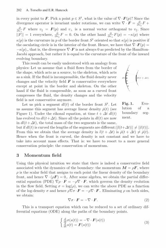
Fig. 1. Evo-lution of aboundary seg-ment.

This result can be easily understood with an analogy fromphysics: Let us assume that a fluid flows from the border ofthe shape, which acts as a source, to the skeleton, which actsas a sink. If the fluid is incompressible, the fluid density neverchanges and the velocity field F is conservative everywhereexcept at point in the border and skeleton. On the otherhand if the fluid is compressible, as soon as a curved frontcompresses the fluid, the density changes and the velocityfield is not conservative anymore.

Let us pick a segment dl(t) of the border front St. Letus assume this segment has average linear density ρ(t) (seeFigure 1). Under the eikonal equation, at time t + ∆t dl(t)has evolved to dl(t+∆t). Since all the points in dl(t) are nowin dl(t+∆t), the total mass of the two segments is the same,but if dl(t) is curved the lengths of the segments are different:||l(t+∆t)|| %= ||l(t)||.From this we obtain that the average density in l(t + ∆t) is ρ(t + ∆t) %= ρ(t).Hence when the front is curved, the density is not constant and we have totake into account mass effects. That is: we have to resort to a more generalconservation principle: the conservation of momentum.

3 Momentum field

Using this physical intuition we state that there is indeed a conservative fieldassociated with the dynamics of the boundary: the momentum M = ρF , whereρ is the scalar field that assigns to each point the linear density of the boundaryfront, and hence ∇ · (ρF ) = 0,. After some algebra, we obtain the partial differ-ential equation (PDE) ∇ρ · F = −ρ∇ · F . which goversn the density evolutionin the flow field. Setting σ = log(ρ), we can write the above PDE as a functionof the log-density σ and hence ρ∇σ ·F = −ρ∇ ·F .. Eliminating ρ on both sides,we obtain:

∇σ · F = −∇ · F . (2)

This is a transport equation which can be reduced to a set of ordinary dif-ferential equations (ODE) along the paths of the boundary points.

{ddtσ(s(t)) = −∇ · F (s(t))ddts(t) = F (s(t))

(3)

202 A. Torsello and E.R. Hancock

We can derive this equation by analyzing the change of density of segment dlin Figure 1. We know that ρ(t)||dl(t)|| = m. where dl(t) is the evolution of theborder segment dl at time t, m is its mass, and ρ(t) and κ(t) are the segment’saverage linear density and curvature at time t.

After a small interval of time ∆t, the segment length will be ||dl(t + ∆t)|| =||dl(t)|| κ(t)

κ(t+∆t) + O(∆t2), and the curvature κ(t + ∆t) = κ(t)1−κ(t)∆t + O(∆t2).

From these equations and the conservation of mass, we have: ρ(t + ∆t)− ρ(t) =ρ(t) κ(t)∆t

1−κ(t)∆t + O(∆t2). Taking the limit for ∆t→ 0 and ||dl||→ 0, we have:

ddtρ(s(t))ρ(s(t))

= κ(s(t)), (4)

where s(t) is the trajectory under the eikonal equation of the limit point thesegment dl tends to as ||dl||→ 0. Integrating (4) and using the fact that κ(p) =−∇ · F , we find: log(ρ(s(t))) = − ∫ t

0∇ · F (s(τ)) dτ.

4 Computing the density

To obtain the momentum field we need to integrate the density field in theinterior of the shape. Since images have a finite resolution, we need to discretizethe solution in the image lattice.

One approach is to express the PDE (2) as a system of difference equations.The difference equations form a linear system that is then solved to obtain thelog-density σ = log(ρ). The problem with this approach is that the skeleton isa set of singularities of the momentum field, hence the density can have verydifferent values at opposite sides of a skeletal branch. The result is that thelinear system will have no solution and even trying to approximate a solutionusing a residual descent methods would force the density values the solution tooscillate wildly on points near the skeleton.

4.1 Integration in Time

In order to overcome this problem we need to be sure that the difference operatorused in the equations never cross a skeletal branch. One way to guarantee thisis to integrate the equation in the time domain: so that the formulae giving thevalue of ρ at points in the boundary front at time t reference values of ρ onlyat points in the fronts at previous times. We can obtain this by integrating theODE (3) along the paths of the boundary points.

We opt to use the second order Cranck-Nicolson method, that is, for eachpoint (x, y) in the interior of the shape, we have the equation:

σ(s(t)) = σ(s(t− 1))− 12[∇ · F (s(t)) +∇ · F (s(t− 1))]. (5)

Using this equation we can calculate the log-density at of a point of the borderat time t referencing only values of the log-density at points that belong thefront at previous times. Since the evolution never crosses the skeleton, we areguaranteed not to cross skeletal branch through our calculations.

203Curvature Dependent Skeletonization

4.2 Integration in Space

σ(x, y′)σ(x′, y′)

σ(x′, y)

σ(x − Fx, y − Fy)

F

σ(x, y)

Fig. 2. Integra-tion along theboundary path.

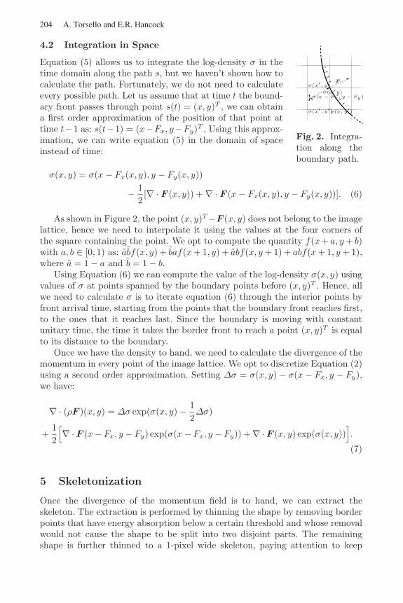
Equation (5) allows us to integrate the log-density σ in thetime domain along the path s, but we haven’t shown how tocalculate the path. Fortunately, we do not need to calculateevery possible path. Let us assume that at time t the bound-ary front passes through point s(t) = (x, y)T , we can obtaina first order approximation of the position of that point attime t−1 as: s(t−1) = (x−Fx, y−Fy)T . Using this approx-imation, we can write equation (5) in the domain of spaceinstead of time:

σ(x, y) = σ(x− Fx(x, y), y − Fy(x, y))

− 12[∇ · F (x, y)) +∇ · F (x− Fx(x, y), y − Fy(x, y))]. (6)

As shown in Figure 2, the point (x, y)T−F (x, y) does not belong to the imagelattice, hence we need to interpolate it using the values at the four corners ofthe square containing the point. We opt to compute the quantity f(x + a, y + b)with a, b ∈ [0, 1) as: abf(x, y) + baf(x + 1, y) + abf(x, y + 1) + abf(x + 1, y + 1),where a = 1− a and b = 1− b.

Using Equation (6) we can compute the value of the log-density σ(x, y) usingvalues of σ at points spanned by the boundary points before (x, y)T . Hence, allwe need to calculate σ is to iterate equation (6) through the interior points byfront arrival time, starting from the points that the boundary front reaches first,to the ones that it reaches last. Since the boundary is moving with constantunitary time, the time it takes the border front to reach a point (x, y)T is equalto its distance to the boundary.

Once we have the density to hand, we need to calculate the divergence of themomentum in every point of the image lattice. We opt to discretize Equation (2)using a second order approximation. Setting ∆σ = σ(x, y)− σ(x− Fx, y − Fy),we have:

∇ · (ρF )(x, y) = ∆σ exp(σ(x, y)− 12∆σ)

+12

[∇ · F (x− Fx, y − Fy) exp(σ(x− Fx, y − Fy)) +∇ · F (x, y) exp(σ(x, y))

].

(7)

5 Skeletonization

Once the divergence of the momentum field is to hand, we can extract theskeleton. The extraction is performed by thinning the shape by removing borderpoints that have energy absorption below a certain threshold and whose removalwould not cause the shape to be split into two disjoint parts. The remainingshape is further thinned to a 1-pixel wide skeleton, paying attention to keep

204 A. Torsello and E.R. Hancock

the shape connected and not to shorten the skeleton by eliminating endpoints.Expressed in pseudo-code the thinning process of shape S is as follows:

For each point p in distance order

if is simple(S \ p) and −∇ · ρF (p) < εthen S = S \ p

For each remaining point p in distance order

if is simple(S \ p) and not is endpoint(S,p)then S = S \ p

The predicate is simple determines whether the shape is still connected afterthe removal of point p by checking only the points in the neighborhood of p: theshape S \ p is connected if the point in the neighborhood of p, excluding p, areconnected. Similarilly, is endpoint determines whether p is an endpoint only byinspecting the neighborhood of p: the point is an endpoint if it has at most twoneighboring points and those points are horizontally or vertically adjacent.

6 Experimental Comparison

In this section we try to characterize the differences between the Hamilton-Jacobi skeletonization method and our density-corrected approach. We startby providing a qualitative analysis of the difference in the divergence of thevelocity and momentum fields. Secondly we provide an analysis of the noiseand thresholding sensitivity of the two methods. Finally we provide a morequantitative analysis of the localization properties of the two skeletonizationmethods.

Fig. 3. Differences in the velocityand momentum fields. Left to right:shape, ∇ · F , log(ρ), and ∇ · ρF

Figure 3 shows, for a few selectedshapes in our database, the values ofthe divergence of the velocity field∇ · F ,log(ρ), and ∇ · ρF . In this pictures whitecorresponds to a large positive values,black to a large negative value and 0 isrepresented by a 50% intensity gray.

It is very clear from the pictures thatthe divergence of the velocity field is not0 in correspondence with a curved bound-ary. Furthermore, quantization in the lo-calization of the border causes the initialborder to be very jagged, and this high-frequency, low-amplitude noise is trans-ported and amplified throughout the ve-locity field, yielding a noisy and poorlylocalized skeleton. Conversely, the densitycorrection in the momentum field damp-ens the noise.

To counter quantization noise from theborder, we need to smooth the distance

205Curvature Dependent Skeletonization

Fig. 4. The effect ofsmoothing on skeletonextraction.

map and select an appropriate skeletonizationthreshold. Pick too big a smoothing radius orthreshold and some branches of the skeleton willbe thinned away, pick values too small and theextracted skeleton will have a lot of spuriousbranches (See Figure 4). In this section we charac-terize the effects on the extracted skeleton of thesmoothing radius and the skeletonization thresh-old.

Figure 4 Displays the effects of very low (left)and very high (right) values of smoothing radiusand skeletonization threshold on a test shape.The picture show, top to bottom, the divergenceof the velocity field, the uncorrected Hamilton-Jacobi skeleton, the divergence of the momentumfield, and the skeleton extracted using the density-corrected method. what these picture show is thatthe density corrected method is much less sensi-tive to the amount of smoothing and the value ofthe threshold.

Next we characterize the localization proper-ties of the skeleton extracted using the Hamilton-Jacobi and the new density corrected method on awide range of shapes. To this purpose we computehow the value of the divergence of the velocity and momentum field distributeover distance to the extracted skeleton. Figure 5 plots an histogram of how non-skeletal points distribute over distance and divergence value on our test shape.The figure shows that the Hamilton-Jacobi skeleton has a non-negligible amountof high divergence values even at high distance from the extracted skeleton.

0

0.2

0.4

0.6

0.8

1.

Energy

0

3.8

7.6

11.4

15.2

19.

Distance

0

0.01

0.02

0.03

0.04

0.05

0

0.2

0.4

0.6

0.8Energy

0

0.2

0.4

0.6

0.8

1.

Energy

0

3.8

7.6

11.4

15.2

19.

Distance

0

0.01

0.02

0.03

0.04

0.05

0

0.2

0.4

0.6

0.8Energy

(a) Hamilton-Jacobi (b) Density corrected

Fig. 5. Histogram over value of (negative) divergence of the field and distance to skele-ton

In an experiment we tried to quantify the localization of the skeleton on adatabase of shapes. To this purpose we used a database of 50 shapes and we his-togrammed the distribution of field divergence over the distance to the skeletonfor both the velocity and the momentum field. We then take, for each shape, themean of this divergence-distribution as a measure of divergence-localization.

206 A. Torsello and E.R. Hancock

0

0.05

0.1

0.15

0.2

0.25

0.3

0.35

0 1 2 3 4 0

0.1

0.2

0.3

0.4

0.5

0.6

0 1 2 3 4

(a) Hamilton-Jacobi (b) Density corrected

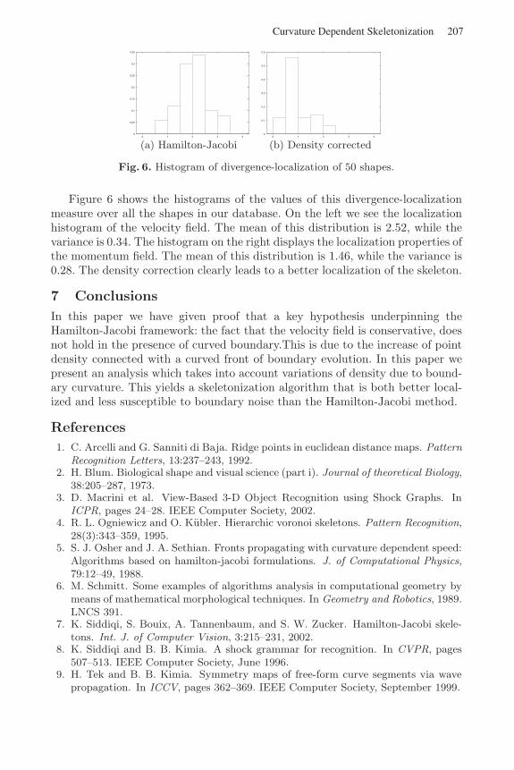
Fig. 6. Histogram of divergence-localization of 50 shapes.

Figure 6 shows the histograms of the values of this divergence-localizationmeasure over all the shapes in our database. On the left we see the localizationhistogram of the velocity field. The mean of this distribution is 2.52, while thevariance is 0.34. The histogram on the right displays the localization properties ofthe momentum field. The mean of this distribution is 1.46, while the variance is0.28. The density correction clearly leads to a better localization of the skeleton.

7 Conclusions

In this paper we have given proof that a key hypothesis underpinning theHamilton-Jacobi framework: the fact that the velocity field is conservative, doesnot hold in the presence of curved boundary.This is due to the increase of pointdensity connected with a curved front of boundary evolution. In this paper wepresent an analysis which takes into account variations of density due to bound-ary curvature. This yields a skeletonization algorithm that is both better local-ized and less susceptible to boundary noise than the Hamilton-Jacobi method.

References

1. C. Arcelli and G. Sanniti di Baja. Ridge points in euclidean distance maps. PatternRecognition Letters, 13:237–243, 1992.

2. H. Blum. Biological shape and visual science (part i). Journal of theoretical Biology,38:205–287, 1973.

3. D. Macrini et al. View-Based 3-D Object Recognition using Shock Graphs. InICPR, pages 24–28. IEEE Computer Society, 2002.

4. R. L. Ogniewicz and O. Kubler. Hierarchic voronoi skeletons. Pattern Recognition,28(3):343–359, 1995.

5. S. J. Osher and J. A. Sethian. Fronts propagating with curvature dependent speed:Algorithms based on hamilton-jacobi formulations. J. of Computational Physics,79:12–49, 1988.

6. M. Schmitt. Some examples of algorithms analysis in computational geometry bymeans of mathematical morphological techniques. In Geometry and Robotics, 1989.LNCS 391.

7. K. Siddiqi, S. Bouix, A. Tannenbaum, and S. W. Zucker. Hamilton-Jacobi skele-tons. Int. J. of Computer Vision, 3:215–231, 2002.

8. K. Siddiqi and B. B. Kimia. A shock grammar for recognition. In CVPR, pages507–513. IEEE Computer Society, June 1996.

9. H. Tek and B. B. Kimia. Symmetry maps of free-form curve segments via wavepropagation. In ICCV, pages 362–369. IEEE Computer Society, September 1999.

207Curvature Dependent Skeletonization