CM–UTAD, Preprint number 10

centro de matematicacm–utad

Combining and scaling descent andnegative curvature directions

Catarina P. Avelino, Javier M. Morguerza, Alberto Olivares and

Francisco J. Prieto

2008-10

pre-publicacoes

CE

NT

RO

DE MATEMÁ

TIC

A

UTAD

Centro de Matematica

Univ. de Tras-os-Montes e Alto Douro

Quinta de Prados, 5001–801 – Vila Real

Portugal

Combining and scaling descent and negative curvaturedirections

Catarina P. Avelino 1 Javier M. Moguerza 2 Alberto Olivares 2 Francisco J. Prieto 3

Dept. of Mathematics Dept. of Statistics and Operational Research Dept. of StatisticsUTAD, Vila Real, Portugal Univ. Rey Juan Carlos, Madrid, Spain Univ. Carlos III de Madrid, SpainE-mail: cavelino@utad.pt E-mail: javier.moguerza@urjc.es E-mail: franciscojavier.prieto@uc3m.es

ABSTRACT

The aim of this paper is the study of different approaches to combine and scale,in an efficient manner, descent information for the solution of unconstrainedoptimization problems. We consider the situation in which different directionsare available in a given iteration, and we wish to analyze how to combine thesedirections in order to provide a method more efficient and robust than thestandard Newton approach. In particular, we will focus on the scaling processthat should be carried out before combining the directions. We derive sometheoretical results regarding the conditions necessary to ensure the convergenceof combination procedures following schemes similar to our proposals. Finally,we conduct some computational experiments to compare these proposals witha modified Newton’s method and other procedures in the literature for thecombination of information.

Keywords: Line search; negative curvature; nonconvex optimization

AMS: 49M37, 65K05, 90C30

1 Introduction

We are interested in the study of algorithms to compute in an efficient manner solutions forunconstrained nonconvex problems of the form:

minx

f(x), (1)

where f : Rn → R is at least twice continuously differentiable. This problem has been extensivelystudied in the literature (see for example Gill and Murray [6] or Fletcher [4]), and different classesof algorithms have been proposed to compute local solutions of the problem. Most of these meth-ods are based on the generation of a sequence of iterates, updated using the information derivedfrom a single search direction. In most cases, the methods compute an approximation to theNewton direction based on second-order approximations to the problem, and ensure reasonableglobal convergence properties by adjusting the size of the direction through either a linesearchor a trust-region approach.

Nevertheless, it has been noted in the literature that in most practical cases it is possible togenerate in each iteration additional information to update the iterates at a cost that is not sig-nificantly higher than that required by the classical Newton approach, see for example More andSorensen [13], Fiacco and McCormick [3], or Forsgren and Murray [5]. The previous referencesshow the theoretical advantages of including directions of negative curvature as a part of anoptimization algorithm. However, there are just a few works treating practical aspects regarding

1This author was supported by Portugal’s FCT postdoctoral grant SFRH/BPD/20453/2004.2This author was partially supported by Spanish grants MEC MTM2006-14961-C05-05 and URJC-CM-2006-

CET-03913This author was partially supported by grant MTM2004-02334 of the Spanish Ministry of Education

1

the use of this kind of information (see, for instance, Moguerza and Prieto [11, 12]). Thereforeit seems interesting to consider the potential improvement that the use of this information (forexample descent and negative curvature directions) may imply for an unconstrained optimizationalgorithm, both in terms of its efficiency and its robustness. Also, for large-scale problems itmay be computationally expensive to obtain an exact Newton direction in each iteration. Themethods most commonly used are based on quasi-Newton approximations to the Hessian ma-trix, or in approximate solutions to the Newton system of equations. In these cases, the analysisof potential improvements based on combining several of these approaches seems particularlyrelevant, as no practical evidence suggests that any of the approximate Newton methods are ingeneral superior to the others, and no clear evidence exists to support a strategy based on the apriori selection of one of them.

The use of combinations of directions has been analyzed in the literature for example inMore and Sorensen [13], Mukai and Polak [14], Goldfarb [7], Moguerza and Prieto [11, 12] orOlivares et al. [15]. Although out of the scope of this paper, based on the conjugate gradientmethodology there are linesearch procedures for unconstrained optimization which are useful forsolving large scale problems. These methods have well-known convergence properties (see Hagerand Zhang [10] and the references therein), and have been used in some practical engineeringapplications (see, for instance, Sun et al. [18]). There are some other works using directions ofnegative curvature within conjugate gradient schemes (see Sanmatıas and Vercher [16] and thereferences therein). For instance, in Gould et al. [8], in each iteration the best direction is chosenand a standard linesearch is conducted. Another method based in the selection of directions issuggested by Sanmatıas and Roma [17].

Our aim in this paper is to show that scaling the negative curvature directions and eventuallyother directions before performing a line search yields significant improvements in the efficiencyof optimization algorithms. We will consider the particular case when the directions availableare the Newton direction, the gradient and a negative curvature direction. Our approach isclosely related to the standard Newton’s method. Therefore it provides a more direct evaluationof the potential advantages of a combined information approach, when compared to the Newtonalgorithm. Also, the adjustments of the parameters to obtain efficient implementations of thecombination algorithms are simpler within this setting. We implement some proposals in anefficient manner and study the conditions that must be imposed on these approaches to ensurereasonable global convergence properties to second-order KKT points of problem (1). In addition,we compare their practical performance and effectiveness through a computational experimentbased on a set of 119 small optimization problems from the CUTEr collection [9]. The results andtheir analysis provide important insights both for practical applications in an improved Newtonmethod setting and for possible extensions to large-scale problems.

The rest of the paper is organized as follows: in Section 2 we describe the algorithms proposedto compute local solutions for unconstrained optimization problems. Section 3 presents severalglobal convergence results for the algorithms. Section 4 describes the computational experimentwe have carried out. Finally, in Section 5 we present some final comments and conclusions.

2 General description of the algorithms

In this section we present and describe two algorithmic models for the solution of problem (1).Our description of the algorithms starts with a presentation of a common framework to bothmethods, and then introduces the different approaches specific to each algorithm. Given a set ofp directions dik, computed in an iteration k of the optimization algorithm, our common approachfor all the alternatives that we consider in this work is to define a combination of these directions

2

to obtain a search direction dk as

dk =p∑

i=1

αikdik, (2)

where αik, i = 1, . . . , p, are the coefficients to be determined by the proposed procedures atiteration k. Within this common framework, all the procedures compute a sequence of iterates{xk} from an initial approximation x0, as

xk+1 = xk + dk.

As already mentioned, an important and related task is the adequate scaling of the directionsused in the algorithm (see Moguerza and Prieto [11, 12]). While the standard Newton directionis well-scaled, particularly close to the solution, other alternative search directions may not be,implying a potential inefficiency in the resulting algorithm. Our proposal handles these problemsby adjusting the scale of the available directions through the application of a few iterations of anoptimization algorithm on a simplified local model for the problem. The computation of a setof values for αik on a smaller subspace as an optimization problem has already been treated byByrd et al. [1]. In particular, we propose and analyze two different algorithms to compute thecoefficients in the combination: a Newton method that, given the directions dik, is applied todetermine the initial values of αik for a linesearch; and a mixed approach that computes a set ofvalues for αik by solving a trust-region subproblem, and then performing a linesearch to obtainthe next iterate.

In what follows, and to improve the clarity of the presentation of convergence results inSection 3, we use a slightly modified notation for the directions combined in (2). We denote asdik those directions that are related to descent properties for problem (1), while we introducethe notation dik for the directions related to negative curvature properties of (1), if they areavailable at iteration k. In this way, dk in (2) is obtained from the available directions as

dk ≡∑

i

αikdik +∑

i

αikdik, (3)

for appropriate values of the scalars αik, αik.

Main Algorithm

Step 0 [Initialization] Select x0 ∈ IRn and constants ω∗ > 0, σ ∈ (0, 1).Set k = 0.

Step 1 [Test for convergence] If

‖∇f(xk)‖ ≤ ω∗ and λmin(∇2f(xk)) ≥ −ω∗,

then stop.

Step 2 [Computation of the search directions] Compute dik and dik.

Step 3 [Computation of steplengths] Compute αik, αik and define

dk =∑

i αikdik +∑

i αikdik.

Step 4 [New iterate] Set xk+1 = xk + dk, k = k + 1 and go to Step 1.

Table 1: General description of the algorithms

3

The general framework (the basic algorithm) is summarized in Table 1, where λmin(H) denotesthe smallest eigenvalue of a given matrix H. Note that we use the Newton direction wheneverit satisfies a sufficient descent condition. The motivation for this choice is to ensure a quadraticlocal convergence rate for the algorithm. This choice works well in practice, and is consistentwith the good local properties of the Newton direction close to a local solution. The methodsdiffer only in the way the values for step lengths αik and αik are computed, in particular, theway in which Step 3 is carried out. This step is described in Table 2. More specifically, ourproposals are obtained by performing Step 3c in two different manners. This step corresponds tothe scaling process that should be carried out before combining the directions. Next, we describeeach one of the two proposed implementations for this step.

Step 3 - Computation of steplengths

Step 3a [Initialization] Set k = 0. Select initial steplengths αi0 and αi0,ξ ∈ (0, 1), σ ∈ (0, 1) and a positive integer kmax.

Step 3b [Test for convergence] Let

dk =∑

i αikdik +∑

i αikdik.

If∥∥∇f(xk + dk)

∥∥ ≤ ω∗ or k = kmax, then go to Step 4e.

Step 3c [Computation of αik and αik] Apply either Newton’s method ora trust-region approach to update αik and αik.

Step 3d [New iterate] Set k = k + 1 and go to Step 4b.

Step 3e [Linesearch] Compute

dk = ξl(∑

i αikdik +∑

i αikdik),

where l is the smallest nonnegative integer such that

f(xk + dk) ≤ f(xk) + σ(∇f(xk)T dk + min

(0, dT

k∇2f(xk)dk

)).

Step 3f [Return] Return to the Main Algorithm with αik = ξlαik

and αik = ξlαik.

Table 2: Computation of steplengths

2.1 Newton-based Scaling Method (NSM)

Our first proposal is based on the application of Newton steps to obtain reasonable values forthe steplengths. Once a reasonable set of values is obtained, either because the gradient of theobjective function is small enough or because a sufficient number of Newton steps have beentaken, the resulting values are further refined by imposing a sufficient descent condition andperforming a linesearch to obtain a sufficient descent direction as a combination of the availabledirections in the current iteration. We will denote this algorithm as NSM.

Since the Newton direction is well-scaled, in our proposals we adjust only the steplengthsassociated with the gradient and the negative curvature directions, that is, we keep fixed thesteplength associated with the original Newton direction. In this way, the scaling of these twodirections will be adequate related to the Newton direction.

We now consider the different computations associated with Step 3c in Table 2 for algorithm

4

NSM. For this method, the value for the final direction is obtained by adjusting the steps alongthe directions by computing Newton updates for the problem

min(αi,αi)

f

(xk +

∑

i

αikdik +∑

i

αikdik

)(4)

by determining the solutions for the system

Hkk

(∆αik∆αik

)= −gkk, (5)

where ∆αik and ∆αik denote the changes in the corresponding steplengths, and

Hkk ≡(

dTik

dTik

)∇2f

(xk +

∑

i

αikdik +∑

i

αikdik

)(

dik dik

)

gkk ≡(

dTik

dTik

)∇f

(xk +

∑

i

αikdik +∑

i

αikdik

).

That is, we project the Hessian and the gradient on the subspace determined by the searchdirections. Finally, we update

αi(k+1) = αik + ∆αik, αi(k+1) = αik + ∆αik. (6)

In summary, we perform for Step 3c in NSM the operations indicated in Table 3.

Computation of steplength - Algorithm NSM

Step 3c [Computation of αik and αik] Solve system (5) and obtain theupdated steplengths from (6).

Table 3: Step 3c performance for NSM algorithm

2.2 Trust-Region Scaling Method (TRSM)

A second, closely related proposal, computes updates for the steplengths using a trust-regionapproach, instead of the direct application of the Newton update. Nevertheless, it still carriesout a linesearch once a sufficient number of steps have been taken, as in the preceding case. Wewill denote this algorithm as TRSM.

Consider now the implementation of Step 3c in Algorithm TRSM. Now we obtain the updatesfor the steplengths by computing a solution for the trust-region problem

min gTkk

(δαikδαik

)+ 1

2

(δαik δαik

)Hkk

(δαikδαik

)

s.t∥∥(

δαik δαik

)∥∥ ≤ ∆k,(7)

and then updating the corresponding values using (6), as before. Step 3c in TRSM is imple-mented as indicated in Table 4.

5

Computation of steplength - Algorithm TRSM

Step 3c [Computation of αik and αik] Solve problem (7) and obtain theupdated steplengths from (6).

Table 4: Step 3c performance for TRSM algorithm

3 Convergence properties

In this section we study the global convergence properties of the algorithms described in thepreceding section. We believe the analysis of these general versions of the algorithms providesinsights beyond the particular implementations considered in Section 4 for the computationaltests.

The goal of the algorithms is the computation of local solutions for unconstrained optimizationproblems of the form given in (1), where we will assume in this Section that f : Rn → R is athree-times differentiable function. These algorithms generate a sequence of iterates {xk} froman initial point x0 and a combination of directions obtained in each iteration. These directionsshould capture the descent and negative curvature available in the iteration.

In order to establish convergence results for the sequence {xk} we need to assume that problem(1) and the initial point x0 satisfy some regularity conditions. In particular, in what follows wewill assume that the following properties hold:

A1. The level set of f at the initial point,

S0 ≡ {x ∈ Rn : f(x) ≤ f(x0)}is compact.

A2. The function f has continuous third derivatives on S0.

Before considering any detailed convergence analysis, it is important to note that the basiciteration in either of the algorithms consists of the computation of the search directions followedby two steps to determine the step dk:

• the computation of a combination of the directions, that is, the computation of steplengthsαik and αik in either of the algorithms, and

• the performance of a conventional (backtracking) linesearch on the resulting direction tocompute steplengths αik = ξlαik, αik = ξlαik, that result in the computation of a step dk

satisfying the descent condition

f(xk + dk) ≤ f(xk) + σ(∇f(xk)T dk + min(0, dTk∇2f(xk)dk)), (8)

where 0 < σ < 1 is a prespecified constant.

The traditional approach to establish the convergence of the sequence {xk} is based oncondition (8) and the satisfaction of some sufficient descent property by dk. In the case ofthe proposed algorithms, and due to the use of negative curvature directions, the equivalent tothe sufficient descent condition used in the proofs below is given by

min(gT

k dk, dTk Hkdk

) ≤ γ min(−‖gk‖2, λmin(Hk)

), (9)

for some positive constant γ and all k. The following result shows that these conditions aresufficient to ensure convergence to a second-order KKT point.

6

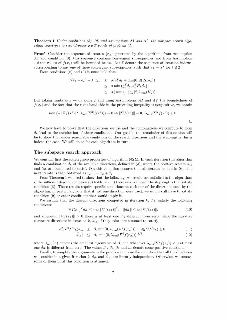
Theorem 1 Under conditions (8), (9) and assumptions A1 and A2, the subspace search algo-rithm converges to second-order KKT points of problem (1).

Proof Consider the sequence of iterates {xk} generated by the algorithm; from AssumptionA1 and condition (8), this sequence contains convergent subsequences and from AssumptionA2 the values of f(xk) will be bounded below. Let I denote the sequence of iteration indexescorresponding to any one of these convergent subsequences, such that xk → x∗ for k ∈ I.

From conditions (8) and (9) it must hold that

f(xk + dk)− f(xk) ≤ σ(gTk dk + min(0, dT

k Hkdk))≤ σ min

(gT

k dk, dTk Hkdk

)

≤ σγ min(−‖gk‖2, λmin(Hk)

).

But taking limits as k → ∞ along I and using Assumptions A1 and A2, the boundedness off(xk) and the fact that the right-hand side in the preceding inequality is nonpositive, we obtain

min(−‖∇f(x∗)‖2, λmin(∇2f(x∗))

)= 0 ⇒ ‖∇f(x∗)‖ = 0, λmin(∇2f(x∗)) ≥ 0.

¤We now have to prove that the directions we use and the combinations we compute to form

dk lead to the satisfaction of these conditions. Our goal in the remainder of this section willbe to show that under reasonable conditions on the search directions and the steplengths this isindeed the case. We will do so for each algorithm in turn.

The subspace search approach

We consider first the convergence properties of algorithm NSM. In each iteration this algorithmfinds a combination dk of the available directions, defined in (3), where the positive scalars αik

and αik are computed to satisfy (8); this condition ensures that all iterates remain in S0. Thenext iterate is then obtained as xk+1 = xk + dk.

From Theorem 1 we need to show that the following two results are satisfied in the algorithm:i) the sufficient descent condition (9) holds, and ii) there exist values of the steplengths that satisfycondition (8). These results require specific conditions on each one of the directions used by thealgorithm; in particular, note that if just one direction were used, we would still have to satisfycondition (9) or other conditions that would imply it.

We assume that the descent directions computed in iteration k, dik, satisfy the followingconditions:

∇f(xk)T dik ≤ −β1‖∇f(xk)‖2, ‖dik‖ ≤ β2‖∇f(xk)‖, (10)

and whenever ‖∇f(xk)‖ > 0 there is at least one dik different from zero; while the negativecurvature directions in iteration k, dik, if they exist, are assumed to satisfy

dTik∇2f(xk)dik ≤ β3 min(0, λmin(∇2f(xk))), dT

ik∇f(xk) ≤ 0, (11)‖dik‖ ≤ β4|min(0, λmin(∇2f(xk)))|1/3, (12)

where λmin(A) denotes the smallest eigenvalue of A, and whenever λmin(∇2f(xk)) < 0 at leastone dik is different from zero. The values β1, β2, β3 and β4 denote some positive constants.

Finally, to simplify the arguments in the proofs we impose the condition that all the directionswe consider in a given iteration k, dik and dik, are linearly independent. Otherwise, we removesome of them until this condition is attained.

7

The preceding conditions are not sufficient to ensure that (9) is satisfied. For example, in theclassical framework (one descent direction) we would also need to ensure that the steplengthsremain bounded away from zero. In our proposed algorithm, based on the use of a combinationof directions, the situation is more complex. We need to impose boundedness conditions on thescalars αik and αik throughout the algorithm, as in the classical approach, but we also needconditions on the interaction of the different directions, in particular the negative curvaturedirections. This issue will be discussed in greater detail below.

Consider the following set of conditions:

• The steplengths must be nonnegative and bounded above in the algorithm, that is, thereexists a positive constant κα such that for all k,

0 ≤ αik ≤ κα, 0 ≤ αik ≤ κα. (13)

The nonnegativity of the steplengths ensures that the resulting step dk will be a descentdirection, as each one of the directions dik and dik is a descent direction. The upper boundis just a safeguard against unreasonable implementation choices.

• If in a given iteration k we have significant descent compared to the negative curvatureavailable in that iteration, that is, if

mini

gTk dik ≤ γ min

idT

ik∇2f(xk)dik (14)

holds for some prespecified positive constant γ independent of the iteration, then thesteplength of at least one of the descent directions must be bounded below, that is, theremust exist a positive constant γ such that for all these iterations,

maxi

αik ≥ γ. (15)

This condition is equivalent to the boundedness condition for the classical framework, atleast for the descent directions.

• If (14) does not hold in iteration k, implying that we have more negative curvature thandescent, then for some positive constant γ and all such iterations it must hold that

dTk∇2f(xk)dk ≤ γ min

idT

ik∇2f(xk)dik. (16)

This last condition is not given in the form of a bound on the steplengths, as it affectsboth the directions and the steplengths. It corresponds to the difficult case we mentionedbefore, and its complication is associated to the possible interactions between directions ofnegative curvature. Later in this section we analyze this case in greater detail and presentan alternative condition that is simpler to implement. To simplify the proofs, we providenow a result based on this alternative condition.

The next Lemma shows that under the preceding conditions it holds that condition (9) issatisfied. To simplify the notation in what follows we will denote gk ≡ ∇f(xk) and Hk =∇2f(xk).

Lemma 1 Under assumptions A1, A2 and conditions (10)– (12), (13), (15) and (16), inequality(9) holds for some positive constant γ and all k.

8

Proof Consider an iteration k where condition (14) holds. We have from the definition of dk,(3), the nonnegativity of the steplengths imposed in (13), and (10) that

gTk dk =

∑

i

αikgTk dik +

∑

i

αikgTk dik ≤ −β1‖gk‖2

∑

i

αik ≤ −β1γ‖gk‖2.

Also, from (10) and all j it holds that gTk djk ≥ −β2‖gk‖2, implying together with (14) that

−β2‖gk‖2 ≤ mini

gTk dik ≤ γ min

idT

ik∇2f(xk)dik ≤ γβ3λmin(Hk),

and as a consequence −‖gk‖2 ≤ (γβ3/β2)λmin(Hk), implying

min(gT

k dk, dTk Hkdk

) ≤ gTk dk ≤ −β1γ‖gk‖2

=β1γ

max(1, β2/(γβ3))min(−‖gk‖2,−β2/(γβ3)‖gk‖2)

≤ β1γ

max(1, β2/(γβ3))min(−‖gk‖2, λmin(Hk)).

Consider now iterations k where condition (14) does not hold. From condition (16) we have that

min(gT

k dk, dTk Hkdk

) ≤ dTk Hkdk ≤ γ min

idT

ikHkdik,

and the fact that condition (14) does not hold implies

min(gT

k dk, dTk Hkdk

) ≤ (γ/γ)mini

gTk dik.

Conditions (10) and (11) on the descent and negative curvature directions can now be used toobtain

min(gT

k dk, dTk Hkdk

) ≤ γ min(β3λmin(Hk),−(β1/γ)‖gk‖2

)(17)

andmin

(gT

k dk, dTk Hkdk

) ≤ γ min (β3, β1/γ)min(λmin(Hk),−‖gk‖2

). (18)

The desired result follows from the bounds in (17) and (18), letting

γ = min (β1γ/ max(1, β2/(γβ3)), γ min (β3, β1/γ)) .

¤We now take a more detailed look at condition (16) and the difficulties associated with

iterations where different directions of negative curvature are present and negative curvaturedominates descent, that is, condition (14) does not hold.

The complexity of this situation, compared to a standard linesearch algorithm, stems fromtwo asymmetries that exist between descent and negative curvature directions: i) while directionsof negative curvature must satisfy some descent condition as in (11), directions of descent arenot required to satisfy any condition related to negative curvature; and ii) while the descentproperties of the different directions are additive, their negative curvature properties are not.

We need an additional degree of control on the descent directions and their influence onthe negative curvature. We introduce a positive constant κα, and we require that, whenevercondition (14) does not hold at iteration k, the stepsizes of the descent directions satisfy

αik ≤ κα ≤ κα. (19)

9

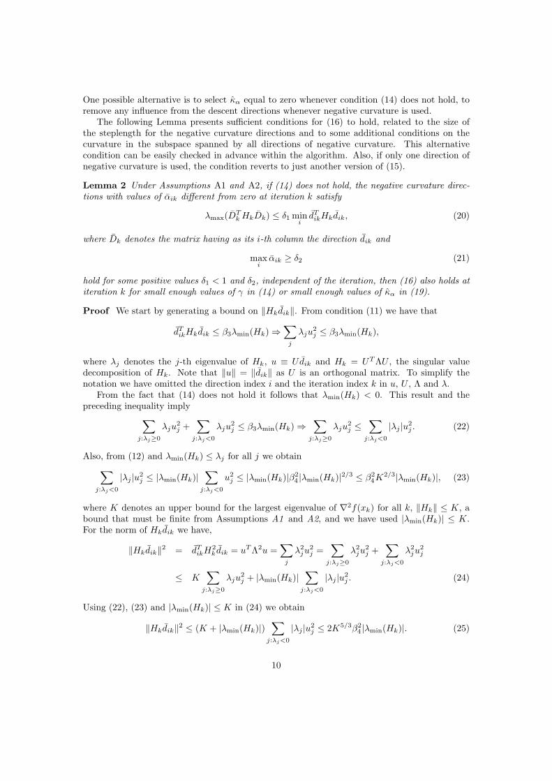
One possible alternative is to select κα equal to zero whenever condition (14) does not hold, toremove any influence from the descent directions whenever negative curvature is used.

The following Lemma presents sufficient conditions for (16) to hold, related to the size ofthe steplength for the negative curvature directions and to some additional conditions on thecurvature in the subspace spanned by all directions of negative curvature. This alternativecondition can be easily checked in advance within the algorithm. Also, if only one direction ofnegative curvature is used, the condition reverts to just another version of (15).

Lemma 2 Under Assumptions A1 and A2, if (14) does not hold, the negative curvature direc-tions with values of αik different from zero at iteration k satisfy

λmax(DTk HkDk) ≤ δ1 min

idT

ikHkdik, (20)

where Dk denotes the matrix having as its i-th column the direction dik and

maxi

αik ≥ δ2 (21)

hold for some positive values δ1 < 1 and δ2, independent of the iteration, then (16) also holds atiteration k for small enough values of γ in (14) or small enough values of κα in (19).

Proof We start by generating a bound on ‖Hkdik‖. From condition (11) we have that

dTikHkdik ≤ β3λmin(Hk) ⇒

∑

j

λju2j ≤ β3λmin(Hk),

where λj denotes the j-th eigenvalue of Hk, u ≡ Udik and Hk = UT ΛU , the singular valuedecomposition of Hk. Note that ‖u‖ = ‖dik‖ as U is an orthogonal matrix. To simplify thenotation we have omitted the direction index i and the iteration index k in u, U , Λ and λ.

From the fact that (14) does not hold it follows that λmin(Hk) < 0. This result and thepreceding inequality imply

∑

j:λj≥0

λju2j +

∑

j:λj<0

λju2j ≤ β3λmin(Hk) ⇒

∑

j:λj≥0

λju2j ≤

∑

j:λj<0

|λj |u2j . (22)

Also, from (12) and λmin(Hk) ≤ λj for all j we obtain∑

j:λj<0

|λj |u2j ≤ |λmin(Hk)|

∑

j:λj<0

u2j ≤ |λmin(Hk)|β2

4 |λmin(Hk)|2/3 ≤ β24K2/3|λmin(Hk)|, (23)

where K denotes an upper bound for the largest eigenvalue of ∇2f(xk) for all k, ‖Hk‖ ≤ K, abound that must be finite from Assumptions A1 and A2, and we have used |λmin(Hk)| ≤ K.For the norm of Hkdik we have,

‖Hkdik‖2 = dTikH2

k dik = uT Λ2u =∑

j

λ2ju

2j =

∑

j:λj≥0

λ2ju

2j +

∑

j:λj<0

λ2ju

2j

≤ K∑

j:λj≥0

λju2j + |λmin(Hk)|

∑

j:λj<0

|λj |u2j . (24)

Using (22), (23) and |λmin(Hk)| ≤ K in (24) we obtain

‖Hkdik‖2 ≤ (K + |λmin(Hk)|)∑

j:λj<0

|λj |u2j ≤ 2K5/3β2

4 |λmin(Hk)|. (25)

10

From (3), for the value of interest, dTk Hkdk, we can write

dTk Hkdk =

∑

i,j

αikαjkdTikHkdjk + 2

∑

i,j

αikαjkdTikHkdjk +

∑

i,j

αikαjkdTikHkdjk, (26)

and for the different terms of this sum the following inequalities hold: for the first term, usingthe bound on ‖Hk‖, (10) and (19) we have

∑

i,j

αikαjkdTikHkdjk ≤ κ2

αK∑

i,j

‖dik‖‖djk‖ ≤ Kκ2αn2

1β22‖gk‖2, (27)

where n1 denotes a bound on the maximum number of directions of descent used in any iteration.For the second term, from (10), (25), (13) and (19),

2∑

i,j

αikαjkdTjkHkdik ≤ 2κακα

∑

i,j

‖dik‖‖Hkdjk‖ ≤ 2κακαn1n2β2‖gk‖β4

√2K5/3|λmin(Hk)|,

(28)where now n2 denotes a bound on the maximum number of directions of negative curvature usedin any iteration.

Finally, the third term can be written as∑

i,j

αikαjkdTikHkdjk = aT

k DTk HkDkak,

where ak is a vector having its i-th component equal to αik. From (20) we obtain the followingbound ∑

i,j

αikαjkdTikHkdjk ≤ λmax(DT

k HkDk)‖ak‖2 ≤ δ1δ22 min

idT

ikHkdik, (29)

where we have used ‖ak‖ ≥ δ2, from (21).We now combine these bounds, writing them in terms of either ‖gk‖2 or λmin(Hk). To do

that, we need to rewrite the bound for the intermediate term (28) using the arithmetic/geometricmean inequality as

2κακαn1n2β2‖gk‖β4

√2K5/3|λmin(Hk)| ≤ 1

2δ1δ22β3|λmin(Hk)|+ 4κ2

ακ2αn2

1n22β

22β2

4K5/3

δ1δ22β3

‖gk‖2.(30)

Combining the bounds from (27), (29) and (30) and replacing them in (26) we obtain

dTk Hkdk ≤ Kκ2

αn21β

22

(1 +

4κ2αn2

2β24K2/3

δ1δ22β3

)‖gk‖2 + δ1δ

22

(12β3|λmin(Hk)|+ min

idT

ikHkdik

). (31)

From (11) we have that

12β3|λmin(Hk)| ≤ − 1

2 mini

dTikHkdik ⇒ 1

2β3|λmin(Hk)|+ mini

dTikHkdik ≤ 1

2 mini

dTikHkdik,

and replacing this bound in (31) we obtain

dTk Hkdk ≤ Kκ2

αn21β

22

(1 +

4κ2αn2

2β24K2/3

δ1δ22β3

)‖gk‖2 + 1

2δ1δ22 min

idT

ikHkdik. (32)

11

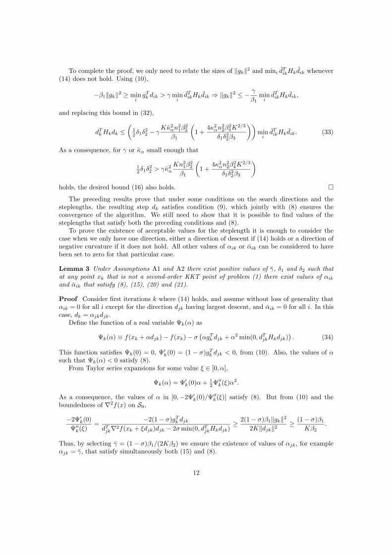
To complete the proof, we only need to relate the sizes of ‖gk‖2 and mini dTikHkdik whenever

(14) does not hold. Using (10),

−β1‖gk‖2 ≥ mini

gTk dik > γ min

idT

ikHkdik ⇒ ‖gk‖2 ≤ − γ

β1min

idT

ikHkdik,

and replacing this bound in (32),

dTk Hkdk ≤

(12δ1δ

22 − γ

Kκ2αn2

1β22

β1

(1 +

4κ2αn2

2β24K2/3

δ1δ22β3

))min

idT

ikHkdik. (33)

As a consequence, for γ or κα small enough that

12δ1δ

22 > γκ2

α

Kn21β

22

β1

(1 +

4κ2αn2

2β24K2/3

δ1δ22β3

)

holds, the desired bound (16) also holds. ¤The preceding results prove that under some conditions on the search directions and the

steplengths, the resulting step dk satisfies condition (9), which jointly with (8) ensures theconvergence of the algorithm. We still need to show that it is possible to find values of thesteplengths that satisfy both the preceding conditions and (8).

To prove the existence of acceptable values for the steplength it is enough to consider thecase when we only have one direction, either a direction of descent if (14) holds or a direction ofnegative curvature if it does not hold. All other values of αik or αik can be considered to havebeen set to zero for that particular case.

Lemma 3 Under Assumptions A1 and A2 there exist positive values of γ, δ1 and δ2 such thatat any point xk that is not a second-order KKT point of problem (1) there exist values of αik

and αik that satisfy (8), (15), (20) and (21).

Proof Consider first iterations k where (14) holds, and assume without loss of generality thatαik = 0 for all i except for the direction djk having largest descent, and αik = 0 for all i. In thiscase, dk = αjkdjk.

Define the function of a real variable Ψk(α) as

Ψk(α) ≡ f(xk + αdjk)− f(xk)− σ(αgT

k djk + α2 min(0, dTjkHkdjk)

). (34)

This function satisfies Ψk(0) = 0, Ψ′k(0) = (1 − σ)gTk djk < 0, from (10). Also, the values of α

such that Ψk(α) < 0 satisfy (8).From Taylor series expansions for some value ξ ∈ [0, α],

Ψk(α) = Ψ′k(0)α + 12Ψ′′k(ξ)α2.

As a consequence, the values of α in [0,−2Ψ′k(0)/Ψ′′k(ξ)] satisfy (8). But from (10) and theboundedness of ∇2f(x) on S0,

−2Ψ′k(0)Ψ′′k(ξ)

=−2(1− σ)gT

k djk

dTjk∇2f(xk + ξdjk)djk − 2σ min(0, dT

jkHkdjk)≥ 2(1− σ)β1‖gk‖2

2K‖djk‖2 ≥ (1− σ)β1

Kβ2.

Thus, by selecting γ = (1 − σ)β1/(2Kβ2) we ensure the existence of values of αjk, for exampleαjk = γ, that satisfy simultaneously both (15) and (8).

12

Consider now iterations k such that (14) does not hold. Again, without loss of generality letαik = 0 for all i and also αik = 0 for all i except for the direction having the largest negativecurvature, djk, so that dk = αjkdjk. As a consequence of these choices, (20) holds trivially inthis case.

To consider (21) we define a function Ψk analogous to Ψk, as

Ψk(α) ≡ f(xk + αdjk)− f(xk)− σ(αgT

k djk + α2dTjkHkdjk

).

Note that our assumption that (14) does not hold implies dTjkHkdjk < 0.

Consider now the Taylor series expansion of Ψk up to its third order term,

Ψk(α) = Ψk(0) + Ψ′k(0)α + 12 Ψ′′k(0)α2 + 1

6 Ψ′′′k (ξ)α3,

for some value ξ ∈ [0, α]. Analogously to the preceding case, we have Ψk(0) = 0, Ψ′k(0) =(1 − σ)gT

k djk ≤ 0 and Ψ′′k(0) = (1 − 2σ)dTjkHkdjk < 0. As a consequence, all sufficiently small

values of α satisfy Ψk(α) < 0 and as a consequence condition (8) holds for them. In particular,as Ψ′k(0) ≤ 0, all values of α in [0,−3Ψ′′k(0)/Ψ′′′k (ξ)] satisfy Ψk(α) ≤ 0 and (8).

Note that from Assumptions A1 and A2, as xk ∈ S0, there exists a constant K3 such thatΨ′′′k (ξ) ≤ K3‖djk‖3. Then, from (11) and (12) we have

−3Ψ′′k(0)Ψ′′′k (ξ)

=−3(1− 2σ)dT

jkHkdjk

Ψ′′′k (ξ)≥ 3(1− 2σ)β3|λmin(Hk)|

K3‖djk‖3

≥ 3(1− 2σ)β3|λmin(Hk)|K3β3

4 |λmin(Hk)| =3(1− 2σ)β3

K3β34

.

From this result, if we select δ2 = 3(1− 2σ)β3/(2K3β34) in (21) we ensure the existence of values

of αjk, for example αjk = δ2, that satisfy simultaneously (20), (21) and (8). ¤

Trust-region and linesearch approach

Consider now the case of Algorithm TRSM, combining a trust-region approach and a linesearchon the direction obtained from the trust-region. In iteration k of this algorithm, the directionssatisfying conditions (10), (11) and (12) are combined by solving a trust-region problem of theform

mina gTk Dka + 1

2aT DTk HkDka

s.t. ‖a‖ ≤ ∆k,(35)

where gk ≡ ∇f(xk), Hk ≡ ∇2f(xk), Dk is a matrix having as columns the descent and negativecurvature directions dik and dik and ∆k is a positive scalar.

We will impose the condition that the value of ∆k satisfies for all k

∆ ≤ ∆k ≤ ∆, (36)

where ∆ and ∆ are two prespecified constants. Note that in this algorithm, due to the use ofa linesearch to compute the final size of dk, it should be possible to select the value of ∆k withgreater freedom than in the case of a pure trust-region algorithm, as the linesearch should correctfor any deviation in the scale of dk.

We also need to tighten slightly the bound on the size of dik (12) in those cases when we havea significant amount of descent. Whenever −‖∇f(xk)‖2 ≤ λmin(∇2f(xk)) < 0 we require

‖dik‖ ≤ β4 min(‖∇f(xk)‖, |λmin(∇2f(xk))|1/3

)(37)

13

to hold instead of condition (12). We still assume that the descent and negative curvaturedirections satisfy (10) and (11), and that all of them are linearly independent, as before.

Let ak denote the optimal value for a in (35), and define a search direction as dk = Dkak. Astandard linesearch in carried out along this direction to find a scalar αk satisfying condition (8)for αkdk.

The following results analyze the convergence properties of this approach. The first result isequivalent to Lemma 1 in the case of a subspace search.

Lemma 4 Under the preceding assumptions and conditions, for dk = Dkak it holds that

min(gT

k dk, dTk Hkdk

) ≤ γ min(−‖gk‖2, λmin(Hk)

), (38)

for some positive constant γ and all k.

Proof Consider the three different cases for the solution of (35):

• Case I: λmin(Hk) > 0, ‖ak‖ < ∆k and ak = −(DTk HkDk)−1DT

k gk.

• Case II: ‖ak‖ = ∆k and ak = −(DTk HkDk + κI)−1DT

k gk for an appropriate positive valueκ > −min(0, λmin(DT

k HkDk)).

• Case III: DTk gk is orthogonal to all eigenvectors associated with λmin(DT

k HkDk) < 0. Forthis case ‖ak‖ = ∆k and ak = −(DT

k HkDk − λmin(DTk HkDk)I)+DT

k gk + ξvmin, where ξ isan appropriate scalar and vmin is an eigenvector associated with λmin(DT

k HkDk).

Let

τk =

0 if Case I holds,κ if Case II holds,

−λmin(DTk HkDk) if Case III holds.

From dk = Dkak and the fact that DTk HkDk + τkI is a positive definite matrix, for Cases I and

II we have

dk = −Dk(DTk HkDk + τkI)−1DT

k gk

gTk dk = −gT

k Dk(DTk HkDk + τkI)−1DT

k gk ≤ − ‖DTk gk‖2

λmax(DTk HkDk) + τk

gTk dk + dT

k Hkdk = −gTk Dk(DT

k HkDk + τkI)−1DTk gk

+ gTk Dk(DT

k HkDk + τkI)−1DTk HkDk(DT

k HkDk + τkI)−1DTk gk

= −τkgTk Dk(DT

k HkDk + τkI)−2DTk gk = −τk‖(DT

k HkDk + τkI)−1DTk gk‖2

= −τk‖ak‖2

For Case III it holds that gTk Dkvmin = 0, and as a consequence

dk = −Dk(DTk HkDk + τkI)+DT

k gk + ξDkvmin

gTk dk = −gT

k Dk(DTk HkDk + τkI)+DT

k gk ≤ − ‖DTk gk‖2

λmax(DTk HkDk) + τk

gTk dk + dT

k Hkdk = −gTk Dk(DT

k HkDk + τkI)+DTk gk

+ gTk Dk(DT

k HkDk + τkI)+DTk HkDk(DT

k HkDk + τkI)+DTk gk

− 2ξgTk Dk(DT

k HkDk + τkI)+DTk HkDkvmin + ξ2vT

minDTk HkDkvmin

= −τkgTk Dk((DT

k HkDk + τkI)+)2DTk gk − τkξ2vT

minvmin

= −τk‖ − (DTk HkDk + τkI)+DT

k gk + ξvmin‖2 = −τk‖ak‖2

14

where we have also used

DTk HkDkvmin = −τkvmin

(DTk HkDk + τkI)+vmin = 0.

In summary, it holds for all three cases that

gTk dk ≤ − ‖DT

k gk‖2λmax(DT

k HkDk) + τk(39)

andgT

k dk + dTk Hkdk = −τk‖ak‖2. (40)

For those iterations where we have −‖gk‖2 ≤ min(0, λmin(Hk)), from (10) and for at leastone component i,

(DTk gk)i ≤ −β1‖gk‖2 ⇒ ‖Dkgk‖ ≥ β1‖gk‖2,

and also from (10) and (37),

‖Dk‖2 ≤ ‖Dk‖2F =∑

i

‖dki‖2 +∑

j

‖dkj‖2 (41)

≤∑

i

β22‖gk‖2 +

∑

j

β24 min(‖gk‖2, |λmin(Hk)|2/3) ≤ mmax(β2

2 , β24)‖gk‖2, (42)

where m denotes a bound on the maximum number of directions used by the algorithm in a giveniteration and ‖ · ‖F denotes the Frobenius norm. Let KH and Kg denote two positive constantssuch that ‖Hk‖ ≤ KH and ‖gk‖ ≤ Kg for all k. The existence of these constants follows fromAssumptions A1 and A2. Using these bounds on (39) we have

gTk dk ≤ − ‖DT

k gk‖2λmax(DT

k HkDk) + τk≤ − β2

1‖gk‖4KH‖Dk‖2 + τk

≤ − β21

mmax(β22 , β2

4)KH + τk/‖gk‖2 ‖gk‖2. (43)

From the preceding results and a given iteration k we have for the different cases:

• Case I: it holds that ‖gk‖3 ≥ 0 = |min(0, λmin(DTk HkDk))| and also τk = 0. From (43) we

have

min(gTk dk, dT

k Hkdk) ≤ gTk dk ≤ − β2

1

m max(β22 , β2

4)KH‖gk‖2

≤ β21

mmax(β22 , β2

4)KHmin

(−‖gk‖2, λmin(Hk)). (44)

• Cases II and III: We have ‖ak‖ = ∆k and from (40) and τk ≥ −λmin(DTk HkDk) we also

havegT

k dk + dTk Hkdk = −τk∆2

k ≤ ∆2λmin(DTk HkDk).

Assume that ‖gk‖2 ≤ |min(0, λmin(Hk)| holds. Then

min(gTk dk, dT

k Hkdk) ≤ 12 (gT

k dk + dTk Hkdk) ≤ 1

2∆2λmin(DTk HkDk) ≤ 1

2∆2β4λmin(Hk)

≤ 12∆2β4 min

(−‖gk‖2, λmin(Hk)). (45)

15

Assume now the opposite condition holds, that is, ‖gk‖2 > |min(0, λmin(Hk)|. For CaseIII, using (42) we have that

τk

‖gk‖2 =−λmin(DT

k HkDk)‖gk‖2 ≤ ‖Hk‖‖Dk‖2

‖gk‖2

≤ KHm max(β22 , β2

4)‖gk‖2‖gk‖2 ≤ mKH max(β2

2 , β24).

For Case II, from ‖ak‖ = ∆k and (42) we have

∆k = ‖(DTk HkDk + τkI)−1DT

k gk‖ ≤ ‖DTk gk‖

λmin(DTk HkDk) + τk

⇒ τk ≤ ‖DTk gk‖∆k

− λmin(DTk HkDk) ≤ ‖Dk‖‖gk‖

∆k+ KH‖Dk‖2

≤√

mmax(β2, β4)∆k

‖gk‖2 + KHm max(β22 , β2

4)‖gk‖2

⇒ τk

‖gk‖2 ≤√

mmax(β2, β4)∆k

+ mKH max(β22 , β2

4).

Defining ω ≡ mKH max(β22 , β2

4) +√

m max(β2, β4)/∆k we obtain for Cases II and III thebound

τk

‖gk‖2 ≤ ω, (46)

and replacing it in (43) we obtain

gTk dk ≤ − β2

1

mmax(β22 , β2

4)KH + ω‖g2

k‖. (47)

From (47) and the condition ‖gk‖2 > |min(0, λmin(Hk)| it follows that

min(gTk dk, dT

k Hkdk) ≤ gTk dk ≤ − β2

1

mmax(β22 , β2

4)KH + ω‖g2

k‖

≤ β21

m max(β22 , β2

4)KH + ωmin

(−‖gk‖2, λmin(Hk)). (48)

The desired result is a consequence of (44), (45) and (48). ¤We now establish that the search direction obtained from the trust region, together with

an appropriate linesearch procedure, such as for example a backtracking linesearch, providesa globally convergent algorithm. Note that in this case, by taking into account the specificprocedure used to compute the steplengths and their resulting properties, we do not need toimpose any additional conditions such as those introduced for algorithm NSM in (13), (15),(20) and (21).

Theorem 2 Under the preceding conditions and assumptions, algorithm TRSM converges tosecond-order KKT points of problem (1).

Proof We start by proving the existence of a lower bound on the steplength taken on the searchdirection dk obtained from the solution of the trust-region problem. We use a strategy similarto the one in the proof of Lemma 3, that is, we define a function of a real variable Ψk(α) as

Ψk(α) ≡ f(xk + αdk)− f(xk)− σ(αgT

k dk + α2 min(0, dTk Hkdk)

). (49)

16

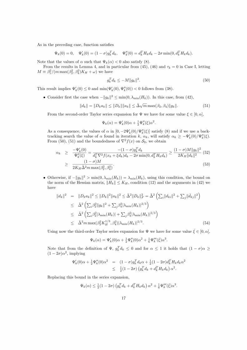
As in the preceding case, function satisfies

Ψk(0) = 0, Ψ′k(0) = (1− σ)gTk dk, Ψ′′k(0) = dT

k Hkdk − 2σ min(0, dTk Hkdk).

Note that the values of α such that Ψk(α) < 0 also satisfy (8).From the results in Lemma 4, and in particular from (45), (46) and τk = 0 in Case I, letting

M ≡ β21/(mmax(β2

2 , β24)KH + ω) we have

gTk dk ≤ −M‖gk‖2. (50)

This result implies Ψ′k(0) ≤ 0 and min(Ψ′k(0), Ψ′′k(0)) < 0 follows from (38).

• Consider first the case when −‖gk‖2 ≤ min(0, λmin(Hk)). In this case, from (42),

‖dk‖ = ‖Dkak‖ ≤ ‖Dk‖‖ak‖ ≤ ∆√

m max(β2, β4)‖gk‖. (51)

From the second-order Taylor series expansion for Ψ we have for some value ξ ∈ [0, α],

Ψk(α) = Ψ′k(0)α + 12Ψ′′k(ξ)α2.

As a consequence, the values of α in [0,−2Ψ′k(0)/Ψ′′k(ξ)] satisfy (8) and if we use a back-tracking search the value of α found in iteration k, αk, will satisfy αk ≥ −Ψ′k(0)/Ψ′′k(ξ).From (50), (51) and the boundedness of ∇2f(x) on S0, we obtain

αk ≥ −Ψ′k(0)Ψ′′k(ξ)

=−(1− σ)gT

k dk

dTk∇2f(xk + ξdk)dk − 2σ min(0, dT

k Hkdk)≥ (1− σ)M‖gk‖2

2KH‖dk‖2 (52)

≥ (1− σ)M2KH∆2m max(β2

2 , β24)

. (53)

• Otherwise, if −‖gk‖2 > min(0, λmin(Hk)) = λmin(Hk), using this condition, the bound onthe norm of the Hessian matrix, ‖Hk‖ ≤ KH , condition (12) and the arguments in (42) wehave

‖dk‖2 = ‖Dkak‖2 ≤ ‖Dk‖2‖ak‖2 ≤ ∆2‖Dk‖2F = ∆2(∑

i‖dki‖2 +∑

j‖dkj‖2)

≤ ∆2(∑

iβ22‖gk‖2 +

∑jβ

24 |λmin(Hk)|2/3

)

≤ ∆2(∑

iβ22 |λmin(Hk)|+ ∑

jβ24 |λmin(Hk)|2/3

)

≤ ∆2m max(β22K

1/3H , β2

4)|λmin(Hk)|2/3. (54)

Using now the third-order Taylor series expansion for Ψ we have for some value ξ ∈ [0, α],

Ψk(α) = Ψ′k(0)α + 12Ψ′′k(0)α2 + 1

6Ψ′′′k (ξ)α3.

Note that from the definition of Ψ, gTk dk ≤ 0 and for α ≤ 1 it holds that (1 − σ)α ≥

(1− 2σ)α2, implying

Ψ′k(0)α + 12Ψ′′k(0)α2 = (1− σ)gT

k dkα + 12 (1− 2σ)dT

k Hkdkα2

≤ 12 (1− 2σ)

(gT

k dk + dTk Hkdk

)α2.

Replacing this bound in the series expansion,

Ψk(α) ≤ 12 (1− 2σ)

(gT

k dk + dTk Hkdk

)α2 + 1

6Ψ′′′k (ξ)α3.

17

Analogously to the preceding case, from (40) we have (1 − 2σ)(gT

k dk + dTk Hkdk

)< 0. As

a consequence, all sufficiently small values of α satisfy Ψk(α) < 0 and as a consequencecondition (8) holds for them. In particular, if a backtracking search is conducted, the valueαk obtained from the search will satisfy

αk ≥ −3(1− 2σ)(gT

k dk + dTk Hkdk

)

Ψ′′′k (ξ)≥ −3(1− 2σ)∆2λmin(Hk)

K3‖dk‖3 (55)

where we have used the bound Ψ′′′k (ξ) ≤ K3‖dk‖3, (40) and τk ≥ −λmin(Hk), as undercondition −‖gk‖2 > λmin(Hk) only Cases II and III are possible for the solution of thetrust-region problem; in particular, ‖ak‖ = ∆k ≥ ∆ must hold.

From (54) and (55) we obtain

αk ≥ − 3(1− 2σ)∆2λmin(Hk)

K3∆3m3/2 max(β32K

1/2H , β3

4)|λmin(Hk)|=

3(1− 2σ)∆2

K3∆3m3/2 max(β32K

1/2H , β3

4). (56)

Combining (53) and (56), for all k it holds that

αk ≥ min

((1− σ)M

2KH∆2m max(β22 , β2

4),

3(1− 2σ)∆2

K3∆3m3/2 max(β32K

1/2H , β3

4)

)≡ α > 0. (57)

Let I denote the iterations belonging to any convergent subsequence, xk → x∗. Thesesubsequences exist from assumption A1. For k ∈ I, from conditions (8) and (38) it must holdthat

f(xk + dk)− f(xk) ≤ σαk(gTk dk + min(0, dT

k Hkdk))≤ σα min

(gT

k dk, dTk Hkdk

)

≤ σαγ min(−‖gk‖2, λmin(Hk)

).

Taking limits as k →∞ along I and using Assumptions A1 and A2, the boundedness of f(xk)and the fact that the right-hand side in the preceding inequality is nonpositive, we obtain

min(−‖∇f(x∗)‖2, λmin(∇2f(x∗))

)= 0 ⇒ ‖∇f(x∗)‖ = 0, λmin(∇2f(x∗)) ≥ 0.

¤In the following section we present a particular implementation of this approach that selects

d1k = −H−1k gk, the Newton direction, in all iterations where it is defined. It also chooses (ak)1 =

1 and computes the remaining components of ak solving the equivalent version of the trust-regionproblem (35). In this particular case, letting a =

(1 aT

)T and Dk =(

d1k Dk

), where Dk

denotes a matrix having as columns all search directions, except for the Newton direction, anda denotes the corresponding coefficients, this subproblem has the form

mina (gk + Hkd1k)T Dka + 12 aT DT

k HkDkas.t. ‖a‖ ≤ ∆k,

but as gk + Hkd1k = 0, we obtain the equivalent problem

mina12 aT DT

k HkDkas.t. ‖a‖ ≤ ∆k.

(58)

A solution of this problem is

18

• ak = 0 if λmin(DTk HkDk) > 0, or

• ‖ak‖ = ∆k andDT

k HkDkak = λmin(DTk HkDk)ak,

otherwise, that is, an eigenvector associated with the smallest eigenvalue of λmin(DTk HkDk).

And as a consequence, the search direction for the linesearch part of the algorithm is given bydk = d1k + Dkak = d1k + dk, where dk is either equal to zero if the matrix Hk is positivedefinite, or a direction of negative curvature satisfying (11) and (12) otherwise, and with a sizethat is bounded below. Thus, the conditions introduced for the combination of directions in thepreceding section also hold in this case and the algorithm also converges to second-order KKTpoints.

4 Implementation and Numerical Results

4.1 Implementation of the algorithms

The algorithms we have chosen to implement and test in this paper are particular versions ofthose described in Section 2, algorithms NSM and TRSM. In the preceding section we havestudied the convergence properties of the more general versions of the algorithms, but thesegeneral versions must be specified in greater detail before they can be implemented. In thefollowing paragraphs we describe the specific implementations we have used in our numericalexperiments.

• Search directions. We compute just two descent directions, a Newton direction d1k and thenegative gradient d2k,

d1k = −B−1∇f(xk), d2k = −∇f(xk),

where B = ∇2f(xk), if ∇2f(xk) is positive definite, otherwise, B is a suitable approxima-tion for ∇2f(xk) to ensure that condition (10) is satisfied.

We also use a single negative curvature direction, that we denote as d3k, whenever it isavailable at iteration k and satisfies conditions (11) and (12), or (37) if algorithm TRSMis used.

• Nonnegative steplengths. We introduce an additional step in algorithm NSM to ensurethat the steplengths remain positive and bounded in all iterations. For a given positiveconstant κα we compute:

Step 3c’ [Projection] Let α2(k+1) and α3(k+1) be the values obtained fromStep 3c. Set α2(k+1) = min(max(0, α2(k+1)), κα)

and α3(k+1) = min(max(0, α3(k+1)), κα).

After this projection step, the resulting combination of directions dk is still a descentdirection, as it is a nonnegative linear combination of descent directions.

From a theoretical point of view, this step ensures the satisfaction of condition (13) for thegradient and negative curvature direction.

19

• Unit Newton step. For both algorithms the value for the search direction in iteration k,dk, has been obtained by fixing α1k = 1, that is, the step taken along the Newton directionis set to 1 before the linesearch step (Step 3e) is carried out.

If in addition to this, the initial values for the other steplengths, α20 and α30, are takento be equal to zero, close to the solution we may take Newton steps, and we may attain aquadratic rate of convergence.

Note that this choice of step for the Newton direction does not affect the convergenceproofs. For algorithm NSM it ensures the satisfaction of condition (15), as long as γin (14) is chosen to be small enough (see Lemma 2). Regarding algorithm TRSM, theconvergence for this case has been already discussed at the end of Section 3.

4.2 Computational experiments

We have carried out some computational experiments to compare the two proposals describedin the preceding sections with an implementation of a modified linesearch Newton’s method(LSNM), that is, an implementation of Newton’s method including a modification of the Hessianmatrix to compute the descent direction in those iterations where significant negative curvature isdetected, as well as an implementation of a more sophisticated Newton’s method using the Moreand Sorensen [13] approach (MSNM) that incorporates negative curvature through a quadraticcurvilinear search.

Numerical results have been obtained for a number of test problems from the CUTEr col-lection [9]. We have included the 119 nonlinear unconstrained problems of dimension between1 and 500, having continuous second derivatives, to ensure that the directions of interest wereavailable for all of them.

The algorithms and the test problems have been implemented and executed using MATLAB6.5 for Linux. In all cases we have considered the default starting points x0 provided by CUTEr.

The algorithms introduced in Section 2 use some parameters. For our implementation, wehave chosen the values σ = 0, ξ = 0.5, δ = ∆0 = kmax = 1; the convergence tolerance ω∗ specifiesthe final accuracy requested by the user, and it has been set to the value 10−8. The maximumnumber of iterations allowed was set to 1000.

4.2.1 Analysis of the results

Tables 5 and 6 present the numerical results obtained for the different algorithms. In these tableswe have used the following notation:

• n: Number of variables.

• iter: Iteration count.

• fgeval: Number of function and gradient evaluations.

• LSNM: Line search Newton method

• MSNM: More-Sorensen Newton method.

• NSM: Newton-based Scaling method.

• TRSM: Trust-Region Scaling method.

20

If the maximum number of iterations is reached (iter > 1000), we do not consider the associatednumber of function and gradient evaluations in Table 5.

Table 7 provides a summary of the results. It is clear that the best results are obtained by thetwo proposals presented in this work. Both the average iteration counts and the average numberof function evaluations are significantly lower for our proposals, compared to the two alternativeswe have considered. In particular, the average reductions in the number of iterations obtainedusing the NSM and the TRSM methods with respect to the LSNM method are respectively23.30% and 35.84%. Regarding the reductions for the number of function evaluations the resultsare 17.49% and 36.62% respectively.

With respect to the LSNM method, the reductions in iterations and function evaluationsare far more marked than the increases. For the NSM method, the largest deterioration in thenumber of iterations amounted to 51.32% (problem LOGHAIRY), while the largest improvementwas 81.82% (problem DIXMAANE). Regarding the TRSM algorithm, the largest deteriorationin the number of iterations amounted to 48% (problem VIBRBEAM), while the largest im-provement was 92.72% (problem DIXMAANC). Similar results are obtained when comparingthe number of function evaluations.

Notice the large number of iterations and function evaluations for the MSNM algorithmwhen solving all the DIXMAAN problems, and problems BIGGS6, HUMPS or SNAIL. Forinstance, in Table 6, for the DIXMAAN problems, the number of iterations in which negativecurvature is used is clearly larger when the MSNM method is used. In these cases the scalingof the descent directions seems to be specially relevant. For these problems our two proposalsreduce drastically the number of iterations and moderately the number of function evaluations.It is important to remark that, excluding these problems, the MSNM algorithm provides similarresults to those obtained using the LSNM algorithm. These problems are an example of theimportance of an adequate scaling of the directions.

Regarding the impact of the use of negative curvature on the whole set of 119 problems, forthose problems where negative curvature were detected, Table 6 shows the number of iterationswhere it was used. Negative curvature was detected for approximately 50% percent of theproblems. For the NSM method, the average number of iterations per problem where a directionof negative curvature was used is 24.25, that is, 61.07% of the average number of iterations perproblem. For the TRSM method this percentage is similar, 62.81%. For the MSNM methodthis percentage increases up to 70.14%, again because of the DIXMAAN problems. If we restrictthe results only to those problems where negative curvature was detected, the average reductionsin the number of iterations obtained using the NSM and the TRSM methods with respect to theLSNM method are respectively 26.01% and 40.52%. Regarding the reductions for the numberof function evaluations the results are 18.14% and 37.60% respectively. Therefore, it is apparentthe effect of the use of negative curvature in the successful performance of the methods.

4.2.2 Evaluation of the performance

In [2], Dolan and More have defined the performance profile of a solver as a (cumulative) distribu-tion function for a given performance metric. We have evaluated and compared the performanceof the solvers LSNM (Line search Newton method), MSNM (More-Sorensen Newton method),NSM (Newton-based Scaling method) and TRSM (Trust-Region Scaling method) on the setP of 119 test problems from the CUTEr collection.

We have considered two performance metrics, the number of iterations needed to attain thedesired accuracy (since each iteration implies a considerable amount of work) and the corre-sponding number of function evaluations, both giving information on solvers robustness andefficiency.

21

Let p denote a particular problem of P and s a particular solver. The idea is to compare theperformance of solver s on problem p with the best performance by any solver on this particularproblem. As in [2], we define the performance ratios as

rjp,s =

tip,s

min{tip,s : 1 ≤ s ≤ ns

} , with i ∈ {1, 2} ,

where tjp,s refers to the number of iterations, for j = 1, and the number of function evaluations,for j = 2, required to solve problem p by solver s, and ns refers to the number of solvers. If asolver does not solve a problem, we set the values of its performance ratios to large parametersrjM , with rj

M > rjp,s.

In order to obtain an overall assessment of each solver on the set P, we define the followingcumulative distribution functions,

ρjs(τ) =

1np

size{p ∈ P : rj

p,s ≤ τ}

, with j ∈ {1, 2} ,

where ρjs(τ), j = 1, 2, is the probability that the performance ratio rj

p,s is within a factor of τ ofthe best possible ratio and np is the number of problems in P.

For τ = 1, the probability ρjs(1) of a particular solver s is the probability that the value of

the metric for the solver will be the best one among all solvers. The approximate values for theprobabilities ρj

s(τ), j = 1, 2, when τ = 1, 2, 3, are given in Table 8.Regarding the number of iterations, from this table we see that TRSM has the highest

probability of being the optimal solver. On the other hand, considering the number of functionevaluations, we observe that LSNM has the highest probability of being the optimal solver.

In Figures 1 and 2 we represent the performance profiles on a log2 scale [2], i.e., we plot

τ 7−→ 1np

size{p ∈ P : log2(r

jp,s) ≤ τ, j = 1, 2

}.

For large values of τ , the probability function ρjs(τ) provides information about the total

proportion of problems that a given code is able to solve. Thus, if we are interested in the prob-ability that a solver will be successful, we should consider ρj

s(τ) for all solvers as τ becomes large(rj

M ). Figures 1 and 2 are plotted using a log2 scale to provide a more compact representation ofthe available data (if a linear scale were used, it would be necessary to include the whole interval[0, 1024] to be able to include the largest values rj

p,s < rjM , j = 1, 2).

In Figures 1 and 2, we see that both NSM and TRSM solve the highest number of problems(about 96%). In Figure 1 we conclude that TRSM dominates all other solvers, since the perfor-mance profile for TRSM lies above all others for all performance ratios τ . Note that these resultsdo not imply that TRSM solves every problem with a smaller number of iterations. For τ ≥ 4,solver NSM has the same performance as TRSM. In Figure 2 we see that, for 1 ≤ τ ≤ 4.3,TRSM solves the largest number of problems requiring a number of function evaluations thatis less than τ times that of any other solver. For τ ≥ 6, NSM is the only solver that attains thesame best performance as TRSM. Considering all these facts, we conclude that the best resultsare obtained by the two proposals presented in this work.

5 Conclusions

In this paper we have studied different approaches to combine information in an efficient mannerwithin an algorithm to solve unconstrained optimization problems. We show that negative

22

Figure 1: Performance profile in a log2 scale − number of iterations

Figure 2: Performance profile in a log2 scale − number of function evaluations

23

curvature can be used successfully if some safeguards are taken into account. These safeguardsrefer mainly to the scaling problem that arises when dealing with descent directions of a differentnature. In particular, we have proposed two procedures for the combination of the gradient,a modified Newton direction and a negative curvature direction. The procedures calculate, byperforming a small number of iterations of a Newton’s method or a trust-region method in a lowdimensional subspace, the weights associated to the linear combination of the directions. In thisway, this step can be viewed as a previous scaling of the directions. Then a linesearch procedureon the weights is carried out.

Our recommendation is that any algorithm using directions that arise from a different natureshould include an scaling process before proceeding to the combination of the directions. Thisis the key point in the success of the algorithms proposed in this paper.

These results still require further work. In particular, the current environment of implemen-tation does not allow the testing of the algorithms for large-scale problems. Nevertheless, giventhe success of the results for the problems in the test set, it seems to provide a promising startingpoint.

References

[1] Byrd, R. H., Schnabel, R. B. and Shultz, G. A., Approximate solution of the trust regionproblem by minimization over two-dimensional subspaces, Mathematical Programming, 40,pp. 247-263, 1998.

[2] Dolan, E. and More, J., Benchmarking optimization software with performance profiles,Mathematical Programming, 91(2), pp. 201-213, 2002.

[3] Fiacco, A. V. and McCormick, G. P., Nonlinear programming: sequential unconstrainedminimization techniques, Society for Industrial and Applied Mathematics, Philadelphia,1990.

[4] Fletcher, R., Practical Methods of Optimization, Volume 1, Unconstrained Optimization,John Wiley & Sons, New York and Toronto, 1980.

[5] Forsgren, A. and Murray, W., Newton methods for large-scale linear equality-constrainedminimization, SIAM J. Matrix Anal. Appl., 14, pp. 560-587, 1993.

[6] Gill, P. E., Murray, W. and Wright, M. H., Practical Optimization, Academic Press, Londonand New York, 1981.

[7] Goldfarb, D., Curvilinear path steplength algorithms for minimization which use directionsof negative curvature, Mathematical Programming, 18, pp. 31-40, 1980.

[8] Gould, N. I. M., Lucidi, S., Roma, M. and Toint, Ph. L., Exploiting negative curvaturedirections in linesearch methods for unconstrained optimization, Optimization Methods andSoftware, 14, pp. 75-98, 2000.

[9] Gould, N. I. M., Orban, D. and Toint, Ph. L., CUTEr (and SifDec), A Constrained and Un-constrained Testing Environment, revisited, ACM Transactions on Mathematical Software,29, pp. 373-394, 2003.

[10] Hager, W. W. and Zhang, H., A new conjugate gradient method with guaranteed descentand an efficient line search, SIAM J. Optim., 16, pp. 170-192, 2005.

24

[11] Moguerza, J. M. and Prieto, F. J., An augmented Lagrangian interior-point method usingdirections of negative curvature, Mathematical Programming, 95, pp. 573-616, 2003.

[12] Moguerza, J. M. and Prieto, F. J., Combining search directions using gradient flows, Math-ematical Programming, 96, pp. 529-559, 2003.

[13] More, J. J and Sorensen, D. C., On the use of directions of negative curvature in a modifiedNewton method, Mathematical Programming, 16, pp. 1-20, 1979.

[14] Mukai, H. and Polak, E., A second-order method for the general nonlinear programmingproblem, J. Optim. Theory Appl., 26, pp. 515-532, 1978.

[15] Olivares A., Moguerza J. M. and Prieto. F. J., Nonconvex optimization using an adaptedlinesearch, European Journal of Operational Research, pages to be assigned, 2007

[16] Sanmatıas, S. and Vercher, E., A generalized conjugate gradient algorithm, J. Optim. TheoryAppl., 98, pp. 489-502, 1998.

[17] Sanmatıas, S. and Roma, M., Un metodo de busqueda lineal con direcciones combinadaspara la optimizacion irrestringida, Actas del XXVI Congreso Nacional de Estadıstica eInvestigacion Operativa, Ubeda, Spain, 2001.

[18] Sun, J., Yang, X. and Chen, X., Quadratic cost flow and the conjugate gradient method,European J. Oper. Res., 164, pp. 104-114, 2005.

25

Iterations Function EvaluationsProblem n LSNM MSNM NSM TRSM LSNM MSNM NSM TRSM

AKIVA 2 6 6 6 6 7 7 7 7ALLINITU 4 6 9 7 6 9 12 21 10ARGLINA 200 1 1 1 1 2 2 2 2ARWHEAD 500 6 6 6 6 7 7 7 7

BARD 3 9 12 9 9 10 19 10 10BDQRTIC 500 9 9 9 9 10 10 10 10BEALE 2 6 6 6 6 39 23 41 41BIGGS6 6 39 71 27 24 67 113 73 79BOX3 3 8 8 8 8 9 9 9 9

BRKMCC 2 3 3 3 3 4 4 4 4BROWNAL 200 15 32 26 13 148 522 398 111BROWNBS 2 6 8 6 6 73 43 77 77

BROWNDEN 4 8 8 8 8 9 9 9 9BROYDN7D 500 82 84 84 82 5208 5216 5386 5329

BRYBND 500 10 11 10 10 15 16 19 19CHNROSNB 50 41 62 41 41 60 120 77 77

CLIFF 2 27 27 27 27 28 28 28 28CRAGGLVY 500 14 14 14 14 15 15 15 15

CUBE 2 26 27 17 20 37 35 104 58DECONVU 61 > 1000 179 > 1000 > 1000 —— 1757 —— ——DENSCHNA 2 6 6 6 6 7 7 7 7DENSCHNB 2 6 6 6 6 35 21 37 37DENSCHNC 2 10 10 10 10 11 11 11 11DENSCHND 3 45 48 45 45 76 69 75 73DENSCHNE 3 11 9 11 11 18 10 20 20DENSCHNF 2 6 6 6 6 7 7 7 7DIXMAANA 300 5 309 6 6 22 3768 19 19DIXMAANB 300 114 256 78 23 2045 3299 2052 224DIXMAANC 300 151 288 51 11 2526 4230 1188 120DIXMAAND 300 167 380 89 25 3501 4999 2548 355DIXMAANE 300 33 264 6 18 235 2088 34 197DIXMAANF 300 201 381 168 22 4569 5471 4642 237DIXMAANG 300 205 488 135 45 4234 7752 3687 598DIXMAANH 300 236 566 44 27 4777 7427 646 336DIXMAANI 300 34 277 17 15 231 2447 151 133DIXMAANJ 300 245 404 154 273 4347 6740 3566 9332DIXMAANK 300 253 598 203 179 4263 8270 5697 4304DIXMAANL 300 285 603 107 70 5519 9716 1672 1383DIXON3DQ 100 1 1 1 1 2 2 2 2

DJTL 2 > 1000 > 1000 > 1000 > 1000 —— —— —— ——DQDRTIC 500 1 1 1 1 2 2 2 2DQRTIC 500 27 27 27 27 28 28 28 28

EDENSCH 36 12 12 12 12 13 13 13 13

Table 5: Overall comparison of iteration and function evaluation counts

26

Iterations Function Evaluations

Problem n LSNM MSNM NSM TRSM LSNM MSNM NSM TRSM

ENGVAL2 3 15 14 15 15 21 17 20 20ERRINROS 50 32 35 32 28 85 113 127 112

EXPFIT 2 5 9 5 5 8 14 10 10FLETCHCR 100 157 298 148 150 184 585 259 271FMINSURF 121 30 15 35 30 266 59 413 314FREUROTH 500 37 42 8 8 4646 5426 595 595GENROSE 500 624 > 1000 > 1000 > 1000 41661 —— —— ——

GROWTHLS 3 19 26 28 15 36 44 79 44GULF 3 22 20 23 24 49 61 69 95HAIRY 2 28 25 41 16 277 255 198 143

HATFLDD 3 17 23 17 20 21 31 23 30HATFLDE 3 17 25 17 22 23 44 27 72HEART6LS 6 499 399 703 434 1693 1480 3646 2369HEART8LS 8 304 211 171 203 1034 818 992 1108

HELIX 3 15 12 15 15 23 25 31 31HIELOW 3 5 6 4 4 7 10 8 8

HILBERTA 2 1 1 1 1 2 2 2 2HILBERTB 10 1 1 1 1 2 2 2 2HIMMELBB 2 11 9 12 13 13 11 16 17HIMMELBF 4 > 1000 > 1000 > 1000 > 1000 —— —— —— ——HIMMELBG 2 5 6 5 5 8 9 14 14HIMMELBH 2 4 4 4 4 33 19 35 35

HUMPS 2 75 160 82 144 419 1307 484 813JENSMP 2 9 9 9 9 10 10 10 10KOWOSB 4 9 10 6 12 14 15 17 40LIARWHD 500 11 11 11 11 12 12 12 12LOGHAIRY 2 37 103 76 61 201 514 375 311MANCINO 100 5 7 5 5 6 8 6 6

MARATOSB 2 671 734 362 220 993 1074 2495 1746MEXHAT 2 27 27 21 23 31 32 28 28MEYER3 3 131 166 108 112 190 239 260 248MOREBV 500 1 1 1 1 2 2 2 2

MSQRTALS 100 > 1000 > 1000 385 642 —— —— 5437 10023MSQRTBLS 100 > 1000 > 1000 > 1000 443 —— —— —— 6444

NONDIA 500 6 6 6 6 7 7 7 7NONDQUAR 500 21 21 21 21 22 22 22 22OSBORNEA 5 17 6 19 19 24 12 41 41OSBORNEB 11 21 > 1000 16 16 69 —— 58 58PALMER1C 8 1 1 1 1 2 2 2 2PALMER1D 7 1 1 1 1 2 2 2 2PALMER2C 8 1 1 1 1 2 2 2 2PALMER3C 8 1 1 1 1 2 2 2 2

Table 5: Overall comparison of iteration and function evaluation counts (cont.)

27

Iterations Function Evaluations

Problem n LSNM MSNM NSM TRSM LSNM MSNM NSM TRSM

PALMER4C 8 1 1 1 1 2 2 2 2PALMER5C 6 1 1 1 1 2 2 2 2PALMER6C 8 1 1 1 1 2 2 2 2PALMER7C 8 1 1 1 1 2 2 2 2PALMER8C 8 1 1 1 1 2 2 2 2PENALTY1 500 40 40 35 35 44 43 40 40PENALTY2 100 18 18 18 18 19 19 19 19PENALTY3 100 287 13 184 205 427 18 736 1141POWELLSG 500 18 18 18 18 19 19 19 19

POWER 500 34 34 34 34 35 35 35 35QUARTC 500 27 27 27 27 28 28 28 28ROSENBR 2 21 22 18 18 29 29 30 30

S308 2 9 9 8 8 11 11 12 12SCHMVETT 500 3 3 3 3 4 4 4 4

SINEVAL 2 41 44 27 29 65 63 104 86SINQUAD 500 17 9 17 17 38 20 42 42SISSER 2 18 18 18 18 19 19 19 19SNAIL 2 62 105 42 48 112 219 116 215

SPMSRTLS 499 > 1000 > 1000 141 > 1000 —— —— 3525 ——SROSENBR 500 8 8 6 6 10 10 9 9STRATEC 10 16 15 18 15 24 28 50 38

TOINTGOR 50 6 6 6 6 7 7 7 7TOINTGSS 500 1 1 1 1 2 2 2 2TOINTPSP 50 17 14 17 17 40 26 62 62TOINTQOR 50 1 1 1 1 2 2 2 2TQUARTIC 500 1 1 1 1 2 2 2 2

TRIDIA 500 1 1 1 1 2 2 2 2VARDIM 200 28 28 28 28 29 29 29 29

VAREIGVL 50 29 26 29 29 34 47 38 38VIBRBEAM 8 13 22 20 25 35 56 81 129WATSON 12 23 > 1000 27 26 79 —— 148 121WOODS 100 39 76 32 33 62 190 66 60YFITU 3 35 33 28 31 49 47 53 63

ZANGWIL2 2 1 1 1 1 2 2 2 2

Table 5: Overall comparison of iteration and function evaluation counts (cont.)

28

Problem MSNM NSM TRSM

AKIVA 0 0 0ALLINITU 2 2 2ARGLINA 0 0 0ARWHEAD 0 0 0

BARD 3 3 3BDQRTIC 0 0 0BEALE 0 0 0BIGGS6 14 12 11BOX3 1 1 1

BRKMCC 0 0 0BROWNAL 25 21 7BROWNBS 0 0 0

BROWNDEN 0 0 0BROYDN7D 74 75 72

BRYBND 4 5 5CHNROSNB 1 1 1

CLIFF 0 0 0CRAGGLVY 0 0 0

CUBE 0 0 1DECONVU 179 —— ——DENSCHNA 0 0 0DENSCHNB 0 0 0DENSCHNC 0 0 0DENSCHND 5 4 6DENSCHNE 3 8 8DENSCHNF 0 0 0DIXMAANA 301 3 3DIXMAANB 250 74 20DIXMAANC 279 46 7DIXMAAND 374 85 21DIXMAANE 256 3 10DIXMAANF 376 163 18DIXMAANG 478 130 40DIXMAANH 562 40 23DIXMAANI 267 12 11DIXMAANJ 400 150 272DIXMAANK 591 199 175DIXMAANL 600 103 68DIXON3DQ 0 0 0

DJTL —— —— ——DQDRTIC 0 0 0DQRTIC 0 0 0

EDENSCH 0 0 0

Table 6: Overall comparison of the number of iterations in which negative curvature is detected

29

Problem MSNM NSM TRSM

ENGVAL2 1 1 1ERRINROS 13 11 12

EXPFIT 1 1 1FLETCHCR 0 0 0FMINSURF 1 11 8FREUROTH 34 2 2GENROSE —— —— ——

GROWTHLS 5 7 5GULF 12 6 9HAIRY 14 27 8

HATFLDD 1 2 2HATFLDE 5 1 6HEART6LS 386 696 425HEART8LS 201 163 197

HELIX 5 4 4HIELOW 1 1 1

HILBERTA 0 0 0HILBERTB 0 0 0HIMMELBB 8 10 11HIMMELBF —— —— ——HIMMELBG 1 1 1HIMMELBH 0 0 0

HUMPS 113 65 121JENSMP 0 0 0KOWOSB 3 1 5LIARWHD 0 0 0LOGHAIRY 80 61 51MANCINO 2 1 1

MARATOSB 1 59 23MEXHAT 0 0 0MEYER3 4 5 8MOREBV 0 0 0

MSQRTALS —— 374 632MSQRTBLS —— —— 430

NONDIA 0 0 0NONDQUAR 0 0 0OSBORNEA 4 3 3OSBORNEB —— 3 3PALMER1C 0 0 0PALMER1D 0 0 0PALMER2C 0 0 0PALMER3C 0 0 0

Table 6: Overall comparison of the number of iterations in which negative curvature is detected(cont.)

30

Problem MSNM NSM TRSM

PALMER4C 0 0 0PALMER5C 0 0 0PALMER6C 0 0 0PALMER7C 0 0 0PALMER8C 0 0 0PENALTY1 0 0 0PENALTY2 0 0 0PENALTY3 4 19 46POWELLSG 0 0 0

POWER 0 0 0QUARTC 0 0 0ROSENBR 0 0 0

S308 0 0 0SCHMVETT 0 0 0

SINEVAL 0 0 0SINQUAD 2 10 10SISSER 0 0 0SNAIL 3 3 1

SPMSRTLS —— 129 ——SROSENBR 0 0 0STRATEC 5 5 4

TOINTGOR 0 0 0TOINTGSS 0 0 0TOINTPSP 0 0 0TOINTQOR 0 0 0TQUARTIC 0 0 0

TRIDIA 0 0 0VARDIM 0 0 0

VAREIGVL 16 23 23VIBRBEAM 10 10 19WATSON —— 27 26WOODS 25 4 3YFITU 3 3 5

ZANGWIL2 0 0 0

Table 6: Overall comparison of the number of iterations in which negative curvature is detected(cont.)

LSNM MSNM NSM TRSM

iter 49.27 76.25 37.79 31.61feval 488.68 780.55 403.21 309.74

Table 7: Average numbers of iterations and function evaluations over the test problems, excludingthose problems where an algorithm may have failed

31

LSNM MSNM NSM TRSM

ρ1s(1) 0.55 0.52 0.66 0.69

ρ1s(2) 0.84 0.76 0.87 0.93

ρ1s(3) 0.86 0.82 0.91 0.94

ρ2s(1) 0.64 0.55 0.48 0.55

ρ2s(2) 0.86 0.80 0.81 0.87

ρ2s(3) 0.86 0.81 0.88 0.91

Table 8: Approximate values for the probabilities ρjs(τ), j = 1, 2, when τ = 1, τ = 2 and τ = 3.

32