
URBAN POLITICAL ECOLOGY Theoretical concepts, challenges, and suggested future directions

Abstract approved:
AN ABSTRACT OF THE DISSERTATION OF
Erica Ann Hoffa Smithwick for the degree of Doctor of Philosophy in ForestScience presented on October, 19 2001.Title: Potential Carbon Storage at the Landscape Scale in the Pacific Northwest,U.S.A.
Signature redacted for privacy.
Mark E. Harmon
Signature redacted for privacy.I - Warren B. Cohen
Estimates of potential carbon (C) storage can be used to constrain
predictions of future carbon sequestration and to understand the degree to which
disturbances, both natural aid anthropogenic, affect C storage. An upper bound on
C storage in the Pacific Northwest (PNW) of the United States was estimated using
field data from old-growth forests, which are near steady-state conditions and have
been relatively undisturbed for long periods of time. The sites were located across
a broad, biogeographical gradient in western Washington and Oregon, allowing
comparison of potential carbon storage given a wide range of climate, soils, and
vegetation conditions. Total ecosystem carbon (TEC) ranged from 195 Mg C ha'
in eastern Oregon to 1127 Mg C ha1 at the Oregon coast. A simple, area-weighted
average of TEC to a soil depth of 1 m was 671 Mg C ha1. Compared to estimates
of current C storage, up to 338 Mg C ha1 could be stored in addition to current
stores in this region. A new model called MAXCARB was developed to predict
potential carbon storage over a large area (approximately 1 0 ha), in part to better
understand the role of disturbances on potential carbon storage. MAXCARB

simulates the effects of climate, soils, or vegetation on potential carbon storage at
steady state, for a range of natural and anthropogenic disturbance regimes. Initial
results indicate that as the average interval between disturbance events increased,
the steady-state C stores at the landscape scale increased. Predictions were well
correlated to observed C stores in the PNW. Spatial interactions affect C flux
processes at multiple levels of spatial interactions. Using another model,
STANDCARB, the relative effect of edge-induced, tree mortality (mainly due to
wind), and light limitations, on C dynamics were assessed for several artificial
forest landscapes. Emergent behaviors resulting from the interaction of these
processes were present at all levels of spatial interaction (stand and landscape).
However, the magnitude of the emergent behaviors depended on the spatial
structure of the landscape and the level of spatial interaction that was considered.
When wind- mortality was high (8 times above natural mortality rates), the
dynamics of C processes in fragmented landscapes was not captured using an
additive approach. The spatial arrangement of patches on the landscape led to
emergent behaviors for one case. However, in many cases, emergent behaviors
were mt significant or could be accounted for with traditional modeling methods.

© Copyright by Erica Ann Hoffa SmithwickOctober 19, 2001
All Rights Reserved

Potential Carbon Storage at the Landscape Scale in thePacific Northwest, U.S.A.
byErica Ann Hoffa Smithwick
A DISSERTATION
submitted to
Oregon State University
in partial fulfillment ofthe requirement for the
degree of
Doctor of Philosophy
Presented October 19, 2001Commencement June 2002

ACKNOWLEDGMENTS
I am deeply thankful to my major advisor, Mark Harmon, for the constancy
of his support and encouragement, and for all the hours spent in deep discussions.
His expectations that I think "out of the box" scientifically will remain a constant
challenge and source of inspiration. I would also like to thank the rest of my
conmiittee. Particularly, I would like to thank Warren Cohen, my co-major
advisor, for his support, especially for his contribution to remote sensing work that,
while not included in the dissertation, has been part of my intellectual stimulation
at OSU. I would also like to thank Julia Jones, for her enthusiasm and curiosity,
and David Turner for joining my committee at late notice. Finally, I would like to
thank Barbara Bond, who served on my committee for most of my time at OSU and
whose dedication to her work has partially inspired my own. I am indebted to the
following sources of funding for this work: the NASA-LCLUC (Land-Cover,
Land-Use Change Program), an H.J. Andrews Long Term Ecological Research
Grant (DEB-9632921), a National Science Foundation Fellowship in Landscape
Ecology through Oregon State University, and the Richardson Endowment to the
College of Forestry, Oregon State University.
A special thanks goes to Jimm Domingo, whose collaboration on the design
of the MAXCARB model, as well as his programming skill, was invaluable.
Moreover, his positive attitude and jovial spirit made it a joy to work with him
("pea-brain" and all). I would also like to thank Gody Spycher for his assistance in
the design of computer code to analyze the old-growth data.

I may never have embarked upon such an intellectual voyage, and surely
never would have seen it to completion, were it not for the support and inspiration I
received from family and friends. The inspiration took many forms: the
companionship on long runs in the forest, bike rides in the Corvallis countryside,
easy evenings doing yoga, and good food and pleasant company during warm
summer nights and cool winter evenings. To my many friends who contributed to
these experiences, I am indebted. They kept me healthy in mind, body, and soul
and gave me a perspective on life I will cherish. I would especially like to
acknowledge the inspiration of my father, whose dissertation endeavor many years
earlier, is surely the reason I am writing this today. Any successes in the writing of
this work can only be attributed to the father, while any failures can only be
attributed to the daughter.
To Penny, Pebbles, Petey, and Ashley, I am in awe of your unswerving love
and humor. Thank you for keeping me laughing, and reminding me that a day in
the forest, or out in the sun on the back porch, is better than any day by the
computer. To Pearce, I am more thankful than I can express. You have suffered
through many drafts, and made many sacrifices, always wearing a smile, to make
this dissertation come real for me. I am deeply thankful for your benevolence, your
consult, your friendship, and your love.

CONTRIBUTION OF AUTHORS
Dr. Mark Harmon was involved in the design, analysis and writing of each
manuscript. Suzanne Remillard was responsible for the soil data. She also assisted
in the writing of the methods section of the first manuscript and in the understory
vegetation calculations. Dr. Steve Acker provided the data sets necessary to
develop some allometric equations, and provided consultation on the data
collection in the permanent plots. Jerry Franldin established the permanent plot
network. James Domingo added modifications to the STANDCARB model in the
second manuscript. In the third manuscript, he assisted in the conceptual design of
the MAXCARB model and wrote the computer code.

TABLE OF CONTENTS
Page
CHAPTER 1: INTRODUC'IION 1
CHAPTER 2: POTENTIAL UPPER BOUNDS OF CARBONSTORES IN FORESTS OF THE PACIFIC NORTHWEST 5
Abstract 6
Introduction 8
Methods 11
Site Description 11
Above- and Belowground Tree C 19
Understory C 22
Coarse Woody Debris C 23Fine Woody Debris C 24
Organic Horizon C 24Mineral Soil C 24Epiphytes 26
Results 26
Discussion 36
Confidence in Site Estimates 36Role of Disturbance 37
Regional Implications 38Comparison with Global Studies 40Why Does Old-growth in the PNW Store So Much C 42C Sequestration and Economic Implications 43
Conclusions 44
Acknowledgments 45
References 46
TABLE OF CONTENTS (Continued)
Page
CHAPTER 3: A MODEL IO PREDICT POTENTIAL C STORAGEAS A FUNCTION OF DISTURBANCE REGIMES ANI) CLIMATE.... 52
Abstract 53
Introduction 54
Model Description 57
Overview 57
General Approach 62
STEADY-STATE Module 64Description 64
Calculations 66
CLIMATE Module 67Description 67Calculations .. 67
DISTURBANCE Module .. 70
Description 70Calculations 72Disturbance Event Transfers . 75
Age-dependent Rate Functions . 76
Simulation Experiments . 77
Results 81
Simulating Natural Disturbance Regimes . 81
Simulating Regulated Disturbance Regimes . 86Calibration with STANDCARB 88Comparison with Observed Old-growth Forest Data
at the H.J. Andrews 93Sensitivity Analysis 95Comparison with Observed Old-growth Forest Data
inthePNW . 95
Discussion 106

TABLE OF CONTENTS (Continued)
Page
Conclusions 113
Acknowledgments 114
References 115
CHAPTER 4: EXAMINING MULTISCALE EFFECTS OF LIGHTLIMITATIONS AND EDGE-INDUCED MORTALITY ONCARBON STORES iN FOREST LANDSCAPES 120
Abstract 121
Introduction 122
Methods 128
Model Description 128
Modeling Light Processes 130
Modeling Wind Mortality 132Model Parameterization and Calibration 134
Model Simulation Experiments 138
Stand Scale 140
Landscape Scale 143
Results 146
Cell-to-Cell Patterns in Carbon Stores 146
Cell-to-Cell Emergent Behaviors 151
Cell-to-Cell * Process Patterns in Species Dynamics 153Cell-to-Cell * Process Emergent Behaviors 157
Cell-to-Cell * Age Patterns in Carbon Stores 157Cell-to-Cell * Age Emergent Behaviors 159Patch-to-Patch Patterns Across Edge Zones 159
Live Stores 162Dead Stores 166
Total Stores 170Patch-to-Patch Emergent Behaviors 173
Patch-to-Patch * Process Emergent Behaviors 173
Patch-to-Patch * Structure Emergent Behaviors 176

TABLE OF CONTENTS (Continued)
Page
Discussion 176
Conclusions 186
Acknowledgments 188
References 189
CHAPTER 5: CONCLUSIONS AND FUTURE DIRECTIONS 192
Conclusions 193
Future Directions 195
BIBLIOGRAPHY 201
APPENDICES 217

LIST OF FIGURES
Figure Page
2.1. Locations of sites used to measure old- growth biomass in thePNW within each of the physiographic provinces .. 13
2.2. Boxplot of mean stand Total Ecosystem Carbon (TEC) byprovince 27
2.3. Average percentage of TEC in measured C pools for standsin the Oregon Cascades province 32
2.4. Boxplots describing C storage estimates from the literature for(a) live (b) detrital and (c) SOC pools, corrpared to the averageC storage among provinces in the PNW (this study) 41
3.1. Overall conceptual structure of MAXCARB, showing theDISTURBANCE, STEADY-STATE, and CLIMATE Modulesand their interactions 59
3.2. Flowchart of the calculations used in the MAXCARB model,showing the relationship between the DISTURBANCE,STEADY-STATE, and CLIMATE Modules .. 60
3.3. Cascade of calculations used in the STEADY-STATE Moduleto calculate landscape-average, steady-state mass 65
3.4. Flowchart of the calculations used in the DISTURBANCEModule 71
3.5. Conceptual representation of the age -class structure forregulated and natural disturbance regimes 73
3.6. Examples of dynamic rate functions used in the DISTURBANCEModule: (a) branch respiration (b) coarse root pruning 78
3.7. Example of dynamic rate function for foliage mass used in theDISTURBANCE Module 79
3.8. Comparison of fire flux (loss) between a 200-year and50-year natural disturbance (fire) regime 82

LIST OF FIGURES (Continued)
Figure Page
3.9. Comparison of total mass through time for a 200-year anda 50-year natural disturbance (fire) regime .. 83
3.10. Comparison of the respiration flux (loss) of total carbonbetween a 200-year and a 50-year natural disturbance (fire)regime 84
3.11. Landscape-average rates of burn loss calculated in theDISTURBANCE Module for live, dead, and stable pools 85
3.12. Effect of rotation interval on landscape-average steady-statecarbon stores, expressed as a percent of maximum total stores 87
3.13. Comparison of MAXCARB and STANDCARB steady-statecarbon stores for all live pools 89
3.14. Comparison of MAXCARB and STANDCARB steady-statecarbon stores for all dead pools 90
3.15. Comparison of MAXCARB and STANDCARB steady-statecarbon stores for all stable pools.... . 91
3.16. Comparison of steady-state carbon stores in live, dead, andstable pools between STANDCARB, MAXCARB, andold- growth forest data (Hi. Andrews, Oregon Cascades) .. 94
3.17. Results of a sensitivity test on the rates in the DISTURBANCEModule showing the effect of changing tree mortality rates± 10 % on total carbon stores 96
3.18. Results of a sensitivity test on the rates in the DISTURBANCEModule showing the effect of changing allocation ratios ± 10 %on total carbon stores 97
3.19. Results of a sensitivity test on the rates in the DISTURBANCEModule showing the effect of changing respiration rates ± 10 %on total carbon stores 98

LIST OF FIGURES (Continued)
Figure Page
3.20. Predicted (MAXCARB) vs. observed (old-growth forest data)steady-state carbon stores 99
3.21. Temporal variation in (a) monthly minimum and (b) monthlymaximum temperature for the five ecoregions represented byold- growth forest data 102
3.22. Temporal variation in (a) monthly precipitation and (b) monthlyradiation for the five ecoregions represented by old-growth forestdata 103
3.23. Linear regression between mean annual precipitation of observed(old- growth forest sites) and the difference between predicted(MAXCARB) and observed carbon stores at steady-state 105
4.1. Conceptual structure of carbon pools and vegetation layers forSTANDCARB2.0 129
4.2. Arrangement of cells in STANDCARB, representing the spatialstructure used to calculated light limitations and wind mortality ... 131
4.3. Graphical representation of elevated mortality rates acrossan edge 135
4.4. Artificial landscape cutting patterns used to drive the model . 139
4.5. Example of the zones used to calculate carbon stores withinLandscape AD . 145
4.6. Total (live+dead+stable) carbon stores in Landscape OG as afunction of processes included in the simulations ... 147
4.7. Old-growth carbon stores in live, dead, and total carbon poolsas a function of simulations with either no light limitations orwind mortality, or simulations with wind mortality set to k=8 150
4.8. Emergent behaviors due to interactions at the cell- to- cell level.....152

LIST OF FIGURES (Continued)
Figure Page
4.9. Effect of increasing k values on the number of upper trees forPSME (Douglas-fir, Pseudotsuga menziesii) and TSHE (westernhemlock, Tsuga heterophylla) for simulations with only windmortality included 154
4.10. The trend in (a) total dead and (b) total live carbon through timefor simulations with only wind mortality included (k set to 3 or 8),only light- limitations included, or neither included (None) forLarxlscape OG . 155
4.11. Effect of increasing k values on the number of upper trees forPSME (Douglas-fir, Pseudotsuga menziesii) and TSHE(western hemlock, Tsuga heterophylla) for simulations withboth light and wind mortality limitations included 156
4.12. Emergent behaviors due to the cell-to-cell * process interactions.. 158
4.13. The trend in (a) total live and (b) total dead carbon through timefor simulations with only wind mortality included (k set to 3 or 8),only light- limitations included, or neither included (None) forLandscape Y (young) 160
4.14. Emergent behaviors due to the cell-to-cell * age interactions . 161
4.15. Live carbon by zone for different light and wind simulations for(a) foliage and (b) fine root pools in Landscape AD 163
4.16. Live carbon by zone for different light and wind simulations for(a) heartwood and (b) sapwood poois in Landscape AD . 164
4.17. Live carbon by zone for different light and wind simulations for(a) branch and (b) coarse root pools in Landscape AD 165
4.18. Dead carbon by zone for different light and wind simulations for(a) foliage and (b) fine root pools in Landscape AD 167
4.19. Dead carbon by zone for different light and wind simulations for(a) sapwood and (b) heartwood pools in Landscape AD 168
4.20. Dead carbon by zone for different light and wind simulations for(a) branch and (b) coarse root pools in Landscape AD 169

LIST OF FIGURES (Continued)
Figure Page
4.21. Effect of light limitations and wind mortality on (a) total live and(b) total dead carbon, by zone, in Landscape AD 171
4.22. Effect of light limitations and wind mortality on (a) total stableand (b) total (live+dead+stable) carbon, by zone, in LandscapeAD 172
4.23. Emergent behaviors due to patch-to-patch interactions .. 174
4.24. Emergent behaviors due to patch-to-patch * process interactions.... 175
4.25. Emergent behaviors due to patch-to-patch * structure interactions... 177
4.26. Results of a simple mixing model showing the potential errorscaused by edge-induced, emergent behaviors for increasing patchwidths 184

LIST OF TABLES
Table Page
2.1. Stand characteristics of the five study provinces in the PNW 14
2.2. Average C poois for 43 old-growth stands in the PNW . 28
2.3. The relative amounts of understory, above- and below-groundtree, detrital, and soil carbon in the five provinces as a percentof Total Ecosystem Carbon (TEC) . 34
3.1. Constants in the DISTURBANCE Module after calibration withSTANDCARB 92
3.2. Site parameter values used in the CLIMATE Module ofMAXCARB to predict total carbon stores at steady-state formultiple sites in the Pacific Northwest, U.S.A 101
4.1. Calibration of modeled carbon pools in STANDCARB v.2.0to old-growth forest pools 136
4.2. Description of methodology used to test for emergentbehaviors at various levels of spatial interaction . 142
4.3. The effect of Neighbor functions (wind andlor light) on averagecarbon stores for different landscape cutting patterns 148

LIST OF APPENDICES
Appendix Page
Species names, foliage biomass equations, and globalcomparison of old-growth forest data from Chapter 2 218
Abbreviations used in descriptions of the MAXCARBmodel 230
The calculations in the DISTURBANCE Moduleof MAXCARB .. 232
The calculations in the STEADY-STATE Moduleof MAXCARB 266
B. The calculations in the CLIMATE Moduleof MAXCARB 276

LIST OF APPENDIX FIGURES
Figure Page
C. 1. Foliage mass as a function of age 236
Branch to bole ratio as a function of age . 237
Coarse root to bole ratio as a function of age . 237
The rate of heartwood formationas a function of age 238
The rate of heart-rot formation as a function of age 239
The rate of sapwood respiration as a function of age 240
The rate of heart-rot respiration as a function of age 240
The rate of branch respiration as a function of age 241
The rate of coarse root respiration as a function of age .. 241
The rate of foliage turnover as a function of age 242
The rate of fine root turnover as a function of age 243
The rate of branch pruning as a function of age .. 244
The rate of coarse root pruning as a function of age 244
The mortality rate of trees as a function of age 245
C.15. The decay rate of dead fo1ia inputs as a function of age . 246
The decay rate of dead sapwood inputs as a function of age .. 247
The decay rate of dead heartwood inputs as a function of age 247
The decay rate dead branch inputs as a function of age .. 248
The decay rate of dead coarse root inputs as a function of age 248
C.20. The decay rate dead fine root inputs as a function of age 249

LIST OF APPENDIX TABLES
Table Page
A. 1. Scientific and common names of observed tree species andtheir abbreviations 219
Source of equations used to calculate foliage biomass 220
Comparison with estimates from the literature for vegetation,detritus, and soil carbon stores in ecosystems around the globe......222
B.1. Abbreviations used in the MAXCARB module equations 231
C. 1. The age-dependent functions used by the DISTURBANCEModule . 234
C.2. Equations for landscape-average rate-constants in theDISTURBANCE Module 262

Potential Carbon Storage at the Landscape Scale in thePacific Northwest, U.S.A.
CHAPTER 1
INTRODUCTION
Erica A. H. Smithwick

In recent decades, there has been increased interest in quantifying the
carbon (C) cycle due to evidence of increasing carbon dioxide (CO2) in the
atmosphere, attributed to industrialization and the associated release of CO2 from
fossil fuels (Baes et al. 1977). This increase in atmospheric CO2, among other
greenhouse gases such as methane (CH4), nitrous oxide (N20), and water vapor
(H20), is presumed to be the basis of current and future climate change (Baird
1999; Hansen et al. 2000; Schimel et al. 2000; Levitus et al. 2001). Nations are
now urged to ameleriorate climate change that exceeds natural variability by
stabilizing greenhouse gas concentrations in the atmosphere according to Article 2
of the United Nations Framework Convention on Climate Change (Watson et al.
1997).
To mitigate C increases in the atmosphere, a full accounting of the C cycle
is necessary. Carbon is exchanged between the atmosphere, the oceans, the
terrestrial biosphere, and, over long time periods, sedimentary rocks. To
understand the C cycle, one must understand the exchanges and stores of C among
these global reservoirs. Thus, a "C budget" refers to the balance of C in the
atmosphere, terrestrial biosphere, sediments, rocks, and oceans after accounting for
the fluxes in and out of the reservoirs (or "pools"), and the exchanges between
pools. Since C is assumed to be relatively stable in sediments and rocks, fluxes are
typically estimated for the atmosphere, terrestrial biosphere, and oceans. Sources
of C reflect the net release of C from one pooi to another, while sinks of carbon
reflect the net absorption of C in one pooi relative to another. At a global scale,
between 1989 and 1998, global emissions from fossil fuel burning and cement
2

production averaged 6.3 + 0.6 Gt C yr'. After subtracting C uptake in the ocean
(2.3 ± 0.8 Gt C yf1) and the atmosphere (3.3 ± 0.2 Gt C yf1), there remained a net
terrestrial uptake of 0.7 ± 1.0 Gt C yf1. Additionally, 1.6 ± 0.8 Gt C yr' was
released from land-use change, resulting in a residual C sink of 2.3 ± 1.3 Gt C yf1
(Watson et al. 2000). Recent research has indicated that this "missing" C sink may
be due to either the regrowth of Northern Hemisphere temperate forests, enhanced
growth caused by CO2 fertilization and nitrogen deposition, andlor climate
warming that has resulted in a lengthening in the growing season at high- latitudes.
Despite these advances in our understanding, there is still considerable uncertainty
about the constraints to further increases in atmospheric C at a global scale. To
constrain global C budgets more precisely, current scientific research on the
terrestrial C cycle is focused on locating C sources and sinks regionally, and
understanding the local ecosystem- level stores of C and other nutrients as well as
their responses to anthropogenic and natural stresses. Towards this end, the spatial
and temporal variability of the sources and sinks of C must be better understood at
broad and fine scales.
One of the major uncertainties in the terrestrial C cycle is the role of
disturbances, both natural and anthropogenic, on future C storage. It is difficult to
explicitly model the effects of disturbance on the global C cycle because the
resolution of global models is too large to detect most individual disturbance
events, even though disturbance effects may be embedded within estimates of
broad-scale processes. Conversely, studies at fine scales, while providing
information on specific disturbance events, are also not appropriate for
3

understanding the role of disturbances because the resolution is too small to detect
the effects of overarching disturbance regimes. The landscape-scale provides a
tractable link between fme-scale measures of disturbance events and the C storage
implications at broad-scales. The landscape- scale is also an appropriate scale to
study the impact of disturbances because it is possible to observe both disturbance
events as well as the spatial and temporal pattern of disturbance regimes.
In this dissertation, I present field-based estimates of the upper bounds of C
storage across a broad, biogeoclimatic gradient in western Oregon and Washington
(Chapter 2). I demonstrate that this region has the potential to store more C than is
currently stored. This is of interest to ecosystem scientists as it elucidates the
variation in the upper bounds of C storage across a gradient of substrate,
vegetation, and climate. I then present a new model that places an per bound on
C storage at the landscape scale and predicts potential C storage in response to
disturbance regimes and climate (Chapter 3). The novelty of this research lies in
the development of a methodology to directly determine the effect of regulated and
natural disturbance regimes on steady-state C storage. This research is of interest
to global C modelers as it provides a tool to study C storage at a tractable spatial
scale, yielding results on the effects of disturbance processes that may be
appropriate for inclusion in global models. Finally, I present a heuristic modeling
exercise that determines whether emergent behaviors result from spatial pattern-
process interactions at several spatial scales (Chapter 4). The importance of this
research is that it helps in scaling information between stand and landscape scales,
assessing common assumptions of spatial homogeneity in ecosystem modeling.
4

CHAPTER 2
POTENTIAL UPPER BOUNDS OF CARBON STORES IN FORESTS OFTHE PACIFIC NORTHWEST
Erica A. H. Smithwick, Mark E. Harmon, Suzanne M. Remillard, Steve A. Acker,and Jeny F. Franklin
Submitted to Ecological Applications,Ecological Society of America, Ithaca, NY
Accepted August 05, 2001
5

Abstract
Placing an upper bound to carbon (C) storage in forest ecosystems helps to
constrain predictions on the amount of C that forest management strategies could
sequester and the degree to which natural and anthropogenic disturbances change C
storage. The potential, upper bound to C storage is difficult to approximate in the
field because it requires studying old-growth forests, of which few remain. In this
paper, we put an upper bound (or limit) on C storage in the Pacific Northwest
(PNW) of the United States using field data from old- growth forests, which are
near steady- state conditions. Specifically, the goals of this study were: (1) to
approximate the upper bounds of C storage in the PNW by estimating total
ecosystem carbon (TEC) stores of 43 old- growth forest stands in 5 distinct
biogeoclimatic provinces, and (2) to compare these TEC storage estimates with
those from other biomes, globally. Finally, we suggest that the upper bounds of C
storage in forests of the PNW are higher than current estimates of C stores,
presumably due to a combination of natural and anthropogemc disturbances, which
indicates a potentially substantial and economically significant role of C
sequestration in the region. Results showed that coastal Oregon stands stored, on
average, 1127 Mg C ha' (1006 to 1245 Mg C ha1, n=8), which was the highest for
the study area, while stands in eastern Oregon stored the least, 195 Mg C ha' (158
to 252 Mg C ha1, n=4). In general, Oregon coastal stands (average = 1127 Mg C
had, range = 1006 to 1245 Mg C ha', n=8) stored slightly more than Washington
coastal stands (average = 820 Mg C ha1, range = 767 to 993 Mg C ha1, n=7).
Similarly, stands in the Oregon Cascades (average = 829 Mg C ha1, range = 445 to
6

1097 Mg C ha1, n=14) stored more, on average, than the Washington Cascades
(average 754 Mg C ha', range = 463 to 1050 Mg C ha', 11=10). A simple, area-
weighted average TEC storage to 1 m soil depth (TEC1 oo) for the PNW was 671
Mg C ha1. When soil was included only to 50 cm (TEC50), the area-weighted
average was 640 Mg C ha1. Subtracting estimates of current forest C storage
(obtained from the literature) from the potential, upper bound of C storage in this
study, a maximum of 338 Mg C ha' (TEC100) could be stored in PNW forests in
addition to current stores.
7

Introduction
Managing forests to enhance carbon sequestration is one means of reducing
CO2 concentrations in the atmosphere to mitigate potential tfreats from global
climate change (Vitousek 1991; Brown 1996). The magnitude and duration of
carbon (C) sequestration over the long term can be constrained by knowing the
upper bounds (or limit) of C storage, relative to current C storage. The use of
"baseline" studies in science has been heralded as a way to bound scientific
understanding. For example, Bender et al. (2000) conclude that scientists ". . .need
to have baseline studies from relatively un-impacted regions of the earth to discern
mechanisms and magnitudes of modern human impacts, and, importantly, examine
factors that influenced carbon and nutrient dynamics in pre- industrial
environments." We suggest that setting an upper bound to carbon sequestration
potential is equally necessary to constrain estimates of uncertain C sequestration
predictions, and ideally to inform scientists and managers of the limits of the
system. Once the upper bounds of C storage are identified over broad
biogeoclimatic gradients, C sequestration, and its economic implications, can be
assessed most effectively.
One way to measure past changes in carbon storage from the terrestrial
biosphere to the atmosphere is to measure the change in C stores in terrestrial
ecosystems between two points in time. This has been called the 'difference'
approach (Turner et al. 2000a). It has been used to measure changes in forest
inventory data over time (Kauppi et al. 1992, Krankina and Dixon 1994) and to
estimate the change in landscape C stores over time using multi-date remote
8

9
sensing imary (Cohen et al. 1996). Similarly, the difference approach can be
used to constrain potential carbon sequestration by substracting current C storage
from the upper bounds.
However, while there is significant information on current C stores, it is
difficult to constrain the magnitude and duration of C sequestration potential
because few stands exist in which the upper bounds of carbon storage can be
measured directly. Most forests never reach their upper bound of C storage due to
the combined effects of anthropogenic andlor natural disturbances that cause a
reduction in C storage from their potential. While old-growth forests maintain
higher levels of C storage than are found earlier in succession (Odum 1969; Janisch
and Harmon 2002; Franldin et al., in press), managed forests in temperate regions
may contain as little as 30 % of the living tree biomass and 70 % of the soil C
found in old- growth forests (Cooper 1983). Disturbances of old-growth temperate
forests may reduce C storage for at least 250 years and with continual harvesting, C
storage may be reduced indefinitely (Harmon et al. 1990).
Due to the lack of field data to estimate the upper bounds of C sequestration
potential, models are used to predict future C sequestration. However, many
ecosystem models rely on current, rather than potential, estimates of C densities (C
storage on an area basis) to initiate and validate model simulations, such as from
remote sensing. Current C density estimates may reflect integrated ecosystem
responses to past degradation andlor disturbance processes. For example, Brown et
al. (1991) suggest that current C densities in the tropics reflect historical
degradation by selective logging and other forms of human disturbance. Regrowth

10
in these and other secondary forests may have a larger role in explaining the
"missing" C sink than previously thought (Houghton et al. 1998).
It is also difficult to estimate C sequestration potential since most field
studies do not account for all manageable pools of C. By including Total
Ecosystem Carbon (TEC), we provide sufficient data from which managers will be
able to make accurate predictions about how much carbon can be sequestered in the
future. We additionally calculate TEC to a depth of 100 cm (TEC100) and to a
depth of 50 cm (TEC50), since the latter may be more amenable for C sequestration
activities in the short term. We present TEC values to 100 cm unless otherwise
specified to fully account for the upper bounds of these ecosystems.
In this paper we: (1) approximate the upper bounds of C storage in the
Pacific Northwest (PNW) region of the United States by estimating TEC of 43 old-
growth forest stands in 5 biogeoclimatic zones, and (2) compare these TEC storage
estimates to those from other regions, globally. These old-growth forests are at or
near steady-state (inputs outputs) based on recent studies (Turner and Long 1975;
Long and Turner 1975; DeBell and Franldin, 1987; Acker et al., in press; Franklin
et al. in press). The stands have not experienced catastrophic disturbances for 150
to 1200 years, and are therefore appropriate locations to determine the upper
bounds of C storage in the absence of human or natural disturbances. Certainly, the
stands have had minor gap-phase disturbances such as single-tree mortality events
from wind or disease. However, these are endogenous disturbances (Bormann and
Likens 1979), resulting in an oscillation of steady-state conditions around a mean.
In this paper, we are concerned with an estimate of the long-term, upper bound of C
11
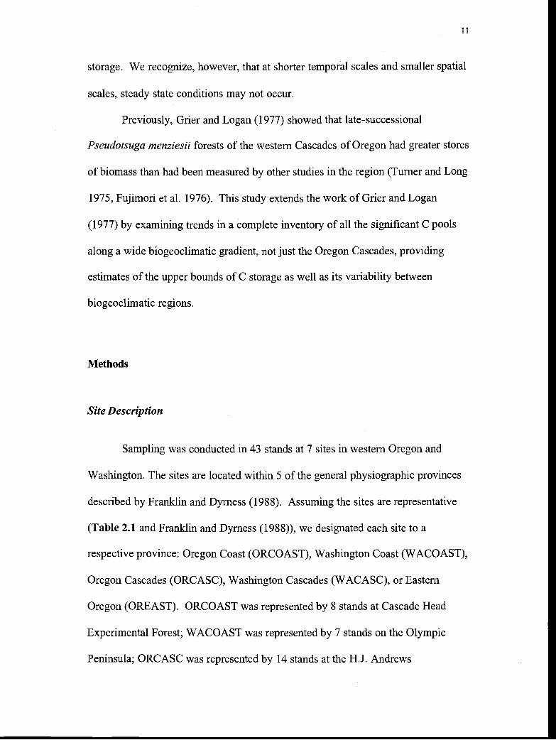
storage. We recognize, however, that at shorter temporal scales and smaller spatial
scales, steady state conditions may not occur.
Previously, Grier and Logan (1977) showed that late-successional
Pseudotsuga menziesii forests of the western Cascades of Oregon had greater stores
of biomass than had been measured by other studies in the region (Turner and Long
1975, Fujimori et al. 1976). This study extends the work of Grier and Logan
(1977) by examining trends in a complete inventory of all the significant C pools
along a wide biogeoclimatic gradient, not just the Oregon Cascades, providing
estimates of the upper bounds of C storage as well as its variability between
biogeoclimatic regions.
Methods
Site Description
Sampling was conducted in 43 stands at 7 sites in western Oregon and
Washington. The sites are located within 5 of the general physiographic provinces
described by Franidin and Dyrness (1988). Assuming the sites are representative
(Table 2.1 and Franldin and Dyrness (1988)), we designated each site to a
respective province: Oregon Coast (ORCOAST), Washington Coast (WACOAST),
Oregon Cascades (ORCASC), Washington Cascades (WACASC), or Eastern
Oregon (OREAST). ORCOAST was represented by 8 stands at Cascade Head
Experimental Forest; WACOAST was represented by 7 stands on the Olympic
Peninsula; ORCASC was represented by 14 stands at the H.J. Andrews

12
Experimental Forest; WACASC was represented by 10 stands at Mt Rainer
National Park and Wind River Experimental Forest (T.T. Munger Research Natural
Area); and OREAST was represented by 4 stands at Metolius Research Natural
Area and Pringle Falls Research Natural Area (Figure 2.1 and Table 2.1).
All sites were part of a permanent plot network designed to observe and
monitor changes in composition, siructure, and functions of forest ecosystems over
long time periods (see Acker et al. 1998 for a complete description of the history
and characteristics of the network). The 43 old-growth sites used in this study are
located on lands managed by either the United States Forest Service (USFS) or the
National Park Service and are maintained by the H.J. Andrews Experimental Forest
Long-Term Ecological Research program (LTER) and The Cascade Center for
Ecosystem Management (a cooperative effort between Oregon State University, the
Pacific Northwest Research Station of the USFS, and the Willamette National
Forest). Data from the network is stored in the Forest Science Data Bank of the
Department of Forest Science at Oregon State University.
The youngest stands in our study were at Cascade Head, in the ORCOAST.
Their average age is 150 years, having developed after a catastrophic crown fire,
the Nestucca Burn, in the late 1840s (Harcombe 1986; Acker et al., in press).
Stands at the Olympic Peninsula have not hid a stand-replacing disturbance for 230
to 280 years, while the remaining stands have not had a catastrophic disturbance for
450 to 1200 years (Table 2.1).
In the PNW, there is a strong east-west gradient in precipitation and
temperature. Climate is generally mild and moist in the coastal sites, with cooler

Olympic NP(WACOAST)r
Cascade flea(OR COAST)
.4>
'"Pringle Falls7 (OREAS)
SubAlpIne
Mt. RalerHP(W.CASC)
WMd Rker(WACASC)
HJ Andrews
Washington
Figure 2.1. Locations of sites used to measure old-growth biomass in the PNWwithin each of the physiographic provinces.
13
(OREAST)
(ORCASC)
Orepn

Table 2.1. Stand characteristics of the five study provinces in the PNW.
Site Stand Name Stand Size Lat. Long.. Elev. Age' Temp. 2 #soil # Habitat Dominant(if applicable) Abbrev.(ha) N (°) W (°) (m) (yrs) (°C) (mm) pits3 plots Type4 Species4
OREGON CASCADES (ORCASC)
H.J. Andrews RSOI 1.0 44.202 122.257 510 460 11.4 1719 2 16 PSME/HODI PSME,ACMA
RSO2 1.0 44.2 17 122.243 520 460 10.9 1868 2 16 TSHE/BENE PSME, TSHE
RSO3 1.0 44.260 122.159 950 460 7.8 2202 2 16 TSHE-ABAM/ PSME, THPLRHMA-LIBO
RSO7 0.3 44.2 13 122.148 490 460 5.8 2260 2 1 TSHE!OXOR PSME, TSHE
RS1O 0.3 44.213 122.217 610 450 10.1 2003 2 1 TSHE/RHMA PSME, TSHE/GASH
RS12 0.3 44.227 122.122 1020 460 7.0 2332 2 1 ABAM/VAAL! PSME, TSHECOCA
RS15 0.3 44.212 122.236 720 460 8.9 1906 2 1 TSHE/POMU PSME, TSHE
RS16 0.3 44.214 122.241 670 460 10.3 1869 2 1 TSHE/CACH PSME,PILA
RS2O 1.0 44.222 122.249 700 450 10.4 1859 1 16 PSME/HODI PSME,PILA

Table 2.1. (Continued)
RS22 1.0 44.274 122.140 1290 450 3.8 2282 2 16 ABAM/VAME/ ABPR, PSMEXETE
RS23 1.0 44.227 122.123 1020 450 7.1 1240 2 16 ABAM/VAAL/ TSHE, PSMECOCA
RS27 1.0 44.254 122.175 790 450 8.5 2118 2 24 TSHE-ABAM! PSME, TSHERHMA-LIBO
RS29 1.0 44.231 122.146 800 450 8.0 2264 2 16 TSHE-ACCl/ PSME, THPLPOMU
RS31 1.0 44.262 122.181 900 450 8.1 2101 2 16 TSHE-ABAM/ PSME, THPLRHMA-LIBO
OREGON COAST (ORCOAST)
Cascade Head CHO1 0.4 45.046 123.897 305 150 8.3 2658 2 4 TSHE/OXOR TSHE, PISI
CHO3 0.4 45.044 123.901 280 150 8.6 2660 2 4 TSHE/OXOR TSHE, P1ST
CHO4 0.4 45.065 123.941 259 150 9.0 2554 2 4 TSHE/OXOR TSHE, P1ST
CHO5 0.4 45.065 123.942 259 150 9.0 2552 2 4 TSHE/OXOR TSHE, PISI
CHO7 0.4 45.063 123.939 244 150 8.7 2559 2 4 TSHE/OXOR TSHE, P1ST
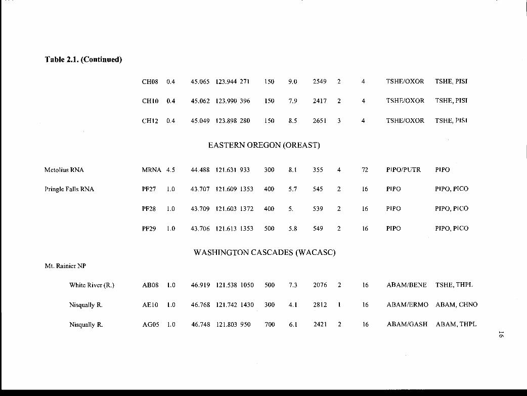
Table 2.1. (Continued)
CHO8 0.4 45.065 123.944 271 150 9.0 2549 2 4 TSHE/OXOR TSHE, P1ST
CH1O 0.4 45.062 123.990 396 150 7.9 2417 2 4 TSHE/OXOR TSHE, P1ST
CH12 0.4 45.049 123.898 280 150 8.5 2651 3 4 TSHE/OXOR TSHE,PISI
EASTERN OREGON (OREAST)
MetoliusRNA MRNA 4.5 44.488 121.631 933 300 8.1 355 4 72 PIPO/PUTR PIPO
PringleFallsRNA PF27 1.0 43.707 121.609 1353 400 5.7 545 2 16 PIPO PIPO,PICO
PF28 1.0 43.709 121.603 1372 400 5. 539 2 16 PIPO PIPO, PICO
PF29 1.0 43.706 121.613 1353 500 5.8 549 2 16 PIPO PIPO,PICO
WASHINGTON CASCADES (WACASC)
Mt. Rainier NP
WhiteRiver(R.) ABO8 1.0 46.919 121.538 1050 500 7.3 2076 2 16 ABAM/BENE TSHE,THPL
Nisqually R. AE1O 1.0 46.768 121.742 1430 300 4.1 2812 1 16 ABAM/ERMO ABAM, CHNO
Nisqually R. AGO5 1.0 46.748 121.803 950 700 6.1 2421 2 16 ABAM/GASH ABAM, THPL

Table 2.1. (Continued)
Nisqually R. AV06 1.0 46.777 121.783 1060 750 6.0 2658 2 16 ABAM/VAAL ABAM, TSHE
Nisqually R. T004 1.0 46.741 121.887 640 750 8.8 2166 2 16 TSHE/OPHO TSHE, PSME
Ohanapecosh R. A003 1.0 46.827 121.546 853 1000 6.6 2257 1 16 ABAM/OPHO ABAM, TSHE
Ohanapecosh R. AVO2 1.0 46.823 121.551 841 1000 5.4 2249 1 16 ABAM/VAAL ABAM, TSFTE
Carbon R. AV14 1.0 46.960 121.843 1080 1200 3.9 2500 2 16 ABAM/VAAL ABAM, TSHE
Carbon R. T011 1.0 46.995 121.880 610 550 8.1 2112 2 16 TSHE/OPHO PSME, TSHE
Wind River
T.T. Munger RNA MUNA 4.5 45.828 121.969 411 470 7.8 2496 8 21 TSHE/BENE PSME, TSHE
WASHINGTON COAST (WACOAST)
Olympic Peninsula
S. Fork Hoh R. HRO1 1.0 47.779 123.908 244 280 8.2 3669 2 16 TSHE/OXOR TSHE, PISI
S. Fork Hoh R. HRO2 1.0 47.779 123.908 244 280 8.2 3669 2 16 TSHE/OXOR TSHE, P1ST
S. Fork Hoh R. HRO2 1.0 47.779 123.908 250 280 8.2 3669 2 16 TSHE/OXOR TSHE, P151
S. Fork Hoh R. HRO4 1.0 47.779 123.908 250 280 8.2 3669 2 16 TSHE/OXOR TSHE, P151
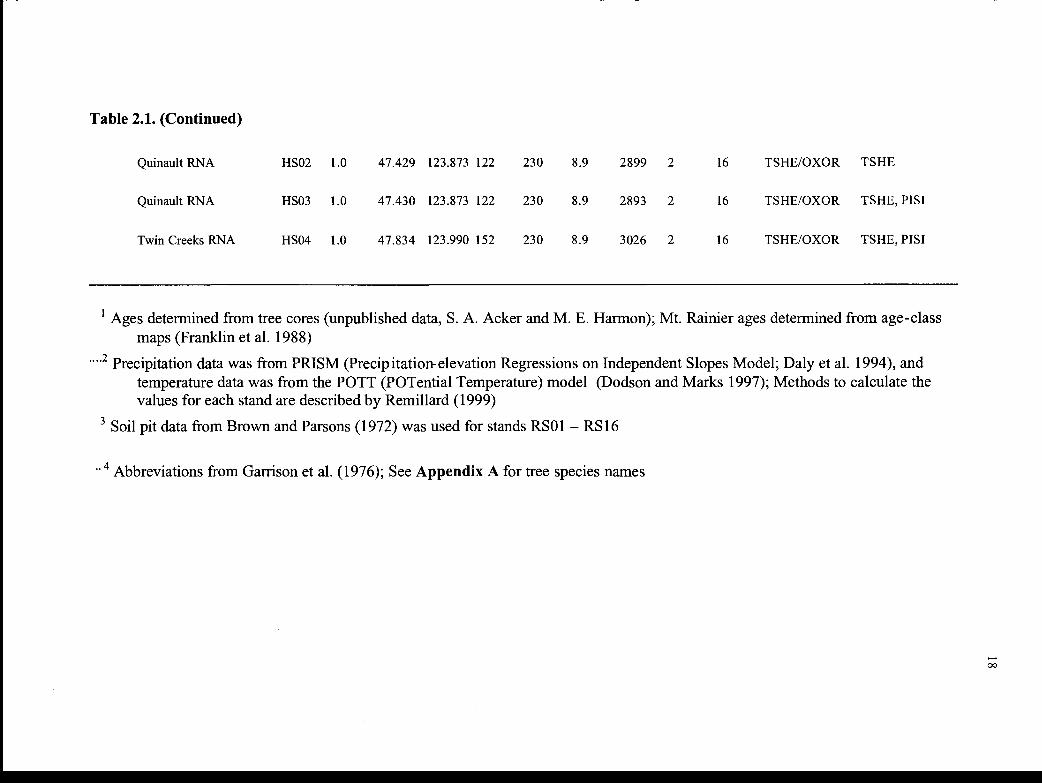
1 Ages determined from tree cores (unpublished data, S. A. Acker and M. E. Harmon); Mt. Rainier ages determined from age-classmaps (Franklin et al. 1988)
.2 Precipitation data was from PRISM (Precipitation-elevation Regressions on Independent Slopes Model; Daly et al. 1994), andtemperature data was from the POTT (POTential Temperature) model (Dodson and Marks 1997); Methods to calculate thevalues for each stand are described by Remillard (1999)
Soil pit data from Brown and Parsons (1972) was used for stands RSO1 - RS16
Abbreviations from Garrison et al. (1976); See Appendix A for tree species names
Table 2.1. (Continued)
Quinault RNA HSO2 1.0 47.429 123.873 122 230 8.9 2899 2 16 TSHE/OXOR TSHE
Quinault RNA HSO3 1.0 47.430 123.873 122 230 8.9 2893 2 16 TSHE/OXOR TSHE, PISI
Twin Creeks RNA HSO4 1.0 47.834 123.990 152 230 8.9 3026 2 16 TSHE/OXOR TSHE, P1ST

19
temperatures at high elevations, and lower precipitation east of the mountains. For
example, mean annual temperature ranges from 11.4 °C at a low elevation stand in
H.J. Andrews to 3.8 °C at Pringle Falls. Mean annual precipitation ranges from
3669 nm at the South Fork of the Hoh River, Olympic Peninsula, to 355 mm at
Metolius RNA. Sites within the Oregon and Washington coastal provinces are
represented by Tsuga heterophylla-Picea sitchensis habitats, while higher elevation
sites are represented by P. menzsiesii-Thuja heterophylla habitats. East of the
Cascades, Pinus ponderosa habitats predominate.
At each site, between 3 and 14 stands were sampled. Each stand was
composed of 1 to 72 (median = 16) plots (Table 2.1). In addition to aboveground
measurements within the stand, soil C was estimated from soil pits located just
outside the ireasured area of the stand. The C pools (Mg C ha1) that were
measured are described below. A biomass:C ratio of 2:1 was used for all
calculations except for soil organic carbon estimates, where C density values were
calculated directly. Unless otherwise described, TEC for each stand was calculated
as an average of the plots on a per hectare basis. TEC for each province (e.g.,
ORCASC, ORCOAST, etc.) was calculated as the average of the stands in that
province.
Above- and Belowground Tree C
Estimation of above and belowground tree C included the following pools:
stem wood, stem bark, live and dead branches, foliage, live and dead coarse roots,
and fine roots. In each stand, the diameters of all trees (>5 cm diameter at breast

20
height (DBH)) were measured. The biomass of stem wood, stem bark, and live and
dead attached branches, were calculated by applying species-specific allometric
equations from BIOPAK (Means et al. 1994). In some cases, species-specific
equations were not available so we made substitutioiE with equations for similar
species. We tested the effect of these substitutions by switching equations within
and between families of tree species (while maintaining the observed distribution of
DBH). In general, within- family conifer substitutions accounted for very small
variations in biomass (e.g., 2.7 %, Abies amabilis forAbiesprocera). Between
family conifer substitutions were more significant (e.g., 19 %, T heterophylla for
A. amabilis) but were rare. Hardwoods only occupied 1.3 % of the stems in the
region so we assumed that uncertainty in these equations was not significant.
Foliage carbon stores were calculated from leaf area index (LAI, n? m2)
using species-specific leaf area (SLA, g cni2) estimates found in the literature
(Appendix A). We obtained estimates of LAI by calculating sapwood area
(SA, cni2), or sapwood thickness, from DBH using species-specific biomass
equations (Appendix A). Predicting LAI from SA is preferable to prediction of
LAI directly from DBH, as the latter overestimates LAI and leaf mass for mature
and old-growth forests (Marshall and Waring 1986; Turner et al. 2000b). We
derived species-specific allometric equations to predict SA from DBH for P.
sitchensis, Pinus con torta and Pinus ponderosa using data from the permanent
plots and published data from western softwoods (Lassen and Okkonen 1969). We
applied appropriate substitution equations when species-specific allometric
equations were lacking (Appendix A).

21
Fine-root biomass was not directly measured due to time constraints and
due to its spatial and temporal variability. Instead, we assumed that fine root
biomass is approximately 2% of total aboveground biomass (Table 7 in Grier and
Logan 1977). Since approximately 1.6 times more fine root biomass is present in
dry sites than wet sites (Table 3 in Santantonio and Hermann (1985)), we assumed
that approximately 3 % of above- ground biomass (2 % * 1.6) is allocated
belowground in OREAST, where precipitation is limited (Gholz 1980). This is in
general agreement with current understanding about tree physiology that, in water
or nutrient limited sites, more NPP is allocated to fine roots (Waring and Running
1998).
We estimated live, coarse-root biomass (>10 mm diameter) for each tree
from equations for P. menziesii in Santantomo et al. (1977) and corrected the
values for different tree species using species-specific green densities (U.S. Forest
Products Laboratory 1974). Dead, coarse-root biomass was estimated by assuming
that it is the same proportion of coarse woody debris (logs + snags) as the
proportion of live coarse root biomass is to aboveground tree biomass. For
example, at stand RSO 1 (H.J. Andrews), live coarse root biomass is 29 % of
aboveground tree biomass (live and dead branches, foliage, stem bole, stem bark).
Therefore, we assumed that dead, coarse-root biomass was 29 % of coarse woody
debris (29 % of 44.9) or 13.1 Mg C ha1. In this calculation, we assumed that the
ratio of above- and below- ground decomposition rates does not diverge through
time. We tested this assumption by calculating dead, coarse-root biomass with
differing decay rates and comparing the ratio of roots to boles through time. We
22
would need to double the decay rates of dead, coarse-roots to see a 10 % decrease
in the ratio of roots to boles. Given the range of decay rates for this region reported
by Chen et al. (2001), we would not expect this to be the case. Thus, we have
confidence that this assumption is appropriate.
Alternatively, to improve confidence in our estimates, we calculated coarse-
and fme-root biornass with a regression equation developed by Cairns et al. (1997),
which predicts total root biomass from aboveground biomass. We then calculated
fme-root biomass as a ratio of fine roots to total roots (Figure 4 in Cairns et al.
1997). We compared the fine, and live, coarse-root biomass estimates from these
two methods. Since the methods used in Santantonio et al. (1977) allow for the
separation of live and dead, coarse-roots, we present these root estimates in the
final TEC calculations.
Understory C
To determine understory C, dimensional measurements including cover
and/or basal diameters were taken within each stand Small tree (<5 cm) and shrub
diameters, as well as shrub and herb cover, were measured along 4 transects within
the stand. Transects were either 25 m or 50 m in length, depending on stand size.
The percent of shrub and herb cover was measured using line transects.
Herb cover classes were noted for each species in 0.2 by 0.5 m micro-plots placed
at systematic intervals of approximately 1 m. Diameters of shrub and small tree
stems were tallied in a 1- rn-wide belt transect by species and basal diameter classes
(i.e., diameter at ground). Allometric biomass equations for total aboveground

23
biomass (BAT) were selected using BIOPAK (Means et al. 1994) by assembling
the appropriate combination of equations describing components of biomass. For
shrubs, if we could not predict BAT by one equation, we used a combination of
equations, (e.g., entire aboveground = live branch+ total stem + total foliage). We
assigned a substitute equation for shrub and herb species whose biomass equations
could not be found, or whose basal areas or cover values were outside of the range
for which the species-specific equations were developed. Total biomass per stand
was calculated by summing the biomass per species on each transect and then
averaging the biomass per transect for each stand.
Coarse Woody Debris C
Coarse woody debris (CWD) included standing and fallen detrital bioimss
10 cm diameter; m in length). For each fallen tree, we measured the length,
end diameter, and middle diameter. For each snag, we measured the height and end
diameters. In addition to these dimensions, we recorded the species and decay
class of each piece. The decay class is an index of the stage of decay of the log or
snag, indicating its physical and biological characteristics, density, and nutrient
content (Harmon and Sexton 1996). We converted the data to volumes and then to
biomass using wood densities specific to its decay-class and species (Harmon and
Sexton 1996).

Fine Woody Debris C
Downed, fine woody debris biomass (1 cm to 10 cm diameter) was
estimated by harvesting downed branches and twigs in five, 1-rn2 micro-plots
placed evenly abng the transects used to sample herbs, shrubs, and small trees. The
fresh weight of dead branches was determined on a portable electronic scale
(Harmon and Sexton 1996) and sub-samples were weighed in the field and later
oven dried to determine a dry:wet weight correction factor.
Organic Horizon C
This pool included the forest floor and buried rotten wood. A 5-cm diameter
corer was used to collect samples of the 0 horizon at 5 locations along each
transect that was used to sample fine woody debris. We separated the samples into
fine, litter-derived material and coarse, wood-derived material based on color and
texture. Each core sample was oven-dried (55 °C), weighed and analyzed for LOT
(loss on ignition) to determine ash- free mass, which was used to calculate the
proportion of organic matter in the sample. Organic matter was converted to C
using a 2:1 ratio of ash- free biomass to C.
Mineral Soil C
Mineral soil organic C (SOC. Mg C ha') estimates for these stands were
reported by Remillard (1999), and detailed methods are described therein; we will
24

25
describe the methods briefly here. On the perimeter of each stand, one to three 1-rn3
soil pits were used for a total of 79 soil pits. Pits were located to best represent the
stand in terms of slope, aspect, vetation-density and cover. The number of soil
pits per stand ranged from one to eight, depending on soil heterogeneity. At each
pit, soil samples were collected from three mineral soil layers (0- to 20-cm, 20- to
50-cm, and 50- to 100-cm).
SOC was calculated on a layer basis:
SOC=C*D*S*L* 100
Where C is the organic C concentration (g C kg1) of the C-bearing fraction; D is
the bulk density (g cni3) of this fraction; S is the C-bearing fraction as a proportion
of total sample volume; L is the layer depth (cm); and 100 is the conversion factor
(108 cni2 ha' 106 Mg g') to yield the desired units (Mg C ha').
To obtain the organic C concentration, samples were sieved and hand-sorted
into the following components: <2 mm C-bearing soil fraction, 2- to 4-mm C-
bearing soil fraction, > 4-mm C-bearing soil fraction, >2 mm rock (non-C bearing),
and >2-mm buried wood, roots, and charcoal. The C-bearing fraction >2 mm were
either hardened soil aggregates or soft, weathered rocks, which have been shown to
be nutrient-rich and an important component of C stores (Ugolini et al. 1996; Corti
et al. 1998; Cromack et al. 1999). Buried wood, roots, and charcoal accounted for
<3 % of the sample mass and were disregarded in mineral SOC estimates. Sub-
samples (50 to bOg) of the <2-mm, 2- to 4-mm, and >4-mm C-bearing fractions
were analyzed for total C and N concentration using a LECO CSN 2000 analyzer
by the Central Analytical Laboratory, Oregon State University, Corvallis. A mass-

26
weighted C concentration was computed for each size class by knowing the total C
concentration (g C k1) and the oven-dry mass of the material. Bulk density was
determined for each soil layer with a core sampler for non-rocky soils or by
excavating a known volume of soil for rocky soils. In addition to these 79 soil pits,
data from Brown and Parsons (1972) for 8 soil pits (0-100 cm depth) in the H.J.
Andrews, ORCASC, were also used (Table 2.1).
Epiphytes
We did not include epiphytes in our estimate of TEC. Epiphytes may
account for only 0.06% of aboveground tree biomass (e.g., 17.8 kg of 29,174 kg in
Pike et al. 1977), or perhaps even less (0.003%; Harmon et al., In review),
indicating that the exclusion of this pooi does not lead to significant underestimates
of total C stores.
Results
There was significant variation of TEC100 averages between provinces
(Figure 2.2) and among the stands (Table 2.2). ORCOAST stands stored, on
average, 1127 Mg C ha' (1006 to 1245 Mg C ha', n=8), which was the highest for
the study area, while stands in OREAST stored the least, 195 Mg C ha1 (158 to
252 Mg C ha1, n=4). In general, ORCOAST stands (average=1 127 Mg C ha1,
range=1006 to 1245 Mg C ha1, n=8) stored slightly more than WACOAST stands
(average = 820 Mg C ha', range = 767 to 993 Mg C ha1, n=7). Similarly,

1400
1200
C-)
1000
- 800
I:::F2 200
27
0N= 8 7 14 10 4
OROST WAOAST ORCASC WACASC OREAST
Province
Figure 2.2. Boxplot of mean stand Total Ecosystem Carbon (TEC) by province.

Table 2.2. Average C pools for 43 old-growth stands in the PNW. Units are Mg C ha1.
Stand Live Deadbranch branch
Foliage Stem Stembark wood
Fine Live Dead Fine Forestroots coarse coarse woody floor
roots roots debris
Rotten Logs Snags Soilwood
Shrubs Herbs Total
ORCASC
RSO1 18.0 4.0 4.2 57.4 208.5 5.8 85.0 13.1 9.5 13.3 0.0 20.8 24.1 122.5a 1.0 nmb 587.4
RSO2 28.6 4.9 4.7 55.5 230.8 6.5 93.6 19.7 16.4 22.5 0.0 45.0 23.4 122.5a 0.6 nm 674.8
RSO3 42.1 7.1 5.4 60.1 309.3 8.5 136.0 34.2 29.2 18.3 15.9 60.6 45.9 122.5a 2.2 nm 897.3
RSO7 37.1 6.3 4.2 71.0 299.8 8.4 106.9 15.3 13.1 13.0 17.1 38.9 21.1 122.5a 0.2 nm 775.0
RS1O 22.4 5.3 5.1 57.8 227.1 6.4 69.1 9.3 13.9 16.1 10.5 35.6 7.1 122.5a 1.6 nm 609.9
RS12 66.2 11.0 4.9 98.0 441.7 12.4 152.8 24.2 7.0 31.3 25.2 32.3 66.1 122.5a 1.5 nm 1097.3
RS15 42.3 6.9 4.4 98.9 380.0 10.6 141.4 32.2 11.0 7.5 0.0 33.9 87.3 122.5a 0.1 nm 978.9
RS16 28.9 5.1 4.0 86.9 306.3 8.6 115.9 14.6 8.3 22.9 0.0 18.5 35.8 122.5a 2.2 nm 780.5
RS2O 16.9 4.0 4.4 50.3 186.5 5.2 71.4 5.9 13.8 21.3 0.0 12.4 9.4 41.9 0.1 0.4 443.8
RS22 31.0 5.2 8.9 53.0 244.2 6.8 93.9 46.0 33.3 28.5 22.2 69.0 98.5 179.2 0.5 0.3 920.4
RS23 52.5 8.6 4.3 43.9 262.6 7.4 99.0 25.5 5.1 18.5 26.0 36.6 59.1 102.8 1.7 0.3 753.9
RS27 54.8 9.4 5.9 108.1 452.4 12.6 189.8 17.9 12.6 23.3 11.2 54.3 5.1 121.8 0.5 0.3 1079.8
RS29 45.2 7.2 4.4 91.4 413.9 11.2 198.3 20.5 9.7 6.4 29.8 49.5 8.5 146.5 0.6 0.4 1043.4
RS3I 45.4 7.5 5.9 88.3 364.7 10.2 157.0 27.4 8.6 19.5 0.0 75.9 13.4 143.2 1.7 0.2 969.0

Table 2.2. (Continued)
ORCOAST
CHO1 77.5 12.5 6.3 22.0 291.9 8.2 102.8 22.2 18.1 16.9 54.9 53.5 35.0 472.3 2.3 0.1 1196.4
CHO3 60.6 9.6 5.8 22.3 389.1 9.7 148.7 21.8 15.2 21.4 0.0 45.0 26.5 346.7 0.8 0.3 1123.5
CHO4 55.9 9.4 6.9 26.4 416.3 10.3 153.0 21.4 11.2 27.7 24.5 40.0 32.0 407.4 2.6 0.2 1245.2
CHO5 56.1 8.8 6.7 26.5 448.5 10.9 170.0 18.3 18.1 16.7 23.8 45.0 14.0 339.2 0.8 0.3 1203.8
CHO7 69.1 11.3 6.8 24.1 338.9 9.0 119.1 16.1 17.4 30.5 25.7 40.0 21.0 275.4 1.0 0.1 1005.7
CH08 73.1 11.8 6.9 21.7 285.5 8.0 94.4 18.6 20.0 40.3 4.4 54.0 24.5 377.2 2.0 0.1 1042.4
CH1O 51.8 7.7 5.6 21.1 400.0 9.7 155.5 16.3 16.8 13.8 3.4 34.5 16.5 326.3 0.8 0.4 1080.4
CH12 67.7 10.9 5.8 20.7 317.1 8.4 115.7 26.3 18.4 13.1 37.6 69.4 26.5 380.1 0.9 0.3 1118.9
OREAST
MRNA 13.9 1.6 0.5 15.6 53.0 2.5 24.9 8.6 6.9 14.9 0.0 14.3 14.8 58.7 1.0 0.3 231.6
PF27 11.2 1.0 0.4 11.7 44.0 2.1 20.1 5.3 8.5 6.1 0.0 8.9 9.0 29.2 0.0 0.0 157.5
PF28 13.0 1.3 0.4 14.4 49.6 2.4 22.7 4.3 10.1 8.6 0.0 9.3 5.6 32.1 0.1 0.0 173.7
PF29 17.6 1.6 0.8 17.7 71.7 3.3 36.1 5.5 8.2 10.1 0.0 8.8 7.9 27.0 0.2 0.0 216.5
WACASC
ABO8 42.5 7.1 12.5 25.4 197.2 5.7 94.1 21.0 11.2 11.3 61.1 57.4 6.3 59.9 0.5 0.2 613.3
AE1O 37.1 11.2 9.2 34.1 271.2 7.3 99.1 11.8 24.1 11.2 21.2 25.6 17.8 262.6 1.2 0.0 844.9
AGO5 33.0 7.5 9.1 47.1 266.8 7.3 99.2 20.2 10.0 9.0 41.8 53.1 20.8 54.7 0.6 0.1 680.2
A003 60.6 12.6 11.4 47.7 380.2 10.2 147.0 28.6 10.5 17.5 27.5 55.3 44.3 95.9 0.3 0.2 949.6

Table 2.2. (Continued)
a Values are average from other reported values in the field
b nm = not measured
0
AVO258.4 11.8 9.1 35.4 284.9 8.0 96.2 27.8 10.4 26.9 45.9 84.9 30.4 109.3 1.8 0.1 841.1
AVO6 24.1 5.1 8.6 24.0 147.9 4.2 48.2 12.9 6.0 28.3 18.1 32.1 24.0 78.1 1.5 0.3 463.1
AV14 53.7 11.9 8.7 30.8 295.1 8.0 121.7 9.8 15.0 6.5 37.3 20.2 12.2 204.8 1.4 0.2 837.2
MJJNA 41.1 7.2 4.8 49.3 248.5 7.0 31.8 3.8 9.4 33.3 17.1 16.6 24.9 116.6 1.4 0.8 613.5
T004 43.4 7.1 4.4 39.7 266.1 7.2 100.1 9.2 5.8 30.8 25.1 4.6 28.5 75.6 0.5 0.3 648.5
T011 55.0 8.7 5.1 68.1 419.8 11.1 159.6 36.1 20.9 16.3 13.9 85.6 40.3 109.0 0.2 0.4 1050.1
WACOAST
HRO1 39.7 5.6 6.1 13.5 240.2 6.1 95.3 26.3 5.4 6.7 21.5 73.1 11.0 216.5 nm nm 767.0
HRO2 51.0 5.8 8.6 17.6 389.5 9.4 161.5 26.5 17.2 8.2 15.8 66.4 11.3 204.2 nm nm 993.0
HRO3 31.2 3.4 5.4 9.9 236.9 5.7 99.5 22.6 13.2 8.8 12.1 53.0 12.0 109.0 nm nm 622.8
HRO4 59.5 7.8 6.9 14.5 332.7 8.4 137.1 18.6 5.6 10.3 0.0 44.8 12.5 131.6 nm nm 790.3
HSO2 61.7 9.5 5.9 14.5 237.3 6.6 89.3 23.8 7.7 10.1 0.0 74.7 13.1 288.5 0.2 0.4 843.3
HSO3 50.8 7.5 7.4 14.5 266.6 6.9 100.6 18.7 9.2 18.4 19.3 50.5 14.0 264.6 0.3 0.4 849.7
HSO4 53.9 8.2 6.6 24.7 289.6 7.7 116.3 35.0 6.0 23.0 30.7 87.0 28.4 153.3 0.8 0.5 871.6

31
ORCASC stands (average = 829 Mg C ha', range = 445 to 1097 Mg C ha', n14)
stored more, on average, than the WACASC (average = 754 Mg C ha1, range =
463 to 1050 Mg C ha1, n=10). The lowest C density among the 43 stands was at
Pringle Falls, OREAST (PF27), where only 158 Mg C ha1 was stored, while the
highest C density was at stand CHO4 at Cascade Head, ORCOAST, with
1245 Mg C ha'.
Almost all C pools were consistent between provinces in their percent of
TEC (calculated from Table 2.2; Figure 2.3). The live branch pool averaged 5.9
% (± 0.4 %) of TEC100 for all provinces (n = 5). The dead branch and foliage pool
averaged 0.9 % (± 0.1 %) and 0.7 % (± 0.1 %), respectively. Stem wood averaged
33.8 % (± 1.7 %) while stem bark averaged 5.1 % (± 1.4 %) ofTEC100. The fine-
root pool averaged 1.0 % (± 0.1 %) of TEC100 for all provinces while live and dead
coarse roots averaged 13.4 % (± 0.5 %) and 2.6 % (± 0.2 %), respectively. The
standard deviation of fine-root biomass could be much larger or smaller since fine-
root biomass was calculated simply as a ratio to above-ground biomass and
therefore represents the variability of the latter numbers. Fine woody debris
averaged 2.0 % (± 0.6 %), forest floor averaged 2.7 % (± 0.6 %), and rotten wood
averaged 1.8 % (± 0.7 %). The log pool averaged 5.6 % (± 0.6 %) and the snag
pool averaged 3.3 % (± 0.6%). Of all ecosystem C pools, stem wood was the most
significant component, ranging from 28.0 % ofTEC100 in OREAST stands to
37.0 % in the Cascades (Figure 2.3).

2
Woody
Dea
liii ItIJIuIuIuuip''nnn..
an
Snags
Logs 5%
Rotten Wood I
Forest FloorFineDebris 2%
Herbs, Shrubs0%
d CoarseRoots 3% Fine Roots 1%
Figure 2.3. Average percentage of TEC in measured C pools for stands in theOregon Cascades province (rounded to the nearest whole number); other provinceswere similar (see text).
32
Live Branch 4 Dead 8ranch 1%
4% oIl age 1%

33
Average SOC values varied widely between provinces (fable 2.3),
highlighting the large biogeoclimatic variability in the PNW. The percent of
SOC100 relative to TEC100 ranged from 15.0 % in the Washington Cascades to
32.0 % in the Oregon Coast, with a mean of 21.1 % (Standard Error (SE) = 3.3 %).
ORCOAST stands stored ten times the SOC that is stored in OREAST (365.5
versus 36.7 Mg C ha1). ORCOAST stands stored, on average, 130 Mg C ha" more
SOC than stands at WACOAST and about 3 times as much as was found in the
stands in the Oregon and Washington Cascades. As a percent of TEC5O, S0050
was, in general, a smaller proportion of total C, ranging from 11.4 % in the
WACASC to 24.5 % in ORCOAST (average = 16.5 %, SE = 2.4 Mg C ha').
In each of the 5 provinces, total tree C, total detrital C, and total understory
C were consistent percentages of TEC, respectively (fable 2.3). Understory
biomass was very small in all provinces (average = 0.1 %, SE = 0.02 %). Above-
ground tree C (live and dead branches, foliage, stem wood and bark), was the
largest component of TEC100 and TEC50. Above-ground tree C was between 41 %
and 52 % of TEC100 (average = 46 %, SE = 2.1 %) and 45 % to 54 % of TEC50
(average 49 %, SE = 1.7 %). Below-ground tree C (fine roots, live and dead
coarse roots) ranged from 14.4 % (ORCOAST) to 18.4 % (ORCASC) of TEC100
(average = 17.0 %, SE = 0.71 %) and from 16.0 % (ORCOAST) to 19.0 %
(WACOAST) of TEC50 (average = 17.9 %, SE = 0.6 %). ORCOAST had the
lowest percent of total tree C. This is because soil C represents a larger proportion
of TEC at ORCOAST relative to the other provinces (Table 2.3).

Table 2.3. The relative amounts of understory, above- and below-ground tree, detrital, and soil carbon in the five provinces(ORCASC = Oregon Cascades, ORCOAST = Oregon Coast, OREAST = Eastern Oregon, WACASC = Washington Cascades,WACOAST = Washington Coast) as a percent of Total Ecosystem Carbon (TEC). Percent values outside of parentheses (%ioo)represent calculations with TEC 100a; values inside parentheses (%50) represent calculations with TEC50'.
a Understory + Tree + Soil Organic Carbon from 0-100cm (S0C100)
b Understory + Tree + Soil Organic Carbon from 0-50cm (S0050)
Shrubs + herbs
d Live and dead branch, foliage, stem bark, stem wood
C Fine roots, live and dead coarse roots
C Fine woody debris, forest floor, rotten wood, logs, snags (excluding dead coarse roots, dead branches)
IOOYEC5Ob Understoryc Above-ground Treed Below-ground Treee Detritale
Province Mg C ha4 Mg C ha4 Mg C ha4 %io°/o) Mg C ha4 %i(°/o) Mg C ha' %i(°/o) Mg C ha4 %i(°/o) Mg C ha Mg C ha4 %(°/o)
ORCASC 829.4 805.7 1.1 0.13 (0.14) 431.7 52.0 (53.6) 152.6 18.4 (18.9) 121.4 14.6 (15.1) 122.5 98.8 14.8 (12.3)
ORCOAST 1127.0 1009.0 1.6 0.14 (0.16) 464.7 41.2 (46.1) 161.8 14.4 (16.0) 133.5 11.8 (13.2) 365.5 247.5 32.4 (24.5)
OREAST 194.8 187.0 0.4 0.21 (0.21) 85.3 43.9 (45.6) 34.5 17.7 (18.4) 37.9 19.5 (20.3) 36.7 28.9 18.8 (15.5)
WASCASC 754.2 719.3 1.2 0.16 (0.17) 380.2 50.4 (52.9) 125.4 16.6 (17.4) 130.7 17.3 (18.2) 116.6 81.7 15.5 (11.4)
WACOAST 819.7 767.7 0.4 0.05 (0.01) 363.5 44.3 (47.4) 146.0 17.8 (19.0) 114.4 14.0 (14.9) 195.4 143.0 23.8 (18.6)

35
Detrital carbon (fine woody debris, dead coarse roots, dead branches, forest floor,
rotten wood, logs, snags) ranged from 14.5 % in the ORCOAST to 23.2 % of TEC
in the OREAST (mean = 19 %, SE = 1.5 %) for TEC100 and from 13.2 %
(ORCOAST) to 20.3 % (OREAST) for TEC50 (mean = 16.3 %, SE = 1.3 %).
Stands in eastern Oregon had much less detritus C (45.2 Mg C ha1) compared to
coastal and Cascades stands (145.7 to 163.9 Mg C ha'), even though the percent
relative to TEC was the greatest. Among detrital pools, however, there was
significant variation between provinces (Table 2.2). ORCOAST had 46 % more
fine woody debris and forest floor C than WACOAST and 39 % more snag C.
However, WACOAST had 35 % more C in the form of logs than ORCOAST.
ORCASC and WACASC stands had a similar distribution of C in their detrital
pools, although the WACASC stands had >60 % more rotten wood than ORCASC.
The percentage of root C relative to TEC differs depending on the method
used to estimate root C. When using the regression equation developed by Cairns et
al. (1997), TRCD averaged 13.4 % of TEC. When using the Santantomo et al.
(1977) equations, and adjusting for species density, roots averaged 17.0 % of TEC.
Root to shoot ratios (R:S) were the same for the ORCOAST and ORCASC
regardless of which method was used. Both methods showed higher R:S for stands
in OREAST, where more resources are stored belowground.
Discussion
Confidence in Site Estimates
As a proportion of TEC, estimation errors of the foliage pooi are not
significant. Foliage C is only 0.7 %, on average, of TEC in these old-growth forests
and, therefore, even gross estimation errors would not significantly affect TEC.
Indeed, we would have to increase the foliage pool 18 times to increase TEC by
10 %. Similarly, we would have to increase shrub C 100 times to increase TEC by
10 %. Nonetheless, prediction of foliage and understory C is critical for estimation
of productivity and further species-specific equations need to be developed for this
purpose.
Because of the effort required to directly measure coarse- and fme-root C,
we used published allometric relationships instead. Review of the available root
literature is complicated because measurements often reflect limited spatial and
temporal domains, making comparisons difficult, and because different authors use
dissimilar definitions of fine- and coarse-roots. Dead coarse-root biomass averaged
2.6 % of TEC. We would need to increase dead, coarse-root C by five times to
change TEC by 10 %. We would have to increase fme-root C eleven times to
increase TEC by 10 %. Therefore, although our estimates of these pools are rough,
we have confidence that small changes in these pools will not affect TEC
significantly. In contrast, live, coarse-root C is 13.4 % of TEC. Therefore, we
would need to increase this pool only 1.5 times to see a 10 % increase in TEC.
36

37
Estimation errors in the stem wood pooi have the potential to provide the
greatest uncertainty in TEC since this pool represents the largest proportion of TEC
(34 %, on average). Yet, these are the pools about which we have the most
confidence since over 14,000 trees were measured for stem wood volume and since
the allometric equations used to calculate biomass are well documented and
validated (see BIOPAK, Means et al. 1994).
In addition, by including coarse soil aggregates and estimating Soc to a
depth of 1 m, the soil C estimates used in this study represent an improvement on
previous regional estimates of C storage in the PNW. Remillard (1999) found that
39 to 66 % of soc in soil pits was below 20-cm and up to 44 % of SOC was found
in C-bearing material >2- mm. Therefore, reducing the degree that these C pools are
underestimated results in more reliable estimates of the upper bounds of C storage
in this region.
Role of Disturbance
Our estimates of the upper bounds of C storage simply place a limit on C
storage for the region, based on the unrealistic assumption that all forests
eventually reach old-growth conditions. Instead, natural disturbances such as fire,
windstorms, landslides, as well as land conversion and management create a
mosaic of age classes on a landscape (Bormann and Likens 1979). In theory, some
old- growth stands persist due to the stochastic nature of disturbance processes
(Johnson and Van Wagner 1985), but natural and managed landscapes will store
less C than landscapes covered completely by old-growth forests because of the

38
high proportion of younger forests, which store less C than old- growth forests
(Harmon et al. 1990). Despite these caveats, the theoretical construct of a
completely old-growth landscape is useful as a neutral model (Gardner et al. 1987)
in which one predicts the pattern (of C storage) in the absence of a process (Turner
1989) (e.g., human or natural disturbances). Such models could be used to
distinguish systematically the effects of different management strategies on C
storage. By bounding estimates of C sequestration potential, managers can
determine the efficacy of different sequestration strategies relative to their
potential. Further, they would be able to determine the potential economic and
environmental costs and benefits of various management strategies. By providing
an upper bound on C storage in the region (based on sites where those processes
have been absent), we place an upper limit on the results of such analyses.
Regional Implications
To estimate the upper bounds of C storage for the PNW region, we
multiplied the proportional area of each province (based on the area of the
corresponding vegetation provinces in Franklin and Dyrness (1988)) by the average
C storage in each province. These area-weighted estimates for each province were
then summed. We used the following approximations of the area of each province
to calculate the weighted estimates: P. sitchensis zone in Oregon (i.e., ORCOAST)
was 8 % of the study area; P. sitchensis in Washington (i.e., WACOAST) was
9 %; T heterophylla in Oregon (i.e. ORCASC) and Washington (i.e., WACASC)
was 32 % and 17 %, respectively; Pinusponderosa (i.e., OREAST) was 13 %; and

39
A. amabilis (subalpine zone) was 21 % (adapted from Fig. 27 in Franklin and
Dyrness (1988)). Since subalpine stands were not represented by our study sites,
we used a value of 401 Mg C ha1 in the A. amabilis zone, taken as the average
from studies by Boone et al. (1988, Fig.1), Kimmins and Krumlik (1973, Tables 6
and 7 (assuming soil and roots are each 20 % of live biomass)) and Grier et al.
(1981, Table 2). Without a more formal geospatial analysis, this weighting
procedure is a good first attempt at a regional estimate, allowing us to further
constrain our estimate of the upper bounds of C storage. Before weighting, the
average, upper bound of C storage was 745 Mg C ha1 (n = 43 stands) to a depth of
100 cm. After weighting, the average upper bound of C storage was 671
Mg C ha'. Recalculating to SOC to 50 cm, a depth more amenable to forest
sequestration practices in the short-term, the average, upper bound of C storage was
640 Mg C ha1. For the latter calculation, SOC in the subalpine zone was assumed
to be half of that in the former calculation to 100 cm.
At the regional level, exogenous disturbances such as increasing CO2,
natural disturbances, and climate change will further change the regional capacity
to store additional C. The eventual regional capacity to sequester C in the PNW
may be, therefore, much different than the potential capacity we outline here.
Regional predictions of actual carbon sequestration will require a more detailed
accounting of all significant endogenous and exogenous factors that control it.
However, by constraining these estimates with the potential values we describe, it
may be possible to place limits on the system.

Comparison with Global Studies
The C densities we measured in old-growth forests of the PNW are higher
than C density values reported for any other type of vegetation, anywhere in the
world (Figure 2.4; Appendix A). Unfortunately, comparisons of our study to other
carbon-density estimates is hampered since estimates often reflect sites whose
disturbance histories are poorly documented. The biomass (or C) estimates of other
studies often include effects of non-catastrophic, disturbance legacies (e.g. selective
logging, light fires) or may represent stands which are in early to middle stages of
succession after a stand-clearing disturbance such as a harvest, blow down, or
heavy fire. Moreover, definitions of major ecosystem pools (live, detrital, soil)
differ among studies. For example, Schlesinger (1977) defined detrital C as "the
total carbon in dead organic matter in the forest floor and in the underlying mineral
soil layers," while Grier and Logan (1977) excluded soil C in their definition of
detritus. In general, the distinction between litter, detritus, and soil C is not
consistent between studies, making comparisons difficult (Matthews 1997).
Other limited studies in the region have demonstrated the potential of PNW
old-growth forests to support large amounts of biomass. Fujimori et al. (1976),
measuring only stem, branch, and leaf dry weights, reported biomass values of 669
to 882 Mg ha1 (335 to 441 Mg C ha1) in P. sitchensis, Tsuga heterophylla, and A.
amabilis zones in Oregon and Washington. Means et al. (1999) estimated
aboveground biomass (trees, foliage, shrubs, herbs) at t1 H.J. Andrews forest as
965 ± 174 Mg ha1 (or 483 ± 87 Mg C ha'). Grier and Logan (1977), who studied
40

700
2 400-0
300
100-
0
300
20cr
100
(a)
0
Figure 2.4. Boxplots describing C storage estimates from the literature for (a) live(b) detrital and (c) SOC pools, compared to the average C storage among provincesin the PNW (this study).
41
Temperate Forests SavaniralWoodtends AridTropical Forests Sorest This Study
20 200
100
0
(c)
0
0
Temperate AridSorest This Study
Forests Savanna/WoodlandsTropical Forests
Temperate Forests SavannaWoodtsnds AridTropical Forests Sorest This Study
42
a 450-year old-growth stand in Watershed 10 of the H.J. Andrews, found total organic
matter accumulations, including SOC to 1 m, ranging from 1008 to 1514 Mg ha' (or
504 to 757 Mg C ha1). These studies at the H.J. Andrews were within the range of
TEC that we measured at the H.J. Andrews (445 to 1097 Mg C ha').
Why Does Old-growth in the PNW Store So Much C?
Trees in the PNW can reach massive sizes. Mild fall and winter conditions in
much of the PNW facilitate continued productivity by coniferous evergreens at a time
when deciduous trees are not able to photosynthesize. In addition, long, dry summers
further hinder deciduous tree growth (Waring and Franklin 1979). Large conifer trees
are able to maintain their growth by continued water conductivity through long, dry
summers, which is facilitated with a tracheid xylem structure (Mencuccini and Grace
1996). The absence of frequent fires or storms in the productive regions of the PNW
further supports massive trees with long lifetimes (Waring and Franldin 1979). In
high-elevation sites, winter dormancy by coniferous tree species facilitates survival in
cold conditions (Havrenek and Tranquillini 1995).
The large size of PNW trees means that they occupy a hrge proportion of
ecosystem C storage relative to the national average. For example, Turner et al.
(1995) estimated that half of actual total forest C in the conterminous U.S. was in the
soil and that only 33 % was in trees. Woody debris represented 10 % of total C; the
forest floor was 6 % and the understory was 1 % of total forest C. Birdsey et al.
(1993) similarly estimated that only 31 % of total C in the U.S. is currently in tree C
(51 % merchantable: 17 % roots, 3 % foliage, 6 % snags, 24 % other) and 59 % was

43
soil C. Litter, humus and downed, coarse woody debris comprised 9 % while
understory was 1 % of total C. These national averages are different than the 15-32 %
Soc and 53-67 % tree C in the old-growth stands reported in this study. It should be
noted that the absolute amount of SOC in the PNW is higher than the global average,
although the relative proportion of ecosystem C that they represent is less due to the
large amount of tree C in old-growth PNW forests. The detailed methods used to
measure SOC probably allowed us to find higher absolute C stores for this pool.
However, the large proportion of tree C in this system, relative to the other studies
mentioned above, indicates that the PNW may be more amenable to storing C through
management and conservation efforts than other systems which store more C in soil.
C Sequestration and Economic Implications
Future C management (e.g., Parson and Keith 1998) will require information
on the upper bounds of C storage and the extent to which current forest C storage
differs from it. In the U.S., Birdsey (1992) used national forest inventory data and
other selected studies to estimate current (1987) organic C storage for trees, soil, forest
floor, and understory vegetation. In this assessment, PNW frests accounted for 39 %
of TEC in the United States. Total C averaged 193.6 Mg C ha1 for Oregon forests and
227.1 Mg C ha1 for Washington forests (mean = 208.3 Mg C ha1, weighted by forest
area in Birdsey (1992)). Turner et al. (1995) report an average C storage in PNW
forests of 330 Mg C ha1. These studies present estimates that are significantly lower
than our regional approximation of the upper bounds of C storage (671 Mg C ha1 for

44
TEC100 and 640 Mg C ha' for FEC50). In fact, our estimate is twice that of Turner et
al. (1995) and more than 3 times that of Birdsey (1992).
Subtracting the estimate of Turner et al. (1995) of average current C storage in
western Oregon and Washington from the upper bound of C storage in the region,
forests could, theoretically, store an additional 310 to 341 Mg C ha1. To increase the
C store to this level would require forest management aimed toward C sequestration,
which may include protection from catastrophic, natural disturbances, lengthening of
harvest rotations, and improvement in soil C storage.
Given recent estimates of the value of C in economic analyses (e.g., Romm et
al. 1998) the average worth of each hectare of forest could be thousands of dollars for
additional C sequestration. Multiplied by the area of forest in Oregon and
Washington, this additional C storage would be worth billions of dollars (given the
current value of the dollar). While we realize it is unlikely that large areas may be
converted to old-growth forests given the other demands on timber resources, this
rough calculation indicates a significant economic value that C storage could represent
in this region.
Conclusions
Old-growth forest ecosystems can be used as an upper bound (or upper limit)
on additional C sequestration potentiaL Currently, forest C storage in the PNW is less
than this upper bound due to management practices and natural disturbances that
lower the average age of the forests, reducing the time for large tree boles, detrital
45
biomass, and soil C to accrue. The retive effect of natural disturbances, and human
management on future C sequestration can be best gauged by comparisons to the
upper bounds of C storage as presented in this study. The upper bound (or limit) of
the global, terrestrial biosphere to sequester additional carbon could be improved with
similar studies in other regions. If management strategies were such to allow forests to
return closer to the C stores found in old-growth forests, the PNW would have
considerable ability to sequester additional C. This could have significant economic
implications.
Acknowledgments
This research was made possible by funding from the Pacific Northwest Research
Station Long-Term Ecosystem Productivity Program, and Interagency Agreement DW
12936179 between USEPA and the Pacific Northwest Research Station. All stands
are associated with the H.J. Andrews Long Term Ecological Research (LTER)
program, grant number DEB-963292 1.

References
Acker, S. A., P.A. Harcombe, M.E. Harmon, and S.E. Greene. In press. Biomassaccumulation over the first 150 years in a coastal Oregon spruce-hemlockforest. Vegetation Science.
Acker, S.A., W.A McKee, M.E. Harmon, and J.F. Franldin 1998. Long-term researchon forest dynamics in the Pacific Northwest: a network of permanent forestplots. In Forest Biodiversity in North, Central, and South America and theCaribbean: Research and Monitoring, F. Dallmeier and J.A. Comiskey (Eds.).The Parthenon Publishing Group, Inc., New York, New York, pp. 93-106.
Bender, M., C. Field, L.O. Hedin, J. Schimel, E. Sundquist, R. Berner, J. Galloway, F.Mackenzie, M. Torn, K.H. Freeman, J Hedges, C. Mora, R. Stallard, S.C.Wofsy, and W.H. Schlesinger. 2000. The Changing C Cycle: A TerrestrialFocus, Report of the Workshop on the Terrestrial C Cycle. The NationalScience Foundation, Division of Earth Sciences.
Birdsey, R.A., A.J. Plantinga, and L.S. Heath. 1993. Past and prospective carbonstorage in United States forests. Forest Ecology and Management 58: 33-40.
Birdsey, R.A. 1992. Carbon storage and accumulation in United States forestecosystems. USDA Forest Service, Gen. Tech. Rep. WO-59, 5 'pp.
Boone, R.D., P. Sollins, and K. Cromack, Jr. 1988. Stand and soil changes along amountain hemlock death and regrowth sequence. Ecology 69: 7 14-722.
Bormann, F H and G.E. Likens. 1979. Catastrophic disturbance and the steady state innorthern hardwood forest. American Scientist 67: 660-669.
Brown, R.B. and R.B. Parsons. 1972. Soils of the reference stands - Oregon IBP.Internal Report 128. College of Forest Resources, University of Washington,Seattle, Washington, 84 pp.
Brown, S. 1996. Mitigation potential of carbon dioxide emissions by management offorests in Asia. Ambio 25: 273-278.
Brown, S., A.J.R. Gillespie, and A.E. Lugo. 1991. Biomass of tropical forests of southand southeast Asia. Canadian Journal of Forest Research 21: 111-117.
Cairns, M.A., S. Brown, E.H. Helmer, and G.A. Baumgardner. 1997. Root biomassallocation in the world's upland forests. Oecologia 111: 1-11.
Chen, H., M.E. Harmon, and R.P. Griffiths. 2001. Decomposition and nitrogenrelease from decomposing woody roots in coniferous forests of the Pacific
46

47
Northwest: a chronosequence approach. Canadian Journal of Forest Research31: 246-260.
Cohen, W.B., M.E. Harmon, D.O. Wallin, and M. Fiorella. 1996. Two decades ofcarbon flux from forests of the Pacific Northwest. BioScience 46: 836-844.
Cooper, C.F. 1983. Carbon storage in managed forests. Canadian Journal of ForestResearch 13: 155-166.
Corti, G., F.C. Ugolini, aiiI A. Agnelli. 1998. Classing the soil skeleton (greater thantwo millimeters): proposed approach and procedure. Soil Science Society ofAmerica Journal 62: 1620-1629.
Cromack, K., Jr., R.E. Miller, O.T. Helgerson, R.G. Smith, and H.W. Anderson. 1999.Soil carbon and nutrients in a coastal Oregon Douglas- fir plantation with redalder. Soil Science Society of America Journal 63: 232-239.
Daly, C., R.P. Neilson, D.L. Phillips. 1994. A statistical-topographic model formapping climatological precipitation over mountainous terrain. Journal ofApplied Meteorology 33: 140-158.
DeBell, D.S. and J.F. Franldin. 1987. Old-growth Douglas-fir and western hemlock: a36-year record of growth and mortality. Western Journal of Applied Forestry2: 111-114.
Dodson, R. and D. Marks. 1997. Daily air temperature interpolation at high spatialresolution over a large mountainous region. Climate Research 8: 2-20.
Franklin, J. F., T. A. Spies, R. Van Pelt, A. Carey, D. Thornburgh, D.R. Berg, D.Lindenmayer, M. B. Harmon, W. Keeton, and D. C. Shaw. In press.Disturbances and the structural development of natural forest ecosystems withsome implications for silviculture. Forest Ecology and Management.
Franklin, J.F. and D.T. Dyrness. 1988. Natural Vegetation of Oregon and Washington,Oregon State University Press, Corvallis, Oregon, U.S.A.
Franldin, J.F., W.H. Moir, M.A. Hemstrom, S.E. Greene, and B.G. Smith. 1988. Theforest communities of Mount Rainier National Park. Scientific MonographSeries Number 19. U.S. Deparatment of the Interior, National Park Service,Washington, D.C., 194 pp.
Fujimori, T., S. Kawanabe, H. Saito, C.C. Grier, and T. Shidei. 1976. Biomass and netprimary production in forests of three maj or vegetation zones of thenorthwestern United States. Jourml of the Japanese Forestry Society 58: 360-373.

48
Gardner, R.H. B.T. Mime, M.G. Turner, and R.V. O'Neill. 1987. Neutral models forthe analysis of broad-scale landscape pattern. Landscape Ecology 1: 19-28.
Garrison, G.A., J.M. Skovlin, C.E. Poulton, and A.H. Winward. 1976. Northwest plantnames and symbols for ecosystem inventory and analysis. Gen. Tech.Rep.PNW-GTR-46. Portland, Oregon: USDA, Forest Service, Pacific NorthwestForest and Range Experiment Station, 263 pp.
Grier, C.C. and R.S. Logan. 1977. Old-growth Pseudotsuga Menziesii communities ofa western Oregon watershed: biomass distribution and production budgets.Ecological Monographs 47: 373-400.
Grier, C.C., K.A. Vogt, M.R. Keyes, and R.L. Edmonds. 1981. Biomass distributionand above- and below-ground production in young and mature Abies amabiliszone ecosystems of the Washington Cascades. Canadian Journal of ForestResearch!!: 155-167.
Harcombe, P.A. 1986. Stand development in a 130-year-old spruce-hemlock forestbased on age structure aiil 50 years of mortality data. Forest Ecology andManagement 14: 41-58.
Harmon, M.E., K. Bible, M.J. Ryan, H. Chen, and J. Klopatek. In review. Production,respiration, and overall carbon balance in an old- growth Pseudotsuga/Tsugaforest ecosystem.
Harmon, M.E. and J. Sexton. 1996. Guidelines for measurements of woody detritus inforest ecosystems. U.S. LTER Network Office: University of Washington,Seattle, Washington.
Harmon, M.E., W.K. Ferrell, and J.F. Franklin. 1990. Effects on carbon storage ofconversion of old-growth forests to young forests. Science 247: 699-702.
Havrenek, W.M. and W. Tranquillini. 1995. Physiological processes during winterdormancy and their ecological significance. In Ecophysiology of ConiferousForests, W.K. Smith and T.M. Hinckley (Eds.), Academic Press, San Diego,California, pp. 95-124.
Houghton, R.A., E.A. Davidson, and G.M. Woodwell. 1998. Missing sinks,feedbacks, and understanding the role of terrestrial ecosystems in the globalcarbon balance. Global Biogeochemical Cycles 12: 25-34.
Janisch, J.E. and M.E. Harmon. 2002. Successional changes in live and dead woodstores: Implications for net ecosystem productivity. Tree Physiology 22: 77-89.
Johnson, E.A. and C.E. Van Wagner. 1985. The theory and use of two fire historymodels. Canadian Journal of Forest Research 15: 214-220.

49
Kauppi, P.E., K. Mielikainen, and K. Kuusela. 1992. Biomass and carbon budget ofEuropean forests from 1971-1990. Science 256: 70-74.
Kimmins, J.P. and G.J. Krumlik. 1973. Comparison of the biomass distribution andtree form of old virgin forests at medium and high elevations in the mountainsof South Coastal British Columbia, Canada. JUFRO Working Party on theMensuration of Forest Biomass, presented in Vancouver, B.C., August 20-24.
Krankina, O.N. and R.K. Dixon. 1994. Forest management options to conserve andsequester terrestrial carbon in the Russian Federation. World ResourcesReview 6: 88-101.
Lassen, L.E. and E.A. Okkonen. 1969. Sapwood thickness of Douglas-fir and fiveother western softwoods. FPL-124, Oregon State University, Corvallis,Oregon, USA.
Long, J.N. and J. Turner. 1975. Aboveground biomass of understorey and overstoreyin an age sequence of four Douglas-fir stands. Journal of Applied Ecology 12:179- 188.
Marshall, J.D. and R.H. Waring. 1986. Comparison of methods of estimated leaf-areaindex in old-growth Douglas-fir. Ecology 67: 975-979.
Matthews, E. 1997. Global litter production, pools, and turnover times: Estimates frommeasurement data and regression models. Journal of Geophysical Research.102: 18,771 - 18,800.
Means, J.E., S.A. Acker, D.J. Harding, J.B. Blair, M.A. Lefsky, W.B. Cohen, M.E.Harmon, and W.A. McKee. 1999. Use of large-footprinting scanning airbornelidar to estimate forest stand characteristics in tl western Cascades of Oregon.Remote Sensing of Environment 67: 298-308.
Means, J.E., HA. Hansen, G.J. Koerper, P.B. Alaback, and M.W. Klopsch. 1994.Software for Computing Plant biomass - BIOPAK Users Guide. PNW-GTR-340, U.S.D.A., Forest Service, Pacific Northwest Research Station.
Mencuccini, M. and J. Grace. 1996. Hydraulic conductance, light interception andneedle nutrient concentration in Scots pine stands and their relations with netprimary productivity. Tree Physiology 16:459-468.
Odum, E.P. 1969. The strategy of ecosystem development. Science 164: 262-269.
Parson, E.A. and D.W. Keith. 1998. Fossil fuels without CO2 emissions. Science 282:1053- 1054.

50
Pike, L.H., R.A. Rydell, and W.C. Denison. 1977. A 400-year-old Douglas-fir tree andits epiphytes: biomass, surface area, and their distributions. Canadian Journalof Forest Research 7: 680-699.
Remillard, S.M. 1999. Soil Carbon and Nitrogen in Old-Growth Forests in WesternOregon and Washington, M.S. Thesis, Oregon State University, Corvallis,Oregon, U.S.A.
Romm, J., M. Levine, M. Brown, and E. Petersen. 1998. A Road map for U.S. carbonreductions. Science 279: 669-670.
Santantonio, D. and R.K. Hermann. 1985. Standing crop, production, and turnover offine roots on dry, moderate, and wet sites of mature Douglas-fir in westernOregon. Annals of Science Forestry 42: 113-142.
Santantonio, D., R.K. Hermann, and W.S. Overton. 1977. Root biomass studies inforest ecosystems. Pedobiologia 17: 1-31.
Schlesinger, W.H. 1977. Carbon balance in terrestrial detritus. Annual Review ofEcology and Systematics 8: 51-81.
Turner, D.P., W.B. Cohen, and R.E. Kennedy. 2000a. Alternative spatial resolutionand estimation of carbon flux over a managed forest landscape in WesternOregon. Landscape Ecology 45: 441-452.
Turner, D.P., S.A. Acker, J.E. Means, and S.L. Garman. 2000b. Assessing alternativeallometric algorithms for estimating leaf area of Douglas- fir trees and stands.Forest Ecology and Management 126: 61-76.
Turner, D.P., G.J. Koerper, M.E. Harmon, and J.J. Lee. 1995. A carbon budget forforests of the conterminous United States. Ecological Applications 5: 421-436.
Turner, J. and J.N. Long. 1975. Accumulation of organic matter in a series ofDouglas- fir stands. Canadian Journal of Forest Research 5: 681-690.
Turner, M.G. 1989. Landscape ecology: the effect of pattern on process. AnnualReview of Ecology and Systematics 20: 171-97.
Ugolini, F.C., G. Corti, A. Agnelli, and F. Piccardi. 1996. Mineralogical, physical, andchemical properties of rock fragments in soil. Soil Science 161: 521-542.
U.S. Forest Products Laboratory. 1974. Wood Handbook: wood as an engineeringmaterial. USDA Agricultural Handbook 72, Revised.
Vitousek, P.M. 1991. Can planted forests counteract increasing atmosplric carbondioxide? Journal of Environmental Quality 20: 348-354.

Waring, R.H. and S.W. Running. 1998. Forest Ecosystems: Analysis at MultipleScales, Academic Press, San Diego, California, 370 pp.
Waring, R.H. and J.F. Franklin. 1979. Evergreen coniferous forests of the PacificNorthwest. Science 204: 1380-1386.
51

CHAPTER 3
Erica A. H. Smithwick, Mark E. Hannon, and James B. Domingo
52
A MODEL TO PREDICT POTENTIAL C STORAGE AS A FUNCTION OFDISTURBANCE REGIMES AND CLIMATE

Abstract
Disturbances remain a key uncertainty in constraining the global carbon
cycle in part because of the difficulty in scaling these fine-scale processes to the
global level. Here we present a new model (MAXCARB) that predicts the
potential response of carbon (C) storage in live, dead, stable, and forest product
pools over a large area (approximately 1 ha) to climate and disturbance. To scale
the effects of disturbances to broader scales, we simulate disturbance regimes,
building on established principles in landscape ecology. For a given disturbance
regime, the effects of disturbance events and successional dynamics at the fine
scale are simulated by MAXCARB with age-dependent equations that predict how
fluxes and mass of C stores change through time. Simulation results from the
model compared favorably to simulation results from a finer-scaled model
(STANDCARB) indicating that processes and carbon pools were treated
consistently between the models. Comparison of model predictions matched data
from old-growth forests in the Pacific Northwest, U.S.A, along a wide
biogeoclimatic gradient (slope of regression line = 0.92, r2= 0.94). Analyses of the
results indicate that fine- scale heterogeneity in disturbance processes can be
captured at broad scales by simulating disturbance regimes rather than discrete
disturbance events. Increased understanding of the variation in ecosystem
processes with age will facilitate using this scaling approach.
53
Introduction
Current scientific research on the terrestrial C cycle is focused on
constraining global estimates of the "missing" C sink (Dai and Fung, 1993; Ciais,
1995; Goulden et al., 1996; Houghton et al., 1998; Holland and Brown, 1999;
Potter et al., 1999; Fung, 2000; Pacala et al., 2001) and locating C sources and
sinks regionally ( Houghton, 1993; Cohen et al., 1996; Fan et al., 1998; Melillo et
al., 1988; Houghton, 1999; Fang et al., 2001; Potter et al., 2001). One goal of C
cycle research is to predict the role of the terrestrial biosphere in future mitigation
of atmospheric CO2 increases under changing climate and disturbance conditio ns.
However, the global potential to store C under future disturbance regimes resulting
from climate change is not known (Dale, 1997; Schimel et al., 1997).
At intermediate (regional to continental) scales, disturbances are often
accounted for indirectly by using historical input data (such as land-cover maps
derived from remote sensing) to drive ecosystem models. For example, Schimel et
al. (2000) used historical inventory data and satellite maps to drive three different
ecosystem models (Biome-BGC, Century, and TEM), which account for increasing
CO2 and climate change, to evaluate C storage by ecosystems of the United States.
Potter et al. (2001) combined satellite-derived greenness estimates and fire counts
with an ecosystem production model (CASA) to evaluate regional C flux in
response to deforestation and biomass burning in tropical forests during the early
1990s. Cohen et al. (1996) used biogeoclimatic maps and satellite land cover maps
to drive a regional ecosystem model (LANDCARB) in the Pacific Northwest
between 1972 and 1991 to assess how changes in disturbance regimes, from one
54

55
consisting of natural fires to one consisting of clear-cut harvesting, affected C
storage. The abandonment of former agricultural lands, resulting in afforestation
(Houghton et al., 1999), or the encroachment of woody biomass into areas that
were previously grazed (Sedjo, 1992; Dixon et al., 1994; Hibbard, 1995), may also
result in changes in C storage over time. As all these studies indicate, historical
land-use changes may be the dominant factor controlling C storage at regional
scales (Casperson et al., 2000).
However, including disturbance processes in global models is difficult
because global models tend to be driven, in large part, by ecophysiological factors
and therefore have limited capacity to predict the effect of disturbance processes
directly (Peng, 2000). At global scales, current dynamic vegetation models assume
that climate is the predominant factor controlling the composition and structure of
vegetation and largely ignore the effects of disturbances processes (Peng, 2000).
Initial attempts to include natural disturbances as part of a larger model (e.g.,
Lenihan et al., 1998, White et al., 2000) require data that are generally unavailable
at broad scales. Moreover, most global models do not simulate anthropogenic
disturbances, such as land-use change, into the future (Peng, 2000). To date, an
efficient methodology to assess the effect of disturbances on potential C storage at
broad scales is lacking.
Predicting the effects of future disturbances on global C cycling would be
enhanced by an efficient methodology to scale information on disturbance
processes from the regional scale to broader scales. At regional scales, individual
disturbance events can be discerned, but at global scales individual disturbance

56
events are not directly observable, except in rare cases. Therefore, scaling
approaches must summarize disturbance processes without explicitly depending on
the exact prediction (in space and time) of individual disturbance events, which is
impractical at global scales. A way to scale disturbances to broader scales is to use
the concept of disturbance regimes. Derived from empirical observations, and
building on principles of landscape ecology, a disturbance regime summarizes both
the type and frequency of disturbance events for a broad area. It has been used to
reconstruct historical forest age-class structures and to explain current age-class
distributions of ecosystems within a landscape.
Here, we use the concept of disturbance regimes to predict the impact of
simulated disturbances on steady. state C storage. This provides a mechanism to
scale the effects of disturbance processes to an area of any size with the same
disturbance regime. These concepts are incorporated into a new model
(MAXCARB) that predicts the response of potential C storage over a large area
(approximately 1 ha) to disturbance regimes and climate. By calculating
potential C storage in the absence of exogenous disturbances, MAXCARB can be
used to investigate the effect of climate on potential C storage at steady state. In
addition, by simulating the effects of natural or regulated disturbance regimes on
landscape- scale C stores, MAXCARB can be used to investigate the relative effects
of different disturbance regimes on potential C storage. In this way, MAXCARB
can efficiently and systematically test the effect of changing disturbance regimes
and climate on potential C storage. This efficiency is useful for constraining
estimates of future C storage at broad scales.

Model Description
Overview
MAXCARB, a computer simulation model written in C, is part of a larger
modeling strategy (Cohen et al., 1996), used to measure the temporal and spatial
patterns of C storage over the Pacific Northwest region of the United States. In this
approach, multiple models are used to simulate processes at different scales. As
part of this modeling strategy, MAXCARB is used to constrain regional estimates
from the top down by placing an upper limit on production, decomposition, and C
stores. Another model, STANDCARB (Harmon and Domingo, 2001; Harmon and
Marks, in press), is used to constrain regional estimates from the bottom up by
placing limits on the rate that C pools change over time. Actual stores at the
regional scale are calculated using LANDCARB (Cohen et al., 1996; Wallin et al.,
1996), which responds to observed changes in land-cover, as indicated by remote
sensing.
MAXCARE predicts potential C stores in live, dead, stable (decay-
resistant), and forest products pools for a steady-state landscape using assumptions
of climate and soil constraints on growth and decomposition that are similar to
many ecosystem process models (e.g., Running and Coughlan, 1988; Harmon and
Marks, in press). Currently, the model is parameterized for the Pacific Northwest
region of the United States but it can be parameterized for other regions as well.
The model has two spatial modes: point-mode, where the model computes
steady- state C stores for a single site (i.e., location); and grid-mode, where the
57

58
model computes stores for a region represented by a rectangular grid of sites.
When used to examine regional patterns of steady-state C stores, the region can be
divided up into ecoregions, each representing a specific species composition and
disturbance regime. Five types of input data are used to predict stores spatially:
temperature, precipitatior elevation, solar radiation, and soil characteristics
(texture, depth, and rockiness).
MAXCARB consists of three modules: STEADY-STATE, CLIMATE, and
DISTURBANCE (Figure 3.1). At the center of the model design is the STEADY-
STATE Module, which calculates steady-state C stores for all live, dead, stable,
and forest product pools. To calculate these stores, the STEADY-STATE Module
uses "landscape-average" rate-constants for ecoregions that are computed by the
DISTURBANCE Module (Figure 3.2). The DISTURBANCE Module computes
the rate-constants for each ecoregion by simulating fluxes and stores through time.
This simulation includes disturbance events defined by the disturbance regime
prescribed for each ecoregion. The user can choose not to run the
DISTURBANCE Module, in which case the landscape-average rates can be read
from a file manually created by the user, or generated during a previous simulation.
The CLIMATE Module adjusts the growth, respiration, and decomposition rates in
the STEADY- STATE Module for the combined effects of water, light, and
temperature limitations, as specified by the site's climate data.
Temporally, the DISTURBANCE Module operates on an annual time-step,
while the CLIMATE Module operates on a monthly time-step. The calculations in
the STEADY- STATE Module represent equilibrium solutions (see below) and

Input Files
ClimateIndices
PoolMasses
Ecoregion Disturbance RegimeAge-dependent Rates
Landscape-average Rates
Pool Masses
Site Climate DataClimate Parameters
Input Files
Figure 3.1. Overall conceptual structure of MAXCARB, showing theDISTURBANCE, STEADY STATE, and CLIMATE Modules and tlirinteractions.
59
at Steady-stat OutputFiles

DisturbanceModule
no
VSimulate disturbanceregIme and calculatelandscape-average
rates
Have landscape-averagerates for sites ecoregion?
Start withfirst site
yes
Climate Module Steady-state Module
Begin
Initialize
climate indices
Calculate
climate indices
Caktfleta steady *state pools
Vculate steady -
state pools
V4 Pools < threshold?)
Go to
next site
60
Figure 3.2. Flowchart of the calculations used in the MAXCARE model, showingthe relationship between the DISTURBANCE, STEADY-STATE, and CLIMATEModules.
yes
V no
Last site?
yes
End
61
therefore have no specific time-step. Because they represent steady-state solutions,
analysis of transient responses to changes in climate or disturbance regimes with
MAXCARB is not recommended.
MAXCARB calculates the effects of disturbance regimes at the ecoregion-
scale (typically> 1 ha). However, MAXCARB calculates the effects of climate
at scales for which these data are typically available (approximately 1 ha and
greater). By using this approach we are able to portray effects of climate gradients
across sites within each ecoregion.
MAXCARB was designed to work with a finer-scale model. The rationale
was that an existing, stand-scale model, STANDCARB 2.0 (Harmon and Domingo,
2001), predicts stand- level responses to disturbances (Harmon and Marks, in press)
but is inefficient at predicting C storage over broad areas. MAXCARB
incorporates the general dynamics of STANDCARB, but is simple enough to
facilitate calculations over broad areas. Specifically, STANDCARB 2.0 simulates
species succession and replacement due to disturbance, a feature common to gap
simulation models (Shugart et al., 1988). STANDCARB also simulates the effect
of climate on growth, respiration, and decomposition rates, as in other ecosystem
process models. STANIDCARB simulates mixed species, mixed age-class forests
by simulating a number of cells within a stand. Each cell represents the
approximate area occupied by a single, mature tree (between 0.01 and 0.062 ha).
Each cell is represented by four layers of vegetation (upper trees, lower trees,
shrubs, and herbs), with each vegetation layer having up to seven live parts. Each
cell also has nine detrital poois and three stable C pools. MAXCARB simplifies

62
the dynamics of STANDCARB 2.0 by solving potential C stores with an
equilibrium solution, without explicitly tracking the growth of each stand, or every
layer and species within each stand. By simplifying the time dynamics, it is
possible to extrapolate information across space more efficiently with MAXCARB
than STANDCARB by minimizing the number of calculations necessary.
However, MAXCARE remains similar to STANDCARB in tint it uses the same C
poois, climate calculations, and parameterization, thus making it easier to compare
the behavior between the two models.
General Approach
MAXCARB predicts potential C stores at steady state by simulating a
system in which a constant flux, divided by a modifying rate-constant, yields a
constant store at steady-state (Olson, 1963). By definition, an ecosystem at steady-
state has equal fluxes into and out of the ecosystem to maintain constant mass:
input fluxss = output_fluxss.
Rates at steady-state equal the rate at which mass is leaving a pool:
ratess = fluxss I massss,
where mass ss represents the steady-state store for each pool (mass area1), fluxss
equals the steady-state fluxes (inputs) to each pool (mass area1 time1), and ratess
equals the steady-state rate (time'), which is the rate that mass leaves the pool.
Rearranging, the steady-state mass can be predicted from the steady-state flux and
rate:
massss = fluxss I rates.
63
Conceptually, a landscape is composed of multiple ecosystems, the age-
structure of which are determined by the landscape's disturbance regime. Thus, the
above equations will apply at the landscape scale, as well as the ecosystem scale, as
long as the rates, inputs, and masses are averages for all the ecosystems within the
landscape, and the disturbance regime is constant. These concepts are useful for
MAXCARB as it allows us to scale processes typically employed at an ecosystem
scale to a broader scale, given the corresponding rates, fluxes, and masses are
known for the larger area. For example, Equation 2 can be described as:
(4) rateLA= fIuxLA/ massLft
where rateLA, fluxLA, and massLA, calculated in the DISTURBANCE Module, equal
landscape-average values rather than those of a specific ecosystem.
Although one could assume that rate-constants controlling the input and
output of mass are the same for each ecosystem age-class, there is increasing
empirical evidence, recently reviewed by Bond and Franldin (2002), of significant
age-related change at the level of individual trees (Yoder et al., 1994) and forest
stands (Janisch and Harmon, 2002; Bond and Franklin, 2002). If ecosystem rate-
constants are not actually constant through succession, models that do not account
for this age-dependency may incorporate error. To capture these age-related
dynamics at broad scales, we used STANDCARB to develop equations that define
how rates change as a function of stand age. The age-dependent equations
implicitly capture the effects of different species and vegetation layers. Thus, we
were able to simplify MAXCARB by not including these successional dynamics
explicitly.
64
In the STEADY-STATE Module, steady-state mass is calculated with the
following general equation:
(5) massss = fluxss I (rateLA* indexc).
Landscape-average rates (rateLA) are passed from the DISTURBANCE Module and
then modified by indices calculated in the CLIMATE Module (indexc). The
climate indices estimate the constraints of temperature, precipitation, and solar
radiation on production, respiration, and decomposition.
STEADY-STATE Module
Description
The STEADY STATE Module (Figure 3.3) calculates the steady-state
stores of seven live C pools, eight dead C pools, three stable pools, and one forest
product pooi. The live pools are: foliage, sapwood, heartwood, heart rot, branches,
coarse roots, and fine roots. Live C pools transfer material to their respective
detrital counterpart, with the exception that dead heartwood is a combination of
inputs from both heartwood and heart rot. Dead sapwood and dead heartwood are
additionally separated into snags and logs so that the effects of position on
microclimate can be modeled. All detrital pools can potentially add material to one
of the three relatively decay-resistant stable pools: stable foliage, stable wood, and
stable soil.

'V
Input
V
dead foliage decirv
dead foliage
4cad j!jue lrtnttcr
Input
stable foliage
sapwood
4--- irable foliage decay
hearrwrod forrnali,'r
V
Sspwood rflOrtit hnnec*l lrr
+ V
itipUt Input
sapwood snag decag..snag fall
stable wood decas - -
hearrtvood monalttvbeast rot fDrintioa
Inpht
heart ro rnortiliti
+
Ie wood
*
heart ran fortoar on
heart rot reapiratsonheart rot mortat,l
hea''1
14---- hcwtwood arsag decay, snag fall
- - Jog decaylog transfer
I
Input
hrarrch1bole ratio
- + V
input Input
dead branch
V
coarse root
rOM II)O{ZIII}
dead coarse roots decaylrI c,arsc roota transfer I
dhdcoarse roots
stable soil
tine root, Iqliagc ratio
+ 'V
fine roots
deadfloots
inputV
branch mortalybranch prune I
VV
Input Input
steady-state foliagedisturbance adjustment - _growth rate
foliage transfer
sapwood respiration
branch respiration
aod mortality
branch moity
heartwood formation
branch prune
dead brunch decaydead branch trunsr1
dead branch banadir
dead coarse rootlranafer
stable soil decay
coarse root:bole ratio
coarse roots respirationcoarse roots mortalitycoarse roots prune
dead fine roots decaydead fine roots transfer I
Figure 3.3. Cascade of calculations used in the STEADY-STATE Module to calculate landscape-average, steady-state mass.
foliage mortalityfoliage turnover coarse roots
coarse root pouse roots turnover

Calculations
Foliage and fine-root stores are solved directly from ecoregion- specific
parameters, rather than Equation 5. The foliage stores for a given disturbance regime
and climate are determined by the steady- state foliage and the degree to which
disturbances reduce foliage from steady-state stores (calculated in the
DISTURBANCE Module). The steady-state, fme-root stores are determined by the
fme-root to foliage ratio, calculated in the DISTURBANCE Module.
The steady- state C store for all other C pools is calculated in a cascade of
equations (Figure 3.3). The steady-state C store is equal to the input flux (from the
pools "above" the pool of interest, i.e., the "donor" pool) divided by the rates
modifying the output of mass (to the pool "below" it in the cascade) (Equation 5;
specific equations described in Appendix D). Input fluxes are calculated from the
mass of the contributing pools multiplied by landscape-average rates derived from
the DISTURBANCE Module. Output fluxes are calculated from the mass of the
current pool multiplied by landscape-average rates from the DISTURBANCE
Module. The CLIMATE Module further modifies respiration, decay, and transfer
rates for the given site by calculating climate indices.
66

CLIMATE Module
Description
The CLIMATE Module is derived from STANDCARB 2.0 and explained in
detail elsewhere (Harmon and Domingo, 2001). We will only review its general
methodology here (equations in Appendix E). The CLIMATE Module estimates the
effect of temperature, precipitation, and solar radiation on production, respiration,
and decomposition. These effects are calculated each month and then averaged
yearly to yield the annual indices used by the STEADY-STATE Module.
Calculations
Production, respiration, and decomposition rates are potentially constrained
by available light, mean monthly temperature, and/or monthly moisture conditions.
Light limitations constrain production by modifiing foliage mass. Temperature
limitations on growth are calculated by assuming there is an optimal mean daytime
temperature and growth decreases when temperatures are above or below this
optimum (Running and Coughlan, 1988). Water limitations are calculated by
assuming that there is an exponential reduction in production due to soil moisture
limitations (Emmingham and Waring, 1977).
Available water is calculated by first calculating precipitation interception.
Interception by the canopy, woody detritus, and forest floor is calculated
sequentially. First, canopy interception is calculated assuming that interception of
precipitation increases linearly with increasing foliage mass. Woody detritus (dead
67
68
sapwood, dead heartwood, and dead branches) intercepts precipitation that was not
intercepted by the canopy. The interception by each dead wood pooi is calculated as
a function of its mass, current water store, and the maximum moisture content
defined for that pool. Precipitation not intercepted by the canopy or dead wood
pools enters the forest floor (dead foliage and stable foliage). Interception by the
dead foliage and stable foliage pools is a function of the mass of each pool, its
current water store, and the maximum moisture content specified for each pooi.
Monthly total potential evapotranspiration is calculated using a modification
of the Priestly- Taylor method (Bonan, 1989; Jones, 1992), which estimates total
evaporative flux over a wet surface. Total potential evapotranspiration for a month
is assumed to be proportional to the estimated monthly solar irradiance and the
monthly mean air temperature. The constants used to solve the Priestly-Taylor
method are empirically derived after Jensen and Haise (1963) from elevation and
mean minimum and maximum daily temperatures for the warmest month of the year.
To estimate the potential amount of transpiration by plants, total potential
evapotranspiration is reduced by the amount of evaporation from canopy interception
and detritus pools. This yields a monthly potential transpiration loss assuming that
leaf mass and soil water stores are at a maximum. The actual transpiration losses
each month are controlled by the soil water stores and the foliage mass. The effect
of foliage mass is linear and determined by the ratio of current-year foliage mass to
steady-state foliage mass. The effect of soil moisture on transpiration is calculated
by assuming that when the soil water potential is below -0.3 MPa, transpiration
decreases exponentially (Emmingham and Waring, 1977). Volumetric moisture

69
content is converted to water potential using a reciprocal function similar to Running
and Coughian (1988).
Detrital pool and mineral soil moisture content are calculated monthly and
represent the balance of inputs through precipitation and outputs via
evapotranspiration. For mineral soil, the monthly input is the water that has not been
intercepted by the canopy, dead wood, or the forest floor poois. The loss of water
from mineral soil is controlled solely by plant transpiration, assuming evaporative
losses from mineral soil are minimal The rate of water loss from detrital pools is
calculated from the monthly evaporative demand (a function of radiation and
temperature) and a pool-specific drying constant.
We assume that moisture controls decomposition in two ways. The first is by
matric potential, which limits decomposition when the fiber saturation point is
reached. The second is by low oxygen diffusion when the moisture content is high,
which significantly limits coarse wood decomposition (Harmon et al., 1986). We
model the matric potential and diffusion limitation portions separately from the
minimum and maximum moisture contents. The overall effect of moisture is
calculated by multiplying these two indices.
Temperature controls decomposition in two ways. First, there is an increase
in respiration rate with temperature following a Qio curve. Second, there is a lethal
temperature limit that arrests decomposer activity. These functions are calculated
from the Qio rate, monthly mean air temperature, and monthly optimum temperature
for decomposition. The combined effects of moisture and temperature on

70
decomposition are calculated by multiplying the moisture and temperature-limitation
indices.
DISTURBANCE Module
Description
The DISTURBANCE Module (Figure 3.4) calculates landscape-average
rate-constants for each ecoregion that are used by the STEADY-STATE Module.
The rationale for this module is that rates controlling allocation, growth, and
decomposition change as a forest ages. Following a disturbance, live, dead, and
stable C are recalculated given rate-constants for the new stand age. Currently,
MAXCARB only supports catastrophic disturbances, which kill all live plants and
reset the age of the stand to zero. The return interval (the number of years between
disturbance events) is determined by a user-prescribed disturbance regime for that
ecoregion. There are two general types of disturbance regimes simulated in
MAXCARB: regulated and natural. Disturbances that leave the living stand
relatively intact (e.g., gap formation) are included implicitly.
By definition forests managed in a regulated disturbance regime are
represented by an equal distribution of age-classes on the landscape; thus, the same
stand area is available for harvest each year. It follows that disturbances in a
regulated regime reoccur at a given location at an interval equal to the regime's
disturbance interval, e.g., a site with a 100-year, clear-cut, harvest regime will be
harvested every 100 years. Sites are never older than the user-defined disturbance

L
BEGIN
V
t=i, Agel4,
Calculate AgODIStUth8flCO
Calculate Pools
4,
Age=ORecalculate Age
4t = t
V
END
yes
Calculate landscapeaverages for rates
Disturbance Module
- not - t+1Age = Age+1
Figure 3.4. Flowchart of the calculations used in the DISTURBANCE Module.
71
Age=Ageo?no
yesj,
Adjust Pools for dsturbance

72
interval. Building on these landscape-scale concepts, regulated disturbance regimes
in MAXCARB are simulated through time for a given ecoregion. The user sets the
disturbance interval, which exactly defines the number of years between disturbance
events.
In a natural disturbance regime, a Poisson random process determines the
occurrence of disturbance events through time (Figure 3.5). For simplicity,
MAXCARB simulates a natural disturbance regime with a negative exponential
distribution (Van Wagner, 1978). The negative exponential distribution, and the
related Weibull distribution, form the basis of the most common conceptual models
used in the literature to explore the recurrence of disturbance events on a landscape
(Johnson and Van Wagner, 1985; Van Wagner, 1978; Johnson and Gutsell, 1994).
Simulating natural disturbance regimes with a negative exponential, rather than the
Weibull distribution, assumes that stand age does not affect the susceptibility of the
stand to the natural disturbance event. Thus, stands may survive past the mean
disturbance interval due to random chance (see the tail of the distribution in Figure
3.5), not because old-stands are less susceptible to burning, as in the Weibull
distribution. Eventually, our goal is to allow the user to choose the appropriate
probability distribution function for their area of interest.
Calculations
The DISTURBANCE Module calculates C stores through time for an
ecoregion. Carbon stores and fluxes are calculated for all pools described in the
STEADY-STATE Module. Rather than spatially track the stores and fluxes at

1.
0
0.
0
0
Regulated RegimeAverage age = 50 years1% in each age class
0.4 Natural Disturbance RegimeVan Wagners (1978) Negative Exponential
0.3 DistributionAverage age = 100 years
0.
0.0
0 100 200 300 400 500
Age, years
Figure 3.5. Conceptual representation of the age-class structure for regulated andnatural disturbaire regimes.
73
600 700 800

74
multiple locations within a landscape in a short period of time, we calculate the
stores of C within a single ecoregion over a long period of time to calculate
landscape-average rate-constants. These calculations are based on the same
landscape-scale principles as a spatial simulation, although here we substitute space
for time. This assumes that there is no significant spatial interaction between the
age-classes in the landscape affecting C storage.
The C stores for each pooi are a function of the stores in the previous year,
plus inputs and outputs from the pool over that year. The general equation for these
calculations is:
(6) pool:mass (age) =pool:mass (age-i) + input:flux - output:flux
The calculations are based on the same pools in tl STEADY-STATE
Module, so there is also a similar set of cascading calculations between pools. Input
fluxes are calculated from the mass of contributing pools and rate constants
modifying the input to the current pool. Output fluxes are calculated from the mass
of the current pooi and rate constants modifying the transfer of mass to subsequent
poois (transfer rates, mortality rates, formation rates, or pruning rates), the loss of
mass to the atmosphere (respiration rates for live pools, and decay rates for detrital
pools), and the loss or transfer of mass due to disturbance-events. Output fluxes will
be a function of some combination of these transfers and losses, depending on the
pool being calculated. For example, live poois do not have a decay loss so they are a
function of transfers and respiration losses only. Equations are described in detail in
Appendix C.

Time_End
Mass
The landscape- average rate constants are thus a function of the disturbance regime,
since the average age of the landscape is determined by the frequency of the
disturbance event since the fluxes and masses of the pools are determined by age -
dependent rates.
Disturbance Event Transfers
When a disturbance event occurs, the DISTURBANCE Module determines
the amount of C that is transferred to other pools (i.e., from live pools to dead pools),
or lost (i.e., to the atmosphere, in the case of a fire). If the disturbance is a harvest,
the DISTURBANCE Module determines the amount of bole mass removed to the
75
After the fluxes and pooi masses are calculated for the current simulation
year, running totals for each of these values are updated. When a disturbance event
occurs, the stand age is reset to zero, the stand develops again, and masses and fluxes
are recalculated at the new stand age. The longer the disturbance interval for a
natural disturbance regime, the longer the simulation must be run to capture the
average dynamics of the site through time.
To calculate the landscape-average rate constants, the DISTURBANCE
Module uses the same equation as the STEADY-STATE Module, but solves for the
landscape- average rates using the sum of the masses ai1 fluxes (described generally
in Equation 4):
Time_End
(7) RateLA = Flux

76
forest products pooi and the amount of live pool mass transferred to the dead pooi. If
the disturbance is a fire, the DISTURBANCE Module determines the amount of
mass that is lost to the atmosphere through combustion and the amount of live pool
mass transferred to the dead pool. Each live and dead pool may be consumed by fire
to a different degree, as specified by the user.
Age-dependent Rate Functions
Carbon fluxes and stores in the DISTURBANCE Module are modified by
rate functions that can be either constant or dynamic. As an example of dynamic rate
functions, mortality may be higher during middle stages of succession due to stem
competition. However, since equations describing dynamic changes in rates with
ecosystem age are currently uncommon, we tested both approaches to parameterize
the DISTURBANCE Module. We first developed equations describing how
ecosystem rates change with time based on the output from multiple runs of the
more-detailed model, STANDCARB 2.0. STANDCARB was run for a 10 x 10 grid
of cells for 1000 years and outputs were analyzed to estimate the change in the
following rates through time: allocation ratios of live parts, formation of heartwood
and heart-rot, respiration of live parts, tree mortality, branch and coarse-root pruning,
decay and turnover of dead poois, and transfer rates to stable pools. Independent
simulations were run for scenarios with a clear-cut harvest interval of 50, 100, and
150 years, to determine the effects of disturbance on modifying rate-constants
through time. Each simulation was repeated 5 times to minimize the variability
common to gap-phase models; yearly output from the model was averaged for the 5

77
simulations. Functions were fit to the output that described the general trend in rates
or pools through time (Figure 3.6 and Figure 3.7; Appendix C). Functions fit one
of several forms, including a step function, the Chapman-Richards equation (Causton
et al., 1978, Cooper, 1983, Richards, 1959), or a modification of the Chapman-
Richards equation.
In the second method, we used rate constants derived by calibrating
MAXCARB to STANDCARB. These rate constants do not reflect a single species
or lifeform, but rather, they capture the general dynamics through time of the
STANDCARB model. Therefore, they provide a straightforward test of the
conceptual design of the model and form the basis of results presented in this paper.
Simulation Experiments
To demonstrate the potential of MAXCARB to predxt C storage over a
broad area, we ran simulations with the model in several ways. Our goal was to
demonstrate that MAXCARB is consistent with its conceptualization, facilitating its
use at regional scales. First, we ran MAXCARB separately for 50-year aiil 200-year
natural disturbance (fire) regimes to demonstrate the effect of disturbance interval on
flux, mass, and landscape-average rate calculations in the DISTURBANCE Module.
Second, we tested the sensitivity of MAXCARB to disturbance interval,
running separate simulations for 40-, 60-, 80-, 100-, or 120-year regulated
disturbance regimes (harvest + site preparation fire) for the H.J. Andrews in the

.- 0.005w>
0.004 -0.C,
0.003 -C,
0.002
0.001
0.000
0
Age-dependent Branch Respiration Equation
a) Modeled -0- Calculated
100 200 300 400 500
Age (years)
78
Figure 3.6. Examples of dynamic rate functions used in the DISTURBANCEModule: (a) branch (BR) respiration and (b) coarse root (CR) pruning Modeled linesrepresent output from the STANDCARB model, while Calculated lines represent thefit of the rate- function.
0 100 200 300 400 500
Age (years)
Age-dependent Coarse-Root Pruning Equation
b) -0-Modeled -0-Calculated
0.006

0U-
25
20
10
5
Age-dependent Foliage Equation
Modeled -- Calculated
79
0 100 200 300 400 500
Age (years)
Figure 3.7. Example of dynamic rate function for foliage mass used in theDISTURBANCE Module. Modeled lines represent output from the STANDCARBmodel, while Calculated lines represent the fit of the rate- function.

80
Oregon Cascades. We compared results to C stores predicted by the STANDCARB
model (Harmon and Marks, in press).
Third, we calibrated the age-dependent rate file in the DISTURBANCE
Module of MAXCARB with parameters derived from diagnostic output from
STANDCARB. Both models were parameterized for Douglas- fir in the Oregon
Cascades at the H.J. Andrews. We compared steady-state live, dead, and stable
pools from MAXCARB to similar pools calculated by 1000-year simulations with
STANDCARB. Comparisons of C pools in these tests verified whether steady-state
stores could be predicted more efficiently using MAXCARB.
Fourth, we performed a sensitivity test on the age-dependent rates in the
DISTURBANCE Module, which, we expected, were the largest source of potential
enor. Our goal was to determine how potential changes in disturbance regimes
might affect total C stores at steady-state. We did this by changing each parameter
in the rate file independently two times, + 10 % and 10 % of its initial value, and
reran the simulation, comparing the effect of this change on total C stores at steady-
state.
Finally, w used MAXCARE to predict the steady- state C stores for multiple
sites along a broad biogeoclimatic gradient and compared the results to observed old-
growth C stores (Smithwick et al., in press). Each site was run using climate and
radiation characteristts by using its closest climate and radiation station, determined
from the Western Regional Climate Center and the Solar Radiation Monitoring
Laboratory at the University of Oregon, respectively. Soil characteristics were

defined from the H.J. Andrews Long Term Ecological Research databank
(http ://www.fsl.orst.edullter/datafr.htm).
Results
Simulating Natural Disturbance Regimes
Simulations of natural fire regimes with the DISTURBANCE Module
indicated that as the mean return time of fires lengthened, fluxes occurred less
frequently but resulted in greater losses of mass for each fire (Figure 3.8).
Occasionally, natural fires occurred at shorter intervals in the longer regime, each of
which resulted in less loss of mass. However, averaging over time, more mass was
lost to the atmosphere for longer disturbance intervals since mass had a longer time
to accrue (Harmon et al., 1990; Figure 3.9). The disturbance regime also affected
fluxes through time. For instance, total respiration losses were larger for the 200-
year regime than the 50-year regime (Figure 3.10) since respiration is a function of
pool-specific respiration rates and pool mass, which is affected by disturbance. As a
result of these changes in fluxes and mass (Equation 4), the landscape-average rate
of burn loss was lower for the 200- year regime than the 50-year regime (Figure
3.11). As a consequence of these changes in landscape-average rates in the
DISTURBANCE Module, the 200- year regime stored 31.2 % more total C at steady-
state than the 50-year regime (891.9 Mg C ha1 vs. 613.4 Mg C ha1).
81

800
700 -
600 ->
500 -
400 -U)(00-J 300 -C)
U-200 -
100 -
I
50-year natural fire regime 200-year natural fire regime
82
0 100 200 300 400 500 600 700 800 900 1000
Simulation time (years)
Figure 3.8. Comparison of fire flux (loss) between a 200-year and 50-year naturaldisturbance (fire) regime.

3000
2500 -
2000 --SC.)
1500 -U)(0
1000 -
500 -
83
1-50-year natural fire regime 200-year natural fire regime
7/70 100 200 300 400 500 600 700 800 900 1000
Simulation time (years)
Figure 3.9. Comparison of total mass through time for a 200-year and a 50-yearnatural disturbance (fire) regime.

25
(1
I/i
it
84
0 100 200 300 400 500 600 700 800 900 1000
Simulation Time (years)
Figure 3.10. Comparison of the respiration flux (loss) of total carbon between a200-year and a 50-year natural disturbance (fire) regime
1-50-year natural fire regime 200-year natural fire regime

0.016
0.014
0.012
0.010
a 0.008
0.006
w0.
0.004
V0.002-j0.000
ID 50-year natural fire regime 200-year natural fire regimel
85
Live Dead Stable
Pool
Figure 3.11. Landscape-average rates of bum loss calculated in theDISTURBANCE Module for live, dead, and stable poois.
Simulating Regulated Disturbance Regimes
Simulations of regulated disturbance regimes with the DISTURBANCE
Module demonstrated that as the rotation interval increased, the steady-state store of
C increased (Figure 3.12). Thus, at a rotation interval of 40 years, the live and dead
stores of C predicted by MAXCARB were only 36 % of the C stores that would be
stored in the absence of any disturbances. As the time between harvests increased,
the landscape stored proportionately more so that in a 120-year rotation interval, 64
% of the maximum was stored. Both STANDCARB and MAXCARB predicted a
similar rate of increase in landscape C stores with a lengthening of the disturbance
regime (Figure 3.12). MAXCARB predicted higher C stores compared to
STANDCARB because MAXCARB was parameterized for Douglas- fir and
STANDCARB was parameterized for mixed stands of Douglas- fir and western
hemlock. Importantly, MAXCARB predicted these results in a fraction of the time
(several minutes) than the more detailed model, STANDCARB (several hours).
Thus, these tests showed that one could more efficiently predict steady- state C stores
using MAXCARB than STANDCARB.
86

70%
60% -
50% -E
40% -
30% -
e20% -
10% -
0%
0 STANDCARB MAXCARB
20 40 60 80 100 120 140
Rotation Interval
Figure 3.12. Effect of rotation interval on landscape-average, steady- state carbonstores, expressed as a percent of maximum total stores. STANDCARB data is takenfrom Harmon and Marks (in press).
87

Calibration wit/i S TA ND CARB
Steady-state C stores from MAXCARB and STANDCARB compared
favorably between the two models (Figures 3.13, 3.14, and 3.15) after calibration of
the age-dependent rates in the DISTURBANCE Module of MAXCARB (Table 3.1).
Standard errors for STANDCARB represent deviations from multiple runs of a
stochastic model, but it was not possible to calculate standard errors for MAXCARE
since results are equilibrium solutions. Thus, if MAXCARB C stores were ± 2
standard errors of both STANDCARB, we assumed the MAXCARB results were not
significantly different. All live, dead, and stable C poois predicted by MAXCARB
were within 2 standard errors of the STANDCARB results except for the dead
branch pool (11.8 ± 1.2 Mg C ha1 for STANDCARB and 9.6 Mg C ha1 for
MAXCARB) and the stable soil pool (137 ± 5.7 Mg C ha1 for STANDCARB and
130.7 Mg C ha1 for MAXCARB). Total C stores (live + dead + stable pools) were
1060.8 ± 105.2 Mg C ha' for STANDCARB and 1034.9 Mg C ha' for MAXCARB.
88

140-.c
200
180 -
160 -
120-
0)100-
C280-C.) 60-
40 -
20 -
0 Standcarb II Maxcarb
I-Foliage Sapwood Heartwood HeartRot Branch CoarseRoot FineRoot
Pool
89
Figure 3.13. Comparison of MAXCARB and STANDCARB steady-state carbonstores for all live poo1s
70
5
C)
60 -
10 -
0 Standcarb Maxcarb
P IDead Foliage Dead Dead
Sapwood Heartwood
Pool
Figure 3.14. Comparison of MAXCARB and STANDCARB steady-state carbonstores for all dead poois.
I
I IDead Branch Dead Coarse Dead
Root FineRoot
90

200
160 -
O 120-
100-C
I
91
0.o 80-
0 60 -
40 -
20 -
Stable Foliage Stable Wood Stable Soil
Pool
Figure 3.15. Comparison of MAXCARE and STANDCARB steady-state carbonstores for all stable pools.
180 -0 Standcarb Maxcarb

Table 3.1. Constants in the DISTURBANCE Module after calibration withSTANDCARB.
Name Value UnitsFoliage Mass 17.8 Mg /haBole growth efficiency 1.0 unitless
Live Pool RatiosBranch to bole ratio 0.45 unitlessCoarse root to bole ratio 0.75 unitlessFine root to foliage ratio 0.75 unitless
Bole Formation RatesHeartwood formationHeartrot formation
Respiration RatesSapwood respirationHeart rot respirationBranch respirationCoarse root respiration
Turnover RatesFoliage turnoverFine root turnover
Pruning RatesBranch pruningCoarse root pruning
Tree Mortality
Input Decay RatesDead foliage decayDead sapwood decayDead heartwood decayDead branch decayDead coarse root decayDead fine root decay
Stable Decay RatesStable foliage decayStable wood decayStable soil decay
Transfer RatesDead foliage transferDead sapwood snags transferDead sapwood logs transferDead heartwood snags transferDead heartwood logs transferDead branch transferDead coarse roots transferDead fine roots transfer
0.02 yf'0.01 yr
0.025 yr0.006 yr0.015 yf'0.015
0.2 yf'0.5 yf'
0.02 yf'0.005 yf'
0.006 yf'
0.15 yf'0.03 yf'0.01 yf'0.10 yf'0.07 yf'0.15 yf'
0.12 yf'0.04 yf'0.02 yf'
0.15 yf'0.07 yf'0.03 yf'0.15 yf'0.037 yf'0.15 yf'0.08 yf'0.10 yf'
92

Comparison with Observed Old-growth Forest Data at H.J. Andrews
There is good agreement between all three sources of steady-state C-store
predictions at the H.J. Andrews: STANDCARB, MAXCARB, and old-growth forest
data, which were described in Table 2.2 and Smithwick et al. (in press) (Figure
3.16). Standard errors for the old-growth data reflect the variation among 14 stands
sampled at the H.J. Andrews. The largest pools (live boles (stem wood and stem
bark), dead wood, and stable soil) were not significantly different between the
models and the old- growth data. Modeled predictions of live foliage C, live branch
C, live coarse root C, and dead coarse root C were significantly greater than
observed old growth data, while live fine roots and fine wood debris (dead branches)
were significantly less. Live pools equaled 620.3 (± 57.0) Mg C ha' for
STANDCARB, 614.3 Mg C ha1 for MAXCARB, and 557.2 (± 45.6) Mg C ha1 for
the old-growth forest. Dead pools equaled 149.4 (± 21.4) Mg C ha1 for
STANDCARB, 139.8 Mg C ha' for MAXCARB, and 132.0 (± 23.3) Mg C ha1 for
the old-growth forest. Total C for the old- growth forest at the H.J. Andrews was
811.7 (± 76.6) Mg C ha1. Total C for STANDCARB and MAXCARB was
considerably greater when the stable wood pool was included (1060 (± 105.2) Mg C
ha and 1035.0 Mg C ha1, respectively) and comparable when the stable wood pooi
was excluded (907.5 (± 84.1) Mg C ha1 and 884.8 Mg C ha1, respectively). This
test indicates good agreement between modeled and observed steady-state C stores at
the site-level. However, agreement could be improved through better
parameterization of rates controlling stable pools.
93

o STAN DCARBa MAXCARB0 OLD-GROWTH
450
400
350
300.c- 250
200
150
U) I-. 4- 0
w.2 0 02 2 =a, 0
(5 00U
E C)C) - Pools
U) =D) 0o U)
+U)C(5
oU)D00
94
Figure 3.16. Comparison of steady-state carbon stores in live, dead, and stable poolsbetween STANDCARB, MAXCARB, and old-growth forest data (H.J. Andrews,Oregon Cascades). Error bars represent two standard errors around the mean.

Sensitivity Analysis
Generally, total C stores predicted by MAXCARB were not sensitive to 10 %
changes of the rates in the DISTURBANCE Module. Tree mortality was the most
sensitive parameter (initially set at 0.6 % yf1, Table 3.1). Total C stores increased
4 % when mortality was reduced 10 % (Figure 3.17). The next most sensitive
parameters were respiration rates and allocation ratios. However, changing
allocation ratios or respiration rates by ± 10 % did not change total C stores by more
than 2 % (Figures 3.18 and 3.19).
Comparison with Observed Old-growth Forest Data in the PNW
MAXCARB showed good agreement between predicted (modeled) and
observed results among multiple sites in the Pacific Northwest (Figure 3.20). A
comparison of predicted and observed results was made by evaluating the slope of
the regression line, fitting the predicted data, to the 1:1 line, which reflects perfect
agreement between predicted and observed data. The slope of the regression line
was 0.92, indicating a close agreement between stead-state C stores predicted by
MAXCARB and the old-growth data (y = 0.9201x + 132.27, r2 = 0.944). In general,
MAXCARB seemed to overpredict steady-state C stores, as indicated by the positive
intercept. However, the relationship between predicted and observed varied between
sites. Among the sites examined, eastern Oregon stored the least amount of C at
steady state for both MAXCARB predictions and observed data. MAXCARB
predicted a store of 310 Mg C ha1, which is more than the 195 Mg C ha'
95

>
0
-4.0% -3.0% -2.0% -1.0% 0.0% 1.0% 2.0% 3.0% 4.0% 5.0%
Percent Difference in Total Stores
Figure 3i7. Results of a sensitivity test on the rates in the DISTURBANCEModule, showing the effect of changing tree mortality rates ± 10 % on total carbonstores.
Tree Mortality-10%
Tree Mortality+10%
96
0
C0
4-U0
FRF -10%
FRF +10%
CRB -10%
CRB +10%
BRB -10%
BRB +10%
-4.0% -3.0% -2.0% -1.0% 0.0% 1.0% 2.0% 3.0% 4.0%
Percent Difference in Total Stores
Figure 3.18. Results of a sensitivity test on the rates in the DISTURBANCEModule, showing the effect of changing allocation ratios ± 10 % on total carbonstores (FRF = fine root to foliage ratio, CRB = coarse root to bole ratio, and BRB =branch to bole ratio).
97

FRR -1 0%
FRR +10%
CRR -1 0%
98
Figure 3.19. Results of a sensitivity test on the rates in the DISTURBANCEModule, showing the effect of changing respiration rates ± 10 % on total carbonstores (FRR = fine root respiration, CRR = coarse root respiration, BRR = branchrespiration, SWR = sapwood respiration).

1400
1200 -
1000 -
800 -
, 600 -0
w400 -
200 -
Total Carbon
OREAST(Metoli
ORCOA
y = O.9201x + 132.27R2 = 0.94.4
1:1
WACASC(Rainier)
AWACASC(Wind River)
WAC' Elwha)
CASC (H.J. Andrews)
99
Otis)
0 200 400 600 800 1000 1200 1400
Observed (Mg C I ha)
Figure 3.20. Predicted (MAXCARB) vs. observed (old-growth foist data) steady-state carbon stores. OREAST = Eastern Oregon, WACASC = WashingtonCascades, WACOAST = Washington Coast, ORCASC = Oregon Cascades,ORCOAST = Oregon Coast. Names in parentheses represent the climate site forwhich MAXCARB was parameterized.

100
(range 158 to 232 Mg C ha1) measured in the field (fable 2.2, Smithwick et al., in
press). The Washington Cascades sites were predicted by MAXCARB to store 921
Mg C ha' at Rainier and 712 Mg C ha at Wind River, whereas the mean store for
old- growth stands was 754 Mg C ha1. The range of values from the old-growth
stands sampled in the Washington Cascades was actually between 463 Mg C ha1 and
1050 Mg C ha', encompassing the values predicted by MAXCARB. Coastal
Washington was predicted by MAXCARB to store 921 Mg C ha1, which was within
the range of the observed data (623 to 993 Mg C ha1) but lower than the mean C
store in coastal Washington (820 Mg C ha'). MAXCARB may predict greater
steady-state C stores in coastal Washington than was observed because MAXCARE
was parameterized for the Elwha climate station, which is at a lower elevation than
the observed stands (located at a higher elevation within the Olympic National Park
(Chapter 2)). The closest agreement between observed and predicted C stores was at
the Oregon coast site, which was predicted by MAXCARB to store 1167 Mg C ha',
while the average for the old-growth forest was 1130 Mg C ha (range = 1006 to 1245
Mg C ha1).
Steady- state C storage in coastal Washington more closely resembled storage
in the Washington and Oregon Cascades sites than in coastal Oregon. Sites in the
Cascades exhibit a wider range in temperature minimums and maximums through
the year compared to coastal sites (Table 3.2, Figure 3.21). The Washington coast
site receives less precipitation than the Oregon coast site through the year (Table 3.2,
Figure 3.22). Thus, the low precipitation in coastal Washington may explain the
lower C storage compared to coastal Oregon.
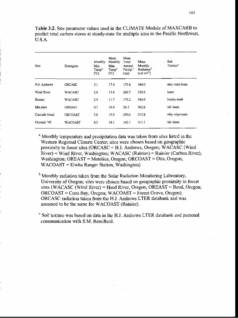
101
Table 3.2. Site parameter values used in the CLIMATE Module of MAXCARB topredict total carbon stores at steady-state for multiple sites in the Pacific Northwest,U.S.A.
a Monthly temperature and precipitation data was taken from sites listed in theWestern Regional Climate Center; sites were chosen based on geographicproximity to forest sites (ORCASC = H.J. Andrews, Oregon; WACASC (WindRiver) = Wind River, Washington; WACASC (Rainier) = Rainier (Carbon River),Washington; OREAST = Metolius, Oregon; ORCOAST = Otis, Oregon;WACOAST = Elwha Ranger Station, Washington)
b Monthly radiation taken from the Solar Radiation Monitoring Laboratory,University of Oregon; sites were chosen based on geographic proximity to forestsites (WACASC (Wind River) = Hood River, Oregon; OREAST Bend, Oregon;ORCOAST = Coos Bay, Oregon; WACOAST = Forest Grove, Oregon).ORCASC radiation taken from the H.J. Andrews LTER databank and wasassumed to be the same for WACOAST (Rainier).
C Soil texture was based on data in the H.J. Andrews LTER databank and personalcommunication with S.M. Remillard.
Mean MeanMonthly Monthly Total Mean Soil
Site Ecoregion Mi Max. Annual Monthly Texture'Tempa Tempa Precip.a Radiation"(°C) (°C) (cm) (cal cm)
H.J. Andrews ORCA5C 3.1 17.8 173.8 344.0 silty-clay-loam
Wind River WACASC 2.6 15.4 260.7 329.8 loam
Rainier WACASC 2.9 11.7 175.2 344.0 loamy-sand
Metolius OREAST 0.7 16.4 26.5 362.6 silt-loam
Cascade Head ORCOAST 5.8 15.0 250.6 313.8 silty-clay-loam
Olympic NP WACOAST 4.3 14.1 142.1 311.1 silt-loam

Aug Sep Oct Nov
a)
12
10C',
00
EE -2E
May Jun Jul Aug Sep Oct
102
Figure 3.21. Temporal variation in (a) monthly minimum and (b) monthlymaximum temperature for the five ecoregions represented by old-growth forest data.
-6
-8
35.0
30.000
25.0
20.0
15.0E'C
10.0
0 5.0
0.0
Jan Feb Mar Apr May Jun Jul Dec
Month

Sep Oct Nov
Nov Dec
50
45
E 40
030
0..' 250> 20
15
10
5
0
Jan Feb Mar
OREASTWACOAST
800
700E
600e
500
400
300
' 2000
(U
0
Jan Feb Mar Apr May Jun Jul Aug Dec
Month
Figure 3.22. Temporal variation in (a) monthly precipitation and (b) monthlyradiation for the five ecoregions represented by old-growth forest data.
103
Apr May Jun Jul
Month
ORCOAST
Aug Sep Oct
ORCASC

104
Differences between observed and predicted steady-state C stores are better
explained by diffrences in mean annual precipitation (Figure 3.23) than by other
climate variables (data not shown); however, the relationship was weak. As
precipitation decreased, the differences between the predicted and observed values
increased (R2 = 0.41). This indicates that the model did a better job predicting
steady-state C stores in regions that receive greater precipitation compared to sites
that receive less.

105
-100 -50 0 50 100 150 200
Predicted - Observed Carbon (Mg C/ha)
Figure 3.23. Linear regression between mean annual precipitation of observed (old-growth forest sites) and the difference between predicted (MAXCARB) andobserved carbon stores at steady-state.
0
0
CC
C(ci
3,
250 -
200 -
150 -
100 -
50 -
y = -0.7562x + 226.38R2=0.4153
0

Discussion
To constrain uncertainty of the terrestrial biosphere's role in the global C
cycle, it is helpful to bound predictions, particularly when human impacts, which
may change the pace and direction of system trajectories, are unknown. Baseline
studies provide a lower bound to system dynamics (what is the system's origin?)
(Bender et al., 2000). It is equally helpful to place an upper bound (what is the upper
limit of the system's response?), although these studies are rare. In MAXCARB, we
present a model that can predict an upper bound of forest C storage at steady-state.
The prediction can be useful for heuristic purposes to explore how uncertainty is
affected by forcings outside the equilibrium state, such as from climate change
In addition, MAXCARB operates at the regional scale, providing a means of
characterizing uncertainties at broader and finer scales. This is because highlighting
the significant processes at regional scales allows a better characterization of the
important processes at broader and finer scales. Specifically, regional processes are
constrained by processes at the global scale while finer- scale processes provide the
mechanistic understanding necessary to predict regional-scale dynamics (O'Neill,
1988).
As part of this process, understanding the role of disturbances at regional
scales is critical for constraining estimates of the role of the terrestrial biosphere in
mitigation of atmospheric CO2 increases (Potter et al., 1999; Schimel et al., 2001).
For instance, Kurz aril Apps (1999) recently assessed net ecosystem productivity in
Canada's forests over a 404 Mha area and showed that increases in fires and insect
damage have reduced C storage over the region.
106

107
Using MAXCARB, we studied the potential response of C storage to changes
in disturbance regimes at the regional scale. Results indicated that lengthening the
landscape rotation interval in a regulated (clear-cut) disturbance regime increased
steady-state C storage, implying that C sequestration potential is partially determined
by the disturbance regime. Specifically, landscape-average rates, which constrain
steady-state C storage, were dependent on the simulated disturbance regime. These
rates provide a mechanism whereby information on disturbance processes from
regional scales can be translated to broader scales. Specifically, landscape-average
rates could be used to modify parameters in a broad- scale model for disturbance
regimes at regional scales. Because MAXCARB is an efficient model in terms of the
time required for simulations, this is a tractable approach at broad scales.
We evaluated results of MAXCARB by comparing results with
STANDCARB and with data from old-growth forests. While this is not an
independent validation (since landscape-average rates from the DISTURBANCE
Module are used to calculate steady-state C stores), it demonstrates that the same
solution can be achieved with the more efficient model.
Comparisons between modeled predictions and observed data for the H.J.
Andrews generally showed good agreement for most pools from both models.
Differences for some poois, e.g., live coarse roots and live branches, may be because
old- growth estimates were derived with allometric equations, or they may be due to
parameterization of the model. The good agreement between the observed and
modeled stable soil C pooi is significant since this pooi is the last pool in the cascade
of equations in MAXCARE and is most likely to be in error as errors from preceding
108
calculations accumulate. Again, while not a validation of the model, this suggests
that errors did not substantially accumulate during the cascade of equations.
There was also good agreement between predicted and observed old-growth
data at multiple sites in the PNW. However, we did not include the stable wood pool
in this comparison, which would have increased the difference between predicted
and observed steady-state C stores. Comparing predicted and observed stable wood
poois is difficult since dead and stable poois are not distinguished in the obserd
data, but are separately modeled in MAXCARB. Also, parameterization of stable
wood is difficult because the steady-state C store is detennined by transfer (e.g., snag
fall) and decay rates. Either of these rates may be in error. More information is
needed to assess decay and transfer rates of dead wood at the landscape- level to
better evaluate model predictions.
Despite these caveats, we were able to predict steady-state C stores
reasonably well compared to data from old-growth forests, in response to a wide
variation in biogeodlimatic conditions in the PNW. As outlined by Smithwick et al.
(in press, Chapter 2), eastern Oregon stored the least C at steady-state, while coastal
Oregon stored the most. Eastern Oregon appears to be limited by precipitation and
extreme minimum and maximum temperatures, while coastal Oregon enjoys mild
winters and a less- severe summer drought. Precipitation and temperature are
variable in the Washington and Oregon Cascades resulting in intermediate steady-
state C stores for sites in these ecoregions. 'While the site we modeled at the
Washington coast has moderate temperature ranges, it receives less precipitation than
the Oregon coast, resulting in a lower steady-state C store. Differences between

109
predicted and observed values appear to be inversely related to mean annual
precipitation, indicating MAXCARB yields increasing error at drier sites.
MAXCARB is one of many models being developed to capture fine- scale
dynamics at broader scales. For example, Amiro et al. (2000) suggested that NPP
trajectories could be used as spatial averages to support broader-scale carbon models
in fire-prone regions of Canada. Leibowitz et al. (2000) developed a general
framework for assessing landscape-level functions based on the operation of
ecosystem units comprising the landscape. Moorcroft et al. (2001) present a new
model (ED) to scale gap-models to large scales, accounting for stochastic
disturbance events operating at the level of the individual. Similar to MAXCARB,
ED attempts to capture processes, including disturbances, at large scales without
modeling individual organisms, thereby increasing computer efficiency at broad
scales. The methodology with ED is statistically-based, capturing the size- and age-
structured variability that is inherent in sub-grid cell heterogeneity.
In both MAXCARB and ED, rules governing the sub-grid cell heterogeneity
and processes are not well understood and require more research. In MAXCARB,
we assume that disturbance events over a landscape can be simplified with a
disturbance regime. The assumption that a landscape is in steady-state with regard to
its disturbance regime is robust over very long time scales and across broad spatial
resolutions. However, in actual landscapes, and for shorter time-scales and narrower
spatial domains, these assumptions may be invalid. Few empirical studies exist over
the long time periods and broad spatial scales as is needed to evaluate error in these
conceptual models. Error may be incorporated in MAXCARB by assuming steady-
110
state landscapes if species dispersal and migration are not fully accounted for. For
example, the age-dependent functions in MAXCARB's DISTURBANCE Module
presume the user is able to define a priori the species composition after disturbance
events (integrating any dynamic changes in species composition during succession).
In reality, for very short, repeated disturbance intervals, late-successional species
may not be able to successfully regenerate and may not be able to migrate into the
stand. At very long disturbance intervals, early successional species may disappear
from the system if their dispersal is limited. However, these errors should not
substantially affect the estimates of steady- state C stores presented here, given the
long lifespan of tree species in the PNVsT and the rotation intervals we used.
However, caution should be used when applying the model to other areas where
species may have shorter lifespans and disturbances are infrequent or rare.
The landscape- level concept of simulating disturbance events based on a
probability distribution builds on established concepts in forestry, ecosystem science,
and landscape ecology. For example, at the stand-scale, the classic "J-shaped" curve
is used to describe the sustainable distribution of height and diameter classes of
uneven-aged forests. At the landscape scale, there are many probability distributions
that have been put forth to capture the dynamics of natural disturbance events
through time. For example, Zhang et al. (2001) recently suggested that mixed
Weibull distributions might ultimately be used to capture dynamics in uneven-aged
stands. These disturbance distributions require continued empirical testing to be
used with confidence at broad scales. A future improvement to MAXCARB may be

111
the user-defined option of choosing one of a family of distributions to determine how
the choice affects potential carbon storage.
One limitation of assessing ecological processes at broad spatial and temporal
scales is understanding and summarizing successional trends (Amiro et al., 2000).
This is particularly evident with MAXCARB as age-dependent functions are critical
for correctly parameterizing the DISTURBANCE Module. In this paper, we present
data using age-dependent rates derived with simulations from the STANDCARB
model. A sensitivity test on these rates showed that total stores were not greatly
affected by moderate changes (± 10 %). Yet, there remains considerable uncertainty
for some parameters, such as allocation ratios, suggesting that even a change in 10 %
of the original value may not reflect the uncertainty in that parameter. More
empirical work is needed to narrow the uncertainty of these parameters. In the
meantime, continued work with other models, such as STANDCARB, may allow
better parameterization. The relatively good fit between total stores of both models
and field data indicates that further improvement of parameters may be minimal to
significantly improve agreement. Summarizing changes in ecosystem function with
age is an emerging, evolving arena of research (Bond and Franklin, 2002) and as
new empirical knowledge is gained at finer scales, it can be incorporated into the
MAXCARB structure.
Another source of potential error in MAXCARB is the assumption that
spatial interaction of heterogeneous patches does not significantly affect steady-state
C stores. Future grid-mode simulations of MAXCARB may incorporate error by not
accounting for the effect of spatial interactions (see Chapter 4). More research

112
would clarify the importance of sub-grid cell heterogeneity. Pierce and Running
(1995) assessed the significance of averaging sub-grid cell variations on estimates of
net primary production and concluded that aggregating climate indices to a 1 -degree
land surface area was more important in causing error than aggregating
topographical, soils, and vegetation variation. To avoid this problem, MAXCARB's
design allows for climate variation at the scale at which data is available, within
broader regions of disturbance regimes
MAXCARB also does not include the constraints of nutrient cycling on
potential C stores. This simplification was made although nitrogen and other
nutrients can constrain growth in this region. Therefore, application of the current
MAXCARB model to situations with these limitations may incorporate error.
Assessing error when information is translated from fine to broad scales is
difficult. Translating processes at finer scales as a functional response at a larger
scale can lead to error (King et al. 1991). Precisely defining functionality at larger
scales is a challenge since most empirical data is derived at the plot level. We
suggest that the landscape scale is an appropriate level on which to examine
disturbance processes. Predicting steady-state C stores across a wide gradient of
climate, soils, and disturbance regimes at the regional scale facilitates assessment of
the relative importance of these interacting factors on C storage in the long term.

Conclusions
Scaling mechanisms are needed to incorporate disturbance processes at broad
scales efficiently and accurately. We present a new model that is able to predict
potential carbon stores across a given region in response to biogeographical variation
in climate, soils, dominant species composition and, importantly, the effect of
disturbance regimes. By assessing disturbance regimes at the landscape-scale, we
were able to implicitly include disturbance processes at a broad scale without having
to individually model each stand within the landscape. We used information about a
landscape's steady- state disturbance regime to calculate landscape- average rate
constants that determine its steady-state mass. We used a detailed succession model
to predict changes in key rates at broad scales, negating the reed to model
successional pathways explicitly.
By comparing this model to data from old-growth forests and to steady-state
results from a finer-scale model, we have confidence that MAXCARB can constrain
estimates of the upper bounds of C storage in the PNW. Additionally, we also found
that, as the disturbance interval was lengthened, the potential amount of total C
stores on the landscape increased.
Currently, disturbance is a key uncertainty in global carbon studies, and
MAXCARB could be used to parameterize global models for the effect of
disturbance at regional scales and to assess the relative effect of disturbances on
potential C storage.
113

Acknowledgments
This research was made possible by funding from the Pacific Northwest
Research Station Long-Term Ecosystem Productivity Program, an NSF Graduate
Research Traineeship award to Oregon State University, and Interagency Agreement
DW 12936179 between USEPA and the Pacific Northwest Research Station. All
stands are associated with the H.J. Andrews Long Term Ecological Research (LTER)
program, grant number DEB-9632921.
114

References
Amiro, B.D., Chen, J.M. and Liu J. 2000. Net primary productivity following forestfire for Canadian ecoregions. Can. J. For. Res. 30, 939-947.
Bender, M., Field, C., Hedin, L.O., Schimel, J., Sundquist, E., Berner, R., Galloway,J., Mackenzie, F., Torn, M., Freeman, K.H., Hedges, J., Mora, C., Stallard,R., Wofsy, S.C., and Schlesinger, W.H. 2000. The Changing C Cycle: ATerrestrial Focus, Report of the Workshop on the Terrestrial C Cycle. TheNational Science Foundation, Division of Earth Sciences.
Bonan, G.B. 1989. A computer model of the solar radiation, soil moisture, and soilthermal regimes in boreal. Ecol. Model. 45, 275-306.
Bond, B.J. and J.F., Franklin 2002. Aging in Pacific Northwest forests: a selectionof recent research. Tree Physiology 22: 73-76.
Caspersen, J.P., Pacala, S.W., Jenkins, J.C., Hurtt, G.C., Moorcroft, P.R., andBirdsey, R.A. 2000. Contributions of land-use history to C accumulation inU.S. forests. Science 290, 1148-1151.
Causton, D.R., Elias, C.O., and Hadley, P. 1978. Biometrical studies of plantgrowth. Plant, Cell, and Environ. 1, 163-184.
Ciais, P. 1995. A large northern hemisphere terrestrial CO2 sink indicated by the13C/12C ratio of atmospheric CO2. Science 269, 1098-1102.
Cohen, W.B., Harmon, M.E., Wallin, D.O., and Fiorella, M. 1996. Two decades ofC flux from forests of the Pacific Northwest. Bioscience 46, 836-844.
Cooper, C.F. 1983. C storage in managed forests. Can. J. For. Res. 13, 155-166.
Dai, A. and Fung, I.Y. 1993. Can climate variability contribute to the "missing" CO2sink? Global Biogeochem. Cycles 7, 599-609.
Dale, V.H. 1997. The relationship between land-use change and climate change.Ecol. Appl. 7, 753-769.
Dixor R.K., Brown, S., Houghton, R.A., Solomon, A.M., Trexler, M.C., andWisniewski, J. 1994. C pools and flux of global forest ecosystems. Science263, 185-190.
Emmingham, W.H. and Waring, R.H. 1977. An index of photosynthesis forcomparing forest sites in western Oregon. Can. J. For. Res. 7, 165-174.
115

116
Fan, S., Gloor, M., Mahiman, J., Pacala, S., Sarmiento, J., Takahashi, T., and Tans,P., 1998. A large terrestrial C sink in North America implied by atmosphericand oceanic C dioxide data and models. Scieite 282, 442-446.
Fang, J., Anping, C., Peng, C., Zhao, S., and Ci, L. 2001. Changes in forest biomassC storage in China between 1949 and 1998. Science 292, 2320-2322.
Fung, I. 2000. Variable C Sinks. Science 290, 1313.
Goulden, M.L., Munger, J.W., Fan, S-M, Daube, B.C., and Wofsy, S.C. 1996.Measurements of C sequestration by long-term eddy covariance: methods anda critical evaluation of accuracy. Global Change Biol. 2, 169-182.
Harmon, M.E., Franidin, J.F., Swanson, F.J., Sollins, P., Gregory, S.V., Lattin, J.D.,Anderson, N.H., Cline, S.P., Aumen, N.G., Sedell, J.R., Leinkaemper, G.W.,Cromack Jr., K., and Cummins, K.W. 1986. Ecology of coarse woody debrisin temperate ecosystems. Adv. Ecol. Res. 15, 133-302.
Harmon, M.E., Ferrell,W.K., and Franklin, J.F. 1990. Effects on carbon storage ofconversion of old-growth forests to young forests. Science 247, 699-702.
Harmon, M.E. and Domingo, J.B. 2001. A user's guide to STANDCARB version2.0: A model to simulate the C stores in forest stands. Department of ForestScience, Oregon State University, Corvallis, Oregon.
Harmon, M.E. and Marks, B. In press. Effects of silvicultural treatments on carbonstores in Douglas- fir/western hemlock Forests in the Pacific Northwest, USA.Can. J. For. Res., In Press. Harmon, M. E. and B. Marks.
Hibbard, K.A. 1995. Landscape Patterns of C and Nitrogen Dynamics in aSubtropical Savanna: Observations and Models. Ph.D. Dissertation, TexasA&M University.
Holland, E.A. and Brown, S. 1999. North American C Sink: Technical Comments.Science 283, 1815a.
Houghton, R.A. 1993. Is C accumulating in the northern temperate zone? GlobalBiogeochem. Cycles 7, 611-617.
Houghton, R.A. 1999. The annual net flux of C to the atmosphere from changes inland use 1850-1990. Tellus 51B, 298-313.
Houghton, R.A., Davidson, E.A., and Woodwell, G.M. 1998. Missing sinks,feedbacks, and understanding the role of terrestrial ecosystems in the globalC balance. Global Biogeochem. Cycles 12, 25-34.
Houghton, R.A., Hackler, J.L., and Lawrence, K.T. 1999. The U.S. C budget:contributions from land-use change. Science 285, 574-578.

117
Janisch, J.E. and Harmon, M.E. 2002. Successional changes in live and dead woodstores: Implications for net ecosystem productivity. Tree Phys. 22, 77-89.
Jensen, M.E. and Haise, H.R. 1963. Estimating evapotranspiration from solarradiation. J. Irrigation and Drainage Engineering 89, 15-41.
Johnson, E.A. and Gutsell, S.L. 1994. Fire frequency models, methods andinterpretations. Adv. in Ecol. Res. 25, 239-287.
Johnson, E.A. and Van Wagner, C.E. 1985. The theory and use of two fire historymodels. Can. J. For. Res. 15, 2 14-220.
Jones, HG. 1992. Plants and microclimate: a quantitative approach toenvironmental plant physiology. Cambridge University Press.
King, A.W., Johnson, A.R. and O'Neill, R.V. 1991. Transmutation and functionalrepresentation of heterogeneous landscapes. Lands. Ecol 5: 239-253.
Kurz, W.A. and Apps, M.J.. A 70-year retrospective analysis of carbon fluxes in theCanadian forest sector. Ecol. Appl. 9, 526-547.
Lenihan, J.M., Daly, C., Bachelet, D., and Neilson, R.P. 1998. Simulating broad-scale fire severity in a dynamic global vegetation model. Northwest Science72, 91-103.
Leibowitz, S.G., Loehie C., Lin, B. - L. and Preston E.M. 2000. Modeling landscapefunctions and effects: a network approach. Ecol. Model. 132: 77-94.
Melillo, J.M., Fruci, J.R., Houghton, R.A., Moore, B., and Skole, D.L. 1988. Land-use change in the Soviet Union between 1850 and 1980: Causes of a netrelease of CO2 to the atmosphere. Tellus 40B. 116-128.
Moorcroft, P.R., G.C. Hum, and S.W. Pacala. 2001. A method for scaling vegetationdynamics: the Ecosystem Demography model (ED). Ecol. Monographs 71,557-586.
Olson, J.S. 1963. Energy storage and the balance of producers and decomposers inecological systems. Ecol. 44, 322-331.
O'Neill, R.V. 1988. Heirarchy theory and global change. In: Rosswall, T.,Woodmansee, R.G., and Risser, P.G. (Eds.) Scales and Global Change JohnWiley & Sons, Ltd., pp 29-45.
Pacala, S.W., Hurtt, G.C., Baker, D., Peylin, P., Houghton, R.A., Birdsey, R.A.,Heath, L.S., Sundquist, E., Stallard, R., Ciais, P., Moorcroft, P.R., Casperson,J.P., Shevliakova, E., Moore, B., Kohlmaier, G., Holland, E.A., Gloor, M.,Harmon, M.E., Fan, S.-M., Sarmiento, J., Goodale, C.L., Schimel, D., and

Field, C.B. 2001. Consistent land- and atmosphere-based U.S. C sinkestimates. Science 292, 2316-23 19.
Peng, C. 2000. From static biogeographical model to dynamic global vegetationmodel: a global perspective on modeling vegetation dynamics. Ecol. Model.135, 33-54.
Pierce, L.L. and Running, S.W. 1995. The effects of aggregating sub-grid landsurface variation on large-scale estimates of net primary production.Landscape Ecol. 10, 239-253.
Potter, C. S., Klooster, S., and Brooks, V. 1999. Interannual variability in terrestrialnet primary production: exploration of trends and controls on regional toglobal scales. Ecosystems 2: 36-48.
Potter, C., Genovese, V.B., Klooster, S.A., Bobo, M., and Torregrosa, A. 2001.Biomass burning losses of C estimated from ecosystem modeling andsatellite data analysis for the Brazilian Amazon region. Atmos. Environ. 35,1773- 1781.
Richards, F.J. 1959. A flexible growth function for empirical use. J. Exper. Bot. 10,290-300.
Running, S.W. and Coughlan, J.C. 1988. A general model of forest ecosystemprocesses for regional applications I. Hydrologic balance, canopy gasexchange and primary production processes. Ecol. Model. 42, 125-154.
Schimel,D.S., House, J.I., Hibbard, K.A., Bousquet, P., Ciais, P., Peylin, P.,Braswell, B.H., Apps, M.J., Baker, D., Bondeau, A., Canadell, J., Churkina,G., Cramer, W., Denning, A.S., Field, C.B., Friedlingstein, P., Goodale, C.,Heimann, M., Houghton, R.A., Melillo, J.M., Moore III, B., Murdiyaio D.,Noble, I., Pacala, S.W., Prentice, I.C., Raupach, M.R., Rayner, P.J., Scholes,R.J., Steffen, W.L., Wirth, C. 2001. Recent patterns and mechanisms ofcarbon exchange by terrestrial ecosystems. Nature 414, 169-172.
Schimel, D., Melillo, J., Tian, H., McGuire, A.D., Kicklighter, D., Kittel, T.,Rosenbloom, N., Runnings, S., Thornton, P., Ojima, D., Parton, W., Kelly,R., Sykes, M., Neilson, R., Rizzo, B. 2000. Contribution of increasing CO2and climate to carbon storage by ecosystems in the United States. Science287, 2004-2006.
Schimel, D.S., VEMAP Participants, and Braswell, B.H. 1997. Continential scalevariability in ecosystem processes: models, data, and the role of disturbance.Ecol. Monog. 67, 251-271.
Sedjo, R.A. 1992. Temperate forest ecosystems in the global C cycle. Ambio 21,274-277.
118

119
Shugart, H.H., Michaels, P.J., Smith, T.M., Weinstein, D.A., and Rastetter, E.B.1988. Simulation models of forest succession. In: Rosswall, T.,Woodmansee, R.G., Risser, P.G. (Eds.) Scales and Global Change. JohnWiley & Sons, Ltd., New York.
Smithwick, E.A.H., Harmon, M.E., Domingo, J.B. In press. Potential upper boundsof carbon stores in forests of the Pacific Northwest. Ecological Applications.
Van Wagner, C.E. 1978. Age-class distribution and the forest fire cycle. Can. J.For. Res. 8, 220-227.
Wallin, D.O., Swanson, F.J., Marks, B., Cissel, J.H., Kertis, J., 1996. Comparison ofmanaged and pre- settlement landscape dynamics in forest of the PacificNorthwest, USA. For. Ecol. Manag. 85, 291-309.
White, A., Cannel!, M.G.R., and Friend, A.D. 2000. The high latitude terrestrialcarbon sink: a model analysis. Global Change Biol. 6, 227-245.
Yoder, B.J., Ryan, M.G., Waring, R.H., Schoett, A.W., Kaufman, M.R., 1994.Evidence of reduced photosynthetic rates in old trees. For. Sci. 40, 5 13-527.
Zhang, L., Gove, J.H., Liu, C., Leak, W.B. 2001. A finite mixture of two Weibul!distributions for modeling the diameter distributions of rotated- sigmoid,uneven-aged stands. Can. J. For. Res. 31, 1654 1659.

CHAPTER 4
120
EXAMINING MULTISCALE EFFECTS OF LIGHT LIMITATIONS ANDEDGE-INDUCED MORTALiTY ON CARBON STORES IN
FOREST LANDSCAPES
Erica A. H. Smithwick, Mark B. Harmon, and James B. Domingo

121
Abstract
Analyses of carbon (C) dynamics at broad scales usually do not consider
spatial interactions. The assumption is that C dynamics can be modeled within
homogenous patches (i.e., even-aged) and then summed to predict broad-scale
dynamics (an additive approach). We reexamine this additive approach by using a
forest process model to estimate the relative effects of edge-induced, tree mortality
(mainly due to wind) and light limitations on C dynamics in artificial forest
landscapes with various spatial structures. We analyzed simulation results to
examine possible emergent behaviors due to spatial interactions at multiple levels
of pattern-process interactions. Emergent (i.e., non-additive) behaviors were
observed at all levels of scale examined, indicating that emergent behaviors did not
necessarily cease as one proceeded from the patch to the landscape level, as we had
expected. However, the magnitude of the emergent behaviors depended on the
level of spatial interaction considered as well as the type and intensity of the
processes that were included. In all cases, patch-to-patch interactions resulted in
significant emergent behaviors when process interactions were strong but were not
significant when interactions were weaker. In one case, the magnitude of emergent
behaviors differed among the landscapes, indicating that patch-to-patch interactions
may not be accounted for by a simple correction for edge effects unless spatial
interactions are addressed. The implication is that some dynamics of C flux
processes in fragmented hndscapes may not be captured at broad-scales using an
additive approach, whereas in other cases spatial interactions are small enough to
be ignored.
Introduction
Quantif'ing the exchange of C between the terrestrial biosphere and the
atmosphere is necessary to constrain the global C budget and potentially manage
for C sequestration (e.g., Brown 1996; Schultze et al. 2000; Watson et al. 2000).
As a result, estimates of C exchange over broad scales are needed to validate
regional and global C models. Since it is impractical to directly measure C flux for
every ecosystem over a broad area, it is necessary to make assumptions about how
to scale local information derived from select sites to a larger area.
A simple way to scale information to broader extents is through a
'distributional' or 'additive' approach (Baker 1989) and, traditionally, many C flux
research projects have been attempted in this way (e.g., Cohen et al. 1996;
Houghton et al. 2000). Carbon flux has a strong vertical component in that C is
transferred from the biosphere to the atmosphere through decomposition and
respiration, and from the atmosphere to the biosphere through photosynthesis.
Thus, when accounting for the net flux of an ecosystem, the balance of vertical
inputs and outputs should indicate the directionality of C transfer either into the
ecosystem or the atmosphere. It follows that by knowing the net C flux of several
landscape elements, and summing the fluxes for the area of each landscape
element, it should be possible to calculate the net landscape flux.
However, processes affecting C flux such as mortality, respiration, and
decomposition may change horizontally across forest edges, influencing C storage
in neighboring patches. These horizontal processes have been inadequately
described in most carbon flux research. The change in horizontal processes can be
122

123
linear or non- linear across this zone. If the change is linear, the response at the
edge is a result of the degree of mixing of the two neighboring patches (the "matrix
effect" of Lidicker (1999)). An additive model can handle this linear change. By
contrast, if the change is non- linear (enhanced, diminished, or asymptotic), the
response of the system at the edge cannot be explained completely by the mixing of
the two neighboring patches. As a result, averaging the properties of the
neighboring patches is not sufficient to predict behavior at broad-scales using
traditional additive approaches (Lidicker 1999). Therefore, landscape- level
estimates of C flux may diverge from patch- level estimates if these horizontal
processes are included. The differences between the two approaches can be
attributed to landscape- level "emergent behaviors" (i.e., behaviors at the landscape
scale that cannot be predicted solely from the additive properties of the patches).
A landscape, which, by the definition we employ here, is composed of
patches of interacting stands or ecosystems (Forman and Godron 1981), is a useful
spatial unit in which to evaluate the impact of forest edges at broad scales. If
emergent behavior is important, landscape C flux may be dependent on patch
topology, the spatial relationships among patches in a landscape. Indeed, a central
tenet of landscape ecology is that spatial heterogeneity and scale matter when
interpreting ecological patterns and processes (Risser 1987, Wiens 1998) Since
forest edges are common components of many landscape mosaics (Forman and
Godron 1981; Franklin and Forman 1987), horizontal processes across forest edges
may be important in landscape-scale C budgets. Theoretically, it has been shown

124
that the spatial patterns of edges on the landscape, created by different disturbance
regimes, result in different ecological responses (Franklin and Forman 1987).
Recent evidence suggests that at short time- scales the horizontal flux of C
can be significant, even in areas presumed homogenous. Interpretation of the
resultant flux over a broad area must account for this horizontal heterogeneity. For
example, eddy correlation techniques were designed to measure the vertical flux of
CO2 and water vapor between the vegetation, soil, and atmosphere over an
ecosystem, allowing the calculation of the net amount of material entering and
leaving the ecosystem at a very fine temporal resolution over a fairly broad area.
However, due to horizontal movement of air masses, the source area of the
measured fluxes does not necessarily equal the "footprint" of the eddy flux tower
(Turner and Gregory, in review ; Kaharabata et al. 1997; Wofsy et al. 1993;
Goulden et al. 1996). The direction and magnitude of this source discrepancy may
change at time scales of hours (differing wind directions) to decades (changing land
types and/or age-class structure), making it difficult to avoid. Airborne and eddy-
flux measures of C exchange may not agree due to fine- scale spatial heterogeneity
(Desj ardins et al. 1997), indicating that simple additive approaches may not be
sufficient to capture broad-scale fluxes.
Research on long-term edge effects, primarily from observational field
studies, also indicates important horizontal effects across forest edges. Particularly,
increased light penetration and susceptibility to wind turbulence cause differences
between the edge and the interior. Increased light at forest edges causes a
difference in the competitive advantage of different species and life forms, although
125
the effect is dependent on stand age, aspect, and moisture conditions (Raimey et al.
1981; Lovejoy et al. 1984; Williams-Linera 1990). In addition to changes in light
conditions, the openings at forest edges often result in increased exposure to wind
and thus increased rates of tree- mortality. In the tropics, Laurance et al. (1997)
found that, with time, carbon stores of live vegetation within 100 m of an edge
boundary were reduced 36 % compared to that before fragmentation. In the same
area, Laurance et al. (1998) showed that the mean mortality rate was 3 to 4 times
higher in forests within 60 m of edges (4.01 % vs. 1.27 %), while Ferreira and
Laurance (1997) reported mortality rates that were elevated 7 or 8 times in edge
plots compared to interior forest plots. In Pamma, Williams-Linera (1990) showed
that the edge to interior ratio of trees that died after the edges were created was
14:1. In North American temperate forests, increased mortality at edges in old-
growth Douglas-fir (Pseudotsuga menzeizii) has also been recorded. Eighty-
percent of the blow-down associated with a forest windthrow event in the Bull Run
Basin in northwestern Oregon was due to the proximity of the stands to recent
clear-cut edges (Sinton et al. 2000). Chen et al. (1992) showed a greater number of
snags and logs at forest edges, indicating elevated rates of tree- mortality at forest
edges compared to the interior forest.
Light and wind interact in the edge zone, causing concomitant changes. For
example, windthrow in the Bull Run Basin has favored the development of shade-
tolerant species along edges and reduced the presence of old- growth Douglas- fir,
which is susceptible to wind mortality after being newly exposed (Sinton et al.
2000). A similarly complex response to light and wind was observed at Wind

126
River, in southern Washington, where Douglas- fir and western hemlock (Tsuga
heterophylla) seedlings increased, but Pacific Silver fir (A bies amabilis) seedlings
and saplings decreased in abundance (Chen et al. 1992). In the tropics, secondary
plant species that depend on high light conditions are able to invade reserve
margins as prevailing winds cause an increase in standing dead, broken, and fallen
trees (Lovejoy et al. 1984). Thus, multiple ecological processes may operate
simultaneously at patch edges (particularly light and wind), potentially resulting in
complex emergent behavior that cannot be assessed by examining processes
independently.
In this paper, we use a forest process model (STANDCARB) to simulate the
effects of wind mortality and light limitations on carbon storage within different
artificial landscape structures. Our general research question is: can landscape
carbon storage be predicted using the additive approach, whereby the value of the
landscape is equal to the area-weighted sum of the properties of the patches?
Specifically, does the interaction of these two processes (light and wind) result in
non- linear interactior among patches that are not predictable using additive
approaches? Finally, if emergent behaviors (defined here as the differences beyond
expected variation of an additive model) are present at one spatial scale due to
interactions at the lower levels, do they cease to be important at broader scales?
There were two specific objectives with this modeling exercise. The first
objective was to analyze the effect of cell-to-cell interactions at the stand scale.
Here, a cell is approximately 0.03 ha, which represents the area that would be
occupied by a typical mature tree in the Pacific Northwest. Cell- to-cell interactions

127
are determined by examining results within a homogenous landscape, i.e., where
there is only one type of patch and thus no patch-to-patch interactions. The second
objective was to analyze the effects of patch-to-patch interactions at the landscape
scale. A patch represents a collection of cells within a simulated landscape. Patch
size ranged from 0.03 ha to approximately 5 ha, depending on the type of artificial
landscape being simulated. Interactions between patches are determined by
examining results within heterogeneous landscapes, where there is a mix of old and
young age-classes on the landscape. We also examined the effect of patch structure
in a landscape, i.e., the arrangement of patches, as it might affect possible emergent
behavior at the landscape scale. By comparing results at two scales of interaction,
our goal was to determine if carbon storage was predictable using an additive
approach, or, conversely, whether emergent behaviors due to the interaction of light
and wind processes were evident. Despite a generally accepted notion that spatial
heterogeneity is important (King et al. 1991; Risser 1999), it is difficult to
determine at what scale, and under what circumstances, this is so. The goal of this
research is to elucidate the scales over which assumptions of spatial homogeneity
will hold. This research has significant implications for carbon cycle modeling
since carbon models that operate at broad scales make assumptions of spatial
homogeneity, although the implications may extend to other ecological fields in
which spatial scale is important.

128
Methods
Model Description
STANDCARB v.2.0 (Harmon and Domingo 2001; Harmon and Marks, in
press) was used in these simulations. This model simulates the dynamics of live
and dead pools of carbon in mixed-species, mixed-age-class, forest stands and is
also able to simulate the effects of harvests or fire on carbon storage.
STANDCARB is similar to gap models since each stand is simulated with many
replicate cells, which are then averaged to obtain stand values. In addition,
STANDCARB can be parameterized for specific species based on characteristics
defming their growth, mortality, and decomposition. As a result, the species
composition changes through time during succession in response to the species'
competitiveness. STANDCARB is also similar to many ecosystem-process models
in that growth, mortality, decomposition, and other significant ecosystem processes
are calculated in response to abiotic factors such as climate and site characteristics.
Temporally, STANDCARB is run on an annual time step for all live and dead
carbon pools through succession, although climate variables, affecting tree
establishment, growth, and decomposition are computed monthly.
Within each cell in STANDCARB, there are 4 vegetation layers (upper tree,
lower tree, shrub layer, and herb layer), each of which has up to seven live pools,
eight detrital pools, and three stable carbon pools (Figure 4.1). For example, the
upper and lower tree layers are comprised of seven live pools: (1) foliage, (2) fme-
roots, (3) branches, (4) sapwood, (5) heartwood, (6) coarse-roots, and (7) heart-rot.

LowerTreeLayer
DetritaPools
StablePools
Heart Rot CoarscRoots
aFolo: IraioIi ipw,d It\I Fliw
Roots
V__I(,IUittC
k-ad IktdHi ilk Ii
I
Sanwood( knI
I I triwc.i'dI )id C.ir':
ROO1
Dead FInLRooH
V V.Stable
Stable WoodStable
Soil
Upper Shrub HerbTree Layer LayerlLayer Layer
Detritus PoolsI
IStable Pools
I II
I- - - - 1
I I
I I I
I I
L
Figure 4.1. Conceptual structure of carbon pools and vegetation layers forSTANDCARB 2.0.
129
I

130
Shrubs do not have heartwood or heart-rot since they do not form a bole, and herbs
do not have any woody components. Each tree layer can be a different species,
whereas the shrub and herb layers are each represented by a single "species." Live
carbon pools transfer material to their detntal counterpart to account for the pools
available for decomposition processes. Dead sapwood and dead heartwood are
additionally separated into snags and logs so that the effects of position on
microclimate can be modeled. All detrital poois in a cell can potentially add
material to the three, relatively decay-resistant, stable C pools: 1) stable foliage, (2)
stable wood, and (3) stable soil.
Here, we describe a modification to STANDCARB that allows the model to
calculate tree exposure to wind at each cell and to increase natural tree-mortality
rates in proportion to increased tree exposure. With this change, cells in
STANDCARB can interact spatially with both light and wind, which affects
growth, decomposition, and mortality processes within cells.
Modeling Light Processes
Light influences several processes in STANDCARB: (1) the establishment
of tree species based on their light requirements, (2) growth rates through
modification of foliage mass, and (3) decomposition, through influences in detritus
moisture contents. To determine the direct and diffuse light reaching a particular
cell, STANDCARB uses a function called NeighborLight. NeighborLight
calculates the angle to the tallest tree along each of 8 cardinal transects surrounding
the cell of interest (Figure 4.2). By knowing the angle of the sun from the cell of

B
i urm.._u iraar ,4aru uum.r_III Ine
131
Figure 4.2. Arrangement of cells in STANDCARB, representing the spatialstructure used to calculated light limitations and wind mortality. A boundary zonesurrounds the simulation cells, representing vegetation outside of the simulationarea. The arrows indicate the directions of transects used to determine shadingeffects and exposure to wind.

132
interest, given information about the latitude, aspect, and slope of the site being
simulated, it is possible to calculate the direct and diffuse light reaching the cell.
For diffuse light, the average angle from these 8 transects is used to calculate
incoming radition. For direct light, a weighted average of the E, SE, S, SW, and W
transects is used (Harmon and Domingo 2001). In addition, cell width (which can
be set by the user) determines the amount of light entering a cell since, for a given
height, wider cells allow more direct and diffuse light to enter. This is important
because the minimum light requirements are different for different tree species, and
the species composition will affect the amount of carbon that is predicted. We ran
a series of simulations to test the effect of cell width of 15 m, 20 m, and 25 m on
carbon and found a significant response of cell width on carbon storage, with larger
cells retaining more carbon than smaller cells. We chose an intermediate cell width
of 17 m, which is approximately equal to the canopy width of old- growth trees in
the Pacific Northwest. All simulations that are described in this paper were run
with a 20 x 20 cell matrix, for a total of 400 cells, representing an area of
115,600m2 (or 11.56 ha).
Modeling Wind Mortality
We recognize that wind is an especially complex process in forest
ecosystems and we do not attempt to mimic its behavior exactly. Rather, we
estimated its effect by making the assumption that tree mortality is augmented by
increased exposure to wind. We refer to "wind mortality" for simplification,
although we imply that there is, more explicitly, an elevated tree-mortality rate

133
where cells are more-exposed, as at patch edges. We modeled exposure as a
function of slope, aspect, and tree heights, which are important factors resulting in
higher mortality rates at forest edges after catastrophic wind events (Lovejoy et al.
1984; Foster 1988; Foster and Boose 1992; Chen et al. 1992).
In previous versions of STANDCARB, tree mortality is initially high due to
tree competition and then decreases to a density- independent value that is a
function of the maximum age of the tree species, which sets the probability that the
tree will die in any given year. Here, we assumed that mortality in a cell would
increase due to wind turbulence in cells that were more exposed relative to those
that were more sheltered. We took advantage of the existing model structure in
NeighborLight to calculate a new function, called NeighborWind, to calculate the
relative exposure of trees in a cell. NeighborWind determines exposure to wind by
calculating the angle from the tree height in the cell of interest to the average tree
height along each of the 8 surrounding transects Figure 4.2). The length of the
transect (the number of cells from which average transect height is calculated) is set
by the user. In these simulations, we used a transect length of 10 cells (170 m for a
cell width of 17 m). NeighborWind then takes the average angle for the 8 transects.
The angle is normalized so that negative numbers indicate increased exposure (the
tree in the cell of interest is taller than neighboring cells, meaning it has a higher
mortality rate). The transects can also be weighted by aspect so that if there is a
directionality to the wind- induced mortality, it can be specified by the user.
However, in this paper, all the transects received equal weighting. We then defined
a new parameter, k, to equal the ratio of the maximum mortality rate at a

134
completely exposed cell to the base mortality rate (Figure 4.3). We used k values
equal to 2, 3, 5, or 8 times the baseline mortality rate, which are realistic estimates
for increased wind mortality at edges given the current literature (Laurance et al.
1998; Ferreira and Laurance 1997; Chen et al. 1992). Both NeighborLight and
NeighborWind can be set by the user as either on or off, which allows the user to
manipulate the interactions of light and wind during the simulations.
Model Parameterization and Calibration
To calibrate the model, we used data from old-growth stands in the H.J.
Andrews LTER permanent plot network (Acker et al. 1998) reported in Smithwick
et al. (in press). The goal of this calibration was to fit the relative proportion of
pools in tl old-growth forest data (presumed to be at steady-state by Smithwick et
al. (in press)) to the steady-state model results (average of years 500 to 1000). The
categories reported in Smithwick et al. (in press) did not exactly match those output
from the nDdel so it was necessary to assign pools to their appropriate category
(Table 4.1). Then, we adjusted the model parameters in the mortality, growth, site,
and decomposition driver files in STANDCARB to match the relative proportion of
pools in the old-growth field data. For simplicity, we presumed an equal ratio of
Douglas- fir and western hemlock tree seedlings to initiate the simulations.
Parameters affecting mortality, pruning, and turnover varied between
species. The maximum mortality rate was lower for Douglas- fir (0.009 yf1) than
for western hemlock (0.011 yr) and the maximum age for Douglas- fir was set at
1200 years versus 800 years for western hemlock. Pruning rates for branches and

Maximummortality rateat exposed cell
A
I_ J- tAi .52
k * Baseline mortality rate
Baselinemortalityrate
135
Figure 4.3. Graphical representation of elevated mortality rates across an edge. InSTANDCARB, k is equal to the wind mortality rate divided by the baseline ("gap-phase") mortality rate.

136
Table 4.1. Calibration of modeled carbon pools in STANDCARB v.2.0 to old-growth forest pools (Smithwick et al., in press).
Old-growth Pools % of Total Standcarb Pools % of Total
Live Branch 4.1 Live Branch 4.7
Dead Branch 0.8
Foliage 0.6 Foliage 0.9
Stem Wood 46.4 Sapwood+Heartwood+Heartrot 43.2
Fine Roots 1.0 Fine Roots 0.7
Coarse Roots 14.8 Coarse Roots 13.6
Fine Woody Debris 1.7 Dead Branch 1.3
Dead Roots 2.6 Dead (Fine + Coarse) Roots 3.5
Forest Floor 2.3 Dead Foliage + Stable Foliage 2.5
Rotten Wood 1.4 Stable Wood 2.2
Soil 14.9 Soil 15.6
Logs 5.1 Non- salvagable Logs 7.3
Snags 4.4 Non-salvagable Snags 4.4

137
coarse-roots were the same for both species (0.02 yr1 and 0.005 yf1, respectively).
Time close, the time required for the tree to have its maximum branch extension,
was set at 120 years for Douglas- fir and 100 years for western hemlock. Foliage
turnover rates were slightly faster for western hemlock (0.25 yr1 vs. 0.20 yf') than
Douglas- fir as the latter retains leaves longer, but fine root turnover rates were the
same (0.5 yr').
Growth parameters were also slightly different between species. Western
hemlock was set to establish when only 5 % of the total available light reached the
cell, but Douglas-fir, which generally requires more light for establishment, was set
to require 10 % of total light for successful establishment. Both species had similar
allocation ratios of fine roots to foliage (0.33) but Douglas- fir had higher rates of
heartwood formation than western hemlock (0.059 yr' vs. 0.022 yf'), reflecting its
thinner sapwood, a higher coarse root to bole ratio (0.62 vs. 0.52), and a lower
branch to bole ratio (0.11 vs. 0.34).
Finally, decomposition parameters, which affect the rates of decay and
turnover, were different for different tree species and different carbon pools.
Foliage, fine-roots, coarse-roots, and branch decay rates (0.15 yf'), as well as
sapwood decay rates (0.07 yf), were the same for both species. Heartwood decay
was slower for Douglas-fir (0.02 yf') than for western hemlock (0.07 yr1). Stable
soil decay rates were set at 0.007 yf' to mimic the relatively high decomposition
resistance of this pool. All dead pools transferred material to the stable pools at
differing rates. The rate of transfer from the dead foliage pool to the stable foliage
pool was 0.057 yr1, which indicates a relatively fast decomposition rate of the dead

138
foliage pool. By contrast, the rate of transfer from the dead branch pool to the
stable wood pooi was 0.003 yf1, which indicates a slower rate of decomposition for
wood pools.
Model Simulation Experiments
We used STANDCARB in 1000-year simulation experiments of artificial
landscapes with varying age-class structures, representing a range of possible
management regimes: Landscape Y (100% Young), Landscape OG (100% Old-
Growth), Landscape AIC (50% young and 50% old, Aggregated Interior Cut),
Landscape AIF (50% young and 50% old, Aggregated Interior Forest), Landscape
CH (50% young and 50% old, Checkerboard cut), and Larilscape AD (50% young
and 50% old, Aggregated Directional cut, where the upper half is cut and the lower
half remains uncut) (Figure 4.4). For landscapes with a simulated harvest regime
(all except Landscape OG), STANDCARB was run 2 times, one with a harvest
regime of 50 years and one with a harvest regime of 100 years. All harvests
occurred after year 500, once the species composition had stabilized. For example,
the 100-year harvest patterns were prescribed at years 500, 600, 700, 800, 900, and
1000. Only years 500 to 1000 were used to calculate results. For brevity, only the
100-year simulations will be described here but results for both regimes were
similar.
Simulations were run with one of four interactions of light limitations and
wind mortality: (1) light limitations OFF and wind mortality OFF, which served as
a control, (2) light limitations ON, wind mortality OFF, (3) light limitations OFF

cot
C0000 00000000000
e_0_o_c_c_o_0_0_o_0_
139
l0O%Cut l00%Old 50%01d150%Young(homogenous) (homogenous) (heterogeneous)
AggregatedInterior Cut
V OG AIC
50%Old/50%Young 50%01d150%Young 50%01d150%Young(heterogeneous) (heterogeneous) (heterogeneous)Aggregated Checkerboard AggregatedInterior Forest Directional
AIF CII AD
Figure 4.4. Artificial landscape cutting patterns used to drive the model (0=uncut,1=cut). Each cutting pattern was used for simulations of 100-year and 50-yearharvesting regime. Eachpattem describes a landscape with either a homogenous(Y, OG) or heterogeneous (AIC, AIF, CH, AD) patch structure.
000000000000000000000000000000000000000000000000000000000000
000000000000000000000000000000000000000000000000000000000000

140
and wind mortality ON, and, finally, (4) light limitations ON and wind mortality
ON, which simulated the interaction between the processes. For all simulations in
which wind mortality was included, simulations were run at k set to 2, 3, 5, or 8.
We tested for statistical significance of emergent behaviors by first
identifying the control (or additive) calculation for each case (detailed below and in
Table 4.2). We then compared the control to the appropriate simulation results, in
which the interactions of interest were present. We tested for statistical
significance by first calculating the standard deviation from the mean of the five
replicate runs of the model for the simulation of interest. It is necessary to account
for this expected variability in model results since STANDCARB has stochastic
elements. We then compared the mean of the control to that of the simulation. If
that difference was greater than two standard deviations, then we considered it to be
significant. This is a conservative test since it implies that 95% of the observations
do not overlap the mean. If, after accounting for the variability in the model, the
mean of the simulation was significantly different from the control, then we
considered emergent behaviors to be present.
Stand Scale
To observe the effects of light and wind processes on carbon stores at the
stand scale, we were interested in the cell- to- cell interactions within a patch and not
the spatial variability between patches. Thus, these comparisons were made in
Landscape OG and Landscape Y, which are homogeneous patch-types.

141
We examined emergent behaviors among 3 types of cell- to-cell interactions
at the stand scale: (1) cell-to-cell, (2) cell-to-cell * process, and (3) cell-to-cell *
age (I able 4.2). The first interaction (cell-to-cell) reflected the interaction between
cells with regard to a certain process, i.e., light or wind. The goal was to determine
the relative effect of light and wind on carbon stores, relative to when neither is
included.
The second interaction (cell-to-cell * process) reflected the interactions of
light and wind processes acting together and not their individual effects. Our
assumption was that an additive combination of the effects of light limitations on
carbon stores, simulated independently (CL), and the effects of wind mortality on
carbon stores, simulated independently (Cw), should equal the carbon stores when
both light and wind processes were included together in the same simulation (CLW).
It follows that any difference in carbon stores would be due to an emergent
behavior, that is, behavior not predictable by a combination of the processes
simulated independently.
The third type of interaction (cell- to-cell * age) reflects the interactions due
to the age of the landscape. Simply, we asked whether cell-to-cell interactions are
different between Landscape OG and Landscape Y. Our hypothesis was that older
landscapes, which exhibit more tree height variability, might result in larger
emergent behaviors than young landscapes, which have a more uniform canopy
height distribution. Emergent behaviors are indicated as significant differences
between results of Landscape OG and those of Landscape Y.
The establishment and persistence of a species in the stand is a function of

Table 4.2. Description of methodology used to test for emergent behaviors at various levels of spatial interaction. CL carbon (C)stores for simulation with only light limitations included, Cw = carbon stores for simulation with only wind mortality included, CLWcarbon stores when both were included, and C0 = carbon stores when neither process was included in the simulation experiments. OGis the old-growth age-class structure; Y is the young age-class structure; OG*Y is any heterogeneous age-class structure, representingAIC, AIF, CH, and AD (Figure 4.3).
Cell-to-cell * age
Patch-to-patch
Patch-to-patch * process
Patch-to-patch * structure
Cwy (or CW-OG)CLY (or CL-OG)CLWY (or CLW-oG)
CWOG.Y
CLOG*YCLWOG*Y
CLW/ CoOG.y
CWOG.YCLOG*Y
CLWOG*Y
Do the process effects vary with landscape age?
Do patches interact within heterogeneous landscapes?
Do the processes interact within heterogeneous landscapes?
Do the process effects vary with patch age structure?
Cell-to-cell CoOG (or CWOG (or Cwy) Do cells interact within homogenous landscapes?CoOG (or C) CLOG (or CLY)
Cell-to-cell * process (CWOG / C0IJG) * (CLJG / C000) CLWOG / CØOG Do the processes interact within homogenous landscapes?(Cwy / C0) * (Q-y / C0) CLWy/ Coy
CWOG (or Cw-y)CLOG (or CL-y)CLWOG (or CLW-y)
(Cw00 + Cw-y)/2(CLOG + CL-y)/2(CLWOG +
(CLOG.y/ COG.Y) * (CWOG.yI CoG.y)
average (CWOG.y)average (CLOG.y)average (CLWOG*y)
Level ofInteraction Control Treatment Emergent Behaviors Ouestion

143
the available light and mortality rates and therefore, we expected, would be
determined by the particular light and wind processes included in the simulation.
In particular, the species composition of a simulation would be determined by
whether or not light and wind processes were allowed to interact between cells in a
homogenous stand. Growth, respiration, and decomposition rates are
parameterized differently for different species in STANDCARB and, as a result,
carbon stores are likely to be affected by a change in species composition.
Landscape Scale
To determine whether patch-to-patch interactions caused emergent behavior
at the landscape scale, we used artificial landscapes with a heterogeneous patch
structure. A patch ranged in size from just one cell (0.03 ha) for Landscape CH to
50 % of the cells in the landscape, or approximately 5 ha for Landscapes AD, AIC,
AIF. We examined 3 types of patch-to-patch interactions: (1) patch-to-patch, (2)
patch-to-patch * process, and (3) patch-to-patch * structure (Table 4.2). The first
interaction (patch-to-patch) reflects the interaction of patches within heterogeneous
landscapes with regard to a certain process. Our goal was to determine whether
carbon storage in heterogeneous landscapes is equal to the average of independent
simulations of Landscape OG and Landscape Y, since heterogeneous landscapes
are simply an equal mixture of old and young age-classes.
The second type of interaction (patch-to-patch * process) reflects the
interaction of processes in heterogeneous landscapes. This type of interaction is

144
similar to the cell-to-cell * process interaction, except that we are now concerned
with heterogeneous rather than homogenous landscapes.
The third type of interaction (patch-to-patch * structure) reflects possible
emergent behaviors due to the effect of spatial structure, i.e., the arrangement of
patches on the landscape. To test for emergent behaviors, we compare each
heterogeneous landscape to the mean of all the heterogeneous landscapes. If there
are no emergent behaviors, each landscape should be approximately equal to the
mean. Differences from the mean, therefore, reflect emergent behaviors caused by
the spatial arrangement of the patches on the landscape.
To further explore patch-to-patch interactions, we modified STANDCARB
to predict average carbon across "zones" of the simulated stand. The user can
designate a cell or group of cells as a unique zone. Carbon stores in each zone are
then the average of the carbon stores from each cell in that zone. Here we present
results from Landscape AD, in which a zone represents one row of cells (Figure
4.5). In this way, average carbon stores could be output horizontally across the
landscape, allowing modeled responses to be evaluated spatially between patches,
i.e., from a cut region to an uncut region (across an "edge'). To determine whether
carbon was changed at the edge, we calculated the average live and dead carbon for
years 500 to 1000 (in foliage, fme-roots, branches, sapwood, heartwood, coarse-
roots, and heart-rot pools), as well as their totals in each of the 20 zones. In
Landscape AD, half the stand was cut every 100 years and half remained uncut.
Therefore, 10 zones represented re- growing vegetation from the disturbance event
(zones CO through C9), while 10 zones represented old-growth forest (zones UO
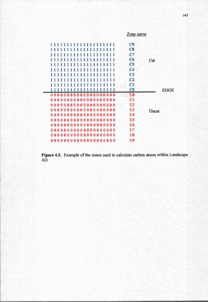
Uncut
EDGE
145
Figure 4.5. Example of the zones used to calculate carbon stores within LandscapeAD.
I1I!IiII1IIII1iTI111 I11IIII1IIIIIII1IIII tI1I1II1I11III1LIIII II1I1IT1II11II1J1I1I I111111I1111I11IJII1 11JIIiiT111I11IT1TTI 1I1IJII1LI1IiI1IIiIT 1I11I1tIIJIIIIIIIIII I111IIITJI111II1JII1 1It1IIi1IiI111IJIJ1I
Zone name
Cut
C9csC7C6C5C4c3C2ClCo
00000000000000 000 000 00000000000000000000 00000000000000000000 00000000000000000000
000 00000000000000000 000000000000000 00000
00000000000000000000 00000000000000000000 00000000000000000000 00000000000000000000

through U9). The border of the patches was thus between zone CO and zone UO,
although the effect to which the carbon stores were affected by the processes was
examined in zones "deeper" within each patch type.
Results
Cell-to-Cell Patterns in Carbon Stores
Light and wind processes within homogenous patches affected carbon
stores differently. For example, light limitations were more important than wind
mortality in changing total forest carbon until wind mortality was set very high
(k=8) (Figure 4.6). In Landscape OG, light limitations caused a reduction of total
carbon of 369 Mg C ha1 from the control (1204 Mg C ha minus 835 Mg C ha')
(Table 4.3). When wind mortality was included, total carbon was reduced by 114
Mg C ha1 (k=2), 213 Mg C ha1 (k=3), 332 Mg C ha' (k=5), and 434 Mg C ha1
(k=8). Thus, at low k values, light limitations reduced carbon stores 2 to 3 times
more than wind mortality; as k was increased, the effect of wind mortality on
decreasing carbon stores became similar to the effect of light limitations.
When wind was included in the simulations, total carbon stores appeared
less responsive than if live or dead stores were analyzed separately, due to the
compensatory dynamics of live and dead stores with regard to wind mortality
(Figure 4.7). Specifically, in all cases, when light- limitations were included, there
was a decrease in both live and dead stores; yet, when wind mortality was included,
live carbon decreased but dead carbon increased relative to the control.
146

1500
1200
900
600
300
Old-Growth Carbon Stores
0None Light Wind Wind Wind Wind
k=2 k=3 k=5 k=8
Figure 4.6. Total (live+dead+stable) carbon stores in Landscape OG as a functionof processes included in the simulations: None (neither light limitations or windmortality included), Light (only light limitations included), Wind (only windmortality included, at various levels of k)
147

148
Table 4.3. The effect of Neighbor functions (wind andlor light) on averagecarbon stores (calculated for years 500 through 1000) for different landscapecutting patterns (OG = old-growth, Y = young, AIC = aggregated interior cut,AIF = aggregated interior forest, CH =checkerboard, AD=aggregateddirectional; Figure 4.3). Standard deviations are in parentheses, rounded to nearestwhole number. On'y results from the 100-year cutting patterns are shown.
Landscape
Neighbor k value OG Y AIC AIF CH AD
LIVE
None na 825(12.5) 248(1.1) 540(4.7) 542(9.4) 541(14.7) 541(3.6)
Light na 572(2.4) 245(0.4) 409(6.0) 395(6.2) 415(9.9) 402(10.9)
Wind 2 655(3.2) 231(0.4) 433(5.2) 439(2.7) 419(7.9) 426(6.3)
Wind 3 526(8.9) 216(0.6) 361(6.2) 366(7.2) 347(3.6) 361(4.7)
Wind 5 382(3.8) 171(0.3) 253(3.4) 260(3.2) 238(2.4) 281(2.7)
Wind 8 273(2.1) 148(0.1) 191(2.8) 195(1.7) 182(2.1) 216(1.2)
Light+Wind 2 475(6.5) 239(0.5) 354(4.6) 341(5.7) 350(3.9) 350(3.3)
Light+Wind 3 409(6.1) 233(0.5) 317(4.5) 310(5.0) 314(5.5) 312(3.6)
Light+Wind 5 341(5.9) 196(0.4) 212(1.6) 211(2.7) 208(1.8) 273(4.4)
Light+Wind 8 283(2.3) 184(12) 183(1.0) 183(1.6) 179(0.9) 237(2.0)
DEAD
None na 288(3.6) 164(0.6) 226(1.6) 226(4.3) 225(4.9) 223(3.2)
Light na 186(2.8) 158(1.3) 161(1.1) 154(1.3) 158(3.2) 162(2.7)
Wind 2 336(1.8) 182(0.2) 261(2.8) 257(2.1) 265(1.5) 262(2.4)
Wind 3 363(3.7) 198(1.1) 281(1.6) 278(3.1) 284(3.4) 281(1.8)
Wind 5 384(1.1) 205(0.6) 298(2.2) 296(1.9) 301(0.9) 303(2.4)
Wind 8 388(1.0) 223(0.2) 307(1.0) 306(1.1) 307(0.2) 316(1.4)
Light+Wind 2 194(5.1) 163(1.4) 173(1.5) 166(3.9) 172(2.4) 170(3.2)
Light+Wind 3 199(5.3) 168(1.2) 180(1.2) 173(2.5) 180(1.6) 179(2.3)
Light+Wind 5 211(2.9) 156(0.5) 159(1.1) 153(1.6) 159(1.2) 189(2.8)
Light+Wind 8 232(1.2) 167(0.8) 175(0.8) 169(1.0) 173(0.9) 205(1.2)

Table 4.3. (Continued)
Landscape
Neighbor k value OG Y AIC AIF CH AD
149
STABLE
None na 90(03) 72(04) 81(0.3) 81(0.5) 81(0.5) 81(0.3)
Light na 81(0.4) 70(0.1) 72(0.3) 71(0.4) 72(0.5) 73(0.6)
Wind 2 97(0.5) 73(0.2) 85(0.6) 85(0.4) 86(0.2) 85(0.3)
Wind 3 101(0.5) 74(0.2) 88(0.2) 88(0.3) 89(0.2) 88(0.4)
Wind 5 106(0.2) 59(0.1) 70(0.4) 70(0.3) 71(0.2) 91(0.2)
Wind 8 109(0.1) 61(0.1) 72(0.2) 72(0.1) 72(0.1) 94(0.3)
Light+Wind 2 84(0.7) 70(0.2) 76(0.1) 75(0.8) 76(0.4) 76(0.5)
Light+Wind 3 86(1.4) 71(0.3) 79(0.5) 76(0.8) 79(0.1) 78(0.5)
Light+Wind 5 91(1.2) 52(0.1) 50(0.3) 49(0.2) 49(0.3) 81(0.8)
Light+Wind 8 96(0.5) 53(1.0) 52(0.3) 51(0.1) 51(0.2) 84(0.4)
TOTAL
None na 1203(16.5)484(2.2) 847(6.6) 848(14.1) 847(20.1) 845(7.1)
Light na 839(5.5) 473(1.9) 643(7.4) 620(7.9) 646(13.5) 636(14.2)
Wind 2 1089(5.4) 487(0.8) 780(8.6) 781(5.2) 770(9.5) 773(8.9)
Wind 3 991(13.1) 488(1.9) 730(8.0) 734(6.5) 720(7.3) 730(6.9)
Wind 5 871(5.1) 435(1.0) 621(6.0) 626(5.4) 610(3.5) 675(5.3)
Wind 8 770(3.2) 432(0.5) 571(4.1) 573(2.9) 562(2.4) 626(2.9)
Light+Wind 2 753(12.3) 473(2.1) 602(6.2) 582(10.4) 598(6.6) 595(7.0)
Light+Wind 3 695(12.8) 471(2.0) 576(6.2) 560(8.2) 572(7.1) 569(6.5)
Light+Wind 5 643(10.0) 403(1.0) 421(3.0) 414(4.5) 415(3.3) 544(8.0)
Light+Wind 8 610(3.9) 404(1.4) 410(2.0) 403(2.7) 403(1.9) 527(3.6)

1500
1200
900
600
300
Old-growth Carbon Stores
150
None 0 Wind k8
LIVE DEAD TOTAL
Carbon Pool
Figure 4.7. Old- growth carbon stores in live, dead, and total carbon poois as afunction of simulations with either no light limitations or wind mortality (None), orsimulations with wind mortality set to k=8 (Wind k8).

151
For instance, in Landscape OG, when wind mortality was included independently,
live carbon decreased 552 Mg C ha1 (825 Mg C ha' for the control to 273 Mg C
ha' when k was set to 8) (Table 4.3) and dead carbon increased 100 Mg C ha1
(288 Mg C ha for the control to 388 Mg C ha' when k was set to 8). Thus, the
change in total carbon stores (after accounting for the small change in stable pools)
was 433 Mg C ha* We initially tested emergent behaviors for each of the live,
dead, stable, and total pools. For simplicity, only tests for total carbon will be
presented in the results, although it should be recognized that these integrate the
differences in live, dead, and stable stores.
Cell-to-Cell Emergent Behaviors
For all simulations in Landscape OG, carbon stores were significantly
different from the control (e.g., after accounting for 95 % of the model variation)
Figure 4.8). When only light limitations were included, total carbon stores were
reduced 30.3 % (standard deviation (SD) = 1.3 %) from the control. When only
wind mortality was included (at k set to 8), carbon stores were reduced by 36.0 %
(SD = 0.8 %). When both light limitations and wind mortality were included,
carbon stores were reduced by approximately 49.3 % (SD 1.3%) (k = 8).
In contrast, emergent behaviors in Landscape Y were not consistently
observed. For example, when only light limitations were included, emergent
behaviors were not significant. When wind mortality was included, results were
significant only when k was set to 5 or greater. The largest reduction

D -0.2-
o -0.4 -0
2-0.8-
-1.0
L W2 W3 W5 W8 LW2 LW3 LW5 LW8
Process Included
Figure 4.8. Emergent behaviors due to interactions at the cell-to-cell level. Valuesrepresent the proportional difference of the treatments from the control. Thecontrol is defmed in Table 4.2. Values different from 0 reflect emergent behaviors.Error bars represent two standard deviations from the mean of five repetitions foreach simulation.
Do cells interact within homogenot landscapes?
152
1.0Cell-to-Cell- 0.8 -
0I.-
0.6- LIOG E:IY
E 0.4-
0.2
0.0 I

153
(approximately 16.6 % ± 0.5 %) was when light and wind were both included and k
was set to 5.
Cell-to-Cell * Process Patterns in Species Dynamics
Species composition, as evidenced by the number of upper trees in the
canopy, was affected by whether light limitations or wind mortality was included.
When wind mortality was modeled in the absence of light limitations, there was a
sinusoidal pattern in species dominance in the upper canopy through time, the
amplitude of which increased as the k value increased (Figure 4.9). Western
hemlock first appeared in the canopy after canopy closure, due to gap formation of
the Douglas-fir. The sinusoidal pattern of species dominance continued through
the simulation since both Douglas- fir and western hemlock were able to re-enter the
upper canopy due to advanced regeneration in the lower tree layer. With higher k-
values, these oscillations resulted in increasing oscillations of carbon stores (Figure
4.10). Typically, Douglas- fir would not be able to re-enter the canopy due to its
higher light requirements for establishment. Indeed, with light limitations included,
Douglas- fir never received enough light to re-enter the upper canopy after the
initial canopy closure (Figure 4.11) and the canopy continued to be dominated by
western hemlock. The timing of the initial transition from Douglas- fir to western
hemlock was also determined by which processes were allowed to interact. When
k was increased from 3 to 8 the transition to western hemlock from Douglas-fir was
about 50 years earlier, indicating that western hemlock was able to dominate earlier
by replacing Douglas- fir more quickly, essentially hastening the succession

-h-- Douglas fir Upper Trees k=8 -- Western hemlock Upper Trees k=8Douglas fir Upper Trees k=3 -s- Western hemlock Upper Trees k=3
450
400
350
300w0.a. 250
0U).a 150E
100z50
Figure 4.9. Effect of increasing k values on the number of upper trees for PSME (Douglas-fir, Pseudotsuga menziesii) andTSHE (western hemlock, Tsuga heterophylla) for simulations with only wind mortality included.
0 200 600 800400
Time
1000

C)
400 -
U)a,L..0
Cl)
200 -
1200
-c
C)a) 800 -U,
0U)
400 -
LandscapeOG
400 600Time
400 600Time
800
800
None NeighborLightNeighborWind k=3 A NeighborWind k=8
Figure 4.10. The trend in (a) total dead and (b) total live carbon through time forsimulations with only wind mortality included (k set to 3 or 8), only lightlimitations included, or neither included (None) for Landscape OG (old-growth).Note the different y-axis range between live and dead carbon.
1000
100
155
5 200
5 200

-h- Douglas fir Upper Trees k=8 -9- Western hemlock Upper Trees k=8-A-- Douglas fir Upper Trees k=3 -'--Western hemlock Upper Trees k=3
450
400
w 350
':300050
'I-00). 150E
z50
0
0 200 400 600 800 1000Time
Figure 4.11. Effect of increasing k values on the number of upper trees for PSME (Douglas-fir, Pseudotsuga menziesii) andTSHE (western hemlock, Tsuga heterophylla) for simulations with both light limitations and wind mortality included.

157
process (Figure 4.9 and Figure 4.11). The effect of this transition was not due to
light limitations since the pattern developed both when light limitations were
included as well as when they were not; rather, the earlier transition was most
likely due to the faster removal of the upper canopy tree-species at higher levels of
wind mortality.
Cell-to-Cell * Process Emergent Behaviors
In this test, significant differences from the control were apparent when k
was set to 5 or 8 but were not significant at lower levels of wind mortality (Figure
4.12). The direction of these differences (less than or greater than the control)
differed between the two landscapes. In Landscape OG, carbon stores were 5.8 %
(± 3.1 %) greater when the processes interacted when k was set to 5, and 13.7 % (±
1.3 %) greater when k was set to 8, compared to that calculated using the additive
approach. In contrast, in Landscape Y, carbon stores were 5.2 % (± 0.5 %) lower
when k was set to 5 and only 1.6 % (± 0.5 %) higher when k was set to 8.
Cell-to-Cell * Age Patterns in Carbon Stores
When there was a regular harvest event across the stand (Landscape Y), the
effect of light limitation and wind mortality processes was reduced compared to the
older landscape (Landscape OG). For example, in Landscape OG, both light
limitations and wind mortality reduced carbon stores from the control, when neither

I .0
0.80
O.6
0.4
0.2
0.0
-0.2
O -0.4t-0.6
-0.8
-1.0
Do processes interact within homogeneous landscapes?
158
LW2 LW3 LW5
Process Included
Figure 4.12. Emergent behaviors due to the cell- to-cell * process interactions.Values represent the proportional difference of the treatments from the control.The control is defined in Table 4.2. Values different from 0 reflect emergentbehaviors. Error bars represent two standard deviations from the mean of fiverepetitions for each simulation.
Cell-to-Cell * Process
LW8
159
was included (Figure 4.10). However, in Landscape Y (Figure 4.13), the
simulations that included light limitations are indistinguishable after year 500 from
the control, indicating that light interactions were less pronounced in the younger
landscape than the older landscape.
Cell-to-Cell * Age Emergent Behaviors
Emergent behaviors resulting from cell-to-cell interactions in Landscape
OG were higher than those in Landscape Y for all simulations (Figure 4.14).
Emergent behaviors were 28.7 % (± 0.2 %) higher in Landscape OG than
Landscape Y when only light was included and between 30.0 % (± 0.02 %) and
40.0 % (± 0.2 %) higher when both light and wind interacted.
Patch-to-Patch Patterns Across Edge Zones
Results across ed zones in Landscape AD showed that carbon stores were
affected both by light limitations and wind mortality, indicating that patch-to-patch
interactions were important. The relative effect of these processes at the edge was
different depending on the type of interaction included and the pools considered
(i.e., live, dead, stable, or total).
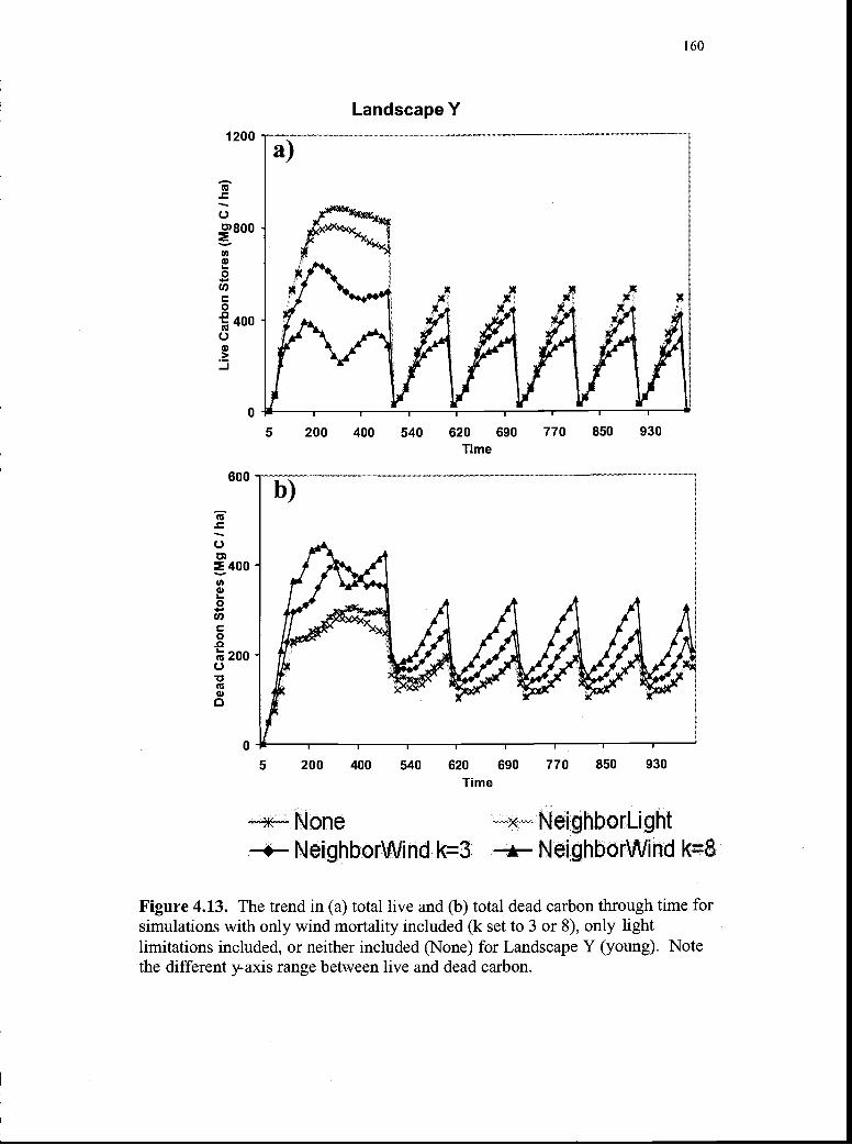
1200
C.)
a)400
U)C)I-0Cl)
C0.0I- 200C.)
CC
0)
Landscape Y
I-
5 200 400 540 620 690 770 850 930Time
5 200 400 540 620 690 770 850 930Time
*-' None NeicjhborLightNeighborWind k=3 *-- NeighborWind k=8
Figure 4.13. The trend in (a) total live and (b) total dead carbon through time forsimulations with only wind mortality included (k set to 3 or 8), only lightlimitations included, or neither included (None) for Landscape Y (young). Notethe different y- axis range between live and dead carbon.
160

1.0
0.8 -2
0.6-
0.4-
0.2 -
0.0
-0.2 -
5 -0.4 -
00.. -2- -0.8 -
-1.0
Does the process effect vary with landscape age?
161
DOG-v
L W2 W3 W5 W8 LW2 LW3 LW5 LW8
Process Included
Figure 4.14. Emergent behaviors due to the cell- to-cell * age interactions. Valuesrepresent the proportional difference of the treatments from the control. Thecontrol is defmed in Table 4.2. Values different from 0 reflect emergent behaviors.Error bars represent two standard deviations from the mean of five repetitions foreach simulation.

Live Stores
In the cut and uncut patch, light limitations and wind mortality processes
had different effects on live carbon across all zones (Figure 4.15, 4.16, and 4.17).
In the cut patch, live carbon stores for all pools were decreased for at least 3 zones
from the edge (equivalent to approximately 50 m) when only light limitations were
included. In contrast, when only wind mortality was included, live carbon stores
across the cut patch were not affected (at any k-value).
In the uncut patch, live carbon in zone 'U0' (one cell width into the uncut
patch) was greater than the average carbon stores across all zones in the uncut patch
when only light limitations were included. This is presumably due to the increase
of light at the edge. Yet, when only wind mortality was included, the live carbon
stores decreased for all pools in zone 'U0', due to the increased exposure to wind at
the edge. As an example of the effect of wind mortality, the average store of live
heartwood in the uncut patch across all zones was 193 ± 5.4 Mg C ha1 but was
only 181 Mg C ha1 at the edge, a difference of approximately 12 Mg C ha1. Ask
was increased, these differences ranged from 16 to 23 Mg C ha (Figure 4.16a).
Sapwood also decreased between 6 and 9 Mg C ha1at the edge with wind
mortality, depending on the k value (Figure 4.16b). When light limitations and
wind mortality were both included, there was an increase in live carbon near the
edge of the uncut patch, indicating the dominating effect of light, despite decreases
in live carbon stores due to wind mortality.
162

'None Nalghbortight-.- NeighboWnd kJ2 a-- WeghborWnd k8---Neighbo gt*NeyhbotWind k2 - Ne borLht+NehborWfl K8
a)
C9 C8 C7 C6 C5 C4 C3 C2 Cl CO UO UI U2 U3 U4 U5 U6 U7 U8 U9
Cut Uncut
C9 C8 C7 C6 C5 C4 C3 C2 Cl CO UO Ui U2 U3 U4 U5 U6 U7 U8 U9
Figure 4.15. Live carbon by zone for different light and wind simulations for (a)foliage and (b) fine-root pools in Landscape AD. Zones CO to C9 are cut every 50years after year 500, while zones UO to U9 remain uncut. Results are the averagefor years 500 to 1000 for each zone.
163
Cut UncutI
12
10
0a)
C01
0a)C)Ca
U-a)>
2
0
12
(a.0 1000)
0.0
0600
04C
U-a)>
0

None - t%1eIghbrLght
k2 *NeighborWnd k8- Nehboti t4NeighboWind K2 NesgaborLght4 Neighbor Wnø k8
300
2 250C.)
C)
2000.0I-
150
100
: 50
0C9 C8 C7 C6 C5 C4 C3 C2 CI co UO UI U2 U3 U4 U5 U6 U7 U8 U9
140
120 -
C)
100 -
C
. 80-0o 60-0
0CO C8 C7 C6 C5 C4 C3 C2 Cl CO UO UI U2 U3 U4 U5 U6 U7 U8 U9
Figure 4.16. Live carbon by zone for different light and wind simulations for (a)heartwood and (b) sapwood pools in Landscape AD. Zones CO to C9 are cut every50 years after year 500, while zones UO to U9 remain uncut. Results are theaverage for years 500 to 1000 for each zone. Note different y.axis scales.
164
-J20

Ncno te,ghborUght.--NegnborWind k=2 a-F4egPboriNnd k8-- k2 --- NegborL.ight+NeighborWnd kz8
-j- 50 -
C.)
D)40-
C0
30
20-C)>
60
0C9 C8 C7 CS C5 C4 C3 C2 Cl CO UO Ui U2 U3 U4 U5 U6 U7 US U9
C9 CS C7 C6 C5 C4 C3 C2 Cl CO UO UI U2 U3 U4 U5 U6 U7 U8 U9
165
Figure 4.17. Live carbon by zone for different light and wind simulations for (a)branch and (b) coarse root pools in Landscape AD. Zones CO through C9 are cutevery 50 years after year 500, while zones UO through U9 remain uncut. Resultsare the average for years 500 to 1000 for each zone. Note different y-axis scales.

Dead Stores
Dead carbon pools in the cut patch showed a decrease within three zones of
the edge when only light limitations were included (Figure 4.18, 4.19, and 4.20).
When only wind mortality was included, there were no observable differences at
the edge, although the absolute amount of dead carbon was higher than for the
control (no light or wind) for all zones in the cut patch, due to the increased
mortality.
Dead carbon pools in the uncut patch increased near the edge when wind
mortality was included, although this effect was only apparent for dead sapwood
(Figure 4.19b) and, similar to the live poois, was observable for only one zone
width. Dead sapwood increased from an average of 57 ± 3.6 Mg C ha' across all
zones to 65 Mg C ha' in zone 'UO' when k was set to 2. When k was set to 8, dead
sapwood averaged 124 Mg C ha1 ± 7.1 Mg C ha across all zones but was 141 Mg
C ha in zone 'UO'. This is an increase near the edge of almost 17 Mg C ha*
Differences between the average carbon across all zones and the carbon in zone
'UO' were not significant for other poois, averaging around 1 Mg C ha* When
both light limitations and wind mortality were included, carbon stores were
generally within the range of carbon stores in simulations when each process was
simulated independently. However, when the processes interacted at k set to 8,
dead branch carbon storage was consistently higher for the uncut patch, and
somewhat higher at the edge of the cut patch, compared to other pools (Figure
4.20a).
166

None NeèghborLghtaNeighborWind k=2 eNeighboriAhnd k4- k'2 . NelghbghtNeIghboWuiO k=8
I-
16
14
O 12-a)
10 -0
0
25
2-
'C20-
a)
5-
0C)0
0
a)
-
Cut Uncut
0) CO N- (0 It) (I) CJ 0 0 C"J (I) 10 (0 N- CO C)0000000000
167
Figure 4.18. Dead carbon by zone for different light and wind simulations for(a) foliage, and (b) fine root carbon pools for Landscape AD. Zones CO through C9are cut every 50 years after year 500, while zones UO through U9 remain uncut.Results are the average for years 500 to 1000 for each zone. Note different y-axisscales.
0 0 .- C'l C) CC) CO N- CO C)000 D DCO N- CO CC)000000

Nono " NeighborLghtNeghborWnd k2 -NcighboWnd k4
k-2 t--- Neghbo Lgtt+NeghbotWnø k=B
160
gioo -I-
O 80-00 60-
C,)
20-
00) U) N- CO U) 0) C'J 0 0 C\1 0) U) (0 N- U) 0)0000000000=) ) ) D ) :) D
0) U) N- (0 U) 0) C\1 0 0 - C') U) CO N- U) 0)0000000000:):) D :) :D D :)
Figure 4.19. Dead carbon by zone for different light and wind simulations for (a)sapwood and (b) heartwood pools in Landscape AD. Zones CO through C9 are cutevery 50 years after year 500, while zones UO through U9 remain uncut. Resultsare the average for years 500 to 1000 for each zone. Note different y-axis scales.
168
,1 20
140C.)

25
20C.)
0
hborLghthborWnd k=8hboL9ht+NeI9hl
C) U) N- (0 U) ) 0 0 .- () U) (0 N- U) C)0000000 000
0) (0 N- (0 U) - C.) ( 0 0 C C.) U) (0 N- (0 0)0000000000 DFigure 4.20. Dead carbon by zone for different light and wind simulations for (a)branch and (b) coarse root pools in Landscape AD. Zones CO through C9 are cutevery 50 years after year 500, while zones UO through U9 remain uncut. Resultsare the average for years 500 to 1000 for each zone. Note different y-axis scales.
169

Total Stores
Total live carbon stores (the sum of all the live pools) in the cut patch
averaged 200 ± 62.7 Mg C ha1 across all zones when only light limitations were
included (Figure 4.21a). However, near the edge of the cut patch (zone CO), the
total live carbon store was 47 Mg C ha', a decrease of 154 Mg C ha1. The
difference was negligible (1 Mg C ha') for zones C3 to C9, indicating that most of
the reduction in carbon stores due to light limitations was at the edge of the cut
stand. When only wind mortality was included, the reductions in total live biomass
at the edge compared to the average of all zones in the cut patch ranged from 2
(when k was set to 2) to 78 Mg C ha1 (when k was set to 8). When both light
limitations and wind mortality were included, total live stores decreased at the edge
of the cut patch (up to 137 Mg C had, when k was set to 2), similar to the
simulations with only light included. In the uncut patch, for all simulations, total
live carbon stores did not appear to change significantly across the zones.
Total dead carbon stores (the sum of all the dead pool results in Figure
4.21b) showed no change across all zones in the cut patch. In the uncut patch, total
dead poois were increased near the edge, from 3 Mg C ha1 (with light limitations)
to 19 Mg C ha1 (with light limitations and wind mortality, k=2).
Total carbon pools (total live + total dead + total stable) (Figure 4.22b)
showed no significant trend near the edge in the uncut patch. In the cut patch, there
was a decrease in carbon stores near the edge, ranging from large differences such
as 254 Mg C ha1 when only light limitations were included and 230 Mg C ha1
when both light limitations and wind mortality were included (k=5) to smaller
170

oneNeI9hborWnd k=2Neibfli1Neflbo,Wnd
1000
900 -
2 800-(; 700 -
600 -
500-
400 --J
300-0
200-
450
400
E 350C)
:' 300
2 250
0 200
0o 150
100 -
50
0
NeighborLight
WeighbotWnd k8k8
0) N- (0 (C) C) C'J 0 0 C\1 C) U) (0 N- (0 0)0000000000 ) D D
U) C) C)1 0 0 - C. C') U) (0 N- (0 0)
171
Figure 4.21. Effect of light limitations and wind mortality on: (a) total live and (b)total dead carbon, by zone, in Landscape AD. Zones CO through C9 are cut every100 years after year 500, while zones UO through U9 remain uncut. Results are theaverage for years 500 to 1000 for each zone.

None N&ghbotghtNcihbrWnd k2 oJgbbofWfld k8NeghborLgrne9hxWInd k2 - NeghtoUght+eghbQrWafld k'8
120
c100-c
1400
1200
1000
8000
600-
400 -
200 -
0
Cut 4 Uncut
0) LU N- (0 LU C) U) 0 0 U) LU (0 N- (0 0)0000000000=) ) ) ) :) :) D D
0) (0 N- (0 (0 0) 0) 0 0 C') 0) LU (0 N- (0 0)0000000000 :
172
Figure 4.22. Effect of light limitations and wind mortality on: (a) total stable and(b) total (live+dead+stable) carbon, by zone, in Landscape AD. Zones CO throughC9 are cut every 100 years after year 500, while zones UO through U9 remainuncut. Results are the average for years 500 to 1000 for each zone
60
.0m
40
020
0

173
differences such as 1 or 2 Mg C ha when only wind mortality was included (k=2,
3, and 8).
Patch-to-Patch Emergent Behaviors
Emergent behaviors due to patch-to-patch interactions were evidenced by
differences between the carbon stores in heterogeneous landscapes and the carbon
stores of independent simulations of old growth and young landscapes that were
additively combined (Figure 4.23). However, emergent behaviors were not
significant until the k value was set to 5 or 8. At these high k values, landscapes
AIC, AIF, and CH had 21 or 22 % (± 2.0 %) less carbon in the heterogeneous
landscapes than would be predicted from an additive approach. In contrast,
landscape AD had between 4.0 % (± 2.0 %) and 1.0 % (± 3.0 %) greater total
carbon stores.
Patch-to-Patch * Process Emergent Behaviors
Emergent behaviors due to patch-to-patch * process interactions were
significant when k was set to 3, 5, or 8 for all heterogeneous landscapes Figure
4.24). Differeires from the control are small when k is set to 3 (4.0 % SD 2 %).
When k is set to 5, landscape AIC, AIF, and CH are approximately 11.0 % (SD =
2.0 %) lower and landscape AD is 7.0 % (SD = 3.0 %) higher than the control.
When k is set to 8, landscapes AIC, AIF, and CH are about 5.0 % (SD = 1.0 %)
lower than the control, although landscape AD is 12.0 % (SD = 1.0 %) higher.

1.0
0.8 -
0.6 -
0.4 -
0.2 -
0.0
-0.2 -
-0.4 -
-0.6 -
-0.8 -
-1.0
.t1IJ Ju £ I
174
Do patches interact within heterogeneous landscapes?
AIC DAIF CH AD
Patch-to-Patch
L W2 W3 W5 W8 LW2 LW3 LW5 LW8
Process Included
Figure 4.23. Emergent behaviors due to patch-to-patch interactions. Valuesrepresent the proportional difference of the treatments from the control. Thecontrol is defmed in Table 4.2. Values different from 0 reflect emergent behaviors.Error bars represent two standard deviations from the mean of five repetitions foreach simulation.

1.0
Do processes interact within heterogeneous landscapes?
AIC nA1F CH rAD
0.4-
0.2-
0.0 b
-0.2-C.2 -0.4-0
-0.8 -
-1.0
Patch-to-Patch * Process
175
LW2 LW3 LW5 LW8
Process Included
Figure 4.24. Emergent behaviors due to patch-to-patch * process interactions.Values represent the proportional difference of the treatments from the control.The control is defined in Table 4.2. Values different from 0 reflect emergentbehaviors. Error bars represent two standard deviations from the mean of fiverepetitions for each simulation.
Patch-to-Patch * Structure Emergent Behaviors
The arrangement of patches on a heterogeneous landscape did not result in
emergent behaviors until k was set to 5 or 8 (Figure 4.25). The magnitude of the
emergent behaviors, as evidenced by the proportional difference from the control
(Figure 4.2), was dissimilar among different heterogeneous landscapes; the largest
differences were found when light and wind interacted. When k was set to 5 or 8,
landscapes AIC, AIF, and CH had between 6.0 % and 8.0 % (SD = 1.7 to 3.6 %)
lower biomass than the average carbon store of the simulated landscapes.
Landscape AD showed an opposite trend, being 21.0 % (SD = 1.7 to 3.6 %) higher
than the control.
Discussion
Light and wind processes, which affect forest carbon storage, are complex
in spatially heterogeneous landscapes. For example, increased mortality at forest
edges may or may not be compensated for by increased growth of trees and shrubs
in response to changed light environments. In addition, potential changes in
species composition due to new edge openings may modify growth and
decomposition processes. Given the uniqueness of the edge zone, understanding
these compensatory processes in the edge zone is important at local scales. At
broad scales, the influence of the edge zone is less clear. First, the effect of forest
edges may be minimal relative to the broad scale patterns that are of interest.
Second, if processes are linear across edges, it is possible that edge effects will be
176

1.0
!0.4
0.2-
0.0
-0.2-Co -0.4 -t0
-0.8 -
-1.0
Does the effect of the process vary with differentlandscape age structure?
AIC üAIF CH rEAD
I-&I I+* J1,} '1FI
177
Patch-to-Patch * Structure
L W2 W3 W5 W8 LW2 LW3 LW5 LW8
Process Included
Figure 4.25. Emergent behaviors due to patch-to-patch * structure interactions.Values represent the proportional difference of the treatments from the control.The control is defined in Table 4.2. Values different from 0 reflect emergentbehaviors. Error bars represent two standard deviations from the mean of fiverepetitions for each simulation. Comparisons between bars reflect differencesbetween landscapes, due to the different age structures.

178
minimal at broad scales as edge effects are averaged out across patches. Third, if
edge effects are predictable at broad scales, it may be possible to use the edge zone
as another unit in an additive approach. However, if multiple processes interact in
heterogeneous landscapes, it is likely that edge effects will not be predictable at
broad scales due to emergent behaviors. Our modeling exercises were based on a
simple analysis of only two processes, light limitations and wind mortality, which
are affected by the spatial heterogeneity of tree heights of only two species, Douglas-
fir and western hemlock. Simulations were also performed over artificial landscapes
for simplicity and do not capture the natural complexity of real landscapes.
Nevertheless, results suggest that, in some instances, these processes may lead to
emergent behaviors that influence carbon storage at multiple scales, including the
landscape level. In such instances, scaling of information from the patch scale to the
landscape scale may result in an inaccurate prediction at broader scales.
Our results indicated that increased exposure to wind caused an increase in
the dead carbon stores by increasing mortality. These results were not surprising
given our assumption that wind increases levels of tree mortality. However, the
pattern was less obvious when looking at total carbon stores. In fact, total carbon
stores decreased because the reduction in live carbon stores was greater than the
increase in dead carbon stores. Thus, the results stress the importance of looking at
results for all significant ecosystem pools of carbon because totals hide important
changes within specific pools. This was apparent when looking at the average
carbon stores for a landscape, the zoned results within a landscape patch, or the time
trends.

179
In addition to increasing dead carbon stores, increased levels of wind
mortality caused changes in species composition. In STANDCARB, species respond
differently to the same environmental conditions (e.g., the light environment). As a
result, earlier openings in the canopy due to wind may accelerate increases in shade-
tolerant species undergoing advance regeneration. Changes in species composition
may also affect carbon stores indirectly since species influence rates of growth,
respiration, and decomposition differently. Our results indicated that species
transitions were accelerated with increasing wind mortality, resulting in
simultaneous changes in carbon stores. While others have demonstrated that the
creation of new edge environments may lead to changes in species composition
(Sinton et al. 2000; Chen et al. 1992), there has been little work to relate these
changes to carbon stores. A combination of targeted modeling and fieldwork is
necessary to determine the persistence of these potential changes in ecosystem
succession and to attribute changes in carbon (or nutrient) stores either to the
interaction of multiple processes or to a specific process.
By simulating a zone structure within our simulated landscapes, we were able
to examine the location of "edge effects" due to wind and/or light. Our results
indicate that the effects of light limitations were primarily located at the edge since
carbon stores were reduced in the cut patch for at least 50 m, presumably due to
shading by the uncut patch. The relative response of light limitations was varied for
different pools of carbon, e.g., a larger increase in dead sapwood than other pools at
high levels of wind mortality. However, we did not detect the effects of wind
mortality in cut patches beyond one cell width. There may be several reasons for

180
this. First, given the relatively coarse resolution of the cells, we may have missed
finer-scale dynamics. Second, and probably more importantly, a limitation of
STANDCARB is that each cell can only be affected by wind mortality once per year.
Thus, there is a time step limit on wind propagation through a stand and continuous
effects of wind mortality within a year cannot be simulated. In future modeling of
edge effects it would be helpful to consider shorter time- steps for wind disturbances
within a year.
We did not include many other processes known to be potentially important
at forest edges and which may influence carbon stores in fragmented landscapes.
For example, future modeling would be improved by incorporating the transfer of
material between neighboring cells, i.e. the exchange of fallen wood, or the
competition of roots below-ground. These relationships were not included here
given the complex nature of the interactions. In addition, STANDCARB does not
have a nitrogen cycling component and therefore it was not possible to model
nutrient cycling interactions at the edge, which may be important (T. Redding, T.
Hayes, personal communication). In addition, wind-mortality events may be
stochastic, e.g., in the form of a blowdown, whereas our modeled increases in
mortality were constant through time. An improvement to the modeling strategy
employed here would be to invoke a stochastic component to wind-mortality that
would be more closely related to actual temporal patterns in wind mortality events.
Even given these limitations, we were able to show that light and wind
interacted, leading to emergent behaviors at the stand-scale (based on interactions of
processes among cells) and the landscape-scale (based on interactions of processes

181
between patches). It follows that, based on the current mechanistic understanding of
independent effects of light and wind processes as expressed in the STANDCARB
model, we may not be able to make accurate predictions of carbon at the stand or
landscape scale. Instead, the interaction of light and wind processes requires
attention. Calculating the independent effects of light and wind processes in an
additive approach, may lead to either an overestimate or underestimate of carbon
storage depending on the type of interaction, the processes considered, the magnitude
of the processes, and the age of the landscape. For example, cell-to-cell interactions
were larger for old-growth landscapes than young landscapes. One would expect
more variation in old-growth landscapes because of their larger height variability.
This suggests that one could ignore cell-to-cell interactions in young stands but not
older ones. Also, emergent behaviors in some cases was not significant until very
high k values, indicating that they may be minimal in areas with low wind mortality
and could be dealt with by models that included both processes.
Interactions at the landscape scale show that patches interact with each other
when the k value is high and that this effect exceeds the expected variability in the
model. The effect is largest when light and wind are simulated together. However,
the effect can be either postive or negative, depending on the landscape being
simulated. One reason for this may be the interactions of processes across patches,
demonstrated by the patch-to-patch * process test. In the latter test, an additive
approach was not sufficient to predict carbon stores when processes interacted in
heterogeneous landscapes and when the wind mortality was high. Further, our
results indicate that artificial landscapes with different spatial structures resulted in

182
different levels of emergent behaviors. These emergent behaviors at the landscape
scale, due to the interactions of patches, ranged from + 21 % to 22 %, depending
on the type of interaction, the landscape structure, the type of processes considered,
and the magnitude of the processes.
Our results indicate that emergent behaviors due to process interactions
across patches are important, even though most carbon models do not include these
effects. Typically, the assumption is that these edge effects are either insignificant or
will "cancel out" over broad-scales. If processes are asymptotic or non- linear across
edges, however, edge zones must be considered separately as part of an additive
approach to scale carbon stores to a fragmented landscape. We found that emergent
behaviors across edges are significant at high k values (i.e., >5), ranging from +12 %
to 11 %, but are not significant at lower k values.
Given that our tests for emergent behaviors at the landscape scale largely
examined one patch size, it would be helpful if there were a simple way to estimate
the magnitude of this effect for a range of patch sizes. Assuming the relative effects
of emergent behaviors are a function of the relative width of edge effects relative to
patch width, we can extrapolate the effects for other square-shaped patches,
assuming a constant edge width. In our simulations, the maximum edge width was
approximately 51 m (3 cells into a patch 10 cells wide, where each cell is 17 m).
Since the simulated patches were 170 m wide, the edge -affected area represents
approximately 30 % of the patch and this resulted in potential errors of ± 20 % based
on the emergent behaviors we observed. Typical harvest cuts may be between 20
and 40 ha, much larger than the patches simulated here, with less edge-affected area.

183
The potential for errors is thus between 5 % and 7 % (Figure 4.26). Similarly,
around larger patches, such as from natural fires, the potential for error would be
from less than 1 % to 4 %. It should be noted, however, that the trend in forest
management is to reduce the size of clear-cut patches. As the average cut size for
harvests is reduced, the relative amount of edge-affected area would increase
suggesting errors due to emergent behaviors might be larger than we observed.
Using an additive approach, it may be possible to adjust values in a
fragmented landscape to account for the area affected by edges as described above.
Specifically, describing the edge zone as another patch may be all that is necessary to
include patch interactions at broader scales. Yet, an additive solution to edges in
fragmented landscapes may not be the appropriate solution if the arrangement of
patches on the landscape is also important, because an additive solution does not
consider topological relationships. Indeed, we found that, when the wind mortality
was set wry high (8 times the base mortality rate) the level of emergent behavior of
one landscape, the aggregated directional (AD), was significantly different than that
found in the other landscapes, by almost 28 %. The different response of landscape
AD from the other landscapes may be due to the fact that there are proportionately
fewer cells that are considered to be edge cells than in the other spatial structures.
One would then expect larger differences between the checkerboard (which has the
highest edge length) and the other aggregated cuts. However, we did not observe
this pattern. Instead, it is more likely that Landscape AD has more interior cells
(unaffected by an edge) than the other landscapes. With more interior cells, both
dead and live biomass increase and the relative effects of light limitations and wind

120
._ 100 -
.0E
>E 60-..
20->03
Maximum, simulated effect
184
0 200 400 600 800 1000 1200 1400
Patch width (m)
Figure 4.26. Results of a simple mixing model showing the potential errors causedby edge-induced, emergent behaviors for increasing patch widths. The maximum,simulated effect observed here is ± 20 % at a patch width of 170 m. Calculationsassume a constant edge width of 51 m.

185
mortality are reduced. Elucidation of the role of spatial pattern in influencing these
emergent behaviors is needed and a more precise study of landscape pattern indices
(Krummel et al. 1987; Li 2000) may be useful in this effort to identify landscapes
with differing potential to exhibit emergent behaviors. Our results suggest that the
spatial arrangement of age classes was significant in one case (landscape AD, under
high k values) but was not significant among other landscape structures. This
indicates that more research is needed to elucidate the cause of these emergent
behaviors and, especially, to determine the effect of wind mortality at forest edges
across a broader range of conditions and environments.
Emergent behaviors have been previously identified in several disciplines.
Bella (1997) suggested that organizational systems of a technological society are
complex, adapting, and nonlinear; they display emergent behaviors that cannot be
reduced to the level of the individual. The decline of Pacific Northwest salmon,
Bella (1997) suggests, is partly due to the hesitance to accept and identify these
emergent behaviors in the organizational structure that is responsible for their
management. In the field of conservation biology, Lidicker (1999) suggests that
emergent behavior at habitat edges are of "central importance." In this paper, we
suggest that spatial emergent behaviors are also important in the context of
ecosystem process modeling. Despite the increasing evidence over the short and
long term that horizontal processes across edges are important, and despite the
generally recognized notion that assumptions of scale limit prediction, there have
been few studies to systematically test the effect of complex, nonlinear processes at
multiple scales. Here, we presented a novel, modeling analysis to assess the

186
importance of emergent behaviors on carbon storage. By using artificial landscapes,
and coupling them to an ecosystem process model, we provided various null models
for generating predictions about carbon storage in fragmented landscapes (With
1997). While this approach may not lend itself to predictions on real landscapes in a
spatially-explicit context, one may still be able to make quantitative predictions
about the effect of forest edges on carbon storage, thereby elucidating new
methodologies to cope with fragmentation issues at multiple scales. Particularly, the
goal of this work is to alert modelers to assumptions of spatial homogeneity, which
may or may not hold when complex, nonlinear dynamics are applied in
heterogeneous landscapes.
Conclusions
Forest edges are likely to affect landscape processes, although their relative
effect on carbon storage has not been evaluated previously at the landscape scale.
We asked whether the interactions of processes at broad, spatial scales can be
predicted from the interactions of the processes at finer, spatial scales and whether
emergent behaviors, if present, cease to be important at broader scales.
In cell-to-cell interactions, light- limitation interactions were more important
than edge-induced, wind mortality in changing carbon stores unless the elevated
mortality rate was 8 times the base level. Light and wind interactions also affected
the degree to which Douglas- fir and western hemlock were able to regenerate in
canopy openings, indirectly affecting carbon stores. In patch-to-patch interactions,
we observed changes in carbon storage at the boundaries between patches.

187
We found that spatial interactions at all levels were potentially significant and
resulted in emergent behaviors in both homogenous and heterogeneous landscapes.
Cell-to-cell interactions are part of most (non-point) model structures and thus these
spatial interactions are straightforward to include; were this the only type of spatial
interaction then additive scaling to broader scales would be possible. Similarly, if
patch-to-patch interactions were the only type of interaction then we might be able to
suggest a simple correction for edge zones. However, the fact that we detected
emergent behaviors among landscapes with different spatial structures in one
instance indicates that the spatial arrangement of patches on the landscape may be
important when scaling information to broader scales. An additive correction for
edge zones, therefore, may not capture the variability in patch-to-patch interactions
in all cases. The potential error of not accounting for these emergent behaviors
depends on the relative area of the edge relative to patch size and the level effect of
the emergent behaviors. More understanding of how processes interact at the local
level may be necessary before predictions of carbon dynamics can be made
accurately at broad scales.

Acknowledgments
We are grateful to Julia Jones, Barbara Bond, Dave Turner, and Warren
Cohen for providing helpful conmients on early drafts of this paper. The work was
supported by NASA-LCLUC (Land-Cover, Land-Use Change Program), an H. J.
Andrews Long Term Ecological Research Grant (DEB-9632921), a National Science
Foundation Fellowship in Landscape Ecology through Oregon State University, and
the Richardson Endowment to the College of Forestry, Oregon State University.
188

References
Acker, S.A., McKee, A., Harmon, M.E., and Franklin, J F 1998. Long-term researchon forest dynamics in the Pacific Northwest: a network of permanent forestplots. In Forest Biodiversity in North, Central and South America, and theCaribbean: Research and Monitoring, UNESCO and The ParthenonPublishing Group, Paris, pp. 93-106.
Baker, W.L. 1989. A review of models of landscape change. Landscape Ecol. 2: 111-133.
Bella, D.A. 1997. Organizational systems and the burden of proof. In Pacific Salmonand their Ecosystems, D.J. Strouder, P.A. Bisson, R.J. and Naiman (Eds.),Chapman and Hall, New York, pp 617-638.
Brown, S. 1996. Mitigation potential of carbon dioxide emissions by management offorests in Asia. Ambio 25: 273-278.
Chen, J., Franidin, J F, and Spies, T. A. 1992. Vegetation responses to edgeenvironments in old-growth Douglas-fir forests. Ecol. Appi. 2: 387-396.
Cohen, W.C., Harmon, M.E., Wallin, D.O., Fiorella, M. 1996. Two decades ofcarbon flux from forests of the Pacific Northwest. BioScience 46: 836-844.
Desjardins, R.L., MacPherson, J.I., Mahrt, L., Schuepp, P., Pattey, E., Neumann, H.,Baldocchi, D., Wofsy, S., Fitzjarrald, D., McCaughey, H., and Joiner, D.W.1997. Scaling up flux measurements for the boreal forest using aircraft-towercombinations. J. Geophys. Res. 102: 29,125 - 29,133.
Ferreira, L.V. and Laurance, W.F. 1997. Effects of forest fragmentation on mortalityand damage of selected trees in Central Amazonia. Cons. Biol. 11: 797-801.
Forman, R.T.T. and Godron, M. 1981. Patches and structural components for alandscape ecology. BioScience 31: 73 3-740.
Foster, D.R. 1988. Species and stand response to catastrophic wind in central NewEngland, U.S.A. J. Ecol. 76: 135-151.
Foster, D.R. and Boose, E.R. 1992. Patterns of forest damage resulting fromcatastrophic wind in central New England, USA. J. Ecol. 80: 79-98.
Franidin, J.F. and R.T.T. Forman. 1987. Creating landscape patterns by forestcutting: ecological consequences and principles. Lands. Ecol. 1: 5-18.
189

190
Goulden, M.L., Munger, J.W., Fan, S.-M., Daube, B.C., and Wofsy, S.C. 1996.Measurements of carbon sequestration by long-term eddy covariance:methods and a critical evaluation of accuracy. Global Change Biol. 2: 169-182.
Harmon, M.E. and Domingo, J.B. 2001. A Users Guide to STANDCARB version2.0: A Model to Simulate the Carbon Stores in Forest Stands. Department ofForest Science, Oregon State University, Corvallis, Oregon.
Harmon, M.E. and Marks, B. In press. Effects of silvicultural treatments on carbonstores in forest stands. Can. J. For. Res.
Houghton, R.A., Skole, D.L., Nobre, C.A., Hackler, J.L., Lawrence, K.T.,Chomentowski, W.H. 2000 Annual fluxes of carbon from deforestation andregrowth in the Brazilian Amazon. Nature 403: 301-304.
Kaharabata, S.K., Schuepp, P.H., Ogunjemiyo, S., Shen, S., Leclerc, M.Y.,Desjardins, R.L., and MacPherson, J.I. 1997. Footprint considerations inBOREAS. J. Geophys. Res. 102: 29,113-29,124.
King, A.W., Johnson, A.R. and O'Neill, R.V. 1991. Transmutation and functionalrepresentation of heterogeneous landscapes. Lands. Ecol. 5, 23 8-253.
Krummel, J.R., Gardner, R.H., Sugihara, G., O'Neill, R.V., and Coleman, P R 1987.Landscape patterns in a disturbed environment. Oikos 48: 32 1-324.
Laurance, W.F., Laurance, S.G., Ferreira, L.V., Merona, J.M.R., Gascon,C., andLovejoy, T.E. 1997. Carbon collapse in Amazonian forest fragments. Science278: 1117-1118.
Laurance, W.F., Ferreira, L.V., Rankin-de-Merona, J.M., and Laurance, S.G. 1998.Rain forest fragmentation and the dynamics of Amazonian tree communities.Ecol. 79: 2032-2040.
Li, B.-L. 2000. Fractal geometry applications in description and analysis of patchpatterns and patch dynamics Ecol. Model. 132: 33-50.
Lidicker Jr.,W.Z. 1999. Responses of mammals to habitat edges: an overview.Lands. Ecol. 14: 333-343.
Lovejoy, T.E., Rankin, J.M., Bierregaard Jr., R.O., Brown, K.S., Emmons, L.H., andVan der Voort, M.E. 1984. Ecosystem decay of Amazon forest fragments. InExtinctions, Nitecki, M.H. (Ed.), The University of Chicago Press: Chicagoand London, pp. 295-326.
Ranney, J.W., Brunner, M.C., and Levenson, J.B. 1981. The importance of edge inthe structure and dynamics of forest islands. In Forest Island Dynamics inMan-Dominated Landscapes, Springer Verlag, New York, NY, pp. 67-96.

191
Risser, P.G. 1987. Landscape ecology: state of the art. In Landscape Heterogeneityand Disturbance, Turner, M.G. (Ed.), Springer-Verlag, New York, NewYork, pp. 3-13.
Risser, P.G. 1999. Landscape ecology: does the science only need to change at themargin? In Landscape Ecological Analysis: Issues and Applications,Kiopatek, J.M., and Gardner, R.H. (Eds.), Springer, New York, New York,pp. 3-10.
Schultze, E.-D., Wirth, C., Heimann, M. 2000. Managing forests after Kyoto.Science 289: 2058-2059.
Sinton, D.S., Jones, J.A., Ohmann, J.L., and Swanson, F.J. 2000. Windthrowdisturbance, forest composition, and structure in the Bull Run Basin, Oregon.Ecol. 81: 2539-2556.
Smithwick, E.A.H. and M.E. Harmon. In press. Potential upper bounds of carbonstores in forests of the Pacific Northwest. Ecol. Appl.
Turner, D.P. and Gregory, M. In review. Spatially-distributed modeling of grossprimary production and evapotranspiration over the flux tower footprint overa boreal forest site. Agric. For. Meteorol.
Watson, R., et al. 2000. Land Use, Land-Use Change, and Forestry, Summary forPolicymakers, Special Report of Working Group II of the IntergovernmentalPanel on Climate Change
Wiens, J.A. 1998. Landscape ecology: scaling from mechanisms to management. InPerspectives in Ecology: A Glance from the VII International Congress ofEcology, Farina, A. (Ed.), Springer-Verlag, New York, New York, pp. 13-24.
Williams-Linera, G. 1990. Vegetation structure and environmental conditions offorest edges in Panama. J. Ecol. 78: 356-373.
With, K.A. 1997. The application of neutral landscape models in conservationbiology. Cons. Biol. 11: 1069-1080.
Wofsy, S.C., Goulden, M.L., Munger, J.W., Fan, S.-M., Bakwin, P.S., Daube, B.C.,Bassow, S.L., and Bazzaz, F.A. 1993. Net exchange of CO2 in a mid-latitudeforest. Science 260: 1314-1317.

CHAPTER 5
CONCLUSIONS AND FUTURE DIRECTIONS
Erica A. H. Smithwick
192

Conclusions
In this research, I evaluated potential carbon (C) storage at the landscape- scale.
I summarized field data from 43 old-growth sites across a wide biogeoclimatic
gradient in the Pacific Northwest of the United States (PNW) to approximate the upper
bounds of C storage in the region. I developed a new model (MAXCARB) to predict
potential carbon storage across a region in response to climate and disturbance
regimes. In addition, I modified an existing forest process model (STANDCARB) to
test general assumptions for scaling ecosystem processes from stands to landscapes.
The major conclusions of this research are the following:
On average, total ecosystem carbon (TEC) in old-growth forest stands in the
PNW ranged from 195 Mg C ha' in eastern Oregon to 1127 Mg C ha1 in
coastal Oregon. These estimates included all significant C pools (live and dead
branches, foliage, stem bark and wood, fine and coarse roots, fine and coarse
woody debris, forest floor, rotten wood, herbs, shrubs, and soil to 1 m).
A simple, area-weighted estimate of TEC storage for the region indicated that
the upper bounds of C storage is 671 Mg C ha when soil C is estimated to a
depth of 1 m, and 640 Mg C ha' when soil C is estimated to a depth of 50 cm.
TEC estimates in the region were larger than estimates of current C storage
from other mature ecosystems throughout the globe, based on a review of the
available literature.
Reported estimates of TEC storage for the PNW are lower than estimates of
the upper bounds presented here, indicating that the region has the potential to
store a maximum of 338 Mg C ha1 more C than is currently stored.
193

194
Management for potential C sequestration must also account for natural
disturbances, economic ramifications, and a myriad of natural resource
objectives.
Functions describing how ecosystem rates changed through forest succession
were developed with STANDCARB; these functions were used in
MAXCARB to determine fluxes and stores in a landscape for a particular
disturbance regime, negating the need to explicitly simulate succession.
Site- level predictions of MAXCARB compared favorably to observed, old-
growth forest data across the PNW gradient, and to simulation results from
STANDCARB. MAXCARB predicted broad-scale potential C storage more
efficiently than STANDCARB.
Landscape-average rate constants calculated in the DISTURBANCE Module
of MAXCARB could be used in the future to parameterize global models for
the effects of disturbances at finer scales.
Simulation results from STAND CARB indicated that emergent behaviors,
resulting from the interaction of ecological processes, were apparent at all
levels of scale examined (cell-to-cell and patch-to-patch). However, the
magnitude of the emergent behaviors depended on the scale considered as well
as the type and severity of the processes. In some cases, emergent behaviors
were negligible (i.e., when elevated wind mortality at forest edges was
minimal) Emergent behavior at the patch-to-patch level was significant at the
highest level of wind mortality simulated but was not significant at lower
levels.

195
Emergent behaviors were dependent on the spatial arrangement of patches in
the landscape but only in one arrangement (landscape AD). The reason for
different levels of emergent behaviors caused by different spatial arrangement
of patches is not intuitive, implying that future work must evaluate when
spatial arrangement is important. Identification of thresholds, defining scales
at which spatial heterogeneity is significant, may be important. Spatial indices
may prove useful in this effort.
Old-growth forests exhibited more emergent behaviors than young forests,
presumably due to the spatial complexity of the canopy. Thus, an additive
model may be appropriate to describe the interaction of processes when
emergent behaviors are minimal (the young forest) but increasing complexity
of vegetation structure may limit the application of additive approaches in
older forests.
Future Directions
Landscape ecology concerns itself with the elucidation of spatial relationships
across multiple scales (Levin 1992; O'Neill et al. 1996). For a broad region such as
the Pacific Northwest, this conceptual approach can be useful to understand
interactions of biogeoclimatic conditions and disturbance on C storage. There exists
considerable uncertainty about the regional variability of C cycle processes,
particularly the role of land use change and natural disturbances (Schimel et al. 2001).
To constrain global predictions of the C cycle, an efficient methodology is needed to

196
scale information from regional scales to broader scales. In this research, by
examining old-growth forest data and developing a novel nrdeling approach, I
presented a methodology by which this could be achieved. I also assessed,
heuristically, the degree spatial interactions at a finer scale could limit the application
of additive approaches to scaling, i.e., those that assume spatial homogeneity. Taken
together, this work uses principles developed in landscape ecology, ecosystem science,
and forestry to address uncertainties in the C cycle.
For example, MAXCARB allows the prediction of landscape-average rate-
constants as a function of disturbance regimes, which are currently not incorporated
into most global ecophysiological models. Yet, MAXCARB is capable of providing
rate-constants that could be used by global models to implicitly capture the effects of
disturbances.
In addition, global models typically have a coarse resolution and cannot
incorporate many finer-scale processes such as the horizontal interactions between
patches on a landscape. This has the potential to cause errors at the global scale since
horizontal processes, such as across forest edges, may not be implicitly captured by
additive approaches to scaling. While emergent behaviors at the stand-scale can be
dealt with by some models (such as non-point, ecosystem-scale models), emergent
behaviors at the landscape scale due to patch-to-patch interactions would pose larger
difficulties since most models do not account for spatial heterogeneity at the landscape
scale. The spatial arrangement of patches on the landscape was only significant for
one artificial landscape, indicating the possible importance of spatial interactions in

197
this case. However, under typical levels of light and wind interactions from the
literature, spatial interactions were not significant.
Results of the latter study indicate that more research must be pursued to
accurately model C storage in fragmented landscapes and to determine in which cases
emergent behavior is important. Toward this goal, more information on the effects of
horizontal processes across edges is critical. Abiotic patterns across forest edges, such
as changes in microclimate conditions, have been studied in both temperate (Chen et
al. 1992; Weathers et al. 2001) and tropical systems (Kapos et al. 1993), although the
effects of those patterns on biotic processes are less clear. Changes in species and
lifeforms at edges may influence carbon and nutrient storage, but the magnitude of
these effects, as well as their persistence through succession, are unknown. Moreover,
processes across edges may be best represented by non- linear (or bi- modal, or multi-
modal) functions indicating that rates controlling these processes may be controlled by
the interaction of multiple processes (Lidicker 1999; Tom Hayes, unpublished data).
Such complexity will be informed by future field work that identifies underlying
processes. Prediction of their effects may require improved models that incorporate
spatial complexity.
Further validation and development of MAXCARB would be assisted by
further conceptual work to define the landscape-scale responses to disturbance
regimes. For example, the landscape age-class distribution can be predicted to follow
a negative exponential distribution by assuming a Poisson random variable controls
the mean return time of the disturbance. However, there are many other disturbance
distributions that may be appropriate to explain observed age-class distributions that

198
do not follow a negative exponential distribution. Recently, Zhang and others (2001)
suggested that a finite mixture of multiple Weibull distributions might better fit
empirical tree height data in some uneven-aged management situations. While these
distributions (the 'J-shaped', the Weibull) are typically used for silvicultural
applications, they also might be used to define the distributions of age-classes across a
landscape.
MAXCARB would be improved with more studies defining the age-
dependency of ecological rates. These rates are meant to integrate successional
dynamics after disturbance events. Proportions of life-forms and species change
through succession, potentially affecting rates of ecosystem production (Janisch and
Harmon 2002). Yet, little is known about the functional ramifications of these
different successional pathways over the long term. Even for a single species,
physiological processes may change with age or height (e.g., Yoder et al. 1994). In
addition, allocation ratios may change as a function of stand age, concomitant with
fertility and climate factors (Klopatek et al. 2002). Yet, there is little work to identify
the generality of these ideas across different ecosystems. Determining these age-
dependent rates requires more empirical data on successional dynamics after different
disturbance events. Once these relationships are known, they can potentially be fit to
one of a mily of equations (e.g., Chapman-Richards or Michaelis-Menton).
MAXCARB would also be improved by further empirical work defining other
ecological processes that control potential C storage. Nitrogen dynamics, for example,
were not included in the model at this time since there is little empirical data on
nitrogen stores in some ecosystem pools, such as woody detritus. However, after

199
disturbances, the concentrations of nitrogen and other nutrients may be altered
(DeBano and Conrad 1978; Jensen et al. 2001), affecting productivity (Reed et al.
2001) and potentially influencing long-term C storage. Parameters defining tree
mortality, growth, and decomposition rates are also likely to be affected by changes in
nutrient cycling after disturbances.
Prediction of potential C storage under changing climate conditions, rather
than using average climate conditions of the past, will require a more dynamic
modeling scenario in which vegetation and disturbance regimes change in response to
changing climate. For example, species dispersal may be changed under future
climate scenarios, which may alter how steady-state C storage affects disturbance
regimes, particularly if different species are more or less capable of surviving. Also,
changes in land use should affect future climate predictions. This was not in the scope
of the current work and is partly the focus of evolving global dynamic ecosystem
models (e.g., Kucharik et al. 2000). Yet, MAXCARE could be used to predict
multiple steady-state scenarios that would constrain potential C storage predictions.
The assumption of steady-state conditions in old- growth forests requires
further empirical data, including monitoring above- and below-ground mortality and
growth rates. Moreover, it would be helpful to monitor a wider range of sites to
determine the extent to which stable conditions are persistent across the landscape.
Understanding how vegetation responds to different intensities and types of
disturbances, across a wide biogeoclimatic gradient, is also important.
The idea that different spatial arrangements of patches on a landscape result in
varying degrees of emergent behaviors is a ripe area of research. Different patch

200
arrangements may determine the degree of shading within the landscape. As part of
this process, it would be helpful to have a wider range of artificial structures simulated
than the simple structures presented here. Future modeling efforts with
STANDCARB should also examine the role of aspect and elevation on light
limitations.
Future improvements to STANDCARB include the incorporation of new
information on edge effects in temperate forests (T. Hayes and T. Redding, personal
communication). Empirical evidence indicates that nonlinear dynamics at forest edges
may be common for some processes such as nutrient cycling, respiration, and
decomposition. Modification of processes already included in STANDCARB by
indices of edge exposure might elucidate other situations in which emergent behaviors
are important.

BIBLIOGRAPHY
Acker, S.A., W.A. McKee, M.E. Harmon, and J.F. Franklin 1998. Long-termresearch on forest dynamics in the Pacific Northwest: a network ofpermanent forest plots. In: Forest Biodiversity in North, Central, and SouthAmerica and the Caribbean: Research and Monitoring, Dallmeier, F. andComiskey, J.A. (Eds.), The Parthenon Publishing Group, Inc., New York,New York, pp. 93-106.
Acker, S. A., P.A. Harcombe, M.E. Harmon, and S.E. Greene. In press. Biomassaccumulation over the first 150 years in a coastal Oregon spruce-hemlockforest. Vegetation Science.
Amiro, B.D., J.M. Chen, and J. Liu. 2000. Net primary productivity followingforest fire for Canadian ecoregions. Canadian Journal of Forest Research30: 939-947.
Atjay, G.L., P. Ketner, and P. Duvigneaud. 1979. Terrestrial primary productionand phytomass. In: The Global Carbon Cycle, Bolin, B., Degens, E. T.,Kempe, S., and Ketner, P. (Eds.), John Wiley and Sons, New York, NewYork, pp. 129-182.
Baird, C. 1999. Environmental Chemistry, 2nd Ed. W. H. Freeman and Company,New York, New York, 557 pp.
Baker, W.L. 1989. A review of models of landscape change Landscape Ecology 2:111- 133.
Bella, D.A. 1997. Organizational systems and the burden of proof. In PacificSalmon and their Ecosystems, D.J. Strouder, P.A. Bisson, R.J. Naiman,Eds., Chapman and Hall, New York, pp 6 17-638.
Bender, M., C. Field, L.O. Hedin, J. Schimel, E. Sundquist, R. Berner, J. Galloway,F. Mackenzie, M. Torn, K.H. Freeman, J. Hedges, C. Mora, R. Stallard,S.C. Wofsy, and W.H. Schlesinger. 2000. The Changing C Cycle: ATerrestrial Focus, Report of the Workshop on the Terrestrial C Cycle. TheNational Science Foundation, Division of Earth Sciences.
Birdsey, R.A. 1992. Carbon storage and accumulation in United States forestecosystems. USDA Forest Service Gen. Tech. Rep. WO-59, 51 pp.
Birdsey, R.A., A.J. Plantinga, and L.S. Heath. 1993. Past and prospective carbonstorage in United States forests. Forest Ecology and Management 58: 3 3-40.
201
Bonan, G.B. 1989. A computer model of the solar radiation, soil moisture, and soilthermal regimes in boreal. Ecological Modelling 45: 275-306.

202
Bond, B.J. and J.F., Franldin. 2002. Aging in Pacific Northwest forests: a selectionof recent research. Tree Physiology 22: 73-76.
Bond, B.J., B.T. Farnsworth, R.A. Coulombe, and W.E. Winner. 1999. Foliagephysiology and biochemistry in response to light gradients in conifers withvarying shade tolerance. Oecologia 120: 183-192.
Boone, R.D., P. Sollins, and K. Cromack, Jr. 1988. Stand and soil changes along amountain hemlock death and regrowth sequence. Ecology 69: 7 14-722.
Bormann, F.H. and G.E. Likens. 1979. Catastrophic disturbance and the steadystate in northern hardwood forest. American Scientist 67: 660-669.
Brown, R.B. and R.B. Parsons. 1972. Soils of the reference stands - Oregon IBP.Internal Report 128. College of Forest Resources, University ofWashington, Seattle, 84 pp.
Brown, S. 1996. Mitigation potential of carbon dioxide emissions by managementof forests in Asia. Ambio 25: 273-278.
Brown, S. and A.E. Lugo. 1982. The storage and production of organic matter intropical forests and their role in the global carbon cycle. Biotropica 14: 161-187.
Brown, S., A.J.R. Gillespie, and A.E. Lugo. 1991. Biomass of tropical forests ofsouth and southeast Asia. Canadian Journal of Forest Research 21: 111-117.
Busing, R.T., E.E.C. Clebsch, and P.S. White. 1993. Biomass and production ofsouthern Appalachian cove forests reexamined Canadian Journal of ForestResearch 23: 760-765.
Cairns, M.A., S. Brown, E.H. Helmer, and G.A. Baumgardner. 1997. Root biomassallocation in the world's upland forests. Oecologia 111: 1-11.
Caspersen, J.P., S.W. Pacala, J.C. Jenkins, G.C. Hurtt, P.R. Moorcroft, and R.A.Birdsey, 2000. Contributions of land-use history to C accumulation in U.S.forests. Science 290: 1148-1151.
Causton, D.R., C.O. Elias, and P. Hadley. 1978. Biometrical studies of plantgrowth. Plant, Cell, and Environment 1: 163-184.
Ciais P. 1995. A large northern hemisphere terrestrial CO2 sink indicated by the13C/12C ratio of atmospheric CO2. Science 269: 1098-1102.
Chen, if, M.E. Harmon, and R.P. Griffiths. 2001. Decomposition and nitrogenrelease from decomposing woody roots in coniferous forests of the Pacific

Northwest: a chronosequence approach. Canadian Journal of ForestResearch 31: 246-260.
Chen, J., J.F. Franidin, and T.A. Spies. 1992. Vegetation responses to edgeenvironments in old-growth Douglas-Fir forests. Ecological Applications 2:387-396.
Cohen, W.B., M.E. Harmon, D.O. Wallin, and M. Fiorella. 1996. Two decades ofcarbon flux from forests of the Pacific Northwest. BioScience 46: 836-844.
Cooper, C.F. 1983. Carbon storage in managed forests. Canadian Journal of ForestResearch 13: 155-166.
Corti, G., F.C. Ugolini, and A. Agnelli. 1998. Classing the soil skeleton (greaterthan two millimeters): proposed approach and procedure. Soil ScienceSociety of America Journal 62: 1620-1629.
Cromack Jr., K., R.E. Miller, O.T. Helgerson, R.G. Smith, and H.W. Anderson.1999. Soil carbon and nutrients in a coastal Oregon Douglas- fir plantationwith red alder. Soil Science Society of America Journal 63: 232-239.
Crow, T.R. 1978. Biomass and production in three contiguous forests in northernWisconsin. Ecology 59: 265-273.
Dai, A. and I.Y. Fung. 1993. Can climate variability contribute to the "missing"CO2 sink? Global Biogeochemical Cycles 7: 599-609.
Dale, V.H. 1997. The relationship between land-use change and climate change.Ecological Applications 7: 753-769.
Daly, C., R.P. Neilson, and D.L. Phillips. 1994. A statistical-topographic model formapping climatological precipitation over mountainous terrain. Journal ofApplied Meteorology 33: 140-158.
DeBano, L.F. and C.E. Conrad. 1978. The effects of fire on nutrients in a chaparralecosystem. Ecology 59: 489-497.
DeBell, D.S. and J.F. Franklin. 1987. Old-growth Douglas-fir and westernhemlock: a 36-year record of growth and mortality. Western Journal ofApplied Forestry 2: 111-114.
Desjardins, R.L., J.I. MacPherson, L. Mahrt, P. Schuepp, E. Pattey, H. Neumann,D. Baldocchi, S. Wofsy, D. Fitzjarrald, H. McCaughey, and D.W. Joiner.1997. Scaling up flux measurements for the boreal forest using aircraft-tower combinations. Journal of Geophysical Research 102: 29,125 - 29,133.
203

Dixon, R.H., S. Brown, R.A. Houghton, A.M. Solomon, M.C. Trexier, and J.Wisniewski. 1994. Carbon pools and flux of global forest ecosystems.Science 263: 185-190.
Dodson, R. and D. Marks. 1997. Daily air temperature interpolation at high spatialresolution over a large mountainous region. Climate Research 8: 2-20.
Emmingham, W.H., R.H. Waring. 1977. An index of photosynthesis forcomparing forest sites in western Oregon. Canadian Journal of ForestResearch 7: 165-174.
Fan 5, M. Gloor, J. Mah1mar S. Pacala, J. Sarmiento, T. Takahashi, and P. Tans.1998. A large terrestrial C sink in North America implied by atmosphericand oceanic C dioxide data and models. Science 282: 442-446.
Fang J, C. Anping, C. Peng, S. Zhao, and L. Ci. 2001. Changes in forest biomass Cstorage in China between 1949 and 1998. Science 292: 2320-2322.
Fearnside, P.M., and R.I. Barbosa. 1998. Soil carbon changes from conversion offorest to pasture in Brazilian Amazonia. Forest Ecology and Management108: 147-166.
Ferreira, L.V. and W.F. Laurance. 1997. Effects of forest fragmentation onmortality and damage of selected trees in Central Amazonia. ConservationBiology 11: 797-801.
Forman, R.T.T. and M. Godron. 1981. Patches and structural components for alandscape ecology. Bioscience 31: 733-740.
Foster, D.R. 1988. Species and stand response to catastrophic wind in central NewEngland, U.S.A. Journal of Ecology 76: 135-151.
Foster, D.R. and ER. Boose. 1992. Patterns of forest damage resulting fromcatastrophic wind in centml New England, USA. Journal of Ecology 80:79-98.
Franldin, J.F. and D.T. Dyrness. 1988. Natural Vegetation of Oregon andWashington, Oregon State University Press, Corvallis, Oregon.
Franklin, J.F. and R.T.T. Forman. 1987. Creating landscape patterns by forestcutting: Ecological consequences and principles. Landscape Ecology 1: 5-18
Franidin, J.F., W.H. Moir, M.A. Hemstrom, S.E. Greene, and B.G. Smith. 1988.The forest communities of Mount Rainier National Park. ScientificMonograph Series Number 19. US Deparatment of the Interior, NationalPark Service, Washington, D.C., 194 pp.
204
Franklin, J. F., T. A. Spies, R. Van Pelt, A. Carey, D. Thornburgh, D.R. Berg, D.Lindenmayer, M. E. Harmon, W. Keeton, and D. C. Shaw. In press.Disturbances and the structural development of natural forest ecosystemswith some implications for silviculture. Forest Ecology andManagement.
Fujimori, T., S. Kawanabe, H. Saito, C.C. Grier, and T. Shidei. 1976. Biomass andnet primary production in forests of three major vegetation zones of thenorthwestern United States. Journal of the Japanese Forestry Society 58:360-373.
Fung, I. 2000. Variable C Sinks. Science 290: 1313.
Gardner, R.H. B.T. Milne, M.G. Turner, and R.V. O'Neill. 1987. Neutral modelsfor the analysis of broad- scale landscape pattern. Landscape Ecology 1: 19-28.
Garrison, G.A., J.M. Skovlin, C.E. Poulton, and A.H. Winward. 1976. Northwestplant names and symbols for ecosystem inventory and analysis, Gen.Tech.Rep. PNW-GTR-46. USDA Forest Service, Pacific Northwest Forestand Range Experiment Station, Portland, Oregon, 263 pp.
Gaston, G., S. Brown, M. Lorenzini, and K.D. Singh. 1998. State and change incarbon poois in the forests of tropical Africa. Global Change Biology 4: 97-114.
Gholz, H.L. 1980. Structure and productivity of Juniperus occidentalis in CentralOregon. American Midland Naturalist 103: 251-261.
Gholz, H.L., F.K. Fitz, and R.H. Waring. 1976. Leaf area differences associatedwith old-growth forest communities in the western Oregon Cascades.Canadian Journal of Forest Research 6: 49-57.
Goulden, M.L., J.W. Munger, S.-.M. Fan, B.C. Daube, and S.C. Wofsy, S.C. 1996.Measurements of carbon sequestration by long-term eddy covariance:methods and a critical evaluation of accuracy. Global Change Biology 2:169-182.
Gower, S.T., C.C. Grier, D.J. Vogt, and K.A. Vogt. 1987. Allometric relations ofdeciduous (Larix occidentalis) and evergreen conifers (Pinus contortus andPseudotsuga menziesii) of the Cascade Mountains in central Washington.Canadian Journal of Forest Research 17: 630-634.
Grier, C.C. 1976. Biomass, productivity and nitrogen-phosphorus cycles inhemlock-spruce stands of the central Oregon coast. In: Proceedings:Western Hemlock Management Conference, Atkinson, W.A. and Zasoski,
205

206
R.J. (Eds.), College of Forest Resources, University of Washington, Seattle,Washington, pp. 71-8 1.
Grier, C.C. and R.S. Logan. 1977. Old-growth Pseudotsuga Menziesii communitiesof a western Oregon watershed: biomass distribution and productionbudgets. Ecological Monographs 47: 373-400.
Grier, C.C. and R.H. Waring. 1974. Conifer foliage mass related to sapwood area.Forest Science 20: 205-206.
Grier, C.C., K.A. Vogt, M.R. Keyes, and R.L. Edmonds. 1981. Biomassdistribution and above- and below-ground production in young and matureAbies amabilis zone ecosystems of the Washington Cascades. CanadianJournal of Forest Research 11: 155-167.
Grigal, D.F. and L.F. Ohmann. 1992. Carbon storage in upland forests of the LakeStates. Soil Science Society of America Journal 56: 935-943.
Guild, L.S., J.B. Kauffman, L.J. Ellingson, D.L. Cummings, and E.A. Castro. 1998.Dynamics associated with total aboveground biomass, C, nutrient pools,and biomass burning of primary forest and pasture in Rondonia, Brazilduring SCAR-B. Journal of Geophysical Research 103: 32,091 - 32,100.
Hansen, J. M.Sato, R. Ruedy, A. Lacis, and V. Oinas. 2000. Global warming in thetwenty- first century: an alternative scenario. Proceedings of the NationalAcademy of Sciences 97 (18): 9875-9880.
Harcombe, P.A. 1986. Stand development in a 130-year-old spruce-hemlock forestbased on age structure and 50 years of mortality data. Forest Ecology andManagement 14: 41-58.
Harmon, M.E. and J. Sexton. 1996. Guidelines for measurements of woody detritusin forest ecosystems. U.S. LTER Network Office, University ofWashington, Seattle, Washington.
Harmon, Mark E. and J.B. Domingo. 2001. A User's Guide to STANDCARBversion 2.0: A Model to Simulate the C stores in Forest Stands. Departmentof Forest Science, Oregon State University, Corvallis, Oregon.
Harmon, M.E. and B. Marks. In press. Effects of silvicultural treatments on carbonstores in Douglas- fir/western hemlock Forests in the Pacific Northwest,USA. Canadian Journal of Forest Research.
Harmon, M.E., J.F. Franidin, F.J. Swanson, P. Sollins, S.V. Gregory, J.D. Lattin,N.H. Anderson, S.P. Cline, N.G. Aumen, J.R. Sedell, G.W. Leinkaemper,K. Cromack Jr., and K.W. Cummins. 1986. Ecology of coarse woody

207
debris in temperate ecosystems. Advances in Ecological Research 15: 133-302.
Harmon, M.E., W.K. Ferrell, and J.F. Franklin. 1990. Effects on carbon storage ofconversion of old-growth forests to young forests. Science 247: 699-702.
Harmon,M.E., J.M. Harmon, W.K. Ferrell, and D. Brooks. 1996. Modeling carbonstores in Oregon and Washington forest products: 1900-1992. ClimaticChange 33: 521-550.
Harmon, M.E., K. Bible, M.J. Ryan, H. Chen, and J. Kiopatek. In review.Production, respiration, and overall carbon balance in an old-growthPseudotsuga/Tsuga forest ecosystems.
Havrenek, W.M. and W. Tranquillim 1995. Physiological processes during winterdormancy and their ecological significance. In: Ecophysiology ofConiferous Forests, Smith, W.K. and T.M. Hinckley (Eds.), AcademicPress, San Diego, California, pp. 95-124.
Hibbard, K.A. 1995. Landscape Patterns of C and Nitrogen Dynamics in aSubtropical Savanna: Observations and Models. Ph.D. Dissertation, TexasA&M University.
Holland, E.A. and S. Brown. 1999. North American C sink: technical comments.Science 283: 1815a.
Houghton, R.A. 1993. Is C accumulating in the northern temperate zone? GlobalBiogeochemical Cycles 7: 611-617.
Houghton, R.A. 1999. The annual net flux of C to the atmosphere from changes inland use 1850-1990. Tellus 51B: 298-313.
Houghton, R.A., R.D. Boone, J.R. Fruci, J.E. Hobbie, J.M. Melillo, C.A. Palm, B.J.Peterson, G.R. Shaver, and G.M. Woodwell. 1987. The flux of carbon fromterrestrial ecosystems to the atmosphere in 1980 due to changes in land use:geographic distribution of the global flux. Tellus 39B: 122-139.
Houghton, R.A., E.A. Davidson, and G.M. Woodwell. 1998. Missing sinks,feedbacks, and understanding the role of terrestrial ecosystems in the globalC balance. Global Biogeochemical Cycles 12: 25-34.
Houghton, R.A., J.L. Hacider, K.T. Lawrence. 1999. The U.S. C budget:contributions from land-use change. Science 285: 574-578.
Houghton, R.A., Skole, D.L., Nobre, C.A., Hackler, J.L., Lawrence, K.T.,Chomentowski, W.H. 2000. Annual fluxes of carbon from deforestation andregrowth in the Brazilian Amazon. Nature 403: 30 1-304.
208
Janisch, J.E. and M.E. Harmon. 2002. Successional changes in live and dead woodstores: Implications for net ecosystem productivity. Tree Physiology 22: 77-89.
Jensen, M.E. and H.R. Haise. 1963. Estimating evapotranspiration from solarradiation. Journal of Irrigation and Drainage Engineering 89: 15-41.
Jensen, M., A. Michelsen and M. Gashaw. 2001. Responses in plant, soil inorganicand microbial nutrient pools to experimental fire, ash and biomass additionin a woodland savanna. Oecologia 128: 85-93.
Johnson, E.A. and S.L. Gutsell. 1994. Fire frequency models, methods andinterpretations. Advances in Ecological Research 25: 239-287.
Johnson, E.A. and C.E. Van Wagner. 1985. The theory and use of two fire historymodels. Canadian Journal of Forest Research 15:214-220.
Jones, H.G. 1992. Plants and Microclimate: A Quantitative Approach toEnvironmental Plant Physiology. Cambridge University Press, Cambridge,428 pp.
Kaharabata, S.K., P.H. Schuepp, S. Ogunjemiyo, S. Shen, M.Y. Leclerc, R.L.Desjardins, and J.I. MacPherson. 1997. Footprint considerations inBOREAS. Journal of Geophysical Research 102: 29,113 - 29,124.
Kapos, V., G. Ganade, E. Matsui and R.L. Victoria. 1993. Deltal3C as an indicatorof edge effects in tropical rainforest reserves. Journal of Ecology 81: 425-432.
Kaufmann, M.R. and C.A. Troendle. 1981. The relationship of leaf area and foliagebiomass to sapwood conducting area in four subalpine forest tree species.Forest Science 27: 477-482.
Kauppi, P.E., K. Mielikainen, and K. Kuusela. 1992. Biomass and carbon budget ofEuropean forests from 1971-1990. Science 256: 70-74.
Keyes, M.L. and C.C. Grier. 1981. Above- and below-ground net production in 40-year-old Douglas-fir stands on low and high productivity sites. CanadianJournal of Forest Research 11: 599-605.
Kimmins, J.P. and G.J. Krumlik. 1973. Comparison of the biomass distribution andtree form of old virgin forests at medium and high elevations in themountains of South Coastal British Columbia, Canada. TUFRO Working

209
Party on the Mensuration of Forest Biomass, paper presented in Vancouver,B.C., August 20-24.
King, A.W., Johnson, A.R. and O'Neill, R.V. 1991. Transmutation and functionalrepresentation of heterogeneous landscapes. Landscape Ecology 5: 238-253.
Kiopatek, J.M. 2002. Belowground carbon pools and processes in different agestands of Douglas-fir. Tree Physiology 22: 197-204.
Krankina, O.N. and R.K. Dixon. 1994. Forest management options to conserve andsequester terrestrial carbon in the Russian Federation. World ResearchReview 6: 88-101.
Krankina, O.N., M.E. Harmon, and J.K. Winjum. 1996. Carbon storage andsequestration in the Russian forest sector. Ambio 25: 284-288.
Krummel, J.R., R.H. Gardner, G. Sugihara, R.V. O'Neill, and P.R. Coleman. 1987.Landscape patterns in a disturbed environment. Oikos 48: 321-324.
Kucharik, C.J., J.A. Foley, C. Delire, V.A. Fisher, M.T. Coe, J.D. Lenters, C.Young-Molling, N. Ramankutty. 2000. Testing the performance of aDynamic Global Ecosystem Model: water balance, carbon balance, andvegetation structure. Global Biogeochemical Cycles 14: 795-825.
Kurz, W.A. and M.J. Apps. A 70-year retrospective analysis of carbon fluxes in theCanadian forest sector. Ecological Applications 9: 526-547.
Lassen, L.E. and E.A. Okkonen. 1969. Sapwood thickness of Douglas- fir and fiveother western softwoods. FPL- 124, Oregon State University, Corvallis,Oregon.
Laurance, W.F., L.V. Ferreira, J.M Rankin-de-Merona, and S.G. Laurance. 1998.Rain forest fragmentation and the dynamics of Amazonian treecommunities. Ecology 79: 2032-2040.
Laurance, W.F., S.G. Laurance, L.V. Ferreira, J.M.R. Merona, C. Gascon, and T.E.Lovejoy. 1997. Carbon collapse in Amazonian forest fragments. Science278: 1117-1118.
Lenihan, J M., C. Daly, D. Bachelet, R.P. Neilson. 1998. Simulating broad-scalefire severity in a dynamic global vegetation model. Northwest Science 72:9 1-103.
Levin, S.A. 1992. The problem of pattern and scale in ecology. Ecology 73: 1943-1967.

210
Levitus, S. J.I. Antonov, J. Wang, T.L. Delworth, K.W. Dixon, A.J. Baldocchi.2001. Anthropogenic warming of the earth's climate system. Science 292:267-270.
Li, B. -L. 2000. Fractal geometry applications in description and analysis ofpatchpatterns and patch dynamics. Ecological Modelling 132: 33-50.
Lidicker Jr.,W.Z. 1999. Responses of mammals to habitat edges: an overview.Landscape Ecology 14: 333-343.
Leibowitz, S.G., C. Loehie, B. -L. Lin, and E.M. Preston. 2000. Modeling landscapefunctions and effects: a network approach. Ecological Modelling 132: 77-94.
Lovejoy, T.E., J.M. Rankin, R.O. Bierregaard Jr., K.S. Brown, L.H. Emmons,M.E. Van der Voort. 1984. Ecosystem decay of Amazon forest fragments.In: Extinctions, Nitecki, M.H. (Ed.), The University of Chicago Press:Chicago and London, pp. 295-326.
Long, J.N. and J. Turner. 1975. Aboveground biomass of understorey andoverstorey in an age sequence of four Douglas-fir stands. Journal ofApplied Ecology 12: 179-188.
Marshall, J.D. and R.H. Waring. 1986. Comparison of methods of estimated leaf-area index in old-growth Douglas-fir. Ecology 67: 975-979.
Matthews, E. 1997. Global litter production, pools, and turnover times: estimatesfrom measurement data and regression models. Journal of GeophysicalResearch 102: 18,771 - 18,800.
Means, J.E., S.A. Acker, D.J. Harding, J.B. Blair, MA. Lefsky, W.B. Cohen, M.E.Harmon, and W.A. McKee. 1999. Use of large-footprint scanning airbornelidar to estimate forest stand characteristics in the western Cascades ofOregon. Remote Sensing of Environment 67: 298-308.
Means, J.E., H.A. Hansen, G.J. Koerper, P.B. Alaback, and M.W. Klopsch. 1994.Software for Computing Plant Biomass - BIOPAK Users Guide, PNW-GTR-340, U.S.D.A. Forest Service, Pacific Northwest Research Station,Portland, Oregon.
Means, J.E., P.C. MacMillan, K. and Cromack Jr. 1992. Biomass and nutrientcontent of Douglas-fir logs and other detrital pools in an old-growth forest,Oregon, U.S.A. Canadian Journal of Forest Research 22: 1536-1546.
Melillo, J.M., J.R.Fruci, R.A. Houghton, B. Moore, and D.L. Skole. 1988. Land-use change in the Soviet Union between 1850 and 1980: causes of a netrelease of CO2 to the atmosphere. Tellus 40B: 116-128.

211
Mencuccini, M. and J. Grace. 1996. Hydraulic conductance, light interception andneedle nutrient concentration in Scots pine stands and their relations withnet primary productivity. Tree Physiology 16: 459-468.
Moorcroft, P.R., G.C. Hum, and S.W. Pacala. 2001. A method for scalingvegetation dynamics: the Ecosystem Demography model (ED). EcologicalMonographs 71: 557-586.
Odum, E.P. 1969. The strategy of ecosystem development. Science 164: 262-269.
Olson, J.S. 1963. Energy storage and the balance of producers and decomposers inecological systems. Ecology 44: 322-331.
Olson, P. 1978. Changes in the global carbon cycle and the biosphere. ORNL/EIS-109. ORNL, l69pp.
O'Neill, R.V. 1988. Heirarchy theory and global change. In: Scales and GlobalChange, Rosswall, T., Woodmansee, R.G., and Risser P.G. (Eds.), JohnWiley & Sons, Ltd., New York, New York, pp. 29-45.
O'Neill, R.V., C.T. Hunsaker, S.P. Timmins, B.L. Jackson, K.B. Jones, K.H.Riitters, J.D. Wickham 1996. Scale problems in reporting landscape patternat the regional scale. Landscape Ecology 11: 169-180.
Pacala, S.W., G.C. Hurtt, D. Baker, P. Peylin, R.A. Houghton, R.A. Birdsey, L.S.Heath, E. Sundquist, R. Stallard, P. Ciais, P.R. Moorcroft, J.P. Casperson,E. Shevliakova, B. Moore, G. Kohlmaier, E.A. Holland, M. Gloor, M.E.Harmon, S.-M. Fan, J. Sarmiento, C.L. Goodale, D. Schimel, and C.B.Field. 2001. Consistent land- and atmosphere-based U.S. C sink estimates.Science 292: 2316-2319.
Parson, E.A. and D.W. Keith. 1998. Fossil fuels without CO2 emissions. Science282: 1053-1054.
Peng, C. 2000. From static biogeographical model to dynamic global vegetationmodel: a global perspective on modeling vegetation dynamics. EcologicalModelling 135: 33-54.
Pierce, L.L. and S.W. Running 1995. The effects of aggregating sub-grid landsurface variation on large - scale estimates of net primary production.Landscape Ecology 10: 239-253.
Pike, L.H., R.A. Rydell, and W.C. Denison. 1977. A 400-year-old Douglas-fir treeand its epiphytes: biomass, surface area, and their distributions. CamdianJournal of Forest Research 7: 680-699.
212
Potter, C.S., S. Klooster, and V. Brooks. 1999. Interannual variability in terrestrialnet primary production: exploration of trends and controls on regional toglobal scales. Ecosystems 2: 3 6-48.
Potter, C, V.B. Genovese, S.A. Klooster, M. Bobo, A. Torregrosa. 2001. Biomassburning losses of C estimated from ecosystem modeling and satellite dataanalysis for the Brazilian Amazon region. Atmospheric Environment 35:1773-1781.
Prescott, C.E., P. Corbin, and D. Parkinson. 1989. Biomass, productivity, andnutrient-use efficiency of aboveground vegetation in four Rocky Mountainconiferous forests. Canadian Journal of Forest Research 19: 309-317.
Ranney, J.W., M.C. Brunner, and J.B. Levenson. 1981. The importance of edge inthe structure and dynamics of forest islands. In: Forest Island Dynamics inMan-Dominated Landscapes, Springer-Verlag, New York, New York, pp.67-96.
Reed, R.A., M.E. Finley, W.H. Romme, and M.G. Turner. 2001. Aboveground netprimary production and leaf-area index in early postfire vegetation inYellowstone National Park. Ecosystems 2: 88-94.
Remillard, S.M. 1999. Soil Carbon and Nitrogen in Old-Growth Forests in WesternOregon and Washington, M.S. Thesis, Oregon State University, Corvallis.
Richards, F.J. 1959. A flexible growth function for empirical, use. Journal ofExperimental Botany 10: 290-300.
Risser, P.G. 1987. Landscape ecology: state of the art. In: Landscape Heterogeneityand Disturbance, Turner, M.G. (Ed.), Springer-Verlag, New York, NewYork, pp. 3-13.
Risser, P.G. 1999. Landscape ecology: does the science only need to change at themargin? In: Landscape Ecological Analysis: Issues and Applications,Klopatek, J.M., and Gardner, R.H. (Eds.), Springer, New York, New York,pp. 3-10.
Rogers, R. and T.M. Hincldey. 1979. Foliage weight and area related to currentsapwood area in oak. Forest Science 25: 298-303.
Romm, J.M. Levine, M. Brown, and E. Petersen. 1998. A Road map for U.S.carbon reductions. Science 279: 669-670.
Running, S.W. and J.C. Coughlan. 1988. A general model of forest ecosystemprocesses for regional applications I. Hydrologic balance, canopy gasexchange and primary production processes. Ecological Modelling 42:125- 154.

213
Santantonio, D. and R.K. Hermann. 1985. Standing crop, production, and turnoverof fine roots on dry, moderate, and wet sites of mature Douglas- fir inwestern Oregon. Annals of Science Forestry 42: 113-142.
Santantonio, D., R.K. Hermann, and W.S. Overton. 1977. Root biomass studies inforest ecosystems. Pedobiologia 17: 1-31.
Schimel, D.S., VEMAP Participants, and B.H. Braswell. 1997. Continental scalevariability in ecosystem processes: models, data, and the role ofdisturbance. Ecological Monographs 67: 251-271.
Schimel, D., I.G. Enting, M.Heimann, T M L Wigley, D. Raynaud, D. Alves, U.Siegenthaler. 2000. CO2 and the Carbon Cycle. In: The Carbon Cycle,Wigley, T.M.L. and Schimel, D.S. (Eds.), Cambridge University Press,New York, New York, pp 7-36.
Schimel, D., J. Melillo, H. Tian, A.D. McGuire, D. Kicklighter, T. Kittel, N.Rosenbloom, S. Runnings, P. Thornton, D. Ojima, W. Parton, R. Kelly, M.Sykes, R. Neilson, B. Rizzo 2000. Contribution of increasing CO2 andclimate to carbon storage by ecosystems in the United States. Science 287:2004-2006.
Schimel,D.S., J.I. House, K.A. Hibbard, P. Bousquet, P. Ciais, P. Peylin, B.H.Braswell, M.J. Apps, D. Baker, A. Bondeau, J. Canadell, G. Churkina, W.Cramer, A.S. Denning, C.B. Field, P. Friedlingstein, C. Goodale, M.Heimann, R.A. Houghton, J.M. Melillo, B. Moore III, D. Murdiyarso, I.Noble, S.W. Pacala, I.C. Prentice, M.R. Raupach, P.J. Rayner, R.J. Scholes,W.L. Steffen, C. Wirth. 2001. Recent patterns and mechanisms of carbonexchange by terrestrial ecosystems. Nature 414: 169-172.
Schlesinger, W.H. 1977. Carbon balance in terrestrial detritus. Annual Review ofEcology and Systematics 8: 51-81.
Schultze,E. -D., C. Wirth, and M. Heimann 2000. Managing forests after Kyoto.Science 289: 2058-2059.
Sedjo, R.A. 1992. Temperate forest ecosystems in the global C cycle. Ambio 21:2 74-277.
Shugart, H.H., P.J. Michaels, T.M. Smith, D.A. Weinstein, and E.B. Rastetter.1988. Simulation models of forest succession. In: Scales and GlobalChange, Rosswall, T., Woodmansee, R.G., and Risser, P.G. (Eds.), JohnWiley & Sons, Ltd., New York, New York.
Sinton, D.S., J.A. Jones, J.L. Ohmann, and F.J. Swanson. 2000. Windthrowdisturbance, forest composition, and structure in the Bull Run Basin,Oregon. Ecology 81: 2539-2556.

214
Snell, J.A.K. and J.K. Brown. 1978. Comparison of tree biomass estimators - DBHand sapwood area. Forest Science 24: 455-457.
Smithwick, E.A.H. and M.E. Harmon. In press. Potential upper bounds of carbonstores in forests of the Pacific Northwest. Ecological Applications.
Sollins, P., C.C. Grier, F.M. McCorison, K. Cromack, Jr., and R. Fogel. 1980. Theinternal element cycles of an old- growth Douglas- fir ecosystem in westernOregon. Ecological Monographs 50: 261-285.
Turner, D.P., G.J. Koerper, M.E. Harmon, and J.J. Lee. 1995. A Carbon budget forforests of the conterminous United States. Ecological Applications 5: 421-436.
Turner, D.P., W.B. Cohen, and R.E. Kennedy. 2000a. Alternative spatial resolutionand estimation of carbon flux over a managed forest landscape in WesternOregon. Landscape Ecology 15: 441-452.
Turner, D.P., S.A. Acker, J.E. Means, and S.L. Garman. 2000b. Assessingalternative allometric algorithms for estimating leaf area of Douglas-firtrees and stands. Forest Ecology and Management 126: 61-76.
Turner, D.P. and M. Gregory. In review. Spatially-distributed modeling of grossprimary production and evapotranspiration over the flux tower footprintover a boreal forest site. Agricultural and Forest Meteorology.
Turner, J. and J.N. Long. 1975. Accumulation of organic matter in a series ofDouglas-fir stands. Canadian Journal of Forest Research 5: 681-690.
Turner, M.G. 1989. Landscape ecology: The effect of pattern on process. AnnualReview of Ecology and Systematics 20: 171-97.
Ugolini, F.C., G. Corti, A. Agnelli, and F. Piccardi. 1996. Mineralogical, physical,and chemical properties of rock fragments in soil. Soil Science 161: 521-542.
U.S. Forest Products Laboratory. 1974. Wood Handbook: Wood as an EngineeringMaterial. USDA Agricultural Handbook 72, revised edition.
Van Wagner, C.E. 1978. Age-class distribution and the forest fire cycle. CanadianJournal of Forest Research 8: 220-227.
Vitousek, P.M. 1991. Can planted forests counteract increasing atmospheric carbondioxide? Journal of Environmental Quality 20: 348-354.

Vitousek, P.M., T. Fahey, D.W. Johnson, and M.J. Swift. 1988. Elementinteractions in forest ecosystems: succession, allometry and input-outputbudgets. Biogeochemistry 5: 7-34.
Wallin, D.O., F.J. Swanson, B. Marks, J.H. Cissel, J. Kertis. 1996. Comparison ofmanaged and pre-settlement landscape dynamics in forests of the PacificNorthwest, USA. Forest Ecology and Management 85: 29 1-309.
Waring, R.H. and J.F. Franidin 1979. Evergreen coniferous forests of the PacificNorthwest. Science 204: 1380-1386.
Waring, R.H. and S.W. Running 1998. Forest Ecosystems: Analysis at MultipleScales, Academic Press, San Diego, California, 370 pp.
Waring, R.H., H.L. Gholz, C.C. Grier, and M.L. Plummer. 1977. Evaluating stemconducting tissue as an estimator of leaf area in four woody angiosperms.Canadian Journal of Botany 55: 1474-1477.
Waring, R.H., K. Newman, and J. Bell. 1981. Efficiency of tree crowns andstemwood production at different canopy leaf densities. Forestry 54: 129-157.
Waring, R.H., P.E. Schroeder, and R. Oren. 1982. Application of the pipe modeltheory to predict canopy leaf area. Canadian Journal of Forest Research 12:556-560.
Watson, R., M.C. Zinyowera, R.H. Moss, D.J. Dokken (Eds.) 1997. The RegionalImpacts of Climate Change: An Assessment of Vulnerability. SpecialReport of Working Group II of the International Panel on Climate Change.
Watson, R. et al. 2000. Land Use, Land-Use Change, and Forestry, Sunmiary forPolicymakers, Special Report of Working Group II of theIntergovernmental Panel on Climate Change.
Weathers, K.C., M.L. Cadenasso, S.T.A. Pickett. 2001. Forest edges as nutrient andpollutant concentrators: potential synergisms between fragmentation, forestcanopies and the atmosphere. Conservation Biology 15: 1506-1514.
White, A., M.G.R. Cannel!, and A.D. Friend. 2000. The high latitude terrestrialcarbon sink: a model analysis. Global Change Biology 6: 227-245.
Whitehead, D., D.U.U. Okali, and F.E. Fasehun. 1981. Stomata! response toenvironmental variables in two tropical forest species during the dry seasonin Nigeria. Journal of Applied Ecology 18: 571-587.
215
216
Whitehead, D., W.R.N. Edwards, and P.G. Jarvis. 1984. Conducting sapwood area,foliage area, and permeability in mature trees of Picea sitchensis and Pinuscontorta. Canadian Journal of Forest Research 14: 940-947.
Whittaker, R.H. 1975. Communities and Ecosystems, MacMillan Publishing Co.,Inc., New York, New York, 385 pp.
Whittaker, R.H. and G.E. Likens. 1973. Carbon in the biota. In: Carbon and theBiosphere, Woodwell, G. M. and Pecan, E.V. (Eds.), U.S. Atomic EnergyCommission Symposium Series 30, National Technical InformationService, Springfield, Virginia, pp. 281-302.
Wiens, J.A. 1998. Landscape ecology: scaling from mechanisms to management.In: Perspectives in Ecology: A Glance from the VII International Congressof Ecology, Farina, A. (Ed.), Springer-Verlag, New York, New York, pp.13-24.
Williams-Linera, G. 1990. Vegetation structure and environmental conditions offorest edges in Panama. Journal of Ecology 78: 356-373.
With, K.A. 1997. The application of neutral landscape models in conservationbiology. Conservation Biology 11: 1069-1080.
Wofsy, S.C., Goulden, M.L., Munger, J.W., Fan, S.-M., Bakwin, P.S., Daube, B.C.,Bassow, S.L., and Bazzaz, F.A. 1993. Net exchange of CO2 in a mid-latitude forest. Science 260: 1314-1317.
Yoder, B.J., M.G. Ryan, R.H. Waring, A.W. Schoett, M.R. Kaufman. 1994.Evidence of reduced photosynthetic rates in old trees. Forest Science 40:5 13-527.
Zhang, L., J.H. Gove, C. Liu, W.B. Leak. 2001. A finite mixture of two Weibulldistributions for modeling the diameter distributions of rotated- sigmoid,uneven-aged stands. Canadian Journal Forest Research 31: 1654-1659.

APPENDICES
217

218
Appendix A. Species names, foliage biomass equations, and global comparison of
old-growth forest data from Chapter 2.

Table A.1. Scientific and common names of observed tree speciesand their abbreviations (Garrison et al. 1976).
Scientific Name Common Name Abbreviation
Abies amabiis
Abies concolor
Abies grandis
Abies lasiocarpa
Abies procera
Acer macrophyllum
Alnus rubra
Arbutus menziesii
Castanopsis chiysophy!Ia
Calocedrus decurrens
Chamaecyparis nootkatensis
Cornus nutallii
Pin us contorta
Pinus lambertiana
Pinus monticola
Pinus ponderosa
Picea sitchensis
Pseudotsuga menzeseii
Quercus garryana
Rhamnus purshiana
Taxus brevifolia
Thuja plicata
Tsuga heterophylla
Tsuga merensiana
Silver fir
White fir
Grand fir
Subalpine fir
Noble fir
Bigleaf maple
Red alder
Pacific madrone
Golden chinkapin
Incense cedar
Alaska cedar
Pacific dogwood
Lodgepole pine
Sugar pine
Western white pine
Ponderosa pine
Sitka spruce
Douglas-fir
Oregon white oak
Cascara buckthorn
Pacific yew
Western red cedar
Western hemlock
Mountain hemlock
ABAM
ABCO
ABGR
ABLA
ABPR
ACMA
ALRU
ARME
CACH
CADE
CHNO
CONU
PICO
PILA
PIMO
P1 P0
PISI
PSME
QUGA
RHPU
TAB R
THPL
TSHE
TSME
219

Table A.2. Source of equations used to calculate foliage biomass.
Scientific Name1
ABAM
ABCO
ABGR
ABLA
ABPR
ACMA
ALRU
ARME
CACH
CADE
CHNO
CONU
PICO
P1 LA
PIMO
DBH to Sapwood Area
see Tsuga heterophylla
see Tsuga heterophylla
see Tsuga heterophylla
see Tsuga heterophylla
see Tsuga heterophylla
see Thujaplicata
see Thujaplicata
see Acer macrophyllum
from Lassen and Okorien 1969
see Pseudotsuga menzeseii
see Pseudotsuga menzeseii
SaDwood Area: Leaf Area
Waring et at. 1982
see Pinus mont/cola
Waring et at. 1982
Kaufman and Troendle 1981a
Grier and Waring 1974b
Waring et at. 1977
see Acer macmphyllum
see Acer macrophyllum
Waring et at. 1977
see Thujaplicata
see Thujaplicata
see Acer macrophyllum
d
see Pinus monticola
Snell and Brown 1978
SDecific Leaf Area2
Ghotzetat. 1976
see Pin us monticola
Gholzetal. 1976
Kaufmann and Troendte 1981
Ghotzetat. 1976
Kaufmann and Troendte 1981C
Kaufmann and Troendle l98l
Kaufmann and Troendte l98l
Kaufmann and Troendte l98l
see Thujaplicata
see Thujaplicata
Kaufmann and Troendte 1981C
Bond etat. 1999e
see Psedotsuga menzesll
see Pinus contorta

Table A.2. (Continued)
Scientific Name1 DBH to Sapwood Area Sapwood Area: Leaf Area Specific Leaf Area2
PIPO S. Acker Waring et at. 1982 Bond et al. 1999e
P1St from Lasseri and Okonen l96g Whitehead et aL1984 Kaufmann and Troendle 1981
PSME S. Acker, N. McDowell Waring et at. 1982 Gholz et at. 1976
QUGA Rogers and Hinktey 1979 Kaufmann and Troendle 1981c
RHPU see Acer macrophyllum Kaufmann and Troendle 1981c
TABR see Tsuga heterophy!Ia see Tsuga heterophy/la Gholz et at. 1976
THPL S. Acker Turner et at. 2000b Ghotz et at. 1976
TSHE S. Acker Waring et at. 1982 Ghotz et at. 1976
TSME see Tsuga heterophylla Waring et at. 1982 see Tsuga heterophylla
1 As given in Tabte A.12 Converted to projected area by dividing by 2.3, untess otherwise noteda Converted to projected area by dividing by 2.5 in Waring et at. 1982b Converted from biomass to teaf area in Waring et at. 1981Originally for aspen, Populus tremuloides, divided by 2 to covert from totat leaf area to projected leaf area
d Used LA:SA =0.16, average from literature (Gower et at. 1987, 0.14, Waring et at. 1982, 0.15, Kaufman and Troendte 1981,0.18, Whitehead etat. 1981, 0.17)
e Calculated from LMA (leaf mass per area)Equation originally for Picea enge/mannll
g Originally for Quercus a/ba

222
Table A.3. Comparison with estimates from the literature for vegetation, detritus, and soilcarbon stores in ecosystems around the globe. Reported biomass values were convertedto carbon by assuming a 2:1 biomass to carbon ratio. Units are Mg C ha1. Unless standage is specifically noted, carbon (C) refers to an average value for that ecosystem. Whenpools were not described in detail, the summary variable, as described by the authors, wasincluded.
VegetationForest Type C Store Reference Age
PoolsIncludeda
Pseudotsuga-TsugaH.J. Andrews, Oregon Cascades
Temperate Forest557 This Study 450 12,3,4,5,6,7,8,9
Pseudotsuga-Tsuga 435 Gner and Logan 1977 450 1,2,3,4,5,6,7,8,9H.J. Andrews, Oregon Cascades
Pseudofsuga-Tsuga 398 Fujimon et al. 1976 >500 1,2, 3, 4,5Middle Santiam, Oregon Cascades
Pseuodotsuga-Tsuga 331 Fujimod et al. 1976 90-110 See AboveBlue River, Oregon Cascades
Pseudotsuga menziesjiH.J. Andrews, Oregon Cascades
587 Means et al. 1992 450 Total abovegroundlive tree C
Tsuga-Picea 436 Fujimori et al. 1976 100-120 See AboveCascade Head, Oregon Coast
Tsuga-Picea 598 This Study 150 See AboveCascade Head, Oregon Coast
Abies-Pseudotsuga 440 Fujimori et al. 1976 100-130 See AboveWildcat Mountain, Oregon
Pinus Ponderosa 113 This Study 300-500 See AboveEastern Oregon
Abies-Pseudotsuga-Thuja 480 This Study 300-1200 See AboveWashington Cascades
Abies-Pseudotsuga 422 Fujimori et al. 1976 310 See AboveGoat March RNA, Washington
Abies amabilis 293 Grier et al. 1981 180 1,2,3,4,6,7,8,9,10Washington Cascades
Tsuga-Picea 479 This Study 122-250 See AboveWashington Coast
Giant Temperate Conifer 312 Vitousek et al. 1988 old growth 1,2,3,4,5
Temperate EvergreenN. Amer., Europe, China,Pacific-developed, N.Africa,Middle East
160 Houghton et al. 1987,Houghton 1999
undisturbed Above- and below -ground live biomassof trees and groundcover (Averagevalues fromreferences therein)
Temperate Evergreen 175 Whittaker 1975 not specified
Temperate Broadleaf Evergreen 158 Vitousek et al. 1988 mature 1,2,4,8,9 (Averagevalue from referencestherein)

Table A.3. (Continued)
Forest Type
Temperate Broadleaved Forest
Temperate Broadleaf Deciduous
Temperate DeciduousN. Amer, Europe, China,Pacific-developed
Mid Latitudinal Belt
Pseudo fsuga menziesiiWashington
Tsuga canadensis or Pinus strobus,Wisconsin
Tsuga mertensiannaWaldo Lake, Oregon
Cove forestsSouthern Appalachian, Tennessee
Closed-canopy forestsLake States, USA
Picea engelmannll-Abies lasiocarpaSouthwestern Alberta
TropicaVSubtropical Closed Forest
Tropics (6 forest categories)
Lowland-moist forest
Tropics (3 forest categories)
Tropics (6 categories)
Tropics (2 categories)
TropicsRondonia, Brazil
Closed Tropical ForestsSouth Asia
Low Latitudinal Belt
Tropical Rain Forest
Tropical Seasonal Forest
VegetationC Store Reference Age
100 Houghtonetal. 1999
143 Vitousek et al. 1988
135 Houghton etal. 1987,Houghton 1999
57 Dixonetal. 1994
278 Keyes and Grier 1981 40
286 Crow 1978 225
158 Booneetal. 1988 >400
236 Busing et al. 1993
150 Grigal and Ohmann 1992
102 Prescottetal. 1989 350
247
46-183
185
Tropical Forest
Vitousek et al. 1988 mature
Brown and Lugo 1982
Brown and Lugo 1982
113-189 Atjayetal. 1979
70-180 Olson 1978
160-200 Whittaker and Likens 1973
178-200 Guild et al. 1998
25-265 Brown et al. 1991 mature,undisturbed
121 Dixon et al. 1994
225 Whittaker 1975
175 Whittaker 1975
Above- andBelowground treeliving and dead mass(Average value fromreferences therein)
1,2,3,4,8,9High productivity se
Upper bound ofestimate
Aboveground tree
1,2,4,5
Total above-ground, 8
1,2,6,7,10
See Above
Weighted by area offorest typeMaximum, not area-weighted
1,11,12,15, dicotseedlings, rootmat,palm
Mean totalabovegroundtree C ( >10cm dbh)
See Abwe
See Above
See Above
Temperate Deciduous 150 Whittaker 1975 See Above
223
PoolsIncludeda
See Above
See Above
See Above

Table A.3. (Continued)
Tropical/subtropicalwoodland/savanna
WoodlandTropical, Asia
Tropical WoodlandLatin America
Temperate Grassland,N.Amer., Europe China,N. Africa, Pacific-developed,Middle East
Temperate Grassland, USSR
Grassland, Latin America
Grassland, Tropical Asia
Temperate WoodlandNAmer., Pacific-developed
Open Forest, Sub-Saharan Africa
Woodland and shrubland
Savanna
Temperate Grassland
Savanna/Woodland/Grassland
54 Vitouseketal. 1988
60 Houghton et al. 1999
55 Houghton 1999
7 Houghton 1999
10 Houghton 1999
10 Houghton 1999
60 Houghton 1999
27 Houghton 1999
30 Houghton 1999
30 Whittaker 1975
20 Whittaker 1975
8 Whittaker 1975
224
See Above
See Above
See Above
See Above
See Above
See Above
See Above
See Above
See Above
See Above
See Above
See Above
Tropical Moist Forests 250West Africa
Tropical Moist ForestChina, Pacific-developed, N. Africa,Middle East, Tropical Asia
Warm Coniferous FortLatin America
Tropical Equatorial Forest,Latin America
Tropical Seasonal ForestLatin America
Tropical Seasonal ForestTropical Asia
Closed ForestSub-Saharan Africa
250 Houghton 1999 See Above
168 Houghton 1999 See Above
200 Houghton 1999 See Above
140 1-loughton 1999 See Above
150 Houghton 1999 See Abtwe
136 Houghton 1999 See Above
Vegetation PoolsForest Type C Store Reference Age I nd udeda
Lowland Moist Forests 178 Gaston et al. 1998 Above- andAfrica belowground,
maximum

Table A.3. (Continued)
Forest Type
Forest type
VegetationC Store Reference
Boreal/Northern Latitudes
PoolsAge Included3
Detritus PoolsC Store Reference Age Includeda
Temperate Forest
225
Pseuodotsuga-Tsuga 150 This Study 12,13,14,15,16,17Oregon Cascades
Pseuodotsuga-Tsuga 133 Sollins et al. 1980 350-550 12,16Oregon Cascades
Pseugotsugamenziesll 207 Meansetal. 1992 450 12,13,15Oregon Cascades
Tsuga-Picea 164 This Study See AboveOregon Coast
Pin us pondemsa 45 This Study See AboveEastern Oregon
Abies-Pseudotsuga-Thuja 158 This Study See AboveWashington Cascades
Tsuga-Picea 146 This Study See AboveWashington Coast
Pseudotsuga-Tsuga 133 Grier and Logan 1977 12, 13, 14,15,16,17Oregon Cascades
Northern/subalpine Conifer 117 Vitousek et al. 1988 See Above
High Latitudinal Belt 64 Dixon et al. 1994 See Above
Boreal Forest 100 Whittaker 1975 See Above
Boreal Forest, NAmer., Eur., USSR 90 Houghton 1999 See Above
Pinus-Picea-Larix-Abies 48 Krankina et al. 1996 2 ( >6 cm dbh)Boreal Forest (taiga), Russia
Tundra and Alpine 3 Whittaker 1975 See Above
Desert/Arid
Juniper Woodland 21 Gholz 1980 uneven-aged 1,2, 3,4,530-350
Desert and semidesert shrub 4 Whittaker 1975 See Above
Grass Savanna, Africa 6 Gaston et al. 1998 See Above
Desert Scrub, N. Africa, Middle East 6 Houghton 1999 See Above
Desert Scrub, Latin America 12 Houghton 1999 See Above

Woodland and Shrubland
Tropical Savanna
Boreal Forest
Tundra and Alpine
Pinus-Picea-Larix-AbiesBoreal forests (taiga), Russia
Desert Scrub and Semidesert
Swamp and Marsh
Forest Type
Oregon Cascades
69 Schlesinger 1977
37 Schlesinger 1977
Boreal/Northern Latitudes
149 Schlesinger 1977
216 Schlesinger 1977
30 Krankinaetal. 1996 mixed
Desert/Arid
56 Schlesinger 1977
Other
343 Schlesinger 1977
SOC Reference
Temperate Forest
123 Remillard 1999
226
1986
Tropical Savanna/Woodland
(10 studies)
(22 studies)
(31 studies)
12,13,14,15, slash;average value for allRussian forests
(22 studies)
(10 studies)
Depth(when described, cm)
100
Table A.3. (Continued)
Forest typeDetritusC Store Reference Age
PoolsaIncluded
Temperate Forest 118 Schlesinger 1977b (45 studies)
Temperate Grassland 192 Schlesinger 1977 See Above;
Tsuga mertensianna 72 Booneetal. 1988 17, 12, 13 (their TableWaldo Lake, Oregon I ;Fig. 3) Assumed
abovegroundbiomass = 45% C
Abies mabiIis 195 Grieretal. 1981 180 5,12,13,14,15Washington Cascades
Tsuga heterophylla 106 Grier 1976 121 12Coastal Washington
Tropical Forest
Tropical Forest 104 Schlesinger 1977 (22 studies)
Tropical Montane rain forest 11 Edwards and Grubb 1977 Cited in Harmon et al.
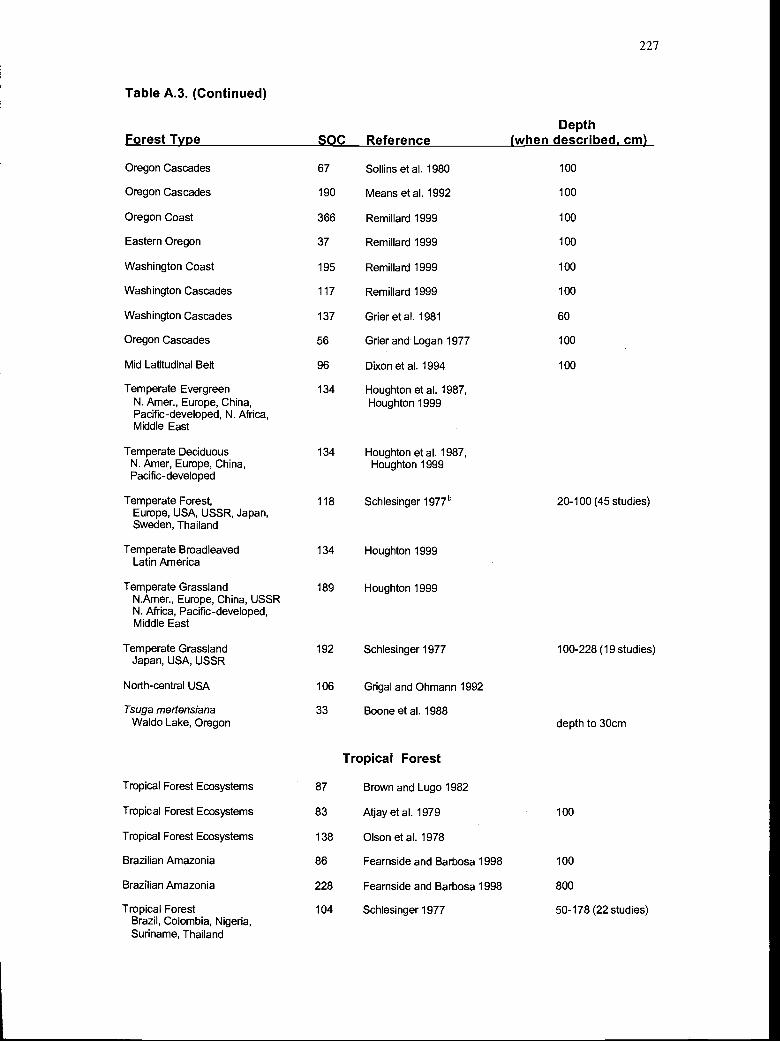
Table A.3. (Continued)
Forest TyDe
Oregon Cascades
Oregon Cascades
Oregon Coast
Eastern Oregon
Washington Coast
Washington Cascades
Washington Cascades
Oregon Cascades
Mid Latitudinal Belt
Temperate EvergreenN. Amer., Europe, China,Pacific-developed, N. Africa,Middle East
Temperate DeciduousN. Amer, Europe, China,Pacific-developed
Temperate Forest,Europe, USA, USSR, Japan,Sweden, Thailand
Temperate BroadleavedLatin America
Temperate GrasslandN.Anier., Europe, China, USSRN. Africa, Pacific-developed,Middle East
Temperate GrasslandJapan, USA, USSR
North-central USA
Tsuga mertensianaWaldo Lake, Oregon
Tropical Forest Ecosystems
Tropical Forest Ecosystems
Tropical Forest Ecosystems
Brazilian Amazonia
Brazilian Amazonia
Tropical ForestBrazil, Colombia, Nigeria,Suriname, Thailand
SOC Reference
67 Sollins et at. 1980
190 Means etal. 1992
366 Remillard 1999
37 Remillard 1999
195 Remillard 1999
117 Remillard 1999
137 Grieretal. 1981
56 Grier and Logan 1977
96 Dixonetal. 1994
134 Houghton etal. 1987,Houghton 1999
134 Houghtonetal. 1987,Houghton 1999
118 Schlesinger 1977b
134 Houghton 1999
189 Houghton 1999
192 Schlesinger 1977
106 Grigal and Ohmann 1992
33 Booneetal. 1988
Tropical Forest
87 Brown and Lugo 1982
83 Atjayetal. 1979
138 Olson etal. 1978
86 Fearnside and Barbosa 1998
228 Feamside and Barbosa 1998
104 Schlesinger 1977
Depth(when described. cm)
100
100
100
100
100
100
60
100
100
227
20-100 (45 studies)
100-228(19 studies)
depth to 30cm
100
100
800
50-178(22 studies)

Table A.3. (Continued)
Forest TyDe
Warm Coniferous ForestLatin America
Tropical Equatorl ForestLatin America
Tropical Seasonal ForestLatin Amenca
Tropical Seasonal ForestTropical Asia
Tropical Moist ForestChina, Pacific- developed, N. Africa,Middle East, Tropical Asia
GrasslandLatin America
GrasslandTropical Asia
WoodlandNAmer., Pacific-developed,Latin Amercia
Open ForestSub-Saharan Africa
Woodland and ShrublandEurope, USA
Tropical SavannaAfrica, Thailand, Venezuela
Woodland, Tropical Asia
Closed Forest, Sub-Saharan Africa
Boreal ForestN.Amer., Europe, USSR
Boreal ForestCanada, Sweden, USA, USSR
High Latitudinal Belt
134 Houghton 1999
98 Houghton 1999
98 Houghton 1999
80 Houghton 1999
120 Houghton 1999
42 Houghton 1999
50 Houghton 1999
69 Houghton 1999
50 Houghton 1999
69 Schlesinger 1977
37 Schlesinger 1977
50 Houghton 1999
100 Houghton 1999
Boreal Forest
206 Houghton 1999
149 Schlesinger 1977
343 Dixon et al. 1994
Desert/Arid
Desert Scrub 58 Houghton 1999N. Africa, Middle East, Latin America
228
20-60(10 studies)
20-100(33 studies)
61-230(22 studies)
100
Low Latitudinal Belt 123 Dixon etal. 1994 100
Woodlands/Savannas/Grasslands
DepthSOC Reference (when described. cm)

a lFoliage, 2=Bole, 3=Bark, 4=Live Branches, 5=Dead Branches, 6=Shrubs, 7=Herbs, 8=Coarse Roots, 9=FirieRoots, 10=Epiphytes or Mosses, 11=Grasses, 12=Logs, 13=Snags, 14=Stumps, 15=Forest Floor, 16=FineWoody Debris, I 7Rotten Wood
b Schlesinger (1977) includes total detritus to a depth of 50 cm as well as surface litter and soil
229
Table A.3. (Continued)
Forest TVDe SOC ReferenceDepth
(when described. cm)
Desert Scrub and Semidesert 56 Schlesinger 1977 33-173(22 studies)USA, USSR
Other
Tundra and Alpine 216 Schlesinger 1977 35-175(31 studies)Canada, Sweden, USA, USSR
Swamp and Marsh 686 Schlesinger 1977 60-29 1 (10 studies)Canada, England, USA, USSR

Appendix B. Abbreviations used in descriptions of the MAXCARB model.
230

Table B.1. Abbreviations used in the MA)(CARB module equations.
Pools
SW SapwoodHW HeartwoodBR BranchesFOL FoliageCR Coarse-rootFR Fine-rootHR Heart-rotDead Dead poolItalics Generalized pool
Fluxes, Rates
Input Input fluxOutput Output flux
Climate variables
Evap EvaporationMm MinimumMax MaximumMon MonthlyTemp TemperatureThru_Fall ThroughfallPot PotentialDelta Change in
Subscripts
LA Landscape-averageD Calculated in the DISTURBANCE ModuleSS Calculated in the STEADY-STATE
ModuleC Calculated in the CLIMATE Module
Arithmetric terms
exp (x)x'y x'Avg Average
231

Appendix C. The calculations in the DISTURBANCE Module of MAXCARB.
232

233
OVERVIEW
The purpose of the DISTURBANCE Module is to calculate the landscape-average
rate-constants used in the STEADY-STATE Module. To accomplish this objective, the
DISTURBANCE Module simulates carbon stores through time for an ecoregion's
disturbance regime. The simulation has an annual time-step. The user specifies the
simulation length.
Generally, landscape-average rates are calculated by summing fluxes and masses
over the length of the simulation. Fluxes and masses of carbon pools are calculated with
rates. In the DISTURBANCE Module, the rates that describe changes in fluxes and mass
of carbon pools are set to vary with age. They can be represented by a set of constants, or
dynamic, age-dependent functions that capture age-dependent behavior. The user
specifies these rate functions. The development of dynamic age-dependent functions is
described in detail in the next section.
At the core of the DISTURBANCE Module are annual calculations of flux and
mass, which use these rate functions. The third section of this appendix describes these
annual calculations. The fourth section describes how the carbon stores are adjusted
when disturbance events occur. The final section describes how the DISTURBANCE
module uses the results of the annual calculations to calculate the landscape-average rate
constants.

234
AGE-DEPENDENT FUNCTIONS
The list of age-dependent functions used by the DISTURBANCE Module are listed
in the table below.
Table C.1. The age-dependent functions used by the DISTURBANCE Module.
These age functions have a format similar to formulas used in common
spreadsheet applications. There are several built-in functions that the user may use in the
definition of an age function. One such built-in function is the "if" function, which can be
Category Functions
Production FOL_massbole_growth
Live Pool Ratios BR_bole_ratioCR_bole_ratioFR_FOL_ratio
Bole Formation Rates HW_formationHR_formation
Respiration Rates SW_respirationHR_respirationBR_respirationCR_respiration
Turnover Rates FOL_turnoverFR_turnover
Prune Rates BR_pruneCR_ prune
Mortality Rates tree_mortalitypercent_snags
Input Decay Rates dead_FOL_input_decaydead_SW_input_decaydead_H W_input_decaydead_BR_input_decaydead_CR_input_decaydead_FR_input_decay
Stable Decay Rates stable_FOL_decaystable_wood_decaystable_soil_decay
Transfer Rates dead_FOL_transferdead_SW_snags_transferdead_SW_logs_transferdead_H W_snags_transferdead_H W_logs_transferdead_BR_transferdead_CR_transferdead_FR_transfer

FOL Mass
Foliage mass through time is calculated with a modified Chapman-Richards
equation.
FOL_mass (age) = CR( 0.1, 2)* mCR( 0.03, 120, 15, ecoregion:steady_state_foliage)
Bole Growth
The bole growth is currently set to 1 since the CLIMATE module accounts for
climate effects.
bole_growth (age) = I
235
used to select between two values based upon a condition:
if( condition, value T, value ) = valueT if the condition is true; value F otherwise.
These conditional statements can be used to develop step-functions. Other built-in
functions include a Chapman-Richards function and a Modified Chapman-Richards
function, which are named "CR" and "mCR" respectively, and are defined as follows:
CR(b1, b2)=(1 _exp(_bi* aget))" b2
mCR(b1, b2, b3, b4) = b4 - ( b b3) * CR(b1, b2)
where:
bi = rate of increaseb2 = lagb3 = mm, maxb4 = max, mm
= the current age
The rest of this section describes the specific age functions used to produce the
MAXCARB results, and how these functions were created from output from STANDCARB.
Production

Age-dependent Foliage Equation
Modeled -- Calculated
236
BR-Bole Ratio
Conceptually, in STANDCARB, the branch to bole ratio is equal to the proportion
of bole allocation that is allocated to branches. The ratio in STANDCARB is developed
from species-specific, allometric equations (Means et al. 1994). In MAXCARB, the branch
to bole ratio changes with stand age in the following way:
(3) BRbole_ratio (age) = mCR( 0.3, ecoregion:time_close, 0.12, 1.4)
The branch to bole ratio is initially high due to the large proportion of shrubs early in
succession. After a period of shrub dominance, the branch to bole ratio reflects an
average of Douglas-fir and western hemlock ratios.
0 100 200 300 400 500
Age (years)
Figure C.1. Foliage mass as a function of age.
Live Pool Ratios
25
20
a)
15
10
0LI
5

1.6
0
Age-dependent BR:Bole Ratio Equation
ModeIed CalcuIated
100 200 300
Age (years)
Figure C.2. Branch to bole ratio as a function of age.
CR-Bole Ratio
(4) CR_bale_ratio (age) = mCR( 0.3, 120, 0.6, 1.5)
Age-dependent CR:BoIe Ratio Equation
ModeIed CaIcuIated
237
0 100 200 300 400 500
Age (years)
Figure C.3. Coarse root to bole ratio as a function of age.
The coarse-root to bole ratio is initially high due to the large proportion of shrubs early in
succession. After a period of shrub dominance, the coarse-root to bole ratio reflects an
1.4
0.
0
0 0.6-
.0.4-.Cu
0.0
400 500

HW Formation
The rate of heartwood formation as a function of age was developed from
parameters in the STANDCARB model. We assumed that heartwood formation decreases
from a maximum of 0.059 for Douglas-fir to a minimum of 0.02 for western hemlock as the
latter species occupies more of the stand later in succession.
HW_formation (age) = mCR( 0.02, 60, 0.02, 0.059)
Age-dependent Heartwood Formation Rate Equation
--caIcuIated
238
average of Douglas-fir and western hemlock ratios.
FR-FOL Ratio
While the two previous ratios are allocation ratios, this ratio of fine roots to foliage
is function of pool size.
FR_FOL_ratio (age) = 0.33
Bole Formation Rates
0 100 200 300 400 500
Age (years)
Figure C.4. The rate of heartwood formation as a function of age.
HR Formation
The rate at which heart-rot is formed is assumed to be insignificant for a certain
number of years in the early stages of tree growth. This number of years is known as the
"heart-rot lag'; it is a function of species in STANDCARB but is an average value for an

0.025
(5
0.020
0.015 -
00.010 -
EI-0
U-0.005 -I0.000
0
The respiration rates for sapwood, branch and coarse-root pools were developed
from the respiration fluxes and pool masses output by the STAN DCARB model.
Dominance by shrubs and herbs during early successional stages results in higher
respiration rates than later successional stages.
SW Respiration
(8) SW_respiration (age) = 0.025 * CR( 0.1, 5)
239
ecoregion in MAXCARB, based on the ecoregion's species composition. The rate of heart-
rot formation was calculated from parameters in STANDCARB using the rate of heart-rot
formation for Douglas-fir until year 500, and then the rate of heart-rot formation for western
hemlock after that year. The final equation is a simple step-function:
(7) HR_formation (age) = if ( t < ecoregion:HR_lag, 0, if ( t < 500, 0.01, 0.02))
Age-dependent HR Formation Rate Equation
- Calculated
200 400 600 800 1000
Age (years)
Figure C.5. The rate of heart-rot formation as a function of age.
Respiration Rates
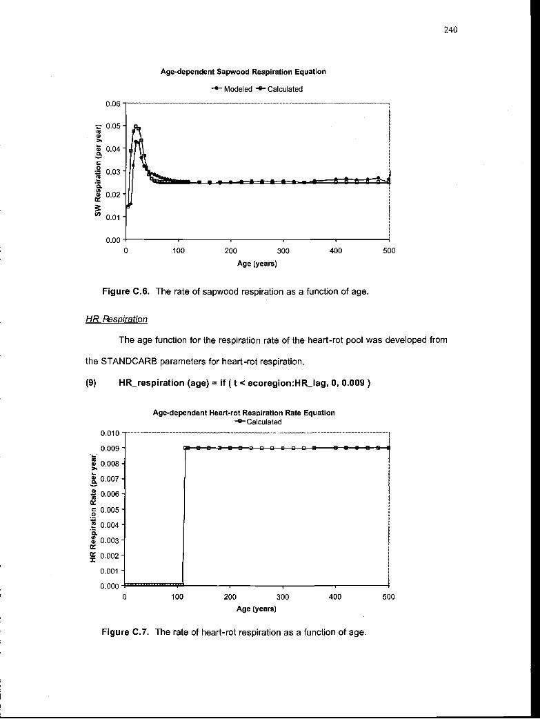
0.010
0.009
0.008
0.007
0.006
0.005
0.0040.
0.003
0.002
0.001
0.000
Age-dependent Sapwood Respiration Equation
- Modeled -- Calculated
240
0 100 200 300 400 500
Age (years)
Figure C.7. The rate of heart-rot respiration as a function of age.
0 100 200 300 400 500
Age (years)
Figure C.6. The rate of sapwood respiration as a function of age.
HR Respiration
The age function for the respiration rate of the heart-rot pool was developed from
the STANDCARB parameters for heart-rot respiration.
(9) HR_respiration (age) = if ( t < ecoregion:HR_lag, 0, 0.009)
Age-dependent Heart-rot Respiration Rate Equation-B--Calculated

BR Respiration
BR_respiration (age) = CR( 0.2, 2)* mCR( 0.2, ecoregion:time_close, 0.015, 0.055)
Age-dependent Branch Respiration Equation
--- Modeled -i- Calculated
z 0.05 -C)>'I-w 0.040.C
0.03-'CI-0.'CC) 0.02
0.06
0.01 -
0.00
0.05
0.05
0.04C)
0.040)
. 0.03C
0.03
0.02
0.02
C.' 0.01
0.01
0.00
241
0 100 200 300 400 500
Age (years)
Figure C.9. The rate of coarse root respiration as a function of age.
0 100 200 300 400 500
Age (years)
Figure C.8. The rate of branch respiration as a function of age.
CR Respiration
CR_respiration (age) = CR( 0.18, 4) * mCR( 0.12, 10, 0.015, 0.06)
Age-dependent Coarse-root Respiration Equation
-S- Modeled -e Calculated

Turnover Rates
FOL Turnover
The rate of foliage turnover was computed from STANDCARB's output (transfer
diagnostics), by dividing the annual turnover input to dead foliage by foliage mass.
(12) FOL_turnover (age) CR( 0.05, 2 ) * mCR( 0.1, 10, 0.2, 0.9)
Age-dependent Foliage Turnover Rate Equation
-s-- Calculated -4-Modeled
1.0
0.9-
0.8-
0.3--Jo 0.2-U-
0.1
0.00 100 200 300 400 500
Age (years)
Figure C.10. The rate of foliage turnover as a function of age.
FR Turnover
(13) FR_turnover (age) = ( CR( 0.2, 2) * mCR( 0.15, 120, 0.47, 0.5))* mCR( 0.4, 120, 0.5, 0.45)
242

Age-dependent Fine-root Turnover Rate Equation
-s-- Calculated --- Modeled
The rates of pruning for both branch and coarse-root pools were developed from
STANDCARB's output (transfer diagnostics), by dividing the mass being transferred from
the live pool due to pruning by the mass of its corresponding dead pool.
BR Prune
(14) BR_prune (age) = 0.02 * CR( 0.3, 5)
243
0 100 200 300 400 500
Age (years)
Figure C.11. The rate of fine root turnover as a function of age.
Prune Rates

0
0.03
0.02C)>'4)
.: 0.02C)
0.01
0.00
0.006
z. 0.005 -CC
C)>'0.004 -
0.0)
0.003-C)
0.002 -
0.001
0.0000
Age-dependent Branch Pruning Equation
Modeled -B-- Calculated
100 200 300 400 500
Age (years)
Figure C.13. The rate of coarse root pruning as a function of age.
244
0 100 200 300
Age (years)
Figure C.12. The rate of branch pruning as a function of age.
CR Prune
(15) CR_prune (age) = 0.005 * CR( 0.3, 5)
Age-dependent Coarse-Root Pruning Equation
-- Modeled -B-- Calculated
400 500

Mortality Rates
Tree Mortality
The mortality of trees through time is given by the following equation:
(16) tree_mortality (age) = mCR( 0.2, 120, 0.005, 0.015) * CR( 0.3, 2)
Age-dependent Tree Mortality Equation
° Rate(Mort Trees)
0016
- 0.014 -0
0.012 -00.o 0.010 -
0.008 -
0.006 -
0.004 -
0.002 -
0.000
0
1'
100 200 300 400 500
Age (years)
Figure C.14. The mortality rate of trees as a function of age.
This function was developed from the relationship between the maximum mortality rate
(when the maximum amount of light is absorbed) and the mortality rate for old-growth
forests in STANDCARB. To develop this equation, we assumed a maximum mortality rate
of about 0.015 and a minimum, old-growth mortality rate of 0.005. In STANDCARB,
maximum mortality rates for tree species in the Pacific Northwest range from
approximately 0.008 to 0.018.
Percent Snags
The percent of snags through time is defined with the following equation:
(17) percent_snags (age) = if( t < ecoregion:time_close, snags_open,snags_closed).
The percent of snags equals that of an open canopy before time close. After time close,
the percent of snags equals that of a closed canopy. The user specifies the percent of
245

snags in open and closed canopies for the ecoregion being simulated.
Input Decay Rates
The decay rates associated with the input to the dead pools were calculated from
STANDCARB.
Dead FOL input Decay
dead_FOL_input_decay (age) = mCR( 0.3, 120, 0.35, 0.5)
Age-dependent Dead-FOL input decay rate equation
ModeIed CaIcuIated
0.6
a,0.
0.5
' 0.4-0a,o v0.>C
0.2-
0.1-0
0
246
0 100 200 300 400 500
Age (years)
Figure C.15. The decay rate of dead foliage inputs as a function of age.
Dead SW input Decay
dead_SW_input_decay (age) = mCR( 0.3, 120, 0.07, 0.01)

0.08
0.07 ->.I-e 0.06 -
0.05
0.04-U0
0.03 -
0.c 0.02 -
0.01 -
0
0.025
Age-dependent SW Input Decay Rate
'-Modeled '-Calculated
247
0 100 200 300 400 500
Age (years)
Figure C.16. The decay rate of dead sapwood inputs as a function of age.
Dead HW Input Decay
(20) dead_.HW_input_decay (age) = mCR( 0.3, 120, 0.02, 0)
Age-dependent HW Input Decay Rate Equation
ModeIed CaIcuIated
0 100 200 300 400 500
Age (years)
Figure C.17. The decay rate of dead heartwood inputs as a function of age.
Dead BR Input Decay
(21) dead_BR_input_decay (age) = mCR( 0.3, 120, 0.15, 0.1 )
9 0.020
U0.
0.015
>aU
0.010
0.C
0.005
0.000
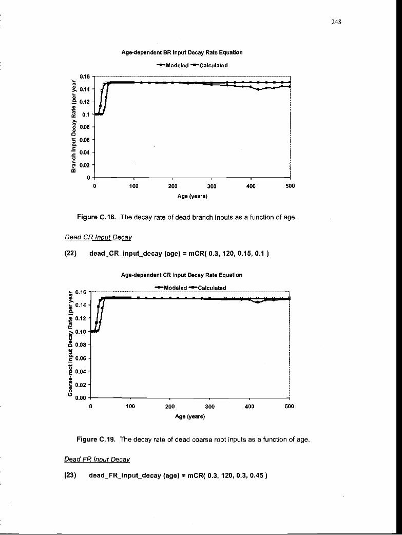
C)
. 0.12C)
CC0.1
0.08 -
' 0.06 -a.
0.04-
0.02 -
0
0 100 200 300 400 500
Age (years)
Figure C.18. The decay rate of dead branch inputs as a function of age.
Dead CR Inøut Decay
dead_CR_input_decay (age) = mCR( 0.3, 120, 0.15, 0.1 )
Age-dependent CR Input Decay Rate Equation
Age-dependent BR Input Decay Rate Equation
ModeIed CaIcuIated
0.16
0 100 200 300 400 500
Age (years)
Figure C.19. The decay rate of dead coarse root inputs as a function of age.
Dead FR Inout Decay
dead_FR_input_decay (age) = mCR( 0.3, 120, 0.3, 0.45)
248
ModeIed Calculated0.16
0.14a.0 0.12CC
>. 0.10CC
U
0.08
2 0.06
0.04
0.02
0.00

, 0.5
> 0.45
> 0.3-0.25 -00.2-
0..E 0.15 -02 0.1
0.05 -LI
0
0
Figure C.20. The decay rate of dead fine root inputs as a function of age.
Stable Decay Rates
These are all constants based on the associated STANDCARB parameters.
Stable FOL Decay
stable_FOL_decay (age) 0.20
Stable Wood Decay
stable_wood_decay (age) = 0.05
Stable Soil Decay
stable_soil_decay (age) = 0.012
Transfer Rates
Age-dependent FR Input Decay Rate Equation
ModeIed CaIcuIated
100 200 300
Age (years)
400 500
249
The transfer rates for all the dead pools were calculated from the non-cohort
version of the STANDCARB model, accounting for time lags under optimum decomposition
conditions (Harmon and Domingo, 2001).
Dead FOL Transfer
dead_FOL_transfer (age) 0.057

Dead SW Snacis Transfer
dead_SW_snags_transfer (age) = 0.009
Dead SW Logs Transfer
dead_SW_logs_transfer (age) = 0.010
Dead HW Snags Transfer
dead_HW_snags_transfer (age) = 0.009
Dead HW Logs Transfer
dead_HW_logs_transfer (age) = 0.016
Dead BR Transfer
dead_BR_transfer (age) = 0.0033
Dead CR Transfer
dead_CR_transfer (age) 0.016
Dead FR Transfer
dead_FR_transfer (age) = 0.022
250

ANNUAL POOL CALCULATIONS
This section describes the calculations that are performed for each annual time-
step in a simulation of the DISTURBANCE Module.
Pool Mass
For each time-step, the mass of each carbon pools is computed, prior to
accounting for any disturbance events that occur in the time-step:
pool: masst, before disturbance
To determine the pool's mass for the end of a time-step, the pre-disturbance mass is
adjusted for all events that occur in that time-step. If no disturbances occur, then
pool: masst = pool: masst, before disturbance
If only a harvest event occurs, then
pool:masst = pooI:mass, after harvest
If only a fire event occurs (with or without a preceding harvest event), then
pool:mass pool:mass, after fire
The calculations related to disturbance events are described at the end of this section.
Foliage & Fine Roots
Foliage mass is calculated directly from the age-dependent function, which
describes how foliage mass changes with age. Fine root mass is thus a function of foliage
mass and the age-dependent, fine root to foliage ratio.
foliage:mass t, before disturbance = FOL_mass( age t)
fine_roots:mass t, before disturbance = foliage:mass t, before disturbance* FR_FOL_ratio( age t)
Transfer Fluxes
Both pools transfer mass to their corresponding dead pools because of turnover
and tree mortality.
pool:turnover = pool:mass t, before disturbance * pool..turnover( age )
pool:mortality_transfer = pool:mass t, before disturbance * tree_mortality( age t)
251

Mass and Fluxes - All Other Pools
Mass
For all pools other than foliage and fine-roots, their masses change during a time-
step based on the fluxes into and out of the pools during the time-step.
pool: masst, before disturbaice = pool: mass + pool: in puts - pool:outputt
Outout Fluxes
In general, a pool's output flux consists of a loss to the atmosphere and transfers
to other pools.
pool:output = pool:loss + pool:transfers
A pool may not have any losses; for example, heartwood has no respiration loss. A pool
may have no transfers (e.g., stable pools) or multiple transfers (e.g., sapwood, heartwood).
lnøut Flux
In general, a pool's input flux is the sum of the transfer fluxes from one or more
contributing pools.
Live Pools
252
Respiration Loss
For the sapwood, heart-rot, branch and coarse-root pools, each pool's loss is due
to respiration.
pool:loss = pool:respiration_loss
pool: respiration_loss = pool:mass t_i * pool_respiration( age t)
Mortality Transfer
All live pools other than foliage and fine-roots transfer mass to their corresponding
dead pools because of tree mortality.
pool: mortality_transfer = pool:mass * tree_mortality( age t)
Sapwood
253
Input Flux
The input flux to the sapwood pool assumes that allocation of mass to sapwood is
proportional to foliage mass.
sapwood:input foliage:mass * bole_growth( age t)
Transfer Flux
The sapwood pool transfers mass to dead sapwood (Eqn. 46) and heartwood.
sapwood:transfers = sapwood:formation_transfer+ sapwood:mortaIity_transfer
sapwood:formation_transfer = sapwood:mass t-i * HW_formation( age t)
Heartwood
lnøut Flux
heartwood:input = sapwood:formationjransfer
Loss Flux
Heartwood has no loss since it does not respire.
heartwood:Ioss t = 0
Transfer Flux
The heartwood pool transfers mass to dead heartwood (Eqn. 46) and heart-rot.
heartwood:transfers = heartwood:formation_transferheartwood:mortality_transfert
heartwood:formation_transfer = heartwood:mass -i * HRjormation( age t)
Heart-Rot
Input Flux
heartrot:input = heartwood:formation_transfer
Transfer Flux
Heart-rot transfers mass only to dead heartwood (Eqn. 46).
heartrot:transfers = heartrot:mortality_transfert

Branch, Coarse Roots
254
Input Flux
The input fluxes to the branch and coarse-root pooi are proportional to the
sapwoods input flux.
pool:input_flux = sapwood:input * pool_bole_ratio( age t)
The rationale is that the allocation to branches and coarse roots is a fixed proportion of the
allocation to sapwood.
Transfer Flux
Both pools contribute to their corresponding dead pool because of pruning and
tree mortality (Eqn. 46).
pool:transfers = pool:pruning_transfer + pooI:mortality_transfer
pool:pruning_transfer = pool:mass * pooLprune( age t)
Detrital Pools
Loss Flux
All detrital pools (dead and stable) lose mass due to decomposition.
detrital_pool:loss = detrital_pool:decay_loss
Non-composite Dead Pools
A non-composite dead pool is a dead pool that is not composed of other pools.
The only composite dead pools are the dead bole pools (dead sapwood and dead
heartwood); they each are composed of two pools: snags and logs. These snag and log
pools are non-composite pools.
Decay Loss
The decay loss for a non-composite pool is based on the pool's decay rate.
dead_pool:decayjoss = dead_pool:mass t-i * dead_pool:decay_rate
Decay Rates - Input & Pool
The input flux to a non-composite pool has an associated decay rate. This input
decay rate is used in a simple weighted average to compute the pool's overall decay rate.

dead_pool:decay_rate = weighted_average( dead_pool:input_decay_rate t,dead_pool:input t,dead_pool:decay_rate t,dead_pool:mass t-i)
weighted_average ( rate , mass1,rate 2 mass2) = ( rate i * mass i + rate 2 * mass 2)
I( mass i + mass2)
Transfer Flux
A non-composite pool transfers mass to a stable pool with the exception of the
snag pools, which transfer mass to their corresponding log pools. The transfer flux out of a
non-composite pool is based on the pool's transfer rate.
dead_pool:transfers = dead_pool:mass t-i * dead_pool_transfer( age t)
Dead Foliage, Dead Fine Roots
255
Input Flux
The input fluxes to these pools are the transfer fluxes from their corresponding live
pools due to turnover (Eqn. 40) and tree mortality (Eqn. 41).
dead_pool: input = Iive_pool:tu move rt + live_pool: mortality_transfer
The decay rate associated with the input flux is just an age function.
dead_pool:input_decay_rate = dead_pool_input_decay( age t)
Dead Branch, Dead Coarse Roots
Input Flux
The input fluxes to these pools are the transfer fluxes from their corresponding live
pools (Eqn. 57).
dead_pool: in put = live_pool:transfers
Like dead foliage and dead fine-roots, the decay rate associated with the input flux is just
an age function (see Equation 65).
Dead Bole Pools - Dead Sapwood, Dead Heartwood
logs.
Each dead bole pool is composed of two internal pools representing snags and

256
Input Flux
The input flux to a dead bole pool is the sum of the mortality transfer(s) from its
corresponding live pool(s) (Eqn 46).
dead_sapwood:in put = sapwood:mortality_transfer
dead_heartwood: input = heartwood :mortality_transfer+ heartrot:mortaIity_transfer
Like the other dead pools, the decay rate associated with this input flux is age-dependent
(see Equation 65).
The input flux of a dead bole pool is separated into its snag and log pools. The
input flux to the log pool includes the transfer flux from the snag pool (Eqn. 63).
dead_bole:snags:in put t = dead_bole:in pUtt * percent_snags( age t)
dead_bole:logs:in put dead_bole:logs:in put_from_live+ dead_bole:snags:transfers
dead_bole: logs: input_from_live t = dead_bole: inputt- dead_bole:snags:in put
The decay rate associated with the snag's input flux is simply the dead bole's input decay
rate.
dead_bole:snags:input_decay_rate = dead_bole:input_decay_rate
However, the decay rate associated with the log's input flux is a weighted average (Eqn.
62) of the decay rates associated with the two components of its input flux.
dead_bole:logs:input_decay_rate t = weighted_average(dead_bole:input_decay_rate ,
dead_bole: logs: input_from_live ,
dead_bole:snags:decay_rate ,
dead_bole:snags:transfers t-i)
Decay Loss
The decay loss for a dead bole pool is the sum of the decay losses from its snag
and log pools.
dead_boIe:decay_loss = dead_boIe:snags:decay_loss+ dead_bole:logs:decay_loss
Transfer Flux
The transfer flux out of a dead bole pool is simply the transfer flux out of its log

pool.
(75) dead_bole:transfers = dead_bole: logs:transfers
Stable Pools
In put Flux
The input flux to a stable pool is the sum of the transfer flux(es) from its
corresponding dead pool(s) (Eqns. 63 and 75).
stable_foliage:input = dead_foliage:transferst
stable_wood:input = dead_sapwood:transferst+ dead_heartwood:transfers+ dead_heartrot:transfers
stable_soil:input = dead_coarse_roots:transfers+ dead_fine_roots:transferst
Decay Rate
The decay rate for a stable pools is age-dependent.
stable_pool:decay_rate = stable_pool_decay( age t)
257

258
CALCULATIONS FOR A DISTURBANCE EVENT
There are two types of disturbance events simulated by MAXCARB, harvests and
fires. In addition, harvests may have fires due to site preparation. Fires are considered to
be part of a natural disturbance regime, whereas harvests are considered to be part of a
regulated disturbance regime.
In years in which there is a disturbance event, there are additional losses and
transfers from the pools other than those described in the previous section. For live pools,
mass may be lost to the atmosphere (i.e., combustion), or transferred to its corresponding
dead pool after a fire disturbance event. Additionally, if the disturbance event is a harvest,
live pool mass may be transferred to the forest products pool. For dead pools, mass may
be also lost to the atmosphere after fire (either for a natural fire event, or a site-preparation
fire for a harvest event), and there may be an addition of mass to the dead pools from the
live pools after harvest or fire. Dead pools do not transfer material to stable pools during
disturbance events.
Currently, only catastrophic disturbance events are supported. With a catastrophic
disturbance event, each live pool is completely killed, i.e., its mass is 0 after the event.
The effects of natural disturbances in MA)(CARB are to increase (1) transfers from
live pools to dead pools and (2) losses from all pools due to combustion, i.e., in the case of
fire. The effects of regulated harvests in MA)(CARB are to increase (1) transfers from live
pools to dead and forest products pools and (2) losses through site preparation fires, i.e., in
the case of forest harvesting.
Regulated Disturbances (Harvest)
The mass of each pool before a harvest event is always the mass after the annual
pool calculations.
(80) pool:mass t, before harvest = pool:mass t, before disturbance
Live Pools
Since harvest events are catastrophic, all live pools are reduced to zero after the

259
disturbance event.
Iive_pool:mass t, after harvest = 0
Non-bole Pools - Live and Dead
Each live non-bole pool (foliage, branch, coarse roots, fine roots) transfers all its
mass that was cut to its corresponding dead pool.
Iive_pool:cut_transfer = I!ve_pool:mass t, before harvest
dead_pool:mass t, after harvest = dead_pool:mass t, before harvest+ Iive_poo!:cut_transfer
Bole Pools - Live and Dead
When each live bole pool (sapwood, heartwood, and heart-rot) is cut, a user-
specified portion of its mass is taken off site (i.e., harvested).
Iive_bole:harvest_transfer t = Iive_bole:mass t, before harvest * percent_taken
Iive_bole:cut_transfer iive_bole:mass t, before harvest- Iive_bole:harvest_transfer t
The portion of the live bole pools cut but not taken is transferred into the log pools of their
corresponding dead pools.
dead_sapwood:logs:mass t, after harvest dead_sapwood:ogs:mass t, before harvestsapwood:cut_transfer
s:mass t, after harvest =dead_heartwood:logdead_heartwood:logs:mass t, before harvest+ heartwood:cut_transfer+ heartrot:cut_transfer
dead_bole:snags:mass t, after harvest = dead_bole:snags:mass t, before harvest
dead_bole:mass t, after harvest = dead_bo!e:snags:mass t, after harvest+ dead_bole:logs:mass t, after harvest
Stable Pools
Harvest events do not affect the stable pools in this version of MAXCARB.
Natural Disturbances (Fire)
There are three intensity levels for fire events: low, medium, high. The mass of
each pool before a fire event depends upon whether there was a preceding harvest event.

260
If there's no harvest before the fire, then
pool:mass t, before fire = pool:mass t, before disturbance
If there is a harvest before the fire (i.e., it's a site-prep fire), then
pool:mass t, before fire = pool:mass t, after harvest
Live Pools
Since fire events are assumed to be catastrophic, all live poois are reduced to zero
after the disturbance event.
Iive_pool:mass t, after fire = 0
A portion of each live pool is transferred to its corresponding dead pool; the percentage is
specified by the user, and is a function of the fire's intensity.
Iive_pool:burn_transfer t = llve_pooI:mass, beforefire* %_transfer_to_dead00i (fire_intensity)
The remaining portion is lost to the atmosphere.
live_pool:burn_loss = live_pool:masst, before fire live_pool:burn_transfer
Dotrital Pools
All non-composite dead pools and stable pools lose a percentage of their mass to
the atmosphere due to combustion. The user specifies the percentage of a pool's mass
that remains after a fire.
de(rital_pool: burn_loss t = detrital_pool:masst, before fire* (100% - %_remaining (fire_intensity))
Dead Pools
For non-bole dead pools (dead foliage, dead branch, dead coarse roots, and dead
fine roots), the pool's mass is adjusted for the burn loss and the transfer from the
corresponding live pool.
dead_pool:mass t, after fire = dead_pool:mass t, before fire dead_pool:burn_loss+ live_pool: burn_transfer
For the dead bole pools, the transfer from the corresponding live pool(s) is added to the
snag pool.
dead_sapwood :snags:mass t, afterfire = dead_sapwood:snags:mass t, before fire- dead_sapwood:snags:burn_loss+ sapwood:burn_transfer t

261
s:mass t,afterfiredead_heartwood:snagdead_heartwood:snags:mass t, before fire- dead_heartwood:snags: burn_loss+ heartwood:burn_transfer+ heartrot: burn_transfer
dead_bole:logs:mass t, afterfire = dead_bole:Iogs:mass t, before fire- dead_bole:logs:burn_loss
dead_bole:mass t,afterfire = dead_bole:snags:mass t, after fire+ dead_bole:logs:mass t, after fire
Additionally, decay rates are adjusted based on the decay rate associated with the input
from disturbances. Thus:
dead_pool:decay_rate {t, after event} = weighted_averagedead_pool: input_decay_rate t,live_pool: (cut or burn]_transfer t,dead_pool: decay_rate t, before event,dead_pool: mass t, before event

LANDSCAPE-AVERAGE RATE-CONSTANTS
The general equation describing the landscape-average rate-constant is:
Time_End Time_End
Rate LA pool : flux t = (pool : mass t rate(age) t)
Time_End Time_End
mass mass
where S poo/:fluxt equals the sum of the lux for all years in the simulation, and S
pool:mass (age) equals the sum of the mass for all years in the simulation for that pool
(equations listed in the table below). Since the rate.constants vary with age, the sum over
time of the fluxes based on those rate-constants will be different for different disturbance
regimes. Since the fluxes affect the accumulation of mass through time, the sum of a
pool's mass will also be different for different disturbance regimes and therefore must be
weighted by the mass of the pools, as reflected in the above equation.
Years With No Disturbances
For computing landscape averages, the disturbance-related transfers
(cut_transfer, burn_transfer, burn_loss) of the pools are all set to 0 in those years when a
disturbance event does not occur. Furthermore, the mass of each pool before a
disturbance is simply the mass after the annual pool calculations (Eqns. 80 and 90).
Table C.2. Equations for landscape-average rate-constants in the DISTURBANCE Module.
262
RateLA Equation
FOL_d 1st_adjustment
averagea (foliage: mass t)
ecoregion :steady_state_foliage
BR_bole_ratioCR_bole_ratio
sumb ( pool:in put t)
sum (sapwood:input t)

263
FR_FOL_ratiosum ( fine_roots:mass t, before disturbance)
sum ( foliage:mass t, before disturbance)
HW_formationsum (sapwood:formation_transfer t)
sum (sapwood:mass )
HR_formationsum (heartwood: formation_transfer t)
sum ( heartwood:mass t-i)
SW_respirationHR_respirationBR_respirationCR_respiration
sum (poo/:respiration_Ioss t)
sum ( pool:m ass t-i)
BR_pruneCR_prune
sum (poo/:pruning_transfer t )
sum ( pool:mass t-i)
FOL_mortalityFR_mortality
sum (pool: mortality_transfer
sum ( pool:mass , disturbance)
BR_mortalityCR_mortalitySW_mortalityHW_mortalityHR_mortality
sum (pool: mortality_transfer t)
sum (pool:mass t-i)
FOL_turnoverFR_turnover
sum (pool _turnover t)
sum ( pool:mass t, bfO disturbance)

264
%_snagssum ( dead_sapwood:snags:input t)
sum ( dead_sapwood:input t)
dead_FOL_decaydead_SW_snags_decaydead_SW_logs_decaydead_HW_snags_decaydead_H W_logs_decaydead BR decaydead_CR_decaydead_FR_decaystable_FOL_decaystable_wood_decaystable_soil_decay
sum (poo/:decay_loss t)
sum (poo/:mass t-i)
dead_FOL_transferdead SW snags transferdead_SW_logs_transferdead_H W_snags_transferdead_HW_logs_transferdead_BR_transferdead_CR_transferdead_FR_transfer
sum ( poo/.transfers t)
sum ( poo/:mass t-i)
SW_burn_lossHW_burn_lossHR_burn_lossBR_burn_lossCR_burn_loss
dead FOL burn lossdead_SW_snags_burn_lossdead_SW_logs_burn_lossdead_HW_snags_burn_lossdead_H W_logs_burn_lossdead_BR_burn_lossdead_CR_burn_lossdead_FR_burn_loss
stable_FOL_burn_lossstable_wood_burn_lossstable_soil_burn_loss
sum (pool:burn_loss t)
sum (pool:mass t,beforefire)

a average ( pool:attribute ) = sum(pool:attribute t) I # of years in T
b sum ( pool:attribute t) =? pool:attribute for all tin T
T = the set of years selected for landscape averages; it is constructed by skipping the firstS years. S is specified by the user.
265
FOL_cut_transferSW_cut_transferHW_cut_transferHR_cut_transferBR_cut_transferCR_cut_transferFR_cut_transfer
sum (pool: cut_transfer t)
sum ( pool:mass t, before harvest
FOL_bu rn_transferSW_ burn_transferHW_burn_transferHR_burn_transferBR_burn_transferCR_burn_transferFR_burn_transfer
sum (poo/:burn_transfer t)
sum ( pool:mass t, before The)
SW_harvest_transferHW_harvest_transferHR_harvest_transfer
sum ( pool:harvest_transfer t)
sum ( pool:m ass t, before harvest)

Appendix D. The calculations in the STEADY-STATE Module of MAXCARB.
266

267
STEADY-STATE POOL MASS
For every pool except foliage and fine-roots, the pool's landscape-average mass at
steady-state (mass area1) is the pool's input flux (mass area1 time1) divided by the pool's
landscape-average rate-constant (tim&1).
(1) pool:massss = poo!:input I pool:rateLA
The pool's landscape-average rate-constant is the sum of the all landscape-average rate-
constants that affect the output of mass from the pool for a given disturbance regime.
These rate-constants include the rates of mass loss and transfer due to a disturbance
event. They are all calculated in the DISTURBANCE Module, and hence, are denoted by
the subscript "D' or "te, D. Some of these rates are adjusted for climate by multiplying
them by climate indices from the CLIMATE Module (denoted by the subscript "c").

LIVE POOLS
Transfer Flux
Each live pool transfers mass to other pools. This transfer flux is based on the
pool's transfer rate.
(2) pool:transfer = pool: mass55 * pool:transfer_rate
Transfer rates for each pool are described in the following sections.
Foliage, Fine-Roots
Steady-State Mass
The masses of the foliage and fine-root pools are solved directly, rather than with
Equation (1). The foliage mass is the ecoregion's steady-state foliage mass adjusted for
the ecoregion's disturbance regime.
foliage: massss = ecoregion:steady_statejoliage * FOL_dist_adjustm entD
The ecoregion's steady-state foliage mass is based on the ecoregion's light extinction
coefficient (the degree to which light is dissipated through a typical vegetation canopy) and
its light compensation point (the minimum percentage of light necessary for growth).
ecoregion:steady_state_foliage = - log( ecoregion:light_comp_point)I ecoregion:light_ext_coeff
This equation is based on the Beer-Lambert equation, which describes an inverse
proportionality between light availability and the amount of leaf area.
The mass of the fine-root pool is a proportion of the foliage mass that is allocated
to fine-roots.
fine_roots: massss = foliage:mass55 * fine_roots_fohage_ratioD
Transfer Rate
For the foliage and fine-root pools, the rate at which each pool transfers mass to its
corresponding dead pool is based on the live pool's turnover rate, mortality rate, and
transfer rates due to disturbances.
pool:transfer_rate = pool_turnoverrate, D + pool_mortality rateD+ pool_burn_transfer rate, D + pool_cut_transfer rate, D
268

Sapwood
Input Flux
The input flux to the sapwood pool is assumed to be directly proportional to the
foliage mass (Eqn. 3). This proportion is by the ecoregion's bole growth efficiency
multiplied by the production index from the CLIMATE Module.
sapwood:input = foliage:massss* ( ecoregion:bole_growth_efficiency * production_indexc)
Rate
The landscape-average rate-constant for the sapwood pool is based on its
respiration rate (adjusted for climate), the formation rate of heartwood, its loss rate due to
fires, its transfer rate to dead sapwood (Eqn. 13), and its transfer rate to the forest-products
pool.
sapwood:rateLA (SW_respiration rate,D * sapwood:respiration_indexc)+ HW_formation rate, D + SW_burn_loss rate, o+ sapwood:transfer_rate + SW_harvest_transfer rate, D
Heartwood
Input Flux
The input flux to the heartwood pool is the amount of sapwood that forms (i.e.,
becomes) heartwood.
heartwood:input = sapwood:massss * HW_formation te, D
Rate
The landscape-average rate-constant for the heartwood pool is based on the
formation rate of heart-rot, heartwood's loss rate due to fires, its transfer rate to dead
heartwood (Eqn. 13), and its transfer rate to the forest-products pool.
heartwood : rate LA = HR_formation rate, D + HW_burn_loss rate, D+ heartwood:transfer_rate + HW_harvest_transfer rate, o
269

Heart-rot
Inout Flux
The input flux to the heart-rot pool is the amount of heartwood that forms (i.e.,
becomes) heart-rot.
heartrot:input = heartwood:massss * HR_formation rate,D
Rate
The landscape-average rate-constant for the heart-rot pool is based on its
respiration rate (adjusted for climate), its loss rate due to fires, its transfer rate to dead
heartwood (Eqn. 13), and its transfer rate to the forest-products pool.
heartrot:rateLA= ( HR_respiration rate,D * heartrot:respiration_indexc)+ HR_burn_lossrate,D + heartrot:transfer_rate+ HR_harvest_transferrate, D
Live Bole Pools
Transfer Rate
The rate at which a live bole pool transfers mass to its corresponding dead pooi is
a combination of the live pool's mortality rate and transfer rates due to disturbances.
Iive_bole:transfer_rate = live_bole_mortality rate, D+ live_bole_burn_transfer rate, o+ live_bole_cut_transfer rate, D
Harvest Transfer Flux
Each live bole pool transfers some of its mass to the forest-products pool based on
its individual harvest transfer rate.
live_bole: harvest_transfer = live_bole: massss* live_bole_harvest_transferrate, D
270
Input Flux
For the branch and coarse-root pools, the pool's input flux is based on the
sapwood's input flux (Eqn. 7).
poo!:input = sapwood:input * pool_bole_ratioD
Rates
For the branch and coarse-root pools, the rate at which each pool transfers mass
to its corresponding dead pool is based on the live pool's pruning rate, mortality rate, and
transfer rates due to disturbances.
pool:transfer_rate = pool_prune te,D + pool_mortalityrate,D+ pool_burn_transferrate, D + pool_cut_transferrate, D
For each of these pools, its landscape-average rate-constant is based on its respiration
rate (adjusted for climate), its loss rate due to fires, and its transfer rate to its dead pool
(previous equation).
poo/:rateLA (pool_respiration rate,D *pool:respiration_jndexc)+ pool_burn_loss rate, D + pool:transfer_rate
Branch, Coarse Roots
271

272
DEAD POOLS
Transfer Flux
Each dead pooi transfers mass to other pools. This transfer flux is calculated in
the same way as for live pools (Eqn. 2), and is based on the pool's transfer rate. Transfer
rates for each pool are described in the following sections.
Rates - Non -composite Pools
A non-composite dead pool is a dead pool that is not composed of other pools.
The only composite dead pools are the dead bole pools (dead sapwood and dead
heartwood); they each are composed of two pools: snags and logs. These snag and log
pools are non-composite pools.
For each non-composite dead pool, its landscape-average rate-constant is based
on its decay and transfer rates adjusted for climate, and its loss rate due to fires.
dead_pool:rateLA= ( dead_pool_decayte, D + dead_pool_transfer rate, D)* dead_pool:decay_indexc+ dead_pool_burn_loss rate, D
Dead Foliage, Dead Branch, Dead Roots
Input Flux
For dead foliage, dead branch, dead coarse-roots and dead fine-roots, their input
flux is just the transfer flux from its corresponding live pool (Eqn. 2).
dead_pool: input = live_pool:transfer

273
Dead Bole Pools
Snags and Logs
Each dead bole pool - dead sapwood and dead heartwood - is composed of two
internal pools representing snags and logs.
Input Flux
The input flux to each dead bole pool - dead sapwood and dead heartwood - is
the transfer flux(es) from its corresponding live bole pool(s) (Eqn. 2).
dead_sapwood:input = sapwood:transfer
dead_heartwood : input = heartwood:transfer + heartrot:transfer
This input flux is divided between the pool's snag and log pools. The input flux to the log
pool also includes the transfer from the snag pool (Eqn. 2).
dead_bole:snags:input = deadbole:input * %_snag
deadbole:logs:input dead_bo!e:input * (100% - %_snagso)+ deadbole:snags:transfer
Steady State Mass
The masses of the snag and log pools are each determined using Equation (1);
however, the steady-state mass of a dead bole pool is just the sum of the masses of its
snag and log pools.
dead_bole:mass55 = dead_bole:snags:massss + dead_bolElogs:massss
Rate
Because of the previous equation, a dead bole pool has no landscape-average
rate-constant. However, its snag and log pools each have their landscape-average rate-
constant determined using Equation (18).
Transfer Flux
The transfer flux from each of the snag and log pools is determined using Equation
(2). The transfer flux from a dead bole pool is just the transfer flux from its log pool.
dead_bo!e:transfer = dead_bole:logs:transfer

274
STABLE POOLS
Input Flux
The input to a stable pool is the sum of the transfer fluxes from its corresponding
dead pools (Eqns. 2 & 25).
stable_foliage: input = dead_foliage:transfer
stable_wood:input = dead_sapwood:transfer + dead_heartwood:transfer+ dead_branch:transfer
stable_soil: input = dead_coarse_roots:transfer + dead_fine_roots:transfer
Rate
For each stable pool, its landscape-average rate-constant is based on its decay
rate (adjusted for climate) and its loss rate due to fires.
stab! e_pool:rateLA (stable_pool_decay rate, D * stable_pool:decay_indexc)+ stable_pool_burn_loss rate, o

FOREST PRODUCTS
275
In put Flux
The input flux to the forest products pooi is based on the sum of the transfer fluxes
from the live bole pools (sapwood, heartwood, and heart-rot) due to harvesting (Eqn. 14).
These fluxes are modified by a manufacturing efficiency that accounts for the proportion of
harvested boles that remain after the manufacturing process. This efficiency is an input
parameter specified by the user.
forest_products:input = (sapwood:harvest_transfer +heartwood:harvest_transfer +heartrot:harvest_transfer)
* manufacturing_efficiency
Rate
The landscape-average rate-constant for the forest products pool is just the
landscape-average decay rate of forest products
forest_products: rate LA = forest_products_decay
This decay rate is an input parameter specified by the user, who may have determined it
using another model such as ForProd (Harmon et al. 1996).

Appendix E. The calculations in the CLIMATE Module of MAXCARB.
276

The respiration index of a pool (000/:respiration_index) is calculated as a function
of the mean annual temperature of a site (mean_annual_temp) and the ecoregion's 010
value for that pool's respiration:
pool:respiration_index = pool:Q10 A ((mean_annual_temp - 10)/10),
where mean_annual_temp equals:
Dec
mean_annual_temp = ( temp_24 month ) /12,month = Jan
where temp_24moflth is specified in the site's climate text file.
277
OVERVIEW
The purpose of the CLIMATE Module is to calculate the effects of climate on
processes that ultimately determine a site's carbon storage. Specifically, the CLIMATE
Module calculates a set of indices controlling production (production_index), respiration
(respiration_index), and decomposition (decay_index), which are then passed to the
STEADY STATE Module where they modify rates that are used to calculate steady-state
stores:
(1) rate C (with climate effects) = rate (without climate effects) * climate_index.
Together, these climate indices affect steady-state carbon storage by accounting for the
temperature and moisture limitations of the site. Temperature and moisture indices are
calculated monthly and are multiplied together at the end of each month to describe the
overall monthly climate limitation. The resulting monthly indices are averaged for a year
and then passed to the STEADY STATE Module.
RESPIRATION INDICES
278
PRODUCTION INDICES
Each living pooi has a production index which is an annual average of monthly
production indices. The annual production index is initially set equal to one in the
CLIMATE Module and is reduced by temperature and moisture limitations, which limit the
rate of production of living biomass at each site. In addition to indicating the response of
production, it also controls transpiration. The annual production index is the average of the
monthly production indices.
Dec
pool:production_index = ( pool: production_index month ) / 12month = Jan
A monthly production index has a temperature-related component and a moisture-
related component. For each month the product of these two indices is computed:
pool :production_index month = pool :temp_prod_index month *pool.moist_prod_indexmonth
Temperature Production Index
The temperature production index (temp_prod_index month) determines the effect of
temperature on net photosynthesis of each layer. The curve used to simulate this
relationship is taken from Running and Coughlan (1988) and defines the mean daytime
temperature (temp_day month) response according to a minimum and maximum temperature
compensation point (temp_minecotegon and temp_maxeregion) as defined for the ecoregion
in the ecoregion.prm input file. The daily (24-hour) mean temperature (temp_24 month) is
converted to the mean daytime temperature using the mean maximum temperature for the
month:
temp_day month = 0.212 * (temp_maxecoregion - temp_24 month) + temp_24 month
Essentially, temp_prod_index month is a relative index of the response of each site
to its average monthly daytime temperature. If the mean daytime temperature exceeds
either the minimum or maximum temperature compensation points for an ecoregion, then

279
the temperature production index at that site is set to zero. If the daytime temperature is
within those mits then:
temp_prod_index month = [(temp_maxecoregion - temp_day month)*
(temp_daymoflth - temp_mi flecoregion)] /[(temp_maxecorjon - pool.lemp_opt) * (pool:tem p_opt- temp_minecoregion)],
where the optimum temperature (temp_opt) for a pool is the average of the minimum and
maximum temperatures:
pool:temp_opt = (temp_maxecoregion - temp_minecoregion) I 2.
Moisture Production Index
The moisture production index function (moist_prod_index month) determines the
effect of soil moisture on the production of live biomass. The overall effect of water
potential on production for each month is:
moist_prod_index month = water_logging_index month * drought_index month
where the water_logging_index month is the reduction due to water logged conditions for that
month and drought_index month is the reduction due to drought conditions during the month.
Currently, we assume there is no effect on production when water logging occurs:
water_logging_index month = I
However, in a future version we hope to implement a reduction in productivity when the
water potential is less than -0.1 MP. This would provide for a more realistic assumption for
sites with poor drainage and water logging.
When soil water potential (stable_soil:water_potential month) is below -0.3 MPa, we
assume that productivity decreases exponentially as a function of drought (Emmingham
and Waring 1977). The equation describing this response is:
drought_index month = I -( I exp( 5 * stable_soil:water_potential month

Stable_soil:water_potential month is described below (see Water Potential section).
DECAY INDICES
The monthly decay index (poo/:decay_index) determines the combined effects of
temperature and moisture on the decomposition rate of each detrital pool and the stable
soil pool for each month:
Dec
(11) pool:decay_index = ( pool:decay_index month ) /12.month = Jan
For each detritus pool, or the stable soil pool, the monthly decay index is:
pool:decay_index month = poo/:temp_decay_index month * pool: moistdecay_index month
The temperature decay index (poo/:temp_decay_index month) and the moisture decay index
(poo/:moist_decay_index month) are described below.
Temperature Decay Index
This function determines the effect of temperature on the decomposition rate of the
detrital and soil pools. The monthly temperature decay index for each month and each
pool is given by the following equation:
pool:temp_decay_index month = pool:temp_increase month * pool.temp_IimitflOflth
where poo/:temp_increase month assumes an increase in respiration rate with temperature
following a Q10 type curve:
pool:temp_increase month = pool :Q0 A ((temp_24 month 10)/lO)
where the respiration rate of the layer at 10 °C is assumed to be 1.0, and poo/:Q10 is the
rate at which respiration increases with a 10 °C increase in temperature and temp_24 month
is the temperature of a given month. The Q10 for each pool is specified in the decay
parameter file (detrital_pool_parms.txt).
The second part of the temperature limitation to decomposition reflects the effect
of a lethal temperature limit (poo/:temp_limit month) that arrests decomposer activity. The
equation is:
280

pool:temp_limit month = exp[ - (temp_24 moi)th / (pool :temp_opt +pool:temp_Iag))"°° :temP_ShaPe1
where pool :temp_opt is the optimum temperature for decomposition of a detritus pooi and
pool:temp_lag and pool :temp_shape are parameters that determine the shape of the
response curve. These parameters are also found in the detrital_pool_parms.txt file.
Moisture Decay Index
We assume that the moisture content of the pools controls decomposition in two
ways. The first is by matric potential limitations, which makes water unavailable for
decomposers. For most detrital forms, decomposition ceases when the moisture content
reaches the fiber saturation point. The second is caused by poor oxygen diffusion, when
the moisture content is too high. For most detrital layers this is not a problem. However,
coarse wood respiration is often limited by this factor. We model the matric potential and
diffusion limitation portions separately. The combined effect of matric and diffusion
limitations for each detritus pool or for the stable soil pool for each month is:
pool:moist_decay_index month = pool:matric_limitmonth * pool:diffusejimitmonth
The equation for the matric potential limitation (poo/:matric_limit month) of each
detrital pool or the stable soil pool for each month is:
pool:matric_Umit month = (1 - exp[ - pool:increase_rate *I poo!:moisture_content month +
pool matric_lag)]) pool :matnc_shape
where pool :matric_shape is a dimensionless number that determines when the matric limit
is reduced to the point that decay can begin to occur. For all detritus pools except the
stable soil pool, the moisture content (%) is based on the mass of water divided by the dry
mass of the pool at steady state. For the stable soil pool, the moisture content is based on
volume of water divided by volume of soil. The pool :matric_lag parameter is used to offset
the curve to the left or right. The parameters are in the decay_parms_funcs.txt file. The
poo/:increase_rate is the parameter determining the point at which the matric limitation
ends:
pool:increase_rate = 3/ pool :moist_min
281

282
where the minimum moisture content (pool:moist mm (%)) reflects the minimum water
necessary for decomposition to occur.
The diffusion limitation (poo/:diffuse_limit month) is designed to mimic the reduction
in decomposition caused when the substrate becomes water saturated. Water saturation
causes a reduction in oxygen diffusion, reducing decomposition. This function remains at
I until the maximum moisture content (without diffusion limitations) is reached. The
function decreases to 0 when moisture content exceeds the maximum for decomposition to
occur. This function is calculated for each detrital pool for each month:
(19) pool:diffuse_limit month = exp[-(pool:moisture_content month I(pool: moist_max + pool:d iffuse_lag)) pool :diffuse_shapej
where pool:moist_max is the maximum moisture content without diffusion limitations,
pool:diffuse_shape is a dimensionless number that determines the range of moisture
contents where diffusion is not limiting, and pool:diffuse_lag is a parameter used to shift
the point when moisture begins to limit diffusion.
MOISTURE CONTENT
To calculate the effect of water stores in detritus pools on the moisture decay
index, values have to be converted to moisture content based on mass:
pool:moisture_content month = pool:water_mass month I pool:mass5s
where poo/:massss is the mass from the STEADY STATE Module of each detritus pool
during the year being considered. The mass of water (poo/:water_mass month) covering one
hectare in one centimeter of depth is 100 Mg. Therefore each 1 cm of water stored in a
detrital layer is:
pool:water_mass month = pool:watermth * 100 Mg ha cm
where pool:watermoflth equals the monthly water store (described in Water Stores section).
The dead fine root moisture content (dead_fine_roots:moisture_content month) is
assumed to equilibrate rapidly with the surrounding soil and humus. It is therefore
assumed to be the same as the stable_foliage pool:

283
dead_fine_roots:moisture_content monthstable_foliage:moisture_contentmonth
Dead coarse root moisture content (dead_coarse_roots: moisture_content month) 15
controlled by the moisture of the surrounding mineral soil (Chen and Harmon, in prep.).
When the soil is saturated we assume that the dead coarse root pool reaches its maximum
moisture content. Therefore, if
dead_coarse_roots: moisture_content month = 100%,
then
oisture_content monthdead_coarse_roots:mdead_coarse_roots:moist_store_max.
When the moisture content of the mineral soil is less than saturated (<100%), we assume
the dead coarse roots and mineral soil are in equilibrium. However, since mineral soil
moisture content is expressed in volumetric terms and dead coarse roots in mass terms we
must convert units. Then,
oisture content month =dead_coarse_roots:m2 * stable_soil:moisture_contentmonth
The moisture content of the soil (stable_soil:moisture_content month) is calculated on a
volumetric basis relative to the maximum water storage (stable_soil:water_max) of the
particular site being examined:
stable_soil: moisture_content month = stable_soil :water month /stable_soil:water_max,
where stable_soil:water_max is equal to the maximum amount of water (in cm) a site's soil
can hold:
stable_soil:water_max = soil_texture:water_max_per * soil_depth *%_fine_soil,
and the percent of fine soil (%_fine_soil) equals the fraction of the soil that is fragments
less than 2 mm in diameter:
%_fine_soil = 100% - %_rocks
The percent of rocks greater than or equal to 2 mm (%_rocks), the soil depth to 100 cm
(soil_depth), and the soil texture (soil_texture) are defined in the site input file. The value

Soil Water Potential
This function converts the volumetric moisture content of soils to water potential
(stable_soil:water_potential month (MPa)). Water potential does not increase appreciably
from zero when the soil is near saturation; thus, the water potential is set to zero when the
soil moisture content (stable_soil:moisture_content month) is greater to or equal to 90 %.
Otherwise, the soil water potential is represented by a reciprocal function modified by an
asymptote:
stable_soil:water_potential month = soil_texture:water_pot_asym +soil_texture:water_pot_1 Istable_soil :moisture_content month
where soil_texture:water_pot_asym simulates the behavior of coarse textured soils that
yield considerable water without changing their water potential. Soil_texture:water_pot_1
is the fraction of the water stores when the water potential is equal to 1 MPa. When this
latter water potential is reached, moisture becomes limiting to transpiration and production.
The values of soil_texture:water_pot_asym and soil_texture:water_pot_1 are defined in the
soil texture input file (soil_textures.txt) for a given soil texture.
WATER STORES
284
of soiI_texture:water_max_per is defined in the soil texture input file (soil_textures.txt) for a
given soil texture.
WATER POTENTIAL
The water stores are computed for all detrital pools except the root pools. A pool's
water stores is based on the water entering into and leaving out of the pool.
pooI:waterflth = month + pool:water_in month -pool:water_outmonth
The site's water balance is estimated by calculating the inputs and outputs of water to and
from each pool. Inputs are calculated as a function of intercepted precipitation. Outputs

285
are calculated as a function of evaporation and transpiration. There is a maximum limit for
the pool's water stores, based on its mass:
pool:max_water = pool:massss * pool:moist_store_max /100 (Mg ha cm1)
For stable soil, there is a small non-zero minimum (0.01) to prevent the water potential
from becoming undefined:
stable_soil :available_watermonth = max (0.01, stable_soil:waterprevious month +stable_soil:delta_watermth)
where,
stable_soil :delta_watermonth = stable_soil:water_in month -stable_soil :water_outmonth.
Runoff is the excess water beyond the soil's maximum capacity:
stable_soil:watermonth = mm (stable_soil:available_watermorith,stable_soil:water_max),
where stable_soil:runoff month equals 0 if stable_soil:available_water month =
stable_soil:water_max. Otherwise, stable_soil:runoff month is the difference between the
available water and the maximum water store for the stable soil pool
(stable_soil :available_water month - stable_soil:water_max).
The water stores for the month of January are based on December's water stores
from the previous iteration of calculating climate indices. However, the masses of the
detrital pools are updated between each iteration. Because the dead wood pools and the
forest floor pools have their moisture contents based on mass, their December's water
stores must first be adjusted for each pool's new mass. For the first iteration for January,
the pool's water content for the previous month is assumed to be zero. For all other
iterations, the pool's water content of the previous month is equal to the adjusted value for
December of the previous iteration.
Currently, the CLIMATE Module can be configured to use one of two methods for
adjusting the December's water stores. In the first method, the maximum limit for the
pool's water stores is updated for the pool's new mass. If December's water stores exceed
this new limit, then the steady-state stores are adjusted down to this limit:
poo!:waterD( iteration iI) = mm (pool:max...wateriteration i

pool:waterDec (iteration
In the second method, the water stores for December are adjusted to maintain the same
moisture content for the month of December.
(37) pool:water Dec (iteration I-I) adjusted = pool:mass iteration i *pool: moistu re_contentoec,iteration i-I)!100 Mg ha1 cm1
WATER INPUT
For detrital pools, the water input is the amount of precipitation falling throught the
canopy that the pooi intercepts:
pool:water_in month = pool:interception month.
Thus, the total dead wood pool interception (dead_wood_interception month) is equal to the
sum of the interception of all dead wood pools:
dead_wood_interception month = pool:interception monthfor all dead wood pools
and the amount of throughfall through the dead pools is equal to the difference between
the inputs from the canopy (canopy_thru_fall month defined below) and the interception by
the dead wood pools:
dead_wood_thru_falI month = canopy_thru_fall month -dead_wood_interception month
Similarly, the water input to the forest floor pools (dead and stable foliage pools) is the
amount of precipitation falling through the dead wood that the pool intercepts.
pool:water_in month = pool:interception month
and the total forest floor interception for the month (forest_floor_interception month) is the
sum of the interception of dead foliage and stable foliage pools:
forest_floor_interception month = pool:interception monthfor both forest floor pools
and the amount of through fall from these pools is the difference between water entering
the pool and that which is intercepted:
forest_floor_wood_thru_fall mont!, = dead_wood_thru_fall month -forest_floor_interceptionmoflth
286

For the soil, the water input is the amount of precipitation falling through the forest floor
pools.
stable soil :water_i n nth = forest_floor_thru_fall month
INTERCEPTION
The monthly canopy interception rate (interception_rate month) is a function of the
mean monthly precipitation (precipitation month) and the mass of foliage at steady state. The
interception rate generally decreases with increasing precipitation (Rothacher 1963, Lee
1980, Ward and Robinson 1990.) This relationship is simulated by:
interception_rate month = canopy_intercept_mm + (1- canopy_intercept_mm) *
exp(-O.75 * precipitation month),
where canopy_intercept_mm is the minimum interception (per Mg) of foliage for an
ecoregion (set in ecoregion.txt input file).
The interception also increases linearly with increasing foliage mass. This
simulates the increase in interception observed with stand age and density (Ward and
Robinson 1990). The amount of precipitation intercepted by canopy foliage in a given
month is:
canopy_interception month = precipitation month * interception_rate month *foliage:massss
where foIiage:mass is the mass of foliage from the STEADY STATE Module.
Canopy throughfall (canopy_thru_fall month) is the fraction of the precipitation that is
not intercepted by the canopy and thereby allowed to pass through the canopy each
month:
canopy_th ru_fall month = precipitation month - canopy_interception month
Interception by the dead wood pools (snags, logs, dead branches, and stable
wood) and forest floor pools (dead and stable foliage) is the difference between the water
entering the pool and its potential interception (poo/:pot_interception month)
(47) pool: interception month = min(pool: precip_in put month , pool: pot_interceptionmonth)
287

288
The detrital pools intercept precipitation in order of the "highest" pooi to the
"lowest" pool. In other words, the precipitation input to a pool is the precipitation falling
through the next higher pool. The order of the pools is the snag pools, followed by all other
dead wood pools, and then the forest floor pools:
Snag pools: 1. Dead Sapwood: Snags2. Dead Heartwood: Snags
Remaining Dead Wood pools: 3. Dead Sapwood: LogsDead Heartwood: LogsDead BranchStable Wood
Forest Floor pools: 7. Dead Foliage8. Stable Foliage
Precipitation input to the dead sapwood snags pool (dead_sapwood:snags:
precip_inputmonth) equals the through fall from the canopy. For all other pools, the input is
the amount passing through the next highest pool, where:
pool:thru_fall month = pool:precip_input month - pool:interception month
A detritus pool's potential interception is the smaller of two potentials: one based
on area (poo/:max_pot_intercept_area month) and another based on storage capacity
(poo/:max_pot_intercept_cap month). The minimum of the two determines how much water
is intercepted and stored by the dead wood pools.
pool: pot_interception month mm (pool:max_pot_intercept_area month,pool:max_pot_intercept_cap month)
The remainder is passed to the dead foliage pools.
The maximum, potential interception based on area is:
pool: max_pot_intercept_area month = pool:projected_area *pool: precip_inputmonth.
The projected area of each dead wood pool (pool:projected_area (%)) is calculated from its
mass and the area to mass ratio:
pool:projected_area = pool:mass * pool:area_mass_ratio,
where pool :projected_area is the projected area of the cell surface area (%) and
pool:area_mass_ratio is the ratio of the projected area to the mass of the woody detrital

289
pool (dimensionless). If the pool is a forest floor pool and its mass is >3 Mg/ha, then the
projected area equals 100%.
The maximum potential based on the storage capacity
(poo/:max_pot_intercept_cap month) is equal to the difference between the maximum water
stores for that iteration and the mass of water in that pool:
(52) pool:max_pot_intercept_cap month = pool:max_water iteration i -pool:water_masslnonth.
WATER OUTPUT
For detritus and forest floor pools, the water output is the water lost through
evaporation:
poo!:water_out month = pool:water_loss month
where the amount of water lost through the evaporative process is the minimum of the
pool's available water (poo/:available_water month) and the maximum water loss for that pool
(poo/:max_water_loss month)
pool:water_loss month = mm (pool:available_water month,pool:max_water_loss month )
and where
pool:available_watermonth = pool:waterpreyjous month + poo!:water_mn month.
The maximum water loss for the pool equals the water of the previous month
(poo/:waterprevious month) if the rate at which water is lost (poo/:water_lossrate month) is greater
than or equal to 1, indicating all the available water is evaporated. If, however, the rate is
less than 1, the maximum water loss equals the water of the previous month multiplied by
the rate of water loss. The rate of water loss is a function of the monthly evaporative
demand and a constant (defined in the detritaLpool_parms.txt input file) that defines the
rate of drying:
pool:water_loss_rate month = pool:evap_demand month * pool:drying_constant.
The evaporative demand of a pool depends on its position, i.e., whether it is upright as for
snags, or on the ground as for detrital pools, since the position modifies the microclimatic

290
conditions that modify evaporation, If the average daily temperature for the month is less
than zero, evaporative demand is assumed to be zero. Otherwise, the evaporative
demand equals the average daily temperature for the month multiplied by the radiation
input to the pool. The radiation input is a function cf the monthly solar radiation and the
amount of light received by the pool:
posit!on:radiation_input month = solar_rad month * position:lightjn.
The CLIMATE Module can be set to use one of two methods for computing the
total evaporation from the detrital pools. In the first method, the detritus evaporation for the
month equals the total water loss from all dead wood and forest floor pools. In the second,
the detritus evaporation for the month equals a detrital evaporative percent
(detritus_evap_%) multiplied by the total potential evapotranspiration for the month
(total_PETmont see below).
The water output from the soil pool equals the water lost just from transpiration,
assuming there is always plant cover or forest floor cover.
stable_soil:water_out month = transpiration month
Transpiration
The potential amount of transpiration by plants (pot_trans month) can be calculated
in two ways. In the first, it is equal to the total potential evapotranspiration (total_PETmonth)
minus water lost by interception from the canopy pools and by evaporation from the
detritus pools:
pot_trans month = totaLPET month - canopy_interception month -detritus evaporationmonth
In the second method for calculating potential transpiration, it is set as a constant
percentage of potential evapotranspiration (total_PET month)
pot_trans month = pot_trans_% * total_PET month.
Pot_trans month is set so it cannot go below zero. If the interception and evaporation terms
are larger than total_PETmont potential transpiration is set to zero.

291
Potential transpiration yields a monthly potential transpiration loss assuming that
leaf mass and soil water stores are at a maximum. The actual transpiration losses each
month (transpiration month) are additionally controlled by the moisture production index of
the previous month and the foliage mass:
transpiration month = pot_trans month * moist_prod_index previous month*
foliage_ratio
where moist_prod_index previous month is calculated in the moisture production index function
(described above) and foliage_ratio is the ratio of the current foliage to the maximum
possible foliage mass:
foliage_ratio = foliage_mass5 I ecoregion:maximum_foliage
Foliage_massss is the landscape-average foliage mass from the STEADY STATE Module
and ecoregion:maximum_foliage is the maximum total foliage mass possible for a given
ecoregion. Max_foliage is calculated from the light compensation point and the light
extinction coefficient for each ecoregion.
Potential Eva potranspiration
This function calculates the monthly total potential evapotranspiration (PET, in cm)
of the site using a modification of the Priestly-Taylor method (Bonan 1989, Jensen 1973,
Campbell 1977). Total potential evapotranspiration for a month (total_PET month) is
assumed to be a function of the solar radiation (solar_rad month)' the monthly mean air
temperature (temp_24 month), the number of days in a month (num_days month), two
constants, CT and TX, and the latent heat of vaporization (lat_heat_vapor month).
total_PET month = CT * ( temp_24 month + TX) * solar_rad month * num_daysmonth Ilat_heat_vapor month
The constants CT and TX are empirically derived and calculated after Jensen and Haise
(1963):
CT = 1 /(38 - ( 2 * elevation I 305) + 380 I (sat_vap_pres_max -sat_vap_pres_min))
TX = 2.5 + (0.14 * (sat_vap_pres_max - sat_vap_pres_min)) + elevation I 550,

292
where elevation is the elevation (m) of the site, sat_vap_pres_min and sat_vap_pres_max
are the saturation vapor pressures (in mbars) for the mean minimum (temp_mm) and mean
maximum (temp_max) daily temperatures for the warmest month of the year:
sat_vap_pres_max sat_vap_pres (temp_max ,est month)
sat_vap_pres_min = sat_vap_pres ( temp_mm warmest month)
The vapor saturation pressures are calculated from the appropriate air temperatures using
Bosen's (1960) approximation:
sat_vap_pres = 33.8639 * ((0.00738 * T+ 0.8072)8 - O.000019*(1.8 * T+ 48) +0.001316)
The latent heat of vaporization (cal) for each month and is calculated as follows:
lat_heat_vapor month = 597 - 0.568 * temp_24 month
Copyright © 2022 FDOKUMEN