Stochastic parallel gradient descent optimization based ... - arXiv
Upload
khangminh22Category
view
4download
0
Self-Spacing Algorithms for
Continuous Descent Approaches
Alexander in ’t Veld

Cover picture: c©2000 Thomas J. Miller
Printed by Wohrmann Print Service, Zutphen, The Netherlands
Copyright c©2011 by A.C. in ’t Veld. All rights reserved. No part of this publicationmay be reproduced, stored in a retrieval system, or transmitted, in any form orby any means, electronic or mechanical, photocopying, recording, or otherwise,without the prior permission in writing from the proprietor.
Self-Spacing Algorithms for
Continuous Descent Approaches
PROEFSCHRIFT
ter verkrijging van de graad van doctoraan de Technische Universiteit Delft,
op gezag van de Rector Magnificus prof.ir. K.C.A.M. Luyben,voorzitter van het College voor Promoties,
in het openbaar te verdedigen op 9 juni 2011 om 12.30 uur.
door
Alexander Christiaan IN ‘T VELD
ingenieur luchtvaart- en ruimtevaarttechniek
geboren te Rotterdam
Dit proefschrift is goedgekeurd door de promotor:
Prof. dr. ir. M. Mulder
Copromotor:
Dr. ir. M.M. van Paassen
Samenstelling promotiecommissie:
Rector Magnificus Technische Universiteit Delft, voorzitterProf. dr. ir. M. Mulder Technische Universiteit Delft, promotorDr. ir. M.M. van Paassen Technische Universiteit Delft, copromotorProf. dr. ir. J.A. Mulder Technische Universiteit DelftProf. J.-P. Clarke, Sc.D. Georgia Institute of TechnologyProf. dr. ir. J.M. Hoekstra Technische Universiteit DelftIr. J.H.L. Boering to70 Holding BVProf. dr. J. Dankelman Technische Universiteit DelftProf. dr. R. Curran Technische Universiteit Delft, reservelid
ISBN 978-90-8570-765-3
Summary
Self-Spacing Algorithms forContinuous Descent Approaches
Alexander in ’t Veld
The focus in aircraft noise regulations has shifted from technical measures, such asthe development of quieter engines, to operational measures. These can be politi-cal such as the imposition of night curfews, or putting a cap on the yearly numberof flights at a particular airport, but can also be procedural in the form of noiseabatement flight procedures. As a result, research efforts have increased in the areaof flight procedures that generate less noise impact on the environment. In addi-tion, the environmental impact of gaseous emissions has become an increasinglyimportant aspect of these research efforts.
Research into noise abatement has naturally centered on airport arrival and depar-ture procedures, as sound only becomes noise when it is experienced negativelyby people on the ground, i.e., during those phases of a flight that are operatedon, or close to, the ground. Research has resulted in a number of effective noiseabatement departure procedures that have been adopted by the InternationalCivil Aviation Organization (ICAO). Noise abatement for arrival procedureshas proven to be more difficult to achieve, however, as noise-effective procedures
vi Summary
generally showed to be difficult to implement in a high traffic density environment.
This thesis focuses on aircraft arrival procedures. When looking at the optimalarrival profile, noise impact can be mitigated through:
• reducing the noise at the source, and
• increasing the distance to the receiver.
From a procedural point of view, the reduction of source noise can be accomplishedby selecting low thrust settings and by delaying the deployment of the landinggear and lift generating devices, as these increase airframe noise. Increasing thedistance between noise source and receiver is usually addressed in the proceduredesign by avoiding overflying cities and towns, but also by eliminating levelflight segments at low altitudes, effectively increasing the average altitude of theflight. Extended research efforts to design the optimal noise abatement approachprocedure indicate that a Continuous Descent Approach (CDA) without any levelflight segments achieves the greatest reduction in noise impact.
Most of the work in this thesis investigates the Three-Degree Decelerating Ap-proach (TDDA), which is a particular implementation of a continuous descent ap-proach. This type of approach is flown at idle-thrust, following a relatively steep,three degree trajectory to the runway. The result is a procedure where the aircraftis decelerating, aiming to be configured for landing no sooner than at a stabiliza-tion point close to the runway, maintaining idle-thrust up to that point, controllingairspeed only by the timing of subsequent flap and landing gear selections.
The problem with this and similar idle-thrust approach procedures is that differentaircraft exhibit varying speed profiles, due to differences in aircraft aerodynamicperformance, the aircraft’s mass and the control strategy of the flight crew. Thesefactors combined make the task of safely spacing and separating the aircraft con-verging to a runway very difficult for air traffic controllers. As a result, controllershave to increase the minimum spacing of approaching aircraft, thereby greatly re-ducing the number of aircraft that can land on a runway in an hour.
Typically, aircraft will be gradually decelerating to reach their final approach speedclose to the runway, presenting the controller with a string of aircraft that are allcatching up to the aircraft directly in front of them. This leaves the controller withthe undesirable task of assessing whether the final spacing between any pair ofaircraft will still match the minimum separation criteria. This stands in sharpcontrast to current practice where aircraft receive speed, heading and altitudeinstructions from ATC, resulting in less optimal approach trajectories in terms ofnoise and emissions, but also in a situation where a human controller can managehigh volumes of traffic.
vii
Two obvious strategies to solve this issue are 1) to develop a tool to support thecontroller in closely spacing decelerating aircraft, and/or 2) to develop a tool toallow the flight crew to manage their relative spacing to their preceding aircraft inthe arrival flow.
This thesis explores the possibilities of introducing closely spaced decelerating con-tinuous descent approaches by addressing the problem from the flight deck, al-though realistically, a future scenario incorporating these kind of advanced con-tinuous descent approaches will probably see advancements both in the controllerwork station and on the flight deck.
For this research it is assumed that some form of data-link is available to enable theexchange of information between aircraft and ATC, and among aircraft. This is inline with SESAR’s notion of system wide information management (SWIM) beingpart of future ATM. The exact form of this data-link is of no importance to theresearch presented here, but generally it is assumed that aircraft are equipped withAutomatic Dependent Surveillance - Broadcast (ADS-B). Two possible scenarios areinvestigated; one is a form of self-spacing where aircraft are required to control theirdeceleration in such a way that the minimum safe distance to the aircraft in frontis not violated. The other is a slightly different scenario where air traffic controlissues the aircraft with a Required Time of Arrival (RTA) at the runway, making theflight crew responsible for arriving at the assigned time. In both these scenarios,the flight crew becomes responsible for meeting an ATC requirement, based on thehypothesis that the flight crew has the best information on and control over theirflight track and speed profile.
Distance-based self-spacing requires the ability to accurately estimate the trajectoryof the lead aircraft as well as the own trajectory. It turns out that trajectory predic-tion of sufficient accuracy requires detailed knowledge of the lift-drag polar in allaircraft configurations as well as a good estimate of the current operating mass ofthe aircraft. It is feasible to have this information available for the own aircraft, buthaving this information up-to-date for every possible preceding aircraft is harderto achieve. In this thesis, good results were obtained by extrapolating a set oflead aircraft ground speed, position and altitude data which are assumed to beavailable through ADS-B. In order to get a workable solution, knowledge aboutthe lead aircraft’s final approach speed and the altitude where he aims to haveachieved that speed are also necessary, both of which are conveniently assumed tobe available as part of the ’intent information’ broadcast through ADS-B.
Based on these estimates of the own trajectory and the lead aircraft, an algorithmwas developed that constantly optimizes the appropriate times to close the powerlevers, select the gear down and select the flaps in such a way that the aircraft fliesthe TDDA while maintaining a safe separation behind the lead aircraft. MonteCarlo simulations show that this algorithm is robust against errors in the windestimation, aircraft mass estimate and accuracy of the drag-coefficient. Errors inthe estimates of the headwind component of up to ±20 kts, estimate errors of

viii Summary
aircraft mass of ±10% and errors in the drag-coefficient of ±10% showed no loss ofseparation at all and only a slight degradation of the noise impact due to the earlyre-application of thrust on short final of ±0.3 NM before the normal reference point.
A cockpit interface was then developed that uses the flap schedule algorithm todrive cues on the primary flight display and the navigation display to inform theflight crew when to select the next configuration and to show how the current andfinal predicted spacing is developing. This display was tested in the SIMONA re-search simulator and in actual flight using the Cessna Citation II laboratory aircraftoperated by TU Delft and NLR, to investigate the usefulness of this display and thefeasibility of the whole self-spacing scenario. It was found that most pilots are ca-pable of performing the TDDA without help from the developed display, as long asthe aircraft were correctly spaced to begin with and the lead aircraft behaved nom-inally. However, in non-nominal cases, managing both the TDDA and achievingthe correct spacing generally proved to be too difficult for pilots. In those cases, theuse of the flight deck display improved performance drastically, while achievinga reduction in pilot workload, proving the feasibility of distance based self-spacing.
The main advantage of the alternative to distance-based spacing, i.e., time basedself-separation, is that no on-board knowledge of the lead aircraft is required.Separation is assured just by meeting a required time of arrival (RTA), as issuedby ATC. The flap scheduling algorithm was modified to combine flying the TDDAwhile trying to meet the RTA. Piloted simulator experiments showed similar resultsas for the distance-based case. Pilots performed better with the display, especiallyin situations where large errors were introduced into the wind predictions, or theRTA was chosen to be only barely achievable. In all cases, the use of the augmenteddisplays showed a significant reduction in pilot workload, as compared to the runswithout augmented displays.
Now that both distance-based and time based solutions have proven to be feasible,a comparison was conducted to assess the effects on landing runway capacity.Up to this point only combinations of two aircraft had been studied and noinformation was yet available on the behavior and stability of a chain of multipleaircraft. Monte Carlo simulations were performed with random mixes of fivedifferent aircraft types, operating at masses varying from maximum take-off massto dry operating mass, flying a TDDA in chains of eight aircraft. Pilot behaviorwas varied, as were the wind profiles and the initial spacing error.
In the distance-based scenario, each aircraft in the stream is reacting to thebehavior of its preceding aircraft, which could lead to string instability effects.These effects were not found however, during the Monte Carlo simulation. Timebased separation has the advantage that string instability effects are not possibleas there is no direct interaction between aircraft. In terms of capacity both methods
ix
were able to achieve around 39 aircraft per hour on a single runway, or about90% of the theoretical maximum capacity for the same combination of aircraft.Distance-based spacing performed slightly better, because any increase in spacingis absorbed by the chain as the algorithm aims for the minimum separation.In the case of time based spacing this loss of capacity goes uncorrected as theRTAs are not updated during the run. On the other hand, this aspect of timebased separation means that no action will be taken by the flight crew whenthe preceding aircraft is unexpectedly decelerating too soon and separationcould be violated. In this case a controller or an airborne separation assurancesystem should intervene, while in the distance-based scenario this situation will beclearly displayed and automatically reacted upon by the flap scheduling algorithm.
In conclusion, both distance-based and time based self-separation scenarios wereshown to be a feasible solution to the capacity problem. Self-separation relievesthe air traffic controller of the spacing task during the approach, reducing the con-troller’s workload while maintaining current runway throughput numbers. How-ever, both scenarios still require a proper set-up by ATC. For distance-based spac-ing, the required initial spacing on final approach is dependent on the combinationof aircraft types and mass. The same holds when determining the required times ofarrival of subsequent aircraft. Research is ongoing on how ATC can be supportedin the task of determining the proper initial spacing or required arrival time, butthis is beyond the scope of this thesis. The results indicate that runway throughputnumbers comparable to current levels are possible, while maintaining stability inthe string of arriving aircraft.
It is clear that the next problem to solve is the correct initial spacing of aircraft beforethey begin the approach procedure, which needs to be optimized for each aircraftcombination. Although it is unlikely the TDDA as presented in this work will beimplemented in its current form, the results presented in this thesis will be usefulin the future development of advanced arrival procedures within the scope of theSESAR and NextGen program.

x
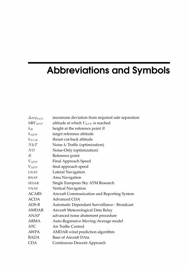
Abbreviations and Symbols
∆sepsafe maximum deviation from required safe separation
h@VAPP altitude at which VAPP is reached
hR height at the reference point R
hAPP target reference altitude
hTCB thrust cut-back altitude
N&T Noise & Traffic (optimization)
NO Noise-Only (optimization)
R Reference point
VAPP Final Approach Speed
VAPP final approach speed
LNAV Lateral Navigation
RNAV Area Navigation
SESAR Single European Sky ATM Research
VNAV Vertical Navigation
ACARS Aircraft Communication and Reporting System
ACDA Advanced CDA
ADS-B Automatic Dependant Surveillance - Broadcast
AMDAR Aircraft Meteorological Data Relay
ANAP advanced noise abatement procedure
ARMA Auto-Regressive Moving-Average model
ATC Air Traffic Control
AWPA AMDAR wind prediction algorithm
BADA Base of Aircraft DAta
CDA Continuous Descent Approach
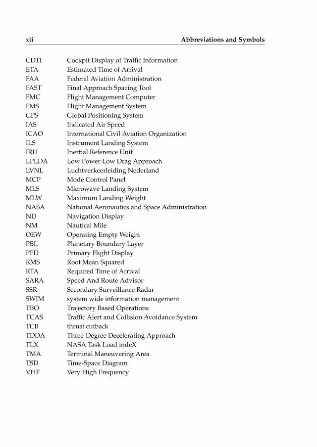
xii Abbreviations and Symbols
CDTI Cockpit Display of Traffic Information
ETA Estimated Time of Arrival
FAA Federal Aviation Administration
FAST Final Approach Spacing Tool
FMC Flight Management Computer
FMS Flight Management System
GPS Global Positioning System
IAS Indicated Air Speed
ICAO International Civil Aviation Organization
ILS Instrument Landing System
IRU Inertial Reference Unit
LPLDA Low Power Low Drag Approach
LVNL Luchtverkeerleiding Nederland
MCP Mode Control Panel
MLS Microwave Landing System
MLW Maximum Landing Weight
NASA National Aeronautics and Space Administration
ND Navigation Display
NM Nautical Mile
OEW Operating Empty Weight
PBL Planetary Boundary Layer
PFD Primary Flight Display
RMS Root Mean Squared
RTA Required Time of Arrival
SARA Speed And Route Advisor
SSR Secondary Surveillance Radar
SWIM system wide information management
TBO Trajectory Based Operations
TCAS Traffic Alert and Collision Avoidance System
TCB thrust cutback
TDDA Three-Degree Decelerating Approach
TLX NASA Task Load indeX
TMA Terminal Maneuvering Area
TSD Time-Space Diagram
VHF Very High Frequency
Contents
Summary v
Abbreviations and Symbols xi
1 Introduction 11-1 Historic background . . . . . . . . . . . . . . . . . . . . . . . . . . . . . 11-2 Aircraft noise mitigation . . . . . . . . . . . . . . . . . . . . . . . . . . . 21-3 Noise abatement procedures . . . . . . . . . . . . . . . . . . . . . . . . . 3
1-3-1 Engine emissions . . . . . . . . . . . . . . . . . . . . . . . . . . . 41-4 Air traffic control . . . . . . . . . . . . . . . . . . . . . . . . . . . . . . . 5
1-4-1 Three-Degree Decelerating Approach . . . . . . . . . . . . . . . . 71-5 Self-spacing scenarios . . . . . . . . . . . . . . . . . . . . . . . . . . . . 8
1-5-1 Distance based self-spacing . . . . . . . . . . . . . . . . . . . . . 81-5-2 Time based spacing . . . . . . . . . . . . . . . . . . . . . . . . . 91-5-3 Scope . . . . . . . . . . . . . . . . . . . . . . . . . . . . . . . . . 9
1-6 Performance metrics . . . . . . . . . . . . . . . . . . . . . . . . . . . . . 91-7 Thesis outline . . . . . . . . . . . . . . . . . . . . . . . . . . . . . . . . . 10References . . . . . . . . . . . . . . . . . . . . . . . . . . . . . . . . . . . . . . 12
2 Trajectory Prediction 152-1 Abstract . . . . . . . . . . . . . . . . . . . . . . . . . . . . . . . . . . . . 152-2 Introduction . . . . . . . . . . . . . . . . . . . . . . . . . . . . . . . . . . 162-3 Proposed scenario . . . . . . . . . . . . . . . . . . . . . . . . . . . . . . 17
2-3-1 ADS-B . . . . . . . . . . . . . . . . . . . . . . . . . . . . . . . . 182-4 Algorithm . . . . . . . . . . . . . . . . . . . . . . . . . . . . . . . . . . . 18
2-4-1 Wind model . . . . . . . . . . . . . . . . . . . . . . . . . . . . . 192-5 Least Square Estimate . . . . . . . . . . . . . . . . . . . . . . . . . . . . 192-6 Intent information . . . . . . . . . . . . . . . . . . . . . . . . . . . . . . 212-7 Accuracy . . . . . . . . . . . . . . . . . . . . . . . . . . . . . . . . . . . 22
xiv Contents
2-8 Conclusions and future research . . . . . . . . . . . . . . . . . . . . . . . 23References . . . . . . . . . . . . . . . . . . . . . . . . . . . . . . . . . . . . . . 24
3 Pilot Support Interface 253-1 Abstract . . . . . . . . . . . . . . . . . . . . . . . . . . . . . . . . . . . . 253-2 The Three-Degree Decelerating Approach . . . . . . . . . . . . . . . . . 27
3-2-1 Description of the procedure . . . . . . . . . . . . . . . . . . . . 273-2-2 The problem of separation . . . . . . . . . . . . . . . . . . . . . 283-2-3 Delegating the separation task to the pilot . . . . . . . . . . . . 29
3-3 Algorithm design . . . . . . . . . . . . . . . . . . . . . . . . . . . . . . . 303-3-1 Block A: Lead trajectory prediction algorithm . . . . . . . . . . . 303-3-2 Block B: Own trajectory prediction . . . . . . . . . . . . . . . . . 323-3-3 Block C: Separation trend prediction . . . . . . . . . . . . . . . . 333-3-4 Block D: Flap schedule optimization algorithms . . . . . . . . . . 33
3-4 Pilot support interface design . . . . . . . . . . . . . . . . . . . . . . . . 343-4-1 TDDA support . . . . . . . . . . . . . . . . . . . . . . . . . . . . 34
3-5 Experiment . . . . . . . . . . . . . . . . . . . . . . . . . . . . . . . . . . 373-5-1 Method . . . . . . . . . . . . . . . . . . . . . . . . . . . . . . . . 37
3-6 Results and discussion . . . . . . . . . . . . . . . . . . . . . . . . . . . . 393-6-1 Pilot controls . . . . . . . . . . . . . . . . . . . . . . . . . . . . . 393-6-2 Throttle . . . . . . . . . . . . . . . . . . . . . . . . . . . . . . . . 403-6-3 Cue response . . . . . . . . . . . . . . . . . . . . . . . . . . . . . 403-6-4 Operational performance . . . . . . . . . . . . . . . . . . . . . . 413-6-5 Separation goals . . . . . . . . . . . . . . . . . . . . . . . . . . . 413-6-6 Noise goals . . . . . . . . . . . . . . . . . . . . . . . . . . . . . . 423-6-7 Pilot workload . . . . . . . . . . . . . . . . . . . . . . . . . . . . 43
3-7 Conclusions . . . . . . . . . . . . . . . . . . . . . . . . . . . . . . . . . . 43References . . . . . . . . . . . . . . . . . . . . . . . . . . . . . . . . . . . . . . 44
4 Distance Based Self-Spacing 474-1 Abstract . . . . . . . . . . . . . . . . . . . . . . . . . . . . . . . . . . . . 474-2 Introduction . . . . . . . . . . . . . . . . . . . . . . . . . . . . . . . . . . 484-3 The Three-Degree Decelerating Approach and Support System . . . . . 49
4-3-1 The Approach Procedure . . . . . . . . . . . . . . . . . . . . . . 494-3-2 The Optimization Algorithm . . . . . . . . . . . . . . . . . . . . 494-3-3 The Pilot Support Interface . . . . . . . . . . . . . . . . . . . . . 50
4-4 The Enhanced TDDA Algorithm . . . . . . . . . . . . . . . . . . . . . . 504-4-1 Structure of the Flap Optimization Algorithm . . . . . . . . . . . 524-4-2 Lead Trajectory Prediction . . . . . . . . . . . . . . . . . . . . . 534-4-3 Own Trajectory Prediction . . . . . . . . . . . . . . . . . . . . . 574-4-4 Separation Trend Prediction . . . . . . . . . . . . . . . . . . . . . 604-4-5 Start Altitude Optimization . . . . . . . . . . . . . . . . . . . . . 604-4-6 Noise and Traffic Optimization . . . . . . . . . . . . . . . . . . . 62
4-5 Experiment 1: Monte Carlo Simulations . . . . . . . . . . . . . . . . . . 634-5-1 Method . . . . . . . . . . . . . . . . . . . . . . . . . . . . . . . . 63
xv
4-5-2 Results and Discussion: General performance analysis . . . . . . 654-5-3 Results and Discussion: Robustness analysis . . . . . . . . . . . . 68
4-6 Experiment 2: In-flight Investigation . . . . . . . . . . . . . . . . . . . . 704-6-1 Method . . . . . . . . . . . . . . . . . . . . . . . . . . . . . . . . 704-6-2 Results and Discussion . . . . . . . . . . . . . . . . . . . . . . . . 724-6-3 Conclusions . . . . . . . . . . . . . . . . . . . . . . . . . . . . . . 72
4-7 Experiment 3: Piloted Simulator Tests . . . . . . . . . . . . . . . . . . . 744-7-1 Method . . . . . . . . . . . . . . . . . . . . . . . . . . . . . . . . 744-7-2 Results . . . . . . . . . . . . . . . . . . . . . . . . . . . . . . . . 774-7-3 Discussion and Conclusions . . . . . . . . . . . . . . . . . . . . . 81
4-8 Conclusions . . . . . . . . . . . . . . . . . . . . . . . . . . . . . . . . . . 814-9 Acknowledgments . . . . . . . . . . . . . . . . . . . . . . . . . . . . . . 82References . . . . . . . . . . . . . . . . . . . . . . . . . . . . . . . . . . . . . . 82
5 Stochastic Wind Profile Estimation 855-1 Abstract . . . . . . . . . . . . . . . . . . . . . . . . . . . . . . . . . . . . 855-2 Introduction . . . . . . . . . . . . . . . . . . . . . . . . . . . . . . . . . . 86
5-2-1 AMDAR Characteristics . . . . . . . . . . . . . . . . . . . . . . . 865-2-2 The Wind Prediction Algorithm . . . . . . . . . . . . . . . . . . . 87
5-3 Physical Wind Model . . . . . . . . . . . . . . . . . . . . . . . . . . . . . 885-3-1 The Atmospheric Stability . . . . . . . . . . . . . . . . . . . . . . 905-3-2 The Mathematical Wind Model in Neutrally Stable Atmosphere . 92
5-4 AMDAR wind prediction algorithm (AWPA) . . . . . . . . . . . . . . . . 935-4-1 Kalman Filtering and Algorithm Design . . . . . . . . . . . . . . 955-4-2 Wind profile construction . . . . . . . . . . . . . . . . . . . . . . 100
5-5 Wind Prediction Performance Evaluation . . . . . . . . . . . . . . . . . . 1025-5-1 Check on relevant parameters . . . . . . . . . . . . . . . . . . . . 1025-5-2 Performance accuracy . . . . . . . . . . . . . . . . . . . . . . . . 106
5-6 Conclusions . . . . . . . . . . . . . . . . . . . . . . . . . . . . . . . . . . 106References . . . . . . . . . . . . . . . . . . . . . . . . . . . . . . . . . . . . . . 107
6 Time Based Spacing 1096-1 Abstract . . . . . . . . . . . . . . . . . . . . . . . . . . . . . . . . . . . . 1096-2 Introduction . . . . . . . . . . . . . . . . . . . . . . . . . . . . . . . . . . 1106-3 Continuous Descent Approaches . . . . . . . . . . . . . . . . . . . . . . 111
6-3-1 Description of the procedure . . . . . . . . . . . . . . . . . . . . 1116-3-2 Time based separation . . . . . . . . . . . . . . . . . . . . . . . . 112
6-4 Support System Design . . . . . . . . . . . . . . . . . . . . . . . . . . . 1136-4-1 Wind profile prediction . . . . . . . . . . . . . . . . . . . . . . . 1136-4-2 Track and time prediction . . . . . . . . . . . . . . . . . . . . . . 1166-4-3 Optimization of support system performance . . . . . . . . . . . 117
6-5 Pilot Interface . . . . . . . . . . . . . . . . . . . . . . . . . . . . . . . . . 1186-5-1 Conventional Display . . . . . . . . . . . . . . . . . . . . . . . . 1186-5-2 Augmented Display . . . . . . . . . . . . . . . . . . . . . . . . . 119
6-6 Experiment . . . . . . . . . . . . . . . . . . . . . . . . . . . . . . . . . . 122
xvi Contents
6-6-1 Independent variables . . . . . . . . . . . . . . . . . . . . . . . . 1226-6-2 Experiment design . . . . . . . . . . . . . . . . . . . . . . . . . . 1226-6-3 Apparatus . . . . . . . . . . . . . . . . . . . . . . . . . . . . . . . 1226-6-4 Aircraft . . . . . . . . . . . . . . . . . . . . . . . . . . . . . . . . 1236-6-5 Scenario . . . . . . . . . . . . . . . . . . . . . . . . . . . . . . . . 1236-6-6 Procedure . . . . . . . . . . . . . . . . . . . . . . . . . . . . . . . 1236-6-7 Dependent measures . . . . . . . . . . . . . . . . . . . . . . . . . 1246-6-8 Hypotheses . . . . . . . . . . . . . . . . . . . . . . . . . . . . . . 124
6-7 Results and Discussion . . . . . . . . . . . . . . . . . . . . . . . . . . . . 1256-7-1 Operational Performance . . . . . . . . . . . . . . . . . . . . . . 1256-7-2 Pilot workload . . . . . . . . . . . . . . . . . . . . . . . . . . . . 128
6-8 Conclusions . . . . . . . . . . . . . . . . . . . . . . . . . . . . . . . . . . 1296-9 Recommendations . . . . . . . . . . . . . . . . . . . . . . . . . . . . . . 129References . . . . . . . . . . . . . . . . . . . . . . . . . . . . . . . . . . . . . . 129
7 Self-spacing in High-Density Arrival Streams 1337-1 Abstract . . . . . . . . . . . . . . . . . . . . . . . . . . . . . . . . . . . . 1337-2 Introduction . . . . . . . . . . . . . . . . . . . . . . . . . . . . . . . . . . 1347-3 Three-Degree Decelerating Approach . . . . . . . . . . . . . . . . . . . . 135
7-3-1 Description of the Procedure . . . . . . . . . . . . . . . . . . . . 1357-3-2 Self-Spacing Task . . . . . . . . . . . . . . . . . . . . . . . . . . 136
7-4 Aircraft Intent-Based Trajectory Prediction . . . . . . . . . . . . . . . . . 1387-4-1 Aircraft Intent Description of the TDDA . . . . . . . . . . . . . . 1397-4-2 Point of Minimum Separation . . . . . . . . . . . . . . . . . . . . 1397-4-3 Intent-Based Trajectory Prediction . . . . . . . . . . . . . . . . . 140
7-5 TDDAs in Arrival Streams . . . . . . . . . . . . . . . . . . . . . . . . . . 1407-5-1 Factors that Affect the TDDA Control Space . . . . . . . . . . . 1407-5-2 Effect of Initial Separation on TDDA . . . . . . . . . . . . . . . . 1417-5-3 Initial Separation Constraints - Distance Based Self-Spacing . . . 1427-5-4 Initial Separation Constraints - Time Based Self-Spacing . . . . . 142
7-6 Fast-Time TDDA Simulation Tool . . . . . . . . . . . . . . . . . . . . . 1447-6-1 Aircraft Model . . . . . . . . . . . . . . . . . . . . . . . . . . . . 1447-6-2 Pilot Response Time and Wind . . . . . . . . . . . . . . . . . . . 1457-6-3 Setting the RTA and Initial Separation . . . . . . . . . . . . . . . 145
7-7 Distance- and Time Based Self-Spacing Performance . . . . . . . . . . . 1467-7-1 Noise Goal . . . . . . . . . . . . . . . . . . . . . . . . . . . . . . 1467-7-2 Separation . . . . . . . . . . . . . . . . . . . . . . . . . . . . . . 1477-7-3 Capacity . . . . . . . . . . . . . . . . . . . . . . . . . . . . . . . 148
7-8 Sensitivity Analysis . . . . . . . . . . . . . . . . . . . . . . . . . . . . . . 1507-8-1 Initial Control Space Prediction . . . . . . . . . . . . . . . . . . . 1517-8-2 Initial Separation Distribution . . . . . . . . . . . . . . . . . . . . 1527-8-3 Starting Altitude . . . . . . . . . . . . . . . . . . . . . . . . . . . 1537-8-4 Initial Speed . . . . . . . . . . . . . . . . . . . . . . . . . . . . . 1547-8-5 Aircraft Weight . . . . . . . . . . . . . . . . . . . . . . . . . . . . 155
7-9 Discussion . . . . . . . . . . . . . . . . . . . . . . . . . . . . . . . . . . . 155
xvii
7-10 Conclusion . . . . . . . . . . . . . . . . . . . . . . . . . . . . . . . . . . 156References . . . . . . . . . . . . . . . . . . . . . . . . . . . . . . . . . . . . . . 156
8 Conclusions and recommendations 1598-1 Key factors . . . . . . . . . . . . . . . . . . . . . . . . . . . . . . . . . . 160
8-1-1 Procedure constraints . . . . . . . . . . . . . . . . . . . . . . . . 1608-1-2 Aircraft drag and thrust data . . . . . . . . . . . . . . . . . . . . 1608-1-3 Aircraft operating mass . . . . . . . . . . . . . . . . . . . . . . . 1618-1-4 Wind data . . . . . . . . . . . . . . . . . . . . . . . . . . . . . . 1618-1-5 Pilot technique . . . . . . . . . . . . . . . . . . . . . . . . . . . . 161
8-2 Results . . . . . . . . . . . . . . . . . . . . . . . . . . . . . . . . . . . . 1628-2-1 Self-spacing performance . . . . . . . . . . . . . . . . . . . . . . 1628-2-2 Pilot workload . . . . . . . . . . . . . . . . . . . . . . . . . . . . 1628-2-3 Landing runway capacity . . . . . . . . . . . . . . . . . . . . . . 162
8-3 Recommendations . . . . . . . . . . . . . . . . . . . . . . . . . . . . . . 1638-3-1 Developments in ATM research . . . . . . . . . . . . . . . . . . . 1638-3-2 Pilot support interface . . . . . . . . . . . . . . . . . . . . . . . . 1638-3-3 Air traffic controller support . . . . . . . . . . . . . . . . . . . . 1648-3-4 Procedure design . . . . . . . . . . . . . . . . . . . . . . . . . . . 165
References . . . . . . . . . . . . . . . . . . . . . . . . . . . . . . . . . . . . . . 165
Samenvatting 167
Curriculum vitae 173
Acknowledgments 175

xviii
List of Figures
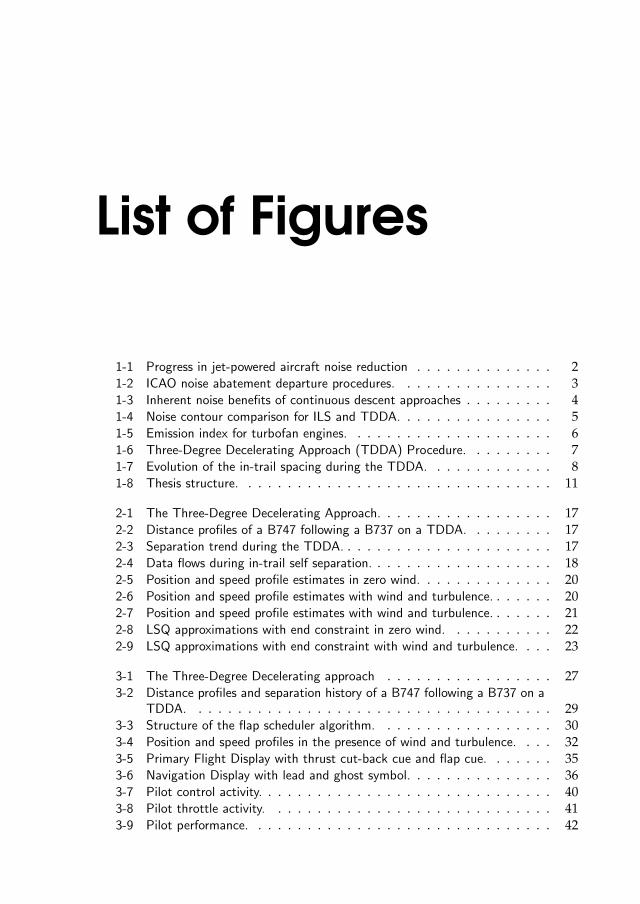
1-1 Progress in jet-powered aircraft noise reduction . . . . . . . . . . . . . . 21-2 ICAO noise abatement departure procedures. . . . . . . . . . . . . . . . 31-3 Inherent noise benefits of continuous descent approaches . . . . . . . . . 41-4 Noise contour comparison for ILS and TDDA. . . . . . . . . . . . . . . . 51-5 Emission index for turbofan engines. . . . . . . . . . . . . . . . . . . . . 61-6 Three-Degree Decelerating Approach (TDDA) Procedure. . . . . . . . . 71-7 Evolution of the in-trail spacing during the TDDA. . . . . . . . . . . . . 81-8 Thesis structure. . . . . . . . . . . . . . . . . . . . . . . . . . . . . . . . 11
2-1 The Three-Degree Decelerating Approach. . . . . . . . . . . . . . . . . . 172-2 Distance profiles of a B747 following a B737 on a TDDA. . . . . . . . . 172-3 Separation trend during the TDDA. . . . . . . . . . . . . . . . . . . . . . 172-4 Data flows during in-trail self separation. . . . . . . . . . . . . . . . . . . 182-5 Position and speed profile estimates in zero wind. . . . . . . . . . . . . . 202-6 Position and speed profile estimates with wind and turbulence. . . . . . . 202-7 Position and speed profile estimates with wind and turbulence. . . . . . . 212-8 LSQ approximations with end constraint in zero wind. . . . . . . . . . . 222-9 LSQ approximations with end constraint with wind and turbulence. . . . 23
3-1 The Three-Degree Decelerating approach . . . . . . . . . . . . . . . . . 273-2 Distance profiles and separation history of a B747 following a B737 on a
TDDA. . . . . . . . . . . . . . . . . . . . . . . . . . . . . . . . . . . . . 293-3 Structure of the flap scheduler algorithm. . . . . . . . . . . . . . . . . . 303-4 Position and speed profiles in the presence of wind and turbulence. . . . 323-5 Primary Flight Display with thrust cut-back cue and flap cue. . . . . . . 353-6 Navigation Display with lead and ghost symbol. . . . . . . . . . . . . . . 363-7 Pilot control activity. . . . . . . . . . . . . . . . . . . . . . . . . . . . . . 403-8 Pilot throttle activity. . . . . . . . . . . . . . . . . . . . . . . . . . . . . 413-9 Pilot performance. . . . . . . . . . . . . . . . . . . . . . . . . . . . . . . 42

xx List of Figures
4-1 The Three-Degree Decelerating Approach . . . . . . . . . . . . . . . . . 494-2 Augmented Primary Flight Display and Navigation Display. . . . . . . . . 514-3 Structure of the flap scheduler algorithm . . . . . . . . . . . . . . . . . . 534-4 Lead trajectory prediction: polynomial fit through ADS-B data . . . . . 554-5 Lead trajectory prediction: underestimation of the lead’s ground speed . 564-6 The difference between kinematic flight path angle γk and aerodynamic
flight path angle γa . . . . . . . . . . . . . . . . . . . . . . . . . . . . . 584-7 Force diagram for ’point mass’ aircraft model . . . . . . . . . . . . . . . 584-8 Own trajectory prediction model . . . . . . . . . . . . . . . . . . . . . . 604-9 Airspeed as function of along track distance. . . . . . . . . . . . . . . . . 614-10 Predicted trajectories and accuracy. . . . . . . . . . . . . . . . . . . . . . 634-11 Logarithmic wind model with backing and veering effect. . . . . . . . . . 664-12 Thrust cut-back altitudes in case of a fastman lead trace. . . . . . . . . 664-13 Deviation from 2.5 NM safe separation for a nominal lead type under all
wind conditions. . . . . . . . . . . . . . . . . . . . . . . . . . . . . . . . 674-14 Deviation from 2.5 NM safe separation for a fastman lead type under all
wind conditions. . . . . . . . . . . . . . . . . . . . . . . . . . . . . . . . 674-15 Altitude at which VAPP is reached for a nominal lead type under all wind
conditions. . . . . . . . . . . . . . . . . . . . . . . . . . . . . . . . . . . 674-16 Altitude at which VAPP is reached for a fastman lead type under all wind
conditions. . . . . . . . . . . . . . . . . . . . . . . . . . . . . . . . . . . 674-17 Robustness performance for a fastman lead and wind prediction error of
+/-10 kts and +/-20 kts. . . . . . . . . . . . . . . . . . . . . . . . . . . 694-18 Robustness performance for a fastman lead in zero-wind and aircraft mass
error of +/-500 kg. . . . . . . . . . . . . . . . . . . . . . . . . . . . . . . 694-19 Robustness results for a fastman lead in zero-wind and drag coefficient
error of +/-5% and +/-10%. . . . . . . . . . . . . . . . . . . . . . . . . 694-20 Flap/gear behavior, separation trend, and longitudinal wind component
of one representative run during the second experiment flight. All datais sampled at 10 Hz. (Note: a positive wind component is a tailwind.) . 73
4-21 Predicted and actual wind speed profiles during the simulation experi-ments. A positive value indicates headwind. . . . . . . . . . . . . . . . . 74
4-22 The means and 95% confidence intervals of the altitude at which VAPP
was reached. . . . . . . . . . . . . . . . . . . . . . . . . . . . . . . . . . 784-23 The means and 95% confidence intervals of the deviations from the min-
imum safe separation throughout the whole approach. A negative valueindicates safe separation violation. . . . . . . . . . . . . . . . . . . . . . 78
4-24 The mean and 95% confidence intervals of the pilot response time onflap and gear cues. . . . . . . . . . . . . . . . . . . . . . . . . . . . . . . 80
4-25 Histogram of the pilot response time on the thrust cut-back cue. . . . . 804-26 The means and 95% confidence intervals for the normalized TLX scores. 80
5-1 Calculation of the Wind Speed Vector . . . . . . . . . . . . . . . . . . . 875-2 Influence of pressure gradient force, Coriolis force and friction force on
movement of air in Northern hemisphere. . . . . . . . . . . . . . . . . . 89
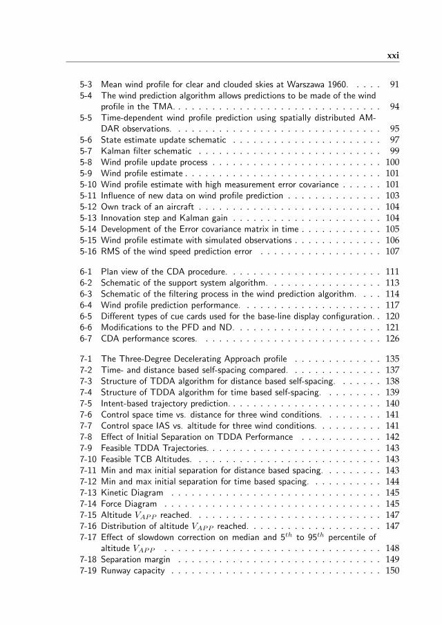
xxi
5-3 Mean wind profile for clear and clouded skies at Warszawa 1960. . . . . 915-4 The wind prediction algorithm allows predictions to be made of the wind
profile in the TMA. . . . . . . . . . . . . . . . . . . . . . . . . . . . . . . 945-5 Time-dependent wind profile prediction using spatially distributed AM-
DAR observations. . . . . . . . . . . . . . . . . . . . . . . . . . . . . . . 955-6 State estimate update schematic . . . . . . . . . . . . . . . . . . . . . . 975-7 Kalman filter schematic . . . . . . . . . . . . . . . . . . . . . . . . . . . 995-8 Wind profile update process . . . . . . . . . . . . . . . . . . . . . . . . . 1005-9 Wind profile estimate . . . . . . . . . . . . . . . . . . . . . . . . . . . . . 1015-10 Wind profile estimate with high measurement error covariance . . . . . . 1015-11 Influence of new data on wind profile prediction . . . . . . . . . . . . . . 1035-12 Own track of an aircraft . . . . . . . . . . . . . . . . . . . . . . . . . . . 1045-13 Innovation step and Kalman gain . . . . . . . . . . . . . . . . . . . . . . 1045-14 Development of the Error covariance matrix in time . . . . . . . . . . . . 1055-15 Wind profile estimate with simulated observations . . . . . . . . . . . . . 1065-16 RMS of the wind speed prediction error . . . . . . . . . . . . . . . . . . 107
6-1 Plan view of the CDA procedure. . . . . . . . . . . . . . . . . . . . . . . 1116-2 Schematic of the support system algorithm. . . . . . . . . . . . . . . . . 1136-3 Schematic of the filtering process in the wind prediction algorithm. . . . 1146-4 Wind profile prediction performance. . . . . . . . . . . . . . . . . . . . . 1176-5 Different types of cue cards used for the base-line display configuration. . 1206-6 Modifications to the PFD and ND. . . . . . . . . . . . . . . . . . . . . . 1216-7 CDA performance scores. . . . . . . . . . . . . . . . . . . . . . . . . . . 126
7-1 The Three-Degree Decelerating Approach profile . . . . . . . . . . . . . 1357-2 Time- and distance based self-spacing compared. . . . . . . . . . . . . . 1377-3 Structure of TDDA algorithm for distance based self-spacing. . . . . . . 1387-4 Structure of TDDA algorithm for time based self-spacing. . . . . . . . . 1397-5 Intent-based trajectory prediction. . . . . . . . . . . . . . . . . . . . . . . 1407-6 Control space time vs. distance for three wind conditions. . . . . . . . . 1417-7 Control space IAS vs. altitude for three wind conditions. . . . . . . . . . 1417-8 Effect of Initial Separation on TDDA Performance . . . . . . . . . . . . 1427-9 Feasible TDDA Trajectories. . . . . . . . . . . . . . . . . . . . . . . . . . 1437-10 Feasible TCB Altitudes. . . . . . . . . . . . . . . . . . . . . . . . . . . . 1437-11 Min and max initial separation for distance based spacing. . . . . . . . . 1437-12 Min and max initial separation for time based spacing. . . . . . . . . . . 1447-13 Kinetic Diagram . . . . . . . . . . . . . . . . . . . . . . . . . . . . . . . 1457-14 Force Diagram . . . . . . . . . . . . . . . . . . . . . . . . . . . . . . . . 1457-15 Altitude VAPP reached. . . . . . . . . . . . . . . . . . . . . . . . . . . . 1477-16 Distribution of altitude VAPP reached. . . . . . . . . . . . . . . . . . . . 1477-17 Effect of slowdown correction on median and 5th to 95th percentile of
altitude VAPP . . . . . . . . . . . . . . . . . . . . . . . . . . . . . . . . 1487-18 Separation margin . . . . . . . . . . . . . . . . . . . . . . . . . . . . . . 1497-19 Runway capacity . . . . . . . . . . . . . . . . . . . . . . . . . . . . . . . 150
xxii List of Figures
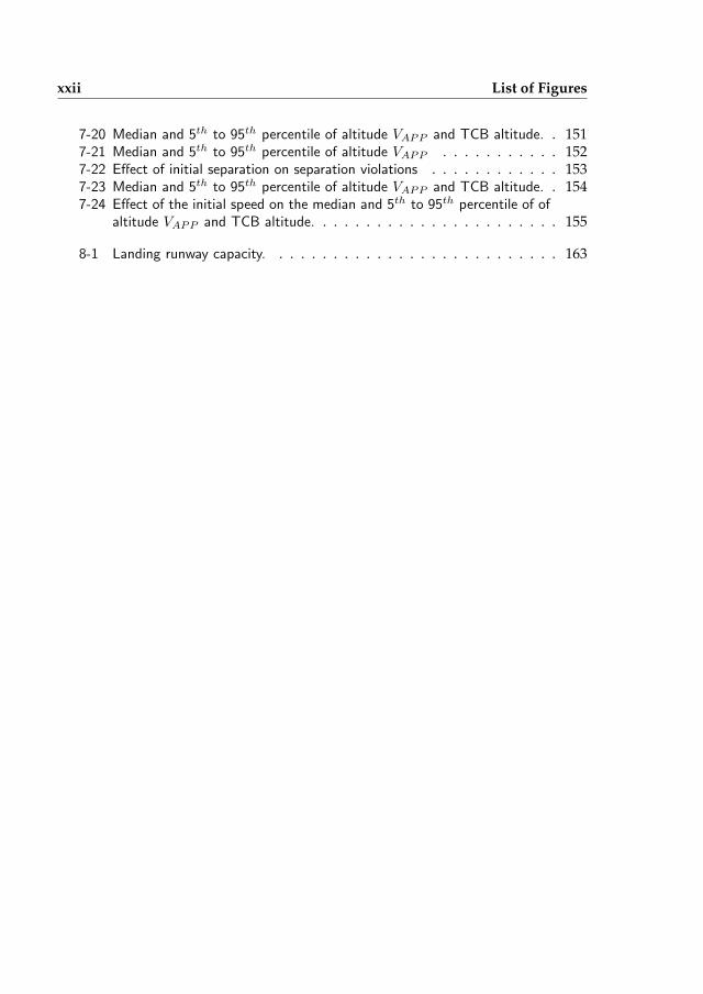
7-20 Median and 5th to 95th percentile of altitude VAPP and TCB altitude. . 1517-21 Median and 5th to 95th percentile of altitude VAPP . . . . . . . . . . . 1527-22 Effect of initial separation on separation violations . . . . . . . . . . . . 1537-23 Median and 5th to 95th percentile of altitude VAPP and TCB altitude. . 1547-24 Effect of the initial speed on the median and 5th to 95th percentile of of
altitude VAPP and TCB altitude. . . . . . . . . . . . . . . . . . . . . . . 155
8-1 Landing runway capacity. . . . . . . . . . . . . . . . . . . . . . . . . . . 163
List of Tables
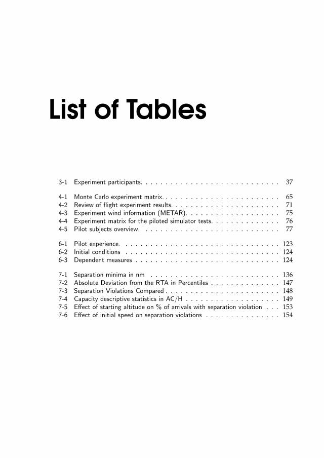
3-1 Experiment participants. . . . . . . . . . . . . . . . . . . . . . . . . . . . 37
4-1 Monte Carlo experiment matrix. . . . . . . . . . . . . . . . . . . . . . . . 654-2 Review of flight experiment results. . . . . . . . . . . . . . . . . . . . . . 714-3 Experiment wind information (METAR). . . . . . . . . . . . . . . . . . . 754-4 Experiment matrix for the piloted simulator tests. . . . . . . . . . . . . . 764-5 Pilot subjects overview. . . . . . . . . . . . . . . . . . . . . . . . . . . . 77
6-1 Pilot experience. . . . . . . . . . . . . . . . . . . . . . . . . . . . . . . . 1236-2 Initial conditions . . . . . . . . . . . . . . . . . . . . . . . . . . . . . . . 1246-3 Dependent measures . . . . . . . . . . . . . . . . . . . . . . . . . . . . . 124
7-1 Separation minima in nm . . . . . . . . . . . . . . . . . . . . . . . . . . 1367-2 Absolute Deviation from the RTA in Percentiles . . . . . . . . . . . . . . 1477-3 Separation Violations Compared . . . . . . . . . . . . . . . . . . . . . . . 1487-4 Capacity descriptive statistics in AC/H . . . . . . . . . . . . . . . . . . . 1497-5 Effect of starting altitude on % of arrivals with separation violation . . . 1537-6 Effect of initial speed on separation violations . . . . . . . . . . . . . . . 154

xxiv

1Introduction
1-1 Historic background
When the first jet airliners started operations in the early 1960s and travel by air be-came more commonplace, the noise that accompanied these early, low by-pass ra-tio jet aircraft turned out to be a hindrance to people. In September 1968 in BuenosAires, the Assembly of the International Civil Aviation Organization (ICAO) rec-ognized the need to address ’noise in the vicinity of aerodromes’ and adopted thefirst resolution on this matter, which was further elaborated in 1969 during a specialmeeting in Montreal.1, 2
During this meeting it was decided to develop standards for aircraft noise cer-tification and the first design aspects of noise abatement departure and arrivalprocedures were discussed. Also guidance on land-use planning around airportswas published. This was further elaborated by the Commission on Aircraft Noise(CAN) which ultimately led to the publication of ICAO Annex 16, which wasadopted in 1972.1, 2, 7
Initially, the focus on aircraft noise reduction lay squarely on the production ofquieter engines. Aircraft are certified based on the maximum sound levels theyproduce during different flight phases and in different aircraft configurations. Astime progresses, the regulations are amended and new aircraft have to meet moreand more stringent noise certification standards, ultimately resulting in quieter air-craft.1, 2, 7
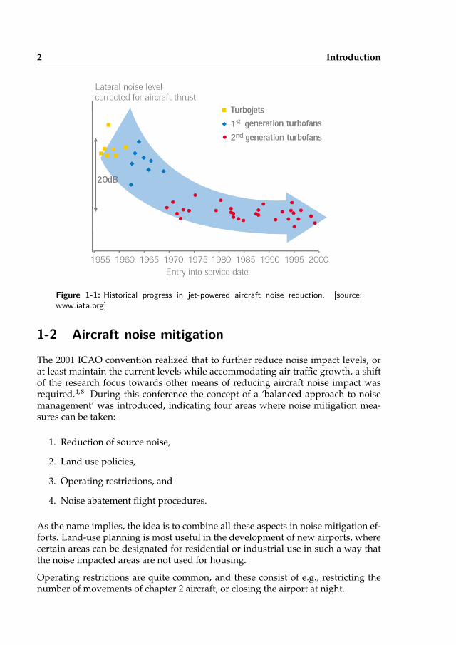
The phasing out of older, noisier aircraft (so-called ‘Chapter 2’ aircraft) has nowalmost been completed at most airports in Europe and the United States. As can beseen in Figure 1-1, the noise levels of jet-powered aircraft have reduced some 50%over the last 50 years, but the point of diminishing returns has been reached. Unlessa completely different form of propulsion is introduced in aviation, the noise levelsproduced by future generations of aircraft can not be expected to be significantlylower than current levels.
2 Introduction
Figure 1-1: Historical progress in jet-powered aircraft noise reduction. [source:www.iata.org]
1-2 Aircraft noise mitigation
The 2001 ICAO convention realized that to further reduce noise impact levels, orat least maintain the current levels while accommodating air traffic growth, a shiftof the research focus towards other means of reducing aircraft noise impact wasrequired.4, 8 During this conference the concept of a ‘balanced approach to noisemanagement’ was introduced, indicating four areas where noise mitigation mea-sures can be taken:
1. Reduction of source noise,
2. Land use policies,
3. Operating restrictions, and
4. Noise abatement flight procedures.
As the name implies, the idea is to combine all these aspects in noise mitigation ef-forts. Land-use planning is most useful in the development of new airports, wherecertain areas can be designated for residential or industrial use in such a way thatthe noise impacted areas are not used for housing.
Operating restrictions are quite common, and these consist of e.g., restricting thenumber of movements of chapter 2 aircraft, or closing the airport at night.
1-3 Noise abatement procedures 3
(a) NADP 1 (b) NADP 2
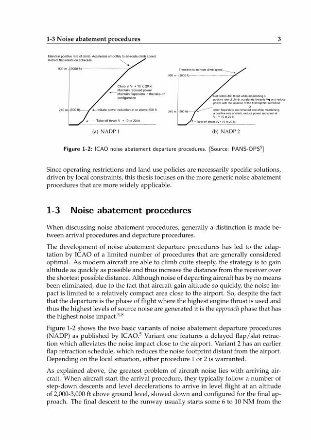
Figure 1-2: ICAO noise abatement departure procedures. [Source: PANS-OPS5]
Since operating restrictions and land use policies are necessarily specific solutions,driven by local constraints, this thesis focuses on the more generic noise abatementprocedures that are more widely applicable.
1-3 Noise abatement procedures
When discussing noise abatement procedures, generally a distinction is made be-tween arrival procedures and departure procedures.
The development of noise abatement departure procedures has led to the adap-tation by ICAO of a limited number of procedures that are generally consideredoptimal. As modern aircraft are able to climb quite steeply, the strategy is to gainaltitude as quickly as possible and thus increase the distance from the receiver overthe shortest possible distance. Although noise of departing aircraft has by no meansbeen eliminated, due to the fact that aircraft gain altitude so quickly, the noise im-pact is limited to a relatively compact area close to the airport. So, despite the factthat the departure is the phase of flight where the highest engine thrust is used andthus the highest levels of source noise are generated it is the approach phase that hasthe highest noise impact.5, 8
Figure 1-2 shows the two basic variants of noise abatement departure procedures(NADP) as published by ICAO.5 Variant one features a delayed flap/slat retrac-tion which alleviates the noise impact close to the airport. Variant 2 has an earlierflap retraction schedule, which reduces the noise footprint distant from the airport.Depending on the local situation, either procedure 1 or 2 is warranted.
As explained above, the greatest problem of aircraft noise lies with arriving air-craft. When aircraft start the arrival procedure, they typically follow a number ofstep-down descents and level decelerations to arrive in level flight at an altitudeof 2,000-3,000 ft above ground level, slowed down and configured for the final ap-proach. The final descent to the runway usually starts some 6 to 10 NM from the
4 Introduction
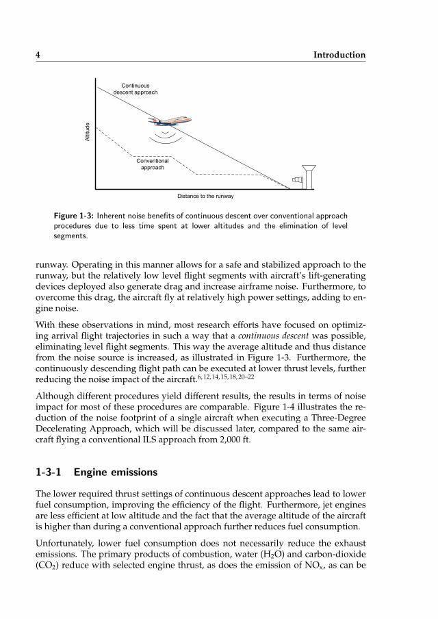
Figure 1-3: Inherent noise benefits of continuous descent over conventional approachprocedures due to less time spent at lower altitudes and the elimination of levelsegments.
runway. Operating in this manner allows for a safe and stabilized approach to therunway, but the relatively low level flight segments with aircraft’s lift-generatingdevices deployed also generate drag and increase airframe noise. Furthermore, toovercome this drag, the aircraft fly at relatively high power settings, adding to en-gine noise.
With these observations in mind, most research efforts have focused on optimiz-ing arrival flight trajectories in such a way that a continuous descent was possible,eliminating level flight segments. This way the average altitude and thus distancefrom the noise source is increased, as illustrated in Figure 1-3. Furthermore, thecontinuously descending flight path can be executed at lower thrust levels, furtherreducing the noise impact of the aircraft.6, 12, 14, 15, 18, 20–22
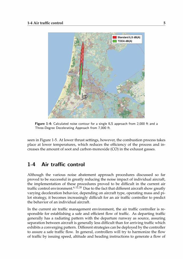
Although different procedures yield different results, the results in terms of noiseimpact for most of these procedures are comparable. Figure 1-4 illustrates the re-duction of the noise footprint of a single aircraft when executing a Three-DegreeDecelerating Approach, which will be discussed later, compared to the same air-craft flying a conventional ILS approach from 2,000 ft.
1-3-1 Engine emissions
The lower required thrust settings of continuous descent approaches lead to lowerfuel consumption, improving the efficiency of the flight. Furthermore, jet enginesare less efficient at low altitude and the fact that the average altitude of the aircraftis higher than during a conventional approach further reduces fuel consumption.
Unfortunately, lower fuel consumption does not necessarily reduce the exhaustemissions. The primary products of combustion, water (H2O) and carbon-dioxide(CO2) reduce with selected engine thrust, as does the emission of NOx, as can be
1-4 Air traffic control 5
Figure 1-4: Calculated noise contour for a single ILS approach from 2,000 ft and aThree-Degree Decelerating Approach from 7,000 ft.
seen in Figure 1-5. At lower thrust settings, however, the combustion process takesplace at lower temperatures, which reduces the efficiency of the process and in-creases the amount of soot and carbon-monoxide (CO) in the exhaust gasses.
1-4 Air traffic control
Although the various noise abatement approach procedures discussed so farproved to be successful in greatly reducing the noise impact of individual aircraft,the implementation of these procedures proved to be difficult in the current airtraffic control environment.6, 12, 20 Due to the fact that different aircraft show greatlyvarying deceleration behavior, depending on aircraft type, operating mass and pi-lot strategy, it becomes increasingly difficult for an air traffic controller to predictthe behavior of an individual aircraft.
In the current air traffic management environment, the air traffic controller is re-sponsible for establishing a safe and efficient flow of traffic. As departing trafficgenerally has a radiating pattern with the departure runway as source, assuringseparation between aircraft is generally less difficult than for arriving traffic whichexhibits a converging pattern. Different strategies can be deployed by the controllerto assure a safe traffic flow. In general, controllers will try to harmonize the flowof traffic by issuing speed, altitude and heading instructions to generate a flow of

6 Introduction
Figure 1-5: Emission index of a turbofan engine for CO and NOx.[Source: IPCC19]
more or less equally behaving aircraft lining up for the landing runway.
When introducing continuous descent approaches, the associated individual de-scent and speed profiles make the controller’s task more difficult. E.g., when Am-sterdam Airport Schiphol implemented the RNAV-night transitions, a reduction oflanding runway capacity of approximately 50% was experienced.16, 17 Because thepredictability of the arriving aircraft was reduced, controllers had to increase thespacing to assure safe separation.
The Continuous Descent Approaches at London’s Heathrow Airport work aroundthis by issuing speed and heading instructions and informing pilots of the numberof track miles to the runway. The absence of level flight segments means that theseare technically Continuous Descent Approaches (CDA), but at constant speeds anddifferent lateral paths, these procedures are far from optimal from a noise impactperspective.
For the purpose of this thesis the latter will be referred to as vectored CDAs and theformer as RNAV-CDAs as these have prescribed ground tracks. One could arguethat spreading the ground tracks distributes the noise, and lowers the peak cumu-lative noise footprint. However, current development in air traffic managementmoves towards optimized 4-D trajectories.
In Europe, the program for Single European Sky ATM Research (SESAR) definesso-called business trajectories, which will be the optimal trajectory for the aircraftinvolved, but also optimized for noise abatement, fuel consumption and other traf-fic.9 In the United States, the Federal Aviation Administration (FAA) is working ona similar concept, defining Trajectory Based Operations (TBO) in its NextGen pro-gram.10 In both programs, the notion of a vectored CDA is difficult if not impossibleto reconcile with an optimal descent profile, instead opting for the development ofthe RNAV-CDA.
This thesis will therefore only address the RNAV-CDA, and aims to develop vari-ous strategies to cope with the profile uncertainty and subsequent arrival spacing
1-4 Air traffic control 7
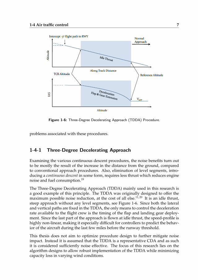
Figure 1-6: Three-Degree Decelerating Approach (TDDA) Procedure.
problems associated with these procedures.
1-4-1 Three-Degree Decelerating Approach
Examining the various continuous descent procedures, the noise benefits turn outto be mostly the result of the increase in the distance from the ground, comparedto conventional approach procedures. Also, elimination of level segments, intro-ducing a continuous descent in some form, requires less thrust which reduces enginenoise and fuel consumption.19
The Three-Degree Decelerating Approach (TDDA) mainly used in this research isa good example of this principle. The TDDA was originally designed to offer themaximum possible noise reduction, at the cost of all else.11, 20 It is an idle thrust,steep approach without any level segments, see Figure 1-6. Since both the lateraland vertical paths are fixed in the TDDA, the only means to control the decelerationrate available to the flight crew is the timing of the flap and landing gear deploy-ment. Since the last part of the approach is flown at idle thrust, the speed-profile ishighly non-linear, making it especially difficult for controllers to predict the behav-ior of the aircraft during the last few miles before the runway threshold.
This thesis does not aim to optimize procedure design to further mitigate noiseimpact. Instead it is assumed that the TDDA is a representative CDA and as suchit is considered sufficiently noise effective. The focus of this research lies on thealgorithm designs to allow robust implementation of the TDDA while minimizingcapacity loss in varying wind conditions.
8 Introduction
(a) B747 following B737. (b) B737 following B747
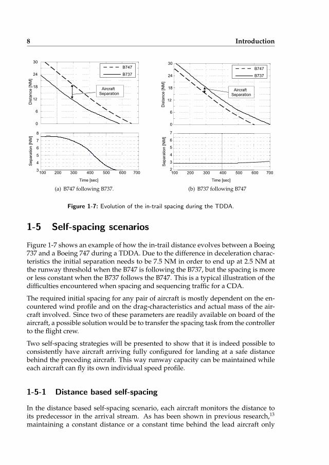
Figure 1-7: Evolution of the in-trail spacing during the TDDA.
1-5 Self-spacing scenarios
Figure 1-7 shows an example of how the in-trail distance evolves between a Boeing737 and a Boeing 747 during a TDDA. Due to the difference in deceleration charac-teristics the initial separation needs to be 7.5 NM in order to end up at 2.5 NM atthe runway threshold when the B747 is following the B737, but the spacing is moreor less constant when the B737 follows the B747. This is a typical illustration of thedifficulties encountered when spacing and sequencing traffic for a CDA.
The required initial spacing for any pair of aircraft is mostly dependent on the en-countered wind profile and on the drag-characteristics and actual mass of the air-craft involved. Since two of these parameters are readily available on board of theaircraft, a possible solution would be to transfer the spacing task from the controllerto the flight crew.
Two self-spacing strategies will be presented to show that it is indeed possible toconsistently have aircraft arriving fully configured for landing at a safe distancebehind the preceding aircraft. This way runway capacity can be maintained whileeach aircraft can fly its own individual speed profile.
1-5-1 Distance based self-spacing
In the distance based self-spacing scenario, each aircraft monitors the distance toits predecessor in the arrival stream. As has been shown in previous research,13
maintaining a constant distance or a constant time behind the lead aircraft only
1-6 Performance metrics 9
works for aircraft that exhibit largely the same dynamic properties. The distancebased concept presented in this thesis uses a trajectory prediction algorithm thatassumes the availability of aircraft status information through some form of datalink such as ADS-B as proposed in FAA’s NextGen program.3, 10 Also, in SESAR’sfuture ATM scenario the notion of System Wide Information Management (SWIM)is introduced, so in this thesis it is assumed that necessary information is availablethrough an (airborne) network.9
The position information is used to construct a descent profile of the lead aircraftwhich is compared with the own predicted profile. The algorithm assures that theminimum distance between the predicted profiles is maintained. This means that itis entirely possible for the algorithm to start increasing the deceleration of the ownaircraft, when the aircraft are still 10 NM apart.
1-5-2 Time based spacing
In this scenario, it is assumed that air traffic control has the means to comparethe future trajectories of the aircraft in the arrival stream and issues each aircraft aRequired Time of Arrival (RTA) at the runway threshold. Instead of controlling thein-trail distance, aircraft are expected to meet the RTA with a predetermined degreeof accuracy. It will be shown that safe separation can be assured by merely havingaircraft adhere to their RTA.
The obvious advantage of this form of spacing is that no knowledge of the dynam-ics of the preceding aircraft is required on board the own aircraft. An algorithmwas designed to meet this time-goal while still satisfying the goals of the TDDA.
1-5-3 Scope
Both the distance based and the time based scenarios require a proper set-up byATC. The initial spacing needs to be correct and the issued RTAs need to be withinthe controllability range of the aircraft. Current development in this research isfocused on developing tools for the air traffic controller to help sequence, space andmonitor aircraft for idle-thrust CDAs. These developments are outside the scope ofthis thesis, however. Here it is assumed that the initial spacing is taken care of andthe RTA are correctly calculated.
1-6 Performance metrics
In order to draw any conclusion about the performance of the developed algo-rithms, a number performance metrics have been identified.

10 Introduction
First of all, combining the self-spacing task with the execution of a TDDA must bepossible. In order to assess this the altitude at which thrust is re-applied is mea-sured as an indicator for the effectiveness of the TDDA as noise abatement pro-cedure. Earlier thrust application means a degradation of the noise performance.Furthermore, the actual in-trail distance achieved is a measure of the success of theself-spacing task. The aim is to finish the procedure at the minimum safe sepa-ration, as this generates the highest runway throughput. A larger in-trail spacingconstitutes a capacity loss, but a smaller spacing indicates a loss of separation andwill result in the in-trail aircraft having to perform a missed approach.
After it is established that the algorithms work in principle, a sensitivity analysiswill be performed to investigate the robustness of the solution. This will provide anindication on whether implementation of the procedure is feasible under realisticoperational uncertainties.
Another aspect that needs attention is the additional workload for the flight crew.During piloted experiments an assessment of the overall workload needs to be per-formed to verify that the introduction of the self-spaced TDDA does not result inunacceptable workload levels.
Finally, it needs to be investigated how the achievable landing runway throughputlevels compare to the current traffic levels experienced at major airports.
Summarizing, the goal of this thesis is to develop the algorithms and thepilot support systems necessary to allow self-spaced TDDAs to be flown inrealistic wind conditions. The performance of the time based and distancebased algorithms is compared, both in terms of flight crew workload andthe accuracy with which the procedure can be flown.
1-7 Thesis outline
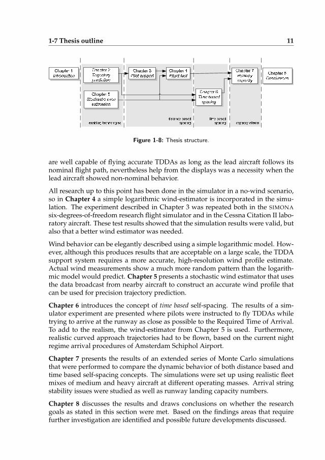
This thesis consists of a number of publications on different aspects of this research.The way in which these papers are related is illustrated in Figure 1-8 and explainedbelow.
In the concept of self-spacing it is necessary to have a good estimate of the speed-and altitude profiles of the leading aircraft. In Chapter 2 a trajectory predictionalgorithm is introduced that is based on ADS-B position reports and aircraft intentinformation. This algorithm stands at the very basis of the work presented in therest of the chapters.
Chapter 3 presents a pilot support interface that was developed to assist the flightcrew in flying a TDDA, while simultaneously controlling the spacing with the leadaircraft. Tests of this interface in the fixed-base human-machine interface laboratoryof the Control and Simulation section, showed that, while experienced airline pilots
1-7 Thesis outline 11
Figure 1-8: Thesis structure.
are well capable of flying accurate TDDAs as long as the lead aircraft follows itsnominal flight path, nevertheless help from the displays was a necessity when thelead aircraft showed non-nominal behavior.
All research up to this point has been done in the simulator in a no-wind scenario,so in Chapter 4 a simple logarithmic wind-estimator is incorporated in the simu-lation. The experiment described in Chapter 3 was repeated both in the SIMONA
six-degrees-of-freedom research flight simulator and in the Cessna Citation II labo-ratory aircraft. These test results showed that the simulation results were valid, butalso that a better wind estimator was needed.
Wind behavior can be elegantly described using a simple logarithmic model. How-ever, although this produces results that are acceptable on a large scale, the TDDAsupport system requires a more accurate, high-resolution wind profile estimate.Actual wind measurements show a much more random pattern than the logarith-mic model would predict. Chapter 5 presents a stochastic wind estimator that usesthe data broadcast from nearby aircraft to construct an accurate wind profile thatcan be used for precision trajectory prediction.
Chapter 6 introduces the concept of time based self-spacing. The results of a sim-ulator experiment are presented where pilots were instructed to fly TDDAs whiletrying to arrive at the runway as close as possible to the Required Time of Arrival.To add to the realism, the wind-estimator from Chapter 5 is used. Furthermore,realistic curved approach trajectories had to be flown, based on the current nightregime arrival procedures of Amsterdam Schiphol Airport.
Chapter 7 presents the results of an extended series of Monte Carlo simulationsthat were performed to compare the dynamic behavior of both distance based andtime based self-spacing concepts. The simulations were set up using realistic fleetmixes of medium and heavy aircraft at different operating masses. Arrival stringstability issues were studied as well as runway landing capacity numbers.
Chapter 8 discusses the results and draws conclusions on whether the researchgoals as stated in this section were met. Based on the findings areas that requirefurther investigation are identified and possible future developments discussed.
12 REFERENCES
References
[1] Resolutions Adopted by the Assembly and Index to Documentation, 16th Ses-sion of the Assembly. Technical Report Doc 8779/A16-RES, International CivilAviation Organization (ICAO), Buenos Aires, Argentina, Sep 1968.
[2] ICAO News Release, Major Progress Made towards Solution to Aircraft NoiseProblems. Montreal, Canada, Nov 24 1969.
[3] Minimum Aviation System Performance Standards for Automatic DependentSurveillance Broadcast (ADS-B). Technical Report RTCA/DO-242, RTCA, Inc.,Washington DC, USA, Feb 1998.
[4] Resolutions Adopted by the Assembly and Index to Documentation, 33rd Ses-sion of the Assembly. Technical report, International Civil Aviation Organiza-tion (ICAO), Montreal, Canada, Sep 25 - Oct 5 2001.
[5] Procedures for Air Navigation Services - Aircraft Operations, Volume 1 - FlightProcedures. Technical Report Doc 8168-Ops/611, International Civil AviationOrganization (ICAO), Oct 2006.
[6] Sourdine II, Final Report. Technical Report D9-1, National Aerospace Labora-tory (NLR), Aug 31 2006.
[7] Annex 16 to the Convention on International Civil Aviation: EnvironmentalProtection, Volume 1 - Aircraft Noise. Technical Report AN16-1, InternationalCivil Aviation Organization (ICAO), Jul 2008.
[8] Guidance on the Balanced Approach to Aircraft Noise Management. Tech-nical Report Doc 9829-AN/451, Second Edition, International Civil AviationOrganization (ICAO), 2008.
[9] SESAR Master Plan-Deliverable 5. Technical Report DLM-0710-001-02-00,SESAR Consortium, Apr 2008.
[10] FAA’s NextGen Implementation Plan. Technical report, Federal Aviation Ad-ministration (FAA), Mar 2010.
[11] J.-P. Clarke. A Systems Analysis Methodology for Developing Single Event NoiseAbatement Procedures. Sc.D. Dissertation, Massachusetts Institute of Technol-ogy, Cambridge (MA), USA, 1997.
[12] R. A. Coppenbarger, R. W. Mead, and D.N. Sweet. Field Evaluation ofthe Tailored Arrivals Concept for Datalink-Enabled Continuous Descent Ap-proaches. In AIAA Aviation Technology, Integration and Operations Conference(ATIO), number AIAA-2007-7778, Belfast, Northern Ireland, Sep 18-20 2007.
13
[13] J. C. M. de Groot, M. Mulder, and M. M. van Paassen. Distance-Based Self-Spacing in Arrival Streams. In Proceedings of the AIAA Guidance, Navigation,and Control Conference, number 2005-6275, San Francisco (CA), USA, Aug 15-18 2005.
[14] J. L. de Prins, K. F. M. Schippers, M. Mulder, M. M. van Paassen, A. C. in ‘t Veld,and J.-P. Clarke. Enhanced Self-Spacing Algorithm for Three-Degree Deceler-ating Approaches. AIAA Journal of Guidance, Control & Dynamics, 30(5):576–590, Mar-Apr 2007.
[15] E. Dinges. Determining the Environmental Benefit of Implementing Continu-ous Descent Approach Procedures. In 7th USA/Europe Air Traffic ManagementR&D Seminar (ATM 2007), Barcelona, Spain, July 2-5 2007.
[16] L. J. J. Erkelens. Research on Noise Abatement Procedures. Technical Re-port NLR TP 98066, National Aerospace Laboratory (NLR), Amsterdam, TheNetherlands, Feb 1998.
[17] L. J. J. Erkelens. Development of Noise Abatement Procedures in The Nether-lands. Technical Report NLR TP 99386, National Aerospace Laboratory (NLR),Amsterdam, The Netherlands, Nov 1999.
[18] N. T. Ho and J.-P. Clarke. Mitigating Operational Aircraft Noise Impact byLeveraging on Automation Capability. In Proceedings of the AIAA Aircraft, Tech-nology, Integration and Operations Forum, number AIAA 2001-5239, pages 1–8,Los Angeles (CA), USA, Oct 16-18 2001.
[19] J. E. Penner, D. H. Lister, D. J. Griggs, D. J. Dokken, and M. McFarland. Avi-ation and the Global Atmosphere. Technical report, Intergovernmental Panelon Climate Change (IPCC), Cambridge, UK, Jun 1999.
[20] L. Ren, J.-P. Clarke, and N. T. Ho. Achieving Low Approach Noise withoutSacrifying Capacity. In 22nd Digital Avionics Systems Conference, number AIAA-2001-5239, pages 1–9, Indianapolis (IN), USA, Oct 12-16 2003.
[21] I. Wilson and F. Hafner. Benefit Assessment of Using Continuous DescentApproaches at Atlanta. In Digital Avionics Systems Conference, volume 1, pages2.B.2– 2.1–7, Washington DC, USA, Oct 30-Nov 3 2005.
[22] F. J. M. Wubben and J. J. Bussink. Environmental Benefits of ContinuousDescent Approaches at Schiphol Airport Compared with Conventional Ap-proach Procedures. Technical Report NLR-TP-2000-275, National AerospaceLaboratory (NLR), Amsterdam, The Netherlands, May 2000.

14
2
Trajectory Prediction
Trajectory Prediction for Self Separation During Decelerating Approaches in aData-link Environment
A.C. in ’t Veld and J.-P. Clarke
Proceedings of AIAA conference on Aircraft Technology, Integration and Opera-tions (ATIO), AIAA 2002-5887, Los Angeles, 2002
2-1 Abstract
Previous research on aircraft noise abatement has resulted in a few promising flightprocedures, such as the 3◦ decelerating approach (TDDA), that reduce the noise im-pact of aircraft operations on the community. The TDDA procedure incorporatesan approach flown at a constant glide path angle with idle thrust resulting in asignificant reduction of the noise footprint. The primary difficulty with deceler-ating approaches however is that different types of aircraft have different rates ofdeceleration. Thus, air traffic controllers are unable to estimate the separation be-tween two consecutive aircraft that is necessary at the beginning of the approachto insure safe in trail separation throughout the entire procedure, and they add abuffer to the required separation to compensate for this uncertainty. Actual im-plementation of a similar procedure at Amsterdam Schiphol airport and LondonHeathrow has shown a reduction of airport landing capacity of nearly 50%. Oneway to minimize the noise impact while maximizing aircraft throughput might beto delegate the task of separating the aircraft during the approach to the pilot, i.e.to instruct the pilot to maintain a certain separation from the preceding aircraftwhile the controller assumes a monitoring role. New airborne surveillance equip-ment such automatic dependant surveillance broadcast (ADS-B) will increase thelevel of traffic information available in the cockpit, in particular the ground- and
16 Trajectory Prediction
air-vectors of all aircraft in the vicinity will be available to the flight managementsystem (FMS). This paper discusses how this information can be used to predict thetrajectory of the preceding aircraft and how this information when combined withan own aircraft trajectory calculation can be used for self-separation purposes.
2-2 Introduction
The impact of aircraft noise on residential communities near airports is an increas-ing impediment to the expansion of airports around the world. This is particularlytrue in Europe where the impact of airport noise on the community has reachedthe point where it threatens to limit and in some cases actually does restrict airportcapacity growth.
It has been shown that improvements are possible particularly in the approachphase of a flight.1, 2, 4, 5 In the terminal maneuvering area (TMA) the current prac-tice is to slow aircraft down and have them descent to low altitudes of 2,000 to 3,000feet relatively far from the runway to sequence them for final approach. Due to thelow speeds, aircraft typically fly with their flaps partial extended, which meansthey have to use higher thrust settings to offset the flap-induced drag. The combi-nation of slow speeds and low altitudes are very detrimental to the aircraft noiseimpact. Thus, significant reductions in aircraft approach noise are possible if theaircraft stay at higher altitudes and fly faster as long as possible. With these obser-vations in mind several advanced noise abatement procedures (ANAPs) have beendeveloped. Examples include the 3◦ decelerating approach (TDDA), the continu-ous descent approach (CDA), the advanced CDA (ACDA) and the low power lowdrag approach (LPLDA) . The features common to all these procedures are that theaircraft descend to the runway at low or idle thrust, with no level flight segmentsthus significantly reducing the noise impact on the community.
In this paper it is assumed that the aircraft are flying the TDDA, which requiresthe aircraft to descend from 7,000 feet and follow a three degree glide-path to therunway at idle thrust. The aircraft start out at a speed of 250 knots and decelerate asthey descend to the runway due to aerodynamic drag, all the while optimizing themoments of flap selection in order to reach the final approach speed at 1,000 feetabove the runway. At the 1,000 feet point thrust is then added to maintain the finalapproach speed and the aircraft then continues for a normal flare and touchdown.
One key issue with the TDDA is that air traffic controllers (ATC) find it very difficultto space consecutive aircraft during a decelerating approach. Actual implementa-tion of the CDA at Amsterdam’s Schiphol airport has resulted in a reduction inlanding capacity of nearly 50%, thus limiting use of this procedure to the low trafficdensity hours of the night.4, 5 The problem lies in the fact that different aircraft willhave different deceleration characteristics, which makes it very hard for controllersto estimate the initial separation necessary to ensure safe separation throughout theentire procedure. As can be seen in Figures 2-2 and 2-3, for the case of a Boeing 747
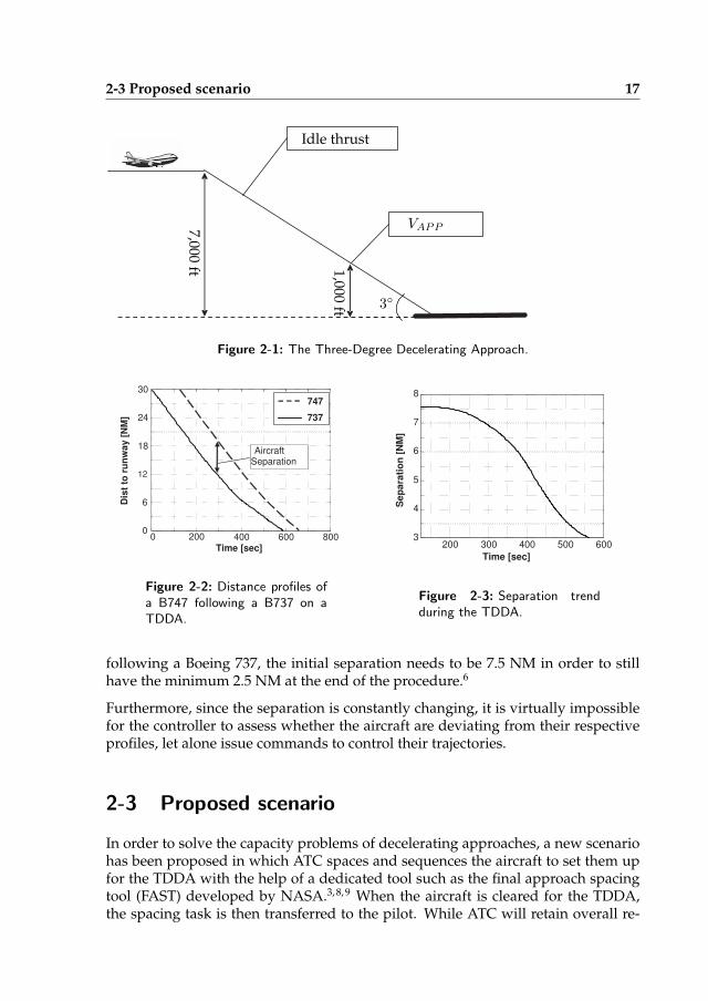
2-3 Proposed scenario 17
Idle thrust
VAPP
3◦
1,000ft
7,000ft
Figure 2-1: The Three-Degree Decelerating Approach.
0 200 400 600 800 0
6
12
18
24
30
Dis
t to
ru
nw
ay
[N
M]
Time [sec]
Aircraft Separation
747
737
Figure 2-2: Distance profiles ofa B747 following a B737 on aTDDA.
200 300 400 500 600 3
4
5
6
7
8
Time [sec]
Sep
ara
tio
n [
NM
]
Figure 2-3: Separation trendduring the TDDA.
following a Boeing 737, the initial separation needs to be 7.5 NM in order to stillhave the minimum 2.5 NM at the end of the procedure.6
Furthermore, since the separation is constantly changing, it is virtually impossiblefor the controller to assess whether the aircraft are deviating from their respectiveprofiles, let alone issue commands to control their trajectories.
2-3 Proposed scenario
In order to solve the capacity problems of decelerating approaches, a new scenariohas been proposed in which ATC spaces and sequences the aircraft to set them upfor the TDDA with the help of a dedicated tool such as the final approach spacingtool (FAST) developed by NASA.3, 8, 9 When the aircraft is cleared for the TDDA,the spacing task is then transferred to the pilot. While ATC will retain overall re-
18 Trajectory Prediction
A
B
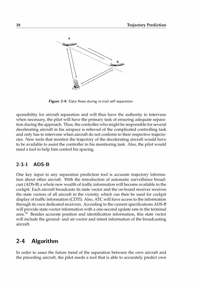
Figure 2-4: Data flows during in-trail self separation.
sponsibility for aircraft separation and will thus have the authority to intervenewhen necessary, the pilot will have the primary task of ensuring adequate separa-tion during the approach. Thus, the controller who might be responsible for severaldecelerating aircraft in his airspace is relieved of the complicated controlling taskand only has to intervene when aircraft do not conform to their respective trajecto-ries. New tools that monitor the trajectory of the decelerating aircraft would haveto be available to assist the controller in his monitoring task. Also, the pilot wouldneed a tool to help him control his spacing.
2-3-1 ADS-B
One key input to any separation prediction tool is accurate trajectory informa-tion about other aircraft. With the introduction of automatic surveillance broad-cast (ADS-B) a whole new wealth of traffic information will become available in thecockpit. Each aircraft broadcasts its state vector and the on-board receiver receivesthe state vectors of all aircraft in the vicinity, which can then be used for cockpitdisplay of traffic information (CDTI). Also, ATC will have access to the informationthrough its own dedicated receivers. According to the current specifications ADS-Bwill provide state-vector information with a one-second update rate in the terminalarea.10 Besides accurate position and identification information, this state vectorwill include the ground- and air-vector and intent information of the broadcastingaircraft.
2-4 Algorithm
In order to asses the future trend of the separation between the own aircraft andthe preceding aircraft, the pilot needs a tool that is able to accurately predict own
2-5 Least Square Estimate 19
aircraft trajectory as well as the trajectory of the leading aircraft. Comparison ofthese two trajectories then yields the separation trend. Previous research has shownthat it is possible to predict own aircraft trajectory with adequate accuracy using arelatively simple aerodynamic model of the aircraft.7 However, using such a modelto predict the future trajectory of the preceding aircraft during the TDDA wouldrequire an elaborate database of aerodynamic data for all common airliners. Tocircumvent the need for such a database, we have developed an algorithm thatwould predict the future speed- and position-profile based on ADS-B data alone.
2-4-1 Wind model
Since wind can significantly influence the trajectories of aircraft, accurate wind datais required for accurate trajectory prediction. It is assumed that very accurate winddata will be available in the cockpit as each ADS-B equipped aircraft will be trans-mitting its ground- and air-vector. Combining these two vectors yields the wind-vector, so each aircraft that has completed the TDDA procedure will essentiallyhave broadcast a complete wind profile for the approach path. Every consecutiveaircraft will update this profile, so a very accurate average wind profile will thus beavailable to the separation algorithm. With enough data even a trend in the windprofile could be incorporated into the calculations.
In order to test the robustness of the algorithm under realistic wind conditions, awind model was introduced to the simulations, consisting of a basic aerodynamicboundary layer model. White noise variations were added to this model to capturethe uncertainties of turbulence. All the simulations were run under two conditions;a no wind scenario and a scenario where the wind model was introduced. In thelatter case the prediction algorithm had knowledge of the nominal wind profile,but not of the white noise variations.
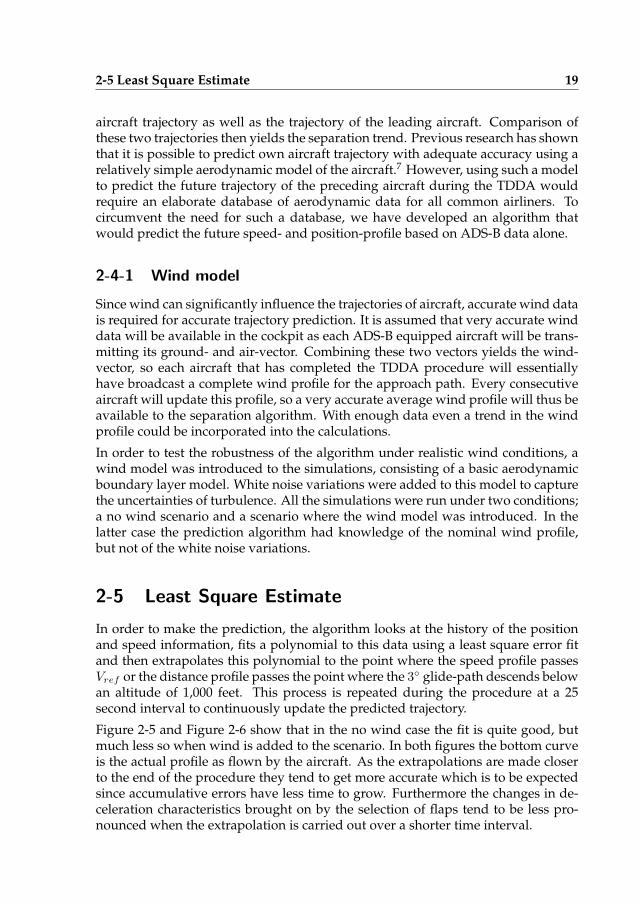
2-5 Least Square Estimate
In order to make the prediction, the algorithm looks at the history of the positionand speed information, fits a polynomial to this data using a least square error fitand then extrapolates this polynomial to the point where the speed profile passesVref or the distance profile passes the point where the 3◦ glide-path descends belowan altitude of 1,000 feet. This process is repeated during the procedure at a 25second interval to continuously update the predicted trajectory.
Figure 2-5 and Figure 2-6 show that in the no wind case the fit is quite good, butmuch less so when wind is added to the scenario. In both figures the bottom curveis the actual profile as flown by the aircraft. As the extrapolations are made closerto the end of the procedure they tend to get more accurate which is to be expectedsince accumulative errors have less time to grow. Furthermore the changes in de-celeration characteristics brought on by the selection of flaps tend to be less pro-nounced when the extrapolation is carried out over a shorter time interval.
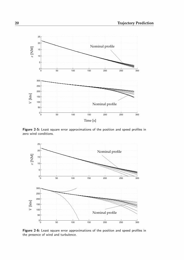
20 Trajectory Prediction
0 50 100 150 200 250 3000
5
10
15
20
25
0 50 100 150 200 250 3000
50
100
150
200
250
300
V[k
ts]
x[N
M] Nominal profile
Nominal profile
Time [s]
Figure 2-5: Least square error approximations of the position and speed profiles inzero wind conditions.
0 50 100 150 200 250 3000
5
10
15
20
25
0 50 100 150 200 250 3000
50
100
150
200
250
300
V[k
ts]
x[N
M]
Nominal profile
Nominal profile
Figure 2-6: Least square error approximations of the position and speed profiles inthe presence of wind and turbulence.
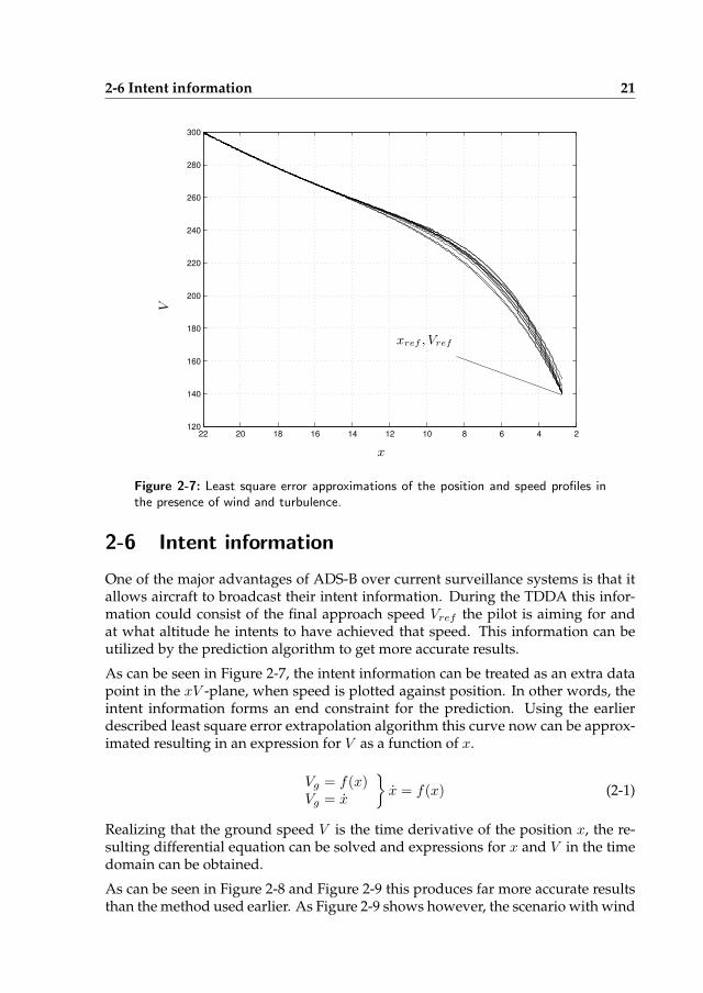
2-6 Intent information 21
246810121416182022120
140
160
180
200
220
240
260
280
300
V
x
xref , Vref
Figure 2-7: Least square error approximations of the position and speed profiles inthe presence of wind and turbulence.
2-6 Intent information
One of the major advantages of ADS-B over current surveillance systems is that itallows aircraft to broadcast their intent information. During the TDDA this infor-mation could consist of the final approach speed Vref the pilot is aiming for andat what altitude he intents to have achieved that speed. This information can beutilized by the prediction algorithm to get more accurate results.
As can be seen in Figure 2-7, the intent information can be treated as an extra datapoint in the xV -plane, when speed is plotted against position. In other words, theintent information forms an end constraint for the prediction. Using the earlierdescribed least square error extrapolation algorithm this curve now can be approx-imated resulting in an expression for V as a function of x.
Vg = f(x)Vg = x
}
x = f(x) (2-1)
Realizing that the ground speed V is the time derivative of the position x, the re-sulting differential equation can be solved and expressions for x and V in the timedomain can be obtained.
As can be seen in Figure 2-8 and Figure 2-9 this produces far more accurate resultsthan the method used earlier. As Figure 2-9 shows however, the scenario with wind
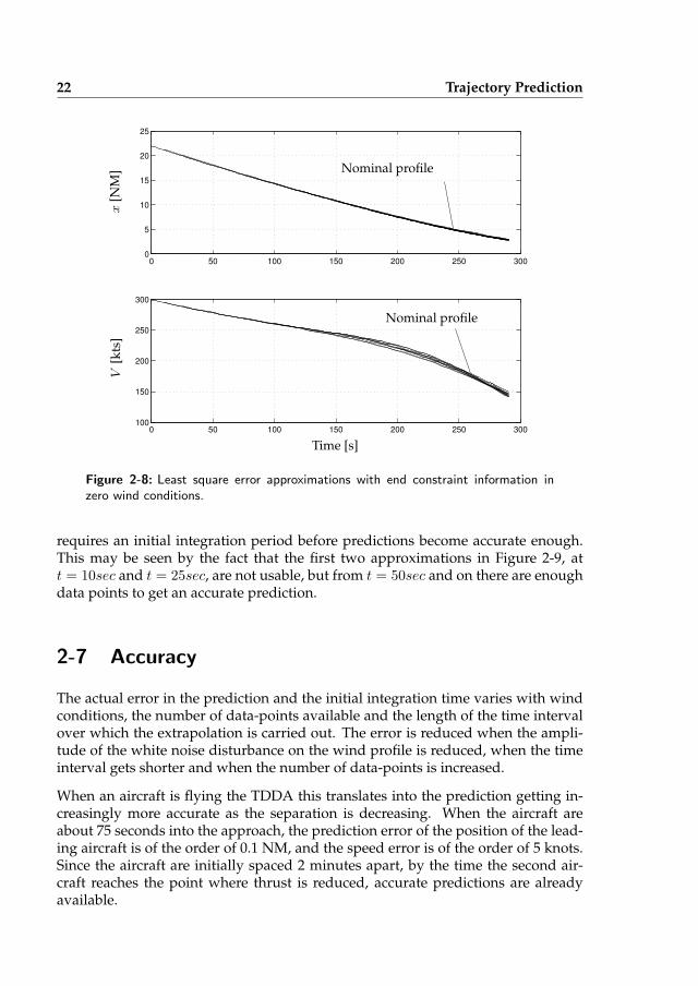
22 Trajectory Prediction
0 50 100 150 200 250 3000
5
10
15
20
25
0 50 100 150 200 250 300100
150
200
250
300
V[k
ts]
x[N
M]
Nominal profile
Nominal profile
Time [s]
Figure 2-8: Least square error approximations with end constraint information inzero wind conditions.
requires an initial integration period before predictions become accurate enough.This may be seen by the fact that the first two approximations in Figure 2-9, att = 10sec and t = 25sec, are not usable, but from t = 50sec and on there are enoughdata points to get an accurate prediction.
2-7 Accuracy
The actual error in the prediction and the initial integration time varies with windconditions, the number of data-points available and the length of the time intervalover which the extrapolation is carried out. The error is reduced when the ampli-tude of the white noise disturbance on the wind profile is reduced, when the timeinterval gets shorter and when the number of data-points is increased.
When an aircraft is flying the TDDA this translates into the prediction getting in-creasingly more accurate as the separation is decreasing. When the aircraft areabout 75 seconds into the approach, the prediction error of the position of the lead-ing aircraft is of the order of 0.1 NM, and the speed error is of the order of 5 knots.Since the aircraft are initially spaced 2 minutes apart, by the time the second air-craft reaches the point where thrust is reduced, accurate predictions are alreadyavailable.
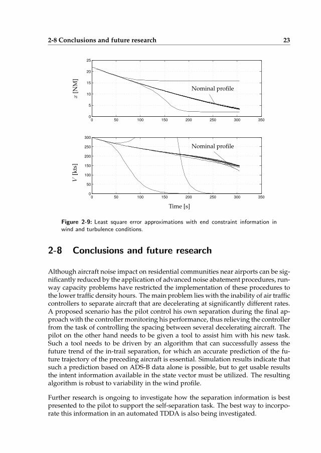
2-8 Conclusions and future research 23
0 50 100 150 200 250 300 3500
5
10
15
20
25
0 50 100 150 200 250 300 3500
50
100
150
200
250
300
V[k
ts]
x[N
M]
Nominal profile
Nominal profile
Time [s]
Figure 2-9: Least square error approximations with end constraint information inwind and turbulence conditions.
2-8 Conclusions and future research
Although aircraft noise impact on residential communities near airports can be sig-nificantly reduced by the application of advanced noise abatement procedures, run-way capacity problems have restricted the implementation of these procedures tothe lower traffic density hours. The main problem lies with the inability of air trafficcontrollers to separate aircraft that are decelerating at significantly different rates.A proposed scenario has the pilot control his own separation during the final ap-proach with the controller monitoring his performance, thus relieving the controllerfrom the task of controlling the spacing between several decelerating aircraft. Thepilot on the other hand needs to be given a tool to assist him with his new task.Such a tool needs to be driven by an algorithm that can successfully assess thefuture trend of the in-trail separation, for which an accurate prediction of the fu-ture trajectory of the preceding aircraft is essential. Simulation results indicate thatsuch a prediction based on ADS-B data alone is possible, but to get usable resultsthe intent information available in the state vector must be utilized. The resultingalgorithm is robust to variability in the wind profile.
Further research is ongoing to investigate how the separation information is bestpresented to the pilot to support the self-separation task. The best way to incorpo-rate this information in an automated TDDA is also being investigated.
24 Trajectory Prediction
References
[1] J.-P. Clarke. Systems Analysis of Noise Abatement Procedures Enabled byAdvanced Flight Guidance Technology. Journal of Aircraft, 37, no. 2(AIAA 97-0490), Mar-Apr 2000.
[2] J.-P. Clarke and R. J. Hansman. A Systems Analysis Methodology for Devel-oping Single Event Noise Abatement Procedures. Technical Report ASL-97-1,MIT - Aeronautical Systems Laboratory, Cambridge (MA), USA, Jan 1997.
[3] T. J. Davis, K. J. Krzeczowski, and C. Bergh. The Final Approach Spacing Tool.In 13th IFAC Symposium on Automatic Control in Aerospace, Palo Alto (CA), USA,Sep 1994.
[4] L. J. J. Erkelens. Research on Noise Abatement Procedures. Technical Re-port NLR TP 98066, National Aerospace Laboratory (NLR), Amsterdam, TheNetherlands, Feb 1998.
[5] L. J. J. Erkelens. Development of Noise Abatement Procedures in The Nether-lands. Technical Report NLR TP 99386, National Aerospace Laboratory (NLR),Amsterdam, The Netherlands, Nov 1999.
[6] N. T. Ho and J.-P. Clarke. Mitigating Operational Aircraft Noise Impact byLeveraging on Automation Capability. In AIAA 1st Aircraft, Technology Inte-gration, and Operations Forum (ATIO), number AIAA-2001-5239, Cambridge,UK, 2001.
[7] M. F. Koeslag. Advanced Continuous Approaches, an Algorithm Design forthe Flight Management System. Technical Report NLR-TR-2001-359, NationalAerospace Laboratory (NLR), Amsterdam, The Netherlands, Mar 1999.
[8] K. K. Lee and T. J. Davis. The Development of the Final Approach SpacingTool (FAST): A Cooperative Controller-Engineer Design Approach. Journal ofControl Engineering Practice, 4(8):1161–1168, Aug 1996.
[9] C. Quinn and J. E. Robertson III. A Human Factors Evaluation of Active FinalApproach Spacing Tool Concepts. In 3rd USA/Europe Air Traffic ManagementR&D Seminar, Napoli, Italy, Jun 2000.
[10] RTCA, Inc., Washington, USA. Minimum Aviation System Performance Standardsfor Automatic Dependent Surveillance Broadcast (ADS-B), Feb 1998.
3
Pilot Support Interface
Pilot Support Interface for Three-degree Decelerating Approach Procedures
A.C. in ’t Veld, M. Mulder, M.M. van Paassen and J.-P. Clarke
The International Journal of Aviation Psychology, Vol. 19. No. 3, July 2009, Pages 287-308
3-1 Abstract
Previous research on aircraft noise abatement has resulted in some promising flightprocedures to mitigate noise impact, such as the three-degree decelerating ap-proach (TDDA). A problem with decelerating approaches, however, is that theytypically lead to increased spacing, which in turn results in a significant reductionof runway landing capacity. A possible solution to this problem might be to del-egate the task of separating the aircraft during the approach to the pilot. To aidthe pilot, an algorithm has been developed that predicts the trajectory of the pre-ceding aircraft and optimizes the flap schedule based on this prediction. Off-linesimulations indicate that using this system runway throughput numbers of up to98% of the capacity of a conventional instrument landing system (ILS) approachcan be achieved.18 To assess practical implementation issues and to investigate pi-lot appreciation, a piloted experiment was conducted, for which a pilot supportinterface has been developed that presents the future separation information in anintuitive fashion. The experiment showed that it is indeed possible for pilots toperform the spacing task while flying a TDDA. The pilot support interface signifi-cantly reduces pilot workload when compared to a baseline display. Also the effectsof off-nominal lead pilot behavior on pilot performance are reduced by the use ofonline flap schedule optimization and separation prediction.
26 Pilot Support Interface
The impact of aircraft noise on residential communities near major airports isan impediment to the expansion of airports around the world. At a number ofairports the impact of airport noise on the community has reached the point whereit threatens to and in some cases actually does restrict airport capacity growth.Current practice for aircraft approaching an airport for landing is to slowdownand descend to low altitudes between 2,000 and 3,000 ft relatively far from therunway to sequence for final approach. Due to the low speeds, aircraft typicallyfly with the flaps partially extended, requiring higher thrust settings to offset theflap-induced drag. This mode of operation is very detrimental to the aircraft noiseimpact. Thus, significant noise reductions seem possible if the aircraft would stayat higher altitudes and keep the speed up as long as possible.
With these observations in mind, several advanced noise abatement proce-dures (ANAPs) have been developed. Examples include the three-degree deceler-ating approach (TDDA), the (advanced) continuous descent approach ((A)CDA)and the low-power-low-drag approach.2, 3, 7, 8, 13 The features common to all theseprocedures are that the aircraft descend to the runway at low or idle thrust withno level flight segments, thus significantly reducing the noise impact on thecommunity.
Although successful in reducing noise, runway capacity problems have restrictedthe implementation of the noise abatement procedures to the lower traffic densityhours. The main problem lies with the inability of air traffic controllers to separateaircraft that are decelerating at significantly different rates. The major contributorsto the variability of the aircraft trajectories are the aerodynamic properties of theaircraft type, the current flight mass, pilot intent, and the wind conditions. Con-trollers typically start applying larger separations between aircraft to compensatefor these uncertainties, resulting in fewer aircraft being handled per hour.7, 13
On board the aircraft, knowledge about the aircraft’s aerodynamic properties,current flight mass, and pilot intent is readily available. Hence, smaller separationdistances seem possible when the spacing task is delegated to the pilot, relievingthe controller from the task of controlling the spacing between several deceleratingaircraft. Before the separation task can be transferred to the flight deck, two itemsneed to be addressed. Although the necessary information is in itself available onthe flight deck, this information needs to be integrated first to be able to accuratelypredict the approach trajectory and speed profile to allow the flight crew toconsistently and predictably fly the decelerating approach in varying operationalconditions. Furthermore, support must be given to the pilots to be able to performthe self-separation task. For the self-spacing task, cockpit displays are needed thatexceed the capabilities of current airborne collision avoidance systems.
This article describes the design and evaluation of a pilot support interface that
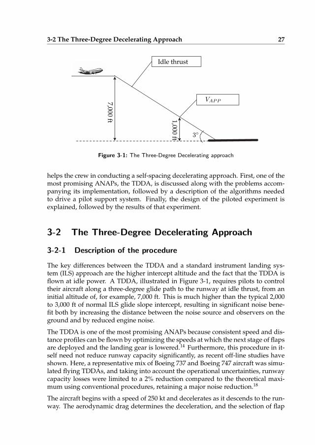
3-2 The Three-Degree Decelerating Approach 27
Idle thrust
VAPP
3◦1,000
ft
7,000ft
Figure 3-1: The Three-Degree Decelerating approach
helps the crew in conducting a self-spacing decelerating approach. First, one of themost promising ANAPs, the TDDA, is discussed along with the problems accom-panying its implementation, followed by a description of the algorithms neededto drive a pilot support system. Finally, the design of the piloted experiment isexplained, followed by the results of that experiment.
3-2 The Three-Degree Decelerating Approach
3-2-1 Description of the procedure
The key differences between the TDDA and a standard instrument landing sys-tem (ILS) approach are the higher intercept altitude and the fact that the TDDA isflown at idle power. A TDDA, illustrated in Figure 3-1, requires pilots to controltheir aircraft along a three-degree glide path to the runway at idle thrust, from aninitial altitude of, for example, 7,000 ft. This is much higher than the typical 2,000to 3,000 ft of normal ILS glide slope intercept, resulting in significant noise bene-fit both by increasing the distance between the noise source and observers on theground and by reduced engine noise.
The TDDA is one of the most promising ANAPs because consistent speed and dis-tance profiles can be flown by optimizing the speeds at which the next stage of flapsare deployed and the landing gear is lowered.14 Furthermore, this procedure in it-self need not reduce runway capacity significantly, as recent off-line studies haveshown. Here, a representative mix of Boeing 737 and Boeing 747 aircraft was simu-lated flying TDDAs, and taking into account the operational uncertainties, runwaycapacity losses were limited to a 2% reduction compared to the theoretical maxi-mum using conventional procedures, retaining a major noise reduction.18
The aircraft begins with a speed of 250 kt and decelerates as it descends to the run-way. The aerodynamic drag determines the deceleration, and the selection of flap
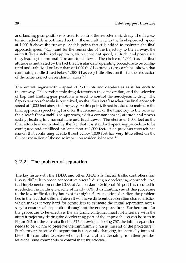
28 Pilot Support Interface
and landing gear positions is used to control the aerodynamic drag. The flap ex-tension schedule is optimized so that the aircraft reaches the final approach speedat 1,000 ft above the runway. At this point, thrust is added to maintain the finalapproach speed (Vapp) and for the remainder of the trajectory to the runway, theaircraft flies a stabilized approach, with a constant speed, attitude, and power set-ting, leading to a normal flare and touchdown. The choice of 1,000 ft as the finalaltitude is motivated by the fact that it is standard operating procedure to be config-ured and stabilized no later than at 1,000 ft. Also previous research has shown thatcontinuing at idle thrust below 1,000 ft has very little effect on the further reductionof the noise impact on residential areas.3, 7
The aircraft begins with a speed of 250 knots and decelerates as it descends tothe runway. The aerodynamic drag determines the deceleration, and the selectionof flap and landing gear positions is used to control the aerodynamic drag. Theflap extension schedule is optimized, so that the aircraft reaches the final approachspeed at 1,000 feet above the runway. At this point, thrust is added to maintain thefinal approach speed (Vapp) and for the remainder of the trajectory to the runway,the aircraft flies a stabilized approach, with a constant speed, attitude and powersetting, leading to a normal flare and touchdown. The choice of 1,000 feet as thefinal altitude is motivated by the fact that it is standard operating procedure to beconfigured and stabilized no later than at 1,000 feet. Also previous research hasshown that continuing at idle thrust below 1,000 feet has very little effect on thefurther reduction of the noise impact on residential aereas.3, 7
3-2-2 The problem of separation
The key issue with the TDDA and other ANAPs is that air traffic controllers findit very difficult to space consecutive aircraft during a decelerating approach. Ac-tual implementation of the CDA at Amsterdam’s Schiphol Airport has resulted ina reduction in landing capacity of nearly 50%, thus limiting use of this procedureto the low-traffic-density hours of the night.7, 8 As mentioned earlier, the problemlies in the fact that different aircraft will have different deceleration characteristics,which makes it very hard for controllers to estimate the initial separation neces-sary to ensure safe separation throughout the entire procedure. Furthermore, forthe procedure to be effective, the air traffic controller must not interfere with theaircraft trajectory during the decelerating part of the approach. As can be seen inFigure 3-2, for the case of a Boeing 747 following a Boeing 737, the initial separationneeds to be 7.5 nm to preserve the minimum 2.5 nm at the end of the procedure.10
Furthermore, because the separation is constantly changing, it is virtually impossi-ble for the controller to assess whether the aircraft are deviating from their profiles,let alone issue commands to control their trajectories.
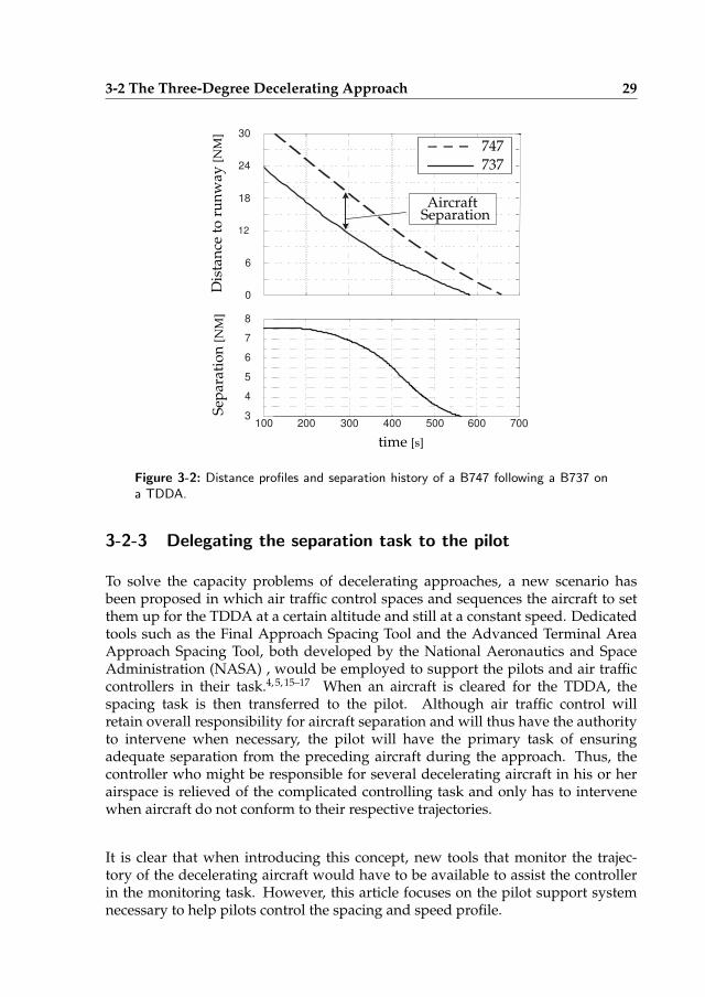
3-2 The Three-Degree Decelerating Approach 29
0
6
12
18
24
30
3
4
5
6
7
8
200 300 400 500 600 700 100
747
737
Dis
tan
ceto
run
way
[NM
]
time [s]
Sep
arat
ion
[NM
]
AircraftSeparation
Figure 3-2: Distance profiles and separation history of a B747 following a B737 ona TDDA.
3-2-3 Delegating the separation task to the pilot
To solve the capacity problems of decelerating approaches, a new scenario hasbeen proposed in which air traffic control spaces and sequences the aircraft to setthem up for the TDDA at a certain altitude and still at a constant speed. Dedicatedtools such as the Final Approach Spacing Tool and the Advanced Terminal AreaApproach Spacing Tool, both developed by the National Aeronautics and SpaceAdministration (NASA) , would be employed to support the pilots and air trafficcontrollers in their task.4, 5, 15–17 When an aircraft is cleared for the TDDA, thespacing task is then transferred to the pilot. Although air traffic control willretain overall responsibility for aircraft separation and will thus have the authorityto intervene when necessary, the pilot will have the primary task of ensuringadequate separation from the preceding aircraft during the approach. Thus, thecontroller who might be responsible for several decelerating aircraft in his or herairspace is relieved of the complicated controlling task and only has to intervenewhen aircraft do not conform to their respective trajectories.
It is clear that when introducing this concept, new tools that monitor the trajec-tory of the decelerating aircraft would have to be available to assist the controllerin the monitoring task. However, this article focuses on the pilot support systemnecessary to help pilots control the spacing and speed profile.
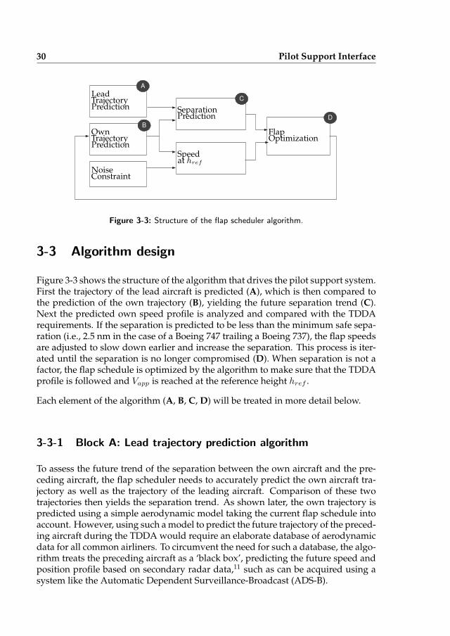
30 Pilot Support Interface
A
B
C
D
LeadTrajectory
Trajectory OptimizationFlapOwn
NoiseConstraint
Separation
Speedat href
Prediction
Prediction
Prediction
Figure 3-3: Structure of the flap scheduler algorithm.
3-3 Algorithm design
Figure 3-3 shows the structure of the algorithm that drives the pilot support system.First the trajectory of the lead aircraft is predicted (A), which is then compared tothe prediction of the own trajectory (B), yielding the future separation trend (C).Next the predicted own speed profile is analyzed and compared with the TDDArequirements. If the separation is predicted to be less than the minimum safe sepa-ration (i.e., 2.5 nm in the case of a Boeing 747 trailing a Boeing 737), the flap speedsare adjusted to slow down earlier and increase the separation. This process is iter-ated until the separation is no longer compromised (D). When separation is not afactor, the flap schedule is optimized by the algorithm to make sure that the TDDAprofile is followed and Vapp is reached at the reference height href .
Each element of the algorithm (A, B, C, D) will be treated in more detail below.
3-3-1 Block A: Lead trajectory prediction algorithm
To assess the future trend of the separation between the own aircraft and the pre-ceding aircraft, the flap scheduler needs to accurately predict the own aircraft tra-jectory as well as the trajectory of the leading aircraft. Comparison of these twotrajectories then yields the separation trend. As shown later, the own trajectory ispredicted using a simple aerodynamic model taking the current flap schedule intoaccount. However, using such a model to predict the future trajectory of the preced-ing aircraft during the TDDA would require an elaborate database of aerodynamicdata for all common airliners. To circumvent the need for such a database, the algo-rithm treats the preceding aircraft as a ‘black box’, predicting the future speed andposition profile based on secondary radar data,11 such as can be acquired using asystem like the Automatic Dependent Surveillance-Broadcast (ADS-B).
3-3 Algorithm design 31
Enabling technology: ADS-B One key input to any separation prediction tool isaccurate trajectory information about other aircraft.With the introduction of ADS-Ba new wealth of traffic information will become available to the pilot. Each aircraftbroadcasts its state vector and the on-board receiver receives the state vectors of allaircraft in the vicinity, which can then be used for cockpit display of traffic infor-mation (CDTI). Also, air traffic control will have access to the information throughits own dedicated receivers. According to the current specifications, ADS-B willprovide state-vector information with a 1-sec update rate in the terminal area (ac-cording to the standards set by the Radio Technical Commission for Aeronautics1).Besides accurate position and identification information, this state vector will in-clude the ground and air vector and intent information of the broadcasting aircraft.During the TDDA the intent information could consist of the final approach speedVapp the pilot is aiming for and at what altitude he or she intends to have achievedthat speed. As shown later, this information can be used by the separation predic-tion algorithm.
Data collection and fitting As the lead aircraft is approaching the runway,decelerating and aiming to reach its Vapp at 1,000 ft, it is broadcasting its statevector every second. These data are received on board the ownship and storedin the flight management system. The trajectory prediction algorithm then fitsa third-order polynomial through the collected position and velocity data usinga leastsquare-error fit. Because sole extrapolation of a higher order polynomialwould lead to unpredictable results, the intent information is used as an extradata point to help the data-fitting process. The intent information is used asfollows: Assuming the intent information consists of the final approach speedVapp of the lead aircraft and altitude href at which the pilot wants to haveachieved that speed, it still is not clear at which time the lead expects to reachhref. In other words, the data still lack a constraint in the time domain. To workaround this problem, first the lead aircraft’s Vapp (indicated airspeed) is cor-rected for altitude and (predicted) wind to get an estimated Vgref (ground speed).Then the lead’s href is combined with the glide path angle γ of the ILS to yield xref .
It is clear from Figure 3-4, where ground speed is plotted against position, thatthe intent information now forms an extra data point in the xV -plane. When aleastsquare-error curve is fitted to this data set, an expression for Vg as a function ofx can now be obtained. Realizing that the Vgref ground speed Vg is the time deriva-tive of the position x, the resulting ordinary differential equation can be solved andexpressions for x and Vg in the time domain can be obtained:
Vg = f(x)Vg = x
}
x = f(x) (3-1)
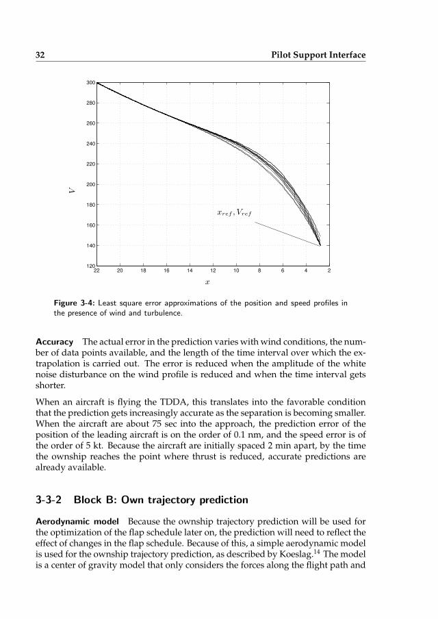
32 Pilot Support Interface
246810121416182022120
140
160
180
200
220
240
260
280
300
V
x
xref , Vref
Figure 3-4: Least square error approximations of the position and speed profiles inthe presence of wind and turbulence.
Accuracy The actual error in the prediction varies with wind conditions, the num-ber of data points available, and the length of the time interval over which the ex-trapolation is carried out. The error is reduced when the amplitude of the whitenoise disturbance on the wind profile is reduced and when the time interval getsshorter.
When an aircraft is flying the TDDA, this translates into the favorable conditionthat the prediction gets increasingly accurate as the separation is becoming smaller.When the aircraft are about 75 sec into the approach, the prediction error of theposition of the leading aircraft is on the order of 0.1 nm, and the speed error is ofthe order of 5 kt. Because the aircraft are initially spaced 2 min apart, by the timethe ownship reaches the point where thrust is reduced, accurate predictions arealready available.
3-3-2 Block B: Own trajectory prediction
Aerodynamic model Because the ownship trajectory prediction will be used forthe optimization of the flap schedule later on, the prediction will need to reflect theeffect of changes in the flap schedule. Because of this, a simple aerodynamic modelis used for the ownship trajectory prediction, as described by Koeslag.14 The modelis a center of gravity model that only considers the forces along the flight path and
3-3 Algorithm design 33
perpendicular to it:
ΣFZ : 0 = L−mgcosγΣFX : mx = T −D +mgsinγ
(3-2)
The lift and drag coefficients are known for the ownship, as are the thrust coeffi-cients, and these can be used to find the acceleration x. The resulting accelerationalong the flight path x is then integrated in time to yield the predicted speed anddistance profiles. A more elaborate treatment of this method can be found in.6
3-3-3 Block C: Separation trend prediction
Now that predictions for both the lead trajectory and the own trajectory are avail-able, a separation trend is readily derived by superpositioning the two distanceprofiles. The minimum predicted separation is then determined by locating theminimum value of the separation trend.
3-3-4 Block D: Flap schedule optimization algorithms
To assist the pilot in the timing of the flap selections, a flap schedule optimizationalgorithm has been developed12, 14 that runs onboard the aircraft and calculates atwhat speed each flap setting should be selected to arrive at the 1,000 ft point at Vapp;refer also to Figure 3-3. This flap scheduler works in one of two modes.
In capture mode, the algorithm calculates the altitude at which the thrust should beset to flight-idle so that the runway can be reached using the nominal flap sched-ule. The corresponding altitude is the thrust-cut altitude. Descending below thisaltitude causes the flap scheduler to switch to hold mode.
In hold mode, the flap scheduling algorithm predicts the own speed profile based onthe current speed and the current flap schedule. When the difference between thepredicted Vapp is more than 2 kt, the flap schedule is adjusted and the model is runagain. This process is repeated until the predicted speed difference is less than 2 kt.
Self-spacing constraint The flap scheduler as presented so far does not, however,provide a means to aid the pilot in his self-spacing task. Therefore the algorithm hasbeen extended to account for the minimum safe separation constraint. The sched-uler optimizes the flap speeds as before, but now also checks whether the predictedown profile will put the ownship too close to the preceding aircraft. When it turnsout that this will be the case, the flap schedule is adjusted until a safe separationcan be assured during the whole approach.
The consequence of such an adjustment is, of course, that the aircraft will deviatefrom the optimal speed profile for the TDDA and therefore it is inevitable that Vapp
34 Pilot Support Interface
will be reached at a higher altitude, thus decreasing the noise benefits of the proce-dure. As shown later, the experiment results indicate that the increase in altitudewill typically be less than 500 ft, so an increase in the produced noise will mostlikely be almost negligible. Only in extreme cases, when the aircraft are sequencedmuch too close, will the altitude at which Vapp is reached increase to higher values,but typically not above 2,500 ft. In these extreme cases the noise impact during thelast 2,000 ft would be comparable to a standard ILS approach, so the noise benefitswould still be worthwhile.
3-4 Pilot support interface design
After the flap schedule has been optimized, the information has to be presentedto the pilot in a meaningful way. To do so, a number of displays were designedwith the following ideas in mind: First, the display should enhance the situationawareness of the pilot in such away that he or she not only knows where he or sheis in relation to the other planes in the vicinity, but also where he or she will be inthe future. Furthermore, the display should support the pilot in his or her task ofaccurately flying the TDDA profile with only flap and gear timing to control his orher speed. Finally, the display should depart as little as possible from current dis-play formats to facilitate pilot acceptance, so a modification of an existing displaybecomes more feasible.
3-4-1 TDDA support
Thrust cue As explained in the previous sections, the first critical pilot action isthe thrust cutback. The altitude at which this should occur as calculated by thealgorithm is presented by a bug on the altitude tape of the primary flight display(PFD) in the form of the letter ‘T’, as represented in Figure 3-5. The thrust cut-back altitude is recalculated every second, updated for the current situation, andpresented in numerical format underneath the altitude tape. In order to provide astable cue, the thrust cut-back altitude is no longer updated when the aircraft hasdescended to within 500 feet of its value.
Flap cue In order to inform the pilot when to select the next stage of flaps a cuewas added to the speed tape of the PFD). This cue consists of the letter F and apointer (see Figure 3-5). In doing so, the pilot has an intuitive display of the dif-ference between his or her current speed and the optimal speed for his or her nextstage of flaps, which in turn give the pilot an indication of the time left before hisor her next required action without the need for displaying the numerical value ofthe flap speed.
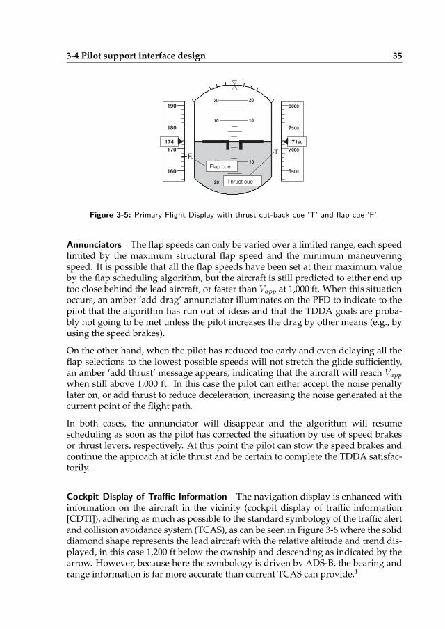
3-4 Pilot support interface design 35
160
170
180
190
174
6 500
7 000
7 500
8 000
10 10
10 10
20 20
71 60
F
Flap cue
20 20
T
Thrust cue
Figure 3-5: Primary Flight Display with thrust cut-back cue ’T’ and flap cue ’F’.
Annunciators The flap speeds can only be varied over a limited range, each speedlimited by the maximum structural flap speed and the minimum maneuveringspeed. It is possible that all the flap speeds have been set at their maximum valueby the flap scheduling algorithm, but the aircraft is still predicted to either end uptoo close behind the lead aircraft, or faster than Vapp at 1,000 ft. When this situationoccurs, an amber ‘add drag’ annunciator illuminates on the PFD to indicate to thepilot that the algorithm has run out of ideas and that the TDDA goals are proba-bly not going to be met unless the pilot increases the drag by other means (e.g., byusing the speed brakes).
On the other hand, when the pilot has reduced too early and even delaying all theflap selections to the lowest possible speeds will not stretch the glide sufficiently,an amber ‘add thrust’ message appears, indicating that the aircraft will reach Vapp
when still above 1,000 ft. In this case the pilot can either accept the noise penaltylater on, or add thrust to reduce deceleration, increasing the noise generated at thecurrent point of the flight path.
In both cases, the annunciator will disappear and the algorithm will resumescheduling as soon as the pilot has corrected the situation by use of speed brakesor thrust levers, respectively. At this point the pilot can stow the speed brakes andcontinue the approach at idle thrust and be certain to complete the TDDA satisfac-torily.
Cockpit Display of Traffic Information The navigation display is enhanced withinformation on the aircraft in the vicinity (cockpit display of traffic information[CDTI]), adhering as much as possible to the standard symbology of the traffic alertand collision avoidance system (TCAS), as can be seen in Figure 3-6 where the soliddiamond shape represents the lead aircraft with the relative altitude and trend dis-played, in this case 1,200 ft below the ownship and descending as indicated by thearrow. However, because here the symbology is driven by ADS-B, the bearing andrange information is far more accurate than current TCAS can provide.1
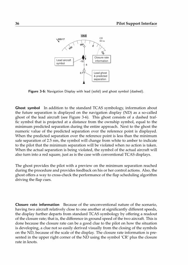
36 Pilot Support Interface
separation
068
E
120
060
030
020/17
- 12
5
2.7 Lead ghost & predicted
Lead aircraft
symbol
CR 42 kts
Closure rate
information
Figure 3-6: Navigation Display with lead (solid) and ghost symbol (dashed).
Ghost symbol In addition to the standard TCAS symbology, information aboutthe future separation is displayed on the navigation display (ND) as a so-calledghost of the lead aircraft (see Figure 3-6). This ghost consists of a dashed traf-fic symbol that is projected at a distance from the ownship symbol, equal to theminimum predicted separation during the entire approach. Next to the ghost thenumeric value of the predicted separation over the reference point is displayed.When the predicted separation over the reference point is less than the minimumsafe separation of 2.5 nm, the symbol will change from white to amber to indicateto the pilot that the minimum separation will be violated when no action is taken.When the actual separation is being violated, the symbol of the actual aircraft willalso turn into a red square, just as is the case with conventional TCAS displays.
The ghost provides the pilot with a preview on the minimum separation reachedduring the procedure and provides feedback on his or her control actions. Also, theghost offers a way to cross-check the performance of the flap scheduling algorithmdriving the flap cues.
Closure rate information Because of the unconventional nature of the scenario,having two aircraft relatively close to one another at significantly different speeds,the display further departs from standard TCAS symbology by offering a readoutof the closure rate; that is, the difference in ground speed of the two aircraft. This isdone because the closure rate can be a good clue to the pilot on how the situationis developing, a clue not so easily derived visually from the closing of the symbolson the ND, because of the scale of the display. The closure rate information is pre-sented in the upper right corner of the ND using the symbol ‘CR’ plus the closurerate in knots.
3-5 Experiment 37
3-5 Experiment
To test the self-spacing scenario and to assess the operational uncertainties of self-separation in a realistic fashion, a piloted experiment was conducted to determinethe effects of different scenarios on pilot performance, workload, and situationawareness and how these ultimately reflect on runway capacity numbers. Anothermeasurement of the experiment was the feedback from the pilots on the displaydesign and their appreciation of the self-spacing concept.
3-5-1 Method
Participants and instructions Ten professional airline pilots, all men, were invitedto participate in the experiment, 6 of whom had many years of experience on theBoeing 747. After a thorough briefing on the displays and the procedure, they wereasked to manually fly a TDDA in a Boeing 747, following a conventional straight-inILS glide path with the engines running at flight idle, following a Boeing 737. Pilotperformance was scored based on how accurately the TDDA profile was followedand how close to the minimum safe separation the approach was finished. The min-imum safe separation was set to 2.5 nm and as a measure for TDDA performancethrottle inputs and flap deflections were measured.
Table 3-1: The five pilot support interfaces that were tested in the experiment.
Display Flap Cues CDTI
1 (base-line) Fixed TCAS + CR2 Noise optimized TCAS + CR3 Noise+Traff.opt. TCAS + CR4 Noise optimized Lead ghosting5 Noise+Traff.opt Lead ghosting
Apparatus The experiment was conducted in the Human-Machine InteractionLaboratory of the faculty of Aerospace Engineering of Delft University. This labo-ratory consists of a fixed-base simulator that has two 18-in. LCD screens on whichthe PFD, ND, and mode control panel of a Boeing 747-400 were projected. Further-more the simulator has a hydraulic side-stick and rudder pedals. Because the goalof this experiment was to determine the performance of pilots during instrumentflight conditions, no outside visual information was shown.
Aircraft and weather model As no Boeing 747-400 model was available, the air-craft flown was a Boeing 747-200, simulated through a realistic nonlinear model.Although this meant a B747-200 model was flown using a B747-400 flight deck
38 Pilot Support Interface
setup, the pilots indicated that the characteristics of the two models were simi-lar enough to not pose a distraction. The aircraft was flown with the yaw-damperengaged to improve lateral stability. At the beginning of each run the aircraft wascontrolled by autopilot (fly level at 7,000 ft) and autothrottle (fly at 250 kt IAS). Atthe start of each measurement run, these systems both had to be deactivated bythe pilot. The weather model was set to ICAO International Standard Atmosphereconditions and zero wind.
Independent variables Two independent variables were defined. First of all, dif-ferent combinations of the display elements were tested, resulting in five pilot sup-port interfaces, listed in Table 3-1: (1) the baseline interface; that is, a standard TCASdisplay augmented with a closure rate readout and a fixed, precomputed trajectoryprediction algorithm; this algorithm uses a standard flap deflection scheme that is,unlike the other algorithms, not updated during the approach; (2) and (3) the stan-dard TCAS interface with the online trajectory prediction algorithms that optimizefor noise only (2) or for noise and separation at runway threshold (3); and (4) and (5)the combination of these two algorithms with a TCAS display that was augmentedwith a ghost symbol, showing the predicted separation at runway threshold. Sec-ond, three different lead aircraft approach trajectories were defined: (a) a nominalapproach, on which the precomputed flap schedule was based; (b) a fast lead ap-proach, where, because of tardy pilot action, the preceding aircraft decelerates veryslowly relative to the nominal approach and the average ground speed is abovenominal; and (c) a slow lead approach, the complement of (b), where, because ofaggressive pilot action, the target aircraft decelerates very quickly resulting in av-eraging a lower ground speed. Note that the baseline interface only provides pilotswith a correct flap schedule for the nominal approach. In all other approaches, thisinterface will not give the right flap schedule as the preceding aircraft does not flythe nominal approach.
Experiment design The experiment is set up as a 5 × 3 factorial: five display con-ditions and three lead traces give 15 conditions for each pilot. During the trainingruns, each pilot was exposed to all 15 conditions to get acquainted with all the dis-play configurations. During the measurement runs, each condition was flown onlyonce to limit the total time needed for each pilot to one work day. The order inwhich the conditions were flown was randomized to prevent learning effects.
Procedure The task was to fly a TDDA approach to a fictitious airport and stayat a safe distance from a preceding aircraft. In all cases the preceding aircraft wasa Boeing 737 flying a TDDA as well. The behavior of this aircraft was one of theexperiment independent variables. The experiment consisted of 15 approaches,each starting with straight and level flight at 7,000 ft, 250 kt IAS, and established onthe localizer. After the pilot had a chance to form a mental picture of the situation,he had to disconnect the autopilot. After glide-slope interception, the procedure
3-6 Results and discussion 39
called for maintaining 250 kt until reaching the thrust cutback altitude, where thethrust levers were pulled back to flight idle and the deceleration began.
The pilots were instructed that after the thrust had been set to idle, they were notto advance the throttle levers until reaching the final approach speed. This way itis easier to compare results between pilots and the altitude at which Vapp is reachedcan be used as a performance indicator. The pilots were further instructed thatunder no circumstances were they to let the actual in-trail distance become lessthan 2.5 nm, but no pilot action was required to close the gap should the separationincrease.
After each run, the pilots filled out a NASA Task Load Index (NASA-TLX) form,9
and after the last run they were requested to complete a questionnaire to give theiropinion on the different aspects of the experiment.
Dependent measures The path-tracking performance was measured by record-ing vertical and cross-track errors and heading errors relative to the three-degreeILS glide path. Pilot control actions on the side-stick, throttle, and flap selectorwere also measured. Furthermore the adherence to the flap cues was measured byrecording the time between the appearance of the cue and the pilot response to thatcue.
As operational performance parameters, the altitude at which Vapp was reachedwas recorded as a measure for noise impact; the separation at 1,000 ft was consid-ered as a measure for separation performance. Finally, pilot workload was mea-sured using the NASA-TLX.
Hypotheses It was hypothesized that pilots would perform better when they aresupported by an interface that provides them on-line (i.e., optimized in real time)information on the flap schedule needed to successfully fly the TDDA while main-taining a safe separation from the leading aircraft. The effect of the non-nominallead traces was expected to degrade pilot performance, but not when the pilot issupported by the interface. Also it was expected that the most complete displayswould lower the workload for the TDDA scenario as compared to the baseline dis-play.
3-6 Results and discussion
3-6-1 Pilot controls
Figure 3-8 shows the pilot stick activity. The mean roll activity is more or less con-stant, but the spread is larger for lead type 3 (slow lead), F2,18 = 3.338, p = 0.058,most noticeably for the displays unaugmented for traffic; Displays 1 (baseline) and4 (noise only + ghost). This is caused by the fact that a number of pilots applied
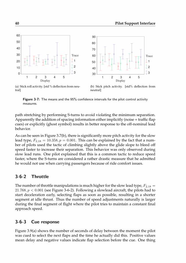
40 Pilot Support Interface
Display 5 4 3 2 1
60
50
40
30
20
10
0
Trace
1
2
3
(a) Stick roll activity. [std % deflection from neu-tral]
Display 5 4 3 2 1
90
80
70
60
50
40
30
Trace
1
2
3
(b) Stick pitch activity. [std% deflection fromneutral]
Figure 3-7: The means and the 95% confidence intervals for the pilot control activitymeasures.
path stretching by performing S-turns to avoid violating the minimum separation.Apparently the addition of spacing information either implicitly (noise + traffic flapcues) or explicitly (ghost symbol) results in better response to the off-nominal leadbehavior.
As can be seen in Figure 3.7(b), there is significantly more pitch activity for the slowlead type, F2,18 = 10.358, p = 0.001. This can be explained by the fact that a num-ber of pilots used the tactic of climbing slightly above the glide slope to bleed offspeed faster to increase their separation. This behavior was only observed duringslow lead runs. One pilot explained that this is a common tactic to reduce speedfaster, where the S-turns are considered a rather drastic measure that he admittedhe would not use when carrying passengers because of ride comfort issues.
3-6-2 Throttle
The number of throttle manipulations is much higher for the slow lead type, F2,18 =21.768, p < 0.001 (see Figure 3-6-2). Following a slowlead aircraft, the pilots had tostart deceleration early, selecting flaps as soon as possible, resulting in a shortersegment at idle thrust. Thus the number of speed adjustments naturally is largerduring the final segment of flight where the pilot tries to maintain a constant finalapproach speed.
3-6-3 Cue response
Figure 3.9(a) shows the number of seconds of delay between the moment the pilotwas cued to select the next flaps and the time he actually did this. Positive valuesmean delay and negative values indicate flap selection before the cue. One thing
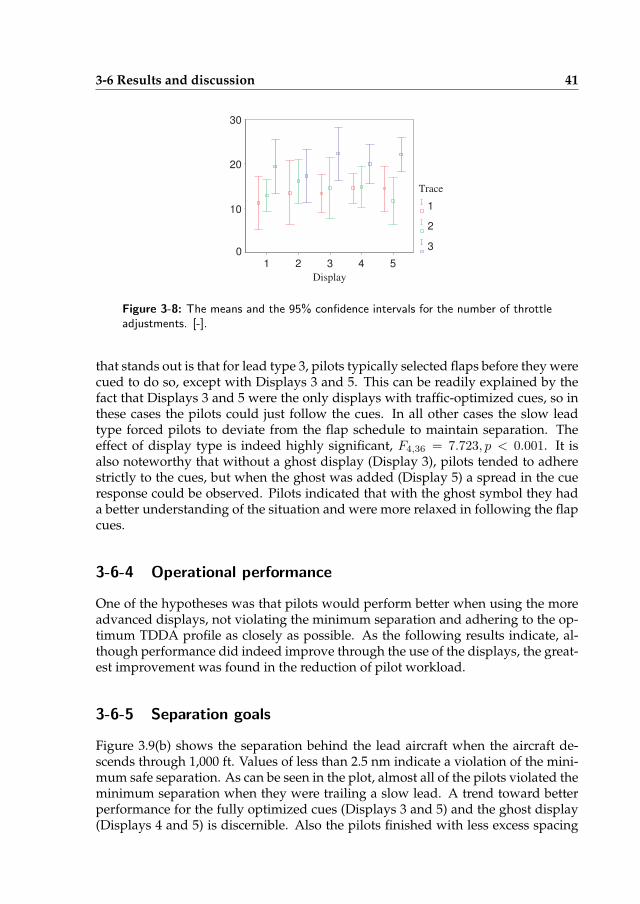
3-6 Results and discussion 41
Display
5 4 3 2 1
30
20
10
0
Trace
1
2
3
Figure 3-8: The means and the 95% confidence intervals for the number of throttleadjustments. [-].
that stands out is that for lead type 3, pilots typically selected flaps before they werecued to do so, except with Displays 3 and 5. This can be readily explained by thefact that Displays 3 and 5 were the only displays with traffic-optimized cues, so inthese cases the pilots could just follow the cues. In all other cases the slow leadtype forced pilots to deviate from the flap schedule to maintain separation. Theeffect of display type is indeed highly significant, F4,36 = 7.723, p < 0.001. It isalso noteworthy that without a ghost display (Display 3), pilots tended to adherestrictly to the cues, but when the ghost was added (Display 5) a spread in the cueresponse could be observed. Pilots indicated that with the ghost symbol they hada better understanding of the situation and were more relaxed in following the flapcues.
3-6-4 Operational performance
One of the hypotheses was that pilots would perform better when using the moreadvanced displays, not violating the minimum separation and adhering to the op-timum TDDA profile as closely as possible. As the following results indicate, al-though performance did indeed improve through the use of the displays, the great-est improvement was found in the reduction of pilot workload.
3-6-5 Separation goals
Figure 3.9(b) shows the separation behind the lead aircraft when the aircraft de-scends through 1,000 ft. Values of less than 2.5 nm indicate a violation of the mini-mum safe separation. As can be seen in the plot, almost all of the pilots violated theminimum separation when they were trailing a slow lead. A trend toward betterperformance for the fully optimized cues (Displays 3 and 5) and the ghost display(Displays 4 and 5) is discernible. Also the pilots finished with less excess spacing

42 Pilot Support Interface
Display
5 4 3 2 1
60
40
20
0
-20
-40
-60
Trace
1
2
3
(a) Time between the presentation of the flapcue and the pilot’s response to it. [s]
Display
5 4 3 2 1
1.5
1.0
0.5
0.0
-0.5
-1.0
Trace
1
2
3
(b) Separation when descending through 1,000feet. [NM]
Display
5 4 3 2 1
4000
3000
2000
1000
0
-1000
Trace
1
2
3
(c) Altitude at which VAPP was reached. [ft]
Display
5 4 3 2 1
3
2
1
0
-1
-2
Trace
1
2
3
(d) Means and the 95% confidence intervals forthe normalized TLX ratings. [-]
Figure 3-9: The means and the 95% confidence intervals for pilot performance mea-sures.
when they have more support from the display; however, the effect of the displayis not statistically significant. One point worth noting here is that Display 1 was nota real baseline display, in that the traffic information delivered by ADS-B is moreaccurate than current TCAS can provide. Also, current cockpits lack the display ofclosure rate information as used in the experiment. Almost all pilots indicated inthe questionnaire that they found this closure rate information to be very useful,with some pilots even claiming that they used the closure rate in lieu of the ghostdisplay.
3-6-6 Noise goals
As can be expected, the altitude at which Vapp is reached is higher for the slow leadruns, as can be seen in Figure 3.9(c). Again, when pilots are presented with fully
3-7 Conclusions 43
optimized cues, but no ghost symbol to verify it (Display 3), they tend to closelyfollow the clues. Also it is clear that the pilots typically were capable of reachingVapp at 1,000 ft without help from the cuing algorithm, as there is little difference inperformance between the displays.
3-6-7 Pilot workload
After each measurement run the pilots were asked to fill out a NASA-TLX sheet toassess the workload they had experienced. The results, averaged and normalizedinto z scores for all pilots, are shown in Figure 3.9(d).
Clearly, the slow lead caused a substantially higher workload than the other leadtypes, although this effect seems to be less for Display 3 (noise only + ghost) andalso for the displays with traffic-optimized cues (Displays 4 and 5). In fact the effectseems to be absent for Display 5. Indeed, the effect of the lead type is highly signif-icant, F2,18 = 12.875, p < 0.001, and the type of display is also found to be highlysignificant on pilot workload, F4,36 = 6.409, p < 0.001, which indicates that thedeveloped displays do indeed reduce the pilot workload where the unaugmenteddisplays do not.
3-7 Conclusions
An automated tool has been presented for determining the flap position changesduring a TDDA procedure, in which the pilot also maintains separation with thepreceding aircraft. The cues for flap selection are given as bugs on the speed in-dicator. A navigation display with traffic information and a presentation of futureseparation and closure rate enables monitoring and controlling of the separationwith the preceding aircraft.
The experiment results indicate a significant reduction in pilot workload with thenew pilot support interface. The TDDA task itself was generally performed ade-quately by all pilots with or without help from the automation, as long as the leadaircraft did not deviate from the nominal profile. The use of on-line separation pre-diction and flap optimization reduced the effect of off-nominal lead pilot behavioron the performance, although no statistical significance could be shown using only10 pilots. Larger scale research is required to investigate whether the trend towardbetter separation performance with the displays can be statistically verified.
The flap optimization algorithm as presented in this article basically functions inone of two modes; that is, it will optimize the schedule to reach a reference altitudeshortly before touchdown at the final approach speed until it detects that the min-imum separation will be violated, at which time the algorithm neglects any noiseimpact and just starts reducing the speed to increase separation. Further researchshould be carried out to investigate whether it is possible to control the flap speedsto reach both goals simultaneously.

44 REFERENCES
References
[1] Minimum Aviation System Performance Standards for Automatic DependentSurveillance Broadcast (ADS-B). Technical Report RTCA/DO-242, RTCA, Inc.,Washington DC, USA, Feb 1998.
[2] J.-P. Clarke. Systems Analysis of Noise Abatement Procedures Enabled byAdvanced Flight Guidance Technology. Journal of Aircraft, 37, no. 2(AIAA 97-0490), Mar-Apr 2000.
[3] J.-P. Clarke and R. J. Hansman. A Systems Analysis Methodology for Devel-oping Single Event Noise Abatement Procedures. Technical Report ASL-97-1,MIT - Aeronautical Systems Laboratory, Cambridge (MA), USA, Jan 1997.
[4] T. J. Davis, D. R. Isaacson, J. E. Robinson III, W. den Braven, K. K. Lee, andB. Sanford. Operational Test Results of the Passive Approach Spacing Tool.In IFAC 8th Symposium on Transportation Systems 97, Chania, Greece, Jun 16-181997.
[5] T. J. Davis, K. J. Krzeczowski, and C. Bergh. The Final Approach Spacing Tool.In 13th IFAC Symposium on Automatic Control in Aerospace, Palo Alto (CA), USA,Sep 1994.
[6] J. L. de Prins, K. F. M. Schippers, M. Mulder, M. M. van Paassen, A. C. in ‘t Veld,and J.-P. Clarke. Enhanced Self-Spacing Algorithm for Three-Degree Deceler-ating Approaches. AIAA Journal of Guidance, Control & Dynamics, 30(5):576–590, Mar-Apr 2007.
[7] L. J. J. Erkelens. Research on Noise Abatement Procedures. Technical Re-port NLR TP 98066, National Aerospace Laboratory (NLR), Amsterdam, TheNetherlands, Feb 1998.
[8] L. J. J. Erkelens. Development of Noise Abatement Procedures in The Nether-lands. Technical Report NLR TP 99386, National Aerospace Laboratory (NLR),Amsterdam, The Netherlands, Nov 1999.
[9] S. G. Hart and L. E. Staveland. Development of a Multi-Dimensional WorkloadRating Scale: Results of Empirical and Theoretical Research. Human MentalWorkload, pages 139–183, 1988.
[10] N. T. Ho and J.-P. Clarke. Mitigating Operational Aircraft Noise Impact byLeveraging on Automation Capability. In Proceedings of the AIAA Aircraft, Tech-nology, Integration and Operations Forum, number AIAA 2001-5239, pages 1–8,Los Angeles (CA), USA, Oct 16-18 2001.
[11] A. C. in ‘t Veld and J.-P. Clarke. Trajectory Prediction or Self-Separation dur-ing Decelerating Approaches in a Data-Link Environment. In AIAA AircraftTechnology, Integration and Operations (ATIO) Forum, number 2002-5887, LosAngeles (CA), USA, Oct 2002.
45
[12] A. C. in ‘t Veld, M. Mulder, M. M. van Paassen, and J.-P. Clarke. Pilot Sup-port for Self-Separation during Decelerating Approaches. In 12th InternationalSymposium on Aviation Psychology (IJAP), Dayton (OH), USA, Apr 2003.
[13] A. D. Kershaw, D. P. Rhodes, and N. A. Smith. The Influence of ATC in Ap-proach Noise Abatement. Napoli, Italy, Jun 13-16 2000.
[14] M. F. Koeslag. Advanced Continuous Approaches, an Algorithm Design forthe Flight Management System. Technical Report NLR-TR-2001-359, NationalAerospace Laboratory (NLR), Amsterdam, The Netherlands, Mar 1999.
[15] K. K. Lee and T. J. Davis. The Development of the Final Approach SpacingTool (FAST): A Cooperative Controller-Engineer Design Approach. Journal ofControl Engineering Practice, 4(8):1161–1168, Aug 1996.
[16] R. M. Oseguera-Lohr, G. W. Lohr, and T. S. Abbot. Evaluation of Opera-tional Procedures for Using a Time-Based Airborne Inter-Arrival Spacing Tool.In AIAA Aircraft Technology, Integration and Operations Forum (ATIO), number2002-5824, Los Angeles (CA), USA, Oct 2002.
[17] C. Quinn and J. E. Robertson III. A Human Factors Evaluation of Active FinalApproach Spacing Tool Concepts. In 3rd USA/Europe Air Traffic ManagementR&D Seminar, Napoli, Italy, Jun 2000.
[18] L. Ren, J.-P. Clarke, and N. T. Ho. Achieving Low Approach Noise withoutSacrifying Capacity. In 22nd Digital Avionics Systems Conference, number AIAA-2001-5239, pages 1–9, Indianapolis (IN), USA, Oct 12-16 2003.

46
4
Distance Based Self-Spacing
Enhanced Self-Spacing Algorithm for Three-Degree Decelerating Approaches
J.L. de Prins, K.F.M. Schippers, M. Mulder, M.M. van Paassen, A.C. in ’t Veld andJ.-P. Clarke
AIAA Journal of Aircraft, Vol 30, No. 2, Mar-Apr 2007, Pages 576-590
4-1 Abstract
A current trend in aircraft noise abatement around airports is exploiting the benefitsof procedural means with computational aids, such as on-board and ground-basedtrajectory prediction algorithms and displays. The challenge for these upcomingAdvanced Noise Abatement Procedures is to mitigate the noise impact without sac-rificing runway capacity. The proposed solution, implemented in the Three-DegreeDecelerating Approach (TDDA), is to delegate the task of separating the aircraft tothe cockpit during the approach. To assist the pilots, a flap/gear scheduling algo-rithm with a complementary interface has been developed that takes noise nuisanceand in-trail separation into account. The design and functionality of this pilot sup-port system is presented in-depth and evaluated with three experiments. Off-lineMonte-Carlo simulations indicated an adequate and consistent performance androbustness of the self-spacing algorithm for various wind and traffic scenarios. Apilot-in-the-loop simulator experiment verified that with the aid of the algorithm,pilots were able to execute the noise abatement procedure consistently while main-taining safe separation at all times. The support system showed to reduce pilotworkload up to an effort level comparable to current standard approaches. Thewhole concept was demonstrated with an in-flight exploratory investigation which
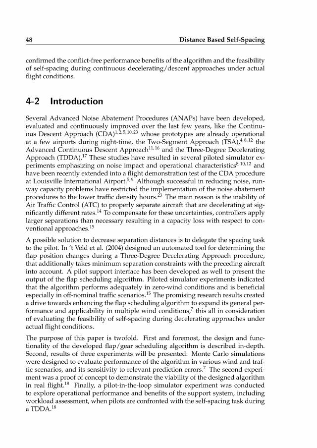
48 Distance Based Self-Spacing
confirmed the conflict-free performance benefits of the algorithm and the feasibilityof self-spacing during continuous decelerating/descent approaches under actualflight conditions.
4-2 Introduction
Several Advanced Noise Abatement Procedures (ANAPs) have been developed,evaluated and continuously improved over the last few years, like the Continu-ous Descent Approach (CDA)1, 2, 5, 10, 23 whose prototypes are already operationalat a few airports during night-time, the Two-Segment Approach (TSA),4, 8, 12 theAdvanced Continuous Descent Approach11, 16 and the Three-Degree DeceleratingApproach (TDDA).17 These studies have resulted in several piloted simulator ex-periments emphasizing on noise impact and operational characteristics8, 10, 12 andhave been recently extended into a flight demonstration test of the CDA procedureat Louisville International Airport.5, 9 Although successful in reducing noise, run-way capacity problems have restricted the implementation of the noise abatementprocedures to the lower traffic density hours.23 The main reason is the inability ofAir Traffic Control (ATC) to properly separate aircraft that are decelerating at sig-nificantly different rates.14 To compensate for these uncertainties, controllers applylarger separations than necessary resulting in a capacity loss with respect to con-ventional approaches.15
A possible solution to decrease separation distances is to delegate the spacing taskto the pilot. In ’t Veld et al. (2004) designed an automated tool for determining theflap position changes during a Three-Degree Decelerating Approach procedure,that additionally takes minimum separation constraints with the preceding aircraftinto account. A pilot support interface has been developed as well to present theoutput of the flap scheduling algorithm. Piloted simulator experiments indicatedthat the algorithm performs adequately in zero-wind conditions and is beneficialespecially in off-nominal traffic scenarios.15 The promising research results createda drive towards enhancing the flap scheduling algorithm to expand its general per-formance and applicability in multiple wind conditions,7 this all in considerationof evaluating the feasibility of self-spacing during decelerating approaches underactual flight conditions.
The purpose of this paper is twofold. First and foremost, the design and func-tionality of the developed flap/gear scheduling algorithm is described in-depth.Second, results of three experiments will be presented. Monte Carlo simulationswere designed to evaluate performance of the algorithm in various wind and traf-fic scenarios, and its sensitivity to relevant prediction errors.7 The second experi-ment was a proof of concept to demonstrate the viability of the designed algorithmin real flight.18 Finally, a pilot-in-the-loop simulator experiment was conductedto explore operational performance and benefits of the support system, includingworkload assessment, when pilots are confronted with the self-spacing task duringa TDDA.18
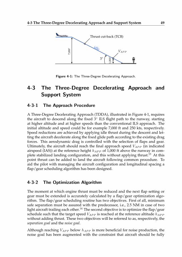
4-3 The Three-Degree Decelerating Approach and Support System 49�Thrust cut-back (TCB)
VAPP
1,00
0’
7,00
0’
3◦
idle
Figure 4-1: The Three-Degree Decelerating Approach.
4-3 The Three-Degree Decelerating Approach andSupport System
4-3-1 The Approach Procedure
A Three-Degree Decelerating Approach (TDDA), illustrated in Figure 4-1, requiresthe aircraft to descend along the fixed 3◦ ILS flight path to the runway, startingat higher altitude and at higher speeds than the conventional ILS approach. Theinitial altitude and speed could be for example 7,000 ft and 250 kts, respectively.Speed reductions are achieved by applying idle thrust during the descent and let-ting the aircraft decelerate along the fixed glide path according to the existing dragforces. This aerodynamic drag is controlled with the selection of flaps and gear.Ultimately, the aircraft should reach the final approach speed VAPP (in indicatedairspeed (IAS)) at the reference height hAPP of 1,000 ft above the runway in com-plete stabilized landing configuration, and this without applying thrust.15 At thispoint thrust can be added to land the aircraft following common procedure. Toaid the pilot with managing the aircraft configuration and longitudinal spacing aflap/gear scheduling algorithm has been designed.
4-3-2 The Optimization Algorithm
The moment at which engine thrust must be reduced and the next flap setting orgear must be extended is accurately calculated by a flap/gear optimization algo-rithm. The flap/gear scheduling routine has two objectives. First of all, minimumsafe separation must be assured with the predecessor, i.e., 2.5 NM in case of twolight aircraft trailing each other.14 The second objective is to optimize the flap/gearschedule such that the target speed VAPP is reached at the reference altitude hAPP
without adding thrust. These two objectives will be referred to as, respectively, theseparation goal and the noise goal.
Although reaching VAPP below hAPP is more beneficial for noise production, thenoise goal has been augmented with the constraint that aircraft should be fully

50 Distance Based Self-Spacing
established in landing configuration as close to hAPP as possible. Therefore, in theremainder of this paper, re-engaging thrust below hAPP will also be referenced asa decline in ’noise’ performance.
Since the TDDA is executed with idle thrust along a fixed flight path, the momentsof thrust cut-back, flap and gear selection are the only control options to properlyachieve the goals. During the descent, the number of control options gradually de-creases as thrust is fixed at idle and flaps are selected one by one. Consequently, it isdesirable to keep the largest control authority for the latest flap setting, in both tun-ing directions, such that the algorithm is still able to correct unexpected deviationsduring the final part of the TDDA. Hereby, the performance of the TDDA objectivescan be maximized. The complete flap/gear tuning algorithm is elaborated in detailin section 4-4. For simplicity, the flap/gear optimization algorithm will be referredto as the flap algorithm or flap scheduler from this point on.
4-3-3 The Pilot Support Interface
To support the pilot in his task of flying the TDDA, cues have been added to thePrimary Flight Display (PFD) and Navigation Display (ND),15, 18 see Figure 4-2. Agreen Thrust cue ’T’ on the altitude indicator exhibits the thrust cut-back altitude. Agreen Flap cue ’F’ on the airspeed indicator shows the speed of the aircraft at whichthe next flap has to be selected. A yellow ’G’ cue indicates the optimized speed oflanding gear selection. The calculated airspeed at which the flap or gear shouldbe extended, is shortened to the term flap speed and gear speed in the remainder ofthis paper. When speed brakes or thrust are required, ADD DRAG or ADD THRUST
annunciations pop-up.
The Navigation Display (ND) is provided with continuous information on aircraftin the vicinity using standard Traffic Alert and Collision Avoidance System (TCAS)symbology. Additionally, the display has been augmented with information on thefuture separation trend by adding a predicted separation arc.18 The separation arc in-dicates the difference between predicted separation at the threshold and minimumsafe separation with respect to the current position of the lead aircraft. Thus, whenthe arc is below the lead aircraft, safe separation is guaranteed. On the other hand,an arc encapsuling the lead indicates future violation of safe separation. In this way,the separation arc serves as an interactive safety corridor, which facilitates pilot’sinterpretation of the situation.
4-4 The Enhanced TDDA Algorithm
A prediction and optimization algorithm has been developed15, 16 and enhanced7
to aid the pilot with his self-spacing task and his task to arrive with VAPP at thereference height. The routine determines at what altitude thrust should be reducedand at what speed each flap setting and the gear should be selected. This section
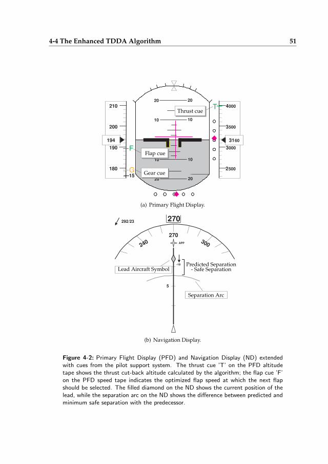
4-4 The Enhanced TDDA Algorithm 51
180
190
200
210
194
2 500
3 000
3 500
4 000
20 20
10 10
10 10
20 20
31 60
F
15
T
G
Thrust cue
Flap cue
Gear cue
(a) Primary Flight Display.
270
270
240 300 APP
292 / 23
5
-18 Predicted Separation- Safe SeparationLead Aircraft Symbol
Separation Arc
(b) Navigation Display.
Figure 4-2: Primary Flight Display (PFD) and Navigation Display (ND) extendedwith cues from the pilot support system. The thrust cue ’T’ on the PFD altitudetape shows the thrust cut-back altitude calculated by the algorithm; the flap cue ’F’on the PFD speed tape indicates the optimized flap speed at which the next flapshould be selected. The filled diamond on the ND shows the current position of thelead, while the separation arc on the ND shows the difference between predicted andminimum safe separation with the predecessor.
52 Distance Based Self-Spacing
presents a detailed description of the algorithm’s prediction methods and controllaws to satisfy the noise and separation goals simultaneously, under various atmo-spheric conditions.
4-4-1 Structure of the Flap Optimization Algorithm
The design of the flap optimization algorithm is illustrated in Figure 4-3. First thetrajectory of the lead aircraft is predicted. Next, a prediction of the own trajectoryis made given the last calculated flap schedule, current aircraft state and estimatedwind. Both traces are then compared, yielding the predicted separation trend. Ifseparation is expected to be violated, the flap selection moments are tuned to slowdown earlier and hence increase separation. To determine the proper flap speeds,the iteration process first distinguishes between the situations where the aircraft isabove or below the thrust cut-back altitude (hTCB). These situations respectivelycorrespond to the CAPTURE mode and the HOLD mode of the flap scheduler, re-spectively:
• In CAPTURE mode the algorithm calculates the altitude at which the thrustshould be set to flight-idle (hTCB). This altitude is determined by the startaltitude optimization routine such that safe separation is assured while still be-ing able to reach the reference height without applying thrust. As soon as thecalculated start altitude is reached the algorithm switches to HOLD mode.
• In HOLD mode, the flap scheduler runs the Noise & Traffic (N&T ) optimizationroutine to adjust the flap/gear speeds. If however, in this part of the ap-proach, separation is predicted to be violated, the noise and separation goalscan not be combined anymore. Flaps must be extended at higher speeds todecelerate earlier and increase spacing. Consequently, the aircraft will get toVAPP too early and extra thrust is required. The algorithm will now primarilytune the flaps to guarantee safe separation before the target speed is lookedafter.
The flap schedule tuning process is a binary search algorithm,15 starting with acoarse flap-tuning routine, followed by a fine-tuning process to determine a sat-isfying flap schedule. During the rough-tuning, the first coming flap stage is setto its upper/lower bound, followed by the next flap and so on until the relevantconstraint (separation or noise) is overcorrected. At each adjustment the trajec-tory and separation trend are recalculated to check with the constraints. The upperand lower bounds for each flap speed are given by the flap placard speed and theminimum maneuvering speed, respectively. The applicable constraints are furtherdiscussed in the description of the Noise & Traffic optimization of section 4-4-6.When the relevant criterion is exceeded, the last adjusted flap setting is fine-tunedto get the constraint within its demanded margins. Fine-tuning is done by settingthe last tuned flap speed to midpoint between the nominal speed and the last set
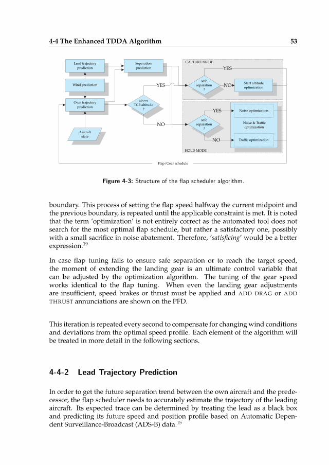
4-4 The Enhanced TDDA Algorithm 53
Lead trajectory
Own trajectory
prediction
prediction
prediction
Wind prediction
Separation
Aircraft
state
above
TCB altitude
optimization
optimizationseparation
separation
safe
safe
?
?
?
CAPTURE MODE
HOLD MODE
YES
YES
YES
NO
NO
NO
Start altitude
Noise optimization
Traffic optimization
Noise & Traffic
Flap/Gear schedule
Figure 4-3: Structure of the flap scheduler algorithm.
boundary. This process of setting the flap speed halfway the current midpoint andthe previous boundary, is repeated until the applicable constraint is met. It is notedthat the term ’optimization’ is not entirely correct as the automated tool does notsearch for the most optimal flap schedule, but rather a satisfactory one, possiblywith a small sacrifice in noise abatement. Therefore, ’satisficing’ would be a betterexpression.19
In case flap tuning fails to ensure safe separation or to reach the target speed,the moment of extending the landing gear is an ultimate control variable thatcan be adjusted by the optimization algorithm. The tuning of the gear speedworks identical to the flap tuning. When even the landing gear adjustmentsare insufficient, speed brakes or thrust must be applied and ADD DRAG or ADD
THRUST annunciations are shown on the PFD.
This iteration is repeated every second to compensate for changing wind conditionsand deviations from the optimal speed profile. Each element of the algorithm willbe treated in more detail in the following sections.
4-4-2 Lead Trajectory Prediction
In order to get the future separation trend between the own aircraft and the prede-cessor, the flap scheduler needs to accurately estimate the trajectory of the leadingaircraft. Its expected trace can be determined by treating the lead as a black boxand predicting its future speed and position profile based on Automatic Depen-dent Surveillance-Broadcast (ADS-B) data.15
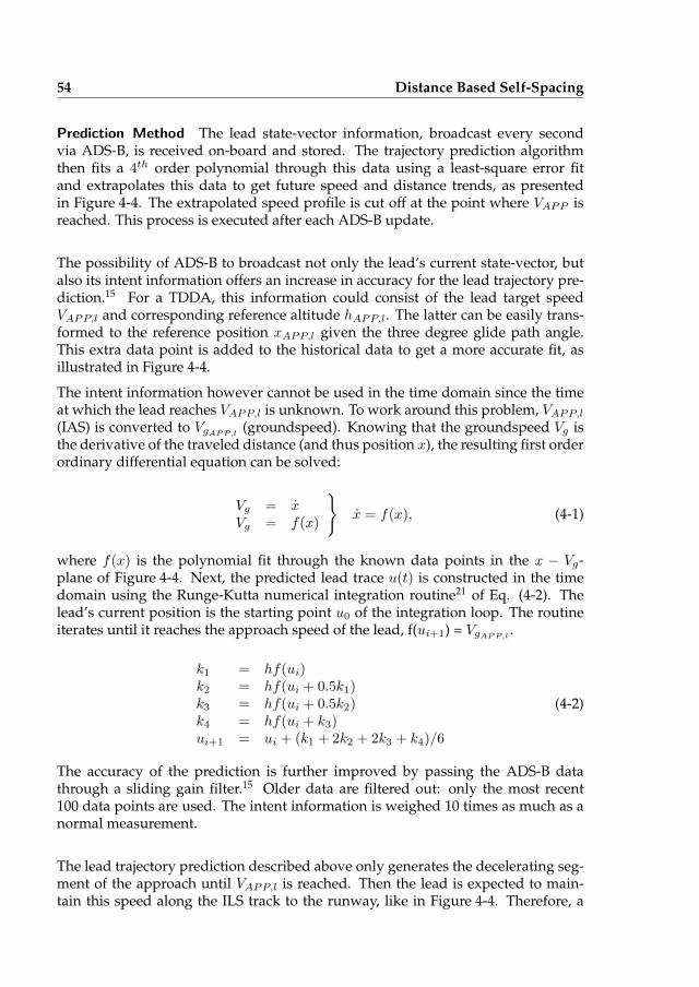
54 Distance Based Self-Spacing
Prediction Method The lead state-vector information, broadcast every secondvia ADS-B, is received on-board and stored. The trajectory prediction algorithmthen fits a 4th order polynomial through this data using a least-square error fitand extrapolates this data to get future speed and distance trends, as presentedin Figure 4-4. The extrapolated speed profile is cut off at the point where VAPP isreached. This process is executed after each ADS-B update.
The possibility of ADS-B to broadcast not only the lead’s current state-vector, butalso its intent information offers an increase in accuracy for the lead trajectory pre-diction.15 For a TDDA, this information could consist of the lead target speedVAPP,l and corresponding reference altitude hAPP,l. The latter can be easily trans-formed to the reference position xAPP,l given the three degree glide path angle.This extra data point is added to the historical data to get a more accurate fit, asillustrated in Figure 4-4.
The intent information however cannot be used in the time domain since the timeat which the lead reaches VAPP,l is unknown. To work around this problem, VAPP,l
(IAS) is converted to VgAPP,l(groundspeed). Knowing that the groundspeed Vg is
the derivative of the traveled distance (and thus position x), the resulting first orderordinary differential equation can be solved:
Vg
Vg
==
xf(x)
}
x = f(x), (4-1)
where f(x) is the polynomial fit through the known data points in the x − Vg-plane of Figure 4-4. Next, the predicted lead trace u(t) is constructed in the timedomain using the Runge-Kutta numerical integration routine21 of Eq. (4-2). Thelead’s current position is the starting point u0 of the integration loop. The routineiterates until it reaches the approach speed of the lead, f(ui+1) = VgAPP,l
.
k1k2k3k4ui+1
=====
hf(ui)hf(ui + 0.5k1)hf(ui + 0.5k2)hf(ui + k3)ui + (k1 + 2k2 + 2k3 + k4)/6
(4-2)
The accuracy of the prediction is further improved by passing the ADS-B datathrough a sliding gain filter.15 Older data are filtered out: only the most recent100 data points are used. The intent information is weighed 10 times as much as anormal measurement.
The lead trajectory prediction described above only generates the decelerating seg-ment of the approach until VAPP,l is reached. Then the lead is expected to main-tain this speed along the ILS track to the runway, like in Figure 4-4. Therefore, a
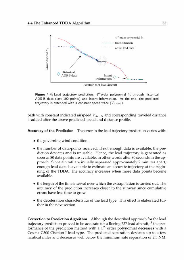
4-4 The Enhanced TDDA Algorithm 55
Position x of lead aircraft
Gro
un
dsp
eedVg
4thorder polynomial fit
actual lead trace
trace extension
Intentinformation
HistoricalADS-B data
Figure 4-4: Lead trajectory prediction: 4thorder polynomial fit through historical
ADS-B data (last 100 points) and intent information. At the end, the predictedtrajectory is extended with a constant speed trace (VAPP,l).
path with constant indicated airspeed VAPP,l and corresponding traveled distanceis added after the above predicted speed and distance profile.
Accuracy of the Prediction The error in the lead trajectory prediction varies with:
• the governing wind condition.
• the number of data-points received. If not enough data is available, the pre-diction deviates and is unusable. Hence, the lead trajectory is generated assoon as 80 data points are available, in other words after 80 seconds in the ap-proach. Since aircraft are initially separated approximately 2 minutes apart,enough lead data is available to estimate an accurate trajectory at the begin-ning of the TDDA. The accuracy increases when more data points becomeavailable.
• the length of the time interval over which the extrapolation is carried out. Theaccuracy of the prediction increases closer to the runway since cumulativeerrors have less time to grow.
• the deceleration characteristics of the lead type. This effect is elaborated fur-ther in the next section.
Correction to Prediction Algorithm Although the described approach for the leadtrajectory prediction proved to be accurate for a Boeing 737 lead aircraft,15 the per-formance of the prediction method with a 4th order polynomial decreases with aCessna C500 Citation I lead type. The predicted separation deviates up to a fewnautical miles and decreases well below the minimum safe separation of 2.5 NM.
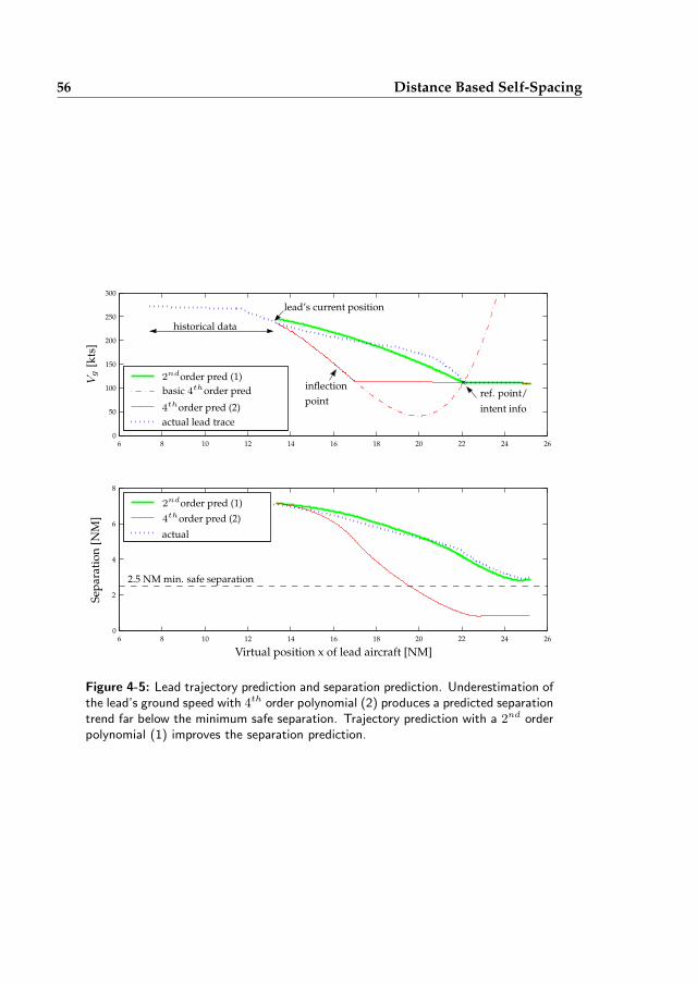
56 Distance Based Self-Spacing
0
0
50
100
150
200
250
300
2
4
6
6
6
8
8
8
10
10
12
12
14
14
16
16
18
18
20
20
22
22
24
24
26
26
Virtual position x of lead aircraft [NM]
Vg
[kts
]
2ndorder pred (1)
4thorder pred (2)
basic 4thorder pred
actual lead trace
inflection
pointintent info
ref. point/
Sep
arat
ion
[NM
]
2.5 NM min. safe separation
actual
2ndorder pred (1)
4thorder pred (2)
lead’s current position
historical data
Figure 4-5: Lead trajectory prediction and separation prediction. Underestimation ofthe lead’s ground speed with 4
th order polynomial (2) produces a predicted separationtrend far below the minimum safe separation. Trajectory prediction with a 2
nd orderpolynomial (1) improves the separation prediction.
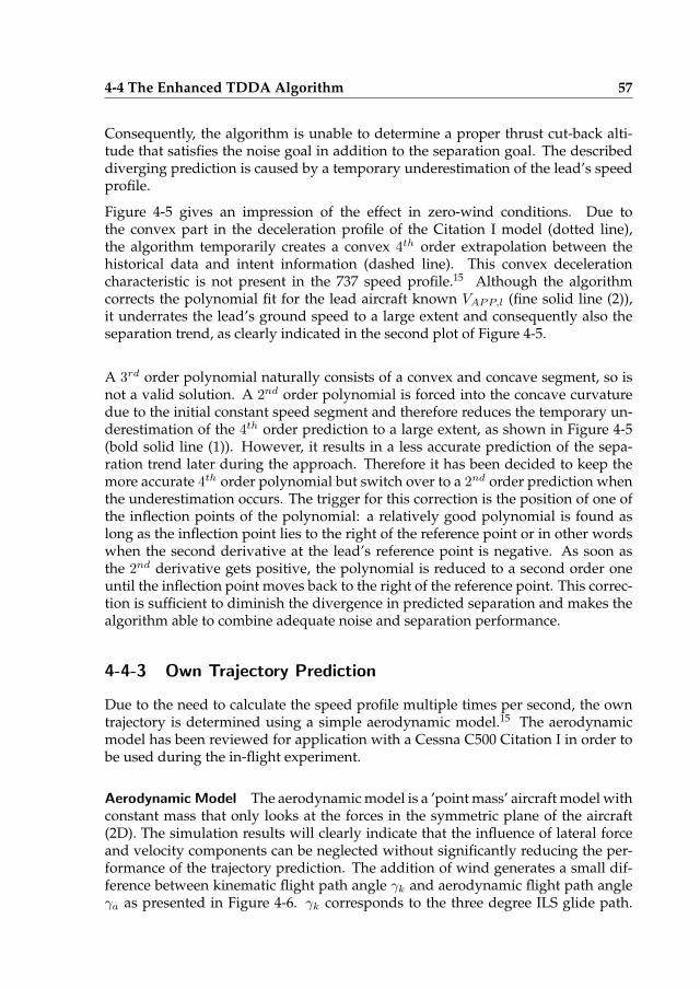
4-4 The Enhanced TDDA Algorithm 57
Consequently, the algorithm is unable to determine a proper thrust cut-back alti-tude that satisfies the noise goal in addition to the separation goal. The describeddiverging prediction is caused by a temporary underestimation of the lead’s speedprofile.
Figure 4-5 gives an impression of the effect in zero-wind conditions. Due tothe convex part in the deceleration profile of the Citation I model (dotted line),the algorithm temporarily creates a convex 4th order extrapolation between thehistorical data and intent information (dashed line). This convex decelerationcharacteristic is not present in the 737 speed profile.15 Although the algorithmcorrects the polynomial fit for the lead aircraft known VAPP,l (fine solid line (2)),it underrates the lead’s ground speed to a large extent and consequently also theseparation trend, as clearly indicated in the second plot of Figure 4-5.
A 3rd order polynomial naturally consists of a convex and concave segment, so isnot a valid solution. A 2nd order polynomial is forced into the concave curvaturedue to the initial constant speed segment and therefore reduces the temporary un-derestimation of the 4th order prediction to a large extent, as shown in Figure 4-5(bold solid line (1)). However, it results in a less accurate prediction of the sepa-ration trend later during the approach. Therefore it has been decided to keep themore accurate 4th order polynomial but switch over to a 2nd order prediction whenthe underestimation occurs. The trigger for this correction is the position of one ofthe inflection points of the polynomial: a relatively good polynomial is found aslong as the inflection point lies to the right of the reference point or in other wordswhen the second derivative at the lead’s reference point is negative. As soon asthe 2nd derivative gets positive, the polynomial is reduced to a second order oneuntil the inflection point moves back to the right of the reference point. This correc-tion is sufficient to diminish the divergence in predicted separation and makes thealgorithm able to combine adequate noise and separation performance.
4-4-3 Own Trajectory Prediction
Due to the need to calculate the speed profile multiple times per second, the owntrajectory is determined using a simple aerodynamic model.15 The aerodynamicmodel has been reviewed for application with a Cessna C500 Citation I in order tobe used during the in-flight experiment.
Aerodynamic Model The aerodynamic model is a ’point mass’ aircraft model withconstant mass that only looks at the forces in the symmetric plane of the aircraft(2D). The simulation results will clearly indicate that the influence of lateral forceand velocity components can be neglected without significantly reducing the per-formance of the trajectory prediction. The addition of wind generates a small dif-ference between kinematic flight path angle γk and aerodynamic flight path angleγa as presented in Figure 4-6. γk corresponds to the three degree ILS glide path.
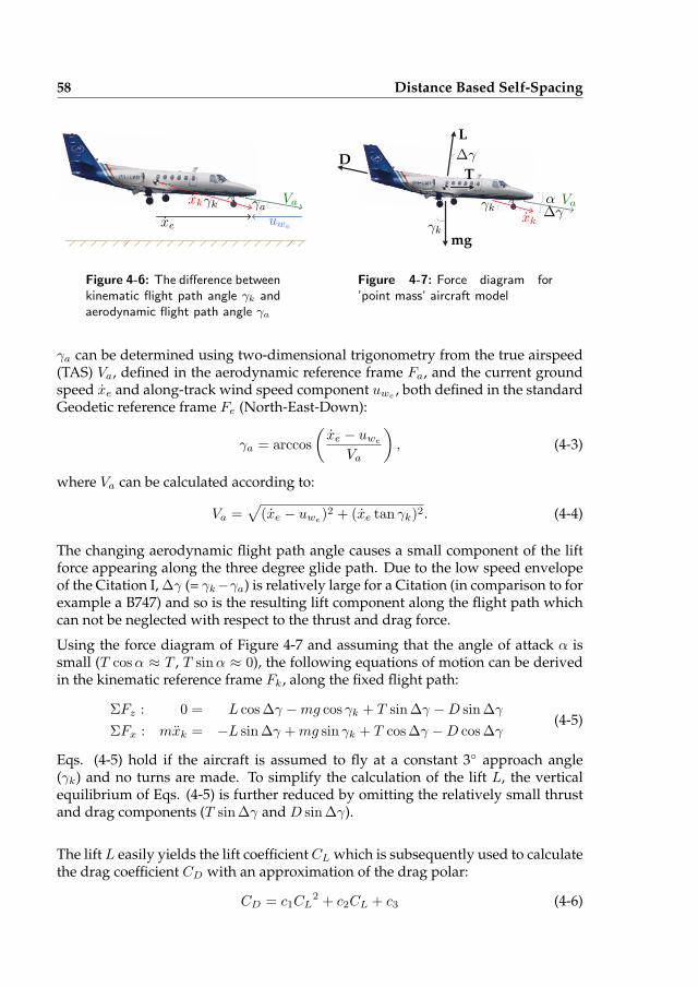
58 Distance Based Self-Spacing
xe
xk Va
uwe
γaγk
Figure 4-6: The difference betweenkinematic flight path angle γk andaerodynamic flight path angle γa
α
γk
γk
∆γ
∆γVa
xk
L
DT
mg
Figure 4-7: Force diagram for’point mass’ aircraft model
γa can be determined using two-dimensional trigonometry from the true airspeed(TAS) Va, defined in the aerodynamic reference frame Fa, and the current groundspeed xe and along-track wind speed component uwe
, both defined in the standardGeodetic reference frame Fe (North-East-Down):
γa = arccos
(
xe − uwe
Va
)
, (4-3)
where Va can be calculated according to:
Va =√
(xe − uwe)2 + (xe tan γk)2. (4-4)
The changing aerodynamic flight path angle causes a small component of the liftforce appearing along the three degree glide path. Due to the low speed envelopeof the Citation I, ∆γ (= γk−γa) is relatively large for a Citation (in comparison to forexample a B747) and so is the resulting lift component along the flight path whichcan not be neglected with respect to the thrust and drag force.
Using the force diagram of Figure 4-7 and assuming that the angle of attack α issmall (T cosα ≈ T , T sinα ≈ 0), the following equations of motion can be derivedin the kinematic reference frame Fk, along the fixed flight path:
ΣFz : 0 = L cos∆γ −mg cos γk + T sin∆γ −D sin∆γ
ΣFx : mxk = −L sin∆γ +mg sin γk + T cos∆γ −D cos∆γ(4-5)
Eqs. (4-5) hold if the aircraft is assumed to fly at a constant 3◦ approach angle(γk) and no turns are made. To simplify the calculation of the lift L, the verticalequilibrium of Eqs. (4-5) is further reduced by omitting the relatively small thrustand drag components (T sin∆γ and D sin∆γ).
The lift L easily yields the lift coefficient CL which is subsequently used to calculatethe drag coefficient CD with an approximation of the drag polar:
CD = c1CL2 + c2CL + c3 (4-6)
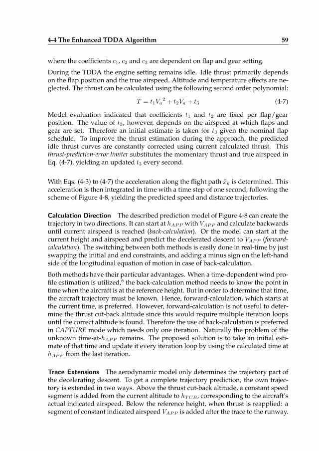
4-4 The Enhanced TDDA Algorithm 59
where the coefficients c1, c2 and c3 are dependent on flap and gear setting.
During the TDDA the engine setting remains idle. Idle thrust primarily dependson the flap position and the true airspeed. Altitude and temperature effects are ne-glected. The thrust can be calculated using the following second order polynomial:
T = t1Va2 + t2Va + t3 (4-7)
Model evaluation indicated that coefficients t1 and t2 are fixed per flap/gearposition. The value of t3, however, depends on the airspeed at which flaps andgear are set. Therefore an initial estimate is taken for t3 given the nominal flapschedule. To improve the thrust estimation during the approach, the predictedidle thrust curves are constantly corrected using current calculated thrust. Thisthrust-prediction-error limiter substitutes the momentary thrust and true airspeed inEq. (4-7), yielding an updated t3 every second.
With Eqs. (4-3) to (4-7) the acceleration along the flight path xk is determined. Thisacceleration is then integrated in time with a time step of one second, following thescheme of Figure 4-8, yielding the predicted speed and distance trajectories.
Calculation Direction The described prediction model of Figure 4-8 can create thetrajectory in two directions. It can start at hAPP with VAPP and calculate backwardsuntil current airspeed is reached (back-calculation). Or the model can start at thecurrent height and airspeed and predict the decelerated descent to VAPP (forward-calculation). The switching between both methods is easily done in real-time by justswapping the initial and end constraints, and adding a minus sign on the left-handside of the longitudinal equation of motion in case of back-calculation.
Both methods have their particular advantages. When a time-dependent wind pro-file estimation is utilized,6 the back-calculation method needs to know the point intime when the aircraft is at the reference height. But in order to determine that time,the aircraft trajectory must be known. Hence, forward-calculation, which starts atthe current time, is preferred. However, forward-calculation is not useful to deter-mine the thrust cut-back altitude since this would require multiple iteration loopsuntil the correct altitude is found. Therefore the use of back-calculation is preferredin CAPTURE mode which needs only one iteration. Naturally the problem of theunknown time-at-hAPP remains. The proposed solution is to take an initial esti-mate of that time and update it every iteration loop by using the calculated time athAPP from the last iteration.
Trace Extensions The aerodynamic model only determines the trajectory part ofthe decelerating descent. To get a complete trajectory prediction, the own trajec-tory is extended in two ways. Above the thrust cut-back altitude, a constant speedsegment is added from the current altitude to hTCB , corresponding to the aircraft’sactual indicated airspeed. Below the reference height, when thrust is reapplied: asegment of constant indicated airspeed VAPP is added after the trace to the runway.
60 Distance Based Self-Spacing
Flapschedule
coefficient
table aerodynamic
model
model
equations of
motion
wind modelTAS −→ IAS
atmosphere
Fk → Fe
Fk → Fe
TAS, γaIAS
TAS
ρ
ρ
ρ h
h
xe
T,D
xstartxstart
cn ,tn ∫∫ xxkxk
Figure 4-8: Own trajectory prediction model. The start position vector xstart andstart velocity xstart could be either the current aircraft position and speed (forward-calculation) or the reference point and approach speed vector (back-calculation).
4-4-4 Separation Trend Prediction
With the predicted trajectories for the lead and the own aircraft, the separationtrend can be easily calculated. Since the separation trend shows ‘closing character-istics’, the minimum predicted separation is found at or near the runway threshold.No additional smoothing filter is required.
4-4-5 Start Altitude Optimization
The optimization of the start altitude makes the algorithm able to achieve goodnoise performance in combination with safe in-trail spacing. The idea is to alterhTCB in such a way that minimum predicted separation increases to a safe levelwhile still being able to reach the target speed without applying thrust. When pre-dicted separation gets problematic after thrust cut-back, it is no longer possible tosatisfy both goals. Then, flaps must be extended at higher speeds to decelerate ear-lier and increase spacing. Consequently, the aircraft will get to VAPP too early andextra thrust is required.
The start altitude optimization process only alters hTCB when separation ispredicted to get dangerous (Figure 4-3). When safe spacing is guaranteed, noactions are taken. In case of separation excess, the algorithm could also schedulea lower hTCB . However, this requires further investigation into the design of thealgorithm’s control laws in order to achieve similar performance results as for theconducted Monte Carlo simulations (section 4-5).
Although separation is increased in HOLD mode by extending flaps sooner (athigher airspeeds), the mode of thought for the start altitude optimization is
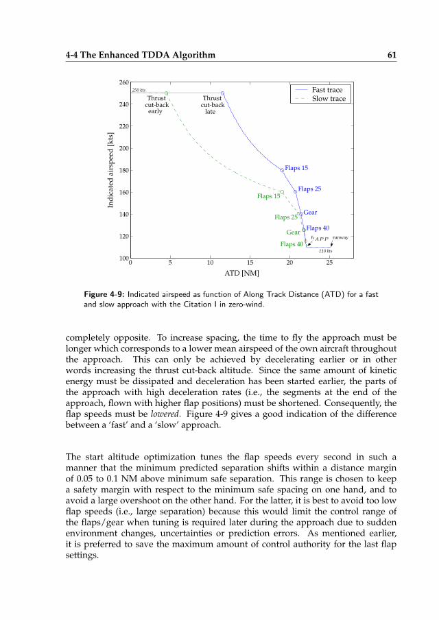
4-4 The Enhanced TDDA Algorithm 61
100
120
140
160
180
200
220
240
260
0 5 10 15 20 25
Fast traceSlow trace
ATD [NM]
Ind
icat
edai
rsp
eed
[kts
]
ThrustThrustcut-backcut-back
early late
Flaps 15
Flaps 25
Gear
Flaps 40
Flaps 15
Flaps 25
Gear
Flaps 40
110 kts
250 kts
hAPP runway
Figure 4-9: Indicated airspeed as function of Along Track Distance (ATD) for a fastand slow approach with the Citation I in zero-wind.
completely opposite. To increase spacing, the time to fly the approach must belonger which corresponds to a lower mean airspeed of the own aircraft throughoutthe approach. This can only be achieved by decelerating earlier or in otherwords increasing the thrust cut-back altitude. Since the same amount of kineticenergy must be dissipated and deceleration has been started earlier, the parts ofthe approach with high deceleration rates (i.e., the segments at the end of theapproach, flown with higher flap positions) must be shortened. Consequently, theflap speeds must be lowered. Figure 4-9 gives a good indication of the differencebetween a ‘fast’ and a ‘slow’ approach.
The start altitude optimization tunes the flap speeds every second in such amanner that the minimum predicted separation shifts within a distance marginof 0.05 to 0.1 NM above minimum safe separation. This range is chosen to keepa safety margin with respect to the minimum safe spacing on one hand, and toavoid a large overshoot on the other hand. For the latter, it is best to avoid too lowflap speeds (i.e., large separation) because this would limit the control range ofthe flaps/gear when tuning is required later during the approach due to suddenenvironment changes, uncertainties or prediction errors. As mentioned earlier,it is preferred to save the maximum amount of control authority for the last flapsettings.
62 Distance Based Self-Spacing
The coarse and fine-tuning processes are according to the search strategy of sec-tion 4-4-1. First, flap speeds are altered roughly to their limits until minimum pre-dicted separation overshoots one of the boundaries of the desired separation mar-gin. Next, if necessary, the previously shifted flap is fine-tuned to get separationwithin the margin.
4-4-6 Noise and Traffic Optimization
As soon as the aircraft passes the calculated thrust cut-back altitude or idle thrust isset too early, the Noise & Traffic optimization routine is activated. N&T optimiza-tion continues until the aircraft passes the altitude of the reference height plus 200ft in order to avoid late changes of the last flap speed(s).
The Optimization Constraints The N&T algorithm first determines the own tra-jectory using the last updated flap schedule and predicts the minimum separation.If all constraints are still met, no changes to the flap schedule are necessary and thealgorithm stops the current loop. The constraints for N&T optimization are:
• Separation goal: predicted separation must be larger than minimum safe sep-aration. If not, flap/gear speeds must be lowered.
• Noise goal: the aircraft must reach VAPP at the reference height of 1,000 ft.This constraint is included in the algorithm by checking the difference ∆h be-tween hAPP and the predicted altitude where the aircraft reaches VAPP (seeFigure 4-10). When ∆h is positive the aircraft is flying too slow and flap/gearspeeds must be lowered. A negative ∆h indicates that the aircraft is too fast,so flaps have to be extended earlier. A tuning margin for ∆h of ±5 ft is taken,since the altitude corresponding to VAPP can only be predicted with an accu-racy of maximum 10 ft.
The separation goal has always priority over the noise goal since safety prevails. Incase one of the above constraints is violated, the binary search algorithm looks fora satisfying flap schedule.
The Flap Optimization Process The flap scheduling process has a rough and fine-tuning cycle, as discussed in section 4-4-1. Flap speeds are increased when separa-tion is in danger OR ∆h is negative (< 5ft). Flap speeds are decreased when ∆his positive (> 5ft) AND separation is not a problem. After each flap speed change,the trajectory is recalculated. If tuning for separation, the algorithm increases flapspeeds to slowdown faster. Hence thrust will be applied before reaching hAPP (∆his positive). The algorithm is aware of this and will try to reduce the duration ofapplying thrust to a minimum. This is achieved by scheduling the own aircraft asclose as possible behind the lead, so within the +0.05/+0.1 NM separation margin.
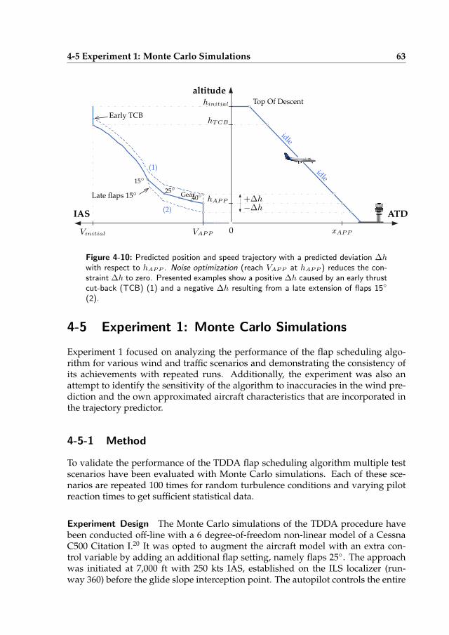
4-5 Experiment 1: Monte Carlo Simulations 63
IAS ATD
altitude
0
−∆h+∆h
VAPP xAPP
hAPP
hinitial
Vinitial
hTCB
Top Of Descent
15◦
25◦
40◦Gear
Early TCB
Late flaps 15◦
(1)
(2)
idle
idle
Figure 4-10: Predicted position and speed trajectory with a predicted deviation ∆h
with respect to hAPP . Noise optimization (reach VAPP at hAPP ) reduces the con-straint ∆h to zero. Presented examples show a positive ∆h caused by an early thrustcut-back (TCB) (1) and a negative ∆h resulting from a late extension of flaps 15◦
(2).
4-5 Experiment 1: Monte Carlo Simulations
Experiment 1 focused on analyzing the performance of the flap scheduling algo-rithm for various wind and traffic scenarios and demonstrating the consistency ofits achievements with repeated runs. Additionally, the experiment was also anattempt to identify the sensitivity of the algorithm to inaccuracies in the wind pre-diction and the own approximated aircraft characteristics that are incorporated inthe trajectory predictor.
4-5-1 Method
To validate the performance of the TDDA flap scheduling algorithm multiple testscenarios have been evaluated with Monte Carlo simulations. Each of these sce-narios are repeated 100 times for random turbulence conditions and varying pilotreaction times to get sufficient statistical data.
Experiment Design The Monte Carlo simulations of the TDDA procedure havebeen conducted off-line with a 6 degree-of-freedom non-linear model of a CessnaC500 Citation I.20 It was opted to augment the aircraft model with an extra con-trol variable by adding an additional flap setting, namely flaps 25◦. The approachwas initiated at 7,000 ft with 250 kts IAS, established on the ILS localizer (run-way 360) before the glide slope interception point. The autopilot controls the entire
64 Distance Based Self-Spacing
approach, disengaged the auto-throttle at hTCB , extends flaps and gear at the cal-culated speeds and re-engages the auto-throttle when reaching VAPP to hold thisvelocity. VAPP was set at 110 kts IAS, hAPP at 1,000 ft.
Another Cessna Citation I performing a TDDA has been selected as a leading air-craft and was initially separated 7.5 NM in front of the own aircraft. Its trajectorytook the governing winds into account. The actual wind profiles were definedaccording to a time-constant, rotating, logarithmic wind model.7, 22 The modeldemonstrated a so-called backing and veering effect of the wind vector as illus-trated in Figure 4-11. Wind prediction of the flap algorithm is taken identical to theactual wind profile, disregarding turbulence.
The Monte Carlo experiment was divided in two parts. First, general performancehas been evaluated following a complete test matrix. Secondly, several errors havebeen introduced in the algorithm to explore its robustness.
General Performance Analysis: Independent Variables Three independent vari-ables were varied, listed in Table 4-1, totally resulting in 36 scenarios. First, threelevels of optimization were investigated: (1) the baseline scenario, which uses a fixed’standard’ flap/gear deflection scheme. Only hTCB is calculated to comply with thegoverning predicted wind. (2) Noise-Only optimization (NO), where separation isnot taken into account. (3) Noise and Traffic optimization (N&T), which includesthe separation goal as well.
Secondly, two lead aircraft approach characteristics: (1) a ’nominal’ approach, deter-mined using the ’standard’ flap/gear schedule; (2) a ’fastman’ approach where theleading aircraft decelerates early because of early pilot deceleration actions.
Finally, six wind conditions: (1) zero-wind scenario; (2) and (3) head wind conditionsof 20 and 40 kts; (4) 60 kts crosswind coming from a 45◦ direction with respect tothe approach path; (5) 40 kts pure crosswind; and (6) tailwind of 20 kts.
Robustness Analysis To evaluate the robustness in flap scheduler performancethe following deviations were analyzed: (1) error between the actual and predictedwind profile, (2) error in predicted aircraft mass, and (3) error in approximated dragpolar of Eq. (4-6). Only scenarios with a fastman leader are interpreted. Naturally,this traffic scenario is of more interest as it demands more optimization effort.
Random Disturbances Two random disturbances made each run of the MonteCarlo simulation unique. The first variation is turbulence based on Dryden spectrawith additional arbitrary ”patchy” characteristics which introduces low-frequencygusts.3 Secondly, pilot response times to the thrust cut-back, flap and gear cueswere varied according to a Poisson probability distribution with a mean time delayof 1.75 seconds. The Poisson distribution has been leveled-off at 5 seconds, herebydefining the maximum delay.
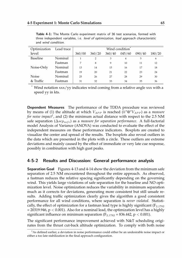
4-5 Experiment 1: Monte Carlo Simulations 65
Table 4-1: The Monte Carlo experiment matrix of 36 test scenarios, formed withthree independent variables, i.e. level of optimization, lead approach characteristic
and wind condition.
Optimization Lead trace Wind condition*
level 360/00 360/20 360/40 045/60 090/40 180/20
Baseline Nominal 1 2 3 4 5 6
Fastman 7 8 9 10 11 12
Noise-Only Nominal 13 14 15 16 17 18
Fastman 19 20 21 22 23 24
Noise Nominal 25 26 27 28 29 30
& Traffic Fastman 31 32 33 34 35 36
* Wind notation xxx/yy indicates wind coming from a relative angle xxx with aspeed yy in kts.
Dependent Measures The performance of the TDDA procedure was reviewedby means of (1) the altitude at which VAPP is reached (h”@”VAPP ) as a measurefor noise impact1, and (2) the minimum actual distance with respect to the 2.5 NMsafe separation (∆sepsafe) as a measure for separation performance. A full-factorialmodel Analysis of Variance (ANOVA) was conducted to evaluate the effect of theindependent measures on these performance indicators. Boxplots are created tovisualize the center and spread of the results. The boxplots also reveal outliers inthe data which are presented in the plots with a circle. These outliers are extremedeviations and mainly caused by the effect of immediate or very late cue response,possibly in combination with high gust peaks.
4-5-2 Results and Discussion: General performance analysis
Separation Goal Figures 4-13 and 4-14 show the deviation from the minimum safeseparation of 2.5 NM encountered throughout the entire approach. As observed,a fastman reduces the relative spacing significantly depending on the governingwind. This yields large violations of safe separation for the baseline and NO opti-mization level. Noise optimization reduces the variability in minimum separationmuch as it corrects for deviations, generating more consistent but still unsafe re-sults. Adding traffic optimization clearly gives the algorithm a good consistentperformance for all wind conditions, where separation is never violated. Statisti-cally, the effect of optimization for a fastman lead type is highly significant (F2,1782
= 20319.946, p < 0.001). Also for a nominal lead, the optimization level has a highlysignificant influence on minimum separation (F2,1782 = 836.442, p < 0.001).
The significant performance improvement achieved with N&T scheduling origi-nates from the thrust cut-back altitude optimization. To comply with both noise
1As defined earlier, a deviation in noise performance could either be an undesirable noise impact oreither a too late stabilization in the final approach configuration.

66 Distance Based Self-Spacing
ue [kts] ve [kts]
h[f
t]
4,500
3,000
1,500
0
0
0
-20
-10
24
6
North (Xe )East (Ye )
Figure 4-11: Logarithmic windmodel for a wind with direction360 and speed of 20 kts in theupper free atmosphere, showingthe backing and veering effect.
Wind [deg/kts]
hT
CB
[ft]
OptimizationBaselineNON&T
360/0 360/20 360/40 045/60 090/40 180/20
2,500
3,000
3,500
4,000
4,500
5,000
5,500
6,000
Figure 4-12: Thrust cut-back al-titudes in case of a fastman leadtrace.
and separation goals as good as possible, TCB heights are raised as presented inFigure 4-12. A positive outcome is the lower noise production, which is penalizedhowever with a reduced downward control authority of the flaps and gear sincethe margin with respect to its lower speed boundary decreases.
A small excess in final separation can be observed caused by the limited accuracyof the lead trajectory prediction during the initial part of the approach (2nd orderfit, Figure 4-5). The form of the lead aircraft deceleration characteristic primarilyeffects the performance of the separation prediction. The exact deceleration rate ofthe lead depends on both the governing wind and the lead’s behavior type. Thesetwo independent variables even significantly interact with each other to get theresulting actual minimum separation (F5,1188 = 17349.046, p < 0.001 for NO opti-mization). Notice that also the aircraft type of the lead has an influence. So theactual separation trend is highly variable and therefore hard to predict accuratelymost of the time. Increasing the accuracy of the separation prediction algorithm isexpected to be a challenging quest.
Noise Goal As expected and shown in Figures 4-15 and 4-16, h@VAPP lies consis-tently closer to the targeted 1,000 ft when the algorithm schedules the flaps and gearaccordingly (F2,1782 = 1944.213, p < 0.001 and F2,1782 = 334.689, p < 0.001, for, re-spectively, the nominal and fastman lead). A post-hoc analysis on the optimizationlevel (Student-Newman-Keuls (SNK), p = 0.05) reveals that the difference betweenbaseline and optimization is indeed significant. On the other hand, the mutual dif-ference between the two algorithm levels (NO and N&T) is not significant. Thealgorithm can reach similar performance with respect to noise for all headwindtype conditions, independent from the fact that separation was predicted to be indanger or not. Lead type has no significant influence on h@VAPP (F = 0.273, p =0.601). Hence, noise and separation goals can be combined excellently.
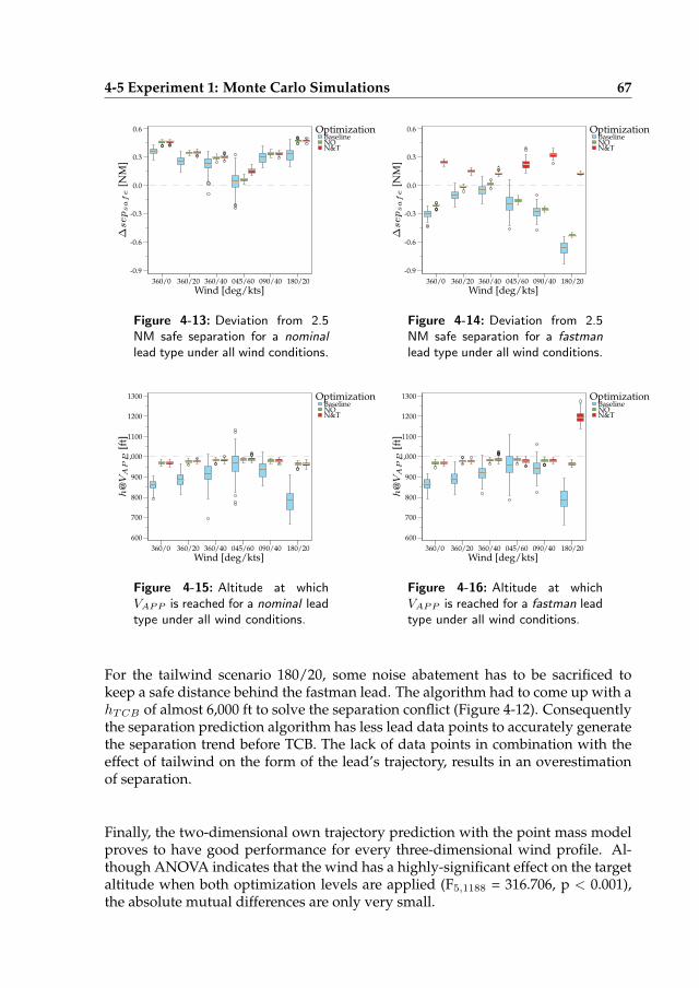
4-5 Experiment 1: Monte Carlo Simulations 67
Wind [deg/kts]
OptimizationBaselineNON&T
360/0 360/20 360/40 045/60 090/40 180/20
0.0
-0.3
0.3
-0.6
-0.9
0.6∆sepsafe
[NM
]
Figure 4-13: Deviation from 2.5NM safe separation for a nominal
lead type under all wind conditions.
Wind [deg/kts]
OptimizationBaselineNON&T
360/0 360/20 360/40 045/60 090/40 180/20
0.0
-0.3
0.3
-0.6
-0.9
0.6
∆sepsafe
[NM
]
Figure 4-14: Deviation from 2.5NM safe separation for a fastman
lead type under all wind conditions.
eplacements
Wind [deg/kts]
OptimizationBaselineNON&T
360/0 360/20 360/40 045/60 090/40 180/20
600
700
800
900
1,000
1100
1200
1300
h@VA
PP
[ft]
Figure 4-15: Altitude at whichVAPP is reached for a nominal leadtype under all wind conditions.
Wind [deg/kts]
OptimizationBaselineNON&T
360/0 360/20 360/40 045/60 090/40 180/20
600
700
800
900
1,000
1100
1200
1300h
@VA
PP
[ft]
Figure 4-16: Altitude at whichVAPP is reached for a fastman leadtype under all wind conditions.
For the tailwind scenario 180/20, some noise abatement has to be sacrificed tokeep a safe distance behind the fastman lead. The algorithm had to come up with ahTCB of almost 6,000 ft to solve the separation conflict (Figure 4-12). Consequentlythe separation prediction algorithm has less lead data points to accurately generatethe separation trend before TCB. The lack of data points in combination with theeffect of tailwind on the form of the lead’s trajectory, results in an overestimationof separation.
Finally, the two-dimensional own trajectory prediction with the point mass modelproves to have good performance for every three-dimensional wind profile. Al-though ANOVA indicates that the wind has a highly-significant effect on the targetaltitude when both optimization levels are applied (F5,1188 = 316.706, p < 0.001),the absolute mutual differences are only very small.
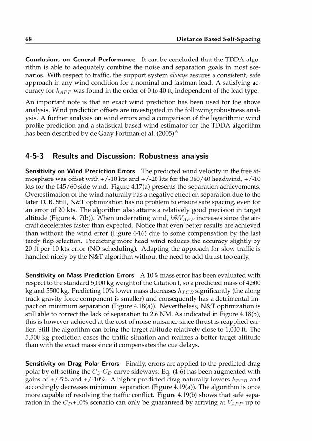
68 Distance Based Self-Spacing
Conclusions on General Performance It can be concluded that the TDDA algo-rithm is able to adequately combine the noise and separation goals in most sce-narios. With respect to traffic, the support system always assures a consistent, safeapproach in any wind condition for a nominal and fastman lead. A satisfying ac-curacy for hAPP was found in the order of 0 to 40 ft, independent of the lead type.
An important note is that an exact wind prediction has been used for the aboveanalysis. Wind prediction offsets are investigated in the following robustness anal-ysis. A further analysis on wind errors and a comparison of the logarithmic windprofile prediction and a statistical based wind estimator for the TDDA algorithmhas been described by de Gaay Fortman et al. (2005).6
4-5-3 Results and Discussion: Robustness analysis
Sensitivity on Wind Prediction Errors The predicted wind velocity in the free at-mosphere was offset with +/-10 kts and +/-20 kts for the 360/40 headwind, +/-10kts for the 045/60 side wind. Figure 4.17(a) presents the separation achievements.Overestimation of the wind naturally has a negative effect on separation due to thelater TCB. Still, N&T optimization has no problem to ensure safe spacing, even foran error of 20 kts. The algorithm also attains a relatively good precision in targetaltitude (Figure 4.17(b)). When underrating wind, h@VAPP increases since the air-craft decelerates faster than expected. Notice that even better results are achievedthan without the wind error (Figure 4-16) due to some compensation by the lasttardy flap selection. Predicting more head wind reduces the accuracy slightly by20 ft per 10 kts error (NO scheduling). Adapting the approach for slow traffic ishandled nicely by the N&T algorithm without the need to add thrust too early.
Sensitivity on Mass Prediction Errors A 10% mass error has been evaluated withrespect to the standard 5,000 kg weight of the Citation I, so a predicted mass of 4,500kg and 5500 kg. Predicting 10% lower mass decreases hTCB significantly (the alongtrack gravity force component is smaller) and consequently has a detrimental im-pact on minimum separation (Figure 4.18(a)). Nevertheless, N&T optimization isstill able to correct the lack of separation to 2.6 NM. As indicated in Figure 4.18(b),this is however achieved at the cost of noise nuisance since thrust is reapplied ear-lier. Still the algorithm can bring the target altitude relatively close to 1,000 ft. The5,500 kg prediction eases the traffic situation and realizes a better target altitudethan with the exact mass since it compensates the cue delays.
Sensitivity on Drag Polar Errors Finally, errors are applied to the predicted dragpolar by off-setting the CL-CD curve sideways: Eq. (4-6) has been augmented withgains of +/-5% and +/-10%. A higher predicted drag naturally lowers hTCB andaccordingly decreases minimum separation (Figure 4.19(a)). The algorithm is oncemore capable of resolving the traffic conflict. Figure 4.19(b) shows that safe sepa-ration in the CD+10% scenario can only be guaranteed by arriving at VAPP up to
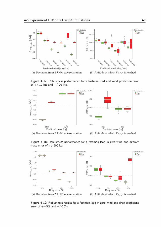
4-5 Experiment 1: Monte Carlo Simulations 69
Predicted wind [deg/kts]
OptimizationNON&T
360/40-10
360/40+10
045/60-10
045/60+10
360/40-20
360/40+20
∆sepsafe
[NM
]
0.0
-0.2
-0.4
0.2
0.4
(a) Deviation from 2.5 NM safe separation
Predicted wind [deg/kts]
OptimizationNON&T
360/40-10
360/40+10
045/60-10
045/60+10
360/40-20
360/40+20
h@VA
PP
[ft]
900
950
1,000
1,050
(b) Altitude at which VAPP is reached
Figure 4-17: Robustness performance for a fastman lead and wind prediction errorof +/-10 kts and +/-20 kts.
Predicted mass [kg]
OptimizationNON&T
4,500 5,500
∆sepsafe
[NM
]
0.0
-0.2
-0.4
-0.6
-0.8
0.2
0.4
0.6
(a) Deviation from 2.5 NM safe separation
Predicted mass [kg]
OptimizationNON&T
4500 5500
h@VA
PP
[ft]
900
950
1,000
1050
1,100
(b) Altitude at which VAPP is reached
Figure 4-18: Robustness performance for a fastman lead in zero-wind and aircraftmass error of +/-500 kg.
Drag error [%]
OptimizationNON&T
-10% -5% +5% +10%
∆sepsafe
[NM
]
0.0
-1.0
-0.5
2.0
1.5
1.0
0.5
(a) Deviation from 2.5 NM safe separation
Drag error [%]
OptimizationNON&T
-10% -5% +5% +10%
h@VA
PP
[ft]
900
1,000
1100
1200
(b) Altitude at which VAPP is reached
Figure 4-19: Robustness results for a fastman lead in zero-wind and drag coefficienterror of +/-5% and +/-10%.
70 Distance Based Self-Spacing
200 ft above the desired hAPP . Considering the amount of drag error and slowerlead, this is still a limited drop in noise performance. For the other scenarios onecan observe an obviously later stabilization in case drag is overvalued and a smallnoise penalty when underrating drag. An absolute target altitude deviation of 50 ftto 100 ft for respectively the 5% and 10% mismatch of CD, is still acceptable.
Conclusions on Algorithm Robustness The sensitivity analysis reveals that theflap/gear scheduling algorithm can cope with errors in wind, mass and drag pre-diction relatively good. The separation goal is always achieved, while the noiseperformance is only little declined. A comparison of all the results indicates thatthe optimization algorithm is most sensitive to mismatches in the drag polar. How-ever drag and lift information can be determined rather accurately with sufficientflight test data.18 Aircraft mass at take-off and fuel consumption should be able tobe calculated with a precision of less than 10% of the total weight. Therefore, thehighest expected error during TDDA operations is probably a mismatch betweenpredicted and actual wind.
4-6 Experiment 2: In-flight Investigation
Experiment 2 was the first attempt to evaluate the feasibility of self-spacing duringcontinuous decelerating approaches in real flight. The experiment should also com-plement the previous Monte Carlo studies, especially in support of the robustnesscharacteristics of the scheduling algorithm. The flight tests, conducted in February2005 at Soesterberg military airport (EHSB), included one test flight and one actualexploratory flight with multiple approaches.18 Only the results of the experimentaddressing the algorithm performance will be described.
4-6-1 Method
Apparatus: Aircraft and TDDA Display The Cessna C550 Citation II laboratoryaircraft of Delft Aerospace, a light twin-engined corporate jet, was used in the testflight. The aircraft has standard three flap settings (flaps UP, 15◦ and 40◦). Likefor the Monte Carlo simulations, a new flap setting was indicated in the cockpit,namely flaps 25◦, to increase the control range of the approach procedure. TheTDDA interface of Figure 4-2 was presented on a 15 inch LCD screen that wasmounted in front of the co-pilot’s seat. The aircraft was equipped with a FlightTest Instrumentation System (FTIS), developed in-house, that gathers the aircraftdata from the on-board Flight Management System (FMS) and ARINC Data Busand publishes this information to a distributed double laptop set-up which ran theTDDA software.
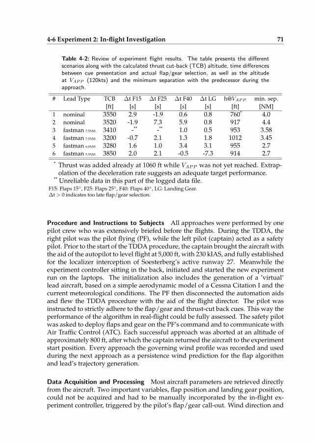
4-6 Experiment 2: In-flight Investigation 71
Table 4-2: Review of experiment flight results. The table presents the differentscenarios along with the calculated thrust cut-back (TCB) altitude, time differencesbetween cue presentation and actual flap/gear selection, as well as the altitudeat VAPP (120kts) and the minimum separation with the predecessor during theapproach.
# Lead Type TCB ∆t F15 ∆t F25 ∆t F40 ∆t LG h@VAPP min. sep.
[ft] [s] [s] [s] [s] [ft] [NM]
1 nominal 3550 2.9 -1.9 0.6 0.8 760* 4.02 nominal 3520 -1.9 7.3 5.9 0.8 917 4.43 fastman 7.5NM 3410 -** -** 1.0 0.5 953 3.584 fastman 7.5NM 3200 -0.7 2.1 1.3 1.8 1012 3.455 fastman 6.0NM 3280 1.6 1.0 3.4 3.1 955 2.76 fastman 5.5NM 3850 2.0 2.1 -0.5 -7.3 914 2.7
* Thrust was added already at 1060 ft while VAPP was not yet reached. Extrap-olation of the deceleration rate suggests an adequate target performance.
** Unreliable data in this part of the logged data file.F15: Flaps 15◦, F25: Flaps 25◦, F40: Flaps 40◦, LG: Landing Gear.∆t > 0 indicates too late flap/gear selection.
Procedure and Instructions to Subjects All approaches were performed by onepilot crew who was extensively briefed before the flights. During the TDDA, theright pilot was the pilot flying (PF), while the left pilot (captain) acted as a safetypilot. Prior to the start of the TDDA procedure, the captain brought the aircraft withthe aid of the autopilot to level flight at 5,000 ft, with 230 kIAS, and fully establishedfor the localizer interception of Soesterberg’s active runway 27. Meanwhile theexperiment controller sitting in the back, initiated and started the new experimentrun on the laptops. The initialization also includes the generation of a ’virtual’lead aircraft, based on a simple aerodynamic model of a Cessna Citation I and thecurrent meteorological conditions. The PF then disconnected the automation aidsand flew the TDDA procedure with the aid of the flight director. The pilot wasinstructed to strictly adhere to the flap/gear and thrust-cut back cues. This way theperformance of the algorithm in real-flight could be fully assessed. The safety pilotwas asked to deploy flaps and gear on the PF’s command and to communicate withAir Traffic Control (ATC). Each successful approach was aborted at an altitude ofapproximately 800 ft, after which the captain returned the aircraft to the experimentstart position. Every approach the governing wind profile was recorded and usedduring the next approach as a persistence wind prediction for the flap algorithmand lead’s trajectory generation.
Data Acquisition and Processing Most aircraft parameters are retrieved directlyfrom the aircraft. Two important variables, flap position and landing gear position,could not be acquired and had to be manually incorporated by the in-flight ex-periment controller, triggered by the pilot’s flap/gear call-out. Wind direction and
72 Distance Based Self-Spacing
speed were calculated by comparing the available ground and airspeed vectors. ILSlocalizer/glide slope together with flight director signals were computer generatedusing GPS positioning data. After all, glide slope signals can not be interceptedduring the initial part of a straight-in approach from 5,000 ft.
4-6-2 Results and Discussion
In Table 4-2, all data of interest for the second experiment flight are summarized. Atotal of six consecutive approaches were performed in which the initial separationwith the lead aircraft was gradually decreased to call in traffic scheduling. As aresult of the slower lead aircraft, the algorithm selected a higher hTCB to ensureconflict resolution. The pilot showed a strict adherence to the flap/gear cues. Theaverage delay between cue presentation and actual flap/gear selection was mea-sured to be 1.17 seconds. A few anomalies in cue follow-up occurred (runs 2 and 6)caused by misinterpretation between pilot and experiment controller, pilot antici-pation to the cues and ATC communication interferences.
For all approaches, minimum separation was never violated, even with a very slowlead aircraft in front (run 6). The target speed VAPP was always reached belowthe target altitude of 1066 ft2 and averaged 950 ft. The lower target altitudes aremainly caused by delays in flap/gear selection and deviations from the 3◦ ILS glidepath once the algorithm stops scheduling the lasts flaps within 200 ft of the targetaltitude.7
The current results show that, with the current algorithm and using persistencewind data, it is possible to perform a TDDA with a small jet aircraft while achievingthe noise and separation goal. Figure 4-20 illustrates the flap and gear behavior,wind information and the in-trail distance with the predecessor for run 4. Thecourse of the flap and gear cues indicates a gentle tuning process that oscillatesnear the nominal speeds. Upper and lower speed boundaries are avoided.
4-6-3 Conclusions
The flight tests were the first to investigate the viability of self-spacing during de-celerating approaches in real flight. The results are well in line with the previouslyconducted Monte Carlo experiments7 and prove that it is possible to perform aTDDA in real-life with the current algorithm and persistence wind data. All ap-proaches showed a consistent target performance in terms of reaching VAPP at thepre-specified altitude, while simultaneously the algorithm managed to take care ofseparation with traffic in front when necessary.
21,000 ft plus field elevation (66 ft).
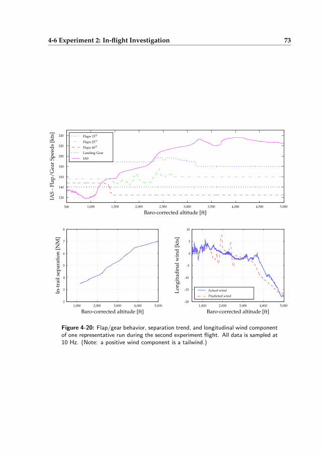
4-6 Experiment 2: In-flight Investigation 73
500
1,0001,000
1,000 1,500
2,0002,000
2,000 2,500
3,0003,000
3,000 3,500
4,0004,000
4,000 4,500
5,0005,000
5,000
2
3
4
6
7
8
120
140
160
180
200
220
240
10
5
5
0
-5
-10
-15
-20
Baro-corrected altitude [ft]Baro-corrected altitude [ft]
Baro-corrected altitude [ft]
IAS
-F
lap
/G
ear
Sp
eed
s[k
ts]
Flaps 15◦
Flaps 25◦
Flaps 40◦
Landing Gear
IAS
In-t
rail
sep
arat
ion
[NM
]
Lo
ng
itu
din
alw
ind
[kts
]
Actual wind
Predicted wind
Figure 4-20: Flap/gear behavior, separation trend, and longitudinal wind componentof one representative run during the second experiment flight. All data is sampled at10 Hz. (Note: a positive wind component is a tailwind.)
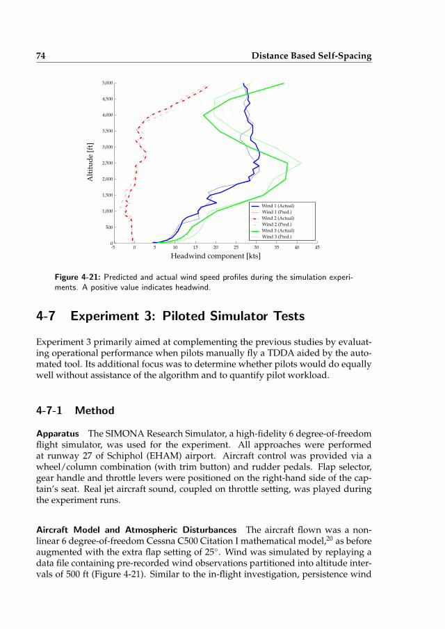
74 Distance Based Self-Spacing
00
500
1,000
1,500
2,000
2,500
3,000
3,500
4,000
4,500
5,000
-5 5 10 15 20 25 30 35 40 45
Headwind component [kts]
Alt
itu
de
[ft]
Wind 1 (Actual)
Wind 2 (Actual)
Wind 3 (Actual)
Wind 1 (Pred.)
Wind 2 (Pred.)
Wind 3 (Pred.)
Figure 4-21: Predicted and actual wind speed profiles during the simulation experi-ments. A positive value indicates headwind.
4-7 Experiment 3: Piloted Simulator Tests
Experiment 3 primarily aimed at complementing the previous studies by evaluat-ing operational performance when pilots manually fly a TDDA aided by the auto-mated tool. Its additional focus was to determine whether pilots would do equallywell without assistance of the algorithm and to quantify pilot workload.
4-7-1 Method
Apparatus The SIMONA Research Simulator, a high-fidelity 6 degree-of-freedomflight simulator, was used for the experiment. All approaches were performedat runway 27 of Schiphol (EHAM) airport. Aircraft control was provided via awheel/column combination (with trim button) and rudder pedals. Flap selector,gear handle and throttle levers were positioned on the right-hand side of the cap-tain’s seat. Real jet aircraft sound, coupled on throttle setting, was played duringthe experiment runs.
Aircraft Model and Atmospheric Disturbances The aircraft flown was a non-linear 6 degree-of-freedom Cessna C500 Citation I mathematical model,20 as beforeaugmented with the extra flap setting of 25◦. Wind was simulated by replaying adata file containing pre-recorded wind observations partitioned into altitude inter-vals of 500 ft (Figure 4-21). Similar to the in-flight investigation, persistence wind
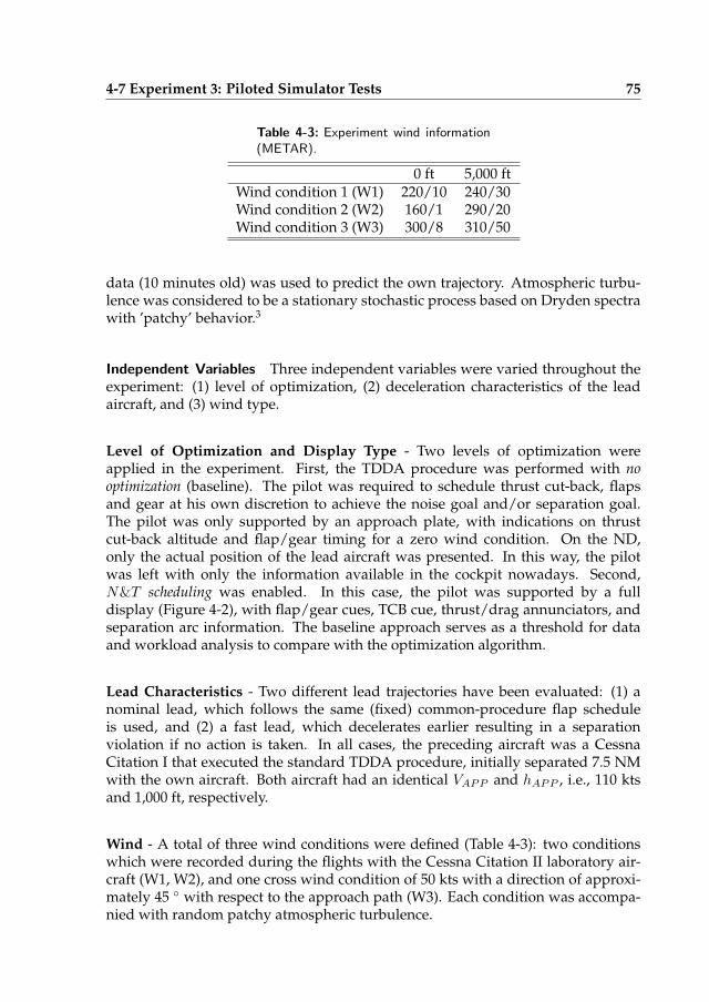
4-7 Experiment 3: Piloted Simulator Tests 75
Table 4-3: Experiment wind information(METAR).
0 ft 5,000 ftWind condition 1 (W1) 220/10 240/30Wind condition 2 (W2) 160/1 290/20Wind condition 3 (W3) 300/8 310/50
data (10 minutes old) was used to predict the own trajectory. Atmospheric turbu-lence was considered to be a stationary stochastic process based on Dryden spectrawith ’patchy’ behavior.3
Independent Variables Three independent variables were varied throughout theexperiment: (1) level of optimization, (2) deceleration characteristics of the leadaircraft, and (3) wind type.
Level of Optimization and Display Type - Two levels of optimization wereapplied in the experiment. First, the TDDA procedure was performed with nooptimization (baseline). The pilot was required to schedule thrust cut-back, flapsand gear at his own discretion to achieve the noise goal and/or separation goal.The pilot was only supported by an approach plate, with indications on thrustcut-back altitude and flap/gear timing for a zero wind condition. On the ND,only the actual position of the lead aircraft was presented. In this way, the pilotwas left with only the information available in the cockpit nowadays. Second,N&T scheduling was enabled. In this case, the pilot was supported by a fulldisplay (Figure 4-2), with flap/gear cues, TCB cue, thrust/drag annunciators, andseparation arc information. The baseline approach serves as a threshold for dataand workload analysis to compare with the optimization algorithm.
Lead Characteristics - Two different lead trajectories have been evaluated: (1) anominal lead, which follows the same (fixed) common-procedure flap scheduleis used, and (2) a fast lead, which decelerates earlier resulting in a separationviolation if no action is taken. In all cases, the preceding aircraft was a CessnaCitation I that executed the standard TDDA procedure, initially separated 7.5 NMwith the own aircraft. Both aircraft had an identical VAPP and hAPP , i.e., 110 ktsand 1,000 ft, respectively.
Wind - A total of three wind conditions were defined (Table 4-3): two conditionswhich were recorded during the flights with the Cessna Citation II laboratory air-craft (W1, W2), and one cross wind condition of 50 kts with a direction of approxi-mately 45 ◦ with respect to the approach path (W3). Each condition was accompa-nied with random patchy atmospheric turbulence.
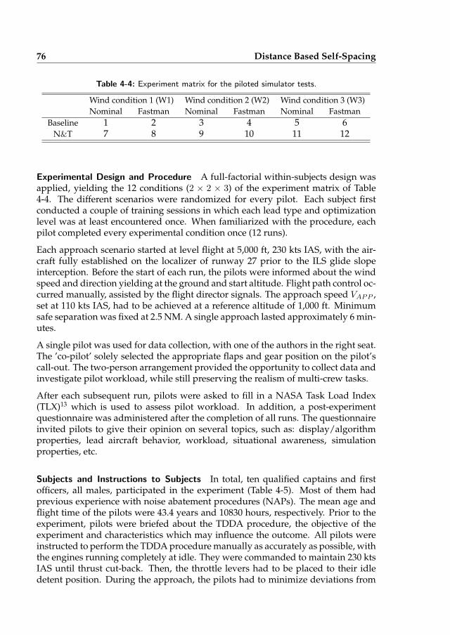
76 Distance Based Self-Spacing
Table 4-4: Experiment matrix for the piloted simulator tests.
Wind condition 1 (W1) Wind condition 2 (W2) Wind condition 3 (W3)
Nominal Fastman Nominal Fastman Nominal Fastman
Baseline 1 2 3 4 5 6N&T 7 8 9 10 11 12
Experimental Design and Procedure A full-factorial within-subjects design wasapplied, yielding the 12 conditions (2 × 2 × 3) of the experiment matrix of Table4-4. The different scenarios were randomized for every pilot. Each subject firstconducted a couple of training sessions in which each lead type and optimizationlevel was at least encountered once. When familiarized with the procedure, eachpilot completed every experimental condition once (12 runs).
Each approach scenario started at level flight at 5,000 ft, 230 kts IAS, with the air-craft fully established on the localizer of runway 27 prior to the ILS glide slopeinterception. Before the start of each run, the pilots were informed about the windspeed and direction yielding at the ground and start altitude. Flight path control oc-curred manually, assisted by the flight director signals. The approach speed VAPP ,set at 110 kts IAS, had to be achieved at a reference altitude of 1,000 ft. Minimumsafe separation was fixed at 2.5 NM. A single approach lasted approximately 6 min-utes.
A single pilot was used for data collection, with one of the authors in the right seat.The ’co-pilot’ solely selected the appropriate flaps and gear position on the pilot’scall-out. The two-person arrangement provided the opportunity to collect data andinvestigate pilot workload, while still preserving the realism of multi-crew tasks.
After each subsequent run, pilots were asked to fill in a NASA Task Load Index(TLX)13 which is used to assess pilot workload. In addition, a post-experimentquestionnaire was administered after the completion of all runs. The questionnaireinvited pilots to give their opinion on several topics, such as: display/algorithmproperties, lead aircraft behavior, workload, situational awareness, simulationproperties, etc.
Subjects and Instructions to Subjects In total, ten qualified captains and firstofficers, all males, participated in the experiment (Table 4-5). Most of them hadprevious experience with noise abatement procedures (NAPs). The mean age andflight time of the pilots were 43.4 years and 10830 hours, respectively. Prior to theexperiment, pilots were briefed about the TDDA procedure, the objective of theexperiment and characteristics which may influence the outcome. All pilots wereinstructed to perform the TDDA procedure manually as accurately as possible, withthe engines running completely at idle. They were commanded to maintain 230 ktsIAS until thrust cut-back. Then, the throttle levers had to be placed to their idledetent position. During the approach, the pilots had to minimize deviations from
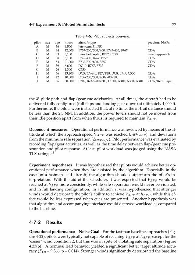
4-7 Experiment 3: Piloted Simulator Tests 77
Table 4-5: Pilot subjects overview.
pilot sex age hours aircraft type previous NAPsA M 36 4,500 Jetstream 31, F50 -B M 44 12,000 B737-200/300/400, B747-400, B767 CDAC M 33 3,100 Lynx helicopter, B737, C550 Steep approachD M 38 6,100 B747-400, B767, B777 CDAE M 54 21,000 B737-700/800, B757 CDAF M 39 6,600 DC10, B767, B737 CDAG M 26 1,300 C550 -H M 66 13,200 DC3/CV640, F27/F28, DC8, B747, C550 CDAI M 42 10,500 B737-200/300/400/700/800 CDAJ M 56 30,000 B707, B737-200/300, DC10, A310, A330, A340 CDA/Red. flaps
the 3◦ glide path and flap/gear cue advisories. At all times, the aircraft had to bedelivered fully configured (full flaps and landing gear down) at ultimately 1,000 ft.Furthermore, the pilots were instructed that, at no time, the in-trail distance shouldbe less than the 2.5 NM. In addition, the power levers should not be moved fromtheir idle position apart from when thrust is required to maintain VAPP .
Dependent measures Operational performance was reviewed by means of the al-titude at which the approach speed VAPP was reached (h@VAPP ), and deviationsfrom the minimum safe separation (∆sepsafe). Pilot performance was evaluated byrecording flap/gear activities, as well as the time delay between flap/gear cue pre-sentation and pilot response. At last, pilot workload was judged using the NASATLX ratings.13
Experiment hypotheses It was hypothesized that pilots would achieve better op-erational performance when they are assisted by the algorithm. Especially in thecases of a fastman lead aircraft, the algorithm should outperform the pilot’s in-terpretation. With the aid of the scheduler, it was expected that VAPP would bereached at hAPP more consistently, while safe separation would never be violated,and in full landing configuration. In addition, it was hypothesized that strongerwinds would deteriorate the pilot’s ability to achieve VAPP at hAPP , while this ef-fect would be less expressed when cues are presented. Another hypothesis wasthat algorithm and accompanying interface would decrease workload as comparedto the baseline.
4-7-2 Results
Operational performance Noise Goal - For the fastman baseline approaches (Fig-ure 4-22), pilots were typically not capable of reaching VAPP at hAPP , except for the’easier’ wind condition 2, but this was in spite of violating safe separation (Figure4.23(b)). A nominal lead behavior yielded a significant better target altitude accu-racy (F1,9 = 9.366, p = 0.014). Stronger winds significantly deteriorated the baseline

78 Distance Based Self-Spacing
performance for a fastman lead(F2,18 = 7.072, p < 0.001), however no statisticallysignificance could be found for the nominal lead (F2,18 = 2.533, p = 0.107).
When presented with the pilot support interface, pilots were clearly capableof reaching the target altitude more consistent which is expressed in the lowervariability and means closer to the target altitude (nominal lead: F1,9 = 10.512,p = 0.010; fastman: F1,9 = 8.668, p = 0.016). Because the algorithm will alwaysprioritize on safe separation, a slower lead aircraft evidently decreases the noisereduction performance of the algorithm (F1,9 = 26.059, p = 0.001). Wind howevershowed to have no significant influence (F2,18 = 2.504, p = 0.110).
1,400
1,300
1,200
1,100
1,000
900
800
1 2 3
OptimizationBaselineN&T
95%
CI
Mea
nh
@V
AP
P[f
t]
Wind condition
(a) Nominal lead aircraft.
1,400
1,300
1,200
1,100
1,000
900
1 2 3
OptimizationBaselineN&T
95%
CI
Mea
nh
@V
AP
P[f
t]
Wind condition
(b) Fastman lead aircraft.
Figure 4-22: The means and 95% confidence intervals of the altitude at which VAPP
was reached.
1.2
1.0
0.8
0.6
0.4
0.2
0.0
-0.2
-0.4
1 2 3
OptimizationBaselineN&T
95%
CI
Mea
n∆sepsafe
[NM
]
Wind condition
(a) Nominal lead aircraft.
0.8
0.6
0.4
0.2
0.0
-0.2
-0.4
1 2 3
OptimizationBaselineN&T
95%
CI
Mea
n∆sepsafe
[NM
]
Wind condition
(b) Fastman lead aircraft.
Figure 4-23: The means and 95% confidence intervals of the deviations from theminimum safe separation throughout the whole approach. A negative value indicatessafe separation violation.
4-7 Experiment 3: Piloted Simulator Tests 79
Separation Goal - Figures 4-23 illustrates the deviations from the minimum safeseparation of 2.5 NM throughout the whole approach. As foreseen, safe separa-tion distinctly decreased with slower lead aircraft (fastman) when pilots are notassisted (F1,9 = 84.125, p < 0.001). They only managed to cope with a fastman inthe first wind scenario, however this was accompanied by a detrimental effect onh@VAPP (Figure 4.22(b)). Actually, the more the pilots were trying to achieve VAPP
at the target altitude, the more they exceeded or tended to exceed the safe separa-tion threshold. The wind characteristics also significantly influenced the separationperformance (F2,18 = 23.600, p < 0.001).
When the algorithm comes into play the scatter in data reduced expressively for anormal decelerating predecessor (W1: F1,9 = 16.552, p = 0.003; W2: F1,9 = 21.288, p= 0.001; W3: F1,9 = 11.684, p = 0.008) and fastman lead. Accordingly as in the base-line, ∆sepsafe becomes much smaller for a fastman lead with respect to a normalpredecessor (F1,9 = 32.790, p < 0.001).
The most important contribution of the algorithm is that safe separation is neverviolated. In fact, the algorithm is able to ”close the gap” in comparison with thebaseline. An ANOVA analysis revealed that optimization had a borderline signifi-cant effect on deviating from 2.5 NM separation with a fastman lead (F1,9 = 4.345,p = 0.067), where the effect is highly significant for wind 2 (F1,9 = 12.602, p = 0.006).
Pilot controls To be fully configured, a total of three flap and one gear activitieshave to be performed. When assisted by the cues, the pilot was able to be fullyconfigured at the end of the TDDA, while this was certainly not always the casefor a baseline approach in the more ’severe’ wind conditions. Wind and optimiza-tion proved to have a (borderline) significant effect on achieving full configuration(respectively F2,18 = 3.273, p = 0.061 and F1,9 = 3.578, p = 0.091). Choosing a tooearly thrust-cut back, forced the pilots to delay flap and gear extension to extendthe glide. So in some cases, this resulted in not selecting the last flap or gear beforeVAPP was reached. No significant differences due to lead behavior were discovered(F1,9 = 2.250, p = 0.168).
The pilot response time on the flap and gear cues demonstrated a trend towardsanticipation on the cues when confronted with a sluggish predecessor (Figure 4-24). Indeed, the effect of lead was analyzed as significant (F1,9 = 9.270, p = 0.014).Pilots were not anticipating on the thrust-cut back cue, but were awaiting the cue(Figure 4-25).
Workload and Post-Test Questionnaire The workload ratings in Figure 4-26show a highly significant decrease in workload with the aid of the current algo-rithm and pilot support interface as expected (F1,9 = 107.622, p < 0.001). No signif-icant differences were found for wind condition (F2,18 = 2.131, p = 0.148).
Pilot comments and subjective ratings given in the post-test questionnaire indicatedthat the pilot support interface was indeed a helpful tool to execute a TDDA, and

80 Distance Based Self-Spacing
Lead BehaviorNominalFastman
1 3
1.0
2.0
3.0
0.0
2
95%
CI
Mea
nP
ilo
tre
acti
on
tim
e[s
]
Wind condition
Figure 4-24: The mean and95% confidence intervals of thepilot response time on flap andgear cues.
Mean = 2.3374Std. Dev. = 2.76742N = 60
0.0 5.0 10.00
2
4
6
8
10
12
14
Fre
qu
ency
[-]
Mean pilot reaction time [s]
Figure 4-25: Histogram of thepilot response time on the thrustcut-back cue.
1.0
0.5
0.0
-0.5
-1.0
1 2 3
OptimizationBaselineN&T
95%
CI
No
rmal
ized
TL
X
Wind condition
Figure 4-26: The means and95% confidence intervals for thenormalized TLX scores.
4-8 Conclusions 81
which in return brought instrument scan, workload and situational awareness to acomparable level as in current ILS approaches.
4-7-3 Discussion and Conclusions
For the tested wind conditions, it can be concluded that when pilots have to timethrust-cut back, flap and gear selection on their own, they are able to reach VAPP atthe projected altitude when a nominal lead is in front. However, pilot performancedeteriorates significantly with more sluggish lead aircraft, either by re-applyingthrust too early to maintain VAPP or by violating minimum safe separation. Adistinctly better and more consistent noise performance is found when optimizedcues are presented, while safe separation with the predecessor is guaranteed atall time. Additionally, the assistance of the algorithm and display clearly decreasespilot workload up to an effort level comparable to current standard approaches. Allin all, the pilot support interface and accompanying scheduling algorithm providesan essential tool to perform Three-Degree Decelerating Approaches.
4-8 Conclusions
The developed prediction and scheduling routine demonstrated to be a valuabletool to achieve adequate and consistent performance in executing a self-separatednoise abatement procedure, like the TDDA.
Off-line Monte Carlo results showed that the optimization algorithm is able to ade-quately combine safe separation with target altitude accuracy in various scenarios.An evaluation of the sensitivity of the algorithm pointed out that the TDDA algo-rithm is able to limit the effect of relatively large prediction errors for wind, aircraftmass and drag of the aircraft to only 200 ft.
The human-in-the-loop simulator experiment showed that, for the tested wind andtraffic conditions, pilots can achieve the target speed at a pre-specified altitude quiteaccurately when tailing a nominal lead without any assistance. However, if facedwith a more sluggish predecessor, larger deviations from the projected target alti-tude were distinguished, while in some cases separation became hazardous. Whenaided by the support tool, a significantly better performance and decreased work-load was reached. The projected target speed was achieved more consistently atthe target altitude, while safe separation was guaranteed at all times. The subjectpilots generally rated the workload level with the TDDA procedure similar to thatwith standard ILS procedures.
The exploratory demonstration flight proved that the current algorithm, using per-sistence wind data, is able to guide the pilot to the projected target altitude rela-tively accurately under actual flight conditions. This all, while guaranteeing againsafe separation with the predecessor throughout the whole approach.
82 REFERENCES
4-9 Acknowledgments
The authors express their gratitude to the staff of Delft University’s Institute forSimulation, Motion and Navigation technologies (SIMONA), in particular to OlafStroosma, for their essential contributions in conducting Experiment 3, and to thestaff of the Delft University Flight Department for their indispensable efforts inrealizing the in-flight experiment. The authors also wish to thank all pilots whoparticipated in the two experiments.
References
[1] Sourdine D3: Establishment of Noise Abatement Solutions. Technical report,Amsterdam, The Netherlands, 2000.
[2] Sourdine D5: Final Report. Technical report, Amsterdam, The Netherlands,2001.
[3] M. Baarspul. Flight Simulation Techniques. Faculty of Aerospace Engineering,Delft University of Technology, Delft, The Netherlands, 1982.
[4] J.-P. Clarke. A Systems Analysis Methodology for Developing Single Event NoiseAbatement Procedures. Sc.D. Dissertation, Massachusetts Institute of Technol-ogy, Cambridge (MA), USA, 1997.
[5] J.-P. Clarke, N. T. Ho, L. Ren, J. A. Brown, K. R. Elmer, K. Tong, and J. K.Wat. Continuous Descent Approach: Design and Flight Test for LouisvilleInternational Airport. AIAA Journal of Aircraft, 41(5):1054–1066, 2004.
[6] W. F. de Gaay Fortman, M. Mulder, M. M. van Paassen, A. C. in ’t Veld, andJ.-P. Clarke. Wind Profile Prediction to Support Three-Degree DeceleratingApproaches. In Proceedings of the AIAA Guidance, Navigation and Control Con-ference & Exhibit, number AIAA 2005-6141, pages 1–23, San Francisco (CA),USA, Aug 15-18 2005.
[7] J. L. de Prins, K. F. M. Schippers, M. Mulder, M. M. van Paassen, A. C. in’t Veld, and J.-P. Clarke. Enhanced Self-Spacing Algorithm for Three-DegreeDecelerating Approaches. In Proceedings of the AIAA Guidance, Navigation andControl Conference & Exhibit, number AIAA 2005-6140, pages 1–22, San Fran-cisco (CA), USA, Aug 15-18 2005.
[8] K. Elmer, J. Wat, G. Gershzohn, B. Shivashankara, J.-P. Clarke, N. T. Ho, L. To-bias, and D. Lambert. A Study of Noise Abatement Procedures Using AmesB747-400 Flight Simulator. In 8th AIAA/CEAS Aeroacoustics Conference & Ex-hibit, number AIAA 2002-2540, pages 1–10, Breckenridge (CO), USA, Jun 17-192002.
REFERENCES 83
[9] K. Elmer, J. Wat, B. Shivashankara, J.-P. Clarke, K. Tong, J. Brown, and A. War-ren. Community Noise Reduction using Continuous Descent Approach: ADemonstration Flight Test at Louisville. In 9th AIAA/CEAS Aeroacoustics Con-ference & Exhibit, number AIAA 2003-3277, pages 1–9, Hilton Head (SC), USA,May 12-14 2003.
[10] K. Elmer, J. Wat, B. Shivashankara, D. McGregor, and D. Lambert. A Con-tinuous Descent Approach Study using Ames B747-400 Flight Simulator. InAIAA’s Aircraft Technology, Integration, and Operations (ATIO) Technical, numberAIAA 2002-5869, pages 1–9, Los Angeles (CA), USA, Oct 1-3 2002.
[11] L. J. J. Erkelens. Research into New Noise Abatement Procedures for the 21st
Century. In AIAA Guidance, Navigation, and Control Conference & Exhibit, num-ber AIAA 2000-4474, pages 1–10, Denver (CO), USA, Aug 14-17 2000.
[12] G. Gershzohn, J. Wat, J. P. Dwyer, K. Elmer, J.-P. Clarke, and N. T. Ho. Ad-vanced Noise Abatement Procedures: An Experimental Study of Flight Oper-ational Acceptability. In AIAA’s Aircraft Technology, Integration, and Operations(ATIO) Technical, number AIAA 2002-5867, pages 1–9, Los Angeles (CA), USA,Oct 1-3 2002.
[13] S. G. Hart and L. E. Staveland. Development of NASA-TLX (Task Load In-dex): Results of Empirical and Theoretical Research. In P. A. Hancock andN. Meshkati, editors, Human Mental Workload, pages 139–183. Elsevier SciencePublishers, Amsterdam, The Netherlands, 1988.
[14] N. T. Ho and J.-P. Clarke. Mitigating Operational Aircraft Noise Impact byLeveraging on Automation Capability. In Proceedings of the AIAA Aircraft, Tech-nology, Integration and Operations Forum, number AIAA 2001-5239, pages 1–8,Los Angeles (CA), USA, Oct 16-18 2001.
[15] A. C. in ’t Veld, M. M. van Paassen, M. Mulder, and J.-P. Clarke. Pilot Supportfor Separation Assurance during Decelerated Approaches. In Proceedings ofthe AIAA Guidance, Navigation and Control Conference & Exhibit, number AIAA2004-5102, pages 1–13, Providence (RI), USA, Aug 16-19 2004.
[16] M. F. Koeslag. Advanced Continuous Descent Approaches, an Algorithm De-sign for the FMS. MSc. Thesis, Faculty of Aerospace Engineering, Delft Uni-versity of Technology, 2001.
[17] L. Ren, J.-P. Clarke, and N. T. Ho. Achieving Low Approach Noise withoutSacrifying Capacity. In 22nd Digital Avionics Systems Conference, number AIAA-2001-5239, pages 1–9, Indianapolis (IN), USA, Oct 12-16 2003.
[18] K. F. M. Schippers, J. L. de Prins, M. Mulder, M. M. van Paassen, A. C. in’t Veld,and J.-P. Clarke. Investigation of a Three-Degree Decelerating Approach ofa Twin Engined Jet Aircraft. In Proceedings of the AIAA Guidance, Navigationand Control Conference & Exhibit, number AIAA 2005-6139, pages 1–28, SanFrancisco (CA), USA, Aug 15-18 2005.

84 Distance Based Self-Spacing
[19] H. A. Simon. Models of Man. Wiley, New York (NY), USA, 1957.
[20] C. A. A. M. van der Linden. DASMAT - Delft University Aircraft SimulationModel and Analysis Tool. Technical Report LR-781, Delft University of Tech-nology, Delft, The Netherlands, Aug 1996.
[21] J. van Kan. Numerieke Wiskunde voor Technici (in Dutch). Delft University Press,Delft, The Netherlands, 2000.
[22] J. Wieringa and P. J. Rijkoort. Windklimaat van Nederland (in Dutch). Staatsuit-geverij, The Hague, The Netherlands, 1983.
[23] F. J. M. Wubben and J. J. Busink. Environmental Benefits of ContinuousDescent Approaches at Schiphol Airport Compared with Conventional Ap-proach Procedures. Technical Report NLR-TP-2000-275, National AerospaceLaboratory (NLR), Amsterdam, The Netherlands, May 2000.
5
Stochastic Wind ProfileEstimation
Real-time Stochastic Wind Profile Estimation using Airborne Sensors
A.C. in ’t Veld, M. Mulder and M.M. van Paassen
submitted to the AIAA Journal of Aircraft, December 2009
5-1 Abstract
Wind is one of the major contributors to uncertainty in continuous descent ap-proach operations. Especially when aircraft that are flying low or idle thrust ap-proaches are issued a required time of arrival over the runway threshold, as isforeseen in some of the future ATC scenarios, the on-board availability of both de-pendable and accurate wind estimates becomes a necessity. This paper presents amethod for real-time estimating the wind profile in the terminal maneuvering area,based on data transmissions of nearby aircraft that produces real-time wind profileestimates in a form that is usable for accurate trajectory prediction. The AMDARwind prediction algorithm (AWPA) is designed to process data that is of the formcurrently used in the Aircraft Meteorological Data Relay (AMDAR)-program. Thealgorithm combines a stochastic estimation based on this data and a traditionallogarithmic estimator in order to be able to produce a valid estimation even whenthere are no data available from other aircraft.
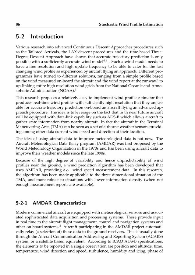
86 Stochastic Wind Profile Estimation
5-2 Introduction
Various research into advanced Continuous Descent Approaches procedures suchas the Tailored Arrivals, the LAX descent procedures and the time based Three-Degree Descent Approach have shown that accurate trajectory prediction is onlypossible with a sufficiently accurate wind model4, 6 . Such a wind model needs tohave a fine resolution and high update frequency to be able to cater for the fastchanging wind profile as experienced by aircraft flying an appraoch. Different pro-grammes have turned to different solutions, ranging from a simple profile basedon the wind measured on-board the aircraft and the wind report at the runway,6 toup-linking entire high resolution wind grids from the National Oceanic and Atmo-spheric Administration (NOAA).4
This research proposes a relatively easy to implement wind profile estimator thatproduces real-time wind profiles with sufficiently high resolution that they are us-able for accurate trajectory prediction on-board an aircraft flying an advanced ap-proach procedure. The idea is to leverage on the fact that in th near future aircraftwill be equipped with data-link capability such as ADS-B which allows aircraft togather state information from nearby aircraft. In fact the aircraft in the TerminalManeuvering Area (TMA) can be seen as a set of airborne weather sensors provid-ing among other data current wind speed and direction at their location.
The idea of using aircraft data to improve meteorological data is not new. TheAircraft Meteorological Data Relay program (AMDAR) was first proposed by theWorld Meteorology Organization in the 1970s and has been using aircraft data toimprove their weather models since the late 1990s.
Because of the high degree of variability and hence unpredictability of windprofiles near the ground, a wind prediction algorithm has been developed thatuses AMDAR, providing a.o. wind speed measurement data. In this research,the algorithm has been made applicable to the three-dimensional situation of theTMA, and more robust to situations with lower information density (when notenough measurement reports are available).
5-2-1 AMDAR Characteristics
Modern commercial aircraft are equipped with meteorological sensors and associ-ated sophisticated data acquisition and processing systems. These provide inputin real time to the aircraft flight management, control and navigation systems andother on-board systems.8 Aircraft participating in the AMDAR project automati-cally relay (a selection of) these data to the ground receivers. This is usually donethrough the Aircraft Communication Addressing and Reporting System (ACARS)system, or a satellite based equivalent. According to ICAO ADS-B specifications,the elements to be reported in a single observation are position and altitude, time,temperature, wind direction and speed, turbulence, humidity and icing, phase of
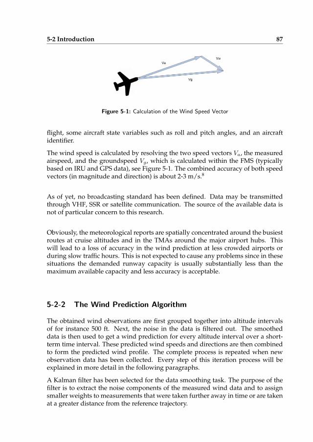
5-2 Introduction 87
Figure 5-1: Calculation of the Wind Speed Vector
flight, some aircraft state variables such as roll and pitch angles, and an aircraftidentifier.
The wind speed is calculated by resolving the two speed vectors Va, the measuredairspeed, and the groundspeed Vg , which is calculated within the FMS (typicallybased on IRU and GPS data), see Figure 5-1. The combined accuracy of both speedvectors (in magnitude and direction) is about 2-3 m/s.8
As of yet, no broadcasting standard has been defined. Data may be transmittedthrough VHF, SSR or satellite communication. The source of the available data isnot of particular concern to this research.
Obviously, the meteorological reports are spatially concentrated around the busiestroutes at cruise altitudes and in the TMAs around the major airport hubs. Thiswill lead to a loss of accuracy in the wind prediction at less crowded airports orduring slow traffic hours. This is not expected to cause any problems since in thesesituations the demanded runway capacity is usually substantially less than themaximum available capacity and less accuracy is acceptable.
5-2-2 The Wind Prediction Algorithm
The obtained wind observations are first grouped together into altitude intervalsof for instance 500 ft. Next, the noise in the data is filtered out. The smootheddata is then used to get a wind prediction for every altitude interval over a short-term time interval. These predicted wind speeds and directions are then combinedto form the predicted wind profile. The complete process is repeated when newobservation data has been collected. Every step of this iteration process will beexplained in more detail in the following paragraphs.
A Kalman filter has been selected for the data smoothing task. The purpose of thefilter is to extract the noise components of the measured wind data and to assignsmaller weights to measurements that were taken further away in time or are takenat a greater distance from the reference trajectory.
88 Stochastic Wind Profile Estimation
For the short-term wind prediction an Auto-Regressive Moving-Average (ARMA)model is used.3 This is a sophisticated statistical model based on the Kalman filterand calculates a forecast value as a linear combination of the last N measured val-ues. Here these values are wind speed and wind direction, expressed in North andEast velocity components VN , VE . The coefficients of the ARMA prediction modelare first determined using a recursive Kalman filter. Then the predicted wind canbe calculated by filling in the previously observed wind parameters into the ARMAmodel.
Finally, the predicted wind profile is created by fitting a cubic spline through thepredicted wind speeds. A cubic spline consists of piecewise polynomials that fol-low the altitude dependent wind predictions smoothly. This way every possiblewind profile can be fitted and predefined models can be avoided.
The strength of this wind prediction algorithm is its flexibility. It provides an accu-rate profile based on a statistical model when sufficient data is present, but revertsto a logarithmic estimation when data are sparse. This has the added benefit thatthe accuracy increases when the traffic density increase, i.e. when the accurate tra-jectory prediction is most important.
5-3 Physical Wind Model
Wind is one of the primary atmospheric factors affecting airplane performance. Itis the movement of air relative to the Earth. Wind can be quantitatively describedwith its velocity and its direction. The wind direction is defined as the directionfrom which the wind originates. Wind direction is defined in the Earth referenceframe FE . The movement of air is mainly the result of three major mechanisms be-ing air pressure gradients, the influence of the rotation of the Earth and the surfacefriction forces.11
1. The air pressure gradients are caused by the uneven distribution of solar heatover the Earth on a large scale (Equator to Polar region) and on a minor scale(local natural and artificial heat sources and sinks like lakes, cities, etc.).
2. The rotation of the Earth induces a force that acts on moving air. This force iscalled the Coriolis force.
3. The surface friction force arises from the relative motion of the air with respectto the ground. The influence of the friction force is naturally larger closerto the Earth’s surface. Its magnitude is mainly dependent on the degree ofroughness of the terrain.
Hence, three mechanisms are able to influence the movement of air. Two of them,the rotation and the solar heating of Earth, define the always present gradient forceG and Coriolis force C. The friction force W on the other hand depends on the
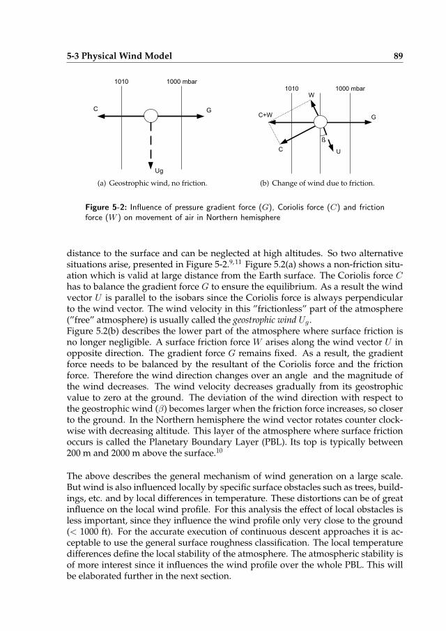
5-3 Physical Wind Model 89
(a) Geostrophic wind, no friction. (b) Change of wind due to friction.
Figure 5-2: Influence of pressure gradient force (G), Coriolis force (C) and frictionforce (W ) on movement of air in Northern hemisphere
distance to the surface and can be neglected at high altitudes. So two alternativesituations arise, presented in Figure 5-2.9, 11 Figure 5.2(a) shows a non-friction situ-ation which is valid at large distance from the Earth surface. The Coriolis force Chas to balance the gradient force G to ensure the equilibrium. As a result the windvector U is parallel to the isobars since the Coriolis force is always perpendicularto the wind vector. The wind velocity in this ”frictionless” part of the atmosphere(”free” atmosphere) is usually called the geostrophic wind Ug .Figure 5.2(b) describes the lower part of the atmosphere where surface friction isno longer negligible. A surface friction force W arises along the wind vector U inopposite direction. The gradient force G remains fixed. As a result, the gradientforce needs to be balanced by the resultant of the Coriolis force and the frictionforce. Therefore the wind direction changes over an angle and the magnitude ofthe wind decreases. The wind velocity decreases gradually from its geostrophicvalue to zero at the ground. The deviation of the wind direction with respect tothe geostrophic wind (β) becomes larger when the friction force increases, so closerto the ground. In the Northern hemisphere the wind vector rotates counter clock-wise with decreasing altitude. This layer of the atmosphere where surface frictionoccurs is called the Planetary Boundary Layer (PBL). Its top is typically between200 m and 2000 m above the surface.10
The above describes the general mechanism of wind generation on a large scale.But wind is also influenced locally by specific surface obstacles such as trees, build-ings, etc. and by local differences in temperature. These distortions can be of greatinfluence on the local wind profile. For this analysis the effect of local obstacles isless important, since they influence the wind profile only very close to the ground(< 1000 ft). For the accurate execution of continuous descent approaches it is ac-ceptable to use the general surface roughness classification. The local temperaturedifferences define the local stability of the atmosphere. The atmospheric stability isof more interest since it influences the wind profile over the whole PBL. This willbe elaborated further in the next section.
90 Stochastic Wind Profile Estimation
5-3-1 The Atmospheric Stability
The atmospheric stability is one of the mechanisms that influences the local windprofile of the planetary boundary layer (PBL). The gradient of the wind velocitywith the altitude depends on the amount of horizontal motion that is exchangedvertically.5 The momentary temperature profile determines this stability, one of themajor factors is the rate of change of air temperature with altitude.2 Due to timeevolution in terms of changing vertical thermal build-up, the boundary layer is arather complicated object. The PBL has three broad types of structure with typicalcharacterizing conditions:5
1. Unstable/convective boundary layers: light winds and a high surface heatflux
2. Neutral boundary layers: high winds and/or small surface heat flux
3. Stable boundary layers: light winds and a negative surface heat flux (mostduring night time)
The strong vertical heat exchange in an unstable atmosphere causes the horizontalwind speed to be maximally exchanged downwards.11 As a result, the mean windhas a sharp increase near the surface. But throughout most of the boundary layerthe mean flow is fairly uniform.5 The stable boundary layer is the most variableof the three kinds of layers and is usually in a continuous state of evolution. Thisusually occurs between the hours of sunset and sunrise when the surface is coolingor when warm air moves over a cool surface. In these conditions there is very littlevertical exchange of wind. This can lead to light winds near the surface and strongwinds up in the atmosphere. Typical wind profiles for a stable atmosphere are illus-trated by the solid line in Figure 5-3. The stable boundary layer is more responsiveto Coriolis accelerations. This leads to the direction of the wind changing over thedepth of the layer by 25-40◦.5
In neutral boundary layers the wind profile does not depend on the vertical heatexchange but only on the surface roughness. The atmosphere has a neutral stabilitywhen clouds are present or in case strong winds occur. Extended cloud coverreduces the warming or cooling of the Earth’s surface leading to little vertical heatexchange. With strong winds the vertical exchange of winds can be consideredpurely mechanical, the thermal effects are negligible.9, 11 The wind profile of aneutral boundary layer lies between the two extremes of a stable and unstableatmospheric condition.
Several wind measurements presented in10 indicate that the difference in wind ve-locity of stable/unstable versus neutral atmospheric conditions remains relativelysmall. For instance, the daily change of mean wind velocity over 18 days of clearsky at an altitude of 124 m varied between 9 m/s (night) and 5 m/s (day).10 Other

5-3 Physical Wind Model 91
clear sky(81 days)
h [km] 1.5
1.0
0.5
cloudy(129 days)
u
Figure 5-3: Mean wind profile for clear and clouded skies at Warszawa 1960: solidline = 0h00, dashed line = 12h00. [Source: Wieringa10]
wind data, presented in Figure 5-3, show a maximum difference of 4 m/s betweenthe stable (solid line) and unstable wind profile (dashed line) at 350 m above theground for 81 days of clear skies. During 129 clouded days the mean maximumdifference was only 1 m/s. The wind profile of a neutral boundary layer lies be-tween the two extremes of a stable and unstable atmospheric condition. So in theexamples above, the maximum deviation of the wind velocity with respect to aneutral wind profile will be smaller than 4 m/s. The measured differences willprobably increase a little for geostrophic winds that are somewhat stronger than8 m/s. Nevertheless the deviations are expected to remain of the same order asthe atmospheric boundary layer tends to get more neutrally stable with increasingwind.
For an efficient execution of a continuous descent approach a good estimationof the wind profile is necessary. The accuracy of the estimation becomes morecritical when stronger winds occur. For these conditions a wind profile for aneutral boundary layer is applicable. In case of light winds and clear skies, thewind profile changes continuously due to the daily evolution of the stability inthe PBL. The daily wind pattern changes from an unstable atmosphere duringthe day to a stable boundary layer during the night. The amplitude of the dailyevolution varies on his turn with the seasons and depends on the climate. It canbe concluded that these atmospheric evolutions are very complex and have muchvariety, so the modeling of the wind could be simplified a lot by assuming neutralstability at all times.
These observations indicate that the neutrally stable wind profile could be taken asan approximation to cover all situations of the planetary boundary layer.
Given the above considerations, it can be concluded that it is justified to assume aneutral atmospheric boundary layer.
92 Stochastic Wind Profile Estimation
5-3-2 The Mathematical Wind Model in Neutrally Stable Atmo-sphere
Different models have been used in literature to describe the wind profile in a neu-trally stable planetary boundary layer. This section discusses these methods anddefines which mathematical model will be used in this research. Before continuingit is important to know that the planetary boundary layer can be subdivided in twolayers:10
• The lowest 20% of the PBL is the surface layer, usually with the top between60-100 m. Here some simplifications may be applied that are not allowed forthe whole PBL, for instance neglecting the Coriolis force.
• The other 80% of the PBL is the so-called ”Ekman layer” where the profile isinfluenced by both friction and Coriolis force.
Since aircraft flying an approach generally need to be configured for landing andmaintaining a stabilized airspeed by the time they reach 1000 ft above the ground,only the wind profile in the ”Ekman layer” is of interest.
Hewitt and Jackson give the following mathematical description of the wind profilein the neutral boundary layer.5 Over the lowest 100 m the profile is logarithmic anddepends on roughness length z0. In the upper part of the boundary layer, the pro-file depends on (z/h) and the power-law profile is a useful approximation. Thereis a systematic turning of the wind with height due to the Coriolis acceleration,ranging from about 5◦ to 20◦. The direction and magnitude of this turning is quitesensitive to changes in surface roughness and upper-layer conditions. Furthermorethe strength of the Coriolis-force is dependent on the latitude.Wind profiles are traditionally estimated with the power-law:10
V = V0
(
h
h0
)p
(5-1)
where the wind speed V at altitude h is dependent on the windspeed V0 at a refer-ence height h0. The exponent p is emperically derived constant, which for neutralystable atmospher is approximataly 1
7.12
Even if the reference point (h0, V0) is chosen to fit the actual situation best, thisequation only yields a very general approximation of the wind profile in the PBL.Especially since the PBL is characterized by the interaction between the free streamwind at higher altitudes and the disturbing forces of friction caused by the earth’sroughness, this approximation can differ significantly from the true wind profile.In order to derive a generally useful model that is not dependent on local surfaceroughness or the local latitude, the power-law is used as a baseline for the firstapproximation of the wind profile and to fill in the gaps when measeurment data issparse. Subsequent estimates of the wind-profile are updated using available datafrom other aircraft as will be explained in the next section.
5-4 AMDAR wind prediction algorithm (AWPA) 93
5-4 AMDAR wind prediction algorithm (AWPA)
The spatial and temporal variations of the wind affect the performance of the air-craft along the approach trajectory in the Earth-fixed reference frame. Accurateknowledge of the wind profile in the TMA is therefore required for an accurateown trajectory prediction and time-to-fly estimates. The wind profile is modeledusing a statistical model. The advantage of such a model is that it does not relyon the physical processes that govern wind behavior but instead uses observationsto estimate any profile shape. On the other hand, a logarithmic profile estimatebased on the power-lawEq. (5-1) is able to provide at least an initial estimate whendata are insufficiently available. This way the algorithm combines the best of bothworld, showing purely stochastic estimator behavior when data are abundant, butstill producing a working estimate when such is data is not available.
In the near future various data-link scenarios are envisaged for instance in theSESAR and NextGen programs.1 As the details of the proposed data-link systemssuch as ADS-B are not yet fully developed, this algorithm is based on the formatof the AMDAR data. With the transmission of AMDAR-like data to nearby aircrafta wealth of meteorological information will become available for processing eitherboard the aircraft or in ground-based system. ACARS is the communication systemmost widely used by aircraft participating in the AMDAR program. The AMDARreports consist of meteorological measurements made on-board the aircraft such ofthe pressure altitude, airspeed, the air temperature and the wind vector, but alsothe aircraft position and altitude.
The structure of the algorithm that drives the wind prediction model is shown inFigure 5.4(a). The wind prediction model is driven by historical Automated Meteo-rological Data Relay (AMDAR) data. AMDAR data consist of meteorological obser-vations such as wind speed and direction as well as position coordinates. They arebroadcast through the Aircraft Communications Addressing and Reporting System(ACARS) to in-trail aircraft which then store the historical data in a Flight Manage-ment System (FMS) database. The data are processed to make estimates of thecurrent and future wind profile by making predictions based on the historical data.The algorithm is designed with a high-traffic scenario in mind but when the num-ber of historical AMDAR observations available is scarce (e.g., between arrival anddeparture peaks), a wind profile can still be constructed using the available data,without making predictions, however.
The algorithm consists of three steps, as illustrated by Figure 5-5. First, AMDARdata of preceding aircraft, each tagged with a corresponding time and altitude in-terval, is collected and stored in the FMS. Second, per altitude interval, the histor-ical AMDAR data are filtered using a Kalman filter to remove measurement noisefrom the observations. The series of historical AMDAR data are then used to de-termine an auto-regressive model of the time series. Third, the wind profile is con-structed by connecting the predictions per altitude interval by linear interpolation.
The prediction algorithm uses incoming ACARS data from other aircraft within a
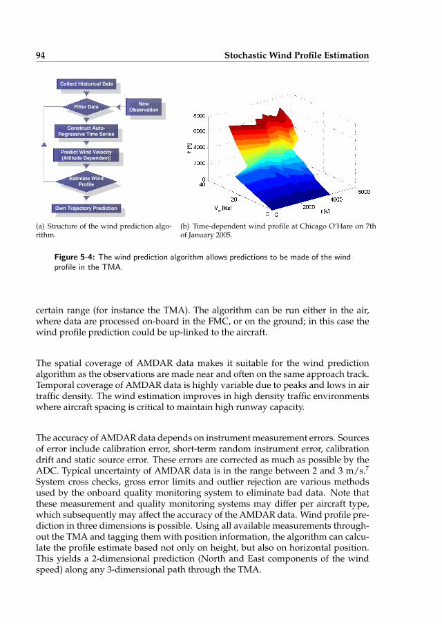
94 Stochastic Wind Profile Estimation
New Observation
Predict Wind Velocity (Altitude Dependent)
Estimate Wind Profile
Construct Auto- Regressive Time Series
Filter Data
Collect Historical Data
Own Trajectory Prediction
(a) Structure of the wind prediction algo-rithm.
(b) Time-dependent wind profile at Chicago O’Hare on 7thof January 2005.
Figure 5-4: The wind prediction algorithm allows predictions to be made of the windprofile in the TMA.
certain range (for instance the TMA). The algorithm can be run either in the air,where data are processed on-board in the FMC, or on the ground; in this case thewind profile prediction could be up-linked to the aircraft.
The spatial coverage of AMDAR data makes it suitable for the wind predictionalgorithm as the observations are made near and often on the same approach track.Temporal coverage of AMDAR data is highly variable due to peaks and lows in airtraffic density. The wind estimation improves in high density traffic environmentswhere aircraft spacing is critical to maintain high runway capacity.
The accuracy of AMDAR data depends on instrument measurement errors. Sourcesof error include calibration error, short-term random instrument error, calibrationdrift and static source error. These errors are corrected as much as possible by theADC. Typical uncertainty of AMDAR data is in the range between 2 and 3 m/s.7
System cross checks, gross error limits and outlier rejection are various methodsused by the onboard quality monitoring system to eliminate bad data. Note thatthese measurement and quality monitoring systems may differ per aircraft type,which subsequently may affect the accuracy of the AMDAR data. Wind profile pre-diction in three dimensions is possible. Using all available measurements through-out the TMA and tagging them with position information, the algorithm can calcu-late the profile estimate based not only on height, but also on horizontal position.This yields a 2-dimensional prediction (North and East components of the windspeed) along any 3-dimensional path through the TMA.
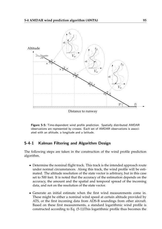
5-4 AMDAR wind prediction algorithm (AWPA) 95
���������t1
t2
t3
Vw
Vw
Vw
h
h
h
Altitude
3◦
Distance to runway
Figure 5-5: Time-dependent wind profile prediction. Spatially distributed AMDARobservations are represented by crosses. Each set of AMDAR observations is associ-ated with an altitude, a longitude and a latitude.
5-4-1 Kalman Filtering and Algorithm Design
The following steps are taken in the construction of the wind profile predictionalgorithm.
• Determine the nominal flight track. This track is the intended approach routeunder normal circumstances. Along this track, the wind profile will be esti-mated. The altitude resolution of the state vector is arbitrary, but in this caseset to 500 feet. It is noted that the accuracy of the estimation depends on theaccuracy, the amount and the spatial and temporal spread of the incomingdata, and not on the resolution of the state vector.
• Generate an initial estimate when the first wind measurements come in.These might be either a nominal wind speed at certain altitude provided byATS, or the first incoming data from ADS-B soundings from other aircraft.Based on these first measurements, a standard logarithmic wind profile isconstructed according to Eq. (5-1))This logarithmic profile thus becomes the
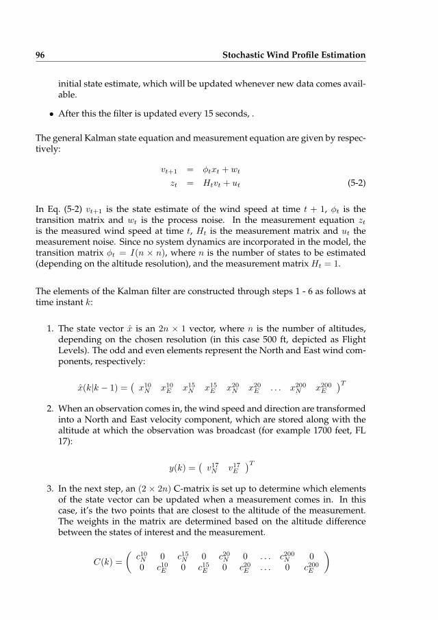
96 Stochastic Wind Profile Estimation
initial state estimate, which will be updated whenever new data comes avail-able.
• After this the filter is updated every 15 seconds, .
The general Kalman state equation and measurement equation are given by respec-tively:
vt+1 = φtxt + wt
zt = Htvt + ut (5-2)
In Eq. (5-2) vt+1 is the state estimate of the wind speed at time t + 1, φt is thetransition matrix and wt is the process noise. In the measurement equation ztis the measured wind speed at time t, Ht is the measurement matrix and ut themeasurement noise. Since no system dynamics are incorporated in the model, thetransition matrix φt = I(n × n), where n is the number of states to be estimated(depending on the altitude resolution), and the measurement matrix Ht = 1.
The elements of the Kalman filter are constructed through steps 1 - 6 as follows attime instant k:
1. The state vector x is an 2n × 1 vector, where n is the number of altitudes,depending on the chosen resolution (in this case 500 ft, depicted as FlightLevels). The odd and even elements represent the North and East wind com-ponents, respectively:
x(k|k − 1) =(
x10N x10
E x15N x15
E x20N x20
E . . . x200N x200
E
)T
2. When an observation comes in, the wind speed and direction are transformedinto a North and East velocity component, which are stored along with thealtitude at which the observation was broadcast (for example 1700 feet, FL17):
y(k) =(
v17N v17E)T
3. In the next step, an (2 × 2n) C-matrix is set up to determine which elementsof the state vector can be updated when a measurement comes in. In thiscase, it’s the two points that are closest to the altitude of the measurement.The weights in the matrix are determined based on the altitude differencebetween the states of interest and the measurement.
C(k) =
(
c10N 0 c15N 0 c20N 0 . . . c200N 00 c10E 0 c15E 0 c20E . . . 0 c200E
)
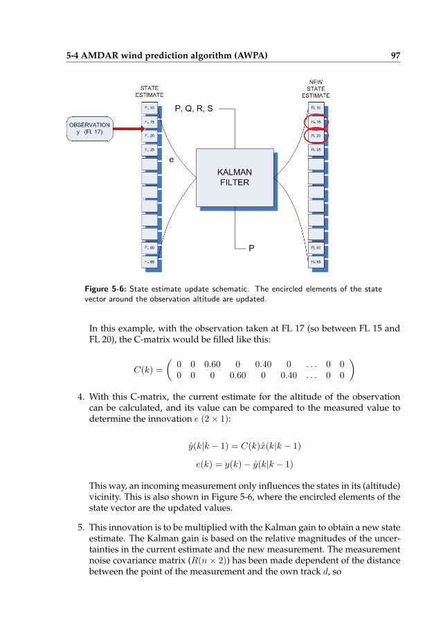
5-4 AMDAR wind prediction algorithm (AWPA) 97
Figure 5-6: State estimate update schematic. The encircled elements of the statevector around the observation altitude are updated.
In this example, with the observation taken at FL 17 (so between FL 15 andFL 20), the C-matrix would be filled like this:
C(k) =
(
0 0 0.60 0 0.40 0 . . . 0 00 0 0 0.60 0 0.40 . . . 0 0
)
4. With this C-matrix, the current estimate for the altitude of the observationcan be calculated, and its value can be compared to the measured value todetermine the innovation e (2× 1):
y(k|k − 1) = C(k)x(k|k − 1)
e(k) = y(k)− y(k|k − 1)
This way, an incoming measurement only influences the states in its (altitude)vicinity. This is also shown in Figure 5-6, where the encircled elements of thestate vector are the updated values.
5. This innovation is to be multiplied with the Kalman gain to obtain a new stateestimate. The Kalman gain is based on the relative magnitudes of the uncer-tainties in the current estimate and the new measurement. The measurementnoise covariance matrix (R(n× 2)) has been made dependent of the distancebetween the point of the measurement and the own track d, so
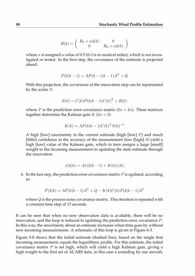
98 Stochastic Wind Profile Estimation
R(k) =
(
R0 + αd(k) 00 R0 + αd(k)
)
where α is assigned a value of 0.5 (if d is in nautical miles), which is not inves-tigated or tested. In the first step, the covariance of the estimate is projectedahead:
P (k|k − 1) = AP (k − 1|k − 1)AT +Q
With this projection, the covariance of the innovation step can be representedby the scalar S:
S(k) = C(k)P (k|k − 1)C(k)T +R(k)
where P is the prediction error covariance matrix (2n × 2n). These matricestogether determine the Kalman gain K (2n× 2):
K(k) = AP (k|k − 1)C(k)TS(k)−1
A high [low] uncertainty in the current estimate (high [low] P ) and much[little] confidence in the accuracy of the measurement (low [high] S) yield ahigh [low] value of the Kalman gain, which in turn assigns a large [small]weight to the incoming measurement in updating the state estimate throughthe innovation:
x(k|k) = Ax(k|k − 1) +K(k)e(k)
6. In the last step, the prediction error covariance matrix P is updated, accordingto:
P (k|k) = AP (k|k − 1)AT +Q−K(k)C(k)P (k|k − 1)AT
where Q is the process noise covariance matrix. This iteration is repeated witha constant time step of 15 seconds.
It can be seen that when no new observation data is available, there will be noinnovation, and the loop is reduced to updating the prediction error covariance P .In this way, the uncertainty about an estimate increases when time goes by withoutnew incoming measurements. A schematic of this loop is given in Figure 6-3.
Figure 5-8 shows that the initial estimate (dashed line), based on the single firstincoming measurement, equals the logarithmic profile. For this estimate, the initialcovariance matrix P is set high, which will yield a high Kalman gain, giving ahigh weight to the first set of ACARS data, in this case a sounding by one aircraft,
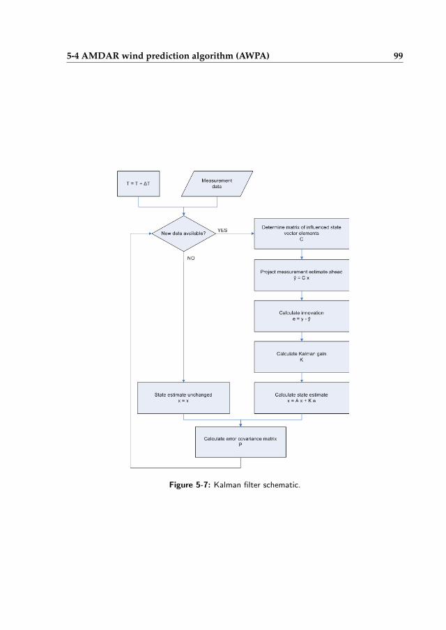
5-4 AMDAR wind prediction algorithm (AWPA) 99
Figure 5-7: Kalman filter schematic.
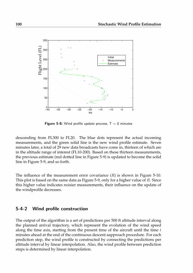
100 Stochastic Wind Profile Estimation
−40 −35 −30 −25 −20 −15 −10 −5 00
50
100
150
200
250
300
350
kts
Initial
Measurements
Estimate
Fli
gh
tL
evel
(FL
)
Figure 5-8: Wind profile update process, T = 0 minutes
descending from FL300 to FL20. The blue dots represent the actual incomingmeasurements, and the green solid line is the new wind profile estimate. Sevenminutes later, a total of 29 new data broadcasts have come in, thirteen of which arein the altitude range of interest (FL10-200). Based on these thirteen measurements,the previous estimate (red dotted line in Figure 5-9) is updated to become the solidline in Figure 5-9, and so forth.
The influence of the measurement error covariance (R) is shown in Figure 5-10.This plot is based on the same data as Figure 5-9, only for a higher value of R. Sincethis higher value indicates noisier measurements, their influence on the update ofthe windprofile decreases.
5-4-2 Wind profile construction
The output of the algorithm is a set of predictions per 500 ft altitude interval alongthe planned arrival trajectory, which represent the evolution of the wind speedalong the time axis, starting from the present time of the aircraft until the time tminutes ahead at the end of the continuous descent aapproach procedure. For eachprediction step, the wind profile is constructed by connecting the predictions peraltitude interval by linear interpolation. Also, the wind profile between predictionsteps is determined by linear interpolation.
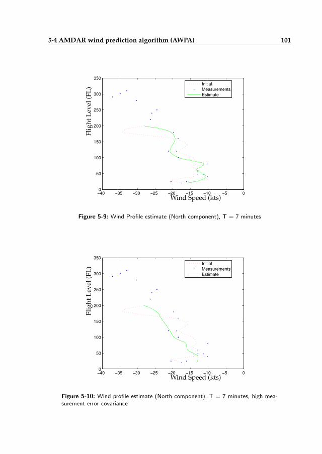
5-4 AMDAR wind prediction algorithm (AWPA) 101
−40 −35 −30 −25 −20 −15 −10 −5 00
50
100
150
200
250
300
350
Initial
Measurements
Estimate
Fli
gh
tL
evel
(FL
)
Wind Speed (kts)
Figure 5-9: Wind Profile estimate (North component), T = 7 minutes
−40 −35 −30 −25 −20 −15 −10 −5 00
50
100
150
200
250
300
350
Initial
Measurements
Estimate
Fli
gh
tL
evel
(FL
)
Wind Speed (kts)
Figure 5-10: Wind profile estimate (North component), T = 7 minutes, high mea-surement error covariance

102 Stochastic Wind Profile Estimation
5-5 Wind Prediction Performance Evaluation
The functioning of the wind predictor in an off-line simulation is visualized in Fig-ure 5-11. For this specific simulation, measurement data from ADS-B soundings atChicago O’Hare (2 January 2005, 14.10pm - 15.05pm) from nine consecutive incom-ing or outgoing aircraft (in multiple bearings) have been used. As these aircraftfly through the TMA, measuring and broadcasting (a.o.) wind speeds, the filter isupdated every time step (15 seconds) where new data has come in. So every timean aircraft passes along its data, a new estimate is made. Figure 5-11 shows the de-velopment of the wind profile with every passing aircraft. For clarity, it is assumedin this simulation that one aircraft finishes its entire approach or departure, beforethe next enters the area of interest.In reality the algorithm handles every incomingmeasurement at any time, regardless of the number of aircraft in the TMA.
Since the filter uses the relative distance between the location of the measurementand the own aircraft to adjust the measurement error covariance matrix R, an arbi-trary 3-dimensional approach path has been set up for the own aircraft. An exampleof this path is shown in Figure 5-12. In fact, the wind profiles as given in Figure 5-11are along this approach track, so in effect they are 3-dimensional.
5-5-1 Check on relevant parameters
The most important parameters calculated in the Kalman filter (as described inSection 5-4-1) are the innovation step (the difference between the ’projection ahead’at a certain point of interest and the value measured at that point) and the Kalmangain. For a single aircraft passing along the altitudes of interest the response ofthese quantities is shown in Figure 5-13. In this case, the altitude range for whicha wind profile is to be constructed is FL10-FL200. As long as the aircraft is abovethis altitude, the broadcast data are not used. It can be seen in Figure 5-13 thatafter approximately 23 minutes the aircraft descends into this altitude range, andits broadcasts are used to update the wind profile estimate. From this momenton, every innovation step is assigned a weight (the Kalman gain, depicted withthe green dotted line), to determine the new estimate for this altitude. The areaof influence of an incoming measurement is indicated by the drop-back of theKalman gain. After a measurement has come in, the gain drops back to zero (firstvery steeply, later more gradually), decreasing the influence of this measurementon other elements of the estimated state vector.
According to Kalman filter theory, the accuracy of an estimate depends on the qual-ity of the system model, the accuracy of the available measurements and the num-ber of them. In this case, the system dynamics are zero, so the accuracy of the windprediction depends on the measurements alone. It is therefore hypothesized thatthe prediction error will decrease as more data becomes available. This is shownin Figure 5-14. Here the mean value of the prediction error covariance matrix P isplotted against time. This (scalar) value p is calculated according to:
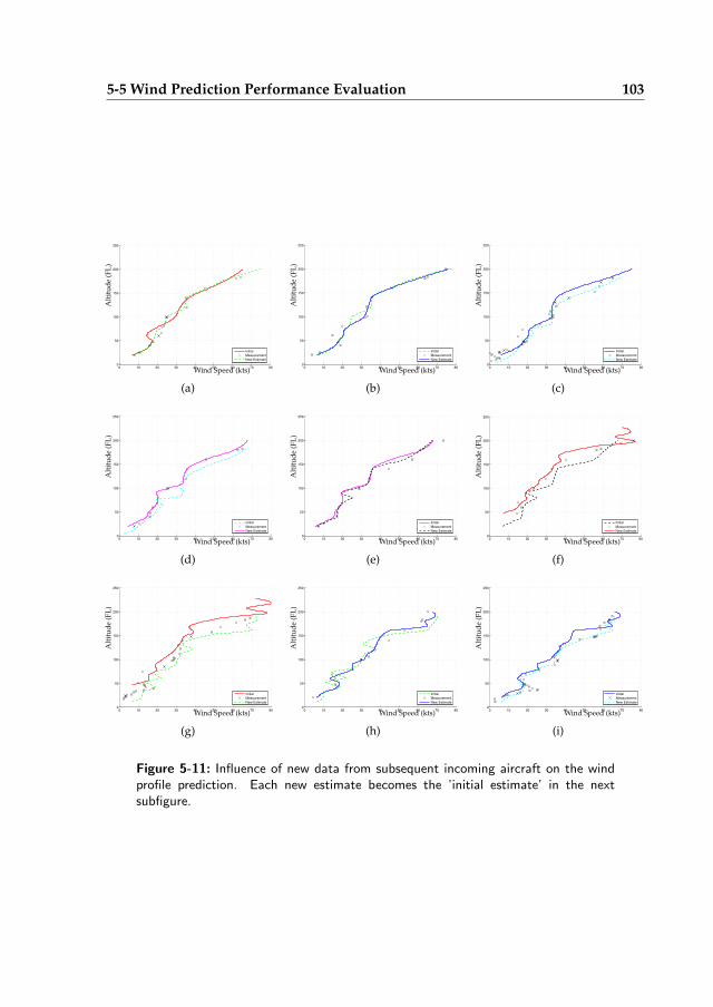
5-5 Wind Prediction Performance Evaluation 103
0 10 20 30 40 50 60 70 800
50
100
150
200
250
Initial
Measurement
New Estimate
Alt
itu
de
(FL
)
Wind Speed (kts)
(a)
0 10 20 30 40 50 60 70 800
50
100
150
200
250
Initial
Measurement
New Estimate
Alt
itu
de
(FL
)
Wind Speed (kts)
(b)
0 10 20 30 40 50 60 70 800
50
100
150
200
250
Initial
Measurement
New Estimate
Alt
itu
de
(FL
)
Wind Speed (kts)
(c)
0 10 20 30 40 50 60 70 800
50
100
150
200
250
Initial
Measurement
New Estimate
Alt
itu
de
(FL
)
Wind Speed (kts)
(d)
0 10 20 30 40 50 60 70 800
50
100
150
200
250
Initial
Measurement
New Estimate
Alt
itu
de
(FL
)
Wind Speed (kts)
(e)
0 10 20 30 40 50 60 70 800
50
100
150
200
250
Initial
Measurement
New Estimate
Alt
itu
de
(FL
)
Wind Speed (kts)
(f)
0 10 20 30 40 50 60 70 800
50
100
150
200
250
Initial
Measurement
New Estimate
Alt
itu
de
(FL
)
Wind Speed (kts)
(g)
0 10 20 30 40 50 60 70 800
50
100
150
200
250
Initial
Measurement
New Estimate
Alt
itu
de
(FL
)
Wind Speed (kts)
(h)
0 10 20 30 40 50 60 70 800
50
100
150
200
250
Initial
Measurement
New Estimate
Alt
itu
de
(FL
)
Wind Speed (kts)
(i)
Figure 5-11: Influence of new data from subsequent incoming aircraft on the windprofile prediction. Each new estimate becomes the ’initial estimate’ in the nextsubfigure.
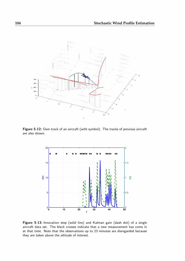
104 Stochastic Wind Profile Estimation
Figure 5-12: Own track of an aircraft (with symbol). The tracks of previous aircraftare also shown.
0 10 20 30 40 500
5
10
15
20
INN
T0 10 20 30 40 50
0
0.5
1
1.5
2
KG
Figure 5-13: Innovation step (solid line) and Kalman gain (dash dot) of a singleaircraft data set. The black crosses indicate that a new measurement has come inat that time. Note that the observations up to 23 minutes are disregarded becausethey are taken above the altitude of interest.
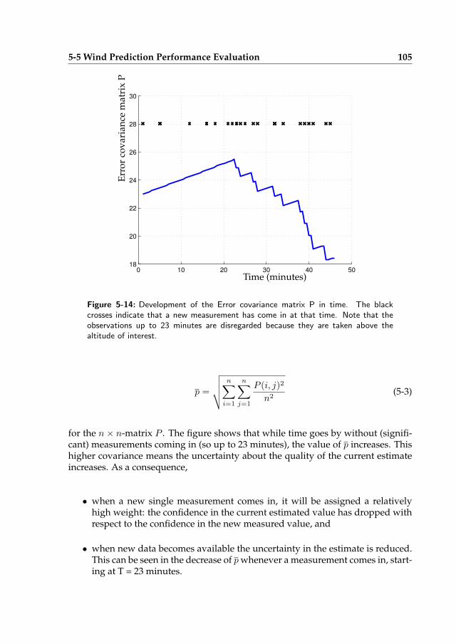
5-5 Wind Prediction Performance Evaluation 105
0 10 20 30 40 5018
20
22
24
26
28
30
Err
or
cov
aria
nce
mat
rix
P
Time (minutes)
Figure 5-14: Development of the Error covariance matrix P in time. The blackcrosses indicate that a new measurement has come in at that time. Note that theobservations up to 23 minutes are disregarded because they are taken above thealtitude of interest.
p =
√
√
√
√
n∑
i=1
n∑
j=1
P (i, j)2
n2(5-3)
for the n × n-matrix P . The figure shows that while time goes by without (signifi-cant) measurements coming in (so up to 23 minutes), the value of p increases. Thishigher covariance means the uncertainty about the quality of the current estimateincreases. As a consequence,
• when a new single measurement comes in, it will be assigned a relativelyhigh weight: the confidence in the current estimated value has dropped withrespect to the confidence in the new measured value, and
• when new data becomes available the uncertainty in the estimate is reduced.This can be seen in the decrease of p whenever a measurement comes in, start-ing at T = 23 minutes.
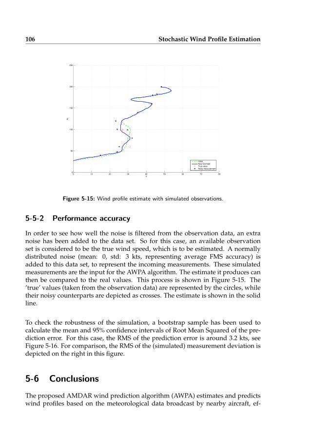
106 Stochastic Wind Profile Estimation
0 10 20 30 40 50 60 70 800
50
100
150
200
250
V
FL
Initial
New Estimate
True value
Noisy measurement
Figure 5-15: Wind profile estimate with simulated observations.
5-5-2 Performance accuracy
In order to see how well the noise is filtered from the observation data, an extranoise has been added to the data set. So for this case, an available observationset is considered to be the true wind speed, which is to be estimated. A normallydistributed noise (mean: 0, std: 3 kts, representing average FMS accuracy) isadded to this data set, to represent the incoming measurements. These simulatedmeasurements are the input for the AWPA algorithm. The estimate it produces canthen be compared to the real values. This process is shown in Figure 5-15. The’true’ values (taken from the observation data) are represented by the circles, whiletheir noisy counterparts are depicted as crosses. The estimate is shown in the solidline.
To check the robustness of the simulation, a bootstrap sample has been used tocalculate the mean and 95% confidence intervals of Root Mean Squared of the pre-diction error. For this case, the RMS of the prediction error is around 3.2 kts, seeFigure 5-16. For comparison, the RMS of the (simulated) measurement deviation isdepicted on the right in this figure.
5-6 Conclusions
The proposed AMDAR wind prediction algorithm (AWPA) estimates and predictswind profiles based on the meteorological data broadcast by nearby aircraft, ef-
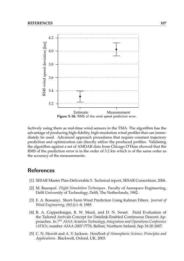
REFERENCES 107
Estimate Measurement
4.2
4.0
3.8
3.6
3.4
3.2
RM
Sw
ind
spee
dd
evia
tio
n[k
ts]
Figure 5-16: RMS of the wind speed prediction error.
fectively using them as real-time wind sensors in the TMA. The algorithm has theadvantage of producing high-fidelity, high-resolution wind profiles that can imme-diately be used. Advanced approach procedures that require constant trajectoryprediction and optimization can directly utilize the produced profiles. Validatingthe algorithm against a set of AMDAR data from Chicago O’Hare showed that theRMS of the prediction error is in the order of 3.2 kts which is of the same order asthe accuracy of the measurements.
References
[1] SESAR Master Plan-Deliverable 5. Technical report, SESAR Consortium, 2006.
[2] M. Baarspul. Flight Simulation Techniques. Faculty of Aerospace Engineering,Delft University of Technology, Delft, The Netherlands, 1982.
[3] E. A. Bossanyi. Short-Term Wind Prediction Using Kalman Filters. Journal ofWind Engineering, (9(1)):1–8, 1985.
[4] R. A. Coppenbarger, R. W. Mead, and D. N. Sweet. Field Evaluation ofthe Tailored Arrivals Concept for Datalink-Enabled Continuous Descent Ap-proaches. In 7th AIAA Aviation Technology, Integration and Operations Conference(ATIO), number AIAA-2007-7778, Belfast, Northern Ireland, Sep 18-20 2007.
[5] C. N. Hewitt and A. V. Jackson. Handbook of Atmospheric Science, Principles andApplications. Blackwell, Oxford, UK, 2003.
108 Stochastic Wind Profile Estimation
[6] J. K. Klooster and K. D. Wichman. 4D Trajectory and Time-of-Arrival Controlto Enable Continuous Descent Arrivals. Honolulu (HI), USA, Aug 18-21 2008.
[7] W. R. Moninger, R. D. Mamrosh, and P. M. Pauley. Automated MeteorologicalReports from Commercial Aircraft. Technical Report ARP 5430, World Meteo-rological Society, 2003.
[8] D. Painting. AMDAR Reference Manual. Technical report, World Meteorolog-ical Organization-AMDAR Panel, 2001.
[9] A. P. W. Steentjes. Design and Development of a Generic Terrain-Based WindAtmosphere Module for Future Flight Simulators. MSc. Thesis, Faculty ofAerospace Engineering, Delft University of Technology, 2001.
[10] J. Wieringa. De Atmosferische Grenslaag (in Dutch). Lecture notes, Faculty ofApplied Sciences, Delft University of Technology, 1987.
[11] J. Wieringa and P. J. Rijkoort. Windklimaat van Nederland (in Dutch). Staatsuit-geverij, The Hague, The Netherlands, 1983.
[12] N. M. Zoumakis and A. G. Kelessis. Methodology for Bulk Approximation ofthe Wind Profile Power-Law Exponent under Stable Stratification. Boundary-Layer Meteorology, 55(1-2):199–203, 1990.
6
Time Based Spacing
Implementing Time Based Spacing for Continuous Descent Approaches inRealistic Wind Conditions
A.C. in ’t Veld, R.D. Groenouwe, M. Mulder and M.M. van Paassen
Submitted to the AIAA Journal of Aircraft, December 2009
6-1 Abstract
Although very effective at mitigating noise impact on the populated areas that sur-round airports, continuous descent approaches generally reduce runway capacitywith respect to standard ILS approaches. Large uncertainties in descent trajectoriesforce air traffic controllers to apply large separations in order to ensure safe opera-tion. In this paper, a solution is presented that addresses the problems of variabilityin deceleration profiles and wind uncertainty. Spacing is done by providing pilotswith a required time of arrival. A support system then helps the pilot in meetingthis time goal. A wind prediction algorithm has been developed that creates a windprofile estimate along the intended three dimensional approach track, using filteredwind data observations broadcast by nearby aircraft. By combining these wind es-timates with a flap scheduling algorithm, accurate on-board track and speed guid-ance becomes available. An interface has been designed that aids the pilot bothin flying a controlled continuous descent approach and in meeting the time targetset by air traffic control. To test the combined support system, a piloted simula-tor experiment was set up. Performance in terms of time goals was found to beconsistent under all tested conditions and significantly better in comparison withthe non-supported condition. Also, workload is acceptable and significantly lower
110 Time Based Spacing
with the display optimization present. Providing the pilot with continuously up-dated time performance information based on actual meteorological circumstanceswas shown to be an important requirement for the implementation of CDAs in atime based spacing environment.
6-2 Introduction
All over the western world, and especially in Europe, aircraft noise is a major limit-ing factor of airport capacity growth.2 Much attention is paid to mitigating airportnuisance affecting the surrounding communities. Many different approaches aretaken, for instance, in the fields of aircraft engine technology and airport infras-tructure planning.1 The approach under study here will focus on noise abatementapproach procedures, and how these can attribute to lowering aircraft noise impacton the ground. In this field there is still significant room for improvement, since theprocedures currently in place hardly make use of advances in guidance, navigationand surveillance technology.
Over the years, several noise abatement approach procedures have been devel-oped.4, 5, 7, 8 Variants include general procedures like different versions of the Con-tinuous Descent Approach, and airport-specific measures.7–9, 16, 25 One character-istic aspect of many of these proposed procedures is that part of the approach iscarried out with more or less idle thrust settings. Also, aircraft avoid flying levelsegments at low altitude, which are typical for the current standard procedures, in-cluding ILS approaches. These new procedures have been shown to reduce aircraftnoise, but at a cost: differences in deceleration between different aircraft perform-ing the descent procedures force air traffic controllers to apply larger initial separa-tions to ensure safe operation. As a result, runway capacity is reduced.6, 9, 14, 18, 22, 23
In this paper a solution to this problem is proposed by introducing a pilot supportsystem that enables time based separation during the approach. In other words,pilots are given a Required Time of Arrival (), rather than radar vectors. It then be-comes the pilot’s task to comply, within bounds, with this time goal, whereas finalresponsibility for safe separation remains with . The resulting system enables con-tinuous descents, while still guaranteeing safe separation. This research focuses inparticular on curved approach procedures under realistic wind conditions. Windhas a major influence on the accuracy of time based separation, and prediction ofthe wind profile encountered during the approach could be of great importance.A tool capable of accurately predicting wind conditions along a three-dimensionalapproach track was developed. Together with an algorithm that calculates the op-timum settings for parameters such as the altitude where thrust is reduced to flightidle, this forms a support system that helps the pilot in flying idle thrust, continu-ous descent approaches while meeting arrival times instructed by ATC. This shouldallow ATC to sequence and space aircraft in the more tightly, eliminating the capac-ity reduction currently associated with many noise abatement procedures.
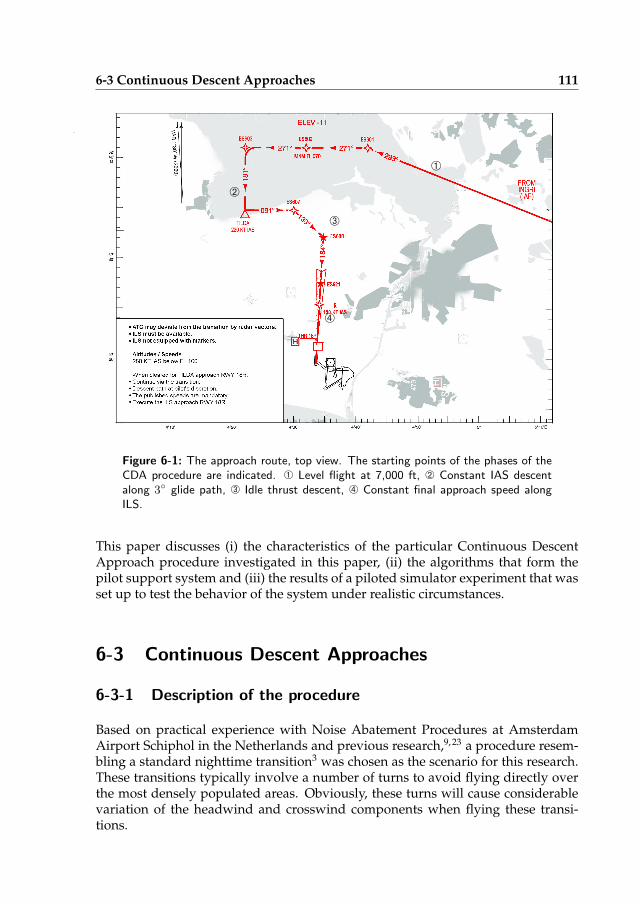
6-3 Continuous Descent Approaches 111
À
Á
Â
Ã
Figure 6-1: The approach route, top view. The starting points of the phases of theCDA procedure are indicated. À Level flight at 7,000 ft, Á Constant IAS descentalong 3
◦ glide path, Â Idle thrust descent, Ã Constant final approach speed alongILS.
This paper discusses (i) the characteristics of the particular Continuous DescentApproach procedure investigated in this paper, (ii) the algorithms that form thepilot support system and (iii) the results of a piloted simulator experiment that wasset up to test the behavior of the system under realistic circumstances.
6-3 Continuous Descent Approaches
6-3-1 Description of the procedure
Based on practical experience with Noise Abatement Procedures at AmsterdamAirport Schiphol in the Netherlands and previous research,9, 23 a procedure resem-bling a standard nighttime transition3 was chosen as the scenario for this research.These transitions typically involve a number of turns to avoid flying directly overthe most densely populated areas. Obviously, these turns will cause considerablevariation of the headwind and crosswind components when flying these transi-tions.
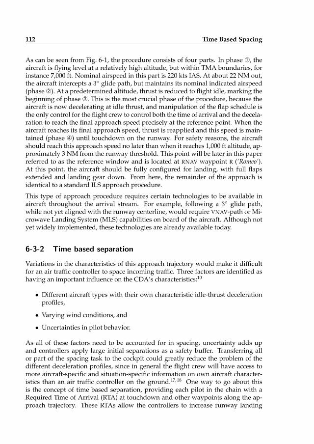
112 Time Based Spacing
As can be seen from Fig. 6-1, the procedure consists of four parts. In phase À, theaircraft is flying level at a relatively high altitude, but within TMA boundaries, forinstance 7,000 ft. Nominal airspeed in this part is 220 kts IAS. At about 22 NM out,the aircraft intercepts a 3◦ glide path, but maintains its nominal indicated airspeed(phase Á). At a predetermined altitude, thrust is reduced to flight idle, marking thebeginning of phase Â. This is the most crucial phase of the procedure, because theaircraft is now decelerating at idle thrust, and manipulation of the flap schedule isthe only control for the flight crew to control both the time of arrival and the decela-ration to reach the final approach speed precisely at the reference point. When theaircraft reaches its final approach speed, thrust is reapplied and this speed is main-tained (phase Ã) until touchdown on the runway. For safety reasons, the aircraftshould reach this approach speed no later than when it reaches 1,000 ft altitude, ap-proximately 3 NM from the runway threshold. This point will be later in this paperreferred to as the reference window and is located at RNAV waypoint R (‘Romeo’).At this point, the aircraft should be fully configured for landing, with full flapsextended and landing gear down. From here, the remainder of the approach isidentical to a standard ILS approach procedure.
This type of approach procedure requires certain technologies to be available inaircraft throughout the arrival stream. For example, following a 3◦ glide path,while not yet aligned with the runway centerline, would require VNAV-path or Mi-crowave Landing System (MLS) capabilities on board of the aircraft. Although notyet widely implemented, these technologies are already available today.
6-3-2 Time based separation
Variations in the characteristics of this approach trajectory would make it difficultfor an air traffic controller to space incoming traffic. Three factors are identified ashaving an important influence on the CDA’s characteristics:10
• Different aircraft types with their own characteristic idle-thrust decelerationprofiles,
• Varying wind conditions, and
• Uncertainties in pilot behavior.
As all of these factors need to be accounted for in spacing, uncertainty adds upand controllers apply large initial separations as a safety buffer. Transferring allor part of the spacing task to the cockpit could greatly reduce the problem of thedifferent deceleration profiles, since in general the flight crew will have access tomore aircraft-specific and situation-specific information on own aircraft character-istics than an air traffic controller on the ground.17, 18 One way to go about thisis the concept of time based separation, providing each pilot in the chain with aRequired Time of Arrival (RTA) at touchdown and other waypoints along the ap-proach trajectory. These RTAs allow the controllers to increase runway landing
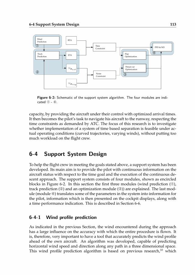
6-4 Support System Design 113
Wind
Track
Prediction
PredictionRTA
ETA
VRest
VRreq
Time
Noise
Constraint
Constraint
Flap
Thrust cut
Optimization
Optimization
PFD & NDÀ
ÁÂ
Ã
Figure 6-2: Schematic of the support system algorithm. The four modules are indi-cated À - Ã.
capacity, by providing the aircraft under their control with optimized arrival times.It then becomes the pilot’s task to navigate his aircraft to the runway, respecting thetime constraints as demanded by ATC. The focus of this research is to investigatewhether implementation of a system of time based separation is feasible under ac-tual operating conditions (curved trajectories, varying winds), without putting toomuch workload on the flight crew.
6-4 Support System Design
To help the flight crew in meeting the goals stated above, a support system has beendeveloped. Its main aim is to provide the pilot with continuous information on theaircraft status with respect to the time goal and the execution of the continuous de-scent approach. The support system consists of four modules, shown as encircledblocks in Figure 6-2. In this section the first three modules (wind prediction (À),track prediction (Á) and an optimization module (Â)) are explained. The last mod-ule (module Ã) translates some of the parameters in the system into information forthe pilot, information which is then presented on the cockpit displays, along witha time performance indication. This is described in Section 6-6.
6-4-1 Wind profile prediction
As indicated in the previous Section, the wind encountered during the approachhas a large influence on the accuracy with which the entire procedure is flown. Itis, therefore, very important to have a tool that accurately predicts the wind profileahead of the own aircraft. An algorithm was developed, capable of predictinghorizontal wind speed and direction along any path in a three dimensional space.This wind profile prediction algorithm is based on previous research,10 which
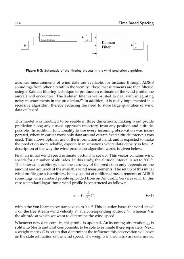
114 Time Based Spacing
y
Calculate Time-Variant
System Matrices
C
R
KalmanFilter
x
P
Figure 6-3: Schematic of the filtering process in the wind prediction algorithm.
assumes measurements of wind data are available, for instance through ADS-Bsoundings from other aircraft in the vicinity. These measurements are then filteredusing a Kalman filtering technique to produce an estimate of the wind profile theaircraft will encounter. The Kalman filter is well-suited to deal with integratingnoisy measurements in the prediction.19 In addition, it is easily implemented in arecursive algorithm, thereby reducing the need to store large quantities of winddata on board.
This model was modified to be usable in three dimensions, making wind profileprediction along any curved approach trajectory, from any position and altitude,possible. In addition, functionality to use every incoming observation was incor-porated, where in earlier work only data around certain fixed altitude intervals wasused. This allows optimal use of the information at hand, and is expected to makethe prediction more reliable, especially in situations where data density is low. Adescription of the way the wind prediction algorithm works is given below.
First, an initial wind speed estimate vector x is set up. This vector contains windspeeds for a number of altitudes. In this study, the altitude interval is set to 500 ft.This interval is arbitrary, since the accuracy of the prediction only depends on theamount and accuracy of the available wind measurements. The set up of this initialwind profile guess is arbitrary. It may consist of unfiltered measurements of ADS-Bsoundings, or a standard profile uploaded from an Air Traffic Services unit. In thiscase a standard logarithmic wind profile is constructed as follows:
x = V0(h
h0
)κ, (6-1)
with κ the Von Karman constant, equal to 0.4.11 This equation bases the wind speedx on the free stream wind velocity V0 at a corresponding altitude h0, whereas h isthe altitude at which we want to determine the wind speed.
Whenever new data come in, this profile is updated. An incoming observation yk issplit into North and East components, to be able to estimate these separately. Next,a weight matrix C is set up that determines the influence this observation will haveon the state estimation of the wind speed. The weights in the matrix are determined
6-4 Support System Design 115
based on the altitude difference between the states of interest and the measurement.With this C-matrix, the current estimate for the altitude of the observation can becalculated, and its value can be compared to the measured value to determine theinnovation e. This way, an incoming measurement only influences the states in itsaltitude vicinity:
y(k|k − 1) = C(k)x(k|k − 1) (6-2)
e(k) = y(k)− y(k|k − 1) (6-3)
This innovation is multiplied with the Kalman gain to obtain a new state estimate.The Kalman gain is based on the relative magnitudes of the uncertainties in thecurrent estimate and the new measurement, represented by the prediction errorcovariance matrix P and the measurement noise covariance matrix R, respectively.Since data from aircraft on the same approach track rather than elsewhere in theTMA are of more use for this prediction, the measurement noise covariance matrixR has been made dependent of the distance between the point of the measurementand the own track d:
R(k) = f(R0, d(k)) (6-4)
Here, R0 represents the uncertainty in an incoming observation, mainly caused bymeasurement error. The accuracy of wind measurements in ADS-B soundings isapproximately 2 kts.20 The prediction error covariance matrix P is given by:
P (k|k − 1) = AP (k − 1|k − 1)AT +Q (6-5)
In this equation, the matrix A represents the system dynamics. However, since thefilter is used only as a noise filtering mechanism, no system dynamics are presentand A reduces to the Identity matrix. Q is the (constant) process noise covariancematrix, which is determined empirically. At the same time as when the initial windprofile is set up, the P matrix is assigned a large value. This represents the largeuncertainty in the accuracy of the profile at this point, and ensures that in the be-ginning, incoming observations have a large influence on the wind profile estimate.With this projection, the covariance of the innovation step e(k) can be representedby the matrix S:
S(k) = C(k)P (k|k − 1)C(k)T +R(k) (6-6)
The covariance matrices together determine the Kalman gain K:
K(k) = AP (k|k − 1)C(k)TS(k)−1 (6-7)
A high uncertainty in the current estimate (high P ) and much confidence in theaccuracy of the measurement (low S) yield a high value of the Kalman gain, which
116 Time Based Spacing
in turn assigns a large weight to the incoming measurement in updating the stateestimate through the innovation. By the same rationale, much confidence in thecurrent estimate and little in the accuracy of an incoming measurement yields asmall value of the Kalman gain and consequently little influence of the observationon the wind speed estimate:
x(k|k) = Ax(k|k − 1) +K(k)e(k) (6-8)
In the last step, the prediction error covariance matrix P is updated, according to:
P (k|k) = AP (k|k − 1)AT +Q−K(k)C(k)P (k|k − 1)AT (6-9)
This iteration is repeated with a constant frequency of 1 Hz. It can be seen thatwhen no new observation data are available, there will be no innovation, and theloop will be reduced to updating the prediction error covariance P . In this way, theuncertainty about an estimate increases when time goes by without new incomingmeasurements. A schematic of this loop is shown in Fig. 6-3.
Interpolation between the updated elements of the state vector yields the windprofile the aircraft is expected to encounter during its approach flight. The resultsof one such wind profile prediction are shown in Fig. 6-4. Here, a random windprofile (crosses) is shown, together with its best estimation (circles) based on theavailable observations. A best fit logarithmic profile (diamonds) is shown for refer-ence. It is clear that the Kalman filtering method is much more capable of capturingthe random variations in realistic wind profiles than a logarithmic profile can. Forthe wind speed profiles used in the piloted simulator experiment (see Section 6-6),the average root mean squared (RMS) of the wind speed prediction error for theKalman filter based predictor is 2 kts, corresponding to the accuracy of the windspeed measurements available through ADS-B soundings. Prediction accuracy ismuch lower for a logarithmic predictor, with RMS values averaging 6 kts, occasion-ally running as high as 9 kts.
6-4-2 Track and time prediction
In the proposed scenario, the track to fly is fixed and determined by RNAV way-points, as shown in Fig. 6-1. During the flight, an algorithm estimates the speed andtime profiles along this track, taking into account the actual condition parameterssuch as predicted wind speed profile along this track, aircraft weight, flap setting,etc. The track prediction, consisting of speeds and times calculated for every pointon the track, is repeated every second.
Between the constant speed segments of initial airspeed and final approach speed,deceleration takes place by selecting a flight idle thrust setting. The decelerationprofile is influenced by varying wind conditions. Flap extension towards landing
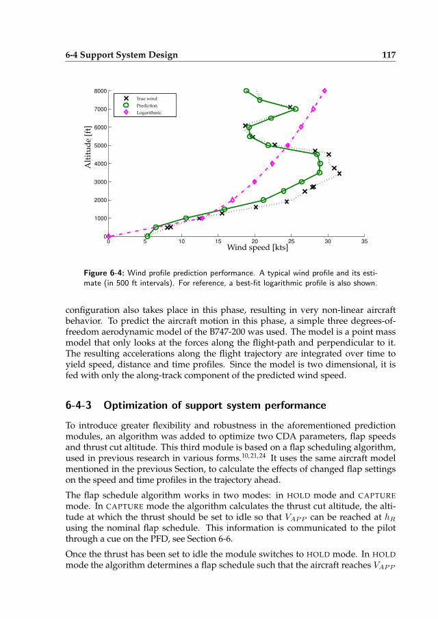
6-4 Support System Design 117
0 5 10 15 20 25 30 350
1000
2000
3000
4000
5000
6000
7000
8000A
ltit
ud
e[f
t]
Wind speed [kts]
True wind
Prediction
Logarithmic
Figure 6-4: Wind profile prediction performance. A typical wind profile and its esti-mate (in 500 ft intervals). For reference, a best-fit logarithmic profile is also shown.
configuration also takes place in this phase, resulting in very non-linear aircraftbehavior. To predict the aircraft motion in this phase, a simple three degrees-of-freedom aerodynamic model of the B747-200 was used. The model is a point massmodel that only looks at the forces along the flight-path and perpendicular to it.The resulting accelerations along the flight trajectory are integrated over time toyield speed, distance and time profiles. Since the model is two dimensional, it isfed with only the along-track component of the predicted wind speed.
6-4-3 Optimization of support system performance
To introduce greater flexibility and robustness in the aforementioned predictionmodules, an algorithm was added to optimize two CDA parameters, flap speedsand thrust cut altitude. This third module is based on a flap scheduling algorithm,used in previous research in various forms.10, 21, 24 It uses the same aircraft modelmentioned in the previous Section, to calculate the effects of changed flap settingson the speed and time profiles in the trajectory ahead.
The flap schedule algorithm works in two modes: in HOLD mode and CAPTURE
mode. In CAPTURE mode the algorithm calculates the thrust cut altitude, the alti-tude at which the thrust should be set to idle so that VAPP can be reached at hR
using the nominal flap schedule. This information is communicated to the pilotthrough a cue on the PFD, see Section 6-6.
Once the thrust has been set to idle the module switches to HOLD mode. In HOLD
mode the algorithm determines a flap schedule such that the aircraft reaches VAPP
118 Time Based Spacing
at hR. This deviation from the nominal schedule can be used to cope with errorscaused by for instance an inaccurate wind prediction, unexpected behavior frompreceding aircraft, etc. In this mode, the algorithm predicts the aircrafts trajectorybased on the current flap schedule. This yields an ETA, which is then compared tothe RTA commanded by ATC:
∆T = ETA−RTA (6-10)
Based on this difference, the flap scheduler does a rough tuning of the flap speedsto either their upper or their lower bounds, depending on the sign of this ∆T . Incase the aircraft is predicted to arrive early, deceleration needs to be faster than thecurrent (nominal) flap schedule will provide. The flap speeds will thus be set totheir upper bounds, and the resulting new trajectory is calculated. This process isrepeated for the consecutive flap speeds, until the target is overshot (∆T changessign). From here, the flap scheduler fine tunes the previous flap speed so that theaircraft arrives exactly at its RTA.
The combination of thrust cut altitude and flap selection speeds ultimately de-termines the CDA performance. Changes in the one parameter necessarily causechanges in the other, if the final configuration and airspeed are to be adhered to. Forexample, if thrust reduction is delayed (executed at a lower altitude), the aircraftwill reach hR with a speed higher than the approach speed. This can be preventedby selecting flaps at speeds higher than according to the nominal schedule, in orderto increase the deceleration rate. The upper and lower bounds of the flap speedshence define the boundaries of the control space the pilot has during the approach.Within this control space, the pilot can maneuver the aircraft to anticipate or delayhis arrival time. The time goal requires that the aircraft touches down within a smalltime window around the RTA. With the aircraft on final approach, the majority ofthe work needed to reach this goal is already done. The flap scheduler algorithmhelps the pilot to fine-tune his exact arrival time. Off-line simulations have shownthat for a straight-in continuous descent approach from 7,000 ft, 250 kts IAS, thiscontrol space is limited to 8-30 seconds, depending on wind conditions.10 For thisreason, it is important that the flight crew is able to steer their aircraft to withinthese bounds, before they start the descent.
6-5 Pilot Interface
6-5-1 Conventional Display
In the base-line condition, the pilot interface consists of a conventional PrimaryFlight Display (PFD), Navigation Display (ND) and a display showing the ModeControl Panel (MCP). The required information for the time based CDA procedureis printed on two cue cards, see Figure 6-5. This cueing system is loosely based
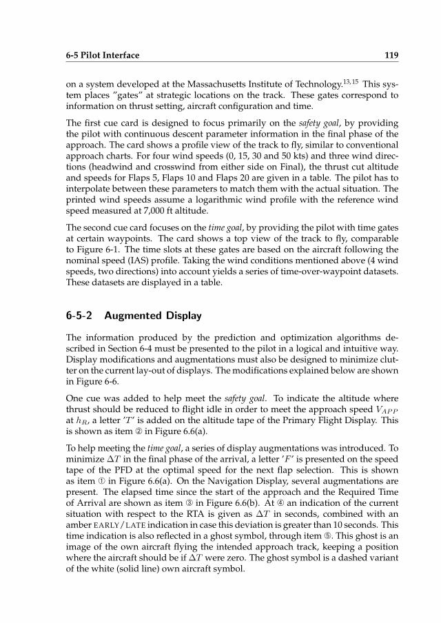
6-5 Pilot Interface 119
on a system developed at the Massachusetts Institute of Technology.13, 15 This sys-tem places ”gates” at strategic locations on the track. These gates correspond toinformation on thrust setting, aircraft configuration and time.
The first cue card is designed to focus primarily on the safety goal, by providingthe pilot with continuous descent parameter information in the final phase of theapproach. The card shows a profile view of the track to fly, similar to conventionalapproach charts. For four wind speeds (0, 15, 30 and 50 kts) and three wind direc-tions (headwind and crosswind from either side on Final), the thrust cut altitudeand speeds for Flaps 5, Flaps 10 and Flaps 20 are given in a table. The pilot has tointerpolate between these parameters to match them with the actual situation. Theprinted wind speeds assume a logarithmic wind profile with the reference windspeed measured at 7,000 ft altitude.
The second cue card focuses on the time goal, by providing the pilot with time gatesat certain waypoints. The card shows a top view of the track to fly, comparableto Figure 6-1. The time slots at these gates are based on the aircraft following thenominal speed (IAS) profile. Taking the wind conditions mentioned above (4 windspeeds, two directions) into account yields a series of time-over-waypoint datasets.These datasets are displayed in a table.
6-5-2 Augmented Display
The information produced by the prediction and optimization algorithms de-scribed in Section 6-4 must be presented to the pilot in a logical and intuitive way.Display modifications and augmentations must also be designed to minimize clut-ter on the current lay-out of displays. The modifications explained below are shownin Figure 6-6.
One cue was added to help meet the safety goal. To indicate the altitude wherethrust should be reduced to flight idle in order to meet the approach speed VAPP
at hR, a letter ’T ’ is added on the altitude tape of the Primary Flight Display. Thisis shown as item Á in Figure 6.6(a).
To help meeting the time goal, a series of display augmentations was introduced. Tominimize ∆T in the final phase of the arrival, a letter ’F ’ is presented on the speedtape of the PFD at the optimal speed for the next flap selection. This is shownas item À in Figure 6.6(a). On the Navigation Display, several augmentations arepresent. The elapsed time since the start of the approach and the Required Timeof Arrival are shown as item  in Figure 6.6(b). At à an indication of the currentsituation with respect to the RTA is given as ∆T in seconds, combined with anamber EARLY/LATE indication in case this deviation is greater than 10 seconds. Thistime indication is also reflected in a ghost symbol, through item Ä. This ghost is animage of the own aircraft flying the intended approach track, keeping a positionwhere the aircraft should be if ∆T were zero. The ghost symbol is a dashed variantof the white (solid line) own aircraft symbol.
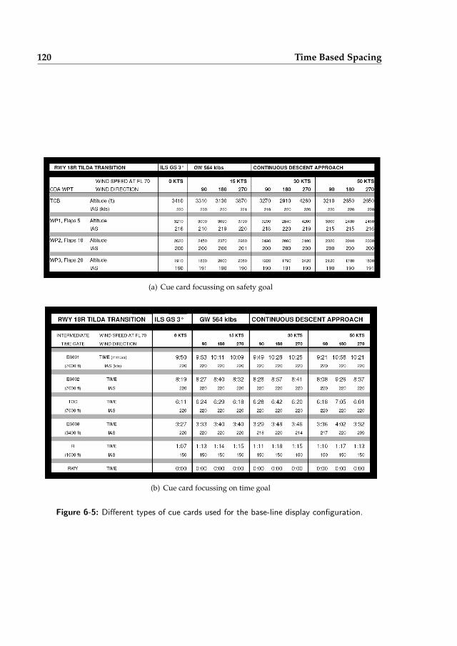
120 Time Based Spacing
(a) Cue card focussing on safety goal
(b) Cue card focussing on time goal
Figure 6-5: Different types of cue cards used for the base-line display configuration.
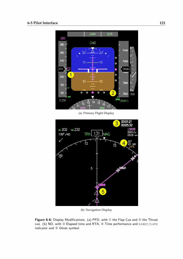
6-5 Pilot Interface 121
(a) Primary Flight Display
(b) Navigation Display
Figure 6-6: Display Modifications. (a) PFD, with À the Flap Cue and Á the Thrustcue. (b) ND, with  Elapsed time and RTA, à Time performance and early/lateindicator and Ä Ghost symbol.
122 Time Based Spacing
6-6 Experiment
To test the effectiveness of time based spacing and identify the operational con-straints of implementation, a piloted experiment was conducted. Seven profes-sional airline pilots tested the system under various operating conditions in a fixedbase flight simulator.
6-6-1 Independent variables
The first independent variable is the display configuration. The baseline conditionis a conventional display layout consisting of a Navigation Display (ND) and Pri-mary Flight Display (PFD). The second display configuration, for the augmentedcondition, consists of an ND and a PFD extended with information derived fromthe flap scheduler and optimization algorithms, as described in Section 6-5.
Second, four different wind conditions are defined that together represent a realisticset of wind conditions that could be encountered during any approach. A typicalwind profile is shown in Figure 6-4. These profiles are all taken from data sets of ac-tual wind measurements, but scaled and rotated to correspond to the wind speedsof interest. These wind conditions, listed in Table 6-2, comprise two headwind con-ditions on Final, and two crosswind conditions. For each wind direction, two windspeeds at the starting altitude of 7,000 ft are defined. The choice for wind speedvalues is such that the lower value could be encountered under normal, regularlyoccurring circumstances. The higher wind speed occurs in more rare situations.The wind speeds for crosswind approaches are lower, in correspondence to cross-wind and headwind limits for landing.
6-6-2 Experiment design
The experiment design matrix is factorial, combining the four wind conditions withboth displays, each condition flown once by each pilot. This yields eight experi-ment runs per pilot. Seven professional airline pilots (over 4,500 flying hours onaverage, see Table 6-1) flew a set of these eight runs, yielding 56 experiment runsin total. Each set was preceded by four to six practice runs, to familiarize the pilotswith the procedure and wind conditions.
6-6-3 Apparatus
The experiment was conducted in a fixed base research simulator at the Con-trol & Simulation Division. The pilots were seated on the copilot side, controllingthe aircraft with a side stick. The Primary Flight Display, Navigation Display andthe Mode Control Panel were shown on two 18” screens. An outside visual wasshown of a landscape with a fictitious airport with two parallel runways.
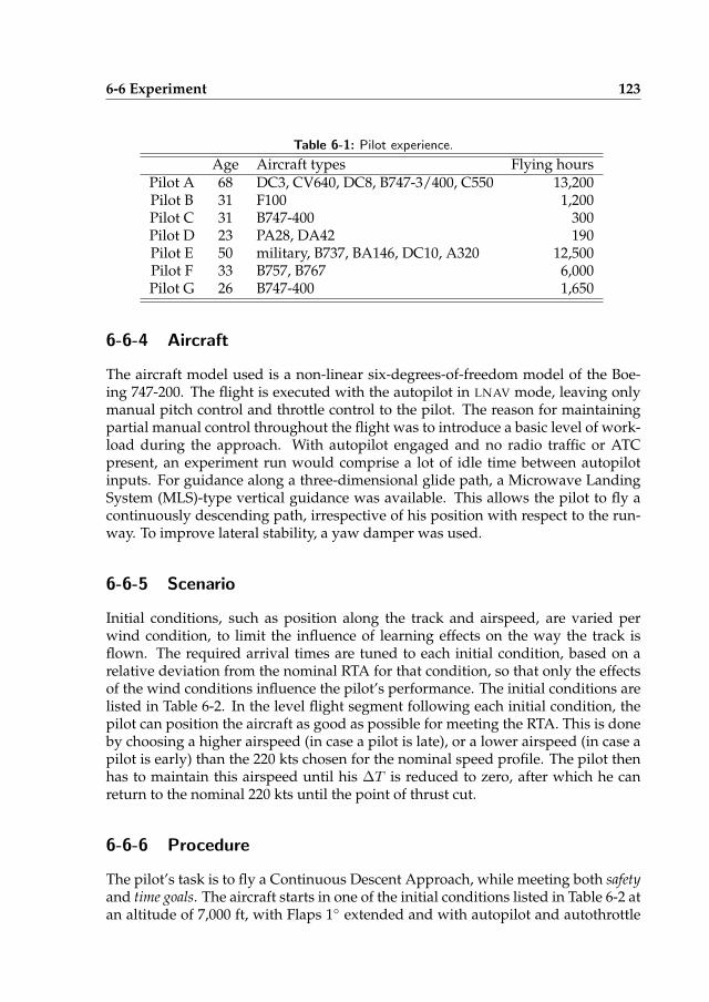
6-6 Experiment 123
Table 6-1: Pilot experience.
Age Aircraft types Flying hoursPilot A 68 DC3, CV640, DC8, B747-3/400, C550 13,200Pilot B 31 F100 1,200Pilot C 31 B747-400 300Pilot D 23 PA28, DA42 190Pilot E 50 military, B737, BA146, DC10, A320 12,500Pilot F 33 B757, B767 6,000Pilot G 26 B747-400 1,650
6-6-4 Aircraft
The aircraft model used is a non-linear six-degrees-of-freedom model of the Boe-ing 747-200. The flight is executed with the autopilot in LNAV mode, leaving onlymanual pitch control and throttle control to the pilot. The reason for maintainingpartial manual control throughout the flight was to introduce a basic level of work-load during the approach. With autopilot engaged and no radio traffic or ATCpresent, an experiment run would comprise a lot of idle time between autopilotinputs. For guidance along a three-dimensional glide path, a Microwave LandingSystem (MLS)-type vertical guidance was available. This allows the pilot to fly acontinuously descending path, irrespective of his position with respect to the run-way. To improve lateral stability, a yaw damper was used.
6-6-5 Scenario
Initial conditions, such as position along the track and airspeed, are varied perwind condition, to limit the influence of learning effects on the way the track isflown. The required arrival times are tuned to each initial condition, based on arelative deviation from the nominal RTA for that condition, so that only the effectsof the wind conditions influence the pilot’s performance. The initial conditions arelisted in Table 6-2. In the level flight segment following each initial condition, thepilot can position the aircraft as good as possible for meeting the RTA. This is doneby choosing a higher airspeed (in case a pilot is late), or a lower airspeed (in case apilot is early) than the 220 kts chosen for the nominal speed profile. The pilot thenhas to maintain this airspeed until his ∆T is reduced to zero, after which he canreturn to the nominal 220 kts until the point of thrust cut.
6-6-6 Procedure
The pilot’s task is to fly a Continuous Descent Approach, while meeting both safetyand time goals. The aircraft starts in one of the initial conditions listed in Table 6-2 atan altitude of 7,000 ft, with Flaps 1◦ extended and with autopilot and autothrottle
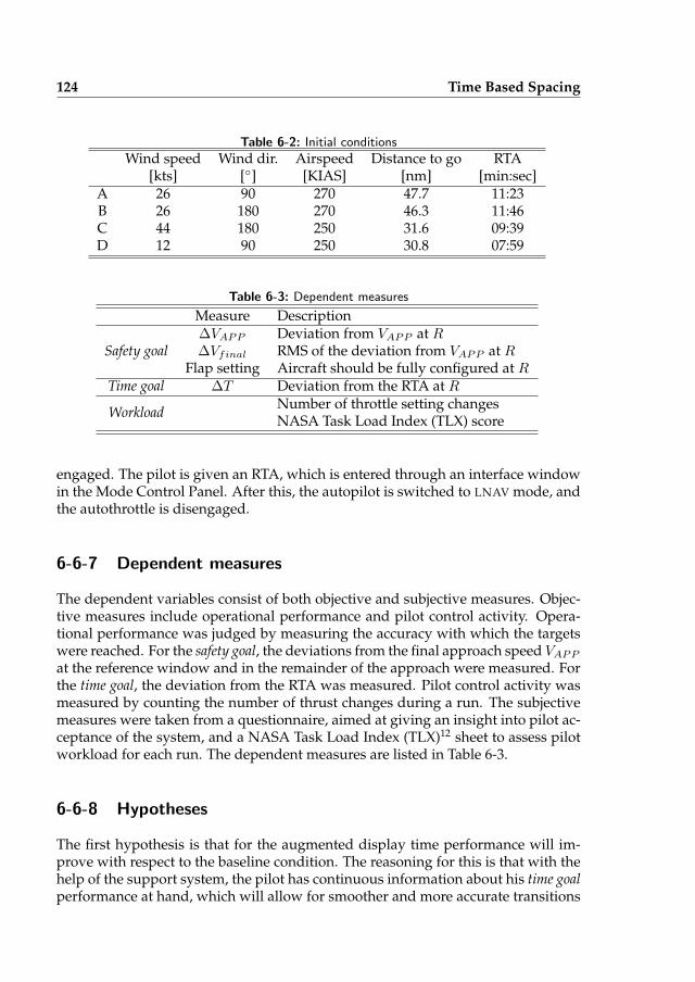
124 Time Based Spacing
Table 6-2: Initial conditions
Wind speed Wind dir. Airspeed Distance to go RTA[kts] [◦] [KIAS] [nm] [min:sec]
A 26 90 270 47.7 11:23B 26 180 270 46.3 11:46C 44 180 250 31.6 09:39D 12 90 250 30.8 07:59
Table 6-3: Dependent measures
Measure Description
Safety goal∆VAPP Deviation from VAPP at R∆Vfinal RMS of the deviation from VAPP at R
Flap setting Aircraft should be fully configured at RTime goal ∆T Deviation from the RTA at R
WorkloadNumber of throttle setting changesNASA Task Load Index (TLX) score
engaged. The pilot is given an RTA, which is entered through an interface windowin the Mode Control Panel. After this, the autopilot is switched to LNAV mode, andthe autothrottle is disengaged.
6-6-7 Dependent measures
The dependent variables consist of both objective and subjective measures. Objec-tive measures include operational performance and pilot control activity. Opera-tional performance was judged by measuring the accuracy with which the targetswere reached. For the safety goal, the deviations from the final approach speed VAPP
at the reference window and in the remainder of the approach were measured. Forthe time goal, the deviation from the RTA was measured. Pilot control activity wasmeasured by counting the number of thrust changes during a run. The subjectivemeasures were taken from a questionnaire, aimed at giving an insight into pilot ac-ceptance of the system, and a NASA Task Load Index (TLX)12 sheet to assess pilotworkload for each run. The dependent measures are listed in Table 6-3.
6-6-8 Hypotheses
The first hypothesis is that for the augmented display time performance will im-prove with respect to the baseline condition. The reasoning for this is that with thehelp of the support system, the pilot has continuous information about his time goalperformance at hand, which will allow for smoother and more accurate transitions
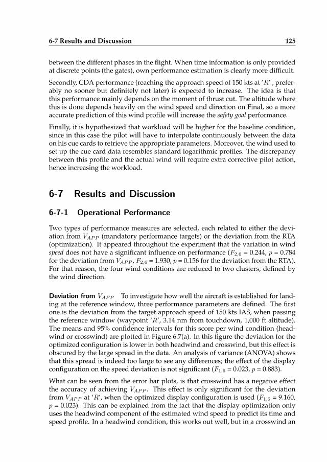
6-7 Results and Discussion 125
between the different phases in the flight. When time information is only providedat discrete points (the gates), own performance estimation is clearly more difficult.
Secondly, CDA performance (reaching the approach speed of 150 kts at ’R’ , prefer-ably no sooner but definitely not later) is expected to increase. The idea is thatthis performance mainly depends on the moment of thrust cut. The altitude wherethis is done depends heavily on the wind speed and direction on Final, so a moreaccurate prediction of this wind profile will increase the safety goal performance.
Finally, it is hypothesized that workload will be higher for the baseline condition,since in this case the pilot will have to interpolate continuously between the dataon his cue cards to retrieve the appropriate parameters. Moreover, the wind used toset up the cue card data resembles standard logarithmic profiles. The discrepancybetween this profile and the actual wind will require extra corrective pilot action,hence increasing the workload.
6-7 Results and Discussion
6-7-1 Operational Performance
Two types of performance measures are selected, each related to either the devi-ation from VAPP (mandatory performance targets) or the deviation from the RTA(optimization). It appeared throughout the experiment that the variation in windspeed does not have a significant influence on performance (F2,6 = 0.244, p = 0.784for the deviation from VAPP , F2,6 = 1.930, p = 0.156 for the deviation from the RTA).For that reason, the four wind conditions are reduced to two clusters, defined bythe wind direction.
Deviation from VAPP To investigate how well the aircraft is established for land-ing at the reference window, three performance parameters are defined. The firstone is the deviation from the target approach speed of 150 kts IAS, when passingthe reference window (waypoint ‘R’, 3.14 nm from touchdown, 1,000 ft altitude).The means and 95% confidence intervals for this score per wind condition (head-wind or crosswind) are plotted in Figure 6.7(a). In this figure the deviation for theoptimized configuration is lower in both headwind and crosswind, but this effect isobscured by the large spread in the data. An analysis of variance (ANOVA) showsthat this spread is indeed too large to see any differences; the effect of the displayconfiguration on the speed deviation is not significant (F1,6 = 0.023, p = 0.883).
What can be seen from the error bar plots, is that crosswind has a negative effectthe accuracy of achieving VAPP . This effect is only significant for the deviationfrom VAPP at ‘R’, when the optimized display configuration is used (F1,6 = 9.160,p = 0.023). This can be explained from the fact that the display optimization onlyuses the headwind component of the estimated wind speed to predict its time andspeed profile. In a headwind condition, this works out well, but in a crosswind an
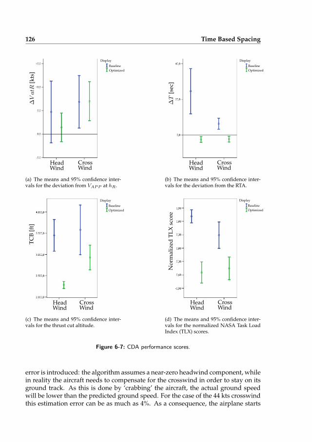
126 Time Based Spacing∆VatR
[kts
]
Head CrossWindWind
Display
Baseline
Optimized
(a) The means and 95% confidence inter-vals for the deviation from VAPP at hR.
∆T
[sec
]
Head CrossWindWind
Display
Baseline
Optimized
(b) The means and 95% confidence inter-vals for the deviation from the RTA.
Head CrossWindWind
Display
Baseline
Optimized
TC
B[f
t]
(c) The means and 95% confidence inter-vals for the thrust cut altitude.
Head CrossWindWind
Display
Baseline
Optimized
No
rmal
ized
TL
Xsc
ore
(d) The means and 95% confidence inter-vals for the normalized NASA Task LoadIndex (TLX) scores.
Figure 6-7: CDA performance scores.
error is introduced: the algorithm assumes a near-zero headwind component, whilein reality the aircraft needs to compensate for the crosswind in order to stay on itsground track. As this is done by ‘crabbing’ the aircraft, the actual ground speedwill be lower than the predicted ground speed. For the case of the 44 kts crosswindthis estimation error can be as much as 4%. As a consequence, the airplane starts
6-7 Results and Discussion 127
lagging behind the original predicted time profile, which in turn causes pilots todelay flap selection in order to maintain a higher airspeed. In many cases, thedeviation from VAPP suffers from this decision, with the average approach speedgoing up from little over 151 kts to 156 kts. For the baseline condition, the dataon the cue cards is based on trial runs, instead of predictor data. Since the windinformation on the cards (based on logarithmic profiles) does not take the effect of‘crabbing’ into account, the deviation from VAPP is not influenced in the crosswindscenario.
The fact that speed performance goes down when the track prediction is less ac-curate (in the crosswind condition) suggests that pilots closely followed the cuespresented on the displays. At the same time, the large spread in speed perfor-mance in the baseline condition indicates significant differences between the differ-ent strategies adopted by each pilot. This is confirmed by the pilots’ answers to aquestionnaire, which showed that they used the CDA-parameter cue card mostlyto determine the thrust cut altitude, but thereafter relied more on their pilot expe-rience to determine flap selection. In the optimized display configuration, the needto look away from the instruments to check the cue cards is eliminated, and pilotsuse the displayed instructions.
Deviation from RTA The main check on the time performance is the deviationfrom the RTA at the reference window. The means and 95% Confidence Intervalsfor this parameter are shown in Figure 6.7(b). Clearly, the average time perfor-mance is better with the aid of display optimization. An ANOVA shows that thisinfluence is indeed significant (F1,6 = 7.368, p = 0.033). Average time performanceis within 4 seconds of the RTA. This is definitely accurate enough to guarantee safeseparation. This result would allow air traffic controllers to space incoming trafficmore tightly, increasing runway throughput capacity. The addition of the proposedautomation to existing cockpit displays enables pilots to fly a time based CDA.
The explanation for this improvement is twofold. First, by providing the pilot withcontinuously updated information on his status, he is able to very accurately adjustthe aircraft’s speed profile to minimize ∆T . In the baseline, the number of interme-diate time gates is limited to four (for conditions C and D in Table 6-2) or five (forconditions A and B). Second, the more accurate wind prediction that is availablein the enhanced display condition yields a better estimate of the optimal altitudefor thrust reduction. This can be seen in Figure 6.7(c), showing the altitude wherepilots cut back on thrust to decelerate the aircraft to 150 kts. Regardless of wind di-rection, this altitude is significantly lower in the optimized display condition thanin the baseline condition (F1,6 = 3.560, p = 0.098). With the used wind profile class inmind (see Figure 6-4), it becomes clear that the logarithmic profile prediction is notable to deal with the increase in wind speed around 3,500 ft. The aircraft encountersmore (head)wind than expected, so its thrust cut altitude should be lowered. Thetrack prediction and optimization routines take this effect into account.
Although the automation provided a major improvement in time performance,speed performance (deviation from VAPP ) was still in the same range as in the
128 Time Based Spacing
baseline situation. This might be due to the fact that the the automation mainlyfocused on achieving the time goal. To strike a better balance between the two per-formance criteria, and to provide a more logical lay out of the presented clues, it isrecommended to let the cues on the Primary Flight Display focus on CDA perfor-mance (arrive stabilized at the reference window), while the cues on the NavigationDisplay (ghost and ∆T ) focus on the time goal. Another improvement would beto integrate the cues more tightly with current procedures. For example, in manyaircraft the landing gear should be lowered between two fixed consecutive flapsettings. To incorporate such information in the pilot support system would easeimplementation and increase acceptability by airlines and flight crew.
6-7-2 Pilot workload
The results for the subjective workload measurements are represented by the nor-malized NASA TLX rating scores in Figure 6.7(d). Workload experienced by thepilots is lower for the optimized display condition, in all wind conditions. Thiseffect is highly significant (F1,6 = 50.390, p < 0.001), an observation that is con-firmed by the questionnaire answers with all pilots indicating a higher workloadin the baseline condition. In contrast, the workload in this type of noise abatementprocedure with the optimization present was considered comparable to that of aconventional ILS approach.
Furthermore, it can be seen that for the baseline condition, the workload score alsodepends on the wind direction. The score is significantly lower in crosswind con-ditions on Final (F1,6 = 12.797 , p = 0.012). Several factors could influence this phe-nomenon. First, in a headwind condition, the full force of the sharp changes inwind speed along the altitude profile is felt. In a crosswind, only one component ofthe wind is of influence, so the absolute change in wind speed is smaller. Anotherfactor might be that the crosswind condition on Final means a headwind conditionbetween waypoints TILDA and EH608 (see Figure 6-1). In many cases, this is thephase where pilots reach the on-time schedule (∆T = 0 and reduce speed from 250or 270 kts to the nominal speed of 220 kts. This is not always an easy task, since aB747 in this situation (Flaps 1◦, gear up, 3◦ glide path, no speed breaks) has a lowdeceleration rate. A headwind in this situation reduces the kinematic flight pathangle, which makes it easier for the pilot to decelerate the aircraft. This increasesthe chances of a stabilized approach and hence reduces pilot workload.
Flying a CDA already puts more demand on the flight crew than a regular arrival,where the basic control task is following ATC vectors. Although the tasks of flyingand navigation are normally shared between the Pilot Flying and the Pilot NotFlying, the pilots interviewed indicated that they would find the sharp increase inworkload as experienced in the base-line scenario unacceptable.
6-8 Conclusions 129
6-8 Conclusions
This paper investigated the feasibility of introducing time based spacing in realistic,three dimensional continuous descent approaches under actual wind conditions.For reasons of safety, it is important that first, the continuous descent ends in astabilized approach configuration and speed some distance before the runway andsecond, pilots are able to meet the required arrival times instructed by ATC, in orderto maintain safe separation throughout the approach.
The development of an FMS based prediction and optimization system combinedwith a pilot support interface enables the flight crew to reach these two goals. Awind prediction algorithm that makes use of weather information broadcast byother aircraft in the TMA makes accurate wind profile prediction along the ap-proach trajectory possible. Wind speed prediction error along a 30-45 nm approachtrajectory is 2 kts. An accurate knowledge of the wind ahead makes sure an optimalthrust cut altitude and flap speed schedule can be selected. The piloted experimentsshow a strong improvement in time performance when continuously updated in-formation on this goal is present on the display. Pilots are able to reach their RTAswithin an average margin of 4 seconds, regardless of wind conditions. The averagespeed performance (being stabilized at a reference window) is unaffected by dis-play optimization, although the presence of automation reduces the spread in thisperformance criterion. The addition of time constraints without extra aids wouldresult in an unacceptable increase in workload, due to the continuous calculationand interpolation the pilots have to perform. Workload is significantly lower withthe display optimization present, and at the same level as in current ILS approachprocedures.
6-9 Recommendations
The piloted experiment shows the feasibility of time-based continuous descentapproach procedures under realistic wind conditions, along a fixed trajectory. Thepilot’s control space to reach an RTA could be greatly enlarged by adopting amore flexible approach route. Shortening or extending the length of the track tofly, similar to the ’tromboning’ technique currently used by ATC, should reducethe need for speed changes, thereby improving predictability of the speed profileduring the approach.
References
[1] Assembly Resolution A33-7: Consolidated Statement of Continuing ICAOPolicies and Practices Related to Environmental Protection. International Civil
130 REFERENCES
Aviation Organization (ICAO), 2001.
[2] Outlook for Air Transport to the Year 2015. Technical Report AT-127, Interna-tional Civil Aviation Organization (ICAO), Sep 2004.
[3] Aeronautical Information Publication AIP. Air Traffic Control The Nether-lands, 2006.
[4] Sourdine II, Final Report. Technical Report D9-1, National Aerospace Labora-tory (NLR), Aug 31 2006.
[5] E. H. Bolz and L. M. Reuss. System Study of Advanced Operational Proce-dures for Noise Reduction. Technical Report NASA (Task Order (TO) 56), Na-tional Aeronautics and Space Administration NASA, Oct 2001.
[6] J.-P. Clarke. Systems Analysis of Noise Abatement Procedures Enabled by Ad-vanced Flight Guidance Technology. Journal of Aircraft, 37(2), Mar-Apr 2000.
[7] J.-P. Clarke, N. T. Ho, L. Ren, J. A. Brown, K. R. Elmer, K. Tong, and J. K.Wat. Continuous Descent Approach: Design and Flight Test for LouisvilleInternational Airport. AIAA Journal of Aircraft, 41(5):1054–1066, 2004.
[8] R. A. Coppenbarger, R. W. Mead, and D. N. Sweet. Field Evaluation of the Tai-lored Arrivals Concept for Datalink-Enabled Continuous Descent Approach.AIAA Journal of Aircraft, 46(4):1200–1209, 2009.
[9] L. J. J. Erkelens. Research into New Noise Abatement Procedures for the 21st
Century. Number AIAA 2000-4474, pages 1–10, Denver (CO), USA, Aug 14-172001.
[10] W. F. de Gaay Fortman, M. M. van Paassen, M. Mulder, A. C. in ’t Veld, andJ.-P. Clarke. Implementing Time-Based Spacing for Decelerating Approaches.AIAA Journal of Aircraft, 44(1):106–118, Jan-Feb 2007.
[11] P. Frenzen and C. A. Vogel. On the Magnitude and Apparent Range of Varia-tion of the Von Karman Constant in the Atmospheric Surface Layer. Boundary-Layer Meteorology, 72:371–392, 1995.
[12] S. G. Hart and L. E. Staveland. Development of NASA-TLX (Task Load Index):Results of Emperical and Theoretical Research. In Human Mental Workload,pages 239–250. Elsevier Science Publishers, Amsterdam, The Netherlands,1988.
[13] N. T. Ho. Design of Aircraft Noise Abatement Approach Procedures for Near-TermImplementation. PhD thesis, Massachusetts Institute of Technology, Cambridge(MA), USA, 2005.
[14] N. T. Ho and J.-P. Clarke. Methodology for Optimizing Parameters of NoiseAbatement Approach Procedures. AIAA Journal of Aircraft, 44(4):1168–1176,2007.
131
[15] N. T. Ho, J.-P. Clarke, R. Riedel, and C. Oman. Cueing System for Near-TermImplementation of Aircraft Noise Abatement Approach Procedures. AIAAJournal of Aircraft, 44(3):718–725, 2007.
[16] A. D. Kershaw, D. P. Rhodes, and N. A. Smith. The Influence of ATC in Ap-proach Noise Abatement. Napoli, Italy, Jun 13-16 2000.
[17] M. F. Koeslag. Advanced Continuous Descent Approaches, an Algorithm De-sign for the FMS. MSc. Thesis, Faculty of Aerospace Engineering, Delft Uni-versity of Technology, 2001.
[18] A. M. P. de Leege, A. C. in ’t Veld, M. Mulder, and M. M. van Paassen. Three-Degree Decelerating Approaches in High-Density Arrival Streams. AIAA Jour-nal of Aircraft, 46(5):1681–1691, Oct 2009.
[19] P. S. Maybeck. Stochastic Models, Estimation and Control, volume 1. AcademicPress, 1979.
[20] D. Painting. AMDAR Reference Manual. Technical report, World Meteorolog-ical Organization-AMDAR Panel, 2001.
[21] J. L. de Prins, K. F. M. Schippers, M. Mulder, M. M. van Paassen, A. C. in’t Veld, and J.-P. Clarke. Enhanced Self-Spacing Algorithm for Three-DegreeDecelerating Approaches. AIAA Journal of Aircraft, 30(2):576–590, Mar 2007.
[22] L. Ren and J.-P. Clarke. Flight-Test Evaluation of the Tool for Analysis of Sep-aration and Throughput. AIAA Journal of Aircraft, 45(1):323–332, Jan-Feb 2008.
[23] L. Ren, J.-P. Clarke, and N. T. Ho. Achieving Low Approach Noise with-out Sacrificing Capacity. In 22nd Digital Avionics Systems Conference, numberAIAA-2001-5239, pages 1–9, Indianapolis (IN), USA, Oct 12-16 2003.
[24] A. C. in ’t Veld, M. M. van Paassen, M. Mulder, and J.-P. Clarke. Pilot SupportInterface for Three-Degree Decelerating Approach Procedures. The Interna-tional Journal of Aviation Psychology, 19(3):287–308, Jul 2009.
[25] F. Wubben and J. Busink. Night Time Restrictions at Amsterdam-Schiphol, anInternational Comparison. Technical report, to70 Aviation and Environment,under Contract of the Ministry of Transport, Public Works and Water Affairs,2004.

132
7
Self-spacing in High-DensityArrival Streams
Three-Degree Decelerating Approaches in High-Density Arrival Streams
A.M.P. de Leege, A.C. in ’t Veld, M. Mulder and M.M. van Paassen
AIAA Journal of Aircraft, Vol.46 No.5, Sep-Oct 2009, Pages 1681-1691
7-1 Abstract
Trajectory unpredictability of aircraft performing continuous descent approachesresults in reduced runway capacity, because more spacing is applied. A possiblesolution to this problem is self-spacing - the transfer of the spacing task from thecontroller to the pilot. Using a fast-time simulation tool the performance differencesbetween distance- and time based self-spacing in high-density traffic in terms ofrunway capacity and separation are quantified for the Three-Degree DeceleratingApproach. Distance based self-spacing is the most promising concept. The averagerunway capacity is 39 aircraft per hour (40% heavy, 60% medium aircraft). Run-way capacity in case of time based self-spacing is 3 aircraft per hour lower, dueto spacing margins applied to lower the separation violation rate to the level ofdistance based spacing. A sensitivity analysis was carried out for distance basedself-spacing. One of the results is that accurately determining the starting time andsubsequently arriving at this time benefits the TDDA performance. TDDA perfor-mance is also affected by the initial speed and altitude as they affect the TDDA’scontrol space.
134 Self-spacing in High-Density Arrival Streams
7-2 Introduction
Continuous Descent Approach (CDA) is a cost effective mean to reduce aircraftnoise, emissions, flight time, and fuel burn.5, 10, 17, 18 Aircraft continuously deceler-ate while on these approaches, which leads to trajectory unpredictability from thestandpoint of a controller who is monitoring inter-aircraft spacing based on peri-odic radar updates of aircraft position. As such, controllers apply larger spacingto prevent vectoring instructions that would conflict with the CDA. Larger spacingbetween aircraft reduces runway capacity down to 50% when compared to conven-tional approaches.3, 11, 13, 14
A possible solution to this problem is the use of in-trail self-spacing.3, 14 The spac-ing task is transferred from the controller to the pilot. Self-spacing is proposedbecause of the availability of precise aircraft performance information and the con-trol strategy onboard the aircraft. The maneuverability of an aircraft while execut-ing a CDA is limited and driven by the aircraft performance, the control strategy,and wind conditions. Information about wind conditions the aircraft is likely toencounter during descent can be made available as described in.7 The flight crewcan plan and execute, with the help of onboard systems, a CDA to remain safelyseparated.6, 9, 12
This paper discusses research into the performance of the Three-Degree Decelerat-ing Approach (TDDA) in high-density arrival streams in a distance- or time basedself-spacing environment. The TDDA is a CDA that lies within the boundaries ofpresent approach procedure limitations and gives the pilot control over the descentpath to fulfill the spacing task.4, 6, 7, 9, 12, 14 In a distance based self-spacing environ-ment the aircraft actively adapts its speed profile to the speed profile of the aircraftflying directly in front. This requires that the aircraft predicts the trajectory of thisleading aircraft. Using the relative state of the leading aircraft to predict the tra-jectory can give rise to transient motions in the arrival stream, hereafter referred toas the ‘slinky effect’, resulting in spacing problems.15 In this research intent-basedtrajectory prediction is introduced for the TDDA to prevent the slinky effect in caseof distance based self-spacing. Another solution to circumvent the slinky effect isa time based self-spacing procedure, which does not require trajectory predictionof the leading aircraft during the TDDA. Its performance was compared with themore common distance based procedure. In the time based environment the air-craft receive a Required Time of Arrival (RTA) for the runway threshold point. TheRTAs are set prior to the start of the TDDA with the aim to keep the aircraft safelyseparated during approach. A fast-time simulation tool was developed to investi-gate the differences in performance between distance- and time based self-spacingin terms of capacity, and loss of separation.
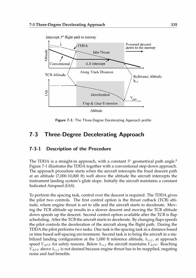
7-3 Three-Degree Decelerating Approach 135
Figure 7-1: The Three-Degree Decelerating Approach profile
7-3 Three-Degree Decelerating Approach
7-3-1 Description of the Procedure
The TDDA is a straight-in approach, with a constant 3◦ geometrical path angle.4
Figure 7-1 illustrates the TDDA together with a conventional step-down approach.The approach procedure starts when the aircraft intercepts the fixed descent pathat an altitude (7,000-10,000 ft) well above the altitude the aircraft intercepts theinstrument landing system’s glide slope. Initially the aircraft maintains a constantIndicated Airspeed (IAS).
To perform the spacing task, control over the descent is required. The TDDA givesthe pilot two controls. The first control option is the thrust cutback (TCB) alti-tude, where engine thrust is set to idle and the aircraft starts to decelerate. Mov-ing the TCB altitude up results in a slower descent and moving the TCB altitudedown speeds up the descent. Second control option available after the TCB is flapscheduling. After the TCB the aircraft starts to decelerate. By changing flaps speedsthe pilot controls the deceleration of the aircraft along the flight path. During theTDDA the pilot performs two tasks. One task is the spacing task in a distance basedor time based self-spacing environment. Second task is to bring the aircraft in a sta-bilized landing configuration at the 1,000 ft reference altitude, href , at approachspeed VAPP for safety reasons. Below href the aircraft maintains VAPP . ReachingVAPP above href is not desired because engine thrust has to be reapplied, negatingnoise and fuel benefits.
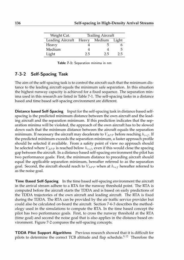
136 Self-spacing in High-Density Arrival Streams
Weight Cat. Trailing AircraftLeading Aircraft Heavy Medium LightHeavy 4 5 6Medium 4 4 5Light 2.5 2.5 2.5
Table 7-1: Separation minima in nm
7-3-2 Self-Spacing Task
The aim of the self-spacing task is to control the aircraft such that the minimum dis-tance to the leading aircraft equals the minimum safe separation. In this situationthe highest runway capacity is achieved for a fixed sequence. The separation min-ima used in this research are listed in Table 7-1. The self-spacing tasks in a distancebased and time based self-spacing environment are different.
Distance based Self-Spacing Input for the self-spacing task in distance based self-spacing is the predicted minimum distance between the own aircraft and the lead-ing aircraft and the separation minimum. If this prediction indicates that the sep-aration minima will be violated, the approach of the own aircraft has to be sloweddown such that the minimum distance between the aircraft equals the separationminimum. If necessary the aircraft may decelerate to VAPP before reaching href . Ifthe predicted minimum exceeds the separation minimum, a faster approach profileshould be selected if available. From a safety point of view no approach shouldbe selected where VAPP is reached below href , even if this would close the spacinggap between the aircraft. In a distance based self-spacing environment the pilot hastwo performance goals: First, the minimum distance to preceding aircraft shouldequal the applicable separation minimum, hereafter referred to as the separationgoal. Second, the aircraft should reach to VAPP when at href hereafter referred toas the noise goal.
Time Based Self-Spacing In the time based self-spacing environment the aircraftin the arrival stream adhere to a RTA for the runway threshold point. The RTA iscomputed before the aircraft starts the TDDA and is based on early predictions ofthe TDDA trajectories of the own aircraft and leading aircraft. The RTA is fixedduring the TDDA. The RTA can be provided by the air traffic service provider butcould also be calculated on-board the aircraft. Section 7-6-3 describes the method-ology used in the simulations to compute the RTA. In the time based concept thepilot has two performance goals. First, to cross the runway threshold at the RTA(time goal) and second the noise goal that is also applies in the distance based en-vironment. Figure 7-2 compares the self-spacing concepts.
TDDA Pilot Support Algorithms Previous research showed that it is difficult forpilots to determine the correct TCB altitude and flap schedule.9, 12 Therefore the
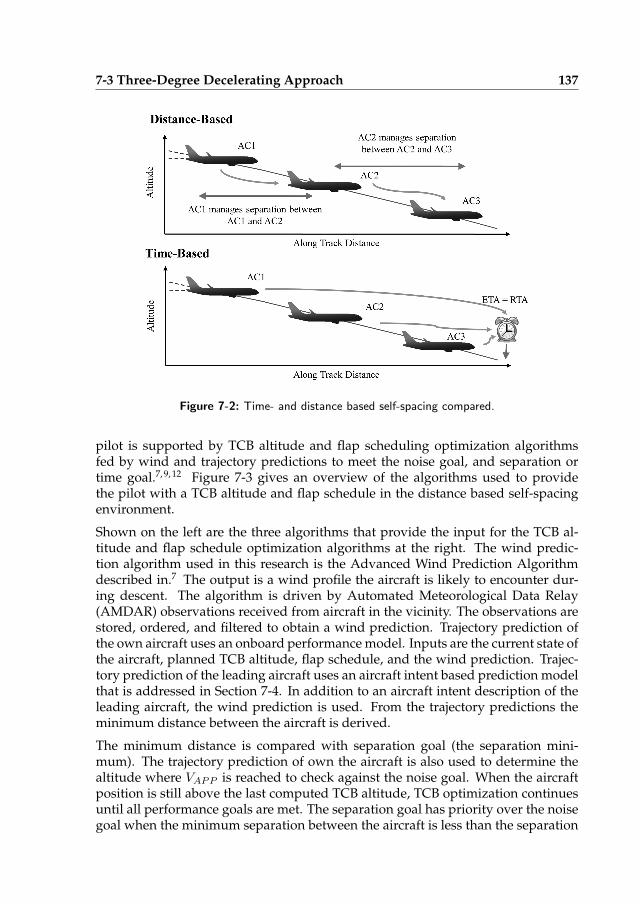
7-3 Three-Degree Decelerating Approach 137
Figure 7-2: Time- and distance based self-spacing compared.
pilot is supported by TCB altitude and flap scheduling optimization algorithmsfed by wind and trajectory predictions to meet the noise goal, and separation ortime goal.7, 9, 12 Figure 7-3 gives an overview of the algorithms used to providethe pilot with a TCB altitude and flap schedule in the distance based self-spacingenvironment.
Shown on the left are the three algorithms that provide the input for the TCB al-titude and flap schedule optimization algorithms at the right. The wind predic-tion algorithm used in this research is the Advanced Wind Prediction Algorithmdescribed in.7 The output is a wind profile the aircraft is likely to encounter dur-ing descent. The algorithm is driven by Automated Meteorological Data Relay(AMDAR) observations received from aircraft in the vicinity. The observations arestored, ordered, and filtered to obtain a wind prediction. Trajectory prediction ofthe own aircraft uses an onboard performance model. Inputs are the current state ofthe aircraft, planned TCB altitude, flap schedule, and the wind prediction. Trajec-tory prediction of the leading aircraft uses an aircraft intent based prediction modelthat is addressed in Section 7-4. In addition to an aircraft intent description of theleading aircraft, the wind prediction is used. From the trajectory predictions theminimum distance between the aircraft is derived.
The minimum distance is compared with separation goal (the separation mini-mum). The trajectory prediction of own the aircraft is also used to determine thealtitude where VAPP is reached to check against the noise goal. When the aircraftposition is still above the last computed TCB altitude, TCB optimization continuesuntil all performance goals are met. The separation goal has priority over the noisegoal when the minimum separation between the aircraft is less than the separation

138 Self-spacing in High-Density Arrival Streams
Figure 7-3: Structure of TDDA algorithm for distance based self-spacing.
minimum. The noise goal has priority over the separation goal when the minimumseparation between the aircraft exceeds the separation minimum. Once below theTCB altitude, flap schedule optimization is started. The flap scheduler is based onthe scheduler developed by de Prins et al.9 The flap scheduler uses a binary searchalgorithm to determine the optimal schedule. The scheduler only optimizes for thenoise goal is only if the separation goal is met, thus giving priority to the separationtask.
The TDDA algorithm structure for time based self-spacing is similar to the structureused for distance based spacing, see Figure 7-4. The minimum distance betweenthe aircraft is no longer computed and is replaced by the Estimated Time of Arrival(ETA), which is checked against the RTA. In the TCB altitude and flap scheduleoptimization algorithms the time goal is treated in a similar way as the separationgoal.
7-4 Aircraft Intent-Based Trajectory Prediction
To prevent the slinky effect during of distance based self-spacing aircraft intent isused to predict the trajectory of the leading aircraft. Captured in the intent is theoutcome of optimization of the trajectory by the TDDA algorithms on-board theleading aircraft. If an aircraft descent profile is disturbed, for instance by a windchange or delayed pilot action, the TDDA algorithm optimizes the trajectory. Thenew trajectory is described in aircraft intent that may be different from the previousintent information, because of the optimization process. The intent is exchangedusing a data-link. Predictions only based on previous states do not account for theongoing optimization process. This can cause unnecessary control actions from thetrailing aircraft that can propagate through the arrival stream resulting in the slinkyeffect.
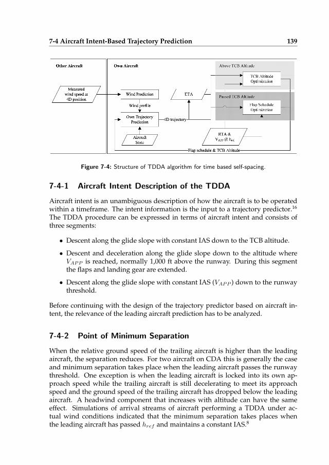
7-4 Aircraft Intent-Based Trajectory Prediction 139
Figure 7-4: Structure of TDDA algorithm for time based self-spacing.
7-4-1 Aircraft Intent Description of the TDDA
Aircraft intent is an unambiguous description of how the aircraft is to be operatedwithin a timeframe. The intent information is the input to a trajectory predictor.16
The TDDA procedure can be expressed in terms of aircraft intent and consists ofthree segments:
• Descent along the glide slope with constant IAS down to the TCB altitude.
• Descent and deceleration along the glide slope down to the altitude whereVAPP is reached, normally 1,000 ft above the runway. During this segmentthe flaps and landing gear are extended.
• Descent along the glide slope with constant IAS (VAPP ) down to the runwaythreshold.
Before continuing with the design of the trajectory predictor based on aircraft in-tent, the relevance of the leading aircraft prediction has to be analyzed.
7-4-2 Point of Minimum Separation
When the relative ground speed of the trailing aircraft is higher than the leadingaircraft, the separation reduces. For two aircraft on CDA this is generally the caseand minimum separation takes place when the leading aircraft passes the runwaythreshold. One exception is when the leading aircraft is locked into its own ap-proach speed while the trailing aircraft is still decelerating to meet its approachspeed and the ground speed of the trailing aircraft has dropped below the leadingaircraft. A headwind component that increases with altitude can have the sameeffect. Simulations of arrival streams of aircraft performing a TDDA under ac-tual wind conditions indicated that the minimum separation takes places whenthe leading aircraft has passed href and maintains a constant IAS.8
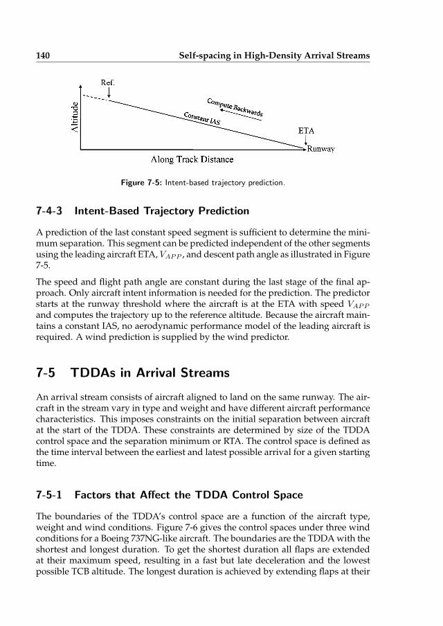
140 Self-spacing in High-Density Arrival Streams
Figure 7-5: Intent-based trajectory prediction.
7-4-3 Intent-Based Trajectory Prediction
A prediction of the last constant speed segment is sufficient to determine the mini-mum separation. This segment can be predicted independent of the other segmentsusing the leading aircraft ETA, VAPP , and descent path angle as illustrated in Figure7-5.
The speed and flight path angle are constant during the last stage of the final ap-proach. Only aircraft intent information is needed for the prediction. The predictorstarts at the runway threshold where the aircraft is at the ETA with speed VAPP
and computes the trajectory up to the reference altitude. Because the aircraft main-tains a constant IAS, no aerodynamic performance model of the leading aircraft isrequired. A wind prediction is supplied by the wind predictor.
7-5 TDDAs in Arrival Streams
An arrival stream consists of aircraft aligned to land on the same runway. The air-craft in the stream vary in type and weight and have different aircraft performancecharacteristics. This imposes constraints on the initial separation between aircraftat the start of the TDDA. These constraints are determined by size of the TDDAcontrol space and the separation minimum or RTA. The control space is defined asthe time interval between the earliest and latest possible arrival for a given startingtime.
7-5-1 Factors that Affect the TDDA Control Space
The boundaries of the TDDA’s control space are a function of the aircraft type,weight and wind conditions. Figure 7-6 gives the control spaces under three windconditions for a Boeing 737NG-like aircraft. The boundaries are the TDDA with theshortest and longest duration. To get the shortest duration all flaps are extendedat their maximum speed, resulting in a fast but late deceleration and the lowestpossible TCB altitude. The longest duration is achieved by extending flaps at their
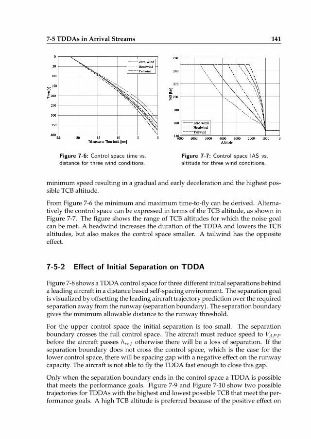
7-5 TDDAs in Arrival Streams 141
Figure 7-6: Control space time vs.distance for three wind conditions.
Figure 7-7: Control space IAS vs.altitude for three wind conditions.
minimum speed resulting in a gradual and early deceleration and the highest pos-sible TCB altitude.
From Figure 7-6 the minimum and maximum time-to-fly can be derived. Alterna-tively the control space can be expressed in terms of the TCB altitude, as shown inFigure 7-7. The figure shows the range of TCB altitudes for which the noise goalcan be met. A headwind increases the duration of the TDDA and lowers the TCBaltitudes, but also makes the control space smaller. A tailwind has the oppositeeffect.
7-5-2 Effect of Initial Separation on TDDA
Figure 7-8 shows a TDDA control space for three different initial separations behinda leading aircraft in a distance based self-spacing environment. The separation goalis visualized by offsetting the leading aircraft trajectory prediction over the requiredseparation away from the runway (separation boundary). The separation boundarygives the minimum allowable distance to the runway threshold.
For the upper control space the initial separation is too small. The separationboundary crosses the full control space. The aircraft must reduce speed to VAPP
before the aircraft passes href otherwise there will be a loss of separation. If theseparation boundary does not cross the control space, which is the case for thelower control space, there will be spacing gap with a negative effect on the runwaycapacity. The aircraft is not able to fly the TDDA fast enough to close this gap.
Only when the separation boundary ends in the control space a TDDA is possiblethat meets the performance goals. Figure 7-9 and Figure 7-10 show two possibletrajectories for TDDAs with the highest and lowest possible TCB that meet the per-formance goals. A high TCB altitude is preferred because of the positive effect on
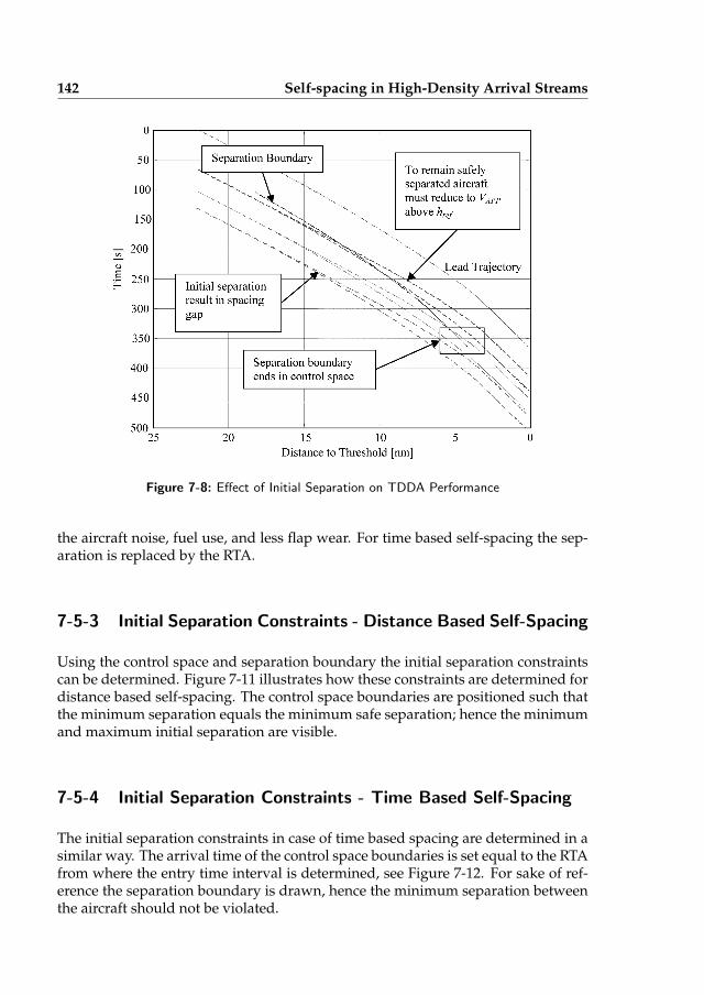
142 Self-spacing in High-Density Arrival Streams
Figure 7-8: Effect of Initial Separation on TDDA Performance
the aircraft noise, fuel use, and less flap wear. For time based self-spacing the sep-aration is replaced by the RTA.
7-5-3 Initial Separation Constraints - Distance Based Self-Spacing
Using the control space and separation boundary the initial separation constraintscan be determined. Figure 7-11 illustrates how these constraints are determined fordistance based self-spacing. The control space boundaries are positioned such thatthe minimum separation equals the minimum safe separation; hence the minimumand maximum initial separation are visible.
7-5-4 Initial Separation Constraints - Time Based Self-Spacing
The initial separation constraints in case of time based spacing are determined in asimilar way. The arrival time of the control space boundaries is set equal to the RTAfrom where the entry time interval is determined, see Figure 7-12. For sake of ref-erence the separation boundary is drawn, hence the minimum separation betweenthe aircraft should not be violated.
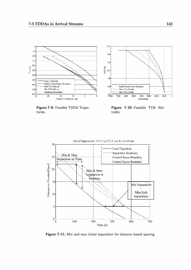
7-5 TDDAs in Arrival Streams 143
Figure 7-9: Feasible TDDA Trajec-tories.
Figure 7-10: Feasible TCB Alti-tudes.
Figure 7-11: Min and max initial separation for distance based spacing.
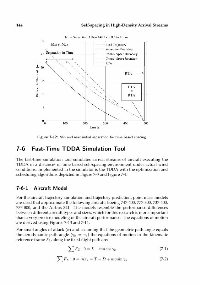
144 Self-spacing in High-Density Arrival Streams
Figure 7-12: Min and max initial separation for time based spacing.
7-6 Fast-Time TDDA Simulation Tool
The fast-time simulation tool simulates arrival streams of aircraft executing theTDDA in a distance- or time based self-spacing environment under actual windconditions. Implemented in the simulator is the TDDA with the optimization andscheduling algorithms depicted in Figure 7-3 and Figure 7-4.
7-6-1 Aircraft Model
For the aircraft trajectory simulation and trajectory prediction, point mass modelsare used that approximate the following aircraft: Boeing 747-400, 777-300, 737-400,737-800, and the Airbus 321. The models resemble the performance differencesbetween different aircraft types and sizes, which for this research is more importantthan a very precise modeling of the aircraft performance. The equations of motionare derived using Figures 7-13 and 7-14.
For small angles of attack (α) and assuming that the geometric path angle equalsthe aerodynamic path angle (γk = γa) the equations of motion in the kinematicreference frame Fk, along the fixed flight path are:
∑
FZ : 0 = L−mg cos γk (7-1)
∑
FX : 0 = mxk = T −D +mg sin γk (7-2)
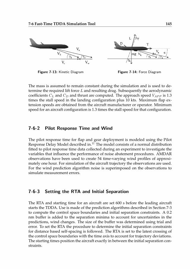
7-6 Fast-Time TDDA Simulation Tool 145
Figure 7-13: Kinetic Diagram Figure 7-14: Force Diagram
The mass is assumed to remain constant during the simulation and is used to de-termine the required lift force L and resulting drag. Subsequently the aerodynamiccoefficients CL and CD and thrust are computed. The approach speed VAPP is 1.3times the stall speed in the landing configuration plus 10 kts. Maximum flap ex-tension speeds are obtained from the aircraft manufacturer or operator. Minimumspeed for an aircraft configuration is 1.3 times the stall speed for that configuration.
7-6-2 Pilot Response Time and Wind
The pilot response time for flap and gear deployment is modeled using the PilotResponse Delay Model described in.11 The model consists of a normal distributionfitted to pilot response time data collected during an experiment to investigate thevariables that influence the performance of noise abatement procedures. AMDARobservations have been used to create 54 time-varying wind profiles of approxi-mately one hour. For simulation of the aircraft trajectory the observations are used.For the wind prediction algorithm noise is superimposed on the observations tosimulate measurement errors.
7-6-3 Setting the RTA and Initial Separation
The RTA and starting time for an aircraft are set 600 s before the leading aircraftstarts the TDDA. Use is made of the prediction algorithms described in Section 7-3to compute the control space boundaries and initial separation constraints. A 0.2nm buffer is added to the separation minima to account for uncertainties in thepredictions, wind changes. The size of the buffer was determined using trial anderror. To set the RTA the procedure to determine the initial separation constraintsfor distance based self-spacing is followed. The RTA is set to the latest crossing ofthe control space boundaries with the time axis to account for trajectory deviations.The starting times position the aircraft exactly in between the initial separation con-straints.
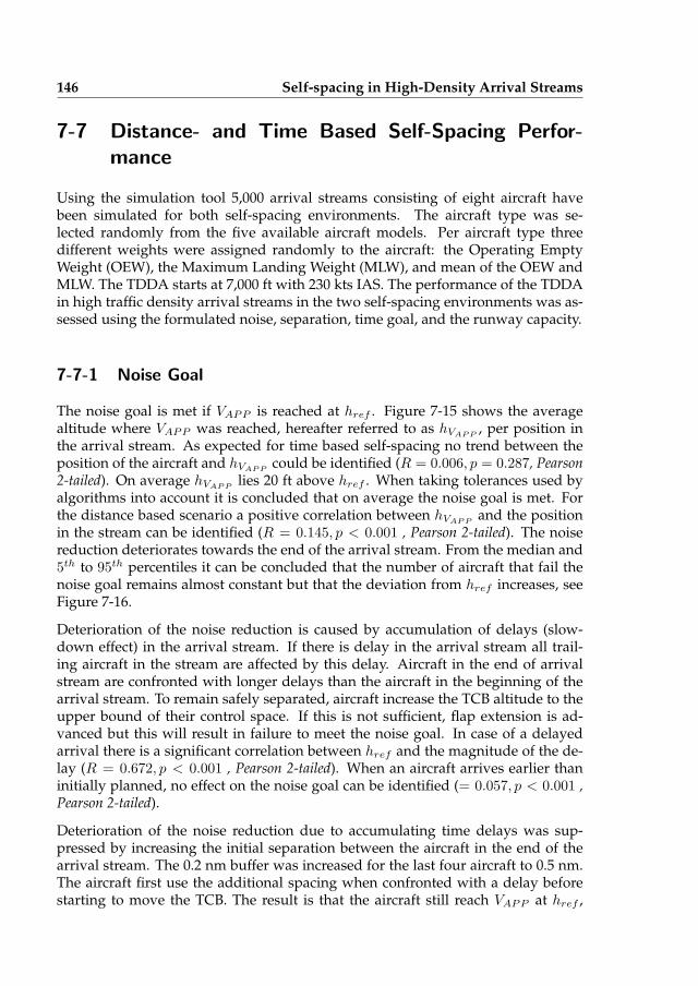
146 Self-spacing in High-Density Arrival Streams
7-7 Distance- and Time Based Self-Spacing Perfor-
mance
Using the simulation tool 5,000 arrival streams consisting of eight aircraft havebeen simulated for both self-spacing environments. The aircraft type was se-lected randomly from the five available aircraft models. Per aircraft type threedifferent weights were assigned randomly to the aircraft: the Operating EmptyWeight (OEW), the Maximum Landing Weight (MLW), and mean of the OEW andMLW. The TDDA starts at 7,000 ft with 230 kts IAS. The performance of the TDDAin high traffic density arrival streams in the two self-spacing environments was as-sessed using the formulated noise, separation, time goal, and the runway capacity.
7-7-1 Noise Goal
The noise goal is met if VAPP is reached at href . Figure 7-15 shows the averagealtitude where VAPP was reached, hereafter referred to as hVAPP
, per position inthe arrival stream. As expected for time based self-spacing no trend between theposition of the aircraft and hVAPP
could be identified (R = 0.006, p = 0.287, Pearson2-tailed). On average hVAPP
lies 20 ft above href . When taking tolerances used byalgorithms into account it is concluded that on average the noise goal is met. Forthe distance based scenario a positive correlation between hVAPP
and the positionin the stream can be identified (R = 0.145, p < 0.001 , Pearson 2-tailed). The noisereduction deteriorates towards the end of the arrival stream. From the median and5th to 95th percentiles it can be concluded that the number of aircraft that fail thenoise goal remains almost constant but that the deviation from href increases, seeFigure 7-16.
Deterioration of the noise reduction is caused by accumulation of delays (slow-down effect) in the arrival stream. If there is delay in the arrival stream all trail-ing aircraft in the stream are affected by this delay. Aircraft in the end of arrivalstream are confronted with longer delays than the aircraft in the beginning of thearrival stream. To remain safely separated, aircraft increase the TCB altitude to theupper bound of their control space. If this is not sufficient, flap extension is ad-vanced but this will result in failure to meet the noise goal. In case of a delayedarrival there is a significant correlation between href and the magnitude of the de-lay (R = 0.672, p < 0.001 , Pearson 2-tailed). When an aircraft arrives earlier thaninitially planned, no effect on the noise goal can be identified (= 0.057, p < 0.001 ,Pearson 2-tailed).
Deterioration of the noise reduction due to accumulating time delays was sup-pressed by increasing the initial separation between the aircraft in the end of thearrival stream. The 0.2 nm buffer was increased for the last four aircraft to 0.5 nm.The aircraft first use the additional spacing when confronted with a delay beforestarting to move the TCB. The result is that the aircraft still reach VAPP at href ,
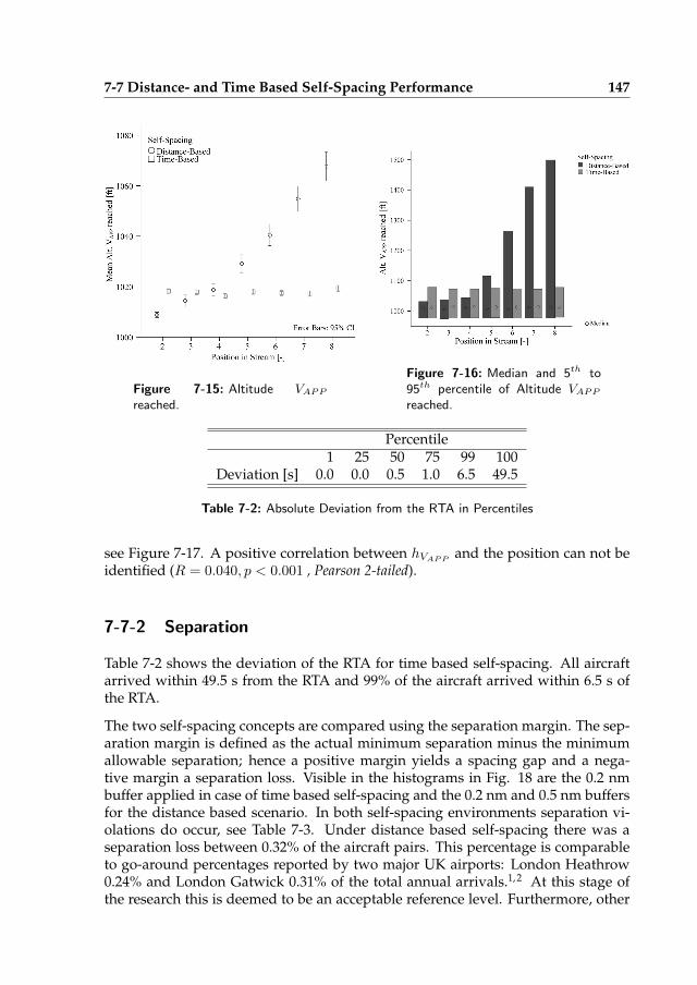
7-7 Distance- and Time Based Self-Spacing Performance 147
Figure 7-15: Altitude VAPP
reached.
Figure 7-16: Median and 5th to95th percentile of Altitude VAPP
reached.
Percentile1 25 50 75 99 100
Deviation [s] 0.0 0.0 0.5 1.0 6.5 49.5
Table 7-2: Absolute Deviation from the RTA in Percentiles
see Figure 7-17. A positive correlation between hVAPPand the position can not be
identified (R = 0.040, p < 0.001 , Pearson 2-tailed).
7-7-2 Separation
Table 7-2 shows the deviation of the RTA for time based self-spacing. All aircraftarrived within 49.5 s from the RTA and 99% of the aircraft arrived within 6.5 s ofthe RTA.
The two self-spacing concepts are compared using the separation margin. The sep-aration margin is defined as the actual minimum separation minus the minimumallowable separation; hence a positive margin yields a spacing gap and a nega-tive margin a separation loss. Visible in the histograms in Fig. 18 are the 0.2 nmbuffer applied in case of time based self-spacing and the 0.2 nm and 0.5 nm buffersfor the distance based scenario. In both self-spacing environments separation vi-olations do occur, see Table 7-3. Under distance based self-spacing there was aseparation loss between 0.32% of the aircraft pairs. This percentage is comparableto go-around percentages reported by two major UK airports: London Heathrow0.24% and London Gatwick 0.31% of the total annual arrivals.1, 2 At this stage ofthe research this is deemed to be an acceptable reference level. Furthermore, other
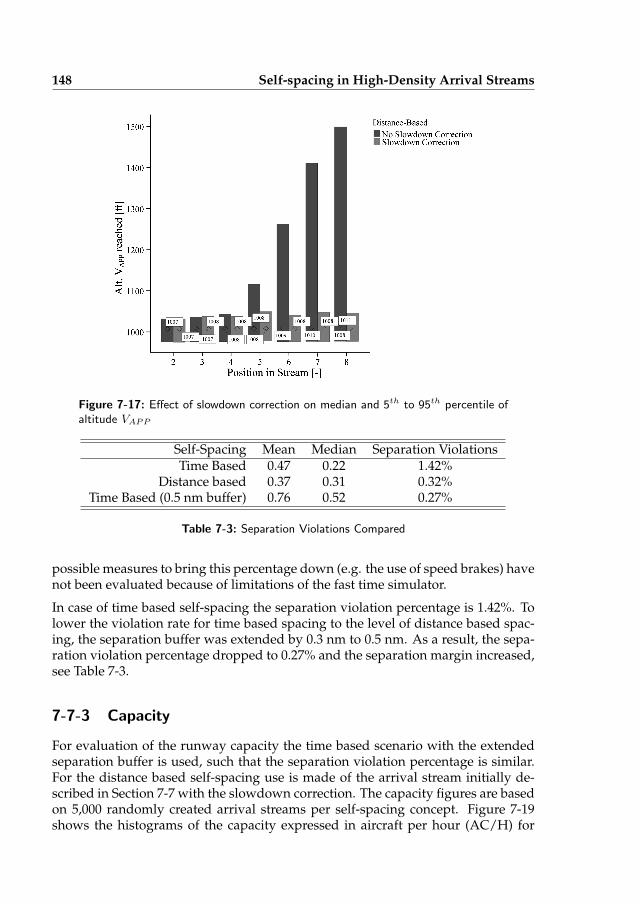
148 Self-spacing in High-Density Arrival Streams
Figure 7-17: Effect of slowdown correction on median and 5th to 95th percentile ofaltitude VAPP
Self-Spacing Mean Median Separation ViolationsTime Based 0.47 0.22 1.42%
Distance based 0.37 0.31 0.32%Time Based (0.5 nm buffer) 0.76 0.52 0.27%
Table 7-3: Separation Violations Compared
possible measures to bring this percentage down (e.g. the use of speed brakes) havenot been evaluated because of limitations of the fast time simulator.
In case of time based self-spacing the separation violation percentage is 1.42%. Tolower the violation rate for time based spacing to the level of distance based spac-ing, the separation buffer was extended by 0.3 nm to 0.5 nm. As a result, the sepa-ration violation percentage dropped to 0.27% and the separation margin increased,see Table 7-3.
7-7-3 Capacity
For evaluation of the runway capacity the time based scenario with the extendedseparation buffer is used, such that the separation violation percentage is similar.For the distance based self-spacing use is made of the arrival stream initially de-scribed in Section 7-7 with the slowdown correction. The capacity figures are basedon 5,000 randomly created arrival streams per self-spacing concept. Figure 7-19shows the histograms of the capacity expressed in aircraft per hour (AC/H) for
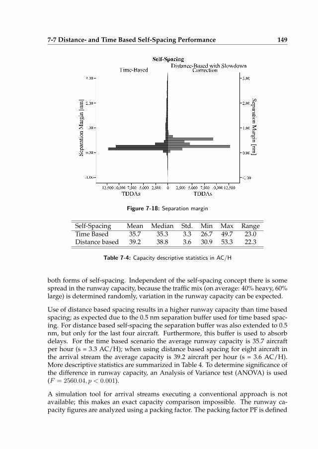
7-7 Distance- and Time Based Self-Spacing Performance 149
Figure 7-18: Separation margin
Self-Spacing Mean Median Std. Min Max RangeTime Based 35.7 35.3 3.3 26.7 49.7 23.0Distance based 39.2 38.8 3.6 30.9 53.3 22.3
Table 7-4: Capacity descriptive statistics in AC/H
both forms of self-spacing. Independent of the self-spacing concept there is somespread in the runway capacity, because the traffic mix (on average: 40% heavy, 60%large) is determined randomly, variation in the runway capacity can be expected.
Use of distance based spacing results in a higher runway capacity than time basedspacing; as expected due to the 0.5 nm separation buffer used for time based spac-ing. For distance based self-spacing the separation buffer was also extended to 0.5nm, but only for the last four aircraft. Furthermore, this buffer is used to absorbdelays. For the time based scenario the average runway capacity is 35.7 aircraftper hour (s = 3.3 AC/H); when using distance based spacing for eight aircraft inthe arrival stream the average capacity is 39.2 aircraft per hour (s = 3.6 AC/H).More descriptive statistics are summarized in Table 4. To determine significance ofthe difference in runway capacity, an Analysis of Variance test (ANOVA) is used(F = 2560.04, p < 0.001).
A simulation tool for arrival streams executing a conventional approach is notavailable; this makes an exact capacity comparison impossible. The runway ca-pacity figures are analyzed using a packing factor. The packing factor PF is defined
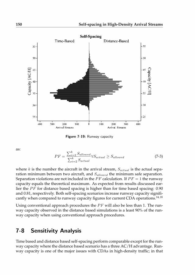
150 Self-spacing in High-Density Arrival Streams
Figure 7-19: Runway capacity
as:
PF =
∑k
i=2 Sallowed∑k
i=2 Sactual
∀Sactual ≥ Sallowed (7-3)
where k is the number the aircraft in the arrival stream, Sactual is the actual sepa-ration minimum between two aircraft, and Sallowed the minimum safe separation.Separation violations are not included in the PF calculation. If PF = 1 the runwaycapacity equals the theoretical maximum. As expected from results discussed ear-lier the PF for distance based spacing is higher than for time based spacing: 0.90and 0.81, respectively. Both self-spacing scenarios increase runway capacity signifi-cantly when compared to runway capacity figures for current CDA operations.14, 18
Using conventional approach procedures the PF will also be less than 1. The run-way capacity observed in the distance based simulations is a least 90% of the run-way capacity when using conventional approach procedures.
7-8 Sensitivity Analysis
Time based and distance based self-spacing perform comparable except for the run-way capacity where the distance based scenario has a three AC/H advantage. Run-way capacity is one of the major issues with CDAs in high-density traffic; in that
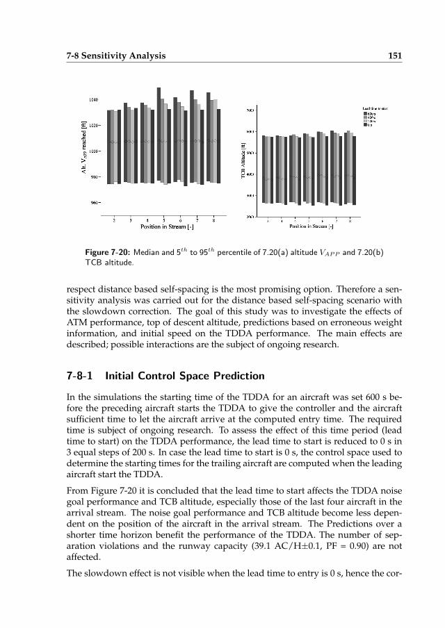
7-8 Sensitivity Analysis 151
Figure 7-20: Median and 5th to 95th percentile of 7.20(a) altitude VAPP and 7.20(b)TCB altitude.
respect distance based self-spacing is the most promising option. Therefore a sen-sitivity analysis was carried out for the distance based self-spacing scenario withthe slowdown correction. The goal of this study was to investigate the effects ofATM performance, top of descent altitude, predictions based on erroneous weightinformation, and initial speed on the TDDA performance. The main effects aredescribed; possible interactions are the subject of ongoing research.
7-8-1 Initial Control Space Prediction
In the simulations the starting time of the TDDA for an aircraft was set 600 s be-fore the preceding aircraft starts the TDDA to give the controller and the aircraftsufficient time to let the aircraft arrive at the computed entry time. The requiredtime is subject of ongoing research. To assess the effect of this time period (leadtime to start) on the TDDA performance, the lead time to start is reduced to 0 s in3 equal steps of 200 s. In case the lead time to start is 0 s, the control space used todetermine the starting times for the trailing aircraft are computed when the leadingaircraft start the TDDA.
From Figure 7-20 it is concluded that the lead time to start affects the TDDA noisegoal performance and TCB altitude, especially those of the last four aircraft in thearrival stream. The noise goal performance and TCB altitude become less depen-dent on the position of the aircraft in the arrival stream. The Predictions over ashorter time horizon benefit the performance of the TDDA. The number of sep-aration violations and the runway capacity (39.1 AC/H±0.1, PF = 0.90) are notaffected.
The slowdown effect is not visible when the lead time to entry is 0 s, hence the cor-
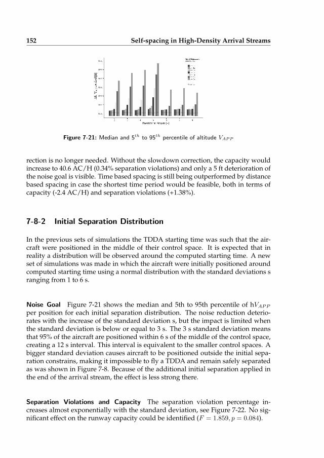
152 Self-spacing in High-Density Arrival Streams
Figure 7-21: Median and 5th to 95th percentile of altitude VAPP
rection is no longer needed. Without the slowdown correction, the capacity wouldincrease to 40.6 AC/H (0.34% separation violations) and only a 5 ft deterioration ofthe noise goal is visible. Time based spacing is still being outperformed by distancebased spacing in case the shortest time period would be feasible, both in terms ofcapacity (-2.4 AC/H) and separation violations (+1.38%).
7-8-2 Initial Separation Distribution
In the previous sets of simulations the TDDA starting time was such that the air-craft were positioned in the middle of their control space. It is expected that inreality a distribution will be observed around the computed starting time. A newset of simulations was made in which the aircraft were initially positioned aroundcomputed starting time using a normal distribution with the standard deviations sranging from 1 to 6 s.
Noise Goal Figure 7-21 shows the median and 5th to 95th percentile of hVAPP
per position for each initial separation distribution. The noise reduction deterio-rates with the increase of the standard deviation s, but the impact is limited whenthe standard deviation is below or equal to 3 s. The 3 s standard deviation meansthat 95% of the aircraft are positioned within 6 s of the middle of the control space,creating a 12 s interval. This interval is equivalent to the smaller control spaces. Abigger standard deviation causes aircraft to be positioned outside the initial sepa-ration constrains, making it impossible to fly a TDDA and remain safely separatedas was shown in Figure 7-8. Because of the additional initial separation applied inthe end of the arrival stream, the effect is less strong there.
Separation Violations and Capacity The separation violation percentage in-creases almost exponentially with the standard deviation, see Figure 7-22. No sig-nificant effect on the runway capacity could be identified (F = 1.859, p = 0.084).
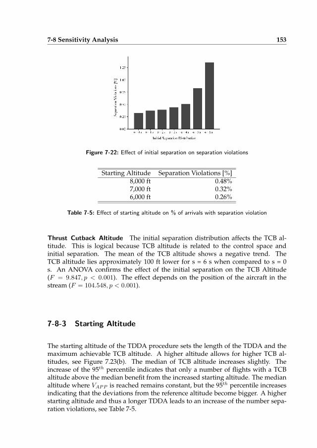
7-8 Sensitivity Analysis 153
Figure 7-22: Effect of initial separation on separation violations
Starting Altitude Separation Violations [%]8,000 ft 0.48%7,000 ft 0.32%6,000 ft 0.26%
Table 7-5: Effect of starting altitude on % of arrivals with separation violation
Thrust Cutback Altitude The initial separation distribution affects the TCB al-titude. This is logical because TCB altitude is related to the control space andinitial separation. The mean of the TCB altitude shows a negative trend. TheTCB altitude lies approximately 100 ft lower for s = 6 s when compared to s = 0s. An ANOVA confirms the effect of the initial separation on the TCB Altitude(F = 9.847, p < 0.001). The effect depends on the position of the aircraft in thestream (F = 104.548, p < 0.001).
7-8-3 Starting Altitude
The starting altitude of the TDDA procedure sets the length of the TDDA and themaximum achievable TCB altitude. A higher altitude allows for higher TCB al-titudes, see Figure 7.23(b). The median of TCB altitude increases slightly. Theincrease of the 95th percentile indicates that only a number of flights with a TCBaltitude above the median benefit from the increased starting altitude. The medianaltitude where VAPP is reached remains constant, but the 95th percentile increasesindicating that the deviations from the reference altitude become bigger. A higherstarting altitude and thus a longer TDDA leads to an increase of the number sepa-ration violations, see Table 7-5.
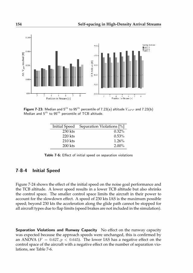
154 Self-spacing in High-Density Arrival Streams
Figure 7-23: Median and 5th to 95th percentile of 7.23(a) altitude VAPP and 7.23(b)Median and 5th to 95th percentile of TCB altitude.
Initial Speed Separation Violations [%]230 kts 0.32%220 kts 0.53%210 kts 1.26%200 kts 2.00%
Table 7-6: Effect of initial speed on separation violations
7-8-4 Initial Speed
Figure 7-24 shows the effect of the initial speed on the noise goal performance andthe TCB altitude. A lower speed results in a lower TCB altitude but also shrinksthe control space. The smaller control space limits the aircraft in their power toaccount for the slowdown effect. A speed of 230 kts IAS is the maximum possiblespeed; beyond 230 kts the acceleration along the glide path cannot be stopped forall aircraft types due to flap limits (speed brakes are not included in the simulation).
Separation Violations and Runway Capacity No effect on the runway capacitywas expected because the approach speeds were unchanged, this is confirmed byan ANOVA (F = 0.627, p < 0.645). The lower IAS has a negative effect on thecontrol space of the aircraft with a negative effect on the number of separation vio-lations, see Table 7-6.
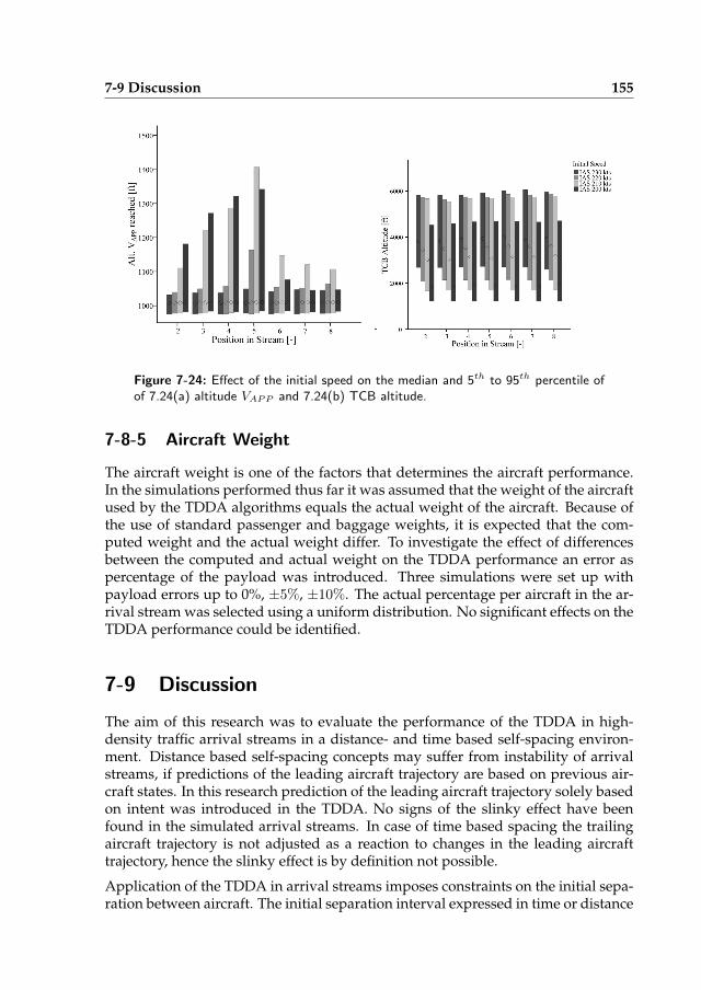
7-9 Discussion 155
Figure 7-24: Effect of the initial speed on the median and 5th to 95th percentile ofof 7.24(a) altitude VAPP and 7.24(b) TCB altitude.
7-8-5 Aircraft Weight
The aircraft weight is one of the factors that determines the aircraft performance.In the simulations performed thus far it was assumed that the weight of the aircraftused by the TDDA algorithms equals the actual weight of the aircraft. Because ofthe use of standard passenger and baggage weights, it is expected that the com-puted weight and the actual weight differ. To investigate the effect of differencesbetween the computed and actual weight on the TDDA performance an error aspercentage of the payload was introduced. Three simulations were set up withpayload errors up to 0%, ±5%, ±10%. The actual percentage per aircraft in the ar-rival stream was selected using a uniform distribution. No significant effects on theTDDA performance could be identified.
7-9 Discussion
The aim of this research was to evaluate the performance of the TDDA in high-density traffic arrival streams in a distance- and time based self-spacing environ-ment. Distance based self-spacing concepts may suffer from instability of arrivalstreams, if predictions of the leading aircraft trajectory are based on previous air-craft states. In this research prediction of the leading aircraft trajectory solely basedon intent was introduced in the TDDA. No signs of the slinky effect have beenfound in the simulated arrival streams. In case of time based spacing the trailingaircraft trajectory is not adjusted as a reaction to changes in the leading aircrafttrajectory, hence the slinky effect is by definition not possible.
Application of the TDDA in arrival streams imposes constraints on the initial sepa-ration between aircraft. The initial separation interval expressed in time or distance
156 REFERENCES
follows from the control space that is a function of the aircraft type and weight, andthe wind conditions.
Under distance based self-spacing there was a separation loss between 0.32% of theaircraft pairs. To lower the violation rate for time based spacing to the level of dis-tance based spacing, the separation buffer to set the RTA was extended by 0.3 nmto 0.5 nm. For the time based scenario the average runway capacity is 35.7 AC/H,when using distance based spacing the average capacity is 39.2 AC/H. The runwaycapacity under distance based self-spacing is 90% of the theoretical maximum ca-pacity. Because distance based self-spacing outperformed time based self-spacingin terms of runway capacity, distance based self-spacing is considered to be themost promising option.
To further evaluate the performance of the TDDA in a distance based self-spacingenvironment a sensitivity study was carried out. Reducing the time between com-puting the TDDA starting time and the actual starting time improves the perfor-mance of the TDDA. However, this also gives the pilot and controller less time totake actions to let the TDDA start on time. The sensitivity analysis also shows thatit is crucial for the aircraft arrive to start the TDDA at the set starting time. Whenaircraft are positioned outside their control space, the performance degrades. Theinitial conditions of the TDDA affect the performance. A higher initial speed resultsin a larger control space, which benefits performance. A higher starting altitude re-sults in higher TCB altitude but also increases the number separation violation. Thetrajectory becomes longer, which increases the uncertainties. Trajectory predictionsbased on erroneous aircraft weight with errors up to 10% of the payload did nothave a significant effect on the performance.
7-10 Conclusion
Distance based self-spacing has a three AC/H runway capacity advantage overtime based self-spacing when the number of separation violations between aircraftis comparable. Runway capacity is one of the major factors limiting the use CDAs;in that respect distance based self-spacing is the most promising option. The ob-served runway capacity is 90% of the theoretical maximum. A sensitivity analy-sis for distance based self-spacing showed that accurately determining the startingtime and the ability to arrive at the starting time with great precision benefits theTDDA performance.
References
[1] BAA London Gatwick, Flight Evaluation Report 2001/02. Technical report,British Airports Authority BAA Gatwick, 2002.
REFERENCES 157
[2] BAA Heathrow, Flight Evaluation Report 2007. Technical report, HeathrowFlight Evaluation Unit (FEU), 2007.
[3] T. S. Abbott. Speed Control Law for Precision Terminal Area In-Trail Self-Spacing. Technical Report NASA/TM-2002-211742, NASA Langley ResearchCenter, Hampton (VA), USA, Jul 2002.
[4] J.-P. Clarke. A Systems Analysis Methodology for Developing Single Event NoiseAbatement Procedures. Sc.D. Dissertation, Massachusetts Institute of Technol-ogy, 1997.
[5] R. A. Coppenbarger, R. W. Mead, and D. N. Sweet. Field Evaluation ofthe Tailored Arrivals Concept for Datalink-Enabled Continuous Descent Ap-proaches. In 7th AIAA Aviation Technology, Integration and Operations Conference(ATIO), number AIAA-2007-7778, Belfast, Northern Ireland, Sep 18-20 2007.
[6] B. A. F. de Beer, M. Mulder, M. M. van Paassen, and A. C. in ‘t Veld. Develop-ment of an Ecological Interface for the Three-Degree Decelerating Approach.In AIAA Guidance, Navigation, and Control Conference & Exhibit, number AIAA-2008-7108, Honolulu (HI), USA, Aug 18-21 2008.
[7] W. F. de Gaay Fortman, M. M. van Paassen, M. Mulder, A. C. in ‘t Veld, andJ.-P. Clarke. Implementing Time-Based Spacing for Decelerating Approaches.AIAA Journal of Aircraft, 44(1):106–118, Jan-Feb 2007.
[8] A. M. P. de Leege. Three-Degree Decelerating Approaches in Arrival Streams. Msc.thesis, Faculty of Aerospace Engineering, Delft University of Technology, Sep2007.
[9] J. L. de Prins, K. F. M. Schippers, M. Mulder, M. M. van Paassen, A. C. in ‘t Veld,and J.-P. Clarke. Enhanced Self-Spacing Algorithm for Three-Degree Deceler-ating Approaches. AIAA Journal of Guidance, Control & Dynamics, 30(5):576–590, Mar-Apr 2007.
[10] E. Dinges. Determining the Environmental Benefit of Implementing Continu-ous Descent Approach Procedures. In 7th USA/Europe Air Traffic ManagementR&D Seminar (ATM 2007), Barcelona, Spain, Jul 2-5 2007.
[11] N. T. Ho and J.-P Clarke. Mitigating Operational Aircraft Noise Impact byLeveraging on Automation Capability. In AIAA 1st Aircraft, Technology, Inte-gration, and Operations Forum (ATIO), number AIAA-2001-5239, Los Angeles(CA), USA, Oct 16-18 2001.
[12] A. C. in ‘t Veld, M. M. van Paassen, M. Mulder, and J.-P. Clarke. Pilot Supportfor Separation Assurance during Decelerated Approaches. In Proceedings of theAIAA Guidance, Navigation, and Control Conference & Exhibit, number AIAA-2004-5102, pages 1–13, Providence (RI), USA, Aug 16-19 2004.
158 Self-spacing in High-Density Arrival Streams
[13] L. Ren and J.-P. Clarke. Flight-Test Evaluation of the Tool for Analysis of Sep-aration and Throughput. AIAA Journal of Aircraft, 45(1):323–332, Jan-Feb 2008.
[14] L. Ren, J.-P. Clarke, and N. T. Ho. Achieving Low Approach Noise withoutSacrifying Capacity. In 22nd Digital Avionics Systems Conference, volume 1,pages 1–9, Indianapolis (IN), USA, Oct 12-16 2003.
[15] G. L. Slater. Dynamics of Self-Spacing in a Stream of In-Trail Aircraft. InProceedings of the AIAA Guidance, Navigation, and Control Conference & Exhibit,number 2002-4927, Monterey (CA), USA, Aug 11-14 2002.
[16] M. A. Vilaplana, E. Gallo, F. A. Navarro, and S. Swierstra. Towards a FormalLanguage for the Common Description of Aircraft Intent. In Digital AvionicsSystems Conference, volume 1, pages 3.C.5–3.1–9, Washington DC, USA, Oct30-Nov 3 2005.
[17] I. Wilson and F. Hafner. Benefit Assessment of Using Continuous DescentApproaches at Atlanta. In Digital Avionics Systems Conference, volume 1, pages2.B.2– 2.1–7, Washington DC, USA, Oct 30-Nov 3 2005.
[18] F. J. M. Wubben and J. J. Bussink. Environmental Benefits of ContinuousDescent Approaches at Schiphol Airport Compared with Conventional Ap-proach Procedures. Technical Report NLR-TP-2000-275, National AerospaceLaboratory (NLR), Amsterdam, The Netherlands, May 2000.
8
Conclusions andrecommendations
The fundamental question that started the research presented in this thesis iswhether or not it is possible to implement continuous descent approach procedureswithout sacrificing landing runway throughput capability.
Continuous Descent Approaches in various forms have shown to result in signifi-cant reductions in aircraft noise impact and as they require less fuel in comparisonto conventional step-down approaches, the implementation of these procedures ishighly desirable. As the required speed and altitude profiles during a CDA varygreatly amongst different aircraft, the task of closely spacing the aircraft is very dif-ficult for the air traffic controller, however. This is the root cause for the capacityreductions typically found when implementing CDA procedures.
CDA is a generic term, basically covering all approach procedures that have nolevel flight segments. A useful distinction can be made between CDAs that requirea fixes lateral path, RNAV-CDAs, and CDAs where ATC can issue vectors as longas the aircraft remain in a continuous descent, vectored CDAs. A good exampleof a vectored CDA is the procedure in use at London Heathrow airport. Generally,vectored CDAs do not suffer from capacity loss because the air traffic controller canstill issue speed and heading commands to closely space the aircraft.
Current developments in the SESAR program emphasize the development of fixedlateral approach trajectories, and fixed trajectories in general which is why this re-search focuses on the RNAV CDA and its associated capacity problems. The solu-tion investigated in this thesis is to delegate the task of in-trail spacing to the flightdeck on the notion that better information on the speed and altitude profile will bemore readily available on the flight deck. Furthermore, the flight crew is in a betterposition to actively control their trajectory behind a preceding aircraft.
Two scenarios have been investigated, one where aircraft are instructed to regulatethe distance behind the preceding aircraft, and one scenario where ATC issues a

160 Conclusions and recommendations
required time of arrival and aircraft are instructed to manage their approach profileto meet that time. Both scenarios relieve the controller of the control task, at thecost of increased workload for the flight crew. The results presented in Chapters 3,4 and 6 show that not only is the workload still acceptable, but also that pilots areindeed capable of accurately achieving the self-spacing or the time-goal, given anadequate flight deck support interface.
8-1 Key factors
Using the flight deck support interfaces presented in this work, it was shown thatpilots are able to robustly handle both distance based self-spacing and time basedspacing. During the development of these flight deck support interfaces, a numberof factors were identified that are of key importance for the accuracy of the gener-ated solutions.
8-1-1 Procedure constraints
The CDA-procedure used throughout this work is the Three Degree DeceleratingApproach, which is defined by a constant three degree descending path from theinitiation point all the way to the runway, flown at idle thrust. This procedure waschosen because it represents the ultimate solution for a single aircraft in terms ofnoise impact. Due to the steep approach angle and the fact that the entire procedureis flown at idle thrust, the available control space is quite small and completing theprocedure while controlling the spacing interval with the preceding aircraft hasproven to be a difficult task.
Because of these drawbacks it is not very likely that the TDDA will ever be imple-mented in its current form, however, it provides a very interesting research case.If it can be shown that it is possible to preserve runway capacity with the TDDA,it follows that other CDA procedures with less stringent operational constraintsshould be feasible as well.
8-1-2 Aircraft drag and thrust data
At the core of the self-spacing algorithm lies the trajectory prediction algorithm.The trajectory predictions require accurate knowledge of the lift-drag polar and theengine thrust as illustrated by the flight test preparations in Chapter 4. Modelscurrently in use by ATC such as BADA 1 do not possess the necessary accuracy togenerate the required speed- and distance profiles. Current state of the art FMSinstallations are capable of accurate trajectory estimations, however this informa-tion is not normally available to ATC. In general aircraft manufacturers are veryreluctant to share this information for economical reasons.
8-1 Key factors 161
In order to implement the spacing concepts as proposed in this work, exchangeof information is vital and a number of scenarios can be envisaged to accomplishthis. On the one end, a ground based database could be used by a central computerto generate all trajectories, on the other end a situation can be envisaged whereeach aircraft calculates its own trajectory and down-links this to ATC or directly tonearby aircraft.
Developments in the field of System Wide Information Management (SWIM) byboth SESAR and NextGen already move towards a system where 4D-trajectoriescan be shared by different users of the air traffic system.
8-1-3 Aircraft operating mass
Closely related to the requirement of accurate lift and drag data is the requirementof knowledge of the current operating mass of the aircraft. Availability of this in-formation is normally not an issue on board the aircraft as the aircraft’s FMS keepstrack of this figure for its performance calculations. If the trajectory prediction isgenerated outside the aircraft, however, information on the current mass must bemade available through other means.
8-1-4 Wind data
It was shown that an accurate wind estimate is necessary to assure performance.The AMDAR Wind Prediction Algorithm (AWPA) presented in Chapter 5 performswell, providing real-time accurate wind estimates as was demonstrated on a set ofAMDAR data for Chicago O’Hare. The AWPA has the benefit of becoming moreaccurate as more data is available, i.e., in high traffic densities, where its accuracyis needed most.
8-1-5 Pilot technique
In current implementations of continuous decent approaches, such as the RNAV
night transition at Amsterdam Schiphol Airport, a lot of freedom is left to the flightcrew to execute the procedure in terms of altitude and speed management. This isthe main reason for the capacity loss associated with this procedure. Also the earlyresearch presented in Chapter 3 showed that flight crews were able to fly the idlethrust approach without help form the cockpit interface as long as the preceedingaircraft behaved predictably, but self-spacing performance was inadequate for non-nominal behavior of the preceding aircraft. The use of a suitable pilot supportsystem such as presented in this chapter assures consistent pilot behavior both fordistance based spacing and time based spacing as was shown in Chapter 6.
162 Conclusions and recommendations
8-2 Results
8-2-1 Self-spacing performance
One of the main findings during the different experiments is that pilots are ableto complete the procedure and space themselves safely behind the leading aircraftwhen the initial spacing is within the control space of the aircraft, i.e., when theaircraft are spaced in such a way that it is physically possible to control the finalspacing during the TDDA by flap and gear timing alone.
The Monte Carlo simulations of Chapter 4 show that the developed algorithm isrobust against errors in the wind estimation, aircraft mass estimate and accuracyof the drag-coefficient. Errors in the estimates of the headwind component of up to±20 kts, estimate errors of aircraft mass of ±10% and errors in the drag-coefficientof ±10% showed no loss of separation at all and only a degradation of the noiseimpact due to re-applying thrust on short final of ±100 feet maximum.
8-2-2 Pilot workload
As expected, the pilot workload does increase due to the added task of self-separation. The different piloted experiments all showed, however, that the overallworkload was still considered acceptable by the pilots, a fact corroborated by theTLX-scores.
8-2-3 Landing runway capacity
When the key uncertainties mentioned in the previous sections are adequately ad-dressed, the TDDA can be flown in a high traffic density environment. In Chapter7 extensive Monte Carlo simulations showed that in both time based and distancebased scenarios runway throughput numbers that are very close to current peak ca-pacity numbers are achievable. Figure 8-1 shows the throughput results for MonteCarlo simulations of strings of 8 different aircraft, operating at random flight mass.An average of 35.7 aircraft per hour on a single runway was found for the timebased scenario, while the distance based scenario showed 39.2 aircraft per hour ona single landing runway. Compared to the absolute maximum possible throughputfor the given traffic stream, expressed as a packing factor, average landing runwaythroughput capacities of 81% and 90% were found for time based and distancebased spacing, respectively.
This shows that the problems encountered when implementing Continuous De-scent Approaches in high traffic densities can indeed be solved, paving the way foractual implementation.
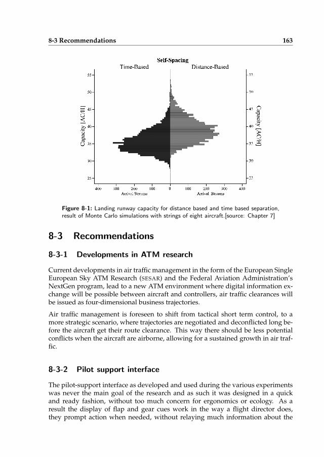
8-3 Recommendations 163
Figure 8-1: Landing runway capacity for distance based and time based separation,result of Monte Carlo simulations with strings of eight aircraft.[source: Chapter 7]
8-3 Recommendations
8-3-1 Developments in ATM research
Current developments in air traffic management in the form of the European SingleEuropean Sky ATM Research (SESAR) and the Federal Aviation Administration’sNextGen program, lead to a new ATM environment where digital information ex-change will be possible between aircraft and controllers, air traffic clearances willbe issued as four-dimensional business trajectories.
Air traffic management is foreseen to shift from tactical short term control, to amore strategic scenario, where trajectories are negotiated and deconflicted long be-fore the aircraft get their route clearance. This way there should be less potentialconflicts when the aircraft are airborne, allowing for a sustained growth in air traf-fic.
8-3-2 Pilot support interface
The pilot-support interface as developed and used during the various experimentswas never the main goal of the research and as such it was designed in a quickand ready fashion, without too much concern for ergonomics or ecology. As aresult the display of flap and gear cues work in the way a flight director does,they prompt action when needed, without relaying much information about the
164 Conclusions and recommendations
urgency of required actions or the size of the control space. The ghost symbol incombination with TCAS-symbology does provide some overview over the situation,and the experimental results show that situation awareness is enhanced by it, but amore thorough theoretical basis should be explored.
Further research is required to optimize the cockpit interface. Currently, interestingwork is being done on energy-based displays. Controlling an aircraft approachingto land can be seen as an energy management problem, starting high and fast in aclean configuration and finishing low and slow and configured for landing. Thereare different strategies to dissipate the excess energy, but the begin and requiredend states are constant, which seems very suitable for an interface that conveys heaircraft’s energy state and energy goals.
Within the scheme of SESAR and NextGen, new tasks and more complex trajectorieswill be possible. Research evaluating the impact of these developments on the flightdeck and designing new interfaces to make full use of the new possibilities will benecessary.
8-3-3 Air traffic controller support
The air traffic controller workstation has been completely neglected in the workpresented. If the controller is to remain responsible for aircraft flying complex,decelerating profiles, some assistance needs to be offered. In fact, the runwaythroughput numbers found during the Monte Carlo simulations presented inChapter 7 could only be obtained by assuring that the initial spacing of the arrivalstream was within the control space of each aircraft.
In future scenarios, the interaction between controllers and pilots will probablychange dramatically with less use of voice communications and an emphasis ofdata-link clearance delivery and aircraft down-linking their own predicted trajec-tories. To cope in such a different environment, new support systems need to bedeveloped in order to maintain the level of safety we enjoy today.
Already work is being done to develop new controller displays to assist in the de-conflicting and spacing of continuous descent approaches.2, 5, 6 A good example isthe development of the Time-Space Diagram (TSD) , a display that can be used tomerge and correctly space different arrival streams of aircraft performing a CDA.The TSD can be used to space any type of CDA, as long as the estimated trajectoriesare known.4 Another example is the development of the Speed and Route Advisor-tool (SARA) by Luchtverkeersleiding Nederland (LVNL), the Dutch air traffic con-trol organization . The SARA-tool allows controllers to sequence aircraft inboundto Amsterdam Schiphol Airport in such a way that they meet an RTA over the initialapproach fix and can follow a fixed RNAV trajectory to the landing runway.
REFERENCES 165
8-3-4 Procedure design
This thesis focused on the Three-Degree Decelerating Approach as an extreme ex-ample of continuous descent approach, being flown completely at flight idle. As aresearch case this makes sense, as the speed profiles vary significantly between air-craft types. However, fixing the entire procedure at a three degree flight path makesfor a difficult procedure to fly, because most aircraft are not able to decelerate in aclean configuration when flying such a steep flight path angle.
Further research should focus on designing more convenient procedures whileleveraging on the results found for the TDDA. A number of research efforts can al-ready be seen in this area, such as the continuous descent trials in Louisville Aiportexecuted by United Parcel Service’s fleet of Boeings 767.3 Also within the schemeof the NextGen program, Continuous Descent Operations are being implementedat Los Angeles International Airport.
References
[1] User Manual for the Base of Aircraft Data (BADA) Revision 3.7. Technical Re-port No. 2009-003, Eurocontrol EEC, 2009.
[2] S. M. B Abdul Rahman, M. Mulder, and M. M. van Paassen. The Effects of AirTraffic Control Sector Design on the Solution Space Diagram. In Proceedings ofthe European Association of Cognitive Ergonomics (ECCE) Conference, pages 261–268, Delft, Aug 25-27 2010.
[3] J.-P Clarke, N. T. Ho, L. Ren, J. A. Brown, K. R. Elmer, K. Tong, and J. K. Wat.Continuous Descent Approach: Design and Flight Test for Louisville Interna-tional Airport. AIAA Journal of Aircraft, 41(5):1054–1066, 2004.
[4] A. M. P. de Leege, A. C. in ’t Veld, M. M. van Paassen, and M. Mulder. A Time-Space Diagram as Controller Support Tool for Advanced Continuous DescentApproach Operations. In Proceedings of the International Air Transport and Oper-ations Symposium (ATOS 2010), Delft, The Netherlands, Apr 14-15 2010.
[5] J. G. d’Engelbronner, M. Mulder, M. M. van Paassen, S. de Stigter, and H. Huis-man. The Use of a Dynamic Solution Space to Predict Air Traffic ControllerWorkload. In Proceedings of the International Air Transport and Operations Sympo-sium (ATOS), Delft, The Netherlands, Apr 14-15 2010.
[6] G. A. Mercado Velasco, M. Mulder, and M. M. van Paassen. Analysis of Air Traf-fic Controller Workload Reduction Based on the Solution Space for the MergingTask. In Proceedings of the AIAA Guidance, Navigation, and Control Conference,number AIAA-2010-7541, Toronto, Canada, Aug 2-5 2010.

166
Samenvatting
Algoritmes voor het Regelen van deOnderlinge Afstand tijdens Geluidsarme
Naderingsprocedures
Alexander in ’t Veld
Bij de ontwikkelingen op het gebied van beperking van geluidsoverlast door vlieg-tuigen is de aandacht verschoven van zuiver technische maatregelen, zoals het on-twikkelen van stillere motoren, naar meer operationele maatregelen. Deze kun-nen van politieke aard zijn, zoals het verminderen van het aantal nachtvluchten,of het instellen van een maximum jaarlijks aantal vliegbewegingen per vliegveld,maar ook procedurele maatregelen zijn mogelijk in de vorm van geluidsbeperk-ende vertrek- en naderingsprocedures. Als gevolg van deze verschuiving is ookde focus van het luchtvaartonderzoek verschoven naar het ontwerpen van vlieg-procedures die minder geluidsimpact hebben op de omgeving. Daarbij is ook hetmilieu-aspect in de vorm van het verminderen van de uitstoot van uitlaatgassen enhet verlagen van het brandstofverbruik een steeds grotere rol gaan spelen.
Onderzoek naar het beperken van geluidsoverlast heeft zich van nature gerichtop de naderings- en vertrekprocedures van luchthavens, aangezien geluid pasoverlast wordt wanneer deze als negatief wordt ervaren door mensen op degrond, oftewel tijdens die fasen van de vlucht die op lage hoogte of op de grond
168 Samenvatting
plaatsvinden. Internationaal onderzoek naar het verminderen van geluidsoverlasttijdens de start van vliegtuigen heeft geresulteerd in een beperkt aantal effectievevertrekprocedures. Deze procedures zijn overgenomen door de InternationalCivil Aviation Organization (ICAO) en inmiddels wereldwijd op verschillendeluchthavens ingevoerd. Het ontwerpen van standaard naderingsprocedures diede geluidsoverlast beperken is echter veel lastiger gebleken. De implementatievan geluidsarme naderingsprocedures blijkt over het algemeen te resulteren in eenonacceptabele afname van het aantal vliegtuigen dat per uur op een landingsbaankan worden verwerkt, waardoor de meeste procedures ongeschikt blijken te zijnvoor toepassing op vliegvelden met een groot verkeersaanbod.
Dit proefschrift beperkt zich derhalve tot naderingsprocedures. Bij het ontwerpenvan een optimaal naderingsprofiel gaat het om het verminderen van de hoeveel-heid geluid van een bron die de ontvanger bereikt. Er zijn in de basis twee manierenom die geluidsimpact te reduceren:
• het beperken van het brongeluid, en
• het vergroten van de afstand tussen de bron en de ontvanger.
Vanuit een procedureel oogpunt kan het brongeluid beperkt worden door eenlager motorvermogen te selecteren maar ook door het uitklappen van het landings-gestel en de liftverhogende vleugelkleppen uit te stellen, aangezien de verstoordeluchtstroom die deze veroorzaken het geluidsniveau aanzienlijk verhoogt. Hetvergroten van de afstand tussen de bron en de ontvanger wordt doorgaans bereiktdoor de aanvliegroutes zo te kiezen dat steden en woonkernen vermeden worden,maar ook door een continue daalvlucht uit te voeren waardoor de gemiddeldehoogte tijdens de nadering toeneemt. Uit verschillende onderzoeken blijkt dateen Continuous Descent Approach (CDA), een procedure die in het geheel geenhorizontale segmenten kent, de beste geluidsreductie bewerkstelligt.
Het merendeel van het werk in dit proefschrift bevat onderzoek naar een bijzon-dere implementatie van de Continuous Descent Approach, de zogenaamde Three-Degree Decelerating Approach (TDDA). Deze procedure wordt gevlogen met min-imaal motorvermogen, langs een relatief steil glijpad van drie graden naar de land-ingsbaan. Dit resulteert in een nadering waarbij het vliegtuig continu vertraagt,met als doel om zonder gas bij te geven pas op het normale stabilisatiepunt vlakvoor de landingsbaan volledig geconfigureerd te zijn voor de landing. Hierbijwordt de vliegsnelheid uitsluitend geregeld door het op het juiste moment se-lecteren van de opvolgende flap-standen en het op het juiste moment neerlatenvan het landingsgestel.
Het probleem met deze en vergelijkbare procedures waar met minimaal mo-torvermogen gevlogen wordt, is dat verschillende vliegtuigtypen door het verschil
169
in aerodynamische eigenschappen ook verschillende snelheidsprofielen hebben.Tevens worden deze profielen beınvloed door de verschillen in vliegtuigmassa ende besturingsstrategie van de bemanning. Bij elkaar opgeteld zorgen deze fac-toren ervoor dat het voor de luchtverkeersleider zeer lastig wordt de verschillendevliegtuigen op een veilige manier kort achter elkaar op te lijnen voor de baan, metals gevolg dat zij noodgedwongen meer afstand tussen opeenvolgende vliegtuigenmoeten aanhouden. Het aantal vliegtuigen dat per uur op een gegeven landings-baan kan landen wordt hierdoor sterk gereduceerd.
Doordat de snelheid van de vliegtuigen tijdens deze procedure continu afneemt,wordt de verkeersleider geconfronteerd met een rij vliegtuigen die allemaallangzaam inlopen op hun voorganger, waarbij het de taak van de verkeersleideris te beoordelen of de uiteindelijke separatie tussen de vliegtuigen volgens deveiligheidseisen voldoende zal zijn. Dit staat in scherp contrast met de huidigemanier van werken waarbij de vliegtuigen koers-, hoogte- en snelheidsinstructiesontvangen van de verkeersleider. Dit resulteert in minder optimale naderingenvanuit geluids- en emissieoogpunt, maar levert wel een situatie op waarin op eenefficiente en veilige wijze grote verkeersvolumes afgehandeld kunnen worden.
Om dit probleem op te lossen liggen twee strategien voor de hand, namelijk 1) eensysteem ontwikkelen om de verkeersleider te ondersteunen bij het oplijnen van de-celererende vliegtuigen, en/of 2) een systeem ontwikkelen waarmee de cockpitbe-manning zelf de afstand achter hun directe voorganger kan regelen.
Het onderzoek gepresenteerd in dit proefschrift richt zich op de tweede strate-gie door het probleem om dicht achter elkaar Continuous Descent Approaches tevliegen te benaderen vanuit de cockpit. Het ligt overigens voor de hand dat eendaadwerkelijke implementatie van een dergelijke naderingsprocedure aanpassin-gen aan zowel de cockpit als de werkplek van de verkeersleider met zich mee zalbrengen.
In dit proefschrift is algemeen aangenomen dat er een vorm van dataverbindingbeschikbaar is die het mogelijk maakt gegevens uit te wisselen zowel tussen devliegtuigen en de luchtverkeersleiding als tussen vliegtuigen onderling. Dit isvolledig in lijn met de visie van SESAR, die voorziet in de introductie van SystemWide Information Management (SWIM) als onderdeel van het toekomstige luchtver-keersleidingssysteem. De exacte implementatie doet voor dit onderzoek niet terzake, maar er is van uitgegaan dat de vliegtuigen zijn voorzien van Automatic De-pendent Surveillance - Broadcast (ADS-B). Twee mogelijke scenario’s zijn onder-zocht: de eerste is een vorm van self-spacing waarbij de vliegtuigen hun deceler-atie dusdanig moeten regelen dat ze zelf zorg dragen voor het handhaven van eenveilige afstand achter hun voorganger. Bij de tweede methode draagt de luchtver-keersleiding de vliegtuigbemanning een zogenaamde Required Time of Arrival (RTA)op, oftewel een tijdstip waarop het vliegtuig boven de baandrempel moet zijn. Hi-erbij is de bemanning zelf verantwoordelijk voor het exact behalen van de RTA. Inbeide scenario’s verschuift de verantwoordelijkheid voor het bereiken van de juiste
170 Samenvatting
separatie naar de vliegtuigbemanning onder de hypothese dat aan boord van hetvliegtuig de beste informatie en controle over de door het vliegtuig gevolgde baanbeschikbaar is.
Voor distance-based self-spacing is het noodzakelijk dat naast het eigen vliegpadook het vliegpad van het te volgen vliegtuig nauwkeurig geschat kan worden.Om een voldoende nauwkeurige schatting te kunnen maken blijkt gedetailleerdekennis van de vliegtuigpolaire in alle verschillende vliegtuigconfiguraties noodza-kelijk, alsook een goede schatting van de momentane massa van het vliegtuig.Het is voorstelbaar dat deze informatie over het eigen vliegtuig aanwezig is, maardeze informatie up-to-date beschikbaar hebben van alle andere vliegtuigen lijktlastiger te bewerkstelligen. In dit proefschrift zijn goede resultaten behaald doorhet extrapoleren van gemeten positie-, hoogte- en snelheidsdata, welke geachtworden beschikbaar te zijn via ADS-B. Hiervoor zijn wel gegevens nodig overde final approach speed van de voorganger en de hoogte waarop deze bereikt zalworden. Gemakshalve is aangenomen dat deze informatie deel uitmaakt van de’intent information’-data die via ADS-B wordt uitgezonden.
Gebruikmakend van de schattingen van het eigen traject en dat van de voorgangeris een algoritme ontwikkeld dat continu het juiste moment om het vermogen tereduceren, de momenten van flap-selectie en het juiste moment om het landings-gestel te selecteren uitrekent. Dit algoritme optimaliseert het flap-schema zodanig,dat het vliegtuig de gehele TDDA kan uitvoeren en gelijktijdig een veilige afstandachter de voorganger handhaaft. Monte Carlo simulaties hebben aangetoonddat dit algoritme robuust is tegen fouten in de schatting van de windsnelheid,de massa van het vliegtuig en de vliegtuigpolaire. Onnauwkeurigheden in dewindsnelheid tot ±20 kts, de vliegtuigmassa tot ±10% en fouten in de groottevan de weerstandscoefficient tot ±10% leverden geen separatieverlies op enzorgden slechts voor een kleine verslechtering van de geluidsimpact doordat devliegtuigen eerder moesten vertragen en daardoor ±0.3 NM verder voor de baanal het vermogen moesten verhogen om de final approach speed vast te houden.
Vervolgens is er een cockpit interface ontwikkeld die dit algoritme gebruikt om eenaantal cues aan te sturen op het primary flight display en het navigation display inde cockpit. Deze cues geven aan de vlieger het beste moment aan om naar de vol-gende vliegtuigconfiguratie te gaan en laten zien hoe de huidige onderlinge afstanden de uiteindelijke separatie zich ontwikkelen.
Deze interface is getest in de SIMONA onderzoekssimulator en tijdens testvluchtenmet het Citation II laboratoriumvliegtuig van de TU Delft en het NLR om debruikbaarheid van het display en de haalbaarheid van het self-spacing concept teonderzoeken. Uit de resultaten blijkt dat de vliegers in staat zijn om zelf de TDDAte vliegen, zonder gebruik te maken van de cues, zolang de voorganger zich aanhet nominale profiel houdt en de initiele onderlinge afstand klopt. Zodra aan dezevoorwaarden niet werd voldaan, bleek het zelf regelen van de onderlinge afstand
171
en het gelijktijdig vliegen van de TDDA een te moeilijke taak. In deze gevallenverbeterde het gebruik van de aangepaste displays het resultaat aanzienlijk, terwijlde werkdruk van de vliegers omlaag ging. Hiermee is de haalbaarheid van hetconcept van distance-based self-spacing aangetoond.
Het alternatief voor distance-based self-spacing, het zogenaamde time-based self-spacing, heeft het grote voordeel dat geen enkele informatie van het voorgaandevliegtuig noodzakelijk is. Een veilige separatie wordt gewaarborgd doordatalle vliegtuigen zich houden aan een required time of arrival (RTA) die doorde luchtverkeersleiding wordt toegekend. Het algoritme is aangepast zodatdeze het flap-schema optimaliseert voor het gelijktijdig vliegen van de TDDAen het bereiken van de landingsbaan op de opgedragen RTA. De resultatenvan experimenten met vliegers in de simulator waren vergelijkbaar die van dedistance-based proeven. De prestaties waren beter als de aangepaste displays ge-bruikt werden, met name in die situaties waarin grote fouten in de windschattingwerden geıntroduceerd, of wanneer de RTA zo gekozen was dat deze zeer moeilijkhaalbaar was. In alle gevallen liet het gebruik van de interface in vergelijking mettests zonder de aangepaste displays een significante afname van de werkdruk vande piloten zien.
Nu is vastgesteld dat zowel de distance-based als de time-based scenario’s eenwerkbare oplossing opleveren, is er een experiment opgezet om beide methodeste vergelijken, met als voornaamste doel de effecten op verkeerscapaciteit teonderzoeken. Tot dat moment was alleen nog gekeken naar combinaties van tweevliegtuigen en waren er nog geen gegevens beschikbaar over de stabiliteitseffectenvan langere reeksen vliegtuigen. Voor dit vergelijkend onderzoek werden MonteCarlo simulaties uitgevoerd met willekeurige reeksen van vijf verschillendevliegtuigtypen, met massa’s varierend tussen de maximum take-off mass en de dryoperating mass. Uit deze vliegtuigtypen werden willekeurige reeksen van achtvliegtuigen opgebouwd die allen een TDDA uitvoeren, de helft van de reeksenvolgens het distance-based en de andere helft volgens het time-based principe.Verder werd het gedrag van de vliegers gevarieerd, evenals de gebruikte wind-profielen en de initiele onderlinge afstand tussen de vliegtuigen.
Wanneer distance-based self-spacing wordt gebruikt, reageert ieder vliegtuig ophet gedrag van zijn voorganger, wat kan leiden tot een instabiele reeks. Gedurendede Monte Carlo simulaties werden deze effecten echter niet gevonden. Time-basedself-spacing heeft het voordeel dat deze effecten niet kunnen optreden omdat deinteractie tusssen de vliegtuigen ontbreekt. In termen van landingscapaciteit washet met beide methoden mogelijk circa 39 vliegtuigen per uur op een landingsbaante laten landen, oftewel circa 90% van de theoretisch maximale capaciteit vandezelfde combinatie van vliegtuigen. Distance-based self-spacing leverde ietsbetere resultaten op, doordat een onverhoopte toename in de onderlinge afstandtussen twee vliegtuigen door het algoritme wordt geabsorbeerd, aangezien het al-
172 Samenvatting
goritme naar de minimale separatie probeert te regelen. Bij de time-based methodewordt een dergelijk verlies aan capaciteit niet weggeregeld aangezien de RTA’s nietwerden aangepast tijdens een run. Dat de RTA’s niet worden bijgewerkt tijdens devlucht heeft tevens als effect dat er geen actie wordt ondernomen door de vliegerswanneer de voorganger onverhoopt te vroeg afremt en een veilige separatie ingevaar komt. In dit geval zal de luchtverkeersleider of een Airborne SeparationAssurance System moeten ingrijpen, terwijl in een distance-based scenario dezesituatie duidelijk wordt weergegeven op het display en er direct door het algoritmeop wordt gereageerd door het flap-schema aan te passen.
Concluderend kan worden vastgesteld dat beide methoden een werkbare strate-gie bieden voor het capaciteitsprobleem bij Continuous Descent Approaches. Hettoepassen van self-spacing ontheft de verkeersleider van zijn taak om de onder-linge afstand te regelen, zodat de werklast van de verkeersleider zou kunnen afne-men, terwijl de huidige capaciteit gehandhaafd kan blijven. Voor beide scenario’sis het echter nog wel noodzakelijk dat de reeks vliegtuigen van tevoren op dejuiste manier wordt opgelijnd door de luchtverkeersleider. Voor distance-basedself-spacing geldt dat de benodigde initiele afstand tussen twee opeenvolgendevliegtuigen afhangt van de beide typen en hun massa op dat moment. Hetzelfdegeldt voor het vaststellen van de RTA’s voor elk vliegtuig. Op dit moment wordtdan ook op uitgebreide schaal onderzoek gedaan hoe de verkeersleider onderste-und kan worden bij het vaststellen van de benodigde separatie en de Required Timeof Arrival, maar zal verder niet in dit proefschrift worden behandeld. De resultatengeven aan dat het mogelijk is vergelijkbare aantallen vliegtuigen per landingsbaanaf te handelen met wat in de huidige operatie het geval is, zonder instabiliteitsef-fecten in de stroom naderende vliegtuigen.
Het is duidelijk dat het volgende probleem dat moet worden opgelost het correctoplijnen van de vliegtuigen is, voordat zij aan de eindnadering beginnen, waarbijelke combinatie van vliegtuigen een andere optimale initiele afstand heeft. Hoewelhet niet erg waarschijnlijk is dat de TDDA in de vorm zoals gepresenteerd in ditonderzoek geımplementeerd zal worden, zijn de gevonden resultaten zeker bruik-baar voor de verdere ontwikkeling van advanced arrival procedures binnen de kadersvan de SESAR en NextGen programma’s.
Curriculum vitae
Alexander Christiaan in ’t Veld was born on a sunny morning on March 2, 1976 inRotterdam. At a very young age he was exposed to aviation as he was frequentlytaken on family trips with a Cessna 172 by his father who was a flight instructor.Shortly after finishing his high-school education at the Erasmiaans Gymnasium inRotterdam he got his private pilot license.
In 1994 he enrolled in the Aerospace Engineering program at the Delft Universityof Technology, where he joined the Control & Simulation group in 2000. By thattime he had already acquired his commercial pilot license which later proved ben-eficial during his research as it allowed him to combine academic knowledge withreal world aviation experience. It will come as no surprise that for his M.Sc. the-sis project he researched the very practical problem of performing noise abatementapproach procedures. A project that came into existence as the result of a success-ful internship in Cambridge, Massachusetts, where he worked on this issue at theMassachusetts Institute of Technology.
After finishing his M.Sc. thesis in 2003 he was offered a job at the Control & Sim-ulation group as a research test pilot and researcher. Part of the job offer includedthe opportunity to continue the work of the M.Sc. thesis project and let it matureinto a Ph.D. project, the result of which lies before you.
Around the same time that Xander graduated, one of the few girls who choose topursue an aerospace engineering degree also graduated, also with the Control &Simulation group. Merlijne and Xander got married in October 2010.
Currently Xander holds the position of chief research test pilot at the faculty ofAerospace Engineering and he continues to work on the research of trajectory basedair traffic management.

174
Acknowledgments
As anyone who has ever tried to pursue a Ph.D. will tell you, it can be a seeminglyendless period of seclusion. Family and friends are kept at arms length, as all at-tention is focused on the research project. My situation was somewhat non-typical,as I did not get a four year grant to work on a specific project, rather I was offeredthe possibility to pursue a Ph.D. as part of my full time job as a research test pi-lot/researcher. This basically meant doing all the Ph.D. stuff outside office hours.On the one hand this construction had the benefit of not having a solid deadlineafter four years, so I was allowed more time to finish the work. On the other handnot having this deadline held the risk of day-to-day tasks and projects diverting myattention away from the research.
I would like to thank Max Mulder and Rene van Paassen for their support andmotivation. On numerous occasions Max had to remind me that what seem to bethe most urgent matters are seldom the most important matters, and more thanonce he was able to get my nose pointed in the right direction again. Rene alwaysamazed me with his ability to instantly come up with a solution to the problem youhave been pondering over for a week. Without his insights none of my algorithmswould ever made it to any of the simulators, or the airplane for that matter.
Furthermore I thank Bob Mulder for offering me the opportunity to start work-ing on my Ph.D. and introducing me to the wonderful combination of academicresearch and the operational world of research flying.
This whole line of research would probably never have started at the Control &Simulation group if it were not for John-Paul Clarke, J-P to his friends, who in2002 took me under his wing during my internship at the Massachusetts Instituteof Technology. At that time J-P was researching the Three-Degree Decelerating Ap-proach that forms the basis for this thesis. His enthusiasm and endless energy (doeshe ever sleep?) made it possible for me to extend the internship project from three
176 Acknowledgments
to seven months, and thereafter to continue the research as a thesis project in Delft,which has resulted in a number of joint publications.
Much of the research presented in this thesis was accomplished in close collabo-ration with graduate students. The simulator-experiments directly leading to thetest flights at Soesterberg would not have been possible without the hard workand dedication of Johan de Prins and Kristof Schippers. Rob Groenouwe and Rickde Gaay-Fortman contributed greatly to the development of the wind predictionalgorithm. Thanks to hard work of Arjen de Leege, who ran the Monte Carlo sim-ulations that provide the first runway throughput estimates, we have been ableto make the first real comparisons between the new procedures and current dayoperation.
The largest sacrifices are often made by people not directly in the spotlight, and Icannot appreciate enough, the love and support I received from Merlijne. She is thelove of my life, and the fact that even though I was already working on my Ph.D.before we even met and that she was still willing to marry me before it was finishedsix years later, is testimony to her unconditional dedication. With her cheerful pres-ence and solid determination she was always able to show me a way out when Iwas stuck, and convince me to continue writing when I was facing one of the manywriter’s blocks that seem to be an inevitable part of the process. This thesis wouldnever have been completed without her.
Copyright © 2022 FDOKUMEN