Stochastic parallel gradient descent optimization based on

decoupling of the software and hardware

Qiang Fu,a,b,c,d

Jörg-Uwe Pott,a Feng Shen,

b,c Changhui Rao

b,c, Xinyang Li

b,c

a Max-Planck-Institut für Astronomie, Königstuhl 17, D-69117 Heidelberg, Germany

b The laboratory on Adaptive Optics, Institute of Optics and Electronics, Chinese Academy of

Science, Chengdu, 610209, China

c The key laboratory on Adaptive Optics, Chinese Academy of Sciences, Chengdu, 610209, China

d Graduate School of Chinese Academy of Science, Beijing, 100039, China

fu@mpia.de

Abstract

We classified the decoupled stochastic parallel gradient descent (SPGD) optimization model into

two different types: software and hardware decoupling methods. A kind of software decoupling

method is then proposed and a kind of hardware decoupling method is also proposed depending on

the Shack-Hartmann (S-H) sensor. Using the normal sensor to accelerate the convergence of

algorithm, the hardware decoupling method seems a capable realization of decoupled method.

Based on the numerical simulation for correction of phase distortion in atmospheric turbulence,

our methods are analyzed and compared with basic SPGD model and also other decoupling

models, on the aspects of different spatial resolutions, mismatched control channels and noise. The

results show that the phase distortion can be compensated after tens iterations with a strong

capacity of noise tolerance in our model.

Keywords

Model free; Model-free control; SPGD; Shack-Hartmann sensor; decoupling methods

1．Introduction

Many optical systems usually work in the stable environment to keep the high performance.

When the stability is disrupted, they usually suffer the performance degradation due to the

dynamic perturbation of external environment like the atmospheric turbulence. Thus, the

perturbation needs to be removed to improve the performance with regard to the laser beam

combination [7], optical imaging in telescope, et al. The active correction methods are usually

used to correct the dynamic distortion. The dominating method is the wave-front conjugation

correction thanks to the accurate measurement by the wave front sensor (WFS) and the key

component deformable mirror (DM) in most cases as corrector. As higher spatial resolution of the

imaging system is required, the actuators of DM need to be increased enormously. Estimation

shows that the efficiency is lowered as N2 when the control actuators number N increased and the

matrix computation involved in Wave-front Conjugation correction (WFC) is only efficient for

low resolution (N<200-300)[4]. The direct substitution with high resolution device in the primary

system is almost infeasible, while the advanced controlling method is necessary.

The other type of the active correction method is the model-free optimization, which is also

named image sharpening correction method and is nearly discarded in the last century due to its

low computation performance and heavy computation burden [9]. Nevertheless, with

improvement of the computation capability of modern computers and the demand of the high

resolution control, it is possible to reactivate this technology which has the advantage of simple

structure without wave-front sensors. Several decades ago, the typical optimization algorithm was

the climbing mountain algorithm [6] and currently turns to the stochastic parallel gradient descent

(SPGD) optimization algorithm [7,8,12,13]. They have low convergence velocity since the normal

performance metric referred to the light intensity is coupled into global control information such

as metrics correlated to light intensity [14]. The convergence velocity of SPGD algorithm is

reduced by N when the control channel N increased [11].

A number of researchers have applied the SPGD algorithm successfully to many aspects like

coherent beams combination [7], laser beam clean-up [27], atmospheric laser communications

[28], et al, where the aberration usually changes slowly. However, very few people concentrate on

the improvement of the algorithm performance to extend it to the more general condition. M.A.

Vorontsov proposed a decoupled SPGD (DSPGD) [14, 16] algorithm incorporating wave-front

senor aiming to decouple the performance metric to accelerate the convergence. However, the

wave-front sensors based on interferometer is not easy to be realized and will make the system

more complex. This may turn the merit of unnecessary WFS to the shortcoming. If and only if the

radically enhanced performance can be gained, it is possible to introduce the WFS in SPGD model.

In this paper, a simple decoupled method is reconsidered based on atmosphere turbulence without

sensors, and also another decoupled method with novel S-H wave-front sensor as a slope sensor is

proposed. These are the main concern of the improvement of SPGD algorithm in this paper. This

may also be extended to other optimized evolving algorithms, such as genetic algorithm [30],

simulated annealing algorithm [31], et al.

In section 2, we firstly classified the decoupled method into two different types, software and

hardware decoupling. In software decoupling, the normal SPGD algorithm depending on the

control of Zernike basis instead of voltages of corrector is considered as a decoupling way which

is analyzed in a new point of view. In hardware decoupling, we then develop a new model which

is delineated explicitly based on normal S-H sensor. In addition, all of the DSPGD control

methods are analyzed based on low orders of Zernike aberration in this part. In section 3, the

mismatched model between wave-front sensor and corrector related to the different control

channels is analyzed in detail. In section 4, the noise tolerance is discussed. In section 5, on the

base of numerical simulation, the DSPGD method is investigated through correcting atmospheric

turbulence aberration on different spatial resolution(8×8, 16×16 and 32×32 control channels).

2. Development of decoupled SPGD optimization technique

2.1. Overview of both SPGD algorithm and original decoupled methods

Firstly, SPGD algorithm will be reviewed below. It is a model-free iteration control method，

which is initialized in 1997 by M.A.Vorontsov [12]. The basic iteration equation is:

1n nu u J u (1)

u is the control vector of voltage which is applied on Deformable Mirror(DM). r is the spatial

coordinate. n is the iteration number. is the ration scale. J is the optimized target function and is

also used to be the performance metric. J is the performance metric variation. ( )u r is the

perturbation voltage vector, which follows the Poisson random distribution or Gaussian random

distribution on each iterative step, e.g. the probability density distribution ( ) 0.5P u .

( )J u r is approximate to gradient ( /du dt ) of control vector. There are many performance

metrics which are commonly used for the specific applications.

2 2

1

( ') ( ') ( , )

( , )

x x y y I x y dxdyJ

I x y dxdy

(2)

2

2 ( , )J I x y dxdy (3)

3 ( , )

RJ I x y dxdy (4)

max

4

max

( , )

( , )

f

th f

I x yJ

I x y (5)

,x and,y are the light intensity distribution centroid, x and y are the distribution coordinates of

light intensity. I(x,y) is the light intensity on every pixel. Imaxf is the experimental maximum light

intensity of far field and Ithmaxf is the theoretical maximum light intensity of far field. As far as we

know, the mean square radius of metric J1 is the most effective performance metric [29] since it

combines the light intensity and location information. J2, J3 and J4 are only referred to the entire

light intensity or partial intensity. J4 is also the definition of Strehl ration.

2

m max exp( )axI F A i , where F{} is the symbol of Fourier transform operator; max() is

the operator of gaining maximum value; A is the wave-front amplitude and φ is the distortion

phase distribution. For different applications, the choice of the performance metrics may be

diverse, but all these performance metrics mentioned in this paper are all on the base of Strehl for

convenience.

Although the convergence can be accelerated by selecting suitable performance metric, it still

needs over hundreds of iterations [29]. The main cause of the slow velocity is the coupled

performance metric. It is also analyzed by M.A.Vorontsov [14] who has put forward several

general decoupled methods. Here, the concept is repeated and some different ideas are generated.

Let’s decouple the J in Eq.(1): 1 2, ..., nJ j j j ; jn is corresponding to the DM actuator

distribution. Then the iterative equation is

1

1 2( ) ( ) ( , ,..., ) ( )n n

nu r u r j j j u r . (6)

The metric variation δj in Eq.(6) is defined in Eq.(4) and usually converges to minimum.

The advantage is that it can accelerate the convergence effectively whereas it makes the

system more complex, since it needs new module such as interferometer. There is not a standard

module like interferometer realized in the system up to now. So the goal that we want to achieve is

to develop a most probable method based on the existing system to explore the decoupling

algorithm.

2.2. Software decoupled method

If we only consider the decoupled metric in Eq.(6), the focus is thus to decompose the

wave-front on an intelligent way. Because the wave-front can usually be decomposed by

orthogonal Zernike basis or Karhunen-Loeve modes [1], the general idea is to look for the

correlation between the orthogonal modes and the control vector.

When we consider the aberration correction of the atmospheric turbulence, there is an

accelerated SPGD method called Model SPGD correction [13]. This method transforms the

optimized voltage vector of corrector to the mode coefficients of wave-front Zernike basis without

introducing any extra hardware. It could be defined as a soft decoupled correction method(SDC)

while the method proposed in[14] could be defined as a decoupled correction method(HDC) with

hardware. In SDC, J is the decoupled metric on the base of Zernike basis. The interested basis

order depends on the number of DM actuator. is the amplitude of ( )u r which is usually a

constant for each control channel. The ration of Zernike basis coefficient varies with different

types of aberrations. For instance, in atmospheric turbulence which is affected by wind [2], the

tip-tilt error and defocusing error take up over 80%. If the jn, the ratio of each decoupled

performance, can be adjusted according to the proportional turbulence Zernike coefficient, or in

another speaking, the perturbation could vary with the Zernike coefficients，we can accelerate the

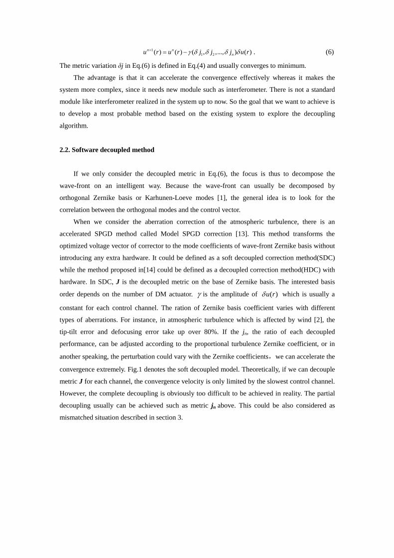
convergence extremely. Fig.1 denotes the soft decoupled model. Theoretically, if we can decouple

metric J for each channel, the convergence velocity is only limited by the slowest control channel.

However, the complete decoupling is obviously too difficult to be achieved in reality. The partial

decoupling usually can be achieved such as metric jn above. This could be also considered as

mismatched situation described in section 3.

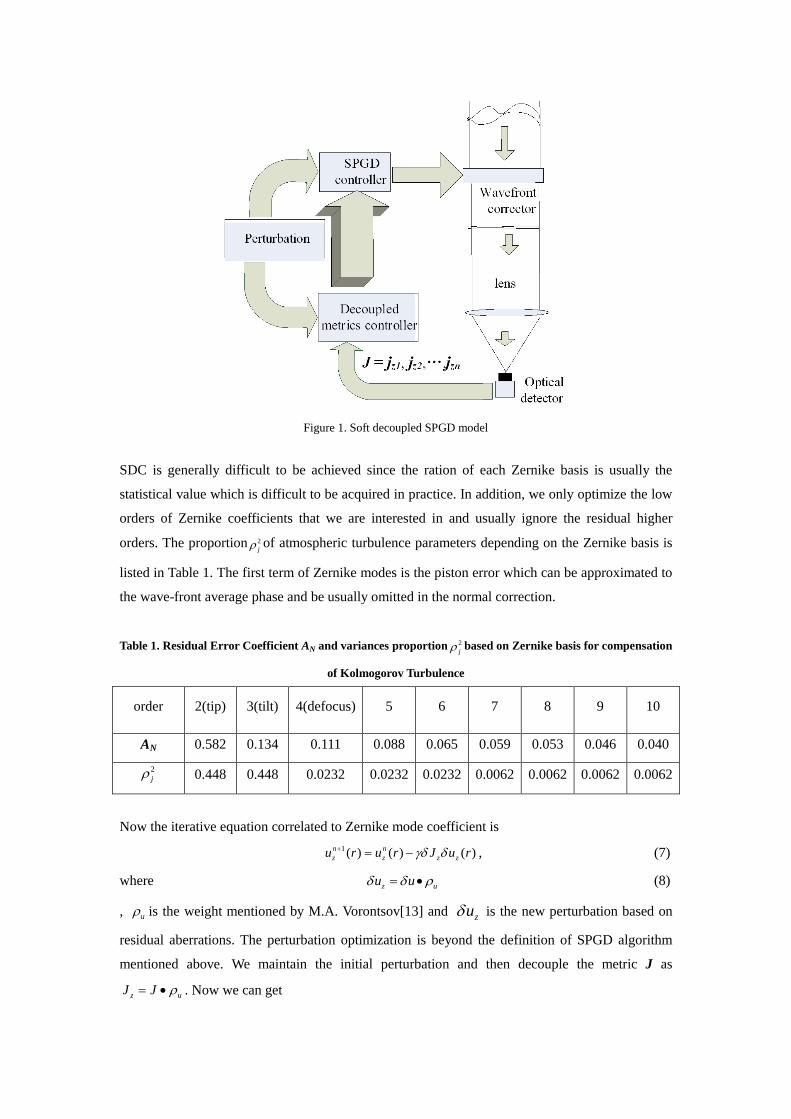
Figure 1. Soft decoupled SPGD model

SDC is generally difficult to be achieved since the ration of each Zernike basis is usually the

statistical value which is difficult to be acquired in practice. In addition, we only optimize the low

orders of Zernike coefficients that we are interested in and usually ignore the residual higher

orders. The proportion 2

j of atmospheric turbulence parameters depending on the Zernike basis is

listed in Table 1. The first term of Zernike modes is the piston error which can be approximated to

the wave-front average phase and be usually omitted in the normal correction.

Table 1. Residual Error Coefficient AN and variances proportion 2

j based on Zernike basis for compensation

of Kolmogorov Turbulence

order 2(tip) 3(tilt) 4(defocus) 5 6 7 8 9 10

AN 0.582 0.134 0.111 0.088 0.065 0.059 0.053 0.046 0.040

2

j 0.448 0.448 0.0232 0.0232 0.0232 0.0062 0.0062 0.0062 0.0062

Now the iterative equation correlated to Zernike mode coefficient is

1( ) ( ) ( )n n

z z z zu r u r J u r , (7)

where z uu u (8)

, u is the weight mentioned by M.A. Vorontsov[13] and zu is the new perturbation based on

residual aberrations. The perturbation optimization is beyond the definition of SPGD algorithm

mentioned above. We maintain the initial perturbation and then decouple the metric J as

z uJ J . Now we can get

1 2( , ..., )z z z znJ j j j (9)

Eq. (9) shows that the performance J is decoupled based on Zernike basis. Then we can write it as

a new type:

1 2( , ,..., )z nJ J jr jr jr . (10)

njr is the nth order of Zernike basis proportion 2

j based on the atmospheric aberration (Table 1)

and J is globally coupled metric which is a scalar. zJ is a vector which is considered to be

the ensemble of individual jr. The updated equation Eq.(7) turns out to be

1( ) ( ) ( )n n

zu r u r J u r .

The distortions of phase correspond to the Kolmogorov turbulence model in the analysis. The

power spectrum of phase fluctuations [19] is expressed by

5/3 11/3

0( ) (0.023 / )G q r q (11)

q is the spatial frequency and r0 is the Fried parameter( it is also the notable coherence length). All

the corrected aberrations in this paper follow this spectrum. Then the software decoupled method

will be analyzed formally in the following.

The variation J of the normal metric of the SPGD algorithm is expressed by

( ) ( )J J J , where 2 21J d r

. Then

2 2 21 1J d r d r

. (12)

is the aperture size of corrector and is the wave-front which is usually decomposed based on

the Zernike mode coefficients 2

j in Table.1. The first term of Eq.(12) is fixed when current is

known and the key point is to maximize the second term. If we consider the aberration based on

the orthogonal Zernike basis, residual aberration and perturbation can be written as below

respectively.

1

N

i i

i

a Z

, 1

N

i i

i

a Z

(13)

ia is the Zernike coefficient and iZ is the Zernike basis. Here, the normal control vector

consists of the voltage of each actuator, so any control vector should be transformed to be the

voltage before it is sent to the corrector. In the Eq.(13), a Au , where u is voltage vector and A

is transform matrix. After perturbation is generated, in order to obtain control voltage, we should

take inverse operator of A. Then *u a A .

The perturbation of basic metric J in Ref [13] associated to uncompensated aberration is

2

0

1

2M

j

j

J

(14)

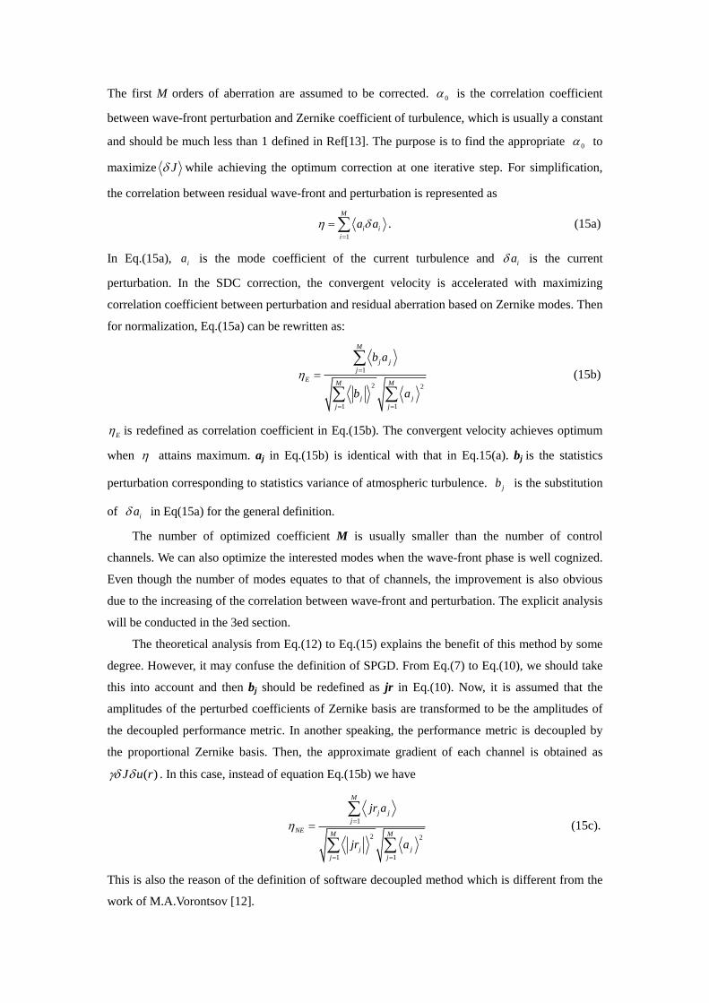
The first M orders of aberration are assumed to be corrected. 0 is the correlation coefficient

between wave-front perturbation and Zernike coefficient of turbulence, which is usually a constant

and should be much less than 1 defined in Ref[13]. The purpose is to find the appropriate 0 to

maximize J while achieving the optimum correction at one iterative step. For simplification,

the correlation between residual wave-front and perturbation is represented as

1

M

i i

i

a a

. (15a)

In Eq.(15a), ia is the mode coefficient of the current turbulence and ia is the current

perturbation. In the SDC correction, the convergent velocity is accelerated with maximizing

correlation coefficient between perturbation and residual aberration based on Zernike modes. Then

for normalization, Eq.(15a) can be rewritten as:

1

2 2

1 1

M

j j

j

EM M

j j

j j

b a

b a

(15b)

E is redefined as correlation coefficient in Eq.(15b). The convergent velocity achieves optimum

when attains maximum. aj in Eq.(15b) is identical with that in Eq.15(a). bj is the statistics

perturbation corresponding to statistics variance of atmospheric turbulence. jb is the substitution

of ia in Eq(15a) for the general definition.

The number of optimized coefficient M is usually smaller than the number of control

channels. We can also optimize the interested modes when the wave-front phase is well cognized.

Even though the number of modes equates to that of channels, the improvement is also obvious

due to the increasing of the correlation between wave-front and perturbation. The explicit analysis

will be conducted in the 3ed section.

The theoretical analysis from Eq.(12) to Eq.(15) explains the benefit of this method by some

degree. However, it may confuse the definition of SPGD. From Eq.(7) to Eq.(10), we should take

this into account and then bj should be redefined as jr in Eq.(10). Now, it is assumed that the

amplitudes of the perturbed coefficients of Zernike basis are transformed to be the amplitudes of

the decoupled performance metric. In another speaking, the performance metric is decoupled by

the proportional Zernike basis. Then, the approximate gradient of each channel is obtained as

( )J u r . In this case, instead of equation Eq.(15b) we have

1

2 2

1 1

M

j j

j

NEM M

j j

j j

jr a

jr a

(15c).

This is also the reason of the definition of software decoupled method which is different from the

work of M.A.Vorontsov [12].

2.3. Hardware decoupled method

The HDC method depicted in Fig.3(a) is on the base of wave-front sensors. The general

wave-front sensors are the interferometers including point diffraction interferometer (PDI) and

Zernike phase contrast interferometer [14] et al. However, these wave-front sensors are too

complex to be realized in DSPGD model especially for atmospheric turbulence. Here, another

useful scheme is described. In the WFC structure, the S-H sensor is a normal wave-front sensor in

adaptive optics systems.

Figure 2. Shack-Hartman wave-front sensor

The principle of S-H sensor is repeated simply again in Fig. 2. The wave-front goes through

micro lens array and then images on the focus. The gradient can be obtained through comparison

between calibration and the real-time images. After that, the wave-front is rebuilt by the gradient

information with different methods. For the typically modal correction, the equations are listed

below:

1

( , ) ( , )N

i i

i

S x y A Z x y

(16)

zA BU (17)

S(x,y) is the gradient distribution of incident wave-front. i is the Zernike order. N is the total

number of Zernike orders. Ai is the ith Zernike polynomial coefficient. Zi(x,y) is the gradient of ith

Zernike polynomial basis. U is the voltage vector of DM. B is the influence function of actuator.

When the gradient is obtained firstly, the Zernike coefficient matrix Az can be calculated from

pseudo-inverse operation of Z. Thus, we get 1*[ ] *A S ZZ Z from Eq.(16). Then the

voltage can be calculated by B on the same methods ( * ( )zU A inv B ) where inv() is the inverse

operation. If we suppose that the total Zernike orders are 30 and the matrix of wave-front pixels

size is 100×100, the size of matrix Ai will be 1×30 and the size of matrix Z will be 30×10000.

The computation budget will be very huge especially over the thousand actuators.

Beam

splitterWave-front

sensor

Metric verctor

calculation

DSPGD

controller

Perturbation

Wavefront

corrector

Beam splitter

Wave-front

sensor

mixedMetric verctor

calculation

Mixed

DSPGD

controller

Perturbation

Wavefront

corrector

PSF

detector

(a) (b)

Figure 3. DSPGD models: (a) standard DSPGD model. (b) mixed DSPGD model.

The ultimate goal we want to achieve for correcting the aberration is to minimize the gradient

of WFS, in another speaking, to flat the wave-front. Each sub-aperture gradient could be the

performance metric applied to SPGD. This can decrease the computation burden effectively at the

cost of reducing the close loop bandwidths. Actually the mass centroid of sub-aperture beam is

only necessary on this method. Then the new metric is

2 2

0 0( ) ( )r x x y yS S S S S (18)

The mass centroid is defined as ( ) ( )

,( ) ( )

x y

xI x yI yS S

I x I y

in the Cartesian coordinate system.

Sx is the mass centroid of x direction coordinate and Sy is on the y direction. Sx0 is the mass cetroid

calibrated on the x direction; Sy0 is calibrated on the y direction; Sr is the relative radius of beam

position which will be the minimum after correction. The reason that we choose Sr rather than

metrics J1, J2, J3 and J4 described in the second section is that the image received by detector for

each sub-aperture has fewer pixels and is insensitive to those metrics. Then，the Eq.(7) becomes

1

1 2( ) ( ) ( , ,..., ) ( )n n

r r rnu r u r S S S u r . (19)

The basic assumption is the identical control channels on both WFS and DM. However, in

practice, the actuators number is usually less than the number of WFS sub-apertures. This is a kind

of mismatched condition which will be specified in the third section. Even though the amount is

equal, the scale is usually not matched. The mismatched scale between DM actuator and WFS

subaperture has been analyzed based on continous surface DM in Ref [14].

2.4. Mixed decoupling method based on hardware

The number of continuous DM actuators is approximated to

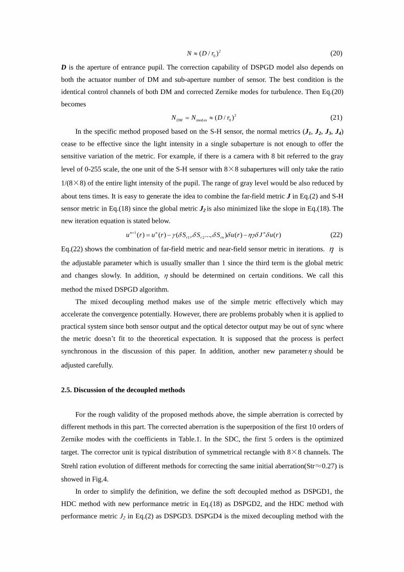
2

0( / )N D r (20)

D is the aperture of entrance pupil. The correction capability of DSPGD model also depends on

both the actuator number of DM and sub-aperture number of sensor. The best condition is the

identical control channels of both DM and corrected Zernike modes for turbulence. Then Eq.(20)

becomes

2

mod 0( / )DM esN N D r (21)

In the specific method proposed based on the S-H sensor, the normal metrics (J1, J2, J3, J4)

cease to be effective since the light intensity in a single subaperture is not enough to offer the

sensitive variation of the metric. For example, if there is a camera with 8 bit referred to the gray

level of 0-255 scale, the one unit of the S-H sensor with 8×8 subapertures will only take the ratio

1/(8×8) of the entire light intensity of the pupil. The range of gray level would be also reduced by

about tens times. It is easy to generate the idea to combine the far-field metric J in Eq.(2) and S-H

sensor metric in Eq.(18) since the global metric J2 is also minimized like the slope in Eq.(18). The

new iteration equation is stated below.

1

1 2( ) ( ) ( , ..., ) ( ) ( )n n n

r r rnu r u r S S S u r J u r (22)

Eq.(22) shows the combination of far-field metric and near-field sensor metric in iterations. is

the adjustable parameter which is usually smaller than 1 since the third term is the global metric

and changes slowly. In addition, should be determined on certain conditions. We call this

method the mixed DSPGD algorithm.

The mixed decoupling method makes use of the simple metric effectively which may

accelerate the convergence potentially. However, there are problems probably when it is applied to

practical system since both sensor output and the optical detector output may be out of sync where

the metric doesn’t fit to the theoretical expectation. It is supposed that the process is perfect

synchronous in the discussion of this paper. In addition, another new parameter should be

adjusted carefully.

2.5. Discussion of the decoupled methods

For the rough validity of the proposed methods above, the simple aberration is corrected by

different methods in this part. The corrected aberration is the superposition of the first 10 orders of

Zernike modes with the coefficients in Table.1. In the SDC, the first 5 orders is the optimized

target. The corrector unit is typical distribution of symmetrical rectangle with 8×8 channels. The

Strehl ration evolution of different methods for correcting the same initial aberration(Str≈0.27) is

showed in Fig.4.

In order to simplify the definition, we define the soft decoupled method as DSPGD1, the

HDC method with new performance metric in Eq.(18) as DSPGD2, and the HDC method with

performance metric J2 in Eq.(2) as DSPGD3. DSPGD4 is the mixed decoupling method with the

iterative function in Eq.(22). Fig.4 shows the almost identical performance of both the soft

decoupled method and the HDC method with new defined metric. The HDC method with metric

J2 only converges to the local extreme value, because the sub-aperture of WFS matched to detector

only has few pixels which are not enough to build up the metric in Eq.(2). Fig. 4 also depicts that

the DSPGD method converges to the extreme value after 20-30 iterations while SPGD method

needs hundreds of iterations.

0 20 40 60 80 1000.2

0.3

0.4

0.5

0.6

0.7

0.8

0.9

1

iterations

Str

ehl

DSPGD1DSPGD2

DSPGD3

SPGD

Figure 4. The different correction methods only for one order Zernike aberration with 8×8 units corrector,

DSPGD1 is soft decoupled method, DSPGD2 is the HDC method with metric Sr in Eq.(18), DSPGD3 is the HDC

method with metric J2 in Eq.(2).

The simple model is built up to compare the proposed method to the classical method in this

part. Almost the identical performance could be achieved by our two proposed methods in this

model and the great advantage of convergence velocity over the normal SPGD algorithm is also

revealed. This model is useful especially for the aberration consisting of low order Zernike modes

like laser purification [27].

3. Discussion of mismatched control channels in decoupled models

The complete decoupling means the elements numbers of both metric variation J and

perturbation ( )u r are equal. However, the WFS sub-apertures and DM actuators are usually not

matched with each other perfectly. Firstly, one sub-aperture of sensor will be matched with more

than one actuator. Secondly, more than one sub-aperture will be matched with one actuator of

corrector.

N J N u

N J N u

(23)

The mismatched situations are listed in Eq.(23). N denotes the element number of the vector.

The mismatched cases are obviously in HDC between sensors and correctors. There is still the

mismatched situation in the SDC model without wave-front sensor. In SDC correction, it is

inevitable to analyze the number of metrics which is more than the number of perturbed control

channel since the orders of Zernike modes are usually less than actuator number of correctors[13].

3.1. Mismatched control channels in SDC

It has been analyzed that the DM with a certain structure has the certain correction capability

when it is applied to atmospheric turbulence [2]. When the DM is fixed on the telescope pupil, the

actuator spacing d is related to r0 which determines the ‘fitting error’ of DM. The analysis [2]

shows that the corrected Zernike modes number should approximately equal to the actuators

number. However, it is impossible to use the identical control channels with actuators in SDC

since the performance has been improved through changing the big number of actuators channels

to a small number of Zernike modes. The first 10 orders of aberrations are the key Zernike

aberration and also the big scale aberration of turbulence [19]. It is feasible and meaningful to

correct the concerned aberration by SDC method. The mixed perturbation applied in SPGD

algorithm has been analyzed in Ref [13] to accelerate the convergence.

It is assumed that the first N orders of Zernike aberration is compensated and the DM

correction capability is the first P orders of aberration where P≥N. Then the residual turbulence

aberration expectation becomes

2 2

1 1

P

r j j

j N j P

J a a

(24)

The first term of Eq.(24) is the residual DM correction capability and the second term is the

ultimately residual error after the DM reaching its limit. The residual errors of turbulence are

5/3

2

0

N N

DA

r

for N≤10 where NA is the fitting coefficient in Table 1 and

5/3

2 3 /2

0

0.2944N

DN

r

for N≥10[2] where N is the corrected orders and 2

N is the residual

variance. During the whole evolution process, we can find that perturbation always exists. The

perturbation is invariable if the scaling factor is fixed. Thus, compared to the WFS correction, this

method would degrade the ultimate performance.

When the convergence goes to the stability, the gradient will achieve the minimum, approximating

zero, and hence the control vector will not vary any more. The components of gradient and

( )zu r are the constants while the only variable is zJ .

The adjustable parameters are the constants which should be adjusted carefully to keep the perfect

performance. In practice, it is relatively difficult to adjust the parameter to be the optimum. Then

an extra term should be added to Eq.(24):

2 2 2

1 1 1

N P

r j j j

j j N j P

J a a

(25)

It is assumed that the first N orders are the optimized targets and the first P orders are the

correction capability of the system in Eq.(25). The first term is the statistical variance of the first N

orders of residual Zernike coefficients referred to perturbation zJ which can be considered as

noise in the fourth section. Then the residual error is

5/3 5/3

2 2

0 0

N r N new

D DA A

r r

,

where 2

r is the residual variance of uncompensated Zernike aberration which are still in the

correction range of DM, D is the aperture diameter of telescope and newA is the new fitting

coefficient.

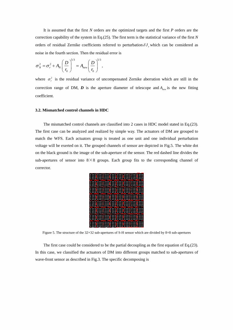
3.2. Mismatched control channels in HDC

The mismatched control channels are classified into 2 cases in HDC model stated in Eq.(23).

The first case can be analyzed and realized by simple way. The actuators of DM are grouped to

match the WFS. Each actuators group is treated as one unit and one individual perturbation

voltage will be exerted on it. The grouped channels of sensor are depicted in Fig.5. The white dot

on the black ground is the image of the sub-aperture of the sensor. The red dashed line divides the

sub-apertures of sensor into 8×8 groups. Each group fits to the corresponding channel of

corrector.

Figure 5. The structure of the 32×32 sub-apertures of S-H sensor which are divided by 8×8 sub-apertures

The first case could be considered to be the partial decoupling as the first equation of Eq.(23).

In this case, we classified the actuators of DM into different groups matched to sub-apertures of

wave-front sensor as described in Fig.3. The specific decomposing is

J

1 2[ , , ..., ]nj j j

11 12 1[ , , ... ]nu u u 21 22 2[ , ,... ],...,nu u u 1 2[ , , ... ]n n nnu u u (26)

j in Eq.(26) is a local metric, corresponding to actuators on the identical numbers, which will

degrade the performance due to the local decoupling. There are 2 different decoupling methods in

this case.

1. The sub-groups are combined to be an individual group applied on single perturbation for

single group where any sub-group 1 2[ , ,..., ]n n nnu u u can be shortened to be the ith element

iu of perturbed control vector in Eq.(26). Each sub-group is applied by the same

perturbation. This method could decrease the resolution of the correctors whereas it is the

complete decoupling.

2. The sub-group is considered to be the sub-system of SPGD where 1 2[ , ,..., ]nu u u could be

a vector for different perturbations. This method is a partial decoupling since each sub-group

could be considered as a individual SGPD system where a single metric obtained from the

sensor will be matched with a single group. The individually iterative equation is

1

( ) ( ) ( ) ( )n n

gi gi giiu r u r j u r

where ( )n

giu r is the updated ith group of control vector at

nth step and ij is the ith element of the metric obtained from the sensor. The actuators

elements of each group are applied to the different perturbations. This method may increase

the resolution of the first method at the cost of decreasing the convergence velocity.

The best method is the combination of these 2 conditions above if there is a unique corrector in the

system. Then we get

1

1 1 2 1 2

2 1 2 11 12 1 1 1 2

( ) ( ) ( , ..., )( ( ), ( ),..., ( ))

( , ..., )([ ( ), ( ),..., ( )] ,...,[ ( ), ( ),..., ( )] )

n n

n n

n n n n nn n

u r u r j j j u r u r u r

j j j u r u r u r u r u r u r

. (27)

1 and 2 are the adjustable parameters for the two methods in Eq.(27) respectively. Eq.(27) is

something like Eq.(22) where the metrics of wave-front sensor and far-field detectors are

combined. Eq.(27) will degenerate to Eq.(22) if the 1 2( , ..., )nj j j are combined together as

J in the second term.

The new idea can be generated that normal SPGD algorithm could be accelerated based on

the analysis above. Firstly, the wave-front with big-scale aberrations are corrected by the grouped

actuators DM as low resolution corrector and then the small scaled aberration could be corrected

by the high resolution corrector. This complicated model is called cascade adaptive optics system

[8].

The second case is common, which we may encounter stated by the second equation of

Eq.(23). Decomposing the whole metric J in Eq.(1) of normal SPGD algorithm, we then get

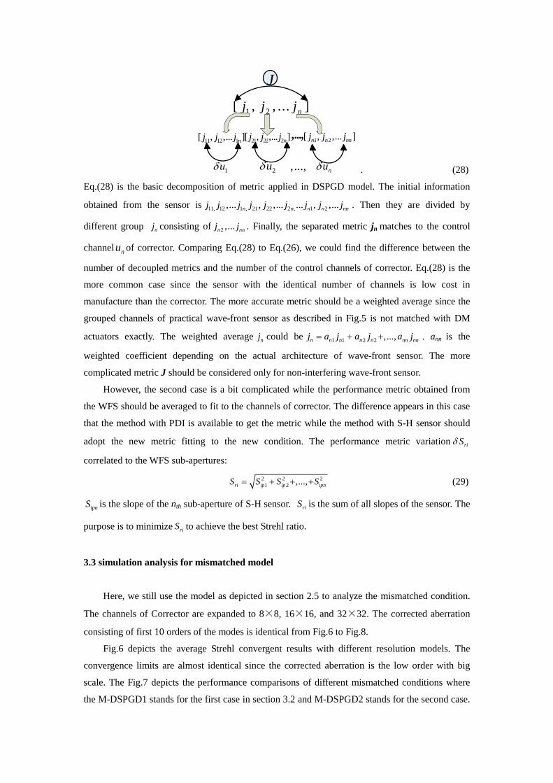
J

1 2[ , , ... ]nj j j

1u 2unu,...,

11 12 1[ , ,... ]nj j j 21 22 2[ , ,... ]nj j j ,...,1 2[ , ,... ]n n nnj j j

. (28)

Eq.(28) is the basic decomposition of metric applied in DSPGD model. The initial information

obtained from the sensor is 11, 12 1 , 21 22 2 , 1 2,... , ,... ... , ,...n n n n nnj j j j j j j j j . Then they are divided by

different group nj consisting of 2 ,...n nnj j . Finally, the separated metric jn matches to the control

channelnu of corrector. Comparing Eq.(28) to Eq.(26), we could find the difference between the

number of decoupled metrics and the number of the control channels of corrector. Eq.(28) is the

more common case since the sensor with the identical number of channels is low cost in

manufacture than the corrector. The more accurate metric should be a weighted average since the

grouped channels of practical wave-front sensor as described in Fig.5 is not matched with DM

actuators exactly. The weighted average nj could be 1 1 2 2 ,...,n n n n n nn nnj a j a j a j . ann is the

weighted coefficient depending on the actual architecture of wave-front sensor. The more

complicated metric J should be considered only for non-interfering wave-front sensor.

However, the second case is a bit complicated while the performance metric obtained from

the WFS should be averaged to fit to the channels of corrector. The difference appears in this case

that the method with PDI is available to get the metric while the method with S-H sensor should

adopt the new metric fitting to the new condition. The performance metric variation riS

correlated to the WFS sub-apertures:

2 2 2

1 2 ,...,ri ip ip ipnS S S S (29)

ipnS is the slope of the nth sub-aperture of S-H sensor. riS is the sum of all slopes of the sensor. The

purpose is to minimize riS to achieve the best Strehl ratio.

3.3 simulation analysis for mismatched model

Here, we still use the model as depicted in section 2.5 to analyze the mismatched condition.

The channels of Corrector are expanded to 8×8, 16×16, and 32×32. The corrected aberration

consisting of first 10 orders of the modes is identical from Fig.6 to Fig.8.

Fig.6 depicts the average Strehl convergent results with different resolution models. The

convergence limits are almost identical since the corrected aberration is the low order with big

scale. The Fig.7 depicts the performance comparisons of different mismatched conditions where

the M-DSPGD1 stands for the first case in section 3.2 and M-DSPGD2 stands for the second case.

The convergence results of partial decoupling of mismatched model with Eq.(27) for two

mismatched conditions in Fig.7(M-DSPGD1 and M-DSPGD2) show that the decreasing the

resolution of DM can accelerate the convergence at the cost of lowering the convergence limit.

The mismatched model in the second case shows that the partial decoupling in Fig.7(M-DSPGD2)

lowers the convergence velocity apparently where it needs about 100 iterations to go to limit for

low order aberration. This is still much better than normal SPGD model which needs over about

200 iterations to go to limit. The convergence limit of Strehl is only about 0.8 in Fig.7 because of

the limitation of DM resolution.

0 20 40 60 80 1000.2

0.3

0.4

0.5

0.6

0.7

0.8

0.9

1

iterations

Str

ehl

8*8

16*16

32*32

Figure 6. Evolution of Metric Strehl with different sub-apertures and matched control channels: 8×8, 16×16 and

32×32, the corrected aberration is a low order Zernike aberration( within first 5 orders).

0 50 100 1500.2

0.4

0.6

0.8

1

iterations

Str

ehl

M-DSPGD2

DSPGD

M-DSPGD1

SPGD

Figure 7. Evolution of Strehl with differently mismatched conditions. Black dot line is for DSPGD model with

matched 8×8 units, red dash line(M-DSPGD1) is for mismatched model with 8×8 units sensor and 16×16 units

DM where resolution of DM is lowered to 8×8 by grouped actuators, blue line (M-DSPGD2) is for mismatched

model with 8×8 units sensor and 16×16 units DM, yellow line is for normal SPGD model of 8×8 units DM without

wave-front sensor.

For the interfering wave-front sensor like PDI, jn could be expressed as

1 2 ,...,n n n nnj j j j which is the same to the second case in Section 3.2. The convergent

velocity of DSPGD method with this metric can achieve the optimum compared to the matched

structure sincenj as the light intensity in Eq.(3) is sensitive to the phase changing. Fig.8 depicts

performance of the hardware DSPGD method based on wave-front sensors differed in

sub-aperture number and the corrector with the identical number of actuators. Different resolution

models show the almost identical performance especially for iterations in Fig.8. There is slight

difference among the convergence limits of three conditions due to the low resolution of

simulation. We just use the simplified model to validate the analysis above, so the precision could

be limited. The more explicit simulation is depicted in section 4.

0 20 40 60 80 1000.2

0.4

0.6

0.8

1

iterations

Str

eh

l

16-8

8-8

32-8

Figure 8. The averaged results of convergence based on different kinds of mismatched corrector and wave-front

sensor. The corrector consists of 8×8 units and the wave-front sensors consist of 8×8 units (blue line), 16×16 units

(red dot) and 32×32 units (black dot-line) respectively

4. The effect of system noise on DSPGD algorithm

In the WFS, it is inevitable to confront the vast majority of noise as analyzed in WFC [20, 24],

but there are still some other problems which should be noted. Because SPGD algorithm is an

iterative method, the random perturbation in Eq.(6) is approximated a part of the noise. Thus, the

perturbation would be analyzed specifically in this part.

According to the source of perturbation, there are two types of SPGD algorithm [21]. One is

the perturbation of algorithm on single direction and the other is the perturbation on double

direction consisting of positive and negative parts in single iteration. Here two types of variation

of metric J in original Eq.(1) are:

1n n nJ J J (30a)

n n nJ J J (30b)

Eq.(30a) shows the single direction which means the metric J is obtained from the different

iterative steps. The iterations in double directions in Eq.(30b) show that the metric J is obtained

from the individual iteration step. nJ and nJ denote the positive and negative perturbation on

each iteration respectively. The iteration of algorithm on double directions is usually superior to

that in the single direction since the former is not sensitive to the variation of performance metric

including noise at the last step. So the perturbation in double directions can accelerate the

convergence better than that in single direction [21].

In Eq.(6), there are 2 elements which are sensitive to the noise. One is the voltage U(r) and

the other is the performance metric (j1, j2,…, jn). In the SPGD algorithm, the perturbed amplitude

must be bigger than noise, otherwise the parameters will be contaminated resulting that the

algorithm can’t converge to the limit. Conversely, the perturbation could not be too larger to

exceed the real gradient, otherwise leading to oscillation of correction all the time with large scale.

Because the performance metric is decoupled to be small elements, the DSPGD model is sensitive

to the noise than normal SPGD. The iterative equation could be written as follow.

1

1 1 1 2 2( ) ( ( ) ) ( , ,..., )( ( ) ( ))n n

i i i i i n inu r u r u j j j j u r u r

(31)

iu stands for the voltage noise; 1ij is the performance noise and ( )u r stands for the

perturbation noise. We can extract the noise terms easily from Eq.(31). Thus, we get

1 2 1 2( , ,..., ) ( ) ( , ,..., ) ( )i i i in i i inu j j j u r j j j u r . (32)

stands for the noise ensemble of all terms and could be also the noise of updated

voltage 1

1 ( )n

iu r

. ( )u r is the perturbation contaminated by the noise. Then

( ) ( ) ( )u r u r u r . Here, the analyzed noise is additive. The multiplicative noises are

usually not taken into account for most detectors. The additive noise usually consists of readout

noise, photos noise and dark current noise, et al. The perturbation noise ( )u r could usually be

neglected, since the noise is always the Gaussian type distributed like the perturbation. Their

summation also fits to the Gauss distributed process. Then the noise of the third term in Eq.(32)

could be a part of iterative process in Eq.(6). Eq.(33) can be shorten to be

1 2( , ,..., ) ( )i i i inu j j j u r . (33)

Eq.(33) seems to be a iterative equation of DSPGD in Eq.(6). The difference is that the optimized

target is the voltage noise iu in Eq.(33) and the noise is random on each iterative step.

Eventually, the main noise sources which we should consider are the noise j of the

performance metric J and voltage noise ( )u r .

0 20 40 60 80 1000.3

0.4

0.5

0.6

0.7

0.8

0.9

1

iterations

Str

ehl

variance ratio0.05

variance ratio0.1

variance ratio0.15

a

0 20 40 60 80 100

0.4

0.5

0.6

0.7

0.8

0.9

1

iterations

Str

ehl

variance ratio 0.05

variance ratio 0.1

varianve ratio 0.15

variance ratio 0.2

b

Figure 9. Strehl evolution for atmospheric turbulence affected by noise of different scale with the model described

in the 2ed section. (a) noise impact on PDI sensor (b) noise impact on S-H sensor.

The calculated model is the same to that in section 2 and the corrector is 8×8 units matched

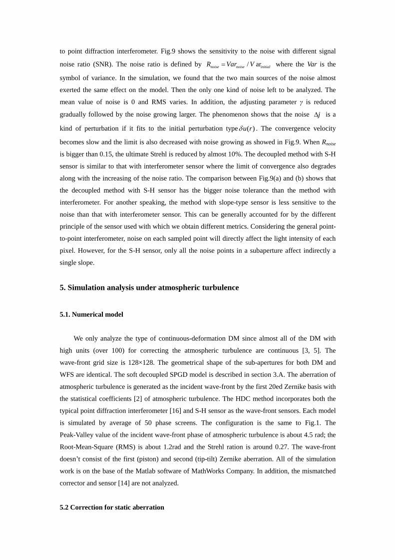
to point diffraction interferometer. Fig.9 shows the sensitivity to the noise with different signal

noise ratio (SNR). The noise ratio is defined by / arnoise noise initialR Var V where the Var is the

symbol of variance. In the simulation, we found that the two main sources of the noise almost

exerted the same effect on the model. Then the only one kind of noise left to be analyzed. The

mean value of noise is 0 and RMS varies. In addition, the adjusting parameter γ is reduced

gradually followed by the noise growing larger. The phenomenon shows that the noise j is a

kind of perturbation if it fits to the initial perturbation type ( )u r . The convergence velocity

becomes slow and the limit is also decreased with noise growing as showed in Fig.9. When Rnoise

is bigger than 0.15, the ultimate Strehl is reduced by almost 10%. The decoupled method with S-H

sensor is similar to that with interferometer sensor where the limit of convergence also degrades

along with the increasing of the noise ratio. The comparison between Fig.9(a) and (b) shows that

the decoupled method with S-H sensor has the bigger noise tolerance than the method with

interferometer. For another speaking, the method with slope-type sensor is less sensitive to the

noise than that with interferometer sensor. This can be generally accounted for by the different

principle of the sensor used with which we obtain different metrics. Considering the general point-

to-point interferometer, noise on each sampled point will directly affect the light intensity of each

pixel. However, for the S-H sensor, only all the noise points in a subaperture affect indirectly a

single slope.

5. Simulation analysis under atmospheric turbulence

5.1. Numerical model

We only analyze the type of continuous-deformation DM since almost all of the DM with

high units (over 100) for correcting the atmospheric turbulence are continuous [3, 5]. The

wave-front grid size is 128×128. The geometrical shape of the sub-apertures for both DM and

WFS are identical. The soft decoupled SPGD model is described in section 3.A. The aberration of

atmospheric turbulence is generated as the incident wave-front by the first 20ed Zernike basis with

the statistical coefficients [2] of atmospheric turbulence. The HDC method incorporates both the

typical point diffraction interferometer [16] and S-H sensor as the wave-front sensors. Each model

is simulated by average of 50 phase screens. The configuration is the same to Fig.1. The

Peak-Valley value of the incident wave-front phase of atmospheric turbulence is about 4.5 rad; the

Root-Mean-Square (RMS) is about 1.2rad and the Strehl ration is around 0.27. The wave-front

doesn’t consist of the first (piston) and second (tip-tilt) Zernike aberration. All of the simulation

work is on the base of the Matlab software of MathWorks Company. In addition, the mismatched

corrector and sensor [14] are not analyzed.

5.2 Correction for static aberration

The soft decoupled correction (DSPGD1) method is shown in Fig.10(a) compared to the

normal SPGD algorithm(red line). The convergence line of soft decoupled SPGD model with

unoptimized perturbation ( u in Eq.(7) with random distribution) is also depicted in Fig.10(a).

Fig.10(b) shows that the improvement of correlation defined in Eq.15(c) between perturbation and

residual wave-front can accelerate the convergence and that is also the reason of definition of

soft-decoupled method(SDSPGD). Further more, the correlation coefficient of the normal SPGD

model (red dot-line) is random showed in Fig.10(b). The correlated coefficient of normal SPGD is

calculated by Eq.15(b) after transforming the perturbation u to the Zernike modes coefficients.

The soft decoupled method is only implemented for the first 10 orders of Zernike aberration which

are the main aberrations for atmosphere turbulence aberration showed in Table.1. The SDC

method can also converge to the extreme value after 30 to 40 iterations. This requires that the

statistic Zernike aberration components of wave-front should be learned previously.

0 20 40 60 80 1000.2

0.3

0.4

0.5

0.6

0.7

iterations

Str

ehl

DSPGD1

SPGD

SSPGD

a

0 50 100 150 2000

0.2

0.4

0.6

0.8

1

iterations

cohere

nt

coeff

icie

nt

DSPGD1

SSPGD

SPGD

b

Figure 10. Comparison between SDC and normal SPGD optimized algorithm. (a) Strehl ration convergence of soft

SPGD(SSPGD) without sensor, normal SPGD(red line) and soft decoupled SPGD(SDSPGD)(b) the evolution of

correlation coefficients between perturbation ( )u r and residual wave-front corresponding to (a).

The results in Fig.11(a) show that the 8×8 channels of low resolution corrector is insufficient

to correct the aberration completely while the high resolution corrector with 16×16 and 32×32

units can compensate the distortion with the limit of Strehl ratio to over 0.9 on the same velocity

only after 30-40 iterations. The comparison of different HDC methods is showed in Fig.11(b). For

the complex aberration, the mixed decoupling method (red dot line) in the Fig.11(b) with S-H

wave-front sensor is superior to the single S-H decoupled method(blue dashed line). The reason is

that S-H sensor is not the point-to-point mapping sensor which could be sensitive to the noise with

small scale. We have showed that the single low order aberration could be corrected based on S-H

sensor as well as PDI sensor in Fig.4. For the turbulence aberration including more than the 10

orders of Zernike aberration, the gradient information is insensitive to the phase variation

compared to the interferometer type sensor. The DSPGD model with S-H sensor is apt to trap in

the local extrimum. In the simulation, we find all the repeated iterations with S-H sensor are

trapped in the local extreme like Fig.11(b) denoted. The metric obtained from S-H sensor

combined with far-filed Strehl could converge to global extremum in Fig11(b).

0 20 40 60 80 1000.2

0.4

0.6

0.8

1

iteat ions

Stre

hl

16×16DS P G D3

32×32 DS P G D3

8×8DS P G D3

a

0 20 40 60 80 100

0.2

0.4

0.6

0.8

1

iterations

Str

ehl

PDI DSPGD

Mix-DSPGD

Soft DSPGD

SPGD

S-H DSPGD

b

Figure 11. Comparison of different DSPGD methods with the identical wave-front. (a) the Strehl convergence of

different spatial resolution corrector matched with point diffraction interferometer sensor on the identical

wave-front based on decoupled method with hardware(b)comparison of different decoupled DSPGD methods

including soft DSPGD(DSPGD1), hardware DSPGD (DSPGD2) with PDI, S-H sensor and mixed hardware

DSPGD(DSPGD4) on the identical 8×8 channels.

The ultimate residual aberration after correction with mixed hardware methods (DSPGD4) is

compared to that with PDI method(DSPGD2) in Fig.12. The S-H wave-front sensor is impossible

to detect the piston type aberration [1], but the 2π ambiguity doesn’t appear. The HDC method

with S-H wave-front sensor is also impossible to correct piston aberration [14], but the 2π

ambiguity exists in most cases as depicted in Fig.12(b). Two adjacent domains are super Owing to

the selected metric slopes of the DSPGD4 method, the DSPGD4 method is able to suppress the 2π

ambiguity since slopes is very sensitive to the variation of the controlling voltage.

a b

20 40 60 80100120

20

40

60

80

100

120

20 40 60 80100120

20

40

60

80

100

120 -6

-4

-2

0

2

-0.5

0

0.5

1

Figure 12. Comparisons of residual wave-fronts after correction of the identically incident wave-front. All

coordinates of images are pixels and the Unit of the colorbar is rad. (a) DSPGD4 correction results with 8×8 units

corrector (b) DSPGD2 correction results with 8×8 units corrector

The advantage of S-H wave-front sensor is that we can use S-H wave-front sensor or other

slope-type sensor effectively under existing WFC system without designing any other complex

device. Although the HDC method is a bit worse than the other decoupled methods, this method

can correct the atmospheric aberration potentially with the easiest method to be implemented. The

iterative correction method relies on the processing power of computation where the normal

SPGD method has been realized by very large scale integration circuit (VLSI)[22,23]. It is

supposed that a static aberration can be corrected at 30-50 iterations showed in this paper and the

WFC correction method bandwidth is about 1k Hz. On the one hand, the situation that there are 3

times of sensor readouts time during each time of iteration of DSPGD model may decrease the

bandwidth severely. On the other hand, there is no big matrix computation in DSPGD method.

This can save a bit time. The ultimate bandwidth can be estimated about 1k/40 Hz on the identical

computation ability for DSPGD correction model compared to the WFC correction.

5.3 Correction for aberration affected by dynamic atmosphere turbulence

The model-free optimization could be considered as an open loop control due to its relatively

slow convergence rate which is implicitly performed on low wind velocity. On the contrary, if the

capability of the device calculation could be improved, the shortcoming of the model would be

overcome on some degree. The dynamic model of the atmospheric turbulence is build up

according to the method in Ref.[25]. The first-order autoregressive model is introduced to describe

the state equation: 1n n nA where n is the current state of atmospheric turbulence, 1n is

the following state and n is the white noise of covariance matrix C . C can be obtained by

TC AC A C where C is the Zernike-basis covariance and AT is the transposition of the

diagonal A defined in Ref.[26]. Thanks to the modal cut-off frequency of the Power Spectral

Density of a Taylor turbulence phase, the diagonal elements could approach to

exp( 0.3( 1) / ( ))ia n V f D where ai is the ith diagonal element, n is the radial order of Zernike

basis, V is the wind velocity, f is the clock frequency and D is the diameter of the telescope.

Currently, the dynamic part is the wave-front n which is shifted by wind V. D/r0 is used to

characterize the atmosphere turbulence strength for the receiver system with the pupil D. Here,

D/r0 is set by classical ratio 6；f is 1000Hz；n is 11 (the amount order is reduced to 72)and D is

0.8m.

The HDC method based on S-H sensor is compared to that based on PDI sensor for

correcting the classical atmosphere turbulence with different wind velocity depicted above. The

number of control channel is 8×8 and The subapertures of both sensors are 32×32. Therefore,

the mismatched model in Eq.(28) is analyzed in this part. We investigated the achieved Strehl ratio

after 100 iterations for different wind velocity on the same D/r0.

0 20 40 60 80 1000

0.2

0.4

0.6

0.8

1

iterations

Str

ehl

1m/s

5m/s

10m/s

0m/s

Figure 13. Correction for dynamic atmosphere turbulence on different wind velocities(1m/s, 5m/s and 10m/s). The

HDC method based on PDI sensor is on the lines of blue type. The HDC based on S-H sensor is on the lines of red

type.

The starting points of all curves in Fig.13 are random since each convergent process is

conducted on the respective turbulence evolution C with the random process noise. When the

wind velocity is increased, both convergent limits are decreased and the convergent processes

become unstable in Fig.13. The worst processes fluctuating severely on the wind velocity 10m/s

means that the wind velocity becomes unacceptable at this level. The convergence with S-H

sensor is a little worse than that with PDI sensor since the method with PDI sensor only make use

of the single perturbation given in Eq.(19), while the method with S-H sensor needs the mixed

perturbation with two kinds of performance metrics given in Eq.(22). For the medium wind

velocity less than 5 m/s, the 40-60 iterations will be needed to achieve the stable correction.

Although the method with S-H sensor is not as good as that with PDI sensor, there is of interest to

explore it in practice since the sensor is commonly used in traditional adaptive optics system. We

have to indicate that the normal SPGD algorithm is not showed here since only the low wind

velocity not more than 1m/s will radically impact the performance (1m/s leading to the lost

convergence) at the same clock frequency to the above.

5.4. Discussion

We have compared the static and dynamic correction above between different methods. In the

dynamic condition, the system seems not fast enough to correct the aberration in the medium

turbulence. It is still necessary to state the algorithm in the other applications. Apart from the

advantage stated, the shortcoming should be focused on as well. The main drawback is that the

bandwidth is deduced severely when the extra sensor is introduced. This may be overcome when

Very Large Scale Integrated Circuit(VLSI) substitutes the normal PC. Because the wave-front

senor is added to the model-free method, the system model may be much more complex. In

addition, the constraint of the specific sensors should be considered such as sensitivity to the noise.

Up to now, there is no standard sensor applied in decoupled method, so a set of sensors should be

tested such as S-H sensor of the slope type sensor and interferometer type sensor. Moreover, the

system correction capability should be estimated based on the WFC method. The comparison

between WFC and model-free method is on the aspects of the control algorithm, system

architecture, residual error, demand for Luminous flux, etc.

6. Conclusion

We mainly concern the improvement of the SPGD algorithm in this paper. The SDC method

and HDC method are discussed explicitly. Based on hardware H-S sensor of the decoupled method,

the wave-front conjugated correction is linked initially and efficiently to SPGD algorithm of

model-free methods. The results of numerical simulation present that it’s not as good as the

completely decoupled SPGD method incorporating interferometer sensors, whereas it is superior

to normal SPGD algorithm. The basic DSPGD method with S-H sensor is not available to achieve

the best convergent limit. It should combine the far field metric or any other global metric

obtained from the sensor to form a mixed DSPGD method achieving the high convergence

velocity when the atmospheric turbulence aberration is corrected. In the current AO system, only

using the algorithm without updating any hardware seems impossible to play a role in the stronger

turbulence. However, there is still the potential prospect applied in the existing optical system

when the slow variation of wave-front aberration appears. The noise impact on DSPGD method is

also analyzed in the paper. The results show that the decoupled method with S-H sensor is more

robust to the influence of noise than that with PDI sensor.

The soft decoupled method could be useful when the wave-front aberration mainly consists

of the low order or big scale error which should be tested in real-time environment. For other

applications, the hardware decoupled correction could be a potential consideration. In addition, the

mismatched control channels could be met frequently for the existing systems which should be

analyzed according to the methods in the paper. The experiment setup will be built up in the lab

incorporating the S-H sensor to test the DSPGD method next.

Acknowledgements

The study program is supported by the MPG-CAS graduate studentship.

References

[1]. F.Roddier (Ed.), Adaptive Optics in Astronomy, Cambridge University Press, New York, 1999

[2]. N. Roddier, Optical Engineering. 29 (1990) 1174.

[3]. H.M. Martin, G. Brusa Zappllim, B.Cuerden et.al. Proc. SPIE. 6272, Advances in Adaptive Optics II 62720U

(2006)

[4]. P. Madec, F. Roddier (Ed), Cambridge University Press, New York, 1999.

[5]. Daniele Gallieni, Enzo Anaclerio, Paolo G. Lazzarini et.al, Proc. SPIE. 4839, Adaptive Optical System

Technologies II 765 (2003)

[6]. Jiang Wanhan, Huang Shufu, Wu Xubin. Chinese Journal of Lasers. 15 (1998) 27.

[7]. V.P.Sivokon and M.A. Vorontsov, J. Opt. Soc. Am. A 15 (1998) 234.

[8]. Mikhail Vorontsov, JimRiker, Gary Carhart et.al, Applied optics. A 48 (2009) 47.

[9]. J. C. Spall. IEEE Trans. on Automatic control. 37(1992) 332.

[10]. T. R. O’Meara, J. Opt. Soc. Am. A. 67 (1977) 306.

[11]. G. Gauwenberghs, Advances in Neural Information Processing Systems(Morgan Kaufman, Los Altos, Calif).

5 (1993) 244

[12]. M.A.Vorontsov, OPTICS LETTERS. 22 (1997) 907.

[13]. M. A. Vorontsov and V. P. Sivokon, J. Opt. Soc. Am. A 15 (1998) 2745.

[14]. M. A. Vomntsov, J. Opt. Soc. Am. A 19(2002) 356.

[15]. M. A.Vorontsov, G. C.Carhart, M.Banta, et al. Proc. SPIE. 5162 (2003) 37.

[16]. M.A. Vorontsov, E. W. Justh, and L.A. Beresnev, J. Opt. Soc. Am. A 18(2001) 1289.

[17]. Piotr Piatrou, Michael Roggemann. Beaconless, APPLIED OPTICS. 46 (2007) 6831.

[18]. R. A. Muller and A. Buffington, J. Opt. Soc. Am. 64 (1974) 1200.

[19]. R.J.Noll, J. Opt. Soc. Am. A 66 (1976) 207.

[20]. José E. Oti, Vidal F. Canales, Manuel P. Cagigal, OPTICS EXPRESS 21 (2003) 2783.

[21]. Huizheng Yang, Dongmei Cai, Xinyang Li ,Wenhan Jiang, Intelligent Control and Automation, 2008. WCICA

7th world congress on, 4391 (2008).

[22]. R.T.Edwards, M. H. Cohen, G. Cauwenbeghs, M. A. Vorontsov, and G. W. Carhart, in Learning on Silicon,

G.Cauwenberghs and M. A. Bayoumi, Eds. Boston, MA: Kluwer, 359 (1999).

[23]. M. H. Cohen, M. A. Vorontsov, G. W. Carhart, and G. Cauwenberghs, Proc. SPIE EUROPTO, 3866 (1999)

176.

[24]. Theam Yong Chew, Richard M.Clare, Richard G. Lane, Opt. Commun. 248 (2005) 359.

[25]. B.Le Roux, J.-M Conan, G. Rousset, L.M. Mugnier, V.Michau, J.Opt.Soc.Am. A 18 (2001)2527.

[26]. Caroline kulcsar, Henri-Francois Raynaud, Cyril Petit, OPTICS EXPRESS. 14 (2006) 7464.

[27]. Liang Yonghui, Wang Sanhong, Long Xuejun, Yu Qifeng, Acta Optical Sinica. Photonics Asia 2007.

International Society for Optics and Photonics. (2007) 68230H.

[28]. Thomas Weyrauch, Mikhail A.Vorontsov, Journal of Optical and Fiber Communications Reports. 1 (2004)

355.

[29]. Piotr Piatrou, Michael Roggemann,APPLIED OPTICS. 46 (2007) 6831.

[30]. Wright A J, Burns D, Patterson B A, et al. Microscopy Research and Technique, 67 (2005) 36.

[31]. Zommer S, Ribak E N, Lipson S G, et al. Optics letters, 31 (2006) 939.