Second gradient poromechanics

International Journal of Solids and Structures 44 (2007) 6607–6629

Second gradient poromechanics

a b, c

www.elsevier.com/locate/ijsolstr

Giulio Sciarra , Francesco dell’Isola *, Olivier Coussya Dip. di Ingegneria Chimica, dei Materiali, delle Materie Prime e Metallurgia, Universita di Roma ‘‘La Sapienza’’,

via Eudossiana 18, 00184 Rome, Italyb Dip. di Ingegneria Strutturale e Geotecnica, Universita di Roma ‘‘La Sapienza’’, via Eudossiana 18, 00184 Rome, Italy

c Institut Navier ENPC, Av. Blaise Pascal, Cite Descartes, F77455 Marne-la-Vallee Cedex 2, France

Received 12 July 2006; received in revised form 13 February 2007; accepted 2 March 2007Available online 7 March 2007

Abstract

Second gradient theories have been developed in mechanics for treating different phenomena as capillarity in fluids,
plasticity and friction in granular materials or shear band deformations. Here, there is an attempt of formulating a secondgradient Biot like model for porous materials. In particular the interest is focused in describing the local dilatant behaviourof a porous material induced by pore opening elastic and capillary interaction phenomena among neighbouring pores andrelated micro-filtration phenomena by means of a continuum microstructured model. The main idea is to extend the clas-sical macroscopic Biot model by including in the description second gradient effects. This is done by assuming that thesurface contribution to the external work rate functional depends on the normal derivative of the velocity or equivalentlyassuming that the strain work rate functional depends on the porosity and strain gradients.
According to classical thermodynamics suitable restrictions for stresses and second gradient internal actions (hyper-stresses) are recovered, so as to determine a suitable extended form of the constitutive relation and Darcy’s law.

Finally a numerical application of the envisaged model to one-dimensional consolidation is developed; the obtainedresults generalize those by Terzaghi; in particular interesting phenomena occurring close to the consolidation external sur-face and the impermeable wall can be described, which were not accounted for previously.� 2007 Elsevier Ltd. All rights reserved.

Keywords: Second gradient materials; Porous media; Thermodynamics; Darcy law; Consolidation

1. Introduction

In standard continuum mechanics constitutive equations are usually formulated by assuming a local state
postulate with regard to both time and space. When applied to fluids, it results in postulating that the (Helm-holtz) free energy depends on the fluid mass density q and on the temperature T only, and not on the spatialgradients of the latter. Because only the first gradient of the fluid velocity is then involved when finally express-ing the fluid mass balance, continuum mechanics based on the local state postulate is generally said to be a firstgradient theory.
* Corresponding author.E-mail address: [email protected] (F. dell’Isola).

0020-7683/$ - see front matter � 2007 Elsevier Ltd. All rights reserved.

doi:10.1016/j.ijsolstr.2007.03.003

mailto:[email protected]

First gradient mechanics reveals to be insufficient when trying to model the vapour–liquid transition via acontinuum approach. Going back to the celebrated works of van der Waals, and restricting attention to a firstgradient theory, the free energy density is known to be a non-convex function of the fluid mass density q. Theminimizers of the energy, which actually govern the stable equilibrium states of the fluid during phase tran-

6608 G. Sciarra et al. / International Journal of Solids and Structures 44 (2007) 6607–6629

sition, are then restricted to the functions taking their values at the energy minima. In order to cure the bista-ble nature of the van der Waals model for phase transition, new information is mandatory. The missinginformation concerns the mechanical equilibrium of the liquid–vapour interface during phase transition. Sincethe mechanical equilibrium of the transition layer between the two co-existing phases is governed by non-localvan der Waals forces, in a continuum approach to phase transition the free energy cannot depend on the localvalue of the mass density only. To be more precise, a first gradient model of phase transition is not capable ofidentifying the topological structure of the interface, which may be irregular or even dense. Accordingly astandard model to remove the bistable nature of a van der Waals-type approach to phase transition is theCahn–Hilliard second gradient model (see Cahn and Hilliard, 1959). Second gradient theory introduces adependence of the energy E on the density gradient according to

Ee ¼ZD

W ðqÞ þ e2jrqj2h i

dv: ð1Þ

In this expression W(q) is a double-well potential and e a small parameter that takes into account the energythat is connected with the formation of interfaces. As shown in Modica (1987a,b), as e! 0+ the solution of
the mvalue
inimization problem associated to the functional (1) converges to the function q0 which takes only thes a and b corresponding to minima of the first gradient energy W(q), while the set

E :¼ fx 2 D : qðxÞ ¼ ag minimizes the surface area of its boundary among all subsets of D having the samevolume. The pressure jump through the liquid/vapor interface is then governed by the usual Young–Laplaceequation in terms of the product of surface tension and mean curvature (see de Gennes, 1985; Anderson et al.,1998). By contrast, when the problem at hand involves a characteristic length having the same order of mag-nitude as the thickness of the layer forming the liquid/vapor interface, the limit procedure e! 0+ does notapply any more and the full procedure of the minimization of the functional (1) is required. This actually oc-curs for phenomena involving thin liquid films (Seppecher, 1993), droplets exhibiting small curvature radius(dell’Isola et al., 1996; Gavrilyuk and Saurel, 2002), or a topological transition associated for instance topinching and fissioning of liquid jets (Lowengrub and Truskinovsky, 1998). In describing these phenomenamore refined models than those based on the simple Young–Laplace equation are needed.

This kind of problem has been discussed in the literature both for the case of a single-component fluid andbinary fluids according to a macroscopic approach (see e.g. Anderson et al., 1998; Seppecher, 1996; Lowen-grub and Truskinovsky, 1998; Lee et al., 2002) considering the compressible, incompressible and quasi-incom-pressible behaviour (see Lowengrub and Truskinovsky, 1998 for a detailed discussion) of the bulk material. Itis worth noticing that quasi-incompressibility means that the overall mass density is not constant, even if mix-ture constituents are incompressible, because of a non-constant constituent mass concentration; in this casethe set of balance laws is enriched by a mass concentration equation (see Lowengrub and Truskinovsky,1998) or a micro-force balance law (see Gurtin et al., 1996). For multiphase systems, as mixtures of non-inter-acting fluids, a second gradient model involving co-capillarity can also be introduced (see e.g. Seppecher, 1987)which is capable of describing the effect of compressibility of the constituents on the behaviour of the mixtureas a whole.

Early formulations of second gradient mechanics of solids (Germain, 1973) consist of considering both thefirst and the second gradient of the displacement, or equivalently the deformation and its spatial gradient, asrelevant candidates in the expression of the deformation working. Extended second gradient mechanics of sol-ids consists of considering both the first and the second gradient of relevant state variables in the expression ofthe free energy.

Following the pioneering work of Biot in poroelasticity (Biot, 1941), poromechanics (Coussy, 2004) is thatbranch of mechanics which deals with the behaviour of deformable porous solids whose internal solid wallsare subjected to the pressure of an interstitial fluid. Once a microscopic description of the porous materialis introduced, it is generally accepted that the macroscopic model can be viewed as a suitable averageof the microscopic one. This requires to identify every reference volume element (RVE) of macroscopic

ch

Font monospazio

6608

continuum mechanics with its centroid (Dormieux and Ulm, 2005). The up-scaling procedure is worked out byassuming uniform strain (stress) boundary conditions for every reference volume in terms of the macroscopicstrain (stress), or periodic boundary conditions. Obviously the microscopic strain (stress) distribution may notbe spatially uniform in the reference element volume because of the included heterogeneities. Therefore there is

G. Sciarra et al. / International Journal of Solids and Structures 44 (2007) 6607–6629 6609

no chance to recover continuity of the microscopic stress vector on the interface between two contiguous ref-erence element volumes using the standard first gradient theory. As a result a macroscopic first gradient theoryis not capable to address the effects associated to neighbouring pores of contiguous reference element volumes.Following Drugan and Willis (1996), one can induce the characteristic size of the reference volume element byrequiring the non-local corrections to the constitutive law to be within a given error percentage of the standardeffective stiffness. In addition to be highly heterogeneous, liquid-saturated porous solids have fluid–solid inter-faces whose thickness may become comparable with the pore size. These are the conceptual reasons for explor-ing higher gradient poromechanics.

Second gradient mechanics for porous solids has actually been already addressed in the framework of thetheory of mixtures in dell’Isola et al. (2000), Sciarra et al. (2001) and dell’Isola et al. (2003) and recently in thatof poromechanics (see Collin et al., 2006) by considering a second gradient behaviour for the solid only. Theapproach developed here extends these results by providing a macroscopic Biot-like theory of poroelasticmaterials for which second gradient effects are associated to both solid and fluid constituents. With respectto the results presented in Collin et al. (2006), here a complete deduction of second gradient poromechanicshas been developed, together with an explicit formulation of a constitutive macroscopic model, consistent withthermodynamics.

In Section 2, some preliminaries are discussed in order to make clear the following developments. In Section3, we extend first gradient poromechanics (Coussy, 2004) to second gradient poromechanics. The approachallows us to express the internal work rate with the help of additional stress fields compatible with the externalwork rate accounting for second gradient effects. In the following sections the second gradient poroelastic con-stitutive equations and modified Darcy’s law are derived from thermodynamics. In the last section, a numer-ical example is developed for treating the classical one-dimensional consolidation problem stated by vonTerzaghi (1946) in the framework of the second gradient poromechanical model. The new model is capableto cure the singular behaviour of Terzaghi’s solution close to the surface on which the consolidating loadingis exerted. The analysis reveals a Mandel-like dilatant effect (Mandel, 1953) in the early consolidation processclose to the impermeable wall.

2. Preliminaries and notations

In this section, we introduce some formalism to be adopted in the following. We in particular point out thedistinction between Eulerian and Lagrangean fields and the way in which the ones transform into the others.According with classical poromechanics, we introduce the Lagrangean field equations starting from the Eule-rian ones, deduced from the Principle of Virtual Powers. It is worth to notice that in the Lagrangean descrip-tion of motion all the fields in the governing equations are regarded as dependent on the reference placementin the initial configuration of the solid; on the other hand in the Eulerian description the governing equationsare prescribed in terms of spatial fields (i.e. fields defined over the current configuration).

Let v(Æ, t) indicate the placement of a solid material particle Xs. This is a diffeomorphism over the Eucledeanplace manifold E, such that x = v(Xs, t) represents the current placement of Xs. F(Æ, t) indicates its gradient. Inthis paper, we explicitly distinguish between the Lagrangean gradient ($0), with respect to the reference placein the configuration of the solid skeleton, and the Eulerian gradient ($), with respect to the current place x.Analogously, the solid Lagrangean and the Eulerian divergence operators will be noted by div0 and div,respectively. All the classical transport formulas can be derived; in particular those ones for a material volumeand for an oriented surface element turn to be

dv ¼ J dv0 nds ¼ J F�Tn0 ds0 ð2Þwhere dv and ds represent the current elementary volume and elementary oriented surface corresponding tothe reference ones dv0 and ds0, moreover J = detF. In the following D will indicate the current domainoccupied by the porous material and D0 its solid reference shape. According with the previous remarks the

ch

Font monospazio

6609

following rules for transforming Eulerian into Lagrangean gradient and divergence for a spatial vector (sec-ond order tensor) field v (V) hold true (for more details see e.g. Truesdell, 1991; Gurtin, 1981):

rv ¼ r0ðv � vÞF�1;�1

(rV ¼ r0ðV � vÞF�1;

�T

(ð3Þ


Jdivv ¼ div0½JF ðv � vÞ� JdivV ¼ div0½JðV � vÞF �;

where v�v and V�v are the Lagrangean fields associated with the spatial v and V by means of the solid place-
mentseconback,
Li ofdoubboun

veloc

and o

map. In this paper overall, as well as intrinsic fluid, stresses and hyper-stresses (these last to account ford gradient contributions) are introduced as Eulerian fields (T,Tf,C,Cf ); however their Lagrangean pullin the reference configuration of the skeleton, will be the only stress fields constitutively prescribed in

terms of a suitable macroscopic potential (see Section 5). We use identities (3) for introducing, at the endof Section 3, the relation between the Cauchy stress tensors (T and Tf) and the Piola–Kirchhoff stress tensors(S and Sf) for the overall porous material and the pure fluid, as well as the relation between the Eulerian (c andcf) and Lagrangean (c and cf) hyper-stress vectors, which univocally prescribe hyper-stresses with some rescr-iting assumptions on admissible second gradient tractions (see Eq. 18).

3. Second gradient poromechanics

We start by recalling second gradient mechanics. For a monophasic continuum referred to by index a, fol-lowing Toupin (1962, 1964), Mindlin (1964), Casal (1972) and Germain (1973) the external working Wext,which accounts for second gradient effects, is a continuous linear functional of the field velocity va (see e.g.dell’Isola and Seppecher, 1997; Degiovanni et al., 2006) such as

WextðvaÞ ¼ZD

ba � va dvþZ

oD

ta � va þ sa �ova

on

� �dsþ

Xne

i¼1

ZLi

tia � va dl; ð4Þ

where D is the current domain (or any of its regular subdomains), oD its boundary and ne the number of edges
the boundary, if any. Moreover ba is the density of body forces, ta the surface traction, sa the so calledle-force (or ‘‘1-normal’’ contact forces) and ti
a the edge force per unit line acting along the ith edge of thedary. Note that o/on is the normal derivative, that is the directional derivative along the outward unit

normal. According to the primary results on second gradient theories stated by Germain (1973) the externalaction sa can be regarded as the sum of two different contributions: (i) an external areal double force workingon the stretching velocity, ($va Æ n � n) along the outward unit normal n of the boundary; (ii) a tangential cou-ple working on the vorticity. If in particular only the vorticity effect was considered then the envisaged modelcould be regarded as a kind of Cosserat continuum where local rotations are prescribed in terms of the velocitygradients (see e.g. Suiker et al., 2001). Consistently with (4), following Germain (1973) the strain working re-lated to second gradient mechanics is now expressed in the form1

W intðvaÞ ¼ZD

½Ta � rva þ Ca � rrva�dv; ð5Þ

where Ta and Ca stand, respectively, for the stress tensor and for the hyper-stress tensor. For the sake of sim-plicity, ignoring inertia forces, the Principle of Virtual Power states that WextðvaÞ ¼W intðvaÞ, whatever the

ity field va. Exploiting this equality, standard procedures lead to the momentum equation

divðTa � divCaÞ þ ba ¼ 0 ð6Þ

and the conditions on the boundary of every regular subdomain of D

ta ¼ ½Ta � divðCaÞ�n� divS ½Can�; sa ¼ ðCanÞn; ð7Þ

n everyone of its edges i = 1, . . . ,ne

ð8Þ

1 From now on the central dot will indicate the inner product between two nth order tensors.

ch

Font monospazio

6610

where divS and stand, respectively, for the surface divergence over the regular parts of the boundary, andfor the jump of u across the ith edge, respectively. Eq. (7) can be reformulated in order to underline how(external) tractions exerted on the regular parts of the boundary depend on the contact surface not onlyvia a linear map acting on the normal unit vector n components, but also via a linear combination of the com-

2


ponents of the curvature tensor N ¼ rSn:

ta ¼ fTa � divCa � divSðC>a Þ>gn� CaN: ð9Þ

Let us now consider a solid–fluid mixture and refer to the solid and fluid constituents by the indices s and f,respectively. At any time a solid–fluid mixture can be viewed as the superposition of two interacting continua,a = s and a = f. Accordingly, the Principle of Virtual Power, and consequently (6)–(8), apply separately to the
solid
Furth

where

obtai

We w

tions(Cou

continuum and to the fluid continuum. In addition Ta and Ca are tensorial volumetric densities with re-
gard to the macroscopic overall volume dv. We may re-express Ta and Ca by introducing tensorial densities Ta
and Ca intrinsic to the constituents by referring them to the volume which the two constituents actually oc-cupy. If n is the Eulerian porosity, then ndv is the current porous volume and, in the case of saturation,we can write

Ts ¼ ð1� nÞTs; Cs ¼ ð1� nÞCs; Tf ¼ nTf ; Cf ¼ nCf : ð10ÞAccordingly, from (6) we finally obtain

divðð1� nÞTs � div½ð1� nÞCs�Þ þ bs ¼ 0; divððnTfÞ � divðnCfÞÞ þ bf ¼ 0: ð11Þ
ermore the body force ba can be split in two terms according to
bs ¼ bs þ bf!s ¼ bs � bs!f ; bf ¼ bf þ bs!f ¼ bf � bf!s ð12Þ
bf!s(resp. bs!f) is the interaction force exerted by the fluid (resp. solid) continuum on the solid (resp.
fluid) continuum. As indicated in (12), by virtue of the action and reaction law, we have bf!s = �bs!f, as it canbe directly recovered from the Principle of Virtual Power (Dormieux et al., 1991). Adding the two equations

ned by successively letting a = s and a = f in (6) we then derive

divðT� divCÞ þ b ¼ 0; ð13Þwhere T and C are, respectively, the overall stress tensor and the overall hyper-stress tensor:

T ¼ð1� nÞTs þ nTf ; ð14Þ
C ¼ð1� nÞCs þ nCf : ð15Þ
The external working Wextmixðvs; vfÞ related to the mixture is the sum of the working related to each constituent.

rite

Wextmixðvs; vfÞ ¼WextðvsÞ þWextðvfÞ: ð16Þ

int
The deformation working Wmix related to the mixture is obtained through exploring the equalityWext
mix ¼W intmix. With the help of (11)2 and of (12)2, by eliminating the unknown interaction force bf!s from

(16), we finally obtain after some straightforward mathematical manipulations

int

Z>
Wmixðv;wÞ ¼
D

½T � rvþ divðnTf wÞ þ C � rrvþ nCf � rrw� divðdivnCfÞ � w�dv; ð17Þ

where, and from now on, we use the notation v = vs and w = vf � vs in view of the forthcoming Lagrangeandescription with regard to the solid skeleton. For the sake of simplicity, the contribution of external bulk ac-

ba has not been considered in (17). The two first terms are the ones related to a first gradient approachssy, 2004), while the remaining terms capture the second gradient effects.

2 In the following formulas the transpose of a third order tensor C is evaluated so as to fulfill the identity:

ðC � vÞ : V ¼ ðC> : VÞ � v; 8v 2 Rn and V 2 LINðRnÞ:

ch

Font monospazio

6611

From now on we restrict our attention only to those second gradient effects that are related to doubleforces, or from the kinematical point of view, to stretching velocities; in other words we assume skew-symmet-ric couples working on vorticity on the boundary to be negligible for both the solid and the fluid constituents.From a physical point of view such an assumption implies both solid granular materials and complex rheo-


logical fluids not to be modeled by the addressed second gradient formulation; on the other hand solid localdilatancies, capillarity of the fluid as well as co-capillarity between the solid and the fluid are going to be takeninto account by the envisaged model (a more detailed discussion of these topics can be found in Section 5). Theformulated hypothesis implies the hyper-stress tensor of both constituents to reduce to the form

Ca ¼ I� ca; a ¼ s; f ; ð18Þ

where I is the second order identity tensor and ca a suitable vector field. According to Eq. (4), the second gra-dient external working is �

Cothat o

we reJ = dtivelygean

wher

4. Th

sa �ova ¼ na½ðI� caÞn�n �

ova ¼ naðca � nÞn �ova ¼ naðca � nÞðrva � n� nÞ; na ¼

1� n; a ¼ s;ð19Þ

on on on n; a ¼ f :

As previously noticed ($va Æ n � n) represents the stretching velocity, thus na(ca Æ n) indicates the so called dou-bly normal double force acting on the ath constituent (see Germain, 1973).

nsider now a Lagrangean description of the porous material, where the initial reference configuration isf the solid skeleton; the internal (generalized) stresses of the solid are therefore pulled back to this initial

configuration via the following relations:

T � rvdv ¼ S � dDdt

dv0; S :¼ JF�1TF�>; ð20Þ

C � rrvdv ¼ ðI� c � rrvÞdv ¼ c � rðdivvÞdv

dD� �>

dD" #

�1 > �1 �1 �1
¼ c � r0dt
C � ðr0CÞ Cdt

C dv0; c :¼ JF c ð21Þ

mind that F is the spatial gradient of the placement map of the solid, C :¼ F>F, D :¼ 12ðC� IÞ and

etF the Cauchy–Green strain tensor, the Green–Lagrange strain tensor and the Jacobian of F, respec-. Moreover dv0 represents the reference volume element such that dv = Jdv0 (see Section 2). The Lagran-overall stresses are represented by S and c, which indicate the second Piola–Kirchhoff stress tensor and

the hyper-stress vector. In the previous formulas $ indicates the Eulerian gradient and $0 the correspondingLagrangean gradient. When introducing also the solid Lagrangean pull back of the fluid stress and hyper-stress

Sf :¼ JF�1TfF�>; cf :¼ JF�1cf ; ð22Þ

the internal deformation working takes, finally, the following form

W int ¼Z

½S� C�1ððr0CÞcÞC�1� � dDþ C�1 � c � r0

dDþ div0

1S>M

� ��
L
D0dt dt Jqf

f� ��
þr0 J�1div0
1

nqf

M � ncf �1

nqf

M � r0½J�1div0ðncfÞ� dv0; ð23Þ

e M :¼ mfF�1w is the Lagrangean filtration vector and mf :¼ Jnqf the Lagrangean fluid mass content.

ermodynamics of second gradient porous media

In this section, the first and the second principle of thermodynamics for the case of fluid saturated secondgradient porous media will be discussed. According to the standard procedure based on the Clausius–Duheminequality we extend the well known results due to Biot (see e.g. Biot, 1941) and determine, following Coussyet al. (1998) and Coussy (2004), a suitable macro-scale potential so as to identify for every state parameter thecorresponding conjugate thermodynamic state variable. Such a potential will be the overall Helmholtz free

ch

Font monospazio

6612

energy. Moreover, prescribing a priori the specific Helmholtz free energy of the fluid, a suitable macro-scalepotential just for the solid skeleton will be obtained by removing the free energy of the fluid from that of thewhole body. In this case some special restrictions will be implied for the envisaged second gradient contribu-tion to the strain energy.


Assume the overall internal energy to be prescribed in the form

e ¼ qsð1� nÞes þ qf nef ; ð24Þ

where ea (a = s, f) is the specific internal energy of the ath constituent and, according to the hypothesis of sat-uration, the volume fraction occupied by the solid is prescribed in terms of the porosity n. It is possible to
prove that Eq. (24) represents the overall internal energy of a first gradient solid–fluid mixture, where the en-ergy o
termstion oLagra

f the solid depends both on solid strain and porosity, whilst the energy of the fluid only depends on the
density of the pure fluid (see e.g. Sciarra, 2001). In a second gradient mixture there is no chance for the specificinternal energy of the ath constituent to depend only on the corresponding specific kinematical parameter (seee.g. Seppecher, 1987). This means that a dependence of the ath specific internal energy on the gradient of thecorresponding apparent field3 should be taken into account. In other words modeling topological transitionsby considering the interfaces as narrow transition layers, where the constituents mix, does not allow to neglectporosity gradients in the overall internal energy (see Lowengrub and Truskinovsky, 1998).
Let us focus attention on the behaviour of the fluid and assume that its constitutive characterization isknown in case of a second gradient description. We aim at capturing the expression for the free energy ofthe skeleton by removing the contribution only due to the fluid constituent from the overall Helmholtz func-tional. This procedure will allow for the determination of the second gradient extended formula for the macro-scale potential of the skeleton with respect to the classical one of the Biot model. We assume the specific energyof the fluid to be a function of sf, 1/qf and $qf, sf being the specific entropy of the fluid; however, according tothe aforementioned remarks, we consider that only gradients of the fluid apparent density are liable to appearin the specific Helmholtz free energy of the fluid. This means that porosity and porosity gradient should beregarded as architectural parameters and can not be considered as state variables: they prescribe where thefluid must be confined, at every time step, but they do not affect the variation of what we claim to labelthe internal energy of the fluid. When evaluating the variation of the internal energy of the fluid, which fillsthe pore space, we therefore are going to regard the Eulerian porosity n and its gradient $n as constants.Apparently, variation of porosity gradient should affect the remaining skeleton potential.

Finally when removing the pure-fluid-energy contribution from the overall free energy W or, in the sameway, when incorporating the variation of the free energy with respect to porosity just in the variation ofthe energy associated to the solid skeleton, we do not regard n and $n as state variables affecting the internalenergy ef (Helmholtz free energy wf) of the fluid.

Using a niggling notation we shall label in the following this variation dn and in particular for the internalenergy of the fluid ef we get

dnef :¼ def jðn;rnÞ¼const ¼oef

oð1=qfÞd

1

qf

� �þ n

oef

orðnqfÞ� drqf þ

oef

osf

dsf : ð25Þ

As we shall see in Section 4.2 this assumption guarantees the Clausius–Duhem inequality to be written in
_ _ _ _ of time derivatives of the macro fields D, r0D, /, r0/, M and $0M, when considering the decomposi-
f the overall Helmholtz free energy in terms of a skeleton and a fluid potential; /, $0/ represent thengean porosity / = nJ and its gradient. Avoiding to consider the aforementioned decomposition, the

Clausius–Duhem inequality will be written in terms of _D, r0_D, _mf , r0 _mf , M and $0M.

According to the requirements of the second principle of thermodynamics a suitable representation formulafor the constitutive relations of (generalized) stresses can be determined for a fluid which fills the whole porespace of a porous solid skeleton; these constitutive relations are summarized in the following formulas,

3 We remind that an apparent kinematical parameter is that which guarantees the ath mass balance to be written in terms the density perunit volume of the mixture.

ch

Font monospazio

6613

oef

oð1=qfÞ¼ � pc

f þ 1þ 1

trI

� �cf

nqf

� rðnqfÞ� �

; ð26Þ

oef

orðnqfÞ¼ � ncf

ðnqfÞ2; ð27Þ

wher(1987are ddrivin

Euler

of th

the m(24),now


devTcf ¼ �qfrðnqfÞ �

oef

orðnqfÞ; ð28Þ

e dev indicates the deviatoric part of a second order tensor. We refer to Casal (1972) and Seppecher) for more details. We underline that pc

f ; devTcf and cf are the (generalized) stresses of the pure fluid; they

efined so as to guarantee Eq. (9) to hold true for the fluid constituent. In particular we remark that theg idea in the identification of the different contributions to the (time) variation of ef (see Eqs. (26)–(28)) is

the same as that used in classical thermodynamics; the fluid pressure is the thermodynamic force which workson the divergence of velocity, the deviatoric stress tensor is the force which works on the deviatoric part of thevelocity gradient, moreover the fluid hyper-stress is the intensive thermodynamic parameter working on thesecond gradient of the velocity (or gradient of the divergence of the velocity, in the considered case).

According to the previous remarks the hyper-stress vector cf depends on the gradient of the specific densityof the fluid as well as on the gradient of porosity. We remark that in Eqs. (26) and (28) a special character c hasbeen introduced to underline that only the conservative part of the fluid pressure and deviatoric stresses is pre-scribed by these formulas; the dissipative contribution, if any, will be characterized by the Clausius–Duheminequality. No special character labels the hyper-stress vector field cf since we aim to account only for purelyconservative contributions working on the second gradient of the velocity.

This representation of the second gradient fluid-specific internal energy provides a proper description ofsurface tension effects and, in particular, of internal capillarity and co-capillarity phenomena (see e.g. Seppe-cher, 1987). Apparently, the derivative of the fluid internal energy with respect to the specific entropy equalsthe absolute temperature T, as in the classical first gradient theory.

In the following, two different deductions of the constitutive theory will be developed according to the rep-resentation formula of the overall Helmholtz free energy which we shall account for; in particular we shalldistinguish the case in which no additional hypotheses will be assumed for this functional from the case inwhich it could be split into a solid and a fluid potential:

W ¼ Ws þ mfwf jðn;rnÞ¼const: ð29Þ

In this formula Ws is the skeleton Lagrangean density of free energy, whilst wf = ef � Tsf is the specific freeenergy of the fluid in terms of the internal energy, entropy and absolute temperature.

Let us now introduce the first and the second principle of thermodynamics; starting in particular from an
ian form of the two principles we deduce the corresponding Lagrangean pull back in the reference con-
figuration of the solid skeleton.

4.1. The first principle

In its general form the first principle of thermodynamics for a porous continuum accounts for the variation
e solid and fluid internal energies following the motion of solid and fluid particles, respectively:
ds

dt

ZD

qsð1� nÞes dvþ df

dt

ZD

qfnef dv ¼W int þ Q�; Q�:¼ �Z

oD

q � nds; ð30Þ

where Q� is the rate of heat externally supplied and q the heat flow vector; moreover da/dt (a = s, f) represents
aterial derivative following the motion of the ath constituent. Let us introduce the overall internal energy e and its Lagrangean pull back in the reference configuration of the solid skeleton E = Je; Eq. (30) readsas
d

dt

ZD0

E dv0 ¼W intL �

ZD0

div0ðef MþQÞdv0; Q :¼ JF�1q; ð31Þ

ch

Font monospazio

ch

Font monospazio

ch

Font monospazio

6614

where d/dt indicates the material time derivative following the motion of the solid skeleton. According toEq. (23), it can be written in the local form

dEdt¼ ½S� C�1ððr0CÞcÞC�1� � dD

dtþ C�1 � c � r0

dDdt� div0 ef þ

pf

qf

þ 1

mf

div0ncf

� �M

� �


þ div0

1

trI

ncf

J� r0

1

nqf

� �Mþ cf

Jqf

div0M�Q

� �þ div0 dev

1

qf

S>f þ ncf �r0

1

nqf

� �� M

J

� �: ð32Þ

In thenal en

Thchoic

fieldsthe h

sityinequ

following we use the overall Lagrangean Helmholtz free energy W = E � TS instead of the overall inter-ergy E; S is the overall Lagrangean density of entropy.is very general form obviously simplifies when considering only a linear problem, which will be oure in the next sections:

dEdt¼ r � de

dtþ I� c � r0

de

dtþ div0

cf

q0f

div0M� ef þvq0

f

� �Mþ devS>f

M

q0f

�Q

� �: ð33Þ

In particular, in this last equation we assumed for the sake of simplicity the initial configuration of the porousmedium to be macroscopically homogeneous. In Eq. (33) r and e represent the linearized stress and strain

; with an abuse of notation pf, cf and c indicate the linearized (generalized) stresses of the fluid andyper-stress of the skeleton.

4.2. The second principle

We now do the same for the integral form of the second principle of thermodynamics in the current con-figuration of the porous medium:

ds

dt

ZD

qsð1� nÞssdvþ df

dt

ZD

qf nsf dv P �Z

oD

q � nT

ds: ð34Þ

Following the same procedure used in order to determine the local form of Eq. (30) pulled back in thereference configuration of the skeleton, we introduce the representation of the overall Lagrangean den-

of entropy S = J(qs(1 � n)ss + qfnsf) = Ss + mfsf and therefore determine the following localality:

dEdt� S

dTdt� dW

dtP �T div0 sfM�

Q

T

� �: ð35Þ

Substituting Eq. (32) into inequality (35) we derive the Clausius–Duhem inequality valid for a second gradientporous continuum

U ¼ Us þ Uf þ Uth P 0; ð36Þ

where the solid dissipation, Us, the fluid dissipation, Uf, and the thermal dissipation, Uth, have theform � �

Us ¼ S� C�1ððr0CÞcÞC�1 � ½C�1r0ðnqfÞ� �cf

q� dD

dtþ C�1 � c � dr0D

dt� cf

Jq� d

dtr0mf

f f

þ gf � 1þ 1

trI

� �ncf � r0

1

mf

� �þ 1

trI

cf

qf

� r0ðJ�1Þ� �

dmf

dt� S

dTdt� dW

dt; ð37Þ

Uf ¼ �r0 ef þpc

f þ pdf

qf

þ 1

mf

div0ðncfÞ þ1

trI

cf

J� 1

q2f

r0qf þr0nnqf

� �� M

þ div0

1

Jqf

devSdf

� ��Mþ 1

Jqf

devSdf

� �� r0M� pd

f

qf

div0Mþ Tr0sf �M; ð38Þ

Uth ¼ �Q

T� r0T : ð39Þ

ch

Font monospazio

6615

If the decomposition (29) holds Eq. (37) must be replaced by

Us ¼ S� C�1ððr0CÞcÞC�1 � ½C�1r0ðnqfÞ� �cf

qf

� �� dD


dt� cf �

d

dtr0/

1 c 1 c 1� �

d/ dT dW


þ pcf þ trI

f

J�nqf

r0ðnqfÞ � f

J� /r0 / dt

� Ssdt� s

dt: ð40Þ

DeduIn

wereOw

placework

Itrosco

ction of Eq. (40) is presented in Appendix A.the fluid dissipation, additional terms associated with dissipative contributions to the fluid-stress tensorintroduced; these terms identify a kind of Brinkman extension of the Darcy law (see Brinkman, 1947).ing to the different nature of the dissipations previously identified we assume the decompling hypothesis

to hold true, substituting the unique inequality (36) by three separate inequalities:

Us P 0; Uf P 0; Uth P 0: ð41Þ

Solid dissipation states that, during isothermal processes, the strain work rate which can be stored by the over-all porous material in the form of free energy, is related not only to first and second gradient of the solid dis-

ment but also to the Lagrangean fluid mass density and its gradient. This means that the mechanicalof the overall body depends both on the solid strain (and the solid strain gradient) and the fluid mass

density (and the fluid mass gradient), which indeed is a well-known result in classical poromechanics (seee.g. Coussy, 2004). Fluid dissipation also deserves attention concerning in particular the pressure like correct-ing terms, due to second gradient, and the non-vanishing contribution related to the presence of deviatoricstresses.

From now on the solid dissipation will be required to vanish (Us = 0), which means that only conservativeinternal actions of the skeleton will be modeled. This assumption means that the overall Helmholtz free energyas well as the Helmholtz free energy of the solid skeleton of the form (29) exhibit the dependancies

W ¼ WðD;r0D;mf ;r0mf ; T Þ; Ws ¼ WsðD;r0D;/;r0/; T Þ; ð42Þ

in other words one neglects the dependence of W and Ws on additional internal state variables vJ (J = 1, . . . ,N)associated to irreversible processes occurring inside the skeleton.

is worth noticing that the kinematic fields appearing on the right-hand side of Eq. (42) guarantee the mac-pic potentials W and W to be invariant under changes of observer: as a matter of facts none of them is
s
* *
affected by the rule of change of the spatial gradient of the placement map (F = QF, F and F being the rep-resentation of the same tensor field in two different frames). This property is only related to the fact that straingradients, appearing in the Helmholtz free energy, are Lagrangean gradients and therefore are intrinsicallyobjective fields; this is not the case when the second gradient model is formulated in the current configurationof the mixture, as it is for the case of second gradient fluids (see e.g. Cahn and Hilliard, 1959). This remark is acrucial step for further developments: as a matter of facts according to the objective dependence of W on (D,$0D, mf, $0mf) and Ws on (D, $0D, /, $0/) we can introduce in the constitutive model not only purely secondgradient corrections, having the same structure as those ones considered for modeling wetting phenomena influids (see e.g. de Gennes, 1985) but also mixed terms with respect to first and second gradient kinematicparameters.
Regarding the dissipation of the fluid we notice that Eq. (38) generalizes the standard dissipation formulaobtained for a first gradient poromechanical model: such a dissipation involves not only the filtration vector M

but also the gradient of M which has been split into its spherical and deviatoric part: div0M and dev$0M,respectively. These two terms are possibly associated to the case of a saturating fluid which exhibits a viscousbehaviour at the micro level. The macroscopic diffusion is described in this case via a kind of Brinkman law.

In the following two sections we shall introduce the second gradient constitutive characterization of theconservative stresses, for the overall and the pure fluid material, as well as the dissipative ones, which willbe only those of the fluid. For what concern dissipative phenomena, following the classical procedure of Cole-man and Noll (1963) we shall establish sufficient constitutive assumptions which guarantee the dissipation

ch

Font monospazio

6616

inequality to hold true; these last will turn to be necessary and sufficient for satisfying the second principle ofthermodynamics in the linearized problem.

5. Constitutive law


Let us now discuss how to determine the constitutive relations for the porous material starting from the
expression of the overall Helmholtz free energy or from the Helmholtz free energy of the skeleton given in Eq. (42). Apparently the material time derivatives of W and Ws read
dWdt¼ oW

oD� dD

dtþ oW

or0D� d

dtr0Dþ

oWomf

dmf

dtþ oW

or0mf

d

dtr0mf þ

oWoT

dTdt; ð43Þ

dWs ¼ oWs � dDþ oWs � d r0DþoWs d/þ oWs d r0/þ

oWs dT; ð44Þ

dt oD dt or0D dt o/ dt or0/ dt oT dt

whichsipati

As w$0D,ferenset of

wherean abdient(50)2,

implies the following constitutive relations for the internal forces S, c, pcf and cf, requiring the solid dis-

on to vanish:

oW ¼ oWs ¼ S� C�1 r Cð Þcð ÞC�1 � C�1r q�

� cf/ ; ð45Þ
0 0 f oD oD Jqf
oW ¼ oWs ¼ C�1 � c; ð46Þ
or D or D 0 0
oWomf

¼ ef þpc

f

qf

� 1þ 1

trI

� �ncf

J� r0

1

nqf

� �� cf

Jqf

� r0J�1;oWs

or0/¼ �cf ; ð47Þ

oWs

o/¼ pc

f þcf

J� 1

trI

1

qf

r0qf � /r0

1

/

� �;

oWor0mf

¼ � cf

Jqf

; ð48Þ

oWoT¼ �S;

oWs

oT¼ �Ss: ð49Þ

e have already noticed in the previous section the dependence of W and Ws on the state parameters (D,mf, $0mf, T) and (D, $0D, /, $0/, T), respectively, guarantees the energy functionals to be frame indif-t, i.e. invariant under a change of observer; this means that every internal force may depend on the whole

state parameters.
In the linearized case, i.e. when considering small deformation about a stress-free reference configuration of
the solid skeleton and assuming isothermal processes, the constitutive laws reduce to

oWoe¼ oWs

oe¼ r;

oWore¼ oWs

ore¼ I� c; ð50Þ

oWom

q0f ¼

oWs

o/¼ pc

f ;oW

ormq0

f ¼oWs

or/¼ �cf ; ð51Þ

f f

r indicates the linearized Piola–Kirchhoff stress and e the small strain; moreover, pcf and cf indicate with

use of notation the linearized stresses and hyper-stresses. In this case the Eulerian and Lagrangean gra-s coincide and consequently no subscript will label nabla operators in the following. According to Eq.

W and Ws do not depend on the complete $e but only on $tre, which means that
c ¼ oW=ortre ¼ oWs=ortre.
Let us now separately discuss constitutive relations which can be obtained by starting from the overallHelmholtz free energy or from the corresponding potential relative to the skeleton only. We decide, in partic-ular, to consider the following formulas for the addressed linearized problem, where for the sake of simplicitywe just consider isotropic second gradient effects:

ch

Font monospazio

6617

W ¼ 1

2Cs½e� � eþMðB � eÞ2n o

þ 1

2M

Dmf

q0f

� �2

�MðB � eÞDmf

q0f

þ rtreþ rDmf

q0f

� �� e

þ css � rtreþ csf �rDmf

q0

� �Dmf

q0þ 1

2Kssjjrtrejj2 þMk2

sf jjrtrejj2n o

þ 1

2MjjrDmf jj2

q0

Eqs.cific s

varia

(ii)

Actangedition


f f f

þM ksfrtre � rDmf

q0f

� �; ð52Þ

W�s ¼1

2Cs½e� � e� B � eDpc

f �1

2NDpc2

f þ ðLssrtreþ LsfrD/Þ � e

� ð‘fs � rtreþ ‘ff � rD/ÞDpcf þ

1

2Kssjjrtrejj2 � KsfrD/ � rtreþ 1

2Kff jjrD/jj2: ð53Þ

(52) and (53) define the overall Helmholtz free energy and a Legendre transformation of that of the spe-olid in the envisaged frame of linearized theory:

W�s ¼ Ws � pcf/; ð54Þ

^ � c
apparently from this last formula it follows that oWs=opf ¼ �/ replaces Eq. (51)1 in the constitutive relationsdeduced from the skeleton potential; the new set of state parameters (extensive variables) is then e, $tr e, pc
f , $/.As we already noticed, frame indifference of the overall and skeleton potentials implies that every intensive

ble (i.e. every thermodynamic force) can depend on the complete set of the conjugate extensive param-
eters; accordingly the following formulation of linearized constitutive relations can be stated:
(i) when prescribing the overall Helmholtz free energy – see Eq. (52)

r ¼ ðCs �MB� BÞ½e� �MBDmf

q0f

þ rtreþ rDmf

q0f

; ð55Þ

Dpcf ¼ M

Dmf

q0�MB � eþ css � rtreþ csf �

rDmf

q0; ð56Þ

f f

c ¼ eþ css

Dmf

q0f

þ ðKss þMk2sfÞrtreþMksf

rDmf

q0f

; ð57Þ

cf ¼ eþ csf

Dmf

q0f

þMrtreþMksf

rDmf

q0f

ð58Þ

when assuming the Helmholtz free energy of the skeleton – see Eq. (53)

r ¼ Cs½e� � BDpcf þ Lssrtreþ LsfrD/; ð59Þ

Nc ¼ L>sse� ‘fsDpc

f þ Kssrtre� KsfrD/; ð61Þ
D/ ¼ B � eþ 1
Dpcf þ ‘fs � rtreþ ‘ff � rD/; ð60Þ

cf ¼ � L>sfeþ ‘ffD/þ Ksfrtre� KffrD/: ð62Þ

cording to classical (poro-) mechanics Cs is the elastic stiffness tensor of the solid skeleton, B the Biotnt tensor and 1/N the inverse Biot tangent modulus; M is related to N according to the following con-

(see e.g. Coussy, 2004): 1/M = 1/N + / /K , where / is the reference Lagrangean porosity and K the
0 f 0 f
bulk modulus of the fluid. Moreover Kss, ksf and M, as well as Kss, Ksf, Kff, describe purely second gradientporoelastic properties, which relate second gradient intensive variables (c and cf) to the gradient of strainand Lagrangean fluid mass content, or porosity, in case of Eqs. (59)–(62). Finally, , , css and csf, aswell as ‘fs, ‘ff, Lss, Lsf describe the poroelastic properties which couple first gradient strain measures to secondgradient intensive variables and, vice-versa, gradients of strain and fluid mass (porosity) to first gradient inten-sive variables.

ch

Font monospazio

6618

It is worth noticing that the mixed terms involved in Eqs. (55)–(58) as well as (59)–(62) are capable incor-porating non-local strain effects when modeling stress constitutive laws and conversely pure strain effects whenmodeling the constitutive relation of hyper-stress. These terms are capable of accounting for the effect of non-local strain and fluid-mass (porosity) changes on the value of local stresses; in other words they consider how


strain energy density associated to a given RVE depends on the energy of the neighbourings. The macroscopicdistribution of stresses in the vicinity of the RVE guarantees not only local equilibrium of the volume and theneighbourings but also surface equilibrium at the boundary of contiguous RVEs. Even when starting from amacroscopically homogeneous initial configuration, fluid mass (porosity) and volume-change gradients can beencountered because, for instance, of non-homogeneous filtration; consequently local stresses arise in theoccurrence of a kind of counter drift-like phenomenon.

Conversely local porosity (or local pore pressure) and local volume changes can affect both skeleton andpore hyper-stresses (c and cf, respectively).

6. The extended Darcy law

In this section, we shall deduce from the fluid dissipation inequality (38) a suitable extension of the classicalDarcy law; in particular corrective terms of the fluid pressure, associated to the divergence of the pore hyper-stress, as well as additional diffusion terms, associated with second derivatives of the filtration vector M, aregoing to be identified in the evolution equation for the motion of the fluid with respect to the solid.

Since the filtration vector M does not equal the rate of change of any state parameter, then, according to theclassical procedure stated by Coleman and Noll (1963), a sufficient condition for the second principle of ther-modynamics to hold is to regard the fluid dissipation as a quadratic form of M, div0M and dev$0M; this yieldsthe following conditions

pdf

qf

¼ �adiv0M;1

Jqf

devSdf ¼ Adevr0M; ð63Þ

� 1

qr0 pc

f þ1

/div0ðncfÞ þ

1

trI

cf

J� 1

nqr0ðnqfÞ

� �þ ½ðr0F�>Þr0qf �

> Fcf

Jq2þr0r0qf

cf

Jq2
f f
Acco

where

of the

condiAs

f f

� 1

/div0ðncfÞ �

cf

mf

� r0ðnqfÞ� �

r0

1

qf

þr0ðadiv0MÞ þ div0ðAdevr0MÞ ¼ AM: ð64Þ

rdingly, Eq. (38) takes now the form

Uf ¼ AM �MþAdevr0M � devr0Mþ aðdiv0MÞ2; ð65ÞA is a second order tensor related to the permeability K ¼ �Jq2

f FA�1, A is a fourth order tensor defined
over the space of second order deviatoric tensors and a is a scalar parameter.
In the linearized case, i.e. when considering small deformations about a stress-free reference configuration
solid skeleton, the Darcy law is given by
� 1

qf

r0ðpcf þ div0cfÞ ¼ AM�r0ðadiv0MÞ � div0ðAdevr0MÞ; ð66Þ

in the isotropic case the second order tensor A is univocally determined by a scalar parameter, such thatA = aI, moreover the fourth order tensor A acts on deviatoric second order tensors according to the following

tion: Adevr0M ¼ a1symðdevr0MÞ þ a2skwðdevr0MÞ � a1 and a2 being suitable scalar parameters.we already noticed the additional friction terms involved in Eq. (64) describe dissipative phenomena

which are not accounted for in the classical Darcy law. Indeed they are dissipative terms associated to secondderivatives of the fluid mass vector, which represents the Lagrangean pull back of the velocity in the referenceconfiguration of the skeleton; this additional dissipation implies the equation governing the behaviour of thefluid to be of Brinkman kind (see Brinkman, 1947). As it is well known this is the extension of the Darcy lawwhen the size of the obstacle to the motion of the fluid is sufficiently small with respect to the characteristic sizeof the inter-obstacle distance (a rational up-scaling of the Navier Stokes equation towards the Darcy and theBrinkman law has been stated in Allaire (1997) for the case of a microscopically incompressible fluid).

ch

Font monospazio

6619

Considering a suitable discretization of a prototype one-dimensional problem the introduced correctiveterms identify a dependence of the pressure gradient at X on the relative velocity of the fluid with respectto the solid in X, X + u and X � u, u being the spatial discretization step. With a naive microscopic interpre-tation we can say that a viscous boundary layer at the solid–fluid interphase exists at the pore scale; this is


sufficiently large to overwhelm from one pore to its neighbour.

7. The consolidation problem: an extension of the classical Terzaghi equations

In this section, we shall produce a rational extension in the frame of second gradient poromechanics of theclassical results on consolidation theory, due to Terzaghi (see e.g. de Boer, 1996; Coussy, 2004). The problemis defined over a one-dimensional space interval (the porous medium) and the time axis; the goal is to describehow the spatial profiles of the fluid pressure change in time when the fluid flows out of the porous materialbecause of the consolidation pressure ð�pÞ applied on the boundary of the porous material. This boundary con-dition is described by means of a Heaviside function, concentrated at time t = 0. The fluid flow is modeled bythe Darcy law, therefore no inertia effect is considered.

In this section, we restrict our attention to the linearized problem, i.e. the one where only small deforma-tions around a stress-free reference configuration of the solid skeleton are taken into account. We regard thelinearized classical Biot poromechanical model as a milestone; we consider the formulation of the model aspresented in Coussy (2004), in particular as regards the initial conditions; we then compare the solution ofthe consolidation problem obtained in this frame with that relative to the introduced second gradient model.As it is well known, the classical Terzaghi solution does not provide a refined description of the fluid pressurebehaviour close to the drained surface of the porous medium; as a matter of fact, no boundary layer effect canbe envisaged by the classical model in the occurrence of the fluid flowing out of the body. As we shall see theproposed second gradient poromechanical model is capable of capturing a progressively decreasing value ofthe fluid pressure at the external surface starting from a non-vanishing initial value.

7.1. The classical Terzaghi consolidation problem

The perturbation of the pressure profile, with respect to its initial value, is determined in the standardframework as the solutions of the diffusive equation

oDpot¼ cr2ðDpÞ ð67Þ

endowed with the following initial and boundary conditions:

wher

of thbulk

Bearisure ispond

Dpðx; 0Þ þMb�ðx; 0Þ ¼ 0; 8x 2 ð0; lÞ; Dpð0; tÞ ¼ 0; Mðl; tÞ ¼ 0; 8t 2 ð0;1Þ ð68Þ4 4
e c denotes the diffusion coefficient, c :¼ kMðKþ3lÞ=ðKu þ 3
lÞ; b is the spherical component of Biot’s
tangent tensor, 1
M :¼ 1N þ

/0

Kfis a function of Biot’s tangent modulus (N), of the fluid bulk modulus (Kf) and

e initial Lagrangean porosity (/(t = 0) = / ), k is the permeability coefficient, whilst K and K are the
0 u
modulus and the undrained bulk modulus of the skeleton.
The initial condition expresses that a kind of instantaneous equilibrium configuration is attained by the
solid skeleton after the pressure �p has been exerted on its free boundary; accordingly, no variation of the fluidcontent can be appreciated at this time; this statement is formalized by assuming that

mfðt ¼ 0þÞ � m0f

q0f

¼ 0; mf ¼ /qf ; ð69Þ

or in other words, the instantaneous response of the porous material to the external loading is undrained.
ng in mind that no bulk and inertia forces are considered in the model, the initial value of the fluid pres-s determined by considering the first integral associated to the balance equations of the solid, the corre-ing boundary conditions, and the constitutive relation

ch

Font monospazio

6620

r0 ¼ 0; 8x 2 ð0; lÞ ð70Þt ¼ rn ¼ ½ð1� nÞrs þ nrf �n ¼ ��pn; in x ¼ 0; x ¼ l ð71Þr ¼ ð2lþ kÞ�� bDp; in 8x 2 ð0; lÞ; ð72Þ

which

lem iBo

t 2 (0

ity fomattegener

one-d


imply

1

Mþ b2

2lþ k

� �Dpðx; 0Þ � b�p

2lþ k¼ 0: ð73Þ

In Eqs. (71) and (72) the Eulerian porosity n coincides with the Lagrangean porosity / since a linearized prob-
s considered.undary condition in x = 0 should describe drainage of the free surface of the porous material when+, +1); this assumption requires that the variation of the traction exerted on the fluid vanishes
tf ¼ nrf n) /p ¼ /0p0: ð74Þ

Terzaghi’s consolidation stays in the frame of a linearized model; therefore, Eq. (74) can be written in the fol-lowing form

/ Dpþ p D/ ¼ 0) DpþMb� ¼ 0; M�1 :¼ /0 þ 1� �

; ð75Þ
0 0 p N 0
p0 being the initial pressure of the fluid into the porous material due to the atmospheric pressure and the grav-
rce. It is worth noticing that initial condition (68)1 is not consistent with boundary condition (75), as ar of fact M 6¼ M since Kf 5 p0; moreover, when considering a water saturated porous material, which isally the case in the consolidation problem, Kf� p0 and therefore the term Mb� in the boundary condi-
tion can be neglected with respect to the corresponding term Mb� in the initial condition. This assumptionimplies Eq. (75) to reduce to Eq. (68)2 in x = 0. Notice that the occurrence of M 6¼ M is crucial in modelingthe consolidation phenomenon; if this were not the case no perturbation of the initial undrained conditionscan arise in the Terzaghi model.

Boundary condition in x = l should describe impermeability, which means that no fluid flux occurs throughthat surface; according to the classical statement of the Darcy law, such an assumption implies the pressuregradient to vanish: Dp 0(l,t) = 0.

The weak point of the Terzaghi model is indeed in the description of the boundary layer close to the drainedexternal surface; as it was already noticed a sharp discontinuity can be detected between the initial pressure,which is constant and non-zero, and the boundary condition in x = 0 which, on the other hand, prescribesdrained conditions, i.e. a vanishing pressure.

7.2. The second gradient formulation of the consolidation problem

Consider now a one-dimensional formulation of the envisaged second gradient model, and in particular the
imensional governing equations coming from the overall balance law (13) and the linearized extended
Darcy law (66). We embrace Terzaghi’s hypothesis of neglecting inertia forces with respect to Darcy like dragactions: therefore both the overall bulk action b and that of the fluid bf are assumed to vanish.

In particular we assume to deal with constitutive relations prescribed in terms of the overall potential W andreduce the linear constitutive relations stated in Eqs. (55)–(58) to the case of vanishing first gradient-secondgradient couplings; in the following we therefore consider = = 0 and cfs = cff = 0. This assumptioncorresponds to account for the effects of the wetting like coupling between the solid and the fluid inside a givenRVE.

The perturbation of the pressure profile, with respect to its initial value, comes in this case from the solutionof the following system of differential equations

ch

Font monospazio

6621

ðkþ 2lÞ�� bpcf � ½Kss þMksfðksf þ bÞ��00 �Mksf

Mpc00

f ¼ �pext; ð76Þ

M b�IV þ 1

Mðpc

fÞIV

� �þMksf�

IV � ðpcf Þ

II � aðq0f Þ

2 b_�II þ 1

Mð _pc

f ÞII

� �þ aðq0

f Þ2 b_�þ 1

M_pc

f

� �¼ 0; ð77Þ

whernon-vrelatito de

gradiinitianitud

vanisx = 0

Co

Eqs.feren

7.3. A

hypo


e a accounts also for the contribution due to the fourth order tensor A and Kss, ksf and M are the onlyanishing scalar components of the corresponding second order tensors introduced in the constitutive

ons – see Eqs. (55)–(58). Thus, in this case we can not deal just with a diffusion equation, but we needtermine the solution of a more complex problem.

Notice that neglecting inertia effects implies, as in the first gradient model, the balance equation of the por-ous material to reduce to a first integral.

The most interesting aspect of the second gradient formulation for the consolidation problem is, however,the statement of boundary and initial conditions: the boundary condition at x = 0 and the initial condition arein this case consistent. Because of the previous assumptions regarding the second gradient constitutive param-eters, the initial condition still remains that of Eq. (68)1. As for the classical consolidation theory, Eq. (9)2

reads at x = 0 as a kind of drainage condition

tf ¼ ðnrf � divðncfÞÞn) /pcf þ /0c

0f ¼ /0p0; ð78Þ

where cf is the only non-vanishing contribution to the hyper-stress vector and p0 is the initial pressure of thefluid. In the frame of a linearized model Eq. (78) implies, according to the linearized constitutive relations (61)and (62),

/ M� �

c 0 00 c 00
Dpf þMb��Mp0
Mðksf þ bÞ� þMðDpf Þ ¼ 0; ð79Þ

where we use the same nomenclature as in Section 7.1. Analogous reasonings as those developed for the first
ent consolidation theory justify neglecting Mb� in Eq. (79), with respect to Mb�, which appears in the l condition; moreover, the second gradient terms of Eq. (79) are assumed to be of the same order of mag-e as the characteristic pressure M:
Mðksf þ bÞMl2

¼ Oð1Þ; M

Ml2¼ Oð1Þ: ð80Þ

The other boundary conditions require impermeability of the wall at x = 0, as in the first gradient model, and
hing double forces (associated to the hyper-stress of the porous material and that one of the pores) atand x = l.nsidering the extended formulation of the Darcy law (see Eq. (66)) and the constitutive laws (55)–(58) we
get

� ðDpcf Þ0 þM

MðDpc

f Þ000 þMðksf þ bÞ�000 � aðq0

f Þ2 b_�0 þ 1

MðD _pc

f Þ0

� �¼ 0; x ¼ l; ð81Þ

�M b�0 þ 1

MðDpc

f Þ0

� ��Mksf�

0 ¼ 0; x ¼ 0; l ksfðDpcf Þ0 þ ½Kss þMksfðksf þ bÞ��0 ¼ 0; x ¼ 0; l: ð82Þ

(76), (77) endowed with boundary conditions (79), (81) and (82) and initial condition (68)1 define the dif-tial problem.

special solution of the second gradient theory of consolidation

In this section, we restrict our analysis to a particular second gradient model; we assume the following
theses for the constitutive parameters:
Kss þMksfðksf þ bÞ ¼ 0; a ¼ 0; ð83Þ

ch

Font monospazio

6622

which means that the constitutive relations for the hyper-stress c only depends on the gradient of the porepressure but not on the strain gradient. The second assumption concerns the extended formulation of theDarcy law: in this case only the conservative additional effect associated to the second derivative of the porehyper-stress is taken into account, whilst the Brinkman-like drag actions are neglected. Condition (83)1 then


allows for reducing Eqs. (76) and (77) to only one partial differential equation, which can be written in a suit-able dimensionless form as

�C4C5pVI þ ðC1 þ bC4ÞpIV � pII � C2½ð1þ b2C3Þ _pII � C3C5 _pIV� þ ½ð1þ b2C3Þ _p � C3C5 _pII� ¼ 0; ð84Þ

where p is the dimensionless pore pressure ðDpcf ¼ MpÞ and

M a M Mðksf þ bÞ Mksf

deriventlyC2 =

timeequat

The swhenlike apartic

real oto the

C1 :¼Ml2

; C2 :¼al2

; C3 :¼kþ 2l

; C4 :¼ðkþ 2lÞl2

; C5 :¼ �Ml2

: ð85Þ

Spatial derivatives are made dimensionless with the characteristic length l of the porous material, whilst time2 2
0 atives are made dimensionless with the characteristic time scale s :¼ al ðqf Þ =M . Condition (83)2 appar-
implies C2 = 0. Notice, Eq. (84) reduces to the classical Terzaghi equation (67) when C1 =C4 = C5 = 0.

Eq. (84) can be solved with the separation of variables technique, which means that we look for solutions ofthe form p(x,t) = X(x)T(t), where x and t are the two dimensionless spatial and time variables. If we divide Eq.(84) by ½ð1þ b2C3ÞX� C3C5X II�T we get

�C4C5X ðxÞVI þ ðC1 þ bC4ÞX ðxÞIV � X ðxÞII

½ð1þ b2C3ÞX ðxÞ � C3C5X ðxÞII�¼ �

_T ðtÞT ðtÞ ¼ const ¼: �k; ð86Þ

the two quantities, required to be equal, separately depend on x and t, respectively. Eq. (86) easily implies the
function T to be T(t) = T0exp(kt); the main goal is therefore to find solutions of the ordinary differentialion
VI IV II 2 II
�C C X þ ðC þ bC ÞX � X þ k½ð1þ b C ÞX� C C X � ¼ 0; ð87Þ 4 5 1 4 3 3 5
endowed with the proper boundary conditions obtained from Eqs. (79), (81) and (82), which considering theseparation of variables technique become:

� C4C5X IVð0Þ þ ðC1 þ bC4ÞX IIð0Þ � X ð0Þ ¼ 0; ð88Þ
III I I C4C5X ð0Þ � ðC1 þ bC4ÞX ð0Þ ¼ 0; �C3C5X ð0Þ ¼ 0; ð89Þ
� C4C5X Vð1Þ þ ðC1 þ bC4ÞX IIIð1Þ � X Ið1Þ ¼ 0; ð90Þ
III I I C4C5X ð1Þ � ðC1 þ bC4ÞX ð1Þ ¼ 0; �C3C5X ð1Þ ¼ 0: ð91Þ
patial differential problem (87)–(91) is homogeneous with k as parameter; it is possible to prove that onlyconsidering negative values of k non-trivial solutions can arise. In this case the differential problem looksn eigenvalue problem. The eigenfunctions change when k belongs to different intervals of the real axis; inular the characteristic equation

�C4C5n3 þ ðC1 þ bC4Þn2 � nþ k½ð1þ b2C3ÞX� C3C5n� ¼ 0; ð92Þ

which is associated to Eq. (87) and is written in terms of the squared characteristic parameter n, can exhibitthree real roots (n1(k),n2(k) 2 Rþ and n3(k) 2 R�) or two complex roots ðn1ðkÞ ¼ n2ðkÞ 2 CÞ and a negative

�
ne (n3(k) 2 R ). We do not present here the complete deduction of the eigenvalue analysis with respectconstitutive parameters; conversely we directly state our claim on this topic: three open subsets (0,k1),
(k1,k2) and (k2,1) (k1 and k2 being positive constants) can be identified on the real axis in such a way thatwhen jkj belongs to the first or the third interval we fall into case I (Eq. (92) admits two positive real rootsand one negative real root), conversely when jkj belongs to the second interval we fall into case II:

ch

Font monospazio

6623

case I n1ðkÞ; n2ðkÞ 2 Rþ and n3ðkÞ 2 R�

X ðx; kÞ ¼ K1 exp½W1ðkÞx� þ K2 exp½�W1ðkÞx� þ K3 exp½W2ðkÞx�þ K4 exp½�W2ðkÞx� þ K5 cos½W3ðkÞx� þ K6 sin½W3ðkÞx�; ð93Þ

With

the eHe

follow

Fig. 1.The in


case IIn1ðkÞ ¼ n2ðkÞ 2 C and n3ðkÞ 2 R�

X ðx; kÞ ¼ K1 exp½x ReW1ðkÞ� cos½x ImW1ðkÞ� þ K2 exp½x ReW1ðkÞ� sin½x ImW1ðkÞ�þ K3 exp½�x ReW1ðkÞ� cos½x ImW1ðkÞ� þ K4 exp½�x ReW1ðkÞ� sin½x ImW1ðkÞ�þ K5 cos½W2ðkÞx� þ K6 sin½W2ðkÞx�: ð94Þ

respect to the inner product in H 3ðIÞðI :¼ ð0; 1ÞÞ

hf ; gi :¼ ð1þ b2C3ÞZ 1

0

fg dxþ ½bC3C5 þ ð1þ b2C3ÞðC1 þ bC4Þ�Z 1

0

f IgI dxþ C5½C4ð1þ b2C3ÞZ Z
1 1
þ bC3ðC1 þ bC4Þ� f IIgII dxþ bC3C4C25 f IIIgIII dx ð95Þ

0 0

igenfunctions associated to different eigenvalues are in both cases orthogonal to one another.re, we present some numerical results obtained for a consolidated clay saturated by water assuming theing values for the constitutive parameters:

ð96Þ

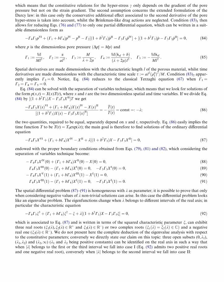
Early time fluid pressure profiles obtained by classical consolidation theory (solid line) and second gradient theory (dashed line).itial value of the fluid pressure is also depicted (black line). Dimensionless time value is explicitly indicated.

ch

Font monospazio

6624

Pressure is made dimensionless so as to deal with a consolidating loading equal to unity:

pðx; 0þÞ ¼ bMKu þ 4

3l

pext

p¼ 1; ð97Þ


moreover, second gradient constitutive parameters are introduced so as to capture a proper boundary layer
effectwithsteps
Fig. 2.initialis expl

close to the drained surface and the impermeable wall. In particular we compare the solution obtainedthe second gradient theory of consolidation to the classical one due to Terzaghi at two characteristic time(see Figs. 1 and 2). The most interesting result of the comparison is the regularizing effect which char-

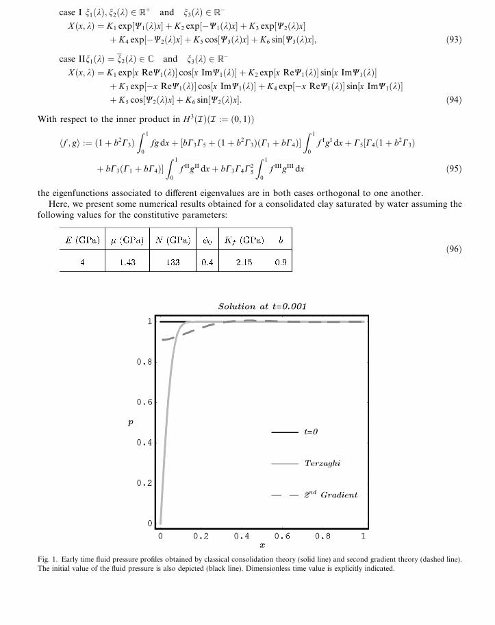
acterizes the second gradient solution: the pressure profile does not fall to a vanishing pressure in x = 0 imme-diately after the initial state but progressively decreases to this limit value for t!1. The obtained picture forthe fluid pressure improves the information on the behaviour of the consolidating porous material close to theexternal surface; in particular we prove that the consolidating process does not proceed as quickly as Ter-zaghi’s model predicts, but the fluid pressure initially hinders pore shrinkage enhancing, on the other hand,the effect of the consolidating pressure more inside the porous material. Reduction of the pore space to theequilibrium regime is therefore not instantaneous even in the vicinity of the external surface but wider thanthat predicted by Terzaghi’s model. Indeed, a non-vanishing pore pressure is still admissible during consoli-dation at the external surface because of a non-vanishing gradient of pore hyper-stress; this is the main reasonboth for the reduction of the pressure jump close to the external surface and the enlargement of the boundarylayer effect (see Fig. 1).

After a suitable time interval the second gradient model predicts a pore pressure increase at the imperme-able wall (x = l) which was not described by Terzaghi’s theory. This effect is mainly due the poor drainage ofthe region which is far from the consolidating surface; this is indeed a quite classical result when considering aporous slab of finite extent (2a) along x and infinitely long in the other direction, sandwiched between twoimpermeable layers and drained at x = ±a (Mandel’s problem, see Mandel, 1953), but it was never modeled

Late time fluid pressure profile obtained by classical consolidation theory (solid line) and second gradient theory (dashed line). Thevalue of the fluid pressure is also depicted (black line). A fluid overpressure at the impermeable wall arises. Dimensionless time valueicitly indicated.

ch

Font monospazio

6625

with a one-dimensional theory of consolidation. As in the case of Mandel’s theory this effect progressivelydecreases when time grows because of dissipative phenomena implied by the Darcy law; this effect is depictedin Fig. 2. These two specific features of the second gradient solution, with respect to the classical one, are reallytypical of second gradient models: actually it is the presence of boundary layers which mostly characterizes


second gradient solutions, even in the absence of double forces. At early evolution times, i.e. when dissipationdoes not dominates the process, second gradient effects rise up close to the boundary of the domain; the char-acteristic size of this neighbourhood determines the intrinsic length of second gradient models. On the otherhand when dissipation starts to dominate the time evolution process, i.e. when time goes to infinity, then theeffect of second gradient becomes smaller and smaller.

It is finally interesting to note that according to the representation formulas of the spatial function X(x), seeEqs. (93) and (94), the second gradient solution does not exhibit the classical Gibbs effect associated to theattempt of recovering a Heavyside function (the initial condition for the fluid pressure) by means of Fourierseries; therefore, the estimate of the effective solution at very early times obtained by truncation of the secondgradient solution is much more refined than the Terzaghi one when accounting for the same number ofeigenfunctions.

8. Concluding remarks

In this paper, the complete deduction of a second gradient poromechanical model is presented starting froma second gradient theory of mixtures; the main result consists of the identification of a properly defined mac-roscopic potential and consequently in the characterization of the second gradient extension of the classicalBiot constitutive relations. Apparently, this is a completely phenomenological model and no explicit relationwith the behaviour of the ath constituent over its characteristic domain has been sketched. In other words,only a macroscopic point of view has been adopted. However even in this frame some remarks can be stated.The key point is in recognizing the cases where the characteristic length of the heterogeneities can be comparedat least with the thickness of the solid/fluid interface: for instance wetting and crack/pore opening phenomena.Further developments will be devoted to state a well grounded second gradient poromechanical model in theframework of micromechanics, on the basis of a proper definition of stresses and hyper-stresses.

In this paper, we prove that, for a second gradient behaviour of the solid and the fluid constituent, i.e.prescribing an external work rate which depends on tractions and double forces, see Eq. (16), and if theextended Cauchy stress theorem holds true, see Eq. (7), then suitable macroscopic Helmholtz free energies(W and Ws) can be determined not only as functions of strain and fluid mass (porosity) but also of strainand fluid mass (porosity) gradient. This result is obtained by considering the thermodynamic restrictionscoming from the first and the second principle of thermodynamics, and in particular from the extendedformulation of the classical Causius–Duhem inequality. According to this result, we prove that a naturalextension of the Biot model can be formulated in order to generalize the classical theory of porous mediato the case of second gradient materials; the introduced additional extensive variables, i.e. gradient of strainand gradient of fluid mass (porosity), play an analogous role as strain and fluid mass (porosity) in the clas-sical model. The corresponding intensive parameters, i.e. the overall hyper-stress and the pure fluid hyper-stress, are constitutively prescribed in terms of first and second gradient deformation variables; moreover,the classical constitutive relations for the overall stress and the fluid mass content (porosity) are correctedby additional second gradient terms (see e.g. Eqs. (55)–(58) and Eqs. (59)–(62) which are valid in the lin-earized case). According to the aforementioned thermodynamic restrictions we prove that the classicalDarcy law becomes a Brinkman-like equation involving the fluid pressure and the velocity of the fluid rel-ative to the solid.

In the last section a numerical example is developed where the corrections due to second gradients areinvestigated for the classical one-dimensional consolidation problem stated by Terzaghi for a homogeneousporous material. Considering the fluid pressure profiles, the differences concern the boundary layers whichnow can be detected in the neighbourhood of the consolidating surface (the external surface – x = 0) andthe impermeable wall (the internal surface – x = l). In particular, the second gradient removes the singularbehaviour due to the initial – boundary condition discontinuity at x = 0 and implies a non-trivial dilatantbehaviour close to the impermeable wall before dissipative diffusion starts to govern the process.

ch

Font monospazio

6626

Appendix A. Dissipation

In this Appendix, we illustrate how Eqs. (37)–(39) can be recovered starting from the general formulation ofthe second principle (35) by means of Eq. (29) which gives the representation formula for the overall Helm-


holtz free energy, and Eq. (32) which provides the local form of the first principle of thermodynamics pulledback into the reference configuration of the skeleton.

Start from Eq. (35) and replace the time derivative of the overall Lagrangean internal energy E with its rep-resentation formula coming from the first principle – see Eq. (32)

½S� C�1ððr0CÞcÞC�1� � dDdtþ C�1 � c � dr0D

dt� div0ðef MþQÞ � div0

1

mf

div0ðncfÞMþpf

qf

M

� �

þ div0

1

trI

cf

J� r0

1

qf

� 1

nqf

r0n� �

M

� �þ dev

ncf

J�r0

1

nqf

� �� Mþ cf

Jqf

div0M

� �

considuced

Splitpute

L :¼the flthe id

Eq. (

þ div0

1

Jqf

devS>f M

� �þ T div0 sfMþ

Q

T

� �� S

dTdt� dW

dtP 0; ð98Þ

der the time derivative of the overall energy W, as defined by Eq. (29), and recall in particular the intro-variation dn

dW ¼ dWs þ wf

dmf þ mf

dnef � sf

dT � Tdsf

� �ð99Þ

dt dt dt dt dt dt

substitute it into Eq. (98) and develop some calculations in the formula so as to obtain
� � � � ½S�C�1ððr0CÞcÞC�1� �dD
dtþC�1�c �dr0D

dtþdiv0

1

Jqf

devS>f M �r0 efþpf

qf

�M� � � � � ��
�r0
1

mf

div0ðncfÞ �M� efþpf

qf

þ 1

mf

div0ðncfÞ div0Mþdev r0

1

nqf

�ncf

J�r0M

þdiv0 dev r0

1

nqf

� ��ncf

J

� �� Mþ 1

trI

cf

J� r0

1

qf

� 1

nqf

r0n� �

div0Mþ 1

trIr0

cf

J� r0

1

qf

� 1

nqf

r0n� ��

�M

þdiv0

cf

Jqf

� �div0Mþ cf

Jqf

�r0div0MþTsf div0Mþr0ðTsfÞ �M�sfM �r0T� 1

Tr0T �Q�Ss

dTdt�dWs

dt

�wf

dmf

dt�mf

dnef

dtþmfT

dsf

dtP0: ð100Þ

the fluid pressure pf into a conservative and a dissipative contribution, say pcf and pd

f , respectively, com-the time derivative of ef according to Eq. (25) and account for the following identity

oef � dnrðnqfÞ ¼ �L � ½F�>r0ðnqfÞ� �oef þ F�1 oef � dnr0ðnqfÞ

orðnq Þ dt orðnq Þ orðnq Þ dt
f f f
¼ � dDdt� ½C�1r0ðnqfÞ� � F�1 oef

orðnqfÞ

� �þ F�1 oef

orðnqfÞ� dn

dtr0ðnqfÞ; ð101Þ

_FF�1 being the gradient of the velocity of the solid. Considering the statement of the balance of mass ofuid pulled back in the reference configuration of the skeleton (dmf/dt + div0M = 0) and bearing in mindentity � ��
d mf d 1 1
dtr0 qf

¼dt qf

r0mf þ mfr0 qf

ð102Þ

¼ d

dt1

qf

� �r0mf þ

1

qf

d

dtðr0mfÞ þ mf

d

dtr0

1

qf

� �þ r0

1

qf

� �dmf

dt

100) reads, according to Eqs. (26)–(28), like this

ch

Font monospazio

6627

S� C�1ððr0CÞcÞC�1 � ½C�1r0ðnqfÞ� �cf

qf

� �� dD


dtþ div0

1

Jqf

devS>f M

� �

�r0 ef þpf

qf

� ��M�r0

1

mf

div0ðncfÞ� �

�Mþ div0 dev r0

1

nqf

� �� ncf

J

� �� M

Cons

we fin

Refer

Allairepp.

Ander


þ dev r01

nqf

� �� ncf

J

� �� r0M� 1

trIr0

cf

J� 1

q2f

r0qf þr0nnqf

� �� M� pd

f

qf

div0Mþ Tr0sf �M

þ 1

qf

pcf þ

1

/r0n � cf � cf � r0

1

J

� �dmf

dtþ cf

J� d

dt1

qf

� �r0mf þ mf

d

dtr0

1

qf

� �� cf

J� d

dtr0/

þ 1

trI

cf

J� 1

q2f

r0qf þr0nnqf

� �dmf

dtþ mf pc

f þ 1þ 1

trI

� �cf

J� r0ðnqfÞ

nqf

� �d

dt1

qf

� �þ ncf

J nqfð Þ2� dn

dtr0ðnqfÞ

" #

� 1

Tr0T �Q� Ss

dTdt� dWs

dtP 0: ð103Þ

idering the equalities

1

trI

cf

J� 1

q2f

r0qf þr0nnqf

� �dmf

dt¼ 1

trI

cf

J� 1

qf

1

nqf

r0ðnqfÞ� �

dmf

dt� � � ��
1 c 1 1 dm d 1 1 c 1 d/
pcf þ trI

f

J�nqf

r0ðnqfÞ qf

f

dtþ mf

dt qf

¼ pcf þ trI

f

J�nqf

r0ðnqfÞ dt

ally get the complete dissipation formula

S� C�1ððr0CÞcÞC�1 � ½C�1r0ðnqfÞ� �cf

qf

� �� dD


dtþ div0

1

Jqf

devS>f M

� ��

�r0 ef þpf

qf

�M�r0

1

mf

div0ðncfÞ �Mþ div0 dev r0

1

nqf

� ncf

J�M

þ dev r0

1

nqf

� �� ncf

J

� �� r0M� 1

trIr0

cf

J� 1

q2f

r0qf þr0nnqf

� �� M� pd

f

qf

div0Mþ Tr0sf �M

þ pcf þ

1

trI

cf

J� 1

nqf

r0ðnqfÞ �cf

J� /r0

1

/

� �d/dt� cf

J� d

dtr0/�

1

Tr0T �Q� Ss

dTdt� dWs

dtP 0:

ences

, G., 1997. One phase Newtonian flow. In: Hornung, U. (Ed.), Homogenization and Porous Media. Springer-Verlag, New York,45–68.

son, D.M., McFadden, G.B., Wheeler, A.A., 1998. Diffuse-interface methods in fluid mechanics. Annu. Rev. Fluid Mech. 30,
139–165.
Biot, M.A., 1941. General theory of three-dimensional consolidation. J. Appl. Phys. 12, 155–164.Brinkman, H.C., 1947. A calculation of the viscous force exerted by a flowing fluid on a dense swarm of particles. Appl. Sci. Res. A 1,

27–34.Cahn, J.W., Hilliard, J.E., 1959. Free energy of a non-uniform system. J. Chem. Phys. 31, 688–699.Casal, P., 1972. La theorie du second gradient et la capillarite. C.R. Acad. Sci. Paris Serie A 274, 1571–1574.Coleman, B.D., Noll, W., 1963. The thermodynamics of elastic material with heat conduction and viscosity. Arch. Rational Mech. Anal.

13, 167–178.Collin, F., Chambon, R., Charlier, R., 2006. A finite element method for poro mechanical modelling of geotechnical problems using local

second gradient models. Int. J. Num. Meth. Engng. 65, 1749–1772.Coussy, O., Dormieux, L., Detournay, E., 1998. From mixture theory to Biot’s approach for porous media. Int. J. Solids Struct. 35 (34–

35), 4619–4635.Coussy, O., 2004. Poromechanics. John Wiley and Sons, Chichester.de Boer, R., 1996. Highlights in the historical development of the porous media theory: toward a consistent macroscopic theory. Appl.

Mech. Rev. 49 (4), 201–261.de Gennes, P.G., 1985. Wetting: statics and dynamics. Rev. Modern Phys. 57 (3), 827–863.Degiovanni, M., Marzocchi, A., Musesti, A., 2006. Edge-force densities and second-order powers. Ann. Matematica 185, 81–103.

ch

Font monospazio

6628

dell’Isola, F., Gouin, H., Rotoli, G., 1996. Nucleation of spherical shell-like interfaces by second gradient theory: numerical simulations.Eur. J. Mech. B/Fluids 15, 545–568.

dell’Isola, F., Seppecher, P., 1997. Edge contact forces and quasi balanced power. Meccanica 32, 33–52.dell’Isola, F., Guarascio, M., Hutter, K., 2000. A variational approach for the deformation of a saturated porous solid. A second gradient

theory extending Terzaghi’s effective stress principle. Arch. Appl. Mech. 70, 323–337.


dell’Isola, F., Sciarra, G., Batra, R.C., 2003. Static Deformations of a Linear Elastic Porous Body filled with an Inviscid Fluid. J. Elasticity72, 99–120.

Dormieux, L., Coussy, O., de Buhan, P., 1991. Modelisation d’un milieu polyphasique par la methode des puissances virtuelles. C. R.Acad. Sci. Paris Serie II 313, 863–868.

Dormieux, L., Ulm, F.J. (Eds.), 2005. Applied micromechanics of porous materials series CISM n. 480. Springer-Verlag, Wien, New York.Drugan, W.J., Willis, J.R., 1996. A micromechanics-based nonlocal constitutive equation and estimates of representative volume element

size for elastic component. J. Mech. Phys. Solids 44 (4), 497–524.Gavrilyuk, S., Saurel, R., 2002. Mathematical and numerical modeling of two-phase compressible flows with micro-inertia. J. Comput.

Phys. 175, 326–360.Germain, P., 1973. La methode des puissances virtuelles en mecanique des milieux continus. Journal de Mecanique 12 (2), 235–274.Gurtin, M.E., 1981. An Introduction to Continuum Mechanics. Academic Press, Boston.Gurtin, M.E., Polignone, D., Vinals, J., 1996. Two-phase binary fluids and immiscible fluids described by an order parameter. Math

Models Meth. Appl. Sci. 6, 815–831.Lee, H.G., Lowengrub, J.S., Goodman, J., 2002. Modeling pinchoff and reconnection in a Hele–Shaw cell. I. The models and their

calibration. Phys. Fluids 14, 492–513.Lowengrub, J., Truskinovsky, L., 1998. Quasi-incompressible Cahn–Hilliard fluids and topological transitions. Proc. R. Soc. Lond. A 454,

2617–2654.Mandel, J., 1953. Consolidation des sols (etude mathematique). Geotechnique 3, 287–299.Mindlin, R.D., 1964. Micro-structure in linear elasticity. Arch. Rat. Mech. Anal. 16, 51–78.Modica, L., 1987a. Theory of phase transitions and minimal interface criterion. Arch. Rat. Mech. Anal. 98, 123–142.Modica, L., 1987b. Gradient theory of phase transitions with boundary contact energy. Ann. Inst. Henri Poincare Analyse non lineaire 4

(5), 487–512.Sciarra, G., dell’Isola, F., Hutter, K., 2001. A solid–fluid mixture model allowing for solid dilatation under external pressure. Continuum

Mech. Thermodyn. 13, 287–306.Sciarra, G., 2001. Modelling of a fluid flux through a solid deformable matrix. PhD Thesis University of Rome ‘‘La Sapienza’’ and

Universite de Toulon et du Var.Seppecher, P., 1987. Etude d’une modelisation des zones capillaires fluides: interfaces et lignes de contact. These Universite. Paris VI.Seppecher, P., 1993. Equilibrium of a Cahn–Hilliard fluid on a wall: influence of the wetting properties of the fluid upon the stability of a

thin liquid film. Eur. J. Mech. B/Fluids 12, 169–184.Seppecher, P., 1996. Moving contact lines in the Cahn–Hilliard theory. Int. J. Eng. Sci. 34 (9), 977–992.Suiker, A.S.J., de Borst, R., Chang, C.S., 2001. Micro-mechanical modelling of granular material. Part I: Derivation of a second-gradient

micro-polar constitutive theory. Acta Mech. 149, 161–180.von Terzaghi, K., 1946. Theoretical Soil Mechanics. John Wiley and Sons.Toupin, R.A., 1962. Elastic materials with couple-stresses. Arch. Rat. Mech. Anal. 11, 385–414.Toupin, R.A., 1964. Theories of elasticity with couple-stress. Arch. Rat. Mech. Anal. 17, 85–112.Truesdell, C.A., 1991. A First Course in Rational Continuum Mechanics, second ed. Academic Press, Boston.

ch

Font monospazio

6629

Second gradient poromechanics

Documents

Transcript of Second gradient poromechanics